
Thè se de doctorat
223
Thèse de doctorat NNT: 2020UPASP075 Optimisation of positron accumulation in the GBAR experiment and study of space propulsion based on antimatter Thèse de doctorat de l’université Paris-Saclay École doctorale n ◦ 576 Particules, hadrons, énergie et noyau : instrumentation, imagerie, cosmos et simulation (Pheniics) Spécialité de doctorat : Physique des particules Unité de recherche: Université Paris-Saclay, CEA, Département de Physique des Particules, 91191, Gif-sur-Yvette, France. Référent: Faculté des sciences d’Orsay Thèse présentée et soutenue en visioconférence totale, le 8 Décembre 2020 par Samuel Niang Composition du jury: Réza Ansari Président Professeur, LAL, Université Paris-Saclay David Cassidy Rapporteur & Examinateur Professeur, University College London Alexandre Obertelli Rapporteur & Examinateur Professeur, HDR, Darmstadt University Gerda Neyens Examinatrice Professeure, KU Leuven et EP Department au CERN Martina Knoop Examinatrice Doctoresse, CNRS et Université d’Aix-Marseille Roland Lehoucq Examinateur Docteur, CEA-E7, IRFU, Université Paris-Saclay Boris Tuchming Directeur de thèse Docteur, HDR, CEA-E6, IRFU, Université Paris-Saclay Patrice Pérez Co-directeur de thèse Docteur d’État, CEA-E6, IRFU, Université Paris-Saclay Dirk Peter van der Werf Co-encadrant de thèse Professeur, Swansea University
-
Upload
khangminh22 -
Category
Documents
-
view
0 -
download
0
Transcript of Thè se de doctorat

Thès
e de
doc
tora
tNNT:2020UPA
SP075
Optimisation of positronaccumulation in the GBAR
experiment and study of spacepropulsion based on antimatter
Thèse de doctorat de l’université Paris-Saclay
École doctorale n576Particules, hadrons, énergie et noyau : instrumentation,
imagerie, cosmos et simulation (Pheniics)
Spécialité de doctorat : Physique des particules
Unité de recherche: Université Paris-Saclay, CEA, Départementde Physique des Particules, 91191, Gif-sur-Yvette, France.
Référent: Faculté des sciences d’Orsay
Thèse présentée et soutenue en visioconférence totale,le 8 Décembre 2020 par
Samuel Niang
Composition du jury:
Réza Ansari PrésidentProfesseur, LAL, Université Paris-SaclayDavid Cassidy Rapporteur & ExaminateurProfesseur, University College LondonAlexandre Obertelli Rapporteur & ExaminateurProfesseur, HDR, Darmstadt UniversityGerda Neyens ExaminatriceProfesseure, KU Leuven et EP Department au CERNMartina Knoop ExaminatriceDoctoresse, CNRS et Université d’Aix-MarseilleRoland Lehoucq ExaminateurDocteur, CEA-E7, IRFU, Université Paris-Saclay
Boris Tuchming Directeur de thèseDocteur, HDR, CEA-E6, IRFU, Université Paris-SaclayPatrice Pérez Co-directeur de thèseDocteur d’État, CEA-E6, IRFU, Université Paris-SaclayDirk Peter van der Werf Co-encadrant de thèseProfesseur, Swansea University
ii
“Of course I dream”, I tell her. “Ev-erybody dreams”.“But what do you dream about?”,she’ll ask.“The same thing everybody dreamsabout”, I tell her. “I dream aboutwhere I’m going”. She always laughsat that.“But you’re not going anywhere,you’re just wandering about”.That’s not true. Not anymore. Ihave a new destination. My jour-ney is the same as yours, the sameas anyone’s. It’s taken me so manyyears, so many lifetimes, but at lastI know where I’m going. Where I’vealways been going. Home. The longway around.
The Day of the Doctor
To Sonia and Alissa.

Résumé de la thèse en français
Chapitre 1 : Introduction
L’antimatière fut découverte mathématiquement par Dirac en 1928 et expérimen-talement par Anderson en 1932 et son étude est encore de nos jours un champ derecherche à part entière, comme au CERN avec le décélérateur d’antiprotons. Laparticularité des antiparticules étant qu’elles peuvent s’annihiler avec leurs partic-ules jumelles de matière et un photon peut se décomposer en une paire particule-antiparticule. Les recherches sur l’antimatière sont particulièrement intéressantescar elles pourraient être la source d’une brèche dans le modèle standard de laphysique, ce qui ouvrirait de nouveaux champs de recherche.
Par ailleurs, d’après le modèle standard de la cosmologie basé sur le modèlestandard de la physique des particules, il y avait autant de matière que d’antimatièreau début de l’histoire de l’univers. Cependant, notre univers semble être constituéuniquement de matière. Il est alors possible qu’une rupture de symétrie dans lesréactions d’annihilation-créations se soit produite. La violation de la symétrie CP,pourrait expliquer en partie cette différence, mais n’est pas la réponse au problème.C’est pour cela que des expériences telles que GBAR étudient d’autres paramètrescomme la gravitation au niveau des particules élémentaires. Une différence dans lecomportement gravitationnel entre la matière et l’antimatière mènerait ainsi à unepercée dans notre connaissance de l’univers.
L’utilisation de l’antimatière dans le domaine du transport spatial sera égalementabordée durant cette thèse. En effet, la réaction d’annihilation a comme avantagede produire des particules légères voyageant à des vitesses proches de celle de la lu-mière et cette énorme quantité d’énergie cinétique ainsi dégagée pourrait être utiliséepour propulser une fusée. L’antimatière serait donc le carburant ayant le meilleurrendement énergétique et rendrait possible le voyage spatial proche de la vitessede la lumière. Cette idée prometteuse a cependant plusieurs limitations. La pre-mière étant qu’il n’y a tout simplement pas de quantité macroscopique d’antimatièreà notre disposition. À l’heure actuelle, il est possible d’en produire mais dans desquantités infinitésimales comparées à ce qui serait nécessaire pour un voyage spatial.Aussi, il n’existe pas pour l’heure de méthodes pour stocker de façon efficace unetelle quantité d’antimatière. Enfin, de telles réactions d’annihilation produisent degrandes quantités de rayons gamma, dont il faudrait protéger la fusée et ses possiblesoccupants, ce qui n’est pas un problème trivial. Mais l’idée d’une telle applicationde l’antimatière demeure quelque chose d’assez attirant pour l’étudier.
iii

iv
Chapitre 2 : L’expérience GBAR
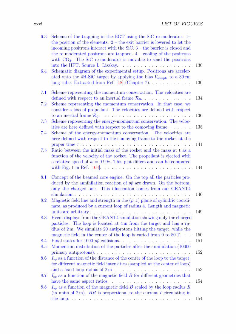
Le but de l’expérience GBAR est de déterminer le comportement gravitationnel del’antimatière au repos en étudiant la chute libre d’un atome d’antihydrogène. Lesdeux composants de cet anti-atome sont les antiprotons, fournis par le décélérateurd’antiprotons ELENA, et les positons fournis par un accélérateur linéaire (LINAC).Le LINAC accélère des électrons jusqu’à 9 MeV qui percutent une cible de tungstèneprovocant la création de paires positons-électrons. La cible est équipée d’un mod-érateur biaisé à 50 V.
Le point clé de l’expérience est la création d’un ion antihydrogène H+. Pour ce
faire, un antiproton réagit deux fois dans un nuage de positronium (état lié d’unélectron et d’un positon) suivant la réaction
p+ Ps→ H + e−,
H + Ps→ H+
+ e−.
La création du positronium passe par la conversion de 1010 positons, à l’aide de sil-ice nano-poreuse. Le LINAC fournissant 3× 10⁷ positons par seconde, ces derniersdoivent être accumulés dans des pièges de Penning, comme présenté dans les chapitres3, 4 et 5. Un piège sera installé pour accumuler les paquets d’antiprotons fournispar le décélérateur ELENA.
Une fois l’anti-ion créé, il est stabilisé à l’aide d’un champ électrique dans lachambre de chute libre. Le positon excédentaire est enlevé à l’aide d’un faisceaulaser, et la chute libre peut être alors observée. Pour le moment, aucun antiprotonn’a pu être piégé car le piège à antiproton est encore en cours d’installation. Lepiégeage des antiprotons commencera lors du redémarrage d’ELENA en 2021. Lachambre de chute libre est toujours en construction et sera installée également en2021.
100 keV𝑝
High Field Trap
Canon à proton 10 keV
Piège
Décélérateur
Bunker
Buffer Gas Trap
Cible
e- 10 MeV
e+ 3 eV
e+ 50 eV
ELENA
Laser Ps*
𝐻 +
𝐻
Refroidissement LASER / photo-détachement
Chambre de
chute libre
e+e+
LINAC
Chambre de réaction
Silice nano-poreuse (Positronium)
Schéma de l’expérience GBAR.

v
Chapitre 3 : Piégeage et transport d’une particulechargéeLe piégeage de particules chargées se fait à l’aide de pièges électromagnétiques nom-més pièges de Penning-Malmberg. Dans le modèle du piège de Penning, un champmagnétique uniforme parallèle à l’axe principal est responsable du confinement ra-dial des particules tandis qu’un potentiel parabolique est responsable du confinementaxial.
z
x y
Mouvement d’une particule dans un piège de Penning-Malmberg. Dans le plan(x, y), le mouvement est composé de deux mouvements circulaires. Suivant l’axe z(parallèle au champ magnétique), il s’agit d’une oscillation.
Pour un grand nombre de particules, on parle de plasma quand la longueur deDebye est petite devant la longueur caractéristique du piège. Dans ce cas, les chargesécrantent le champ électrique du piège. La longueur de Debye est définie par
λD =
√ε0kBT
n0e2,
avec ε0 la permittivité du vide, kB la constante de Boltzmann, n0 la densité departicules et e la charge des particules dans le plasma.
Un autre paramètre important est le paramètre de corrélation
Γ =e2
4πε0akBT∝ a2
λ2D
,
avec a ≡ n−1/30 , la distance moyenne entre les particules. En effet, un plasma faible-
ment corrélé pourra être considéré comme un fluide continu. Dans le cas contraire,il faudra prendre en compte les interactions entre chaque particule. Aussi, dans lecas d’un plasma, il est démontré qu’il existe une densité maximale nommée limitede Brillouin qui est proportionnelle au champ magnétique B:
nB =B2/(2µ0)
mc2,
avec µ0 la perméabilité du vide, m la masse des particules et c la vitesse de lalumière.
Pour comprimer radialement le paquet de particules chargées dans le piège, laméthode du “Rotating Wall” est utilisée. Un potentiel oscillant est appliqué sur une

vi
électrode coupée en 4 et sur chaque partie, le champ oscillant appliqué a une phasede 90 par rapport au champ appliqué sur les électrodes voisines, créant ainsi undipôle oscillant. Avec l’amplitude et la fréquence appropriée, la collection de chargeest compressée.
Dans le cas de particules voyageant dans des zones où le champ magnétiquechange, il faut prendre en compte l’effet de miroir magnétique. En effet, si uneparticule chargée se déplace d’une région avec un champ magnétique Bi à un champmagnétique Bf (parallèles à l’axe principal) avec Bf > Bi, elle sera repoussée sil’angle entre son impulsion et l’axe principal est supérieur à
θimax = arcsin
(√Bi
Bf
).
Pour franchir ce miroir magnétique, il est possible d’accélérer une particule d’énergietotale E, suivant l’axe principal, en ajoutant une énergie cinétique E . L’angle max-imal devient donc
θi,max = arcsin
(√Bi
Bf
E + EE
)> arcsin
(√Bi
Bf
).
Chapitre 4 : Piège à gaz tamponLe piège à gaz tampon (abrégé en BGT pour Buffer Gas Trap) utilisé dans l’expérienceGBAR est un accumulateur à positons basé sur le principe du piège de Greaves-Surko. Il s’agit d’un piège de Penning à trois étages dans lequel des gaz (N2 et CO2)à très faibles pressions ont été injectés. Les positons en provenance du LINAC y per-dent de l’énergie grâce aux collisions inélastiques avec le gaz, permettant le piégeage(grâce au N2) et le refroidissement des particules (grâce au CO2). Le paquet depositons ainsi accumulé peut être compressé radialement grâce à la technique du“Rotating Wall”.
Schéma du piège à gaz tampon.
Les positons sont d’abord accumulés dans le second étage pendant 100 ms. Avecles paramètres définis dans ce chapitre, le temps de vie des positons dans cet étageest d’environ 0.6 s pour un taux de piégeage de 1.7× 10⁶ e+ s−1. Ici, le “RotatingWall” a un rôle essentiel dans l’efficacité du piégeage et dans la compression radiale.
vii
Après cela, le paquet de positons est comprimé axialement en changeant la formedu puits de potentiel électrique, dans l’optique de re-piéger les positons dans letroisième étage du piège. Le temps de vie des positons dans ce troisième étage(∼ 10 s) est assez grand pour commencer un empilement des paquets de positonsdans le troisième étage. 10 paquets correspondant à 10 × 100 ms d’accumulationdans le second étage sont ainsi transférés dans le troisième étage et y sont une foisde plus comprimés radialement à l’aide du “Rotating Wall”.
A l’heure actuelle, le BGT fournit un paquet de ∼ 1.5× 10⁶ e+ chaque seconde(il y a une perte durant la procédure d’empilement dans le troisième étage). Cepaquet va être alors transféré dans le second piège de l’expérience où une nouvelleprocédure d’empilement va avoir lieu afin de piéger le plus de positons possible.
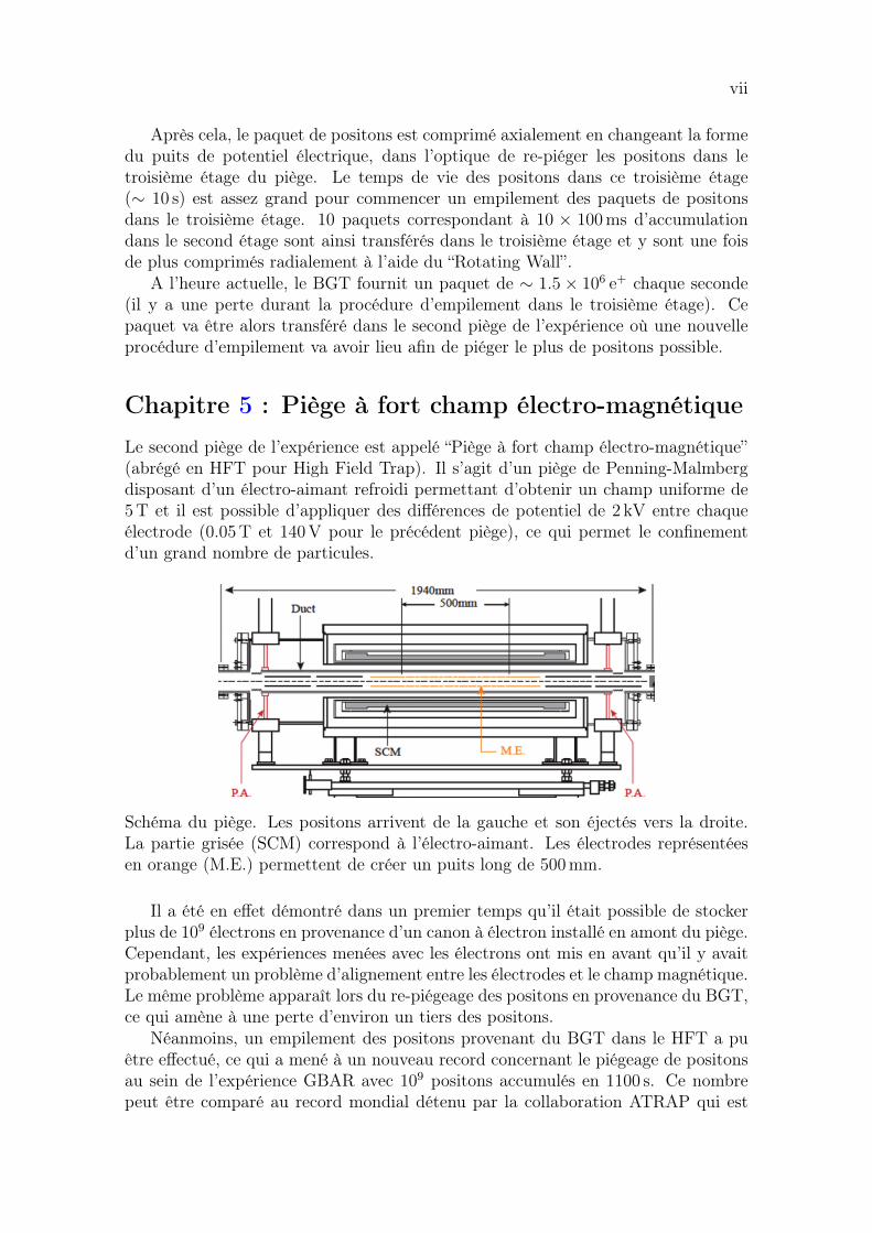
Chapitre 5 : Piège à fort champ électro-magnétique
Le second piège de l’expérience est appelé “Piège à fort champ électro-magnétique”(abrégé en HFT pour High Field Trap). Il s’agit d’un piège de Penning-Malmbergdisposant d’un électro-aimant refroidi permettant d’obtenir un champ uniforme de5 T et il est possible d’appliquer des différences de potentiel de 2 kV entre chaqueélectrode (0.05 T et 140 V pour le précédent piège), ce qui permet le confinementd’un grand nombre de particules.
Schéma du piège. Les positons arrivent de la gauche et son éjectés vers la droite.La partie grisée (SCM) correspond à l’électro-aimant. Les électrodes représentéesen orange (M.E.) permettent de créer un puits long de 500 mm.
Il a été en effet démontré dans un premier temps qu’il était possible de stockerplus de 109 électrons en provenance d’un canon à électron installé en amont du piège.Cependant, les expériences menées avec les électrons ont mis en avant qu’il y avaitprobablement un problème d’alignement entre les électrodes et le champ magnétique.Le même problème apparaît lors du re-piégeage des positons en provenance du BGT,ce qui amène à une perte d’environ un tiers des positons.
Néanmoins, un empilement des positons provenant du BGT dans le HFT a puêtre effectué, ce qui a mené à un nouveau record concernant le piégeage de positonsau sein de l’expérience GBAR avec 109 positons accumulés en 1100 s. Ce nombrepeut être comparé au record mondial détenu par la collaboration ATRAP qui est

viii
de 4× 10⁹ en 14 400 s, montrant ainsi que notre résultat est encourageant. Lesexpériences effectuées avec ce piège ont été réalisées sans utiliser le “Rotating Wall”,ce qui devra être la prochaine étape du développement de la partie piégeage depositons. Après cela, il est envisagé de remplacer le BGT par un refroidissement despositons à l’aide d’un nuage d’électrons à l’entrée du HFT.
Chapitre 6 : Futur du piégeage de positons chezGBAR
Dans ce chapitre, une revue rapide des possibilités d’optimisation du piégeage esteffectuée. Le problème actuel étant que le taux final de piégeage des positons est100 fois inférieur à ce que nous souhaiterions pour produire des H
+ .Ainsi, des améliorations à court terme telles que celles prévues sur le LINAC
sont à venir mais ce ne sera pas suffisant (un facteur autour de 3 est attendu). C’estpour cela que de plus profondes modifications sont à venir telles que l’utilisationd’un re-modérateur au Si-C dans le BGT ou le refroidissement par des électronsdans le HFT.
Au final, ces optimisations pourraient nous permettre d’avoir un taux de piégeage50 fois supérieur au taux actuel. Ainsi, au lieu de créer un H
+ toutes les 100 s, ceserait toutes les 200 s (en accumulant les positons 200 s au lieu de 100 s).
Chapitre 7 : Équations de la fusée
Une partie de cette thèse a été dévolue à l’étude de la propulsion spatiale à anti-matière. Dans notre modèle, des antiprotons sont annihilés sur une cible d’hydrogèneet les particules produites chargées sont redirigées à l’aide d’un miroir magnétiquepour propulser la fusée. Les particules neutres quant à elles quittent le centred’interaction de façon isotropique, ne participant donc pas à l’accélération de lafusée. Si l’on considère qu’une fraction ξ des particules produites sont chargées,l’équation de déplacement de la fusée dans le cadre de la mécanique newtonienneest
v(t) = −ξw ln
(m(t)
m(t0)
)+ v(t0),
avec v la vitesse, m la masse de la fusée et w la vitesse d’éjection des particuleschargées. Le paramètre habituellement utilisé est l’impulsion spécifique définie dansnotre cas comme
Isp =ξw
g,
avec g l’accélération de pesanteur sur Terre. À l’heure actuelle, les fusées couram-ment utilisées ont une Isp de l’ordre de 400 s et comme démontré dans le chapitresuivant, on pourrait espérer une Isp allant jusqu’à 107 s dans le cas d’une propulsionpar antimatière. Cela permettait alors d’atteindre des vitesses proches de la vitessede la lumière. C’est pourquoi l’équation du mouvement dans le cadre de la relativité

ix
restreinte a été présentée dans ce chapitre
v(t) = c
(m(t)m(t0)
)−2ξwc(c+v(t0)c−v(t0)
)− 1(
m(t)m(t0)
)−2ξwc(c+v(t0)c−v(t0)
)+ 1
,
avec c la vitesse de la lumière.
Chapitre 8 : Exemple de moteur à antimatièreNous avons étudié dans ce chapitre le modèle du “Beamed core engine” pour propulserune fusée à l’aide d’antimatière, l’idée étant de diriger un faisceau de particules dansune direction précise pour accélérer la fusée. Dans notre cas, il s’agit d’envoyer unfaisceau d’antiprotons sur une cible d’hydrogène et de rediriger les produits de réac-tion à l’aide d’un miroir magnétique. L’interaction proton-antiproton peut êtresimplifiée en moyenne par la réaction
pp→ 1.5π+ + 1.5π− + 2π0,
ainsi, environ 2/5 de l’énergie est perdue sous forme de particules neutres, les pionsπ0 se désintégrant en γ qui devront être stoppés pour protéger l’intégrité de la fusée.
Une simulation basée sur la bibliothèque GEANT4 a été développée, et nousavons trouvé qu’il est possible d’obtenir une impulsion spécifique de 1.5× 10⁷ s, àl’aide d’un champ magnétique de 30 T dans la géométrie appropriée. Cependant,notre simulation est basée sur la présence d’un canon à antiproton, ce qui pourl’instant n’est pas quelque chose de réaliste.
Une autre limitation est due à la production de rayon γ. En effet, une tellefusée devrait être protégée par un bouclier assez dense pour absorber l’énergie etdisposer de radiateurs assez larges pour évacuer toute la chaleur. Notre étude montreque dans ce cas, il serait très difficile pour une fusée propulsée par antimatière dedépasser une vitesse de 0.05c.


Acknowledgements
During this PhD, I received different kinds of support and I would like to thank allof these people who helped me during this three years.
I would first like to thank my three supervisors, Boris Tuchming, Patrice Pérez,Dirk van der Werf who guided me a lot and gave me all the opportunities to improvemyself as a person and as a scientist. I could say the same from all the membersof GBAR collaboration. This team has been a big part of my life recently andworking with them has been a pleasure. I would like to mention Pauline Cominiand Bongho Kim who made my life happier in the control room as well as Jean-Yves Rousse and Sandrine Javello who made my life easier at CERN. Also, I wouldlike to thank Laszlo Liszkay and Christian Regenfus for their assistance during myexperiments and also Bruno Mansoulié for his substantial help in the correction ofmy manuscript.
In addition, I would like to thank all the interns who worked with me: AnnaliesM. Kleyheeg, Judith Gafriller, Romain Meriot and Benoit Garneret. They workedand helped me a lot and I hope they enjoyed this time together and I wish them tosucceed in their studies.
All this work would not have been possible without CEA and CNES (representedby Stéphane Oriol, Frédérique Masson) which supported my thesis financially andadministratively. I would like to thank these two remarkable institutions whichbelieved in me enough to give me this great opportunity and I would like to thankall the people who had to deal with my case (Gautier Hamel de Monchenault,Georges Vasseur, Martine Oger, Béatrice Guyot, Florian Bauer and more).
It is also important for me to deeply thank the members of the jury: RézaAnsari, David Cassidy, Alexandre Obertelli, Gerda Neyens, Martina Knoop, andRoland Lehoucq. They took time to read and bring corrections or asked questionsto help me to improve my manuscript. Thanks a lot again.
Furthermore, during my PhD, my friends supported me as much as I needed andfor sure this period of my life would not have been the same without them. Thisis why I would like to thank Szabolcs, Riccardo, Shudhashil, McPherlain, Matheus,Jillo, Nick and Julien.
Unfortunately, it is impossible to thank everyone. Therefore, to conclude thislong list, I would like to thank Filippo, my grandparents who supported me a lotduring my long studies and the rest of my family. And finally, my sister Sonia, whosupported me during my entire life.
xi


Contents
1 Introduction 31.1 Discovery of antimatter . . . . . . . . . . . . . . . . . . . . . . . . . . 31.2 Why does antimatter matter? . . . . . . . . . . . . . . . . . . . . . . 4
1.2.1 CPT symmetry . . . . . . . . . . . . . . . . . . . . . . . . . . 41.2.2 Some important experiments . . . . . . . . . . . . . . . . . . . 6
1.3 Antimatter, the future of space travel? . . . . . . . . . . . . . . . . . 71.4 Conclusion . . . . . . . . . . . . . . . . . . . . . . . . . . . . . . . . . 8
2 The GBAR experiment 92.1 Context and aim of the GBAR experiment . . . . . . . . . . . . . . . 92.2 Scheme of the GBAR experiment . . . . . . . . . . . . . . . . . . . . 112.3 Antiproton trapping . . . . . . . . . . . . . . . . . . . . . . . . . . . 122.4 Positronium production . . . . . . . . . . . . . . . . . . . . . . . . . 13
2.4.1 Positron source . . . . . . . . . . . . . . . . . . . . . . . . . . 132.4.2 Positron trapping . . . . . . . . . . . . . . . . . . . . . . . . . 142.4.3 Positronium formation . . . . . . . . . . . . . . . . . . . . . . 15
2.5 H+ production . . . . . . . . . . . . . . . . . . . . . . . . . . . . . . . 17
2.6 H+ cooling and g measurement . . . . . . . . . . . . . . . . . . . . . 18
2.7 Conclusion . . . . . . . . . . . . . . . . . . . . . . . . . . . . . . . . . 20
3 Charged particle trapping and transport 233.1 Penning-Malmberg trap . . . . . . . . . . . . . . . . . . . . . . . . . 24
3.1.1 Electric field . . . . . . . . . . . . . . . . . . . . . . . . . . . . 243.1.2 Classical motion of a particle in the trap . . . . . . . . . . . . 25
3.2 Non neutral plasma . . . . . . . . . . . . . . . . . . . . . . . . . . . . 283.2.1 Conditions to fulfill . . . . . . . . . . . . . . . . . . . . . . . . 283.2.2 Plasma in the Penning-Malmberg trap . . . . . . . . . . . . . 30
3.3 Realistic traps . . . . . . . . . . . . . . . . . . . . . . . . . . . . . . . 323.3.1 Main electric field . . . . . . . . . . . . . . . . . . . . . . . . . 323.3.2 The rotating wall technique . . . . . . . . . . . . . . . . . . . 35
3.4 Magnetic mirroring . . . . . . . . . . . . . . . . . . . . . . . . . . . . 393.4.1 Magnetic moment conservation . . . . . . . . . . . . . . . . . 403.4.2 Mirroring conditions . . . . . . . . . . . . . . . . . . . . . . . 413.4.3 Crossing the magnetic mirror . . . . . . . . . . . . . . . . . . 44
3.5 Conclusion . . . . . . . . . . . . . . . . . . . . . . . . . . . . . . . . . 45
xiii

xiv CONTENTS
4 The Buffer Gas Trap 474.1 Principle of the Surko-Greaves Trap . . . . . . . . . . . . . . . . . . . 484.2 Description of the trap . . . . . . . . . . . . . . . . . . . . . . . . . . 51
4.2.1 Sets of electrodes . . . . . . . . . . . . . . . . . . . . . . . . . 524.2.2 Electric potential . . . . . . . . . . . . . . . . . . . . . . . . . 524.2.3 Magnetic Field . . . . . . . . . . . . . . . . . . . . . . . . . . 544.2.4 Gas and vacuum . . . . . . . . . . . . . . . . . . . . . . . . . 55
4.3 Trap control . . . . . . . . . . . . . . . . . . . . . . . . . . . . . . . . 654.3.1 Vacuum system and magnets control . . . . . . . . . . . . . . 664.3.2 Trapping control . . . . . . . . . . . . . . . . . . . . . . . . . 66
4.4 Positron detection . . . . . . . . . . . . . . . . . . . . . . . . . . . . . 724.4.1 Micro-Channel Plate . . . . . . . . . . . . . . . . . . . . . . . 724.4.2 CsI detector . . . . . . . . . . . . . . . . . . . . . . . . . . . . 73
4.5 Electron repeller . . . . . . . . . . . . . . . . . . . . . . . . . . . . . 744.5.1 Electron repeller version 1 . . . . . . . . . . . . . . . . . . . . 744.5.2 Electron repeller version 2 . . . . . . . . . . . . . . . . . . . . 77
4.6 Accumulation in the first and second stages . . . . . . . . . . . . . . 804.6.1 Gas parameters . . . . . . . . . . . . . . . . . . . . . . . . . . 814.6.2 Rotating Wall optimisation . . . . . . . . . . . . . . . . . . . 844.6.3 Energy distribution after second stage accumulation . . . . . . 85
4.7 Third stage . . . . . . . . . . . . . . . . . . . . . . . . . . . . . . . . 874.7.1 Re-trapping . . . . . . . . . . . . . . . . . . . . . . . . . . . . 874.7.2 RW optimisation . . . . . . . . . . . . . . . . . . . . . . . . . 894.7.3 Energy distribution . . . . . . . . . . . . . . . . . . . . . . . . 924.7.4 Stacking . . . . . . . . . . . . . . . . . . . . . . . . . . . . . . 92
4.8 Conclusion . . . . . . . . . . . . . . . . . . . . . . . . . . . . . . . . . 93
5 The High Field Trap 955.1 Description of the trap . . . . . . . . . . . . . . . . . . . . . . . . . . 96
5.1.1 The super conducting magnet . . . . . . . . . . . . . . . . . . 965.1.2 The electrodes . . . . . . . . . . . . . . . . . . . . . . . . . . . 985.1.3 Temperature probes . . . . . . . . . . . . . . . . . . . . . . . 995.1.4 Trapping control . . . . . . . . . . . . . . . . . . . . . . . . . 101
5.2 Electron gun . . . . . . . . . . . . . . . . . . . . . . . . . . . . . . . . 1045.2.1 Filament characteristics . . . . . . . . . . . . . . . . . . . . . 1045.2.2 Power supply control . . . . . . . . . . . . . . . . . . . . . . . 1065.2.3 Control of the system . . . . . . . . . . . . . . . . . . . . . . . 107
5.3 Electron trapping . . . . . . . . . . . . . . . . . . . . . . . . . . . . . 1095.3.1 Charge counter . . . . . . . . . . . . . . . . . . . . . . . . . . 1095.3.2 Electron accumulation . . . . . . . . . . . . . . . . . . . . . . 110
5.4 Positron trapping . . . . . . . . . . . . . . . . . . . . . . . . . . . . . 1195.4.1 One stack in the HFT . . . . . . . . . . . . . . . . . . . . . . 1195.4.2 Stacking . . . . . . . . . . . . . . . . . . . . . . . . . . . . . . 121
5.5 Conclusion . . . . . . . . . . . . . . . . . . . . . . . . . . . . . . . . . 124

CONTENTS xv
6 Future of the e+ trapping at the GBAR experiment 1276.1 LINAC optimisation . . . . . . . . . . . . . . . . . . . . . . . . . . . 1276.2 BGT optimisation . . . . . . . . . . . . . . . . . . . . . . . . . . . . . 1286.3 Electron cooling . . . . . . . . . . . . . . . . . . . . . . . . . . . . . . 1296.4 Si-C moderator . . . . . . . . . . . . . . . . . . . . . . . . . . . . . . 1296.5 Conclusion . . . . . . . . . . . . . . . . . . . . . . . . . . . . . . . . . 131
7 Rocket equations 1337.1 Classical equations . . . . . . . . . . . . . . . . . . . . . . . . . . . . 1347.2 Classical equations with loss of propellant . . . . . . . . . . . . . . . 1367.3 Relativistic equations . . . . . . . . . . . . . . . . . . . . . . . . . . . 1377.4 Relativistic equations with propellant loss . . . . . . . . . . . . . . . 1417.5 Numerical applications . . . . . . . . . . . . . . . . . . . . . . . . . . 1437.6 Conclusion . . . . . . . . . . . . . . . . . . . . . . . . . . . . . . . . . 143
8 The beamed core 1458.1 Concept . . . . . . . . . . . . . . . . . . . . . . . . . . . . . . . . . . 147
8.1.1 Proton-antiproton annihilation . . . . . . . . . . . . . . . . . . 1478.1.2 Estimates about kinematics in pp annihilation and Isp . . . . . 1488.1.3 Magnetic mirroring . . . . . . . . . . . . . . . . . . . . . . . . 1488.1.4 Scale invariance . . . . . . . . . . . . . . . . . . . . . . . . . . 149
8.2 Results . . . . . . . . . . . . . . . . . . . . . . . . . . . . . . . . . . . 1518.2.1 Presentation of the simulation . . . . . . . . . . . . . . . . . . 1518.2.2 First results . . . . . . . . . . . . . . . . . . . . . . . . . . . . 1518.2.3 Optimisation of the target’s position . . . . . . . . . . . . . . 1538.2.4 Optimisation of the field . . . . . . . . . . . . . . . . . . . . . 153
8.3 Energy evacuation . . . . . . . . . . . . . . . . . . . . . . . . . . . . 1558.3.1 Radiator . . . . . . . . . . . . . . . . . . . . . . . . . . . . . . 1558.3.2 Shield . . . . . . . . . . . . . . . . . . . . . . . . . . . . . . . 156
8.4 Antimatter production and storage . . . . . . . . . . . . . . . . . . . 1578.5 Conclusion . . . . . . . . . . . . . . . . . . . . . . . . . . . . . . . . . 158
9 Conclusion 159
A Useful notions of special relativity 161A.1 Definitions and notations . . . . . . . . . . . . . . . . . . . . . . . . . 161A.2 Composition of velocities . . . . . . . . . . . . . . . . . . . . . . . . . 162A.3 Body under a proper constant acceleration . . . . . . . . . . . . . . . 163
B Dirac Equation 167B.1 Notations . . . . . . . . . . . . . . . . . . . . . . . . . . . . . . . . . 167B.2 Motivation . . . . . . . . . . . . . . . . . . . . . . . . . . . . . . . . . 167B.3 Building of the equation . . . . . . . . . . . . . . . . . . . . . . . . . 168B.4 Solutions . . . . . . . . . . . . . . . . . . . . . . . . . . . . . . . . . . 170B.5 Spin . . . . . . . . . . . . . . . . . . . . . . . . . . . . . . . . . . . . 172
C Buffer Gas Trap electrodes schematics 173

xvi CONTENTS
D HFT probes 177D.1 Temperature probes connections . . . . . . . . . . . . . . . . . . . . . 177D.2 Carbon Glass Resistor based probes abaci . . . . . . . . . . . . . . . 178

List of Figures
1.1 Extracted from Ref. [5]. “A 63 million volt positron passing througha 6 mm lead plate and emerging as a 23 million volt positron. Thelength of this latter path is at least ten times greater than the possiblelength of a proton path of this curvature”. The particle comes frombelow the lead plate, and a magnetic field perpendicular to the planebends the trajectory of the charged particles. The trajectory of theparticle in this configuration shows that the charge is positive. . . . . 5
1.2 Picture of the ELENA ring. . . . . . . . . . . . . . . . . . . . . . . . 61.3 Extracted from Ref. [31]. Payload for a single-staged rocket as a
function of the effective specific impulse in vacuum. Launcher hasan inert mass of 2 t, a propellant load of 12 t. Different ∆V missionrequirements are reported. . . . . . . . . . . . . . . . . . . . . . . . . 8
2.1 Overall scheme of the GBAR experiment. . . . . . . . . . . . . . . . . 112.2 Extracted from Ref. [39, 38]. Schematic of the Pulsed Drift Tube
principle. . . . . . . . . . . . . . . . . . . . . . . . . . . . . . . . . . . 122.3 Left: pictures of the antiproton trap magnet. Right: drawing of the
magnet equipped with the cryogenic system to cool the electrodes. . . 132.4 Extracted from Ref. [44]. Scheme of the linac (vertical structure on
the left) and the positron transfer line. The transfer magnetic field isgenerated by a solenoid wound around the beam pipe and larger coils. 14
2.5 Extracted from Ref. [44]. Cross section of the electron target. The po-tential of the moderator is +V , the rest of the structure is at ground.The copper block (“Cu cooler”) is water cooled. A magnetic field of9.7 mT is parallel to the electron beam. . . . . . . . . . . . . . . . . . 15
2.6 Pictures of the nanoporous silica target obtained by Scanning Elec-tron Microscopy. Left: picture from the top of the target (the positronentrance), one can clearly see the nanopores. Scale: 100 nm. Right:side of the target. One can see the imperfections at the surface. Scale:1 µm. – Source: C2RMF / P. Lehuédé. . . . . . . . . . . . . . . . . . 16
2.7 The positrons go through a Si3N4 window to enter the nanoporoussilica. They are expelled from it under the form of positronium Ps =(e+, e−) and remain in the reaction cavity (volume of 1×1×20mm3).The positronium is excited to optimise the reaction rate with theincoming antiprotons. Source: P. Comini / GBAR Collaboration. . . 16
xvii

xviii LIST OF FIGURES
2.8 Extracted from Ref. [59]. Left: Schematic view of the target area.The gray coloured tubes show the Einzel lenses aimed at focusingthe positron beam. The circular line represents the reaction chamberarea. The positronium converter and the MCP assembly are trans-lated by a linear drive to the center of the chamber. A camera islocated downstream of the MCP assembly to determine the positronbeam profile. The PbWO4 detector and a plastic scintillator (PS)are located at the backside of the target region for the gamma raymeasurement. Right: Drawing of the detector assembly. The photo-multiplier tubes are connected to the PbWO4 crystals. The rectanglecorresponds to the target cavity. . . . . . . . . . . . . . . . . . . . . . 17
2.9 Extracted from Ref. [59]. Raw signal distribution from the PbWO4
detector (averaged data sample). The hatched histogram shows thesignal arising from the e+ beam hitting the MCP while the solidline histogram corresponds to the e+ beam hitting the positroniumconverter. . . . . . . . . . . . . . . . . . . . . . . . . . . . . . . . . . 18
2.10 Extracted from Ref. [36]. Top: Cross sections for antihydrogen pro-duction from different states of positronium (Ps(1s) to Ps(3d)). Thesecross sections correspond to the sum of the antihydrogen states up toH(5d). Bottom: Cross sections for H
+ ion production for Ps(1s) toPs(3d). Only the H ground state is taken into account, the contribu-tion of the other states being negligible. . . . . . . . . . . . . . . . . . 19
2.11 Extracted from Ref. [38]. Left: Simulation of the switchyard. Right:Photograph of the switchyard. . . . . . . . . . . . . . . . . . . . . . . 20
2.12 (a) ITO trap (indium tin oxide). (b) H+ ions injected at 0, laser
beam at 6. (c) Doppler cooling light pressure does not act on H+
ions thus they accumulate at the left side. (d) Double potential wellto separate H
+ ions. (e) H+ ions extraction toward precision trap.
Source: A. Wilzewski, S. Wolf and F. Schmidt-Kaler. . . . . . . . . . 21
2.13 Left: Schematic of the Free Fall Chamber. Right: The FFC sur-rounded by plastic scintillator. . . . . . . . . . . . . . . . . . . . . . . 22
3.1 Representation of a Penning-Malmberg trap. . . . . . . . . . . . . . . 24
3.2 Sectional diagrams of the electrodes of an ideal Penning trap usedto produce a quadratic potential of the same form as given to theequation 3.1.4 (red and blue lines). Left: ∆V > 0. Right: ∆V < 0.In green, the electrostatic field. . . . . . . . . . . . . . . . . . . . . . 25
3.3 Illustration of the motion of a charged particle in a Penning-Malmbergtrap. In the (x, y) plane the motion composed of two circular motions.Along the z axis, there is an oscillation. . . . . . . . . . . . . . . . . . 27
3.4 Density of positrons as a function of the rotation frequency of theplasma. This density is maximal for ωrot = ωc/2, the so-called Bril-louin limit. . . . . . . . . . . . . . . . . . . . . . . . . . . . . . . . . . 31
LIST OF FIGURES xix
3.5 Left: the boundary conditions for one electrode at r = R. Right:representation of the electrode on the (r, z) plane: the real electrode isbetween −z0 and +z0, the rest is a virtual electrode with the potential0 on it. . . . . . . . . . . . . . . . . . . . . . . . . . . . . . . . . . . . 32
3.6 Illustration of the computation of the electric potential for a trapmade of 3 electrodes of 1 cm length. . . . . . . . . . . . . . . . . . . . 34
3.7 Boundary conditions for an electrode split in four. . . . . . . . . . . . 353.8 Representation of the potential produced by a rotating wall with a
frequency ωr according to Equation 3.3.20 and Equation 3.3.22. Theyellow areas represent a potential of +Vr and the blue of −Vr. . . . . 38
3.9 Illustration of a positron following a magnetic field line. . . . . . . . . 393.10 Extracted from Ref. [52]. On this schematic four magnetic field lines
are represented as well as two particles with different initial condi-tions. The cyclotron motion is not represented. In the case of thered positron, we have θi < θimax, then the particle can go across themagnetic mirror and we get a positron with θf > θi. For the greenpositron, θi > θimax and we see that θ is increasing during the travelto reach the point where the particle can only go backward: this isthe magnetic mirror. . . . . . . . . . . . . . . . . . . . . . . . . . . . 42
3.11 Illustration of uniform angular distribution of momenta after themoderator. . . . . . . . . . . . . . . . . . . . . . . . . . . . . . . . . . 43
4.1 Extracted from Ref. [47]. Schematic diagram of a Surko-Greavespositron accumulator, showing the three stages of differential pump-ing and the electrostatic potential. A represents the energy loss byinelastic collisions, B and C represent lower energy collisions. Theelectrostatic potential is set to maximise the positron trapping effi-ciency (between stages ∆V ∼ 9− 10 V). . . . . . . . . . . . . . . . . 49
4.2 Extracted from Ref. [72]. Comparison between the impact excitationof the electronic state (triangles) and positronium formation (circles)cross sections (a0 is the Bohr radius) of N2 (solid) and CO (open). Thevertical bars on the x-axis mark the threshold values for Ps forma-tion in CO (7.21 eV), electronic excitation in CO (8.07 eV), electronicexcitation in N2 (8.59 eV), and Ps formation in N2 (8.78 eV). . . . . . 50
4.3 Picture of the Buffer Gas Trap in the GBAR experiment at CERN(Picture by Ciaran McGrath). . . . . . . . . . . . . . . . . . . . . . . 51
4.4 Buffer Gas Trap electrodes assembled in stages. . . . . . . . . . . . . 534.5 Electric potential vs x and y (for a fixed for z = 0), where x is
the beam axis and y is one of the radial direction. Computationobtained by SIMION [73] with the parameters of the BGT describedin Section 4.2.1. . . . . . . . . . . . . . . . . . . . . . . . . . . . . . . 54
4.6 Schematic of the Buffer Gas Trap. (a) Solenoids used to confined thepositrons in the accumulator. (b) Transport coils. (c) Transport andcompression coil. (d) MCP (see Section 4.4.1). . . . . . . . . . . . . . 56
4.7 Buffer Gas Trap’s magnetic field map. . . . . . . . . . . . . . . . . . 57

xx LIST OF FIGURES
4.8 Schematic of the vacuum system of both traps. Three kinds of pres-sure gauges P, CC: cold cathode gauge, C: capacitance gauge, P:Pirani gauge, FR: full range gauge. . . . . . . . . . . . . . . . . . . . 60
4.9 Schematic of two vessels with one connected to a pump. . . . . . . . . 614.10 Conductances of the pumping restriction elements. Ca: connection
with the turbo-pumps. Cb: half first stage. Cc: half first stage andsecond stage. Cd: half first stage and half second stage. Cf : halfthird stage. Cg: connection with the cryo-pumps. Ce, Ch, Ci: smallpipes. Cj: small pipe and third stage. . . . . . . . . . . . . . . . . . . 62
4.11 (a) P10 as a function of P5 (only N2). (b) P11 as a function of P5(only N2). (c) P10 as a function of P6 (only CO2). (d) P11 as afunction of P6 (only CO2). The blue curves correspond to valuesread with the gauges. The red curves correspond to corrected valuesaccording to Ref. [85]. . . . . . . . . . . . . . . . . . . . . . . . . . . 65
4.12 Labview VI to control the Mass Flow Controller. The input param-eters are the mass-flow (set-points), and the real mass flow are read(gas output). P5 (N2 pressure) and P6 (CO2 pressure) are also shownon the interface. . . . . . . . . . . . . . . . . . . . . . . . . . . . . . . 66
4.13 Graphical user interface to control the Buffer Gas Trap magnets, mon-itor the pressures, and inject gas. . . . . . . . . . . . . . . . . . . . . 67
4.14 Overview of the connections of the Buffer Gas Trap PXI computer.In order not to overload the schematic, Ethernet, GPIB, and Firewireconnections have been merged. The wave generators are controlledthrough GPIB connections, the PCO camera through a Firewire con-nection, and the HV for the MCP are controlled using an Ethernetconnection. . . . . . . . . . . . . . . . . . . . . . . . . . . . . . . . . 69
4.15 User interface for the sequence editor. (a) Duration of the line. (b)Number of steps to go from the previous voltage profile to the newone. (c) Voltages of each HVA (to 6366 card). (d) Output triggers(to 7820R card). (e) Input triggers (to 7820R card). . . . . . . . . . . 70
4.16 Graphic user interfaces running on the PXI computer. (a)The FPGAprogram. (b) Labview VI to load/run/abort a sequence. (c) . Lab-view VI to set the rotating wall wave generator (d). Labview VI toload/run/abort multiple sequences. . . . . . . . . . . . . . . . . . . . 71
4.17 Extracted from Ref. [88]. Schematic layout of an MCP Chevron stack,with two micro-channel plates and a phosphor screen. . . . . . . . . . 72
4.18 Drawing of the MCP support at the exit of the BGT. . . . . . . . . . 734.19 Picture of the electron repeller. A negative potential is applied on
the grid to repel the electrons. . . . . . . . . . . . . . . . . . . . . . . 744.20 Electron number as a function of the potential on the electron repeller
at the entrance of the Buffer Gas Trap. LINAC frequency: 2 Hz. . . . 754.21 (a) CsI signal for a straight through beam at the exit of the Buffer
Gas Trap as a function of a potential barrier at the entrance of thetrap for different potentials on the repeller. (b) Corresponding energydistribution. LINAC frequency: 200 Hz. . . . . . . . . . . . . . . . . . 75

LIST OF FIGURES xxi
4.22 Parameters of the gaussian fit A exp−12
(V−V0σ
)2 (corresponding toFigure 4.21). (a) Energy spread σ of a straight through beam atthe exit of the Buffer Gas Trap as a function of the potential on thecentral electrode of the electron repeller. (b) Mean energy V0. (c)Beam intensity A. LINAC frequency: 200 Hz. . . . . . . . . . . . . . 76
4.23 CsI signal after accumulation in the Buffer Gas Trap’s second stage for100 ms as a function the potential on the repeller. LINAC frequency:200 Hz. . . . . . . . . . . . . . . . . . . . . . . . . . . . . . . . . . . . 76
4.24 Superposition of the curves from Figures 4.20, 4.22 and 4.23. LINACfrequency: 200 Hz. . . . . . . . . . . . . . . . . . . . . . . . . . . . . 77
4.25 (a) positron accumulation curves in the BGT’s second stage for differ-ent potentials on the repeller. (b) Corresponding positron lifetimes.LINAC frequency: 200 Hz. . . . . . . . . . . . . . . . . . . . . . . . . 77
4.26 Pictures of the new electron repeller. The repeller is composed of a setof electrodes connected with resistors. The connection to the powersupply is made at the center and the electrodes at the extremities aregrounded. . . . . . . . . . . . . . . . . . . . . . . . . . . . . . . . . . 77
4.27 Repeller circuit. V0 corresponds to the potential on the center elec-trode defined with a high voltage power supply. V±i are the potentialson the electrodes with V±15 = 0 V because the electrodes at the ex-tremities are grounded. . . . . . . . . . . . . . . . . . . . . . . . . . . 78
4.28 Electric potential at the center of the repeller and on the electrodes.For each electrode, R = 30.5 mm and L = 28.4 mm, with R the radiusand L the length. . . . . . . . . . . . . . . . . . . . . . . . . . . . . . 78
4.29 Electron number at the entrance of the Buffer Gas Trap as a func-tion of the potential on the central electrode of the electron repeller.LINAC frequency: 2 Hz. . . . . . . . . . . . . . . . . . . . . . . . . . 78
4.30 Right: CsI signal for a straight through beam at the exit of the BufferGas Trap as a function of a potential barrier at the entrance of thetrap for different potentials on the central electrode of the repeller.Left: Corresponding energy distribution. LINAC frequency: 200 Hz. . 79
4.31 Parameters of the gaussian fit A exp−12
(V−V0σ
)2 (corresponding toFigure 4.30). (a) Energy spread σ of a straight through beam atthe exit of the Buffer Gas Trap as a function of the potential on thecentral electrode of the electron repeller. (b) Mean energy V0. (c)Beam intensity A. LINAC frequency: 200 Hz. . . . . . . . . . . . . . 79
4.32 Electron flux, positron trapping rate in the Buffer Gas Trap’s secondstage and positron energy spread as a function of the potential on thecentral electrode of the electron repeller. LINAC frequency: 200 Hz. . 80
4.33 Right: positron accumulation curves in the BGT’s second stage fordifferent potentials on the central electron of the repeller. Left: Cor-responding positron lifetimes. LINAC frequency: 200 Hz. . . . . . . . 80
4.34 Potential profiles used in the Buffer Gas Trap first and second stages.The coloured areas represent the positrons. (a) & (b) Accumulationof the incoming positrons from the LINAC. (c) Ejection of the positrons. 81
xxii LIST OF FIGURES
4.35 CsI signal as a function of the number of positrons measured by thecharge counter (0.64 µV/e+). . . . . . . . . . . . . . . . . . . . . . . . 82
4.36 (a) Accumulation curves for different N2 pressures (in 10−4 mbar). (b)Trapping rate as a function of the N2 pressures. (c) Inverse of thelifetime as a function of the N2 pressures. LINAC frequency: 200 Hz. 83
4.37 (a) Accumulation curves for different CO2 pressures (in 10−4 mbar).(b) Trapping rate as a function of the CO2 pressures. (c) Inverse of thelifetime as a function of the CO2 pressures. PN2 = 2.67× 10⁻⁴ mbar.LINAC frequency: 200 Hz. . . . . . . . . . . . . . . . . . . . . . . . . 83
4.38 Accumulation curves for different CO2 and N2 pressures (pressuresin 10−4 mbar). Rotating Wall parameters: 1 V, 2.4 MHz. LINACfrequency: 200 Hz. . . . . . . . . . . . . . . . . . . . . . . . . . . . . 84
4.39 (a) Potential well used to accumulate positrons. The coloured arearepresents the positrons. (b) Predicted RW frequencies as a functionof the energy of the particle. . . . . . . . . . . . . . . . . . . . . . . . 85
4.40 Analysis of an MCP image, after an accumulation in the second stage. 86
4.41 (a) Positron number (red) and FWHM (blue) as a function of therotating wall frequency. For 100 ms accumulation in the second stage.RW amplitude: 1 V. (b) Positron number (red) and FWHM (blue) asa function of the rotating wall amplitude. For 100 ms accumulation inthe second stage. RW frequency: 2.4 MHz. LINAC frequency: 200 Hz. 86
4.42 Potential profiles used in the BGT to determine the energy distribu-tion in the second stage. The coloured areas represent the positrons.The potential barrier at the exit is varied. (a) Accumulation of theincoming positrons from the LINAC. (b) Ejection of the positrons. . . 87
4.43 (a) Positron number as a function of the potential barrier. (b) En-ergy distribution of the positrons after 100 ms accumulation in theBGT second stage. Rotating Wall parameters: 1 V, 2.4 MHz. LINACfrequency: 200 Hz. . . . . . . . . . . . . . . . . . . . . . . . . . . . . 87
4.44 Potential profiles used in the Buffer Gas Trap. The coloured areasrepresent the positrons. (a) Positron accumulation. (b) Axial com-pression of the positrons in the second stage. (c) Ejection from thesecond stage. (d) Re-trapping in the third stage. (e) Axial compres-sion of the positrons in the third stage. (f) Ejection from the thirdstage. . . . . . . . . . . . . . . . . . . . . . . . . . . . . . . . . . . . . 88
4.45 Re-trapped positron number in the third stage as a function of open-ing time of the third stage. Best re-trapping time: δt = 625 ns.LINAC frequency: 200 Hz. . . . . . . . . . . . . . . . . . . . . . . . . 89
4.46 (a) Potential well used to store positrons in the third stage. Thecoloured area represents the positrons. (b) Predicted RW frequenciesas a function of the energy of the particle. . . . . . . . . . . . . . . . 90
4.47 Analysis of an MCP image, after the RW has been applied in thethird stage. . . . . . . . . . . . . . . . . . . . . . . . . . . . . . . . . 90

LIST OF FIGURES xxiii
4.48 (a) Positron number (red) and full width at half maximum (blue) asa function of the rotating wall frequency. For 100 ms accumulation inthe second stage and 2 s waiting in the third stage. RW amplitude:5 V. (b) Positron number (red) and full width at half maximum (blue)as a function of the rotating wall amplitude. For 100 ms accumulationin the second stage and 2 s waiting in the third stage. RW frequency:5.5 MHz. LINAC frequency: 200 Hz. . . . . . . . . . . . . . . . . . . . 91
4.49 Positron number as a function of the trapping time in the third stage.RW parameters: 1 V, 2.4 MHz, 5 V, 5.5 MHz. LINAC frequency:200 Hz. . . . . . . . . . . . . . . . . . . . . . . . . . . . . . . . . . . . 91
4.50 For 100 ms accumulation in the second stage and 100 ms waiting inthe third stage. (a) Number of positrons trapped in the third stageexiting the BGT as a function of the height of the potential barrier.(b) Energy distribution of the positrons in the third stage. RW pa-rameters second stage: 1 V, 2.4 MHz. RW parameters third stage:5 V, 5.5 MHz. LINAC frequency: 200 Hz. . . . . . . . . . . . . . . . 92
4.51 (a) Potential profiles used for the stacking procedure. dV = 0.4 V.(b) Stacking in the third stage. Each stack corresponding to 100 msaccumulation in the second stage. RW parameters second stage: 1 V,2.4 MHz. RW parameters third stage: 5 V, 5.5 MHz. LINAC fre-quency: 200 Hz. . . . . . . . . . . . . . . . . . . . . . . . . . . . . . . 93
4.52 For 10 stacks in the third stage. Each stack corresponding to 100 msaccumulation in the second stage. (a) Number of positrons trappedin the third stage exiting the BGT as a function of the potentialwell. (b) Energy distribution of the positrons in the third stage.RW parameters: 1 V, 2.4 MHz, 5 V, 5.5 MHz. LINAC frequency:200 Hz. . . . . . . . . . . . . . . . . . . . . . . . . . . . . . . . . . . . 93
5.1 High Field Trap pictures. . . . . . . . . . . . . . . . . . . . . . . . . . 96
5.2 High Field Trap schematic. Positrons and electrons arrive from theleft and are dumped to the right. The grey part named SCM corre-sponds to the Superconducting Magnet. The steppers motors (SM inthe figure) allow to move the duct in order to align the magnetic fieldwith the electric field. The main electrodes (M.E.) are represented inorange, they provide a 500 mm length to trap the particles. . . . . . . 97
5.3 Positive direction of drive axis. . . . . . . . . . . . . . . . . . . . . . 97
5.4 The different components to power the HFT’s magnet. (a) Analogconvertor. (b) Power supply. (c) Power breaker. (d) Labview VI tocontrol the analog convertor. . . . . . . . . . . . . . . . . . . . . . . . 98
5.5 Left: 3D view of the electrodes. Right: one of the rotating wallelectrodes. . . . . . . . . . . . . . . . . . . . . . . . . . . . . . . . . . 99
5.6 Extracted from Ref. [51]. Top: Central support with the main elec-trodes. Bottom: The three supports assembled. . . . . . . . . . . . . 99

xxiv LIST OF FIGURES
5.7 Overview of the temperature probes inside the HFT. TGi correspondsto the Gallium-Aluminium-Arsenide diode based probes and CCi tothe thermocouples probe. Hi corresponds to the heaters necessary forthe baking of the system. . . . . . . . . . . . . . . . . . . . . . . . . . 100
5.8 Labview interfaces on the HFT computer for the RW parameters(a) To send the parameters to the RT computer. (b) To check theparameters have been received and there is no problem with the GPIBconnection. . . . . . . . . . . . . . . . . . . . . . . . . . . . . . . . . 102
5.9 Overview of the connections of the HFT’s trapping control system. . 1035.10 Graphical interface showing in real time the potential at the center
of the trap. . . . . . . . . . . . . . . . . . . . . . . . . . . . . . . . . 1045.11 Extracted from the “ES-535W Yttria coated Iridium disc on AEI base
and CB-104 base” datasheet [95]. One can see the support of thefilament, and the Yttrium Oxide disk which is heated to emit electrons.105
5.12 Schematic circuit used to power the electron gun. The “cathode 1”and “cathode 2” outputs go to the filament and obviously, the “anode”output to the anode of the electron gun. . . . . . . . . . . . . . . . . 105
5.13 Schematic circuit to determine the current of emitted electrons (Ian)by the filament of the electron gun. . . . . . . . . . . . . . . . . . . . 106
5.14 Igen and Ian as a function of Vgen. According to Figure 5.13, Vgen andIgen are the voltage and current provided by the generator and Ian thecurrent going through the anode i.e. the current of emitted electrons. 106
5.15 Extracted from Ref. [96]. Remote control input of the generator. . . . 1075.16 Control of the generator . . . . . . . . . . . . . . . . . . . . . . . . . 1075.17 Schematic of the connections. More information concerning the PXI
are presented in Section 5.1.4. . . . . . . . . . . . . . . . . . . . . . . 1085.18 Graphic interface . . . . . . . . . . . . . . . . . . . . . . . . . . . . . 1095.19 Electric circuit of the charge counter. Ccal = 16.4 pF, C1 = 100 nF, C2 =
1 nF. . . . . . . . . . . . . . . . . . . . . . . . . . . . . . . . . . . . . 1105.20 Calibration of the charge counter. Output voltage as a function of
the calibration signal amplitude. . . . . . . . . . . . . . . . . . . . . . 1105.21 Output signals for different biases. One can clearly see that the effect
of the secondary electrons disappears above Vbias = 100 V. . . . . . . . 1115.22 Potential profiles in the HFT. Blue: HFT’s entrance. Red: HFT’s exit.1115.23 Trapped electron number as a function of the accumulation time for
a well at the entrance (a) or at the exit (b) of the HFT Electron gun:Vgen = 2.6 V, Van = 15 V. . . . . . . . . . . . . . . . . . . . . . . . . . 112
5.24 Trapped electron number as a function of the waiting time after 0.25 saccumulation for a well at the entrance (a) or at the exit (b) of theHFT. Electron gun: Vgen = 2.6 V, Van = 15 V. . . . . . . . . . . . . . . 112
5.25 Potential profiles in the HFT. Blue: HFT’s entrance. Red: HFT’s exit.1135.26 Trapped electron number as a function of the accumulation time for
a well at the entrance (a) or at the exit (b) of the HFT. Electron gun:Vgen = 2.6 V, Van = 15 V. . . . . . . . . . . . . . . . . . . . . . . . . . 114

LIST OF FIGURES xxv
5.27 Trapped electron number as a function of the waiting time after 0.6 saccumulation for a well at the entrance (a) or at the exit (b) of theHFT. Electron gun: Vgen = 2.6 V, Van = 15 V. . . . . . . . . . . . . . . 114
5.28 Potential profiles in the HFT. See Table 5.8. . . . . . . . . . . . . . . 1155.29 (a) Trapped electron number as a function of the accumulation time.
(b) Trapped electron number as a function of the waiting time af-ter 0.6 s accumulation corresponding to the potentials presented inTable 5.8. Electron gun: Vgen = 2.6 V, Van = 15 V. . . . . . . . . . . . 115
5.30 Potential profiles in the HFT. See Table 5.10. . . . . . . . . . . . . . 1175.31 (a) Trapped electron number as a function of the accumulation time.
(b) Trapped electron number as a function of the waiting time after2.5 s accumulation in the HFT. Electron gun: Vgen = 2.3 V, Van = 13 V.118
5.32 After the electrodes have been displaced. (a) Trapped electron num-ber as a function of the accumulation time. (b) Trapped electronnumber as a function of the waiting time after 2.5 s accumulation inthe HFT. (c) Comparison with Figure 5.31b. Electron gun: Vgen =2.3 V, Van = 13 V. . . . . . . . . . . . . . . . . . . . . . . . . . . . . . 118
5.33 Potential profiles used in the Buffer Gas Trap and High Field Trap.(a) Transfer into the HFT. (b) Positrons re-trapped. (c) Preparationfor ejection. (d) Ejection. The coloured areas represent the positrons. 119
5.34 (a) CsI signal as a function of the opening time of the HFT. (b) CsIsignal as a function of the trapping time of the positrons in the HFT;the right picture is a zoom of the left one. . . . . . . . . . . . . . . . 120
5.35 (a) Potential profiles used for the stacking procedure. The colouredarea represents the positrons(b) CsI signal as a function of the numberof stack for the successive potential wells. . . . . . . . . . . . . . . . . 121
5.36 (a) Potential profiles used for the stacking procedure. (b) CsI signalas a function of the number of stack for the successive potential wells. 122
5.37 Positron number as a function of the number of stack for the succes-sive potential wells. (a) For the fifth well, with two CsI probes. (b)Starting from the fifth well, the second CsI is used and the data areextrapolated form the left plot. . . . . . . . . . . . . . . . . . . . . . 123
5.38 Positron number as a function of the number of stacks and fit withN(t) = Rτ (1− exp (−t/τ)). The data corresponds to the valuesfrom Figure 5.37 excluding the points corresponding to a saturationsituation. . . . . . . . . . . . . . . . . . . . . . . . . . . . . . . . . . 124
6.1 Slow positron yield of the GBAR positron source as a function of theLINAC frequency. Both the number of positrons per pulse (circles)and the number of positrons per second (positron flux) (triangles) areshown. The yield was measured after more than 30 min operation ata given frequency. Extracted from Ref. [44]. . . . . . . . . . . . . . . 128
6.2 Principle of the trapping and electron cooling of bunches of positronsfrom the LINAC into the HFT. Extracted from Ref. [51]. . . . . . . . 129
xxvi LIST OF FIGURES
6.3 Scheme of the trapping in the BGT using the SiC re-moderator. 1–the position of the elements. 2 – the exit barrier is lowered to let theincoming positrons interact with the SiC. 3 – the barrier is closed andthe re-moderated positrons are trapped. 4 – cooling of the positronswith CO2. The SiC re-moderator is movable to send the positronsinto the HFT. Source L. Liszkay. . . . . . . . . . . . . . . . . . . . . 130
6.4 Schematic diagram of the experimental setup. Positrons are acceler-ated onto the 4H-SiC target by applying the bias Vsample to a 30 cmlong tube. Extracted from Ref. [48] (Chapter 7). . . . . . . . . . . . . 130
7.1 Scheme representing the momentum conservation. The velocities aredefined with respect to an inertial frame R0. . . . . . . . . . . . . . . 134
7.2 Scheme representing the momentum conservation. In that case, weconsider a loss of propellant. The velocities are defined with respectto an inertial frame R0. . . . . . . . . . . . . . . . . . . . . . . . . . 136
7.3 Scheme representing the energy-momentum conservation. The veloc-ities are here defined with respect to the comoving frame. . . . . . . . 138
7.4 Scheme of the energy-momentum conservation. The velocities arehere defined with respect to the comoving frame to the rocket at theproper time τ . . . . . . . . . . . . . . . . . . . . . . . . . . . . . . . . 141
7.5 Ratio between the initial mass of the rocket and the mass at t as afunction of the velocity of the rocket. The propellant is ejected witha relative speed of w = 0.99c. This plot differs and can be comparedwith Fig. 1 in Ref. [103]. . . . . . . . . . . . . . . . . . . . . . . . . . 144
8.1 Concept of the beamed core engine. On the top all the particles pro-duced by the annihilation reaction of pp are drawn. On the bottom,only the charged one. This illustration comes from our GEANT4simulation. . . . . . . . . . . . . . . . . . . . . . . . . . . . . . . . . . 146
8.2 Magnetic field line and strength in the (ρ, z) plane of cylindric coordi-nate, as produced by a current loop of radius 4. Length and magneticunits are arbitrary. . . . . . . . . . . . . . . . . . . . . . . . . . . . . 149
8.3 Event displays from the GEANT4 simulation showing only the chargedparticles. The loop is located at 4 m from the target and has a ra-dius of 2 m. We simulate 20 antiprotons hitting the target, while themagnetic field in the center of the loop is varied from 0 to 80 T. . . . 150
8.4 Final states for 1000 pp collisions. . . . . . . . . . . . . . . . . . . . . 1518.5 Momentum distribution of the particles after the annihilation (10000
primary antiprotons). . . . . . . . . . . . . . . . . . . . . . . . . . . . 1528.6 Isp as a function of the distance of the center of the loop to the target,
for different magnetic field intensities (sampled at the center of loop)and a fixed loop radius of 2 m . . . . . . . . . . . . . . . . . . . . . . 153
8.7 Isp as a function of the magnetic field B for different geometries thathave the same aspect ratios. . . . . . . . . . . . . . . . . . . . . . . . 154
8.8 Isp as a function of the magnetic field B scaled by the loop radius R(in units of 2 m). BR is proportional to the current I circulating inthe loop. . . . . . . . . . . . . . . . . . . . . . . . . . . . . . . . . . . 154

LIST OF FIGURES xxvii
A.1 Two inertial frames linked by a Lorentz special transformation. . . . . 162A.2 Velocities in the classical and relativistic frames for a proper constant
acceleration of 1 ly y−2. Left: velocities computed in the both frames;right: relative differences of the velocities. . . . . . . . . . . . . . . . 165
A.3 Travelled distances in the classical and relativistic frames for a properconstant acceleration of 1 ly y−2. Left: distance computed in the bothframes; right: relatives differences of the distances. . . . . . . . . . . . 165
A.4 For a proper constant acceleration of 1 ly y−2. Left: proper time as afunction of the time in the reference frame; right: travelled distanceas a function of the proper time. . . . . . . . . . . . . . . . . . . . . . 166
C.1 Schematic of the grounded ring at the entrance of the Buffer Gas Trapfirst stage. . . . . . . . . . . . . . . . . . . . . . . . . . . . . . . . . . 173
C.2 Schematic of the electrodes composing the Buffer Gas Trap first stage.173C.3 Left: Schematic of the last electrode of the Buffer Gas Trap first
stage. Right: Schematic of the transition ring between the BGT firststage and second stage. . . . . . . . . . . . . . . . . . . . . . . . . . . 174
C.4 Schematic of the grounded ring at the end of the first stage to supportthe electrodes. . . . . . . . . . . . . . . . . . . . . . . . . . . . . . . . 174
C.5 Schematic of the long electrodes composing the Buffer Gas Trap sec-ond stage. This is also the last electrode of the third stage. . . . . . . 174
C.6 Schematic of the half-length electrodes used for the Rotating Walltechnique in the Buffer Gas Trap second stage. On both electrodes,the same static potential is applied. The electrode described on thebottom picture is split in four, to apply the oscillating potential forthe Rotating Wall technique (see Section 3.3.2). . . . . . . . . . . . . 175
C.7 Top: Schematic of the last electrode of the Buffer Gas Trap secondstage and first electrode of the BGT third stage. Bottom: Schematicof the grounded support ring surrounding the electrodes presented onthe left (see the assembly view in Figure 4.4). . . . . . . . . . . . . . 175
C.8 Schematic of the electrodes composing the main part of the Buffer Gastrap third stage. The schematic on the left present the electrodes onwhich a static potential is applied. On the right, the split electrodesfor the Rotating Wall technique (see Section 3.3.2). . . . . . . . . . . 176
C.9 Schematic of the grounded ring at the exit of the Buffer Gas Trapthird stage. . . . . . . . . . . . . . . . . . . . . . . . . . . . . . . . . 176
D.1 Measurement connector pins. . . . . . . . . . . . . . . . . . . . . . . 177D.2 Abacus for CGR1, CGR2, CGR3. . . . . . . . . . . . . . . . . . . . . 178


List of Tables
2.1 Extracted from Ref. [32]. Eötvös parameters η⊕, η and ηDM werecalculated using the horizontal gravitational accelerations of Earth,Sun and galactic dark matter in comparing accelerations of Berylliumand Titanium, and Beryllium and Aluminium. . . . . . . . . . . . . . 10
4.1 Extracted from Ref. [47]. Summary of trapping efficiencies, nor-malised to nitrogen for a selection of gases. . . . . . . . . . . . . . . . 49
4.2 Extracted from Ref. [48, 72]. Positron interactions with a nitrogenmolecule and respective threshold energies. . . . . . . . . . . . . . . . 50
4.3 Reprinted from [47]. Measured positron cooling times, τc and calcu-lated annihilation times, τa, for selected molecules at a pressure of2× 10−8 Torr (2.7× 10⁻⁸ mbar). Plasma compression rates, n/nmax;are also shown, using the rotating wall technique and these gases forcooling. Ev are the vibrational energy quanta for each gas. . . . . . . 51
4.4 Summary of the electrode connections for the Buffer Gas Trap . . . . 544.5 Table of the different kind of gauges used in the GBAR experiment.
Manufacturer: Pfeiffer Vacuum. The positions of the different gaugesalong the positron line and the BGT system are shown in Figure 4.8. 58
4.6 Extracted from [48] and updated. Table of the pumps used in thetrapping system. The connections and locations are shown in Fig-ure 4.8. Sp: pumping speed. . . . . . . . . . . . . . . . . . . . . . . . 59
4.7 Conductances of the elements of the pumping restriction. The con-ductance names are related to Figure 4.10. . . . . . . . . . . . . . . . 63
4.8 Pumping speeds and net pumping speeds. The names are related toFigure 4.8. The net pumping speeds come from the manufacturers’datasheet. . . . . . . . . . . . . . . . . . . . . . . . . . . . . . . . . . 63
4.9 N2 pressures computed and measured at different positions of thetraps. All the pressures are expressed in mbar. The fourth col-umn corresponds to the computed pressures if we consider that Pb =1× 10⁻³ mbar and the fifth if Pb = 6× 10⁻³ mbar. The last columncorresponds to the measured pressures with the corresponding gaugesfor Pb = 6× 10⁻³ mbar. . . . . . . . . . . . . . . . . . . . . . . . . . . 64
4.10 Voltage used for positron accumulation in the Buffer Gas Trap’s firstand second stages. The electrode names refer to Table 4.4. . . . . . . 81
4.11 Voltage used for positron accumulation and axial compression in theBuffer Gas Trap’s first and second stages. The electrode names referto Table 4.4. The line letters are related to Figure 4.44. . . . . . . . . 88
xxix

LIST OF TABLES 1
5.1 Temperatures read by the Gallium-Aluminium-Arsenide diodes basedprobes in the HFT. . . . . . . . . . . . . . . . . . . . . . . . . . . . . 100
5.2 Temperatures read by the thermocouple probes in the HFT. . . . . . 1015.3 Temperatures read by the Carbon Glass Resistor based probes in the
HFT. . . . . . . . . . . . . . . . . . . . . . . . . . . . . . . . . . . . . 1015.4 Potentials on the electrodes corresponding to the potential profiles in
Figure 5.22. . . . . . . . . . . . . . . . . . . . . . . . . . . . . . . . . 1115.5 Parameters of the fit function N(t) = N1e
−t/τ1 + N2e−t/τ2 according
to the data presented in Figure 5.24. . . . . . . . . . . . . . . . . . . 1135.6 Potentials on the electrodes corresponding to the potential profiles in
Figure 5.25. . . . . . . . . . . . . . . . . . . . . . . . . . . . . . . . . 1145.7 Parameters of the fit function N(t) = N1e
−t/τ1 + N2e−t/τ2 according
to the data presented in Figure 5.27. . . . . . . . . . . . . . . . . . . 1145.8 Potentials on the electrodes corresponding to the potential profiles in
Figure 5.28. . . . . . . . . . . . . . . . . . . . . . . . . . . . . . . . . 1155.9 Parameters of the fit function N(t) = N1e
−t/τ1 + N2e−t/τ2 according
to the data presented in Figure 5.29. . . . . . . . . . . . . . . . . . . 1165.10 Potentials on the electrodes corresponding to the potential profiles in
Figure 5.30. . . . . . . . . . . . . . . . . . . . . . . . . . . . . . . . . 1175.11 Parameters of the fit function N(t) = N1e
−t/τ1 + N2e−t/τ2 according
to the data presented in Figure 5.31b. . . . . . . . . . . . . . . . . . . 1185.12 Parameters of the fit function N(t) = N1e
−t/τ1 + N2e−t/τ2 according
to the data presented in Figure 5.32. . . . . . . . . . . . . . . . . . . 1195.13 Potentials on the electrodes. Potential profiles represented in Fig-
ure 5.33. . . . . . . . . . . . . . . . . . . . . . . . . . . . . . . . . . . 1205.14 Parameters of the fit function N(t) = N1e
−t/τ1 + N2e−t/τ2 according
to the data presented in Figure 5.34b. . . . . . . . . . . . . . . . . . . 1215.15 Results of the fits in Figures 5.37b. The slopes are measured in the
unit of the first CsI detector. . . . . . . . . . . . . . . . . . . . . . . . 1235.16 Potentials on the electrodes just before the ejection for the different
stacking wells. The stacking wells corresponds to the situation inFigure 5.33b and the potentials just before the ejection to the one inFigure 5.33c . . . . . . . . . . . . . . . . . . . . . . . . . . . . . . . . 123
5.17 Comparison to the maximum number of positrons trapped betweendifferent experiments. Data extracted from Ref. [98]. . . . . . . . . . 125
8.1 Some branching fractions for main (rate ≥ 2%) pp annihilation chan-nels. Extracted from Ref. [114]. . . . . . . . . . . . . . . . . . . . . . 147
D.1 Layout of duct measurement connector pins . . . . . . . . . . . . . . 177D.2 Layout of coils measurement connector pins . . . . . . . . . . . . . . 178D.3 Abacus for CGR1 (Refrigerator 2nd head). Temperature range: 1.40 K
to 100 K. Sensor Serial Number: C19051. Sensor Model: CGR1-1-1000-1.4D. Sensor Excitation: 2 mV±50%. . . . . . . . . . . . . . . . 179
D.4 Abacus for CGR2 (Right side coil). Temperature range: 1.40 K to100 K. Sensor Serial Number: C19065. Sensor Model: CGR1-1-1000-1.4D. Sensor Excitation: 2 mV±50%. . . . . . . . . . . . . . . . . . . 180

2 LIST OF TABLES
D.5 Abacus for CGR3 (Left side coil). Temperature range: 1.40 K to100 K. Sensor Serial Number: C19066. Sensor Model: CGR1-1-1000-1.4D. Sensor Excitation: 2 mV±50%. . . . . . . . . . . . . . . . . . . 181

Chapter 1
Introduction
When I was a young man, Dirac wasmy hero. He made a new break-through, a new method of doingphysics. He had the courage to sim-ply guess at the form of an equation,the equation we now call the Diracequation, and to try to interpret itafterwards.
Richard Feynman, 1986
Contents1.1 Discovery of antimatter . . . . . . . . . . . . . . . . . . . . 3
1.2 Why does antimatter matter? . . . . . . . . . . . . . . . . 4
1.2.1 CPT symmetry . . . . . . . . . . . . . . . . . . . . . . . . 4
1.2.2 Some important experiments . . . . . . . . . . . . . . . . 6
1.3 Antimatter, the future of space travel? . . . . . . . . . . 7
1.4 Conclusion . . . . . . . . . . . . . . . . . . . . . . . . . . . . 8
1.1 Discovery of antimatter
Before the Dirac theory of quantum electrodynamics, the state of the art to deter-mine the behaviour of a particle was the Schrödinger equation within the frameworkof quantum mechanics. However, the Schrödinger equation had two shortcomings.Firstly, this equation was not relativistic, and considering that it is easy for anelectron to reach an energy of several hundred keV, i.e., comparable to its restmass-energy, it appeared that a relativistic equation to govern its behaviour had tobe found. Secondly, the spin did not appear naturally and was an ad-hoc elementof the quantum theory. Thus Dirac decided to work on a relativistic theory of theelectron with a spin, and provided in 1928 [1], what is now called the Dirac equation
3

4 CHAPTER 1. INTRODUCTION
(see more in Appendix B.3):
(i~γµ∂µ −mc)ψ = 0, (1.1.1)
where ψ is the wave function, m the mass of the particle, c the speed of light, γµthe Dirac matrices (defined in Appendix B.3). This equation led to a first solution(Appendix B.4):
ψ(+)s (pµ, xµ) = us(
−→p )e−ipµxµ , us(
−→p ) =
√E +mc2
2E
(φs
−→p ·−→σE+mc2
cφs
), (1.1.2)
φs =
(10
)or
(01
), (1.1.3)
describing naturally the electron as a particle with two possible states correspondingto the spin (Appendix B.5). Thereby, the goal of Dirac in finding a relativistic theoryof the electron with a spin was achieved.
However, a non expected solution, describing a particle of “negative” energy andwith a reversed charge also appeared:
ψ(−)s (pµ, xµ) = vs(
−→p )eipµxµ , vs(
−→p ) =
√E +mc2
2E
( −→p ·−→σE+mc2
cφsφs
)(1.1.4)
In order to explain this negative energy solution, Dirac emitted the theory ofa “sea” of electrons. When an electron escapes from this sea it creates a “hole”considered as a negative-energy state and when an electron falls into that “hole”,it annihilates and the energy is released in the form of electromagnetic radiation.In 1931, he postulated that the “hole” could be a particle of the same mass as theelectron, but with an opposite charge, and able to annihilate with an electron. Thehypothetical particle was named “anti-electron” [2].
Considering that such a particle had never been observed, Pauli wrote in 1932:“Recently Dirac attempted the explanation [...] of identifying the holes with anti-electrons, particles of charge +|e| and same mass as that of the electrons. Theexperimental absence of such particles [...] We do not believe, therefore, that thisexplanation can be seriously considered” [3].
In 1932, Anderson discovered experimentally this particle [4, 5], nowadays calledthe positron (see Figure 1.1), validating the Dirac theory in the process.
This breakthrough of Dirac and Anderson paved the way for modern particlephysics as we know it, leading to the Standard Model of particle physics [6, 7, 8, 9,10, 11], which is now a well established theory successfully describing a large amountof experimental results.
1.2 Why does antimatter matter?
1.2.1 CPT symmetry
The study of antimatter is an exciting field of research because it might be anopportunity to find a breach in the Standard Model. This is what we briefly explainnow.

1.2. WHY DOES ANTIMATTER MATTER? 5
Figure 1.1 – Extracted from Ref. [5]. “A 63 million volt positron passing througha 6 mm lead plate and emerging as a 23 million volt positron. The length of thislatter path is at least ten times greater than the possible length of a proton pathof this curvature”. The particle comes from below the lead plate, and a magneticfield perpendicular to the plane bends the trajectory of the charged particles. Thetrajectory of the particle in this configuration shows that the charge is positive.
In physics, three fundamental symmetries are defined. They are associated tothree fundamental transforms: charge conjugation (C), parity transformation (P)and time reversal (T). These symmetries are not necessarily fulfilled, but it has beendemonstrated that the combination of the three transforms, named CPT transform,is a symmetry of a relativistic quantum theory.
The consequence of CPT symmetry is that each particle has a correspondingantiparticle with opposite electric charge, opposite spin, opposite internal quantumnumbers, the same lifetime and inertial mass. The idea is to look for a CPT sym-metry violation, because any asymmetry would be a clue to new physics.
Moreover, in the primordial universe, right after the Big Bang, according to theStandard Model of Cosmology, the amount of matter was equal to the amount ofantimatter [12]. However our visible universe, as far as we know, is made of matter.This fact leads to at least two questions: why is the universe made of matter? Whathappened to antimatter? A small violation of CPT, in addition to a breakthroughin physics, could help in solving this problem [13].
Considering that the hydrogen atom is one of the most well known systems,the study of the antihydrogen atom, which again, according to the CPT theorem,should have the same quantum levels as those of hydrogen, is a relevant lead forCPT violation. Also, the antihydrogen atom is by far the easiest anti-atom to make.This explains why many experiments are working on it, as presented below.

6 CHAPTER 1. INTRODUCTION
1.2.2 Some important experiments
An important step on the way to antihydrogen production (antihydrogen being madeof antiprotons and positrons) was the Bevatron experiment, which detected in 1955,sixty antiprotons [14]. This result was obtained by colliding a ∼ 5.6 GeV protonbeam on a copper target and deflecting the antiprotons. This was a major result,because it was the experimental proof that the Dirac theory of the electron couldbe extended to the proton.
Another step was the production and detection of 11 antihydrogen atoms atCERN in 1996 by the PS210 experiment [15] using the Low Energy AntiprotonRing (LEAR). Antiprotons p were sent on a target to collide with a nucleus (Z)in order to create an e+e− pair coming from a two-photon mechanism or fromvirtual Bremsstrahlung photons. Occasionally, the positron e+ could bind with theantiproton to yield an antihydrogen atom H:
pZ → pγγZ → pe+e−Z → He−Z, (1.2.1a)
pZ → pγ∗Z → pe+e−Z → He−Z. (1.2.1b)
This result was corroborated by a group working at Fermi Lab [16].This last encouraging result led CERN in 1997 to build the Antiproton Decel-
erator (AD) [17] in order to provide slow antiprotons to different experiments, theantiprotons resulting from the collision of a 26 GeV proton beam arising from thePS accelerator, colliding with a target and cooled to 5.3 MeV. Then in 2015 theExtra Low ENergy Antiproton ring (ELENA, see Figure 1.2) [18] was developed todecelerate the antiproton coming from the AD to 100 keV.
Figure 1.2 – Picture of the ELENA ring.
Nowadays, the AD hall (also named Antimatter Factory) is the major place weredifferent collaborations (ALPHA [19], ATRAP [20], ASACUSA [21], BASE [22],AEGIS [23], ALPHA-G [24], and GBAR [25]) perform experiments on antimatter,with the objective of looking for CPT violation and also violation of the WeakEquivalence Principe (see Section 2.1).

1.3. ANTIMATTER, THE FUTURE OF SPACE TRAVEL? 7
Thanks to the AD, huge steps in the study of antimatter occurred over the lasttwo decades. For example in 2002, the ATHENA [26] and ATRAP [27] collabo-rations were the first to produce and observe about 100 cold antihydrogen atoms.Then, the ALPHA collaboration managed to trap antihydrogen atoms for more than1000 s [28]. In 2015, CPT invariance with baryonic antimatter was tested by theBASE collaboration in the measurement of the antiproton-to-proton charge-to-massratio with 2× 10⁻¹⁰ relative precision [29]. Recently, at the end of 2016, the AL-PHA collaboration observed the 1S-2S transition in magnetically trapped atoms ofantihydrogen, with results consistent with CPT invariance at a relative precision ofabout 2× 10⁻¹⁰ [30].
All these experiments have shown that for now, the predictions of the StandardModel are correct within the accuracy of these measurements. Also, other experi-ments, like AEGIS, ALPHA-G and of course GBAR, which is presented in the nextchapter, investigate on the effect of gravity on antimatter.
1.3 Antimatter, the future of space travel?
Using antimatter as a vector of energy is a very appealing idea because 100% ofthe mass could annihilate with matter to obtain energy. For example, there is9× 1010 MJ of usable energy per kilogram of antimatter (if there is the same massof matter for the annihilation). As an element of comparison, one kilogram of dieselrepresents 48.1 MJ by combustion and the global production of energy in 2018 isestimated to 6× 10¹⁴ MJ1.
This huge amount of energy per mass unit is obviously interesting for spacetravel. As will be presented in Chapter 7, for a single stage rocket, the variation ofthe velocity ∆V of the rocket (if ∆V c, where c is the speed of light) is describedby
∆V = w lnMi
Mf
, (1.3.1)
where w is the velocity of ejection of the propellant relative to the rocket frame, Mi
and Mf respectively the total initial and final masses of the rocket. Therefore, ahigh energy per mass unit leads to a possibility to increase the mass of the payloador to increase the final speed of the rocket. Figure 1.3 presents different payloadsfor different final speeds and different specific impulses Isp (Isp = w/g, more detailsin Section 7.1).
About the specific impulse, it is shown in Chapter 8 that it is possible to imaginean engine using antimatter and providing a specific impulse in the order of 107 s(because the products of the pp reactions are ejected with a speed close to the speedof light). To compare, the Vulcain engine, propelling currently the Ariane 5 rocket,has an Isp of 434 s. It means that with the same specifications concerning the masses,the final speed of the rocket can be multiplied by a factor of 100 000.
However, there is a non negligible issue: there are no tons of antimatter available(not even nano-grams) and still no technology to produce and store macroscopicamounts of antimatter (see more in Section 8.4).
114 421 151 kilo ton of oil equivalent according to the International Energy Agency

8 CHAPTER 1. INTRODUCTION
Figure 1.3 – Extracted from Ref. [31]. Payload for a single-staged rocket as a functionof the effective specific impulse in vacuum. Launcher has an inert mass of 2 t, apropellant load of 12 t. Different ∆V mission requirements are reported.
1.4 ConclusionAntimatter, discovered mathematically by Dirac in 1928 and experimentally by An-derson in 1932 is nowadays a very active field of research especially at CERN withthe Antiproton Decelerator facility. It is also especially interesting because it couldbe a way to find a breach in the Standard Model of Physics, and open new fields ofresearch.
Furthermore, the experiments such as the GBAR experiment studying the grav-itation at the level of the elementary particles, would lead to a new breakthroughin our knowledge on the universe if it is shown that the gravitational behaviour ofantimatter is different from that of matter.
The interest in antimatter for space propulsion comes from the annihilation reac-tion. Indeed, if a matter particle meets its twin antimatter particle, they annihilateeach other into lighter particles that have a speed close to the speed of light. Thehuge amount of kinetic energy coming from the annihilation reaction could be usedto have a propellant with a very high specific impulse when it is ejected from therocket and with the highest possible energy density, making possible to reach speedsclose to that of light.
Of course, this attractive idea is limited by two huge issues. First of all: thereis no antimatter on Earth! For now, we know how to produce it, but in ridiculouslysmall quantities compared to the required amount for a spatial trip. Secondly, wedo not have for now a device able to store efficiently a large amount of antimatter.But it remains an exciting idea, which can be at least seriously studied.

Chapter 2
The GBAR experiment
Gravity is a contributing factor innearly 73 percent of all accidents in-volving falling objects.
Dave Barry
Contents2.1 Context and aim of the GBAR experiment . . . . . . . . 9
2.2 Scheme of the GBAR experiment . . . . . . . . . . . . . . 11
2.3 Antiproton trapping . . . . . . . . . . . . . . . . . . . . . . 12
2.4 Positronium production . . . . . . . . . . . . . . . . . . . . 13
2.4.1 Positron source . . . . . . . . . . . . . . . . . . . . . . . . 13
2.4.2 Positron trapping . . . . . . . . . . . . . . . . . . . . . . . 14
2.4.3 Positronium formation . . . . . . . . . . . . . . . . . . . . 15
2.5 H+ production . . . . . . . . . . . . . . . . . . . . . . . . . 17
2.6 H+ cooling and g measurement . . . . . . . . . . . . . . . 18
2.7 Conclusion . . . . . . . . . . . . . . . . . . . . . . . . . . . . 20
2.1 Context and aim of the GBAR experimentA simple way to determine a gravitational field is to do the analogy with an electricfield. Indeed, if the charge density ρ is replaced by the mass density, the equationon the electric field E
∇ · E =ρ
ε0(2.1.1)
becomes for the gravitational field g
∇ · g = −4πGρ. (2.1.2)
The main difference being that in the case of the electric field, two opposites chargesare attracted and two similar charges are repelled and in the case of the gravitational
9

10 CHAPTER 2. THE GBAR EXPERIMENT
field, two positives masses are attracted. Therefore, is it possible to have a negativemass (with antimatter for example)? Can we speak about antigravity for antimatter?
The Weak Equivalence Principle (WEP) states that the trajectory of a particleis independent of its composition and internal structure when it is only submitted tothe gravitational force. In other words, it means that the gravitational mass is equalto the inertial mass. The inertial mass being positive, with the WEP, gravitationalmasses are also positive and attract each other.
The WEP has been tested with high accuracy in the case of matter. One gener-ally defines the Eötvös parameter as
η1,2 =a1 − a2
(a1 + a2)/2=
(mg/mi)1 − (mg/mi)2
((mg/mi)1 + (mg/mi)2) /2(2.1.3)
with a1, a2 the accelerations of two different bodies in the same gravitational field,and mg,mi, the gravitational and inertial masses. If the WEP is valid, one shouldexpect η1,2 = 0.
Be-Ti Be-Alη⊕ (10−13) 0.3± 1.8 −0.7± 1.3η (10−13) −3.1± 4.7 −5.2± 4.0ηDM (10−5) −4.2± 6.2 −2.4± 5.2
Table 2.1 – Extracted from Ref. [32]. Eötvös parameters η⊕, η and ηDM werecalculated using the horizontal gravitational accelerations of Earth, Sun and galacticdark matter in comparing accelerations of Beryllium and Titanium, and Berylliumand Aluminium.
The torsion-balance tests already performed [32] show that in the case of matter,the WEP can be legitimately accepted, with |η| < 10−12 (except for the measurementwith dark matter, see Table 2.1).
Finally, wondering about gravity means wondering if the WEP is still valid forantimatter. Indeed, one idea to understand the matter dominance observed in theuniverse, is that with antimatter WEP is not fulfilled [33]. The GBAR experiment(Gravitational Behaviour of Antihydrogen at Rest [25]) arises from an idea of J.Walz and T. Hänsch [34], to study the free fall acceleration of the antihydrogenatom H.
If we take into account Morrison’s argument [35], it is not possible to observeantigravity because this would lead to a non-conservation of energy with our currentway to understand the gravitational interaction. Moreover, if we accept antigravityhow to explain the fall of a photon in a gravitational field considering that thephoton is its own antiparticle?
This is why the result of the GBAR experiment is awaited, knowing that if arelative difference of ∼ 1% is found between the inertial mass of antimatter andthe gravitational mass of antimatter, it will be the proof that there is something tochange in our current models.
2.2. SCHEME OF THE GBAR EXPERIMENT 11
2.2 Scheme of the GBAR experiment
In the GBAR scheme (general layout shown in Figure 2.1), one first produces H+
ions (one antiproton and two positrons) using the following reactions [36]
p+ Ps→ H + e−, (2.2.1a)
H + Ps→ H+
+ e−, (2.2.1b)
where p is an antiproton and Ps is an positronium atom. Ps consists of the boundstate of a positron and an electron (e+, e−).
The antiprotons, provided by the ELENA decelerator at CERN [18], are de-celerated, trapped and cooled (see Section 2.3) before being sent in the reactionchamber.
100 keV𝑝
High Field Trap
Proton Gun 10 keV
Trap
Decelerator
Bunker
Buffer Gas Trap
Target
e- 10 MeV
e+ 3 eV
e+ 50 eV
ELENA
Laser Ps*
𝐻 +
𝐻
Lasers cooling / photodetach
Free fall chamber
e+e+
LINAC
Reaction chamber
Silica target (Positronium)
Figure 2.1 – Overall scheme of the GBAR experiment.
The positrons required for the positronium formation originate from an electronlinear accelerator (LINAC), after the collision between the electrons and the target.The positrons are first accumulated in a Buffer Gas Trap (a modified Penning-Malmberg trap used to cool the positrons) and transferred into a High Field Trap(a 5 T Penning-Malmberg trap used to store a large amount of positrons). Thistrapping step will be detailed in this thesis.
The positronium target is produced by implantation of about 1010 positrons intoa nanoporous silica film at a kinetic energy of 4 keV [37].
After the H+ ion has been formed it is guided into a Paul trap where it is
subsequently sympathetically cooled using laser cooled Be+ ions [34]. When theanti-ion is cold enough, the extra positron is ripped off using laser pulses. Theacceleration of the resulting neutral H in Earth’s gravitational field is determinedfrom the Free Fall time of the H atoms inferred from the time between the start

12 CHAPTER 2. THE GBAR EXPERIMENT
of the fall given by the laser pulse and their annihilations on the wall of a free fallchamber.
2.3 Antiproton trappingThe antiprotons are provided by the ELENA decelerator at CERN [18] with thefollowing beam parameters [38]:
• beam intensity: 5× 10⁶p per pulse,
• beam energy: 100.0(1) keV,
• pulse shape: 1.3 m, 300 ns,
• beam emittance: 4πmm mrad.
The first stage of the GBAR antiproton line is a decelerator [39] inspired bythe ISOLTRAP heavy ion decelerator [40] whose central element is a Pulsed DriftTube (PDT) as shown in Figure 2.2. The incoming antiprotons, with an energy
Pulsed Drift tube
-99 kVVPDT = Switch 0 V
100 keV pulse300 ns 1.3 m
mm mrad
Ei = p↔
4π
1 keV pulse470 ns 0.2 m
mm mrad
Er = p↔
40π
Figure 2.2 – Extracted from Ref. [39, 38]. Schematic of the Pulsed Drift Tubeprinciple.
Ei = 100 keV, are slowed by the high electric potential applied at the entrance ofthe PDT, VPDT = −99 kV. When the antiprotons are inside the PDT, the tube isswitched from VPDT to ground. Then, the antiprotons exit the tube with an energyEr = Ei−|VPDT| = 1 keV and can be trapped in order to be cooled and compressed.
A 7 T Penning-Malmberg trap [41] (pictures in Figure 2.3) is used under ultra-high vacuum. The capture of antiprotons with a Penning-Malmberg trap has beenfirstly performed in 1986 [42], this is then a well known technique. While potentialbarriers confine the few keV antiprotons axially, the strong magnetic field confinesthem radially. Then, electrons trapped in a harmonic potential well cool the an-tiprotons to a few eV. Applying a rotating electric field generated by an azimuthallysegmented electrode, the antiproton cloud is radially compressed. The antiprotonsare trapped every 110 s (corresponding to the time between two ELENA pulses).

2.4. POSITRONIUM PRODUCTION 13
Figure 2.3 – Left: pictures of the antiproton trap magnet. Right: drawing of themagnet equipped with the cryogenic system to cool the electrodes.
2.4 Positronium production
As explained in section 2.1, the reactions to produce antihydrogen ions H+ presented
in Equations 2.2.1 require the creation of positronium (bound state of e+e−), andconsequently, before that, of positrons. The H
+ production is dependent on thesquare of the positron number (linear dependence on the p number) because theformation is using positronium twice. This is why being able to trap positrons asmuch as possible is an important part of the GBAR experiment.
2.4.1 Positron source
The positrons are generated with a linear accelerator (LINAC) [43, 44] (schemein Figure 2.4). The LINAC accelerates electrons up to an energy of 9 MeV, af-ter which they impinge on a tungsten target where positrons are created throughBremsstrahlung radiation (γ → e+e−).
The choice of a LINAC compared to 22Na radioactive sources is based on:
• the beam intensity, 3× 10⁸ e+ per second for the GBAR LINAC when it willbe fully operating vs a maximum of 107 e+ per second for a 50 mCi radioactivesource;
• the reproducibility in the number of positrons produced, whereas the beamintensity decreases in time for 22Na (22Na has a lifetime of 2.7 years);
• with less than 10 MeV electron energy, there is no persistent radioactivity.
The mean kinetic energy of positrons generated using 9 MeV electrons is about1 MeV. This energy is too large to allow positron trapping and has to be reduced. So,the positrons have to be moderated [44, 45] (scheme of the moderator in Figure 2.5).

14 CHAPTER 2. THE GBAR EXPERIMENT
Figure 2.4 – Extracted from Ref. [44]. Scheme of the linac (vertical structure on theleft) and the positron transfer line. The transfer magnetic field is generated by asolenoid wound around the beam pipe and larger coils.
The principle of a moderator is to implant positrons into a crystal lattice wherethey lose energy until they reach thermal equilibrium with the lattice. In the caseof tungsten and some other materials, the work function of positrons is negative,i.e., the particles gain energy when they leave the metal. In our case the moderatoris made of 12 layers of 20 µm thick tungsten mesh [44]. At the end of the process,the positrons that exit the moderator at 3 eV are accelerated to a kinetic energy of50 eV due to the biasing of the moderator and a spread of energy of a few eV.
Once moderated, the positrons are ready to be accumulated in the Buffer GasTrap (Chapter 4) and, subsequently in the High Field Trap (Chapter 5).
2.4.2 Positron trapping
In the aforementioned scheme it is estimated that a bunch of 1010 compressed andcooled positrons is required to produce a single H
+. The production of ∼ 108e+s−1
provided by the LINAC is not enough and an accumulation of ∼ 100 s is required.The Buffer Gas Trap (BGT) is a Penning-Malmberg trap based on the Surko-
Greaves scheme [46, 47] (originally developed by Surko and subsequently modifiedby Greaves). The BGT was developed at CEA Saclay [48]. It uses N2 as trappinggas and CO2 as cooling gas. The trap is constructed from 3 sets of electrodes. In the

2.4. POSITRONIUM PRODUCTION 15
Figure 2.5 – Extracted from Ref. [44]. Cross section of the electron target. Thepotential of the moderator is +V , the rest of the structure is at ground. The copperblock (“Cu cooler”) is water cooled. A magnetic field of 9.7 mT is parallel to theelectron beam.
first stage, inelastic collisions occur under a typical N2 pressure of 10−3 mbar, whilstthe second one is used for the accumulation at a typical N2 pressure of 10−4 mbar,with the final stage used to store positrons for a dozen of seconds with a typical CO2
pressure of 10−6 mbar. The magnetic field in this trap is ∼ 0.05 T and an electricpotential between −140 V and 140 V is applied to the electrodes, as appropriate.
The High Field Trap [49, 50, 51, 52] is a 5 T Penning-Malmberg trap with 27electrodes each able to hold potentials between −4 kV and 4 kV. The base pressureis lower than 10−9 mbar. This trap is used for long time storage and accumulation.
Both these traps are detailed in Chapters 4 and 5.
2.4.3 Positronium formation
The required positronium for reactions 2.2.1 is produced by positron implantationin a nanoporous silica film target (pictures of the nanoporous film in Figure 2.6),which is placed inside a cavity in the reaction chamber. When the positrons enterthe nanopores, they detach electrons with which they can form bound states ofpositronium. The density of the nanopores is so high that they percolate to producechannels of tubes that reach the surface of the film. The negative work function ofthe positronium atoms with respect to the silica allows them to bounce inside thosetubes until they are expelled in vacuum and produce a positronium cloud [53, 54]in the reaction cavity (see Figure 2.7).
The positron and the electron being two spin-12particles, positronium exists
in two forms. The singlet (spin 0, corresponding to the state 1√2
(|↑, ↓〉 − |↓, ↑〉)),named para-positronium has a lifetime of 125 ps, which is too short to combine with

16 CHAPTER 2. THE GBAR EXPERIMENT
Figure 2.6 – Pictures of the nanoporous silica target obtained by Scanning ElectronMicroscopy. Left: picture from the top of the target (the positron entrance), onecan clearly see the nanopores. Scale: 100 nm. Right: side of the target. One cansee the imperfections at the surface. Scale: 1 µm. – Source: C2RMF / P. Lehuédé.
Figure 2.7 – The positrons go through a Si3N4 window to enter the nanoporoussilica. They are expelled from it under the form of positronium Ps = (e+, e−) andremain in the reaction cavity (volume of 1×1×20mm3). The positronium is excitedto optimise the reaction rate with the incoming antiprotons. Source: P. Comini /GBAR Collaboration.
antiprotons to create antihydrogen. Thankfully, the triplet (spin 1 corresponding tothe states |↑, ↑〉 , |↓, ↓〉 , 1√
2(|↑, ↓〉+ |↓, ↑〉), named ortho-positronium has a lifetime
of 142 ns [55, 56, 57], which is long enough to undergo the reactions described in2.2.1. The efficiency to produce ortho-positronium atoms and eject them outsidethe film is estimated to be ∼ 30%.

2.5. H+ PRODUCTION 17
The magnetic field inside the reaction cavity has to be low enough (< 100 G, theeffect being strong above 2000 G) to avoid ortho-positronium quenching [58], whichmeans a spin-flip of the particles in the presence of a magnetic field, which has forconsequence to turn some ortho-positronium into para-positronium (the maximumbeing one third).
Positronium measurements have been already performed at the GBAR experi-ment as presented in Ref. [59]. Once extracted from the HFT, the positron bunch isaccelerated by a drift tube and focused by Einzel lenses to implant the positrons inthe target. This target can be moved to let the positrons hit a MCP detector (seesection 4.4.1, basically, it is a device to image the radial projection of the bunch).The annihilated positrons are detected using PbWO4 crystals. The crystals convertthe γ resulting from the annihilation into scintillating signals and a photomultiplierconverts these signals into an electric signal. The experimental set up is presentedin Figure 2.8.
Figure 2.8 – Extracted from Ref. [59]. Left: Schematic view of the target area. Thegray coloured tubes show the Einzel lenses aimed at focusing the positron beam.The circular line represents the reaction chamber area. The positronium converterand the MCP assembly are translated by a linear drive to the center of the chamber.A camera is located downstream of the MCP assembly to determine the positronbeam profile. The PbWO4 detector and a plastic scintillator (PS) are located atthe backside of the target region for the gamma ray measurement. Right: Drawingof the detector assembly. The photomultiplier tubes are connected to the PbWO4
crystals. The rectangle corresponds to the target cavity.
Positrons entering the Ps converter yield detected signals in the PbWO4 detec-tor. The distribution of the signal arrival time in the PbWO4 detector shows twocomponents: one peaking contribution arises from direct annihilation and p − Psdecay, while a decreasing exponential component corresponds to the decay of o−Ps,whose lifetime is 142 ns (Figure 2.9).
2.5 H+ production
Once the ortho-positronium cloud (section 2.4.3) is created in the reaction cav-ity (pictures in Figure 2.7), the antiprotons are sent from their storage trap and
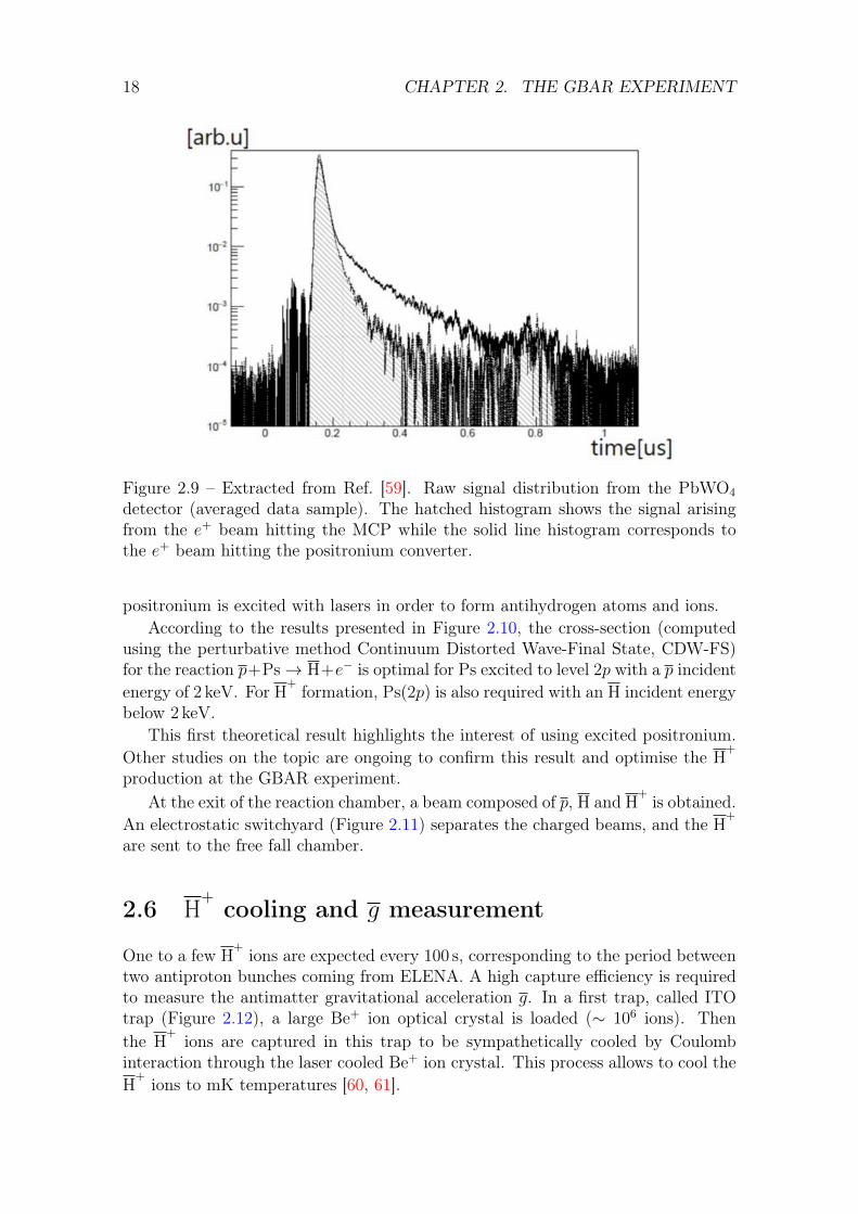
18 CHAPTER 2. THE GBAR EXPERIMENT
Figure 2.9 – Extracted from Ref. [59]. Raw signal distribution from the PbWO4
detector (averaged data sample). The hatched histogram shows the signal arisingfrom the e+ beam hitting the MCP while the solid line histogram corresponds tothe e+ beam hitting the positronium converter.
positronium is excited with lasers in order to form antihydrogen atoms and ions.According to the results presented in Figure 2.10, the cross-section (computed
using the perturbative method Continuum Distorted Wave-Final State, CDW-FS)for the reaction p+Ps→ H+e− is optimal for Ps excited to level 2p with a p incidentenergy of 2 keV. For H
+ formation, Ps(2p) is also required with an H incident energybelow 2 keV.
This first theoretical result highlights the interest of using excited positronium.Other studies on the topic are ongoing to confirm this result and optimise the H
+
production at the GBAR experiment.At the exit of the reaction chamber, a beam composed of p, H and H
+ is obtained.An electrostatic switchyard (Figure 2.11) separates the charged beams, and the H
+
are sent to the free fall chamber.
2.6 H+ cooling and g measurement
One to a few H+ ions are expected every 100 s, corresponding to the period between
two antiproton bunches coming from ELENA. A high capture efficiency is requiredto measure the antimatter gravitational acceleration g. In a first trap, called ITOtrap (Figure 2.12), a large Be+ ion optical crystal is loaded (∼ 106 ions). Thenthe H
+ ions are captured in this trap to be sympathetically cooled by Coulombinteraction through the laser cooled Be+ ion crystal. This process allows to cool theH
+ ions to mK temperatures [60, 61].

2.6. H+ COOLING AND G MEASUREMENT 19
Figure 2.10 – Extracted from Ref. [36]. Top: Cross sections for antihydrogen pro-duction from different states of positronium (Ps(1s) to Ps(3d)). These cross sectionscorrespond to the sum of the antihydrogen states up to H(5d). Bottom: Cross sec-tions for H
+ ion production for Ps(1s) to Ps(3d). Only the H ground state is takeninto account, the contribution of the other states being negligible.
The H+ ions are then transferred into a RF Paul trap named “precision trap”,
where they are cooled to µK temperatures using Raman cooling [62].A laser pulse is sent to remove the extra positron, and the free fall of the neutral
anti-atoms starts. The absorption of the photon and the emission of the positrongive an initial velocity v0 to the ions. The position z can be written as a function

20 CHAPTER 2. THE GBAR EXPERIMENT
Figure 2.11 – Extracted from Ref. [38]. Left: Simulation of the switchyard. Right:Photograph of the switchyard.
of time:z =
1
2gt2 + v0t, g =
mg
mi
g (2.6.1)
The gravity measurement will be performed by detecting the H annihilations onthe vacuum chamber walls. In order to eliminate the cosmic-ray background andto determine precise trajectories of the charged particles coming from the annihila-tion, the free fall chamber (Figure 2.13) will be surrounded by Micromegas trackingdetectors. Also, plastic scintillators will be used to detect the charged pions andprovide the annihilation time with high precision [61].
The uncertainty on g can be written as [63]:
∆g
g= 2
√(∆z
2h
)2
+
(∆v√2gh
)2
(2.6.2)
with h the height the fall, ∆z and ∆v the position and velocity dispersions in thevertical direction.
Heisenberg’s uncertainty principle m∆z∆v ≥ ~/2 limits the relative precisionof(
∆gg
)opt
= 1.7× 10⁻⁴ if g = g and h = 1 m [60]. However, if we take into
account the recoil due to the absorption of the detachment photon, one can assumean uncertainty of ∆v ∼ 1 m s−1 [60], Equation 2.6.2 can be approximated with
∆g
g=√
2∆v√gh
= 0.4 (2.6.3)
per detected atom. So, the 1% resolution can be obtained with about 1600 detectedevents. If we have an event every 100 s, two days of continuous detection are required.
2.7 ConclusionThe purpose of the GBAR experiment is to determine, as said by its name, theGravitational Behaviour of Antimatter at Rest. The corner stone of the experiment
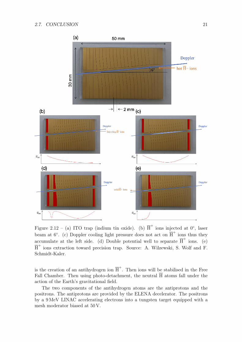
2.7. CONCLUSION 21
Figure 2.12 – (a) ITO trap (indium tin oxide). (b) H+ ions injected at 0, laser
beam at 6. (c) Doppler cooling light pressure does not act on H+ ions thus they
accumulate at the left side. (d) Double potential well to separate H+ ions. (e)
H+ ions extraction toward precision trap. Source: A. Wilzewski, S. Wolf and F.
Schmidt-Kaler.
is the creation of an antihydrogen ion H+. Then ions will be stabilised in the Free
Fall Chamber. Then using photo-detachment, the neutral H atoms fall under theaction of the Earth’s gravitational field.
The two components of the antihydrogen atoms are the antiprotons and thepositrons. The antiprotons are provided by the ELENA decelerator. The positronsby a 9 MeV LINAC accelerating electrons into a tungsten target equipped with amesh moderator biased at 50 V.

22 CHAPTER 2. THE GBAR EXPERIMENT
MicroMegas Triplet
Support mechanics
Raman Laser
Figure 2.13 – Left: Schematic of the Free Fall Chamber. Right: The FFC surroundedby plastic scintillator.
These resulting low energy positrons are accumulated in a Buffer Gas Trap, anda High Field Trap. This step of positron trapping is presented in Chapters 4 and 5.
For the time being, antiprotons have not been trapped yet, because the antipro-ton trap will be delivered during the CERN Long Shut Down. This trapping willbe performed right after the restarting of the ELENA decelerator in 2021. The FreeFall Chamber is under construction and should be delivered beginning 2021.

Chapter 3
Charged particle trapping andtransport
I have an equation, do you have onetoo?
What would have said P. Dirac toR. Feynman in 1946
Contents3.1 Penning-Malmberg trap . . . . . . . . . . . . . . . . . . . 24
3.1.1 Electric field . . . . . . . . . . . . . . . . . . . . . . . . . 24
3.1.2 Classical motion of a particle in the trap . . . . . . . . . . 25
3.2 Non neutral plasma . . . . . . . . . . . . . . . . . . . . . . 28
3.2.1 Conditions to fulfill . . . . . . . . . . . . . . . . . . . . . . 28
3.2.2 Plasma in the Penning-Malmberg trap . . . . . . . . . . . 30
3.3 Realistic traps . . . . . . . . . . . . . . . . . . . . . . . . . 32
3.3.1 Main electric field . . . . . . . . . . . . . . . . . . . . . . 32
3.3.2 The rotating wall technique . . . . . . . . . . . . . . . . . 35
3.4 Magnetic mirroring . . . . . . . . . . . . . . . . . . . . . . 39
3.4.1 Magnetic moment conservation . . . . . . . . . . . . . . . 40
3.4.2 Mirroring conditions . . . . . . . . . . . . . . . . . . . . . 41
3.4.3 Crossing the magnetic mirror . . . . . . . . . . . . . . . . 44
3.5 Conclusion . . . . . . . . . . . . . . . . . . . . . . . . . . . . 45
Penning-Malmberg traps, used to trap charged particles, are made of severalcylindrical electrodes (to create an electrostatic field) and electromagnets (to createa magnetostatic field). They are major elements of many experiments on antimatter.Indeed, antimatter cannot be stored as easily as regular matter, as it has to be keptfar away from any matter component to prevent its annihilation.
23

24 CHAPTER 3. CHARGED PARTICLE TRAPPING AND TRANSPORT
We will examine in this chapter the theory of this kind of traps (Section 3.1) anddetermine useful parameters for the traps of the GBAR experiment (Section 3.2).Also the presentation of a way to compute the electric field in a realistic Penning Trapand some details about the Rotating Wall technique are presented in Section 3.3.Finally, we will explain and determine in Section 3.4 the effect of the magneticmirroring.
3.1 Penning-Malmberg trap
3.1.1 Electric field
As represented in Figure 3.1, an Penning-Malmberg trap is made of 3 cylindricaland concentric electrodes, aligned with a uniform magnetic field B.
To compute the electrostatic field E, we use the electric potential Φ as
∇.E = 0, (3.1.1a)E = −∇Φ, (3.1.1b)4Φ = 0. (3.1.1c)
Figure 3.1 – Representation of a Penning-Malmberg trap.
Due to the symmetries of the problem, the electric and magnetic fields in thecylindrical coordinates r, θ, z can be written:
E = Er + Ez = Er(r, z)er + Ez(r, z)ez, (3.1.2a)B = Bez, (3.1.2b)
with (er, eθ, ez) the unit vectors. We obtain a differential equation for the potential:
1
r
∂
∂r
(r∂Φ
∂r
)+∂2Φ
∂z2= 0 (3.1.3)
It can be shown that a quadratic potential in r and z is a solution of the equation.If we impose the boundary conditions Φ(r,±L)− Φ(r, 0) = ∆V we obtain:
Φ =∆V
2L2
(2z2 − r2
)+ c, (3.1.4)

3.1. PENNING-MALMBERG TRAP 25
with c an arbitrary constant. The expression of the electric field is found by usingthe definition of the potential:
E = −∆V
L2(2zez − rer) . (3.1.5)
This potential can be modelled [41] by an ideal Penning trap as shown in Fig-ure 3.2 using 3 electrodes. The two first (denoted end-cap in Ref. [41]) correspondto an equipotential of the form
z2 = z20 +
r2
2, (3.1.6)
and the third (“ring”) corresponds to an equipotential of the form
z2 =1
2
(r2 − r2
0
), (3.1.7)
choosing z0 and r0 so as to have,
L2 =1
2(2z2
0 + r20). (3.1.8)
z0
r0ring
endcap
B
Ideal Penning trap V > 0
z2 = z20 + r2/2
z2 = (r2 r20)/2
E
z0
r0ring
endcap
B
Ideal Penning trap V < 0
z2 = z20 + r2/2
z2 = (r2 r20)/2
E
Figure 3.2 – Sectional diagrams of the electrodes of an ideal Penning trap used toproduce a quadratic potential of the same form as given to the equation 3.1.4 (redand blue lines). Left: ∆V > 0. Right: ∆V < 0. In green, the electrostatic field.
3.1.2 Classical motion of a particle in the trap
In this section, we discuss the classical motion of a single particle in a Penning trap.The discussion is interesting because it allows to define parameters that are usefulin other sections.

26 CHAPTER 3. CHARGED PARTICLE TRAPPING AND TRANSPORT
To generalise the problem, the variable ε will be used, with ε = +1 for an electronand ε = −1 for a positron, then the electric charge is −εe to obtain the equation ofmotion, we use the expression of the Lorentz force:
ma = −εe (E + v ×B) , (3.1.9)
with m the mass of the positron, and v its velocity.The result of the cross product having no component along the z axis, this
previous equation is decomposed into the (x, y) plane and along the z axis to find acalculation similar to that presented for example in the article of Lowell S. Brownand Gerald Gabrielse [41]:
ρ+εe
m(Er + ρ×B) = 0, (3.1.10a)
z + w2zz = 0, (3.1.10b)
with w2z = −2 εe
m∆VL2 and ρ = rer.
In particular, Equation 3.1.10b shows that to confine the particle along the zaxis we need w2
z > 0, which means having ∆V > 0 for a positron and ∆V < 0 foran electron. So, along this axis, the motion of the particle is described by
z(t) = z0 cos (wzt+ φ0). (3.1.11)
Equation 3.1.10a, which describes the motion in the (x, y) plane can also bewritten
ρ− εωc × ρ−1
2ω2zρ = 0, (3.1.12)
with ωc = eBm> 0, ωc = ωcez.
For a positron (e = 1.602× 10⁻¹⁹ C,m = 9.109× 10⁻³¹ kg), with a magneticfield of 5 T, ∆V = 1 kV and with L = 15 cm:
ωc = 880 GHz, (3.1.13a)ωz = 125 MHz. (3.1.13b)
A first way to solve this differential equation is proposed in the book TrappedCharged Particles [64] and is about writing the relationship 3.1.12 in Cartesiancoordinates:
x+ εωcy −1
2ω2zx = 0, (3.1.14a)
y − εωcx−1
2ω2zy = 0. (3.1.14b)
Defining u = x+ iy, we get the differential equation:
u− iεωcu−1
2ω2zu = 0, (3.1.15)
whose characteristic equation w2−iεωcw− 12ω2z = 0 has w = iε
(ωc2± ω1
)as solutions
with:
ω1 ≡√ω2c
4− ω2
z
2. (3.1.16)

3.1. PENNING-MALMBERG TRAP 27
Both frequencies ω′c and ωm, named respectively reduced cyclotron frequency andmagnetron frequencies are defined as:
ω′c ≡ωc2
+ ω1 =ωc2
+
√ω2c
4− ω2
z
2, (3.1.17a)
ωm ≡ωc2− ω1 =
ωc2−√ω2c
4− ω2
z
2, (3.1.17b)
to get the general solution of Equation 3.1.15:
u = α exp (iεω′ct) + β exp (iεωmt), (3.1.18)
with α, β ∈ C. This leads to the general form of the motion:
x = <(u) = a cos (εω′ct+ φ1) + b cos (εωmt+ φ2), (3.1.19a)y = =(u) = a sin (εω′ct+ φ1) + b sin (εωmt+ φ2), (3.1.19b)
with a, b, φ1, φ2 ∈ R.So in the (xy) plane, the positron has a trajectory composed of two circular
trajectories in the clockwise direction (in the counter clockwise for an electron),with frequencies ωm and ω′c (illustration in Figure 3.3).
z
x y
Figure 3.3 – Illustration of the motion of a charged particle in a Penning-Malmbergtrap. In the (x, y) plane the motion composed of two circular motions. Along the zaxis, there is an oscillation.
It is interesting to notice that the previous definitions impose to fulfil the con-dition: ω2
c
4− ω2
z
2> 0, otherwise we would bring up terms in exp (±ω1t), then the
confinement would be impossible. It is also important to notice that if ∆V is toolarge, then it is not possible to trap. The values in Equation 3.1.13 show that in ageneral use, ωc ωz. In that case, ω
2c
4− ω2
z
2> 0 is fulfilled and the reduced cyclotron
frequency becomes ω′c = ωc − ω2z
2ωcand the magnetron frequency becomes ωm = ω2
z
2ωc.
As a complement, one can notice that the article of Lowell S. Brown and GeraldGabrielse [41] presents another method to solve the case of the electron, this methodis interesting for a quantum treatment of the particle. To adapt this calculation tothe case of a particle with a charge −εe we have to define the vectors V(+) and V(−)

28 CHAPTER 3. CHARGED PARTICLE TRAPPING AND TRANSPORT
as well as the frequency ω+ (ω′c in the previous calculation) and ω− (ωm) by theserelationships:
V(±) = ερ− ω∓ez × ρ (3.1.20a)
ω± =1
2
(ωc ±
√ω2c − 2ω2
z
)(3.1.20b)
These vectors also verify the following differential equation:
V(±) = εω±ez ×V(±) (3.1.21)
This equation represents two vectors rotating at frequencies ω± in the counter clock-wise for an electron, and clockwise for a positron. Then we obtain the ρ vector usingthe definition 3.1.20a:-
ρ = −ez ×
(V(+) −V(−)
)ω+ − ω−
, (3.1.22)
which gives us a vector ρ in the (xy) plane, composed of two rotating vectors atfrequencies ω+ ≡ ω′c and ω− ≡ ωm, as in the previous calculation.
3.2 Non neutral plasma
3.2.1 Conditions to fulfill
A plasma is a collection of charged particles moving under the influence of an externalelectric field. In order to know if the studied system is a plasma, we have to focus ona characteristic scale called the Debye length λD beyond which the external electricfield is screened:
λD =
√ε0kBT
n0e2, (3.2.1)
where ε0 is the vacuum permittivity, kB the Boltzmann constant, n0 the particledensity and e the charge of the particles in the plasma. If we consider L, thecharacteristic length of our trap, we need to verify this first condition:
L λD. (3.2.2)
To understand this, we can use the example given in the book Trapped ChargedParticles [65]. It is about a neutral plasma made of ions (charge +e) and electrons(charge −e) between two ideal electrodes, one with a potential V > 0 and the otherconnected to the ground, and separated by a distance L. In the absence of ionsand electrons, the electric potential between the two electrodes is φ(x) = V
(1− x
L
).
The electrons are attracted by the electrodes at the V potential and the ions by theother, creating a Boltzmann distribution of charges (ne for the electrons, ni for theions) if we suppose a thermal equilibrium at the temperature T :
ne(x) = n0 exp
(eφ(x)
kBT
), (3.2.3a)
ni(x) = n0 exp
(−eφ(x)
kBT
). (3.2.3b)

3.2. NON NEUTRAL PLASMA 29
The Poisson equation gives us a differential equation for the electric potential therebymodified by the charges distribution:
∂2φ
∂x2=
e
ε0(ne(x)− ni(x)) . (3.2.4)
If we assume |eφ/(kBT )| 1 et L λD, we obtain:
φ(x) = V exp(−√
2x/λD
), (3.2.5)
and we find that the field becomes zero for x λD, in other words, the electric fieldis screened by the plasma beyond a characteristic length λD as expected.
Numerically, if we want to trap with a density n0 ∼ 1017 m−3 and a temperaturekBT ∼ 1 eV [52], we can estimate λD as:
λD = 7.4× 10³
√kBT [eV]
n0[m−3](3.2.6a)
= 7.4× 10³
√1
1017 (3.2.6b)
= 20 µm. (3.2.6c)
Also, if we want to consider the plasma as a continuous fluid, the density mustevolve slowly within the average inter-particle space a ≡ n
−1/30 . Since the density
evolves with a characteristic scale λD, we must observe λD n−1/30 , or otherwise
written:
n0λ3D =
(kBT
e2/(ε0a)
) 32
1. (3.2.7)
By observing that the numerator can be related to the kinetic energy and the de-nominator to the potential energy of the mean interaction between two particles ofthe fluid, one can interpret the previous relation differently: the interactions betweenparticles of the fluid are negligible compared to thermal agitation. In an equivalentway, one generally finds in the literature the coupling parameter Γ defined as:
Γ =e2
4πε0akBT∝ a2
λ2D
. (3.2.8)
To summarise, for a strongly correlated plasma (i.e., Γ 1), λD a whichmeans that the collection of charges cannot be considered as a continuous fluid,then all the interactions between particles have to be taken into account . If ourplasma is weakly correlated (i.e., Γ 1), fluid mechanics laws can be used tostudy the plasma and the Boltzmann distribution can describe the thermodynamicequilibrium as done previously.
As an example, let’s see the coupling parameter in the required conditionsfor GBAR experiment. The density is estimated by n0 ∼ 1017 m−3 (then a ∼2× 10⁻⁶ m) and a temperature by kBT ∼ 1 eV. Then the coupling parameter is:
Γ =(1.6× 10⁻¹⁹[C])
2
4π × 8.85× 10−12[C2 s2 kg−1 m−3]× 2× 10−6[m]× 1.6× 10⁻¹⁹[J](3.2.9a)
= 7× 10⁻⁴ 1. (3.2.9b)
In that case, the plasma is weakly correlated.

30 CHAPTER 3. CHARGED PARTICLE TRAPPING AND TRANSPORT
3.2.2 Plasma in the Penning-Malmberg trap
Let’s take a look at the case of a plasma only composed of positrons [65].As explained previously we can use the fluid mechanics to study the behaviour
of our plasma if the relations 3.2.2 and 3.2.7 are respected. To establish the Eulerequation presented in Equation 3.2.10, we work in the cylindrical basis (er, eθ, ez)and we consider three forces:
• an electrostatic force, −en∇φ, with e the charge of the particles in the plasma,n the density and φ the total electric potential;
• magneto-static force, qnv × B, with B = Bez, the magnetic field and v thevelocity of the fluid;
• the pressure force, −∇p, with p the pressure in the fluid.
This gives us the following equation:
mn
(∂v
∂t+ (v.∇)v
)= en (−∇φ+ v ×B)−∇p, (3.2.10)
with m the mass of a particle.Considering we are at the thermal equilibrium, we can affirm that the fluid is
in rotation around the z axis with a frequency of −ωrot (i.e., ∇ × v = −2ωrotez).The − sign comes from the fact that the positrons turn clockwise as shown byEquation 3.1.19 and keeping in mind that this rotation is a mean behaviour of allthe single particles. The speed therefore is written in cylindrical coordinates:
v = −ωrotreθ. (3.2.11)
Let’s begin by the component along the z axis of relation 3.2.10. Because we considerthe plasma as a perfect gas, we can use the relation p = kBTn, which gives:
− en∂φ∂z− kBT
∂n
∂z= 0. (3.2.12)
This relation 3.2.12 can be partially integrated, leaving an r dependent constant ofintegration, N .
n(r, z) = N(r) exp
(−eφ(r, z)
kBT
). (3.2.13)
The component along eθ of relation 3.2.10 being zero, let’s have a look at the relationalong er:
−mnω2rotr = −en
(∂φ
∂r+Bωrotr
)− kBT
∂n
∂r. (3.2.14)
We can also inject Equation 3.2.13 in 3.2.14, which gives a new differential equationfor N :
kBT∂N
∂r= −mωrot (ωc − ωrot) rN, (3.2.15)
with ωc ≡ eBm. This equation can be integrated to get N(r) with a multiplicative
constant:N(r) = C exp
(− 1
kBTωrot(ωc − ωrot)
r2
2
). (3.2.16)

3.2. NON NEUTRAL PLASMA 31
Thus we obtain the expression of n(r, z):
ωrotn(r, z) = C exp
(−eφ(r, z) + φeff(r)
kBT
), (3.2.17)
by defining an effective potential φeff as :
eφeff(r) ≡ 1
2mωrot (ωc − ωrot) r
2. (3.2.18)
This effective potential allows the radial confinement of the plasma. Equa-tion 3.2.17 shows that the effective potential has to fulfil φ(r, z) +φeff(r) > 0,∀(r, z)to make the confinement possible. However, because for some z position we mayhave φ(r, z) = 0, the condition to fulfil is φeff > 0,∀r. This leads to the followingrelations for the frequencies:
0 <ωrot
ωc< 1. (3.2.19)
Another way to understand the problem would be to consider that the plasmais not confined by the magnetic field but by virtual negative charges of densityn0 whose electric potential would be φeff . Thereby, by using the Poisson equation(4φeff = en0/ε0), we obtain the density of charge:
n0 =2mε0e2
ωrot(ωc − ωrot). (3.2.20)
In the article of Malmberg and O’Neil [66], it is explained that the density of thereal particles matches with the uniform density of virtual particles up to a certainradius (cylindrical symmetry). If we assume that the Debye length (Equation 3.2.1)is smaller than the radius of the cylinder, the density of positrons (electrons in thearticle) falls sharply beyond this radius. Indeed, if we consider that the virtualcharges neutralise the charge of our positrons, there is a radius where the supply ofpositrons is exhausted, because there is a finite amount of them.
0 C/2rot
0
nB
n 0
Figure 3.4 – Density of positrons as a function of the rotation frequency of theplasma. This density is maximal for ωrot = ωc/2, the so-called Brillouin limit.
Now we have a relation between the density of particles in the trap, the rotationfrequency and the magnetic field (represented at Figure 3.4):
n =2mε0e2
ωrot(ωc − ωrot). (3.2.21)

32 CHAPTER 3. CHARGED PARTICLE TRAPPING AND TRANSPORT
This relation also indicates that a maximal density of positrons called the Brillouinlimit appears for ωrot = ωc/2 (ωc = eB/m):
nB =mε0ω
2c
2e2=ε0B
2
2m=B2/(2µ0)
mc2, (3.2.22)
with µ0 vacuum permeability and c the speed of light.
3.3 Realistic traps
3.3.1 Main electric field
As shown in Section 3.1.1, in the case of the ideal Penning-Malmberg trap, the po-tential is quadratic. However, in practice the potential cannot be quadratic becauseit cannot be infinite. Besides, the traps are made of more than 3 electrodes to beable to manipulate the particles. Then in this section, we describe how to computeanalytically the electric potential for a set of cylindrical electrodes. This section ismostly inspired by the work presented in the thesis of Christopher Aled Isaac [67].
First of all, only one electrode is taken into account, and the effect of the otherelectrodes will be added using the superposition principle. Therefore, let’s considera cylindrical electrode of radius R and of half-length z0 with a potential V = 1 V.Let’s also consider that there are two infinite cylindrical electrodes of radius R onboth sides of the considered electrode, with a potential V = 0, then the potentialat r = R is φ(R, z) = H(z + z0) − H(z − z0), with H the Heaviside function (seeFigure 3.5). L0 is an integration limit with L0 z0 and we impose φ(r, L0) = 0,∀r.
z0 +z00L0 L0z
0
1
V
Potential at r = R
z0 +z00
-R
+R
0
ElectrodesElectrode V, = 1Virtual electrode, V = 0
Figure 3.5 – Left: the boundary conditions for one electrode at r = R. Right:representation of the electrode on the (r, z) plane: the real electrode is between −z0
and +z0, the rest is a virtual electrode with the potential 0 on it.
To solve the Poisson equation (Equation 3.1.3) it is first assumed that the solutionhas the form:
φ(r, z) = f(r)g(z). (3.3.1)

3.3. REALISTIC TRAPS 33
The Poisson equation becomes
1
f(r)
(1
r
df
dr+
d2f
dr2
)+
1
g(z)
d2g
dz2= 0, (3.3.2)
where the two terms depend on two separate variables. This implies, the first termis equal to a constant ±k2 and the second to the opposite:
1
f(r)
(1
r
df
dr+
d2f
dr2
)= − 1
g(z)
d2g
dz2= ±k2 (3.3.3)
The physical equation has to be the one with +k2 otherwise g would be a hyper-bolic function, which is impossible in our case because we cannot have an infinitepotential. Then we obtain the two following equations
r2 d2f
dr2+ r
df
dr− (kr)2 f(r) = 0, (3.3.4a)
d2g
dz2+ k2g(z) = 0. (3.3.4b)
The solution of the first equation is a modified Bessel function, then f(r) =
I0(kr) =∑∞
m=0 = 1m!Γ(m+1)
(kr2
)2m. The second equation can be integrated as g(z) =
Ak cos (kz) + Bk sin (kz). Because the function has to be even, Bk = 0. Moreover,the boundary conditions give g(L0) = 0 = Ak cos (kL0). Then, the general solutionwill be
φ(r, z) =∑m≥0
AmI0(kmr) cos (kmz), (3.3.5)
with km =(m+ 1
2
)πL0.
Now, to determine Am we use the fact that we know φ(R, z):∫ L0
−L0
dz cos (km′z)φ(R, z) =∑m≥0
AmI0(kmR)
∫ L0
−L0
dz cos (km′z) cos (kmz),∫ z0
−z0dz cos (km′z) =
∑m≥0
AmI0(kmR)L0δm,m′ ,
Am =2 sin (kmz0)
L0kmI0(kmR).
Then, the potential can be written:
φ(r, z, z0) =∑m≥0
2
L0kmsin (kmz0) cos (kmz)
I0(kmr)
I0(kmR)(3.3.6)
To compute numerically the potential, we have to determine a limit for thesummation. For the computations presented in this document, an algorithm similarto Algorithm 1 has been written.

34 CHAPTER 3. CHARGED PARTICLE TRAPPING AND TRANSPORT
Algorithm 1 Computation of φ(r, z, z0)
Require: z0, R, r, zφ = 0i = 0ε = 10−10
e = 1L0 = 20z0
while |e| ≥ ε dok = (i+ 1
2) πL0
e = 2L0k
sin (kz0) cos (kz) I0(kr)I0(kR)
φ = φ+ ei = i+ 1
end while
Thanks to the superposition principle, it is now straightforward to obtain theelectric potential created by N cylindrical and concentric electrodes of same radii.If the electrode n of length 2z0,n is placed at zn under a potential Vn, one writes:
φ(r, z) =N∑n=1
Vnφ(r, z − zn, z0,n). (3.3.7)
An illustration of the computation of the potential at r = 0 using Algorithm 1 ispresented in Figure 3.6. As one can imagine, the smaller the radius of the electrodeis compared to its length, the closer to the potential of the electrode the potentialat r=0 is. It is also interesting to see that one can fit the potential with a quadraticfunction when z z0.
0 z0 3z0 5z0z03z05z0z
0.0
0.2
0.4
0.6
0.8
1.0
Pote
ntia
l (V)
at r
=0
R = 2z0boundary conditionrealistic potentialquad fit
0 z0 3z0 5z0z03z05z0z
0.0
0.2
0.4
0.6
0.8
1.0
Pote
ntia
l (V)
at r
=0
R = z0boundary conditionrealistic potentialquad fit
0 z0 3z0 5z0z03z05z0z
0.0
0.2
0.4
0.6
0.8
1.0
Pote
ntia
l (V)
at r
=0
R = z0/2boundary conditionrealistic potentialquad fit
Figure 3.6 – Illustration of the computation of the electric potential for a trap madeof 3 electrodes of 1 cm length.
However, there are two restrictions for this computation. The first one is thatwe have to ensure that L0 z0,n for all the electrodes, and the second one is that,as said before, all the electrodes must have the same radius, because the boundaryconditions would be incompatible for the different electrodes. In the case of differentradii, it would be better to use a simulation by finite element of the potential.

3.3. REALISTIC TRAPS 35
3.3.2 The rotating wall technique
The principle of the rotating wall technique [68], is to add an angular momen-tum to the plasma to compress it and to compensate the defects of the trap.Indeed, a spatially uniform positron plasma has a canonical angular momentumPθ = Nm(ωc/2 − ωrot) < r2 > [69], where N is the total number of positrons ofmass m, ωrot is the rotation frequency, ωc the cyclotron frequency as introduced inSection 3.1.2 and < r2 > is the mean square radius of the plasma fluid. If one canapply the drift approximation (i.e. ωrot ωc), we clearly have Pθ > 0, and thisis why adding a negative torque decreases the angular momentum, i.e., decreases< r2 > and compresses the plasma.
To add a negative torque, we use a split electrode and apply an oscillating signalof same frequency on each part of the cylindrical electrode, with a constant phaseshift between two neighbour parts. In our case the cylindrical electrode is split in4 and the phase is 90. This section is a re-explanation of what can be found inIsaac’s thesis [67].
To solve the Poisson equation in that case, we consider the potential on theelectrode is Φ(θ), as shown in Figure 3.7. Similarly to what has been done inSection 3.3.1, φ(r = R, θ, z) = Φ(θ) only on the electrode, i.e. for z ∈ [−z0, z0]and the potential is null outside this limit. Also, integration limit L0 z0 such asφ(r, θ, z = L0) = 0 needs to be set.
Φ(θ) =
−Va 3π
4≤ θ < −3π
4
−Vb −3π4≤ θ < −π
4
Va −π4≤ θ < π
4
Vbπ4≤ θ < 3π
4
(3.3.8)
R 0 R
R
0
R
VaVa
Vb
Vb
Figure 3.7 – Boundary conditions for an electrode split in four.
As in Section 3.3.1, one can assume that the potential is a product of three

36 CHAPTER 3. CHARGED PARTICLE TRAPPING AND TRANSPORT
independent functions:φ(r, θ, z) = f(r)g(z)h(θ), (3.3.9)
therefore, the Poisson equation leads to
4φφ
=1
fr
d
dr
(r
df
dr
)+
1
hr2
d2h
dθ2+
1
g
d2g
dz2= 0. (3.3.10)
The same argument as the one used in the previous section can be used again tofind the general expression for g:
gm(z) = A cos(kmz), km =
(m+
1
2
)π
L0
,m ∈ N. (3.3.11)
For the angular part h, again, the fact that the variables are separated leads to:
1
h
d2h
dθ2= ±n2. (3.3.12)
To keep the potential finite at large distances, the only physical equation is the onewith −n2, which gives us the general form for h:
hn(θ) = a cos(nθ) + b sin(nθ). (3.3.13)
In order to find a condition on n, we use the fact that in cylindrical coordinates anyfunction of θ must be 2π-periodic, i.e. h(θ+ 2π) = h(θ), which leads to the coupledequations:
a (cos(2nπ)− 1) + b sin 2nπ = 0,
a sin 2nπ + b (1− cos(2nπ)) = 0.
A non trivial solution (a 6= 0, b 6= 0) requires the determinant of the system to benull, which leads to cos(2nπ) = 1, and then the condition on n is: n ∈ N.
Inserting the previous result in Equation 3.3.10, the previous results leading to
r
f
d
dr
(r
df
dr
)−(k2mr
2 + n2)
= 0, (3.3.14)
the solution for the radial part is then the modified Bessel functions of the first kindof order n:
fn,m(r) = In(kmr) (3.3.15)
All of this gives the general solution of the equation which is:
φ(r, θ, z) =∑n,m≥0
In(kmr)Amn cos(kmz) (amn cos(nθ) + bnm sin(nθ)) . (3.3.16)
Now to determine the coefficients, the boundary condition φ(R, θ, z) = Φ(θ), z ∈[−z0, z0] is used as follows:∫ L0
−L0
φ(R, θ, z) cos(klz)dz =
∑n,m≥0
In(kmR)Amn (amn cos(nθ) + bnm sin(nθ))
∫ L0
−L0
cos(kmz) cos(klz)dz (3.3.17)

3.3. REALISTIC TRAPS 37
Φ(θ)
∫ z0
−z0cos(klz)dz =
∑n,m≥0
In(kmR)Amn (amn cos(nθ) + bnm sin(nθ))L0δm,l,
and then the following expression for Φ is obtained:
Φ(θ) =km
2 sin(kmz0)
∑n≥0
AmnIn(kmR)L0 (amn cos(nθ) + bnm sin(nθ)) . (3.3.18)
By developing Φ as Fourier series:
Φ(θ) =∞∑n=1
4
nπ
(Va sin
(nπ2
)cos(nπ
4
)cos (nθ) + Vb sin
(nπ2
)sin(nπ
4
)sin (nθ)
)(3.3.19)
one can identify amn and bmn, which become now an and bn.Finally, the potential can be written as:
φ(r, θ, z) =∑n,m≥0
In(kmr)Amn cos(kmz) (an cos(nθ) + bn sin(nθ)) (3.3.20)
with
an =4Vanπ
(sin(nπ
2
)cos(nπ
4
))(3.3.21a)
bn =4Vbnπ
(sin(nπ
2
)sin(nπ
4
))(3.3.21b)
Amn = 0 n = 0 (3.3.21c)
Amn =2 sin(kmz0)
kmL0In(kmR)n 6= 0 (3.3.21d)
As said before, we will apply an oscillating potential on each part on the electrodewith a phase of 90 between adjacent parts. Then, Va and Vb are defined as:
Va = VRW cos (ωrt) (3.3.22a)
Vb = VRW cos(ωrt+
π
2
)= −VRW sin (ωrt) (3.3.22b)
An illustration of the potential is presented in Figure 3.8 where it is possible to seethat the equipotentials rotate with the same frequency as the oscillating potential.
However, it is not necessary to use such a complicated expression to predict whatis happening in the trap. Indeed, if it is assumed that the plasma radius is muchsmaller than the radius of the electrode, then a limited expansion can be done. Let’sstart with the limited expansion of In:
In(x) =∑l≥0
1
l!Γ(n+ l + 1)
(x2
)(2l+n)
. (3.3.23)
In that case, x = kmr, with x 1, because r R,L0, and then, the expansionat the first order in x is In(x) = In(0) + I ′n(0)x + o(x). For this computation, thederivative is then required:
I ′n(x) =1
2
∑l≥0
2l + n
l!Γ(n+ l + 1)
(x2
)(2l+n−1)
. (3.3.24)

38 CHAPTER 3. CHARGED PARTICLE TRAPPING AND TRANSPORT
t = 0 t = 2 × (1/8) t = 2 × (2/8) t = 2 × (3/8)
t = 2 × (4/8) t = 2 × (5/8) t = 2 × (6/8) t = 2 × (7/8)
Figure 3.8 – Representation of the potential produced by a rotating wall with afrequency ωr according to Equation 3.3.20 and Equation 3.3.22. The yellow areasrepresent a potential of +Vr and the blue of −Vr.
It is clear that at x = 0, all the terms are null except when 2l + n − 1 = 0, andknowing that n ≥ 1, the only possibility is when n = 1 and l = 0. Then atfirst order, only n=1 gives a non null contribution to the total expansion and withI ′1(0) ≈ 1
2Γ(2)= 1
2, we get I1(kmr) ≈ 1
2kmr. Finally, the recombination of the terms
leads to a1 cos(θ) + b1 sin(θ) = 2√
2πVRW cos(ωrt+ θ).
In the end, with this approximation, the potential is the one of a rotating dipole:
φ(r R, θ, z) ≈ VRWr cos(ωrt+ θ)
(2√
2
πL0
∑m≥0
cos(kmz) sin(kmz0)
I1(kmR)
)(3.3.25)
Isaac also showed in his thesis [67] that by using a quadratic potential and aoscillating dipole
φ(z, r, θ) =V0
2d2
(z2 − r2
2
)+m
qazr cos (θ + ωrt) (3.3.26)
in the motion equations of a particle (which is correct according to what has beenshown before), and adding a viscosity drag force F = −κv, a compression rate Γ isobtained and defined as
Γ =κ
4
(1−
∣∣∣∣ ω√1 + ω2
∣∣∣∣) , (3.3.27)
where
ω =ωr + (ωz + ω−)
δ, (3.3.28a)
δ =a
√ωcωz
, (3.3.28b)
ωc, ωz, ω− defined in Section 3.1.2. In that case, the maximal compression is forω = 0.

3.4. MAGNETIC MIRRORING 39
3.4 Magnetic mirroring
In particle physics experiments such as the GBAR experiment, particles have totravel through different spatial regions, each of them being influenced by a differentsource of magnetic field. These variations in the magnetic field may create what isnamed magnetic mirroring. As a more specific example, if a positron following amagnetic field line approaches a Penning-Malmberg trap with a stronger magneticfield, the positron may be repelled. In this section, the conditions to cross a magneticmirror are presented.
Let’s consider a positron following a magnetic field line. Locally, the field can beapproximated along the z-axis (as presented in Figure 3.9). In the cylindrical framewhere the main axis is the one whose the particle is wrapping around, er, eθ, ez, thevelocity vector can be written:
v = −v⊥eθ + v‖ez, (3.4.1)
with v⊥ = rωc = r eBm, the minus sign coming from the fact that a positron would
go clockwise.
e +
v
v
B
Figure 3.9 – Illustration of a positron following a magnetic field line.
For the rest of the demonstration of the magnetic mirroring effect, we need tointroduce the magnetic moment of the positron. In the case of the positron with acircular trajectory with the frequency ωc = eB
m, the magnetic moment is:
µ =mv2⊥
2B(3.4.2)
Instead of solving the complete dynamic equation in order to know what happenswhen the particle goes from a region with Bi = Biez to a region with Bf = Bfez,the problem can be simplified. If the field evolves slowly compared to characteris-tic durations and lengths of the particle motion, the magnetic moment µ remainsconstant. This is what is called the adiabatic approximation.
A way to determine if this approximation is fulfilled is to compare with thecharacteristic duration 1/ωc = m
qBand characteristic length rc = v⊥
ωc= mv⊥
qB. This

40 CHAPTER 3. CHARGED PARTICLE TRAPPING AND TRANSPORT
leads to write ∣∣∣∣ 1
B
∂B
∂t
∣∣∣∣ ωc, (3.4.3a)∣∣∣∣∇BB∣∣∣∣−1
rc. (3.4.3b)
A particle of ∼ 50 eV energy has a speed of 4 m µs−1. It travels δx = 10 cm inδt = 25 ns. In a magnetic field of ∼ 10 mT, the cyclotron frequency is ωc = 1.8 GHzand if we assume 1
2mv2⊥ ∼ 1 eV, rc = 0.3 mm. We consider that during this travel,
the variation of the magnetic field does not exceed 1BδB = 30 % (as presented in
Figure 4.7 of the Buffer Gas Trap chapter, see the variation on 10 cm at the level ofa cross). With all these parameters, we obtain:∣∣∣∣ 1
B
∂B
∂t
∣∣∣∣ =δB/B
δt= 0.012 GHz ωc (3.4.4a)∣∣∣∣∇BB
∣∣∣∣−1
=δx
δB/B= 30 mm rc (3.4.4b)
So can consider now that we can use the adiabatic approximation.
3.4.1 Magnetic moment conservation
To prove the adiabatic approximation, let’s first consider a magnetic field with acylindrical invariance (such as the one created by a coil or solenoid). In that case,the magnetic field is written as B = Brer + Bzez. The Maxwell-Gauss equation∇ ·B = 0 leads to
Br = −r(∂Br
∂r+∂Bz
∂z
). (3.4.5)
If we consider that we stay close of the axis, a limited expansion gives
Br = r∂Br
∂r. (3.4.6)
Combined with Equation 3.4.5 written r ∂Br∂r
= −Br − r ∂Bz∂z , we obtain
Br = −1
2r∂Bz
∂z. (3.4.7)
Then, the component along the main axis of the magnetic force is F = ev ×Bis Fz = −e rv⊥
2∂Bz∂z
, which can be written
Fz = −µ∂B∂z
. (3.4.8)
This expression can be generalised in 3-dimension as
F‖ = −µdB
dl, (3.4.9)

3.4. MAGNETIC MIRRORING 41
with dl an infinitesimal line element along B.We now have all the elements to prove the adiabatic approximation. Starting
from the Newton equation
mdv
dt= F, (3.4.10)
By multiplying this expression by v‖(m
dv‖dt
= F‖
)v‖,
and considering that v‖ = dsdt, the line element can be removed as
m
2
dv2‖
dt= −µdB
ds= −µdB
ds
ds
dt.
The following expression is obtained
m
2
dv2‖
dt= −µdB
dt. (3.4.11)
To obtain the evolution of µ during the travel of the particle, we have to take intoaccount that the kinetic energy is conserved, then m
2
dv2‖dt
+ m2
dv2⊥dt
= m2
dv2‖dt
+ dµBdt
= 0and the expression of the magnetic moment brings
m
2
dv2‖
dt= −dµB
dt. (3.4.12)
Finally, the combination of Equation 3.4.11 and Equation 3.4.12 gives
dµ
dt= 0 (3.4.13)
which means that the magnetic moment is conserved along the trajectory.
3.4.2 Mirroring conditions
Starting from the adiabatic approximation
µ =mv2⊥
2B= constant, (3.4.14)
the relationship between the perpendicular velocity and the magnetic field is ob-tained:
v2⊥i
B2i
=v2⊥f
B2f
, (3.4.15)
for a particle initially in an area with a magnetic field Bi travelling to an area withBf . If we name θ the angle between the velocity vector and the field line (seeFigure 3.10), then Equation 3.4.15 can be rewritten:
sin2 (θi)
Bi
=sin2 (θf )
Bf
(3.4.16)
⇔ sin2 (θf ) =Bf
Bi
sin2 (θi) (3.4.17)

42 CHAPTER 3. CHARGED PARTICLE TRAPPING AND TRANSPORT
To obtain the mirroring condition, we use the fact that for all θf the condition,sin2 (θf ) ≤ 1 has to be fulfilled if the particle goes across the magnetic mirror. Sothe maximal angle θimax is given by
θimax = arcsin
(√Bi
Bf
). (3.4.18)
Here, it is implicit that Bi < Bf , in the opposite case, there is no magneticmirroring and the condition sin2 (θi) ≤ 1 can be used to obtain the maximal angleof the particles in the Bf field
θfmax = arcsin
(√Bf
Bi
). (3.4.19)
Figure 3.10 – Extracted from Ref. [52]. On this schematic four magnetic field linesare represented as well as two particles with different initial conditions. The cy-clotron motion is not represented. In the case of the red positron, we have θi < θimax,then the particle can go across the magnetic mirror and we get a positron withθf > θi. For the green positron, θi > θimax and we see that θ is increasing duringthe travel to reach the point where the particle can only go backward: this is themagnetic mirror.
As an example, let’s see what is happening with the traps of the GBAR exper-iment. We want to send the positrons arising from the moderator (see Figure 2.5and Ref. [44]) into one of the traps. The magnetic field is Bi = 10 mT from themoderator. If the positrons are sent straight to the Buffer Gas Trap (BGT), themagnetic field is Bf = 0.02 T. In the case of positrons sent straight to the HighField Trap (HFT) the magnetic field is Bf = 5 T. Then, the maximal angle at theexit of the moderator is
θi,BGT = 0.79 rad, (3.4.20)
when the positrons are sent to the BGT and
θi,HFT = 4.5× 10⁻² rad, (3.4.21)

3.4. MAGNETIC MIRRORING 43
when the positrons are sent to the HFT. One can conclude here that only thepositrons with a momentum almost parallel to the magnetic field can enter insidethe HFT, and in the case of the BGT, a larger angular distribution is accepted.
It is also interesting to compute the efficiency of the positron transfer. If we con-sider that the angular distribution is uniform after the moderator [44], the angulardistribution is written f(θ, φ) = 1
2π(see Figure 3.11), then the transfer efficiency is
ε =
∫ φ=2π
φ=0
∫ θ=θimax
θ=0
sin (θ) dθdφ
2π= 1− cos (θimax) = 1− cos
(arcsin
(√Bi
Bf
)),
(3.4.22)noticing that cos (arcsinx) =
√1− x2, the efficiency can be written as:
ε = 1−
√1− Bi
Bf
, (3.4.23)
and the numerical application for the trap gives
εBGT = 0.30, (3.4.24)εHFT = 1.0× 10⁻³. (3.4.25)
x
y
z
[0, 2 ]
[0, max < /2][0, max < /2]
Figure 3.11 – Illustration of uniform angular distribution of momenta after themoderator.
We clearly see that for the BGT, the efficiency is relatively low but at leastwe can transfer a significant part of the positrons. If we try to send the positronsdirectly inside the HFT, the efficiency is drastically low. Thankfully, there is a wayto improve this transfer efficiency in giving extra energy to the particles, this is whatwe will demonstrate in the next paragraph.

44 CHAPTER 3. CHARGED PARTICLE TRAPPING AND TRANSPORT
3.4.3 Crossing the magnetic mirror
A way to cross a magnetic mirror is to give extra momentum along the magnet axisto the particle thanks to an electric potential. To see how it works, let’s consider apositron with a total energy E, a velocity v, and an angle between the momentumand the main axis θi. In this case, we define the “perpendicular” and the “parallel”energy such as
E⊥ =1
2mv2⊥ =
1
2mv2 sin2(θi) = E sin2(θi), (3.4.26)
E‖ =1
2mv2‖ =
1
2mv2 cos2(θi) = E cos2(θi). (3.4.27)
If we give to the particle momentum along the parallel axis using an electricfield, corresponding to an energy E , it is equivalent to add E to the parallel energythereby written
E ′‖ = E cos2(θi) + E = E + E − E sin2(θi). (3.4.28)
Consequently the total energy being now E + E , the parallel energy can also bewritten
E ′‖ = (E + E) cos2(θ′i) = (E + E)− (E + E) sin2(θ′i). (3.4.29)
So the new angle between the momentum and the main axis after acceleration isexpressed as
sin2(θ′i) =E
E + Esin2(θi), (3.4.30)
and Equation 3.4.17 becomes
sin2(θf ) =Bf
Bi
E
E + Esin2(θi). (3.4.31)
This is similar to increasing the initial magnetic field from Bi to B′i with
Bi → B′i = BiE + EE
, (3.4.32)
and if B′i ≥ Bf , the magnetic mirror is counterbalanced.Finally, to know what is the maximal angle allowing to cross the magnetic mirror,
we look for the angle such as sin2(θf ) = 1, leading to
θi,max = arcsin
(√Bi
Bf
E + EE
), (3.4.33)
and the efficiency for an original uniform distribution becomes,
ε = 1−
√1− Bi
Bf
E + EE
. (3.4.34)
If B′i > Bf , we have ε = 1 and
θf,max = arcsin
(√Bf
Bi
E
E + E
)(3.4.35)

3.5. CONCLUSION 45
In the case of the Buffer Gas Trap in the GBAR experiment, the positrons havean energy of E = 3 eV (see Figure 2.5 and Ref. [44]) and are accelerated to E = 50 eV.The magnetic fields are still Bi = 10 mT and Bf = 20 mT. The computation givingB′i = 176 mT > Bf , all the positrons go through the magnetic mirror with
θf,max = 0.34 rad (3.4.36)
If we wanted to send the positrons directly into the HFT, the magnetic fieldbeing Bf = 5 T we would obtain
θi,max = 0.19 rad, (3.4.37)ε = 0.018. (3.4.38)
With an extra-energy of E = 1 kV, as it was the case during the first tests of theGBAR experiment at CEA Saclay [52], we would have
θi,max,HFT = 0.96 rad, (3.4.39)ε = 0.42. (3.4.40)
3.5 ConclusionIn this chapter, it has been shown how to compute the electric field produced by aPenning-Malmberg trap and the behaviour of charged particles trapped in it. Twointeresting parameters have been introduced, the Debye length (Equation 3.2.1)which has to be small compared to the characteristic length of the trap if we wantto consider the collection of particles as a plasma, and the coupling parameter (Equa-tion 3.2.8) which is a scale of correlation of the plasma. A weakly correlated plasmacan be considered as a continuous fluid. Otherwise, the interactions between parti-cles have to be considered. Also, it has been seen that there is a maximal densityof particles in a non neutral-plasma, the Brillouin limit (Equation 3.2.22) which isproportional to the magnetic field.
Furthermore, the rotating wall technique was presented, which is used in thepositron traps of the GBAR experiment. An oscillating potential is added on anelectrode split in 4, and on each part, there is a 90 phase shift with respect to itsneighbours, which creates an oscillating dipole. With the appropriate rotating wallfrequency, the plasma is compressed.
Finally, a complete description of the concept of magnetic mirror was presentedand how to cross this barrier.


Chapter 4
The Buffer Gas Trap
It’s a trap!
Admiral Ackbar, Return of the Jedi
Contents4.1 Principle of the Surko-Greaves Trap . . . . . . . . . . . . 48
4.2 Description of the trap . . . . . . . . . . . . . . . . . . . . 51
4.2.1 Sets of electrodes . . . . . . . . . . . . . . . . . . . . . . . 52
4.2.2 Electric potential . . . . . . . . . . . . . . . . . . . . . . . 52
4.2.3 Magnetic Field . . . . . . . . . . . . . . . . . . . . . . . . 54
4.2.4 Gas and vacuum . . . . . . . . . . . . . . . . . . . . . . . 55
4.3 Trap control . . . . . . . . . . . . . . . . . . . . . . . . . . . 65
4.3.1 Vacuum system and magnets control . . . . . . . . . . . . 66
4.3.2 Trapping control . . . . . . . . . . . . . . . . . . . . . . . 66
4.4 Positron detection . . . . . . . . . . . . . . . . . . . . . . . 72
4.4.1 Micro-Channel Plate . . . . . . . . . . . . . . . . . . . . . 72
4.4.2 CsI detector . . . . . . . . . . . . . . . . . . . . . . . . . . 73
4.5 Electron repeller . . . . . . . . . . . . . . . . . . . . . . . . 74
4.5.1 Electron repeller version 1 . . . . . . . . . . . . . . . . . . 74
4.5.2 Electron repeller version 2 . . . . . . . . . . . . . . . . . . 77
4.6 Accumulation in the first and second stages . . . . . . . 80
4.6.1 Gas parameters . . . . . . . . . . . . . . . . . . . . . . . . 81
4.6.2 Rotating Wall optimisation . . . . . . . . . . . . . . . . . 84
4.6.3 Energy distribution after second stage accumulation . . . 85
4.7 Third stage . . . . . . . . . . . . . . . . . . . . . . . . . . . 87
4.7.1 Re-trapping . . . . . . . . . . . . . . . . . . . . . . . . . . 87
4.7.2 RW optimisation . . . . . . . . . . . . . . . . . . . . . . . 89
47

48 CHAPTER 4. THE BUFFER GAS TRAP
4.7.3 Energy distribution . . . . . . . . . . . . . . . . . . . . . . 92
4.7.4 Stacking . . . . . . . . . . . . . . . . . . . . . . . . . . . . 92
4.8 Conclusion . . . . . . . . . . . . . . . . . . . . . . . . . . . . 93
In this chapter will be presented the experiments performed with the first Pen-ning trap of the GBAR experiment. This trap, named Buffer Gas Trap (BGT), is aclone of the Swansea’s trap [70], itself based on the Surko-Greaves Trap [46, 47].
The purpose of this BGT is to accumulate positrons coming from the linearaccelerator (LINAC) of the experiment, using N2 gas for the capture and CO2 toreduce the energy spread. The positron bunch thus prepared must also be radiallycompressed. This is obtained using the rotating wall technique (principle presentedin Section 3.3.2).
The LINAC provides positrons in pulses. It is used currently with a frequencyof 200 Hz. In the future, this frequency is planned to be increased to 300 Hz. Whenenough positrons are accumulated in the first and second stage of the BGT they aretransferred into a third stage to overcome the trap saturation, and a short lifetime(τ < 1 s) due to the gas pressure (10−3−10−4mbar). In this third stage, the pressureis lower (∼ 10−6 mbar), so positrons can be stored for a longer time (τ ∼ 10 s). Thesequence of accumulation in the first and second stage followed by the transfer tothe third stage is repeated until the maximum amount of positrons in the third stageis reached. In the rest of the document, the transfer operation of positron bunchesfrom one stage to another is named stacking.
Once the positron number in the third stage is large enough, the positrons aresent into another trap named High Field Trap (HFT), that has a higher capacity tostore positrons: this is a stacking procedure which has to be repeated to trap moreand more positrons.
The principle of a Surko-Greaves Trap is presented in Section 4.1, then a completedescription of the BGT is detailed in Section 4.2 as well as the control of the trap inSection 4.3. Then, in Section 4.4 are explained the main concepts of the devices usedto detect the trapped the positrons. Also, a study on the electron repeller placedupstream of the BGT is presented in Section 4.5 because this repeller will have animportance on the trapping efficiency. Finally, the experimental results concerningthe positrons trapping are shown in Section 4.6 and Section 4.7.
4.1 Principle of the Surko-Greaves Trap
The Surko-Greaves Trap (originally developed by Surko and subsequently modifiedby Greaves) has been developed in order to accumulate positrons from radioac-tive sources and to deliver a positron beam, well focused and with a small energyspread [46, 71].
In the Surko-Greaves scheme, the trap is made of three long electrodes and twoshort electrodes at the entrance and exit as presented in Figure 4.1. N2 gas isinjected into the system so that inelastic collisions with the positrons make themloose enough energy to be trapped. The pressure decreases from the entrance to theexit to allow a long term storage in the last stage of the trap.

4.1. PRINCIPLE OF THE SURKO-GREAVES TRAP 49
Figure 4.1 – Extracted from Ref. [47]. Schematic diagram of a Surko-Greavespositron accumulator, showing the three stages of differential pumping and the elec-trostatic potential. A represents the energy loss by inelastic collisions, B and Crepresent lower energy collisions. The electrostatic potential is set to maximise thepositron trapping efficiency (between stages ∆V ∼ 9− 10 V).
The choice of trapping gas is a compromise between its slowing power and therate of positron annihilation. According to the results [47] presented in Table 4.1,N2 is the best choice among all the possible tested gases.
Gas Formula Trapping efficiency (%)Nitrogen N2 100
Carbon monoxide CO 68Oxygen O2 43
Sulfur dioxide SO2 33Hydrogen H2 30
Nitrous Oxide NO2 20Carbon dioxide CO2 16
Sulfur hexafluoride SF6 7Carbonyl sulfide OCS 4
Table 4.1 – Extracted from Ref. [47]. Summary of trapping efficiencies, normalisedto nitrogen for a selection of gases.
As presented in Table 4.2, several reactions can happen between N2 and positrons.In particular, we have to focus on electronic excitation and positronium formation.Electronic excitation makes the positrons lose about 10 eV of kinetic energy whichis suitable for trapping in a ∼ 10 V well. However, its energy threshold of 8.59 eVis close to the energy threshold of positronium formation, 8.78 eV, which has to

50 CHAPTER 4. THE BUFFER GAS TRAP
be avoided. Even if by varying the difference of potentials between electrodes, onecan give more or less energy to favour one of the reactions it is impossible to trappositrons without losing some of them by annihilation.
Name Reaction Energy thresholdAnnihilation e+ + N2 → N2
+ + 2γ -Electronic scattering e+ + N2 → N2 + e+ -Rotational excitation e+ + N2 → N2
rot + e+ ∼ 1 meVVibrational excitation e+ + N2 → N2
vib + e+ ∼ 0.3 eVElectronic excitation e+ + N2 → N2
∗ + e+ 8.59 eVPositronium formation e+ + N2 → N2
+ + Ps 8.78 eVIonisation e+ + N2 → N2
+ + e+ + e− 15.6 eV
Table 4.2 – Extracted from Ref. [48, 72]. Positron interactions with a nitrogenmolecule and respective threshold energies.
Fortunately, as shown in Figure 4.2 there is an energy range of ∼ 3 eV for whichelectronic excitation is more important than positronium formation. Therefore,trapping is possible by fine-tuning the potential well.
Figure 4.2 – Extracted from Ref. [72]. Comparison between the impact excitation ofthe electronic state (triangles) and positronium formation (circles) cross sections (a0
is the Bohr radius) of N2 (solid) and CO (open). The vertical bars on the x-axis markthe threshold values for Ps formation in CO (7.21 eV), electronic excitation in CO(8.07 eV), electronic excitation in N2 (8.59 eV), and Ps formation in N2 (8.78 eV).
Now that the positrons are trapped, the goal is to cool them. In this situation, weare more interested by the rotational and vibrational excitations. The optimal gaswould be the one giving the shortest cooling time with a long lifetime. Accordingto the results [47] presented in Table 4.3 (if the RW technique is used), N2 is apoor cooling gas, and SF6 would be the best but it has bad trapping properties (seeTable 4.1). This is why generally in the experiments using buffer gas traps, bothgases are used.
However, in the case of GBAR experiment, for the time being, it has been decidedto not use SF6, because it is a corrosive gas, which could destroy other sensitive parts

4.2. DESCRIPTION OF THE TRAP 51
of the experiment. Moreover, SF6 is a greenhouse gas and special permissions needto be obtained. This is why we use CO2 , which is the best cooling gas withoutfluorine.
Gas τa (s) τc (s) Ev (eV) n/nmax (s−1)SF6 2190 0.36 0.076, 0.188 10CF4 3500 1.2 0.157 10CO2 3500 1.3 0.291, 0.083 4CO 2400 2.1 0.266 < 0.2N2 6300 115 0.292 < 0.2
Table 4.3 – Reprinted from [47]. Measured positron cooling times, τc and calcu-lated annihilation times, τa, for selected molecules at a pressure of 2× 10⁻⁸ Torr(2.7× 10⁻⁸ mbar). Plasma compression rates, n/nmax; are also shown, using therotating wall technique and these gases for cooling. Ev are the vibrational energyquanta for each gas.
4.2 Description of the trap
The Buffer Gas Trap (BGT) of the GBAR experiment is a Surko-Greaves trap, basedon Swansea’s BGT [70], and developed for CEA Saclay [48]. It is now installed atCERN (April 2018, Figure 4.3).
The purpose of the BGT is to trap the positrons at the exit of the beam linecoming from the LINAC thanks to inelastic collisions with N2 and to cool themthanks to inelastic collisions with CO2 gas. The magnitude of the magnetic fieldinside this trap is about 4× 10⁻² T, the maximum absolute electric potential is140 V.
Figure 4.3 – Picture of the Buffer Gas Trap in the GBAR experiment at CERN(Picture by Ciaran McGrath).

52 CHAPTER 4. THE BUFFER GAS TRAP
4.2.1 Sets of electrodes
All the schematics of the BGT electrodes are presented in Appendix C. The firststage starts with a grounded ring (Figure C.1). The purpose of this ring is to ensurea ground potential at the entrance of the trap, but also, to support the electrodes.
Then, there are 15 cylindrical electrodes of length 24 mm, 16 mm inner diameterand 24 mm outer diameter (Figure C.2). Also, each electrode has a male and femaletip so that they fit into one another. The last electrode is different from the otherelectrodes composing the first stage. This electrode has two male tips, to be em-bedded in a transition ring connecting the first and the second stage (Figure C.3).Both of these transition parts are in contact to be set at the same electric potential.The last electrode is also surrounded by a grounded ring (Figure C.4), in order tosupport the stage.
The Buffer Gas Trap second stage composed of 5 cylindrical electrodes of length49 mm, 41 mm inner diameter and 49 mm outer diameter. Similarly to the first stageelectrodes, they have both male and female tips to be easily embedded, except forthe last one (Figure C.5). The fourth electrode (Figure C.6), is split in two electrodesof length 24 mm, one of them being split in four sections along the circumference forthe Rotating Wall technique (see Section 3.3.2). The fifth and last electrodes of thesecond stage have 3 supports to embed a grounded support ring. The schematics ofthe electrode and the ring are presented in Figure C.7.
At both ends of the third stage there are two electrodes of length 49 mm. Theentrance electrode is the same as the exit electrode of the second stage (Figure C.7).The exit electrode is similar to the long electrodes of the second stage (Figure C.5).In-between, there are twelve electrodes of length 18.4 mm, all of 41 mm inner diame-ter and 49 mm outer diameter. Two of them are split in four sections for the RotatingWall technique (Figure C.8). The stage ends with a grounded ring, supporting theelectrodes and insuring a potential of 0 V at the exit of the system.
All electrodes are assembled using small sapphire balls to prevent the contactbetween the electrodes as presented in Figure 4.4. The nitrogen gas is delivered inthe first stage thanks to an inlet adapter on the first stage’s ninth electrode and theCO2 in the cross between the second and the third stage.
4.2.2 Electric potential
The electric potential is created using High Voltage Amplifiers (HVA), converting ananalog signal into a high voltage. These amplifiers are limited to a maximal voltageof 140 V. Some electrodes have to be at the same potential so it is not necessary tohave one amplifier per electrode. Moreover, some electrodes have to be set at 0 Vextremely quickly (order of few ns) in order to eject a positron cloud or to re-trapone. In that case, fast switches are connected between the HVA and the electrodes.A summary of the electrode connection is presented in table 4.4. All the electrodesof the first stage are at the same potential except the first one.
The electrodes used for the RW technique are not directly connected to HVA.As explained in Section 3.3.2, we want to apply on each part of the electrode split infour a potential V0 +Vr cosωt+ φi with V0 provided by the HVA and the oscillatingpart with waveform generators and splitters, with φi = 0, 90, 180, 270. In

4.2. DESCRIPTION OF THE TRAP 53
Figure 4.4 – Buffer Gas Trap electrodes assembled in stages.
practice one generator is associated to one RW electrode. The generator provides

54 CHAPTER 4. THE BUFFER GAS TRAP
Stage Electrode Name Function1st 1 E0 Entrance
2 to 15, same HVA EF Inelastic collisions2nd 1, 2, 3, same HVA E1,E2,E3 Accumulation well
4 E4 Accumulation well + RW5 E5 Exit of the accumulation well, with fast switch
3rd 1 E6 Trapping well entrance2, 3, 4, 6 E7,E8,E10,E11 First well
5 E9 First well + RW7 E12 First well exit, with fast switch
8, 9, 11, 12, 13 E13,E14,E16,E17,E18 Second well10 E15 Second well + RW14 E19 Second well exit, with fast switch
Table 4.4 – Summary of the electrode connections for the Buffer Gas Trap
two oscillating signals phase-shifted by 90. Each of these signals is connected to asplitter, giving two signals with a 180 shift, so four signals with the same amplitudeand frequency, but with the desired phases, are obtained. Each signal is added tothe static potential provided by the HVA using a RC circuit and finally connectedto the corresponding part of the electrode.
To determine the overall electric potential at different space locations, it is notpossible to use the analytic expressions presented in Equations 3.3.6 and 3.3.7 be-cause the electrodes do not have all same radii, therefore the potential has beenobtained using the SIMION simulation software [73] (see Figure 4.5).
Figure 4.5 – Electric potential vs x and y (for a fixed for z = 0), where x is the beamaxis and y is one of the radial direction. Computation obtained by SIMION [73]with the parameters of the BGT described in Section 4.2.1.
4.2.3 Magnetic Field
As explained in Section 3.2.2, a constant and uniform magnetic field is requiredto radially confine the positron cloud. This is why two solenoids surrounding theelectrodes have been positioned ((a) in Figure 4.6). The solenoid surrounding the

4.2. DESCRIPTION OF THE TRAP 55
first and second stages is 620 mm long and the one surrounding the third stage is420 mm long.
The adiabatic approximation implying that µB =mv2⊥2B
remains constant if Bevolves “slowly” (with v⊥ the orthogonal component of the particle speed), the fol-lowing expression is obtained for a particle going from a region where the magneticfield is Bi to another one where it is Bf :
v2⊥,f
v2⊥,i
=Bf
Bi
. (4.2.1)
To prevent the magnetic mirroring effects discussed in Section 3.4, that would occurif Bf
Bi 1, the magnetic field has be sufficiently high outside of the solenoids. More-
over, we have to ensure that the beam is compressed enough to avoid annihilation.Indeed, we would like to let the beam travel inside a tube to be sent downstream intothe HFT. If we consider that the orthogonal component of the speed is proportionalto the magnetic field (indeed v⊥ = rωc = r qB
m), equation 4.2.1 leads to the following
equation of the radius of the circular movement of the particles:
rfri
=
√Bi
Bf
, (4.2.2)
which shows that an increase of the magnetic field decreases the radius of the beam.To ensure a better compression of the beam, we need to increase the magnetic
field around the tube, and this is the purpose of the larger circular coil, with a135 mm width placed right after the cross after the third stage ((c) in Figure 4.6).In order to guide positrons, six circular coils of 90 mm width are placed on the sidesof the crosses and the stages ((b) in Figure 4.6). The field map of the trap and themagnetic field of each coils and solenoids is presented in Figure 4.7.
The solenoids and the coils are constantly water cooled. A Labview interface(described in Section 4.3 controls the powers supplies, which are interlocked with thewater cooling system. To power the coils and the solenoids 1500 W and 3000 W [74]DC power supplies are used.
4.2.4 Gas and vacuum
A major element of the Buffer Gas Trap system is pressure control. Indeed, asexplained in Section 4.1, the gas pressure has an effect on the positron trappingefficiency, lifetime, and cooling. Moreover, the positron buffer gas accumulator usesrelatively high pressures (∼ 10−3 mbar), the rest of the GBAR equipment takesplace under UHV (Ultra-high Vacuum) and even EHV (Extreme-High Vacuum)conditions (below 10−10 mbar). So the design and control of the BGT system shouldbe such that it does not pollute either the LINAC nor the HFT.
Gauges
The vacuum in the positron line is monitored using a variety of pressure gauges. Inour experiment, four kind of gauges are used:

56 CHAPTER 4. THE BUFFER GAS TRAP
Figure 4.6 – Schematic of the Buffer Gas Trap. (a) Solenoids used to confined thepositrons in the accumulator. (b) Transport coils. (c) Transport and compressioncoil. (d) MCP (see Section 4.4.1).
• The Capacitance gauges are used where there is no high vacuum (not below10−3 mbar), in our case, they will allow us to monitor the N2 and CO2 injection(see P5 and P6 in Figure 4.8).
• The Pirani gauges, which are, similarly to the capacitance gauges, not ap-propriate for high vacuum but can read lower pressures than the capacitancegauges (not below 5× 10⁻⁴ mbar). They are mainly used to be interlockedwith gate valves, to isolate the trap from the rest of the positron line in case ofissues related to the vacuum (see P8, P5 in Figure 4.8) or to let the appropriatepump acting on the system (see P1, ..., P4, P14 in Figure 4.8).
• The Cold Cathode gauges are used where there is a high vacuum (about10−10 mbar), to read the pressures along the positrons line (see P9, ..., P13in Figure 4.8).
• The Full Range gauges are used where a large range of pressure is expected.These gauges are a combination of Pirani and Cold Cathode gauges.
A Full Range gauge, combination of a Hot Cathode gauge and a Pirani gauge isused after the HFT (see Figure 4.8). The characteristics and the references of thegauges used in the experiment are presented in Table 4.5.
Pumps
In order to use the pumping restriction to prevent to much N2 and CO2 coming in thebuffer gas accumulator and in order to maintain a low pressure (below 10−10 mbar)in the rest of the experiment, a combination of different technologies of pumps areused:

4.2. DESCRIPTION OF THE TRAP 57
40 A
30 A
30 A
30 A
200
A90
A90
A
30 A
30 A
Figure4.7–Buff
erGas
Trap
’smag
neticfield
map
.

58 CHAPTER 4. THE BUFFER GAS TRAP
Gauge type Model Minimum MaximumCapacitance PT R24 622 1× 10⁻³ mbar 11 mbar
Pirani PT R26 961A 5× 10⁻⁴ mbar 1× 10³ mbarCold cathode PT R21 261 5× 10⁻¹¹ mbar 1× 10⁻² mbarFull range PT R26 252 5× 10⁻⁹ mbar 1× 10³ mbarFull range PT R27 002 5× 10⁻¹⁰ mbar 1× 10³ mbar
Table 4.5 – Table of the different kind of gauges used in the GBAR experiment.Manufacturer: Pfeiffer Vacuum. The positions of the different gauges along thepositron line and the BGT system are shown in Figure 4.8.
• The dry scroll pumps whose main principle [75, 76] is to use two interleavingspinning scrolls in order to compress and eject the gas out of the system.These pumps are designed for large volumes to reach pressures of the orderof 10−2 mbar. These pumps are used as a first stage of a vacuum system bypumping the system before the other pumps.
• The turbo-molecular pumps. Here the principle is to rotate quickly rotorblades in order to compress and eject the gases [77]. These pumps are usedto pump directly the system after the action of the dry scroll pumps (seeturbo 1 and 2 in Figure 4.8) or to pump before the cryogenic pumps (seeturbo 3 in Figure 4.8). Two pumps of the model we used are able to providea vacuum already convenient for the experiment with an ultimate pressurebelow 10−10 mbar.
• The cryogenic pumps are used to reach ultra-high vacuum in the positron lineand to pump the gas outside of the Buffer Gas Trap. The principle of thesepumps [78, 79] is to present a very cold surface (in our case, about 10 K) to thesystem, and then the gases freezes onto this surface. Thus, helium compressorsare required to constantly cool the pumps. These pumps can be operated invacuum range from 10−3 mbar to 10−12 mbar.
• The ion pump, whose principle is based on a small Penning trap [80, 81]. Anelectron cloud is created and stored in order to ionise the incoming moleculesand then an electric field ejects the ions thereby created. It is of course atechnique which can be used only when a good vacuum is already done (be-low 10−3 mbar), to finally reach an ultimate pressure of 10−11 mbar. On thepositron line, only one pump is used to improve the vacuum in the High FieldTrap.
All the references of the pumps used for the GBAR positron line are detailed inTable 4.6.
The pumps characteristics determine the procedure to start the vacuum system.Indeed, the pumps are working only when they are in their operating range as follows(the names refer to Figure 4.8). Then, the protocol is the following:
• After the isolation of Scroll 1 and Scroll 2 (V1, ..., V6, V12 closed), we startthese pumps. When the pressure at the levels of the pumps (P1 and P7) is

4.2. DESCRIPTION OF THE TRAP 59
Pump Manufacturer Model Sp (L s−1)Scroll 1 Edwards nXDS10i 3.2Scroll 2 Edwards nXDS10i 3.2Turbo 1 Oerlikon Leybold MagW 600 550Turbo 2 Oerlikon Leybold MagW 600 550Turbo 3 Edwards nEXT300D 300Cryo 1 SHI Cryogenics Marathon CP-8 1500Cryo 2 SHI Cryogenics Marathon CP-8 1500Cryo 3 SHI Cryogenics APD 8 1200Cryo 4 SHI Cryogenics APD 8 1200
Ion pump Agilent VacIon Plus 300 Diode 300
Table 4.6 – Extracted from [48] and updated. Table of the pumps used in the trap-ping system. The connections and locations are shown in Figure 4.8. Sp: pumpingspeed.
low enough (10−2 mbar), the valves between the scroll pumps and the turbopumps are opened (V1 and V2), and all the turbo pump are started (Turbo1, 2 and 3). Then the pumping off the whole positron line starts from Cross Iand Cross 2 in opening V11, V14 and V16. V3 is opened to pump Cross V.
• We wait until the pressure before the cryogenic pumps reach 10−4 mbar, wecheck that V8, V9 and V10 are close and then we open the valves before thecryogenic pumps (V1, ..., V6, V12). After switching on Compressor 1 and 2,all the cryogenic pumps can be turned on.
• If the pressure in the cross is low enough (below 10−4 mbar), the valves afterthe cryogenic pump are opened to pump the whole line. The conditions arenow fulfilled to switch on the ion pump.
After half of a day, the pressure is low enough to at least use the Buffer Gas Trapaccumulator.
Conductance and pressures
The pressures are measured in the crosses of the positron line (see Figure 4.8),but an estimation of the pressures in the stages of the buffer gas accumulator isrequired for the trapping optimisation. An easy way to determine the pressures isthe analogy with an electric circuit. In this one, the electric sources correspond tothe vacuum pumps, the electric current to the throughput, and the wire resistancesto the impedances of the pipes. The throughput is conserved for a fixed temperature.
The total conductance (inverse of the impedance) for n vacuum componentsconnected in series is given by [82]
1
CT=
1
C1
+1
C2
+ · · ·+ 1
Cn, (4.2.3)
the conductance C of a component being defined as the ratio of throughput Q tothe pressure differential (P1 − P2) between its two sections. Then we have for each
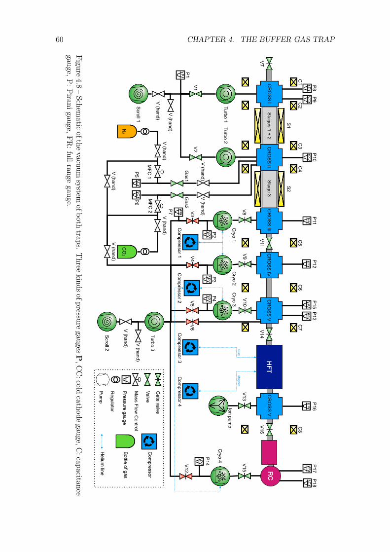
60 CHAPTER 4. THE BUFFER GAS TRAP
V (hand)
V (hand)
V (hand) V
(hand)
V (hand)
V (hand)
CC
PC
CP
CC
CC
CC
PP
P
PFR
P1
P8
P9
P10
P11
P12
P15
P13
P2
P3
P4
P7 V3
V4
V5
V6
Gas1
Gas2
V1
V2
V7
V11
V14
V8
V9
V10
CR
OS
S I
CR
OS
S II
CR
OS
S III
CR
OS
S IV
CR
OS
S V
C1
C2
C3
C4
C5
C6
C7
S1
S2
Stages 1 + 2
Stage 3
V16
FR
P16
V13
CFR
P17
P18
PP
14 V15
V12
Cryo 1
Cryo 2
Cryo 3
Cryo 4
Ion pump
Turbo 1Turbo 2
Turbo 3
Scroll 1
Scroll 2
V (hand)
V (hand)
C
N2
CO
2
P5
P6
C
MFC
1M
FC 2
V (hand)
V (hand)
Pressure gauge
Mass Flow
Control
Regulator
Pum
p
Valve
Gate valve
Com
pressor 1C
ompressor 2
Com
pressor 3C
ompressor 4
DuctMagnet
CR
OS
S V
IHFT
RC
C8
Com
pressor
Bottle of gas
Helium
line
Figure
4.8–Schem
aticofthe
vacuumsystem
ofbothtraps.
Three
kindsofpressuregauges
P,C
C:cold
cathodegauge,C
:capacitancegauge,P
:Piranigauge,F
R:fullrange
gauge.

4.2. DESCRIPTION OF THE TRAP 61
elementQ = C(P1 − P2), (4.2.4)
with the conductance expressed in L s−1 and the throughput in mbar L s−1.The pumping speed being the volume of gas pumped per unit of time, it is defined
by [82]
S =dV
dt=Q
P, (4.2.5)
For a pump connected to the system with an aperture of conductance C, the netpumping speed Sn, also expressed in L s−1, is computed as a function of the pumpingspeed Sp and the conductance C is [82]
1
Sn
=1
Sp
+1
C. (4.2.6)
with Q the throughput and P the pressure. More specifically, for two vesselsconnected with a pipe of conductance C, the first one with a pressure P1 and thesecond with P2, if the second one is connected to a pump of net pumping speed Sn
(see schematic in Figure 4.9), the combination of 4.2.4 and 4.2.5 leads to
Q = C(P1 − P2) = SnP2. (4.2.7)
P1 P2
Sn
C
Q
Figure 4.9 – Schematic of two vessels with one connected to a pump.
The gases are in the molecular flow regime, i.e., the mean free path of themolecules is larger than the diameter of the pipes, and the collisions between themolecules and the walls are more important than the collisions between molecules.One generally considers it is the case when the product of the mean pressure inmbar and the diameter of the pipe in cm is below 0.013 [83]. With a pressure in thesystem below 10−3 mbar and a minimal diameter of 0.1 cm, we can use the followingformulas determined for the molecular flow regime.
In the case of an aperture with a surface A, the conductance is [82]
C = 3.64
√T
MA (L s−1), (4.2.8)
with T in K, M in g mol−1 and A in cm2. For N2 at T = 23 C, we have
C = 11.8A (L s−1). (4.2.9)

62 CHAPTER 4. THE BUFFER GAS TRAP
For a long pipe (L D, L the length and D the diameter), the conductance isgiven by the expression [84]
C = 3.81
√T
M
D3
L(L s−1). (4.2.10)
For N2 at T = 23 C, we have
C = 12.4D3
L(L s−1). (4.2.11)
Finally, in the case of a short pipe (if L < 0.7D [83]), the conductance is
C = 11.8A
1 + L/D. (4.2.12)
Ca
Cb Cc
Cd
Ce Cf
Cg
Ch CiPa PcPg Ph
PiPb
PdPe Pf
Cj
To Turbo 1 To Turbo 2 To Cryo 1 To Cryo 2 To Cryo 3
Figure 4.10 – Conductances of the pumping restriction elements. Ca: connectionwith the turbo-pumps. Cb: half first stage. Cc: half first stage and second stage.Cd: half first stage and half second stage. Cf : half third stage. Cg: connection withthe cryo-pumps. Ce, Ch, Ci: small pipes. Cj: small pipe and third stage.
The calculated conductances of different parts of the system (see Figure 4.10) areshown in Table 4.7 and the net pumping speed of various pumps in Table 4.8. Thenet pumping speeds are computed taking into account the aperture of the pumpsand the pipes that connect them to the crosses according to Equation 4.2.6.
It is now possible to compute the pressures. For this purpose, it is assumed thatthe gas is injected in the middle of the second stage and the pressure at the injectionpoint Pb is a known parameter.
Considering throughput conservation in each cross, similarly to the expression 4.2.7,Equations 4.2.13 are obtained (the variables names are related to Figure 4.10, Ta-

4.2. DESCRIPTION OF THE TRAP 63
Name L(cm) D(cm) C(L s−1)Ca 68.0 15.0 615Cb 19.0 1.6 2.67Cc (19.0, 26) (1.6, 4.1) 2.37Cd (19.0, 13.0) (1.6, 4.1) 2.49Ce 30 2 3.31Cf 17.5 4.1 29.6Cg 43.0 15 973Ch 21.5 3.7 29.2Ci 17 3.7 36.9Cj (30, 35) (2, 4.1) 2.91
Table 4.7 – Conductances of the elements of the pumping restriction. The conduc-tance names are related to Figure 4.10.
Pump D(cm) Sp(L s−1) Sn(L s−1) Sn
Turbo 1 18 550 264 Sn1
Turbo 2 18 550 264 Sn2
Cryo 1 20 1500 509 Sn3
Cryo 2 20 1500 509 Sn4
Cryo 3 20 1200 469 Sn5
Table 4.8 – Pumping speeds and net pumping speeds. The names are related toFigure 4.8. The net pumping speeds come from the manufacturers’ datasheet.
ble 4.7 and Table 4.8):
(Pb − Pa)Cb = PaSn1 (4.2.13a)
⇔ Pa = APb, A =Cb
Cb + Sn1
, (4.2.13b)
(Pb − Pc)Cc = PcSn1 + (Pc − Pg)Cj (4.2.13c)
⇔ Pc = BPb, B =Cc
Cc + (1−D)Sn1 + Cj, (4.2.13d)
(Pc − Pg)Cj = PgSn2 + (Pg − Ph)Ch (4.2.13e)
⇔ Pg = DPc = BDPb, D =Cj
Cj + (1− E)Sn2 + Ch, (4.2.13f)
(Pg − Ph)Ch = PhSn3 + (Ph − Pi)Ci (4.2.13g)
⇔ Ph = EPg = BDEPb, E =Ch
Ch + (1− F )Sn2 + Ci, (4.2.13h)
(Ph − Pi)Ci = PiSn3 (4.2.13i)
⇔ Pi = FPh = BDEFPb, F =Ci
Ci + Sn3
. (4.2.13j)
The conservation of the throughput between the points corresponding to the pres-sures Pb, Pd and Pd, Pc for the second stage (respectively between Pc, Pg and Pf , Pg
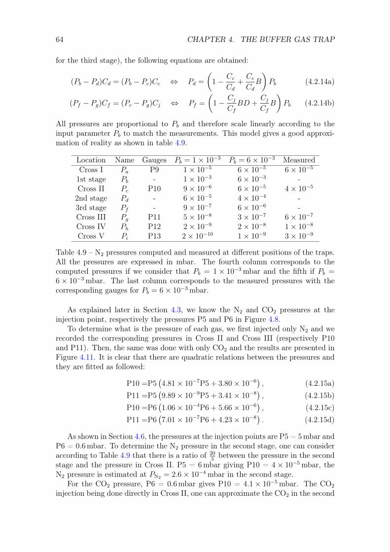
64 CHAPTER 4. THE BUFFER GAS TRAP
for the third stage), the following equations are obtained:
(Pb − Pd)Cd = (Pb − Pc)Cc ⇔ Pd =
(1− Cc
Cd+CcCdB
)Pb (4.2.14a)
(Pf − Pg)Cf = (Pc − Pg)Cj ⇔ Pf =
(1− Cj
CfBD +
CjCfB
)Pb (4.2.14b)
All pressures are proportional to Pb and therefore scale linearly according to theinput parameter Pb to match the measurements. This model gives a good approxi-mation of reality as shown in table 4.9.
Location Name Gauges Pb = 1× 10⁻³ Pb = 6× 10⁻³ MeasuredCross I Pa P9 1× 10⁻⁵ 6× 10⁻⁵ 6× 10⁻⁵
1st stage Pb - 1× 10⁻³ 6× 10⁻³ -Cross II Pc P10 9× 10⁻⁶ 6× 10⁻⁵ 4× 10⁻⁵
2nd stage Pd - 6× 10⁻⁵ 4× 10⁻⁴ -3rd stage Pf - 9× 10⁻⁷ 6× 10⁻⁶ -Cross III Pg P11 5× 10⁻⁸ 3× 10⁻⁷ 6× 10⁻⁷
Cross IV Ph P12 2× 10⁻⁹ 2× 10⁻⁸ 1× 10⁻⁸
Cross V Pi P13 2× 10⁻¹⁰ 1× 10⁻⁹ 3× 10⁻⁹
Table 4.9 – N2 pressures computed and measured at different positions of the traps.All the pressures are expressed in mbar. The fourth column corresponds to thecomputed pressures if we consider that Pb = 1× 10⁻³ mbar and the fifth if Pb =6× 10⁻³ mbar. The last column corresponds to the measured pressures with thecorresponding gauges for Pb = 6× 10⁻³ mbar.
As explained later in Section 4.3, we know the N2 and CO2 pressures at theinjection point, respectively the pressures P5 and P6 in Figure 4.8.
To determine what is the pressure of each gas, we first injected only N2 and werecorded the corresponding pressures in Cross II and Cross III (respectively P10and P11). Then, the same was done with only CO2 and the results are presented inFigure 4.11. It is clear that there are quadratic relations between the pressures andthey are fitted as followed:
P10 =P5(4.81× 10⁻⁷P5 + 3.80× 10⁻⁶
), (4.2.15a)
P11 =P5(9.89× 10⁻⁹P5 + 3.41× 10⁻⁸
), (4.2.15b)
P10 =P6(1.06× 10⁻⁴P6 + 5.66× 10⁻⁶
), (4.2.15c)
P11 =P6(7.01× 10⁻⁷P6 + 4.23× 10⁻⁸
). (4.2.15d)
As shown in Section 4.6, the pressures at the injection points are P5 = 5 mbar andP6 = 0.6 mbar. To determine the N2 pressure in the second stage, one can consideraccording to Table 4.9 that there is a ratio of 20
3between the pressure in the second
stage and the pressure in Cross II. P5 = 6 mbar giving P10 = 4× 10⁻⁵ mbar, theN2 pressure is estimated at PN2 = 2.6× 10⁻⁴ mbar in the second stage.
For the CO2 pressure, P6 = 0.6 mbar gives P10 = 4.1× 10⁻⁵ mbar. The CO2
injection being done directly in Cross II, one can approximate the CO2 in the second
4.3. TRAP CONTROL 65
0 1 2 3 4 5 6 7P5 in mbar
0
10
20
30
40
50P 1
0 ×10
6 mba
r(a)
0 1 2 3 4 5 6 7P5 in mbar
0.00.10.20.30.40.50.60.7
P 11 ×
106 m
bar
(b)
0.0 0.1 0.2 0.3 0.4 0.5 0.6 0.7P6 in mbar
0
10
20
30
40
50
P 10 ×
106 m
bar
(c)readcorrected
0.0 0.1 0.2 0.3 0.4 0.5 0.6 0.7P6 in mbar
0.000.050.100.150.200.250.300.35
P 11 ×
106 m
bar
(d)readcorrected
Figure 4.11 – (a) P10 as a function of P5 (only N2). (b) P11 as a function of P5(only N2). (c) P10 as a function of P6 (only CO2). (d) P11 as a function of P6 (onlyCO2). The blue curves correspond to values read with the gauges. The red curvescorrespond to corrected values according to Ref. [85].
stage with P10. However, the gauges being calibrated for N2 , a correction factor of1.42 [85] is applied to obtain the CO2 pressure. In conclusion, P6 = 0.6 mbar leadsto a CO2 pressure of PCO2 = 2.9× 10⁻⁵ mbar in the second stage.
To check the consistency of this model, we can compare with the positrons life-time measured in Ref. [47] and presented in Table 4.3. For a pressure of P0 =2.7× 10⁻⁸ mbar of N2 or respectively CO2 , the positrons lifetime are τN2 = 6300 sand τCO2 = 2400 s. Considering that the inverse of the lifetime is proportional tothe pressure, then in our situation, we can estimate the lifetime τ with
1
τ=
1
τN2
PN2
P0
+1
τCO2
PCO2
P0
(4.2.16)
This gives a lifetime in the second stage τ = 0.5 s, which is consistent with thelifetime of 0.64 s presented in Section 4.6.
4.3 Trap controlThe trap is controlled using Labview programs and National Instrument devices.In the past, all the system was operated from a PXI (combination of a controllerand a computer) and CRIOs (controllers) were in charge of the vacuum and magnetcontrol through the PXI. The PXI was also in charge of the electrode control anddata acquisition (see Figure 4.14). This has been reorganised in April 2020 and now,a dedicated computer controls the CRIO for the BGT vacuum system and magnets(but also all the vacuum system of the antiproton line) and the PXI is only in chargeof the electrode control and the signal acquisition.

66 CHAPTER 4. THE BUFFER GAS TRAP
4.3.1 Vacuum system and magnets control
To insert N2 and CO2 , a P-I-D algorithm was used to control piezo-electric valves(PEV) [48]. The input parameters were the desired pressures in P5 and P6 andthe PEV were more or less opened to reach these pressures. Because the PEV wereleaking, they have been replaced by Mass Flow Controller [86]. These MFC have aninternal PID and the input parameters are the mass-flow and we read the pressureson the graphical interface (Figures 4.12). The graphical interface is presented inFigure 4.12.
Figure 4.12 – Labview VI to control the Mass Flow Controller. The input parametersare the mass-flow (set-points), and the real mass flow are read (gas output). P5 (N2
pressure) and P6 (CO2 pressure) are also shown on the interface.
The pumps, valves, gauges and the magnets are controlled and monitored throughthe graphical interface presented in Figure 4.13. The CRIOs are in charge of thereading of the different parameters and send all the information to the overwatchcomputer to display them on the interface. The CRIOs, programmed throughFPGA-based programs, are also used for the safety control of the vacuum and ser-vices.
4.3.2 Trapping control
The potentials and the data acquisition related to the BGT are controlled by a PXI.It is a National Instrument computer optimised for experiment control and dataacquisition. The different elements on the PXI are:
• NI PXIe 8135, a Windows 10 computer to run the Labview programs;
• NI PXIe 6366, an analog input voltage card, to acquire some slow signals;
• NI PXIe 7820R, a digital input/output card, the FPGA program is run on it;
• NI PXIe 5160, an oscilloscope, to acquire some fast signals;

4.3. TRAP CONTROL 67
Figure4.13
–Graph
ical
user
interfaceto
controlthe
Buff
erGas
Trap
mag
nets,m
onitor
thepressures,
andinject
gas.

68 CHAPTER 4. THE BUFFER GAS TRAP
• NI PXI 6733, three analog input voltage cards, to control the High-VoltageAmplifiers;
• NI PXI 8252, a FireWire module to control a PCO camera.
A schematic of this system is presented in Figure 4.14.To manipulate the positron cloud in the BGT, electric potential has to be set
and changed at precise moments. For this purpose sequences are written to specifythe potentials on the BGT electrodes. These sequences are written thanks to aLabview program presented in Figure 4.15. Each line of the Sequence Editor has 4main inputs:
• Duration (a in Figure 4.15). This is the duration of the line. If there is nochange of the potential and only the output trigger are changed, the minimalduration time is 12.5 ns, corresponding to the maximal speed of the 7820Rcard. If this duration is set at 0, then it is possible to wait for an input trigger(see last item). If we are changing the potential, the minimal time is 1.35 µsper ramp point, corresponding to the timing properties of the High-VoltageAmplifiers.
• Ramp points (b in Figure 4.15). This is the number of step to go from theprevious potential profile to the new one, in order to change the potential moreor less progressively, as an example, for a positron cloud compression.
• HVA voltages (c in Figure 4.15). If ramp point parameter is 1, then thepotential profile is the one defined at this line for all the line’s duration. Iframp point is greater than one, then the potential will be the one defined hereat the end of the line’s duration. If ramp point is 0, then the potential remainsthe previous one for this line and the program does not invite us to define anew potential profile.
• Output triggers (d in Figure 4.15). The 7820R card provides an output digitalsignal corresponding to what has been defined for the duration of the line.
• Input triggers (e in Figure 4.15). The system waits and remains with theprevious parameters until the 7820R card receives the exact digital input con-figuration defined here.
The sequence editor provides a text file which can be interpreted by a Labviewprogram (b in Figure 4.16). This program converts the text file into an array,defining for each time the configuration of the trap (potentials, triggers, waiting fortriggers). The array is sent to a FPGA program running on the 7820R card (a inFigure 4.16). This card contacts the other cards to execute the sequence. It is alsopossible to prepare the execution of several sequences using the program shown inFigure 4.16-d. The program defines an array for each sequence and send it to theFPGA program. The rotating wall parameters are defined manually before startingan accumulation procedure (c in Figure 4.16).

4.3. TRAP CONTROL 69
NI P
XIe
1082
Slot
1N
I PXI
e 81
35
NI P
XI 8
252
Slot
8•
Fire
wire
Mod
ule
•C
ontro
ller /
C
ompu
ter
NI P
XIe
5160
Slot
4•
Osc
illosc
ope
mod
ule
•2.
5 G
S/s
NI P
XI 6
733
Slot
5, 6
, 7•
8 An
alog
Vol
tage
O
utpu
ts
•1M
S/s
NI P
XIe
7820
RSl
ot 3
•4
x 32
Dig
ital
Inpu
ts/O
utpu
ts
•FP
GA
mod
ule
•80
MH
z
Inte
rnal
PXI
con
nect
ion
NI P
XIe
6366
Slot
2•
8 An
alog
Vol
tage
In
puts
•2
MS/
s•
Mul
tifun
ctio
n
(24
DIO
, 2AO
)
Slow
Det
ecto
rs•
CsI
det
ecto
rs
Anal
og s
igna
l
Hig
h Vo
ltage
Am
plifi
ers
SEQ
UEN
CER
Elec
trode
s
FPG
A co
ntro
l
Fast
det
ecto
rs•
Cha
rge
coun
ters
•Pl
astic
sci
ntilla
tors
Digi
tal s
igna
l
Dig
ital O
utpu
ts•
Sign
al a
cqui
sitio
n•
Hig
h Fi
eld
Trap
•
RW o
n / o
ff•
Trig
gerin
g ot
her d
evic
es
(e.g
. MC
P ca
mer
a)
Dig
ital I
nput
s
•LI
NAC
trig
ger
•H
igh
Fiel
d Tr
ap
Digi
tal s
igna
l
Con
nect
or 0
Con
nect
or 1
MC
P•
PCO
Cam
era
•H
VAEt
hern
et /
GPI
B / F
irew
ire
Rota
ting
Wal
l Wav
e ge
nera
tors
Split
ters
Figure4.14
–Overview
oftheconn
ection
sof
theBuff
erGas
Trap
PXIcompu
ter.
Inorderno
tto
overload
theschematic,E
thernet,
GPIB
,and
Firew
ireconn
ection
sha
vebe
enmerged.
The
wavegene
rators
arecontrolledthroug
hGPIB
conn
ection
s,thePCO
camera
throug
haFirew
ireconn
ection
,and
theHV
fortheMCP
arecontrolledusingan
Ethernetconn
ection
.

70 CHAPTER 4. THE BUFFER GAS TRAP
(a)
(b)(c)
(d)(e)
Figure
4.15–User
interfacefor
thesequence
editor.(a)
Duration
ofthe
line.(b)
Num
berof
stepsto
gofrom
theprevious
voltageprofile
tothe
newone.
(c)Voltages
ofeachHVA
(to6366
card).(d)
Output
triggers(to
7820Rcard).
(e)Input
triggers(to
7820Rcard).

4.3. TRAP CONTROL 71
(a)
(b)
(c)
(d)
Figure4.16
–Graph
icuser
interfaces
runn
ingon
thePXIcompu
ter.
(a)T
heFPGA
prog
ram.(b)La
bview
VIto
load
/run
/abo
rta
sequ
ence.(c).La
bview
VIto
settherotating
wallw
avegenerator(d).
Labv
iew
VIto
load
/run
/abo
rtmultiplesequ
ences.

72 CHAPTER 4. THE BUFFER GAS TRAP
4.4 Positron detection
4.4.1 Micro-Channel Plate
A Micro-Channel Plate (MCP) is an electron multiplier. It allows to detect chargedparticles and is generally combined with a charge collector, or a phosphor screen toobtain the position of the particles.
A typical MCP [87] is a disk composed of 104-107 miniature electron multiplierschannels, parallel one to another. The channels have a diameter around 10 µm-100 µm. The MCP is made of lead glass and the faces are covered by a metalliclayer to create an electric field between the entrance and the exit of the MCP. Thisfield determines the gain of the MCP, as well as α the ratio between the length andthe diameter. Indeed, in the case of a single straight channel, the gain is
G =
(AV
2α√V0
)4V0α2/V
, (4.4.1)
with V , the potential between the faces, V0 the initial energy of a secondary electron(∼ 1 eV), and A a proportionality constant. To increase the gain, it is also possible touse MCP in series. Thus, an incident charged particle at the front induces an electronshower in a channel, and the position of the incident particle can be determined ifthe MCP is followed by a phosphor screen (or the number of incoming particles ifthe gain is known). The electron shower can also create positive ions, depending onthe residual gas pressure at the MCP location. This could reduce the measurementprecision. To prevent this problem, the channels are generally inclined (typically 8)as it is presented in Figure 4.17.
Optional coating forconversion efficiency Conductive coating
Conductive coating
Optional conduction ring
Phosphor screen
Vin
Vout
e−, e+, A+, C−
e−
Figure 4.17 – Extracted from Ref. [88]. Schematic layout of an MCP Chevron stack,with two micro-channel plates and a phosphor screen.
In our case, we use a Chevron MCP manufactured by Photonis. These MCPhave a diameter of 40 mm with channels of 10 µm to get a maximal gain of 107. Aphosphor screen is place right after the MCP to obtain spots with a light proportionalto the number of electrons coming out of each channel. The image of the spots onthe phosphor screen can be collected to obtain physical information such as theradial density (the MCP conserving the radial density of the incoming particles,especially with a short response time below 100 ps). Thus, a mirror is placed at
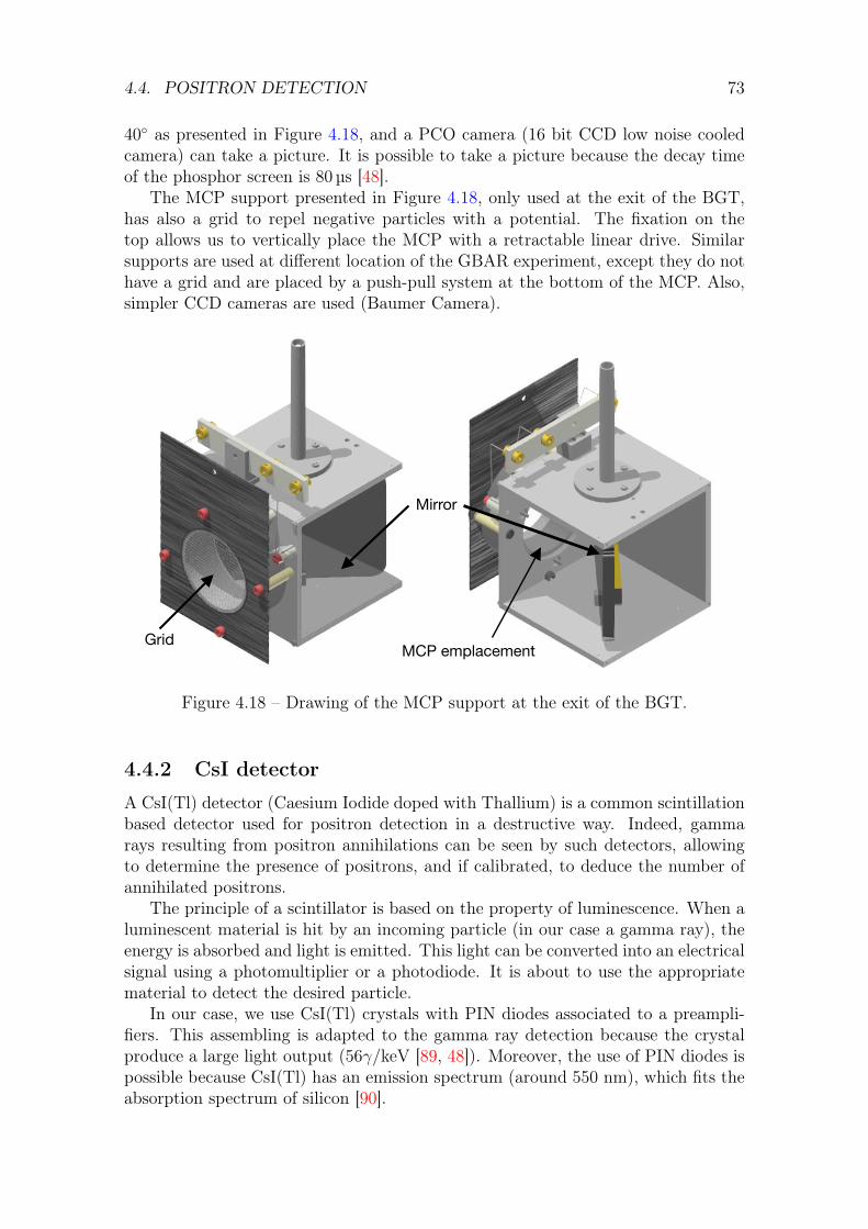
4.4. POSITRON DETECTION 73
40 as presented in Figure 4.18, and a PCO camera (16 bit CCD low noise cooledcamera) can take a picture. It is possible to take a picture because the decay timeof the phosphor screen is 80 µs [48].
The MCP support presented in Figure 4.18, only used at the exit of the BGT,has also a grid to repel negative particles with a potential. The fixation on thetop allows us to vertically place the MCP with a retractable linear drive. Similarsupports are used at different location of the GBAR experiment, except they do nothave a grid and are placed by a push-pull system at the bottom of the MCP. Also,simpler CCD cameras are used (Baumer Camera).
GridMCP emplacement
Mirror
Figure 4.18 – Drawing of the MCP support at the exit of the BGT.
4.4.2 CsI detector
A CsI(Tl) detector (Caesium Iodide doped with Thallium) is a common scintillationbased detector used for positron detection in a destructive way. Indeed, gammarays resulting from positron annihilations can be seen by such detectors, allowingto determine the presence of positrons, and if calibrated, to deduce the number ofannihilated positrons.
The principle of a scintillator is based on the property of luminescence. When aluminescent material is hit by an incoming particle (in our case a gamma ray), theenergy is absorbed and light is emitted. This light can be converted into an electricalsignal using a photomultiplier or a photodiode. It is about to use the appropriatematerial to detect the desired particle.
In our case, we use CsI(Tl) crystals with PIN diodes associated to a preampli-fiers. This assembling is adapted to the gamma ray detection because the crystalproduce a large light output (56γ/keV [89, 48]). Moreover, the use of PIN diodes ispossible because CsI(Tl) has an emission spectrum (around 550 nm), which fits theabsorption spectrum of silicon [90].

74 CHAPTER 4. THE BUFFER GAS TRAP
4.5 Electron repeller
To produce positrons for H+ formation, 9 MeV electrons originating from the LINAC
impinge on a tungsten target where the antiparticles are created by bremsstrahlungradiation (e− + Z → e− + Z + γ), followed by γ conversion. A tungsten meshmoderator slows the positrons down to a fixed energy (3 eV for Tungsten) to a mono-energetic beam with an energy width of a few eV. The positrons are extracted at50 eV.
Electrons, with an energy between 0 and few keV follow the same magnetictransport lines as the positrons and disturb positron trapping. Indeed, the electronsionise the buffer gases, preventing the inelastic collisions required for the trappingto occur.
To remove the electrons, an initial electron repeller had been placed just beforethe Buffer Gas Trap (see Section 4.5.1). This repeller consists in a grid where ahigh voltage is applied. In June 2020, it has been replaced by a second repeller (seeSection 4.5.2) composed of a set of 31 electrodes, connected together using resistors.
4.5.1 Electron repeller version 1
The electron repeller, as shown in Figure 4.19 consists of a tungsten grid (90%transparency) mounted in such a way that a negative potential can be applied.If the voltage is low enough, the electrons are repelled. However, when using largenegative voltages, locally the positrons are accelerated in a non adiabatic way, whichhas an effect on their energy spread and consequently on the trapping rate.
Figure 4.19 – Picture of the electron repeller. A negative potential is applied on thegrid to repel the electrons.
To estimate the electron number per LINAC pulse, a metallic plate at the en-trance of the Buffer Gas Trap (BGT) has been connected to an oscilloscope with atotal capacitance C = 320 pF. With a grounded potential on the repeller, a 107 mVpeak height is detected on the oscilloscope, which corresponds to 2.14× 10⁸ elec-trons per LINAC pulse. The number of electrons per linac pulse decreases withdecreasing voltages on the repeller down to −5 kV, as can be seen in Figure 4.20.

4.5. ELECTRON REPELLER 75
Electrons are no more detected above 2 kV. Then, a potential above 2 kV shouldimprove positron trapping.
102 103
Voltage on the repeller (-V)
107
108
Elec
tron
num
ber
Figure 4.20 – Electron number as a function of the potential on the electron repellerat the entrance of the Buffer Gas Trap. LINAC frequency: 2 Hz.
To determine the positron energy distribution right after the repeller, a poten-tial barrier is applied on the first BGT electrodes. CsI crystals detect the gammarays resulting from the annihilation of the positrons when they intercept a metallicplate placed at the exit of the BGT. Their signals are collected for different po-tentials on the repeller. The results are presented in Figure 4.21-a. Assuming theenergy distribution is gaussian, the signals are fitted with an error function. Thecorresponding energy distributions are shown in Figure 4.21-b, where we clearly ob-serve that the mean value and the spread of energy is significantly influenced by therepeller voltage.
0 10 20 30 40 50 60 70 80Potential barrier (V)
0.000.050.100.150.200.250.30
CsI s
igna
l (V)
(a)0V200V500V700V2000V4000V
0 10 20 30 40 50 60 70 80Potential barrier (V)
0.00
0.02
0.04
0.06
0.08
0.10
Ener
gy d
istrib
utio
n
(b)0V200V500V700V2000V4000V
Figure 4.21 – (a) CsI signal for a straight through beam at the exit of the BufferGas Trap as a function of a potential barrier at the entrance of the trap for differentpotentials on the repeller. (b) Corresponding energy distribution. LINAC frequency:200 Hz.
A smaller energy spread is required to gain better trapping rate in the BGT.Figure 4.22-a shows that the energy spread is increasing with the potential on therepeller (up to 3 kV, it is slightly decreasing after this point). Thus, an optimum hasto be found between the electron number and the spread of energy. Furthermore,Figure 4.22-b shows that the mean energy decreases with the amplitude of thepotential on repeller, which is also correlated with a loss of positrons as shown inFigure 4.22-c.
To determine the trapping rate, positrons are accumulated for 100 ms in thesecond stage and then dumped on a plate at the exit of the BGT (see more details

76 CHAPTER 4. THE BUFFER GAS TRAP
0 1000 2000 3000 4000 5000Potential on the repeller (-V)
0
2
4
6
8
10
12En
ergy
spre
ad (e
V)(a)
0 1000 2000 3000 4000 5000Potential on the repeller (-V)
0
10
20
30
40
50
Mea
n en
ergy
(eV)
(b)
0 1000 2000 3000 4000 5000Potential on the repeller (-V)
0.0
0.2
0.4
0.6
0.8
1.0
Beam
inte
nsity
(arb
) (c)
Figure 4.22 – Parameters of the gaussian fit A exp−12
(V−V0σ
)2 (corresponding toFigure 4.21). (a) Energy spread σ of a straight through beam at the exit of theBuffer Gas Trap as a function of the potential on the central electrode of the electronrepeller. (b) Mean energy V0. (c) Beam intensity A. LINAC frequency: 200 Hz.
on the positron accumulation in Section 4.6). The corresponding CsI signal therebyobtained is proportional to the trapping rate (N = Rτ
[1− e−100 ms/τ
], with N the
positron number in the trap, R the trapping rate and τ the lifetime). The resultsfor different potentials on the repeller are presented in Figure 4.23. This figureclearly shows an optimum for the trapping rate around 500 V on the repeller. Aswe could expect, it corresponds to a voltage providing a small energy spread withfew remaining electrons (see Figure 4.24).
0 1000 2000 3000 4000 5000Repeller voltage(-V)
0.00
0.05
0.10
0.15
0.20
0.25
0.30
CsI s
igna
l (V)
Figure 4.23 – CsI signal after accumulation in the Buffer Gas Trap’s second stagefor 100 ms as a function the potential on the repeller. LINAC frequency: 200 Hz.
The number of positrons in the second stage of the BGT is measured as a functionof accumulation time for different voltages of the repeller. The lifetime of accumu-lated positrons is then measured as a function of the voltage on the repeller grid(Figure 4.25-b). It is clear that the remaining electrons have no effect for a potentialabove 500 V on the repeller.

4.5. ELECTRON REPELLER 77
0 1000 2000 3000 4000 5000Potential on the repeller (-V)
0.0
0.2
0.4
0.6
0.8
1.0No
rmal
ize si
gnal
e numbertrapping ratee + energy spread
Figure 4.24 – Superposition of the curves from Figures 4.20, 4.22 and 4.23. LINACfrequency: 200 Hz.
0 1 2 3 4 5 6accumulation time (s)
0.00
0.05
0.10
0.15
0.20
0.25
CsI s
igna
l (V)
(a)
0V250V500V750V1000V3000V5000V
0 1000 2000 3000 4000 5000repeller potential (-V)
0.0
0.2
0.4
0.6
0.8
1.0
Lifet
ime
(s)
(b)
Figure 4.25 – (a) positron accumulation curves in the BGT’s second stage for dif-ferent potentials on the repeller. (b) Corresponding positron lifetimes. LINACfrequency: 200 Hz.
4.5.2 Electron repeller version 2
As illustrated in Figure 4.22, the electron repeller has an impact on the energy spreadbecause of the non adiabatic transport of the positrons through the grid, influencingthe trapping rate. Also, the presence a grid at the entrance of the trap is responsiblefor a loss of incoming positrons. Therefore, the electron repeller has been replaced(see Figure 4.26) with one which is composed of a set of 31 electrodes with 28.4 mmlength and 61 mm inner diameter to create a more gradual field change.
Figure 4.26 – Pictures of the new electron repeller. The repeller is composed of aset of electrodes connected with resistors. The connection to the power supply ismade at the center and the electrodes at the extremities are grounded.
Therefore, the electrodes are connected together with 4.7 MΩ resistors. Thecentral electrode is connected to a high voltage power supply and the electrodes at
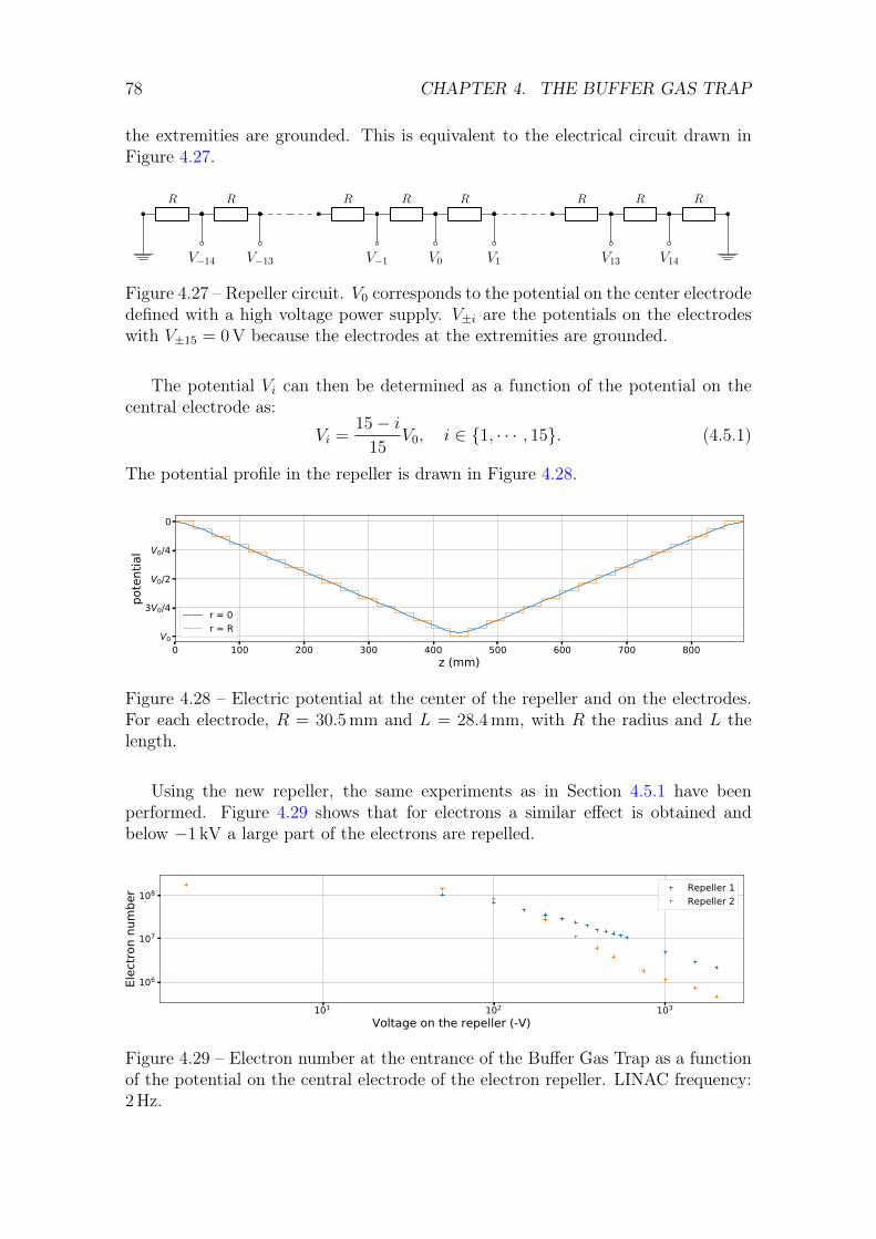
78 CHAPTER 4. THE BUFFER GAS TRAP
the extremities are grounded. This is equivalent to the electrical circuit drawn inFigure 4.27.
R
V−14
R
V−13
R
V−1
R
V0
R
V1
R
V13
R
V14
R
Figure 4.27 – Repeller circuit. V0 corresponds to the potential on the center electrodedefined with a high voltage power supply. V±i are the potentials on the electrodeswith V±15 = 0 V because the electrodes at the extremities are grounded.
The potential Vi can then be determined as a function of the potential on thecentral electrode as:
Vi =15− i
15V0, i ∈ 1, · · · , 15. (4.5.1)
The potential profile in the repeller is drawn in Figure 4.28.
0 100 200 300 400 500 600 700 800z (mm)
0
V0/4
V0/2
3V0/4
V0
pote
ntia
l
r = 0r = R
Figure 4.28 – Electric potential at the center of the repeller and on the electrodes.For each electrode, R = 30.5 mm and L = 28.4 mm, with R the radius and L thelength.
Using the new repeller, the same experiments as in Section 4.5.1 have beenperformed. Figure 4.29 shows that for electrons a similar effect is obtained andbelow −1 kV a large part of the electrons are repelled.
101 102 103
Voltage on the repeller (-V)
106
107
108
Elec
tron
num
ber Repeller 1
Repeller 2
Figure 4.29 – Electron number at the entrance of the Buffer Gas Trap as a functionof the potential on the central electrode of the electron repeller. LINAC frequency:2 Hz.

4.5. ELECTRON REPELLER 79
0 10 20 30 40 50 60 70 80Potential barrier (V)
0.0000.0250.0500.0750.1000.1250.1500.1750.200
CsI s
igna
l (V)
0V100V200V700V3000V5000V
0 10 20 30 40 50 60 70 80Potential barrier (V)
0.00
0.02
0.04
0.06
0.08
0.10
0.12
Ener
gy d
istrib
utio
n 0V100V200V700V3000V5000V
Figure 4.30 – Right: CsI signal for a straight through beam at the exit of theBuffer Gas Trap as a function of a potential barrier at the entrance of the trap fordifferent potentials on the central electrode of the repeller. Left: Correspondingenergy distribution. LINAC frequency: 200 Hz.
The positron energy distribution stays more or less the same no matter thepotential applied on the electron repeller as presented in Figure 4.30.
In more detail, one can see that the width parameter of the gaussian fit remainsconstant around 4 eV as shown in Figure 4.31-a. So, the electron repeller can onlyimprove the trapping efficiency, because it removes the electron, without disturbingthe energy distribution of the positrons. Also, the mean value of the energy remainsperfectly constant with the potential on the repeller (Figure 4.31-b). However, theintensity is still decreasing, but less than with the previous repeller (Figure 4.31-c).
0 1000 2000 3000 4000 5000Potential on the repeller (-V)
0
2
4
6
8
10
12
Ener
gy sp
read
(eV)
(a)Repeller 1Repeller 2
0 1000 2000 3000 4000 5000Potential on the repeller (-V)
0
10
20
30
40
50
Mea
n en
ergy
(eV)
(b)
Repeller 1Repeller 2
0 1000 2000 3000 4000 5000Potential on the repeller (-V)
0.0
0.2
0.4
0.6
0.8
1.0
Beam
inte
nsity
(arb
) (c)
Repeller 1Repeller 2
Figure 4.31 – Parameters of the gaussian fit A exp−12
(V−V0σ
)2 (corresponding toFigure 4.30). (a) Energy spread σ of a straight through beam at the exit of theBuffer Gas Trap as a function of the potential on the central electrode of the electronrepeller. (b) Mean energy V0. (c) Beam intensity A. LINAC frequency: 200 Hz.
Therefore, there is no more optimum of the trapping rate with this new repeller.As presented in Figure 4.32, this rate increases with the potential on the central elec-
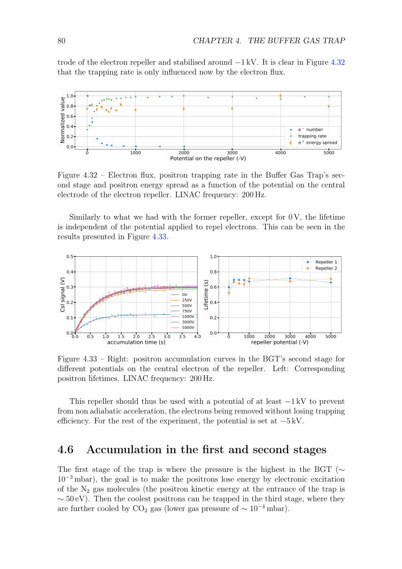
80 CHAPTER 4. THE BUFFER GAS TRAP
trode of the electron repeller and stabilised around −1 kV. It is clear in Figure 4.32that the trapping rate is only influenced now by the electron flux.
0 1000 2000 3000 4000 5000Potential on the repeller (-V)
0.0
0.2
0.4
0.6
0.8
1.0
Norm
alize
d va
lue
e numbertrapping ratee + energy spread
Figure 4.32 – Electron flux, positron trapping rate in the Buffer Gas Trap’s sec-ond stage and positron energy spread as a function of the potential on the centralelectrode of the electron repeller. LINAC frequency: 200 Hz.
Similarly to what we had with the former repeller, except for 0 V, the lifetimeis independent of the potential applied to repel electrons. This can be seen in theresults presented in Figure 4.33.
0.0 0.5 1.0 1.5 2.0 2.5 3.0 3.5 4.0accumulation time (s)
0.0
0.1
0.2
0.3
0.4
0.5
CsI s
igna
l (V)
0V250V500V750V1000V3000V5000V
0 1000 2000 3000 4000 5000repeller potential (-V)
0.0
0.2
0.4
0.6
0.8
1.0
Lifet
ime
(s)
Repeller 1Repeller 2
Figure 4.33 – Right: positron accumulation curves in the BGT’s second stage fordifferent potentials on the central electron of the repeller. Left: Correspondingpositron lifetimes. LINAC frequency: 200 Hz.
This repeller should thus be used with a potential of at least −1 kV to preventfrom non adiabatic acceleration, the electrons being removed without losing trappingefficiency. For the rest of the experiment, the potential is set at −5 kV.
4.6 Accumulation in the first and second stages
The first stage of the trap is where the pressure is the highest in the BGT (∼10−3 mbar), the goal is to make the positrons lose energy by electronic excitationof the N2 gas molecules (the positron kinetic energy at the entrance of the trap is∼ 50 eV). Then the coolest positrons can be trapped in the third stage, where theyare further cooled by CO2 gas (lower gas pressure of ∼ 10−4 mbar).

4.6. ACCUMULATION IN THE FIRST AND SECOND STAGES 81
4.6.1 Gas parameters
The first step of the optimisation of the trapping process focusses on the trappingrate. As explained in the introduction of the BGT principle (Section 4.1), it is knownthat the best trapping gas is N2 , but it is not a good cooling gas, the best beingSF6 [47, 72, 71]. However for safety reasons CO2 is used as cooling gas instead inour experiment. To determine the effect of the gas on the trapping rate, the N2 andCO2 pressures were varied in the system, while the number of positrons accumulatedin the second stage for different amount of time was measured.
The potential profile used for positron accumulation in the BGT’s first and sec-ond stages are shown in Figures 4.34a-b. The first stage is a long section where thepotential is slowly decreasing. It is followed by the second stage where a potentialwell traps the positrons. After an accumulation time t, the positron cloud is sentto the MCP at the exit of the trap (Figure 4.34c). The potentials applied on theelectrodes are presented in Table 4.10.
0 200 400 600 800 1000z (mm)
20
0
20
40
60
80
100
120
140
Pote
ntia
l at r
= 0
(V)
positrons from the LINAC
1st 2nd
(a)
0 200 400 600 800 1000z (mm)
20
0
20
40
60
80
100
120
140
Pote
ntia
l at r
= 0
(V)
1st 2nd
(b)
0 200 400 600 800 1000z (mm)
20
0
20
40
60
80
100
120
140
Pote
ntia
l at r
= 0
(V)
1st 2nd
(c)
Figure 4.34 – Potential profiles used in the Buffer Gas Trap first and second stages.The coloured areas represent the positrons. (a) & (b) Accumulation of the incomingpositrons from the LINAC. (c) Ejection of the positrons.
Electrode E0 EF E1 E2 E3 E4 E5
Accumulation 37.5 V 26.5 V 26 V 25.5 V 22 V 21.15 V 140 VEjection 37.5 V 26.5 V 26 V 25.5 V 22 V 21.15 V 0 V
Table 4.10 – Voltage used for positron accumulation in the Buffer Gas Trap’s firstand second stages. The electrode names refer to Table 4.4.
The gamma rays resulting from positron annihilation on the MCP at the exitof the BGT are detected with CsI detectors. As the peak height of a CsI detectorsignal is proportional to the number of annihilated positrons, a linear calibrationcan be performed with a charge counter A230CF CoolFet [91]. This charge counterprovides a 0.64 µV step output voltage per detected charge. It is biased at 20 V toprevent from secondary electron ejection leading to an overestimate of the charge.
The first CsI counter is placed a few cm from the valve located before the MCP,and the second one is placed about 1 meter above. The number of positrons isvaried by changing the frequency of the LINAC, and the resultant change in CsI

82 CHAPTER 4. THE BUFFER GAS TRAP
signal can be used to determine the correlation between CsI signal and number ofpositrons. The result is presented in Figure 4.35, and the following cross calibrationis obtained:
V1 = 1.69(2)× 10−6 V/e+ (4.6.1)V2 = 1.48(2)× 10−7 V/e+ (4.6.2)
0.0 0.2 0.4 0.6 0.8 1.0 1.2 1.4Number of positrons (×106)
0.0
0.5
1.0
1.5
2.0
2.5
Sign
al C
sI1 (V
)
Ratio=1.69(2) 10 6 VCsI1/e +
0.00
0.05
0.10
0.15
0.20
0.25
0.30
Sign
al C
sI2 (V
)
Ratio=1.48(2) 10 7 VCsI2/e +
Figure 4.35 – CsI signal as a function of the number of positrons measured by thecharge counter (0.64 µV/e+).
The variation of the number of trapped positrons N per unit time decreasesproportionally to the number of positrons in the trap, with a characteristic time τ ,the lifetime. The incoming flux of positrons is characterised by R, the trapping rate.Then the differential equation for the number of positrons reads
dN
dt= −N
τ+R, (4.6.3)
which leads toN(t) = Rτ
(1− e−
tτ
). (4.6.4)
If t τ , then R(t) = Rt, which means that we are in a linear regime and theaccumulated positrons are not yet annihilated in the second stage. The goal is tomaximise R, keeping τ large enough to remain in a linear regime, knowing thatonce the positrons are accumulated in the second stage, they can be transferred andstored in the third stage for a longer time.
N2 effect
The role of N2 pressure on positron trapping is tested by accumulating positrons fordifferent durations and for different N2 pressures. The results of these accumulationsare presented in Figure 4.36a. One can clearly see in Figure 4.36b-c that the trappingrate R and the inverse of the positrons lifetime τ−1 are proportional to the N2
pressure. Considering that we want to have R as large as possible, it would havebeen interesting to see how R evolves with higher pressures. However, it is notpossible to inject more gas for protecting the LINAC. Therefore, the N2 pressure in

4.6. ACCUMULATION IN THE FIRST AND SECOND STAGES 83
the second stage is set at PN2 = 2.67× 10⁻⁴ mbar for the rest of the experiment,corresponding to P5 = 6 mbar according to Section 4.2.4, (P5 pressure at the N2
injection point, see Figure 4.8). This value of PN2 corresponds to the best trappingefficiency within the acceptable range of gas pressure for safe LINAC operation. Inthese conditions, the trapping rate is R = 0.82(3)× 106 e+ s−1, and the lifetime isτ = 0.175(6) s.
0.0 0.5 1.0 1.5 2.0 2.5 3.0 3.5 4.0accumulation time (s)
0.000.020.040.060.080.100.120.140.16
Posit
rons
num
ber (
×106 )
(a)
PN2 = 0.57PN2 = 1.05PN2 = 1.52PN2 = 2.67
0.0 0.5 1.0 1.5 2.0 2.5 3.0PN2 (×10 4 mbar)
0.0
0.2
0.4
0.6
0.8
Trap
ping
rate
(×10
6 e+
.s1) (b)
0.0 0.5 1.0 1.5 2.0 2.5 3.0PN2 (×10 4 mbar)
0
1
2
3
4
5
6
Lifet
ime
1 (s
1 )
(c)
Figure 4.36 – (a) Accumulation curves for different N2 pressures (in 10−4 mbar). (b)Trapping rate as a function of the N2 pressures. (c) Inverse of the lifetime as afunction of the N2 pressures. LINAC frequency: 200 Hz.
CO2 effect
Once the N2 pressure is set, the impact of CO2 pressure on positron trapping istested following the same procedure as for N2. Once again, the trapping rate andthe inverse of the lifetime as a function of the CO2 pressure are linear functions.The only limit is the LINAC safety, then the CO2 pressure in the second stage isset at PCO2 = 0.29× 10⁻⁴ mbar for the rest of the experiment, corresponding toP6 = 0.6 mbar according to Section 4.2.4. In these conditions, the trapping rate isR = 1.60(5)× 106 e+ s−1, and the lifetime is τ = 0.124(4) s.
0.0 0.5 1.0 1.5 2.0 2.5 3.0 3.5 4.0accumulation time (s)
0.00
0.05
0.10
0.15
0.20
Posit
rons
num
ber (
×106 )
(a)
PCO2 = 0.0PCO2 = 0.12PCO2 = 0.18PCO2 = 0.29PCO2 = 0.34
0.000.050.100.150.200.250.300.35PCO2 (×10 4 mbar)
0.000.250.500.751.001.251.501.75
Trap
ping
rate
(×10
6 e+
.s1) (b)
0.000.050.100.150.200.250.300.35PCO2 (×10 4 mbar)
0
2
4
6
8
Lifet
ime
1 (s
1 )
(c)
Figure 4.37 – (a) Accumulation curves for different CO2 pressures (in 10−4 mbar).(b) Trapping rate as a function of the CO2 pressures. (c) Inverse of the lifetime as afunction of the CO2 pressures. PN2 = 2.67× 10⁻⁴ mbar. LINAC frequency: 200 Hz.

84 CHAPTER 4. THE BUFFER GAS TRAP
In the next section, it will be shown that the best Rotating Wall parametersin the second stage are (1 V, 2.4 MHz). In that case, as determined from the ac-cumulation curve presented in Figure 4.38, the trapping rate is increased up toR = 2.30(4)× 106 e+ s−1, and the lifetime up to τ = 0.639(11) s. This is why in therest of the experiment positrons are accumulated in the second stage for 100 ms, tostay in the linear regime.
0.0 0.5 1.0 1.5 2.0 2.5 3.0 3.5 4.0accumulation time (s)
0.0
0.2
0.4
0.6
0.8
1.0
1.2
1.4
Posit
rons
num
ber (
×106 )
PN2 = 2.67, PCO2 = 0, RW offPN2 = 2.67, PCO2 = 0.29, RW offPN2 = 2.67, PCO2 = 0.29, RW on
0.0 0.1 0.2 0.3 0.4 0.5accumulation time (s)
0.0
0.1
0.2
0.3
0.4
0.5
0.6
0.7
0.8
Posit
rons
num
ber (
×106 ) PN2 = 2.67, PCO2 = 0, RW off
PN2 = 2.67, PCO2 = 0.29, RW offPN2 = 2.67, PCO2 = 0.29, RW on
Figure 4.38 – Accumulation curves for different CO2 and N2 pressures (pressures in10−4 mbar). Rotating Wall parameters: 1 V, 2.4 MHz. LINAC frequency: 200 Hz.
To be able to increase the trapping rate by increasing the gas pressure, an extrapumping station will be inserted between the LINAC and the BGT.
4.6.2 Rotating Wall optimisation
Once the positrons accumulated in the Buffer Gas Trap second stage, we would liketo compress them radially and to store them in the BGT’s third stage before sendingthem into the HFT and increase the lifetime. The Rotating Wall technique (RW),as presented in Section 3.3.2 is used for this purpose.
If the particles are considered in a single particle regime the best compressionoccurs when RW the frequency is fRW = fz + fm (Section 3.3.2), with fm themagnetron frequency (defined in Section 3.1.2) and fz the inverse of the time ittakes for a particle to make a round trip in the well.
For a particle in an electric field φ, its energy E and its velocity v are relatedaccording to
E = qφ(z) +1
2mv2, (4.6.5)
with m and q the mass and the charge of the particle. If E is in eV and the particleis a positron, the relation becomes
qE = qφ+1
2mv2. (4.6.6)
Then, if the particle is moving along the z-axis, v = dzdt
and Equation 4.6.6 becomes
dt =
√m
2q
dz√E − φ(z)
. (4.6.7)

4.6. ACCUMULATION IN THE FIRST AND SECOND STAGES 85
Defining z1 and z2, the positions where E = φ, fz can be determined by integrationsuch as
1
fz(E)=
√m
2q
∫ z2
z1
dz√E − φ(z)
. (4.6.8)
The computation of the RW frequency has been performed for different E and theresult is presented in Figure 4.39b. For the computation of fm, we use B = 0.045 T.According to this computation, we expect that the best compression occurs forfRW ∼ 3 MHz.
Figure 4.39 – (a) Potential well used to accumulate positrons. The coloured arearepresents the positrons. (b) Predicted RW frequencies as a function of the energyof the particle.
To determine the best RW parameters, after 100 ms accumulation, the positroncloud is dumped on an MCP at the exit of the BGT and a picture of the phosphorscreen is taken. The x and y profiles are then fitted with gaussian distributions, aspresented in Figure 4.40 (RW parameters: 2.4 MHz, 1 V, MCP parameters: Vgrid =−2000 V, Vin = −100 V, Vout = 1300 V, Vphos = 2400 V). From these fits we obtaintwo radii and we consider that the radius of the cloud is the mean value of them.
The RW amplitude is set at 1 V and the frequency is varied. For each frequency,an MCP picture is taken and the CsI signal is recorded. We would like to find thefrequency maximising the peak height of the CsI signal (proportional to the numberof accumulated positrons), and minimising the radius of the cloud. According tothe graph in Figure 4.41a, this corresponds to a frequency range between 1.6 MHzand 2.5 MHz. Up to 3 MHz the number of accumulated positrons remains constant,while it decreases after this threshold.
The same operation is performed but this time, the RW amplitude is varied.According to the graph in Figure 4.41b, an important compression without lossoccurs between 0 and 1.5 V, with a significant decrease of the radius between 0 and0.8 V. Above 1.5 V the radius is still decreasing along with the number of positrons.
Starting from now and for the following experiments, the RW frequency andamplitude in the BGT’s second stage are set at 2.4 MHz and 1 V.
4.6.3 Energy distribution after second stage accumulation
A potential barrier of amplitude V is set on electrodes at the exit of the trap inorder to determine the energy distribution. Only positrons of kinetic energy along

86 CHAPTER 4. THE BUFFER GAS TRAP
0.0 2.5 5.0 7.5
0
50
100
150
200
pixe
ls
Ax = 239.1 x = 10.2
0 50 100 150 200
0
50
100
150
200
RW frequency: 2.4 MHz, amplitude: 1.0 V
0 50 100 150 200pixels
02468
10
Ay = 230.4 y = 8.1
Figure 4.40 – Analysis of an MCP image, after an accumulation in the second stage.
0.5 1.0 1.5 2.0 2.5 3.0 3.5 4.0Rotating wall frequency (MHz)
0.000
0.025
0.050
0.075
0.100
0.125
0.150
0.175
Dete
cted
pos
itron
s (×1
06 )
0
1
2
3
4
FWHM
(mm
)
(a)
1 2 3 4 5Rotating wall amplitude (V)
0.000
0.025
0.050
0.075
0.100
0.125
0.150
0.175
0.200
Dete
cted
pos
itron
s (×1
06 )
0.0
0.5
1.0
1.5
2.0
2.5
3.0FW
HM (m
m)
(b)
Figure 4.41 – (a) Positron number (red) and FWHM (blue) as a function of the ro-tating wall frequency. For 100 ms accumulation in the second stage. RW amplitude:1 V. (b) Positron number (red) and FWHM (blue) as a function of the rotating wallamplitude. For 100 ms accumulation in the second stage. RW frequency: 2.4 MHz.LINAC frequency: 200 Hz.
the beam axis higher than e × V pass through the potential barrier to yield a de-tected annihilation signal (proportional to the number of accumulated positrons).

4.7. THIRD STAGE 87
The potential profiles are presented in Figure 4.42. The measured signal as a func-tion of V thus represents the cumulative energy distribution. Assuming the energydistribution is gaussian, a complementary error function is fit to the experimentalcumulative distribution.
0 200 400 600 800 1000 1200 1400z (mm)
20
0
20
40
60
80
100
120
140
Pote
ntia
l at r
= 0
(V)
1st 2nd 3rd
(a)
0 200 400 600 800 1000 1200 1400z (mm)
20
0
20
40
60
80
100
120
140
Pote
ntia
l at r
= 0
(V)
1st 2nd 3rd
(b)
Figure 4.42 – Potential profiles used in the BGT to determine the energy distributionin the second stage. The coloured areas represent the positrons. The potentialbarrier at the exit is varied. (a) Accumulation of the incoming positrons from theLINAC. (b) Ejection of the positrons.
The energy distribution is determined after 100 ms accumulation in the secondstage. The results of this experiment are presented in Figure 4.43. The gaussianfit indicates that the energy mean value is E0 = 19.30(2) eV with an energy spreadof σ = 0.68(3) eV (less than the 4 eV energy spread of the mean at the BGT’sentrance).
0 5 10 15 20 25 30 35 40Potential barrier (V)
0.0000.0250.0500.0750.1000.1250.1500.1750.200
e+
num
ber (
×106 )
(a)
0 5 10 15 20 25 30 35 40Potential barrier (V)
0.00.10.20.30.40.50.6
Ener
gy d
istrib
utio
n
(b)
Figure 4.43 – (a) Positron number as a function of the potential barrier. (b) Energydistribution of the positrons after 100 ms accumulation in the BGT second stage.Rotating Wall parameters: 1 V, 2.4 MHz. LINAC frequency: 200 Hz.
4.7 Third stage
4.7.1 Re-trapping
After having been accumulated and compressed in the BGT second stage for 100 ms(Figure 4.44a-b), the positrons are ejected from the BGT second stage and re-trapped into the BGT’s third stage (Figure 4.44c-d). After an adjustable time, they

88 CHAPTER 4. THE BUFFER GAS TRAP
are first radially compressed using the RW technique (detailed in Section 4.7.2), thenthe well is lifted up and the positrons are ejected (Figure 4.44e-f). The potentialapplied on the electrodes for all these steps are presented in Table 4.11.
0 500 1000z (mm)
0
25
50
75
100
125
Pote
ntia
l at r
= 0
(V)
1st 2nd 3rd
(a)
0 500 1000z (mm)
0
25
50
75
100
125
Pote
ntia
l at r
= 0
(V)
1st 2nd 3rd
(b)
0 500 1000z (mm)
0
25
50
75
100
125
Pote
ntia
l at r
= 0
(V)
1st 2nd 3rd
(c)
0 500 1000z (mm)
0
25
50
75
100
125
Pote
ntia
l at r
= 0
(V)
1st 2nd 3rd
(d)
0 500 1000z (mm)
0
25
50
75
100
125
Pote
ntia
l at r
= 0
(V)
1st 2nd 3rd
(e)
0 500 1000z (mm)
0
25
50
75
100
125
Pote
ntia
l at r
= 0
(V)
1st 2nd 3rd
(f)
Figure 4.44 – Potential profiles used in the Buffer Gas Trap. The coloured areasrepresent the positrons. (a) Positron accumulation. (b) Axial compression of thepositrons in the second stage. (c) Ejection from the second stage. (d) Re-trappingin the third stage. (e) Axial compression of the positrons in the third stage. (f)Ejection from the third stage.
E0 EF E1 E2 E3 E4 E5 E6 E7 E8 E9 E10 E11 E12 E13
(a) 37.5 26.5 26 25.5 22 21.15 140 60 15.5 15 14.5 10.5 10 140 140(b) 42.5 32.5 50 40 30 20 140 60 15.5 15 14.5 10.5 10 140 140(c) 42.5 32.5 50 40 30 20 0 0 15.5 15 14.5 10.5 10 140 140(d) 42.5 32.5 50 40 30 20 140 60 15.5 15 14.5 10.5 10 140 140(e) 42.5 32.5 50 40 30 20 140 60 56 52 49 46 43 40 140(f) 42.5 32.5 50 40 30 20 140 60 56 52 49 46 43 40 0
Table 4.11 – Voltage used for positron accumulation and axial compression in theBuffer Gas Trap’s first and second stages. The electrode names refer to Table 4.4.The line letters are related to Figure 4.44.
To raise and lower the potential barriers between the second and the third stage(Figure 4.44c), fast switches having a rise time of the order of a ns are used (insteadof µs for the other High Voltage Amplifiers). They allow to release the positronsalmost simultaneously from the well in the second stage and to capture the positronsproperly in the third stage. The positrons have typical speeds of a few mm ns−1 (at25 eV, v = 3 mm ns−1) and spatial dispersions of a few cm along the magnetic axis.

4.7. THIRD STAGE 89
The transfer time δt has to be determined, i.e., the time during which the poten-tial barriers between the second and third stages have to remain lowered to re-trap inthird stage. For this purpose, the complete accumulation and re-trapping sequenceis performed for different δt. The positrons are then ejected from the third stageand annihilated on the MCP at the exit of the BGT, and the CsI signal resultingfrom this annihilation is recorded to determine the number of positrons re-trappedin the third stage. If δt is too short, the positrons do not reach the third stage, sono positrons are detected at the end of the sequence. If δt is too long, the positronsbounce back and are not re-trapped in the third stage and again, no positrons aredetected. The intermediate situation is when the positrons are re-trapped in thethird stage. This situation corresponds to the first peak in Figure 4.45 presentingthe number of re-trapped positrons as a function of δt.
0 1 2 3 4 5retrapping time ( s)
0.0000.0250.0500.0750.1000.1250.1500.1750.200
e+
num
ber (
×106 )
Figure 4.45 – Re-trapped positron number in the third stage as a function of openingtime of the third stage. Best re-trapping time: δt = 625 ns. LINAC frequency:200 Hz.
Indeed, several peaks are present in Figure 4.45. They result from positronsbouncing back and forth between the potential barrier at the entrance of the thirdstage and the potential at the exit of the second stage. The peaks are smaller andsmaller because these travels back and forth are not without loss. They are alsowider and wider, because the positron cloud is spreading during the travel. After awhile, the bunch is too widened to be integrally trapped. Of course, we only retainthe first peak to set δt = 625 ns, corresponding to a re-trapping efficiency close to100%.
4.7.2 RW optimisation
Using the same method as the one used in Section 4.6.2, an estimation of the bestRW frequency in the third stage is computed for different energies of the particlesand presented in Figure 4.46. This indicates that the best RW value should bearound 5 MHz.
The RW amplitude is set at 5 V and the frequency is varied. For each frequency,an MCP picture is taken to measure the radius of the positron cloud and the CsIsignal is recorded to determine the positron number. An example of such a pictureis shown in Figure 4.47 (Rotating Wall parameters: 5.5 MHz, 5 V, MCP parameters:Vgrid = −2000 V, Vin = −100 V, Vout = 1300 V, Vphos = 2400 V).

90 CHAPTER 4. THE BUFFER GAS TRAP
Figure 4.46 – (a) Potential well used to store positrons in the third stage. Thecoloured area represents the positrons. (b) Predicted RW frequencies as a functionof the energy of the particle.
0 5 10
0
50
100
150
200
pixe
ls
Ax = 297.2 x = 12.1
0 50 100 150 200
0
50
100
150
200
RW amplitude: 5V, frequency: 5.5 MHz
0 50 100 150 200pixels
0.02.55.07.5
10.0
Ay = 292.6 y = 11.1
Figure 4.47 – Analysis of an MCP image, after the RW has been applied in the thirdstage.
As presented in Figure 4.48a, the best compression happens between 5 MHzand 7 MHz. After 7 MHz, the number of positrons is falling abruptly. Then, thefrequency is set at 5.5 MHz and the amplitude is varied. The results presentedin Figure 4.48b show that a significant compression occurs between 0 and 3.5 V.However, some positrons are lost in the process. After 3.5 V the radius remainsconstant, as the positron’s number. For the following experiments, the RW frequency

4.7. THIRD STAGE 91
and amplitude in the BGT’s third stage are set at 5.5 MHz and 5 V.
2 3 4 5 6 7Rotating wall frequency (MHz)
0.00
0.02
0.04
0.06
0.08
0.10
0.12
0.14
0.16
Dete
cted
pos
itron
s (×1
06 )
0
1
2
3
4
5
FWHM
(mm
)
(a)
1 2 3 4 5 6 7 8Rotating wall amplitude (V)
0.000
0.025
0.050
0.075
0.100
0.125
0.150
0.175
0.200
Dete
cted
pos
itron
s (×1
06 )
0
1
2
3
4
5
6
7
FWHM
(mm
)
(b)
Figure 4.48 – (a) Positron number (red) and full width at half maximum (blue) as afunction of the rotating wall frequency. For 100 ms accumulation in the second stageand 2 s waiting in the third stage. RW amplitude: 5 V. (b) Positron number (red)and full width at half maximum (blue) as a function of the rotating wall amplitude.For 100 ms accumulation in the second stage and 2 s waiting in the third stage. RWfrequency: 5.5 MHz. LINAC frequency: 200 Hz.
Similarly to the second stage, we want to determine the lifetime of the positronsin the third stage. Here we start the stopwatch after the accumulation sequence isstopped so that R = 0. Thus the differential equation for the number of positronsbecomes
dN
dt= −N
τ, (4.7.1)
which leads toN(t) = N0e
− tτ . (4.7.2)
To determine the positrons lifetime in the third stage, after the re-trapping ofthe positrons, we wait for different amounts of time, with the RW active, thenthe positrons are ejected and the number of positrons which were in the trap justbefore the ejection is determined using a CsI detector. The number of positrons asa function of the waiting time t (shown in Figure 4.49) is fit with N(t) = N0e
− tτ .
This leads to a lifetime of τ = 9.44(17) s.
0 10 20 30 40 50Trapping time(s)
0.0000.0250.0500.0750.1000.1250.1500.1750.200
e+
num
ber (
×106 )
Figure 4.49 – Positron number as a function of the trapping time in the third stage.RW parameters: 1 V, 2.4 MHz, 5 V, 5.5 MHz. LINAC frequency: 200 Hz.

92 CHAPTER 4. THE BUFFER GAS TRAP
4.7.3 Energy distribution
To determine the energy distribution of the positrons in the third stage, the sameprocedure as the one presented in Section 4.6.3 is used. This time, after 100 mswaiting in the third stage, an adjustable potential barrier is set after the well. Thepositrons are ejected on the MCP to determine the number that have an energygreater than the barrier. The data of this experiment is presented in Figure 4.50a.The number of positrons is then fit with an erfc function to determine the energydistribution (Figure 4.50a). The mean value of the energy of the positrons is thenV0 = 47.3(1) eV and the energy spread is σ = 1.52(12) eV.
25 30 35 40 45 50 55 60 65Potential barrier (V)
0.0000.0250.0500.0750.1000.1250.1500.1750.200
e+
num
ber (
×106 )
(a)
25 30 35 40 45 50 55 60 65Potential barrier (V)
0.000.050.100.150.200.250.30
Ener
gy d
istrib
utio
n
(b)
Figure 4.50 – For 100 ms accumulation in the second stage and 100 ms waiting inthe third stage. (a) Number of positrons trapped in the third stage exiting the BGTas a function of the height of the potential barrier. (b) Energy distribution of thepositrons in the third stage. RW parameters second stage: 1 V, 2.4 MHz. RWparameters third stage: 5 V, 5.5 MHz. LINAC frequency: 200 Hz.
4.7.4 Stacking
The lifetime of τ = 9.44(17) s obtained in the third stage allows to stack in it thepositrons from the second stage where the accumulation time is 100 ms in orderto increase the number of positrons in the third stage. The sequence to re-trappositrons in the third stage is then reproduced. The number of positrons trapped inthe third stage is expected to grow linearly with the number of stacks, providing allthe positrons stored in the third stage remain while other positrons are accumulatedin the second stage.
As shown in Figure 4.51b (crosses), if the potential profiles described in Fig-ure 4.44 are used (i.e., the same as for one stack), then, a saturation is reached for4 stacks. This is because the well is then full. The bottom of the well (electrodesE9,E10 in Table 4.11) is thus decreased of dV for each new stack (resulting potentialprofile in Figure 4.51a). As presented in Figure 4.51b, for dV = 0.4 V, it is possibleto store at least 15 stacks in a linear way.
For the rest of the experiments, dV is set at 0.4 V and 10 stacks will be accumu-lated. With 0.15× 10⁶e+ per stack, the BGT provides 1.5× 10⁶e+ per second for aLINAC flux of ∼ 3× 10⁷e+ per second, so with an overall efficiency of 5%.
Again, as presented in Figure 4.52, an energy distribution determination isperformed for 10 stacks in the third stage. The mean value of the energy isV0 = 47.1(1) eV, with an energy spread of σ = 3.11(10) eV.
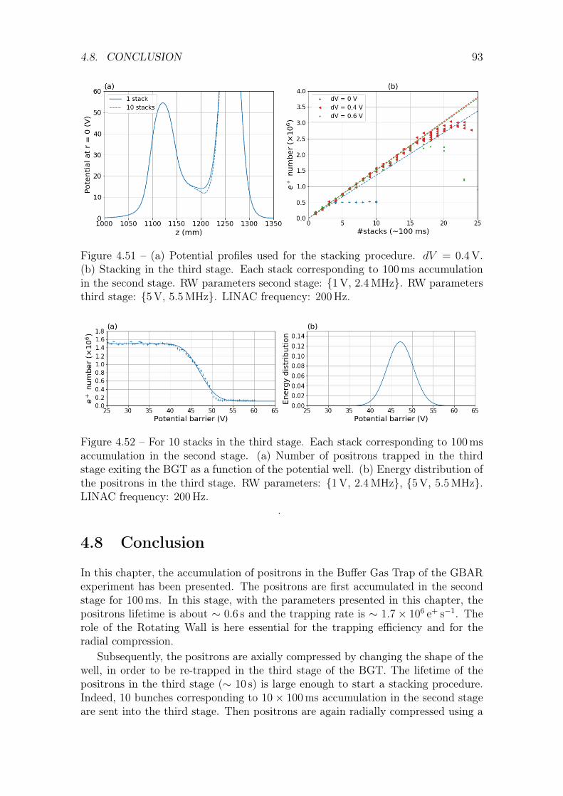
4.8. CONCLUSION 93
Figure 4.51 – (a) Potential profiles used for the stacking procedure. dV = 0.4 V.(b) Stacking in the third stage. Each stack corresponding to 100 ms accumulationin the second stage. RW parameters second stage: 1 V, 2.4 MHz. RW parametersthird stage: 5 V, 5.5 MHz. LINAC frequency: 200 Hz.
Figure 4.52 – For 10 stacks in the third stage. Each stack corresponding to 100 msaccumulation in the second stage. (a) Number of positrons trapped in the thirdstage exiting the BGT as a function of the potential well. (b) Energy distribution ofthe positrons in the third stage. RW parameters: 1 V, 2.4 MHz, 5 V, 5.5 MHz.LINAC frequency: 200 Hz.
.
4.8 Conclusion
In this chapter, the accumulation of positrons in the Buffer Gas Trap of the GBARexperiment has been presented. The positrons are first accumulated in the secondstage for 100 ms. In this stage, with the parameters presented in this chapter, thepositrons lifetime is about ∼ 0.6 s and the trapping rate is ∼ 1.7× 10⁶ e+ s−1. Therole of the Rotating Wall is here essential for the trapping efficiency and for theradial compression.
Subsequently, the positrons are axially compressed by changing the shape of thewell, in order to be re-trapped in the third stage of the BGT. The lifetime of thepositrons in the third stage (∼ 10 s) is large enough to start a stacking procedure.Indeed, 10 bunches corresponding to 10× 100 ms accumulation in the second stageare sent into the third stage. Then positrons are again radially compressed using a

94 CHAPTER 4. THE BUFFER GAS TRAP
Rotating Wall.In conclusion, currently, the BGT provides a bunch of ∼ 1.5× 10⁶ e+ each second
(some losses during the stacking procedure). This bunch has to be transferred in theHigh Field Trap where a stacking procedure can be applied to trap a larger numberof positrons as is presented in the next chapter.

Chapter 5
The High Field Trap
If there is no solution then there isno issue.
A Shadock principle
Contents5.1 Description of the trap . . . . . . . . . . . . . . . . . . . . 96
5.1.1 The super conducting magnet . . . . . . . . . . . . . . . . 96
5.1.2 The electrodes . . . . . . . . . . . . . . . . . . . . . . . . 98
5.1.3 Temperature probes . . . . . . . . . . . . . . . . . . . . . 99
5.1.4 Trapping control . . . . . . . . . . . . . . . . . . . . . . . 101
5.2 Electron gun . . . . . . . . . . . . . . . . . . . . . . . . . . 104
5.2.1 Filament characteristics . . . . . . . . . . . . . . . . . . . 104
5.2.2 Power supply control . . . . . . . . . . . . . . . . . . . . . 106
5.2.3 Control of the system . . . . . . . . . . . . . . . . . . . . 107
5.3 Electron trapping . . . . . . . . . . . . . . . . . . . . . . . 109
5.3.1 Charge counter . . . . . . . . . . . . . . . . . . . . . . . . 109
5.3.2 Electron accumulation . . . . . . . . . . . . . . . . . . . . 110
5.4 Positron trapping . . . . . . . . . . . . . . . . . . . . . . . 119
5.4.1 One stack in the HFT . . . . . . . . . . . . . . . . . . . . 119
5.4.2 Stacking . . . . . . . . . . . . . . . . . . . . . . . . . . . . 121
5.5 Conclusion . . . . . . . . . . . . . . . . . . . . . . . . . . . . 124
In this chapter, the specifications of the High Field Trap, the second positrontrap of the GBAR experiment, are described in Section 5.1. To perform some testswith the trap without using the LINAC, an electron gun has been placed at theentrance of the trap. A description of the gun and the associated control systemis presented in Section 5.2 and the results of the experiments using electrons areshown in Section 5.3 (this work can be compared with the experiments made with
95

96 CHAPTER 5. THE HIGH FIELD TRAP
the same trap at Riken and presented in Ref. [92]). Finally, we present in Section 5.4the results of the experiments based on the re-trapping of the bunches of positronsproduced in the BGT as explained in the previous chapter.
5.1 Description of the trap
The High Field Trap of the GBAR experiment has been built at Riken in Japan[49, 50] and has been given to the GBAR. This Penning-Malmberg trap has beeninstalled at CERN in 2018.
The purpose of this trap in the context of the GBAR experiment is to storethe largest possible quantity of positrons (goal 1010) to produce enough positron-ium atoms for anti-hydrogen ion production. This trap is mainly constituted of asuperconducting magnet able to reach 5 T and a set of 27 electrodes (able to ac-cept a voltage of ±4 kV with a maximal difference between two electrodes of 2 kV).Pictures of the trap are presented in Figure 5.1 and a schematic of the trap inFigure 5.2.
Figure 5.1 – High Field Trap pictures.
The duct being in contact with the electrodes, the entire trapping volume canbe cooled to reach ∼ 10 K. This is obtained with a cryo-head connected to the duct.
The duct and consequently the electrodes can be moved to align the electrodesmain axis with the magnetic field. This alignment is performed thanks to 4 verticalarms, presented in Figure 5.3. The arms can be moved with a precision of 10 µm ona 4 mm range. Since a misalignment creates an E×B drift force which causes theexpansion of the plasma, having the best alignment is essential.
5.1.1 The super conducting magnet
The niobium-titanium coils of the trap’s electromagnet produce a 5 T uniform mag-netic field over 500 mm along the field axis (the total length of the trap being1940 mm) and for a circular section of 4 mm diameter. The uniformity in this regionis estimated as better than 10−3.
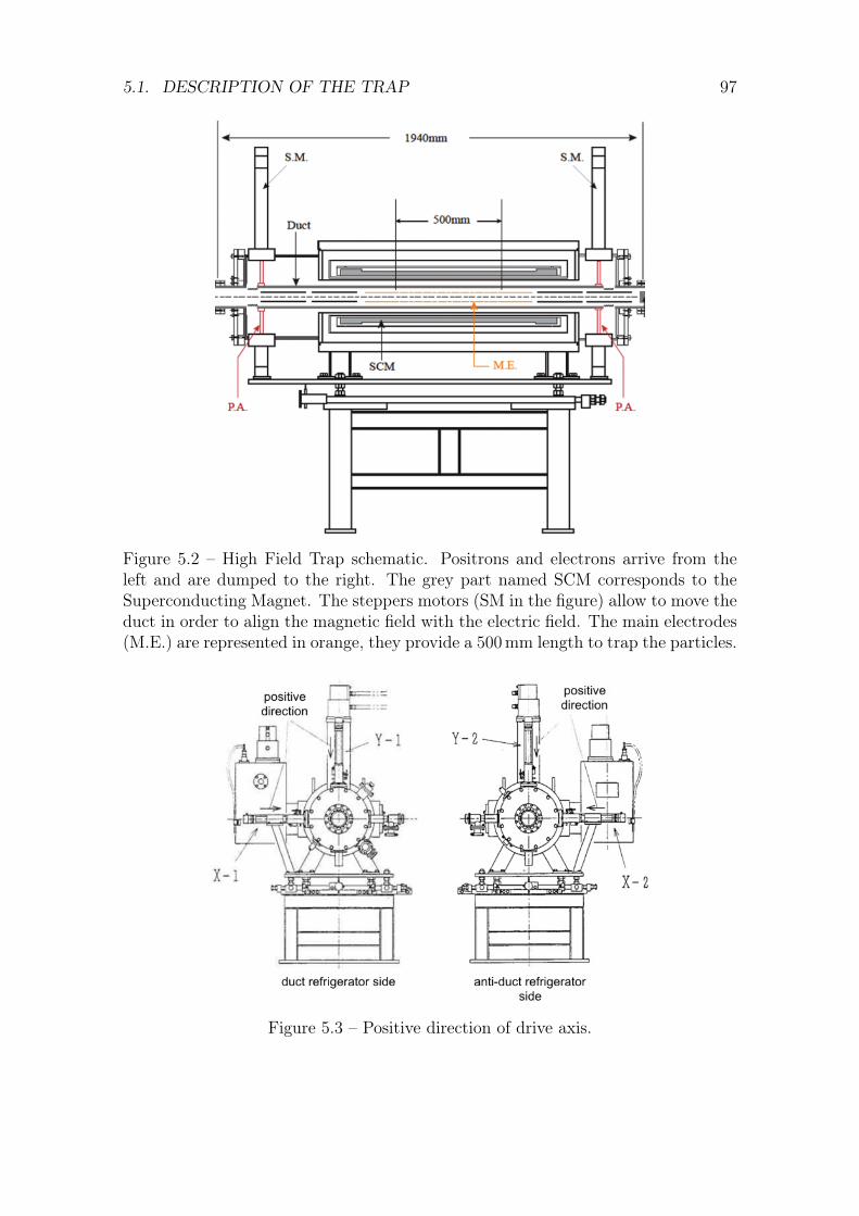
5.1. DESCRIPTION OF THE TRAP 97
Figure 5.2 – High Field Trap schematic. Positrons and electrons arrive from theleft and are dumped to the right. The grey part named SCM corresponds to theSuperconducting Magnet. The steppers motors (SM in the figure) allow to move theduct in order to align the magnetic field with the electric field. The main electrodes(M.E.) are represented in orange, they provide a 500 mm length to trap the particles.
Figure 5.3 – Positive direction of drive axis.

98 CHAPTER 5. THE HIGH FIELD TRAP
To reach 5 T, the coils require to be cooled enough to reach the superconductingstate thanks to a cryogenic head. When cold a 45 min ramp brings the current from0 to 85 A. The electromagnet is surrounded by an insulation vacuum. A secondinsulation vacuum surrounds the duct (Figure 5.2), to keep the center of the ductaround 10 K.
The control of the current is done by three elements: an analog convertor [93](Figure 5.4a), a current generator (Figure 5.4b) and a protection system (Fig-ure 5.4c). The analog convertor is controlled by a Labview program on (Figure 5.4d)a computer through a GPIB connection. The converter controls the current gener-ator, which sends a feedback to the computer.
(a)
(b)
(c)
(d)
Figure 5.4 – The different components to power the HFT’s magnet. (a) Analogconvertor. (b) Power supply. (c) Power breaker. (d) Labview VI to control theanalog convertor.
5.1.2 The electrodes
The electric potential is created by a set of 27 cylindrical electrodes. The inner andouter diameters are respectively of 38 and 40 mm. They are made of oxygen-freecopper, gold plated, and numbered from -13 to 13. The first three electrodes (-13,-12, -11) have respectively lengths of 270 mm, 270 mm, and 160 mm. The setup issymmetric for the last three ones (i.e., 11, 12, 13 have respectively lengths of 160,270, and 270 mm). The remaining electrodes (from -10 to 10) all have a length of20 mm and are separated by 3 mm gaps. Electrodes -2 and 2 (see Figure 5.5) aresplit in 4 azimuthally, for the rotating wall technique (see Section 3.3.2). As shownin Figure 5.6, electrodes -13 and -12, -11 to 11 and, 12, 13 are on three separatedsupports.
It is important to note that, because of the geometry, a difference of potentialbetween two electrodes higher than 2 kV cannot be used. Otherwise, one would

5.1. DESCRIPTION OF THE TRAP 99
Figure 5.5 – Left: 3D view of the electrodes. Right: one of the rotating wall elec-trodes.
create sparks that could damage the system. The potential is applied using HighVoltage Amplifiers [94].
Figure 5.6 – Extracted from Ref. [51]. Top: Central support with the main elec-trodes. Bottom: The three supports assembled.
The electrodes are placed in a duct (see in Figure 5.2) in which the pressure ismaintained below 1× 10⁻⁹ mbar thanks to a cryo-pump upstream and an ion-pumpdownstream the HFT. The temperature of the electrodes in the trap influencesdirectly the trapped plasma cooling, and is a limit for that. The temperature ofthe electrodes is related to the temperature of the duct which is cooled through acryogenic cold head down to a temperature around 10 K.
5.1.3 Temperature probes
As shown in Figure 5.7, several types of temperatures probes are installed inside thetrap to continuously monitor the temperatures of the duct and magnet.

100 CHAPTER 5. THE HIGH FIELD TRAP
Figure 5.7 – Overview of the temperature probes inside the HFT. TGi corresponds tothe Gallium-Aluminium-Arsenide diode based probes and CCi to the thermocouplesprobe. Hi corresponds to the heaters necessary for the baking of the system.
Three kinds of probes are used, the choice of which depends on the range oftemperature we want to read. Some specifications of the probes are shown in Ap-pendix D. To monitor the temperatures of the duct, we use Gallium-Aluminium-Arsenide diodes based probes, as detailed in Table 5.1, with expected values between10 K and 60 K in the working mode. These temperatures are constantly read on anindependent computer thanks to a Labview program.
Probe Location Automatically read in April 2020TG1 Duct left side yes, channel 3, currently brokenTG2 Duct center yes, channel 2TG3 Duct right side yes, channel 1TG4 Second stage of the cold head noTG5 Middle of duct shield yes, channel 4
Table 5.1 – Temperatures read by the Gallium-Aluminium-Arsenide diodes basedprobes in the HFT.
It has to be noticed for a future user of the trap that we figured out that onthe schematics, TG1 and TG3 has been reversed. The best way to know if themeasurement is consistent is to check if we have TG4 < TG1 < TG2 ∼ TG5 < TG3(according to the position of the probes in Figure 5.7). The connector pins arepresented in Figure D.1 and Table D.1.

5.1. DESCRIPTION OF THE TRAP 101
Then, thermocouples are used to measure temperatures as defined in Table 5.2.They are used to measure temperatures between approximatively −150 C and150 C. The most important probes are CC7, CC8 and CC9, corresponding re-spectively to the left, center and right of the duct because they are connected to theheaters necessary for the baking of the tube to improve the vacuum.
Probe DetailsCC1 First stage cold head magnetCC2 Magnet radiation shielding or second stage of the cold headCC3 Magnet radiation shielding left sideCC4 Thermal shield duct left sideCC5 Magnet radiation shielding right sideCC6 Shield duct right sideCC7 Duct left side, to compare with TG1CC8 Duct center, to compare with TG2CC9 Duct right side, to compare with TG3
Table 5.2 – Temperatures read by the thermocouple probes in the HFT.
The magnet is cooled using a helium circuit and compressor in order to reach atemperature of ∼ 4 K. The magnet is insulated from the rest of the device thanks toa thermal shield (see “duct shield” in Figure 5.7): it is an empty cylindrical volumewhere the pressure is about 10−6−10−7mbar. The temperature of the magnet, beingextremely low, we use Carbon Glass Resistors, with a range from 1.4 K to 100 K.As presented in Table 5.3, the probes are placed at 3 different positions: one on thecryostat, and the others on the super-conducting coils.
Probe DetailsCGR1 Cold point of the cold headCGR2 Coils right sideCGR3 Coils left side
Table 5.3 – Temperatures read by the Carbon Glass Resistor based probes in theHFT.
Currently, the temperatures of the magnet are determined manually by measur-ing the values of the resistance and by extrapolating from the abaci presented inTables D.3, D.4, D.5 and Figure D.2. In a next future, this measurement will beautomated.
5.1.4 Trapping control
The trapping control is similar to the one of the BGT (described in Section 4.3.2), itis then performed by a PXI. The main difference is that the NI PXIe 8135 computermodule has been replaced by a NI PXIe 8840 module. This module is a RealTime (RT) computer, allowing to run Real Time Labview programs, insuring atemporal precision and a reproducibility. However, it is not a standard computer,
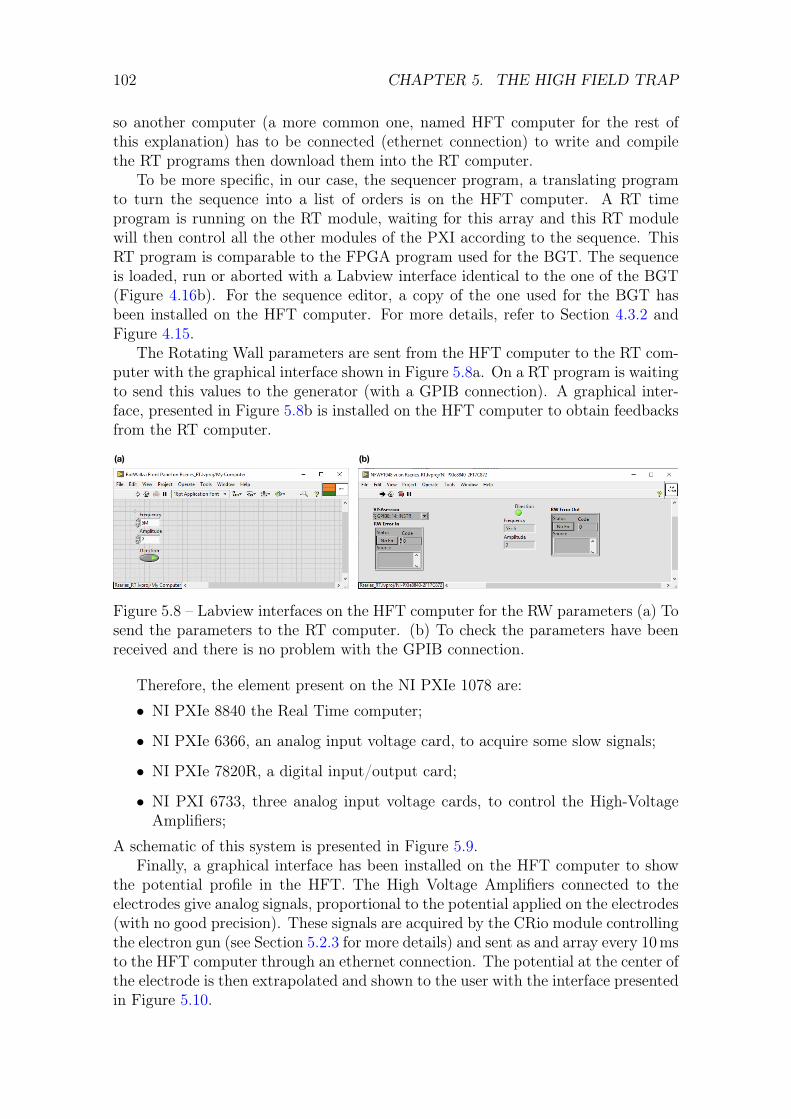
102 CHAPTER 5. THE HIGH FIELD TRAP
so another computer (a more common one, named HFT computer for the rest ofthis explanation) has to be connected (ethernet connection) to write and compilethe RT programs then download them into the RT computer.
To be more specific, in our case, the sequencer program, a translating programto turn the sequence into a list of orders is on the HFT computer. A RT timeprogram is running on the RT module, waiting for this array and this RT modulewill then control all the other modules of the PXI according to the sequence. ThisRT program is comparable to the FPGA program used for the BGT. The sequenceis loaded, run or aborted with a Labview interface identical to the one of the BGT(Figure 4.16b). For the sequence editor, a copy of the one used for the BGT hasbeen installed on the HFT computer. For more details, refer to Section 4.3.2 andFigure 4.15.
The Rotating Wall parameters are sent from the HFT computer to the RT com-puter with the graphical interface shown in Figure 5.8a. On a RT program is waitingto send this values to the generator (with a GPIB connection). A graphical inter-face, presented in Figure 5.8b is installed on the HFT computer to obtain feedbacksfrom the RT computer.
(a) (b)
Figure 5.8 – Labview interfaces on the HFT computer for the RW parameters (a) Tosend the parameters to the RT computer. (b) To check the parameters have beenreceived and there is no problem with the GPIB connection.
Therefore, the element present on the NI PXIe 1078 are:
• NI PXIe 8840 the Real Time computer;
• NI PXIe 6366, an analog input voltage card, to acquire some slow signals;
• NI PXIe 7820R, a digital input/output card;
• NI PXI 6733, three analog input voltage cards, to control the High-VoltageAmplifiers;
A schematic of this system is presented in Figure 5.9.Finally, a graphical interface has been installed on the HFT computer to show
the potential profile in the HFT. The High Voltage Amplifiers connected to theelectrodes give analog signals, proportional to the potential applied on the electrodes(with no good precision). These signals are acquired by the CRio module controllingthe electron gun (see Section 5.2.3 for more details) and sent as and array every 10 msto the HFT computer through an ethernet connection. The potential at the center ofthe electrode is then extrapolated and shown to the user with the interface presentedin Figure 5.10.

5.1. DESCRIPTION OF THE TRAP 103
NI P
XIe
1078
Slot
1
NI P
XIe
8840
•Re
al T
ime
com
pute
r
NI P
XI 6
733
Slot
5, 6
, 7•
8 An
alog
Vol
tage
O
utpu
ts
•1M
S/s
NI P
XIe
7820
RSl
ot 3
•4
x 32
Dig
ital
Inpu
ts/O
utpu
ts
•FP
GA
mod
ule
•80
MH
z
Inte
rnal
PXI
con
nect
ion
NI P
XIe
6366
Slot
2•
8 An
alog
Vol
tage
In
puts
•2
MS/
s•
Mul
tifun
ctio
n
(24
DIO
, 2AO
)
Det
ecto
rs•
CsI
det
ecto
rs
•C
harg
e co
unte
r
Anal
og s
igna
l
Hig
h Vo
ltage
Am
plifi
ers
Elec
trode
s
Ethe
rnet
Digi
tal s
igna
l
Dig
ital O
utpu
ts•
Sign
al a
cqui
sitio
n•
BGT
•El
ectro
n gu
n•
RW o
n / o
ff•
Trig
gerin
g ot
her d
evic
es
Dig
ital I
nput
s
•BG
T tri
gger
Digi
tal s
igna
l
Con
nect
or 0
Con
nect
or 1
GPI
BRo
tatin
g W
all W
ave
gene
rato
rsSplit
ters
SEQ
UEN
CER
+
RW p
aram
eter
s
Com
pute
r in
the
cont
rol r
oom
Figure5.9–Overview
oftheconn
ection
sof
theHFT’s
trap
ping
controls
ystem.

104 CHAPTER 5. THE HIGH FIELD TRAP
Figure 5.10 – Graphical interface showing in real time the potential at the center ofthe trap.
5.2 Electron gun
An electron gun has been placed between the Buffer Gas Trap and the High FieldTrap. In this section, some important characteristics about the electron gun arepresented, like how the system is connected, and how to control it.
5.2.1 Filament characteristics
The principle of the electron gun used in the experiment is the following: a fil-ament heated by a current heats a disk made of Yttrium Oxide (Y2O3) (see inFigure 5.11) [95]. Then the Y2O3 disk emits electrons thanks to an electric fieldgenerated by the difference of potential between both sides of the filament (cath-odes 1 and 2 in Figure 5.12) and the anode. In our system, the anode is a disk witha hole in the middle. In the presence of a magnetic field aligned with the disk axis,which is also the axis of the positron line, the electrons are channeled through thehole and ejected with a kinetic energy corresponding to the voltage applied at theanode. Without magnetic field, the electrons are absorbed by the anode.
Figure 5.12 shows how the electron gun is powered. Two floating ground gener-ators are used [96]. One sets V +
2 = 0 and V −2 = V +1 . The potentials fulfil V +
1 > V −1and V +
2 > V −2 . A 12 V Zener diode is used to apply a difference of potential of12 V between cathode 2 and the anode to extract the electrons. Finally the micro-ammeter between point A and the ground will allow to determine the current ofelectrons that have gone through the hole of the anode.
To study the behaviour of the electron gun, the circuit presented in Figure 5.12has been turned into the one presented in Figure 5.13. Here, one set V +
2 −V −2 = 20 V,

5.2. ELECTRON GUN 105
Figure 5.11 – Extracted from the “ES-535W Yttria coated Iridium disc on AEI baseand CB-104 base” datasheet [95]. One can see the support of the filament, and theYttrium Oxide disk which is heated to emit electrons.
V −1
cathode 1
V +1 cathode 2
filament
V −2
V +2 A
Aground
15 kΩ
anode
B
Figure 5.12 – Schematic circuit used to power the electron gun. The “cathode 1”and “cathode 2” outputs go to the filament and obviously, the “anode” output to theanode of the electron gun.
and connects the anode to the ground. A micro-ammeter is installed between pointsA and C which measures a current named Ian. The voltage Vgen and current Igen
are read on the generator’s monitor. Physically, Igen corresponds to the number ofelectrons injected in the circuit per second. Then some of these electrons are emittedby the filament and go to the anode back to the generator resulting in a current Ian
which is then the number of emitted electrons per second.The measurement of Igen and Ian as a function of Vgen is presented in Figure 5.14.
The first observation is that as expected, the behaviour of the filament is not thebehaviour of a simple linear resistance. However, the plot Igen as a function of Vgen
is different from what we would expect compared to the specifications [95]. Thisdifference is due to the internal resistance of the wires connecting the output “cathode1” and “cathode 2” to the filament (we measured 0.9 Ω of internal resistance of thewires). It is also shown in Figure 5.14 that electrons are emitted after a threshold ofVgen = 1.5 V, Igen = 1.5 A and the current Ian increases quickly after the thresholdto reach about 0.6 mA. The test is not performed for higher Vgen and Igen to avoid

106 CHAPTER 5. THE HIGH FIELD TRAP
V −1
cathode 1
V +1
AIgen cathode 2
filamentV Vgen
AIan
ground
15 kΩ
anode
A
B
C
V −2
V +2
Figure 5.13 – Schematic circuit to determine the current of emitted electrons (Ian)by the filament of the electron gun.
burning the filament which cannot accept a current above Igen = 1.8 A.
0.0 0.5 1.0 1.5 2.0Vgen (V)
0.0
0.5
1.0
1.5
I gen
(A)
Electron emission Van = 20V
0
200
400
600
I an(
A)Figure 5.14 – Igen and Ian as a function of Vgen. According to Figure 5.13, Vgen andIgen are the voltage and current provided by the generator and Ian the current goingthrough the anode i.e. the current of emitted electrons.
By this simple test, one can see that if we use a voltage of Vgen ∼ 2 V, we canemit electrons without burning the filament.
5.2.2 Power supply control
As explained in Section 5.2.1, a current higher than 1.8 A cannot be accepted in theelectron gun filament. The generator providing this current has to be physically lim-ited to prevent exceeding this threshold. Let’s focus on the power supply connectedon the filament, the one providing V ±1 in Figure 5.12.
The power supply is controlled remotely, using a sub-D entrance as presented inFigure 5.15.
Pins 3 and 9, corresponding to V3 and V9, are used to limit the current. For amaximal current of 1.8 A, V3 has to be connected in a way that V3/V9 ≤ 0.18. Thisis why we use a voltage divider as presented in Figure 5.16. Indeed, using Millman’s

5.2. ELECTRON GUN 107
Figure 5.15 – Extracted from Ref. [96]. Remote control input of the generator.
theorem on V3 we have:
V3 =(V1 = 0)/10 kΩ + V9/47 kΩ
1/10 kΩ + 1/47 kΩ= V9
10
10 + 47= 0.175V9
10 kΩ
Vc 10 kΩ V11,voltage programming input
V1, ∅
10 kΩ V3, current programming input
47 kΩ
9, V9 = 5.1 V
Figure 5.16 – Control of the generator
Thereby, it is now impossible to set a current greater than 1.8 A in the filament.Also, it is required to control remotely the voltage going out of this power supply.This is the purpose of voltage V11. The controller provides a signal Vc between −10 Vand 10 V, and we would like to have 5 > V11 > 0 to fulfil the specifications of thepower supply [96]. This is why we have the second voltage divider and the diode inFigure 5.16. Something similar has been done for the second power supply.
However, the system will not work like that. Indeed, according to the datasheet,V1 in Figure 5.16 and V −1 in Figure 5.12 are connected. So if the circuit presentedin Figure 5.16 is directly used, we would have V1 = V −1 = ground, and the electrongun would be short-circuited. This is why we have to use galvanic isolators for thewires going to the controller.
5.2.3 Control of the system
The power supplies [96] are controlled by a NI cRIO 9066 controller. On this cRIO,5 modules are connected:

108 CHAPTER 5. THE HIGH FIELD TRAP
• NI 9205, an analog input module to display the feedback signals from the highvoltage amplifiers which create the electric potential in the HFT (it is notrelevant to have a dedicated cRIO only for that purpose);
• NI 9263, an analog input module to display the feedback signals from theelectron gun power supplies;
• NI 9201, an analog output module to set the voltage of the electron gun powersupplies;
• NI 9402, a digital IO module to get triggers when the electron gun has to beused according to a predefined sequence for the e± trapping;
• NI 9494, a 24 V digital output module to control the push/pull in order toput the electron gun in or out of the beam line.
As explained in Section 5.2.2, the signal wires connected to NI 9205 and NI 9201have to go through galvanic isolators before being connected to the electron gunpower supplies because of a grounding issue. A schematic of how the system isconnected is presented in Figure 5.17.
Figure 5.17 – Schematic of the connections. More information concerning the PXIare presented in Section 5.1.4.
To set the voltage on the power supplies, a graphic interface has been developedand is installed on the computer in charge of the HFT. It is shown in Figure 5.18.With this interface, it is also possible to manually control the electron gun, but itis only relevant to use it for tests. To control the electron gun during a trappingsequence, we use triggers coming from the PXIe, to control the push-pull, and toswitch on/off the power supplies.
5.3. ELECTRON TRAPPING 109
Figure 5.18 – Graphic interface
5.3 Electron trapping
5.3.1 Charge counter
In order to determine the number of trapped electrons, the front surface of the MCPis used as a Faraday cup. The charge counter used in Section 4.6 to determine thenumber of positrons cannot be used since the expected number of charges is aboveits saturation limit. The schematic of the homemade charge counter used here isshown in Figure 5.19.
Basically a charge counter consist of a RC circuit with an oscilloscope attached.When the charges arrive on the MCP front, creating a potential VMCP, they areaccumulated in a capacitor (C2 = 1 nF) and there is a discharge in the resistor(R ∼ 0.5 MΩ). This lead to a step potential (or a large peak, C2R ∼ 0.5 ms)Vout, with the relation Q = VoutC2, with Q the charge actually accumulated in thecapacitor.
This charge does not correspond to the real charge touching the MCP front. Thefirst reason is the presence of secondary electrons. Indeed, some electrons can leavethe MCP to go backward, and this is a source of underestimation of the charge. Apositive potential Vbias has to be applied on the MCP front to solve this problem.However, such a potential is not desired on the acquisition devices. This is why ithas to be decoupled with a capacitance (C1 = 100 nF).
Stray capacitances may add to C2, and a calibration is needed. A pulse generatoris used to generate a pulse of amplitude Vcal, allowing to quickly accumulate chargesin a perfectly known capacitor (Ccal = 1.64(2) pF) and quickly discharge (Ccal ∼900 ns/50 Ω) to simulate charges coming from the MCP front. Knowing Ccal andVcal, the charge is known (Q = CcalVcal), and a calibration can be done to determinethe charge as a function of Vout.
Therefore, electric pulses of varying amplitude Vcal are used and we look at Vout
to determine the charge Q as a function of Vout such as
Q = CcalVcal =1
aCcalVout, (5.3.1)
if Vout is proportional to Vcal (i.e., Vout = aVcal). As it is presented in Figure 5.20,a is obtained by varying Vcal with a = 6.69(2)× 10−3. The error on the charge

110 CHAPTER 5. THE HIGH FIELD TRAP
Vbiais
1 MΩ
VMCP
C1
C2
Vout
Ccal50 Ω ∼ 0.5 MΩ
Vcal
Figure 5.19 – Electric circuit of the charge counter. Ccal = 16.4 pF, C1 =100 nF, C2 = 1 nF.
0 2 4 6 8 10 12Vcal (V)
0.000.010.020.030.040.050.060.070.08
V out
(V)
Figure 5.20 – Calibration of the charge counter. Output voltage as a function of thecalibration signal amplitude.
measurement can be deduced from Equation 5.3.1 as following
∆Q =Vout
a∆Ccal ⊕
Ccal
a∆Vout ⊕
Vout
a2∆a. (5.3.2)
Finally, the number of electrons N can be determined as a function of Vout usingN = Q/e (e = 1.602 176 565(35)× 10−19 C):
N = 1.532× 10¹⁰Vout ±(0.006× 10¹⁰Vout ⊕ 1.532× 10¹⁰∆Vout
)(5.3.3)
To determine the value of Vbias to avoid the secondary electron issue, a bunchof electrons is sent on the MCP’s front for different values of Vbias while Vout ismeasured. The emission of secondary electrons leads to an underestimation of Vout
as observed in Figure 5.21. By increasing Vbias, Vout is increased until there are nomore secondary electrons if Vbias > 80 V. For the following experiments, Vbias is setat 100 V.
5.3.2 Electron accumulation
Narrow wells
Electrons are accumulated in short wells (2 electrodes, i.e., 4.3 cm) or at the entranceeither at the exit of the HFT. The potential profiles and the potential applied onthe electrodes are presented respectively in Figure 5.22 and Table 5.4.

5.3. ELECTRON TRAPPING 111
0 20 40 60 80 100 120 140Vbiais (V)
0.50
0.55
0.60
0.65
0.70
0.75
0.80V o
ut (V
)
Figure 5.21 – Output signals for different biases. One can clearly see that the effectof the secondary electrons disappears above Vbias = 100 V.
z (mm)
500
0
500
V at
r =
0
(a)
z (mm)V
at r
= 0
(b)
0 250 500 750 1000 1250 1500 1750z (mm)
500
0
500
V at
r =
0
(c)
0 250 500 750 1000 1250 1500 1750z (mm)
V at
r =
0(d)
Figure 5.22 – Potential profiles in the HFT. Blue: HFT’s entrance. Red: HFT’sexit.
Electrode -13 -12 -11 -10 -9 -8 -7Electrode -13 -12 -11 7 8 9 10
(a) -900 -900 -900 0 500 500 -920(b) 0 0 0 0 500 500 -920(c) -900 0 0 0 500 500 -920(d) -900 0 0 -920 0 0 -920
Table 5.4 – Potentials on the electrodes corresponding to the potential profiles inFigure 5.22.
The procedure used is the following:
• (a) the electron gun is turned on (warming up time 2.5 s, Vgen = 2.6 V, Van =15 V), a long barrier is applied to repel the incoming electrons, and the accu-mulation potential is set;
• (b) with the electron gun on, the entrance barrier is lowered to accumulateelectrons for an adjustable time;
• (c) the electron gun is turned off, the entrance barrier is raised;
• 100 ms waiting;
• the electrons stay trapped for another adjustable time;

112 CHAPTER 5. THE HIGH FIELD TRAP
• (d) the electron plasma is prepared to be ejected by changing the potential in2.7 ms and in 2000 steps;
• the exit potential is set to 0 V using a fast switch and consequently, the elec-trons are ejected from the trap to the MCP’s front.
Figure 5.23 shows the number of trapped electrons as a function of the accumu-lation time. We could expect a number increasing with time and remaining constantwhen the well is full. However, this is not what we see here. Indeed, after and accu-mulation time of ∼ 0.3 s, there is an instability in the number of detected electrons,inducing large error bars. These error bars are determined with Equation 5.3.3, withan error on the electric signal determined with 10 measurements. After a transi-tional period of few hundred of ms, the instability disappears and the number ofdetected electrons decrease slowly. Our hypothesis is that the hottest electrons areagitated and ejected by the incoming beam explaining the instability. It is also clearin Figure 5.23 that concerning the accumulation, the behaviour is the same if thetrapping occurs at the entrance or the exit of the trap.
0.0 0.1 0.2 0.3 0.4 0.5 0.6 0.7 0.8accumulation time (s)
0.000.020.040.060.080.100.12
dete
cted
e (×
1010
) (a)
0.0 0.1 0.2 0.3 0.4 0.5 0.6 0.7 0.8accumulation time (s)
0.000.020.040.060.080.100.12
dete
cted
e (×
1010
) (b)
Figure 5.23 – Trapped electron number as a function of the accumulation time fora well at the entrance (a) or at the exit (b) of the HFT Electron gun: Vgen =2.6 V, Van = 15 V.
Therefore the accumulation time is set at 0.25 s, in order to produce a stableplasma of ∼ 8× 10⁸ electrons and to study the behaviour of electrons while theyare trapped as presented in Figure 5.24. The number electrons N as a function of the
0 2 4 6 8 10trapping time (min)
0.00
0.02
0.04
0.06
0.08
0.10
dete
cted
e (×
1010
) (a)
0 2 4 6 8 10trapping time (min)
0.00
0.02
0.04
0.06
0.08
0.10
dete
cted
e (×
1010
) (b)
Figure 5.24 – Trapped electron number as a function of the waiting time after 0.25 saccumulation for a well at the entrance (a) or at the exit (b) of the HFT. Electrongun: Vgen = 2.6 V, Van = 15 V.
trapping time t can be fit with N(t) = N1e−t/τ1 +N2e
−t/τ2 . As a first interpretation,

5.3. ELECTRON TRAPPING 113
there could be two populations N1 and N2 with different lifetimes τ1 and τ2 withN2 > N1 and τ2 τ1. However it is more likely that it is the result of a misalignmentof the electrodes with the magnetic field and after a certain time, there is a betterstability of the trapped electrons, explaining the apparent two populations. Theresults of the fit are presented in Table 5.5. Even if in that case, we see that
N1 N2 τ1 τ2
(a) entrance 1.1(1)× 108 7.1(10)× 108 0.45(10) min 45(8) min(b) exit 1.6(2)× 108 6.5(2)× 108 0.94(24) min 120(70) min
Table 5.5 – Parameters of the fit function N(t) = N1e−t/τ1 + N2e
−t/τ2 according tothe data presented in Figure 5.24.
there is a difference between the well at the entrance and the well at the exit, wehave the same order of magnitudes. This difference can be explained with a smallmisalignment, and with the difference of temperature between the entrance and theexit of the trap.
Wide wells
The same experiments as the ones presented in Section 5.3.2 are performed but withwider wells. Instead of using a well made of 2 electrodes, 6 electrodes are used (i.e.,13.5 cm long). The potential profiles are presented in Figure 5.25 and the potentialapplied on the electrodes in Table 5.6.
z (mm)
500
0
V at
r =
0
(a)
z (mm)
V at
r =
0
(b)
0 250 500 750 1000 1250 1500 1750z (mm)
500
0
V at
r =
0
(c)
0 250 500 750 1000 1250 1500 1750z (mm)
V at
r =
0
(d)
Figure 5.25 – Potential profiles in the HFT. Blue: HFT’s entrance. Red: HFT’sexit.
The accumulation curves presented in Figure 5.26 are similar to those for theshort wells (Section 5.3.2). Indeed, there are instabilities when the electron numberreaches the saturation limit after which the instabilities disappear and the numberof accumulated electrons decreases slowly. The duration of the accumulation is setat 0.6 s in order to provide a stable plasma of 2.4× 10⁹ electrons.
The accumulation procedure being defined we estimate the lifetime in the wellthanks to the data presented in Figure 5.27. Here again, it looks like there aretwo populations, one with a short lifetime (∼ 1 min) and one with a longer lifetime(∼ 10 min). The results of the fits are in Table 5.7. It is expected to have a smaller
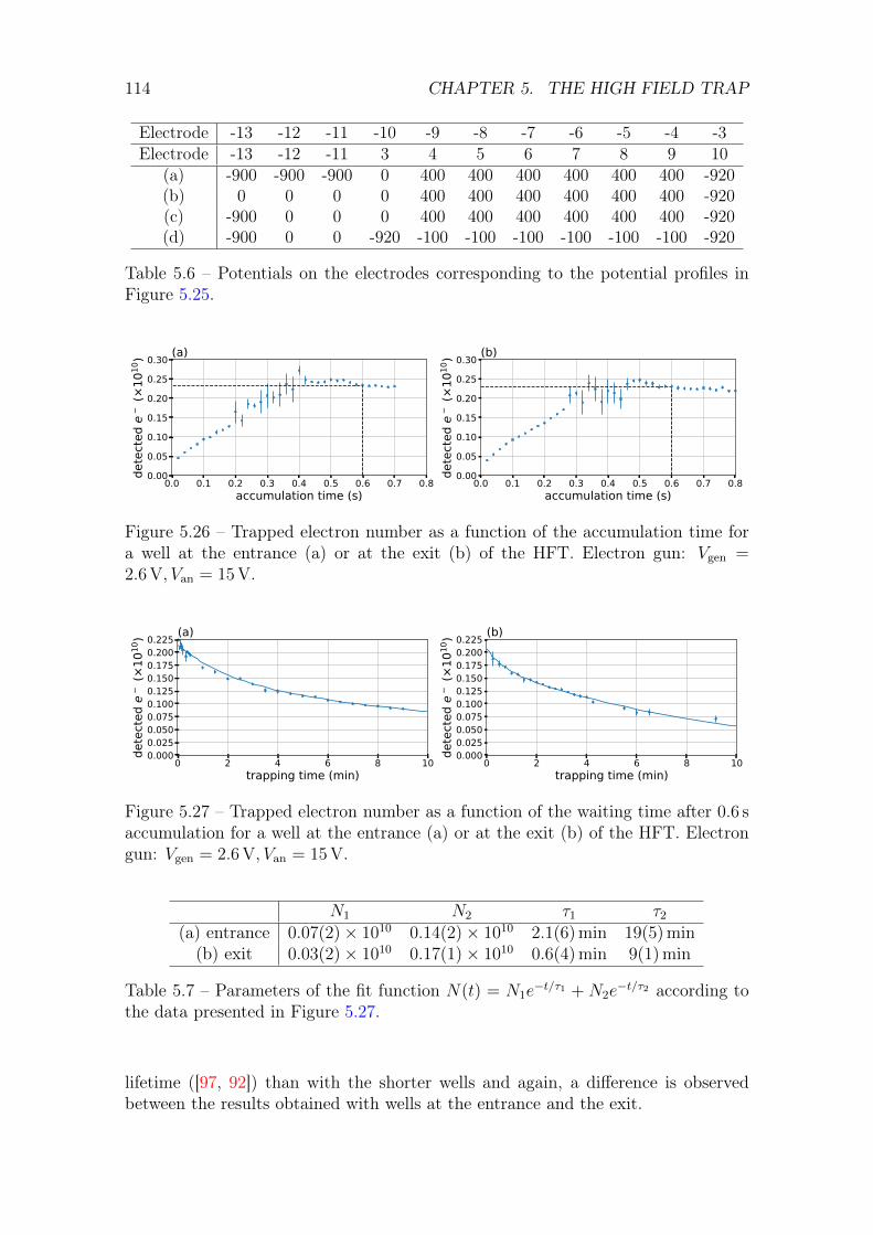
114 CHAPTER 5. THE HIGH FIELD TRAP
Electrode -13 -12 -11 -10 -9 -8 -7 -6 -5 -4 -3Electrode -13 -12 -11 3 4 5 6 7 8 9 10
(a) -900 -900 -900 0 400 400 400 400 400 400 -920(b) 0 0 0 0 400 400 400 400 400 400 -920(c) -900 0 0 0 400 400 400 400 400 400 -920(d) -900 0 0 -920 -100 -100 -100 -100 -100 -100 -920
Table 5.6 – Potentials on the electrodes corresponding to the potential profiles inFigure 5.25.
0.0 0.1 0.2 0.3 0.4 0.5 0.6 0.7 0.8accumulation time (s)
0.000.050.100.150.200.250.30
dete
cted
e (×
1010
) (a)
0.0 0.1 0.2 0.3 0.4 0.5 0.6 0.7 0.8accumulation time (s)
0.000.050.100.150.200.250.30
dete
cted
e (×
1010
) (b)
Figure 5.26 – Trapped electron number as a function of the accumulation time fora well at the entrance (a) or at the exit (b) of the HFT. Electron gun: Vgen =2.6 V, Van = 15 V.
0 2 4 6 8 10trapping time (min)
0.0000.0250.0500.0750.1000.1250.1500.1750.2000.225
dete
cted
e (×
1010
) (a)
0 2 4 6 8 10trapping time (min)
0.0000.0250.0500.0750.1000.1250.1500.1750.2000.225
dete
cted
e (×
1010
) (b)
Figure 5.27 – Trapped electron number as a function of the waiting time after 0.6 saccumulation for a well at the entrance (a) or at the exit (b) of the HFT. Electrongun: Vgen = 2.6 V, Van = 15 V.
N1 N2 τ1 τ2
(a) entrance 0.07(2)× 1010 0.14(2)× 1010 2.1(6) min 19(5) min(b) exit 0.03(2)× 1010 0.17(1)× 1010 0.6(4) min 9(1) min
Table 5.7 – Parameters of the fit function N(t) = N1e−t/τ1 + N2e
−t/τ2 according tothe data presented in Figure 5.27.
lifetime ([97, 92]) than with the shorter wells and again, a difference is observedbetween the results obtained with wells at the entrance and the exit.

5.3. ELECTRON TRAPPING 115
Wider well
Let’s see what is happening with a single wider well (10 electrodes, i.e., 22.7 cm).The potential profiles and the potential applied on the electrodes are respectivelypresented in Figure 5.28 and Table 5.8.
z (mm)
500
0
V at
r =
0
(a)
z (mm)
V at
r =
0
(b)
0 250 500 750 1000 1250 1500 1750z (mm)
500
0
V at
r =
0
(c)
0 250 500 750 1000 1250 1500 1750z (mm)
V at
r =
0
(d)
Figure 5.28 – Potential profiles in the HFT. See Table 5.8.
El. -13 -12 -1 -10 -9 · · · 0 1(a) -900 -900 0 0 400 · · · 400 -920(b) 0 0 0 0 400 · · · 400 -920(c) -900 0 0 0 400 · · · 400 -920(d) -900 0 0 -920 -100 · · · -100 -920
Table 5.8 – Potentials on the electrodes corresponding to the potential profiles inFigure 5.28.
The same behaviour as the one presented in the previous experiment is observedfor the accumulation (Figure 5.29a). This time, accumulating for 0.6 second a stableplasma of 3.5× 10⁹ electrons is obtained. A study of the lifetime in this configuration
0.0 0.2 0.4 0.6 0.8 1.0accumulation time (s)
0.0
0.1
0.2
0.3
0.4
0.5
dete
cted
e (×
1010
) (a)
0 2 4 6 8 10trapping time (min)
0.0
0.1
0.2
0.3
0.4
0.5
dete
cted
e (×
1010
) (b)
Figure 5.29 – (a) Trapped electron number as a function of the accumulation time.(b) Trapped electron number as a function of the waiting time after 0.6 s accu-mulation corresponding to the potentials presented in Table 5.8. Electron gun:Vgen = 2.6 V, Van = 15 V.
is reported in Figure 5.29a and Table 5.9. Compared to Table 5.7, It is observed that

116 CHAPTER 5. THE HIGH FIELD TRAP
N1 N2 τ1 τ2
0.134(2)× 1010 0.183(1)× 1010 0.28(1) min 12.8(2) min
Table 5.9 – Parameters of the fit function N(t) = N1e−t/τ1 + N2e
−t/τ2 according tothe data presented in Figure 5.29.
the lifetime has decreased with the length of the trap. But this time, the fractionsof short-lifetime and long-lifetime population are similar.
From all of these measurements a few remarks can be made. If we want tooptimise the lifetime, it is more interesting to focus on a narrower well. Then, if wewant to increase the number of trapped particles, it is better to increase the depthof the well. If it has not been done earlier, it is because we placed an electricalsafety on the control system to prevent to apply a potential higher than 930 V onthe electrode, to not reach the limit of 2 kV between two electrodes. This safetysystem has been removed now, and we are free to use higher potentials. Also, itmight be interesting to focus on parabolic wells, because it has been shown that thelifetime is higher in that case [92].
Parabolic well
The potential applied on the nth electrode is set such as Vn = −an2 + V0, with V0
the potential applied on the electrode at the center of the well and for this electroden = 0, to ensure a parabolic well, with n ≤ 5. V0 is set at 1000 V and a = 4 V toensure V5 = 0 V.
The energy of the incoming electrons and the heating of the filament are de-creased to avoid the instability issue during the injection. The accumulation pro-cedure has been changed compared to the previous sections, to obtain a sequencecloser to what is described in Ref. [92]:
• (a) the electron gun is turned on (warming up time 2.5 s, Vgen = 2.3 V, Van =13 V), a long barrier is applied to repel the incoming electrons, and the accu-mulation potential is set;
• (b) with the electron gun on, the entrance barrier is lowered to accumulateelectrons for an adjustable time;
• (c) the electron gun is turned off, the entrance barrier is raised;
• 100 ms waiting;
• the electrons stay trapped for another adjustable time;
• (d) the potential at the exit of the well is set at −2 kV, but the fast switchis not triggered, consequently, the voltage on the electrode is still 0 V and thebarrier is raised in few nano seconds at the beginning of the next step;
• (e) the electron plasma is prepared to be ejected by changing the potential in30 ms and in 2000 steps;

5.3. ELECTRON TRAPPING 117
• (f) the exit potential is set to 0 V using a fast switch and consequently, theelectrons are ejected from the trap to the MCP’s front.
The potential profiles are presented in Figure 5.30 and the potentials applied on theelectrodes in Table 5.10. The reason for step (d) is that it is not possible to directlygo from step (c) to step (e). Indeed the fast switch is designed to go to a desiredvoltage quickly, but the rise of the potential after the fast switch is not the same asthe HVA connected directly to the electrodes. Then, without this step, we wouldtake the risk to make the plasma more unstable during the lifting of the well.
z (mm)1000
0
1000
V at
r =
0
(a)
z (mm)
V at
r =
0
(b)
z (mm)1000
0
1000
V at
r =
0
(c)
z (mm)
V at
r =
0
(d)
0 250 500 750 1000 1250 1500 1750z (mm)
1000
0
1000
V at
r =
0
(e)
0 250 500 750 1000 1250 1500 1750z (mm)
V at
r =
0
(f)
Figure 5.30 – Potential profiles in the HFT. See Table 5.10.
El. -13 -12 -10 -9 -8 -7 -6 -5 -4 -3 -2 -1 0 1(a) -100 -100 0 360 640 840 960 1000 960 840 640 360 0 0(b) 0 0 0 360 640 840 960 1000 960 840 640 360 0 0(c) -100 -100 0 360 640 840 960 1000 960 840 640 360 0 0(d) -100 -100 0 360 640 840 960 1000 960 840 640 360 0 -2000(e) -100 -100 -2000 -740 -460 -260 -140 -100 -100 -100 -100 -100 -100 -2000(f) -100 -100 -2000 -740 -460 -260 -140 -100 -100 -100 -100 -100 -100 0
Table 5.10 – Potentials on the electrodes corresponding to the potential profiles inFigure 5.30.
As desired and expected, a softer injection of the electrons prevents from theinstabilities during the accumulation. This can be seen in Figure 5.31a. However,this leads to a longer accumulation time, and this is why this one is set at 2.5 s,providing a stable plasma of 6.6× 10⁹ electrons. Unfortunately, this parabolic welldid not prevent from the loss of a large part of the electrons at the beginning of thetrapping as shown in Figure 5.31b and the results of the fit in Table 5.11. Also, evenif the lifetime is larger for the second population of electrons (∼ 15 min instead of∼ 12 min in the previous section), the difference is not significant enough comparedto our expectation of a few hours.

118 CHAPTER 5. THE HIGH FIELD TRAP
0.0 0.5 1.0 1.5 2.0 2.5accumulation time (s)
0.00.10.20.30.40.50.60.7
dete
cted
e (×
1010
) (a)
0 2 4 6 8 10 12 14 16trapping time (min)
0.00.10.20.30.40.50.60.7
dete
cted
e (×
1010
) (b)
Figure 5.31 – (a) Trapped electron number as a function of the accumulation time.(b) Trapped electron number as a function of the waiting time after 2.5 s accumula-tion in the HFT. Electron gun: Vgen = 2.3 V, Van = 13 V.
N1 N2 τ1 τ2
0.322(4)× 1010 0.335(4)× 1010 0.805(33) min 15.4(3) min
Table 5.11 – Parameters of the fit function N(t) = N1e−t/τ1 +N2e
−t/τ2 according tothe data presented in Figure 5.31b.
From these experiments, we can conclude that it is possible to trap chargedparticles in the HFT for a long time. However, there is an issue during the confine-ment leading to a significant loss of the particles. This may be the resultant of analignment issue between the electrodes and the magnetic field.
Parabolic well after partial realignement
An attempt to find a better alignment has been performed. Basically, we looked atthe electron number for different positions of the duct at different trapping times.However, an optimal position of the electrodes has not been found, even if thesituation has been improved, as presented in Figure 5.32 and Table 5.12 with anelectron lifetime multiplied by a factor of of 2 compared to Table 5.11.
0.0 0.5 1.0 1.5 2.0 2.5 3.0accumulation time (s)
0.0
0.1
0.2
0.3
0.4
0.5
0.6
dete
cted
e (×
1010
) (a)
0.0 2.5 5.0 7.5 10.012.515.017.520.0trapping time (min)
0.0
0.1
0.2
0.3
0.4
0.5
0.6
dete
cted
e (×
1010
) (b)
0.0 2.5 5.0 7.5 10.012.515.017.520.0trapping time (min)
0.0
0.2
0.4
0.6
0.8
1.0
arb.
(c)
Figure 5.32 – After the electrodes have been displaced. (a) Trapped electron num-ber as a function of the accumulation time. (b) Trapped electron number as afunction of the waiting time after 2.5 s accumulation in the HFT. (c) Comparisonwith Figure 5.31b. Electron gun: Vgen = 2.3 V, Van = 13 V.
Even if improvements are possible, we showed in this section that it is possibleto reach around 1010 e− in the HFT. In the next section we use the positron bunch

5.4. POSITRON TRAPPING 119
N1 N2 τ1 τ2
0.183(5)× 1010 0.261(6)× 1010 1.97(11) min 34.60(253) min
Table 5.12 – Parameters of the fit function N(t) = N1e−t/τ1 +N2e
−t/τ2 according tothe data presented in Figure 5.32.
presented in the previous chapter, and stack as many positrons as possible.
5.4 Positron trapping
5.4.1 One stack in the HFT
The Buffer Gas Trap provides a bunch of ∼ 1.5× 10⁶ positrons each second, withthe parameters presented in Chapter 4. The goal is to stack in the High Fieldtrap to reach the maximal number of positrons. We first start with one stack re-trapped into the HFT. The entrance gate of the HFT is opened thanks to a fastswitch, lowering the potential to 0 V for a duration δt which has to be determined(Figure 5.33a). Then the barrier is raised using the fast switch again (Figure 5.33b).Once this positron bunch is captured in the HFT, we wait for a duration t. Then,the potential well is lifted up to prepare the ejection (Figure 5.33c). This changeof potential is made in 4.05 ms with 3000 steps. Finally, the positrons are ejectedout of the trap by lowering the last potential barrier to 0 V with a fast switch(Figure 5.33d). The potentials applied on the electrodes during the sequence arepresented in Table 5.13.
0 500 1000 1500 2000 2500z (mm)
0
50
100
150
Pote
ntia
l at r
= 0
(V)
BGT HFT
(a)
0 500 1000 1500 2000 2500z (mm)
0
50
100
150
Pote
ntia
l at r
= 0
(V)
BGT HFT
(b)
0 500 1000 1500 2000 2500z (mm)
0
50
100
150
Pote
ntia
l at r
= 0
(V)
BGT HFT
(c)
0 500 1000 1500 2000 2500z (mm)
0
50
100
150
Pote
ntia
l at r
= 0
(V)
BGT HFT
(d)
Figure 5.33 – Potential profiles used in the Buffer Gas Trap and High Field Trap.(a) Transfer into the HFT. (b) Positrons re-trapped. (c) Preparation for ejection.(d) Ejection. The coloured areas represent the positrons.
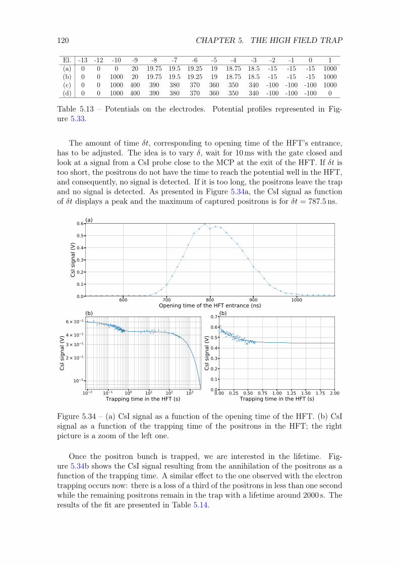
120 CHAPTER 5. THE HIGH FIELD TRAP
El. -13 -12 -10 -9 -8 -7 -6 -5 -4 -3 -2 -1 0 1(a) 0 0 0 20 19.75 19.5 19.25 19 18.75 18.5 -15 -15 -15 1000(b) 0 0 1000 20 19.75 19.5 19.25 19 18.75 18.5 -15 -15 -15 1000(c) 0 0 1000 400 390 380 370 360 350 340 -100 -100 -100 1000(d) 0 0 1000 400 390 380 370 360 350 340 -100 -100 -100 0
Table 5.13 – Potentials on the electrodes. Potential profiles represented in Fig-ure 5.33.
The amount of time δt, corresponding to opening time of the HFT’s entrance,has to be adjusted. The idea is to vary δ, wait for 10 ms with the gate closed andlook at a signal from a CsI probe close to the MCP at the exit of the HFT. If δt istoo short, the positrons do not have the time to reach the potential well in the HFT,and consequently, no signal is detected. If it is too long, the positrons leave the trapand no signal is detected. As presented in Figure 5.34a, the CsI signal as functionof δt displays a peak and the maximum of captured positrons is for δt = 787.5 ns.
600 700 800 900 1000Opening time of the HFT entrance (ns)
0.0
0.1
0.2
0.3
0.4
0.5
0.6
CsI s
igna
l (V)
(a)
10 2 10 1 100 101 102 103
Trapping time in the HFT (s)
10 1
2 × 10 1
3 × 10 1
4 × 10 1
6 × 10 1
CsI s
igna
l (V)
(b)
0.00 0.25 0.50 0.75 1.00 1.25 1.50 1.75 2.00Trapping time in the HFT (s)
0.0
0.1
0.2
0.3
0.4
0.5
0.6
0.7
CsI s
igna
l (V)
(b)
Figure 5.34 – (a) CsI signal as a function of the opening time of the HFT. (b) CsIsignal as a function of the trapping time of the positrons in the HFT; the rightpicture is a zoom of the left one.
Once the positron bunch is trapped, we are interested in the lifetime. Fig-ure 5.34b shows the CsI signal resulting from the annihilation of the positrons as afunction of the trapping time. A similar effect to the one observed with the electrontrapping occurs now: there is a loss of a third of the positrons in less than one secondwhile the remaining positrons remain in the trap with a lifetime around 2000 s. Theresults of the fit are presented in Table 5.14.

5.4. POSITRON TRAPPING 121
N1 N2 τ1 τ2
1.50(4)× 10−1 V 4.47(7)× 10−1 V 2.47(25)× 10−1 s 1.94(27)× 103 s
Table 5.14 – Parameters of the fit function N(t) = N1e−t/τ1 +N2e
−t/τ2 according tothe data presented in Figure 5.34b.
This affects for the overall trapping efficiency (106 positrons are trapped while1.5× 106 were sent), and this problem must be solved if we want to reach 10× 1010
positrons in the trap. For now, even if the situation is not optimal, we have to dealwith this situation.
5.4.2 Stacking
Despite the efficiency issue, the lifetime of the remaining positrons in the trap is longenough to allow a stacking procedure. Thus, every 1.1 second, a bunch of 1.5× 10⁶
positrons from the third stage of the BGT is trapped in the HFT. The potentialsused to trap one bunch in the previous section and presented in Figure 5.33 are alsoused for this sequence.
Figure 5.35 shows the CsI signal when n stacks are trapped and annihilated.After approximatively 40 stacks the CsI signal remains constant, which means thatthe well is full.
650 700 750 800 850 900 950 1000 1050Potential (V) at r = 0
20
10
0
10
20
30
40
50
z (m
m)
(a)
0 20 40 60 80 100 120 140n stacks (~1.1s)
0.00
0.05
0.10
0.15
0.20
0.25
0.30
0.35
0.40
CsI s
igna
l (V)
(b)
Figure 5.35 – (a) Potential profiles used for the stacking procedure. The colouredarea represents the positrons(b) CsI signal as a function of the number of stack forthe successive potential wells.
We would like to increase the number of stacks in the HFT by making the welldeeper. However, we noticed that if the depth is too important, almost all thepositrons are lost. It might be a consequence of the misalignment issue, knowingthat the speed of the first positrons increases with the depth of the well. This iswhy the depth has been firstly set at −15 V. As we will see, when a stable plasma isalready present in the trap, the problem disappears. Our procedure is to stack untilthe saturation limit, then the well is deepened in a way insuring to keep stackingwith the same rate, i.e., to maintain the same slope on the linear part of the graph.

122 CHAPTER 5. THE HIGH FIELD TRAP
This operation is repeated until a new saturation limit is reached. The bottom ofthe well is decreased by applying the same voltage on the electrodes -2, -1 and 0(see Table 5.13).
Therefore, after 40 stacks, the bottom of the well is decreased to −50 V and 70stacks are added. With a potential of −80 V 50 stacks are added, with −120 V,40 more stacks and finally the bottom of the well is lowered to −180 V and then afurther 100 stacks are added to reach a total number of 300 stacks in the trap. Thepotential profiles used for these operations are presented in Figure 5.36a and theexperimental results in Figure 5.36b.
650 700 750 800 850 900 950 1000 1050Potential (V) at r = 0
200
0
200
400
600
z (m
m)
(a)-15 V-50 V-80 V-120 V-180 V
0 50 100 150 200 250 300 350 400n stacks (~1.1s)
0.0
0.5
1.0
1.5
2.0
2.5
CsI s
igna
l (V)
40 110 160 200 300
(b)-15 V-50 V-80 V-120 V-180 V
Figure 5.36 – (a) Potential profiles used for the stacking procedure. (b) CsI signalas a function of the number of stack for the successive potential wells.
From Figure 5.36b, two comments can be made. Firstly, the slopes seem similar,except for the fourth step of the stacking procedure. Data have been taken severaltimes for this configuration, ensuring reproducibility of the measurement. However,when we go to the fifth step, the slope decreases to go back to a value similar to theprevious one. Secondly, the saturation reached with the bottom of the well at−180 Vis not due to the saturation of the well but to a saturation of the CsI detector. Oncethis has been understood, a second detector has been placed further away to providea signal about 10 times smaller than the first detector (11.87 smaller). Then thedata with this well have been taken again with both detectors to be able to comparethe data from the second detector to the one for the first one. This is presentedin Figure 5.37 where we clearly see that the saturation with the second detectorappears later allowing to accumulate 350 stacks. The potential is then loweredconsequently to −250 V and 400 V to add 250 and 400 stacks for a total of 1000stacks as presented in Figure 5.37b. The slope and the limits are summarised inTable 5.15. The slopes decreases (except the fourth one as explained earlier) and thisis not surprising because it reflects that positrons have a lifetime in the trap. Thewell just before the ejection has been changed during the measurements to ensurethat the depth of the trapping well is deeper than the ejection well. These potentialare presented in Table 5.16.
A calibration of the CsI detectors has been performed with a charge counterA230CF CoolFet [91], to determine the number of positrons hitting the MCP front

5.4. POSITRON TRAPPING 123
0 200 400 600 800 10001200n stacks (~1.1s)
0.0
0.5
1.0
1.5
2.0
2.5
3.0
3.5Cs
I sig
nal (
V)(a)
CsI1CsI2 x 10
0 40 110 160200 350 600 1000n stacks (~1.1s)
0.0000.3090.8911.2961.756
2.885
4.691
7.712
CsI s
igna
l (V)
(b)-15 V-50 V-80 V-120 V-180 V-250 V-400 V
Figure 5.37 – Positron number as a function of the number of stack for the successivepotential wells. (a) For the fifth well, with two CsI probes. (b) Starting from thefifth well, the second CsI is used and the data are extrapolated form the left plot.
bottom of the well slope stacking limit−15 V 7.73(21) mV per stack 40−50 V 8.10(5) mV per stack 40 + 70 = 110−80 V 8.10(8) mV per stack 110 + 50 = 160−120 V 8.78(4) mV per stack 160 + 40 = 200−180 V 8.24(8) mV per stack 200 + 150 = 350−250 V 7.82(5) mV per stack 350 + 250 = 600−400 V 7.71(6) mV per stack 600 + 400 = 1000
Table 5.15 – Results of the fits in Figures 5.37b. The slopes are measured in theunit of the first CsI detector.
Bottom of well / El. -10 -9 -8 -7 -6 -5 -4 -3 -2 -1 0 1−15 V to −180 V 1000 400 390 380 370 360 350 340 -100 -100 -100 1000
−250 V 1000 500 495 490 485 480 475 470 -100 -100 -100 1000−400 V 1000 600 600 600 600 600 600 600 -100 -100 -100 1000
Table 5.16 – Potentials on the electrodes just before the ejection for the differentstacking wells. The stacking wells corresponds to the situation in Figure 5.33b andthe potentials just before the ejection to the one in Figure 5.33c
biased at 80 V. By measuring at the same time the CsI signal VCsI (first probe) andthe output voltage of the charge counter Vout, we obtained the following relationship:
Vout = aVCsI, a = 81.9(4). (5.4.1)
The counter giving a signal of v = 0.64 µV per positron, the CsI signal can be thencalibrated such as
N =Vout
v= a
VCsI
v±(
∆aVCsI
v⊕ a∆VCsI
v
), (5.4.2)
which gives numerically,
N = 1.28× 10⁸VCsI ±(6.25× 10⁵VCsI ⊕ 1.28× 10⁸∆VCsI
). (5.4.3)

124 CHAPTER 5. THE HIGH FIELD TRAP
Then, the CsI signals are converted into positrons number and selecting only thepoints when the well are not full and considering that there is a bunch exactlyevery 1.1 s, the Figure 5.38 is obtained. According to this Figure 5.38, it has beenpossible following our procedure to store up to 1× 10⁹ positrons in the HFT in1100 s (an extra-point corresponding to the saturation of the last well has been alsodisplayed to show the maximum amount trapped). Finally, the data are fit with
0 250 500 750 1000 1250 1500 1750 2000t (s)
0.0
0.2
0.4
0.6
0.8
1.0
1.2
1.4
1.6
posit
ron
num
ber x
109
(1.03±0.1)×109
Figure 5.38 – Positron number as a function of the number of stacks and fit withN(t) = Rτ (1− exp (−t/τ)). The data corresponds to the values from Figure 5.37excluding the points corresponding to a saturation situation.
N(t) = Rτ (1− exp (−t/τ)), with R the number of positrons trapped per secondand τ the lifetime. We obtain R = 0.97(10)× 106 s−1 and τ = 6.0(9)× 103 s. Thevalue of R is consistent with the loss observed with one stack while the value of τis really promising because it implies one could reach (∼ 5.8× 10⁹) positrons if theprocedure is continued for a long time of several hours. However the trapping ratehas yet to be increased by about two to reach 1× 10¹⁰ positrons. More over a gainby two order of magnitudes is still needed to get such amount of positrons in 100 s.
5.5 Conclusion
In this chapter the High Field Trap of the GBAR experiment has been presented.This is a 5 T Penning-Malmberg trap allowing a confinement of a large amount ofparticles. Indeed, it was proven in Section 5.3 that it was possible to store muchmore than 109 electrons coming from the electron gun presented in Section 5.2.However, this also showed that there is probably an issue with the alignment of theelectrodes with respect to the magnetic field. The same problem seems to occurduring re-trapping of the positrons coming from the Buffer Gas Trap leading to aloss of about a third of the incoming positrons as presented in Section 5.4.
Nevertheless, a stacking of the positrons has been performed leading to a newrecord concerning the positrons trapping at the GBAR experiment with 109 positrons

5.5. CONCLUSION 125
accumulated in 1100 s. The world record being of 4× 10⁹ in 14 400 s for the ATRAPcollaboration, our result is really encouraging (see Table 5.17).
Device B(T) Nmax × 107 τc(s)UCSD 0.01 30 300FPSI 0.04 10 ∼ 1000
ALPHA 1 3ATHENA 3 120 ∼ 9000ATRAP 1 400 ∼ 14400
GBAR (this work) 5 100 ∼ 1100
Table 5.17 – Comparison to the maximum number of positrons trapped betweendifferent experiments. Data extracted from Ref. [98].
The work presented in this chapter was performed without the use of the RotatingWall technique in the HFT, which is the next step in the positron trapping at theGBAR experiment. With this current settings, the overall efficiency is 3%.


Chapter 6
Future of the e+ trapping at theGBAR experiment
- It’s time for plan B.- We have a plan B?- No ... but it’s time for one.
J. O’Neill, S. Carter, Stargate SG-1
Contents6.1 LINAC optimisation . . . . . . . . . . . . . . . . . . . . . . 127
6.2 BGT optimisation . . . . . . . . . . . . . . . . . . . . . . . 128
6.3 Electron cooling . . . . . . . . . . . . . . . . . . . . . . . . 129
6.4 Si-C moderator . . . . . . . . . . . . . . . . . . . . . . . . . 129
6.5 Conclusion . . . . . . . . . . . . . . . . . . . . . . . . . . . . 131
As explained in the presentation of the GBAR experiment, it would be optimalto deliver 1010 positrons every 100 s in the reaction chamber. With the result inSection 5.4.2, we demonstrated the possibility of 108 positrons trapped in 100 s. Afactor of 100 remains to be gained.
6.1 LINAC optimisation
The first idea is to increase the LINAC frequency to increase the number of incomingpositrons per second. With the latest improvements of the LINAC [44] (end of 2020),it has been shown that the LINAC can operate for a long time at 200 Hz providingbetween 3× 10⁷ and 4× 10⁷ positrons per second. It is reasonable to affirm that inthe next months, the LINAC will be able to run at 300 Hz and it has been shown thatin that case, it could provide 5× 10⁷ positrons per second. Then a factor between1.25 and 1.6 will be gained easily.
The LINAC could even provide more positrons. As shown in Figure 6.1, thenumber of positrons per pulse decreases with the LINAC frequency leading to a
127
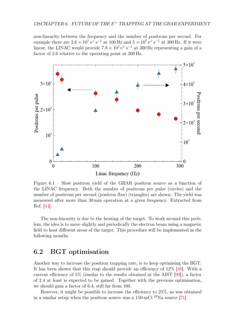
128CHAPTER 6. FUTURE OF THE E+ TRAPPING AT THE GBAR EXPERIMENT
non-linearity between the frequency and the number of positrons per second. Forexample there are 2.6× 10⁷ e+ s−1 at 100 Hz and 5× 10⁷ e+ s−1 at 300 Hz. If it werelinear, the LINAC would provide 7.8× 10⁷ e+ s−1 at 300 Hz representing a gain of afactor of 2.6 relative to the operating point at 200 Hz.
Figure 6.1 – Slow positron yield of the GBAR positron source as a function ofthe LINAC frequency. Both the number of positrons per pulse (circles) and thenumber of positrons per second (positron flux) (triangles) are shown. The yield wasmeasured after more than 30 min operation at a given frequency. Extracted fromRef. [44].
The non-linearity is due to the heating of the target. To work around this prob-lem, the idea is to move slightly and periodically the electron beam using a magneticfield to heat different areas of the target. This procedure will be implemented in thefollowing months.
6.2 BGT optimisation
Another way to increase the positron trapping rate, is to keep optimising the BGT.It has been shown that this trap should provide an efficiency of 12% [48]. With acurrent efficiency of 5% (similar to the results obtained at the AIST [99]), a factorof 2.4 at least is expected to be gained. Together with the previous optimisation,we should gain a factor of 6.4, still far from 100.
However, it might be possible to increase the efficiency to 25%, as was obtainedin a similar setup when the positron source was a 150-mCi 22Na source [71].

6.3. ELECTRON COOLING 129
6.3 Electron coolingThe improvement of the source and the BGT being not enough, a more efficientsetup has to be tested: the electron cooling [51, 52]. This technique is also usingthe fact that we use a LINAC instead of a radioactive source.
As shown in Figure 6.2 the idea is to open and close quickly the HFT’s entrancegate when a bunch of positrons is coming from the LINAC to trap the bunch (theBGT being then used as a simple magnetic guide line). Then the positrons arecooled thanks to coulombic interactions with an electron cloud previously trapped.
Figure 6.2 – Principle of the trapping and electron cooling of bunches of positronsfrom the LINAC into the HFT. Extracted from Ref. [51].
This technique should lead to an overall efficiency of 70% [52], compared to3% (3× 10⁷e+s coming from the LINAC and 1× 10⁶e+s accumulated in the HFT),providing then a factor of 20 and together with the LINAC optimisation, a factorof 50. Taking into account that we are installing an antiproton trap, it shouldbe then possible to accumulate the antiprotons and to send 1010 positrons every200 s (instead of every 100 s). The electron cooling might be a very good solution,considering that all the main elements (LINAC, electron gun and HFT) are alreadyin place and functioning.
6.4 Si-C moderatorAnother idea, currently tested at CEA Saclay and soon implemented at the GBARexperiment is to replace the N2 by a SiC re-moderator [100] in the BGT. The restof the cooling would be performed by the inelastic collisions with the CO2 (schemein Figure 6.3).
With this method still in development (Figure 6.4) the re-moderated positronshave a longitudinal energy of 2.4 eV with an energy spread σ ∼ 1 eV.
If this new setup works then the efficiency of the BGT goes from 5% to 60%,giving a factor of 12. Together with the improvement of the LINAC it gives a factor

130CHAPTER 6. FUTURE OF THE E+ TRAPPING AT THE GBAR EXPERIMENT
Figure 6.3 – Scheme of the trapping in the BGT using the SiC re-moderator. 1– theposition of the elements. 2 – the exit barrier is lowered to let the incoming positronsinteract with the SiC. 3 – the barrier is closed and the re-moderated positrons aretrapped. 4 – cooling of the positrons with CO2. The SiC re-moderator is movableto send the positrons into the HFT. Source L. Liszkay.
Figure 6.4 – Schematic diagram of the experimental setup. Positrons are acceleratedonto the 4H-SiC target by applying the bias Vsample to a 30 cm long tube. Extractedfrom Ref. [48] (Chapter 7).
of 31, which could be a part of the solution and a complete solution if the transferbetween the BGT and the HFT is improved.

6.5. CONCLUSION 131
6.5 ConclusionIn this chapter, a brief overlook of the future optimisations of the positron trappingat the GBAR experiment has been presented. The problem being that the finalrate of the positron trapping is 100 times slower than what we would like for theH
+ production. Short term improvements have been presented such as the LINACoptimisation. However, deeper modifications have to be developed, such as the useof a Si-C re-moderator in the BGT or the electron cooling in the HFT. All together,these optimisations should provide a factor around 50. Then, instead of creating H
+
every 100 s, it would be every 200 s.


Chapter 7
Rocket equations
The most unbelievable part of thefilm is that anyone with a PhD inphysics would go anywhere near 1/4gram of antimatter contained by adevice built by someone with a PhDin physics
Jeffrey Hangst
Contents7.1 Classical equations . . . . . . . . . . . . . . . . . . . . . . . 134
7.2 Classical equations with loss of propellant . . . . . . . . . 136
7.3 Relativistic equations . . . . . . . . . . . . . . . . . . . . . 137
7.4 Relativistic equations with propellant loss . . . . . . . . 141
7.5 Numerical applications . . . . . . . . . . . . . . . . . . . . 143
7.6 Conclusion . . . . . . . . . . . . . . . . . . . . . . . . . . . . 143
In this chapter, we will establish the equations of motion for a rocket. However,if we use antimatter to propel a rocket, we would like to see if it is possible toreach speeds close to the speed of light. In that case we also have to determine theequations of motion of a rocket within the framework of the special relativity.
An idea to reach such speeds would be to annihilate anti-hydrogen atoms andhydrogen atoms at rest (or almost at rest), to generate in majority π+, π−, π0 andphotons with a high momentum to use them as propellant. However, these particleshould be ejected with a momentum in the opposite direction of the motion of therocket and for that, we can use magnetic mirrors to realign the charged particles,but not the neutrals ones which leave the annihilation point in a quasi-isotropic way(it is done in chapter 8). Thus we also have to take into account in our equations aloss of propellant and this is what we will do in this chapter.
In our computations and schemes, we will consider the flux of neutral particlesas two opposite jets, perpendicular to the rocket. But it is obvious that all the
133

134 CHAPTER 7. ROCKET EQUATIONS
directions of the jets are equivalent as long as the jets are opposite (i.e. the sum ofthe momentum is zero).
The equations in the frame of the newtonian mechanics are presented in Sec-tion 7.1 and Section 7.2. As explained above, it is required to adapt the equationsto the frame of the special relativity. It is done in Section 7.4 and Section 7.3. Wefinally present in Section 7.5 some numerical applications.
All this chapter can be compared with the articles of R.H. Frisbee [101, 102, 103]which are reference articles about the antimatter rocket study (but containing somemiscalculations).
7.1 Classical equations
For the computation, we define a closed system Σ∗ with a momentum −→p ∗ composedof the rocket and its propellant. Then the momentum −→p ∗ has to be conserved duringthe ejection of the propellant.
We apply momentum conservation for −→p ∗ relative to an inertial frame R0 be-tween the moments t and t+ dt, of the closed system Σ∗. We note m(t) the rocket’smass, −→v (t) = v(t)−→ex its velocity relative to R0 (assuming the rocket is moving alongthe x axis), dmp the mass of propellant ejected between t and t + dt, −→w = −w−→ex ,the velocity of ejection of the propellant relative to the rocket frame Rr (with w > 0for an acceleration of the rocket and w < 0 for a deceleration).
t t+dt t+dt
Accelerationw > 0
Decelerationw < 0
m(t)m(t+dt) m(t+dt)
v(t)
v(t+dt
)
v(t+dt
)v(
t)-w
v(t)
-w
-dm
-dm
x
y
Figure 7.1 – Scheme representing the momentum conservation. The velocities aredefined with respect to an inertial frame R0.
At moment t + dt, we consider the momentum of the rocket which containspropellant but also the mass of propellant −dm ejected at the relative velocity w.The variation of the mass of the rocket containing propellant corresponds in absolute
7.1. CLASSICAL EQUATIONS 135
value to the mass of propellant ejected during the interval [t, t+ dt].
p∗(t) = m(t)v(t), (7.1.1a)p∗(t+ dt) = m(t+ dt)v(t+ dt)− dm(v(t)− w). (7.1.1b)
Let’s expand the Equation 7.1.1b with Taylor’s expansion of first order:
p∗(t+ dt) =(m(t) + dm)(v(t) + dv)− v(t)dm+ wdm,
p∗(t+ dt) =m(t)v(t) +m(t)dv + wdm,
then we apply the momentum conservation:
p∗(t+ dt)− p∗(t) = 0⇒ m(t)dv + wdm = 0.
This gives us the following differential equation:
dv = −wdm
m. (7.1.2)
This equation, once integrated, leads to:
v(t)− v(t0) = −w ln
(m(t)
m(t0)
). (7.1.3)
The mass of the rocket m(t) is expressed simply by integrating the mass flow(Dm(t) ≤ 0) which is a characteristic data of the rocket.
Dm(t) =dm(t)
dt⇔ m(t) = m(t0) +
∫ t
t0
Dm(t′)dt′. (7.1.4)
At this level of the computation, it is interesting to define the specific impulseIsp [104], a characteristic number used to compare the propellants. If Equation 7.1.2is rewritten as
mdv
dt= −wdm
dt, (7.1.5)
it appears clearly that the thrust force is F = −w dmdt. Then the total impulse is
Itot =
∫ t
0
F (t′)dt′. (7.1.6)
To obtain a characteristic number independent of the rocket (then only related tothe propellant), the specific impulse Isp is defined as the ratio between the totalimpulse and the weight of propellant i.e.
Isp =
∫ t0F (t′)dt
−g∫ t
0dmdt′
dt′, (7.1.7)
expressed in seconds, where g is the gravitational acceleration on Earth. In the caseof w being constant, the specific impulse is
Isp =w
g. (7.1.8)
Another way to understand the Isp is to consider it as the time in seconds duringwhich a propellant can propel its own mass with an acceleration g. Indeed, if dv
dt→ g,
Equation 7.1.2 leads todm
dt+m
Isp
= 0→ m(t) = m0 exp
(− t
Isp
). (7.1.9)

136 CHAPTER 7. ROCKET EQUATIONS
7.2 Classical equations with loss of propellantThis time, we consider that the mass −dm of propellant ejected by the rocketbetween t and t+ dt is ejected for a fraction ξ along the main axis and for a fraction(1 − ξ), along the perpendicular axis on both sides of the rocket such that themomentum along this axis is zero with a speed w′ relative to Rr (Figure 7.2).
In the closed system rocket + ejected propellant at the moment t, the momen-tum along the x axis is written:
p∗(t) = m(t)v(t). (7.2.1)
At the moment t+ dt, we have to consider three terms:
• the momentum of the rocket with propellant inside
• the momentum of the mass −(1− ξ)dm of propellant ejected perpendicularly(but it has a non-zero contribution to the overall momentum along the x axisdue to the velocity v relative to the inertial frame R0)
• the momentum of the mass −ξdm of propellant ejected along the x axis
t t+dt t+dt
Accelerationw > 0
Decelerationw < 0
m(t)m(t+dt)
m(t+dt)v(t) v(t+dt)
v(t+dt)
v(t)-w
v(t)-w
-ξdm
-ξdm-(1-ξ)dm
-(1-ξ)dm
-w’
-w’
w’
w’
v(t)
v(t)
x
y
Figure 7.2 – Scheme representing the momentum conservation. In that case, weconsider a loss of propellant. The velocities are defined with respect to an inertialframe R0.
Also, the momentum conservation can be written:
p∗(t+ dt) = (m+ dm)(v + dv)− (1− ξ)vdm− ξ(v − w)dm,
= p∗(t) +mdv + ξwdm.
This leads to the following differential equation:
dp∗ = mdv + ξwdm. (7.2.2)

7.3. RELATIVISTIC EQUATIONS 137
Thanks to the momentum conservation (i.e. dp∗(t)dt
= 0) we establish this differentialequation for the velocity
dv = −wdm
m, (7.2.3)
where w = ξw. This equation can be easily integrated as
v(t)− v(t0) = −w ln
(m(t)
m(t0)
). (7.2.4)
If we compare the equations 7.1.3 and 7.2.4, we see that finally, the loss ofpropellant described in this model is equivalent to a decrease of the propellantejection velocity, and therefore, to a diminution of the specific impulse defined as
Isp = ξw
g<w
g, (7.2.5)
where g is the acceleration of earth gravity.The result presented in this section differs from what is presented in the first
Frisbee’s article. For example, Eq. 7.2.3 can be compared with Eq. A-20 in Ref. [101](but corrected in Ref. [103]). Indeed, in Eq. A-18, it has been forgotten that thelost propellant has a momentum along the x-axis. With our notations, this equationshould be transformed as
d (mv) = (v − w)ξdm→ d (mv) = −(v − w)ξdm+ (1− ξ) vdm, (7.2.6)
to add the missing component and then the same result as ours would be obtained.
7.3 Relativistic equationsTo obtain the relativistic equations, we need to define 3 frames:
• R0 a reference intertial frame,
• Rr the moving frame of the rocket,
• Rc(t) the comoving frame, an inertial frame coinciding with Rr at a givenmoment t and moving at a constant velocity V = v(t) with respect to R0.
This apparent complication allows us in particular to use the Lorentz transformation(see Appendix A about special relativity) and the laws deriving from it since it onlyapplies for reference frames in uniform rectilinear motion.
We can now apply the energy-momentum conservation in the comoving frame(Figure 7.3).
• proper instant τ (the time in Rr, see definition in Appendix A):
– the rocket is at rest in the comoving frame, the energy-momentum 4-vector is written as
P(τ) =
mc000
,

138 CHAPTER 7. ROCKET EQUATIONS
• proper instant τ + dτ :
– the rocket acquires an infinitesimal velocity dv′ in this frame and its massbecomes m(τ + dτ) = m+ dm,
– A mass dmp of propellant is ejected at relative velocity −w,– P(τ + dτ) = Procket + Pp
Procket =
γ(dv′)(m+ dm)cγ(dv′)(m+ dm)dv′
00
,Pp =
γ(w)dmpc−wγ(w)dmp
00
,
with the function γ(v) = 1√1−( vc )
2 , and at the first order in dv′, γ(dv′) = 1 + o(dv′).
τ τ+dτ τ+dτ
Accelerationw > 0
Decelerationw < 0
m(τ)m(τ+dτ) m(τ+dτ)dv
’
dv’
-w
-w
dmp
dmp
x
y
Figure 7.3 – Scheme representing the energy-momentum conservation. The velocitiesare here defined with respect to the comoving frame.
The energy-momentum conservation (P(τ+dτ) = P(τ)) with Taylor’s expansionof first order in dv′, dm and dmp gives us
γ(w)dmp = −dm,
γ(w)dmp =mdv′
w.
So we get a differential equation comparable to the classical case (Equation 7.1.2):
dv′ = −wdm
m. (7.3.1)
Now, we need to know the dv variation corresponding to the difference of velocitybut in the inertial frame R0. For that, we use the velocity composition law between
7.3. RELATIVISTIC EQUATIONS 139
the inertial frame R0 and the comoving frame Rc (Equation A.2.2):
v′x =vx − V
1− vxV/c2⇒ dv′x =
dvx1− vxV/c2
− (vx − V )× (v/c2)× dvx
(1− vxV/c2)2 ,
however V = v(t), vx = v(t), dvx = dv and dv′x = dv′:
dv′ =dv
1−(vc
)2 .
This leads to the differential equation (similar to Ref. [101], Eq. A-13):
dm
m=−1
w
dv
1−(vc
)2 . (7.3.2)
This equation with separate variables can be easily integrated:∫ m(t)
m(t0)
dm
m=−c2
w
∫ v(t)
v(t0)
dv
1−(vc
)2 =−cw
∫ v(t)/c
v(t0)/c
dx
1− x2,
ln
(m(t)
m(t0)
)=−c2w
ln
((1 + v(t)
c)(1− v(t0)
c)
(1− v(t)c
)(1 + v(t0)c
)
),
(m(t)
m(t0)
)−2wc
=(c+ v(t))(c− v(t0))
(c− v(t))(c+ v(t0)). (7.3.3)
And we finally obtain the expression of v(t):
v(t) = c
(m(t)m(t0)
)−2wc(c+v(t0)c−v(t0)
)− 1(
m(t)m(t0)
)−2wc(c+v(t0)c−v(t0)
)+ 1
, (7.3.4)
with as a reminder w > 0 for an acceleration and w < 0 for a deceleration.Note: with Taylor’s expansion of first order in w
cand v(t0)
c(m(t)
m(t0)
)−2wc
= 1− 2w
cln
(m(t)
m(t0)
),
2w
c 1,
c+ v(t0)
c− v(t0)=
1 + v(t0)c
1− v(t0)c
= 1 + 2v(t0)
c,
v(t0)
c 1,
we can find the expression of v in the classical limit (Equation7.1.3).Looking at the Equation 7.3.4, we need to know what is the expression of m(t).
But it is more difficult than in the previous case because the mass flow rate is definedin the frame associated to the rocket, so we can no longer use Dm(t) = dm(t)
dt. The
article W. L. Bade [105] help us to overcome this problem. Let’s reformulate thedifferential Equation 7.3.2 to correspond to the article:
w
[1− v2
c2
]dm+mdv = 0, (7.3.5)

140 CHAPTER 7. ROCKET EQUATIONS
and we define the mass flow on board the rocket by:
ρ(τ) =dm
dτ, (7.3.6)
with τ the proper time of the rocket, this gives us the evolution of the mass as afunction of τ :
m(τ) = m(τ0) +
∫ τ
τ0
ρ(τ ′)dτ ′. (7.3.7)
The rapidity θ is defined as a function of the proper time θ by
cosh θ =dt
dτ, (7.3.8a)
c sinh θ =dx
dτ, (7.3.8b)
cosh θ being by definition the Lorenz factor γ. Then, the velocity can be expressedas a function of the rapidity
v =dx
dt= c tanh θ, (7.3.9a)
θ(τ) = argthv
c. (7.3.9b)
Injecting 7.3.9a in 7.3.5 and assuming v0 = 0, we obtain
dθ
dτ= − w
m(τ)cρ(τ), (7.3.10)
giving us a expression of θ(τ) thanks to ρ(τ) and m(τ):
θ(τ) = θ(τ0)− w
c
∫ τ
τ0
ρ(τ)
m(τ)dτ ′. (7.3.11)
Then now we have the travelled distance and the corresponding time in the referenceframe as a function of the proper time of the rocket (because the mass flow rate asa function of the proper time is a characteristic of the rocket):
x(τ) = x(τ0) + c
∫ τ
τ0
sinh (θ(τ ′))dτ ′, (7.3.12a)
t(τ) = t(τ0) +
∫ τ
τ0
cosh (θ(τ ′))dτ ′. (7.3.12b)
In summary, we now have the velocity, the travelled distance and the time inthe reference frame as a function of the proper time of the rocket, the whole beingconnected to the mass flow measured on board the rocket.

7.4. RELATIVISTIC EQUATIONS WITH PROPELLANT LOSS 141
7.4 Relativistic equations with propellant lossWe now apply the energy-momentum conservation law, considering that a fractionof propellant is ejected perpendicularly to the rocket in its proper frame Rc (Fig-ure 7.4). We place us in the co-moving frame at the proper time τ .
This time we have to pay more attention to the handled terms. During theamount of time dτ , the rocket lost a mass −dm, so an energy −(dm)c2. This energyis distributed according a fraction ξ for the useful propellant (ejected with a velocity−w along the x axis) and (1−ξ) for the lost propellant (ejected with a velocity ±w⊥):
− (dm)c2 = −(dm)ξc2︸ ︷︷ ︸γ(w)dmp1c
2
−(1− ξ)(dm)c2︸ ︷︷ ︸γ(w⊥)dmp2c
2
. (7.4.1)
So we have dmp1 the mass of propellant ejected along x with a velocity w anddmp2 ejected along the y axis with a relative velocity ±w⊥:
γ(w)dmp1 = −(dm)ξ, (7.4.2a)γ(w⊥)dmp2 = −(1− ξ)(dm). (7.4.2b)
Accelerationw > 0
Decelerationw < 0
x
m(τ)m(τ+dτ)
m(τ+dτ)
dv’
dv’
-w
-w
dmp1
dmp1
y
dmp2
dmp2
-w’
-w’
w’
w’
τ τ+dτ τ+dτ
Figure 7.4 – Scheme of the energy-momentum conservation. The velocities are heredefined with respect to the comoving frame to the rocket at the proper time τ .
Now we can apply the energy-momentum conservation law:
• proper time τ :
– the rocket is at rest in its comoving frame
P(τ) =
mc000

142 CHAPTER 7. ROCKET EQUATIONS
• proper time τ + dτ :
– the rocket acquires a velocity dv′ in that frame
– dmp1 is ejected with the velocity −w along the main axis
– 12dmp2 is ejected with the velocities +w⊥ et −w⊥ along the perpendicular
axis
– P(τ + dτ) = Procket + Pp + Pp⊥1 + Pp⊥2
Procket =
γ(dv′)(m+ dm)cγ(dv′)(m+ dm)dv′
00
Pp =
γ(w)dmp1c−γ(w)dmp1w
00
=
ξdmcξdmw
00
Pp⊥1 =
γ(w⊥)1
2dmp2c
0γ(w⊥)1
2dmp2w⊥0
=
−1
2(1− ξ)dmc
0−1
2(1− ξ)dmw⊥
0
Pp⊥2 =
γ(w⊥)1
2dmp2c
0−γ(w⊥)1
2dmp2w⊥
0
=
−1
2(1− ξ)dmc
012(1− ξ)dmw⊥
0
with the function γ(v) = 1√
1−( vc )2 , and at the first order in dv′, γ(dv′) = 1 + o(dv′).
The conservation of the energy-momentum (P(τ + dτ) = P(τ)) using Taylor’sexpansion of first order in dv′ and dm gives
dv′ = −wdm
m(7.4.3)
with w = ξw. Using the velocity composition law as for the Equation 7.3.1, weobtain a similar differential equation:
dv
1−(vc
)2 = −wdm
m(7.4.4)
which can be integrated as the Equation 7.3.2:(m(t)
m(t0)
)−2wc
=(c+ v(t)) (c− v(t0))
(c− v(t)) (c+ v(t0))(7.4.5)
We can also do the same reasoning as in the classical case with respect to the specificimpulse: the loss of fuel can be interpreted as a reduction of the specific impulse.
Isp = ξw
g

7.5. NUMERICAL APPLICATIONS 143
This result differs strongly from the H.R. Frisbee articles. For example, Eq. 7.4.4can be compared with Eq. A-26 in Ref. [101], or with Eq. 4 in Ref. [102], or withRef. [103]. Here again, the difference comes from that the lost propellant consideredemitted at rest which is not the case (because each element of lost propellant isemitted with a certain velocity relative to the rocket, carrying also a non-zero kineticenergy). A similar work is presented in Ref. [106], giving a result similar to the onepresented in this section.
Once again we can give an expression of the velocity, position, and time thanksto the mass flow, replacing w by w in the expressions of the previous section:
θ(τ) = θ(τ0)− w
c
∫ τ
τ0
ρ(τ)
m(τ)dτ ′ (7.4.6a)
v(τ) = c tanh θ (7.4.6b)
x(τ) = x(τ0) + c
∫ τ
τ0
sinh (θ(τ ′))dτ ′ (7.4.6c)
t(τ) = t(τ0) +
∫ τ
τ0
cosh (θ(τ ′))dτ ′ (7.4.6d)
7.5 Numerical applicationsFor the numerical application we use ξ = 0.4 and w = 0.99c, so with Isp =1.2× 10⁷ s. These values will be justified in Chapter 8 (we will see that we haveξw ∼ 0.4c mainly due to the neutral particles considered as the lost propellant).
In Figure 7.5 the curve are represented m(t0)m(t)
as a function of v(t)/c for v(t0) = 0in the cases
• classical equation without loss of propellant (Equation 7.1.2)
• relativistic equation without loss of propellant (Equation 7.3.2)
• classical equation with loss of propellant (Equation 7.2.3)
• relativistic equation with loss of propellant (Equation 7.4.4)
We then find that, as the equations show, the propellant loss decreases thespecific impulse, more propellant is needed if there is loss to reach the same velocity.As for the relativistic effects, we can see that they are quite weak for velocities< 0.2c, but when they are visible, we can see that they predict a greater propellantexpenditure compared to the predictions of classical mechanics.
7.6 ConclusionWe developed in this chapter the equations of motion of the rocket and we sawthat the classical and relativistic equations give the same results for a velocity smallcompared to the speed of light. However, the classical equations are more simplebut underestimate the mass of propellant and are completely wrong because theyallow a rocket velocity higher than the speed of light.

144 CHAPTER 7. ROCKET EQUATIONS
0.0 0.2 0.4 0.6 0.8 1.0v(t)/c
123456789
10m
(t 0)/m
(t)Comparison of the different models w = 0.99c, v(t0) = 0
classical = 1relativistic = 1classical = 0.4relativistic = 0.4
Figure 7.5 – Ratio between the initial mass of the rocket and the mass at t as afunction of the velocity of the rocket. The propellant is ejected with a relative speedof w = 0.99c. This plot differs and can be compared with Fig. 1 in Ref. [103].
If we consider a fraction 1− ξ of propellant isotropically lost, we simply have toreplace the ejection speed w by w = ξw in the equation without loss.
We will propose in the next chapter, a way to use antimatter to reach suchvelocities and determine w and ξ.
Chapter 8
The beamed core
Une maquette ? Vous n’aviez pasdit que c’était une catapulte ?
Perceval, Kaamelott, livre III
Contents8.1 Concept . . . . . . . . . . . . . . . . . . . . . . . . . . . . . 147
8.1.1 Proton-antiproton annihilation . . . . . . . . . . . . . . . 147
8.1.2 Estimates about kinematics in pp annihilation and Isp . . 148
8.1.3 Magnetic mirroring . . . . . . . . . . . . . . . . . . . . . . 148
8.1.4 Scale invariance . . . . . . . . . . . . . . . . . . . . . . . . 149
8.2 Results . . . . . . . . . . . . . . . . . . . . . . . . . . . . . . 151
8.2.1 Presentation of the simulation . . . . . . . . . . . . . . . . 151
8.2.2 First results . . . . . . . . . . . . . . . . . . . . . . . . . . 151
8.2.3 Optimisation of the target’s position . . . . . . . . . . . . 153
8.2.4 Optimisation of the field . . . . . . . . . . . . . . . . . . . 153
8.3 Energy evacuation . . . . . . . . . . . . . . . . . . . . . . . 155
8.3.1 Radiator . . . . . . . . . . . . . . . . . . . . . . . . . . . . 155
8.3.2 Shield . . . . . . . . . . . . . . . . . . . . . . . . . . . . . 156
8.4 Antimatter production and storage . . . . . . . . . . . . . 157
8.5 Conclusion . . . . . . . . . . . . . . . . . . . . . . . . . . . . 158
In this chapter, we detail a simulation of a beamed core engine based on anantiproton beam. The concept of the beamed core [107, 108, 109, 110] is to focusa beam in a precise direction to move our rocket. Here we annihilate p and p, twomassive particles to obtain light particles with a high kinetic energy (it means withspeed close to the speed of light) to have a propellant with Isp of the same order ofmagnitude as discussed in the previous chapter.
The idea is to force the produced particles to go opposite to the direction ofmotion to participate to the momentum ejected along the z axis (see illustration in
145

146 CHAPTER 8. THE BEAMED CORE
Figure 8.1). To do that we place a coil to create a magnetic mirror to realign asmuch as possible the charged particles. However, it means we loose for the totalmomentum the neutral particles, giving an explanation to the loss rate discussed inSection 7.2 and Section 7.4.
Figure 8.1 – Concept of the beamed core engine. On the top all the particlesproduced by the annihilation reaction of pp are drawn. On the bottom, only thecharged one. This illustration comes from our GEANT4 simulation.
This also explain the choice to focus only on the pp annihilation. Indeed, itis easier to produce and store positrons, but the electrons and positrons are lightcompared to the nucleons. They annihilate into gamma rays of small energies andtheir energy cannot be exploited. Therefore, the most simple antimatter elementcorresponding to our requirements is antiproton.
The results of our simulations, based on the annihilations of antiprotons on anhydrogen target in a presence of a high magnetic field are presented in Section 8.2.Our simulation is based on the GEANT4 library [111].

8.1. CONCEPT 147
Channel Branching fraction in %nπ0(n ≥ 1) 4.1+0.2
−0.6
π+ + π− + π0 5.8± 0.4π+ + π− + 2π0 9.3± 3.0π+ + π− + 3π0 23.3± 3.0π+ + π− + 4π0 2.8± 0.7
2π+ + 2π− 6.9± 0.62π+ + 2π− + π0 19.6± 0.72π+ + 2π− + 2π0 16.6± 1
3π+ + 3π− 2.1± 0.25
Table 8.1 – Some branching fractions for main (rate ≥ 2%) pp annihilation channels.Extracted from Ref. [114].
.
8.1 Concept
8.1.1 Proton-antiproton annihilation
As explained in introduction, the model described in this chapter is based onantiproton-proton annihilation. The interactions of antiproton with matter has beenstudied theoretically for a long time since a first paper in 1956 [112] and are stillstudied (many examples given in Section 1.2.2).
When an antiproton enters into a target of matter, it is first slowed by electro-magnetic interactions with electrons of the target, as would happened for any kindof charged particle. This process also creates electrons-ions pairs in the target. Also,if its kinetic energy is lower than a few eV, it ejects one electron from a given atomand binds with the resulting ions. Then it cascades down to lower energy levelsreleasing X-ray and Auger electrons in the process. Finally, when the lowest energylevel is reached, the antiproton is sufficiently close to the nucleus and annihilateswith a nucleon, which happens to be a proton in the case of the target made ofhydrogen in our simulation.
Many output decay channels exist, possibly involving intermediate resonances(for example: ρ → π+π−) [113], and these channels lead in majority to pions asdetailed in Table 8.1 which presents the branching fractions from the main channels.If the most representative channel are only taken into account the results of theannihilation can be written such as
pp→ 1.5π+ + 1.5π− + 2π0, (8.1.1)
and nπ = 4.98±0.13, nπ± = 3.05±0.04, and nπ0 = 1.93±0.12 [113]. Charged pionsdecay following π+ → µ+ν with a lifetime corresponding to cτ = 7.804 m decaylength. Muons also decay following µ± → e±νν with cτ = 659 m. In the beam coremodel, these charged particles are useful to the propulsion. This is not the case ofneutral pions, which decay instantaneously to γγ (98.8%) or e+e−γ (1.17%).
Among the other products and still representative, there are the kaons particles.These unstable particles [115] are produced at a typical rate of ∼ 5%. Charged kaons

148 CHAPTER 8. THE BEAMED CORE
decay mostly following K+ → µ+ν or K+ → π+π0 with cτ = 3.71 m, therefore, theycan participate, in our model to propel a rocket.
8.1.2 Estimates about kinematics in pp annihilation and Isp
In this section, we use the knowledge of the decay channels presented in the previoussection, considering that all the charged particles can be oriented in a way to increasethe thrust, to estimate the specific impulse (Isp) of the beamed core engine.
We focus on the pions because they are the most representative. Their massesare roughly equal (mπ0 = 135 MeV,mπ± = 140 MeV), then for this computation wewrite the mass of a pion mπ = 140 MeV. As explained in the previous section, inthe most simple picture, 3 charged pions and 2 neutral pions are obtained. Thismeans that the charged particles carry ∼ 60% of the initial energy while the neutralones ∼ 40%.
If we consider the initial particles at rest, the initial energy is twice the massenergy of a proton E = 2mpc
2 = 2× 940 MeV. Therefore the kinetic energy of eachpion is Kπ = 1
5(2mp − 5mπ)c2 = γmπc
2 − mπc2, leading to γ = 2mp
5mπ. Then, each
resulting pion has a velocity (compared to the speed of light c) of
v
c=
√1− 1
γ2= 0.93. (8.1.2)
As the neutral pions decay to two photons π0 → γγ more than 98.8% of thetime, neutral pions yields a high intense radiation of photons. So about 40% of theavailable energy is lost in quasi-isotropic γ radiation. Thankfully, this is not thecase for the charged pions. Therefore, they can theoretically be re-directed using amagnetic field and ejected oppositely to the rocket movement. Considering that thecharged pions carry about 60% of the available energy and travels at ∼ 0.93c, a firstrough estimate of the possible specific impulse is
Isp = 0.6× 0.93c
g= 0.56
c
g= 1.7× 10⁷ s. (8.1.3)
8.1.3 Magnetic mirroring
The magnetic mirror is made of a huge current loop to generate an important mag-netic field. Assuming the main axis is the z axis, the expression of this field is [116]
Bx =Cxz
2α2βρ2
((a2 + r2
)E(k2)− α2K
(k2))
(8.1.4a)
By =Cyz
2α2βρ2
((a2 + r2
)E(k2)− α2K
(k2))
(8.1.4b)
Bz =C
2α2β
((a2 − r2
)E(k2)
+ α2K(k2))
(8.1.4c)
where ρ2 = x2+y2, r2 = x2+y2+z2, α2 = a2+r2−2aρ, β2 = a2+r2+2aρ, k2 = 1−α2
β2 ,C = µ0I
π, K and E are the complete elliptic integrals of the first and second kind,

8.1. CONCEPT 149
respectively, and µ0 the magnetic permeability of vacuum. We have implementedthese formula in the GEANT4 simulation. The corresponding magnetic field linesin the (ρ, z) plane of cylindric coordinates are shown in Figure 8.2.
Figure 8.2 – Magnetic field line and strength in the (ρ, z) plane of cylindric coor-dinate, as produced by a current loop of radius 4. Length and magnetic units arearbitrary.
The effect of the magnetic mirror can be seen in Figure 8.3 where we displaythe trajectories of particle varying the magnetic strength. We clearly see on thesepictures that the charged particles are more aligned with the main axis (whichincreases the Isp) for a strong magnetic field.
8.1.4 Scale invariance
For the case of a current loop of radius R centred around the z-axis at z = 0 , theMaxwell’s equation defining the magnetic field is
−→∇ ×
−→B = µ0
−→j = µ0
−→I δ(z)δ(
√x2 + y2 −R), (8.1.5)
where−→j is the current density, which is then translated into the current loop in-
tensity−→I using the δ functions defining the location of the loop. Such equation
could be generalised for different shape of current loop, using the appropriate δ pa-rameterisation. The trajectory for the particles is obtained considering the Lorentz
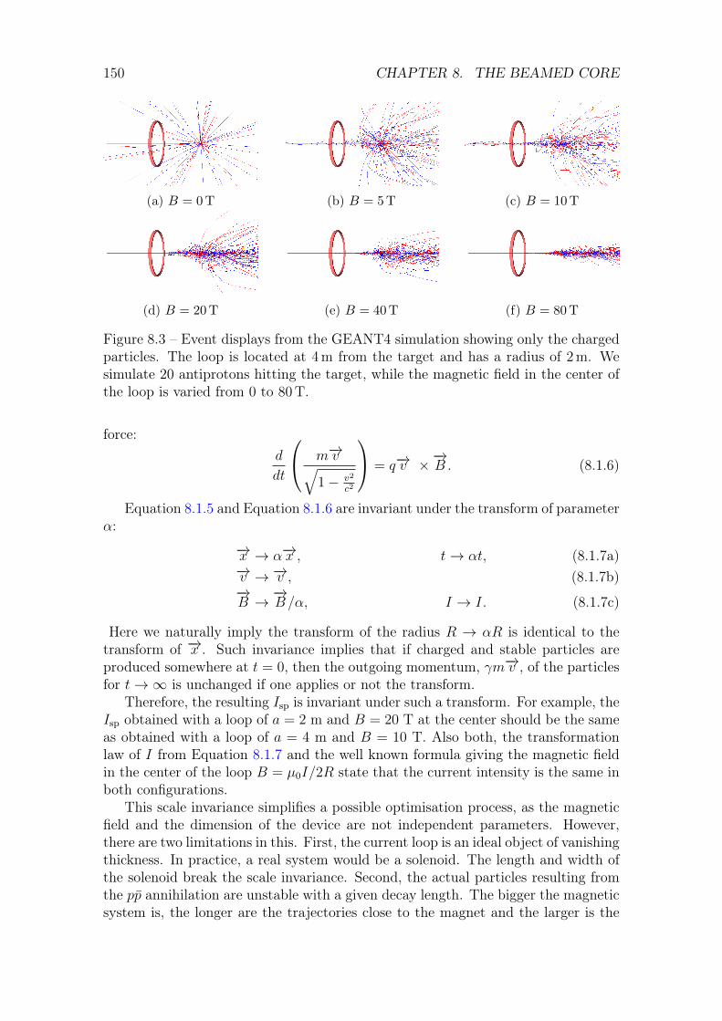
150 CHAPTER 8. THE BEAMED CORE
(a) B = 0 T (b) B = 5 T (c) B = 10 T
(d) B = 20 T (e) B = 40 T (f) B = 80 T
Figure 8.3 – Event displays from the GEANT4 simulation showing only the chargedparticles. The loop is located at 4 m from the target and has a radius of 2 m. Wesimulate 20 antiprotons hitting the target, while the magnetic field in the center ofthe loop is varied from 0 to 80 T.
force:d
dt
m−→v√1− v2
c2
= q−→v ×−→B . (8.1.6)
Equation 8.1.5 and Equation 8.1.6 are invariant under the transform of parameterα:
−→x → α−→x , t→ αt, (8.1.7a)−→v → −→v , (8.1.7b)−→B →
−→B/α, I → I. (8.1.7c)
Here we naturally imply the transform of the radius R → αR is identical to thetransform of −→x . Such invariance implies that if charged and stable particles areproduced somewhere at t = 0, then the outgoing momentum, γm−→v , of the particlesfor t→∞ is unchanged if one applies or not the transform.
Therefore, the resulting Isp is invariant under such a transform. For example, theIsp obtained with a loop of a = 2 m and B = 20 T at the center should be the sameas obtained with a loop of a = 4 m and B = 10 T. Also both, the transformationlaw of I from Equation 8.1.7 and the well known formula giving the magnetic fieldin the center of the loop B = µ0I/2R state that the current intensity is the same inboth configurations.
This scale invariance simplifies a possible optimisation process, as the magneticfield and the dimension of the device are not independent parameters. However,there are two limitations in this. First, the current loop is an ideal object of vanishingthickness. In practice, a real system would be a solenoid. The length and width ofthe solenoid break the scale invariance. Second, the actual particles resulting fromthe pp annihilation are unstable with a given decay length. The bigger the magneticsystem is, the longer are the trajectories close to the magnet and the larger is the

8.2. RESULTS 151
amount of particle decaying in flight while being channeled. The typical decay lengthbeing given by βγcτ ∼ 20 m (see 8.1.1), it is expected to see an effect when themagnetic system has a size not small compared to 20 m.
8.2 Results
8.2.1 Presentation of the simulation
Our simulation is based on the GEANT4 library which is widely used in particleand nuclear physics as a toolkit to simulate particles, their decays, their trajectoryin a magnetic field and their interaction with matter. Our implementation consistsof a cubic hydrogen target of 8 cm3 located on the axis of a current loop. We shot abeam of antiprotons, along the z-axis to produce annihilation onto the target. Theinteractions of particles with matter are described by the “QGSP_BERT_EMX”model [117] included in Geant4.
We first study the outcome of antiproton annihilations. Our simulation providesresults in fair agreement with the expectations presented in Section 8.1.1. Indeed,the final state of each collision provides on average nπ = 5.19± 0.15, nπ± = 3.12±0.12, nπ0 = 2.07 ± 0.08 (uncertainties here are statistical), the π0 decaying quicklyto two γ, such as illustrated in Figure 8.4
Figure 8.4 – Final states for 1000 pp collisions.
8.2.2 First results
We simulate the annihilation of antiprotons on a target of hydrogen (see illustrationin Figure 8.1) including the magnetic field of a current loop. The target is at 4 m ofa 2 m radius loop.
Let’s take the example of a loop generating a 10 T magnetic field. N = 10000 an-tiprotons are annihilated onto a target of hydrogen. The momentum distribution ofthe n = 127631 produced particles is reported in Figure 8.5. As expected, the mean

152 CHAPTER 8. THE BEAMED CORE
momentum along the x axis (and y axis) with px = 0.1032 MeV (py = −0.1421 MeV)is negligible compared to the mean momentum along the z axis with a mean valueof pz = 64.52 MeV. It means this engine yields a force pushing the rocket in theright direction.
2000− 1500− 1000− 500− 0 500 1000 1500 2000 in MevxP
0
5000
10000
15000
20000
25000
30000
35000
40000
45000
Occ
uren
ces
histogram B = 10T, d = 100g/L, N=10000xPhPx
Entries 127631Mean 0.1032Std Dev 96.89
histogram B = 10T, d = 100g/L, N=10000xP
2000− 1500− 1000− 500− 0 500 1000 1500 2000 in MevzP
0
5000
10000
15000
20000
25000
30000
Occ
uren
ces
histogram B = 10T, d = 100g/L, N=10000zPhPz
Entries 127631Mean 64.52Std Dev 152.5
histogram B = 10T, d = 100g/L, N=10000zP
Figure 8.5 – Momentum distribution of the particles after the annihilation (10000primary antiprotons).
To estimate ξw and then the Isp = ξwg, we start from the definition of the energy
(E) and momentum (p) of a particle
E = γmc2, (8.2.1a)p = γmv, (8.2.1b)
which leads tov
c=pc
E. (8.2.2)
Considering v as the mean value of the speed of the particles, we have v = ξw andpz = p. To estimate E, the initial total energy of the protons and antiprotons at

8.2. RESULTS 153
rest E0 = 2Nmpc2 (mp the proton’s mass) is divided by the number of produced
particles n. This lead to
ξw
c=
pzc
mpc2× n
2N=
64.52 MeV
938 MeV× 127631
2× 10000= 0.43. (8.2.3)
Therefore, the specific impulse is Isp = 0.43c/g = 1.3× 10⁷ s.
8.2.3 Optimisation of the target’s position
In the previous section, the distance between the 2 m radius loop and the target wasarbitrary fixed at 4 m. To determined what is the effect of this distances, similarsimulations has been performed for different distances and 4 values of the field. Theresults of these simulations are presented in Figure 8.6. The first observation is that
loop to target distance (m)0 2 4 6 8 10 12 14 16
g/c
×
ISP
0.1
0.2
0.3
0.4
0.5
ISP
(s)
2
4
6
8
10
12
14
16
610×
B=40 T, R=2m
B=30 T, R=2m
B=20 T, R=2m
B=10 T, R=2m
Figure 8.6 – Isp as a function of the distance of the center of the loop to the target,for different magnetic field intensities (sampled at the center of loop) and a fixedloop radius of 2 m
there is an optimal distance for each value of the field. However, this optimal valueremains around 4 m, corresponding to a distance of ∼ 2×R.
8.2.4 Optimisation of the field
The magnetic field strength is varied for different geometry, keeping the aspect ratioR : d = 1 : 2. The resulting Isp as a function of the magnetic field is shown inFigure 8.7. For R = 2 m and d = 4 m, it can be seen that an asymptotic valueclose to Isp = 0.5c/g = 1.5× 10⁷ s is reached for B ≥ 30 T. Namely we findIsp× g/c = 0.467± 0.002, 0.485± 0.002, and 0.497± 0.002, for respectively B = 20,30, and 50 T. The Isp at B = 20 T is just 6% below the asymptotic value whichsounds as a reasonable compromise to work at value of the field not too unrealistic.This corresponds to a current of 6.36× 10⁷ A. Note that in a real system made of asolenoid, this current is shared among the different loops.

154 CHAPTER 8. THE BEAMED CORE
B (T)0 10 20 30 40 50 60 70
g/c
×
ISP
0
0.1
0.2
0.3
0.4
0.5
ISP
(s)
0
2
4
6
8
10
12
14
16
610×
R=2m, Z=4m
R=1m, Z=2m
R=4m, Z=8m
R=8m, Z=16m
Figure 8.7 – Isp as a function of the magnetic field B for different geometries thathave the same aspect ratios.
Figure 8.8, shows the different curves are overlaid when Isp is plotted as a functionof B×R, as expected from the scaling law discussed in Section 8.1.4. This shows thatthe relevant parameter is rather the current intensity circulating in the loop ratherthan the magnetic intensity. A notable departure is however observed for R = 8 m,d = 16 m. This is understood to be due to inflight decays of pions, resulting in asignificant momentum carried by neutrinos before being deflected by the magneticnozzle, as anticipated in Section 8.1.1 and Section 8.1.4.
I/2m (T)0
µRB/2m=0 10 20 30 40 50 60 70
g/c
×
ISP
0
0.1
0.2
0.3
0.4
0.5
ISP
(s)
0
2
4
6
8
10
12
14
16
610×
R=2m, Z=4m
R=1m, Z=2m
R=4m, Z=8m
R=8m, Z=16m
Figure 8.8 – Isp as a function of the magnetic field B scaled by the loop radius R(in units of 2 m). BR is proportional to the current I circulating in the loop.
8.3. ENERGY EVACUATION 155
8.3 Energy evacuationEach collision produces on average four 190 MeV photons in a quasi-isotropic wayi.e. about 760 MeV per collision. Thus the elements of the rocket receive a power of
Pr =dmfuel
dtc2ε
Ω
4π(8.3.1)
where mfuel is the mass of propellant consumed during an acceleration phase (andso dmfuel
dtis the consumed mass of propellant per time unit), ε the fraction of energy
dissipated (∼ 0.4, see Section 8.1.2), and Ω, the solid angle under which one can seefrom the target the considered element of the rocket.
Such amount of radiation would yield damages to the rocket as would do anyionising radiations, and also deposit heat. Thus, the rocket must be shielded againstthe flux of gamma rays. In the following we assume the energy deposited in the shieldis only transformed into heat and do not study the impact of radiation damageswhich are expected to have ageing effects on any kind of shield. However, the heatdeposit in the shield which has to be dissipated by a radiating system represents byitself a major challenge for an antimatter rocket, as we discuss in the following.
8.3.1 Radiator
Let’s consider a metallic radiator. Assuming it behaves like a black body at tem-perature T , its surface S would radiate a power such as described by the Stefan-Boltzmann law:
Pe = SσT 4, (8.3.2)
where σ is the Stefan-Boltzmann constant (σ = 5.670 373× 10−8 W m−2 K−4). Com-bining Equation 8.3.1 and Equation 8.3.2, the required surface to evacuate this poweris obtained:
S =dmfuel
dtc2ε
Ω
4πσT 4. (8.3.3)
During the rocket’s acceleration, a mass mfuel of propellant is consumed to givea speed ∆v to the rocket (with a total mass m). Assuming that the propellant isdelivered constantly and the acceleration duration is τ , the consumed mass per timeunit is then mfuel/τ . Also, it is assumed that the radiator is composed of panels,with a thickness e and a mass per unit volume ρ, the mass of the radiator is relatedto the surface S as
mrad = ρeS
2, (8.3.4)
with a factor 2 because there are 2 faces. Derived from Equation 8.3.3 the followingequation is obtained
mrad =1
rmfuel, r = 8πσ
τT 4
eρc2εΩ. (8.3.5)
The total mass of the rocket before the acceleration mtot, being the sum of themass of the ejected propellant mfuel, the mass of the radiator mrad and the remainingmass of the rocket mrem, Equation 8.3.5 leads to
mtot = (1 + r)mrad +mrem. (8.3.6)

156 CHAPTER 8. THE BEAMED CORE
Let’s estimate the value of r. We consider a one year acceleration phase anda radiator made of tungsten, for its high temperature of fusion (3000 K), with adensity of ρ = 19.3 g cm−3 = 19.3× 10³ kg m−3. Taking ε ∼ 0.4, e = 1 cm, with asolid angle Ω = 0.4π, we obtain r ∼ 3× 10⁻⁴.
r is found to be a small number. This implies that the mass of the radiator isdominant over the rest in the rocket for sizeable amount of antimatter. The rocketequation 7.2.4 becomes
∆v = −Ispg log
(mrem +mfuel/r
mrem +mfuel +mfuel/r
), (8.3.7)
which is independent of the amount of fuel when mfuel/r is large. The reason is thatany supplement of fuel requires an additional mass of radiator. The supplementalfuels serves only to accelerate the supplemental radiators. Thus it is not possibleto reach speed close the Isp, and for mfuel → ∞, ∆v = Ispg log (1 + r). If Isp =1.5× 10⁷ s then maximal speed is ∆v/c = 1.4× 10⁻⁴.
Thereby the mass of the radiator drastically impact the velocity of the rocket. Ifthe tungsten is replaced by PICA (a composite material for thermic shield used byNASA), with a density ρ = 250 kg m−3 and a temperature of fusion T = 1500 K, the rparameter becomes, r = 1.3× 10⁻³, leading to a maximal speed ∆v/c = 6.4× 10⁻⁴.Some optimisation of the geometry can be done to increase the r parameter andconsequently the final speed, however it is hard to see how one could gain more thanone order of magnitude on the r parameter. If we consider ten years of acceleratingphase, we gain one more order of magnitude. So at the end, it is hard to see howone could go beyond a ∆v = 0.06c.
8.3.2 Shield
The radiation energy resulting from the annihilation process first need to be ab-sorbed before being evacuated by the radiators. The photons have to interact withthe matter of a shield placed between the target and the rest of the rocket.
The shield has to be designed to be able to stop the γ, and this is can be donewith the basics information coming from the Particle Data Group [115]. For amaterial with a high atomic number Z (heavier than lead), the probability P0 thatan interaction between a 100 MeV photon and an atomic nucleus results in a (e+, e−)pair is close to 100%. The probability Pi that this photon causes the creation ofsuch a pair after going through a thickness l of material is then
Pi =(1− e−l/l0
), (8.3.8)
where l0 is a characteristic length of the material. In the case of lead, this lengthis lPb = 0.9 cm, which means that a 2.5 cm thickness is enough to turn 99% of theincoming γ to a (e+, e−) pair, leading to an electromagnetic shower. This first pro-cess initiates and electromagnetic cascade of pair productions and Brehmstrahlungemission generating more and more photons and electrons of lower energies. Thecascade ends when the electrons energies are below a critical energy Ec ' 610 MeV
Z+1.2,
then the remaining energy is deposited by ionization and excitation of the mate-rial. The characteristic longitudinal length of the cascade is given by the radiation

8.4. ANTIMATTER PRODUCTION AND STORAGE 157
length X0, which amounts to X0 = 0.56 cm for lead. In practice more than 99% ofthe energy is deposited within 10X0 for a γ of 100 MeV.
Also, in the transverse plane, 99% of the shower energy is contained in a radiusof 3.5RM . RM , the Molière radius, is another characteristic of the material such as
RM = X0EsEc, Es ' 21 MeV. (8.3.9)
RM = 1.6 cm in the case of a 100 MeV radiation in lead. The energy of the showeris therefore essentially contained in a cylinder of 5.5× 10⁻⁴ m3 weighing 6.2 kg andmainly heats the material. So it appears that a shield of a few lPb is enough tocontain almost all of the energy.
In the end, the power received by the shield is colossal: 10× 1010 W m−2, if a tonof antiprotons is annihilated over a year. This power being delivered on a thin layer(a few lPb), one can consider it will be vaporised extremely quickly. A way to solvethis problem would be to move the target further away from the magnetic mirror,but this would decrease the Isp, except if the magnetic field is increased. Then, anew optimal condition taking into account the shield remains to be found.
8.4 Antimatter production and storage
The final limitation of the concept of the beamed core engine is that it requirestones of antimatter. This is really the main limitation, because there is no way toproduce such amount of antimatter, and our current way of storing antimatter donot allow such quantities.
Let’s start with the storage. As presented in detail in Chapter 3, a well knownway to store antimatter is to trap it in Penning traps as non neutral plasma. Andhere comes the first limitation: there is a maximum density of particles which canbe stored in such a trap. This is what is named the Brillouin limit
nB =B2/(2µ0)
mc2, (8.4.1)
where B is the magnetic field, m the mass of one particle, c the speed of light, andµ0 the vacuum permeability.
This lead to a maximal energy per unit volume of εB = B2
2µ0= 0.4 kJ L−1×
(B
1 T
)2,which means that to store one gram of antiprotons, a volume of 108 m3 is required(for a 1 T field). Or if we desire the same compactness of the diesel (40 MJ L−1), a320 T magnet is required (Neurospin magnet at CEA: 11.7 T).
The key would be to store neutral antimatter. Even if it has been possible tostore antihydrogen atoms for 1000 s [28], it was about dozens of atoms, which is farfrom the quantity required for a space travel.
About production, one cannot be very optimistic. Currently, a 26 GeV pro-duction beam of 1013 protons is necessary in order to inject the required 5× 10⁷
antiprotons into the AD to deliver at the end 107 antiprotons per minute [17]. Sothe energy efficiency is of about 4× 10⁻⁸. Furthermore, with this production rate,assuming that all the antiprotons are captured and turned into antihydrogen atoms,

158 CHAPTER 8. THE BEAMED CORE
it will take about 1011 years to obtain a single gram of antihydrogen. It has to be un-derstood that these limitations are more due to the Standard Model of Physics thanto the technology, so except if a source of antimatter is discovered, using antimatteras a propellant remains highly hypothetical.
8.5 ConclusionIn this chapter, the principle of the beamed core engine has been presented. It hasbeen found with a rough estimate that such engine could provide a specific impulseof 1.7× 10⁷ s (to compare with current existing space rocket with Isp ∼ 400 s).
A GEANT4 simulation has been developed to study this model, and we foundthat it is possible to reach 1.5× 10⁷ s, with a 20 T magnetic field and the appropriategeometry.
However, our simulation is based on the presence of a hypothetic antiprotongun which is for now not something realistic. A rocket propelled with antimattershould be shielded against the radiations resulting from the annihilation reactions.It is not clear yet if the shielding and the high mass of the radiator represents aphysical limit or simply a technological challenge. In spite of the promising Isp of1.5× 107 s, our studies suggests that reaching speeds above 0.05c may be impossiblefor an antimatter rocket.
In the end, even if this model has some interesting points in theory, the quantityof antimatter required to make it work is infinitely bigger than what it is possibleto produce.

Chapter 9
Conclusion
Un savant dans son laboratoiren’est pas seulement un technicien,c’est aussi un enfant placé enface des phénomènes naturels quil’impressionnent comme un conte defées.
Marie Sklodovska-Curie
Positron trappingThe goal of the GBAR experiment is to determine the effect of gravity on an antihy-drogen atom. To create antihydrogen atoms by neutralising antihydrogen ions H
+
at the GBAR experiment, 10× 1010 positrons are required. They are then turnedinto positronium atoms which will react twice with antiprotons to give the desiredH
+. Therefore positrons are produced using a 9 MeV LINAC accelerating electronsinto a tungsten target equipped with a mesh moderator biased at 50 V.
The LINAC based source provides 3× 10⁷ positrons per second which then needto be accumulated. They are accumulated into a Buffer Gas Trap, a Penning trapwith N2 and CO2 in it, leading to inelastic collisions which insure the trapping andthe cooling of the positrons. Positrons are accumulated in the second stage for100 ms with a trapping rate of ∼ 1.7× 10⁶ e+ s−1, then they are transferred intothe BGT’s third stage. This accumulation and transfer procedure is reproduced 10times to finally provide a bunch of 1.5× 10⁶ positrons every 1.1 s (a loss happensduring this stacking operation and 100 ms are added for a final radial compressionusing the Rotating Wall technique, the trapping efficiency is then 5%). This newbunch is then ready to be sent and re-trapped into the High Field Trap.
The High Field Trap is a 5 T Penning-Malmberg trap allowing to trap largeamounts of charged particle for hours. We first tested this trap with electrons bytrapping about 5× 10⁹ of them. The experiments on the electrons lead to theconclusion that a better alignment of the electrodes with respect to the magneticfield must be done. However, an acceptable situation has been found allowing tore-trap the positrons with 66% efficiency. Then, accumulating the positrons bunches
159

160 CHAPTER 9. CONCLUSION
coming from the BGT, it has been possible to accumulate 1× 10⁹ positrons in 1100 s.This is a really promising result for the GBAR experiment. For the future, it is aboutto do 10 times more, 10 times faster to collect the desired amount of positrons eachtime the ELENA decelerator provides a bunch of antiprotons.
The trapping efficiency has to be increase, the goal being to trap 1× 10¹⁰
positrons in 100 s. The idea will be then to replace the Buffer Gas Trap by anelectron cloud at the entrance of the High Field Trap. We hope to be able to createour first anti-hydrogen ion in 2021, when ELENA will be back online.
Antimatter rocketUsing antimatter to propel a rocket is a very exciting idea. Indeed, the energyresulting from the antimatter-matter annihilation reaction has a higher intrinsicefficiency than any other propellant. In our study, we focused on the fact that theannihilation reaction proton-antiproton produces particles going close to the speedof light which could be used to accelerate a rocket up to speeds also close to thespeed of light.
The system we studied is named the beamed core engine. The principle is toannihilate protons and antiprotons in a high magnetic field in order to have theannihilation products aligned with the direction of the thrust. Of course, with thismodel, the neutral particles are lost, explaining why we developed the equationsin case of a loss of propellant. A simulator has been developed using GEANT4 toevaluate some parameters such as the intensity of the field and more studies will beperformed to optimise this theoretical engine model. According to our simulation,it is then possible to get a rocket with a specific impulse of Isp ∼ 0.5c
g∼ 1.5× 10⁷ s,
which is outsized if it is compared to the best French rocket (434 s for Vulcain, pro-pelling Ariane 5). However, this model assumes the capability to produce and storea macroscopic number of antiprotons, which might be an insurmountable showstop-per. Also, with this model, a large amount of gamma rays are produced and must beevacuated. This evacuation could be performed using a lead shield and a tungstenradiator, but the presence of these elements decreases drastically the speed of therocket: our studies suggests that reaching speeds above 0.05c may be impossible foran antimatter rocket.

Appendix A
Useful notions of special relativity
A.1 Definitions and notations
Let’s consider the spacetime position 4-vector x of a body in movement relative toan inertial reference frame
x =
ctxyz
. (A.1.1)
For this chapter, we represent a 4-vector a, by one of its components aµ (µ ∈0, 1, 2, 3) and the spatial part −→a .
This space is a Minkowski space if we define the scalar product between two4-vectors 2 4-vectors aµ, bµ by
(a.b) = g(a,b) = aµbµ = ηµνaµbν , (A.1.2a)
η =
1 0 0 00 −1 0 00 0 −1 00 0 0 −1
. (A.1.2b)
The following equation defines the infinitesimal interval of proper time usingds =
√dxµdxµ which is the infinitesimal interval between two events
dτ =1
cds =
1
c
√vµvµdt =
√1− v2
c2dt =
1
γdt, (A.1.3)
with vµ = dxµ
dtet v2 =
(dxdt
)2+(
dydt
)2+(
dzdt
)2.We define the 4-velocity and the 4-acceleration by
u =dx
dτ, (A.1.4a)
a =du
dτ=
d2x
dτ 2. (A.1.4b)
161

162 APPENDIX A. USEFUL NOTIONS OF SPECIAL RELATIVITY
From these definitions follow
(u.u) = c2 > 0, (constant norm and u is time like) (A.1.5a)(a.u) = 0, (a and u orthogonal) (A.1.5b)(a.a) < 0. (a is space like) (A.1.5c)
A.2 Composition of velocities
Let’s consider an inertial frame R and an inertial frame R′ moving at a constantspeed V along the x-axis relative to R (Figure A.1).
O
R
x
y
z
O’
R’
x’
y’
z’
V
P
Figure A.1 – Two inertial frames linked by a Lorentz special transformation.
We note xµ the coordinates in R and x′µ in R′. We can go from one set ofcoordinates to another by a Lorentz transformation
x′µ = Λµνx
ν ,Λ =
γ −βγ 0 0−βγ γ 0 0
0 0 1 00 0 0 1
, (A.2.1)
with γ = 1√1−(Vc )
2 and β = Vc. We apply this relation to an infinitesimal difference
between two events, which gives us the following relations:
cdt′ = cγdt− βγdx,
dx′ = −cβγdt+ γdx,
dy′ = dy,
dz′ = dz.

A.3. BODY UNDER A PROPER CONSTANT ACCELERATION 163
To know the velocity composition law, we use the definition of velocity in bothframes. For example on the x axis, vx = dx
dtand v′x = dx′
dt′:
dx′
dt′=
dx− V dt
dt− Vc2
dx=
vx − V1− vxV
c2
.
And so we obtain the velocity relative to an inertial frame moving along x axis:
v′x =vx − V1− vxV
c2
, (A.2.2)
v′y =1
γ
vy
1− vxVc2
, (A.2.3)
v′z =1
γ
vz
1− vxVc2
. (A.2.4)
A.3 Body under a proper constant accelerationLet’s consider a first inertial frame R with B = (e0, e1, e2, e3) its associated or-thonormal basis and a system of coordinates (ct, x, y, z) and second frame R′ whichis accelerated, with his own associated orthonormal basis B′ = (e0
′, e1′, e2
′, e3′) and
system of coordinates (ct′, x′, y′, z′). We assume these following restrictions:
• the motion is contained in a plane Π = vect (e0, e1), otherwise written
u(t′) = u0(t′)e0 + u1(t′)e1 (A.3.1a)a(t′) = a0(t′)e0 + a1(t′)e1 (A.3.1b)
• R′ is moving along v(t)e1 in the frame R, this leads to
dt =1√
1−(v(t)c
)2dt′ (A.3.2)
• a =√−(a.a) the proper acceleration is constant, so
a2 = (a1)2 − (a0)2 (A.3.3a)c2 = (u0)2 − (u1)2 (A.3.3b)
a0u0 = a1u1 (A.3.3c)
As noticed in the book of E. Gourgoulhon [118], a cannot be a constant becausethe only way to respect the relations A.1.5 would be to have a = 0.
Taking the definition of the four-acceleration A.1.4b (with the notation dτ →dt′), we get the differential equations of u0 and u1:
1√(u0
c
)2 − 1
du0
dt′= a, (A.3.4a)
1√(u1
c
)2+ 1
du1
dt′= ±a. (A.3.4b)

164 APPENDIX A. USEFUL NOTIONS OF SPECIAL RELATIVITY
with + for an acceleration and − for a deceleration. Using the definition of thefour-velocity A.1.4a, we have
uµ =dxµ
dτ= γ
dxµ
dt=
1√1−
(v(t)c
)2vµ(t),
and with the second component, we can write a relation as a function of v:
du1
dt′= ±a
√(u1
c
)2
+ 1,
γdγv
dt= ±a
√(γvc
)2
+ 1,
γdγv
dt= ±aγ,
dγv(t)
dt= ±a. (A.3.5)
Note: Doing a limited expansion at the first order in vc, we get the equations of
classical mechanics:
γ = 1 +1
2
(vc
)2
+ o(vc
)2
,
γv
c=v
c+ o
(vc
),
⇒ dγv(t)
dt=
dv(t)
dt= ±a+ o
(vc
).
If we integrate, considering v(0) = 0 and a positive acceleration we get
v(t) = cat√
c2 + (at)2. (A.3.6)
Integrating 1 a second time, we get the position (considering x(0) = 0)
x(t) =c2
a
√1 +
(at
c
)2
− 1
. (A.3.7)
Using the A.1.3 relation, we get the proper time (see Figure A.2)
τ =
∫ t
0
√1−
(v(λ)
c
)2
dλ =
∫ t
0
dλ
1 +(aλc
)2 =c
aargsh
(at
c
). (A.3.8)
To compare numerically with Newton’s classical mechanics we use a proper con-stant acceleration (a = 1 ly y−2 = 9.5 m s−2) in the classical case (vc) and relativistic
1∫
x√1+x2
=√
1 + x2
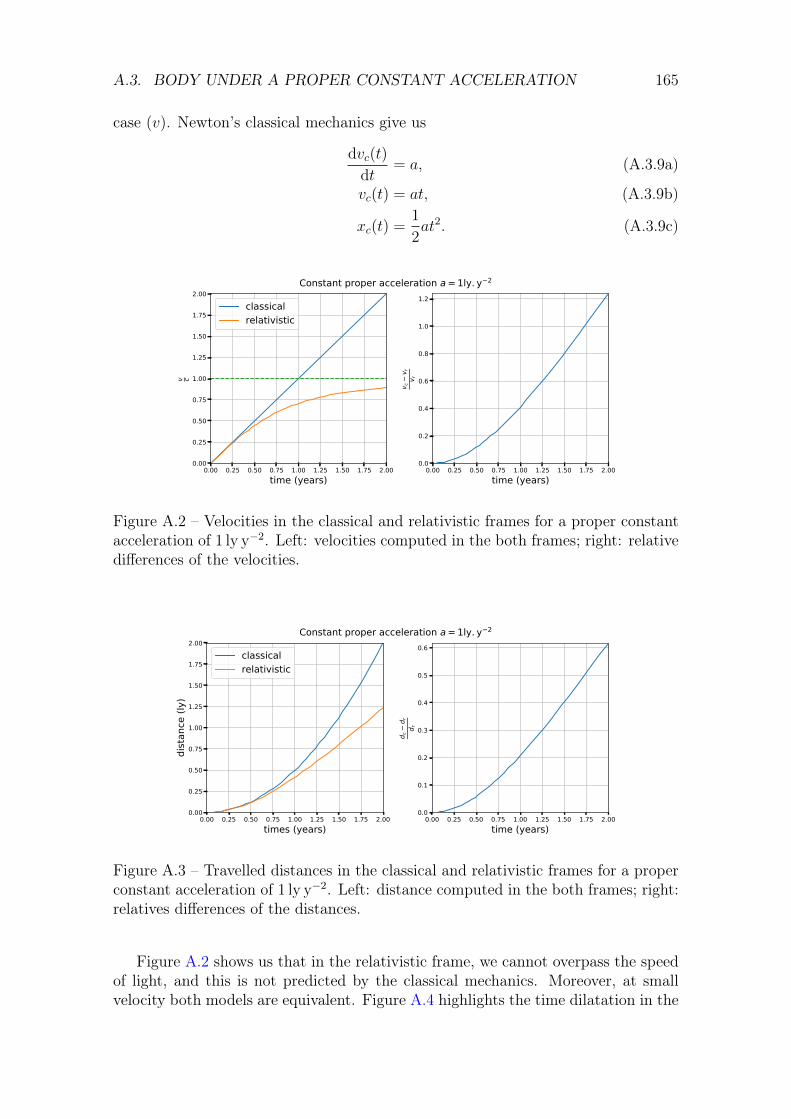
A.3. BODY UNDER A PROPER CONSTANT ACCELERATION 165
case (v). Newton’s classical mechanics give us
dvc(t)
dt= a, (A.3.9a)
vc(t) = at, (A.3.9b)
xc(t) =1
2at2. (A.3.9c)
0.00 0.25 0.50 0.75 1.00 1.25 1.50 1.75 2.00time (years)
0.00
0.25
0.50
0.75
1.00
1.25
1.50
1.75
2.00
v c
classicalrelativistic
0.00 0.25 0.50 0.75 1.00 1.25 1.50 1.75 2.00time (years)
0.0
0.2
0.4
0.6
0.8
1.0
1.2
v cv r
v r
Constant proper acceleration a = 1ly. y 2
Figure A.2 – Velocities in the classical and relativistic frames for a proper constantacceleration of 1 ly y−2. Left: velocities computed in the both frames; right: relativedifferences of the velocities.
0.00 0.25 0.50 0.75 1.00 1.25 1.50 1.75 2.00times (years)
0.00
0.25
0.50
0.75
1.00
1.25
1.50
1.75
2.00
dist
ance
(ly)
classicalrelativistic
0.00 0.25 0.50 0.75 1.00 1.25 1.50 1.75 2.00time (years)
0.0
0.1
0.2
0.3
0.4
0.5
0.6
d cd r
d r
Constant proper acceleration a = 1ly. y 2
Figure A.3 – Travelled distances in the classical and relativistic frames for a properconstant acceleration of 1 ly y−2. Left: distance computed in the both frames; right:relatives differences of the distances.
Figure A.2 shows us that in the relativistic frame, we cannot overpass the speedof light, and this is not predicted by the classical mechanics. Moreover, at smallvelocity both models are equivalent. Figure A.4 highlights the time dilatation in the

166 APPENDIX A. USEFUL NOTIONS OF SPECIAL RELATIVITY
0.00 0.25 0.50 0.75 1.00 1.25 1.50 1.75 2.00times (y)
0.0
0.2
0.4
0.6
0.8
1.0
1.2
1.4
prop
er ti
me
(y)
0.0 0.2 0.4 0.6 0.8 1.0 1.2 1.4proper time (y)
0.0
0.2
0.4
0.6
0.8
1.0
1.2
dist
ance
(ly)
Constant proper acceleration a = 1ly. y 2
Figure A.4 – For a proper constant acceleration of 1 ly y−2. Left: proper time as afunction of the time in the reference frame; right: travelled distance as a functionof the proper time.
moving frame. For example, when 2 years have passed in the reference frame, 1.4years have passed in the moving frame.

Appendix B
Dirac Equation
B.1 NotationsAs defined in A.1, we note in this section of 4-vector x as:
x =
ctxyz
(B.1.1)
we note xµ (or any greek letter) a space-time component of x, −→x the spatial partand xk (or any latin letter) a spatial component. To make the writing easier, thecomponent of a vector and the vector can be used with the same meaning.
The energy-momentum 4-vector is noted and defined as,
p = pµ =
(E/c−→p
), (B.1.2)
with E the energy of a particle, c the speed of light, and −→p the momentum.To make the equation more readable, the partial derivative along a coordinate
xµ, ∂∂xµ
might be written ∂µ. We use Einstein convention of implicitly summing overrepeated indices.
B.2 MotivationThe main idea behind the work from Dirac was to determine an equation ruling thewave function of an electron. Before Dirac established in 1928 his equation [1], theSchrödinger equation was used to describe the behaviour of an electron. Indeed thecorrespondence principle of quantum mechanics E ↔= i~ ∂
∂t, −→p = −i~
−→∇ , leads to
Eψ = Hψ, (B.2.1a)
i~∂ψ
∂t= − ~2
2m
−→∇2ψ + V ψ, (B.2.1b)
with H the Hamiltonian of the system, and ψ the wave function, the first term of Hcorresponding to the kinetic energy (
−→p 2
2m) and V the interaction potential. Thereby
the possible values of the energy E are the eigenvalues of the operator H.
167

168 APPENDIX B. DIRAC EQUATION
However, the Schrödinger equation has two shortcomings. Firstly, it is not rela-tivistic, and considering the mass of an electron, it appears obvious that a relativisticequation to govern its behaviour has to be found. Secondly, the spin does not appearnaturally and it is an ad-hoc element of the quantum theory.
To obtain a relativistic equation, once again, the correspondence principle canbe applied on the relation E2 = (−→p c)2
+ (mc2)2. This leads to the Klein-Gordonequation (~ = c = 1)
(∂µ∂µ +m2)ψ = 0. (B.2.2)
If the wave function really describes the motion of a particle, the Klein Gordonequation has to be compatible with a continuity law:
∂ρ
∂t+−→∇ · −→j = 0. (B.2.3)
And this is the case. Indeed Equation B.2.2 leads to
ψ∗(∂µ∂µ +m2)ψ = 0
ψ(∂µ∂µ +m2)ψ∗ = 0
⇒ ψ∗∂µ∂µψ − ψ∂µ∂µψ∗ = 0
⇔ ∂ti (ψ∗∂tψ − ψ∂tψ∗) +−→∇i(ψ∗−→∇ψ − ψ
−→∇ψ∗
)= 0
which is a continuity law with ρ = i (ψ∗∂tψ − ψ∂tψ∗) and−→j = i
(ψ∗−→∇ψ − ψ
−→∇ψ∗
).
The solution for the Klein-Gordon equation has the form ψ = Ne−ipµxµ . Indeed,
the equation applied to this wave function leads to pµpµ = (mc2)2, i.e. E2 =
(−→p c)2 + (mc2)2. In that case, ρ = 2E|N |2, but there are two solutions for E,±√−→p c)2 + (mc2)2, and this means that ρ might be negative, which is impossible if
we want to understand it as a probability density.The idea is now to try to find a linear expression of the hamiltonian, of the form
H = αkpkc+ βmc2 (B.2.4)
in order to have H2ψ = E2ψ with E2 = (−→p c)2+ (mc2)2. In that case, αk and
β cannot be numbers if we want to preserve rotational invariance. So it will beassumed that αk and β are N ×N matrices and ψ a vector of dimension N > 1.
B.3 Building of the equationWe would like to find an linear hamiltonian for the electron as
H = αkpkc+ βmc2. (B.3.1)
Let’s first see if it is compatible with a continuity law. Starting from Eψ =Hψ ⇔ Eψ† = ψ†H†, the following equations are found:
Eψ = i~∂tψ = αkpkψc+ βψmc2 = −i~cαk∂kψ + βψmc2,
Eψ† = −i~∂tψ† = i~c∂kψ†(αk)† + ψ†β†mc2.

B.3. BUILDING OF THE EQUATION 169
αk, β are hermitian (i.e. αk† = αk, β† = β†) because H is hermitian. We multiplythe first line by ψ† and the second by ψ to finally obtain
i~(ψ†∂tψ + ψ∂tψ
†) = −i~c(ψ†αk∂kψ + ∂kψ†αkψ),
which can be written as a continuity law:
∂t(ψ†ψ
)+ ∂k
(cψ†αkψ
)= 0, (B.3.2)
with ρ = ψ†ψ, j = cψ†αψ and we have ρ ≥ 0, which means that ρ can be understoodas a probability density.
To find a relation between αk and β, we start again from H2ψ = E2ψ, because isit known that E2 = c2
(−→p 2+m2c2
). If we note IN , the neutral element ofMN(C),
we have
(−→α · −→p + βmc)2
=(−→p 2
+m2c2)IN
1
2[αj, αk]pjpk +
1
2αj, αkpjpk + αk, βpk + β2m2c2 =
(−→p 2+m2c2
)IN
So if αk and β fulfil
αj, αk = 2δjkIN , (B.3.3a)αk, β = 0, (B.3.3b)
β2 = IN , (B.3.3c)
then H2ψ = E2ψ is true. Equations B.3.3 describe a Clifford algebra associated tothe metric δjk (δjk = 1 if j = k, δjk = 0 otherwise).
The second equation of B.3.3 lets us know that N is even. Indeed:
αk, β = 0,
αkβ = −βαk,det(αkβ) = det(−βαk),det(αkβ) = (−1)Ndet(αkβ),
1 = (−1)N .
Let’s try with N = 2. We take αk = σk, with σk the Pauli’s matrices
σx =
(0 11 0
), σy =
(0 −ii 0
), σz =
(1 00 −1
), (B.3.4)
which fulfil
[σi, σj] = 2iεijkσk (B.3.5a)σi, σj = 2δij (B.3.5b)⇒ σiσj = δij + iεijkσk (B.3.5c)

170 APPENDIX B. DIRAC EQUATION
Also, B = (I2, σx, σy, σz) can be taken as a basis of hermitian matrices subspace.
Thereby, β can be written as β = xkσk + y.However, in that case, β, αk = 0 leads to β, σk = 0 = 2xk + 2yσk so xk =
y = 0. This means that β has to be null, which not acceptable. We therefore tryN = 4.
For N = 4, let’s have a look at the standard representation of the Clifford algebra(associated to the euclidian metric of R)
αk =
(0 σk
σk 0
), β =
(I2 00 −I2
). (B.3.6)
In that case
Eψ = Hψ,
i~∂tψ = cαkpkψ + βmc2ψ,
i~∂tψ = −i~cαk∂kψ + βmc2ψ,
i~∂0ψ + i~αk∂kψ = βmcψ,
i~(β∂0 + βαk∂k)ψ = mcψ,
and defining γ0 = β and γk = βαk we get
(i~γµ∂µ −mc)ψ = 0, (B.3.7)
which is the Dirac equation, with
γ0 =
(I2 00 −I2
), γk =
(0 σk
−σk 0
), (B.3.8)
the Dirac matrices. Writing ψ = ψ†γ0, the current jµ = (ρ/c,−→j ) is conserved
(∂µjµ = 0) with jµ = cψγµψ.
B.4 SolutionsNow the goal is to solve the Dirac equation
(i~γµ∂µ −mc)ψ = 0, (B.4.1)
and as a reminder, ψ is a 4 dimensions wave function vector.If we assume a wave function of the form ψ = u(pµ) exp
(− i
~pµxµ)with
u(pµ) =
(f(pµ)g(pµ)
),
f, g two 2-dimension vectors, then the Dirac equation leads to
(pµγµ −mc)u(pµ) = 0 (B.4.2)
(E −mc2)f − pkσkcg = 0,
pkσkcf − (E +mc2)g = 0.(B.4.3)

B.4. SOLUTIONS 171
f = 0, g = 0 being solution of B.4.3, the only way to have a non trivial solution isto fulfil (E −mc2)(E +mc2)− pkσkplσlc2, which leads to E2 = (−→p c)2
+ (mc2)2, as
anticipated.
In other words, the system has two eigenvalues ±E = ±√
(−→p c)2+ (mc2)2, one
corresponding to particles with a positive energy, the second to particles with anegative energy.
Let’s start with E > 0:(E −mc2) f −−→p · −→σ cg = 0−→p · −→σ cf − (E +mc2)g = 0
(B.4.4)
⇒ g =−→p · −→σE +mc2
cf (B.4.5)
So, we have two eigenvectors associated to +E, corresponding to f =
(10
)or
(01
):
u↑ = N↑
10
−→p ·−→σE+mc2
c
(10
) , u↓ = N↓
01
−→p ·−→σE+mc2
c
(01
) (B.4.6)
Because ψ has to be a wave function, we can determine N↑ and N↓:∫d3xψ† (−→x ,−→p )ψ (−→x ,−→q ) = δ (−→p −−→q )⇒ |N↑|2 = |N↓|2 =
E +mc2
2E. (B.4.7)
To determine the other wave functions, we perform the following substitutionin Equation B.4.3 E → −E,−→p → −−→p which leads to the relation f =
−→p ·−→σE+mc2
cg.Thereby, two new wave function are obtained:
v↑ = N↑
−→p ·−→σE+mc2
c
(10
)10
, v↓ = N↓
−→p ·−→σE+mc2
c
(01
)01
(B.4.8)
A basis of solution of the Dirac equation can be summarised as
ψ(+)s (pµ, xµ) = us(
−→p )e−ipµxµ , ψ(−)
s (pµ, xµ) = vs(−→p )eip
µxµ , (B.4.9)
with
us(−→p ) =
√E +mc2
2E
(φs
−→p ·−→σE+mc2
cφs
), vs(−→p ) =
√E +mc2
2E
( −→p ·−→σE+mc2
cφsφs
)(B.4.10)
andφs =
(10
)or
(01
). (B.4.11)
us described electrons with 2 possible states for each particle, up and down, corre-sponding to the two spin states. This beautifully fulfils the original goal: a quantumand relativistic equation of the electron naturally encompasses the description of thespin. But there is more, and even more spectacular: the solution vs was first seenas spurious, but Dirac finally proposed that it describes a real particle of chargeopposed to that of the electron. This was the invention of the positron.
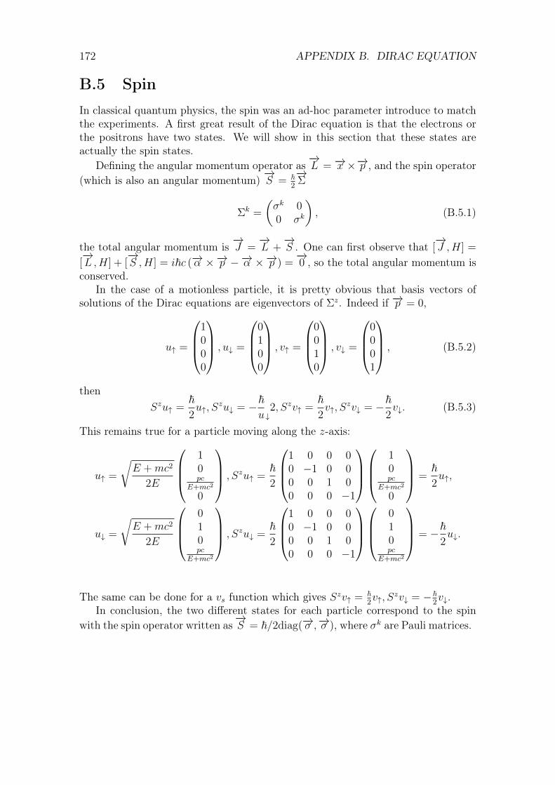
172 APPENDIX B. DIRAC EQUATION
B.5 SpinIn classical quantum physics, the spin was an ad-hoc parameter introduce to matchthe experiments. A first great result of the Dirac equation is that the electrons orthe positrons have two states. We will show in this section that these states areactually the spin states.
Defining the angular momentum operator as−→L = −→x ×−→p , and the spin operator
(which is also an angular momentum)−→S = ~
2
−→Σ
Σk =
(σk 00 σk
), (B.5.1)
the total angular momentum is−→J =
−→L +
−→S . One can first observe that [
−→J ,H] =
[−→L ,H] + [
−→S ,H] = i~c (−→α ×−→p −−→α ×−→p ) =
−→0 , so the total angular momentum is
conserved.In the case of a motionless particle, it is pretty obvious that basis vectors of
solutions of the Dirac equations are eigenvectors of Σz. Indeed if −→p = 0,
u↑ =
1000
, u↓ =
0100
, v↑ =
0010
, v↓ =
0001
, (B.5.2)
thenSzu↑ =
~2u↑, S
zu↓ = −~u↓
2, Szv↑ =~2v↑, S
zv↓ = −~2v↓. (B.5.3)
This remains true for a particle moving along the z-axis:
u↑ =
√E +mc2
2E
10pc
E+mc2
0
, Szu↑ =~2
1 0 0 00 −1 0 00 0 1 00 0 0 −1
10pc
E+mc2
0
=~2u↑,
u↓ =
√E +mc2
2E
010pc
E+mc2
, Szu↓ =~2
1 0 0 00 −1 0 00 0 1 00 0 0 −1
010pc
E+mc2
= −~2u↓.
The same can be done for a vs function which gives Szv↑ = ~2v↑, S
zv↓ = −~2v↓.
In conclusion, the two different states for each particle correspond to the spinwith the spin operator written as
−→S = ~/2diag(−→σ ,−→σ ), where σk are Pauli matrices.

Appendix C
Buffer Gas Trap electrodesschematics
Figure C.1 – Schematic of the grounded ring at the entrance of the Buffer Gas Trapfirst stage.
Figure C.2 – Schematic of the electrodes composing the Buffer Gas Trap first stage.
173

174 APPENDIX C. BUFFER GAS TRAP ELECTRODES SCHEMATICS
Figure C.3 – Left: Schematic of the last electrode of the Buffer Gas Trap first stage.Right: Schematic of the transition ring between the BGT first stage and secondstage.
Figure C.4 – Schematic of the grounded ring at the end of the first stage to supportthe electrodes.
Figure C.5 – Schematic of the long electrodes composing the Buffer Gas Trap secondstage. This is also the last electrode of the third stage.

175
Figure C.6 – Schematic of the half-length electrodes used for the Rotating Walltechnique in the Buffer Gas Trap second stage. On both electrodes, the same staticpotential is applied. The electrode described on the bottom picture is split in four,to apply the oscillating potential for the Rotating Wall technique (see Section 3.3.2).
Figure C.7 – Top: Schematic of the last electrode of the Buffer Gas Trap secondstage and first electrode of the BGT third stage. Bottom: Schematic of the groundedsupport ring surrounding the electrodes presented on the left (see the assembly viewin Figure 4.4).
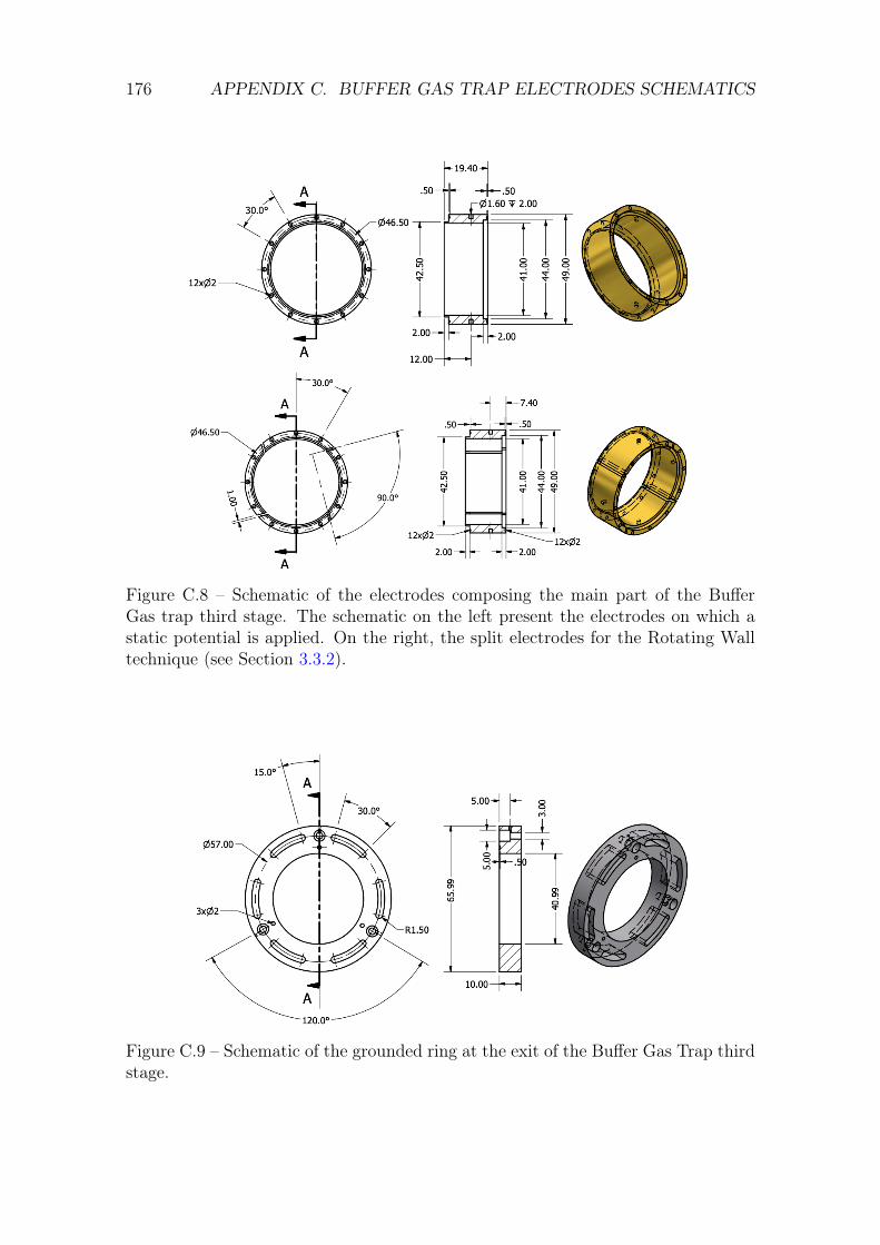
176 APPENDIX C. BUFFER GAS TRAP ELECTRODES SCHEMATICS
Figure C.8 – Schematic of the electrodes composing the main part of the BufferGas trap third stage. The schematic on the left present the electrodes on which astatic potential is applied. On the right, the split electrodes for the Rotating Walltechnique (see Section 3.3.2).
Figure C.9 – Schematic of the grounded ring at the exit of the Buffer Gas Trap thirdstage.

Appendix D
HFT probes
D.1 Temperature probes connections
Figure D.1 – Measurement connector pins.
pin name pin name pin name pin nameA TG1 V+ P TG2 V- a CC5 - p CC9 +B TG5 V- R TG2 V+ b CC5 + q H3 -C TG5 V+ S TG1 I- c CC4 - r H3 +D TG4 I- T TG1 I+ d CC4 + s H2 -E TG4 I+ U TG1 V- e CC3 - t H2 +F TG4 V- V TG5 I+ f CC3 + u H1 -G TG4 V+ W CC7 - g CC2 - v H1 +H TG3 I- X CC7 + h CC2 + w CC8 -J TG3 I+ Y CC6 - i CC1 -K TG3 V- Z CC6 + j CC1 +L TG3 V+ k TG5 I-M TG2 I- m CC8 +N TG2 I+ n CC9 -
Table D.1 – Layout of duct measurement connector pins
177

178 APPENDIX D. HFT PROBES
pin name pin name pin name pin nameA CGR1 V+ P CGR2 V- a CC7 - j CC3 +B CC1 - R CGR2 V+ b CC7 + k CC2 -C CC1 + S CGR1 I- c CC6 - q V4 coil out -H CGR3 I- T CGR1 I+ d CC6 + r V3 coil out +J CGR3 I+ U CGR1 V- e CC5 - s V2- P/L2+K CGR3 V- V CC2 + f CC5 + t V1- P/L2-L CGR3 V+ Y CC8 - g CC4 - u V2+ P/L1-M CGR2 I- Z CC8 + h CC4 + v V1+ P/L1+N CGR2 I+ i CC3 -
Table D.2 – Layout of coils measurement connector pins
D.2 Carbon Glass Resistor based probes abaci
101 102 103 104 105
Resistance ( )
101
102
Tem
pera
ture
(K)
Temperature as a function of the resistanceCGR1CGR2CGR3
Figure D.2 – Abacus for CGR1, CGR2, CGR3.

D.2. CARBON GLASS RESISTOR BASED PROBES ABACI 179
T ρ dρ/dT dlog(ρ)/dlog(T ) T ρ dρ/dT dlog(ρ)/dlog(T )1.4 483554.0 -2780900.0 -8.0514 15.5 54.2987 -4.8252 -1.37741.5 281464.0 -1431900.0 -7.6311 16.0 52.0005 -4.378 -1.3471.6 174277.0 -786870.0 -7.2241 16.5 49.9111 -3.9884 -1.31851.7 113724.0 -459320.0 -6.8662 17.0 48.0042 -3.6467 -1.29141.8 77443.1 -283620.0 -6.5921 17.5 46.2575 -3.346 -1.26581.9 54549.1 -182870.0 -6.3694 18.0 44.6525 -3.0797 -1.24152.0 39564.0 -121740.0 -6.1542 18.5 43.1728 -2.8433 -1.21842.1 29447.3 -83455.0 -5.9515 19.0 41.805 -2.6322 -1.19632.2 22424.2 -58753.0 -5.7642 19.5 40.5369 -2.4434 -1.17542.3 17421.9 -42361.0 -5.5924 20.0 39.3584 -2.2736 -1.15532.4 13779.4 -31182.0 -5.4311 21.0 37.2353 -1.9823 -1.1182.5 11073.6 -23386.0 -5.2796 22.0 35.3765 -1.7428 -1.08382.6 9027.72 -17838.0 -5.1374 23.0 33.7362 -1.5439 -1.05262.7 7455.32 -13818.0 -5.0042 24.0 32.2782 -1.3768 -1.02372.8 6229.24 -10851.0 -4.8773 25.0 30.974 -1.2355 -0.997212.9 5260.42 -8629.4 -4.7573 26.0 29.8 -1.1158 -0.97353.0 4485.61 -6942.5 -4.6432 27.0 28.7371 -1.0123 -0.951123.1 3859.02 -5644.4 -4.5342 28.0 27.7711 -0.92173 -0.929323.2 3347.16 -4634.1 -4.4304 29.0 26.8896 -0.84333 -0.909523.3 2925.01 -3839.6 -4.3319 30.0 26.081 -0.77511 -0.891583.4 2573.82 -3207.9 -4.2377 31.0 25.3368 -0.71668 -0.874433.5 2279.27 -2701.3 -4.148 32.0 24.6494 -0.66099 -0.85813.6 2030.35 -2291.3 -4.0627 33.0 24.0128 -0.61319 -0.842693.7 1818.5 -1956.7 -3.9811 34.0 23.4214 -0.57045 -0.828113.8 1637.03 -1681.6 -3.9035 35.0 22.8705 -0.53195 -0.814073.9 1480.61 -1453.8 -3.8294 36.0 22.3562 -0.49731 -0.800824.0 1345.01 -1263.8 -3.7585 37.0 21.8747 -0.46603 -0.788264.2 1123.3 -969.96 -3.6267 38.0 21.4232 -0.43756 -0.776144.4 951.6 -750.03 -3.505 39.0 20.9988 -0.41171 -0.764644.6 816.369 -602.08 -3.3925 40.0 20.599 -0.38814 -0.753725.8 396.06 -195.21 -2.8587 42.0 19.8653 -0.34675 -0.73316.0 359.918 -167.18 -2.787 44.0 19.2077 -0.3118 -0.714246.5 289.762 -117.32 -2.6318 46.0 18.6147 -0.28202 -0.696917.0 239.721 -85.073 -2.4842 48.0 18.0769 -0.25638 -0.680777.5 202.916 -63.55 -2.3489 50.0 17.5868 -0.23424 -0.665948.0 175.032 -48.911 -2.2355 52.0 17.1381 -0.2149 -0.652068.5 153.288 -38.598 -2.1403 54.0 16.7256 -0.19791 -0.638969.0 135.983 -31.001 -2.0518 56.0 16.3451 -0.18299 -0.626959.5 121.97 -25.307 -1.9711 58.0 15.9926 -0.16972 -0.6155210.0 110.454 -20.95 -1.8967 60.0 15.6652 -0.15791 -0.6048210.5 100.857 -17.57 -1.8292 65.0 14.9395 -0.13345 -0.5806411.0 92.7664 -14.897 -1.7664 70.0 14.3215 -0.1145 -0.5596311.5 85.8708 -12.761 -1.6557 75.0 13.7879 -0.099493 -0.5411912.5 74.7883 -9.6145 -1.607 77.35 13.5613 -0.093501 -0.5333113.0 70.2833 -8.4419 -1.5615 80.0 13.3217 -0.087411 -0.5249213.5 66.3138 -7.4642 -1.5195 85.0 12.9102 -0.077533 -0.5104814.0 62.7937 -6.6394 -1.4803 90.0 12.5436 -0.069351 -0.4975914.5 59.6534 -5.9399 -1.4438 95.0 12.2145 -0.062489 -0.4860215.0 56.8371 -5.3408 -1.4095 100.0 11.9169 -0.056689 -0.4757
Table D.3 – Abacus for CGR1 (Refrigerator 2nd head). Temperature range: 1.40 Kto 100 K. Sensor Serial Number: C19051. Sensor Model: CGR1-1-1000-1.4D. SensorExcitation: 2 mV±50%.

180 APPENDIX D. HFT PROBES
T ρ dρ/dT dlog(ρ)/dlog(T ) T ρ dρ/dT dlog(ρ)/dlog(T )1.4 522593.0 -2996100.0 -8.0264 14.0 62.5701 -6.6493 -1.48781.5 302687.0 -1568900.0 -7.7751 14.5 59.4256 -5.9471 -1.45111.6 185598.0 -852350.0 -7.3479 15.0 56.6063 -5.3457 -1.41661.7 120532.0 -489770.0 -6.9078 15.5 54.0658 -4.9284 -1.38421.8 81974.8 -300770.0 -6.6042 16.0 51.7665 -4.3796 -1.35371.9 57699.0 -193940.0 -6.3863 16.5 49.6765 -3.9889 -1.32492.0 41796.3 -129330.0 -6.1885 17.0 47.7696 -3.5452 -1.29762.1 31039.1 -88810.0 -6.0086 17.5 46.0235 -3.3447 -1.27182.2 23563.7 -62535.0 -5.8385 18.0 44.4192 -3.0778 -1.24722.3 18242.0 -45029.0 -5.6773 18.5 42.9407 -2.8408 -1.22392.4 14375.1 -33047.0 -5.5174 19.0 41.5742 -2.6294 -1.20172.5 11512.7 -24687.0 -5.3608 19.5 40.3076 -2.4402 -1.18052.6 9357.34 -18751.0 -5.21 20.0 39.1308 -2.2701 -1.16032.7 7707.88 -14463.0 -5.0664 21.0 37.0114 -1.9785 -1.12262.8 6426.86 -11316.0 -4.9297 22.0 35.1565 -1.7388 -1.08812.9 5419.19 -8970.0 -4.801 23.0 33.5202 -1.5399 -1.05663.0 4613.83 -7198.1 -4.6803 24.0 32.0662 -1.3728 -1.02753.1 3964.82 -5840.7 -4.5667 25.0 30.7659 -1.2316 -1.00083.2 3435.55 -4788.4 -4.3601 26.0 29.5959 -1.1118 -0.976683.3 2999.57 -3963.5 -4.3605 27.0 28.537 -1.0083 -0.953993.4 2637.18 -3309.1 -4.2663 28.0 27.5749 -0.91802 -0.932183.5 2333.41 -2785.2 -4.1777 29.0 26.6969 -0.83982 -0.912273.6 2076.8 -2361.7 -4.0938 30.0 25.8919 -0.77171 -0.894163.7 1858.48 -2016.2 -4.014 31.0 25.1509 -0.71147 -0.876933.8 1671.51 -1732.3 -3.9381 32.0 24.4667 -0.65798 -0.860573.9 1510.41 -1497.1 -3.8656 33.0 23.833 -0.61035 -0.845114.0 1370.8 -1300.9 -3.796 34.0 23.2443 -0.56776 -0.830474.2 1142.69 -997.3 -3.6656 35.0 22.696 -0.52937 -0.816354.4 966.28 -778.21 -3.5436 36.0 22.1842 -0.49483 -0.8034.6 827.567 -616.97 -3.4294 37.0 21.7053 -0.46363 -0.790334.8 716.8 -496.26 -3.3232 38.0 21.256 -0.43524 -0.77815.0 627.153 -404.3 -3.2233 39.0 20.8339 -0.40945 -0.766475.2 553.694 -333.29 -3.1292 40.0 20.4364 -0.38594 -0.755415.4 492.861 -277.35 -3.0388 42.0 19.707 -0.34465 -0.734535.6 441.978 -233.16 -2.9542 44.0 19.1535 -0.30981 -0.715445.8 399.014 -197.77 -2.8748 46.0 18.4643 -0.28014 -0.697916.0 362.413 -169.24 -2.8019 48.0 17.9302 -0.25462 -0.681636.5 291.4 -118.76 -2.6491 50.0 17.4435 -0.23259 -0.666697.0 240.758 -86.05 -2.5019 52.0 16.9979 -0.21327 -0.652747.5 203.555 -64.191 -2.3651 54.0 16.5885 -0.19648 -0.63968.0 175.407 -49.341 -2.2504 56.0 16.2106 -0.18167 -0.627578.5 153.485 -38.891 -2.1538 58.0 15.8607 -0.16849 -0.616159.0 136.058 -31.203 -2.0641 60.0 15.5357 -0.15677 -0.605459.5 121.96 -25.449 -1.9823 65.0 14.8152 -0.1325 -0.5813210.0 110.384 -21.05 -1.907 70.0 14.2016 -0.11368 -0.5603210.5 100.744 -17.644 -1.8389 75.0 13.6719 -0.098773 -0.5418411.0 92.6215 -14.951 -1.7756 77.35 13.4469 -0.092817 -0.5339111.5 85.7023 -12.802 -1.7178 80.0 13.2091 -0.086761 -0.5254612.0 79.7518 -11.06 -1.6642 85.0 12.8006 -0.076932 -0.5108512.5 74.5885 -9.6379 -1.6152 90.0 12.437 -0.068783 -0.4977513.0 70.0733 -8.4597 -1.5694 95.0 12.1106 -0.061944 -0.4859113.5 66.096 -7.4776 -1.5273 100.0 11.8158 -0.056161 -0.4753
Table D.4 – Abacus for CGR2 (Right side coil). Temperature range: 1.40 K to100 K. Sensor Serial Number: C19065. Sensor Model: CGR1-1-1000-1.4D. SensorExcitation: 2 mV±50%.

D.2. CARBON GLASS RESISTOR BASED PROBES ABACI 181
T ρ dρ/dT dlog(ρ)/dlog(T ) T ρ dρ/dT dlog(ρ)/dlog(T )1.4 487265.0 -2834800.0 -8.145 14.0 58.8825 -6.2687 -1.49051.5 282956.0 -1438200.0 -7.6239 14.5 55.9184 -5.6049 -1.45341.6 175237.0 -793940.0 -7.249 15.0 53.2617 -5.0365 -1.41841.7 113940.0 -465830.0 -6.9502 15.5 50.8685 -4.5478 -1.38571.8 77211.6 -285960.0 -6.6665 16.0 48.7031 -4.124 -1.35481.9 54224.8 -182910.0 -6.4089 16.5 46.7353 -3.7552 -1.32582.0 39260.9 -121460.0 -6.1872 17.0 44.9403 -3.4321 -1.29832.1 29167.9 -83252.0 -5.9939 17.5 43.2968 -3.1479 -1.27232.2 22163.7 -58570.0 -5.8137 18.0 41.787 -2.8965 -1.24772.3 17179.6 -42182.0 -5.6473 18.5 40.3956 -2.6734 -1.22432.4 13554.8 -31007.0 -5.4901 19.0 39.1096 -2.4744 -1.20212.5 10866.4 -23212.0 -5.3403 19.5 37.9177 -2.2964 -1.1812.6 8837.88 -17664.0 -5.1967 20.0 36.8101 -2.1366 -1.16082.7 7282.67 -13648.0 -5.06 21.0 34.8153 -1.8624 -1.12342.8 6073.09 -10691.0 -4.9289 22.0 33.0691 -1.637 -1.08912.9 5119.95 -6808.7 -4.8044 23.0 31.5284 -1.4501 -1.05783.0 4358.95 -6808.7 -4.686 24.0 30.1592 -1.2927 -1.02873.1 3745.01 -5525.1 -4.5735 25.0 28.9348 -1.1598 -1.00213.2 3244.38 -4528.8 -4.4668 26.0 27.8326 -1.0478 -0.978833.3 2832.11 -3747.3 -4.3664 27.0 26.8344 -0.95045 -0.956323.4 2489.56 -3127.2 -4.2709 28.0 25.9281 -0.86414 -0.933193.5 2202.55 -2630.9 -4.1807 29.0 25.102 -0.79007 -0.912753.6 1960.21 -2229.9 -4.0952 30.0 24.3445 -0.72621 -0.894923.7 1754.11 -1902.9 -4.0139 31.0 23.6471 -0.66975 -0.8783.8 1577.68 -1634.4 -3.9367 32.0 23.0029 -0.61954 -0.861863.9 1425.69 -1412.2 -3.8632 33.0 22.4062 -0.57469 -0.846414.0 1294.01 -1227.0 -3.7928 34.0 21.852 -0.5345 -0.831634.2 1078.87 -940.61 -3.6618 35.0 21.3359 -0.49825 -0.817344.4 912.466 -734.17 -3.5403 36.0 20.8543 -0.46561 -0.803764.6 781.575 -582.34 -3.4274 37.0 20.4017 -0.43612 -0.790874.8 676.994 -468.68 -3.323 38.0 19.9812 -0.40934 -0.778495.0 592.312 -381.98 -3.2245 39.0 19.5842 -0.38506 -0.76685.2 522.894 -314.95 -3.1321 40.0 19.2103 -0.36296 -0.755765.4 465.367 -262.41 -3.0449 42.0 18.5243 -0.32421 -0.735085.6 417.197 -220.86 -2.9646 44.0 17.9094 -0.29155 -0.716295.8 376.489 -187.4 -2.8869 46.0 17.3548 -0.26374 -0.699056.0 341.821 -160.21 -2.8122 48.0 16.8519 -0.23977 -0.682956.5 274.784 -111.78 -2.6442 50.0 16.3936 -0.21903 -0.668047.0 227.119 -81.135 -2.5006 52.0 15.9741 -0.2009 -0.653987.5 191.945 -60.818 -2.3764 54.0 15.5886 -0.18493 -0.640628.0 165.274 -46.708 -2.2609 56.0 15.233 -0.17091 -0.62838.5 144.561 -36.682 -2.1569 58.0 14.9039 -0.15843 -0.616569.0 128.139 -29.387 -2.064 60.0 14.5984 -0.14734 -0.605569.5 114.862 -23.966 -1.9822 65.0 13.9215 -0.12442 -0.580910.0 103.959 -19.828 -1.9072 70.0 13.3455 -0.10674 -0.5598910.5 94.8784 -16.624 -1.8398 75.0 12.8479 -0.092825 -0.5418711.0 87.2237 -14.093 -1.7773 77.35 12.6364 -0.087282 -0.5342811.5 80.7 -12.073 -1.7204 80.0 12.4127 -0.081652 -0.5262512.0 75.0877 -10.433 -1.6673 85.0 12.028 -0.072513 -0.5124412.5 70.2172 -9.0915 -1.6185 90.0 11.685 -0.064909 -0.4999413.0 65.9581 -7.9794 -1.5727 95.0 11.3769 -0.05848 -0.4883313.5 62.207 -7.0515 -1.5303 100.0 11.0986 -0.052982 -0.47737
Table D.5 – Abacus for CGR3 (Left side coil). Temperature range: 1.40 K to 100 K.Sensor Serial Number: C19066. Sensor Model: CGR1-1-1000-1.4D. Sensor Excita-tion: 2 mV±50%.


Bibliography
[1] Dirac, P. A. M. “The quantum theory of the electron,” Proceedings of theRoyal Society of London. Series A, Containing Papers of a Mathematical andPhysical Character , 117 (778):610–624 (February 1928).
[2] Dirac, P. A. M. “Quantised singularities in the electromagnetic field,” Pro-ceedings of the Royal Society of London. Series A, Containing Papers of aMathematical and Physical Character , 133 (821):60–72 (September 1931).
[3] Rajasekaran, G. “The discovery of Dirac equation and its impact on present-day physics,” Resonance, 8 (8):59–74 (August 2003).
[4] Anderson, C. D. “The apparent existence of easily deflectable positives,” Sci-ence, 76 (1967):238–239 (September 1932).
[5] Anderson, Carl D. “The Positive Electron,” Physical Review , 43 (6):491–494(March 1933).
[6] Glashow, Sheldon L. “Partial-symmetries of weak interactions,” NuclearPhysics , 22 (4):579–588 (February 1961).
[7] Englert, F. and R. Brout. “Broken Symmetry and the Mass of Gauge VectorMesons,” Physical Review Letters , 13 (9):321–323 (August 1964).
[8] Higgs, Peter W. “Broken Symmetries and the Masses of Gauge Bosons,” Phys-ical Review Letters , 13 (16):508–509 (October 1964).
[9] Guralnik, G. S., et al. “Global Conservation Laws and Massless Particles,”Physical Review Letters , 13 (20):585–587 (November 1964).
[10] Weinberg, Steven. “A Model of Leptons,” Physical Review Letters ,19 (21):1264–1266 (November 1967).
[11] Salam, Abdus. “Weak and Electromagnetic Interactions,” Conf. Proc.,C680519 :367–377 (1968).
[12] Canetti, Laurent, et al. “Matter and antimatter in the universe,” New Journalof Physics , 14 (9):095012 (September 2012).
[13] Kostelecký, V. Alan and Arnaldo J. Vargas. “Lorentz and CPT tests withhydrogen, antihydrogen, and related systems,” Physical Review D , 92 (5)(September 2015).
183

184 BIBLIOGRAPHY
[14] Chamberlain, Owen, et al. “Observation of Antiprotons,” Physical Review ,100 (3):947–950 (November 1955).
[15] Baur, G., et al. “Production of antihydrogen,” Physics Letters B , 368 (3):251–258 (February 1996).
[16] Blanford, G., et al. “Observation of Atomic Antihydrogen,” Phys. Rev. Lett.,80 :3037–3040 (Apr 1998).
[17] Maury, S. “The Antiproton Decelerator: AD,” Hyperfine Interactions ,109 (1/4):43–52 (1997).
[18] Oelert, W. “The ELENA Project at CERN,” Acta Physica Polonica B ,46 (1):181 (2015).
[19] Hangst, Jeffrey S and Paul Bowe. The ALPHA Collaboration AntihydrogenLaser PHysics Apparatus . Technical Report CERN-SPSC-2004-026. SPSC-I-228, Geneva: CERN, September 2004.
[20] Gabrielse, G, et al. Proposal presented to the SPSLC: The production andstudy of cold antihydrogen. Technical Report CERN-SPSC-97-8. SPSC-P-306,Geneva: CERN, 1997.
[21] Azuma, T, et al. Atomic spectroscopy and collisions using slow antiprotons .Technical Report CERN-SPSC-97-19. SPSC-P-307, Geneva: CERN, 1997.
[22] Ulmer, S, et al. Direct High-Precision Measurement of the g-Factor of a SingleAntiproton Stored in a Cryogenic Penning Trap. Technical Report CERN-SPSC-2012-019. SPSC-I-241, Geneva: CERN, June 2012.
[23] Drobychev, G Yu, et al. Proposal for the AEGIS experiment at the CERN an-tiproton decelerator (Antimatter Experiment: Gravity, Interferometry, Spec-troscopy). Technical Report CERN-SPSC-2007-017. SPSC-P-334, Geneva:CERN, June 2007.
[24] Hangst, Jeffrey S. Addendum to the ALPHA Proposal; The ALPHA-g Appa-ratus . Technical Report CERN-SPSC-2016-031. SPSC-P-325-ADD-1, Geneva:CERN, July 2016.
[25] Chardin, G, et al. Proposal to measure the Gravitational Behaviour of An-tihydrogen at Rest . Technical Report CERN-SPSC-2011-029. SPSC-P-342,Geneva: CERN, September 2011.
[26] Amoretti, M., et al. “Production and detection of cold antihydrogen atoms,”Nature, 419 (6906):456–459 (September 2002).
[27] Gabrielse, G., et al. “Background-Free Observation of Cold Antihydrogenwith Field-Ionization Analysis of Its States,” Physical Review Letters , 89 (21)(October 2002).
BIBLIOGRAPHY 185
[28] Andresen, G. B., et al. “Confinement of antihydrogen for 1, 000 seconds,”Nature Physics , 7 (7):558–564 (June 2011).
[29] Ulmer, S., et al. “High-precision comparison of the antiproton-to-protoncharge-to-mass ratio,” Nature, 524 (7564):196–199 (August 2015).
[30] Ahmadi, M., et al. “Observation of the 1S-2S transition in trapped antihydro-gen,” Nature, 541 (7638):506–510 (December 2016).
[31] Maggi, Filippo, et al. “Efficient solid rocket propulsion for access to space,”Acta Astronautica, 66 (11-12):1563–1573 (June 2010).
[32] Wagner, T A, et al. “Torsion-balance tests of the weak equivalence principle,”Classical and Quantum Gravity , 29 (18):184002 (August 2012).
[33] Chardin, Gabriel and Giovanni Manfredi. “Gravity, antimatter and the Dirac-Milne universe,” Hyperfine Interactions , 239 (1) (October 2018).
[34] Walz, J. and T. W. Hänsch. “A Proposal to Measure Antimatter GravityUsing Ultracold Antihydrogen Atoms,” General Relativity and Gravitation,36 (3):561–570 (March 2004).
[35] Nieto, Michael Martin and T. Goldman. “The arguments against “anti-gravity” and the gravitational acceleration of antimatter,” Physics Reports ,205 (5):221–281 (July 1991).
[36] Comini, Pauline, et al. “Antihydrogen ion production from collisions betweenpositronium and keV antiprotons for GBAR,” Hyperfine Interactions , 228 (1-3):159–165 (February 2014).
[37] Crivelli, P., et al. “Measurement of the orthopositronium confinement energyin mesoporous thin films,” Physical Review A, 81 (5) (May 2010).
[38] Latacz, Barbara Maria. Study of the antihydrogen atom and ion production viacharge exchange reaction on positronium. PhD dissertation, Université ParisSaclay, September 2019.
[39] Husson, Audric. Deceleration of antiprotons from CERN’s ELENA syn-chrotron and transport of antimatter beams through the GBAR experiment .PhD dissertation, Université Paris Saclay, December 2018.
[40] Herfurth, F, et al. “A linear radiofrequency ion trap for accumulation, bunch-ing, and emittance improvement of radioactive ion beams,” Nuclear Instru-ments and Methods in Physics Research Section A: Accelerators, Spectrome-ters, Detectors and Associated Equipment , 469 (2):254–275 (August 2001).
[41] Brown, Lowell S. and Gerald Gabrielse. “Geonium theory: Physics of a singleelectron or ion in a Penning trap,” Reviews of Modern Physics , 58 (1):233–311(January 1986).

186 BIBLIOGRAPHY
[42] Gabrielse, G., et al. “First Capture of Antiprotons in a Penning Trap: A Kilo-electronvolt Source,” Physical Review Letters , 57 (20):2504–2507 (November1986).
[43] Howell, R. H., et al. “Production of slow positrons with a 100-MeV electronlinac,” Applied Physics Letters , 40 (8):751–752 (April 1982).
[44] Charlton, M., et al. “Positron production using a 9 MeV electron linac for theGBAR experiment,” Nuclear Instruments and Methods in Physics ResearchSection A: Accelerators, Spectrometers, Detectors and Associated Equipment ,985 :164657 (January 2021).
[45] Coleman, P. G. “The generation and transportation of positron beams.”Positron Beams and Their Applications 11–40, World Scientific, January 2000.
[46] Surko, C. M., et al. “Positron Plasma in the Laboratory,” Phys. Rev. Lett.,62 :901–904 (February 1989).
[47] Greaves, R.G. and C.M. Surko. “Positron trapping and the creation of high-quality trap-based positron beams,” Nuclear Instruments and Methods inPhysics Research Section B: Beam Interactions with Materials and Atoms ,192 (1-2):90–96 (May 2002).
[48] Leite, A.M.M. Development of a buffer gas trap for the confinement ofpositrons and study of positronium production in the GBAR experiment . PhDdissertation, Université Paris Saclay, December 2017.
[49] Oshima, N., et al. “Development of a cold HCI source for ultra-slow collisions,”Nuclear Instruments and Methods in Physics Research Section B: Beam In-teractions with Materials and Atoms , 205 :178–182 (May 2003).
[50] Oshima, N., et al. “New Scheme for Positron Accumulation in Ultrahigh Vac-uum,” Physical Review Letters , 93 (19) (November 2004).
[51] Dupré, Pierre. Piégeage de positons dans un piège de Penning Malmberg, envue de leur accumulation avec un faisceau pulsé. PhD dissertation, UniversitéParis 6, 2011.
[52] Grandemange, Pierre. Trapping and accumulation of positrons from a pulsedbeam produced by a linear accelerator for gravitational interaction of antimatterstudy . PhD dissertation, Université Paris Sud - Paris XI, December 2013.
[53] Liszkay, L., et al. “Positronium reemission yield from mesostructured silicafilms,” Applied Physics Letters , 92 (6):063114 (February 2008).
[54] Liszkay, L., et al. “Mesoporous silica films with varying porous volume fraction:Direct correlation between ortho-positronium annihilation decay and escapeyield into vacuum,” Applied Physics Letters , 95 (12):124103 (September 2009).
[55] Ore, A. and J. L. Powell. “Three-Photon Annihilation of an Electron-PositronPair,” Physical Review , 75 (11):1696–1699 (June 1949).

BIBLIOGRAPHY 187
[56] Brandt, Werner and Irwin Spirn. “Positron Lifetime Spectra in MolecularSubstances,” Physical Review , 142 (1):231–237 (February 1966).
[57] Karshenboim, Savely G. “Precision study of positronium: testing bound stateQED theory,” International Journal of Modern Physics A, 19 (23):3879–3896(September 2004).
[58] Halpern, Otto. “Magnetic Quenching of the Positronium Decay,” PhysicalReview , 94 (4):904–907 (May 1954).
[59] Kim, B.H., et al. “Development of a PbWO4 Detector for Single-Shot PositronAnnihilation Lifetime Spectroscopy at the GBAR Experiment,” Acta PhysicaPolonica A, 137 (2):122–125 (February 2020).
[60] Hilico, Laurent, et al. “Preparing single ultra-cold antihydrogen atoms for free-fall in GBAR,” International Journal of Modern Physics: Conference Series ,30 :1460269 (January 2014).
[61] Indelicato, Paul, et al. “The Gbar project, or how does antimatter fall?,”Hyperfine Interactions , 228 (1-3):141–150 (February 2014).
[62] Monroe, C., et al. “Resolved-Sideband Raman Cooling of a Bound Atom to the3D Zero-Point Energy,” Physical Review Letters , 75 (22):4011–4014 (November1995).
[63] Dufour, G., et al. “Shaping the distribution of vertical velocities of antihydro-gen in GBAR,” The European Physical Journal C , 74 (1) (January 2014).
[64] Thompson, Richard C. Trapped Charged Particles , chapter Chapter one: Pen-ning Traps, 1–33. World Scientific (Europe), 2016.
[65] Dubin, D. H. E. Trapped Charged Particles , chapter Chapter nine: Plasmasin Penning Traps, 179–193. World Scientific (Europe), 2016.
[66] Malmberg, J. H. and T. M. O’Neil. “Pure Electron Plasma, Liquid, and Crys-tal,” Phys. Rev. Lett., 39 :1333–1336 (November 1977).
[67] Isaac, Christopher Aled. Axialisation of particles in a penning-type trap bythe application of a rotating dipole electric field and its application to positronaccumulation. PhD dissertation, Swansea University, 2010.
[68] Huang, X.-P., et al. “Steady-State Confinement of Non-neutral Plasmas byRotating Electric Fields,” Physical Review Letters , 78 (5):875–878 (February1997).
[69] Gould, R. W. “Wave angular momentum in non-neutral plasmas,” AIP Con-ference Proceedings , 498 (1):170–175 (1999).
[70] Clarke, J., et al. “Design and operation of a two-stage positron accumulator,”Review of Scientific Instruments , 77 (6):063302 (June 2006).

188 BIBLIOGRAPHY
[71] Murphy, T. J. and C. M. Surko. “Positron trapping in an electrostatic wellby inelastic collisions with nitrogen molecules,” Phys. Rev. A, 46 :5696–5705(November 1992).
[72] Marler, J. P. and C. M. Surko. “Positron-impact ionization, positronium for-mation, and electronic excitation cross sections for diatomic molecules,” Phys.Rev. A, 72 :062713 (December 2005).
[73] Dahl, David A. “SIMION for the personal computer in reflection,” Interna-tional Journal of Mass Spectrometry , 200 (1-3):3–25 (December 2000).
[74] BV, Delta Elektronika. SM1500-Series 1500 Watts DC Power Supplies . https://www.delta-elektronika.nl/upload/DATA_SHEET_SM1500_V201801.pdf.
[75] Creux, Léon. Rotary Engine. Technical Report, European Patent Office, June1905.
[76] Ushimaru, Kenji. Japanese and American competition in the development ofscroll compressors and its impact on the American air conditioning indus-try . Technical Report, Office of Scientific and Technical Information (OSTI),February 1990.
[77] Iqbal, Munawar, et al. “Design modification in rotor blade of turbo molecu-lar pump,” Nuclear Instruments and Methods in Physics Research Section A:Accelerators, Spectrometers, Detectors and Associated Equipment , 678 :88–90(June 2012).
[78] Tait, P. G. and James Dewar. “4. Preliminary Note “On a New Method ofobtaining very perfect Vacua.”,” Proceedings of the Royal Society of Edinburgh,8 :348–349 (1875).
[79] Baechler, Werner G. “Cryopumps for research and industry,” Vacuum, 37 (1-2):21–29 (January 1987).
[80] Hall, Lewis, et al. Electrical vacuum pump apparatus and method . TechnicalReport, European Patent Office, Jul 1961.
[81] Agilent. Agilent Ion Pumps . http://www.ccsservices.ru/upload/banners/IonPumps.pdf.
[82] Berman, Armand. Vacuum Engineering Calculations, Formulas, and SolvedExercises . Saint Louis, US: Elsevier Science & Technology, 1992.
[83] Variant, Inc. Vacuum Technologies . https://www.agilent.com/cs/library/catalogs/Public/Training.pdf.
[84] Zheng, Sanyi. Conductance Calculation - Molecular Flow, Long Tube of Cir-cular Cross Section. Technical Report, EFD Vacuum Group, April 1993.
[85] Systems, Stanford Research, “Gas Correction Factors for Bayard-Alpert Ionization Gauges.” https://www.thinksrs.com/downloads/pdfs/applicationnotes/IG1BAgasapp.pdf.

BIBLIOGRAPHY 189
[86] Horiba, “High Performance Mass Flow Controller, SEC-Z500x.” https://www.horiba.com/fileadmin/uploads/Semiconductor/Photos/applications/Products/Digital_Mass_Flow_Controller_SEC-Z500X_Series.pdf.
[87] Wiza, Joseph Ladislas. “Microchannel plate detectors,” Nuclear Instrumentsand Methods , 162 (1-3):587–601 (June 1979).
[88] Bolton, P.R., et al. “Instrumentation for diagnostics and control of laser-accelerated proton (ion) beams,” Physica Medica, 30 (3):255–270 (May 2014).
[89] de Haas, J. T. M. and P. Dorenbos. “Advances in Yield Calibration of Scintil-lators,” IEEE Transactions on Nuclear Science, 55 (3):1086–1092 (2008).
[90] Kim, Han Soo, et al. “Fabrication and performance characteristics of aCsI(Tl)/PIN diode radiation sensor for industrial applications,” Applied Ra-diation and Isotopes , 67 (7-8):1463–1465 (July 2009).
[91] coolfet, “A250CF CoolFET Charge Sensitive Preamplifier.”https://www.amptek.com/products/charge-sensitive-preamplifiers/a250cf-coolfet-charge-sensitive-preamplifier.
[92] Mohamed, T., et al. “Comparison of non-neutral electron plasma confinementin harmonic and rectangular potentials in a very dense regime,” Physics ofPlasmas , 20 (1):012502 (January 2013).
[93] Yokogawa. Programmable DC source, Model 7651 .https://cdn.tmi.yokogawa.com/IM7651-01E.is.pdf.
[94] Advanced Energy. Ultravolt HVA Series, Precision High VoltageAmplifier . https://www.advancedenergy.com/globalassets/resources-root/data-sheets/ultravolt-hvaseries-data-sheet.pdf.
[95] Kimball, KPI. ES-535W Y2O3 Disc Cathode Care and Operating Instructions .
[96] BV, Delta Elektronika. ES150 - series . Models used: ES015-10 and ES0300-0.45.
[97] Malmberg, J H, et al. “Experiments With Pure Electron Plasmas,” PhysicaScripta, T2B :288–292 (January 1982).
[98] Fajans, J. and C. M. Surko. “Plasma and trap-based techniques for sciencewith antimatter,” Physics of Plasmas , 27 (3):030601 (March 2020).
[99] Higaki, Hiroyuki, et al. “Accumulation of LINAC based low energy positronsin a buffer gas trap,” Applied Physics Express , 13 (6):066003 (May 2020).
[100] Störmer, J, et al. “Silicon carbide: a new positron moderator,” Journal ofPhysics: Condensed Matter , 8 (7):L89–L94 (February 1996).
190 BIBLIOGRAPHY
[101] Frisbee, Robert and Stephanie Leifer. “Evaluation of propulsion options forinterstellar missions.” 34th AIAA/ASME/SAE/ASEE Joint Propulsion Con-ference and Exhibit . American Institute of Aeronautics and Astronautics, July1998.
[102] Frisbee, Robert. “How to Build an Antimatter Rocket for Interstellar Missions -Systems Level Considerations in Designing Advanced Propulsion TechnologyVehicles.” 39th AIAA/ASME/SAE/ASEE Joint Propulsion Conference andExhibit . American Institute of Aeronautics and Astronautics, July 2003.
[103] Frisbee, Robert. “Optimization of Antimatter Rocket Performance.” 44thAIAA/ASME/SAE/ASEE Joint Propulsion Conference and Exhibit . Ameri-can Institute of Aeronautics and Astronautics, July 2008.
[104] Sutton, George. Rocket propulsion elements . Hoboken, New Jersey: JohnWiley & Sons Inc, 2017.
[105] Bade, W. L. “Relativistic Rocket Theory,” American Journal of Physics ,21 (4):310–312 (April 1953).
[106] Walter, Ulrich. “Relativistic rocket and space flight,” Acta Astronautica,59 (6):453–461 (September 2006).
[107] Vulpetti, GIOVANNI. “Antimatter propulsion for space exploration,” Journalof the British Interplanetary Society , 39 (9):391–409 (1986).
[108] Morgan, D.L. “Concepts for the design of an antimatter annihilation rocket,”J. British Interplanetary Soc., 35 (NASA-CR-168660):405–412 (1982).
[109] Forward, R.L., “Antiproton AnnihilationPropulsion,” 1985.http://www.dtic.mil/dtic/tr/fulltext/u2/a160734.pdf.
[110] Keane, Ronan and Wei-Ming Zhang, “Beamed Core Antimatter Propulsion:Engine Design and Optimization,” 2012.
[111] Agostinelli, S., et al. “Geant4—a simulation toolkit,” Nuclear Instruments andMethods in Physics Research Section A: Accelerators, Spectrometers, Detectorsand Associated Equipment , 506 (3):250–303 (July 2003).
[112] Duerr, Hans-Peter and Edward Teller. “Interaction of Antiprotons with Nu-clear Fields,” Physical Review , 101 (1):494–495 (January 1956).
[113] Klempt, Eberhard, et al. “The antinucleon–nucleon interaction at low energy:Annihilation dynamics,” Physics Reports , 413 (4-5):197–317 (July 2005).
[114] Hori, M., et al. “Analog Cherenkov detectors used in laser spectroscopy exper-iments on antiprotonic helium,” Nuclear Instruments and Methods in PhysicsResearch Section A: Accelerators, Spectrometers, Detectors and AssociatedEquipment , 496 (1):102–122 (January 2003).

BIBLIOGRAPHY 191
[115] Zyla, P A, et al. “Review of Particle Physics,” Progress of Theoretical andExperimental Physics , 2020 (8) (August 2020).
[116] Simpson, James, et al., “Simple Analytic Expressionsfor the Magnetic Field of a Circular Current Loop.”https://ntrs.nasa.gov/archive/nasa/casi.ntrs.nasa.gov/20010038494.pdf.
[117] Ribon, A., et al. “Status of Geant4 hadronic physics for the simulation of LHCexperiments at the start of LHC physics program,” CERN (2010).
[118] Gourgoulhon, E. Relativité restreinte: Des particules à l’astrophysique. Savoirsactuels, EDP Sciences, 2010.


Title: Optimisation of positron accumulation in the GBAR experiment and study ofspace propulsion based on antimatter.
Keywords: Antimatter, Penning-trap, positrons, rocket, beam-cored engine
Abstract: The goal of the GBAR experimentis to determine the effect of gravity on anti-hydrogen atoms. The antihydrogen atoms arecreated by neutralising antihydrogen ions usinglaser pulses. The antihydrogen ions are pro-duced after two positrons capture by antipro-tons flying through a positronium cloud. Inthis scheme, to produce one single antihydrogenatom, 10× 1010 positrons have to be beamedon a nanoporous silica to yield the positroniumcloud. The positrons are produced by a 9 MeVLINAC accelerating electrons into a tungstentarget equipped with a mesh moderator. In thisthesis, we have studied and optimised the accu-mulation and trapping of positrons in two sub-sequent trapping devices.
The LINAC-based source provides 3× 10⁷
positrons per second, which have to be accumu-lated. They are first accumulated into a BufferGas Trap (BGT), a Penning trap, divided in3 stages, with N2 and CO2, leading to inelas-tic collisions which insure the trapping and thecooling of the positrons. The positrons are thenslowed in the first stage and accumulated in thesecond stage for 100 ms with a trapping rate ofabout 1.7× 10⁶ positrons per second, then theyare transferred into the BGT’s third stage. Thisaccumulation and transfer procedure is repeated10 times to finally provide a bunch of 1.5× 10⁶
positrons every 1.1 s (a loss happens during thisstacking operation and 100 ms are added for a fi-nal radial compression using the Rotating Walltechnique, the trapping efficiency is then 5%).This new bunch is then ready to be sent andre-trapped into the High Field Trap.
The High Field Trap is a 5 T multi-ringPenning trap allowing to trap large amounts ofcharged particle for hours. We first tested thistrap with electrons by trapping about 5× 10⁹
of them. The experiments on the electrons leadto the conclusion that a better alignment of theelectrodes with respect to the magnetic field stillneeds to be performed. However, an accept-able situation has been found allowing to re-trapthe positrons with 66% efficiency. Then, ac-cumulating the positrons bunches coming fromthe BGT, it was possible to accumulate 1× 10⁹
positrons in 1100 s. This is a really promising re-sult for the GBAR experiment. For the future,it is about to do 10 times more, 10 times fasterto collect the desired amount of positrons eachtime the ELENA decelerator provides a bunchof antiprotons (every 100 s).
We also studied how it could be possibleto use antimatter to propel a rocket. Indeed,the energy resulting from the antimatter-matterannihilation reaction has a higher intrinsic effi-ciency than any other propellant. In our study,we focused on the proton-antiproton annihila-tion reaction in a high magnetic field in order tohave the annihilation products aligned with thedirection of the thrust. The theoretical modelis named the beam cored engine. A simulatorhas been developed using GEANT4 to evaluatesome parameters such the intensity of the field.According to our simulation, it is possible to geta rocket with a specific impulse of about 0.5c/gi.e., 1.5× 10⁷ s (with c the speed of light and gthe earth’s gravitational acceleration), which ishuge if it is compared to the most modern rocket(434 s for Vulcain, propelling Ariane 5). How-ever, this model assumes the capability to pro-duce and store a macroscopic number of antipro-tons, which might be an insurmountable show-stopper. Also, with this model, a large amountof gamma rays are produced and a solution toevacuate their energy has to be found.
Université Paris-SaclayEspace Technologique / Immeuble DiscoveryRoute de l’Ôrme aux Merisiers RD 128 / 91190 Saint-Aubin, France
Titre : Optimisation de l’accumulation de positons dans l’expérience GBAR etétude de la propulsion spatiale à antimatière
Mots clés : Antimatière, piège de Penning, positons, fusée, beam-cored engine
Résumé : Le but de l’expérience GBARest de déterminer l’effet de la gravité sur desatomes d’anti-hydrogène. Les atomes d’anti-hydrogène sont créés en neutralisant des ionsanti-hydrogène grace à un faisceau laser. Un iond’anti-hydrogène étant produit par la capturede deux positons par un antiproton volant dansun nuage de positronium. Pour cela, 10× 1010
positons doivent être envoyés sur une cible desilicate nanoporeuse de laquelle va ressortir lenuage de positronium.
Les positons sont produits par un LINAC(accélérateur linéaire), accélérant des electronsà 9 MeV sur une cible de tungsten. Ce proces-sus fournissant 3× 10⁷ positons par seconde, lespositons doivent être accumulés. Ils sont dansun premier temps accumulés et refroidis dansun Piège à Gas Tampon. Il s’agit d’un piège dePenning divisé en 3 étages, dans lequel de faiblespressions de gas (N2 et CO2) on été insérés, per-mettant la perte d’énergie des positons incidentspar collisions inélastiques. Ils sont d’abord accu-mulés, dans le second étage pendant 100 ms avecun taux de piégeage d’environ 1.7× 10⁶ positonspar seconde. Après quoi, ils sont transférés dansle troisième étage du piège. Cette opération depiégeage-transfert est répétée 10 fois ce qui four-nit en sortie de ce premier piège 1.5× 10⁶ posi-ton chaque 1.1 s (il y a une perte de positonspendant cette opération de stockage et 100 mssont ajoutées pour une compression radiale enfin de processus). Ce nouveau paquet de posi-tons est donc prêt à être transféré dans le secondpiège de l’expérience.
Ce second piège est un piège de Penningmunit d’un électro-aimant de 5 T, permettantde piéger de grande quantités de particuleschargées sur une période de plusieurs heures.Ce piège a d’abord été testé avec des électrons,en confinant des plasmas allant jusqu’à 5× 10⁹
particules. Ces expériences nous ont amenés à
comprendre qu’il y avait un problème quant àl’alignement des électrodes avec le champ mag-nétique. Problème qui n’a pas pu être résolujusqu’à présent. Cependant, une situation ac-ceptable a été trouvée, permettant ainsi de re-piéger les positons venant du premier piège avecune efficacité de 66%. Ainsi, 1× 10⁹ positonsont pu être piégés en 1100 s. Il s’agit un résul-tat très prometteur pour l’expérience GBAR.A présent, il s’agit de faire 10 fois plus et 10fois plus vite, pour accumuler assez de positonschaque fois que le décélérateur ELENA fournitun paquet d’antiprotons (chaque 100 s).
Nous avons aussi étudiés la possibilité depropulser une fusée en utilisant de l’antimatière.En effet, la réaction d’annihilation matière-antimatière fournit une quantité d’énergie parunité de masse défiant toute concurrence. Nousavons particulièrement étudié le cas de la réac-tion proton-antiprotons en présence d’un fortchamp magnétique. Le champ magnétiqueayant pour but de diriger les particules chargéespour créer une force de poussée, fournissantalors un carburant quittant la fusée à unevitesse proche de celle de la lumière. Pourcette étude, un simulateur se basant sur la bib-liothèque GEANT4 a été développé. D’aprèsnos simulation, il est alors possible d’obtenirun moteur donnant une impulsion spécifiqued’environ 0.5c/g, c’est-à-dire, 1.5× 10⁷ s (avecc la vitesse de lumière et g l’accélération de pe-santeur terrestre), ce qui est démesuré comparéà l’impulsion spécifique des moteurs propulsantles fusées les plus récentes (434 s pour Vulcain,propulsant Ariane 5). Cependant, ce modèlesuppose la possibilité de produire et stocker desquantités macroscopiques d’antiproton, ce quidemeure une limite qui se pourrait être infran-chissable. Également, ce modèle engendre unegrande quantité de rayon gamma et il reste àtrouver une solution pour évacuer leur énergie.
Université Paris-SaclayEspace Technologique / Immeuble DiscoveryRoute de l’Ôrme aux Merisiers RD 128 / 91190 Saint-Aubin, France