Thermal Transport in Cuprates, Cobaltates, and Manganites

Thermal Transport inCuprates, Cobaltates,

and Manganites

Inaugural Dissertation

zur

Erlangung des Doktorgradesder mathematisch-naturwissenschaftlichen Fakultät

der Universität zu Köln

vorgelegt von

Kai Berggold

aus Rottweil

Köln, im September 2006

Berichterstatter: Prof. Dr. A. FreimuthProf. Dr. M. Braden

Vorsitzenderder Prüfungskommission: Prof. Dr. A. Rosch

Tag der mündlichen Prüfung: 5. Dezember 2006

Some years ago I had a conversation with a layman about flying saucers - because I am scientific I know allabout flying saucers! I said "I don’t think there are flying saucers." So my antagonist said, "Is it impossible thatthere are flying saucers? Can you prove that it’s impossible?". "No", I said, "I can’t prove it’s impossible. It’s justvery unlikely". At that he said, "You are very unscientific. If you can’t prove it impossible then how can you saythat it’s unlikely?" But that is the way that is scientific. It is scientific only to say what is more likely and whatless likely, and not to be proving all the time the possible and impossible. To define what I mean, I might havesaid to him, "Listen, I mean that from my knowledge of the world that I see around me, I think that it is muchmore likely that the reports of flying saucers are the results of the known irrational characteristics of terrestrialintelligence than of the unknown rational efforts of extra-terrestrial intelligence." It is just more likely. That is all.

R.P. Feynman

Für Anja

iii

Contents

1. Introduction 1

2. Theory 32.1. Thermal Conductivity . . . . . . . . . . . . . . . . . . . . . . . . . . . . . . . . 3

2.1.1. Lattice Contribution . . . . . . . . . . . . . . . . . . . . . . . . . . . . . 32.1.2. Extended Debye Model . . . . . . . . . . . . . . . . . . . . . . . . . . . 42.1.3. Electronic Contribution . . . . . . . . . . . . . . . . . . . . . . . . . . . 52.1.4. Other Contributions to κ . . . . . . . . . . . . . . . . . . . . . . . . . . 52.1.5. Minimum Thermal Conductivity . . . . . . . . . . . . . . . . . . . . . . 62.1.6. Resonant Phonon Scattering . . . . . . . . . . . . . . . . . . . . . . . . . 6

2.2. Thermopower . . . . . . . . . . . . . . . . . . . . . . . . . . . . . . . . . . . . . 82.3. Figure of Merit . . . . . . . . . . . . . . . . . . . . . . . . . . . . . . . . . . . . 92.4. 4f Orbitals in the Crystal Field . . . . . . . . . . . . . . . . . . . . . . . . . . . 10

2.4.1. Orthorhombic Perovskites . . . . . . . . . . . . . . . . . . . . . . . . . . 112.4.2. Specific Heat and Susceptibility . . . . . . . . . . . . . . . . . . . . . . . 12

3. Experimental 153.1. Measurement of Transport Properties . . . . . . . . . . . . . . . . . . . . . . . . 15

3.1.1. Experimental Framework . . . . . . . . . . . . . . . . . . . . . . . . . . 153.1.2. Measurements with fixed Temperature and Field . . . . . . . . . . . . . 153.1.3. Measurements with Temperatures and Field Sweeps . . . . . . . . . . . 163.1.4. Probes . . . . . . . . . . . . . . . . . . . . . . . . . . . . . . . . . . . . . 16

3.2. Thermal Conductivity . . . . . . . . . . . . . . . . . . . . . . . . . . . . . . . . 163.2.1. Error Sources . . . . . . . . . . . . . . . . . . . . . . . . . . . . . . . . . 173.2.2. Thermal Conductivity Measurements in the Heliox 3He Insert . . . . . . 19

3.3. Thermopower . . . . . . . . . . . . . . . . . . . . . . . . . . . . . . . . . . . . . 213.4. Figure of Merit . . . . . . . . . . . . . . . . . . . . . . . . . . . . . . . . . . . . 223.5. Electrical Polarization and κ in an Electrical Field . . . . . . . . . . . . . . . . 233.6. Check of the Thermocouple Calibration . . . . . . . . . . . . . . . . . . . . . . 24

3.6.1. Magnetic Field Dependence . . . . . . . . . . . . . . . . . . . . . . . . . 26

4. Thermal Conductivity in R2CuO4 274.1. Heat Transport by Magnetic Excitations . . . . . . . . . . . . . . . . . . . . . . 274.2. Structural and Magnetic Properties of R2CuO4 . . . . . . . . . . . . . . . . . . 29

4.2.1. Crystal Structure . . . . . . . . . . . . . . . . . . . . . . . . . . . . . . . 304.2.2. Cu Magnetism in R2CuO4 for R = Pr, Nd, Sm, Eu, and Gd . . . . . . . 314.2.3. Structural Distortions and Magnetism for R = Gd, Eu . . . . . . . . . . 324.2.4. Néel Ordering of the R-Moments at low Temperatures . . . . . . . . . . 344.2.5. Spin Waves . . . . . . . . . . . . . . . . . . . . . . . . . . . . . . . . . . 34

v

Contents

4.3. Thermal Conductivity of R2CuO4: Literature Data . . . . . . . . . . . . . . . . 354.3.1. Thermal conductivity by Nd Spin Waves in Nd2CuO4? . . . . . . . . . . 35

4.4. Samples . . . . . . . . . . . . . . . . . . . . . . . . . . . . . . . . . . . . . . . . 384.4.1. Contributions by Paramagnetic Impurities . . . . . . . . . . . . . . . . . 414.4.2. Thermal Expansion . . . . . . . . . . . . . . . . . . . . . . . . . . . . . . 43

4.5. Experimental Results: Zero Field . . . . . . . . . . . . . . . . . . . . . . . . . . 444.5.1. Gd2CuO4 and Pr2CuO4 . . . . . . . . . . . . . . . . . . . . . . . . . . . 444.5.2. Nd2CuO4, Sm2CuO4, and Eu2CuO4 . . . . . . . . . . . . . . . . . . . . 454.5.3. La2CuO4 + δ . . . . . . . . . . . . . . . . . . . . . . . . . . . . . . . . . . 454.5.4. Discussion: Zero Field . . . . . . . . . . . . . . . . . . . . . . . . . . . . 464.5.5. Mean Free Path and Magnetic Correlation Length . . . . . . . . . . . . 504.5.6. Comparison to 1D systems . . . . . . . . . . . . . . . . . . . . . . . . . 51

4.6. Magnetic-Field Dependence of κ . . . . . . . . . . . . . . . . . . . . . . . . . . 524.6.1. Magnetic Field Dependence at High Temperatures . . . . . . . . . . . . 594.6.2. Discussion: Low-temperature Magnetic-Field Dependence of κ . . . . . . 60

4.7. Conclusions . . . . . . . . . . . . . . . . . . . . . . . . . . . . . . . . . . . . . . 66

5. Thermal Conductivity in Cubic Cobaltates 695.1. The Spin-state Transition in RCoO3 with R = La, Pr, Nd, and Eu . . . . . . . 69

5.1.1. Jahn-Teller Effect . . . . . . . . . . . . . . . . . . . . . . . . . . . . . . . 715.2. Samples . . . . . . . . . . . . . . . . . . . . . . . . . . . . . . . . . . . . . . . . 725.3. Susceptibility Analysis . . . . . . . . . . . . . . . . . . . . . . . . . . . . . . . . 72

5.3.1. CF Analysis of the Susceptibility of PrCoO3 and NdCoO3 . . . . . . . . 735.3.2. Spin-State Transition with variable Energy Gap . . . . . . . . . . . . . . 735.3.3. Impurity Contribution in LaCoO3 . . . . . . . . . . . . . . . . . . . . . 75

5.4. Results . . . . . . . . . . . . . . . . . . . . . . . . . . . . . . . . . . . . . . . . . 795.4.1. LaCoO3 . . . . . . . . . . . . . . . . . . . . . . . . . . . . . . . . . . . . 795.4.2. RCoO3 with R = La, Pr, Nd, and Eu . . . . . . . . . . . . . . . . . . . 805.4.3. RCoO3: Comparison to the Literature . . . . . . . . . . . . . . . . . . . 825.4.4. LaCoO3: Low Temperatures . . . . . . . . . . . . . . . . . . . . . . . . . 825.4.5. LaCoO3: Field Dependence of κ . . . . . . . . . . . . . . . . . . . . . . 855.4.6. LaCoO3: Comparison Zero Field . . . . . . . . . . . . . . . . . . . . . . 855.4.7. LaCoO3: Influence of the Spin-State Transition on κ . . . . . . . . . . . 885.4.8. RCoO3 with R=Pr, Nd, and Eu: Low Temperatures . . . . . . . . . . . 955.4.9. PrCoO3 and NdCoO3: Influence of the Spin-State Transition on κ . . . 955.4.10. Resonant Scattering in PrCoO3 . . . . . . . . . . . . . . . . . . . . . . . 97

5.5. Conclusions . . . . . . . . . . . . . . . . . . . . . . . . . . . . . . . . . . . . . . 99

6. Thermal Transport of La1-xSrxCoO3 and La0.75-xEu0.25SrxCoO3 1016.1. Introduction . . . . . . . . . . . . . . . . . . . . . . . . . . . . . . . . . . . . . . 1016.2. Samples . . . . . . . . . . . . . . . . . . . . . . . . . . . . . . . . . . . . . . . . 1026.3. Experimental Results . . . . . . . . . . . . . . . . . . . . . . . . . . . . . . . . . 1036.4. La1-xSrxCoO3 . . . . . . . . . . . . . . . . . . . . . . . . . . . . . . . . . . . . . 103

6.4.1. Resistivity . . . . . . . . . . . . . . . . . . . . . . . . . . . . . . . . . . . 1036.4.2. Thermal Conductivity . . . . . . . . . . . . . . . . . . . . . . . . . . . . 1046.4.3. Thermopower . . . . . . . . . . . . . . . . . . . . . . . . . . . . . . . . . 1066.4.4. Figure of Merit . . . . . . . . . . . . . . . . . . . . . . . . . . . . . . . . 109

vi

Contents

6.5. La0.75-xEu0.25SrxCoO3 . . . . . . . . . . . . . . . . . . . . . . . . . . . . . . . . 1096.6. Conclusions . . . . . . . . . . . . . . . . . . . . . . . . . . . . . . . . . . . . . . 113

7. Thermal Conductivity of Orthorhombic Manganites 1157.1. Orthorhombic RMnO3 Perovskites . . . . . . . . . . . . . . . . . . . . . . . . . 1157.2. Samples . . . . . . . . . . . . . . . . . . . . . . . . . . . . . . . . . . . . . . . . 1187.3. Thermal Conductivity of RMnO3: Overview . . . . . . . . . . . . . . . . . . . . 1187.4. NdMnO3 . . . . . . . . . . . . . . . . . . . . . . . . . . . . . . . . . . . . . . . . 120

7.4.1. Thermal Conductivity of NdMnO3: Zero Field . . . . . . . . . . . . . . 1217.4.2. Thermal Expansion of NdMnO3 in Magnetic Fields . . . . . . . . . . . . 1227.4.3. Magnetostriction . . . . . . . . . . . . . . . . . . . . . . . . . . . . . . . 1247.4.4. Analysis: Thermal Expansion and Susceptibility . . . . . . . . . . . . . 1267.4.5. The Spin-Flop Transition . . . . . . . . . . . . . . . . . . . . . . . . . . 1337.4.6. Uniaxial Pressure Dependences . . . . . . . . . . . . . . . . . . . . . . . 1347.4.7. Specific Heat . . . . . . . . . . . . . . . . . . . . . . . . . . . . . . . . . 1357.4.8. Thermal Conductivity of NdMnO3: Scattering by Magnetic Excitations 1367.4.9. Thermal Conductivity of NdMnO3: Influence of Magnetic Fields . . . . 138

7.5. TbMnO3 . . . . . . . . . . . . . . . . . . . . . . . . . . . . . . . . . . . . . . . . 1397.5.1. Thermal Conductivity . . . . . . . . . . . . . . . . . . . . . . . . . . . . 140

7.6. Conclusions . . . . . . . . . . . . . . . . . . . . . . . . . . . . . . . . . . . . . . 144

8. Summary 145

A. Additional Measurements 149A.1. TbMnO3 . . . . . . . . . . . . . . . . . . . . . . . . . . . . . . . . . . . . . . . . 149A.2. GdMnO3 . . . . . . . . . . . . . . . . . . . . . . . . . . . . . . . . . . . . . . . 157A.3. GdFe3(BO3)4 . . . . . . . . . . . . . . . . . . . . . . . . . . . . . . . . . . . . . 160A.4. Bechgaard Salts . . . . . . . . . . . . . . . . . . . . . . . . . . . . . . . . . . . . 163A.5. Spin Ladders . . . . . . . . . . . . . . . . . . . . . . . . . . . . . . . . . . . . . 164A.6. Ca3Co2O6 . . . . . . . . . . . . . . . . . . . . . . . . . . . . . . . . . . . . . . . 165A.7. LaCoO3 . . . . . . . . . . . . . . . . . . . . . . . . . . . . . . . . . . . . . . . . 166

List of Figures 169

List of Tables 171

Bibliography 173

Publikationsliste 189

Danksagung 191

Offizielle Erklärung 193

Zusammenfassung 195

Abstract 197

Lebenslauf 199

vii

Contents

viii

1. Introduction

Transition-metal oxides with perovskite- and related structures are well known for their un-usual physical properties arising from strong correlations. La2CuO4 is a parent compound ofhigh-temperature superconductors [1]. LaMnO3 shows the colossal magnetoresistance upondoping [2]. In LaCoO3, the rare example of a temperature-induced spin-state transition isrealized. The interpretation of the complex phenomena observed in these compounds is diffi-cult and often controversially discussed in the literature. A useful tool is to investigate, howthe properties of the systems change, if the La ion is replaced by a smaller rare-earth ion.The resulting structural changes often give additional information, since the key parametersdetermining the physical properties are tuned. The interpretation of the results obtainedfrom these compounds is often complicated by the presence of the rare-earth 4f moments.A key for the data interpretation is therefore a reliable distinction of the effects caused bythe rare-earth ions and the transition-metal complex. Moreover, interactions between thesedifferent magnetic subsystems may lead to additional phenomena. The thermal conductivityof transition-metal oxides often reflects the complex properties of these systems. Frequently,unusual temperature- and magnetic-field dependences are observed. There are various reasonsfor these phenomena: In the quasi one-dimensional spin-ladder systems large contributions tothe heat transport are caused by magnetic excitations [3, 4]. In magnetic systems with largespin-phonon coupling an unusual suppression of the thermal conductivity is observed [5]. Thethermal conductivity is a powerful tool to investigate these phenomena arsing from phononic,electronic, and spin excitations and their interactions

The unusual behavior of the thermal conductivity of La2CuO4 was discovered already morethan one decade ago [6]. In this publication the possibility of a magnetic contribution to theheat transport was discussed. However, the mechanism of the heat transport in La2CuO4is still under debate [7–9]. One aim of the present work is to clarify this issue. Therefore,a systematic study of the thermal conductivity of the related rare-earth cuprates R2CuO4with R = La, Pr, Nd, Sm, Eu, and Gd will be presented. It will be shown that a magneticcontribution to the heat transport is a very fundamental property of the layered cuprates.The results will be compared to one-dimensional systems, and the principal differences of themagnetic contribution to the heat transport between 1D and 2D will be discussed. Moreover,the low-temperature behavior under application of large magnetic fields will be addressed. Ithas been proposed in the literature that at low temperatures an additional magnetic contri-bution of Nd spin waves to the heat conductivity of Nd2CuO4 is induced by the applicationof magnetic fields [10, 11]. The magnetic-field dependences of the thermal conductivity forthe R2CuO4 compounds will be presented. The analysis of the data gives new insight, sinceanother mechanism causing the field-dependences is preferred.

The spin-state transition in LaCoO3 is a long-standing issue in solid-state physics since the1950’s. The question, whether a high-spin state or an intermediate spin-state is thermallypopulated, is discussed controversially up to now. Whereas initially a high-spin state wasproposed, an intermediate-spin state scenario became popular during the last decade [12].

1

1. Introduction

However, very recent results indicate that a high-spin scenario taking into account large spin-orbit coupling effects is a more appropriate description [13]. The thermal conductivity ofLaCoO3 has shown to be quite sensitive to the spin-state transition [9]. However, a quantita-tive analysis of this phenomenon lacks so far. This work presents a systematic study of thethermal conductivity on several LaCoO3 single crystals, to obtain a clear picture of the intrin-sic features. A detailed quantitative treatment of the influence of the spin-state transition tothe thermal conductivity is carried out. A consistent picture will be obtained, including therelated compounds where La is replaced by the rare-earth ions Pr, Nd, or Eu. In addition,the reason for the observed complex field-dependent low-temperature behavior of the thermalconductivity will be clarified.

Upon charge-carrier doping the physical properties of LaCoO3 substantially change. Wepresent a systematic study of the thermal conductivity κ and the thermopower S of singlecrystals of La1-xSrxCoO3 with 0 ≤ x ≤ 0.3. For all Sr concentrations La1-xSrxCoO3 has ratherlow κ values, whereas S strongly changes as a function of x. We discuss the influence of thetemperature- and the doping-induced spin-state transitions of the Co3+ ions on both, S andκ. From S, κ, and the electrical resistivity ρ we derive the thermoelectric figure of meritZ = S2 / κρ. A high figure of merit is a pre-condition for the applicability in thermoelectricdevices. Moreover, the influence of an additional replacement of La by Eu is investigated.

The orthorhombic manganates RMnO3 with R = La. . . Ho have attracted much interest,since in GdMnO3, TbMnO3, and DyMnO3 ferroelectric ordering phenomena embedded ina magnetically ordered phase are observed[14, 15]. This phenomenon is often referred to asmultiferroism. Since ferroelectricity is a structural phenomenon and therefore strongly coupledto the lattice, thermal conductivity is expected to be a useful probe to obtain new insightsin the multiferroic properties of these compounds. This work presents thermal conductivitymeasurements of NdMnO3, GdMnO3, and TbMnO3. The experimental focus is a systematicinvestigation of the magnetic-field dependence of the heat transport by applying the field alongthe different crystallographic axes. In combination with thermal expansion and magnetizationmeasurements it will be shown that resonant scattering by the 4f orbitals has, however, amuch larger influence on the thermal conductivity, than the magnetic and electric orderingtransitions at low temperatures.

This thesis is organized in the following way: In chapter 2, a brief introduction to thetheoretical framework is given. Chapter 3 gives a description of the used setup and experi-mental methods. In chapter 4 a systematic study of the thermal conductivity of the rare-earthcuprates will be presented. Chapter 5 is devoted to the thermal conductivity of rare-earthcobaltates with spin-state transitions. Chapter 6 deals with the thermoelectric properties of Srdoped Cobaltates. The topic of chapter 7 is the heat transport in perovskite-type manganates.In the appendix the results of additional measurements are documented.

2

2. Theory

In this chapter a brief introduction into the thermal conductivity and the thermopower ofsolids will be given. The focus will be to give an overview about conventional mechanismsestablished in the literature, and to quote some important basic relations. For a more detailedintroduction see Refs. [16–20]. Finally, we will present a short introduction into the treatmentof the 4f orbitals of the rare-earth ions in low-symmetry crystals.

2.1. Thermal Conductivity

In a crystal, the thermal conductivity is determined by heat carrying quasiparticles. Thethermal conductivity κ can be generally expressed by the equation [16]:

κ =1dcv` (2.1)

where d denotes the dimensionality, c the specific heat, v the group velocity, and ` the meanfree path of the respective heat carrying excitations. In most cases two kinds of excitationsare responsible for the heat transport: phonons and electrons. The theoretical description isusually based on the Debye model in the first case, and on the electronic gas theory for thelatter case.

2.1.1. Lattice Contribution

The heat carrying excitations in an insulating crystal lattice are phonons. For T ΘD,where ΘD denotes the Debye temperature, the specific heat can be calculated by the Debyeformula [16]

cV =3kB

2π2v3

(kB

~

)3

T 3

∫ θD/T

0

x4ex

(ex − 1)2dx. (2.2)

Here, v is the sound velocity, which is identical to the group velocity in Eq. 2.1. The mainproblem in the calculation of the lattice contribution to κ is the estimation of the mean freepath `. Three kind of scattering processes usually determine `, scattering of phonons byphonons, scattering by lattice imperfections, and scattering at the crystal surface.

At very low temperatures only the latter process is relevant. Then ` is given by a constantwhich is determined by the sample dimension L0. In this case1, it follows from Eqs. 2.1 and2.2:

κ =215

π2kB

(kBT

~

)3 L0

v2. (2.3)

According to Ref. [17], here the averaged sound velocity can be calculated via

v = vl

(2(

vl

vt)2 + 1

)/

(2(

vl

vt)3 + 1

)(2.4)

1At low temperatures the integrand gets small for large x. Therefore one sets ΘD/T → ∞ and usesR∞0

x4ex

(ex−1)2dx = 4π4

15.

3

2. Theory

1 10 100

10

100

1000

(W

/Km

)

T (K)

~T3

LiF(Berman et. al.)

NdGaO3

(Schnelle et al.)

Fits

Figure 2.1.: Thermal conductivity ofLiF (Berman et al. [21]) and NdGaO3

(Schnelle et al. [22]). Lines are fitsby Eq. 2.5. The parameters wereL = 7 (1)mm, ΘD = 700(680) K, v =6000 (4800)m/s, P = 0.07 (3.3) 10−43 s3,U = 2.2 (6.8) 10−18 s, and u = 6(5.6) forLiF (NdGaO3). [22, 23].

from the measured longitudinal and transverse sound velocities vl and vt, respectively. Inthis limit the thermal conductivity follows the T 3 dependence of the specific heat. At hightemperatures ` is mainly determined by Umklapp processes, which result from phonon-phononinteractions. Since at high temperatures the number of excited phonons is proportional toT ,` ∼ 1/T follows. The specific heat becomes temperature independent for T → ΘD. Thus,κ ≈ 1/T follows at high temperatures.

2.1.2. Extended Debye Model

To describe the thermal conductivity more quantitatively, Eqs. 2.1 and 2.2 can be written as

κph =kB

2π2vs

(kB

~

)3

T 3

∫ θD/T

0

x4exτ(ω, T )(ex − 1)2

dx (2.5)

where τ(ω, T ) = v/` is a temperature and frequency dependent scattering rate. Under theassumption that the different scattering processes act independently, one can write τ−1 as asum of the different scattering rates:

τ−1 = τ−1bd + τ−1

pt + τ−1um + τ−1

D + . . . . (2.6)

The used scattering rates have the following meanings:

• τ−1bd = v/L: This is the boundary scattering term, which describes the reflection of

phonons by the crystal surface.

• τ−1pt = Pω4: This term describes point defect scattering, and is the most effective

term in the temperature range, where the phononic maximum of κ occurs. At lowertemperatures, phonons with larger wave length and therefore small ω are the dominantheat carriers, and τ−1

pt is less effective. The physical picture is, that the long wave lengthphonons do not ”see” the small point defects. At high temperatures τ−1

pt is less important,because Umklapp scattering is much more effective. In the data analysis we use P asan adjustable parameter describing the scattering strength.

• τ−1um = UT exp(ΘD/uT ). This term describes Umklapp scattering. The factor U gives

the scattering strength, the parameter u determines at which temperature Umklappscattering sets in.

4


• In some cases other scattering rates may be introduced, as e.g. scattering on planar de-fects τ−1

D = Dω2, which is useful for systems with layered structures (e.g. the cuprates).

For a detailed survey of different scattering rates see e.g. Ref. [24].To illustrate the data analysis by Eqs. 2.5 and 2.6, Fig. 2.1 shows literature data for LiF

and, closer to the compounds investigated in this thesis, NdGaO3 [21, 22]. The Debye temper-atures and sound velocities where taken from the literature [22, 23], and the other parameterswere adjusted to the data. For LiF the general temperature dependence is modelled verywell, particularly the low-temperature T 3 behavior. Around the maximum larger deviationsbetween the fit and the data are observed, which come from the oversimplification of the usedscattering terms. In NdGaO3 the temperature dependence above the maximum is modeledwell, but the fit is much too high for lower temperatures. Here, additional scattering mecha-nisms, like e.g. scattering on spin waves, paramagnetic impurities, etc. play also a role, whichare not included in Eq. 2.6.

2.1.3. Electronic Contribution

Electrons carry a specific heat which is proportional to kBT . Eq. 2.1 is valid for electronicheat transport, too. Here, the Fermi velocity vf is used for the velocity of the electrons, whichyields [16]

κel =π2nk2

BT`

3mvf. (2.7)

Here, n is the electron density and m the electron mass. Because the electron carries chargeand heat simultaneously, usually the Wiedemann-Franz law holds, which connects electricaland thermal conductivity:

κ = LσT, (2.8)

where L denotes the Lorenz number. The free electron gas theory yields the value L0 =2.45 · 10−8W/ΩK2. The Wiedemann-Franz law is valid, if only elastic scattering processesoccur, which is usually the case for low temperatures (only boundary scattering) and for hightemperatures. For intermediate temperatures charge carriers are mainly scattered by phononswhich lowers the value of L.

In good metals, only the electronic contribution to κ is relevant. The reason is that theabsolute values of κel are large, and that phonons are strongly scattered by the electrons. Forbad metals electronic and phononic contributions can be of the same size. For bad insulatorsoften only the phononic contribution is relevant at low temperatures, but through the thermalactivation of electrons the electronic contribution becomes more and more important for hightemperatures.

2.1.4. Other Contributions to κ

In principle, every quasiparticle carrying specific heat and a non-vanishing group velocitycan contribute to the heat transport. Often, the latter condition is the limiting factor, as itis e.g. the case for optical phonons which have only a small dispersion. Furthermore, theadditional quasiparticles can scatter phonons, or are scattered by phonons, which may evenovercompensate the additional contribution to the heat transport.

5

2. Theory

0 4 8

=7

=3

()

=0.5

()

Figure 2.2.: Frequency dependent ther-mal conductivity without resonant scat-tering or ∆ = 0 (dashed line) and for res-onant scattering with different level spac-ings ∆ (solid lines). Inset: Sketch of theresulting thermal conductivity κ(∆).

2.1.5. Minimum Thermal Conductivity

In the Debye model discussed above, ` is not limited to a lowest value, and the 1/T behaviorof κ continues up to highest temperatures. In reality, however, the interatomic distances givea lower limit to `. It follows, that κ will not drop below a minimum value κmin. In thislimit, the concept of well defined phonons is no longer a good approximation, and thereforeother treatments of the minimum thermal conductivity were carried out in the literature. InRef. [25] the authors discuss a model originally based on Einstein, which uses coupled localoscillators to describe κ. The physical picture is that the energy makes ”random walks”, withenergy exchange between nearest and next-nearest neighbors. This treatment results in

κmin =(π

6

)1/3kBn2/3

∑i

vi

(T

Θi

)2 ∫ θD/T

0

x3ex

(ex − 1)2dx, (2.9)

where n = N/V denotes the atomic density and i sums up the different polarizations. TheDebye temperatures Θi for the different polarization directions i are given by

Θi = (~vi/kB)(6π2n)1/3. (2.10)

The comparison of the calculated values κmin to the measured κ at high temperatures yieldsan underestimation of κmin up to a factor of 2 [25]. The minimum thermal conductivity canbe taken into account in Eq. 2.5 by introducing a minimum mean free path `min, and replacingτ(ω, T ) by maxτΣ(ω, T ), lmin/vs.

2.1.6. Resonant Phonon Scattering

Resonant scattering processes can further suppress the phononic heat transport, in additionto the already discussed mechanisms. For resonant processes a two (or multi) -level system isnecessary. The idea is that a phonon with an energy exactly equal to the level splitting ∆ isabsorbed by stimulating a transition, and later on it is remitted. This process is also possiblefor the excited state, then a de-excitation process absorbs the incoming phonon. Because thedirection of the re-emitted phonon is not correlated to the absorbed phonon, both processessuppress the heat transport. A quantum mechanical treatment of this mechanism [27] gives

6


Figure 2.3.: Left panel: Thermal resistance W = 1/κ for Holmium ethylsulfate at Heliumtemperature. The data are taken from Ref. [26]. Right panel: Level scheme of the paramagneticimpurities in Holmium ethylsulfate. The upper level is a singlet and the lower level a doubletwhich splits in a magnetic field due to the Zeeman effect.

the scattering rate of such a resonant scattering process:

τ−1res = R

4ω4∆4

(∆2 − ω2)2· (N0 + N1) . (2.11)

Here, R gives the overall coupling strength, ∆ the energy splitting and N0 and N1 the popu-lation factors of the resonating levels. For a two-level system it directly follows N0 + N1 = 1,which means that τ−1

res becomes temperature independent. The effect of Eq. 2.11 is illustratedin Fig. 2.2. The ω dependent thermal conductivity is 0 for ω = 0 and for ω → ∞, andshows a maximum inbetween. The resonance term is effective in a narrow frequency range.Fig 2.2 illustrates the influence of a resonant process for the case of a two level system, withan increasing gap ∆. For ∆ = 0 no resonance occurs, and with increasing ∆ the resonancesuppresses κ(ω), leading to a suppression of κ(∆) (see inset). If ∆ reaches the maximumof κ(ω) the suppression is most effective again, and for further increasing ∆ the resonancebecomes less effective, and κ(∆) increases again. There are various possible origins of theresonance processes. In Refs. [27, 28] a double-peak structure of κ in SrCu2(BO3)2 could besuccessfully explained by resonant scattering of phonons by magnetic excitations. Anotherfrequent source of resonances is the presence of paramagnetic impurity levels [26, 29, 30]. Aprominent example in this context is holmium ethylsulphate [26]. Fig. 2.3 shows the thermalresistance (1/κ) of holmium ethylsulphate at 4.25K in magnetic fields up to 5.3T. A strongnonmonotonic field dependence is observed. The resonant process is caused by phonons induc-ing transitions of the paramagnetic ions. The level scheme of holmium ethylsulphate containsa singlet and a doublet, the latter splits in a magnetic field by the Zeeman effect. Because ofthe four different transitions, which all have a field-dependent energy gap, the complex fielddependence of κ arises. Note, that Eq. 2.11 describes only the simplest case of a so-calleddirect resonance process. Processes of higher order, where e.g. two phonons are involved, aninelastic processes, where incoming and outcoming phonons have different energies, are alsopossible [31].

7

2. Theory

2.2. Thermopower

The thermopower S is defined by

S =~E∇T

(2.12)

and describes the electrical field2 caused by a heat gradient, with the additional conditionthat no electrical current is allowed to flow. This effect can be reverted. The generation of aheat gradient by an electrical current is called Peltier effect. The Peltier constant Π and thethermopower S are connected via the Onsager relation

Π = ST. (2.13)

A simple picture of the thermopower in metals can be given as follows: In principle, electronsand holes contribute to charge transport. First, we regard only electrons. If a temperaturegradient is applied along the sample, the electrons are faster in the hot side of the sample.Therefore, electrons coming from the hot side of the sample have a larger velocity, which causesan electron diffusion from the hot side to the cold side. Since no current flows, a voltage isgenerated which leads to a steady state.

If electrons and holes are present, the thermovoltage would vanish, if both types of chargecarriers move in the same way. This is not the case in reality because of the different mobilitiesof the quasiparticles. For metals an estimation of the thermopower can be given by

SD = −π2k2

BT

3q

(∂(lnσ(E))

∂E

)E=EF

(2.14)

where σ(E) is the electrical conductivity [32]. The thermopower vanishes for T → 0, whichfollows from the vanishing of the entropy according to the third law of thermodynamics. Acomplication occurs, since the mean free path is generally energy dependent, which causesa different scattering for the electrons coming from the hot end of the sample compared tothe electrons with the opposite direction. The energy dependence of the mean free path isnot known well in general, and can cause a complex behavior of S. At low temperatures afurther effect becomes important: the phonon drag. The considerations above assume randomscattering centers for the electrons. In fact, the temperature gradient over the sample leadsto a phonon flow from the hot end to the cold end of the sample, because in the hot end morephonons are excited. Although the phonons itself do not contribute to the thermopower, theycan ”drag” charge carriers by the phonon-electron interaction, and enhance the thermopowerin this way. At high temperatures this effect is negligible, because phonon-phonon interactiondominates.

The measurement of the thermopower is not straightforward, since the usual setup (seeChp. 3) always measures the sum of the thermopower of the sample and the wires used tomeasure the voltage:

Smeas = SSample − Swire (2.15)

Note, that the thermopower of the wires has a negative sign (see e.g. Ref. [33]. At lowtemperatures one can avoid this problem by the use of superconducting wires, which have avanishing thermopower. It is, however, possible to measure the absolute S directly by the use

2~E = ~E + (1/e)~∇µ is the sum of the electrostatic field ~E and the gradient of the chemical potential µ [32].

8

2.3. Figure of Merit

of the Thompson effect [18]. Herefore, the heating power of a wire is measured, with a heatcurrent and a electrical current applied at the same time. The heating power is given by [32]:

P =dq

dtρj2 +

dκ

dT(∇T )2 − T

dS

dT(∇T ) · j (2.16)

The Thompson heating of the wire can be distinguished from Joule heating, since it changessign, if the sign of the electrical current is changed. Since only the derivative of S is determined,one has to integrate dS/dT and to measure one absolute value to obtain the integrationconstant. This can be done at low temperatures by the use of superconducting wires. Thismethod is complex, and has to be performed very accurately, since the integration of dS/dTis very sensitive to measurement uncertainties. Therefore one usually uses the literature datafor the thermopower of Pb estimated by this method in the literature, and calibrates the usedwires against Pb [18]. For a detailed introduction to the thermopower I refer to Refs. [18–20]


The thermoelectric figure of merit ZT gives a measure for the efficiency of a material forthermoelectric cooling. A simple derivation can be given as follows: A thermoelectric coolertransports heat from a cold to a hot reservoir. The total heat removal rate is given by [19]

qc = STcI −12I2R−K∆T, (2.17)

where S is the thermopower, Tc the temperature of the cold reservoir, I the current, R =ρl/A the resistivity, K = κA/l the thermal conductance, and ∆T the temperature differencebetween the two reservoirs. The first term of Eq. 2.17 is the heat flow caused by the Peltiereffect. The second term is the Joule heating, which has a negative sign, since it warms thecold reservoir. The factor 1/2 comes from the fact that one half of the heat flows to the warmreservoir. The third term describes the zero-current heat transport, which is determind bythe thermal conductivity, and also counteracts the Peltier effect. From Eq. 2.17 it is directlyclear that S has to be maximized, and κ and ρ to be minimized to obtain a high efficiency.Furthermore, an optimal current can be obtained by resolving Eq. 2.17 with respect to ∆T (I)and calculating the maximum value

∆T (I)max =(ST )2

2R − qc

K(2.18)

with the optimum current I = ST/R. Finally one obtains from Eq. 2.18 the relation

qmaxc ∼ S2

KR(2.19)

which motivates the definition of the dimensionless figure merit

ZT =S2T

κρ. (2.20)

For a more detailed introduction into the efficiency of thermoelectric devices, see Ref. [19].

9

2. Theory

L=5, S=1

.

.

.

el-el(F0, F2, F4, F6)

J=4

J=5

J=6

SOζ

(33)

(91)

(9)

(11)

(13)

CfAkm

Cubic Tetr. lower

(n) = degeneracy

4f2

Figure 2.4.: Schematic level splittings of a 4f2 system due to electron-electron repulsion,spin-orbit (SO) coupling and crystal field (CF). Note, that the order of the levels of the splitJ = 4 multiplet in the crystal field is exemplary.

2.4. 4f Orbitals in the Crystal Field

The dimension D of the Hamiltonian of a fn level system is given by(

1414−n

), which can reach

values up to D = 4004 for n = 7. This means also a degeneracy D of the energy levels withoutany interaction. In a crystal (without magnetic field) the Hamiltonian consists of three parts,

H = Hel−el + Hζ +HCF. (2.21)

The first two terms are the same as for a free ion and describe the electron-electron interactionand the spin-orbit (SO) coupling. The third term gives the influence of the crystal field. Theel-el interaction is usually described by Slater integrals Ai=0,2,4,6, and the SO coupling bythe energy ζ. In most cases the relation F i(> 5eV) ζ(≈ 0.1eV) ECF(≈ meV) holds,which allows to take into account only a small sub-space of the original Hamiltonian. This isillustrated for a 4f2 system in Fig. 2.4. Without interaction, one starts with 91 degeneratelevels. The dominant energy scale of the el-el interaction gives a S = 1, L = 5 state accordingto Hunds rules, with 11 × 3 = 33 degenerate energy levels. If SO coupling is turned on, thelevels further split into three levels with J = 4, 5, 6. The level spacing between the J = 4 andJ = 5 state3 is ≈ 0.3 eV≈ 3000K, and usually only the lowest 3H4 state has to be taken intoaccount. However, in many systems (e.g. Sm3+) the higher multiplets are important, too.

In a crystal, the ligand-field further splits the 3H4 multiplet. The energy scales are herebymuch smaller than in the d systems, since the 4f states are highly screened. The crystal fieldHamilton can be written as [34]:

HCf =∑m

m∑k=−m

AkmCk

m, k, m = 0, 2, 4, 6 (2.22)

with the crystal field parameters Akm and the tensor operators Ck

m. The parameters Akm can

be complex for m 6= 0, further the relation Ak−m = (−1m)(Ak

m)∗ generally holds. For higher3Calculated for a Pr3+ ion.

10


symmetries most of the parameters Akm vanish, or depend on each other. For the cubic Oh

symmetry 2 independent energies remain. In the tetragonal D4h symmetry one has to dealwith 5 and for the orthorhombic Cs symmetry with 15 independent parameters. The splittingof the ground state multiplet is different for systems with odd and with even 2J . If 2J is odd,the Kramer’s degeneracy tells, that the J multiplets splits into quartets and doublets. In thelowest symmetry only doublets are realized. If 2J is even, the multiplet splits into singlets,doublets and triplets. Here, only singlets are realized for the lowest symmetry. For a given4f i system and a given symmetry one can determine the principle splitting of the groundstate multiplet. Tab. 2.2 shows these results for the rare earth ions R3+ [35]. Note, that theseresults reflect only the symmetry of the system, and give no information about the order ofthe different levels.

The data analysis was performed with the Mathematica4 package ”CrystalFieldTheory”(CFT) developed by M. Haverkort [36]. This package solves the Hamiltonian Eq. 2.21 byexact diagonalization of the full multiplet. The used Slater integrals F i and the SO couplingconstant ζ obtained from Hartree-Fock calculations by M. Haverkort are listed in Tab. 2.3.

The crystal field is usually investigated by neutron scattering. These measurements yieldthe level scheme, since the transitions between different CF levels are measured. To get theparameters Ak

m, a CF model has to be used and the Akm values are usually fitted to obtain

the best description of the energy level scheme. Here, the analysis is often simplified byonly taking the ground state multiplet into account. In this case, so-called Stevens operatorsare frequently used, which yield a different parameterization of the CF Hamiltonian. Theconversion of the parameters of the Stevens formalism to the Ak

m parameters is complex inlower symmetry systems.

In this work, tetragonal and orthorhombic systems with R3+ ions were investigated. Thecrystal field was studied in detail in the literature for the tetragonal cuprates, which will bediscussed in more detail in Chp. 4.

2.4.1. Orthorhombic Perovskites

In the orthorhombic perovskites one has to deal with 15 independent CF parameters, butusually only a few energy levels are present for the fitting of the Ak

m values. Therefore,usually additional assumptions are made in the data analysis, which restrict the number of freeparameters (see e.g. Refs. [37, 38]). To my knowledge no systematic crystal field investigationsof orthorhombic cobaltates and manganates are available5. However, such investigations havebeen made for related compounds RMO3, with R = Pr, Nd, and Eu; and M =Al, Ga, Fe,and Ni. The structural distortions are similar in these compounds, which leads to similar CFeffects for the same R and different M . We will explore this for the comparison of the availabledata of CF splitting energies for various PrMO3 and NdMO3 compounds.

In PrMO3, the 3H4 multiplet of the Pr3+ ion splits into 9 singlets (see Tab. 2.3). Themeasured crystal-field splitting is indeed very similar for different orthorhombic PrMO3 com-pounds. In Tab. 2.1 the energy levels for various PrMO3 compounds measured by neutronscattering experiments are listed. Note, that because of the different sizes of the scatteringcross section, only 5 or 6 energies can be resolved. According to Tab. 2.1, the energies E2 toE5 are almost identical for M =Fe, Ga and Ni. Larger differences mainly occur for the first

4Mathematica 5.2, Wolfram Research.5In Ref. [39] the authors observe some CF excitations in their investigation of the spin-wave spectrum of

TbMnO3 and PrMnO3.

11

2. Theory

excited level, the energy E1 ranges from 23K to 74K. To resolve this issue, the M -O-M bondangle is also listed in Tab. 2.1. This parameter is useful to characterize the distortion (seealso Chp. 7). From the comparison with E1 a direct correlation can be made, E1 increaseswith increasing bond angle M -O-M . This systematic also holds for PrCoO3 and PrMnO3,where the energies of the first (second) excited level is known from other measurements, seeTab. 2.1.

In NdMO3, the 4H9/2 multiplet of Nd3+ splits into 5 doublets. Here, all transitions areobserved, and the energy splitting is very similar for the different compounds, too. Thesmaller value of E1 in NdFeO3 may indicate a similar dependence on the M -O-M angle asin PrMO3, but this is not clear from the available data. No direct information of the levelschemes of NdCoO3 and NdMnO3 is available.

2.4.2. Specific Heat and Susceptibility

From the eigensystem calculated from Eq. 2.21 the specific heat and the magnetic susceptibilityof the 4f i system is calculated straightforwardly:

Cf i(T ) =∂

∂E

∑Din=1 En exp(− En

kBT )

Z(2.23)

with

Z =Di∑

n=1

exp(− En

kBT). (2.24)

and

χ(T,H) =M(T,H)

H=

∑Din=1 Mn(H) exp(− En

kBT )

ZH(2.25)

withMn(H) = 〈n|(Lz + 2Sz)|n〉. (2.26)

Note, that usually the specific heat is much less sensitive to the CF, since here only the energiesare relevant.

12


RM M -O-M E1 E2 E3 E4 E5 E6 Ref.(Å) () (K) (K) (K) (K) (K) (K)

PrFeO3 0.645 152 [40] 23 171 270 418 673 [41]PrGaO3 0.62 154 [42] 55 171 232 429 754 [41]PrGaO3 59 186 249 441 777 908 [38]PrNiO3 0.56 159 [43] 74 174 235 440 696 [44]PrCoO3 0.545 159 [45] 70 ∗PrMnO3 0.645 150 19 †PrMnO3 20 ‡ 185 ‡

NdGaO3 0.62 153 [46] 132 261 611 789 [47]NdGaO3 153 132 262 606 788 [48]NdFeO3 0.645 151 [49] 120 263 526 705 [37, 50]NdNiO3 0.56 156 [51] 129 220 765 835 [44]NdCoO3 0.545 156 [52]NdMnO3 0.645 150 [53]

Table 2.1.: Ionic radii M [54], M -O-M bond angles, and crystal field energies of PrMO3 andNdMO3. *) Value estimated by thermal expansion, see Sec. 5.4.10. †) Value estimated byspecific heat [55]. ‡) Value estimated by neutron scattering from Ref. [39].

R3+ S L J GS D dfree dcubic dtet dlow

sg db tr qt sg db sg db

Ce 1/2 3 5/2 2F5/2 14 6 1 1 3 3Pr 1 5 4 3H4 91 9 1 1 2 5 2 9Nd 3/2 6 9/2 4I9/2 364 10 1 2 5 5Pm 2 6 4 5I4 1001 9 1 1 2 5 2 9Sm 5/2 5 5/2 6H5/2 2002 6 1 1 3 3Eu 3 3 0 7F0 3003 1 1 1 1Gd 7/2 0 7/2 8S7/2 3432 8 2 1 4 4Tb 3 3 6 7F6 3003 13 2 1 3 7 3 13Dy 5/2 5 15/2 6H15/2 2002 16 2 3 8 8Ho 2 6 8 5I8 1001 17 1 2 4 9 4 17Er 3/2 6 15/2 4I15/2 364 16 2 3 8 8Tm 1 5 6 3H6 91 13 2 1 3 7 3 13Yb 1/2 3 7/2 2F7/2 14 8 2 1 4 4

Table 2.2.: S, L, J , ground state multiplet (GS), dimensionality of the full multiplet D,degeneracies of the ground multiplet for the free ion, cubic, tetragonal, and lower symmetry(sg: singlet, db: doublet, tr: triplet, qt: quartet) [35].

13

2. Theory

Atom# Atom Conf r2 r4 r6 ζ F 0 F 2 F 4 F 6

R3+ (Å2) (Å4) (Å6) (eV) (eV) (eV) (eV) (eV)

58 Ce 4f1 0.367 0.312 1.208 0.087 0.000 0.000 0.000 0.00059 Pr 4f2 0.337 0.265 1.230 0.102 25.711 12.221 7.666 5.51560 Nd 4f3 0.312 0.229 1.252 0.119 26.739 12.719 7.981 5.74261 Pm 4f4 0.291 0.200 1.274 0.136 27.719 13.191 8.278 5.95662 Sm 4f5 0.273 0.177 1.296 0.155 28.665 13.643 8.562 6.16163 Eu 4f6 0.257 0.158 1.318 0.175 29.581 14.079 8.836 6.35764 Gd 4f7 0.243 0.143 1.339 0.197 30.474 14.501 9.100 6.54865 Tb 4f8 0.230 0.129 1.361 0.221 31.344 14.911 9.357 6.73266 Dy 4f9 0.219 0.118 1.383 0.246 32.200 15.312 9.608 6.91267 Ho 4f10 0.208 0.108 1.405 0.273 33.040 15.704 9.853 7.08868 Er 4f11 0.199 0.099 1.427 0.302 33.865 16.089 10.093 7.26069 Tm 4f12 0.190 0.092 1.449 0.333 34.679 16.467 10.328 7.42970 Yb 4f13 0.182 0.085 1.471 0.366 35.483 16.839 10.560 7.596

Table 2.3.: Radial distributions r2,4,6, SO coupling constants ζ, and Slater integrals F i for therare earth ions R3+, calculated by a Hartree-Fock approximation [56].

14

3. Experimental

In this section the used experimental methods will be introduced. The general setup will bediscussed only briefly, since it is the same as used in Ref. [57], where a detailed description isgiven. Extensions of the setup, as the use of a new sample holder for measurements of κ downto 250mK in a 3He system, will be described in more detail. Furthermore, test measurementsto check the used thermocouple calibration will be presented.

3.1. Measurement of Transport Properties

In this thesis measurements of thermal conductivity, thermopower, and resistivity were per-formed. Generally, transport measurements are done providing an external perturbation tothe sample and measuring the response of the sample. In our case, the external perturbationis either an electrical current, or a heat supply. The response is either an electrical voltage ora heat gradient over the sample. Here, only longitudinal effects are regarded, so the responseof the samples is measured in the same spacial direction as the perturbation.

3.1.1. Experimental Framework

The main purpose of the experimental setup is to provide the desired control parameters, aspressure, temperature and magnetic field. Here, pressure is no adjustable control parameter1.

The temperature / the magnetic field is usually either kept fixed, or changed with a constantrate. The control of the magnetic field is in principle easy, since it is based on the control ofelectrical currents, and so static magnetic fields, or magnetic field sweeps are possible simplyby giving the magnet power supply the right commands (within the limits given by the usedmagnet and magnet control system). No further measurement of the field is necessary. Incontrast, the temperature needs a control loop, usually realized by a temperature controllerusing a PID algorithm. This requires the measurement of the temperature, and for measure-ments with fixed temperature it has to be checked, if the temperature is stable enough. Fortemperature sweeps, a stabilization is only needed for the starting value, a constant rate isthen achieved by the controller.

One can group the measurements in those where the data points are taken with fixed tem-perature and magnetic field, and those where one of these quantities is continuously changedduring the measurement.

3.1.2. Measurements with fixed Temperature and Field

Thermal conductivity is usually measured with fixed temperature and field. The procedure ishere as follows: First, the required magnetic field and temperature are set, with the external

1Resistivity measurements are usually done in a gas atmosphere, since here no vacuum is needed, and a fastertemperature control and a better thermalization of the sample is possible. The influence of the atmosphericpressure is, however, negligible.

15

3. Experimental

perturbation of the sample (sample heater) turned off. Then it is waited until certain stabilitycriteria are fullfilled, while data points are continuously taken. This is achieved by takingthe last n (usually n = 150) points and calculating the average, the slope, and the standarddeviation. For the measurement signal(s) the slope and the standard deviation are checked,for the temperature additionally the set point deviation. If all criteria are fullfilled, averagevalues of all measured quantities are calculated over the n points. Then the sample heateris turned on, and again it is waited for all stabilization criteria to be fullfilled, yielding asecond set of values. From the two sets one can calculate the measured quantities, eitherby averaging both values (temperature) or by taking the difference. The latter procedureeliminates the offset values, which are always present due to thermovoltages in the wiringand in the plug connections. This is especially important for the low-voltage signals, as thethermocouple voltage. This procedure is basically the same for all measurements with fixedtemperatures and fields. Resistivity could be performed in the same way, however a factor of√

2 in the resolution can be gained if the current is switched between positive and negativevalues, instead of just turning it off.

3.1.3. Measurements with Temperatures and Field Sweeps

The disadvantage of measurements with fixed temperature and field is, that they are verytime consuming. An accurate temperature stabilization can take a lot of time. Furthermore,only a small amount of the measurement time is used to take actual data points. Thereforeit is desirable to stabilize only temperature or field, and to sweep the other quantity with aconstant rate, taking the measured values continuously. This requires that the response timeof the sample is not too slow and that the correction of offset values is still possible. Thereforethe offset values should not change too fast as a function of temperature / magnetic field. Forthe regarded transport properties, this requirements are usually only fullfilled for resistivitymeasurements. Here, the offsets can be either neglected (insulators), or are taken into accountbe changing the sign of the current periodically in blocks of typically 10− 20 s [33].

3.1.4. Probes

For the thermal transport properties six basically identical probes are available, which allowmeasurements between room temperature and ≈ 5K. The lowest achievable temperature canbe improved to ≈ 2.5 . . . 3K by pumping on the lambda plate. The probes are described indetail in Ref. [57]. For the resistivity measurements either a quick measurement device [33],or a variable temperature insert was used. For the latter a new probe was built up whichcovers the temperature range of 1.5 − 300K and allows the measurement of two samplessimultaneously.


The setup used for the thermal conductivity measurements is sketched in Fig. 3.1. The sampleholder is kept on a temperature T0. A chip heater is mounted on the top of the sample, whichcan produce a heat gradient over the sample. This heat gradient is measured by a thermocoupleattached to the sample. The thermal conductivity is calculated with the following equation

16


Sample Holder

Chip HeaterThermocouple

Sample

jh

0T

TPU

TEL

HF

1l2l

L

ab

Figure 3.1.: Left: Setup for thermal conductivity measurements. Right: geometry used forthe estimation of the radiation losses.

[57]:

κ =UH · IH ·S(T,B)

∆UTE

l

A. (3.1)

Here, UH denotes the Voltage of the sample heater, IH the current of the sample heater, S(T,B)the temperature and field dependent calibration curve of the thermocouple, UTE the voltageof the thermocouple, l the distance between the thermocouple ends, and A the cross section ofthe sample. S(T,B) was determined carefully in Ref. [57], and checked with several referencesamples, see Sec. 3.6.1. The used thermocouples were in most cases Chromel-Au+0.07%Fe,which are perferably used at low temperatures, and in some cases Constantan-Chromel, whichhave a higher sensitivity at high temperatures.

3.2.1. Error Sources

Whereas the voltage and current measurements are very precisely, the determination of thegeometric factors l and A is affected by a large error of ≈ 5− 20%, depending on the samplegeometry. This can be neglected in most cases, since the qualitative behavior of the curves isnot affected. Furthermore, the thermopower of the used thermocouples gives an error up to5%, see Sec. 3.6.1. More crucial are, however, systematic errors which can cause large effects.These are mainly caused by thermal shortcuts by the wiring, or by radiation losses at hightemperatures. Both effects are discussed in detail in Ref. [57]. The error through thermalshortcuts can be minimized by the use of proper wiring, in most cases manganin wires by adiameter of 50 µm. For the measured samples in this thesis the influence of thermal shortcutshas been carefully checked and can be neglected in all cases. Radiation losses depend on thethermal conductivity of the samples and the geometry, and are usually large for samples witha small κ and a large ratio of sample length and cross section, L/A. The latter parametersare often restricted, and therefore radiation losses are often not to avoid. An estimation ofthe radiation losses was e.g. done in [58]. In this reference only the sample surface and theheater surface are taken into account. However, this is not sufficient because the wiring is a

17

3. Experimental

0 100 200 3000

1

2

3

4

5

Small samples AuFe-Chromel thermocouple, 15cm long

A=7.6 10-8 m2,15cm Manganin,30 m

A=7.6 10-8 m2,4cm Manganin,30 m

Large Sample

A=2 10-7 m2

A=7.6 10-8 m2,15cm Cu 50 m

La0.875Sr0.125CoO3

B = 0 T B = 15 T B = 0 T B = 15 T B = 0 T B = 15 T B = 0 T B = 15 T B = 0 T (W

/Km

)

T(K)

Figure 3.2.: Influence of radi-ation losses and thermal short-cuts on La0.875Sr0.125CoO3 withdifferent sample sizes and differ-ent heater wires. The large samplehas a cross section A = 4× 3 mm2

and a length of 8 mm. The smallsample had a length of 3 mm. Thecross section of the small samplewas modified by lapping the sam-ple and is given in the plot.

radiating surface, too. If one considers a typical sample with a× b× c = 1× 1× 2mm3, oneobtains a surface of 9mm2 (without the bottom side). If heater wires with a length of 5 cmand a diameter of 50 µm are taken, these have a surface of 2 ∗ 50 ∗ 0.05 ∗ π = 15.7mm2, whichis larger than the sample surface. This shows, that the wiring has to be taken into account foran estimation of the radiation losses. Fig. 3.2 shows test measurements of small samples withdifferent setups using different wire length. The radiation effects cause large errors at hightemperatures2. A similar estimation as for the sample heater wires can be made for the otherused wires. This can be easily done by extending the approach used in Ref. [58]. Herefore,it has to be taken into account that the thermocouple is not under the influence of the totalheat gradient. One obtains the following relations:

κR = 4σSBT 30

L

A

∑i

Si. (3.2)

Here, σSB is the Stefan Boltzmann constant. The radiation losses lead to an additional termproportional to T 3 to the measured thermal conductivity, i.e. κmeas = κreal + κR. The factorsSi are determined by the surface areas Si and the absorption coefficients εi of the differentradiating surfaces. Summing over all contributions S =

∑i Si we obtain:

S = (a + b)LεP

+ SHεH

+ dHw lHwπεHw

+l1 + l2

2LdTp lTpπεTp

+l1 + l2

2Ld

ChrlChr

πεch

+l

2LdAuFe lAuFeπεAuFe .

(3.3)

Here, εi, di , and li denote the absorption coefficients, diameters and length of the heater wires(Hw), thermopower wires (Tp), Chromel wires of the thermocouple (Chr), and the gold-iron

2The peaks at low temperatures, and the field dependences are systematic errors due to the use of copperwires, which cause thermal shortcuts (see Ref. [57]).

18


Sample lTp κrad(300 K)(W/Km) κrad(300 K)/κ(300 K)

LaCoO3 Mar5a_08 × 0.7 15%LaCoO3 Mar5b_07 × 0.6 16%LaCoO3 Mar5_09 × 0.6 19%LaCoO3 Zo104 × 0.7 33%LaCoO3 EKParis × 0.7 18%TbMnO3 S1 × 0.2 6%TbMnO3 S2 2.0 51%Nd2CuO4 1.1 9%

Table 3.1.: Estimated radiation losses for various samples calculated by Eq. 3.2 and the usedparameters. Additional parameters are: lAuFe = lChr = 0.05 m, lHw = 0.1 m, dHw = 50 · 10−6 m,dChr = dChr = 78 · 10−6 m. The parameter lTp tells, if thermopower wires were used. Nothermopower was measured in S1 of TbMnO3, but a similar wiring for the voltage wires wasused (see Sec. 7.5.1).

wire of the thermocouple (AuFe). SH is the surface are of the heater. For the meaning ofthe other geometric factors see Fig. 3.1. In Tab. 3.1 estimations made for the samples withthe worst geometric factors for the different series are shown. Herefore the individual sampledimensions and wire thicknesses are used. Since the exact length of the wiring was not known,so typical values were used. The absorption coefficients were set so 1 to obtain an upper limit.In most cases the radiation losses are below 10% at room temperature. Larger radiation lossesoccur for the LaCoO3 samples, which have a very low high-temperature thermal conductivity,and for one sample of TbMnO3. For TbMnO3, some of the measurements were corrected.Herefore the factor

∑Si was estimated by the comparison with the reference measurement

of the larger sample (see Chp. 7 and Fig. A.6). The difference of κrad for the two TbMnO3samples is estimated to 1.8W/KM, which is equal to the observed difference of κ(300K) for thedifferent samples. This shows, that the estimation with Eq. 3.2 gives a good estimate of theradiation losses. However, since most of the parameters were not exactly known (e.g typicalwire length), the result should not be taken too literally. Without a reference measurementthe correction of radiation losses is affected by a large uncertainty, and is not recommended.Another error which is relevant at low-temperatures is the heating of the sample with respectto the sample holder, which can get large due to a bad thermal anchoring of the sample [57].If magnetic-field dependent measurements are performed in a transverse-field cryostat (seee.g. Ref. [59]) the probe has to be oriented with respect to the field. Due to the constructionof the probe, this error can be up to 20% if the probe is oriented by visual judgement. Thiserror can be reduced by mounting a Hall probe close to the sample. If only measurementsalong two axes perpendicular to each other are performend, it is sufficient to determine theminimum / maximum of the hall voltage to orient the sample, which can be easily done.

3.2.2. Thermal Conductivity Measurements in the Heliox 3He Insert

The lowest temperature of the used setup is restricted to ≈ 2.5− 3K, and the measurementsbelow 5K are extensive, since pumping on the lambda plate is required. To extent the mea-surement range to lower temperatures, a Heliox3 3He evaporation insert was used. The Heliox

3Oxford Instruments

19

3. Experimental

Sample Holder

Chip Heater

Sample

L jh

0T

T1

T2

Copper Wires

Thermometers

Figure 3.3.: Setup low-temperature thermal conductivity measurements.

has a temperature range from ≈ 250mK to 60K [60]. T. Zabel and O. Heyer have built upa sample holder for transport measurements [60, 61]. The sample holder basically consists ofa copper plate with a calibrated sample thermometer, and contains 16 pins for the electricalconnections, see Fig. 3.4. Below 3K, the use of two thermometers is required to determinethe temperature gradient. This has two main reasons. First, the thermopower vanishes forT → 0, and the signal of the thermocouples gets to small. Second, heating of the samplerequires an exact determination of the sample temperature, because large differences betweensample holder and sample can occur [57]. Note, that radiation losses are negligible in therelevant temperature range, and therefore the much larger surfaces of the thermometers /wires play no role.

The used setup is sketched in Fig. 3.5. Two short pieces of copper wires are attached to thesample with silver epoxy. Small Ruthenium oxide thermometers are used, which are glued tothe copper wires with silver paint. The thermometers are conducted with a 4-wire setup usingthin (30 µm) manganin wires. For the measurement of the thermometer resistivity an AVS-47resistance bridge is used. The bridge measures the resistivity by an AC method which givesthe required high accuracy. Since only one bridge was available, the built-in scanner of theAVS-47 was used, and the thermometers are measured consecutively.

A data point is taken as follows: First, the lower thermometer is chosen via the scanner,and it is waited until both, the sample holder and the sample thermometer are stable, andn (usually n = 50 . . . 100) data points are taken. Then the scanner is switched to the upperthermometer, and immediately another set of n values is taken. These two values of thethermometer resistivity are used for an in-situ calibration of the thermometers, since withthe sample heater turned off, the sample thermometers have the same temperature as thesample holder. Then it is switched again to the lower thermometer, and the sample heater isturned on. Again it is waited until the temperature is stable, and the n values of the lower,and afterwards the upper thermometer are taken. From these two values the temperaturegradient is calculated, using the in-situ calibration. The average of these two temperaturesgives the temperature to which κ is assigned, what rules out errors due to samples heating.This method requires a stable base temperature. The used temperature gradients are in theorder of a few percent of the absolute temperature. For the in-situ calibration a function

20

3.3. Thermopower

Figure 3.4.: Heliox samples holderwith a LaCoO3 sample preparedfor a thermal conductivity measure-ment [62].

T (R) = exp(6∑

i=1

ci · log(R)i) (3.4)

is used, what gives a good approximation [63]. If no calibration values are available fornew thermometers, one first has to perform a run without using the sample heater to get apreliminary calibration. This is necessary for two reasons: First, the appropriate currentsare calculated from the previous temperature gradient, which requires the knowledge of thecalibration. This is important, because the thermal conductivity at low temperatures changesdrastically with the temperature. For a useful temperature gradient, the thermal conductivityhas to be known, and the best approximation is to use the thermal conductivity of the previousmeasurement point. Second, an estimate of the thermal conductivity is necessary, to plan thefurther measurements. For thermometers, which have been already used, one can take acalibration curve from a previous curve, even if these may have slightly changed, since for thefinal data analysis the in-situ calibration is used.

For field dependent measurements at fixed temperatures one has to take into account thefield dependence of the thermometers. Since a complete calibration would be very time con-suming, a different way was chosen: The field dependent resistivity was measured at therequired temperature and at a slightly higher temperature, and for the calibration a linearinterpolation was used, which is a good approximation in a narrow temperature range. Acomparison with points of the temperature dependent measurements proved the validity ofthis method.

3.3. Thermopower

To measure the thermopower two additional wires are attached to the sample. For the mea-surements in this thesis copper wires were used. The thermopower is calculated by

STP = UTP/∆T + SCu (3.5)

where ∆T = UTC/STC is measured analogously to the thermal conductivity measurements.The thermopower of the copper wires has to be added to get the pure sample contribution, seeSec. 2.2. Therefore calibrated copper wires were used [64]. In most cases the thermocoupleswere attached to the thermopower wires close to the sample, which turned out to give very re-liable contacts. The validity of this method was checked by a comparison with a measurementof the same sample with the thermocouple attached directly to the sample.

21

3. Experimental

Sample holder

Chip heaterThermocouple

Sample

jh

0T

Voltage

Sputtered Gold

Figure 3.5.: Setup for the thermal conductivity measurements in electrical field performedfor TbMnO3 (see Chp. 7). The same setup was used for the measurement of the electricalpolarization shown in Fig. 7.21.


The thermoelectric figure of merit ZT is calculated from thermal conductivity, thermopower,and resistivity of the sample via (see Sec. 2.3)

ZT =S2 T

κρ. (3.6)

Usually the thermal conductivity and the thermopower are measured simultaneously in onesetup, whereas the resistivity is measured in a different setup and in most cases on a differentsample. This enlarges the experimental error, which can be estimated as follows: The differentquantities are calculated by

S =UTP

UTC·STC ·

lTC

lTP

κ =UH IH

UTC· lTC

ATP·STC

ρ =UR

IR· AR

lR.

(3.7)

From Eqs. 3.6 and 3.7 it follows

ZT =U2

TP STC lTC IR lR ATP

UTC AR l2TP URUH IH. (3.8)

We assume an error of 10% for all geometric quantities, and an error of 5% for STC, andneglect the errors of the voltage and current measurements. Error propagation gives an errorof ∆ZT/ZT ≈ 25%. If the thermocouples are mounted on the thermopower wires, it followslTC = l, which reduces the error to ≈ 20%. A more precise determination of the thermoelectricfigure of merit is possible with a setup which directly measures ZT , see e.g. Ref. [65].

22

3.5. Electrical Polarization and κ in an Electrical Field

0

10

20

4

6

8

10

10 20 300

500

1000

AQQ(T)

P(T) bg

P || a P || c

I py

ro (1

0-12 A

) TbMnO3 E || c H = 6T || b

P || c paraelectric

a)

I(t)dtQb)

c)

Q(10-1

0 C)

Praw - Pbg

P (C/m

2 )

T (K)

Praw

Figure 3.6.: Data analysisfor the electrical polarization.a) Measured pyrocurrent b)charge Q obtained by inte-grating the pyrocurrent overtime. c) Electrical polar-ization P , with and withoutbackground subtraction.

3.5. Electrical Polarization and κ in an Electrical Field

In Chp. 7 the thermal conductivity of TbMnO3 measured under application of electrical fieldswill be presented. The used setup is shown in Fig. 3.5. An electrical field E = U/d is obtainedby applying a voltage U on two capacitor plates with a distance d. As capacitor plates goldwas sputtered on two opposite surfaces of the sample. To avoid shortcuts with the sampleholder and the thermocouples, a small margin was left. The resistivities between the capacitorplates and sample holder, thermocouple, and heater were checked and were not detectable.In principle the gold surfaces cause a thermal shortcut, which could cause an error for theκ measurement. However, the gold surfaces are very thin and a comparison with a previousmeasurement yielded identical results. During the experiment voltages up to 1000V wereapplied.

The same setup was used to determine the electrical polarization. Herefore, the pyroelectriccurrent was measured by using a Keithley 6517A electrometer in the current mode. From thepyroelectric current, the electrical polarization is calculated via

P =Q

A=

∫I(t)dt

A. (3.9)

For the integration over the time it is necessary to save also the time in the result file. Thedata analysis will be explained in more detail on an example curve: a measurement of thepolarization of TbMnO3 along the c axis with H = 6T || b. In this configuration a polariza-tion should be present for TFE(10K) < T < Tc(35K) [14]. Fig. 3.6 a) shows the measuredpyrocurrent, which is already averaged over 5 points. Note that the measured currents areextremely small (≈ 10−11 A). This makes these measurements very sensitive to any kind ofexternal influences. Usually the measurements could not be performed, if persons were in the

23

3. Experimental

A L

Graphite, M1&M2 0.6× 0.74 = 0.44 mm2 5 mmGraphite, M3 1.5× 0.9 = 1.4 mm2 5 mmElectrolytic iron, thin sample 0.2× 0.6 = 0.12 mm2 5.2 mmElectrolytic iron, thick sample φ = 6.37 mm A = 32mm2 11.6 mm

Table 3.2.: Sample dimensions of the used reference samples. The ”thick sample” was directlycu from the cylinder formed rod, the other samples where cut to cuboids.

laboratory. The measured signal is superposed by a periodic signal, which was present allthe time. The source of this signal could not be identified. Panel b) shows the signal afterthe integration over the time t, which gives the charge Q. A problem is the occurrence of anoffset of Ipyro which leads to an additional linear term in Q. Under the assumption that forT > 35K no polarization is present, this linear contribution is estimated by a linear fit asshown and subtracted. Panel c) finally shows the calculated polarization P , with and withoutthe offset correction. The assumption of a time-independent offset is not perfectly fullfilled,since a residual signal of P remains below T = 10K. The problem of a changing offset wasalways present, especially for measurements in a poling field4. In this case, it took usuallyseveral hours until a stable current was obtained.

3.6. Check of the Thermocouple Calibration

The used thermocouples were recalibrated as discussed in detail in Ref. [57]. The calibrationwas checked by measurements of reference samples. The sample sizes of the used specimensare listed in Tab. 3.2. Here, the geometric error is much smaller than usual, because longsamples which large distances between the thermocouple ends could be used, and the materialproperties (e.g. hardness) allow a precise cutting. In Ref. [57] the measurement of graphiteyield only a fair agreement of the measured thermal conductivity with the reference values.One reason is that the reference thermal conductivity of the graphite reference sample has tobe corrected based on the resistivity and the density of the individual sample, which was nottaken into account in Ref. [57]. In Ref. [66] relations for the corrections are given. For theused sample the values d0 = 1719 kg/m3 and ρ0 = 1.2446Ωm were measured. Fig. 3.7a showsthe reference values, the corrected reference values, and three measurements with the Chromel-Au+0.07%Fe thermocouples. Fig. 3.7b shows the ratio κmeas/κref , with the corrected referencevalues taken. The measurements M1 and M2 suffer from low-temperature thermal shortcuts,because copper wires were used as heater wires (these are the measurements presented inRef. [57]). Therefore K. Kordonis repeated this measurement with the appropriate use ofmanganin heater wires. The resulting curve (solid symbols) is in a good agreement with thereference value (κmeas/κref <≈ 5% in the whole temperature range). As a further check, asecond sample was measured, electrolytic iron [67]. Here, the reference thermal conductivityalso has to be corrected with respect to the residual resistivity which was estimated5 as

4Usually P is measured by cooling the sample under the application of a polling field to avoid domainformature.

5This was done by measuring the residual resistivity ratio and calculating ρ0 according to Ref. [67] to avoidgeometric errors.

24

3.6. Check of the Thermocouple Calibration

55 10 100 30030

50

100

150180

0 100 200 300

0.9

1.0

1.1

1.2

0 100 200 300

40

80

120

0 100 200 300

0.9

1.0

1.1

1.2

c)

Reference (corrected) Thick sample Thin sample Thick sample CC

(W/K

m)

T(K)

Electrolytic iron

b)

/re

f

T (K)

thermal chortcuts

Reference Reference (corr.) M1 M2 M3

(W/K

m)

T (K)

Graphite

a)

d)

/re

f

T (K)

radiation losses

Figure 3.7.: Thermal conductivity κ of reference samples. a) κ of graphite: Reference val-ues, corrected reference values and three sets of measurements using Chromel-Au+0.07%Fethermocouples b) Ratio κmeas/κref for the measurements of graphite. c) κ of electrolytic iron.The reference values of κ, two sets of measurements with Chromel-Au+0.07%Fe thermocouplesand one set with a Constantan-Chromel thermocouple are shown. d) Ratio κmeas/κref for themeasurements of electrolytic iron.

ρ0 = 4.249 · 10−9 Ωm. In comparison to graphite, the correction is only small and only affectsthe low-temperature range. Fig. 3.7c shows the corrected reference curve, and two sets ofmeasurements taken with Chromel-Au+0.07%Fe thermocouples performed with two samples.The first sample (”thin sample”) had a small cross section (see tab Tab. 3.2), which allowedthe measurement down to 6K. This measurement shows a good agreement between 6K and≈ 200K (κmeas/κref / 5%). However, at higher temperatures an upturn of the measuredcurve occurs, which is due to radiation losses. Therefore a second sample was cut with alarge cross section (”thick sample”), which gives a good agreement at high temperatures. Forlower temperatures this measurements does not give good results, because the temperaturegradients were to small. Combining the two sets of measurements again an error below ≈ 5%is estimated.

The Constantan-Chromel thermocouple was only tested with the thick electrolytic ironsample, which gives a good agreement down to 50K. Because these thermocouples are usedfor measurements at higher temperatures, the agreement is satisfactory.

25

3. Experimental

0 4 8 12 16

0.98

1.00

1.02

1.04

1.06

0 20 40 60 800.96

0.98

1.00

1.02

1.04

b)

4K (TC1 / TC2) 5K 10K 20K 50K 80K

(H

)/(0

T)

H (T)

(H

)/(0

T)

TC 1, 14T TC 1, 8T TC 2, 14T TC 2, 8T

T (K)

a)

Figure 3.8.: Test measurements of quartz samples to check the correct field calibration ofthe Chromel-Au+0.07%Fe thermocouples. Two different thermocouples (TC) where used. a)κ(H)/κ(0) vs. T . b) κ(H)/κ(0) vs. H.

3.6.1. Magnetic Field Dependence

To check the magnetic-field dependence of the thermocouple calibration, thermal conductivitymeasurements of a quartz-glass sample was performed. Quartz is a purely phononic heatconductor, and therefore shows a negligible magnetic field-dependence. A further advantageis that the thermal conductivity at low temperatures has very low absolute values, and showsno pronounced temperature dependence. This ensures that no heating of the samples withrespect to the sample holder occurs.

Fig. 3.8 shows the results of these measurements. Panel a) shows the results from tem-perature dependent measurements. The ratio κ(H)/κ(0T) is shown for 8T and 14T for twodifferent thermocouples. The field dependence is below ≈ 4% in the whole investigated tem-perature range. In panel b) measurements with fixed temperatures are shown. Except for5K and 3K the measured field dependence is below 2%. For 5K and 3K and H > 10Tit increases to ≈ 6%, which is rather small, but one has to keep this error in mind for lowtemperatures / high fields.

For the Constantan-Chromel thermocouples the field dependence was not checked, sinceit is almost negligible at higher temperatures, and these thermocouples where not used forlow-temperature field-dependent measurements.

26

4. Thermal Conductivity in R2CuO4

La2CuO4 is well known as parent compound for high-temperature superconductors, which isan intense field of research since more than twenty years [1, 68]. La2CuO4 becomes super-conducting by hole doping, which can be done by e.g. Sr doping. It was discovered onlya short time later, that another class of superconductors exists, based on the compoundsR2CuO4, where the La is replaced by rare earth R = Pr, Nd, Sm, Eu [69, 70]1. In contrastto La2CuO4, superconductivity is created by electron doping here, e.g. with Ce. The simi-larities and differences in the mechanisms of superconductivity between these two classes ofhigh-temperature superconductors puzzle the researchers up to now, and the coupling mecha-nism is not yet understood. Apart from becoming superconductors upon doping, the undopedmother compounds also show a lot of other interesting physics [71, 72]. Although La2CuO4and the R2CuO4 compounds crystallize in different structures, the physics in both compoundsis dominated by the CuO2 square lattice, realizing a two-dimensional spin-system with a largeexchange constant J , which makes these compounds to ideal model systems to investigatetwo-dimensional physics. In contrast to La2CuO4, most of the R2CuO4 compounds contain asecond magnetic subsystem formed by the R ions, which rises a lot of new properties, causedby the additional interactions between the Cu and R magnetic moments, and by the R-Rinteractions itself.

One aspect of such a low-dimensional spin-structure is the question, whether magneticheat transport plays an important role. This is discussed for many compounds, and severalpublications investigate this question for La2CuO4 [6–8, 11]. For the rare-earth cuprates,however, there was no systematic investigation of κ up to now.

In this chapter I will first give a brief overview of low-dimensional spin systems, where mag-netic heat transport was observed. Then I will discuss the structural and magnetic propertiesof the investigated R2CuO4 compounds. After a more detailed view on the available literatureof thermal conductivity data of the cuprates, I will present measurements of κab for R = Pr,Nd, Sm, Eu, and Gd and of κc for R = Pr and Gd in zero field from 5 . . . 300K. The question,if a magnetic contribution to the heat transport is present, will be discussed. In the secondpart the focus will be on the low-temperature data and the influence of magnetic fields. Partsof the results presented in this chapter have been published in Refs. [57, 73, 74].

4.1. Heat Transport by Magnetic Excitations

For insulators, only one low-temperature phononic peak of the thermal conductivity κ isexpected, see Sec. 2.1.2. In contrast, various low-dimensional spin systems show an unusualthermal conductivity κ with a double-peak structure for a heat flow along the low-dimensionaldirection (or directions in 2D) as a function of temperature. There is growing evidence that thisanomalous behavior arises from magnetic excitations contributing to the heat transport. Themost clear experimental evidence is found in the spin-ladder compounds, where a double-peak

1Gd2CuO4 does not become superconducting [70].

27


structure with a huge high-temperature maximum of κ is present for a heat current parallelto the ladder direction, but absent for a heat current perpendicular to the ladders [3, 4]. Forone-dimensional spin-chain systems the experimental results are less clear. For the spin-chaincompounds SrCuO2 and Sr2CuO3 Sologubenko et al. find a sizeable extra contribution to κalong the chain direction, which is missing in the other directions [75]. In the spin-Peierlscompound CuGeO3 κ along the chain direction has two low-temperature maxima and one ofthem was attributed to a magnetic contribution in Ref. [76]. However, this interpretation isquestionable, because a similar double peak is also present in κ perpendicular to the chaindirection [5, 27]. In the Haldane-chain (S = 1) System AgVP2S6, a magnetic contributionplays a role, too [77], but the absolute values are much smaller than in the S = 1/2 systems,Recently, a magnetic contribution to heat transport was discovered in the Haldane-spin systemY2BaNiO5 [78]. The results in 1D systems raise the question whether a sizeable heat currentdue to magnetic excitations is also present in two-dimensional magnets. This was discussed forthe low-temperature thermal conductivity of K2V3O8 and Nd2CuO4 [10, 79, 80]. As alreadymentioned, the latter is one of the insulating parent compounds of high-temperature supercon-ductors containing CuO2 planes, which represent the perhaps most studied two-dimensionalantiferromagnets so far [71]. Whereas the studies on Nd2CuO4 (Refs. [10, 80]) mainly concernthe magnetism of the Nd3+ moments, the influence of the Cu2+ moments on κ is present athigher temperature. In the layered perovskite La2CuO4, the thermal conductivity κab for aheat current along the CuO2 planes exhibits a pronounced double-peak structure with a low-temperature maximum around 25 K and a second one around 250 K. In contrast, the thermalconductivity κc perpendicular to the CuO2 planes has only one low-temperature peak [6–8, 11]. These findings have been interpreted in terms of an additional heat transport parallelto the CuO2 planes due to magnetic excitations. However, a double-peak structure can alsobe explained by phonons only. Any additional scattering mechanism which acts in a narrowtemperature range suppresses κ in that temperature window and as a result κ may exhibittwo peaks. For example, in SrCu2(BO3)2 a double-peak structure is caused by resonant scat-tering of acoustic phonons by magnetic excitations [27, 28]. Such a mechanism does not applyfor La2CuO4. However, La2CuO4 has a structural instability with low-lying optical phononbranches, which could also serve as scatterers for the acoustic phonons. Such an explanationhas been proposed by Cohn et al. for the heat transport data of YBaCuO6+δ, which show asimilar temperature dependence of κab as La2CuO4 [81]. M. Hofmann et al. investigated κab

of Sr2CuO2Cl2, which is almost isostructural to La2CuO4, but shows no structural instabil-ity [27, 82]. A second high-temperature maximum in κab was taken as evidence for the secondpeak of the in-plane heat conductivity being caused by magnetic excitations. Basing on thisobservation it was suggested that a pronounced magnetic contribution to the thermal conduc-tivity is a common feature of the layered cuprates. However, the high-temperature peak ofκab of La2CuO4 is significantly larger and its low-temperature peak is much smaller than thecorresponding peaks observed in Sr2CuO2Cl2. These quantitative differences could arise fromthe absence or presence of a structural instability and/or weak charge carrier doping in thedifferent samples. These findings motivated the systematic study of κab on single crystals ofR2CuO4 with different rare earths R.

28

4.2. Structural and Magnetic Properties of R2CuO4

a × b × c TN ΘD vs P D U u(mm3) (K) (K) (m/s) (10−43s3) (10−18s) (10−31s2/K)

La2CuO4 ab (Ref. 6) 316 21 26 22 4.4La2CuO4 ab (Ref. 11) 323 1.5 11.8 23 5.3La2CuO4 ab (Ref. 11) 313 23.8 4.6 14.1 7La2CuO4 ab (Ref. 7) 308 25.8 26.2 15.3 4.4La2CuO4 c (Ref. 6) 316 15.4 14.6 17.3 6.4La2CuO4 c (Ref. 11) 325

385 [ 83] 5200[ 84]

1.9 15.1 18.8 5.5La2CuO4+δ 0.6 × 3 × 2.5 245Pr2CuO4 ab 7.1 1 8.5 5.8Pr2CuO4 c

1.7 × 1.6 × 1.4 250 361 [ 85] 6000 [ 86]10.3 2.0 13.0 5

Nd2CuO4 ab 2 × 1 × 0.3 5 10.7 11.0 4.9Nd2CuO4 ab (Ref. 80) 275

319 [ 85] 5900 [ 86]0.27 11.1 9.6 4

Sm2CuO4 ab 3.2 × 3.7 × 0.4 353[ 85] 5900 1.2 16.5 21.2 5.2Eu2CuO4 ab 2.6 × 2 × 0.3Gd2CuO4 ab A 11 17.5 2.4 5Gd2CuO4 c A

2 × 0.7 × 1.1 2857.6 40.1 3.5 3.1

Gd2CuO4 ab B 1.6 × 0.9 × 0.4 290350 5900

8.3 10.6 2.6 5

Table 4.1.: Sample sizes, Néel temperatures TN (see text and the respective references). P , D,U and u are fit parameters for the fits of the phononic contribution of κ. P and D describe thescattering on point defects and planar defects, respectively, whereas U and u model Umklappscattering (for details see Sec. 2.1.2). If available, the Debye temperatures ΘD and soundvelocities vs are taken from literature2, otherwise similar values have been used for the fits.


A common feature of La2CuO4 and R2CuO4, with R = Pr, Nd, Sm, Eu, and Gd is the layeredstructure with planes consisting of a CuO2 square lattice. These planes are a good realizationof a two-dimensional antiferromagnetic S = 1

2 Heisenberg square lattice. Bi-magnon Ramanscattering [87] yields exchange constants J between ≈ 1200 − 1400K for T = 300K givenin Table 4.2. Here, only room-temperature values are listed because temperature-dependentvalues are not available for all samples. Note that these values are slightly larger then the low-temperature data, obtained by bi-magnon-plus-phonon absorption from infrared spectroscopyfor La2CuO4 and Sr2CuO2Cl2 [88, 89]. These values have been used in Refs. [27, 57, 82].

Finite inter-plane couplings J⊥ cause three-dimensional antiferromagnetic ordering withNéel temperatures TN ≈ 250 . . . 320K (see Tab. 4.1 and 4.2). In general, the ordering temper-ature is determined by the ratio of the inter- and the intra-plane coupling. However, crystalquality and the oxygen stoichiometry strongly influence TN, too. For example, very smallamounts δ of excess oxygen drastically suppress TN of La2CuO4+δ [90]. Apart from the mag-netic Cu subsystem, the compounds with magnetic rare earth ions R contain another magneticsubsystem. In all these compounds the behavior of the Cu subsystem is very similar. However,the details of the magnetic structure are determined by the competition between the differentcouplings (Cu-Cu, R-R, R-Cu). The main consequences to the magnetic properties are asfollows:

• The two spin lattices allow various magnetic structures, with different relative orien-2Here, the longitudinal sound velocities have been used. The value of the sound velocity is, however, irrelevant

for the used high-temperature extrapolations of the Debye fits. This is easily seen by neglecting L in Eq. 2.5:A change of the sound velocity just rescales the pre-factors P , D, and U .

29


Figure 4.1.: Crystal structure of the R2CuO4 compounds. Left: The T Phase, which is realizedfor La2CuO4. Here, the Cu ions are surrounded by oxygen octahedra. Right: The T’ phase forR = Pr, Nd, Sm, Eu, and Gd. Here, the Cu ions are surrounded by oxygen plaquettes, buthave no apex oxygens.

tions of the spins. In the case of Nd2CuO4 there are temperature-dependent transitionsbetween different magnetic structures.

• For R = Sm and Gd the R-sublattice orders antiferromagnetically itself for low temper-atures (T . 7K). For R = Nd a peak observed in the specific heat at ≈ 1.5K is due toa Schottky contribution, see Sec. 4.2.2.

• The spin-wave spectrum is more complex, the R spins cause additional branches.

In the following sections these effects will be discussed. For a review of the R2CuO4 compoundssee Ref. [72].

4.2.1. Crystal Structure

La2CuO4 crystallizes in the so-called T-phase structure (also called K2NiF4 structure type),see left panel of Fig. 4.1. The CuO4 plaquettes of the planes and the apex oxygen ions formCuO6 octahedra. At high temperatures La2CuO4 is in the high-temperature tetragonal phase(HTT phase). At 530K a structural phase transition takes place [91], where the octahedratilt, leading to the low-temperature orthorhombic phase (LTO), which is stable down to lowesttemperatures. Due to the octahedron tilt the point bisecting the nearest neighbor Cu-Cudistance is no longer a center of inversion symmetry giving rise to a Dzyaloshinski-Moriya(DM) type interaction. Sr2CuO2Cl2 is almost isostructural to La2CuO4 with the La3+ ionsbeing substituted by Sr2+ and the apex O2− by Cl− ions. In Sr2CuO2Cl2 the HTT phase isstable down to the lowest temperature and due to inversion symmetry no DM exchange andconsequently no spin canting occurs. The R2CuO4 compounds crystallize in the tetragonal so-called T’-structure (right panel of Fig. 4.1). While the T structure may be viewed as a stacking

30


R J [K] TCuN [K] TR

N [K] 4f GS

La 1465 250− 324 [11, 71, 72] − 1SPr 1243 250− 280 [92–95] − 3H4

Nd 1248 250− 277 [80, 94–103] −1 4I9/2

Sm 1300 280 [104] 4.9− 6.0 [85, 105–108] 6H5/2

Eu 1300 265 [109] − 7F0

Gd 1292 285− 295 [73, 108, 110–113] 6.4− 7.5 [106, 108, 111, 112, 114] 8S7/2

Sr2CuO2Cl2 1220 245 [71, 72, 89] − −

Table 4.2.: Exchange constants J at 300 K (Ref. [87]), Néel temperatures for various crystalsfrom the literature, magnetic ground state (for a free atom).

of one CuO2 layer followed by two LaO (or SrCl) layers, the stacking of the T’ structure is oneCuO2 layer followed by a layer of R3+ ions, a layer of O2− ions, and finally another layer of R3+

ions. Consequently, there are no apex oxygen ions present in the T’ structure and the basicbuilding blocks are CuO4 plaquettes instead of the CuO6 octahedra of the T structure. ForR = Pr, Nd, and Sm the T’ structure is stable over the entire temperature range. Eu2CuO4and Gd2CuO4 show structural instabilities, which will be discussed in Sec. 4.2.3.

4.2.2. Cu Magnetism in R2CuO4 for R = Pr, Nd, Sm, Eu, and Gd

The antiferromagnetic ordering of the Cu2+ spins is confirmed by neutron diffraction forR = Pr, Nd, Sm, Eu, and Gd. In Tab. 4.2 the Néel temperatures taken from various referencesare listed. The transition temperatures range from TCu

N ≈ 245−295K. Details of the magneticstructure differ depending on R. For Pr2CuO4 a non-collinear ordering of the Cu2+ spins isobserved. In this type of ordering the spins are aligned in the planes, and the orientation ofthe spins in the planes alternates along the [100] and [010] direction, moving along the c axis.Further an induced Pr ordering arises, when the temperature is lowered. However, there is noantiferromagnetic transition of the Pr 4f spins, they order with the same propagation vectoras Cu [94]. In contrast, the magnetic structure for R = Nd is more complex. Two transitionsof the magnetic structure at T = 75 and 30K are found, where the magnetic structure switchesbetween different noncollinear structures[94]. Below 1.5K an increase of the Nd 4f momentwas observed [99]. A peak in the specific heat at the same temperature was attributed to anantiferromagnetic transition of Nd driven by the Nd-Nd exchange interaction [106]. However,as pointed out in Refs. [115, 116], the Nd moments do not order, but are polarized by the Cuordering. The peak in the specific heat can be attributed to a Schottky anomaly due to the Ndlevel splitting. It follows that the Nd moment continuously gets larger if the temperature islowered, as for Pr. The noncollinear spin structure in Nd2CuO4 can be changed by applying amagnetic field. For H ‖ [100] a spin-flop transition at Hc = 4.5T turns the magnetic structureinto a collinear state [117].

For Sm2CuO4 the spin structure is collinear with no reorientation transitions of the Cu2+

spins. However, a Néel transition of the R ions is observed at 5.9K, which will be discussed indetail in Sec. 4.2.4. Eu2CuO4 is the first compound of the series, where a structural distortion

1The observed transition in the specific heat at 1.5 K discussed in Ref. [106] turned out to be a Schottkypeak, see Sec. 4.2.4 and 4.6.2.

31


occurs, see Sec. 4.2.3. In Eu2CuO4, the 4f moments of the Eu3+ ion have a 4f6 configurationleading to an nonmagnetic J = 0 ground state, and the Eu magnetism is dominated by avan Vleck contribution. Consequently, there is no 4f moment, and the magnetic structure isdetermined by the Cu solely [118]. In Ref. [109] the authors proposed two possible magneticstructures, a collinear and a non-collinear one. For R = Gd the structural distortion getsstronger, and leads to a complex magnetic behavior of the Cu subsystem, see also Sec. 4.2.3.Further, as will be discussed in Sec. 4.2.4, as for R = Sm, a low-temperature Néel ordering ofthe Gd moments occurs.

4.2.3. Structural Distortions and Magnetism for R = Gd, Eu

In Eu2CuO4 and Gd2CuO4 structural phase transitions are observed with transition tempera-tures of 170K and 685K, respectively [119, 120]. The structural changes can be described byan alternating rotation of the CuO4 plaquettes around the c axis. The rotation angles amountto 2.3 at 20K for R = Eu and to 5.2 at 300 K for R = Gd [119, 120]. The occurrenceof the phase transition is interpreted as a consequence of an increasing mismatch of differentbond lengths which develops with decreasing size of the R3+ ions. These structural transitionstransform the T’ structure into an orthorhombic structure. However, these crystals are usuallystrongly twinned with respect to the a and the b axes.

Because of the distorted phase at low temperatures, weak ferromagnetism caused by theDM interaction, is possible. Weak ferromagnetism means, that a collective canting of theCu2+ spins leads to a finite macroscopic magnetic moment.

In Gd2CuO4 weak ferromagnetism is established, and was investigated by several groups [112,121–126]. Below TCu

N ≈ 287K a spontaneous magnetic moment arises. The measured momentis mainly caused by the Gd 4f moments, which are polarized by the canted Cu spins (for thedata of our crystals see Fig. 4.7). In principle, one would expect that the weak ferromag-netic moment remains down to lowest temperatures. However, the interactions with the Cusublattice leads to a more complex behavior. If the temperature is lowered, the magneticmoment monotonously increases, but suddenly dispears at Tc = 20K. This was interpretedas a disappearance of the weak ferromagnetism by. Ref. [121]. The authors find by magneti-zation measurements, that the weak ferromagnetism between TGd

N and Tc is restored in smallin-plane magnetic fields & 0.4T. The Néel ordering of Gd at 6.5K will be discussed in thenext section.

For Eu2CuO4 weak ferromagnetism was not seen in Ref. [118], but as pointed out inRef. [127] occurrence of weak ferromagnetism is in principle possible, and depends on thesample preparation, e.g. on the used crucibles. For our sample, however, no weak ferro-magnetic moment is observed, the magnetic susceptibility shows no anomalies in the relevanttemperature range (see Sec. 4.4). The observed anomaly at TCu

N in Ref. [127] requires analready distorted structure at TCu

N ≈ 240K, which is above the observed phase transition tem-perature [120]. A possible reason to explain this contradiction is that the sample in Ref. [127]is already distorted at TCu

N , what seems reasonable, because the investigated sample is notpure Eu2CuO4, but contains a small amount of Gd, which may drive the structural transitionto a higher temperature.

32


Figure 4.2.: Left: Specific heat of Gd2CuO4 taken from Ref. [128]. For H = 0 T a peakat TGd

N = 6.5 K can be attributed to a Néel transition of the Gd moments. TGdN is strongly

suppressed by large magnetic fields. Right: Specific heat of Sm2CuO4 taken from Ref. [129]. Forzero field a similar peak as for Gd2CuO4 is observed, which can be attributed to T Sm

N = 5.9 K.In contrast to Gd2CuO4, a magnetic field of 11 T has only a small effect to the transitiontemperature.

Figure 4.3.: Magnetic structure of R2CuO4 with R=Sm, Gd. The R moments are ferromag-netically aligned in the planes, and antiferromagnetically ordered along the c direction. Thepropagation vector of the R ordering is k = (0, 0, 0), in contrast to the ( 1

2 , 12 , 0) ordering of Cu.

For R=Gd the spins are oriented along the [110] direction, for R=Sm along [001]. The graphsare taken from Ref. [130].

33


4.2.4. Néel Ordering of the R-Moments at low Temperatures

At low temperatures antiferromagnetic Néel ordering of the R moments occurs for R = Gd andSm. Here, the ordering of the 4f moments is a symmetry breaking phase transition, which isdifferent to e.g. Pr2CuO4, where the ordering of the R moments is induced by the Cu ordering.The transition is driven by the R -R exchange interaction. The Néel temperatures are 6.5Kfor Gd, and 5.9K for Sm, for references see Tab. 4.2. Specific heat data, see Fig. 4.2, clearlyshow that a phase transition occurs. The propagation vector of the ordering is k = (0, 0, 0).This might be confusing, since this is a ferromagnetic wave vector. The reason is that thereare two spins in each unit cell with opposite signs. Their moments cancel each other. Evenif the Néel temperatures are almost the same, the nature of the ordering is different for thetwo compounds. Gd2CuO4 is a so-called easy-plane antiferromagnet, whereas Sm2CuO4 is aneasy-axis antiferromagnet. In Gd2CuO4 the R spins form ferromagnetic planes parallel to theCuO2 planes, which are ordered antiferromagnetically along the c direction and are alignedalong the [110] direction, see Fig. 4.3a and Refs. [130, 131]. The corresponding magnetic pointgroup changes from mmm to mm′m. This means that for a mirror symmetry operation alongthe (orthorhombic) b axis the time has to be reversed, too. This is not the case for the otherdirections3. In Sm2CuO4 the magnetic structure looks similar, with the difference that thespins are oriented along the [001] direction, Fig. 4.3b. Here, the magnetic point group denotesm′m′m′. If a magnetic field is applied, for R = Gd the antiferromagnetic transition is almostsuppressed by a field of 11T, whereas for R = Sm the shift of the transition temperatureis only about 100mK, see the specific heat data in Fig. 4.2 (Refs. [128, 129]). The originof the different behavior is based on the different orbital states (see Tab. 4.2). Gd2CuO4has a vanishing orbital moment which causes only a weak coupling to the crystal field. Thecompetition of different weak anisotropy interactions causes the observed spin orientation. Ifan external magnetic field H > Hc is applied, the Zeeman energy leads to a destruction ofthe antiferromagnetic order. This is the spin-flip transition, and above Hc all Gd spins areferromagnetically aligned. At 1.5K magnetization measurements give Hc = 11T [130, 131].Now, the strong suppression of TGd

N can be understood, the value of Hc = 11T correspondsto TGd

N (11 T) ≈ 1.5 K in the temperature-dependent measurement of the specific heat.In Sm2CuO4 the strong orbital moment causes a large single-ion anisotropy, which on the

one hand leads to the orientation of the Sm spins along the c direction, on the other handexplains the observed weak magnetic-field dependence. For a phenomenological description ofthe R ordering in Gd2CuO4 and Sm2CuO4 see e.g. Ref. [130].

4.2.5. Spin Waves

Collective excitations of an ordered antiferromagnet are called spin waves. Because of the twomagnetic subsystems in R2CuO4 different branches are expected for Cu and R. The spin-wave spectrum has been studied experimentally and theoretically for R = Nd and Pr. Themain findings are several low-energy branches, which are associated with the Nd moments(E < 1meV), whereas the Cu branches have higher energies (E > 5meV). It is importantto notice that the spin-wave differs in the different magnetic phases. Sachidanandam et al.proposed a model for the spin-wave spectrum in Nd2CuO4. One prediction is a low-energy

3Note that a spin does not change its sign in a mirror operation, if the direction of the spin is parallel to thenormal vector of the plane. If the spin is oriented parallel to the plane, the sign changes. A simple picturefor this can be drawn by representing the spin as small circuit currents, and mirror these currents.

34

4.3. Thermal Conductivity of R2CuO4: Literature Data

acoustic mode, with a very small gap. This gap can be closed by experimentally accessiblemagnetic fields. Petitgrand et al. investigated experimentally and theoretically mainly thespin-wave spectrum of Pr2CuO4 [132] with similar results.

For the other rare-earth cuprates there are to my knowledge no investigations concerningthe spin-wave excitations. The main reason is the difficulty of neutron-scattering experiments,because of the large neutron absorption cross section of these elements.

4.3. Thermal Conductivity of R2CuO4: Literature Data

The first observation of an unusual temperature dependence of the thermal conductivity κin cuprates was published by Morelli et al. in 1989 [133]. These authors observed a strongincrease of thermal conductivity with increasing temperature after a minimum at about 30K,and attributed this feature to unusual phonon scattering. The first systematic investigationincluding in- and out-of-plane data was published by Nakamura et al. in 1991 [6]. In thispaper the thermal conductivity of La2-xSrxCuO4 was investigated for different crystallographicdirections on single crystals for various Sr-doping levels. Figure 4.4 shows this data. The mostsurprising feature of these curves is the occurrence of a double-peak structure of κ for the abdirection (left panel), which is missing for a heat current along the c direction. Nakamura et al.already suggested the possibility of a magnetic contribution within the ab planes, which wasdenied by Morelli et al. [133]. As already mentioned in the introduction, the interpretationin terms of a magnetic origin was further questioned by Cohn et al. [81]. These authorsinvestigated the in-plane thermal conductivity of YBa2Cu3O7 − x, also showing a double peakstructure, and proposed an explanation based on phonon scattering by optical phonons. Sincethen several publications which address the thermal conductivity of La2CuO4 single crystalshave been published [7, 8, 11]. In Ref. [7] the authors systematically investigated the influenceof Zn and Sr doping for small doping levels. Another focus in the literature is the low-temperature phononic contribution to investigate e.g. superconductivity and stripe phases.In this respect, mainly doped crystals have been measured [11, 134–142].

Compared to the broad database for La2CuO4, literature data of R2CuO4 are scarce. ForPr2CuO4, Inyushkin et al. [143] published in-plane data, but the high-temperature depen-dence of κ is not discussed in this publication. Sologubenko et al. published data of Zn-dopedPr2CuO4 polycrystals. Sun et al. investigated the in-plane an out-of-plane thermal conduc-tivity of Pr1.3La0.7CuO4 for 0.3 ≤ T ≤ 300K [139, 144]. In the first paper the focus is theinfluence of Ce doping, whereas in the second paper magnetic-field dependent measurementsat low temperatures are presented. Further literature data is available for Nd2CuO4 [10, 80].In these publications the authors focus on the low-temperature thermal conductivity andthe influence of magnetic fields (see next section). However, the paper of Jin et al. showsthe in-plane thermal conductivity of Nd2CuO4 up to room-temperature. To my knowledge,no literature data are available for R = Sm, Eu, and Gd as well as for out-of-plane thermalconductivity data for all R2CuO4 compounds.

4.3.1. Thermal conductivity by Nd Spin Waves in Nd2CuO4?

In Ref. [80] Jin et al. investigated the in-plane thermal conductivity of Nd2CuO4 down to2K in magnetic fields applied along different in-plane directions. Fig. 4.5 shows the κab vs.field data of these authors. For the magnetic field applied along the [100] direction and atemperature of 10K, κab first decreases, up to a field Hc = 4.5T, and then increases again.

35


Figure 4.4.: Thermal conductivity data κab (left panel) and κc (right panel) for La2-xSrxCuO4taken from Ref. [6]. For x = 0, a broad maximum is observed in κab at T ≈ 290 K which isabsent for κc. For Sr doping κ is strongly suppressed.

This increase gets stronger at lower temperatures, and is attributed to a magnetic contributionto κab by thermal Nd spin waves. We will call this a ”magnon” contribution, to distinct thiskind of magnetic thermal conductivity from the high-temperature magnetic contribution whichwill be discussed in Sec. 4.5.4. The decrease is attributed to phonon-magnon scattering, andthe authors estimate the magnon contribution to κab by subtracting a linear fit of the low-field thermal conductivity, as depicted in the figure. In this picture the magnetic contributionis only present in a magnetic field, which is attributed to a small spin-wave gap, which isclosed at the critical field Hc, coincident with a spin-flop transition. The authors develop aphenomenological model based on the calculated spin-wave dispersion from Ref. [132].

Li et al. performed a similar investigation, however, they present κab from 10K down to50mK and applied the magnetic field along the a and the c direction [10]. Below ≈ 0.5K thethermal transport becomes ballistic and the heat carrying excitations are only scattered by thecrystal boundaries. The authors argue that below 500mK the thermal conductivity in zerofield is purely phononic due to the spin-wave gap. In a magnetic field of 10T, H ‖ ab, a drasticenhancement of κ is observed. The possible magnon contribution is extracted via κmag =κab(10 T ‖ a) − κab(0T). The extracted magnon contribution is shown in Fig. 4.6. A closerinspection yields a T 2.6 dependence of the phononic part due to specular scattering [145], anda T 3 dependence of the magnetic contribution, what allows a distinction of both contributionsto κab. For higher temperatures the authors conclude from the field dependence of κ withrespect to the direction of the magnetic field that both magnons and phonons scatter stronglyon each other.

The interpretation of the unusual field dependences in terms of magnon contributions /magnon-phonon scattering used in Refs. [10, 80] was questioned by Sun et al. [144]. Theseauthors observed magnetic-field dependences at low temperatures in Pr1.3La0.7CuO4 samples,for measurements along the a and the c axis with magnetic fields applied along different di-

36

4.4. Samples

Figure 4.5.: Magnetic field depen-dent in-plane thermal conductivity ofNd2CuO4 at fixed temperatures from 2to 18 K taken from Ref. [80]. In panela) H is applied along the [100] direction,in panel b) along [110]. The lines areestimated phononic contributions assum-ing phonon-magnon scattering linearlysuppressing κ vs H. In Ref. [80] thedifference of the measured κab and thelines (above Hc = 4.5 T) is attributedto a magnon contribution to κab by spinwaves.

rections. The authors argue that because of the dilution of the Pr moments the magnoncontribution should be negligible. A further argument against a magnon contribution comesfrom the comparison of the temperature of the field Hmin, where the field-dependent mea-surements show the minimum with the spin-flop field Hsf taken from Ref. [146]. Jin et al.attributed the minima in κ(H) to the spin-flop transition, which should give a similar temper-ature dependence of Hmin and Hsf . Sun et al. further argue, that the minimum of κ is causedby resonant scattering process on free S = 1/2 spin moments.

Figure 4.6.: κmag = κab(10 T ‖ab)−κab(0T) vs. T 3 for Nd2CuO4from Ref. [10]. The authors at-tribute the observed T 3 depen-dence to 3D magnons and ar-gue, that the magnon contribu-tion can be distinguished from thephononic contribution (≡ κ(0T)),which has a T 2.6 temperature de-pendence.

37


0 100 200 3000.0

0.2

0.4

0.6

200 220 240 260 280 3001.0

1.5

2.0

2.5

270 280 290 3000.00

0.02

0.04

0 100 200 3000

500

1000

1500

2000

0 10 20 300.2

0.3

0.4

0.5

0.6

Sample A Sample B

Gd2CuO

4

(emu/

mol

) pro

Gd

T (K)

a)bg

d)

Pr2CuO

4

(10-4

emu/

mol

)

(10-4

emu/

mol

)

T (K)

La2CuO

4+

TN

b)

Gd2CuO

4

-bg

(emu/

mol

Gd)

T (K)

Sample A Sample B

Sample A: a = 0.15 TN = 290K = 0.5

Sample B: a = 0.18 TN = 285K = 0.6

c)

Inte

nsity

(a.u.)

T (K)

TGdN

Figure 4.7.: a) Susceptibility for two Gd2CuO4 crystals [147]. There are three anomalies, atTGd

N ≈ 6.5 K, 20 K, and TCuN ≈ 290 K. Inset: The same data up to 30 K. b) Susceptibility of

Gd2CuO4 around TCuN and fits of the weak ferromagnetic moment (lines). c) Neutron scat-

tering intensity of the magnetic ( 12 , 1

2 , 0) reflection of Pr2CuO4 [148]. d) Susceptibility of theLa2CuO4 + δ crystal. The Néel temperature is at the peak position [149].

4.4. Samples

The R2CuO4 single crystals have been grown by S. Barilo from the Institute of Solid State &Semiconductor Physics in Minsk. They were grown in Pt crucibles by the top-seeded solutionmethod as described in Ref. [152]. The La2CuO4 crystal is from F. Nakamura, Departmentof Quantum Matter, ADSM, Hiroshima University. It is grown by a traveling-solvent floating-zone method.

All crystals have been oriented using a Laue camera and cut into rectangular pieces. Samplesizes are listed in Table 4.1. The accuracy of the orientation with respect to the crystal axesis about 2. Since the Sm2CuO4 crystal has approximately the shape of a cuboid, it has notbeen cut. Here, the misalignment with respect to the c axis amounts to ' 10. The shape ofPr2CuO4 and Gd2CuO4 allowed measurements of κc with a heat current jH parallel to the caxis, i. e. perpendicular to the CuO2 planes, and of κab with jH within the CuO2 planes. ForR = Nd, Sm, and Eu, we could only measure κab, because these crystals were very thin withlengths of less 0.4mm parallel to the c axis. For R = Pr, Nd, and Gd we measured κab withjH parallel to the a′ axis of the HTT phase, which has an angle of ' 45 with respect to theorthorhombic a and b axes. For R = Eu and Sm jH had an arbitrary orientation with respectto the a and b axes. Therefore the magnetic field direction in the latter compounds was alsoin an arbitrary in-plane direction for the measurements with H 6= 0T.

The finite DM interaction for R = La and Gd causes a weak ferromagnetic moment, which

38

4.4. Samples

Figure 4.8.: 4f level schemefor Pr2CuO4, Nd2CuO4, andSm2CuO4, taken from Ref. [150].Energies are given in meV. Thelevel schemes are shown for thetetragonal crystal field. The cubiclevel scheme is obtained by settingthe non-cubic part of the crystalfield to zero.

allows an easy determination of the Néel temperatures TN by measurements of the magneticsusceptibility χ. For Gd2CuO4, J. Baier and H. Roth performed measurements of χ(H||ab) ontwo different crystals (labeled Sample A and Sample B) in a SQUID-magnetometer (Cryogen-ics). The curves are measured in a magnetic field of 50mT with increasing temperature aftercooling the samples in the field (field cooled, FC). Fig. 4.7a shows the measured susceptibilityfor both crystals. The low-temperature behavior is complex as discussed in Sec. 4.2.3. AtT ≈ 290K one can see the spontaneous increase of χ with decreasing temperature which iscaused by the weak ferromagnetic moment. Panel b) of Fig. 4.7 shows this temperature rangein more detail. To determine TCu

N , the data are fitted by

χ(T ) = a

(1− T

Tc

)β

+ χ0, (4.1)

what describes a ferromagnetic moment near the transition for T < Tc [16]. The backgroundcontribution is estimated as χ0 = 0.025 emu/mole and is mainly due to the paramagneticsignal of the Gd 4f moments4. The fits yields the values of TN listed in Tab. 4.15, the otherfit parameters are listed in Fig. 4.7. The value TN ' 288K is in agreement with the highestvalues reported for Gd2CuO4 [123, 153].

For R = Pr, Nd, Sm, and Eu susceptibility measurements were performed by M. Krienerin a vibrating sample magnetometer (VSM). The results of these measurements are shown inFig. 4.9. The susceptibilities were also calculated using the CFT Mathematica package[36] (seeSec. 2.4 for details). The crystal field parameters were taken from Refs. [150, 154, 155]. Thetheoretical results were compared to calculations from Ref. [150]. These authors calculatedthe susceptibility for R = Pr, Nd, and Sm, based on the crystal field splitting of the 4f

4We use a temperature independent background contribution χ0, since the weak temperature dependence ofχ0 has no influence on TN.

5These values are slightly smaller than in Ref. [73], since there the background contribution χ0 was neglected.However, the difference of the estimated TN is very small.

39


0 100 200 300 4004

5

6

7

10

20

30

40

50

0 100 200 300 4000.0

0.5

1.0

1.5

2.0

2.5

5

10

15

20

TC

P 0

|| Tovar et al.

T (K)

(10-3

emu/m

ol Eu)

Fit

||

Sm2CuO

4Eu

2CuO

4

Nd2CuO

4

|| Hundley et al.

||

Model

(10-3

emu/m

ol Nd)

|| Hundley et al.

||

Model lit Model CFT

(10-3

emu/m

ol Sm

)

T (K)

TC

P 0

d)c)

b)

Hundley et al.

Model

(10-3

emu/m

ol P

r)

a)

Pr2CuO

4

Figure 4.9.: Magnetic susceptibility of R2CuO4 with R =Pr, Nd, Sm, and Eu. Shown aredata measured by M. Kriener in a VSM in FC configuration in 50 mT (open symbols) andliterature data (close symbols) taken from Refs. [85, 118]. Lines for R = Pr, Nd, and Sm: Ourcalculations of χ. Dotted line for Sm2CuO4: Calculation from Ref. [150]. Line for Eu2CuO4:Fit according to Ref. [151], see text.

multiplet. This calculation is restricted to the Hund’s rule J ground state multiplet, whereasour calculation includes all multiplets. Fig. 4.8 shows the calculated splitting of the (2J + 1)-fold degenerate ground state. Here, the level schemes in the tetragonal and cubic crystal fieldare shown6. The results of our calculations are plotted as solid lines in Fig. 4.7.

Fig. 4.7a shows the data of Pr2CuO4. Here, χ‖ with H ‖ a and χ⊥ with H ‖ c were mea-sured (closed symbols). For comparison data obtained by Hundley et al. [85] are also shown(open symbols) and are in very good agreement with our data. The susceptibility is stronglyanisotropic. The calculated susceptibility χ‖ is somewhat too high, but gives a good descrip-tion of the data, taking into account, that the calculation is based on the experimentallyobtained crystal field energies, with no additional fit parameters. Panel b) presents the resultsof χ‖ for Nd2CuO4. The agreement with the literature and the calculation is also good. Ourcalculated susceptibilities for R = Pr and Nd are in good agreement with the results fromRef. [150]. For Sm2CuO4 (panel c) χ‖ was measured. Here the data are smaller than the datataken from the literature. This may be partly caused by a misalignment of the sample (seeSec. 4.4), since χ⊥ is smaller in Sm2CuO4 [85]. Our calculation gives a good description of thedata, in contrast to the calculation taken from Ref. [150]. The reason herefore is an additionalvan Vleck contribution to χ‖ due to level mixing with the J = 7/2 excited state [150]. This

6According to Ref. [150], the tetragonal crystal field is a unique linear combination of cubic and non-cubicelements. It follows, that the cubic components can be obtained by switching off the noncubic elements.

40

4.4. Samples

effect is negligible for R = Pr and Nd, where the excited states have much higher energies.In Eu2CuO4 (panel d) the van Vleck term of Eu3+ dominates. The data agree qualitativelywith the literature [118]. However, the low-temperature data are too small, and there is anunexpected minimum at T ≈ 50K. The increase at lowest temperatures can be attributed toparamagnetic impurities, but the reason for the minimum is not clear, and has most likely anexperimental reason. At present, the 4f6 Hamiltonian is not implemented in the CFT Math-ematica package[36], so another approach is used. In Eu2CuO4 (Fig. 4.7d) the susceptibilityis also highly anisotropic due to the tetragonal crystal field. M. Hücker performed a detailedanalysis of the anisotropic van Vleck magnetism of Eu3+ in a tetragonal crystal field [151].The Eu3+ van Vleck susceptibility is determined by three parameters, the crystal field param-eter BJ=1

20 , and the level splitting of the 7F0 ground multiplet to the higher J multiplets 7F0

(splitting E1) and 7F2 (splitting E2 = 3E1). A fit by Eq. 8.7 from Ref. [151] yields the valuesBJ=1

20 = −39K and E1 = 590K, and gives a good description of the data7.For La2CuO4+δ, TCu

N can easily be determined by the maximum of the susceptibility [156].H. Hartmann measured the susceptibility χ⊥ in a VSM, in a magnetic field of 0.1T in aFC configuration. Panel d) of Fig. 4.7 shows the data and we obtain TN = 245K, which iscomparatively low (TN (δ = 0) ≈ 325K [11]). This suppression is due to a significant amountof excess oxygen, which the samples adopt automatically if they are stored in air. UsuallyLa2CuO4 + δ samples are annealed in vacuum to obtain a good stoichiometry (δ ≈ 0), buthere the purpose was to measure a sample with a low TN , and the sample was not annealed.Because of phase separation effects, the Néel temperature is not sufficient to determine theoxygen content, this will be discussed in Sec. 4.5.1. The determination of TN from χ(T )does neither work in the undistorted samples with R = Pr, Nd, and Sm, since there is noweak ferromagnetism nor for R = Eu, where the structural transition takes place below TN.According to Ref. [80] there is a slope change of χab at TN in Nd2CuO4. However, we could notreproduce such a feature in χab of our crystal. For Pr2CuO4, D. Senff determined TN ' 250Kat the Laboratoire Leon Brillouin, Saclay by neutron diffraction, see Fig. 4.7c. This value iswell below the maximum values up to TN ' 280K reported for this compound (see Tab. 4.2).

Unfortunately, the Nd2CuO4 crystal is too small for neutron diffraction and this methodcannot be applied for R = Eu and Sm because of the large neutron absorption cross sectionof these elements.

4.4.1. Contributions by Paramagnetic Impurities

At low temperatures an additional contribution due to paramagnetic impurities is possible.In the following we will estimate the impurity contents of our samples, because paramagneticimpurities can play an important role for the thermal conductivity. If the intrinsic suscepti-bility becomes temperature independent for T → 0, an additional Curie-like behavior of thesusceptibility can be observed. This is the case for Pr2CuO4 and Eu2CuO4, see Fig. 4.9. Herethe Curie contribution can be obtained by fitting the low-temperature susceptibility by

χP (T ) = χ0 + C/(T −Θ), (4.2)

where χ0 is the temperature-independent contribution, C the Curie constant and Θ the Curie-Weiss temperature. These fits were performed up to 25K, and the results are listed in Tab. 4.3.

7In Ref. [151] the values E1 = 545K and BJ=120 = −165K were obtained for Sr doped La1.8Eu0.2CuO4 (which

has a different structure).

41


4 6 8 10-5

0

5

10

15

20

25

30

4 5 6 7

-2

-1

0

Eu2CuO

4

Eu2CuO

4

Gd2CuO

4 (ab)

Gd2CuO

4 (ab)

Sm2CuO

4

Sm2CuO

4

c-direction

(1

0-6 /

K)

T (K)

ab-direction

(10-6

/ K

)T (K)

Figure 4.10.: Thermal ex-pansion of R2CuO4 with R= Sm, Eu, and Gd. ForR = Sm αab () and αc

() show large anomalies atT Sm

N , whereas the anomalyin αab for TGd

N (N) is muchsmaller (see Inset). ForR = Eu () no anomaliesare observed [157, 158].

χ(T ) M(H)

H C χ0 Θ n χ0 g n C

10−3 emuKmole 10−3 emu

mole K 10−3 10−3 emumole 10−3 10−3 emuK

mole

Pr2CuO4 ab 11.0 26 −0.76 2.9Pr2CuO4 c 5.0 4.0 −0.38 1.3Eu2CuO4 ab 3.2 11.0 2.1 0.9 11.0 2.0 0.40 1.6

2.4 0.33 1.8Sm2CuO4 ab 3.6 2.0 0.9 3.4

3.0 0.6 5.0Sr2CuO2Cl2 ab 1.24 −4.6 0.3Sr2CuO2Cl2 ab 6.95 0.0 0.2

Table 4.3.: Parameters for the low-temperature paramagnetic susceptibility for R2CuO4 withR = Pr, Sm, and Eu; and Sr2CuO2Cl2. The left side of the table shows the values extractedfrom the temperature-dependent susceptibility measurements (Fig. 4.9); the right sight thevalues estimated by the magnetization curves (Fig. 4.11). If no other values is listed, a g factorof 2 was used for the estimations. The values for Sr2CuO2Cl2 are taken from Ref. [146].

The accuracy of the determination of C is limited, because the assumption of a constantχ0 is not perfectly fullfilled. The g factor of the impurities seems to be anisotropic, fromg||/g⊥ =

√C||/C⊥ it follows an anisotropy of 1.3 . . . 1.5. An other way to estimate the para-

magnetic contribution, is to analyze the magnetization at low temperatures. Fig. 4.11 showsthe magnetization curves at ≈ 2K up to 14T for Eu2CuO4 and Sm2CuO4. In Eu2CuO4, seethe upper panel, M(T ) is almost linear, since the paramagnetic Eu contribution dominates.The paramagnetic impurity contribution MP is extracted by a linear fit MEu = χ0 ∗H + M0

for high magnetic fields, which is subtracted from the data. The total magnetization data arescaled by a factor of 50. The resulting curve is fitted by a Brillouin function

M(H) = NgJµBBJ(x) and x = gJmBH/kBT. (4.3)

N = n ·NA is the amount, J the total momentum and g the g factor of the paramagneticmoments. The size of the Curie constant makes it unlikely that the Curie contribution is

42

4.4. Samples

0 4 8 120

1

2

3

4

5

0

1

2

3

b)

Mpara

J=0.5, g=2.0, n=0.0045 J=0.5, g=3.0, n=0.003

M(10-3

mB/fu

)

H(T)

Mmeas

(*0.1)

Sm2CuO

4 T=2.1K

Mpara

J=0.5, g=2.0, n=0.002 J=0.5, g=2.4, n=0.0016

Mmeas

(*0.02)

M(10-3

mB/fu

Eu2CuO

4 T=1.85K

a)

Figure 4.11.: a): Magnetization of Eu2CuO4. The paramagnetic contribution is extractedby subtracting a linear high-field fit. Lines are calculated magnetization curves according toEq. 5.6. b): The same for Sm2CuO4.

caused by foreign atoms. Further in Ref. [144] χP showed an annealing dependence, whichis not expected if it is caused by foreign atoms. In this paper an amount n ≈ 1% of freeS = 1/2 moments is estimated. Because C is of the same order of magnitude for Pr2CuO4,Pr1.3La0.7CuO4, Sr2CuO2Cl2, and Eu2CuO4, the most likely origin of χP is the occurrence ofnearly free Cu2+ moments due to crystal imperfections or impurity phase inclusions, yieldingJ = 1/2. This explanation was proposed in Sr2CuO2Cl2 [146], where similar values of C wereobserved. The g factor is also not known, so it was either set to 2.0 or fitted. The fits areshown as solid lines in Fig. 4.11. The description of the data is good, with slightly betterfits if g is fitted, too. However, one has to keep in mind the large ”background” from the Rmoments, which makes it likely that MP has an large uncertainty. Therefore the value for theg factor should not be taken to litterally. For Eu2CuO4 the difference of the Curie constantobtained from M(H) and χ(T ) is considerably large (a factor of two), which is due to theuncertainty of the background estimation for both cases.

4.4.2. Thermal Expansion

To check, if the antiferromagnetic Néel transitions of the Sm and Gd moments are presentand to determine the Néel temperatures, the zero-field thermal expansion was measured byM. Kriener. Fig. 4.10 shows the low-temperature data. In the main panel αab and αc forSm2CuO4 are shown. In Sm2CuO4 for both directions a large peak is seen at TN = 5.9K,

43


0 100 200 3000

10

20

30Sample A

Sample A

Sample B

Fitsc*1.25

c

ab

(W

/Km

)

T (K)

Gd2CuO

4

Figure 4.12.: In-plane(κc) and out-of-plane(κab) thermal conductivityof Gd2CuO4. κab wasmeasured on two differentcrystals. Solid lines arefits by the Debye modeland the dashed line is κc

multiplied by a factor of1.25 (see text) [57, 73, 74].

which is typical for a second-order phase transition. In comparison to αc, the anomalies of αab

are much smaller in Sm2CuO4, and plotted enlarged in the inset of Fig. 4.10. For Gd2CuO4a small anomaly is seen at TN ≈ 6.7K, which shows that the Néel transition is present.

The thermal expansion of Eu2CuO4 was measured as a reference by J. Baier. Here, thelattice contribution is dominant, which is much smaller then the effects caused by the Néeltransition. Unfortunately no information about the structural phase transition could be ob-tained in this measurement, because the used dilatometer does not work well for temperatureshigher than ≈ 150K.

4.5. Experimental Results: Zero Field

4.5.1. Gd2CuO4 and Pr2CuO4

Fig. 4.12 shows the thermal conductivity of Gd2CuO4 measured on two different crystals.Sample A allowed to measure κab and κc, whereas Sample B was too thin to measure κc.In Fig. 4.13 we display κab and κc of Pr2CuO4. Apart from differences around the low-temperature maximum, which is very sensitive to the sample quality, the data agree well tothe previously reported κab of Pr2CuO4 [143]. For both compounds κc follows the typicaltemperature dependence of the thermal conductivity of acoustic phonons. As shown by thesolid lines, κc can be reasonably well described within a Debye model. The fits are done usingEqs. 2.5 and 2.6, see Sec. 2.1.2 and the corresponding fit parameters are given in Table 4.1.

In both crystals κab exceeds κc over the entire temperature range. The low-temperaturemaxima of κab and κc for Gd2CuO4 are slightly shifted in temperature. The most strikinganisotropy is, however, the additional, broad maximum of κab around 250 K. Although thelow-temperature maxima of κab strongly differ for the two crystals with R = Gd indicatingdifferences in the crystal quality, the magnitudes of their high-temperature maxima are almostidentical. In Pr2CuO4 κab also shows an additional high-temperature maximum, but itsmagnitude is less pronounced (see section 4.5.4).

The double-peak structures of κab cannot be modeled by the usual Debye model, but itis possible to describe the low-temperature maxima up to about 50 K. Comparing the cor-responding fit parameters of κab and κc (see Tab. 4.1), the largest differences are found for

44


5 10 100 2003

10

0 100 200 3000

10

20

30

40

50

60

1/T

c*1.2

c

ab

(W/K

m)

T (K)

Pr2CuO4

(W/K

m)

T (K)

20

Figure 4.13.: In-plane (κc)and out-of-plane (κab) ther-mal conductivity of Pr2CuO4.Lines are fits by the De-bye model (see text). In-set: The same data on double-logarithmic scales with κc mul-tiplied by a factor of 1.2.The temperature dependencesof κab and κc around thelow-temperature maxima arenearly the same. Above about70K κc follows a 1/T behavior(solid line), whereas an anoma-lous high-temperature upturnis present in κab [57, 73, 74].

the parameter D, which is significantly larger for the fits of κc than for those of κab. Thisparameter gives the strength of phonon scattering by planar defects and it appears reasonablethat due to the layered structure of R2CuO4 scattering by planar defects should be moreeffective for a heat current perpendicular to the planes than for jH within the planes. Thusthe different magnitudes of the low-temperature maxima of κc and κab can be interpreted asa consequence of the layered structure. The high-temperature maxima of κab around 250 Kwill be discussed in section 4.5.4.

4.5.2. Nd2CuO4, Sm2CuO4, and Eu2CuO4

In Fig. 4.14 the in-plane thermal conductivities κab of Nd2CuO4, Sm2CuO4, and Eu2CuO4 areshown. The data of R = Nd and Sm are very similar to each other and also to those of R = Prand Gd. In all crystals κab exhibits a well defined low-temperature peak around 20 K and anadditional broad maximum around 250 K. For R = Nd similar results have been obtained byJin et al. [80], but κab of our crystal is systematically lower in the entire temperature range(see inset of Fig. 4.14). For Eu2CuO4, the low-temperature peak of κab is almost completelysuppressed. As described above, for R = Eu a structural transition takes place at around170K. The suppression of the low-temperature peak is most probably a consequence of thisstructural instability, which prevents a strong increase of the phonon mean free path at lowtemperatures. In contrast, however, the high-temperature maximum of κab is hardly affectedby this structural transition. The high-temperature maximum for Eu2CuO4 is even morepronounced than for the structurally stable crystals with R = Nd and Sm.

4.5.3. La2CuO4 + δ

In contrast to the rare earth cuprates, La2CuO4 can be easily doped by a significant amountof oxygen. For small oxygen doping levels, the main effect is a suppression of TCu

N already forvery small amounts of oxygen [159, 160]. For higher oxygen doping levels, however, the phase

45


0 100 200 3000

10

20

30

0 100 2000

20

40

60Nd2CuO

4

Sm2CuO

4

Eu2CuO

4

(W

/Km)

T (K)

(W/Km)

T(K)

Jin et. al

Figure 4.14.: In-planethermal conductivity ofNd2CuO4, Sm2CuO4, andEu2CuO4. For R = Eu thelow-temperature maximumis suppressed [57, 73]. Theinset compares κab (•) ofour Nd2CuO4 crystal withdata () from Ref. [80].

diagram turns out to be very complex. This is because of a phase separation in oxygen-richand oxygen-poor regions [72, 161] occurs. Temperature-dependent resistivity measurementsshow various transitions, with a complex doping and temperature dependence [162]. The in-plane electrical conductivity σab for our crystal is shown in Fig. 4.15b. Four transitions canbe observed in the measurements, which are clearly seen in the derivative of σab, Fig. 4.15c.The transition at 35K is the superconducting transition. The three transitions at high tem-peratures are labeled Tf , Tm, and Ts in analogy to Ref. [162]. The anomalies at Tf and Tm

are hysteretic. These findings agree with the literature data from Ref. [162]. Comparison ofthe in-plane resistivity with Ref. [162] yields δ ≈ 0.01 for our crystal. The temperature ofthe transition at Ts, was taken as a reference for the comparison.

Fig. 4.15a shows the thermal conductivity results for the ab plane and for the c direction.The qualitative behavior of κab is the same as for La2CuO4 + δ with δ ≈ 0 (Fig. 4.4), adouble-peak structure of κab as a function of temperature. However, the absolute values ofthe low-temperature maximum as well as the high-temperature maximum of κab are smallerfor our sample. An additional anomaly is observed at T = 290K for κab, which is absent forκc. We conclude that the anomaly is due to a change of the magnetic contribution to κab. Asimilar feature was observed in [142] and attributed to the Néel temperature. However, thisturned out not to be the case [162, 163]. The comparison of κab and σab clearly shows thatthe transition in κab can be attributed to the transition at TS , which is much higher than TCu

N

for our crystal, in agreement with Refs. [162, 163].In contrast to TS , the other anomalies seen in σab do not cause any anomalies in the thermal

conductivity.

4.5.4. Discussion: Zero Field

The results of κc of Pr2CuO4 and Gd2CuO4 together with κc of La2CuO4 (Refs. [6–8, 11])clearly reveal that, on the one hand, the out-of-plane thermal conductivities of all thesecompounds of slightly different structures (tetragonal and orthorhombic T’, and orthorhombicT) do not exhibit any indications of an anomalous high-temperature behavior. On the otherhand, all in-plane conductivities clearly show additional broad high-temperature maxima.The fact that these high-temperature maxima are present in crystals without (R2CuO4 with

46


0

2

4

6

8

0

10

20

0 100 200 300-8

-4

0

elab(*10

4)

abFitab

ab c/1.14

c

(W/K

m)

La2CuO

4+ ab

a)

Tm

Tf

c)

ab (1

/m)

TSb)

dab

d (1

/m

K)

T (K)

Tc

Figure 4.15.: a) Thermal conductivity of La2CuO4 + δ for an in-plane (•) and an out-of-plane() heat current. The magnetic contribution to κab can be estimated by κmag = κab−κFit

ab ().For comparison, the difference κab − κc/1.14 is plotted(4), too. Furhermore, the estimatedelectronic contribution to κab is shown (solid line, scaled by a factor of 104). b) In-plane electricalconductivity σab of the same crystal. The transition at TS corresponds to the transition whichis seen in κab. The transitions at 200 K and 250 K are hysteretic, but are not seen in κab. c)Temperature derivative of σab.

R = Pr, Nd, Sm, and Sr2CuO2Cl2) or with (different) structural instabilities (T: R = La;T’: R = Eu and Gd) unambiguously shows that the anomalous contribution to κab does notdepend on the existence of structural instabilities. This complements the previous suggestionbased on a comparative study of κ of Sr2CuO2Cl2 and La2CuO4 (Refs. [27, 82]). The mostnatural explanation for the high-temperature maximum of κab is an additional contributionto the heat transport caused by magnetic excitations.

The similar behavior of κ for all R2CuO4 confirms that such a magnetic contribution κmag

to the in-plane heat transport is an intrinsic property of the CuO2 planes. It remains, however,to be clarified what determines the magnitude of κmag. For a quantitative analysis the in-planethermal conductivity is considered as the sum of a phononic and a magnetic contribution

κab = κph + κmag, (4.4)

which are only weakly coupled to each other. In general, such an Ansatz can be used whenthe characteristic energy scales for the two contributions are well separated from each other.

47


For example, this is usually the case for electronic and phononic heat transport since theFermi temperature is much larger than the Debye temperature, i.e. TF ΘD. In the caseof R2CuO4 it is a priori not clear whether the assumption of weakly coupled phononic andmagnetic contributions is fulfilled, since the magnetic coupling J is only about four timesas large as ΘD (see Table 4.1). However, the experimental observation that κab shows twocharacteristic maxima, which are well separated from each other, encourages to use Eq. (4.4).

In order to separate κmag from κab the assumption is made that in the region of the low-temperature peak κmag is negligibly small. We fit the data for T < 50K (Gd2CuO4: T < 85K)by the Debye model (see Eq. 2.5) and subtract the extrapolation of the fit from the measureddata up to room temperature, i. e. κmag = κab−κfit

ph. For the fit θD, vs and L are not taken asfree fit parameters, but experimentally determined values are used. If no experimental valuesare available as e. g. for Gd2CuO4, values similar to those obtained in the other compounds(see Table 4.1) were taken. The resulting fits hardly change when the upper boundary of thetemperature range is varied by ±10K. This analysis is not possible for Eu2CuO4, becausethe low-temperature maximum is not well-enough pronounced. However, even without afit rather similar values of κmag for R = Nd, Sm, and Eu are expected, because the high-temperature data of κab are very similar for these crystals (see Fig. 4.14). One can check theapplicability of the Debye model to describe the phononic contribution by corresponding fitsof κc, i.e. the temperature range of the fit is restricted to the low-temperature maxima andthen the high-temperature extrapolations of the fits are compared to the measured κc. Asshown in Figs. 4.12 and 4.13 these fits yield a good description of κc for R = Gd over theentire temperature range, whereas in the case of Pr the high-temperature values of κc areslightly underestimated by the fit. This probably arises from the sharper low-temperaturepeak for R = Pr. Since the low-temperature peaks of κab for R = Pr, Nd, and Sm are alsorather sharp, one may expect that the corresponding Debye fits will also underestimate thehigh-temperature values of the phononic contribution of κab and consequently the magneticcontributions κmag may be overestimated to some extent. For the La2CuO4 + δ crystal thelow-temperature maximum is small, and a Debye fit may be not so accurate, so the differenceκmag = κab − κc/1.14 is also plotted, with basically the same result, see Fig. 4.15.

The upper panel of Fig. 4.16 gives a comparison of the resulting κmag of all our R2CuO4

crystals, the previous result of Sr2CuO2Cl2 (Ref. [82]), and κmag obtained from an analysis ofκab measured on Nd2CuO4 (Ref. [80]). For comparison, κmag obtained from the literature dataof various La2CuO4 crystals [6, 7, 11] are also shown. Obviously, the temperature dependenceof κmag is very similar for all crystals, but the magnitude of the broad maximum variesbetween about 7 and 10 W/Km for our Sr2CuO2Cl2 and R2CuO4 crystals and from about12 to 25 W/Km for the various crystals from literature with R = La and Nd [6, 7, 11, 80].Although these differences are not too large, it is unlikely that they simply arise from theexperimental uncertainty in the quantitative determination of κmag.

Because the magnetic properties are rather similar for the different crystals, one expectsthat the different κmag mainly arise from differences in the scattering of the magnetic ex-citations. Possible scattering mechanisms are scattering between magnetic excitations andscattering by defects, phonons, and charge carriers. One may suspect that scattering betweenmagnetic excitations, comparable e. g. to phonon-phonon Umklapp scattering, plays the mostimportant role with respect to the temperature dependence of κmag. A deeper analysis of thisscattering requires a detailed theoretical model for the dynamics of magnetic excitations, buteven without such a model one may conclude that the similar magnetic properties naturallyexplain the similar temperature dependences of κmag of the different compounds.

48


100 200 3000

5

10

15

20

250

5

10

15

240 280 3200

10

20

Sun et. al, T

N = 308 K

La2CuO

4+, T

N=245 K

Nakamura et. al, T

N = 316 K

Yan. et. al, T

N = 324 K

TN = 313 K

mag

(W/K

m)

T (K)

Gd (Sample B)

Sm

R2CuO

4

PrSr

2Cu

2O

2Cl

2

Nd (Jin et. al)

La2CuO

4

m

ag (W

/Km

)

Gd (Sample A)

Nd

TN

Figure 4.16.: Magneticcontributions to the in-planethermal conductivity, calcu-lated via κmag = κab −κph, where κph is determinedby a Debye fit of the low-temperature maximum. Up-per panel: Values calculatedfrom the measurements of κab

of R2CuO4 and from the datafrom Ref. [80]. Lower panel:The same analysis for variousdata of La2CuO4+δ taken fromRef. [6, 7, 11] and of our crys-tal with TN = 245 K. Inset:The maximum of the calcu-lated κmag vs. the Néel temper-ature for La2CuO4+δ [57, 73].

The influence of defects and charge carriers on the thermal conductivity has been inves-tigated in Zn- and Sr-doped La2CuO4 [7, 8]. It has been found that Sr doping suppresseskmag much stronger than Zn doping and kmag vanishes almost completely above about 1%Sr. For both dopands the magnetic system is diluted, either by replacing magnetic Cu2+

by nonmagnetic Zn2+ ions or by the formation of Zhang-Rice singlets due to the introducedholes. However, the mobility of the holes strongly enhances the effect of charge-carrier doping,what is also reflected in a much stronger suppression of TN by Sr doping as compared to Zndoping [164]. As shown in the lower panel of Fig. 4.16, the magnitude of κmag for the variousnominally undoped La2CuO4 crystals varies by about a factor of two. Since it is known thatLa2CuO4+δ is likely to have some excess oxygen, the maximum of κmag is plotted as a functionof TN, which is very sensitive to small amounts of δ (Inset of Fig. 4.16). The observed correla-tion between the magnitude of κmag and TN is a clear indication that the different magnitudesof κmag arise from small amounts of charge carriers in the different crystals [11].

One may suspect that the higher values of κmag of R2CuO4 with R = La and Nd fromRefs. [6, 7, 11, 80] in comparison to our crystals could result from a weak charge carrierdoping in our crystals. The rather low TN ' 250K of our Pr2CuO4 crystal compared to theTN values up to ' 280K reported in literature [93, 94, 165] supports this view. However, thisargumentation can neither explain the low κmag of our Gd2CuO4 with a large TN ' 292Knor does it hold for Sr2CuO2Cl2, which is commonly believed to be very stable with respectto charge carrier doping. Unfortunately, not much is known about possible variations of theoxygen content in R2CuO4. Irrespective of the question of the exact oxygen stoichiometry,our finding that κmag is very similar in crystals with and without structural instabilities leadsto the conclusion that scattering by phonons seems to play a minor role for the magnetic heat

49


0.0 0.1 0.2 0.3 0.4 0.54

10

50100

1000La

2CuO

4

(Yan et al.)

La2CuO

4+

(TN=247K)

Nd2CuO

4

Nd2CuO

4

Pr2CuO

4

Sr2CuO

2Cl

2

/a and

l m/a

T/J

calc

La2CuO

40.0 0.5 1.0 1.5 2.0

0.0

0.2

0.4

c m/k

B

T /J

2D H AFM

Figure 4.17.: Left: Calcu-lated mean free path lm/a =2κmag/cv for R2CuO4 [6, 9,82, 166] together with mag-netic correlation lengths ξm/afrom Refs. [71, 94]. The dataare plotted vs. T/J , for Jsee Tab. 4.2. The dashed lineis the calculated correlationlength. Right: Magnetic spe-cific heat [82].

transport in the CuO2 planes. This is most clearly seen in Eu2CuO4 where the phononiclow-temperature peak of Eu2CuO4 is strongly suppressed by a structural instability whereasits magnetic high-temperature maximum is hardly affected.

4.5.5. Mean Free Path and Magnetic Correlation Length

To check, whether the magnitude of the estimated magnetic contribution is reasonable, weconsider Eq. 2.1 applied for the 2D spin lattice:

κmag =12cmvm`m. (4.5)

The magnetic specific heat cm is calculated by an extrapolation of the high-temperature seriesfor the partition sum, see Ref. [82]. In Fig. 4.17 the result of this calculation is shown. cm

shows a maximum cmax = 0.4613NkB at Tmax = 0.5956J , which is located at about 800K forthe large exchange constants in the cuprates, and therefore far above the temperature rangein which κ was investigated. The group velocity

vm =√

8SZckBJa/~ (4.6)

is calculated via spin-wave theory [57, 82]. Here, a is the lattice constant (in the tetragonalnotation) and Zc the so-called Oguchi correction [167]. The calculated values are in the rangevm ≈ 1..1.2× 105 m/s. The fact that these values are much larger in comparison to the soundvelocity, results from J ΘD. Eq. 4.6 may be used to calculate `m(T ) by using the estimatedκmag. Fig. 4.17 shows the calculated mean free path for R2CuO4, with R = La, Pr, Nd, andfor Sr2CuO2Cl2. At room temperature (T/J = 0.2 . . . 0.3) `m/a ranges between 16 for theLa2CuO4 + δ crystal and 100 for La2CuO4 from Ref. [11]. This is much smaller than thevalues observed in 1D systems [3, 4, 75]. Lowering the temperature, `m strongly increases.Below T/J ≈ 0.07 (≈ 100K) `m cannot be determined because the experimental uncertainty

50


of κmag becomes too large. The temperature dependence of `m explains, why the maximumin κmag is observed at a much lower temperature than the maximum in cm, since the decreaseof `m with increasing temperature overcompensates the increase of cm.

To obtain more insight, the mean free path `m/a can be compared to the magnetic corre-lation length ξm, determined by neutron diffraction. In an ideal 2D AFM ξm = ∞ only holdsfor T = 0. For finite temperatures excited magnons will lower ξm. In the quasi 2D system ofthe cuprates ξm is still large above TN , because TN is mainly determined by the interplaneinteraction, and much smaller then J . Note that this also explains why no anomalies areobserved in cm and κmag [168] at TN . At TN , ξm diverges, and below TN , ξm = ∞ is realized.Fig. 4.17 shows the magnetic correlation length ξm(T ) taken from the Refs. [71, 95]. ξm(T ) isstill large above room temperature, but then strongly decreases. In principle the ξm(T ) curvesfor the different compounds should scale to one curve. One reason, that this is not the case isthe large uncertainty of the experimental ξm(T ). From the comparison of `m and ξm one cansee that `m < ξm holds, which is expected for an ordered state since ξm should conventionallygive an upper boundary for `m. For a comparison to the intrinsic two-dimensional correlationlength, we show a calculation of ξm(T ) given by[72]

ξm(T )a

= 0.5061 exp(1.12J/T )(

1− 0.4464T

J

). (4.7)

This calculation systematically underestimates the measured ξm(T ) above TN, but describesthe temperature dependence very well. The calculated value ξm(T ) is almost exactly equalto the value of `/a for La2CuO4 at room temperature (x ≈ 0.2). From the exponentialtemperature dependence of ξm(T ) the relation `(T ) ξm(T ) holds for all temperatures belowroom temperature. In this sense, the heat transport in the cuprates is rather conventional.

4.5.6. Comparison to 1D systems

In this section we will compare our results concerning the magnetic heat transport in a S = 1/2square lattice with 1D systems. In 1D chains with S = 1 (Haldane chain) the dispersion isgapped, leading to a temperature-dependent group velocity. This is a disadvantage, becausethe group velocity is needed for the calculation of the mean free path. Therefore we willfollow the idea worked out in Ref. [78], and calculate the energy diffusion constants DE(T ) =κm(T )/cm(T )a2. Here, only the calculated magnetic specific heat is needed, which is availablein high accuracy. The constant a is the spin-spin distance and is used to get dimensionlessscales by plotting DE~/J vs. T/J . Fig. 4.18 shows DE~/J vs. T/J for the spin 1/2 chainsSr2CuO3, SrCuO2, and BaCu2Si2O7 (from Refs. [75, 169]) and for the spin 1 chains AgVP2S6

and Y2BaNiO5 (from Refs. [77, 78]). The principle shape of the curves is different dependingon S: For S = 1/2, an increase of DE(T ) with decreasing temperature and a saturation atlow temperatures is observed. In contrast, for S = 1 the values of DE(T ) are much lower andshow a maximum. The dotted lines (1D) and the dashed line (2D) are theoretical estimationscalculated via

a2DE(T ) =1dvm(T )ξm(T ) (4.8)

using Eq. 2.1. Here, calculations of the correlation length ξm(T ) are used, which is the expectedupper limit for `(T ) (see Ref. [78] for details). The calculations lead to a power-law behaviorfor S = 1/2 and a curve showing a maximum for S = 1. The principle shape of these curvesis the same as observed in the experimental data of the S = 1/2 and S = 1 chains. However,

51


10-2 10-1 100

10

100

1000

2D S=1/2

Y2BaNiO

5AgVP

2S

6

Sr2CuO

3

SrCuO

BaCu2Si

2O

7

1D S=1

1D S=1/2

D

E h /k

BJ

TJ-1

La2CuO

4

Figure 4.18.: The energy diffu-sion constant DE(T ), as calcu-lated from the thermal conduc-tivity for various low-dimensionalspin systems. The diffusion con-stants for the 1D chains are takenfrom Ref. [78], and are calcu-lated from thermal conductivitydata from Refs. [75, 77, 78, 169].For La2CuO4 DE was calculatedas described in the text. The dot-ted lines (1D) and the dashed line(2D) are theoretical values calcu-lated via DE = vmξm/da2.

the experimental energy diffusion constants show much higher values, than those calculatedby Eq. 4.8. This clearly shows that the heat transport in 1D systems is anomalous.

To calculate DE(T ) for the 2D cuprates, we use the estimated κmag of La2CuO4 fromRef. [11], since these data show the highest magnetic contribution. The same specific heatcalculation as shown in the previous section is used. The resulting energy diffusion constantincreases with decreasing temperature and saturates at low temperatures (closed circles).This result is very similar to the spin 1/2 chains. For the determination of DE(T ) the samecalculations as in the previous section are used. The temperature dependence of DE(T ) is,however, very different to the 1D systems, since it diverges exponentionally. The calculatedvalues of DE(T ) (dashed line) are equal to the experimental DE(T ) at T/J = 0.22. For lowertemperatures, DE(T ) increases much faster than the experimental values of DE(T ). This isexactly the same observation as already obtained from the comparison of the mean free pathand the correlation length: The thermal transport in the 2D lattice is rather conventional,in contrast to an unconventional behavior of the 1D systems. The unusual experimentalobservation of the magnetic heat transport in 2D is therefore just a consequence of two facts:First, the exchange constant J is very large, which causes a considerable contribution to κ.Second, the exchange constant J is much larger than the Debye temperature, which allowsthe observation of κmag, since it can be distinguished from the phononic contribution.

4.6. Magnetic-Field Dependence of κ

In this section, magnetic-field dependent measurements of κ are presented. For some of themeasurements the temperature range was extended to ≈ 3K. Except for Pr2CuO4 the zero-

52


4 10 20 50810

20

30810

20

3036

b)

0T 8T

8T8T

(W/K

m)

T (K)

9T

(W

/Km

)

Nd2CuO

4 || ab

, : H a jH

: H b || jH

: H || c jH

14T

0T

a)

Figure 4.19.: κ vs. tempera-ture for Nd2CuO4 in various mag-netic fields along all three crys-tallographic axes. a): Zero field(), H ‖ a⊥ jH(,•). b): Zerofield (), H ‖ a⊥ jH(•), H ‖ b ‖jH (4), H ‖ c⊥ jH () . Allcurves were measured with thesame setup. The sketch points upthe alignments of the heat currentand the magnetic fields [57, 73].

field data are the same as already shown in the previous section. Again, the different com-pounds are discussed consecutively. All measurements have been done with the magnetic fieldperpendicular to the heat flow, except for Nd2CuO4, where also other configurations weremeasured.

Nd2CuO4

Fig. 4.19 shows the thermal conductivity of Nd2CuO4 in various magnetic fields. The mea-surements were first performed with H ‖ a ⊥ jH in fields up to 14T. Then the same setupwas measured in a 8T transverse-field cryostat. Unfortunately, during these measurementsthe cooling stage did not work properly8, and the lowest achievable temperature was 4.5Kfor H ‖ a, and even higher for the transverse-field measurements. For H = 9T ‖ a, κab issuppressed by 10% at the maximum. Lowering the temperature, the suppression reduces andthe field dependence changes sign at T ≈ 6K. At 14T the suppression at the maximum isweaker and the sign change the field dependence shifts up to 14K. The relative increase ofκab with respect to the zero-field measurement increases up to about 60% at 5K. For the fieldalong the b and c axis, the thermal conductivity is monotonously suppressed by a field of 8T,for H ‖ b by about 20% and for H ‖ c by about 30% at the maximum. Further, these maximashift slightly to higher temperatures. The curves for 8T, H ‖ a and H ‖ b are qualitativelysimilar, but differ by about 10% at 10K. This can be partly caused by the misalignementin the transverse-field measurements. According to Chp. 3, this misalignement can be up to≈ 20 for the used setup (without Hall probe). If the magnetic field is misaligned, one cancalculate via

κα(H) =√

κa(H||a)2 cos α2 + κa(H||c)2 sinα2 (4.9)

8This problem occurred with a newly setup probe, and was later solved by improving the thermal anchoringof the copper wires to the cooling stage, see Ref. [57].

53


0 4 8 12 160

5

10

15

20

25

30

35

0 4 8 12 16

0.8

1.2

1.6

2.0

0 10 20 304

6

8

10

12

H || a jH

H || a jH

H || a jH

H || b || jH

H || c jH

6.8 K

20 K

30 K

10 K 6 K

4 K

ab (W

/Km

)

H (T)

Nd2CuO

4jH || ab

a)

b)

30 K20 K 10 K

6 K

(H)/

(0T)

H (T)

4.5 K c)m

in (T

)

T(K)

Figure 4.20.: a): κ vs. magnetic field for Nd2CuO4. For T = 10K, 20 K, and 30 K the fieldwas applied along all crystallographic axes; H ‖ a⊥ jH (•), H ‖ b ‖ jH (4), H ‖ c⊥ jH ().b) κ(H)/κ(0 T) vs. H. c) Hmin vs. T . (H)

for the thermal conductivity measured with an angle α of the magnetic field with respect tothe a plane. If the probe is not aligned perfectly in the transverse-field cryostat it follows thatκ(H||b) may be lowered due to the admixture of a κ(H||c) component; as well the measuredκc increases due to a κa component. For this reason we do not discuss the small differencebetween both in-plane directions.

Field-dependent measurements with constant temperatures are presented in Fig. 4.20. Forκa(H ‖ a) almost the same principal behavior is observed at all measured temperatures below30K. The thermal conductivity first decreases, up to a field Hmin, and then strongly increasesagain with further increasing magnetic field. For 6K and 4K an onset of a saturation at about12T is indicated, however this is not clear from the available field range. For κab(H ‖ b) at20K and 10K an onset of a minimum is visible in the data, however the maximum field of8T is too small to observe a possible increase. In contrast, κab behaves differently for H ‖ c,and monotonously decreases up to 8T, and no indication for a saturation is seen.

Fig. 4.20b shows the normalized thermal conductivity κ(H)/κ(0T). The minimum of κa(H)monotonously shifts to higher fields at higher temperatures and broadens. Hmin vs. T is shown

54


2 10 20 3020

30

40

20

40

60

c H || ab 0T

14T

(W/K

m)

T (K)

b)

0T4T 9T 14T

(W

/Km

)

Pr2CuO

4

ab H || ab

a)

Figure 4.21.: a) κab vs.T for Pr2CuO4 in 0 T(N), 4 T (•), 9 T (),and 14 T (H) with thefield applied along thein-plane direction. b) κc

for H = 0 T (4) andH = 14 T (5) with thesame field direction.

in Fig. 4.20c, and Hmin increases roughly linearly with temperature. A detailed discussionand a comparison with literature data will follow in Sec. 4.6.2.

Pr2CuO4

In Fig. 4.21a the in-plane thermal conductivity of Pr2CuO4 is shown9 in 0, 4, 9, and 14T.For a field of 4T there is almost no effect, but for H = 9 and 14T the thermal conductivityis suppressed by the field below T ≈ 25K. The magnetic-field dependence is much smallerthan in Nd2CuO4; about 10% at the maximum. In Fig. 4.22a the magnetic-field dependentmeasurements at fixed temperatures are shown. At 10K, the κ vs. H curve first decreases andthen stays constant above about 12T. For lower temperatures a minimum occurs which shiftsslightly to lower fields for lower T . In comparison to Nd2CuO4 (Fig. 4.22b), the magnetic-fielddependence is weaker. Particularly the strong increase observed in Nd2CuO4 at higher fieldsis missing in Pr2CuO4. In the paper of Jin et al. [80] the authors claim, that they see thesame behavior for κ of Pr2CuO4 and for Nd2CuO4. However, no data are shown10. Fig. 4.22bshows κc with H ‖ a. Here, κ is weakly suppressed by a field of 14T. The effect is only 5%at the maximum of κc, which is close to the experimental resolution for the field-dependenceof κ and will therefore not be discussed further.

9The low-temperature maximum has a slightly higher absolute value as the data presented in Fig. 4.13, whichis due to the experimental uncertainty. The data presented here were measured in a different setup as thedata used for the zero-field analysis.

10The same authors published a preprint, containing a field dependent curve for Pr2CuO4 at 2 K and H ‖ a,which shows a strong increase of κ [170]. Since no systematic data are available, however, a comparison isnot possible.

55


0 4 8 12 16

10

20

30

40

50

60

70

0 4 8 12 16

5K

4K

10K

20K

20K

10K4K

5K

Nd2CuO

4

H(T)

ab (W

/Km

)

Pr2CuO

4

3K

H || a jH

a) b)

H || a jH

H(T)

Figure 4.22.: a): κ vs. magnetic field for Pr2CuO4 at fixed temperatures. b): κ vs. magneticfield for Nd2CuO4 (for comparison).

Sm2CuO4

Fig. 4.23a presents the thermal conductivity of Sm2CuO4 from 3K to 300K in magnetic fieldsof 0 and 14T. At 6K a kink is observed, which can be attributed to the Néel transition of theSm moments. Such an additional small suppression of κ at low temperatures is known fromother antiferromagnets [171]. In a magnetic field of 14T the Néel transition is only shiftedby ≈ 300mK to lower temperatures (see Sec. 4.2.4). This is consistent with the thermalconductivity data, where the dip shifts slightly in a field of 14T. Except this small anomaly,there is no magnetic-field dependence in the whole temperature range within the experimentaluncertainty. The field independence at low temperatures for magnetic fields between 0T and14T is verified by measurements at constant temperatures (see inset of Fig. 4.23).

Gd2CuO4

In Fig. 4.24 the temperature-dependent measurements of the thermal conductivity of Gd2CuO4in magnetic fields of 0T and 14T (c direction: 9T) are presented. For the c direction thereis no detectable magnetic-field dependence above ≈ 25K. For the in-plane direction the low-temperature maximum is suppressed by about 6% in both samples. A surprising new findingis, that the field dependence of κab remains visible up to high temperatures, a feature whichis found in both Gd2CuO4 samples. We will discuss this aspect later in comparison with theother samples.

Next, we consider the low-temperature behavior of κ. Fig. 4.26 shows the temperature-dependent measurements of κab and κc in magnetic fields. For H = 0T a small change of theslope is visible in κab at TGd

N , similar to that observed in Sm2CuO4. Applying a magnetic fieldof 4T, the kink is still visible, but for higher fields no anomaly is identifiable in the κ vs. T

56


3 10 100 3005

10

20

30

40

0 4 8 12

5

10

15

4 57

8

9

0T 14T

T(K)

(W

/Km)

Sm2CuO

4

3K

(W/Km)

H (T)

10K (/1.5)5K

4K

Figure 4.23.: Thermalconductivity of Sm2CuO4in magnetic fields of 0 Tand 14 T. Inset: Magnetic-field dependent measure-ments at 3 K, 4 K, 5 K, and10 K. The latter curve is di-vided by a factor of 1.5.

0 100 200 3000

10

20

30

40

Sample A ab

(W/K

m)

T (K)

Sample B ab

0T

14T

Sample A c0T,9T

Gd2CuO

4

Figure 4.24.: κ vs. tem-perature in different mag-netic fields for Gd2CuO4.κab is shown for both sam-ples in fields of 0 T and14 T. κc was measured infields of 0 T and 9 T. Here,the field independence athigher temperatures wasonly checked at three differ-ent temperatures.

2.5 5 10 305

10

15

20

253035

9T|| c

(W/K

m)

T (K)

TN

0, 4, 9,14, 16 T

|| ab

0T

Gd2CuO

4Sample B

Figure 4.25.: κ vs. tem-perature in different mag-netic fields for Gd2CuO4.For κab several fields be-tween 0 T and 16 T were ap-plied. κc was measured in0 T and 9 T.

57


0 2 4 6 80

4

8

12

0 2 4 6 8 100.9

1.0

1.1

1.2

0 4 8 12 165

10

15

20

25

30

35

PM c(T) M(T)

Hsf(T

)

T (K)

AFb)

c)

3K

4K5K6K

abab

H(T)

30K

7K

Gd2CuO4

20K

15K

10K

7K

8K

6K

5K4K

ab (W

/Km

)

H (T)

3K

a)

Sample B

Figure 4.26.: a): κ of Gd2CuO4 vs. magnetic field at fixed temperatures. The arrows indi-cate the spin-flip field Hc. b) H-T phase diagram of the Gd Néel transition as derived frommagnetization () from Ref. [131] and specific heat (•) from Ref. [128]. c) κ(H)/κ(0 T) vs.T. for Gd2CuO4. Arrows point to the spin-flip field determined from the magnetization (seepanel b).

curves. In contrast to Sm2CuO4, the Néel-transition is suppressed drastically in Gd2CuO4 bymagnetic fields, as shown in Sec. 4.2.4. Fig 4.26b shows the field-dependent Néel-temperatureextracted from the specific heat and magnetization data of Refs. [129] and [131], respectively.The curvature of the phase boundary explains that the kink in κ does not shift much for 4T.Fig. 4.26a shows the measurements of κab vs. field. Here, the Néel transition is seen as smallslope changes. The corresponding spin-flip fields from Ref. [131] are plotted as arrows. InFig. 4.26c, normalized κ(H)/κ(0) curves are shown. The dip in the temperature-dependentzero-field curve is caused scattering of phonons by spin-waves. The κ vs. H curves are almostfield independent below the spin-flip field. Because of the small anisotropy, the spin-flopfield in Gd2CuO4 is below 1T at all temperatures[172]. It follows, that for all investigatedfields the CF anisotropy plays no role. For small fields the Gd moments are aligned almostperpendicular to the applied field. With increasing field, the moments cant towards the fielddirection, until a full alignment is reached at the spin-flip field of HSF = 11T. Because in thecanted phase the moments can precess around the axis of the external field, gapless spin-waveexcitations are possible. This is the reason why the suppression of the thermal conductivityin the AFM phase does not change with field. Above the spin-flip field, an energy gap ofthe spin-wave excitations opens, which becomes larger with increasing field. This presumablyexplains, why the thermal conductivity increases above TSF. The increase of the gap freezesout this scattering channel. Considering the field dependence at higher temperature, the dataresemble to the Nd2CuO4 curves. A magnetic field causes a minimum in κ vs. H. In contrastto Nd2CuO4 and Pr2CuO4, a field Hmin can only be determined for T ≥ 10K.

The total field dependence is large, at 3K κ increases by about 50% between 9T and 14T.

58


0 4 8 12

2

4

6

5 10 100 3002

5

10

15

(W/K

m)

H (T)

10K5K

(W

/Km

)

T(K)

Eu2CuO

4

Figure 4.27.: Thermalconductivity ofEu2CuO4 in mag-netic fields of 0 T and14 T. Inset: Magneticfield-dependent mea-surements at 5 K and10 K.

For κc in H ≤ 9T, the field dependence appears to be less pronounced (see Fig. 4.24), but aquantitative comparison of the anisotropy would require higher-field data.

Eu2CuO4

Fig. 4.27 shows κab of Eu2CuO4 in magnetic fields of 0T and 14T. At low temperatures nosignificant field dependence is observed, which is confirmed by measurements of κ vs. H at5K and 10K. A closer inspection of the field dependence shows, however, that a small fielddependence is present up to high temperatures, what will be discussed in the following section.

4.6.1. Magnetic Field Dependence at High Temperatures

To analyze the field dependence at high temperatures in more detail, Fig. 4.28 shows theratio κ(14T)/κ(0T) for R = Pr, Sm, Eu and Gd. As shown in Fig. 4.24, a considerablylarge field dependence is present up to room temperatures for R = Gd and a weaker one forR = Eu. For R = Pr and Sm, no field dependence11 is observed above 50K. Because κc doesnot change in a field for Gd2CuO4 above T ≈ 30K (see Fig. 4.24), we conclude that it isthe magnetic contribution which is field dependent. In Gd2CuO4, κ(14T)/κ(0T) reaches thevalue 1 at about 300K, which is close to the Néel transition. This makes it likely that the fielddependence is only present in the Néel ordered state. The difference to TN may be caused bythe experimental uncertainty of the field-dependent measurements12. The disappearance ofthe field dependence in Eu2CuO4 could be either attributed to the structural phase transitionor to the Néel transition, since we do not know these transition temperatures for our sample.Because in Gd2CuO4 both, the Néel ordered state and the distorted structure are presentwhen the field dependence arises, and no effect is observed in the undistorted compounds,we suspect that both, the distorted structure and the Néel ordered state are related to themagnetic-field dependence of κab.11For Nd2CuO4, the magnetic-field dependence was only measured up to 60 K. However, in Ref. [80] no field

dependence was detectable between T ≈ 80 K and room temperature.12For R = Pr and Sm the deviation of κ(14T)/κ(0T) from 1 is about 0.5%, whereas κ(14T)/κ(0T) of Gd2CuO4

has to be scaled by about 1% to become 1 at TCuN .

59


100 200 300

0.94

0.96

0.98

1.00

1.02

0 4 8 120.95

0.96

0.97

0.98

0.99

1.00

R = Pr

R = Sm

T (K)

R = Eu

R2CuO4

R = Gd, Sample A

R = Gd, Sample B

a) b)

200K

100KGd2CuO4

abab

H(T)

260 K,..., 300K

Figure 4.28.: a): κ(14 T)/κ(0T) for R2CuO4 with R= Pr (4), Sm (), Eu (5), and Gd(,•) as a function of T . Whereas for Sm and Pr no field dependence is observed to highertemperatures, a small field dependence remains visible up to 200 K for R = Eu and up to≈ 300 K for R = Gd. For the latter, the temperature dependence is exactly the same for bothsamples. b): κab(H)/κab( T) vs. H of Gd2CuO4 at high temperatures.

The reason for these field dependences is unclear. The effect of domains can be ruled out,since the WF moment is saturated at much lower fields in Gd2CuO4 [126].

4.6.2. Discussion: Low-temperature Magnetic-Field Dependence of κ

In this section, we will compare our results to the literature data. Furthermore we will analyzethe different methods used in Refs. [10, 80] to extract a possible magnon contribution to κof Nd2CuO4. We will apply the same analysis to our data and compare the different results.Finally, we will discuss other possible mechanisms to explain the observed magnetic-fielddependences.

Comparison with the Literature Data

Fig. 4.29a shows selected results of κab of Nd2CuO4 in combination with data taken fromthe literature. Jin et al. measured κab down to ≈ 2K in fields of 0 and 9T||a. They do notspecify the relative field direction with respect to the heat flow. Their data are plotted asdashed lines. Li et al. performed measurements of κab down to 50mK in zero field and witha magnetic field of 10T along the a and c direction, applied perpendicular to the heat flow(solid lines) [10]. The absolute value of the thermal conductivity at low temperatures stronglydepends on the sample quality. At 5K the absolute value of κ is 11W/Km for our crystal,5.1W/Km for the sample from Li et al., and 15W/Km for the sample from Jin et al., whatmeans that the quality of our samples lies between the ones used in Refs. [10, 80].

60


2 10 20 400.2

1

10

20

70

0.2 1 10 20200.01

0.1

1

1020

70Jin et. al

10 T H || a j

H

0T

Jin et. al9 T H || a0T

10 T H || a j

H

10 T H || c j

H

0T 9T H a j

H

8T H || c jH

(W/K

m)

T(K)

Nd2CuO

4 || abLi et. al

a)

10 T H || c j

H

b)

(W

/Km

)

T(K)

T3 0T

Li et. al0T

Figure 4.29.: a) Thermal conductivity of Nd2CuO4 in zero field (•), H = 9 T‖ a ⊥ jH (N),and H = 8T‖ c ⊥ jH () in combination with literature data from Ref. [80] (dashed lines) andRef. [10] (solid lines) [57, 73]. b) The data of Li et al. shown to lower temperatures, and zerofield data of our measuremens and from Jin et al.. The line is a low-temperature estimation ofκ, see text.

As in our sample, a sign change of the magnetic-field dependence is present in the data ofJin et al. at ≈ 10K. The data of Li et al. are only shown up to 8K, however a sign change ofthe field dependence is suggested by the temperature dependences of the curves. The changefrom a strong enhancement of κab for H ‖ ab at low temperatures to a weak suppression athigher temperatures seems to be a general feature of Nd2CuO4. However, the strength andtemperature dependence of these effects is strongly sample dependent. In the interpretationof Jin et al., this feature is caused by the competition of magnon-phonon scattering and asizeable magnon contribution: At lower temperatures the suppression due to magnon-phononscattering is overcompensated by the magnon contribution, whereas at higher temperaturesκmag is too small, and only the effect of magnon-phonon scattering is seen (see Fig. 4.5).

The observed sharp dip at 5K in the data of Jin et al. is neither reproduced in the sampleof Li et al. nor in our sample. From our measurement we cannot exclude, that this effect isjust shifted to a lower temperature. Li et al. do not observe such a feature down to 50mK,but since the absolute values of their data are much lower, on cannot rule out that the effect

61


0

5

10

0 10 200.0

0.5

1.00

10

20

0 10 20 30 400

10

20

an

H=9Tb)

(a+bT3)-1

Li et. al

H=10T

lin

ab

Hlin

lin

ab

Hlin

an

c

ab

T

an

c

ab

T

Jin et. al

a)

lin

c)

mag(W

/Km)

T(K)

Figure 4.30.: a) κlinmag = κ(H ‖)−κ(H ‖)lin from Ref. [80] and for our data. b) κan

mag = κ(H‖)−κ(H ⊥) from Ref. [10] (H⊥ = H‖ = 10T) and for our crystal (H⊥ = 8T, H‖ = 9T). Lines arefits as indicated. The insets sketch how the different ∆κ were determined. c) Compilation of a)and b). The huge sensitivity of the proposed magnon contribution κmag on both, the methodof its determination and the different samples, is evident.

is just smeared out.

Estimation of a possible Magnon Contribution

Jin et al. estimated the possible magnon contribution to κ by linear fitting κab(H) for lowfields and subtracting the fits from the data (∆κlin, see Fig. 4.5a. Performing this analysisfor our data, a much smaller ∆κlin is obtained. The reason for this deviation can be seenin the magnetic-field dependent measurements (Fig. 4.19): The data for H ‖ a are alreadylarger than for H ‖ c below Hmin, leading to an overestimation of the phononic contribution.This is not contradictory to the proposed model, since the magnon branch could be alreadythermally populated at these temperatures, even if the spin gap is not fully closed. However,this shows that this kind of estimation of a possible magnon contribution is not very accurate,particularly at higher temperatures.

62


Fig. 4.29b shows the data of Li et al. above ≈ 200mK.13 An enhancement of κab for amagnetic field applied along the ab plane, and a suppression of κab for H ‖ c is observed above≈ 1K. At low temperature the suppression of κc vanishes. The data analysis of Li et al.is as follows: As discussed in Sec. 4.3.1 the enhancement of κ for H ‖ a is attributed to amagnon contribution and the suppression of κ for H ‖ c to scattering of phonons by magnons.Assuming that the suppression of κ is caused by an isotropic phonon-magnon scattering, itfollows that

∆κan = κab(H ‖ ab)− κab(H ‖ c). (4.10)

For their data below 0.5K, Li et al. estimate ∆κan by the difference

∆κLTan = κab(H ‖ ab)− κab(0T), (4.11)

arguing that the field dependence for H ‖ c vanishes below 1K. The resulting ∆κan is plottedin Fig. 4.29b and shows a maximum at ≈ 3K. To describe the temperature dependence of∆κan, the following model is introduced. Based on the assumption that the specific heatof the heat-carrying magnons is nearly saturated at the temperature of the maximum, thedecrease above 3K is attributed to the magnon scattering rate Γm, which is written as a sumof boundary scattering and magnon-phonon scattering:

Γm = Γ0 + ΓP . (4.12)

The first term gives a constant and the latter one is written as ΓP = AP T 3. The fit of the dataof Li et al. yields the values Γ0 = 0.2 and AP = 3.7 · 10−4. The interpretation is that above3K the magnon contribution is strongly suppressed by the phonons, which are populated bythe conventional T 3 dependence of acoustic phonons. Fig. 4.29b shows ∆κan calculated byEq. 4.10 for our data14, and a fit by Eq. 4.12. The calculated ∆κan is much larger for oursample. The comparison of the different ∆κan raises the following questions, if we follow theargumentation of Li et al.:

• A broad maximum occurs at ≈ 11K, which is about 4 times higher in temperature thanthe maximum observed by Li et al.. Li et al. argue that the maximum of ∆κan at 3 Kexactly corresponds to the averaged optical magnon energy of kBT ∗ = 0.25meV= 3K.However, our result yields a four times higher value of T ∗.

• The fit of our data gives a fair description of ∆κan and yields the values Γ0 = 0.1 andΓP = 6.0 · 10−6. The first value is a factor of two smaller in our sample. According toLi et al. the characteristic sample length is given by l0 = 2

√A/π = 0.24mm for their

sample. The value Γ0 should be proportional to l0. For our sample the same estimationgives a larger value of l0 = 0.6mm. Therefore the different values for the boundaryscattering are consistent with the respective sample sizes.

• ΓP is much smaller in our sample, which would yield a much less effective phonon-magnon scattering for our sample. This is not expected, because magnon-phonon scat-tering should be an intrinsic property only depending on the population of the phononspectrum.

13The data of Li et al. are measured down to 50 mK. However, the digitalization of the data was not possibleat the lowest temperatures.

14Since a 9 T curve is not available for H ‖ c, the 8 T curve was extrapolated to 9 T. This is appropriate,because of the almost linear behavior of κ vs. field for this field direction.

63


A further argument of Li et al. towards a magnon contribution to κ is based on power-lawfits of the thermal conductivity at low temperatures. Herefore the low-temperature estimationof κ (Eq. 2.3) is used with l = 2

√A/π. Li et al. argue that κ in zero field is purely phononic

below T ≈ 0.4K. They observe a T 2.6 dependence of κ(0T) and a T 3 dependence of ∆κan.The different exponents are taken as an argument that κ(0T) is of phononic origin, since aT 2.6 dependence of a phononic κ is known to occur due to specular scattering.15 A secondargument comes from the sound velocity v = 3500m/s estimated from Eq. 2.3, since it is of theorder of the experimentally determined values.16 However, both arguments are questionable.First, κ(10T||a) shows a T 2.8 dependence17, what indicates that specular scattering is presentfor this curve, too. Second, specular scattering increases the thermal conductivity, since themean free path becomes larger than the transverse sample dimensions. Fig. 4.29 shows alow-temperature estimation of κ using a pure T 3 dependence. The averaged sound velocity iscalculated by Eq. 2.4, using the experimental values of v, yielding v = 2550m/s. The resultingcurve is only a factor of two smaller than κab with H = 10T||a. In Ref. [173] an increase byκ of more than a factor of 3 was observed in Al2O3 in the same temperature range due tospecular scattering. This clearly shows, that the use of l0 to get an upper limit for κphon isnot possible. Because the extrapolation of the T 3 curve to higher temperature is far aboveour data and the data of Jin et al. (Fig. 4.29b), no further conclusion can be made here.

The uncertainty of the used separation methods is evident from Fig. 4.30c. Here, thedifferent ∆κ from the literature and for our data estimated via the different methods areplotted together. The large spread of the curves shows, that even if the general assumptionswould be right, a reliable extraction of a possible magnon contribution is not possible in theconsidered temperature range.

Phonon-scattering

All the considerations discussed above do not take into account that there may be also othermagnetic-field dependent phonon-scattering mechanisms. Resonant scattering processes candrastically influence κ. In Chp. 7 it is shown that phonon scattering by the 4f momentscauses a strong suppression and large field dependences of κ of NdMnO3 at low temperatures.This may be important for the field dependence of κ of the R2CuO4 samples, too. Themagnetic-field dependence of Nd2CuO4 with a minimum at about 5T may be explained bythe simplest kind of a resonance, namely resonant scattering on a magnetic doublet (see insetof Fig. 4.31). If the doublet is degenerate, no scattering occurs. If the levels are split by theZeeman effect and /or exchange splitting, resonant processes become possible (see Sec. 2.1.6for more details). A resonant scattering process is most effective, if the energy splitting is equalto the frequency of the peak in κ(ω), and becomes weaker for further increasing splitting. Atvery low temperatures an estimate can be made by[17]

~ωmax = 4kBT!= ~ωres, (4.13)

15Specular scattering means reflexion of phonons at the sample boundaries. This increases the mean free path ofthe phonons. Eq. 2.3 is in principle only valid, if all phonons are scattered diffusely at the sample boundaries.Specular scattering enhances the thermal conductivity and leads to a low-temperature dependence κ ∼ T j

with j < 3[17, 173].16vt = 6050m/s, vt = 2550m/s[86].17This value was estimated from the T 2.6 and T 3 power laws in the relevant temperature range, since the

low-temperature data of κ(10T||a) are not available.

64


0 4 8 12 16

1.0

1.5

2.0

0 5

H(T)

Eu2CuO

4

Sm2CuO

4

Nd2CuO

4

Nd2CuO

4(Jin et al.)

Pr2CuO

4

Gd2CuO

4

(H)/

(0T)

5K

()

(K)

res

Figure 4.31.: Relative magnetic-field dependence κ(H)/κ(0 T) vs. H at 5 K for Nd2CuO4,Pr2CuO4, Sm2CuO4, Eu2CuO4, and Gd2CuO4. The inset shows the principle shape of κ(ω)at low temperatures, showing a maximum at 4kBT . The shaded area symbolizes a resonantprocess suppressing κ.

where ωmax is the position of the maximum in the ω dependent thermal conductivity. If theresonance energy is given by the Zeeman splitting we can rewrite Eq. 4.13 a

4kBT!= gµBHmin. (4.14)

The same equation can be used to get an rough estimate of the minimum caused in thetemperature-dependent measurements. The 4f level splitting of the R2CuO4 cuprates is wellknown, see Secs. 2.4 and 4.4. For the magnetic-field dependence of κ only the ground-statemultiplet is relevant, since the excited levels are energetically too high to be significantlyexcited in the relevant temperature range (see Fig. 4.8). In Eu2CuO4 and Pr2CuO4, theground state is a singlet, whereas for Nd2CuO4, Sm2CuO4, and Gd2CuO4 a doublet is realized.The doublets can be split by the Cu-R exchange field, as observed in Nd2CuO4 [174], andby external magnetic fields. Note that the treatment of the 4f moments as free momentsfor R = Gd and Sm is only possible above TR

N . In order to obtain a better comparability,Fig. 4.31 shows the relative magnetic-field dependences κrel = κ(H)/κ(0T) for the differentsamples at 5K. From the direct comparison, the conclusion can be drawn, that only forNd2CuO4 and Gd2CuO4 larger field dependences of κ are observed. These are two of thethree doublet systems, where the ground state splitting could play a role. In Ref. [174] thespecific heat of Nd2CuO4 was investigated at low temperatures. A Schottky peak is observedin zero field, which can be described with a gap ∆0 ≈ 5K. The influence of magnetic fieldsis strongly anisotropic, for H ‖ c almost no effect is observed up to 4T, whereas for H ‖ athe anomaly shifts to higher temperatures in fields up to 8T. This behavior arises from acomplex interplay of the external field and internal exchange fields. Unfortunately the specificheat data have not been measured up to the field of 10T, to allow a direct comparison tothe results of Li et al.. However, we may assume that the observed anisotropy of the specificheat gives the correct trend for higher fields. Such a behavior could in principle explain theobserved behavior of κ observed by Li et al.. Herefore, we consider the temperature-dependent

65


measurements shown in Fig. 4.29b. We assume that a resonant scattering processes causes thedip observed in κ(0T) vs T . According to Eq. 4.13, a gap ∆0 ≈ 5K would cause the strongestsuppression around 1.3K, which is close to that experimentally observed. If the magneticfield is applied along the in-plane direction, the dip shifts to higher temperatures, as expectedfrom an increase of the Nd ground-state gap. For H ‖ c, the position of the dip reamins moreor less unchanged, which is consistent to the insensibility of the gap to a field applied alongthe c direction. In Gd2CuO4 we observed an additional field-independent scattering due tospin waves in the Néel ordered state. At higher temperature the field dependence is similarto Nd2CuO4 and the same scattering mechanisms may apply. In Sm2CuO4, κ is practicallyfield-independent. However, this can be understood since the large uniaxial anisotropy alongthe c axis is a much stronger than the effect of an external field applied within the planes.Now, we consider the singlet systems. In Pr2CuO4, a small field dependence of κ is observed.Because of the singlet ground state the 4f orbitals have no influence to κ at low temperatures.In Chp. 5 it is shown that paramagnetic impurities can also act as resonant scatterers. Theimpurity levels are also split by the Zeemann effect, if a magnetic field is applied, and aretherefore possible resonant scatterers. Here, the scattering strength depends on the impurityamount. In Sec. 4.4.1 we estimated significant impurity amounts in Eu2CuO4, Sm2CuO4,and Pr2CuO4. We may attribute the small observed field dependences for the systems witha singlet ground state to the influence of the paramagnetic impurities. Since for Eu2CuO4no significant field dependences is observed, we conclude that the general influence of thesemoments is much smaller than the influence of the 4f orbitals. The fact that Pr2CuO4 hasthe largest content of impurities (Tab. 4.3) shows that the small field dependence in Pr2CuO4may indeed be caused by scattering by paramagnetic impurities. The small magnetic-fielddependences observed in Pr1.3La0.7CuO4 [139] have presumably the same origin.

4.7. Conclusions

In this chapter we presented measurements of the thermal conductivity of R2CuO4 withR = La, Pr, Nd, Sm, Eu, and Gd. In the first part the zero-field thermal conductivity wasstudied in the temperature range 5 K ≤ T ≤ 300K for both, a heat current perpendicular(R = Pr and Gd) and parallel (R = Pr, Nd, Sm, Eu, and Gd) to the CuO2 planes. The out-of-plane thermal conductivity shows the typical temperature dependence of a purely phononicthermal conductivity with a low-temperature maximum, whose magnitude depends on thecrystal quality. In contrast, the in-plane conductivity for all crystal exhibits a pronounceddouble-peak structure consisting (i) of a low-temperature peak similar to that of the out-of-plane thermal conductivity and (ii) of an anomalous high-temperature contribution with abroad maximum around 250 K. Such an anisotropy between the in-plane and the out-of-planethermal conductivity is also found in La2CuO4. [6–8, 11] The fact that the double-peak ispresent in the structurally stable R2CuO4 with R = Pr, Nd, and Sm unambiguously rules outthe possibility that the double-peak structure is caused by a structural instability, which ispresent for R = La, Eu, and Gd. The qualitative anisotropy between the in-plane and theout-of-plane thermal conductivity and the rather similar high-temperature behavior of theout-of-plane thermal conductivity for all the different crystals gives clear evidence that thisadditional high-temperature contribution arises from a sizeable heat transport by magneticexcitations within the CuO2 planes. Our analysis yields a magnetic contribution to the in-planethermal conductivity between about 7 to 25 W/Km depending on the R system. In weakly

66

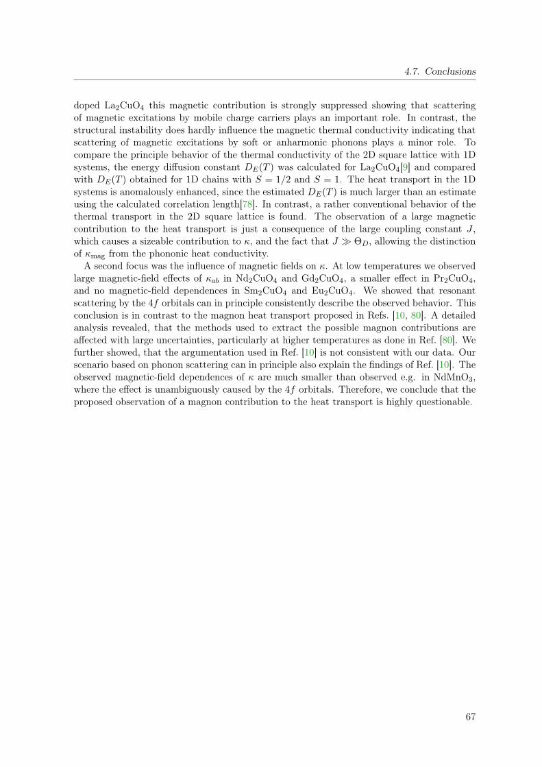
4.7. Conclusions

doped La2CuO4 this magnetic contribution is strongly suppressed showing that scatteringof magnetic excitations by mobile charge carriers plays an important role. In contrast, thestructural instability does hardly influence the magnetic thermal conductivity indicating thatscattering of magnetic excitations by soft or anharmonic phonons plays a minor role. Tocompare the principle behavior of the thermal conductivity of the 2D square lattice with 1Dsystems, the energy diffusion constant DE(T ) was calculated for La2CuO4[9] and comparedwith DE(T ) obtained for 1D chains with S = 1/2 and S = 1. The heat transport in the 1Dsystems is anomalously enhanced, since the estimated DE(T ) is much larger than an estimateusing the calculated correlation length[78]. In contrast, a rather conventional behavior of thethermal transport in the 2D square lattice is found. The observation of a large magneticcontribution to the heat transport is just a consequence of the large coupling constant J ,which causes a sizeable contribution to κ, and the fact that J ΘD, allowing the distinctionof κmag from the phononic heat conductivity.

A second focus was the influence of magnetic fields on κ. At low temperatures we observedlarge magnetic-field effects of κab in Nd2CuO4 and Gd2CuO4, a smaller effect in Pr2CuO4,and no magnetic-field dependences in Sm2CuO4 and Eu2CuO4. We showed that resonantscattering by the 4f orbitals can in principle consistently describe the observed behavior. Thisconclusion is in contrast to the magnon heat transport proposed in Refs. [10, 80]. A detailedanalysis revealed, that the methods used to extract the possible magnon contributions areaffected with large uncertainties, particularly at higher temperatures as done in Ref. [80]. Wefurther showed, that the argumentation used in Ref. [10] is not consistent with our data. Ourscenario based on phonon scattering can in principle also explain the findings of Ref. [10]. Theobserved magnetic-field dependences of κ are much smaller than observed e.g. in NdMnO3,where the effect is unambiguously caused by the 4f orbitals. Therefore, we conclude that theproposed observation of a magnon contribution to the heat transport is highly questionable.

67


68

5. Thermal Conductivity in CubicCobaltates

Among transition-metal oxides cobalt compounds are of particular interest due to the possi-bility of the Co ions to occur in different spin states. LaCoO3 is one of the most prominentexamples, which is in the focus of researchers since several decades [175, 176], and still the na-ture of the spin-state transition is to be clarified. The spin-state transition is visible in variousquantities, like e.g. susceptibility, thermal expansion and specific heat. Recently, it was foundthat the low-temperature thermal conductivity of LaCoO3 is also very unusual [9, 33, 57],which was also attributed to the spin-state transition. However, the mechanism responsi-ble for the observed unusual thermal conductivity is not clear. In this chapter a detailedinvestigation of the thermal conductivity in LaCoO3, PrCoO3, NdCoO3, and EuCoO3 willbe presented. The aim is to develop a consistent picture of the influence of the spin-statetransition on the thermal conductivity. The measurements of κ in PrCoO3 and NdCoO3 wereperformed by H. Anapa [177]. Some of the thermal conductivity data have been already shownin Refs. [33, 57, 166].

5.1. The Spin-state Transition in RCoO3 with R = La, Pr, Nd,and Eu

R3+ Co3+ O2-

Figure 5.1.: Structure of RCoO3 in the cubicnotation. The Co3+ is surrounded by an oxygenoctahedron.

The RCoO3 compounds with R = La, Pr, Nd, and Eu crystallize in a AMO3-type perovskitestructure, see Fig. 5.1. LaCoO3 is slightly rhomboedrally distorted, which is often referredto as pseudo cubic. For the smaller rare-earth ions the type of the distortion changes, andan orthorhombic structure is realized [178–181]. Rare earth ionic radii, lattice constantsand volumes of the unit cells (in cubic notation) with the respective references are listed inTab. 5.2. Resistivity measurements show that all RCoO3 compounds are insulating belowroom temperature [177, 182]. For all RCoO3 the Co3+ ion has a 3d6 configuration, whichis five-fold degenerate for a free ion. In the cubic crystal field these five levels split into

69

5. Thermal Conductivity in Cubic Cobaltates

3d6

t2g (dxy,dyz,dxz)

∆CF

eg (d3z2-r2, dx2-y2)∆JT

LS (S=0) HS (S=2)IS (S=1)

strongly weaklyJahn-Teller active

Figure 5.2.: Splitting of the 3d orbitals in a cubic crystal field and possible spin states for a3d6 configuration. Both, the eg and the t2g levels can be Jahn-Teller active.

the three-fold degenerate t2g and the two-fold degenerate eg level, where the level spacingdenotes ∆cf (see Fig. 5.2) [183]. The eg levels consist of the dx2−y2 and d3z2−r2 orbitals, whichdirectly point to the surrounding oxygen ions. The dxy, dxz, and dyz orbitals of the t2g levelspoint inbetween the oxygen orbitals, yielding a lower energy for the t2g and a higher energyfor the eg levels. The second important energy scale is the Hunds rule energy JH [16]. IfJH is the dominant energy scale (JH ∆cf), the six electrons of the Co3+ ion will haveparallel spin according to Hunds first rule [16], what leads to the high-spin (HS) state withS = 2, see Fig. 5.2. In the other case, JH ∆cf , the crystal field energy will not allow thatelectrons occupy the eg orbitals. Therefore the low-spin (LS) state (S = 0) with 6 electronsin the t2g levels is realized [183]. In recent years several authors proposed another possiblelow-lying spin-state, the so-called intermediate (IS) spin-state with S = 1 [184–201]. InLaCoO3 the unusual situation is realized, that JH and ∆cf are so close that temperature caninduce transitions between different spin states [176]. Fig. 5.3 shows the Co3+ susceptibility ofLaCoO3 and EuCoO3 [202].1 For LaCoO3, at low temperatures, the system is nonmagnetic,and the LS state is realized. The sudden increase of χ for temperatures above ≈ 25K is dueto the thermally driven spin-state transition, where spin states with a magnetic moment getpopulated. The question, if this spin state is an IS or a HS state, has been widely discussedin the literature, and is still under debate [184–201, 203, 204]. The LS-IS state scenariogives a better description of the thermodynamic properties in an analysis based on a two-levelsystem [12, 205]. This analysis works well with a g factor of ≈ 2.3, which is much smaller thanthe g factor recently measured by ESR measurements, g = 3.5. Such a high g factor does notallow a description of the susceptibility in a simple LS-IS or LS-HS model, since the calculatedsusceptibility is much too high. For the description of other thermodynamic properties, likethermal expansion or specific heat, the g factor plays no role. As pointed out in Refs. [13, 204],a way out is the introduction of a spin-orbit coupled HS state (SOcHS). The idea hereby isthat the usual assumption of a quenched orbital moment [16] is not valid, and then theS = 2 HS state couples with a l = 1 orbital moment to an effective moment J = 1 [205].However, the description of the susceptibility only works if a temperature-dependent gap isintroduced [178, 205], see Sec. 5.3.2. None of these models gives an unambiguous picture ofthe spin-state transition in LaCoO3. The newest results [13] prefer a SOcHS scenario. Sincethe IS model gives the best thermodynamic description with a fixed gap (but with the wrong

1The other contributions to the susceptibility are subtracted, this procedure will be discussed in Sec. 5.3.

70

5.1. The Spin-state Transition in RCoO3 with R = La, Pr, Nd, and Eu

0 200 400 600 8000

1

2

3

4

Co3+

(10-3

em

u / m

ol)

T (K)

LaCoO3

EuCoO3

Figure 5.3.: Co3+ susceptibilityof LaCoO3 and EuCoO3. Back-ground contributions have beensubtracted (see Fig. 5.4). [202]

g factor), we will perform the data analysis using both, the IS model with ∆Co = 185 K,ν = 1 and the SOcHS model2. The energy gaps are taken from the susceptibility and thermalexpansion fits of Ref. [205]. The aim hereby is to keep as many parameters as possible fixed.The spin-orbit coupled HS model will also be analyzed, herefore the temperature-dependentenergy gap will be calculated in Sec. 5.3.2.

If La is replaced by the smaller Eu, the LS state is stabilized, which causes a shift ofthe spin-state transition to much higher temperatures, as seen in the susceptibility data forEuCoO3 (Fig. 5.3). A detailed investigation of the evolution of the spin-state transition ofLa1-xEuxCoO3 crystals with 0 ≤ x ≤ 1 can be found in Refs. [178, 206]. However, thesemixed crystals have several disadvantages, in particular in terms of thermal conductivitymeasurements [177]3. This motivated the growth and investigation of RCoO3 single crystalswith R= Pr and Nd [205, 207]. In these compounds the spin gap lies inbetween those ofLaCoO3 and EuCoO3 [205]. For the data analysis of the rare-earth compounds, the IS modelwill be used with the parameters derived from thermal expansion and susceptibility [205].

5.1.1. Jahn-Teller Effect

The Jahn-Teller effect causes a spontaneous distortion of the crystal symmetry, when theenergy gain through lifting the degeneracy of an energy level is bigger than the elastic energywhich is needed to distort the crystal [208]. The eg orbitals split into two singlets, while thecenter of mass remains unchanged (see Fig. 5.2). It follows that for a high-spin state no Jahn-Teller effect is possible for the eg orbital, since the energy gain and loss of the two electronsin the eg orbital exactly cancel each other. The t2g orbital splits into a doublet with the lowerenergy and a singlet. Here, the energy gain is less than for the eg orbital, and the Jahn-Tellereffect is less effective.

As long as the octahedral distortions fluctuate, one speaks of a dynamical Jahn-Teller effect.The other possibility is that the distorted octahedra form a long-range ordered state, whichis called the collective Jahn-Teller effect. The possible influence of the Jahn-Teller effect inLaCoO3 is discussed in Refs. [9, 12, 197, 201, 209–212].

2ν describes an additional orbital degeneracy, see Refs. [12, 205, 206].3The mixed compounds are only available as polycrystals. Moreover, the additional effect of the disorder on

the R site suppresses κ.

71


A[mm2] L[mm]

LaCoO3 Zo104 0.8× 1.5 3.7LaCoO3 Mar5b_07 0.8× 1.4 2.6LaCoO3 Mar5a_08 1.4× 0.8 3.4LaCoO3 Mar5_09 1.1× 0.8 2.3LaCoO3 EKParis 2.3∗ 4.7PrCoO3 1.0× 3.8 2.5NdCoO3 1.7× 2.0 2.8EuCoO3 0.3× 0.9 2

Table 5.1.: Sample sizes of the investigated RCoO3 samples. *) The EKParis crystal has ahalf-moon shaped cross section.

5.2. Samples

All investigated RCoO3 samples are single crystals grown in a floating-zone furnace. Themeasurements of the thermal conductivity of LaCoO3 were performed on five different singlecrystals. The crystal Zo104 was grown by C. Zobel [33] and was used for several investigations,e.g. thermal expansion, susceptibility, and specific heat measurements. [12, 178, 205, 213]The crystal labeled EKParis was grown by G. Dhalenne (Université Paris Sud). The otherthree samples were grown by M. Reuther [214], and are labeled as Mar5a_8, Mar5b_07,and Mar5_09. The EuCoO3 crystal (AR11) was grown by A. Reichl [179], and the PrCoO3(MB15) and NdCoO3 (MB16) crystals by M. Benomar [207].

All measurements have been performed along arbitrary directions. The LaCoO3 crystalsare heavily twinned, so no pronounced direction dependence is expected. The twinning in therare-earth cobaltates was not investigated. Because of the larger anisotropy twinning may beless important.

5.3. Susceptibility Analysis

Fig. 5.4a shows the measured susceptibilities of RCoO3 with R = La, Pr, Nd, and Eu. ForLaCoO3 the measured susceptibility contains the background contributions

χbg = χCW + χvV + χdia, (5.1)

where the first part χCW is a paramagnetic impurity contribution, and the latter consists ofa temperature independent van Vleck contribution χvV of the Co3+ ions and the diamagneticsusceptibility of closed shells χdia. The paramagnetic low-temperature contribution is com-paratively large, which is possibly related to the occurrence of so-called HS polarons [215], aswill be discussed later. In EuCoO3 the van Vleck contribution of the Eu3+ ions becomes largeand temperature dependent [216], what has to be taken into account in Eq. 5.1. Replacing Laby a rare-earth ion, whose ionic radius lies inbetween those of La and Eu, leads to a spin gapinbetween those of LaCoO3 and EuCoO3. Complications arise from the 4f magnetism, whichdominates the measured susceptibility in NdCoO3 and PrCoO3 (see Fig. 5.4). However, aseparation was successfully done in Ref. [205]. The lower panel shows the Co3+ susceptibility,and as expected the onset temperature of the spin-state transition for R = Pr and Nd lies

72


R ∆ISCo(χ) ∆IS

Co(α) ν acubic Vuc rR C(K) (K) (K) (Å) (Å3) (Å)

(emuKmole

)La 185 180 1 3.825 [200] 55.98 [200] 1.160 0.033 [178]Pr 1100 1200 3 3.788 [45] 54.38 [45] 1.126 0.018Nd 1400 1750 3 3.775 [52] 53.78 [52] 1.109Eu 1900 3 3.750 [178, 179] 52.75 [178, 179] 1.066 0.003 [178]

Table 5.2.: Co3+ spin gap ∆Co as derived from susceptibility and thermal expansion inRef. [205] (with degeneracy ν used for the analysis), cubic lattice constant a, cubic unit cell vol-ume Vuc, ionic radii (from Ref. [54]), and Curie constants of the paramagnetic low-temperaturecontribution (see text).

inbetween those for R = La and Eu. The analysis of the susceptibility was done in Ref. [205]based on a two-level system which gives the relation

χCo =NAµ2

Bg2

3kBT· S(S + 1) · ν(2S + 1) · exp(−∆/T )

1 + ν(2S + 1) · exp(−∆/T ). (5.2)

The model dependent parameters are the g factor, the spin S (S = 1 for IS and S = 2 forHS), the spin gap ∆, and an additional orbital degeneracy ν, which can be 1 or 3. For theLS-IS and LS-HS model the values are listed in Tab. 5.2. Except for LaCoO3 only the LS-ISmodel with ν = 1 has been considered (see Ref. [205]). Note that for a SOcHS model, theformula is the same, if one replaces S by J and sets ν = 1.

5.3.1. CF Analysis of the Susceptibility of PrCoO3 and NdCoO3

In principle the susceptibility of the R3+ ions in PrCoO3 and NdCoO3 can be calculatedif the CF parameters are known. No CF investigations are available for these compounds,but as shown in Sec. 2.4 the CF is expected to be very similar in PrNiO3 and NdGaO3.Fig. 5.5 shows the calculated4 inverse susceptibilities and magnetization curves for PrCoO3and NdCoO3 using the CF parameters from Refs. [44, 47]. The general temperature andfield dependences of the R3+ moments are well described by the calculations. In PrCoO3,the calculated susceptibility is anisotropic (panel a). The best agreement between data andcalculation is given for the b direction. The deviations at low temperatures are due to theparamagnetic impurities, and at high temperatures due to the Co3+ susceptibility. Note, thatthe slopes of the different χ−1 curves are nearly identical. This shows that the fit used inRef. [205] to determine the Co3+ susceptibility is a good approximation. Fig. 5.5b showsmagnetization curves a 1.8K. Again, a large anisotropy and a good agreement of the datato the calculated curve for H ‖ b is observed. Fig. 5.5c and d show the results for NdCoO3,with basically the same conclusions. Here, the best agreement is given for the calculation withH ‖ a.

5.3.2. Spin-State Transition with variable Energy Gap

By using the measured g factor of g ≈ 3.5 [204] in Eq. 5.2, the description of the susceptibilitygets worse. A possible way out is the introduction of an effective interaction between the

4The directions are given in the Pbmn notation (see Chp. 7).

73


0

2

4

6

0

1

2

Eu

La

Pr

R = Nd

RCoO3

(1

0-2 e

mu

/ mol

)

a)

0 100 200 300 400 500 6000

1

2

3

4

T (K)

Nd

C

o (10-3

em

u / m

ol)

c)R = La

PrEu

EuCoO3

(1

0-3 e

mu

/ mol

)

LaCoO3

Ug =

0 + C/(T- ) + Eu

vVb)

Figure 5.4.: a) Measured susceptibility for RCoO3 with R=La, Pr, Nd, and Eu. For PrCoO3and NdCoO3 the 4f contribution is dominant. b) Estimation of the background contributionto χ. For EuCoO3 a large Eu van Vleck contribution is present. c) Co3+ contributions tothe susceptibility. The spin-state transition shifts successively to higher temperatures withdecreasing rare earth size. [202, 217]

Co3+ sites, what can be described by a temperature-dependent energy gap [178, 205]. Theunderlying idea is that the population of an excited state hinders the surrounding Co3+ ionsto get excited, what effectively increases the spin gap ∆Co. The temperature-dependent gapcan be calculated by reverting Eq. 5.2, what leads to

∆Co(T ) = T ln(

NAg2µ2BS(S + 1)

3kBT

ν(2S + 1)χCo(T )

− ν(2S + 1))

. (5.3)

Setting J = ν = 1, the temperature-dependent gap shown in Fig. 5.6a is calculated. Notethat the gap should get temperature independent at low temperatures, when the distancebetween excited sites gets large. However, here the gap cannot be determined exactly becauseof the uncertainty of the background contribution below ≈ 25K. This model is supportedby recent experimental results based on soft x-ray absorption spectroscopy and magneticcircular dichroism, where an energy dependent gap with the same temperature dependence isobtained [13]. In Ref. [205] a combined analysis of the susceptibility and thermal expansion

74


0

1

2

3

0 200 4000

1

2

30

4

8

0 4 8 120

1

Data Calculationc b

a

(102 m

ole/

emu)

PrCoO3

a)

1T

SST

SST

1T

c

b

c)

NdCoO3

(102 m

ole/

emu)

T (K)

a

1.8 Kc

b

a

b)

PrCoO3

M (

B/f.

u.)

6K

a

bc

d)

NdCoO3

M (

B/f.

u.)

H (T)

Figure 5.5.: Calculated susceptibilities and magnetization with different field directions usingthe CF parameters of PrNiO3 and NdGaO3 [44, 47] in comparison to the data of PrCoO3 andNdCoO3. The arrows labeled SST show where the Co3+ susceptibility starts to contribute dueto the spin-state transition.

was performed with the LS-IS model. Using the same Ansatz the formula

αCo =3d exp

(∆(T )

T

) (∆(T )− T ∂∆(T )

∂T

)(3 + exp

(∆(T )

T

))2T 2

(5.4)

is obtained for the additional thermal expansion, if the energy gap is temperature dependent.Using the values of ∆(T ) from Fig. 5.6, the thermal expansion can be calculated. The resultis shown in Fig. 5.6b , and is in good agreement with the measured thermal expansion. Thevalue d = 1.8% is obtained. By scaling the thermal expansion and the susceptibility curveswith the scaling procedure from Ref. [205], a scaling factor of 170 emuK/mole is obtained,which is in good agreement with the experimental observation of 180 emuK/mole [205].

5.3.3. Impurity Contribution in LaCoO3

In this section a detailed analysis of the paramagnetic impurity contribution to the susceptibil-ity will be given, with the purpose to analyze the influence of these impurities to the thermalconductivity. Therefore the magnetization measurements were performed on the identicalsamples which were used for the thermal conductivity measurements.

The paramagnetic impurity content can be determined either by temperature-dependentsusceptibility measurements or from the magnetic-field dependent magnetization at low tem-

75


0 100 200 3000

200

400

600

0 50 1000

10

20

30

40

(T

)

T (K)

LaCoO3

132 K+1.65*T

calc

meas

cal

(1

0-6/K

)

T (K)

Figure 5.6.: a) Temperature-dependent energy gap ∆Co forLaCoO3 (symbols) as calculatedfrom the magnetic susceptibilitywith g = 3.5 and an excitedtriplet state, see text. The solidline is a linear fit. b) Anomalousthermal expansion caused by thespin-state transition from [205],and calculation with Eq. 5.4 us-ing ∆(T ).

0 100 200 3000

2

4

6

8

10

0 250

5

Zo104Mar5_a8Mar5_b07Mar5_09EKParis

(10-3

emu/mole)

T (K)

LaCoO3

(10 -

3emu/mole)

Figure 5.7.: Temperature-dependentmagnetic susceptibility measured in afield of 1 T. The low-temperatureparamagnetic impurity contribution isstrongly sample dependent. [218]

peratures. The magnetization measurements were carried out by H. Hartmann [218] at afixed temperature of 3K in a vibrating sample magnetometer (VSM). Because the popula-tion of the IS/HS state is negligible at this temperature, the magnetization contains only twocontributions:

M(H) = Mpara(H) + M0(H), (5.5)

where Mpara is the paramagnetic impurity contribution, and M0(H) is the background. M0(H)consists of the diamagnetic contribution of the core electrons and the paramagnetic van Vlecksusceptibility of the Co3+ electrons,and gives a simple linear contribution M0(H) = χ0 ∗H.The paramagnetic part Mpara(H) is usually described by

Mpara(H) = NgJµBBJ(x) with x = gJµBH/kBT (5.6)

and the so-called Brillouin function BJ(x) [16]. Here, N denotes the number of the paramag-netic moments with spin J . Fig. 5.8 shows the magnetization curves at 3K for the sampleZo104. The linear part of M(H) is obtained by a fit for H > 12T, and the subtraction yieldsthe curves for the paramagnetic contribution in Fig. 5.8 (dashed line). The calculation ofM(H) with Eq. 5.6 does reproduce the field dependence only qualitatively. If the fit range isrestricted to low fields (H ≤ 0.1T), a value J = 5 is obtained (with g = 2). This fit leads toa good description of the initial slope of M(H). The two fit parameters of the linear fit givethe values of Msat and χ0 listed in Tab. 5.3. The paramagnetic part of the susceptibility from

76


0 4 8 120

1

2

3

Mmeas(H)

Mpara(H)

M

(10-2

B/f.u.)

H (T)

LaCoO3 Zo104

Mcalc(H)

Figure 5.8.: Magnetization curve forLaCoO3 at 3 K. The contribution ofthe paramagnetic impurities is estimatedby subtracting a linear contribution esti-mated by a high-field fit (see text). Thecalculated Brillouin function does not de-scribe the data very well. The verti-cal line indicates the field of 1 T, whichwas used for the temperature-dependentmeasurements.

0 4 8 120

1

2

MPa

ra (1

0-2B/f.u.)

Mar5_09

Mar5b_07

H (T)

LaCoO3

Zo104

Mar5a_08 Figure 5.9.: Paramagnetic contributionto the magnetization M(H) of LaCoO3at 3 K for different samples. The lin-ear contribution to M(H) has been esti-mated by high field fits, and subtractedfrom the data.

the temperature-dependent measurements can be determined by fitting the low-temperaturerange by5

χ(T ) = χ0 + C/(T −Θ). (5.7)

The estimation of C from the temperature-dependent susceptibility requires measurements atthe low-field limes, since the paramagnetic impurity part is suppressed in higher fields. χ(T )was measured for all samples in a magnetic field of 1T (see Fig. 5.7). The magnetizationmeasurements (Fig. 5.8) show that M(H) is beyond the linear behavior at 1T. However, forlarge x the Brillouin function BJ(x) goes to 1 and Eq. 5.6 can be replaced by

M(µBH kBT ) = NgJµB. (5.8)

It follows that the saturation magnetization is proportional to N and can therefore be usedas a measure of the impurity content.

A magnetization measurement is not available for the EKParis sample. For this sampleM sat

imp was estimated from the temperature-dependent susceptibility, which was measured in afield of 1T in all samples. Herefore the fact is used, that the shape of all magnetization curvesis almost identical in all samples. It follows that the magnetization at 1T determined fromthe temperature-dependent measurement can be extrapolated to the saturation magnetizationvia

M satimp = [χ(3K, 1T)− χ0] ·M(14T)/M(1T). (5.9)

5A more reliable estimation of C can be achieved by determining χ0 from the high-field slope of M(T ).

77


Specimen χ(3K) Msatimp χ0 M14 T

para/M1 Tpara Msat

imp ∆Msatimp

10−3( emumole

) (10−3 µBf.u.

) (10−4 emumole

) (10−3 µBf.u.)

10−3 µBf.u.)

Zo104 7.6 22.3 2.6 1.7 21.7 0.6Mar5b_07 2.5 6.5 1.7 1.62 6.6 0.1Mar5a_08 3.9 9.8 4.1 1.51 10.9 1.1Mar5_09 1.7 4.8 1.9 1.85 4.4 0.4EKParis 1.5 3.6

Table 5.3.: Parameters for the estimation of the impurity contribution for the different LaCoO3samples, see text.

Here, M(14T)/M(1T) = 1.7 and χ0 = 2.6 · 10−4emu/mole are averaged over the four samples,where magnetization measurements were available. The application of Eq. 5.9 to these foursamples yields values which only slightly deviate from the measured M sat

imp (see Tab. 5.3). Thisensures, that a confident value of M sat

imp is obtained for the sample EKParis with Eq. 5.9.In Ref. [215] the authors investigated the influence of so-called high-spin polarons with S =

10 . . . 16 for slightly Sr-doped La1-xSrxCoO3 crystals (x ≤ 0.01). This analysis is performed bythe use of Eq. 5.6. The idea is that the divalent Sr2+ ions nominally cause the same amountof Co4+ ions, and that these magnetic ions induce a spin-state transition of the neighboringCo3+ ions from LS to IS or HS states. These sites then couple to a high-spin polaron withS = 10 . . . 16. The samples investigated here were Sr free, however, if the samples containadditional oxygen, the same effect may be achieved. An indication herefore is that the valueof J obtained by the Brillouin fits ranges from J = 5 . . . 9.5, if the criteria is to fit the initialslope of the M(T ) curves. This is consistent with Ref. [215], because J decreases for a smallerSr content, and the amount of additional oxygen is presumably very small. The questionremains, why the measured magnetization deviates from a Brillouin function. A possibleexplanation is another kind of magnetic defects contributing significantly to M(H). Moreover,interactions between the magnetic moments can explain such a behavior. In the next chapterthe thermopower of the LaCoO3 crystals will be investigated. The sign of the thermopowergives an information about the sign of the dominant charge carriers. Interestingly, only twoof the samples show a positive thermopower at room temperature, Mar5b_07 and Mar5_09.These are the samples, which have the smallest values of P sat

imp.The concept of magnetic polarons explains the considerably high paramagnetic contribution

to M(H) in LaCoO3. The induction of surrounding ions into the HS/IS state gets less favor-able, if the spin gap is increased. As a consequence, the paramagnetic contribution shouldweaken with increasing energy gap. Therefore we expect a successively decreasing Curie con-stant for RCoO3 with R = Pr, Nd, and Eu. In EuCoO3 the Curie constant is indeed about anorder of magnitude smaller, than in LaCoO3. For R = Pr the estimation of the paramagneticcontribution is shown in Fig. 5.10a. Because of the non-magnetic ground state of the Pr3+ ion(see Sec. 5.3.1), a Curie fit with Eq. 5.7 is possible. χ0 is the temperature independent sum ofthe van Vleck contributions of Co3+ and Pr3+. The fit yields the values χ0 = 0.017 emu/mole,Θ = −0.73K and Cimp = 0.015 emu/moleK. The pure PrCoO3 susceptibility obtained by sub-tracting the impurity contribution is shown as solid line. The inset shows the magnetization ofPrCoO3 at 1.8K. Here, the impurity contribution is estimated as in LaCoO3 by subtractinga high-field linear fit, and analyzing the residual magnetization by Eq. 5.6. The resultingimpurity magnetization is much smaller than the magnetization of the Pr3+ ions (note the

78

5.4. Results

0 100 200 300

1

2

0 4 8 120

1

2

0 4 8 120.0

0.5

1.0

1.5

0

2

4

6

(1

0-2em

u/mole)

T (K)

PrCoO3

(T)

(T)-C/(T- )

a)H=50mT

Mimp

(H)

Mim

p(10-2

B/f.u.)

H (T)

n=0.02 g=2.37 T=1.8 K

b)

(B/f.u.)

H (T)

1.8K, 3K, 4K, 6K, 10K, 20K, 40K

NdCoO3

M(10-1

B/f.u.)

M(H)

Figure 5.10.: a) Susceptibility of PrCoO3 and calculated Pr3+ contribution by subtraction ofthe low-temperature Curie term caused by paramagnetic impurities. Inset: Magnetization at1.8 K and extracted impurity contribution. Note the different scales. b) Low-temperature mag-netization measurements of NdCoO3 at various temperatures. Lines are calculated accordingto Eq. 5.6 taking into account a linear van Vleck contribution.

different scales). The best fit using J = 0.5 for a two-level impurity system yields the valuesnimp = 0.02 and gimp = 2.37. The resulting C = 0.019 emu/moleK is in good agreement withthe result from the analysis of the temperature dependent measurement. The value of C liesinbetween those of LaCoO3 and EuCoO3, which shows indeed the correlation between spingap and paramagnetic impurities.

For R = Nd, Fig. 5.10b, the ground state of the Nd3+ ion is a Kramer’s doublet (seeSec. 5.3.1). The magnetization at low temperatures is determined by the Nd contribution,consistent of a Brillouin and a van Vleck term. The magnetization curves have been fitted6 byEq. 5.6 and an additional term MvV

Nd = 1.5 · 10−6H µB/f.u., estimated from a high-field fit at1.8K. The other values used are J = 0.5, nNd = 1 and the gNd factor is the only adjustable pa-rameter. The resulting g factor is almost constant between 1.8K and 40K, (2.12 ≤ g ≤ 2.19),yielding an average value g = 2.15. Note that the absolute values of the magnetization is muchlarger than the impurity contributions determined for the other compounds. A determinationof the impurity Curie constant C is therefore not possible for NdCoO3.

5.4. Results

5.4.1. LaCoO3

In Fig. 5.11 the thermal conductivity of LaCoO3 is shown (sample Zo104). [57] At first glanceκ seems to be consistent with usual phononic heat transport (see Sec. 2). However, a closerinspection of the data reveals several anomalous features. The thermal conductivity aboveabout 100 K is anomalously small and its temperature dependence is very unusual, since above150 K the thermal conductivity slightly increases with increasing temperature. The smallabsolute values cannot be attributed to strong defect scattering, since conventional defectscattering does not vanish below 100 K so that κ would not increase and show a maximum

6The deviations at low temperatures are likely to be caused by fluctuations of the Nd ordering, which occursat 1.2 K [219].

79


Specimen Tmax κmax κ(300K) S(300K)(K) (W/Km) (W/Km) µV/K

Zo104 28 10 2.2 −700Mar5b_07 28 20 3.5 1000Mar5a_08 32 8 4.4 −600Mar5_09 25 34 3.3 1000EKParis 29 27 4.4 −300PrCoO3 26 26 3.0 −400NdCoO3 23 53 4.8 −400EuCoO3 19 266 8.1 −500

Table 5.4.: RCoO3: Low-temperature maxima and room-temperature values of thermal con-ductivity κ and thermopower S.

below 100 K. Therefore, the small κ and its unusual temperature dependence indicate thatan unusual, additional scattering mechanism is active above about 25K. It is, in principle,possible that low-lying optical phonons cause resonant scattering of acoustic phonons andtherefore suppress the heat current in a certain temperature range. A softening of opticalphonon branches has been observed in Ref. [220]. However, in LaAlO3, having the samestructure, has a conventional thermal conductivity [22]. T it is unlikely that the unusualthermal conductivity is an intrinsic feature of the phonon modes of LaCoO3.

Another source of additional phonon scattering could be the spin-state transition. The ideais that the thermal population of the excited spin state causes additional disorder due to therandom distribution of the populated sites. To motivate this picture, the Co3+ susceptibility ofLaCoO3 is plotted in Fig. 5.11 (right scale). The temperature-dependent spin-state transitionimplies an increasing lattice disorder above 25 K, and therefore an additional suppression ofthe thermal conductivity. The disorder and thus the suppression of κ is most pronounced foran equal number of LS and IS (HS) ions. For an energy gap ∆ ' 185K between the LS andIS/HS states an equal occupation of LS and IS ions is expected around T ' 165K. Thereforethe strong reduction of κ above 25K, its small absolute values and the weak minimum around150 K can arise from temperature-induced LS-IS/HS disorder.

If a magnetic field of 14T is applied, the thermal conductivity is significantly changed below50K. That is not expected for a conventional phononic heat transport, since phonons are notexpected to be field dependent. Furthermore, the energy gap ∆Co is too large to be affectedby a magnetic field in a significant way. Moreover, the field dependence remains below 5K,where practically all Co3+ sites are in the LS state. This suggests that another scatteringmechanism is present at low temperatures, which is magnetic-field dependent.

5.4.2. RCoO3 with R = La, Pr, Nd, and Eu

As shown in Sec. 5.1, the spin-state transition shifts to higher temperature if La is replacedby smaller R ions. This should have an influence on the thermal conductivity, if the picturedepicted above is valid. Fig. 5.12 shows the thermal conductivity in zero field for RCoO3with R = La, Pr, Nd, and Eu. [57, 221]. First, the compound with the smallest ion Eu will

80

5.4. Results

0 20 400

5

10

0 100 200 3000

2

4

6

8

10

(W

/Km

)

T (K)

LaCoO3 Zo104

Co

0 100 200 3000

2

4

6

8

10

C

o (10-3

emu/

mole)

T (K)

T(K)

(W

/Km

)

14T

0T

Figure 5.11.: Left scale:Thermal conductivity ofLaCoO3. Right scale: Co3+

susceptibility of LaCoO3.Inset: Thermal conductiv-ity of LaCoO3 for T < 50 Kin magnetic fields of 0 T and14 T.

be discussed. In contrast to LaCoO3, the thermal conductivity shows comparatively largeabsolute values, and a general temperature dependence as expected for a purely phononicheat conductor. This is confirmed by a Debye fit according to Eq. 2.5. The fit parametersare listed in Tab. 5.5. The low-temperature maximum reaches a value of 250W/Km at 18K,which is about an order of magnitude larger than for LaCoO3. In NdCoO3, κ is lowered in thewhole temperature range in comparison to EuCoO3, but still consistent with a conventionalphononic picture. At the onset temperature of the spin-state transition (see Fig. 5.4) a slightchange of the curvature to a steeper slope is visible. In contrast to NdCoO3, PrCoO3 shows anunusual temperature dependence of κ, which reminds of κ of LaCoO3. The low-temperaturepeak decreases very strongly with increasing temperature. Between 50K and 200K, κ ismore or less temperature independent with a low absolute value κ ≈ 3.5W/Km. Becausethe Co3+ spin gap is too large to account for this anomaly, another explanation is neededfor this behavior. As will be discussed in detail in Sec. 5.4.10, multiplet transitions of the 4forbitals can cause the additional scattering. Above 200K, κ starts to decrease again, with acomparatively sudden slope change. According to the susceptibility measurements (Fig. 5.4)this is the temperature range where the higher spin state becomes excited. This is a furtherhint that the same scattering mechanism is present here, which suppresses κ in LaCoO3 above25K.

Comparing all curves, it is clearly seen that the thermal conductivity is monotonouslysuppressed with increasing rare earth size in the whole temperature range (not taking intoaccount the additional effect for R=Pr). This systematic trend at low temperatures cannotdirectly be attributed to the additional disorder scattering caused by the spin-state transition,because here the population of the excited spin states is negligible. If the suppression of κdue to the spin-state transition would be the only difference between LaCoO3 and EuCoO3,one would expect that the thermal conductivity should not be affected below ≈ 25K. Thiscontradicts the experimental observation. In principle, this finding could arise from a differentsample quality. However, there is no indication for an significantly better crystal quality inEuCoO3 than in LaCoO3. Furthermore, the low-temperature behavior of LaCoO3 is unusual.This is confirmed by the shown Debye fit, which is obtained by keeping all parameters fixed atthe values obtained for EuCoO3, and adjusting the factor P for the point defect scattering toobtain the height of the low-temperature maximum. This gives a hint that usual point defect

81


10 1001

10

100

R=La Zo 104

R=Pr

R=Nd

(W

/Km

)

T (K)

RCoO3R=Eu

"Fit"

Figure 5.12.: Thermal con-ductivity of RCoO3 withR = La, Pr, Nd, and Eu. ForEuCoO3 a Debye fit is shown(solid line). For LaCoO3a Debye fit is shown withthe same parameters, but alarger point-defect scatteringrate P .

scattering is not the only source of the strong suppression of the low-temperature thermalconductivity, since P is the only adjustable parameter which is effective in this temperatureregion.7

5.4.3. RCoO3: Comparison to the Literature

To my knowledge, only Yan et al. have published low-temperature thermal conductivity dataof undoped RCoO3 compounds with R = La, Pr, and Nd [9]. These results are shown inFig. 5.13. Above ≈ 50K these data show the same qualitative and quantitative behavior likeour samples. The broad minima for R = La and Pr are present, showing that these are intrinsicfeatures of the compounds. Differences occur in the heights of the low-temperature maxima,ranging from only 10% for R = Pr up to a factor of 2 for R = Nd and of 5 for LaCoO3. Suchdifferences generally reflect different sample qualities. It follows that the height of the low-temperature peak does not follow such a systematic behavior like in our samples. However,above 100K there is the same monotonous decrease of κ with the ionic size of the rare earth.Furthermore, all absolute values are well below the data from our EuCoO3 crystal.

In Ref. [222, 223] the thermal conductivity of LaCoO3 was investigated above room temper-ature. Here, the interpretation becomes even more difficult. The Debye approximation is nolonger valid, and electronic scattering mechanisms and electronic contributions get relevant.Furthermore, additional effects like excitonic or radiative heat transport may play a role [223].

5.4.4. LaCoO3: Low Temperatures

In this section we present a detailed study of the zero-field thermal conductivity of LaCoO3for five crystals. Furthermore the influence of magnetic fields up to 14T (in some cases 16T)was investigated for all samples. The motivation was to study the unusual low-temperature-and field dependence of κ. In particular, the detailed analysis of the magnetic susceptibilityallows to correlate the influence of the sample-dependent content of paramagnetic impuritiesto κ. For the samples Zo104 and MAR5b_07 the measurement range was extended down to≈ 300mK with the new setup for the Heliox 3He insert (see Sec. 3.2.2).

7It is possible to get a much better fit by using a very small value of L for the sample size, L ≈ 1 · 10−5 [57].

82

5.4. Results

0 100 200 3000

10

20

30

40

50

LaCoO3

PrCoO3

NdCoO3

(W

/Km

)

T (K)

Figure 5.13.: Thermal conductivitydata for LaCoO3, PrCoO3, and NdCoO3taken from Ref. [9].

In order to analyze the whole temperature range, these data are plotted together with themeasurements performed in the conventional setup. In Fig. 5.14a the results for the sampleZo104 are shown.8 In zero field, the temperature dependence follows a T 2 dependence below≈ 10K. In a magnetic field of 14T the thermal conductivity is strongly enhanced below≈ 20K up to almost a factor of 3 at ≈ 2.5K. By further lowering the temperature, the fielddependence becomes smaller and vanishes around 600mK. In field, the slope of κ shows a T 3

behavior below 1K. However, the temperature window is too small to unambiguously confirma power-law behavior. In Fig. 5.14b the data for crystal Mar5b_07 are shown. The moststriking feature is the occurrence of a pronounced dip in zero field around 2K, which contraststhe T 2 dependence of specimen Zo104. For the fields of 6T and 10T, κ is strongly enhancedbelow ≈ 5K, with almost no difference between these two curves. At 14T, κ suddenlydecreases again, and shows the same temperature dependence as specimen Zo104. The 14Tcurve crosses the zero-field curve at 1K, and with decreasing temperature κ decreases muchstronger than κ in zero field.

Fig. 5.15 shows the thermal conductivity vs. magnetic field for the sample Mar5b_07.For a better comparison, all values are normalized to the zero field values. At 3K, κ firstincreases, reaches a maximum at 9T, and then decreases again. Above 13T, κ is almost fieldindependent up to 16T. By lowering the temperature the maximum shifts to lower fields andstrongly increases. At 1.85K the thermal conductivity is enhanced by a factor of 8 at 8Tin comparison to the zero-field value.9 At 330mK, the maximum is much smaller, and κ athigher fields is smaller than in zero field.

From the onset of a T 3 behavior for 14T below 1.5K one may suspect that the temperatureregion is reached, where only boundary scattering is effective. However, two observationscontradict this interpretation: On the one hand, the boundary scattering gives an upper limitof κ, meaning that all other κ values should be below the 14T curve, which is obviouslynot the case in sample Mar5b_07. Furthermore, the estimation of L from Eq. 2.3 yields avalue of L = 2.5 · 10−5m, which is much smaller than the real sample dimension. The non-monotonous complex field dependence in sample Mar5_07 clearly shows that defect scattering

However, the physical meaning of such a fit is questionable.8For sample Zo104, the 0 T and 14 T curves could only be measured above ≈ 500mK. The strong increase of

the thermometer resistance of the used Cernox thermometers restricted the measurement range. For sampleMar5b_07, RuO thermometers were used. Here, all measurements extend to 300mK(see Sec. 3.2.2).

9The 3He measurements have been only measured up to 14 T.

83


0.01

0.1

1

10

0.2 1 10 100 300

0.01

0.1

1

10

0T 6T 10T

14T

T2

(W/K

m)

LaCoO3

T3

Zo104

a)

E

b)

0T 6T 10T 14T

(W/K

m)

T (K)

T3Mar5b_07

H

Figure 5.14.: a) κ of LaCoO3 down to ≈ 400 mK in fields of 0 T and 14 T for sample Zo104.The 3He measurements were performed up to ≈ 8 K and are shown together with the high-temperature data to cover the whole temperature range. The lines show power laws withdifferent exponents. b) The same measurements for sample Mar5b_07.

is not sufficient to explain the data. The dip observed in κ(0T) in sample Mar5b_07 is typicalfor a resonant scattering process [5, 27]. It is well known that paramagnetic impurities cancause such resonant scattering processes at low temperatures leading to complex temperatureand field dependences of κ (see e.g. Sec. 2.1.6) [26, 29, 224].

The simplest case of one resonance can only explain a minimum in κ vs. H, but not amaximum (see Sec. 2.1.6). This leads to the conclusion that at least two resonances areresponsible for the suppression of κ. This is supported by regarding the field-dependentthermal conductivity at 3K in sample Mar5b_07. The sudden stop of the decrease of κ at≈ 13T suggests that here a second resonance occurs (since the first resonance is already seenin the zero-field curve). With this knowledge, the following scenario can be proposed: Atzero field one resonance causes a dip in κ at 2K. This resonance shifts to higher energiesin magnetic fields, what explains the increase of κ for low fields and low temperatures. Asecond resonance belongs to a transition initially having an energy which is too high to leadto significant scattering. This gap becomes smaller at high fields leading to the maximum andsudden decrease of κ. A possible level scheme causing such a behavior is shown in Fig. 5.14b.Since, we do not know the level scheme for the impurities in LaCoO3, this scenario should notbe taken too litterally. In the next section the other samples will be considered, to see if a

84

5.4. Results

0 4 8 12 16

2

4

6

8

10K

4K3K

0.33K

1.3K

(H

)/ (0

)

H (T)

1.85K

LaCoO3

Mar5b_07

Figure 5.15.: κ vs. H forLaCoO3, sample Mar5b_07, downto 0.33 K. The data down to3 K are measured with the conven-tional setup, whereas for the lowertemperatures the 3He insert wasused.

consistent picture can be drawn.

5.4.5. LaCoO3: Field Dependence of κ

Fig. 5.16 shows the field-dependent measurements for four samples at fixed temperaturesbetween 3K and 50K. Some general features can be seen:

• At the highest temperatures, κ(H) weakly decreases with increasing magnetic field.

• At low temperatures and below 8T, κ(H) increases approximately linearly. The slope ofκ(H) increases with decreasing temperature, and is different for the different samples.

• For two of the samples the additional effect of a suppression of κ for T < 3K andH > 8T occurs, the specimens Mar5b_07 and Mar5_09. These are the only twospecimens, which have a positive thermopower at room temperature (see Tab. 5.4; thethermopower measurements of LaCoO3 will be presented in Chp. 6).

In the temperature-dependent measurements, see Fig. 5.17, the additional resonance leads toa more complex structure for the samples Mar5b_07 and Mar5_09. This provides a furtherhint that at least two resonances are responsible for the suppression of κ. One, which becomesweaker in magnetic fields, and a second one, which is only present in the samples Mar5b_07and Mar5_09.

5.4.6. LaCoO3: Comparison Zero Field

In this section, all zero-field measurements of κ of LaCoO3 will be compared. Fig. 5.18 showsκ vs. T for all samples in the temperature range of 3 ≤ T ≤ 300K.10 First, we will regard κ athigher temperatures. All samples show the broad minimum with Tmin = 120 . . . 190K. Thisseems to be a large range, however, one has to keep in mind that the position of such a broadminimum is shifted easily by e.g. differences of the tail of the low-temperature maximum. Thelarge differences at room temperature are surprising, in particular the low values for sampleZo104. Geometry errors and radiation losses may be responsible for the differences between10The sample EKParis was only measured above 5 K.

85


1.0

1.5

2.0

2.5

0.5

1.0

1.5

2.0

2.5

0.8

0.9

1.0

1.1

0 4 8 12 16

0.8

1.2

1.6

10K5K

4K3K

Zo104

50K20K

4K

4K3K

Mar5b_07

LaCoO3

20K10K

20K10K

3K

Mar5a_8

50K

H(T)

50K10K 20K

5K4K

Mar5_09 3K

Figure 5.16.: Thermal conductivity of LaCoO3 vs. magnetic field for various samples downto 3 K. The data are shown normalized to the zero-field value. Note the different scales of they axes.

most of the samples (see Sec. 3.2.1), but the reason for the low values of sample Zo104 remainsunclear.

At low temperatures a strong sample dependence of κ is observed. The height of the low-temperature peak varies from 8 to 34W/Km, and the position shifts between 24 and 34K,see Tab. 5.4. Interestingly, below ≈ 20K all samples grown in cologne show nearly the sametemperature dependence, whereas sample EKParis has a steeper slope, which could be relatedto either the used constituents, or details of the growing method. As discussed above, thesuppression of κ at low temperatures is most likely largely determined by resonant scatteringon paramagnetic impurity levels. Therefore the height of the low-temperature peak shouldcorrelate with the estimated paramagnetic impurity level Pimp. In a simple approach weneglect all other scattering mechanisms at Tmax and get

κmax ∼1

τres∼ 1

Pimp. (5.10)

In the inset of Fig. 5.18, κmax is plotted vs. Pimp. A fit by Eq. 5.10 describes the generaltrend quite well. The question may arise, why the field dependences do not correlate in thesame way with Pimp. The explanation is that the conventional defect scattering is different forthe different samples. To illustrate this, Fig. 5.19 shows a sketch of the frequency dependent

86

5.4. Results

0.3

1

5

10

3 10 501

5

10

400.71

10

20

0.2

1

5

10

3 10 501

5

10

40

(W

/Km

)

Zo104

LaCoO3

T (K)

Mar5_09

0T 6T 10T 14T

Mar5b_07

(W

/Km

)

Mar5a_8

(W

/Km

)

T (K)

EKParis

Figure 5.17.: κ vs. T for all LaCoO3 samples in various magnetic fields. For the samplesMar5a_8 and EKParis, only 0 T and 14 T values are shown, because the field dependence issmall and approximately linear with field.

87


3 10 100 3000.15

1

5

10

40

0 10 200

102030

ZO104 Mar5_09 Mar5_a8 Mar5_b7 EKParis

(W

/Km

)

T (K)

LaCoO3

P()

max

(W/K

m)

Figure 5.18.: κ ofLaCoO3 for all in-vestigated samples.Inset: Maximumthermal conductivityκmax vs. paramagne-tic impurity contentPimp. The line isa fit according toEq. 5.10

2

()

1

4Figure 5.19.: Solid line: Sketch of thefrequency dependent thermal conductiv-ity at low temperatures. Dashed line:ω4 dependence of point defect scatter-ing. The shaded areas symbolize regions,where a resonance suppresses κ(ω).

thermal conductivity. Defect scattering mainly suppresses κ(ω) at high frequencies with aω4 dependence (dotted line). If we assume that a field-dependent resonance acts in the leftshaded are, it will have a strong influence on κ. This suppression is not so much influencedby the defect scattering, since ω is too low. On the other hand, if a field-dependent resonanceacts in the right shaded area, it is less effective, since this part of the frequency spectrum ofκ is suppressed anyway by point defect scattering. The influence of the conventional defectscattering is supported by the fact that the two samples with the smallest field dependences,Mar5a_8 and EKParis, are those where κmax lies below the fit according to Eq. 5.10.

5.4.7. LaCoO3: Influence of the Spin-State Transition on κ

Because the sample Mar5_09 has a low content of paramagnetic impurities, and the highestlow-temperature peak of κ, the data of this sample will be used for the further analysis. Thishas the advantage that the effects caused by the spin-state transition can be better separatedfrom the low-temperature scattering processes. We will perform the analysis for the LS/ISmodel with a fixed gap of 185K and for the SOcHS scenario.

Before the data will be analyzed more quantitatively, the low absolute value of κ at high

88

5.4. Results

0 100 200 3000

1

2

3

4

5

6

(W

/Km

)

T (K)

LaCoO3, Mar5_09

deb, 1/ = vs/5.3A°Figure 5.20.: Thermal con-ductivity of LaCoO3 (SampleMar5_09) and Debye thermalconductivity with l = lmin = 5.3Å.

temperature has to be addressed. As shown in Sec. 2.1.5, the Debye approximation (Eq. 2.5)is not a good approximation anymore, if the mean free path is of the order of the latticeconstant. Applying the Ansatz from Cahill et al. [25](Eq. 2.9), we calculate a value κmin =1.2W/Km, summing over all three branches with the averaged sound velocity vs = 3900m/sfrom Ref. [225] and the volume density n = 9.1 · 1022 /cm3. The calculated κmin is about afactor 3 smaller than the observed κ(300K). This is close to the usual underestimation of thismodel of a factor of two [25], which shows that limiting effects have to be taken into account.

Because the data will be modeled by Eq. 2.5, an estimate has to be made when limitingeffects will play a role in this model. Therefore we calculate κ = 1

3cvlmin where lmin isa constant. If the assumption is made that κ already reaches a minimum value, lmin can becalculated by taking the room temperature value of κ, which yields a value of lmin = 5.3Å. Theresulting temperature-dependent curve, calculated according to Eq. 2.5, is plotted togetherwith κ for LaCoO3 in Fig. 5.20. From the comparison of the temperature dependence, theconclusion can be drawn that limiting effects are significant above 200K, and may extend toever lower temperatures. Therefore the following analysis gets worse for temperatures above150K.

As discussed in Sec. 5.4.1, the additional disorder caused by the spin-state transition canin principle explain the suppression of the thermal conductivity, what will be discussed morequantitatively now.

For the analysis EuCoO3 is taken as a reference compound, with the assumption thatalmost all additional scattering in LaCoO3 for T & 50K is due to the spin-state transition.To illustrate the principle idea, Fig. 5.21 shows the thermal resistivity w = 1/κ for LaCoO3and EuCoO3. Assuming that the additional thermal resistance at high temperatures is totallydetermined by the disorder scattering induced by the spin-state transition, one may write:

τdis ∝ wdis ∝ wLa − wEu. (5.11)

This is of course a very crude estimation, since it totally neglects the ω dependence of κ.However, from the temperature dependence of wdis it is seen that the scattering significantlychanges above 35K. The steep increase of wdis below 35K can be attributed to the variouslow-temperature scattering processes which have been discussed in Sec. 5.4.4. The assumptionthat these scattering processes vanish for higher temperatures is supported by the temperaturedependence of w(T ) below 35K.

89


0 100 200 3000.0

0.1

0.2

0.3

0.4

wLa-w

Eu

LaCoO3,

Mar5_09

w

(Km

/W)

T (K)

EuCoO3

~nIS

*nLS

Figure 5.21.: Thermal re-sistances W for LaCoO3 andEuCoO3 and the differencewLa − wEu. The solid line is theproduct of the populations ofthe LS and IS state, scaled onwLa − wEu.

A successful approach to describe the thermal conductivity in disordered mixed alloys, isthe so-called Nordheim-rule [226], which tells that the additional scattering is proportional tox(x − 1), where x is the number fraction of one of the constituents. For the disorder causedby the population of the IS/HS states this reads:

τdis ∼ nIS/HS ·nLS ∼t exp(−∆Co/T )

(1 + t exp(−∆Co/T ))2, (5.12)

where t is the total degeneracy of the excited level. Fig 5.22 shows the calculated curves forτdis in the LS-IS scenario, with ∆Co = 185K taken from the susceptibility analysis [205]. Thetemperature dependence of wdis is described well in a temperature range from ≈ 40 . . . 150KThis finding gives a strong indication that the thermal conductivity is indeed suppressed bythe spin-state transition.

A better data analysis should include the ω dependence of κ, what can be done in thefollowing way: The scattering rate

1τEu

=1

τbd+

1τpt

+1

τum(5.13)

is calculated by fitting the thermal conductivity of the reference compound EuCoO3 (for thefit parameters see Tab. 5.5). Here, θD = 600K and vs = 3900m/s are the literature values forLaCoO3 [188, 225]. With these values the fit already shown in Fig. 5.12 is obtained. Next, weassume that the thermal conductivity of LaCoO3 is determined by the scattering rate

1τLa

=1

τbd+

1τbd

+1

τum+

1τdis

(5.14)

with1

τdis= C(T ) ·ω4, (5.15)

where the conventional scattering rates are not changed.11 Using the parameters obtained bythe fit of EuCoO3 we can calculate C(T ) by determining the 1/τdis(T ) which is necessary to11This assumes the ω4 dependence of point defect scatterers. In principle, other ω dependences are possible.

A analysis performed with ω2 and ω0 is shown in the appendix (Fig. A.25)

90

5.4. Results

0 100 2000

1

2

T(K)

C(T

) (10

-40 s3 )

S=1, =1

= (T)

Figure 5.22.: Estimated scatter-ing rates C(T ) for LaCoO3 accord-ing to Eq. 5.16. The calculationwith Eq. 5.12 are shown as solidlines.

describe the LaCoO3 data. The resulting C(T ) starts to increase at about 40K and shows amaximum at T ≈ 130K. Next, we calculate the temperature-dependent prefactor C(T ). Weassume

C(T ) = C0 ·nLS ·nIS/HS, (5.16)

where C0 is a temperature independent prefactor describing the scattering strength. Theresulting curves for C(T ) calculated for ∆Co = 185 K and ν = 1 in the LS-IS scenario, andthe SOcHS scenario are shown as lines in Fig. 5.22. The only adjustable parameter is theconstant C0, which was fitted in a range from 30K to 150K. With the LS-IS model a goodagreement of measured and calculated scattering rate is obtained up to 150K. The deviationfor T & 150K should not be taken into account, because here limiting effects start to play arole. The second fit is obtained by the SOcHS model, here the temperature-dependent energygap was used in Eq. 5.12. The calculated curves for the LS/IS and the SOcHS scenario arenearly identical below 100K. Above the calculated values of the SOcHS model give largervalues than for the IS model.

We conclude that the calculated scattering rate which is necessary to model the thermalconductivity for LaCoO3, with EuCoO3 as a reference compound, can be described assuming aω4 dependence of the scattering term. The temperature-dependent prefactor can be modeledby a two-level system for the spin-state transition for both, either the LS-IS or SOcHS model.

∆ P Cm=4 lmin

(K) (10−43 s3) (10−40s3) (Å)

Fig. 5.12 EuCoO3 3.7 0LaCoO3 300 0

Fig. 5.23 LaCoO3 185 23.6 5.3 0/2.3LaCoO3 ∆(T ) 28.6 12 0/1.5

Table 5.5.: Fit parameters for the Debye fits of LaCoO3 shown in Fig. 5.23. The otherparameters are taken from EuCoO3 and the same for all fits: U = 4.9 · 10−31s2/K, and u = 7.6.

As shown above, an additional scattering rate τdiss according to Eq. 5.12 is strongly sup-ported by comparing the temperature dependence to the estimated scattering rates using

91


20 50 100 3001.5

5

10

2

5

10

40

b) SOcHS scenario

lmin

=0 l

min=1.5A

(W/K

m)

T (K)

LaCoO3 Mar5_09

S=1, =185K S=1, =185K, l

min=2.3

(W/K

m)

IS scenarioa)

Figure 5.23.: Modelation of κ for LaCoO3 in the extended Debye model. a) Fits obtained bythe LS-IS model with fixed energy gap. b) Fits with the temperature-dependent energy gapfrom the SOcHS model.

EuCoO3 as a reference. In the following, this knowledge will be used to describe the thermalconductivity of LaCoO3 with an additional scattering rate τdiss. Again, we restrict our anal-ysis to temperatures above ≈ 35K, and keep most of the parameters fixed by the Debye fitof EuCoO3. However, we will also fit the prefactor P of the point-defect scattering, since thenumber of point defects of course varies in different crystals, and the effect on the thermalconductivity is not negligible above 35K. However, there are only two free parameters for thefits, P and C0. Again, the results will be presented for the LS-IS as well as for the SOcHSmodel. Fig. 5.23a shows κ of specimen Mar5_09 on double-logarithmic scales. The fit forthe LS-IS is shown as a solid line, and gives a good description of the data from 30 . . . 200K.The deviation at high temperatures can be explained by the very small mean free path, andthe mentioned limiting of κ. A simple way is to limit the frequency-dependent scatteringrate 1/τ to a value vs/lmin, as discussed in Sec. 2.1.5. This way is different to the estimationused above, since it also takes into account the frequency dependence of κ. lmin was adaptedwithout changing the other parameters. The calculated κ including lmin is shown as dashedline in Fig. 5.23a. In Fig. 5.23b the results using the SOcHS scenario are shown. Both modelsdescribe the thermal conductivity well over a large temperature range. The difference of theresulting curves is very small, and none of the models is preferred by the thermal conductivitymeasurements.

92

5.4. Results

0 20 40 60 800

1

2

3

CV(T) /3 B

(T)

(1

0-6/K

)

T (K)

EuCoO3

Figure 5.24.: Scaling of thermal expansionand specific heat of EuCoO3 with Eq. 5.21.The used parameters are: Vuc = 52.75Å3,γ = 2.3 and B = 230GPa. [205, 228]

Scattering Strength

The anomalous temperature dependence of κ can be understood by the scattering caused bythe spin-state transition. However, the question remains if the scattering strength can beanalyzed in a quantitative way. Therefore we assume that the scattering is caused by thevolume differences of the Co3+ ions in different spin states. Such an analysis was successfullydone for mixed semiconductor alloys of the Form AxB1−x in Ref. [227]. The scattering rateby point defects is given in Ref. [24]:

1τP

=a3Γ4πv3

s

·ω4 ≡ Ccalc0 ·ω4, (5.17)

where a denotes the lattice constant and vs the sound velocity. For Γ we write

Γ = x(x− 1)

[(∆M/M)2 + 2

(∆B

B− 6.4γ

∆R

R

)2]

(5.18)

following the notation of Ref. [227]. Here, ∆M/M , ∆B/B, and ∆R/R denote the relativedifferences of the mass, the bulk modulus, and the radii of the different pure compounds Aand B. In our case this corresponds to LaCoO3 in the LS or in a hypothetical pure IS/HSstate. The bulk modulus is defined as

B = −V∂V

∂p. (5.19)

The constant γ is the Grüneisen parameter defined by

γ = −∂(lnωD)∂(lnV )

, (5.20)

which is a measure of the lattice anharmonicity. In the semiconductor mixed alloy of Ref. [227]values of γ = 0.25 . . . 0.5 are obtained. In LaCoO3 the thermal expansion is mainly due to thespin-state transition. Therefore we use EuCoO3 as a reference. The Grüneisen parameter canbe obtained by scaling the thermal expansion and the specific heat using the data of Ref. [205]and

α =γcV

3B. (5.21)

We do not now the bulk modulus B of EuCoO3 and therefore use the value of B = 230GPaof NdCoO3 from Ref. [228]. Fig. 5.24 shows the thermal expansion and the scaled specific

93


O2-

Co3+

R = rO+rCoa Figure 5.25.: Geometry usedfor the estimation of ∆R/R inLaCoO3.

heat. The curves can be scaled by the value γ = 2.3. ∆M/M plays no role in our case. Thetemperature dependence of the bulk modulus of LaCoO3 (B = 122GPa [228]) was investigatedin Ref. [225]. Between 5 and 200K a relative change of approximately 20% is observed. At200K a the population of the HS/IS state is of the order of 50% , yielding a value ∆B/B ≈ 0.4.This term can be neglected, since the resulting values of the ∆R/R term will be much larger.

Next, we turn to the question, how ∆R/R is calculated. The principle idea is sketched inFig. 5.25. We neglect the La ions, since they are irrelevant for the disorder scattering. TheCoO6 octahedra are treated as ”balls”. This leads to a simple cubic lattice with a = 3.82Å.The ”ionic” radius is given by the Co-O bond length in this treatment. The ionic radii of theCo3+ ions in the different spin states, taken from Ref. [54], are 0.545Å for the LS, and 0.61Åfor the HS state12. To obtain the relative length change of the bond length, we use the oxygenbond length of 1.35Å, yielding the values listed in Tab. 5.6. In Ref. [229] a value of 0.56Åfor the IS radius has been derived. The ionic radii from Ref. [54] are derived from real bondlength of Co3+ systems in the LS or HS system. In contrast, the value for the IS state is basedon a model calculation for LaCoO3, since no system with an unambiguous IS of Co3+ state isknown. This means that the value of 0.56Å cannot directly be compared to the HS/IS radii ofRef. [54]. Therefore we show for comparison also results obtained by the simple assumptionrIS = (rLS + rHS)/2 = 0.578Å. In Tab. 5.6 the resulting values of ∆R/R are listed.

Another way to treat the problem, is to regard the virtual change of the cubic latticeconstant if all spins are excited in the higher spin state. This value is given by the parameterd resulting from the susceptibility / thermal expansion scaling analysis in Ref. [205]. InTab. 5.6 the values of d for both scenarios are listed. The value for the IS scenario is takenfrom Ref. [205], the value for the SOcHS scenario was derived in Sec. 5.3.2.

From the prefactor Ccalc0 for the scattering rate from the thermal conductivity fits we cal-

culate γ. We obtain values between 13 . . . 43, depending on the model and the term used for∆R/R. These values are larger than the estimated value for EuCoO3, but of the right orderof magnitude. The exact value is very sensitive to the used parameters and the details of themodel, since some of the parameters are quadratic or cubic in Eqs. 5.18 and 5.17. Thereforewe will not discuss the differences of the different estimations . Yan. et al. [9] who measuredthe thermal conductivity of LaCoO3, PrCoO3, and NdCoO3 and attributed the suppressionof κ in LaCoO3 to the spin-state transition. They suggested that the dynamical Jahn-Tellerfluctuations strongly enhance the scattering strength. The proposed idea is that fluctuat-ing octahedra distortions provide much more effectice scatterers, than static ones. Such anexplanation has been proposed by the same authors to explain the thermal conductivity inmanganates. Our data show, that there is no need to involve the dynamics. The static scat-

12The ionic radii listed in Ref. [54] are calculated from Co-O bond lengths by subtracting the O bond lengthr0 = 1.45Å.

94

5.4. Results

model rIS lCoLS−O lCoHS/IS−O long ∆l/l γfitl d γfit

d Cfit0

Å Å Å % % 10−40s3

LS-IS 0.56 1.895 1.91 0.8 37 0.7 43 5.3LS-IS 0.578 1.895 1.928 1.7 16SOcHS 1.895 1.96 3.4 13 1.8 25 12

Table 5.6.: Parameters for the estimation of the scattering strength caused by volume differences ofthe Co3+ ions.

tering caused by the volume changes of the Co3+ ions is sufficient to explain the suppressionof κ. A possible way to resolve this issue, is to investigate a related system with only staticdisorder. A system which is promising for this purpose is LaAlO3, which has the same crys-tal structure. In Ref. [22] it was shown that LaAlO3 has a conventional high-temperaturedependence of κ, which large absolute values, comparatively to LaAlO3. The ionic radius ofAl3+ is r = 0.535Å. As dopands one could use Ga, with a ionic radius of r = 0.62Å. This isvery similar to the ionic radii of Co3+ in the different spin states. However, of course here themass difference of the different dopands plays a role.

5.4.8. RCoO3 with R=Pr, Nd, and Eu: Low Temperatures

In Fig. 5.26 field-dependent measurements of κ for EuCoO3, PrCoO3, and NdCoO3 are pre-sented. The principle behavior is the same for all three samples: the low-temperature maxi-mum is monotonously suppressed with increasing magnetic field. The largest effect is observedin NdCoO3, here at Tmax = 24K and 14T κ is reduced by 37%. For PrCoO3 the suppressionis smaller, 25% at Tmax = 15K. For EuCoO3 the reduction amounts only to 5%, which is closeto the experimental uncertainty for the measurements in magnetic field. Several mechanismscould play a role for the field dependence of κ. First, resonant scattering by paramagneticimpurities may also apply here. In LaCoO3, κ always is enhanced for low temperatures andlow fields, whereas κ is always suppressed in the other RCoO3 compounds. In contrast toLaCoO3, here also the 4f orbitals of the rare-earth ions are present. This may lead to anadditional field-dependent scattering in NdCoO3, where the ground-state doublet splits in themagnetic field.

In Sec. 5.3.3 we argued that the paramagnetic impurity content systematically decreaseswith the smaller rare-earth ions. The reason herefore is presumably that induced spin-statetransitions (polarons) are less likely, if the spin gap increases. The intrinsic spin-state transi-tion cannot be responsible for the systematic increase of κ with R at low temperatures, sinceno thermal population is present. From the correspondence of the increase of κ and Cimp withR the influence of paramagnetic impurities seems indeed to dominate the phonon scatteringat low temperatures. This is a further hint that the defect-induced magnetic polarons are ageneral feature of these compounds.

5.4.9. PrCoO3 and NdCoO3: Influence of the Spin-State Transition on κ

To analyze κ of PrCoO3 and NdCoO3, the same procedure as for LaCoO3 was used to obtainthe temperature-dependent prefactor C(T ) for the additional scattering (see Sec. 5.4.7). InFig. 5.27a, C(T ) for NdCoO3 is shown. The absolute values are of course smaller than for

95


0 100 200 3000

100

200

0

20

40

0

5

10

15

20

25

30

0 4 8 12

0.8

1.0

0 4 8 120.6

0.8

1.0

0T14T

(W/K

m)

T (K)

Fits

EuCoO3

NdCoO3

(W

/Km

)

0T5T10T14T

(W/K

m)

PrCoO3

0T5T10T14T

20K

(H)/

(0)

H (T)

15K

15K

25K

(H)/

(0)

H (T)

Figure 5.26.: Thermal conductivity of RCoO3 as a function of temperature in different mag-netic fields. The insets show field-dependent measurements at fixed temperatures.

LaCoO3, because κ is larger. C(T) increases for T > 20K, reaches a plateau around 150K,but then increases again above 230K. The reason for the second increase is likely to bethe onset of the spin-state transition. To show this, we use again Eq. 5.12 to calculate thecontribution of the scattering which is produced by the spin-state transition, using the LS-ISmodel. Herefore, we only change the energy gap ∆, and leave the prefactor C0 the same asin LaCoO3. It turns out that the value of the energy gap is crucial. For the calculation,the value ∆Co = 1750K from thermal expansion is taken. If the resulting scattering rate issubtracted from the measured scattering rate, the additional increase disappears completely.This clearly indicates that the increase of C(T ) above 200K is indeed caused by the spin-statetransition. Using the prefactor of C(T ) obtained from the SOcHS model13 for LaCoO3, theresult is basically the same, if the energy gap is slightly shifted to 1900K.

Regarding PrCoO3, a peak at 80K is observed, which is caused by an additional effect,as will be discussed in Sec. 5.4.10. For further increasing T , again a saturation of C(T )is observed. Here, the values of the spin gap determined from susceptibility and thermalexpansion only differ by about 100K. By subtracting the calculated C(T) with the energygap determined from χ, a smooth curve is obtained, which is approximately linear with T . Of13Note, that here no temperature-dependent gap has to be used, since the amount of excited spins states is

still small, and the interactions leading to the temperature-dependent gap may be neglected.

96

5.4. Results

100 200 3000.0

0.5

1.0

0.0

0.1

0.2

b)

C(T)-CIS(T)

C(10-4

0 s3 )

T (K)

PrCoO3

C(T)

=1100K, S=1, =3

=1750K, S=1, =3

C(10-4

0 s3 )

NdCoO3

C(T)-CIS(T)

C(T)

a)

Figure 5.27.: a) Calculated scattering rates for NdCoO3 (closed symbols), together with thescattering rate estimated by Eq. 5.12 (line), and the difference of both (open symbols). b) Thesame for PrCoO3.

course, the residual scattering rate is not known, but again the change of the curvature is atthe temperature where the spin-state transition develops. Using C0 from the SOcHS model,the different prefactor of C(T ) would give the same results with an energy gap of 1400K,which is still reasonable. The fact that for all compounds only the energy gap is changed,and the prefactor for the scattering strength is the same, is clear evidence that the spin-statetransition suppresses κ of PrCoO3 and NdCoO3 in the same way as in LaCoO3.

5.4.10. Resonant Scattering in PrCoO3

In PrCoO3 an additional scattering mechanism must be present below 200K, since in the rele-vant temperature range the Co3+ IS/HS spin states are not significantly populated. The originfor an additional scattering channel is most probably scattering by the 4f orbitals. The effectof 4f orbitals to the thermal conductivity is known e.g. from rare earth garnets [230], wherean additional suppression of κ was observed. The idea is again based on resonant scatteringprocesses: A phonon is absorbed by causing a transition between different multiplet levels ofan 4f multiplet, and then re-emitted in an arbitrary direction (see Sec. 2.1.6), causing addi-tional thermal resistance. A mechanism based on random ionic volume changes as proposedfor LaCoO3 seems not likely because the 4f orbitals are inner shells. As discussed in Sec. 2.4,the 3H4 multiplet of the Pr3+ ions splits into 9 singlets in the orthorhombic CF. To my knowl-edge there are no experimental investigations of the 4f CF splitting for PrCoO3 and NdCoO3.

97


0 50 100 1500

2

4

0

1

2

3

b)

Csch

PrCoO3

NdCoO3

EuCoO3

C/T

(10-1

J/m

oleK

2 )

T (K)

Clat

(1

0-6/K

)

PrCoO3

sch

= 70K

a)

Figure 5.28.: a) Low-temperature ther-mal expansion of PrCoO3, with esti-mated Schottky contribution. b) Specificheat of PrCoO3, NdCoO3, and EuCoO3,shown as C/T . Lines are estimatedSchottky- and lattice contributions, seetext.

From the analysis of the susceptibility measurements (see Sec. 5.3.1) we know that the CFparameters of NdGaO3 and PrNiO3 are good approximations for NdCoO3 and PrCoO3. Theenergy splitting to the first excited 4f level in PrCoO3 can be obtained by the analysis ofthe low-temperature thermal expansion. Fig. 5.28a shows the zero-field thermal expansionα [205]. α shows a maximum at 30K, which can be attributed to a Schottky contribution.The calculated14 Schottky contribution of a two-level system with non-degenerate levels yieldsan energy gap ∆ = 70K which is slightly lower than the value observed in PrNiO3 [44].

Further evidence for the correctness of this approach comes from the specific heat. Fig. 5.28bshows C/T for PrCoO3, NdCoO3, and EuCoO3, from Ref. [205]. In EuCoO3, C/T has thelowest values, which are purely phononic at low temperatures. Above ≈ 100K a contributionof the first excited multiplet appears. The additional specific heat for R = Pr and Nd is dueto the Schottky contribution of the 4f orbitals. The low-temperature increase of C/T inNdCoO3 below ≈ 10K is due to fluctuations, which are precursors of a Néel ordering of theNd moments at T = 1.2K [219]. The Schottky contribution to C/T was calculated with theCF parameters of PrNiO3 and NdGaO3 (see Sec. 5.3.1). Since we know the energy of the firstexcited level of PrCoO3 from the thermal expansion, we corrected this energy.

Fig. 5.29a shows the thermal conductivity of PrCoO3 together with the thermal expansion.To model the data, Eq. 2.11 is used to calculate the scattering rate for a direct resonant process.For the fits the Debye temperature, sound velocity and sample length are kept fixed, whereasP , U , and u are adjusted to fit the data. The fits have been restricted to T ≥ 20K, sinceat low temperatures other processes may be relevant, as discussed in the previous sections.The fit parameters are listed in the caption of Fig. 5.29. For the partition sum, the energylevels up to E4 have been taken into account. In a first attempt, resonant scattering betweenthe ground state level E0 = 0 and E1 = 70K is considered, yielding the fit labeled F01.

14For details of the calculation of the splitting of a Schottky contribution to the thermal expansion seeSec. 7.4.2.

98

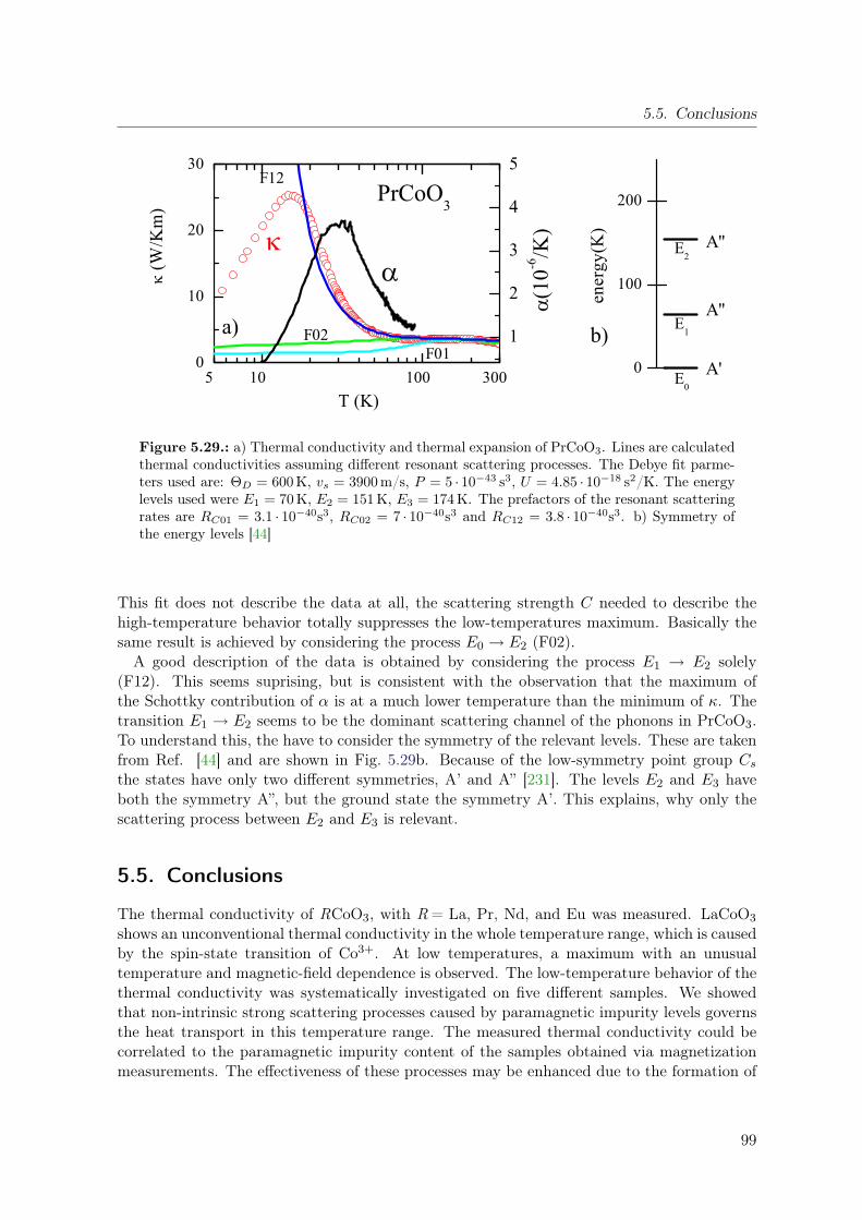
5.5. Conclusions

0

10

20

30

5 10 100 300

1

2

3

4

5

0

100

200F12

F02

(W

/Km

)

PrCoO3

F01a)

(1

0-6/K

)

T (K)

A'E0

b)

E2

A''

ene

rgy(

K)

A''E

1

Figure 5.29.: a) Thermal conductivity and thermal expansion of PrCoO3. Lines are calculatedthermal conductivities assuming different resonant scattering processes. The Debye fit parme-ters used are: ΘD = 600 K, vs = 3900 m/s, P = 5 · 10−43 s3, U = 4.85 · 10−18 s2/K. The energylevels used were E1 = 70K, E2 = 151K, E3 = 174K. The prefactors of the resonant scatteringrates are RC01 = 3.1 · 10−40s3, RC02 = 7 · 10−40s3 and RC12 = 3.8 · 10−40s3. b) Symmetry ofthe energy levels [44]

This fit does not describe the data at all, the scattering strength C needed to describe thehigh-temperature behavior totally suppresses the low-temperatures maximum. Basically thesame result is achieved by considering the process E0 → E2 (F02).

A good description of the data is obtained by considering the process E1 → E2 solely(F12). This seems suprising, but is consistent with the observation that the maximum ofthe Schottky contribution of α is at a much lower temperature than the minimum of κ. Thetransition E1 → E2 seems to be the dominant scattering channel of the phonons in PrCoO3.To understand this, the have to consider the symmetry of the relevant levels. These are takenfrom Ref. [44] and are shown in Fig. 5.29b. Because of the low-symmetry point group Cs

the states have only two different symmetries, A’ and A” [231]. The levels E2 and E3 haveboth the symmetry A”, but the ground state the symmetry A’. This explains, why only thescattering process between E2 and E3 is relevant.

5.5. Conclusions

The thermal conductivity of RCoO3, with R = La, Pr, Nd, and Eu was measured. LaCoO3shows an unconventional thermal conductivity in the whole temperature range, which is causedby the spin-state transition of Co3+. At low temperatures, a maximum with an unusualtemperature and magnetic-field dependence is observed. The low-temperature behavior of thethermal conductivity was systematically investigated on five different samples. We showedthat non-intrinsic strong scattering processes caused by paramagnetic impurity levels governsthe heat transport in this temperature range. The measured thermal conductivity could becorrelated to the paramagnetic impurity content of the samples obtained via magnetizationmeasurements. The effectiveness of these processes may be enhanced due to the formation of

99


magnetic polarons. Concerning the whole RCoO3 series, we observed a systematic increase ofthe thermal conductivity from R = La to Eu. At low temperatures, this observation cannotdirectly be attributed to the spin-state transition. The analysis of the thermal conductivity incombination with susceptibility measurements suggests a scenario, where magnetic polaronssignificantly scatter phonons at low temperatures. Because the polaron formation becomesless likely when the spin gap is increased, the systematic increase of the thermal conductivityfrom La to Eu results.

Above T ≈ 30K, a strong suppression of the thermal conductivity is observed in all samples.The resulting very low absolute value of the thermal conductivity up to room temperature is anintrinsic feature of the thermal conductivity of LaCoO3. We showed that this unusual behaviorof the heat transport is a consequence of the spin-state transition. The Co3+ ion has a largerionic radius in the thermally activated IS/HS state than in the LS ground state. The randomdistribution of the LS and IS/HS states causes an additional lattice disorder which stronglysuppresses the thermal conductivity. To check this scenario also quantitatively, we estimatedthe additional scattering-rate due to the spin-state transition. Herefore we used EuCoO3as a reference compound, where the influence of the spin-state transition is negligible belowroom temperature. We were able to describe the temperature dependence of the additionalphonon scattering by a model based on the Nordheim rule. Such a model was successfullyused in the literature to describe the thermal conductivity of mixed semiconductor alloys.Our model works with the LS-IS scenario with a spin gap of 185K estimated by susceptibilitymeasurements [12] as well as with the recently proposed model based on a spin-orbit coupledhigh-spin state [13]. In PrCoO3 and NdCoO3, the spin-state transition shifts gradually tohigher temperatures. In PrCoO3, an additional scattering mechanism could be identified,which is attributed to resonant scattering by the 4f orbitals of Pr3+.

Despite the additional effect in PrCoO3, we could show that the spin-state transition in-fluences the thermal conductivity at high temperatures in PrCoO3 and NdCoO3 in the sameway as in LaCoO3. The change of the scattering rates due to the spin-state transition couldbe modeled using the parameters estimated from LaCoO3. This is clear evidence that thespin-state transition indeed causes the suppression of the thermal conductivity due to theadditional disorder. We explored the scattering mechanism in detail and quantitatively inves-tigated the scattering strength for LaCoO3. Our results show, that the static volume changesof the Co3+ ions caused by the spin-state transition are sufficient to explain the observedbehavior of the thermal conductivity. This is in contrast to the scenerio proposed in Ref. [9],which proposes that dynamical fluctuations are responsible for the strong suppression of thethermal conductivity.

100

6. Thermal Conductivity, Thermopower,and Figure of Merit of La1-xSrxCoO3 andLa0.75-xEu0.25SrxCoO3

In this chapter measurements of the thermal conductivity and the thermopower of La1-xSrxCoO3with 0 ≤ x ≤ 0.3 and La0.75-xEu0.25SrxCoO3 with 0 ≤ x ≤ 0.4 will be presented. From theseresults and the electrical resistivity the thermoelectric figure of merit will be calculated, whichis of interest for the applicability for thermoelectric devices. The zero- field measurements forLa1-xSrxCoO3 are partly from C. Zobel [33], the measurements of the thermal conductivity andthe thermopower of La0.75-xEu0.25SrxCoO3 were performed by H. Anapa [177]. The resistivitymeasurements were carried out by C. Zobel and C. Hanebeck [33, 232]. The experimentalmethods used in this section are described in the Secs. 3.2, 3.3, and 3.4. The main results ofthis chapter have been published in Ref. [166].

6.1. Introduction

In Sec. 5.1 the thermally driven spin-state transition in LaCoO3 was discussed [12, 176, 185,189, 190, 205, 233, 234]. During the last years cobaltates with layered CoO structures havealso become subject of intense studies. [203, 235–242] It has been proposed that various ofthese compounds would also show temperature-dependent spin-state transitions of the Co3+

and/or Co2+ ions, but an unambiguous proof of such spin-state transitions is still missing (seee. g. Ref. [203]).

Recently, the observation of superconductivity in NaxCoO2 · y H2O has attracted much at-tention. [243] The water-free parent compound NaxCoO2 became prominent some years agoalready in a different context. [244] It was found that NaxCoO2 with x = 0.6 has a metallicelectrical conductivity σ, but a low thermal conductivity κ and, in addition, a large ther-mopower S. The combination of large σ, small κ, and large S values is a precondition foreffective thermoelectric cooling. The performance of thermoelectric devices depends on theso-called thermoelectric figure of merit Z = S2 / κρ where ρ = 1/σ denotes the electricalresistivity. For an effective cooling, ZT values (T is the absolute temperature) of order unityshould be reached and are found for instance in Bi-based alloys, some thin-film devices orquantum dot superlattices. [245, 246] For comparison, typical metals have much smaller ZTvalues of order 10−4. In this respect it was quite surprising that NaxCoO2 has ZT' 0.03 for150 K ≤ T ≤ 300K. The enhanced figure of merit of NaxCoO2 mainly arises from an enhancedthermopower. [247] Based on a study of the magnetic-field dependence S(H) of NaxCoO2 ithas been argued that the spin entropy is the likely source for the large thermopower. [248]

A large thermopower occurs also in La1-xSrxCoO3. [249] This motivated the study of thetransport properties of this series in order to determine experimentally the ZT values andtheir dependence on temperature and doping. Another motivation for this study was thatthe previous results do not give a consistent picture of the transport properties. For example,

101

6. Thermal Transport of La1-xSrxCoO3 and La0.75-xEu0.25SrxCoO3

x δ x δ

0 0.005 0.125 -0.0060.002 0.003 0.15 -0.0170.01 0.002 0.18 0.0000.04 -0.001 0.25 -0.0250.08 0.000 0.3 -0.004

Table 6.1.: Oxygen content δ of theLa1-xSrxCoO3 + δ crystals determined bythermogravimetric analysis. [166, 253]

from various anomalous features in the temperature dependences of S, ρ, and the magneticsusceptibility χ a complex phase diagram was proposed for the La1-xSrxCoO3 system. [249] Ithas, however, been argued that the occurrence of some of these anomalous features dependson the preparation technique of the polycrystals. [250] In fact, the phase diagram derived fromρ(T ) and χ(T ) measured on La1-xSrxCoO3 single crystals [205, 213, 251] is much less complexthan the previous one [249]. Moreover, the temperature dependences of S for undoped LaCoO3reported in Refs. [176] and [252] are contradictory. For T > 400K both reports find a positivethermopower of order +50µV/K, which slightly increases with decreasing temperature. ForT < 400K, however, a further increase of S with a maximum of about +1200µV/K around100 K is found in Ref. [176], whereas a sign change of S and a decrease to about −400 µV/Kfor T ' 200K is reported in Ref. [252]. The thermal conductivity of the La1-xSrxCoO3 systemhas to my knowledge not yet been studied at all.

6.2. Samples

The single crystals of La1-xSrxCoO3 with x > 0 used in this study have been grown by afloating-zone technique in an image furnace by C. Zobel [33]. For further details of the samplecharacterization by X-ray diffraction, magnetization, and resistivity measurements see alsoRefs. [12, 178, 205, 205, 213, 213, 254] For discussion of the thermal conductivity of undopedLaCoO3 see Chp. 5. The thermopower for LaCoO3 was measured on the same five specimensused for the thermal conductivity measurements. As a reference for the thermal conductivityof the undoped LaCoO3 the specimen ZO104 is used1. The La0.75-xEu0.25SrxCoO3 samples,with x = 0, 0.1, 0.2, 0.3, and 0.4, are polycrystals prepared by a standard solid-state reactionby A. Reichl, see Ref. [179]. For further details of the characterization of these samples seealso Ref. [232].

The nominal valence of the Co ions does not only depend on the Sr content, but also onthe oxygen concentration, i. e. the amount n of charge carriers in La1-xSrxCoO3 + δ is givenby n = x + 2δ. Positive (negative) values of n mean hole (electron) doping and formallyan amount n of the Co3+ ions is transformed into Co4+ (Co2+). In the case of hole dopingthis formal description must not be taken literally, because due to the high oxidation stateof Co4+ the holes are likely to enter the oxygen 2p states. Note that depending on the spinstates of the various Co ions hole and electron doping may be strongly different with respectto charge transport due to the so-called spin-blockade effect [255, 256]. Because of the highoxidation state of Co4+, one may suspect that with increasing Sr concentration the amountof oxygen vacancies also increases, i. e. an increasing x could be partially compensated by adecreasing δ. In order to check this the oxygen content of the entire series La1-xSrxCoO3 + δ

1This crystal was grown at the same time like the rest of the La1-xSrxCoO3 series.

102

6.3. Experimental Results

0 200 400 60010-4

10-2

100

102

104

106

108 La1-xSr

xCoO

3

x = 0 0.010.02 0.040.08 0.1250.18 0.25

0.3

(cm

)

T (K)

0 100 2000.0

1.0

0T 15T

(10-3

cm)

x = 0.18 0.25 0.3

T (K)

Figure 6.1.:Resistivity of La1-xSrxCoO3. for0 ≤ x ≤ 0.3. For consecutive dop-ing an insulator-metal transitionoccurs for x ≈ 0.18 [213, 260]. In-set: Resistivity of La1-xSrxCoO3for x ≥ 0.18 below 300 K. Here,the ferromagnetic order is seen at157, 209, and 227 K for x = 0.18,0.25, and 0.3, respectively [205,213]. For x = 0.25 the resistivityis also shown in a magnetic field of15 T (Dotted line) [261].

was determined by thermogravimetric analysis (TGA/SDTA851, Mettler-Toledo). Pieces ofabout 50 mg of the single crystals have been ground and heated up to 900C in a reducingatmosphere (N2 with 5 % H2) in order to decompose La1-xSrxCoO3 + δ into La2O3, SrO andelementary Co. [257–259] The value of δ is then calculated from the measured weight loss.The reproducibility of this method was tested by repeatedly measuring amounts of about50 mg from the same badge of a LaCoO3 polycrystal. The different results agree to each otherwithin ±0.01, which is comparable to the uncertainty of the same and alternative methodsof oxygen-content determination in cobaltates. [257–259] A scatter of ±0.01 is also present inthe determined oxygen contents of the La1-xSrxCoO3 + δ crystals (see Table 6.1). A linear fitof δ(x) yields a weak decrease dδ/dx = −0.05. The analysis reveals a 10% reduction of thecharge-carrier content with respect to the Sr content. We do not calculate n = x+2δ for eachcrystal individually, because the scatter of δ would correspond to a scatter of the charge carriercontent of ±0.02, which can be excluded for the studied crystals from the measurements ofthe magnetization and resistivity (see Ref. [205, 213]). Both quantities vary monotonouslyas a function of x for 0 ≤ x ≤ 0.3. Thus the scatter of n between samples with neighboringx is much smaller than their difference ∆x, which amounts e. g. to only 0.01 for the lowestconcentrations. This conclusion is also confirmed by the data presented in this chapter. Theonly exception is the thermopower of nominally undoped LaCoO3, which will be discussed inmore detail below.

6.3. Experimental Results

6.4. La1-xSrxCoO3

6.4.1. Resistivity

The temperature and doping dependent resistivity of LaCoO3 is shown in Fig. 6.1 [260].Undoped LaCoO3 is an insulator2. With increasing Sr doping, the resistivity drastically de-

2The additional transition above room-temperature is discussed in Refs. [33, 213], and not the scope of thisinvestigation.

103


0 100 200 3000

5

10

0.3

0.25

x = 0.18 x = 0.125

x = 0.01 0.02 0.04 0.08

x = 0.002

x = 0 La1-x

SrxCoO

3

(W

/Km

)

T (K)

Figure 6.2.: Thermal conduc-tivity of LaCoO3 as a func-tion of temperature for differ-ent doping x. [33, 166, 262]

creases, and an insulator-metal (IM) transition occurs at x ≈ 0.18. For the metallic samplesferromagnetic order is observed, [205, 213] which causes an anomaly in the resistivity at theferromagnetic transition temperature Tc. The lowered resistivity in the ferromagnetic statecan be explained by the double-exchange interaction, hopping between neighboring ferromag-netically aligned sites lowers the energy of the system and increases the conductivity. If amagnetic field is applied, the ferromagnetic state is stabilized, the consequence is that thetransition shifts to a higher temperature and smears out, as seen in the inset of Fig. 6.1. Themagnetic field is most effective around the transition temperature, see Sec. 6.4.3.

6.4.2. Thermal Conductivity

Fig. 6.2 shows the thermal conductivity of La1-xSrxCoO3. For x = 0 the data for the crystalZO104 are shown. In Chp. 2 the thermal conductivity of insulators was discussed. The mainresults was that an T 3 dependence of κ for T → 0K is expected . At intermediate temperaturesa maximum of κ occurs, and at high temperatures κ follows roughly a 1/T dependence.

As discussed in detail in Chp. 5, the thermal conductivity of LaCoO3 is quite unusual. Themain result is that strong additional scattering due to the spin-state transition suppresses κin the whole temperature range investigated. The thermal conductivity of the crystal withx = 0.002 is similar to that of pure LaCoO3, but the low-temperature maximum of κ is alreadystrongly suppressed. For higher Sr doping this maximum is almost completely absent and κincreases continuously with increasing temperature. The room temperature values of κ liebetween 2 and 3 W/Km for all crystals with x ≤ 0.18. We attribute the drastic suppressionof κ at low temperatures to a Sr-induced disorder, which hinders a strong increase of ` forT → 0K. Probably this disorder does not solely arise from the bare difference between La3+

and Sr2+ ions. From magnetization measurements it is found that for x ≤ 0.01 so-calledmagnetic polarons with high spin values (S = 10− 16) are formed, [215] see Sec. 5.3.3.

Due to such a polaron formation the disorder is strongly enhanced for the lowest Sr con-centrations, whereas for larger x the polarons start to overlap and the enhancement becomesless effective. Samples with x > 0.18 show metallic conductivity and ferromagnetic order atlow temperatures, see Inset of Fig. 6.1. In this concentration range one expects that mag-netic polarons become much less important. However, the low-temperature peak of κ remainsabsent, since the Sr concentration is so large that the bare doping-induced lattice disorder

104

6.4. La1-xSrxCoO3

0 100 200 3000

5

10

100 200 3000.0

0.2

0

1

x = 0.25 -ch

x = 0.04

x = 0.25 B = 15T B = 0

La1-xSrxCoO3

(W/K

m)

T(K)

(B)- (0)

B = 15 T 10 T 5 T (W

/Km

)T (K)

T [ (B)- (0)]

T* (1

07 K/

m)

Figure 6.3.: Thermal conductivity κ of La1-xSrxCoO3 with x = 0.25 as a function of temper-ature measured in 15 T () and in zero magnetic field (− ·−). The solid line is the phononiccontribution κph of the x = 0.25 crystal, which is obtained by κph = κ(B) − LT σ(B)using the electrical conductivity σ and the Lorenz number L. For comparison κ of thex = 0.04 sample (O) is also depicted. The Inset shows the magnetic-field dependences∆κ(B) = κ(B) − κ(B = 0) (, left y scale) and T ∆σ(B) = T [σ(B)− σ(B = 0)] (—, righty scale) for B = 5, 10, and 15T, respectively. The value of the Lorenz number is obtainedfrom the field- and temperature-independent scaling factor between both quantities, i. e. viaL = ∆κ(B) / [T ∆σ(B)] = 2.9 · 10−8 V2/K2. [33, 166, 262]

is sufficient to suppress the low-temperature peak. Moreover, the Sr doping induces mobilecharge carriers, which serve as additional scatterers for the phonons.

The mobile charge carriers for larger x are expected to transport heat, too. The totalthermal conductivity therefore consists of a phononic contribution and a contribution of mo-bile charge carriers, i. e. κ = κph + κch. Usually, κch can be estimated by the Wiedemann-Franz law, which relates κch to the electrical conductivity according to κch ' L0 σ T . Here,L0 = 2.44 · 10−8 V2/K2 denotes the Sommerfeld value of the Lorenz number. From theroom temperature values of ρ κch(300K) ' 0.4, 0.9, 1.6 and 2.7 W/Km is estimated forx = 0.125, 0.18, 0.25 and 0.3, respectively, and κch κ for smaller x. Additional heatconduction by charge carriers is therefore relevant for metallic La1-xSrxCoO3 only and ex-plains why the crystals with x ≥ 0.25 have significantly larger κ(T ) values for T > 100Kthan the insulating samples with x < 0.18. For x = 0.25 and 0.3 anomalies of κ occuraround 200 K and 230 K, respectively, i. e. close to the respective ferromagnetic ordering tem-peratures Tc = 209, 227K. [205, 213]. Below Tc, κ increases and we attribute this to thedecrease of ρ below Tc, [205, 213] which leads to a corresponding increase of κch. Since thecharge transport close to Tc depends on a magnetic field in La1-xSrxCoO3, [263] one may an-alyze κch for x = 0.25 in more detail by comparing the magnetic-field dependences of κ andσ = 1/ρ (Fig. 6.3). An increase of κ with increasing field is found, that is most pronouncedaround 200 K where the strongest magnetic-field induced suppression of ρ is observed, too,see Fig. 6.1 [263] Under the reasonable assumption of a negligible field dependence of κph weobtain ∆κ(T,B) = κ(T,B)−κ(T, 0) = κch(T,B)−κch(T, 0), and the Lorenz number is given

105


0 100 200 3000

200

400

600

800

1000

-10

0

10

20

30

40

x = 0.002 0.01 0.02 0.04 0.08 0.125 0.18

S (

V/K

)

T (K)

x = 0.3

B = 0, 5, 10, 15Tx = 0.25

La1-xSrxCoO3

x = 0.18

S (

V/K

)

Figure 6.4.: Thermopower S of La1-xSrxCoO3 as a function of temperature for different dopingx > 0. For x = 0.25 S(T ) is also shown for different magnetic fields. [33, 166, 264]

by the relation L = ∆κ(T,B) / T∆σ(T,B) with ∆σ(T,B) = σ(T,B) − σ(T, 0). As shownin the inset of Fig. 6.3 the scaling relation between ∆κ and T∆σ(T,B) is well fulfilled overthe entire temperature and magnetic-field range studied here. From this scaling the valueL = 2.9 · 10−8 V2/K2 is estimated, which is about 20% larger than L0. The phononic thermalconductivity for x = 0.25 is then obtained by κph = κ(B)−LT σ(B) and found to agree wellwith those of the low-doped samples.

6.4.3. Thermopower

The thermopower measurements of the La1-xSrxCoO3 series for x > 0 are presented in Fig. 6.4.For the crystal with the lowest Sr content x = 0.002 a large positive thermopower which in-creases with decreasing temperature is found. We could not determine S for highly insulatingcrystals with ρ & 109 Ωcm as it is the case for this crystal below about 100 K. With increas-ing Sr content S systematically decreases and for 0.01 ≤ x ≤ 0.18 all S(T ) curves showmaxima which become less pronounced and slightly shift towards higher temperature. Notethat additional anomalies observed in the temperature dependence S(T ) of polycrystallineLa1-xSrxCoO3 (Ref. [249]) are not reproduced by the single-crystal data. Such a differencehas already been observed in magnetization data, and gives further evidence that these ad-ditional anomalies are not an intrinsic feature of La1-xSrxCoO3. For the metallic sampleswith x ≥ 0.25 S(T ) varies only weakly with temperature between 300 K and Tc. Around Tc

106

6.4. La1-xSrxCoO3

0 100 200 300-1000

-500

0

500

1000

1500

-0.1 0.0 0.1 0.2 0.3

-500

0

500

1000

S (

V/K

)

T (K)

EK ParisZO104

Mar5a_08

Mar5b_07

Mar5_09

S(30

0K)

(V

/K)

charge carrier content x-2

La1-x

SrxCoO

3-

Figure 6.5.: Top: Thermopower S as a function of temperature for 5 different crystals ofnominally undoped LaCoO3. Bottom: Room-temperature values S(300 K) as a function of thecharge carrier concentration n = x + 2δ for Sr-doped () and pure (•) LaCoO3. The lines arecalculated via Eq. (6.1). [33, 166, 265]

a sharp kink occurs and S strongly decreases. For x = 0.3 there is even a sign change andS becomes negative for T < 170K. The sensitivity of S to the magnetic ordering indicatesthat a considerable contribution of S arises from magnetic entropy. Therefore, one may alsoexpect a pronounced magnetic-field dependence S(B) as has been pointed out recently. [248]As shown in Fig. 6.4 indeed a strong magnetic-field induced suppression of S is found, thatis most pronounced around Tc. This arises from the fact that the magnetic entropy may bestrongly reduced by available magnetic-field strengths only around Tc. For higher temper-atures thermal disorder becomes too large (kBT gµBB) and for T Tc the magneticentropy is already frozen by the magnetic exchange coupling.

At high enough temperatures the thermopower is expected to be determined by the so-calledHeikes formula (see e. g. Ref. [266]). This general expression has been refined for the case ofdoped cobaltates in Ref. [267] to

S = −kB

e

[ln

(n

1− n

)+ ln

(g3

g4

)]. (6.1)

Here, n denotes the content of Co4+ ions and g3 (g4) is the number of possible configurations ofthe Co3+ (Co4+) ions, which is, in general, given by the product of orbital and spin degeneracy.

107


If different spin states of the Co3+/4+ ions are close enough in energy, the number of possibleconfigurations may further increase. [267]

0 100 200 3000.00

0.01

0.02

0.03

0.04La1-xSrxCoO3

x = 0.002 0.01 0.02 0.04 0.08 0.125 0.18 0.25 0.3

Figu

re o

f Merit

ZT

T (K)

Figure 6.6.: Figure ofmerit of La1-xSrxCoO3 asa function of temperaturefor different doping x.

In the lower panel of Fig. 6.4.3 the room-temperature values of S for La1-xSrxCoO3 are shown(open symbols, x > 0) as a function of the charge carrier content n = 0.9 ·x as determined bythermogravimetric analysis (see Sec. 6.2). A fit of the experimental data via Eq. 6.1 with theratio g3/g4 as the only fit parameter yields g3/g4 ' 1.8. The saturation magnetization of thesamples showing ferromagnetic order (x > 0.18) is best described by assuming an S = 1/2low-spin state for Co4+ and an S = 1 intermediate-spin state for Co3+. [205, 213] For thiscombination of spin states a ratio g3/g4 = 3/2 is expected, which is independent from thepossible orbital degeneracies ν = 1 or 3 as long as both, the Co4+ LS and Co3+ IS state havethe same ν. If one assumes that the energy of the Co3+ LS state is close to that of the Co3+

IS state, the ratio increases to g3/g4 = 2 and 5/3 for ν = 1 and 3, respectively. For all ofthese cases the experimental data are reasonably well described by Eq. 6.1. However, this doesnot exclude other spin-state combinations, since Eq. 6.1 is derived for the high-temperaturelimit, whereas in Fig. 6.4 the room-temperature values of S are considered and at least forthe samples with x < 0.25 the S(T ) curves have a more or less pronounced negative slope at300 K. Thus, it is possible that for higher temperatures a larger g3/g4 ratio would be obtainedin the fit. In addition, there are also other combinations of spin states yielding g3/g4 ratiosclose to 1.8, but these are not supported by the measured saturation magnetization. Despitethese uncertainties we interpret the doping dependence of S(300 K) as further evidence forthe Co4+

LS/Co3+IS combination suggested from the magnetization and resistivity data. [213]

According to Eq. 6.1 the thermopower is expected to diverge for a vanishing hole content,i. e., when the nominally undoped LaCoO3 is approached. For electron doping one may stillapply Eq. 6.1, but with a positive sign and g4 for the degeneracy of Co2+. The dashed linein Fig. 6.4 is calculated for g4 = 4 as expected for Co2+ in a HS state. A large negative ther-mopower has been observed recently in electron-doped La1−xCexCoO3. [255] For nominallyundoped LaCoO3, a different sign of S for different crystals is found. This is shown in theupper panel of Fig. 6.4. Although these crystals have been grown under the same conditions,either a large negative or a large positive thermopower can be obtained. We suspect that thisextreme sensitivity of S results from weak deviations in the oxygen content of LaCoO3 + δ,which cause small concentrations 2δ of hole or electron doping depending on the sign of δ.

108

6.5. La0.75-xEu0.25SrxCoO3

Already extremely small values of |δ| < 0.002, which are well below the accuracy of oxygendetermination in cobaltates, would be sufficient to explain the observed thermopower valueswith |S| > 500 µV/K in LaCoO3 + δ. We also suspect that there are weak inhomogeneities ofthe oxygen content in each sample, which can strongly influence the sign and also the tem-perature dependence of the measured thermopower. Most probably, this is also the reasonfor the contradictory results for S(T ) obtained in Refs. [176, 252]. It should be mentionedthat this extreme sensitivity S(δ) is expected only for the (almost) undoped LaCoO3, whereasfor samples with a finite Sr content the drastic influence of such small variations of δ rapidlydecreases with increasing x.

6.4.4. Figure of Merit

In Fig. 6.6 the thermoelectric figure of merit of La1-xSrxCoO3 is presented. Since the thermalconductivity for all x is rather low, one precondition for large ZT values is already fulfilledfor the entire La1-xSrxCoO3 series. The very low-doped samples show in addition very largethermopower values, but their resistivities are also large and thus prevent large ZT values.Small resistivities are obtained for large x, but these samples also have smaller thermopowervalues. Thus the optimum figure of merit is obtained in the intermediate doping range. Amaximum ZT ' 0.035 around 225 K is found for x = 0.125, which is as large as the valueobserved in NaxCoO2. [244] These values are among the largest observed in transition metaloxides so far, but are still too small for technical applications. This raises the question, howan improvement of ZT is possible. One possibility, additional substitution of La by Eu, willbe discussed in the next section.


A way to tune the physical properties of the La1-xSrxCoO3 system is doping with Eu, whichis isovalent to La and so does not change the nominal valence of the system. The main effectis chemical pressure due to the smaller Eu ion size. [54] The Sr-free series La1-xEuxCoO3 hasbeen investigated by resistivity and susceptibility measurements in the whole doping range0 ≤ x ≤ 100. [178, 179, 206] The measurements of the magnetic susceptibility reveal that thespin gap to the IS/HS state increases from ∆Co ≈ 188K for LaCoO3 to ∆Co > 1900K forEuCoO3. [178, 206] For La0.75Eu0.25CoO3, the spin gap is determined as ∆Co ≈ 440K, morethan twice as large as in LaCoO3. [178, 206] The influence of Sr doping was investigated onsamples of the series La0.75-xEu0.25SrxCoO3 with x = 0.1, 0.2, 0.3, and 0.4 (see Ref. [179]). Asalready mentioned, these samples are polycrystalline, in contrast to the La1-xSrxCoO3 samples.The lower panel of Fig. 6.7 shows the zero field resistivities [271]. As for La1-xSrxCoO3,increasing Sr doping causes an insulator-metal transition. In contrast to La1-xSrxCoO3, theabsolute values of the resistivity are higher for the same doping level3, and a higher dopinglevel is required to induce the IM transition. [232]

As shown in the previous section, the large values of ZT are mainly due to the increased spinentropy which causes a large thermopower. In the Eu-doped samples the spin gap is larger.As a consequence, a higher doping level is required in La0.75-xEu0.25SrxCoO3 in comparisonto La1-xSrxCoO3 to obtain the same population of the LS- IS/HS states and therefore the

3A quantitative comparison is difficult for two reasons: There are no crystals available with the same dopingin both series. [232]. Further polycrystals are compared with single crystals.

109


0.1 0.2 0.3 0.410-4

10-3

10-2

0 100 2001x10-41x10-31x10-21x10-11x1001x1011x1021x103

x=0.4x=0.3

x=0.2

( c

m)

T (K)

La0.75-xEu0.25SrxCoO3

x=0.1

2x10-4

5x10-4

1x10-3

cm

)

14T0T

14T

x=0.3

x=0.4

0T

25% Eu 0% Eu

30

0K (

cm)

Sr doping x

Figure 6.7.:Lower panel: Resistivity of La0.75-xEu0.25SrxCoO3. for 0.1 ≤ x ≤ 0.4. For consecutive dopingan insulator-metal transition occurs for x ≈ 0.3 [268]. Upper panel: resistivity for x = 0.3 andx = 0.4 in magnetic fields of 0 and 14 T. Inset: room temperature values of ρ vs. Sr doping xfor La1-xSrxCoO3 and La0.75-xEu0.25SrxCoO3.

same entropy at a given temperature. It follows, that the enhancement of the thermopower isshifted to a higher Sr doping x for Eu doped samples. This could increase the figure of meritand motivated to determine ZT

Fig. 6.9 shows the thermal conductivity data [270] for La0.75-xEu0.25SrxCoO3 with x =0 . . . 0.4. For x = 0 the thermal conductivity is almost identical to LaCoO3, which seemssuprising, since the disorder introduced by the Eu should suppress the thermal conductiv-ity. This shows, that the suppression of the low-temperature maximum of La1-xSrxCoO3 forhigher doping levels mainly arises from scattering by charge carriers. With Sr doping, thelow-temperature maximum is suppressed as in La1-xSrxCoO3, and the thermal conductivitymonotonously increases with temperature. The absolute values of the lattice contribution atroom temperature, calculated by the Sommerfeld value L0, denote 2.2, 3.8, 3.4, and 1.5W/Kmfor 0.1 ≤ x ≤ 0.4. Performing the same scaling procedure as for La1-xSrxCoO3 for the fielddependent thermal conductivity curves (see Ref. [177]), one gets L = 2.0 · 10−8 V2/K2. Incontrast to LaCoO3, where the estimated L is ≈ 20% higher than L0, here L is about 20%lower. The inset of Fig. 6.9 shows the electronic contribution to the thermal conductivity,calculated with the value of L from the scaling analysis. However, the estimated room tem-perature lattice contributions do not show a systematic behavior, [177] which may be related

110


0.2 0.40

100

0

10

20

30

14T0T

0T

x=0.4 Tc= 210 K

x=0.3 Tc= 175 K

S(V

/K)

14T

0 100 200 300

0

50

100

150

x=0.1

x=0.4

x=0.3

x=0.2 Tc= 125 K

S(V

/K)

Temperature (K)

La0.75-x

Eu0.25

SrxCoO

3

0% Eu 25% Eu

S(

V/K

)

x

Figure 6.8.: Lower Panel: Thermopower of La0.75-xEu0.25SrxCoO3 for 0.1 ≤ x ≤ 0.4. Upperpanel:Thermopower of La0.75-xEu0.25SrxCoO3 for x = 0.3 and x = 0.4 in magnetic fields of 0and 14 T. Arrows mark the ferromagnetic transition temperature. Inset: Room temperaturevalues of the thermopower vs. Sr doping x for La1-xSrxCoO3 and La0.75-xEu0.25SrxCoO3. [269]

0 100 200 3000

2

4

6

8

10

12

x=0.2

x=0.4

x=0.2

x=0.1

x=0.3

(W/K

m)

T (K)

x=0

0 100 2000

1

2

3

4

14T0T

x=0.3

x=0.4

La0.75-x

Eu0.25

SrxCoO

3

14T0T

Figure 6.9.: Thermal conductivity of La0.75-xEu0.25SrxCoO3 for 0.1 ≤ x ≤ 0.4. Inset: thermalconductivity for x = 0.3 and 0.4 in magnetic fields of 0 and 14 T (Symbols). Lines are electroniccontributions to κ calculated by the Wiedemann-Franz law with L = 2.0 · 10−8 V2/K2. [270]

111


0.0 0.1 0.2 0.3 0.40.00

0.01

0.02

0.03

0 100 200 3000.00

0.01

0.02

0.03

0.04

x=0.1

x=0.2

x=0.3

x=0.4

x=0.18

x=0.125

x=0.08

La1-xSrxCoO3

ZT

T (K)

La0.75-x

Eu0.25

SrxCoO

3

La0.75-x-y

EuySr

xCoO

3

Figu

re of m

errit

ZT

(300

K)

Nominal Sr doping x

25% Eu

0% Eu

Figure 6.10.: Upper Panel: Figure of Merit of La0.75-xEu0.25SrxCoO3 for 0.1 ≤ x ≤ 0.4(Symbols). For Comparison the curves for La1-xSrxCoO3 with x = 0.08, 0.125, and 0.18are shown (lines). Lower Panel: Room temperature values of ZT for La1-xSrxCoO3 andLa0.75-xEu0.25SrxCoO3 vs. Sr doping level x. Errorbars are drawn assuming a relative error of30%.

to the polycrystal nature of the crystals, and does not allow a more detailed analysis. How-ever, the absolute values of the lattice contribution are of the same order of magnitude as forLa1-xSrxCoO3 (≈ 2.5W/Km).

Fig. 6.8 shows the thermopower. In the lower panel the zero field data are shown. Thegeneral findings are the same as for La1-xSrxCoO3, a large positive thermopower which isstrongly suppressed for the higher doping levels. The inset shows the room-temperature valuesvs. Sr doping x for both series, the Eu doped crystals have indeed a higher thermopower atthe same Sr doping level. The upper panel of Fig. 6.8 shows the thermopower for x = 0.3 andx = 0.4, which show the same behavior as La1-xSrxCoO3 with x = 0.25 and x = 0.3, takinginto account the differences in Tc. Consequently, the explanation for the anomaly at Tc of theferromagnetic transition and the field dependence is the same as for e.g. La0.75Sr0.25CoO3,see e.g. Sec. 6.4.1. [232]

Calculating the thermoelectric figure of merit, we find the results shown in Fig. 6.10, togetherwith some results from the La1-xSrxCoO3 crystals for comparison. The main result is that ZTdoes not change significantly with Eu doping. The absolute value at the maximum is smaller,

112

6.6. Conclusions

ZT= 0.02 at 300K instead of x = 0.025 at 250K. However, it is likely that the maximumvalues of ZT is achieved for x inbetween 0.1 and 0.2, and approximately the same as observedin LaCoO3. Here one has to keep in mind, that the uncertainty of ZT is comparatively high,since it is calculated from three independent measurements (In Sec. 3.4 a relative error of≈ 20 . . . 25% was derived). In order to get an better estimate of the doping dependence ofZT , the room temperature values vs. doping level x are shown in the lower panel of Fig. 6.10.The figure shows that the maximum of ZT is shifted to a higher doping level, but does notsignificantly change the absolute value at room temperature.

6.6. Conclusions

We have presented a systematic study of the thermal conductivity and the thermopower of aseries of single crystals of La1-xSrxCoO3 + δ. The thermal conductivity is strongly suppressedfor the entire doping range. In pure LaCoO3 this suppression most probably arises from locallattice distortions due to a temperature-induced spin-state transition of the Co3+ ions. Forsmall finite x, a spin-state transition of the Co3+ ions may be induced by the neighboringmagnetic Co4+ ions, and so-called high-spin polarons can be formed, which also cause latticedisorder. For larger x this effect becomes less important, and scattering of phonons by mobilecharge carriers plays the main role for the suppression of the thermal conductivity. Thisconclusion can be drawn, since in Sr-free La1-xEuxCoO3 the low-temperature peak is stillpresent. The static disorder caused by the different ion sizes of La and Sr seems to play a minorrole. For finite doping a large, positive thermopower, which strongly depends on temperatureand doping, is found. The room temperature values of the thermopower follow a dopingdependence that is expected from a modified Heikes formula, [267] if an intermediate-spin statefor Co3+ and a low-spin state for Co4+ is assumed as it is suggested from magnetization andresistivity data. [213] In nominally undoped LaCoO3 for different crystals either a large positiveor a large negative thermopower is observed. This is likely a consequence of weak deviations(|δ| < 0.002) from the nominal oxygen content causing small amounts of hole or electrondoping. Most probably, a weak oxygen off-stoichiometry is also the reason for the contradictoryresults of the thermopower reported for LaCoO3 previously. [176, 252] For the crystal withx = 0.25 both, the thermal conductivity and the thermopower show a significant magnetic-field dependence in the temperature range around the ferromagnetic ordering temperature.The field dependence of the thermal conductivity can be traced back to a field-dependentcharge carrier contribution to the heat current, and the field dependence of the thermopowerindicates that it contains a sizeable contribution arising from magnetic entropy. From theresistivity ρ, the thermopower S and the thermal conductivity κ the thermoelectric figure ofmerit Z = S2 / κρ was calculated, which strongly depends on both, doping and temperature.A maximum of ZT ' 0.035 is obtained for x = 0.125 and 200 K ≤ T ≤ 250K. This valueis large, but yet too small for technical applications. Additional Eu increases the resistivityand the thermopower at a given Sr doping level, what shifts the maximum of ZT to a higherdoping level. However, within the experimental error no change in the maximum value of ZTis observed.

113


114

7. Thermal Conductivity of OrthorhombicManganites

The search for magnetoelectric materials, with the possibility to induce magnetic orderingby electric fields and vice versa, has increased the interest in so-called multiferroic materials,in which magnetic and ferroelectric ordering phenomena coexist [14]. The orthorhombic rareearth manganites of the form RMnO3 are of particular interest in this focus, since for R = Gd,Tb, and Dy a ferroelectric phase develops in a magnetically ordered phase. These compoundsshow complex magnetic structures driven by frustration effects, and there are indications thatthe ferroelectric order is driven by the complex magnetic ordering phenomena. In this chaptera brief introduction into the RMnO3 series will be given. Then the results of the thermalconductivity measurements on NdMnO3, GdMnO3, and TbMnO3 will be presented. We willcompare our results to recent literature of Zhou et al. [272]. These authors proposed a generalscenario to explain the thermal conductivity in the orthorhombic manganates. By a detailedanalysis of the thermal conductivity of NdMnO3 and TbMnO3 in combination with resultsfrom thermal expansion we will show that the explanation given in Ref. [272] et al. may bedoubted.

7.1. Orthorhombic RMnO3 Perovskites

(a)

ab

c

O

La/RE

Mn

Figure 7.1.: Structure of RMnO3. The Per-ovskite structure has an orthorhombic distortionof the GdFeO3 type, which increases with decreas-ing rare earth size. The degree of this distortioncan be characterized by the averaged Mn-O-Mnbond angle.

The mother compound of the RMnO3 series, LaMnO3, crystallizes in an orthorhombiccrystal structure. The orthorhombic unit cell has the symmetry Pbmn1. With respect to thecubic perovskite structure, the distortion is of the GdFeO3 type. It arises from the fact thatthe La-O bond length is ”too small” in comparison to the Mn-O bond length. The GdFeO3distortion is characterized by a tilting of the MnO6 octahedra, where b is the tilting axis, and a

1In the Pbnm notation the a axis is the smallest, and the c axis the longest axis. An alternative notation isthe space group Pnma, with the transformations: Pbnm → Pnma: a → b, b → c, and c → a.

115

7. Thermal Conductivity of Orthorhombic Manganites

Figure 7.2.: Phase diagramof RMnO3 as a function ofthe planar Mn-O-Mn bond an-gle, which characterizes theGdFeO3 type distortion. Forthe smaller distortions an A-type antiferromagnet is real-ized. The Néel temperatureis successively suppressed withdecreasing Mn-O-Mn bond an-gle. For R = Gd, Tb, andDy complex magnetic struc-tures are realized. Taken fromRefs. [15, 273, 274].

rotation around the c axis, see Fig. 7.1. The electronic structure of LaMnO3 is determined bythe five-fold degenerate 3d orbitals, which split up in the (locally) cubic crystal field into theenergetically lower t2g orbital (three-fold degenerate) and the energetically higher eg orbital(two-fold degenerate). The spin state is fully determined by the dominating Hund’s ruleenergy, leading to a t42ge

1g configuration. This means that one electron occupies the eg orbital

leading to a Jahn-Teller distortion. In LaMnO3, a Jahn-Teller ordered state is realized belowTJT ≈ 750K [275]. The Jahn-Teller ordering is of the d type [276], which means that theelongation axes of the octahedra alternate within the ab plane, and a ferro-type ordering ispresent along the c axis.

If La is replaced by smaller rare earth ions, the GdFeO3 distortion increases, which can becharacterized by the Mn-O-Mn bond angle. For the smaller rare earth the ordered Jahn-Tellerstate is stabilized, and TJT increases, up to ≈ 1500K [277–279] (not shown). Fig. 7.2 showsthe Mn-O-Mn T phase diagram of RMnO3 with R = Nd, . . ., Ho.

At low temperatures, the orbital ordering leads to an A type antiferromagnetic ordering ofMn below TMn

N ≈ 140K in LaMnO3. This type of ordering is characterized by a ferromagneticordering within the ab planes, and an antiferromagnetic ordering along the c axis [280–282].The Hamiltonian of the magnetic system denotes

H =∑i,j

Jij(SiSj)− Λ∑

i

Szi2. (7.1)

Here, Jij are the coupling constants. The nearest neighbor (NN) couplings can be groupedinto the ferromagnetic nearest-neighbor coupling JFM

NN in the ab plane with the coordinationnumber z = 4 and the antiferromagnetic coupling constant JAFM

NN along the c direction withz = 2. The second term of Eq. 7.1 takes the single-ion anisotropy into account [283]. Note,that the summation in Eq. 7.1 counts every bond twice, what has to be considered whenthe absolute values of the different J are discussed. By applying spin-wave theory the valuesJFM

NN = −9.6K and JAFMNN = 6.7K are obtained in Ref. [284]. From these values a mean-field

116

7.1. Orthorhombic RMnO3 Perovskites

JFMNN JAFM

NN JAFMNNN /JFM

NN Λ T calcN (K) Θcalc (K) T exp

N (K)

−0.83 meV 0.58 meV 0.17 meVLaMnO3 [284] −9.6 K 6.7 K 1.8 K207 100 140 [55]

−0.84 meV 0.61 meV 0.15 meVLaMnO3 [286] −9.7 K 7 K 1.8 K211 99 140 [55]

−0.56 meV 0.6 meV 0.08 meVPrMnO3 [39] −6.5 K 7 K 0.9 K160 48 100 [55]

−0.15 meV 0.5 meV 0.13 meVTbMnO3 [39] −1.7 K 5.8 K 1.5 K74 18.6 42 [287]

−0.14 meV 0.58 meV 0.14 meVTbMnO3 [285] −1.6 K 6.6 K80%

1.6 K78 27 42 [287]

Table 7.1.: Exchange fields of various RMnO3 compounds, single-ion anisotropy Λ, mean-fieldvalues for TN and Θ, frustration, TN from experiment. Note that the different authors usedifferent definitions of J and Λ. The values have been converted to the Hamiltonian Eq. 7.1,which is the convention used in Ref. [284]

calculation [32, 284] yields

TNN =

23S(S + 1)

∑i

zi|Ji| =23S(S + 1)(4JFE

NN + 2JFENN) (7.2)

Θ =23S(S + 1)

∑i

ziJi (7.3)

for the Néel and the Curie-Weiss temperature. In Tab. 7.1 I compare the values of TN and Θ,calculated via Eqs. 7.1 and 7.3 from the exchange constants determined by inelastic neutronscattering [39, 284–286] to the experimentally determined TN. The calculated Néel temper-ature for LaMnO3 overestimates the measured TN by ≈ 40%. The mean-field calculationdescribes the suppression of TN, which shows that the main reason for the suppression is theweakening of the exchange constant JFM

NN within the planes. The overestimation of TN by theMF calculation is similar for all compounds.

The spin-orbit coupling causes a Dzyaloshinski-Moriya type interaction. The consequenceis a canting of the spins along the c direction causing a weak ferromagnetic (WF) moment inthe AFM ordered state. In LaMnO3 and PrMnO3 values of M0 ≈ 0.1µB of the WF momenthave been determined in the literature [55, 288].

Furthermore, a larger distortion suppresses the NN antiferromagnetic exchange interaction,whereas the NNN ferromagnetic exchange interaction remains more or less constant, whichdestabilizes the A type ferromagnetic ordering. The resulting frustration leads to complexorder phenomena for R = Gd, Tb and Dy [14, 206, 274, 289–296].

Starting with R = Dy, RMnO3 can also crystallize in a hexagonal structure. For R = Er,. . . , Lu only the hexagonal structure is realized by the usual growth methods. However,recently the orthorhombic manganites with R = Er, . . . , Lu have also been prepared [297]by high-pressure synthesis. This method is based on the fact that the perovskite structureis more dense than the hexagonal structure and therefore favorable under high pressure. Inthe perovskite RMnO3 compounds with R = Ho. . . Lu an E type antiferromagnetic orderingis stabilized at low temperatures, with TN ≈ 40K. Note that the complex order phenomenain GdMnO3, TbMnO3, and DyMnO3 are located in the region of the phase diagram, where

117


a[mm] b[mm] c[mm]

NdMnO3 1.5 1.8 1.2GdMnO3 1.7 2.0 1.45TbMnO3 A 2.00 1.1 1.5TbMnO3 B 2.00 1.6 0.14

Table 7.2.: Sample sizes of the investigated RMnO3 samples.

neither the A-type nor the E-type antiferromagnetism can be stabilized.

7.2. Samples

All samples were grown in a floating-solvent image furnace by A.M. Balbashov (see e.g.Ref. [298]). The samples have been oriented by a Laue camera, and have been cut intoconvenient forms. Samples sizes are listed in Tab. 7.2. The NdMnO3 sample was orientedand cut into a cuboid by D. Meier (see Ref. [287]). The same specimen was used for thezero-field thermal expansion measurements [287], and all measurements presented in this sec-tion. The GdMnO3 sample was already cut, and had only an approximate cuboid-formedshape. This sample is the same specimen used for the thermal expansion measurements inRefs. [273, 287, 291]. For the measurements of TbMnO3 two samples were used. Sample Abroke into pieces while performing a measurement with a magnetic field of 11T along the caxis. Such a destruction of the samples in the same magnetic field direction was also observedin thermal expansion measurements [287], and is presumably caused by large torque forcesacting on the sample. Therefore another sample was oriented and cut, and used for the rest ofthe measurements. The results were reproducible very well for the measurements at low tem-peratures and in magnetic fields. Small samples dependences occurred for H = 0 below 10K(see Sec. A.1). Because of the small cross section of sample B, the measurements at highertemperatures had non-negligible radiation losses. These measurements had to be corrected,as shown in Sec. A.1. For the temperature-dependent measurements the geometric error wasslightly corrected by scaling the curves, if measurements with different setups are shown, toget a consistent data set. The corrections amount to only a few percent. As a reference themeasurements of sample A were taken.

7.3. Thermal Conductivity of RMnO3: Overview

Recently, Zhou et al. [272, 297] published thermal conductivity data of orthorhombic RMnO3manganites2. The authors present zero-field data for R = La, Gd, Tb, Dy, Eu, Y, and Lu,which are shown in Fig. 7.3a. Zhou et al. argue that TbMnO3 and DyMnO3 show a ”glassy-like”thermal conductivity, whereas the other compounds are phonon-like. The latter argument isbased on the high-temperature slope of the thermal conductivity [297]: Whereas a decreasingbehavior of κ with decreasing temperature is observed above T ≈ 100K for R = Tb and Dy,κ increases for the other RMnO3 compounds. The unusual temperature dependence of κ for

2Ref. [297] focuses on the hexagonal manganites. Here, the situation is completely different, since othermechanisms, like ”rattling” of Mn ions may play a role. The data for the orthorhombic Perovskites LuMnO3

and YMnO3 shown in Ref. [297] are the same as in Ref. [272].

118

7.3. Thermal Conductivity of RMnO3: Overview

0 100 200 3000

5

10

|| a

|| a

Nd

Gd

(W/K

m)

T (K)

Tb

RMnO3

|| b

Figure 7.3.: a) Literature data of κ in RMnO3 with R = La, Gd, Tb, Dy, Eu, Y, and Lu fromRef. [272]. b) Our zero-field results of the thermal conductivity of NdMnO3, TbMnO3, andGdMnO3. Note that the scale is the same as in a).

R = Tb and Dy is attributed to magnetic-coupling fluctuations due to the unusual orderingphenomena in these compounds.

Fig. 7.3b presents our zero-field data for R = Nd, Gd, and Tb. For TbMnO3 the data are ingood agreement with the literature above ≈ 30K. In particular, the broad minimum around100K seems to be an intrinsic feature of TbMnO3. At low temperatures, the literature datahave higher values. The sample used in Ref. [272] seems to have less impurity scattering thanour sample.

For GdMnO3 there is no good agreement with the literature data. The room-temperaturevalues are approximately the same. Zhou et al. observe an negative slope of κ at highertemperatures, and a broad maximum around 100K. Further, at Tc a steep increase of κ isobserved with decreasing temperature. Our measurements also show an increase of κ whenthe temperature is lowered. However, this increase is much weaker. We observe a maximumof κ at around 120K, which is very broad and shows lower absolute values than the datafrom Ref. [272]. At low temperatures the largest differences occur, since κ in our samplestrongly decreases to very low absolute values. The sharp anomaly of κ at Tc is missing.Instead, κ drops to very low absolute values in our sample. This large differences show thatin our sample additional phonon-scattering is present. In principle, this can be caused by apoor crystal quality or a large number of cracks. Another explanation could be the observedlow-temperature mixed-phase bahavior [273, 291]. At present, it is not clear if this is anintrinsic feature of GdMnO3. Such effects may lead to the observed large suppression of κ atlow temperatures. In NdMnO3 we observe a decrease of κ with decreasing temperature. Thisis in contrast to the proposed scenario of Zhou et al., since in NdMnO3 a conventional A-typeantiferromagnetic order is realized. At the Néel temperature a sharp minimum is observed,and κ shows a maximum at around 30K.

From the results of NdMnO3 we conclude that the correlation between the high-temperaturebehavior of κ to the type of the proposed ordering mechanism at low temperatures is not valid

119


Figure 7.4.: a) Magnetization of NdMnO3 with H || a, b, and c. b) Specific heat of NdMnO3in zero field and in H = 5T || c. From Ref. [55].

in general. To further resolve this issue, we will perform a detailed analysis of the thermalconductivity of TbMnO3 and NdMnO3. Due to a possible non-intrinsic suppression of κ inGdMnO3, we will not further consider these measurements3.

7.4. NdMnO3

Before the thermal conductivity of NdMnO3 will be discussed in more detail, a short introduc-tion into the physical properties of NdMnO3 will be given. In NdMnO3, the Néel temperatureis shifted to ≈ 88K compared to LaMnO3 with TN= 140K. The Néel transition is observedas a peak in the specific heat [55], see Fig. 7.4b. TN is hardly changed by a magnetic fieldof 5T. The Néel transition also causes large anomalies in thermal-expansion measurementsalong all crystallographic axes [287], see Fig. 7.5. The sign of the anomaly is positive in αb

and αc, whereas the anomaly is negative in αa. The sign of the anomaly in the uniaxialthermal expansion corresponds to the sign of the uniaxial pressure dependence of TN, whate.g. means that TMn

N shifts to higher temperatures for uniaxial pressure applied along the band c axis. The observed behavior for αa and αb correlates with the orthorhombic splittingε = (b − a)/(a + b). Pressure along the a axis decreases the orthorhombic splitting, leadingto an increase of the Mn-O-Mn bond angle, and therefore a suppression of TN. For pressurealong the b direction the effect is just the other way around. However, the positive sign of theanomaly of αc is due to an enhancement of the inter-plane coupling constant JAFM

NN [273, 287].

As seen in both, specific heat and thermal expansion, an additional low-temperature peakis present below ≈ 30K, which can be attributed to a Schottky contribution. The J = 9/2ground state multiplet of the 4f shell of Nd is split into five doublets in the crystal field (seeSec. 2.4). As shown in Refs. [55, 299] the doublet with the lowest energy further splits bythe Nd-Mn exchange interaction. The splitting amounts to ∆0 ≈ 20K. This explains thecomparatively low value of ∆0, since the next doublet is expected at a much higher energy.The specific heat data [55] and spectroscopic measurements [299] yield values for the zero-field splitting ∆0 of 21.6K and 20.0K, respectively. These values well agree with ∆0 = 19.6K

3The whole set of measurements of κ in GdMnO3 is shown in the appendix (Sec. A.2).

120

7.4. NdMnO3

0 40 80 120 160

-1

0

1

2

T(K)

(10-5

/K) c

b

NdMnO3

a

Figure 7.5.: Thermal expansionof NdMnO3 in zero field. Shownare measurements along the crys-tal axes a, b, and c [287].

obtained from the zero-field thermal expansion [287]. The Schottky contribution to the specificheat (per site) of a two-level system is given by [205]

csch

= kB ·∆2

T 2· τ1τ2 exp(−∆/T )(τ1 + τ2 exp(−∆/T ))2

, (7.4)

where τ1 and τ2 are the degeneracies of the levels, and ∆ is the energy splitting. It followsthat the height of the peak of the specific heat is solely determined by the degeneracies ofthe two levels. The specific heat data from Ref. [55] are described best with τ1 = τ2 = 1,which is consistent with to singlets generated by the splitting of the ground state doublet.From the specific heat (Refs. [55, 300]) it is known that the Schottky peak is strongly fielddependent. The energy splitting shifts to higher temperature with increasing field. Hembergeret al. determine a value of ∆ ≈ 30K in a magnetic field of 5T.

The magnetization at 5K is highly anisotropic. For H ‖ c, a spontaneous moment of ≈1.7µB/f.u. for small H and an increase up to 2.6 µB/f.u. at 14T is observed. For H ‖ b, aspin-flop transition occurs at H ≈ 11T. The interpretation of the magnetization is difficult,because both Mn and Nd moments contribute, and the Mn-Nd interaction plays an importantrole, see Sec. 7.4.4 and Ref. [55].

7.4.1. Thermal Conductivity of NdMnO3: Zero Field

Fig. 7.6 shows the thermal conductivity of NdMnO3 between 5K and 300K measured alongthe b direction (symbols). At 25K, κ shows a maximum with a relatively low absolute valueof 6W/Km. With increasing temperature, κ decreases until a value of 4.6W/Km at the Néeltemperature TMn

N = 89K is reached. At TMnN , a sudden change to a positive slope of κ is

observed, and above TMnN the thermal conductivity monotonously increases up to an absolute

value of 6.4W/Km at room temperature. The correlation between the sharp minimum of κat TMn

N is clearly seen by the comparison with the specific heat, which is shown as a solidline. A further small anomaly is observed below 20K, a small dip which seems to be relatedto the Schottky contribution in the same temperature range. From Ref. [55] we know thatthe Schottky peak shifts to a higher temperature in a field of 5T. Therefore, we will ex-plore the field dependence of the Schottky contribution by thermal-expansion measurements(Secs. 7.4.2 - 7.4.6) before we will proceed with the discussion of the magnetic-field dependent

121


4 10 100 300

5

6

7

10 1000.2

0.4

0.6

0.8

1

NdMnO3 || b

(W

/Km

)

T (K)

C/T

(J/m

oleK

2 )

T (K)

C/T

TN

Figure 7.6.: Thermal con-ductivity and specific heatC/T [55] of NdMnO3 in zerofield.

measurements of κ in Sec. 7.4.9. Furthermore we will analyze the magnetic contribution tothe specific heat (Sec. 7.4.7), which will be connected to the κ measurements in Sec. 7.4.8.

7.4.2. Thermal Expansion of NdMnO3 in Magnetic Fields

For a precise determination of the field dependence of the Schottky contribution and the inves-tigation of the Mn-Nd exchange coupling, field-dependent thermal-expansion measurementswere performed. From the zero-field thermal expansion (Fig. 7.5) the b direction seemed tobe most promising, since the Schottky contribution is most pronounced along this direction.The thermal expansion αb was measured with H ‖ c by using a low-temperature dilatome-ter [61, 301] at temperatures between ≈ 500mK and 25K and magnetic fields of 0 . . . 14T.Furthermore, the measurements of αc with H ‖ c were performed along the c direction withthe same setup.

The measurements with the other field directions turned out to be much more difficult.Several runs, with different configurations were performed, which all showed large anoma-lies, however, were not reproducible. These anomalies turned out to be artefacts due to thelarge magnetic moment of the samples along the c direction causing a large torque (see e.g.Ref. [287]). Therefore, the thermal expansion along the b direction with H ‖ b was measuredby J. Baier in another dilatometer [273]. This probe has the advantage that the sample is fixedby a significantly higher contact pressure than in the low-temperature probe. The measure-ments in this dilatometer gave reliable results and were performed between 5K and 25−35K.

Fig. 7.7a shows the thermal expansion αb of NdMnO3 in magnetic fields between 0T and14T applied along the c direction. The curve for H = 0 is in good agreement with the zero-fielddata from Fig. 7.5. With increasing magnetic field, the Schottky peak shifts monotonously tohigher temperatures, as expected from the specific heat measurements [55, 300]. For the dataanalysis, Eq. 7.4 is used in combination with the Grüneisen scaling [287, 302], leading to

αsch =kB

Vuc

∂ ln(∆)∂p

(∆T

)2 e−∆/T

(1 + e−∆/T )2(7.5)

in the case of two singlets. Here, Vuc is the volume of the unit cell (in cubic notation), and∂ ln(∆)

∂p is the relative pressure dependence of the energy gap ∆. Note that this value can have

122

7.4. NdMnO3

0 5 10 15 20 250

1

2

3

4

5

T(K)

b (1

0-6/K

)

0, 2, 4, 5, 6, 8, 10, 12, 14T

NdMnO3

|| b H || c

Figure 7.7.: Thermal expan-sion αb of NdMnO3 for H ‖ c.The solid lines are calculatedSchottky contributions.

a positive or negative sign yielding a Schottky peak with a positive or negative sign. Fig. 7.7bshows the fits performed via Eq. 7.5 for αb with H ‖ c. Here, it turned out that no backgroundsubstraction was necessary, since αb is almost totally determined by αsch in the investigatedtemperature range.

Fig. 7.8a shows the thermal expansion αc with H ‖ c. Here, the Schottky contribution hasa negative sign. For H = 0T the absolute values of αc are much smaller than for αb, and thebackground contribution αbg is no longer negligible. For the analysis it is assumed that αbg ispurely phononic and follows a T 3 behavior in the relevant temperature range. The estimationof αbg was done by subtracting a function cT 3 from all curves, and optimizing c to get a gooddescription for all field values. The best results were obtained with αbg = 1.5 · 10−10T 3/K4,the resulting curve is plotted as a solid line in Fig. 7.8a.

The rest of the analysis was done like for αb. The resulting fit parameters are listed inTab. 7.3. Fig. 7.9 shows the derived energy gap and the pressure dependence of the energygap vs. magnetic field. The values of ∆ are in excellent agreement for both measurementdirections, and show a linear field dependence.

The pressure dependence of the energy gap ∂ ln(∆)∂pi

, however, shows a different behavior for

both measurement directions. For αb,∂ ln(∆)

∂p decreases from 4.7%/GPa at 0T to 3%/GPa at14T, whereas for αc an decrease from −1.2%/GPa at 0T to −3.6%/GPa at 14T is observed,very similar to the decrease observed for αb. Fig. 7.10a shows the temperature-dependentthermal expansion αb with H ‖ b for magnetic fields up to 8T. Here, the behavior of theSchottky contribution is totally different to that observed for H ‖ c. For small fields (H ≤3T) no effect is observed within the experimental resolution. For higher fields the peak issuppressed, and disappears completely for H = 8T. The temperature of the maximum onlyweakly shifts to higher temperature. Because of the decreasing size of the Schottky peak, theuncertainty of the determination of the energy gap increases, as shown by the error bars. Fora magnetic field of 10T applied along the b direction a new anomaly arises with a maximumat 10K. This peak shifts to higher temperatures with further increasing field, and develops amore complex structure. The new anomaly is caused by the spin-flop transition and can bebetter analyzed by measurements of the magnetostriction.

123


-3

-2

-1

0

1

2

3

0 5 10 15 20 25-4

-3

-2

-1

0

NdMnO3

c (10-6

/K)

ph

|| c H || c

a)

b)

0, 2, 4, 6, 8, 14T

c-ph c

(10-6

/K)

T (K)

Schottky

Figure 7.8.: a) Thermal expansion of NdMnO3 along the c axis for H ‖ c. The solid line showsthe estimated phononic background contribution. b) Calculated thermal expansion consistingof the sum of the Schottky and the phononic contribution.

7.4.3. Magnetostriction

The additional effects for H ≥ 8T can also be nicely seen in magnetostriction measurements.Here, the temperature is kept fixed, and the relative length change of the sample ∆L/Lis measured while the magnetic field is changed with a constant rate of 100mT/min. Theresulting curves for T = 5, 10, 15, and 20K are shown in Fig. 7.11. No hysteresis effectswere observed, and therefore only the measurements with increasing field are shown. At 5Kthe anomaly is located between 9 and 11T, which corresponds to the spin-flop transitionobserved in the magnetization for H ‖ b (see Fig. 7.4). The transition itself shows an unusualstructure. There are presumably given by two peaks, a broader one with a negative sign, anda sharp peak with positive sign. The latter peak is located at a slightly higher field, causingan asymmetric shape of the curve. This ”double-peak” structure remains present when thetemperature is increased. However, the transition field increases faster for the broad peak withthe negative sign. This leads to a nearly symmetric structure at 10K, whereas at 20K thepeak with the positive sign occurs clearly at a lower field value. At 40K only the peak withthe negative sign is visible, and the onset of the downturn of the broader peak. The reasonfor these additional structures is unclear up to now. We can not exclude that the complexbehavior of the magnetostriction is caused by a torque effect, which could be different below

124

7.4. NdMnO3

0 4 8 12

20

30

40

50

0 4 8 12-5

-4

-3

-2

-1

0

1

2

3

4

5

20

22

24

b H || c

c H || c

H (T)

c) c H || c

b H || c b

H || b

ln

/p

(%/G

Pa)

H (T)

NdMnO3

a)

b)b H || b

Figure 7.9.: Results of the analysis of the Schottky contribution to α in NdMnO3. a) Pressuredependence of the energy gap vs. H. b) Energy gap vs. H. Lines are fits, see text.

and above the spin-flop transition.In order to get a measure of the temperature dependence of the spin-flop transition, in the

inset of Fig. 7.11a the peak position of the sharp peak is plotted versus temperature4. Theobserved temperature dependence is unexpected. Conventionally, the spin-flop field decreaseswith increasing temperature. From the almost linear behavior a zero-temperature spin-flopfield of H0T

SF = 9.5T can be extracted. The spin-flop transition will be treated quantitativelyin Sec. 7.4.5

αc H ‖ c αb H ‖ c αb H ‖ b

H ∆ ∂ ln(∆)∂p ∆ ∂ ln(∆)

∂p ∆ ∂ ln(∆)∂p

(T) (K) (%/GPa) (K) (%/GPa) (K) (%/GPa)

0 20.3 4.6 21.1 1.0 21.1 3.91 21.1 3.92 25.4 4.3 25.2 1.9 21.4 3.74 30.0 3.9 31.1 2.6 22.0 3.05 32.1 3.86 34.8 3.6 34.6 2.9 22.9 2.18 38.8 3.5 39.5 3.210 43.5 3.312 47.1 3.214 52.0 3.1 51.4 3.6

Table 7.3.: Fit-parameters for the Schottky contribution of NdMnO3.

125


5 10 15 20 25 30 35

0

5

10

0

2

4

b)

8T

up down

b (10-6

/K)

T (K)

14T

12T

10T

up dw

b(10-6

/K)

8T

6T

4T

0T, 1T, 3T

NdMnO3

|| bH || b

a)

Figure 7.10.: Thermal expansion αb of NdMnO3 for H ‖ b. Panel a) shows the measurementsup to 8 T, panel b) from 8 T to 14 T. For 14 T only a measuremet with decreasing field wasperformed.

7.4.4. Analysis: Thermal Expansion and Susceptibility

In this section a combined analysis of the thermal expansion and of the magnetization mea-surements at 5K from Ref. [55] will be presented5. The different directions have to be treateddifferently. The splitting of the Nd ground state doublet is determined by two parameters:The external magnetic field Hi and the exchange interaction JMn-Nd

i , with i = a, b, c. Theexternal field Hi causes a linear term

∆(Hi) = gNdi Hi (7.6)

of the energy splitting6. Note, that Eq. 7.6 is only valid if the energy splitting of the groundstate doublet is small in comparison to the energy of the first excited doublet ( ∆D2 ≈ 200K).

To take into account the exchange interaction, usually a mean-field approximation is used.Herfore one approximates Eq. 7.1 by replacing all terms acting on a spin i by a term

HMF = J〈S〉Si, (7.7)4The result would hardly change if we define TSF otherwise.5The following calculations are performed in cgs units, with the convention 104 G= 1 T. Energies will be given

in Kelvin, and the magnetization is units of µB/f.u. (f.u = formula unit).6We restrict the analysis to the main axes, so only the man axes components of the g tensor are needed. In

the following gi always means the g factor of the ground state Nd doublet for H||i.

126

7.4. NdMnO3

0

2

4

6

8

10

0 4 8 12

-5

0

5

10

15

0 10 20 30

10

12

14

30K

20K

10K

L/L

(10-5

)

NdMnO3

5K

a)

b)

30K

20K

10K

(10-5

/T)

H(T)

|| b || H5K

HSF

(T)

T (K)

Figure 7.11.: Magnetostriction of NdMnO3 along the b direction with H ‖ b for T = 5, 10,20, and 30 K. a) Relative length change ∆L/L. b) λ = ∂(∆L/L)/∂H. Inset: Estimated HSF

vs. T with a linear fit.

where 〈S〉 is the (constant) mean field, written as an expectation value 〈S〉. In contrast to anexternal field the exchange interaction only acts on the spin [303]. To simplify the model weintroduce, however, an effective exchange field

Hexc ∼ J〈S〉 ⇒ H = Hex

c · gµB(Lz + 2Sz) (7.8)

which is treated like an external magnetic field. An external field causes a linear splitting ofdegenerate energy levels (Zeeman effect). Therefore, the use of an exchange field to modelthe exchange interaction is only a good approximation, if the exchange interaction has also alinear effect with respect to the magnetic field. The advantage of the use of an exchange field isthat the total effective field can be obtained by a vector addition of the different components.

Field Direction H ‖ b

Fig. 7.12a illustrates the situation for H ‖ b. Here, we restrict the analysis to fields below thespin-flop transition (the spin-flop transition will be analyzed in Sec. 7.4.5). The exchange fieldalong the c direction is proportional to MMn

0,c ≡ M0 and can be written as

Hexc = cM0 =

∆0kB

gcµB(7.9)

127


c

b

B

Bex

µg

kMcH

Nd

00

~ ∆==

bH

22eff bex HHH +=

a): H || b b): H || c

( )HMcH ex Nd0~ χ+=

cH

cex HHH +=eff

Nd

~g

ac =

Nd

Nd

Nd

0

g

Ha

g

k

B

B χ

µ+

∆=

Figure 7.12.: Calculation of the total effective field. a) H ‖ b. b) H ‖ c.

We assume that the exchange field is not changed by a magnetic field along b. The argumentherefore is that the energy gain and loss of the two sublattices of the AFM exactly cancel7. Itfollows that the total effective field is given by

Heff =√

(Hexc )2 + H2

b . (7.10)

For the calculation of the susceptibility with the CFT Mathematica [36] package the crystalfield parameters Am

k are required8. To my knowledge, there are no such investigations availablein the literature for NdMnO3. However, as shown in Sec. 2.4, the CF is not so much differentfor different NdAO3 compounds, and therefore the Am

k parameters of NdGaO3 from Ref. [48]will be used. We will refer to this result as the CF calculation.

Since ~MMn(Hb) points along the c direction, Mb(Hb) is solely determined by the Nd suscep-tibility. First Hex

c was determined by adjusting the field H = (0, 0,Hexc ) to produce the ground

state splitting ∆0 ≈ 20K. This yields Hexc = 12T. The magnetization Mb(Hb) was calculated

by using the field H = (0,Hb,Hexc ). The result of this calculation is shown as a dashed line

in Fig. 7.13a. The principal behavior of Mb(Hb) is described well. However, the calculatedvalues underestimate the data by a factor ≈ 1.5 in the whole investigated field range. Weconclude that the use of the CF parameters from NdGaO3 gives only a qualitative descriptionof Mb(H). Note, that the use of the magnetization data to adopt the CF parameters is notuseful, since we have to deal with 15 CF parameters, and do not know the real level schemeof NdMnO3.

Mb(H) is given by the sum of the contribution of the localized spins and a van Vleck contri-bution. We perform a model calculation similar to that of Ref. [55], where both contributionsare treated independently (this analysis will be called TM for thermal expansion /magnetiza-tion). In reality, however, both parameters are determined by the same Hamiltonian, Eq. 2.21.The usual Brillouin function [16] describing the magnetization of a doublet in a magnetic field

7This is only valid for T = 0. Because of 5 KTN the parallel susceptibility is negligible.8For the calculation of M the 4 R sites in a unit cell have in principle to be treated separately, see Sec. 2.4.

However, it turned out that all sites give the same contribution to M for the regarded cases.

128

7.4. NdMnO3

0

1

2

0 4 8 120

1

2

H || b Data (Hemberger et. al) Calc (

Br+

vV)

Calc (CF)

MB/f.

u.)

NdMnO3

Spin Flop

a)

b)

Data (Hemberger et. al) Calc (

Br+

vV+M

0+

Mn)

Calc (CF) Calc (CF+M

0+

Mn)

MB f.

u.)

H (T)

H || c

Figure 7.13.: Magnetization M(H) of NdMnO3 from Ref. [55] and different model calcula-tions, see text. a) H ‖ b. b) H ‖ c.

can be obtained by starting with the potential

Φ(H) = −kBT cosh(

∆(H)2T

), (7.11)

and calculating

M(H) = −∂Φ(H)∂H

. (7.12)

To calculate Mb(Hb) one has to use the field-dependent energy gap ∆(Hb). From Eqs. 7.10and 7.9 it follows:

∆(Hb) =

√∆2

0 +g2bH

2Bµ2

B

k2B

. (7.13)

The resulting magnetization reads:

Mb(H) =g2bHbµB tanh

(√∆2

0+g2b H2

b µ2B

k2B

/2T

)2kB

√∆2

0 + g2b H2

b µ2B

k2B

+ χvVb ·Hb. (7.14)

Therefore three parameters determining M(H): ∆0, the g factor, and the van Vleck suscepti-bility χvV

b . The determination of the parameters is done as follows: First the g factor is fixedby fitting Eq. 7.13 to the ∆(Hb) curve derived from the thermal expansion data. The result ofthis fit is shown in Fig. 7.9c and yields the value gb = 2.3. The uncertainty of this fit is rather

129


H ‖ b H ‖ cgb χvV

b gc χvVc M0 χMn a

(10−6/G) (10−6/G) (µB /f.u.) (10−6/G) (105G)

TM TS 1.5 0.0 1.0 6.2 3.01.7 9.0 1.7 1.5 0.65 3.6 4.6

2.0 3.0 0.33 1.4 9.42.3 6.0 2.3 4.0 0.10 0.4 28

2.5 4.5 0.0 0.0 782.9 3.0

CF 2.5 0.62 CF 2.55 1.6 0.2 0.8EM 2.2 0.65 2.5 4.7

Table 7.4.: Parameters for the susceptibility analysis in NdMnO3. TM: Combined analysisthermal expansion / magnetization. CF: Analysis using the crystal field program. EM: Analysisusing single-site energy minimization.

large because of the large uncertainty of the determination of ∆(Hb) from the small Schottkypeaks in αb. Performing the fit with the upper and lower boundaries of the error bars of ∆(Hb)the values gb = 1.7 and gb = 2.9 are obtained. Using Eq. 7.14, χvV

b is determined by fittingthe magnetization data. Fig. 7.13 shows the result for gb = 2.3 which gives a good descriptionof the data. The results for the other g values are not shown since the resulting Mb(H) isnearly the same. In Tab. 7.4 the resulting parameters are listed. From the results of the CFcalculation we can also extract a g factor and a van Vleck contribution, also listed in Tab. 7.4.The comparison of both methods shows that the g factor is the same within the resolution ofthe TM method. The main difference is, that the Schottky contribution calculated with theCF method is about an oder of magnitude too small to explain the magnetization. A possibleorigin of this discrepancy is a lower lying first excited doublet, leading to a larger admixtureof the excited states and a higher van Vleck contribution.

Field Direction H ‖ c

The determination of Mc(H) is more complex. First, the field-dependent magnetic momentof the Mn ions gives an additional contribution

Mc,Mn(Hc) = M0 + χMnHc (7.15)

to the magnetization. Second, the field dependence of Mc,Mn(H) leads to a field-dependentexchange field Hex

c (H). Here, the exchange field and the applied field Hc add, since theypoint in the same direction. The calculation of Mc,Nd with the CF program is similar to theb direction. The zero field splitting is described by (0, 0,Hc

ex) = 12T. If a magnetic field ofHc = 14T is turned on, the calculation gives a gap of 45K. The difference to the observedgap of 52K is due to the enhancement of the exchange splitting. This can be included andthe field dependence of the energy gap is described by the field

H = (0, 0, 12T + Hc + gHc) (7.16)

130

7.4. NdMnO3

with g = 0.50. From the resulting Nd magnetization we can determine the Mn contributionwith MMn

0 = Mmeasc (0T )−MNd

c = 0.22 and χMn = M0 · g14T = 0.8 · 10−6/G. The resulting Mc(H)

is shown in Fig. 7.13b. Again, the principle behavior is described correct, but the increase ofthe calculated magnetization is too small.

Therefore we will also calculate Mc(H) as we have done for H ‖ b. The field dependence ofthe energy gap can be written as

∆(Hc) =µB

kB(aM0 + aχMnH + g

NdH) (7.17)

where a denotes the Nd-Mn exchange coupling constant, M0 the weak ferromagnetic moment ofthe Mn moments in zero field, χMnH the field-dependent part of the WF moment, and g

Nd≡ gc

the g factor of Nd along the c direction. The value a ·M0 = ∆0kBµB

= 3.1 · 105 G is calculatedfrom Eq. 7.17, using ∆0 = 20.5K from the zero-field thermal expansion. From the derivative ofEq. 7.17 and the field dependence of the gap ∆(Hc) we obtain aχMn+gc = kB

µB2.25 · 10−4 = 3.35.

The total magnetization along the c direction is calculated via Eq. 7.12 [55], leading to:

Mc(H) = M0 + MvV0 +

12gc tanh

(∆(Hc)

2T

)+ (χMn + χvV

c )Hc. (7.18)

χvVc is the van Vleck term of Nd for H ‖ c. Using the magnetization data we find:

Mb(0) = 1.75 µB/f.u. = M0 + MvV0 +

12gc tanh

(20.5 K2 · 5 K

)(7.19)

Mb(14T) = 2.65 µB/f.u. = M0 + MvV0 +

12gc tanh

(52 K2 · 5 K

)+ χvV

c · 14T. (7.20)

for the spontaneous magnetization9 for H → 0 and H = 14T. The van Vleck contribution islinear in the total effective field and is calculated by

χvV(H) = v

(aχMn

gcHc + Hc

)(7.21)

andMvV

0 = v∆0kB

µBgc. (7.22)

The Eqs. 7.19 - 7.22 are fully determined, if one of the parameters a, M0, v, χMn , or gNd

isknown. We take gc as a free parameter and calculate the other parameters by solving the givenequation system. The reasonable range of gc is limited by two conditions: If gc is too small,M0 would become negative, and if gc is to large χvV would become negative. The results forthe different gc are listed in Tab. 7.4.

Another starting point to tackle the problem is to consider the single-site energy (referredas EM for energy minimization). In LaMnO3 and PrMnO3 the value M0 ≈ 0.1µB/f.u. isobserved [55], which is due to the DM interaction. The DM interaction is presumably almostthe same in PrMnO3 and NdMnO3. In NdMnO3, however, one has to take into account thatthe system can gain additional energy by the splitting of the Nd ground state due to theNd-Mn exchange interaction. It follows from JNd−Mn ∼ M0 that a further canting of the

9For small fields domain formation occurs. Therefore we take the linear extrapolation of Mc(H), H > 0.1 Tfor H → 0.

131


DM0M

0M

c

b

Mnα

0α

FENNJ

AFMNNJAFM

NNJ4µ B

FENNJ

Figure 7.14.: Schematic picture ofthe Mn spins of NdMnO3 in the cbplane.

Mn spins is favorable. For the calculation the relevant energies will be parameterized by theMn canting angle α, see Fig. 7.14. Here, only JAFM

NN , the DM interaction, and the single-ionanisotropy are taken into account. The latter term is not known for NdMnO3, so we take thevalue Λ = 0.9K from PrMnO3 [304]. However, the result is only slightly influenced by thevalues of Λ. The energy per Mn site for small angles α is given by

Eex,DM(α) = −E0 cos (2α)− 2D sin (α)− Λ[2 cos(α)]2 (7.23)

withE0 = 2 · 2 ·J〈S〉 = 112K. (7.24)

Here, we use 〈S〉 = S2 = 4 and JAFMNN = 7K from PrMnO3 [304]. This is reasonable, since

JAFMNN does not change much with R (see Tab. 7.1). The first factor 2 takes the coordination

number z = 2 along the c direction into account. The second factor 2 is needed because ofthe definition of J in Eq. 7.1. Assuming M0 = 0.1µB, we can calculate α = arctan(0.1/4)and D by finding the minimum of Eq. 7.23. via the condition ∂E(α)/∂α = 0. As a result weobtain D = 5.7K. In the next step we include the Zeeman energies of the Nd and Mn spins,the exchange, and the single-ion anisotropy interactions which yields:

Etot(α, Hc) = −E0 cos (2α)− 2D sin (α)− µB

kBMMn(α)Hc −

gcµB

2kBHc − Eex(α)− Λ[2 cos(α)]2

(7.25)with

MMn(α) = gMnSMn sin(α) = 4 sin(α) (7.26)

Eex(α) =µBa

2kBMMn(α). (7.27)

For H = 0 we know the energy gain due to the exchange coupling:

EH=0ex =

µBa

2kBM0 = ∆0/2 = 10.3K (7.28)

The minimization of Eq. 7.25 is now straightforward: First ∂Etot(α)/∂α = 0 is solved forH = 0 under the additional condition Eq. 7.28, yielding the values for M0, α0 and a. ThenEq. 7.25 is minimized again for a field Hf

c > 0, yielding the values Mf and αf . Then, χMn iscalculated by

χMn = (Mf −M0)/Hf . (7.29)

132

7.4. NdMnO3

0 5 10 15

-120

-110

c

b0M1

4 B

0M

2

4B

Hext

SF a) HH

SF b) HH

c

b

c

b0M1

4 B

0M

2

4B

Hext

SF a) HH

SF b) HH

(H) = (H<HSF

)

H (T)

(H) = (H>HSF

) HcalcSF

=11T

Figure 7.15.: Calculation of thespin flop field in NdMnO3.

Finally, gc is calculated from Eq. 7.17 (setting Hc = 0). The resulting values are listed inTab. 7.4 in the line termed EM.

A comparison of the different results shows, that a unique set of parameters cannot beestablished. Comparing the results from TM and EM, the TM results with smaller g valuesgive a better agreement with the other parameters. The g factor from CF is too large, whichis presumably caused by the difference of the CF of NdMnO3 to the used CF parameters fromNdGaO3. We suspect, that the van Vleck contribution coming from the CF calculation is alsotoo small, even if the discrepancy is not as large as in the H ‖ b configuration.

7.4.5. The Spin-Flop Transition

In a simple antiferromagnet with uniaxial anisotropy a spin-flop transition occurs when thefield is applied parallel to the spins. The reason is, that the energy gain through the cantingin the field is larger than the uniaxial anisotropy energy. In NdMnO3 the situation is morecomplex, but the idea is the same: one has to compare the energies of both phases. Hereforewe adapt Eq. 7.25 for H ‖ b in the following cases:

• H < HSF: This is the situation shown in Fig. 7.15a. The angle α1 = 8 is determined bythe previously calculated zero-field canting due to the DM interaction. Since we assumethat the spin canting is parallel to the c direction, the magnetic field term cancels.Further we do not include the Nd Zeeman term, since it is the same for both phases.

• H > HSF: This is the situation shown in Fig. 7.15b. Here, the DM term cancels, sincethe spin canting has no c component. The sine of the single-ion anisotropy has to bereplaced by a cosine in the chosen angle parameterization. The angle α2Hb = 8.9 +(3.9 · 10−5)/G, which depends on the magnetic field, has been calculated according tothe previous section, with the same modifications used in Eq. 7.30. We assume, that theMn-Nd exchange constant a is isotropic and end with the following equations:

∆H<HSF(Hb) = −E0 cos 2α1 − 2D sin(α1)−µBa

2kB·M0 − Λ[2 cos(α1)]2 (7.30)

∆H>HSF(Hb) = −E0 cos 2α2 −4µB

kBsin(α2)Hb −

µBa

2kB·M(α2)− Λ[2 sin(α2]2 (7.31)

133


In Fig. 7.15 the calculated values are shown. The term for H < HSF gives a constant offset.The term for H > HSF starts at a higher value but has a negative slope. The value Λ =0.9K is taken from PrMnO3 [304]. The intersection of the curves gives the spin-flop field ofHSF = 11T. This is in an good agreement with the expected zero-temperature spin-flop fieldof ≈ 9.5T (see Sec. 7.4.2).

This considerations are only valid for T = 0. For larger temperatures, thermal activationbecomes important. In this case we expect a decrease of the angles αi. Furthermore theparallel susceptibility of the Mn is no longer negligible, and the spontaneous moment M0 willchange. The unusual temperature dependence of TSF is likely to result from the complexinterplay of the different parameters.

7.4.6. Uniaxial Pressure Dependences

In this section the measured uniaxial pressure dependences of the energy gap (shown inFig. 7.9) will be analyzed quantitatively.10

Uniaxial Pressure Dependence: H ‖ b

For H ‖ b the field dependence of the energy gap is given by Eq. 7.13. We restrict the analysisto the field range below the spin-flop transition. The uniaxial pressure dependence for theenergy gap along the b axis is given by

∂ ln (∆(Hb))∂pb

=∆0

∂∆0∂pb

+ 2µ2Bgb

k2B

∂gb∂pb

·H2b

∆20 + µ2

Bg2b

k2B·H2

b

(7.32)

This function depends on ∆0 and gb, which we calculated, and on the pressure dependences∆0/∂pb and ∂gb/∂pb. Fig. 7.9 shows a fit of Eq. 7.32 to the measured uniaxial pressuredependence. The data are described very well by the fit. The resulting uniaxial pressuredependences are ∂∆0/∂pb = 4%/GPa and ∂gb/∂pb = −7.4%/GPa.

A B aM0 aχMn

+ gc∂ ln(∆0)

∂pi

(G/GPa) (10−7/GPa) (105G) () %/GPa

αb H ‖ c 0.144 6.8 3.1 3.35 4.7αc H ‖ c −0.035 −18 3.1 3.35 −1

∆0∂∆0∂pb

2µ2Bgb

k2B

∂gb

∂pb∆2

0µ2

Bg2b

k2B

∂ ln(∆0)∂pb

(10−4K2/GPa) (10−14K2/G2GPa) (K2) (10−8K2/G2) %/GPa

αb H ‖ b 1.7 −1.8 441 2.4 4.0

Table 7.5.: Parameters of the analysis of the Schottky contribution in NdMnO3. For H ‖ cthe measurement direction i of αi is either b or c.

10In the following Hb (Hc) means a field in b (c) direction, respectively.

134

7.4. NdMnO3

Uniaxial Pressure Dependence: H ‖ c

For H ‖ c the relative pressure dependence of the gap is given by

∂ ln∆(Hc)∂pi

=∂a∂pi

M0 + a · ∂M0∂pi

+(

∂a∂pi

·χMn + a · ∂χMn

∂pi+ ∂g

Nd∂pi

)·Hc

aM0 + (aχMn + gNd

) ·Hc≡ A + B ·Hc

aM0 + (aχMn + gNd

) ·Hc

(7.33)with

A =∂a

∂pi·M0 + a · ∂M0

∂pi[G/GPa] (7.34)

B =∂a

∂pi·χMn + a · ∂χMn

∂pi+

∂gNd

∂pi[1/GPa] (7.35)

and i = b, c. The parameters A and B are obtained by fitting the ∂ ln(∆)∂pi

(Hc) curves. Thefits are shown as solid lines in Fig. 7.9 and yield a good description for αb,c with H ‖ c. ForH = 0 the uniaxial pressure dependence of ∆0 follows from Eq. 7.33:

∂ ln∆0

∂pi=

A

aM0(7.36)

yielding the values ∂∆0/∂pb = 4.7%/GPa and ∂∆0/∂pc = −1%/GPa. Because ∆0 is inde-pendent of the field direction, the measurements with H ‖ b and H ‖ c should give the sameresult within the experimental uncertainty, which is the case.

The equations Eq. 7.34 and 7.35 contain five possible pressure dependent parameters. InEq. 7.34 ∂a/∂pi as well as ∂M0/∂pi are presumably pressure dependent since these parametersare related to the structural distortion. Therefore it is not possible to further dissolve theEqs. 7.34 and 7.35.

7.4.7. Specific Heat

For a quantitative analysis of κ the magnetic contribution Cm to the specific heat is needed [305,306]. To determine Cm, the other contributions to C have to be subtracted. The backgroundcontribution Cbg in NdMnO3 is given by acoustic and optical phonons as well as the Schottkyspecific heat of the Nd-doublet CF excitations. Because of Cbg Cm, a calculation of Cbg

with the required precision is difficult. Therefore we will use NdGaO3 as a reference com-pound. From Sec. 2.1.6 we know that the crystal field splitting is presumably very similarin NdGaO3 and NdMnO3, except of the additional splitting of the ground state due to theMn exchange field. Fig. 7.16a shows the specific heat of NdMnO3 [307] and NdGaO3 [22].At high temperatures the curves are nearly identical showing that the phononic and Schottkycontributions are indeed very similar for NdGaO3 and NdMnO3. Therefore we calculate

Cm = C(NdMnO3)− C(NdGaO3)− C∆0sch . (7.37)

The latter term is calculated by Eq. 7.5 and takes the additional splitting of the Nd ground-state doublet in NdMnO3 into account. The resulting Cm is shown in Fig. 7.16a and witha logarithmic y scale in panel b). Cm monotonously increases up to TN where the peak ofthe phase transition is visible. Above TN, still a sizeable contribution of Cm is present whichslowly decays. To check this analysis, we calculate

Sm(T ) =∫ T

0

Cm

TdT, (7.38)

135


0 100 200 300

0

20

40

60

80

100

0 100 200 3000

10

20

0 100 200 300

0.1

1

10

T(K)

NdMnO3

NdGaO3

NdMnO3-NdGaO

3

C (J

/mol

eK)

a)

c)

Sm

ag(J

/mol

eK)

T (K)

R ln 5

C (J

/mol

eK)

T(K)

b)

Figure 7.16.: a) Specific heat of NdMnO3 NdGaO3 and extracted magnetic contribution.b) Magnetic contribution Cm to the specific heat in double-logarithmic scales. c) Calculatedmagnetic entropy. The line is the estimated total entropy of the Mn moments.

which is the magnetic entropy of the Mn moments. The total entropy of the Mn moments isgiven by R ln(2S + 1) = 13.4 J/MoleK, where R is the gas constant. This condition is wellfullfilled as seen in Fig. 7.16c.

7.4.8. Thermal Conductivity of NdMnO3: Scattering by Magnetic Excitations

From Fig. 7.6 it is obvious that the observed sharp dip in κ is related to the Néel transition.The influence of the Néel transition on the thermal conductivity was investigated theoreticallyin Refs. [305, 306]. An additional scattering rate

τ−1m = MT 2Cm(T )ω4 (7.39)

is derived, where M gives the scattering strength, and Cm is the magnetic specific heat ofthe system. Note, that fluctuations cause a sizeable contribution to Cm above TN. Fig. 7.17ashows the thermal conductivity of NdMnO3 in zero field. For the fit the scattering rate Eq. 7.39was included in the Debye formula Eq. 2.5. The fit parameters are listed in Tab. 7.6. Thefit gives an approximate description of the data for T > TN. Below TN a large increase ofthe fit occurs. Thus the anomalous high-temperature behavior of the thermal conductivityof NdMnO3 can be explained by a strong suppression of the phononic κ due to scattering

136

7.4. NdMnO3

3

10

20

50

0 100 200 3000

10

20

10 100

5

10

20

0T Fit mag

(W/K

m)

NdMnO3

a)

b)

(W

/Km

)

T (K)

LaMnO3 (Zhou et al.)

Fit

(W/K

m)

T (K)

TMnN

Figure 7.17.: a) Thermal conductivity κb of NdMnO3. The solid line is a fit with the extendedDebye model, see text. The y axis is shown on a logarithmic scale. b) Thermal conductivity ofLaMnO3 from Ref. [272] and fit. Inset: κ of LaMnO3 on double-logarithmic scales.

by magnetic excitations of the antiferromagnetic ground state of Mn. This explains the de-creasing temperature dependence from room temperature down to TMn

N and the followingincrease. Since at lowest temperatures the magnetic excitations freeze out, an restoration of κis expected11. The absence of the increase at low temperatures will be addressed in the nextsection.

For comparison, Fig. 7.17b shows the thermal conductivity of LaMnO3 taken from Ref. [308].In contrast to NdMnO3 the anomaly at TMn

N is only very weak (see inset). The Debye fit ap-plied without an additional scattering describes the data very well. This shows that theinfluence of the antiferromagnetic transition acts differently for the different compounds.

P [10−43 s3] U [10−31 s2/K] u Ds[s] `min[Å] M [10−41m3s3/KJ]

LaMnO3 3.1 11.4 1 33 5.5NdMnO3 10 2.5 13 5 2.8 2.8

Table 7.6.: Fit parameter Debye fits for LaMnO3 and NdMnO3. The Debye temperatureΘD = 600K was determined from the specific heat [55]. The sound velocity vs = 4200m/s wasestimated with Eq. 2.10.

137


5

10

15

20

4 10 50 100

2

4

6

8

0T

8T10T

14T12T

6T5T4T

1T

(W/K

m)

NdMnO3 || b H || c

2T0, 8, 14T

a)

b)

H || b

2T 2T 4T 4T 6T 6T 8T 8T

(W/K

m)

T (K)

H || a

0T

1

B

H

E

A0

Figure 7.18.: a) Thermal conductivity of NdMnO3 along the b axis in magnetic fields up to14 T with H ‖ c. Inset: Schematic picture of the splitting of the Nd 4f moments in magneticfields b) κb in magnetic fields up to 8 T with H ‖ b and H ‖ a.

7.4.9. Thermal Conductivity of NdMnO3: Influence of Magnetic Fields

Fig. 7.18 shows the magnetic-field dependent measurements of κ of NdMnO3. All curveswhere obtained with one setup. The measurements for H ‖ a and H ‖ c where performedin a transverse-field cryostat. For these field directions, a Hall probe mounted close to thesample was used to orient the sample with respect to the magnetic field direction. Thisrestricts the misalignment error to a few percent. Fig. 7.18a shows the data with H ‖ cin fields up to 14T. The influence of the magnetic field can be grouped into to regions:Below 25K, κ monotonously increases with the field, causing a strong enhancement of κat the lowest temperature. At T ' 25K all curves intersect, and above this temperatureκ is gradually suppressed by the field. This suppression is most pronounced around 50Kand is monotonously lowered at higher temperatures, but is still present at TMn

N . The fielddependence at the lowest temperature (≈ 6K) can be understood as follows: In zero-field, κis suppressed by resonant scattering processes on the two-level system of the Nd ground-statemultiplet with the splitting ∆0 ≈ 20K. From the thermal expansion with H ‖ c we know, thatthe splitting ∆(H) strongly increases, up to ≈ 50K at 14T. This decreases the probability

11Such a behavior is e.g. observed for GdFe3(BO3)4, see Sec. A.3.

138

7.5. TbMnO3

of the resonant processes and leads to an enhancement of κ with magnetic field. The largeabsolute values of κ at 14T clearly show that the low zero-field values of κ are not related to apoor sample quality. This also shows that the scattering by the 4f moments is the dominantprocess at low temperatures.

The additional resonant scattering explains, why the quantitative calculation of the previoussection is not able to explain κ below TN. For all fields, κ is far below the fit shown in Fig. 7.17.In order to explain the observed field dependences at intermediate temperatures, the nextexcited doublet of Nd may also play a significant role. This could e.g. explain the sign changeof the field dependence at T ≈ 35K: If the lower branch of the first excited doublet of the Ndcomes close to the upper branch of the ground state doublet, scattering between these levelsmay become relevant (see the sketch in Fig. 7.18a. This process requires a thermal populationof the states and is therefore not effectice at low temperatures. However, the energy schemeof the first excited level is not known. Furthermore, it is not know how the phonon scatteringby the magnetic excitations changes in a magnetic field. The consequence is that there aretoo many uncertainties for a more elaborated analysis.

Fig. 7.18b shows κ for the other field directions. In contrast to H ‖ c, κ is monotonouslysuppressed in the whole temperature range. The effect for H ‖ a and H ‖ b is almost thesame. Below ≈ 20K the suppression is stronger for H ‖ b. The gap ∆ increases only weaklyfor H ‖ b. This would imply a weak increase of κ following the picture from above. Since thisis not the observed behavior, another mechanism seems to be present. For H ‖ b, a possibleorigin is the presence of fluctuations as a precursor of the spin-flop transition. The onset ofthe spin-flop transition is visible in the magnetostriction already above 6T, what supportsthis picture. However, data above 8T are not available for this field-direction, so this is notclear. Furthermore, the thermal conductivity is also suppressed for H ‖ a, where no spin-flopoccurs. Since the sample is weakly twinned [55], this could be a reason for the suppressionalong the a direction.

7.5. TbMnO3

Before we will present the magnetic-field dependent measurements of κ, a short introductioninto the phase diagram of TbMnO3 will be given. TbMnO3 is the first compound of theRMnO3 series in which ferroelectricity is established over a large temperature and magnetic-field range. In Ref. [289] the phase diagram was explored via polarization and dielectricmeasurements. In zero field the polarization points along the c direction. A refined phasediagram based on thermal expansion measurements in Ref. [287] is shown in Fig. 7.19. Inzero field, the system transforms from a paramagnetic phase into an incommensurate anti-ferromagnetic phase (HT-ICAFM) at TN = 41K. At Tc = 27K, a transition into anotherincommensurate antiferromagnetic phase with a different propagation vector (LT-ICAFM)occurs. These phase boundaries are hardly magnetic-field dependent. For H ‖ a and H ‖ b,the application of magnetic fields leads to a transition into a commensurate canted antifer-romagnetic phase (CAFM), which is accompanied by a polarization flop from P ||c to P ||a.The thermal-expansion measurements show that no direct transition from the HT-ICAFM tothe CAFM phase occurs. Even at the highest fields, the system passes the LT-ICAFM phase.The main difference between H ‖ a and H ‖ b (above 10K) is the much larger hysteresis ofthe LT-ICAFM → CAFM transition for H ‖ a. The application of high magnetic fields alongthe c axis leads to a transition into a paraelectric canted AFM phase, instead of a polarization

139


0

1 0

2 0

3 0

4 0

P | | a

C A F MT F E , C

T N

T F E

P | | cL T - I C A F M

H T - I C A F M

p a r a m a g n e t i c∆ a / a | | H

0

1 0

2 0

3 0

4 0

T F E , C

T F E

T N

m a g n e t o s t r i c t i o n t h e r m a l e x p a n s i o n d H / d t > 0 d T / d t > 0 d H / d t < 0

d T / d t < 0

C A F ML T - I C A F MP | | c P | | a

H T - I C A F M

p a r a m a g n e t i c

Te

mpera

tur (K

)∆ b / b | | H

0 4 8 1 2 1 60

1 0

2 0

3 0

4 0∆ c / c | | H

T F E

T N

c a n t e d A F Mp a r a e l e c t r i cP | | c

L T - I C A F M

H T - I C A F M

p a r a m a g n e t i c

M a g n e t f e l d ( T )

Figure 7.19.: H − T phase diagram of TbMnO3 derived from thermal expansion and magne-tostriction [273, 291]. For H||c > 8 T the phase boundaries are taken from Ref. [289].

flop. Note that thermal expansion for H ‖ c could only be measured for H ≤ 7T. Thereforethe phase boundaries with H > 8T shown in Fig. 7.19 are taken from Ref. [289].

For all magnetic field directions a very complex low-temperature and low-field behaviorwith various transitions is observed below 10K. The reason for these effects is presumablythe interplay of different interactions (Tb-Mn, Tb-Nd, etc.) which have similar energy scales.The details of these mechanisms are presently not understood. The thermal conductivitymeasurements below 10K turned out to be very sensitive to these transitions. However, thepresent knowledge does not allow a detailed interpretation of this low-temperature behaviorof κ. In this chapter only the results with T ≥ 10K will be discussed. The whole set ofmeasurements is shown in the appendix (Sec. A.1).

7.5.1. Thermal Conductivity

Fig. 7.20 presents the thermal conductivity κ of TbMnO3 along the b direction. In zero field,κ monotonously decreases from a value of 5W/Km at room temperature down to a minimum

140

7.5. TbMnO3

10 50 100 3000

1

2

3

2

3

4

2

3

4

2

3

4

8T || a 8T || b 16T || b 8T || c

d)

(10-5

/K)

T (K)

b 0T

TFE

TN

|| a H || b

b)

0T 8T 14T

(W/K

m)

TFE 0T

8T 14T

(W/K

m) TbMnO3

a)

|| a H || a

TN

TFE

TN

|| a H || c

c)

0T 8T 11T

(W/K

m)

Figure 7.20.: Thermal conductivity κa of TbMnO3. a) H ‖ a. b) H ‖ b. c) H ‖ c. d) Thermalexpansion αb in zero field, and with magnetic fields applied along a, b, and c.

at T ≈ 90K. Further lowering the temperature, κ increases and a maximum at T = 34K witha relatively low absolute value κ ≈ 3W/Km is reached. Comparing the thermal conductivitywith the thermal expansion, see panel d), a maximum of αb is reached at the same temperatureswhere κ runs through its minimum. The maximum in αb is presumably caused by a Schottkycontribution from the 4f states of Tb3+ [287]. The J = 6 state of Tb3+ splits into 13 singletsin an orthorhombic crystal field. To my knowledge, the energy level scheme is not known12,and there have also been no investigations of the crystal-field splitting of other orthorhombicTbAO3 compounds in the literature. The analysis of the thermal expansion data by Eq. 7.5yields an energy gap13 of ≈ 190K [287]. From the comparison with thermal expansion it islikely that the minimum of κ at≈ 100K is caused by a resonant scattering process, as discussed

12In Ref. [304] a peak at 4 meV was observed in a neutron scattering experiment, which was attributed to aCF excitation. These measurements are restricted to 10 meV.

13In principle, a mixture of several Schottky contributions, or a (approximate) degeneracy of the levels is alsopossible.

141


for PrCoO3 in Sec. 5.4.10. This scenario is supported by the magnetic field dependences ofκ and α. For H ‖ a and H ‖ c, κ is suppressed over a broad temperature range, whereasfor H ‖ b, an enhancement of κ is observed. In a field of 14T the field dependence of κ isdetectable up to a comparatively high temperature of 150K. To compare the field dependenceof κ to the Schottky peak in αb, Fig. 7.20 shows magnetic-field dependent measurements ofαb with the field applied along all crystallographic axes. Although the magnetic-field curvesof αb only extend to 50K, it is clearly seen that the Schottky contribution is either enhancedor suppressed for the different field directions. From the comparison of the field dependencesof α and κ, we can derive the direct correlation: When αb increases, κ is suppressed, while κis enhanced, when αb decreases. This correlation clearly suggests that the suppression of κ isa consequence of resonant scattering between CF levels of the 4f shell of Tb3+.

The influence of TN and TFE on κ is hardly detectable. Weak dips are observed at the tran-sition temperatures (see arrows in Fig. 7.20). However, the shape of the thermal conductivitycurves is not changed. Because of the low absolute values of κ, we conclude that these effectsplay almost no role, since the scattering by the 4f moments is dominant.

Below TFE one can distinguish the measurements with H parallel to the a and b axis, wherea transition from the LT-ICAFM to the cAFM phase occurs, from those with H ‖ c, where thesystem turns from the LT-ICAFM to the paraelectric cAFM phase, if a large field is applied.For the latter case, a sharp increase of κ is observed when the paraelectric cAFM phase isreached, see Fig. 7.20c. The pronounced hysteresis of the 8T curve, shows the first ordernature of the transition. At 11T the transition shifts to a higher temperature, but the curvesat 8T and 11T are almost identical, if the system is in the same phase. For H = 8T||b, asudden increase is observed when the system goes from the LT-ICAFM phase to the cAFMphase (see Fig. 7.20b). Since at the same time a polarization flop from P ||a to P ||c takesplace, one may suspect that this increase is related to the formation of ferroelectric domains.However, we could rule out this possibility as will be shown in the next section. Anotherpossible explanation is that the additional suppression of the thermal conductivity in the LT-ICAFM phase is cause by the incommensurability: The symmetry of the system is lowered,causing additional thermal resistance.

Thermal Conductivity in Electric Fields

As in the magnetic equivalent, ferroelectric domains occur in the ferroelectric state, if thesystem is cooled in zero electric field. To investigate, whether the additional disorder causedby the domains has an influence on the thermal conductivity, measurements under applicationof electric fields were performed, which will be presented in this section.

For the electric-field dependent measurements one needs two capacitor plates, which arerealized by sputtering gold on two opposite sides of the samples (see Sec. 3.5 for experimentaldetails). Since the electric field is given by E = U/d, where U is the applied voltage, and dthe distance between the capacitor plates, large fields may be achieved by making the samplesthin in the direction of E. The electric field was applied along the c direction. Thereforesample B was cut with a small c length of 0.14mm.

To check the existence of domains, first the polarization Pc was measured. For the experi-mental details of the polarization measurements see Sec. 3.5. Fig. 7.21a shows the results ofthe measurements of Pc below 30K with H ‖ b. For H = 0T the transition to the polarizedstate is clearly seen at 28K. Below, Pc increases until it reaches its saturation value at lowtemperatures. For H = 3T no change is observed, except below 10K, which is due to the

142

7.5. TbMnO3

10 20 30-600

-400

-200

0

200

400

600

10 20 301

2

3

0T

H || bE || c

3T5.5T

8T

TbMnO3

P(

C/m

2 )

T(K)

H || b

0T E l= 1400V/mm

E = -1400V/mm

0T

E=0 E=1400V/mm

0T

3T 5.5T

8T

(W/K

m)

T (K)

Figure 7.21.: a) Polarization P of TbMnO3. All measurements with H > 0 T were donewithout a polling field. b) Thermal conductivity of TbMnO3 without (symbols) and withapplication of electric fields (lines).

above-mentioned complex low-temperature phases. For H = 5.5T the polarization flop to theP ||a phase is observed as expected from the phase diagram (Fig. 7.19). Below the transitiontemperature the polarization P ||c drops to zero14.

The polarization of TbMnO3 was investigated in detail in [289]. The comparison to theliterature data yields lower values for our sample, which can be explained by the formation ofdomains. The literature data were measured in a FC configuration. This means that a largeelectric field is applied above the transition temperature, and then the sample is cooled tothe starting temperature of the measurement, which hinders the domain formation. Then theelectric field is turned off, and the measurements are performend without an applied field. Incontrast, the presented measurements were performed without the application of an electricfield. To prove the existence of domains, some zero-field measurements were performed witha field cooled configuration. The dashed line in Fig. 7.21a shows P measured after coolingthe sample in a field of 1400V/mm, having about 30% larger absolute values. Further, theapplication of a negative voltage aligns the electric polarization with a different sign, as seenby the measurement in −1400V/mm. The application of electric fields (not shown) up to7200V/mm did not cause a further change of P . We conclude that we are able to controlthe domain structure. Fig. 7.21a shows κb with H = 0, 3, 5.5, and 8T applied along the bdirection. For the thermal conductivity, the application of electric fields up 1400V/mm yieldsexactly the same results as for the measurements without electric field. We conclude that theferroelectric domain structure is not the reason for the increase of κ in the P ||c phase.

14The residual Polarization below 10 K and H > 5 T arises from the drift of the background signal, see Sec. 3.5.

143


7.6. Conclusions

In this chapter we presented thermal conductivity measurements of the orthorhombic man-ganites RMnO3 with R = Nd, Gd, and Tb. The thermal conductivity of NdMnO3 shows avery unusual behavior. The antiferromagnetic transition at TN= 81K leads to a strong sup-pression of the thermal conductivity over a large temperature range. This is in contrast toLaMnO3, where a much weaker influence of the Néel transition to the heat transport was ob-served. The calculated scattering rates using the magnetic specific heat qualitatively describethe observed behavior around TN and at higher temperatures. At low temperatures the ther-mal conductivity is further suppressed by another scattering mechanism. The ground-statedoublet of Nd is split by ∆ ≈ 20K due to exchange interaction with the canted Mn moments.Additional resonant scattering processes by this two-level system further suppress the thermalconductivity. A systematic investigation of the thermal expansion in magnetic fields up to14T shows that ∆ strongly increases in magnetic fields applied along the c axis. A detailedanalysis in combination with the magnetic susceptibility clarified details of this mechanism.The increase of ∆ in magnetic fields has a large impact on the heat transport. With increasingmagnetic field, a strong increase of κ at low temperatures is observed. For higher tempera-tures a gradual change to a suppression of κ with increasing magnetic field takes place. Apossible explanation of the sign change of the field dependence is that phonon-scattering bythe first excited Nd doublet becomes also important. However, the interplay of the scatteringmechanism of magnetic excitations and 4f moments as well as the lack of the knowledge ofthe Nd energy scheme prevent a more quantitative analysis in this temperature range difficult.In TbMnO3 a strongly suppressed thermal conductivity is observed in the whole temperaturerange, too. As the main mechanism suppressing κ we identified resonant scattering by theTb 4f moments. This conclusion was drawn from the comparison of the temperature andfield dependences of κ with those of the thermal expansion α. In contrast, the transitionsat Tc and TFE only cause very weak anomalies in κ. At low temperatures complex field de-pendences occur. The transition from the LT-ICAFM into the cAFM phase for H||a, b andinto the paraelectric canted AFM phase for H||c leads to an increase of the thermal conduc-tivity. The ferroelectric domain structure has no influence on the heat transport, as shownby measurements of the polarization and of the thermal conductivity under application ofelectric fields. The additional suppression of κ seems to be caused by the incommensurabilityof the LT-ICAFM phase, which lowers the lattice symmetry. In GdMnO3 κ shows very lowabsolute values at low temperatures. This is in contrast to the literature data [272]. Theobserved behavior seems to reflect non-intrinsic properties and we did not further considerthe measurements on this sample. In Ref. [272] Zhou et al. proposed that the low absolutevalues of the thermal conductivity of TbMnO3 are caused by complex magnetic and electricordering phenomena. However, such an explanation is much too simplistic, since scatteringby the crystal-field split 4f orbitals of Tb3+ is neglected. Our results of κ of NdMnO3 andTbMnO3 show that such resonant scattering strongly suppresses κ. All measurements notdiscussed in this chapter, are shown in the appendix.

144

8. Summary

In this thesis the thermal transport properties of transition-metal oxides were investigated. Inthe rare-earth cuprates R2CuO4 with R = La, Pr, Nd, Sm, Eu, and Gd the role of magneticexcitations for the heat transport was studied. For the cobaltates RCoO3 with R = La, Pr, Nd,and Eu the goal was to study the influence of the spin-state transition on the thermal conduc-tivity κ. In the Sr-doped cobaltates La1-xSrxCoO3 with 0 ≤ x ≤ 0.3 and La0.75-xEu0.25SrxCoO3with 0 ≤ x ≤ 0.4 the thermoelectric properties and the thermoelectric figure of merit were thefocus of the investigation. In the orthorhombic manganites RMnO3 with R = Nd, Gd, andTb the question was addressed, to which extent magnetic and electric ordering phenomenainfluence the thermal conductivity.

The unconventional thermal conductivity of the layered cuprated has been controversiallydiscussed in the literature. Nakamura et al. [6] suggested a magnetic contribution of κ, whereasCohn et al. [81] proposed a purely phononic scenario. To clarify this issue, a systematic studyby thermal conductivity measurements of R2CuO4 with R = La, Pr, Nd, Sm, Eu, and Gdwas carried out. The zero-field thermal conductivity is studied in a temperature range of5 K ≤ T ≤ 300K for both, a heat current perpendicular (R = Pr and Gd) and parallel(R = Pr, Nd, Sm, Eu, and Gd) to the CuO2 planes. The out-of-plane thermal conductivityshows the typical temperature dependence of a purely phononic thermal conductivity with alow-temperature maximum, whose magnitude depends on the crystal quality. In contrast, thein-plane conductivity for all crystal exhibits a pronounced double-peak structure consisting (i)of a low-temperature peak similar to that of the out-of-plane thermal conductivity and (ii) ofan anomalous high-temperature contribution with a broad maximum around 250 K. Such ananisotropy between the in-plane and the out-of-plane thermal conductivity is also observed inLa2CuO4 by several authors. The fact that the double-peak is present in the structurally stableR2CuO4 with R = Pr, Nd, and Sm unambiguously rules out the possibility that the double-peak structure is caused by a structural instability, which is present for R = La, Eu, and Gd.The qualitative anisotropy between the in-plane and the out-of-plane thermal conductivityand the rather similar high-temperature behavior of the out-of-plane thermal conductivity forall the different crystals gives clear evidence that this additional high-temperature contribu-tion arises from a sizeable heat transport by magnetic excitations within the CuO2 planes.The data analysis yields a magnetic contribution to the in-plane thermal conductivity betweenabout 7 to 25 W/Km depending on the R system. In weakly charge-carrier doped La2CuO4,this magnetic contribution is strongly suppressed showing that scattering of magnetic excita-tions by mobile charge carriers plays an important role. In contrast, the structural instabilitydoes hardly influence the magnetic thermal conductivity indicating that scattering of magneticexcitations by soft or anharmonic phonons plays a minor role. To compare the principle be-havior of the thermal conductivity of the two-dimensional square lattice with one-dimensionalsystems, the energy diffusion constant DE(T ) is calculated for La2CuO4 and compared withDE(T ) obtained for various one-dimensional chains with S = 1/2 and S = 1. The heat trans-port in the one-dimensional systems is anomalously enhanced, since the estimated DE(T ) ismuch larger than an estimate using the calculated correlation length. In contrast, a rather

145

8. Summary

conventional behavior of the thermal transport in the two-dimensional square lattice is found.The observation of a large magnetic contribution on the heat transport is just a consequenceof the large coupling constant J , which causes a sizeable contribution to κ, and the fact thatJ ΘD, allowing the distinction of κmag from the phononic heat conductivity.

A second focus is the influence of magnetic fields on the thermal conductivity. At lowtemperatures large magnetic-field effects are observed for the in-plane thermal conductivityof Nd2CuO4 and Gd2CuO4, a smaller effect in Pr2CuO4, and no magnetic-field dependencesin Sm2CuO4 and Eu2CuO4. It is shown, that resonant scattering processes by the 4f orbitalscan consistently describe the observed behavior. This conclusion is in contrast to the magnonheat transport proposed for Nd2CuO4 by Jin et al. [80] and Li et al. [10]. A comparativeanalysis of the different experimental results of Nd2CuO4 analysis reveals, that the proposedmethods to extract the possible magnon contributions are highly uncertain. Moreover, theobserved magnetic-field dependences in Nd2CuO4 are much smaller than those observed e.g.in NdMnO3, where the effect is unambiguously caused by the 4f orbitals. This shows thatthe attribution of the observed magnetic-field dependences to a magnon contribution to κ, asproposed by by Li et al., is highly questionable.

The influence of the spin-state transition to the thermal conductivity of Cobaltates is in-vestigated in RCoO3 with R = La, Pr, Nd, and Eu. A main result is that the unconventionalthermal conductivity of LaCoO3 can be attributed to the spin-state transition. At low tem-peratures, a maximum of κ with an unusual temperature and magnetic-field dependence isobserved. The low-temperature behavior of the thermal conductivity is systematically inves-tigated on five different LaCoO3 crystals. It is shown that non-intrinsic strong scatteringprocesses caused by paramagnetic impurity levels governs the heat transport in this temper-ature range. The measured thermal conductivity could be correlated to the paramagneticimpurity content of the samples obtained via magnetization measurements. The effectivenessof these processes may be enhanced due to the formation of magnetic polarons. Concerningthe RCoO3 series, a systematic increase of the thermal conductivity from R = La to Eu isobserved. At low temperatures, this observation cannot directly be attributed to the spin-state transition. The analysis of the thermal conductivity in combination with susceptibilitymeasurements suggests a scenario, where magnetic polarons significantly scatter phonons atlow temperatures. Because the polaron formation becomes less likely when the spin gap isincreased, the systematic increase of the thermal conductivity from La to Eu results. AboveT ≈ 30K, a strong suppression of the thermal conductivity is observed in all samples. Theresulting very low absolute value of the thermal conductivity up to room temperature is anintrinsic feature of the thermal conductivity of LaCoO3. This unusual behavior of the heattransport is a consequence of the spin-state transition. The Co3+ ion has a larger ionic radiusin the thermally activated higher-spin state than in the low-spin ground state. The randomdistribution of the low-spin and the higher-spin states causes an additional lattice disorderwhich strongly suppresses the thermal conductivity. To check this scenario also quantitatively,the additional scattering-rate due to the spin-state transition is estimated. Herefore EuCoO3is used as a reference compound, where the influence of the spin-state transition is negligiblebelow room temperature. The temperature dependence of the additional phonon scatteringcan be described by a model based on the Nordheim rule. Such a model was successfully usedin the literature to describe the thermal conductivity of mixed semiconductor alloys. Theproposed model works well with both, the low-spin/intermediate-spin scenario with a spingap of 186K estimated by susceptibility measurements as well as with the recently proposedmodel based on a spin-orbit coupled high-spin state.

146

In PrCoO3 and NdCoO3, the spin-state transition shifts gradually to higher temperatures.The spin-state transition influences the thermal conductivity at high temperatures in PrCoO3and NdCoO3 in the same way as in LaCoO3. The change of the scattering rates due to thespin-state transition can be modeled using the parameters estimated from LaCoO3. Thisis clear evidence that the spin-state transition indeed causes the suppression of the thermalconductivity due to the additional disorder. The scattering mechanism is explored in detailand the scattering strength for LaCoO3 is quantitatively described. The results shows thatthe static volume changes of the Co3+ ions caused by the spin-state transition are sufficient toexplain the observed behavior of the thermal conductivity. This is in contrast to the scenariogiven by Yan et al.[9], which proposes that dynamic fluctuations are responsible for the strongsuppression of the thermal conductivity. In PrCoO3, an additional scattering mechanism couldbe identified, which is attributed to resonant scattering by the 4f orbitals of Pr3+.

The thermal conductivity of La1-xSrxCoO3 for 0 ≤ x ≤ 0.3 is strongly suppressed forall x. For small finite x, a spin-state transition of the Co3+ ions may be induced by theneighboring magnetic Co4+ ions, and so-called high-spin polarons can be formed. For largerx this effect becomes less important, but scattering of phonons by mobile charge carriers alsoplays a role for the suppression of the thermal conductivity. For finite doping a large, positivethermopower is observed, which strongly depends on temperature and doping. The roomtemperature values of the thermopower follow a doping dependence that is expected from amodified Heikes formula. In nominally pure LaCoO3 the different crystals either have a largepositive or a large negative thermopower. We suspect that this is a consequence of weakdeviations from the nominal oxygen content causing small amounts of hole or electron doping.For the sample with x = 0.25 both, the thermal conductivity and the thermopower showa significant magnetic-field dependence in the temperature range around the ferromagneticordering temperature. The field dependence of the thermal conductivity can be traced backto a field-dependent charge carrier contribution to the heat current, and the field dependenceof the thermopower indicates that it contains a sizeable contribution arising from magneticentropy. For the intermediate doping x = 0.125 rather large values of the thermoelectricfigure merit are found, which is calculated from the resistivity, thermopower and thermalconductivity data. This value is large, but yet too small for technical applications.

The thermal conductivity of the orthorhombic manganites RMnO3 with R = Nd, Gd, andTb turned out to be very complex. In particular, the thermal conductivity of NdMnO3 shows avery unusual behavior. The antiferromagnetic transition at TN= 81K causes a strong suppres-sion of the thermal conductivity over a large temperature range. This is contrast to LaMnO3,where a much weaker influence of the Néel transition to the heat transport was observed inthe literature. The calculated scattering rates using the magnetic specific heat qualitativelydescribe the observed behavior of the thermal conductivity in NdMnO3 around TN and athigher temperatures. At low temperatures the thermal conductivity is also influenced by an-other scattering mechanism. The ground-state doublet of Nd is split by ∆ ≈ 20K due toexchange interaction with the canted Mn moments. Additional resonant scattering processesby this two-level system further suppress the thermal conductivity. A systematic investiga-tion of the thermal expansion in magnetic fields up to 14T shows that ∆ strongly increases inmagnetic fields applied along the c axis. A detailed analysis in combination with the magneticsusceptibility clarified details of this mechanism. The increase of ∆ in magnetic fields has alarge impact on the heat transport. With increasing magnetic field, a strong increase of κ atlow temperatures is observed. At higher temperatures, κ is determined by the interplay ofthe scattering mechanism cause by the antiferromagnetic transitions and the 4f orbitals. In

147

8. Summary

TbMnO3, a strongly suppressed thermal conductivity is observed in the whole temperaturerange, too. As the main mechanism suppressing κ resonant scattering by the Tb 4f orbitalscan be identified. This conclusion is drawn from the comparison of the temperature and fielddependences of κ with those of thermal expansion α. In contrast, the transitions at Tc and TFE

only cause very weak anomalies in κ. At low temperatures complex field dependences occur.The transition from the low-temperature incommensurate antiferromagnetic into the cantedantiferromagnetic phase for H||a, b and into the paraelectric canted antiferromagnetic phasefor H||c leads to an increase of the thermal conductivity. The electrical domain structurehas, however, no influence on the heat transport, as shown by measurements of the electri-cal polarization and of the thermal conductivity under application of electrical fields. Theadditional suppression of κ seems to be caused by the incommensurability of the low-fieldlow-temperature phase, which reduces the lattice symmetry. Zhou et al. [272] proposed thatthe low absolute values of the thermal conductivity of TbMnO3 are caused by the complexmagnetic and electric ordering phenomena. However, such an explanation is much too sim-plistic, since scattering by the crystal-field split 4f orbitals of Tb3+ is neglected. The resultsof κ of NdMnO3 and TbMnO3 clearly show that such resonant scattering strongly suppressesκ. Therefore, in TbMnO3 the ferroelectric and magnetic transitions at low temperature haveno additional effect.

In conclusion, complex temperature and magnetic-field dependences occurred in all inves-tigated transition-metal oxide classes. Two important effects related to the transition-metalions have been found: Heat transport by magnetic excitations in the cuprates, and a largesuppression of the thermal conductivity in the cobaltates induced by the disorder due to thespin-state transition. Moreover, complex low-temperature and field dependences arise as aconsequence of resonant scattering mechanisms, either by paramagnetic impurities, or by the4f orbitals of the rare-earth ions. In some cases, mostly pronounced in NdMnO3, the interplayof the transition-metal and rare-earth ions significantly influences the thermal conductivity,too.

148

A. Additional Measurements

A.1. TbMnO3

5 10 15 204 6 8 10

1

2

3

4

10 20 30 40 50

1

2

3

4

H

5.5T

T (K)

4.75T

0T

6.5T

14T

3T

0T

8T

0T

2T3T

4T

8T

5.5T

3T

(W/K

m)

T (K)

1.25T

1.75T1.5T

H

|| a H || bTbMnO3

(W/K

m)

T (K)

Figure A.1.: Thermal conductivity of TbMnO3, κ||a, H ‖ b. a) Selected magnetic fieldsbetween 0 T and 14 T. b) Magnetic fields between 0 T and 3 T. c) Magnetic fields between 3 Tand 8 T. (4,N): Measurements with increasing T . (5,H): Measurements with decreasing field.The hysteretic bahavior of the field curves is shown in Fig. A.3. The sudden increase of κ withdecreasing temperature for H ≥ 5.5 T

149


10 20 30 40 50

1

2

3

4

4 6 8 10 12

1.0

1.5

2.0

2.5

|| a H || a

TbMnO3

(W/K

m)

T (K)

14T

14T, 8T, 5.5T, 4T, 2T, 1T, 0T

4T, 5.5T, 8T

1.5T 1.25T

1T

2T

1.75T

0T

Figure A.2.: Thermal conductivity of TbMnO3, κ||a, H ‖ b. H = 0 . . . 14 T. Inset: Fieldrange up to 8 T in detail.

5 10 15 201

2

3

4

5

6

(W/K

m)

T (K)

6T

5T

5.5T6.5T

7T

4.75T

|| a H || b

TbMnO3

Figure A.3.: Thermal conductivity of TbMnO3, κ||a, H ‖ b, hysteretic behavior of the mea-surements in magnetic fields. (4,N): Measurements with increasing T . (5,H): Measurementswith decreasing field.

150

A.1. TbMnO3

3 5 10 150

1

2

3

4

5

H

T

0 3 5.5 1403

10

8 H

T

0 3 5.5 1403

10

8

(W/K

m)

T (K)

TbMnO3

|| a H || b

5.5T

3T

0T

14T

Figure A.4.: Thermal conductivity TbMnO3, κ||a, H ‖ b. Additional measurements down to3 K(•) in combination with the measurements from Fig. A.1.

0 20 40

2

3

S1S2

(W/K

m)

T (K)

|| a 0T

TbMnO3

Figure A.5.: Thermal conductivity TbMnO3, κ||a. Zero-field data of the two different samples.

151


0 100 200 3001

2

3

4

0 100 200 300

2

3

4

5

6

Ref. 0T 0T raw 0T corrected 14T raw 14T corrected

(W/K

m)

T (K)

TbMnO3

|| a H || a

Ref. raw corrected

(W/K

m)

T (K)

Figure A.6.: Correction of the radiation losses of κb of the small TbMnO3 sample. Thereference is the measurement on the large sample (see Tab. 7.2).

152

A.1. TbMnO3

0 20 400

1

2

3

0

2

4

b)

k || b H || c

6T 7T

0T

8T

(W/K

m)

T (K)

8T

5.5T

(W/K

m)

0T

3T

TbMnO3

k || b H || b

a)

Figure A.7.: Thermal conductivity of TbMnO3, κ||b. a) Measurements with H ‖ b. b) Mea-surements with H ‖ c.

153


0 4 8 120

1

2

3

4

1

2

3

H (T)

(W/K

m)

3K5K

10K15K

|| a H || b

H

T

0 1405

10

50

H

T

0 1405

10

50

Sample 2

TbMnO3

(W/K

m)

5K

10K

15K

20K44K25K

40K

8K6K

|| a H || a

Sample 1

Figure A.8.: Thermal conductivity of TbMnO3, κ||a, H ‖ b. Measurements of κ(H) at fixedtemperatures. a) Measurements with H ‖ a. The data up to 8 T are from Sample S1, the dataup to 14 T from sample S2. Differences are present at low fields and low temperatures (see alsoFig. A.5). b) Measurements with H ‖ b. At low temperatures hysteresis effects are present.The sketch shows how the points were taken in the H-T plane. For the 3 K curve see Fig. A.4.

0 2 4 6 8

0.5

1.0

1.5

2.0

5K

6K

5K

10K

15K

6K

(W/K

m)

H (T)

5K

7K

7K

shifted values

TbMnO3 || b H || c

Figure A.9.: Thermal conductivity of TbMnO3, κ||b, H ‖ c. Measurements of κ(H) at fixedtemperatures. Inset: Low-field hysteretic behavior, values shifted by a constant offset).

154

A.1. TbMnO3

0 2 4 6 80

1

2

3

4

-4

-2

0

2

4

6

8

8K

|| a H || b

3K

12K15K

10K7K6K

5K

H (T)

(W/K

m)

8K

40K 44K25K

TbMnO3

a)

b)

7K

6K

5K

d/d

H (W

/Km

T)12K

10K

Figure A.10.: a) Thermal conductivity of TbMnO3, κ||a, H ‖ b. Measurements of κ(H) atfixed temperatures. b) Derivative dκ/dH vs. H for low temperatures.

155


1

2

3

4

1

2

3

4

0 4 8 12

0

1

2

3

0 4 8 12

0

1

2

3

15K

TbMnO3

(W/Km)

|| a H || a

10K

35K

a)

20K

b)

15K

10K

(W/Km)

|| a H || b

30K

d)

15K

10K

w (1

0-1Km

/W)

H (T)

LT-ICAFM cAFM

c)

15K

10K

w (1

0-1Km

/W)

H (T)

LT-ICAFM cAFM

Figure A.11.: Thermal conductivity κb of TbMnO3 vs. H at fixed temperatures. a) Mea-surements at 10 K, 15 K and 30 K. with H ‖ a. b) Measurements at 10 K, 15 K and 35 K. withH ‖ b. To analyze the change of the thermal conductivity at the transition from the LT-ICAFMto the cAFM phase, Fig. A.11 a) and b) shows κ vs. H with fields applied along the a and bdirection. We attribute the field dependencies above 20 K to the scattering by the 4f moments.From the curve at 10 K with H ‖ b we conclude that in the LT-ICAFM phase an additionalscattering rate is present, which disappears at the transition field. Since at high fields the slopeof κ vs. H is the same like for T = 30 K, we conclude that the additional low-temperaturescattering mechanism totally disappears. Furthermore, the scattering due to the 4f momentsseems to change not much between 35 K and 10 K. This allows to calculate the relative changeof the thermal resistance due to the phase tansition by ∆w = 1/κ(H) − ∆w4f − wstatic Thethermal resistance change ∆w4f due to the 4f moments is estimated from the measurementat 35 (30)K. The field-independent scattering by static effects is given by the constant wstatic,based on the assumption that the additional low-field scattering vanishes at 14 T. The result ofthis estimation is shown in Fig. A.11 c) and d). At the same temperature, the additional ther-mal resistance of the LT-ICAFM phase is very similar for both field directions. The responsiblescattering mechanism disappears if the cAFM phase is reached. The only difference betweenthe both field directions is that for H ‖ a the transition is much broader than for H ‖ b. Thissupports the results from the thermal expansion, where also a much broader transition wasobserved for H ‖ a.

156

A.2. GdMnO3

A.2. GdMnO3

0 20 40 60

7

8

0 100 200 3000

1

2

3

4

5

6

(2)

(10-2

W/K

2 m)

T (K)

(d)

0T-(2)0T-(1)

H

T

H(1)

IC-AFMcAFM

(W

/Km

)

T (K)

GdMnO3 || a H = 0T

PM IC-AFM

Figure A.12.: Zero-field thermal conductivity of GdMnO3 along the a direction. At roomtemperature, κ has a value of 6 W/Km, which stay approximately constant down to 100 K.Below 100 K, κ decreases linearly with temperature, and reaches very low absolute values. Thetemperature dependence reminds to the thermal conductivity of highly disordered crystals,where the low-temperature phonon peak is completely suppressed. At the transition fromthe PM to the IC-AFM phase, a small anomaly is seen in κ. To resolve this in more detail,the inset shows κ/T vs. T below 50 K. At the second transition from the IC-AFM phaseno anomaly is observed. However, as known from the thermal expansion measurements, forthe zero-field measurements no pure cAFM phase is present, and only a coexistence regionof both phases is realized. To examine the zero-field thermal conductivity in the pure cAFMphase, the same idea like in Refs. [273, 291] was applied: The sample was cooled down to12 K, then a magnetic field of 8 T with H ‖ a was applied and removed without changing thetemperature. Then κ was measured with increasing temperature. The resulting curve has ananomaly at the transition temperature, and has higher absolute values in the cAFM phase.This is consistent with the expectation, that the additional disorder in a mixed phase furthersuppresses κ. However, the resulting thermal conductivity is still very low, and decreasing withdecreasing temperature. The conclusion is that still another very effective scattering mechanismis present at low temperatures.

157


0 2 4 6 8

0.4

0.8

1.2

1.612K, H || a

15K, H || b

12K, H || c

5K, H || a5K, H || b

(W/K

m)

H (T)

GdMnO3 || a

5K, H || c

Figure A.13.: Thermal conductivity vs. H of GdMnO3. Shown are measurements at 5 Kand 12 K with fields applied along all crystallographic axes. At 12 K with H ‖ a the thermalconductivity of the zero field curve has a value of ≈ 0.8 W/Km, which increases to ≈ 1.3 W/Kmat 1 T. For higher fields only a small further increase is observed. Removing the field, κ doesnot follow the curve with increasing field, instead the value of ≈ 1.3 W/Km remains down to0 T. At 5 K the sudden increase is observed at about 2 T. Here the curve should drop down tothe zero-field value if the field is removed. Unfortunately the sample fell of the samples holderat 8 T in two different setups when the field of 8 T with H ‖ a was applied. The reason is thelarge torque moments acting on the sample. However, for H ‖ c in principle the same behavioris expected from the phase diagram, just with a smaller coexistence region. The measurementsalong this field direction show the expected behavior: At 12 K the sample remains in the cAFMphase, whereas the this phase is (partly) left at 5 K, seen in a downturn of the curve withdecreasing field at 1 T.[r][]

158

A.2. GdMnO3

5 10 15 20 25 300

1

2

1

2

1

2

18 211.6

1.8

10 20

0.06

0.08

0T 0T (After 8T at 12K) 2T 4T 8T

(W/K

m)

T (K)

|| a H || c

|| a H || b

(W/K

m)

(W/K

m)

|| a H || a

GdMnO3

2T

/T(W

/K2 m

)

T (K)

Figure A.14.: Thermal conductivity κ of GdMnO3 in magnetic fields. a) H ‖ a. Inset: Hys-teresis at Tc for Ha = 2 T. b) H ‖ b Inset: κ/T . c) H ‖ c. For H ‖ a and H ‖ c the thermalconductivity increases at the transition to the cAFM phase if the temperature is lowered. Fur-ther decreasing the temperature, the decreasing behavior of κ is restored a few Kelvin lower.For H ‖ a a hysteretic behavior is observed in all investigated fields, as shown exemplaryly inthe inset for H = 2T. For H ‖ c each magnetic field curve was only measured along one direc-tion, but according to the phase diagram no pronounced hysteresis is expected. In contrast, forH ‖ b the magnetic field dependence is less pronounced. At the transition to the cAFM phase inmagnetic fields, the anomaly is much weaker than for the other field directions. The inset showsκ/T , where the weak anomaly at Tc is better resolved. In contrast to the other magnetic-fielddirections, here the field curves cross the zero field curve and the following decrease is stronger.Whereas the ferroelectric transitions produces sharp transitions in the thermal expansion, here,below 10 K no anomalies are identifiable. This corresponds to the almost field independentmeasurements at 5 K and 12 K in Fig. A.13. Here, only a small hysteretic behavior is observedfor fields below ≈ 2 T. From these observations one can summarize, that TN and TC can beobserved in small anomalies, which show the same hysteretic bahavior like observed in the ther-mal expansion, especially the low-field coexistence region of the IC-AFM and the cAFM phase.The ferroelectric phase transition, however, seems to have a minor influence on κ. However,from the absolute values one can conclude that these are only minor effects and that a veryeffective scattering mechanism suppresses κ in the whole temperature range.

159


A.3. GdFe3(BO3)4

0 100 200 300

0

10

20

30

2

3

4

5

T (K)

(1

0-6/K

)

GdFe3(BO

3 )4

|| [010]

|| [001]

(W/K

m)

|| [010]

Figure A.15.: Thermal conductivity of GdFe3(BO3)4 in zero field along the [010] and the [001]axis. The GdFe3(BO3)4 crystal is from A. Vasiliev (Moskau State University). It was cuttedto a cuboid with the dimensions 1 × 1 × 2mm3. Note, that because of the trigonal structurethe following relations between direct and reciprocal space hold: [010]=(120), (001)=[001],(100)=[2-10]. The thermal conductivity shows two anomalies: One caused by a structuralphase transition at 150 K and second caused by an transition to an antiferromagnetic orderedstate. For further information about the system see Refs. [309–316]. Line: Thermal expansionmeasured by D. Meier [287].

10 201.5

2.0

2.5

3.0

10 20 30

GdFe3(BO

3 )

4

jH || [001]j

H || [001]

H || [010]

0T 0.5T 1T 2T 4T 8T

T (K)

(W/K

m)

H || [001]

0.5T H || [2-10] 1T H || [2-10] 8T H || [2-10] 14T H || [2-10]

T (K)

Figure A.16.: Thermal conductivity of GdFe3(BO3)4 with jH || [001]. Left panel: H|| [001].Right panel: H|| [010] and [2-10].

160

A.3. GdFe3(BO3)4

10 203

4

5

10 20 30

GdFe3(BO

3 )

4

jH || [010]j

H || [010]

H || [010]

0T 0.5T 1T 2T 4T 8T

T (K)

(W/K

m)

H || [001]

8T [2-10] 14T [2-10]

T (K)

Figure A.17.: Thermal conductivity of GdFe3(BO3)4 with jH ||[010]. Left panel: H||[001].Right panel: H||[010] and [2-10].

0 2 4 6 81.5

2.0

2.5

3.0

3.5

H || [010] H || [001] H || [2-10]

12K

15 K20K12K9K

7K

6K

H (T)

(W/K

m)

GdFe3(BO

3 )4

5K

|| [001]

Figure A.18.: Thermal conductivity κ vs H of GdFe3(BO3)4 at fixed temperatures withjH ||[001] and H||[010], [001], and [2-10].

161


0 2 4 6 83

4

5

H || [010] H || [001] H || [2-10]

15K

H (T)

(W/Km

)

GdFe3(BO

3 )4

25K

6K

20K

7K

12K9K

5K

|| [010]

Figure A.19.: Thermal conductivity κ vs H of GdFe3(BO3)4 at fixed temperatures withjH ||[010] and jH ||[010], [001], and [2-10].

0 100 200 300

2

3

4

5

6

7

0 500

50

100

Fit 1

T(K)

GdFe3(BO

3 )4

|| [001]

(W/Km)

Fit 2

C (J/m

oleK

)

T (K)

Cmag

Ctot

Figure A.20.: Analysis thermal conductivity GdFe3(BO3)4. Fit1: Debye fit using only conven-tional scattering mechanisms. Fit2: Debye fit using the additional scattering term of Eq. 7.39.The used magnetic contribution to the specific heat is shown in the inset, together with thelattice specific heat [317].

162

A.4. Bechgaard Salts

A.4. Bechgaard Salts

0 100 200 3000

2

4

0.0

0.4

0.81

2

3

4

5

c)

=UHI

Hl/A/U

TES(T)

=(Fe

AFe

/UTE_Fe

/lFe

/S(T))l/A/UTE

S(T)

(W/K

m)

T (K)

b)

(TMTSF)2PF

6

(TMTTF)2PF

6 =U

HI

Hl/A/U

TES(T)

=(Fe

AFe

/UTE_Fe

/lFe

/S(T))l/A/UTE

S(T) =(

Fe0.7A

Fe/U

TE_Fe/l

Fe/S(T))l/A/U

TES(T)

(W/K

m)

TC1 TC2

SampleElectrolyticiron

T0Heater

TC1 TC2

SampleElectrolyticiron

T0Heater

(TMTTF)2PF

2

(TMTSF)2PF

2

(TMTTF)2PF

2 without TC2

P In/P

Out

a)

Figure A.21.: Thermal conductivity of Bechgaard salts. The samples are from M. Dressel.The thermal conductivity has been remeasured after it turned out that the data in [318,319] suffer from large systematic errors due to the used wiring. The setup was extended bythe use of an electronic iron sample connected in series with the actual sample. From thetemperature gradient over the iron sample the heat current was calculated via the knownthermal conductivity. This allowed the estimation of the radiation losses by the subtraction ofthe power applied to the sample heater, and the power which reached the iron sample.

163


A.5. Spin Ladders

0 100 200 3000

50

100

Lit. (Hess) P1 0T P2 0T P1 14T P2 14T

(W/K

m)

T (K)

Sr14Cu24O41

Figure A.22.: Thermal conductivity of Sr14Cu24O41, measured on two different samples. Thesamples were grown by M. Reuther [214]. In addition to the low-temperature maximum a hugehigh-temperature maximum is observed. The qualitative agreement to the literature data fromRef. [3] is well. The samples show an even larger high-temperature peak. No magnetic fielddependence is observed at low temperatures.

5 10 50 100 3003

10

50

100

0T14T

(W/K

m)

T (K)

La8Ca

7O

19

Figure A.23.: Thermal conductivity of the four-rung ladder compound La8Ca7O19 along theladder direction. The sample was grown by M. Reuther [214]. In contrast to Sr14Cu24O41, nounusual temperature dependence is observed.

164

A.6. Ca3Co2O6

A.6. Ca3Co2O6

5 10 50 100 3004

10

50

100

0T14 T

(W

/Km

)

T (K)

Ca3Co

2O

6

|| c H || c

Figure A.24.: Thermal conductivity of Ca3Co2O6. The sample is from A. Maignan (Labora-toire CRISMAT, France). The thermal shows a conventional phononic behavior.

165


A.7. LaCoO3

0

2

4

6

0 50 100 150 2000

1

2

30

1

2

m=2

m=2

m=0

C(T

) (a.

u.) m=4

a) LaCoO3, Mar5_09

S=1, =1

c)

C(T

)(10

-15 s

)

T (K)

m=4

= (T)

b)

C(T

) (10-4

0 s3 )

S=1, =1

= (T)

C(T) = C0nISnHS

1/dis

= C(T) m

Figure A.25.: Estimated scattering rates C(T ) for LaCoO3 according to Eq. 5.16. The calcula-tion with Eq. 5.12 are shown as solid lines. Different ωm dependencies of the disorder-scatteringrate were used.

166

List of Figures

2.1. Thermal conductivity of LiF and NdGaO3 . . . . . . . . . . . . . . . . . . . . . 42.2. Sketch resonant scattering . . . . . . . . . . . . . . . . . . . . . . . . . . . . . . 62.3. Thermal resistance and level scheme of Holmium ethylsulfate. . . . . . . . . . . 72.4. Energy levels 4f2 . . . . . . . . . . . . . . . . . . . . . . . . . . . . . . . . . . . 10

3.1. Setup for thermal conductivity. . . . . . . . . . . . . . . . . . . . . . . . . . . . 173.2. Thermal conductivity of small samples . . . . . . . . . . . . . . . . . . . . . . . 183.3. Setup low-temperature thermal conductivity measurements . . . . . . . . . . . 203.4. Setup Heliox . . . . . . . . . . . . . . . . . . . . . . . . . . . . . . . . . . . . . 213.5. Setup κ in E field and electrical polarization . . . . . . . . . . . . . . . . . . . . 223.6. Data analysis electrical Polarization . . . . . . . . . . . . . . . . . . . . . . . . 233.7. Thermal conductivity of reference samples . . . . . . . . . . . . . . . . . . . . . 253.8. Thermocouple test; magnetic field dependence . . . . . . . . . . . . . . . . . . . 26

4.1. Crystal structure T and T’-phase . . . . . . . . . . . . . . . . . . . . . . . . . . 304.2. Specific heat of R2CuO4 with R=Sm, Gd . . . . . . . . . . . . . . . . . . . . . 334.3. Magnetic structures of R2CuO4 with R=Sm, Gd . . . . . . . . . . . . . . . . . 334.4. Literature La2-xSrxCuO4 . . . . . . . . . . . . . . . . . . . . . . . . . . . . . . . 364.5. Literature data Nd2CuO4 by Jin et al. . . . . . . . . . . . . . . . . . . . . . . . 374.6. κmag vs. T 3 Nd2CuO4 by Li et al.. . . . . . . . . . . . . . . . . . . . . . . . . . 374.7. Susceptibility R2CuO4 . . . . . . . . . . . . . . . . . . . . . . . . . . . . . . . . 384.8. 4f level scheme for Pr2CuO4, Nd2CuO4, and Sm2CuO4. . . . . . . . . . . . . . 394.9. Magnetic susceptibility of R2CuO4 . . . . . . . . . . . . . . . . . . . . . . . . . 404.10. Thermal expansion α forR2CuO4 with R = Sm, Eu, and Gd . . . . . . . . . . . 424.11. Magnetization of Sm2CuO4 and Eu2CuO4. . . . . . . . . . . . . . . . . . . . . . 434.12. Thermal Conductivity of Gd2CuO4 . . . . . . . . . . . . . . . . . . . . . . . . . 444.13. Thermal Conductivity of Pr2CuO4 . . . . . . . . . . . . . . . . . . . . . . . . . 454.14. κ vs. temperature in zero field for R2CuO4 with R=Nd,Eu, and Sm . . . . . . 464.15. thermal conductivity and resistivity of La2CuO4 + δ. . . . . . . . . . . . . . . . 474.16. Magnetic contributions to κ in R2CuO4 . . . . . . . . . . . . . . . . . . . . . . 494.17. Mean free path and magnetic correlation length for R2CuO4 . . . . . . . . . . . 504.18. Diffusion constants low-dimensional spin-systems . . . . . . . . . . . . . . . . . 524.19. κ vs. temperature for Nd2CuO4 in magnetic fields . . . . . . . . . . . . . . . . 534.20. κ vs. magnetic field for Nd2CuO4 . . . . . . . . . . . . . . . . . . . . . . . . . . 544.21. κ vs. Temperature for Pr2CuO4 . . . . . . . . . . . . . . . . . . . . . . . . . . . 554.22. κ vs. magnetic field for Pr2CuO4 . . . . . . . . . . . . . . . . . . . . . . . . . . 564.23. Thermal conductivity of Sm2CuO4 in magnetic fields. . . . . . . . . . . . . . . 574.24. κ vs. T ; whole temperature range. . . . . . . . . . . . . . . . . . . . . . . . . . 574.25. κ vs. T and field for Gd2CuO4 at low temperatures . . . . . . . . . . . . . . . . 57

167

List of Figures

4.26. κab of Gd2CuO4 in magnetic fields . . . . . . . . . . . . . . . . . . . . . . . . . 584.27. Thermal conductivity of Eu2CuO4 in magnetic fields. . . . . . . . . . . . . . . . 594.28. κ(14T)/κ(0T)T for R2CuO4 with R= Pr, Sm, Eu, and Gd . . . . . . . . . . . 604.29. κ(T,H) for Nd2CuO4 in comparison to the literature . . . . . . . . . . . . . . . 614.30. Estimated magnetic contributions Nd2CuO4. . . . . . . . . . . . . . . . . . . . 624.31. Relative magnetic-field dependence for R2CuO4 at 5K . . . . . . . . . . . . . . 65

5.1. Structure of RCoO3. . . . . . . . . . . . . . . . . . . . . . . . . . . . . . . . . . 695.2. 3d orbital in a crystal field and spin states. . . . . . . . . . . . . . . . . . . . . 705.3. Co3+ susceptibility of LaCoO3 and EuCoO3 . . . . . . . . . . . . . . . . . . . . 715.4. Susceptibility of RCoO3 for R=La, Pr, Nd, and Eu. . . . . . . . . . . . . . . . 745.5. CF calculation susceptibility and magnetization of PrCoO3 and NdCoO3. . . . 755.6. Temperature-dependent energy gap ∆Co for LaCoO3 and α(T ) . . . . . . . . . 765.7. χ(T ) for different LaCoO3 samples . . . . . . . . . . . . . . . . . . . . . . . . . 765.8. M(T ) LaCoO3. . . . . . . . . . . . . . . . . . . . . . . . . . . . . . . . . . . . . 775.9. M(T ) for different . . . . . . . . . . . . . . . . . . . . . . . . . . . . . . . . . . 775.10. Magnetization and susceptibility of PrCoO3 and NdCoO3 . . . . . . . . . . . . 795.11. Thermal conductivity and thermal expansion in LaCoO3. . . . . . . . . . . . . 815.12. Thermal conductivity of RCoO3 with R = La, Pr, Nd, and Eu . . . . . . . . . . 825.13. Literature data LaCoO3, PrCoO3, and LaCoO3. . . . . . . . . . . . . . . . . . . 835.14. Thermal conductivity of LaCoO3 down to 300mK . . . . . . . . . . . . . . . . 845.15. κ vs. H for LaCoO3, sample Mar5b_07, down to 300mK. . . . . . . . . . . . . 855.16. κ vs. H for LaCoO3, down to 3K for several samples. . . . . . . . . . . . . . . 865.17. κ vs. T for all LaCoO3 samples in various magnetic fields. . . . . . . . . . . . . 875.18. κ of LaCoO3 for all investigated samples. . . . . . . . . . . . . . . . . . . . . . 885.19. Sketch κ(ω) . . . . . . . . . . . . . . . . . . . . . . . . . . . . . . . . . . . . . . 885.20. κmin LaCoO3. . . . . . . . . . . . . . . . . . . . . . . . . . . . . . . . . . . . . . 895.21. Thermal resistivity w for LaCoO3 and EuCoO3. . . . . . . . . . . . . . . . . . . 905.22. Calculated scattering rates C(T ) for LaCoO3 . . . . . . . . . . . . . . . . . . . 915.23. Modelation of κ for LaCoO3. . . . . . . . . . . . . . . . . . . . . . . . . . . . . 925.24. Scaling of thermal expansion and specific heat of EuCoO3 . . . . . . . . . . . . 935.25. Sketch of volume changes LaCoO3 . . . . . . . . . . . . . . . . . . . . . . . . . 945.26. Thermal conductivity of RCoO3 in magnetic fields . . . . . . . . . . . . . . . . 965.27. Scattering rates for PrCoO3 and NdCoO3. . . . . . . . . . . . . . . . . . . . . . 975.28. Schottky contributions to thermal expansion and specific heat RCoO3 . . . . . 985.29. Resonant scattering in PrCoO3 . . . . . . . . . . . . . . . . . . . . . . . . . . . 99

6.1. Resistivity of La1-xSrxCoO3 . . . . . . . . . . . . . . . . . . . . . . . . . . . . . 1036.2. Thermal conductivity LaCoO3 . . . . . . . . . . . . . . . . . . . . . . . . . . . . 1046.3. Thermal conductivity LaCoO3 in magnetic fields . . . . . . . . . . . . . . . . . 1056.4. Thermopower of LaCoO3 . . . . . . . . . . . . . . . . . . . . . . . . . . . . . . 1066.5. Thermopower of undoped LaCoO3 . . . . . . . . . . . . . . . . . . . . . . . . . 1076.6. Figure of Merit of LaCoO3 . . . . . . . . . . . . . . . . . . . . . . . . . . . . . . 1086.7. Resistivity of La0.75-xEu0.25SrxCoO3 . . . . . . . . . . . . . . . . . . . . . . . . 1106.8. Thermopower of La0.75-xEu0.25SrxCoO3 . . . . . . . . . . . . . . . . . . . . . . . 1116.9. Thermal conductivity of La0.75-xEu0.25SrxCoO3 . . . . . . . . . . . . . . . . . . 1116.10. Figure of Merit of La0.75-xEu0.25SrxCoO3 . . . . . . . . . . . . . . . . . . . . . . 112

168

List of Figures

7.1. Structure RMnO3 . . . . . . . . . . . . . . . . . . . . . . . . . . . . . . . . . . . 1157.2. Phase diagram of RMnO3 . . . . . . . . . . . . . . . . . . . . . . . . . . . . . . 1167.3. Thermal conductivity of RMnO3 for various R and literature data . . . . . . . 1197.4. Magnetization and specific heat of NdMnO3. . . . . . . . . . . . . . . . . . . . 1207.5. Thermal expansion of NdMnO3 in zero field . . . . . . . . . . . . . . . . . . . . 1217.6. κ and C/T of NdMnO3 . . . . . . . . . . . . . . . . . . . . . . . . . . . . . . . 1227.7. Thermal expansion αb of NdMnO3 for H ‖ c . . . . . . . . . . . . . . . . . . . . 1237.8. Thermal expansion αc of NdMnO3 for H ‖ c . . . . . . . . . . . . . . . . . . . . 1247.9. Schottky contribution to α in NdMnO3 . . . . . . . . . . . . . . . . . . . . . . . 1257.10. Thermal expansion αb of NdMnO3 for H ‖ b . . . . . . . . . . . . . . . . . . . . 1267.11. Magnetostriction NdMnO3 . . . . . . . . . . . . . . . . . . . . . . . . . . . . . . 1277.12. Calculation of the total effective field. . . . . . . . . . . . . . . . . . . . . . . . 1287.13. Magnetization M(H) of NdMnO3 and model calculations . . . . . . . . . . . . 1297.14. Schematic picture for the calculation Mn Canting in NdMnO3 . . . . . . . . . . 1327.15. Calculation spin-flop field in NdMnO3 . . . . . . . . . . . . . . . . . . . . . . . 1337.16. Specific heat analysis NdMnO3 and LaMnO3. . . . . . . . . . . . . . . . . . . . 1367.17. Analysis thermal conductivity NdMnO3 and LaMnO3 . . . . . . . . . . . . . . 1377.18. Thermal conductivity of NdMnO3 along the b axis in magnetic fields . . . . . . 1387.19. H − T phase diagram of TbMnO3 . . . . . . . . . . . . . . . . . . . . . . . . . 1407.20. Thermal conductivity κb of TbMnO3. . . . . . . . . . . . . . . . . . . . . . . . . 1417.21. Polarization of TbMnO3 and κ in electric fields . . . . . . . . . . . . . . . . . . 143

A.1. Thermal conductivity of TbMnO3, κ||a, H ‖ b. . . . . . . . . . . . . . . . . . . 149A.2. Thermal conductivity of TbMnO3, κ||a, H ‖ a . . . . . . . . . . . . . . . . . . . 150A.3. Thermal conductivity of TbMnO3, κ||a, H ‖ b, hysteresis . . . . . . . . . . . . . 150A.4. Thermal conductivity TbMnO3, κ||a, H ‖ b, low-temperature measurements . . 151A.5. Thermal conductivity TbMnO3, κ||a, zero field . . . . . . . . . . . . . . . . . . 151A.6. Thermal conductivity TbMnO3, correction radiation losses . . . . . . . . . . . . 152A.7. Thermal conductivity of TbMnO3, κ||b, H ‖ b, H ‖ c . . . . . . . . . . . . . . . 153A.8. κ vs. H of TbMnO3, κ||a, H ‖ b . . . . . . . . . . . . . . . . . . . . . . . . . . 154A.9. κ vs. H of TbMnO3, κ||b, H ‖ c . . . . . . . . . . . . . . . . . . . . . . . . . . . 154A.10.Thermal conductivity of TbMnO3, κ||a, H ‖ b. . . . . . . . . . . . . . . . . . . 155A.11.Thermal conductivity κb of TbMnO3 vs. H . . . . . . . . . . . . . . . . . . . . 156A.12.Thermal conductivity of GdMnO3 in zero field . . . . . . . . . . . . . . . . . . 157A.13.Thermal conductivity vs. H of GdMnO3. . . . . . . . . . . . . . . . . . . . . . 158A.14.Thermal conductivity of GdMnO3 in magnetic fields. . . . . . . . . . . . . . . . 159A.15.Thermal conductivity of GdFe3(BO3)4 in zero field . . . . . . . . . . . . . . . . 160A.16.Thermal conductivity of GdFe3(BO3)4 with jH || [001] . . . . . . . . . . . . . . 160A.17.Thermal conductivity of GdFe3(BO3)4 with jH ||[010] . . . . . . . . . . . . . . . 161A.18.κ vs H of GdFe3(BO3)4 with jH ||[001] . . . . . . . . . . . . . . . . . . . . . . . 161A.19.κ vs H of GdFe3(BO3)4 with jH ||[010] . . . . . . . . . . . . . . . . . . . . . . . 162A.20.[κ of GdFe3(BO3)4, analysis . . . . . . . . . . . . . . . . . . . . . . . . . . . . . 162A.21.Thermal conductivity of Bechgaard Salts . . . . . . . . . . . . . . . . . . . . . . 163A.22.Thermal conductivity of Sr14Cu24O41 . . . . . . . . . . . . . . . . . . . . . . . . 164A.23.Thermal conductivity of La8Ca7O19 . . . . . . . . . . . . . . . . . . . . . . . . 164A.24.Thermal conductivity of Ca3Co2O6 . . . . . . . . . . . . . . . . . . . . . . . . . 165A.25.Scattering rates C(T ) for LaCoO3, different ωm dependencies . . . . . . . . . . 166

169

List of Figures

170

List of Tables

2.1. Crystal field energies PrMO3 and NdMO3 . . . . . . . . . . . . . . . . . . . . . 132.2. Some properties of R3+ ions . . . . . . . . . . . . . . . . . . . . . . . . . . . . . 132.3. Parameters R3+ . . . . . . . . . . . . . . . . . . . . . . . . . . . . . . . . . . . . 14

3.1. Estimated radiation losses . . . . . . . . . . . . . . . . . . . . . . . . . . . . . . 193.2. Sample dimensions of the used reference samples . . . . . . . . . . . . . . . . . 24

4.1. Samples properties and Debye fit parameters for R2CuO4 . . . . . . . . . . . . 294.2. J , TN , and magnetic groundstate for R2CuO4. . . . . . . . . . . . . . . . . . . 314.3. Parameters low-temperature susceptibility for R2CuO4 and Sr2CuO2Cl2. . . . . 42

5.1. Sample sizes RCoO3 . . . . . . . . . . . . . . . . . . . . . . . . . . . . . . . . . 725.2. RCoO3: Key parameters . . . . . . . . . . . . . . . . . . . . . . . . . . . . . . . 735.3. Parameters LaCoO3, impurity estimation . . . . . . . . . . . . . . . . . . . . . 785.4. κ in RCoO3: Some κ and S values. . . . . . . . . . . . . . . . . . . . . . . . . . 805.5. Fit parameter Debye fits LaCoO3 . . . . . . . . . . . . . . . . . . . . . . . . . . 915.6. Parameters scattering strength caused by volume differences of the Co3+ ions. . 95

6.1. Oxygen content δ of the La1-xSrxCoO3 + δ crystals . . . . . . . . . . . . . . . . . 102

7.1. Exchange constants and MF calculations RMnO3 . . . . . . . . . . . . . . . . . 1177.2. Sample sizes RMnO3 . . . . . . . . . . . . . . . . . . . . . . . . . . . . . . . . . 1187.3. Fit-parameters Schottky contribution of NdMnO3 . . . . . . . . . . . . . . . . . 1257.4. Parameters for the susceptibility analysis in NdMnO3. . . . . . . . . . . . . . . 1307.5. Parameters Schottky peak NdMnO3 . . . . . . . . . . . . . . . . . . . . . . . . 1347.6. Fitparameter RMnO3 . . . . . . . . . . . . . . . . . . . . . . . . . . . . . . . . 137

171

List of Tables

172

Bibliography

[1] J.G. Bednorz and K.A. Müller. Z. Physik B 64, 189–193 (1986). 1, 27

[2] J.M.D. Coey, M. Viret, and S. v. Molnár. Adv. in Phys. 48, 167–293 (1999). 1

[3] C. Hess, C. Baumann, U. Ammerahl, B. Büchner, F. Heidrich-Meisner, W. Brenig, andA. Revcolevschi. Phys. Rev. B 64, 184305 (2001). 1, 28, 50, 164

[4] A.V. Sologubenko, K. Gianno, H.R. Ott, U. Ammerahl, and A. Revcolevschi. Phys.Rev. Lett. 84, 2714 (2000). 1, 28, 50

[5] M. Hofmann, T. Lorenz, A. Freimuth, G.S. Uhrig, H. Kageyama, Y. Ueda, G. Dhalenne,and A.M. Revcolevschi. Physica B 312, 597 (2002). 1, 28, 84

[6] Y. Nakamura, S. Uchida, T. Kimura, N. Motohira, K. Kishio, K. Kitazawa, T. Arima,and Y. Tokura. Physica C 185-189, 1409 (1991). 1, 27, 28, 29, 35, 36, 46, 48, 49, 50,66, 145

[7] X.F. Sun, J. Takeya, S. Komiya, and Y. Ando. Phys. Rev. B 67, 104503 (2003). 1, 27,28, 29, 35, 46, 48, 49, 66

[8] C. Hess, B. Büchner, U. Ammerahl, L. Colonescu, F. Heidrich-Meisner, W. Brenig, andA. Revcolevschi. Phys. Rev. Lett. 90, 197002 (2003). 1, 27, 28, 35, 46, 49, 66

[9] J.-Q. Yan, J.-S. Zhou, and J.B. Goodenough. Phys. Rev. B 69, 134409 (2004). 1, 2, 50,67, 69, 71, 82, 83, 94, 100, 147

[10] S.Y. Li, L. Taillefer, C.H. Wang, and X.H. Chen. Phys. Rev. B 95, 156603 (2005). 1,28, 35, 36, 37, 60, 61, 62, 67, 146

[11] J.-Q. Yan, J.-S. Zhou, and J.B. Goodenough. Phys. Rev. B 68, 104520 (2003). 1, 27,28, 29, 31, 35, 41, 46, 48, 49, 50, 52, 66

[12] C. Zobel, M. Kriener, D. Bruns, J. Baier, M. Grüninger, T. Lorenz, P. Reutler, andA. Revcolevschi. Phys. Rev. B 66, 020402 (2002). 1, 70, 71, 72, 100, 101, 102

[13] M.W. Haverkort, Z. Hu, J.C. Cezar, T. Burnus, H. Hartmann, M. Reuther, C. Zobel,T. Lorenz, A. Tanaka, N.B. Brookes, H.H. Hsieh, H.-J Lin, C.T. Chen, and L.H Tjeng.Acceped by PRL (2006). 2, 70, 74, 100

[14] T. Kimura, S. Ishihara, H. Shintani, T. Arima, K.T. Takahashi, K. Ishizaka, andY. Tokura. Nature 426, 55–58 (2003). 2, 23, 115, 117

[15] T. Goto, T. Kimura, G. Lawes, A.P. Ramirez, and Y. Tokura. Phys. Rev. Lett. 92,257201 (2004). 2, 116

[16] C. Kittel. Einführung in die Festkörperphysik. R. Oldenburg Verlag 12. edition (1999).3, 5, 39, 70, 76, 128

173

Bibliography

[17] R. Bermann. Thermal Conduction in Solids. Clarendon Press Oxford (1976). 3, 64

[18] R.D. Barnard. Thermoelectricity in Metals and Alloys. Taylor and Francis Ltd London(1972). 3, 9

[19] R.R. Heikes. Thermoelectricity. Interscience Publishers New York (1961). 3, 9

[20] F.J. Blatt and P.A. Schroeder. Thermoelectric Power of Metals. Plenum Press NewYork (1976). 3, 9

[21] R. Berman and J.C.F. Brock. Proc. Roy. Soc. Lond. A289, 46 (1965). 4, 5

[22] W. Schnelle, R. Fischer, and E. Gmelin. J. Phys. D – Applied Phys. 34, 846 (2001). 4,5, 80, 95, 135

[23] C.V. Briscoe and C.F. Squire. Phys. Rev. 106, 1175 (1957). 4, 5

[24] P.G. Klemens. Proc. Phys. Soc. A68, 1113 (1955). 5, 93

[25] D.G. Cahill, S.K. Watson, and R.O. Pohl. Phys. Rev. B 46, 6131 (1992). 6, 89

[26] P.V.E. Mcclintock, I.P. Morton, R. Orbach, and H.M. Rosenberg. Proc. Roy. Soc. Lond.A298, 359 (1967). 7, 84

[27] M. Hofmann. PhD thesis, Universität zu Köln (2001). 6, 7, 28, 29, 47, 84

[28] M. Hofmann, T. Lorenz, G.S. Uhrig, H. Kierspel, O. Zabara, A. Freimuth, H. Kageyama,and Y. Ueda. Phys. Rev. Lett. 87, 047202 (2001). 7, 28

[29] C.K. Chau. Phys. Rev. B 6, 287 (1972). 7, 84

[30] R. Orbach. Phys. Rev. Lett. 8, 393 (1962). 7

[31] R. Orbach. Proc. Roy. Soc. Lond. 77, 821 (1961). 7

[32] N.W. Ashcroft and N.D. Mermin. Solid State Physics. Saunders College Publishing NewYork (1976). 8, 9, 117

[33] C. Zobel. PhD thesis, Universität zu Köln (2002). 8, 16, 69, 72, 101, 102, 103, 104, 105,106, 107, 185, 186

[34] M. Haverkort. PhD thesis, Universität zu Köln (2005). 10

[35] U. Walter. J. Phys. Chem. Solids 45, 401 (1984). 11, 13

[36] CrystalFieldTheory version 0.0756, Mathematica package by M. Haverkort (2006). 11,39, 41, 128

[37] M. Loewenhaupt. Physica B 163, 479 (1990). 11, 13

[38] A. Podlesnyak, S. Rosenkranz, F. Fauth, W. Marti, H.J. Scheel, and A. Furrer. J. Phys.– Condens. Matter 6, 4099 (1994). 11, 13

[39] R. Kajimoto, H. Mochizuki, H. Yoshizawa, H. Shintani, T. Kimura, and Y. Tokura. J.Phys. Soc. Japan 74, 2430 (2005). 11, 13, 117

[40] I. Sosnowska and P. Fischer. J. Less Common Metals 111, 109 (1985). 13

174

Bibliography

[41] K. Feldmann, K. Hennig, L. Kaun, B. Lippold, M.M. Lukina, S. Matthies, W. Matz,and E. Warming. phys. stat. sol. (b) 72, 817 (1975). 13

[42] W. Marti, P. Fischer, F. Altorfer, H.J. Scheel, and M. Tadin. J. Phys. – Condens. Matter6, 127 (1994). 13

[43] P. Lacorre, J.B. Torrance, J. Pannetier, A.I. Nazzal, P.W. Wang, and T.C. Huang. J.of Solid State Chem. 91, 225 (1991). 13

[44] S. Rosenkranz, M. Medarde, F. Fauth, J. Mesot, M. Zolliker, A. Furrer, U. Staub,P. Lacorre, R. Osborn, R.S. Eccleston, and V. Trounov. Phys. Rev. B 60, 14857 (1999).13, 73, 75, 98, 99

[45] H.W. Brinks, H. Fjellvåg, A. Kjekshus, and B.C. Hauback. J. of Solid State Chem. 147,464–477 (1999). 13, 73

[46] W. Marti, P. Fischer, J. Schefer, and F. Kubel. Z. f. Krist. 211, 891 (1996). 13

[47] A. Podlesnyak, S. Rosenkranz, F. Fauth, W. Marti, A. Furrer, A. Mirmelstein, and H.J.Scheel. J. Phys. – Condens. Matter 5, 8973 (1993). 13, 73, 75

[48] W. Marti, M. Medarde, S. Rosenkranz, P. Fischer, A. Furrer, and C. Klemenz. Phys.Rev. B 52, 4275 (1995). 13, 128

[49] V.A. Streltsov and N. Ishizawa. Acta. Cryst. B 55, 1 (1999). 13

[50] R. Przenioslo, I. Sosnowska, M. Loewenhaupt, and A. Taylor. J. Magn. Magn. Mat.140, 2151 (1995). 13

[51] J.L. Garciamunoz, J. Rodriguezcarvajal, P. Lacorre, and J.B. Torrance. Phys. Rev. B46, 4414 (1992). 13

[52] H. Taguchi. J. of Solid State Chem. 122, 297–302 (1996). 13, 73

[53] T. Mori, N. Kamegashira, K. Aoki, T. Shishido, and T. Fukuda. Materials Letters 54,238 (2002). 13

[54] R.D. Shannon. Acta. Cryst. A 32, 751 (1976). 13, 73, 94, 109

[55] J. Hemberger, M. Brando, R. Wehn, V.Yu. Ivanov A.A. Mukhin, A.M. Balbashov, andA. Loidl. Phys. Rev. B 69, 064418 (2004). 13, 117, 120, 121, 122, 126, 128, 129, 131,137, 139

[56] Private communication, M. Haverkort, (2006). 14

[57] K. Berggold. diploma thesis, Universität zu Köln (2002). 15, 16, 17, 18, 19, 20, 24, 27,29, 44, 45, 46, 49, 50, 53, 61, 69, 79, 80, 82

[58] C. Heß. PhD thesis, Universität zu Köln (2002). 17, 18

[59] N. Johannsen. diploma thesis, Universität zu Köln (2003). 19

[60] T. Zabel. PhD thesis, Universität zu Köln (2004). 20

[61] O. Heyer. diploma thesis, Universität zu Köln (2005). 20, 122

175

Bibliography

[62] Photograph by O. Heyer, (2005). 21

[63] Private communication, A. Sologubenko (2006). 21

[64] B. Zeini. PhD thesis, Universität zu Köln (1997). 21

[65] W.C. Myers and R.T. Bate. Rev. Sci. Instrum. 31, 464 (1960). 22

[66] J.G. Hust. Nat. Bur. Stand. Special Publication 260-89 (1984). 24

[67] Report of Investigation, Research Materials 8420 and 8421 (Datenblatt). National Bu-reau of Standards (1984). 24

[68] P.A. Lee, N. Nagaosa, and X.G. Wen. Rev. Mod. Phys. 78, 17 (2006). 27

[69] Y. Tokura, H. Takagi, and S. Uchida. Nature 337, 345 (1989). 27

[70] J.T. Markert, E.A. Early, T. Bjornholm, S. Ghamaty, B.W. Lee, J.J. Neumeier, R.D.Price, C.L. Seaman, and M.B. Maple. Physica C 158, 178 (1989). 27

[71] M.A. Kastner, R.J. Birgeneau, G. Shirane, and Y. Endoh. Rev. Mod. Phys. 70, 897(1998). 27, 28, 31, 50, 51

[72] D.C. Johnston. Normal-state magnetic properties of single-layer cuprate high-temperature superconductors and related materials. Elsevier Science B.V. (1997). 27,30, 31, 46, 51

[73] K. Berggold, T. Lorenz, J. Baier, M. Kriener, D. Senff, H. Roth, A. Severing, H. Hart-mann, A. Freimuth, S. Barilo, and F. Nakamura. Phys. Rev. B 73, 104430 (2006). 27,31, 39, 44, 45, 46, 49, 53, 61

[74] K. Berggold, T. Lorenz, J. Baier, M. Kriener, D. Senff, S.D Barilo, and A. Freimuth.Physica B 378, 1064 (1996). 27, 44, 45

[75] A.V. Sologubenko, K. Gianno, H.R. Ott, A. Vietkine, and A. Revcolevschi. Phys. Rev.B 64, 054412 (2001). 28, 50, 51, 52

[76] Y. Ando, J. Takeya, D.L. Sisson, S.G. Doettinger, I. Tanaka, R.S. Feigelson, and A. Ka-pitulnik. Phys. Rev. B 58, R2913 (1998). 28

[77] A.V. Sologubenko, S.M. Kazakov, H.R. Ott, T. Asano, and Y. Ajiro. Phys. Rev. B 68,094432 (2003). 28, 51, 52

[78] K. Kordonis, A.V. Sologubenko, T. Lorenz, S. W. Cheong, and A. Freimuth. Phys. Rev.Lett. 97, 115901 (2006). 28, 51, 52, 67

[79] B.C. Sales, M.D. Lumsden, S.E. Nagler, D. Mandrus, and R. Jin. Phys. Rev. Lett. 88,095901 (2002). 28

[80] R. Jin, Y. Onose, Y. Tokura, D. Mandrus, P. Dai, and B.C. Sales. Phys. Rev. Lett. 91,146601 (2003). 28, 29, 31, 35, 36, 37, 41, 45, 46, 48, 49, 55, 59, 60, 61, 62, 67, 146

[81] J.L. Cohn, C.K. Lowe-Ma, and T.A. Vanderah. Phys. Rev. B 52, R13134 (1995). 28,35, 145

176

Bibliography

[82] M. Hofmann, T. Lorenz, K. Berggold, M. Grüninger, A. Freimuth, G.S. Uhrig, andE. Brück. Phys. Rev. B 67, 184502 (2003). 28, 29, 47, 48, 50

[83] A. Junod. in Physical Properties of High Temperature Superconductors volume 2.D.M. Ginsberg (Ed.), World Scientific Singapore (1989). 29

[84] T. Suzuki, T. Fukase, S. Wakimoto, and K. Yamada. Physica B 284-288, 479 (2000).29

[85] M.F. Hundley, J.D. Thompson, S-W. Cheong, Z. Fisk, and S.B. Oseroff. Physica C 158,102 (1989). 29, 31, 40

[86] D.V. Fil, I.G. Kolobov, V.D. Fil, S.N. Barilo, and D.I. Zhigunov. Czech. J. Phys. 46,Supp. 4, 2155 (1996). 29, 64

[87] S.L. Cooper, G. A. Thomas, A. J. Millis, P. E. Sulewski, J. Orenstein, D. H. Rapkine,S-W. Cheong, and P.L. Trevor. Phys. Rev. B 42, R10785 (1990). 29, 31

[88] M. Grüninger, D. van der Marel, A. Damascelli, A. Erb, T. Nunner, and T. Kopp. Phys.Rev. B 62, 12422 (2000). 29

[89] J. Lorenzano and G.A. Sawatzky. Phys. Rev. B 52, 9576 (1995). 29, 31

[90] C.Y. Chen, R.J. Birgeneau, M.A. Kastner, N.W. Preyer, and T. Thio. Phys. Rev. B 43,392 (1991). 29

[91] M. Braden, W. Schnelle, W. Schwarz, N. Pyka, G. Heger, Z. Fisk, K. Gamayunov,I. Tanaka, and H. Kojima. Z. Physik B 94, 29 (1994). 30

[92] P. Allenspach, S.W. Cheong, A. Dommann, P. Fischer, Z. Fisk, A. Furrer, H.R. Ott,and B. Rupp. Z. Physik B 77, 185 (1989). 31

[93] D.E. Cox, A.I. Goldman, M.A. Subramanian, J. Gopalakrishnan, and A.W. Sleight.Phys. Rev. B 40, 6998 (1989). 31, 49

[94] M. Matsuda, K. Yamada, K. Kakurai, H. Kadowaki, T.R. Thurston, Y. Endoh, Y. Hi-daka, R.J. Birgeneau, M.A. Kastner, P.M. Gehring, A.H. Moudden, and G. Shirane.Phys. Rev. B 42, 10098 (1990). 31, 49, 50

[95] T.R. Thurston, M. Matsuda, K. Kakurai, K. Yamada, Y. Endoh, R.J. Birgeneau, P.M.Gehring, Y. Hidaka, M.A. Kastner, T. Murakami, and G. Shirane. Phys. Rev. Lett. 65,263 (1990). 31, 51

[96] J. Akimitsu, H. Sawa, T. Kobayashi, H. Fujiki, and Y. Yamada. J. Phys. Soc. Japan58, 2646 (1989). 31

[97] Y. Endoh, M. Matsuda, K. Yamada, K. Kakurai, Y. Hidaka, G. Shirane, and R. J.Birgeneau. Phys. Rev. B 40, 7023 (1989). 31

[98] G.M. Luke, B.J. Sternlieb, Y.J. Uemura, J.H. Brewer, R. Kadono, R.F. Kiefl, S.R. Kre-itzman, T.M. Riseman, J. Gopalakrishnan, A.W. Sleight, M.A. Subramanian, S. Uchida,H. Takagi, and Y. Tokura. Nature 338, 49 (1989). 31

177

Bibliography

[99] J.W. Lynn, I.W. Sumarlin, S. Skanthakumar, W-H. Li, R.N. Shelton, J.L. Peng, Z. Fisk,and S-W. Cheong. Phys. Rev. B 41, 2569 (1990). 31

[100] S. Skanthakumar, H. Zhang, T.W. Clinton, W.H. Li, and J.W. Lynn. Physica C 160,124 (1989). 31

[101] S. Skanthakumar and J.W. Lynn. Physica C 170, 175 (1990). 31

[102] S. Skanthakumar, J.W. Lynn, J.L. Peng, and Z.Y. Li. J. Magn. Magn. Mat. 104, 519(1992). 31

[103] S. Skanthakumar, J.W. Lynn, J.L. Peng, and Z.Y. Li. Phys. Rev. B 47, 6173 (1993). 31

[104] S. Skanthakumar, J.W. Lynn, J.L. Peng, and Z.Y. Li. J. Appl. Phys. 69, 4866 (1991).31

[105] Y. Dalichaouch, B.W. Lee, C.L. Seaman, J.T. Markert, and M.B. Maple. Phys. Rev. B64, 599 (1990). 31

[106] S. Ghamaty, B.W. Lee, J.T. Markert, E.A. Early, T. Bjornholm, C.L. Seaman, and M.B.Maple. Physica C 160, 217–222 (1989). 31

[107] B. Jiang, B.-H O, and J.T. Markert. Phys. Rev. B 45, 2311 (1992). 31

[108] C.L. Semann, N.Y. Ayoub, T. Bjøornhom, E.A. Early, S. Ghamaty, B.W. Lee,J.T. Markertand J.J Neumeier, P.K. Tsai, and M.B. MAPLE. Physica C 159, 391(1989). 31

[109] T. Chattopadhyay, J.W. Lynn, N. Rosov, T.E. Grigereit, S.N. Barilo, and D.I. Zhigunov.Phys. Rev. B 49, 9944 (1994). 31, 32

[110] T. Chattopadhyay, P.J. Brown, B. Roessli, A.A. Stepanov, S.N. Barilo, and D.I. Zhi-gunov. Phys. Rev. B 46, 5731 (1992). 31

[111] S. Oseroff, D. Rao, F. Wright, M. Tovar, D.C. Vier, S. Schultz, J.D. Thompson, Z. Fisk,and S.W. Cheong. Sol. State Commun. 70, 1159 (1989). 31

[112] J.D. Thompson, S-W. Cheong, S.E. Brown, Z. Fisk, S.B. Oseroff, M. Tovar, D.C. Vier,and S. Schultz. Phys. Rev. B 39, 6660 (1989). 31, 32

[113] G. Xiao, M.Z. Cieplak, and C.L. Chien. Phys. Rev. B 40, 4538 (1989). 31

[114] T. Chattopadhyay, P.J. Brown, A.A. Stepanov, A.I. Zvyagin, S.N. Barilo, and D.I.Zhigunov. J. Magn. Magn. Mat. 104, 607 (1992). 31

[115] P. Adelmann, R. Ahrens, G. Czjzek, G. Roth, H. Schmidt, and C. Steinleitner. Phys.Rev. B 46, 3619 (1992). 31

[116] J-M. Louis, G. Chouteau, A.A. Stepanov, J. Voiron, S.N. Barilo, and D.I. Zhigunov.Phys. Rev. B 46, 14301 (1992). 31

[117] A.S. Cherny, E.N. Khatsko, G. Chouteau, J.M. Louis, A.A. Stepanov, P. Wyder, S.N.Barilo, and D.I. Zhigunov. Phys. Rev. B 45, 12600 (1992). 31

178

Bibliography

[118] M. Tovar, D. Rao, J. Barnett, S.B. Oseroff, J.D. Thompson, S-W. Cheong, Z. Fisk, D.C.Vier, and S. Schultz. Phys. Rev. B 39, 2661 (1989). 32, 40, 41

[119] M. Braden, W. Paulus, A. Cousson, P. Vigoureux, G. Heger, A. Goukassov, P. Bourges,and D. Petitgrand. Europhys. Lett. 25, 625 (1994). 32

[120] P. Vigoureux, A. Gukasov, S.N. Barilo, and D. Zhigunov. Physica B 234, 815 (1997).32

[121] A.A. Stepanov, P. Wyder, T. Chattopadhyay, P.J. Brown, G. Fillion, I.M. Vitebsky,A. Deville, B. Gaillard, S.N. Barilo, and D.I. Zhigunov. Phys. Rev. B 48, 12979 (1993).32

[122] T. Chattopadhyay, P. J. Brown, and B. Roessli. J. Appl. Phys. 75, 6816 (1994). 32

[123] J. Mira, J. Rivas, D. Fiorani, R. Caciuffo, D. Rinaldi, C. Vázquez-Vázquez, J. Mahía,M.A. López-Quintela, and S.B. Oseroff. Phys. Rev. B 52, 16020 (1995). 32, 39

[124] A. Butera, M. Tovar, S.B. Oseroff, and Z. Fisk. Phys. Rev. B 52, 13444 (1995). 32

[125] V.A. Pashchenko, S. Huant, A.A. Stepanov, and P. Wyder. Phys. Rev. B 61, 6889(2000). 32

[126] H. Martinho, A.A. Martin, N.O. Moreno, J.A. Sanjurjo, C. Rettori, S.B. Oseroff, Z. Fisk,P.G. Pagliuso, and J.L. Sarrao. Physica B 305, 48 (2001). 32, 60

[127] A.D. Alvarenga, D. Rao, J.A. Sanjurjo, E. Granado, I. Torriani, C. Rettori, S. Oseroff,J. Sarrao, and Z. Fisk. Phys. Rev. B 53, 837 (1996). 32

[128] T. Holubar, H. Michor, G. Chaudyand, G. Hilscher, M. Vybornov, and P. Rogl. PhysicaB 194, 201–202 (1994). 33, 34, 58

[129] T. Holubar, G. Schaudy, N. Pillmayr, G. Hilscher, M. Divis, and V. Nekvasil. J. Magn.Magn. Mat. 104, 479 (1992). 33, 34, 58

[130] H. Wiegelmann, I.M. Vitebsky, A.A. Stepanov, A.G.M. Jansen, and P. Wyder. Phys.Rev. B 55, 15304 (1997). 33, 34

[131] T. Chattopadhyay, P.J. Brown, A.A. Stepanov, P. Wyder, J. Voiron, A.I. Zvyagin, S. N.Barilo, D. I. Zhigunov, and I. Zobkalo. Phys. Rev. B 44, 9486 (1991). 34, 58

[132] D. Petitgrand, S.V. Maleyev, Ph. Bourges, and A.S. Ivanov. Phys. Rev. B 59, 1079(1999). 35, 36

[133] D.T. Morelli, J. Heremans, G. Doll, P.J. Picone, H.P. Jenssen, and M.S. Dresselhaus.Phys. Rev. B 39, 804 (1989). 35

[134] O. Baberski, A. Lang, O. Maldonado, M. Hücker, B. Büchner, and A. Freimuth. Euro-phys. Lett. 44, 335 (1998). 35

[135] M. Sera, K. Yamamoto, M. Hiroi, N. Kobayashi, O. Fujita, A. Ogiwara, and J. Akimitsu.Phys. Rev. B 56, 14771 (1997). 35

[136] M. Sera, M. Maki, M. Hiroi, N. Kobayashi, T. Suzuki, and T. Fukase. Phys. Rev. B 52,R735 (1995). 35

179

Bibliography

[137] D.G. Hawthorn, R.W. Hill, C. Proust, F. Ronning, M. Sutherland, E. Boaknin,C. Lupien, M.A. Tanatar, J. Paglione, S. Wakimoto, H. Zhang, L. Taillefer, T. Kimura,M. Nohara, H. Takagi, and N.E. Hussey. Phys. Rev. Lett. 90, 197004 (2003). 35

[138] X.F. Sun, S. Komiya, J. Takeya, and Y. Ando. Phys. Rev. Lett. 90, 117004 (2003). 35

[139] X.F. Sun, Y. Kurita, T. Suzuki, S. Komiya, and Y. Ando. Phys. Rev. Lett. 92, 047001(2004). 35, 66

[140] C. Hess, B. Buchner, U. Ammerahl, and A. Revcolevschi. Phys. Rev. B 68, 184517(2003). 35

[141] X.F. Sun, S. Komiya, and Y. Ando. Phys. Rev. B 67, 184512 (2003). 35

[142] M.F. Hundley, R.S. Kwok, S.W. Cheong, J.D. Thompson, and Z. Fisk. Physica C 172,455 (1991). 35, 46

[143] A.V. Inyushkin, A.N. Taldenkov, L.N. Demyanets, T.G. Uvarova, and A.B. Bykov.Physica B 194-196, 479 (1994). 35, 44

[144] X.F. Sun, I. Tsukada, T. Suzuki, S. Komiya, and Y. Ando. Phys. Rev. B 72, 104501(2005). 35, 36, 43

[145] J.M. Ziman. Electrons and Phonons. Oxford University Press (1960). 36

[146] D. Vaknin, S.K. Sinha, C. Stassis, L.L. Miller, and D.C. Johnston. Phys. Rev. B 41,1926 (1990). 37, 42, 43

[147] Measurements of χ(T ) for Gd2CuO4 by J. Baier and H. Roth. 38

[148] Determination of TN of Pr2CuO4 by D. Senff. 38

[149] Measurements of χ(T ) for La2CuO4 by H. Hartmann. 38

[150] R. Sachidanandam, T. Yildirim, A.B. Harrisand A. Aharony, and O. Entin-Wohlman.Phys. Rev. B 56, 260 (1997). 39, 40

[151] M. Hücker. PhD thesis, Universität zu Köln (1999). 40, 41

[152] S.N. Barilo, D.I. Zhigunov, and S.V. Shiryaev. Physico-Chemical Fundamentals ofGrowth and Properties of R2−xMexCuO4 (Me=Sr, Ce). In: High Temp. Supercond.volume 1. H.S. Freyhardt, R. Flukiger, M. Peuckert, Informationsgesellschaft Verlag(1993). 38

[153] P.W. Klamut. Phys. Rev. B 50, 13009 (1994). 39

[154] A.T. Boothroyd, S.M. Doyle, D.MK. Paul, and R. Osborn. Phys. Rev. B 45, 10075(1992). 39

[155] T. Strach, T. Ruf, M. Cardona, C.T. Lin, S. Jandl, V. Nekvasil, D.I. Zhigunov, S.N.Barilo, and S.V. Shiryaev. Phys. Rev. B 54, 4276 (1996). 39

[156] T. Thio, T.R. Thurston, N.W. Preyer, P.J. Picone, M.A. Kastner, H.P. Jenssen, D.R.Gabbe, C.Y. Chen, R.J. Birgeneau, and A. Aharony. Phys. Rev. B 38, R905 (1988). 41

180

Bibliography

[157] Measurements of α(T ) for Sm2CuO4 and Gd2CuO4 by M. Kriener, see [205] (2005). 42

[158] Measurements of α(T ) for Eu2CuO4 by J. Baier, see [273] (2005). 42

[159] D.C. Johnston, S.K. Sinha, A.J. Jacobson, and J.M. Newsam. Physica C 153, 572(1988). 45

[160] N.W. Preyer, R.J. Birgeneau, C.Y. Chen, D.R. Gabbe, H.P. Jenssen, M.A. Kastner, P.J.Picone, and T. Thio. Phys. Rev. B 39, 11563 (1989). 45

[161] J.D. Jorgensen, B. Dabrowski, S.S. Pei, D.G. Hinks, L. Soderholm, B. Morosin, J.E.Schirber, E.L. Venturini, and D.S. Ginley. Phys. Rev. B 38, 11337 (1988). 46

[162] J.D. Yu, Y. Inaguma, M. Itoh, M. Oguni, and T. Kyomen. Phys. Rev. B 54, 7455(1996). 46

[163] J.D. Yu, M. Itoh, T. Huang, Y. Inaguma, and T. Nakamura. Physica C 235, 1323(1994). 46

[164] M. Hücker, V. Kataev, J. Pommer, J. Haraß, A. Hosni, C. Pflitsch, R. Gross, andB. Büchner. Phys. Rev. B 59, R725 (1999). 49

[165] I.W. Sumarlin, J.W. Lynn, T. Chattopadhyay, S.N. Barilo, D.I. Zhigunov, and J.L.Peng. Phys. Rev. B 51, 5824 (1995). 49

[166] K. Berggold, M. Kriener, C. Zobel, A. Reichel, M. Reuther, R. Müller, A. Freimuth,and T. Lorenz. Phys. Rev. B 72, 155116 (2005). 50, 69, 101, 102, 104, 105, 106, 107

[167] T. Oguchi. Phys. Rev. 117, 117 (1960). 50

[168] K. Sun, J.H. Cho, F.C. Chou, W.C. Lee, L.L. Miller, D.C. Johnston, Y. Hidaka, andT. Murakami. Phys. Rev. B 43, 239 (1991). 51

[169] A.V. Sologubenko, H.R. Ott, G. Dhalenne, and A. Revcolevschi. Europhys. Lett. 62,540 (2003). 51, 52

[170] B. Sales, R. Jin, and D. Mandrus. cond-mat/0401154 (2004). 55

[171] G.A. Slack. Phys. Rev. B 122, 1451 (1961). 56

[172] R.F. Jardim, C.H. Westphal, C.C. Becerra, and A. Paduan-Filho. Phys. Rev. B 45,10485 (1992). 58

[173] R.O. Pohl and B. Stritzker. Phys. Rev. B 25, 3608 (1982). 64

[174] N.T. Hien, V.H.M. Duijn, J.H.P. Colpa, J.J.M. Franse, and A.A. Menovsky. Phys. Rev.B 57, 5906 (1998). 65

[175] J.B. Goodenough and P.M. Raccah. J. Appl. Phys. 36, 1031 (1965). 69

[176] M.A. Señarís-Rodríguez and J.B. Goodenough. J. of Solid State Chem. 116, 224 (1995).69, 70, 101, 102, 109, 113

[177] H. Anapa. diploma thesis, Universität zu Köln (2004). 69, 71, 101, 110, 184, 186

181

Bibliography

[178] J. Baier, S. Jodlauk, M. Kriener, A. Reichl, C. Zobel, H. Kierspel, A. Freimuth, andT. Lorenz. Phys. Rev. B 71, 014443 (2005). 69, 70, 71, 72, 73, 74, 102, 109

[179] A. Reichl. diploma thesis, Universität zu Köln (2002). 69, 72, 73, 102, 109

[180] G. Demazeau, M. Pouchard, and P. Hagenmuller. J. of Solid State Chem. 9, 202 (1974).69

[181] G. Thornton, B.C. Tofield, and A.W. Hewat. J. of Solid State Chem. 61, 301 (1986).69

[182] S. Yamaguchi, Y. Okimoto, and Y. Tokura. Phys. Rev. B 54, R11022 (1996). 69

[183] S. Sugano, Y. Tanabe, and H. Kamimura. Multiplets of Transition-Metal Ions in Crys-tals. Academic Press New York and London 1. edition (1970). 70

[184] R.H. Potze, G.A. Sawatzky, and M. Abbate. Phys. Rev. B 51, 11501 (1995). 70

[185] M.A. Korotin, S.Y. Ezhov, I.V. Solovyev, V.I. Anisimov, D.I. Khomskii, and G.A.Sawatzky. Phys. Rev. B 54, 5309 (1996). 70, 101

[186] M. Itoh, M. Mori, M. Sugahara, T. Yamauchi, and Y. Ueda. Physica B 230-232,756–758 (1997). 70

[187] T. Saitoh, T. Mizokawa, A. Fujimori, M. Abbate, Y. Takeda, and M. Takano. Phys.Rev. B 55, 4257 (1997). 70

[188] S. Stølen, F. Grønvold, H. Brinks, T. Atake, and H. Mori. Phys. Rev. B 55, 14103(1997). 70, 90

[189] S. Yamaguchi, Y. Okimoto, and Y. Tokura. Phys. Rev. B 55, 8666 (1997). 70, 101

[190] K. Asai, A. Yoneda, O. Yokokura, J.M. Tranquada, G. Shirane, and K. Kohn. J. Phys.Soc. Japan 67, 290 (1998). 70, 101

[191] Y. Tokura, Y. Okimoto, S. Yamaguchi, H. Taniguchi, T. Kimura, and H. Takagi. Phys.Rev. B 58, 1699 (1998). 70

[192] Y. Kobayashi, N. Fujiwara, S. Murata, K. Asai, and H. Yasuoka. Phys. Rev. B 62, 410(2000). 70

[193] Y. Kobayashi, N. Fujiwara, S. Murata, K. Asai, and Y. Yasuoka. Physica B 281&282,512–513 (2000). 70

[194] S. Xu, Y. Moritomo, K. Mori, T. Kamiyama, T. Saitoh, and A. Nakamura. J. Phys.Soc. Japan 70, 3296 (2001). 70

[195] S.R. English, J. Wu, and C. Leighton. Phys. Rev. B 65, 220407 (2002). 70

[196] P. Ravindran, H. Fjellvåg, A. Kjekshus, P. Blaha, K. Schwarz, and J. Luitz. J. Appl.Phys. 91, 291 (2002). 70

[197] G. Maris, Y. Ren, V. Volotchaev, C. Zobel, T. Lorenz, and T.T.M. Palstra. Phys. Rev.B 67, 224423 (2003). 70, 71

182

Bibliography

[198] I.A. Nekrasov, S.V. Streltsov, M.A. Korotin, and V.I. Anisimov. Phys. Rev. B 68,235113 (2003). 70

[199] T. Vogt, J.A. Hriljac, N.C. Hyatt, and P. Woodward. Phys. Rev. B 67, 140401(R)(2003). 70

[200] O. Haas, R.P.W.J. Struis, and J.M. McBreen. J. of Solid State Chem. 177, 1000–1010(2004). 70, 73

[201] A. Ishikawa, J. Nohara, and S. Sugai. Phys. Rev. Lett. 93, 136401 (2004). 70, 71

[202] Measurements of the susceptibility for LaCoO3 and EuCoO3 by M. Kriener and J. Baier,see Refs.[302] (2001) and [206] (2002). 70, 71, 74

[203] Z. Hu, H. Wu, M. W. Haverkort, H. H. Hsieh, H.-J. Lin, T. Lorenz, J. Baier, A. Reichl,I. Bonn, C. Felser, A. Tanaka, C. T. Chen, and L. H. Tjeng. Phys. Rev. Lett. 92, 207402(2004). 70, 101

[204] S. Noguchi, S. Kawamata, K. Okuda, H. Nojiri, and M. Motokawa. Phys. Rev. B 66,94404 (2002). 70, 73

[205] M. Kriener. PhD thesis, Universität zu Köln (2005). 70, 71, 72, 73, 74, 75, 76, 90, 93,94, 98, 101, 102, 103, 104, 105, 108, 121, 181

[206] J. Baier. diploma thesis, Universität zu Köln (2002). 71, 109, 117, 183

[207] M. Benomar. PhD thesis, Universität zu Köln (in Vorbereitung). 71, 72

[208] H.A. Jahn and E. Teller. Proc. Roy. Soc. Lond. 161, 220 (1937). 71

[209] Z. Ropka and R. J. Radwanski. Physica B 312-313, 777–779 (2002). 71

[210] F. Fauth, E. Suard, and V. Caignaert. Phys. Rev. B 65, 060401 (2001). 71

[211] D. Louca and J.L. Sarrao. Phys. Rev. Lett. 91, 155501 (2003). 71

[212] D. Louca. Physica B 329-333, 835–836 (2003). 71

[213] M. Kriener, C. Zobel, A. Reichl, J. Baier, M. Cwik, K. Berggold, H. Kierspel, O. Zabara,A. Freimuth, and T. Lorenz. Phys. Rev. B 69, 094417 (2004). 72, 102, 103, 104, 105,108, 113

[214] M. Reuther. diploma thesis, Universität zu Köln (2005). 72, 164

[215] S. Yamaguchi, Y. Okimoto, H. Taniguchi, and Y. Tokura. Phys. Rev. B 53, 2926 (1996).72, 78, 104

[216] J.H. van Vleck. The Theory of Electric and Magnetic Susceptibilities. Oxford UniversityPress (1965). 72

[217] Measurements of the susceptibility for PrCoO3 and NdCoO3 by S. Jodlauk, see Ref.[320](2005). 74

[218] Measurements of χ(T ) and M(H) for the samples Mar5b_07, Mar5a_08, Mar5_09,and ZO104 by H. Hartmann, see [321] (2005). 76

183

Bibliography

[219] F. Bartolome, M.D. Kuzmin, J. Bartolome, J. Blasco, J. Garcia, and F. Sapina. Sol.State Commun. 91, 177 (1994). 79, 98

[220] Y. Kobayashi, T.S. Naing, M. Suzuki, M. Akimitsu, K. Asai, K. Yamada, J. Akimitsu,P. Manuel, J.M. Tranquada, and G. Shirane. Phys. Rev. B 72, 174405 (2005). 80

[221] Measurements of the thermal conductivity for PrCoO3 and NdCoO3 by H. Anapa, seeRef.[177] (2004). 80

[222] C.G.S. Pillai and A.M. George. Int. J. Thermophys. 12, 207 (1991). 82

[223] P. Gerthsen and F. Kettel. J. Phys. Chem. Solids 25, 1023 (1964). 82

[224] G.A. Toombs and F.W. Sheard. J. Phys. – Condens. Matter 6, 1467 (1973). 84

[225] S. Murata, S. Isida, M. Suzuki, Y. Kobayashi, K. Asai, and K. Kohn. Physica B 263-264, 647–249 (1999). 89, 90, 94

[226] L. Nordheim. Phys. Rev. B 401, 607 (1931). 90

[227] B. Abeles. Phys. Rev. 131, 1906 (1963). 93

[228] J.-S Zhou, J.-Q Yan, and J.B. Goodenough. Phys. Rev. B 71, 220103 (2005). 93, 94

[229] P.G. Radaelli and S.-W. Cheong. Phys. Rev. B 66, 94408 (2002). 94

[230] G.A. Slack and D.W. Oliver. Phys. Rev. B 4, 592 (1971). 97

[231] J.L. Prather. Atomic energy levels in crystals. National Bureau of Standards monograph19 (1961). 99

[232] C. Hanebeck. diploma thesis, Universität zu Köln (2002). 101, 102, 109, 112, 186

[233] G.H. Jonker and J.H. Van Santen. Physica XIX, 120 (1953). 101

[234] K. Asai, O. Yokokura, N. Nishimori, H. Chou, J.M. Tranquada, G. Shirane, S. Higuchi,Y. Okajima, and K. Kohn. Phys. Rev. B 50, 3025 (1994). 101

[235] T. Vogt, P.M. Woodward, P. Karen, B.A. Hunter, P. Henning, and A.R. Moodenbaugh.Phys. Rev. Lett. 84, 2969 (2000). 101

[236] E. Suard, F. Fauth, V. Caignaert, I. Mirebeau, and G. Baldinozzi. Phys. Rev. B 61,11871 (2000). 101

[237] Y. Moritomo, T. Akimoto, M. Takeo, A. Machida, E. Nishibori, M. Takata, M. Sakata,K. Ohoyama, and A. Nakamura. Phys. Rev. B 61, R13325 (2000). 101

[238] M. Respaud, C. Frontera, J.L. García-Muñoz, M.A.G. Aranda, B. Raquet, J.M. Broto,H. Rakoto, M. Goiran, A. Llobet, and J. Rodríguez-Carvajal. Phys. Rev. B 64, 214401(2001). 101

[239] H. Wu. Phys. Rev. B 64, 92413 (2001). 101

[240] J. Wang, Weiyi Zhang, and D. Y. Xing. Phys. Rev. B 64, 64418 (2001). 101

[241] S. Roy, M. Khan, Y.Q. Guo, J. Craig, and N. Ali. Phys. Rev. B 65, 64437 (2002). 101

184

Bibliography

[242] E. Rose. diploma thesis, Universität zu Köln (2006). 101

[243] K. Takada, H. Sakurai, E. Takayama-Muromachi, F. Izumi, R.A. Dilanian, andT. Sasaki. Nature 422, 53 (2003). 101

[244] K. Takahata, Y. Iguchi, D. Tanaka, T. Itoh, and I. Terasaki. Phys. Rev. B 61, 12551(2000). 101, 109

[245] R. Venkatasubramanian, E. Siivola, T. Colpitts, and B. O’Quinn. Nature 413, 597(2001). 101

[246] T.C. Harmann, P.J. Taylor, M.P. Walsh, and B.E. LaForge. Science 297, 2229 (2002).101

[247] I. Terasaki, Y. Sasago, and K. Uchinokura. Phys. Rev. B 56, R12685 (1997). 101

[248] Y. Wang, N.S. Rogado, R.J. Cava, and N.P. Ong. Nature 423, 425 (2003). 101, 107

[249] M.A. Señarís-Rodríguez and J.B. Goodenough. J. of Solid State Chem. 118, 323 (1995).101, 102, 106

[250] P.S. Anil Kumar, P.A. Joy, and S.K. Date. J. Appl. Phys. 83, 7375 (1998). 102

[251] M. Itoh, I. Natori, S. Kubota, and K. Motoya. J. Phys. Soc. Japan 63, 1486 (1994). 102

[252] S.R. Sehlin, H.U. Anderson, and D.M. Sparlin. Phys. Rev. B 52, 11681 (1995). 102,109, 113

[253] Measurements of the oxygen content of La1-xSrxCoO3 with x = 0 . . . 0.3 by T. Lorenzand S. Heiligen (2005). 102

[254] R. Lengsdorf, M. Ait-Tahar, S.S. Saxena, M. Ellerby, D.I. Khomskii, H. Micklitz,T. Lorenz, and M.M. Abd-Elmeguid. Phys. Rev. B 69, 140403(R) (2004). 102

[255] A. Maignan, D. Flahaut, and S. Hébert. The European Phys. J. B 39, 145–148 (2004).102, 108

[256] A. Maignan, V. Caignaert, B. Raveau, D. Khomskii, and G. Sawatzky. Phys. Rev. Lett.93, 026401 (2004). 102

[257] M. James, D. Cassidy, D.J. Goossens, and R.L. Withers. J. of Solid State Chem. 177,1886–1895 (2004). 103

[258] D.J. Goossens, K.F. Wilson, M. James, A.J. Studer, and X.L. Wang. Phys. Rev. B 69,134411 (2004). 103

[259] K. Conder, E. Pomjakushina, A. Soldatov, and E. Mitberg. Mater. Res. Bull. 40, 257–263 (2005). 103

[260] Measurements of the zero-field resistivity for La1-xSrxCoO3 by C. Zobel, see Ref.[33](2002). 103

[261] Measurements of the field-dependent resistivity for La1-xSrxCoO3 with x = 0.25 by M.Zittarz, see Ref.[322] (2002). 103

185

Bibliography

[262] Measurements of the thermal conductivity La1-xSrxCoO3 for x = 0.002 . . . 0.18 by C.Zobel, see Ref.[33] (2002). 104, 105

[263] R. Mahendiran and A.K. Raychaudhuri. Phys. Rev. B 54, 16044 (1996). 105

[264] Measurements of the thermopower in La1-xSrxCoO3 for x = 0.002 . . . 0.18 by C. Zobel,see Ref.[33] (2002). 106

[265] Measurements of the thermopower in La1-xSrxCoO3 for x = 0.002 . . . 0.18 and for crystalEKParis by C. Zobel, see Ref.[33] (2002). 107

[266] P.M. Chaikin and G. Beni. Phys. Rev. B 13, 647 (1976). 107

[267] W. Koshibae, K. Tsutsui, and S. Maekawa. Phys. Rev. B 62, 6869 (2000). 107, 108, 113

[268] Measurements of the resistivity for La0.75-xEu0.25SrxCoO3 with x = 0.1,0.2, 0.3, and 0.4by C. Hanebeck, see Ref.[232] (2002 ). 110

[269] Measurements of the thermopower for La0.75-xEu0.25SrxCoO3 with x = 0, 0.1,0.2, 0.3,and 0.4 by H. Anapa, see Ref.[177] (2004). 111

[270] Measurements of the thermal conductivity for La0.75-xEu0.25SrxCoO3 with x = 0, 0.1,0.2,0.3, and 0.4 by H. Anapa, see Ref.[177] (2004). 110, 111

[271] Measurements of the resistivity for La0.75-xEu0.25SrxCoO3 with x = 0, 0.1,0.2, 0.3, and0.4 by C. Hanebeck, see Ref.[232] (2002). 109

[272] J.S. Zhou and J.B. Goodenough. Phys. Rev. Lett. 96, 247202 (2006). 115, 118, 119,137, 144, 148

[273] J. Baier. PhD thesis, Universität zu Köln (2006). 116, 118, 119, 120, 122, 140, 157, 181

[274] T. Arima, T. Goto, Y. Yamasaki, S. Miyasaka, K. Ishii, M. Tsubota, T. Inami, Y. Mu-rakami, and Y. Tokura. Phys. Rev. B 72, 100102(R) (2005). 116, 117

[275] J. Rodríguez-Carvajal, M. Hennion, F. Moussa, A.H. Moudden, L. Pinsard, andA. Revcolevschi. Phys. Rev. B 57, R3189 (1998). 116

[276] Masatoshi Imada, Atsushi Fujimori, and Yoshinori Tokura. Rev. Mod. Phys. 70, 1039(1998). 116

[277] J.S. Zhou and J.B. Goodenough. Phys. Rev. B 68, 144406 (2003). 116

[278] B. Dabrowski, S. Kolesnik, A. Baszczuk, O. Chmaissem, T. Maxwell, and J. Mais. J. ofSolid State Chem. 178, 629 (2005). 116

[279] G. Maris, V. Volotchaev, and T.T.M. Palstra. New J. Phys. 6, 153 (2004). 116

[280] J.B. Goodenough, A. Wold, R.J. Arnott, and N. Menyuk. Phys. Rev. 124, 373 (1961).116

[281] E.O. Wollan and W.C. Koehler. Phys. Rev. 100, 545 (1955). 116

[282] S. Ishihara, J. Inoue, and S. Maekawa. Phys. Rev. B 55, 8280 (1997). 116

[283] D. Senff. diploma thesis, Universität zu Köln (2003). 116

186

Bibliography

[284] F. Moussa, M. Hennion, J. Rodriguez-Carvajal, H. Moudden, L. Pinsard, andA. Revcolevschi. Phys. Rev. B 54, 15149 (1996). 116, 117

[285] Private communication, D. Senff (2006). 117

[286] K. Hirota, N. Kaneko, A. Nishizawa, and Y. Endoh. J. Phys. Soc. Japan 65, 3736(1996). 117

[287] D. Meier. diploma thesis, Universität zu Köln (2006). 117, 118, 120, 121, 122, 139, 141,160

[288] M. Paraskevopoulos, F. Mayr, J. Hemberger, A. Loidl, R. Heichele, D. Maurer,V. Muller, A.A. Mukhin, and A.M. Balbashov. J. Phys. – Condens. Matter 12, 3993(2000). 117

[289] T. Kimura, G. Lawes, T. Goto, Y. Tokura, and A.P. Ramirez. Phys. Rev. B 71, 224425(2005). 117, 139, 140, 143

[290] N. Aliouane, D.N. Argyriou, J. Strempfer, I. Zegkinoglou, S. Landsgesell, and M.v.Zimmermann. Phys. Rev. B 73, 020102 (2006). 117

[291] J. Baier, D. Meier, K. Berggold, J. Hemberger, A. Balbashov, J.A. Mydosh, andT. Lorenz. Phys. Rev. B 73, 100402(R) (2006). 117, 118, 119, 140, 157

[292] M. Kenzelmann, A.B. Harris, S. Jonas, C. Broholm, J. Schefer, S.B. Kim, C.L. Zhang,S.-W. Cheong, O.P. Vajk, and J.W. Lynn. Phys. Rev. Lett. 95, 087206 (2005). 117

[293] T. Kimura, S. Ishihara, H. Shintani, T. Arima, K.T. Takahashi, K. Ishizaka, andY. Tokura. Phys. Rev. B 68, 060403(R) (2003). 117

[294] S. Quezel, F. Tcheou, J. Rossat-Mignoda, G. Quezel, and E. Roudaut. Physica B 86-88,916–918 (1977). 117

[295] J. Zukrowski, M. Wasniowska, Z. Tarnawski, J. Przewoznik, J. Chmist, A. Kozlowski,K. Krop, and M. Sawicki. Acta Physica Polonica B 34, 1533–1535 (2003). 117

[296] T. Goto, Y. Yamasaki, H. Watanabe, T. Kimura, and Y. Tokura. Phys. Rev. B 72,220403(R) (2005). 117

[297] J.-S Zhou, J.B. Goodenough, J.M. Gallardo-Amores, E. Morán, M.A. Alario-Franco,and R. Caudillo. Phys. Rev. B 74, 014422 (2006). 117, 118

[298] A.M. Balbashov, S.G. Karabashev, Y.M. Mukovskiy, and S.A. Zverkov. J. CrystalGrowth 167, 365 (1996). 118

[299] A.A. Mukhin, V.Y. Ivanov, V.D. Travkin, and A.M. Balbashov. J. Magn. Magn. Mat.226, 1139 (2001). 120

[300] J.G. Cheng, Y. Sui, Z.N. Qian, Z.G. Liu, J.P. Miao, X.Q. Huang, Z. Lu, Y. Li, X.J.Wang, and W.H. Su. Sol. State Commun. 134, 381 (2005). 121, 122

[301] S. Stark. diploma thesis, Universität zu Köln (in Vorbereitung). 122

[302] M. Kriener. diploma thesis, Universität zu Köln (2001). 122, 183

187

Bibliography

[303] Private communication, J. Hemberger (2006). 127

[304] R. Kajimoto, H. Yoshizawa, H. Shintani, T. Kimura, and Y. Tokura. Phys. Rev. B 70,012401 (2004). 132, 134, 141

[305] K. Kawasaki. Prog. Theor. Phys. 29, 801 (1963). 135, 136

[306] H. Stern. J. Phys. Chem. Solids 26, 153 (1965). 135, 136

[307] Private communication, J. Hemberger (2006). 135

[308] J.-Q. Yan, J.-S. Zhou, and J.B. Goodenough. Phys. Rev. B 70, 014402 (2004). 137

[309] A.I. Pankrats, G.A. Petrakovskii, L.N. Bezmaternykh, and O.A. Bayukov. Sov. Phys.JETP 99, 766 (2004). 160

[310] A.K. Zvezdin, S.S. Krotov, A.M. Kadomtseva, G.P. Vorob’ev, Y.F. Popov, A.P. Py-atakov, L.N. Bezmaternykh, and E.A. Popova. JETPL 81, 272 (2005). 160

[311] F. Yen, B. Lorenz, Y.Y. Sun, C.W. Chu, L.N. Bezmaternykh, and A.N. Vasiliev. Phys.Rev. B 73, 054435 (2006). 160

[312] S.A. Klimin, D. Fausti, A. Meetsma, L.N. Bezmaternykh, P.H.M. van Loosdrecht, andT.T.M. Palstra. Acta. Cryst. B 61, 481 (2005). 160

[313] A.M. Kadomtseva, Yu.F. Popov, G.P. Vorobév, K.I. Kamilov, A.P. Pyatakov, V.Yu.Ivanov, A.A. Mukhin, and A.M. Balbashov. Sov. Phys. JETP Lett. 81, 22–26 (2005).160

[314] R.Z. Levitin, E.A. Popova, R.M. Chtsherbov, A.N. Vasiliev, M.N. Popova, E.P.Chukalina, S.A. Klimin, P.H.M. van Loosdrecht, D. Fausti, and L.N. Bezmaternykh.Sov. Phys. JETP Lett. 79, 423 (2004). 160

[315] A.D. Balaev, L.N. Bezmaternykh, I.A. Gudim, V.L. Temerov, S.G. Ovchinnikov, andS.A. Kharlamova. J. Magn. Magn. Mat. 258, 532 (2003). 160

[316] A.N. Vasiliev, E.A. Popova, L.N. Bezmaternykh, V.L. Temerov, and Z. Hiroi. Sov. Phys.JETP 102, 262 (2006). 160

[317] J.-S Zhou, J.-Q Yan, and J.B. Goodenough. J. Magn. Magn. Mat. 300, 382 (2006). 162

[318] T. Lorenz, M. Hofmann, M. Gruninger, A. Freimurth, G.S. Uhrig, M. Dumm, andM. Dressel. Nature 418, 614 (2002). 163

[319] T. Lorenz, M. Hofmann, M. Gruninger, A. Freimuth, G.S. Uhrig, M. Dumm, andM. Dressel. Nature 440, 707 (2006). 163

[320] S. Jodlauk. diploma thesis, Universität zu Köln (2005). 183

[321] H. Hartmann. diploma thesis, Universität zu Köln (2005). 183

[322] M.A. Zittartz. PhD thesis, Universität zu Köln (2003). 185

188

Publikationsliste

Teilpublikationen dieser Arbeit

1. Evidence for large magnetic heat current in insulating layered cupratesM. Hofmann, T. Lorenz, K. Berggold, M. Grüninger, A. Freimuth, G.S. Uhrig, andE. BrückPhysical Review B 67, 184502 (2003)

2. Magnetic heat transport in R2CuO4 with R = La, Pr, Nd, Sm, Eu, and GdK. Berggold, T. Lorenz, J. Baier, M. Kriener, D. Senff, H. Roth, A. Severing, H. Hart-mann, A. Freimuth, S. Barilo, and F. NakamuraPhysical Review B 73, 104430 (2006)

3. Thermal conductivity of R2CuO4, with R = La, Pr and GdK. Berggold, T. Lorenz, J. Baier, M. Kriener, D. Senff, S. Barilo, and A. FreimuthPhysica B 378, 1064 (2006)

4. Thermal Conductivity, thermopower, and figure of merit of La1−xSrxCoO3

K. Berggold, M. Kriener, C. Zobel, A. Reichel, M. Reuther, R. Müller, A. Freimuth,and T. LorenzPhysical Review B 72, 155116 (2005)

5. Uniaxial pressure dependencies of the phase transitions in GdMnO3

J. Baier, D. Meier, K. Berggold, J. Hemberger, A. Balbashov, J.A. Mydosh, and T. Lorenzcond-mat/0605515, akzeptiert bei Journal of Magnetism and Magnetic Materials (Pro-ceedings of ICM’06)

6. Hysteresis effects in the phase diagram of multiferroic GdMnO3

J. Baier, D. Meier, K. Berggold, J. Hemberger, A. Balbashov, J.A. Mydosh, and T. LorenzPhysical Review B 73, 100402(R) (2006)

7. Tagungsbeiträge zu

• Frühjahrstagungen der Deutschen Physikalischen Gesellschaft, Arbeitskreis Fest-körperphysik in den Jahren 2003 bis 2006

• International Workshop of SFB 608 on Strongly Correlated Transition Metal Com-pounds, Köln, 2003

• The International Conference on Strongly Correlated Electron Systems (SCES),Wien, 2005

• Joint Symposium of SFB 608 and „Graduiertenkolleg“ 549 on Functional TransitionMetal Compounds & Multiferroics, Köln, 2005

• DPG - spring meeting of the Division Condensed Matter and EPS - 21st GeneralConference of the Condensed Matter Division, Dresden, 2006

189

Bibliography

Weitere Publikationen

1. Structure, magnetization, and resistivity of La1−xMxCoO3 (M=Ca, Sr, andBa)M. Kriener, C. Zobel, A. Reichl, J. Baier, M. Cwik, K. Berggold, H. Kierspel, O. Zabara,A. Freimuth, and T. LorenzPhysical Review B 69, 094417 (2004)

2. Magnetoresistance, specific heat and magnetocaloric effect of equiatomicrare-earth transition-metal magnesium compoundsH. Hartmann, K. Berggold, S. Jodlauk, I. Klassen, K. Kordonis, T. Fickenscher, R. Pöttgen,A. Freimuth, and T. Lorenz.Journal of Physics - Condensed Matter 17, 7731 (2005).

190

Danksagung

An dieser Stelle möchte ich allen danken, die zum Erfolg dieser Arbeit und zu einer schönenZeit beigetragen haben.

Bei Herrn Prof. Freimuth möchte ich mich bedanken, dass er mir es ermöglicht hat, dieseArbeit anzufertigen. Seine Vorlesung hat mich einst in die Festkörperphysik gebracht, unddurch sein Engagement für den SFB hat er hervorragende Bedingungen für das Anfertigendieser Arbeit geschaffen. Insbesonders möchte ich mich dafür bedanken, dass er mir bei meinemWunsch nach einem Auslandsaufenthalt sehr behilflich war und mir sehr interessante sechsMonate in San Diego ermöglicht hat.

Herrn Prof. Mydosh danke ich für sein großes Engagement als Lehrstuhlvertreter.Mein ganz besonderer Dank gilt Thomas Lorenz für seinen unermüdlichen Einsatz im Dien-

ste der Wissenschaft, ohne den ich um einiges unwissender wäre. „Gib mir mal nen Zettel...“endete meistens in vielen Zetteln, die auf weit verzweigte Weise oft schon die Lösung des Pro-blems enthielten. Insbesonders möchte ich auch für die sehr hilfreichen Korrekturen1, auch zuden unmöglichsten Zeiten („Ich les das noch..“) danken, (samt den anschaulichen Beispielen),ohne die die Arbeit wohl mehr eine Art Stilblütensammlung wäre (mit sprechenden Tabellenusw).

Herrn Prof. Braden danke ich für die Bereitschaft das Gutachten zu erstellen, und für diverseErklärungen zu den Kupraten (was sind das denn für Striche an den m’s?).

Herrn Prof. Rosch danke ich für die Bereitschaft, das zweite Gutachten zu erstellen.Joachim Hemberger danke ich für Proben, Daten, und die vielen bunten Bilder die daraus

resultiert sindI would like to thank Prof. Maple for the opportunity to work in his lab and for an very

interesting time at the UCSD.Maurits Haverkort danke ich für die geduldige Einführung in das „CFT“ package, und für

die Gabe und die Bereitschaft die Physik dahinter so schön zu erklären, dass auch „Laien“ wasverstehen.

I’d like to thank Alexandr Sologubenko for the very helpful discussions about the interpre-tation of the data.

Meinem treuen Gegenüber seit... ich weiß nicht vielen Jahre, Jörg Baier, gilt mein persön-licher Dank für eine tolle Zeit, viele lustige Momente, das Segeln, für unzählige Ratschlägein allen Lebenslagen, die Kunst des Reklamierens, die Hilfsbereitschaft in jeder Hinsicht, diegute Laune, und die Liste ließe sich endlos fortführen.

Auch meinen anderen Bürogefährten möchte ich für das beste Büro überhaupt danken,Eva für ihre (immer freundliche) Abwehr von meinem auswucherndem Blätterwald, diversenHilfen bei „schwierigsten“ Rechnungen, ..., Reinhard danke ich für die immer wieder neuen(fast) nobelpreiswürdigen Ideen und für ausführlichste Erläuterungen zur Gruppentheorie imallgemeinen und im besonderen ... nur den Kobold der immer die Stifte der Anderen stiehlt,den hab ich leider nie erwischt.

1Hierbei danke ich auch für das Durchgehenlassen des 4004-Niveausystems.

191

Bibliography

Dem Botschafter der Wahrheit, Niko Johannsen danke ich für großartige Ideen die Welt zuverbessern, die Wahrheit, und für apt-get install.

Chrischtina Hilgers danke ich für für diverse nette Schwätzchen, kleine „Gemeinheiten“, undfürs Grillen.

Alex Gößling danke ich für Mathematica-Hilfen, den Ringaustausch, und sonntägliche Kaf-feepausen.

Kostas Kordonis danke ich für die Einführung in die Transportmesserei, und für Fishermansund Obst.

Markus Kriener danke ich für die Hilfsbereitschaft in vielen Dingen, und seit neuestem demBericht aus Fernost.

Olli Heyer danke ich, dass ich das tolle Dilatometer auch mal benutzen durfte, und dafürdas es so robust ist.

Den Werkstätten und Angestellten des Instituts danke ich für die Anfertigung von vielerleiDingen, die Reparaturen, das Helium, die Erledigung des Papierkrams, und für vieles mehr.

Carmen Handels danke ich für die allmorgendliche freundliche Begrüßung, und ihre Hilfs-bereitschaft in all den kleinen wichtigen Alltagsdingen.

Allen nicht namentlich genannten gegenwärtigen und ehemaligen Mitgliedern des zweitenInstitutes sei für die vielen Hilfestellungen in vielerlei Hinsicht gedankt.

Den guten Kaffee- und Wasser-geistern dank ich für die lebenswichtigen Getränke.Der anderen Seite des Ganges, Matthias Cwik, Daniel Senff, Olaf Schumann und Paul

Steffens danke ich für viele Hilfen auf den Gebieten Computer, Manganante ,Neutronen, Flo-werpower, Kobaltate, Hirn, und vieles mehr.

To the Maple group: Thanks for the nice time!Dano: Thanks for the friendship and all the fun stuff!Der DPG danke ich dafür, dass die Frühjahrstagungen meistens nicht in Regensburg statt-

gefunden haben.Sebastian Stark danke ich für die abendlichen Spaziergänge und fürs Gute-Nacht sagen.den Radfahrern danke ich für schnelle Dienstagsrunden und eine tolle Alpentour (das waren

doch die Alpen, oder???)Den Klettererern dank ich für das Radfahrersatzprogramm (was keine Latexabart ist)Thomas Fuchs danke ich für die tolle Zusammenarbeit während des Physikstudiums.Dank gilt auch Annette, Anne, Albert, Aleks, Arnd, Claudi, Doris, Eva, Frank, Jens, Jiri,

Michael, Roswitha, Sandra, Thorsten, Yvonne, Wolfgang; für schöne Jahre.Meinen Brüdern Malte, Lars und Jan danke ich für die schönen (leider viel zu seltenen)

Besuche.Meinen Eltern danke ich für die Unterstützung und dafür dass sie mir diesen Lebensweg

möglich gemacht haben.Mein ganz besonderer Dank geht an Anja, für alles.

192

Offizielle Erklärung

Ich versichere, dass ich die von mir vorgelegte Dissertation selbständig angefertigt, die benutz-ten Quellen und Hilfsmittel vollständig angegeben und die Stellen der Arbeit - einschließlichTabellen, Karten und Abbildungen -, die anderen Werken im Wortlaut oder dem Sinn nachentnommen sind, in jedem Einzelfall als Entlehnung kenntlich gemacht habe; dass diese Dis-sertation noch keiner anderen Fakultät oder Universität zur Prüfung vorgelegen hat; dasssie - abgesehen von den in der Publikationsliste angegebenen Teilpublikationen - noch nichtveröffentlicht worden ist sowie, dass ich eine solche Veröffentlichung vor Abschluss des Pro-motionsverfahrens nicht vornehmen werde. Die Bestimmungen dieser Promotionsordnung sindmir bekannt. Die von mir vorgelegte Dissertation ist von Prof. Dr. A. Freimuth betreut worden.

Köln, den 28. September 2006

Kai Berggold

193

Bibliography

194

Zusammenfassung

Gegenstand der vorliegenden Arbeit ist die Untersuchung der thermischen Transporteigen-schaften dreier Klassen von Übergangsmetalloxiden: Kupraten, Kobaltaten und Manganaten.Die geschichteten Kuprate R2CuO4 mit R = La, Pr, Nd, Sm, Eu und Gd zeigen eine unge-wöhnliche Wärmeleitfähigkeit κ. Zwei Maxima werden für κ als Funktion der Temperatur füreinen Wärmestrom entlang der CuO2-Ebenen beobachtet, während für einen Wärmestromsenkrecht zu den CuO2-Ebenen nur ein konventionelles phononisches Tieftemperaturemaxi-mum auftritt. Es wird gezeigt, dass das Hochtemperaturmaximum durch Wärmetransportmagnetischer Anregungen auf dem CuO2 Quadratgitter verursacht wird. Ein weiteres Ergeb-nis ist, dass das komplexe Tieftemperatur- und Magnetfeldverhalten von κ in Nd2CuO4 amwahrscheinlichsten durch zusätzliche Phononenstreuung verursacht wird anstatt durch ma-gnonischen Wärmetransport, wie es in der Literatur vorgeschlagen wurde. In den KobaltatenRCoO3 mit R = La, Pr, Nd und Eu wird ein temperaturgetriebener Spinübergang der Co3+-Ionen beobachtet. Es wird gezeigt, dass die zusätzliche Gitterunordnung durch die zufälligeVerteilung der besetzten angeregten Spinzustände eine starke Unterdrückung der Wärmeleit-fähigkeit von LaCoO3 für Temperaturen oberhalb von 25K verursacht. Dieser Effekt ist inNdCoO3 und PrCoO3 wegen der größeren Spin-Anregungslücke viel schwächer ausgeprägt.Eine quantitative Analyse wird durchgeführt, basierend auf EuCoO3 als Referenzsubstanz.Ein wesentliches Ergebnis ist, dass statische Unordung ausreicht die Unterdrückung von κ zuerklären. Eine dynamische Jahn-Teller Verzerrung, wie sie in der Literatur vorgeschlagen wur-de, ist nicht notwendig um die Stärke der Streuung zu beschreiben. Unterhalb von 25K wird κim wesentlichen durch resonante Streuung an paramagnetischen Verunreinigungszuständen be-stimmt, welche z.B. durch nicht stöchiometrischen Sauerstoffgehalt verursacht werden können.Eine derartige Unterdrückung der Wärmeleitfähigkeit durch resonante Streuprozesse ist z.B.von Holmiumethylsulfat bekannt. Dieser Effekt ist in LaCoO3 am ausgeprägtesten, vermutlichdurch die Bildung magnetischer Polaronen. In den dotierten La1-xSrxCoO3 Verbindungen mit0 ≤ x ≤ 0.25 wird eine große Thermokraft, eine niedrige Wärmeleitfähigkeit und ein nennens-werter thermoelektrischer Nutzfaktor gefunden. Hier wird κ in Folge der durch Sr-Substitutioninduzierten magnetischen Polaronen stark unterdrückt, wogegen die große Thermokraft durcheinen großen Entropiebeitrag verursacht wird, der durch die unterschiedlichen Spinzuständevon Co3+ und Co4+ zustande kommt. In den orthorhombischen Manganaten NdMnO3 undTbMnO3 werden komplexe Temperatur- und Magnetfeldabhängigkeiten von κ beobachtet.In Kombination mit magnetfeldabhängigen Messungen der thermischen Ausdehnungs wirdgezeigt, dass der dominierende Effekt, der κ beeinflusst, durch resonante Streuung an 4f -Momenten gegeben ist. Sowohl die komplexe magnetische Struktur von TbMnO3 bei tiefenTemperaturen als auch die Ferroelektrizität scheinen nur einen schwachen Einfluss auf dieWärmeleitfähigkeit zu haben.

195

Bibliography

196

Abstract

The subject of this thesis is the investigation of the thermal transport properties of threeclasses of transition-metal oxides: Cuprates, cobaltates, and manganites.

The layered cuprates R2CuO4 with R = La, Pr, Nd, Sm, Eu, and Gd show an anomalousthermal conductivity κ. Two maxima of κ are observed as a function of temperature for a heatcurrent within the CuO2 planes, whereas for a heat current perpendicular to the CuO2 planesonly a conventional phononic low-temperature maximum of κ is present. Evidence is provi-ded that the high-temperature maximum is caused by heat-carrying excitations on the CuO2

square lattice. Moreover, it is shown that the complex low-temperature and magnetic-fieldbehavior of κ in Nd2CuO4 is most likely caused by additional phonon scattering rather thanby heat-carrying Nd magnons, as it was proposed in the literature. In the cobaltates RCoO3with R = La, Pr, Nd, and Eu, a temperature-induced spin-state transition of the Co3+ ionsoccurs. It is shown that the additional lattice disorder caused by the random distribution ofpopulated higher spin states causes a large suppression of the thermal conductivity of LaCoO3for T > 25K. The effect is much weaker in PrCoO3 and NdCoO3 due to the increased spingap. A quantitative analysis of the responsible mechanisms based on EuCoO3 as a referencecompound is provided. A main result is that the static disorder is sufficient to explain the sup-pression of κ. No dynamical Jahn-Teller distortion, as proposed in the literature, is necessaryto enhance the scattering strength. Below 25K, κ is mainly determined by resonant phononscattering on paramagnetic impurity levels, e.g. caused by oxygen non-stoichiometry. Such asuppression of the thermal conductivity by resonant scattering processes is e.g. known fromHolmium ethylsulfate. This effect is most pronounced in LaCoO3, presumably due to magneticpolaron formation. In the doped compounds La1-xSrxCoO3 with 0 ≤ x ≤ 0.25, a large thermo-power, a low thermal conductivity, and a considerable large thermoelectric figure of merit isfound. Here, κ is strongly suppressed by the Sr-induced magnetic polarons, whereas the largethermopower arises from a large entropy contribution due to the different spin states of Co3+

and Co4+. In the orthorhombic manganites NdMnO3 and TbMnO3 complex temperature andfield dependencies of κ are observed. In combination with magnetic-field dependent thermalexpansion measurements it is shown that the dominating effect determining κ is resonantphonon scattering by the 4f orbitals of the R3+ ions. The complicated magnetic structure ofTbMnO3 at low temperature as well as the ferroelectricity has only a minor influence on thethermal conductivity.

197

Bibliography

198

Lebenslauf

Kai BerggoldAdresse Vogelsanger Str. 64

50823 Köln

Geburtsdatum 14. 03. 1975Geburtsort Rottweil

Familienstand ledig

Schulausbildung1981 - 1985 Grundschule, Rottweil1985 - 1994 Droste-Hülshoff-Gymnasium, Rottweil

Juli 1994 Abitur

WehrdienstJuli 1994 -Juni 1996

StudiumOktober 1996 - März 2003 Physik-Studium an der Universität zu Köln

März 2002 - März 2003 Diplomarbeit bei Prof. Dr. A. FreimuthII. Physikalisches Institut, Universität zu Köln

Thema: Wärmetransport in den ÜbergangsmetalloxidenRCoO3 (R=La, Eu) und R2CuO4 (R=La, Pr, Nd, Gd)

PromotionMärz 2003 - Dezember 2006 Promotion bei Prof. Dr. A. Freimuth

II. Physikalisches Institut, Universität zu Köln

Thema: Thermal Transport inCuprates, Cobaltates, and Manganites

Februar 2004 - August 2004 Forschungsaufenthalt beiProf. M. B. MapleUniversity of California, San Diego

199

Thermal Transport in Cuprates, Cobaltates, and Manganites

Documents

Transcript of Thermal Transport in Cuprates, Cobaltates, and Manganites