arX

iv:a

stro

-ph/

0703

362v

1 1

4 M

ar 2

007

The ZEPLIN II dark matter detector: data

acquisition system and data reduction

G.J. Alner a, H.M. Araujo b,a, A. Bewick b, C. Bungau a,b,

B. Camanzi a, M.J. Carson c,∗, H. Chagani c, V. Chepel d,D. Cline e, D. Davidge b, J.C. Davies c, E. Daw c, J. Dawson b,

T. Durkin a, B. Edwards b,a, T. Gamble c, J. Gao e,C. Ghag f,W.G Jones b, M. Joshi b, E.V. Korolkova f, V.A. Kudryavtsev c,

T. Lawson c, V.N. Lebedenko b, J.D. Lewin a, P.K. Lightfoot c,A. Lindote d, I. Liubarsky b, M.I. Lopes d, R.Luscher a,

P. Majewski c, K. Mavrokoridis c, J.E. McMillan c, B. Morgan c,D. Muna c, A.S. Murphy f, F. Neves d, G. G. Nicklin c, W. Ooi e,

S.M. Paling c, J. Pinto da Cunha d, S.J.S. Plank f,

R.M. Preece a, J. Quenby b, M. Robinson c, C. Silva d,V.N. Solovov d, N.J.T. Smith a, P.F. Smith a, N.J.C. Spooner c,

T.J. Sumner b, C. Thorne b, D. Tovey c, E. Tziaferi c,R.J. Walker b, H. Wang e, J. White g, F.L.H. Wolfs h

aParticle Physics Department, Rutherford Appleton Laboratory, Chilton, UK

bBlackett Laboratory, Imperial College London, UK

cDepartment of Physics & Astronomy, University of Sheffield

dLIP-Coimbra & Department of Physics, University of Coimbra, Portugal

eDepartment of Physics & Astronomy, University of California, USA

fSchool of Physics, University of Edinburgh, UK

gDepartment of Physics, Texas A&M University, USA

hDepartment of Physics & Astronomy, University of Rochester, USA

Abstract

ZEPLIN II is a two-phase (liquid/gas) xenon dark matter detector searching forWIMP-nucleon interactions. In this paper we describe the data acquisition systemused to record the data from ZEPLIN II and the reduction procedures which pa-rameterise the data for subsequent analysis.

Key words: Dark matter experiments, data acquisition, data analysis

Preprint submitted to Elsevier 14 February 2011

PACS: 95.35.+d, 07.05.Hd, 07.05.Kf

1 Introduction

The ZEPLIN II dark matter detector has been operational at the Boulby Mineunderground laboratory since 2005. Its principle aim is to detect and measurethe faint nuclear recoil signal from galactic Weakly Interacting Massive Par-ticles (WIMPs). ZEPLIN II is a two-phase (liquid/gas) xenon detector whichhas an increased sensitivity over previous UK Dark Matter Collaboration ex-periments NaIAD [1] and ZEPLIN I [2]. By measuring both the primary andsecondary scintillation signals produced by particles interacting in the tar-get volume [3,4,5] this technique has the potential to improve discriminationbetween nuclear recoils expected from WIMP interactions (also produced inneutron collisions with nuclei) and electron recoils (caused by γ-rays and elec-tron interactions, e.g. β-particles). The differential energy spectrum of thesenuclear recoil events is expected to be featureless and smoothly decreasingwith detected recoil energies which are less than 100 keV for WIMP masses inthe range 10-1000GeVc2 [6]. Dark matter experiments need to be capable ofdetecting recoil energies of a few keV in order to place the most stringent lim-its on the rate of WIMP interactions. In scintillator experiments this requiressensitivities to single photoelectrons. Due to the extended waveform digitisa-tion and fine resolution, a large volume of data is collected (∼8 TBytes/yr,excluding calibration data). The data requires efficient processing and mustbe stored for subsequent analysis. Reduction procedures capable of parame-terising the data have been developed to process the waveforms and output aset of parameters representative of the original waveform.

In this paper we present a brief description of the detector followed by amore detailed discussion of the data acquisition system and data reductionprocedures. In our companion paper [7] we present initial results from thefirst underground run of ZEPLIN II.

2 The Detector

ZEPLIN II consists of 31 kg of liquid xenon contained in a 50 cm diametercopper vessel (Figure 1). The target volume is viewed from above by 7 ETL

∗ Corresponding author.Email address: m.j.carson@sheffield.ac.uk (M.J. Carson).

2

D742QKFLB 130mm photomultiplier tubes (PMTs) in a close-packed hexag-onal pattern. Two steel grids and a mesh act as electrodes which define theelectric field in the detector. Two of the grids are positioned above and be-low the liquid surface; these are the top and bottom grids which define theelectroluminescence and charge extraction fields. The wire mesh is located atthe bottom of the target defining the drift field in the active volume of thetarget. PTFE lining the inside of the copper vessel acts both as a supportstructure for the high voltage grids and a reflector. The target is maintainedat liquid xenon temperature by an IGC PFC330 Polycold system [8]. Circu-lation of the xenon through SAES getters (model PS11-MC500) [9] ensuresimpurities do not reduce the performance of the target. The copper vessel issurrounded by a stainless steel jacket which provides an insulating vacuum.The detector sits in a liquid scintillator veto system viewed from above by 10ETL 9354KA 200mm PMTs. The upper half of detector/veto system is sur-rounded by hydrocarbon slabs (separated by Gd-loaded resin sheets) shieldingthe target from external background neutrons (the liquid scintillator veto actsas its own neutron shield). The entire apparatus is housed in a lead “castle”which shields against external background γ-rays.

In normal (two-phase) operating mode ZEPLIN II is designed to detect thevacuum ultra-violet scintillation and ionisation charge signal of an interact-ing particle. The scintillation light comes from the initial particle interaction(prompt de-excitation of Xe∗2 dimer to dissociative ground state). Under anapplied electric field, a fraction of the ionisation electrons are drifted to theliquid surface where they are removed by the extraction field into the gasphase producing a secondary scintillation pulse through electroluminescence.We adopt the convention of naming the primary and secondary signals S1 andS2 respectively.

The region between the bottom grid and the cathode defines the active volumeof the detector and contains a drift field of ∼1 kV/cm. The electron driftvelocity in this region is about 2.0mm/µs. Field shaping rings embedded in thePTFE support structure keep the drift field lines parallel. The top grid definesboth the extraction and electroluminescence fields in the region between thetop and bottom grids. The time delay between the S1 and S2 signals permitsthe depth of the particle interaction to be reconstructed.

3 Data Acquisition System

Figure 2 shows the signal path from PMT to the data acquisition system(DAQ). PMT gains are equalised to give about 4.5mV per photoelectron (pe)output. The 7 PMT signals from the target are first passively split by a 50Ωsplitter: one line is fed to a ×10 amplifier, the other to the signal input of the

3

DAQ (channels ACQ1 to ACQ7 in Figure 2). From the amplifier the signals arefed to discriminator D1 which outputs 50mV/channel for input signals above17mV (approximately 2/5 of the spe signal). The logic sum of the signals isthen fed to discriminator D2 which outputs a NIM pulse to dual timer T2when 5 out of 7 PMTs detect a signal above the 17mV threshold level. Atthe same time, T2 sends a 100µs square-wave pulse to the veto input of D1to prevent further triggers until the whole waveform is read by the DAQ. Theamplified signal from the central PMT (PMT 1) is also attenuated before goinginto discriminator D3. Due to the relative placing of the PMTs and the PTFEsupport/reflector structure, the central PMT sees a larger signal (on average)than the outer PMTs. Large amplitude signals can cause optical feedback inthe target giving rise to many noise pulses of long duration. Signals exceeding apre-set threshold of 200mV (see below for explanation) are vetoed by the dualtimer T2 which sends a 1ms inhibit signal to D1 to prevent optical feedbacksignals from triggering the system. This also has the effect of reducing thetrigger rate by 60%, reducing data processing and data storage requirements.The 10 PMT signals from the veto feed 10 channels of a discriminator/bufferNIM module. The sum of the discriminator outputs is passed into a seconddiscriminator whose threshold is set to output a logic pulse if at least 3 of theveto PMTs fire in coincidence. This pulse is delayed by 100 ns in a delay lineand the output is added to the analog sum of the veto PMT outputs.

The waveform hardware consists of DC265 M2M ACQIRIS digitizers embed-ded in CC103 ACQIRIS [10] crates. These are based on CompactPCI technol-ogy interfaced through the PCI bus. The digital conversion of signals has an8 bit resolution, a conversion rate of up to 500MSamples/s, a bandwidth of150MHz and a memory of 2MPoints/channel. Each 200µs waveform is sam-pled at 2 ns intervals. LINUX-based software reads out the digitised waveformswhich are then written to disc. Monitoring of all target parameters such astemperature and pressure is done with a 64 channel Datascan [11] module viathe serial port on the DAQ computer.

Signals exceeding an amplitude of 200mV are vetoed by the DAQ electronics.In addition, an upper cut of 180mV is implemented in software. Signals abovethis threshold are above the energy range of interest for dark matter searchesbut the effect, in terms of efficiency, must be estimated. Figure 3 shows theefficiency as a function of energy calculated from data taken with and withoutthe software threshold - but keeping the additional 200mV saturation cut onthe central PMT in both cases. The efficiency is 100% up to 30 keV.

In order to investigate the fraction of events lost due to DAQ dead time ded-icated pulser measurements were performed. The pulser was set to output apulse of amplitude 0.81V with 0.2ms duration. For a waveform of 100,000samples at 2 ns per sample the maximum recordable rate was 22Hz, corre-sponding to a dead-time of ∼50ms. In a non-paralyzable model, where events

4

occuring during dead periods do not extend the dead-time, the measured eventrate n is given by n = m/(1−mτ) [12], where m is the observed event rate andτ is the dead-time. The typical observed background rate in the target is 2Hzwhich corresopnds to a loss of ∼10% of events (since m/n = 1/(1− nτ)). Fordata taken with an AmBe neutron source located approximately 1m abovethe target the true event rate was 34.4Hz which corresponds to a loss of 67%.For a 60Co source located in the same position the loss was 78% with a trueevent rate of 70Hz.

4 Data Reduction

A raw data file with 2000 events is approximately 250MB compressed (eachwaveform has 100,000 points and there are 7 PMT channels plus 1 veto channelfor each event). Approximately 25GB of data (excluding calibration runs) isrecorded each day. The data are then written to magnetic digital tape on anADIC Scalar 100 tape robot system [13]. Each tape can store 100GB of data.The data are subsequently transferred to an Apple XGrid capable of reducing∼0.6TB of data per day.

Raw data are reduced with a LINUX-based application which reads in the bi-nary data files and outputs a set of numeric parameters representing each pulsefound on each waveform. The software consists of an event viewer, allowingthe examination of each trace in each PMT and reduction algorithms whichprocess the waveforms from each channel. All peaks in each waveform mustbe identified and parameterised according to height, width, area and time-constant. Pulse parameters are then written to reduced data files in HBOOKntuple format [14] for subsequent analysis. The user must specify a number ofinput variables for the peak-finding algorithms, these are discussed in turn.

4.1 Input Parameters

Different length signal cables from the PMTs to the DAQ and differing PMTcharacteristics can induce delays in the pulse arrival times in each channel.In addition, differences in transit times in the PMTs can induce delays up to∼40 ns. Pulses detected coincidently in several channels can appear spread outin the summed waveform if these delays are not corrected. This can lead topeaks in the summed waveform being incorrectly parameterised as separatepulses. Figure 4 shows the distribution of pulse mean arrival times in eachPMT relative to the central PMT (PMT1) for uncorrected data. Channelsare shifted in software by their delay with respect to PMT1 and the summedwaveform calculated.

5

To facilitate peak-finding a smoothing function is applied to the summed wave-form. This ensures that small amplitude fluctuations do not get mis-identifiedas valid signal pulses. The amplitude ht at each sample is smoothed as

St =

∑tsm/2

t=−tsm/2 ht

Ntsm/2

−tsm/2

(1)

where tsm is the smoothing timescale and is an input parameter to the reduc-tion. Figure 5 shows a single photoelectron spectrum from the central PMTparameterised with different values of tsm from 5ns up to 50 ns. The largervalue of tsm = 50ns can be seen to ’wash-out’ lower energy pulses resulting ina shift in the peak of the spectrum to higher energies. A value of tsm = 12nswas chosen as it correctly reproduces the mean value of the spe calibrations.

All pulses above a user-defined software threshold are tagged, up to a maxi-mum of 10. The software threshold depends on the full-scale of the DAQ and isset to 2mV (almost 1/2 pe) for data aquired with a full scale of 200mV. Thisrange was chosen as a compromise between energy resolution for S1 signalsand the dynamic range for S2 pulses. The smoothed amplitude hs is used onlyto locate peaks on the summed waveform, all other parameterisation uses theunsmoothed original data.

We define a clustering timescale which allows closely spaced peaks on thewaveform to be grouped together to form a single pulse. A low energy S2 signalcan appear as separate peaks spread out over several µs (the total width ofS2 is determined by the distance between the top grid and the liquid surface).Figure 6 shows the effect of different clustering values on the same pulse. Aclustering of 50 ns causes peaks p3, p5 and p6 to be identified as separatepulses from p4. Increasing the clustering timescale to 400 ns correctly groupsall peaks as a single pulse.

4.2 Output Parameters

The baseline for each waveform is calculated on an event-by-event and channel-by-channel basis. An initial baseline is calculated from the mean of the first500 data points. However, this is not sufficient because the baseline tends towander bay a few mV during the event. A box-car smoothing algorithm witha width of 5000 ns is used to calculate a wandering baseline to compensate forthis effect. As the wandering baseline is calculated, any data point deviatingby more than 5× the RMS noise from the current value of the baseline isexcluded from the baseline calculation. This prevents the wandering baselinefrom following the slow S2 signals from the gas phase of the data.

6

An initial scan is made of the waveform on the sum channel for pulses withamplitudes above the software threshold. The start time of each pulse ts(i)(see Figure 7) where i is the index of the pulse (up to the maximum of 10) isthen used to find the proper start time of the pulses tp(i) on the baseline. Thedifference between the end and start time defines the pulse widths w(i). Onceall pulses on the summed waveform are identified, each individual channel isscanned in the time windows w(i). Each tp(i) is used to define a time t0(i), atwhich 10% of the total charge of the pulse is detected. This is then used tocalculate the charge mean arrival time τ as in Equation 2.

τ =

∑tp+wt=t0 ht.(t − t0)

∑tp+wt=t0 ht

(2)

where ht is the largest amplitude within the time window. The FWHM of thepulse is calculated starting from the time at which ht is observed and tracingoutwards in both directions to the times at which the pulse height falls to ht/2.Another measure of the full width half maximum (LFWHM) is calculated bytracing the pulse height to its half maximum value by starting at both thebeginning and end of each pulse.

The RMS noise of the waveform is the mean deviation of the data from thebaseline in the pre-trigger region.

NRMS =

√

∑

ht2

N(3)

Pulse area A (in units of nV.s) is defined as the integrated area of the pulsein the time window and is intended as the best measure of the total chargeassociated with the pulse.

A =tp+w∑

t=tp

At (4)

The summed veto signal is parameterised according to its height, arrival timeand total integrated charge following the same procedure for signal pulses fromthe target. Table 1 lists all pulse parameters calculated.

5 Data Analysis

Reduced data files consist of parameters for each pulse found on each of the 7PMT channels defined by those pulses found on the sum channel. All parame-tersied waveforms must be analysed to extract the required S1 and S2 signals.

7

The secondary ionisation signal will be delayed from the primary scintillationsignal by an amount which depends upon the depth of the interaction in thetarget. The drift velocity of ionistation electrons (which is determined by thedrift field) is typically 2.0mm/µs. The longest drift time is the time taken forionisation electrons from the cathode to reach the bottom grid and is about75µs. Since the DAQ can trigger on either the S1 or S2 signal, waveformsare recorded 100µs on each side of the trigger position. The waveform timewindow was chosen to be [-200,0]µs with the trigger at -100µs. Events whichtrigger on the primary will have a secondary signal in the range [-100,0]µs andthose events which trigger on the secondary will have a primary scintillationsignal in the range [-200,-100]µs. In either case, secondary ionisation signalsonly occur in the range [-100,0]µs. The first step in the analysis involves scan-ning this region for pulses on the sum channel which are greater than 1V.ns inenergy (see below). All pulses greater than 1V.ns in this range are tagged aspossible S2 signals. Next, the [-200,-100]µs region of the wavefom is scannedfor the primary sciltillation pulse. Coincident pulses with an amplitude greaterthat 1.7mV in any 3 out of 7 channels are tagged as possible S1 candidates.An additional cut of τ > 150 ns for S2 and 2 ns< τ < 50 ns for S1 is applied(the efficiencies for these and other selection criteria are discussed in [7]). Wereject those events with more than 1 S2 signal as WIMPs do not multiplescatter. We also reject events with more than 1 primary scintillation pulse.All events with only one S1 and only one S2 are accepted.

The 1V.ns selection criteria ensures that small single electron signals do notget mis-identified as S2. Figure 8 shows a typical cluster of single electronpulses spread over 600 ns with a total energy of 0.5V.ns. Each peak appears indifferent channels at different times (not shown) but the clustering parametergroups them together in a single pulse. Low energy nuclear recoils are expectedto produce more than one ionisation electron so the probability of rejectinggenuine S2 signals is low. To investigate this further, we plot the distributionof S2 for S1 in a restricted energy range in Figure 9. The distribution peaks at∼10V.ns and is roughly Gaussian in shape with a noise contribution impingingon the distribution from the left. Fitting an exponential plus Gaussian tothe S2 spectrum allows us to calculate the efficiency of the 1V.ns cut byintegrating the area of the Gaussian above 1V.ns and dividing by the totalarea. Requiring a minimum of 1V.ns for S2 results in loss of approximtely8% of events (92% efficiency) between 5-10 keV. However, the fitted Gausianextends to below zero, which is unphysical, and so this loss is overestimated.For higher energies the efficiency is close to 100%.

To convert the observed pulse energy (in mV) to electron equivalent energy (inkeV) calibrations were performed with a 57Co (two spectral lines at 122 keVand 136 keV) source located beneath the target volume and delivered by adedicated source delvivery mechanism. 10,000 events were recorded with wave-forms 200µs in duration and with a drift field of 1 kV/cm. S1 and S2 signals

8

were extracted from the parameterised data as described. Figure 10 shows thecalibration spectrum with a fit to the peak at 2.54V.ns. This corresponds to∼67 pe (1 pe ≈ 0.038V.ns) which gives a light-yield of ∼0.55 pe/keV for thisdata. This corresponds to ∼ 1.1 pe/keV at 0-field assuming a 50% scintillation-yield loss with a drift field of 1 kV/cm.

6 Summary

We have described the data acquisition system for the ZEPLIN II dark matterexperiment which uses ACQIRIS digitizers to record the event waveforms fromthe detector. Approximately 8TB of dark matter data per year are recorded.Data reduction procedures have been developed to parameterise the data; upto 0.6TB of data per day can be reduced.

7 Acknowledgements

This work has been funded by the UK Particle Physics And Astronomy Re-search Council (PPARC), the US Department of Energy (grant number DE-FG03-91ER40662) and the US National Science Foundation (grant numberPHY-0139065). We acknowledge support from the Central Laboratories for theResearch Councils (CCLRC), the Engineering and Physical Sciences ResearchCouncil (EPSRC), the ILIAS integrating activity (Contract R113-CT-2004-506222), the INTAS programme (grant number 04-78-6744) and the ResearchCorporation (grant number RA0350). We also acknowledge support from Fun-dao para a Cincia e Tecnologia (pro ject POCI/FP/FNU/63446/2005), theMarie Curie International Reintegration Grant (grant number FP6-006651)and a PPARC PIPPS award (grant PP/D000742/1). We would like to grate-fully acknowledge the strong support of Cleveland Potash Ltd., the owners ofthe Boulby mine, and J. Mulholland and L. Yeoman, the underground facil-ity staff.

References

[1] G.J.Alner et al., Phys. Lett. B 616 (2005) 17-24.

[2] G.J.Alner et al., Astropart. Phys. 23 (2005) 444-462.

[3] G.J. Davies et al., Phys. Lett. B 320 (1994) 395.

[4] H. Wang, PhD Thesis, UCLA, 1999.

9

[5] D.B. Cline et al., Astropart. Phys. 12 (2000) 373.

[6] J.D.Lewin and P.F.Smith, Astropart. Phys. 6 (1996) 87-112.

[7] G.J.Alner et al. (2007), Submitted to Astroparticle Physics

[8] www.polycold.com

[9] www.saesgetters.com

[10] www.acqiris.com

[11] www.msl-datascan.com

[12] G. F. Knoll, Radiation Detection and Measurement, third edition. Wiley

[13] www.adic.com

[14] wwwasdoc.web.cern.ch/wwwasdoc/ hbook html3/hboomain.html

10

Table 1Waveform parameters calculated by reduction procedure.

Parameter Explanation

B Baseline level for each channel

NRMS RMS noise level for each channel

tp Start time of all pulses on each waveform

t0 Time of arrival of 10% of the pulse charge

w Width of each pulse in each channel

A Area of each pulse in each channel

h Height of each pulse in each channel

FWHM Pulse FWHM measured from maximum pulse height

LFWHM Pulse FWHM measured from pulse start and pulse end time

τ Charge mean arrival time

tv Start time of veto pulse

hv height of veto pulse

Av Integrated area of veto pulse

11

Fig. 1. Schematic of ZEPLIN II showing the relative positions of the electric fieldgrids and the liquid/gas interface where T is top grid, B is bottom grid and C isthe cathode.

12

50 Ω

50 Ω

50 Ω

50 Ω

50 Ω

50 Ω

50 Ω

VETOPMTs1−10

5−FOLDCOINC

IN

VETO

OUT

OUT

START

OUT

VETO

OUT

START

OUT

START

OUT

IN

ACQ4

ACQ2

ACQ1

ACQ3

ACQ5

ACQ6

ACQ7

ACQ8

TRIG

ACQIRIS

PMT7

PMT6

PMT5

PMT4

PMT3

PMT2

PMT1

x10

x10

x10

x10

x10

x10

x10

IN1

IN2

IN3

IN4

IN5

IN6

IN7

ANALOGSUM

NIMSUM

5−FOLDCOINC DELAY

100 ns

OUTSUM

NIM

DAQ

ANALOGSUM

D1

D2

D3

T1

T2

ATTENUATOR

Fig. 2. Signal path from target and veto PMTs to DAQ via trigger electronics.

13

Fig. 3. Software saturation cut efficiency as a function of energy. Efficiency is 100%up to 30 keV.

14

Fig. 4. Mean signal delay ∆1i between PMT 1 and PMT i. The ∆1i are 3.927 ns,7.941 ns, 8.737 ns, 10.07 ns, 6.294 ns and 6.916 ns for i = 2 . . . 7 respectively.

15

Fig. 5. Single photoelectron spectra for PMT 1 with different values of tsmooth: 5 ns(dashed line), 12 ns (solid line), 20 ns (dotted line) and 50 ns (dash-dot line). Thespectrum peaks at ∼0.035 pe/keV

16

-0.05

-0.04

-0.03

-0.02

-0.01

0

0.01

-97500 -97000 -96500 -96000 -95500 -95000

Sig

nal (

V)

Time (ns)

p3

p4

p5

p6

(a)

-0.05

-0.04

-0.03

-0.02

-0.01

0

0.01

-97500 -97000 -96500 -96000 -95500 -95000

Sig

nal (

V)

Time (ns)

p6

(b)

Fig. 6. Ionisation pulse parameterised with 50 ns clustering (top) showing that fourdifferent pulses (p3 to p6) have been identified. With 400 ns clustering (bottom)these have been correctly grouped into a single pulse p6.

17

w

t s

0t

t

t p

h

Fig. 7. Basic pulse parameters. ht is the signal amplitude above the baseline, tp isthe start time of the pulse and t0 is the time at which 10% of the total charge hasarrived. w is the pulse width defined by the start and end time of the peak.

18

-0.012

-0.01

-0.008

-0.006

-0.004

-0.002

0

0.002

0.004

-96500 -96400 -96300 -96200 -96100 -96000 -95900

Sig

nal (

V)

Time (ns)

p6

Fig. 8. Typical noise event due to single electrons extracted from the liquid givingrise to an electroluminescence signal in the gas.

19

Fig. 9. AmBe S2 distribution for S1 between 5 keV and 10 keV (dashed histogram).The solid histogram is the distribution excluding events near the top and bottomgrids. Superimposed is the Gaussian fit (plus exponential noise) to the data.

20

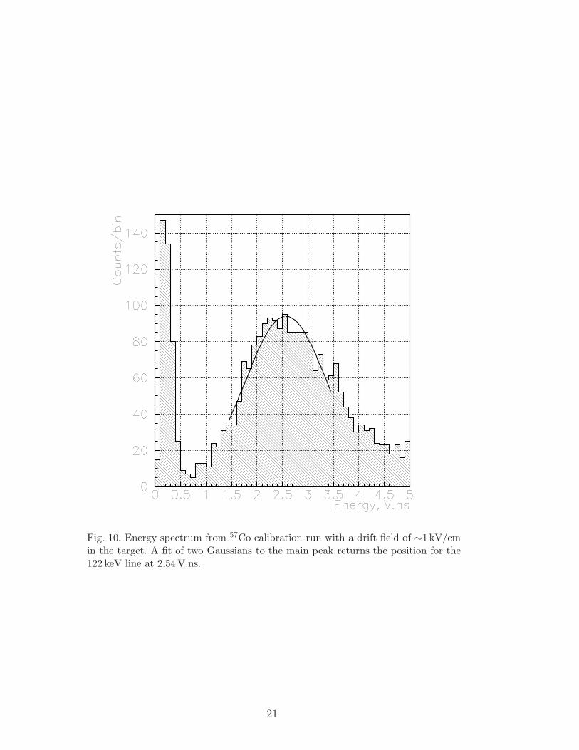
Fig. 10. Energy spectrum from 57Co calibration run with a drift field of ∼1 kV/cmin the target. A fit of two Gaussians to the main peak returns the position for the122 keV line at 2.54 V.ns.

21