U.S. DEPARTMENT OF COMMERCENational Technical Information Service

AD-A025 219

ACQUISITION, REDUCTION, AND ANALYSIS OF

ACOUSTICAL DATA, AN UNCLASSIFIED SUMMARY OF

ACOUSTICAL WORKING GROUP STUDIES

CBS LABORATORIES

PREPARED FOR(

NAVAL AIR DEVELOPMENT CENTER

JUNE 1974

- . -- - . -- - -

-- 4 M, IN. -

i~i1A.

0,

£ N4l ifEPRODUClop,

TINA TECH1CA

>OMTO EVCA EAI~Eg FCUEC

4i IGFED.V. 26

DJoI1IONsrl~4Pv~ f. uli ~o~

41, i ~nUhi~~~

ow- ~ I ''

LJNCLASSIFIEDSECURITY CLASSIFICATION OF THIS PAGE ("Thon Data Entered)

REPORT DOCUMENTATION PAGE READ INSTRUCTIONSBEFORE COMPLETING FORM

I. REPORT NUMBER 2. GOVT ACCESSION NO 3. RECIPIENT'S CATALOG NUMBERNADC-AWG-SU 1

4. TITLE (and Subtitle) S. TYPE OF REPORT & PERIOD COVEREDFinal Unclassified Summary

ACQUISITION, REDUCTION, AND ANALYSIS OF -Uls e1.

ACOUSTICAL DATA, Unclassified Summary, 1967 - 19T4Acoustical Working Group Studies 6. PERFORMING ORG. REPORT NUMBER

NADC-AWG-SU

7. AUTHCR(#) Acoustical Working Group 8. CONTRACT OR GRANT NUMBER(e)

Benjamin B. Bauer, Technical Editor N62269-7l-C-0258(CBS Laboratories)

PERORUNGJac R. Harris. AG Chairman (NAC)• EFRIGORGANIZATION NAME AND ADDRESS 1O. PROGRAM ELEMENT. PROJECT. TASK

AREA & WORK UNIT NUMBER;Naval Air Development Center

Warminster, Pa. 18974 N/A

II. CONTROLLING OFFICE NAME AND ADDRESS 12. REPORT DATE

Naval Air Development Center June 1974Warminster, Pa. 18974 13. NUMBER OF PAGES

14. MONITORING AGENCY NAME & AODRESS(I! Clff1rent from Controlling 0111ce) 15. SECURITY CLASS. (of this report)

N/A UNCLASSIFIED

15a. DECL ASSI FICATION/DOWNGRADINGSCHEDULE N/A

16. DISTRIBUTION STATEMENT (of this Report)

N/A

17. DISTRIBUTION STATEMENT (of the abstract ent red In Block 20, It different from Report)

N/A

It. SUPPLEMENTARY NOTES

N/A Rim $m ,ECT OW4It. KEY WORDS (Continue on e.vere Ide I n~ceear' and Identify by lbock numba,)

Data collection Time domain format Propagation dataData reduction Directional sensors Man-made soundsData analysis Arrays Natural soundsCategorizing data Correction techniques Ray theoryFrequency domain format Mathematical modeling Normal mode theory

20. ABSTRACT (Co A lnue on rveme side It necenary and Identify by block number)

With the ending of American military involvement in the Indochina conflictit became appropriate to summarize the unclassified aspects of those in-vestigations which might have a reference value to future scientific work-ers both in the civilian and military endeavors. The investigations ofthe Acoustical Working Gioup (AWG), a committee of knowledgeable personsfrom various civilien and Deptrbment of Defense agencies responsible forperforming acoustical studies relevant to the Indochina conflict, clearly

DD JA 1473 EDITION OF, NOV, 1 IOBSOLETE UNCLASS IFIEDS/N 0102-014-6601 I

SECURITY CLASSIFICATION I'IF THIS PAGE (n'hon Dats a416t00

UNCLASS IFIED-LLJ4ITY CLASSIFICATION OF THIS PAGE(Whew Date Entered)

fall in this category. T-hey embrace, in general, the study of sound prop-egation, a subject important to noise abatement, hearing protection, andother ecological and environmental concerns. Some of these studies (morethan 50 formal reports were prepared in a period of five years) also aresignificant in a general academic sense and as such have been selected toappear in this vol~me. The topics covered are data acquisition, reduction,analysis, acoustical propagation, and the characteristics of sound sources.

f

1k

I

T NCLASS IFIEDSECURITY CLASIFICATION; OF THIS PAGE(When Data Entertd)

2- bo ... oowe ooo

ACQUISITION, REDUCTION, AND ANALYSIS

OF ACOUSTICAL DATA

AN UNCLASSIFIED SUMMARY OF

ACOUSTICAL WORKING GROUP STUDIES

NADC REPORT NO. AWG-SIU

DEPARTMENT OF THE NAVY

NAVAL AIR DEVELOPMENT CENTER n- D C

WARMINSTER, PA. JUN 4 197

1974 L L LJu

A

DISTUTPIIO S iL2 IAppove& foz pu lic rle o

Dintrilbuli0o Un]li6ted

PRODUCT ENDORSEMENT - The discussion or instructions concern-ing comIuercial products herein do not constitute an endorsement bythe Government nor do they convey or imply the license or right to usesuch products.

III

Library of Congress Catalog Card Number: 74-600100

Printed for the Naval Air Development Center by CBS Laboratories,Stainford, Connecticut, a division of CBS Inc.

This book is dedicated to the first Director

and the Techmical Director of the Defense Coyn-

munications Planning Group, later renamed the

Defense Special Projects Group, LTGEN Alfred

D. Starbird, USA(RET) and Mr. David Israel, and

to their respective successors, GEN John D.

Lavelle, USAF(RET) and LTGEN John R. Deane,

Jr., USA, whose vision and encouragement chart-

ed the mission of the Acoustical Woring Group.

.10

00

il

OF

DEPARTMENT OF THE NAVYNAVAL. AIR DEVELOPMENT CENTER

WARMINSTER. PA. 18974

ACOUSTICAL WORKNG GROUP STUDIES

ACQUISITION, REDUCTION, AND ANALYSIS

OF ACOUSTICAL DATA

UNCLASSIFIED SUMMARY

REPORT NO. NADC-AWG-SU May 1974

ABSTRACT

With the ending of American military involvement in theIndochina conflict it became appropriate to summarizethe unclassified aspects of those investigations whichmight have a reference value to future scientific work-ers both in -the civilian and military endeavors. Theinvestigations of the Acoustical Working Group (AWG),a committee of knowledgeable persons from various civil-ian and Department of Defense agencies responsible forperforming acoustical studies relevant to the Indochinaconflict, clearly fall in this category. They embrace,in general, the study of sound propagation, a subjectimportant to noise abatement, hearing protection, andother ecological and environmental concerns. Some ofthese studies (more than 50 formal reports were preparedin a period of five years) also are significant in ageneral academic sense and as such have been selected toappear in this volume. The topics covered are data ac-quisition, reduction, analysis, acoustical propagation,and the characteristics of sound sources.

Benjamin B. Bauer, Technical EditorJack R. Harris, Chairman

v

FOREWORD

In early 1967 a committee of knowledgeable persons from industryand the Department of Defense was formed under the title of "Acous-tical Working Group" (AWG), i-.s chairman reporting to the Naval Ai"(later Electronics) Systems Command. The functions of the Group wereto conduct studies and to advise on matters relating to acoustics, ,ithspecial emphasis in the areas of sound propagation, reception, andsignal processing and associated engineering disciplines. Formed tomeet the needs of certain classified projects in the Department ofDefense, the Group operated in a manner similar to the divisions ofthe National Defense Research Committee (INDRC) of World War II. TheGroup's original membership comprised:

Mr. Benjamin B. Bauer - CBS LaboratoriesMr. Edward T. Hooper - Naval Air Systems CommandMr. Rowland 11. McLaughlin - Univeisity of MichiganDr. John C. Munson - Naval Air Systems Command.I1r. Joseph Petes - Naval Ordnance Laborator-y: Mr. Forrest C. Titcomb - Naval Research Laboratory

SCDR Jack R. Harris - Naval Air Development Center, Chairman

Later, as program emphasis changed, the Group was expanded to include:

Mr. Edward J. Foster - CBS LaboratoriesDr. Paul E. Grant - Department of DefenseMr. Donald Grogan - Picatinny Arsenal (Army)Mr. Robert F. Hand - University of MichiganMr. C. William Hargens - Franklin Institute (Consultant)Mr. James R. Howard - Naval Air Development Center1-r. Sidney Krieg - Naval Air Development CenterLT Robert H. Marks - Department of DefenseMr. Richard G. Satz - Picatinny Arsenal (Army)Dr. Tsute Yang - Villanova University (Consultant)

Though the group as originally constituted was dissolved when its

mission was completed, some of its studies were of sufficient generalinterest to warrant republication in a summary fashion. This reportencapsulates, as appropriate, all of the unclassified aspects of AWGstudies including procedures and results, with Chapters 1 and 2 pre-viously separately reported. Classified summary results are expectedto be reported at a later date. The technical editor appointed forthese efforts was Mr. Benjamin B. Bauer of CBS Laboratories. He wasresponsible for editing the material contributed by appropriate AWGmembers.

JACK R. HARRIS

Scientific OfficerNaval Air Development Center

Pr~ii aeblank vii

Acoustical Working Group Studies

ACQUISITION, REDUCTION, AND ANALYSIS

OF ACOUSTICAL DATA

PREFACE

This volume is a collection of techniques related to thescience of data acquisition, reduction and analysis developedand used by the Acoustical Working Group in the course of itsstudies, together with a summary of the essential theoreticalprinciples needed to understand their proper use. A catalogof the data gatheree by AWG in the course of its studies isprovided. And, since verL'al descriptions cannot replace theaural experience, a 7-inch, 33-1/3 rpm disk record containingsome of the exotic, as well as common, sounds studied by AWG isincluded in a Docket inside the back cover of the book. Accessto the cat.Eloged data can be obtained by persons with justifiedrequirements upon application tc the Commander, U. S. Naval AirDevelopment Center, Warminster, Pennsylvania.

The publication of this volume at this time is believedto be of special importance in view of the burgeoning interestin the practice of noise control and environmental acoustics,which is so heavily dependent on accurate measurements and mean-ingful data reduction. Admittedly, much of the specific infor-mation discussed here will have no direct application to homeenvironments, nevertheless, the experience documented in thisvolume will prove to be extremely useful to the civilian practi-tioner. For one, under a single cover the text offers a completedescription of the methodology of obtaining accurate and reliableacoustical data and manipulating it into useful formats. To anexecutive responsible for decision-making in connection withacoustical studies, such a compendium is of imense benefit, for

Preceding page blank ix

L

it helps him to assess realistically the magnitude of a giventask and to chart accurately its successful execution. To thepersonnel planning the details of the project, or going into thefield without extensive prior sound-measurement experience, thisvolume providez detailed guidance on how to select and use equip-

ment, and how to maintain proper records and implement calibra.ionprocedures--which may well spell the difference between successand failure. And, to the data analyst, the text offers a varietyof alternative methods for reduction and presentation of data,

and suggestions for interacting with the data gathering teamsfor maximum information yield per umit effort.

Reviewing briefly the contents of this volume, Chapter One,which previously had been published as Report No. NIADC-AWG-Sl on

31 March 1969, is a collection of techniques and precautiousmeasures that have been found useful in gathering acoustical data,especially under inclement field conditions. It encourages thepractitioner to prepare careflly for the mission, to make speci-fic plans, to devise and acquire suitable instrumentation, and inother ways to perform preparatory tasks which ensure that the de-sired rcults are effectively obtained.

Chapter Two, previously issued as Report Io. INADC-AWG-S2 on1 October 1971, begins with the classification of the variousaspects of data reduction and analyzes their interface with thedata gathering function. This is followed by a review of the

theoretical aspects of various methods of frequency- and time-domain analyses, a description of the instruments and recommendedpractices for their use, and suggestions about presentation ofresults. It should be noted at this writing that modern computerteclmology has now provided us with new and sophisticated tools--such as the Fast Fourier Transform and the Integrating FrequencyAnalyzer--which were just coming into their own during AWGstudies; nevertheless, the basic considerations in Chapter Twoare as applicable today as they were during the early stages ofAWG work.

Chapter Three is a compendium of the various aspects ofsound-wave propagation that should be clearly kept in mind byall persons engaged in acoustical data acquisition, reduction,and analysis. This chapter summarizes the basic ray and thenormal-mode theories and reviews the effects of temperature,wind, channeling, scattering, etc. that will be especially use-ful to those engaging in the studies of distant propagation ofsound in urban and suburban settings. Examples of propagationbehavior in the air are given.

x

Chapter Four develops a logical procedure for catalogingthe results of acoustical studies and provides a useful com-pilation of examples of various types of sound studied by AWG.

It also contains a selective catalog of the detailed reports

prepared by AWG. And, finally, the disk record furnished with

the volume provides the naturalist and the urbanologist alikewith a sampler of interesting acoustical- signatures.

Having been privileged.to participate in the work of AWGsince its inception, the Technical Editor cannot help but observe

how useful this volume might have been had it been available tothe Committee at the outset, rather than toward the end of itsmission. This would have saved countless annoyances and madeour task much easier. But this is akin to wishing that in youthwe had the expe-ience gathered during a lifetime. In providingthis summary of AWG studies, we trust that future workers innoise control and environmental acoustics will profit by availingthemselves of the tec., iques here outlined, and thus be able toperform more effective service on behalf of a quieter world.

A few words of credit are in order. What has distinguishedAWG from other Committees and Boards in which this TechnicalEditor has participated is the resolute and tireless dedicationof its members, all of whom have made significant contributionsto the work of the Committee and to the preparation of its reports;with special mention due its indefatigable Chairman who always pro-vided effective and inspir7ing'leadership and invariably managed tosee each task through even when all else seemed to fail. In addi-

tion, he was a principal contributor tc. numerous AWG reports and touhis final volume. An expression of gratitude also is accorded toSherman Levin of CBS Laboratories who managed the editorial and pro-duction work for many AWG reports and for this final volume.

Benjamin B. BauerStamford, ConnecticutMay 1974

xi

CONENTS

ABSTRACT .. . . . . . . . . . . .. . . . . . . . . . . v

FOREWORD .........................

PREFACE . . . . . . . . . . . . . . . . . . . . . .. ix

I CHAPTER ON4E

DATA ACQUISITION

1.1 INTRODUCTION ................................ 1-1

1.2 PREPARING FOR AN ACOUSTICAL DATAGATHERING MISSION ........................ 1-1

1.2.A Analysis of Objectives ....................... 1-11.2.B Recognizing the Need for Special Equipment .. 1-21.2.C Utilizing P'ractice Runs ...................... 1-21.2.D Advance Information Desirable ................ 1-3

1.3 PLANNING THE MISS ION ........................ 1-31.3.A General .................................... 1-31.3.B Site Selection .............................. 1-4i1.3.C Site Plan ................................... 1-41.3.D Dimensions, Distances, Parameters .............1-41.3.E Data Sheet .................................. 1-51.3.F Climatic Conditions ......................... 1-51-3-G Importance of Field Laboratory ............... 1-52,.3.H The Personnel ............................. !-1.3.1 Conclusion .................................. 1-6

1.4h EQUIPIMNT CONSIDERATIONS ..................... 1-61.14.A Custody of Equipment ......................... 1-6

Preceding page blankxiii

COM S (Cont.)

1.4.B Supplementary Tools and Equipmenb ........... 1-71.h.C Ranges of Level and Frequency ............... 1-71.4.D Measurement and Recording of Atmospheric

Conditions ............................... 1-81.4.E Wind Effects ................................ 1-81.4F Multiplicity of Sites and Time Correlation .. 1-91.4.G Batteries, Illumination ..................... 1-91.4.11 Typical Arrangement of Apparatus ............ 1-91.4.1 Selection of Microphones .................... 1-121.4.J Wind-and-Rain Screens ....................... 1-131.4.K Line Driving Amplifiers ..................... 1-161.4.L RF Pickup ................................... 1-181.4.M Electrolysis ................................ 1-201.4.N Controlling the Recording Level ............. 1-201.4.0 Tape Recorders .............................. 1-221.4.P Recorder Calibrator ......................... 1-231.4.Q Recording Tape .............................. 1-23

1.5 FIELD PROCEDURES ............................ 1-233.5.A General ..................................... 1-231.5.B Development of the Test Plan ................ 1-241.5.C Equipment and Personnel Requirements ........ 1-291.5.D Scheduling the Tasks ........................ 1-301.5.E Implementing the Plan ....................... 1-311.5.F Communications .............................. 1-33

1.6 FIELD LABORATORY PROCEDURES ................. 1-34

1.7 1RITTEN FIELD PROCEDURES .................... 1-35

CHAPTER TWO

DATA ANALYSIS AND REDUCTICN

2.1 II_ RODUCTION ................................ 2-12.1.A Purpose ..................................... 2-1

xiv

CONTENTS (Cont.)

2.1.B General Aspects of Data Reduction and

Analysis ................................. 2-12.1.C Categorization of Data ...................... 2-32.1.D Definitions and Units ....................... 2-5

2.2 THEORY AND PRACTICE OF DATA REDUCTIONAND ANALYSIS ............................. 2-10

2.2.A Introduction ................................ 2-102.2.B Fourier Series .............................. 2-112.2.C Fourier Integral ............................ 2-132.2.D Signal Characteristics in the Frequency

Domain ................................... 2-142.2.E Practical Approach to Frequency Analysis .... 2-202.2.F Signal Characteristics in the Time Domain ... 2-302.2.G Correlation in the Time Domain .............. 2-342.2.H Utilization of Time Domain Information ...... 2-36

2.3 FREQUENCY DOMAIN DATA ANALYSIS .............. 2-37

2 3.A Introduction ................................ 2-372.3.B Constant Bandwidth (Af) Analysis ............ 2-492.3.C Proportionate Bandwidth (Af/f) Analysis ..... 2-522.3.D Real-Time Analysis .......................... 2-602.3.E Other Techniques ............................ 2-65

2.4 TIME DEPENDENT FREQUENCY DOMAINDATA REDUCTION ........................... 2-66

2.4.A Introduction ................................ 2-662.4.B Sonograph-Type Display ...................... 2-662.4.C Contour Graph Display ....................... 2-682.4.D 3-D Spectral Display ........................ 2-68

2.5 TIME DOMAIN DATA REDUCTION .................. 2-702.5.A Introduction ................................ 2-702.5.B Raw Data Reduction and Display .............. 2-722.5.C Envelope Data Reduction and Display ......... 2-74

2.6 SPECIAL DATA REDUCTION TECHNIQUES ........... 2-782.6.A introduction ................................ 2-782.6.B Azimuth Location ............................ 2-7G2.6.C Detection of Elevation ...................... 2-80

xv

CONTENTS (Cont.)

2.6.D Detection via Correlation ................... 2-842.6.E Arrays ..................................... 2-862.6.F DEMON ........ 2-90

2.7 MODELING .................................... 2-922.7.A Introduction ................................ 2-92

2.7.B Basic Considerations for Modeling ........... 2-922.7.C Model Structure, Sources .................... 2-942.7.D Model Structure, Transducers ................ 2-942.7.E Model of Sound Propagation .................. 2-95

ICHAPTER THREE

PROPAGATION

3.1 INTRODUCTION ................................ 3-1

3.2 ANALYSIS OF SOUND PROPAGATION ............... 3-23.2.A Introduction ................................ 3-23.2.B Excess Attenuation .......................... 3-23.2.C Dependence on Humidity and Scattering ....... 3-3

3.3 RAY PATH THEORY ............................. 3-113.3.1. Refraction .................................. 3-43.3.B Effects of Temperature and Wind ............. 3-53.3.C Temperature Gradients ....................... 3-63.3-D Sound Channeling ............................ 3-8

3.4 NORMAtL-MODE THEORY .......................... 3-8

3.5 SCATTERING ;AND REVERBEFIATION ................ 3-14

3.6 SUMMARY OF FIELD RESULTS .................... 3-163.6.A Description of Test Procedures .............. 3-163.6.B Summary of Field Results .................... 3-18

xvi

CONTENTS (Cont)

3.7 DISCUSSION AND CONCLUSIONS ................... 3-213.7.A Attenuation Coefficients and Time Constants .3-213.7.B Predetection and Post-Detection Filtering .. 3-303.7.C Propagation of Explosive Sounds .............. 3-30

CHAPTER FOUJR

CHARACTERISTICS OF SOUND SOURCES

4.1 INTRODUCTION ................................ 4-14.1.A General Remarks ............................. 4-14.1-.B Presentation of Data ........................ 4-34.1.C Cataloging Sounds ........................... 4-54.1.D Source Characteristics ....................... 4-7

4.2 NATURAL SOUNDS .............................. 4-94.2.A General ..................................... 4-94.2 .B Caracteristics of Natural Sounds .............4-104.2.C Jungle Sounds ............................... 4-104.2.D Wind....................................... 1-124.2.E Rain....................................... 4-14

4.3 MAN-MADE SOUNS ............................. 4-144.3.A General Remarks ............................. 4-.44-3.B Truck Signatures ............................ 4-204.3.C Notes on Internal Combustion Engine

Signatures ............................... 4-224.3.D Aircraft .................................... 4-304.3.E Personnel ................................... 4-404.3.F Impulse ................................... -74.3.G Boats (Air Path Over Water) .................. 4-b24.3.H1 Boats (Underw'ater Sound) ..................... 4-444.3.1 Aerodynamic Noise .......................... 4-5

4.4 TOPICAL SUMARY OF USEFUL SOUND DATA .......... 4-46

xv12

COHTENTS (Cont.)

BIBLIOGRAPHY ................................ 5-1

APPENDIXES: WRITTEN FIELD PROCEDURESA. Field Calibration Procedure .......... A-iB. Field Test Operation Procedure ..... B-IC. Field Equipment Check List ........... C-1D. Field Log ............................ D-1E(l). Before-Use Equipment Checkout and

Calibration for Sound Level Meter .. E(l)-1E(2). Before-Use Equipment Checkout and

Calibration for Preamplifier ....... E(2)-lE(3). Before-Use Equipment Checkout and

Calibration for Microphone ......... E(3)-l

INDEX ....................................... I-i

DD FOPM 1473 ................................

A 7-inch, 33-1/3 rpm disk record containingrepresentative sounds studied by AWG is in-cluded in a pocket inside the back cover.

xviii

r

ILLUSTRATIONS

CHAPTER ONE

DATA ACQUISITION

FIGURE PAGE

1-1 Photograph and Block Diagram of Typical Arrange-ment of Apparatus for Data Gathering ...... 1-10

1-2 Calibration of the Equipment ................. 1-111-3 Typical Condenser Microphone (1/2" Diam.) .... 1-141-4 Typical Ceramic Microphone (15116" Diam.) .... 1-14

1-5 Typical Dynamic Microphone (1-1/8" Diam.) .... 1-151-6 Wind-and-Rain Screen for the Acoustical

Data-Gathering Microphone ................. 1-151-7 Windscreen-Testing Equipment ................. 1-171-8 Windscreen Effectiveness (10 mph Wind) ..... .. 1-171-9 Line-Driving Amplifier Schematic ............. 1-191-10 Line Driving Capability ...................... 1-191-11 Modified Sound Level Meter ................... 1-211-12 Square Wave Calibrator with Circuit Diagram .. 1-25

CHAPTER TWO

DATA ANALYSIS AND REDUCTION

2-1 Spectrum of Unweighted Window ................ 2-232-2 Comparison of Various Weighting Functions .... 2-232-3 Spectrum of a Sliding Tone,

Uniform Weighting ....................... 2-272-4 Spectrum of a Linear One-Sided Frequency

Slide, Uniform Weighting .................. 2-272-5 Spectral Response of the Filter

h(x) = cos2 rx to a Sliding Tone ........... 2-272-6 Spectral Comparison of White Noise

and Delta Function ........................ 2-312-7 Pictorial. Representation of Signal Envelope

Showing Rise Time (TR), Duration (TD),and Fall Time (TF) ....................... 2-35

xix

ILLUSTRATIOS (Cont.)

FIGURE PAGE

2-8. Pressure Spectrum Levels Obtained by One-ThirdOctave Analysis of a Continuous Signal andMasking Noise Source, Normalized to 1 HzBandwidth .................................... 2-41

2-9. Signal-to-Noise Ratio Plot Derived from Super-position of Spectra Shown in Figure 2-8 ... 2-41

2-10. One-Third-Octave Analysis of a ContinuousNoise Source Showing the Effects of Band-width Normalization ........................ 2-43

2-11. Spectrum Analysis of a Complex Sir al Using aConstant Bandwidth (20 Hz) Analyzer ........ 2-46

2-12. Spectrum Analysis of a Complex Signal Using a

1/3-Octave Analyzer ......................... 2-46

2-13. Signal-to-Noise Ratio Estimated for the Com-binabion of Noise Shown in Figure 2-8 andComplex Signal Shown in Figure 2-11 ........ 2-47

2-14. Signal-to-Noise Ratio Estimated for the Com-bination of Noise Shown in Figure 2-8 and.Complex Signal Shown in Figure 2-12 ........ 2-47

2-15. Block Diagram of Typical Constant BandwidthAnalyzer ................................... 2-51

2-16. Spectrum Translation ......................... 2-512-17. Af Analysis of 1 kHz Square Wave .............. 2-532-18. Parallel or Contiguous Band Analyzer .......... 2-552-19. Contiguous Band Analyzer Filter Response ...... 2-552-20. Contiguous Band Analyzer with Commutated

Detector ................................... 2-572-21. Swept Proportionate Bandwidth Analyzer ........ 2-572-22. Block Diagram of Analyzer and Integrator ...... 2-572-23. Example of Af/f Pnalysis of the Noise Generated

by a 10 mph Wind Speed on a Microphone ..... 2-582-24. Simplified Block Diagram of Real-Time

Analyzer .................................. 2-61

2-25. 2-1/2 Ton, 6 x6 , M35A1 5 mpn; 1st Gear; 1500rpm, Exhaust Away from Miciophone (LeftSide) 16-Second Average ................... 2-63

2-26. 2-1/2 Ton, 6x6, M35Ai 10 mph; 2nd Gear; 1700

rpm, Exhaust Aray from h. crophone (LeftSide) 16-Seccnd Average ................... 2-63

2-27. Example of Sonograph Display (AnalysisBandwidth 2.8 Hz) ......................... 2-67

XX

II

ILLUSTRATIONS (Cont.)

FIGURE PAGE

2-28. Example of Contour Graph Display ............. 2-672-29. Example of 3-D Spectral Display .............. 2-692-30. Typical Oscilloscope Traces of Measurements of

Sound Pressure of Explosions Taken at Dis-tances ot 50' and 140' from the Event ...... 2-73

2-31a. Response of a 5-Pole Butterworth Low-PassFilter to Square Wave ..................... 2-75

2-31b. Response of 5-Pole Bessel Low-Pass Filter toSquare Wave ............................... 2-75

2-32. Block Diagram of Electronic Input Processor .. 2-752-33. Detector Linearity Calibration ............... 2-772-34. Examples of Time Domain Analysis ............. 2-792-35. Directional Characteristic of Gradient

Microphone ................................ 2-792-36a. Acoustic Azimuth Locator (Microphone Array) .. 2-812-36b. Acoustic Azimuth Locator (Processor) ......... 2-812-37. Apparatus for Simultaneous Generation of

Multiple Microphone Patterns .............. 2-822-38. Microphone Sensitivity Patterns: (a) Omni-

directional Pattern; (b) Gradient Pattern;(c) Donut Pattern; d) Cardioid Pattern ... 2-83

2-39. Block Diagram of Up/Down Sensor .............. 2-852-40. Correlation Plot of Moving Vehicle ........... 2-852-41. Correlation Plot from Aircraft ............... 2-872-42. Enhanced Correlation Plot from Aircraft ...... 2-872-43. Four-Microphone Linear Array ................. 2-892-44. Four-Microphone Linear Array Polar Pattern

for k = X/4............................ 2-892-45. Four-Microphone Linear Array Polar Pattern

for k = X/2 .............................. 2-892-46a. Sonograph Display of Raw Data ............... 2-932-46b. Sonograph Display of D,,ON Data ............. 2-93

CHAPTER THREE

PROPAGATION

3-1. Snell's Law: c1 /c 2 = sin @./sin G2 ........... 3-5

xxi

ILLUSTRATIONS (Cont.)

FIJURE PAGE

3-2. Construction of Ray Direction ................. 3-73-3. Sound Rsys in a Medium of Negative

Temperature Gradient ....................... 3-73-4. Example of Temperature Profiles at Three

Times of Day ............................... 3-93-5. Velocity Profile and Ray Diagram .............. 3-93-6, Formation of a Sound Channel .................. 3-93-7. Sound Pressure Versus Depth for the First

Four Modes for a Pressure-Release (Soft)Surface and a Rigid (Hard) Bottom .......... 3-13

3-8. Plane-Wave Equivalents of the First and SecondModes in a Duct with a Pressure-ReleaseSurface and a Rigid Bottom ................. 3-13

3-9. Propagation Paths Between a Source and aReceiver in Deep Water ..................... 3-13

3-10. Typical Pressure Signature Near 1.5-gram

Charge of TNT .............................. 3-153-11. Pressure/Time for Ideal Shock Waves ........... 3-173-12. Spectrum level of Shock-Wave Portion of 1.5-

gram Charge of TNT Recorded in Woods ....... 3-173-13. Signal-to-Noise Ratio Versus Frequency for

500 ft Distance and Various BackgroundNoises; Source 1.5-gram Explosion TNT ...... 3-19

3-14. Amplitude Versus Time Presentations (1 ms/cm);Frequency Limits 50 to 5000 Hz ............. 3-22

3-25. Amplitude Versus Time Pceseutations (50 ms/cm);Frequency Limits 50 to 1000 Hz ............. 3-23

3-16. Amplitude Versus Time Presentations (1 ms/cm);Frequency Limits 50 to 5000 Hz ............. 3-24

3-17. Time Domain (10 ms/cm) Presentations forSignal (No. 1 Shot, 50 Feet, West Leg, SiteTwo) Plus Random Noise for Different Pre-detection Bandwidth ........................ 3-25

3-18. Post Detection Outputs for Various RC LowPass Filters, Predetection Bandvidth

60 to 200 Hz ............................... 3-263-19. Typical Background Noise Time Domain

Presentations .............................. 3-193-20. Pressure Spectrum Level Versus Frequency for

Background Noise, Site 2, 100 Hz AnalysisBandwidth for Three Different SamplesWithin One Minute .......................... 3-28

xxii

ILLUSTRATIONS (Cont.)

FIGURE PAGE

3-21. Pressure Spectrum Level Versus Frequency forLight Rain, Runs 2 and 3 Have RaindropNoise; 100 Hz Analysis Bandwidth, Site 3 ... 3-29

CHAPTER FOUR

CHARACTERISTICS OF SOUND SOURCES

h-1. Kay Analyzer Section Spectrograms Taken atTimes T1 and T2 . . . . . . . . . . . . . . . . . . . . . . . . . . . . 4-5

4-2. One-Third Octave Analysis of a ContinuousNoise Source Showing the Effects of Band-width Normalization Modified by Additionof Calculated Normalization Corrections .... 4-9

4-3. Quiet Jungle Spectrum Laowing Insect NoiseLevel at Observation Distance (Normalizedto 1 Hertz Bandwidth) ...................... 4-13

4-h. Sound Spectrometer Identification of theFrequency Location, Pulse Rate and Dura-tion of a Distinct Chirping Sound in aNoisy Environment .......................... 4-13

4-5. Wind Noise Spectrum ........................... 4-154-6. Wind Noise as a Function of Wind Speed (in the

Frequency Range 20 Hz-20 kHz) Measured Withand Without Windscreen ..................... 4-15

4-7. Typical Response Characteristics for CeramicMicrophones (a) 1-in., (b) 1/2-in . ....... 4-16

h-8. Wind hoise Fluctuations Relative to BirdCall BPL ................................ .. 4-17

4-9. Wind Noise Fluctuations Against BackgroundSound of Running Stream .................... 4-1T

4-10. Rain Spectrum ................................. 4-194-11, Spectrogram, Broadband and Narrow Band, for a

5-Ton Diesel Truck at 10 mph, 2nd Gear ..... 4-244-12. Spectrogram, Broadband and Narrow Band, for a

5-Ton Diesel Truck at 20 mph, 4th Gear ..... 4-244-13. Truck Classification by Spectral Analysis ..... 4-25

xxiii

ILLUSTRATIONS (Cont.)

FIGURE PAGE

4-14. Engine Idle Spectrum, LargeReciprocating Engine ...................... 4-26

4-15- Engine idle Spectrum, Large ReciprocatingEngine, Portion of Figure 4-1, Expandedfor Greater Detail .......................... -7

4-16. Engine Idle Spectrum, Large ReciprocatingEngine, Portion of Figure 4-15 FurtherExpanded .................................... 14-28

4-17, Large Reciprocating Engine, 2nd Gear Spectrm .. 1-294-18. Large Reciprocating Engine, 4th Gear Spectrum 4-314-19. Jet Aircraft Characteristics ................... 4-354-20. Jet Aircraft at 10,000-ft Altitude ............. 4-354-21. Jet Aircraft Signature Contour Map 10,000 ft

Overhead .................................... 4-364-22. Piston Aircraft at 1000-ft Altitude ............ 4-364-23- Jet Aircraft at 1,000-ft Altitude, 1/3-Octave

Analysis Digitally Computed Fast-FourierTransform, Normalized to 1 Hz EffectiveBandwidth ................................... 4-37

4-24. Piston Aircraft at 5000-ft Altitude, 1/3-OctaveAnalysis Digitally Computed Fast FourierTransform, Normalized to 1 Hz EffectiveBandwidth ................................... 4-37

4-25. Jet Aircraft Signature Showing Effect ofMultipath Propagation ....................... 4-38

4-26- Piston Aircraft Overflight ..................... 4-394-27. Spectrum Analysis for 1.5-Gram Explosive Shots

at 500 Feet, Range Site 1, East Leg, 100-HzAnalysis Bandwidth .......................... 4-43

xxiv

- s .. . . .. ..--- -s. -. - , , .. .... ....

NADC-AWG-SU

1.1-1.2.A

CHAITER on: DATA ACQUISITION

1.1 INTRODUCTION

The development of a system of acoustical detection for iden-tification and reaction requires the initial acquisition of acous-tical data upon which the system parameters wiLl be based. Muchof this data will be obtained outdoors in all kinds of weather,at various remote locations, and often under difficult and evenhazardous conditions. These circumstances present the acousticalsurveyor with a whole new set of problems normally not encoun-tered in the laboratory. This chapter describes the principlesof good engineering practice necessary to assure the acquisitionof accurate and reliable data in remote areas under extreme en-vironmental conditions. The information contained in this chapteris based to a large extent upon experience acquired during theperformance of Acoustical Working Group (AWG) missions. Thechapter can be used as the basis for practical data gatheringmissions with appropriate modifications to --uit the particularcircumstances.

1.2 PREPARING FOR AN ACOUSTICAL DATA GATHERING MISSION

A. Analysis of Objectives

The basic, but often neglected, task before starzing a dataacquisition mission is a careful analysis of objectives, whichmust be related to time and equipment limitations and to the,problems that may be expected in carrying out the mission. Oncea test is started it may become necessary to forego some objec-tives for others and, therefore, priorities should be attachedto the various objectives. For example, a recording techniquemight be needed for sound detection and analysis which is dif-ferent from that used for sound reproduction and simulation.If a choice must be made, it should be clearly understood which

1-1

NADC-AWG-SU

1. 2.A-1. 2. C

objective of the mission is the more important to avoid possibledisappointment.

An equally important aspect of the ultimate objectives isthe early recognition of the type of data reduction that will berequired. Unless the data reduction program has been plannedand its needs established prior to collecting the data, it isvery likely that more data than needed will be collected, butthe information content of the data may be insufficient for theneeds of the program.

B. Recognizing the Need for Special Equipment

Frequently, the type of terrain and the nature of the testmake it necessary to provide special instrumentation which mustbe designed and fabricated before the data acquisition task be-gins. Thus, as much advance notice as possible should be givento allow for readying the equipment. In one instance, beforeacquiring the signatures of certain vehicles, it was ascertained(fortunately in time to take remedial action) that the radiotransmission link introduced frequency response distortion whichrequired the construction of compensatory devices prior to re-cording. This corrective action taken during the definition andplanning phase enabled the mission to succeed where otherwiseit might have failed.

C. Utilizing Practice Runs

A preliminary, or "dry," run under conditions simulatingas close as practicable the actual test is almost invariablyfound to be helpful during the definition and planning stages.The dry run reveals the limitations of the equipment and person-nel and allows remedial action which would be difficult, if notimpossible, to take in the field. It also provides an opportu-nity to train new team members and to optimize the goals of themission in line with the capabilities of the available equipmentand time. A dry run is especially useful when a new parameteris introduced into the tests. For example, in a test which in-cluded the combined measurements of aerial and underwater sounds,the dry run revealed that some commercial hydrophones do nothave suitable electrostatic shielding. This factor is of no con-

1-2

' NADC-AWG-SU

1.2. C-1, 3.A

sequence for a sensor meant to operate at a depth of 100 feet ormore, but when used in shallow water in combination with land-basedinstrumentation, it was found that severe electrostatic pickup wasencountered requiring construction of special amplifiers and shield-ing devices. The mission would surely have been a failure if this"dry" run had not been conducted during the planning stages.

D. Advance Information Desirable

Sometimes security considerations severely limit the avail-ability ahead of time of the detailed information needed to carryout an acoustical data-gathering mission. In this circumstance,planning cannot properly begin until the team arrives at the testsite. However, as much information as security allows should besought in advance to help in planning and in determining theequipment to be taken to the site.

Contrary to a popular misconception, the weight and bulkof equipment necessary for conducting acoustical surveys can beconsiderable. To adequately prepare for expected contingencies,in addition, can involve very sizable quantities of material.For one recent data acquisition test, to adequately equip a four-man field team it was necessary to commercially airlift 2800pounds of equipment -- the largest single excess baggage loadin the history of the airline.

1.3 PLAITNING THE MISSION

A. General

The general plan begins with a study of objectives, consid-eration of the types of sounds to be recorded, selection and studyof the site and terrain, decisions concerning equipment and personnelrequired, and the time period(s) during which survey informationis to be obtained. The result of preparation of the plan is a FieldProcedure (discussed in Section 1.5) detailing (1) how to conductthe particular test, (2) what equipment to provide, (3) the respon-sibility of various team members, and (4) what is expected to becontained in the data. The development of a Field Procedure re-quires considerable experience, and the following are some high-light factors which should be considered.

1-3

NADC-AWG-SU

1. 3.8-1.3.D

B. Site Selection

Ideally, the measurements should be made at a site and underconditions similar to those f3r which the end product is intendedto be used. Frequently, however, this is not feasible and alter-native sites must be selected. A site should be chosen which isoperationally and acoustically similar to the ultimate use area.For example, the forest area should include similar trees to pro-vide the same type of canopy, scrub, or open terrain as in theexpected area of operation. Besides the forest area considera-tions, one should look for similar fauna and a simi.ar backgroundnoise level as in the ultimate operation. Finally, security con-siderations and support considerations must be phased into theselection of a site. This is especially true in cases in whichclassified materiel is to be employed during the test.

C. Site Plan

During the preparation of the mission, a map of the site ismost helpful. If one is not available, a sketch to approximatescale should be made at the earliest opportunity. In addition,photographs (especially aerial) are very helpful. Both the photo-graphs and the map will be found useful not only for planning thetest, but also for subsequent reduction of the collected data and,ultimately, preparation of the written report. The plan or mapshould indicate all the important details such as types of terrainand/or vegetation and any possible sources of anomalies and inter-fering sounds--hills and streams, buildings, etc.--which mayshield the sound, create an echo, etc.

D. Dimensions, Distances, Parameters

Provision should be made for establishing dimensions anddistances and for measuring other important variables. For ex-ample, if the purpose of the test is to measure the sounds ofvehicles along a road, stakes or markers or other suitable sight-ing devices should be provided to enable the drivers and observ-ers to read the positions as a function of time. If speed is oneof the variables, then the plar should include means for deter-mining and recording it. Things taken for granted often may foila plan. For instance, all the preparations for a vehicle speed-

mnN • g m • • • ; '

" N • • " • •

NADC-AWG-SU

1.3.D-1.3.G

vs.-sound-level test may be defeated if the speedometer on thetest vehicle is inoperative.

E. Data Sheet

A data sheet should be prepared which lists the acousticalevents to be recorded, together with a checklist of importantauxiliary information--wind, rain, time, etc. It should be re-membered, however, that an observer busy operating a tape recorderand adjusting its gain for maximum information does not have thetime to do much writing and a second man should be at the site tokeep the written log. Since a written log may get separated fromthe tape, all comments should be recorded on a voice track whichmust be provided for this purpose. The major importance of thewritten log is as an aid in data reduction. A well documentedlog provides the analyst a means of rapidly locating Rey segments

of data without the necessity of listening to the entire tape.For this purpose, correlation of the logs with a recorded timecode is invaluable.

F. Climatic Conditions

Climatic conditions, the time of the year, and whether it isday or night have an important bearing upon the plan. Despitecareful moisture-proofing, most equipment is subject to malfunctionwhen left outdoors in the rain, or when high humidity combined withtemperature changes causes moisture condensation. In this circum-stance special precautions, such as frequent desiccation, are needed

G. Importance of Field Laboratory

Usually it becomes important to provide a field laboratory,suitably air conditioned, to permit the equipment to be maintainedand to allow it to dry out and become stabilized and be recalibrateat intervals. The field laboratory also can be provided withequipment for preliminary scanning or taking a "quick look" atthe data. A great advantage of such preliminary reduction isthat the test plan may then be somewhat modified to insure thatthe ultimate objectives are raet. A safe should be provided forstoring all classified papers, tapes, and devices. Under un-favorable conditions when there is no time or opportunity to

1-5

NADC-AWG-SU

1. 3. G-1. 4.A

provide a field laboratory, minor maintenance can be carried outin the field or in a hotel room. Under extremely unfavorableconditions-as with tests which extend for several uninterrupeddays in rain and humidity--less precise, but more sturdy, equip-ment may have to be used. The detailed requirements for the fieldlaboratory are discussed later in Section 1.6.

H. The Personnel

The staffing of the team and assignment of tasks constitutean important part of the plan. Sending several people to a re-mote location involves considerable expense. On the other hand,it is usually not practical or advisable tc field less than twopeople per site (or minimum of three if the equipment must beremoved and redeployed each day). The age and health of the teammembers must be related to the stress involved, and such mattersas security clearmlices, passports, insurance, vaccination, andeven personal domestic problems may become formidable obstaclesto an otherwise perfect plan. Experience in field procedures is,of course, extremely important and although not every member ofthe field team need have prior experience, at least two men persite should be fully familiar with the operation and limitationsof the equipment.

I. Conclusion

The above brief description mentions only the most importantfactors to which the planner must address himself. The planshould always be evolved with the participation of the group leaderwho will be in charge of the team performing the tests and, ifpossible, with the advice of the more experienced field personnel.A more complete checklist for the items to be considered duringa plan and the equipment needed for a mission are suggested laterin this chapter, and in Appendix C.

1.4 EQUIPMENT CONSIDERATIONS

A. Custody of Equipment

One member bf the team must be placed in charge of the equip-ment and should be provided with a list of items for which he willbe accountable. In a multichannel system, the p3r-channel cost for

1-6

i NADC-AWG-SU

1.4.A-1.4. C

a suitabl3 microphone, preamplifier, line driver, and auxiliaryequipment runs in the thousands of dollars, and a multichannelportable tape recorder is also very expensive. Specially-builtshould be made to safeguard the equipment, to store it safelywhen the site is unattended, and to arrange for its deploymenton site in a timely manner. Provision must be made for pro-tecting both equipment and personnel from the weather. Theshelter must be located sufficiently far from the sensor loca-

tions to prevent its affecting the data. For example, humanactivity will inhibit local fauna sounds and so the recordingsite should be at least 1000 feet from the microphones. Duringthe AWG program, vans, tents, and station wagons have all beenused as equipment shelters. The ideal situation is to have avan in which the equipment may be permanently mounted and movedfrom site to site.

B. Supplementary Tools and Equipment

Not only is it necessary to furnish safeguards for expen-sive equilment, but provisions should be made for each site tohave a tool kit, flashlight and batteries, climbing equipment,and other items depending upon circumstances. One should con-sider those items which although within easy reach in the labo-ratory are inaccessible in the field.

C. Ranges of Level and Frequency

The expected ranges of level and frequency and type of datareduction desired play an important part in the selection ofequipment for data acquisition. For example, FM recording pre-serves the low frequency response and amplitude and phase integ-.city of data, while direct recording provides greater high-fre-quency range capability and greater time-capacity-per-reel.Changing reels of tape during the data acquisition process alwaysinvolves delays, and it is desirable to record only the minimumfrequency range at the slowest possible speed that will realizethe full potential of the rest. Although this requires that thefrequency range and S/N of the equipment exceed the range of thedata, it is wasteful, for example, to record with a 10 kHz and50 dB S/N capability if the sensor itself has a 1 kHz and 30 dBS/N range. On the other hand, it must be remembered that themaximum frequency ranges specified by the equipment manufacturersoften strain the performance limits of the equipment, and there-fore a generous margin for tolerance should be provided.

1-7

NADC-AWG-SU

1. 4. D-1. 4.E

D. Measurement and Recording of Atmospheric Conditions

If the atmospheric conditions form an important part of theplan, provision should be made for their measurement and record-ing. As an illustration, if rain is part of the test, the meas-urement of rain in terms of inches per hour is a much more mean-ingful quantity than the mere statement "hard rain," "mediumrain," etc. For this purpose, a simple rain gauge can be impro-vised of a tin can with its top removed. It is ideal if themeteorological data is recorded lirectly onto the magnetic tape.

E. Wind Effects

Wind is usually an important element, responsible for varioustypes of noise. it creates turbulence around the sound measuringmicrophone. It induces movement of the microphone often result-ing in that object coming in contact with others. It causesleaves to strike each other and excites resonances in open objects.By the interaction of cables and strings with the wind, the so-called "aeolian tones" are generated. All these effects shouldbe carefully considered, together with an evaluation of their im-portance or decision about methods for coping with them in the

field. For example, microphones and housings can be provided withwindscreens, but whereas the windscreen affects microphone high-frequency response and, as has been discovered only recently,also affects the low frequency response of certain directionalmicrophones, it must be preplanned and not makeshift.

Since wind is apt to be an important factor, usually it isalso important to provide a means for measuring and recording itsvelocity vs. time. (As a minimum, provision should be made inthe data log for making a notation of the approximate wind condi-tions, e.g. "slight wind causing the rustle of leaves.") Windvelocity can be measured with an anemometer. One type of gaugeis dependent upon rotating vanes or buckets, but its inertia doesnot allow wind gusts to be measured accurately. An electricalgauge based on the hot wire principle permits the measurement andrecording of the velocity of wind and wind gusts. Ideally, onedata channel should be used to record the output of the hot wireanemometer .hen the objective of the test is concerned with windactivity, e.g. the determination of the effectiveness of awindscreen.

I

= I1-8

NADC-AWG-SU

2. 4. F-1.4.H

F. Multiplicity of Sites and Time Correlation

The question of using, say, four-channel recorders at twosites vs. one seven-channel recorder interconnected by long cablesat one site depends upon equipment availability and the test param-eters. In general, the attempt is made to minimize the number ofindividual recording sites, provided the test can be adequately mon-itored from a smaller number of sites.

When time correlation among various tape recorders is neces-sary, a master time code such as IRIG-B should be transmittedthroughout the area and each recording site provided with a suit-able receiver.

The distance between the microphone and the recorder is animportant factor sice, in connection with the expected signal lev-els and energy srectrum, it determines -he power required to drivethe cable. These fa--tors should be considered in the plan and thenecessary cables and line drivers fabricated and tested ahead oftime inasmuch as a defective cable can cause major trouble in thelield. More about this will be found in Section K, below, and sub-sequent sections.

G. Batteries, Illumination

Batteries for running the recording equipment present aspecial problem and an adequate supply of batteries and/or stor-age batteries and recharging facilities must be provided. Ifnight operation is scheduled, suitable lights will be required.

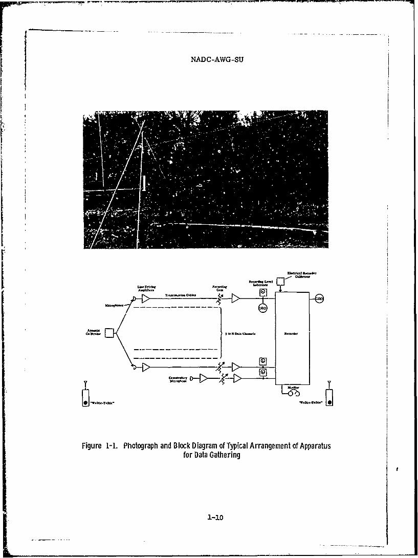
H. Typical Arrangement of Apparatus

An illustration of the interconnections and apparatus fordata gathering is shown in Figure 1-1. One tc N microphones areplaced in appropriate locations which must be an adequate dis-tance away from the tape recorder to prevent site activity fromaffecting the data. Each microphone is connected to a transmis-sion cable through an amplifier capable of driving the line. Atthe recorder, means must be provided for adjusting and monitor-ing the recording level. At least one track of the tape record-er is allocated for field operator commentary.

The prime calibration of the set-up is made using a knownacoustic source at the microphones as seen in Figure 1-2. Thesource may be a General Radio (1562A) Calibrator, a pistonphone,or calibrated bullhorn loudspeaker to be described. By thesemeans the signal level on the tape can be directly correlated

1-9

NADC-AWG-SU

ItCrt

TnmJ.Ck.

Figure 1-1. Photograph and Block Diagram of Typical Arrangement of Apparatusfor Data Gathering

1-i0

I NADC-A7WG-SU

Figure 1-2. Calibration of the Equipment

NADC-AWG-SU

1.4.H-1.4.I

with acoustic sound pressure level. A recorder calibrator capa-ble of providing a known electrical signal to the recorder isfrequently valuable both for recorder set-up and for establish-ing approximate acoustic level in those cases in which the fieldacoustic calibration is impracticable but where previous calibra-

tion data on the microphone is available.

Some means of monitoring the level of the recording is nec-essary to insure that the signal is well above the recorder noiselevel and below the overload point. Of course, the system noiselevel and overload point should have been previously establishedin the laboratory and documented for reference.

Earphones should be used in conjunction with the recordingmeter for monitoring the recording since one can usually deter-mine the existence of an acoustic anomaly most readily by listen-ing. An oscilloscope and/or peak reading storage meter suchas an impact meter is ideal for monitoring peak factors which arenot indicated on a meter. Such apparatus is imperative when re-cording impulsive data. It should be possible to monitor bothbefore and after recording to determine that the data is, indeed,being properly recorded.

Finally, "walkie-talkie" communication between the fieldoperator who may be calibrating the microphones and the tape re-corder operator is a great asset.

I. Selection of Microphones

Microphone characteristics can be considered under two clas-sifications. One of these concerns the directional characteris-tics of the microphone and the other concerns the frequency re-sponse and the particular type of transduction employed. In theformer category, a distinction can be made between the omnidirec-tional (pressure) microphones, gradient (velocity) microphones,cardioid microphones, and other higher order directional arrays.For most acoustical data gathering conditions, the omnidirection-al microphone is used. In some cases, however, the use of a di-rectional microphone may be appropriate especially if one wishesto either maximize or minimize sound sources from a particularlocation.

The second method of classification is by transducer tyje,i.e. condenser, piezoelectric (ceramic) or dynamic. Each oi thethree types of microphones offers certain advantages as well as

1-12

NADC-AWG-SU

i.4..I-1.4.J

disadvantages which must be considered. The condenser microphone(Figure 1-3) has the simplest physical construction and offers thebest frequency response and phase linearity and lends itself read-ily to precise calibration. Because the diaphragm of the conden-ser microphone is extremely light and is resonated in the upperrange of the bandwidth desired, the microphone is relatively insen-sitive to vibration. The main disadvantage of this type of micro-phone lies in its high source impedance which, unless special pre-cautions are taken, makes it sensitive to moisture. This handicaplimits the use of condenser microphones to laboratory applicationwhere the atmospheric conditions can be held under control.

The second type of microphone, the piezoelectric unit, is shownin Figure 1-4. Like the condenser microphone, it has flat frequencyresponse at audio frequencies and therefore, in the field, it is suf-ficient to calibrate its response at a few points. Because of itslower source impedance, it offers improved moisture immunity overthe condenser unit. The stiff and light transducer structure usedinsures low sensitivity to vibration. The piezoelectric microphone,such as the General Radio P-5 with suitable preamplifier and rain-and-wind screen (discussed in the following section), has been theprincipal data-gathering microphone in AWG work.

The final generic type microphone is the moving-coil dynamicoutlined in Figure 1-5. This unit is rugged and moisture-resistant.Its source impedance is very low, allowing long cable runs withoutthe need for preamplifiers. Because the frequency response is notas uniform as the previously described microphones, field calibra-tion of the unit at a few points is insufficient and the use of ananechoic chamber, is required. Furthermore, since the coil of thedynamic unit is relatively heavy and is resonated below 1000 Hz, itis more sensitive to mechanical vibration pickup than the other mi-crophones. Nevertheless, under conditions of extreme humidity andcontinuous use without the opportunity of dessication and recalibra-tion, the dynamic microphone (such as Model 655, especially moisture-proofed and anti-fungus-treated, manufactured by Electro Voice) hasbeen found to be extremely useful.

J. Wind-and-Rain Screens

To minimize the effect of wind turbulence around the sensor,a special wind-and-rain screen for acoustical data-gathering mi-crophones has been developed. As seen in Figure 1-.6, a preampli-fier is housed within the upper part of the enclosure and is pro-tected by a water proof seal. Since the problem o ' ind noise canbe extremely severe and flavor the acoustic data with the aero-

1-13

NADC-AWG-SU

I.I 900

c0

I 100 z I .00 10,000HZ

Figure 1-3.. Typical Condenser Microphone (112" Diam.)

9o

I e

1 0

2 o .-- -- '

1 00 1Hx I000 Z 10,

Figure 1-4. Typical Ceramic Microphone (15116"Diam.)

i-3.4

NADC-AWG-SU

0

06

*0

10 0P

Figure 1-5. Typical Dynamic Mircophone(118 Da.

Figure 1-6. Wind-and-Rain Screen for the Acoustical Data-GatheringMicrophone

1-15

NADC-AWG-SU

1. 4.J-.4.K

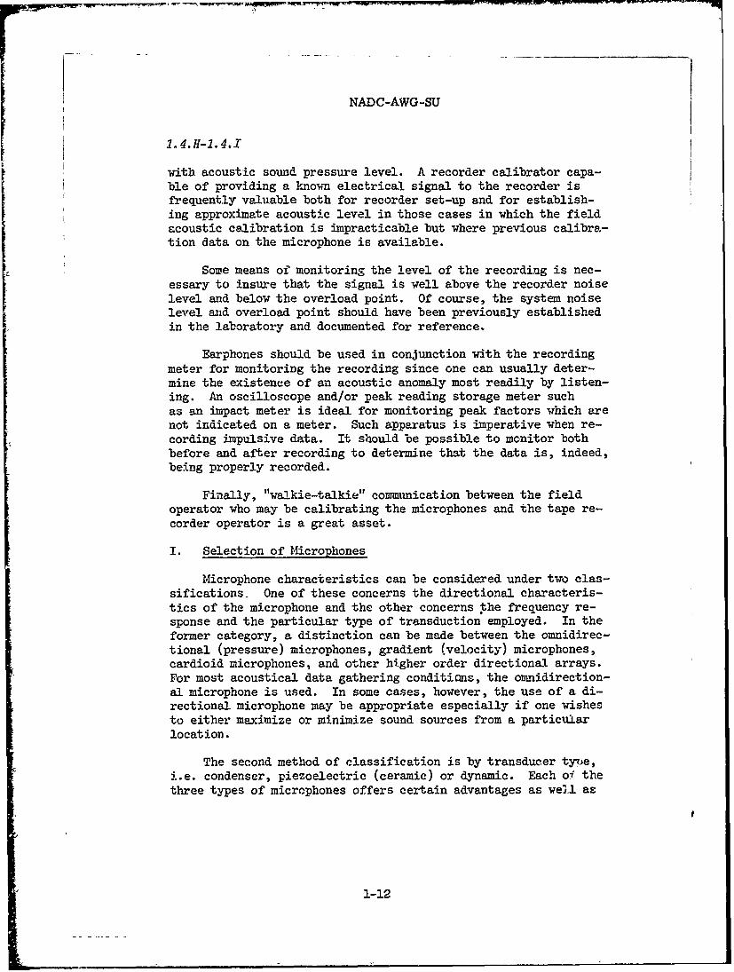
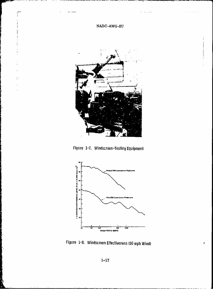
dynamic shape of the sensor chosen, CBS Laboratories developeda -indscreen testing machine capable of generating 30 mph Vind.This apparatus (Figure 1-7) has been used in the development of anew acoustical data-gathering windscreen which offers consider-

able improvement over the unprotected microphone. As seen inFigure 1-8, in the critical lower frequency regions in whichwind noise is most severe, a 25 dB improvement is noted. Thewindscreen portion is easily removed for acoustical calibration

of the microphone (Figure 1-2). It is important to provide a mi-crophone calibration in the anechoic chamber including the wind-screen to determine how it affects the overall response.

K. Line Driving Amplifiers

In setting up the apparatus for acoustical data gatheringthe engineer will, of course, check the output impedance of hispreamplifier to assure that the frequency response will not bedegraded by the cable capacitance. With the use of liberal

amounts of feedback in the preamplifier, the output impedance isusually very low and it would appear that long cables would notaffect the accuracy of the date acquisition. What is frequentlyoverlooked, however, is the capability of the amplifier to sup-ply sufficient current required by the line capacitance. Very

often the maximum output current capability of commercial pre-amplifiers is not specified.

Consider the problem of driving a 1000-foot cable with a10 kFlz signal whose magnitude is 1 volt rms. The cable capaci-tance is typically 50 pF/ft so that the total capacitance amountsto .05 jiF. At 10 kHz, the reactance of tiis capacitor is about310 ohms so that a peak drive current capability of 4.6 mA is re-quired. Two questions, then, must be answered: Is the outputimpedance of the preamplifier much lower than 310 ohms so thatthe frequency response will not be degraded?; and, Can the ampli-fier supply 4.6 mA of current to drive the cable capacitance?.The answer to both of these questions must be "yes" if the systemis to be used. Note that whereas the requirement on output im-pedance is independent of the signal levels, the drive capabilitymust be considered a function of the expected signal levels. Forexample, if we want to use this amplifier to drive a 3-volt rmssignal, it must be capable of producing peak currents of 14 mA.

In.order to assure accurate data acquisition, a new comple-mentary symmetry emitter follower line-driving amplifier has beendeveloped (Figure 1-9). This amplifier accepts a single-ended in-put signal and uses a phase-splitter to drive id.atical outputamplifiers, resulting in a balanced output configuration. A corn-

1-16

NADC-AWG-SU

Figure 1-7. Windscreen -Testing Equipment

-Wk CU Lb..tWd.. Ww'..

1-5

NADC-AWG-SU

1.4.K-1.4.L

plementary symmetry approach is employed to deliver the highpeak currents required to charge the line capacitance. The out-puts are, in effect, miniature class A-B amplifiers capable ofdelivering 100 mA peaks.

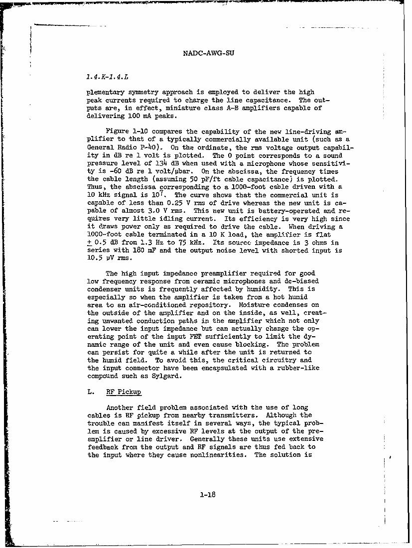
Figure 1-10 compares the capability of the new line-driving am-plifier to that of a typically commercially available unit (such as aGeneral Radio P-40). On the ordinate, the rms voltage output capabil-ity in dB re 1 volt is plotted. The 0 point corresponds to a soundpressure level of 134 dB when used with a microphone whose sensitivi-ty is -60 dB re 1 volt/pbar. On the abscissa, the frequency timesthe cable length (assuming 50 pF/ft cable capacitance) is plotted.Thus, the abscissa corresponding to a 1000-foot cable driven with a10 kHz signal is 107. The curve shows that the commercial unit iscapable of less than 0.25 V rms of drive whereas the new unit is ca-pable of almost 3.0 V rms. This new unit is battery-operated and re-quires very little idling current. Its efficiency is very high sinceit draws power only as required to drive the cable. When driving a1000-foot cable terminated in a 10 K load, the amplifier is flat+ 0.5 dB from 1.3 Hz to 75 kHz. Its source impedance is 3 ohms inseries with 180 mF and the output noise level with shorted input is10.5 pV rms.

The high input impedance preamplifier required for goodlow frequency response from ceramic microphones and dc-biasedcondenser units is frequently affected by humidity. This isespecially so when the amplifier is taken from a hot humidarea to an air-conditioned repository. Moisture condenses onthe outside of the amplifier and on the inside, as well, creat-ing unwanted conduction paths in the amplifier which not onlycan lower the input impedance but can actually change the op-erating point of the input FET sufficiently to limit the dy-namic range of the unit and even cause blocking. The problemcan persist for quite a while after the unit is returned tothe humid field. To avoid this, the critical circuitry andthe input connector have been encapsulated with a rubber-likecompound such as Sylgard.

L. RF Pickup

Another field problem associated with the use of longcables is RF pickup from nearby transmitters. Although thetrouble can manifest itself in several ways, the typical prob-lem is caused by excessive RF levels at the output of the pre-amplifier or line driver. Generally these units use extensivefeedback from the output and RF signals are thus fed back tothe input where they cause nonlinearities. The solution is

1-18

1.7 K~+ Vx V

C- ~ x IMBAA IZOAJ lO/.

cct~ R' C

120fl.r

C.ZOJM ctl-

W1K Ca~f 5IO/

;t M 470I

+ 4f- "

C'

Figure 1-9. Line-Driving Amplifier Schematic

IznprTrd Lkae Drve Preamplfer

.410 -

- 0 13%AS wth -5 W ro~ we)Typical Commwercial Preamipifier

-20

0

to' 10 17 oFREQUENCY X CABLZ LENGTH IN FEET

(SO P/~f Capeclimnce)

Ffgure 1-10. Line Driving Capability

1-19

NADC-AWG-SU

1.4.L-1.4.N

to use RF traps at the output of the line driver. Carefulattention must be paid to the quality and location of ground-ing points. Finally, all transmitting equipment should bekept as far as possible (at least 100 feet away) from themeasuring microphones and the recording setups.

M. Electrolysis

When the preamplifier is powered by direct current throughthe same transmission line that carries the signal, one canexperience under certain circumstances noise impulses which

sound like crackling. This noise has been attributed to elec-trolyzation in the line and has been successfully eliminated bypowering the preamplifiers from local batteries.

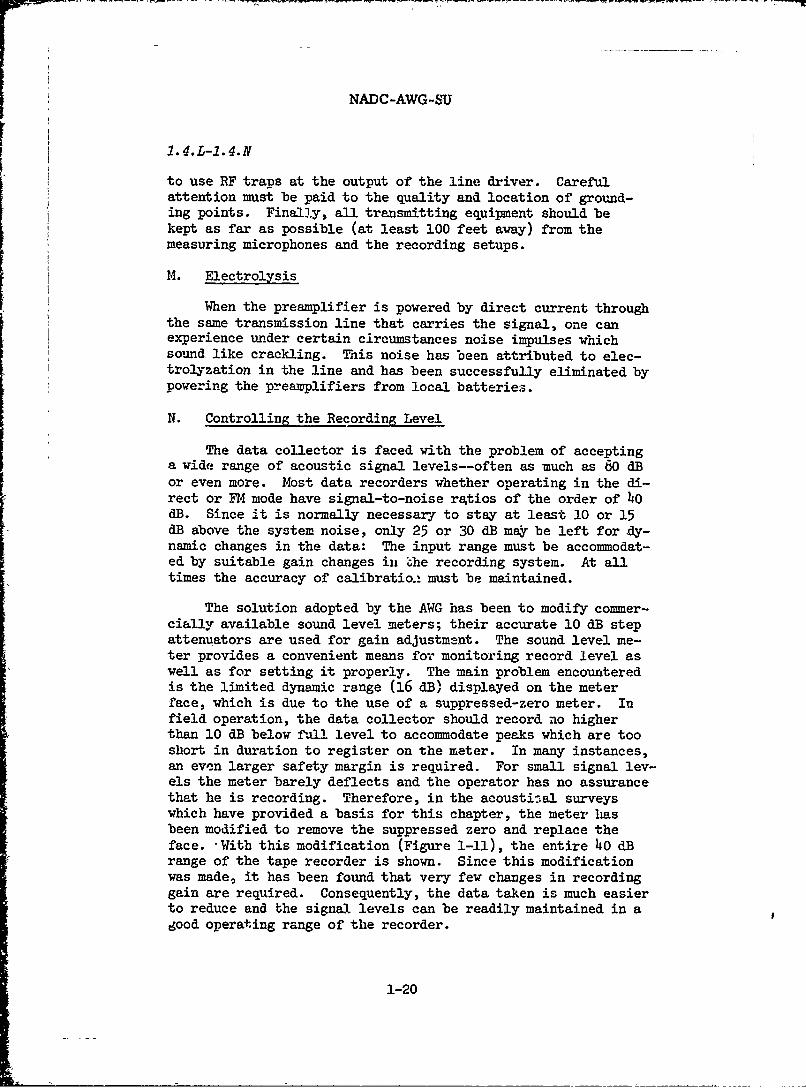
N. Controlling the Recording Level

The data collector is faced with the problem of acceptinga wide range of acoustic signal levels--often as much as 80 dBor even more. Most data recorders whether operating in the di-rect or F74 mode have signal-to-noise ratios of the order of 40dB. Since it is normally necessary to stay at least 10 or 15dB above the system noise, only 25 or 30 dB ma y be left for dy-namic changes in the data: The input range must be accommodat-ed by suitable gain changes in *he recording system. At alltimes the accuracy of calibration must be maintained.

The solution adopted by the AWG has been to modify commer-cially available sound level meters; their accurate 10 dB stepattenuators are used for gain adjustment. The sound level me-ter provides a convenient means for monitoring record level aswell as for setting it properly. The main problem encounteredis the limited dynamic range (16 dB) displayed on the meterface, which is due to the use of a suppressed-zero meter. Infield operation, the data collector should record no higherthan 10 dB below fall level to accommodate peaks which are tooshort in duration to register on the meter. In many instances,an even larger safety margin is required. For small signal lev-els the meter barely deflects and the operator has no assurancethat he is recording. Therefore, in the acousti.:al surveyswhich have provided a basis for this chapter, the meter hasbeen modified to remove the suppressed zero and replace theface. -With this modification (Figure 1-11), the entire 40 dBrange of the tape recorder is shown. Since this modificationwas made, it has been found that very few changes in recordinggain are required. Consequently, the data taken is much easierto reduce and the signal levels can be readily maintained in agood operating range of the recorder.

1-20

NADC-AWG-SU

Figure 1-11. Modified Sound Level Meter

1-21

NADC-AWG-SU

1.4.N-1.4.0

When recording impact data or other transient phenomena,it is helpful to have available a portable oscilloscope and apeak-storing meter such as an impact analyzer. This equipmentwill allow the operator to monitor the peak recording leveleven for signals whose duration is too short for the sound levelmeter's ballistics to follow. The multiple track recordingtechnique using staggered recording levels may be the only so-lution to capture vital data which cannot be repeated and whoselevel is unknown in advance.

Amplifiers are available which sense the signal level andautomatically change their gain in known controllable steps.Frequently, however, this automatic feature can hamper oper-ations since the amplifier does not have the same knowledgeof future events which is available to the human operator.Thus; gain changes may be more frequent than necessary withautomatic equipment. Also, a separate track for recordinggain changes usually is needed.

0. Tae Recorders

The choice of a tape recorder is critical in the acquisitionof good data. The need for light weight and battery operationlimits the choice of instruments available. Certain sacrificesin recording versatility and reliability have been made in thedesign of truly portable equipment. Both 1/4" and 1/2" IRIGformat Lockheed Model 417 recorders have been used in the fieldwith very good success. These units allow a choice of record-ing speeds to suit most acoustical data-gathering requirements.Frequently it is necessary to record in parallel using both theF1 and Direct modes to cover the frequency range desired. Forexample, in the Direct mode, at 7-1/2 ips a typical frequencyresponse would extend from 100 Hz to 25 kHz. To record lowerfrequencies, the FM capability is used to cover the range fromDC to 2500 Hz.

The FM mode has accuracy advantages over the Direct mode inthat recorder amplitude variations have a minimal effect. Where-as amplitude stability in the Direct mode cannot be guaranteed tobetter than approximately 1.0 dB, in the FM mode stability of 0.1dB can be achieved. Furthermore, the phase characteristics aremore readily controlled in FM than in Direct recording. This isespecially important in situations in which wave shape, ratherthan mere frequency content, is important.

1-22

NADC-AWG-SU

1.4.P-!.5.A

P. Recorder Calibrator

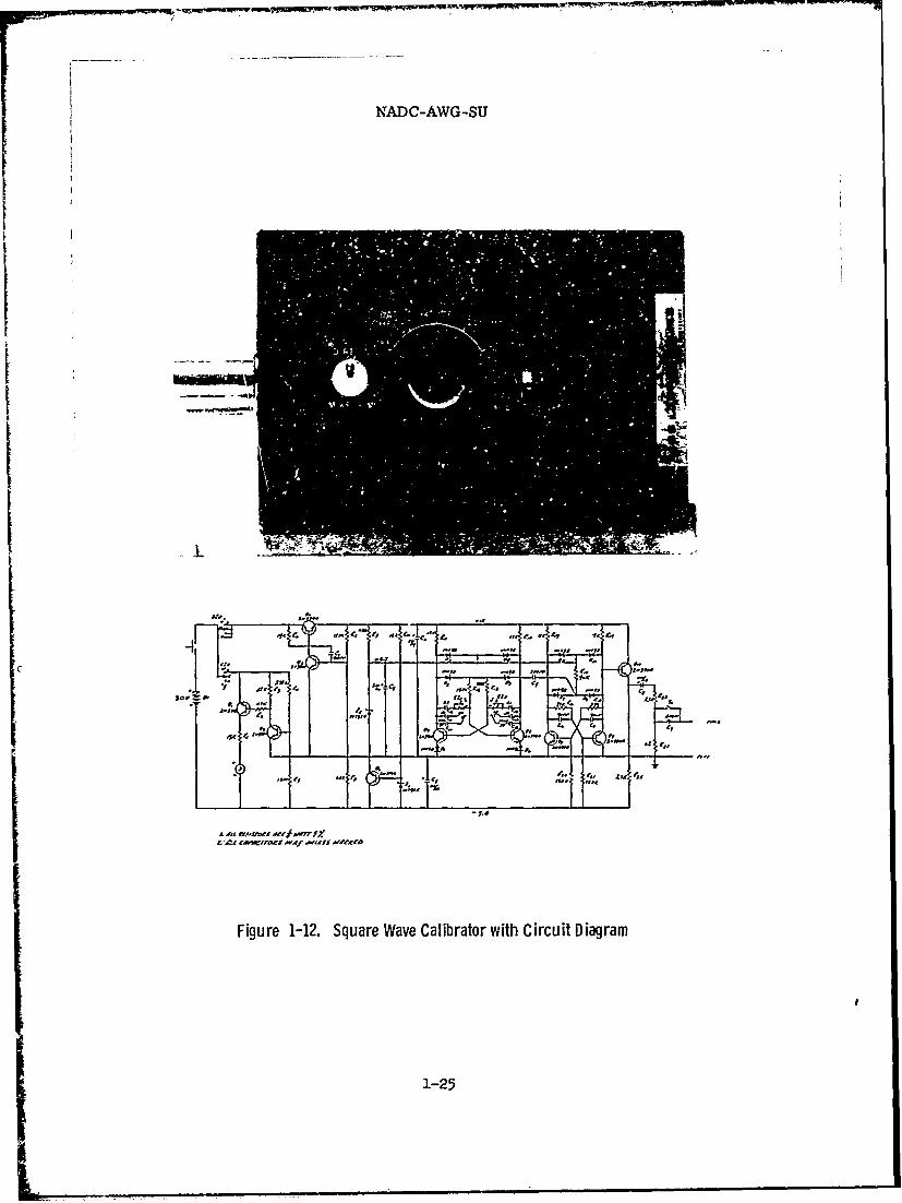
It is advantageous to make an electrical field calibrationof the tape recorder to establish its response, noise level,and maximum recording level. The latter measurement allows oneto rapidly set up the proper record level for duplication. Al-though a complete calibrated frequency sweep is ideal and shouldbe used wherever possible, a square wave calibrator has been de-veloped for situations in which a more rapid calibration is re-quired. This unit produces signals of 25 Hz, 250 Hz, and 2500Hz. The level of the signal is very stable and compatible withthe tape recorder requirements. With this signal recorded onthe tape, a means is provided in data reduction for ascertain-ing the entire frequency response of the recordqr. By frequen-cy analyzing the square wave signal at the data reduction center,the harmonic analysis produced can be compared with that of atrue square wave, verifying the recorder performance. Seen inFigure 1-12, together with its schematic, the unit is small andrugged.

0.. Recording Tape

A high grade instrumentation tape should be used. A poly-ester backing is recommended. One-end-one-half-mil tape pro-vides lower print-through and greater strength than one-mil tape,but the latter can be used where extra recording time per reelis desirable. Tape thinner than one mil should be avoided.

Extreme care should be taken to avoid contamination of thetape. It should be stored in a plastic bag and a covering box.One should not touch the recording surface of the tape, thusavoiding fingerprinting which causes dropouts. Sufficientleader and trailer should be left to allow tape threading with-out contamination of the data.

After recording, the tape should be protected from stray

magnetic fields. Shielding containers are ideal for this.

1.5 FIELD PROCEDURES

A. General

The single most important factor in assuring the success ofa data-gathering mission is adequate planning and implementationof field procedures. Regardless of the sophistication of thefiel.' equipment, success of the endeavor is Jeopardized if suf-ficient effort is not devote&. to this initial step. Conversely,

1-23

NADC-AWG-SU

1..A-1.5.B

the suitability of the equipment for the task at hand is deter-mined by the plan and if the planning is done sufficiently inadvance of the test, as is proper, adequate equipment will beprovided in time for the mission.

B. Development of the Test Plan

The key to the development of an adequate test plan is theforeknowledge of the use to which the data is to be put, i.e.the goals of the testing program. Each test must have its ownpurpose which must be clearly spelled out. The pressure ofscheduling frequently tempts one to skimp on the identificationof the purpose of each test. However, the time saved at the out-set is most assuredly lost later in attempting to cull the wheatfrom the chaff of data taken.

For example, if the purpose of a specific test is to deter-mine the effectiveness of a certain design change, say, that ofa different windscreen on a device, the test plan must providefor sufficient controls on the experiment to separate definitivelythis change from all others. The plan must include provisionsfor the testing of Device A with the new windscreen simultaneouslywith identical Device B with the old windscreen. The windscreensshould subsequently be interchanged to remove the efrect of indi-vidual device characteristics. The devices should be checked dur-ing periods of wind and also in periods of calm. Obviously, windvelocity measurement should be recorded. The instrument used forthis should be capable of measuring peak velocities during gustsrather than simple averages. If the device employs circuitrywhich changes its characteristics as a function of ambient noise,the tests must be run under various ambient conditions.

In short, a complete knowledge of the device to be testedand the results expected from the test are necessary in crder toformulate a plan which takes into consideration all fcreseeablecontingencies and which assures that the causes and effects canbe assigned without ambiguity. Thus, even if the organizationwhich fields the data-gathering team is not also charged withthe responsibility for preparing the test plan, it should parti-cipate in formulation of the plan from the very inception.

Once the purpose of the test has been defined, the fieldteam leader can prepare the detailed test plan. The contentsof the plan and the detail to which it is drawn up will varydepending upon the test to be performed, its location and itsduration, etc. Typical examples of a Calibration Procedureand a Test Operation Procedure are shown in Appendixes A and B.

1-24

NADC-AWG-SU

I

- 'a-f 4 L'I.. ... 4, " .. T 'd4 Ar-,

i-2 -

L*Ic e.w~**wx -ww ^".E

Figure 1-12. Square Wave Calibrator with Circuit Diagram

1-25

-9F- _ FrF9 -

NADC-AWG-SU

These were prepared for a specific one-day test during which out-puts of two or three sensors were recorded at each of several sites.The Calibration Procedure was followed and performed the day beforethe actual test since COMEX ("Commence Exercise") was quite early(0600). In addition, on test day a brief calibration procedure wasperformed on all of the data gathering microphones.

The key portions of the Calibration Procedure are:

1. Voice annotation of:

a. Test Designation and Classification of Tapeb. Location of Test and Test Sitec. Reel Number and Previous Reel Numberd. Datee. Timef. Personnel at Siteg. Recorder Identification

(1) Make(2) Model(3) Serial Number(4) Recording Speed(5) Track Identification, i.e. which infor-

mation is recorded on which trackh. Site Description including Sensor Locations

2. Noise Level Measurements:

a. Recorder noise alone, i.e. recorder inputterminals shorted directly.

b. System noise, i.e. data lines terminated atmicrophone end. This should be repeated for everyrecord level setting which one anticipates using. Thetermination should be equivalent to the source imped-ance of the microphone.

3. Identification of Sensors:

Each sensor is connected individually to the re-corder and identified by speaking into it or by caus-ing it to respond in some way. This gives a positiveindication on the tape as to which sensor is which re-gardless of possible later discrepancies in tape mark-ings or handling. Markings on the tape reel, alone, areinsufficient since it is possible to zransfer the tape

1-26

NADC-AWG-SU

1.5.B

to a different reel which may have erroneous or inap-plicable markings. While each sensor is being identi-fied directly, a voice commentary is made to identifythe sensor and the entire associated data-gathering

chain.

4. Overall Acoustic Calibrations:

a. The data-gathering microphones are calibratedusing a General Radio 1562A Sound Level Calibrator.This unit produces a precise ll4 dB re 0.0002 dynes/cm 2 sound pressure level at a variety of frequencies.

b. Other acoustic sensors are calibrated using aportable oscillator, battery-powered amplifier, andtrumpet. Using this equipment, a sound field is setup in "che vicinity of the item to be calibrated. Thesound field is measured using a calibrated sound levelmeter. The field is probed all around the item toassure uniformity of field. Annotation is made of thesound pressure level used.

c. In both cases above, the setting of the record-ing level control, i.e. the sound level meter, is an-notated.

5. Derived Calibrations:

In some cases it is not possible to put a primayacoustic calibration signal on each reel of tape. 'Forexample, in the particular case for which the proceduresillustrated here were written, the test could not behalted once underway. Thus, it was necessary tc estab-lish derived calibrations on each reel of tape. Thesederived calibrations can be related in level to the over-all acoustic signals. Therefore, on the calibrationtape, in addition to the overall acoustic signal, a 250Hz square wave (from the square wave calibrator) was re-corded. (To cover a broader range, 25 Hz and 2500 Hzwave also could have been recorded.) This same signalwas subsequently recorded on each reel of tape when itwas not possible to perform the acoustic calibration.By once establishing the relationship between squarewave level and acoustic signal level from the calibra-tion tape, one can derive acoustic signal levels forall subsequent tapes. The square wave signal has an-other purpose in that a spectrum analysis of the sig-nal when compared with the theoretical relationship be-tween the harmonics of a square irave will indicate thefrequency response of the data recording system.

1-27

NADC-AWG-SU

1.5.B

6. Voice Annotation of the calibration procedure which'ws used and the method uhich is to be followed indata reduction to establish true sound pressure levels.

A Test Operation Procedure is prepared for the actual test,itself. It is invaluable in assuring uniformity in methodologyand also serves as a checklist of things to do on each reel of tape.The key portions of the procedure are:

1. Voice Annotation of:

a. Test Designation and Classification of Tapeb. Purpose of the Testc. Identification of Reel Number in the Seriesd. Location of Test and Test Sitee. Datef. Timeg. Recorder Identification

(1) Make(2) Model(3) Serial Number(h) Recording Speed(5) Track Identification

h. Sensor Location, i.e. Height, etc.

2. Secondary Calibration using the Square Wave Cali-brator track-by-track

3. Identification of Sensors:

Each sensor is connected individually to the re-corder and identified as to location, etc. by speak-ing into it or causing it to respond in some way. Thisgives a positive identification on the tape as to whichsensor is which regardless of possible later discrepan-cies in tape markings or handling. Mrkings on thetape reel alone are insufficient since i is possibleto transfer the tape to a different reel which may haveerroneous or inapplicable markings. While each sensoris being identified directly, a voice commentary is madeto identify the sensor and the entire associated data-gathering chain.

. Overall Acoustic Calibrations:

Same as Step 4 in the Calibration Procedure.

1-28

NADC-AWG-SU

1.5.B-1.5.C

5. Annotation:

a. Personnel at Siteb. Description of Site

(1) Terrain(2) Foliage(3) Local anomalies(h) Weather conditions

(5) Other pertinent data

6. At this point the site is ready for data gatheringand informs Central Control of the fact.

7. This procedure should be follow-d for each reelof tape taken during the test. If .his is not possibledue to time limitations, at least the first two stepsmust be performed for each reel. The entire procedureis then performed once at the beginning of the day'stesting and again at the end.

C. Equipment and Personnel Requirements

During tLe planning phase of the test, after the purdcse hasbeen established, the equipment required for the exercis, is deter-mined and made ready for the field. An Equipment Checkli.-: (shownin Appendix C) is made up for each site. Using it assures thatmissing, defective, or insufficient equipment is recognized at a.early stage in the mission in time for remedial gathering missions.Special requirements arise on occasion which are not included onthe general list. These are added as needed and the list revised.When the time arrives for deployment to the sites, each site cap-tain uses the checklist to load his equipment. If this list hasbeen properly prepared, each site should be self-sufficient forordinary operation and also for those contingencies which have beenanticipated by experience and careful preplanning.

At this point, it is time to determine the personnel re-quirements including any local assistance that may be available.The best approach is to list the tasks and assign personnel anddates and times to each task. For the actual test, itself, threepersons per site are desirable. Occasionally four cure requiredand sometimes two per site are sufficient. In general, one per-con is needed for every four tracks of recording to handle themonitor'ng and the recording level adjustments. If the data tobe recorded will necessitate frequent and/or utiforewarned changesii recording level (such as would be the case with unscriptedaircraft tests), it is best to plan on one man fur every t.o

1-29

NADC-AWG-SU

1.5. C-1.5.D

tracks of data. One man is required to keep the written detailedfield log (Appendix D). If the location and testing require theuse of a "spotter," another man must be added to the roster.

Regardless of other considerations, safety dictates that asingle man should never be left in the field alone. Under diffi-cult jungle conditions, two men are needed to calibrate the micro-phones, which means a minimum of three people per site required.However, some of the tasks, such as keeping the field log andspotting do not require technically trained personnel, and itmay be possible to use such local assistance as might be avail-ab)D at a military base.

The above requirements are based on a test of relativelyshort duration. If the test is planned to continue for morethan 12 or 14 hours on a single day, or will exceed an 8-hour-per-day-average over several days, backup teams should be pro-vided. This is especially the case if the tests are performedunder severe conditions such as in a jungle environment in therainy season. If the tests are to continue over a period ofseveral months, the teams should be rotated at reasonable inter-vals, typically every two to four weeks depending upon fieldconditions. it must be remembered that situations change rapidly

during tests and the field team is called upon to make rapidand accurate decisions concerning the conduct of the test, opera-tion of the equipment, and performance of the measurements. ifthe personnel are strained beyond reasonable capacity, theiralertness will suffer affecting their accuracy and efficiency.

D. Scheduling the Tasks

All of the above planning and preparation sbould be donebefore deployment to the field. This presupposes a sufficientperiod of time between the initiation of preparations and thetest itself. The time required for adequate preparation will,of course, depend upon the type of test involved, similarityto past tests, and expected duration. In general, however,at least a two-week period should be set aside for preparation.If an entirely new field of exploration is to be opened, aperiod of four weeks or even longer should be planned for ade-

quate organization.

Based upon the test plan which has been drawn up, aschedule of events should be prepared. Designating the dayof commencement of the test (COMEX) X-Day, a dry run includingsystem calibration should be performed on day X-minus-1. Itis preferable to have all 'ork finished by noon of day X-1.

1-30

NADC-AWG-SU

1. 5.D-1. 5.E

A last-minute briefing should be held early that afternoonand the rest of the day devoted to laying out the cables andtesting th,.m for continuity, RF pickup, noise, etc. If thereare extensive amounts of cable to be laid, or if the terrainis especially severe, one or two extra days should be set aside

for this task. On day X-2 the equipment should be packedaccording to site and in accordance with the checklist pre-pared previously. It will then be ready for deployment on dayX-1. Previously arranged suitable security measures for theequipment should be placed in effect by noon of day X-1. Thesites for the sensors should be selected the day before be-ginning laying of the cable, i.e. day X-3 or sooner. A checkthat the cable has been properly laid should be made the after-noon of day X-2.

In locating the sites, due care must be taken of theacoustic propagation expected between the sound sources andthe sensors. For example, a different arrangement may beneeded for studying propagation loss than when accumulatingsignature data on vehicular noise. The trees or locations forhanging the sensors can be blazed with suitable cloth or string.At the time the sites are planned, a map of each site should be

prepared. The distances from the sensors to benchmarks whichcan be found on master maps should be measured and noted. Avertical. diagram of sensor deployment should be made, and Po-laroid pictures of the terrain should be taken.

In addition to the site preparation, there are many sup-porting operations which must be arranged in the days beforeCOMEX. These include communications between members of eachsite's data-gathering team, and between each site and a centralclearing headquarters. Further, transportation to the sitesmust be provided as well as food, shelter, and suitable cloth-ing for the personnel involved in the site activities. Sheltermay be in the forTa of a tent, van, or station wagon large enoughto house the equipment. Both the men and equipment must beadequately shielded from sun and rain. The logistics of trans-porting the men to the various sites on the day of the testmust be carefully studied in advance. In general, a strictschedule must be adhered to and planning and teamwork are ofthe essence.

E. Implementing the Plan

During the afternoon of day X-l. a briefing should be heldto alert the team to ary last-minute changes, and to go overthe test script if one is available, or, if not, to discuss

1-31

NADC-AWG-SU

1. 5.E

the types of signals which are likely to be encountered dur-ing the test. Depending upon the types of signals to be re-corded, the leader will instruct the team concerning the bestrecording level to be used. For example, if impulsive soundsare expected, or if the 3ound pressure 2.evel is expected torise abruptly without warning, he may instruct the team toleave 20-30 dB of headroom in setting ambient recording levels.On the other hand, if the recording is of a slowly varying sig-nal such as the ambient, he may instruct them to leave only10 dB headroom. He may alert the team to any special loggingrequirements which may be appropriate to the particular data tobe taken. In general, this is the time again to go over anydeviations from the normal procedure.

On X-day, the teams should be transported to the field andin position at least one hour before COMEX. if possible, atwo-hour period should be prescribed. This gives the team areasonable opportunity to calibrate the equipment properly,make appropriate annotations, sand call for replacements on anyequipment which might prove defective at the very last moment.Any "extra" time -ill be useful for prepazing labels to go on-to the reels of tape as they are recorded. During the actualtest the field operators will be kept extremely busy settingrecording levels, monitoring the quality of the recordingsaurally, and keeping correct logs.

Besides logs of events as they occur, the teams should keeplogs of equipment failure. In the severe environment and withthe handling under which the data-gathering equipment operates,failure rates are apt to be ouite high. It is important, there-fore, to know what type of equipment is failing and in what wayit is proving defective so that appropriate steps may be takento improve its reliability in the future.

As soon as possible after the test, a debriefing should beheld by the team leader to cull the information required for anaccurate trip report. This session should cover any difficul-ties each team encountered, the steps taken to remedy them,any deviations from the plan which were necessitated, commentsas to the quality of the recordings, suggested ways of improv-ing the quality of the recordings on future tests of a similarnature, etc.

On the day of the test, the team leader should be in readycommunication with the site teams and with the exercise direc-tors. Decisions which cannot be made at the sites by the teammembers are referred to the team leader, who may have to visit

1-32

NADC-AWG-SU

1. 5. E-1. 5. F

the particular site to investigate a problem at hand, deliver

back-up equipment, etc. At the end of each day's exercise(s)all of the recordings are delivered to the team leader. Priorto X-Day, arrangements should have been made concerning the

disposition of the recordings such as storage and/or trans-portation to their final destination, with special care givento the handling of any classified material. The tapes shouldbe protected preferably with shielding cans to prevent acci-dental demagnetization. As an emergency measure, a few inchesof air space (at least four inches) around the tapes will helpif cans are not available and the stray fields are low.

From the timetable outlined above, it becomes clear thatthe field team should be at the testing area from three toseven days in advance of COMEX, depending upon the extensive-ness of the testing and the advance preparation which might bereouired.

F. Communications

Second in importance only to adeqaate planning, is goodfield communications. Regardless of the high degree of priorplanning and scripting, it is virtually impossible for the testto go exactly according to plan. For this reason alone, commu-nications between the field teams and headquarters are essen-tial if successful signal gathering is to be accomplished. Com-munication by field radio is convenient, however, a fairly largenumber of rad2.os are required and may not be available at a par-ticular site. Further, there may be a question of compromisingsecurity when the radio is used. In such a case, the answer maybe wired field telephones. If these are to.be employed, suffi-cient lead time must be left to allow communications lines to bestrung.

In addition to requiring communications to accommodate changesin program plan, the field team may need a virtually continualcommunication link for certain types of tests. For example, ifthe purpose of the test is to record overflights of aircraftin a dense jungle, it may be necessary to give each team noticethat an overflight is imminent just prior to the action so thatthey can adjust recording levels and identify the particular air-craft. Unless so alerted, it is sometimes difficult to tell thatan aircraft is approaching until it is practically directly over-head. By this time the tape is severely overloaded and the datahas been lost. However, such continuous notification can put asevere strain on the communication link if it is expected to serveother purposes as -jell. Thus, it may be necessary to allocate a

1-33

NADC-AWG-SU

1.5.F-1.6

communications link exclusively to the data gathering teams.Alternately, spotters for each team can be provided with fieldtelephone communications at their site. Whichever form ittakes, adequate communications must be furnished to permitsuccess of the data gathering mission.

1.6 FIELD LABORATORY PROCEDURES

A field laboratory is provided for the checkout and main-tenance of the field equipment. Even for the shortest of tests,it is good practice to thoroughly test the data gathering systembefore deployment to the field since calibration can be upsetduring transportation from the home base. The need for a fieldlaboratory is even greater when the testing program extends overa considerable period of time. Here, the laboratory should besuitably equipped for repair and maintenance of equipment as wellas checkout.

In addition to initial checkout prior to the first day oftesting, all equipment should be cleaned and tested as soon aspossible after the exercise. During lengthy data-gatheringmissions, double sets of equipment may have to be provided sothat one set may undergo maintenance procedures while the otheris in use. Additional people may also be required to performthe procedures.

In Appendix E, calibration procedures are given fcr thesound level meter, preamplifier and microphone. Besides main-tenance of this equipment, the most critical function of thefield laboratory is the maintenance of the tape recorders.Being an electromechanical device, the tapq recorder is excep-tionally prone to malfunction in the field. It must be scru-pulously cleaned, heads must be demagnetized, and mechanicalcomponents such as drive belts checked and periodically replaced.Besides this mechanical upkeep, the tape recorder's sophisticatedelectronics design necessitates a careful checkout of its recordand reprodace electronics. To fully check out and adjust a taperecorder and associated field equipment requires at least a falleight-hour day.

In addition to maintenance of equipment, battery storage andrecharging facilities are maintained in the field laboratory. Therecharging cycle for a nickel-cadmium battery is 13 hours. It canbe seen that several sets of batteries and recharging facilitiesare required if this type of battery is used.

When accumulating data -.n a very humid environment, a desic-

1-34

NADC-AWG-SU

1.6-1.7

cator and a supply of disiccant should be included in the fieldlaboratory equipment. This can be used to dry ou, microphonesand high impedance circuits such as are found in tVx;_ -eamplifi,.rsand sound level meters.

Especially, during long data-gathering missions it is aQvis-able to provide the field laboratory with sufficient data reduc-tion equipment to take a "quick look" at the data being receivedfrom the field. On the basis of this preliminary reduction, planscan be modified or key aspects of the test repeatel as requiredto assure accurate and reliable data.

1.7 WRITTEN FIELD PROCEDURES

Representative field procedures are appended as follows:

Appendix A: Field Calibration Procedure

Appendix B: Field Test Operation Procedure

Appendix C: Field Equipment Check List

Appendir D: Field Log

Appendix E(l): Before-Use Equipment Checkout and Cali-bration for Sound Level Meter

Appendix E(2): Befcre-Use Equipment Checkout end Cali-bration for Preamplifier

Appendix E(3): Before-Use Equipment Checkout and Cali-bration for Microphone

1-35

NADC-AWG-SU

2.1.A-2.1.B.

CHAPTER TWO: DATA ANALYSIS AND REDUCTION

2.1 INTRODUCTION

A. Purpose

The purpose of this chapter is twofold: 1) to discuss inbroad terms the appropriate factors to be considered in datareduction and analysis; and (2) to describe, with examrles,many practical ways in thich data can be manipulated into for-mats useful to an analyst. While the mathematical relation-ships for the various data transformations are stated, it isnot the purpose of this chapter to validate these relationships.Such validations are available in many standard texts, some ofwhich are referenced. Finally, while most of the discussionin this chapter is oriented to audio-frequency data, with ap-propriate scaling factors the techniques are equally adaptableto seismic, infrasonic, ultrasonic, and similar phenomena.

B. General Aspects of Data Reduction and Analysis

Data acquisition, reduction, and analysis should be viewedas an integrated process. One begins with the establishment ofrealistic objectives and the formulation of hypotheses and plansrespecting the type of data acquisition and reduction that willbe required as described in chapter 1. Such preparatory workenables the analyst to proceed with dispatch to the task of pro-cessing the data as soon as it becomes available. The resultsof an acoustical data-acquisition mission are usually containedin one or more reels of tape, supplemented by plans, logs anddebriefings of the data-acquisition teams.l The actual task ofdata reduction and analysis can be said to begin at this point.

1See Chapter 1, pp. 1-23 to 1-34.

2-1

NADC-AWG-SU

2.1.B

Almost invariably, the first task of the analyst is to per-form a preliminary overall review of the newly acquired data, toclassify it in accordance with various categories and priorities,and then to proceed to "reduce it," that is, to transform it intocompact and manageable formats in order to extract from it theneeded information. The task of categorizing and evaluating datarequires considerable experience and judgment which cannot bespelled out in procedural detail. The general principles, how-ever, are summarized in subsection 2.1.C. The successful outcomeof a data mission is often ensured by proper utilization of datain these various categories.

Because the results of-analysis often lead to the designof electroacoustical or electronic devices, the data is usuallyreduced in terms of its frequency and/or time-domain attributes,which provide essential information to the equipment designer.A considerable portion of this chapter is devoted to the variousfrequency and time domain data-reduction procedures that havebeen applied successfully to the tasks of the Acoustical WorkingGroup (AWG).

Often, the resul.ts of frequency domain and time-domain anal-ysis suggest the neces-Ity of employing special data-reductiontechniques or apparatus for the detection and acquisition of thetargets of interest against background noise or other interferingphenomena. Cogent among these are the temporal correlation ofsignals received by two or more spaced-apart transducers; or com-parison of signals received by coincident transducers with dif-ferential directional characteristics; or the use of special di-rectional arrays which augment the S/N in certain directions; andeven demodulation methods which reveal the existence of sonicphenomena which might not have been acquired with conventionallyavailable acoustic detectors. The varieties and configurations ofsuch special techniques and devices are limited only by the skilland inventiveness of the analyst and the designer; some of thesedevised during AWG tasks are outlined in Section 2.6.

It should be noted that the terms "reduction" and "analysis"sometimes have been used interchangeably. The term "frequencyanalysis" is deeply ingrained in the language of the mathemati-cian to denote reduction in the frequency domain, and we haverespected this tradition in the preparation of this chapter.The term "data reduction" usually involves the process of for-mulating or plotting mathematical concepts in the time domain.For example, a time series representing sound-pressure level

2-2

NADC-AWG-SU

2.1.B-2.I.C

may be "reduced" in terms of its peak-level envelope as a func-tion of time, or in terms of intensity variation of its fre-quency attributes as a function of time. As a last step afterdata reduction, data analysis is employed to apply these resultsto the solution of the problem at hand.

A useful tool for the analyst and the designer is a mathe-matical model of a signal, or a background noise, or a data-acquisition detector, etc., which allows the performance of the

system to be analyzed by means of a computer. In a text of thisnature, the complete range of modeling techniques cannot be fullyexplored; however, models of the simplest concepts employed inthe work of the AWG are given toward the end of the chapter.

C. Categorization of Data

1. Primary Data

Data reduction, as defined in the previous subsection, is aprocess of transforming raw data into other formats, the pur-pose being to produce formats that are more easily related toobjectives than are the original data. To begin with, let usconsider the primary data. Primary data is the physical datadirectly related to the objective. It is that data which isreduced and analyzed to achieve the objective.

Two general t.ypes of data are processed: time-ordered dataand time-random data. For the most part, the AWG-acquired datawas time ordered. The distinction between the two types isthat for the time-ordered data there is useful information inthe exact sequence of values encountered, whereas for time-randomdata there is no such useful information.

To illustrate time-ordered data: the sound ou.,..'it of a gas-soline engine exhibits, with time, certain interestL;.- cyclicalsound outputs that would be destroyed if one were to a-.troy thesequence of instantaneous sound outputs; at the same tim:.-, how-ever, the frequencies of the major cyclical components ar.. notconstant, but instead wander in some random fashion. In ccii-trast to this type of data, if one were to measure the detectivnranges of an acoustic-detection system working against a giventarget, the sequence of ranges obtained for sequential targetruns would constitute time-random data. No information wouldbe destroyed if the sequence of ranges were changed.

The reductions (transformations)for time-ordered datashould preserve pertinent aspects of the original sequencing

2-3

NADC-AWG-SU

2.1.C

information, since such information in these signals is useful.There are two general types of transformation possible: (1) atransformation that destroys no information in the original--this is a one-to-one type of transformation; and (2) a transfor-mation that destroys information in the original data--this isa many-to-one type of transformation. in the first type oftransformation, one can combine the transformed data to recon-struct the original data in its entirety. The Fourier Trans-form (see subsection 2.2.C.) is theoretically a one-to-onetransformation since a given set of Fourier components, suit-ably combined, produces a unique original signal. In practice,this is only approximately true, since one would have to takean infinitely long data sample and reconstruct it with an in-finite set of oscillators to exactly transform the data. In-asmuch as one customarily selects only a segment of data foranalysis, an exact transformation is not obtained.

In the second type of transformation, one cannot combinetransformed data to produce a unique original signal. The power-spectral-density transformation is an example of the second kindof reduction. A given power-spectral density does not corre-spond to a unique original signal, but instead pertains to many.

Signals to be reduced may contain unique time-ordered in-formation in many aspects, either of waveform shape or of wave-form parameters derived from the signals. Waveform shapes in-volve sequential details in the instantaneous signal values,or in composites of these details, like envelopes. Time-domainreduction is often used to process waveform-shaped signal aspects.Waveform parameters are items such as peak-to-average ratios,rms values, phases, etc. Information-destroying reductions high-light particular signal aspects by eliminating extraneous aspects,thereby allowing one to focus attention more easily on the zig-nificant features.

2. Calibration Data

Calibration inforwation is required to ascertain absolutedimensions of data. For example, suppose one requires that thevoltage analogs of sound recorded on magnetic tape be scaled interms of sound pressure level. This is made possible, in con-venient form, by recording a signal of known sound pressure oneach reel of tape to be analyzed.2

System performance validation data is a part of calibrationinformation. It is introduced into test procedures to ensurethat the data characteristics are valid and not due to the par-ticular data acquisition and reduction techniques. Good vali-

2See Chapter 1.

2-4

NADC-AWG-SU

2.1.C-2.1.D

dation data is absolutely necessary to resolve anomalies arisingin data reduction.

The validation data contains test data on the acquisitionsystem to determine its limitations and usefulness. Such datais usually acquired in the laboratory both prior and subsequentto the field tests, and also in the field during the test. Amongother things, this data includes such items as acquisition sys-tem bandwidth, dynamic range, noise level and frequency stability.The data should validate the fact that established system perfor-mance has not changed during the test, or it shoiLld provide thenecessary correction information for those system changes whichdo occur.

3. Test Procedure Data

Test procedure data is taken to provide the means for properinterpretation of the results of data reduction. Without goodtest procedure data, one cannot recheck, interpret, or extrapo-late the results of a given test.

The test procedure data includes the detailed test plav -the time correlation of the test events with other test datE. Villustrate, if certain targets are run, information should be re-corded on model number, speed, altitudes and other aspects -hatwould uniquely characterize the target. Information on envi-,-)(-ment, acquisition system settings, unusual test factors, foy -=

ample, are also of importance during the reduction. The absenceof these procedure data limits, at best, the use of good primarydata and, at worst, renders it useless.

The process of .categorization of data as outlined above as-sists the analyst with the planning of the data reduction tasksand ensures that the reduced data can be reliably applied to thesolution of mission objectives.

D. Definitions and Units

To avoid misinterpretations, the following terminology isused hereafter. The reader is referred to ANSI Standard Sl.l-1960for a complete listing of acoustical terminology and definitions.

Periodic Quantity. A periodic quantity is anoscillating quantity whose values recur forcertain increments of the independent variable.

Note 1: If a periodic quantity v is a func-tion of t, then

v= F(t) = F(t + T)where T, a constant, is a period of v.

2-5

NADC-AWG-SU

2.1.D

Primitive Period (Period). The primitive periodof a periodic quantity is the smallest incrementof the independent variable for which the func-tion repeats itself.

Note 1: If no ambiguity is likely, the prim-

itive period is simply called the period of thefunction.

Frequency. The frequency of a function periodicin time is the reciprocal of the primitive period.The unit is the Hertz (Hz).

Angular Frequency (Circul - Frequency). The angu-lar frequency of a periodic quantity, in radiansper unit time, is che frequency multiplied by 27T.The usual symbol i:s w.

Peak-to-Peak Value. The peak-to-peak value of an

oscillating quantity is the algebraic differencebetween the extremes of the quantity.

Phase of a Periodic quantity. The phase of aperiodic quantity, for a particular value of theindependent variable, is the fractional part ofa period through which the independent variablehas advanced, measured from an arbitrary refer-ence.

Harmonic. A harmonic is a sinusoidal quantityhaving a frequency that is an integral multipleof the frequency of a periodic quantity to whichit is related.

Ambient Noise. Ambient noise is the all-encom-passing noise associated with a given environment,being usually a composite of sounds from manysources near and far.

Random Noise. Random noise is an oscillationwhose instantaneous magnitude is not specifiedfor any given instant of time. The instantaneousmagnitudes of a random noise are specified onlyby probability distribution functions giving thefraction of the total time that the magnitude,or some sequence of magnitudes, lies within aspecified range.

2-6

NADC-AWG-SU

2.1..D

Spectrum. The spectrum of a function of time isa description of its resolution into components,each of different frequency and (usuaUy) differ-ent amplitude and phase.

Spectrum Density (Power Spectrum). Thc spectrumdensity of an oscillation is the mean-square am-plitude of the output of an ideal filter withxnity gain responding to the oscillation, per unitbondwidth; i.e., the limit for vanishingly smallbandwidth of the quotient of the mean-square am-plitude divided by the bandwidth.

Line Spectrum. A line spectrum is a spectrumwhose components occur at a number of discrete

frequencies.

Continuous Spectrum. A continuous spectrum isthe spectrum of a wave the components of whichare continuously distributed over a frequencyrange.

Microbar, Dyne per Square Centimeter. A micro-bar is a unit of pressure commonly used in acous-tics. One microbar is equal to 1 dyne per squarecentimeter.

Sound Pressure. The sound pressure at a pointis the total instantaneous pressure at thatpoint in the presence of a sound wave minus thestatic pressure at that point.

Maximum Sound Pressure. The maximum sound pres-sure of any given cycle of a periodic wave isthe maximum absolute value of the instantaneoussound pressure occurring during that cycle.

Peak Sound Pressure. The peak sound pressure forany specified time interval is the maximum abso-lute value of the instantaneous sound pressure inthat interval.

Effective Sound Pressure (Root-Mean-Square SoundPressure). The effective sound pressure at a

point is the root-mean-square value of the in-stantaneous sound pressures, over a time inter-val at the point under consideration. In the

case of periodic sound tressures, the interval

2-7

NADC-AWG-SU

2.1.Dmust be an integral number of periods or an in-terval that is long compared to a period. Inthe case of nonperiodic sound pressures, the in-terval should be long enough to make the valueobtained essentially independent of small changesin the length of the interval.

Sound Energy. The sound energy of a given partof a medium is the T.otal energy in this part ofthe medium minus the energy which would existin the same part of the medium with no soundwaves present.

Sound Intensity (Sound-Energy Flux Density)(Sound-Power Density). The sound intensityin a specified direction at a point is theaverage rate of sound energy transmitted inthe specified direction through a unit areanormal to this direction at the point con-sidered.

Level. In acoustics, the level of a quantityis the logarithm of the ratio of that quantityto a reference quantity of the same kind. Thebase of the logarithm, the reference quantity,and the kind of level must be specified.

Sound Pressure Level. The sound pressure level,in decibels, of a sound is 20 times the logarithmto the base 10 of the ratio of the pressure ofthis sound to the reference pressure. The ref-erence pressure shall be explicitly stated.

Note 1: The following reference pressures arein comon use:

(a) 2 X 10-4 microbar(b) 1 microbar

Reference pressure (a) is in general use for meas-urements concerned with hearing and with sound -,.air and liquids, while (b) has gained widespreadacceptance for calibration of transducers and vari-ous kinds of sound measurements in liquids.

Band Pressure Level. The band pressure level ofa sound for a specified frequency band is thesound pressure level for the sound contained with-in the restricted band. The reference pressuremust be specified.

Note: The band may be specified by its lowerand upper cutoff frequencies, or by its geometric

2-8

NADC-AWG-SU

2.1.D

center frequency and bandwidth. The width of theband may be indicated by a prefatory modifier; e.g.,octave band (sound pressure) level, half-octave bandlevel, third-octave band level, 50-Hz band level.

Spectrum Level (Spectrum Density Level). The spec-trum level of a specified signal at a particularfrequency is the level of that part of the signalcontained within a band 1 Hz wide, centered at theparticular frequency. Ordi:arily this has signifi-cance only for a signal having a continuous distri-bution of components within the frequency range underconsideration. The words "spectrum level" cannotbe used alone but must appear in combination with aprefatory modifier, e.g., pressure, velocity, voltage.

Sound Level. Sound level is a weighted sound pres-sure level, obtained by the use of metering charac-teristics and the weightings A, B, or C specifiedin American Standard Sound Level Meters for Meas-urement of Noise and Other Sounds, Z24.3-944. Theweighting employed must always be stated. The ref-erence pressure is 0.0002 microbar.

Transmission Loss. Transmission loss is thereduction in the magnitude of some character-istic of a signal, between two seated pointsin a transmission system.

Microphone. A microphone is an electroacoustictransducer that responds to sound waves and de-livers essentially equivalent electric waves.

Pressure Microphone. A pressure microphone isa microphone in which the electric output sub-stantially corresponds to the instantaneoussound pressure of the impressed sound wave.

Directional Microphone. A directional micro-phone is a microphone the response of whichvaries 5ignificantly with the direction ofsound incidence.

Directional Resvolise Pattern (Beam Pattern).The directional response pattern of a trans-ducer used for sound emission or reception isa description, often presented graphically,of the response of the transducer as a func-tion of the direction of the transmitted orincident sound waves in a specified plane andat a specified frequency.

2-9

NADC-AWG-SU

2.2.A

2.2 THEORY AND PRACTICE OF DATA REDUCTION AND ANALYSIS

A. Introduction

While man lives in a time-domain world, the recognition ofrany natural and man-made sounds is based upon the repetitiveaspects of the time series. Such natural manifestations can beidentified in the song of a bird, in the cry of an animal, or inthe aeolian tones caused by wind passing through the branches ofa tree. Most man-made sounds such as the cyclic repetitivenessof a truck engine, the whine of a saw mill and the humming ofpower lines can be usefully and conveniently recognized in termsof repetition rate, or in the frequency of energy interchange be-tween the potential and kinetic states.

Data reduction consists of the extraction of salient fea-tures from the raw data. There are two principal types of datareduction--reductions in the frequency domain (usually calledfrequency analysis) and reductions in the time domain (to be dis-cussed in more detail in the following sections). From the util-ization of bath types of data reduction, information is gainedabout the phenomenon which allows it to be ..,ore fully character-ized and understood. As a result of this data reduction, identi-fication and categorization of the occurrence from its acousticsignature can be made.

By transforming the data into the frequency domain, usingthe techniques described in subsections 2.2.B, C, D and E, one canidentify the regions o, maximum energy concentration. Often, adistinctive "siFnature" which is characteristic of only one typeof phenomenon is evident. In this case, the source of the datacan be identified. In other cases, it is impossible to determinethe precise origin of the data and yet, through frequency analysis,the most appropriate bandpass characteristics for sensor equip-ment can be determined. This allos optiium reception of one typeof data with rejection of other types. By identifying the desiredtype of signal and the undesired types as noise, one can improvethe signal-to-noise ratio of the sensor system.

Specific types of occurrences can often be identified bytheir signatures in the time domain as well. The rate of in-crease and/or decrease in signal level, whether it be of theinstafitaneous signal itself or the signal envelope, is often aclue to the identification of the signal. Similarly, the ratesof change of signal in the time domain can be used to designcircuits which will separate the desired signal from the sur-rounding noise. As a result of time-domain analysis, automatic

~210

NADC-AWG-SU

2.2.A-2.2.B

gain-control constants as well as post-detection filtering timeconstants can be determined.

Whether it be in the time or frequency domains. the tech-niques of data reduction in both their theoretical anl practicalaspects will be covered in the following sections. Very fre-quently, the methods used to reduce the data have serious effectsupon the data itself and the conclusions to be drawn from the re-duction. These occurrences will be discussed, as well as the in-terpretations which should be applied to the results of data re-duction.

B. Fourier Series3

In general, periodic data stemming from natural occurrencescan be analyzed into a sequence of harmonically related frequencycomponents. The data which naturally occurs as a time series e.g.,sound pressure as a function of time. t, can thus be converted in-to a frequency series, e.g., sound-pressure level as a fuqction offrequency. Such a transformation from the time domain into thefrequency domain is acccmplished by Fourier Analysis. Assumingthat the time series is deterministic, -. e., that its behavior ispredictable in the form of a mathematical equation and that it isperiodic (the function repeats identically and regularly every Tseconds), the transformation into the frequency domain yields adiscrete series of components at a fundamental frequency, fo, equalto l/T and harmonics thereof. The phenomenon can therefore be com-pletely specified for all time by a series of the form

X(t) = 22 + 2 [an cos 2in(t/T) + bn sin 2nn(t/T)] (2-1)

n=1where the Fourier coefficients an and b. are giver. by

2fan - X(t) cos 2Vn(t/T)dt n = 0, 1, 2 ...... (2-2)

0

and

f= f X(t) ain 2An(t/T)dt n 1, 2, 3...... (2-3)

0

where 21/T is the fundamental angular frequency, U. and uhere theangtlar frequecy of harmonic components, wn, is 21rn/T.

3See, for example, Mischa Schwartz, information Transmission,Modulation and Toise, McGraw-Hill Book Company, Inc., 1959.

2-11

NADC-AWG-SU

2.2.B

Alternately, the Fourier Series given in Eq. (2-1) can berewritten as

X(t) = co +Z cn cos [2nn(t/T) - 9 n (2-4)

n=l

whereco = ao/20

a~nd

e = 2 +b 2 n = 1, 2, 3 ....... (2-5)n n b

-n = tan 1 (bn/an) n = 1, 2, 3 ....... (2-6)

from which we can say that any periodic time series can be ex-pressed as the summation of a steady-sta'ce or d-c term (co ) andharmonically related oscillators of frequency f = n/T, ampli-

tude cn and relative phase angle On. An alternate form of theFourier series, which is frequently used, is in exponential nota-tion. It can be shown readilv that Eq. (2-1) is equivalent to

x(t) = dn exp[j27Tn(t/T)] (2-7)

where

dn = 1 / -2nt/T)]dtdn (2-8)

0

Data which can be transformed identically into a FourierSeries are called Periodic Quantity. (Simple Periodic Quantityrefers to a pure sinusoidal signal--a rare occurrence in nature.)An example of this type of data Is the sound or vibration froma reciprocating engine. Assuming that the engine has been oper-ating from all time and will continue to operate for all time--an impossible but nevertheless practical assumption for any rea-sonable data period--the data can be identically transformedfrom the time to the frequency domain by a Fourier Series sinceall the data is harmonically related.

Data which stems from multiple sources may not be complexperiodic even if the signals from each of the sources is complexperiodic. For example, consider two nonsynchronized reciprocatingengines such as on an aircraft. Each engine produces data which

2-12

NADC-AWG-SU

2.2.B-2.2. C

is complex periodic. However, if the ratio of the fundamentalperiods is an irrational number, the fundamental period of the"beats" will not be a subharmonic of the fundamental period ofthe engine, and so a Fourier Series cannot be built on the beatfrequency as a furaamental. Such data is called "almost-periodic."Although it is not possible to completely describe such data witha Fourier Series, useful information on the relative strengths ofthe signal lines can be obtained. That is, it is possible anduseful to describe the data as a series of lines at nonharmonical-ly related frequencies. However, it will not be possible to es-

tablish the phase relationships of the various components withrespect to the time reference and so it is not possible to returnto the time domain frcm the frequency domain.

C. Fourier Integral

As set forth in the previous section, data stemming fromperiodic occurrences can be transformed from the time domain tothe frequency domair by expansion into a Fourier series basedupon the reciprocal of the period as the fundamental frequency.This series is made of discrete lines at the fundamental fre-quency and its harmonics. All of the signal energy is concen-trated at these discrete frequencies, and dsually there are onlya finite number of them. Thus, one can say that cl2/.cn 2 per-cent of the total energy is at the fandamental frequency, c22 /ECn2 percent at the second harmonic, c3

2/Zcn2 percent at thethird harmonic, etc.

4

Frequently, the data to be analyzed stems from a transientphenomenon5 which has a finite duration and-does not repeat it-

The commonly used term '% n-th harmonic distortion" refersto the % amplitude, and not the % total energy of the complexsignal, and it is equal to the square root of the percentages ofthe total energy as defined in this paragraph.

5 Actually, since no phenomenon has continued from t -

and will continue to t = +-, all natural data is "transient."However, if the data has existed and will exist for many periods.the assumption of infinite duraticn is Justified for all practi-cal purposes, and the Fourier series ia applicable. The non-infinite duration reflects itself as a "broadening" of each spec-tral line into a sin_ pulse. The width of the "broadening" is

inversely proportional to the duration of the phenomenon. Thus,if the phenomenon occurs for an arbitrarily large number ofperiods, the width of the line and the subsequent error can be

made arbitrarily small.

2-13

NADC-AWG-SU

2.2. C-2.2.D

self, even if within the event there may be oscillatory functions.Since there is no period to form the basis of the series, onecannot expand the data into a discrete Fourier series. Examplesof clearly transient phenomena are the backfire of an engine(considered by itself), the report of a gun, or a supersonic boom.The amplitude-time history of these phenomena can neverthelessbe transformed into the amplitude-frequency domain by the FourierIntegral. The transformation, rather than resulting in a seriesof discrete lines, yields a continuum of amplitudes versus fre-quency. The form of the Fourier Integral is similar to that ofthe series with the summation going to an integration. Customarily,the exponential form is used. Thus, the phenomenon is describedby

y(t) = j Y(jw)eJwt dw (2-9)2T

where the Fourier transform Y(jw) is in general complex and isgiven by 0

Y(jW) = J y(t)e-Jwt dt (2-10)

The complex transform Yjw) can be expressed as a real modulus andexponential argument. Thus,

= Yciw) Iei(W) (2-11)

where IY(jw)I is the amplitude spectrum of the transformation ande(w) carries the phase information.

Although one cannot speak of the energy of a specific har-monic when dealing with the transient phenomenon, one can speakof an amplitude or energy density as a function of frequency.Thus, one can identify regions of energy concentration, rates ofrolloff, etc. From this information, system bandpass requirementsfor optimum signal-to-noise ratios can be established.

D. Signal Characteristics in the Frequency Domain

1. Ideal Signals

Signals which occur in an ideal world fit into seven basiccategories. All signals are made up of combinations of theseseven basic types. The seven are: stationary periodic, sta-tionary complex, quasi-sinusoidal, stationary random, transient,

2-14

NADC-AWG-SU

2.2.D

non-stationary periodic or complex, and non-stationary random.

a. Stationary Periodic

The simplest signal is described by

F(t) = F(t + T) (2-12)

where T is a constant. The signal thus repeats identically when-ever t = t + T. The smallest value of T for which Eq. (2-12) holdsis called the primitive period, or period, T . The fundamental fre-quency of a periodic wave, fo, is equal to 12To . A common exampleof a periodic signal is a sine wave.

F(t) = K sin(t + ) (2-13)

where

K is a constant peak amplitude

w is a constant angular frequency,equal to 2ufO

is a constant phase angle

Any stationary periodic signal of finite amplitudewith but a finite number of discontinuities in one period maybe expanded in a Fourier series.

b. Stationary Complex

A stationary complex signal is one which is pro-duced by the addition of a combination of incommensurable periodicsignals. An example is

F(t) = cos clt + cos w2t (2-14)

which is not periodic if w and c2 are incommensurable (for ex-ample, wI = 1 and W2 = v2). The particular function shown isalmost periodic, which means that the difference between it andan approximating periodic signal can be made arbitrarily small,during any finite'time of interest, if the period of the approxi-mating signal is made sufficiently long.

c. Quasi-Sinusoidal (Phase-Coherent Function)

A quasi-sinusoidal signal is a sinewave-like signalwhose amplitude, frequency and/or phase are slowly varying func-

2-15

NADC-AWG-SIT

2.2.D

tions of time. Such a function may be periodic or almost periodic.An example is an amplitude- or frequency-modulated signal.

d. Stationary Random

The previously discussed signals may be determinedfor all time by a knowledge of the values and behavior of a rela-tively small number of coefficients. This is not true of a ran-dom signal whose amplitude at any time is a random function. Thecharacteristics of a random signal thus must be defined in termsof statistics and statistical averages. A stationary random sig-nal is one whose statistical functions are constant with time. Agiven stationary random signal is describable in the amplitudedomain by its probability density function and in the frequencydomain by its power-spectral density function.

e. Transient

These signals are time varying functions whose

significant behavior occurs over a restricted time interval.

f. Non-Stationar Periodic or Complex

These signals are similar to stationary periodicor stationary complex; however, the parameters of the signal(amplitude, frequency, phase of each component) are functionsof independent variables, which may be random.

g. Non-Stationary Random

A non-stationary random signal is one whose statis-tical functions vary with time. The most common physical situa-tions encountered in noise-control engineering are of this type.

2. Real Signals

Any real signal, if examined in sufficieatly fine detail,is

a. Transient, since it must have begunat some time

b. Non-stationary random

The essence of signal analysis is to determine the categoryto which a particular signal can be fitted and the parameterswhich describe its behavior "ith sufficient accuracy for the in-

2-16

NADC-AWG-SU

2.2.D

tended purpose of the analysis. Thus, a signal from a crystal-controlled oscillator would be considered to be stationary peri-odic if used as a local oscillator for a transmitter, but quasi-sinusoidal, or even non-stationary periodic, if used as a secon-dary frequency standard.

This is a very real problem. Consider the analysis of the

sounds of a truck moving down a road apparently at constant speedpast a fixed microphone. The truck engifie is turning at 30 rps.and being a six-cylinder, four-cycle engine, some cylinder firesevery 1/90 of a second.

The truck radiates acoustical energy from the engine, ex-haust and body, excited by the seemingly periodic firings of theengine, the random irregularities of the road surface and the per-iodic irregularities of the tires and drive train. But the bodyvibrations might be quite regular, as determined by the suspensionsystem. Engine firings are frequently not very periodic, since theapparent 90 Hz fundamental output of the engine is actually a sum-mation of six non-stationary periodic signals of 15 Hz, and re-sponses can be measured in the vicinity of many multiples of 15Hz. The amplitude of the entire sound ensemble is a function ofboth the changing distance to the microphone and the changing as-

pect. Furthermore, the truck signals will be intermixed with suchother signals as the background sound environment, electronic sys-tem noise, etc., and will be affected by the Doppler effect.

The analysis of the sounds of a real object therefore is nota simple matter. It is often necessary to analyze the same datamany times in order to choose different sets of measurement para-

meters to bring out different characteristics of the signal. Forexample, in the case of a truck, spectrum analysis with 1 Hz reso-lution would accurately locate the line frequency structure, whilemeasurement with h Hz resolution would more accurately determineline amplitude structure and variation. 'ITe of a tracking filteror high-speed plotter may permit determination of other variationsin structure. For parameters which are random functions, aver-aging is necessary to determine mean parameters and to obtain somemeasure of statistical reliability; however, the signal may besuch that desired averaging time is not available. (If the truckgoes 15 mph and the road is 220 feet long, then only 10 secondsof data are available, for example.)

It is evident that the type of analysis used for real signalsrequires considerable judgment and experience on the part of theanalyst.

2-17

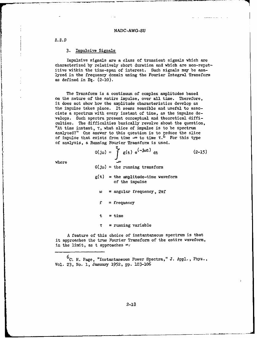
NADC-AWG-SU

2. 2.D

3. Impulsive Signals

Impulsive signals are a class of transient signals which arecharacterized by relatively short duration and which are non-repet-itive within the time-span of interest. Such signals may be ana-lyzed in the frequency domain using the Fourier Integral Transformas defined in Eq. (2-10).

The Transform is a continuum of complex amplitudes basedon the nature of the entire impulse, over all time. Therefore,it does not show how the amplitude characteristics develop asthe impulse takes place. It seems sensible and useful to asso-ciate a spectrum with every instant of time, as the impulse de-velops. Such spectra present conceptual and theoretical diffi-culties. The difficulties basically revolve about the question,"At time instant, T, what slice of impulse is to be spectrumanalyzed?" One answer to this question is to reduce the sliceof impulse that exists from time - to time T.6 For this typeof analysis, a Running Fourier Transform is used.

G(jw) = f g(t) e dt (2-15)

where -

G(jw) = the running transform

g(t) = the amplitude-time waveformof the impulse

W = angular frequency, 2nf

f = frequency

t = time

T = running variable

A feature of this choice of instantaneous spectrum is thatit approaches the true Fourier Transform of the entire waveform,in the limit, as t approaches -:

6C. H. Page, "Instantaneous Power Spectra," J. Appl., Phys.,

Vol. 23, No. 1, January 1952, pp. 103-106

2-18

NADC-AWG-SU

2.2.D

The spectra resulting from Eq. (2-15) may be of two gen-eral types:

1. Spectra containing a zero frequencycomponent

2. Spectra not containing zero frequencycomponent

In order for the spectrum of a time waveform to have azero frequency component, the waveform must have some residualarea when positive and negative areas under the entire impulseare added 7 Such amplitude-time waveforms are not theoreticallypossible in free air since free air is not a medium that cantransmit a pressure-time waveform like a unit step function.This means that free air will not transmit sound-pressure changesof zero frequency. Theoretically, then, the medium can onlyproduce impulses that have no DC frequency component.8

4. Practical Considerations of Impulse Signal Handling

In practice, the limited dynamic ranges of the recordingand processing equipment can result in a distorted impulsebeing finally reduced. The distorted impulse may have a netarea under the waveform, and therefore a DC component in itsspectrum. For minimum distortion, FM recording 9 and equip-ment having a large dynamic range and low-frequency cutoffsare necessary.10

7F. Skodde, "Low Frequency Measurements Using CapacitiveTransducers," B & K Technical Review, No. 1, 1969, p. 14.

8H. P. Olsen, "Frequency Analysis of Single Pulses," B & KTechnical Review, No. 3, 1969, p. 8; see also, W. B. Snow,"Survey of Acoustic Characteristics of Bullet Shade Waves,"IEEE Trans. on Audio & Electroacoustics, Vol. AU-15, No. 4,1967, p. 163.

9E. D. Sunde, "Theoretical Fundamentals of Pulse Trans-mission - I," Bell System Technical Journal, May 1954, p.773 ff; see also, K. G. Kittleson, "Introduction to Measurementand Description of Shock," B & K Technical Review, No. 3, 1966.

10M. J. Crocker and L. C. Southerland," The Effects UponShock Measurements of Limited Response Instrumentation," WyleLaboratories,Research Staff Report WR 65-1, January 1965.

2-19

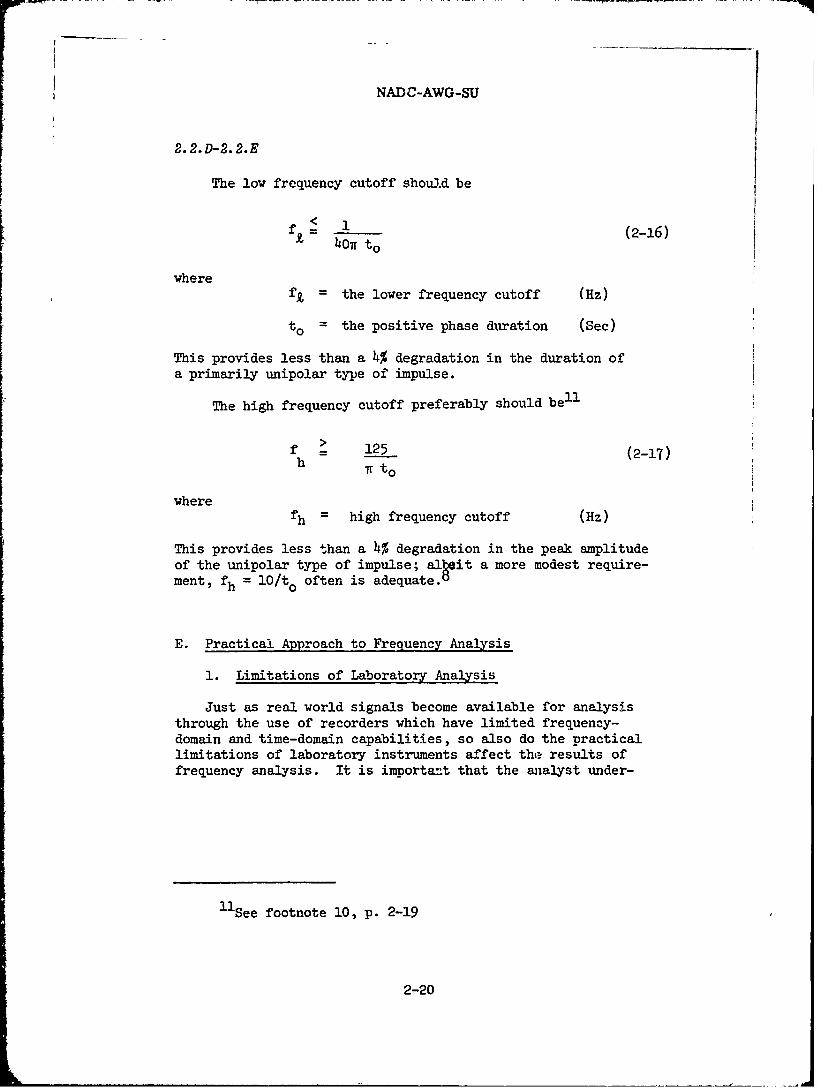
NADC-AWG-SU

2.2.D-2.2.E

The low frequency cutoff should be

ft = 1 (2-16)4or t o

whereft = the lower frequency cutoff (Hz)

to = the positive phase duration (Sec)

This provides less than a 4% degradation in the duration ofa primarily unipolar type of impulse.

The high frequency cutoff preferably should be l l

f h 125 (2-17)h 7Tt o

wherefh= high frequency cutoff (Hz)

This provides less than a 4% degradation in the peak amplitudeof the unipolar type of impulse; al it a more modest require-ment, fh = 10/to often is adequate. °

E. Practical Approach to Frequency Analysis

1. Limitations of Laboratory Analysis

Just as real world signals become available for analysisthrough the use of recorders which have limited frequency-domain and time-domain capabilities, so also do the practicallimitations of laboratory instruments affect the results offrequency analysis. It is important that the analyst under-

llSee footnote 10, p. 2-19

2-20

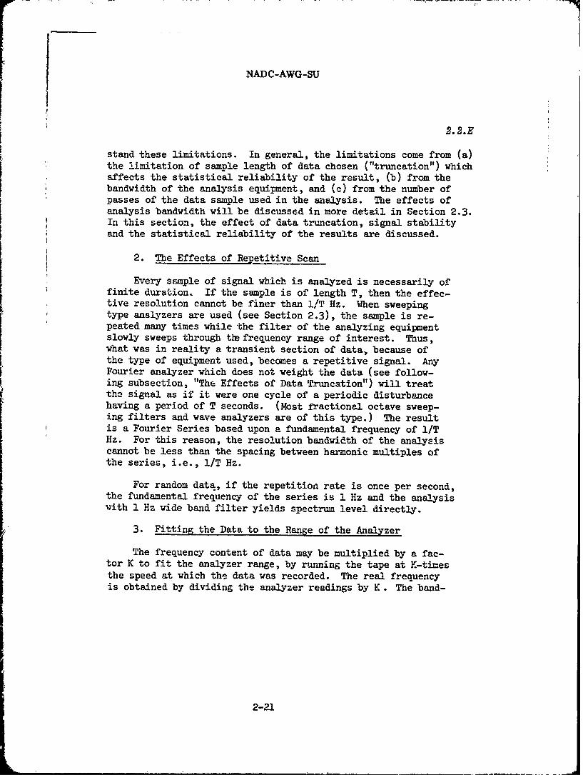
NADC-AWG-SU

2.2.E

stand these limitations. In general, the limitations come from (a)the limitation of sample length of data chosen ("truncation") whichaffects the statistical reliability of the result, (b) from thebandwidth of the analysis equipment, and (c) from the number ofpasses of the data sample used in the analysis. The effects of

analysis bandwidth will be discussed in more detail in Section 2.3.In this section, the effect of data truncation, signal stabilityand the statistical reliability of the results are discussed.

2. The Effects of Repetitive Scan

Every sFimple of signal which is analyzed is necessarily of

finite duration. If the sample is of length T, then the effec-tive resolution cannot be finer than l/T Hz. When sweepingtype analyzers are used (see Section 2.3), the sample is re-peated many times while 'the filter of the analyzing equipmentslowly sweeps through ti frequency range of interest. Thus,

what was in reality a transient section of data, because ofthe type of equipment used, becomes a repetitive signal. AnyFourier analyzer which does not weight the data (see follow-ing subsection, "The Effects of Data Truncation") will treatthe signal as if it were one cycle of a periodic disturbancehaving a period of T seconds. (Most fractional octave sweep-ing filters and wave analyzers are of this type.) The resultis a Fourier Series based upon a fundamental frequency of I/THz. For this reason, the resolution bandwidth of the analysiscannot be less than the spacing between harmonic multiples ofthe series, i.e., l/T Hz.

For random data, if the repetition rate is once per second,the fundamental frequency of the series is 1 Hz and the analysiswith 1 Hz wide band filter yields spectrum level directly.

3. Fitting the Data to the Range of the Analyzer

The frequency content of data may be multiplied by a fac-tor K to fit the analyzer range, by running the tape at K-tinezthe speed at which the data was recorded. The real frequencyis obtained by dividing the analyzer readings by K. The band-

2-21

NADC-AWG-SU

2.2.E

width of analysis should also. be divided by K.

1. The Effects of Data Truncation

Since only a limited sample of data is taken for analysis,there is an unavoidable analysis error. This is true even ifthe signal being analyzed is stationary periodic. The cause oferror can be understood by realizing that a T-second sample willappear to any analyzer as a periodic signal with period T multi-plied by a window function F(t), where

< <

F(t) = 1, 0 t = T and (2-18)

F(t) = 0, otherwise (2-19)

Consequently, the Fourier Transform produced by an ideal

analyzer of the T-second sample will be that of the equivalentFourier Series of the sample convolved with the transform of thefunction F(t). If the original signal is u sine wave of fre-quency fo, then the Fourier Transform Y(Jw) of a T-second por-tion of the sine wave is

YQ ) -_ sin w(f - fo)T (2-20)Y (f - fo)T

This has pronounced sidelobe structure (Figure 2-1) at intervalsof l/T Hz. The first sidelobe is down only 13.2 dB and the320th sidelobe is down 60 dB.

Since the desired form of transform of the original sinewave is simply a single line at fo, it is customary to "shape"the window function, F(t), so that the transform of a finitesample of a sine wave closely resembles a single line.

That is, the window function is made other than rectangularin order to minimize its effect on the analysis. This is doneby weighting the data samples nonuniformly from -T/2 St =T/2.The effect is to widen the resolution bandwidth of the analyzersomewhat fro li/T Hz, but in return to drastically reduce thesidelobe structure. Modern real time analyzers frequently em-ploy this weighting technique (see subsection 2.3.D).

qthree coumon windows used in analog spectrum analyzers are

~2-22

NADC-AWG-SU

LO

0.8- ±0~~i701.7_

INPUT WAVEFORM

0.4 -

0.3 -

0.2 -

0.1 - -- '

0 7

-5 -4 -3 -2 -1 0 1 2 3 4 5 6 7 8 9 10

NORMALIZED FREQUENCY I I/T UNITS

Figure 2-1. Spectrum of Unweighted Window

1.9 1 .0 *0.7

0.9 -0.4

0.7 0.2

0.6 0.1

0.___ 0.7

0.4 0.4 1

0.3 0.2

0.2 x 01o., !0.01oo ---------0.1 0.0207r 2

0 1 2 3 0.001NORMALIZED FREQUENCY

IN IT UNITS 0.002sin 7r fT 0.001 1

1 rf 0 1 2 3

2 Dolph-Cbeb7cbeff NORMALIZED FREQUENCYIN l/T UNITS

3 Hamming4 TrIplt

Co.Inosqed

Figure 2-2. Comparison of Various Weighting Functions

2-23

NADC-AWG-SU

2.2.E

the Triplet having a form- (n/T)t 2 Wt T <5 S T

--c e --o= t = - ( 2 -2 1 )T 2 2

the Hamming

F(t) = 0.54 + o.46 cos 2wt T _ t < T (2-22)T 2 2

and the Cosine-Squared

F(t) = cos 2 . T < < TF.. .==o t = - (2 - 2 3 )

T 2 2

The Triplet response has no sidelobes but a broad main lobe(1.73 times that of an unweighted window at the 3 dB down point,15/T at -40 dB and 50/T at -60 dB).

The Hamming has a slightly narrower main lobe (1.5 timesthat of an unweighted window) and a strongest sidelobe (thethird) level of -42.8 dB, with other sidelobes falling off as1/f from the third.

The Cosine-Squared window has an intermediate width mainlobe (1.59 times that of an unweighted window) and a strongestsidelobe (first) level of -31.4 db, with other sidelobes fallingoff as i/f3 from the first, so that the fourth sidelobe is down54 dB. For comparison, the fourth sidelobe of the Hamming is down43 dB. Figure 2-2 shows a comparison of several weighting schemes.12

5. Effect of Signal Stability 1 3

Frequently, as with data stemming from moving sources, thereal analysis signal contains strong line components whose fre-quency varies with time. It is important to understand how theanalysis equipment treats these signals and the errors whichoccur thereby.

The effect of the frequency stability of the source can oeseen by examining the analyzer response to a sliding tone. Asliding tone is defined as a quasi-sinusoid whose frequency

12C. L. Temes, "Sidelobe Suppression in a Range-Channel

Pulse Compression Radar," IRE Trans. on Military Eleetronics,April 1962, pp. 162-169.

13W. Gersch and J. M. Kennedy, "Spectral Measurementsof Sliding Tones," IRE Trans. CT-7, August 1960.

2-24

NADC-AWG-SU

2.2.E

changes linearly with time.

s(t) = exp 2nj(fot + kt2 ) _ T t _T (2-214)2 2

The total amount of frequency slide (Af) is kT where k isthe rate of frequency sweep in Hz per second, in the analysistime interval T, so that the frequency excursion of the signalin resolution bandwidths, l/T, is

n = k.T2 (2-25)

The spectrum for a given value of n depends both on n andon the window function F(t). The spectrum of a sliding tonewith a rectangular window function is shown in Figure 2-3. Forsmall n, the major effect is a sizable increase in sidelobelevel and a consequent broadening of the spectrum line, espe-cially in a logarithmic plot. For large n, say n> 50, there isan approximately equal distribution of energy across the band.Thus, the spectrum of a sliding tone having n = 100 will be ap-proximately 100 resolution bandwidths wide and will have a spec-trum level of 20 dB down from that of an equal energy stable sig-nal.

For intermediate values of n, the Fourier Transform is quitecomplex (see Figure 2-h, which shows responses for a one-sidedslide). There is a reduction in the peak amplitude of the spec-trum (relative to that of a steady tone) according to the follow-ing table:

n Amplitude Reduction, dB

0 01 0.32 1.04 4.06 7.78 9.6

This is less than would be expected by equal power divis-on overthe frequency range. The sidelobe structure broadens and, forn = 6 and higher, there may be a minimum at the center frequencyrather than a maximum.

For Cosine-Squared weighting (see Figure 2-5) the effect isfar less, both in terms of amplitude response r d in terms ofsidelobe structure. A moderate slide actually .ooths over thesidelobes. For n = 4, there is a peak loss of .oout 1 dB. and

2-25

NADC-AWG-SU

2.2.E

almost nothing for n = 2. The Triplet shows similar behavior,with responses down as follows:

n Amplitude Loss, dB

0 01 02 0.24 0.78 3.0

16 4.832 8.0

Therefore, for Triplet or Cosine-Squared weighting, a totalfrequency instability of 4 resolution bandwidths per analysistime will produce relatively unimportant effects on broadeningand amplitude reduction.

When analyzing a signal of varying frequency, it is neces-sary to widen the resolution bandwidth and reduce the ana]ysistime to achieve an accurate indication of the peak. spectralline level. For example, suppose one is analyzing the signalfrom an accelerating vehicle and the engine speed is changing 10%per second, then a 30 Hz nominal line would change 3 Hz/second.If an analysis bandwidth of 1 Hz were used and the time samplewere 1 second, n would be 3 which for Triplet weighting wouldresult in a line level accurate to about 0.5 dB. For the fifthharmon.c, however, the frequency slide would be 15 Hz/second andthe resolution and sample time would result in n = 15, resultingin an error of almost 5 dB. To get an accurate indication ofthe level of the fifth harmonic, one should increase the resolu-tion bandwidth to 2 Hz and reduce the sample time to 1/2 second.This results in n equal to 3.75 and reduces the error to abouto.6 dB.

6. Statistical Reliability

The emanations from manV sources and backgrounds are ba-sically random in nature. The spectra from such sources willshow statistical fluctuations, and the standard deviation ofthese fluctuations depends on the number of degrees of freedomof the analysis. The number of degrees of freedom of a singleFourier analysis of duration T and resolution l/T is two, sincefor each spectral component an amplitude and a phase may be in-dependently specified. The number of degrees of freedm maybe increased by averaging or integrating spectra of a number ofindependent time samples of the signal. Since the time taken toanalyze one sample of data is equal to I/B where B is the anal-

2-26

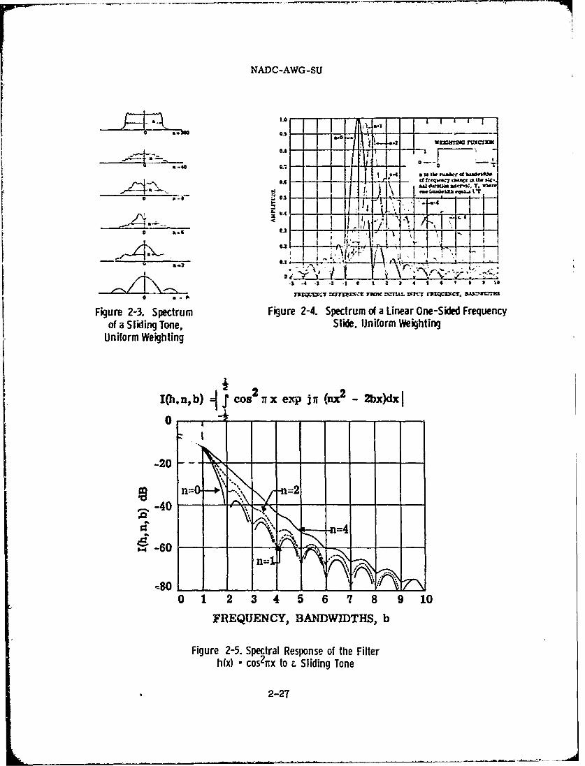
NADC-AWG-SU

u- -- -,• 5.81 .1 -- •

s ~"a t I T. VI.,n

0 a.- - -

A-2I-% -4 -3 -2 .11 9I II 2I 3I so1• ,, i •

Figure 2-3. Spectrum Figure 2-4. Spectrum o( a Linear One-Sided Frequencyof a Sliding Tone, Slide, Uniform Weighting

Uniform Weighting

I(h ,nb) C cos 2 rx e.V ji (nx2 2bx)dxI

0 T

-20

n=" ,. =2

-=4-60

-- So/ *

0 1 2 3 4 5 6 7 8 9 10

FREQUENCY, BANDWIDTHS, b

Figure 2-5. Spectral Response of the Filterh(x) -cos2 Tx to z, Sliding Tone

2-2T

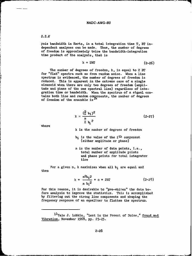
NADC-AWG-SU

2.2.E

ysis bandwidth in Hertz, in a total integration time T, BT in-dependent analyses can be made. Thus, the number of degreesof freedom is approximately twice the bandwidth-integrationtime product of the analysis, that is

k = 2BT (2-26)

The number of degrees of freedom, k, is equal to 2 BTfor "flat" spectra such as from random noise. When a linespectrum is evidenced, the number of degrees of' freedom isreduced. This is apparent in the extreme case of a singlesinusoid when there are only two degrees of freedom (ampli-tude and phase of the one spectral line) regardless of inte-gration time or bandwidth. When the spectrum of a signal con-tains both line and random coponents, the nimber of degreesof freedom of the ens~ble is-

k = b) 2 (2-27)

n

wherek is the number of degrees of freedom

bi is the value of the ith component(either amplitude or _hase)

n is the number of data points, i.e.,total number of amplitude pointsand phase points for total integratortime

For a given n, k maximizes when all bi are equal and

then

k n2 b2 n = 2ET (2-28)

n bi2

For this reason, it is desirable to "pre-whiten" the data be-fore analysis to improve the statistics. This is accomplishedby filtering out the strong line components and shaping thefrequency response of an equalizer to flatten the spectrum.

lbYale J. Lubkin, "Lost in the Forest of Noise," Sound and

Vibration, November 1968, pp. 23-25.

2-28

NADC-AWG-SU

2.2.E

After analysis, the complementary equalization is applied tothe spectrum to correct it. The value of the coherent line3is established by separate analysis and reinserted into thespectrum. When the lines are not removed from the spectrum,the value of k in the vicinity of the line is decreased by afactor approximating the ratio of the line width to tbhe anal-

ysis bandwidth.

For random data, the anticipated spread in the expectedvalues of spectral components is called the confidence inter-val and is a function of the protability of the spectra ofthe random data exceeding this spread. It can be shown thatthe standard deviation of the value of the spectral lines fromGaussian data is given by

1 Z(2-29)

Based on this formula, the following table of confidence inter-vals is calculated. Note that this uncertainty applies strictlyonly to Gaussian randoc spectra and is due to the nature of ran-dom signal and not to the analysis.

_ _ f__ _ide--e LeTel

P- k - - - -

1 2 3.6 9.8 1,.8 13 5. 16 7.2 23

2 h . .. 3 7.5 k.5 9.2 5-T 13

2.5 5 2.7 A.9 3.5 6.k 4.1 7.8 5.3 12

8 Z.2 3.6 2.9 4.7 3.4 5.7 4.& 7.8

5 10 2.0 3.1 2.6 4.1 3.1 Ej.9 L.L 6.7

10 20 i.5 2.1 2.0 2.7 2.3 3.2 3.0 4.3

25 S;L 1.0 1.3 1.3 1.6 1.6 1.9 2.0 2.5

CA0 103 O.7 0.8 0.9 1.0 1.0 1.2 1.3 1.6

10 20 0.5 0.5 0.7 0.7 0.6 0.8 1.0 1.0

250 500 0.4 C.h 0.h 0.4 0.5 0.5 0.7 0.7

500 10M') 0.3 0.3 0.3 0.3 0.h 0.4. 0.5 0.5

2-29

NADC-AWG-SU

2.2.E-2.2.F

For example, for any particular resolution element (spectralline) for k = 8, there is an 80% probability that the measuredvalue will lie between +2.2 and -3.6 dB of the true value.

It is desirable, then, to integrate the signal spectrum foras long a time as possible in order to increase k for a givenresolution bandwidth and so decrease the confidence interval. Ifthe signal is not stable, then the length of time that one canintegrate is limited, and the confidence interval is correspond-ingly wide. Alternately, one may increase the resolution band-width to raise k when signal instability prevents increasing theintegration time. In this case, one trade 5off frequency reso-lution for amplitude accuracy in the band.

F. Signal Characteristics in the Time Domain

1. General

The importance of time domain analysis lies in its abilityto aid directly in the design of electronic detection devices.Often, it is insufficient to know the power spectrum density ofthe signals to be detected because there may exist noise sourcesvith significant energy in the same portion of the spectrum asthe desired signal. The key difference between the desired sig-nal and the noise may reside in the relative phases of the com-ponents. For example, both white noise and a delta function havea flat power density spectrum, i.e., equal power per unit frequen-cy (see Figure 2-6). (Strictly speaking, the frequency transformof delta function extends from - to +-.) There is, however, acoherent relationship among the phases of the components which con-stitute a delta function and a random relationship between those ofwhite noise. The result in the time domain is a random distribu-tion of levels for white noise and, for the delta function, a zerolevel everywhere except at zero reference time where the level ap-proaches infinity. These two signals can be distinguished readilyin the t.me domain by their different amplitudes but, because ofequivalent power density spectra, it is difficult to distinguishthem in the frequency domain.

157his is a manifestation of Uncertainty Principle as ap-plied .o signal analysis. See B. B. Bauer,"Octave-Band Spec-tral Distribution of Recorded Music," J. Audio Eng. Soc., Ai)ril1970.

2-30

NAD C-AWG-SU

2.2.F

0

fil

Time Domain Frequency Domain

WHITE 1NOSE

E

o E

Time Domain Frequency Domin

DELTA FUNCTION

Figure 2-6. Spectral Comparison of White Noise and Delta Function

Sometimes, a key difference between two signals is a differ-ence of power level variation with time. Thus, an acceleratingtruck exhibits a variation in power level as it accelerates inturn through each gear with sudden decreases in level as the gearsare shifted. Such variations can be used to distinguish the truckfrom other sources. The variation in power level can be measuredon a broadband basis, but it is frequently best to restrict theband to that frequency region wnere the most distinguishable vari-ation occurs. This ability to detect those sources whIch change

2-31

NADC-AWG-SU

with time in some prescribed manner provides a powerful identifica-tion tool.

The time-domain information discussed above is from a singlesensor. A very powerful application of time-domain analysis iscorrelation in which the product of two signals is integrated withtime to determine the degree to which they correspond in time. Thetwo signals may be received by two different spaced-apart sensors(spatial correlation) or from the same sensor YIth one of the sig-nals delayed in time with respect to the other (time correlation).The result of correlation is an i?,provement in signal-to-noiseratio since, if the experiment is properly designei, the correlatedsignals from the same source will produce a greater output thancorrelated random signals.

A detection scheme which uses multiple sensors operating indifferent signals fields (i.e., acoustic, seismic, infrared, etc.)can provide much improved signal identification, without requiringthe use of sophisticated correlation systems. In these cases, itmight be considered that a detection coincidence criteria for theindividual sensors constitutes a simple form of correlation. inany case, coincidence detection in multiple signal fields withinthe scope of time-domain analysis is based on the interrelation-ship of the variables with time and not on their individual char-acteristics.

2. Time-Domain Characteristics

It is helpful to define certain terms used in time-domainanalysis especially since they are frequentlyr used with differentmeanings in different texts.

Envelope. The envelope is the locus of pointswhich are the extremes or a function betweenaxis crossings. Typically, the envelope isthe pair of curves one of which Joins each ofthe peak positive signal excursions and theother of which Joins each of the peak negativesignal excursions (Figure 2-7).

Rectified Envelope. Frequently, the functionof interest is the envelope of the signal afterrectification. In such case, the type of rec-tification should be designated, e.g., positivelyrectified envelope, negatively rectified envelope,or full-wave rectified envelope. The rectifiedenvelope of a signal will depend upon the amountof "smoothing," if any, provided by the low passfilter after rectification.

2-32

NADC-AWG-SU

2.2.F

Rise Time. This is the time required for thespecified time function or envelope to increasefrom 10% to 90% of its maximum value. An accu-rate estimate of this parameter requires a goodsignal-to-noise ratio. When the nature of thesignal is such that ro such idealistic approxi-

mation can be made, the definition of the 10%value for the signal is oftn specified in what-ever form is most useful to the circuit designer.The more ccmrn definitions are the point atwhich the rms signal exceeds the m noise by10% or hen the peak signal exceeds the ealknoise by 10%. In such cases, the con-iticnsunder which the determinaticn was =ade =ust testated (Figure 2-7).

Fall Time. This is the -i=e requireld for the iri-nal to diminish fr-m 931 of its =axi =;1ituleto 01% of its naxt==. The same sigar.l-tc-nzizelimitations discussed concerning rise tire are i-'posed on any attempt to precisely measure the fm/ltime parameter (Figure 2-7).

Signal fluration. Sbe signal ?'.r&aAzn is =n±1dtre!to be the time ericd tetween the 1:14 T:int :f :nrise characteristic an! the 1 CInt cf the falcharacteristic. The usefP4/ezs :f "thiz tarare.-is associated with the Itsigm zf A3 retvw-r.cz.can aid the desg-ner SL de-dIr.F ±e a 7rt :f ziF-nal supressicn tc be expezte- frc= a art. '.arcircuit (F-Igure -- 7).

Signal Gradient. Ls these i-stan: c vt-'r-e --!z ri-nal cannot be a p ximated ty a :se :f straistt*lines ivresentir.F "rlse," . ardI-a,it is necessar:F tc- descrie the %ar-ie *t-e

in a se-what zore traereive 'an'r. -:.:-tdescr.ption can he cbtainedl y zsa-.Ir.F the sig-nal envelope and pic-tirg the anz-:-nt :f t~a~ -tween akiacent sap-es. 'Mis Trcze! re Fr;e- aplot which Fives the Aes! er a lete !e:zriz-tlen of the nanrzr in whizh the signal level ha-zfluctuated vith time. There are three area :!r !-cision hich =.st a -nany an sn:,rsis :f tt.iztype. Th'ese are: the ietef_ tv o'-!n-, the :-pling rate, and the necessity of s=!A--thin.r thro.g-the averaging of several adjacent sa:.les.

2-33

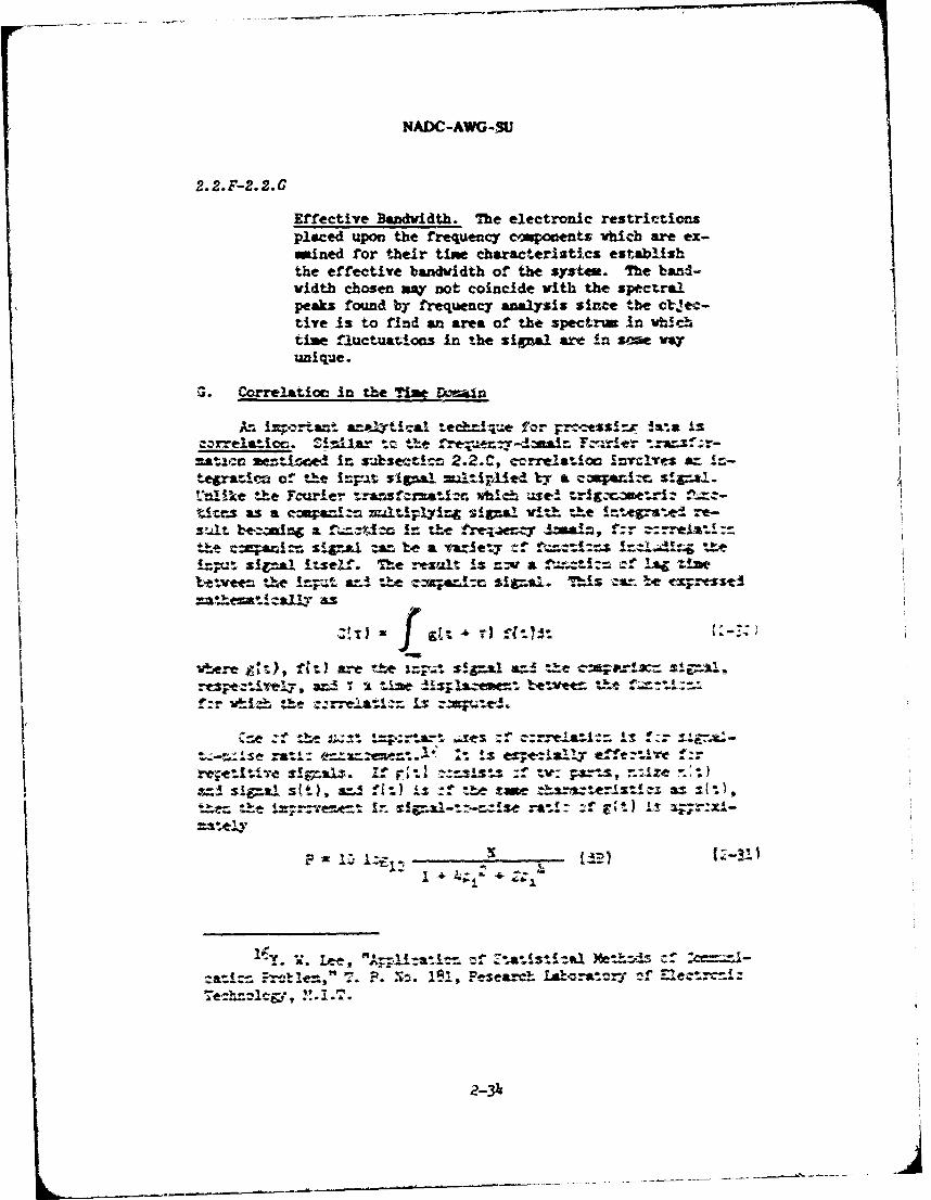
NADC-AWIG-SU

2.2.F-2.2.G

Effective Bandwidth. The electronic restrictionsplaced upon the frequency co~sponents whtich are ex-mined for their time characteristics establishthe effective bandwidth of the sysrtem. 'The bani-width chosen uay Dot coincide with the spectralpea"s found by frequency analysis since the ct.!ec-tive Is to find an area. of the spectru7m In "th!ch,time fiuctuzations in the sigma arm in scae way

An iq a.~ icl tech:c?:e fXIn or r.-ts1r -4va is

=&-Ucc seztiocel In s;-Aseti 2.2.C, ccrrelation -nvc!res an i---tegrm-lea e the in-Ft sigma!ltiyAxtt t-y avai ~.!:nlike tht Tcurle' raszan ,sbidh usel trig.xc-metriz ~:

U=as a C~m;*=!= iti~~gslwt h intega.e- re-

the z=V=!= s!i n*A zs be a varlet :f 1=11-41=6 tbe"" !V=1 snl tSelf. The Mev~lt IS =ZVa fl Ze

btweez the 1= ;" =4 tte ZA;SA=i %!CMA1. '!hs z ze t-Cst

-J, ftl are t!he =7.i sIS-zai =! t!he .x s

t~ V~hthe ~a A~ is -. 4

,.e z? tte z t a zis:f :aini fzr

ra.is A ex-rt--all.y CAzt:l.zulv z

~nisZ-"st-t), =14~ 11%~) Is -f the sine a~rs~ s x(.),!the -e~k*_ in 1~l:-ni rate!: :f F~kt) Is

~~~ +z 4;4

zf a

19311,~f Peeac 1A*_t-1 '

NADC-AVIG-U

-O- -d

Sho" tut . iw ffw ra lowd tos

7hea*. ~t--t cuz ztce.kza s!'a ecazn**.ef1 r

Sigma # rnti- ri-ez is :.I' et-'Q != IZ

d3--C a flvisl a *Is: bsez sii :be-fe~?hIs cia d4=seFa in ae sIca1 ine iF- I ±eerea

tht~ bpre:.ec la- s~e catie-iz :f h isigmal vr.. isl camgie c-id-= as tIte sce vareo tIed 1-1 ;aths,a tedi~za, vsi-!m- to- at use peIin crima42It &=&Ie. A1 deeS*pAI transfe. f rltl o a eicm isrcuit. ~is*r~z

wiac'3s~ :~z~, ai~~ ' rs.i~2-35~~rr

NADC-AWG-SU

Z- -t.r r:- kT-.he a selfn %,yst vindch can accoItodate

w. e - i= bt:h sigmal level and. -wankng noise sources,Is lm _-ezzar--- a;:!y :se -.cans of signal level control. Inr- :ri'.y-f th-e .rjstkeas,- this i.s acccr-pl!shed by integrat-av f e_"-- - er& the sensor and applying it to

r~i~ r-c 'rz -r feedback networ. The place in theff -. v!ch this control voltage is derived is

te l9" be lez er fer:= t-he knowledge of the characteristics

zf "tet- t: te l e'te-zled. it is not unusual for control sig-

-3zt: te _t.i-'- fr= several areas of the circuit so as to.... l ̂ - -- ==Ise rejection without degrading the detection

-lat-114ty =r i.easing the false alarm rate. The areas most-e=_-nel fzr zuch cont-rol voltage are:

a. syetral energy in separate noise sensingah~une!

b. the integrated average energy in the datachannel having time constants longer orshorter than the desired signal, and,

c. a filtered post-detection channel forsensing signals not having the same en-velope spectrum as the desired signal.

The last technique may actually be a differentiating networkwhich can be considered as a post-detection high-pass filter. Akrnowledge of the signal rise time characteristic will allow thedesigner to optimize a differentiation network for a particularclass of signals. This same information is necessary to designthe attack times of AGC networks to be applied to the signal chan-nel.

If the entire signal envelope has to be retained to achievereliable detection and identification of the signal, it will benecessary to examine closely the duration of the signal to assurethat an AGC network is applied which acts as rapidly as possiblewithout degrading the desired signal. The rate at which the AGCnetwork recovers after the passage of a signal can be optimizedif the fall time of the signal is known. In those instances wherethe manner in which a signal decays is unique enough to aid thedesign of identification logic, this consideration is especiallyimportant. It may be necessary to follow the controlled ampli-fier by a differentiator of some sort -which has been optimized

2-36

-fie

by a ifeenia

o sesot

hchha

ee otmie

NADC-AWG-SU

2.2.H-2.3.A

for the desired negative-going envelope (toward zero). Such con-siderations are also vital if the sensor is required to detectmany successivr targets, since an improperly chosen decay time maydesensitize the system for the later signals of the group.

2. Post-Detection Filtering

If the signal of interest has an envelope shape whichitself contains reasonably unique spectral characteristics, itis often beneficial to apply some form of post-detection filter-ing. The reason for mentioning this subject under the topic of

time domain is twofold: (a) the signal being filtered is thetime envelope of the signal--not the original signal itself, and(b) the application of differentiation networks (special high-pass filter) is directly related to the time structure of thesignal.

It is entirely possible that a separate time-domain analysismay be required on the output of the post-detection filtering net-work. An example of this sort is a detector for a signal whoseenvelope fluctuates at a rate which is a direct function of thesource location.. Here, it is necessary to design a post-detectioncombination filter whose individual AGC rates are determined bythe sweep rate of the pulsating signal. This example is mentionedto indicate the areas where time-domain studies much simplify de-sign procedures. The application of differentiating networks- forthe examination of decay characteristics is often overlooked. Theexistence of such unique signals is not nearly as rare as one mightthink.

2.3 FREQUENCY DOMAIN DATA ANALYSIS

A. Introduction

1. Types of Analysis

A variety of devices has been deveioped for measuring powerspectra of a stationary periodic signal '; however, al analoganalyzers employ the same basic functions--filtering, detection,averaging, and displaying the result on a meter or other outputdevice. In some cases, the signal is filtered by a narrow-bandfilter, for which the center frequency is varied to obtain the

171f the signal is not stationary periodic, a portion there-of is stored and repeated so as to present a stationary periodic

signal to the analyzer.

2-37

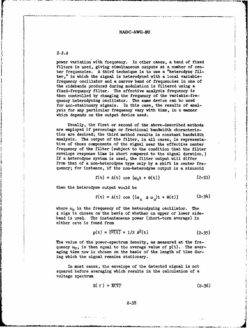
NADC-AWG-SU

2.3.A

power variation with frequency. In other cases, a band of fixedfilters is used, giving simultaneous outputs at a number of cen-ter frequencies. A third technique is to use a "heterodynq fil-ter," in which the signal is heterodyned with a local variable-frequency oscillator and a narrow band of frequencies in one ofthe sidebands produced during modulation is filtered using afixed-frequency filter. The effective analysis frequency isthen controlled by changing the frequency of the variable-fre-quency heterodyning oscillator. The same device can bo usedfor non-stationary signals. In this case, the results of anal-ysis for any particular frequency vary with time, in a mannerwhich depends on the output device used.

Usually, the first or second of the above-described methodsare employed if percentage or fractional bandwidth characteris-tics are desired; the third method results in constant bandwidthanalysis. The output of the filter, in all cases, is representa-tive of those components of the signal near the effective centerfrequency of the filter (subject to 'the condition that the filterenvelope response time is short compared to the signal duration.)If a heterodyne system is used, the filter output will differfrom that of a non-heterodyne type only by a shift in center fre-quency; for instance, if the non-heterodyne output is a sinusoid

f(t) = A(t) cos [wot + e(t)] (2-33)

then the heterodyne output would be

f(t) = A(t) cos [(wc ± Wo)t + et)] (2-34)

where wc is the frequency of the heterodyning oscillator. The

± sign is chosen on" the basis of whether en upper or lower side-band is used. The instantaneous power (short-term average) ineither case is found from

p(t) = f2CtT = 1/2 A2 (t) (2-35)

The value of the power-spectrum density, as measured at the fre-quency wo, is then equal to the average value of p(t). The aver-aging time now is chosen on the basis of the length of time dur-ing which the signal remains stationary.

In most cases, the envelope of the detected signal is notsquared before averaging which results in the calculation of avoltage spectrum

E( f) = :T (2-36)

2-38

NADC-AWG-SU

2..3.A

This procedure can be justified on the basis that the averageand rms values of a narrow-band signal are related by a factorthat remains relatively constant, regardless of the amplitudedistribution of the signal before filtering. For instance,this factor for a sine wave is 2 f//w or 0.903. For a Gaussiansignal (Rayleigh envelope) it isV/2 or 0.887. The differenceis less than 2%, even though the amplitude distribution for asine wave is markedly different from a Gaussian distribution.

2. Presentation of Data

Selection of the proper information to consider (or display)is vital to proper interpretation of signal characteristics. Someof the types of displays which are in common use today are spec-trum "snapshot." spectrum time plot, and single-line behavior.

a. Spectrum "snapshot." A spectrum is computed on

the basis of an integration time, T, with selected analysis band-width. The display consists of an X-Y plot of spectral powerdensity -versus frequency. Examples of this display format aregiven in subsection 2.3.D (Figure 2-25). This approach gives aquantative understanding of the signal characteristics providedthe spectrum is stationary, i.e., it does not change with time.Generally, an appropriate integration time is determined experi-mentally--if the results of the analysis do not change appreci-ably over one integration period, the choice is satisfactory.

b. Spectrum time plot. When the signal is not sta-tionary, an intensity-modulated X-Y plot can be ased to show thebehavior of the spectrum as a function of time. Frequency istaken along one axis, time along the other, and intensity modu-lation is used to give the spectral level at a given frequencyand time. The time-wise character of the signal under study givesinsight into the physical processes of signal generation, pro-vides an overview of th6 signal structure and its behavior, andprovides a basis for rejection of signals from unwanted sources(since the behavior with time of signals from different sourceswill normally be different). The chief disadvantage of thistype of display is that the information extracted from it tendsto be of qualitative rather than quantitative nature. Exam-ples of spectrum-time plots are given in subsection 2.4 (Figures2-27 and 2-28). An alternate approach to the spectrum-time plotis the "3-D spectral display" which depicts the results of manysequential spectral analyses in a pseudo-three-dimensional man-ner. Such a representation is seen in Figure 2-29.

2-39

NADC-AWG-SU

2.3.A

c. Single-line behavior. Devices, such as thephase-locked loop, can be used to study the behavior of a single

4"line." Typically, the phase c! the data signal is comparedagainst thLt of a signal produced by a local oscillator. Thecomparison voltage is used to adjust automatically the frequencyof the local oscillator so that the two signals remain in phase.The comparison voltage is thus a measure of the instantaneousfrequency of the data signal. Either the amplitude or the fre-quency of the "line" may be shown as a function of time in anX-Y plot. This type of presentation is valuable for studyingthe behavior of an individual "line," but gives little insightinto the total signal characteristics.

3. Interpretation of Data

* It is necessary to take a close look at the manner inwhich the signal analyses and noise analyses are performed toprevent serious misinterpretation of the results. If the sig-nals and the noise are of the same character (for example, bothare random in character), the results of their analys.)s by thesame techniques will yield directly comparable results. Figure2-8 shows such a case in which the signal and the noise spectraare continuous, and a direct overlay is useful as a guide to thesystem designer. A plot of the signal-to-noise ratio derivedfrom Figure 2-8 is shown in Figure 2-9. By matching this curvewith an input bandpass filter, the designer can begin to optimizethe detectability of the signal.

a. Random Signals. In interpreting data, a problem mayarise from the fact that the detected output usually is a functionof the filter bandwidth. Practically, the spectrum levels are ob-tained with octave-, 1/3-octave-, 1/10-octave, or constant-band-width filters. The results of signal analysis obtained with dif-ferent bandwidths are not directly comparable with each other. Theresulting spectral plot is then said to be in terms of SpectrumDensIty Levels, often called simply "Spectrum Levels." It becomesnecessary to modify the measured values by some proper factor sothat the data taken with analyzers of different bandwidth can becompared meaningfully.

Bandwidth correction or "normalization" of random sig-nals is accomplished by dividing the output power reading by thebandwidth. In terms of levels, this is equivalent to diminishingthe level by 10 log Af, dB, where Af is the bandwidth of the fil-ter in Hz. It should be noted that with constant fractional band-width filters,Af increases with frequency f; thus Af = Ff, where F

2-4o

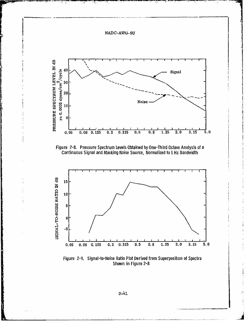
f NADC-AWG- SU

Signal

CII 30

2 15

0-

0

-

5--

0.05 0.08 0.125 0.2 0.315 0.5 0.8 1.25 2.0 3.15 5.0

Figure 2-9. Signal-to-Noise Ratio Plot Derived from Superposition of SpectraShown in Figure 2-8

2-1

NADC-AWG-SU

1

2.3.A

is the fraction of bandwidth used, and the needed correction is-10 log Ff, to produce a result whose amplitude is equivalentto that produced by a filter with a 1 Hz bandwidth. For example,the analysis shown in Figure 2-10 was done with a 1/3-octave anal-yzer and a filter bandwidth correction was applied as describedabove. The effect of such a bandwidth normalization is shown inthe dash line. Bandwidth normalization helps to prevent errors ininterpretation. It should be pointed out that the uncorrectedm.alyzer output gives the impression that the signal has a greatdeal of high frequency power when, in fact, the power density isvery low in that part of the spectrum.

Strong single-frequency lines of a stationary spectrumare unaffected by the filter bandwidth, and the correction factordescribed in the preceding paragraph is not applicable to them,as discussed in subsequent paragraphs.

The pro,.ess of bandwidth normalization is rooted in twobasic concepts which are common to the field of "noise measure-ment." The .irst consideration is the characterization of noisein terms of its power-spectrum density. This form of presentationwas defined by early researchers as the average power per-cyclebandwidth, thus requiring real-filter systems to be corrected ifthis form of presentation were desired. In addition, and close-ly related to this, researchers in the field of noise measurementneeded a means of validating and comparing measurements made withdifferent analyzing schemes. It was found that when "white" noisewas applied to the real analyzers being used, and the individualfilter output voltage was divided by the square root of the filterbandwidth (or dividing the power reading by the bandwidth), the re-sulting spectrum was indeed flat with frequency. This, then, pro-vided a means of validating the many analyses schemes availab'e,and increased the confidence in the physical interpretation of thedata being presented by the discipline.

In some instances, this form of correction was designedinto the analysis system by electrically de-emphasizing the data(3 dB/octave for 1/3-octave systems). In the data analyzed forthe AWG effort, this concept is retained with all corrections be-ing accomplished manually so that their magnitude could be chang-ed to better suit the known physics of the data.

When the bandwidth, Af, is given in terms of the upper andlower cutoff frequencies, the amount of correction, C, applied to the

-

2-42

NADC-AWG-SU

2.3.A

70

60

o a 1/3-Octve Filter Outputa 50

>. 40 .

~~~Normalized Filter Output "',

30

20 ' I I I I ! I I ! ""I

0.02 0.0315 0.05 0.08 0.125 0.2 0.315 0.5 0.8 1.0FREQUENC'Y IN WILOHERTZ

Figure 2-10. One-Third-Octave Analysis of a Continuous Noise SourceShowing the Effects of Bandwidth Normalization

signal level can be calculated from the following expression(for whose derivation see, for example L. L. Beranek, AcousticMeasurements, John Wiley and Sons, New York (1949), pp. 563-564.

C =-l0 log (fa - fb), dB (3)

where

fa = upper cutoff frequency

fb = lower cutoff frequency

The bandwidth correction method described above assumesthat the signal spectrum being measured is roughly constantover the bandwidth of the filter element and, if a voltage de-tector rather than a power detector is used, that the phase in-formation across the band is randoai. Tis assumption isgenerally of sufficient accuracy to cause no concern in theanalysis of signals whose spectra are continuous. The signal

2-43

NADC-AWG-SU

2.3.A

must vary rather abruptly with frequency to change the conclusionswhich would result from this simple procedure. The problem associ-ated with this procedure and its application to signals having peri.-odic components lies in the fact that the spectrum of an individualline may be narrower than the filter applied to the data. In thisinstance, the amplitude of the line will not be a function of fil-ter bandwidth until the filter is made narrower than the equivalentbandwidth of the line. For example, a narrow-line component whosepower is distributed over a spectral band equal to 1% of its centerfrequency will have the same amplitude when viewed through a 1/3-octave filter or a 1/10-octave filter.

c. Phase and Amplitude Coherence. In addition to the above-mentioned considerations of using a 10 log bandwidth correction fornormalization of spectral levels, a complexity occurs with signalswhich tend to have phase and amplitude coherency across the analysisbandwidth. One example of such a signal would be that of an explo-sion which results in a frequency amplitude and phase behrwior fair-ly consistent over a given analysis bandwidth. For this case the be-havior of the peak signal voltage level will decrease by 20 log band-width versus 10 log bandwidth as the analysis resolution is diminish-ed. Generally signals which are transient in nature will behave thisway, and require care in determining the meaningfulness of the normal-ized spectral output. In real life, such transient signals will be-have with the peak measured amplitude level decreasing between 10 and20 log bandwidth depending on the degree of the amplitude and phaseconsistency and the type of detector employed. A true power detectorwill measure the power level regardless of phase coherency and so a10 log bandwidth correction is applicable (subject to the "narrowline" problem discussed below). When voltage detectors are used, how-ever, the proper correction will be a function of phase coherency inthe band. Peak voltage detectors are frequently employed in the anal-ysis of transients because of the difficulty of properly averaging ashort duration signal.

In a practical sense, there are two methods of dealing withthis situation which have been applied in analysis. The least troub-lesome technique is to apply the simple filter bandwidth correctionto all data and to emolain the amount of correction and its meaningin the accompanying text. This procedure allows the signature user

to consider the possible effects such a change would have on this sys-tem and he may remove any corrections which may confuse his date in-terpretation.

A somewhat more accurate picture of the complex spectrum canbe obtained if a closer look is taken at this process of bandwidthnormalizatioi. In particular, it should be remembered that the nor-malization is a means of accommodating the scale of amplitude (voltage, f

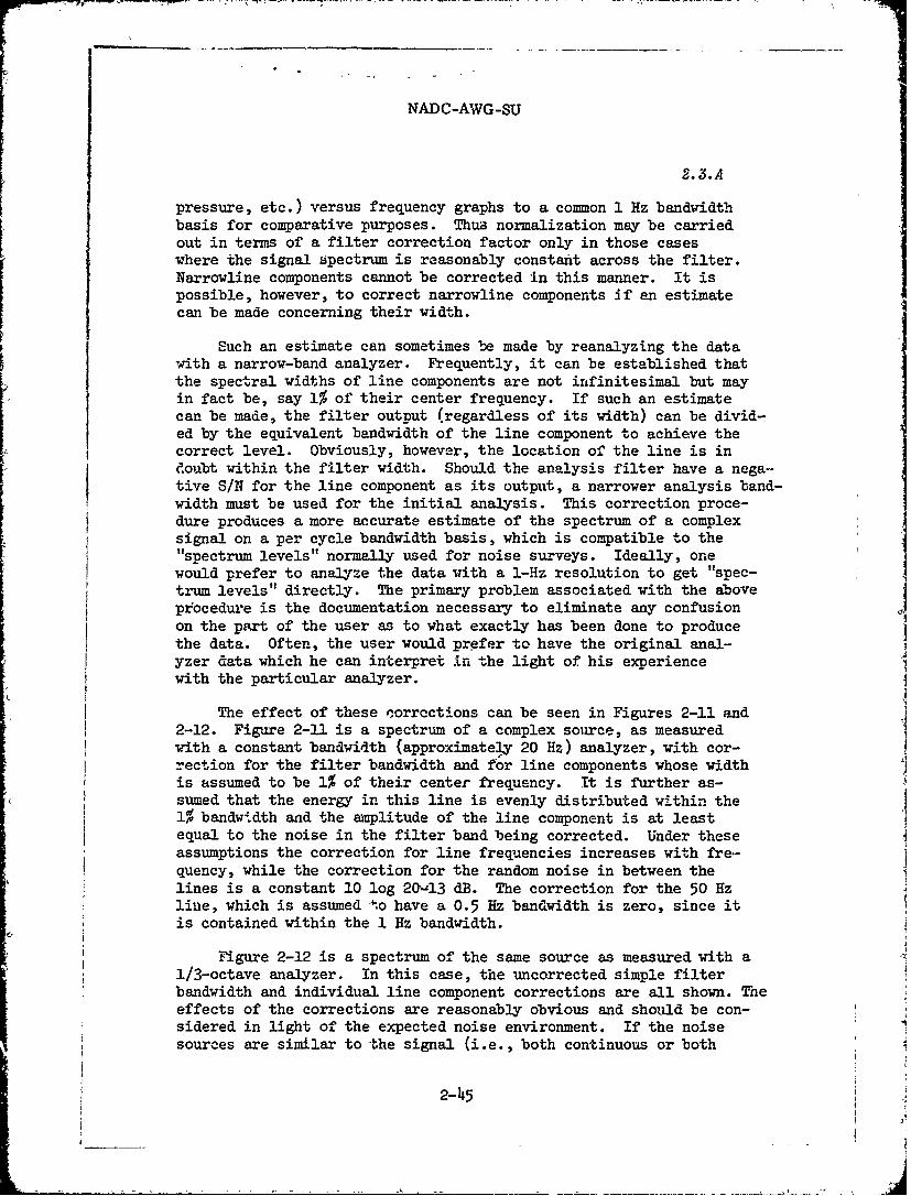
NADC-AWG-SU

2.3.A

pressure, etc.) versus frequency graphs to a common 1 Hz bandwidthbasis for comparative purposes. Thus normalization may be carriedout in terms of a filter correction factor only in those caseswhere the signal spectrum is reasonably constant across the filter.Narrowline components cannot be corrected in this manner. It ispossible, however, to correct narrowline components if an estimatecan be made concerning their width.

Such an estimate can sometimes be made by reanalyzing the datawith a narrow-band analyzer. Frequently, it can be established thatthe spectral widths of line components are not infinitesimal but mayin fact be, say 1% of their center frequency. If such an estimatecan be made, the filter output (regardless of its width) can be divid-ed by the equivalent bandwidth of the line component to achieve thecorrect level. Obviously, however, the location of the line is inc.oubt within the filter width. Should the analysis filter have a nega-tive S/N for the line component as its output, a narrower analysis band-width must be used for the initial analysis. This correction proce-dure produces a more accurate estimate of the spectrum of a complexsignal on a per cycle bandwidth basis, which is compatible to the"spectrum levels" normally used for noise surveys. Ideally, onewould prefer to analyze the data with a 1-Hz resolution to get "spec-trum levels" directly. The primary problem associated with the aboveprocedure is the documentation necessary to eliminate any confusionon the psrt of the user as to what exactly has been done to produce

the data. Often, the user would prefer to have the original anal-yzer data which he can interpret in the light of his experiencewith the particular analyzer.

The effect of these corrections can be seen in Figures 2-11 and2-12. Figure 2-11 is a spectrum of a complex source, as measuredwith a constant bandwidth (approximately 20 Hz) analyzer, with cor-rection for the filter bandwidth and for line components whose widthis assumed to be 1% of their center frequency. It is further as-sumed that the energy in this line is evenly distributed within the1% bandwidth and the amplitude of the line component is at leastequal to the noise in the filter band being corrected. Under theseassumptions the correction for line frequencies increases with fre.-quency, while the correction for the random noise in between thelines is a constant 10 log 20-13 dB. The correction for the 50 Hzline, which is assumed t.o have a 0.5 Hz bandwidth is zero, since itis contained within the 1 Hz bandwidth.

Figure 2-12 is a spectrum of the same source as measured with a1/3-octave analyzer. In this case, the uncorrected simple filterbandwidth and individual line component corrections are all shown. Theeffects of the corrections are reasonably obvious and should be con-sidered in light of the expected noise environment. If the noisesources are similar to the signal (i.e., both continuous or both

2-45

NADC-AWG-SU

WC44

so .

S60

?i50 001 nlzrOtu ;'iV40I *

'-' 20 i L B -' widfh Corrected "

10 I

0.i&s '-~ . . i 0. 1.00.02 0. 1 '10 oo1 ot; o, ' 0.0815. ' o.'t O' ol . ' "

=R ,,MCY IN KLO4HERTZ

Figure 2-11. Spectrum Analysis of a Complex Signal Using a Constant Band-width (20 Hz) Analyzer. Broken-Line Curve Shows Effect of Bandwidth Cor-

rection Assuming a Uniform Line Width of 1% of Its Center Frequency

cq 90

Z s

70 Analyzer Output

60

0 A

b0 /for Flter

10 --

Bandwidth Corrected for Signal

0.0i 0.0315 0.05 0.08 0.125 0.2 O.S3. 0.5 0.8 1.0

Figure 2-12. Spectrum Analysis of a Comp!ex Signal Using a 1/3-OctaveAnalyzer. Large Broken-Line Curve Shows Effect of Bandwidth Correc-

tion Assuming a Uniform Line Width of 1% of Its Center Fre-jency. Dot-ted Portion Shows What the Corrected Graph Would Have Been if Simple

Bandwidth Correction Had Been Used.

2-46

WAD C-AWG-SU

40

00

20

I/ Normalizedfo/10 Ia ,An wilter

-20-

0.02 6.0315 0.05 0.08 0.15 0.2 0.315 0. 0.8 1.0

FREQUENCY flX KWLHERTZ

Figure 2-13. Signal-to-Noise Ratio Estimated for the Combination of NoiseShown in Figure 2-8 and Complex Signal Shown in Figure 2-11

60

50

040 -Filter Output

30-A

20-%%

o 10 9 v

0~ 1 140\

Normalized forNo-10 /Signal and Filter

-20

0.02 0.0315 0.05 0.08 0. 125 0.2 0.315 0.5 0.8 1. 0

FREQUENCY Uf KLOHERTZ

Figure 2-14. Signal-to-Noise Ratio Estimated for the Combination of NoiseShown in Figure 2-8 and Complex Signal Shown in Figure 2-12

2-417

NADC-AWG-SU

2.3.A

complex with line structure), the superposition of their signatures isa useful measure of the expected S/N regardless of the method used, aslong as it is the same for both.

Figure 2-13 shows a typical signal-to-noise plot for the con-tinuous noise source of Figure 2-11 and the complex signature present-ed in Figure 2-10. We see the expected S/N with and without correc-tions. Likewise, the same noise source is compared to the spectrum de-rived from the 1/3-octave analysis (Figure 2-12) and the resulting cor-rected and uncorrected S/N ratios are shown in Figure 2-14.

A word should be said about the units used in acoustical dataanalysis. In general, the levels may be reported as relative levels orabsolute levels. Usually, the acoustic reference level is 0.0002 micro-bar (dyne/cm2 ) in air, and 1 microbar in water.

The level of sound pressure measured with a given filter band-width is referred to as Sound Pressure Level (SPL) in (1/3-octave, etc.)bandwidth, or Band Pressure Level (BPL). When the analysis bandwidthis 1 Hz, or when normalized to I Hz bandwidth as described above, it isreferred to as Pressure Spectrum Density Level, or simp.y Pressure Spec-trum Level. A commonly used instrument, the General Radio Type 1564-AAnalyzer is continuously tunable from 2.5 Xz to 25 kHz in four ranges.A i/3-octave band and a 1/10-octave band are provided. Charts for con-verting from the measured band levels to the spectrum level are given inthe Handbook of Noise Measurement, General Radio Company, by A. P. G.Peterson and E. E. Gross, Jr.

4. Calibration of Spectral Analysis Measuring Equipment

The most widely used method of calibrating frequency analysis equip-ment for effective bandwidth Af is to process a band-limited white noiseof known total bandwidth F and a sine wave of adjustable frequency f.The analyzer is tuned to maximum reading with a given sine wave input ofgiven frequency and voltage E applied to the input terminals. The powerinput then is 2/RP = E21 (2-38)

where R is the analyzer input resistance. The analyzer rms output volt-age indicator is adjusted to a reference value. Next, white noise of rmsvoltage E is applied to the input terminals producing the same input pow-er P, but resulting in an indication which is a G-fraction of the referencevalue. Then, the effective noise bandwidth of the analyzer at the frequencyf is Aff = G2F (2-39)

The "whiteness" and the bandwidth of tie noise source can be verified witha constant bandwidth analyzer.

2-48

NADC-AWG-SU

Usually, the spectrum is displayed on a logarithmic scale,in dB, in order to show more detail for the low power componentsThe accuracy of the logarithmic amplifier can be measured byvarying the amplitude of the calibration signal, usually in dis-crete steps corresponding to a fixed number of dB.

B. Constant Bandwidth (Af) Analysis

1. Af Instrumentation

The constant bandwidth systems are so named because theiranalysis bandwidth Af is invariant with frequency. However.,most of these analyzers have several bandwidths available whichcan be selected by the operator and which remain constant atall frequencies.

The constant bandwidth analyzers commonly use a heterody-ing approach to synthesize a narrow constant-bandwidth filterwhich is swept through the passband. In these systems (Figure 2-15) the original signal is caused to modulate a sine wavesource (cpxrier) in a balanced modulator. The carrier is sup-pressed by the balanced modulator so that the output consists

only of two sidebands symmetrically placed about the carrierfrequency at frequencies W. + O o where w. is the carrier angu-lar frequency and wo is the intelligence angular frequency(Figure 2-16). The amplitude of the sidebands is proportionalto the amplitude of the input signal and to the amplitude ofthe carrier. The latter is held constant so that the ampli-tude of the sidebands is proportional only to the amplitudeof the input signal. The effect is to translate the originaloutput spectrum to a higher frequency region- A narrow-bandfixed bandpass filter at wf is used to select the signal ele-ments within + Wd of bf where Wd is the half-angular bandwidthof the filter. Usually, quartz crystal filters are used forstability and high-Q and bandwidths of 1, 10 and 100 Hz arecommon. The output of the filter is detected, filtered, anddisplayed. The effect is to synthesize a filter of half-angu-lar bandwidth ad at wo where

o = wc - af (2-40)

where wc is the carrier frequency and wf is the fixea filterfrequency.

By varying wc the effective filter frequency wo is cor-respondingly varied. Eq. (2-40) applies to the case here thelower sideband is selected by the filter. This is the typi-

2-49

NADC-AWG-SU

2.3.B

cal approach since it maximizes the bandwidth which can be anal-yzed at a given filter frequency without aliasing.

An input low pass filter is customarily used to preventaliasing which occurs if the input frequency region extends intothe lower sideband region. This would happen if the input spec-trum contained components above one-half the lowest carrier fre-quency. In the case where the lower sideband is selected foranalysis, the lowest carrier frequency equals the filter fre-quency, i.e., c f for a synthesized filter at wo = 0.

Actually, a filter is seldom synthesized at wo = 0 sinceimperfect cancellation of carrier (always a practical problem)would pass through the filter and contaminate the reading.There is a lower limit to the frequency at which one can syn-thesize the filter since, for low frequencies, the upper andlower sidebands (as .:ell as carrier leakage) are close togetherand the finite slope of the bandpass filter cannot reject theunwanted components. It is possible to use the phase-shiftmethod of single sideband generation to suppress the unwantedsideband by say, 40 dB and,with extra care in carrier suppres-sion, the lower limit of the device can be extended.

Typical specifications for a constant bandwidth analyzerof this type are:

Input Range -- 20 Hz to 54 kHz

Bandwidth -- 3, 10, and 50 Hz

Filter Frequency -- 100 kHz

Carrier Frequency 100.020 kHz to154.00 kHz

The advantage of these schemes is the ability to have a singlefilter which can be made very near ideal. The bandwidth of sucha tuned network can be made very narrow since a constant-frequencytuned circuit is used which can be designed to have good selectivity.This gives the necessary resolution for the measurement of very nar-row line components in the data. The SSB technique described is use-ful to relatively low frequencies (as low as 2 Hz) when the degreeof carrier suppression can be made quite good.

An example of Af analysis is shown in Figure 2-17.

2-50

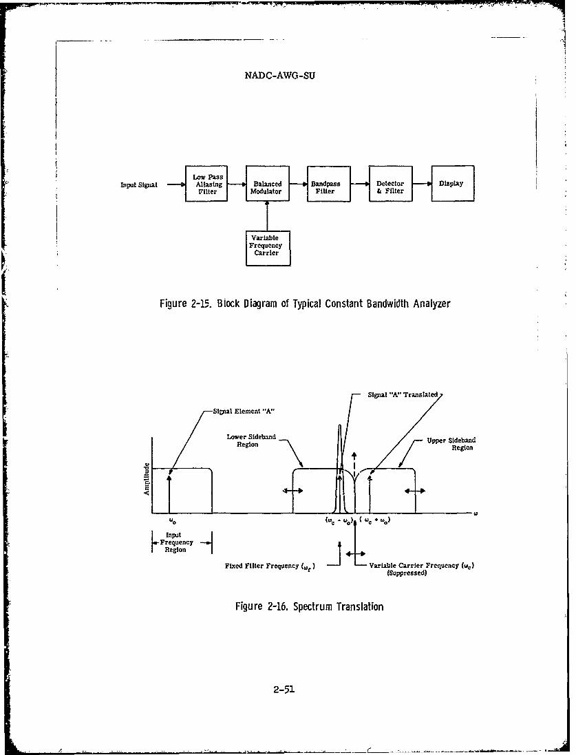
> NADC-AWG-SU

Input Signal Aliasing Balanced Bandpass DetectorDipa

Figure 2-15. Bljock Diagram of Typical Constant Bandwidth Analyzer

Signal "A" Translated

Signal Element "A"

Lower Sideband Upper SidebandRegion Region

E 4-

FFrequency 4V. Crir -

Fixed Filter Frequency (of Variable CrirFrequency (wc)(Suppressed)

Figure 2-16. Spectrum Translation

2-51

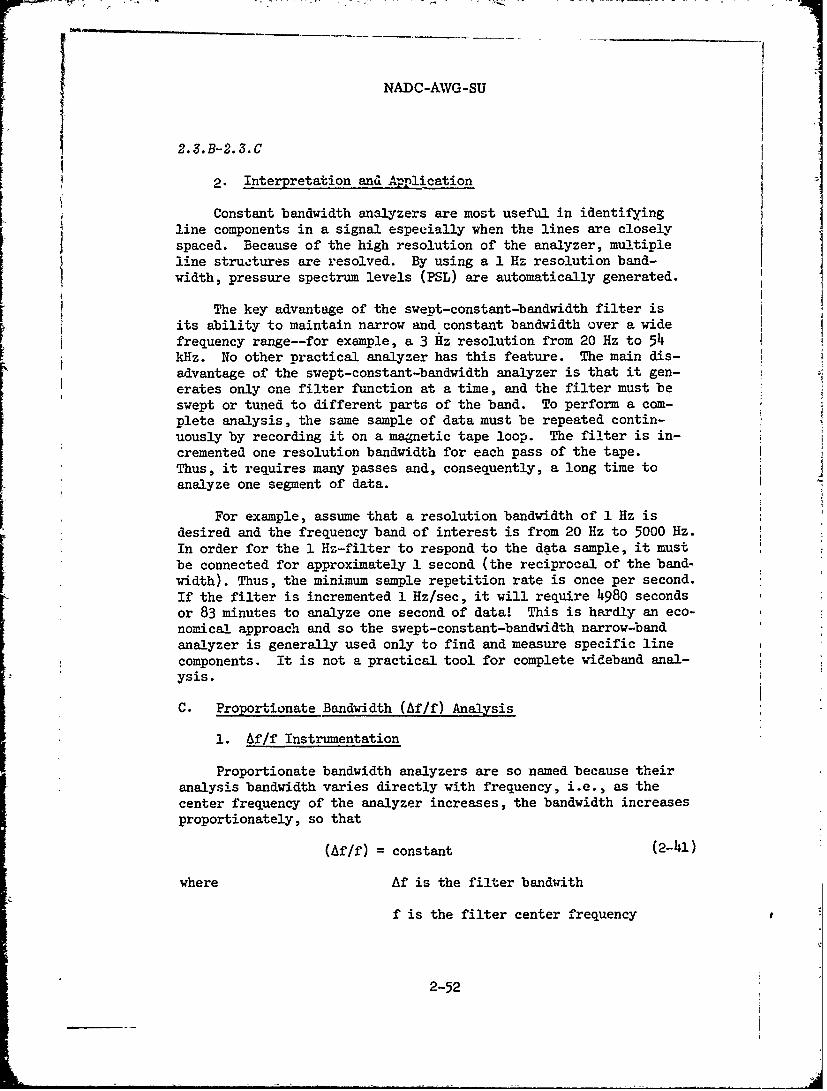
NADC-AWG-SU

2.3.B-2.3.C

2. Interpretation and Application

Constant bandwidth analyzers are most useful in identifyingline components in a signal especially when the lines are closelyspaced. Because of the high resolution of the analyzer, multipleline structures are resolved. By using a 1 Hz resolution band-width, pressure spectrum levels (PSL) are automatically generated.

The key advantage of the swept-constant-bandwidth filter isits ability to maintain narrow and constant bandwidth over a widefrequency range--for example, a 3 Hz resolution from 20 Hz to 54kHz. No other practical analyzer has this feature. The main dis-advantage of the swept-constant-bandwidth analyzer is that it gen-erates only one filter function at a time, and the filter must beswept or tuned to different parts of the band. To perform a com-plete analysis, the same sample of data must be repeated contin-uously by recording it on a magnetic tape loop. The filter is in-cremented one resolution bandwidth for each pass of the tape.Thus, it requires many passes and, consequently, a long time toanalyze one segment of data.

For example, assume that a resolution bandwidth of 1 Hz isdesired and the frequency band of interest is from 20 Hz to 5000 Hz.In order for the 1 Hz-filter to respond to the data sample, it mustbe connected for approximately 1 second (the reciprocal of the band-width). Thus, the minimum sample repetition rate is once per second.If the filter is incremented 1 Hz/sec, it will require 4980 seconds

or 83 minutes to analyze one second of data! This is hardly an eco-nomical approach and so the swept-constant-bandwidth narrow-bandanalyzer is generally used only to find and measure specific linecomponents. it is not a practical tool for complete wideband anal-ysis.

C. Proportionate Bandwidth (Af/f) Analysis

1. Af/f Instrumentation

Proportionate bandwidth analyzers are so named because theiranalysis bandwidth varies directly with frequency, i.e., as thecenter frequency of the analyzer increases, the bandwidth increasesproportionately, so that

(Af/f) = constant (2-41)

where Af is the filter bandwith

f is the filter center frequency

2-52

IwpNACAGS

Figure 2-17. Af Analysis of I kHz Square Wave

2-53

NADC-AWG-SU

2.3.C

The bandwidth is thus a constant fraction of an-octave. Typicalproportionate bandwidth analyzers have filter bands of 1/10-octave, 1/3-octave and one octave, although 1% and 10% wide fil-ters are also in common use.

a. Contiguous Band Analyzers

Proportionate bandwidth analyzers can be divided intotwo categories, parallel or contiguous band analyzers and sweptanalyzers. A contiguous band analyzer consists of a bank of fil-ters whose inputs are driven in parallel (Figure 2-18). In gen-eral, these filters intersect at their half-power points and havebandwidths which are a constant percentage of their center fre-quency (Figure 2-19).

This type of analyzer can continously display all ofthe spectral components on a multichannel oscillograph, thus as-sisting rapid data reduction. Such a multichannel data displayis especially useful for examination of the time characteristicsof the many portions of tie spectrum. This aspect is especiallyimportant if the signal is non-stationery. Some of the availableanalyzers apply commutation to the output of the filter bank sothat a single detector can be used (Figure 2-20). This destroyssome of the above advantages.

The primary disadvantage of the contiguous band anal-yzer is the cost of a large number of filters with sufficientskirt selectivity to enable wide dynamic-range signals to be re-solved.

b. Swept Band Analyzer

The second category of proportionate Af/f bandwidthanalyzers is the so-called "swept" analyzer (Figure 2-21). As inthe swept-constant-bandwidth analyzer, a single filter is sweptthrough the band of interest. Here, however, the filter bandwidthis a constant fraction of the center frequency. This type of per-formance is obtainable with variably tuned L-C filters. The sweptproportionate bandwidth analyzer maintains one of the main advan-tages of contiguous proportionate bandwidth filters in that thesystem resolution is independent of frequency. This type ofanalyzer.offers several realistic advantages, such as low cost,small size, low pow-er consumption, and simplicity of operation.M -.e improvements are gained at the expense of the continuousreadout of the entire spectrum which the contiguous band analyzeris able to provide, resulting in diminished ability to analyzenon-stationary signals.

2-54

--- M

NADC-AWG-SU

Ban I eetrIFilte AveagIr[HBad2Dtftre agItrFilte Aveagerr22i

Fnu igur -8aarlelrCotgosBadAaye

Band eetr

Figure 2-19. Contiguous Band Analyzer Filter Response

2-55

NADC-AWG-SU

2.3. C

Since only a sin',le filter and detector are used, asample of data is normally recorded on a magnetic tape loop andrepeated as the filter center frequenct; is moved. Since the band-ridth of the filter varies directly with frequency, the filtercan be swept at a constant number of octaves per unit time. Thisgreatly speeds up the analysis. For example, a 1/3-octave analyzercan be swept at a rate of roughly one octave every 3 seconds. Inthe band from 20 Hz to 5000 Hz, there are approximately 8 octaves.The analysis of such a band ean be performed in about 24 secondsusing a 1/3-octave analyzer or 80 seconds using a 1/10-octaveanalyzer. Nevertheless, since the analyzer does not operate inreal time, one cannot get a continuous readout on non-stationarysignals. Further, since the analysis time is constant, the time-bandwidth (BT) product varies with frequency. Thus, the statis-tical accuracy of the analysis varies, being better at higherthan at lower frequencies. Of course, since the bandwidth isgreater at higher frequencies, one knows less about the exactfrequency of each component, even though one knows the band energywith greater accuracy. An example of Af/f bandwidth analysis isgiven in Figure 2-23.

c. Swept Band Analyzer with Integration

An interesting adaptation of 1/10-octave swept filteranalyzer, which includes a 1 second integration, has been used forsome AWG studies. Figure 2-22 is a block diagram of the analyzerand integrator. The signal to be analyzed is recorded on a looptape recorder. The loop is marked (for example, with a piece ofreflecting foil) to indicate the "start" of the loop. This startmark is used to synchronize the subsequent integrator. The sig-nal is filtered by a 1/10-octave sweepinA analyzer which, slowlyscans through the desired range. The scan rate is kept well be-low 1/10-octave per second. The output of the analyzer is rec-tified and integrated in a "true" manner by charging a capacitorwithout leakage resistor. The time for integration iv, 1 second,as determined by the length of the tape loop. When the "start"mark is reached, any capacitor charge is transferred to a holdingcircuit and the integrator is returned to 0 in preparation for thenext pass. Meanwhile, the transferred charge is displayed on agraphic-level recorder chart. A balanced modulator is used toconvert the average power level to a form useable by the graphic-level recorder. At the end of the pass, the charge on the capa-citor again is transferied and displayed. Thus, the chart recordindicates the energy level in the 1/10-octave band, i.e., thepower level, integrated over a 1-second period.

2-56

- ------------- A

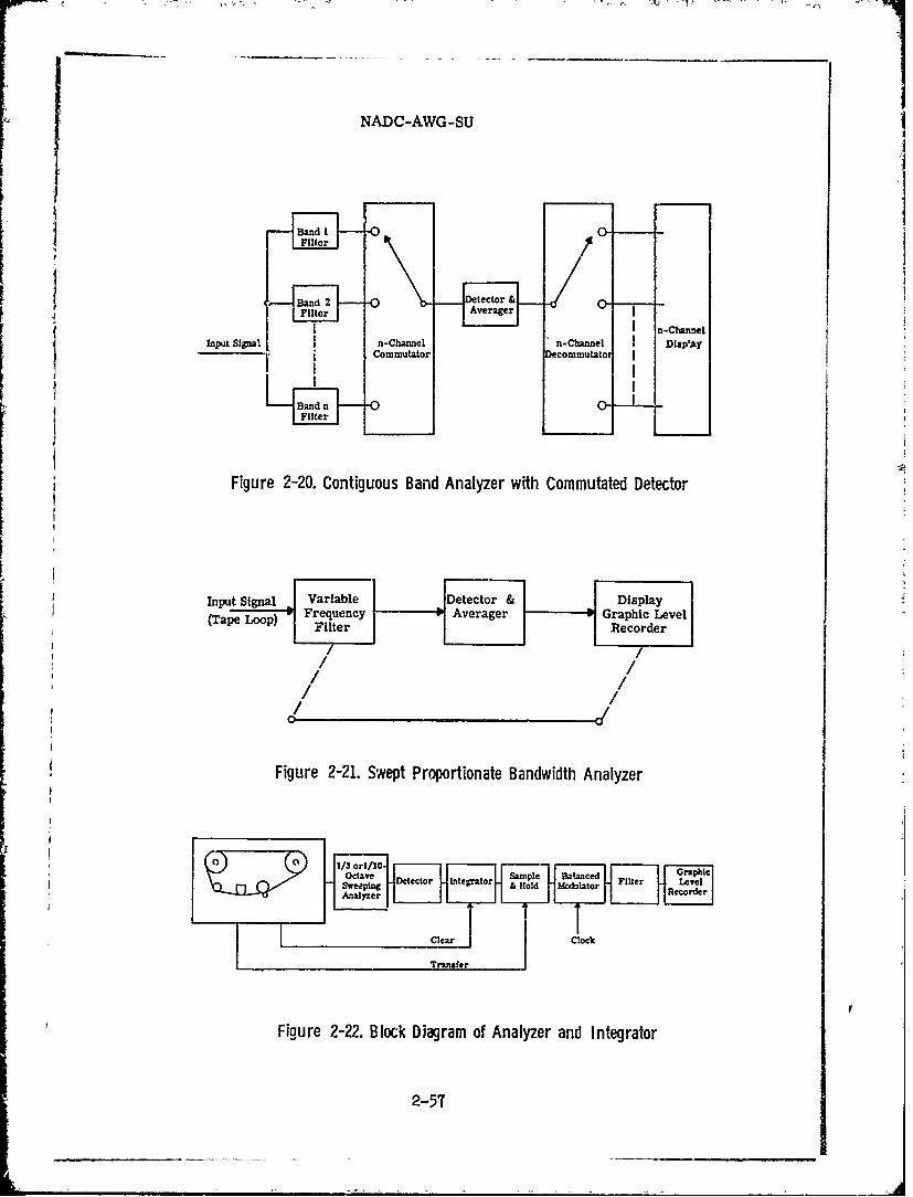
j NADC-AWG-SU

I~~~ XIIUt Ihl nChane

r Figure 2-20. Contiguous Band Analyzer with Commutated Detector

Input Signal Variable Detector & Display4

(Tape Loop) Frequency Averager Graphic Level

Figure 2-21. Swept Proportionate Bandwidth Analyzer

Transfer

Figure 2-22. Block Diagram of Analyzer and Integrator

2-57

NADC-AWG-SU

2.3.C

By repeating a signal every T seconds, a line seriesis generated based on a fundamental frequency, l/T and its harmoniccomponents. By choosing a repctition rate of 1 second, the linespectra is based on a 1 Hz fundamental. Analysis of random pheno-mena with a 1/10-octave filter produces a 1/10-octave band soundpressure level plot. When analyzing transient signals, which takeplace during a fraction of the loop length, an approximation totrue pressure spectrum level is obtained. Analysis of such tran-sient signals is helped by using 'a "window" to isolate the transientphenomena from background noise. This "window" is synchronized intime from the "start" mark of the tape. It is used to gate onlythe desired portion of the tap& loop into the analyzer. Surround-

ing background noise is thus rinimized while maintaining the 1-second repetition rate. Strong single-line signals result in read-ings div> ctly indicative of their SPL.

0

0 -20ClfVtaM1 Xrh

FRF UENCY

Figure 2-23. Example of flf Analysis of the Noise Generated by a 10 mph Wind Speedon a Microphone

2-58

NADC-AWG-SU

2.3.C

2. Interpretation and Applications

Care must be taken in interpreting the data from proportionatebandwidth analyzers. Since the filter bandwidth is not constant,but increases with increasing center frequency, the statisticalaccuracy for a given analysis time is greater at high frequencies

than at low when examining broadband signals. Further, when suchan analyzer is used to examine "white" noise, i.e. noise with anequal energy density per cycle, the indicated output or band pres-sure level increases at a 3 dB/octave rate corresponding to thedoubling of the filter bandwidth every octave. Based on this,some analysts impose a 3 dB/octave negative slope on either theinput or output data to compensate for the variable bandwidth. Itshould be remembered that such a correction is valid only for whitenoise which is only approximated in practice by random phenomena.Furthermore, any frequency analyzer will yield the correct valuefor an isolated line component directly since, if there is no othercomponent within the filter bandwidth, the output is independent ofthe filter bandwidth. In this case, no correction for filter band-width should be applied. The corrections, if any, to be applied inparticular instances are discussed more fully in subsection 2.3.A.3.

The relatively poor resolution oi the proportionate bandwidtnanalyzer can either be an advantage or disadvantage depending uponthe data sought. For example, if the signal to be analyzed con-sists of relatively widely spaced line components with frequencyinstability, the wider bandwidth of the proportionate bandwidthanalyzer can encompass the line even as it dithers. Thus, the out-put of the anaJ.yzer is proportionate to the total energy of the line.Of course, no information is gleaned about the dither rate or evenif dither exists. On the other hand, if two lines fall into thesame filter bandwidth, they cannot be separated air their relativestrengths remain unknown. Also, if a line component is buried innoise, the relatively wide bandwidth does not allow one to ascertainthe existence of the line.

From the above, it can be seen that no single method of analysisis able to provide all aspects of data that may be of interest. Somea priori knowledge of the rignal composition is helpful in decidingon the best approach to analysis and in subsequent interpretation of

results. A trained human ear is often the best preliminary guide asto the method of analysis which is apt to be the most appropriate inany particular case.

2-59

NADC-AWG-SU

2.3.D

D. Real-Time Analysis

1. Real-Time Instrumentation

In general, the previously described frequency analyzers donot have the capability of performing the analysis in "real time,"that is, keeping up with a continuously changing non-stationaryseries. The real-time analyzer is similar to the constant-band-width-swept-filter analyzer described in subsection 2.3.B.1; how-ever, the data sample is stored in a digital delay line and israpidly recirculated. This translates the data up in frequencyso that a rapid analysis can be performed. The stored data iscontinuously updated by dropping one element in time and addinganother as the circulation proceeds, so that, for all intents andpurposes, the analysis is carried out piecewise on overlappingframes of a series which differ from each other by a predeterminedsmall-time interval. The resulting spectrum is customarily dis-played on an oscilloscope screen with frequency and spectral in-tensity information along the horizontal and vertical deflectionco-ordinates, respectively. Also, any desired number of displayscan be summed for the purpose of obtaining an average over a num-ber of frames, stored in an accumulator, and either displayed onthe oscilloscope, or graphed with an X-Y plotter.

The detailed operation of a real-time analyzer is shown in

Figure 2-24. The input signal is low-pass filtered to prevent

aliasing in the subsequent sampler. The data is then sampled ata rate at least twice the highest frequency transmitted by thefilter. Usually, a sampling rate of three times the upper frequencyis chosen. The samples are then converted into digital words whoselength is commensurate with the accuracy required. Typically, anine bit word is used. This provides quantization to 512 levelsfor a dynamic range of 54 dB. The digital words are st.ored in adelay line memory and recirculated at a-rate such that the entiredata stream in the .ine is passed once between each smple periodof the input signal. As each new sample of the signal enters thedelay line, it replaces the oldest data sample in storage.

The output from the recirculating delay line is converted toan analog signal by a high-speed D-A converter. This high-frequencyanalog signal is analyzed using a heterodyning method similar tothat described in subsection 2.3.B.1. That is, the high-speed sig-nal is multiplied by a local oscillator frequency. The sidebandsare then passed through a fixed narrow bandwidth crystal filterwhich selects the lower sideband for detection. The local oscil-lator sign'l is stepped throgh the range of interest by the mas-ter clock of the analyzer.

2-60

J NADC-AWG-SU

l~uator Cytl Detector Amplitude

(0kHz, BW)

Freqiency

Figure 2-4 ipiidBokDiagramn of Real-Time Analyzer

2-61.

NADC-AWG-SU

2.3.D

Real-time analyzers are categorized by the "number of lineanalysis" they are capable of performing. This quality factoris a function of the amount of storage in the delay line. Forexample, a 500 point analyzer is capable of synthesizing, ineffect, 500 parallel filters throughout the band of interest.Normally, the bandwidth of the filters and the cor.responding anal-ysis bandwidth are selectable by switch; however, the bandwidthwhich can be handled will always be 500 times the resolution band-width. Such a device may provide for a 1-Hz analysis bandwidthup to a highest frequency of 500 Hz. The 500-Hz signal will besampled at a rate of 1500 samples per second. In order to providethe 1-Hz resolution bandwidth, the sample duration in the recir-culating delay line must correspond to 1 second of real time.Thus, 1500 samples are stored in the delay line at any given time.Alternately, the instrument could have been set to handle a databandwidth of 5 kHz with a 10-Hz resolution. In this case, thesample duration which would have filled the delay line would havebeen 100 milliseconds and the total number of points would againbe 1500.

In order to minimize the errors due to the non-infinite datasample, the real-time analyzer generally applies some sort of windowweighting function to the data. This concept was covered in sub-section 2.2.E.4. Typically, cosine-squared weighting is employedin a real-time analyzer. An unfortunate result of the weightingfunction is to increase the effective bandwidth of the synthasizedfilters. For cosine-squared weighting, this amounts to about 50%That is, a 500-line analyzer set to a 500-Hz bandwidth synthesizeseffective filter bandwidths of 1.5 Hz rather than 1 Hz.

2. Accumulator and Averager

A useful adjunct to the real-time analyzer is the companionintegrator or averager. This device determines the average spec-tral level over a given number of ensembles. In a typical instru-ment, it can be set to average the results of from 2 to say 1024spectral analyses. This is a very powerful tool for detectingline structure in the presence of noise. Averaging the data overa period of time improves the time bandwidth product and, thus,the statistical accuracy of the results. In general, one shouldaverage over the largest number of ensembles possible consistentwith the stability of the data.

The ty -ical averager used with a real-time analyzer accumu-lates the data in a second recirculating digital delay line. Asthe data from each of the effective filters enters the averager,it is digitized and placed in the delay line. The recirculationrate of the delay line is synchronized with the data flow ratefrom the analyzer, so that each filter has its own section or

2-62

NADC-AWG-SU

2.3. D

"bin" of delay line. With every recirculation of the data, thenew output is added to the previous value in eacn bin,* the sum Ibeing representative of the average. The date can then be readout ofl any suitable display. Eamales of real-time analysis oftruck data are shown below in Figurez; 2-25 and 2-26.j

.... .. ... ITHTA~eH-IT; 42517; 730 .MCh~ly, n WtIAverg. 1stce: 00 mter

I. .

4 -40

__ 2-31 Ton, 6x6, M35AI10 mph; 2nd Gear 170 RPM

Exhaust Awy from Mkrhonej~j. QftSide) 16SecndAvorage

FROO(JENCY IN~ HERTZ

.- 63 ... Tp1-7 /2/7 :0P 4

NADC-AWG-SU

2.3. D

3. Interpretation and Applications

The spectra produced by a real-time analyzer are very simi-lar to those of the constant bandwidth analyzer of subsection2.3.B, since the real-time analyzer is a constant bandwidth de-vice. The key difference between them is that the constant band-width analyzer must be swept through the band of interest at sucha slow rate as to make it impractical for complete broadband anal-ysis. The real-time analyzer, on the other hand, synthesizes theeffect of a parallel filter bank. of constant bandwidth filters.Thus, it processes the data in real time and the analyst can ob-serve the stationarity of the analysis. Alternately, he can accu-mulate and average the spectrum produced over a period of time.

The drawback of the real-time analyzer is the number ofparallel filters it can syn+ esfse. This is directly related tothe cost of the device. Typically 200- and .500-point analyzersare available. One thousand-point analyzers also have been madefor special purposes.

Because the total number of filters is fixed, the normalway to increase the input bandwidth which the analyzer willaccommodate is to widen the analysis bandwidth. The analysis1andwidth is given by

Af = (k fmax)/n (2-42)

whereAf = the analysis bandwidth

k = the widening factor due to theweighting function (typically 1.5)

fmax = the upper frequency limit of the range

n = the number of analysis points

If greater resolution is required in a limited high fre-quency region, external frequency translators can be used toshift the desired region into the high-resolution range of theanalyzer. For example, one can employ single sideband techniqueto scale the region, say, from 100 kHz to 100.5 kHz down to 0to 500 Hz which can be handled with a real-time analyzer with1.5 Nz resolution.

2-64

NADC-AWG-SU

2.3.E

E. Other Techniques

1. Fast Fourier Transform

Recently, high-speed digital computation techniques havebecome available for spectral analysis. Foremost among theseis the so-called Fast Fourier Transform (FFT) by Cooley andTukey.18 The FFT greatly reduces the number of steps requiredto perform a numerical Fourier analysis, which has made thecalculation economically feasible for relatively large datasamples. The advent of very high-speed minicomputers, espe-cially those employing high-speed read only memories (ROM) forstoring key portions of the FFT algorithms, has provided real-time FFT capability to beyond 20 kHz.

The key advantage of the FFT approach is that it providesphase as well as amplitude information on the signal components.Further, the FFT algorithms can be configured to calculate otheranalysis functions, correlation convolution, cepstrum analysis,power spectrum analysis, etc.

In addition to the FET, there are other techniques, such

as the Walsh Transform which essentially performs a similarfunction using a different mathematical approach.

18 j. W. Cooley and J. W. Tukey, "Algorithm of the Machine

Calculations of Complex Fourier Series," Mathematics of Computation,Vol. 19, No. 90, April 1965, pp. 297-301.

2-65

NADC-AWG-SU

2.4.A-2.4.B

2.4 TIME DEPENDENT FREQUENCY DOMAIN DATA REDUCTION

A. Introduction

In Section 2.3 the different categories of frequency domaindata analysis equipment were described. These equipments arecapable of analyzing a given time segment of data. producing asingle plot of the average spectral levels versus frequency. Whenused in this manner the dimension of time is missing. With reallife data the energy distribution" is seldom stationary with time.Relative spectral energies shift in both amplitude and location asthe scenario changes. Thus, as a rainstorm starts and builds up onemight find an overall increase in broadband acoustic level. Thesong of a bird might cause the repetitive appearance of strong ]spectral lines. As a vehicle passes the data collection point,one would see spectral lines relating to the engine firing rate Ibuild up and decay. Their location in the frequency plane wouldshift depending upon the Doppler effect and the instantaneousfiring rate. One can, of course, observe the changing pattern of 4data in an oscilloscope display of a real-time analyzer. Thismethod,however, does not provide a hard copy of one spectralpattern for convenient analysis. Several means for reducing thesedata in time domain, by rapidly plotting or displaying these mul-tiple 'snapshot" spectra are available and will be described below.

B. Sonograph-Type Display

The basic problem involved in displaying time-dependent fre-quency-domain analyses is that of plotting three variables--level, frequency, and time--on a two-dimensional surface, i.e.,paper, oscilloscope, etc. The different types of display equip-ment reflect different approaches to the solution of this problem.

An example of the sonograph-type display is shown in Figure 2-27. In this approach, the two axes represent frequency and

time. The amplitude of the spectral component is representedby the density of darkness of the lines. Each new spectrum isdisplayed as a new line across the page (vertically).

The major limitation of a normal sonograph display is itsrelatively crude indication of spectral level. The dynamic rangeof the plot is such that a relatively few shades of gray can bedistinguished. For this reason, asL AGC is sometimes employed be-fore the sonograph to adjust the signal level to its range of op-eration. The time and frequency definition of the sonograph canbe quite good. Typically, 4 inches of paper is allocated for thefrequency axis.

2-66

---------- i

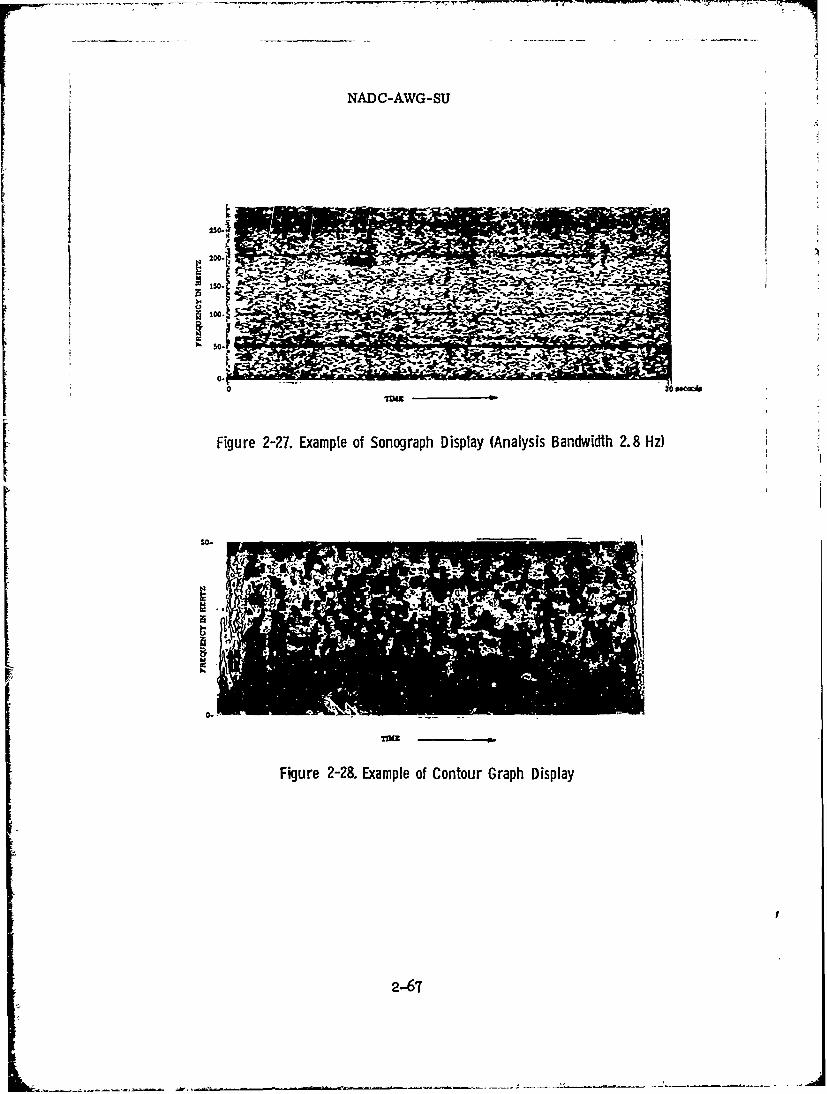
- ~ ~ ~ ~ ~ ~ ~ ~ -- --- 47~. - - - -- - - ~ - -

NADC-AWG-SU

ISO

0.

TDM

Figure 2-28. Example of Contour Graph Display

2-67

I

NADC-AWG-SU

2.4.B-2.4.C

The major advantage of the sonograph is the ease with vhichone can identify subjects of interest whose signature consistsof spectral lines whether stable in frequency or not. Such tar-gets appear as a darkening of the trace at some point on the fre-quency axis. If the line is not frequency stable, the darkenedsection will take on a "slant" as a function of time. The "track"of the subject is still readily apparent.

C. Contour Graph DispLay

As with the sonograph, the contour graph dibelays frequencyand time on the two major axes of the paper. However, ratherthan indicating spectral amplitude by intensity variations, thecontour graph draws lines which are the locus of points of equalspectral energy. The result is analogous to a topographical mapwhere lines of equal altitude are drawn--hence the name "contourgraph." Typically a 42 dB dynamic range is accommodated utilizingseven shades of gray with a resolution of 6 dB for each shade.

As -with the sonograph, the resolution ef the frequency andtime axes is quite good. However, the spectral level indicationis necessarily discrete since a line is drawn through points ofcorresponding levels. The next line indicates a level X dB differ-ent from the previous one. One can interpolate between the linesto estimate spectral level but one cannot be confident of thedistribution of levels between the contours. As the leveldifference between contours is diminishedthe lines become some-what difficult to follow.

On a contour graph subjects of interest having either line ornarrow band signatures usually appear as a clustering of closedcontours similar to the way a mountain, or if extended in time, amountain range, would appear on a topographical map. An exampleof a contour graph display is shown in Figure 2-28.

D. 3-D Spectral Display

The 3-D spectral display is a device used with the real-timeanalyzers described in subsection 2.3.D. This approach attemptsa pseudo three-dimensional display on the face of an oscilloscopeby a technique similar to that used by a draftsman in making aprojection drawing. The abscissa or X-axis represents frequency,the Y-axis represents time and the Z-axis amplitude. One spectraafter another are plotted on the oscilloscope face with a slightshift in origin position to give the three-dimensional effect. The

26

2-68

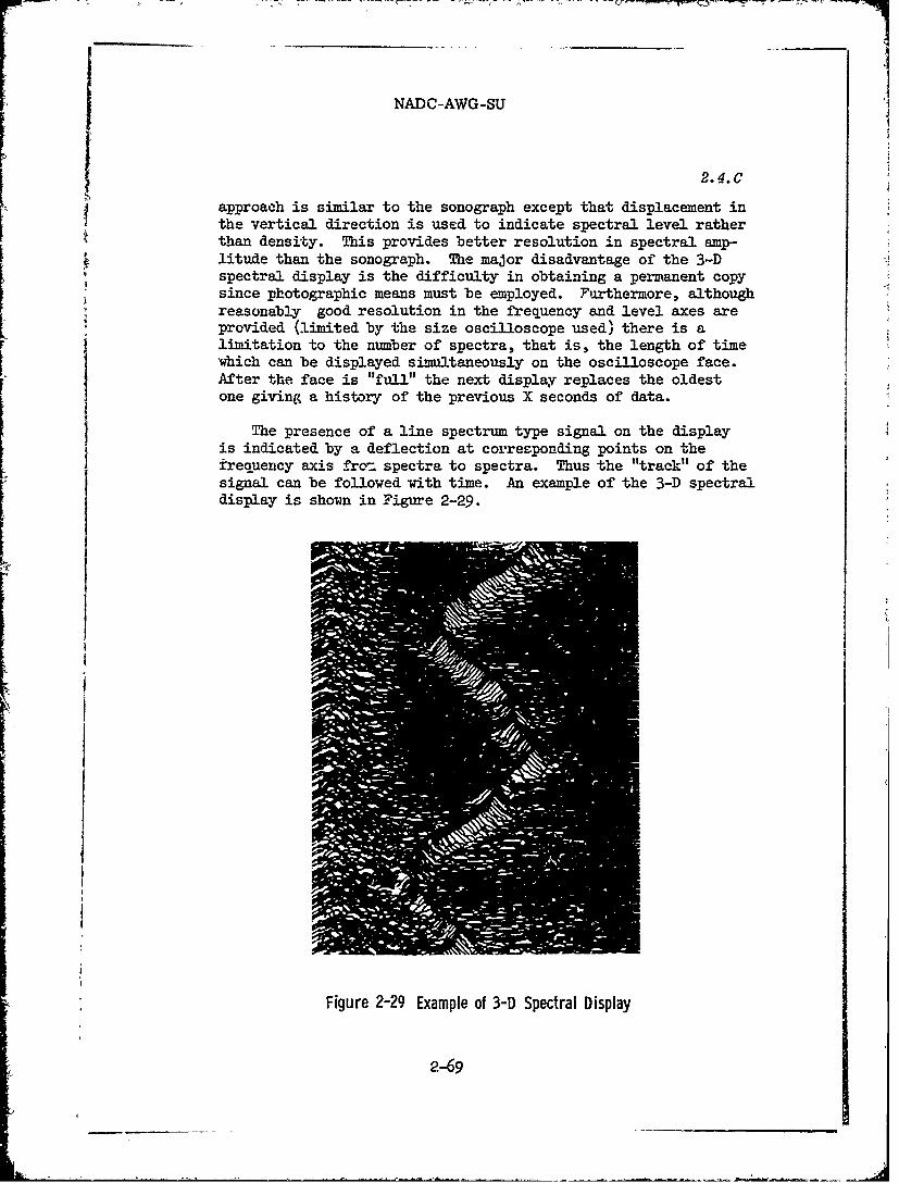
NADC-AWG-SU

2.4.C

approach is similar to the sonograph except that displacement inthe vertical direction is used to indicate spectral level ratherthan density. This provides better resolution in spectral amp-litude than the sonograph. The major disadvantage of the 3-Dspectral display is the difficulty in obtaining a permanent copysince photographic means must be employed. Furthermore, althoughreasonably good resolution in the frequency and level axes areprovided (limited by the size oscilloscope used) there is alimitation to the number of spectra, that is, the length of time

which can be displayed simultaneously on the oscilloscope face.After the face is "full" the next display replaces the oldest

one giving a history of the previous X seconds of data.

The presence of a line spectrum type signal on the displayis indicated by a deflection at corresponding points on thefrequency axis fro- spectra to spectra. Thus the "track" of thesignal can be followed with time. An example of the 3-D spectraldisplay is shown in Figure 2-29.

Figure 2-29 Example of 3-D Spectral Display

2-69

NADC-AWG-SU

2.5.A

2.5 TIME DOMAIN DATA REDUCTION

A. Introduction

As discussed in subsections 2.2.F. through 2.2.H., it is use-ful to determine the characteristics of data in the time domain aswell as, or in lieu of, the characteristics of the data in the fre-quency domain. An obvious example is the detection of an impulsivesignal whose characteristics are much more readily identified bythe shape of the pulse than by its frequency content. A more subtleexample is the identification of, say, a certain type of vehiclewhose "distinguishing characteristic might be the rate of rise andthe decay of sound level.

1. Raw Data and Envelope Data

In each of the above cases, a distinguishing feature wouldbe found in time domain analysis. In the case of the impulse, thedistinguishing feature was in the raw data; for example, the timerise of pressure pulse. In the case of the vehicle, the distin-guishing feature was the rate of change of the average sound level,characterized by the slope of the rectified envelope of the soundpressure level. These two examples demonstrate two of the majorcategories of time domain data reduction, i.e., raw data reductionand display, and envelope or rectif3ea data reduction and display.

2. Equipment for Time Function Display

The selection of a device or technique to display time func-tions is faciliated if the user is familiar with the limitationsand special features of each of the techniques:available. As ofthis writing, there are over 200 manufacturers of time functiondisplay equipment exclusive of those who produce oscilloscopes.The techniques which are currently being applied as well as a sum-mary of their characteristics is shown in Table 1. There may wellbe improved systems or special models available which a particularmanufacturer may have recently developed which may not be includedin Table 2-1.

The selection of a display device should be approached bymaking a checklist of the available system parameters and theirimportance in. a particular application. The following list repre-sents the order in which the parameters are likely to be considered:

a. Frequency Response. Can the the recorder displaythe signal frequencies of interest, or the rate of change of the

2-70

NADC-AWG-SU

01..4

0 o .4.4 .

4' 4)4) m 0 0 0p C; V4 V 4

.4C4 .4 .E4I I I

.24

88C8

u0 -

C aE H a m

2-72.

NADC-AWG-SU

2.5.A-2. 5.B

envelope? It is necessary to remember that an impulse displaygenerally requires that the galvanometer have a natural resonanceat least 1.6 times the highest frequency component of the pulse.This criteria is necessary to prevent the phase shift character-istics of the galvanometer from distorting the pulse. Other re-quirements follow from the rules for handling impulsive data out-lined in subsection 2.2.D.4.

b. Resolution. Can the recorder resolve the high fre-quency components of the signal at a paper speed compatible withthe total signal display duration? Systems with high resolutioncan operate at slower paper speeds for a given signal frequency.

The total duration of the recording is often vital if the parame-ter being examined requires continuous or long duration display.

c. Recording Medium, The necessity for reproduc-ibility and/or prolonged handling must be considered in selectinga technique. In addition, the cost of some recording mediumsmay put their use out of reach of a particular program. Theselection of a medium is also affected by the length of rollswhich are readily available if the display is of long duration.The selection of the recording medium is also closely associatedwith the necessary speed with which the finished record must bemade available.

d. Portability. Will the recorder be used forlaboratory -use only, or will it be used for field display? Thesize, weight, and power consumption of recorders vary con-siderably and cover the entire range from a few pounds and witha clock spring drive all the way to hundreds of pounds withseveral hundreds of watts power consumption.

e. Compatibility. If currently there is displayequipment in the data laboratory it is often important to remaincompatible with the many expensive accessories which have beenaccuraulated. This consideration is generally not importantunti, the selection has been narrowed to a few systems, arZ- ofwhich could be used.

B. Raw Data Reduction and Display

In general raw data is displayed when one wants to ex-amine the instantaneous pressure of the disturbance. This happensmost frequently when one is investigating impulsive phenomena suchas explosions. In these cases the rise time of the impulse can bevery short requiring a high speed display device, that is, one withextended frequency response such as an oscilloscope or light-beamoscillograpb. An example of the raw data of sound pressure of explo-sions followed by reverberation and scattering is shown in Figure2-30. When the raw data has relatively limited bandwidth pen re-corders can be used for display.

2-72

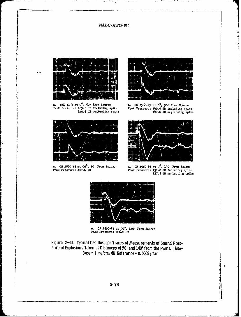
NADC-AWG-SU

a. B8K 4134 at 60, 50' Frcm -Source b. GR -1560-P5 at 00 50' Frcsi SourcePeak Pressure: 11,5.5 dB including spike Peak Pressure: 146.5 dB including spike

140.5 dB neglecting spike 142.0 dB neglecting spike

SB neglctin spike

C. GR 1560-P5 at 90 , 50' From Source d. GR 15E0-P5 at 00, 140' From SourceIPeak Pressure: 142.0 dB Peak Pressure: 131.0 dB including spike

e. GR 156o..P5 at 900, 140' Frcm Source

Peak Pressure: 126.0 dB

Figure 2-30. Typical Oscilloscope Traces of Measurements of Sound Pres-sure of Explosions Taken at Distances of 50' and 140' from the Event. Time-

Base~ 1 mslcm; dB Reference= 0.0002 pbar

2-73

NADC-AWG-SU

2.5.B-2.5.C ,

Frequently, to improve the signal-to-noise ratio of the dis- Jplay, the raw data is prefiltered to remove those frequency com-ponents not essential to the data. Care must be taken in selec-ting the prefilter. Generally, one performs a frequency analysison the data first to determine the pass band of the major energycomponents and selects the filter accordingly. One must becautious, however, to preserve the relative phase relationshipsbetween the components in the pass band. If a non-constant timedelay (that is a non-linear phase) filter is used, the signalcomponents will emerge from the filter at different times and theresultant signal will not resemble the original in either shapeor peak level. Figure 2-31 compares the output from two ior pass °

filters driven from a square wave source. The non-constatut timedelay of the Butterworth filter produces a ringing characteristicon the output signal which is not present on the Bessel filter

output.

C. Envelope Data Reduction and Display

As described in subsection 2.2.H., envelope data reduction ismost useful in establishing the appropriate AGC rates and indetermining the best post-detection filter constants, for a givensystem. Based upon the rates of change of the average ambientlevels and the rates of change of the desired signal level, onecan select circuit constants to maximize the probability ofdetection.

1. Instrumentation for Rectified Data Display

Although one may employ many of the devices described in Tab..le l,it is frequently desirable to display the envelope of a giventime sequence on a graphic level recorder. This device is commonlyavailable and can produce a permanent, inexpensive, logarithmiclevel plot versus time. The relatively slow ballistics of thegraphic level recorder can be modified with the aid of an electronicinput processor to allow the recording of brief impulsive sounds,even if it cannot improve the resolution between rapidly repeatedsounds. Such an electronic accessory also makes it possible tosimulate the effect of meter or device ballistics. A system of thistype has been employed in the preparation of the time domain infor-mation in several AWG reports and its description is included hereinfor this reason.

Figure 2-32 is a block diagram of the device. An inputbuffer amplifier is used to present a hiGh impedance (100 K) tothe data reduction recorder. The input buffer amplifier also pro-vides a precise 12 dB gain and is capable of driving the 600 ohmdecade attenuator which follows. A subsequent amplifier with

2-74

NADC-AWG-SU

TIME -~TIM -

Figu re 2-31a. Response of a 5-Pole B utterworth Figu re 2-31b. Response of 5-Pol e BesselLow-Pass Filter to Square Wave Low-Pass Filter to Square Wave

DK~dI

Figure 2-32. Block Diagram of Electronic Input Processor

2-T5j

NADC-AWG-SU

2.5.C

40 dB gain terminates the decade attenuator and increases the 4

signal level for the subsequent detector. This configurationallows the decade attenuator to be set for a 52 dB insertion tloss. By reducing the amount of E*tenuation, the overall gainof the system can be controlled in a precise fashion. The de-tector can be either of the peak, averaging, or rms variety.For most of the AWG work, a wide dynamic range (in excess of40 dB) full-wave rectifier was used as the detector. The detec-tor is followed by an RC filter with variable attack and decaytimes. These time constants can be adjusted in accordance withthe requirements of the data reduction. Typically, a decay timeof 400 milliseconds is used to insure that the graphic level re-corder pen reaches the maximum level of short duration signals.Depending upon the purposes of the reduction, attack times from1 to 50 milliseconds have been used.

The logarithmic potentiometers which are typical of graphiclevel recorders function only with AC signals. Plctting timeseries data on a logarithmic scale is especially valuable to thecircuit designer since growth and decay times of the time seriescan be read off directly in dB per second. Referring to theblock diagram, a balanced modulator is used to convert the en-velopoe level data to a proportional AC signal. A 10 kHz carrierfrequency was used and the subsequent band pass filter was suf-ficiently wide to preserve all significant sideband components.

A plot of the linearity of the level analysis equipment des-cribed above is shown in Figure 2-33. The input level was variedin 5 dB steps, and the chart record shown a linearity within approx-imately 1/2 dB over a 40 dB range.

By properly adjusting the attack and release time constants,in conjunction with the damping of the pen motor servo-mechanism,the ballistics of a variety of devices can be simulated. As anexample, Table 2-2 compares the chart-record results with readingsfrom a standard sound-level meter. For steady-state signals, thetwo devices will indicate the same value. Over a fairly wide rangeof dynamic conditions, the chart record agrees within 1 dB in bothmaximum and minimum fluctuations with the readings of a sound-levelmeter.

Examples of time-domain analysis are shown in Figure 2-34.

2-76

NADC-AWG-SU

_______ T~e SimDtorf;u Calibration

Lee I& te

TI~k ON TINE OFF SUM READING BALLISTIC COMPENSATOR(MS)S(d) READING

31179 1 8-314 +112

31 637-1/2+ 1128 +112

31 31 66-112

31 153124

31 7 1314

31 3 3-4

63 127 7-112 +' 1-1/2 7-114 + 1-112

63 63 5-112 + 112 5-314 + 112

63 31 3 +1/2 3-1/2 +112

63 15 0 114

63 7 -3 -4

2-7T

NADC-AWG-SU

2.6.A-2.6.B

2.6 SPECIAL DATA REDUCTION TECHNIQUES

A. Introduction

In addition to the standard frequency and time domain datareduction, other techniques are often employed to cull out specialsignificant aspects of the data. For example, it might be sig-nificant to know the direction from which the sound arrived. Inthat case, one might employ directional microphones, or arrays ofmicrophones, either directional or omnidirectional, from whichthe direction of arrival can be determined by special tech-niques. Or, one might find the amplitude variations of the dataof special significance and so demodulate the signal before stan-dard frequency and time domain reduction. Several of the moreuseful techniques will be discussed in this section.

B. Azimuth Location

One useful approach to determining the azimuth of sound arrivalrelies upon the special directional characteristics of the gradientmicrophone. This microphone, which in its simplest form consists ofa diaphragm exposed to the sound on both sides, produces an outputproportional to the pressure difference across the diaphragm, i.e.,to the pressure spatial gradient.19 (See Figure 2-35.) It can read-ily be shown that for wavelengths considerably greater than the micro-

phone dimensions the output, El,is given by

E kp cos 9 voits (2-43)

where:

k is a constant determined by the microphone dimensions and thetransducer sensitivity in volts per microbar

p is the pressure of plane progressive sound wave in microbars

0 is the angle between the direction of sound traveland the axis of maximum sensitivity of the microphone

If a second microphene, identical to the first is placed inclose proximity but with its axis of maximum sensitivity orientedat right angles to the first, its output E2 is:

19 See, for example, H. F. Olson, Acoustical Engineering, D. Van

Nostrend Co., Inc., Princeton, N. J., 1957.

2-78

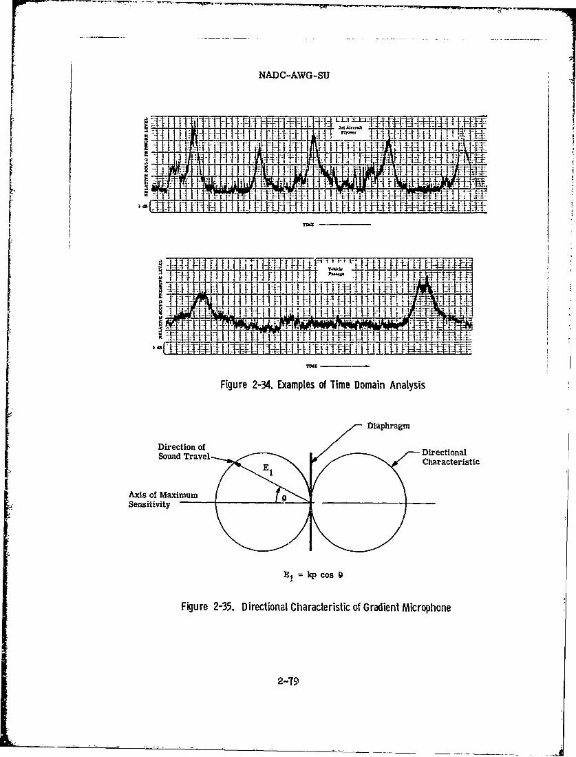
I - NADC-AWG-SU

-1 710tJ II I

T ill fIU-f

DiecioalFiur 234 EAmpefTm oanAayiSV n rvl ietoa

Cdrcers8

Hi U1

Axi Hof Maximum-H-Sensiivit

Figure 2-35. D E alhresi of e roaint Mnlyirshn

2-aprag

NADC-AWG-SU

2.6.B-2.6.C

E2 = kp sin 0 volts (2-44)

where, k, p and 0 are defined as before. Dividing the two'signalsgives

sin 0(E2/E1 ) = s 9 = tan 0 (2-45)

cos 9

That is, the ratio of the two signals is equal to the tangent ofthe angle of sound arrival independent of signal strength. Thisapproach has been used in the acoustic azimuth locator shown inFigure 2-36.20 In this device the signal levels from a pair ofmatched gradient microphones after suitable filtering and proces-

sing are divided to display the azimuth vector to the sound source.

The same approach has been used very successfully in locatingcontinuous sound sources such as vehicles. The line spectra fromsuch devices allow one to select and lock on to a single line foranalysis. This greatly improves the effective signal-to-noise ra-tio and thus the accuracy of the device. When tracking continuousI ' line sources, a pressure microphone is normally incorporated inthe array to eliminate the quadrant ambiguity in Eq. (2-45). Thesense of polarity of the pressure signal [p in Eq. (2-43) and (2-44)]is given by this microphone so that the signs of E1 and E2 given byEqs. (2-43) and (2-44) uniquely determine the quadrant from whichthe sound arrived.

C. Detection of Elevation

By combining several gradient and pressure microphones in vari-ous ways, a number of interesting functions can be obtained. Forexample, it becomes possible to determine the elevation of soundarrival as well as its azimuth. A microphone array utilizing theseconcepts is shown in Figure 2-37. By properly processing the out-puts from a pressure microphone and a pair of space-orthogonally-related gradient microphones the microphone sensitivity patterns ofFigure 2-38 can be achieved simultaneously from the one multiplesensor. Besides the omnidirectional pattern of the pressure micro-phone and the cosine patterns of the gradient microphones, a donutpattern (omnidirectional in the X-Y plane with first order gradientnulls in the vertical plane) and upward and downward oriented car-dioid patterns are achieved, By different processing still otherpatterns can be obtained. By comparing the outputs from the dif-ferent microphone subarrays as shown in Figure 2-39, the direction

20EC0M-02226-F, "Development of 3600 Acoustics1 Mortar Loca-

tor Experimental Development Model," Final Report, U. S. Army Elec-tronics Command, Ft. Monmouth, N. J.,March 1968

2-80

NADC ,.AWG-SUI

IV-

Figure 2-36a. Acoustic Azimuth Locator (Microphone Array)

F~ure 2-36b. Acoustic Azimuth Locator (Processor)

283

NADC-AWG-SU

Figure 2-37. Apparatus for Simultaneous Generation of MultipleMicrophone Patterns

2-82

NADC-AWG-SU

(a) (b)

(C) (d)

Figure 2-38. Microphone Sensitivity Patterns: (a) Omnidirectional Pattern;(b) Gradient Pattern; (c) Donut Pattern; (d) Cardloid Pattern

2-83

NADC-AWG-SU

2.6.C-2.6.D

of sound arrival can be determined. In this case, all synthesizedmicrophone patterns are normalized to unity for horizontally ar-riving sounds. The normalization applies to the maximum sensiti-vity point of the gradient transducers. It should be noted tkatin practical applications the microphone array should be locatedsufficiently above ground to avoid errors from ground reflections.

D. Detection via Correlation

A direction-finding technique which uses a completely differ-ent approach, but which also can determine the angle of arrival,uses cross-correlation between two spaced sensors. Unlike thecomparative technique, the ability to determine more than one an-gle of arrival simultaneously also can be achieved. Basically,the correlation integral (see subsection 2.2.G) is,

G(T) = f g(t + T) f(t)dt (2-46)

where g(t), f(t) are the time domain signals from the two sensors,T is a time displacement (between the functions) at which thecorrelation is computed. Suppose g(t) and f(t) are two outputsfrom the same source at different distances from the microphones.As T is -varied continuously in a cyclical manner, each time itcorresponds with the delay caused by the difference in path lengthbetween source and sensors, a maximum in G(T) will occur. Ifthe sensor spacing is small compared to the distance to the source,it becomes simple to convert T directly into angle. Zero Tdenotes a source always on a line that is the perpendicular bi-sector of the line connecting the two sensnrs. If the source iscontinuous, one can also effect a correlation. However, in a plotof G(T) more than one peak can occur. Figure 2-40 is a plot ofG(T) along the abscissa for a truck moving approximately alongthe perpendicular bisector of the line connecting the microphones,since the correlation peaks around zero degrees.

Figure 2-41 is a plot of the correlation function between apair of vertically displaced microphones with an aircraft as thesound source. In this case, besides the peak correlation achievedinitially at about zero degrees, there is evidence of, secondarycorrelation peaks due to sound reflections. Figure 2-42 is similarto Figure 2-41 except that only the correlation peeks are plotted.This "enhancement" makes the data easier to interpret.

Although correlation has advantages over the comparative

2-84

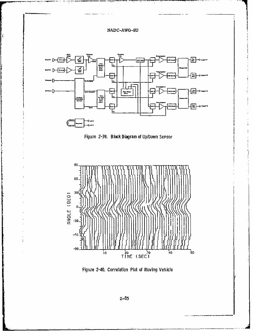
T-U

-~--r -c

awl

c-pI

r- D -wt

Figure 2-39. Block Diagram of Up/Down Sensor

G fl

10 20 0 O so

TIME (SEC)

Figuire 2-40. Correlation Plot of Moving Vehicle

2-85

NADC-AWG-SU

2.6.D-2.6.E

necessary), it does suffer in requiring reasonable physical dimuen-system (multi-angle determination and no input calibration

sions for a given frequency; the distance required is normallymany wavelengths; without this the correlation peak would be verysmall. Another problem occurs if the source produces a singlefrequency. Then the correlation maximum is not unique and willoccur at every T equal to the period of the signal. In general,real life targets with cyclical outputs such as aircraft havesufficient non-redundancy in correlation peaks to produce amaximum.

E. Arrays

To cover the subject of steerable arrays in depth is beyondthe scope of this chapter. However, it is useful to discussbriefly a simple array to illustrate the concept and indicate thepower of the approach. Arrays are constructed from multiplemicrophones spaced apart from each other. The outputs from themicrophones are combined. In the simplest case the microphonesare omnidirectional or pressure units although directional sensorscan be employed to advantage. Typically the outputs are summedusually with different weighting factors and possibly with dif-ferent time delay networks. The result is a polar sensitivitypattern which is highly directional, albeit, the directionalityis a function of frequenry or, more precisely, of wavelength.The array theory is analogous to that employed in the design ofradio antenna arrays and is similar in many respects to diffrac-tion in optics. Consider aa array of four microphones, 1, 2, 3,and 4, equally spaced with intersensor distance k (Figure 2-43).Assume the outputs are added so that

E = E1 + E2 + E3 + E4 (2-47)

where the E's are the instantaneous values of voltage output ofthe respective microphones.

Assume a sinusoidal sound source at infinity so that the wavefront is parallel and of equal peak pressure pm at each sensor.Then for a wavefront at angle 0 to the array,

.E = kpm exp J(wt + 3 sinG) (2-48)2c

E2 =kpm exp J(Wt + 1__ sine) (249)2c

2-86

NADC-AWG-SU

90_ 1

60 1 S

-930 r )60

CD

'1030 230JJs

S,-, II I I,

TIME !'SECi

AIRCRAFT - ?V I - BEGIN 100300 F- v%9 CR SF':i=2O0

Figure 2-41- Cornilaton Plot from Aircraft

90-

so

- 0

tj~j

I.J

II

3C Zs

T1[1E (SEC)

KC99FT

- TPPE t - BIN IC0O 3 - -. -

Figure 2-42. Enhanced Correlation Plot from Aircraft

2-8T

j

- -- ,* ;- - -

NADC-AVG-SU

2. 6. E

E kp exp J(wt - sine) (2-50)3 m 2 c

hee= kpm exp J(Wt - _ sine) (2-51)

where:

k is the microphone sensitivity constant

w is the angular frequency of the source

c is the velocity of propagation

By defining

RW sinO _

X - 217r sine (2-52)c A

and by normalizing to

kpm = 1 (2-53)

Equation 2-47 becomes

E = exp j(wt) {[exp J(2 X) + exp -J(l X)] +

[exp J(12 X) + exp -j (I X)]] (2-54)2 2

= exp J(wt) [2 cos (I x) + 2 cos (I x)] (2-55)

2 2

For spacing of 1/4 wavelength

X = w/2 sin e (2-56)

so that the normalized output in dB as a function of 0 for L = X/4 is:

Output = 20 log {2[cos ( -sin) + cos(I sinO)Jd.B (2-57)4 11

which is plotted in Figure 2-44. The gain for £ = A/2 is plottedin Figure 2-45.

2-88

_____I

NADC-AWG-SU

[ Wavefronts

0

Microphone lqcropbone Micropbone Ml1cropbone12 + 3 4

Figure 2-43. Four-Microphone Linear Arrady

2-89

NADC-AWG-SU

2.6.E-2.6.F

The above exercise illustrates the patterns which can beachieved by linear arrays and shows that the pattern is fre-quency sensitive. By using more microphones, higher orderpatterns can be achieved. By combining the signals through con-trollable delays, the pattern can be electrically steered.

F. D4ON

Occasionally the rate of variation cf the signal strength isof more significance than the signal itself. For example, the"beating" between two engines may be more characteristic of adevice than the engine sound itself. In such a case the basesignal can be considered as a carrier which is amplitude modu-lated by the desired information. Then it is appropriate todemodulate the signal before analysis. This procedure goesunder the appellation, DEVION.

One ordinarily thinks of the amplitude modulation process asone that involves a carrier of given frequency modulated in amp-litude by information whose components have frequencies that aremuch lower than the carrier frequency. For the simple case of asingle frequency as the modulation, the resultant waveform canbe expressed as:

e(t) = All + m cos Limt + 0 m)] [sin 6ct + Oc)] (2-58)

where

e(t) = instantaneous amplitude of the waveform (volts)

A = the amplitude of the carrier (volts)

m = the modulation index (numeric)

m = the modulating angular frequency (radians/sec)

Wc = the carrier angular frequency (radians/sec)

Om = the phase of the modulating signal (radians)

Oc the phase of the carrier signal (radians)

To obtain the information, mA cos w t from the composite am-plitude modulated signal, one feeds the ,ignal through an AM detec-

2-90

NADC-AWG-SU

2.6.F

tor (or demodulator) which strips off signal amplitude and disre-gards the carrier. One way of looking at the demodulator is to con-sider it an item that is sensitive only to amplitude variations andnob to phenomena such as frequency or phase variations which are inquadrature ,tth amplitude variations. 2 1 This is to say that if thecarrier were to vary in frequency over some given range, the demodu-lated output .'ould not be affected.

The above concept of amplitude modulation may be broadened

by allowing the carrier frequency, amplitude and phase to change.This results in a waveform

e2(t) [f(t)] [1 + m(t) g(t)] (2-59)

where

e2 (t) = instantaneous amplitude of thewaveform (volts)

f(t) = instanbaneous amplitude of arandom waveform of given band-width (vol.ts)

m(t) = modulation index (numeric)

g(t) = instantaneous amplitude of awaveform having frequenciesmuch lower than those in f(t) (volts)

When e2 (t) is passed through an AM detector, the output isessentially g(t), that is, the output is the envelope of f(t).

A sounud analog of e2 (t) may be encountered. It may beseen that there is envelope information in the composite sig--

nal so that AM detection must first be effected to reduce thistype of data.

The uisefulness of the DEMON technique is demonstrated inFigures 2-4 6a and 2-46b which depict identical frequency analysesof the same. data, one before and one after demodulation. A dis-tinct structure is apparent in the demodulated data which doesnot appear in the analysis of the raw data.

21 See A.Hund, Frequency Modulation, McGraw-Hill Book Co.,

Inc., 1942, p. 3.

2-91

Von rM 'W ", f 7--F -

NADC-AWG-SU

2.7.A-2.7.B

2.7 MODELING

A. Introduction

The term model, as used in signal analysis, is a mathemati-cal expression describing a phenomenon, in general terms. Thepurpose of the model is to provide a means for estimating theperformance of a system or a device mathematically without physi-cally testing it. Thus, a design may be evaluated even beforeit is engineered or produced, or a complete scenario can be anal-yzed to predict a system performance. Obviously, the validityof the evaluation depends upon the validity and completeness ofthe model. Modeling for acoustic detection systems encompassesnot only the system model, but source, noise, and propagationmodels. These techniques are discussed in this section.

B. Basic Considerations for Modelin.

The function of a model is to provide a simplified mathe-matical expression approximating the behavior of a real functionto an accuracy sufficient for the purpose for which the model isto be used. Models should have several important characteristics.

1. Their accuracy should be commensurate with the accuracyof the data. Typically, this means that the model should fitthe data to within a few decibels. Accuracies greater than afew decibels usually are not warranted because of the accumula-tion of inaccuracies in microphone calibration, distance esti-mation, recording accuracy, analysis equipment accuracy andlinearity and sensitivity of the simulated system to small changesin signal level.

2. They should include all parameters of significance.Significance is a quantitative term rather than a qualitativeterm, and a parameter of significance is one which affects themodel by more than a few decibels.

j. They should be of a form suitable for entry into a com-puter. This means that they should be piecewise linear in deci-bels, and without significant discontinuities. If this is notpossible, they should be given in tabular form.

4. In view of the general inadequacy of theories basedon excessively idealized models, the models should conform tomeasured parameters rather than calculated ones. Only in theevent that some important parameter cannot be measured shouldtheoretical results be used. In every case where measurementsconflict with theory, the results of measurements should beemployed.

2-92

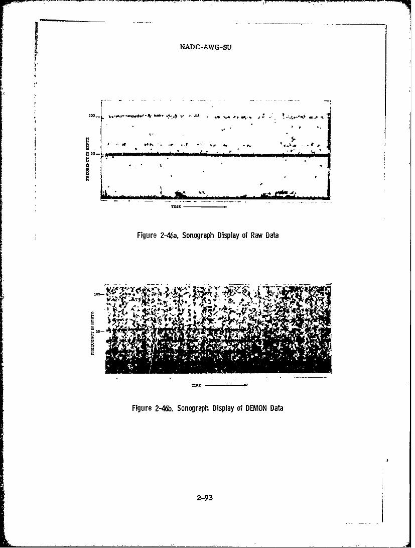
J NADC-AWG-SU

10 -

-W I ~

- WA

TWE

Figure 2-46a. Sonograph Display of Raw Data

10-

s2o-

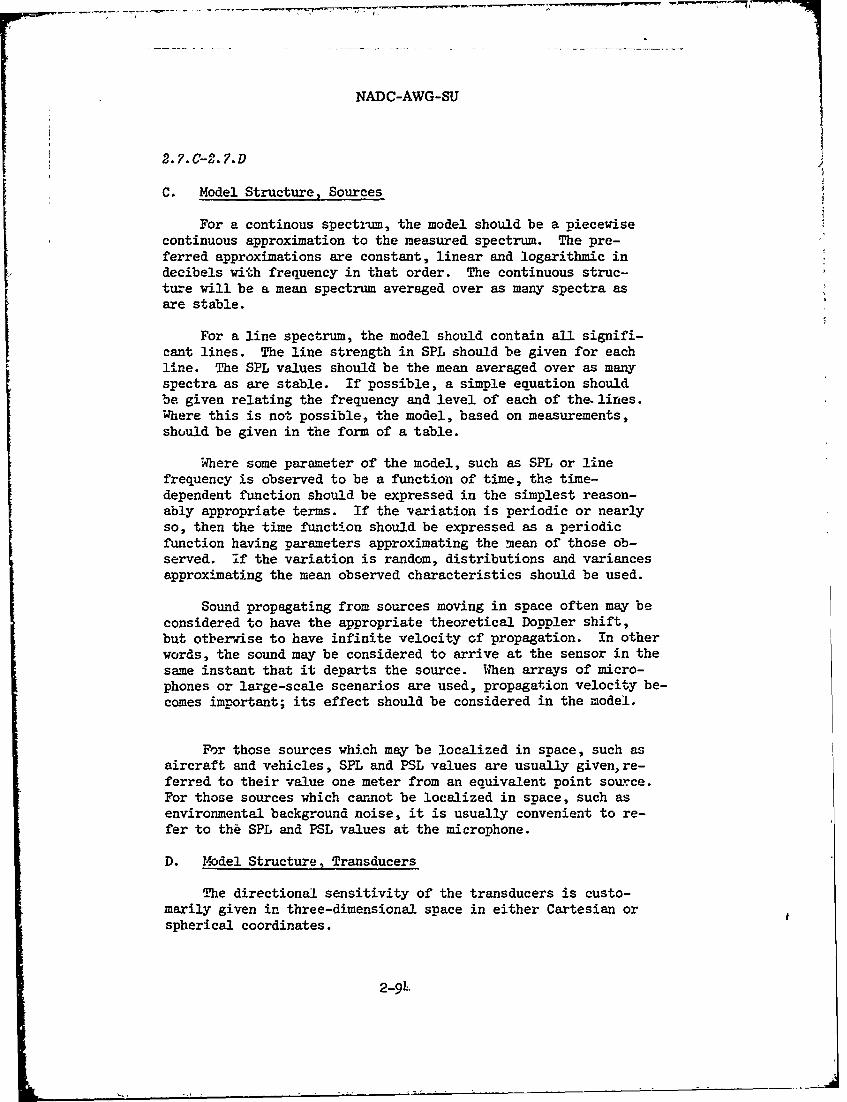
NADC-AWG-SU

2. 7.C-2. 7.D

C. Model Structure, Sources

For a continous spectrum, the model should be a piecewisecontinuous approximation to the measured spectrum. The pre-ferred approximations are constant, linear and logarithmic indecibels with frequency in that order. The continuous struc-ture will be a mean spectrum averaged over as many spectra asare stable.

For a line spectrum, the model should contain all signifi-cant lines. The line strength in SPL should be given for eachline. The SPL values should be the mean averaged over as manyspectra as are stable. If possible, a simple equation shouldbe given relating the frequency and level of each of the. lines.Where this is not possible, the model, based on measurements,shuuld be given in the form of a table.

Where some parameter of the model, such as SPL or linefrequency is observed to be a function of time, the time-dependent function should be expressed in the simplest reason-ably appropriate terms. If the variation is periodic or nearlyso, then the time function should be expressed as a periodicfunction having parameters approximating the mean of those ob-served. if the variation is random, distributions and variancesapproximating the mean observed characteristics should be used.

Sound propagating from sources moving in space often may beconsidered to have the appropriate theoretical Doppler shift,but otberwise to have infinite velocity of propagation. In otherwords, the sound may be considered to arrive at the sensor in thesame instant that it departs the source. When arrays of micro-phones or large-scale scenarios are used, propagation velocity be-comes important; its effect should be considered in the model.

For those sources which may be localized in space, such asaircraft and vehicles, SPL and PSL values are usually given, re-ferred to their value one meter from an equivalent point source.For those sources which cannot be localized in space, such asenvironmental background noise, it is usually convenient to re-fer to the SPL and PSL values at the microphone.

D. Model Structure, Transducers

The directional sensitivity of the transducers is custo-marily given in three-dimensional space in either Cartesian orspherical coordinates.

2-91

NzADC-AWG-SU

2. 7.D-2. 7.E

For each transducer, the ratio between the rms voltagethat would be produced in a perfectly diffused sound fieldof constant frequency and given sound pressure and the rmsvoltage pr6duced in response to a plane progressive sinusoi-dal sound wave arriving in the direction of maximum sensi-tivity should be given. This ratio is termed the RandomResponse.

The formulae for directional sensitivity of a number oftransducers can be found in standard acoustical texts.22

E. Model of Sound Propagation

The process of sound traveling through a complex propa-gation environment may be mathematically modeled in terms ofenvironment parameters. A first-order modeling techniquetreats the environment as an invariant linear filter, and thesound sources as a time waveform (signature) whose frequencycomponents are determinable. Both the source-signature andthe filter characteristics of the environment are determinedexperimentally. The mathematical model then becomes:

SPL r(f, r, 9) = SPLo(f, 9) + B(f, r, 9) (2-60)

(dB re 0.0002 Pbar)

where

SPL (f, r, 9) = sound pressure level of a given fre-r quency component of the signature at

range r, and angle 9 from the sourcein dB re 0.0002 pbar

SPL0 (f, 9) = sound pressure level of a given fre-quency component of the signature, atunit distance from the source, in a giv-en direction 9 in dB re 0.0002 pbar.

B(f, r, 9) = the attenuation,dB, caused by the en-vironment in a given direction, at agiven frequency and as a function ofrange

r = range from source

22See footnote 19, p. 2-78

2-95

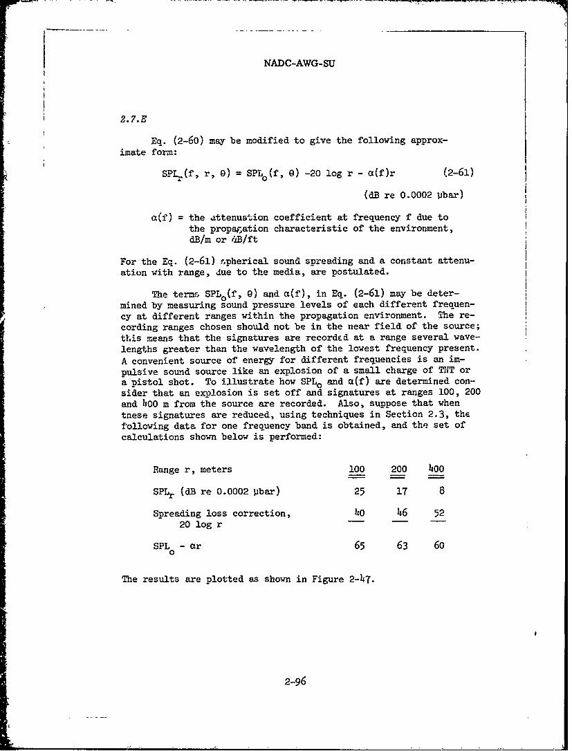
NADC-AWG-SU

2.7.E

Eq. (2-60) may be modified to give the following approx-

imate form:

SPLr(f, r, 9) = SPLo(f, 9) -20 log r - c(f)r (2-61)

(dB re 0.0002 pbar)

a(f) = the attenuation coefficient at frequency f due tothe proparation characteristic of the environment,dB/m or UB/ft

For the Eq. (2-61) F.pherical sound spreading and a constant attenu-ation with range, due to the media, are postulated.

The terms SPLo(f, 9) and c(f), in Eq. (2-61) may be deter-mined by measuring sound pressure levels of each different frequen-

cy at different ranges within the propagation environment. The re-

cording ranges chosen should not be in the near field of the source;this means that the signatures are recordEd at a range several wave-lengths greater than the wavelength of the lowest frequency present.

A convenient source of energy for different frequencies is an im-

pulsive sound source like an explosion of a small charge of TNT ora pistol shot. To illustrate how SPLo and a(f) are determined con-sider that an explosion is set off and signatures at ranges 100, 200and 400 m from the source are recorded. Also, suppose that when

tnese signatures are reduced, using techniques in Section 2.3, thefollowing data for one frequency band is obtained, and the set ofcalculations shown below is performed:

Range r, meters 100 200 400

SPLr (dB re 0.0002 pbar) 25 17 8

Spreading loss correction, 4o 46 52

20 log r

SPL - ar 65 63 600

The results are plotted as shown in Figure 2-47.

2-96

NADC-AWG-SU

2.7.E

The slope of a regression line through the points is a(f),in dB/m. The dispersion of the measured points about the lineindicates how well the constant factor a(f) models the attenu-ation phenomenon. The intersection of the line with the ordi-nate at r = 0 is SPLo(f, 0) for the given environment.

Equation (2-61) for the above conditions (which we designate A)

may then be rewritten as follows:

SPIr(fA, @A) = 66.5 - 20 log r - 0.0162r (dB re 0.0002 bar) (2-62)

The above procedure may then be c- ried out for remaining per-

tinent frequencies and directions of propagation that characterizethe source and the medium. Results may then be extrapolated to fit

othersimilar environments, or other ranges not measured; care is

necessary not to overextend the extrapolation. Normally, the ex-

periment would be done many times with many more data points. When

a line is fitted to the data, the scatter will give an idee of theuncertainty of the data.

A more sophisticated approach to modeling, yielding approxi-matelythe same result but a better statistical determination ofthe parameters involved, is the use of regression analysis. Here,more complicated forms of modeling can be investigated with com-parative ease, along with an ability to determine the significanceand confidence of the various terms.2

3Ca0

o65-

-Slope, .Cz : --0162d1lm

160.

0 100 2n 300 40 5 0

RANGE IN METERS

Figure 2-47. Graph for Estimating SPL and (X

23j. R. Harris, "A Study of Using Multiple Nonlinear Regres-

sion Analysis for Acoustical Modeling," Report No. NADC-SD-7027,Naval Air Development Center, Warminster, Pa., 19 June 1970.

2-97

NAPC-AWG-SU

3.1

CHAPTER THREE: PROPAGATION

3.1 INTRODUCTIO

Sound waves travel from source to receiver through open at-mosphere that is by its nature in constant motion and fluctuation.Density and temperature, wind and humidity, are never uniform ina given volume of open air under observation nor are they constantin time. The lon~ger the transmission path through atmosphere, themore important is the effect of the interposed ground conditionson the received sound. Because the atmosphere is neither homoge-neous nor quiescent and the ground covering can vary to a largeextent, pr.opagation of sound in open space constitutes a compli-cated statistical problem. It is the purpose of this chapter topresent a combination cf theory and empiricism on propagationstudies made of acoustical signals in various types of atmospher-ic conditions and foliage using as a basis the experimental datagathered in the years between 1966 and 1970.

In the study of propagation of sound, two approaches usuallyare used, one being the ray path theory and the other the normalmode theory. Each of these approaches is best adapted to specif-ic situations. The ray path method is appropriate to the studyof propagation in the atmosphere when the boundary conditions aremainly due to ground. This approach is treated in subsections3.3.A through 3.3.D. The normal mode is more convenient when mul-tiple and well-defined boundary conditions exist such as those wefind in shallow water with both the bottom and surface reflectionspresent. This method is discussed in Section 3.4. The real worldproblem in air is complicated by scatter as described in Section3.5. Empirical fit is appropriate in these cases with the model-ing being determined by physical considerations as derived fromrrq path theory, which is discussed in Section 3.2. In the stud-ies undertaken, except for a few isolated cases where strong tem-perature inversions and/or heavy canopy foliage allowed some chan-neling to take place, this latter type of modeling appeared to bequite adequate. Other aspects of modeling are treated in Sec-tion 2.7.

3-1

NADC-AWG-SU

3. 2-3.2.B

3.2 ANALYSIS OF SOUND PROPAGATION

A. Introduction

Ordinarily, the decrease in sound-pressure level at a dis-tance from the source in an ideal, homogeneous, loss-free atmosphere is most affected by the spreading of the sound waveswhich are radiated by the source. The sound-pressure amplitudefrom a point source varies inversely as the distance from thesource. That is, there is a drop in sound-pressure level of6 dB with each doubling of distance away from the source.

At distances large compared with its size, the sound sourcecan be treated as a point, even though it is not physically verysma.ll. If we know that sound-pressur- level Lo at distance ro,theoretically the sound pressure level L in the same directionat another distance r is given by

L = Lo - 20 log (r/r 0 ), dB (3-1)

B. Excess Attenuation

It has been established experimentally that the level ofthe recei.red signal after it has travelled some distance alongthe ground is almost always below the level which would be ex-pected if sound propagation had taken place in homogeneous airat rest over a perfectly smooth reflecting ground plane. Thedifference between the attenuation actually observed and thatdue to spherical spreading alone is frequently referred to as"excess attenuation" (Ae)44 This is a useful quality fordescribing the transmission path between source and receiveracoustically. The excess attenuation depends, generally speak-ing, on the frequency of the transmitted sound and the distancebetween source and receiver and on the ever changing character-istics of the atmosphere. The sound pressure level equation isthus modified as follows:

L = L 1 - 20 log r- Ae, dB (3-2)

The excess attenuation Ae depends on the following factors:

241L. L. Beranek, ed., Noise and Vibration Control, McGraw-

Hill Book Co., Inc., New York, 1971, p. 169. It is equivalent tothe quantity "transmission anomaly" in Principles and Applicationsof Underwater Sound, U. S. Gov't. Printing Office, NAVMAT, P-9674,Dept. of the Navy, 1968, p. 8.

3-2

NADC-AWG-SU

3.2. B-3.2. C

1. molecular absorption of sound in the air

2. refraction of sound waves due to the presenceof vertical temperature gradient and windgradient

3. attenuation and scattering of sound by trees,bushes, and other solid obstacles

The contributions of each of the above factors to theoverall excess attenuation are not strictly independent in thegeneral case although, as a first approximation, some of theseeffects can be regarded as independent. Under most practicalconditions, the excess attenuation at a given frequency of thesound is directly proportional to distance. So we have

L = L1 - 20 log r - or, dB (3-3)

where a designates the excess attenuation per unit distance. Eq.(3-3) of course expresses the same law as has been previously for-mulated in Eq. (2-61) assuming that the direction of propagation 0is a constant.

C. Dependence on Humidity and Scattering

The molecular absorption of sound energy in air dependson frequency and humidity. I has been determined theoreticallyand confirmed experimentally2o by a number of investigators.Over open level ground, appreciable vertical temperature andwind gradients almost always exist; the former because of theheat exchange between the ground and the atmosphere, the latterbecause of the friction between the moving air and the ground.Because of these gradients, the speed of sound varies withheight above the ground and sound waves are refracted, that isto say, bent upward or downward. Under these conditions, thestraight line transmission characteristic of the sound is re-duced.

Scattering refers to deflection of sound energy from its

25H. 0. Kneser, "Interpretation of the Anomalous Sound

Absorption in Air and Oxygen in Terms of Molecular Collisions,"J. Acoust. Soc. Am., Vol. 5, 1933, p. 122.

26 E. J. Evans, and E. N. Bazley, "The Absorption of Soundin Air at Audio Frequencies," Acoustica, Vol. 6, 1956, p. 238.

3-3

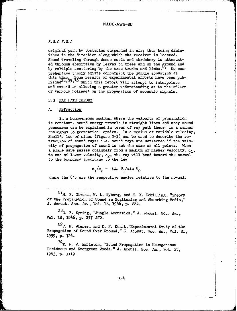
NADC-AWG-SU

3.2. C-3.3.A

original path by obstacles suspended in air; thus being dimin-ished in the direction along which the receiver is located.Sound traveling through dense woods and shrubbery is attenuat-ed through absorption by leaves on trees and on the ground andby multiple scattering by the tree trunks and limbs. No com-prehensive theory exists concerning the jungle acoustics atthis time. Some results of experimental efforts have been pub-lished2 ,29,30 which this report will attempt to interpolateand extend in allowing a greater understanding as to the efCectof various foliages on the propagation of acoustic signals.

3.3 RAY PATH THEORY

A. Refraction

In a homogeneous medium, where the velocity of propagationis constant, sound energy travels in straight lines and many sound

phenomena ceu be explained in terms of ray path theory in a manneranalogous ;.o geometrical optics. In a medium of variable velocity,Snell's law of sines (Figure 3-1) can be used to describe the re-fraction of sound rays; i.e. sound rays are deflected if the velo-city of propagation of sound is not the same at all points. Whena plane wave passes obliquely from a medium of higher velocity, cl,to one of lower velocity, 02 , the ray will bend toward the normalto the boundary according to the law

c /C = sin 0 /sin e1 2 1 2

where the e's are the respective angles relative to the normal.

2 -TM. P. Givens, W. L. Nyborg, and H. K. Schilling, "Theory

of the Propagation of Sound in ScaLtering and Absorbing Media,"J. Acoust. Soc. Am., Vol. 18, 1946, p. 284.

28 C. F. Eyrring, "Jungle Acoustics," J. Acoust. Soc. Am.,

Vol. 18, 1946, p. 257-270.

29F. M. Wiener, and D. N. Keast,"Experimental Study of the

Propagation of Sound Over Ground," J. Acoust. Soc. Am., Vol. 31,1959, p. 724.

30T. F. W. Embleton, "Sound Propagation in HomogeneousDeciduous and Evergreen Woods," J. Acoust. Soc. Am., Vol. 35,1963, p. 1119.

3-h

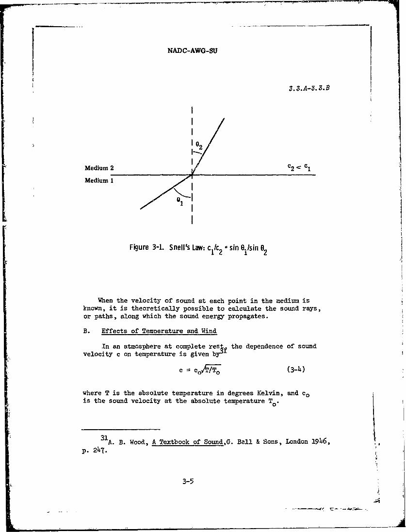
NADC-AWG-SU

3.3.A-3.3.B

I-.

Medium 2 c2 1

Medium I

sI

Figure 3-1. Snell's Law: c kc sin 8 /sin 81 2 i '2

When the velocity of sound at each point in the medium isknown, it is theoretically possible to calculate the sound rays,or paths, along which the sound energy propagates.

B. Effects of Teimnerature and Wind

In an atmosphere at complete rest, the dependence of soundvelocity c on temperature is given by

c = Co/€ (3-4)

where T is the absolute temperature in degrees Kelvin, and cois the sound velocity at the absolute temperature TO.

31A. B. Wood, A Textbook of Sound,G. Bell & Sons, London 19h6,p. 247.

3-5

. = -- = ,, , ,, - =,

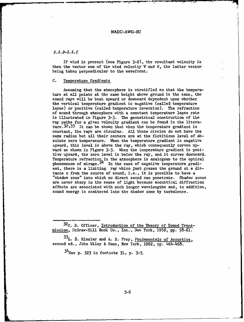
NADC-AWG-STJ

3.3.B-3.3. C

If wind is present (see Figure 3-2), the resultant velocity isthen the vector sum of the wind velocity V and E, the latter vectorbeing taken perpendicular to the -wavefront.

C. Temperature Gradients

Assuming that the atmosphere is stratified so that the tempera-ture at all points at the same height above ground is the same, thesound rays will be bent upward or downward dependent upon whetherthe vertical temperature gradient is negative (called temperaturelapse) or positive (called temperature inversion). The refractionof sound through atmosphere with a constant temperature lapse rateis illustrated in Figure 3-3. The geometrical construction of theray paths for a given velocity gradient can be found in the litera-ture.32,33 It can be shmn that -,hen the temperature gradient isconstant, the rays are circular. All these circles do not have thesame radius but all their centers are at the fictitious level of ab-solute zero temperature. When the temperature gradient is negativeupward, this level is above the ray, which consequently curves up-ward as shown in Figure 3-3. When the temperature gradient is posi-tive upward, the zero level is below the ray, and it curves downward.Temperature refraction in the atmosphere is analogous to the opticalphenomenon of mirage.34 In the case of negative temperature gradi-ent, there is a limiting ray which just grazes the ground at a dis-tance x from the source of sound, i.e., it is possible to have at shadow zone" into which no direct sound can penetrate. Shadow zonesare never sharp in the sense of light because acoustical diffractioneffects are associated with much longer wavelengths and, in addition,sound energy is scattered into the shadow zone by turbulence.

32C. B. Officer, Introduction of the Theory cf Sound Trans-

mission, McGraw-Hill Book Co., Inc., iew York, 2958, pp. 58-61.

3 3 L. E. Kinsler and A. R. Frey, Fundamentals of Acoustics,second ed., John Wiley & Sons, New York, 1962, pp. 464-468.

34See p. 323 in footnote 31, p. 3-5.

3-6

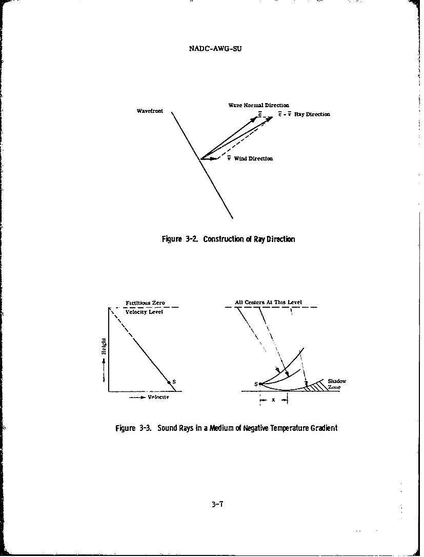
NADC-AWG-SU

WaTe Normal DirectionWavefront Ray Direction

1Wbod Dire&tion

Figure 3-2. Construction of Ray Direction

Fictitious Zero All Centers At This Level

\ Velocity Lerel

\\ \

S Siuaw

Figure 3-3. Sound Rays in a Medium of Negative Temperature Gradiernt

3-7

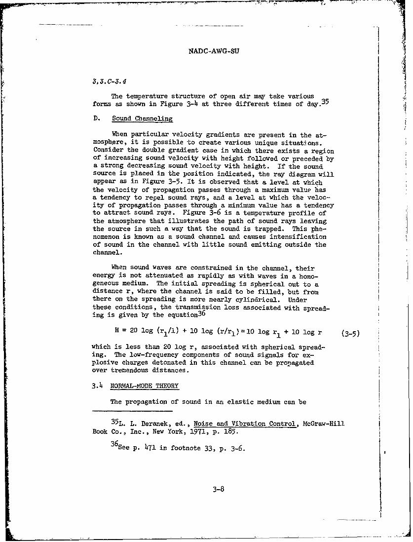
NADC-AWG-SU

3.3. C-3.4

The temperature structure of open air may take various

forms as shown in Figure 3-4 at three different times of day. 3 5

D. Sound Channeling

When particular velocity gradients are present in the at-mosphpre, it is possible to create various unique situations.Consider the double gradient case in which there exists a regionof increasing sound velocity with height followed or preceded bya strong decreasing sound velocity with height. If the soundsource is placed in the position indicated, the ray diagram willappear as in Figure 3-5. It is observed that a level at which

the velocity of propagation passes through a maximum value hasa tendency to repel sound rays, and a level at which the veloc-ity of propagation passes through a minimum value has a tendencyto attract sound rays. Figure 3-6 is a temperature profile ofthe atmosphere that illustrates the path of sound rays leavingthe source in such a way that the sound is trapped. This phe-nomenon is known as a sound channel and causes intensificationof sound in the channel with little sound emitting outside thechannel.

When sound waves are constrained in the channel, theirenergy is not attenuated as rapidly as with waves in a homo-geneous medium. The initial spreading is spherical out to adistance r, where the channel is said to be filled, but fromthere on the spreading is more nearly cylindrical. Underthese conditions, the transmission loss associated with spread-ing is given by the equation3

6

H = 20 log (r!/i) + 10 log (r/r1)=10 log rI + 10 log r

which is less than 20 log r, associated with spherical spread-ing. The low-frequency components of sound signals for ex-plosive charges detonated in this channel can be propagatedover tremendous distances.

3. 4 NOIL4AL-MODE THEORY

The propagation of sound in an elastic medium can be

35L. L. Deranek, ed., Noise and Vibration Control, McGraw-HillBook Co., Inc., New York, 1971, p. 185.

36See p. 471 in footnote 33, p. 3-6.

3-8

NADC-AWG-SU

LAP- Torsions With H, rma l vwk With Hol'tm

Figure 3-4. Example of Temperature Profiles at Three Times of Day

ZI

-------- Velocity Range

SI

Figure 3-5. Velocty Profile and Ray Diagram

----- Tem~erature 4.Ramp

Figure 3-6. Formation of a Sound Channel

3-9

AA

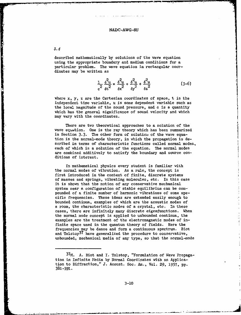
NADC-AWG-SU

3.4

described mathematically by solutions of the wave equationusing the appropriate boundary and medium conditions for aparticular problem. The wave equation in rectangular coor-dinates may be written as

2 2 2 262u u + § (3-6)c 6t2 6x2 6y2 6z2

where x, y, z are the Cartesian coordinates of space, t is theindependent time variable, u is some dependent variable such asthe local magnitude of the sound pressure, and c is a quantity

which has the general significance of sound velocity and whichmay vary with the coordinates.

There are two theoretical approaches to a solution of thewave equbtion. One is the ray theory which has been summarizedin Section 3.3. The other form of solution, of the wave equa-tion is the normal-mode theory, in which the propagation is de-scribed in terms of characteristic functions called normal modes,each of which is a solution of the equation. The normal modesare combined additively to satisfy the boundary and source con-ditions of interest.

In mathematical physics every student is familiar withthe normal modes of vibration. As a rule, the concept isfirst introduced in the context of finite, discrete systemsof masses and springs, vibrating molecules, etc. In this caseit is shown that the motion of any conservative mechanicalsystem near a configuration of stable equilibrium can be com-

pounded of a finite number of harmonic vibrations of some spe-cific frequencies. These ideas are extended easily enough tobounded continua, examples of which are the acoustic modes ofa room, the characteristic modes of a crystal, etc. In thesecases, there are infinitely many discrete eigenfunctions. Whenthe normal mode concept is applied to unbounded continua, theexamples are the treatment of the electromagnetic modes of in-finite space used in the quantum theory of fields. Here thefrequencies may be dense and form a continuous spectrum. Biotand Tolstoy37 have generalized the procedure to conservative,unbounded, mechanical media of any type, so that the normal-mode

37M. A. Biot and I. Tolstoy, "Formulation of Wave Propaga-tion in Infinite Media by Normal Coordinates with an Applica-tion to Diffraction," J. Acoust. Soc. Am., Vol. 29, 1957, pp.381-391.

3-10

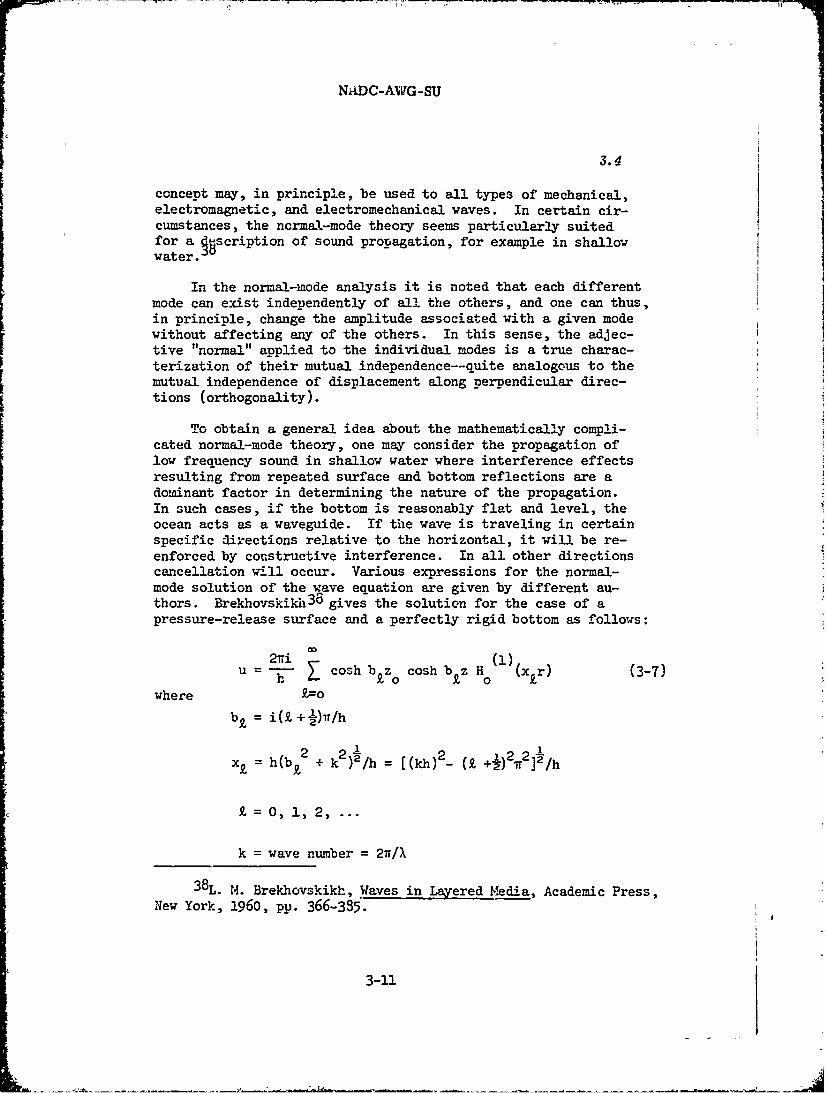
NADC-AWG-SU

3.4

concept may, in principle, be used to all types of mechanical,electromagnetic, and electromechanical waves. In certain cir-cumstances, the ncrma.l-mode theory seems particularly suitedfor a iscription of sound propagation, for example in shallowwater.

In the normal-mode analysis it is noted that each differentmode can exist independently of all the others, and one can thus,in principle, change the amplitude associated with a given modewithout affecting any of the others. In this sense, the adjec-tive "normal" applied to the individual modes is a true charac-terization of their mutual independence--quite analogous to themutual independence of displacement along perpendicular direc-tions (orthogonality).

To obtain a general idea about the mathematically compli-cated normal-mode theory, one may consider the propagation oflow frequency sound in shallow water where interference effectsresulting from repeated surface and bottom reflections are adominant factor in determining the nature of the propagation.In such cases, if the bottom is reasonably flat and level, theocean acts as a waveguide. If the wave is traveling in certainspecific ;1i-ections relative to the horizontal, it will be re-enforced by constructive interference. In all other directionscancellation will occur. Various expressions for the normal-mode solution of the wave equation are given by different au-thors. Brekhovskikh 3o gives the solution for the case of apressure-release surface and a perfectly rigid bottom as follows:

Goo2Tri (1h-- coshb Zz 0cosh bz H (x r) (3-7)

where 2=obZ = i (9 + )Vir/h

2 2-2 1 2 1 2 2x = h(b k + k2 )2/h = [(kh) 2 - (X +f) 7T]2/h

£ = 0, 1, 2,

k = wave number = 2n/X

38L. M. Brekhovskikh, Waves in Layered Media, Academic Press,New York, 1960, pp. 366-385.

3-11

NADC-AWG-SU

3.4

h = water depth

zo = source depth

z = receiver depth

HO = Hankel function of the first kind

Modes propagating without attenuation are those for which theargument (x~r) of the Hankel function is real; those are themodes for which kh> 7T/2 or h>.X/4, that is,. those for which thewater depth is greater than one-quarter wavelength. The fre-quency corresponding to h = X/4 is termed the cutoff frequency;frequencies lower than the cutoff frequency are propagated inthe channel only with attenuation and are not effectively trap-ped in the duct. The variation of pressure with depth of thefirst four modes is shown in Figure 3-7.

Each mode can be conceived to correspond to a pair ofwaves incident upon the boundaries at an angle B and propa-gating in a zigzag fashion by successive reflections. Forthe first two modes these equivalent plane waves are shownin Figure 3-8, where the lines denote the pressure modes(zero pressure) and the + and - signs give tbe polarity ofthe pressure between the pressure modes.

For the case of sound transm.ssion in deep sea, the normal-mode solution is different from the shallow water transmissionin that deep water is considered to be underlain by an elasticmedium instead of a fluid (sedimentary) medium. Adequatetreatment can be found in the literature.39 Figure 3-9 illus-trates the different types of propagation path that exist be-tween a source and a receiver in the deep sea.40 At short range(a), there is a nearly straight-line path between the two, andthe transmission loss is determined by spherical spreading,plus a loss due to absorption if the frequency is high enough,and modified by interference effects of the surface reflectionfor a near-surface source and receiver.

39See pp. 161-184 in footnote 32, p. 3-6.

40R. J. Urick, Principles of Underwater Sound for Engineers,McGraw-Hill Book Co., Inc., New York, 1967, p. 15.

3-12

NADC-AWG-SU

Mode Number n-0 n-1 n.2 n,-3

Figure 3-7. Sound Pressure Versus Depth for the First Four ModesFor a Pressure-Release (Soft) Surface and a Rigid (Hard) Bottom

.++-+

B

L!

Figure 3-& Plane-Wave Equivalents of the First and Second Modes In aDuct with a Pressure-Release Surface and a Rigid Bottom

(a) (d)

~) VjKj (e)

Figure 3-9. rropagation Paths Between a Source and a Receiverin Deep Water

3-13

NADC-AWG-SU

3.4-3.5

At longer ranges, propagation occurs in the mixed-layerchannel (b), involving repeated surface reflections and leak- Iage out of the channel to a receiver below. Propagation mayoccur also via "bottom-bounce" reflected paths (c), which suf-fer a reflection loss at the sea bottom and along which thetransmission loss is determined by spherical spreading plusabsorption and by the bottom-reflection loss. At still great-er ranges, convergence-zone transmission (d) takes place where,within a zone a few miles wide, convergence gains between 5and 20 dB occur, depending on the depth. Beyond the first pairof convergence half-zones, the transmission between a shallowsource and a shallow receiver involves multiple reflectionsfrom the bottom (e). In the deep sound channel, long-rangepropagation occurs over internally reflected paths (f) and isespecially good when both source and receiver lie on the chan-nel axis.

3.5 SCATTERING AND REVERBERATION

When a sound wave encounters an obstacle, some portionof the wave is deflected from its original course. It isusual to define the difference between tht actual wave and theundisturbed wave--which would be present if the obstacle werenot there-as the "scattered" wave. When a plane wave, forinstance, strikes a body in its path, in addition to the un-disturbed plan wave there is a scattered wave, spreading outfrom the obstacle in all directions, distorting and interfer-ing with the plane wave. If the obstacle is very large com-pared with the wavelength (as it usually is for light wavcsand very seldom is for sound), half of this scattered wavespreads out more or less uniformly in all directions fromthe scatterer, and the other half is concentrated behindthe obstacle in such a manner as to interfere destructivelywith the unchanged plane wave behind the obstacle, creatinga sharp-edged shadow there. This is the case of geometricaloptics; in this case the half of the scattered wave spread-ing out uniformly is called the "reflected" wave, and thehalf responsible for the shadow is called the "interfering"wave. if the obstacle is very small compared with the wave-length (as it often is for sound waves), all the scatteredwave is propagated out in all directions, and there existsno sharp-edged shadow. In the intermediate cases, where theobstacle is about the same size as the wavelength, a varietyof curious interference phenomena can occur.

3-14

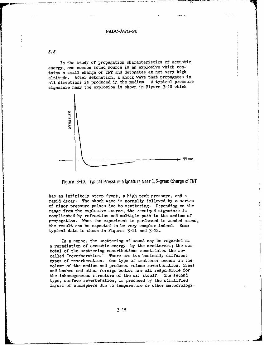
NADC-AWG-SU

3.5

In the study of propagation characteristics of acousticenergy, one common sound source is an explosive which con-tains a small charge of TNT and detonates at not very highaltitude. After detonation, a shock wave that propagates inall directions is produced in the medium. A typical pressuresignature near the explosion is shown in Figure 3-10 which

Time

Figure 3-10. Typical Pressure Signature Near 1.5-gram Charge of TNT

has an infinitely steep front, a high peak pressure, and arapid decay. The shock wave is normally followed by a seriesof minor pressure pulses due to scattering. Depending on therange from the explosive source, the received signature iscomplicated by refraction and multiple path in the medium ofpro nagation. When the experiment is performed in wooded areas,the result can be expected to be very complex indeed. Sometypical data is shown in Figures 3-11 and 3-12.

In a sense, the scattering of sound may be regarded asa reradiation of acoustic ener&v by the scatterers ; the sumtotal of the scattering contributions constitutes the so-called "reverberation." There are two basically differenttypes of reverberation. One type of scatterer occurs in thevolume of the medium and produces volume reverberation. Treesand bushes and other foreign bodies are all responsible forthe inhomogeneous structure of the air itself. The secondtype, surface reverberation, is produced by the stratifiedlayers of atmosphere due to temperature or other meteorologi-

3-15

NADC-AWG-SU

3.5-3.6.A

cal factors. Reverberations are heard as a long, slowly de-caying, quivering ton&l blast following the original blast.Th ,1tory of scattering of sound waves is extremely complicat-ed ' beyond the scope of this chapter. Because the direc-tion of scattering is normally back toward the source, theterm back-scattering is often used in practice. Whereas theattenuation and absorption of sound is of interest to mostacoustics engineers, back-scattering is of importance to com-munication problems which involve ranging techniques. It

must be taken into account under these circumstances.

3.6 SUMMARY OF FIELD RESULTS

A. Description of Test Procedures

To determine the effect of various jungle foliages on thepropagation characteristics of acoustic energy in the air, aseries of controlled tusts was conducted in north Florida,the Panama Canal Zone, Lousiana rice fields, and tlie Thailandjungles during the period of time between 1966 and 1970. Ingeneral, a well controlled omnidirectional explosive sound

source, which assured repetitiveness, was used with microphonesplaced at various distances from the source in the medium whichwas essentially uniform. The various ground-cover conditionsare grouped as follows:

1. Heavy elephant grass, a tall undergrowth from six toeight feet in height which could limit forward visibility toone or two feet, with slender reeds, densely packed. Such foli-ages were found at Panama and Suutheast Asia.

2. Heavy double canopy, a typical equator-like rain forestwhere palm trees were densely packed, with a penetrating visibi-lity of about 50 feet, such as encountered at a typical site inPanama.

Dept. of the Navy, "Echoes, Scattering, and Reverberation,"Principles and Applications of Underwater Sound, Ch. 5, 1968.

1 2L. L. Beranek, "Disturbance of Plane Sound Waves by Obstacle%

and by Finite Baffles," Acoustic Measurements, Ch. 3, John Wiley& Sons, New York, 1949

3-16

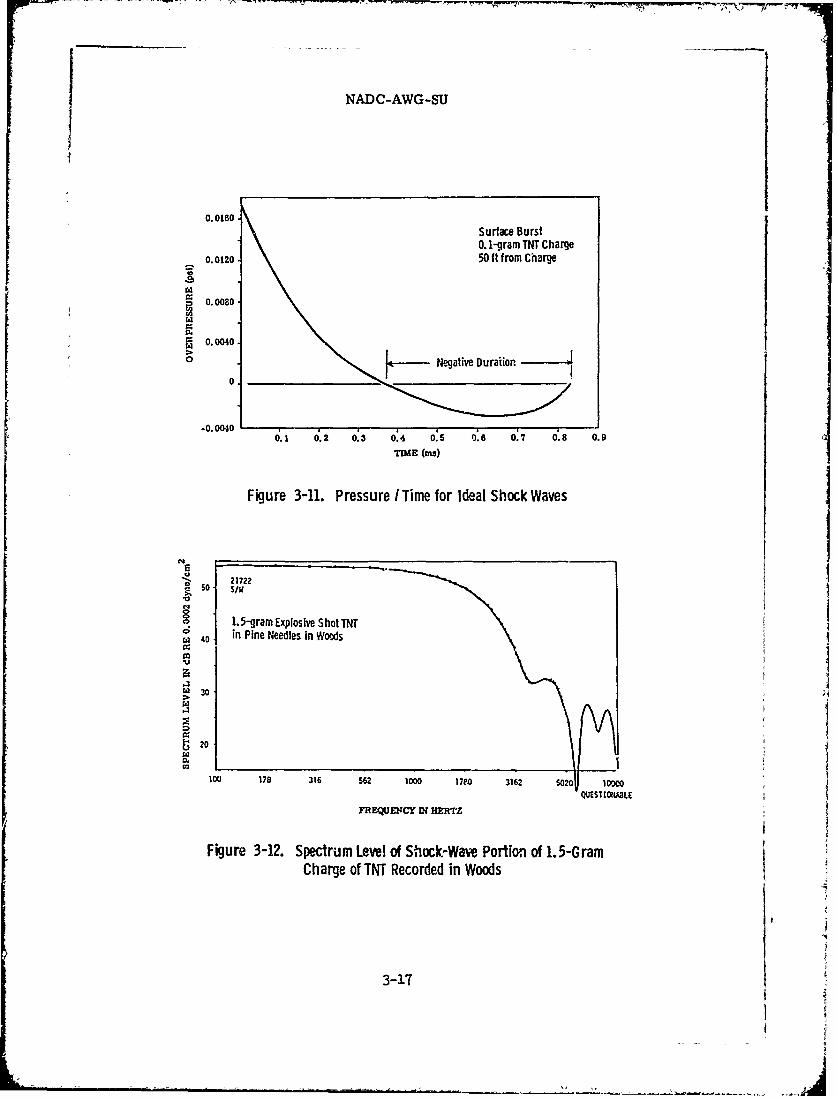
NAD C-AWG-SU

0.0160.Surface Burst

0. 1-gram TNT Charge0.0120 50 ft from Charge

* 0.0080-

S0.0040.

Negative Duraion

-0.00400. 0.2 0.3 0.4 0.5 0.6 0.7 0.8 0.9

TME (mS)

Figure 3-11. Pressure I Time for Ideal Shock Waves

21722

o1 1.5-gram Explosive Shot TNT

S40 in Pine Needles in Woods

14 30

20 '142

100 178 316 562 1000 17E0 3162 5020 10000QUESTI LE.

FREQUWE1CY IN HERTZ

Figure 3-12. Spectrum Level of Shock-Wave Portion of 1.5-GramCharge of TNT Recorded in Woods

3-17

NADC-AWG-SU

3.6.A-3.6.B

3. Light forest with small leaves, typical of pine treeforests in north Florida. Here the presence of tree trunks isthe predominant obstacle in the acoustical path with relative-ly small absorption due to the absence of large leaves.

4. Clear space, essentially light wooded area or complete-ly open space wheres in the absence of vertical temperaturegradients, the propagation is influenced by the medium andthe spherical spreading loss.

The tests were done with explosives containing 1.5-gram chargeof TNT, placed in the foliage about 25 feet off access trails.They were detonated on a hard firing base by impact. The micro-phones were located at varying distances suspended off the ground,and free of any immediate obstacle.

The sound measuring equipment and test technique have beendescribed in detail in Chapters 1 and 2. Simultaneous tape re-cordings were made from the various microphones which had beencalibrated so that the recorded signals could be evaluated inabsolute levels. As a further precaution, 10-dB stei attenua-tions were incorporated to insure tha- no overload occurred inthe recording system.

The collected data was analyzed both in the time domain andthe frequency domain as a function of distance from the explo-sive charge. From the findings of hundreds of experiments per-formed in this project an insight as to the effect of the natureof propagation characteristic was empirically derived. Theseresults are summarized in the next section.

B. Summary of Field Results

1. Propagation Losses

The field data was analyzed on the basis of the mathematicalmodel given by the following equation as explained in Chapter2, pp. 95-97:

SPL = A(f) - B(r,f) loglor - a(f)r (3-8)

where A, B, and a are coefficients that are dependent upon thebracketed quantities, range r and frequency f. The attenua-tion coefficients a(f) are calculated and summarized in Table3-1, for frequencies from 50 Hz to 2000 Hz. In general, the

3-18

NADC-AWG-SU

Table 3-1. Attenuation Coefficients as a Function of Frequency and Foliage

ATTENUATION COEFFICIENTS a, dB per foot

Lightly WoodedHeavy Elephant Double Canopy Florida Clear Spoce

Grass Palm Trees Pine Forest (bove river)FzQU==CT 6 ft Lcrophone 6 ft Microphone 30 ft Microphone 1 ft MicrophoneN Height Height Height Height

50 0.04 - 0.05 0.02

100 0.01 - 0.05 0.02 - 0.025 ----

200 0.01' - 0.05 0.02 - 0.03 0.01 0.005

500 0.0 - 0.05 0.U2 - 0.03 0.016 0.008

1000 0.05 - 0.055 0.02 - 0.03 0.02 0.008

2000 o.o6 - o.065 0.01' 0.025 O.O1T

NOTE: 1. When a range of experinental values wes obtainedthe range liits are shoimn

2. 20 log r spreading loss aasu-ed

.50

MW -jPM 0 m oA (AN l)

0

FlIq 3Cf D1 NUZ

Figure 3-13. Signal-to-Noise Ratio Versus Frequency for 500 ft Distanceand Various B3ckground Noises; Source 1.5-Gram Explosion INT

3-19

NADC-AWG-SU

3.6.B

results are in agreemept with other investigators, for example,the results of Eyring.43 The spreading loss coefficient B inthis analysis was taken as 20 for spherical spreading, whichis strictly valid for a point source in a homogeneous, un-bounded medium.

It is noted from Table 3-1 that different microphone heightswere used for the collection of data, depending on conditions.

During the test there were indications that, in the presence ofthick foliage, the attenuatibn is greater with lower microphonepositions above ground than with the high microphone position.

In clear space the spreading loss, as a function of distance andsource component frequency, appears to some degree to be depen-dent upon the refraction caused by temperature and wind gradient.The height of the microphone off ground can make quite a differ-ence in its reception of the sound energy. I

This observation suggests that in studies of this nature,the microphone position should be related to the application Ifor which the data will be used.

2. Ancillary Results

Figure 3-13 portrays the signal-to-noise ratios versusfrequency at 500 feet for the source signal in differentbackground noises. This normally maximum expected detec-tion range was chosen because a design optimization in band-pass is more critical at greater ranges.

43~

See footnote 28, p. 3-4.

*When the medium has plane-paralleled upper and lower bounds,

as explained in connection with channel formation, the spreadingof waves is no longer spherical because sound cannot cross thebounding planes. Beyond a certain range, the sound-pressure levelradiated from the source acts as if it were distributed over thesurface of a cylinder having a radius equal to the effective rangeand a height equal to the separation of the two parallel planes.Then the inverse first-power relation applies; i.e., a loss of 3dB (instead of 6 dB) per doubling of the range. Unpublished re-sults at NADC validate the magnitude of spreading loss coefficientvariation in practical cases ranging from 10 to 20.

3-20

NADC-AWG-SU

3.6.B-3.7.A

Mhe time domain evaluation of the propagation character-istics of explosive signals was obtained through the oscillo-grams of amplitude versus time at various distances from thesource. Figures 3-14 through 3-16 are typical of the resultfor small explosive shots of 1.5 grams of TNT (at 50 ft and500 ft for two different test sites). This data providedguidance for the design of pre- and post-detection filteringand the desired AGC constants.

The effects of predetection filtering and post-detectionfiltering on signal plus noise are depicted in Figures 3-17and 3-18, respectively.

The time domain pictures of some of the background noisesare included in Figure 3-19. The pressure spectrujm level ver-sus frequency curves are given in Figures 3-20 and 3-21.

It was observed during AWG studies that the rise and decaytime envelopes of the impulsive signals are significantly af-fected by the nature of the medium and the distance from thesource, probably due to reverberation and scattering.

3.7 DISCUSSION AND CONCLUSIONS

A. Attenuation Coefficients and Time Constants

Refraction due to wind and temperature gradients can modifyordinary spreading losses, but no corrections were necessary forthe data presented here. As expected, high frequencies are atten-uated more than low frequencies. It must be emphasized that theseparate effects of leaves, stems, and ground on the propagationof acoustic energy are not simply linear in nature, since there Iwill always be some interaction between parts; for example, multi-ple reflections between the bottom of the canopy and the soil inthC caSe of sparse undergrowth and between contiguous leaves andstems in the case of brush. These interactions are -'c:; difficultto evaluate either by experimental or analytical means. However,intuitively it seems reasonable that these interactions are smalland can be ignored to first approximation. Generally, leaf area

and accompanying stems will increase attenuation, especially athigh frequencies. Again, the increase in the attenuation coef-ficient with plant density is not linear.

Figure 3-13 is useful in determining the acoustic band-pass in order to optimize the S/N ratio of a system. It is

3-21

.1|

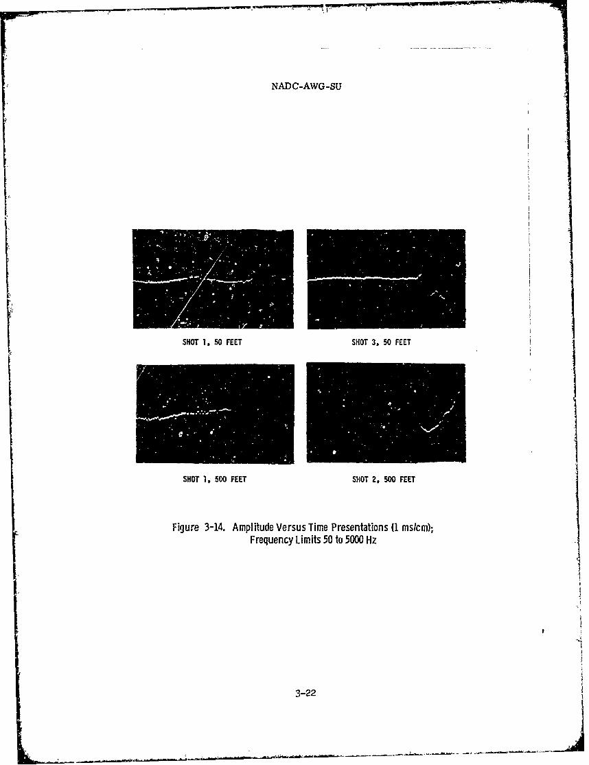
NADC-AWG-SU

SHOT 1. 50 FEET SHOT 3, 50 FEET 1! ' 1

SHOT 1, 500 FEET SHOT 2, 500 FEET

Figure 3-14. Amplitude Versus Time Presentations (1 mslcm); IFrequency Limits 50 to 5000 Hz

3-22

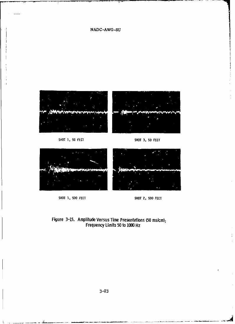
NADC-AWG-SU

SHOT 1, 50 FEET SHOT 3, 50 FEET

SHOT 1. 500 FEET SHOT 2, 500 FEET

Fiure 3-15. Amplitude Versus Time Presentations (50 mslcm);Frequency Limits 50 to 1000 Hz

3-23

NADC-AWG-SU I

rFl

SHOT 1, 50 FEET SHOT 2, 50 FEET

SHOT 1, SCO FEET SHOT 2, 500 FEET

Figure 3-16. Amplitude Versus Time Presentations (1 mslcm);Frequency Limits 50 to 5000 Hz

3---

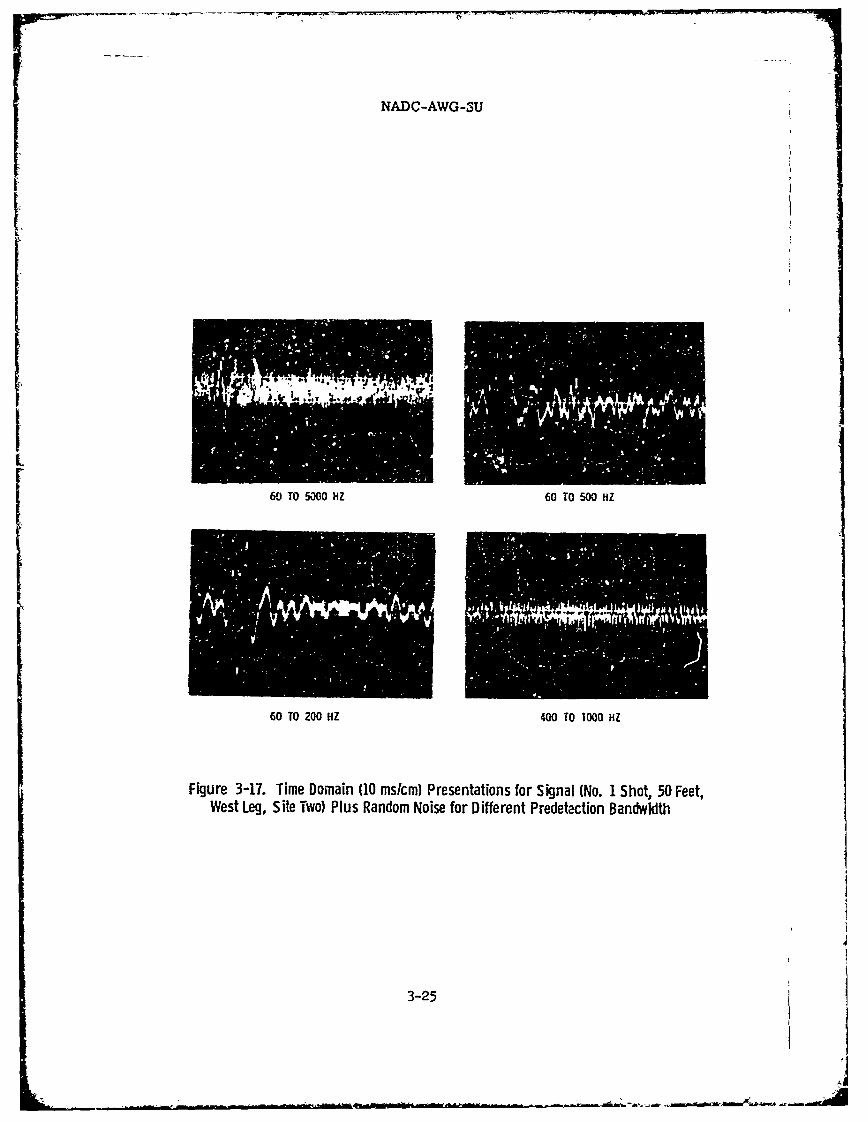
NADC-AWG-SU

60 TO 5000 HZ 60 TO 500 HZ

60 TO 200 HZ 400 TO 1000 HZ

Figure 3-17. Time Domain (10 mslcm) Presentations for Signal (No. 1 Shot, 50 Feet,West Leg, Site Two) Plus Random Noise for Different Predetection Bandwidth

3-25

NADC-AWG-SUJ

NO FILTERING LOW PASS FILTERING OF TIMECONSTANT (RC) 2 x 10-3 SEC

LOW PASS FILTERING OF TIMECONSTANT (RC) 1 xc 101 SEC

Figure 3-13. Post Detection Outputs for Various RC Low Pass Filters,Predetection Bandwidth 60 to 200 Hz

3-26

NADC-AWG-SU

BACKGPOUND NOISE -10 .4S/Cv' RAIN NOISE WITH WATER CIROPLET O.s0 MS/C4

BACKGROUND N.OISE - I FSIC4 RAIN NOISE VITHC.T i~ATEr Z-CPLEUNOISE - I MSIC4

Figure 3-19. Typical Background Noise Time Domain Presentations

3-2T

NADC-AWG-SU

+9.

0

6

+6.00

0+3+

cij

.1 0 . +

rza

-3

E-40

1

raCl) -6.

-10p0 500 100 1500 2000 2500

FREQUENCY IN HERTZ jFigure 3-20. Pressure Spectrum Level Versus Frequency for Background Noise,Site 2, 100 Hz Analysis Banwith for, Three Diffferent Samples Within One Minute

3-28

NADC-AWG-SU

+16"

LEVEL 'I

0 ~+13- 2'-6

CM'

a

?j +7-

1

S-

W

0 500 1000 1500 2000 250 3000

FREQUENCY IN HERTZ

Figure 3-21. Pressure Spectrum Level Versus Frequency for Light Rain. Runs 2and 3 Have Raindrop Noise; 100 Hz Analysis Bandwidth, Site 3

3-29

L- j

NADC-AWG-SU

3.7.A-3.7.C

evident from the three curves that the bandpass which shouldbe used for a near optimum S/N ratio varies considerably withthe type of background noise and also probably with differentmedia. The tests performed at various sites at differenttimes seem to be consistent. The S/N ratio at the lower endof the frequency spectrum, say, from 50 t3 1000 Hz, showsthat the choice of bandwidth is not too critical.

The time domain study typified by Figures 3-14 to 3-16reveals that the rise time of initial pulse changes apprecia-

bly with distance from the charge. From the approximate re-lationship that rise time is equal to the inverse of threetimes the upper half-power frequency, the total analysis sys-tem has about a 70 Usec capability, with the 5000 Hz bandwidthof the analyzer being the major restricting unit. The 50-footshot oscillograms show approximately this rise time, whereasthe 500-foot oscillograms have a rise time twice as large.

A further investigation of the time domain picturesshows that shot-to-shot correlation is not so predictableand greatly- dependent upon range. In general, one my skythat at greater ranges the envelopes have an alnost expo-nential decay characteristic, while time constant increasesconsiderably with range--tens of milliseconds at closerange to hundreds of milliseconds at greater ranges.

B. Predetection and Postdetectic'n Filtering

The advantage of predetection filtering was made evi-dent by Figure 3-15 wherein the output fro= a rdo= nisegenerator was -ixed with the signal for different ban .-widths 60-5000 Hz, 60-500 Hz, 60-2oo Hz, and 4CO--73 Hz.The opti-ni bandwidth reflects the point where the axienergy of the shot occurred. The effect of post-detectknfiltering rhtwn in Figure 3-18 is to Iprove both , the thresh-old and signal duration characteristics as discussed in M2a-ter 2, subsection 2.2.H.

C. TPrc.-agation of Explosive Sounds

Clarsically, ar, explosicn in free space in the time d-=ain has a very short rise time with pressures in the nrnlr_-ear regicn, followed by an approximately exponential decaybelow the a=biect prezsure and a final return to a=bient tres-sare. The frequency spectr= of this signal is continuszwith increasing intensity as it approaches the lower freuen-

3-30

NADC..AWG-SU

J. 7. C

cies, where a broad peak is reached. As the shock wave prop-agates, it decreases in intensity because of spreading lossand other excess attenuation that occurs in air for finite so-plitude waves. From the many tests performed on the small ex-plosive shots of 1.5 gram of TNT in covered environment, someof the pertinent conclusions are:

1. In thick foliage, a broad energy peak be-tween 600 and 1000 Hz at 50 feet would shift to 200 and 350 Hzat 150 feet, and to 60 and 100 z at 500 feet.

2. If a microphone is within 8 to 10 diametersbehind or alongside an object relative to the source, the measur-ed pressure-time characteristic exhibits a slow and irregularrise time.

3. Terrain absorption losses appear to af-fect the shock vave as they do the steady-state sounds.

4. Great variability has been observed inthe output levels and spectra as a function of the nature ofthe terrain upon'vhichbthe explosive charge is resting.

5. For the small explosive shot of 1.5 grinof 7T fired in the open, the speetrm decoys at about 7 dBper octave 4bove 2 kiz. For the charge fired in the voodsthe decay above 2 kHz is about. trice that in the open, .. e.,approxi mtely 1? dS per octave.

6. The results obtalned for propagatioc ofsourd over open level terrain viii not in general apply wherethe transmission path is predcuinently in woods. This is trubecause in dense woods, the vind velocity and vertical windgradients are very mch sUaller for a given wind velocity abovethe treetops than the v!nd velocity and vertical rind pra&dentsover oe-n level ground.

7. "three i crtt parameter. af ectiW thetransmission of sound energy in wooed %reas are the f lagearea,. trunk and I&b density. and ground inedanc*. Accordlnto a recent paper .the canof can efectively be rvresente

"j. Aylor. "3oise heducticn by Yegetation and Ground,"J. Acoust. Soc. A ., Vol. 51, 1972, p. 19T

3-31

BEST AVAILABLE COPY

NADC-AWG -SU

3. 7. C

by a single thin vail of umknovn surface area densities tosound transmission, because of mltiple scattering betveen leayes.The formula for the loss through a thin solid vall is given byb5

A l23 log3 o(wsf/al.5) (3-9)

for air at 200 C, vhere s is the area density or the density timesthe thickness of the val, and f is the frequency of the soundsource. Qualitatively, this means that reducing leaf area decreasesthe eiffective vall thickness and increasing frequency increases theeffective vail thickness.

As far as tht size of the trees is concerned, littleenergy is scattered by a rigid cylinder when the sound vave-length is large compared te the cylinder radius. 7hus , atten-uation through forests by scattering of lov-freqecy soundis negligible. On the other hnd. when the sod varelengthis £28.1 cmpared to the cylinder radius, scattering of higb-frequency sound is significant.

Fo- the effect of soil on sod propagation, softer, =eporous surfaces atteate nre at lcex froque=7 for strgrazing i=idence and have mre specific freqcy selectithan b&rder, less porva surfaces.

5- S -. 139in foo,-,te 33. p. 3-E.

RE._T AVAILABLE COPY 3-32

NADC-AWG -SU

4. l.A

CHAM POWD: CRARACTRIMCS OF S~XJZD SOL1PCW

A. Cemeral1 Remarks

"be preeeding tta-e rba*trs bave dealt with te %et--ocfDaa Acq--isition, Dal-a Analysis amd Retwo1cc, and vtb the

th~e-*-&-t and emirial expects of Sc~zd Po.P~gzIcc. 41 tlw e z~~ma.- an d tx,.rae-. e~=,e zfteAt

aat±.a=&Zyzeq1. 4.L- r-edact-1 dar1m the tim~e .- *= of' thr Ak

7h nt--t of tb AM1 &Ia-vetJ hauT bet

"be v-rw-!tt--ft.-a =xmber. of Fvnltjets. Zand t-be. cb-

ec-iei*- :ea --- &like Se* th erclaa ~I? ~~v-a1~

is ~ valuble &2e- %&let.t bus tral

t* vtc afl :

a*! 1. cclwr~w a wll as sic-c~Z

A:* t be awailable, AVG repoe x w. reviewq Vitt tbw tIzspecie 1 cms.Ical d6ac b--*?h zao.=rwv Wbd umes

scq=s. Ube fouas differ, am aalzvqr ha& bet =&Se u-c 9s1ffr~ee~s

4-1

P- ST AVAILABLE COPY

NADC-AWG -mi

4. 1. A

Xany of the described sounds come fra di fferent- decices buhave the sam fuamental origin, for exam~ple, vibrati~n~g surfaces.gears, bearings motors, fas, Impeet. detonations or ae.-od7y-=cand hydrodynamic effects. A brief list coged to illustratethis point is given in 1lftle 4-1 vhich enmrates a few familiarcategories of noisy prodwtcs * and vith each the eo-rrespodine baicsotnd-prodbzci g sedhnilsn.

18k 4-L Pt bmy Sources d O~ i WO-Knon Pn~cb

IM IP aIseq: Pam_ Coeasl

!,e- 0 no vI tw sw~' bowevi vow-* J

IftO"I -f

B EST AVAI jLAPLE CO PY

NADC-AWG -NJ

As already mentioned. there are differences In the fomrts oftbe data, and the problem of InterpretatIon Is lessened by tktngsdvantag of the explamtions and definitions vhIch Chapter 2 pro-Vides. ?be data eataloget berwin Is In various states of ref~re-nent or provessing. ?bese va:y from caq1ettly rav to those aecially treated In accordance vit4 their mission objectives.

A con~1ler of amotic data mt decide vbether the mater.alIs for a gen~eral reedership or for progrmsn-orien'.ed specialists.Demmzae of this mcertalmty. a gvveral selection of data. rtp1liea--"It to the tbw oL* "Tcnlg Utilization" In c~rillan areas. hasbeen attemted.

B. Pre-.w*aoa ef Data

mot rwcported data, h avine been reduced &~ A analyzed at lif-felreet ;poims in time In a wariety of ways, d-'es not fit neatly

1~the a~opter 2 deffinitions. It bemme aecessa~ry. therefore.c. interpret the data contained In thbe reports to relate the in-

fc~st t : ccorable form In oa r st~xves. The Improvementof vtls Ws-aton Is cwof the uni objec-tives of tthe pret.ecteftcier. 1. e. . Inumther mrwee-oc .3f data to com 'o0~2.

Frtte pwo. of .dent 1.1icatiorm &tiad categorization by attri-tw-e aata ma e clasw1ied '.= a mm'tr of vvqs wz 4ext2:A!fiec by

:1 of Pece I.., Siwr-A Caracteristics in?w.vqsmcyu

'&rft S14MLIS (See pp. Z-lh to -le)3--w-atemryz periodic

~mieid.I ~e-ve.rent 1.1metioe'

P-3cT'T A\NL-ArPLE COPY

NADC-AWG-SU

4.1.8

Real signalsTransientNon-stationary random

Time Domain Characteristics (See p. 2-32)EnvelopeRectified envelopeRiseFall timeSignal durationSignal gradientEffective bandwidth

3. Place

4. Program in which derived

5. Collecting Group

6. Format

The primary data developed by the many groups involved in theAWG programs have not been reduced and analyzed to yield all of theattributes mentioned in the above list. Many of the characteristicsreferred to in the list, however, are to be found in the AWG reports.The various analyses most commonly encountered are described in Chap-ter 2 which contains examples of various forms such as One-Third Oc-tave Analysis (p. 2-43), Spectrum Analysis (p.2-46), Af/f Analysis(p. 2-58), Sonograph With and Without Contouring (pp. 2-67, 2-93),

3-D Spectral Display (p. 2-69), Oscillograms (p. 2-73) and CorrelationPlots (p. 2-87).

Among the most important descriptions of sounds is the spectralcontent which may be given in several ways. In some cases it has theappearance of line spectra. This is shown very well by the Kay Anal-yzer which displays spectral lines horizontally (Figure h-1). Otherdisplays are in the form of a frequency plot derived from a period ofintegration.

4-4

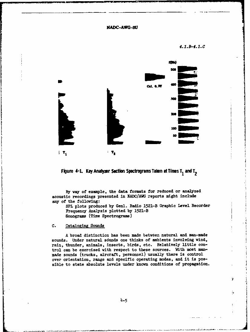
NADC-AWG-SU

4.1.B-4.1.C

CaL 0.2W *

m g ipopo

5

T1 T2

Figure 4-L Kay Analyar Section Spectrograms Taken at Times T1 and T2

By way of example, the data formats for reduced or analyzedacoustic recordings presented in NADC/AWG -eports might includeany of the following:

SPL plots produced by Genl. Radio 1521-B Graphic Level RecorderFrequency Analysis plotted by 1521-BSonograms (Time Spectrograms)

C. Cataloging Sounds

A broad distinction has been made between natural and man-made

sounds. Under natural sounds one thinks of ambients involving wind,rain, thunder, animals, insects, birds, etc. Relatively little con-trol can be exercised with respect to these sources. With most man-

made sounds (trucks, aircraft, personnel) usually there is controlover orientation, range and specific operating modes, and it is pos-sible to state absolute levels under known conditions of propagation.

IA4-

"-5

.... ... . . .. . .. J

NADC-AWG-SIU

4.1.C

Keeping in mind the above broad classification, the follovingcharacteristics of various so'mds may be cataloged in terms of Attrib-utes, Applications, and Instrumentation characteristics.

Natral Atmospheric< RinNatra Q in -

Zoologicalcatao of Acoustic AirAcousticWater

I LandMan-made L

SEE LATER TABLES & LISTS

AttributesSpectral Data (frequency content), Line Spectra

"Characteristics"(Frequency dither modulation)(Including explanation of background contributions)

Time HistoryShort (Envelope, amplitude modulation)

(Frequency modulation)Long (Occurrence)Continuous vs. fluctuating sounds

Statistical analysis for fluctuatingsound

IntensitySourcePerceived (propagation as influenced by

normal environment including maskingfactors)

Sound-level gradient46 (time or distance)Observation distancePeak SPL

dB excursionInitial peak SPL at 1 ft

University of Michigan, Willow Run Laboratory, "Analysis ofAcoustical Surveillance Parameters," by R. F. Hand, No. 1099-5-F,Final Report, March 1969.

4-6

NADC-AWG-SU

4.1.C-4.1.D

Forms (Signatures)Depends upon equipmentProcessing techniques

Properties of the sound to be catalogedSpectral DataTime history

Short (Envelope, modulation)Long (Occurrence)

ApplicationsInest

Detection, location and classificationTechniques of display

Techniques of triangulation (positioning)ComputationalAnalogCorrelation

Masking of sounds in surveillance systemsInstrumentation

Continuous and fluctuating sounds' intensityL tatistical level sorting

Rejection of sound from particular directions.

D. Source Characteristics

Ideally the full analysis plots of frequency content or of SPLvs time would be presented. However this constitutes more detailthan is desired in the type of documentation assembled here althoughit would provide the maximum information on the particular sound.

For the purposes of this report it has been decided that a fewcharacteristics such as those listed below would suffice. They per-mit numerical tabulation rather than a requirement for graphic plotsand spectrum analyzer signature formats which would constitute anIdentification Manual.

In all that is reported the investigator must decide how muchwill be said about the surrounding acoustical environment. Eitherhe or the reader must determine the importance of this factor andits probable influence on the data.

4-I

"-7

+ , + ,' .++ + d. + . .. . d + " + J "-+ +, .L . .... . . ..... . ... .. .. - J.

NADC-AWG-SU

4.1.D

Typici.1 Signature Charlcteristics

1. Mair energy locations in the acoustic spectrum (lines)(as defined in -pp. 2-30 to 2-33)

2. Rise and fal. times3. Signal duration (for transient types)4. Effective bandwidth5. Type of signal (as defined in pp. 2-i to 2-19)6. Frequency dmmin slope7. Test Notes: air path, microphone distance, data reference,

i.e., tape no., track no., location on tape8. frequency instability (short term) of lines

There is usually a discrepancy between the reported sound char-acteristic and those that would have been perceived under "ideal"measuring conditions. This difference can be charged to the influenceof surroundings. One learns early, in the practice of acoustics thatthe sound emitter, the surroundings and the listener must be consider-ed as a system.

Our presentation, unlike the NASA survey,4T does not attempt toexplain the mechanisms of sound generation or suppression: As far aspossible we merely represent the characteristics of the sound fieldas a source without environmental modification,

Normalization to a 1-Hertz bandwidth has been performed on some

of the data. An example of nomalization is given on page 2-43. Fig-

ure 2-10 is repeated here as Figure 4-2 shoving the detailed correc-

tions derived from -10 log Ff where F is the fraction of bandwidth

used.

Truck signatures-shoving predominant lines below 62 Hz were ob-tained upon subsequent analysis of the recorded data. The analysiswas performed with several types of sound spectrometers. Typical6 dB contoured spectrograms having approximately 50 dB dynamic rangeare available for many truck operating conditions and provide thebasis for the characteristic data tabulated in this report. Someanalyses were made oygr the spectrum from zero to 640 Hz with a 0.8Hz bandwidth filter.

4TAthey, S. W., "Acoustics Technology -- A Survey," NASA, SP-5093G.P.O. Washington, D. C., 1970.

14NADC-AWG-32, 23 May, 1969.

4-8

Ij:...........

NADC-AWG-SU

Z""-

4.2.

20 jMSoMAiu Fift. __ __ __ __ Ij: -31

__ _ __ _ __ _ ___ __ .4i *

0.0 OUSS 6.a 11.61 6.16 6.2 do .8.

wREQMicr W U11MM

Figure 4-2. One-Third Octave Analysis of a Continuous Noise SourceShowing the Effects of Bandwidth Normalization Modified by Addition of

Calculated Normalization Corrections

4.2 NAMrRAL SOUNIDS

A. General

Classification of natural sounds can be arranged according to

the source, the acoustical parameters, the geographical region inwhich the tests were conducted, test code names (mission designa-tion), date, etc. All of these have been used in the NADC tapelibrary listing and cross-reference system. However, the mostcommonly used data retrieval entry is the "name" of the soundsource. Occasionally, geographical area is of interest for stud-ies of combat surveillance, enemy detection, etc.

Most of the acoustic data obtained by AWG was analyzed for usein surveillance. The background sounds thought to pose an interfer-

ence threat to such systems were of primary interest. For example,rain has been studied because of the similarity of its spectralcharacteristics to pistol signatures .49 Special filter techniques

h9CBS Laboratories, "CBS Laboratories Dye Marker Acoustical

Assistance, Analysis of CBS Tape No. 00057," Report No. 5-25-DR-012,Stamford, Conn., 14 July 1967, p. 51

4-9

NADC-AWG-SU

4.2.A-4.2. C

have also been devised, as a result of ths work, to discriminatebetween truck sounds and rain background.

1lthough the specific purposes mentioned above justified thegathering of these data, the potential use of the information ismuch broader, extending now into civilian environmental areas.

B. Characteristics of Natural Sounds

Particular observations on certain source characteristicsare given in Table h -2 under appropriate headings.

More specific data on sounds produced by a variety of

interesting animals are listed in Table 4-3.

C. Jungle Sounds5 5

Under apparently quiet conditions ambient sound pressure levelsbetween 30 dB and 50 dB exist in the Jungle, with between 2 and 5dBper octave decrease with increasing frequency over the major part ofthe spectrum.

50 Laboratories, "CBS Laboratories' Dye Marker, Acoustical

Assistance Analysis of CBS Tape No. 00055," Report No. 5025-DR-013,Stamford, Conn. July 1967.

51Howard, J. R. and S. Krieg, "Summary Relrt of Acoustic Datafor Phase II System," Naval Air Development Center, Jobnsville, Pa.,1 October 1967, p. 2. Note: This reference contains data on filterbandwidths and AGC response time for optimum detection of the listedsounds in various ambients.

52NADC-AWG Letter Report No. 22, 12 June, 1967NADC-AWG, Letter Report No. 22, 13 July, 196T

53NADC-AWG, Letter Report No. 24, 13 July, 1961

SNADC-AWG, Letter Report No. 28, 31 October, 1967.

5 5 See pp. 1, 2, and 3 in footnote 52.

4-1o

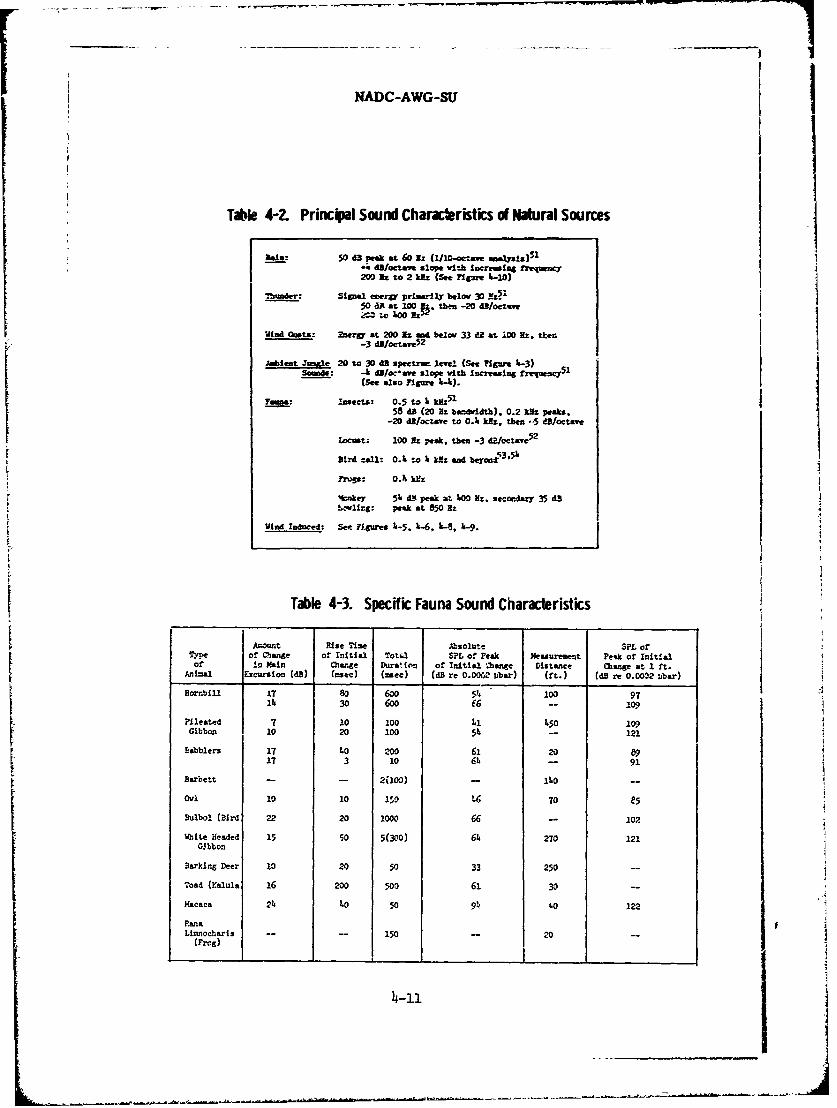
NADC-AWG-SU

Tle 4-2. Principal Sound Characristcs of Natural Sources

AlSLas 50 d3 Peak at 60 Nt (X/10-oW-m mialsis) 5 1

*4 dflomae slope '" I Inc eaing fequency200 It to 2 kiz (See Y1Mre 4.10)

Thnder. : Signal emerr priil..ly below 30 Nz5 1

0 0 at 00 0.l rten -20 dDl/oczav

Wind usts: nergy at 200 Zz and below 33 d3 at iO0 Rz. t.en-3 Ml/oct8,',e2

Ambient Jamie 20 to 30 43 spectr level (See Tigure 4-3)SCUm.d: -4 di/oc-ave slope with Increasing f;quenc y'1

(See also FIgure " ).

.. uma: jects: 0.5 to % kftzl.58 d3 (20 Rz bandwidth), 0.2 kHz peaks.

-20 d~foctve to o-4 kjlz, the 5 e.alotave

z ¢ust ., 00 Ift peak .then -3 d /oc ave 52

Bir"d =al: .4 t~o h klz and beon T'3 5 4

Frip: O.h ,~

4 - kl e y 5 4l 4 p e k a t & M, O z , s e o e d r y 3 5 d 3

Llirg: peak at 850 Hz

Wind Induced; See Figures s-5. X4, 4h-a. 1-9.

Table 4-3. Specific Fauna Sound Characteristics

Amount Pise Time Absolute SPL ofType of Change or Initial Tota SP of Peak Meaurement Pesk of Initialof Ein Main .Change Dural [o. '.,lange Distance Mange at I ft.Anizal xcrsio ( ) sec) ( see) ( B re 0.00 62 U~bar) (ft.) (dB re 0.0032 Ubar)

flor'.bill IT 80 600 51, 100 9711 30 6o (6 - 209

Pileated 7 10 100 &j L50 109Gibbon 10 20 100 54 -- 121

Eabblers 17 tO 200 61 20 8917 3 10 64 -- 91

Barbett -- -- 2(100) - IlO --

Ov 10 10 150 L6 70 85

Bulbol (Bird 22 20 1000 66 -- 102

White Headed 15 50 5(300) 64s 270 121Gibbon

Barking Deer 10 20 50 33 250 --

Toad (alula 16 200 501 61 30 --

macaca 24 to 50 94 40 122

RanaLimnocharis -- 150 -- 20 --

(Frog)

4-11_____

NADC-AWG-U

4.2.C-4.2.D

Figure I-3 shows a quiet jungle spe ct and insect noiselevel (normaJ1ized to a 1-cycle bandwidth). WEFurther info iationon this subject is to be found in C. yri ng's publication. I

Figure 4-4 in contoured sonogran format, displays with even

greater detail the transient spectral phenomena of a chirping junglebird against the ambient sounds.

D. Wind

In our tabulation of Characteristics of Natural Sound Sources(Table 4-2), we merely list data on spectral characteristics. Windis such an important factor in outdoor low-level measurements or inwindy locations that it deserves further coment.

Chapter 1, Data Acquisition. discusses the wind effects andthe use of windscreens. In addition it is noted that wind noise isa frustrating factor in critical low-frequency regions of the spectrum.Noise levels and spectral properties of wind interacting with typicalcommercial microphones are given in Figures 1-8 and 4-5 for variousvelocities. These figures further indicate the increase in vind noisewith wind velocity from 10 mph to 25 mph. A difference of 15 dB isnoted in this example.

4Wind direction relative to the microphone has a more proncunced

effect than other low-frequency sounds because of the mechanism bywhich the noise is generated, i.e., interaction of the air with thediaphragm enclosure and its shield which results in turbulence. Windnoises that arise from the rustling of .eaves etc. should be distin-guished from that above and are characteristic of the materials actedupon. A tabulation of all these would indeed be long. Usually the

56University of Michigan, Willow Run Laboratory, "Optimizationof Acoustic Surveillance Systems," by R. F. Hand, No. 850-4-F, FinalReport

57 See footnote 281, p. 3-4.

4-12

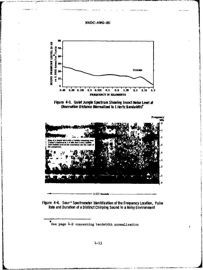
NADC-AWG-SU

soX 130-

0

0.05 0.06 0.125 0.2 0.315 0.5 0.8 1.Z 2.0 3.15 5.0lIDQUCY W MoULZa

Figure 4-3. Quiet Jungle Spectrum Showing Insct Noise Lvel atObservation Distance (Normalized to 1 Hertz BandNdthr

F Frequency

It of a jw* id tw h a rai ly r ap.Uhg o.

Rpten Duration of a Dsn C SI

ound n a Nois EI .d we) WU s- th o rninm a id ne r aitfio-009-q~u).

'- 1-2/3 Secoad

Figure 4-4. Sourp" Spectrometer Identification of the Frequency Location, PulseRate and Duration of a Distinct Chirping Sound in a Noisy Environment

See page 4-9 concerning bandwidth normalization

4-13

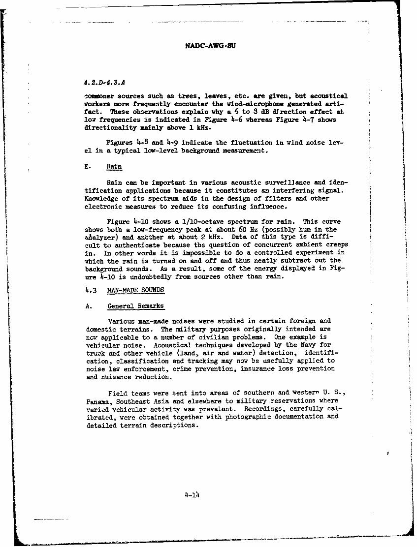
NADC-AWG-SU

4.2.--4.3.A

2omoner sources such as trees, leaves, etc. are given, but acousticalworkers more frequently encounter the vind-microphone generated arti-fact. These observations explain why a 6 to 8 dB direction effect atlow frequencies is indicated in Figure 4-6 whereas Figure 4-7 showsdirectionality mainly above 1 kHz.

Figures 1-8 and 4-9 indicate the fluctuation in wind noise lev-el in a typical low-level background measurement.

E. Rain

Rain can be important in various acoustic surveil]ance and iden-tification applications because it constitutes an interfering signal.Knowledge of its spectrum aids in the design of filters and otherelectronic measures to reduce its confusing influence.

Figure 4-10 shows a 1/10-octave spectrum for rain. This curveshows both a low-frequency peak at about 60 Hz (possibly hum in theaalyzer) and another at about 2 kHz. Data of this type is diffi-cult tu authenticate because the question of concurrent ambient creepsin. In other words it is impossible to do a controlled experiment inwhich the rain is turned on and off and thus neatly subtract out thebackground sounds. As a result, some of the energy displayed in Fig-ure 4-10 is undoubtedly from sources other than rain.

4.3 MAN-MADE SOUNDS

A. General Remarks

Various man-made noises were studied in certain foreign anddomestic terrains. The military purposes originally intended arenov applicable to a number of civilian problems. One example isvehicular noise. Acoustical techniques developed by the Navy for

truck and other vehicle (land, air and water) detection, identifi-cation, classification and tracking may now be usefully applied tonoise law enforcement, crime prevention, insurance loss preventionand nuisance reduction.

Field teams were sent into areas of southern and vestert U. S.,Panama, Southeast Asia and elsewhere to military reservations wherevaried vehicular activity was prevalent. Recordings, carefully cal-ibrated, were obtained together with photographic documentation anddetailed terrain descriptions.

4-14

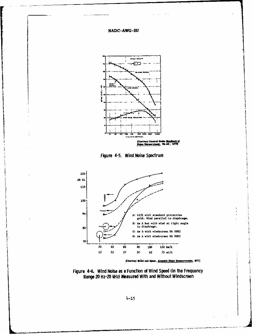
NADC-AWG-SU

- T

5.0 WIVE

So

so .0 nO oe "0 o t

(cm.siy Goveral Yto UIn mok oNoise Nemmm 7h aL

k Figure 4-5. Wind Noise Spectrum

120-

dB SL

110-

10042

F 4A: 4131 with standard protectiongrid. Wind parallel to diaphragm.

3: As A but with wind at right angle

R C : As B with windscreen dA 0052

747D: As A with vindcrn VA 0082

12 25 37 50 62 75 mi/h

(Cou'tsy ariia zi Kjamr, Aeomste Nose Iemureinia, 3671)

Figure 4-6. Wind Noise as a Function of Wind Speed (in the FrequencyRange 20 Hz-20 kdiz) Measured With and Without Windscreenj

4-15

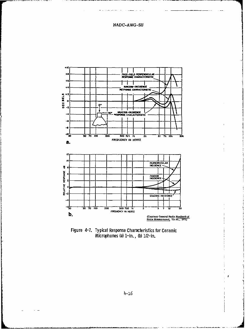
NADC-AWG-SUj

~1-f i~f WWUEO4CH~TCftS1IC5

46~

= IN -IN11111 - W-OI- CAZIfIjI 3 cC

50 70 to0 200 500 M0 its 21 5? 7 10k Wi0

* FREQENCY IN HRTZ

inffWEaULI

(Cuts GEnea ai doko

4oz esrmnt t 7~!

Figue 47. ypicl Rspose Caraterstic fo CeamiMicopone () 1in, () /2INIENE

2-IW-2 EE

GRZIG NCOj ~

NADC-AWG-SU

Bird Call

I ' | I I I I10-

b 0.05 '.08 0.125 0.2 0.315 0.5 0.8 1.25 2.0 3..5 5.0FREQUENCY INI ERTZ

Figure 4-& Wind Noise Fluctuations Relative to Bird Call BPL

5o.40 - Wind

8 30 -

S20 -

10

9 -10 -10.05 0.08 0.125 0.2 0.315 0.5 0.8 1.25 2.0 3.15 5.0

FREQUENCY IN KILOHERTZ

Figure 4-9. Wind Noise Fluctuations Against lackground Soundof Running Stream

4-17

NADC-AWG-.SU

4.3.4

ian Sound analysis programs were established in military and civil-ian laboratories in the U. S. They produced spectral and intensitydata together with special analyses involving electrically sophisti-I I cated instrumentation.

The question arises concerning the complexity of systems em-ploying computers and whether civilian uses could justify the cost.One example of complex analysis is considered below.

A signature may consist of a relatively uniform continuousdistribution of frequencies with spectral lines superimposed. Ex-perience in detecting and classifying sounds has shown that the dis-crete spectral line components are most important.

In presenting data on sounds in general, whether man-made ornatural, there is always the question of how detailed the descrip-tion shall be. The discrete spectral line is a case in point, forwe may simply note its presence or we can track it and describe its

dynamics. The latter can be done using a phase-lock tracking loop.This is one way a spectral line's individual behavior can be util-ized for characterization, i.e., a step beyond the mere recognitionof its presence. Often this characteristic of line stability canbe used to distinguish between man-made and natural sounds. Theability of the phase-locked system to track line frequency is dis-cussed more specifically in the following subsection on truck sig-natures.

It should be remembered that acoustic identification of soundsmay often be supplemented by seismic signals obtained at the sametime. Seismic information may thus present an additional and decid-ing variable for discrimination purposes.

Much of the sound data collected by NADC could be termed "fly-by". That is, the characteristics of sounds generated by a vehiclenearing and passing the closest point of approach, CPA, were record-ed. This information was important to the uses of the Navy's vehi-cle detection and identification program. Such recordings revealedthe essential dynamic effects such as Doppler, multipath propagationand aspect effects. These data were useful to the Navy's need atthe time but would also have to be taken into account in similar ci-vilian uses into which the technology might be transferred. Onethinks immediately of automatic or instrument-aided identificationof vehicles and aircraft in an environmental noise monitoring sys-tem.

J4-18

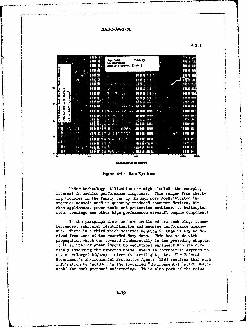
NADC-AWG-SU

4.3-.A

NU 0ftUAC. 50 NtL

r sosp in-

ndte technology uti lizati on one might include the emerging

spetio mehod usd i quntiy-poduedconsumer devices, kit-che apliaces poer ool an prducionmachinery to helicopter

rtrbearings and other high-performance aircraft engine components.

Inteparagraph above be have mentioned two technology trans-ferrences, vehicular identification and machine performance diagno-sis. There is a third which deser'es mention in that it waiy be de-rived from some of the recorded Navy data. This has to do withpropagation which was covered fundamentally in the preceding chapter.

It is an item of great import to acoustical engineers who are cur-rently assessing the expected noise levels in communities exposed to

new or enlarged highways, aircraft overflight, etc. The FederalGovernment's Environmental Protection Agency (EPA) requires that suchinformation be included in the so-called "Environmental Impact State-ment" for each proposed undertaking. It is also part of the noise

4-19

NADC-AWG-SU

4.3.A-4.3.B

assessment procedure rec nded by the Gffice of Housing and UrbanDevelopment (HUD). The Department of Transportation (DOT) is simi-larly involved. Not only is there to be a prediction of propagatednoise levels, but means of abatement and control through the selec-tion of terrain heights, landscaping and other features are to beproposed. The Navy data may be useful here, because the influenceof terrain can be derived in many cases. Some of the logs containsite descriptions which are quite accurate and hence can relate land-scape influences and sound propagation. This could form the basisfor a separate study using the considerable resources in the Navylibrary of sound recordings. In other words, it should be possibleto extract the terrain influences without redoing the field tests, agreat saving of effort.

B. Truck Signatures

Truck signatures are influenced by many factors including theenvironment, road conditions, the drLver's driving habits as wellas muffler design and the engine characteristics of a particular ve-hicle. To distinguish between different trucks by means of theiracoustic signatures, use may be made of both time _nd frequency do-main (spectral) data. However, it has been found5 that althoughdifferences in the behavior of short-term instabilities of the timedomain signature can be observed, the predominant spectral compo-nents are wore useful for classification of the vehicles.

The vehicle noise sources include the body, tires, transmis-sion, differential and engine as detailed below. These are seldompure tones, especially in power tr'ains which have rich harmonic con-terit.

1. Signature Analysis

Factors included in the identification process are:

Crankshaft Rate (CSR)Cylinder Firing Rate (CFR or CR)Engine Firing Rate (EFR)Predominant Harmonic PatternDrive Train Components (DT)Engine Idle Signature4th Gear Signature3rd Gear Signature2nd Gear SignatureHarmonic GroupingGear Mesh Line (M)

4-20

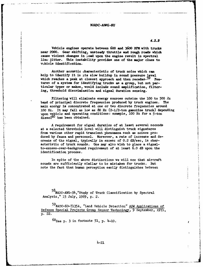
NADC-AWG-SU

4.3.B

Vehicle engines operate between 600 and 3600 RPM with trucksnear 2000. Gear shifting, unsteady throttle and rough roads whichcause violent changes in oad upon the engine result in spectralline Jitter. This instability provides one of the major clues tovehicle identificntion.

Another acoustic characteristic of truck noise which canhelp to identify it is its slow buildup in sound pressure levelwhich reaches a peak at closest approach and then recedes. 59 Fea-tures of a system for identifying trucks as a group, but not par-ticular types or makes, would include sound amplification, filter-ing, thzeshold discrimination and signal duration sensing.

Filtering will eliminate energy sources outside the 100 to 500 Azband of principal discrete frequencies produced by truck engines. Themain energy is concentrated at one or two discrete frequencies around100 Hz. It may fall as low as 80 Hz (2-1/2-ton gasoline truck) dependingupon vehicle and operating conditions: example, 100 Hz for a 5-tondiesel66 has been obtained.

A requirement for signal duration of at least several secondsat a selected threshold level will distinguish truck signaturesfrom various other rapid transient phenomena such as noises pro-duced by fauna and personnel. Moreover, a rate of increase and de-creaqe of the signal, typically in excess. of 0.2 dB/sec, is char-acteristic of truck sounds. One may also wish to place a signal-to-excess-over-background requirement of at least 6.0 dB upon theidentification process.

In spite of the above distinctions we will see that aircraft[ sounds are sufficiently similar to be mistaken for trucks. Butnote the fact that human perception easily distinguishes between

58NADC-AWG-34,"Study of Truck Classification by SpectralAnalysis," 15 July, 1969, p. 2.

59 NADC-SD-7135A, "Land Vehicle Detection" ASW Applications ofDefense Special Projects Group Sensor Technology, 9 September, 1971,Sp. 22.

60See p. 3 in footnote 51, p. 4-10.

4-21

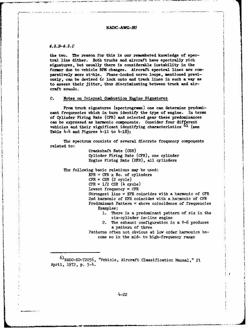
NADC-AWG-SU

4. 3.B-4.3.C

the two. The reason for this is our remembered knowledge of spec-tral line dither. Both trucks and aircraft have spectrally richsignatures, but usually there is considerable instability in theformer due to vehicle RPM changes. Aircraft spectral lines are com-paratively more st-ble. Phase-locked servo loops, mentioned previ-ously, can be devised tc lock onto and track lines in such a way asto assess their Jitter, thus discriminating between truck and air-craft soundz.

C. Notes on internal Combustion Engine Signatures

From truck signatures (spectrograms) one can determine predomi-nant frequencies which in turn identify the type of engine. In terms

of Cylinder Firing Rate (CFR) and selected gear these predominancescan be expressed as harmonic components. Consider four dif erentvehicles and their significant identifying characteristics l (seeTable 4-4 and Figures 4-n to 4-18):

7he spectrum consists of several discrete frequency componentsrelated to:

Crankshaft Rate (CSR)Cylinder Firing Rate (CFR), one cylinderEngine Firing Rate (EFR), all cylinders

The following basic relations may be used:EFR = CFR x No. of cylindersCFR = CSR (2 cycle)CFR = 12 CSR cycle)

Lowest frequency = CFRStrongest line = EFR coincides with a harmonic of CFR2nd harmonic of EFR coincides with a harmonic of CFRPreddminant Pattern = above coincidence of frequencies

Examples:1. There is a predominant pattern of six in the

six-cylinder in-line engine2. The exhaust configuration in a V-6 produces

a pattern of threePatterns often not obvious at low order harmonics be-

come so in the mid- to high-frequency range

6 1NADC-SD-72058, "Vehicle, Aircraft Classification Manual," 21

April, 1972, p. 5-4.

4-22

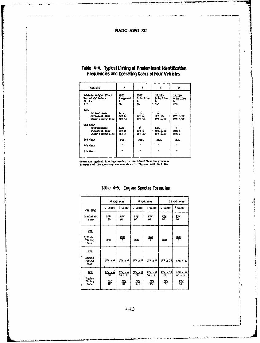
NADC-AWG-SU

Table 4-4. Typical Listing o Predowinant IdentificationFrequencies and Operating Gears of Four Vehicles

?v1C1z A 3C

Vre i c e e .' g htz ( 2 b ) 1 9 7 0 7 91' T 1 8 2 30 9.Z,3. 0Xa. of" Cy'lm. ers 2 opposed 6 i 1-do 6. in M-a7 e 6 I= line

N.P. 24 $ 2%0 20

Predoomiance xooe 6 6 6Stroget line as CYR 6 CF is ME 6112

Other strong line M 12 R 12 CYR 6112 CYR 6112 1 6112

2nd Gear"redwlnae Non 6 sc-_e 3 -Strozest 2-,e CY 2 Cr 6 M 6112 (F- 6

3rd Gear etc. etc. etc. etc.

%.th Gear

5th Gear

These are typical listings useful In the Ident'ficticat process.Exmples of the spectrogram ee shown in Figures 1-21 to 4-18.

Table 4-5. Engine Spectra Formulae

6 Cyli dor 8 Cylinder 12 Cylinder

2 Cycle & Cycle 2ycle i. Cycle 2 Cycle S Cycle

Crankshaft M M RW MP Mk RPM

Cylinder CS CSR CSRFiring CSR 2 CSR 2 CSR 2Rate

Ehgian;Firing CFR x 6 CFR x 6 CFI x 8 CFR x 8 CFR x 12 CFR x 12Rate

RP'ix6 iP'sx6 RPM x 8 RPm x 8 RPI x ]2 RPM x l2

-gine - - 2 60 x 2

Firing W P REM M M Me10 20 7.5 15 5 10

4-23

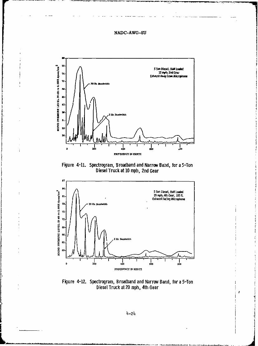
NADC-AWG--SU

S7. 5 Ton Diesel. Half Loalld

74- 10 orb 2nd GWiExhaust MaIrom hkr~on

o.

In

0 200 400 GOO W0

7REWEN0CY IN MERV.

Figure 4-11. Spectrogram, Broadband and Narrow Banid, for a 5-TonDiesel Truck at 10 mph, 2nd Gear

87

84.E~ 5Ton Diesel, Half Loaded

81. 20 mph; 4th Gear, 1001It.

F- Exhaust Facingj MicrophoneIs. 20 Hz Blandwidth

V721

9/

63- k 2 Hz Bandwidth

I 0 200 400 500 8oo

Figure 4-12. Spectrogram, Broadband and Narrow Band, for a 5-TonDiesel Truck at 20 mph, 4th Gear

4-24

NADC-AWG-SU

U t l vs U

« iN2 tj 'j

2" 3.8 (R)

2 N 4N SH 11 )

This signature is from a Dodge 3/4-ton Power Wagon with a weaponscarrier body and a 4-cycle,6-cylinder, gasoline engine operatingat 2280 rpm. Signature is not typical as vehicle is stationary.The CFR is 19.0, CSR is 38.0, and EFR is 114.0. The A-line isprobably from the water pump and the B-line is probably from thegenerator. A-SR is 46.3 aL 2780 rpm, thus A-SR/Eng-CSR is 1.22/1.B-SR is 103.0 at 6180 rpm, thus B-SR/Eng-CSR is 2.73/1. No bodyresonance reinforcement effect is seen, as the3 signature appearsexceptionally uniform across the spectrum.

Figure 4-13. Truck Classification by Spectral Analysis

4-25

NADC-AWG-WU

U-

- - ,

C -i

t

- EA

Figure 4-14. Engine Idle Spectrum, Large Reciprocating Engine

F4-26

i i.

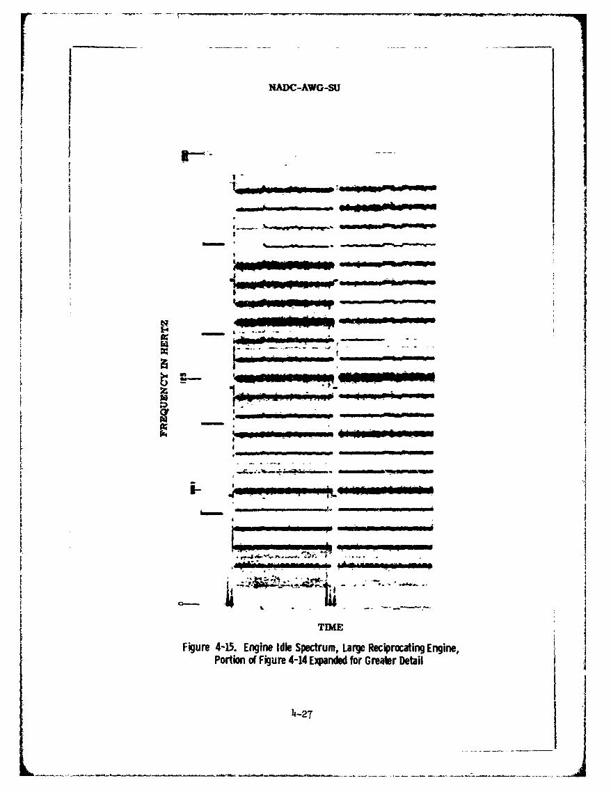
NADC-AWG-SU

I"W

4 .... . . .

Ir-* , I- - - Ip - i -- -

T-1

TIME

Figure 4-15. Engine Idle Spectrum, Large Reciprocating Engine,Portion of Figure 4-14 Expanded for Grear Detail

4-27

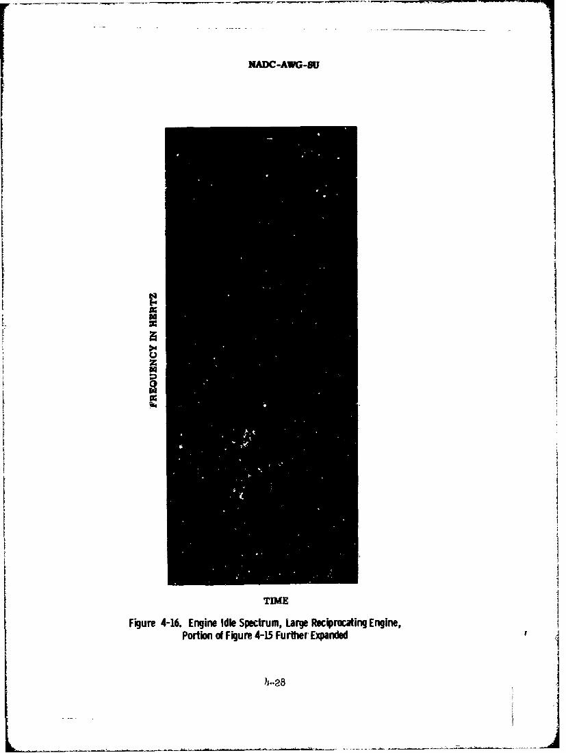
NADC-AWG-SU

M

z

TIME

Figure 4-16. Engine Idle Spectrum, Large Recirocating Engine,Portion of Figure 4-15 Further Expanded

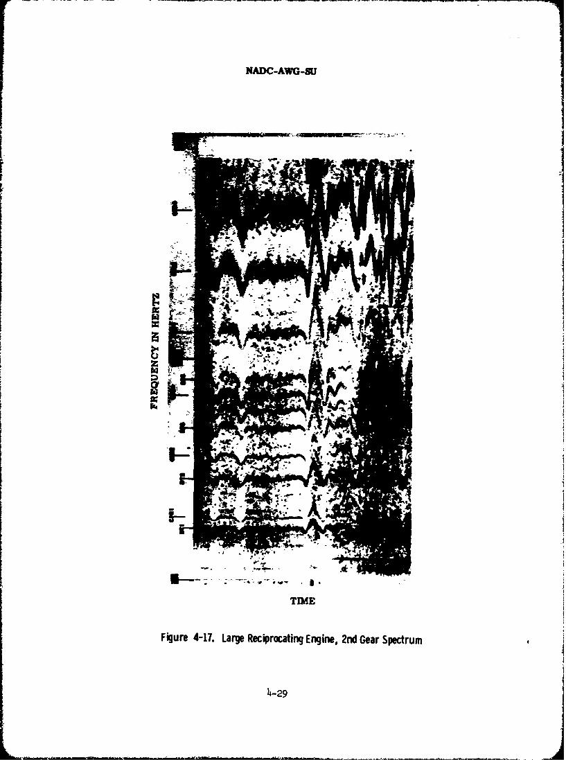
NADC-AWG-StJ

TIME

4-2

NADC-AWG-SU

4.3. C-4.3.D

Drive Train and Accessory Lines (DT) Components are useful forclassification purposes.

Accessory lines are not necescarily harmonically related toother engine lines.

CFR and DT lines can usually be placed in a harmonic set. (SeeEngine Idle Signatures, Figures 4-i4 to h-16.)

Table 4-5 (p. 4-23) gives conventional calculations for enginefrequencies. However, these cannot be relied upon to give the exhaustfrequenc:es in engines whose dimensions are such that the physical

spacing between successively firing cylinders approaches the distancetravelled by an exhaust pulse between firings.62 In these cases thereare several frequencies other than the conventionally calculated one,and the latter will be absent.

Spectrograms indicating EFR, CR, CSR harmonics for a Dodge3/4-ton Power Wagon (4-cycle, 6-cylinder gasoline engine opera-ting at 2280 rpm) are illustrated in Figure 4-13.

Engine Idle spectrograms for a large reciprocating engine(Figures 4-14, 15 and 16) illustrate the large number of linesthat may be observed. Figures 4-17 and 4-18 show the result oftransient effects when the engine is operated successively in 2ndand 4th gear and contrasts with the idle condition above. Thesharpness of lines in these spectrograms attests to the discrete-ness of engine freqaencies when observed with suitable equipment.

D. Aircraft

In considering-aircraft sounds one would like to have thefollowing field-collected data:

1. Spectral characteristics of aircraft as acoustic sources.2. Acoustic levels generated by aircraft as a functionl of

their distance from the sensor.3. Influence of altitude, terrain, aspect, clouds (atmos-

pherics in general) as well as aircraft type and mode of operation.4. Spectral characteristics of masking phenomena such as

vehicles, fauna and varicus other natural or man-made sounds.5. Time domain features of masking phenomena.

62W B. Diboll, "The Measurement and Prediction of Exhaust Fre-

quencies in Large Internal Combustion Engines," ASME 72-DGP-2, Ameri-can Society of Mechanical Engineers. I,

4-30

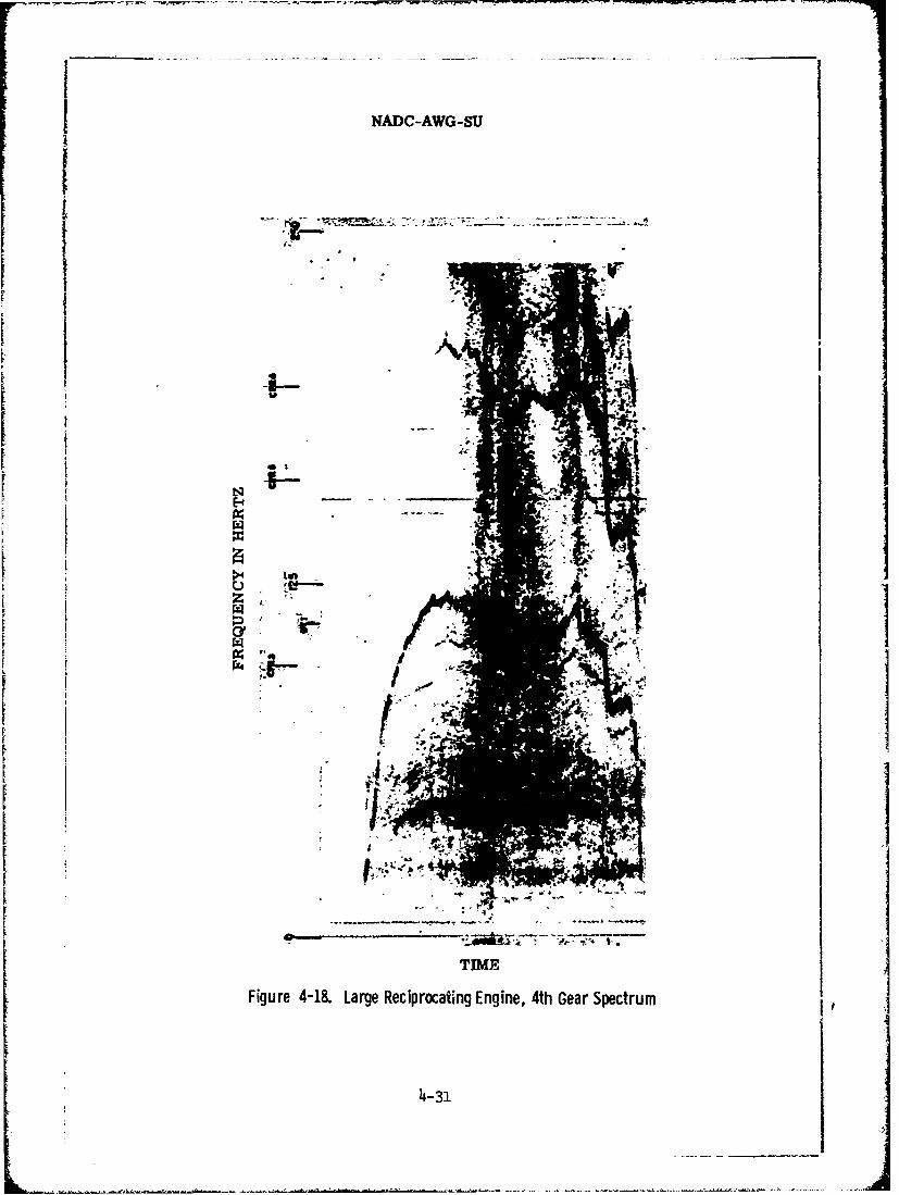
NADC-AWG-SU

-ILL-

TIMFiue41.LreRcpoainfnie t erSetu

4-3

NADC-AWG-SU

4.3.D

Since many of these factors are interrelated, i.e., influenceeacb other, and constitute a large number of variables, a rather ex-tensive measurement program would be required to present the totalpicture. Moreover, there are no completely adequate means of de-termining and describing such things as terrain characteristicsand atmospherics. Therefore a degree of generalization inevitablyenters.

In the data which follov some of the listed factor are ignor-ed. For example, aspect effects become merged with changes in dis-

tance during overflight experiments, An aircraft at 10,000 ft. al-titude is still 2 miles distant when it is directly overhead, butits aspect in this condition is quite different than when 2 landmiles away.

General evaluations or comparisons of the sound level gradi-ents (with time) for different types of aircraft must be made withcare. It is important to note in this regard that a particular jetaircraft may be especially fast and hence produce different gradi-ents for this reason. The large differences in speed during vari.-ous stages of flight will of course influence its characteristic asa sound soux. e. 6 3

The investigation of aircraft noise goes back to the NationalAdvisory Committee for Aeronautics (NACA), NASA's predecessor. NAC

9l.publications on aircraft engine mufflers appeared as early as 1916. 4

The problem of civil aircraft noise and its elimination was simi-larly reported in 1928. NASA, formed in 1958, has become a majorsource of information on the mechanisms gf noise generation injets. The fundamental work of Lighthill 5 in England in the 50'sprovided the basis for the analysis of these phenomena. Anotherarea of NASA investigations of interest to us concerns turbojetaircraft engine compressor noise. To gain entry into the exten-sive literature on the theory and characteristics of these noise

63See pp. 'e-4 in footnote 46, p. 4-6.

64Diederichs, H. amd G. B. Upton, "Mufflers for Aeronautic Engines,"

National Advisory Committee on Aeronautics, NACA Report No. 10, 1916.

65Lighthill, M. J. "On Sound Generated Aerodynamically," Proc.

Royal Soc. (London), 1952, 1959.

4-,32

NADC-AWG-SU

4.3.D

sources reference is made to a 1970 NASA technology utilizationpublication. 6

The aircraft acoustic data contained in the present Navy(NADC) publication are less concerned with the mechanisms of noiseproduction and ways of abatement. Rather the contribution of re-cent NADC work lies in reporting practical chara-teristics of themeasured sounds and ways in which they may be identified selectively.

It is to be expected that among all the many reports givingspectral data on aircraft sounds there must be some variation in thedata presented. One cannot say therefore that a definite spectralcharacteristic, such as -6 dB per octave, etc., exists. More real-istically one displays iypical data for a variety of craft in a num-ber of situations.

The -6 dB per octave slope is noted on the Jet characteristicin Figure 4-19. However, the data given in Table 4-6 can be shownto deviate from this form in various ways depending on conditions offlight. We see spectral characteristics in general that vary between-2.5 and -10 dB per octave. With all of these factors in mind ye pre-sent the following data:

Table 4-6. Summary of Aircraft Snatures

TYPE OF AIRCRAFT AIRCRAFT SIGNAITURES

Jet Impulsive in nature, most of energy below300 Hz. -6 dB/octave with increasingfrequency (Figure 4-19). Smooth analy-sis spectrum obtained with 20 Hz band-width.

Prop Line spectra apparent when analysis band-width is 2 Hz, smooth speczrum when analy-sis bandwidth is 20 Hz. Spectral peaksbelow 200 Hz.

aSignal energy primarily below 300 Hz

66See pp. 52-65 in footnote 4T, p. 4-8.

4-33

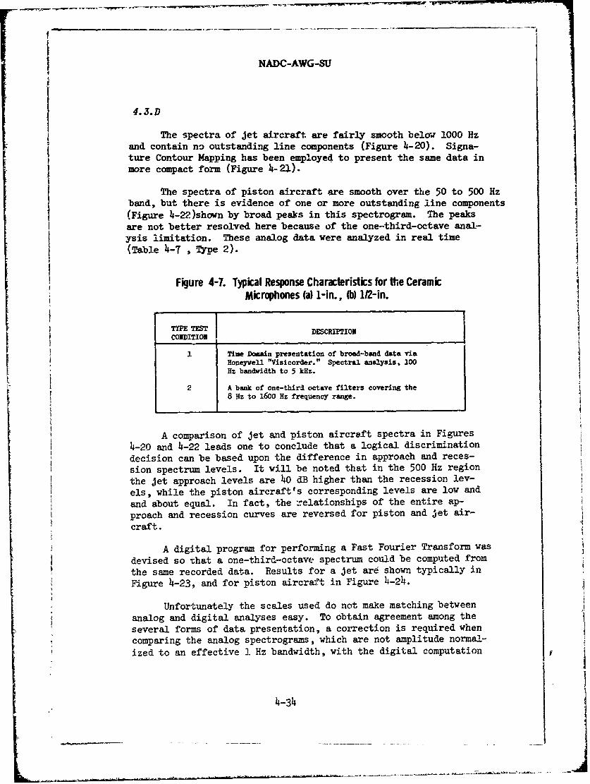
NADC-AWG-SU

I4.3.D

The spectra of jet aircraft are fairly smooth below 1000 Hzand contain no outstanding line components (Figure 4-20). Signa-ture Contour Mapping has been employed to present the same data in

more compact form (Figure 4-2-).

The spectra of piston aircraft are smooth over the 50 to 500 Hz

band, but there is evidence of one or more outstanding line components(Figure 4-22)shown by broad peaks in this spectrogram. The peaksare not better resolved here because of the one-third-octave anal-

ysis limitation. These analog data were analyzed in real time(Table 4-T , Type 2).

Figure 4-7. Typical Response Characteristics for the CeramicMicrophones (a) 1-in., (b) 1/2-in.

TM TEST DESCRIPTIONCONDITION

I Time Domain presentation of broad-band data viaHoneywell "Visicorder." Spectral analysis, 100Hz bandwidth to 5 kHz.

2 A bank of one-thir-1 octave filters covering the

8 Hz to 1600 Hz frequency range.

A comparison of jet and piston aircraft spectra in Figures4-20 and 4-22 leads one to conclude that a logical discrimination

decision can be based upon the difference in approach and reces-

sion spectrum levels. It will be noted that in the 500 Hz region

the jet approach levels are 40 dB higher than the recession lev-els, while the piston aircraft's corresponding levels are low and

and about equal. In fact, the rxelationships of the entire ap-

proach and recession curves are reversed for piston and 'et air-

craft.

A digital program for performing a Fast Fourier Transform was

devised so that a one-third-octave spectrum could be computed from

the same recorded data. Results for a jet are shown typically in

Figure 4-23, and for piston aircraft in Figure 4-24.

Unfortunately the scales used do not make matching betweenanalog and digital analyses easy. To obtain agreement among theseveral forms of data presentation, a correction is required whencomparing the analog spectrograms, which are not amplitude normal-

ized to an effective 1 Hz bandwidth, with the digital computation

4-34

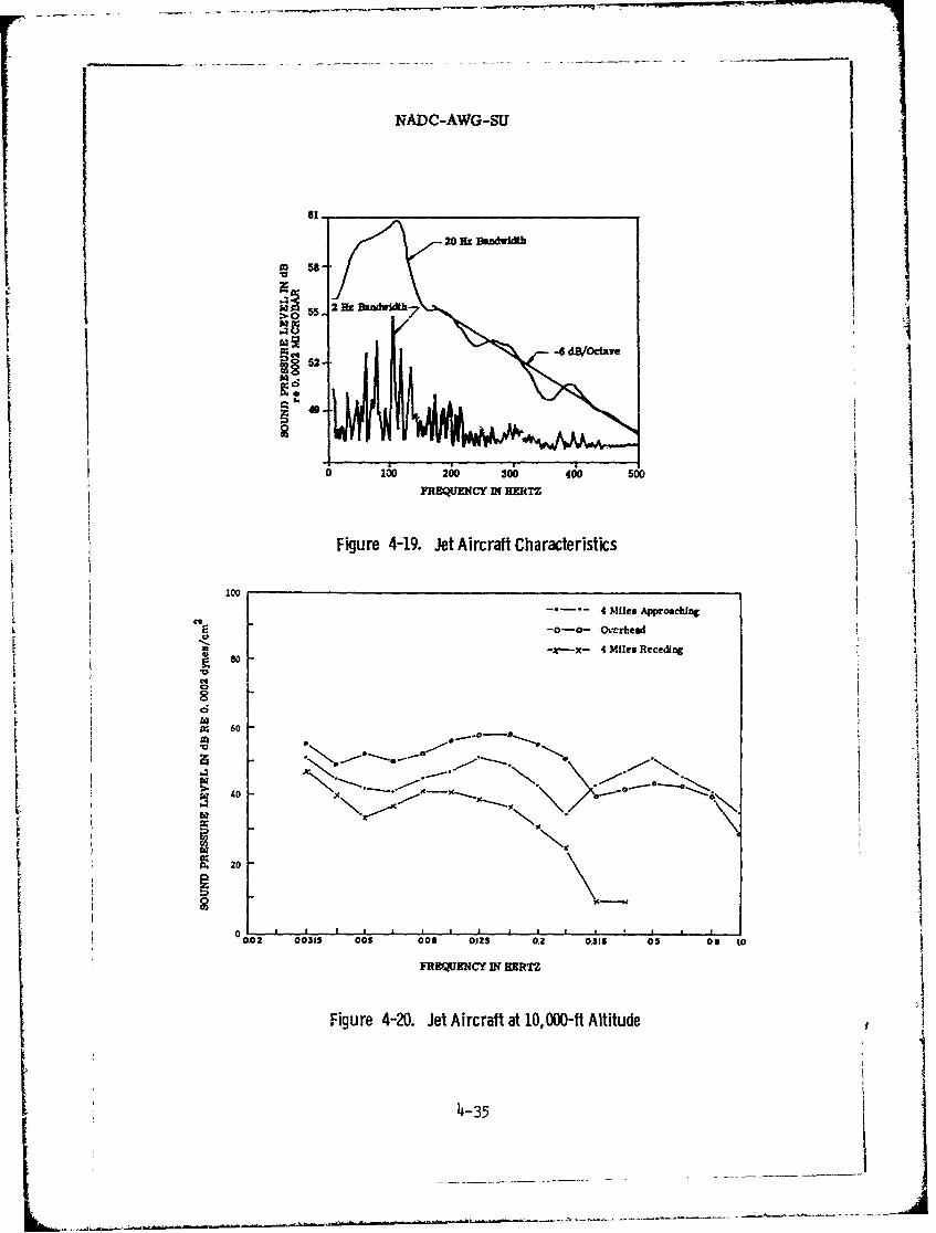
NADC-AWG-SU

20 BR Bandwidtfh

m58-

10 16 6 0 0 0

-~--4 Miles Arcing

-40

0G 2 00315 005 08 OS .2 0.316 5 st

Figure 4-20. Jet Aircraft at 10,000-ft Altitude

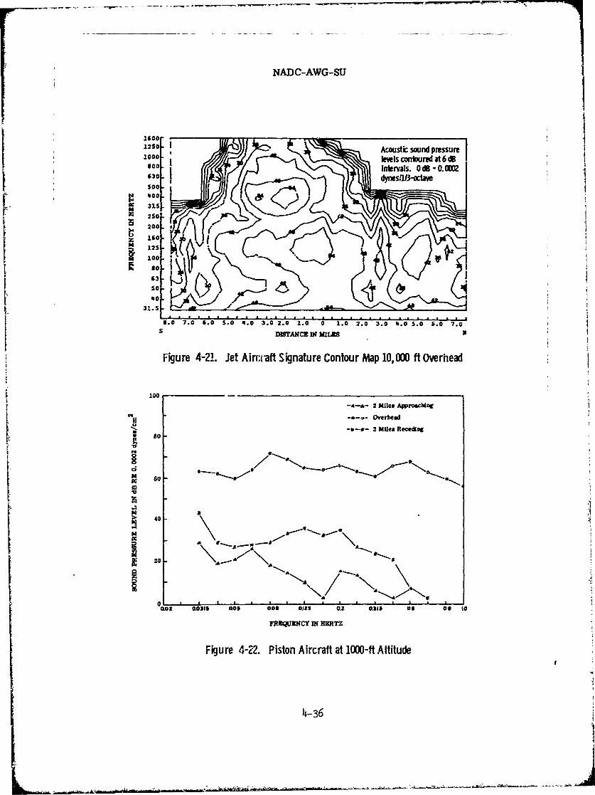
NADC-AWG-SU

1600

1250 I custic sound pressure10oo lees conlixuredit6 dB

3o dynes~q13-octaveinevl"OBOO0

315

500

V6 -• 20 ,.-

31.5

,.0 "7.0o .", o,o" 1.0 3.0 2.0o 1.0o o "1' 2"o' 3.o" .,0"s'o 'So "',5o'.S DI"ANC3€ gIN HC

Figure 4-2.1. Jet Ainrm-aff Signature Contour Map 10,0001 ft Overhead

200

100 g 4 . eA at nu Miles Approacheg

-o- ,-Overh ead

" -a-* - 2 Miles Recedlog

o

4 0

20

20

, zc ruse ooLIS as JOoo ils 02 0o315 as 00 to

F'BE! IWiCY IN MMTZI

Figure 4-22. Piston Aircraft at 1000-ft Altitude

4-36

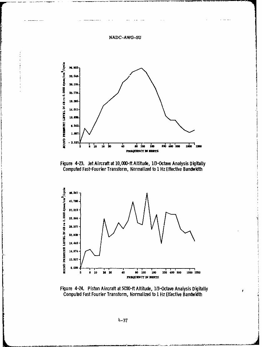
NADC-AWG-SU

3Lw28.164-

o

14.011-

10

1.07.

-2.5272 5 a310 16 20 40 801001ase 340056 'NO 00O 1250

7 UrCY i UULM

Figure 4-23. Jet Aircraft at 10,000-ft Altitude, 1/3-Octave Analysis DigitallyComputed Fast-Fourier Transform, Normalized to 1 Hz Effective Bandwidth

4247A

u 41.7SO

37.312-

32. 844 -

U. ll377 -tV,- 19.442 -

414.974 -

(€10.507-

5 a 10 is1 J 40 80 100 160 320 4W0 00 IWO 1I2W

lXQMWCY IN

Figure 4-24. Piston Aircraft at 5C0M-ft Altitude, 1/3-Octave Analysis DigitallyComputed Fast Fourier Transform, Normalized to 1 Hz Effective Bandwidth

4-37

NADC-AWG-SU

I4.3.D

(Fast Fourier Transform method) which is normalized (see p. 2-40).A correction must be added to the latter as follows:

The correction, c = 10 log (fa-%),6T where fa is the lovercutoff frequency and fb is the upper cutoff frequency, must beadded. For one-third-octave analysis, fa-fb equals 23% of thecenter frequency of the filter. (See Figure 4-2 for illustrationof this correction applied to one-third-octave data).

A typical time spectrogram for a small jet at 1000 ftshows the distribution of energy slopes at approximately2.5 dB per octave (Figure 4-25). The characteristic moirepattern is produced by a source whose energy is distrbu,ed con-tinuously over the frequency range and the multipath propagationgeometry between the source and the microphone. Certain bandsof frequencies experience degrees of reinforcement, and othersdestr-uctive interference. It must be observed that the patternis a product of the propagation geometry and not the source.

Zii

Figure 4-25. Jet Aircraft Signature Showing Effect of Multipath Propagation

The influence of altitude on the aeoustic levels generated byan aircraft as a function of distance frcm the sensor in surfacemiles is illustrated by the two plots in Figure 4-26. Here we seethat the peak level and specially the gradients are affected.

67SeeSePP. 563-564 in footnote 35.

4-38

NADC-AWG-SU

70-

g30-

20. _ _ ____

F-6 -4 -2 0 2 4 6

DISTANCE I MULE

0

*~70-

40 40-

0

'.

Figure 4-26. Piston Aircraft Overflight

4 ,39

-- - --3 O 2 4 6

-- -~~- ~- -

NADC-AWIG-MJ

4.3.H

X. Personnel

A nuber of cammon personnel sOUnds are considered. These in-clude walking (footsteps), talking, coughing, outdoor vood chopping.Footsteps out of doors, except on pavement or on snapping branches,etc., are generally faint and hard to distinguish at ranges of more

than a few yards. Speech, on the other hand, follows the same typeof characteristic as the ccmm aly used SIL (Speech IntelligibilityLevel) curves vhich depend upon abient noise level. Soe possiblelevels are given below.

Personnel Signatures6 8 , 69

Footsteps at 10 feet (detection range), cutdoor.Signal Peak: 36 dB rel. to 0.0002 jibar(outdoor ambient noise 21 dB)Fluctuations + 1 dB. Depending upon time

constants of recording system used.Mcst of energy in 1 to 3 kHz region

Terrain: muddy, rough and broken surface.Test conditions: Table 4-8, Type 1

Talking, outdoor. Southeast Asian voices 1 octavehigher than American. 100 ft. (detec-tion range). 42 dB peak, main energybelow 1 kHz.

Test conditions: Table 4-8, Type 260 dB (classical male voice) at 1 ft.Talking, Speech Intelligibility Level (SIL)

Chopping, outdoor at 100 ft (detection range)Using "Energy Detection Systems,"adaptive filter and correlationcould be bette',Cutting 6-in. diameter trees.41 dB peak to h kHz at 96 ft.

1 to 3 kHz (classical wood chop)39 dB P.S.L., 1 Hz bandwidth, at 1 ft.S/N 13 dB at 100 ftTest condition: Table 4-7, Type 2

6 1NADC, "Preliminary Report of POTLID Personnel Test," 22 August

1968, pp. 8, 9.

69See "Personnel Detection," p. 24 in footnote 59, p. 4-21.

4-40

NADC-AWG-SU

4.3.P

F. IILs

The ignition and firing of engines, detonations, ordnanceexplorions of all sizes and kinds constitute impulsive sound.Under Natural Sounds we have mentioned nearby thunder (TableJ.-2) and the phonations of certain fauna. 7 0 A 1.5-graa smalexplosive may be taker as a good impulse example. On rock itproduces a peak SPL of approximately 95 dB re 0.0002 11bar at100 ft, the spectral peak below 1 klz. The b-monic structurefalls from 90 dB at 1 kHz vith a declination of approximately2 dB per octave after the initial fall rate of 10 dB at 1 kHz.

Test conditions for the data given above were Type 4,Table 4-8.

Tabe 4-A Test Method Wnd Equpment

TM TM

1 GR 16 microphone (3 basndwidth 5 Nz to 8 klz -10 kft),system upper frequency 1niton. High, 20 ft, and1o, 2 ft, placemmt at three locstions, 10, 20 -- d 10ft from the trail. Microphones, 300 ft from recordingsite, utlized PhO preamp, set an XIO. Recorders,

lockbeed &17, used 1/2-in. tape at 3-3/1, ips, 1 V rminput for full record level, direct record mole (3 dBban idth 100 Nz to .2.5 kz), United system lower endfrequency response. SIX, GR 1551C, monitored with ear-phones and scopes as was recorder output. GR 15 2 cali-

brator used as well, a a square vave Input to 1551C eachreel.

2 Same as I but microphone placement at 16, 32, and 96 ft

3 Recorder, Lockheed lllC, 1/2-in. reel, 7-1/2 1pm, FM,Analyzed 2 Nz and 20 Hz bandidth.

4 2203 3 & K Sound Level Meter. B & K microphone. Record-er, Kudelski, 1/l-in. full track; 15 ip direct record.Analysis by GASL , analysis bmndidth 100 Nz, samplesize 0.1 sec.

5 Recorder, Lockheed 4llC, 7-1/2 ips, direct. Analysis

bandwidth 100 Is, input filter 5 klz bandwidth.

70See p. 5 in footnote 51, P. 41-O.

L-43

NADC-AWG-,U

At 500 ft a 1.5-gram explosive prxluced a spectral peak ofT5 dB below 1 kHz, the characteristic falling at 10 dB per octave(Figure 4-27). Test conditions here were Type 5, Table 4-8. Arumber of analyses shows a secondary spectral peak at 2 kHz, ap-proximately half the height of the main one. The recordings whichdisplay a double peak are usually taken at 100 ft range. Thecalculated impulse source level at 1 ft is approximately 140 dB(0.0002 dyne/c,2,200-500 Hz).

The spectral decay rate varies markedly when firings are shift-ed from open ground into a woods. 2or example, in the open the spec-trtm decays at 7 dB/octave above 2 kHz, while in the woods it is 14dB/octave. Ti A listener's subjective impression of the tone of suchsounds surely would be influenced by this effect, all of which re-emphasizes the fact that the surroundings at the time the sound char-acteristics were recorded m'ly have an important effect upon what wesay they are.

Impulse sounds generally are detected by equipment designedfor that purpose if they rise above the background by at least 12dB and the signal rate of increase is 16 dB/sec or more.72

G. Boats (Air Path Over Water)

Motorized Boats.-'

The boats used in these tsts were wooden, round-bottomed,approximately 16.5 ft in length.

The engine was a one-cylinder, one-cycle, Clinton ratedat 4-1/2 horsepower running at 1430 rpm under load with full throttle.Essentially inboard installation with long direct-coupled shaft char-acterized the mechanical arrangement.

Ranges studied varied from 15 ft (CPA) to 400 ft.

71NADC-SY-6703, "Analysis of Acoustical Data from Tests Performedon 27 November, 1966," 14 March, 1967, p. B-3.

72See p. 24 in footnote 59, p. 4-21.

73NADC-AWG-31, 0 Jan. 1969, pp. 24-29. (Spectrogras given in

Appendix consists of CBS Laboratories' Rpt. No. 5025-DR-027, pp. 34-61)

4-42

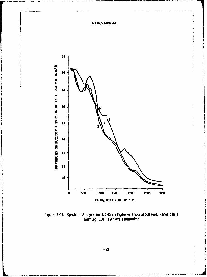
NADC-AWG-SU

59

556

0I

53

S9

4 2

II

3S3

35

0 SOO 1000 1500 2000 2500 3000

FREQUENCY IN HERTZ

Figure 4-27. Spectrum Analysis for 1.5-Gram Explosive Shots at .500 Feet, Range Sit 1,East Leg, lO0-Hz Analysis Bandwidth

4-43

NADC-AWG-SU

4.3.G-4.3.H

The spectrum (25 to 2500 Hz) was smooth at 45 dB from 40to 500 Hz, then -10 dB per octave to 1 kHz. Some data indicates a100 Hz peak, then 3 dB per octave to 1.5 kHz. This data applies toan air microphone at ranges 15 to 400 ft and 1/10 octave SPL anaysis.Under these conditions levels of 70 dB at the closest point of approach,CPA, (15 ft) are reached.

The microphone data shows strong line frequency structurebased upon the engine reciprocation rate of 12.2 Hz for 1430 rpm. Thisstructure is also somewhat apparent in the hydrophone data.

H. Boats (Underwater Sound)

Motorized Boats:

The boats used in these tests were similar to those describ-ed above.

Shallow hydrophone data analyzed on the basis of 1/10-octave shows peaks at 40 Hz which are -20 dB re 1 dyne/cm2 , then -10dB per octave from 40 Hz to 400 Hz. Hoiever, the hydrophone optimumenergy band for these boats is in the 2000 Hz to 9000 Hz region becauseof reduced background noise in this part of the spectrum. The soundappears to be caused by cavitation near the propeller.

The peak pressures reached at the CPA in the 2000 Hz to9000 Hz band are 110 and 140 dynes/sq cm for deep and shallow hydro-phones, respectively.

A secondary, low-frequency region, probably associatedwith the propeller rate, also appears.

Electric Discharge7 5

This method of generating strong acoustic pulses in

water has been studied and shown feasible although not efficientin seawater owing to the latter's high conductivity. Electriccapacitors of 15 IF and 20 kV rating have been used in a systemhaving a maximum energy capability of 9000 J. Acoustic pressurein fresh water was 156 PSI peak (140.6 dB re 1 degree/cm2) at oneyard for an initial energy of 1700 J. In salt water an initiallarge ourrent reduces the available capacitor voltage, hence peakdischarge current an: pressure.

741See pp. 42, 43, 76 in footnote 73, p. 4-42.

75Fairchild Hiller, "Studies on an Electric Discharge Underwater

Sound Source," Rpt. No. PCD-TR-68-16.

4

L-........

NADC-AWG-.SU

4.3.H-4.3.1

Large Ships

The periodic pulsation sounds of large ship propellersare caused by cavitation. Frequently the beat is pulsating in ac-

cordance with the number of blades, and occasionally one blade wibe noiser than the others, thus producing an accented signature.',iIn such cases the shaft rotation rate and number of blades can bedetermined.

I The spectra of ship sounds in general are continuous.

This broad distribution of energy decreases in sound level at 6 dBper octave with increasing frequency. Most of the audible outputis below 2000 Hz. There is some pure tone content, and a time pat-tern of intensity which may be subject to interpretation as to ori-gin or cause.

7 7

I. Aerodynamic Noise

Broadband noise generated by various forms of gas turbulenceresults from the operation of modern aircraft. Jet-generated tur-bulence is evident everywhere. Fundamental mechanisms7 -of soundgeneration by this type of source have been completely disclosedin the literature related to aeronautics and astronautics, industrialpneumatic systems, etc., and measured characteristics are given.

76See Vol. 7 in footnote 42, p. 3-16.

77L. W. Camp, "Underwater Acoustics," Interscience, John Wiley& Sons, N. Y., 1970.

See Vol. 211A, 1952 and Vol. 222A, 1959 in footnote 65, p. 4-32.

4-4

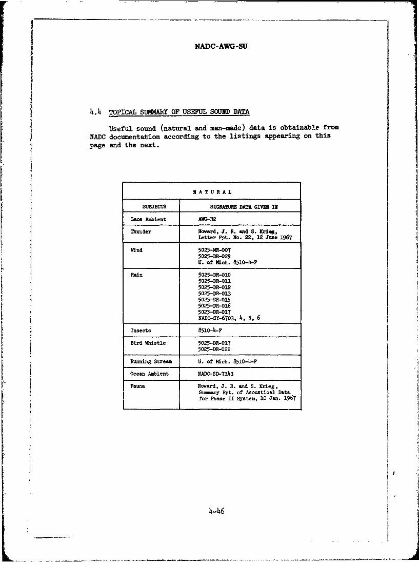
NADC-AWG-SU

I

4.4 TOPICAL SUMMARY OF USEFUL SOUND DATA

Useful sound (natural and man-made) data is obtainable fromNADC documentation according to the listings appearing on thispage and the next.

I

INATURALSUBJECTS SIGNATURE DATA GIVE IN

Laos Ambient AWG-32

Thinder Howard, J. R. and S. Kriq,Letter Ppt. No. 22, 12 June 1967

Wind 5025-MR-OOT5025-DR-029U. of Rich. 8510-4-F

Rain 5025-DR-010I5025-DR-Oll

5025-DR-0125025-DR-0135025-DR-0155025-DR-o165025-DR-01NADC-SY-6703, 4, 5, 6

Insects 8510-4-F

Bird Whistle 5025-DR-01{5025-DR-022Running Stream U. of Mich. 8510-4-F

Ocean Ambient NADC-SD-713

I Fauna Howard, J. R. and S. Krieg,Summary Rpt. of Acoustical Datafor Phase II System, 10 Jan. 1967

4

II

iI24-246

L -. -

NADC-AWG-SU

X A N-M ADE

SOJBECTS SrGIATU EI DATA GIVEN II

Vehicles AWG-315025-DR-027NADC-SD--T.'9NAC-SD-T791

Trucks AWG-32AWG-33AWG-34sAWG-3TNADC-SY-61'15NADC-SY-6803U. of Mich. 1099-5-F5025-DR-0085025-DR-0095025-DE-0105025-DR-0135025-DR-O165025-DR-026NADC-72058-SD

Explosicns AWG-35NADC-SY-6703NADC-SY-670NADc-SY-6705NADC-SY-6706U. of Mich. 8510-1-PU. of Mich. 85 10..4-rHoward, J. R., S. Krieg, Summary Rpt. of

Acoustic Data for Phase II System,NADC, i0 Jan. 1967

5025-DR-0125025-RT-0085025-RT-0095025-RT-010

Aircraft NADC-SY-6803NADC-SY-6715NADC-72058-SD5025-DR-026

Motorized Boats AG-31SSG-365025-DR-0275025-DR-028

Rocket Mortars AFCRL-68-0457

SSG-38

Pistol 5025-DR-012

Shots 5025-DR-017

4-47I

NADC-AWG-SU

Bibliogrephyj

BIBLIOGRAPHY

Albers, V. M., Handbook of Underwater Acoustics, State College,Pa., Pennsylvania State University Press, 1960

• Underwater Acoustics, New York City, Plenum Press,1965.

Aastin, M. E., "Time and Frequency Domain Analysis of RandomSignals," Sound and Vibration, October 1970, pp. 18-21

Aylor, D., "Noise Reduction by Vegetation and Ground," J.Acoust. Soc. Am., Vol. 51, 1972, p. 197

Athey, S. W., "Acoustics Technology--A Survey," NASA-SP-5093,G. P. 0. Washington, D. C., National Aeronautics and SpaceAdministration, 1970

Bauer, B. B., "Octave-Band Spectral Distribution of RecordedMusic," J. Audio Eng. Soc., April 1970

Bendat, J. S., "Modern Methods for Random Data Analysis," Soundand Vibration, July 1969, pp. 14-21

Bendat, J. S. and A. G. Piersol, Measurement and Analysis of

Random Data, New York, John Wiley & Sons, 1966'

Beranek, L. L., "Disturbance of Plane Sound Waves by Obstaclesand Finite Baffles," Acoustic Measurements, Ch. 3New York, John Wiley & Sons, 1949

, ed., Noise and Vibration Control, New York,

McGraw-Hill Book Co., Inc., 1971, .8,169, 185, 563-564

Biot, M. A. and I. Tolstoy, "Formulation of Wave Propagation in !Infinite Media by Normal Coordinates with an Application toDiffraction," J. Acoust. Soc. Am., Vol. 29, 1957, pp. 381- 2

391

Blackman, R. B. and J. W. Tukey, The Measurement of Power Spec-true, New York, Dover Publications, 1958

Brekhovskikh, L. M., Waves in Layered Media, New York, AcademicPress, 1960, pp. 366-385

5-1. !

NADC-AWG-SU

Broch, J. T., Acoustic Noise Measurements, 2nd ed., Naertm Denmark,

Briiel & Kjaer, 197I"

Camp, L. W., "Underwater Acoustics," Interscience, New York,John Wiley & Sons, 19T0

Cooley, J. W. and J. W. Tukey, "Algorithm of the Machine Calcula-tion of Complex Fourier Series," Mathematics of Computation,Vol. 19, No. 9o, April 1965, p. 29T-331

Cooley, J. W., "Applications of the Fast Fourier Transform Method,"Proc. of IB( Scientific Coputing Symposium, June 1966, pp.83-96

Crocker, M. J. and L. C. Southerland, "The Effects Upon ShockMeasurements of Limited Response Instrumentation," Wyle Labora-tories, Research Staff Report WR 65-1. January 1965

Davenport, W. B. Jr., and W. L. Root, Random Signals and Noise, NewYork, McGraw-Hill Book Co., Inc., 1958

Diboll, W. B., "The Measurement and Prediction of Exhaust Frequen-cies in Large Internal Combustion Engines," AS14E 72-DGP-2,American Society of Mechanical Enineers

Diederichs, H. and G. B. Upton, "Mufflers for Aeronautic Engines," Nation-al Advisory Committee on Aeronautics, NACA Report No. 10, 1916

Dolph, C. L., "A Current Distribution for Broadside Arrays WhichOptimizes the Relationship Between Beam Width and Side-LubeLe'el," Proc. IRE on Waves and Electronics, June 1946,pp. 335-378

Embleton, T. F. W., "Sound Propagation in Homogeneous Deciduousand Evergreen Woods," J. Acoust. Soc. Am., Vol. 35, 1963,p. 1119

Evans, E. J., and E. N. Bazley, "The Absorption of Sound in Air atAudio Frequencies," Acoustica, Vol. 6, 1956, p. 238

Erring, C. F., "Jungle Acoustics," J. Acoust. Soc. Am., Vol. 18,

1946, p. 257

Gersch, W. and J. M. Kennedy, "Spectral Measurements of SlidingTones," IRE Trans. CT-7, August 1960

5-2

NADC-AWG-Wu

Bibliography

Gersch, W., "The Effects -f Time weighting the Input to A SpeetrumAnalyzer," in T" s. on Circuit Theory, June 1961, pp.

"Choice of the Shape of the Input to a Spectrua Analyzerin Terms of its Effect on Transient Selectivity and SignalDetectability," I National Convention Record, Pt. 2, 1959, pp.T9-88

Given4, M. P., W. . Ny.borg, 6nd H. K. Schilling, "Theory of tbh

Propagation of Sound in-Scattering and Absorbing Media," J.

Acoust. Soc. Am., Vol. 18, 19h6, p. 284

Goldman, S., Frequency Analyris-, Modulation and Noise, New York,' I~Dver Publi cations, 1948 '

information Theory, New York, Dover Publications, 1953

Hand, R. F., "Analysis of Acoustical Surveillance Parameters,"Uniersity of Michigan, Willow Run Laboratory, No. 1099-5-F,Ann Arbor, Vdch., March 1969

- "Gr4timization of Acoustic Surveillance Systems,"University of Michigan, Wllow Run Laboratory, No. 8510-4-F,Final Report

Harris, J. R.7. "A Study of Using- Multiple Nonlinear RegressionAnalysis for Acoustical Modeing," Report o. NADC-SD-7027,Uarminster, Pa., Naval Ait Development Center, 19 June 1970

Howard, J. H. and S. Krieg, "Summary Report of Acoustic Data forPhase II System," Warmirs-ter Pa., ravai Air D--velopementCenter, 1 October 1967

Hund, A., Vrequency Modulation. New York, McGraw-Hill Book -Co., Inc.,1942, p. 3

Hunt, F. V., Electroacoustlcs, Cekrbridge, Mass., Harvar& Univer-sity Press, 1954

Kittleson, K. G., "Introduction to Measurement and Description ofShock," Technical Review, No., 3, Naerur, Denmark, Bruel &Kjaer, 1966

Kinsler, L. E. and A. R. Frey, Fun 1mentals of Acoustics, 2nd ed.,New York, John Wiley & Sons, 1962, pp. 139, 464-468, 471

5-3

NADC-AWG-SU

$ J BiblZiographyKneser, 5. 0., "Interpretation of the Anomalous Sound Absorption

in Air and Oxygen in Terms of Molecular Collisions," J.Acoust. Sac. An., Vol. 5, 1933, p. 122

Kundert, W. R. anu A. P. G. Peterson, "Spectrum Analysis of Station-ary Noise Signals," Sound and Vibration, June 1969, pp. 16-24

Lampard, D. G., "Generalization of the Wiener-Khintchine Theorem to

Nonstationary Processes," J. Appl. Phys., Vol. 25, No. 6, June1954, pp. 802-803

Lee, Y. W., "Application of Statistical Methods of CommunicationProblem," T. R. No. 181, Cambridge, Mass., Massachusetts Insti-tute of Technology, Research Laboratory of Electronic Technology

Lighthill, M. J., On Sound Generated Aerodynamically, london, Proc.

Royal Soc. Vol 211A, 1952, Vol 222A, 1959

Lindsay, R. B., Mechanical Radiation, New York, McGraw-Hill BookCo., Inc., 1960

Lubkin, Y. J., "Lost in the Forest of Noise," Sound and Vibration,Nov. 1968, pp. 23-25

Morse, P. M. and K. U. Ingard, Theoretical Acoustics, New York,McGraw-Hill Book Co., Inc., 1970

0ff"cer, C. B. Introduction to the Theory of Sound Transmission,New York, McGraw-Hill Book Co., Inc., 1958, pP. 58-61

Olsen, H. P., "Frequency Analysis of Single Pulses," Technical Re-view No. 3, Naerum, Denmark, Bruel & Kjaer, 1969, p. 8

Olson, H. F., Acoustical Engineering, Princeton, N. J., Van NostrandCo., Inc., 1957

I Page, C. H., "Instantaneous Power Spectra," J. Appl. Phys., Vol. 23,

No. 1, .Tanuary 1.952, pp. 103-106

Papoulis, A., The Fourier Integral and Its Applications, New York,Mc~raw-Hill Book Co., Inc., 1965[

. .,Probabilit3, Random Variables, and Stochastic Processes,New York, McGraw-Hill Book Co., Inc., 1965

f

5-14

NADC-AWG-SU

Bibliography

Peterson, A. P. G. and E. E. Gross, Jr., Handbook of 3oiseMeasurement, Tth ed., Concord, Mass., General RadioCo., 1972, pp. 174-175

Rayleigh, Lord; Tteory of Sound, New York, Dover Publications,1945

Rosenblatt, M., ed., Time Series Analysis, New York, JohnWiley & Sons, 1963

Schwartz, M., I.nformation TransmissionModulation and Noise,New York, McGraw-Hill Book Co., Inc., 1959

Skodde, F., "Low Frequency Measurements Using Capacitive Trans-ducers." Technical Review No. 1, Naerum, Denmark, Bruel &Kjaer, 1969, p. 1 4

Snow, W. B., "Survey of Acoustic Characteristics of BulletShade Waves," IEEE Trans. on Audio and Electroacoustics ,'Vol. AU-15, No. h, 1967, p. 163

Sunde, E. D., "Theoretical Fundamentals of Pulse Transmission - IBell Systems Technical Journal, May 1954, p. 773ff

Temes, C. L., "Sidelobe Suppression in a Range-Channel PulseCompression Radar," IRE Trars. on Military Electronics,April 1962, pp. 162-169

Urick, R. J., Principles of Underwater Sound for Engineers, NewYork, McGraw-Hill Book Co., Inc., 1967, p. 154

Weber, E., Linear Transient Analysis, Vols. 1 & 2, New York,John Wiley & Sons, 1954

Whalen, A. D., Detection of Signals in Noise, New York, AcademicPress, 1971

Wiener, F. M. and D. N. Keast, "Experimental Study of The Prop-agation of Sound Over Ground," J. Acoust. Soc. Am., Vol.31, 1959, p. 724

Wood, A. B., A Textbook of Sound, London, G. Bell & Sons, 1946,pp. 247, 323

5-5

NADC-AWG-SU

Bibliography

CBS Laboratories, "CBS Laboratories Dye Merker AcousticalAssistance, Analysis of CBS Tape No. 0005T," Report

No. 5025-DR-012, Stamford, Conn. 14 July 1967, p. 51

, "CBS Laboratories De Marker Acoustical Assistance,Analysis of CBS Tape No. 00055," Report No. 5025-DR-013,Stamford, Conn. 17 July 1967

Department of the Navy, "Echoes, Scattering and Reverberation,"

Principles and Applications of Underwater Sound, p. 8, Ch. 5,Vol. 7, NAVMAT, P-967T, Washington, D. C., U. S. GovernmentPrinting Office, 1968

Fairchild Hiller, "Studies on an Electric Discharge UnderwaterSound Source," Report No. PCD-TR-68-16

Geological Society of America, "Propagatiun of Sound in the Ocean,"Mem. 27, Boulder, Colorado, 1948

National Aeronautics and Space Administration, by S. W. Athey,"Acoustics Technology--A Survey," NASA SP-5093, G. P. 0.,Washington, 1970

Naval Air Development Center, "Analysis of Acoustical Data from

Tests Performed on 27 Nov., 1966,", Phase Report No. 1,NADC-SY-6703, Warminster, Pa., 14 March 196T, p. B-3

, Supplement No. 1 to "Analysis of Acoustical Datafrom Tests Perforuted on 27 Nov. 1966," Phase Report No. 2,

NADC-SY67TO, Warminster, Pa,, 27 March 1967, p. 3

,Supplement No. 2 to 'Analysis of Acoustical Datafrom Tests Performed on 27 Nov. 1966," Phase Report No. 3,NADC-SY-6705, Warminster, Pa., 27 March 1967,

Naval Air Development Center, ASW Applications of Defense SpecialProjects Group Sensor Technology, "Land Vehicle Detection,"NADC-SD-7135A, Warminster,Pa., 9 Sept. 1971, pp.2-', 22', 24, 61

_ , "Vehicle Classification," NADC-SD7191, Final Report

No. 6, Warminster, Pa., 6 Dec., 1971

JIf

5-6

NADC-AWG-Sl

Bib~iography

"Vehicle, Aircraft Classification Manual," NADC-SD-2058, Warminster, Pa., 21 Apr. 19T2, p. 5-4

"Preliminary Report of POTLID Personnel Test,"Warminster, Pa., 22 Aug., 1968, pp. 8, 9

NADC-AWG Letter Report No. 22, Warminster, Pa.,12 June 196T

NADC-AWG Letter Report No. 24, Warminster, Pa.,13 July, 196T

, NADC-AWG Letter Report No. 28, Warminster, Pa.,

31 Oct., 196T

, NADC-AWG-31, Appendix: 5025-DR-02T, Warminster,Pa., I0 Jan. 1969, pp. 24-29, 34-61

NADC-AWG-32, Warninster, Pa., 23 I-a 1969

NADC-AWG-3,"Study of Truck glassification bySpectral Analysis," Warminster, Pa., 15 Julv, 1969, p. 2

U. S. Arr Electronics Command, "Development of 3600 AcousticalMortar Locator Experimental Development Model," ECOM-02226-F,Final Report, Ft. Monmouth, N. J., March 1968

University of Michigan, Willow Run Laboratory, "Analysis ofAcoustical Surveillance Parameters, by R. F. Hand, No. 1099-5-F, Final Report, Ann Arbor, Mich., March 1969

"Optimization of Acoustic Surveillance Systems," by

R. F. Hand, No. 8510-4-F, Final Report, Ann Arbor, Mich.

5-7

NADC-AWG-SU

APPENDIXES

WRITTEN FIELD PROCEDURES

A. FieM Calibration Procedure

6. Field Test Operation Procedure

C. Field Equipnment Check List

D. Fiel Log

EQ). Before-Use Equipment Checkout and Calibrationfor Sound Level Meer

E(M. Before-Use Equipment Checkout and Calibrationfor Preamplifier

EM3. Before-Use Equipment Checkout and Calibration

for Microphone

A-I

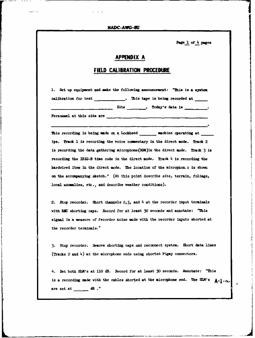
NADC-AWG-SU

Page I of 4 pages

AP!'ENDIX A

FIELD CALIBRATION PROCEDURE

1. Set up equipment and make the following announcement: "2his is a system

caliration for test _ This tape is being recorded at

Site . Today's date is .

Personmel at this site are

This recording is being wade c. a Lockheed machine operating at

Jps. Track I is recording the voice coentary in the direct mode. Track 2

is recording the data gathering microphone(DGK)in the direct mode. Track 3 is

recording the IRIG-B time code in the direct mode. Track 4 is recording the

hardwired item in the direct mode. The location of the microphon, s is shown

on the acccmpanyiyog sketch." (At this point describe site, terrain, foliage,

local anomalies, etc., and describe weather conditions).

2. Stop recorder. Short channels 2,3, and 4 at the recorder input terminals

with BW shorting caps. Record for at least 30 seconds and annotate: "This

signal is a measure of recorder noise made with the recorder inputs shorted at

the recorder terminals."

3. Stop recorder. Remove shorting caps and reconnect system. Short data lines

(Tracks 2 and 4) at the microphone ends using shorted Pigmy connectors.

4. Set both SU's at 310 dB. Record for at least 30 seconds. Annotate: "This

is a recording made with the cables shorted at the microphone end. Ite A--are set at d_ ."

NADC-AWG-SU

Page 2 of 4 pages

5. Repeat 4 for SI settings of 100 dB, 90 dB, 80 dB, 70 dB, 60 dB, 50 dB, 40 0.

6. Connect the DGc (data gathering microphone). Start recording and announce

into -.he DGK "I am speaking directly into the D, serial numer

at Site " Annotate an coentary track: "A si is no bein re-

Ic~~ ~~ c_____r_ e(____corded an Track 2 in the direct mode. ?his signal is coming fro the IDG,

serial nuber . The serial number of the associated SEX is 2'

7. Disconnect the ODIL

B. Connect the bardwired iteK. Start recording and announce into the hardwired

item: "I an speaking directly into a hardvired item, serial number

at Site 2' Annotate on ccmentary track: "A zignal is now being re-

corded on Track 4 In the direct mode. This signal is ccming from the hardwired

item, serial number . The serial number of the associated SIX is

9. Reconnect the IM. Set SIX at i0 dB. Annotate: "The signals which wll

be recorded come from a General Radio 1562A Sound Level Calibrator. In each

case the level is 114 dB re 0.0002 dynes/c-. 7he signals serve to calibrate

the IUK recorded on Track 2. The SIX is set at 110 dB." Record at I1Atst 30

seconds of each frequency on the calibrator annotating each as follows: "Me

present signal is _ _ Hz."

10. DIsconect the DM microphone cable from the S1X. Set SIX at 110 dB.

Insert CMS square wave calibrator intou SL. Set calibrator to 250 Hz and de-

press button. Annotate: "I am recording a 250 Hz square wave on Track 2. The

A-2

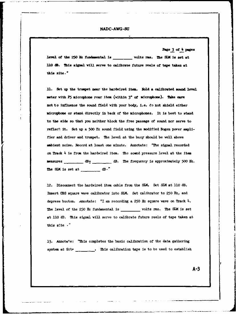
NADC-AWG-SU

Page 3 of 4 pages

level of the 250 Ifz fun tal is volts zus. 1he SIX is set at

110 D. This signal will serve to calbraze future reels of tape taken at

this site."

11. Set up the trmpet near the hardwired item. Hld a calibrated sewd level

meter with P5 microphone rear item (within 3" of microphone). Take care

not to influence the sound field with your body, i.e. e- not shield either

mlcrophone or stand directly in back of the microphones. It is best to stand

to the side so that you neither block the free passage of sound nor serve to

reflect it. Set up a 500 Yz sound field using the modified Bogen pover ampli-

fier and driver and trumpet. The level at the buoy should be well above

ambient noise. Record at least one minute. Annotate: "Me signal. recorded

on Track 4 is from the hardvired item. The sound pressure level at the item

measures _ dB+ _ dB. The frequency is approximately 500 Hz.

Me SIX is set at dB."

12. Disconnect the hardwired item cable from the SLM. Set SLM at 110 dB.

Insert CBS square wave calibrator into SIX. Set calibrator to 250 Hz, and

depress buzton. Annotate: "I am recording a 250 Hz squxare wave on Track 4.

The level of the 250 Hz fundamental is volts rms. The SIX is set

at 110 dB, This signal will serve to calibrate future reels of tape taken at

this site•

13. Annotake: "This ccmpletes the basic calibration of the data gathering

system at Site Th is calibration tape is to be used to establish

A-3

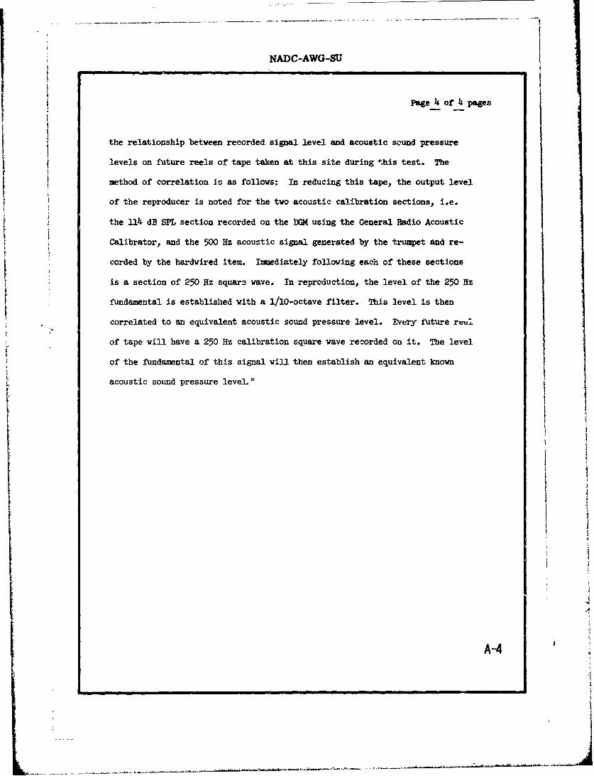
NADC-AWG-SU

Page 4 of 4 pages

the relationship between recorded signal level and acoustic sound pressure

levels on future reels of tape taken at this site during t.his test. The

method of correlation is as follows: In reducing this tape, the output level

of the reproducer is noted for the two acoustic calibration sections, i.e.

the 114 dB SPL section recorded on the D(G using the General Radio Acoustic

Calibrator, and the 500 Hz acoustic signal generated by the trumpet and re-

corded by the hardwired item. Immediately following each of these sections

is a section of 250 Hz squar3 wave. In reproduction, the level of the 250 Hz

fundamental is established with a 1/10-octave filter. This level is then

correlated to an equivalent acoustic sound pressure level. Every future reci

of tape will have a 250 Hz calibration square wave recorded on it. The level

of the fundamental of this signal will then establish an equivalent known

acoustic sound pressure leveL"

I

A-4

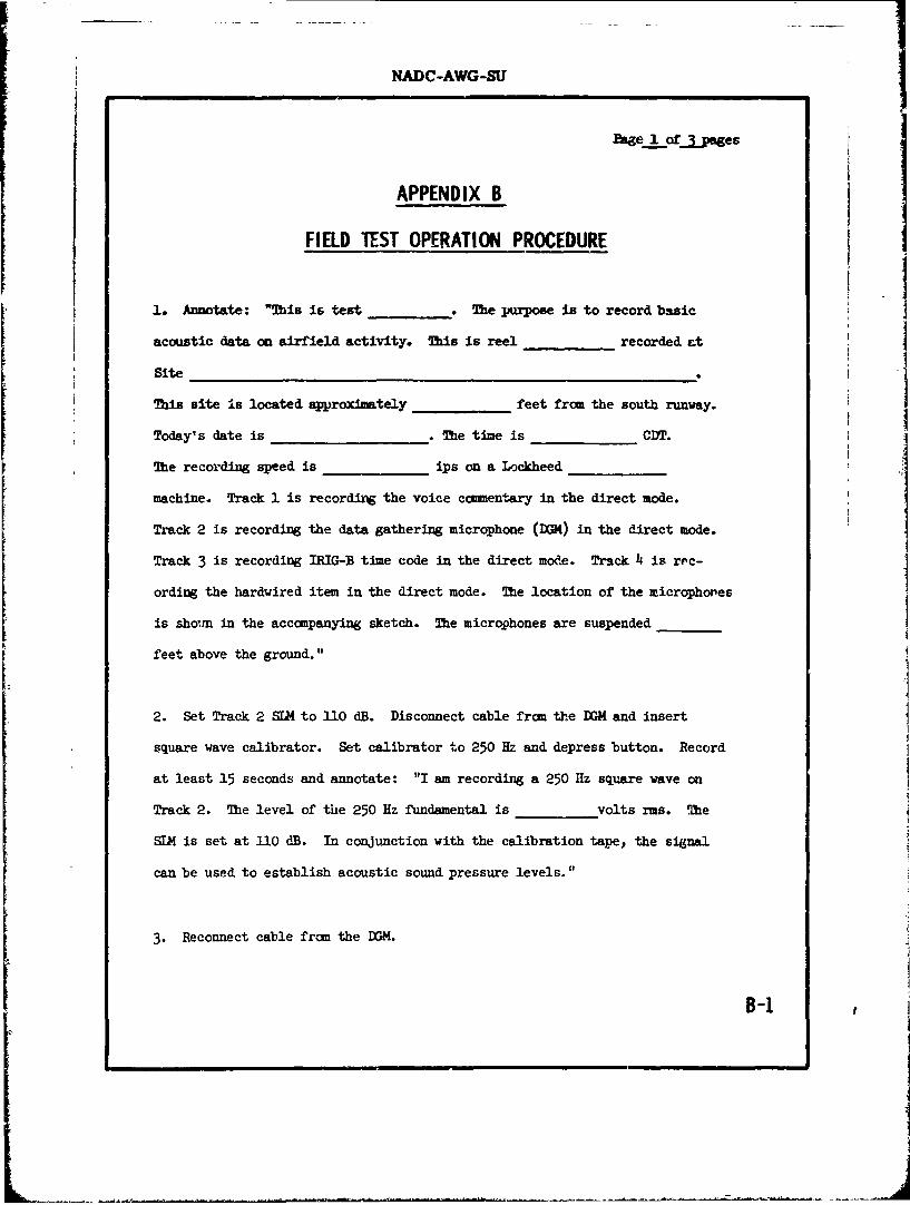
NADC-AWG-SU

Phve 1of 3_pges

APPENDIX B

FIELD TEST OPERATION PROCEDURE

1. Annotate: "This is test _ The purpose Is to record basic

acoustic data on airfield activity. This is reel recorded c-t

Site

This site is located approximately feet from the south runway.

Today's date is . The time is CDT.

The recording speed is ips on a Lockheed

machine. Track 1 is recording the voice commentary in the direct mode.

Track 2 is recording the data gathering microphone (DGM) in the direct mode.

Track 3 is recording IRIG-B time code in the direct mode. Track 4 is rec-

ording the hardwired item in the direct mode. The location of the microphones

is shoim in the accompanying sketch. The microphones are suspended

feet above the ground."

2. Set Track 2 SLM to 110 dB. Disconnect cable from the DGM and insert

square wave calibrator. Set calibrator to 250 Hz and depress button. Record

at least 15 seconds and annotate: "I am recording a 250 Hz square wave on

Track 2. The level of the 250 Hz fundamental is volts rms. 'Me

SLM is set at 110 dB. In conjunction with the calibration tape, the signal

can be used to establish acoustic sound pressure levels."

3. Reconnect cable from the DGM.

B-1

NADC-AWG-SU

Phge_2 of_ pages

4. Set Track 4 SW4 to 110 dB. Disconnect cable and insert square wave cali-

brator. Set calibrator to 250 Hz, and depress button. Record at least 15

seconds and annotate: "I am recording a 250 Hz square wave on Track 4. The

level of the 250 Hz fundamental is volts rms. The SIX is set at

110 dB. In conjunction with the calibration tape, the signal can be used to es-

tablish acoustic sound pressure levels." Reconnect cable from hardwired item.

I5. Disconnect hardwired item from field end of cable.

6. Reconnect the DGH. Start recording and announce into the DGM: "I am speak-

ing. directly into the DGM, serial number , at Site ."

Annotate on ccmentary track: "A signal is now being recorded on Track 2 in

the direct mode. This signal is coning from the DGM, serial number ------

The serial number of the associated SIM is "

(- Disconnect the DGM.

8. Connect the hardwired item. Start recording and announce into the hardwired

item. "I am speaking directly into a hardwired item, serial number

at Site ." Annotate on commentary track: "A signal is now being rec-

orded on Track 4 in the direct mode. This signal is coming from the hardvired

item, serial number . The serial number of the associated M is

4

9. Reconnect the DGM. Set 5124 at 110 dB. Annotate: "The signals which will

be recorded come from a General Fadio 1562A Sound Level Calibrator. In each

B-2 1,

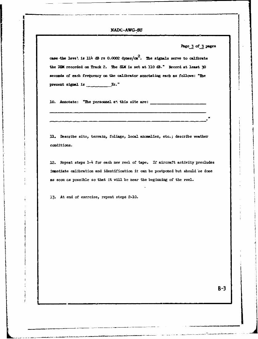
NADC-AWG-SU

Page 3 of 3 Pages

case-the leve ' is .14 dB re 0.0002 dynes/m 2 . 7he signals serve to cabrate

the DW recorded on Track 2. ?he S[I is set at 110 dB." Record at least 30

seconds of each frequency on the calibrator annotating each as follows: "The

present signal is Xz."

10. Annotate: "The personnel a, this site are: _

11. Describe site, terrain, foliage, local anomalies, etc.; describe weather

conditions.

12. Repeat steps 1-4 for each new reel of tape. If aircraft activity precludes

immediate calibration and identification it can be postponed but should oe done

as soon as possible so that it will be near the beginning of the reel.

13. At end of exercise, repeat steps 2-10.

B-3

& -4

|j[M

....

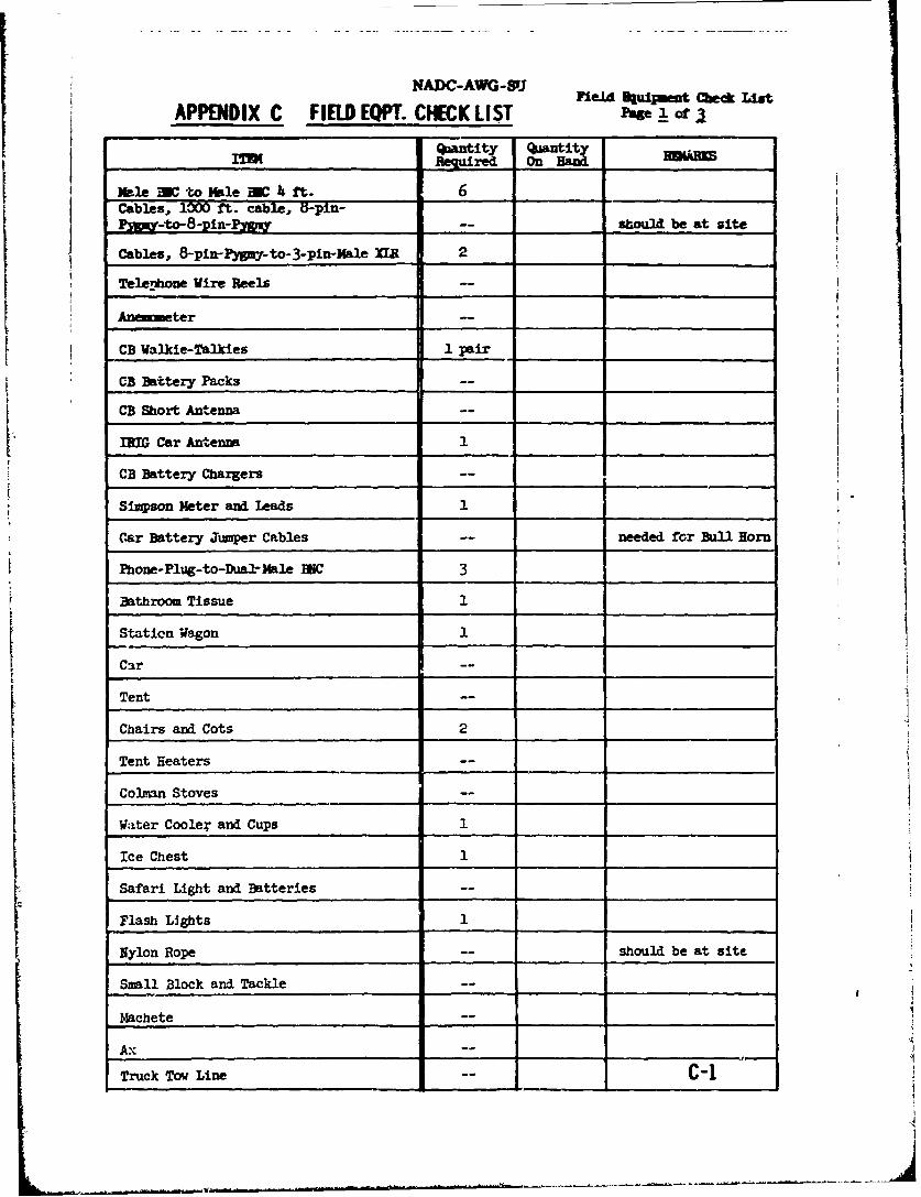
NADC-AWG-5'J Field Htutneat Cbck ListAPPENDIX C FIELD EQPT. CHECKLIST Page 1: ot :1

Wantit ruant

~le aC to Mle mac 4 ft. 6Cables, 1000 ft. cable, U-pin-Pyw-to-8-pin-Pymm -- should be at site

Cables, 8-pin.-PYPv/-to-3-pin-Male IR 2

Telekwone Wire Reels --

Anemometer _

CB Walkie-Talkies 1 pair

CB Battery Packs --

CB Short Antenna

II1 Car Antenna 1

CB Battery Chargers --

Simpson Meter and Leads 1

Car Battery jumper Cables -- needed for Bull Horn

Phone-Plug-to-Dual- Male BUC 3

Bathroom Tissue 1

Station Wagon 1

Car --

Tent --

Chairs and Cots 2

Tent Heaters --

ColmaI Stoves --

Water Cooler and Cups 1

Ice Chest 1

Safari Light and Batteries --

Flash Lights 1

Nylon Rope -- should be at site

Small Block and Tackle --

Machete --

Ax To__Line_--_C- _

Truck Tow Line C-1

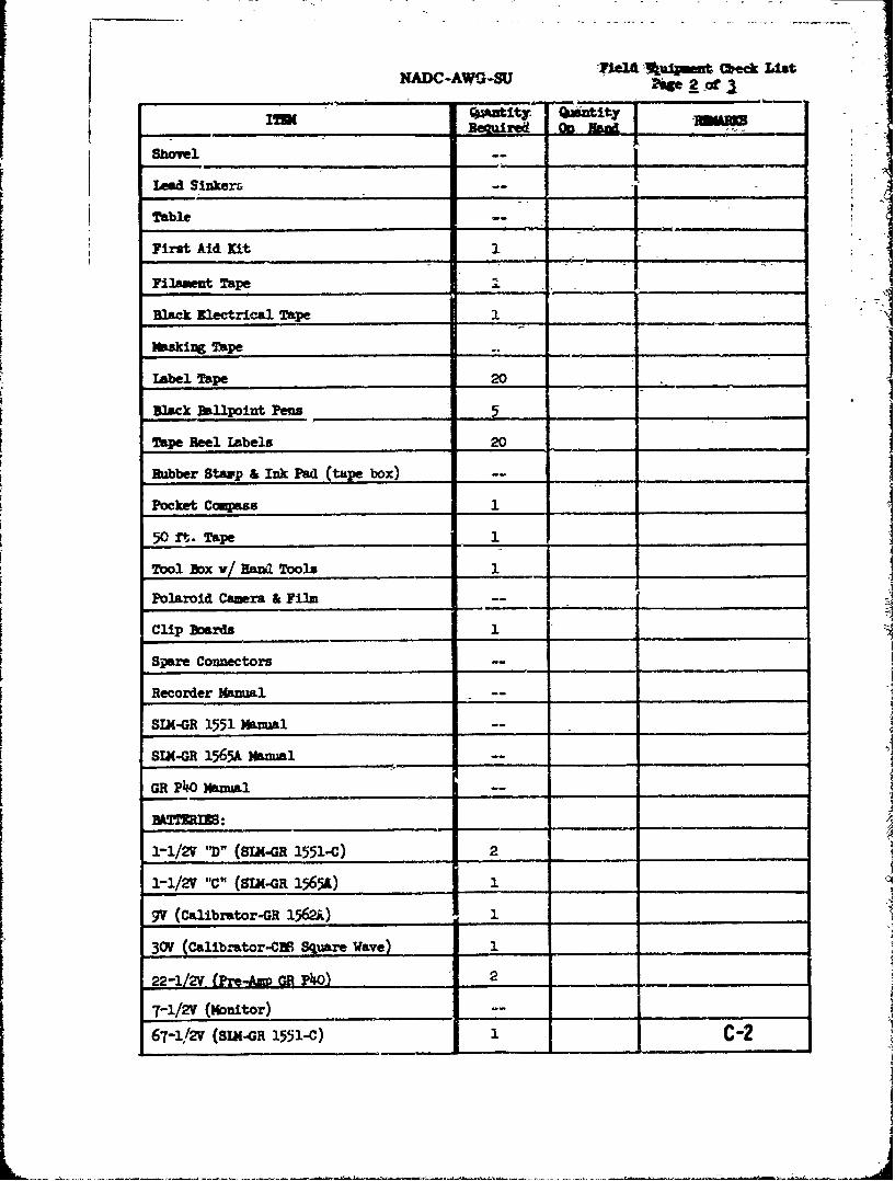
hel t J.t ck LitNADC-AWS-SU Page 2 of L

Shovel_

Lead Sinkers -- -

Table -

First Aid Kit 1 _

Filament Tape_ _ ,__,

Black Electrical Tape I " -\

Masking Tape ______ -

label Tape 20 _ _"

Black Pllpoint Peus 5

Tape Reel Labels 20

Rubber Stapp & Ink Pad (tape box) --

Pocket Compass 1

50 ft. Tape 1

Tool BOx v/ ana1 Tools 1

Polaroid Camera & Film --

Clip Boards 1Spare Connectors -

Recorder Manual

SIX-OR 1551 Manual

sIN-OR 1565A Manual

GR P40 Manual

1-1/2V "D" (SIX-OR 1551-C) 2

1-1/2V "C"s (SIX-OR 1565A) 1 -

9V (Calibrator-GR 1562A) 1

30V (Calibrator-CM Square Wave) !

22-1/n (Pre-w oi P40o) 2

7-1/2V (Monitor) __--

67-1/2 (SIN-GR 1551-C) 1 C-2

J Field Buipmnt Check ListNADC-AWG-SUPage of

i=1% manity RaI;- - l' , - . .. _ _ __ _ __ _

iRecorder,, 14 n

Nicad Battery Packs for Tape Recorder 2

Charger for Nicad Battery Packs --

Recorder Power Supply and Cables

Empty Reels, 1/2" --

ERqty Reels, 1/4" 1

Recording Tape, 112" --

Recording Tape, 1/4" 10

Cables, Recorder-to-Car-Batteries --

Q-tips and Alcohol

Head Demagnetizer --

Spare Belts -for Recorders 1.

Sound Level Meters GR1551 2

Sound Level Meters GR1565A i

Microphones GR P5 1

Preamplifiers and Housings 1

Sound Level. Calibrator 1562A 1 __

Square Wave Calibrator 1 I

Data Sheets 40

i Commentary Microphone Switch Box 1Cable-male i3C to edge track inputwith built-in attenuator

Monitor / IRIG Radio & Battery Pack 1

Headphones - Koss low

Mnitor Box - Amplifier ir/Selecto~r Swait chCables, Male WC to Male 3KC2 ft. long

MC "T" 8

Hardwired Item IBatter,-PFo;ered Oscilloscope --

Bttery Power Cables for Sco -- C-3A.G. Powet Cables for Sco --

- ~ - --

NADC-AWG-SU

ZECREST NOFORN(WHEN FILLED IN) APPENDIX D FIELD LOG

Field Operators Data SheeL Page _ of

TEST LOCATION DATE_

OPERATORS(TEAM LEADER)

REEL NUMBER if any

Tape Recorder (Type)

Sound Level Calibrator General Radio 1562A

Square Wave Calibrator CBS

Microphone #1 Microphone General Radio PISPreamplifie r General Radio P40SIX4 General Radio 1551CLength of able to Sound Level Meter fet4HIe'ight of Microphone above ground - ~Rainshield or Windscreen, if any _____

Microphone #2 Microphone General Radio P5

PreamplifierLenera! Radin P40SU14 General Radio 1551C

Lenth of Cable to Sound Ljvel Meter _ ___

Height of' Miernghnn anve griin- ft

Rainshield or Windscreen, if P-v type)

Microphone #3 Microphone General Radio P5_Preamplifier General Radio PLO __.__

SLM General Radio 1551CLength of Cable to Sound Level Meter __ fet

Height of Microphone above around __ feet

Rainshield or Windscreenif any [y )

Peak Levels Impact Analyzer General Radiol56-r,6B

_ _ _ _ _ _ Sound Level Meter General Radio WI165A

Recording Speed

TRAC? __ INFORMATION SOUND LEVEL METER READINGS

1 CAL. FREQ'S MIC # MIC W MIC #

2 ACTUAL SIM ACTUAL SLM ACTUAL SIM

LEVEL SETTING LEVEL SETTING LEVEL SETTING

4 400 Hz dB dB dB5 ,_-.2000 Hz dB dB dB

6 1000 Hz dB dB dB7,, 500 Hz dB dB dB7250Hz dB dB dB

125 Hz dB dB dB f

Terrain

v erhe

) SECRET NOFORN D-1(over) (WHEN FILLED IN)

ILm IL= IN)__ _ _ _TIOL OR___ _ - -M SIX _____ ____ PEAK_ __ _

_ _C _ _ ___=

11 - -2 JI__ __ _ READG_ -

dL

SERT o.

_ _~ _nz IN -

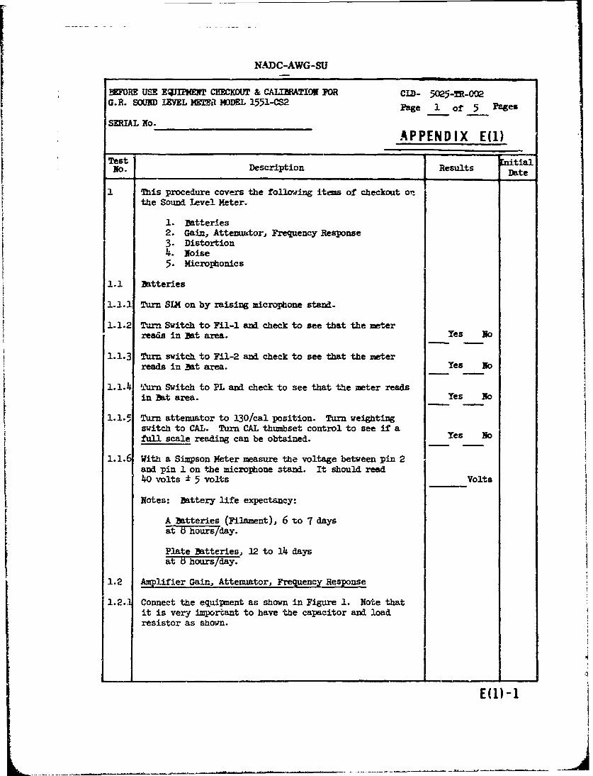
N.ADC-AWG-SU

NFORE USV EZQJPME CHBCKOUT & CAIXBPATIOF FOR CI)- 5025-M-OWG.R. SOUND LEFL METR MODEL 1551-CS2 Page 1 of 5 Pages

SERIAL No.APPENDIX E(1)

Test InitialNo. Description Results

1 This procedure covers the folowing items of checkout onthe Sound Level Meter.

I. Batteries2. Gain, Attenuator, Frequency Response3. Distortion4. Noise5. Microltonics

1.1 Batteries

1.1.1 Turn SIX on by raising microphone stand.

1.1.2 Turn Switch to Fil-i and check to see that the meterreads in Bat area. Yes No

1.1.3 Turn switch, to F11-2 and check to see that the meterreads in Bat area. Yes No

1.1.4 'Arn Switch to PL and check to see that the meter readsin Bat area. Yes No

1.1.5 Turn attenuator to 130/cal position. Tun weightingswitch to CAL. Turn CAL thumbset control to see if a

full scale reading can be obtained. Yes so

1.1.6 With a Simpson Meter measure the voltage between pin 2and pin 1 on the microphone stand. It should read

40 volts * 5 volts Volts

Notes: Battery life expectancy:

A Batteries (Filament), 6 to 7 daysat 6 hours/day.

Plate Batteries, 12 to 14 days

1.2 Amplifier Gain, Attenuator, Frequency Response

1.2.. Connect the equipanent as shown in Figure 1. Note thatit is very imporiant to have the capacitor and loadresistor as shown.

E(1)-1

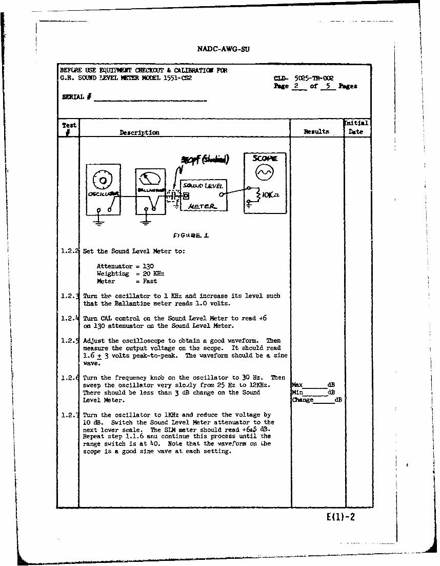
NADC-AWG-SU

BE SE EqUnAWr CHECKOUT & CALI'RATIC FORG.R. SOUND LEVEL HER MOUEL 1551-CS2 CW- 5025-TR-0(2

Page 2 of 5 Pages

Test Ita

Deseription Results Date

1.2.2 Set the Sound Level Meter to:

Attenuator = 130Weigting = 20O~Meter = Fast

1.2.3 Turn the oscillator to 1 KHz and increase its level suchIthat the Ballantine meter reads 1.0 volts.

1.2. Turn CAL control on the Sound Level Meter to read .6Son 130 attenuator on the Scund Level Meter.

1.2. Adjust the oscilloscope to obtain a good waveform. Thoenmeasure the output voltage on the scope. It should read1.6 + 3 volts peak-to-peak. The waveform should be a sine

1.2. Turn the frequency knob on the oscillator to 30 Hz. Then

sweep the oscillstor very sloily frosi 25 Hz t~o 12KHz. _____dB

There should be less than 3 dB change on the Sound Mn dLevel Meter. (2 ange dB

1.2." Turn the oscillator to 1KHz and reduce the voltage by10 dB. Switch the Sound Level Meter attenuator to thenext lower scale. The SL)4 meter should read +6* c3.Repeat step 1.1.6 arna continue this process until therange switch is at 40. Note that the vave form on Lhe

scope is a good sine w~ave at each setting.

E(1)-2

LA Sir

0C) ......EVE

NADC-AWG-SU

BEFcR2 USE EQUIPMEN CHECKOUT & CALIBRMTIC FOR - 5c -c0G.R. SCWlD I-VEL MEER MCD:- 1551-CS2 Page 3 of 5 Pates

IERAL i

Test tial

Description Results Date

Atten tr dMeter dsSetting e Cme120 dB dB

71090

70

60504 0

1.3 Distrtion Measurement

1.3.1 Connect the Distortion Analyzer to the output of the STY.Return the attenuator of the Sound Level Meter to 130.Turn the oscillator to 100 Hz and bring up the level toreaO +10 dB (full scale) on the SIX meter.

1.3.2 Turn the Distortion analyzer to Set Level and theattenuator knob to 100%. Adjust the Input Control togive full scale on the Distortion Analyzer Meter.

1,3.3 Turn to Distortion and adjust the frequency dial to 100 Hzand null the meter. Switch the attenuator to 30% and nullusing the frequency dial. Repeat on 10% and 3% settings.Once the null is obtained adjust the balance knob for aminimum reading. Read the percent distortion. It shouldbe less than 1.25%.

SIX Set at ,13

100 Hz_

1.3.4 Turn the oscillator to 1000 Hz and repeat steps 1.3.2 and1.2.3. 1KHz,_-

1.3.5 Turn the oscillator to 10 KHz and repeat steps 1.3.2 and1.3.3. 10 KHz,

-iD-iE(1)-3 ]

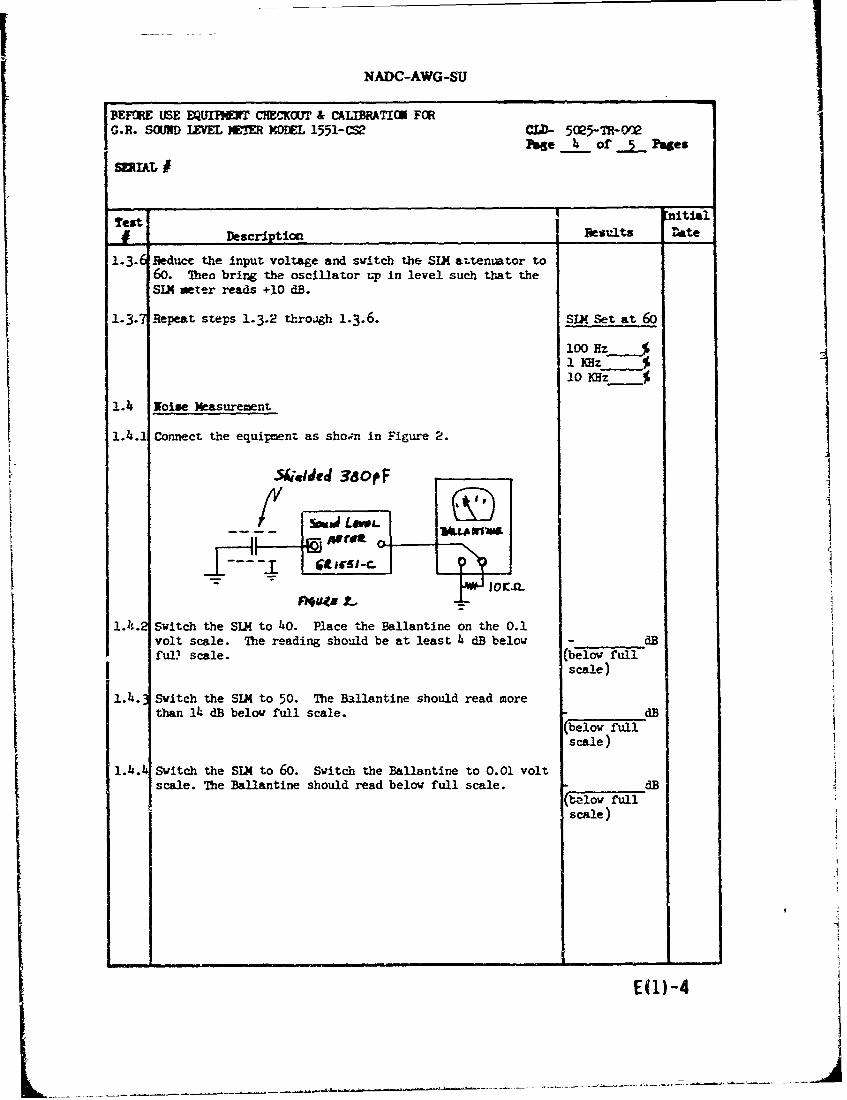
NADC-AWG-SU

I BEFORE USE EQUIPAUT CYWHEOUT & CALIBRATION FORG.R. SOUND EVEL METER )ODL 1551-CS2 CLD- 505-TR-

Page 4 or _5 Pages

SERAL

T Enitial

# Description tstults Late

1.3.6 Reduce the input voltage and switch the SIX aLtenuator to60. Ten bring the oscillator up in level such that theSIX meter reads +10 dB.

1-3.7 Repeat steps 1.3.2 throigh 1.3.6. Six Set at 60

100 Hz %1 Hz%

1.4 Noise Measurement

1.4.1 Connect the equipment as sho;n in Figure 2.

Sdeilded 36oiF

1.1,.2 Svitch the SIX to 40. Place the Ballantine on the 0.1

volt scale. The reading should be at least 4 dB below - dBfuD scale. (below full

scale)

1.4. 3 Switch the SIX to 50. The Ballantine should read morethan 14 dB below full scale. dB

(below fullscale)

1.4.4 Switch the SIX to 60. Switch the Ballantine to 0.01 voltscale. The Ballantine should read below full scale. ____o___dB

(bealow fullscale)

E(1)-4

NADC-AWG-SU

BEFORE USE EIPAENT CHECKO T & CALIBRATION FORG. R. SOUND IVEL METER MODEL 1551-CS2 CLD- 5025-TR-002

Page -5 of 5 Pages

SSIAL#________ __

Test Initiel# Description Results Date

1.4.5 Repeat Step 1.4.3 except increase the Sound level Meter in 70, - dB10 dB steps. The meter should read more than 10 dB below (below Full

full scale on the 0.01 volt setting for each position abov S'ale)60 on the SIM. 80, dB

90,- dB100, dB110, - dB120,- dB130,- dB

1.5 Microphanics

1.5.1 Place the SIX in the 40 positio, gently tap its caseon all sides. The meter should not bounce above 0 dB. dB

(max meterswing)

E(1)-5

NADC-AWG-SU

IFU(KT CHECNKUT AV CALIBRATION FORG.R PRA~GLIFER K)]L 160P40Page 1 of _J_ Pages

S AL #APPENDIX E(2)

C~ITAcT # PEBT# f ______

Test EnitialDescription Results Date

1. This procedure covers the following items of checkout onthe preamplifier:

1. Gain2. Response3. Distortion4. Noise

1.1 Gain, Response1.1.1 Connect the equipment as shown in Figure 1. Use only a

calibrated sound level meter.

.... I o, |@SCILIATIe

1.1.2 Switch the preamplifier to the Xl position. Turn thesound level meter to the 120 dB setting. Place thevoltmeter in the 1.0 volt range.

1.1.3 Set the o9cillator to 1 kHz and adjust the level controlso that a 1.0 volt peak-to-peak signal is read on the Good Waveformupper beam of the scope. Observe that the lower beamgives a wave that is similar in shape to the upper beam. ___Yes __NO

It should be a 1.5 + 0.3 volt peak-to-peak level.Vp top

E(2)-1

NADC-AWG-SU

EgIr1]U CHECKOUT AID CALIBRATION FOR 5 -- 0G.R. PREPJG MLIFI J01EL 1560-P40 Page 2 of - Pages

COPC mmRw= #

Test nitialDescription Reaults Date

1.1.4 Record the dB reading on the voltmeter. Then very slowly + Mx.sweep the oscillator from 30 Hz to 12 kHz. There should rebe no more than a 3 dB variation over this range. Min. mm

dB ch e

1.1.5 Switch the SIM to 130 attenuator setting. Increase theoscillator voltage so that the SI reads full scale. Clipping atThere should be no noticeable clipping on the lower 140 dBscope waveform. (Note: This is the maXinmu useful level (+10 on theof the preamp. Any increase in input voltage will cause 130 scale)waveform clipping.) Yes No

1.2 Distortion

1.2.1 With the same setup as Figure 1, connect the DistortionAnalyzer to the output of the SIM. Place the attenuatoron the SIX to 120 dB.

1.2.2 Adjust the frequency of the oscillator to 100 Hz andbring up the level to give full scale (+10 dB) on the SIM.Switch the Distortion Analyzer to set level and 100%.

1.2.-3 Adjust the level control on the Distortion Analyzer toread full scale on its meter. Switch to Distortion andturn the frequency knob to 100 Hz. This will null outthe signal. Turn to 30ec, 10% and then 3% while nullingthe meter using the frequency knob. Then adjust thebalance control for the lowest meter reading (nulled).

1.2.4 The distortion measurement should be lower than 1.25%. 100 HzDistortion

1.2.5 Turn the oscillator frequency to 1 kHz. Then repeatStep 1.2.3. The distortion measured should be less 1 kHzthan 1.25%. Distortion

1.2.6 Turn the cillator frequtcy to 10 kHz. Repeat Step1.2.3. The distortion should be less than 1.25%. 10 kHz %

Distortion

E2)-2

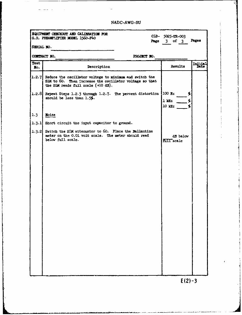
NADC-AWG-SU

IG.IR. CWKW AD C 0- CLU- 5025-M-003Page 3 of 3 Pages

SIAL 40.

COnZRACT 50. PROJECT NO.Test .ta

No. Description Results

1.2.7 Reduce the oscillator voltage to mini a switch theSIX to 60. Then ±-ncrease the oscillator voltage so thatthe SIX reads Pill scale (+10 dB).

1.2.8 Repeat Steps 1.2.3 through 1.2.7. The percent distortion 100 Nz %shoulA. be less than 1.5%- 1 kHz -

10 kHz %

1. 3 Noise

1.3.1 Short circuit the input capacitor to ground.

1.3.2 Switch the SIX attenuator to 60. Place the Ballantinemeter on the 0.01 volt scale. The meter should read d3 belowbelow full scale. ?=scale

E(2)-3

NADC-AWG-SU

U SE cm== ',PRO== FCR GR 1560-P5 mIco=OcLK D- 5025-T-005

Page 1 of 3 P~ges81L#" APPENDIX E(3)

Test nta

1 Description Results Date

1. This procedure covers the following items of checkout:

1. General sensitivity and Response.

2. Reciprocity calibration.

1.1 General calibration using GH IsA calibrator.

1.1.1 Plug the microphone into a calibrated sound level meter,or into a calibrated pre-amplifier and Sound Level Metercombination. Turn on equipment by raising the mic holder,and svitch the attenuator to 110 cale.

1.1.2 Start the 1562A calibrator by first turning the knobcounterclockwise for 1 second and observe the batteryindicator light. Then switch to I Hz. Listen to seeif a tone is heard. Make sure the large hole adapter isplugged into the calibrator.

1.1.3 SIo place the calibrator on the microphone, (rapidmovement will cause excessive pressure on the microphonediaphragm and destroy the unit). The SIX should readnear +4 dB on the 110 setting. If it is close turn theCAL knob for a +4 dB reading.

1.1.4 Tlurn the Calibrator to 2KHz and record the dB reading. 2KHz dBRepeat for the other frequencies. There should be less lKz +Tthan ± 1 dB variation over the frequency range. 500 It

250 Hz

125 Hz

1.2 Reciprocity Calibreion

1.2.1 Connect the equipoent as shown in Figure 1.

.A--

?€,-)-1

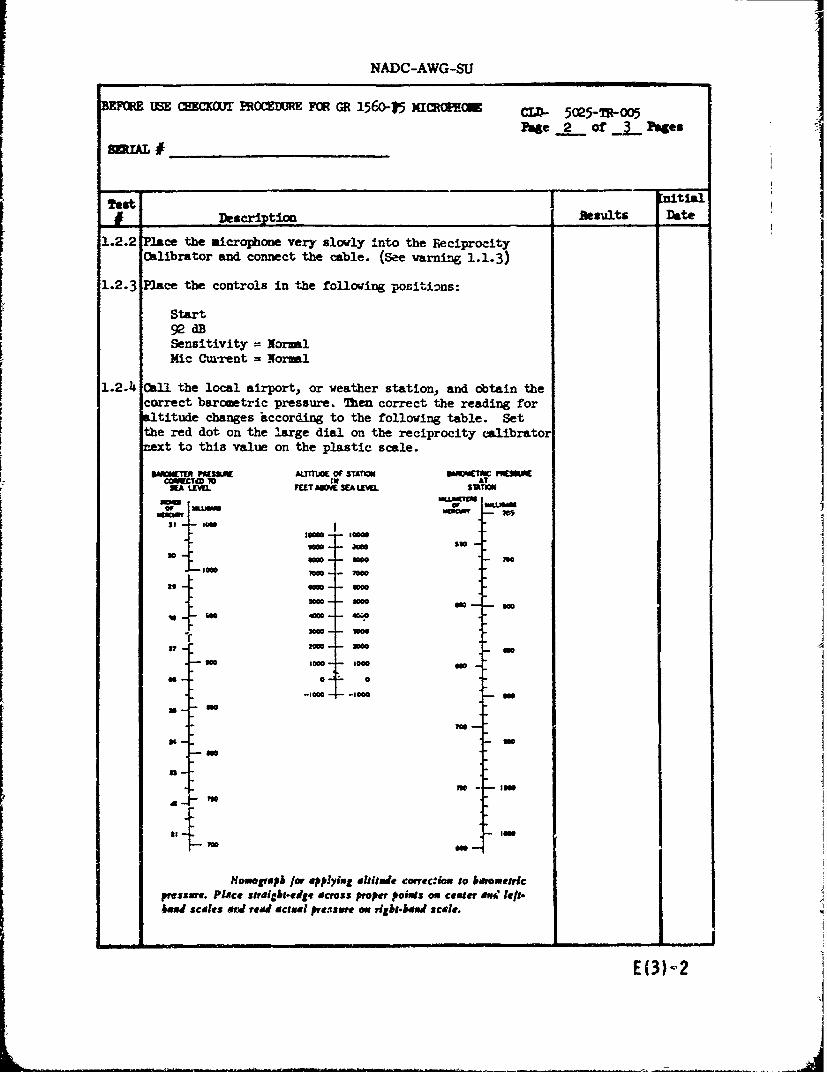
NADC-AWG-SU

US.ETE CtZKOWf PROMMME FM GR 156o-15 micom.m CzL- 5025-R- 005Page 2 of 3.. Pages

# Dscriptioni.eiJt t

1.2.2 Place the microphone very slowly into the ReciprocityCalibrator and connect the cable. (see warning 1.1.3)

1.2.3 Place the controls in the following positionas:j

start

Sensitivity = orml

1.2.4 001 the local airport, or weather station, and ctain the

1:1110= 1 INA

- Sao

30 0 OW70

-I1M 7 -17000

29no am--a

- ~ ~ S -:~~'5~w E 9M

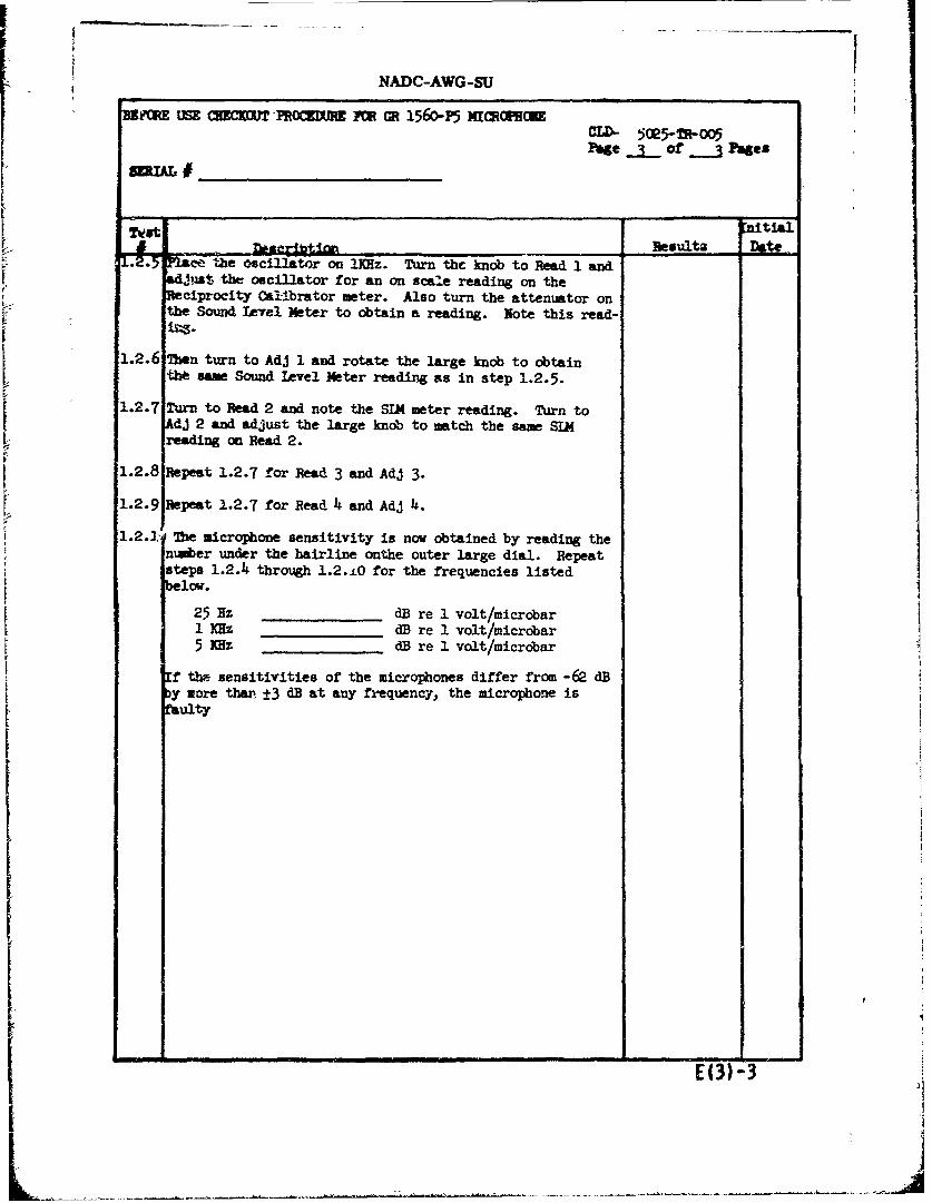
r[ NADC-AWG-SU

II

U(eW USE CMECM b-1R FM GR 1560-15 micRomm

ce the oscillator on !KHz. Turn the knob to Read 1 andNat the oscillator for an on scale reading on theciprocity Calibrator meter. Also turn the attenuator onthe Sound Leel Meter to obtain a reading. Note this read-

1.2.6 Then turn to AdJ 1 and rotate the large knob to obtain

the same Sound Level Meter reading as in step 1.2.5.

1.2.7 Turn to Read 2 and note the SIM meter reading. Turn toAdJ 2 and adjust the large knob to match the same SIMreading on Read 2.

1.2.8 Repeat 1.2.7 for Read 3 and AdJ 3.

1.2.9 Repeat 1.2.7 for Read 4 and Adj 4.1.2.3I The microphone sensitivity is now obtained by reading the

number under the hairline onthe outer large dial. Repeat

steps 1.2.4 through 1.2.±0 for the frequencies listedlow.

25 RZ dB re 1 volt/microbar1 KEz dB re 1 volt/microbar5 KHz dB re 1 volt/micrdbar

f the sensitivities of the microphones differ from -62 dBby more than ±3 dB at any frequency, the microphone isfaulty

E(3)-3

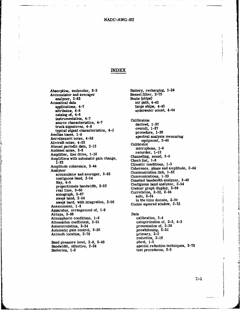
NADC-AWG-SU

INDEX

Absorption, molecular, 3-3 Battery, recharging, 1-34Accumulator and averager Bessel filter, 2-75

analyzer, 2-62 Bokts (ships)Acoustical data air path, 4-42

applications, 4-7 large ships, 4-45attributes, 4-6 underwater sound, 4-44catalog of, 4-6instrumentation, 4-7 Calibraionsource characteristics, 4-7 derived, 1-27truck signatures, 4-8 derve, 1-27typical signal characteristics, 4-3 roverall, 1-27Aeoia4tne, -8procedure, 1-26

Amlifi, ines, d , 1spectral analysis measuringAerwdyn itic noise, 4-58 eqli t, -Aircraft noise, 4-32 quipmenttor4

Almost periodic data, 2-13 microphone, 1-9Ambient noise, 2-6 r cre,11Amplifier, line drive, 1-16 Chnelinge, sond1-12Amplifiers with automatic gain change, Checkelist, soud,3-

Am1t- ecoeene224 Climatic conditions, 1-5Amplitude coherence, 2-44 Coherence, phase and amplitude, 2-44Analyzer

accumulator and averager, 2-62 Communication link, 1-33

contiguous band, 2-54 Communications, 1-33

Kay, 4-5 Constant bandwidth analyzer, 2-49

proportionate bandwidth, 2-52 Contiguous band analyzer, 2-54real time, 2-60 Contour graph display, 2-68sonograph, 2-67 Correlation, 2-32, 2-84swept band, 2-54 auto, 2-34swept band, 2-56 in the time domain, 2-34swept band, with integration, Co-56 sqaeMino,22Anemometer, 1-8 Cosine squared window, 2-23

Apparatus, arrangement of, 1-9Arrays, 2-86 DataAtmospheric conditions, 1-8 calibration, 2-4Attenuation coefficient, 3-21 categorization of, 2-3, 4-3Autocorrelation, 2-34 presentation of, 2-39Automatic gain control, 2-36 prewhitening, 2-28

Azimuth location, 2-78 1Timary, 2-3reduction, 2-10

Band pressure level, 2-8, 2-48 sheet, 1-5Bandwidth, effective, 2-34 special reduction techniques, 2-78Batteries, 1-9 test procedures, 2-5

I-i

__j

NADC-AWG-SU

INDEX

Data analysis angular, 2-6frequency domain, 2-37 Frequency analysis, 2-20, 2-37

Data gathering mission, 1-1 Frequency domainobjectives, 1-1 data analysis, 2-37planning, 1-3 data reduction, 2-66practice ("dry") runs, 1-2

Debriefings, 1-32 Gain control, automatic, 2-36Definitions and units, 2-5Delta function, 2-30 Hamming window, 2-23DEMON, 2-90 Harmonic, 2-6Detection High frequency cutoff, 2-20

through correlation, 2-84 Humidity, effect of, 3-3through multiple sensors, 2-32

Directional response Ilumination, 1-9pattern, 2-9 Impact data, 1-22

Display recording, 1-20contour graph, 2-68 Impact meter, 1-12

rectified data, 2-75 Implementation plan, 1-313 -D spectral, 2-68 Impulse signal handling, 2-19, 4-41

Doppler effect, 2-17 Impulsive data, 1-12Dyne per square cm (see Microbar)

Jungle sounds, 4-10, 4-11Electric discharge, 4-44Elevation, detection of, 2-80 Kay Analyzer, 4-5Envelope, 2-32

rectified, 2-32 Level, 2-8Equipment, 1-2 Line drive amplifier, 1-16

check list, 1-6 drive capability, 1-16custody of, 1-6 emitter-follower, 1-16failure logs, 1-31 signal capability, 1-16for time function display, 2-70 Log of events, 1-5requirements, 1-30 Low-frequency cutoff, 2-20selection of, 1-7supplementary, 1-6 Magnetic shielding cans, 1-33weight and bulk, 1-3 Magnetic tape, 1-22

Excess attenuation, 3-2 Microbar, 2-7Explosive sounds Microphone

propagation of, 3-30 calibrator, 1-9condenser, 1-13

Fall time, 2-33 definition, 2-9False alarm rate, 2-36 directional, 2-9Field laborattory procedues, 1-34 dynamic, 1-13Field procedures, 1-23 gradient, 1-12, 2-78Filter omnidirectional, 1-12

Bessel, 2-75 piezoelectric, 1-13Butterworth, 2-75 pressure, 1-12

Filtering selection of, 1-12predeteetion, 3-21, 3-30 transducer, 1-12post-detection, 2-37, 3-21, 3-30 velocity, 1-12

Fourier integral, 2-13 wind-and-rahL screen, 1-13Fourier series, 2-11 Model structureFourier transform, fast, 2-65, 4-34 sources, 2-94

Fourier transform, running, 2-18 transducers, 2-94Frequency, 2-6 Modeling, 2-92

1-2

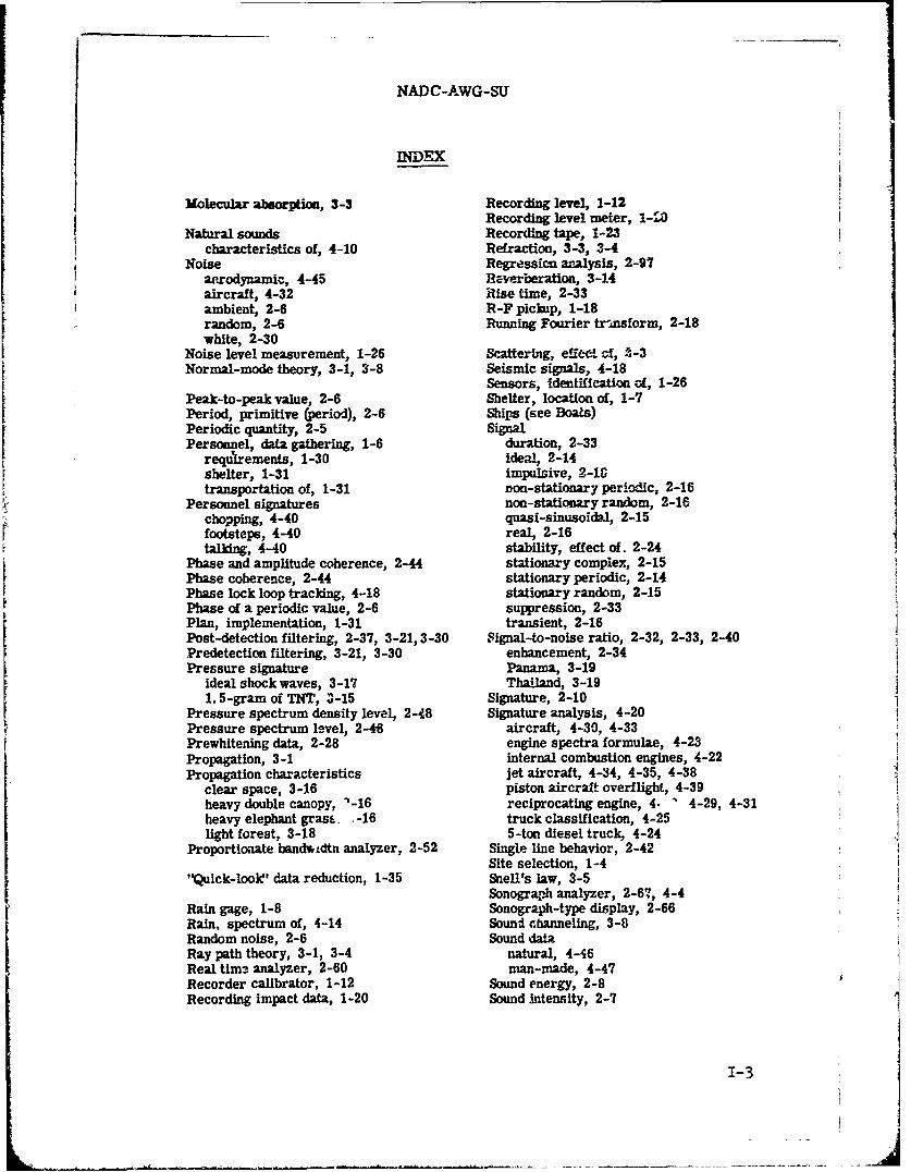
NADC-AWG-SU

INDEX

Molecular absorption, 3-3 Recording level, 1-12Recording level meier, 1-40

Natural sounds Recording tape, 1.-23characteristics of, 4-10 Refraction, 3-3, 3-4

Noise Regressicn analysis, 2-97aerodynamic, 4-45 Reverberation, 3-14aircraft, 4-32 Rise time, 2-33ambient, 2-6 R-F pickup, 1-18random, 2-6 Running Fourier tr'ansform, 2-18white, 2-30

Noise level measurement, 1-26 Scattering, effec s-f, -3-3Normal-mode theory, 3-1, 3-8 Seismic signals, 4-18

Sensors, identification Uf, 1-28Peak-to-peak value, 2-6 Shelter, location of, 1-7Period, primitive (period), 2-6 Ships (see Boals)Periodic quantity, 2-5 SignalPersonnel, data gathering, 1-6 duration, 2-33

requirements, 1-30 ideal, 2-14shelter, 1-31 impulsive, 2-10transportation of, 1-31 non-stationary periodic, 2-16

Personnel signatures non-stationary random, 2-16chopping, 4-40 quasi-sinusoidal, 2-15

footsteps, 4-40 real, 2-16talking, 4-40 stability, effect of. 2-24

Phase and amplitude coherence, 2-44 stationary complex, 2-15Phase coherence, 2-44 stationary periodic, 2-14Phase lock loop tracking, 4-18 stationary random, 2-15Phase of a periodic value, 2-6 suppression, 2-33Plan, implementation, 1-31 transient, 2-16Post-detection filtering, 2-37, 3-21,3-30 Signal-to-noise ratio, 2-32, 2-33, 2-40Predetection filtering, 3-21, 3-30 enhancement, 2-34Pressure signature Panama, 3-19

ideal shock waves, 3-17 Thailand, 3-191.5-gram of TNT, 3-15 Signature, 2-10

Pressure spectrum density level, 2-48 Signature analysis, 4-20Pressure spectrum level, 2-46 aircraft, 4-30, 4-33Prewhitening data, 2-28 engine spectra formulae, 4-23Propagation, 3-1 internal combustion engines, 4-22Propagation characteristics jet aircraft, 4-34, 4-35, 4-38

clear space, 3-16 piston aircraft overflight, 4-39heavy double canopy, -16 reciprocating engine, 4. " 4-29, 4-31heavy elephant grass -16 truck classification, 4-25light forest, 3-18 5-ton diesel truck, 4-24

Proportionate bandwdtrl analyzer, 2-52 Single line behavior, 2-42Site selection, 1-4

"Quick-look' data reduction, 1-35 Snell's law, 3-5Sonograph analyzer, 2-67, 4-4

Rain gage, 1-8 Sonograph-type display, 2-66Rain, spectrum of, 4-14 Sound channeling, 3-8Random noise, 2-6 Sound dataRay path theory, 3-1, 3-4 natural, 4-46Real tim3 analyzer, 2-60 man-made, 4-47Recorder calibrator, 1-12 Sound energy, 2-8Recording impact data, 1-20 Sound intensity, 2-7

1-3

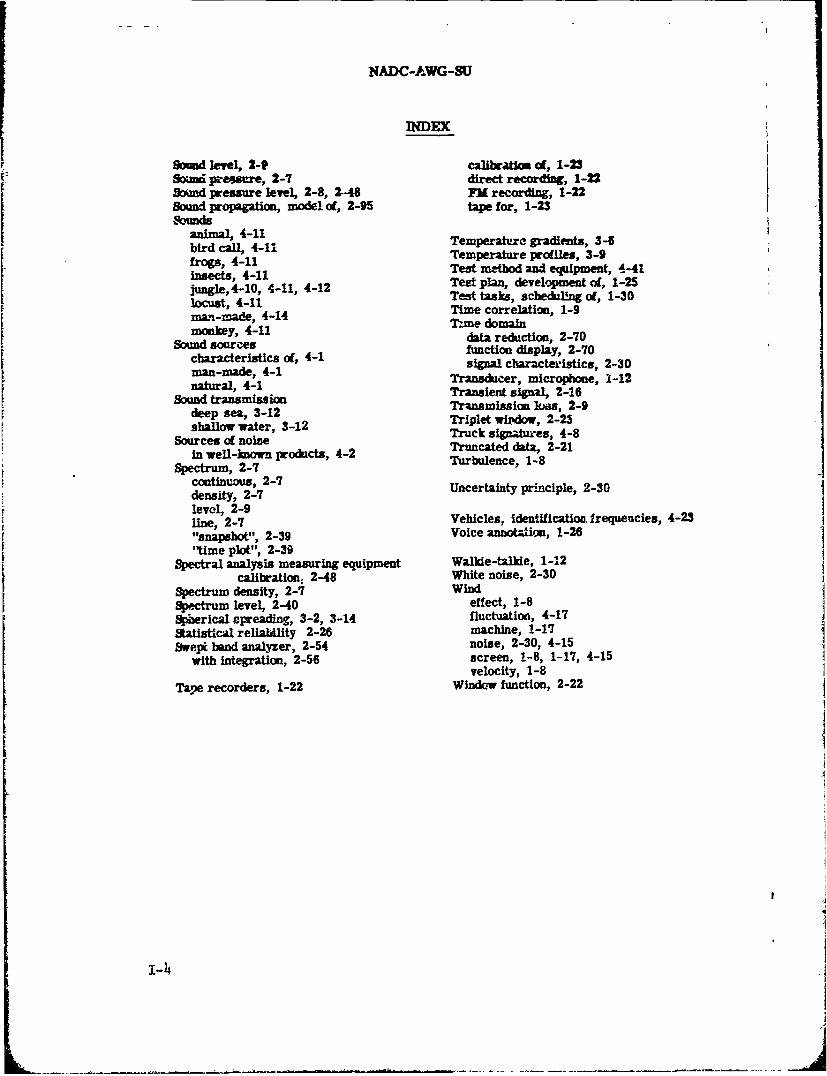
NADC-AWG-SU

INDEX

Soud level, 2-9 callbratkm of, 1-23Soznd preossae, 2-7 direct recwdg, 1-22

ptmd pressure level, 2-8, 2-48 FM recording, 1-22Bound propagation, model of, 2-95 tape for, 1-23

animal, 4-11 Temperature gradients, 3-5bird call, 4-11 Temperature profiles, 3-9insects, 4-11 Test method and equipment, 4-41

Tezt plan, development of, 1-25jungle,4-10, 4-11, 4-12 Test tasks, schedul!ng c, 1-30locust, 4-11 Time correlation, 1-9ma-made, 4-14 Tme domainmonkey,data reduction, 2-70

Sound sources function display, 2-70characteristics of, 4-1 signal characteristics, 2-30man-made,Tnsducer, microphone, 1-12natural, 4-1 Transient signl, 2-16

Sound transmission Transmien s , 2-9deep sea, 3-12 Transmission kis, 2-9

Triplet wixxdow, 2-23shallow water, 3-12 Trucle signtoes, 4-8Sources of noise uc data, 2-

in well-known products, 4-2 Truncated data, 2-21

Spectrum, 2-7 Turbulence, 1-8continuous, 2-7density, 2-7 Uncertainty principle, 2-30level, 2-9line, 2-7 Vehicles, identlflcatio. frequencies, 4-23

"snapshot", 2-39 Voice annotzion, 1-26'time plot", 2-39

Spectral analysis measuring equipment Walkie-talkie, 1-12calibration. 2-48 White noise, 2-30

Spectrum density, 2-7 WindSpectrum level, 2-40 effect, 1-8Spherical spreading, 3-2, 3-14 fluctuation, 4-17Statistical reliability 2-26 machine, 1-17awel* band analyzer, 2-54 noise, 2-30, 4-15

with integration, 2-56 screen, 1-8, 1-17, 4-15velocity, 1-8

Tape recorders, 1-22 Window function, 2-22

1-lI