Instrumentation And Data Acquisition Projects By Sophomore ...

Session 2548

Proceedings of the 2004 American Society for Engineering Education Annual Conference & Exposition

Copyright © 2004, American Society for Engineering Education

Instrumentation and Data Acquisition Projects

by Sophomore-Level EET Students

Biswajit Ray Matthew Colosimo, Gregory Kehoe, and Benjamin Naylor

Associate Professor Undergraduate Students

Electrical & Electronics Engineering Technology

Bloomsburg University of Pennsylvania

Bloomsburg, PA 17815

Abstract

Student-initiated projects as part of an instrumentation and data acquisition course for

sophomore-level electronics engineering technology students are presented. The three

instrumentation projects reported in this paper are a dc motor drive system, a liquid level control

system, and an environmental automation system. All three projects focused on instrumentation

system development incorporating multiple sensors/actuators, GPIB-interfaced instrument

control, data acquisition hardware, LabVIEW software, and implementation of hysteresis or

on/off control scheme. These projects were carried out during the final four weeks of the

semester after eleven weeks of lecture/lab sessions. Success of the student project experience

was assessed based on defined learning and teaching objectives.

Introduction

The ability to conduct and design experiments is rated as one of the most desirable technical

skills of engineering and engineering technology graduates1. Specifically, the referenced survey

indicates that employers want graduates with a working knowledge of data acquisition, analysis

and interpretation; an ability to formulate a range of alternative problem solutions; and computer

literacy specific to their profession. Additionally, potential employers of our EET graduates are

in the automated manufacturing and testing sector of the industry; and that motivated the creation

of an instrumentation and data acquisition course2 based on a thorough review of experiment-

based data acquisition-supported instrumentation courses at other institutions3-6

. This three-

credit course meets for two one-hour lectures and one three-hour laboratory per week. The

distinction between lecture and laboratory hours is blurred in this exploration and project driven

course since the lab/lecture hours are used interchangeably based on students’ need. The first

three weeks of the fifteen-week semester are primarily devoted to LabVIEW7 programming.

During the next eight weeks, the concepts and integration of sensors and actuators, interface

electronics, data acquisition and instrument control hardware/software are covered. The final

four weeks are reserved for student-initiated laboratory design projects8-10

. This paper focuses

on some of the instrumentation projects implemented by students in the spring-2003 semester.

Early in the semester students develop project topics with appropriate feedback/guidance from

the instructor. A feasibility report is required of each group by the eighth week of the fifteen-

week semester. The feasibility study is quite detailed as it requires preliminary ideas supported

by circuit schematics, parts list, LabVIEW program flow chart, and project completion schedule.

Students are in charge of selecting the necessary sensors and actuators. If a part needs to be

Page 9.747.1

Session 2548



purchased, students are responsible for selecting a vendor and obtaining the price quote. A

minimum of four sensors/actuators and two computer-controlled instruments are required to be

part of any project. Students also use the well-equipped departmental shop for fabrication and

metal/wood work to support their projects. A formal presentation and a final report are due at

the last lab meeting. Some of the projects successfully completed by students are: dc motor

drive system, liquid level control system, environmental automation system, 3-phase power

quality monitoring system, smoke/fire detection paging system, and wireless data logging

system.

The following sections present a summary of assessment tool and project objectives, laboratory

setup, description of dc motor drive, liquid level control, and environmental automation projects,

and student feedback.

Assessment tool and project objectives

The shortcomings of using standardized end of semester assessments can be avoided by using a

series of multiple short assessments during a semester, in which assessments are designed

specifically for the course and the student body. This assessment-improvement-feedback

process11

substantially reduces the turn-around time (i.e., improves bandwidth), making it easier

to evaluate the effectiveness of teaching or curriculum changes on the learning experience. The

major learning and teaching objectives for the project experience are listed below. A list of

questions was prepared based on the stated objectives, and the survey was conducted during the

third, ninth, and fifteenth week of the semester to aid students’ learning assessment.

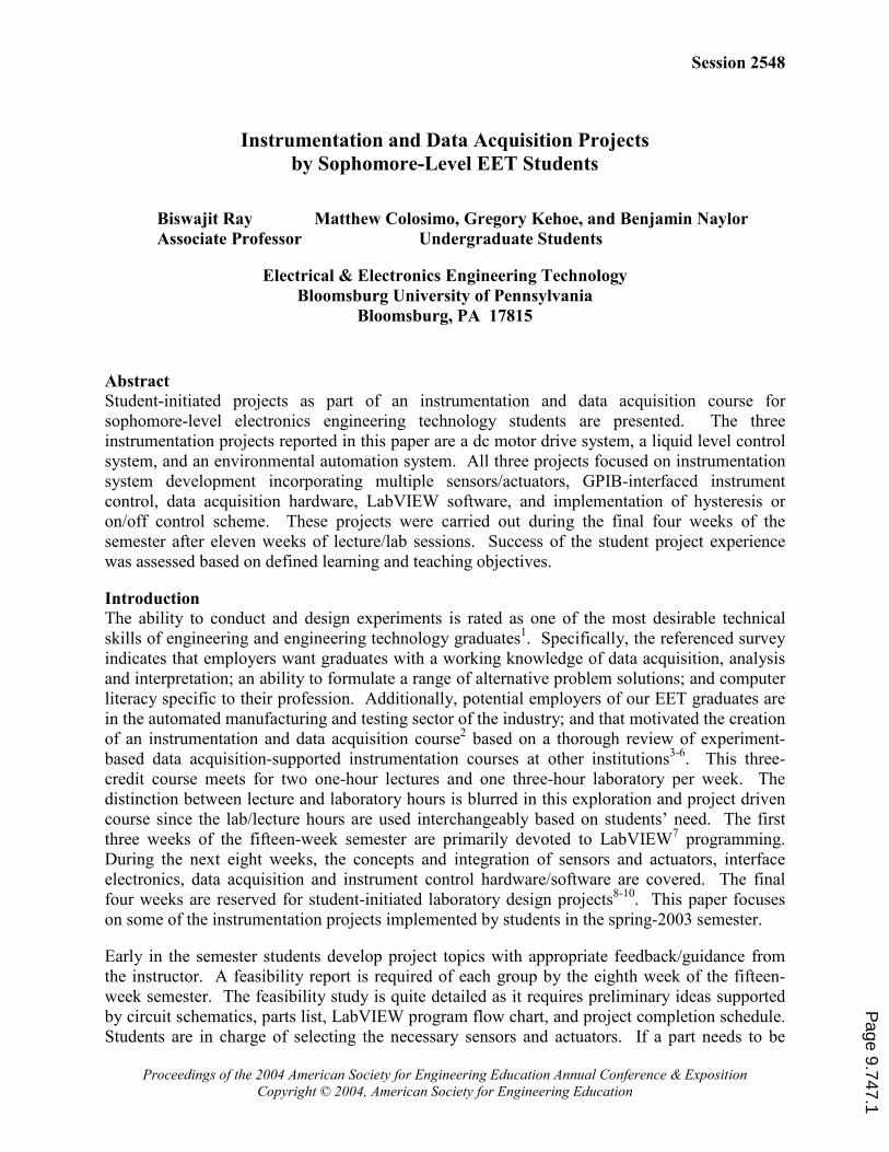
Project Learning Objectives: Project Teaching Objectives:

• Gain experience in interpreting technical

specifications and selecting sensors and transducers

for a given application

• Foster discovery, self-teaching, and encourage

desire and ability for life-long learning

• Understand terminologies associated with

instrumentation systems

• Provide an experience in designing an

instrumentation system based on specifications

• Gain experience in developing computerized

instrumentation systems for industrial processes

using multiple sensors, interface electronics, data

acquisition card, and GPIB and serial instruments

• Develop soft skills including teamwork, open-

ended problem solving, formal report writing and

presentation

Laboratory setup

Each station is equipped with a PC, and GPIB/RS-232 interfaced instruments such as digital

multimeter, triple output laboratory power supply, arbitrary function generator, and color two-

channel digital oscilloscope. The instrumentation and data acquisition specific software and

hardware are briefly described below.

Software: LabVIEW 6.0 from National Instruments7

Data acquisition (DAQ) board: Model 6024E from National Instruments

• 16 single-ended or 8 differential analog input channels, 12 bit resolution, 200 kS/s

• 2 analog voltage output channels, 12 bit resolution, 10 kHz update rate

• 8 digital I/O channels with TTL/CMOS compatibility; and Timing I/O

GPIB controller board:

• IEEE 488.2 compatible architecture (eight-bit parallel, byte-serial, asynchronous data transfer)

• Maximum data transfer rate of 1 MB/sec within the worst-case transmission line specifications

Signal conditioning accessory:

• Model SC-2075 from National Instruments

• Desktop signal breakout board with built-in power supplies, connects directly to 6024E DAQ board

Page 9.747.2

Session 2548



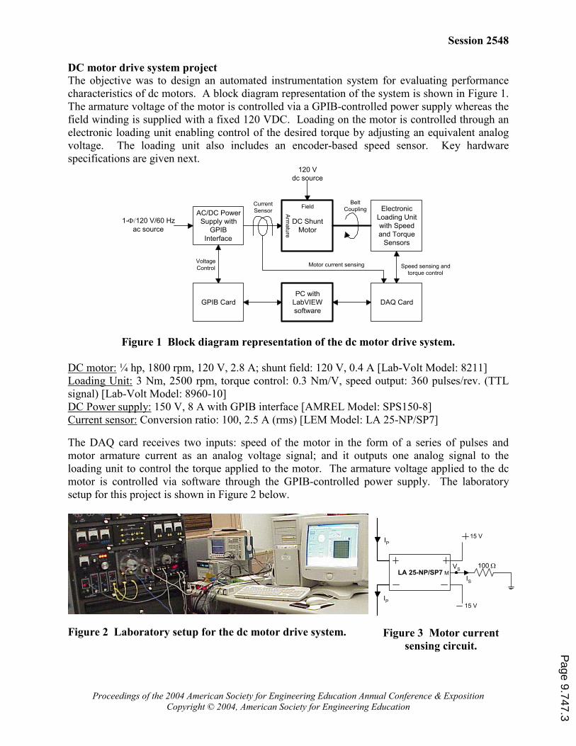
DC motor drive system project

The objective was to design an automated instrumentation system for evaluating performance

characteristics of dc motors. A block diagram representation of the system is shown in Figure 1.

The armature voltage of the motor is controlled via a GPIB-controlled power supply whereas the

field winding is supplied with a fixed 120 VDC. Loading on the motor is controlled through an

electronic loading unit enabling control of the desired torque by adjusting an equivalent analog

voltage. The loading unit also includes an encoder-based speed sensor. Key hardware

specifications are given next.

AC/DC Power

Supply with

GPIB

Interface

DC Shunt

Motor

Electronic

Loading Unit

with Speed

and Torque

Sensors

PC with

LabVIEW

software

GPIB Card DAQ Card

Armature

FieldCurrent

Sensor

1-Φ/120 V/60 Hz

ac source

Voltage

Control

120 V

dc source

Belt

Coupling

Motor current sensing Speed sensing and

torque control

Figure 1 Block diagram representation of the dc motor drive system.

DC motor: ¼ hp, 1800 rpm, 120 V, 2.8 A; shunt field: 120 V, 0.4 A [Lab-Volt Model: 8211]

Loading Unit: 3 Nm, 2500 rpm, torque control: 0.3 Nm/V, speed output: 360 pulses/rev. (TTL

signal) [Lab-Volt Model: 8960-10]

DC Power supply: 150 V, 8 A with GPIB interface [AMREL Model: SPS150-8]

Current sensor: Conversion ratio: 100, 2.5 A (rms) [LEM Model: LA 25-NP/SP7]

The DAQ card receives two inputs: speed of the motor in the form of a series of pulses and

motor armature current as an analog voltage signal; and it outputs one analog signal to the

loading unit to control the torque applied to the motor. The armature voltage applied to the dc

motor is controlled via software through the GPIB-controlled power supply. The laboratory

setup for this project is shown in Figure 2 below.

Figure 2 Laboratory setup for the dc motor drive system.

LA 25-NP/SP7 M

15 V

15 V

100 Ω

IS

IP

VS

IP

Figure 3 Motor current

sensing circuit.

Page 9.747.3

Session 2548



The current sensor used is a Hall effect based closed-loop current transducer providing complete

electrical isolation between the measured current and the output signal. As shown in Figure 3,

use of a 100 Ω resistor in the secondary current path provides a secondary voltage (VS) for the

DAQ system that represents the current signal being measured. The encoder output of the speed

signal is first filtered for high-frequency noise, via a simple R-C filter, before connecting it to

one of the counters of the DAQ board to calculate motor speed.

The implementation of a constant-speed motor drive system was undertaken without the

knowledge and use of feedback control system design concepts. This was achieved by recording

off-line the required armature voltage data as a function of load torque to maintain a constant

motor speed of 1275 rpm. The recorded data was then used to obtain a linear relationship

between the required armature voltage and load torque in order to implement the constant-speed

drive. The experimental data is shown in Figure 4. It can be seen that the motor speed range

obtained is approximately 1275 ± 5 rpm as the load was varied from 0 to 0.9 Nm, representing a

steady-state speed error of 0.4%. The automated open-loop control may be sufficient for low

performance drive systems; however, the appropriate next step would be to implement a closed-

loop PID controller under LabVIEW environment.

Figure 4 Constant speed operation of a dc motor drive system.

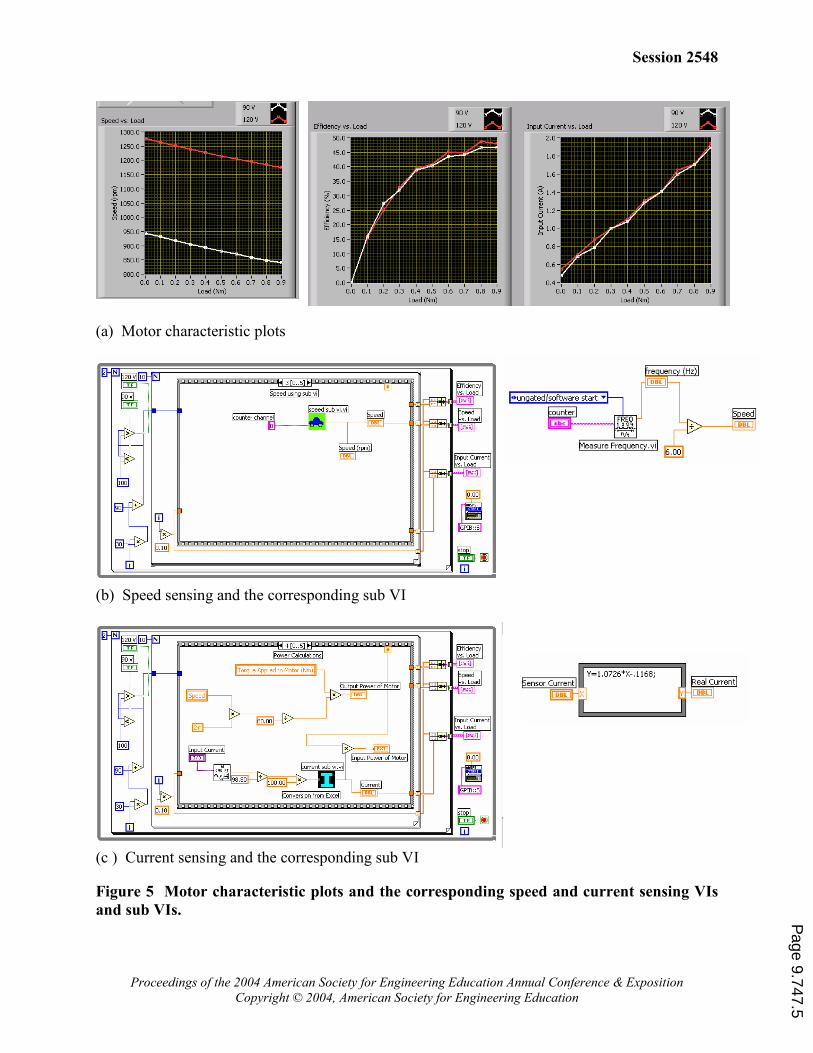
Next, the motor characteristics under variable load are obtained for armature voltages of 90 V

and 120 V. Specifically, speed-torque, efficiency-torque and armature current-torque

characteristics are obtained for operation from no-load (0 Nm) to full-load (0.9 Nm). The

graphical display and the corresponding speed and current measurement LabVIEW diagrams are

shown in Figure 5. The following observations can be made from the plots in Figure 5(a): for a

given load, the relationship between speed droop and loading is approximately linear; efficiency

of the motor is increasing with increasing load since the no-load loss is significant for this ¼ hp

motor; and the relationship between armature current and output torque is approximately linear

and practically independent of armature voltage since the motor flux is kept constant.

Speed and current sensing virtual instruments (VIs) and subVIs are shown in Figures 5(b) and

(c), respectively. A built-in frequency measurement subVI is used to calculate the motor speed

and a current measurement subVI is created to correlate measured current with real current per

calibration data obtained off-line.

Page 9.747.4

Session 2548



(a) Motor characteristic plots

(b) Speed sensing and the corresponding sub VI

(c ) Current sensing and the corresponding sub VI

Figure 5 Motor characteristic plots and the corresponding speed and current sensing VIs

and sub VIs.

Page 9.747.5



Liquid level control system project

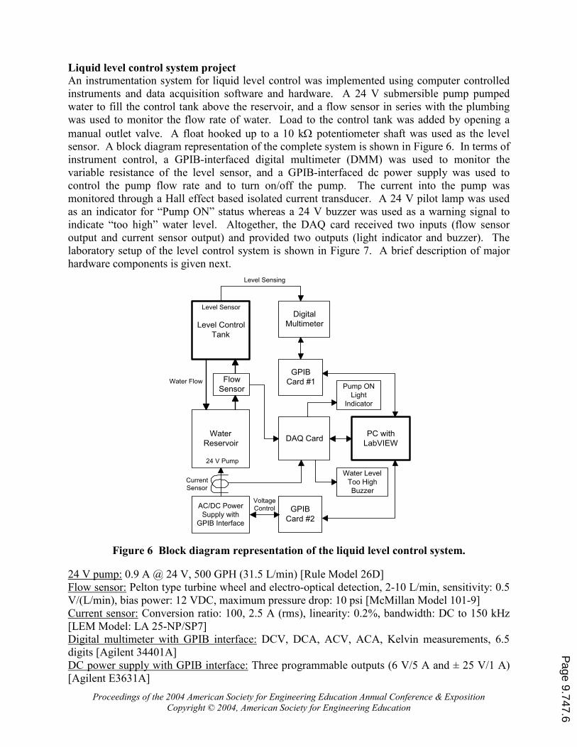
An instrumentation system for liquid level control was implemented using computer controlled

instruments and data acquisition software and hardware. A 24 V submersible pump pumped

water to fill the control tank above the reservoir, and a flow sensor in series with the plumbing

was used to monitor the flow rate of water. Load to the control tank was added by opening a

manual outlet valve. A float hooked up to a 10 kΩ potentiometer shaft was used as the level

sensor. A block diagram representation of the complete system is shown in Figure 6. In terms of

instrument control, a GPIB-interfaced digital multimeter (DMM) was used to monitor the

variable resistance of the level sensor, and a GPIB-interfaced dc power supply was used to

control the pump flow rate and to turn on/off the pump. The current into the pump was

monitored through a Hall effect based isolated current transducer. A 24 V pilot lamp was used

as an indicator for “Pump ON” status whereas a 24 V buzzer was used as a warning signal to

indicate “too high” water level. Altogether, the DAQ card received two inputs (flow sensor

output and current sensor output) and provided two outputs (light indicator and buzzer). The

laboratory setup of the level control system is shown in Figure 7. A brief description of major

hardware components is given next.

Water

Reservoir

Level Control

Tank

24 V Pump

Water Flow Flow

Sensor

Level Sensor

AC/DC Power

Supply with

GPIB Interface

Digital

Multimeter

GPIB

Card #2

GPIB

Card #1

DAQ Card

Current

Sensor

PC with

LabVIEW

Pump ON

Light

Indicator

Water Level

Too High

Buzzer

Voltage

Control

Level Sensing

Figure 6 Block diagram representation of the liquid level control system.

24 V pump: 0.9 A @ 24 V, 500 GPH (31.5 L/min) [Rule Model 26D]

Flow sensor: Pelton type turbine wheel and electro-optical detection, 2-10 L/min, sensitivity: 0.5

V/(L/min), bias power: 12 VDC, maximum pressure drop: 10 psi [McMillan Model 101-9]

Current sensor: Conversion ratio: 100, 2.5 A (rms), linearity: 0.2%, bandwidth: DC to 150 kHz

[LEM Model: LA 25-NP/SP7]

Digital multimeter with GPIB interface: DCV, DCA, ACV, ACA, Kelvin measurements, 6.5

digits [Agilent 34401A]

DC power supply with GPIB interface: Three programmable outputs (6 V/5 A and ± 25 V/1 A)

[Agilent E3631A]

Page 9.747.6



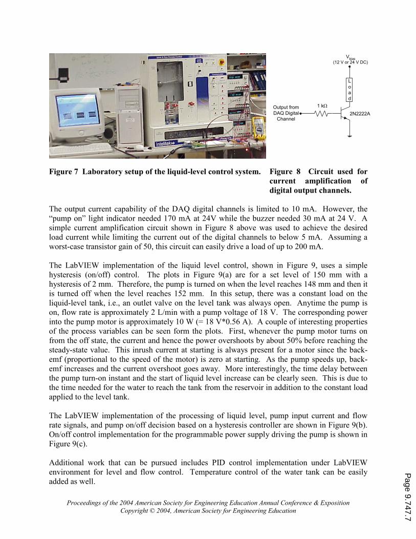
Figure 7 Laboratory setup of the liquid-level control system.

L

o

a

d

2N2222A

Vbias

(12 V or 24 V DC)

1 kΩOutput from

DAQ Digital

Channel

Figure 8 Circuit used for

current amplification of

digital output channels.

The output current capability of the DAQ digital channels is limited to 10 mA. However, the

“pump on” light indicator needed 170 mA at 24V while the buzzer needed 30 mA at 24 V. A

simple current amplification circuit shown in Figure 8 above was used to achieve the desired

load current while limiting the current out of the digital channels to below 5 mA. Assuming a

worst-case transistor gain of 50, this circuit can easily drive a load of up to 200 mA.

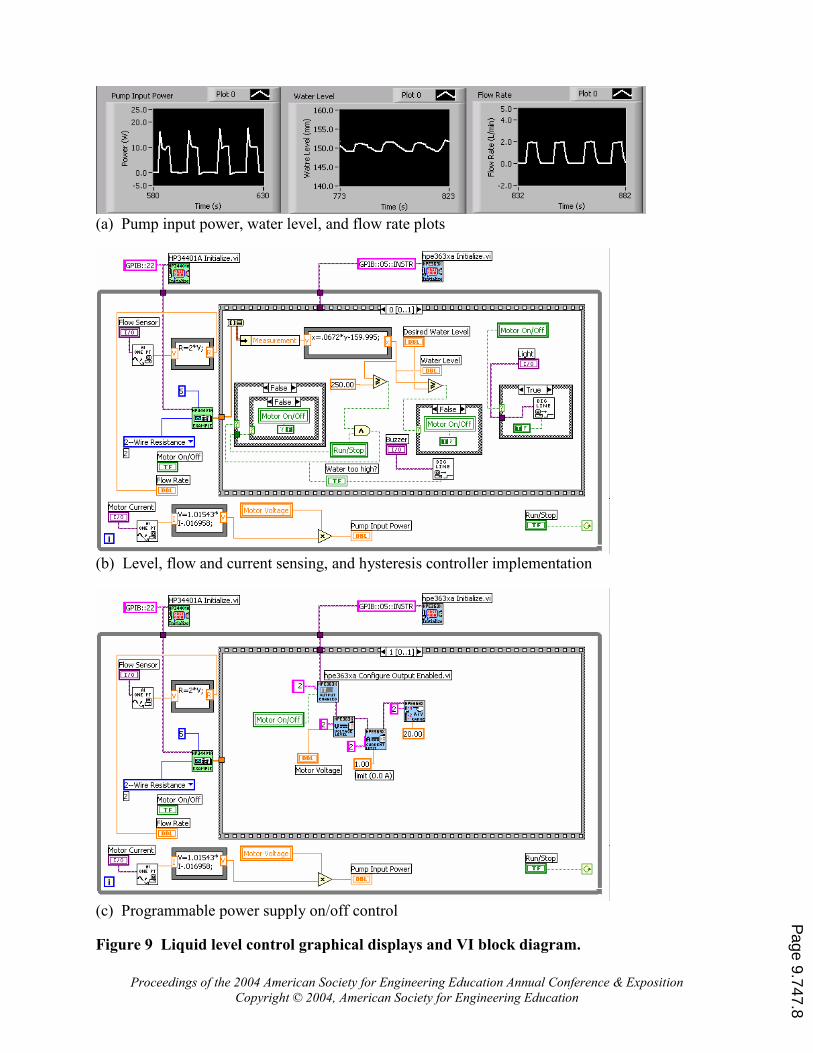
The LabVIEW implementation of the liquid level control, shown in Figure 9, uses a simple

hysteresis (on/off) control. The plots in Figure 9(a) are for a set level of 150 mm with a

hysteresis of 2 mm. Therefore, the pump is turned on when the level reaches 148 mm and then it

is turned off when the level reaches 152 mm. In this setup, there was a constant load on the

liquid-level tank, i.e., an outlet valve on the level tank was always open. Anytime the pump is

on, flow rate is approximately 2 L/min with a pump voltage of 18 V. The corresponding power

into the pump motor is approximately 10 W (= 18 V*0.56 A). A couple of interesting properties

of the process variables can be seen form the plots. First, whenever the pump motor turns on

from the off state, the current and hence the power overshoots by about 50% before reaching the

steady-state value. This inrush current at starting is always present for a motor since the back-

emf (proportional to the speed of the motor) is zero at starting. As the pump speeds up, back-

emf increases and the current overshoot goes away. More interestingly, the time delay between

the pump turn-on instant and the start of liquid level increase can be clearly seen. This is due to

the time needed for the water to reach the tank from the reservoir in addition to the constant load

applied to the level tank.

The LabVIEW implementation of the processing of liquid level, pump input current and flow

rate signals, and pump on/off decision based on a hysteresis controller are shown in Figure 9(b).

On/off control implementation for the programmable power supply driving the pump is shown in

Figure 9(c).

Additional work that can be pursued includes PID control implementation under LabVIEW

environment for level and flow control. Temperature control of the water tank can be easily

added as well.

Page 9.747.7



(a) Pump input power, water level, and flow rate plots

(b) Level, flow and current sensing, and hysteresis controller implementation

(c) Programmable power supply on/off control

Figure 9 Liquid level control graphical displays and VI block diagram.

Page 9.747.8



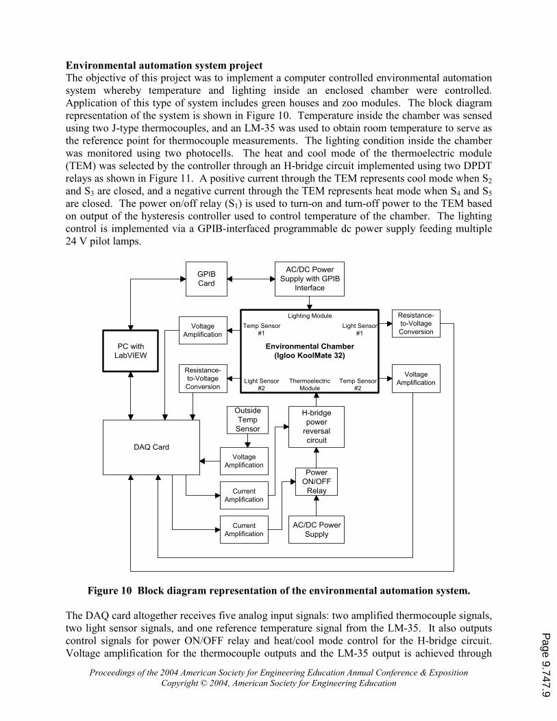
Environmental automation system project

The objective of this project was to implement a computer controlled environmental automation

system whereby temperature and lighting inside an enclosed chamber were controlled.

Application of this type of system includes green houses and zoo modules. The block diagram

representation of the system is shown in Figure 10. Temperature inside the chamber was sensed

using two J-type thermocouples, and an LM-35 was used to obtain room temperature to serve as

the reference point for thermocouple measurements. The lighting condition inside the chamber

was monitored using two photocells. The heat and cool mode of the thermoelectric module

(TEM) was selected by the controller through an H-bridge circuit implemented using two DPDT

relays as shown in Figure 11. A positive current through the TEM represents cool mode when S2

and S3 are closed, and a negative current through the TEM represents heat mode when S4 and S5

are closed. The power on/off relay (S1) is used to turn-on and turn-off power to the TEM based

on output of the hysteresis controller used to control temperature of the chamber. The lighting

control is implemented via a GPIB-interfaced programmable dc power supply feeding multiple

24 V pilot lamps.

Environmental Chamber

(Igloo KoolMate 32)

Thermoelectric

Module

Lighting Module

Light Sensor

#1

Light Sensor

#2

Temp Sensor

#1

Temp Sensor

#2

H-bridge

power

reversal

circuit

Power

ON/OFF

Relay

AC/DC Power

Supply

Outside

Temp

Sensor

AC/DC Power

Supply with GPIB

Interface

GPIB

Card

PC with

LabVIEW

DAQ Card

Voltage

Amplification

Resistance-

to-Voltage

Conversion

Voltage

Amplification

Current

Amplification

Current

Amplification

Voltage

Amplification

Resistance-

to-Voltage

Conversion

Figure 10 Block diagram representation of the environmental automation system.

The DAQ card altogether receives five analog input signals: two amplified thermocouple signals,

two light sensor signals, and one reference temperature signal from the LM-35. It also outputs

control signals for power ON/OFF relay and heat/cool mode control for the H-bridge circuit.

Voltage amplification for the thermocouple outputs and the LM-35 output is achieved through

.747.9



the use of low-cost instrumentation amplifier (AD622 from Analog Devices) as shown in Figure

12. The gain of the amplification stage is easily adjusted with the variable gain resistor (RG).

The digital outputs used to drive the relay coils go through a current amplification stage as

shown in Figure 8. The variable resistance of the photoresistor light sensors is changed to a

variable voltage signal using a simple voltage divider circuit.

Thermoelectric

Module

S1

S2

S4

S3

S5

12 V

Power ON/OFF

Relay

Figure 11 H-bridge used in selecting

heat/cool mode for TEM.

15 V

15 V

65

4

71

8

2

3

RG AD622

VOUT

to Analog

Input Channel

of DAQ

Figure 12 Voltage amplification circuit.

Figure 13 below shows the experimental setup of the environmental control system. The major

hardware used is the Igloo KoolMate 32 cooling/heating unit. This is a 48 W (4 A @ 12 V), 32-

quart unit and cools to 45oF below outside temperature or heats to 155

oF, and includes a 12 V

brushless fan for dissipation of heat into the ambient air. The exterior of the cooling/heating unit

is made of high-density polyethylene while the interior is made of polypropylene for effective

thermal insulation. This unit uses thermoelectric technology based on the Peltier effect12

, a

phenomenon discovered in 1834. The Peltier effect occurs whenever electrical current flows

through two dissimilar conductors. Depending on the direction of current flow, the junction of

the two conductors will either absorb or release heat. Semiconductors (usually Bismuth

Telluride) are the material of choice for producing the Peltier effect. As shown in Figure 14, by

arranging N and P-type pallets in a ‘couple’ and forming a junction between them with a plated

copper tab, it is possible to configure a series circuit which can keep all of the heat moving in the

same direction. It is possible to connect many pallets together in rectangular arrays to create

practical TEMs. The most common TEMs now in use - connecting 254 alternating N and P-type

pallets – can run from a 12 to 16 V dc supply and draw only 4 to 5 A.

Figure 13 Experimental setup for the environmental

automation system.

N P Hole

flow

Electron

flow

Absorbed

Heat

Absorbed

Heat

Released

HeatReleased

Heat

Figure 14 TEM building block.

Page 9.747.10



Some of the advantages of thermoelectric technology over compressor-based technology are

cooling of small areas, both heating and cooling with the same unit, operation independent of

mounting and physical orientation, and no need of evaporative chemicals which may be harmful

to the environment.

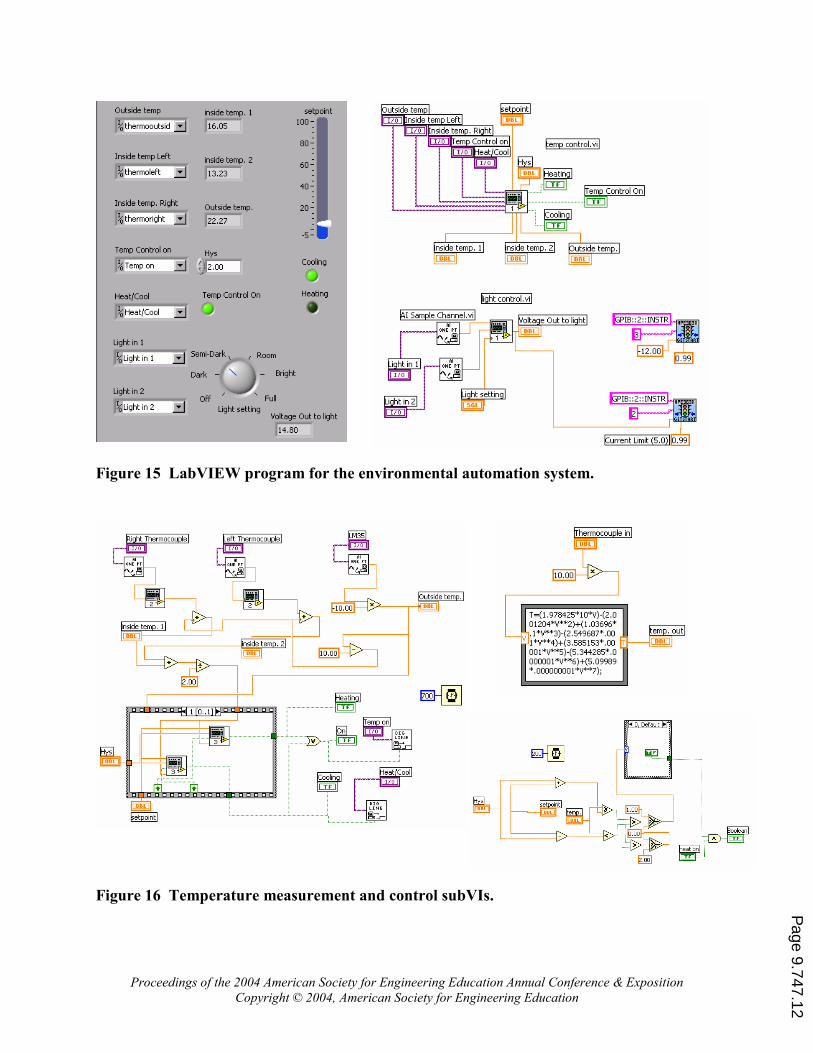
The LabVIEW programming for this project, shown in Figure 15, is very structured and uses

subVIs very effectively. The top level program consists of two subVIs, one for temperature

measurement and control and the other for light measurement and control. Sensor outputs are

read and control outputs are fed either to the relay coils or to control output voltage of the GPIB-

interfaced power supply for lighting control. Figure 16 shows the temperature measurement and

control subVI including the thermocouple measurement subVI and hysteresis controller subVI it

uses. The lighting control was implemented through the use of a GPIB-interfaced dc power

supply by increasing/decreasing its voltage in steps of 0.5 V until the desired lighting was

achieved.

Student feedback on project experience

The process of developing, implementing, and testing a project from scratch was an excellent

experience for most students. The majority of students were pleased with the project structure,

though a few suggested that the project duration within the instrumentation and data acquisition

course be extended to at least six weeks instead of the currently allocated four weeks.

Qualitative feedback from students is presented below through their comments.

Liked working with software and hardware integration

Enjoyed working with partner

Applying classroom knowledge to real-world examples was interesting

Great to have specification-based project development experience

Just getting to do a self-developed lab project was fun

Very interesting course……making me lean towards computer-based automation career

Organize a brain-storming session for developing project ideas early in the semester

Reliance on partner was a problem

Allocate more time to the coverage of interface electronics design

Include some biomedical measurements application

Summary

Experience with student-initiated projects within the instrumentation and data acquisition course

is presented. A few students struggled at the beginning of the four-week-long project period in

defining the scope of their work, as this was their first experience with project-based learning. It

was also observed that many students had not had to design, debug and test a system that had

multiple functional blocks in previous courses. Most students had difficulty breaking the design

into functional modules and designing and testing them separately before putting them together.

Improving student competence in this area will be incorporated at the next offering of projects

within the instrumentation and data acquisition course. Overall, the experience has been very

rewarding and challenging for the instructor as well as the students. More assessment data needs

to be gathered to ensure that the stated learning and teaching objectives are met.

Page 9.747.11



Figure 15 LabVIEW program for the environmental automation system.

Figure 16 Temperature measurement and control subVIs.

Page 9.747.12



Bibliography 1. J. D. Lang et al., “Industry Expectations of New Engineers: A Survey to Assist Curriculum Designers,” Journal

of Engineering Education, pp. 43-51, Jan 1999.

2. B. Ray, “An Instrumentation and Data Acquisition Course for Electronics Engineering Technology Students,”

ASEE Annual Conference Proceedings, 2003.

3. H. Sumali, “An Instrumentation and Data Acquisition Course at Purdue University,” ASEE Annual Conference

Proceedings, 2002.

4. S. C. Crist, “A Laboratory-Based Instrumentation Course for Non-EE Majors,” ASEE Annual Conference

Proceedings, 2001.

5. C. Chen, “Using LabVIEW in Instrumentation and Control Course,” ASEE Annual Conference Proceedings,

2001.

6. A. Bruce Buckman, “A Course in Computer-based Instrumentation: Learning LabVIEW with Case Studies,”

Int. Journal of Engineering Education, Vol. 16, No. 3, pp. 228-233, 2000.

7. www.ni.com

8. C. Yeh et al., “Undergraduate Research Projects for Engineering Technology Students,” ASEE Annual

Conference Proceedings, 2003.

9. J. S. Dalton et al., “Mini-Lab Projects in the Undergraduate Classical Controls Course,” ASEE Annual


10. R. Bachnak et al., “Data Acquisition for Process Monitoring and Control,” ASEE Annual Conference

Proceedings, 2003.

11. T. Rutar et al., “Short-term course assessment, improvement, and verification feedback loop,” ASEE Annual


12. “Peltier”, www.naijiw.com/peltier/peltier.html

BISWAJIT RAY

Biswajit Ray is currently with the Electrical & Electronics Engineering Technology program at the Bloomsburg

University of Pennsylvania. Previously, he was with the Department of Electrical & Computer Engineering at the

University of Puerto Rico – Mayaguez, and EMS Technologies, Nocross, GA.

Page 9.747.13

Instrumentation And Data Acquisition Projects By Sophomore ...

Documents

Transcript of Instrumentation And Data Acquisition Projects By Sophomore ...