
Synchronous data acquisition with wireless sensor networks
352
Advances in Automaon Engineering Band 4 Editor: Clemens Gühmann Universitätsverlag der TU Berlin Jürgen Helmut Funck Synchronous data acquision with wireless sensor networks
-
Upload
khangminh22 -
Category
Documents
-
view
0 -
download
0
Transcript of Synchronous data acquisition with wireless sensor networks
Advances in Automation Engineering Band 4
Editor: Clemens Gühmann
Universitätsverlag der TU Berlin
Jürgen Helmut Funck
Synchronous data acquisition with wireless sensor networks


Jürgen Helmut FunckSynchronous data acquisitionwith wireless sensor networks

The scientific series Advances in Automation Engineering is edited by Prof. Dr.-Ing. Clemens Gühmann.

Advances in Automation Engineering | 4
Jürgen Helmut Funck
Synchronous data acquisitionwith wireless sensor networks
Universitätsverlag der TU Berlin

Bibliographic information published by the Deutsche NationalbibliothekThe Deutsche Nationalbibliothek lists this publication in the Deutsche Nationalbibliografie; detailed bibliographic data are available on the Internet at http://dnb.dnb.de.
Universitätsverlag der TU Berlin, 2018http://verlag.tu-berlin.de
Fasanenstr. 88, 10623 BerlinTel.: +49 (0)30 314 76131 / Fax: -76133E-Mail: [email protected]
Zugl.: Berlin, Techn. Univ., Diss., 2017Gutachter: Prof. Dr.-Ing. Clemens GühmannGutachter: Prof. Dr.-Ing. Gerd SchollGutachter: Prof. Dr.-Ing. Reinhold Orglmeister Die Arbeit wurde am 12. Oktober 2017 an der Fakultät IV unter Vorsitz von Prof. Dr.-Ing. Olaf Hellwich erfolgreich verteidigt.
This work is protected by copyright.
Cover image: vickysandoval22 | https://www.flickr.com/photos/115327016@N06/12603289253/ | CC BY 2.0https://creativecommons.org/licenses/by/2.0/
Print: docupoint GmbHLayout/Typesetting: Jürgen Helmut Funck
ISBN 978-3-7983-2980-5 (print) ISBN 978-3-7983-2981-2 (online)
ISSN 2509-8950 (print)ISSN 2509-8969 (online)
Published online on the institutional Repository of the Technische Universität Berlin:DOI 10.14279/depositonce-6716http://dx.doi.org/10.14279/depositonce-6716

Credits
This thesis is the result of my time as research assistant at the Chair of ElectronicMeasurement and Diagnostic Technology at the Technische Universitat Berlin. I’d liketo take this opportunity to give my special thanks to Prof. Dr.-Ing. Clemens Guhmann,the head of this chair, who encouraged my research into the topic and has shown aconsistent, benevolent interest in my work.
Furthermore, I’d like to thank Prof. Dr.-Ing. Gerd Scholl, head of the Chair of ElectricalMeasurement Engineering at the Helmut-Schmidt-University, University of the FederalArmed Forces Hamburg, and Prof. Dr.-Ing. Reinhold Orglmeister, head of the Chairof Electronics and Medical Signal Processing at the Technische Universitat Berlin, forspending their time to examine this rather comprehensive thesis. My thanks also goto Prof. Dr.-Ing. Olaf Hellwich, head of the Chair of Computer Vision and RemoteSensing at the Technische Universitat Berlin, who acted as a mentor for me in my firstyears of study and now chaired my doctoral committee.
I’d also like to express my appreciation for my former colleagues at the Chair of Elec-tronic Measurement and Diagnostic Technology, the talks and discussions with whominspired and encouraged me. They contributed to an amiable working atmosphere thatwas a constant source of support.
I owe thanks to the members of the joint mechatronic workshop of the Chairs of Elec-tronic Measurement and Diagnostic Technology and of Electronic and Medical SignalProcessing for helping me to refit and extent the induction motor test bench as well asfor etching innumerable PCB-layouts for my research.
Furthermore, I thank Dr.-Ing. Henri Kretschmer and Mr. Torsten Huter from the Virte-nio GmbH for readily supporting me, when I had questions regarding the sensor nodesor their programming.
I also like to thank the students who I was allowed to counsel during their projects,bachelor’s and master’s theses. They helped to extend the capabilities of the wirelesssensor network and thus made it more useful not only for my research but also for otherresearch projects.
Finally, I’d like to thank my friends and family for their unconditional support andunderstanding during all phases of my research.
v


Abstract
Wireless sensor networks (WSN) are predicted to play a key role in future technologicaldevelopments like the internet of things. Already they are beginning to be used inmany applications not only in the scientific and industrial domains. One of the biggestchallenges, when using WSNs, is to fuse and evaluate data from different sensor nodes.Synchronizing the data acquisition of the nodes is a key enabling factor for this. So farresearch has been focused on synchronizing the clocks of the nodes, largely neglectingthe implications for the actual measurement results.
This thesis investigates the relation between synchronization accuracy and quality ofmeasurement results. Two different classes of time synchronous data acquisition areinvestigated: event detection and waveform sampling. A model is developed that de-scribes a WSN as a generic multi-channel data acquisition system, thus enabling directcomparison to other existing systems. With the help of this model it is shown, that syn-chronization accuracy should best be expressed as uncertainty of the acquired timinginformation. This way, not only the contribution of the synchronization to the over-all measurement uncertainty can be assessed, but also the synchronization accuracyrequired for an application can be estimated.
The insights from the uncertainty analysis are used to develop two distinct approachesto synchronous data acquisition: a proactive and a reactive one. It is shown that thereactive approach can also be used to efficiently implement synchronous angular sam-pling, i.e. data acquisition synchronous to the rotation of a machine’s shaft. Further-more, testing methods are suggested, that evaluate the synchronized data acquisition ofan existing WSN as a whole. These methods can be applied to other data acquisitionsystems without changes, thus enabling direct comparisons.
The practical realization of a WSN is described, on which the developed data acqui-sition methods have been implemented. All implementations were thoroughly testedin experiments, using the suggested testing methods. This way it was revealed, that asystem’s interrupt handling procedures may have a strong influence on the data acquisi-tion. Furthermore, it was shown that the effective use of fixed-point arithmetic enablessynchronous angular sampling in real-time during a streaming measurement. Finally,two application examples are used to illustrate the utility of the implemented data ac-quisition: the acoustic localization of two sensor nodes on a straight line and a simpleorder tracking at an induction motor test bench.
vii

Kurzfassung
Drahtlose Sensor Netzwerke (WSN) werden voraussichtlich entscheidend fur techni-sche Entwicklungen wie das Internet der Dinge sein. Schon jetzt werden sie in zahl-reichen Anwendungen u.a. in Wissenschaft und Industrie eingesetzt. Eine der großtenHerausforderungen hierbei ist, die Daten von verschiedenen Sensorknoten gemeinsamauszuwerten. Dies ist oft dann nur sinnvoll moglich, wenn die Daten synchron auf-genommen wurden. Bisher konzentrierte sich Forschung auf die Synchronisation derUhren auf den Sensorknoten. Die Auswirkungen auf die Messergebnisse selbst wurdenhingegen kaum untersucht.
Diese Dissertation untersucht die Zusammenhange zwischen Synchronisationsgenau-igkeit und Qualitat der Messergebnisse. Zwei Klassen von zeitsynchroner Datenerfas-sung werden dabei betrachtet: die Detektion von Ereignissen und die Aufnahme vonKurvenformen. Es wird ein Modell entwickelt, welches ein WSN als ein allgemeinesmehrkanaliges Datenerfassungssystem beschreibt. Dies ermoglicht den direkten Ver-gleich zwischen WSN und anderen Messsystemen. Weiter wird mit Hilfe des Modellsgezeigt, dass die Synchronisationsgenauigkeit vorzugsweise als Unsicherheit der Zeit-information angegeben werden sollte. Hierdurch kann nicht nur der Beitrag der Syn-chronisation zur gesamten Messunsicherheit bestimmt, sondern auch die von einer An-wendung tatsachlich benotigte Synchronisationsgenauigkeit abgeschatzt werden.
Ausgehend von den durch die Unsicherheitsbetrachtung gewonnenen Erkenntnissenwerden ein proaktiver und ein reaktiver Ansatz zur synchronen Datenaufnahme entwi-ckelt. Mit dem reaktiven Ansatz konnen Messdaten auch effizient drehwinkelsynchron,d. h. synchron zur Drehbewegung einer Maschinenwelle, aufgenommen werden. Eswerden Testverfahren vorgeschlagen, mit denen sich die Synchronizitat der Datenerfas-sung fur ein WSN als Ganzes uberprufen lasst. Diese Verfahren lassen sich unverandertauf andere Messsysteme anwenden und ermoglichen somit direkte Vergleiche.
Es wird die praktische Umsetzung eines WSN beschrieben, auf dem die entwickeltenMethoden zur Datenerfassung implementiert wurden. Alle Implementierungen wurdenmit den vorgeschlagenen Testverfahren untersucht. Hierdurch konnte gezeigt werden,dass die Interrupt-Bearbeitung der Sensorknoten entscheidenden Einfluss auf die Mess-datenerfassung hat. Weiter konnte durch den Einsatz von Fixed-Punkt-Arithmetik diedrehwinkelsynchrone Datenerfassung in Echtzeit realisiert werden. Schließlich wird dieNutzlichkeit der implementierten Datenerfassung an zwei Anwendungen gezeigt: derakustischen Ortung zweier Sensorknoten sowie einer einfachen Ordnungsanalyse.
viii

Contents
1. Introduction 11.1. Thesis structure . . . . . . . . . . . . . . . . . . . . . . . . . . . . . . 21.2. Thesis contribution . . . . . . . . . . . . . . . . . . . . . . . . . . . . 3
2. Literature review 52.1. Wireless sensor networks . . . . . . . . . . . . . . . . . . . . . . . . . 5
2.1.1. Hardware . . . . . . . . . . . . . . . . . . . . . . . . . . . . . 52.1.2. Software . . . . . . . . . . . . . . . . . . . . . . . . . . . . . 132.1.3. Network topologies . . . . . . . . . . . . . . . . . . . . . . . . 162.1.4. Network protocols . . . . . . . . . . . . . . . . . . . . . . . . 182.1.5. Conclusions . . . . . . . . . . . . . . . . . . . . . . . . . . . . 27
2.2. Time synchronization protocols . . . . . . . . . . . . . . . . . . . . . . 282.2.1. Classes of synchronization . . . . . . . . . . . . . . . . . . . . 282.2.2. Building blocks of synchronization protocols . . . . . . . . . . 302.2.3. Evaluation of synchronization protocols . . . . . . . . . . . . . 352.2.4. Synchronization protocols for wireless sensor networks . . . . . 362.2.5. Synchronization protocols in other domains . . . . . . . . . . . 402.2.6. Conclusions . . . . . . . . . . . . . . . . . . . . . . . . . . . . 44
2.3. Data Acquisition with wireless sensor networks . . . . . . . . . . . . . 442.3.1. Data acquisition . . . . . . . . . . . . . . . . . . . . . . . . . 452.3.2. Time synchronous data acquisition . . . . . . . . . . . . . . . . 482.3.3. Wireless sensors and smart sensors . . . . . . . . . . . . . . . 492.3.4. Conclusions . . . . . . . . . . . . . . . . . . . . . . . . . . . . 51
2.4. Synchronous angular sampling . . . . . . . . . . . . . . . . . . . . . . 522.4.1. Significance and applications . . . . . . . . . . . . . . . . . . . 522.4.2. Algorithms . . . . . . . . . . . . . . . . . . . . . . . . . . . . 54
2.5. Conclusions . . . . . . . . . . . . . . . . . . . . . . . . . . . . . . . . 56
3. Theoretical foundations 593.1. Time and synchronization . . . . . . . . . . . . . . . . . . . . . . . . . 59
3.1.1. Time . . . . . . . . . . . . . . . . . . . . . . . . . . . . . . . 593.1.2. Clocks . . . . . . . . . . . . . . . . . . . . . . . . . . . . . . 613.1.3. Synchronization . . . . . . . . . . . . . . . . . . . . . . . . . 633.1.4. Generalized time . . . . . . . . . . . . . . . . . . . . . . . . . 63
ix
Contents
3.2. Data acquisition . . . . . . . . . . . . . . . . . . . . . . . . . . . . . . 633.2.1. Uniform sampling . . . . . . . . . . . . . . . . . . . . . . . . 643.2.2. Nonuniform sampling . . . . . . . . . . . . . . . . . . . . . . 663.2.3. Data acquisition structures . . . . . . . . . . . . . . . . . . . . 68
3.3. Digital resampling . . . . . . . . . . . . . . . . . . . . . . . . . . . . 703.3.1. Spectral effects and filter requirements . . . . . . . . . . . . . . 703.3.2. Filter algorithms . . . . . . . . . . . . . . . . . . . . . . . . . 743.3.3. Number formats . . . . . . . . . . . . . . . . . . . . . . . . . 83
3.4. Quality of measurements and signals . . . . . . . . . . . . . . . . . . . 873.4.1. Measurement uncertainty . . . . . . . . . . . . . . . . . . . . . 873.4.2. Signal quality . . . . . . . . . . . . . . . . . . . . . . . . . . . 923.4.3. Estimation of signal parameters . . . . . . . . . . . . . . . . . 94
4. Modeling 994.1. System model . . . . . . . . . . . . . . . . . . . . . . . . . . . . . . . 99
4.1.1. Event detection . . . . . . . . . . . . . . . . . . . . . . . . . . 994.1.2. Waveform sampling . . . . . . . . . . . . . . . . . . . . . . . 100
4.2. Acquisition errors . . . . . . . . . . . . . . . . . . . . . . . . . . . . . 1014.2.1. Event detection . . . . . . . . . . . . . . . . . . . . . . . . . . 1014.2.2. Waveform sampling . . . . . . . . . . . . . . . . . . . . . . . 1064.2.3. Specification of synchronization precision . . . . . . . . . . . . 113
4.3. Estimation of the required synchronization precision . . . . . . . . . . 1134.4. Approaches to time synchronous data acquisition . . . . . . . . . . . . 114
4.4.1. Event detection . . . . . . . . . . . . . . . . . . . . . . . . . . 1154.4.2. Waveform sampling . . . . . . . . . . . . . . . . . . . . . . . 115
4.5. Approaches to synchronous angular sampling . . . . . . . . . . . . . . 1164.6. Testing data acquisition systems . . . . . . . . . . . . . . . . . . . . . 118
4.6.1. Synchronous event detection . . . . . . . . . . . . . . . . . . . 1184.6.2. Synchronous waveform sampling . . . . . . . . . . . . . . . . 1194.6.3. Synchronous angular sampling . . . . . . . . . . . . . . . . . . 121
5. Implementation 1235.1. Wireless sensor network for experiments . . . . . . . . . . . . . . . . . 124
5.1.1. Sensor nodes . . . . . . . . . . . . . . . . . . . . . . . . . . . 1245.1.2. Execution environment . . . . . . . . . . . . . . . . . . . . . . 1285.1.3. TDMA-protocol . . . . . . . . . . . . . . . . . . . . . . . . . 1345.1.4. Data acquisition framework . . . . . . . . . . . . . . . . . . . 1355.1.5. Application transducers . . . . . . . . . . . . . . . . . . . . . 1475.1.6. Installation at induction motor test bench . . . . . . . . . . . . 157
5.2. Time synchronous data acquisition . . . . . . . . . . . . . . . . . . . . 1595.2.1. Synchronization services . . . . . . . . . . . . . . . . . . . . . 1595.2.2. Event detection . . . . . . . . . . . . . . . . . . . . . . . . . . 1655.2.3. Waveform acquisition . . . . . . . . . . . . . . . . . . . . . . 165
x

Contents
5.3. Synchronous angular sampling . . . . . . . . . . . . . . . . . . . . . . 1685.3.1. Choice of resampling algorithm . . . . . . . . . . . . . . . . . 1685.3.2. Filter adaptation . . . . . . . . . . . . . . . . . . . . . . . . . 1725.3.3. Filter design . . . . . . . . . . . . . . . . . . . . . . . . . . . 1725.3.4. Implementation of filter algorithm . . . . . . . . . . . . . . . . 1745.3.5. Network integration . . . . . . . . . . . . . . . . . . . . . . . 177
6. Experiments 1816.1. Wireless sensor network . . . . . . . . . . . . . . . . . . . . . . . . . 181
6.1.1. Power consumption . . . . . . . . . . . . . . . . . . . . . . . . 1816.1.2. Data throughput . . . . . . . . . . . . . . . . . . . . . . . . . 188
6.2. Time synchronous event detection . . . . . . . . . . . . . . . . . . . . 1926.2.1. Experimental setup . . . . . . . . . . . . . . . . . . . . . . . . 1936.2.2. Relative drift of clocks . . . . . . . . . . . . . . . . . . . . . . 1946.2.3. Synchronization precision . . . . . . . . . . . . . . . . . . . . 1956.2.4. Power consumption . . . . . . . . . . . . . . . . . . . . . . . . 2036.2.5. Conclusions . . . . . . . . . . . . . . . . . . . . . . . . . . . . 204
6.3. Application example: acoustic localization . . . . . . . . . . . . . . . . 2056.3.1. Model . . . . . . . . . . . . . . . . . . . . . . . . . . . . . . . 2056.3.2. Estimation of required synchronization accuracy . . . . . . . . 2066.3.3. Experiments . . . . . . . . . . . . . . . . . . . . . . . . . . . 2076.3.4. Results . . . . . . . . . . . . . . . . . . . . . . . . . . . . . . 2096.3.5. Uncertainty analysis . . . . . . . . . . . . . . . . . . . . . . . 2126.3.6. Conclusions . . . . . . . . . . . . . . . . . . . . . . . . . . . . 216
6.4. Time synchronous waveform acquisition . . . . . . . . . . . . . . . . . 2176.4.1. Experimental setup . . . . . . . . . . . . . . . . . . . . . . . . 2176.4.2. Signal quality . . . . . . . . . . . . . . . . . . . . . . . . . . . 2186.4.3. Missing samples . . . . . . . . . . . . . . . . . . . . . . . . . 2246.4.4. Power consumption . . . . . . . . . . . . . . . . . . . . . . . . 2256.4.5. Conclusions . . . . . . . . . . . . . . . . . . . . . . . . . . . . 226
6.5. Synchronous angular sampling . . . . . . . . . . . . . . . . . . . . . . 2276.5.1. Analysis of measurement chain for angular sampling . . . . . . 2276.5.2. Test of resampling algorithms . . . . . . . . . . . . . . . . . . 2316.5.3. Acquisition of generated signals . . . . . . . . . . . . . . . . . 2366.5.4. Data acquisition at motor test bench . . . . . . . . . . . . . . . 2406.5.5. Conclusions . . . . . . . . . . . . . . . . . . . . . . . . . . . . 246
7. Conclusions and outlook 2477.1. Summary . . . . . . . . . . . . . . . . . . . . . . . . . . . . . . . . . 2477.2. Conclusions . . . . . . . . . . . . . . . . . . . . . . . . . . . . . . . . 2487.3. Outlook . . . . . . . . . . . . . . . . . . . . . . . . . . . . . . . . . . 250
Bibliography 263
xi

Contents
Appendix 285
A. Sensor Nodes 287
B. Evaluating the polynomial kernel of a transposed Farrow filter 291
C. Application sensors 294C.1. Microphone . . . . . . . . . . . . . . . . . . . . . . . . . . . . . . . . 294C.2. Current and voltage sensors . . . . . . . . . . . . . . . . . . . . . . . . 295C.3. Rotary encoder . . . . . . . . . . . . . . . . . . . . . . . . . . . . . . 297
D. Angular resampling filer 298D.1. Filter design . . . . . . . . . . . . . . . . . . . . . . . . . . . . . . . . 298D.2. MATLAB implementation . . . . . . . . . . . . . . . . . . . . . . . . 300D.3. C implementations . . . . . . . . . . . . . . . . . . . . . . . . . . . . 302
D.3.1. C floating-point implementation . . . . . . . . . . . . . . . . . 302D.3.2. C fixed-point implementation . . . . . . . . . . . . . . . . . . 306D.3.3. C header files for floating- and fixed-point . . . . . . . . . . . . 313
E. Results of event timestamping experiments 315E.1. Network configuration 2 . . . . . . . . . . . . . . . . . . . . . . . . . 315E.2. Network configuration 3 . . . . . . . . . . . . . . . . . . . . . . . . . 317E.3. Network configuration 4 . . . . . . . . . . . . . . . . . . . . . . . . . 319E.4. Network configuration 5 . . . . . . . . . . . . . . . . . . . . . . . . . 321E.5. Network configuration 6 . . . . . . . . . . . . . . . . . . . . . . . . . 323E.6. Network configuration 7 . . . . . . . . . . . . . . . . . . . . . . . . . 324E.7. Network configuration 8 . . . . . . . . . . . . . . . . . . . . . . . . . 326
xii

Nomenclature
Notations
Notation DescriptionE(x) expectation value of random variable xQm.n Q-format of a fixed-point numberVar(x) variance value of random variable xX( jω) Fourier transform of x(t)∆x systematic error in x∆x difference in xx empirical mean of xδx random error in xϵx error in measurement of xF
x(t)
Fourier transform of x(t)
O( f (x)) Bachmann–Landau notation, i.e. grows asymptotically like f (x)σx true standard deviation of xX matrixx vectorx estimate or measurement value of xx value or measurement for x that is afflicted by errora b event a happened before event bf (x) mathematical functionfX probability density function of random variable Xsx empirical standard deviation of xux standard measurement uncertainty of xx′ modified version of x′/quantity similar to, but different from xx(t) continuous time signalx[n] discrete time signalxn nth member of a set of values
xiii

Symbols
Symbols
Symbol Description UnitG weighting factor of probability distributionH transfer function of a LTI-systemL interpolation factorM decimation factorNi ith sensor nodeN number of elements or samplesOS R oversampling ratioO signal order, i.e. signal component whose frequency is
an integer multiple of the rotational frequencyP0.25 25 %-percentile of a distributionP0.75 75 %-percentile of a distributionP probabilityQm.n Q-format of a fixed-point numberQ filter orderR rate change factorTs sampling interval sTclock clock resolution sTsync (re)synchronization interval sTtick clock resolution sT time interval sUk expanded uncertainty with coverage factor k arbVdc DC voltage VVpp peak-to-peak voltage VV electrical voltage VW signal bandwidth rad/sΦ angle interval radαt significance level of a statistical testαrms RMS-value of a signal arbαrot angular acceleration rad/s2
α amplitude of a sine wave arbδ Dirac delta functionη RMS-value of signal noise arbωN Nyquist frequency rad/sωp filter passband edge rad/sωs sampling frequency rad/sωsignal signal frequency rad/sωstop filter stopband edge rad/sω angular frequency rad/sϕ rotation angle rad
xiv

Symbol Description Unitρ clock drift ppmσ true standard deviationϑ temperature °Cc(t) clock sci sensitivity factor of uncertainty contribution arbfg filter 3 dB-cutoff frequency Hzfϕ angular rate 1/revf frequency Hzhc counter of a clockh impulse response of a LTI-systemk coverage factor of uncertaintyl counting indexnrot rotational speed rpmn counting indexpt p-value of a t-testp clock precision sq numeric resolution or counting indexs empirical standard deviationt time instant suc combined standard uncertainty arbu standard uncertainty arbvsound speed of sound m/sv degrees of freedomw white noise arbx generic quantity or signal arb
Abbreviations
6LoWPAN IPv6 over Low-Power Wireless Personal Area Networks
ADC analog-to-digital converter
API application programmers interface
ASCII American Standard Code for Information Interchange
BIPM International Bureau of Weights and Measures
BLE Bluetooth low energy
BNC Bayonet Neil-Concelman connector
BSD Berkley Software Distribution
xv

Abbreviations
CAN Controller Area Network bus
CIC cascaded integrator-comb filter
CMOS complementary metal-oxide-semiconductor
CMSIS Cortex Microcontroller Software Interface Standard
CoAP Constraint Application Protocol
CPU central processing unit
CRC cyclic redundancy check
CSMA carrier sense multiple access
CSMA/CA carrier sense multiple access with collision avoidance
CRB Cramer-Rao bound
DAG directed acyclic graph
DAQ data acquisition
DC direct current
DFT discrete Fourier transform
DSP digital signal processor
DSSS direct-sequence spread spectrum
DMA direct memory access
DMM digital multimeter
DTLS Datagram Transport Layer Security
ECG electrocardiogram
EMSP Chair of Electronics and Medical Signal Processing at the TU Berlin
ETA Elapsed Time on Arrival
EU European Union
FFD full-function device
FFT fast Fourier transform
FIFO first in, first out buffer
FIR finite impulse response filter
FPU floating-point unit
FTSP Flooding Time-Synchronization Protocol
xvi

Abbreviations
GPIO general-purpose input/output pin
GPS Global Positioning System
GUM guide to the expression of uncertainty in measurement
HTTP Hypertext Transfer Protocol
HRTS Hierarchy Referencing Time Synchronization
ID identification number
IEC International Electrotechnical Commission
IETF Internet Engineering Task Force
IIR infinite impulse response filter
IP Internet Protocol
IPv6 Internet Protocol version 6
IRQ interrupt request
ISA International Society of Automation
ISM industrial, scientific and medical
ISO International Organization for Standardization
LED light-emitting diode
LLN low-power and lossy network
LTI linear time-invariant system
LOADng Lightweight Ad hoc On-Demand - Next Generation
MAC medium access control
MDT Chair of Electronic Measurement and Diagnostic Technology at the TU Berlin
MEMS microelectromechanical systems
MSTL MDT smart transducer library
MUX multiplexer
NAD noise and distortion
NCAP network-capable application processor
NTP Network Time Protocol
OS operating system
OSR oversampling ratio
xvii

Abbreviations
PC personal computer
PCB printed circuit board
PI proportional-integral
PHY physical layer
PLL phase-locked loop
PLC power-line-cycle
PPG Photoplethysmogram
PPS one pulse per second
PTP Precision Time Protocol
RAM random access memory
RBS Reference Broadcast Synchronization
RC resistor-capacitor circuit/oscillator
RDC radio duty-cycling
rev revolution
RF radio frequency
RFD reduced-function device
RITS Routing Integrated Time Synchronization
RMS root-mean-square value
RMSE root-mean-square error
RPL Routing Protocol for Low-Power and Lossy Networks
RTC real-time clock
RTP Real-Time Transport Protocol
RTSI Real-Time System Integration bus
SAR successive approximation ADC
SCTS Self-Correcting Time Synchronization
S&H sample-and-hold
SI International System of Units
SINAD signal-to-noise and distortion ratio
SNMP Simple Network Management Protocol
xviii

Abbreviations
SNR signal-to-noise ratio
SPI serial peripheral interface
STFT short-time Fourier transform
TCP Transmission Control Protocol
TDMA time division multiple access
TEDS transducer electronic data sheet
THD total harmonic distortion
THE total harmonic energy
TIM transducer interface module
TPSN Timing-Sync Protocol for Sensor Networks
TSCH time-synchronized channel hopping
TSMP Time Synchronized Mesh Protocol
UART universal asynchronous receiver transmitter
µC microcontroller
UDP User Datagram Protocol
USB Universal Serial Bus
UTC Coordinated Universal Time
VM virtual machine
WISA Wireless Interface for Sensors and Actuators
WLAN wireless local area network
WSN wireless sensor network
WTIM wireless transducer interface module
xix


1. Introduction
Wireless sensor networks (WSN) are networks of small, low-cost sensing deviceswith integrated processing capabilities that communicate wirelessly with each other[64, 138, 50]. They are seen as a key component in technological visions like ambientintelligence [64], the internet of things [128] or cyber-physical systems [80]. Alreadya broad spectrum of applications for WSNs has been explored in areas including envi-ronmental monitoring, health care, home automation, condition monitoring, industrialautomation and scientific data acquisition [64, 138, 50].
The key advantage of WSNs is the ease of installation and extension that arises fromnot having to lay cables [64, 81, 113, 63, 59]. The resulting reduction in workingtime together with reduced material usage can lead to significant cost reductions [64,63]. Furthermore, digitizing and processing sensor data directly at the spot, where itis acquired, can increase its quality as well as its utility. Other advantages of WSNsare the mobility of the wireless sensing devices [64] and the possibility to easily extendtheir capabilities through software updates [63].
WSNs are a comparatively new research topic, with only few publications before theyear 2000 [138]. However, in the last 16 years, WSNs have enjoyed strongly increas-ing attention from scientist and science funding bodies [138]. WSNs are an inherentlymultidisciplinary area of research. The topics involved range from the miniaturizationof electronic components over energy storage, low power electronics, radio communi-cation and software design to measurement data processing and user interaction [64].
One of the biggest challenges, when using WSNs, is to efficiently combine and processthe measurements from multiple sensor nodes. Knowing the time relation betweendata from different nodes is a prerequisite for deriving a consistent observation of theenvironment. Therefore, synchronizing the data acquisition of multiple nodes is of keyimportance. So far, a lot of research effort has been put into accurately and efficientlysynchronizing the clocks of wireless sensor nodes [79, 119, 64]. However, the effectof the synchronization accuracy on the quality of measurement results has hardly beenstudied. Not even a commonly accepted measure of synchronization accuracy seemsto exist. Furthermore, the focus on synchronizing clocks has occluded the fact, that inmany applications it is more important to synchronize to external events or processes.An example of this is the angular position of a rotation machine in synchronous angularsampling.
1

1. Introduction
The goal of this thesis is to investigate key metrological aspects of synchronous dataacquisition with WSNs, especially the relation between synchronization accuracy andquality of measurement results. The results of this investigation are used to optimizestrategies for time synchronous data acquisition. Furthermore, the strategies for timesynchronous sampling are generalized, in order to enable synchronous angular sam-pling on a WSN. A focus is put on applications in the scientific and industrial domains.As WSNs are a very multidisciplinary topic, this thesis aims to be understandable toreaders from various backgrounds in engineering and computer science. Therefore,fundamental concepts from the individual disciplines are briefly introduced before theirusage.
1.1. Thesis structure
This thesis is structured as follows:
Chapter 2 - Literature reviewThe current literature on WSN, time synchronization and synchronous angular sam-pling is reviewed in this section. Through this, key concepts and terminology in thosefields are introduced as well. The results of this review are used to identify deficienciesin the current state of the art. At the end of the chapter the guiding questions of thisthesis are formulated.
Chapter 3 - Theoretical foundationsThis chapter lays the theoretical foundations for those following. It starts by reviewingthe essential properties of time, synchronization and clocks. After this, the structuresand theorems fundamental to data acquisition are given. The basic ideas and algorithmsfor digital resampling are treated, as they will be used to process and synchronize datain later chapters. Finally, the concept of measurement uncertainty as defined by theguide to the expression of uncertainty in measurement (GUM) and quality indicatorsfor acquired waveforms are introduced.
Chapter 4 - ModelingThe models and quantitative measures, that describe the effect of synchronization ac-curacy on the quality of measurements, are developed in this chapter. Building on thismodeling, a method to estimate the required synchronization accuracy is derived. Fur-thermore, strategies for the synchronous data acquisition with WSNs and methods totest the synchronization precision are developed.
Chapter 5 - ImplementationThis chapter describes the WSN that was built-up for this thesis and used in the experi-ments. First, the general aspects of the WSN are introduced, including the sensor nodesand software environment, that were chosen. Second, the software framework for dataacquisition and applications sensors, that were developed for this thesis are described.
2
1.2. Thesis contribution
Furthermore, the installation of the WSN at an induction motor test bench is presented.Finally, the implementations of time synchronized data acquisition and synchronousangular sampling on the WSN are described in detail.
Chapter 6 - ExperimentsThe experiments, which were done to characterize the implementations of synchronousdata acquisition, and their results are presented in this chapter. First, the data throughputand power consumption of the WSN are investigated. Next, the synchronous eventtimestamping of the WSN is examined and used for the acoustic localization of sensornodes. Furthermore, experimental results for synchronous waveform acquisition withthe WSN are discussed. The chapter concludes with synchronous angular samplingexperiments on simulated signals as well as at an induction motor test bench.
Chapter 7 - Conclusions and outlookThis chapter summarizes and discusses the key results of the investigations. As a re-sult of this discussion, answers to the guiding questions of this thesis are formulated.Finally, possible directions for new research following this thesis are outlined.
1.2. Thesis contribution
The key contributions of this thesis can be summarized as follows:
1. Models for the time synchronous data acquisition with WSNs have been devel-oped (see section 4.1 and 4.2). Those, models have been proven to be useful fordescribing and optimizing synchronous data acquisition with a WSN (see section4.4).
2. Measures of quality for synchronous data acquisition have been defined in sec-tion 4.2. These measures can be used to calculate the measurement uncertaintyaccording to the GUM as demonstrated for the example of acoustic localizationin section 6.3.
3. It has been shown, that influences other than synchronization errors, e.g. signalnoise, analog group delay and even the clock resolution itself, can lead to equiv-alent errors in the measurement result (see sections 4.2 and 6.3). Thus, furtheroptimizing the synchronization accuracy is not sensible, if its influence is smallcompared to those other error sources.
4. It has been shown in section 4.2.1.6, that the uncertainty of a synchronized clockcan be expressed through an effective clock resolution. This enables a fast andintuitive evaluation of synchronized time sources. In this, the effective clockresolution is similar to the effective number of bits, which is commonly used tocharacterize analog-to-digital converters.
3

1. Introduction
5. A procedure, that can be used estimate the required synchronization accuracygiven the maximum desired uncertainty in the measurement result, has been de-fined in section 4.3. This appears to be the first systematic approach to determin-ing the synchronization accuracy required for an application.
6. Methods to test synchronous data acquisition that can easily be applied to anydata acquisition system have been defined in section 4.6. Thus, a direct compar-ison between WSNs and other data acquisition systems becomes possible for thefirst time (see sections 6.3 and 6.4).
7. Two distinct approaches to time synchronous data acquisition have been identi-fied: a proactive and a reactive one (see section 4.4). The characteristic advan-tages and disadvantages of these approaches have been analyzed and investigatedin experiments (see sections 6.2 and 6.4).
8. Experiments on synchronous data acquisition have been done, which show thatdelays in the sensor node software can cause errors in synchronous data acquisi-tion, that are far larger than the synchronization errors of the clock. These delayswere mostly caused by interrupt blocking sections in the duty-cycling operationsof the node (see section 6.2). This shows that the real-time performance of a sen-sor node is essential to synchronous data acquisition capabilities. All subsystemsof the sensor node software should be designed with this in mind.
9. It has been shown in section 4.5 that resampling a signal, that has been acquiredat a constant time interval, over a constant angle interval, is equivalent to trans-ferring the signal from a nonuniform angle sampling grid to a uniform one. Thisenables a better founded treatment of the problem, by using nonuniform samplingtheory.
10. Synchronous angular sampling has been implemented on the WSN in real-time(see sections 5.3 and 6.5). This was achieved through the efficient use of fixed-point arithmetic. It is, to the best of the author’s knowledge, the first such imple-mentation on a WSN.
4
2. Literature review
This chapter presents a review of the literature on synchronous data acquisition withwireless sensor networks. An overview of the currently available hard- and softwareas well as the state-of-the-art protocols is given in section 2.1. Due to their specialrelevance to the purpose of this thesis time synchronization protocols are reviewed sep-arately in section 2.2. Section 2.3 gives an overview of current applications and solu-tions for data acquisition with wireless sensor networks. The literature on a special typeof synchronized data acquisition: synchronous angular sampling is reviewed in section2.4. Finally the conclusions that can be drawn from the literature review are presentedin section 2.5.
2.1. Wireless sensor networks
Wireless sensor networks (WSNs) are defined by most authors as networks of small,low-cost devices with sensing, processing and communication capabilities [64, 138,50]. Despite the literal meaning of the term, it is generally understood that they can alsocontain actuator components [64]. This section gives an overview of the state-of-the-artin WSNs regarding hardware, software and protocols with a focus on applications inthe scientific and industrial domain.
2.1.1. Hardware
The electronic devices that form WSNs are called wireless sensor nodes, motes or sim-ply sensors [50]. In [64], their main components are named as: sensor and actuatorcircuits, microprocessor, wireless communication interface and power supply. Withinthe past years many different hardware platforms for wireless sensor nodes have beendeveloped. Overviews of the platforms used by the scientific community can be foundin [10, 184, 166]. A review of different platforms for the use in industrial applicationscan be found in [59].
The sensor nodes used by the scientific community are often just bare printed circuitboards (PCBs) and do not include a power supply or actual sensing circuits. The pur-pose of these nodes is to serve as basic test systems in a lab environment. Alternatively,
5

2. Literature review
they can be used as a generic basis for building application specific sensor nodes. Ofthose basic general purpose nodes, the family of mica nodes, originally developed atthe university of Berkeley and later marketed by Crossbow and Memsic inc., have beenamongst the most widely used [184, 64, 138, 50, 56, 87, 77, 42]. The Tmote Sky sensornodes [183] have served as a reference platform for the Contiki operating system [186]for a long time. Now, nodes like the Z1 [192] or econotag [167] gradually replacethem [186]. Other sensor nodes used by the scientific community are the GINA [92]and MANTIS [13] nodes. Examples of sensor nodes developed at German universi-ties are the SPISA (Technische Universitat Berlin) [117, 181], ESB (Freie UniversitatBerlin) [50] and INGA [171] nodes (Technische Universitat Braunschweig) nodes. Inrecent years an increasing number of sensor nodes using ARM’s Cortex-M3 core haveemerged, e.g. the Preon32 [179] or OpenMote-CC2538 [176].
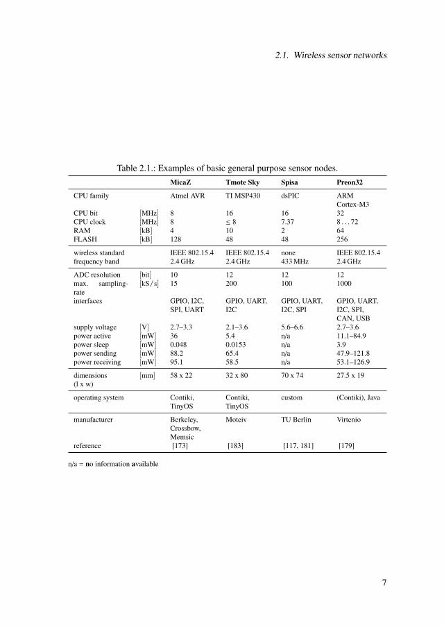
Table 2.1 shows the key features of typical general purpose nodes. A more comprehen-sive table of sensor nodes is provided in appendix A (tables A.1 to A.3). Unfortunately,different manufacturers specify the power consumption for different operational condi-tions. Likewise, sensor nodes do contain a differing amount of components, e.g. theMicaZ includes a battery holder, whereas the Preon32 does not even include a volt-age regulator. Thus, the numbers for power supply and dimensions merely illustratethe range that can be found, but are not well suited for direct comparisons betweenindividual nodes.
Apart from the general purpose sensor nodes, application specific sensor nodes havebeen developed in research projects (see table 2.2). Examples are the sensor nodedeveloped for condition monitoring in the ECoMoS project [63] or a pulseoximeterdeveloped by the chair of Electronics and Medical Signal Processing (EMSP) at theTU Berlin [108]. Examples of commercial sensor nodes that are tailored to specificapplications are the wireless temperature sensor STM 330 by EnOcean and the wirelessdata acquisition module WSN-3202 by National Instruments.
Based on the properties of the sensor nodes described above as well as literature onWSNs the common properties of the key components: controller, communication in-terfaces, clocks, sensing hardware and power supply will be given in the following.
6
2.1. Wireless sensor networks
Table 2.1.: Examples of basic general purpose sensor nodes.MicaZ Tmote Sky Spisa Preon32
CPU family Atmel AVR TI MSP430 dsPIC ARMCortex-M3
CPU bit [MHz] 8 16 16 32CPU clock [MHz] 8 ≤ 8 7.37 8 . . . 72RAM [kB] 4 10 2 64FLASH [kB] 128 48 48 256
wireless standard IEEE 802.15.4 IEEE 802.15.4 none IEEE 802.15.4frequency band 2.4 GHz 2.4 GHz 433 MHz 2.4 GHz
ADC resolution [bit] 10 12 12 12max. sampling-rate
[kS/s] 15 200 100 1000
interfaces GPIO, I2C,SPI, UART
GPIO, UART,I2C
GPIO, UART,I2C, SPI
GPIO, UART,I2C, SPI,CAN, USB
supply voltage [V] 2.7–3.3 2.1–3.6 5.6–6.6 2.7–3.6power active [mW] 36 5.4 n/a 11.1–84.9power sleep [mW] 0.048 0.0153 n/a 3.9power sending [mW] 88.2 65.4 n/a 47.9–121.8power receiving [mW] 95.1 58.5 n/a 53.1–126.9
dimensions(l x w)
[mm] 58 x 22 32 x 80 70 x 74 27.5 x 19
operating system Contiki,TinyOS
Contiki,TinyOS
custom (Contiki), Java
manufacturer Berkeley,Crossbow,Memsic
Moteiv TU Berlin Virtenio
reference [173] [183] [117, 181] [179]
n/a = no information available
7

2. Literature review
Table 2.2.: Examples of application specific sensor nodes.ECoMoS EMSP STM300/330 WSN-3202
CPU family TITMS320C55x
TI MSP430 8051 n/a
CPU clock [MHz] 16 16 16 n/a
wireless protocol custom Bluetooth EnOcean IEEE 802.15.4frequency band 868 MHz 2.4 GHz 868 MHz 2.4 GHz
sampling-rate [S/s] ≥ 32, 000 500 ∼ 0.001 (typ.) ≤ 1
sensors vibration pulseoximeter temperature analogvoltage
application vibrationanalysis,conditionmonitoring
buildingautomation
pollutionmonitoring
dataacquisition
power supply thermalharvester
batteries solarharvester
batteries,external
life on batteries ∞ > 24 h ∞ 1 m–3 ysupply voltage [V] 1.8 ∼ 3.3 V 2.1–4.5 3.6–30max. power [mW] 36 146.9 99 n/apower sleep [mW] < 0.01 n/a ≥ 0.0006 n/a
dimensions [mm] 58 x 45(h x ∅)
n/a 43 x 16 x 8(l x w x h)
42 x 86 x 124(l x w x h)
reference [63] [108][209, 206, 207]
[175]
n/a = no information available
8

2.1. Wireless sensor networks
2.1.1.1. Controller
Wireless sensor nodes almost exclusively use microcontrollers that have a Harvard ar-chitecture [130]. They contain a central processing unit (CPU), non-volatile programmemory (FLASH), volatile data memory (RAM) as well as a number of peripheralunits, like analog-to-digital converters (ADCs), timers or digital communication inter-faces. The microcontrollers used tend to be small, low-cost and low-power models.
In the past 8 bit microcontrollers like those of the AVR family from Atmel and 16 bitmicrocontrollers like those of the MSP430 family from Texas Instruments were usedalmost exclusively. Their processor clock was typically in the range of 4–16 MHz.Memory sizes were in the range of 2–16 kB for the RAM and 48–256 kB for theFLASH. Typical examples of this class of sensor nodes are the Micaz [173], TmoteSky [183] or Z1 [192] sensor nodes. Despite some authors predicting that the ad-vances in computer technology would not lead to more capable sensor nodes [130],there has been a trend towards more powerful microcontrollers in recently developedsensor nodes. They are mostly based on low-power ARM processors with Cortex-M3core and feature processor clocks of up to 72 MHz, RAM sizes of up to 96 kB andFLASH sizes of up to 512 kB. Examples are the econotag [167], Preon32 [179] orOpenMote-CC2538 [176].
Most microcontrollers have a power consumption in the range of several 10 mW whenoperating, but can reduce it to 1–100 µW by entering a sleep-mode. Most microcon-trollers offer a set of different sleep modes that allow the user to select the remainingfunctionality. An analysis given in [63] shows that using a more potent microcon-troller may result in a lower overall power consumption because calculations are fin-ished quicker and the node can rest longer in sleep-mode. In other words, more potentmicrocontrollers often have a better efficiency in terms of energy per executed instruc-tion [63].
2.1.1.2. Communication interfaces
The second essential component of a wireless sensor node is its wireless communica-tion interface. In most cases it uses electromagnetic waves in the radio frequency (RF)spectrum as a transmission medium 1. See section 2.1.4.1 for a discussion of transmis-sion standards and frequency bands.
Most wireless sensor nodes, e.g. the MicaZ [173] and Preon32 [179], use dedicatedtransceiver chips. These transceivers take care of the low level communication, likemodulation and demodulation. They usually contain a buffer for incoming as wellas outgoing data and have a digital interface over which the controller can read and
1Examples of other transmission media are sound and ultrasound waves as well as infrared and visible lightpulses [64].
9
2. Literature review
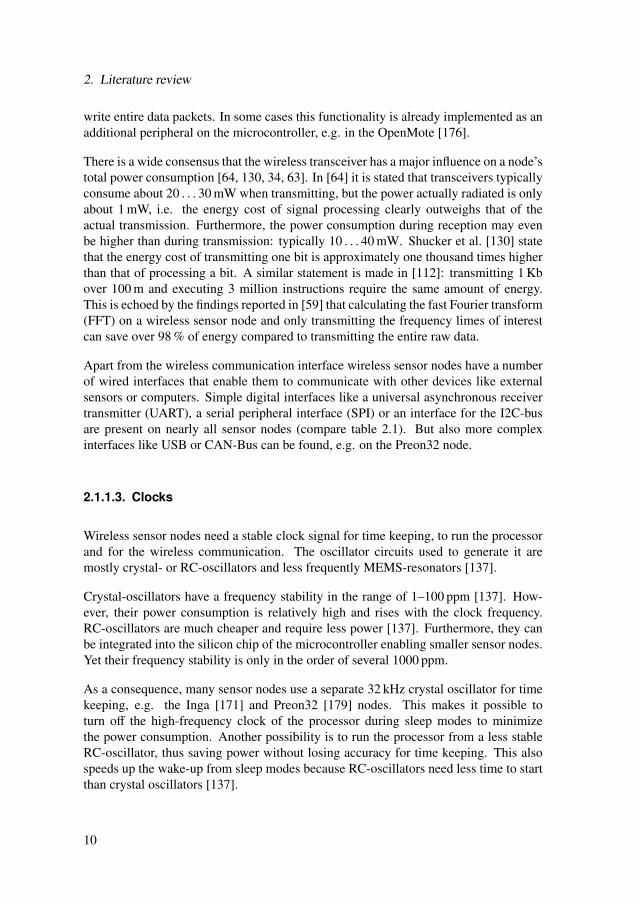
write entire data packets. In some cases this functionality is already implemented as anadditional peripheral on the microcontroller, e.g. in the OpenMote [176].
There is a wide consensus that the wireless transceiver has a major influence on a node’stotal power consumption [64, 130, 34, 63]. In [64] it is stated that transceivers typicallyconsume about 20 . . . 30 mW when transmitting, but the power actually radiated is onlyabout 1 mW, i.e. the energy cost of signal processing clearly outweighs that of theactual transmission. Furthermore, the power consumption during reception may evenbe higher than during transmission: typically 10 . . . 40 mW. Shucker et al. [130] statethat the energy cost of transmitting one bit is approximately one thousand times higherthan that of processing a bit. A similar statement is made in [112]: transmitting 1 Kbover 100 m and executing 3 million instructions require the same amount of energy.This is echoed by the findings reported in [59] that calculating the fast Fourier transform(FFT) on a wireless sensor node and only transmitting the frequency limes of interestcan save over 98 % of energy compared to transmitting the entire raw data.
Apart from the wireless communication interface wireless sensor nodes have a numberof wired interfaces that enable them to communicate with other devices like externalsensors or computers. Simple digital interfaces like a universal asynchronous receivertransmitter (UART), a serial peripheral interface (SPI) or an interface for the I2C-busare present on nearly all sensor nodes (compare table 2.1). But also more complexinterfaces like USB or CAN-Bus can be found, e.g. on the Preon32 node.
2.1.1.3. Clocks
Wireless sensor nodes need a stable clock signal for time keeping, to run the processorand for the wireless communication. The oscillator circuits used to generate it aremostly crystal- or RC-oscillators and less frequently MEMS-resonators [137].
Crystal-oscillators have a frequency stability in the range of 1–100 ppm [137]. How-ever, their power consumption is relatively high and rises with the clock frequency.RC-oscillators are much cheaper and require less power [137]. Furthermore, they canbe integrated into the silicon chip of the microcontroller enabling smaller sensor nodes.Yet their frequency stability is only in the order of several 1000 ppm.
As a consequence, many sensor nodes use a separate 32 kHz crystal oscillator for timekeeping, e.g. the Inga [171] and Preon32 [179] nodes. This makes it possible toturn off the high-frequency clock of the processor during sleep modes to minimizethe power consumption. Another possibility is to run the processor from a less stableRC-oscillator, thus saving power without losing accuracy for time keeping. This alsospeeds up the wake-up from sleep modes because RC-oscillators need less time to startthan crystal oscillators [137].
10

2.1. Wireless sensor networks
2.1.1.4. Sensing hardware
The actual sensors used in wireless sensor nodes are highly application specific andgenerally the same that are used in other sensing devices, e.g. thermocouples in [39] orMEMS accelerometers in [80]. According to [149] the cost for the sensors can easilysurpass that of the rest of the node hardware. The controllers of wireless sensor oftencontain a number of peripheral modules that help interfacing to sensor circuits.
One of the most important is the ADC, which can be used to digitize analog volt-ages. The ADCs in wireless sensor nodes are mostly successive approximation (SAR)types with a resolution of 10–12 bit and a maximum sampling rate in the order of 10–100 ksamples/s, in some cases up to 1 Msamples/s (see table 2.1). Furthermore, the con-trollers usually contain a number of timer modules, which can be used to measuretimes. They are 8–32 bit wide and can be clocked through a variable prescaler eitherdirectly from the processor clock or from an external oscillator.
2.1.1.5. Power supply
For the user to have the full benefit of a wireless sensor not only its communication butalso its power supply has to work without wires [76]. As a consequence most wirelesssensor networks are currently using batteries for power supply [121]. Other types ofenergy storage, e.g. ultracapacitors, have been investigated, but one disadvantage iscommon to all: the finite capacity of the storage limits the maximum time that thesensor node can be operated [121].
A possibility to overcome this limitation is to obtain electrical energy from ambient en-ergy sources. This energy-harvesting or -scavenging has been investigated for a varietyof energy sources including: solar radiation, thermal gradients, mechanical vibrationsand RF-energy [121, 64, 114]. A range of commercial energy harvesting solutions forsolar, thermal and mechanical energy is provided by the company EnOcean [169]. ThePowercast Corporation offers a solution to harvest energy from RF-sources in the 850–950 MHz frequency band [178]. A problem common to all energy harvesting solutionsis that the amount of power actually available may strongly vary over time. Thus, theyhave to be combined with an energy storage and power management circuitry that pro-vides a continuous power supply to the sensor node [64].
Table 2.3 shows an overview of the energy- and power densities that typically can beexpected from energy storages and energy harvesting solutions. Comparing that to thepower consumption of wireless sensor nodes in tables 2.1 and 2.2 shows that poweron a wireless sensor node is scarce. Only very large energy storages or harvesters cansustain the active power consumption of a wireless sensor node, which typically is ofthe order of several 10 mW, for a long time. Therefore it is often important to put thenode into a sleep mode, where the power consumption is much less (0.001–1 mW), as
11

2. Literature review
Table 2.3.: Typical energy- and power densities of power supplies for wireless sensornodes.
Power source Power density Energy density Reference[mW/cm2] [J/cm3]
primary battery 0.090 mW/cm3·yr a 2880 [121]secondary battery 0.034 mW/cm3·yr a 1080 [121]
solar (outside) 10 - [114]solar (inside) 0.01 - [114]temperature difference 0.025–10 - [114]vibrations 0.004–0.1 - [114]RF-harvesting 0.0001–0.001 - [114]
aMean power density for one year of operational lifetime.
often as possible. In some applications, however, it may be more feasible to use a mainsconnected power supply that obliterates these restrictions on power consumption (seee.g. [113]).
A possibility to keep many advantages of a mains powered solution without having touse wires is to transmit power through electromagnetic coupling. Powercast, for exam-ple, sells a transmitter that generates RF-energy for its corresponding harvesters.
Another means of wireless power transmission is inductive power transfer with looselycoupled coils [101, 160]. ABB provides an inductive power supply with a frequencyof 120 kHz for their wireless automation products that is capable of supplying 10–100 mW to all sensors within a 6 × 6 × 3 m volume [136]. A wireless temperaturesensor developed under the supervision of the author uses a closely coupled inductivepower supply with a frequency of 3 kHz and secondary power output of 112 mW [Fun6,Stud4].
2.1.1.6. Cost and size
Many authors, e.g. [50], envisage wireless sensor nodes that are so small that they arebarely visible and can be deployed nearly everywhere. Another vision often expressedis that sensor nodes will become so cheap that they can be deployed in huge masseswithout significant cost [50]. In this context wireless sensor nodes are often referred toas smart dust [50].
Today’s wireless sensor nodes are still quite far away from this vision. Accordingto [149] the term smart rocks might be more fitting for them. The PCBs of most wirelesssensor nodes have edge lengths of several centimeters. Adding power supply and casingvolumes of 10 . . . 1000 cm3 are easily reached. Although it has been demonstrated that
12

2.1. Wireless sensor networks
complete sensors nodes with a volume below 1 cm3 are technologically possible [99,100], this kind of miniaturized sensor nodes does not appear to be used in most practicalapplications. Possible reasons are the costs and the design limitations connected tominiaturization.
According to [149] the typical a cost of one sensor node is about 100 $. This is in goodagreement with the price for a single OpenMote-CC2538 which is 90¤ as of June 2015[176]. When adding a power supply and a casing this cost often increases significantly.Application specific sensor circuits can add to the price of a sensor node even more[149]. Kagelmaker et al. estimated the cost for one complete sensor node includinghousing, sensors and energy harvester to be about 800¤ in the ECoMoS project [63].The entire cost of installing and running the system of 1000 sensors over a ten yearperiod was estimated to be 865,000¤. Comparing this to the 1,450,000¤ estimatedfor a similar system using a wired field bus the wireless solution is significantly cheaper.This is due to cheaper hardware (1,320,000¤wired vs. 805,000¤wireless) and greatlyreduced installation costs (120,000¤ wired vs. 10,000¤ wireless) [63].
2.1.2. Software
There is a wide consensus that the severely limited energy supply, computing power,memory size and communication bandwidth present unique challenges to software de-sign for WSN [34, 130, 64]. Many projects have therefore been using simple pro-grams that are specifically designed for the given application and run directly on thesensor nodes [63, 60, 108]. However, also a number of operating systems, that arespecially designed for wireless sensor nodes, have been described [34, 130, 64, 30]and used [113, 42, 87, 77]. These operating systems are often so minimal that theymay not even be operating systems in the conventional sense [130] but rather executionenvironments as [64] suggests.
A review of wireless sensor operating systems (OSs) as of 2011 is given by Duttaand Dunkels in [34]. The main tasks of such OSs are described as providing a higherlevel abstraction of hardware as well as managing energy consumption, task executionand communication. The key advantage of using an OS is that it makes applicationprograms simpler and more portable. Wireless sensor OSs are seen to be similar toembedded real-time operating systems regarding the hardware constraints. A majordifference, however, is the much higher communication intensity in wireless sensorOSs [34].
Dutta and Dunkels [34] argue that since wireless sensor nodes have to simultaneouslyread sensors, process data and communicate with other nodes, concurrent process ex-ecution is essential. As opposed to the multi-threaded execution model found in con-ventional OSs, many wireless sensor OSs use an event driven one. Under this model
13
2. Literature review
external or internal events cause the execution of handler functions that are usually exe-cuted to the end. The entire program can be modeled as a state machine with the handlerfunctions managing the transitions. Advantages of the event based model are reportedto be greatly reduced memory requirements and shorter execution times. This modelworks very well as long as the CPU is idle most of the time and handler functions exe-cute fast. If, however, longer calculations are performed, the CPU may be blocked for along time, as handler functions often cannot be interrupted [34]. Shucker [130] arguesthat this is a major disadvantage, because the programmer always needs to care aboutthe execution time and porting algorithms from other platforms becomes complicated.As a consequence, hybrid execution models like protothreads have been developed,which allow for a programming style similar to multi-threaded systems but avoid theuse of multiple stacks [34, 32]. Other approaches implement multi-threading librarieson top of an event-driven kernel [34].
Another challenge for wireless sensor OSs is the efficient management of memory. Itis stated in [34] that in order to avoid fragmentation of data memory, dynamic memoryallocation is usually avoided. Instead the programmer preallocates static buffers fordifferent tasks. This also has the advantage that the memory requirements of a programare mostly known at compile time [34].
It is stated in [34], that in order to minimize the power consumption, unused compo-nents need to be switched off whenever possible. Doing this duty-cycling through thetask management of the OS or the device drivers helps to keep application programssimple [34]. However, Shucker [130] argues that the energy management is often moreefficient when controlled by the application, as it has more knowledge about the futurebehavior of the program.
Shucker [130] states that the network communication stack of a wireless sensor OSmay be much more complex than the application program. Due to this complexitycommunication protocols are discussed separately in section 2.1.4.
2.1.2.1. Wireless sensor operating systems
Dutta and Dunkels name TinyOS and Contiki as the two most widely known wirelesssensor OSs [34]. This view is supported by [8]. Other operating systems mentionedin [34] are: Mantis OS (MOS), SOS and LiteOS. Due to their relevance to the re-cent research on WSNs the key characteristics TinyOS and Contiki shall be introducedbriefly:
TinyOS [189, 85] is an open source operating system developed specifically for wire-less sensor networks. It was started by the University of Berkeley together with IntelResearch and Crossbow Technology around the year 2000. Now, it is developed by a
14

2.1. Wireless sensor networks
worldwide community [154, 189]. TinyOS is written in NesC, a dialect of C that en-ables the user to create applications by connecting different components through spec-ified interfaces [85, 130]. It supports an event-based execution model where every taskis invoked by an event and runs to completion [64, 130]. Furthermore, TinyOS containsa comprehensive network communication stack. TinyOS is widely used throughout thescientific community. In [64] it is even regarded as the de-facto standard OS for wire-less sensor networks. Many wireless sensor protocols have first been implemented forTinyOS, e.g. the FTSP time synchronization protocol [87] and the CTP data collectionprotocol [43]. The weaknesses of TinyOS are that its unusual programming model cre-ates a comparatively steep learning curve and that it is not well suited for longer runningcomputations [142]. Newer versions of TinyOS include a multi-threading library thataims to reduce these problems [142].
Contiki [186, 30] is an open source operating system designed for wireless sensor net-works. It was started in 2002 by Adam Dunkels at the Swedish Institute of ComputerScience and is now being developed by a worldwide community [151]. It is closelylinked to the company Thingsquare later founded by Adam Dunkels [186, 140]. Contikiis written in the C programming language. Like TinyOS it uses an event driven execu-tion model, but supported optional multi-threading from the beginning [30]. Contiki’skey features are protothreads, a very memory efficient way of thread-like program-ming [32], and a full IP networking stack [186]. Amongst its other features are theability to dynamically load code during runtime, a lightweight file system for flashmemories and a command shell [30, 186]. The target application area of Contiki isthe internet of things [186]. Contiki is used in a variety of commercial products in-cluding clip-on powerline sensors, smart thermostats and an urban noise monitoringsystem [186].
More recently developed OSs are Nano-RK [174, 36], RIOT OS [182, 8] and OpenOS[177, 147]. Nano-RK is a preemptive real-time operating system for wireless sensornetworks developed at the Carnegie Mellon University. The first paper about it waspublished in 2005 [36]. Nano-RK explores a number of alternative concepts in real-time communication [174]. However, it seems not to be used outside the CarnegieMellon University. RIOT OS was first released in 2013 [182]. Its aim is to bridge thegap between standard OS and wireless sensor OS [8]. RIOT OS is implemented in Cand C++. It puts a stronger emphasis on real-time capabilities than TinyOS or Contiki.RIOT OS also uses an IP-based network stack and is oriented towards the internet ofthings [182]. The OpenWSN project had its first release in 2011 [177]. It is focused ondeveloping an open source network communication stack for the internet of things thatis based on standards like IEEE 802.15.4 and 6LoWPAN. However, it also contains asimple priority based non-preemptive scheduler called OpenOS [8].
In [5] the embedded real-time operating system FreeRTOS [170] is extended with awireless communication stack and used for a WSN. Another alternative to using aspecialized wireless sensor OS is programming the wireless sensor nodes using higher
15

2. Literature review
level programming environments like the Java virtual machine marketed by Virtenio[190] or LabVIEW that is supported by some sensor nodes from National Instruments[175].
2.1.3. Network topologies
According to [64] a WSN can be represented as a graph, where each sensor node isrepresented as a node. An edge exists between two nodes, if they can communicatedirectly. The topology of a WSN is defined as the subset of this graph that is actuallyused for communication [64]. It is commonly assumed that the network graph of aWSN and thus also its topology may change frequently due to node mobility or changesin the environment [34, 64, 194].
Three general classes of WSN topologies are described in [64]: In a flat topology allnodes have the same functionality, whereas in a hierarchical topology some nodes havespecialized roles. A typical form of the latter is a network where several nodes forma backbone and communication only takes place to and along the backbone as shownin figure 2.1e. The third class is a clustered topology, where nodes are grouped intoclusters. Communication takes place mostly within these clusters. Cross-cluster com-munication is only possible via gateway nodes.
In [34] three different types of nodes for a hierarchical network topology are defined:Leaf nodes have the least processing power and tightest power constraints. They onlyacquire data and communicate with the next mesh node. Mesh nodes, having slightlymore power available, also relay communication for other nodes. Finally root nodesor base stations establish the connection to the user or external networks. They aredescribed as being mains-powered and having significantly more processing and stor-age capabilities than mesh or leaf nodes [34]. A similar concept is described in theIEEE 802.15.4 standard [194]. Here, reduced-function devices (RFDs) communicateonly with the next full-function device (FFD). FFDs can communicate with FFDs aswell as RFDs.
Apart from those general classes, a number of typical topology forms are described inthe literature. In [34] a star topology is described where all nodes only communicatedirectly with a central coordinator (see figure 2.1a). Furthermore, a multi-hop meshis described, where the topology graph can take any form (figure 2.1c). It is statedin [34] that a multi-hop mesh has higher reliability and reach as well as lower powerconsumption compared to a star. In [64] it is, however, reported that multi-hop commu-nication only radiates less power in form of radio waves, but may in total consume morepower due to additional computations on the forwarding nodes. In [120] two additionalnetwork topologies are described: networked star (figure 2.1d) and tree (figure 2.1b).
16

2.1. Wireless sensor networks
Figure 2.1.: Topologies for WSNs.
A discussion of WSN topologies for industrial applications is given in [38]. It is statedthat star networks are more power efficient but can handle only small numbers of nodes.Mesh networks, on the other hand, can cover larger ranges with many nodes but needmore power and have higher latencies [38]. A possible compromise is seen in a star-mesh hybrid topology, which seems to be equal to the networked star described in [120].In [59] it is stated that the star topology fits naturally with monitoring applications, sinceall nodes will usually be placed around the device to be monitored. If multiple devicesare monitored, [59] suggests to extend the concept and use a topology equivalent to thenetworked star topology.
Another kind of classification is made in [38, 120] by distinguishing between ad-hocand infrastructure networks. Whereas infrastructure networks extend already exist-ing wired networks with wireless communication in the last hop, ad-hoc networks aremulti-hop wireless networks that dynamically adapt to changes in the environment.
The IEEE 802.15.4 standard uses a similar approach to network topology and definesa star network with a static topology, as well as a peer-to-peer (mesh) network thatcan self-organize and may come in the form of a clustered tree similar to a networkedstar [194].
17

2. Literature review
2.1.4. Network protocols
General reviews of WSN protocols can be found in [138, 64, 50, 34]. They largely stressthe need for wireless protocols to deal with frequent and unpredictable transmission er-rors, while efficiently using the scarce resources of the sensor nodes. WSNs are there-fore also often characterized as low-power and lossy networks (LLNs) [109, 144]. Spe-cific discussions of protocols for industrial applications found in [125, 53, 23, 38, 59]largely agree with that but emphasize the need for secure and reliable data transmis-sions. Furthermore, depending on the application, guaranteed maximum transmissiondelays are required [23, 136]: > 10 ms for process automation and data acquisition, 1–10 ms for control applications, maintenance and diagnosis applications may even workwithout hard timing guarantees [23].
The required data throughput is reported to be higher in industrial applications than inother applications [59] of WSNs. Yet, it is not always a top priority [136].
Network communication involves many different tasks, which are commonly addressedby a number of different protocols. They are typically categorized into several layerssimilar to those defined in the ISO/OSI reference model [38, 34, 64]. The followingprotocol layers for WSNs are described in [38]:
• physical layer (ISO/OSI layer 1)
• data link layer (ISO/OSI layer 2)
• network layer (ISO/OSI layer 3)
• transport layer (ISO/OSI layer 4)
• upper layers (ISO/OSI layer 5–7)
Similar layer definitions can be found in [34, 64]. A review of the most relevant proto-cols in the different layers is given in the following sections. This is concluded with anoverview of the most widely used protocol stacks.
2.1.4.1. Physical layer (PHY)
The physical layer (PHY) mainly deals with encoding and transmission of the data us-ing some physical medium [64]. In most applications electromagnetic waves in the RFspectrum are used as transmission medium [64]. Mostly license-free industrial, scien-tific and medical (ISM) radio frequency bands are chosen, of which the 2.4 GHz bandis by far the most popular [64]. Sometimes also the 433 MHz or 868 MHz frequencybands are used. In those bands it is possible to achieve a higher transmission rangeat the same radiated power. Yet, they can only sustain lower data rates [198]. Higherfrequency bands on the other hand, have the advantage of favoring smaller antennasizes [64].
18

2.1. Wireless sensor networks
There is a wide consensus that a number of physical phenomena can cause frequentand unpredictable transmission errors, referred to as fading [64, 34, 136, 21]. Exam-ples are dampening or reflection of electromagnetic waves by static or moving objectsin the transmission path [64, 136, 21]. Since the frequency bands used by wireless sen-sor networks are open also to other wireless transmission systems, interference betweendifferent radio signals is also a major issue [64, 136]. It is even common for the originalsignal to be interfered by its own reflections 2 [64]. Furthermore, wireless communica-tion can be disturbed by electromagnetic radiation from machinery. It is interesting tonote in this context that according to [136] typical industrial processes do not radiatesignificant power at frequencies above 1.5 GHz.
According to [64] one approach to address these problems is to use direct-sequencespread spectrum (DSSS) modulation. It multiplies the original signal with a pseudo-random sequence known to both transmitter and receiver. This spreads the signal energyover a wider frequency band and lets it appear to be random noise to other systems. Atthe same time the receiver can recover the signal more easily from a noisy backgroundby using correlation techniques [64]. Another method, discussed in [64, 136] is thefrequent and pseudo-random change of transmission frequency. This reduces the likeli-hood of an interference destroying larger parts of the transmission [136]. Furthermore,several antennae at different locations may be used simultaneously to reduce the likeli-hood of fading 3 [136].
Several physical layer protocols have been standardized. According to [34] the onedefined by the IEEE 802.15.4 standard [194] is the most popular in WSNs. It is intendedfor simple, low-cost radio systems with limited power and short transmission range. In[59] it is also reported to be the best suited for industrial applications. Table 2.4 showsthe frequency bands, transmission channels and data rates defined in the IEEE 802.15.4standard [194]. In all bands DSSS is used to achieve a more robust transmission [194].The radiated power is not defined in the standard, but it is stated that typically it is inthe range of −3 . . . 10 dBm [194].
Table 2.4.: Frequency bands, transmission channels and data rates in the IEEE 802.15.4standard [194].
Frequency band Number of Channels Bit rate Region[MHz] [kbps]
868–868.6 1 20 Europe902–928.0 10 40 North America
2400–2483.5 16 250 worldwide
2This phenomenon is called multi-path fading.3This technique is called antenna-diversity.
19

2. Literature review
The physical layers defined in the standards IEEE 802.15.1 (Bluetooth) and IEEE802.11 (WLAN) have also been discussed for the use in wireless sensor networks[59, 198, 23]. Both use the 2.4 GHz frequency band and define higher data rates thanIEEE 802.15.4: 1 Mbit/s in IEEE 802.15.1 and > 10 Mbit/s in IEEE 802.11 [23]. Fur-thermore, IEEE 802.15.1 uses frequency hopping to increase transmission robustness[23]. However, the radiated power and the power consumption of the transceiver chipsare significantly higher for IEEE 802.15.1 and IEEE 802.11 than for IEEE 802.15.4[59, 23]. Therefore, [59] concludes that they are not well suited for the use in wire-less sensor networks. Nevertheless, the company ABB uses a modified version of theIEEE 802.15.1 physical layer in their industrial wireless products [136, 205]. The ver-sion 4.0 of the Bluetooth specification introduced the Bluetooth Smart technology alsoknown as Bluetooth low energy (BLE). It is much more power efficient than the originalBluetooth [164]. Compared to IEEE 802.15.4, BLE appears to be significantly moreefficient at low data rates (≪ 1 kB/s), whereas at higher data rates (≥ 1 kB/s) it is aboutequal4 [131, 98]. While BLE appears to be increasingly adopted in consumer products,applications using it for WSNs currently seem to be rare.
2.1.4.2. Data link layer
Karl and Willig [64] state that in WSNs the most important function of the data linklayer is to coordinate the access to the shared communication medium. One reason forthis is that minimizing the listening and idle times of the wireless transceiver is essentialto saving energy. Another reason is that multiple nodes sending at the same time on thesame frequency channel will destroy each others’ messages, which is called a collision.Therefore the medium access control (MAC) is treated as a separate layer in [64]. It hasa key influence on the throughput efficiency, stability, fairness and delay of the wirelesscommunication [64].
In [64] two classes of MAC-protocols are distinguished: contention- and schedule-based. In contention-based protocols every node tries to transmit whenever it has dataready [64]. This may lead to collisions which waste energy and reduce the data through-put. Therefore, protocols try to avoid collisions, i.e. by listening for an ongoing trans-mission before starting their own or through randomized transmission delays [64]. Tosave energy nodes, typically listen only for short periods of time. The sending nodesthen try to learn about the listening times of their neighbors and only send data whenthose are listening [64, 34].
In schedule-based MAC-protocols every node is assigned a time slot for transmis-sion [64]. This has the advantage of avoiding collisions while enabling higher through-put and more precisely timed sleeping periods. The major disadvantage of schedule-
4A direct comparison between IEEE 802.15.4 and BLE is difficult, as their power consumptions are stronglydependent on the chosen transmission parameters. In case of IEEE 802.15.4 it is even dependent on theMAC protocol used.
20
2.1. Wireless sensor networks
based protocols is the effort that is needed to setup and adapt the schedule to changingrequirements. This makes it especially difficult to manage large and frequently chang-ing networks. In addition, the schedule needs to be communicated to the participatingnodes and all nodes need to be synchronized to a common time, which both introduceadditional communication and memory overhead [64].
A classic example of a contention-based MAC-protocol is carrier sense multiple accesswith collision avoidance (CSMA/CA) [64]. Here a node listens before sending data.If an ongoing transmission is detected the node waits for a random period of time andthen tries again. If the channel is free the node sends its data and waits for an acknowl-edgement from the receiver. If no acknowledgment is received within a given period oftime, it assumes that the transmission failed and tries to send the data again.
The ContikiMAC protocol, introduced in [29], is a contention-based MAC-protocoloptimized for energy efficiency. It is based on a review of previously existing protocolsin [34]. In ContikiMAC a receiver periodically wakes up and checks the channel forRF-energy. If this suggests that a transmission is underway, it keeps its receiver on toreceive the packet. Otherwise is goes back to sleep. When a node needs to send data, itrepeatedly transmits the packet until it receives an acknowledgement. By recording thetiming of the acknowledgements a sender learns about the receiver’s sleep schedule andcan use this information to minimize the number failed transmission attempts. In [29]it is reported that ContikiMAC needs significantly less energy for a wake-up operationof the receiver than previous protocols. As this is deemed the most frequent operationin the network, ContikiMAC is therefore seen to be very energy efficient [29].
A classic example of a schedule-based MAC-protocol is time division multiple access(TDMA) [64]. Here, time is divided into periodically repeating frames. Each timeframe consists of a number of time slots which can be assigned to individual nodes fortheir transmissions. Typically a beacon packet is transmitted at the beginning of everyframe to synchronize all nodes.
The Time Synchronized Mesh Protocol (TSMP), introduced in [110], is a schedule-based protocol optimized for the use in industrial applications. Here nodes are assignedtime-frequency slots for their send and receive operations. Typically the frequencychannel is changed after every slot to increase robustness5. Time synchronization isachieved by including timestamps in the data and acknowledgement packets. When nocommunication has taken place for a long time (≈ 48 s), so-called keepalive packetsare sent to maintain synchronization. Delivery rates above 99.9 % at duty-cycles ofabout 0.01 % have been reported for TSMP [110]. A MAC-protocol very similar toTSMP has recently been defined in IEEE 802.15.4e, an extension to the IEEE 802.15.4standard [204]. The general approach of TSMP and IEEE 802.15.4e is referred to astime-synchronized channel hopping (TSCH) by some authors [135].
5This technique is called frequency-hopping.
21

2. Literature review
The classic IEEE 802.15.4 defines a schedule-based MAC-protocol that contains con-tention access periods, i.e. time-slots that are not dedicated to any node but in which allnodes can access the channel using CSMA/CA [194].
Other data link layer tasks named in [64] are framing, error control, flow control andlink management. Typically the data is organized into relatively short frames or packets,e.g. 127 bit in the IEEE 802.15.4 standard. Furthermore, error checking mechanismslike the cyclic redundancy check (CRC) [64, 194] are employed. Also, data link framesare often encrypted [194, 203, 110].
2.1.4.3. Network layer
Routing, packet forwarding and packet format adaptation are named as typical networklayer services in [34]. It is also stated in [34] that unlike in conventional networksmany-to-one (data collection) and one-to-many (data dissemination) are the dominantcommunication patterns in WSN. Direct communication of individual nodes (one-to-one) is deemed to be rare. Similar views are also expressed in [109, 64]. Furthermore,the topology of a WSN changes much more frequently than that of a conventional wirednetwork. Therefore, the routing protocols originally developed for wired networks, aregenerally not well suited for WSNs [64].
Flooding is a primitive approach to data forwarding in a multi-hop WSN, which is oftendescribed in the literature [34, 64, 50]. Here a sending node broadcasts its data to all itsneighbors, which in turn re-broadcast it to their neighbors. This way the entire networkis flooded with the data. A unique message identifier ensures that every packet is resentexactly once by every node. While flooding is effective in ensuring that the data reachesits destination, it leads to a lot of unnecessary packets being sent and may also increasenumber of packet collisions [34].
According to [64], routing algorithms that calculate minimum cost paths for packettransmission in a wireless network perform best in terms of energy consumption anddata throughput. Typical cost metrics are the number of hops from source to destina-tion [64], the expected energy for end-to-end transmission [64] or the expected num-ber of transmission attempts in individual hops [34]. In [64] two classes of routingprotocols are described: proactive protocols maintain accurate routing information allthe time, while reactive protocols only build it when needed. Furthermore, protocolsthat calculate the routing paths in a centralized or distributed fashion can be distin-guished [64]. Finally, the routing information may be stored by the nodes or a packetmay contain the route it is to be sent along6 [21].
A list of requirements on routing protocols for WSNs in industrial application is givenin [109]. It advocates the use of a proactive protocol and states that the routing protocol
6This is called source-routing.
22

2.1. Wireless sensor networks
should support multiple cost metrics, prioritize packets depending on the applicationand quickly recompute paths in case of topology changes. Load balancing should bedone between different nodes and their energy state should be taken into account. Fur-thermore, the protocol should support redundant routes.
A proactive routing protocol that has been designed by the Internet Engineering TaskForce (IETF) to meet the requirements set in [109] is the Routing Protocol for Low-Power and Lossy Networks (RPL) [155]. It has received considerable attention in theliterature [34, 128, 144]. According to [144] it has been found to show satisfactoryperformance especially regarding the speed of route repairs.
Furthermore, [144] compares RPL to a state-of-the-art reactive routing protocol: theLightweight Ad hoc On-Demand - Next Generation (LOADng) protocol [24]. The keyfinding is that RPL outperforms LOADng in nearly all scenarios. The only exceptionis a network with extremely low traffic [144].
According to [109] networking protocols for WSNs should be compatible to version sixof the Internet Protocol (IPv6), as it supports a large address space and provides easyconnectivity to other networks, e.g. industrial Ethernet solutions. In [34] it is stated thatthe layered architecture of IP-protocols allows to retain many optimizations for WSNsand at the same time ensures interoperability with other networks. A standardized so-lution to efficiently transport IPv6 network traffic over IEEE 802.15.4 based wirelesslinks is 6LoWPAN [128]. It defines header compression mechanisms that significantlyreduce transmission overhead [34, 128]. Furthermore, it supports splitting larger IPv6data packets (up to 64 kB) into smaller fragments that fit into the much smaller wirelessdata frames [128]. However, this fragmentation requires large memory buffers on thereceiver side as all received fragments of not yet reassembled packets have to be stored.The loss of individual fragments can further complicate the situation. Therefore, it isrecommended in [128] to avoid fragmentation in the network layer whenever possi-ble. 6LoWPAN has received considerable attention in the literature [34, 128, 203] andhas been implemented on most wireless operating systems and protocol stacks includ-ing Contiki [186], TinyOS [70], RiotOS [182] and OpenWSN [177] (see also section2.1.2.1).
2.1.4.4. Transport layer
According to [34] reliable and unreliable data transfer, congestion avoidance and flowcontrol are common transport layer services. Furthermore, encryption is often used inthe transport layer to provide confidential end-to-end communication [203, 21]. Flam-mini et al. [38] state that the transport layer is usually only implemented in WSNs ifthey are to be accessed through other networks, e.g. the internet.
23

2. Literature review
The problem of reliable end-to-end data transfer has often been discussed in the con-text of the transport layer: Dutta and Dunkels [34] state that the end-to-end acknowl-edgments needed in this context generally cause too much traffic for WSNs. Karl andWillig [64] also argue that it is not practical to achieve reliable end-to-end data transfersolely in the transport layer. Instead it should also be dealt with in the network andapplication layer.
Various WSN-specific transport layer protocols are discussed in [64]. However, it isalso stated there that no generally applicable protocol has emerged yet [64]. Due to theincreasing use of IP-based protocols in WSNs much attention has been given to the useof the two dominant internet transport layer protocols: TCP and UDP. Both protocolsare frequently implemented as part of WSN-operating systems, e.g. Contiki [186],TinyOS [70], RiotOS [182] or OpenWSN [177] (see also section 2.1.2.1).
The Transmission Control Protocol (TCP) is a connection oriented protocol that ensuresreliable transmission through end-to-end acknowledgments [128]. However, it gener-ates a significant amount of additional protocol data [128]. Furthermore, its congestioncontrol mechanism reduces the packet-rate whenever data loss is detected resulting insuboptimal performance on lossy links [64]. Therefore [128] and [64] agree that TCPis generally not well suited for the use in WSNs.
The User Datagram Protocol (UDP) is a connectionless protocol that uses best-effortdata transmission [128]. 6LoWPAN provides a header compression mechanism thateliminates most of the protocol overhead from UDP [128]. According to [128] UDP is asuitable choice for most applications in WSNs and is also most frequently used. UDP’slack of end-to-end reliability can be compensated by a suitable application protocol[33].
2.1.4.5. Upper layers
According to [38, 34] all protocol layers above the transport layer are usually condensedinto a generic application layer in WSNs. Data representation and transfer of dataitems are the typical services of this layer [34]. Shelby and Bormann state that it isoften feasible to use standard internet application protocols like HTTP, SNMP or RTPin WSNs [128]. A lightweight alternative to the Hypertext Transfer Protocol (HTTP)for the implementation of web services is the Constraint Application Protocol (CoAP)[129]. It is implemented in many wireless operation systems, e.g. Contiki [73] andOpenWSN [147]. Application layer protocols for industrial field buses like the HARTprotocol have also been used as application level protocols in WSNs [109, 133]. TheIEEE Standard for a Smart Transducer Interface for Sensors and Actuators also definesan application layer protocol that can be used on top of a 6LoWPAN-based WSN (seesection 2.3.3).
24

2.1. Wireless sensor networks
2.1.4.6. Protocol stacks
A number of different protocol stacks for WSNs have been developed. Figure 2.2 givesan overview of the most prominent ones in the context of industrial automation and theinternet of things.
Figure 2.2.: Protocol stacks for wireless sensor networks.
The Wireless Interface for Sensors and Actuators (WISA) was developed by ABB forthe use in the control level of factory automation [136]. It comprises a complete wire-less ecosystem consisting of a protocol stack, wireless sensor and actuator nodes aswell as a wireless power supply (see also section 2.1.1.5). It is optimized for hightransmission reliability, minimum latency transmission and a high node density. Theoverall data throughput was not a priority [136]. Commercial products based on WISAhave been available since 2004. Although WISA was originally an entirely proprietarytechnology, efforts appear to be made to turn it into an industrial standard [145]. As aphysical layer, WISA uses a modified version of IEEE 802.15.1 (Bluetooth) which usesantenna diversity to make the transmission more robust [136]. In the data link layer acustom TDMA-MAC is used in combination with frequency hopping and frequency di-vision duplex. No network layer protocols are implemented since only a star topologyis supported. A simple custom protocol with acknowledgments from the base station isused in the transport layer. In [136] a telegram error rate below 10−9 is reported. Thetransmission latency is given as 1–5 ms in the typical and 20 ms in the worst case [136].Furthermore, it is shown that the performance of a WISA transmission deteriorates onlyslightly under the influence of a wireless local area network (WLAN) [136].
The WirelessHART standard is developed by the HART Communication Foundationas a part of the HART field bus for process automation. The first version of the Wire-lessHART specification was officially released in 2007 [21]. WirelessHART uses thephysical layer of IEEE 802.15.4 in the 2.4 GHz band [21]. Its data link layer is based onthe TSMP protocol [110]. Encryption is used both in the data link and in the transport
25
2. Literature review
layer. In the network layer three different centralized proactive routing algorithms aresupported: graph routing, source routing and superframe routing. All can be use to builda self-organizing and self-healing multi-hop mesh network with redundant transmissionpaths. In the transport layer end-to-end acknowledgments are used to ensure reliabletransmission. The application layer of WirelessHART is the same as in HART, allowingfor seamless integration of WirelessHART devices into a HART network [21].
The ISA100.11a standard is developed by the International Society of Automation(ISA) [203]. Its first version was officially released in 2009. ISA100.11a is intendedto be used in non-critical industrial monitoring and control applications that toleratelatencies in the order of 100 ms. It was designed to enable scalable and extensiblenetworks with robust and deterministic communication on low energy nodes. TheISA100.11a standard is intended to be compatible with a wide range of existing com-munication standards including e.g. HART, FOUNDATION Fieldbus, Modbus andPROFIBUS [23]. ISA100.11a uses the physical layer of IEEE 802.15.4 in the 2.4 GHzband [203]. Its data link layer is based on the TSMP protocol [110]. The network layerof ISA100.11a is intended to be compatible with IPv6 networks using 6LoWPAN, whilea custom centralized proactive routing protocol is used. Various network topologies aresupported including star, star-mesh and mesh. UDP is used in the transport layer anda custom object oriented protocol in the application layer [203]. ISA100.11a definesencryption mechanisms in both the data link and the transport layer.
ZigBee is a wireless standard developed by the ZigBee Alliance [188]. It is indented forthe use in applications like home and building automation, smart metering and healthcare [74]. The first ZigBee specification was released in 2004. Since then it has beenupdated and extended multiple times [74]. ZigBee uses IEEE 802.15.4 as physical anddata link layer [74]. In the network layer ZigBee uses three different routing protocols:a proactive tree-based protocol, an on-demand protocol (AODV [106]) and source rout-ing [74]. ZigBee has an object based application layer that defines application profilesincluding: home automation, building automation, health care and smart energy [74].Furthermore, security and encryption are managed at the application layer [74]. Severalcommercial implementations of ZigBee are available, e.g.: BitCloud (Atmel) [163],EmberZNet PRO (Silicon Labs) [168], Z-Stack (Texas Instruments) [161].
The OpenWSN project aims to implement an open source protocol stack for the inter-net of things based on open standards [147, 177]. It is developed at the University ofBerkeley and other research institutions. Its first release was in 2011. OpenWSN usesIEEE 802.15.4 as physical and IEEE 802.15.4e as a data link layer [147]. The networklayer employs IPv6 with 6LoWPAN header compression and RPL as a routing proto-col. The user can choose between UDP and TCP as transport layer protocols. In theapplication layer CoAP or standard internet protocols like HTTP are used. Encryptionin the link layer as well as end-to-end encryption using DTLS is supported [177].
Scholl et al. report ZigBee as being widespread in home automation, WirelessHART asthe de-facto standard for process automation and WISA as most promising for factory
26

2.1. Wireless sensor networks
automation [125]. Christin et al. compared the WISA, WirelessHART, ISA100.11a,ZigBee and IEEE 802.15.4e for the use in industrial automation with a focus on theirreal-time performance and security mechanisms [23]. They concluded that Wireless-HART and ISA100.11a offered the most complete set of real-time mechanisms. Thoseprotocols were said to be well suited for process automation but still failed to satisfy thestrict real-time requirements of many factory automation applications [23]. WISA wasreported to perform better in this respect but also to have higher energy demands and tohave problems with interoperability. ZigBee was judged to be insufficient for industrialapplications due to lacking frequency diversity mechanisms. At the time of writingof [23] the IEEE 802.15.4e standard was still under development but was deemed to bevery promising.
2.1.5. Conclusions
WSNs are networks of small, low-cost sensor or actuator modules. Today the typicalvolume of a module is in the range of 10 . . . 1000 cm3 and its typical cost between100 and 1000¤. Thus the expected cost reduction from the use of WSNs is estimatedbe mainly due to reduced installation and maintenance costs but sometimes also dueto cheaper hardware. The modules are commonly based on low-cost and low-powermicrocontrollers. An increase in memory sizes and computing power has been visibleover the past years with 32 bit ARM controllers being increasingly favored over 8 or16 bit architectures. The key limitations of wireless sensor nodes are energy supply, costand size. Today, most sensor nodes are powered from batteries that can only supply afinite amount of energy. Energy harvesting solutions have the potential of overcomingthis limitation. Yet at the moment, they can only generate very low amounts of electricalpower, which in addition may vary greatly over time and are often difficult to predict.Thus, whenever it is not possible to power the nodes from mains power or with aninductive power supply, power saving strategies are of great importance. The mosteffective strategy for this purpose seems to be duty-cycling, i.e. operating parts of thesensor node only for a short time and then putting them to sleep.
The limitations of the sensor hardware in terms of size, cost and power also limit thesoftware that can be run on a wireless sensor node. This has lead to the developmentof specialized operating systems that aim to reduce the processor and memory usage.Yet also here, a trend towards programming models also found on standard computersis visible.
In addition to the limited energy, frequent changes and data loss in the wireless trans-mission medium pose major challenges for communication protocols in WSNs. Thus,a plethora of specialized communication protocols has been suggested. However, mostonly address one of the many communication tasks and compatibility with other pro-tocols is not always warranted. In the physical layer IEEE 802.15.4 transceivers inthe 2.4 GHz band are predominantly used. The protocols for the MAC layer can be
27
2. Literature review
divided into two classes: contention-based and scheduled protocols. In industrial ap-plications there is a clear preference for scheduled protocols, as they provide a greaterdegree of determinism and more data throughput. This is, however, at the expense offlexibility. Additionally, frequency hopping is often used to increase the robustness tointerference. In the networking and application layers there is a trend towards IPv6-based protocols as they simplify the integration of WSNs into existing networks. TheRPL routing protocol, which proactively maintains a routing tree, is commonly used inthis context. Smaller networks, especially in industrial applications, often make use ofa much simpler star topology. Already, a number of standardized protocol stacks havebeen suggested. In the industrial domain WirelessHART and ISA100.11a are the mostprominent. ISA100.11a is designed towards IPv6-compatibility and displays interest-ing parallels to the OpenWSN-stack, which is mainly oriented towards the internet ofthings.
2.2. Time synchronization protocols
Time synchronization is widely seen as an important service in a WSN [79, 119, 64].Romer et al. [119] state that it is needed to communicate the time of observations oractions to the user, to manage communication within the WSN and to interpret sensorreadings. The challenge for time synchronization protocols in WSN is reported to bethe management of a possibly large network with dynamically changing topology, whileputting a minimum burden on the scarce resources of the sensor nodes [119]. Typicaltradeoffs described in [119] are those between synchronization quality on the one handand the additional communication, computation or memory use on the other hand.
This section reviews the current state-of-the-art regarding time synchronization in WSNs.Summaries of synchronization protocols for WSNs can be found in [79, 119, 64].There, the numerous existing protocols are classified according to a number of crite-ria that are given in section 2.2.1. Furthermore, the protocols are commonly subdividedinto several blocks, which are presented in section 2.2.2. Evaluation methods for wire-less sensor nodes, commonly found in the literature, are given in section 2.2.3. Section2.2.4 presents an overview of the currently most relevant time synchronization protocolsfor WSNs. Finally, section 2.2.5 reviews a number of time synchronization protocolsfrom other domains and compares them to those used in WSNs.
2.2.1. Classes of synchronization
It is pointed out in [119] that time synchronization may have many different forms. Inorder to choose the optimal time synchronization approach for a given application it isvital to realize the form of synchronization actually needed. This section summarizesthe classes of time synchronization commonly found in the literature.
28

2.2. Time synchronization protocols
Internal or external: Romer et al. [119] distinguish between internal and externaltime synchronization. While internal time synchronization only requires all member ofa network to be synchronized, external time synchronization additionally requires thesynchronization to an externally provided time scale. A similar distinction can be foundin [64].
Implicit or explicit: According to [119] time synchronization may be done implicitlyby adding synchronization information to packets that would be sent anyway. Alterna-tively it can be done explicitly by sending dedicated synchronization messages.
Continuous or on-demand: In continuous synchronization, synchronization be-tween the nodes is always upheld, while in on-demand synchronization it is achievedonly when needed [119]. According to [119] on-demand synchronization may eitherbe triggered by external events or when a certain time instant is reached. A priori timesynchronization, as described in [64], is similar to continuous synchronization, as itachieves synchronization before it is actually needed. A posteriori or post-facto timesynchronization achieves a synchronization of timestamps for an event after the eventhas occurred [64]. It is described as an example of event triggered on-demand synchro-nization [119].
Scope: According to [119] the scope of synchronization defines which nodes actu-ally take part in it. In [64] synchronization protocols are classified as to which nodesthey actually synchronize: In broadcast synchronization all nodes within a broadcastdomain are synchronized. In receiver-receiver synchronization all nodes that receive asignal are synchronized but not the sending node. In sender-receiver the sender and thereceiver are synchronized.
Absolute or relative: Relative or rate synchronization only ensures that time inter-vals are the same on all nodes, i.e. it makes all clocks run at the same rate. Absolutesynchronization additionally ensures that all clocks show the same time [119, 64].
Synchronization or transformation: Synchronization is mostly defined as makingdifferent clocks show the same time [119]. However, an alternative may be to transformthe timestamps when communicating events to other nodes instead of actually changingthe node’s clock [119].
Instants or intervals: According to [119] time information may either be repre-sented by a single time value, possibly with an added uncertainty measure, or as timeintervals, where the true time is assumed to be between a lower and an upper bound. Asimilar notion is expressed in [64] where it is stated that synchronization protocols mayeither give absolute or stochastic guarantees on their precision.
29

2. Literature review
Kusy et al. [77] analyzed the applications of WSNs that require time synchronization.They concluded that most applications’ needs can be satisfied by one of the four canon-ical time synchronization services shown in table 2.5. It is stated that virtual globaltime is often implemented because it is conceptually simple. Yet, it is argued that thisrequires continuous, a priori synchronization and often causes an unnecessarily highcommunication overhead. It is found that the majority of services requiring time syn-chronization can be implemented with less effort using only on-demand or a posteriorisynchronization [77].
Table 2.5.: Canonical time synchronization services and their typical applicationsaccording to [77].
Canonical service Synchronization class Typical application
event timestamping on-demand, a posteriori intrusion detectioncountersniper systemsource localization
data series timestamping continuous habitat monitoring(during acquisition), structural monitoringon-demand (otherwise), environment monitoringa priori/a posteriori volcano event monitoring
target classificationbeamforming
virtual global time continuous, a priori debugging traces
coordinated action on-demand, a priori scheduled data collectioncommunications scheduling
2.2.2. Building blocks of synchronization protocols
Time synchronization protocols are structured into several blocks in [64, 119]: Resyn-chronization event detection or synchronization maintenance decides when it is timefor nodes to synchronize. Remote clock reading obtains the present value of a remoteclock. Remote clock estimation establishes the relation between a local and a remoteclock using one or more readings. Clock correction decides how synchronization er-rors are compensated. Finally, synchronization mesh setup deals with the organizationin multi-hop networks. This section gives a summary of the main techniques used inevery block.
30

2.2. Time synchronization protocols
2.2.2.1. Synchronization maintenance
Both [119] and [64] report that in order to continuously maintain synchronization, ithas to be refreshed periodically, because node clocks tend to drift apart. In [119] anequation for the maximum resynchronization period Tround is given:
Tround ≤ϵt,max − ϵt,sample
ρmax. (2.1)
Here, ϵt,sample is the remaining error directly after synchronization, ϵt,max is the maxi-mum accepted synchronization error and ρmax the maximum drift of the clock.
2.2.2.2. Remote clock reading
The task of remote clock reading is to establish the values of a remote clock and thelocal clock at a common time instant. Figure 2.3 shows the message exchanges in themost common remote clock reading techniques.
Figure 2.3.: Remote clock reading techniques according to [119]: a) unidirectional syn-chronization, b) round-trip synchronization, c) reference broadcast.
In unidirectional synchronization a node Ni simply sends a message containing its localclock value tia to a second node N j (see figure 2.3a). Thus, the time of reception isknown to be tib = tia + d > tia, where d is the delay. Now a common reading of theclocks may be estimated by: tia ≈ t j
b − (dmin + dmax)/2, where dmin and dmax are theupper and lower bounds for the delay [119]. Often efforts are made to minimize thedelay so that it can be neglected d ≈ 0 [87]. An advantage of unidirectional synchro-nization is that it is possible for one sending node to synchronize many receiving nodeswith only one broadcast message [119].
31
2. Literature review
In round trip-synchronization the node N j sends a synchronization request to node Niwhich sends back the timestamp tib (see figure 2.3b). Node N j then estimates the timet jb ≈ t j
c − D/2, where D is the round trip transmission delay. This way node N j cansynchronize to node Ni. However, in order for node Ni also to synchronize to nodeN j at least one additional message needs to be send. Compared to unidirectional syn-chronization round-trip synchronization has the advantage that it puts an upper boundon the synchronization error since t j
a < t jb < t j
c. Its major disadvantage is that it onlyperforms pairwise synchronization causing the number of message exchanges to in-crease linearly with the number of nodes. Thus, modifications exist where other nodessynchronize themselves by listening to the communication between N j and Ni [119].
In reference broadcast synchronization two nodes Ni and N j or more listen to a broad-cast message sent by the node Nk (see figure 2.3c). Then node Ni sends its timestamptia to node N j which can calculate the time t j
b ≈ tia + D, where D = t jb − t j
a is the delaybetween the reception of the broadcast from Nk and the message from N j, that can bemeasured locally on N j. The main advantage of the reference broadcast synchroniza-tion is that the delays from node Nk to Ni and N j are usually almost equal d ≈ d′, thusa very small synchronization error can be achieved [119].
In all clock reading techniques presented above the message delays d play an importantrole. It is stated in [119] that the uncertainty of transmission delays in WSNs are largecompared to those in wired networks. Five sources of transmission delays are givenin [87]:
1. Send time: time between the application issuing the send command and the startof the medium access.
2. Medium access time: time that the node spends waiting for access to the trans-mission medium.
3. Transmission/reception time: time that it takes to transmit the message. It isidentical to the time that is needed to receive it.
4. Propagation time: time needed for the radio signal to travel from the sender tothe receiver
5. Receive time: time between the reception of the signal and the arrival of the datain the application.
Similar lists can also be found in [79, 119]. Figure 2.4 shows typical values for thedifferent delay times given in [87]. The key result is that the processing of the packetand especially the channel access can cause large uncertainties while the transmissionprocess itself is largely deterministic. Therefore, many authors recommend generatingthe timestamps at the lowest level possible, i.e. in the MAC- or physical layer [119,87, 77]. A further analysis of timestamping errors on the Mica2 sensor node in [87]revealed that the interrupt latencies were the largest source of uncertainty in this case.
32
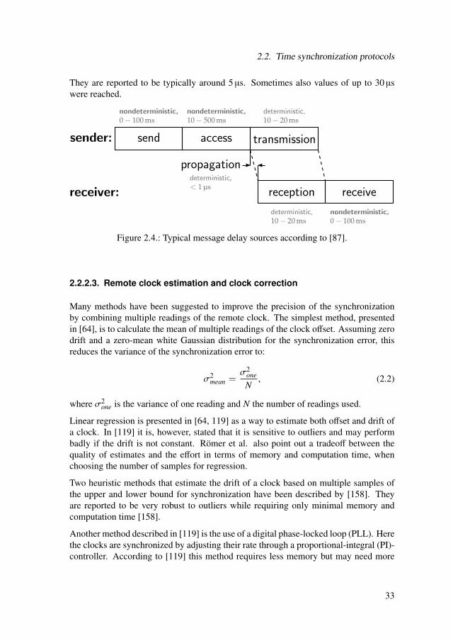
2.2. Time synchronization protocols
They are reported to be typically around 5 µs. Sometimes also values of up to 30 µswere reached.
Figure 2.4.: Typical message delay sources according to [87].
2.2.2.3. Remote clock estimation and clock correction
Many methods have been suggested to improve the precision of the synchronizationby combining multiple readings of the remote clock. The simplest method, presentedin [64], is to calculate the mean of multiple readings of the clock offset. Assuming zerodrift and a zero-mean white Gaussian distribution for the synchronization error, thisreduces the variance of the synchronization error to:
σ2mean =
σ2one
N, (2.2)
where σ2one is the variance of one reading and N the number of readings used.
Linear regression is presented in [64, 119] as a way to estimate both offset and drift ofa clock. In [119] it is, however, stated that it is sensitive to outliers and may performbadly if the drift is not constant. Romer et al. also point out a tradeoff between thequality of estimates and the effort in terms of memory and computation time, whenchoosing the number of samples for regression.
Two heuristic methods that estimate the drift of a clock based on multiple samples ofthe upper and lower bound for synchronization have been described by [158]. Theyare reported to be very robust to outliers while requiring only minimal memory andcomputation time [158].
Another method described in [119] is the use of a digital phase-locked loop (PLL). Herethe clocks are synchronized by adjusting their rate through a proportional-integral (PI)-controller. According to [119] this method requires less memory but may need more
33
2. Literature review
time to converge than linear regression. Furthermore, the frequent clock updates fromthe control loop may interrupt sleep-periods of the controller and increase its energyconsumption [119].
A number of maximum-likelihood estimators have been suggested that optimally es-timate the clock offset or drift when the synchronization error is not Gaussian dis-tributed [64, 83, 141]. Many of their authors assume an exponentially distributed mes-sage delay during synchronization [83, 141]. Finally, various Kalman filter designshave been suggested for time synchronization in WSN [2, 6, 86, 67].
2.2.2.4. Network organization
When synchronizing nodes in a multi-hop network to a common reference the synchro-nization needs to be somehow propagated in the network. Romer et al. [119] state thatthe simplest solution, i.e. relying on the network layer and synchronizing all nodesdirectly to a reference node in a logically one-hop topology, will result in large syn-chronization errors. This is due to message delays along multiple physical hops beingvery difficult to predict and control. It is argued in [119], that instead synchronizationalgorithms should deal with the multi-hop communication directly. A common obser-vation in this context is that the overall synchronization error increases with the numberof hops [119, 44]. This section summarizes the techniques commonly used to solve thisproblem.
In out-of band synchronization all nodes can communicate directly with at least onemaster node [119]. The master nodes themselves have access to the reference time,e.g. through a GPS receiver. This method is conceptually very simple as it removesthe multi-hop synchronization problem. However, it is seldom feasible as out-of bandsynchronization sources like GPS are often too expensive or not available [119].
Another approach is to form clusters of nodes that can reach each other through broad-cast messages [119]. Within such a cluster the nodes can be synchronized using singlehop unidirectional or reference broadcast synchronization. Some nodes may belong tomultiple clusters and serve as time gateways that translate time information from onecluster to the other. There is a tradeoff between the size of a cluster on the one handand the synchronization error, energy consumption or the translation effort on the otherhand [119].
According to [119] the formation of synchronization trees, similar to those used byrouting algorithms (compare section 2.1.4), is the most common technique for multi-hop synchronization. It is stressed that this tree should be optimized towards havinga minimum depth and that it needs to be dynamically repaired on topology changes.A disadvantage of tree-based multi-hop synchronization is that physically co-locatednodes may have large distances in the tree resulting in large local synchronization er-rors. Schmid et al. [123] argue that while it may seem attractive from an efficiency
34

2.2. Time synchronization protocols
point of view to use the same tree for routing and synchronization, this will result in asuboptimal synchronization quality. They suggest that to construct the tree for synchro-nization the frequency error variance of a node should be used as a cost metric insteadof the expected number of transmissions used by many routing protocols.
In the unstructured approach the multi-hop synchronization problem is not explicitlysolved [119]. Instead, nodes add synchronization information to packets that are trans-mitted for other reasons. The advantage of this approach is that its communicationoverhead is very low [119].
2.2.3. Evaluation of synchronization protocols
Synchronization protocols may be evaluated with regard to various criteria. Karl andWillig [64] name the following:
• precision
• energy consumption
• memory usage
• error tolerance
Romer et al. [119] additionally stress the importance of the convergence time, i.e. thetime a protocol needs to establish synchronization.
2.2.3.1. Precision measures
According to [119] the precision is to be given as a single scalar value for an entirenetwork. They define the instantaneous precision p(t) as:
p(t) = maxi, j
ci(t) − c j(t)
where ci(t) is the clock value of the i-th node at the time t. It is also mentioned in [119]that alternative definitions of the precision exist that use the standard deviation, theaverage absolute value or the 99 %-quantile of the pairwise clock difference instead ofthe maximum.
Furthermore, a steady state precision P is defined in [119]. It describes the synchro-nization precision in a network after the initial stabilization of the synchronization. Thetime needed to reach this steady state is called the convergence time tconv. It is definedas:
P = maxt
p(t)
, t ≥ tconv
Alternative definitions use the average instead of the maximum [119].
35

2. Literature review
It is stated in [119] that the usage of these differing precision measures often makesresults reported by different authors difficult to compare. The fact that the precisionheavily depends on the scope and time, for which it is measured, further complicatesthe situation [119].
2.2.3.2. Evaluation methods
Several methods have been used to evaluate synchronization protocols. Romer et al.[119] summarize them as: measurements on target platform, simulations and analyticcalculations. Measurement on the target platform are reported to provide the most real-istic precision values but do not scale well with network size. Simulations on the otherhand can handle also very large networks and make it simple to keep external condi-tions constant. Finally, analytic calculations are the only way to determine absoluteworst-case boundaries.
It is stated in [119] that no common benchmark for synchronization algorithms is avail-able yet. This is attributed to the diversity of synchronization algorithms and theirrespective applications.
2.2.4. Synchronization protocols for wireless sensor networks
A large number of synchronization protocols have been suggested for WSNs. Table 2.6gives an overview of the most prominent or interesting protocols. For each protocolthe classes of synchronization, types of building blocks used and assumptions made aregiven. More extensive overviews can be found in [79, 119, 64].
Reference Broadcast Synchronization (RBS) was the first protocol to use referencebroadcasting to minimize synchronization errors. It uses linear regression to determinethe relative offsets and drifts of all clocks in a broadcast domain [119, 35]. Thesevalues are then used to transform timestamps on transmission from one node to another[119]. Multiple broadcast domains can be linked through gateway nodes resulting ina clustered network organization [119, 35]. The synchronization error in this setup isreported to grow only with O(
√n) [119].
Hierarchy Referencing Time Synchronization (HRTS) is another protocol that utilizesreference broadcasting [119]. The main difference to RBS is that HRTS uses a centralnode to collect the reception timestamps of the broadcast, whereas in RBS the nodesexchange them directly [119]. Furthermore, HRTS uses a separate frequency channelfor synchronization and organizes the network in a tree [119, 26].
36

2.2. Time synchronization protocols
Table 2.6.: Overview of time synchronization protocols for WSN.Protocol RBS HRTS FTSP RITS TPSN SCTS TSCH
clas
ses
Internal/External I E I I E E IImplicit/Explicit E E E I E E mostly ICont./On-demand C/O C C O C/O C Cscope subsets all all subset all all allRate/Offset R&O O R&O O O R&O (R)&OSync./Transf. T S S T S S S
assu
mpt
ions
broadcast com. X X X - X X -bidirectional com. - X - - X - Xconstant rate - - - X - - -bounded drift - - - - - - Xextra sync. channel - X - - - - -MAC timestamping - - X X X - X
bloc
ks clock reading RB RB UD UD RT UD specialclock estimation LR ONE LR ONE ONE PLL ONEorganization cluster tree flood routing tree 1-hop DAG
source [119] [119] [119] [77] [119] [118] [135]
abbreviations clock reading: UD=unidirectional, RT=round-trip RB=reference broadcastabbreviations clock estimation: LR=linear regression, ONE=one sample, PLL=phase-locked loop
The Flooding Time-Synchronization Protocol (FTSP) uses broadcast messages to syn-chronize all nodes in a broadcast domain to a central reference node. The nodes syn-chronized this way start sending broadcast messages themselves leading to a synchro-nization flood. To minimize synchronization errors due message delay uncertaintyFTSP timestamps incoming and outgoing messages directly in the MAC-layer. Fur-thermore, linear regression is used to determine offset and drift of the nodes’ clocks[119, 87]. In FTSP the node with the lowest ID is always chosen as the central refer-ence. This way only internal time synchronization can be achieved, because it is notguaranteed that this node has access to an external time reference. Yet, it also enablesthe network to easily recover from node failures [119]. Some authors see FTSP as thecurrent de facto standard for time synchronization in WSNs [124].
Routing Integrated Time Synchronization (RITS) is an on-demand, a posteriori syn-chronization protocol. It is based on the Elapsed Time on Arrival (ETA) primitivewhere nodes transmit the elapsed time since an event instead of its timestamp. Ne-glecting clock drift between the time of an event and the reception of the message, areceiving node can calculate the event timestamp on its local timescale by subtract-ing the elapsed time from the reception timestamp. Like in FTSP timestamping in theMAC-layer is used to minimize synchronization errors. In Routing Integrated TimeSynchronization (RITS) this elapsed time is simply updated with the transmission de-lay in every node that a message passes. The communication overhead introduced by
37

2. Literature review
RITS is minimal as no additional synchronization messages are sent, only a field withelapsed time needs to be added to every message [77].
The Timing-Sync Protocol for Sensor Networks (TPSN) uses round-trip synchroniza-tion and MAC-layer timestamping to achieve very accurate synchronization. The net-work is organized in a spanning tree [119].
The Self-Correcting Time Synchronization (SCTS) uses a digital phase-locked loop(PLL) to synchronize several clocks. Time information is transmitted in FTSP-likebroadcasts. SCTS is claimed to efficiently compensate for offset and drift errors whileneeding less memory and computation time than approaches using linear regression[118].
A number of MAC-protocols employ TSCH in order to achieve both, robust commu-nication and time synchronization (see section 2.1.4.2). When using TSCH, receivingnodes measure the difference between the start of a time slot, as determined from theirlocal clocks, and the actual time when the transmission starts. This offset is then trans-mitted back to the sending node in an acknowledgement packet. To prevent loosingsynchronization, when no regular communication is happening for a long time, nodesissue special synchronization messages called keepalive packets. For this purpose ev-ery node has an estimate of its maximum local clock drift which it uses to calculate themaximum allowed time between two synchronization events (compare section 2.2.2).Network-wide synchronization is achieved by assigning one or more synchronizationparents to every node thus creating a directed acyclic graph (DAG).
Table 2.7 shows reported experimental results for the precision of the synchronizationprotocols described above. It is striking that different authors report largely differentresults for the RBS and TPSN protocols. This may be due to the use of different sensornodes, clock resolutions Tclock and synchronization periods Tsync. But also differencesin the software implementations and experimental methods may play a role. In caseof the TPSN protocol the huge differences between the values reported by [42] and[118] may also be related to the fact that [42] measured timestamp differences betweennodes directly after a posteriori synchronization, while [118] continuously monitoredthe clock differences of the number of nodes between periodic synchronizations.
Due to the differences in the experimental methods and precision measures a directcomparison of the protocols is hardly possible. Yet, it can be concluded that with cur-rent synchronization protocols precisions in the order of 1–10 µs can be achieved fora single hop. The results given for FTSP at different synchronization periods Tsyncshow that a more frequent exchange of synchronization messages improves the syn-chronization accuracy. When the number of hops increases, the synchronization preci-sion decreases for all protocols. On direct comparison by the same authors protocolslike SCTS that correct offset and drift have a clear advantage over those like TPSN thatonly correct offset [118].
38
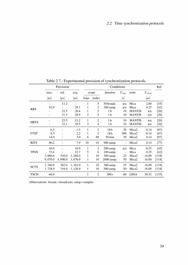
2.2. Time synchronization protocols
Table 2.7.: Experimental precision of synchronization protocols.Precision Conditions Ref.
max. std. avg. scope duration Tsync node Tclock
[µs] [µs] [µs] hops nodes [s] [µs]
RBS
- 11.2 - 1 5 30 broadc. n/a Mica 2.00 [35]93.0 - 29.1 1 2 200 samp. n/a Mica 0.25 [42]- 22.5 20.4 1 2 1 h 10 MANTIS n/a [26]- 31.5 28.9 3 4 1 h 10 MANTIS n/a [26]
HRTS - 23.5 21.2 1 2 1 h 10 MANTIS n/a [26]- 32.1 29.5 3 4 1 h 10 MANTIS n/a [26]
FTSP6.5 - 1.5 1 2 18 h 30 Mica2 0.14 [87]8.5 - 2.2 1 2 18 h 300 Mica2 0.14 [87]
14.0 - 3.0 6 60 50 min 30 Mica2 0.14 [87]
RITS 80.2 - 7.9 10 45 900 samp. - Mica2 0.14 [77]
TPSN44.0 - 16.9 1 2 200 samp. n/a Mica 0.25 [42]73.6 - 22.7 5 6 100 samp. - Mica 0.25 [42]
3, 860.0 530.0 1, 280.0 1 10 300 samp. 25 Mica2 16.00 [118]9, 070.0 4, 000.0 3, 070.0 1 10 2000 samp. 50 Mica2 16.00 [118]
SCTS 1, 760.0 282.0 1, 162.0 1 10 300 samp. 25 Mica2 16.00 [118]1, 728.0 316.0 1, 126.0 1 10 500 samp. 50 Mica2 16.00 [118]
TSCH 60.0 1 2 500 s 60 GINA 30.52 [135]
Abbreviations: broadc.=broadcasts, samp.=samples
39
2. Literature review
2.2.5. Synchronization protocols in other domains
Time synchronization is important not only for WSN. A number of time synchro-nization techniques have been developed in different domains, some of which are inwidespread use and very mature. This section presents the most well known of thosesynchronization techniques outside and analyzes them for their relevance to WSN.
2.2.5.1. Internet: NTP
The Network Time Protocol (NTP) is used to synchronize the clocks of computersconnected to the internet [96]. It was first standardized by the IETF in 1985 [94] and hasrecently been updated to its fourth version [95]. According to [96] NTP is continuouslybeing used by 10–20 million servers and clients all over the world.
In NTP a client synchronizes to a server using round-trip synchronization [97]. Clockoffset and drift are estimated and digital PLL is used to control the clocks [97]. Thenetwork organization is based on a tree-structure, which is independent of the underly-ing physical network. At the root is a server that has access to national time standards,e.g. through GPS or DCF77 (see sections 2.2.5.3 and 2.2.5.4). The depth of the treeis measured in strata, where a stratum 1 server is at the root, stratum 2 servers syn-chronize to stratum 1 servers, etc. [96]. Many stratum 1 servers and thus also manysynchronization-trees exist on the internet. Clients may synchronize with many differ-ent servers in order to make use of redundancy and diversity effects [97]. Thus, theymay be part of more than one tree. The synchronization accuracy of NTP is generallyreported to be in the order of several milliseconds [96, 27], but efforts are being madeto achieve microsecond precision [96].
Romer et al. argue that while being most advanced and time-tested NTP is not wellsuited for the use in WSNs [119]. It is said to consume too much energy, as servers needto be always reachable by clients, the digital PLL-requires frequent processor activityand only continuous synchronization is supported. Furthermore, it is deemed to benot flexible enough as its hierarchy is mostly static and configured manually. Also thenetwork independent nature of its hierarchy is seen to be detrimental, as it may causelarge and unpredictable end-to-end delays that the protocol is not designed to meet.Finally, it is stated that NTP does not scale well over many strata/hops. Thus, time needsto be injected at many places in a large network, as it is done in the internet [119].
2.2.5.2. Industrial automation: PTP
The Precision Time Protocol (PTP) was developed to enable sub-microsecond syn-chronization in Ethernet networks [27, 200]. Additional design goals were to minimize
40

2.2. Time synchronization protocols
computational requirements, network load and administration effort. PTP is standard-ized in the IEEE 1588 and IEC 61588 standards. It is part of many real-time automationbus systems, e.g. Ethernet/IP or PROFInet. Today PTP is used in a large number of ap-plications like motion control, energy distribution, data-acquisition and geo-sciences.
PTP uses a tree structured network organization where slave clocks synchronize to theirrespective masters. A clock that is a slave to one clock and a master to others is calleda boundary clock. The clock that is used as the reference for the entire network iscalled grandmaster (see figure 2.5). PTP defines a Best-Master-Clock-Algorithm thatautomatically builds an optimal synchronization tree based on clock parameters likeprecision, stratum, drift or variance [27].
In PTP the remote clock reading works as follows: a master synchronizes its slavesthrough unidirectional synchronization (see figure 2.6). First a Sync-message is sentand later a Follow UP-message that contains the timestamp tM
sync of the Sync-message.Afterwards, the slave can calculate its offset tSo f f using the receive timestamp tSsync ofthe SYNC-message: tSo f f = tM
sync − tSsync + d. In this two-message design the only time-critical operation is the generation of send and receive timestamps which is usuallyperformed directly in the hardware. The rest of the protocol can be implemented insoftware minimizing the requirements on the hardware. To improve the accuracy of thesynchronization the transmission delay d is measured from time to time using a round-trip technique (messages Delay Req and Delay Resp in figure 2.6). However, in orderfor this mechanism to work transmission delays have to be symmetric and constant.Therefore, network switches should usually serve as boundary clocks in order to avoidvariable forwarding delays affecting the synchronization [27]. PTP requires a controlloop on the slaves to adjust the local clock to the master clock based on the calculatedoffsets, but does not define an algorithm for this [27, 200].
In [27] the precision of pure software PTP implementations is reported to be typicallyin the range of 10 . . . 200 µs. An implementation using hardware-generated timestampsand a 50 MHz crystal-oscillator is reported with a precision of 60 ns [27].
Although PTP was originally designed for Ethernet networks it can theoretically beimplemented on any multi-cast network [27]. Cho et al. [22] implemented PTP for aWSN using specialized synchronization hardware as well as a temperature controlledcrystal oscillator with a frequency of 37.5 MHz and an accuracy of 1.5 ppm. Tomaet al. [143] implemented PTP on a commercial XBee module. Wobschall et al. [157]state that an unmodified implementation of PTP is not well suited for WSNs. The mainreason is that standard PTP messages are too large for a single IEEE 802.15.4 frame andtherefore require fragmentation. They suggest using a modified version with shortenedmessages and without Follow Up-messages. A different modification is suggested in[37]. Here the timing information of the Follow Up-message is integrated into thesecond fragment of the Sync-message. Table 2.8 gives an overview of the reportedperformance for the individual PTP implementations.
41

2. Literature review
Figure 2.5.: PTP network structure [200]. Figure 2.6.: PTP synchronization mes-sage exchange [200].
It can be observed that like in table 2.7 very different precision values are reported forthe same synchronization protocol. Furthermore, the values show that, using special-ized synchronization hardware as well as a high clock resolution and short synchroniza-tion intervals, synchronization precisions well below 1 µs can be achieved. However,the energy consumption is expected to rise under these conditions. Unfortunately, notall authors report values for this.
2.2.5.3. Countrywide: DCF77
DCF77 is a long wave radio transmitter that is used to disseminate the official time inthe Federal Republic of Germany [57]. Similar transmitters are used in many othercountries (see [153]). The DCF77 transmitter uses a highly accurate carrier frequencyof 77.5 kHz and has a transmission range of about 2000 km [57]. Bits are transmitted bylowering the signal amplitude for 0.1 s or 0.2 s at the beginning of a second. This way amessage containing the current time is transmitted every minute. Additionally, pseudo-random phase noise is added to the signal to enable a more accurate synchronization ofreceivers. For two receivers spaced 50 km apart a maximum synchronization error of20 . . . 50 µs is reported [57]. The DCF77 system is essentially a unidirectional broadcastsynchronization protocol similar to one-hop FTSP. According to [64] it is not feasibleto use systems like DCF77 in WSNs as he receiving circuits are generally too large, toocostly and too energy-hungry. Furthermore, it may not be possible to pick up the signaleverywhere due to occlusions by buildings or terrain [64].
42

2.2. Time synchronization protocols
Table 2.8.: Performance of PTP implementations for WSNs.Precision P Conditions Ref.
max. std. avg. duration Tsync Tclock platform[µs] [µs] [µs] [mW] [s] [µs]
0.045 n/a 1000 samp. 0.02 0.027 special sync.hardware, TXCO
[22]
2.283 0.350 0.481 0.154 24 h 5.00 0.500 XBee [143]10 1 n/a 2.00 0.063 special sync.
hardware,precision crystal
[157]
100 0.1 n/a 10.00 0.063 special sync.hardware,precision crystal
[157]
0.500 n/a 50 samp. 1.00 0.534 SunSPOT [37]
Tsync = synchronization interval, Tclock = clock resolution
2.2.5.4. Global: GPS
Today the Global Positioning System (GPS) is the world’s principle source of accu-rate time [3]. It uses a system of satellites that possess highly stable synchronizedatomic clocks. The GPS-system time is synchronized to the Coordinated UniversalTime (UTC) as estimated by the United States Naval Observatory [3] (compare section3.1.1). Each satellite continuously broadcasts messages containing its position and thecurrent GPS-system time. After receiving timestamped messages from four differentsatellites a receiver can set-up four equations and solve them for the unknowns posi-tion (three coordinates) and GPS-system time [3]. This way synchronization precisionsof 20–500 ns are achieved [57, 3]. Using the signal from one GPS-satellites as a ref-erence broadcast, even higher synchronization accuracies of 5–20 ns can be achieved.This method, called GPS Common-View is used by the international standards organi-zations for time transfer between different timing centers [3]. Many observations overa long period of time and complex signal processing algorithms are necessary to reachthe high accuracies given above [3].
According to [64] it is not feasible to use GPS as a source of synchronized time inWSNs. The receiving circuits are deemed to be too large, too costly and to energy-hungry. In addition, it is probably not possible to receive the GPS signal everywherewireless sensor nodes are deployed.
2.2.5.5. Laboratory equipment: digital pulses
Many laboratory devices use digital pulses transmitted through a wire to synchronouslytrigger data acquisition. One example is the Real-Time System Integration bus (RTSI)
43
2. Literature review
used in data acquisition cards from National Instruments [208]. Furthermore, manyfrequency normals and GPS receivers output a one pulse per second (PPS) signal forother devices to synchronize to [57, 11].
2.2.6. Conclusions
Time synchronization is a multi-faceted problem. Depending on the application differ-ent classes of time synchronization are actually needed. Optimizing a synchronizationprotocol for a specific application may result in increased performance and efficiency.In WSNs the weak processors and small memories of the sensor nodes together with thesmall communication bandwidth pose significant challenges for time synchronizationprotocols. Most critical for the synchronization precision are the transmission delaysduring the synchronization procedure. Timestamps should therefore be generated asclose as possible to the actual sending process. Estimating and correcting the clock’sdrift can greatly reduce the required synchronization interval. Many different synchro-nization protocols have been suggested for WSNs. Unfortunately the absence of acommon precision metric and varying experimental methods make direct comparisonsdifficult if not impossible. Furthermore, the properties of the underlying hardware, es-pecially the stability and resolution of the clock, have a major influence on the observedperformance. Yet, FTSP with a reported precision in the order of several microsecondsand a relatively simple design may currently be considered to be the best protocol. Onthe other hand the trend towards MAC-layer protocols with integrated time synchro-nization, like IEEE 802.15.4e, may set a different de facto standard in the future, as theyprovide time synchronization at no additional cost. Implementations of PTP on wirelesssensor nodes show that with optimized hardware and frequent synchronization, evenprecisions of 50 ns can be achieved. Those come close to the precisions achieved bystate-of-the-art synchronization techniques in other domains with wired PTP or GPS.However, it remains an open question whether the use such high precision synchro-nization techniques is really feasible in practical applications and whether the benefitsjustify the effort. Similarly filtering techniques ranging from simple moving-average tocomplex Kalman filters may be used to increase the synchronization precision or lowerthe message exchange rate. Yet it is not clear, where the optimal tradeoff betweencomputational complexity and synchronization accuracy lies.
2.3. Data Acquisition with wireless sensor networks
Data acquisition is one of the major applications for WSNs. Section 2.3.1 presentsan overview of data acquisition applications reported in the literature. The relation ofwireless sensors to smart sensors is examined in section 2.3.3. Finally, section 2.3.2looks into strategies for time-synchronous data acquisition.
44

2.3. Data Acquisition with wireless sensor networks
2.3.1. Data acquisition
Welsh [149] reports on his experience with a WSN for volcano monitoring. In thisapplication 10–20 sensor nodes recorded seismic and acoustic signals with a samplingrate of 100 samples/s. The deployment of the nodes was rather sparse and irregular withnodes placed several hundreds of meters apart. Finally, it was observed that the scien-tists tended to be rather conservative regarding the data acquisition. Welsh summarizedthis with the sentence [149]:
Scientists simply want all of the data produced by all of the sensors, all ofthe time.
Thus, it was suggested that WSNs should transmit data based on an application domainspecific prioritization in order to minimize wireless traffic. Additionally, all data shouldbe logged to a local memory on every node for later analysis.
A deployment of a WSN for process monitoring in an oil refinery is reported in [113].Fifteen Tmote Sky nodes were connected to flow and pressure sensors that were alreadyinstalled. All data was logged at central base station. To facilitate debugging all nodeswere individually coupled with industrial personal computers (PCs) that were accessi-ble through Ethernet. Power over Ethernet was used to power both nodes and industrialPCs. The entire deployment covered an area of 2500 m2 with at most 3 hops betweena node and the base station. The nodes’ software used the Contiki operating systemextended with a TDMA-based MAC-layer and a custom tree-based routing protocol.Data collection over a period of 30 min showed an end-to-end data loss below 0.25 %.The average power consumption of all nodes except the base station was in the rangeof 0.1 . . . 1 mW.
Pflugradt et al. [108] describe a WSN for the monitoring of cardiovascular activity.They used custom sensor nodes with two MSP430 microcontrollers, where one ac-quired data and the other managed the wireless communication. In contrast to mostother applications Bluetooth was used for the wireless transmission. The nodes wereequipped with an electrocardiogram (ECG) or Photoplethysmogram (PPG) and a three-axis accelerometer, all of which were sampled at a rate of 500 samples/s. The microcon-troller responsible for data acquisition was always active and continuously acquiringsamples, but the Bluetooth interface was set to sleep mode between the wireless mes-sages to save power. The resulting mean active current is reported to be 40 mA. Asthe sensor nodes were supplied by lithium-ion batteries with a capacity of 1300 mAh,continuous measurements were possible for more than 24 h.
Medina et al. [91] present a WSN that, using ultrasonic ranging, can determine nodepositions with an accuracy below 1 mm. IEEE 802.15.4/ZigBee is used together witha TDMA-MAC-layer for the wireless communication. The network topology is a one-hop star. Time synchronization in the MAC-layer is used to minimize power consump-tion by activating the wireless transceiver only when communication is expected. In the
45

2. Literature review
given application, the nodes have an average current consumption of 11.8 mA allow-ing for 167 h of operation. Ultrasonic pulses with a carrier frequency of 40 kHz weregenerated at the sending nodes and sampled with a rate of 17.78 kHz at the receivingnodes using a bandpass sampling scheme. The sampled signal was fed through a digitalcorrelator. Further digital signal processing on the nodes determined the time-of-flightof the ultrasonic pulses, which was used to calculate the node’s position.
Hou and Bergman describe a WSN for condition monitoring of electrical motors [60].IEEE 802.15.4/ZigBee is used for the wireless transmission. The network consists ofone coordinator and three leaf nodes using a single-hop star topology. Current andvibration signals are recorded with a sampling rate of 3.1 ksamples/s. The fast Fouriertransform (FFT) is used to compute the signal spectra locally on the nodes. A neu-ral network classifier performs local fault classification. Only the classification resultsare transmitted to the coordinator where decision level fusion is done. One diagno-sis run consists of data acquisition, signal processing and result communication. Thesensor enters into a sleep state between the diagnosis runs. An analysis of energy con-sumption showed that running the fast Fourier transform (FFT) and neural network onthe node needs only 22.3 mJ per run, whereas transmitting the raw data would require33.7 mJ. Using two AAA alkaline batteries as power source this enabled 121 h of oper-ation with one diagnosis run every 3 s. Using a fixed-point FFT-algorithm instead of afloating-point, this could be increased to 150 h. The system was demonstrated to detectimbalances as well as loose feet, i.e. an inadequate motor fixture.
Another wireless condition monitoring system was developed in the ECoMoS project[63, 12, 156]. Here the aim was to detect bearing faults of machines in a paper factory.A custom node hardware was designed that contained a vibration sensor, a fixed-pointdigital signal processor (DSP) and a thermal energy harvester. Wireless transmissionwas done in the 868 MHz band using a custom protocol. Vibration data was sampledwith a rate of 32 ksamples/s. The signal spectrum was calculated and evaluated directlyon the nodes. Only the diagnosis results were transferred to a central control station.One diagnosis consisting of measurement, evaluation and transmission was reported tolast for 10 s and to need less than 250 mJ. Using a similar sleeping pattern as in [60] theenergy obtained from the thermoelectric harvester was sufficient to run one diagnosisevery 30 min.
A very different wireless sensor for machine vibration monitoring is described in [61].It uses a two-processor architecture, where an 8 bit processor with integrated wirelessinterface manages the communication and a more powerful 32 bit ARM Cortex-M3processor manages the data acquisition. IEEE 802.15.4 is used in beacon-enabled modefor the MAC-layer. Data is acquired at a rate of 20 ksamples/s, stored to a Micro-SD cardand only transmitted after the acquisition. The system is reported to consume 403.3 mWin full operation and 0.518 mW in full sleep. Using a 1000 mAh lithium battery asenergy source, this leads to a lifetime of 9.17 h in operation and 297.6 d in sleep mode.Table 2.9 gives an overview the described data acquisition applications and the usednode hardware.
46

2.3. Data Acquisition with wireless sensor networks
Table 2.9.: Examples of data acquisition with WSNs.E
xam
ple
Volc
ano
mon
itori
ngPr
oces
sm
onito
ring
Med
ical
Ultr
ason
icra
ngin
gC
ondi
tion
mon
itori
ngC
ondi
tion
mon
itori
ngV
ibra
tion
mea
sure
men
t[1
49]
[113
][1
08]
[91]
[60]
[63,
12,1
56]
[61]
num
bero
fnod
es10
–20
153
74
n/a
2ne
twor
kex
tent
200.
..40
0m
betw
een
node
s25
00m
2hu
man
body
2–6
mbe
twee
nno
des
lab
desk
fact
ory
n/a
topo
logy
n/a
tree
,3ho
psst
ar,1
hop
star
,1ho
pst
ar,1
hop
man
yst
ars,
1ho
p,ba
ckbo
ne
star
,1ho
p
PHY
n/a
IEE
E80
2.15
.4,
2.4
GH
zB
luet
ooth
,2.
4G
Hz
IEE
E80
2.15
.4,
2.4
GH
zIE
EE
802.
15.4
,2.
4G
Hz
IEE
E80
2.15
.4,
868
MH
zIE
EE
802.
15.4
,2.
4G
Hz
MA
Cn/
aT
DM
AB
luet
ooth
TD
MA
IEE
E80
2.15
.4cu
stom
IEE
E80
2.15
.4(b
eaco
ned)
exec
utio
nen
viro
nmen
tcu
stom
Con
tiki
(mod
ified
)cu
stom
cust
omcu
stom
cust
omcu
stom
sens
orno
decu
stom
Tm
ote
Sky
cust
om,2µC
cust
omcu
stom
cust
omcu
stom
,2µC
sens
ors
seis
mom
eter
,ge
opho
nepr
essu
re,fl
owac
cele
ratio
n,E
CG
,PPG
ultr
asou
ndvi
brat
ion,
curr
ent
vibr
atio
nvi
brat
ion
sam
plin
gra
te[k
sam
ples
/s]
0.1
n/a
0.5
17.7
83.
132
20da
taac
quis
ition
n/a
n/a
cont
inuo
usbu
rsts
burs
tsbu
rsts
burs
tsac
tivity
inte
rval
n/a
n/a
-6.
4s
3s
30m
inn/
a
sync
hron
izat
ion
n/a
none
peri
odic
beac
ons
peri
odic
beac
ons
none
none
peri
odic
beac
ons
sync
h.ac
cura
cy-
-10
0µs
<1µs
--
87.8
5ns
onno
desi
gnal
proc
essi
ngn/
ano
neno
neco
rrel
atio
n,pe
ak-d
etec
tion
FFT,
neur
alne
twor
kFF
T,di
agno
sis
none
pow
ersu
pply
batte
rym
ains
pow
erba
ttery
batte
ryba
ttery
ther
m.e
nerg
yha
rves
ter
batte
ry
avg.
pow
er[m
W]
n/a
0.1...1
120
35.4
≤7.
4≈
0.5
403.
3op
erat
ion
time
n/a
∞>
24h
167
h15
0h
∞9.
17h
n/a=
noin
form
atio
nav
aila
ble,
Tsy
nc=
sync
hron
izat
ion
inte
rval
,Tcl
ock=
cloc
kre
solu
tion
47

2. Literature review
2.3.2. Time synchronous data acquisition
Time synchronous data acquisition is essential to many but not all application exam-ples presented in the previous section. Pflugradt et al. [108] used two different wirelesssenor nodes to measure the Pulse Transit Time, i.e. the time between a peak in theElectrocardiogram and the start of the pulse wave. Any synchronization error directlyleads to an error in this measurement. Both, nodes trigger their sampling with a timerclocked from a 16 MHz crystal oscillator with 50 ppm accuracy. Synchronization mes-sages were sent at an interval of 250 ms. The nodes adjusted their local timer values inorder to compensate for offset and drift. This way a maximum sampling jitter of 100 µscould be achieved.
Medina et al. measured the time-of-flight of ultrasonic pulses to determine the nodepositions [91]. Sending and receiving nodes were synchronized through two synchro-nization messages sent by the network coordinator at the beginning of a TDMA-frame,i.e. every 6.4 s. As in PTP, the first message was used as a common reference pointand the second message contained the exact time at which the first was sent (comparesection 2.2.5.2). The timestamps were generated directly in the MAC-layer to achievea good precision. All nodes in the network used the synchronization information tocalculate their local drifts and offsets. To lower the standard deviation of consecutivedrift estimates an IIR-lowpass filter was used. The calculated drifts and offsets wereused by the sending nodes to calculate the correct time for sending a pulse and by thereceiving nodes to correct the pulse detection times. A detailed analysis of the measure-ment error for the time-of-flight given in [91] shows that a clock offset causes a biasin the measurement and a drift a bias that changes over time. With the offset and driftcompensation of the clock this error was smaller than 0.01 µs. A much larger bias ofabout 250 µs was introduced through the group delay of the receivers’ analog bandpassfilters. Therefore, it was suggested in [91] to remove this influence by calibration.
Another error contribution came from the variance of the correlator output which de-pends on the signal-to-noise (SNR) of the received ultrasonic signal. It was estimated tobe about 0.71 µs in [91]. Finally, the clock resolution was identified as a major influencefactor. At a clock resolution of 1 µs its error contribution was found to be about 0.6 µs.The overall error of the time-of-flight measurement was reported to be 0.6 . . . 1.9 µs fordistances between the nodes of 2 . . . 5.5 m. The error increases with the distance due toa reduction in the SNR of the received signal. The resulting positioning accuracy wasreported as 0.31 . . . 0.64 mm.
The wireless sensor presented for vibration measurement in [61] uses periodic messagesat an interval of 2 s for synchronization. The corresponding start of frame pulses fromthe wireless transceiver are wired directly to a microcontroller interrupt and used toadjust both offset and drift of an internal timer, which used to trigger the sampling ofthe input signal. This way an average synchronous triggering error of 87.85 ns (max.190 ns) between two neighboring nodes was achieved during the acquisition of 200samples.
48

2.3. Data Acquisition with wireless sensor networks
An even more powerful wireless system for synchronous data acquisition is describedin [159]. It is based on a 600 MHz ARM Cortex-A8 processor and uses WLAN fordata transmission. The sampling rate is synchronized to the PPS output signal of a GPSreceiver. This way, a synchronous triggering error of 15 ns could be achieved at a sam-pling rate of 100 ksamples/s. No information is given on the systems power consumptionor cost. Yet, it is to be assumed that the system is too costly and needs too much powerto be considered a wireless sensor node in the conventional sense.
2.3.3. Wireless sensors and smart sensors
Smart sensors are increasingly being used in measurement applications. Accordingto [57] a smart sensor not only converts a physical or chemical signal into an electricalone, but also digitizes it and performs signal processing. The signal processing maytake any form ranging from simple scaling to complex filtering or self-calibration algo-rithms. The IEEE 1451 standard defines a smart transducer as a sensor or actuator that. . . provides functions beyond those necessary for generating a correct representationof a sensed or controlled quantity . . . with the aim to facilitate its integration into ap-plication setups [196]. Thus, according to these definitions every wireless sensor nodeas described in section 2.1 is also a smart sensor.
2.3.3.1. The IEEE 1451 family of standards
The IEEE 1451 family of standards has been introduced with the aim to improve inter-operability between transducers from different manufactures, thus enabling a plug-and-play style of use [196]. It defines a transducer as a device that is either a sensor or an ac-tuator. Every smart transducer under the IEEE 1451 standard should be described by atransducer electronic data sheet (TEDS), which contains all relevant information aboutit in a standardized machine-readable form. Transducers are connected to transducerinterface modules (TIMs). They provide a standardized command interface, containthe TEDS and perform signal conversion as well as conditioning. Many TIMs may beconnected to a network-capable application processor (NCAP). It provides a networkbased user interface and can perform arbitrary processing functions. Figure 2.7 showsan overview of the IEEE 1451 reference model. Various different hardware interfacesare defined for the communication between TIMs and NCAP including USB, CAN,WLAN, Bluetooth, ZigBee and 6LoWPAN. A short summary of the current membersof the IEEE 1451 family is given in table 2.10.
49

2. Literature review
Figure 2.7.: IEEE 1451 reference model according to [196]. Grayed out parts are outof scope for IEEE 1451.
Table 2.10.: Members of IEEE 1451 family of standards.
Standard Contents
IEEE 1451.0 Common functionalities, commands and TEDSIEEE 1451.1 Common object model and interface specificationsIEEE 1451.2 Point-to-point communication interface between TIM and NCAPIEEE 1451.3 Wired bus communication between TIM and NCAP,
e.g. USB or CANIEEE 1451.4 Mixed analog/digital interface between transducers and TIMIEEE 1451.5 Wireless communication between TIM and NCAP, e.g. 6LoWPAN
50

2.3. Data Acquisition with wireless sensor networks
2.3.3.2. IEEE 1451 in wireless sensor networks
IEEE 1451 is explicitly intended to be used in WSNs. Adaptation layers for the com-munication between NCAP and TIM over 6LoWPAN and other wireless technologiesare defined in IEEE 1451.5 [197]. Higuera and Polo [54, 55] describe an implementa-tion of IEEE 1451 for TinyOS using TelosB sensor nodes. They discuss three possiblenetwork architectures for implementing IEEE 1451 on a WSN: In the first, there is onlyone NCAP. It is also the gateway node that connects the WSN to another network, e.g.the internet. In the second, multiple NCAPs are connected via a backbone network.Finally in the third, the WSN is not connected to any other network and the NCAPserves as network coordinator. In all three cases the other nodes in the network work asTIMs.
A very similar implementation using the same operating system and node hardwareis described in [45]. The memory footprint of this implementation is reported with2.900 kB RAM and 26.660 kB Flash on the TIM 3.295 kB RAM and 19.014 kB FLASHon the NCAP. A HTTP-server was implemented on the NCAP to allow access fromweb applications. Five wireless transducer interface modules (WTIMs) with light, tem-perature and humidity sensors were constructed and tested on a university campus. Thefinal intended application was the monitoring of a wildlife habitat.
2.3.4. Conclusions
Wireless data acquisition has been used in a wide range of applications. Most appli-cations still rely on customized hard- and software solutions. Quite often, relativelypowerful hardware is used for the nodes, e.g. a two processor architecture where onemanages the data acquisition and the other the communication. This, however, comesat a clear penalty regarding power consumption. The vast majority of data acquisitionapplications use batteries for power supply. Operational lifetimes range from severalhours to about half a year, depending on the highly application specific power con-sumption. Applications using energy harvesting are currently rare. Reasons may bethe relatively low amount of power that can be harvested and a difficult design process.When possible, mains powered solutions are chosen, as they significantly reduce thedesign effort and provide an unlimited operational lifetime.
In the MAC-layer schedule based protocols are used almost exclusively. The presentedapplications use only few nodes (2. . . 20). Thus, a simple one-hop star topology is usedin the majority of cases. The only application with a multi-hop network uses a three-hoptree topology.
The, MAC-protocols are the major source of time synchronization, which is generallyperformed in a continuous manner. Specialized synchronization protocols are generally
51

2. Literature review
not used. However, key techniques like MAC-layer timestamping and drift compensa-tion are often adopted. A very interesting finding of [91] is that the measurement errorscaused by synchronization inaccuracies may be marginalized by other error influences,like the input signal noise.
The sampling rates used for data acquisition vary in the range of several samples to tensof kilosamples per second. Two major acquisition patterns can be observed: continu-ous streaming and acquisition bursts with longer sleep periods in between. The latteris especially used to minimize power consumption in monitoring applications. Anotherstrategy to minimize the amount of data transmitted as well as to save power is to pro-cess the data directly on the nodes and only transmit the results. The users of the data,on the other hand, often prefer to have access to the entire raw data. A possible com-promise may be only transmitting the processed data but storing the raw data locally onthe sensor nodes for offline analysis.
As all wireless sensor nodes digitize and process the acquired data they may be con-sidered smart sensors. The IEEE 1451 defines a standardized interface to all kinds ofsmart sensing systems that abstracts from the underlying communication architecture.Wireless sensor nodes that use this standard may be integrated more easily into futuremeasurement applications.
2.4. Synchronous angular sampling
Synchronous angular sampling is an important tool for the analysis and diagnosis ofrotating machinery. It is also referred to as synchronous sampling [72], angle do-main sampling [15] or angular sampling [9, 17]. Section 2.4.1 briefly introduces thedefinition of synchronous angular sampling and its main uses. An outline of currentalgorithms for synchronous angular sampling is given in section 2.4.2.
2.4.1. Significance and applications
Synchronous angular sampling is commonly defined as the acquisition of samples atequidistant angular steps with reference to a rotating shaft [72, 15, 17]. Thus the orders,i.e. phasors that rotate with instantaneous frequencies that are integer multiples ofthe reference shaft’s rotational frequency, will appear at constant frequencies in thesampled signal, even if the rotational speed of the shaft is changing over time [15].This significantly simplifies later processing of the order signals, as signal processingand analysis methods are commonly defined for constant frequency signals [15]. Figure2.8 illustrates the process of synchronous angular sampling.
52

2.4. Synchronous angular sampling
Figure 2.8.: Principle of synchronous angular sampling.
A concept closely related to synchronous angular sampling is order tracking. In [18, 72]it is defined as:
Frequency analysis of the instantaneous root-mean-square values of pe-riodic components of rotating machine vibrations as a function of rota-tional speed.
However, in [15, 17] any digital signal processing method intended primarily for rotat-ing machinery is named order tracking.
According to [15] synchronous angular sampling is the second most often used methodin rotating machine analysis and diagnosis. Its key advantage is the possibility to per-form a leakage free discrete Fourier transform (DFT) with a constant order resolutionover time [15]. Its major disadvantage is that this order resolution is not very high,which causes problems at non-stationary order amplitudes [15].
According to [72] the main application of synchronous angular sampling is the analysisand diagnosis of rotating machinery at variable speeds. This is especially interesting,as it allows covering the entire speed range of a machine in a short time. This way,critical resonant frequencies and instabilities in rotors or bearings can be detected. Fur-thermore, varying the rotational speed helps to decide whether observed phenomenaare rotation related or not. Finally, specific errors can be detected, since they often giverise to signal components at characteristic orders [72].
53

2. Literature review
2.4.2. Algorithms
Originally, synchronous angular sampling was performed by directly controlling thesampling instants with a rotational encoder connected to the reference shaft [72, 18](see figure 2.8). This, however, has the disadvantage that a variable anti-aliasing filteris needed, which in general is difficult to construct and very expensive [72, 15]. Forthese reasons synchronous angular sampling, today, is almost exclusively performeddigitally. In this case the signal is first acquired at a constant analog sampling rate overtime and later resampled at the desired angular instants [18, 15] (see figure 2.9).
Figure 2.9.: Principle of synchronous angular resampling.
This synchronous angular resampling, was introduced by Hewlett Packard in 1989 [15,111], but the details were considered to be proprietary and not published. Today, manycommercial hard- and software products provide synchronous angular resampling, butthe implementation details are generally not disclosed [14].
A simple method for synchronous angular resampling has been described in [17]. Here,spline-interpolation is used to obtain the signal values at the desired angular instants.However, this method is only suitable for small speed changes as the lowpass charac-teristic of the spline-interpolation is not very good and would lead to aliasing errorsduring resampling at larger speed changes (compare section 3.3.2).
Two more sophisticated methods for synchronous angular resampling have been pub-lished in [14]. The first is upsampled linear interpolation, where the signal is first up-sampled by a factor L and then interpolated to the desired angular instants using linearinterpolation (see figure 2.10). The lowpass filter after the upsampling suppresses inter-polation images and ensures that the signal is sufficiently narrow-band to be used in thelinear interpolation. In order to avoid aliasing errors the sampling rate at the output ofthe linear interpolator needs to be at least as large as the original sampling rate. As thiscan lead to undesired oversampling, an optional decimation stage can be used to reduce
54

2.4. Synchronous angular sampling
the output rate by a factor M. The SNR of the output signal is strongly influenced bythe upsampling factor L: higher L lead to a better SNR. Simulations in [14] resulted inan SNR of 50 dB at L = 2 and one of 60 dB at L = 16. The method generally requiresa high computational effort. However, this can be reduced by calculating only thoseupsampled values actually needed for the interpolation as well as by using polyphaseinterpolation and decimation filters (compare section 3.3.2.1).
Figure 2.10.: Block diagram of upsampled linear interpolation algorithm [14].
The second method for synchronous angular resampling presented in [14] is an upsam-pled interpolation filter. Here samples are interpolated at the desired angular instantsusing truncated sinc-interpolation. This corresponds to first reconstructing a continuoussignal from the acquired samples, continuously filtering it with a lowpass filter and thensampling it again (see figure 2.11). The impulse response of the lowpass filter is equalto a truncated sinc-function. It is stressed in [14] that this method is computationallyvery efficient as it only requires 12–18 multiply and add operations per output sample, ifthe values of the sinc-function have been calculated in advance. However, a large num-ber of these precalculated values are needed. If fewer values are used more broadbandnoise is introduced in the output signal. The SNR of the method is reported to be inthe range of 70 . . . 80 dB for 18 times 512 to 8192, i.e. 9.216 . . . 147.456, precalculatedvalues.
Figure 2.11.: Block diagram of upsampled interpolation filter [14].
55

2. Literature review
2.5. Conclusions
WSNs are networks of small, low-cost sensor and actuator devices. Although WSNshave been a subject of research for more than 15 years this field is still very much indevelopment. The trend in wireless sensor node hardware is towards low-power 32 bitARM processors. Radio transceivers based on the IEEE 802.15.4 standard using the2.4 GHz frequency band are used in the majority of applications. In most cases wirelesssensor nodes are powered using batteries. Applications based on energy harvesting lookinteresting but are still very rare. Reasons are the low amount of power harvested andproblems to reliably predict it during system design. Thus, the power consumption ofwireless sensor nodes has to be minimized regardless of whether batteries or energyharvesting is used. However, in some applications it is feasible to power the nodesdirectly from the power grid or through an inductive power supply. In these cases,power consumption is much less critical.
Starting from very diverse experimental systems and protocols wireless sensor softwareis slowly converging towards some standards. There is a tendency to use solutionsalready known from conventional systems, e.g. multi-threading schedulers or IP-basednetwork protocols. Yet, the limitations of wireless sensor nodes in terms of powerconsumption, computational power and memory size still pose major challenges forsoftware development. Today a number of specialized operating systems for WSNare available. Yet, many applications still use entirely custom execution environments.For the MAC-layer, protocols based on time-synchronized channel hopping (TSCH)are increasingly being used not only in industrial applications. In the networking andhigher protocol layers, a trend towards IPv6-based protocols is clearly visible. TheIEEE 1451 standard defines a common interface not only to wireless sensors but to allkinds of smart sensors. It may greatly ease system integration efforts in the future.
Time synchronization is a key factor in many applications using WSNs. It has beenshown to be a multi-faceted problem with much room for optimization by tailoring thekind of time synchronization to the individual application. A plethora of protocols fortime synchronization has been suggested. The generation of timestamps in the MAC-layer, as close as possible to the actual sending process, has been shown to be key tomaximizing synchronization precision. Direct comparisons between synchronizationprotocols are very difficult, as precision numbers reported in the literature are oftenbased on different assumptions and measurement methods. Furthermore, the propertiesof the underlying hardware, especially the stability and resolution of the clock, have amajor influence. Yet, some authors see the FTSP-protocol as the current state-of-the-artfor time synchronization in WSN. A different kind of standard for time synchronizationin WSN may well be set by time synchronized MAC-protocols that are already predom-inantly used as a means for synchronization in data acquisition applications. Variousexperiments with synchronization on wireless sensor nodes have shown that synchro-nization accuracies well in the sub-microsecond region can be realized, thus coming
56

2.5. Conclusions
close the accuracy provided in other domains by state-of-the-art synchronization tech-niques like PTP or GPS. However, such high synchronization accuracies always requirea high effort in terms of communication and processor load. Thus, they may even turnout to be incompatible with a number of applications. The main challenge here seemsnot to be to achieve maximum synchronization accuracy, but to find the right balancebetween effort and precision for a given application. Surprisingly little research hasbeen done on this question so far.
Data acquisition applications using WSN often use duty-cycling to minimize theirpower consumption. Two major activity patterns can be distinguished: In the first asensor node continuously acquires and sends data. In the second a sensor node acquiresone block of data, processes and transmits it and then enters a sleep mode until the nextacquisition is due. Processing the data on the nodes and only transmitting the resultscan greatly reduce the amount of wireless traffic as well as the power consumption.Yet, access to the raw data may be essential in some applications. Practically all dataacquisition application today simply use a continuous, a priori time synchronization,although this strategy is argued to be suboptimal by authors that concentrate on timesynchronization protocols.
Synchronous angular sampling is frequently used to analyze and diagnose rotating ma-chinery. As it synchronizes the sampling to the rotation of a reference shaft, it maybe seen as a special case of synchronized data acquisition that is distinct from timesynchronized data acquisition. Only few algorithms for synchronous angular samplinghave been published. No implementation of synchronous angular sampling using aWSN is known to the author. Yet, distributing the task over multiple wireless sensorscould be very attractive, as it can greatly reduce installation times and costs.
Based on this analysis of the current state-of-the-art four major questions have beenidentified that have not yet been sufficiently addresses:
• How can synchronization precision be defined and measured in a way that ismeaningful for measurement applications?
• Which synchronization precision is sufficient for a given application?
• Which is the best strategy for time synchronized sampling?
• How can synchronous angular sampling be best implemented on a WSN?
The aim of this dissertation is to provide answers to those questions.
57


3. Theoretical foundations
This chapter summarizes the theoretical background necessary for understanding themodeling and analysis in this thesis. First, in section 3.1, a definition of synchronizationis given and its relations to time and time measurement through clocks are investigated.In order to better understand the influence of synchronization on the acquired data,the basics of data acquisition using uniform and nonuniform sampling are presentedin section 3.2. An important tool to synchronize data after its acquisition is digitalresampling. Its theoretical background and fundamental algorithms are given in section3.3. Finally, the state of the art quality indicators for measurement results and acquiredsignals are discussed in section 3.4. Those indicators will be used to assess the influenceof synchronization errors on measurement results in the following chapters.
3.1. Time and synchronization
The Oxford advanced learners dictionary defines the verb to synchronize as to makesomething happen at the same time as something [148]. Thus, in order to understandsynchronization it is essential to know what “at the same time” means. The concept oftime itself is closely linked to its representation through clocks.
This section starts with a brief summary of the philosophical and technical aspects oftime in section 3.1.1. In the next step, in section 3.1.2, the mathematical modelingof clocks as a source of time is discussed. This modeling is used to define synchro-nization in the context of WSNs in section 3.1.3. Finally, section 3.1.4 shows that thefundamental properties of time do not only apply to physical time itself.
3.1.1. Time
Time appears to be fundamental to our everyday lives. Most of us intuitively use itdaily without problems. Yet, its actual definition has puzzled philosophers for cen-turies [75]. The early Christian philosopher Augustine de Hippo famously wrote in his“Confessions” [104]:
What, then, is time? If no one asks me, I know what it is. If I wish toexplain it to him who asks me, I do not know.
59

3. Theoretical foundations
He also writes later [104]:
Yet I say with confidence that I know that if nothing passed away, therewould be no past time; and if nothing were still coming, there would beno future time; and if there were nothing at all, there would be no presenttime.
This also appears to express the basic consensus in the philosophy of time: time some-how manifests itself through the change of things (compare [75]). In one of the fun-damental papers on synchronization in computer science, Lamport writes about time[78]:
It is derived from the more basic concept of the order in which eventsoccur.
Within classical physics, physical time is the one universal reference that can be used tounambiguously order all events [20, 78, 193]. Yet, a consequence of Einstein’s specialtheory of relativity is that even the order of events is dependent on the position of theobserver [20]. However, within the scope of this thesis the classical view of a universaltime will be used, since in most practical measurement setups dimensions and speedsare small enough to neglect relativistic effects.
In order to define a quantitative representation of the abstract physical time, i.e. atimescale which allows for the unique ordering of events, two things are needed: afixed reference point in time and a measure of the time interval, between an event andthis point. However, there is no one and only true choice for either [3]. Historically,humans have measured larger time intervals by the change of night and day as well asthe coming and going of the seasons. Both are linked to the earth’s celestial movements,which were the original reference for the system of time units that is used today: oneday equaling one revolution of the earth around its own axis, is divided into 24 hours,which in turn are divided into 60 minutes each and every minute into 60 seconds. Aperiod of 365 days equals approximately one revolution of the earth around the sun.
Since irregularities in the earth’s movements were discovered later, other natural pro-cesses were used to define time intervals [3]. Today the internationally agreed definitionof the basic time unit, the second, is [195]:
The second is the duration of 9 192 631 770 periods of the radiation cor-responding to the transition between the two hyperfine levels of the groundstate of the caesium 133 atom.
The second is currently the basic physical unit that can be reproduced with the highestaccuracy [3].
The international reference timescale, the UTC, is established by the International Bu-reau of Weights and Measures (BIPM) based on aggregate data from atomic clocksaround the world [3]. In order to keep UTC synchronized with earth’s movement
60

3.1. Time and synchronization
around the sun, leap years, i.e. years with one extra day, are introduced at regularintervals. Furthermore, leap seconds can be introduced by international agreement atthe end of a month [3]. The reference time point for UTC is the supposed year ofChrist’s birth. A number of other timescales exist, that like UTC use the second as thebasic unit of time intervals but have different reference points. A famous example isthe Unix time, which is used by many computers. It measures time in seconds since00:00:00 on the first of January 1970 [150].
3.1.2. Clocks
Devices that measure physical time are called clocks. Today they are almost exclusivelymade up of an oscillator, which generates events at a fixed time interval, and a counter,which counts them [119, 3]. Examples of this design are mechanical clocks, wherethe oscillator is realized as a pendulum and the counter by a gearbox with a dial; digitalclocks with quartz oscillators and digital counting circuits; or even atomic clocks, wherephoton emissions of caesium 133 atoms are used to generate an electrical signal at9,192,631,770 Hz, whose periods are counted [3]. In order for such a clock to representa standardized timescale, e.g. UTC, the point in time at which it was started needs to beadded to the counter value. This immediately leads to the following widely used clockmodel [118, 64, 119]:
c(t) = hc(t)Tclock + t0. (3.1)
Here, the clock value c at the time t is given by the value of a counter hc scaled with itscounting period Tclock and shifted by an offset t0 1.
Bearing in mind that the key characteristic of time is the ordering of events, this modelcan be generalized as follows: a clock is a function c, that maps physical time t to a realnumber such that [118, 64, 119]:
t1 < t2 ⇒ c(t1) < c(t2). (3.2)
A slightly different clock definition is given in [78]. Here, a clock is defined as amapping C of real numbers to events, such that C(a) < C(b), if event a happenedbefore event b:
a b⇒ C(a) < C(b). (3.3)
An ideal clock according to (3.1) would map physical time onto itself [118]:
cideal(t) = t. (3.4)
1The counter value hc is by definition discrete. However, this fact is not paid much attention to by mostauthors [118, 64, 119]. Instead clock and counter are largely treated as if they where continuous.
61

3. Theoretical foundations
Thus, its clock rate f (t) would be exactly one at all times [119, 118]:
fideal(t) =dcideal(t)
dt= 1, ∀t. (3.5)
However, the rate of a real clock generally differs from this ideal, i.e. the clock has adrift ρ , 0 [119]:
ρ(t) = f (t) − 1. (3.6)
This may be caused, e.g. by production tolerances of the oscillator or by temperaturevariations. A drift of ρ = −1 would mean that a clock has stopped. With a drift ofρ < −1 a clock would run backwards. Thus, a reasonable assumption for most practicalclocks is [119]:
ρ(t) > −1, ∀t. (3.7)
In many applications the clock drift changes only very slowly with time. Thus, a modelwith constant drift can be used for short timespans [119]:
f (t) = const.⇒ ρ(t) = const. (3.8)
Often manufacturers give an upper bound on the clock driftρ(t) ≤ ρmax, ∀t, which
can be incorporated into the model. If timespans are so large that the change of drift be-comes relevant, it is usually reasonable to assume an upper bound Θmax for the changerate [119]:
dρ(t)dt≤ Θmax. (3.9)
Apart from the low frequency changes in clock rate, which are generally referred to asdrift, every oscillator shows some fluctuations in its period from cycle to cycle. Thisphenomenon is called jitter and can be described by adding a random error δt(t) to theclock value:
c jit(t) = hc(t)Tclock + t0 + δt(t) (3.10)
Finally, a real clock may also differ from the ideal clock by a constant offset:
∆c = c(t) − cideal(t). (3.11)
This may be due to inaccuracies in the clock’s assumed starting time.
62

3.2. Data acquisition
3.1.3. Synchronization
As already stated in the introduction to this section, synchronization makes things hap-pen at the same time. With reference to clocks, this generally means that two clocksshow the same clock value at the same physical time. Thus, two clocks ci(t) and c j(t)are synchronized to the precision p if [64]:ci(t) − c j(t)
< p (3.12)
If this condition holds true for all pairs of clocks from a set i, j ∈ 1, 2, . . . , N, it iscalled a synchronized set of clocks. If the ideal clock is included in the set, the set iscalled externally synchronized, if not, it is called internally synchronized [64, 119].
The difference ϵsync.(t) = ci(t) − c j(t) is called the synchronization error. It is theresult of the individual clocks’ drift, jitter and offset with reference to physical time(see section 3.1.2).
3.1.4. Generalized time
From the previous discussion of time and clocks, it becomes apparent that the keyproperty of physical time, i.e. its ability to order events, may not be exclusive to it.
Any function that fulfills the clock property (3.3) can be used, to uniquely order events,regardless of whether it is synchronized to physical time or not. The only propertyrequired by (3.3) is that the function is monotonically increasing. Thus, also otherphysical quantities may be used as a substitute for time in a given application. Oneexample would be the rotational position of a machine shaft, provided that it doesn’tstop or change direction (see also sections 2.4 and 4.5).
Any such clock or group of clocks can be seen as creating its own individual timescale.However, combining observations from different timescales is only possible, if theclocks have been synchronized. Seen in this light, the key function of internationaltime standards, like the second or the UTC, is to facilitate the communication of timeinformation.
3.2. Data acquisition
Data acquisition is the process of obtaining data from measurements for storage andanalysis [84]. Today, data acquisition is mostly done with acquisition systems thatproduce digital data for storage and processing on a computer system. Two very distincttypes of data acquisition are treated in this thesis:
63

3. Theoretical foundations
1. In event detection the occurrence of an event, e.g. a sound pulse or the cross-ing of a light barrier, is detected and the time of occurrence is recorded, i.e. atimestamp is assigned to the event.
2. In waveform sampling a digital representation of a physical signal, e.g. voltageor sound, is obtained [201]. This process involves both the sampling at discretetime instants and the quantization of the amplitude values [66, 48]. The result-ing digital representation is called a waveform. It consists of a set of amplitudevalues with timing information. The latter may be given directly as a set of timevalues or indirectly through the timestamp of one sample and a constant samplinginterval.
3.2.1. Uniform sampling
Sampling is the conversion of a continuous signal x(t) into a discrete one x[n] by takingits value at discrete time instants tn. For uniform sampling the timing instants are givenby a constant sampling interval Ts [102]:
x[n] = x(tn) = x(nTs). (3.13)
The Nyquist-Shannon sampling theorem states that a signal x(t) is uniquely determinedby its samples x[n], if its Fourier transform X( jω) is zero for frequencies larger thanhalf the sampling frequency ωs [102]:
X( jω) = 0 for |ω| ≥ωs
2=π
Ts. (3.14)
The frequency ωN = ωs2 is called the Nyquist frequency and 2ωN the Nyquist rate
[102].
3.2.1.1. Spectrum of uniformly sampled signals
Sampling can be modeled mathematically by the multiplication of the signal x(t) witha comb function s(t) [102] 2:
s(t) =∞∑
n=−∞δ(t − nTs) (3.15)
xs(t) = x(t)s(t), (3.16)
2The resulting signal xs is strictly speaking still continuous, but it is only nonzero at the sampling instants.
64
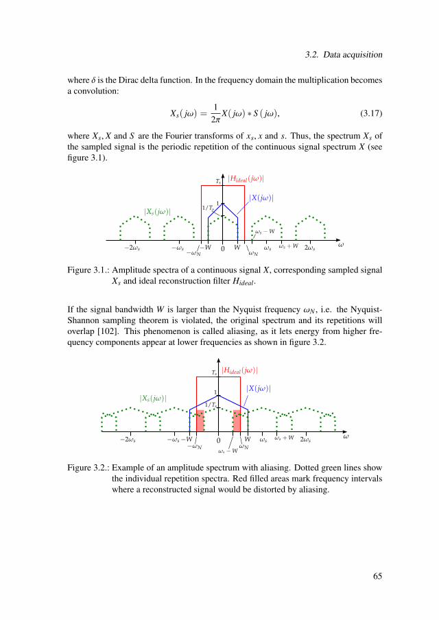
3.2. Data acquisition
where δ is the Dirac delta function. In the frequency domain the multiplication becomesa convolution:
Xs( jω) =1
2πX( jω) ∗ S ( jω), (3.17)
where Xs, X and S are the Fourier transforms of xs, x and s. Thus, the spectrum Xs ofthe sampled signal is the periodic repetition of the continuous signal spectrum X (seefigure 3.1).
Figure 3.1.: Amplitude spectra of a continuous signal X, corresponding sampled signalXs and ideal reconstruction filter Hideal.
If the signal bandwidth W is larger than the Nyquist frequency ωN , i.e. the Nyquist-Shannon sampling theorem is violated, the original spectrum and its repetitions willoverlap [102]. This phenomenon is called aliasing, as it lets energy from higher fre-quency components appear at lower frequencies as shown in figure 3.2.
Figure 3.2.: Example of an amplitude spectrum with aliasing. Dotted green lines showthe individual repetition spectra. Red filled areas mark frequency intervalswhere a reconstructed signal would be distorted by aliasing.
65

3. Theoretical foundations
3.2.1.2. Reconstruction of uniformly sampled signals
A consequence of the Nyquist-Shannon sampling theorem is that the continuous signalcan be perfectly recovered from its samples, if they are free of aliasing. From thespectral representation of the sampled signal in figure 3.1 it is apparent that this can bedone by applying an ideal lowpass filter with the cutoff frequency ωN [102]:
X( jω) = Xr( jω) = Hideal( jω)Xs( jω) (3.18)x(t) = xr(t) = hideal(t) ∗ xs(t) (3.19)
=∞∑
n=−∞x[n]
sin [π(t − nTs)/Ts]
π(t − nTs)/Ts(3.20)
3.2.2. Nonuniform sampling
For nonuniform sampling the time interval between the sampling instants is not con-stant. Instead the signal is acquired at a set of time instants tnn∈ [88]. A conse-quence of this is that no unique sampling frequency can be defined anymore and thatthe Nyquist-Shannon sampling theorem does not apply. However, a sampling theoremfor nonuniform sampling given in [88] states, that a continuous signal is uniquely de-termined by its nonuniform samples tn, if the average sampling frequency is abovethe Nyquist rate [88]:
If the nonuniform samples tn satisfy the Nyquist rate on average, it canuniquely represent a band-limited signal [. . . ] if the samples are not thezero-crossings of a band-limited signal of the same bandwidth. The set tnis then called a sampling set.
[. . . ]If the average sampling rate is higher than the Nyquist rate, irrespective
of the set tn, there is always a unique solution.
3.2.2.1. Spectrum of nonuniformly sampled signals
In [89, 88] the spectrum of nonuniformly sampled signals has been derived, for thecase that the nonuniform sampling instants tn deviate from a uniform grid nTs by afinite amount, i.e.:
tn = nTs + Θ(tn), (3.21)
where Θ(tn) is a band-limited function. Then the signal xs sampled at the nonuniformtime instants tn can be modeled as the product of the original signal x and the comb
66
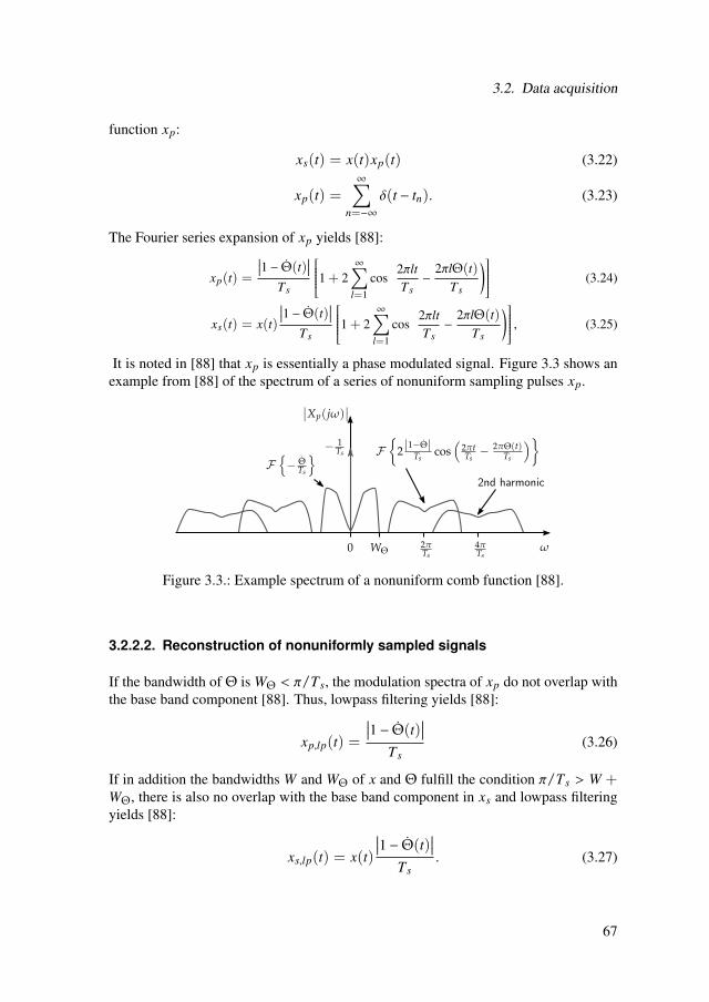
3.2. Data acquisition
function xp:
xs(t) = x(t)xp(t) (3.22)
xp(t) =∞∑
n=−∞δ(t − tn). (3.23)
The Fourier series expansion of xp yields [88]:
xp(t) =
1 − Θ(t)
Ts
⎡⎢⎢⎢⎢⎢⎢⎣1 + 2∞∑
l=1
cos(
2πltTs−
2πlΘ(t)Ts
)⎤⎥⎥⎥⎥⎥⎥⎦ (3.24)
xs(t) = x(t)
1 − Θ(t)
Ts
⎡⎢⎢⎢⎢⎢⎢⎣1 + 2∞∑
l=1
cos(
2πltTs−
2πlΘ(t)Ts
)⎤⎥⎥⎥⎥⎥⎥⎦ , (3.25)
It is noted in [88] that xp is essentially a phase modulated signal. Figure 3.3 shows anexample from [88] of the spectrum of a series of nonuniform sampling pulses xp.
Figure 3.3.: Example spectrum of a nonuniform comb function [88].
3.2.2.2. Reconstruction of nonuniformly sampled signals
If the bandwidth of Θ is WΘ < π/Ts, the modulation spectra of xp do not overlap withthe base band component [88]. Thus, lowpass filtering yields [88]:
xp,lp(t) =
1 − Θ(t)
Ts(3.26)
If in addition the bandwidths W and WΘ of x and Θ fulfill the condition π/Ts > W +WΘ, there is also no overlap with the base band component in xs and lowpass filteringyields [88]:
xs,lp(t) = x(t)
1 − Θ(t)
Ts. (3.27)
67
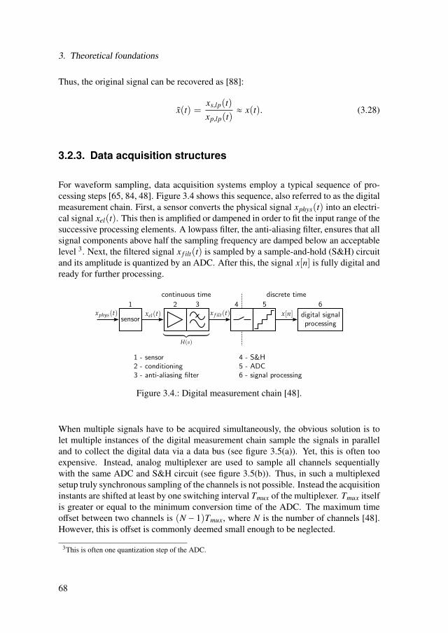
3. Theoretical foundations
Thus, the original signal can be recovered as [88]:
x(t) =xs,lp(t)xp,lp(t)
≈ x(t). (3.28)
3.2.3. Data acquisition structures
For waveform sampling, data acquisition systems employ a typical sequence of pro-cessing steps [65, 84, 48]. Figure 3.4 shows this sequence, also referred to as the digitalmeasurement chain. First, a sensor converts the physical signal xphys(t) into an electri-cal signal xel(t). This then is amplified or dampened in order to fit the input range of thesuccessive processing elements. A lowpass filter, the anti-aliasing filter, ensures that allsignal components above half the sampling frequency are damped below an acceptablelevel 3. Next, the filtered signal x f ilt(t) is sampled by a sample-and-hold (S&H) circuitand its amplitude is quantized by an ADC. After this, the signal x[n] is fully digital andready for further processing.
Figure 3.4.: Digital measurement chain [48].
When multiple signals have to be acquired simultaneously, the obvious solution is tolet multiple instances of the digital measurement chain sample the signals in paralleland to collect the digital data via a data bus (see figure 3.5(a)). Yet, this is often tooexpensive. Instead, analog multiplexer are used to sample all channels sequentiallywith the same ADC and S&H circuit (see figure 3.5(b)). Thus, in such a multiplexedsetup truly synchronous sampling of the channels is not possible. Instead the acquisitioninstants are shifted at least by one switching interval Tmux of the multiplexer. Tmux itselfis greater or equal to the minimum conversion time of the ADC. The maximum timeoffset between two channels is (N − 1)Tmux, where N is the number of channels [48].However, this is offset is commonly deemed small enough to be neglected.
3This is often one quantization step of the ADC.
68

3.2. Data acquisition
(a) parallel
(b) multiplexed
Figure 3.5.: Structures of multi-channel data acquisition systems [48].
69
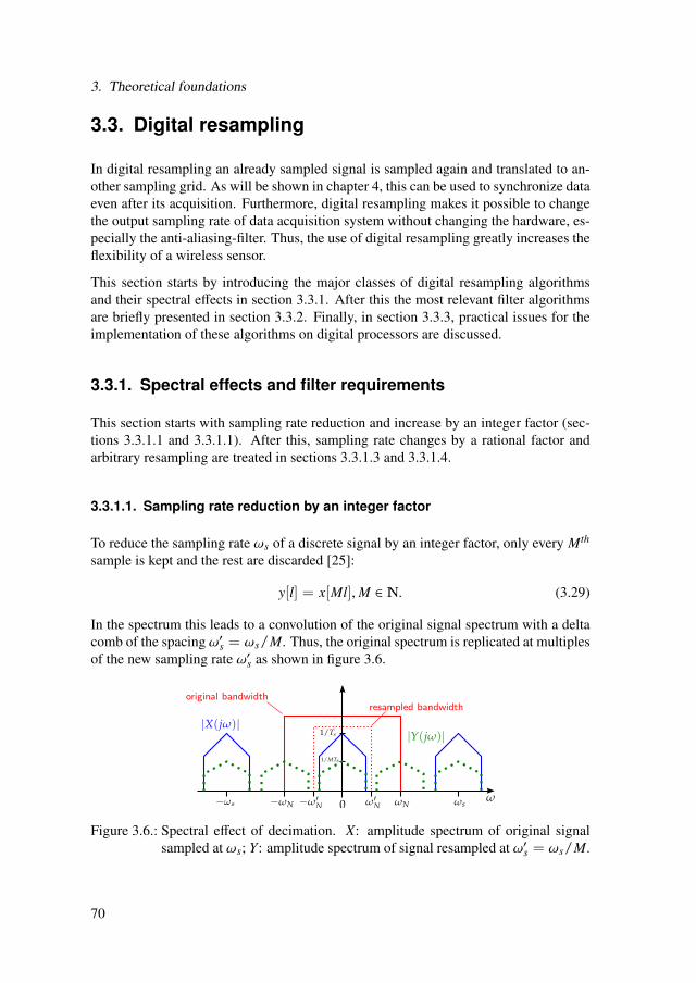
3. Theoretical foundations
3.3. Digital resampling
In digital resampling an already sampled signal is sampled again and translated to an-other sampling grid. As will be shown in chapter 4, this can be used to synchronize dataeven after its acquisition. Furthermore, digital resampling makes it possible to changethe output sampling rate of data acquisition system without changing the hardware, es-pecially the anti-aliasing-filter. Thus, the use of digital resampling greatly increases theflexibility of a wireless sensor.
This section starts by introducing the major classes of digital resampling algorithmsand their spectral effects in section 3.3.1. After this the most relevant filter algorithmsare briefly presented in section 3.3.2. Finally, in section 3.3.3, practical issues for theimplementation of these algorithms on digital processors are discussed.
3.3.1. Spectral effects and filter requirements
This section starts with sampling rate reduction and increase by an integer factor (sec-tions 3.3.1.1 and 3.3.1.1). After this, sampling rate changes by a rational factor andarbitrary resampling are treated in sections 3.3.1.3 and 3.3.1.4.
3.3.1.1. Sampling rate reduction by an integer factor
To reduce the sampling rate ωs of a discrete signal by an integer factor, only every Mth
sample is kept and the rest are discarded [25]:
y[l] = x[Ml], M ∈ . (3.29)
In the spectrum this leads to a convolution of the original signal spectrum with a deltacomb of the spacing ω′s = ωs/M. Thus, the original spectrum is replicated at multiplesof the new sampling rate ω′s as shown in figure 3.6.
Figure 3.6.: Spectral effect of decimation. X: amplitude spectrum of original signalsampled at ωs; Y: amplitude spectrum of signal resampled at ω′s = ωs/M.
70

3.3. Digital resampling
If the original signal x has a bandwidth larger than the new Nyquist frequency ω′N =ω′s/2, the spectral replications overlap and aliasing occurs. To avoid this, a digitallowpass filter is commonly used before decimation (see figure 3.7).
Figure 3.7.: Sampling rate reduction by an integer factor (decimation).
In order to avoid all aliasing, the filter H in figure 3.7 needs to have a stopband thatstarts at the new Nyquist frequency ω′N and dampens all signal components below anacceptable error threshold δs. The passband ωp of the filter should encompass theentire signal bandwidth that is to be used for further evaluation. In the passband theripple caused by the filter should not exceed an error threshold δp. Figure 3.8(a) showsthis type A tolerance scheme together with the signal spectra V after filtering and Yafter decimation [93]. The required steepness of the filter is dependent on the relativewidth of the passband ∆ω = 2π(ω′N − ωp)/ωs. Thus, at high rate change factorsM the passband quickly gets very narrow and very steep filters with high orders arerequired:
∆ω = 2πω′N −ωp
ωs=
2πωs
(ωs
2M−ωp
)(3.30)
⇒ ∆ω <π
M. (3.31)
However, the required steepness of the filter can be reduced by accepting aliasing inthe filter’s transition band (see figure 3.8(b)). This is only a minor concession, as thetransition band is generally not used for further evaluation [93]. In fact, the only signalbands that really need to be damped below δs, are the frequency bands of ±ωp aroundmultiples of the new sampling frequency ω′s, as they are mapped to the filter’s passbandduring decimation (see figure 3.8(c)). Very efficient filter structures exist for this typeC tolerance scheme (compare section 3.3.2).
71

3. Theoretical foundations
(a) Type A: no aliasing.
(b) Type B: aliasing in transition bands.
(c) Type C: only passband aliasing free.
Figure 3.8.: Tolerance schemes for digital anti-aliasing filters (after [93]). V is the sig-nal amplitude spectrum after filtering and Y the signal amplitude spectrumafter decimation. Red shaded areas mark the frequency bands where alias-ing may occur.
72

3.3. Digital resampling
3.3.1.2. Sampling rate increase by an integer factor
In order to increase the sampling rate of a discrete signal by an integer factor L, L − 1zero-valued samples are inserted between two samples of the original signal [25]:
y[l] =
x[
lL
], for l = 0,±L,±2L, . . . ; L ∈
0, otherwise(3.32)
This interpolation leads to an increase of the signal bandwidth (see figure 3.9). Thus,in general, components from the spectral repetitions around the original sampling rateωs appear in the baseband of the interpolated signal. This effect, called imaging, canbe suppressed by filtering the interpolated signal with a lowpass filter (see figure 3.10).This filter also needs to have a gain of L in order to obtain an amplitude of 1/T ′s =L/Ts in the output signal [122, 102]. Similar to an anti-aliasing filter, an anti-imagingfilter can be designed to suppress all signal components above the original Nyquistfrequency. However, the frequency bands critical for imaging, are actually only thoseof ±W around multiples of the original sampling rate ωs. Thus, it is sufficient for thefilter to dampen only those bands. This can be used to construct very efficient filters,especially for highly oversampled input signals.
Figure 3.9.: Spectral effect of interpolation. X: spectrum of original signal at samplingrate ωs.
Figure 3.10.: Sampling rate increase by an integer factor (interpolation).
73

3. Theoretical foundations
3.3.1.3. Sampling rate change by a rational factor
Digital resampling that changes the sampling rate by a rational factor R = L/M caneasily be achieved by combining an interpolator and a decimator with the integer factorsL and M [25]. In this case, the digital lowpass filters after the interpolator and beforethe decimator can be replaced by one that fulfills the spectral requirements of both ananti-aliasing and an anti-imaging filter. This approach has been successfully been usedto resample acquired data from motors at constants speeds in [47].
Figure 3.11.: Digital resampling with rational rate change factor.
3.3.1.4. Arbitrary resampling
In order to resample a signal at arbitrary time instants the hybrid discrete/continuousmodel shown in figure 3.12 is used [7, 46]. First, the original discrete signal x[n] ismodulated with a delta comb and filtered with a lowpass filter. If an ideal lowpass wasused, this would implement the reconstruction theorem (3.20). Otherwise the resultingcontinuous signal y is an approximation of the original continuous signal. After thereconstruction, the continuous signal y is sampled at the desired new sampling instantslT ′s. Thus, the lowpass filter also serves as anti-aliasing filter for the sampling stage.Although this process contains continuous intermediate signals and processing steps,fully discrete filtering algorithms can be obtained from it [7, 46]. One example is thetransposed Farrow filter, which is described in section 3.3.2.4.
Figure 3.12.: Hybrid discrete/continuous model of digital resampling [7].
3.3.2. Filter algorithms
This section introduces a number of basic digital resampling algorithms. A focus is puton decimation filters, as they are more relevant for this thesis.
74

3.3. Digital resampling
3.3.2.1. FIR filters
Lowpass filters with finite impulse response (FIR) are well suited for interpolation anddecimation with integer rate change [25, 122]. The transfer function and differenceequation of an FIR filter are [102, 25]:
H(z) =Q∑
q=0
h[q]z−q (3.33)
y[n] =Q∑
q=0
h[q] · x[n − q], (3.34)
where Q is the filter order and h the impulse response of the filter. The differenceequation of a FIR-decimator with the structure from figure 3.7 can be directly obtainedby combining (3.29) and (3.34):
y[l] = v[Ml] (3.35)
v[n] =Q∑
q=0
h[q] · x[n − q] (3.36)
y[l] =Q∑
q=0
h[q] · x[Ml − q], (3.37)
A consequence of (3.37) is that although the lowpass filtering logically comes beforethe decimation, it is possible to calculate the entire FIR filter at the lower output rate.This is also referred to as the polyphase implementation of an FIR decimator, as it in-volves creating Q+ 1 intermediate signals v, whose phase differs by one input samplingperiod (compare 3.13(a)). Corresponding polyphase FIR interpolation filters can alsobe derived [25].
Unlike infinite impulse response (IIR) filters, FIR filters are always stable and can bedesigned with a linear phase response. Since FIR decimation and interpolation filtersin polyphase implementation are as efficient as IIR filters, FIR filters are generallypreferred in resampling applications [122, 25]. Anti-aliasing filters of types A and B canbe easily designed with FIR filters. Furthermore, iterative least-squares and equirippledesign algorithms for FIR filters, allow approximating nearly any desired frequencyresponse [102, 47].
A major disadvantage of FIR resampling filters is that the required filter order increasesquickly with the rate change factor. Therefore, they are primarily used at small factors(range 1 . . . 10).
75

3. Theoretical foundations
(a) Efficient filter structure.
0 0.5 1 1.5 2−120
−100
−80
−60
−40
−20
0
ω/ω’s [1]
mag
nit
ud
e [d
B]
(b) Example frequency response.
Figure 3.13.: FIR decimation filter.
The minimum filter order Q of an FIR lowpass filter using equiripple design can beestimated as [102]:
Q =−10 log10(δpδs) − 13
2.324∆ω, (3.38)
where δp and δs are the allowed frequency response ripple in the pass- and stopbandand ∆ω = 2π (ωstop −ωp) /ωs is the normalized transition bandwidth. For a type Adecimation filter the stopband edge ωstop is directly dependent on the decimation rationM:
ωstop = ω′N =ωs
2M(3.39)
As the passband edge ωp has to be smaller than ωstop, it can be written as:
ωp = a ·ωstop, 0 < a < 1 (3.40)
=aωs
2M(3.41)
Thus the transitional bandwidth becomes:
∆ω =2πωs
(ωs
2M−
aωs
2M
)(3.42)
=π
M(1 − a) (3.43)
Thus, the required filter order is proportional the rate change factor:
Q =−10 log10(δpδs) − 13
2.324π(1 − a)·M (3.44)
76

3.3. Digital resampling
Table 3.1 shows the computational and memory requirements of a polyphase FIR deci-mator. A key feature of this filter is that the rate of mathematical operations, i.e. addi-tions and multiplications, is independent of the high input sampling frequency.
Table 3.1.: Computational and memory requirements of a polyphase FIR-decimator.
filter order Qbuffer number Qaddition rate Q · ω
′s
2πmultiplication rate (Q + 1) · ω
′s
2πoperation rate (2Q + 1) · ω
′s
2π
3.3.2.2. CIC filter
A different class of filters for decimation and interpolation with integer rate changesare cascaded integrator-comb (CIC) filters [58]. Their key feature is that they do notrequire any multiplications and can thus be implemented very efficiently. As shown infigure 3.14(a), a CIC-decimator of the order Q consists of a cascade of Q integratorsbefore the decimation and Q comb filters after it [58]. In a CIC-interpolator the combfilters come before and the integrators after the interpolation.
(a) Filter structure.
0 2 4 6−120
−100
−80
−60
−40
−20
0
ω/ω’s [1]
mag
nit
ud
e [d
B]
(b) Example magnitude frequency response.
Figure 3.14.: CIC decimation filter.
The frequency response of a CIC filter referenced to the higher sampling rate is:
H(z) =(
1 − z−MP
1 − z−1
)Q
=
⎡⎢⎢⎢⎢⎢⎢⎢⎣MP−1∑q=0
z−q
⎤⎥⎥⎥⎥⎥⎥⎥⎦Q
. (3.45)
77
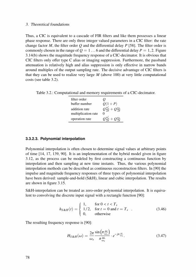
3. Theoretical foundations
Thus, a CIC is equivalent to a cascade of FIR filters and like them possesses a linearphase response. There are only three integer valued parameters in a CIC filter: the ratechange factor M, the filter order Q and the differential delay P [58]. The filter order iscommonly chosen in the range of Q = 1 . . . 6 and the differential delay P = 1, 2. Figure3.14(b) shows the magnitude frequency response of a CIC-decimator. It is obvious thatCIC filters only offer type C alias or imaging suppression. Furthermore, the passbandattenuation is relatively high and alias suppression is only effective in narrow bandsaround multiples of the output sampling rate. The decisive advantage of CIC filters isthat they can be used to realize very large M (above 100) at very little computationalcosts (see table 3.2).
Table 3.2.: Computational and memory requirements of a CIC-decimator.
filter order Qbuffer number Q(1 + P)addition rate Qω
′s
2π + Qωs2π
multiplication rate 0operation rate Qω
′s
2π + Qωs2π
3.3.2.3. Polynomial interpolation
Polynomial interpolation is often chosen to determine signal values at arbitrary pointsof time [14, 17, 139, 90]. It is an implementation of the hybrid model given in figure3.12, as the process can be modeled by first constructing a continuous function byinterpolation and then sampling at new time instants. Thus, the various polynomialinterpolation methods can be described as continuous reconstruction filters. In [90] theimpulse and magnitude frequency responses of three types of polynomial interpolationhave been derived: sample-and-hold (S&H), linear and cubic interpolation. The resultsare shown in figure 3.15.
S&H-interpolation can be treated as zero-order polynomial interpolation. It is equiva-lent to convolving the discrete input signal with a rectangle function [90]:
hS &H(t) =
⎧⎪⎪⎪⎨⎪⎪⎪⎩1, for 0 < t < Ts1/2, for t = 0 and t = Ts0, otherwise
. (3.46)
The resulting frequency response is [90]:
HS &H(ω) =2πωs
sin(π ωωs
)π ωωs
· e− jπ ωωs . (3.47)
78
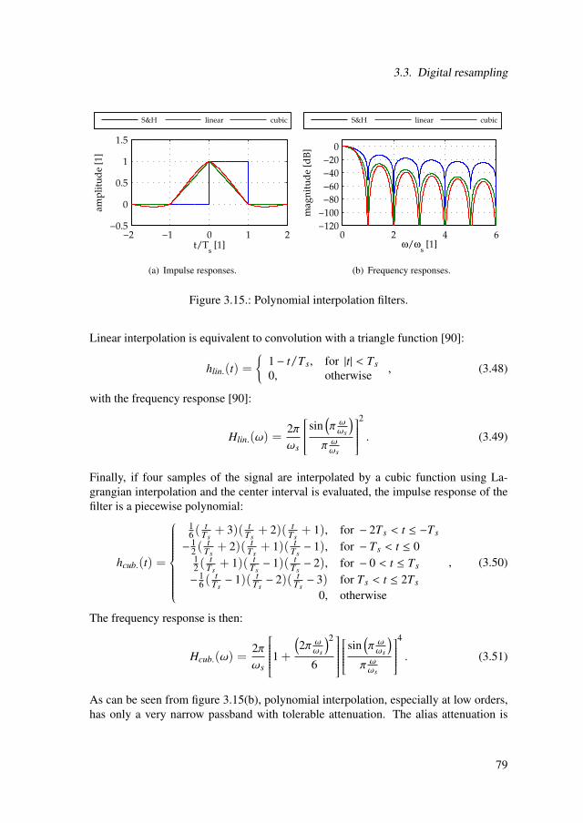
3.3. Digital resampling
−2 −1 0 1 2−0.5
0
0.5
1
1.5
t/Ts [1]
amp
litu
de
[1]
S&H linear cubic
(a) Impulse responses.
0 2 4 6−120
−100
−80
−60
−40
−20
0
ω/ωs [1]
mag
nit
ud
e [d
B]
S&H linear cubic
(b) Frequency responses.
Figure 3.15.: Polynomial interpolation filters.
Linear interpolation is equivalent to convolution with a triangle function [90]:
hlin.(t) =
1 − t/Ts, for |t| < Ts0, otherwise , (3.48)
with the frequency response [90]:
Hlin.(ω) =2πωs
⎡⎢⎢⎢⎢⎢⎢⎣ sin(π ωωs
)π ωωs
⎤⎥⎥⎥⎥⎥⎥⎦2
. (3.49)
Finally, if four samples of the signal are interpolated by a cubic function using La-grangian interpolation and the center interval is evaluated, the impulse response of thefilter is a piecewise polynomial:
hcub.(t) =
⎧⎪⎪⎪⎪⎪⎪⎪⎪⎪⎪⎨⎪⎪⎪⎪⎪⎪⎪⎪⎪⎪⎩
16 (
tTs
+ 3)( tTs
+ 2)( tTs
+ 1), for − 2Ts < t ≤ −Ts
− 12 (
tTs
+ 2)( tTs
+ 1)( tTs− 1), for − Ts < t ≤ 0
12 (
tTs
+ 1)( tTs− 1)( t
Ts− 2), for − 0 < t ≤ Ts
− 16 (
tTs− 1)( t
Ts− 2)( t
Ts− 3) for Ts < t ≤ 2Ts
0, otherwise
, (3.50)
The frequency response is then:
Hcub.(ω) =2πωs
⎡⎢⎢⎢⎢⎢⎢⎢⎢⎣1 +(2π ωωs
)2
6
⎤⎥⎥⎥⎥⎥⎥⎥⎥⎦⎡⎢⎢⎢⎢⎢⎢⎣ sin
(π ωωs
)π ωωs
⎤⎥⎥⎥⎥⎥⎥⎦4
. (3.51)
As can be seen from figure 3.15(b), polynomial interpolation, especially at low orders,has only a very narrow passband with tolerable attenuation. The alias attenuation is
79
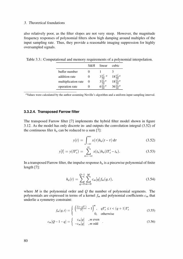
3. Theoretical foundations
also relatively poor, as the filter slopes are not very steep. However, the magnitudefrequency responses of polynomial filters show high damping around multiples of theinput sampling rate. Thus, they provide a reasonable imaging suppression for highlyoversampled signals.
Table 3.3.: Computational and memory requirements of a polynomial interpolation.
S&H linear cubic
buffer number 0 1 3addition rate 0 3ω
′s
2πa 18ω
′s
2πa
multiplication rate 0 3ω′s
2πa 18ω
′s
2πa
operation rate 0 6ω′s
2πa 36ω
′s
2πa
aValues were calculated by the author assuming Neville’s algorithm and a uniform input sampling interval.
3.3.2.4. Transposed Farrow filter
The transposed Farrow filter [7] implements the hybrid filter model shown in figure3.12. As the model has only discrete in- and outputs the convolution integral (3.52) ofthe continuous filer ha can be reduced to a sum [7]:
y(t) =∫ ∞
−∞
x(τ)ha(t − τ) dτ (3.52)
y[l] = y(lT ′s) =∞∑
n=−∞x(tn)ha(lT ′s − tn). (3.53)
In a transposed Farrow filter, the impulse response ha is a piecewise polynomial of finitelength [7]:
ha(t) =Q−1∑q=0
M∑m=0
cm[q] fm(q, t), (3.54)
where M is the polynomial order and Q the number of polynomial segments. Thepolynomials are expressed in terms of a kernel fm and polynomial coefficients cm thatunderlie a symmetry constraint:
fm(q, t) =
⎧⎪⎪⎨⎪⎪⎩(
2(t−qT ′s)T ′s
− 1)m
, qT ′s ≤ t < (q + 1)T ′s0, otherwise
(3.55)
cm[Q − 1 − q] =
cm[q] , m even−cm[q] , m odd . (3.56)
80

3.3. Digital resampling
The fractional interval µn ∈ [0, 1) specifies the location of the nth input sample withreference to the lthn output sample, which is the output sample that occurs directly at orbefore it:
tn = (µn + ln)T ′s. (3.57)
The polynomial kernel fm evaluated for t = lnT ′s − tn can be expressed as 4:
fm(q, lT ′s − tn) =
(1 − 2µn)m , µn , 0(−1)m , µn = 0 . (3.58)
Substituting (3.54) to (3.56), (3.58) into (3.53) and rearranging the order of summationyields:
y(lT ′s) =M∑
m=0
Q−1∑q=0
cm[q]
⎡⎢⎢⎢⎢⎢⎢⎢⎢⎢⎢⎣nup(q,l)∑
n=nlow(q,l)
Basis multipliers x(tn) fm(q, lT ′s − tn)
⎤⎥⎥⎥⎥⎥⎥⎥⎥⎥⎥⎦ Integrate & dump Cm
, (3.59)
where nlow(q, l) and nup(q, l) mark the lower and upper boundaries of the interval,where ha is nonzero. The filtering equation 3.59 can be expressed as the structureshown in figure 3.16.
Figure 3.16.: Structure of the transposed Farrow filter [7, 82].
The filter is made up of M + 1 parallel branches, each consisting of an integrate-and-dump (I&D) block and a fixed FIR subfilter Cm(z) of the filter order Q − 1. The inputsamples x[n] are multiplied with powers of (1− 2µn) or −1 and the results are accumu-lated in the I&D blocks. At every output sampling instant lT ′s ,their outputs are fed intothe subfilters Cm(z) and the accumulators of the I&D blocks are reset. The output ofthe transposed Farrow filter is obtained by summing over the outputs of all subfilters.
4In [7] only fm(q, lT ′s − tn) = (1 − 2µn)m is given. Yet, calculations of the author show that this leads toerrors, if the function is evaluated for lT ′s − tn = 0, i.e. µn = 0. See appendix B for details.
81
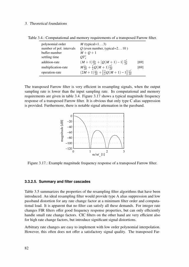
3. Theoretical foundations
Table 3.4.: Computational and memory requirements of a transposed Farrow filter.
polynomial order M (typical=1. . . 3)number of pol. intervals Q (even number, typical=2. . . 10 )buffer-number M + Q + 1settling time QT ′saddition-rate (M + 1)ωs
2π + [Q(M + 1) − 1] ω′s
2π [69]multiplication-rate M ωs
2π +12 Q(M + 1)ω
′s
2π [69]operation-rate (2M + 1)ωs
2π +[
32 Q(M + 1) − 1
]ω′s2π
The transposed Farrow filter is very efficient in resampling signals, when the outputsampling rate is lower than the input sampling rate. Its computational and memoryrequirements are given in table 3.4. Figure 3.17 shows a typical magnitude frequencyresponse of a transposed Farrow filter. It is obvious that only type C alias suppressionis provided. Furthermore, there is notable signal attenuation in the passband.
0 1 2 3−120
−100
−80
−60
−40
−20
0
ω/ω’s [1]
mag
nit
ud
e [d
B]
Figure 3.17.: Example magnitude frequency response of a transposed Farrow filter.
3.3.2.5. Summary and filter cascades
Table 3.5 summarizes the properties of the resampling filter algorithms that have beenintroduced. An ideal resampling filter would provide type A alias suppression and lowpassband distortion for any rate change factor at a minimum filter order and computa-tional load. It is apparent that no filter can satisfy all these demands. For integer ratechanges FIR filters offer good frequency response properties, but can only efficientlyhandle small rate change factors. CIC filters on the other hand are very efficient alsofor high rate change factors, but introduce significant signal distortions.
Arbitrary rate changes are easy to implement with low order polynomial interpolation.However, this often does not offer a satisfactory signal quality. The transposed Far-
82
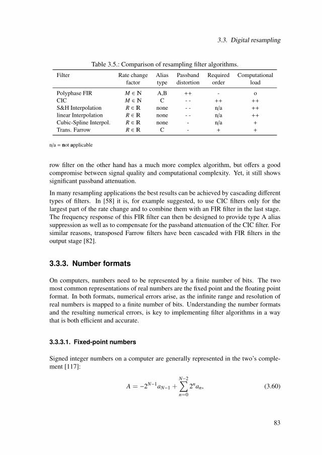
3.3. Digital resampling
Table 3.5.: Comparison of resampling filter algorithms.
Filter Rate change Alias Passband Required Computationalfactor type distortion order load
Polyphase FIR M ∈ A,B ++ - oCIC M ∈ C - - ++ ++
S&H Interpolation R ∈ none - - n/a ++
linear Interpolation R ∈ none - - n/a ++
Cubic-Spline Interpol. R ∈ none - n/a +
Trans. Farrow R ∈ C - + +
n/a = not applicable
row filter on the other hand has a much more complex algorithm, but offers a goodcompromise between signal quality and computational complexity. Yet, it still showssignificant passband attenuation.
In many resampling applications the best results can be achieved by cascading differenttypes of filters. In [58] it is, for example suggested, to use CIC filters only for thelargest part of the rate change and to combine them with an FIR filter in the last stage.The frequency response of this FIR filter can then be designed to provide type A aliassuppression as well as to compensate for the passband attenuation of the CIC filter. Forsimilar reasons, transposed Farrow filters have been cascaded with FIR filters in theoutput stage [82].
3.3.3. Number formats
On computers, numbers need to be represented by a finite number of bits. The twomost common representations of real numbers are the fixed point and the floating pointformat. In both formats, numerical errors arise, as the infinite range and resolution ofreal numbers is mapped to a finite number of bits. Understanding the number formatsand the resulting numerical errors, is key to implementing filter algorithms in a waythat is both efficient and accurate.
3.3.3.1. Fixed-point numbers
Signed integer numbers on a computer are generally represented in the two’s comple-ment [117]:
A = −2N−1aN−1 +N−2∑n=0
2nan, (3.60)
83
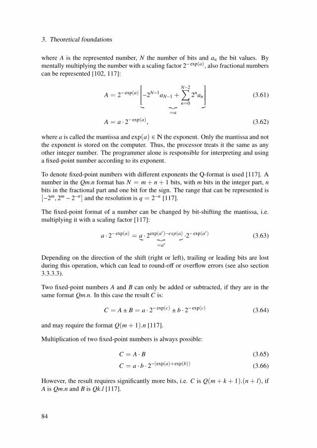
3. Theoretical foundations
where A is the represented number, N the number of bits and an the bit values. Bymentally multiplying the number with a scaling factor 2− exp(a), also fractional numberscan be represented [102, 117]:
A = 2− exp(a)
⎡⎢⎢⎢⎢⎢⎢⎣−2N−1aN−1 +N−2∑n=0
2nan
⎤⎥⎥⎥⎥⎥⎥⎦ =a
(3.61)
A = a · 2− exp(a), (3.62)
where a is called the mantissa and exp(a) ∈ the exponent. Only the mantissa and notthe exponent is stored on the computer. Thus, the processor treats it the same as anyother integer number. The programmer alone is responsible for interpreting and usinga fixed-point number according to its exponent.
To denote fixed-point numbers with different exponents the Q-format is used [117]. Anumber in the Qm.n format has N = m + n + 1 bits, with m bits in the integer part, nbits in the fractional part and one bit for the sign. The range that can be represented is[−2m, 2m − 2−n] and the resolution is q = 2−n [117].
The fixed-point format of a number can be changed by bit-shifting the mantissa, i.e.multiplying it with a scaling factor [117]:
a · 2− exp(a) = a · 2exp(a′)−exp(a) =a′
·2− exp(a′) (3.63)
Depending on the direction of the shift (right or left), trailing or leading bits are lostduring this operation, which can lead to round-off or overflow errors (see also section3.3.3.3).
Two fixed-point numbers A and B can only be added or subtracted, if they are in thesame format Qm.n. In this case the result C is:
C = A ± B = a · 2− exp(c) ± b · 2− exp(c) (3.64)
and may require the format Q(m + 1).n [117].
Multiplication of two fixed-point numbers is always possible:
C = A · B (3.65)
C = a · b · 2−(exp(a)+exp(b)) (3.66)
However, the result requires significantly more bits, i.e. C is Q(m + k + 1).(n + l), ifA is Qm.n and B is Qk.l [117].
84

3.3. Digital resampling
Division is similar to multiplication:
C =AB
(3.67)
C =ab· 2−(exp(a)−exp(b)) (3.68)
However, the result is in the format Q(m + l + 1).(n + k), if A is Qm.n and B is Qk.l[117].
3.3.3.2. Floating-point numbers
The biggest drawback of fixed-point number formats is their small dynamic range, i.e.it is generally not possible to accurately represent very small and very big numberswithin the same number format, due to the fixed exponent [102]. Therefore floatingpoint numbers, store the exponent as well as the mantissa. This makes it possible todynamically adapt the exponent to the size of the number. The IEEE 754 standarddefines the following representation for a 32 bit floating point number [16]:
A = (−1)s(0.5 + f )2p−126, (3.69)
where s is the sign bit, f a 23 bit number, that represents an unsigned fraction in therange [0, 0.5), and p an unsigned 8 bit integer, denoting the exponent.
Arithmetic operations with floating-point numbers essentially work the same way aswith fixed-point numbers. Yet, for floating-point numbers the computer has to performthe format changes necessary to keep a constant number of bits dynamically during thecalculations. On powerful modern computers these calculations are accelerated by ahardware floating-point unit (FPU). Yet, on the low-cost embedded microprocessorstypically used in WSN, a FPU is usually not available [117]. Thus, fixed-point calcu-lations generally run significantly faster than floating-point calculations on such hard-ware, as the programmer can minimize the needed format conversions in advance.
3.3.3.3. Numerical errors
Numerical errors arise in digital computations regardless of whether fixed- or floating-point numbers are used. In general, two types of numerical errors can be distinguished:overflow and quantization errors. The following analysis focuses on fixed-point arith-metic as it is more relevant for the use in WSN (compare section 3.3.3.2).
Overflow errors arise when the result of a calculation needs more bits than are presentin the output variable, e.g. when the sum of two 8 bit numbers is 100 + 50 = 150,but the largest representable output value is 127, because the output variable is also
85

3. Theoretical foundations
8 bit. This may cause large nonlinear errors, as the number wraps around and may beinterpreted as negative, e.g. −106 in the example above. An interesting property ofthe two’s complement is that, if the sum of multiple values is within the representablerange, it will be calculated correctly, even if intermediate results overflow [102].
Quantization errors arise because numbers cannot be represented with infinite precision.They are often also referred to as round-off or truncation errors, depending on whethera number is rounded to the closest number, which can be represented within the givenresolution, or simply truncated after the least significant bit.
Digital filters are affected by quantization errors in two ways: First, the quantizationof their coefficients changes the filter characteristic. Second, quantization of resultscreates additional noise in the output signal. Regarding the coefficient quantization FIRfilters are far less sensitive than IIR filters [102, 16]. Furthermore, higher order FIRfilters are more strongly affected than lower order ones, as their zeros are placed moreclosely together [102]. In [71] it is even shown, that when approximating a desiredfrequency response with an FIR filter having finite wordlength coefficients, there isa filter order Qmax, beyond which the approximation quality does not improve. Theexact value of Qmax is dependent on both the number of bits for the coefficients and thedesired frequency response. Calculation of Qmax is only possible through an iterativesearch algorithm. In [71], Qmax is calculated to be in the range of 36 . . . 53 for 12 bitcoefficients and six different target frequency responses.
The additional noise in the output signal, caused by result quantization, is generallymodeled to be stationary, white and uncorrelated with the signal. Its distribution isassumed as uniform with a variance of [16] (see also section 3.4.2.1):
σ2q =
q2
12. (3.70)
For a Qth-order FIR filter with rounding after every multiplication the output noisevariance is [102, 16]:
σ2q = (Q + 1)
q2
12. (3.71)
If, however, the intermediate results are not rounded after every multiplication andinstead an accumulator with double-wordlength is used the output noise variance isonly [102, 16]:
σ2q =
q2
12, (3.72)
as rounding only takes place at the output stage. This optimization is only possiblein fixed-point arithmetic, because in floating-point arithmetic rounding automaticallytakes place after every operation. Thus, using fixed-point arithmetic offers better controlover quantization errors and may, in some cases, even enable more accurate calculations[16].
86

3.4. Quality of measurements and signals
3.4. Quality of measurements and signals
A key characteristic of any measurement or data acquisition device is the quality of theresults that can be expected from it. The measurement uncertainty, which is introducedin section 3.4.1, today is the accepted way to express the quality of any single valuedmeasurement result. For acquired signals, that consist of a set of samples other qual-ity measures are used. These are introduced in section 3.4.2. Sine wave signals arefrequently used to assess the performance of measurement systems (compare section4.6). Therefore, algorithms to estimate their parameters and purity are given in section3.4.3.
3.4.1. Measurement uncertainty
The concept of measurement uncertainty is defined by the guide to the expression ofuncertainty in measurement (GUM) [199]. This international standard aims to pro-vide a universal method for evaluating and expressing the uncertainty of measurementresults. The GUM has been created by a joint working group of a number of interna-tional institutions including the International Organization for Standardization (ISO),the International Electrotechnical Commission (IEC) and the International Bureau ofWeights and Measures (BIPM). It is the basis of many national standards like the DIN1319 [57].
3.4.1.1. Concepts
The measurement uncertainty is a quantitative measure of trust in the measurement re-sult . . . that characterizes the dispersion of values that could reasonably be attributedto the measurand [199]. It can only be applied to a measurand, which is a well definedphysical quantity that can be characterized by a single value [199]. The GUM recom-mends using the standard deviation to express the measurement uncertainty. Often themeasurement result is not obtained directly from an observation of the measurand, butcalculated from a number of input quantities, that have been measured. Measurementuncertainty is understood to be caused by influence quantities, i.e. quantities that arenot the measurand, but have an effect on the measurement result [199]. Thus, influencequantities can be seen as a special type of input quantity.
A related concept is the measurement error, which is the difference between the trueand the observed value. As in practice the true value cannot be determined exactly, themeasurement error is an idealized concept [199]. Commonly, the error ϵx is modeledas having a systematic component ∆x and a random component δx:
ϵx = ∆x + δx, (3.73)
87

3. Theoretical foundations
The systematic error ∆x is constant and repeatable, while the random error δx arisesfrom unpredictable, stochastic temporal or spacial variations. The GUM assumes thatall known significant systematic effects have been removed from the measurement re-sult prior to its evaluation [199]. Thus, the measurement uncertainty is only caused byrandom and unknown systematic errors.
3.4.1.2. Evaluation of the uncertainty
The general procedure for evaluating the uncertainty of a measurement, given in [107],is as follows:
1. Model relationship between measurand and input quantities
2. Record measurements
3. Calculate results and uncertainties
4. Report results
A procedure, that focuses more on the calculation of the uncertainty itself, is given inthe GUM [199]:
1. Express mathematical relationship between the measurand Y and the input quan-tities Xi: Y = f (X1, . . . , XN)
2. Determine estimates xi for input quantities Xi
3. Calculate standard uncertainty u(xi) for each input quantity Xi
4. Evaluate covariances between input quantities
5. Determine estimate y for measurand Y
6. Calculate combined standard uncertainty uc(y) of measurand
7. Calculate expanded uncertainty Uk = kuc(y)
In the following, the calculation of the standard, combined and expanded uncertainty isdescribed in more detail.
88

3.4. Quality of measurements and signals
Calculation of the standard uncertainty
When evaluating the standard uncertainties of the input quantities Xi, the GUM distin-guishes between type A and type B evaluation [199]:
Type A evaluation is based on empirical data. For N independent measurements xi,n ofthe input quantity Xi, the estimate xi is in most cases given as the arithmetic mean:
xi = Xi =1N
N∑n=1
xi,n (3.74)
The standard uncertainty u(xi) of this estimate is the empirical standard deviation s(xi)of the estimate xi, which is calculated from the individual observations as follows:
s(xi) =
√1
N − 1
N∑n=1
(xi,n − xi)2 (3.75)
u(xi) = s(xi) =s(xi)√
N(3.76)
The degrees of freedom v should always be given with the uncertainty; in this case:v = N − 1.
Another frequent application is the estimation of the parameters ai of a M-th orderlinear model [49, 199]:
y = X a + ϵ (3.77)
with:
y = (y1, · · · , yN)T (3.78)
X =
⎛⎜⎜⎜⎜⎜⎜⎜⎜⎜⎜⎝1 x1 · · · xM
1...
.... . .
...1 xN · · · xM
N
⎞⎟⎟⎟⎟⎟⎟⎟⎟⎟⎟⎠ (3.79)
a = (a0, · · · , aM)T , (3.80)
where X is a matrix containing the observed input values, y a vector of observed outputvalues, a is the parameter vector and ϵ a vector with noise. Then, the estimate a of theparameters that minimizes the noise energy in a least-squares sense is:
a =(XT · X
)−1 =D
·XT · y (3.81)
89
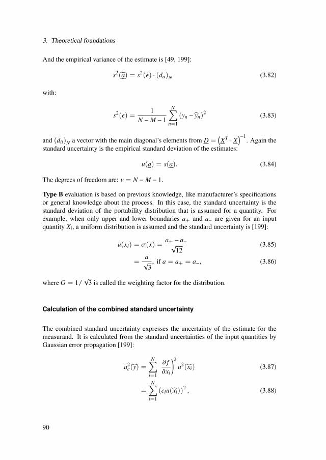
3. Theoretical foundations
And the empirical variance of the estimate is [49, 199]:
s2 (a) = s2(ϵ) · (dii)N (3.82)
with:
s2(ϵ) =1
N −M − 1
N∑n=1
(yn − yn)2 (3.83)
and (dii)N a vector with the main diagonal’s elements from D =(XT · X
)−1. Again the
standard uncertainty is the empirical standard deviation of the estimates:
u(a) = s(a). (3.84)
The degrees of freedom are: v = N −M − 1.
Type B evaluation is based on previous knowledge, like manufacturer’s specificationsor general knowledge about the process. In this case, the standard uncertainty is thestandard deviation of the portability distribution that is assumed for a quantity. Forexample, when only upper and lower boundaries a+ and a− are given for an inputquantity Xi, a uniform distribution is assumed and the standard uncertainty is [199]:
u(xi) = σ(x) =a+ − a−√
12(3.85)
=a√
3, if a = a+ = a−, (3.86)
where G = 1/√
3 is called the weighting factor for the distribution.
Calculation of the combined standard uncertainty
The combined standard uncertainty expresses the uncertainty of the estimate for themeasurand. It is calculated from the standard uncertainties of the input quantities byGaussian error propagation [199]:
u2c (y) =
N∑i=1
(∂ f∂xi
)2
u2(xi) (3.87)
=N∑
i=1
(ciu(xi))2 , (3.88)
90

3.4. Quality of measurements and signals
Table 3.6.: Coverage factors and confidence levels for a Gaussian distribution [199].
Coverage factor k [1] 1.000 1.645 1.960 2.000 2.576 3.000Confidence level p [%] 68.27 90.00 95.00 95.45 99.00 99.73
where f is a function expressing the mathematical relationship between input quantitiesXi and measurand y and ci is the sensitivity coefficient of Xi. When there is correlationbetween the input quantities, the propagation law needs to be extended [199]:
u2c (y) =
N∑i=1
(ciu(xi))2 + 2
N−1∑i=1
N∑j=i+1
cic ju(xi)u(x j)r(Xi, X j), (3.89)
where r(Xi, X j) is the correlation coefficient for the input quantities Xi and X j.
Calculation of the expanded uncertainty
Often the expanded uncertainty Uk = kuc (y) is given in addition to the combined stan-dard uncertainty [107, 199]. Its meaning is that the interval y±Uk encompasses a largeportion of the value distribution of y [199]. This concept is similar to the confidenceinterval in statistics. However, the definitions only match exactly, when all contributinguncertainties have been obtained from type A evaluation [199]. The coverage factor kdetermines the size of the portion from the value distribution that is covered. It is gen-erally not possible to link k exactly with a level of confidence, as the exact probabilitydistribution of y is usually unknown [199]. However, in most applications an approx-imately Gaussian distribution is assumed, due to the central limit theorem [57]. Table3.6 shows a selection of coverage factors and confidence levels for a Gaussian distribu-tion. In metrology the common choice for the coverage factor is k = 2 [57, 107, 199].
Reporting of results
When reporting a measurement result, the estimate y of the measurand and its combinedstandard uncertainty should be given [199]. This is often done in the form of a completemeasurement result [107]:
Y = y ± uc (y) (3.90)
If the extended uncertainty is used instead of the standard one, the coverage factor khas to be given. In addition, the estimates for the input quantities together with theiruncertainties, sensitivity coefficients and degrees of freedom should be given, in order
91

3. Theoretical foundations
Table 3.7.: Example of an uncertainty budget.in
fluen
ce
estim
ate
assu
med
unce
rtai
nty
dist
ribu
tion
wei
ght
stan
dard
unce
rtai
nty
sens
itivi
tyco
effici
ent
degr
ees
offr
eedo
m
unce
rtai
nty
cont
ribu
tion
δ S E√
G u c v u
δI 1.000 A 0.010 A uniform 1/√
3 0.006 A 10.00 V 1 0.058 WδU 10.00 V 0.010 V uniform 1/
√3 0.006 V 1.000 A 1 0.006 W
uc 10.000 W 1 0.058 WUk=2 10.000 W 0.116 W
to make the calculation of the result transparent [199]. In [107] it is suggested to presentthis information as an uncertainty budget in a table. Table 3.7 shows an example of suchan uncertainty budget. This presentation also helps to analyze the relative strengths ofdifferent input quantities and to optimize measurement setups, in order to minimizeuncertainty.
3.4.2. Signal quality
When acquiring a physical signal, the result is a digital waveform, which is character-ized not by a single value, but by a set of samples (compare section 3.2). Thereforequantities other than the measurement uncertainty are needed to express its quality asa whole5. This section briefly presents the errors, which may occur in signals andmeasures to quantify the relative magnitude of those errors.
3.4.2.1. Signal errors
In general, signal errors can be interpreted as additive amplitude errors:
x(t) = x(t) + ϵx(t), (3.91)
where x is the error-free signal and ϵ is an error term.
5These quality measures themselves are measurands that can be attributed with a measurement uncertainty.
92

3.4. Quality of measurements and signals
Common systematic signal errors with linear effect are offset, gain, phase shift:
ϵx,o f f (t) = const. (3.92)ϵx,gain(t) = a · x(t), a ∈ , a = const. (3.93)ϵx,shi f t(t) = x(t + ϵt) − x(t), ϵt ∈ , ϵt = const. (3.94)
The consequence of (3.94) is, that the timing error ϵt can equally be expressed as anamplitude error ϵx. Small time errors ϵt can be easily transformed into amplitude errorsand vice versa, by locally linearizing the signal [201, 65]:
ϵx(t0) =dx(t)
dt
t=t0
· ϵt(t0) (3.95)
ϵt(t0) =
⎛⎜⎜⎜⎜⎜⎝ dx(t)dt
t=t0
⎞⎟⎟⎟⎟⎟⎠−1
· ϵx(t0). (3.96)
Another kind of systematic error occurs, when a signal is fed through an amplifier witha non-linear characteristic a(x):
xnon−lin.(t) = a (x(t)) · x(t). (3.97)
This also alters the frequency content of the signal and may especially give rise to newharmonic components, called harmonic distortions [201, 84].
Random signal errors are often modeled as zero-mean Gaussian white noise ϵx(t) =w(t), but also other probability distributions may occur [84]. A common type of addi-tive amplitude noise is the quantization noise that occurs in data acquisition systems,when the continuous signal amplitude is discretized. The quantization error ϵq is dis-tributed uniformly over the interval [−q/2, q/2], where q is the quantization step of thedata acquisition system. The expectation value and variance of the quantization noiseare [66]:
E(ϵq(t)) = 0 (3.98)
Var(ϵq(t)) =q2
12. (3.99)
3.4.2.2. Signal purity measures
Three ratios are commonly used to quantify the purity of signals: the SINAD, the SNRand the THD. The signal-to-noise and distortion (SINAD) is the ratio of a signal’s root-mean-square (RMS) value αrms to that of noise and distortion (NAD) [201], i.e. theRMS of the error ϵ in (3.91):
S INAD =αrms
NAD. (3.100)
93

3. Theoretical foundations
The NAD can be split up into the energy of noise η2 and the total energy of harmonicdistortions THE [201]:
NAD2 = η2 + T HE. (3.101)
This leads to the definitions of the signal-to-noise (SNR) ratio and the total harmonicdistortion (THD) [201]:
S NR =αrms
η(3.102)
T HD =
√T HEαrms
. (3.103)
All three ratios are commonly expressed in the logarithmic pseudo-unit Decibel (dB),e.g.:
S INADdB = 20 log10 (S INAD) dB. (3.104)
3.4.3. Estimation of signal parameters
In order to assess the quality of an acquired waveform, signal parameters like the am-plitude, or purity measures like the SNR need to be estimated from the samples. Thissection presents algorithms to estimate the parameters of acquired sine wave signals(section 3.4.3.1), the phase difference between two sine waves (section 3.4.3.1) as wellas the purity of a sine wave (section 3.4.3.3).
3.4.3.1. Sine wave parameters
A sine wave signal is sufficiently characterized by four parameters: amplitude α, offsetx0, phase shift ϕ and angular frequency ω [201]:
x(t) = α sin(ωt + ϕ) + x0, (3.105)
Alternatively, every sine wave can be expressed as the sum of a sine and a cosine com-ponent:
x(t) = A0 cos(ωt) + B0 sin(ωt) +C0, (3.106)
with α =√
A20 + B2
0, ϕ = − arctan( B0
A0
)and x0 = C0 [201]. The standard IEEE 1057
recommends two algorithms to estimate the parameters of a recorded sine wave signal[201].
94

3.4. Quality of measurements and signals
The first algorithm, referred to as the three-parameter algorithm, can be used to estimatethe parameters: amplitude, phase and offset, when the frequency ω of the signal isknown [201]. The algorithm minimizes the sum of squared approximation errors:
ϵ2 =N∑
n=1
(x[n] − A0 cos(ωtn) − B0 sin(ωtn) −C0)2 , (3.107)
where x[n] are the signal samples taken at the times tn. The least-squares estimate sof the parameter vector s = (A0, B0, C0)
T is obtained through a closed form linearequation:
s =(DT
0 D0
)−1 (DT
0 x)
, (3.108)
with D0 =
⎛⎜⎜⎜⎜⎜⎜⎜⎜⎜⎜⎝cos(ωt1) sin(ωt1) 1
......
...cos(ωtN) sin(ωtN) 1
⎞⎟⎟⎟⎟⎟⎟⎟⎟⎟⎟⎠ and x = (x1, . . . , xN)T .
The second algorithm, referred to as the four-parameter algorithm, estimates all pa-rameters of a sine wave, i.e. does not require the signal frequency to be known [201].Based on an initial estimate of the signal parameters, it iteratively improves the estimatethrough the following equations:
si+1 =(DT
i Di
)−1 (DT
i x)
(3.109)
ωi+1 = ωi + ∆ωi+1 (3.110)
with
Di =
⎛⎜⎜⎜⎜⎜⎜⎜⎜⎜⎜⎜⎝cos(ωit1) sin(ωit1) 1 −Ait1 sin(ωit1) Bit1 cos(ωit1)
......
......
...cos(ωitN) sin(ωitN) 1 −AitN sin(ωitN) Bit1 cos(ωitN)
⎞⎟⎟⎟⎟⎟⎟⎟⎟⎟⎟⎟⎠and
si =(Ai, Bi, Ci, ∆ωi
)T.
The algorithm is reported to converge rapidly and achieve good results after fewer thansix iterations [201].
95

3. Theoretical foundations
The Cramer-Rao bound (CRB) is a lower bound to the variance of an estimator like thethree- and four-parameter algorithms. Thus, it can be used to get an impression of theestimate’s quality and how it is influenced by various quantities. In [4] the CRB for theestimation of sine parameters have been derived:
Var(α) ≥ CRB(α) =2η2
N(3.111)
Var(ϕ) ≥ CRB(ϕ) =
⎧⎪⎪⎪⎨⎪⎪⎪⎩2η2
N·α2 = 1N·S NR2 , three-parameter estimation
8η2
N·α2 = 4N·S NR2 , four-parameter estimation
(3.112)
Var(x0) ≥ CRB(x0) =η2
N(3.113)
Var(ω) ≥ CRB(ω) =24η2
N3 · α2 =12
N3 · S NR2 , four-parameter estimation (3.114)
Thus, all estimates improve with an increasing number of samples and deteriorate withincreasing signal noise. The variance of the phase estimate increases by a factor of fourwhen the frequency has to be estimated as well.
3.4.3.2. Phase difference
The phase difference ∆ϕ of two sine waves x1,2 with the same frequency can be es-timated by estimating their phases ϕ1,2, using the three- or four parameter algorithmintroduced above, and calculating the difference [115, 127]:
∆ϕ = ϕ1 − ϕ2 (3.115)
However, when the frequency of the two sine waves is unknown, more accurate resultscan be obtained by estimating the parameters of both sine waves simultaneously [115].The resulting seven parameter algorithm minimizes following error term [115]:
ϵ2 =N∑
n=1
(x1[n] − A1 cos(ωtn) − B1 sin(ωtn) −C1)2
+N∑
n=1
(x2[n] − A2 cos(ωtn) − B2 sin(ωtn) −C2)2 , (3.116)
where A1, B1, C1 are the parameters of the first sine wave, A2, B2, C2 those of the secondsine wave and ω is their common frequency. Minimization of the error term is doneiteratively, similar as in the four parameter algorithm. The phase differences estimatedwith this seven parameter algorithm have been found to show only half the variance ofthe estimates obtained from the four parameter algorithm [115]. According to [127],the seven parameter algorithm is currently the most accurate and robust algorithm forthe estimation of phase difference.
96
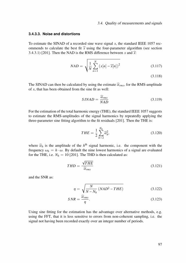
3.4. Quality of measurements and signals
3.4.3.3. Noise and distortions
To estimate the SINAD of a recorded sine wave signal x, the standard IEEE 1057 rec-ommends to calculate the best fit x using the four-parameter algorithm (see section3.4.3.1) [201]. Then the NAD is the RMS difference between x and x:
NAD =
√1N
N∑n=1
(x[n] − x[n])2 (3.117)
(3.118)
The SINAD can then be calculated by using the estimate αrms, for the RMS-amplitudeof x, that has been obtained from the sine fit as well:
S INAD =αrms
NAD(3.119)
For the estimation of the total harmonic energy (THE), the standard IEEE 1057 suggeststo estimate the RMS-amplitudes of the signal harmonics by repeatedly applying thethree-parameter sine fitting algorithm to the fit residuals [201]. Then the THE is:
T HE =12
Nh∑h=2
α2h, (3.120)
where αh is the amplitude of the hth signal harmonic, i.e. the component with thefrequency ωh = h · ω. By default the nine lowest harmonics of a signal are evaluatedfor the THE, i.e. Nh = 10 [201]. The THD is then calculated as:
T HD =
√T HEαrms
(3.121)
and the SNR as:
η =
√N
N − Nh(NAD2 − T HE) (3.122)
S NR =αrms
η. (3.123)
Using sine fitting for the estimation has the advantage over alternative methods, e.g.using the FFT, that it is less sensitive to errors from non-coherent sampling, i.e. thesignal not having been recorded exactly over an integer number of periods.
97


4. Modeling
In this chapter models of synchronous data acquisition with WSNs are developed. Thiswill provide first answers to the central questions of this thesis. First, the modeling ofa WSN as a data acquisition system is introduced in section 4.1. Section 4.2 describesthe modeling of acquisition errors, which leads to the definition of a useful measure ofsynchronization precision. This basis is used in section 4.3 to develop a strategy forestimating the synchronization precision necessary in a given application. Approachesto time synchronous data acquisition are suggested in section 4.4 and approaches tosynchronous angular sampling in section 4.5. Finally, section 4.6 suggests ways to testthe synchronization precision in the individual data acquisition scenarios.
4.1. System model
This section introduces the model of a synchronous multi-channel event detection sys-tem as well as that of a multi-channel waveform sampling system.
4.1.1. Event detection
In a multi-channel event detection system, every channel i detects events and assignstimestamps ti to them. The event detection is synchronous if all channels observing thesame event a assign the same timestamp to it:
ti(a) = t j(a) ∀i, j. (4.1)
The model is equally applicable to WSNs as to other multi-channel event detectionsystems. In a WSN, one or more channels may be located on a single node. Figure 4.1shows the model applied to a WSN.
99
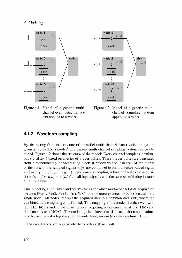
4. Modeling
Figure 4.1.: Model of a generic multi-channel event detection sys-tem applied to a WSN.
Figure 4.2.: Model of a generic multi-channel sampling systemapplied to a WSN.
4.1.2. Waveform sampling
By abstracting from the structure of a parallel multi-channel data acquisition systemgiven in figure 3.5, a model1 of a generic multi-channel sampling system can be ob-tained. Figure 4.2 shows the structure of the model: Every channel samples a continu-ous signal xi(t) based on a series of trigger pulses. These trigger pulses are generatedfrom a monotonically nondecreasing clock at predetermined instants. At the outputof the system, the sampled signals xi[n] are combined to form a vector-valued signalx[n] = (x1[n], x2[n], . . . , xM [n]). Synchronous sampling is then defined as the acquisi-tion of samples xi[n] = xi(tn) from all input signals with the same set of timing instantstn [Fun2, Fun4].
This modeling is equally valid for WSNs as for other multi-channel data acquisitionsystems [Fun1, Fun2, Fun4]. In a WSN one or more channels may be located on asingle node. All nodes transmit the acquired data to a common data sink, where thecombined output signal x[n] is formed. This mapping of the model matches well withthe IEEE 1451 standard for smart sensors: acquiring nodes can be treated as TIMs andthe data sink as a NCAP. The modeling also shows that data acquisition applicationstend to assume a star topology for the underlying system (compare section 2.1.3).
1This model has been previously published by the author in [Fun2, Fun4].
100

4.2. Acquisition errors
4.2. Acquisition errors
The first central question of this thesis is how synchronization precision can be definedin a way that is meaningful for measurement applications. To answer this question, theinfluence of synchronization and more generally timing errors on the final measurementresult is modeled. This modeling is based on the concepts of the GUM that were intro-duced in section 3.4.1. First, the modeling of event detection is done in section 4.2.1.In a second step, waveform sampling is treated in section 4.2.2. Finally, section 4.2.3concludes on a useful measure for synchronization precision.
4.2.1. Event detection
In case of event detection the measurement result is a single number, i.e. the time in-stant tevent at which the event occurred (compare section 3.2). Although comparativelysimple, event detection already involves several steps. A typical acquisition chain isshown in figure 4.3.
Figure 4.3.: Data acquisition chain for event detection.
First, the physical quantity that contains the event is transformed to an electrical quan-tity by a sensor, e.g. a photodiode in a rotary encoder. Then, an analog signal processingstage amplifies and filters the resulting electrical signal, in order to make the event eas-ier to detect. Next the processed signal is converted into a one-bit digital signal by athreshold comparator. The occurrence of an event is signified by a rising or falling edgein the digital signal. This edge triggers the reading of a clock by a digital circuit, oftena microcontroller. The resulting clock value is the timestamp tevent of the event.
101

4. Modeling
The measurement result is expressed in accordance to (3.90) as:
t′event = tevent ± ut. (4.2)
Here, ut is the uncertainty of tevent. This uncertainty is caused by unknown delays in theacquisition steps or errors of the clock. The overall error ϵt in tevent shall be modeled asthe sum of a systematic component ∆t and a random component δt:
tevent = tevent + ϵt (4.3)= tevent + ∆t + δt. (4.4)
The contribution of the individual processing steps to the error ϵt and the measurementuncertainty ut is analyzed in the following.
4.2.1.1. Analog stage
The sensor and analog signal processing are summarized as the analog stage of theevent detection chain. Due to various phenomena like internal capacities or inertia,many sensors have a lowpass characteristic. More generally, sensors are often modeledas linear time-invariant (LTI)-systems (H1 in figure 4.3). Likewise, the amplificationand filtering during the analog signal processing is generally modeled as a LTI-system(H2 in figure 4.3). The group delay of these systems influences the event’s propagationalong the chain. Its error contribution is modeled to be purely systematic ∆t,ana. Thereason for this is that the components of sensors and analog circuitry generally do notchange their properties over time, apart from a small temperature drift.
4.2.1.2. Threshold comparator
In the threshold comparator, amplitude errors ϵx of the input signal change the time,at which an edge is generated, by ϵt,comp. For small errors ϵx the time error is givenby (3.96). Constant amplitude errors, like gain or offset errors, result in a systematiccomponent ∆t,comp of ϵt,comp. Random amplitude noise causes a random error δt,comp.As amplitude noise is commonly modeled to be zero-mean and Gaussian, δt,comp is alsoassumed to be zero-mean and Gaussian, with a standard deviation of:
σt =
⎛⎜⎜⎜⎜⎜⎝ dx(t)dt
t=t0
⎞⎟⎟⎟⎟⎟⎠−1
σx, (4.5)
where t0 is the time of detection and σx is the standard deviation of the amplitudenoise.
102

4.2. Acquisition errors
4.2.1.3. Digital circuit
The propagation delays in digital circuits are usually constant. Thus, a constant com-ponent ∆t,digi is contributed. However, when using the interrupt of a microcontroller todetect a digital edge and read the clock, interrupt blocking code sections may introducea random delay δt,int (see also section 5.1.2.1). If an interrupt blocking code section isTblock long, recurs with a period Trep and is uncorrelated with the event to be detected,the probability of it causing a delay is:
Pdelay =Tblock
Trep. (4.6)
Its length is distributed uniformly between 0 and Tblock. The situation is the same, if theblocking section occurs randomly with a probability of Pdelay. If Tblock varies randomlybetween Tblock,min and Tblock,max, the edges of the uniform distribution will round off atthe edges, as large delays are less likely in this case. The exact form depends on thedistribution of Tblock. When multiple blocking sections occur independently of eachother their probability densities superpose.
4.2.1.4. Clock reading
When reading a discrete clock c at a time instant t1 the result is the clock’s countervalue hc,1 = hc(t1). This is commonly transformed into a time reading using the clockmodel from (3.1):
t1 = hc,1Tclock + t0. (4.7)
However, as the clock counter is only incremented at discrete time instants, the infor-mation actually contained in the reading, is that t1 is somewhere in the interval betweentwo clock updates:
hc,1Tclock + t0 ≤ t1 < (hc,1 + 1)Tclock + t0. (4.8)
Thus, there is a random error δt,read in the clock reading, that is uniformly distributedover the interval (−Tclock, 0], (see figure 4.4(a)). The expectation value is:
E(δt,read) = −Tclock
2, (4.9)
i.e. the time estimate t1 is biased. The variance of δt,read is:
Var(δt,read) =T 2
clock
12. (4.10)
103

4. Modeling
(a) single clock reading (b) difference of two readings
Figure 4.4.: Probability density distributions of clock reading errors.
A clock reading t1 often only becomes useful when the difference ∆t to another readingt2 is calculated, i.e.:
∆t = t2 − t1. (4.11)
In this case, the probability density function fX,∆(δ∆t) of the random error δ∆t in ∆t isobtained from those of the single clock readings through convolution:
fX,∆(δ∆t) =
∫ δ∆t
−∞
fX,t(u) fX,t(δ∆t − u) du. (4.12)
The result is a triangular distribution (see figure 4.4). This assumes that the two clockreadings, i.e. the reading instants’ relative positions to the clock updates, are statisti-cally independent. It is not necessary that the clocks or reading instants are uncorre-lated. With the same clock resolution for both readings, the expectation value of δ∆tis:
E(δ∆t) = 0, (4.13)
i.e. the estimate ∆t = t2 − t1 is unbiased, even though the individual estimates t1,2 are.The variance of δ∆t is:
Var(δ∆t) = 2Var(δt,read) =T 2
clock
6. (4.14)
4.2.1.5. Clock errors
The clock value itself may contain errors, e.g. an offset t0 , t0 (compare (4.7)) or adrift error ρ , 0. Offset errors cause a systematic error contribution:
∆t,o f f = t0 − t0. (4.15)
104

4.2. Acquisition errors
Table 4.1.: Summary of error influences on the detection time tevent
Influence Cause Distributionsy
stem
atic ∆t,ana group delay of analog circuitry -
∆t,comp constant amplitude errors -∆t,digi propagation delay in digital circuit -∆t,o f f clock offset error -
rand
om
δt,comp amplitude noise Gaussianδt,read clock reading uniform/triangularδt,int interrupt delay approximately uniformδt,dri f t clock drift error uniformδt,sync synchronization error approximately Gaussian
If the drift is constant ρ(t) = a, the clock error ϵc increases linearly with time:
ϵc = c(t) − t = at, with a = const. (4.16)
Often synchronization algorithms are used to limit the maximum clock error ϵc,max byperiodically resetting the error to a value ϵc,min that is close to zero (compare section2.2.2.1). In this case the drift error of the clock becomes a sawtooth function. Thus,when reading the clock at random instants, the resulting error δt,dri f t is uniformly dis-tributed between ϵc,min and ϵc,max.
The synchronization process itself may also introduce an error δt,sync into the clockvalue. Many publications report this to be approximately Gaussian distributed [124,22, 35, 26]. However, also non-Gaussian error distribution are reported, e.g. bimodalin [42] and one-side truncated Gaussian in [77]. Apparently, the synchronization erroris the combination of many error influences that, due to the central limit theorem, oftenverges on a Gaussian distribution but may also differ significantly from it.
4.2.1.6. Conclusions
Table 4.1 summarizes the modeled systematic and random error influences on event de-tection times. The distribution of the combined random error δt is a superposition of theindividual influences and depends very much on their relative strengths. If, for example,the drift error is dominating, an approximately uniform distribution is expected. Whilea dominant influence from amplitude noise would lead to a Gaussian distribution. Ifnone of the influences dominates the others, an approximately Gaussian distribution isexpected due to the central limit theorem.
The known systematic influences should be used to correct the estimate tevent of theevent time. The variance of the unknown systematic influences and that of the combined
105

4. Modeling
random error influences constitute the uncertainty of the measurement (compare section3.4.1):
t′event = tevent − ∆t,known =tevent,corr
±
√Var(∆t,unknown) + Var(δt)
=ut
. (4.17)
A measure for timestamping precision that allows for easy comparison between differ-ent systems can be obtained by solving (4.10) for the clock resolution Tclock:
Tclock =√
12σt, (4.18)
where σt is the standard deviation of a clock reading. If this is replaced with the timinguncertainty ut, an effective clock resolution Tclock,e f f is obtained:
Tclock,e f f =√
12ut. (4.19)
It can be interpreted as the clock resolution of an ideal timestamping system withthe same timestamping uncertainty. Thus, it enables fast and intuitive comparisonsof timestamping systems, like the effective number of bits does for ADCs.
4.2.2. Waveform sampling
An acquired waveform consists of a number of signal values x[n] and their correspond-ing sampling instants tn. As signals are usually sampled on a uniform sampling grid,the sampling instants are often specified only implicitly through the sampling intervalTs and the timestamp of the first sample t0.
tn = nTs + t0. (4.20)
Errors in the signal values may result from the sensor, analog signal processing or thecharacteristic of the ADC. They are commonly categorized as follows (see also section3.4.2.1):
• offset error
• gain error
• non-linear distortion
• additive noise2
2This includes quantization noise.
106

4.2. Acquisition errors
As in the case of event detection, errors in the acquired time values can arise from delaysalong the digital measurement chain or errors of the clock. In a WSN one cause may bethe suboptimal synchronization between the individual nodes. Yet similar effects mayalso occur in non-wireless acquisition devices, e.g. through multiplexed acquisition orpropagation delays of the clock signal on its path. It is often not possible to distinguishbetween errors in the signal and errors in the time values, as both may change theshape of the signal in the same way (see section 3.4.2.1). Thus, a common approachis to assume the time information to be exact and to attribute all errors to the signalvalues.
In the following, the signal errors that arise from the time base errors offset, drift (con-stant and changing), jitter and time step are analyzed. For each error, its effect on anacquired sine wave and its spectrum is shown as an example. The errors are modeledas happening before the sampling of the signal. Thus, continuous signals and spec-tra are analyzed. The acquired waveform is obtained by sampling the error containingsignals. An analysis largely identical to this section has been published by the authorin [Fun2, Fun4].
4.2.2.1. Offset
An offset error ∆t0 in the time instants causes a time shift in the sampled waveform:
to f f set,n = tn + ∆t0 (4.21)x(to f f set,n) = x(nTs + ∆t0) = xo f f set(tn). (4.22)
Due to the shift property of the Fourier transform [103] the spectrum Xo f f set(ω) of theacquired waveform is phase shifted towards the spectrum of the original signal:
Xo f f set(ω) = X(ω) · exp (− jω∆t0) (4.23)= X(ω) · exp (− j∆ϕ) (4.24)
with
∆ϕ = ω∆t0. (4.25)
107

4. Modeling
0 50 1000
0.5
1
sample no.
sam
pli
ng
in
stan
t [s
]
0 50 100
−1
0
1
sample no.si
gn
al [
arb
.]
0 0.2 0.40
0.2
0.4
0.6
normalized frequency
mag
nit
ud
e [a
rb.]
ideal offset
Figure 4.5.: Effect of time offset on an acquired sine wave.
4.2.2.2. Constant drift
When the actual time instants drift away from the ideal ones by a constant rate ρ, theresulting waveform is stretched or compressed along the time axis:
tdri f t,n = [1 + ρ] · tn (4.26)x(tdri f t,n) = x([1 + ρ] · nTs) = xdri f t(tn). (4.27)
Due to the time-frequency scaling property of the Fourier transform [103] the spectrumof the sampled waveform is a frequency scaled version of the original one:
Xdri f t(ω) =1
|1 + ρ|X
(ω
1 + ρ
)(4.28)
=1
|1 + ρ|X (ω) (4.29)
with
ω =ω
1 + ρ. (4.30)
4.2.2.3. Jitter
Jitter between the ideal and real-time instants can be modeled by the addition of zero-mean white Gaussian noise wt:
t jitter,n = tn + wt(tn). (4.31)
108

4.2. Acquisition errors
0 50 1000
0.5
1
sample no.
sam
pli
ng
in
stan
t [s
]
0 50 100
−1
0
1
sample no.si
gn
al [
arb
.]
0 0.2 0.40
0.2
0.4
0.6
normalized frequency
mag
nit
ud
e [a
rb.]
ideal constant drift
Figure 4.6.: Effect of constant timing drift on an acquired sine wave.
As can be seen form (3.95), the effect of jitter in the sampling instants is equivalent toadditive amplitude noise wx:
wx(tn) =dx(t)
dt
t=tn
·wt(tn) (4.32)
x(t jitter,n) = x(nTs + wt(tn)) (4.33)= x(nTs) + wx(tn) = x jitter(tn) (4.34)
If the signal is completely linear, like a triangle or sawtooth, the distribution of wx willbe the same as that of wt. Otherwise, its distribution will be shaped by the distributionof the signal’s gradient dx(t)/dt. In the spectrum this noise is spread over a broad bandof frequencies (see figure 4.7). In [134] it is shown, that for a periodic signal x(t) thepower of this noise is:
η2jit =
M∑m=1
a2mω
2mσ
2t
2, (4.35)
where am are the Fourier coefficients of x(t) at the frequencies ωm and σ2t = Var(wt).
For a sine signal x(t) = α sin(ωt) equation (4.35) reduces to:
η2jit,sin =
α2ω2σ2t
2. (4.36)
In this case, the signal’s SNR as a result of timing jitter is [65] (compare (3.102)):
S NR =α/√
2η jit,sin
=1ωσt
(4.37)
S NRdB = 20 log10
(1ωσt
). (4.38)
109

4. Modeling
The denominator in equation 4.38 can also be treated as the standard deviation of anangle jitter:
σϕ = ωσt (4.39)
S NRdB = 20 log10
(1σϕ
). (4.40)
0 50 1000
0.5
1
sample no.
sam
pli
ng
in
stan
t [s
]
0 50 100
−1
0
1
sample no.
sig
nal
[ar
b.]
0 0.2 0.40
0.2
0.4
0.6
normalized frequencym
agn
itu
de
[arb
.]
ideal jitter
Figure 4.7.: Effect of timing jitter on an acquired sine wave.
4.2.2.4. Steps and changing drift
Instantaneous updates to the underlying clock, e.g. by a synchronization protocol, maycause steps in the time grid:
tstep,n =
tn − ∆t0 n < n0tn n ≥ n0
. (4.41)
Alternatively, more gradual updates may be done, e.g. through a PLL. This causes achanging drift in the signal:
tdri f t,change,n = [1 + ρ(n)] · tn. (4.42)
In both cases the effect on the acquired waveform can be modeled by frequency modu-lating the original one with:
ω(t) = 2πdt(t)
dt. (4.43)
The result is a complex non-linear distortion of the signal that adds a number of modu-lation bands to the waveform’s spectrum (compare section 3.2.2.1).
110

4.2. Acquisition errors
0 50 1000
0.5
1
sample no.
sam
pli
ng
in
stan
t [s
]
0 50 100
−1
0
1
sample no.
sig
nal
[ar
b.]
0 0.2 0.40
0.2
0.4
0.6
normalized frequency
mag
nit
ud
e [a
rb.]
ideal time step
Figure 4.8.: Effect of a time step on an acquired sine wave.
0 50 1000
0.5
1
sample no.
sam
pli
ng
in
stan
t [s
]
0 50 100
−1
0
1
sample no.
sig
nal
[ar
b.]
0 0.2 0.40
0.2
0.4
0.6
normalized frequency
mag
nit
ud
e [a
rb.]
ideal changing drift
Figure 4.9.: Effect of changing drift on an acquired sine wave.
111

4. Modeling
4.2.2.5. Correction of signal errors
If the actual acquisition times tn of the samples are known, it is theoretically possi-ble to perfectly correct the distortion to the acquired signal, as long as the samplingtheorems for uniformly or for nonuniformly sampled signals apply (see sections 3.2.1and 3.2.2). However, the interpolation methods given by the sampling theorems cannotbe evaluated exactly, as they involve infinite sums. Even their approximate evaluationis often too computationally expensive. Yet, practical interpolation methods exist thatwork well as long as the sampling rate is significantly larger than the signals Nyquistrate (compare section 3.3). They can be used to correct for the phase shift of a tim-ing offset or the signal stretching of a constant drift error. The interpolation methodsfor nonuniformly sampled signals are generally more complex than those for uniformlysampled ones (compare section 3.3 and 5.3.1). Yet, the available algorithms also enablethe reconstruction of signals affected by changing drift, if the actual acquisition timesare known with enough precision.
4.2.2.6. Measurement uncertainty
As stated in [199] a measurement uncertainty can only be attributed to a single value(see also section 3.4.1.1). In the case of a sampled waveform, one approach is to at-tribute an uncertainty to every signal value:
Xn = x[n] ± u(x[n]). (4.44)
Assuming that the uncertainty influences are stationary, the same uncertainty u(x[n]) =ux can be used for all samples n.
The contribution ux, jit of timing jitter to the uncertainty ux of a periodic signal is givenby (4.35):
u2x, jit = σ
2x, jit =
M∑m=1
a2mω
2mσ
2t
2, (4.45)
where am are the Fourier coefficients of x(t) at the frequencies ωm. More generally, thejitter induced uncertainty, for any band-limited signal x(t), is bounded through the firstmoment M1 of its Fourier transform X(ω) [105, 66]:
u2x, jit ≤ M2
1σ2t (4.46)
M1 =1ω
∫ W
0|ω|
X(ω) dω, (4.47)
where W is the bandwidth of the signal.
112

4.3. Estimation of the required synchronization precision
Small uncertainties of the timing offset or small and frequent timing steps can also beexpressed through a variance σ2
t and converted into amplitude uncertainties with equa-tions (4.45) and (4.46). Yet, for drift errors and rare larger time steps, it is not possibleto derive a meaningful uncertainty this way, because they are not well described by avariance.
However, in many cases not the entire waveform is of interest, but only some of itsproperties, e.g. its amplitude, phase or frequency. In those cases it is more sensibleto treat these properties as the measurands and attribute uncertainties directly to them.In this case (4.25) can be used to transform between timing and phase and (4.30) totransform between drift and frequency uncertainty.
4.2.3. Specification of synchronization precision
A result of the previous modeling is that a timing uncertainty expressed as a standarddeviation can be easily transformed into a contribution to the measurement uncertaintyin many cases: e.g. the measurement of event timestamps, signal values or signalphase. The knowledge of a systematic timing error ∆t can similarly be used to correctthe measurement result. Thus, specifying the synchronization precision by a timingoffset ∆t and a standard deviation σt or a single timing uncertainty ut appears to bemost useful. To compare different systems the effective clock resolution as defined in(4.18) may be used.
4.3. Estimation of the required synchronizationprecision
The error modeling of the previous section can be used to give an answer to the ques-tion, which synchronization precision is needed for a given application. The basicapproach is to set an upper limit to the overall measurement uncertainty and then useuncertainty analysis to calculate the maximum allowed timing uncertainty (comparesection 3.4.1). More precisely, the following procedure is suggested:
1. Define the measurand of the application and set an upper limit uc,max for theallowed measurement uncertainty. If it appears easier to set an upper limit ϵmaxfor the measurement error, use a suitably high coverage factor k and convert thisinto an uncertainty uc,max = ϵmax/k (compare section 3.4.1.2).
2. Build a mathematical model of the relationship between measurand and inputquantities, especially the relationship between the measurand and the acquisitiontiming. The equations given in section 4.2 can be helpful in this step.
113

4. Modeling
3. Obtain a first estimate for the maximum allowed timing uncertainty, by assumingthat it is the only error influence and inverting (3.88):
ct =
∂ f∂t
(4.48)
ut,max =uc,max
ct(4.49)
4. Refine this estimate by taking the uncertainty contributions of other input quanti-ties into account and build an uncertainty budget. If not sufficient information onthe other uncertainty contributions is available, ut,max should be chosen such thatthere is a margin for unknown uncertainties. The overall uncertainty uc,max canbe modeled as the combination of the maximum timing uncertainty ut,max andthe combined uncertainty uother of all other influences:
u2c,max = (ctut,max)
2 + u2other (4.50)
⇔ 1 =
(ctut,max
uc,max
)2
+
(uother
uc,max
)2
(4.51)
⇔ctut,max
uc,max=
√1 −
(uother
uc,max
)2
(4.52)
The values of ctut,max/uc,max at given values for the margin uother/uc,max areshown in table 4.2. When the margin is at 50 % the timing uncertainty can stilluse 86.6 %. Reducing the contribution of the timing uncertainty below 10 % willhardly ever be necessary, because it does not significantly increase the uncertaintymargin any more.
Table 4.2.: Uncertainty margin for other influences at given timing uncertainty.
uncert. margin uother/uc,max [%] 25.0 50.0 66.6 80.0 90.0 99.5timing uncert. ctut,max/uc,max [%] 96.8 86.6 74.6 60.0 43.6 10.0
4.4. Approaches to time synchronous dataacquisition
In this section approaches to time synchronous data acquisition are developed for eventdetection (section 4.4.1) and waveform sampling (section 4.4.2). They are based onthe classification of time synchronization protocols into a priori and a posteriori syn-chronization introduced in section 2.2.1 and the analysis of acquisition errors in section4.2.
114
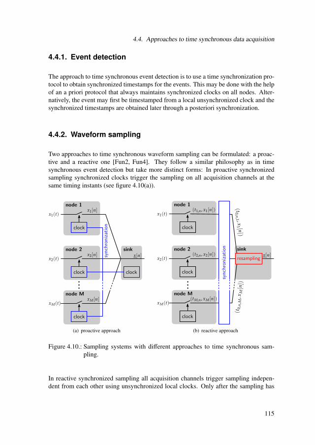
4.4. Approaches to time synchronous data acquisition
4.4.1. Event detection
The approach to time synchronous event detection is to use a time synchronization pro-tocol to obtain synchronized timestamps for the events. This may be done with the helpof an a priori protocol that always maintains synchronized clocks on all nodes. Alter-natively, the event may first be timestamped from a local unsynchronized clock and thesynchronized timestamps are obtained later through a posteriori synchronization.
4.4.2. Waveform sampling
Two approaches to time synchronous waveform sampling can be formulated: a proac-tive and a reactive one [Fun2, Fun4]. They follow a similar philosophy as in timesynchronous event detection but take more distinct forms: In proactive synchronizedsampling synchronized clocks trigger the sampling on all acquisition channels at thesame timing instants (see figure 4.10(a)).
(a) proactive approach (b) reactive approach
Figure 4.10.: Sampling systems with different approaches to time synchronous sam-pling.
In reactive synchronized sampling all acquisition channels trigger sampling indepen-dent from each other using unsynchronized local clocks. Only after the sampling has
115

4. Modeling
been done, timestamps are assigned to the samples from a synchronized clock (see fig-ure 4.10(b)). This may be done directly on the acquiring node using an a priori syn-chronized clock. Alternatively it can also be done during transmission to the sink usinga posteriori synchronization. Under the reactive approach, the samples from differentchannels will in general not have been sampled at the same timing instants, i.e. theyare not synchronous according to the definition in section 4.1.2. However, it is possibleto obtain synchronous samples through interpolation and resampling as long as the sig-nals have been sampled in accordance with the Shannon-Nyquist theorem (see section3.2.1). Accurate resampling is even possible when the original samples do not lie on auniform sampling grid (see section 3.2.2).
A hybrid approach that combines the proactive and reactive elements is also possible[Fun2, Fun4]: The samples are acquired based on a synchronized clock and later theyare timestamped in order to increase precision.
In the proactive approach the most effort is put into triggering acquisition at the righttime. This requires a very good real-time performance of the underlying soft- andhardware. Corrections made to the sampling clock, e.g. by a time synchronizationalgorithm will lead to increased timing jitter or signal distortion. No extra effort isneeded for signal processing in the proactive approach.
In the reactive approach by contrast, the extra effort needed before and during acquisi-tion is minimal. The only crucial point at this stage is the generation of accurate time-stamps. After the acquisition, significant effort is needed for the resampling of acquiredwaveforms. The quality of the measurement result greatly depends on the accuracy ofthe algorithms used for resampling. So far, practical realizations of synchronized wave-form sampling seem to use only the proactive approach [108, 91, 61, 159].
4.5. Approaches to synchronous angular sampling
In analogy to time synchronous waveform sampling a proactive and a reactive approachto synchronous angular sampling can be formulated. In the proactive approach thesampling is controlled as to record the signal at equidistant angular instants. In thereactive approach the signal is recorded at equidistant time instants and only later re-sampled to the desired equidistant angular instants. Both approaches have already beenused, though not under those names. Today, the reactive approach, also known as syn-chronous angular resampling, is generally favored over the proactive one. The mainreason for this is that directly sampling at the desired angular instants leads to a vari-able sampling frequency. This requires a variable anti-aliasing filter which is mostlytoo complex or expensive to be realized (compare section 2.4.2).
116

4.5. Approaches to synchronous angular sampling
In order to better understand the process of angular resampling, its signal theoreticbackground was investigated. As stated in section 3.1.4 any monotonically nondecreas-ing quantity can be used as “time”. Thus, a signal’s representation in angle domain, i.e.as a function of the rotation angle ϕ, is just as valid as its representation in time domain,i.e. as a function of time t. The only constraint is, that the direction of rotation doesnot change, because otherwise ϕ would not be monotonically nondecreasing. By ap-plying the Fourier transform to a signal in time domain it is transformed into frequencydomain. In analogy to this, applying the Fourier transform to a signal in angle domaintransforms it to order domain, where the order is the analog of the frequency. A sig-nal in angle domain, in general, has a different shape and different “time-frequency”properties than the same signal in time domain. The amplitude properties of the signal,however, remain unchanged. Figure 4.11 shows an example of a signal x, that is repre-sented in time and in angle domain. In angle domain the signal is a constant frequencysine wave. In time domain it is a linear chirp function. This illustrates that, more gen-erally, signals recorded from rotation machinery at changing speeds, are non-stationaryin time domain but stationary in angle domain. Thus, representing such signals in angledomain greatly simplifies later signal processing. This is the key advantage of syn-chronous angular sampling and the reason for its frequent use in the analysis of rotationmachinery (see also section 2.4).
Figure 4.11.: Representation of the same signal in time- and angle domain. The markedpositions show time, angle and signal values of a uniform sampling gridwith spacing Ts in time domain.
A signal sampled on a uniform sampling grid in time domain, will in general, havebeen sampled on a nonuniform sampling grid in angle domain and vice versa (see fig-ure 4.11). Thus, the process of synchronous angular resampling (see section 2.4)
117

4. Modeling
can be described as transferring a signal from a nonuniform angular sampling gridϕn = ϕ(tn) = ϕ(nTs) to a uniform angular sampling grid ϕl = lΦs. This insight en-ables the application of nonuniform sampling theory to the problem (see section 3.2.2).Furthermore, it allows the use of resampling algorithms developed in other domains.Thus, the treatment of synchronous angular sampling becomes more comprehensiveand theoretically better founded than previous approaches (compare section 2.4.2).
4.6. Testing data acquisition systems
In order to get meaningful results, the test measurements should be as similar as pos-sible to the later application. Yet, at the same time they should not to cause too muchextra cost and provide repeatable and comparable results. So far publications on WSN-synchronization have mostly focused on measuring the synchronization precision ofclocks. This however, makes it difficult to compare the results to non-wireless acqui-sition systems, where usually no figure is given for synchronization precision. Fur-thermore, other parts of the system that may have a significant influence on the mea-surement results, e.g. interrupt delays, are neglected. Therefore, this section presentstesting methods that focus on the systems’ overall performance. They are all appli-cable to WSNs as well as to non-wireless data acquisition systems, in order to enabledirect comparisons between the two. Three data acquisition scenarios are treated: eventdetection (section 4.6.1), waveform sampling (section 4.6.2) and synchronous angularsampling (section 4.6.3).
4.6.1. Synchronous event detection
Synchronous event detection by several event detectors means that all assign the sametimestamp to the same event (compare (3.3)). The most straight forward way to test thisis to generate an event that is detected by all detectors. This method has already beenused to characterize the synchronization of clocks in [119, 87]. In the simplest case, theevent is a digital edge that is wired to the interrupt inputs of all sensor nodes as shownin figure 4.12. In order to avoid a bias from the test setup, it should be ensured thatthe propagation time from the event’s source is the same for all detectors. To obtainrepresentative results, the timestamps of many different events should be evaluated.Doing this, the intervals between the events should be randomized, in order to avoidcorrelation with internal processes of the WSN. Furthermore, the time between twoevents should be significantly larger than the maximum expected synchronization error,in order to avoid ambiguities in matching timestamps to events.
The obtained timestamps can be used to estimate the measurement error. If all detec-tors were perfectly synchronized, they would all generate exactly the same timestamp.
118

4.6. Testing data acquisition systems
Figure 4.12.: Setup for testing synchronous event detection.
Thus, the pairwise timestamp difference ∆t is a measure of the synchronization error.Its mean ∆t and standard deviation s∆t should be calculated for every detector pair. Theresults can be readily used within the error model introduced in section 4.2.1. The stan-dard deviation s∆t can also be used to calculate the effective clock resolution (comparesection 4.2.3 and equation (4.14)):
Tclock,e f f =√
6s∆t (4.53)
A deeper insight may be gained by evaluating the histogram of the timestamp differ-ences. Its shape may offer indications regarding the dominant error influences (comparesection 4.2.1.6). Furthermore, the average relative drift of the clocks can be obtainedthrough linear regression.
4.6.2. Synchronous waveform sampling
Synchronous waveform sampling has been defined to be the acquisition of samplesfrom multiple channels at the same timing instants (see section 4.1.2). Thus, it is sug-gested to test it by simultaneously acquiring the same signal on all channels (see figure4.13) [Fun1].
It is further suggested to use a sine wave signal, as signal generators for high accu-racy sine waves are readily available. Furthermore, the use of sine waves allows foreasy spectral analysis and separation between linear and non-linear effects, as they are
119

4. Modeling
Figure 4.13.: Setup for testing multi-channel waveform sampling.
eigenfunctions to LTI-systems. Many of the test methods for single-channel digitizingwaveform recorders defined in the standard IEEE-1057 [201] are based on the acquisi-tion of a reference sine wave.
The parameters of the sine wave used for the test need to be chosen with care. Itspeak-to-peak amplitude should cover most of the system’s analog input range, in orderto minimize the effect of quantization errors. A coverage of more than 90 % is rec-ommended in [201]. Yet, clipping should be avoided, as it may introduce significantdistortion into the acquired signal. Furthermore, it is recommended that in order to ob-tain precise test results, an integer number J ≥ 5 of signal periods should be recorded.The signal frequency ωsignal should be chosen such that the sampling instants lie atdifferent phase angles in every signal period, i.e.:
ωsignal =JMωs, (4.54)
where ωs is the sampling frequency and M the number of acquired samples. Then,J should be chosen to be a relative prime to M [201]. Finally, the tests should berepeated at several frequencies that together span the expected frequency range of theapplication, as the properties of ADCs are often frequency dependent [201].
Using the algorithms introduced in section 3.4.3, the error influences modeled in section4.2.2 can be readily estimated from the acquired sine waveforms. The frequency ωrecof the acquired waveform can be estimated with high accuracy using the four parameteralgorithm introduced in section 3.4.3.1. By comparing it to the known true frequency ofthe sine wave ωsignal the frequency error ϵ f and clock drift ρ of the acquisition channelcan be obtained:
ϵω = ωrec −ωsignal (4.55)
ρ =ωrec
ωsignal− 1 =
ϵωωsignal
. (4.56)
120

4.6. Testing data acquisition systems
The four parameter algorithm also estimates the amplitude and offset of the waveform,which can be used to determine the gain and offset error of the acquisition channel.
A time offset error ϵt0 between two channels leads to a phase difference ∆ϕ in therecorded signals [Fun1]:
ϵt0 =∆ϕωsignal
. (4.57)
Similar to the synchronous event detection in section 4.6.1 the phase shift during thetransmission from the signal source should the same for all channels, in order to avoid abias from the setup. The algorithm introduced in section 3.4.3.2 can estimate the phasedifference between two sine waves with an accuracy even higher than that of the fourparameter algorithm, if their frequency is identical. This assumption will hold true inthe suggested setup, as long as the frequency drift between the individual channels isnegligible. However, the estimate for the phase difference can only be unambiguous forthe interval [−π, π). Thus, the signal period should be chosen larger than the maximumexpected time offset error.
The SNR of an acquired waveform can be estimated using the algorithm introducedin section 3.4.3.3. Time jitter during acquisition, caused e.g. by a synchronizationalgorithm, will decrease the SNR. Yet, it is hardly possible to determine the jitter basedon the SNR as many other influences contribute to it, e.g. additive amplitude noise.Thus, it is suggested to observe the influence of the synchronization by comparing theSNR of the same data acquisition system with and without synchronization.
The THD can also be estimated for an acquired waveform (compare section 3.4.3.3).Changing clock drifts or clock adjustments during the acquisition increase it. Again,it is not feasible to determine their strengths from the measured THD due to otherinfluence, e.g. the input non-linearity. Instead, their influence should be observed bycomparing the THD with and without synchronization.
The estimation algorithms for the THD and SNR are closely linked and it is oftendifficult to distinguish between harmonic- and noise energy. Therefore, it is often morefeasible to use the SINAD, which expresses their combined strength.
4.6.3. Synchronous angular sampling
To test synchronous angular sampling algorithms the use of linear chirp signals is rec-ommended in [14]. They are representative of signals from a machine undergoing aspeed change. In addition, a pulse signal is needed that has pulses at equidistant phaseangles thus simulating a tachometer signal. This choice of test signal is adopted here,also because linear chirp signals are transformed into constant frequency sine wavesby synchronous angular sampling. This is very convenient, as it allows using the same
121
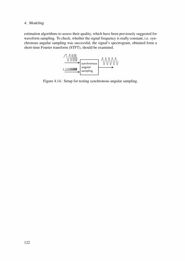
4. Modeling
estimation algorithms to assess their quality, which have been previously suggested forwaveform sampling. To check, whether the signal frequency is really constant, i.e. syn-chronous angular sampling was successful, the signal’s spectrogram, obtained form ashort-time Fourier transform (STFT), should be examined.
Figure 4.14.: Setup for testing synchronous angular sampling.
122

5. Implementation
To test the modeling of the previous chapter in real measurements a WSN was built upand algorithms for time synchronization as well as data acquisition were implementedon it. The primary aim was to realize all variants of synchronous data acquisitiondiscussed in chapter 4. A target application was data acquisition at a test bench forinduction motors. Furthermore, the WSN should be easily adapted to new tasks infuture research projects. Especially the monitoring and diagnosis of machines wereintended as prospective applications. Another aim was to use the WSN for studentprojects as well as bachelor and master theses.
Based on these design goals the following requirements were defined:
• support for continuous data acquisition with on-line transmission
• support for signal processing directly on the sensor nodes
• high transmission data rates
• low transmission latency
• easy integration into an induction motor test bench
These requirements are in conflict with a very low-power operation. Furthermore, us-ing comparatively large batteries or even mains power was feasible in most places atthe test bench. Therefore, the WSN was not optimized for minimum power consump-tion. In order to integrate well with the existing test bench infrastructure, the WSNneeded to support suitable hard- and software interfaces. Furthermore sensors were re-quired to measure digital signals, low voltage analog signals, voltages and currents atthe induction motor, sound and temperature. In order to keep the implementation effortmanageable and to accurately represent the state-of-the-art it was decided to build uponalready existing hard- and software wherever feasible.
This chapter is structured as follows: Section 5.1 describes the hardware as well as thesoftware of the WSN and its integration into the induction motor test bench. The im-plementations of time synchronization and time synchronous data acquisition are pre-sented in section 5.2. Finally, section 5.3 describes the implementation of synchronousangular sampling.
123
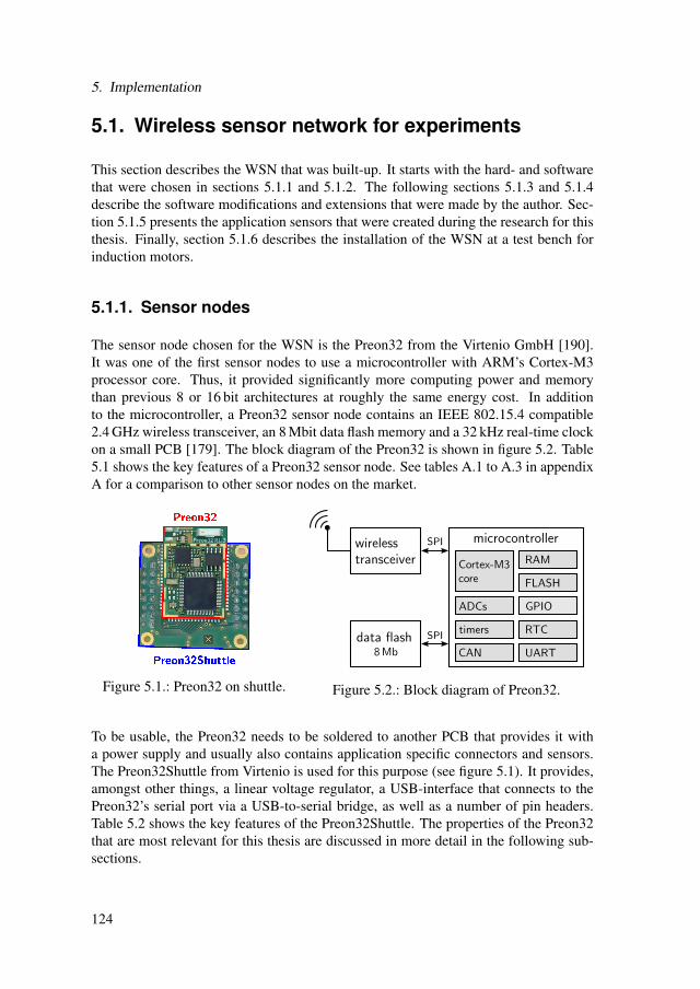
5. Implementation
5.1. Wireless sensor network for experiments
This section describes the WSN that was built-up. It starts with the hard- and softwarethat were chosen in sections 5.1.1 and 5.1.2. The following sections 5.1.3 and 5.1.4describe the software modifications and extensions that were made by the author. Sec-tion 5.1.5 presents the application sensors that were created during the research for thisthesis. Finally, section 5.1.6 describes the installation of the WSN at a test bench forinduction motors.
5.1.1. Sensor nodes
The sensor node chosen for the WSN is the Preon32 from the Virtenio GmbH [190].It was one of the first sensor nodes to use a microcontroller with ARM’s Cortex-M3processor core. Thus, it provided significantly more computing power and memorythan previous 8 or 16 bit architectures at roughly the same energy cost. In additionto the microcontroller, a Preon32 sensor node contains an IEEE 802.15.4 compatible2.4 GHz wireless transceiver, an 8 Mbit data flash memory and a 32 kHz real-time clockon a small PCB [179]. The block diagram of the Preon32 is shown in figure 5.2. Table5.1 shows the key features of a Preon32 sensor node. See tables A.1 to A.3 in appendixA for a comparison to other sensor nodes on the market.
Figure 5.1.: Preon32 on shuttle. Figure 5.2.: Block diagram of Preon32.
To be usable, the Preon32 needs to be soldered to another PCB that provides it witha power supply and usually also contains application specific connectors and sensors.The Preon32Shuttle from Virtenio is used for this purpose (see figure 5.1). It provides,amongst other things, a linear voltage regulator, a USB-interface that connects to thePreon32’s serial port via a USB-to-serial bridge, as well as a number of pin headers.Table 5.2 shows the key features of the Preon32Shuttle. The properties of the Preon32that are most relevant for this thesis are discussed in more detail in the following sub-sections.
124

5.1. Wireless sensor network for experiments
Table 5.1.: Key features of Preon32 [179].
CPU family ARM Cortex-M3CPU clock 8 . . . 72 MHzRAM 64 kBprogram-FLASH 256 kBdata-FLASH 8 Mb
wireless standard IEEE 802.15.4frequency band 2.4 GHz
ADC resolution 12 bitmax. sampling-rate 1000 kSamples/s
interfaces GPIO, UART, I2C,SPI, CAN, USB
supply voltage 2.7–3.6 Vdimension(l x w x h) 27.5 x 19.0 x
3.3 mm
operating system (Contiki), Java
Table 5.2.: Key features of Preon32Shuttle[180].
peripherals 4 LEDs2 buttons
digital interfaces 2x16 pin headers withGPIOs, ADCs, UART,etc.1 USB2.0 connector
supply voltage 3.6 . . . 13.2 Voperating voltage 3.3 V
(linear voltage reg.)
dimensions(l x w x h)
32 x 33 x 14 mm
5.1.1.1. Clocks and timers
The Preon32 contains three different oscillator circuits whose properties are summa-rized in table 5.3. A cascade of adjustable frequency divide and multiply circuits gen-erates the system clock for the CPU-core and the peripherals from a given clock source(see figure 5.3). Using the internal 8 MHz RC-oscillator as a source, a system clockin the range of 8 . . . 36 MHz can be generated. The maximum system clock rate of72 MHz can only be achieved, when using the clock signal from the wireless trans-ceiver. This configuration, however, greatly increases the current consumption as itrequires the wireless transceiver to permanently stay in active mode (compare section5.1.1.4). Therefore the sensor nodes were run with a system clock of 36 MHz generatedfrom the RC-oscillator throughout all experiments.
Figure 5.3.: Clock sources and their distribution on the Preon32.
125

5. Implementation
Table 5.3.: Properties of clock sources on the Preon32.
Oscillator Frequency Tolerance
internal RC-oscillator 8 MHz 2.2 % a
transceiver output 1 MHz ≤ 40 ppmwatch crystal 32.768 kHz 20 ppm
atemperature = −10 . . . 80 °C
The microcontroller of the Preon32 contains a total of seven 16 bit timers. They can allbe clocked from the system clock with a variable prescaler and can be used to measuretimes or generate periodic interrupts. Four of the 16 bit timers also have quadratureencoder inputs. Furthermore, the microcontroller contains an integrated real-time clockmodule. It has a 32 bit counting register and is clocked from the 32.768 kHz watchcrystal.
5.1.1.2. Analog-to-digital converter
The microcontroller of the Preon32 contains two 12 bit analog-to-digital converters(ADCs). Each can be run at a maximum sampling rate of 1 MSample/s and possesses 15multiplexed input channels. To efficiently acquire large blocks of data the ADCs canbe configured to write the acquired data directly into an assigned memory space usingdirect memory access (DMA), i.e. without the involvement of the CPU. It is also pos-sible to automatically switch channels after every sample, i.e. doing time multiplexedmulti-channel acquisition with one ADC (compare section 3.2.3).
5.1.1.3. Wireless transceiver
The Preon32 uses the wireless transceiver AT86RF231 from Atmel. Together with itspredecessor the AT86RF230 it is one of the most frequently used chips in wireless sen-sor nodes. The AT86RF231 handles signal modulation as well as demodulation andhas a 128 Byte on-chip first in, first out (FIFO)-buffer for incoming and outgoing pack-ets. It uses the 2.4 GHz frequency band and is compatible to IEEE 802.15.4, ZigBeeand WirelessHART [162]. The transceiver can automatically verify the checksum of areceived packet and send an acknowledgement. Also a number of automatic retransmis-sions can be configured in case no acknowledgement is received. The microcontrollercommunicates with the wireless transceiver through a SPI-interface. In addition, a dig-ital line goes from the transceiver to the microcontroller that can trigger interrupts atvarious transceiver events, including the start of packet reception [162].
126

5.1. Wireless sensor network for experiments
5.1.1.4. Power consumption and sleep modes
The microcontroller of the Preon32 supports four power modes (see table 5.4). In RUN-NING mode, the CPU is active and performs operations. Furthermore, all peripheralsmay be operated or shut-down depending on the application’s needs. The power con-sumption in RUNNING-mode is highly dependent on the system clock frequency andthe state of the peripherals. In IDLE-mode the CPU is shut-off, but the system clock isstill running so that the peripherals can continue operating. In STANDBY-mode, alsothe system clock and the internal RC-oscillator are deactivated. Thus, no peripheralscan operate any more. The only exceptions are the RTC that operates from an externalwatch-crystal and the external interrupts. The deepest sleep-mode is the POWEROFF-mode, which shuts-off the power supply to the entire processor core. This causes thecontents of the registers and RAM to be lost except for a few special backup-registers.The wireless transceiver of the Preon32 has a complex state machine with a total of 13different states. However, most of these states are purely transitional and only active fora very short time [162]. Thus, its power consumption is determined by the three majorstates: RECEIVE, TRANSMIT and SLEEP.
Table 5.4.: Major operating states and sleep modes of microcontroller and wirelesstransceiver on the Preon32. Values for Isupply are taken from [179].
Mode Isupply Description[mA]
µC
RUNNING 3.7a full operation28.3b
IDLE n/a CPU off, peripherals and internal RC-oscillator activeSTANDBY 1.3 CPU off, peripherals and oscillators deactivatedPOWEROFF 0.026 CPU off, core voltage off, RAM contents lost
tran
scei
ver RECEIVE 12.3 listening for incoming packets
TRANSMIT 14 sending a packetSLEEP 20 nA entire transceiver disabled
aCPU-clock = 8 MHzbCPU-clock = 72 MHz
127

5. Implementation
5.1.2. Execution environment
The Contiki operating system was chosen as the central part of the WSN’s softwareexecution environment. Contiki is specifically designed for WSNs and offers a widerange of attractive features including a multi-process execution model, a set of differenttime services, comprehensive power management and profiling mechanisms as well asa complete IPv6-based networking stack (see also section 2.1.2.1). Compared to theother widely used wireless sensor operating system, TinyOS, Contiki has the advan-tage of using standard C and a module-based approach. Thus, it is more accessible tobeginners, especially students. Other OSs appeared immature (Nano-RK) or were notavailable (RIOT OS, OpenOS) at the time of decision (first half of 2010). The use of anembedded real-time operating system like FreeRTOS was precluded, as the integrationof wireless communication was poor at the time. Originally, the Preon32 was intendedto be programmed in the Java-Programming language. While this approach enablesprogrammers to quickly build programs for common applications, it very much limitsthe access to the capabilities of the underlying hardware. Furthermore, the exact tim-ing of operations is very difficult to control in such a virtualized execution environmentand its overhead too high to allow for the implementation of powerful signal processingalgorithms.
The software execution environment of the WSN is completed by three other compo-nents: a firmware library with drivers for the Preon32 hardware, the Contiki platformfor the Preon32, i.e. an adaptation layer and the CMSIS-DSP-library. The driver li-brary as well as the Preon32 Contiki platform were created by Virtenio. While thesource code for the Preon32 platform was available to the author, the driver library wasprovided in binary form only. Contiki OS itself is open source and was obtained fromthe official repository1. The version used was the development branch (Contiki 3.x) asof September 5th 20142. Table 5.5 summarizes the software components, as well astheir authors and licenses. In the following subsections Contiki’s key features with re-gard to this theses goals are described. More information about Contiki and its internalscan be found in [187, 186].
Table 5.5.: Components of the software execution environment.
Software Component Author Form License
Hardware driver library Virtenio GmbH binary proprietaryDSP-library ARM source code & proprietary, free
binary of chargeContiki-Preon32 platform Virtenio GmbH source code proprietaryContiki OS Contiki community source code BSD (3-clause )
1https://github.com/contiki-os/contiki2git hash of commit: 4c4c468907534238d7962f0bb2315694e86da3a0
128
5.1. Wireless sensor network for experiments
5.1.2.1. Process and event handling
A Contiki process consists of a protothread (see section 2.1.2.1) plus some managementinformation. Every Contiki deployment contains at least one process that is startedautomatically after the system has booted. Other processes may be started during thecourse of the program. Many Contiki services, e.g. the network stack, use processesthat are started on initialization [187].
Contiki manages processes with a simple cooperative scheduler [187]. This means thatprocesses cannot be interrupted by the scheduler. Instead processes themselves releasethe CPU, when they are done or wait for events. Thus, the programmer needs to ensurethat no process blocks the CPU for too long. When a process releases the CPU, thescheduler invokes the next process that is ready to run. Contiki’s multithreading library,which would allow also for preemptive multitasking, is currently not available on thePreon32 platform.
Contiki supports inter-process communication through synchronous and asynchronousevents [187]. When a synchronous event is posted, the sending process immediatelystops operating and the receiving process is invoked with the event. Once the receivingprocess has finished executing, the sending process continues to run. When an asyn-chronous event is posted, it is stored in a queue and delivered to the receiving processthe next time it is run. A special type of asynchronous event is the poll event. It ensuresthat the receiving process is run as soon as possible, i.e. the next time the scheduler isexecuted.
In contrast to process events, interrupts are generated by the hardware and handledby predefined functions. On the Preon32 platform interrupts and processes togetherform exactly two preemption levels: Interrupts can preempt processes, but neither caninterrupts preempt other interrupts nor processes other processes. No prioritization ofinterrupts or processes is currently supported.
In order to achieve a good real-time performance, events have to be handled with amaximum guaranteed latency and the variance of the actual latency should be low. Dueto the design of Contiki’s process scheduling, only interrupts are suitable for this onthe Preon32 platform. However, also interrupt-latencies can be adversely affected bythe program design. Firstly, an interrupt routine that is executed, blocks other inter-rupts. Thus, interrupt handler functions should finish quickly. A common pattern isto only do the time critical part of the interrupt response in the handler and send anevent to a process, which does the rest. Secondly, hardware drivers often deactivateinterrupt-handling during critical hardware interactions, e.g. the initialization of the ra-dio transceiver. Thus, both the maximum execution time of interrupt routines and themaximum length of critical code sections determine the maximum latency for interrupthandling.
129
5. Implementation
5.1.2.2. Time services
The Contiki operating system provides a number of time services that can be usedby applications. The clock module provides the system time, which on the Preon32platform is derived from the real-time clock of the microcontroller. When a sensornode is powered on, the clock is initialized with zero and keeps running as long as thepower supply is connected. The hardware driver library uses a virtual 64 bit registerto count the ticks of the real-time clock (RTC). One RTC-tick is Ttick,rtc = 2−14 s ≈61.0 µs. Thus, it can run for about 3.6 · 107 y without wrap-around. However, the clockvalues in the Contiki operating system are 32 bit values. They can be read either in theunit of seconds or clock ticks, which is Ttick,clock = 2−7 s ≈ 7.81 ms on the Preon32platform.
A number of timer libraries that use the clock module are available in Contiki. Thetimer library allows to set a timer that expires in a given time interval starting fromthe current time. The program needs to actively check whether the timer has alreadyexpired or not [187]. In the etimer library a Contiki process is run in the backgroundthat periodically checks all etimers for expiration [187]. When an expired etimer isdetected, an asynchronous event is sent to the process that started the etimer. A similarmechanism is provided by the ctimer library. Here a callback function is executed onexpiration [187].
Since all timer services described above require the software to check for expiration,they are not suited for real-time operation. The rtimer library, on the other hand, reliesdirectly on hardware interrupts [187]. When an rtimer expires, a predefined handlerfunction is called directly from the interrupt routine. To allow for a finer time resolu-tion, the rtimer library uses a separate clock module [187], which on the Preon32 plat-form is the unscaled RTC: Ttick,rtimer = Ttick,rtc = 2−14 s. As the rtimer clock valueis 32 bit wide, it wraps-around after about 72.8 h. In contrast to the software timer li-braries, the rtimer library is restricted to handle only one timer at a time. Furthermore,rtimer tasks need to be short as they execute in the interrupt context (compare section5.1.2.1). Since the rtimer is essential for implementing synchronous data acquisitionits relevant functions are shown in listing 5.1.
Finally, the hardware driver library also provides access to the 16 bit hardware timers ofthe microcontroller (see section 5.1.1.1). Their clocks are derived from the microcon-troller’s system clock instead of the real-time clock. Thus, a much higher resolutionscan be achieved. Yet, the timing precision is lower, due to the less precise oscillator.The hardware timers can also trigger interrupts and thus may be used as a replacementfor the rtimer, when the lower width and precision are not critical.
130

5.1. Wireless sensor network for experiments
1 / * ** D e s c r i p t i o n : p o s t a r e a l − t i m e t a s k
3 * Parame ter s :* t a s k : p o i n t e r t o t h e t a s k
5 * t i m e : t i m e i n s t a n t when t h e t a s k i s t o be e x e c u t e d* d u r a t i o n : unused argument
7 * f u n c : a f u n c t i o n t o be c a l l e d when t h e t a s k i s e x e u t e d* p t r : p o i n t e r t h a t w i l l be p as se d as argument t o f u n c
9 * Re tu rn v a l u e : 0 −> f a i l u r e , o t h e r w i s e −> s u c c e s s* /
11 i n t r t i m e r s e t ( s t r u c t r t i m e r * t a s k , r t i m e r c l o c k t t ime ,r t i m e r c l o c k t d u r a t i o n , r t i m e r c a l l b a c k t func , void * p t r ) ;
13
/ * *15 * D e s c r i p t i o n : g e t t h e c u r r e n t t i m e
* /17 # d e f i n e RTIMER NOW ( ) r t i m e r a r c h n o w ( )
19 / * ** D e s c r i p t i o n : g e t t h e t i m e t h a t a t a s k l a s t was e x e c u t e d
21 * Parame ter s :* t a s k : t h e t a s k
23 * Re tu rn v a l u e : t h e t i m e t h a t a t a s k l a s t was e x e c u t e d* /
25 # d e f i n e RTIMER TIME ( t a s k ) ( ( t a s k )−> t ime )
Listing 5.1: Key rtimer API-functions.
5.1.2.3. Network communication stack
Contiki’s network communication stack is implemented in a layered architecture, thatuses a layer definition slightly different from the ISO/OSI reference model (see figure5.4, compare section 2.1.4). While the network and transport layers are condensedinto a common network layer, the data link layer is split up into three separate layers:the MAC-, radio duty-cycling (RDC)- and framer-layer. For every layer interaction aninterface is defined, that allows for the modules in the individual layers to be exchangedindependently of each other. This makes it relatively easy to modify and extend thenetwork stack. Furthermore, Contiki supports a number of attributes that are assignedto packets, and influence their processing in the various layers. Figure 5.4 shows anoverview of Contiki’s network stack and the different options in the individual layers.
In the physical or radio layer, only one module is available, which is the driver for thePreon32’s transceiver chip. It was created by Virtenio and consists of an upper-layer,for which the source code was available, and a lower-layer in binary form. The framer-layer creates and parses MAC-layer data frames. Contiki provides an IEEE 802.15.4compatible framer (framer-802154) and a framer to create packets with only minimalprotocol overhead (framer-nullmac). Only the former was used for this thesis.
131

5. Implementation
Figure 5.4.: Layers and modules of Contiki’s network stack..
The RDC-layer is responsible for duty-cycling the wireless transceiver of a sensor node.A minimal implementation that simply always keeps the transceiver on is providedby the nullrdc module. Alternatively, a module implementing the ContikiMAC-protocol [29] was used for this thesis. ContikiMAC tries to minimize the on-time ofthe transceiver (see also section 2.1.4.2). Another low-power radio duty-cycling proto-col X-MAC [19] is also available on Contiki. It is a precursor of ContikiMAC and hasbeen largely superseded by it.
The MAC-layer coordinates the access of multiple nodes to the common communi-cation channel. Here Contiki provides a dummy implementation nullmac. It simplyallows any node to send right away without any checks or collision avoidance mecha-nisms. In addition, a classic CSMA/CA is provided. No TDMA implementation waspresent. Therefore a basic one was created by the author (see section 5.1.3).
In the network layer, Contiki provides one of the world’s leading implementations ofIPv6 for WSNs. It uses 6LoWPAN-header compression to minimize protocol over-head. The RPL-protocol is used for multi-hop routing and UDP for data transport. Analternative layer is provided by the rime network module [28]. It originally studiedinnovative ways of structuring the network stack of a WSN. However, today, there isa strong trend towards IPv6-based solutions (see section 2.5) and therefore this optionwas favored.
132

5.1. Wireless sensor network for experiments
5.1.2.4. Time synchronization service
Contiki already provides a simple time synchronization service in the timesynchmod-ule. It is described in section 5.2.1 to allow for a better overview on the implementedtime synchronization services.
5.1.2.5. Power management
In order to minimize power consumption, Contiki supports the duty-cycling of the CPUas well as the radio transceiver. The duty-cycling of the transceiver is implemented inthe RDC layer of the network communication stack (see section 5.1.2.3).
The duty-cycling of the CPU is implemented in the main scheduler loop (see also sec-tion 5.1.2.1). Whenever no process is ready to run, the processor sleeps in a low-powermode. It is scheduled to wake up, when the next etimer expires (see section 5.1.2.2).When an interrupt occurs the sleep period aborted. For the Preon32 the IDLE-mode waschosen as the sleep mode. Its power consumption is larger than that of the STANDBYmode, yet it allows for peripherals to continue operating and thus does not interferewith ongoing measurements.
Contiki contains a mechanism called powertrace that profiles the power consumptionof a sensor node during operation without any external instrumentation [31]. It sim-ply uses the rtimer to measure the accumulated times that the CPU spends runningand sleeping. The same is done for the power modes of the transceiver. Based onthe assumption that the power consumption in one state is always the same, a node’soverall power consumption can be estimated from this data. The power estimates ofthe powertrace module for the Preon32 are experimentally verified in section 6.1.1.Powertrace is used throughout chapter 6 to observe the effects of different data acqui-sition algorithms on the nodes’ power consumption.
5.1.2.6. Command shell
Contiki provides a simple text-based command shell that is accessed through the serialinterface of a sensor node. Commands are passed as a single line terminated by a linefeed character (ASCII: 10). Parameters are passed in the same line as the commandand separated by spaces (ASCII: 32). The output of shell commands is also printed tothe serial line. When a command is detected, a corresponding process is started. Shellcommands are defined together with their processes in application specific modules.During the initialization of the shell, all commands are registered with the main shellengine. This mechanism makes it very easy to add, remove or define new commands.The Contiki shell supports Unix-like pipelines making it easy to use the output of onecommand as input for another.
133

5. Implementation
5.1.3. TDMA-protocol
Scheduled MAC-protocols are generally seen as advantageous in industrial measure-ment applications, because they provide high data rates and are deterministic (seesection 2.1.4). Unfortunately, the Contiki operating system did not provide a usablescheduled MAC-protocol (see section 5.1.2). For this reason, a simple TDMA MAC-protocol was implemented. The design goals were to increase the data throughput, toavoid packet collisions and to integrate time synchronization into the MAC-protocol.To keep the development effort feasible, a number of simplifications were made: Only asingle hop star topology is supported and the schedule is static. Every node has exactlyone slot within a frame, during which it can send one packet. The TDMA-session startsimmediately after the coordinator has booted and never ends.
Figure 5.5 shows the structure of a single TDMA frame. In the beginning a beacon-packet is sent a by the coordinator node that contains a frame counter and the currenttimestamp. It serves to synchronize the nodes in the network. After the beacon, thenodes can send packets in their slots. These may be unicast messages to the coordinatoror broadcast messages to the entire network. The length Tslot of a time slot is the time-on-air of the largest supported packet plus a grace time that accounts for inaccuraciesin message timing.
Figure 5.5.: Structure of a TDMA frame.
Table 5.6 shows the parameters that were chosen for the WSN together with the re-sulting theoretical maximum data throughput. The resulting maximum latency by theMAC-layer is equal to the time T f rame needed for one frame.
Precise timing of send operations is essential for the operation of a TDMA-protocol.As discussed in section 5.1.2.1, the optimal timing service for such tasks is the rtimer.Yet, using it for the TDMA-protocol would have had a number of important disad-vantages. Firstly, the send operation of the radio driver only returns after the entirepacket has been sent. Thus, calling it directly from an rtimer-task would block otherinterrupts for up to 4.3 ms. This would make precise timestamping of external eventsimpossible. Secondly, using the rtimer for the TDMA-protocol would make it im-possible to use it elsewhere, e.g. to trigger the acquisition of data. Therefore, it was
134

5.1. Wireless sensor network for experiments
Table 5.6.: Chosen TDMA-protocol parameters and theoretical performance.
para
met
er n 3max. packet size 110 ByteTbeacon 2.747 ms (45 Ticks)Tslot 6.714 ms (110 Ticks)
resu
lt T f rame 21.667 ms (355 Ticks)max. throughput/node 46.2 packet/s (40.6 kbps)max. overall throughput 138.5 packet/s (138.5 kpbs)
1 Tick = 2−14 s ≈ 61.0 µs
decided to use an internal hardware timer of the Preon32 instead. Furthermore, thepackets are not directly sent in the timer interrupt routine. Instead, a poll event is issuedto a Contiki-process that does the sending. As significant latencies may occur on thispath, the sending process checks, whether there is still enough time within the slot, justbefore actually sending. If this check fails, the sending of the packet is postponed tothe next slot. This way, of course, the actual data throughput is reduced, but it was stillacceptable for the purpose of this thesis.
In order to save power, the leaf nodes turn off their wireless transceivers when they areneither transmitting nor expecting a transmission from another node. The coordinatornode always has its radio on, as it is assumed to have access to mains-power.
5.1.4. Data acquisition framework
In order to easily adapt the WSN to a multitude of data acquisition scenarios a softwareframework, called the MDT smart transducer library (MSTL), was developed. It isbased on the IEEE 1451 standard, as this describes a powerful generic smart data acqui-sition architecture, that is equally applicable to wireless and non-wireless measurementsystems (see also section 2.3.3). However, not all required features of IEEE 1451 wereimplemented in MSTL. Currently the framework allows for one-shot as well as con-tinuous data acquisition. Furthermore, it is possible to discover the nodes of a networkand to remotely configure the acquisition channels.
Figure 5.6 shows the communication model of the MSTL. It follows mostly the IEEE-1451 reference model (compare figure 2.7). One or more Preon32 sensor nodes, actingas TIMs, acquire data from sensors, e.g. through their ADCs. A further Preon32 sensornode serves as NCAP and provides the user interface. The function of the MSTL is toprovide generic interfaces for the interaction of transducer drivers and TIMs, TIMs andNCAP as well as NCAP and user applications. Thus, transducers or TIMs can be addedor removed with only minimal modifications.
135
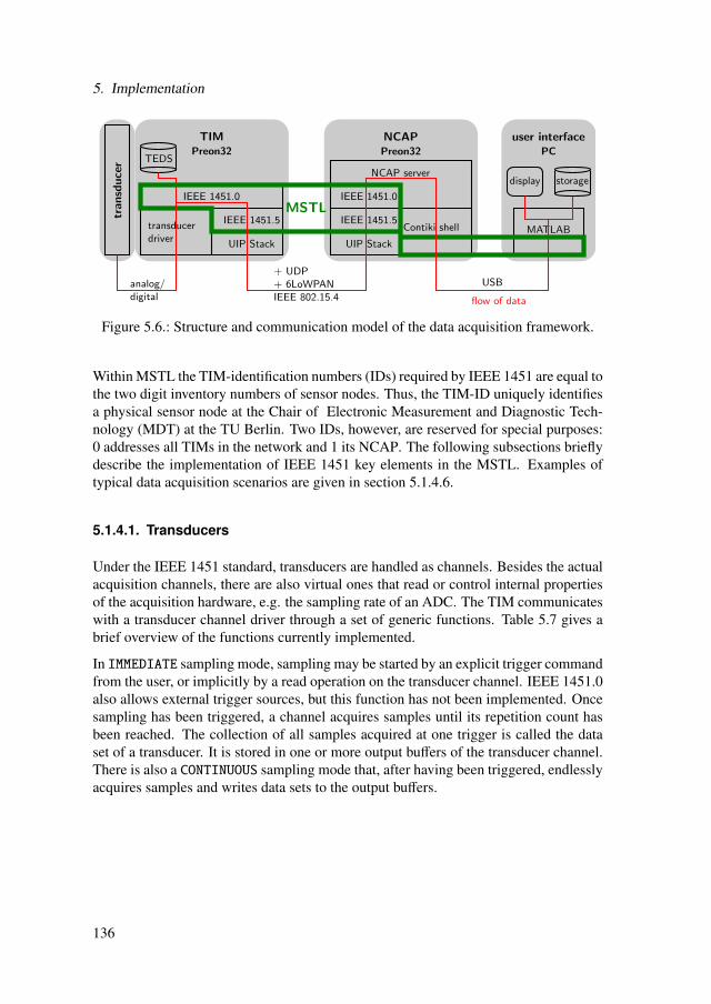
5. Implementation
Figure 5.6.: Structure and communication model of the data acquisition framework.
Within MSTL the TIM-identification numbers (IDs) required by IEEE 1451 are equal tothe two digit inventory numbers of sensor nodes. Thus, the TIM-ID uniquely identifiesa physical sensor node at the Chair of Electronic Measurement and Diagnostic Tech-nology (MDT) at the TU Berlin. Two IDs, however, are reserved for special purposes:0 addresses all TIMs in the network and 1 its NCAP. The following subsections brieflydescribe the implementation of IEEE 1451 key elements in the MSTL. Examples oftypical data acquisition scenarios are given in section 5.1.4.6.
5.1.4.1. Transducers
Under the IEEE 1451 standard, transducers are handled as channels. Besides the actualacquisition channels, there are also virtual ones that read or control internal propertiesof the acquisition hardware, e.g. the sampling rate of an ADC. The TIM communicateswith a transducer channel driver through a set of generic functions. Table 5.7 gives abrief overview of the functions currently implemented.
In IMMEDIATE sampling mode, sampling may be started by an explicit trigger commandfrom the user, or implicitly by a read operation on the transducer channel. IEEE 1451.0also allows external trigger sources, but this function has not been implemented. Oncesampling has been triggered, a channel acquires samples until its repetition count hasbeen reached. The collection of all samples acquired at one trigger is called the dataset of a transducer. It is stored in one or more output buffers of the transducer channel.There is also a CONTINUOUS sampling mode that, after having been triggered, endlesslyacquires samples and writes data sets to the output buffers.
136

5.1. Wireless sensor network for experiments
Table 5.7.: Transducer and TEDS commands.
Command Description
setDataRepetition sets the number of samples acquired at one triggersetSamplingMode sets the sampling mode of the channelsetDataTransmissionMode sets the transmission mode of the channelreadDataSetSegment reads a segment from the data set of the transducerwriteDataSetSegment writes a segment to the data set of the transducertriggerCommand triggers data acquisition (sensor) or data output (actuator)channelOperate puts the channel into operating modechannelIdle puts the channel into idle modedeviceClear clears the channel’s in- and output buffersreadDataRepetitionCount read the number of samples at one trigger
queryTEDS retrieves information about a TEDS (size, attributes, etc.)readTEDSSegment reads a segment from a TEDSwriteTEDSSegment writes a segment of a TEDS
The transmission of the acquired data sets from a transducer’s output buffer to theNCAP is governed by the transmission mode. In user initiated mode (ON COMMAND)the buffer is only read when the user issues a read command to the NCAP. In stream-ing mode, data is automatically transmitted to the NCAP. This may happen either ata fixed time interval (INTERVAL) or whenever a buffer is full (BUFFERFULL). Refer toIEEE 1451.0 [196] for a more in depth description of the commands and their function-ality.
5.1.4.2. TIM
The TIMs manage the transducers and relay data between them and the NCAP. Onstart-up the Contiki application running on the TIMs calls an initialization function forevery transducer channel, which registers its interface functions with the TIM. Thus,transducer channels can be added and removed with only minimal changes to the TIMsoftware. After start-up, the TIM application starts a Contiki process that listens forcommands from the NCAP on UDP-Port 5689. When a command arrives the corre-sponding transducer driver function is selected and called based on the channel numberas well as the numerical ID of the command as defined in IEEE 1451.0 [196]. If thecommand requires a response to be sent to the NCAP, the transducer driver needs tocall the corresponding functions from IEEE 1451.0 network layer. Commands regard-ing the TEDS are not handled by the individual transducer drivers. Instead a commonTEDS manager module has been implemented. For every TEDS it maintains one fileon Contiki’s FLASH file system, which it reads and writes as needed. IEEE 1451.0specifies a number of different TEDS-types to describe different aspects of TIMs andtransducers [196]. Table 5.8 gives an overview of the TEDS-types that are currentlyimplemented in the MSTL.
137
5. Implementation
Table 5.8.: Types of TEDS implemented in the MSTL.
TEDS-type Contents
Calibration-TEDS scaling information to convert transducer data to SI-unitsMeta-TEDS general information about a TIM and its transducersName-TEDS user-defined transducer channel nameTransducerChannel-TEDS general information about a transducer channelPHY-TEDS information about the communication interface of the TIM
5.1.4.3. NCAP
The NCAP manages the TIMs in the network. It contains RAM-buffers for the TEDSand measurement data received from the transducer channels. Furthermore, it providesa user interface to the WSN through the Contiki-shell (see next section 5.1.4.5). Asensor node that acts as a NCAP can additionally also run the TIM application andacquire data. When the NCAP and this local TIM communicate, the IEEE 1451.0 layerbypasses the IEEE 1451.5 layer and relays the messages directly. The TIM applicationitself is identical to that running on normal TIM nodes.
5.1.4.4. Network layer
The network layer manages the transmission of commands and measurement data be-tween NCAP and TIMs by packing them into 6LoWPAN messages and passing thoseto Contiki’s network stack. As Contiki’s networking stack does not support interleavedreception of IPv6-packet fragments from different packets, fragmentation of largermessages is handled by the MSTL-network layer. In the current implementation themaximum MSTL-payload per packet is 60 Bytes and the maximum allowed size of anIEEE 1451.0 message is 256 Bytes.
5.1.4.5. User interface
Contiki’s shell is used on the NCAP to provide a user interface to the data acquisitionframework. Table 5.9 shows an overview of the implemented shell commands. Most ofthem were adopted from the HTTP-application programmers interface (API) defined inIEEE 1451.0 [196]. Only the streaming functions are not from this API. The parametersto the commands are mostly transmitted as plain text separated by white spaces. Only,larger blocks of data are transferred to the NCAP as binary data encoded in an ASCII-character stream with base64 encoding [62] (commands WriteData and WriteTeds).All commands return two 16 bit binary numbers followed by the command specificreturn data. The first is the error codes as defined in IEEE 1451.0 and the second thenumber of data bytes that follow. The command specific return data is a block of binarydata.
138

5.1. Wireless sensor network for experiments
Table 5.9.: Implemented user commands.
Group Command Description
discovery TIMDiscovery get IDs numbers of known TIMsTransducerDiscovery get transducer channel numbers on TIM
transducer- ReadData read data from transducer (one-shot)access MeasurementUpdate get buffered measurement data
WriteData write data to transducer (one-shot)
TEDS- ReadTeds read TEDS from transducermanager WriteTeds write TEDS on transducer
UpdateTedsCache update TEDS cache on NCAP
transducer- SendCommand send command to transducermanager StartTrigger trigger start of measurement
streaming StartStream start continuous measurementStopStream stop continuous measurement
In order to simplify user access to the WSN, a MATLAB class interface that commu-nicates with the NCAP using its command shell has been created by the author. Itprovides equivalent functions for all shell commands from table 5.9. Furthermore, aLabVIEW program [Stud1] and an Android application [Stud14] that interface with theNCAP shell have been implemented in student projects.
5.1.4.6. Example acquisition scenarios
To illustrate the working of the data acquisition framework a simple one-shot and acontinuous measurement will be described in more detail.
Listing 5.2 shows the MATLAB script of the one-shot measurement. After connectingto the NCAP (lines 11,12) the program looks for connected TIMs and their channels(line 14 to 27). Figure 5.7 shows the sequence of communication during this pro-cess. To get a list of all known TIMs the script sends the TIMDiscovery commandto the shell of the NCAP. In the consequence the IEEE 1451 layers query the RPL-neighbor table of the node and a list is returned that contains the IDs of all TIMs towhich routes are known. The actual discovery of new nodes is done independently bythe RPL-routing engine. When the TIM with the ID 41 has been found, the NCAPstops the search and obtains a list of the TIM’s transducer channels by issuing theTransducerDiscovery command. The IEEE 1451 layers then obtain the contents ofthe META-TEDS from the TIM, which contains the needed information. After this pro-cess the contents of the META-TEDS is cached on the NCAP, so that no transmissionbetween TIM and NCAP takes place when its contents is read in line 30 of listing 5.2.At this stage, also other TEDS of the channel could be read to obtain more informationabout its properties and purpose, e.g. Name- or Channel-TEDS.
139

5. Implementation
1 %% Parame ter s %%t imID = 4 1 ; % ID o f TIM t o a c q u i r e da ta from
3 adcChanne l = 1 ; % c h a n n e l t o a c q u i r e da ta fromp e r C h a n n e l = 2 ; % c h a n n e l t o c o n t r o l sa m p l i n g p e r i o d
5 muxChannel = 3 ; % c h a n n e l t o c o n t r o l t h e adc muxt i m e o u t = TimeDura t ion ( 3 , 0 ) ; % t i m e o u t f o r a c q u i s i t i o n (3 s )
7 mode = IEEE1451 . SamplingMode . IMMEDIATE ; % s a m p l i n g mode
9 t r y%% 0 . c o n n e c t i o n S e t u p
11 ncap = IEEE1451 ( ) ;ncap . c o n n e c t ( ’/dev/ttyUSB2’ ) ;
13
%% 1 . scan f o r TIMs15 t imsFound = [ ] ;
f p r i n t f ( 1 , ’tim discovery’ ) ;17 whi le ( ˜ i s e m p t y ( s e t d i f f ( t imID , t imsFound ) ) )
pause ( 1 )19 f p r i n t f ( 1 , ’.’ ) ;
21 % read c o n n e c t e d TIMst imsFound = ncap . t i m D i s c o v e r y ( ) ;
23 endf p r i n t f ( 1 , ’OK\n’ ) ;
25
%% 2 . read c h a n n e l s27 c h a n n e l s = ncap . t r a n s d u c e r D i s c o v e r y ( t imID ) ;
29 %% 3 . Read TEDstedsTimMeta = ncap . r e a d T e d s ( timID , chanID , t i m e o u t , . . .
31 IEEE1451 . T e d s C l a s s .META) ;
33 %% 4 . c o n f i g u r e t r a n s d u c e r% s e t number o f samples per b l o c k t o 128
35 ncap . sendCommand ( timID , adcChannel , t i m e o u t , . . .IEEE1451 . CommandClass . XDCR IDLE , . . .
37 IEEE1451 . CommandsXdcrIdle . SET XDCR CH REPETITION COUNT , 1 2 8 ) ;% s e t s a m p l i n g p e r i o d t o 1000 mirco s
39 ncap . w r i t e D a t a ( timID , perChanne l , t i m e o u t , mode , u i n t 3 2 ( 1 0 0 0 ) ) ;% s e t i n p u t mux o f adc t o c h a n n e l 19
41 ncap . w r i t e D a t a ( timID , muxChannel , t i m e o u t , mode , u i n t 8 ( 1 9 ) ) ;
43 %% 5 . s i n g l e − s h o t measurementd a t a = ncap . r e a d D a t a ( timID , adcChannel , t i m e o u t , mode ) ;
45 catch e x c e p t i o nd i s p ( e x c e p t i o n . g e t R e p o r t ( ) ) ;
47 end
49 %% 6 . C o n n e c t i o n shutdownd e l e t e ( ncap )
Listing 5.2: MATLAB example of transducer discovery and one-shot acquisition.
140

5.1. Wireless sensor network for experiments
Figure 5.7.: Sequence diagram of the transducer discovery process.
After having detected the TIM and its channels, one transducer channel, an ADC, isconfigured (lines 35 to 41 in listing 5.2). The sequence of communication is illus-trated by figure 5.8. First, the number of samples per data block is set by sending thesetDataRepetition command to the transducer channel with the help of the shellcommand SendCommand.
After this, two virtual actuator channels are written that control properties of ADC:the sampling period (in µs) and the analog input multiplexer. In each case the shellcommand WriteData is used. This first puts the corresponding channel into operationmode (command: channelOperate) and then writes data to its data set (command:writeDataSetSegment). Finally, the channel is put back into idle state (command:channelIdle).
The data acquisition itself is done in line 44. Its communication sequence is shown infigure 5.9. The shell command ReadData is used to first put the acquisition channel intooperating mode. The subsequent reading of the data set triggers the data acquisition onthe channel. When the acquisition is finished, the data is returned to the NCAP, whichrelays it to the PC.
141

5. Implementation
Figure 5.8.: Sequence diagram of the transducer configuration.
Figure 5.9.: Sequence diagram of one-shot acquisition.
142
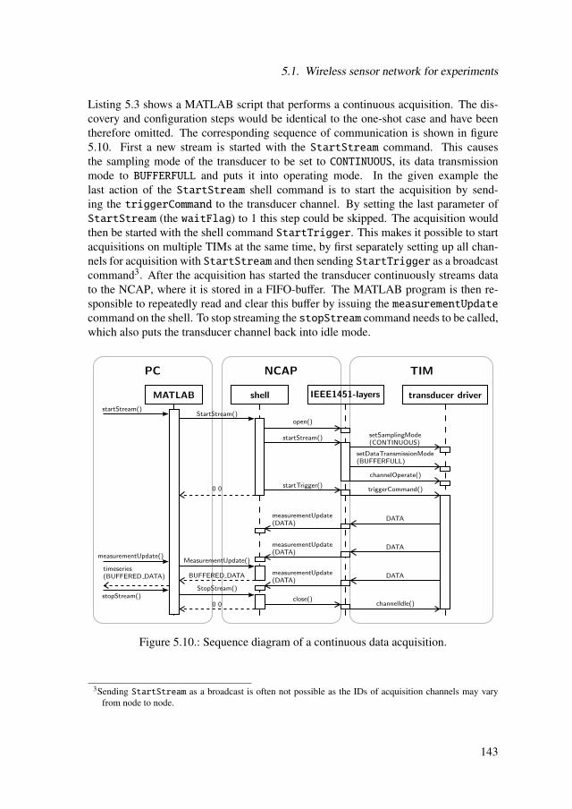
5.1. Wireless sensor network for experiments
Listing 5.3 shows a MATLAB script that performs a continuous acquisition. The dis-covery and configuration steps would be identical to the one-shot case and have beentherefore omitted. The corresponding sequence of communication is shown in figure5.10. First a new stream is started with the StartStream command. This causesthe sampling mode of the transducer to be set to CONTINUOUS, its data transmissionmode to BUFFERFULL and puts it into operating mode. In the given example thelast action of the StartStream shell command is to start the acquisition by send-ing the triggerCommand to the transducer channel. By setting the last parameter ofStartStream (the waitFlag) to 1 this step could be skipped. The acquisition wouldthen be started with the shell command StartTrigger. This makes it possible to startacquisitions on multiple TIMs at the same time, by first separately setting up all chan-nels for acquisition with StartStream and then sending StartTrigger as a broadcastcommand3. After the acquisition has started the transducer continuously streams datato the NCAP, where it is stored in a FIFO-buffer. The MATLAB program is then re-sponsible to repeatedly read and clear this buffer by issuing the measurementUpdatecommand on the shell. To stop streaming the stopStream command needs to be called,which also puts the transducer channel back into idle mode.
Figure 5.10.: Sequence diagram of a continuous data acquisition.
3Sending StartStream as a broadcast is often not possible as the IDs of acquisition channels may varyfrom node to node.
143

5. Implementation
%% Parame ter s %%2 N = 2 4 ; % number o f samples t o a c q u i r e per b l o c k
Nb = 1 6 ; % number o f b l o c k s t o a c q u i r e4 t imID = 4 1 ; % ID o f TIM t o a c q u i r e da ta from
adcChanne l = 1 ; % c h a n n e l t o a c q u i r e da ta from6 t i m e o u t = TimeDura t ion ( 3 , 0 ) ; % t i m e o u t f o r a c q u i s i t i o n (3 s )
8 t r y%% 0 . c o n n e c t i o n S e t u p
10 ncap = IEEE1451 ( ) ;ncap . c o n n e c t ( ’/dev/ttyUSB2’ ) ;
12
%% 1 . d i s c o v e r and c o n f i g u r e t r a n s d u c e r14 % . . . ( s e e one− s h o t a c q u i s i t i o n )
16 %% 2 . s t r e a m i n g measurement% s t a r t
18 ncap . s t a r t S t r e a m ( timID , adcChannel , 0 ) ;
20 % r e c e i v e da tad a t a = [ ] ;
22 t 0 = 0 ;t i c ( ) ;
24 whi le ( i s e m p t y ( d a t a ) | | ( d a t a . Length < (N*Nb ) ) )% t r y t o g e t da ta new da ta
26 temp = ncap . measurementUpdate ( timID , adcChanne l ) ;i f ( ˜ i s e m p t y ( temp ) && ( max ( [ temp . Length ] ) >0) )
28 d a t a = append ( da t a , temp ) ;t i c ( )
30 f p r i n t f ( 1 , ’.’ ) ;e l s e
32 pause ( 0 . 1 )end
34
% check f o r t i m e o u t36 i f ( t o c ( )> t i m e o u t . s e c )
e r r o r ( ’timed out waiting for data’ ) ;38 end
end40
catch e x c e p t i o n42 d i s p ( e x c e p t i o n . g e t R e p o r t ( ) ) ;
end44
%% 3 . s t o p s t r e a m i n g46 t r y
ncap . s t o p S t r e a m ( t imID ) ;48 f p r i n t f ( 1 , ’DONE\n’ ) ;
catch e x c e p t i o n50 d i s p ( e x c e p t i o n . g e t R e p o r t ( ) ) ;
end52
%% 4 . c o n n e c t i o n shutdown54 d e l e t e ( ncap )
Listing 5.3: MATLAB example of continuous acquisition.
144
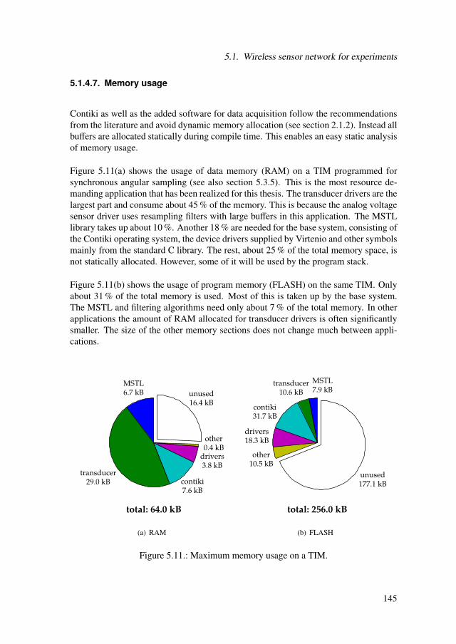
5.1. Wireless sensor network for experiments
5.1.4.7. Memory usage
Contiki as well as the added software for data acquisition follow the recommendationsfrom the literature and avoid dynamic memory allocation (see section 2.1.2). Instead allbuffers are allocated statically during compile time. This enables an easy static analysisof memory usage.
Figure 5.11(a) shows the usage of data memory (RAM) on a TIM programmed forsynchronous angular sampling (see also section 5.3.5). This is the most resource de-manding application that has been realized for this thesis. The transducer drivers are thelargest part and consume about 45 % of the memory. This is because the analog voltagesensor driver uses resampling filters with large buffers in this application. The MSTLlibrary takes up about 10 %. Another 18 % are needed for the base system, consisting ofthe Contiki operating system, the device drivers supplied by Virtenio and other symbolsmainly from the standard C library. The rest, about 25 % of the total memory space, isnot statically allocated. However, some of it will be used by the program stack.
Figure 5.11(b) shows the usage of program memory (FLASH) on the same TIM. Onlyabout 31 % of the total memory is used. Most of this is taken up by the base system.The MSTL and filtering algorithms need only about 7 % of the total memory. In otherapplications the amount of RAM allocated for transducer drivers is often significantlysmaller. The size of the other memory sections does not change much between appli-cations.
MSTL6.7 kB
transducer29.0 kB contiki
7.6 kB
drivers3.8 kB
other0.4 kB
unused16.4 kB
total: 64.0 kB
(a) RAM
MSTL7.9 kB
transducer10.6 kB
contiki31.7 kB
drivers18.3 kB
other10.5 kB
unused177.1 kB
total: 256.0 kB
(b) FLASH
Figure 5.11.: Maximum memory usage on a TIM.
145

5. Implementation
Figure 5.12(a) shows the usage of data memory (RAM) on the NCAP. The largest partis the NCAP application that uses about one third of the entire memory, most of it tobuffer incoming data. Contiki, the MSTL and the device drives each use about 15 %.The memory consumption of Contiki and the MSTL is again mostly determined by thesize of network communication buffers. For the device drivers the size of the serialcommunication buffer is by far the largest part.
Figure 5.12(b) shows the usage of the program memory (FLASH) on the same NCAP.About one third of the entire memory is used. The MSTL and NCAP application to-gether need only about 10 % of the total memory, the rest is taken up by the base system.The investigated NCAP configuration is suitable for a wide range of applications with-out any changes. The only exception is when a local TIM is run on the same node (seesection 5.1.4.3). In this case the size of communication buffers can be reduced in orderto make room for it in the data memory.
MSTL10.0 kB
transducer0.5 kB
NCAP21.2 kB
contiki10.0 kB
drivers9.2 kB
other2.9 kB
unused10.2 kB
total: 64.0 kB
(a) RAM
MSTL16.0 kB
transducer3.4 kB
NCAP7.5 kB
contiki35.9 kB
drivers16.5 kB
other9.6 kB
unused167.0 kB
total: 256.0 kB
(b) FLASH
Figure 5.12.: Maximum memory usage on a NCAP.
146

5.1. Wireless sensor network for experiments
5.1.5. Application transducers
A number of application transducers have been implemented for the data acquisitionframework described in the previous section. They include both hardware modulesand transducer drivers. Table 5.10 gives an overview of the transducers as well as thecommands and operating modes supported by them. The microphone and the curren-t/voltage sensor are not included in table 5.10, as they are pure hardware modules thatrely on software drivers already shown in the table. All transducers’ hardware andsoftware will be described in more detail in the following.
Table 5.10.: Overview of commands and operation modes supported by the individualapplication transducers.
Sens
or
pow
ertr
ace
digi
tale
vent
digi
tala
ctua
tor
anal
ogvo
ltage
rota
ryen
code
r
Cha
nnel
Name AD
C
sam
ple
peri
od
AD
C-M
UX
filte
rsel
ect
filte
rcoeff
.
deci
mat
ion
ratio
Type VS S A S VA VA VA VA VA S
Com
man
ds
setDataRepetition XsetSamplingMode X XsetDataTransmissionMode XreadDataSetSegment X X XwriteDataSetSegment X X X X X XtriggerCommand X X XchannelOperate X X X X X X X X X XchannelIdle X X X X X X X X X XdeviceClear X X XreadDataRepetitionCount X
Sam
plin
gm
odes IMMEDIATE X X X X X X X X X
CONTINUOUS X X X
Tran
smis
sion
mod
es ON COMMAND X X X X X X X X XBUFFERFULL X XINTERVAL X
Abbreviations channel type: A=actuator, S=sensor, VA=virtual actuator, VS=virtual sensor
147

5. Implementation
5.1.5.1. Powertrace sensor
The powertrace sensor is a virtual sensor that integrates Contiki’s powertrace mecha-nism into the data acquisition framework (see also 5.1.2.5). Thus, it enables wirelesstransmission of powertrace statistics. Whenever the sensor is read it returns a data setwith the current powertrace data. Table 5.11 shows the data set of the powertrace sen-sor. It includes the accumulated times the sensor node has spent in the individual powermodes since the node has booted and since the last read of powertrace data. The pro-tocol statistics at the end of the data set allow analyzing the power consumption of theindividual protocols in more detail. Listening and transmit times are given for both in-coming and outgoing packets, to account for acknowledgement or beacon packets thatare sent in the opposite direction.
5.1.5.2. Digital event sensor
The digital event sensor uses a user-interrupt request (IRQ) of the Preon32 to generatea timestamp whenever an event occurs. Both the IRQ and the event type (rising/fallingedge) are configured statically at compile time. The sensor supports both one-shot andcontinuous operation. Figure 5.13 shows the block diagram of the sensor.
Figure 5.13.: Block diagram of digital event sensor.
Whenever the configured interrupt occurs, the Preon32’s rtimer is read and the times-tamp written to the sensor’s data set. Table 5.12 shows the structure of the sensor’s dataset. The first field is one if an event occurred since the sensor was last cleared. Other-wise it is zero. The event counter contains the number of events since the sensor wasinitialized. Finally, the last field contains the timestamp of the event. The sensor hasa buffer that holds exactly one data set, which can be read through the sensor channel.If the sensor is in continuous operation the data set is send and the sensor is clearedimmediately after an event occurred. Section 5.2.2 describes how the sensor can beused for time synchronous event detection.
148
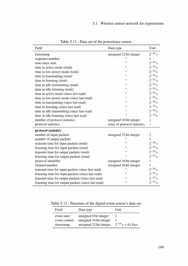
5.1. Wireless sensor network for experiments
Table 5.11.: Data set of the powertrace sensor.
Field Data type Unit
timestamp unsigned 32 bit integer 2−14 ssequence number “ 1time since start “ 2−14 stime in active mode (total) “ 2−14 stime in low power mode (total) “ 2−14 stime in transmitting (total) “ 2−14 stime in listening (total) “ 2−14 stime in idle transmitting (total) “ 2−14 stime in idle listening (total) “ 2−14 stime in active mode (since last read) “ 2−14 stime in low power mode (since last read) “ 2−14 stime in transmitting (since last read) “ 2−14 stime in listening (since last read) “ 2−14 stime in idle transmitting (since last read) “ 2−14 stime in idle listening (since last read) “ 2−14 snumber of protocol statistics unsigned 16 bit integer 1protocol statistics array of protocol statistics −
protocol statisticsnumber of input packets unsigned 32 bit integer 1number of output packets “ 1transmit time for input packets (total) “ 2−14 slistening time for input packets (total) “ 2−14 stransmit time for output packets (total) “ 2−14 slistening time for output packets (total) “ 2−14 sprotocol identifier unsigned 16 bit integer 1channel number unsigned 16 bit integer 1transmit time for input packets (since last read) “ 2−14 slistening time for input packets (since last read) “ 2−14 stransmit time for output packets (since last read) “ 2−14 slistening time for output packets (since last read) “ 2−14 s
Table 5.12.: Structure of the digital event sensor’s data set.
Field Data type Unit
event state unsigned 8 bit integer 1event counter unsigned 16 bit integer 1timestamp unsigned 32 bit integer 2−14 s ≈ 61.0 µs
149

5. Implementation
5.1.5.3. Digital actuator
The digital actuator is a simple transducer that controls a digital output pin of thePreon32. Only single shot operation is supported. The pin of the actuator is config-ured statically at compile time. The actuator’s data set consists of a single signed 8 bitinteger. Writing a zero to the actuator channel causes a logic low-level at the outputpin, writing a positive value causes a logic high-level. When a negative value is writ-ten, the pin generates a digital pulse of 1 ms length (see table 5.13). Figure 5.14 showsthe block diagram of the digital actuator.
Figure 5.14.: Block diagram of digitalactuator.
Table 5.13.: Control values of digitalactuator.
Channel value Output pin
> 0 HIGH= 0 LOW< 0 PULSE (1 ms)
5.1.5.4. Analog voltage sensor
This sensor serves to acquire analog voltage signals using the Preon32’s ADC. It sup-ports both one-shot and continuous operation. Signal filtering, resampling and scalingfunctions are included in the sensor, making it the most complex and versatile that wasimplemented.
Figure 5.15 shows the block diagram of the analog voltage sensor. The entire sensorcontains one sensor- and five virtual actuator channels that control various propertiesof the acquisition and signal processing. At the input, the ADC-multiplexer, controlledthrough a virtual actuator, selects the analog input channels that are sampled. In ad-dition to the 16-ADC-channels of the Preon32, two virtual ADC-channels return sim-ulated signals: a ramp-signal and a unit impulse. Another two channels are reservedfor the Preon32’s internal voltage reference and temperature sensor. Up to 8 channelscan be selected by the multiplexer at any time. If multiple channels are selected, theyare acquired time-multiplexed (compare section 3.2.3) and the output signal is vectorvalued. The samples in the vector are stored in interleaved mode, i.e. all samples ac-quired at the same time are stored consecutively and the channel changes from sampleto sample [196]. The analog voltage sensor operates on blocks of data. Their size canbe set through the repetition count of the ADC sensor channel. Another virtual actuatorcontrols the sampling period of the ADC.
150

5.1. Wireless sensor network for experiments
Figure 5.15.: Block diagram of analog voltage sensor.
The acquired data is written to a memory space using DMA-transfer (compare section5.1.1.2). This memory space is used as an acquisition buffer that can contain up to twoblocks of data. During continuous acquisition these two blocks are alternately writ-ten and an interrupt is triggered every time one of them has been fully written. Insidethe corresponding interrupt routine, the data block is copied to the processing buffer,which is a FIFO-buffer that can hold up to 3 data blocks. The acquired data may befiltered using an FIR-filter with up to 128 coefficients. The filtering algorithm is takenfrom the CMSIS-DSP-library provided by ARM. Filter coefficients and decimation ra-tio are controlled by virtual actuator channels. It is preceded by a CIC-decimator thatcan be configured at compile time. Alternatively, the acquired data may be resampledwith a simple S&H-resampler or the resampling filter discussed in section 5.3. Thefiltered data can be rescaled using a linear function, e.g. to convert it into units of theInternational System of Units (SI). The gain and offset for this operation are loadedfrom the channels calibration-TEDS. Finally, the output data is stored in one-blockoutput buffer, where it can be accessed through the ADC-sensor channel.
Table 5.14 shows the structure of the analog voltage sensor’s output data set. The firstfield is the sampling period, with which the samples were acquired. It is followed by thetimestamp of the first sample and the repetition count, which is the number of samplesper channel. At the end of the data set is an array with the samples. Section 5.2.3describes the generation of timestamps during the acquisition process and shows howthe sensor can be used for synchronous data acquisition.
151

5. Implementation
Table 5.14.: Structure of analog voltage sensor’s data set.
Field Data type Unit
sample period unsigned 32 bit integer 2−30 s ≈ 0.931 nstimestamp unsigned 32 bit integer 2−14 s ≈ 61.0 µsrepetition count unsigned 16 bit integer 1samples array of signed 16 bit integers depends on scaling
5.1.5.5. Microphone
The microphone module contains a simple circuit that can be plugged on top a Preon32-Shuttle, in order to detect short bursts of sound. The module was designed and threeprototypes built within a Bachelor’s project [Stud22] supervised by the author of thisdissertation. No dedicated software driver was created for the microphone moduleInstead the digital event sensor, described previously in this section, was used. Figure5.16 shows the block diagram of the microphone module. The signal of an electretmicrophone is fed through a highpass filter ( fg = 50 Hz) and amplified with a variableamplifier. Within this process the negative part of the signal is cut off. After this, acomparator, with configurable threshold and hysteresis, generates digital pulses out ofthe signal. This digital signal is connected to a user interrupt of the Preon32. Thecomplete circuit diagram of the microphone module is given in appendix C.1.
Figure 5.16.: Block diagram of microphone module.
5.1.5.6. Current and voltage sensor
A sensor module was created that measures the currents and voltages of a 3-phaseelectric motor. No dedicated software driver was created for it. Instead the analogvoltage sensor, previously described in this section, is used. Figure 5.17 shows the blockdiagram of the sensor module. It consists of four submodules: one current/ voltagetransducer module for every phase and a signal conditioning module. The voltages aremeasured towards a virtual star point created by the internal resistances (47 kΩ) of thevoltage transducers.
152
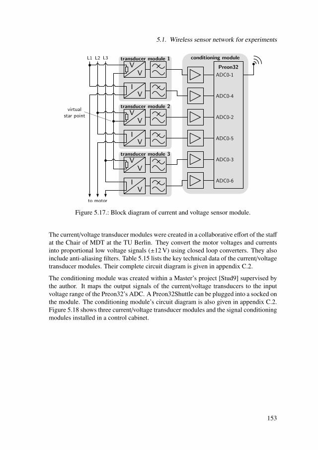
5.1. Wireless sensor network for experiments
Figure 5.17.: Block diagram of current and voltage sensor module.
The current/voltage transducer modules were created in a collaborative effort of the staffat the Chair of MDT at the TU Berlin. They convert the motor voltages and currentsinto proportional low voltage signals (±12 V) using closed loop converters. They alsoinclude anti-aliasing filters. Table 5.15 lists the key technical data of the current/voltagetransducer modules. Their complete circuit diagram is given in appendix C.2.
The conditioning module was created within a Master’s project [Stud9] supervised bythe author. It maps the output signals of the current/voltage transducers to the inputvoltage range of the Preon32’s ADC. A Preon32Shuttle can be plugged into a socked onthe module. The conditioning module’s circuit diagram is also given in appendix C.2.Figure 5.18 shows three current/voltage transducer modules and the signal conditioningmodules installed in a control cabinet.
153

5. Implementation
Figure 5.18.: Three current/voltage transducer modules and signal conditioning moduleinstalled in a control cabinet.
Table 5.15.: Technical data of the current/voltage transducer module.
voltage measurementinput range ±720 Vinternal resistance 47 kΩconversion factor (Vout/Vin) 1/60 V/V
current measurementinput range ±22 Anominal input current 10 ARMSinternal resistance 30 mΩconversion factor (Vout/Iin) 9/20 V/A
anti-aliasing filtercharacteristic 8th-order lowpassa
cutoff frequency 2.0 kHzoutput voltage range ±12 V
afour 2nd-order Butterworth lowpass connected in series
5.1.5.7. Rotary encoder
The rotary encoder sensor acquires timestamps at equidistant angular intervals Φ thatcan be used e.g. for synchronous angular sampling (see section 5.3). The sensor onlysupports continuous operation. Figure 5.19 shows the block diagram of the sensor.
The sensor hardware consists of a circuit board (see figure 5.20) that houses a Preon32on a shuttle and provides an interface to an incremental rotary encoder. The interface tothe encoder is a standard quadrature output with two square wave signals Ua1 and Ua2.Depending on the direction of rotation the phase shift between the signals is 90 ° or -90 °. One period of the signals is equivalent to one angular step. In addition, a reference
154

5.1. Wireless sensor network for experiments
pulse is generated every time the encoder crosses its zero position. All three signals aretransmitted by the rotary encoder as differential signals that are converted to standard3.3 V CMOS-logic levels by comparators on the sensor board. The quadrature inputsare connected to the quadrature encoder interface of one of the Preon32’s hardwaretimers. The complete circuit diagram of the sensor board is given in appendix C.3.
Figure 5.19.: Block diagram of rotary encoder sensor.
The quadrature encoder interface of the timer automatically detects the direction ofrotation and generates one counting pulse for every edge of the two signals, leadingto four counts per signal period. When the value in the counter register reaches thevalue stored in a compare register an interrupt is generated and the counter is reset. Inthe interrupt routine, the current time of the sensor node’s rtimer is stored. This waytimestamps are generated at uniform angular intervals. Alternatively, the timestampgeneration can be triggered with a user interrupt. This enables the simulation of arotary encoder signal with a simple square wave generator.
The generated timestamps are stored in a buffer. An etimer is used to transmit bufferedtimestamps at a fixed time interval. Table 5.16 shows the contents of the data set trans-mitted by the sensor. The first field is the angular interval Φ, at which the timestamps
155

5. Implementation
have been generated. Next is the angular position ϕ0 of the first timestamp in the dataset. It is obtained by summing over all angular intervals since the sensor started operat-ing. The repetition count denotes the number of timestamps in the data set. In order toreduce the amount of data, only the first timestamp t0 in the data set is stored with full32 bit resolution. For the other timestamps, the difference ∆T to the preceding times-tamp is stored as a 16 bit value. At the given rtimer resolution of 61 µs this means,that two timestamps may not be more than 2 s apart. This is not a significant limitationas rotary processes usually generate timestamps at a much higher rate.
Figure 5.20.: Rotary encoder sensor board with Preon32.
Table 5.16.: Structure of the rotary encoder sensor’s data set.
Field Data type Unit
Φ unsigned 32 bit integer 2−16 °ϕ0 unsigned 32 bit integer °repetition count unsigned 16 bit integer 1t0 unsigned 32 bit integer 2−14 s ≈ 61.0 µs∆T array of signed 16 bit integers 2−14 s ≈ 61.0 µs
The standard configuration of the rotary encoder sensor used for this thesis, generates30 timestamps per revolution. At rotary speeds in the range of 15 to 1500 rpm thisleads to timestamp intervals in the range of 133 to 1.33 ms. The standard transmissioninterval is 100 ms, leading to 0 . . . 76 timestamps being transmitted per interval.
156

5.1. Wireless sensor network for experiments
5.1.6. Installation at induction motor test bench
As the targeted application area of the WSN was motor test benches, an existing testbench for an induction motor was equipped with wireless sensors. The test bench wasdriven by a three-phase squirrel-cage induction motor. The mechanical load was gener-ated by a DC-motor, which was run as generator whose output energy was dissipated ata 1.9Ω load resistance. Table 5.17 shows the specification data of the two motors.
Table 5.17.: Specification data of induction- and DC-motor.
induction motor SIEMENS 1LA5 107-4AA20supply voltage 380 Vsupply frequency 50 Hzrated current 6.8 Arated power 3 kWcos ϕ 0.81 1rated speed 1415 rpm
DC-motor SIEMENS 1GG5104-OEK30-2BU7Zsupply voltage 18–150 Vrated speed 50–2440 rpmrated current 25,5–26,0 Arated power 0,07–3,20 kW
Both motors were connected through a torque shaft (HBM T30FN) with a rated torqueof 50 Nm and a rated speed of 3000 rpm. It measured the torque and shaft speed, gen-erating proportional analog voltage signals for both quantities. These signals wererecorded by the test bench PC using a USB6009 data acquisition (DAQ)-card fromNational Instruments. An optical incremental rotary encoder (Heidenhain ROD426)with 6000 pulses/revolution was connected to the end of the shaft behind the direct cur-rent (DC)-motor (see figure 5.22). The induction motor was driven by an inverter(SINAMCIS G120), which controlled both the amplitude and frequency of the mo-tor’s supply voltage. The entire test bench was controlled by a PC that ran a dedicatedLabVIEW-Program.
In order to install the WSN at the test bench, the NCAP was connected to a USB-portof the control PC (see figures 5.21 and 5.24). The current/voltage sensor described insection 5.1.5 was installed in the control cabinet of the test bench, where it measuredthe voltages and currents at all three-phases of the induction motor (see figure 5.23).The TIM of this sensor will be referred to as data TIM in this thesis. Another TIMwith a rotary encoder sensor module (see section 5.1.5) was connected to the rotaryencoder (rotation TIM in figure 5.22). The wireless recording of the induction motor’srotor temperature was realized through a TIM installed in the shaft of the test bench.Furthermore, a TIM with a vibration sensor was installed at the test bench. However,
157

5. Implementation
the last two TIMs were not used in experiments for this thesis and have therefore notbeen described in detail.
Figure 5.21.: Test bench with installed wireless sensors.
Figure 5.22.: Rotary encoder and TIM at the back-side of the breaking engine.
Figure 5.23.: Control cabinetwith data TIM.
158

5.2. Time synchronous data acquisition
Figure 5.24.: Test bench setup.
5.2. Time synchronous data acquisition
This section describes the mechanisms for time synchronous data acquisition that wereimplemented. The aim was to support both approaches to synchronous data acqui-sition outlined in section 4.4. First, section 5.2.1 describes the implementation of thetime synchronization services. The following sections describe their application to timesynchronous event detection (section 5.2.2) and analog waveform acquisition (section5.2.3).
5.2.1. Synchronization services
Contiki’s timesynch service (see section 5.1.2) was used for a priori synchronization.It was modified, in order to exploit the time synchronization already provided by theTDMA-protocol (see section 5.1.3) [Fun4]. For a posteriori synchronization, the ETA-primitive (see section 2.2.4) was implemented [Fun4]. Essential for both synchroniza-tion services is the precise timestamping of packets in the radio driver.
159

5. Implementation
5.2.1.1. Timestamping in radio-driver
The timestamping was implemented by the author in the upper level of the radio driver,which was available as source code (radioAdv.c) (see also section 5.1.2).
For outgoing packets, Contiki requires a radio driver to distinguish between normaldata packets, which should be sent unaltered, and synchronization packets, where atimestamp should be written to the last four bytes. This is done through the packettype attribute that is set to TIMESTAMP for the latter. Timestamping on for the Preon32was implemented such that the current rtimer-timestamp is written to an outgoingsynchronization packet just before it is transferred from the processor to the transceiver-chip. Care was taken to disable all automatic back-off and retransmission mechanismsof the transceiver chip (compare section 5.1.1.3 and [162]). This way, the delay timeTsend,delay between timestamp generation and transmission is deterministic and as shortas possible on this hardware platform. However, Tsend,delay depends linearly on thenumber of bytes Nbyte, f rame in the transmitted radio frame. The following equation wasdetermined empirically and used to correct the generated timestamps:
Tsend,delay =Nbyte, f rame + 163 Byte
15 Byte/Tick, (5.1)
where one clock-Tick is 61,0 µs.
For incoming packets, reception timestamps should always be generated and stored ina packet attribute. On the Preon32, the provided hardware driver of the transceiverdid already generate precise rtimer timestamps using the receive interrupt line of thetransceiver (compare section 5.1.1.3). So those were just transferred to the packet at-tribute.
5.2.1.2. A priori synchronization
Contiki’s time synchronization service timesynch is scarcely documented, but seemsto be a simplified version of FTSP: Every node runs a Contiki process, the timesynchprocess, that periodically broadcasts a synchronization message with its current rtimertime (see figure 5.25). The message also contains the authority level of a node, whichdescribes its distance from the reference node, i.e. the reference node has the authoritylevel zero, the nodes in one-hop distance from it authority level one, etc. When a nodereceives a synchronization message with a lower authority level than its own, it calcu-lates its local clock offset tlocal
o f f from its local reception timestamp tlocalrecv and the remote
send timestamp tremotesend :
tlocalo f f = tremote
send − tlocalrecv . (5.2)
In addition, it sets its own authority level to that of the received message plus one.
160

5.2. Time synchronous data acquisition
Figure 5.25.: Remote clock reading technique of Contiki’s timesynch a priori syn-chronization service.
The global synchronized time is calculated by adding the local offset to the local rtimertime. Applications can access it by calling the function timesynch time (see listing5.4). This synchronized time is also included in the synchronization messages that anode itself broadcasts.
The interval Tsync between two messages starts a defined minimum value and is doubledafter every message until a defined maximum value is reached. When a node changesits authority level, the interval is reset again to its minimum value. The aim of thismechanism is probably to quickly achieve synchronization in the beginning or aftertopology changes and to minimize the number of messages, when synchronization inthe network has stabilized. To avoid collisions between synchronization messages fromdifferent nodes, a randomized delay is introduced in the timesynch process4 beforethe synchronization message is actually sent. Similar mechanisms are used for theroute maintenance within the RPL routing protocol [109] or the CTP data collectionprotocol [43].
As the timesynch service uses the unidirectional remote clock reading technique (com-pare section 2.2.2.2), it is essential that the delay d between the generation of send andreception timestamps is constant and as small as possible, if a good synchronizationprecision is to be reached. Therefore the Contiki timesynch module relies on the ra-dio driver to generate the timestamps right at transmission and reception. This approachhas been shown to enable high synchronization accuracies (see also section 2.2.4).
TDMA-Integration The TDMA-MAC described in section 5.1.3 is ideally suited tobe combined with an a priori time synchronization. Therefore, a modified version of thetimesynch service was created by the author [Fun4], which does not generate synchro-nization messages by itself. Instead, the TDMA-beacons are used for synchronization.
4i.e. in the application layer.
161
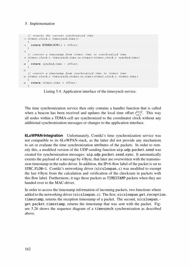
5. Implementation
/ / r e t u r n s t h e c u r r e n t s y n c h r o n i z e d t i m e2 r t i m e r c l o c k t t i m e s y n c h t i m e ( )
4 re turn RTIMER NOW ( ) + o f f s e t ;
6
/ / c o n v e r t a t i m e s t a m p from r t i m e r t i m e t o s y n c h r o n i z e d t i m e8 r t i m e r c l o c k t t i m e s y n c h t i m e t o r t i m e r ( r t i m e r c l o c k t s y n c h e d t i m e )
10 re turn s y n c h e d t i m e − o f f s e t ;
12
/ / c o n v e r t a t i m e s t a m p from s y n c h r o n i z e d t i m e t o r t i m e r t i m e14 r t i m e r c l o c k t t i m e s y n c h r t i m e r t o t i m e ( r t i m e r c l o c k t r t i m e r t i m e )
16 re turn r t i m e r t i m e + o f f s e t ;
Listing 5.4: Application interface of the timesynch service.
The time synchronization service then only contains a handler function that is calledwhen a beacon has been received and updates the local time offset tlocal
o f f . This wayall nodes within a TDMA-cell are synchronized to the coordinator clock without anyadditional synchronization messages or changes to the application interface.
6LoWPAN-Integration Unfortunately, Contiki’s time synchronization service wasnot compatible to its 6LoWPAN-stack, as the latter did not provide any mechanismto set or evaluate the time synchronization attributes of the packets. In order to rem-edy this, a modified version of the UDP-sending function uip udp packet send wascreated for synchronization messages: uip udp packet send sync. It automaticallyextents the payload of a message by 4 Byte, that later are overwritten with the transmis-sion timestamp in the radio driver. In addition, the IPv6-flow label of the packet is set toSYNC FLOW=1. Contiki’s networking driver (sicslowpan.c) was modified to exemptthe last 4 Byte from the calculation and verification of the checksum in packets withthis flow label. Furthermore, it tags these packets as TIMESTAMP packets when they arehanded over to the MAC-driver.
In order to access the timestamp information of incoming packets, two functions whereadded to the networking driver (sicslowpan.c). The first, sicslowpan get receptiontimestamp, returns the reception timestamp of a packet. The second, sicslowpan -get packet timestamp, returns the timestamp that was sent with the packet. Fig-ure 5.26 shows the sequence diagram of a timesynch synchronization as describedabove.
162
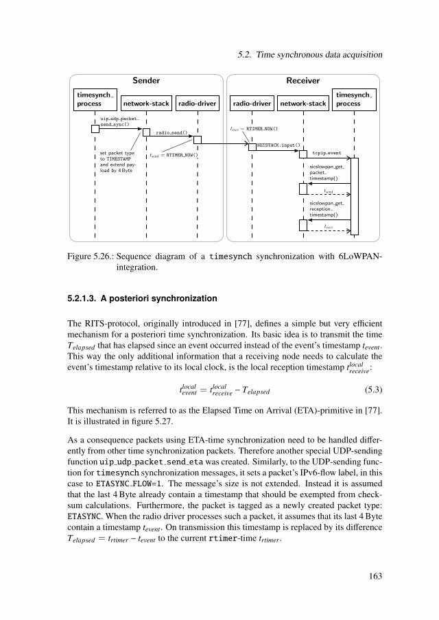
5.2. Time synchronous data acquisition
Figure 5.26.: Sequence diagram of a timesynch synchronization with 6LoWPAN-integration.
5.2.1.3. A posteriori synchronization
The RITS-protocol, originally introduced in [77], defines a simple but very efficientmechanism for a posteriori time synchronization. Its basic idea is to transmit the timeTelapsed that has elapsed since an event occurred instead of the event’s timestamp tevent.This way the only additional information that a receiving node needs to calculate theevent’s timestamp relative to its local clock, is the local reception timestamp tlocal
receive:
tlocalevent = tlocal
receive − Telapsed (5.3)
This mechanism is referred to as the Elapsed Time on Arrival (ETA)-primitive in [77].It is illustrated in figure 5.27.
As a consequence packets using ETA-time synchronization need to be handled differ-ently from other time synchronization packets. Therefore another special UDP-sendingfunction uip udp packet send etawas created. Similarly, to the UDP-sending func-tion for timesynch synchronization messages, it sets a packet’s IPv6-flow label, in thiscase to ETASYNC FLOW=1. The message’s size is not extended. Instead it is assumedthat the last 4 Byte already contain a timestamp that should be exempted from check-sum calculations. Furthermore, the packet is tagged as a newly created packet type:ETASYNC. When the radio driver processes such a packet, it assumes that its last 4 Bytecontain a timestamp tevent. On transmission this timestamp is replaced by its differenceTelapsed = trtimer − tevent to the current rtimer-time trtimer.
163

5. Implementation
Figure 5.27.: Remote clock reading technique of the ETA-primitive for a posteriori syn-chronization.
In contrast to Contiki’s packet attributes, the IPv6-flow label of a packet is transmittedwith the packet. Therefore, the networking layer of the receiving node is able to rec-ognize packets using ETA-synchronization. When it does so, it calculates the event’stimestamp using (5.3). This timestamp is then written to the packet. Applications canaccess this timestamp with a call to sicslowpan get packet timestamp. Figure5.28 shows the sequence diagram of sending a packet with RITS-synchronization.
Figure 5.28.: Sequence diagram of sending a packet with RITS-synchronization.
164

5.2. Time synchronous data acquisition
5.2.2. Event detection
Time synchronous event detection was implemented using the digital event sensor de-scribed in section 5.1.5.2. A priori as well as a posteriori synchronized event detectionis supported. The focus was on continuous data acquisition, as this was relevant for thetargeted applications. In both approaches, a 32 bit wide timestamp with a resolution of∆t = 61, 0 µs is generated within the handler function of a user IRQ. In the case of apriori synchronization this timestamp is obtained from the timesynch-service. Whena posteriori synchronization is used, the current rtimer time is used instead.
At the start of a continuous measurement, the transducer driver starts a Contiki processthat waits for events. When an event occurs, the IRQ-handler sends a poll event tothis process (see also section 5.1.2.1), which in turn sends the data set with the eventtimestamp to the NCAP through the IEEE 1451 layers. If a priori synchronization isused, a standard data message is sent. If a posteriori synchronization is used, the mes-sage is marked as an ETA-message. Figure 5.29 shows the communication sequenceduring continuous synchronized event detection with a priori synchronization and fig-ure 5.30 that for a posteriori synchronization. A thorough experimental evaluation ofboth approaches is given in section 6.2. The IMMEDIATE acquisition mode can, at thisstage, only be used in combination with a priori synchronization. It was not used forexperiments within the scope of this thesis.
Figure 5.29.: Continuous event detection with a priori synchronization. Differences tofigure 5.30 are highlighted in green.
5.2.3. Waveform acquisition
Time synchronous waveform acquisition has been implemented using the analog volt-age sensor described in section 5.1.5.4. It can acquire analog waveforms using eitherthe proactive or the reactive approach introduced in section 4.4.2. A precursor of thisimplementation has been described by the author in [Fun4]. The reactive approach maybe combined with a priori or a posteriori time synchronization. Again the focus wason continuous acquisition for both approaches. Like in the continuous event detectiona Contiki process, in this case the daq process, which manages the data transfer, isstarted at the beginning of the acquisition.
165

5. Implementation
Figure 5.30.: Continuous event detection with a posteriori synchronization. Differencesto figure 5.29 are highlighted in red.
5.2.3.1. Proactive approach
In the proactive approach the ADC is run with a block size of one, i.e. after hav-ing been triggered it acquires one sample. The rtimer is used to trigger the ADCat synchronized time instants. If more than one sample is acquired within one block,their sampling intervals are generated by one of the Preon32’s 16 bit timers (see section5.1.1.1).
Listing 5.5 shows the Contiki process that runs the data acquisition. The nth samplinginstant tsample,n on the global timescale is defined as:
tsample,n = t0 + Ts · n, (5.4)
where t0 is the start of acquisition and Ts the sampling interval. Using the timesynch-service, the sampling instants on the global timescale are converted to the local rtimertimescale of each node. This way the rtimers of all participating nodes are setto trigger acquisition synchronously. Similar to the event detection process shownin figure 5.29, the ADC issues an interrupt when the acquisition of one block hasbeen completed. The corresponding interrupt handler then issues a poll event to thedaq process, which in turn reads the data and sends it to the NCAP.
5.2.3.2. Reactive approach
The reactive approach has been implemented in two variants. The first one is very sim-ilar to the proactive approach, which facilitates direct comparisons. It is used duringthe experimental comparison of both approaches in section 6.4. Listing 5.6 shows thecorresponding daq process. The only differences to the proactive acquisition processin listing 5.5 are that the sampling instants are calculated without synchronization. In-stead, the data is sent using a posteriori synchronization with the RITS protocol (seesection 5.2.1.3). The timestamp of the acquired data is derived from the rtimer and
166

5.2. Time synchronous data acquisition
1 PROCESS THREAD( d a q p r o c e s s , ev , d a t a )
3 s t a t i c s t r u c t r t i m e r r t ;s t a t i c i n t i ;
5
PROCESS BEGIN ( ) ;7
f o r ( i =0; i <n s a m p l e s ; i ++) 9 / * r e s e t r t i m e r * /
r t i m e r s e t (& r t , t i m e s y n c h t i m e t o r t i m e r ( t 0+SAMPLE PERIOD* i ) , 1 ,t r i g g e r s a m p l e ,NULL) ;
11
/ * y i e l d cpu u n t i l sample has been a c q u i r e d * /13 PROCESS YIELD UNTIL ( ev == PROCESS EVENT POLL ) ;
15 / * read da ta and send i t * /r e a d a n d s e n d ( ) ;
17
PROCESS END ( ) ;19
re turn 0 ;21
Listing 5.5: Proactive acquisition process.
set in the interrupt handler of the ADC, which is called at the end of acquisition. Thisprocedure is similar to the reactive event detection process shown in figure 5.30.
The second variant of the reactive approach uses a priori instead of a posteriori timesynchronization. This has been proven to be advantageous in situations where highdata rates require using the TDMA-MAC and it is not desired to trigger the acquisi-tion directly from the program, e.g. to reduce the processor load or the sampling jitter.This variant of reactive synchronized data acquisition is used for the synchronous an-gular sampling in section 5.3. The ADC is used in continuous acquisition mode in thisvariant, i.e. it continuously acquires data triggered by an internal 16 bit timer of thePreon32 (see section 5.1.1.1). The acquired data is written to the acquisition buffer ofthe analog sensor using DMA-transfer (see section 5.1.5.4). Every time, one completeblock has been acquired, the ADC-interrupt is triggered. Within the interrupt handler atimestamp is generated using the timesynch service. This timestamp corresponds tothe acquisition time of the last sample in the block. Using also the timestamps fromprevious blocks the sampling rate and the acquisition time of the first sample can becalculated with reference to synchronized time (compare section 5.3.5).
167

5. Implementation
1 PROCESS THREAD( d a q p r o c e s s , ev , d a t a )
3 s t a t i c s t r u c t r t i m e r r t ;s t a t i c i n t i ;
5 s t a t i c r t i m e r c l o c k t t p r e v ;
7 PROCESS BEGIN ( ) ;
9 f o r ( i =0; i <n s a m p l e s ; i ++) / * r e s e t r t i m e r * /
11 r t i m e r s e t (& r t , t p r e v+SAMPLE PERIOD , 1 , t r i g g e r s a m p l e ,NULL) ;
13 / * y i e l d cpu u n t i l sample has been a c q u i r e d * /PROCESS YIELD UNTIL ( ev == PROCESS EVENT POLL ) ;
15
/ * read da ta and send i t * /17 r e a d a n d s e n d e t a ( ) ;
19 / * save l a s t t i m e o f e x e c u t i o n * /t p r e v = RTIMER TIME(& r t ) ;
21
PROCESS END ( ) ;23
re turn 0 ;25
Listing 5.6: Reactive acquisition process.
5.3. Synchronous angular sampling
This section describes the implementation of synchronous angular sampling on theWSN. A partly identical description has been submitted for publication by the au-thor in [Fun7]. As stated previously in sections 2.4.2 and 4.5 digital resampling isthe most feasible approach to synchronous angular sampling. Section 5.3.1 discussesthe choice of resampling algorithm, section 5.3.2 its adaptation to synchronous angu-lar sampling. The design procedure for the chosen algorithm is given in section 5.3.3.Numeric details of its implementation are discussed in section 5.3.4. Finally, section5.3.5 describes the integration of the resampling into the data acquisition frameworkintroduced in section 5.1.4.
5.3.1. Choice of resampling algorithm
An algorithm for synchronous angular resampling should provide output signals with agood SINAD, i.e. high SNR and low THD, for a wide range of rotational speeds andalso at fast speed changes (compare sections 2.4.2 and 4.5). Its input sampling rateωin has to stay constant. It is given a lower bound by the maximum rotation frequencyωrot,max and the maximum order Omax in the output signal through the Shannon-Nyquistsampling theorem:
ωin ≥ 2ωrot,max ·Omax. (5.5)
168
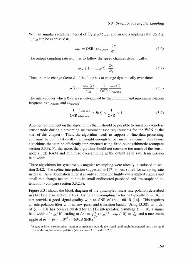
5.3. Synchronous angular sampling
With an angular sampling interval of Φs ≤ π/Omax and an oversampling ratio OSR ≥1, ωin can be expressed as:
ωin = OSR ·ωrot,max ·2πΦs
. (5.6)
The output sampling rate ωout has to follow the speed changes dynamically:
ωout(t) = ωrot(t) ·2πΦs
. (5.7)
Thus, the rate change factor R of the filter has to change dynamically over time:
R(t) =ωout(t)ωin
=1
OSRωrot(t)ωrot,max
. (5.8)
The interval over which R varies is determined by the minimum and maximum rotationfrequencies ωrot,min and ωort,max:
1OSR
ωrot,min
ωrot,max≤ R(t) ≤
1OSR
≤ 1. (5.9)
Another requirement on the algorithm is that it should be possible to run it on a wirelesssensor node during a streaming measurement (see requirements for the WSN at thestart of this chapter). Thus, the algorithm needs to support on-line data processingand must be computationally lightweight enough to be run in real-time. This favorsalgorithms that can be efficiently implemented using fixed-point arithmetic (comparesection 3.3.3). Furthermore, the algorithm should not consume too much of the sensornode’s little RAM and minimize oversampling at the output as to save transmissionbandwidth.
Three algorithms for synchronous angular resampling were already introduced in sec-tion 2.4.2. The spline-interpolation suggested in [17] is best suited for sampling rateincrease. As a decimation filter it is only suitable for highly oversampled signals andsmall rate change factors, due to its small undistorted passband and low stopband at-tenuation (compare section 3.3.2.3).
Figure 5.31 shows the block diagram of the upsampled linear interpolation describedin [14] (see also section 2.4.2). Using an upsampling factor of typically L = 16, itcan provide a good signal quality with an SNR of about 60 dB [14]. This requiresan interpolation filter with narrow pass- and transition bands. Using (3.38), an orderof Q = 101 has been calculated for an FIR interpolator, assuming L = 16, a signalbandwidth of ωin/10 leading to ∆ω = 2π
Lωin(ωin/2 −ωin/10) = π
20 , and a maximumripple of δ1 = δ2 = 10−3 (=60 dB SNR) 5.
5A type A filter is required as imaging components outside the signal band might be mapped onto the signalband during linear interpolation (see sections 3.3.1 and 3.3.2.3).
169

5. Implementation
Figure 5.31.: Block diagram of upsampled linear interpolation algorithm [14].
The rate change factor of the filter is:
Rup,lin(t) =LM
Rlin(t), (5.10)
where the only dynamic factor is the rate change factor Rlin of the linear interpolator.However, the output sampling rate of the linear interpolator ωlin must not be smallerthan the original sampling rate ωin in order to avoid aliasing, i.e. L · Rlin(t) ≥ 1. Thus,both the interpolation filter and the linear interpolator have to be run at least at therelatively high input sampling rate. In addition, the downsampling factor M of theoutput decimator has to be at least as large as the ratio between minimum and maximumspeed:
M =ωlin
ωout≥ωin
ωout,min(5.11)
with (5.6) and (5.7):
M ≥ OSR ·ωrot,max
ωrot,min(5.12)
M ≥ωrot,max
ωrot,min=
nrot,max
nrot,min. (5.13)
Considering that the filter order of an FIR decimator is proportional to its downsamplingfactor (see (3.44)), this means that the filter order increases with the speed range to becovered. Using (3.38), an order of Q = 101 has been calculated under the assumptionof M = 10, ∆ω = 2π
Mωout(ωout/2 − ωout/4) = π
20 and a maximum ripple of δ1 =
δ2 = 10−3 (=60 dB SNR). For a speed range of nrot,max/nrot,min = 100 it would beabout Q = 1000. Such high filter orders are not only problematic because of increasedoperation rate and memory consumption, they also require a high numeric resolution inorder to accurately represent their coefficients, especially when fixed-point arithmeticis used (compare section 3.3.3.3). The numeric examples in [14] only cover a range of180 . . . 720 rpm, i.e. nrot,max/nrot,min = 4.
Another algorithm described in [14] is the upsampled interpolation filter (see also sec-tion 2.4.2). It uses the hybrid model for resampling (see section 3.3.1.4) and replacesinterpolation filter and linear interpolator with a quasi continuous sinc-filter. This waya better signal quality (SNR: 70. . . 80 dB) can be achieved at a reduced computationalload. However, a very large number of precalculated values for the filter’s impulse re-sponse is required to achieve this efficiency. In [14] examples with 18 times 512 to
170

5.3. Synchronous angular sampling
8192, i.e. 9.216 . . . 147.456, precalculated values are given. This means that assum-ing a 32 bit resolution6, at least 32 kB of memory would be needed to store all values,which is too much for most sensor nodes. Furthermore, the upsampled interpolationfilter, suffers from the same problem regarding the high order of the output decimationfilter as the upsampled linear interpolation.
As synchronous angular resampling can be reduced to a nonuniform reconstructionproblem (see section 4.5), algorithms suggested for this task in other domains may alsobe used. A survey of nonuniform reconstruction algorithms for software defined radioreceivers is given in [139]. As the algorithms for this task also need to be capable ofreal-time online data processing, there is a match with the requirements outlined above.The conclusion of [139] is that algorithms based on lowpass filtering and polynomialinterpolation are the most interesting for the task.
Algorithms based on low pass filtering employ the hybrid model of a resampling filter(compare figure 3.12). First, the continuous signal is reconstructed by modulating adelta comb with the acquired samples and feeding it through a lowpass filter. Thenthe continuous signal is resampled at the desired instants. However, this reconstructionmethod is only exact for uniformly sampled signals and an ideal lowpass filter. Ifapplied to nonuniformly sampled signals it leads to multiplicative noise in the outputsignal (compare (3.27)).
Polynomial interpolation algorithms that use small polynomial orders suffer from thesame problem as the spline interpolation in [17] that was discussed above. With higherpolynomial orders the quality can be improved, but then the computational load quicklybecomes too high [139].
Another reconstruction filter for radio communication was proposed in [82]. It is basedon the method described by (3.28). Its block diagram is shown in figure 5.32. Theinput signal, sampled at the time instants tn, is denoted as x(tn) = x[n]. TransposedFarrow filters are used to do the low-pass filtering of xs and xp as well as to translatethe samples to a common uniform sampling grid with the sampling interval Tout/M.Two additional FIR lowpass filters with the transfer function G(z) are used to narrowthe transition bands and to remove transition band noise [82]. It was observed in [82]that the input sampling rate of the transposed Farrow filters should be at least fourtimes the signal bandwidth, in order to achieve a good reconstruction quality. Thus,the FIR decimator D(z) with a downsampling factor of M is used at the output. Thisfilter structure is capable of offering a good signal quality [82]. M is generally small,e.g. 2, thus the pass- and transition bands of the FIR-filters G and D are relativelylarge, enabling reasonably small filter orders. As all filters are designed with respect tothe output frequency, this is independent of the input speed range. Thus, this filteringalgorithm appears to be the best option for synchronous angular resampling with aWSN.
6Lower resolutions are unlikely to provide satisfactory results, as the value of the sinc function is 1 at the
171

5. Implementation
Figure 5.32.: Reconstruction filter proposed in [82].
5.3.2. Filter adaptation
The chosen resampling algorithm, as given in figure 5.32, translates a signal from anonuniform sampling grid tn to a uniform one tl = lTout. In order to use the al-gorithm for synchronous angular resampling, the input time instants tn need to be re-placed with the angular instants ϕn = ϕ(tn) and the output sampling interval Tout withthe angular interval Φout. Yet in a practical setup, usually only the timestamps tn andtϕ,l′ = t(l′Φout) are available (compare section 5.3.4), where l′ is the counting index atM-times the output rate. Thus, the angular instants ϕn need to be calculated by linearinterpolation:
ϕn =Φout/M
tϕ,l′n+1 − tϕ,l′n
(tn − tϕ,l′n
)+ l′n ·
Φout
M, (5.14)
where tϕ,l′n+1 > tn ≥ tϕ,l′n . However, the quantity that is actually needed for the operationof a transposed Farrow filter is the fractional interval µn (compare section 3.3.2.4). Forsynchronous angular resampling, it can be calculated as follows:
µn = M ·ϕn
Φout− ⌊M ·
ϕn
Φout⌋ (5.15)
=tn − tϕ,l′n
tϕ,l′n+1 − tϕ,l′n. (5.16)
As the upper and lower Farrow filter in figure 5.32 use the same fractional interval µn,its calculation only needs to be done once for both filters. Figure 5.33 shows the blockdiagram of the filter with the modifications for synchronous angular resampling.
5.3.3. Filter design
The filter was designed assuming an input frequency ωin ≥ 2ωout and a signal band-width of Wsig ≤ ωout/4 (compare section 5.3.1). Thus, the passband edge was chosenas ωp = 0.25ωout, the stopband edge as ωstop = 0.5ωout and the decimation factor ofthe output stage as M = 2.
center and the values at the edges are very small.
172

5.3. Synchronous angular sampling
Figure 5.33.: Resampling filter adapted to synchronous angular resampling.
The coefficients for the transposed Farrow filter were taken from [7]. The impulseresponse of this filter consists of N = 4 polynomials of the order M = 3. The FIR filterG at the output of the Farrow filter was designed with the help of MATLAB, using anoptimal least-squares design. Its passband characteristic was designed in such a waythat it compensates for the passband ripple of the transposed Farrow filter. The filterorder of G is Q = 61. The Output FIR decimator D was designed with MATLAB,using an optimal equiripple design. It has a filter order of Q = 34. The MATLAB codeused for the filter design is given in appendix D.1.
The magnitude frequency responses of the individual filters are shown in figure 5.34,that of the entire filter cascade in figure 5.35. The latter neglects effects from demodu-lation by the divisor.
The entire designed filter has a maximum passband ripple of 0.004 dB and a minimumstopband attenuation of 62.8 dB. Better results might be achieved using the methodfor the calculation of optimal coefficients described in [146]. Yet, the current filtercharacteristics were already sufficient for the targeted applications.
0 1 2 3 4 5 6 7 8 9 10−120
−100
−80
−60
−40
−20
0
ω/ωout
[1]
mag
nit
ud
e [d
B]
farrow filter G(z) D(z)
Figure 5.34.: Magnitude frequency responses of individual filters.
173

5. Implementation
0 1 2 3 4 5 6 7 8 9 10−120
−100
−80
−60
−40
−20
0
ω/ωout
[1]
mag
nit
ud
e [d
B]
Figure 5.35.: Magnitude frequency response of cascade: transposed Farrow, G and D.
5.3.4. Implementation of filter algorithm
At first the filter was implemented and tested in MATLAB. The implementation fol-lowed directly from the filter structure in figure 5.33 and the equation of the transposedFarrow filter introduced in section 3.3.2.4. Its code is given in appendix D.2. After-wards, it was implemented in C, in order to be run on the Preon32. Since Preon32’sprocessor does not possess an FPU, it was not possible to run a floating-point imple-mentation of the algorithm in real-time. Therefore, the final implementation for thePreon32 was done in fixed-point arithmetic. Section 6.5.2 presents test results compar-ing the MATLAB, floating-point C and fixed-point C implementations of the algorithm.The fixed-point implementation of the algorithm is described in more detail in the fol-lowing.
5.3.4.1. Fixed-Point implementation
The transposed Farrow filter and the calculation of the fractional interval were imple-mented by the author. For the FIR filters G and D library functions from the CMSISDSP library, provided by ARM [165], were used. To minimize the computational loadand memory requirements of the implementation a 16 bit fixed-point format (Q0.15)was chosen for the in- and output values of the filter (compare section 3.3.3). This alsocovers the full digital output range of the ADC. However, it was not feasible to use thisfixed point format throughout the entire filter algorithm for the following reasons:
1. The size of a Farrow filter’s output values is about N-times that of the inputvalues x, where N is the number of input samples that contribute to one outputsample. Thus, a 32 bit format (Q16.15) was chosen for the outputs of the Farrowfilters and the following FIR-filtering. Also, the coefficients of the FIR-filterswere taken as 32 bit numbers (Q0.31).
174
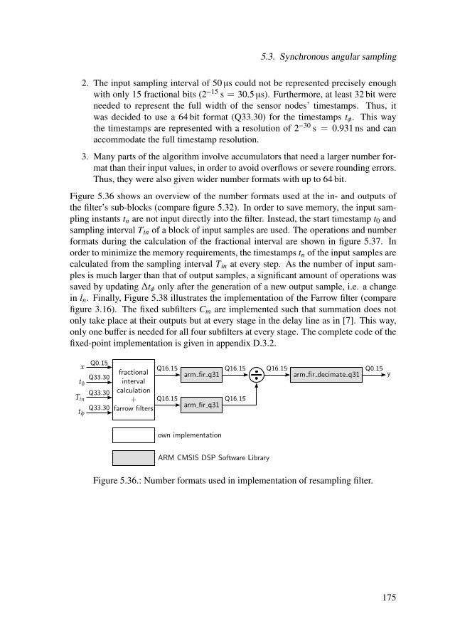
5.3. Synchronous angular sampling
2. The input sampling interval of 50 µs could not be represented precisely enoughwith only 15 fractional bits (2−15 s = 30.5 µs). Furthermore, at least 32 bit wereneeded to represent the full width of the sensor nodes’ timestamps. Thus, itwas decided to use a 64 bit format (Q33.30) for the timestamps tϕ. This waythe timestamps are represented with a resolution of 2−30 s = 0.931 ns and canaccommodate the full timestamp resolution.
3. Many parts of the algorithm involve accumulators that need a larger number for-mat than their input values, in order to avoid overflows or severe rounding errors.Thus, they were also given wider number formats with up to 64 bit.
Figure 5.36 shows an overview of the number formats used at the in- and outputs ofthe filter’s sub-blocks (compare figure 5.32). In order to save memory, the input sam-pling instants tn are not input directly into the filter. Instead, the start timestamp t0 andsampling interval Tin of a block of input samples are used. The operations and numberformats during the calculation of the fractional interval are shown in figure 5.37. Inorder to minimize the memory requirements, the timestamps tn of the input samples arecalculated from the sampling interval Tin at every step. As the number of input sam-ples is much larger than that of output samples, a significant amount of operations wassaved by updating ∆tϕ only after the generation of a new output sample, i.e. a changein ln. Finally, Figure 5.38 illustrates the implementation of the Farrow filter (comparefigure 3.16). The fixed subfilters Cm are implemented such that summation does notonly take place at their outputs but at every stage in the delay line as in [7]. This way,only one buffer is needed for all four subfilters at every stage. The complete code of thefixed-point implementation is given in appendix D.3.2.
Figure 5.36.: Number formats used in implementation of resampling filter.
175

5. Implementation
Figure 5.37.: Number formats used in the calculation of the fractional interval.
Figure 5.38.: Number formats used in the implementation of the Farrow filter.
176

5.3. Synchronous angular sampling
5.3.5. Network integration
Figure 5.39 shows the network layout that was chosen for synchronous angular resam-pling. One TIM, the data TIM, acquires analog samples uniformly over time using theanalog voltage sensor described in section 5.1.5.4. It is synchronized to the clock of theNCAP with the timesynch-service (see section 5.2.1.2) and uses the second variant ofreactive synchronous sampling described in section 5.2.3.2. The maximum acquisitionblock size is 2048 samples with one block per 102.4 ms. As described in section 5.2.3.2,the data acquisition process generate a timestamp tend at the last sample of every block.Using the timestamp from the previous block, the actual sampling interval Tin,i of theith block is calculated:
Tin,i =tend,i − tend,i−1
2048(5.17)
Before this division, the 32 bit timestamps (Q17.14) are extended to the 64 bit format(Q33.30) used by the filter and shifted 16 digits to the left. Due to the averaging over211 samples, the effective time resolution after the division is 2−(14+11) s = 29.8 ns 7,which allows for an accurate representation of the sampling interval (nominally 50 µs).The resampling filter itself is integrated into the processing stage of the analog sensor(compare figure 5.15).
Figure 5.39.: Network layout for synchronous angular resampling.
7The numerical resolution is of course 2−30 s = 0.931 ns.
177
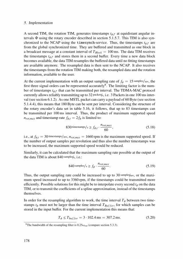
5. Implementation
A second TIM, the rotation TIM, generates timestamps tϕ,l′ at equidistant angular in-tervals Φ using the rotary encoder described in section 5.1.5.7. This TIM is also syn-chronized to the NCAP using the timesynch-service. Thus, the timestamps tϕ,l′ arefrom the global synchronized time. They are buffered and transmitted as one block ina broadcast message at a constant interval of TBlock = 100 ms. The data TIM receivesthe timestamps tϕ,l′ and stores them in a second buffer. Every time a new data blockbecomes available, the data TIM resamples the buffered data until no fitting timestampsare available anymore. The resampled data is then sent to the NCAP. It also receivesthe timestamps from the rotation TIM making both, the resampled data and the rotationinformation, available to the user.
At the current implementation with an output sampling rate of fϕ = 15 samples/rev, thefirst three signal orders can be represented accurately8. The limiting factor is the num-ber of timestamps tϕ,l′ that can be transmitted per interval. The TDMA-MAC protocolcurrently allows reliably transmitting up to 32 packets/s, i.e. 3 Packets in one 100 ms inter-val (see section 6.1.2). As one MSTL packet can carry a payload of 60 Byte (see section5.1.4.4), this means that 180 Byte can be sent per interval. Considering the structure ofthe rotary encoder’s data set in table 5.16, it follows, that up to 83 timestamps canbe transmitted per 100 ms interval. Thus, the product of maximum supported speednrot,max and timestamp rate fϕ,t = 2 fϕ is limited to:
830 timestamps/s ≥ fϕ,t ·nrot,max
60, (5.18)
i.e., at fϕ,t = 30 timestamps/rev, nrot,max = 1660 rpm is the maximum supported speed. Ifthe number of output samples per revolution and thus also the number timestamps wasto be increased, the maximum supported speed would be reduced.
Similarly, it can be calculated that the maximum sampling rate possible at the output ofthe data TIM is about 840 samples/s, i.e.:
840 samples/s ≥ fϕ ·nrot,max
60. (5.19)
Thus, the output sampling rate could be increased to up to 30 samples/rev, or the maxi-mum speed increased to up to 3360 rpm, if the timestamps could be transmitted moreefficiently. Possible solutions for this might be to interpolate every second tϕ on the dataTIM, or to transmit the coefficients of a spline approximation, instead of the timestampsthemselves.
In order for the resampling algorithm to work, the time interval Tϕ between two time-stamps tϕ must not be larger than the time interval TBu f f er, for which samples can bestored in the input buffer. For the current implementation this means that:
Tϕ ≤ Tbu f f er = 3 · 102.4 ms = 307.2 ms. (5.20)
8The bandwidth of the resampling filter is 0.25ωout (compare section 5.3.3).
178
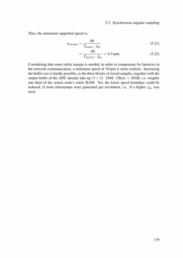
5.3. Synchronous angular sampling
Thus, the minimum supported speed is:
nrot,min =60
Tϕ,max · fϕ,t(5.21)
=60
Tbu f f er · fϕ,t= 6.5 rpm. (5.22)
Considering that some safety margin is needed, in order to compensate for latencies inthe network communication, a minimum speed of 10 rpm is more realistic. Increasingthe buffer size is hardly possible, as the three blocks of stored samples, together with theoutput buffer of the ADC already take up (3 + 2) · 2048 · 2 Byte = 20 kB, i.e. roughlyone third of the sensor node’s entire RAM. Yet, the lower speed boundary could bereduced, if more timestamps were generated per revolution, i.e. if a higher fϕ,t wasused.
179


6. Experiments
This chapter presents the experiments that were done to evaluate the performance ofthe WSN for the three types of synchronous data acquisition modeled in chapter 4 andwhose implementations were described in chapter 5. Section 6.1 describes the mea-surements of the WSN’s power consumption and data throughput. The results of thesemeasurements are used to better interpret the performance of the data acquisition inthe following experiments. Section 6.2 shows experiments to evaluate the synchronousevent detection of the WSN. Its influence in a practical application, the acoustic local-ization of sensor nodes, is analyzed in section 6.3. Section 6.4 presents measurementsto test the synchronous waveform sampling of the WSN. Finally, experiments on syn-chronous angular sampling are given in section 6.5. Throughout this chapter the indi-vidual physical sensor nodes used, will be identified by their unique IDs (see section5.1.4).
6.1. Wireless sensor network
This section presents experiments that were done to determine basic characteristics ofthe used WSN: its power consumption (section 6.1.1), data throughput and transmis-sion reliability (section 6.1.2). Although these were not in the focus of this thesis andtherefore have not been fully optimized, they still are relevant performance metrics.
6.1.1. Power consumption
As power is often scarce in WSNs the power consumption of a wireless sensor nodeis an important performance metric (compare section 2.1.1). The Contiki operatingsystem used in this thesis provides a mechanism called powertrace that estimatesthe power consumption of a node during operation. The experiments presented in thissection serve to calibrate the powertrace mechanism for the Preon32 sensor node.Furthermore, the powertrace estimates were validated through comparison with mea-surements from a digital multimeter (DMM).
181

6. Experiments
6.1.1.1. Experimental setup
Figure 6.1 shows the experimental setup used to measure the current of the sensornodes. A sensor node, mounted on a Preon32Shuttle, was connected to a laboratorypower supply (Gossen 33K7EU5/2x25R1) with Vin = 3.8 V. The actual supply voltageVsupply = 3.3 V of the Preon32 was generated from this by a linear voltage regulatoron the Preon32Shuttle (see also section 5.1.1). A DMM (FLUKE 8846A) was used tomeasure the supply current. In some experiments a second node was used to communi-cate with and collect powertrace data from the node whose current consumption wasmeasured.
The integration time Tinter for the dual-slope ADC of the multimeter was set to 100power-line-cycles (PLC). At the given power-line frequency of 50 Hz this resulted inTinter = 2 s. Thus, the current measurement of the multimeter was the average currentdrawn by the sensor node over this time. A PC connected to the serial interface ofthe multimeter was used to automatically acquire current readings with a MATLAB-script. The Preon32 was run from its internal RC-oscillator at a system clock frequencyof 36 MHz throughout these experiments as well as in all other experiments in thischapter (compare section 5.1.1).
Figure 6.1.: Experimental setup used to measure the supply current of a node.
6.1.1.2. Current consumption measurement
The first round of experiments served to measure a sensor node’s current consumptionin the different power states. For this purpose a set of simple Contiki applications wascreated that all enter an infinite loop after initialization (see figure 6.2). Thus, the con-trol over the microcontroller stays with the application and never returns to the Contikischeduler (compare section 5.1.2). In order to measure the current consumption of thedifferent microcontroller power modes, the wireless transceiver was turned off duringthe initialization of the program. Then in the infinite loop the microcontroller was re-peatedly put to sleep in the selected power mode for 10 min (see figure 6.2 a)). To get animpression of how processor operations affect its current consumption a variable was
182

6.1. Wireless sensor network
repeatedly incremented within the loop instead of calling the sleep routine (see figure6.2 b)). This will be referred to as power mode BUSY in the following descriptions.In order to measure the transceiver’s listening current consumption, it was turned on atthe initialization of the program and the microcontroller was set to sleep in RUNNINGmode in the infinite loop (see figure 6.2 c)). Finally, the sleep routine in the infinite loopwas replaced by the sending of a wireless packet of maximum length (127 Byte) (seefigure 6.2 d)). This way the node was sending out packets at the maximum possiblerate. For this case, both the maximum (3 dBm) and the minimum (-17 dBm) transmis-sion power setting of the transceiver were investigated.
Figure 6.2.: Activity diagrams of test applications used to measure a sensor node’s cur-rent consumption.
In the experiments, the program for the investigated power mode was first compiledand downloaded to the sensor node via its USB-interface. Then the USB-Interfacewas disconnected from the sensor node and the power supply was connected to thepower socket of the Preon32Shuttle. After resetting the node and waiting for 1 min,10 automated measurements of the node’s supply current were taken over a period ofapproximately 10 s. This was repeated for every investigated power mode.
Table 6.1 shows the results of the current measurements with node number 41. Thecurrent values Isupply are the average values from the N = 10 measurements. Theuncertainties Uk,I are the expanded uncertainties that were calculated for a coveragefactor of k = 2 from the standard deviation smeas of the measurement values and thespecified uncertainty uDMM of the multimeter [40, 41]:
Uk,I = k ·
√s2
meas
N+ u2
DMM (6.1)
183

6. Experiments
Table 6.1.: Current consumption of node 41 measured for the different power modes.
Mode Current consumption
microcontroller transceiver Isupply Uk=2,I unit
BUSY OFF 19.903 0.107 mARUNNING OFF 17.273 0.063 mAIDLE OFF 6.778 0.016 mASTANDBY OFF 65.133 0.076 µAPOWEROFF OFF 25.404 0.010 µA
RUNNING LISTEN 30.861 0.161 mABUSY TX (3 dBm) 28.654 0.014 mABUSY TX (-17 dBm) 24.875 0.021 mA
Comparing the measured values in table 6.1 to the specification values in table 5.4, thecurrent consumption measured for the POWEROFF mode matches very well. Also thevalues for the BUSY, RUNNING and IDLE modes are within the expected range. It isworth noting that there is quite a large difference in current consumption (about 15 %)between the microcontroller sleeping in RUNNING mode and the processor constantlyincrementing a variable (BUSY mode). The current measured for the STANDBY modeis significantly lower than the one given in the specifications (1.3 mA). Interestingly, asimilar value could be measured by skipping the initialization of the wireless transceiverduring the Contiki boot. The wireless transceiver apparently consumes more current,when left uninitialized compared to being shut-down after initialization.
To separate the listening current consumption of the wireless transceiver from that ofthe microcontroller, the current consumption measured for the RUNNING mode withtransceiver off was subtracted from that measured during RUNNING mode with lis-tening for wireless communication. The resulting value is about 1 mA higher than thespecified current consumption (see tables 5.4 and 6.2).
To obtain the transmitting current consumption of the wireless transceiver the currentconsumption measured for the processor in BUSY mode was subtracted from that mea-sured during transmission. This was chosen, because the processor was constantly busygenerating and sending packets to the wireless transceiver during these measurements.The resulting current consumption (about 8.7 mA for 3 dBm) is, however, much lowerthan the one specified in table 5.4. To further investigate this phenomenon, a 10Ω re-sistor was connected in series to the Preon32Shuttle and the voltage drop over it wasmeasured with an oscilloscope (PicoScope 2205MSO). Figure 6.3 shows an extract ofthe measured current trace. Obviously, the current consumption is periodically chang-ing, with a period of about 6.5 ms. The length of the upper plateau (about 4 ms) fitswell with time-on-air (∼ 4.3 ms) that is expected for the packet length used. Thus, thetransceiver apparently does not stay in transmitting mode all the time, but goes throughsome intermediate states although the controller is constantly sending packets to it. As
184

6.1. Wireless sensor network
a consequence the average current consumption is lower than that of the transmit state.For this reason the current of the upper plateau in the trace was used to determine thecurrent in transmit state instead of the multimeter measurement. Its mean value was34.2 mA and its standard deviation 0.22 mA over a total of 20 periods. Taking theprecision of the oscilloscope ±15 mV and that of the resistor ±0.1Ω into account theexpanded uncertainty of the measurement was calculated. The results given in table 6.2match very well with the specifications.
−2 0 2 4 6 8 10 12 14 16 18
10
20
30
40
time [ms]
amp
litu
de
[mA
]
node current mean current in plateau
Figure 6.3.: Node current during transmission.
Finally, the measured current values were assigned to the four power modes usedby Contiki’s powertrace mechanism (see section 5.1.2). The CPU-active mode inpowertrace (short: cpu) was equated with the BUSY mode of the processor. For thelow-power mode (short: lpm) the IDLE mode of the processor was used, as this is themode Contiki’s scheduler switches to when no process is running (see 5.1.2.5). Thecurrent consumption for the listen and transmit modes in powertrace were calculatedby subtracting the current consumption of the microcontroller from measured currentvalues as explained above. For the transmit mode (short: tx) the maximum transmissionpower of 3 dBm was assumed, as this is the standard setting in Contiki.
Table 6.2.: Current consumption assigned to powertrace modes.
Powertrace mode Current consumption
Imode Uk=2,mode unit
cpu active (cpu) 19.90 0.11 mAlow power (lpm) 6.78 0.02 mAlisten (listen) 13.59 0.17 mAtransmit (tx) 14.30 1.78 mA
185
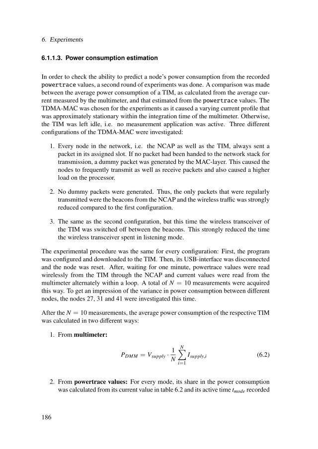
6. Experiments
6.1.1.3. Power consumption estimation
In order to check the ability to predict a node’s power consumption from the recordedpowertrace values, a second round of experiments was done. A comparison was madebetween the average power consumption of a TIM, as calculated from the average cur-rent measured by the multimeter, and that estimated from the powertrace values. TheTDMA-MAC was chosen for the experiments as it caused a varying current profile thatwas approximately stationary within the integration time of the multimeter. Otherwise,the TIM was left idle, i.e. no measurement application was active. Three differentconfigurations of the TDMA-MAC were investigated:
1. Every node in the network, i.e. the NCAP as well as the TIM, always sent apacket in its assigned slot. If no packet had been handed to the network stack fortransmission, a dummy packet was generated by the MAC-layer. This caused thenodes to frequently transmit as well as receive packets and also caused a higherload on the processor.
2. No dummy packets were generated. Thus, the only packets that were regularlytransmitted were the beacons from the NCAP and the wireless traffic was stronglyreduced compared to the first configuration.
3. The same as the second configuration, but this time the wireless transceiver ofthe TIM was switched off between the beacons. This strongly reduced the timethe wireless transceiver spent in listening mode.
The experimental procedure was the same for every configuration: First, the programwas configured and downloaded to the TIM. Then, its USB-interface was disconnectedand the node was reset. After, waiting for one minute, powertrace values were readwirelessly from the TIM through the NCAP and current values were read from themultimeter alternately within a loop. A total of N = 10 measurements were acquiredthis way. To get an impression of the variance in power consumption between differentnodes, the nodes 27, 31 and 41 were investigated this time.
After the N = 10 measurements, the average power consumption of the respective TIMwas calculated in two different ways:
1. From multimeter:
PDMM = Vsupply ·1N
N∑i=1
Isupply,i (6.2)
2. From powertrace values: For every mode, its share in the power consumptionwas calculated from its current value in table 6.2 and its active time tmode recorded
186
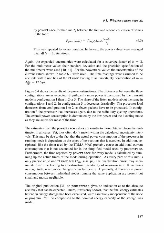
6.1. Wireless sensor network
by powertrace for the time Ti between the first and second collection of valuesin the loop:
Ppwrt.,mode,i = VsupplyImodetmode
Ti(6.3)
This was repeated for every iteration. In the end, the power values were averagedover all N = 10 iterations.
Again, the expanded uncertainties were calculated for a coverage factor of k = 2.For the multimeter values their standard deviation and the precision specification ofthe multimeter were used [40, 41]. For the powertrace values the uncertainties of thecurrent values shown in table 6.2 were used. The time readings were assumed to beaccurate within one tick of the rtimer leading to an uncertainty contribution of ut =Trtc√
12= 17.6 µs.
Figure 6.4 shows the results of the power estimations. The differences between the threeconfigurations are as expected. Significantly more power is consumed by the transmitmode in configuration 1 than in 2 or 3. The share of the listen mode is about the same inconfigurations 1 and 2. In configuration 3 it decreases drastically. The processor loaddecreases from configuration 1 to 2, as fewer packets have to be processed. In config-uration 3 the processor load increases again, due to the radio duty-cycling operations.The overall power consumption is dominated by the low power and the listening modeas they are active for most of the time.
The estimates from the powertrace values are similar to those obtained from the mul-timeter in all cases. Yet, they often don’t match within the calculated uncertainty inter-vals. This may be due to the fact that the actual power consumption of the processor inrunning mode is dependent on the types of instructions that it executes. In addition, pe-ripherals like the timer used by the TDMA-MAC probably cause an additional currentconsumption that is not accounted for in the simplified model used by powertrace.Furthermore, the time reported by powertrace for every mode is calculated by sum-ming up the active times of the mode during operation. As every part of this sum isonly precise up to one rtimer tick (Trtc ≈ 61 µs), the quantization errors may accu-mulate over time leading to an estimation uncertainty of unknown size. It increasesin magnitude, when mode changes occur frequently. Apparently, differences in powerconsumption between individual nodes running the same application are present butsmall and mostly negligible.
The original publication [31] on powertrace gives no indication as to the absoluteaccuracy that can be expected. There, it was only shown, that the final energy estimatesbefore an energy storage had been exhausted, were essentially independent of the nodeor program. Yet, no comparison to the nominal energy capacity of the storage wasmade.
187

6. Experiments
1 2 30
20
40
60
80Node 27
Configuration
Pav
g [
mW
]
1 2 3
Node 31
Configuration
1 2 3
Node 41
Configuration
DMM
pwrt. lpm
pwrt. cpu
pwrt. listen
pwrt. tx
Figure 6.4.: Power consumption of nodes as calculated from current measurements withmultimeter (DMM) and as estimated from powertrace (pwrt.). The errorbars show the expanded uncertainty Uk=2.
6.1.1.4. Conclusions
The current consumption of one node was measured for the different power modesusing a relatively simple setup. Comparison with the specification values showed anessentially good match. Yet, it was also shown that modeling the power consumptionwith a small number of different modes is a significant simplification. Therefore, it isnot always trivial to achieve and observe these modes in real operation.
Nevertheless, the power consumption estimated using powertrace about matches thatobtained from current measurements with a multimeter. Significant deviations wereobserved, that are probably due to simplifications in the powertrace approach. Never-theless, the powertrace estimates are very useful for observing the effect of softwarechanges on the power consumption and for comparing the contributions of differentcomponents.
6.1.2. Data throughput
In order to determine the transmission bandwidth usable for data collection in laterexperiments, the data throughput and the reliability of transmission were measuredfor the WSN. The IEEE 802.15.4 standard defines a bit rate of 250 kbps for wirelesscommunication in the 2.5 GHz band [194]. However, already the data link layer definedin IEEE 802.15.4 introduces an overhead so that the actually usable data bandwidth issignificantly lower. Delays caused by the MAC-layer as well as failed transmissions and
188

6.1. Wireless sensor network
consequent retransmissions further reduce the actual data throughput. As MAC-layeroperations are always performed on a per packet basis, it is often more meaningful toevaluate MAC-layer performance in terms of packets per time instead of data amountper time. This section presents experiments that evaluate the RDC- and MAC-layerprotocols used for this thesis (see also section 5.1.2) in terms of packet rate versustransmission success and power consumption.
6.1.2.1. Experimental setup
To evaluate the performance of the MAC-layer, a simple test setup was used, whereone or more nodes each transmitted 1000 UDP-packets at a fixed rate. All packets hada payload of 60 Byte. An additional receiver node was used to count the number ofsuccessfully received packets. At the end of the experiment, this count was used tocalculate the percentage of successful transmissions. Furthermore, powertrace datawas recorded during the experiment.
Table 6.3 shows the three configurations of RDC- and MAC-layer that were investi-gated. For all layer-configurations two different network topologies were examined:one sender and one receiver (one-to-one) as well as two senders and one receiver (two-to-one). The packet rate was varied between 1 and 64 packets/s for the one-to-one trans-mission and between 1 and 42 packets/s for the two-to-one transmission. For the TDMA-MAC the receiving node was chosen to be the coordinator, as this configuration istypical of data acquisition applications.
Table 6.3.: Configuration of network layers investigated for data throughput.
Conf. RDC-layer MAC-layer
1 nullrdc CSMA2 ContikiMAC CSMA3 TDMA TDMA
6.1.2.2. Transmission success
Figure 6.5 shows the success rate during transmissions for one-to-one transmissions.Up to 32 packets/s, the success rate is 100 % for all investigated network configurations.After this there is a clear drop in the transmission success for the TDMA-MAC whilethe other two configurations maintain a near 100 % success rate even at the maximuminvestigated packet rate of 64 packets/s. The reason for this is that the simple TDMA-MAC, used in this thesis, is statically configured for a network of three nodes. Thus,in one-to-one transmission only a third of the total bandwidth can be used. This limi-tation does not apply if CSMA-based protocols are used. With the TDMA-MAC, the
189
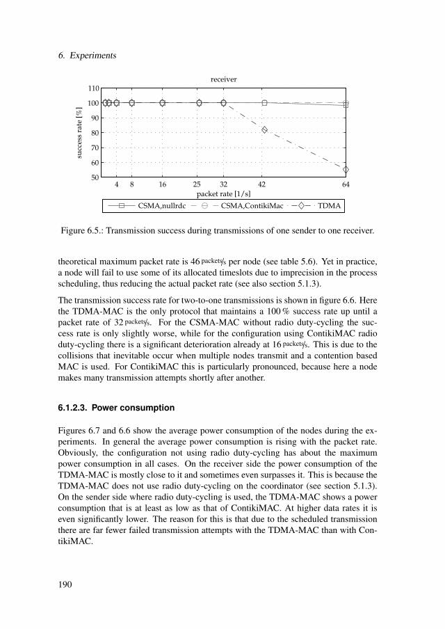
6. Experiments
4 8 16 25 32 42 6450
60
70
80
90
100
110receiver
packet rate [1/s]
succ
ess
rate
[%
]
CSMA,nullrdc CSMA,ContikiMac TDMA
Figure 6.5.: Transmission success during transmissions of one sender to one receiver.
theoretical maximum packet rate is 46 packets/s per node (see table 5.6). Yet in practice,a node will fail to use some of its allocated timeslots due to imprecision in the processscheduling, thus reducing the actual packet rate (see also section 5.1.3).
The transmission success rate for two-to-one transmissions is shown in figure 6.6. Herethe TDMA-MAC is the only protocol that maintains a 100 % success rate up until apacket rate of 32 packets/s. For the CSMA-MAC without radio duty-cycling the suc-cess rate is only slightly worse, while for the configuration using ContikiMAC radioduty-cycling there is a significant deterioration already at 16 packets/s. This is due to thecollisions that inevitable occur when multiple nodes transmit and a contention basedMAC is used. For ContikiMAC this is particularly pronounced, because here a nodemakes many transmission attempts shortly after another.
6.1.2.3. Power consumption
Figures 6.7 and 6.6 show the average power consumption of the nodes during the ex-periments. In general the average power consumption is rising with the packet rate.Obviously, the configuration not using radio duty-cycling has about the maximumpower consumption in all cases. On the receiver side the power consumption of theTDMA-MAC is mostly close to it and sometimes even surpasses it. This is because theTDMA-MAC does not use radio duty-cycling on the coordinator (see section 5.1.3).On the sender side where radio duty-cycling is used, the TDMA-MAC shows a powerconsumption that is at least as low as that of ContikiMAC. At higher data rates it iseven significantly lower. The reason for this is that due to the scheduled transmissionthere are far fewer failed transmission attempts with the TDMA-MAC than with Con-tikiMAC.
190

6.1. Wireless sensor network
4 8 16 25 32 42 6450
60
70
80
90
100
110receiver
packet rate [1/s]
succ
ess
rate
[%
]
CSMA,nullrdc CSMA,ContikiMac TDMA
Figure 6.6.: Transmission success during transmissions of two senders to one receiver.
4 8 16 25 32 42 6420
40
60
80
100
120receiver
packet rate [1/s]
avg
. po
wer
[m
W]
4 8 16 25 32 42 6420
40
60
80
100
120sender
packet rate [1/s]
CSMA,nullrdc CSMA,ContikiMac TDMA
Figure 6.7.: Average power consumption during transmissions of one sender to one re-ceiver.
191
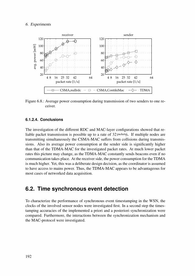
6. Experiments
4 8 16 25 32 42 6420
40
60
80
100
120receiver
packet rate [1/s]
avg
. po
wer
[m
W]
4 8 16 25 32 42 6420
40
60
80
100
120sender
packet rate [1/s]
CSMA,nullrdc CSMA,ContikiMac TDMA
Figure 6.8.: Average power consumption during transmission of two senders to one re-ceiver.
6.1.2.4. Conclusions
The investigation of the different RDC and MAC-layer configurations showed that re-liable packet transmission is possible up to a rate of 32 packets/s. If multiple nodes aretransmitting simultaneously the CSMA-MAC suffers from collisions during transmis-sions. Also its average power consumption at the sender side is significantly higherthan that of the TDMA-MAC for the investigated packet rates. At much lower packetrates this picture may change, as the TDMA-MAC constantly sends beacons even if nocommunication takes place. At the receiver side, the power consumption for the TDMAis much higher. Yet, this was a deliberate design decision, as the coordinator is assumedto have access to mains power. Thus, the TDMA-MAC appears to be advantageous formost cases of networked data acquisition.
6.2. Time synchronous event detection
To characterize the performance of synchronous event timestamping in the WSN, theclocks of the involved sensor nodes were investigated first. In a second step the times-tamping accuracies of the implemented a priori and a posteriori synchronization werecompared. Furthermore, the interactions between the synchronization mechanism andthe MAC-protocol were investigated.
192

6.2. Time synchronous event detection
6.2.1. Experimental setup
The experimental setup shown in figure 6.9 follows the test procedure for event detec-tors that was introduced in section 4.6.1. For the experiments a WSN with one NCAPand two TIMs was used. Interrupt inputs of all three nodes were connected to the digi-tal output of a fourth sensor node that did not participate in the WSN. The connectionswere made with four identical 50Ω Bayonet Neil-Concelman (BNC)-cables of 1.3 mlength. On both TIMs and the NCAP the event sensor described in section 5.1.5.2 wasused in continuous acquisition mode. The time synchronized event detection mecha-nism described in section 5.2.2 was used to generate a timestamp every time a pulsewas detected. These timestamps were transmitted to the NCAP, from where they wereread by a computer.
The time between two pulses was chosen randomly from the interval [1.5, 2.5 ]s, us-ing the pseudo-random number generator of the standard C-library, on the pulse node.During the experiments data on the nodes’ power supply was collected using Contiki’spowertrace mechanism (see also sections 5.1.2 and 6.1.1). Furthermore, the clockcorrections performed by the synchronization algorithm were recorded via the USBinterface of each node.
Figure 6.9.: Experimental setup used for event timestamping tests.
Table 6.4 shows the network configurations that were investigated during the exper-iments. The CSMA-MAC was always used in combination with the ContikiMAC-protocol. But, the actual radio duty-cycling was turned off in configurations 1 to 6,in order to prevent it from influencing the timestamping. The same was done for theTDMA-MAC. Furthermore, the synchronization interval of the a priori timesynchprotocol was varied. For every configuration a total of 1000 timestamp triples wererecorded over about 33 min.
193
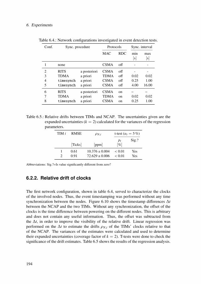
6. Experiments
Table 6.4.: Network configurations investigated in event detection tests.
Conf. Sync. procedure Protocols Sync. interval
MAC RDC min max[s] [s]
1 none CSMA off - -
2 RITS a posteriori CSMA off - -3 TDMA a priori TDMA off 0.02 0.024 timesynch a priori CSMA off 0.25 1.005 timesynch a priori CSMA off 4.00 16.00
6 RITS a posteriori CSMA on − −
7 TDMA a priori TDMA on 0.02 0.028 timesynch a priori CSMA on 0.25 1.00
Table 6.5.: Relative drifts between TIMs and NCAP. The uncertainties given are theexpanded uncertainties (k = 2) calculated for the variances of the regressionparameters.
TIM i RMSE ρN,i t-test (αt = 5 %)
pt Sig.?[Ticks] [ppm] [%]
1 0.61 10.376 ± 0.004 < 0.01 Yes2 0.91 72.629 ± 0.006 < 0.01 Yes
Abbreviations: Sig.?=Is value significantly different from zero?
6.2.2. Relative drift of clocks
The first network configuration, shown in table 6.4, served to characterize the clocksof the involved nodes. Thus, the event timestamping was performed without any timesynchronization between the nodes. Figure 6.10 shows the timestamp differences ∆tbetween the NCAP and the two TIMs. Without any synchronization, the offset of theclocks is the time difference between powering on the different nodes. This is arbitraryand does not contain any useful information. Thus, the offset was subtracted fromthe ∆t, in order to improve the visibility of the relative drift. Linear regression wasperformed on the ∆t to estimate the drifts ρN,i of the TIMs’ clocks relative to thatof the NCAP. The variances of the estimates were calculated and used to determinetheir expanded uncertainties (coverage factor of k = 2). T-tests were done to check thesignificance of the drift estimates. Table 6.5 shows the results of the regression analysis.
194

6.2. Time synchronous event detection
0 200 400 600 800 1000 1200 1400 1600 1800 20000
1000
2000
3000
t [s]
∆t[T
icks]
TIM 1
TIM 2
0.00
61.04
122.07
183.11
∆t[m
s]
Figure 6.10.: Recorded timestamp differences of TIMs to NCAP without time synchro-nization. The initial clock offset was removed to improve the visibility ofthe relative drifts.
The root-mean-square error (RMSE) of the linear fits is low (< 1 Tick) for both nodes.Thus, the behavior of their clocks can be well described by a constant drift model forthe observed time interval. The relative drift between the NCAP and TIM2 is aboutseven times larger than that between NCAP and TIM1. This may be linked to the fact,that TIM2 (i.e. node 41) is from a different hardware revision than the other two (i.e.nodes 27 and 31) and uses a different clock oscillator.
6.2.3. Synchronization precision
Network configurations 2 to 8 shown in table 6.4 were used to investigate approachesto synchronized event detection. In addition, the effects of the synchronization intervalas well as the influence of the MAC and RDC layer were studied.
For the configurations (3-5,7,8) using a priori synchronization, the maximum expectedsynchronization error ϵt,max can be calculated using (2.1). The drift values were takenfrom table 6.5. The synchronization error right after one synchronization event wasassumed to be ϵt,sample = 0.5 Tick. This is motivated by the fact that a clock can onlybe set with a resolution of 1 Tick. Thus, it may not be possible to set the clock closerthan 0.5 Tick to the actual time (compare section 4.2.1.4). Table 6.6 shows the resultsof this calculation. Ideally, the absolute values of the timestamp differences betweenthe nodes should be smaller or equal to the calculated values rounded to the next largerinteger.
195
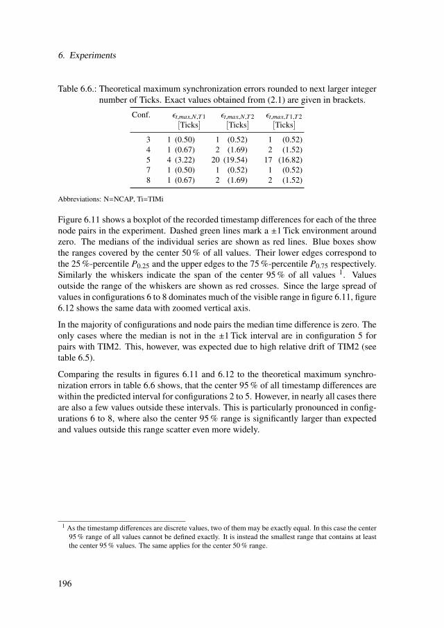
6. Experiments
Table 6.6.: Theoretical maximum synchronization errors rounded to next larger integernumber of Ticks. Exact values obtained from (2.1) are given in brackets.
Conf. ϵt,max,N,T1 ϵt,max,N,T2 ϵt,max,T1,T2[Ticks] [Ticks] [Ticks]
3 1 (0.50) 1 (0.52) 1 (0.52)4 1 (0.67) 2 (1.69) 2 (1.52)5 4 (3.22) 20 (19.54) 17 (16.82)7 1 (0.50) 1 (0.52) 1 (0.52)8 1 (0.67) 2 (1.69) 2 (1.52)
Abbreviations: N=NCAP, Ti=TIMi
Figure 6.11 shows a boxplot of the recorded timestamp differences for each of the threenode pairs in the experiment. Dashed green lines mark a ±1 Tick environment aroundzero. The medians of the individual series are shown as red lines. Blue boxes showthe ranges covered by the center 50 % of all values. Their lower edges correspond tothe 25 %-percentile P0.25 and the upper edges to the 75 %-percentile P0.75 respectively.Similarly the whiskers indicate the span of the center 95 % of all values 1. Valuesoutside the range of the whiskers are shown as red crosses. Since the large spread ofvalues in configurations 6 to 8 dominates much of the visible range in figure 6.11, figure6.12 shows the same data with zoomed vertical axis.
In the majority of configurations and node pairs the median time difference is zero. Theonly cases where the median is not in the ±1 Tick interval are in configuration 5 forpairs with TIM2. This, however, was expected due to high relative drift of TIM2 (seetable 6.5).
Comparing the results in figures 6.11 and 6.12 to the theoretical maximum synchro-nization errors in table 6.6 shows, that the center 95 % of all timestamp differences arewithin the predicted interval for configurations 2 to 5. However, in nearly all cases thereare also a few values outside these intervals. This is particularly pronounced in config-urations 6 to 8, where also the center 95 % range is significantly larger than expectedand values outside this range scatter even more widely.
1 As the timestamp differences are discrete values, two of them may be exactly equal. In this case the center95 % range of all values cannot be defined exactly. It is instead the smallest range that contains at leastthe center 95 % values. The same applies for the center 50 % range.
196

6.2. Time synchronous event detection
−40
−30
−20
−10
0
10
20
30
40
∆t N
,T1[Ticks]
−2.441
−1.221
0.000
1.221
2.441
∆t N
,T1[m
s]
−40
−30
−20
−10
0
10
20
30
40
∆t N
,T2[Ticks]
−2.441
−1.221
0.000
1.221
2.441
∆t N
,T2[m
s]
−2.441
−1.221
0.000
1.221
2.441
∆t T
1,T2[m
s]
2 3 4 5 6 7 8−40
−30
−20
−10
0
10
20
30
40
∆t T
1,T2[Ticks]
CSMARITSoff
TDMA(0.02,0.02)
off
CSMATS(0.25,1)
off
CSMATS(4,16)
off
CSMARITSon
TDMA(0.02,0.02)
on
CSMATS(0.25,1)
on
Network configuration
Figure 6.11.: Recorded timestamp differences with synchronization. The red lines markthe median. The blue boxes show the center 50 % and the whiskers thecenter 95 % of all values. Values outside these ranges are drawn as redcrosses.
197

6. Experiments
−4−2
02468
10121416
∆t N
,T1[Ticks]
−0.244
0.000
0.244
0.488
0.732
0.977
∆t N
,T1[m
s]
−4−2
02468
10121416
∆t N
,T2[Ticks]
−0.244
0.000
0.244
0.488
0.732
0.977
∆t N
,T2[m
s]
−0.244
0.000
0.244
0.488
0.732
0.977
∆t T
1,T2[m
s]
2 3 4 5 6 7 8−4−2
02468
10121416
∆t T
1,T2[Ticks]
CSMARITSoff
TDMA(0.02,0.02)
off
CSMATS(0.25,1)
off
CSMATS(4,16)
off
CSMARITSon
TDMA(0.02,0.02)
on
CSMATS(0.25,1)
on
Network configuration
Figure 6.12.: Recorded timestamp differences with synchronization with zoomed verti-cal axis. The red lines mark the median. The blue boxes show the center50 % and the whiskers the center 95 % of all values. Values outside theseranges are drawn as red crosses.
198

6.2. Time synchronous event detection
Table 6.7.: Estimated statistical parameters of timestamp difference distribution.
Conf. Nodes mean std. skew ex. krut. pgauss n2σ Tclock,e f f[Ticks] [Ticks] [1] [1] [%] [%] [Ticks]
2 N T1 -0.14 0.72 11.2 251.0 < 0.01 99.9 1.82 N T2 -0.24 0.72 11.4 260.2 < 0.01 99.9 1.82 T1 T2 -0.10 0.58 -0.0 -0.0 < 0.01 99.9 1.4
3 N T1 0.20 0.68 -1.2 6.1 < 0.01 98.0 1.73 N T2 0.21 0.69 -1.2 6.1 < 0.01 98.3 1.73 T1 T2 0.01 0.60 0.0 0.1 < 0.01 99.7 1.5
4 N T1 0.12 0.84 -3.6 23.9 < 0.01 98.1 2.14 N T2 0.22 0.94 -3.6 25.3 < 0.01 98.1 2.34 T1 T2 0.10 0.71 0.1 0.0 < 0.01 97.4 1.7
5 N T1 1.12 0.91 -0.1 -0.5 < 0.01 92.6 2.25 N T2 9.14 5.37 -0.0 -1.2 < 0.01 100.0 13.25 T1 T2 8.02 4.62 -0.0 -1.2 < 0.01 100.0 11.3
6 N T1 -1.29 3.70 -5.6 38.0 < 0.01 96.6 9.16 N T2 -1.52 3.77 -5.3 34.6 < 0.01 96.8 9.26 T1 T2 -0.23 5.25 0.2 17.7 < 0.01 95.1 12.9
7 N T1 -1.39 5.10 -3.2 9.7 < 0.01 92.7 12.57 N T2 -1.49 5.24 -3.2 9.5 < 0.01 93.1 12.87 T1 T2 -0.10 5.24 -0.5 12.1 < 0.01 92.8 12.8
8 N T1 0.31 4.43 -2.1 25.6 < 0.01 94.4 10.98 N T2 0.66 4.19 -3.0 28.2 < 0.01 93.4 10.38 T1 T2 0.35 6.12 -0.3 12.4 < 0.01 96.0 15.0
Abbreviations: N=NCAP; T1=TIM1; T2=TIM2; std.= standard deviation; ex. kurt.= excess kurtosis;pgauss= p-value of a χ2 goodness of fit test for a Gaussian distribution; n2σ= percentage of values within a±2σ interval
For further examination, the histograms of timestamp differences are shown in figure6.13. Fitted Gaussian probability density functions are also shown; as the analysisin section 4.2.1 revealed that an approximately Gaussian error distribution is likely.Table 6.7 shows a summary of statistical parameters that where estimated from therecordings.
The histograms for configurations 2 to 4, especially those of the pair (TIM1, TIM2),visually appear to agree quite well with a Gaussian distribution. Yet, all histogramsclearly fail a χ2 goodness-of-fit test for a Gaussian distribution. The reason appears tobe a lack of values in the tails of the distributions. The histograms of the pairs that in-volve TIM2 in configuration 5 seem to approximate a uniform distribution. Histogramsof configurations 6 to 8 show a wide spread of infrequent extreme values and sometimesmultiple modes, that both cause large standard deviations.
199
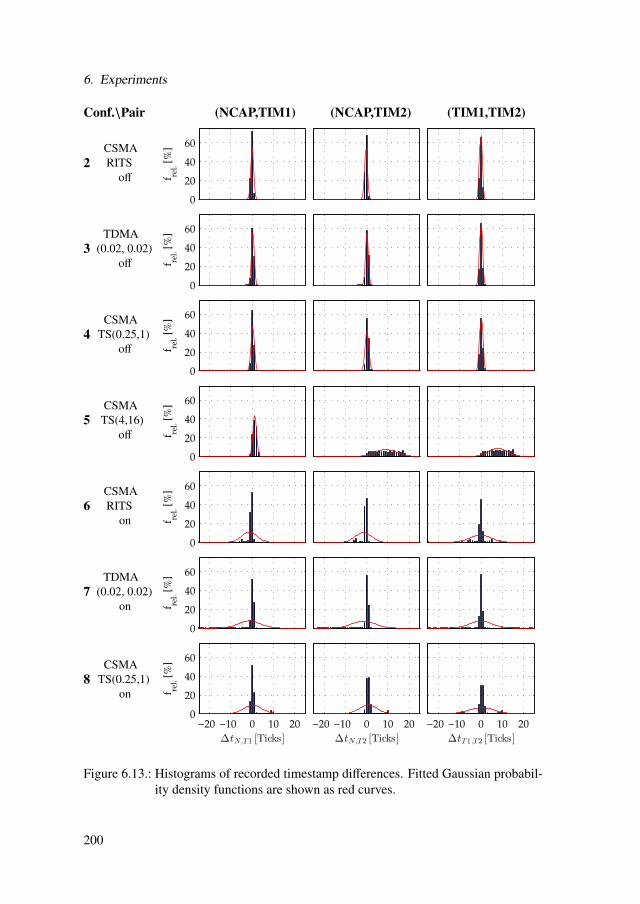
6. Experiments
Conf.\Pair (NCAP,TIM1) (NCAP,TIM2) (TIM1,TIM2)
2CSMARITS
off
−20 −10 0 10 200
20
40
60
∆tN,T1 [Ticks]
f rel. [
%]
−20 −10 0 10 20
∆tN,T2 [Ticks]
−20 −10 0 10 20
∆tT1,T2 [Ticks]
3TDMA
(0.02, 0.02)off
−20 −10 0 10 200
20
40
60
∆tN,T1 [Ticks]
f rel. [
%]
−20 −10 0 10 20
∆tN,T2 [Ticks]
−20 −10 0 10 20
∆tT1,T2 [Ticks]
4CSMA
TS(0.25,1)off
−20 −10 0 10 200
20
40
60
∆tN,T1 [Ticks]
f rel. [
%]
−20 −10 0 10 20
∆tN,T2 [Ticks]
−20 −10 0 10 20
∆tT1,T2 [Ticks]
5CSMATS(4,16)
off
−20 −10 0 10 200
20
40
60
∆tN,T1 [Ticks]
f rel. [
%]
−20 −10 0 10 20
∆tN,T2 [Ticks]
−20 −10 0 10 20
∆tT1,T2 [Ticks]
6CSMARITS
on
−20 −10 0 10 200
20
40
60
∆tN,T1 [Ticks]
f rel. [
%]
−20 −10 0 10 20
∆tN,T2 [Ticks]
−20 −10 0 10 20
∆tT1,T2 [Ticks]
7TDMA
(0.02, 0.02)on
−20 −10 0 10 200
20
40
60
∆tN,T1 [Ticks]
f rel. [
%]
−20 −10 0 10 20
∆tN,T2 [Ticks]
−20 −10 0 10 20
∆tT1,T2 [Ticks]
8CSMA
TS(0.25,1)on
−20 −10 0 10 200
20
40
60
∆tN,T1 [Ticks]
f rel. [
%]
−20 −10 0 10 20
∆tN,T2 [Ticks]
−20 −10 0 10 20
∆tT1,T2 [Ticks]
Figure 6.13.: Histograms of recorded timestamp differences. Fitted Gaussian probabil-ity density functions are shown as red curves.
200

6.2. Time synchronous event detection
An observation common to all configurations is that the histograms of the pairs, whichconsist of the NCAP and one TIM, are often skewed and have a strong excess kurtosis.The histograms of the pair that consists of two TIMs, on the other hand, mostly havea skew close to zero and less excess kurtosis. Also the means and standard deviationsof timestamp differences tend to be smaller for this pair. A not perfectly compensateddelay in the transmission of synchronization timestamps between NCAP and TIMs isa plausible explanation for this behavior. In most cases the percentage n2σ of valuesthat are within an interval of two standard deviations is larger than 95 %. In the othercases it is at least 92 %. This shows that even though the histograms of the timestampdifference significantly differ from a Gaussian distribution, their standard deviations arestill a useful measure of the spread of values.
The values given for Tclock,e f f in table 6.7 show that in the best configurations (2 to 4)the loss of timestamping precision due to synchronization can be roughly equated toputting a factor of 1.5 to 2.3 on the clocks resolution, i.e. about one bit of the clocksresolution is effectively lost (see also section 4.2.3).
A comparison to the performance of other synchronization protocols from the literatureis problematic due to differences in the underlying platform and experimental methods(see also section 2.2.4). Yet, it can be noted that the observed synchronization precisionis in the same order of magnitude as the results from other state-of-the-art protocols(compare table 2.7). An interesting fact is that the resolutions of the underlying clocksreported in the literature are disproportionately higher than in the present experiments.Thus, the implemented synchronization protocol may be said to be especially efficientin utilizing the clock resolution.
In configuration 5 the distribution of timestamp differences for pairs including TIM2resembles a uniform distribution rather than a Gaussian one. As pointed out in section4.2.1 this indicates a dominant error influence from clock drift. This is confirmed bythe timestamp differences and clock updates during the first 100 s that are shown infigure 6.14. Here the sawtooth behavior typical of a drifting clock that is periodicallycorrected by a synchronization algorithm is clearly visible when TIM2 is involved.Further evidence to this point is that the drift of TIM2 relative to the NCAP and TIM1has been found to be particularly strong (see section 6.2.2). In the other configurationusing a priori synchronization this behavior is in theory also present. Yet, it is muchweaker and probably shadowed by other influences. Another effect of the clock drift is abias in the mean timestamp difference of ∆tmax/2. This explains the increased medianvalue for configuration 5 observed in figure 6.12. Unfortunately, a classic correlationanalysis of the timestamp differences could not be performed, as they were acquirednonuniformly over time. Yet, apart from configuration 5 there is no obvious periodicityin the time difference values.
201

6. Experiments
0 10 20 30 40 50 60 70 80 90 100−40
−20
0
20
40
∆t N
,T1[T
icks]
0 10 20 30 40 50 60 70 80 90 100−40
−20
0
20
40
∆t N
,T2[T
icks]
0 10 20 30 40 50 60 70 80 90 100−40
−20
0
20
40
∆t T
1,T2[T
icks]
t [s]
0 10 20 30 40 50 60 70 80 90 100−20
0
20
40
∆cT1[T
icks]
0 10 20 30 40 50 60 70 80 90 100−20
0
20
40
∆cT2[T
icks]
t [s]
Figure 6.14.: First 100 s of recorded timestamp differences and clock updates for con-figuration 5.
Another phenomenon that needs further analysis is the occurrence of unusually largetimestamp differences especially in configurations 6 to 8. The most probable cause forthis are code sections during which interrupts are blocked (compare section 5.1.2.1).Table 6.8 shows a number of such code sections that could be identified. Their lengthwas obtained by setting a general-purpose input/output (GPIO)-pin high during theirexecution and measuring the pulse width with a logic analyzer (Tektronix TLA 704).The maximum execution time of the radio interrupt correlates very well with the max-imum timestamping differences observed in configurations 3 and 4. The duration ofthe radio on and off operations of the TDMA-MAC match equally well with the times-tamping differences observed in configuration 7. The maximum timestamp differencesobserved in configurations 6 and 8 correspond to the maximum execution time of anrtimer task that ContikiMAC uses in its radio duty-cycle.
202
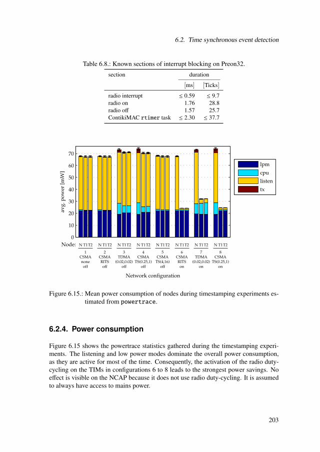
6.2. Time synchronous event detection
Table 6.8.: Known sections of interrupt blocking on Preon32.
section duration
[ms] [Ticks]
radio interrupt ≤ 0.59 ≤ 9.7radio on 1.76 28.8radio off 1.57 25.7ContikiMAC rtimer task ≤ 2.30 ≤ 37.7
0
10
20
30
40
50
60
70
avg
. po
wer
[m
W]
Node: N T1T2 N T1T2 N T1T2 N T1T2 N T1T2 N T1T2 N T1T2 N T1T2
1CSMAnoneoff
2CSMARITSoff
3TDMA
(0.02,0.02)off
4CSMA
TS(0.25,1)off
5CSMA
TS(4,16)off
6CSMARITSon
7TDMA
(0.02,0.02)on
8CSMA
TS(0.25,1)on
Network configuration
lpm
cpu
listen
tx
Figure 6.15.: Mean power consumption of nodes during timestamping experiments es-timated from powertrace.
6.2.4. Power consumption
Figure 6.15 shows the powertrace statistics gathered during the timestamping experi-ments. The listening and low power modes dominate the overall power consumption,as they are active for most of the time. Consequently, the activation of the radio duty-cycling on the TIMs in configurations 6 to 8 leads to the strongest power savings. Noeffect is visible on the NCAP because it does not use radio duty-cycling. It is assumedto always have access to mains power.
203

6. Experiments
In a priori synchronization smaller synchronization periods lead to increased powerconsumption from CPU operations and transmission activity. However, this effect isstrongest on the NCAP and only small the TIMs. Active radio duty-cycling furtherincreases the active power of the CPU. A posteriori synchronization is always slightlymore power efficient than a priori, due to reduced CPU active times. The TDMA-MACalways causes more power consumption than the CSMA-MAC due to higher activityrates.
6.2.5. Conclusions
The majority of the measured timestamp differences are within the expected bounds forsynchronization precision. Interrupt blocking code sections were identified as the causeof a relatively small number of more extreme values. If no significant drift occurs be-tween synchronization events, the distribution of the timestamp differences looks verysimilar to a Gaussian distribution. Yet, it tends to be more strongly centered. Further-more, transmission delays between NCAP and TIMs often cause a slight asymmetry inthe distribution. Yet, a Gaussian model still seems to be a useful approximation in mostcases. No significant advantages of either a priori or a posteriori synchronization withregard to synchronization precision could be found. The best, i.e. minimal, standarddeviation for both approaches was about s∆t = 0.60 Ticks. Thus the timing uncertaintyof the WSN is at least:
ut =s∆t√
2= 0.42 Ticks = 25.9 µs. (6.4)
This can also be interpreted as the loss of less than one bit on the clocks effectiveresolution. The absolute value of the observed synchronization precision is in the sameorder of magnitude as that reported in the literature for state-of-the-art synchronizationprotocols. In relation to the underlying clock resolution it even clearly better.
The power consumption of the sensor nodes during the experiments was found to bemost strongly influenced by their current consumption in low power mode and the lis-tening current of the radio transceiver. Thus, using radio duty-cycling is the most ef-fective way to save power. Yet, the duty-cycling operation was found contain a numberof interrupt blocking sections that adversely affect the timestamping precision. Thiseffect illustrates the complex interactions of software on small resource constraint sys-tems like wireless sensor nodes. Overcoming this trade-off is not easy as hardwareduty-cycling often requires wait periods that should not be interrupted. Yet, it is keyto achieving both low-power and high precision operation. In a priori synchronizationsmaller synchronization periods cause higher power consumption. This effect, however,is strongest on the NCAP where at the same time it is not very critical. Yet, in a multi-hop network this increase is expected to be also visible on mesh nodes, which may havemore constrained power supplies. A posteriori synchronization generally seems to have
204
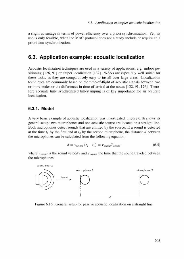
6.3. Application example: acoustic localization
a slight advantage in terms of power efficiency over a priori synchronization. Yet, itsuse is only feasible, when the MAC protocol does not already include or require an apriori time synchronization.
6.3. Application example: acoustic localization
Acoustic localization techniques are used in a variety of applications, e.g. indoor po-sitioning [126, 91] or sniper localization [132]. WSNs are especially well suited forthese tasks, as they are comparatively easy to install over large areas. Localizationtechniques are commonly based on the time-of-flight of acoustic signals between twoor more nodes or the differences in time-of-arrival at the nodes [132, 91, 126]. There-fore accurate time synchronized timestamping is of key importance for an accuratelocalization.
6.3.1. Model
A very basic example of acoustic localization was investigated. Figure 6.16 shows itsgeneral setup: two microphones and one acoustic source are located on a straight line.Both microphones detect sounds that are emitted by the source. If a sound is detectedat the time t1 by the first and at t2 by the second microphone, the distance d betweenthe microphones can be calculated from the following equation:
d = vsound (t2 − t1) = vsoundTsound. (6.5)
where vsound is the sound velocity and Tsound the time that the sound traveled betweenthe microphones.
Figure 6.16.: General setup for passive acoustic localization on a straight line.
205

6. Experiments
6.3.2. Estimation of required synchronization accuracy
The measurand is the distance d. Its maximum location uncertainty is chosen as uc,max =1 cm. Equation (6.5) already models the relationship between measurand and time-stamps. The sensitivity coefficients for the timestamps t1 and t2 are:
ct =
∂d∂t1,2
= vsound. (6.6)
Thus, the first upper limit for the timing uncertainty ut,max is:
u2c,max = (ctut,max)
2 from t1
+ (ctut,max)2
from t2
(6.7)
⇒ ut,max =uc,max√
2vsound(6.8)
with vsound = 343 m/s at ϑ = 20 °C [68]
⇒ ut,max = 20.6 µs. (6.9)
As nothing is known about other uncertainty influences, e.g. comparator noise andjitter, at this point, a suitable error margin has to be included. Table 6.9 shows the max-imum timing uncertainty needed for various localization uncertainties and uncertaintymargins.
Table 6.9.: Maximum timing uncertainty ut,max of a single timestamp in µs for differentmaximum location uncertainties ud,max and uncertainty margins for vsound =343 m/s.
uncertainty margin/ud,max 0.0 % 50.0 % 90.0 % 99.5 %
10 cm 206.15 178.53 89.86 20.595 cm 103.08 89.27 44.93 10.292 cm 41.23 35.71 17.97 4.121 cm 20.62 17.85 8.99 2.061 mm 2.06 1.79 0.90 0.21
Previous experiments have shown, that the timestamping uncertainty of the WSN usedis at least ut = 25.9 µs (see section 6.2). Comparing this to the values in table 6.9,a localization accuracy of about 2 cm should be achievable. If the observed accuracywas significantly worse, uncertainty influences other than the synchronization accuracy,would need to be reduced in order to improve it. In order to have a realistic chance ofreaching a localization accuracy of 1 cm the timestamping uncertainty would need to
206

6.3. Application example: acoustic localization
be reduced to about 17.85 µs. However, it is unlikely that this can be achieved at thegiven clock resolution. The uncertainty of the clock reading that is caused by the clockresolution is already ut,clock = Tclock/
√12 = 17.62 µs and every time synchronization
procedure will cause at least a small extra uncertainty.
6.3.3. Experiments
Figure 6.17 shows the experimental setup that was realized. Two TIMs were equippedwith the microphone modules described in section 5.1.5. A piezo buzzer (MulticompMCKPI-G2210L-3672) was used as a sound source. Its resonant frequency is specifiedas (4.2± 0.5) kHz and its sound pressure as 90 dB at distance of 10 cm and an operatingvoltage of 12 V [202]. The two sensor nodes with microphones and the piezo buzzerwere placed along the edge of a laboratory bench (see figure 6.17). Microphones andpiezo buzzer were oriented perpendicular to the bench’s plane, as this was found to leadto more stable sound detections and also simplified fixation. Short burst of sound wereperiodically generated by the buzzer, which was connected to the output of a waveformgenerator (HAMEG HM8150). The buzzer was turned on and off using a square wavewith a frequency of 1 Hz, a pulse width of 1 ms and an amplitude of 10 V.
Figure 6.17.: Setup for acoustic localization experiments.
207

6. Experiments
As described in section 5.1.5.5, the microphone modules set a digital output high whenthe sound level crosses a threshold. As no low-pass filtering is done, this usually leadsto a train of digital pulses with about one pulse per signal period (see figure 6.18). Theoutputs of the microphone modules were connected to interrupt-inputs of the corre-sponding sensor nodes. Detection timestamps where generated in the correspondinginterrupt handlers. The interrupt of the sensor nodes were disabled for 2 ms after thedetection of a pulse. This avoided the generation of multiple timestamps per soundburst. In addition to the sensor nodes, the digital outputs of the microphone moduleswere connected to the inputs of a frequency counter (HAMEG HM8123). It measuredthe interval Tsound,cnt. between the first pulse on the first input and the consecutive pulseon the second input.
The WSN was configured with the TDMA-MAC and a priori time synchronization(see section 5) as this combination had been proven to offer both good synchronizationaccuracy (see section 6.2) and high transmission reliability (see section 6.1.2). Radioduty-cycling (RDC) was deactivated by default, as it had been found to cause significanttimestamping errors (see section 6.2). Nevertheless, measurements with active RDCwere recorded at selected distances in order to investigate the effect of the additionalerrors. Timestamps generated at the TIMs were transmitted to the NCAP and readinto a PC. There the timestamps were matched and the time intervals Tsound,wsn werecalculated. Two timestamps t2 and t1 were taken to belong to the same sound burst,if t2 > t1 and t2 − t1 < 10 ms. This corresponds to a maximum accepted distance of3.43 m at a sound velocity of 343 m/s (literature value for ϑ = 20 °C [68]); which ismuch more than the maximum distance of 1.8 m possible in the setup.
6.3.3.1. Procedure
Before the experiments both microphone modules were placed at the maximum dis-tance from the piezo buzzer and their amplifiers were set to generate approximatelythe same output voltage. Figure 6.18 shows the output of one microphone amplifier to-gether with the module’s digital output in this configuration. During the experiments thedistance d between the two TIMs was varied between 20 . . . 100 cm in steps of 10 cm.For every distance N = 60 time intervals were recorded with both the WSN and thefrequency counter. For the distances 30, 50, 70, 90 cm also measurements with activeRDC were recorded. During the experiments room temperature and air humidity wererepeatedly monitored using a standard consumer thermo- and hygrometer (TechnoLineWS9119). The temperature was in the range of 26-28 °C and the humidity between40 and 45 % throughout the experiments. Furthermore, the air velocity was repeatedlymeasured using a thermal anemometer (Testo 405-V1). It was below 0.02 m/s in allmeasurements.
208

6.3. Application example: acoustic localization
−10 −5 0 5 10
0
1
2
3
time [ms]
amp
litu
de
[V]
amplifier
digital
Figure 6.18.: Example output of microphone amplifier and digital pin.
6.3.4. Results
The time intervals measured by the frequency counter at the distances of 20, 40, 60,80 and 100 cm were used to calibrate the localization system. The measurements werefound to contain a number of values that significantly deviated from the majority ofvalues. This was, probably caused by a microphone module triggering on a differentpeak from time to time. To remove these outliers a filter was applied, that selected themedian of three consecutive samples. Thus, Nsamp = 20 samples per distance wereused for calibration. Linear regression was used to calculate vsound and d0 in the modelequation below.
d = vsoundTsound + d0. (6.10)
Figure 6.19 shows the measured time intervals and the calibration curve. The numericalresults of the calibration process are given in table 6.10. Both, slope and offset ofthe calibration curve have been proven to be statistically significant in a t-test (p <10−27). The slope of the calibration curve is significantly lower than the speed of soundexpected at the given environmental conditions (vsound = 347, 5 m/s at ϑ = 27 °C[68]). This may indicate that the sound received by the sensor nodes did not simplytravel straight along the line of connection but was influenced by multipath effects, likee.g. reflection and superposition (see also the discussion of error influences in section6.3.5).
The measurements taken at the distances of 30,50,70 and 90 cm were used to validatethe fitted model. The RMSE for the validation points given in table 6.10 is equal to thatof the fit, showing that the model is also valid for non-calibration points. Judging bythe graph in figure 6.19 and the data in table 6.10 the fitted model seems to be a validrepresentation of the localization process. Yet, the comparatively high RMSE indicatesa significant amount of uncertainty in the model.
209
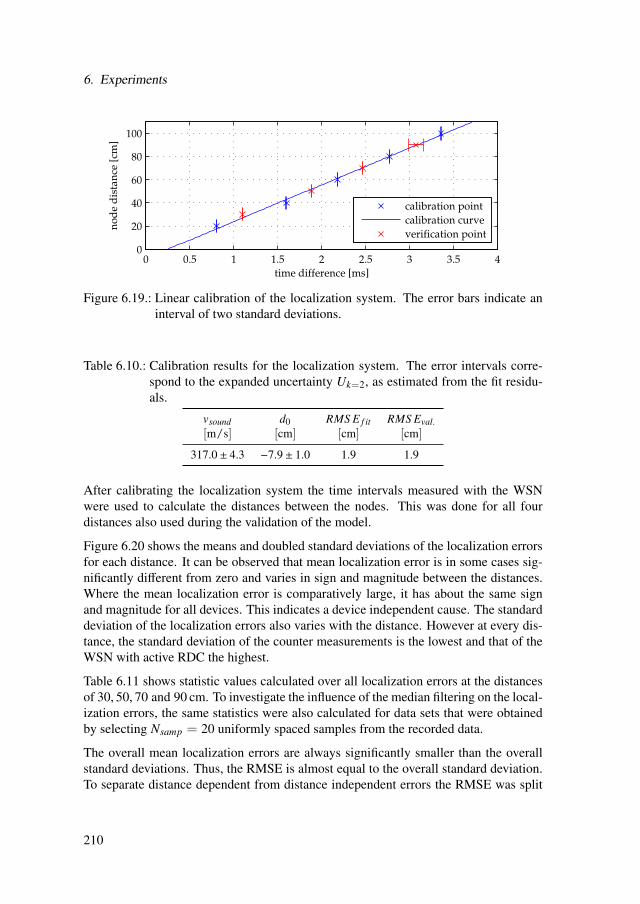
6. Experiments
0 0.5 1 1.5 2 2.5 3 3.5 40
20
40
60
80
100
time difference [ms]
no
de
dis
tan
ce [
cm]
calibration point
calibration curve
verification point
Figure 6.19.: Linear calibration of the localization system. The error bars indicate aninterval of two standard deviations.
Table 6.10.: Calibration results for the localization system. The error intervals corre-spond to the expanded uncertainty Uk=2, as estimated from the fit residu-als.
vsound d0 RMS E f it RMS Eval.[m/s] [cm] [cm] [cm]
317.0 ± 4.3 −7.9 ± 1.0 1.9 1.9
After calibrating the localization system the time intervals measured with the WSNwere used to calculate the distances between the nodes. This was done for all fourdistances also used during the validation of the model.
Figure 6.20 shows the means and doubled standard deviations of the localization errorsfor each distance. It can be observed that mean localization error is in some cases sig-nificantly different from zero and varies in sign and magnitude between the distances.Where the mean localization error is comparatively large, it has about the same signand magnitude for all devices. This indicates a device independent cause. The standarddeviation of the localization errors also varies with the distance. However at every dis-tance, the standard deviation of the counter measurements is the lowest and that of theWSN with active RDC the highest.
Table 6.11 shows statistic values calculated over all localization errors at the distancesof 30, 50, 70 and 90 cm. To investigate the influence of the median filtering on the local-ization errors, the same statistics were also calculated for data sets that were obtainedby selecting Nsamp = 20 uniformly spaced samples from the recorded data.
The overall mean localization errors are always significantly smaller than the overallstandard deviations. Thus, the RMSE is almost equal to the overall standard deviation.To separate distance dependent from distance independent errors the RMSE was split
210
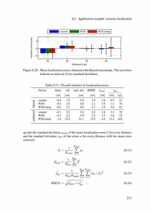
6.3. Application example: acoustic localization
30 50 70 90
−5
0
5
distance [cm]
loca
tio
n e
rro
r [c
m]
counter WSN WSN,sleep
Figure 6.20.: Mean localization errors obtained with filtered timestamps. The error barsindicate an interval of two standard deviations.
Table 6.11.: Overall statistics of localization errors.
Device mean std. max. abs RMSE smean sdev.
[cm] [cm] [cm] [cm] [cm] [cm] [µs]
filte
red counter -0.4 1.9 5.4 1.9 1.8 0.7 21
WSN -0.4 2.0 4.6 2.1 1.8 1.1 34WSN,sleep -0.2 2.7 8.5 2.7 1.8 2.0 63
unfil
tere
d counter -0.1 2.2 5.4 2.2 1.8 1.2 39WSN -0.3 2.2 5.0 2.2 1.5 1.6 52WSN,sleep 1.0 13.9 51.1 13.9 4.4 13.2 418
up into the standard deviation smean of the mean localization errors ϵ for every distanceand the standard deviation sdev of the errors ϵ for every distance with the mean errorremoved:
ϵi =1
Nsamp
Nsamp∑j=1
ϵi j (6.11)
s2mean =
1Ndist
Ndist∑i=1
ϵ2i (6.12)
s2dev =
1NdistNsamp
Ndist∑i=1
Nsamp∑j=1
(ϵi j − ϵi)2 (6.13)
RMS E =√
s2mean + s2
dev , (6.14)
211

6. Experiments
with Nsamp the number of samples per distance and Ndist the number of distances. It isstriking to see, that in the filtered case smean is independent of the measurement device.In contrast to this, sdev clearly increases from the frequency counter over the WSNto the WSN with active RDC. In the unfiltered case the localization errors increasedrastically for the WSN with active RDC, whereas in the other cases the increase isonly slight. This shows, that the median filtering not only removes outliers caused byacoustic effects, but also those caused by interrupt blocking code sections (see alsosection 6.2).
6.3.5. Uncertainty analysis
The standard deviations of the localization error in table 6.11 match well with the lo-calization precision of about 2 cm estimated in section 6.3.2. For further analysis ofthe individual uncertainty contributions the measurement model (6.5) is extended witha number of error quantities:
d = vsound (Tsound + δprop + δT ) + d0 + δmodel. (6.15)
Here d0 is the localization offset that is the result of all constant error influences. It iscompensated by the calibration processes. The error influences that are dependent onthe distance between the nodes are expressed as modeling error δmodel. Random errorinfluences that affect the propagation of the sound burst and its detection are summa-rized as δprop and δT is the error of the time interval measurement. Table 6.12 shows asummary of physical error influences that contribute to the individual quantities.
Table 6.13 shows the uncertainty budget for δT of the counter. According the counter’sspecifications, the time interval measurement is affected by three error influences: theresolution of the clock δres,counter, a system error δsys,counter and the accuracy of theinternal time base δbase,counter [51]. The latter depends on the length of the time in-terval. Here it was calculated for an interval of 3.4 ms which is slightly more than themaximum interval measured during the experiments. The combined measurement un-certainty of the counter uc,T ,counter is about three orders of magnitude smaller than theoverall standard deviation sdev for the counter in table 6.11. Therefore, sdev,counter canbe used as an estimate for the uncertainty uprop ≈ sdev,counter that is introduced by δprop.Similarly, the overall standard deviation of the mean errors smean for the counter in table6.11 is used as an estimate for the uncertainty umodel ≈ smean,counter that is introducedby δmodel.
212

6.3. Application example: acoustic localization
Table 6.12.: Influence quantities affecting the localization measurement.C
ateg
ory
Influ
ence
Eff
ect
Trea
tmen
t
cons
tant
dist
ance
rand
omde
pend
ent
posi
tion
yard
stic
kac
cura
cyx
negl
ecte
d(=
1.3
mm
)po
sitio
ning
erro
rx
negl
ecte
d(≤
1m
m)
rel.
posi
tion
ofm
icro
phon
ex
com
pens
ated
byca
libra
tion
(d0)
acou
stic
soun
dre
peat
abili
tyx
mod
eled
(δpr
op)
exte
rnal
nois
ex
mod
eled
(δpr
op)
airm
ovem
ent
xx
com
pens
ated
byca
libra
tion
(vso
und),
mod
eled
(δpr
op)
soun
dda
mpi
ngx
mod
eled
(δm
odel
)m
ultip
ath
prop
agat
ion
xm
odel
ed(δ
mod
el)
elec
tric
ampl
ifier
nois
ex
mod
eled
(δpr
op)
ampl
ifier
gain
xco
mpe
nsat
edby
calib
ratio
n(d
0)m
icro
phon
ese
nsiti
vity
xco
mpe
nsat
edby
calib
ratio
n(d
0)gr
oup
dela
yx
com
pens
ated
byca
libra
tion
(d0)
trig
gert
hres
hold
xco
mpe
nsat
edby
calib
ratio
n(d
0)tr
igge
rjitt
erx
mod
eled
(δpr
op)
time
inte
rrup
tlat
ency
xm
odel
ed(δ
T)
mea
sure
-cl
ock
reso
lutio
nx
mod
eled
(δT
)m
ent
cloc
ksy
nchr
oniz
atio
nx
mod
eled
(δT
)
213

6. Experiments
Table 6.13.: Uncertainty budget for time interval measurement with frequency counter.
influ
ence
estim
ate
assu
med
unce
rtai
nty
dist
ribu
tion
wei
ght
stan
dard
unce
rtai
nty
sens
itivi
tyco
effici
ent
degr
ees
offr
eedo
m
unce
rtai
nty
cont
ribu
tion
δ S E√
G u c v u
δres,counter 10.0 ns R 1/√
3 5.8 ns 1 ∞ 5.8 nsδsys,counter 4.0 ns R 1/
√3 2.3 ns 1 ∞ 2.3 ns
δbase,counter 1.7 ns R 1/√
3 1.0 ns 1 ∞ 1.0 ns
uc,T ,counter 6.3 ns 1 ∞ 6.3 ns
The estimates for uprop and umodel obtained from the frequency counter measurementswere used to build uncertainty budgets for the localization measurements with all threedevices. The standard deviations given in table 6.7 for the nodes 31 (T1) and 41 (T2) inconfigurations 3 and 7 are used as estimates for the uncertainty uT of the time intervalmeasurement with the WSN. Tables 6.14 to 6.16 show the corresponding uncertaintybudgets. The RMSE of the measured localization errors are given for comparison.
The estimated uncertainty of the distance measurement matches quite well with themeasured RMSE from the filtered samples in case of the frequency counter and theWSN without RDC. In case of the WSN with RDC estimated the uncertainty matchesroughly the RMSE from the unfiltered samples. This shows again, that the median fil-tering is also effective in removing outliers caused by synchronization or timestampingerrors.
It is apparent that the influence of time interval measurement uncertainty on the overalllocalization uncertainty quickly decreases as it gets smaller. Consequently, the local-ization uncertainty for the frequency counter is only about 20 % smaller than that forthe WSN, although the counter’s time interval measurement uncertainty is about threeorders of magnitude better. Considering an idealized WSN, where only the clock reso-lution of Ttick = 2−14 s contributes to the time interval measurement uncertainty, yieldsa localization uncertainty of 2.1 cm. Thus, only 0.1 cm or 4.5 % of the localizationuncertainty can be attributed to synchronization or timestamping errors.
214

6.3. Application example: acoustic localization
Table 6.14.: Uncertainty budget for localization with frequency counter.
influ
ence
stan
dard
unce
rtai
nty
sens
itivi
tyco
effici
ent
degr
ees
offr
eedo
m
unce
rtai
nty
cont
ribu
tion
δ u c v u
uc,T ,counter 6.3 ns 317.0 m/s ∞ 2.0 µmuprop 0.7 cm 1 76 0.7 cmumodel 1.8 cm 1 76 1.8 cm
ud 76 1.9 cm
RMSE (filtered) 80 1.9 cmRMSE (unfiltered) 80 2.2 cm
Table 6.15.: Uncertainty budget for localization with WSN.
influ
ence
stan
dard
unce
rtai
nty
sens
itivi
tyco
effici
ent
degr
ees
offr
eedo
m
unce
rtai
nty
cont
ribu
tion
δ u c v u
uT ,WS N 36.6 µs 317.0 m/s 999 1.2 cmuprop 0.7 cm 1 76 0.7 cmumodel 1.8 cm 1 76 1.8 cm
ud 76 2.3 cm
RMSE (filtered) 80 2.1 cmRMSE (unfiltered) 80 2.2 cm
215
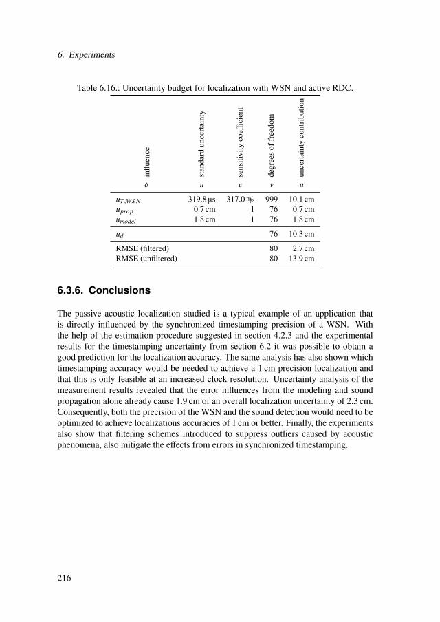
6. Experiments
Table 6.16.: Uncertainty budget for localization with WSN and active RDC.
influ
ence
stan
dard
unce
rtai
nty
sens
itivi
tyco
effici
ent
degr
ees
offr
eedo
m
unce
rtai
nty
cont
ribu
tion
δ u c v u
uT ,WS N 319.8 µs 317.0 m/s 999 10.1 cmuprop 0.7 cm 1 76 0.7 cmumodel 1.8 cm 1 76 1.8 cm
ud 76 10.3 cm
RMSE (filtered) 80 2.7 cmRMSE (unfiltered) 80 13.9 cm
6.3.6. Conclusions
The passive acoustic localization studied is a typical example of an application thatis directly influenced by the synchronized timestamping precision of a WSN. Withthe help of the estimation procedure suggested in section 4.2.3 and the experimentalresults for the timestamping uncertainty from section 6.2 it was possible to obtain agood prediction for the localization accuracy. The same analysis has also shown whichtimestamping accuracy would be needed to achieve a 1 cm precision localization andthat this is only feasible at an increased clock resolution. Uncertainty analysis of themeasurement results revealed that the error influences from the modeling and soundpropagation alone already cause 1.9 cm of an overall localization uncertainty of 2.3 cm.Consequently, both the precision of the WSN and the sound detection would need to beoptimized to achieve localizations accuracies of 1 cm or better. Finally, the experimentsalso show that filtering schemes introduced to suppress outliers caused by acousticphenomena, also mitigate the effects from errors in synchronized timestamping.
216
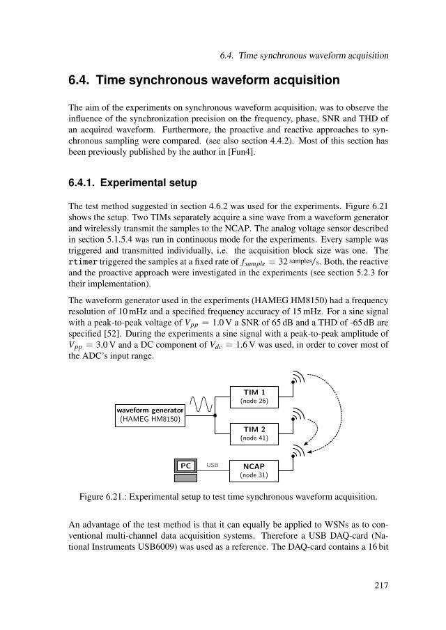
6.4. Time synchronous waveform acquisition
6.4. Time synchronous waveform acquisition
The aim of the experiments on synchronous waveform acquisition, was to observe theinfluence of the synchronization precision on the frequency, phase, SNR and THD ofan acquired waveform. Furthermore, the proactive and reactive approaches to syn-chronous sampling were compared. (see also section 4.4.2). Most of this section hasbeen previously published by the author in [Fun4].
6.4.1. Experimental setup
The test method suggested in section 4.6.2 was used for the experiments. Figure 6.21shows the setup. Two TIMs separately acquire a sine wave from a waveform generatorand wirelessly transmit the samples to the NCAP. The analog voltage sensor describedin section 5.1.5.4 was run in continuous mode for the experiments. Every sample wastriggered and transmitted individually, i.e. the acquisition block size was one. Thertimer triggered the samples at a fixed rate of fsample = 32 samples/s. Both, the reactiveand the proactive approach were investigated in the experiments (see section 5.2.3 fortheir implementation).
The waveform generator used in the experiments (HAMEG HM8150) had a frequencyresolution of 10 mHz and a specified frequency accuracy of 15 mHz. For a sine signalwith a peak-to-peak voltage of Vpp = 1.0 V a SNR of 65 dB and a THD of -65 dB arespecified [52]. During the experiments a sine signal with a peak-to-peak amplitude ofVpp = 3.0 V and a DC component of Vdc = 1.6 V was used, in order to cover most ofthe ADC’s input range.
Figure 6.21.: Experimental setup to test time synchronous waveform acquisition.
An advantage of the test method is that it can equally be applied to WSNs as to con-ventional multi-channel data acquisition systems. Therefore a USB DAQ-card (Na-tional Instruments USB6009) was used as a reference. The DAQ-card contains a 16 bit
217

6. Experiments
successive-approximation ADC with four multiplexed inputs, two of which were usedto sample the sine wave from the generator simultaneously. As only input voltageranges symmetrical to 0 V are supported by the DAQ-card, an input range of ±2 V waschosen for the experiments. The peak-to-peak amplitude of the waveform generatorwas set to Vpp = 3.8 V and its DC-component to Vdc = 0 V. Otherwise the sameparameter settings as for the WSN were used.
Table 6.17 gives an overview of the configurations that were investigated. Radio duty-cycling was deactivated in all experiments. Two sine frequencies were used: one lowand one high relative to the WSN’s sampling rate. They were chosen following therecommendations outlined in section 4.6.2.
Table 6.17.: Configurations for waveform acquisition tests.
Conf. Device MAC Sync. protocol Sampling approach fsignalfsignalfsample
[Hz] [1]
1 Preon32 TDMA TDMA-timesynch proactive, hybrid 0.27 0.0082 Preon32 TDMA TDMA-timesynch proactive, hybrid 7.11 0.2223 Preon32 CSMA RITS reactive, none 0.27 0.0084 Preon32 CSMA RITS reactive, none 7.11 0.222
5 USB6009 - - - 0.27 0.0086 USB6009 - - - 7.11 0.222
For each configuration 100 waveforms of 2048 synchronously acquired samples wererecorded from each node. By taking the samples recorded with the reactive approachbefore the resampling and discarding the timestamps a set of unsynchronized wave-forms was obtained. A set of waveforms for the hybrid approach was generated byusing the timestamps recorded within the proactive approach to do a resampling of thedata. During configurations 1 and 2 the histogram of clock updates was recorded inaddition to the sampled data.
6.4.2. Signal quality
The frequency error ϵ f , the offset error ϵt0 as well as the SNR and THD of the wave-forms were calculated as described in section 4.6.2. Table 6.18 shows the means andstandard deviations of the results calculated over all N = 100 waveforms for everyconfiguration. Figure 6.22 shows the means of the estimated pairwise time offsets.The error bars indicate and interval of two standard deviations. As all approaches tosynchronized sampling show significantly lower offsets than the unsynchronized case,figure 6.23 shows the same data with a zoomed y-Axis.
218

6.4. Time synchronous waveform acquisition
Table 6.18.: Frequency errors ϵ f and time offset errors ϵt0 calculated from the acquiredwaveforms.
Synch. fsignal ϵt0 ϵ f
Approach TIM 1 TIM 2
mean std. mean std. mean std.[Hz] [µs] [µs] [mHz] [mHz] [mHz] [mHz]
none 0.27 2575.1 4589.4 −3.9 2.8 −3.9 2.8reactive 0.27 −8.1 81.3 −3.9 2.8 −3.9 2.8proactive 0.27 −7.7 70.5 4.44390 0.00042 4.44388 0.00037hybrid 0.27 −9.6 68.9 4.44390 0.00043 4.44388 0.00037DAQ-card 0.27 14.1 8.8 −4.86757 0.00008 −4.86758 0.00007
none 7.11 2081.6 3121.7 −3.82316 0.0030 −3.3526 0.0068reactive 7.11 495.8 157.6 −3.78406 0.0030 −3.678 0.013proactive 7.11 2.2 2.6 −1.0 4.3 −1.0 4.3hybrid 7.11 1.1 2.4 −1.0 4.3 −1.0 4.3DAQ-card 7.11 17.7 0.3 −3.73427 0.00076 −3.73427 0.00076
−5
0
5
10
ǫt0[m
s]
none
reac
tive
proac
tive
hybrid
DA
Q−ca
rd
(a) fsignal = 0.27 Hz
−5
0
5
10
ǫt0[m
s]
none
reac
tive
proac
tive
hybrid
DA
Q−ca
rd
(b) fsignal = 7.11 Hz
Figure 6.22.: Mean pairwise time shifts Tshi f t. The error bars indicate an interval oftwice the standard deviation.
219

6. Experiments
−0.2
−0.1
0
0.1
0.2
ǫt0[m
s]
none
reac
tive
proac
tive
hybrid
DA
Q−ca
rd
(a) fsignal = 0.27 Hz
−0.2
−0.1
0
0.1
0.2
ǫt0[m
s]
none
reac
tive
proac
tive
hybrid
DA
Q−ca
rd
(b) fsignal = 7.11 Hz
Figure 6.23.: Mean pairwise time shifts Tshi f t with zoomed y-axis. The error bars indi-cate an interval of twice the standard deviation.
The offset in the unsynchronized case is surprisingly small (ca. 2.5 ms). This is becausethe acquisition was started with the same broadcast message on both TIMs. This way,the nodes were implicitly synchronized to some degree. The remaining time offsetwas only due to timing differences in the process scheduling of the individual nodes.In nearly all cases, the standard deviation is smaller at the higher signal frequencycompared to the lower. This is due to the time offset estimate being less sensitive tovariance in the phase estimate at higher signal frequencies (compare (4.57)).
For all approaches to synchronized sampling the time offsets are minimal at the lowersignal frequency ( fsignal = 0.27 Hz). They vary only in a range of roughly two ticks ofthe rtimer TTick ≈ 61.0 µs. For the higher signal frequency ( fsignal = 7.11 Hz), thetime offset from the reactive approach shows a big increase. This is due to the linearinterpolation used in the reactive approach being less accurate at signal frequenciesclose to the WSN’s Nyquist frequency ( fsample/2 = 16 Hz) (compare section 3.3.2).The time offset of the DAQ-card is caused by its analog input multiplexer (see section3.2.3). The mean offset is larger than in most cases of synchronized sampling with theWSN, but the standard deviation is significantly smaller.
The estimates for the frequency error ϵ f , shown in table 6.18, are much smaller thanthe specified frequency accuracy of the generator (15 mHz [52]). Thus, no drift errorcould be detected for either of the acquisition methods or the DAQ-card.
To get a further insight into the performance of the sensor nodes’ clocks their averagesampling rate was calculated from the acquired sample timestamps (see 6.17). The factthat the sampling rate is always exactly 32 samples/s for the resampled data (reactive and
220

6.4. Time synchronous waveform acquisition
hybrid approach) just shows that the resampling algorithm wrote the correct samplinginterval into the waveforms it generated. In the unsynchronized measurements it canbe observed that the sampling frequency of TIM2 (node 42) was off by -1.89 mHz (-59.1 ppm), while it was only 0.25 mHz (7.8 ppm) for TIM1 (node 26). These resultscorrelate well with the drifts of nodes 31 and 41 relative to node 27 given in table 6.5.Thus, the observed difference in sampling rates is probably due to drift errors of thenodes’ real-time clocks. The resulting frequency error in the recorded signal wouldbe 0.05555 mHz for TIM1 and -0.41993 mHz for TIM2 at the higher signal frequency(7.11 Hz). This matches with the observed difference in frequency errors for two TIMsin the unsynchronized case (see table 6.18). In the proactively synchronized measure-ments the error in sampling rate is significantly smaller, showing the effectiveness ofthe synchronization.
Table 6.19.: Average sampling rates calculated from sample timestamps.
Synch. fsignal fsApproach TIM 1 TIM 2
mean std. mean std.[Hz] [samples/s] [samples/s] [samples/s] [samples/s]
none 0.27 32.00025 0.00014 31.99811 0.00003reactive 0.27 32.00000 0.00000 32.00000 0.00000proactive 0.27 31.99999 0.00003 32.00002 0.00004hybrid 0.27 32.00000 0.00000 32.00000 0.00000
none 7.11 32.00024 0.00002 31.99811 0.00003reactive 7.11 32.00000 0.00000 32.00000 0.00000proactive 7.11 32.00000 0.00003 32.00003 0.00003hybrid 7.11 32.00000 0.00000 32.00000 0.00000
The results of the SNR estimation are given in figure 6.24. In the unsynchronized casethe data acquisition is not influenced by any synchronization algorithm. Thus, the SNRfor this case indicates the general performance of the ADC and is used as a reference.It is, however, about 10 dB lower than the specified SNR of the waveform generatorand about 17 dB lower than the ideal SNR of a 12 bit ADC. This may be due to noisefrom the sensor nodes’ other components affecting the signal quality. Furthermore, itis observed that TIM1 generally shows a slightly lower SNR than TIM2. The SNR ofthe signals acquired with the DAQ-card matches well with the specified SNR of thewaveform generator (65 dB). At the lower signal frequency all approaches show a SNRclose to that of the unsynchronized data. At the higher signal frequency the SNR of thereactive approach is much lower than for the other approaches. This again, is causedby a decrease in interpolation accuracy close to the Nyquist frequency.
221

6. Experiments
30
40
50
60
70
SN
R [
dB
]
none
reac
tive
proac
tive
hybrid
DA
Q−ca
rd
TIM1/Ch1
TIM2/Ch2
(a) fsignal = 0.27 Hz
30
40
50
60
70
SN
R [
dB
]
none
reac
tive
proac
tive
hybrid
DA
Q−ca
rd
(b) fsignal = 7.11 Hz
Figure 6.24.: Signal SNR.
To investigate why the SNR of TIM2 is about 15 dB lower than that of TIM1 for thereactive approach at the higher signal frequency, two acquired waveforms, one fromTIM1 and one from TIM2, were also resampled for output sampling rates other thanthe desired 32 samples/s. If the original sampling rate of TIM1 is chosen as the outputsampling rate for the resampling, the SNR is about equal to that in the unsynchronizedcase (51.3 dB) and much lower for TIM2 (30.1 dB). If the original sampling rate ofTIM2 is chosen for the resampling, it is the other way around (TIM1: 30.1 dB; TIM2:54.5 dB). If the average of the original sampling rates is taken the SNR is 35.8 dB forboth nodes. At resampled rates of 31.5 and 32.5 samples/s the SNR is 20.9 dB. Thus,the decrease in SNR seems to grow with increasing sampling rate change during theresampling. This again shows the poor performance of the used interpolation at signalfrequencies close to the Nyquist frequency.
Although the differences are not statistically significant, it is also worth noting, thatthe SNR of the data acquired with the proactive approach is constantly slightly lowerthan that of the unsynchronized data. At the higher signal frequency this differenceis a little bigger that at the lower. To check whether this could be related to an in-creased jitter from clock updates, the histograms of the clock updates shown in figure6.25 were evaluated. They show that in most synchronization intervals the clock didnot need to be updated because it was still synchronized (clock correction zero). In theother cases the corrections are mostly very small (1-2 Ticks). This behavior is consis-tent with the clock update histograms obtained for the same synchronization methodduring the event detection experiments (see appendix E.2). Inserting the standard devi-ation calculated from the histogram data into (4.38) the SNR was calculated assumingtime base jitter to be the only noise source. The results were 83.4 dB for the lower and55.0 dB for the higher signal frequency. Comparing this to the SNR in the unsynchro-
222
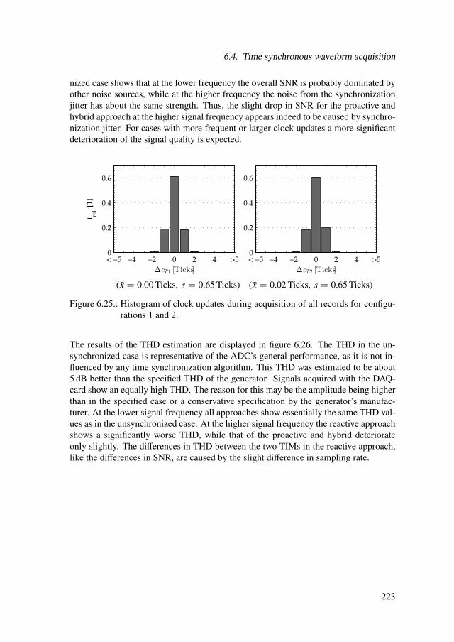
6.4. Time synchronous waveform acquisition
nized case shows that at the lower frequency the overall SNR is probably dominated byother noise sources, while at the higher frequency the noise from the synchronizationjitter has about the same strength. Thus, the slight drop in SNR for the proactive andhybrid approach at the higher signal frequency appears indeed to be caused by synchro-nization jitter. For cases with more frequent or larger clock updates a more significantdeterioration of the signal quality is expected.
< −5 −4 −2 0 2 4 >50
0.2
0.4
0.6
f rel. [
1]
∆cT1 [Ticks]
< −5 −4 −2 0 2 4 >50
0.2
0.4
0.6
∆cT2 [Ticks]
(x = 0.00 Ticks, s = 0.65 Ticks) (x = 0.02 Ticks, s = 0.65 Ticks)
Figure 6.25.: Histogram of clock updates during acquisition of all records for configu-rations 1 and 2.
The results of the THD estimation are displayed in figure 6.26. The THD in the un-synchronized case is representative of the ADC’s general performance, as it is not in-fluenced by any time synchronization algorithm. This THD was estimated to be about5 dB better than the specified THD of the generator. Signals acquired with the DAQ-card show an equally high THD. The reason for this may be the amplitude being higherthan in the specified case or a conservative specification by the generator’s manufac-turer. At the lower signal frequency all approaches show essentially the same THD val-ues as in the unsynchronized case. At the higher signal frequency the reactive approachshows a significantly worse THD, while that of the proactive and hybrid deteriorateonly slightly. The differences in THD between the two TIMs in the reactive approach,like the differences in SNR, are caused by the slight difference in sampling rate.
223
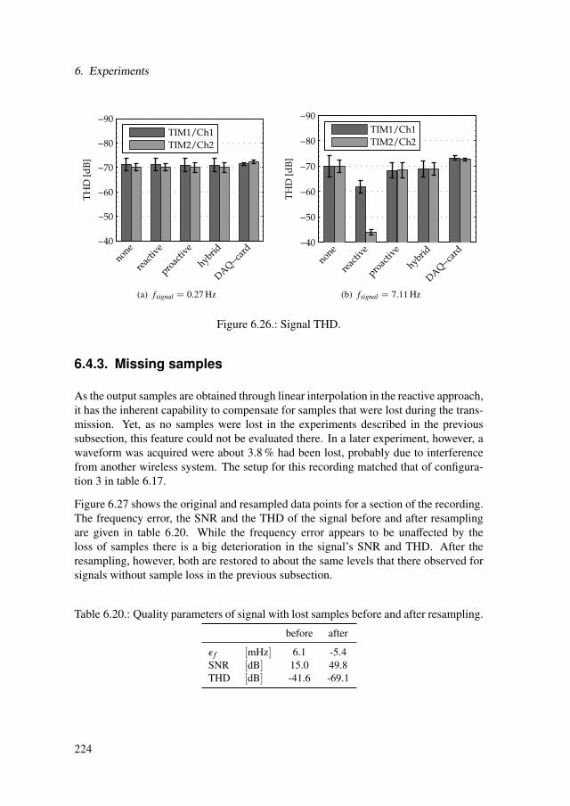
6. Experiments
−90
−80
−70
−60
−50
−40
TH
D [
dB
]
none
reac
tive
proac
tive
hybrid
DA
Q−ca
rd
TIM1/Ch1
TIM2/Ch2
(a) fsignal = 0.27 Hz
−90
−80
−70
−60
−50
−40
TH
D [
dB
]
none
reac
tive
proac
tive
hybrid
DA
Q−ca
rd
TIM1/Ch1
TIM2/Ch2
(b) fsignal = 7.11 Hz
Figure 6.26.: Signal THD.
6.4.3. Missing samples
As the output samples are obtained through linear interpolation in the reactive approach,it has the inherent capability to compensate for samples that were lost during the trans-mission. Yet, as no samples were lost in the experiments described in the previoussubsection, this feature could not be evaluated there. In a later experiment, however, awaveform was acquired were about 3.8 % had been lost, probably due to interferencefrom another wireless system. The setup for this recording matched that of configura-tion 3 in table 6.17.
Figure 6.27 shows the original and resampled data points for a section of the recording.The frequency error, the SNR and the THD of the signal before and after resamplingare given in table 6.20. While the frequency error appears to be unaffected by theloss of samples there is a big deterioration in the signal’s SNR and THD. After theresampling, however, both are restored to about the same levels that there observed forsignals without sample loss in the previous subsection.
Table 6.20.: Quality parameters of signal with lost samples before and after resampling.
before after
ϵ f [mHz] 6.1 -5.4SNR [dB] 15.0 49.8THD [dB] -41.6 -69.1
224

6.4. Time synchronous waveform acquisition
5.5 6 6.5 7 7.50
1
2
3
time [s]
amp
litu
de
[V]
original resampled
Figure 6.27.: Section of signal showing recorded and resampled data points. Intervalswith missing samples are highlighted.
6.4.4. Power consumption
In later experiments, powertrace data was collected during waveform acquisition withthe WSN. The network configurations 1 to 4 shown in table 6.17 were investigated.Figure 6.28 shows the results.
Like in sections 6.1.1 and 6.2.4 the average power consumption is dominated by the lis-tening consumption of the radio transceiver and the low power mode of the CPU. Alsosimilar to section 6.2.4, the configurations using the proactive approach show a slightlyincreased power consumption of the NCAP compared to those using the reactive one.The more critical power consumption of the TIMs, however, is practically the samefor both approaches. The increased NCAP power consumption is caused by the send-ing of synchronization packets as well as more CPU activity. If the resampling duringthe reactive approach was done on the NCAP instead of the PC, this would increasethe power consumption of the NCAP in the reactive case, diminishing the differenceto the proactive case or even reversing the relation. If the network was to spend moretime without any transmission of measurement data, the reactive approach is expectedto have larger advantages over the proactive one in terms of power consumption, as itdoesn’t require regular synchronization messages.
225

6. Experiments
0
10
20
30
40
50
60
70
80
avg
. po
wer
[m
W]
Node: N T1 T2 N T1 T2 N T1 T2 N T1 T2
1,2TDMA0.27 Hz
1,2TDMA7.11 Hz
3,4CSMA0.27 Hz
3,4CSMA7.11 Hz
Configuration
lpm
cpu
listen
tx
Figure 6.28.: Mean power consumption of nodes doing synchronous waveform sam-pling.
6.4.5. Conclusions
Both approaches to synchronized sampling show comparable synchronization accura-cies close to the resolution of the underlying clock. Also the SNR and THD of theacquired signals were found to be close to those acquired without synchronization es-pecially for signals whose frequency is low compared to the sampling rate. For thereactive approach a huge decrease in SNR and THD was observed at a higher signalfrequency. The reason for this is the characteristic of the linear interpolation that wasused (compare section 3.3.2). More advanced interpolation techniques like cubic-splineinterpolation or an approach based on nonuniform sampling are likely to offer a bettersignal quality at higher frequencies, but also require more computational effort. Forthe proactive approach a small decrease in SNR caused by clock updates, could bedetected.
In the investigated settings the energy consumption for both approaches is nearly thesame. However, at significantly larger transmission intervals the reactive approach isexpected to perform better, as it does not require regular synchronization messages.
226

6.5. Synchronous angular sampling
6.5. Synchronous angular sampling
To evaluate the synchronous angular sampling algorithm presented in section 5.3 andits implementation on the WSN, several simulations and experiments were done. Firstthe effects of different components in the measurement chain on signals sampled overthe angle are examined during simulations in section 6.5.1. Section 6.5.2 presents sim-ulations to detect possible differences between the different implementations of the al-gorithm. The performance of the algorithm running on a WSN is investigated by re-sampling signals from a waveform generator, in section 6.5.3. Finally, experimentsusing synchronous angular resampling with a WSN at a motor test bench are pre-sented in section 6.5.4. Most of this chapter has already been published by the authorin [Fun5, Fun7].
6.5.1. Analysis of measurement chain for angular sampling
To investigate the effect of the components in the measurement chain on signals sam-pled over the angle, simulations in MATLAB/SIMULINK were done. They startedwith an idealized sampling model as introduced in section 2.4.1. Then step by step,components were added to model non-ideal effects found in real measurement setups.The parameters of the measurement chain were chosen in accordance with those of theWSN (compare section 5).
6.5.1.1. Simulation setup
Figure 6.29 shows the setup used for the simulations. A rotating machine is simulated,that accelerates linearly from 15 to 1500 rpm within 2 s. The rotation angle ϕ is obtainedby integrating over the speed signal. A cosine function with ϕ as its argument representsa harmonic signal at the second order of rotation. The rotation angle ϕ is also used togenerate sampling pulses at equidistant angular intervals of Φs = 2π/25.
Table 6.21 shows the different configurations of the simulation setup that were used.The first simulated the ideal synchronous angular sampling model introduced in sec-tion 2.4.1. Then, in configuration 2, a zero-order hold was added, that sampled thecontinuous input signal at equidistant time instants tn = nTs = n/ fs before the an-gular resampling. To investigate the effect of the analog sampling frequency fs it wasdoubled in configuration 3. In order to account for the amplitude quantization by anADC, a 12 bit-quantizer was added in configuration 4. Finally, configurations 5 and 6investigated the effect of the group delay from an analog anti-aliasing filter. The filterused was a continuous 8th-order lowpass filter with a cutoff-frequency of 2 kHz.
227
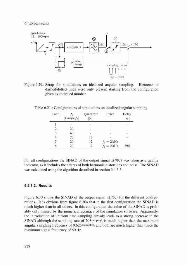
6. Experiments
Figure 6.29.: Setup for simulations on idealized angular sampling. Elements indashed/dotted lines were only present starting from the configurationgiven as encircled number.
Table 6.21.: Configurations of simulations on idealized angular sampling.
Conf. fs Quantizer Filter Delay[ksamples/s] [bit] [µs]
1 - - - -2 20 - - -3 40 - - -4 20 12 - -5 20 12 fg = 2 kHz -6 20 12 fg = 2 kHz 290
For all configurations the SINAD of the output signal x(lΦs) was taken as a qualityindicator, as it includes the effects of both harmonic distortions and noise. The SINADwas calculated using the algorithm described in section 3.4.3.3.
6.5.1.2. Results
Figure 6.30 shows the SINAD of the output signal x(lΦs) for the different configu-rations. It is obvious from figure 6.30a that in the first configuration the SINAD ismuch higher than in all others. In this configuration the value of the SINAD is prob-ably only limited by the numerical accuracy of the simulation software. Apparently,the introduction of uniform time sampling already leads to a strong decrease in theSINAD although the sampling rate of 20 ksamples/s is much higher than the maximumangular sampling frequency of 0.625 ksamples/s and both are much higher than twice themaximum signal frequency of 50 Hz.
228
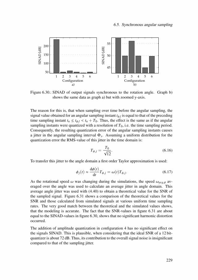
6.5. Synchronous angular sampling
1 2 3 4 5 6
50
100
150
200
Configuration a)
SIN
AD
[d
B]
1 2 3 4 5 6
45
50
55
Configuration b)
SIN
AD
[d
B]
Figure 6.30.: SINAD of output signals synchronous to the rotation angle. Graph b)shows the same data as graph a) but with zoomed y-axis.
The reason for this is, that when sampling over time before the angular sampling, thesignal value obtained for an angular sampling instant tϕ,l is equal to that of the precedingtime sampling instant tn ≤ tϕ,l < tn + T0. Thus, the effect is the same as if the angularsampling instants were quantized with a resolution of T0, i.e. the time sampling period.Consequently, the resulting quantization error of the angular sampling instants causesa jitter in the angular sampling interval Φs. Assuming a uniform distribution for thequantization error the RMS-value of this jitter in the time domain is:
Tϕ, j =T0√
12. (6.16)
To transfer this jitter to the angle domain a first order Taylor approximation is used:
ϕ j(t) ≈dϕ(t)
dtTϕ, j = ω(t)Tϕ, j. (6.17)
As the rotational speed ω was changing during the simulations, the speed ωavg,ϕ av-eraged over the angle was used to calculate an average jitter in angle domain. Thisaverage angle jitter was used with (4.40) to obtain a theoretical value for the SNR ofthe sampled signal. Figure 6.31 shows a comparison of the theoretical values for theSNR and those calculated from simulated signals at various uniform time samplingrates. The very good match between the theoretical and the simulated values shows,that the modeling is accurate. The fact that the SNR-values in figure 6.31 are aboutequal to the SINAD-values in figure 6.30, shows that no significant harmonic distortionoccurred.
The addition of amplitude quantization in configuration 4 has no significant effect onthe signals SINAD. This is plausible, when considering that the ideal SNR of a 12 bit-quantizer is about 72 dB. Thus, its contribution to the overall signal noise is insignificantcompared to that of the sampling jitter.
229
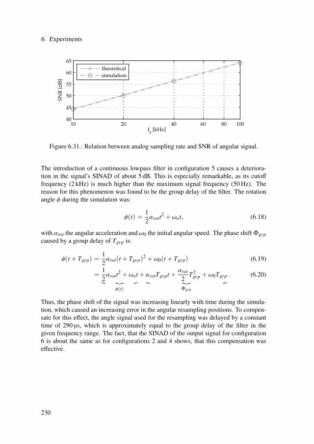
6. Experiments
10 20 40 60 80 10040
45
50
55
60
65
f0 [kHz]
SN
R [
dB
]
theoretical
simulation
Figure 6.31.: Relation between analog sampling rate and SNR of angular signal.
The introduction of a continuous lowpass filter in configuration 5 causes a deteriora-tion in the signal’s SINAD of about 5 dB. This is especially remarkable, as its cutofffrequency (2 kHz) is much higher than the maximum signal frequency (50 Hz). Thereason for this phenomenon was found to be the group delay of the filter. The rotationangle ϕ during the simulation was:
ϕ(t) =12αrott2 +ωot, (6.18)
with αrot the angular acceleration and ω0 the initial angular speed. The phase shift Φgrpcaused by a group delay of Tgrp is:
ϕ(t + Tgrp) =12αrot(t + Tgrp)
2 +ω0(t + Tgrp) (6.19)
=12αrott2 + ωot ϕ(t)
+ αrotTgrpt +αrot
2T 2
grp +ω0Tgrp Φgrp
. (6.20)
Thus, the phase shift of the signal was increasing linearly with time during the simula-tion, which caused an increasing error in the angular resampling positions. To compen-sate for this effect, the angle signal used for the resampling was delayed by a constanttime of 290 µs, which is approximately equal to the group delay of the filter in thegiven frequency range. The fact, that the SINAD of the output signal for configuration6 is about the same as for configurations 2 and 4 shows, that this compensation waseffective.
230
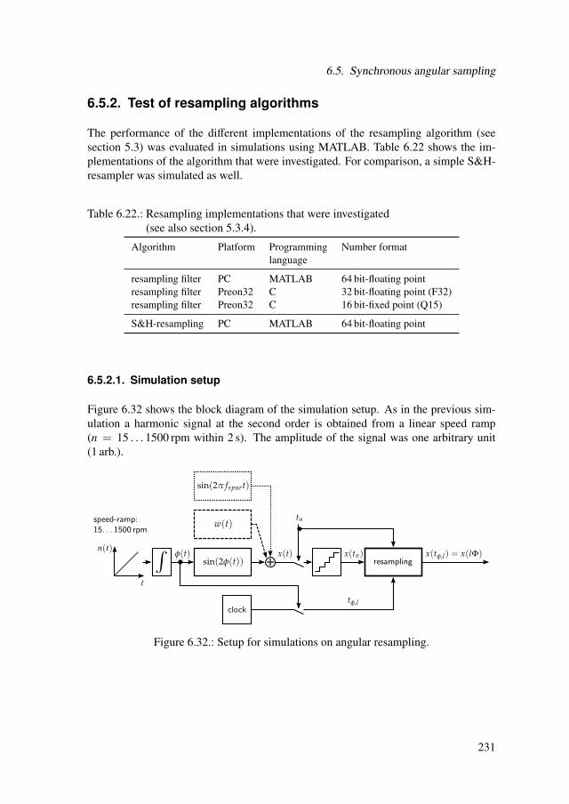
6.5. Synchronous angular sampling
6.5.2. Test of resampling algorithms
The performance of the different implementations of the resampling algorithm (seesection 5.3) was evaluated in simulations using MATLAB. Table 6.22 shows the im-plementations of the algorithm that were investigated. For comparison, a simple S&H-resampler was simulated as well.
Table 6.22.: Resampling implementations that were investigated(see also section 5.3.4).
Algorithm Platform Programming Number formatlanguage
resampling filter PC MATLAB 64 bit-floating pointresampling filter Preon32 C 32 bit-floating point (F32)resampling filter Preon32 C 16 bit-fixed point (Q15)
S&H-resampling PC MATLAB 64 bit-floating point
6.5.2.1. Simulation setup
Figure 6.32 shows the block diagram of the simulation setup. As in the previous sim-ulation a harmonic signal at the second order is obtained from a linear speed ramp(n = 15 . . . 1500 rpm within 2 s). The amplitude of the signal was one arbitrary unit(1 arb.).
Figure 6.32.: Setup for simulations on angular resampling.
231
6. Experiments
The signal was sampled at time instants tn distributed uniformly over time at a samplingrate of 20 ksamples/s. To simulate the influence of the ADC the signal was quantizedwith a resolution of 12 bit. The rotation angle ϕ(t) was also used to sample the sys-tem clock at 25 equidistant angular intervals per revolution, generating the timestampstϕ,l = t(lΦs). The timestamps tϕ,l were quantized with the resolution of the Preon32’srtimer: Trtc = 2−14 s. To check the rejection of noise, zero-mean white Gaussiannoise with a standard deviation of σ = 10−2 arb. was added in a second simulation.In a third simulation, the rejection of spurious frequencies was checked by adding aconstant frequency sine at fspur = 1.25 kHz with an amplitude of 1 arb. instead of thenoise.
The simulated samples x(tn) and timestamps t(lΦs) were fed into the resampling filterdescribed in section 5.3, in order to obtain the signal x(lΦs) sampled uniformly overthe rotation angle. The S&H resampling can be described to as zeroth-order polyno-mial resampling (see also 3.3.2). Higher polynomial orders would not have improvedperformance here, because the resolution of the timestamps ∆t ≈ 61 µs was alreadybigger than the sampling period Tin = 50 µs.
A sine fit, using the four-parameter algorithm described in 3.4.3, was performed on theresampled signals and their RMS-value, frequency and SINAD were calculated.
The same simulated signals were resampled using the MATLAB implementation of thefilter on a PC, as well as the two C implementations on a sensor node. For the latter thesimulated input data was sent to and the resampled signal received from a sensor nodevia its USB-interface. The evaluation of the output signals was done in MATLAB on aPC in all cases.
To measure the computational load of the algorithm on the sensor node, a sine wavesignal with a constant frequency of 50 Hz and an input sampling rate of 20 ksamples/s
was resampled for a speed of 1500 rpm and an angular rate of 25 samples/rev. The timeneeded to resample 8192 input samples (i.e. 256 output samples) was measured usingthe internal clock of the sensor node.
6.5.2.2. Signal quality
The deviations of the output signals’ RMS-values from the nominal RMS-value of√1/2 arb. are shown in figure 6.33. No error bars are given because only one input
sequence was used in each case. It was exactly the same for all three implementations.No systematic difference in terms of RMS-deviation is observed between the imple-mentations. The key observation is that the deviations are very small (absolute value≤ 2 · 10−4) in all cases.
232

6.5. Synchronous angular sampling
−200
−100
0
100RMS-Error
[ppm]
only chirp with noise with spurious
Q15
F32
MATLAB
Figure 6.33.: RMS-error of resampled chirp signals.
Figure 6.34 shows the deviations from the nominal order of 2. It is observed that theorder error for the fixed-point implementation (Q15) is always slightly larger than forthe floating-point (F32) or MATLAB-implementation. Yet, the key observation is thatthe deviations are very small (absolute value < 10−6) in all cases.
−1.0
−0.9
−0.8
−0.7
−0.6
−0.5
Order-Error
[ppm]
only chirp with noise with spurious
Q15
F32
MATLAB
Figure 6.34.: Order-error of resampled chirp signals.
The results for the SINAD of the resampled signals are shown in figure 6.35. Allimplementations perform about equally well, with only a slight disadvantage for thefixed-point-implementation. The S&H-resampling always results in a lower SINAD.This is especially prominent in the simulation with a spurious component, where itdrops to 0.5 dB.
233

6. Experiments
0
10
20
30
40
50
SIN
AD
[dB]
only chirp with noise with spurious
Q15
F32
MATLAB
S&H
Figure 6.35.: SINAD of resampled chirp signals.
To further illustrate the effect of the spurious component the input and output signalsfor this simulation as well as the corresponding spectrograms are given in figure 6.36.The input signal with the spurious component is given in figure 6.36 a), its spectrogramin figure 6.36 b). As the frequency of the spurious component is much higher thanthe maximum output sampling frequency, it cannot be resampled correctly under theNyquist theorem:
fout,max = 25 ·1500 rpm
60= 625 Hz < 2 fspur. (6.21)
Without the resampling filter, this leads to a heavily noised signal; as the spuriouscomponent is aliased into the frequency band many times (see figure 6.36 c) and d)).The resampling filter, by contrast, completely eliminates the spurious component, andoutputs a clean constant sine wave at the order two (see figure 6.36 e) and f)). Thus, itis effective in suppressing aliasing during resampling.
6.5.2.3. Computational load
The time needed to resample a constant frequency sine wave with 8192 input and 256output samples on the Preon32 was measured to be 655.5 ms for the floating-point and68.2 ms for the fixed-point implementation. In order to be suitable for real-time oper-ation in the designated measurement system, the filtering algorithm needs to process2048 input samples within 102.4 ms and still leave enough time for radio communi-cation and buffer handling (see also section 5.3.5). Thus, it is not possible to use thefloating-point implementation (expected time 163.9 ms). The fixed-point implementa-tion, however, is well suited (expected time 17.1 ms). Its causes a computational loadof only about 16.7 %.
234

6.5. Synchronous angular sampling
time/angular signal time-frequency/order distributionin
putx(t)
a)
0 0.5 1 1.5 2−2
−1
0
1
2
time [s]
amp
litu
de
[arb
.]
b)
0.5 1 1.50
0.5
1
1.5
time [s]
f [k
Hz]
S&H
resa
mpl
ing
x(lΦ
s)
c)
0 5 10−2
−1
0
1
2
angle [rad/2π]
amp
litu
de
[arb
.]
d)
2 4 6 8 10 12 140
5
10
angle [rad/2π]
ord
er [
1]
resa
mpl
ing
filte
rx(
lΦs)
e)
0 5 10−2
−1
0
1
2
angle [rad/2π]
amp
litu
de
[arb
.]
f)
2 4 6 8 10 12 140
5
10
angle [rad/2π]
ord
er [
1]
Figure 6.36.: Results of angular resampling a signal with spurious component.
235
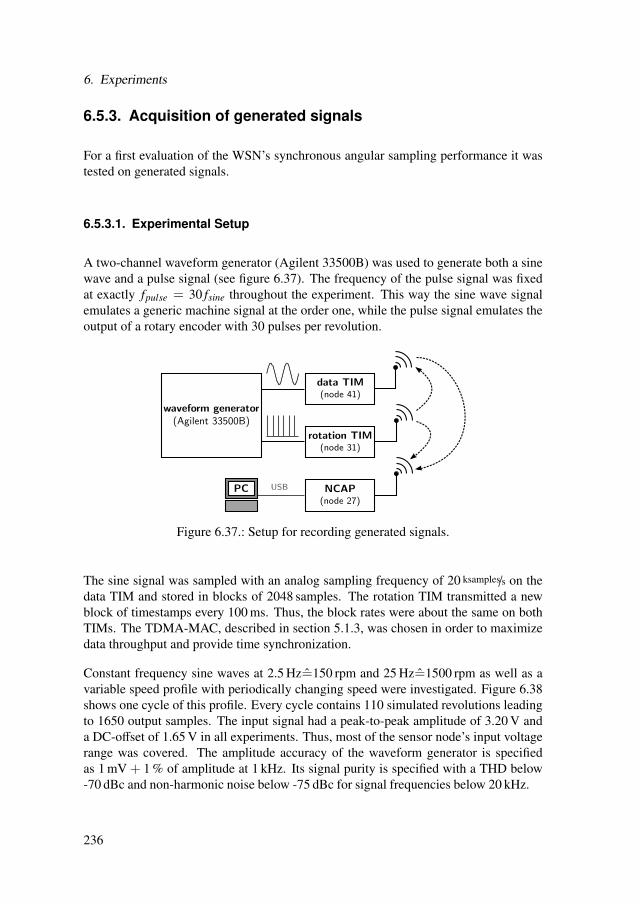
6. Experiments
6.5.3. Acquisition of generated signals
For a first evaluation of the WSN’s synchronous angular sampling performance it wastested on generated signals.
6.5.3.1. Experimental Setup
A two-channel waveform generator (Agilent 33500B) was used to generate both a sinewave and a pulse signal (see figure 6.37). The frequency of the pulse signal was fixedat exactly fpulse = 30 fsine throughout the experiment. This way the sine wave signalemulates a generic machine signal at the order one, while the pulse signal emulates theoutput of a rotary encoder with 30 pulses per revolution.
Figure 6.37.: Setup for recording generated signals.
The sine signal was sampled with an analog sampling frequency of 20 ksamples/s on thedata TIM and stored in blocks of 2048 samples. The rotation TIM transmitted a newblock of timestamps every 100 ms. Thus, the block rates were about the same on bothTIMs. The TDMA-MAC, described in section 5.1.3, was chosen in order to maximizedata throughput and provide time synchronization.
Constant frequency sine waves at 2.5 Hz=150 rpm and 25 Hz=1500 rpm as well as avariable speed profile with periodically changing speed were investigated. Figure 6.38shows one cycle of this profile. Every cycle contains 110 simulated revolutions leadingto 1650 output samples. The input signal had a peak-to-peak amplitude of 3.20 V anda DC-offset of 1.65 V in all experiments. Thus, most of the sensor node’s input voltagerange was covered. The amplitude accuracy of the waveform generator is specifiedas 1 mV + 1 % of amplitude at 1 kHz. Its signal purity is specified with a THD below-70 dBc and non-harmonic noise below -75 dBc for signal frequencies below 20 kHz.
236

6.5. Synchronous angular sampling
Resampling using the resampling filter, S&H resampling and direct sampling were usedto acquire the signals. In direct sampling the synchronous angular sampling is achievedfor constant speeds by setting the sampling rate of the analog-to-digital converter to therequired output rate. For variable speeds this method is, of course, not applicable. Atotal of 100 recordings with 2048 output samples were acquired for every combinationof input signal and sampling method. Like in the experiments in section 6.5.2 the RMS-value, order and SINAD of the resampled signals were calculated using sine fitting.
0 1 2 3 4 5 6 7 80
150
1500
time [s]
spee
d [
rpm
]
Figure 6.38.: One period of the variable speed profile used in waveform generator ex-periments.
The same setup was also used to measure the average power consumption of the senornodes during acquisition using Contiki’s powertrace mechanism. For this purposeone recording was evaluated at each constant speed: 150 rpm and 1500 rpm.
6.5.3.2. Signal quality
Figure 6.39 shows the mean RMS-values over all 100 recordings. The error bars indi-cate an interval of two standard deviations. It is observed that the measured RMS-valuesare about equal for all sampling methods. All values are well within the specified accu-racy of the generators amplitude setting.
237

6. Experiments
1.120
1.130
1.140
amplitude[V
RMS]
150 rpm 1500 rpm variable
filter
S&H
direct
Figure 6.39.: RMS-values of acquired generator signals. The solid horizontal line indi-cates the nominal value set at the waveform generator. The dashed hori-zontal lines indicate the specified accuracy of this setting
Figure 6.40 shows the mean order of the recorded signals. It is observed that the orderof the resampled signals matches very well with the nominal setting for all speeds,regardless of whether the resampling filter or S&H-resampling was used. The orderof signals recorded with direct sampling deviates by about 0.4 %. This is probablydue to the limited resolution and accuracy of the sampling frequency setting of thesensor node. However, these results also show that resampling is very effective incompensating for those effects.
0.995
0.996
0.997
0.998
0.999
1.000
order
[1]
150 rpm 1500 rpm variable
filter
S&H
direct
Figure 6.40.: Order of acquired generator signals. The nominal order is indicated bythe horizontal line.
238

6.5. Synchronous angular sampling
Figure 6.41 shows the mean SINAD of the recorded signals. The SINAD of the re-sampled signals is significantly higher at 150 rpm than at 1500 rpm, whereas it staysconstant for directly sampled signals. This is probably due to the output sampling timeintervals being larger at lower speeds, while the resolution of the angular timestampsstays constant. As a consequence the relative time base jitter is smaller at lower speeds.Furthermore, the resampling filter removes the noise energy of signal components withf > 0.25 fout. Thus, it causes a strong increase in SINAD at lower speeds. In caseof the S&H resampling and direct sampling the noise energy of the higher frequencycomponents is instead aliased to the lower bands. The SINAD from the variable speedrecordings is in between that of the 150 rpm and 1500 rpm recordings for the suggestedfilter. For the S&H resampling it is even lower than that of the 150 rpm recordings.
35
40
45
50
55
60
65
SIN
AD
[dB]
150 rpm 1500 rpm variable
filter
S&H
direct
Figure 6.41.: SINAD of acquired generator signals.
6.5.3.3. Power consumption
An early finding of the experiments on power consumption was that putting the CPUinto low power mode caused infrequent glitches in the resampled data. The delaysduring by the duty-cycling of the CPU apparently cause overflows in the acquisitionbuffers. This points to a suboptimal behavior of the process scheduling mechanism,since the computational load calculated in section 6.5.2 as well as the powertrace datashown in figure 6.42 indicate that the CPU is far from working at maximum load. Dueto the problems with CPU duty-cycling, the results for the signal quality describedabove were obtained with CPU duty-cycling deactivated.
239
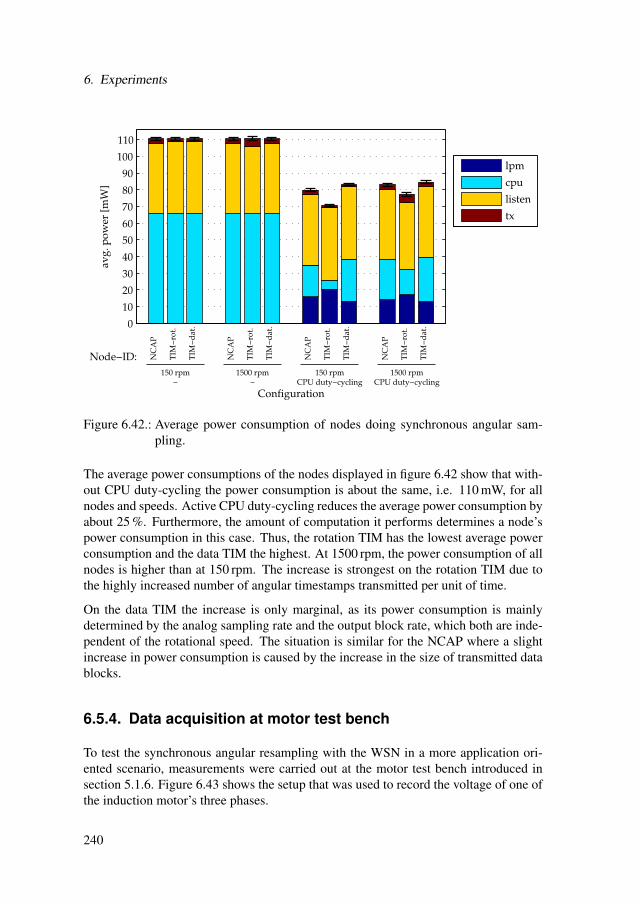
6. Experiments
0
10
20
30
40
50
60
70
80
90
100
110
avg
. po
wer
[m
W]
Node−ID: NC
AP
TIM
−ro
t.
TIM
−d
at.
NC
AP
TIM
−ro
t.
TIM
−d
at.
NC
AP
TIM
−ro
t.
TIM
−d
at.
NC
AP
TIM
−ro
t.
TIM
−d
at.
150 rpm−
1500 rpm−
150 rpmCPU duty−cycling
1500 rpmCPU duty−cycling
Configuration
lpm
cpu
listen
tx
Figure 6.42.: Average power consumption of nodes doing synchronous angular sam-pling.
The average power consumptions of the nodes displayed in figure 6.42 show that with-out CPU duty-cycling the power consumption is about the same, i.e. 110 mW, for allnodes and speeds. Active CPU duty-cycling reduces the average power consumption byabout 25 %. Furthermore, the amount of computation it performs determines a node’spower consumption in this case. Thus, the rotation TIM has the lowest average powerconsumption and the data TIM the highest. At 1500 rpm, the power consumption of allnodes is higher than at 150 rpm. The increase is strongest on the rotation TIM due tothe highly increased number of angular timestamps transmitted per unit of time.
On the data TIM the increase is only marginal, as its power consumption is mainlydetermined by the analog sampling rate and the output block rate, which both are inde-pendent of the rotational speed. The situation is similar for the NCAP where a slightincrease in power consumption is caused by the increase in the size of transmitted datablocks.
6.5.4. Data acquisition at motor test bench
To test the synchronous angular resampling with the WSN in a more application ori-ented scenario, measurements were carried out at the motor test bench introduced insection 5.1.6. Figure 6.43 shows the setup that was used to record the voltage of one ofthe induction motor’s three phases.
240

6.5. Synchronous angular sampling
Figure 6.43.: Setup for experiments at motor test bench.
Like in the experiments described in the previous subsection, measurements were takenat constant speeds of 150 rpm and 1500 rpm as well as at a variable speed profile. Thevariable speed profile was generated by periodically changing the speed setting of theinverter between 150 rpm and 1500 rpm. The actual speed gradient was limited by theinverter’s settings and breaking capabilities, so that a ramp signal similar to that in figure6.38 was expected. Again, resampling with the suggested filter, S&H resampling anddirect sampling were used to acquire the motor voltage. For comparison, it was alsoacquired with a DAQ-card (USB6009, National Instruments) at a constant samplingrate of 20 ksamples/s. A total of 10 recordings with 2048 output samples were acquiredfor every combination of speed setting and acquisition method. For the experimentsat constant speed the RMS-value, order and SINAD were calculated using a sine fit asdescribed in section 3.4.3. For the variable speed experiments no meaningful sine fitwas possible, as the motor voltage changes its amplitude with the speed.
The torque shaft of the test bench outputs an analog voltage signal that is proportionalto the shaft speed. This signal was also recorded with the DAQ-card and used as a refer-ence for the speed readings. Furthermore, a frequency counter (HM8123, Hameg) wasused to measure the average rotational speed and the frequency of the motor voltage.
241
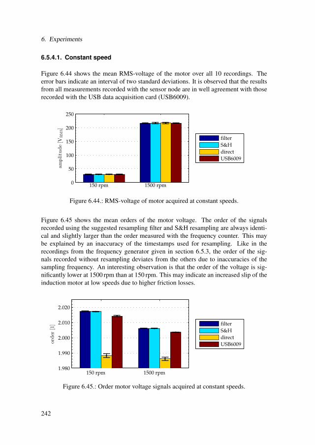
6. Experiments
6.5.4.1. Constant speed
Figure 6.44 shows the mean RMS-voltage of the motor over all 10 recordings. Theerror bars indicate an interval of two standard deviations. It is observed that the resultsfrom all measurements recorded with the sensor node are in well agreement with thoserecorded with the USB data acquisition card (USB6009).
0
50
100
150
200
250
amplitude[V
RMS]
150 rpm 1500 rpm
filter
S&H
direct
USB6009
Figure 6.44.: RMS-voltage of motor acquired at constant speeds.
Figure 6.45 shows the mean orders of the motor voltage. The order of the signalsrecorded using the suggested resampling filter and S&H resampling are always identi-cal and slightly larger than the order measured with the frequency counter. This maybe explained by an inaccuracy of the timestamps used for resampling. Like in therecordings from the frequency generator given in section 6.5.3, the order of the sig-nals recorded without resampling deviates from the others due to inaccuracies of thesampling frequency. An interesting observation is that the order of the voltage is sig-nificantly lower at 1500 rpm than at 150 rpm. This may indicate an increased slip of theinduction motor at low speeds due to higher friction losses.
1.980
1.990
2.000
2.010
2.020
order
[1]
150 rpm 1500 rpm
filter
S&H
direct
USB6009
Figure 6.45.: Order motor voltage signals acquired at constant speeds.
242
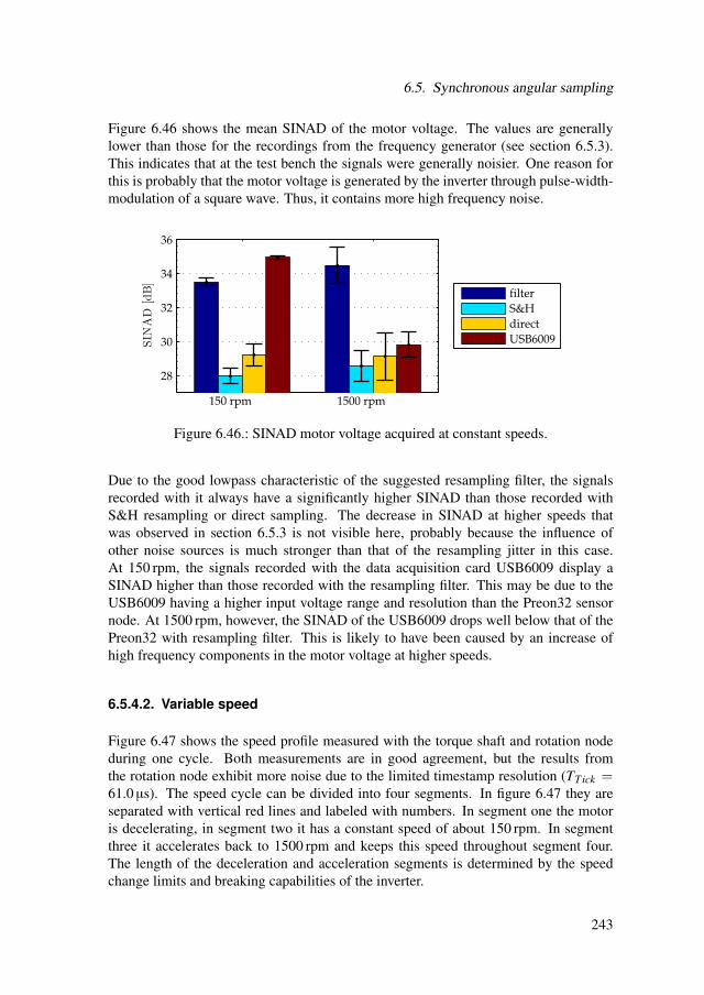
6.5. Synchronous angular sampling
Figure 6.46 shows the mean SINAD of the motor voltage. The values are generallylower than those for the recordings from the frequency generator (see section 6.5.3).This indicates that at the test bench the signals were generally noisier. One reason forthis is probably that the motor voltage is generated by the inverter through pulse-width-modulation of a square wave. Thus, it contains more high frequency noise.
28
30
32
34
36
SIN
AD
[dB]
150 rpm 1500 rpm
filter
S&H
direct
USB6009
Figure 6.46.: SINAD motor voltage acquired at constant speeds.
Due to the good lowpass characteristic of the suggested resampling filter, the signalsrecorded with it always have a significantly higher SINAD than those recorded withS&H resampling or direct sampling. The decrease in SINAD at higher speeds thatwas observed in section 6.5.3 is not visible here, probably because the influence ofother noise sources is much stronger than that of the resampling jitter in this case.At 150 rpm, the signals recorded with the data acquisition card USB6009 display aSINAD higher than those recorded with the resampling filter. This may be due to theUSB6009 having a higher input voltage range and resolution than the Preon32 sensornode. At 1500 rpm, however, the SINAD of the USB6009 drops well below that of thePreon32 with resampling filter. This is likely to have been caused by an increase ofhigh frequency components in the motor voltage at higher speeds.
6.5.4.2. Variable speed
Figure 6.47 shows the speed profile measured with the torque shaft and rotation nodeduring one cycle. Both measurements are in good agreement, but the results fromthe rotation node exhibit more noise due to the limited timestamp resolution (TTick =61.0 µs). The speed cycle can be divided into four segments. In figure 6.47 they areseparated with vertical red lines and labeled with numbers. In segment one the motoris decelerating, in segment two it has a constant speed of about 150 rpm. In segmentthree it accelerates back to 1500 rpm and keeps this speed throughout segment four.The length of the deceleration and acceleration segments is determined by the speedchange limits and breaking capabilities of the inverter.
243

6. Experiments
0 1 2 3 4 5 6 7 80
150
500
1000
1500
time [s]
spee
d [
rpm
]
1 2 3 4
Preon32 torque shaft
Figure 6.47.: Speed profile acquired during one cycle. Vertical red lines separate thefour segments of the profile.
Figure 6.48 shows the speed profile, motor voltage and order spectrogram of the samecycle as figure 6.47 with the rotation angle instead of the time as x-axis. The orderspectrogram was obtained by calculating the STFT for the resampled signal. A rect-angular window of 60 samples, i.e. two revolutions, was used. It is obvious from thespectrogram that the signal is constantly at the second order of rotation. Furthermore,the spectrogram displays hardly any signs of leakage components, which shows thatresampling has worked as expected. In segment three an increased noise level can beobserved. This may be due to the modulation spectra arising from the change of ampli-tude in this segment. Furthermore, also noise from the inverter power electronics mayhave an influence.
In segment one no such effects are visible, possibly because the speed gradient wasmuch less there. The voltage amplitude in figure 6.48 matches well with the RMS-values measured at constant speeds (compare figure 6.44).
244
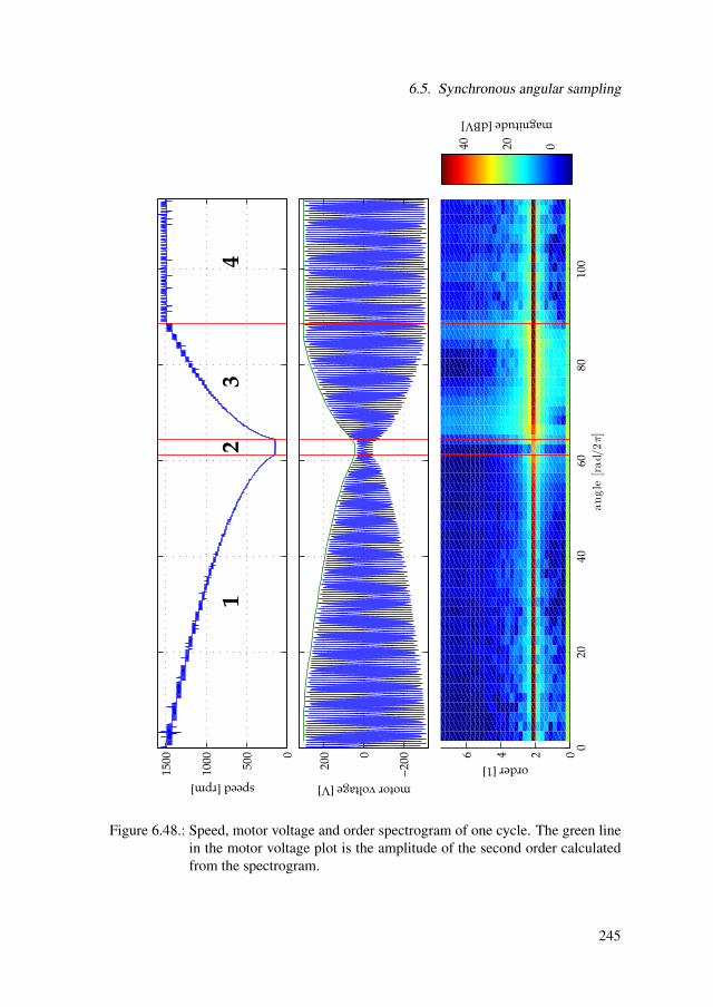
6.5. Synchronous angular sampling
0
500
1000
1500
12
34
speed [rpm]
−20
00
200
motor voltage [V]
020
4060
8010
00246
angle
[rad/2π]
order [1]
magnitude [dBV]
02040
Figure 6.48.: Speed, motor voltage and order spectrogram of one cycle. The green linein the motor voltage plot is the amplitude of the second order calculatedfrom the spectrogram.
245

6. Experiments
6.5.5. Conclusions
The simulations in section 6.5.2 show that the implemented resampling filter can ef-fectively convert a linear chirp into a constant order sine signal. The SINAD of theoutput signal is always higher when using the resampling filter compared to a simpleS&H-resampler. This advantage increases in the presence of additive white Gaussiannoise and is especially high frequency spurious components. The quality of the outputsignal is the same for all implementations of the filter. This shows that on the targetedplatform the round-off errors in the calculations are negligible in relation to those fromthe amplitude and time-quantization during acquisition. The fixed-point implementa-tion of the resampling filter is the only one that can be run in real-time on the targetedWSN. It is about ten times faster than the floating-point implementation, but still offersthe same signal quality.
Experiments in sections 6.5.3 and 6.5.4 show that the implemented synchronous angu-lar sampling scheme can successfully be run on a WSN. The signals acquired with theresampling filter show no significant drawbacks in terms of signal quality compared toacquiring the signal directly without resampling. At high downsampling ratios there iseven a significant increase in SINAD.
246

7. Conclusions and outlook
This chapter starts by summarizing the key findings of this thesis in section 7.1. Fromthis, conclusions are drawn in section 7.2 regarding the answers to the guiding questionsformulated at the end of chapter 2. Finally, an outlook on possible directions for futureresearch is given in section 7.3.
7.1. Summary
In chapter 4, generic models for systems doing synchronous event detection and syn-chronous waveform sampling were introduced. The key feature of these models is thatthey can be used to describe WSNs as well as more conventional DAQ systems. Usingthese models as a basis, the influence of synchronization errors on the measurement re-sult has been modeled and compared to other error influences, like signal noise, analoggroup delays or the clock resolution itself. The main result of this analysis is that theeffect of synchronization errors on the measurement result is in many cases the sameas that of other error influences. It has been suggested to describe the synchronizationerror by a mean and a standard deviation and apply measurement uncertainty analy-sis, as defined in the GUM, to evaluate the influence of all error influences. Using theconcept of measurement uncertainty, also a general procedure, that allows estimatingthe synchronization accuracy required for a given application, has been suggested insection 4.3. This method was shown to work well for practical experiments on acousticlocalization in section 6.3.
Building on the developed models and error analysis, two approaches to time synchro-nized DAQ were derived in section 4.4 a proactive and a reactive one. In the proactiveapproach data acquisition is steered by synchronized clocks, while in the reactive onedata acquisition is initially unsynchronized. The synchronization only takes place dur-ing later signal processing. Both approaches have been implemented on a WSN usingstate of the art commercial sensor nodes and the Contiki operating system (see chapter5). For the data acquisition a software framework inspired by the IEEE 1451 stan-dard has been implemented, that already allows to flexibly access a number of differentsensors through a unified MATLAB interface. For time synchronization a simplifiedversion of the FTSP protocol was used.
247
7. Conclusions and outlook
Both approaches were tested for synchronous event detection and synchronous wave-form acquisition in experiments (see sections 6.2 and 6.4). No clear advantages ofany approach over the other regarding synchronization precision or power consump-tion could be found. The distribution of synchronization errors during the experimentson synchronous event detection was found to be similar to a Gaussian distribution, butto significantly differ from it regarding the frequency of extreme values. A synchroniza-tion precision close to the clock resolution could be achieved, highlighting the discretenature of time values in a WSN. This shows the relevance of the clock resolution forsynchronized DAQ. Furthermore, it was shown that the overall timestamping precisionof a WSN can be characterized by an effective clock resolution (see sections 4.2.1.6 and6.2). Another important result of the experiments is that interrupt blocking sections inthe duty-cycling code of the sensor nodes’ operating system caused significant errorsin the synchronized data acquisition. This shows that the entire software of a wirelesssensor node should show a good real-time performance in order to enable accuratelysynchronized DAQ.
In addition to time synchronous data acquisition, synchronous angular sampling wasinvestigated. As discussed in section 4.5, a reactive approach is much better suited forits implementation. This way, expensive anti-aliasing filters with variable frequencyresponse are not needed and also the real-time requirements on the sensor node soft-ware can be relaxed. Furthermore, the resampling of data acquired at a uniform timeinterval to a uniform angle-interval was shown to be equivalent to the problem of re-constructing a uniformly sampled waveform from nonuniform samples. A powerfulreconstruction filter, which had originally been developed for communication systems,was implemented on the WSN (see section 5.3) using fixed-point arithmetic. The ex-periments presented in section 6.5 show, that the implemented filter provides a goodalias-suppression over a wide range of speeds and even at fast speed changes. Fur-thermore, it was shown that it is capable of real-time data acquisition at an inductionmotor test bench. The described fixed-point implementation provides about the samesignal quality in terms of SINAD, amplitude and frequency error as a floating pointimplementation, but only requires 10 % of its computation time.
7.2. Conclusions
At the end of chapter 2 four central questions were formulated, that could not satisfac-torily be answered from the current scientific literature. The analysis and experimentspresented in this thesis were aimed at these questions. Now as a conclusion, answers tothem shall be attempted:
248

7.2. Conclusions
How can synchronization precision be defined and measured in a way that ismeaningful for measurement applications?
Synchronization precision should be defined as a timing uncertainty characterized by astandard deviation (see section 4.2.3). This facilitates the calculation of the measure-ment uncertainty for the final measurement result. Furthermore, the influence on theSNR of an acquired signal can be easily calculated this way. Finally, the timing uncer-tainty can be easily transformed into an effective clock resolution that enables easy andintuitive comparison between different clock systems.
To measure the synchronization precision a method should be used that is as close aspossible to the final application. This reduces the danger of accidentally neglectingsignificant effects. For synchronous event detection, applying the same digital pulse toall channels and evaluating the difference in timestamps has been found to be effective.Similarly, acquiring the same sine wave with all channels works for synchronous wave-form acquisition (see section 4.6). The major advantage of both methods is that theycan equally be applied to WSN and other DAQ systems, thus enabling direct compar-isons.
Which synchronization precision is sufficient for a given application?
The synchronization precision required by an application can be calculated using mea-surement uncertainty analysis (see section 4.3). The information required for this is theacceptable uncertainty in the end result and the uncertainty contributions from othererror influences, e.g. signal noise, analog group delay, delays in multiplexed ADCs etc.Even if the exact strength of those influences is not known, it is possible to estimate therequired synchronization precision. As rule of thumb, the synchronization precision isusually sufficient, if it causes an uncertainty in the end result of less than 50 % of theoverall uncertainty margin (see section 4.3). The experimental results in section 6.3show that optimizing the synchronization precision alone may not lead to the desiredresult, as the influence of other error sources may be significant.
Which is the best strategy for time synchronized sampling?
Two approaches to time synchronized sampling were developed: a proactive and areactive one (see section 4.4). The proactive one directly steers the sampling timesbased on synchronized clocks. Thus, it requires a deep integration into the acquisitionprocess and very good real-time properties of the underlying software. Especially athigh sampling rates this may be difficult to achieve. Furthermore, corrections to theclocks during the acquisition may badly affect the SNR and THD of the signal (seesection 4.2.2).
249
7. Conclusions and outlook
Under the reactive approach the data is initially acquired without synchronization. Syn-chronization takes place later during data processing. This way, there is no interferencewith the data acquisition of the ADC and no effort needs to be put into maintaining syn-chronized clocks all the time. However, the a posteriori synchronization of the acquireddata through digital resampling only works well, if significant oversampling is used.
The implementations of the proactive and reactive approach for this thesis, performedabout equally well in terms of power consumption and synchronization precision duringthe experiments. Thus, the choice of approach should be guided by the anticipatedpattern of communication (see sections 6.2 and 6.4). The proactive approach matchesbetter with regular and the reactive better with irregular communication patterns.
How can synchronous angular sampling be best implemented on a WSN?
Synchronous angular sampling is better implemented with the reactive approach. Thisway, the difficult direct control of the ADC is not necessary and no anti-aliasing filterswith variable frequency response are required (see section 4.5). As synchronous an-gular sampling can be described as a nonuniform reconstruction problem, an efficientfilter, originally developed for communication systems, could be adopted from the lit-erature (see section 5.3). An implementation of this filter in fixed-point arithmetic hasbeen shown to enable real-time data acquisition at an induction motor test bench. Fur-thermore, the filter provides a good signal quality in terms of SINAD and effectivealias-suppression.
7.3. Outlook
The analysis presented in this thesis allows for a consistent treatment of the measure-ment uncertainty that arises from synchronization errors. Furthermore, the timing un-certainty expressed as a standard deviation was identified as the key quantity in speci-fying and assessing synchronization precision. It is to be hoped that these insights willbe adopted by a wider audience and lead to a better comparability between publishedresults. Furthermore, the direct comparison between WSNs and other DAQ systems,which is now possible, can help to establish WSNs as just another type of measurementsystem.
As the experimental results in chapter 6 have shown, the real-time performance of WSNsoftware has a significant influence on the synchronized data acquisition. Here, con-cepts are needed that solve the current conflict between efficient duty-cycling and dataacquisition. One approach might be to make better use of interrupt prioritization, whichis supported by many modern microcontrollers. Also, more recent operating systems
250

7.3. Outlook
for WSN like RIOT OS appear to offer better real-time performance than Contiki. Nev-ertheless, efficiently integrating the various algorithms, which have been developed fordifferent tasks in WSN, into one well performing system, appears to be a major chal-lenge for the future. This could possibly be significantly eased through better hardwaresupport. The timestamping operation for example, which is central to time synchro-nization and data acquisition, could be done much more accurately and efficiently bydedicated hardware.
A hardware coupling between a synchronized clock and an ADC might also make itpossible to use the proactive approach to synchronized waveform sampling at highersampling rates. The performance of the reactive approach at higher signal frequencieson the other hand, might be improved by using more powerful resampling algorithmslike e.g. the filter suggested for synchronous angular sampling.
The resampling filter itself, might also profit from a hardware implementation. Espe-cially the idea of combining it with a delta-sigma modulator and this way building adelta-sigma ADC with reactively synchronized output seems interesting. Furthermore,the filter might be extended to simultaneously resample multiple input channels. Thismight be done quite efficiently, as the lower branch of the filter, which filters the time-stamps, could be used for all channels simultaneously. Currently, the limiting factorfor the filter with regard to the supported speed range and maximum signal order at theoutput is the transmission bandwidth of the WSN. This might be overcome by findinga way to encode and transmit timestamps more efficiently, e.g. as spline functions.
In general, more efficient encoding and compression techniques could increase the util-ity for WSN in scientific and industrial applications. One approach might be to ex-tend the efficient compression techniques for text and image data suggested in [116]to other kinds of measurement data. Furthermore, there seems to be great potential indistributing the processing steps in a WSN such that the amount of data transmitted isminimized.
251


List of Figures
2.1. Topologies for WSNs. . . . . . . . . . . . . . . . . . . . . . . . . . . . 172.2. Protocol stacks for wireless sensor networks. . . . . . . . . . . . . . . 252.3. Remote clock reading techniques according to [119]: a) unidirectional
synchronization, b) round-trip synchronization, c) reference broadcast. . 312.4. Typical message delay sources according to [87]. . . . . . . . . . . . . 332.5. PTP network structure [200]. . . . . . . . . . . . . . . . . . . . . . . . 422.6. PTP synchronization message exchange [200]. . . . . . . . . . . . . . . 422.7. IEEE 1451 reference model according to [196]. Grayed out parts are
out of scope for IEEE 1451. . . . . . . . . . . . . . . . . . . . . . . . 502.8. Principle of synchronous angular sampling. . . . . . . . . . . . . . . . 532.9. Principle of synchronous angular resampling. . . . . . . . . . . . . . . 542.10. Block diagram of upsampled linear interpolation algorithm [14]. . . . . 552.11. Block diagram of upsampled interpolation filter [14]. . . . . . . . . . . 55
3.1. Amplitude spectra of a continuous signal X, corresponding sampledsignal Xs and ideal reconstruction filter Hideal. . . . . . . . . . . . . . . 65
3.2. Example of an amplitude spectrum with aliasing. Dotted green linesshow the individual repetition spectra. Red filled areas mark frequencyintervals where a reconstructed signal would be distorted by aliasing. . . 65
3.3. Example spectrum of a nonuniform comb function [88]. . . . . . . . . . 673.4. Digital measurement chain [48]. . . . . . . . . . . . . . . . . . . . . . 683.5. Structures of multi-channel data acquisition systems [48]. . . . . . . . . 693.6. Spectral effect of decimation. X: amplitude spectrum of original signal
sampled at ωs; Y: amplitude spectrum of signal resampled at ω′s =ωs/M. . . . . . . . . . . . . . . . . . . . . . . . . . . . . . . . . . . . 70
3.7. Sampling rate reduction by an integer factor (decimation). . . . . . . . 713.8. Tolerance schemes for digital anti-aliasing filters (after [93]). V is the
signal amplitude spectrum after filtering and Y the signal amplitudespectrum after decimation. Red shaded areas mark the frequency bandswhere aliasing may occur. . . . . . . . . . . . . . . . . . . . . . . . . . 72
3.9. Spectral effect of interpolation. X: spectrum of original signal at sam-pling rate ωs. . . . . . . . . . . . . . . . . . . . . . . . . . . . . . . . 73
3.10. Sampling rate increase by an integer factor (interpolation). . . . . . . . 733.11. Digital resampling with rational rate change factor. . . . . . . . . . . . 743.12. Hybrid discrete/continuous model of digital resampling [7]. . . . . . . . 74
253
List of Figures
3.13. FIR decimation filter. . . . . . . . . . . . . . . . . . . . . . . . . . . . 763.14. CIC decimation filter. . . . . . . . . . . . . . . . . . . . . . . . . . . . 773.15. Polynomial interpolation filters. . . . . . . . . . . . . . . . . . . . . . 793.16. Structure of the transposed Farrow filter [7, 82]. . . . . . . . . . . . . . 813.17. Example magnitude frequency response of a transposed Farrow filter. . 82
4.1. Model of a generic multi-channel event detection system applied to aWSN. . . . . . . . . . . . . . . . . . . . . . . . . . . . . . . . . . . . 100
4.2. Model of a generic multi-channel sampling system applied to a WSN. . 1004.3. Data acquisition chain for event detection. . . . . . . . . . . . . . . . . 1014.4. Probability density distributions of clock reading errors. . . . . . . . . . 1044.5. Effect of time offset on an acquired sine wave. . . . . . . . . . . . . . . 1084.6. Effect of constant timing drift on an acquired sine wave. . . . . . . . . . 1094.7. Effect of timing jitter on an acquired sine wave. . . . . . . . . . . . . . 1104.8. Effect of a time step on an acquired sine wave. . . . . . . . . . . . . . . 1114.9. Effect of changing drift on an acquired sine wave. . . . . . . . . . . . . 1114.10. Sampling systems with different approaches to time synchronous sam-
pling. . . . . . . . . . . . . . . . . . . . . . . . . . . . . . . . . . . . 1154.11. Representation of the same signal in time- and angle domain. The
marked positions show time, angle and signal values of a uniform sam-pling grid with spacing Ts in time domain. . . . . . . . . . . . . . . . . 117
4.12. Setup for testing synchronous event detection. . . . . . . . . . . . . . . 1194.13. Setup for testing multi-channel waveform sampling. . . . . . . . . . . . 1204.14. Setup for testing synchronous angular sampling. . . . . . . . . . . . . . 122
5.1. Preon32 on shuttle. . . . . . . . . . . . . . . . . . . . . . . . . . . . . 1245.2. Block diagram of Preon32. . . . . . . . . . . . . . . . . . . . . . . . . 1245.3. Clock sources and their distribution on the Preon32. . . . . . . . . . . . 1255.4. Layers and modules of Contiki’s network stack. . . . . . . . . . . . . . 1325.5. Structure of a TDMA frame. . . . . . . . . . . . . . . . . . . . . . . . 1345.6. Structure and communication model of the data acquisition framework. 1365.7. Sequence diagram of the transducer discovery process. . . . . . . . . . 1415.8. Sequence diagram of the transducer configuration. . . . . . . . . . . . . 1425.9. Sequence diagram of one-shot acquisition. . . . . . . . . . . . . . . . . 1425.10. Sequence diagram of a continuous data acquisition. . . . . . . . . . . . 1435.11. Maximum memory usage on a TIM. . . . . . . . . . . . . . . . . . . . 1455.12. Maximum memory usage on a NCAP. . . . . . . . . . . . . . . . . . . 1465.13. Block diagram of digital event sensor. . . . . . . . . . . . . . . . . . . 1485.14. Block diagram of digital actuator. . . . . . . . . . . . . . . . . . . . . 1505.15. Block diagram of analog voltage sensor. . . . . . . . . . . . . . . . . . 1515.16. Block diagram of microphone module. . . . . . . . . . . . . . . . . . . 1525.17. Block diagram of current and voltage sensor module. . . . . . . . . . . 153
254
List of Figures
5.18. Three current/voltage transducer modules and signal conditioning mod-ule installed in a control cabinet. . . . . . . . . . . . . . . . . . . . . . 154
5.19. Block diagram of rotary encoder sensor. . . . . . . . . . . . . . . . . . 1555.20. Rotary encoder sensor board with Preon32. . . . . . . . . . . . . . . . 1565.21. Test bench with installed wireless sensors. . . . . . . . . . . . . . . . . 1585.22. Rotary encoder and TIM at the backside of the breaking engine. . . . . 1585.23. Control cabinet with data TIM. . . . . . . . . . . . . . . . . . . . . . . 1585.24. Test bench setup. . . . . . . . . . . . . . . . . . . . . . . . . . . . . . 1595.25. Remote clock reading technique of Contiki’s timesynch a priori syn-
chronization service. . . . . . . . . . . . . . . . . . . . . . . . . . . . 1615.26. Sequence diagram of a timesynch synchronization with 6LoWPAN-
integration. . . . . . . . . . . . . . . . . . . . . . . . . . . . . . . . . 1635.27. Remote clock reading technique of the ETA-primitive for a posteriori
synchronization. . . . . . . . . . . . . . . . . . . . . . . . . . . . . . . 1645.28. Sequence diagram of sending a packet with RITS-synchronization. . . . 1645.29. Continuous event detection with a priori synchronization. Differences
to figure 5.30 are highlighted in green. . . . . . . . . . . . . . . . . . . 1655.30. Continuous event detection with a posteriori synchronization. Differ-
ences to figure 5.29 are highlighted in red. . . . . . . . . . . . . . . . . 1665.31. Block diagram of upsampled linear interpolation algorithm [14]. . . . . 1705.32. Reconstruction filter proposed in [82]. . . . . . . . . . . . . . . . . . . 1725.33. Resampling filter adapted to synchronous angular resampling. . . . . . 1735.34. Magnitude frequency responses of individual filters. . . . . . . . . . . . 1735.35. Magnitude frequency response of cascade: transposed Farrow, G and D. 1745.36. Number formats used in implementation of resampling filter. . . . . . . 1755.37. Number formats used in the calculation of the fractional interval. . . . . 1765.38. Number formats used in the implementation of the Farrow filter. . . . . 1765.39. Network layout for synchronous angular resampling. . . . . . . . . . . 177
6.1. Experimental setup used to measure the supply current of a node. . . . . 1826.2. Activity diagrams of test applications used to measure a sensor node’s
current consumption. . . . . . . . . . . . . . . . . . . . . . . . . . . . 1836.3. Node current during transmission. . . . . . . . . . . . . . . . . . . . . 1856.4. Power consumption of nodes as calculated from current measurements
with multimeter (DMM) and as estimated from powertrace (pwrt.).The error bars show the expanded uncertainty Uk=2. . . . . . . . . . . 188
6.5. Transmission success during transmissions of one sender to one receiver. 1906.6. Transmission success during transmissions of two senders to one receiver.1916.7. Average power consumption during transmissions of one sender to one
receiver. . . . . . . . . . . . . . . . . . . . . . . . . . . . . . . . . . . 1916.8. Average power consumption during transmission of two senders to one
receiver. . . . . . . . . . . . . . . . . . . . . . . . . . . . . . . . . . . 1926.9. Experimental setup used for event timestamping tests. . . . . . . . . . . 193
255

List of Figures
6.10. Recorded timestamp differences of TIMs to NCAP without time syn-chronization. The initial clock offset was removed to improve the visi-bility of the relative drifts. . . . . . . . . . . . . . . . . . . . . . . . . 195
6.11. Recorded timestamp differences with synchronization. The red linesmark the median. The blue boxes show the center 50 % and the whiskersthe center 95 % of all values. Values outside these ranges are drawn asred crosses. . . . . . . . . . . . . . . . . . . . . . . . . . . . . . . . . 197
6.12. Recorded timestamp differences with synchronization with zoomed ver-tical axis. The red lines mark the median. The blue boxes show the cen-ter 50 % and the whiskers the center 95 % of all values. Values outsidethese ranges are drawn as red crosses. . . . . . . . . . . . . . . . . . . 198
6.13. Histograms of recorded timestamp differences. Fitted Gaussian proba-bility density functions are shown as red curves. . . . . . . . . . . . . . 200
6.14. First 100 s of recorded timestamp differences and clock updates for con-figuration 5. . . . . . . . . . . . . . . . . . . . . . . . . . . . . . . . . 202
6.15. Mean power consumption of nodes during timestamping experimentsestimated from powertrace. . . . . . . . . . . . . . . . . . . . . . . . 203
6.16. General setup for passive acoustic localization on a straight line. . . . . 2056.17. Setup for acoustic localization experiments. . . . . . . . . . . . . . . . 2076.18. Example output of microphone amplifier and digital pin. . . . . . . . . 2096.19. Linear calibration of the localization system. The error bars indicate an
interval of two standard deviations. . . . . . . . . . . . . . . . . . . . . 2106.20. Mean localization errors obtained with filtered timestamps. The error
bars indicate an interval of two standard deviations. . . . . . . . . . . . 2116.21. Experimental setup to test time synchronous waveform acquisition. . . . 2176.22. Mean pairwise time shifts Tshi f t. The error bars indicate an interval of
twice the standard deviation. . . . . . . . . . . . . . . . . . . . . . . . 2196.23. Mean pairwise time shifts Tshi f t with zoomed y-axis. The error bars
indicate an interval of twice the standard deviation. . . . . . . . . . . . 2206.24. Signal SNR. . . . . . . . . . . . . . . . . . . . . . . . . . . . . . . . . 2226.25. Histogram of clock updates during acquisition of all records for config-
urations 1 and 2. . . . . . . . . . . . . . . . . . . . . . . . . . . . . . . 2236.26. Signal THD. . . . . . . . . . . . . . . . . . . . . . . . . . . . . . . . . 2246.27. Section of signal showing recorded and resampled data points. Intervals
with missing samples are highlighted. . . . . . . . . . . . . . . . . . . 2256.28. Mean power consumption of nodes doing synchronous waveform sam-
pling. . . . . . . . . . . . . . . . . . . . . . . . . . . . . . . . . . . . 2266.29. Setup for simulations on idealized angular sampling. Elements in dashed/-
dotted lines were only present starting from the configuration given asencircled number. . . . . . . . . . . . . . . . . . . . . . . . . . . . . . 228
6.30. SINAD of output signals synchronous to the rotation angle. Graph b)shows the same data as graph a) but with zoomed y-axis. . . . . . . . . 229
6.31. Relation between analog sampling rate and SNR of angular signal. . . . 230
256

List of Figures
6.32. Setup for simulations on angular resampling. . . . . . . . . . . . . . . 2316.33. RMS-error of resampled chirp signals. . . . . . . . . . . . . . . . . . . 2336.34. Order-error of resampled chirp signals. . . . . . . . . . . . . . . . . . . 2336.35. SINAD of resampled chirp signals. . . . . . . . . . . . . . . . . . . . . 2346.36. Results of angular resampling a signal with spurious component. . . . . 2356.37. Setup for recording generated signals. . . . . . . . . . . . . . . . . . . 2366.38. One period of the variable speed profile used in waveform generator
experiments. . . . . . . . . . . . . . . . . . . . . . . . . . . . . . . . . 2376.39. RMS-values of acquired generator signals. The solid horizontal line
indicates the nominal value set at the waveform generator. The dashedhorizontal lines indicate the specified accuracy of this setting . . . . . . 238
6.40. Order of acquired generator signals. The nominal order is indicated bythe horizontal line. . . . . . . . . . . . . . . . . . . . . . . . . . . . . 238
6.41. SINAD of acquired generator signals. . . . . . . . . . . . . . . . . . . 2396.42. Average power consumption of nodes doing synchronous angular sam-
pling. . . . . . . . . . . . . . . . . . . . . . . . . . . . . . . . . . . . 2406.43. Setup for experiments at motor test bench. . . . . . . . . . . . . . . . . 2416.44. RMS-voltage of motor acquired at constant speeds. . . . . . . . . . . . 2426.45. Order motor voltage signals acquired at constant speeds. . . . . . . . . 2426.46. SINAD motor voltage acquired at constant speeds. . . . . . . . . . . . 2436.47. Speed profile acquired during one cycle. Vertical red lines separate the
four segments of the profile. . . . . . . . . . . . . . . . . . . . . . . . 2446.48. Speed, motor voltage and order spectrogram of one cycle. The green
line in the motor voltage plot is the amplitude of the second order cal-culated from the spectrogram. . . . . . . . . . . . . . . . . . . . . . . 245
B.1. Reference points for evaluation of polynomial kernel. . . . . . . . . . . 292
C.1. Circuit diagram of the microphone module [Stud22]. . . . . . . . . . . 294C.2. Circuit diagram of the signal conditioning module [Stud9]. . . . . . . . 295C.3. Circuit diagram of current/voltage transducer modules. . . . . . . . . . 296C.4. Circuit diagram of rotary encoder interface circuit board. . . . . . . . . 297
E.1. Timestamp differences recorded with configuration 2 versus time. . . . 315E.2. Histogram of timestamp differences for configuration 2. . . . . . . . . . 316E.3. Timestamp differences recorded with configuration 3 versus time. . . . 317E.4. Clock changes recorded with configuration 3 versus time. . . . . . . . . 318E.5. Histograms of timestamp differences for configuration 3. . . . . . . . . 318E.6. Histograms of recorded clock updates for configuration 3. . . . . . . . . 318E.7. Timestamp differences recorded with configuration 4 versus time. . . . 319E.8. Clock updates recorded with configuration 4 versus time. . . . . . . . . 320E.9. Histograms of timestamp differences for configuration 4. . . . . . . . . 320E.10. Histograms of recorded clock updates for configuration 4. . . . . . . . . 320
257

List of Figures
E.11. Timestamp differences recorded with configuration 5 versus time. . . . 321E.12. Clock updates recorded with configuration 5 versus time. . . . . . . . . 322E.13. Histograms of timestamp differences for configuration 5. . . . . . . . . 322E.14. Histograms of recorded clock updates for configuration 5. . . . . . . . . 322E.15. Timestamp differences recorded with configuration 6 versus time. . . . 323E.16. Histograms of timestamp differences for configuration 6. . . . . . . . . 323E.17. Timestamp differences recorded with configuration 7 versus time. . . . 324E.18. Clock updates recorded with configuration 7 versus time. . . . . . . . . 325E.19. Histograms of timestamp differences for configuration 7. . . . . . . . . 325E.20. Histograms of recorded clock updates for configuration 7. . . . . . . . . 325E.21. Timestamp differences recorded with configuration 8 versus time. . . . 326E.22. Clock updates recorded with configuration 8 versus time. . . . . . . . . 327E.23. Histograms of timestamp differences for configuration 8. . . . . . . . . 327E.24. Histograms of recorded clock updates for configuration 8. . . . . . . . . 327
258

List of Tables
2.1. Examples of basic general purpose sensor nodes. . . . . . . . . . . . . 72.2. Examples of application specific sensor nodes. . . . . . . . . . . . . . . 82.3. Typical energy- and power densities of power supplies for wireless sen-
sor nodes. . . . . . . . . . . . . . . . . . . . . . . . . . . . . . . . . . 122.4. Frequency bands, transmission channels and data rates in the IEEE
802.15.4 standard [194]. . . . . . . . . . . . . . . . . . . . . . . . . . 192.5. Canonical time synchronization services and their typical applications
according to [77]. . . . . . . . . . . . . . . . . . . . . . . . . . . . . . 302.6. Overview of time synchronization protocols for WSN. . . . . . . . . . 372.7. Experimental precision of synchronization protocols. . . . . . . . . . . 392.8. Performance of PTP implementations for WSNs. . . . . . . . . . . . . 432.9. Examples of data acquisition with WSNs. . . . . . . . . . . . . . . . . 472.10. Members of IEEE 1451 family of standards. . . . . . . . . . . . . . . . 50
3.1. Computational and memory requirements of a polyphase FIR-decimator. 773.2. Computational and memory requirements of a CIC-decimator. . . . . . 783.3. Computational and memory requirements of a polynomial interpolation. 803.4. Computational and memory requirements of a transposed Farrow filter. . 823.5. Comparison of resampling filter algorithms. . . . . . . . . . . . . . . . 833.6. Coverage factors and confidence levels for a Gaussian distribution [199]. 913.7. Example of an uncertainty budget. . . . . . . . . . . . . . . . . . . . . 92
4.1. Summary of error influences on the detection time tevent . . . . . . . . . 1054.2. Uncertainty margin for other influences at given timing uncertainty. . . 114
5.1. Key features of Preon32 [179].. . . . . . . . . . . . . . . . . . . . . . . . . . . . . . . . . . . . . . 125
5.2. Key features of Preon32Shuttle [180]. . . . . . . . . . . . . . . . . . . 1255.3. Properties of clock sources on the Preon32. . . . . . . . . . . . . . . . 1265.4. Major operating states and sleep modes of microcontroller and wireless
transceiver on the Preon32. Values for Isupply are taken from [179]. . . . 1275.5. Components of the software execution environment. . . . . . . . . . . . 1285.6. Chosen TDMA-protocol parameters and theoretical performance. . . . 1355.7. Transducer and TEDS commands. . . . . . . . . . . . . . . . . . . . . 1375.8. Types of TEDS implemented in the MSTL. . . . . . . . . . . . . . . . 138
259
List of Tables
5.9. Implemented user commands. . . . . . . . . . . . . . . . . . . . . . . 1395.10. Overview of commands and operation modes supported by the individ-
ual application transducers. . . . . . . . . . . . . . . . . . . . . . . . . 1475.11. Data set of the powertrace sensor. . . . . . . . . . . . . . . . . . . . . 1495.12. Structure of the digital event sensor’s data set. . . . . . . . . . . . . . . 1495.13. Control values of digital actuator. . . . . . . . . . . . . . . . . . . . . . 1505.14. Structure of analog voltage sensor’s data set. . . . . . . . . . . . . . . . 1525.15. Technical data of the current/voltage transducer module. . . . . . . . . 1545.16. Structure of the rotary encoder sensor’s data set. . . . . . . . . . . . . . 1565.17. Specification data of induction- and DC-motor. . . . . . . . . . . . . . 157
6.1. Current consumption of node 41 measured for the different power modes.1846.2. Current consumption assigned to powertrace modes. . . . . . . . . . . 1856.3. Configuration of network layers investigated for data throughput. . . . . 1896.4. Network configurations investigated in event detection tests. . . . . . . 1946.5. Relative drifts between TIMs and NCAP. The uncertainties given are
the expanded uncertainties (k = 2) calculated for the variances of theregression parameters. . . . . . . . . . . . . . . . . . . . . . . . . . . 194
6.6. Theoretical maximum synchronization errors rounded to next larger in-teger number of Ticks. Exact values obtained from (2.1) are given inbrackets. . . . . . . . . . . . . . . . . . . . . . . . . . . . . . . . . . . 196
6.7. Estimated statistical parameters of timestamp difference distribution. . . 1996.8. Known sections of interrupt blocking on Preon32. . . . . . . . . . . . . 2036.9. Maximum timing uncertainty ut,max of a single timestamp in µs for dif-
ferent maximum location uncertainties ud,max and uncertainty marginsfor vsound = 343 m/s. . . . . . . . . . . . . . . . . . . . . . . . . . . . 206
6.10. Calibration results for the localization system. The error intervals cor-respond to the expanded uncertainty Uk=2, as estimated from the fitresiduals. . . . . . . . . . . . . . . . . . . . . . . . . . . . . . . . . . 210
6.11. Overall statistics of localization errors. . . . . . . . . . . . . . . . . . . 2116.12. Influence quantities affecting the localization measurement. . . . . . . . 2136.13. Uncertainty budget for time interval measurement with frequency counter.2146.14. Uncertainty budget for localization with frequency counter. . . . . . . . 2156.15. Uncertainty budget for localization with WSN. . . . . . . . . . . . . . 2156.16. Uncertainty budget for localization with WSN and active RDC. . . . . . 2166.17. Configurations for waveform acquisition tests. . . . . . . . . . . . . . . 2186.18. Frequency errors ϵ f and time offset errors ϵt0 calculated from the ac-
quired waveforms. . . . . . . . . . . . . . . . . . . . . . . . . . . . . 2196.19. Average sampling rates calculated from sample timestamps. . . . . . . 2216.20. Quality parameters of signal with lost samples before and after resam-
pling. . . . . . . . . . . . . . . . . . . . . . . . . . . . . . . . . . . . 2246.21. Configurations of simulations on idealized angular sampling. . . . . . . 228
260

List of Tables
6.22. Resampling implementations that were investigated(see also section 5.3.4). . . . . . . . . . . . . . . . . . . . . . . . . . . 231
A.1. General purpose sensor nodes. . . . . . . . . . . . . . . . . . . . . . . 288A.2. General purpose sensor nodes (continued) . . . . . . . . . . . . . . . . 289A.3. General purpose sensor nodes (continued) . . . . . . . . . . . . . . . . 290
261


Bibliography
[1] Abrach, H. et al.: MANTIS: System Support for multimodAl NeTworks of In-situSensors. In Proceedings of the 2Nd ACM International Conference on WirelessSensor Networks and Applications, WSNA ’03, pp. 50–59, New York, NY, USA,2003. ACM, ISBN 1-58113-764-8. DOI:10.1145/941350.941358.
[2] Abubakari, H.: IEEE 1588 Style Synchronization over a Wireless Link. Mas-ter’s thesis, University of Akron, 2008. http://etd.ohiolink.edu/view.cgi?acc_num=akron1226631636.
[3] Allan, D.W., N. Ashby, and C.C. Hodge: The Science of Timekeeping. HewlettPackard Application Note 1289, 1997. http://literature.agilent.com/litweb/pdf/5965-7984E.pdf, visited on 2015-05-12.
[4] Andersson, T. and P. Handel: IEEE Standard 1057, Cramer-Rao bound and theparsimony principle. Instrumentation and Measurement, IEEE Transactions on,55(1):44–53, Feb. 2006, ISSN 0018-9456. DOI:10.1109/TIM.2005.861497.
[5] Aoun, M., J. Catalano, and P. Stok: Distributed Task Synchronization in WirelessSensor Networks. In Proceedings of the 6th European Conference on WirelessSensor Networks, EWSN ’09, pp. 150–165, Berlin, Heidelberg, 2009. Springer-Verlag, ISBN 978-3-642-00223-6. DOI:10.1007/978-3-642-00224-3 10.
[6] Aoun, M., A. Schoofs, and P. van der Stok: Efficient time synchronizationfor wireless sensor networks in an industrial setting. In Proceedings ofthe 6th ACM conference on Embedded network sensor systems, SenSys ’08,pp. 419–420, New York, NY, USA, 2008. ACM, ISBN 978-1-59593-990-6.DOI:10.1145/1460412.1460482.
[7] Babic, D. and M. Renfors: Reconstruction of non-uniformly sampled signal us-ing transposed Farrow structure. In Circuits and Systems, 2004. ISCAS ’04. Pro-ceedings of the 2004 International Symposium on, vol. 3, pp. 221–224, 2004.DOI:10.1109/ISCAS.2004.1328723.
[8] Baccelli, E. et al.: RIOT OS: Towards an OS for the Internet of Things. In ComputerCommunications Workshops (INFOCOM WKSHPS), 2013 IEEE Conference on,pp. 79–80, Apr. 2013. DOI:10.1109/INFCOMW.2013.6970748.
263
Bibliography
[9] Badaoui, M.E. and F. Bonnardot: Impact of the non-uniform angular sampling onmechanical signals. Mechanical Systems and Signal Processing, 44(1–2):199–210,2014, ISSN 0888-3270. DOI:10.1016/j.ymssp.2013.10.008. Special Issue on In-stantaneous Angular Speed (IAS) Processing and Angular Applications.
[10] Basaran, C. et al.: Critical evaluation of platforms commonly used in embeddedwisents research. Techn. rep., Embedded WiSeNts consortium, 2006.
[11] Beard, R.L. and J.D. White: GPS Application to Time Transfer and Dissemination.GPS Solutions, 3(1):17–25, 1999, ISSN 1080-5370. DOI:10.1007/PL00012774.
[12] Benecke, S., E. Kravcenko, and R. Wirth: BMBF-Verbundprojekt ”ECoMoS” -Energieautarkes Condition Monitoring System. Abschlussbericht, Technische Uni-versitat Berlin, Forschungsschwerpunkt Technologien der Mikroperipherik, 2012.DOI:10.2314/GBV:757447449.
[13] Bhatti, S. et al.: MANTIS OS: An embedded multithreaded operating system forwireless micro sensor platforms. MOBILE NETWORKS & APPLICATIONS,10(4):563–579, Aug. 2005, ISSN 1383-469X. DOI:10.1007/s11036-005-1567-8.2nd International Workshop on Wireless Sensor Networks and Application (WSNA2003), San Diego, CA, SEP 19, 2003.
[14] Blough, J.: Adaptive Resampling - Transforming from the time to the Angle do-main. In 24th Conference and Exposition on Structural Dynamics 2006, IMAC-XXIV, 2006.
[15] Blough, J.R.: A survey of DSP methods for rotating machinery analysis, whatis needed, what is available. Journal of Sound and Vibration, 262(3):707–720,2003, ISSN 0022-460X. DOI:10.1016/S0022-460X(03)00118-4. 2001 India-USASymposium on Emerging Trends in Vibration and Noise Engineering.
[16] Bomar, B.W.: Finit Wordlength Effects. In Digital signal processing fundamen-tals. CRC Press, 2009, ISBN 978-1-4200-4606-9.
[17] Bonnardot, F. et al.: Use of the acceleration signal of a gearbox in or-der to perform angular resampling (with limited speed fluctuation). Mechan-ical Systems and Signal Processing, 19(4):766–785, 2005, ISSN 0888-3270.DOI:10.1016/j.ymssp.2004.05.001.
[18] Brandt, A. et al.: Main principles and limitations of current order tracking meth-ods. Sound and Vibration, 39(3):19–22, 2005, ISSN 1541-0161.
[19] Buettner, M. et al.: X-mac: A short preamble mac protocol for duty-cycledwireless sensor networks. In in SenSys, pp. 307–320, 2006, http://www.cs.colorado.edu/˜rhan/Papers/xmac_sensys06.pdf.
264
Bibliography
[20] Caligiuri, L.M. and A. Nastro: About the conventionality of simultaneity and syn-chronization. In 20th IMEKO TC4 Symposium on Measurements of ElectricalQuantities, 2014.
[21] Chen, D., M. Nixon, and A. Mok: WirelessHART. Springer, 2010,ISBN 978-1-4419-6047-4. DOI:10.1007/978-1-4419-6047-4.
[22] Cho, H., S. Son, and Y. Baek: Implementation of a precision time protocolover low rate wireless personal area networks. In Computer Systems Archi-tecture Conference, 2008. ACSAC 2008. 13th Asia-Pacific, pp. 1–8, Aug. 2008.DOI:10.1109/APCSAC.2008.4625431.
[23] Christin, D., P.S. Mogre, and M. Hollick: Survey on Wireless Sensor Net-work Technologies for Industrial Automation: The Security and Quality ofService Perspectives. Future Internet, 2(2):96–125, 2010, ISSN 1999-5903.DOI:10.3390/fi2020096.
[24] Clausen, T. et al.: The Lightweight On-demand Ad hoc Distance-vector RoutingProtocol - Next Generation (LOADng), July 2012. https://tools.ietf.org/html/draft-clausen-lln-loadng-05, DRAFT.
[25] Crochiere, R.E. and L.R. Rabiner: Multirate Digital Signal Processing. PrenticeHall, 1983, ISBN 0-13-605162-6.
[26] Dai, H. and R. Han: TSync: a lightweight bidirectional time synchronization ser-vice for wireless sensor networks. SIGMOBILE Mob. Comput. Commun. Rev.,8(1):125–139, 2004, ISSN 1559-1662. DOI:10.1145/980159.980173.
[27] Dreher, A. and D. Mohl: Prazise Uhrzeitsynchronisation: Der StandardIEEE 1588. https://belden.picturepark.com/Website/Publisher.
aspx?Page=Belden&AssetContainerId=1250, visited on 2015-04-21, rev. 1.2.
[28] Dunkels, A.: Rime - a lightweight layered communication stack for sensor net-works. In European Conference on Wireless Sensor Networks (EWSN), Jan. 2007,http://www.sics.se/˜adam/dunkels07rime.pdf.
[29] Dunkels, A.: The ContikiMAC Radio Duty Cycling Protocol. SICS Techni-cal Report T2011:13, 2011, ISSN 1100-3154, http://www.sics.se/˜adam/dunkels11contikimac.pdf.
[30] Dunkels, A., B. Gronvall, and T. Voigt: Contiki - a lightweight and flexibleoperating system for tiny networked sensors. In Local Computer Networks,2004. 29th Annual IEEE International Conference on, pp. 455–462, Nov. 2004.DOI:10.1109/LCN.2004.38.
265
Bibliography
[31] Dunkels, A. et al.: Software-based On-line Energy Estimation for Sen-sor Nodes. In Proceedings of the 4th Workshop on Embedded NetworkedSensors, EmNets ’07, pp. 28–32. ACM, 2007, ISBN 978-1-59593-694-3.DOI:10.1145/1278972.1278979.
[32] Dunkels, A. et al.: Protothreads: Simplifying Event-driven Programmingof Memory-constrained Embedded Systems. In Proceedings of the 4thInternational Conference on Embedded Networked Sensor Systems, Sen-Sys ’06, pp. 29–42, New York, NY, USA, 2006. ACM, ISBN 1-59593-343-3.DOI:10.1145/1182807.1182811.
[33] Duquennoy, S. et al.: Leveraging IP for Sensor Network Deployment. In Proceed-ings of the workshop on Extending the Internet to Low power and Lossy Networks(IP+SN 2011), Chicago, IL, USA, Apr. 2011.
[34] Dutta, P. and A. Dunkels: Operating systems and network protocols for wire-less sensor networks. Philosophical Transactions of the Royal Society of Lon-don A: Mathematical, Physical and Engineering Sciences, 370(1958):68–84, 2011,ISSN 1364-503X. DOI:10.1098/rsta.2011.0330.
[35] Elson, J., L. Girod, and D. Estrin: Fine-grained network time synchronizationusing reference broadcasts. SIGOPS Oper. Syst. Rev., 36(SI):147–163, 2002,ISSN 0163-5980. DOI:10.1145/844128.844143.
[36] Eswaran, A., A. Rowe, and R. Rajkumar: Nano-RK: an energy-awareresource-centric RTOS for sensor networks. In Real-Time Systems Sympo-sium, 2005. RTSS 2005. 26th IEEE International, pp. 256–265, Dec. 2005.DOI:10.1109/RTSS.2005.30.
[37] Ferrari, P. et al.: Time distribution in IPv6 Wireless Sensor Networks. InPrecision Clock Synchronization for Measurement Control and Communica-tion (ISPCS), 2011 International IEEE Symposium on, pp. 69–74, 2011.DOI:10.1109/ISPCS.2011.6070149.
[38] Flammini, A. et al.: Wired and wireless sensor networks for industrial applica-tions. Microelectronics Journal, 40(9):1322–1336, 2009.
[39] Flammini, A. et al.: A real-time Wireless Sensor Network for temperature moni-toring. In Industrial Electronics, 2007. ISIE 2007. IEEE International Symposiumon, pp. 1916–1920, June 2007. DOI:10.1109/ISIE.2007.4374900.
[40] FLUKE: 8845A/8846A Digitial Multimeter - User Manual, 3rd ed., June 2006.
[41] FLUKE: Understanding specifications for precision multimeters, 2011. Applica-tion Note.
266

Bibliography
[42] Ganeriwal, S., R. Kumar, and M.B. Srivastava: Timing-sync protocol for sensornetworks. In SenSys ’03: Proceedings of the 1st international conference on Em-bedded networked sensor systems, pp. 138–149. ACM, 2003.
[43] Gnawali, O. et al.: Collection Tree Protocol. Technical Report SING-09-01, 2009,http://sing.stanford.edu/pubs/sing-09-01.pdf, visited on 2011-09-23.Stanford University.
[44] Greunen, J. van and J. Rabaey: Lightweight time synchronization for sensor net-works. In Proceedings of the 2Nd ACM International Conference on Wireless Sen-sor Networks and Applications, WSNA ’03, pp. 11–19, New York, NY, USA, 2003.ACM, ISBN 1-58113-764-8. DOI:10.1145/941350.941353.
[45] Guevara, J. et al.: A framework for WSN using TinyOS and the IEEE1451 stan-dard. In Communications (LATINCOM), 2011 IEEE Latin-American Conferenceon, pp. 1–5, Oct. 2011. DOI:10.1109/LatinCOM.2011.6107420.
[46] Gockler, H.G. and A. Groth: Multiratensysteme. J. Schlembach Fachverlag, 2004,ISBN 3-935340-29-X.
[47] Guhmann, C.: Stromanalyse zur Diagnose seriengefertigter Universalmotoren.PhD thesis, TU Berlin, 1995, ISBN 3-89574-087-X.
[48] Guhmann, C.: Messdatenverarbeitung. TU Berlin, lecture notes, Mar. 2011.
[49] Guhmann, C.: Modellbildung und Echtzeitsimulation technischer Systeme - Kapi-tel 7. TU Berlin, lecture notes, Dec. 2015.
[50] Haenselmann, T.: Wireless Sensor Networks. Oldenbourg Verlag, 2011, ISBN978-3-486-70798-4.
[51] HAMEG Instruments: 3 GHz Programmable Counter HM8123, HM8123-X -User Manual. 2015-09-15.
[52] HAMEG Instruments: Arbitrary Function Generator 12.5 MHz HM8150 -Datasheet. 2014-06-22.
[53] Heynicke, R., D. Kruger, and G. Scholl: Wireless automation. In SENSOR+TESTConference, 2011.
[54] Higuera, J. and J. Polo: Understanding the IEEE 1451 standard in 6loWPAN sen-sor networks. In Sensors Applications Symposium (SAS), 2010 IEEE, pp. 189–193,2010. DOI:10.1109/SAS.2010.5439427.
[55] Higuera, J. and J. Polo: IEEE 1451 Standard in 6LoWPAN Sensor Networks Usinga Compact Physical-Layer Transducer Electronic Datasheet. Instrumentation andMeasurement, IEEE Transactions on, 60(8):2751–2758, 2011, ISSN 0018-9456.DOI:10.1109/TIM.2011.2129990.
267

Bibliography
[56] Hill, J. and D. Culler: Mica: a wireless platform for deeply embed-ded networks. Micro, IEEE, 22(6):12–24, Nov. 2002, ISSN 0272-1732.DOI:10.1109/MM.2002.1134340.
[57] Hoffmann, J. (ed.): Taschenbuch der Messtechnik. Fachbuchverl. Leipzig im Carl-Hanser-Verl., 4th ed., 2004. ISBN 3-446-22860-8.
[58] Hogenauer, E.: An economical class of digital filters for decimation and in-terpolation. Acoustics, Speech and Signal Processing, IEEE Transactions on,29(2):155–162, Apr. 1981, ISSN 0096-3518. DOI:10.1109/TASSP.1981.1163535.
[59] Hou, L. and N. Bergmann: System requirements for industrial wireless sensornetworks. In Emerging Technologies and Factory Automation (ETFA), 2010 IEEEConference on, pp. 1–8, 2010. DOI:10.1109/ETFA.2010.5641163.
[60] Hou, L. and N.W. Bergmann: Novel Industrial Wireless Sensor Networks forMachine Condition Monitoring and Fault Diagnosis. Instrumentation and Mea-surement, IEEE Transactions on, 61(10):2787–2798, 2012, ISSN 0018-9456.DOI:10.1109/TIM.2012.2200817.
[61] Huang, Q., B. Tang, and L. Deng: Development of high synchronous acquisitionaccuracy wireless sensor network for machine vibration monitoring. Measurement,66(0):35–44, 2015, ISSN 0263-2241. DOI:10.1016/j.measurement.2015.01.021.
[62] Josefsson, S.: The Base16, Base32, and Base64 Data Encodings. RFC 4648, Oct.2006. https://tools.ietf.org/html/rfc4648.
[63] Kagelmaker, U. and F. Hillenbrand: BMBF-Verbundprojekt ”ECoMoS”: En-ergieeffiziente Messdatenerfassung und -verarbeitung fur ein energieautarkes Con-dition Monitoring System. Abschlussbericht, IMC Meßsysteme GmbH, Berlin,2012. DOI:10.2314/GBV:742582418.
[64] Karl, H. and A. Willig: Protocols and Architectures for Wireless Sensor Networks.Wiley, 2005, ISBN 978-0-470-09510-2.
[65] Kester, W. (ed.): The Data Conversion Handbook. Analog Devices Inc., 2004,ISBN 0-916550-27-3.
[66] Kiencke, U. and R. Eger: Messtechnik : Systemtheorie fur Elektrotechniker.Springer, 2008, ISBN 978-3-540-78428-9. DOI:10.1007/978-3-540-78429-6.
[67] Kim, J.S. et al.: Robust clock synchronization in wireless sensor networksthrough noise density estimation. Signal Processing, IEEE Transactions on,59(7):3035–3047, July 2011, ISSN 1053-587X. DOI:10.1109/TSP.2011.2141660.
[68] Kinsler, L.E. et al.: Fundamentals of acoustics. Wiley, 4th ed., 2000,ISBN 0-471-84789-5.
268

Bibliography
[69] Klingler, F.M. and H.G. Gockler: Conversion between arbitrary samplingrates: An implementation cost trade-off study for the family of farrowstructures. In Proc. 5th Karlsruhe Workshop on Software Radios, pp.1–8, 2008, http://www.dsv.ruhr-uni-bochum.de/imperia/md/content/public/wsr08_klinglergoeckler.pdf.
[70] Ko, J. et al.: A.: Evaluating the Performance of RPL and 6LoWPAN. In in TinyOS.In: Workshop on Extending the Internet to Low power and Lossy Networks (IP+SN2011), 2011.
[71] Kodek, D.M.: Length limit of optimal finite wordlength FIR filters.Digital Signal Processing, 23(5):1798–1805, 2013, ISSN 1051-2004.DOI:10.1016/j.dsp.2013.07.004.
[72] Kolerus, J. and J. Wassermann: Zustandsuberwachung von Maschinen. expert-Verl., 4th ed., 2011, ISBN 978-3-8169-2597-2.
[73] Kovatsch, M., S. Duquennoy, and A. Dunkels: A Low-Power CoAP for Contiki.In Mobile Adhoc and Sensor Systems (MASS), 2011 IEEE 8th International Con-ference on, pp. 855–860, Oct. 2011. DOI:10.1109/MASS.2011.100.
[74] Krauße, M. and R. Konrad: Drahtlose ZigBee-Netzwerke : ein Kompendium.Springer, 2014, ISBN 978-3-658-05821-0.
[75] Kreuzer, J.: ”Wenn mich niemand danach fragt, weiß ich es.“ – Die Re-alitat der Zeit. Hamburger Akademie der Wissenschaften, Nov. 2015.http://www.awhamburg.de/fileadmin/redakteure/Downloads/2015-
11-26_AkadVL_Kreuzer_Handout.pdf, visited on 2016-04-30, handout.
[76] Kruger, D., R. Heynicke, and G. Scholl: Wireless sensor/actuator-network withimproved coexistence performance for 2.45 GHz ISM-band operation. In Systems,Signals and Devices (SSD), 2012 9th International Multi-Conference on, pp. 1–5,2012. DOI:10.1109/SSD.2012.6198099.
[77] Kusy, B. et al.: Elapsed time on arrival: a simple and versatile primitive forcanonical time synchronisation services. International Journal of Ad Hoc and Ubiq-uitous Computing, 1(4):239–251, 2006. DOI:10.1504/IJAHUC.2006.010505.
[78] Lamport, L.: Time, clocks, and the ordering of events in a dis-tributed system. Commun. ACM, 21(7):558–565, 1978, ISSN 0001-0782.DOI:http://doi.acm.org/10.1145/359545.359563.
[79] Lasassmeh, S. and J. Conrad: Time synchronization in wireless sensor networks:A survey. In IEEE SoutheastCon 2010 (SoutheastCon), Proceedings of the, pp.242–245, 2010. DOI:10.1109/SECON.2010.5453878.
[80] Lee, E.A. and S.A. Seshia: Introduction to Embedded Systems - A Cyber-PhysicalSystems Approach. LeeSeshia.org, 2011, ISBN 978-0-557-70857-4.
269

Bibliography
[81] Lee, H.C. et al.: The Tube: A Rapidly Deployable Wireless Sensor Platformfor Supervising Pollution of Emergency Work. Instrumentation and Measure-ment, IEEE Transactions on, 61(10):2776–2786, Oct. 2012, ISSN 0018-9456.DOI:10.1109/TIM.2012.2200392.
[82] Lehtinen, V. et al.: Error Spectrum Analysis of Time-Variant Recon-struction from Nonuniform Sampling. In Signal Processing Symposium,2006. NORSIG 2006. Proceedings of the 7th Nordic, pp. 78–81, 2006.DOI:10.1109/NORSIG.2006.275281.
[83] Leng, M. and Y.C. Wu: Low-Complexity Maximum-Likelihood Estimator forClock Synchronization of Wireless Sensor Nodes Under Exponential Delays. Sig-nal Processing, IEEE Transactions on, 59(10):4860–4870, 2011, ISSN 1053-587X.DOI:10.1109/TSP.2011.2160857.
[84] Lerch, R.: Elektrische Messtechnik. Springer, 2007.
[85] Levis, P. et al.: TinyOS: An Operating System for Sensor Networks. In Weber, W.,J. Rabaey, and E. Aarts (eds.): Ambient Intelligence, pp. 115–148. Springer BerlinHeidelberg, 2005, ISBN 978-3-540-23867-6. DOI:10.1007/3-540-27139-2 7.
[86] Liu, Q. et al.: AdaSynch: A General Adaptive Clock Synchronization SchemeBased on Kalman Filter for WSNs. Wireless Personal Communications,63(1):217–239, 2012, ISSN 0929-6212. DOI:10.1007/s11277-010-0116-3.
[87] Maroti, M. et al.: The flooding time synchronization protocol. In SenSys ’04:Proceedings of the 2nd international conference on Embedded networked sensorsystems, pp. 39–49. ACM, 2004.
[88] Marvasti, F.: Nonuniform sampling: theory and practice. No. 1 in Informationtechnology–transmission, processing, and storage. Kluwer Academic/Plenum Pub-lishers, 2001, ISBN 9780306464454.
[89] Marvasti, F. et al.: Reconstruction of speech signals with lost samples. SignalProcessing, IEEE Transactions on, 40(12):2897–2903, 1992, ISSN 1053-587X.DOI:10.1109/78.175734.
[90] McFadden, P.: Interpolation techniques for time domain averaging of gearvibration. Mechanical Systems and Signal Processing, 3(1):87–97, 1989,ISSN 0888-3270. DOI:http://dx.doi.org/10.1016/0888-3270(89)90024-1.
[91] Medina, C., J.C. Segura, and A. de la Torre: A Synchronous TDMA Ultra-sonic TOF Measurement System for Low-Power Wireless Sensor Networks. In-strumentation and Measurement, IEEE Transactions on, 62(3):599–611, 2013,ISSN 0018-9456. DOI:10.1109/TIM.2012.2218056.
270

Bibliography
[92] Mehta, A. and K. Pister: WARPWING: A complete open source controlplatform for miniature robots. In Intelligent Robots and Systems (IROS),2010 IEEE/RSJ International Conference on, pp. 5169–5174, Oct. 2010.DOI:10.1109/IROS.2010.5649382.
[93] Milic, L.: Multirate Filtering for Digital Signal Processing. Information ScienceReference, 2009.
[94] Mills, D.: Network Time Protocol (NTP). RFC 958, Sept. 1985. https://tools.ietf.org/html/rfc958, visited on 2015-04-20, Obsoleted by RFCs 1059, 1119,1305.
[95] Mills, D. et al.: Network Time Protocol Version 4: Protocol and Algorithms Spec-ification. RFC 5905 (Proposed Standard), June 2010. http://www.ietf.org/rfc/rfc5905.txt, visited on 2015-05-12.
[96] Mills, D.L.: Network Time Protocol (NTP) - General Overview, 2004. https://www.eecis.udel.edu/˜mills/database/brief/overview/overview.pdf,visited on 2015-05-12.
[97] Mills, D.L.: NTP Architecture, Protocol and Algorithms, 2007. http://
www.eecis.udel.edu/˜mills/database/brief/arch/arch.pdf, visited on2015-05-11.
[98] Narendra, P., S. Duquennoy, and T. Voigt: BLE and IEEE 802.15.4 in the IoT:Evaluation and Interoperability Considerations. In International Conference onInteroperability in IoT (EAI InterIoT 2015), 2015, http://soda.swedishict.se/5923/, visited on 2016-10-03.
[99] Niedermayer, M.: Methodik zum Entwurf von miniaturisierten, energieautarken,verteilten Funksensorknoten. PhD thesis, TU Berlin, 2007.
[100] Niedermayer, M., H. Scholtz, and R. Wirth: BMBF-Verbundprojekt ”ECoMoS”:Miniaturisierungstechnologien fur Energieautarke Condition Monitoring Systeme.Abschlussbericht, Fraunhofer-Institut fur Zuverlassigkeit und Mikrointegration,2012. DOI:10.2314/GBV:757442536.
[101] Nong, H. and J. Lin: Design of loosely coupled inductive power transfersystems for instrumented wheelset. In Electronic Measurement Instruments,2009. ICEMI ’09. 9th International Conference on, pp. 1–670–1–674, 2009.DOI:10.1109/ICEMI.2009.5274779.
[102] Oppenheim, A.V. and R.W. Schafer: Discrete-Time Signal Processing. PearsonEducation Limited, 3rd ed., 2013, ISBN 978-1-292-02572-8.
[103] Oppenheim, A.V., A.S. Willsky, and S.H. Nawab: Signals and systems. Prentice-Hall, 2nd ed., 1996, ISBN 0-13-814757-4.
271

Bibliography
[104] Outler, A.C.: Augustine: Confessions, newly translated and edited, 1955.http://www.georgetown.edu/faculty/jod/augustine/conf.pdf, visitedon 2016-08-13.
[105] Papoulis, A.: Error analysis in sampling theory. Proceedings of the IEEE,54(7):947–955, July 1966, ISSN 0018-9219. DOI:10.1109/PROC.1966.4940.
[106] Perkins, C., E. Belding-Royer, and S. Das: Ad hoc On-Demand Distance Vector(AODV) Routing. RFC 3561 (Experimental), July 2003. http://www.ietf.org/rfc/rfc3561.txt.
[107] Pesch, B.: Bestimmung der Messunischerheit nach GUM. Books On DemandGmbH, Norderstedt, 2004, ISBN 3-8830-1039-8.
[108] Pflugradt, M. et al.: A novel pulseoximeter for bluetooth synchronized mea-surements in a body sensor network. In Education and Research Confer-ence (EDERC), 2014 6th European Embedded Design in, pp. 21–25, 2014.DOI:10.1109/EDERC.2014.6924351.
[109] Pister, K. et al.: Industrial Routing Requirements in Low-Power and Lossy Net-works. RFC 5673 (Informational), Oct. 2009. http://www.ietf.org/rfc/rfc5673.txt.
[110] Pister, K.S.J. and L. Doherty: TSMP: Time Synchronized Mesh Protocol. InProceedings of the IASTED International Symposium Distributed Sensor Networks,2008.
[111] Potter, R.: New order tracking method for rotating machinery. S V Sound andVibration, 24(9):30–34, 1990.
[112] Pottie, G.J. and W.J. Kaiser: Wireless integrated network sensors. Commun.ACM, 43(5):51–58, 2000, ISSN 0001-0782. DOI:10.1145/332833.332838.
[113] Pottner, W.B. et al.: WSN Evaluation in Industrial Environments First resultsand lessons learned. In 3rd Workshop on Performance Control in Wireless SensorNetworks 2011 (PWSN 2011) in conjuction with IEEE DCOSS 2011, pp. 1–8, 2011.
[114] Raju, M.: Energy Harvesting - ULP meets energy harvesting: A game-changingcombination for design engineers. Techn. rep., Texas Instruments, 2008.
[115] Ramos, P.M. and A.C. Serra: A new sine-fitting algorithm for ac-curate amplitude and phase measurements in two channel acquisi-tion systems. Measurement, 41(2):135–143, 2008, ISSN 0263-2241.DOI:10.1016/j.measurement.2006.03.011. Advances in Measurements ofEelectrical Quantities.
[116] Rein, S.: Low Complexity Text and Image Compression for Wireless Devices andSensors. PhD thesis, TU Berlin, 2010. DOI:10.14279/depositonce-2484.
272

Bibliography
[117] Rein, S. and M. Reisslein: Low-Memory Wavelet Transforms for Wireless SensorNetworks: A Tutorial. Communications Surveys Tutorials, IEEE, 13(2):291–307,Feb. 2011, ISSN 1553-877X. DOI:10.1109/SURV.2011.100110.00059.
[118] Ren, F., C. Lin, and F. Liu: Self-correcting time synchronization using refer-ence broadcast in wireless sensor network. Wireless Communications, IEEE,15(4):79–85, Aug. 2008, ISSN 1536-1284. DOI:10.1109/MWC.2008.4599225.
[119] Romer, K., P. Blum, and L. Meier: Time Synchronization and Calibration inWireless Sensor Networks. In Handbook of Sensor Networks: Algorithms and Ar-chitectures. Wiley, 2005, ISBN 978-0-471-68472-5.
[120] Romer, K. and F. Mattern: The design space of wireless sensor net-works. Wireless Communications, IEEE, 11(6):54–61, 2004, ISSN 1536-1284.DOI:10.1109/MWC.2004.1368897.
[121] Roundy, S. and L. Frechette: Energy Scavenging and Nontraditional PowerSources for Wireless Sensor Networks. In Handbook of Sensor Networks: Algo-rithms and Architectures. Wiley, 2005, ISBN 978-0-471-68472-5.
[122] Schafer, R. and L. Rabiner: A digital signal processing approach to inter-polation. Proceedings of the IEEE, 61(6):692–702, 1973, ISSN 0018-9219.DOI:10.1109/PROC.1973.9150.
[123] Schmid, T. et al.: A case against routing-integrated time synchronization.In Proceedings of the 8th ACM Conference on Embedded Networked Sen-sor Systems, SenSys ’10, pp. 267–280, New York, NY, USA, 2010. ACM,ISBN 978-1-4503-0344-6. DOI:10.1145/1869983.1870010.
[124] Schmid, T., P. Dutta, and M.B. Srivastava: High-resolution, low-power timesynchronization an oxymoron no more. In IPSN ’10: Proceedings of the 9thACM/IEEE International Conference on Information Processing in Sensor Net-works, pp. 151–161, New York, NY, USA, 2010. ACM, ISBN 978-1-60558-988-6.DOI:10.1145/1791212.1791231.
[125] Scholl, G. et al.: Wireless Automation. In 16th International Conference OnSensors and Measurement Technology, 2013.
[126] Schweinzer, H. and G. Kaniak: Ultrasonic device localization and its potentialfor wireless sensor network security. Control Engineering Practice, 18(8):852–862,Aug. 2010, ISSN 0967-0661. DOI:10.1016/j.conengprac.2008.12.007.
[127] Sedlacek, M. and M. Krumpholc: Digital measurement of phase difference -a comparative study of dsp algorithms. Metrology and Measurement Systems,XII:427–448, 2005, ISSN 0860-8229.
[128] Shelby, Z. and C. Bormann: 6LoWPAN: The Wireless Embedded Internet. Wiley,2009, ISBN 978-0-470-74799-5.
273

Bibliography
[129] Shelby, Z., K. Hartke, and C. Bormann: The Constrained Application Protocol(CoAP). RFC 7252 (Proposed Standard), June 2014. http://www.ietf.org/rfc/rfc7252.txt.
[130] Shucker, B. et al.: Embedded Operating Systems for Wireless MicrosensorNodes. In Handbook of Sensor Networks: Algorithms and Architectures. Wiley,2005, ISBN 978-0-471-68472-5.
[131] Siekkinen, M. et al.: How low energy is bluetooth low energy? Compara-tive measurements with ZigBee/802.15.4. In Wireless Communications and Net-working Conference Workshops (WCNCW), 2012 IEEE, pp. 232–237, Apr. 2012.DOI:10.1109/WCNCW.2012.6215496.
[132] Simon, G. et al.: Sensor network-based countersniper system. In Pro-ceedings of the 2nd International Conference on Embedded Networked Sen-sor Systems, SenSys ’04, pp. 1–12. ACM, 2004, ISBN 1-58113-879-2.DOI:10.1145/1031495.1031497.
[133] Song, J. et al.: WirelessHART: Applying Wireless Technology in Real-TimeIndustrial Process Control. In Real-Time and Embedded Technology andApplications Symposium, 2008. RTAS ’08. IEEE, pp. 377–386, Apr. 2008.DOI:10.1109/RTAS.2008.15.
[134] Souders, T. et al.: The effects of timing jitter in sampling systems. Instru-mentation and Measurement, IEEE Transactions on, 39(1):80–85, Feb. 1990,ISSN 0018-9456. DOI:10.1109/19.50421.
[135] Stanislowski, D. et al.: Adaptive Synchronization in IEEE802.15.4e Net-works. Industrial Informatics, IEEE Transactions on, 10(1):795–802, 2014,ISSN 1551-3203. DOI:10.1109/TII.2013.2255062.
[136] Steigmann, R. and J. Endresen: Introduction to WISA. Tech. Rep. V2.0, ABBSTOTZ-KONTAKT GmbH, 2006.
[137] Stojcev, M.K., L.R. Golubovic, and T.R. Nikolic: Clocks, Power and Syn-chronization in Duty-Cycled Wireless Sensor Nodes. Facta Universitatis (NIS),24:183–208, 2011.
[138] Stojmenovic, I. (ed.): Handbook of Sensor Networks: Algorithms and Architec-tures. Wiley, 2005, ISBN 978-0-471-68472-5.
[139] Sun, Y.R. and S. Signell: Algorithms for nonuniform bandpass samplingin radio receiver. In Circuits and Systems, 2003. ISCAS ’03. Proceed-ings of the 2003 International Symposium on, vol. 1, pp. I–1–I–4, 2003.DOI:10.1109/ISCAS.2003.1205485.
[140] Thingsquare: The World at Your Fingertips. http://www.thingsquare.com/,visited on 2015-02-27.
274

Bibliography
[141] Tian, X. et al.: Maximum likelihood estimation based on time synchronizationalgorithm for wireless sensor networks. In Computing, Communication, Control,and Management, 2009. CCCM 2009. ISECS International Colloquium on, vol. 4,pp. 416–420, 8-9 2009. DOI:10.1109/CCCM.2009.5267612.
[142] TinyOS: FAQ. http://tinyos.stanford.edu/tinyos-wiki/index.php/FAQ, visited on 2015-02-27.
[143] Toma, D.M. et al.: Precision timing in TDMA-based Wireless Sensor Networkthrough IEEE 1588 standard. In 19th Symposium IMEKO TC 4 Symposium and17th IWADC Workshop Advances in Instrumentation and Sensors Interoperability,2013.
[144] Tripathi, J., J.C. de Oliveira, and J. Vasseur: Proactive versus reactive rout-ing in low power and lossy networks: Performance analysis and scalabil-ity improvements. Ad Hoc Networks, 23(0):121–144, 2014, ISSN 1570-8705.DOI:10.1016/j.adhoc.2014.06.007.
[145] Vallestad, A.E.: WISA becomes WSAN - from proprietary technology to indus-try standard. In Wireless Summit, Oslo, 2012. http://www.ifea.no/wp-content/uploads/2012/04/A-Vallestad-WISA_becomes_WSAN-
Wireless-Summit-2012.pdf, visited on 2015-04-18.
[146] Vesma, J. and T. Saramaki: Interpolation filters with arbitrary frequency re-sponse for all-digital receivers. In Circuits and Systems, 1996. ISCAS ’96., Con-necting the World., 1996 IEEE International Symposium on, vol. 2, pp. 568–571,1996. DOI:10.1109/ISCAS.1996.541788.
[147] Watteyne, T. et al.: OpenWSN: a standards-based low-power wireless develop-ment environment. Transactions on Emerging Telecommunications Technologies,23(5):480–493, 2012, ISSN 2161-3915. DOI:10.1002/ett.2558.
[148] Wehmeier, S. (ed.): Oxford Advanced Learner’s Dictionary of Current English.Oxford University Press, 7th ed., 2005, ISBN 978-0-19-4316569.
[149] Welsh, M.: Sensor networks for the sciences. Commun. ACM, 53:36–39, 2010.DOI:10.1145/1839676.1839690.
[150] Wikipedia contributors: Unix time. Wikipedia, The Free Encyclope-dia. https://en.wikipedia.org/w/index.php?title=Unix_time&oldid=736472521, visited on 2016-08-31.
[151] Wikipedia contributors: Contiki. Wikipedia, The Free Encyclopedia,2014. http://en.wikipedia.org/w/index.php?title=Contiki&oldid=
636293925, visited on 2015-02-27.
275
http://www.ifea.no/wp-content/uploads/2012/04/A-Vallestad-WISA_becomes_WSAN-Wireless-Summit-2012.pdf
http://www.ifea.no/wp-content/uploads/2012/04/A-Vallestad-WISA_becomes_WSAN-Wireless-Summit-2012.pdf

Bibliography
[152] Wikipedia contributors: Sun SPOT. Wikipedia, The Free Encyclopedia,2014. https://en.wikipedia.org/w/index.php?title=Sun_SPOT&oldid=619609396, visited on 2015-06-18.
[153] Wikipedia contributors: Radio clock. Wikipedia, The Free Encyclope-dia, 2015. http://en.wikipedia.org/w/index.php?title=Radio_clock&oldid=655864422, visited on 2015-05-09.
[154] Wikipedia contributors: TinyOS. Wikipedia, The Free Encyclopedia,2015. http://en.wikipedia.org/w/index.php?title=TinyOS&oldid=
647685711, visited on 2015-02-27.
[155] Winter, T. et al.: RPL: IPv6 Routing Protocol for Low-Power and Lossy Net-works. RFC 6550 (Proposed Standard), Mar. 2012. http://www.ietf.org/rfc/rfc6550.txt.
[156] Wirth, R. and S. Guttowski: BMBF-Verbundprojekt ”ECoMoS”: Energieau-tarkes Condition Monitoring System. Abschlussbericht, GfM Gesellschaft f.Maschinendiagnose mbH, 2012. DOI:10.2314/GBV:737579714.
[157] Wobschall, D. and Y. Ma: Synchronization of wireless sensor networks using amodified IEEE 1588 protocol. In Precision Clock Synchronization for MeasurementControl and Communication (ISPCS), 2010 International IEEE Symposium on, pp.67–70, 2010. DOI:10.1109/ISPCS.2010.5609778.
[158] Yoon, S., C. Veerarittiphan, and M.L. Sichitiu: Tiny-sync: Tight time synchro-nization for wireless sensor networks. ACM Trans. Sen. Netw., 3(2):8, 2007,ISSN 1550-4859. DOI:10.1145/1240226.1240228.
[159] Yuan, Y. et al.: Industrial high-speed wireless synchronous data acquisitionsystem with real-time data compression. Measurement, 46(9):3482–3487, 2013,ISSN 0263-2241. DOI:10.1016/j.measurement.2013.06.043.
[160] Zangl, H. et al.: Wireless Communication and Power Supply Strategy forSensor Applications Within Closed Metal Walls. Instrumentation and Mea-surement, IEEE Transactions on, 59(6):1686–1692, 2010, ISSN 0018-9456.DOI:10.1109/TIM.2009.2026602.
[161] A fully compliant ZigBee 2012 solution: Z-Stack. Texas Instruments. http://www.ti.com/tool/z-stack, visited on 2015-04-17.
[162] AT86RF231. Atmel. http://www.atmel.com/devices/at86rf231.aspx,visited on 2015-06-30.
[163] BitCloud - ZigBee PRO. Atmel. http://www.atmel.com/tools/bitcloud-zigbeepro.aspx, visited on 2015-04-17.
[164] Bluetooth Smart Technology: Powering the Internet of Things. http://www.bluetooth.com/pages/bluetooth-smart.aspx, visited on 2015-05-05.
276

Bibliography
[165] CMSIS - Cortex Microcontroller Software Interface Standard. http://www.arm.com/products/processors/cortex-m/cortex-microcontroller-
software-interface-standard.php, visited on 2015-03-19.
[166] Contiki Hardware. http://www.contiki-os.org/hardware.html, visitedon 2015-01-31.
[167] Econotag II. http://www.redwirellc.com/collections/frontpage/
products/econotag-ii, visited on 2015-02-04.
[168] EmberZNet PRO ZigBee® Protocol Stack Software. Silicon Labs.https://www.silabs.com/products/wireless/zigbee/Pages/zigbee-
software.aspx, visited on 2015-04-17.
[169] EnOcean Dolphin – the platform for energy harvesting wireless sensor tech-nology. https://www.enocean.com/fileadmin/redaktion/pdf/press/
enocean_dolphin_EN.pdf, visited on 2015-02-04.
[170] FreeRTOS™- Market leading RTOS. http://www.freertos.org/, visited on2015-02-27.
[171] INGA - Inexpensive Node for General Applications. https://www.ibr.cs.tu-bs.de/projects/inga/, visited on 2015-01-28.
[172] Mica2 - Wireless Measurement System. http://www.snm.ethz.ch/snmwiki/Projects/Mica2, visited on 2015-02-10.
[173] MICAz - Wireless Measurement System. http://www.memsic.com/
userfiles/files/Datasheets/WSN/micaz_datasheet-t.pdf, visited on2015-02-10.
[174] Nano-RK: A Wireless Sensor Networking Real-Time Operating System. http://www.nanork.org/projects/nanork/wiki, visited on 2015-02-27.
[175] NI Wireless Sensor Networks. http://www.ni.com/wsn/, visited on 2015-02-04.
[176] OPENMOTE-CC2538. http://www.openmote.com/hardware/openmote-cc2538-en.html, visited on 2015-02-04.
[177] OpenWSN Home. https://openwsn.atlassian.net/wiki/display/OW/Home, visited on 2015-02-27.
[178] Powercast: RF Energy Harvesting and Wireless Power for Low-Power Ap-plications. http://www.powercastco.com/PDF/powercast-overview%20%282012%29.pdf, visited on 2015-02-04.
[179] Preon32 — Innovative 2.4 GHz radio module for Preon32-Series by Virte-nio. http://www.virtenio.com/en/products/radio-module.html, visitedon 2015-01-28.
277

Bibliography
[180] Preon32Shuttle — Expansion module for Preon32-Series by Virtenio. http://www.virtenio.com/en/products/evaluation-module.html, visited on2015-06-30.
[181] Projekt Spisa - Signal Processing Sensor Applications. TU Berlin, Chair ofElectronic Measurement and Diagnostic Technology. https://www.mdt.tu-berlin.de/menue/forschung/abgeschlossene_forschungsprojekte/
projekt_spisa/, visited on 2016-10-08.
[182] RIOT: The friendly Operating System for the Internet of Things. http://www.riot-os.org/, visited on 2015-02-27.
[183] The Sensor Network Museum™- Tmote Sky. http://www.snm.ethz.ch/
snmwiki/Projects/TmoteSky, visited on 2015-01-31.
[184] SNM - The Sensor Network Museum™. http://www.snm.ethz.ch/, visitedon 2015-01-31.
[185] TELOSB Mote Platform. http://www.memsic.com/userfiles/files/
Datasheets/WSN/6020-0094-02_B_TELOSB.pdf, visited on 2015-06-18.
[186] The Contiki OS (Homepage). http://www.contiki-os.org/, visited on2015-01-28.
[187] The Contiki Wiki. https://github.com/contiki-os/contiki/wiki, vis-ited on 2015-07-07.
[188] The ZigBee Alliance. http://www.zigbee.org/, visited on 2015-04-11.
[189] TinyOS. http://www.tinyos.net/, visited on 2015-02-27.
[190] Virtenio GmbH - smart wireless devices. http://www.virtenio.com/en/,visited on 2015-02-26.
[191] XBee® Multipoint RF Modules. http://www.digi.com/pdf/ds_
xbeemultipointmodules.pdf, visited on 2015-06-18.
[192] Z1 Platform. http://zolertia.com/products/z1, visited on 2015-01-28.
[193] ITU-T Recommendation G.810, Definitions and terminology for synchronisationnetworks, Aug. 1996.
[194] IEEE Standard for Information technology– Local and metropolitan areanetworks– Specific requirements– Part 15.4: Wireless Medium Access Control(MAC) and Physical Layer (PHY) Specifications for Low Rate Wireless PersonalArea Networks (WPANs). IEEE Std 802.15.4-2006 (Revision of IEEE Std 802.15.4-2003), pp. 1–320, Sept. 2006. DOI:10.1109/IEEESTD.2006.232110.
[195] The International System of Units (SI). Bureau International des Poids etMesures, 8th ed., 2006, ISBN 92-822-2213-6.
278

Bibliography
[196] IEEE Standard for a Smart Transducer Interface for Sensors and Actua-tors - Common Functions, Communication Protocols, and Transducer ElectronicData Sheet (TEDS) Formats. IEEE Std 1451.0-2007, pp. 1–335, Sept. 2007.DOI:10.1109/IEEESTD.2007.4338161.
[197] IEEE Standard for a Smart Transducer Interface for Sensors and Ac-tuators Wireless Communication Protocols and Transducer Electronic DataSheet (TEDS) Formats. IEEE Std 1451.5-2007, pp. C1–236, Oct. 2007.DOI:10.1109/IEEESTD.2007.4346346.
[198] VDI/VDE-Richtlinie 2185: Radio based communication in industrial automa-tion, 2007.
[199] Evaluation of measurement data - Guide to the expression of uncertainty in mea-surement (JCGM 100:2008), 2008. http://www.bipm.org/utils/common/documents/jcgm/JCGM_100_2008_E.pdf, visited on 2015-08-03.
[200] IEEE Standard for a Precision Clock Synchronization Protocol for NetworkedMeasurement and Control Systems. IEEE Std 1588-2008 (Revision of IEEE Std1588-2002), pp. c1–269, July 2008. DOI:10.1109/IEEESTD.2008.4579760.
[201] IEEE Standard for Digitizing Waveform Recorders. IEEE Std1057-2007 (Revision of IEEE 1057-1994), pp. 1–168, Apr. 2008.DOI:10.1109/IEEESTD.2008.4494996.
[202] MCKPI-G2210L-3672 (Datasheet). Multicomp, 2009. http://www.newark.com/pdfs/datasheets/spc/25R0627.pdf, visited on 2015-11-14.
[203] Wireless systems for industrial automation: process control and related applica-tions. Standard ISA-100.11a-2011, 2011.
[204] IEEE Standard for Local and metropolitan area networks–Part 15.4: Low-RateWireless Personal Area Networks (LR-WPANs) Amendment 1: MAC sublayer.IEEE Std 802.15.4e-2012 (Amendment to IEEE Std 802.15.4-2011), pp. 1–225,Apr. 2012. DOI:10.1109/IEEESTD.2012.6185525.
[205] Reliable factory automation - Wireless Automation, 2012. http:
//www05.abb.com/global/scot/scot397.nsf/veritydisplay/
da2ecccaededc5cdc1257c210039f241/$file/3ADR071023B0201.pdf,visited on 2015-02-04.
[206] Scavenger Transceiver Module STM 300 / STM 300C / STM 300U. enO-cean, Nov. 2012. https://www.enocean.com/de/enocean_module/stm-
300-data-sheet.pdf, visited on 2015-06-15, Data Sheet.
[207] STM 3xy wireless sensor transmitter module family. enOcean, June2013. https://www.enocean.com/de/enocean_module/White_Paper_STM_3xy_EN_20.pdf, visited on 2015-06-09, White Paper.
279

Bibliography
[208] Motion Synchronization Using RTSI. National Instruments, Nov. 2014. http://www.ni.com/white-paper/3522/en/, visited on 2015-06-17.
[209] Sensor Transmitter Module STM 330 / STM 331 / STM 330C / STM 332U /STM 333U. EnOcean, Mar. 2015. https://www.enocean.com/de/enocean_module/stm-330-data-sheet.pdf, visited on 2015-06-15, Data Sheet, V1.2.
280

Publications
[Fun1] Funck, J. and C. Guhmann: Verfahren zur Messung von Synchro-nisationsfehlern in mehrkanaligen Messsystemen. In Schmitt, R.(ed.): XXVI. Messtechnisches Symposium des Arbeitskreises derHochschullehrer fur Messtechnik e.V. (AHMT), pp. 155–166. AHMT,2012, ISBN 978-3-8440-1312-2.
[Fun2] Funck, J., R. Knoblich, D. Scholz, S. Nowoisky, and C. Guhmann: Draht-loses Messsystem fur Temperaturen in Kraftfahrzeugkupplungen. tm - Tech-nisches Messen, 80(3):84–91, Apr. 2013. DOI:10.1524/teme.2013.0014.
[Fun3] Funck, J. and C. Guhmann: Time-Synchronous Sampling in Wireless Sen-sor Networks. In 19th IMEKO TC4 Symposium Measurements of Electri-cal Quantities, 2013, ISBN 978-84-616-5438-3, http://www.imeko.org/publications/tc4-2013/IMEKO-TC4-2013-058.pdf.
[Fun4] Funck, J. and C. Guhmann: Comparison of approaches to time-synchronoussampling in wireless sensor networks. Measurement, 56(0):203–214, 2014,ISSN 0263-2241. DOI:10.1016/j.measurement.2014.07.001.
[Fun5] Funck, J. and C. Guhmann: Design of a flexible filter for synchronous resam-pling in wireless sensor networks. In 20th IMEKO TC-4 International Sym-posium, Sept. 2014, ISBN 978-92-990073-2-7, http://www.imeko.org/publications/tc4-2014/IMEKO-TC4-2014-196.pdf.
[Fun6] Bock, A., D. Liu, J. Funck, A. Giedymin, R. Burke, and C. Guhmann:Wireless Sensor for Temperature and Flux Measurements in an AxialFlux Machine. In SENSOR 2015, 17th International Conference onSensors and Measurement Technology, 2015, ISBN 978-3-9813484-8-4.DOI:10.5162/sensor2015/C2.1.
[Fun7] Funck, J. and C. Guhmann: A flexible filter for synchronous angular resam-pling with a wireless sensor network. Measurement, 98:393–406, 2017,ISSN 0263-2241. DOI:10.1016/j.measurement.2016.07.062.
281


Supervised students’ theses
[Stud1] Ardanuy, X.: Design of a GUI based on the implemented IEEE1451 standardin a Wireless Sensor Network. Bachelor thesis, TU Berlin, July 2014.
[Stud2] Bjorn: Interpolation und Nachabtastung von Messdaten aus einem drahtlosenSensornetzwerk. Master thesis, TU Berlin, May 2014.
[Stud3] Bock: Inbetriebnahme und Plausibilisierung eines Sensors zur Messung derRotortemperatur eines Asynchronmotors. Studienarbeit, TU Berlin, Nov.2013.
[Stud4] Bock, A.: Implementation of a Wireless Sensor System on an Axial Flux Motor.Diploma thesis, TU Berlin, Feb. 2015.
[Stud5] Burisch, P.: Induktive Energieversorgung eines drahtlosen Temper-aturmesssystems. Diploma thesis, TU Berlin, Apr. 2014.
[Stud6] Erik, B.: Entwurf und Charakterisierung eines Energy-Harvesting-Moduls fureinen drahtlosen Sensorknoten. Diploma thesis, TU Berlin, Nov. 2011.
[Stud7] Haase, P.: Implementation einer CAN-Schnittstelle fur einen Intelligenten Sen-sorknoten. Bachelor thesis, TU Berlin, Jan. 2012.
[Stud8] Henckell, B.: Ladezustandsschatzung fur batteriebetriebene Sensoren. Bach-elor thesis, TU Berlin, Aug. 2013.
[Stud9] Hopp, T.: Intelligenter Sensor zur Leistungsmessung im Dreiphasennetz. Mas-ter thesis, TU Berlin, May 2013.
[Stud10] Jahnel, A.: Fourier-basierte Ordnungsanalyse mit einem drahtlosen Sensor-knoten. Bachelor thesis, TU Berlin, July 2014.
[Stud11] Kallenbach, E.: Machbarkeitsstudie bezuglich eines energieautarken Strom-sensors. Bachelor thesis, TU Berlin, Oct. 2013.
[Stud12] Klemm, E.: Bestimmung und Korrektur dynamischer Messfehler von Temper-atursensoren. Bachelor thesis, TU Berlin, June 2014.
[Stud13] Krauskopf, S.: Messdatenerfassung mit einem drahtlosen Sensornetzwerk.Bachelor thesis, TU Berlin, Jan. 2013.
283

Supervised students’ theses
[Stud14] Krauskopf, S.: Anbindung eines Android Smartphones an ein drahtloses Sen-sornetzwerk. Master thesis, TU Berlin, Sept. 2014.
[Stud15] Matern, S.: Drahtloses Sensormodul zur Demonstration von Anwendungs-beispielen. Bachelor thesis, TU Berlin, Sept. 2015.
[Stud16] Moksha Birk: Zeitsynchronisation in einem drahtlosen Single-Hop Sensor-netzwerk. Bachelor thesis, TU Berlin, Mar. 2013.
[Stud17] Pawlikowski, J.: Energieautarker drahtloser Sensorknoten zur Raumklimaer-fassung. Diploma thesis, TU Berlin, Apr. 2015.
[Stud18] Pertiller, A.: Vergleichende Untersuchung von Verfahren zur Schatzung desSignal-Rausch-Verhaltnisses von Analog/Digital-Umsetzern. Diploma thesis,TU Berlin, Sept. 2012.
[Stud19] Peters, O.: Entwurf eines intelligenten Korperschallsensors. Studienarbeit,TU Berlin, Nov. 2012.
[Stud20] Peters, O.: Diagnose von Unwuchten mit einem drahtlosen intelligentenKorperschallsensor. Diploma thesis, TU Berlin, June 2013.
[Stud21] Pilgrim, B.: Integration eines drahtlosen Sensornetzwerkes in eine CAN-Busbasierte Messdatenaufnahme. Diploma thesis, TU Berlin, Feb. 2013.
[Stud22] Roubal, F.: Akustische Ortung mit einem drahtlosen Sensornetzwerk. Bache-lor thesis, TU Berlin, Aug. 2013.
[Stud23] Scholz, D.: Entwicklung eines drahtlosen Temperaturmesssystems fur eineEinscheibentrockenkupplung. Diploma thesis, TU Berlin, Mar. 2012.
[Stud24] Siegmund, R.: Elektrische Steuerung einer Gleichstrommaschine als mecha-nische Last. Bachelor thesis, TU Berlin, May 2012.
[Stud25] Stallenberger, B.: Aufbau eines automatisierten Testsytems furAnalog/Digital-Umsetzer. Bachelor thesis, TU Berlin, Dec. 2011.
[Stud26] Stallenberger, B.: Interpolation und Nachabtastung von Messdaten aus einemdrahtlosen Sensornetzwerk. Master thesis, TU Berlin, May 2014.
284

Appendix

A. Sensor Nodes
287
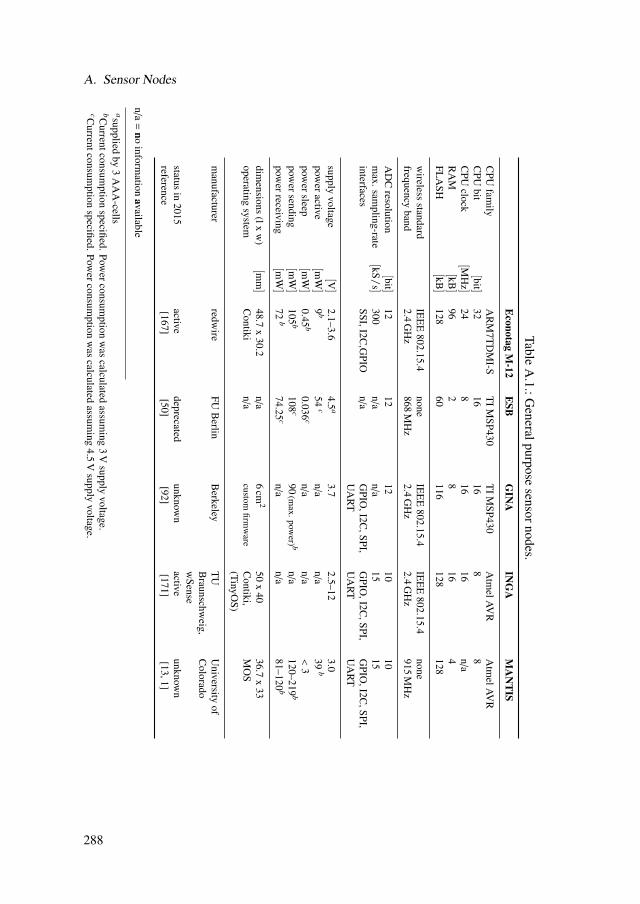
A. Sensor Nodes
TableA
.1.:Generalpurpose
sensornodes.E
conotagM
-12E
SBG
INA
ING
AM
AN
TIS
CPU
family
AR
M7T
DM
I-ST
IMSP430
TIM
SP430A
tmelAV
RA
tmelAV
RC
PUbit
[ bit]32
1616
88
CPU
clock[ M
Hz]
248
1616
n/a
RA
M[ kB
]96
28
164
FLA
SH[ kB
]128
60116
128128
wireless
standardIE
EE
802.15.4none
IEE
E802.15.4
IEE
E802.15.4
nonefrequency
band2.4
GH
z868
MH
z2.4
GH
z2.4
GH
z915
MH
z
AD
Cresolution
[ bit]12
1212
1010
max.sam
pling-rate[ kS/
s]300
n/a
n/a
1515
interfacesSSI,I2C
,GPIO
n/a
GPIO
,I2C,SPI,
UA
RT
GPIO
,I2C,SPI,
UA
RT
GPIO
,I2C,SPI,
UA
RT
supplyvoltage
[ V]
2.1–3.64.5
a3.7
2.5–123.0
poweractive
[ mW]
9b
54c
n/a
n/a
39b
powersleep
[ mW]
0.45b
0.036c
n/a
n/a
<3
powersending
[ mW]
105b
108c
90(m
ax.power) b
n/a
120–219b
powerreceiving
[ mW]
72b
74.25c
n/a
n/a
81–120b
dimensions
(lxw
)[ m
m]
48.7x
30.2n/a
6cm
250
x40
36.7x
33operating
systemC
ontikin/a
customfirm
ware
Contiki,
(TinyOS)
MO
S
manufacturer
redwire
FUB
erlinB
erkeleyT
UB
raunschweig,
wSense
University
ofC
olorado
statusin
2015active
deprecatedunknow
nactive
unknown
reference[167]
[50][92]
[171][13,1]
n/a=
noinform
ationavailable
asuppliedby
3A
AA
-cellsbC
urrentconsumption
specified.Powerconsum
ptionw
ascalculated
assuming
3V
supplyvoltage.
cCurrentconsum
ptionspecified.Pow
erconsumption
was
calculatedassum
ing4.5
Vsupply
voltage.
288
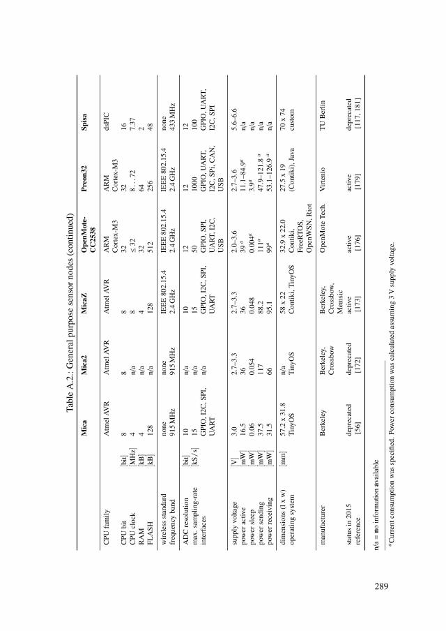
Tabl
eA
.2.:
Gen
eral
purp
ose
sens
orno
des
(con
tinue
d)M
ica
Mic
a2M
icaZ
Ope
nMot
e-C
C25
38Pr
eon3
2Sp
isa
CPU
fam
ilyA
tmel
AVR
Atm
elAV
RA
tmel
AVR
AR
MC
orte
x-M
3A
RM
Cor
tex-
M3
dsPI
C
CPU
bit
[bit ]
88
832
3216
CPU
cloc
k[M
Hz ]
4n/
a8
≤32
8...7
27.
37R
AM
[kB]
4n/
a4
3264
2FL
ASH
[kB]
128
n/a
128
512
256
48
wir
eles
sst
anda
rdno
neno
neIE
EE
802.
15.4
IEE
E80
2.15
.4IE
EE
802.
15.4
none
freq
uenc
yba
nd91
5M
Hz
915
MH
z2.
4G
Hz
2.4
GH
z2.
4G
Hz
433
MH
z
AD
Cre
solu
tion
[bit ]
10n/
a10
1212
12m
ax.s
ampl
ing-
rate
[kS/
s ]15
n/a
1550
1000
100
inte
rfac
esG
PIO
,I2C
,SPI
,U
AR
Tn/
aG
PIO
,I2C
,SPI
,U
AR
TG
PIO
,SPI
,U
AR
T,I2
C,
USB
GPI
O,U
AR
T,I2
C,S
Pi,C
AN
,U
SB
GPI
O,U
AR
T,I2
C,S
PI
supp
lyvo
ltage
[V]
3.0
2.7–
3.3
2.7–
3.3
2.0–
3.6
2.7–
3.6
5.6–
6.6
pow
erac
tive
[mW]
16.5
3636
39a
11.1
–84.
9an/
apo
wer
slee
p[m
W]
0.06
0.05
40.
048
0.00
4a3.
9an/
apo
wer
send
ing
[mW]
37.5
117
88.2
111a
47.9
–121
.8a
n/a
pow
erre
ceiv
ing
[mW]
31.5
6695
.199
a53
.1–1
26.9
an/
a
dim
ensi
ons
(lx
w)
[mm]
57.2
x31
.8n/
a58
x22
32.9
x22
.027
.5x
1970
x74
oper
atin
gsy
stem
Tiny
OS
Tiny
OS
Con
tiki,
Tiny
OS
Con
tiki,
Free
RTO
S,O
penW
SN,R
iot
(Con
tiki)
,Jav
acu
stom
man
ufac
ture
rB
erke
ley
Ber
kele
y,C
ross
bow
Ber
kele
y,C
ross
bow
,M
emsi
c
Ope
nMot
eTe
ch.
Vir
teni
oT
UB
erlin
stat
usin
2015
depr
ecat
edde
prec
ated
activ
eac
tive
activ
ede
prec
ated
refe
renc
e[5
6][1
72]
[173
][1
76]
[179
][1
17,1
81]
n/a=
noin
form
atio
nav
aila
ble
a Cur
rent
cons
umpt
ion
was
spec
ified
.Pow
erco
nsum
ptio
nw
asca
lcul
ated
assu
min
g3
Vsu
pply
volta
ge.
289
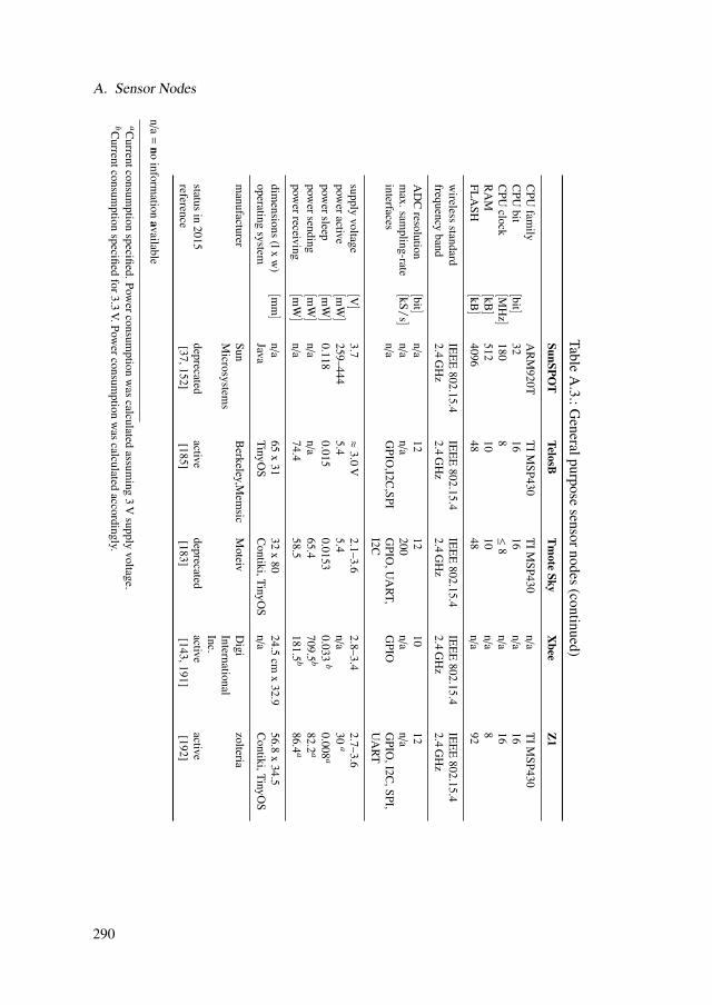
A. Sensor Nodes
TableA
.3.:Generalpurpose
sensornodes(continued)
SunSPOT
TelosBT
mote
SkyX
beeZ
1
CPU
family
AR
M920T
TIM
SP430T
IMSP430
n/a
TIM
SP430C
PUbit
[ bit]32
1616
n/a
16C
PUclock
[ MH
z]180
8≤
8n/a
16R
AM
[ kB]
51210
10n/a
8FL
ASH
[ kB]
409648
48n/a
92
wireless
standardIE
EE
802.15.4IE
EE
802.15.4IE
EE
802.15.4IE
EE
802.15.4IE
EE
802.15.4frequency
band2.4
GH
z2.4
GH
z2.4
GH
z2.4
GH
z2.4
GH
z
AD
Cresolution
[ bit]n/a
1212
1012
max.sam
pling-rate[ kS/
s]n/a
n/a
200n/a
n/a
interfacesn/a
GPIO
,I2C,SPI
GPIO
,UA
RT,
I2CG
PIOG
PIO,I2C
,SPI,U
AR
T
supplyvoltage
[ V]
3.7≈
3.0V
2.1–3.62.8–3.4
2.7–3.6pow
eractive[ m
W]
259–4445.4
5.4n/a
30a
powersleep
[ mW]
0.1180.015
0.01530.033
b0.008
a
powersending
[ mW]
n/a
n/a
65.4709.5
b82.2
a
powerreceiving
[ mW]
n/a
74.458.5
181.5b
86.4a
dimensions
(lxw
)[ m
m]
n/a
65x
3132
x80
24.5cm
x32.9
56.8x
34.5operating
systemJava
TinyOS
Contiki,TinyO
Sn/a
Contiki,TinyO
S
manufacturer
SunM
icrosystems
Berkeley,M
emsic
Moteiv
Digi
InternationalInc.
zolteria
statusin
2015deprecated
activedeprecated
activeactive
reference[37,152]
[185][183]
[143,191][192]
n/a=
noinform
ationavailable
aCurrentconsum
ptionspecified.Pow
erconsumption
was
calculatedassum
ing3
Vsupply
voltage.bC
urrentconsumption
specifiedfor3.3
V.Powerconsum
ptionw
ascalculated
accordingly.
290

B. Evaluating the polynomial kernelof a transposed Farrow filter
The filter equation of a transposed Farrow filter is [7]:
y(lT ′s) =M∑
m=0
Q−1∑q=0
x(tn)ha(lT ′s − tn) (B.1)
with
ha(t) =Q−1∑q=0
M∑m=0
cm[q] fm(q, t) (B.2)
and
fm(q, t) =
⎧⎪⎪⎨⎪⎪⎩(
2(t−qT ′s)T ′s
− 1)m
, qT ′s ≤ t < (q + 1)T ′s0, otherwise
, (B.3)
compare (3.53) to (3.55). The following derivation is given in [7], for the evaluation ofthe polynomial kernel fm at the time t∗ = lT ′s − tn with qT ′s ≤ t∗ < (q + 1)T ′s:
t∗ = lT ′s − tn , inserting (3.57): tn = (µn + ln)T ′s (B.4)= lT ′s − (µn + ln)T ′s (B.5)= (l − ln)T ′s − µnT ′s (B.6)= (q + 1 − µn)T ′s (B.7)
Inserting (B.7) into (B.3) yields:
fm(q, lT ′s − tn) =(
2 ((q + 1 − µn)T ′s − qT ′s)T ′s
− 1)m
(B.8)
= (2(q + 1 − µn − q) − 1)m (B.9)= (1 − 2µn)
m (B.10)
291
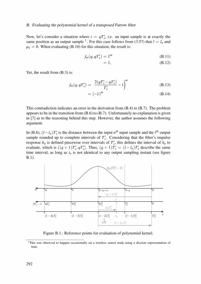
B. Evaluating the polynomial kernel of a transposed Farrow filter
Now, let’s consider a situation where t = qT ′s, i.e. an input sample is at exactly thesame position as an output sample 1. For this case follows from (3.57) that l = ln andµn = 0. When evaluating (B.10) for this situation, the result is:
fm(q, qT ′s) = 1m (B.11)= 1, (B.12)
Yet, the result from (B.3) is:
fm(q, qT ′s) =(
2(qT ′s − qT ′s)T ′s
− 1)m
(B.13)
= (−1)m (B.14)
This contradiction indicates an error in the derivation from (B.4) to (B.7). The problemappears to be in the transition from (B.6) to (B.7). Unfortunately no explanation is givenin [7] as to the reasoning behind this step. However, the author assumes the followingargument:
In (B.6), (l− ln)T ′s is the distance between the input nth input sample and the lth outputsample rounded up to complete intervals of T ′s. Considering that the filter’s impulseresponse ha is defined piecewise over intervals of T ′s, this defines the interval of ha toevaluate, which is ((q + 1)T ′s, qT ′s]. Thus, (q + 1)T ′s = (l − ln)T ′s describe the sametime interval, as long as tn is not identical to any output sampling instant (see figureB.1).
Figure B.1.: Reference points for evaluation of polynomial kernel.
1This was observed to happen occasionally on a wireless sensor node using a discrete representation oftime.
292

However, if tn is identical to an output sampling instant, the fractional interval becomesµn = 0 and (l− ln)T ′s = qT ′s due to (B.3). Thus, the case of µn = 0 does appear to havebeen overlooked in [7]. Therefore, (B.10) needs to be extended as follows, in order toalways yield correct results:
fm(q, lT ′s − tn) =
(1 − 2µn)m , µn , 0(−1)m , µn = 0 . (B.15)
293

C. Application sensors
C.1. MicrophoneSchmitt-Trigger
VorstufeMikrofon
Hochpass
Stützkondensator für IC
Impedanzwandler
RESETNGPIO37
GPIO36GPIO35
GPIO34GPIO33
GPIO32GPIO25
GPIO24(GPIO23)
(GPIO22)(GPIO21)
GPIO20GPIO19
GPIO18
GPIO1GPIO0
GPIO6GPIO8
GPIO7
GPIO10GPIO9
GPIO12GPIO11
GPIO14GPIO13
GPIO16GPIO15
VDD
GND
GNDGND
VDD
VDD
VDDGND
VDD
VDDGNDGND
GND
GND
10k
10k 10k
470k
6.8n
100n
500k
500k
500k
MCP6004-I/PP
MCP6004-I/PP
MCP6004-I/PP
MCP6004-I/PP
GND
R1
R4 R3
R2
C1
C2
1 2
TR1
13
2
TR21 3
2
TR31
3
2
P112
34
56
78
910
1112
1314
1516 P21
23
45
67
89
1011
1213
1415
16
JP11
JP21
JP41
JP8 1
JP51
JP61
411
IC1D13 12
14
IC1B6 5
7
9 108
IC1C
IC1A2 3
1
JP31
JP7 1
Florian RoubalAUTHOR:
Figure C.1.: Circuit diagram of the microphone module [Stud22].
294

C.2. Current and voltage sensors
C.2. Current and voltage sensors
ADC1
ADC2
ADC3
ADC4
ADC5
ADC6
PTC
Fuse
TL07
4DTL
074D
TL07
4DTL
074D
100k
100k
26,1k
100k
100k
100k
15,4k
100k
100k
TL07
4DTL
074D
TL07
4DTL
074D
100k
100k
15,4k
100k
100k
100k
16,5k
100k
100k
15,4k
26,1k
100k
26,1k
TL07
4DTL
074D
100k
16,5k
100k
100k
100k
16,5k
100k
100k
TL07
4DTL
074D
10u
10u
10u10
0u
100k
100k
100k
91k 100k
12k 100k
TL07
4DTL
074D
TL07
4D
TL07
4D
100k20k
PREO
N32
LP29
50Z
GND
DUAL
-BNC
DUAL
-BNC
DUAL
-BNC
100n
100u
100u
1u
100n
100n
100n
100n
IC1A
2 31
IC1B
6 57
IC1C
9 108
IC1D
13 1214
R1_U
U
R2_U
U
R3_F
1C_U
U R4_U
U
R5_U
U
4 11
R2_U
V
R3_F
1E_U
V R4_U
V
R5_U
V
IC2A
2 31
IC2B
6 57
IC2C
9 108
IC2D
13 1214
R1_U
W
R2_U
W
R3_F
1E_U
W R4_U
W
R5_U
W
R2_IU
R3_IU
R4_IU
R5_IU
4 11
R3_F
1E_U
UJP
1 12
34
JP2 1
23
4
JP3 1
23
4
R3_F
1C_U
VR1
_UV
R3_F
1C_U
W
IC3C
9 108
IC3D
13 1214
R2_IV
R3_IV
R4_IV
R5_IV
R2_IW
R3_IW
R4_IW
R5_IW
IC3A
2 31
IC3B
6 57
4 11
C1 C2C3
L1X1
-1
X1-2
R1_IW
R1_IV
R1_IU
R1_ADD_F1C R2_ADD_F1C
R1_ADD_F1E R2_ADD_F1E
JP4 1
23
4
IC4C
9 108
IC4A
2 31
IC4B
6 57
IC4D
13 1214
4 11
R2_ADD_STROMR1_ADD_STROM
15P1
13P1
11P1
16P1
14P1
12P1
9P1
7P1
10P1
8P1
5P1
3P1
1P1
6P1
4P1
2P1
15P2
13P2
11P2
16P2
14P2
12P2
9P2
7P2
10P2
8P2
5P2
3P2
1P2
6P2
4P2
2P2
U$1
GND
I3
O1
2
IC5
C4
U V W
JP5 1 2
C5
L2 L3
C6
C7C8
C9C1
0
DC2 +V
IN1
-VIN
12+V
OUT
11
-VOU
T2
14 231324
COM
1015
COM
322
D1
11
UV
UV
UU
UU
IU
IU
UW
UW
IV
IV
IW
IW
IW_IN
IW_IN
IV_IN
IV_IN
IU_IN
IU_IN
UU_IN
UU_IN
UV_IN
UV_IN
UW_IN
UW_IN
U_AD
D_F1
C
U_AD
D_F1
C
U_AD
D_F1
E
U_AD
D_F1
E0V0V 0V 0V
0V0V
0V0V
0V0V
0V
0V 0V 0V
0V
0V
0V 0V 0V 0V 0V 0V
0V
0V
V+
V+
U_ADD_SPANNUNG
12V
U_AD
D_ST
ROM
U_ADD_STROM
VDD
P1P2
DC/D
C CO
NVER
TER
Figure C.2.: Circuit diagram of the signal conditioning module [Stud9].
295

C. Application sensors
21.12.15 16:28 f=0.69 /home/jfunck/Forschung/Stromwandler/Stromwandler_eagle/CurrentVoltageTransformer.sch (Sheet: 1/1)
TL074CDSMDTL074CDSMD
TL074CDSMDTL074CDSMD
3k96k8
15n
6n8GND
TL074CDSMD
TL074CDSMDTL074CDSMD
TL074CDSMD
GND
+15V
-15V
3k96k8
15n
6n8GND
3k96k8
15n
6n8GND
3k96k8
15n
6n8GNDGND
GND82
GND
-15V
+15V
100n100n
GND GND
64Y-5,0k
64Y-5,0k 4k74k7 4k7
4k7
GND
4k7
4k7
GND
8282
82
+15V
-15V
100n100n
GNDGND
64Y-500+15V-15V
10k10k
100n
47k
47k47k
47k
+15V
-15V
TL074CDSMDTL074CDSMD
TL074CDSMDTL074CDSMD
3k96k8
15n
6n8GND
TL074CDSMD
TL074CDSMDTL074CDSMD
TL074CDSMD
GND
+15V
-15V
3k96k8
15n
6n8GND
3k96k8
15n
6n8GND
3k96k8
15n
6n8GNDGND
GND
180
GND
-15V
+15V
100n100n
GND GND
64Y-5,0k
64Y-5,0k 4k74k7 4k7
4k7
GND
4k7
4k7
GND
LV_25-P/SP5
180180
180
+15V
100n100nGNDGND
64Y-500+15V-15V
10k10k
100n
-15V
100nGND
100nGND
100nGND
100nGND
rad 470/35
rad 470/35
100n
100n
GND
MKDS_5/2-9,50
MKDS_5/2-9,50
KSI1-5085MMKSI1-5085MMKSI1-5085MM
1-227161-0
1-227161-0
1-227161-0
1-227161-0
MKDS_5/2-9,50
MKDSN1,5/5-5,08
22-23-2021
2 31
IC12A
6 57
IC12B
9 108
IC12C
13 1214
IC12D
411
R101R102
C102
C1012 3
1IC11A
6 57
IC11B910
8IC11C
131214
IC11D
411
R103R104
C104
C103
R105R106
C106
C105
R107R108
C108
C107
RM104
C114C115
1 3
2
POT103
13
2
POT101
R109R110
R113
R115
R116
R117RM101RM103
RM102
C109C110
13
2
POT102
R111R112
C111
RV2
RV4RV3
RV1
2 31
IC22A
6 57
IC22B
9 108
IC22C
13 1214
IC22D
411
R201R202
C202
C2012 3
1IC21A
6 57
IC21B910
8IC21C
131214
IC21D
411
R203R204
C204
C203
R205R206
C206
C205
R207R208
C208
C207
RM204
C214C215
1 3
2
POT203
13
2
POT201
R209R210
R213
R215
R216
R217LEM2
I+I-
V+V- M
RM201RM203
RM202
C209C210
13
2
POT202
R211R212
C211
C112C113C212C213
C5C6
C7C8
V+MV-
P1P2P3P4P5P6P7P8P9P10
U$2
LA_35-NP
INOUT
F2X1-1X1-2
X2-1
X2-2
12J13
12J1
12J2 12
J3 12J4 12J5
12J6 12J7 12J8
12J9 12
J10 12J11
X3 X5 X6 X7
X8-1
X8-2
X9-1
X9-2
X9-3
X9-4X9-5
X4-1X4-2
++
Figure C.3.: Circuit diagram of current/voltage transducer modules.
296

C.3. Rotary encoder
C.3. Rotary encoder
21.12
.15 14
:13 /h
ome/j
funck
/Forsc
hung
/wsn
/A Or
ganis
ation
und B
erich
te/11
_Sch
altplä
ne/D
rehge
berTe
stplat
ine/D
rehge
berTe
stplat
ine_0
2.sch
(She
et: 1/
1)
4050
N
4050
N
4050
N
4050
N
4050
N
4050
N
GND
GND
10uF
100n
F
100n
F GND
+3V3
+5V
GREEN150R
GND
YELLOW56R
GND
+5V
+3V3
+5V
L494
0V5
GND
GND
+3V3
120R 120R 120R 220p
F22
0pF
GND
220p
F22
0pF
GND
220p
F22
0pF
GND
GND
GND
GND
+5V
100n
F
+5V GND
GND
23
IC1A 4
5IC
1B 67
IC1C
109
IC1D 12
11IC
1E 1514
IC1F
81 IC1PVDD VSS
16
27
38
49
5
X1
C1C2
C3
F1
LED1R1
LED2R2
VI1
2
VO3
IC3
GND
2 13IC2A
AM26
LS32
AC
6 75IC2B
AM26
LS32
AC
10 911IC2C
AM26
LS32
AC
14 1513IC2D
AM26
LS32
AC
8GNDVCC
16 IC2P
ENAB
LE
IC2E
NAM
26LS
32AC
R3 R4 R5
C4C5
C6C7
C8C9
12345678910
111213141516
JP1
12345678910
111213141516
JP2
C10
LSP1 LSP2
12
JP53
45
6
LSP3 LSP4
GND
T1-C
H1,AD
C0-1,
GPIO
6T1
-CH3
,USA
RT1-R
X,ADC
0-3,G
PIO8
UIRQ
7,DAC
1,SPI0
-SCK
,ADC0
-5,GP
IO10
UIRQ
8,SPI0
-MOS
I,ADC
0-7,G
PIO12
ADC0
-15,G
PIO14
ADC0
-9,GP
IO16
VDD1
VDD2
ADC0
-8,GP
IO15
ADC0
-14,G
PIO13
SPI0-
MISO
,ADC0
-6,GP
IO11
UIRQ
6,DAC
0,SPI-
NSS,A
DC0-4
,GPIO
9T1
-CH2
,USA
RT1-T
X,ADC
0-2,G
PIO7
UIRQ
0,T0-C
H0,C
AN0-T
X,I2C
0-SDA
,GPIO
0UI
RQ1,T
0-CH1
,CAN
0-RX,I
2C0-S
CL,G
PIO1
GND
RESE
TNGP
IO36
,SPI2-
MISO
,JTAG
-NTR
STGP
IO37
,SPI2-
MOSI
GPIO
35,SP
I2-SC
K,JTA
G-TD
OGP
IO34
,SPI-N
SS,JT
AG-TD
I,UIR
W14
GPIO
32,JT
AG,TM
S,UIR
Q12
GPIO
33,JT
AG-TC
K,UIR
Q13
GPIO
25GP
IO24
GPIO
22,SP
I-RF-M
ISOGP
IO23
,SPI-R
F-MOS
IGP
IO21
-SPI-
RF-S
CKGP
IO20
,USA
RT2-C
K,SPI1
-NSS
,UIR
Q11
GPIO
18,U
SART
2-TX,I
2C-S
CL,U
IRQ9
GPIO
19,U
SART
2-RX,I
2C-S
DA,U
IRQ1
0
PREO
N32-S
HUTT
LEP1
P2
UA0_
PUA
0_N
UA1_
PUA
1_N
UA2_
PUA
2_N
+
Figure C.4.: Circuit diagram of rotary encoder interface circuit board.
297

D. Angular resampling filer
D.1. Filter design
1 %% Farrow f i l t e r% Farrow c o e f f i c i e n t s
3 c o e f f F a r = [ 1 /4 8 , 1 /1 6 , 1 /1 6 , 1 / 4 8 ;2 3 /4 8 , 5 /1 6 , −1 /16 , −1 /16;
5 2 3 /4 8 , −5 /16 , −1 /16 , 1 / 1 6 ;1 /4 8 , −1 /16 , 1 /1 6 , −1 /4 8 ] ;
7
M = s i z e ( c o e f f F a r , 2 ) −1;9 N = s i z e ( c o e f f F a r , 1 ) ;
%% FIR f i l t e r (G) a t o u t p u t s o f Farrow f i l t e r s11 wp = 0 . 5 ; % passband r e l a t i v e t o h a l f o f o u t p u t f r e q u e n c y [ 1 ]
OSRout = 2 ; % o v e r s a m p l i n g r a t i o a t i n p u t o f o u t p u t s t a g e [ 1 ]13
% band− s p e c i f i c a t i o n t o compensa te Farrow f i l t e r passband drop15 F1 = l i n s p a c e ( 0 , wp /OSRout , 2 0 ) ;
[ h f a rpb , ˜ ] = f r e q p s ( c o e f f F a r ( (1+N / 2 ) : end , : ) ’ , F1 * ( OSRout / 2 ) , 1 / ( OSRout ) ) ;17 D1 = 1 . / h f a r p b ;
D1 ( i s n a n ( D1 ) ) = 1 ;19 F2 = l i n s p a c e ( 0 . 4 , 1 , 1 0 0 ) ;
D2 = z e r o s ( 1 , l e n g t h ( F2 ) ) ;21
% c a l c u l a t e FIR f i l t e r c o e f f i c i e n t s u s i n g l e a s t − s q u a r e s o p t i m i z a t i o n23 d = f d e s i g n . arbmag ( ’N,B,F,A’ , 6 1 , 2 , F1 , D1 , F2 , D2 ) ;
hG = d e s i g n ( d , ’firls’ ) ;25 coef fG = hG . Numerator ;
27
%% Ouput d e c i m a t o r (D)29 % d e c i m a t i o n and r i p p l e s p e c i f i c a t i o n
tSNR = 7 4 ; % t a r g e t SNR [ dB ]31 As = tSNR ; % s t o p b a n d r i p p l e [ dB ]
dp = s q r t ( 2 ) *10ˆ( − tSNR / 2 0 ) ; % passband r i p p l e [ 1 ]33 Ap = 20* log10 ( (1+ dp ) / (1 − dp ) ) ; % passband r i p p l e [ dB ]
d = f d e s i g n . d e c i m a t o r ( OSRout , ’lowpass’ , ’fp,fst,ap,ast’ , . . .35 wp /OSRout , 0 . 5 , Ap , As ) ;
% c a l c u l a t e FIR d e c i m a t o r c o e f f i c i e n t s u s i n g e q u i r i p p l e method37 hD = e q u i r i p p l e ( d ) ;
coe f fD = hD . Numerator ;
Listing D.1: MATLAB code to calculate the coefficients of angular resamplingfilter.
298

D.1. Filter design
f u n c t i o n [ h , f ] = f r e q p s ( c , f , T )2 % f u n c t i o n [ h , f ] = f r e q p s ( c , f , T )
% −−−−−−−−−−−−−−−−−−−−−−−−−−−−−−−−−−−−−−−−−−−−−−−−−−−−−−4 % f i l e n a m e : f r e q p .m
% a u t h o r : Juergen Funck ( j u e r g e n . funck@tu− b e r l i n . de )6 % o r g a n i s a t i o n : TU B e r l i n
% p r o j e c t : wsn8 % d a t e : 1 4 . 0 2 . 2 0 1 4
% −−−−−−−−−−−−−−−−−−−−−−−−−−−−−−−−−−−−−−−−−−−−−−−−−−−−−−10 % d e s c r i p t i o n : c a l c u l a t e s t h e magni tude f r e q u e n c y r e s p o n s e o f a c o n t i n u o u s
% p i e c e w i s e p o l y n o m i a l f i l t e r as d e s c r i b e d i n12 % Vesma1996 ” I n t e r p o l a t i o n f i l t e r s w i t h a r b i t r a r y f r e q u e n c y
% r e s p o n s e f o r a l l − d i g i t a l r e c e i v e r s ” and Babic200814 % ” Polynomia l −Based I n t e r p o l a t i o n F i l t e r s f o r DSP−A p p l i c a t i o n s ” ( p . 42)
% i n p u t : c − c o e f f i c i e n t m a t r i x16 % f − f r e q u e n c y v e c t o r
% T − p o l y n o m i a l i n t e r v a l l e n g t h18 %
% o u t p u t h − f r e q u e n c y r e s p o n s e20 % f − f r e q u e n c y v e c t o r
22 % g e t d i m e n s i o n s[m, n ] = s i z e ( c ) ;
24 M = m−1;N = 2*n ;
26
h = z e r o s ( 1 , l e n g t h ( f ) ) ;28
f o r i =1: l e n g t h ( f )30 f o r n = 0 : ( (N / 2 ) −1)
f o r m=0:M32 h ( i ) = h ( i ) + c (m+1 , n+1) *G( n ,m, f ( i ) ,T ) ;
end34 end
end36
end38
f u n c t i o n g = G( n ,m, f , T )40 w = 2* p i * f *T ;
i f ( mod (m, 2 ) ==0)42 % even m
g = 2* cos (w*( n+0 . 5 ) ) * ( ( ( −1 ) ˆ (m / 2 ) ) * f a c t o r i a l (m) * P s i (m, f , T ) + s i n c ( f *T ) ) ;
44 e l s e% odd m
46 g = 2*( ( −1) ˆ ( (m+1) / 2 ) ) * f a c t o r i a l (m) * s i n (w*( n+0 . 5 ) ) * P s i (m, f , T ) ;end
48 end
50 f u n c t i o n p = P s i (m, f , T )k = 0 : f l o o r ( (m−1) / 2 ) ;
52
p = sum ( ( ( p i * f *T ) . ˆ ( 2 * k−m) ) . * ( ( −1) . ˆ k ) . / f a c t o r i a l (2* k ) . * . . .54 ( s i n c ( f *T ) − cos ( p i * f *T ) . / ( 2 * k+1) ) ) ;
end
Listing D.2: Function to calculate the frequency response of a piecewise polynomialfilter.
299

D. Angular resampling filer
D.2. MATLAB implementation
1 [ y2 ] = r e s a m p l e A n g u l a r F a r r o w ( d ou b l e ( x ) , 1 / param . f i n , t p h i , [ ] , hFarOut ) ;
3 % o u t p u t s t a g ey = f i l t e r ( hout , do ub l e ( y2 ) ) ;
5 Mout = f l o o r ( ( l e n g t h ( y )−param . N s e t t l e ) / param . f o u t ) * param . f o u t ;y = r e s h a p e ( y ( param . N s e t t l e + ( 1 : Mout ) ) , [ ] , 1 ) ;
Listing D.3: MATLAB implementation of angular resampling filter.
f u n c t i o n [ y , s t a t e , l k ] = r e s a m p l e A n g u l a r F a r r o w ( x , Tin , t p h i , s t a t e , hFarOut )2 % f u n c t i o n [ y , s t a t e ] = resampleAngu larFarrow ( x , tend , t p h i )
% −−−−−−−−−−−−−−−−−−−−−−−−−−−−−−−−−−−−−−−−−−−−−−−−−−−−−−4 % f i l e n a m e : r e s a m p l e A n g u l a r B l o c k .m
% a u t h o r : Juergen Funck ( j u e r g e n . funck@tu− b e r l i n . de )6 % o r g a n i s a t i o n : TU B e r l i n
% p r o j e c t : wsn8 % d a t e : 2 2 . 0 1 . 2 0 1 4
% −−−−−−−−−−−−−−−−−−−−−−−−−−−−−−−−−−−−−−−−−−−−−−−−−−−−−−10 % d e s c r i p t i o n : p e r f o r m e s a n g u l a r r e s a m p l i n g on a b l o c k o f da ta
% i n p u t : x − i n p u t s i g n a l12 % t e n d − t i m e o f l a s t sample
% ( t i m e o f f i r s t sample i s i m p l i c i t l y t 0 =0)14 % t p h i − r e s a m p l i n g t i m e s w i t h r e f e r e n c e t o s t a r t o f b l o c k
% s t a t e − s t r u c t u r e c o n t a i n i n g t h e i n i t a l f i l t e r s t a t e16 %
% o u t p u t : y − re sampled s i g n a l18 % s t a t e − s t r u c t u r e c o n t a i n i n g t h e f i n a l f i l t e r s t a t e
% −−−−−−−−−−−−−−−−−−−−−−−−−−−−−−−−−−−−−−−−−−−−−−−−−−−−−20 %% p a r a m e t e r s
% c o e f f i c i e n t s o f f a r row f i l t e r22 % c ( n ,m) , n = 1 . . . 4 , m= 1 . . . 4
c = [ 1 /4 8 , 1 /1 6 , 1 /1 6 , 1 / 4 8 ;24 2 3 /4 8 , 5 /1 6 , −1 /16 , −1 /16;
2 3 /4 8 , −5 /16 , −1 /16 , 1 / 1 6 ;26 1 /4 8 , −1 /16 , 1 /1 6 , −1 /4 8 ] ;
M = s i z e ( c , 2 ) −1;28 N = s i z e ( c , 1 ) ;
30 %% i n i t i a l i z a t i o n% far row b u f f e r s
32 Min = l e n g t h ( x ) ;Mout = l e n g t h ( t p h i ) ;
34 y = z e r o s ( 1 , Mout ) ;
36 i f ( i s e m p t y ( s t a t e ) )s t a t e . e taX = z e r o s (M+1 ,1) ;
38 s t a t e . e t a P = z e r o s (M+1 ,1) ;s t a t e . yXbuf = z e r o s (N, 1 ) ;
40 s t a t e . yPbuf = z e r o s (N, 1 ) ;s t a t e . zX = z e r o s ( 1 , l e n g t h ( hFarOut . Numerator ) −1) ;
42 s t a t e . zP = z e r o s ( 1 , l e n g t h ( hFarOut . Numerator ) −1) ;end
44
l k = 1 ;46
%% f i l t e r loop48 % loop over a l l i n p u t samples
f o r k=1: Min50 % n e x t o u t p u t i n t e r v a l
whi le ( ( ( k−1) * Tin ) > t p h i ( l k +1) )
300

D.2. MATLAB implementation
52 i f ( ( l k +1) < Mout )% c a l c u l a t e o u t p u t sample
54 f o r n=0 : (N−1)i f ( n<(N−1) )
56 s t a t e . yXbuf ( n+1) = s t a t e . yXbuf ( n+2) ;s t a t e . yPbuf ( n+1) = s t a t e . yPbuf ( n+2) ;
58 e l s es t a t e . yXbuf ( n+1) = 0 ;
60 s t a t e . yPbuf ( n+1) = 0 ;end
62
% sum over p o l y n o m i a l o r d e r64 f o r m=0:M
s t a t e . yXbuf ( n+1) = s t a t e . yXbuf ( n+1)+c ( n+1 ,m+1) * s t a t e . e taX (m+1) ;
66 s t a t e . yPbuf ( n+1) = s t a t e . yPbuf ( n+1)+c ( n+1 ,m+1) * s t a t e . e t a P (m+1) ;
end68 end
70 % f i n a l o u t p u t sample[ tempX , s t a t e . zX ] = f i l t e r ( hFarOut . Numerator , 1 , s t a t e . yXbuf ( 1 ) , s t a t e
. zX ) ;72 [ tempP , s t a t e . zP ] = f i l t e r ( hFarOut . Numerator , 1 , s t a t e . yPbuf ( 1 ) , s t a t e
. zP ) ;
74 y ( l k ) = tempX / tempP ;
76 % i n c r e m e n t o u t p u t i n d e xl k = l k +1;
78
% r e s e t i n t e g r a t o r b u f f e r80 s t a t e . e taX = z e r o s (M+1 ,1) ;
s t a t e . e t a P = z e r o s (M+1 ,1) ;82 e l s e
break ;84 end
end86 mu = ( ( k−1) * Tin− t p h i ( l k ) ) / ( t p h i ( l k +1)− t p h i ( l k ) ) ;
f = (2* c e i l (mu) −1) *(1−2*mu) ;88
f o r m=0:M90 s t a t e . e taX (m+1) = s t a t e . e taX (m+1) + x ( k ) * ( f ˆm) ;
s t a t e . e t a P (m+1) = s t a t e . e t a P (m+1) + ( f ˆm) ;92 end
end94
%% p o s t p r o c e s s i n g96 % c u t away s u r p l u s samples a t t h e end
y = y ( 1 : ( lk −1) ) ;98 end
Listing D.4: MATLAB implementation of the transposed Farrow filter forresampling.
301

D. Angular resampling filer
D.3. C implementations
D.3.1. C floating-point implementation
# i n c l u d e "dev/leds.h"2 # i n c l u d e "arm_math.h"
4 # i n c l u d e "angularResampler.h"# i n c l u d e "firCoeff_f32.h"
6
/ *−−−−−−−−−−−−−−−−−−−−−−−−−−−−−−−−−−−−−−−−−−−−−−−−−−−−−−−−−−−−−−−−−−−−−−−−−−− * /8 s t a t i c s t r u c t
UInt8 pad ;10 a n g u l a r F a r r o w R e s a m p l e r f 3 2 f a r r o w ;
a r m f i r i n s t a n c e f 3 2 Gp ;12 a r m f i r i n s t a n c e f 3 2 Gx ;
a r m f i r d e c i m a t e i n s t a n c e f 3 2 D;14 f l o a t 3 2 t saveP ;
f l o a t 3 2 t saveX ;16 f l o a t 3 2 t GpBuf [ FIR BUFFER SIZE ] ;
f l o a t 3 2 t GxBuf [ FIR BUFFER SIZE ] ;18 f l o a t 3 2 t GpSta t e [ FIR BUFFER SIZE + FARROW OUTPUT FIR TAPS − 1 ] ;
f l o a t 3 2 t GxSta t e [ FIR BUFFER SIZE + FARROW OUTPUT FIR TAPS − 1 ] ;20 f l o a t 3 2 t D S t a t e [ FIR BUFFER SIZE + OUTPUT FIR TAPS −1] ; r e s a m p l e r ;
22 / *−−−−−−−−−−−−−−−−−−−−−−−−−−−−−−−−−−−−−−−−−−−−−−−−−−−−−−−−−−−−−−−−−−−−−−−−−−− * /void
24 a n g u l a r R e s a m p l e r i n i t f 3 2 ( void )
26 / * i n i t i a l i z e f i l t e r D * /a r m f i r d e c i m a t e i n i t f 3 2 (& r e s a m p l e r . D, OUTPUT FIR TAPS , DECIMATION FACTOR ,
28 o u t p u t F i r C o e f f , r e s a m p l e r . DSta te , FIR BUFFER SIZE ) ;
30 / * i n i t i a l i z e f i l t e r s G * /a r m f i r i n i t f 3 2 (& r e s a m p l e r . Gp , FARROW OUTPUT FIR TAPS ,
f a r r o w O u t p u t F i r C o e f f ,32 r e s a m p l e r . GpSta te , FIR BUFFER SIZE ) ;
a r m f i r i n i t f 3 2 (& r e s a m p l e r . Gx , FARROW OUTPUT FIR TAPS ,f a r r o w O u t p u t F i r C o e f f ,
34 r e s a m p l e r . GxSta te , FIR BUFFER SIZE ) ;
36 / * i n i t i a l i z e fa r ro w f i l t e r * /a n g u l a r F a r r o w R e s a m p l e r i n i t f 3 2 (& r e s a m p l e r . f a r r o w ) ;
38
/ *−−−−−−−−−−−−−−−−−−−−−−−−−−−−−−−−−−−−−−−−−−−−−−−−−−−−−−−−−−−−−−−−−−−−−−−−−−− * /40 UInt32
a n g u l a r R e s a m p l e r p r o c e s s f 3 2 ( a n g u l a r F a r r o w R e s a m p l e r I n p u t f 3 2 * in , f l o a t 3 2 t *out , UInt32 * l k )
42
/ * i n i t l o c a l v a r i a b l e s * /44 UInt32 b l o c k S i z e = 0 ;
46 / * p r e p a r e o u t p u t * /a n g u l a r F a r r o w R e s a m p l e r O u t p u t f 3 2 f a r O u t ;
48 f a r O u t . yP = r e s a m p l e r . GpBuf+ r e s a m p l e r . pad ;f a r O u t . yX = r e s a m p l e r . GxBuf+ r e s a m p l e r . pad ;
50
/ * fa r row f i l t e r * /52 * l k = a n g u l a r F a r r o w R e s a m p l e r p r o c e s s f 3 2 (& r e s a m p l e r . f a r row , in , &f a r O u t ) ;
54 / * r ed uc e b l o c k l e n g t h t o n e x t lower even s i z e * /
302

D.3. C implementations
b l o c k S i z e = * l k −1 + r e s a m p l e r . pad ;56 i f ( b l o c k S i z e % 2)
b l o c k S i z e −= 1 ;58 r e s a m p l e r . pad = 1 ;
r e s a m p l e r . saveX = r e s a m p l e r . GxBuf [ b l o c k S i z e ] ;60 r e s a m p l e r . saveP = r e s a m p l e r . GpBuf [ b l o c k S i z e ] ;
62 e l s e
r e s a m p l e r . pad = 0 ;64
66 / * FIR G * /a r m f i r f 3 2 (& r e s a m p l e r . Gp , r e s a m p l e r . GpBuf , r e s a m p l e r . GpBuf , b l o c k S i z e ) ;
68 a r m f i r f 3 2 (& r e s a m p l e r . Gx , r e s a m p l e r . GxBuf , r e s a m p l e r . GxBuf , b l o c k S i z e ) ;
70 / * d i v i s o r * /f o r ( i n t i =0; i <b l o c k S i z e ; i ++)
72 r e s a m p l e r . GxBuf [ i ] = r e s a m p l e r . GxBuf [ i ] / r e s a m p l e r . GpBuf [ i ] ;
74
/ * f i r d e c i m a t o r * /76 a r m f i r d e c i m a t e f 3 2 (& r e s a m p l e r . D, r e s a m p l e r . GxBuf , out , b l o c k S i z e ) ;
78 / * add samples t h a t were n o t p r o c e s s e d t o b e g i n n i n g o f n e x t b l o c k * /i f ( r e s a m p l e r . pad == 1)
80 r e s a m p l e r . GpBuf [ 0 ] = r e s a m p l e r . saveP ;r e s a m p l e r . GxBuf [ 0 ] = r e s a m p l e r . saveX ;
82
84 re turn ( b l o c k S i z e /DECIMATION FACTOR) ;
Listing D.5: Floating-point C implementation of the angular resampling filter.
1 # i n c l u d e "angularFarrowResampler.h"
3 f l o a t 3 2 t f a r r o w C o e f f f 3 2 [N POLY*(M POLY+1) ] = 1 . 0 / 4 8 . 0 , 1 . 0 / 1 6 . 0 , 1 . 0 / 1 6 . 0 ,1 . 0 / 4 8 . 0 ,
2 3 . 0 / 4 8 . 0 , 5 . 0 / 1 6 . 0 , − 1 . 0 / 1 6 . 0 , − 1 . 0 / 1 6 . 0 ,5 2 3 . 0 / 4 8 . 0 , − 5 . 0 / 1 6 . 0 , − 1 . 0 / 1 6 . 0 , 1 . 0 / 1 6 . 0 ,
1 . 0 / 4 8 . 0 , − 1 . 0 / 1 6 . 0 , 1 . 0 / 1 6 . 0 , − 1 . 0 / 4 8 . 0 ;7 / *−−−−−−−−−−−−−−−−−−−−−−−−−−−−−−−−−−−−−−−−−−−−−−−−−−−−−−−−−−−−−−−−−−−−−−− * /
void9 a n g u l a r F a r r o w R e s a m p l e r i n i t f 3 2 ( a n g u l a r F a r r o w R e s a m p l e r f 3 2 * r e s a m p l e r )
11 i f ( r e s a m p l e r != NULL) f a r r o w F i l t e r i n i t f 3 2 (& r e s a m p l e r −> f i l t e r X ) ;
13 f a r r o w F i l t e r i n i t f 3 2 (& r e s a m p l e r −> f i l t e r P ) ;
15
/ *−−−−−−−−−−−−−−−−−−−−−−−−−−−−−−−−−−−−−−−−−−−−−−−−−−−−−−−−−−−−−−−−−−−−−−− * /17 s i z e t
a n g u l a r F a r r o w R e s a m p l e r p r o c e s s f 3 2 ( a n g u l a r F a r r o w R e s a m p l e r f 3 2 * r e s a m p l e r ,19 a n g u l a r F a r r o w R e s a m p l e r I n p u t f 3 2 * in , a n g u l a r F a r r o w R e s a m p l e r O u t p u t f 3 2 *
o u t )
21 s i z e t k = 0 ;s i z e t l k = 1 ;
23 f l o a t 3 2 t f [M POLY+1 ] ;
25 f o r ( k=1; k<=in −>Min ; k++) / * n e x t o u t p u t i n t e r v a l * /
27 whi le ( ( ( k−1) * in −>Tin ) > in −> t p h i [ l k ] )
303

D. Angular resampling filer
i f ( ( l k +1) < in −>Mout ) 29 / * c a l c u l a t e o u t p u t sample s * /
out−>yX [ lk −1] = f a r r o w F i l t e r o u t p u t f 3 2 (& r e s a m p l e r −> f i l t e r X ) ;31 out−>yP [ lk −1] = f a r r o w F i l t e r o u t p u t f 3 2 (& r e s a m p l e r −> f i l t e r P ) ;
33 / * i n c r e m e n t o u t p u t i n d e x * /l k ++;
35
e l s e
37 / * s t o p p r o d u c i n g o u t p u t samples * /break ;
39
41
/ * c a l c u l a t e n e x t f r a c t i o n a l i n t e r v a l * /43 f a r r o w F i l t e r f r a c I n t e r s f 3 2 ( in −>Tin , in −> t p h i , k , lk , f ) ;
45 / * up da t e s t a t e o f f a r row f i l t e r s f o r f r a c t i o n a l i n t e r v a l * /f a r r o w F i l t e r u p d a t e f 3 2 (& r e s a m p l e r −> f i l t e r X , f , in −>x [ k−1] ) ;
47 f a r r o w F i l t e r u p d a t e f 3 2 (& r e s a m p l e r −> f i l t e r P , f , 1 ) ;
49
re turn l k ;51
/ *−−−−−−−−−−−−−−−−−−−−−−−−−−−−−−−−−−−−−−−−−−−−−−−−−−−−−−−−−−−−−−−−−−−−−−− * /
Listing D.6: Floating-point C implementation of the transposed Farrow filter forresampling.
# i f n d e f FARROW FILTER H2 # d e f i n e FARROW FILTER H
4 # i n c l u d e "arm_math.h"
6 # d e f i n e M POLY 3 / * p o l y n o m i a l o r d e r * /# d e f i n e N POLY 4 / * number o f p o l y n o m i a l s e g m e n t s * /
8
t y p e d e f s t r u c t f a r r o w F i l t e r S t r u c t f 3 2 f a r r o w F i l t e r f 3 2 ;10
e x t er n f l o a t 3 2 t f a r r o w C o e f f f 3 2 [ ] ;12
/ * * s t r u c t u r e t o ho ld t h e c o e f f i c i e n t s and s t a t e o f a fa r row f i l t e r * /14 s t r u c t f a r r o w F i l t e r S t r u c t f 3 2
f l o a t 3 2 t * c o e f f ; / * p o i n t e r t o c o e f f i c i e n t s * /16 f l o a t 3 2 t e t a [M POLY+1 ] ; / * e ta −v a l u e b u f f e r * /
f l o a t 3 2 t ybuf [N POLY ] ; / * o u t p u t v a l u e b u f f e r * /18 ;
20 / * * i n i t i a l i z e s a fa r r ow f i l t e r s t r u c t u r e * /s t a t i c i n l i n e void
22 f a r r o w F i l t e r i n i t f 3 2 ( f a r r o w F i l t e r f 3 2 * f i l t e r )
24 f i l t e r −> c o e f f = f a r r o w C o e f f f 3 2 ;memset ( f i l t e r −>e t a , 0 , (M POLY+1) * s i z e o f ( f l o a t 3 2 t ) ) ;
26 memset ( f i l t e r −>ybuf , 0 , N POLY* s i z e o f ( f l o a t 3 2 t ) ) ;
28
/ * * c a l c u l a t e s t h e f r a c t i o n a l i n t e r v a l f o r a n g u l a r r e s a m p l i n g * /30 s t a t i c i n l i n e void
f a r r o w F i l t e r f r a c I n t e r s f 3 2 ( f l o a t 3 2 t Tin , f l o a t 3 2 t * t p h i , s i z e t k , s i z e t lk, f l o a t 3 2 t * fm )
32
i n t m=0;
304

D.3. C implementations
34 f l o a t 3 2 t f =0;f l o a t 3 2 t mu = ( ( k−1) * Tin − t p h i [ lk −1] ) / ( t p h i [ l k ] − t p h i [ lk −1] ) ;
36
i f (mu==0) 38 f = −1;
40 e l s e
f = (1−2*mu) ;42
44 fm [ 0 ] = 1 ;fm [ 1 ] = f ;
46 f o r (m=2; m<(M POLY+1) ; m++) fm [m] = fm [m−1]* f ;
48
50
/ * * u p d a t e s t h e i n t e r n a l s t a t e o f a f a r r ow f i l t e r w i t h a new f r a c t i o n a li n t e r v a l * /
52 s t a t i c i n l i n e voidf a r r o w F i l t e r u p d a t e f 3 2 ( f a r r o w F i l t e r f 3 2 * f i l t e r , f l o a t 3 2 t * f , f l o a t 3 2 t x )
54
i n t i =0;56
f o r ( i =0; i <(M POLY+1) ; i ++) 58 f i l t e r −> e t a [ i ] = f i l t e r −> e t a [ i ] + x* f [ i ] ;
60
62 / * * c a l c u l a t e s a new o u t p u t sample from a far row f i l t e r * /s t a t i c i n l i n e f l o a t 3 2 t
64 f a r r o w F i l t e r o u t p u t f 3 2 ( f a r r o w F i l t e r f 3 2 * f i l t e r )
66 i n t n=0;i n t m=0;
68
f o r ( n=0; n<N POLY ; n++) 70 i f ( n<(N POLY−1) )
f i l t e r −>ybuf [ n ] = f i l t e r −>ybuf [ n+1 ] ;72
e l s e
74 f i l t e r −>ybuf [ n ] = 0 ;
76
/ * sum over p o l y n o m i a l o r d e r * /78 f o r (m=0; m<(M POLY+1) ; m++)
f i l t e r −>ybuf [ n ] = f i l t e r −>ybuf [ n ] + f i l t e r −> c o e f f [ ( N POLY*n )+m]*f i l t e r −> e t a [m] ;
80
82
/ * r e s e t i n t e g a t o r b u f f e r * /84 f o r (m=0; m<(M POLY+1) ; m++)
f i l t e r −> e t a [m] = 0 ;86
88 / * r e t u r n f i n a l o u t p u t sample * /re turn f i l t e r −>ybuf [ 0 ] ;
90
92 # e n d i f / * FARROW FILTER H * /
Listing D.7: Helper functions for the transposed Farrow filter (C floating-point).
305

D. Angular resampling filer
D.3.2. C fixed-point implementation
# i n c l u d e "dev/leds.h"2 # i n c l u d e "arm_math.h"
# i n c l u d e "lib/list.h"4 # i n c l u d e "lib/memb.h"
6 # i n c l u d e "angularResampler.h"# i n c l u d e "firCoeff_q15.h"
8
# d e f i n e DEBUG DEBUG NONE10 # i n c l u d e "net/ip/uip-debug.h"
12 # d e f i n e BLOCK SIZE 2048# d e f i n e MAX BUFFER BLOCKS 2
14 / *−−−−−−−−−−−−−−−−−−−−−−−−−−−−−−−−−−−−−−−−−−−−−−−−−−−−−−−−−−−−−−−−−−−−−−−−−−− * /s t r u c t i n p u t D a t a B l o c k
16 s t r u c t i n p u t D a t a B l o c k * n e x t ;UInt32 r e a d I n d ;
18 a n g u l a r F a r r o w R e s a m p l e r I n p u t q 1 5 i n ;i n t 1 6 d a t a [ BLOCK SIZE ] ;
20 ;/ *−−−−−−−−−−−−−−−−−−−−−−−−−−−−−−−−−−−−−−−−−−−−−−−−−−−−−−−−−−−−−−−−−−−−−−−−−−− * /
22 s t a t i c s t r u c t UInt8 pad ;
24 a n g u l a r F a r r o w R e s a m p l e r q 1 5 f a r r o w ;a r m f i r i n s t a n c e q 3 1 Gp ;
26 a r m f i r i n s t a n c e q 3 1 Gx ;a r m f i r d e c i m a t e i n s t a n c e q 3 1 D;
28 q 3 1 t saveP ;q 3 1 t saveX ;
30 q 3 1 t GpBuf [ FIR BUFFER SIZE ] ;q 3 1 t GxBuf [ FIR BUFFER SIZE ] ;
32 q 3 1 t DBuf [ FIR BUFFER SIZE / 2 ] ;q 3 1 t GpSta t e [ FIR BUFFER SIZE + FARROW OUTPUT FIR TAPS − 1 ] ;
34 q 3 1 t GxSta t e [ FIR BUFFER SIZE + FARROW OUTPUT FIR TAPS − 1 ] ;q 3 1 t D S ta t e [ FIR BUFFER SIZE + OUTPUT FIR TAPS −1] ;
36 r e s a m p l e r ;/ *−−−−−−−−−−−−−−−−−−−−−−−−−−−−−−−−−−−−−−−−−−−−−−−−−−−−−−−−−−−−−−−−−−−−−−−−−−− * /
38 voida n g u l a r R e s a m p l e r i n i t q 1 5 ( t i m e s t a m p F u n c t popTimestamp )
40
/ * i n i t i a l i z e f i l t e r D * /42 a r m f i r d e c i m a t e i n i t q 3 1 (& r e s a m p l e r . D, OUTPUT FIR TAPS , DECIMATION FACTOR ,
o u t p u t F i r C o e f f q 3 1 , r e s a m p l e r . DSta te , FIR BUFFER SIZE ) ;44
/ * i n i t i a l i z e f i l t e r s G * /46 a r m f i r i n i t q 3 1 (& r e s a m p l e r . Gp , FARROW OUTPUT FIR TAPS ,
f a r r o w O u t p u t F i r C o e f f q 3 1 ,r e s a m p l e r . GpSta te , FIR BUFFER SIZE ) ;
48 a r m f i r i n i t q 3 1 (& r e s a m p l e r . Gx , FARROW OUTPUT FIR TAPS ,f a r r o w O u t p u t F i r C o e f f q 3 1 ,
r e s a m p l e r . GxSta te , FIR BUFFER SIZE ) ;50
/ * i n i t i a l i z e fa r ro w f i l t e r * /52 a n g u l a r F a r r o w R e s a m p l e r i n i t q 1 5 (& r e s a m p l e r . f a r row , popTimestamp ) ;
54 / * i n i t i a l i z e r e s a m p l e r * /r e s a m p l e r . pad = 0 ;
56 r e s a m p l e r . saveP = 0 ;r e s a m p l e r . saveX = 0 ;
58
/ *−−−−−−−−−−−−−−−−−−−−−−−−−−−−−−−−−−−−−−−−−−−−−−−−−−−−−−−−−−−−−−−−−−−−−−−−−−− * /
306

D.3. C implementations
60 UInt8a n g u l a r R e s a m p l e r p r o c e s s q 1 5 ( a n g u l a r F a r r o w R e s a m p l e r I n p u t q 1 5 * in ,
x d c r D a t a B l o c k * o u t )62
/ * i n i t l o c a l v a r i a b l e s * /64 UInt32 b l o c k S i z e = 0 ;
UInt8 blockDone = 0 ;66 UInt32 l k = 0 ;
68 / * p r e p a r e o u t p u t * /a n g u l a r F a r r o w R e s a m p l e r O u t p u t q 1 5 f a r O u t ;
70 f a r O u t . ph i0 = 0 ;f a r O u t . dph i = 0 ;
72 f a r O u t . yP = r e s a m p l e r . GpBuf+ r e s a m p l e r . pad ;f a r O u t . yX = r e s a m p l e r . GxBuf+ r e s a m p l e r . pad ;
74
/ * fa r ro w f i l t e r * /76 l k = a n g u l a r F a r r o w R e s a m p l e r p r o c e s s q 1 5 (& r e s a m p l e r . f a r row , in , &fa rOu t , &
blockDone ) ;
78 / * s e t o u t p u t a n g l e i n f o r m a t i o n * /i f ( r e s a m p l e r . pad >0)
80 f a r O u t . ph i0 −= ( r e s a m p l e r . pad * f a r O u t . dph i ) >>16;
82 out−> t imes t amp = f a r O u t . ph i0 ;out−> s a m p l e p e r i o d = DECIMATION FACTOR* f a r O u t . dph i ;
84
/ * r ed uc e b l o c k l e n g t h t o n e x t lower even s i z e * /86 b l o c k S i z e = l k −1 + r e s a m p l e r . pad ;
i f ( b l o c k S i z e % 2) 88 b l o c k S i z e −= 1 ;
r e s a m p l e r . pad = 1 ;90 r e s a m p l e r . saveX = r e s a m p l e r . GxBuf [ b l o c k S i z e ] ;
r e s a m p l e r . saveP = r e s a m p l e r . GpBuf [ b l o c k S i z e ] ;92
e l s e
94 r e s a m p l e r . pad = 0 ;
96
/ * FIR G * /98 a r m f i r q 3 1 (& r e s a m p l e r . Gp , r e s a m p l e r . GpBuf , r e s a m p l e r . GpBuf , b l o c k S i z e ) ;
a r m f i r q 3 1 (& r e s a m p l e r . Gx , r e s a m p l e r . GxBuf , r e s a m p l e r . GxBuf , b l o c k S i z e ) ;100
/ * d i v i s o r * /102 f o r ( i n t i =0; i <b l o c k S i z e ; i ++)
i f ( r e s a m p l e r . GpBuf [ i ]==0) 104 / * p r e v e n t d i v i s i o n by z e r o * /
r e s a m p l e r . GxBuf [ i ] = 0 ;106
e l s e
108 i n t 6 4 t temp = r e s a m p l e r . GxBuf [ i ] ;temp <<= 1 5 ;
110 r e s a m p l e r . GxBuf [ i ] = ( q 3 1 t ) ( temp / r e s a m p l e r . GpBuf [ i ] ) ;
112
114 / * f i r d e c i m a t o r * /a r m f i r d e c i m a t e q 3 1 (& r e s a m p l e r . D, r e s a m p l e r . GxBuf , r e s a m p l e r . DBuf ,
b l o c k S i z e ) ;116
/ * c o n v e r t t o q15 and copy t o o u t p u t * /118 f o r ( i n t i =0; i <( b l o c k S i z e /DECIMATION FACTOR) ; i ++)
out−>sample s [ i ] = ( q 1 5 t ) r e s a m p l e r . DBuf [ i ] ;120
307
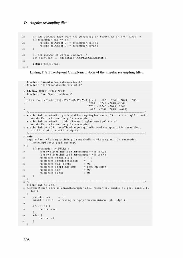
D. Angular resampling filer
122 / * add samples t h a t were n o t p r o c e s s e d t o b e g i n n i n g o f n e x t b l o c k * /i f ( r e s a m p l e r . pad == 1)
124 r e s a m p l e r . GpBuf [ 0 ] = r e s a m p l e r . saveP ;r e s a m p l e r . GxBuf [ 0 ] = r e s a m p l e r . saveX ;
126
128 / * s e t number o f o u t p u t sample s * /out−> r epCoun t = ( b l o c k S i z e /DECIMATION FACTOR) ;
130
re turn blockDone ;132
Listing D.8: Fixed-point C implementation of the angular resampling filter.
# i n c l u d e "angularFarrowResampler.h"2 # i n c l u d e "lib/timestampBuffer_64.h"
4 # d e f i n e DEBUG DEBUG NONE# i n c l u d e "net/ip/uip-debug.h"
6
q 1 5 t f a r r o w C o e f f q 1 5 [N POLY*(M POLY+1) ] = 683 , 2048 , 2048 , 683 ,8 15701 , 10240 ,−2048 ,−2048 ,
15701 ,−10240 ,−2048 , 2048 ,10 683 , −2048 , 2048 , −683 ;/ *−−−−−−−−−−−−−−−−−−−−−−−−−−−−−−−−−−−−−−−−−−−−−−−−−−−−−−−−−−−−−−−−−−−−−−− * /
12 s t a t i c i n l i n e u i n t 8 t g e t I n i t i a l R e s a m p l i n g I n s t a n t s ( q 6 3 t t s t a r t , q 6 3 t t r e f ,a n g u l a r F a r r o w R e s a m p l e r q 1 5 * r e s a m p l e r ) ;
s t a t i c i n l i n e u i n t 8 t u p d a t e R e s a m p l i n g I n s t a n t s ( q 6 3 t t r e f ,a n g u l a r F a r r o w R e s a m p l e r q 1 5 * r e s a m p l e r ) ;
14 s t a t i c i n l i n e q 6 3 t nextTimeStamp ( a n g u l a r F a r r o w R e s a m p l e r q 1 5 * r e s a m p l e r ,u i n t 3 2 t * phi , u i n t 3 2 t * dph i ) ;
/ *−−−−−−−−−−−−−−−−−−−−−−−−−−−−−−−−−−−−−−−−−−−−−−−−−−−−−−−−−−−−−−−−−−−−−−− * /16 void
a n g u l a r F a r r o w R e s a m p l e r i n i t q 1 5 ( a n g u l a r F a r r o w R e s a m p l e r q 1 5 * r e s a m p l e r ,t i m e s t a m p F u n c t popTimestamp )
18
i f ( r e s a m p l e r != NULL) 20 f a r r o w F i l t e r i n i t q 1 5 (& r e s a m p l e r −> f i l t e r X ) ;
f a r r o w F i l t e r i n i t q 1 5 (& r e s a m p l e r −> f i l t e r P ) ;22 r e s a m p l e r −> t p h i l S t a t e = −1;
r e s a m p l e r −> t p h i l n e x t S t a t e = −1;24 r e s a m p l e r −>d e l t a T p h i = 0 ;
r e s a m p l e r −>popTimestamp = popTimestamp ;26 r e s a m p l e r −>p h i = 0 ;
r e s a m p l e r −>dph i = 0 ;28
30 / *−−−−−−−−−−−−−−−−−−−−−−−−−−−−−−−−−−−−−−−−−−−−−−−−−−−−−−−−−−−−−−−−−−−−−−− * /s t a t i c i n l i n e q 6 3 t
32 nextTimeStamp ( a n g u l a r F a r r o w R e s a m p l e r q 1 5 * r e s a m p l e r , u i n t 3 2 t * phi , u i n t 3 2 t *dph i )
34 i n t 6 4 t new = 0 ;u i n t 8 t v a l i d = r e s a m p l e r −>popTimestamp(&new , phi , dph i ) ;
36
i f ( v a l i d ) 38 re turn new ;
40 e l s e
re turn −1;42
308

D.3. C implementations
44 / *−−−−−−−−−−−−−−−−−−−−−−−−−−−−−−−−−−−−−−−−−−−−−−−−−−−−−−−−−−−−−−−−−−−−−−− * /s t a t i c i n l i n e u i n t 8 t
46 g e t I n i t i a l R e s a m p l i n g I n s t a n t s ( q 6 3 t t s t a r t , q 6 3 t t r e f ,a n g u l a r F a r r o w R e s a m p l e r q 1 5 * r e s a m p l e r )
48 whi le ( ( r e s a m p l e r −> t p h i l S t a t e < 0) | |
( r e s a m p l e r −> t p h i l n e x t S t a t e < 0) | |
50 ( r e s a m p l e r −> t p h i l n e x t S t a t e <= t s t a r t ) ) / * t r y u p d a t i n g t i m e s t a m p s * /
52 i f ( ! u p d a t e R e s a m p l i n g I n s t a n t s ( t r e f , r e s a m p l e r ) ) / * up da t e n o t p o s s i b l e * /
54 re turn 0 ;
56
58 / * e n s u r e u pda t e t o new t 0 i n any case * /r e s a m p l e r −> t p h i l = r e s a m p l e r −> t p h i l S t a t e − t r e f ;
60 r e s a m p l e r −> t p h i l n e x t = r e s a m p l e r −> t p h i l n e x t S t a t e − t r e f ;r e s a m p l e r −>d e l t a T p h i = ( r e s a m p l e r −> t p h i l n e x t − r e s a m p l e r −> t p h i l ) >>EXP Q ;
62
re turn 1 ;64
/ *−−−−−−−−−−−−−−−−−−−−−−−−−−−−−−−−−−−−−−−−−−−−−−−−−−−−−−−−−−−−−−−−−−−−−−− * /66 s t a t i c i n l i n e u i n t 8 t
u p d a t e R e s a m p l i n g I n s t a n t s ( q 6 3 t t r e f , a n g u l a r F a r r o w R e s a m p l e r q 1 5 * r e s a m p l e r )68
u i n t 3 2 t tempPhi =0 , tempDphi = 0 ;70 q 6 3 t temp = nextTimeStamp ( r e s a m p l e r , &tempPhi , &tempDphi ) ;
72 i f ( temp < 0) / * no v a l i d t i m e s t a m p i n b u f f e r * /
74 re turn 0 ;
76 e l s e
/ * up da t e t i m e s t a m p s t a t e * /78 r e s a m p l e r −> t p h i l S t a t e = r e s a m p l e r −> t p h i l n e x t S t a t e ;
r e s a m p l e r −> t p h i l n e x t S t a t e = temp ;80
r e s a m p l e r −> t p h i l = r e s a m p l e r −> t p h i l S t a t e − t r e f ;82 r e s a m p l e r −> t p h i l n e x t = r e s a m p l e r −> t p h i l n e x t S t a t e − t r e f ;
r e s a m p l e r −>d e l t a T p h i = ( r e s a m p l e r −> t p h i l n e x t − r e s a m p l e r −> t p h i l )>>EXP Q;
84
r e s a m p l e r −>p h i = tempPhi ;86 r e s a m p l e r −>dph i = tempDphi ;
88 re turn 1 ;
90
/ *−−−−−−−−−−−−−−−−−−−−−−−−−−−−−−−−−−−−−−−−−−−−−−−−−−−−−−−−−−−−−−−−−−−−−−− * /92 s i z e t
a n g u l a r F a r r o w R e s a m p l e r p r o c e s s q 1 5 ( a n g u l a r F a r r o w R e s a m p l e r q 1 5 * r e s a m p l e r ,94 a n g u l a r F a r r o w R e s a m p l e r I n p u t q 1 5 * in , a n g u l a r F a r r o w R e s a m p l e r O u t p u t q 1 5 *
out , u i n t 8 t * blockDone )
96 s i z e t l k = 1 ;q 1 5 t f [M POLY+1 ] ;
98 u i n t 1 6 t s c a l e O u t = 0 x8000 ;
100 PRINTF ( "angularFarrowResampler_process_q15... x=%i,%i,%i,...\n" , in −>x [ 0 ] , in−>x [ 1 ] , in −>x [ 2 ] ) ;
102 * blockDone = 0 ;
309

D. Angular resampling filer
104 / * g e t i n i t i a l t i m e s t a m p s * /i f ( ! g e t I n i t i a l R e s a m p l i n g I n s t a n t s ( in −> t 0 +( in −>k+1) * in −>Tin , in −> t0 ,
r e s a m p l e r ) ) 106 re turn l k ;
108
/ * p r e p a r e o u t p u t * /110 out−>ph i0 = r e s a m p l e r −>p h i ;
out−>dph i = r e s a m p l e r −>dph i ;112
/ * f i l t e r loop * /114 f o r ( ; in −>k< in −>Min ; in −>k++)
/ * n e x t o u t p u t i n t e r v a l * /116 whi le ( ( ( in −>k+1) * in −>Tin ) >= r e s a m p l e r −> t p h i l n e x t )
i f ( l k < in −>Mout ) 118 / * c a l c u l a t e o u t p u t sample s * /
out−>yX [ lk −1] = ( f a r r o w F i l t e r o u t p u t q 1 5 (& r e s a m p l e r −> f i l t e r X ) ) ;120 out−>yP [ lk −1] = 2*( f a r r o w F i l t e r o u t p u t q 1 5 (& r e s a m p l e r −> f i l t e r P )
) ;
122 / * i n c r e m e n t o u t p u t i n d e x * /l k ++;
124 i f ( ! u p d a t e R e s a m p l i n g I n s t a n t s ( in −> t0 , r e s a m p l e r ) ) re turn l k ;
126
128 e l s e
/ * s t o p p r o d u c i n g o u t p u t samples * /130 re turn l k ;
132
134 / * c a l c u l a t e n e x t f r a c t i o n a l i n t e r v a l * /f a r r o w F i l t e r f r a c I n t e r s q 1 5 ( in −>Tin , r e s a m p l e r −> t p h i l , r e s a m p l e r −>
d e l t a T p h i , in −>k , f ) ;136
/ * up da t e s t a t e o f f a r row f i l t e r s f o r f r a c t i o n a l i n t e r v a l * /138 f a r r o w F i l t e r u p d a t e q 1 5 (& r e s a m p l e r −> f i l t e r X , f , in −>x [ in −>k ] ) ;
f a r r o w F i l t e r u p d a t e q 1 5 (& r e s a m p l e r −> f i l t e r P , f , s c a l e O u t / 2 ) ;140
142 / * r e s e t i n p u t i n d e x * /* blockDone = 1 ;
144 re turn l k ;
146 / *−−−−−−−−−−−−−−−−−−−−−−−−−−−−−−−−−−−−−−−−−−−−−−−−−−−−−−−−−−−−−−−−−−−−−−− * /
Listing D.9: Fixed-point C implementation of the transposed Farrow filter forresampling.
# i f n d e f FARROW FILTER Q15 H2 # d e f i n e FARROW FILTER Q15 H
4 # i n c l u d e "arm_math.h"# i n c l u d e "dev/leds.h"
6
/ * e x p o n e n t o f choosen Q f o r m a t * /8 # d e f i n e EXP Q ( 1 4 )
10 / * r e p r e s e n t a t i o n o f u n i t ( 1 ) i n choosen Q f o r m a t * /# d e f i n e UNIT Q (1<<EXP Q )
12
# d e f i n e M POLY 3 / * p o l y n o m i a l o r d e r * /
310

D.3. C implementations
14 # d e f i n e N POLY 4 / * number o f p o l y n o m i a l s e g m e n t s * /
16 t y p e d e f s t r u c t f a r r o w F i l t e r S t r u c t q 1 5 f a r r o w F i l t e r q 1 5 ;
18 e x t er n q 1 5 t f a r r o w C o e f f q 1 5 [ ] ;
20 / * * s t r u c t u r e t o ho ld t h e c o e f f i c i e n t s and s t a t e o f a fa r row f i l t e r * /s t r u c t f a r r o w F i l t e r S t r u c t q 1 5
22 q 1 5 t * c o e f f ; / * p o i n t e r t o c o e f f i c i e n t s * /q 3 1 t e t a [M POLY+1 ] ; / * e ta −v a l u e b u f f e r * /
24 q 6 3 t ybuf [N POLY ] ; / * o u t p u t v a l u e b u f f e r * / ;
26
/ * * i n i t i a l i z e s a fa r row f i l t e r s t r u c t u r e * /28 s t a t i c i n l i n e void
f a r r o w F i l t e r i n i t q 1 5 ( f a r r o w F i l t e r q 1 5 * f i l t e r )30
f i l t e r −> c o e f f = f a r r o w C o e f f q 1 5 ;32 memset ( f i l t e r −>e t a , 0 , (M POLY+1) * s i z e o f ( q 3 1 t ) ) ;
memset ( f i l t e r −>ybuf , 0 , N POLY* s i z e o f ( q 6 3 t ) ) ;34
36 / * * c a l c u l a t e s t h e f r a c t i o n a l i n t e r v a l f o r a n g u l a r r e s a m p l i n g * /s t a t i c i n l i n e void
38 f a r r o w F i l t e r f r a c I n t e r s q 1 5 ( q 6 3 t Tin , q 6 3 t t p h i l , q 3 1 t d e l t a T p h i , s i z e t k ,q 1 5 t * fm )
40 i n t m=0;q 3 1 t f = 0 ;
42
q 3 1 t mu = 0 ;44 q 3 1 t num = ( k+1) * Tin − t p h i l ;/ / q 3 1 t num = k * Tin − t p h i l ;
46
i f ( d e l t a T p h i !=0) 48 mu = num / d e l t a T p h i ;
50 e l s e
l e d s o n ( LEDS RED ) ;52
54 i f (mu==0) f = −UNIT Q ; / * = −1 i n Q17 . 1 4 f o r m a t * /
56
e l s e
58 f = ( UNIT Q−2*mu) ;
60
fm [ 0 ] = UNIT Q ; / * = 1 i n Q1 . 1 4 f o r m a t * /62 fm [ 1 ] = f ;
f o r (m=2; m<(M POLY+1) ; m++) 64 fm [m] = ( ( q 3 1 t ) fm [m−1]* f )>>EXP Q ;
66
68 / * * u p d a t e s t h e i n t e r n a l s t a t e o f a f a r r ow f i l t e r w i t h a new f r a c t i o n a li n t e r v a l * /
s t a t i c i n l i n e void70 f a r r o w F i l t e r u p d a t e q 1 5 ( f a r r o w F i l t e r q 1 5 * f i l t e r , q 1 5 t * f , q 1 5 t x )
72 i n t i =0;
74 f i l t e r −> e t a [ 0 ] = f i l t e r −> e t a [ 0 ] + x ;
311

D. Angular resampling filer
76 f o r ( i =1; i <(M POLY+1) ; i ++) q 3 1 t temp = ( q 3 1 t ) x* f [ i ] ;
78 f i l t e r −> e t a [ i ] = f i l t e r −> e t a [ i ] + ( temp>>EXP Q ) ;
80
82 / * * c a l c u l a t e s a new o u t p u t sample from a far row f i l t e r * /s t a t i c i n l i n e q 3 1 t
84 f a r r o w F i l t e r o u t p u t q 1 5 ( f a r r o w F i l t e r q 1 5 * f i l t e r )
86 i n t n=0;i n t m=0;
88
f o r ( n=0; n<N POLY ; n++) 90 i f ( n<(N POLY−1) )
f i l t e r −>ybuf [ n ] = f i l t e r −>ybuf [ n+1 ] ;92
e l s e
94 f i l t e r −>ybuf [ n ] = 0 ;
96
/ * sum over p o l y n o m i a l o r d e r * /98 f o r (m=0; m<(M POLY+1) ; m++)
q 6 3 t temp = ( q 6 3 t ) f i l t e r −> c o e f f [ ( N POLY*n )+m]* f i l t e r −> e t a [m] ;
100 f i l t e r −>ybuf [ n ] = f i l t e r −>ybuf [ n ] + temp ;
102
104 / * r e s e t i n t e g r a t o r b u f f e r * /f o r (m=0; m<(M POLY+1) ; m++)
106 f i l t e r −> e t a [m] = 0 ;
108
/ * r e t u r n f i n a l o u t p u t sample * /110 re turn ( f i l t e r −>ybuf [0]>>15) ;
112
# e n d i f / * FARROW FILTER H * /
Listing D.10: Helper functions for the transposed Farrow filter (C fixed-point).
312

D.3. C implementations
D.3.3. C header files for floating- and fixed-point
1 # i n c l u d e "mstl/mstl.h"# i n c l u d e "angularFarrowResampler.h"
3
/ * * b u f f e r s i z e i f f i l t e r s G * /5 # d e f i n e FIR BUFFER SIZE 160
7 / * ** \ b r i e f i n i t i a l i z e s t h e a n g u l a r r e s a m p l e r
9 * /void a n g u l a r R e s a m p l e r i n i t f 3 2 ( void ) ;
11 void a n g u l a r R e s a m p l e r i n i t q 1 5 ( t i m e s t a m p F u n c t popTimestamp ) ;
13 / * ** \ b r i e f p r o c e s s a b l o c k o f i n p u t samples
15 * \param i n i n p u t s t r u c t u r e* \param o u t o u t p u t s t r u c t u r e
17 * \ r e t u r n number o f o u t p u t samples p r o c e s s e d* /
19 UInt32 a n g u l a r R e s a m p l e r p r o c e s s f 3 2 ( a n g u l a r F a r r o w R e s a m p l e r I n p u t f 3 2 * in ,f l o a t 3 2 t * out , UInt32 * l k ) ;
UIn t8 a n g u l a r R e s a m p l e r p r o c e s s q 1 5 ( a n g u l a r F a r r o w R e s a m p l e r I n p u t q 1 5 * in ,x d c r D a t a B l o c k * o u t ) ;
Listing D.11: Common header for C implementations of the angular resamplingfilter.
1 # i f n d e f ANGULAR FARROW RESAMPLER H# d e f i n e ANGULAR FARROW RESAMPLER H
3
# i n c l u d e "farrowFilter_f32.h"5 # i n c l u d e "farrowFilter_q15.h"
# i n c l u d e "arm_math.h"7
t y p e d e f u i n t 8 t (* t i m e s t a m p F u n c t ) ( i n t 6 4 t * t imes tamp , u i n t 3 2 t * phi0 ,u i n t 3 2 t * dph i ) ;
9
t y p e d e f s t r u c t r e s a m p l e r S t a t e S t r u c t f 3 2 a n g u l a r F a r r o w R e s a m p l e r f 3 2 ;11 t y p e d e f s t r u c t r e s a m p l e r S t a t e S t r u c t q 1 5 a n g u l a r F a r r o w R e s a m p l e r q 1 5 ;
t y p e d e f s t r u c t a n g u l a r F a r r o w R e s a m p l e r I n S t r u c t f 3 2a n g u l a r F a r r o w R e s a m p l e r I n p u t f 3 2 ;
13 t y p e d e f s t r u c t a n g u l a r F a r r o w R e s a m p l e r I n S t r u c t q 1 5a n g u l a r F a r r o w R e s a m p l e r I n p u t q 1 5 ;
t y p e d e f s t r u c t a n g u l a r F a r r o w R e s a m p l e r O u t S t r u c t f 3 2a n g u l a r F a r r o w R e s a m p l e r O u t p u t f 3 2 ;
15 t y p e d e f s t r u c t a n g u l a r F a r r o w R e s a m p l e r O u t S t r u c t q 1 5a n g u l a r F a r r o w R e s a m p l e r O u t p u t q 1 5 ;
17 s t r u c t a n g u l a r F a r r o w R e s a m p l e r I n S t r u c t f 3 2
f l o a t 3 2 t * x ; / * a r r a y o f i n p u t s i g n a l v a l u e s * /19 f l o a t 3 2 t Tin ; / * i n p u t sa m p l i n g i n t e r v a l * /
f l o a t 3 2 t * t p h i ; / * a r r a y o f o u t p u t s a m p l i n g i n s t a n t s * /21 s i z e t Min ; / * number o f i n p u t samp les * /
s i z e t Mout ; / * number o f o u t p u t s a m p l i ng i n s t a n t s * /23 ;
s t r u c t a n g u l a r F a r r o w R e s a m p l e r I n S t r u c t q 1 5
25 q 1 5 t * x ; / * a r r a y o f i n p u t s i g n a l v a l u e s * /q 6 3 t Tin ; / * i n p u t s am p l i n g i n t e r v a l * /
27 q 6 3 t t 0 ; / * t i m e s t a m p o f f i r s t sample * /s i z e t Min ; / * number o f i n p u t samp les * /
29 s i z e t Mout ; / * number o f o u t p u t s a m p l i ng i n s t a n t s * /
313

D. Angular resampling filer
s i z e t k ; / * i n d e x t o read * /31 ;
33 s t r u c t a n g u l a r F a r r o w R e s a m p l e r O u t S t r u c t f 3 2
f l o a t 3 2 t * yX ;35 f l o a t 3 2 t * yP ; ;
37 s t r u c t a n g u l a r F a r r o w R e s a m p l e r O u t S t r u c t q 1 5
u i n t 3 2 t ph i0 ;39 u i n t 3 2 t dph i ;
q 3 1 t * yX ;41 q 3 1 t * yP ; ;
43
s t r u c t r e s a m p l e r S t a t e S t r u c t f 3 2
45 f a r r o w F i l t e r f 3 2 f i l t e r X ; / * f i l t e r f o r t i m e s i g n a l * /f a r r o w F i l t e r f 3 2 f i l t e r P ; / * f i l t e r f o r p u l s e s i g n a l * /
47 ;s t r u c t r e s a m p l e r S t a t e S t r u c t q 1 5
49 f a r r o w F i l t e r q 1 5 f i l t e r X ; / * f i l t e r f o r t i m e s i g n a l * /f a r r o w F i l t e r q 1 5 f i l t e r P ; / * f i l t e r f o r p u l s e s i g n a l * /
51 q 6 3 t t p h i l S t a t e ;q 6 3 t t p h i l n e x t S t a t e ;
53 q 6 3 t t p h i l ;q 6 3 t t p h i l n e x t ;
55 q 3 1 t d e l t a T p h i ;u i n t 3 2 t p h i ;
57 u i n t 3 2 t dph i ;t i m e s t a m p F u n c t popTimestamp ;
59 ;
61 / * * i n i t i a l i z e r e s a m p l e r w i t h d e f a u l t v a l u e s * /void a n g u l a r F a r r o w R e s a m p l e r i n i t f 3 2 ( a n g u l a r F a r r o w R e s a m p l e r f 3 2 * r e s a m p l e r ) ;
63 void a n g u l a r F a r r o w R e s a m p l e r i n i t q 1 5 ( a n g u l a r F a r r o w R e s a m p l e r q 1 5 * r e s a m p l e r ,t i m e s t a m p F u n c t popTimestamp ) ;
s i z e t a n g u l a r F a r r o w R e s a m p l e r p r o c e s s q 1 5 ( a n g u l a r F a r r o w R e s a m p l e r q 1 5 * r e s a m p l e r,
65 a n g u l a r F a r r o w R e s a m p l e r I n p u t q 1 5 * in , a n g u l a r F a r r o w R e s a m p l e r O u t p u t q 1 5 *out , u i n t 8 t * blockDone ) ;
67 / * * p r o c e s s e s a b l o c k o f da ta * /s i z e t a n g u l a r F a r r o w R e s a m p l e r p r o c e s s f 3 2 ( a n g u l a r F a r r o w R e s a m p l e r f 3 2 * r e s a m p l e r
,69 a n g u l a r F a r r o w R e s a m p l e r I n p u t f 3 2 * in , a n g u l a r F a r r o w R e s a m p l e r O u t p u t f 3 2 *
o u t ) ;
71 # e n d i f / * ANGULAR FARROW RESAMPLER H * /
Listing D.12: Common header for C implementations of the transposed Farrow filterfor resampling.
314

E. Results of event timestampingexperiments
This section shows the recordings of timestamp differences and clock updates for allexperiments describes in section 6.2. Refer to table 6.4 for information on the individualnetwork configurations.
E.1. Network configuration 2
0 200 400 600 800 1000 1200 1400 1600 1800 2000−40
−20
0
20
40
∆t N
,T1[T
icks]
0 200 400 600 800 1000 1200 1400 1600 1800 2000−40
−20
0
20
40
∆t N
,T2[T
icks]
0 200 400 600 800 1000 1200 1400 1600 1800 2000−40
−20
0
20
40
∆t T
1,T2[T
icks]
t [s]
Figure E.1.: Timestamp differences recorded with configuration 2 versus time.
315

E. Results of event timestamping experiments
−20 −10 0 10 200
20
40
60
∆tN,T1 [Ticks]
f rel. [
%]
−20 −10 0 10 20
∆tN,T2 [Ticks]
−20 −10 0 10 20
∆tT1,T2 [Ticks]
Figure E.2.: Histogram of timestamp differences for configuration 2.
316

E.2. Network configuration 3
E.2. Network configuration 3
0 200 400 600 800 1000 1200 1400 1600 1800 2000−40
−20
0
20
40
∆t N
,T1[T
icks]
0 200 400 600 800 1000 1200 1400 1600 1800 2000−40
−20
0
20
40
∆t N
,T2[T
icks]
0 200 400 600 800 1000 1200 1400 1600 1800 2000−40
−20
0
20
40
∆t T
1,T2[T
icks]
t [s]
Figure E.3.: Timestamp differences recorded with configuration 3 versus time.
317

E. Results of event timestamping experiments
0 200 400 600 800 1000 1200 1400 1600 1800 2000−20
0
20
40
∆cT1[T
icks]
0 200 400 600 800 1000 1200 1400 1600 1800 2000−20
0
20
40
∆cT2[T
icks]
t [s]
Figure E.4.: Clock changes recorded with configuration 3 versus time.
−20 −10 0 10 200
20
40
60
∆tN,T1 [Ticks]
f rel. [
%]
−20 −10 0 10 20
∆tN,T2 [Ticks]
−20 −10 0 10 20
∆tT1,T2 [Ticks]
Figure E.5.: Histograms of timestamp differences for configuration 3.
−40 −20 0 20 400
20
40
60
80
100
∆c31 [Ticks]
rel.
fre
qu
ency
[%
]
−40 −20 0 20 400
20
40
60
80
100
∆c41 [Ticks]
Figure E.6.: Histograms of recorded clock updates for configuration 3.
318

E.3. Network configuration 4
E.3. Network configuration 4
0 200 400 600 800 1000 1200 1400 1600 1800 2000−40
−20
0
20
40
∆t N
,T1[T
icks]
0 200 400 600 800 1000 1200 1400 1600 1800 2000−40
−20
0
20
40
∆t N
,T2[T
icks]
0 200 400 600 800 1000 1200 1400 1600 1800 2000−40
−20
0
20
40
∆t T
1,T2[T
icks]
t [s]
Figure E.7.: Timestamp differences recorded with configuration 4 versus time.
319

E. Results of event timestamping experiments
0 200 400 600 800 1000 1200 1400 1600 1800 2000−20
0
20
40
∆cT1[T
icks]
0 200 400 600 800 1000 1200 1400 1600 1800 2000−20
0
20
40
∆cT2[T
icks]
t [s]
Figure E.8.: Clock updates recorded with configuration 4 versus time.
−20 −10 0 10 200
20
40
60
∆tN,T1 [Ticks]
f rel. [
%]
−20 −10 0 10 20
∆tN,T2 [Ticks]
−20 −10 0 10 20
∆tT1,T2 [Ticks]
Figure E.9.: Histograms of timestamp differences for configuration 4.
−40 −20 0 20 400
20
40
60
80
100
∆c31 [Ticks]
rel.
fre
qu
ency
[%
]
−40 −20 0 20 400
20
40
60
80
100
∆c41 [Ticks]
Figure E.10.: Histograms of recorded clock updates for configuration 4.
320

E.4. Network configuration 5
E.4. Network configuration 5
0 200 400 600 800 1000 1200 1400 1600 1800 2000−40
−20
0
20
40
∆t N
,T1[T
icks]
0 200 400 600 800 1000 1200 1400 1600 1800 2000−40
−20
0
20
40
∆t N
,T2[T
icks]
0 200 400 600 800 1000 1200 1400 1600 1800 2000−40
−20
0
20
40
∆t T
1,T2[T
icks]
t [s]
Figure E.11.: Timestamp differences recorded with configuration 5 versus time.
321

E. Results of event timestamping experiments
0 200 400 600 800 1000 1200 1400 1600 1800 2000−20
0
20
40
∆cT1[T
icks]
0 200 400 600 800 1000 1200 1400 1600 1800 2000−20
0
20
40
∆cT2[T
icks]
t [s]
Figure E.12.: Clock updates recorded with configuration 5 versus time.
−20 −10 0 10 200
20
40
60
∆tN,T1 [Ticks]
f rel. [
%]
−20 −10 0 10 20
∆tN,T2 [Ticks]
−20 −10 0 10 20
∆tT1,T2 [Ticks]
Figure E.13.: Histograms of timestamp differences for configuration 5.
−40 −20 0 20 400
20
40
60
80
100
∆c31 [Ticks]
rel.
fre
qu
ency
[%
]
−40 −20 0 20 400
20
40
60
80
100
∆c41 [Ticks]
Figure E.14.: Histograms of recorded clock updates for configuration 5.
322

E.5. Network configuration 6
E.5. Network configuration 6
0 200 400 600 800 1000 1200 1400 1600 1800 2000−40
−20
0
20
40
∆t N
,T1[T
icks]
0 200 400 600 800 1000 1200 1400 1600 1800 2000−40
−20
0
20
40
∆t N
,T2[T
icks]
0 200 400 600 800 1000 1200 1400 1600 1800 2000−40
−20
0
20
40
∆t T
1,T2[T
icks]
t [s]
Figure E.15.: Timestamp differences recorded with configuration 6 versus time.
−20 −10 0 10 200
20
40
60
∆tN,T1 [Ticks]
f rel. [
%]
−20 −10 0 10 20
∆tN,T2 [Ticks]
−20 −10 0 10 20
∆tT1,T2 [Ticks]
Figure E.16.: Histograms of timestamp differences for configuration 6.
323

E. Results of event timestamping experiments
E.6. Network configuration 7
0 200 400 600 800 1000 1200 1400 1600 1800 2000−40
−20
0
20
40
∆t N
,T1[T
icks]
0 200 400 600 800 1000 1200 1400 1600 1800 2000−40
−20
0
20
40
∆t N
,T2[T
icks]
0 200 400 600 800 1000 1200 1400 1600 1800 2000−40
−20
0
20
40
∆t T
1,T2[T
icks]
t [s]
Figure E.17.: Timestamp differences recorded with configuration 7 versus time.
324

E.6. Network configuration 7
0 200 400 600 800 1000 1200 1400 1600 1800 2000−20
0
20
40
∆cT1[T
icks]
0 200 400 600 800 1000 1200 1400 1600 1800 2000−20
0
20
40
∆cT2[T
icks]
t [s]
Figure E.18.: Clock updates recorded with configuration 7 versus time.
−20 −10 0 10 200
20
40
60
∆tN,T1 [Ticks]
f rel. [
%]
−20 −10 0 10 20
∆tN,T2 [Ticks]
−20 −10 0 10 20
∆tT1,T2 [Ticks]
Figure E.19.: Histograms of timestamp differences for configuration 7.
−40 −20 0 20 400
20
40
60
80
100
∆c31 [Ticks]
rel.
fre
qu
ency
[%
]
−40 −20 0 20 400
20
40
60
80
100
∆c41 [Ticks]
Figure E.20.: Histograms of recorded clock updates for configuration 7.
325

E. Results of event timestamping experiments
E.7. Network configuration 8
0 200 400 600 800 1000 1200 1400 1600 1800 2000−40
−20
0
20
40
∆t N
,T1[T
icks]
0 200 400 600 800 1000 1200 1400 1600 1800 2000−40
−20
0
20
40
∆t N
,T2[T
icks]
0 200 400 600 800 1000 1200 1400 1600 1800 2000−40
−20
0
20
40
∆t T
1,T2[T
icks]
t [s]
Figure E.21.: Timestamp differences recorded with configuration 8 versus time.
326

E.7. Network configuration 8
0 200 400 600 800 1000 1200 1400 1600 1800 2000−20
0
20
40
∆cT1[T
icks]
0 200 400 600 800 1000 1200 1400 1600 1800 2000−20
0
20
40
∆cT2[T
icks]
t [s]
Figure E.22.: Clock updates recorded with configuration 8 versus time.
−20 −10 0 10 200
20
40
60
∆tN,T1 [Ticks]
f rel. [
%]
−20 −10 0 10 20
∆tN,T2 [Ticks]
−20 −10 0 10 20
∆tT1,T2 [Ticks]
Figure E.23.: Histograms of timestamp differences for configuration 8.
−40 −20 0 20 400
20
40
60
80
100
∆c31 [Ticks]
rel.
fre
qu
ency
[%
]
−40 −20 0 20 400
20
40
60
80
100
∆c41 [Ticks]
Figure E.24.: Histograms of recorded clock updates for configuration 8.
327

Advances in Automation EngineeringHrsg.: Prof. Dr.-Ing. Clemens GühmannISSN 2509-8950 (print)ISSN 2509-8969 (online)
1. Nowoisky, Sebastian: Verfahren zur Identifikation nichtlinearer dynami-scher Getriebemodelle. - 2016. - VIII, 224 S. ISBN 978-3-7983-2854-9 (print) 15,00 EUR ISBN 978-3-7983-2855-6 (online)DOI 10.14279/depositonce-5420
2. Huang, Hua: Model-based calibra-tion of automated transmissions. - 2016. - XXIV, 134 S. ISBN 978-3-7983-2858-7 (print) 14,00 EUR ISBN 978-3-7983-2859-4 (online)DOI 10.14279/depositonce-5461
3. Röper, Jan: Entwicklung eines virtuellen Getriebeprüfstands. - 2017. - xxvi, 133 S. ISBN 978-3-7983-2951-5 (print) 14,00 EUR ISBN 978-3-7983-2592-2 (online)DOI 10.14279/depositonce-6073

Sync
hron
ous d
ata
acqu
isiti
on w
ith w
irele
ss se
nsor
net
wor
ks
Universitätsverlag der TU Berlin
Advances in Automation Engineering Band 4
Wireless sensor networks (WSN) are predicted to play a key role in future technological developments. One of the biggest challenges, when using WSN, is synchronizing the data acquisition of different nodes. This thesis investigates the relation between synchroniza-tion accuracy and quality of measurement results. A WSN is modeled as a generic multi-channel data acquisition system. With the help of this model it is shown, that synchroni-zation accuracy should be expressed as uncertainty of the timing information. This way, not only the contribution of the synchronization to the overall measurement uncertainty can be assessed, but also the synchronization accuracy required for an application can be estimated. Two distinct approaches to synchronous data acquisition are developed: a proactive and a reactive one. It is shown that the reactive approach facilitates data acqui-sition synchronous to the rotation of a machine‘s shaft. The practical realization of a WSN is described, on which the developed data acquisition methods have been implemented.Two application examples are used to illustrate the utility of the implemented data acqui-sition: the acoustic localization of two sensor nodes on a straight line and a simple order tracking at an induction motor test bench.
Jürg
en H
elm
ut F
unck
4
Synchronous data acquisition with wireless sensor networks
Editor: Clemens Gühmann
Universitätsverlag der TU Berlin
I S B N 9 7 8 - 3 - 7 9 8 3 - 2 9 8 0 - 59 783798 329805
ISBN 978-3-7983-2980-5 (print)ISBN 978-3-7983-2981-2 (online)
http://verlag.tu-berlin.de
Jürgen Helmut Funck
Synchronous data acquisition with wireless sensor networks