arX

iv:0

708.

2291

v1 [

astr

o-ph

] 1

6 A

ug 2

007

Submitted to The Astrophysical Journal

The WEBT Campaign on the Blazar 3C 279 in 20061

M. Bottcher2, S. Basu2, M. Joshi2, M. Villata3, A. Arai4, N. Aryan5, I. M. Asfandiyarov6,

U. Bach3, R. Bachev7, A. Berduygin8, M. Blaek9, C. Buemi12, A. J. Castro-Tirado11, A. De

Ugarte Postigo11, A. Frasca12, L. Fuhrmann30,13,3, V. A. Hagen-Thorn17, G. Henson14, T.

Hovatta16, R. Hudec9, M. Ibrahimov6, Y. Ishii4, R. Ivanidze15, M. Jelınek11, M. Kamada4,

B. Kapanadze15 M. Katsuura4, D. Kotaka4, Y. Y. Kovalev30,31, Yu. A. Kovalev31, P.

Kubanek9, M. Kurosaki4, O. Kurtanidze15, A. Lahteenmaki16, L. Lanteri3, V. M.

Larionov17, L. Larionova17 C.-U. Lee18, P. Leto10, E. Lindfors8, E. Marilli12, K. Marshall19,

H. R. Miller19, M. G. Mingaliev32, N. Mirabal20, S. Mizoguchi4, K. Nakamura4, E.

Nieppola16, M. Nikolashvili15, K. Nilsson8, S. Nishiyama4, J. Ohlert21, M. A. Osterman19,

S. Pak23, M. Pasanen8, C. S. Peters24, T. Pursimo25, C. M. Raiteri3, J. Robertson26, T.

Robertson27 W. T. Ryle19, K. Sadakane4, A. Sadun5, L. Sigua15 B.-W. Sohn18, A.

Strigachev7, N. Sumitomo4, L. O. Takalo8, Y. Tamesue4, K. Tanaka4, J. R. Thorstensen24,

G. Tosti13, C. Trigilio12, G. Umana12, S. Vennes26, S. Vitek11, A. Volvach28, J. Webb29 M.

Yamanaka4, H.-S. Yim17,

– 2 –

2Astrophysical Institute, Department of Physics and Astronomy,

Clippinger 339, Ohio University, Athens, OH 45701, USA

3Istituto Nazionale di Astrofisica (INAF), Osservatorio Astronomico di Torino,

Via Osservatorio 20, I-10025 Pino Torinese, Italy

4Astronomical Institute, Osaka Kyoiku University, Kashiwara-shi,

Osaka, 582-8582 Japan

5Department of Physics, University of Colorado at Denver,

Campus Box 157, P. O. Box 173364, Denver, CO 80217-3364, USA

6Ulugh Beg Astronomical Institute, Academy of Sciences of Uzbekistan,

33 Astronomical Str., Tashkent 700052, Uzbekistan

7Institute of Astronomy, Bulgarian Academy of Sciences,

72 Tsarigradsko Shosse Blvd., 1784 Sofia, Bulgaria

8Tuorla Observatory, University of Turku, 21500 Piikkio, Finland

9Astronomical Institute, Academy of Sciences of the Czech Republic,

CZ-251 65 Ondrejov, Czech Republic

10Istituto di Radioastronomia, Sezione di Noto, C. da Renna Bassa –

Loc. Casa di Mezzo C. P. 141, I-96017 Noto, Italy

11Instituto de Astrofisica de Andalucia, Apartado de Correos, 3004, E-18080 Granada, Spain

12Osservatorio Astrofisico di Catania, Viale A. Doria 6,

I-95125 Catania, Italy

13Osservatorio Astronomico, Universita di Perugia, Via B. Bonfigli,

I-06126 Perugia, Italy

14East Tennessee State University and SARA Observatory,

Department of Physics, Astronomy, and Geology, Box 70652, Johnson City, TN 37614

15Abastumani Observatory, 383762 Abastumani, Georgia

16Metsahovi Radio Observatory, Helsinki University of Technology,

Metsahovintie 114, 02540 Kylmala, Finland

17Astronomical Institute, St. Petersburg State University,

Universitetsky pr. 28, Petrodvoretz, 198504 St. Petersburg, Russia

18Korea Astronomy & Space Science Institute, 61-1 Whaam-Dong, Yuseong-Gu,

Daejeon 305-348, Korea

19Department of Physics and Astronomy, Georgia State University,

Atlanta, GA 30303, USA

20Department of Astronomy, University of Michigan,

830 Dennison Building, Ann Arbor, MI 48109-1090, USA

– 3 –

ABSTRACT

The quasar 3C 279 was the target of an extensive multiwavelength monitor-

ing campaign from January through April 2006. An optical-IR-radio monitoring

campaign by the Whole Earth Blazar Telescope (WEBT) collaboration was or-

ganized around Target of Opportunity X-ray and soft γ-ray observations with

Chandra and INTEGRAL in mid-January 2006, with additional X-ray coverage

by RXTE and Swift XRT. In this paper we focus on the results of the WEBT

campaign.

The source exhibited substantial variability of optical flux and spectral shape,

with a characteristic time scale of a few days. The variability patterns throughout

the optical BVRI bands were very closely correlated with each other, while there

was no obvious correlation between the optical and radio variability. After the

ToO trigger, the optical flux underwent a remarkably clean quasi-exponential

decay by about one magnitude, with a decay time scale of τd ∼ 12.8 d.

21Michael Adrian Observatory, Astronomie-Stiftung Trebur,

Fichtenstrae 7, D-65468 Trebur, Germany

23Department of Astronomy and Space Science, Kyung Hee University,

Seocheon, Gilheung, Yongin, Gyeonggi, 446-701, South Korea

24Department of Physics and Astronomy, Dartmouth College, MS 6127,

Hannover, NH 03755, USA

25Nordic Optical Telescope, Apartado 474, E-38700 Santa Cruz de La Palma,

Santa Cruz de Tenerife, Spain

26Florida Institute of Technology and SARA Observatory, 150 West University Boulevard,

Melbourne, FL 32901-6975, USA

27Ball State University and SARA Observatory, Department of Physics and Astronomy,

Munice, IN 47306, USA

28Crimean Astrophysical Observatory, Nauchny, Crimea 98409, Ukraine

29Florida International University and SARA Observatory,

University Park Campus, Miami, FL 33199, USA

30Max-Planck-Institut fur Radioastronomie, Auf dem Hugel 69,

D-53121 Bonn, Germany

31Astro Space Center of Lebedev Physical Institute, Profsoyuznaya 84/32,

Moscow 117997, Russia

32Special Astrophysical Observatory, Nizhnij Arkhyz, Karachai-Cherkessia 369167, Russia

– 4 –

In intriguing contrast to other (in particular, BL Lac type) blazars, we find

a lag of shorter-wavelength behind longer-wavelength variability throughout the

RVB wavelength ranges, with a time delay increasing with increasing frequency.

Spectral hardening during flares appears delayed with respect to a rising optical

flux. This, in combination with the very steep IR-optical continuum spectral

index of αo ∼ 1.5 – 2.0, may indicate a highly oblique magnetic field configuration

near the base of the jet, leading to inefficient particle acceleration and a very steep

electron injection spectrum.

An alternative explanation through a slow (time scale of several days) accel-

eration mechanism would require an unusually low magnetic field of B . 0.2 G,

about an order of magnitude lower than inferred from previous analyses of simul-

taneous SEDs of 3C 279 and other FSRQs with similar properties.

Subject headings: galaxies: active — Quasars: individual (3C 279) — gamma-

rays: theory — radiation mechanisms: non-thermal

1. Introduction

Flat-spectrum radio quasars (FSRQs) and BL Lac objects are active galactic nuclei

(AGNs) commonly unified in the class of blazars. They exhibit some of the most violent

high-energy phenomena observed in AGNs to date. Their spectral energy distributions

(SEDs) are characterized by non-thermal continuum spectra with a broad low-frequency

component in the radio – UV or X-ray frequency range and a high-frequency component

from X-rays to γ-rays. Their electromagnetic radiation exhibits a high degree of linear

polarization in the optical and radio bands and rapid variability at all wavelengths. Radio

interferometric observations often reveal radio jets with individual components exhibiting

apparent superluminal motion. At least episodically, a significant portion of the bolometric

flux is emitted in > 100 MeV γ-rays. 46 blazars have been detected and identified with high

confidence in high energy (> 100 MeV) γ-rays by the Energetic Gamma-Ray Experiment

Telescope (EGRET) instrument on board the Compton Gamma-Ray Observatory (CGRO,

Hartman et al. 1999; Mattox, Hartman, & Reimer 2001).

In the framework of relativistic jet models, the low-frequency (radio – optical/UV)

emission from blazars is interpreted as synchrotron emission from nonthermal electrons in a

1For questions regarding the availability of the data from the WEBT campaign presented in this paper,

please contact the WEBT President Massimo Villata at villata@oato.inaf.it

– 5 –

relativistic jet. The high-frequency (X-ray – γ-ray) emission could either be produced via

Compton upscattering of low frequency radiation by the same electrons responsible for the

synchrotron emission (leptonic jet models; for a recent review see, e.g., Bottcher 2007a), or

due to hadronic processes initiated by relativistic protons co-accelerated with the electrons

(hadronic models, for a recent discussion see, e.g., Mucke & Protheroe 2001; Mucke et al.

2003).

The quasar 3C279 (z = 0.538) is one of the best-observed flat spectrum radio quasars,

not at last because of its prominent γ-ray flare shortly after the launch of CGRO in 1991.

It has been persistently detected by EGRET each time it was observed, even in its very

low quiescent states, e.g., in the winter of 1992 – 1993, and is known to vary in γ-ray

flux by roughly two orders of magnitude (Maraschi et al. 1994; Wehrle et al. 1998). It has

been monitored intensively at radio, optical, and more recently also X-ray frequencies, and

has been the subject of intensive multiwavelength campaigns (e.g., Maraschi et al. 1994;

Hartman et al. 1996; Wehrle et al. 1998).

Also at optical wavelengths, 3C 279 has exhibited substantial variability over up to two

orders of magnitude (R ∼ 12.5 – 17.5). Variability has been observed on a variety of different

time scales, from years, down to intra-day time scales. The most extreme variability patterns

include intraday variability with flux decays of . 0.1mag/hr (Kartaltepe & Balonek 2007).

Observations with the International Ultraviolet Explorer in the very low activity state of

the source in December 1992 – January 1993 revealed the existence of a thermal emission

component, possibly related to an accretion disk, with a luminosity of LUV ∼ 2×1046 erg s−1

if this component is assumed to be emitting isotropically (Pian et al. 1999). Pian et al.

(1999) have also identified an X-ray spectral variability trend in archival ROSAT data,

indicating a lag of ∼ 2 – 3 days of the soft X-ray spectral hardening behind a flux increase.

Weak evidence for spectral variability was also found within the EGRET (MeV – GeV)

energy range (Nandikotkur et al. 2007). At low γ-ray flux levels, an increasing flux seems

to be accompanied by a spectral softening, while at high flux levels, no consistent trend was

apparent.

The quasar 3C 279 was the first object in which superluminal motion was discovered

(Whitney et al. 1971; Cotton et al. 1979; Unwin et al. 1989). Characteristic apparent speeds

of individual radio components range up to βapp ∼ 17 (Cotton et al. 1979; Homan et al.

2003; Jorstad et al. 2004), indicating pattern flow speeds with bulk Lorentz factors of up to

Γ ∼ 17. Radio jet components have occasionally been observed not to follow straight, ballistic

trajectories, but to undergo slight changes in direction between parsec- and kiloparsec-scales

(Homan et al. 2003; Jorstad et al. 2004). VLBA polarimetry indicates that the electric field

vector is generally well aligned with the jet direction on pc to kpc scales (Jorstad et al. 2004;

– 6 –

Ojha et al. 2004; Lister & Homan 2005; Helmboldt et al. 2007), indicating that the magnetic

field might be predominantly perpendicular to the jet on those length scales.

A complete compilation and modeling of all available SEDs simultaneous with the 11

EGRET observing epochs has been presented in Hartman et al. (2001a). The modeling was

done using the time-dependent leptonic (SSC + EIC) model of Bottcher, Mause, & Schlickeiser

(1997); Bottcher & Bloom (2000) and yielded quite satisfactory fits for all epochs. The re-

sults were consistent with other model fitting works (e.g., Bednarek 1998; Sikora et al. 2001;

Moderski et al. 2003) concluding that the X-ray – soft γ-ray portion of the SED might be

dominated by SSC emission, while the EGRET emission might require an additional, most

likely external-Compton, component. The resulting best-fit parameters were consistent with

an increasing bulk Lorentz factor, but decreasing Lorentz factors of the ultrarelativistic elec-

tron distribution in the co-moving frame of the emission region during γ-ray high states,

as compared to lower γ-ray states (Hartman et al. 2001a). However, such an interpretation

also required changes of the overall density of electrons, and the spectral index of the in-

jected electron power-law distribution, which did not show any consistent trend with γ-ray

luminosity.

Hartman et al. (2001b) have investigated cross correlations between different wavelength

ranges, in particular, between optical, X-ray, and γ-ray variability. In that work, a general

picture of a positive correlation between optical, X-ray and γ-ray activity emerged, but no

consistent trends of time lags between the different wavelength ranges were found.

The discussion above illustrates that, in spite of the intensive past observational efforts,

the physics driving the broadband spectral variability properties of 3C 279 are still rather

poorly understood. For this reason, Collmar et al. (2007b) proposed an intensive multiwave-

length campaign in an optical high state of 3C 279, in order to investigate its correlated

radio – IR – optical – X-ray – soft γ-ray variability. The campaign was triggered on Jan.

5, 2006, when the source exceeded an R-band flux corresponding to R = 14.5. It involved

intensive radio, near-IR (JHK), and optical monitoring by the Whole Earth Blazar Telescope

(WEBT2, see, e.g. Raiteri et al. 2006; Villata et al. 2007, and references therein) collabora-

tion through April of 2006, focusing on a core period of Jan. and Feb. 2006. In order to

illustrate the source’s behaviour leading up to the trigger in January 2006, previously un-

published radio and optical data from late 2005 are also included in the analysis presented in

this paper. X-ray and soft γ observations were carried out by all instruments on board the

International Gamma-Ray Astrophysics Laboratory (INTEGRAL) during the period of Jan.

13 – 20, 2006. Additional, simultaneous X-ray coverage was obtained by Chandra and Swift

2http://www.to.astro.it/blazars/webt

– 7 –

XRT. These observations were supplemented by extended X-ray monitoring with the Rossi

X-Ray Timing Explorer (RXTE). In this paper, we present details of the data collection,

analysis, and results of the WEBT (radio – IR – optical) campaign. Preliminary results of

the multiwavelength campaign have been presented in Collmar et al. (2007a) and Bottcher

(2007a,b), and a final, comprehensive report on the result of the entire multiwavelength

campaign will appear in Collmar et al. (2007b).

Throughout this paper, we refer to α as the energy spectral index, Fν [Jy] ∝ ν−α. A

cosmology with Ωm = 0.3, ΩΛ = 0.7, and H0 = 70 km s−1 Mpc−1 is used. In this cosmology,

and using the redshift of z = 0.538, the luminosity distance of 3C 279 is dL = 3.1 Gpc.

2. Observations, data reduction, and light curves

3C 279 was observed in a coordinated multiwavelength campaign at radio, near-IR,

optical (by the WEBT collaboration), X-ray (Chandra, Swift, RXTE PCA, INTEGRAL

JEM-X), and soft γ-ray (INTEGRAL) energies. The overall timeline of the campaign, along

with the measured long-term light curves at radio and optical frequencies is illustrated in

Fig. 1. Simultaneous X-ray coverage with all X-ray / soft γ-ray telescopes mentioned above

was obtained in the time frame Jan. 13 – 20, as indicated by the gray shaded area in Fig.

1. Detailed results of those high-energy observations will be presented in Collmar et al.

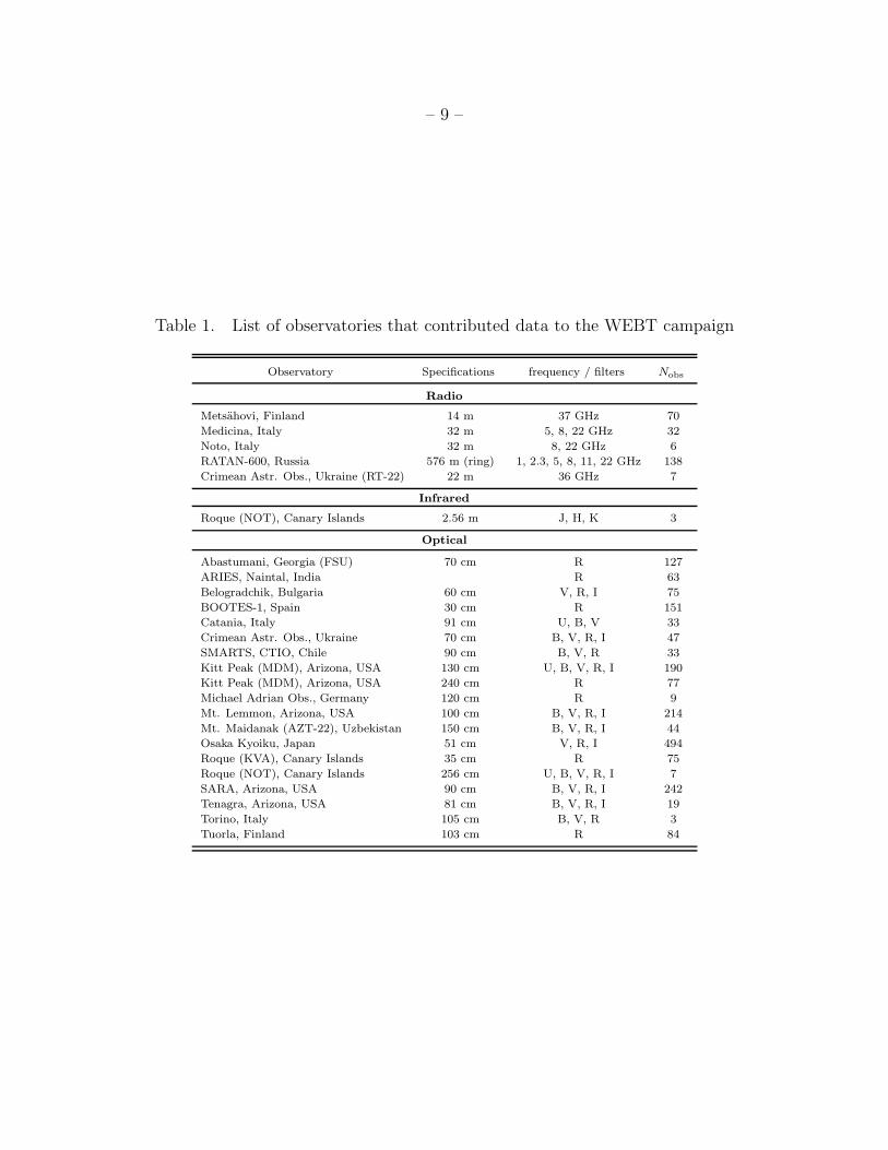
(2007b). Table 1 lists all participating observatories which contributed data to the WEBT

campaign. In total, 25 ground-based radio, infrared, and optical telescopes in 12 countries

on 4 continents contributed 2173 data points.

2.1. Optical and near-infrared observations

The observing strategy and data analysis followed to a large extent the standard pro-

cedure for the optical data reduction for WEBT campaigns which is briefly outlined below.

For more information on standard data reduction procedures for WEBT campaigns see

also: Villata et al. (2000); Raiteri et al. (2001); Villata et al. (2002); Bottcher et al. (2003);

Villata et al. (2004a,b); Raiteri et al. (2005); Bottcher et al. (2005)

It had been suggested that, optimally, observers perform photometric observations al-

ternately in the B and R bands, and include complete (U)BVRI sequences at the beginning

and the end of each observing run. Exposure times should be chosen to obtain an opti-

mal compromise between high precision (instrumental errors less than ∼ 0.03 mag for small

telescopes and ∼ 0.01 mag for larger ones) and high time resolution. If this precision re-

– 8 –

13.0

13.5

14.0

14.5

15.0

15.5

16.0

16.5

UBVRI

720 730 740 750 760 770 780 790 800 810 820 830 840JD - 2453000

12

14

16

18

Flux

[Jy

]

37Gz22 GHz8 GHz5 GHz

Dec Jan Feb Mar Apr2005 2006

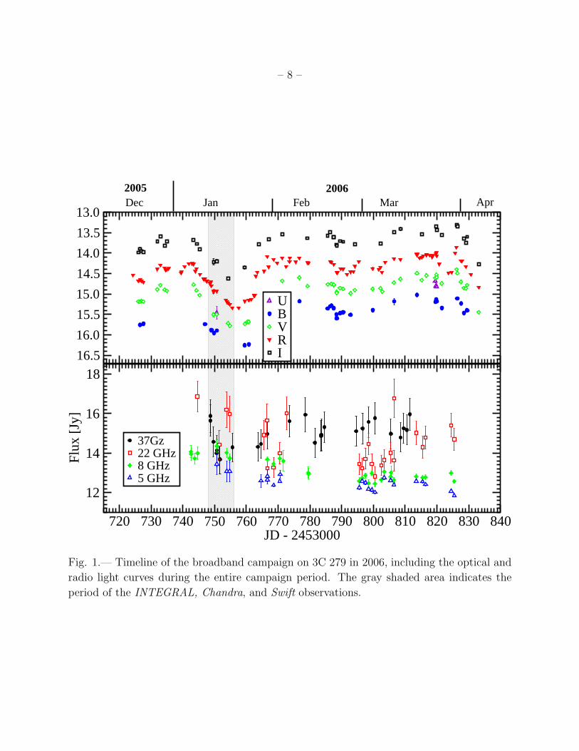
Fig. 1.— Timeline of the broadband campaign on 3C 279 in 2006, including the optical and

radio light curves during the entire campaign period. The gray shaded area indicates the

period of the INTEGRAL, Chandra, and Swift observations.

– 9 –

Table 1. List of observatories that contributed data to the WEBT campaign

Observatory Specifications frequency / filters Nobs

Radio

Metsahovi, Finland 14 m 37 GHz 70

Medicina, Italy 32 m 5, 8, 22 GHz 32

Noto, Italy 32 m 8, 22 GHz 6

RATAN-600, Russia 576 m (ring) 1, 2.3, 5, 8, 11, 22 GHz 138

Crimean Astr. Obs., Ukraine (RT-22) 22 m 36 GHz 7

Infrared

Roque (NOT), Canary Islands 2.56 m J, H, K 3

Optical

Abastumani, Georgia (FSU) 70 cm R 127

ARIES, Naintal, India R 63

Belogradchik, Bulgaria 60 cm V, R, I 75

BOOTES-1, Spain 30 cm R 151

Catania, Italy 91 cm U, B, V 33

Crimean Astr. Obs., Ukraine 70 cm B, V, R, I 47

SMARTS, CTIO, Chile 90 cm B, V, R 33

Kitt Peak (MDM), Arizona, USA 130 cm U, B, V, R, I 190

Kitt Peak (MDM), Arizona, USA 240 cm R 77

Michael Adrian Obs., Germany 120 cm R 9

Mt. Lemmon, Arizona, USA 100 cm B, V, R, I 214

Mt. Maidanak (AZT-22), Uzbekistan 150 cm B, V, R, I 44

Osaka Kyoiku, Japan 51 cm V, R, I 494

Roque (KVA), Canary Islands 35 cm R 75

Roque (NOT), Canary Islands 256 cm U, B, V, R, I 7

SARA, Arizona, USA 90 cm B, V, R, I 242

Tenagra, Arizona, USA 81 cm B, V, R, I 19

Torino, Italy 105 cm B, V, R 3

Tuorla, Finland 103 cm R 84

– 10 –

quirement leads to gaps of 15 – 20 minutes in each light curve, we suggested to carry out

observations in the R band only. Observers were asked to perform bias and dark correc-

tions as well as flat-fielding on their frames, and obtain instrumental magnitudes, applying

either aperture photometry (using IRAF or CCDPHOT) or Gaussian fitting for the source

3C 279 and four recommended comparison stars. This calibration has then been used to

convert instrumental to standard photometric magnitudes for each data set. In the next

step, unreliable data points (with large error bars at times when higher-quality data points

were available) were discarded. Our data did not provide evidence for significant variability

on sub-hour time scales. Consequently, error bars on individual data sets could be further

reduced by re-binning on time scales of typically 15 – 20 min. The data resulting at this

stage of the analysis are displayed in the top panel of Fig. 1.

In order to provide information on the intrinsic broadband spectral shape (and, in

particular, a reliable extraction of B - R color indices), the data were then de-reddened using

the Galactic Extinction coefficients of Schlegel et al. (1998), based on AB = 0.123 mag and

E(B − V ) = 0.029 mag3.

Possible contaminations of the optical color information could generally also arise from

contributions from the host galaxy and the optical – UV emission from an accretion disk

around the central supermassive black hole in 3C 279. However, these contributions are not

expected to be significant in the case of our campaign data: Assuming absolute magnitudes

of MV ∼ −23 and MB ∼ −21 for typical quasar host galaxies at z ∼ 0.5 (e.g. Floyd et al.

2004; Zakamska et al. 2006), their contribution in the V and B band, respectively, at the

distance of 3C 279 would be Vgal ∼ 19.5 and Bgal ∼ 21.6, respectively. These are at least

about four magnitudes fainter than the actually measured total B and V magnitudes during

our campaign, and thus negligible. The possible contribution of an accretion disk can be

estimated on the basis of the thermal component for which Pian et al. (1999) found evidence

in IUE observations during the 1992/1993 low state of 3C 279. Their best fit to this compo-

nent suggests U ∼ 18.6 and B ∼ 21 (and much fainter contributions at lower frequencies),

which corresponds to a contribution of . 2.5 % to the total B and U magnitudes measured

during our campaign. Therefore, both the host galaxy and the accretion disk contribution

are neglected in our further analysis.

The only infrared observations obtained for this campaign were one sequence of JHK

exposures taken on January 15, 2006, with the 2.56 m NOT on Roque de los Muchachos on

the Canary Island of La Palma. The resulting fluxes are included in the SED displayed in

Fig. 8.

3http://nedwww.ipac.caltech.edu/

– 11 –

2.1.1. Optical light curves

The optical (and radio) light curves from December 2005 to April 2006 are displayed in

Fig. 1. The densest coverage was obtained in the R band, and the figure clearly indicates

that the variability in B, V, and I bands closely tracks the R-band behaviour. The coverage

in the U band was extremely sparse and does not allow any assessment of the U-band light

curve during our campaign. Therefore, the U-band will be ignored in the following discussion,

and we will describe the main features of the variability behavior based on the R-band light

curve.

The optical light curves show variability with magnitude changes of typically . 0.5mag on

time scales of a few days. The most notable exception to this relatively moderate variability

is the major dip of the brightnesses in all optical bands right around our coordinated X-ray /

soft γ-ray observations in January 2006 (≈ JD 2453742 – 2453770). In the R-band, the light

curve followed an unusually clean exponential decay over 1.1 mags. in 13 days, i.e., a slope

of dR/dt = 0.085 mag/day or a flux decay as F (t) = F (t0) e−(t−t0)/τd with a decay constant

of τd = 12.8 d. Only moderate intraday deviations on a characteristic scale of . 0.1 mag/d

are superposed on this smooth exponential decay.

In contrast to the smooth decline of the optical brightness during January 6 – 20, 2006,

the subsequent re-brightening to levels comparable to those before the dip, appears much

more erratic and involves a remarkably fast rise by ∼ 0.5mag within ∼ 1 d on Jan. 27 (JD

2453763). Unfortunately, the detailed shape of this fast rise was not well sampled in our

data set. If this was a quasi-exponential rise with a slope of dR/dt ∼ 0.5 mag/d, it would

correspond to a rise time scale of τr ∼ 2.2 d.

2.2. Radio observations

At radio frequencies, 3C 279 was monitored using the 14 m Metsahovi Radio Telescope

of the Helsinki University of Technology, at 37 GHz, the 32-m radio telescope of the Medicina

Radio Observatory near Bologna, Italy, at 5, 8, and 22 GHz, the 32-m antenna of the Noto

Radio Observatory on Sicily, Italy, at 8 and 22 GHz, the 576-m ring telescope (RATAN-600)

of the Russian Academy of Sciences, at 1, 2.3, 5, 8, 11, and 22 GHz, and the 22-m RT-22

dish at the Crimean Astrophysical Observatory, Ukraine, at 36 GHz.

The Metsahovi data have been reduced with the standard procedure described in Terasranta et al.

(1998). The resulting 37 GHz light curve is reasonably well sampled during the period mid-

January – mid-March 2006. Inspection by eye in comparison to the optical light curves

displayed in Fig. 1 appears to indicate that the optical and 37 GHz light curves follow simi-

– 12 –

lar variability patterns with a radio lead before the optical variability by ∼ 5 days. However,

a discrete cross-correlation analysis between the R-band and 37 GHz radio light curves did

not reveal a significant signal to confirm this suggestion.

Also included in Fig. 1 are the radio light curves at 5, 8, and 22 GHz. For details of

the analysis of data from the Medicina and Noto radio observatories at those frequencies,

see Bach et al. (2007). As already apparent in Fig. 1, most of the data at frequencies below

37 GHz were not well sampled on the . 3-months time scale of the 2006 campaign, and any

evidence for variability did not show a discernable correlation with the variability at higher

(radio and optical) frequencies.

All radio data contributed to this campaign are stored in the WEBT archive (see

http://www.to.astro.it/blazars/webt/ for information regarding availability of the data).

Radio data at all observed frequencies have been included in the quasi-simultaneous SED

for Jan 15, 2006, shown in Fig. 8. Given the generally very moderate radio variability at

frequencies below 37 GHz, a linear interpolation between the two available data points near-

est in time to Jan. 15, 2006, was used to construct an estimate of the actual radio fluxes at

that time.

3. Optical spectral variability

In this section, we will describe spectral variability phenomena, i.e. the variability of

spectral (and color) indices and their correlations with monochromatic source fluxes. We will

concentrate here on the optical spectral variability as indicated by a change of the optical

color. In particular, our observing strategy was optimized to obtain a good sampling of

the B – R color index as a function of time. Since our data did generally not indicate

substantial flux changes on sub-hour time scales, we extracted B – R color indices wherever

both magnitudes were available within 20 minutes of each other. Fig. 2 shows the B – R

color history over the entire campaign, compared to the B and R band light curves. Overall,

there is no obvious correlation between the light curves and the color behavior of the source

on long time scales. However, two short-term sequences attracted our attention: There

is a sequence of brightness decline accompanied by a spectral hardening (declining B – R

index) around JD 2453750 (Jan. 14, 2006), and another sequence of a brightness increase

accompanied by a spectral softening around JD 2453790 – 2453806 (Feb. 23 – Mar. 11).

However, we caution that incomplete sampling, in particular in the B-band may introduce

spurious effects.

A similar trend was recently observed in a multiwavelength WEBT campaign on the

– 13 –

0.91

1.11.21.3

B -

R

15

15.5

16

16.5

B

720 740 760 780 800 820 840JD - 2453000

14

14.5

15

15.5

R

Segment 1 Segment 2

Fig. 2.— Light curve of the B and R magnitudes and the B – R color index of 3C 279 over

the duration of the entire campaign.

– 14 –

4e14 5e14 6e14 7e14 8e14ν [Hz]

2e12

3e12

1e12

4e12

νFν

[Jy*

Hz]

Dec. 23Jan. 15Jan. 24Feb. 20Mar. 25

I R V B U

Fig. 3.— Snap-shot optical (BVRI) continuum spectra for 5 epochs during our campaign.

All measurements for each individual spectrum were taken within ≤ 20 min. of each other.

– 15 –

quasar 3C 454.3 (Villata et al. 2006), where it could be interpreted as a “little blue bump”

due to the unresolved contribution from optical emission lines in the ∼ 2000 – 4000 A wave-

length range in the rest frame of the quasar, in particular from Fe II and Mg II (Raiteri et al.

2007). In order to test whether such an interpretation would also be viable in the case of

3C 279, we have compiled several simultaneous snap-shot optical continuum (BVRI) spectra

at various brightness levels (Fig. 3). All measurements for each individual spectrum dis-

played in Fig. 3 have been taken within ≤ 20 min. of each other. Only the spectrum of

Jan. 15 shows a significant deviation from a pure power-law in the B band; and in that case,

there was simultaneous U band coverage, which matched a straight power-law extrapolation

of the VRIJHK spectrum. If the spectral upturn towards the blue end of the spectrum were

due to an unresolved Mg II / Fe II line contribution, it should emerge even more clearly in

the Jan. 24 spectrum, which is characterized by a lower optical continuum flux level than

the Jan. 15 spectrum. Therefore, the compilation of spectra in Fig. 3 does not provide any

support for the existence of an essentially non-variable continuum component at the blue

end of the spectrum. For this reason, we believe that the color changes that we found in our

data are in fact intrinsic to the blazar jet emission.

Fig. 4 illustrates our impression from Fig. 2, that there is no clear overall trend

of source (R-band) brightness with optical spectral hardness. However, the figure clearly

illustrates that the scatter of the B – R color index is significantly larger at larger source

brightness, indicating that spectral variability is more likely to occur when the source is

bright. Specifically, for R > 14.5, the data is consistent with a roughly constant value of B –

R = 1.09, corresponding to a spectral index of αo = 1.9 for a power-law continuum spectrum

with Fν,o[Jy] ∝ ν−αo . At brightness levels R < 14.5, spectral variability by ∆(B−R) . 0.35,

corresponding to ∆αo . 0.85, is observed.

In Fig. 5, we focus on two ∼ 1-month optical flares, around mid-Jan. – mid-Feb.

2006, and late Feb. – late March 2006, as indicated by the gray shaded segments 1 and 2,

respectively, in Fig. 2. The number labels in the color-magnitude diagrams in Fig. 5 indicate

the time ordering of the points. While there is no obvious trend discernible in Segment 1,

Segment 2 suggests the presence of a spectral hysteresis pattern: The spectral softening

around JD 2453790 – 2453806 (Feb. 23 – Mar. 11), already mentioned above, precedes the

main brightness increase. Subsequently, the optical continuum hardens while the source is

still in a bright state. We need to caution that due to the poor sampling of the B band

light curve during segment 2, the significance of the tentative hysteresis found here may be

questionable. However, such hysteresis would naturally lead to a B-band time lag behind the

R-band, for which we do find a 3.9 σ evidence from a discrete correlation function analysis

as described in the following section.

– 16 –

14.014.515.0R

0.9

1.0

1.1

1.2

1.3

B-R

Fig. 4.— Color-magnitude diagram for the entire campaign period.

– 17 –

1414.414.815.2R

1

1.1

1.2

1.3

B-R

14.014.214.4R

2

13

4

56

8

76

1

2

3

4

5

Segment 1 Segment 2

Fig. 5.— Color-magnitude diagrams for the two time segments marked in Fig. 2, with time

ordering indicated by the numbers in the two panels.

– 18 –

To our knowledge, such a spectral hysteresis has never been observed at optical wave-

lengths for any flat-spectrum radio quasar. It is reminiscent of the spectral hysteresis

occasionally seen at X-ray energies in high-frequency peaked BL Lac objects (HBLs, e.g.

Takahashi et al. 1996; Fossati et al. 2000; Kataoka et al. 2000). However, the spectral hys-

teresis observed in the X-rays of HBLs is generally clockwise (i.e., spectral hardening pre-

cedes flux rise; softening precedes flux decline), and can be interpreted as the synchrotron

signature of fast acceleration of ultrarelativistic electrons, followed by a gradual decline on

the radiative cooling time scale (e.g., Kataoka et al. 2000; Kusunose, Takahara, & Li 2000;

Li & Kusunose 2000; Bottcher & Chiang 2002). In our case, the direction of the spectral

hysteresis is counterclockwise (i.e., spectral softening precedes the flux rise; spectral harden-

ing precedes flux decline). Possible physical implications of such hysteresis phenomena will

be discussed in §6.

4. Inter-band cross-correlations and time lags

The result of an occasional counterclockwise hysteresis in 3C 279, as found in the pre-

vious section, immediately suggests the existence of a characteristic time lag of higher-

frequency behind lower-frequency variability. In order to investigate this, we evaluated the

discrete correlation function (DCF, Edelson & Krolik 1988) between the R band and the

other optical light curves. In our notation, a positive value of the time lag ∆τ would indi-

cate a lag of the R-band light curve behind the comparison light curve. As mentioned earlier,

the radio (and near-IR) light curves are too sparsely sampled and yielded no significant fea-

tures in the DCF. Fig. 6 shows the DCF between the R band and the V band (top panel)

and the B band (bottom panel), using a sampling time scale of ∆τ = 1 d. We have done

the same analysis using various other values of ∆τ , which yielded results consistent with the

ones described below. We chose to show the results for ∆τ = 1 d because they provided the

best compromise between dense time scale sampling and reduction of error bars.

The DCFs reveal clear correlations between the different optical wavebands, with peak

values around 1. This confirms our previous impression from inspection by eye, that the

variability patterns in all optical wavebands track each other very closely.

The resulting DCFs have then been fitted with a symmetric Gaussian, F0 e−(τ−τ0)2/(2σ2).

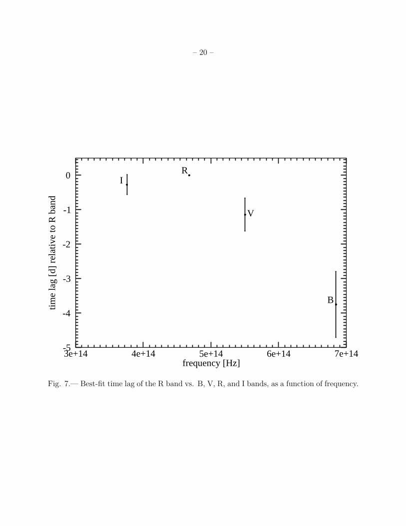
This analysis yields non-zero offsets of the best-fit maxima, τ0 at the ∼ 3 – 4σ level. Specif-

ically, we find τ0 = (−1.14 ± 0.48) d for the V band and τ0 = (−3.75 ± 0.96) d for the B

band. This indicates a hard time lag of higher-frequency variability behind the variability at

lower frequencies in the B-V-R frequency range. However, this trend does not continue into

the I band. This is illustrated in Fig. 7, where we plot the best-fit time lags as a function of

– 19 –

-0.5

0

0.5

1

1.5

2

2.5

DC

F

-50 -40 -30 -20 -10 0 10 20 30 40 50time lag [d]

-0.5

0

0.5

1

1.5

2

2.5

DC

F

V vs. R

B vs. R

Fig. 6.— Discrete correlation functions between V and R (top panel), and B and R (bottom

panel), respectively. The solid curves indicate the best fit with a symmetric Gaussian.

This leads to a best-fit maximum correlation at τ0 = (−1.14 ± 0.48) d for the V band and

τ0 = (−3.75 ± 0.96) d for the B band, indicating a lag of the V and B band light curves

behind the R-band.

– 20 –

3e+14 4e+14 5e+14 6e+14 7e+14frequency [Hz]

-5

-4

-3

-2

-1

0

time

lag

[d]

rela

tive

to R

ban

d

IR

V

B

Fig. 7.— Best-fit time lag of the R band vs. B, V, R, and I bands, as a function of frequency.

– 21 –

photon frequency. However, we need to add a note of caution: The rather sparse sampling of

the B- and V-band light curves leads to large error bars on the DCFs. Clearly, alternative,

more complex representations, e.g., multiple Gaussians and/or asymmetric functions, will

also provide acceptable fits to the observed DCFs and may lead to different quantitative

results concerning the involved time lags. Future observations with denser B- and V-band

sampling are needed in order to test the robustness of the trend found here.

The hard lag found in this analysis may be physically related to the ∼ 2 – 3 d time

lag of the soft X-ray spectral index behind the flux in ROSAT observations of 3C 279 in

December 1992 – January 1993 (Pian et al. 1999). Possible physical interpretations will be

discussed in §6.

5. Broad-band spectral energy distribution

The most complete broadband coverage of 3C 279 during our campaign was obtained

on January 15, 2006. On that day, the only near-infrared (JHK) exposures were taken with

the NOT, and simultaneous radio observations at 5, 8, 22, and 37 GHz were available as

well. This is also within the time window of the X-ray and soft γ-ray observations, although

in most cases, a meaningful extraction of spectral information required the integration over

most of the high-energy observing period, January 13 – 20, 2006 (Collmar et al. 2007a).

The total snap-shot SED composed of all available radio, near-IR, optical, X-ray, and soft

γ-ray observations around January 15, 2006 is displayed in Fig. 8, where all near-IR and

optical data are taken within ±1/2 hr of UT 05:00 on January 15. The figure compares the

January 2006 SED to previous SEDs from the bright flare during the first EGRET observing

epoch in June 1991, the low state of December 1992 / January 1993 (both SEDs adapted

from Hartman et al. 2001a), and a previous multiwavelength campaign around INTEGRAL

AO-1 observations of 3C 279 in a low state in June 2003 (Collmar et al. 2004).

While the optical (presumably synchrotron) emission component clearly indicates that

the source was in an elevated state compared to previous low states, the simultaneous X-ray

– soft-γ-ray spectrum is perfectly consistent with the low-state spectra of 1992/1993 and

2003. This is a very remarkable result and will be discussed in detail in a companion paper

about the results of the entire multiwavelength campaign (Collmar et al. 2007b).

The NIR – optical continuum can be very well represented by a single power-law with

a spectral index of αo = 1.64 ± 0.04, corresponding to an underlying non-thermal electron

distribution with a spectral index of p = 4.28± 0.08, if the optical continuum is synchrotron

emission. As already pointed out in Hartman et al. (2001a) for a comparison between various

– 22 –

109

1011

1013

1015

1017

1019

1021

1023

1025

ν [Hz]

1010

1011

1012

1013

1014

νFν

[Jy

Hz]

3C279

P1 (June 1991 flare)P2 (Dec. 92 / Jan. 93)June 2003Jan. 2006

Fig. 8.— Simultaneous snap-shot spectral energy distributions of 3C 279 at various epochs.

Data pertaining to the multiwavelength campaign in January 2006 are plotted with red

triangles. All IR and optical data were taken within ±1/2 hr of UT 05:00 on Jan. 15, 2006;

the X-ray and soft γ-ray data represent the time-averaged spectra throughout the respective

observing windows in Jan. 2006, which included Jan. 15 for all instruments. Model fits to

the EGRET P1 and P2 SEDs are calculated using a time-dependent leptonic (SSC + EC) jet

model, and taken from Hartman et al. (2001a). The June 2003 SED is from Collmar et al.

(2004).

– 23 –

EGRET observing epochs over ∼ 10 years and confirmed by our campaign data on time scales

of weeks – months (see §3), the optical spectral index in 3C 279 does not show any systematic

correlation with the brightness state of the source, and Fig. 8 indicates that in our high-

state observations of 2006, the continuum spectral slope is not significantly different from

the slopes observed in the low states of 1992/1993 and 2003.

6. Discussion

In this section, we discuss some general physical implications and constraints that our

results can place on source parameters. In the following discussion, we will parameterize

the magnetic field in units of Gauss, i.e., B = 1 BG Gauss, and the Doppler boosting factor

D = (Γ[1 − βΓ cos θobs])−1 in units of 10, i.e., D = 10 D1 where Γ is the bulk Lorentz

factor of the emitting region, βΓ c is the corresponding speed, and θobs is the observing

angle. The characteristic variability time scale is of the order of 1 – a few days, so we write

tobsvar ≡ 1 tobs

var,d. In the same sense, we parameterize the time lag of the B band behind the

R band as τ obsBR ≡ 1 τ obs

BR,d d with τ obsBR,d ∼ 3. The observed variability time scale yields an

estimate of the size of the emitting region, R ≡ 1015R15 cm through R . c D/(1 + z) tobsvar .

We find R15 . 17 D1 tobsvar,d.

The (co-moving) energies of electrons emitting synchrotron radiation at their character-

istic peak frequencies in the R and B bands are

γR = 3.7 × 103 (BG D1)−1/2

γB = 4.5 × 103 (BG D1)−1/2 (1)

The steep underlying electron spectrum with p = 4.5, inferred from the steep optical

continuum, might indicate that the entire optical spectrum is produced by electrons in the

fast-cooling regime. This implies that the radiative cooling time scale of electrons emitting

synchrotron radiation in the optical regime is shorter than the characteristic escape time

scale of those electrons. The respective time scales in the co-moving frame, t′esc and t′cool can

be written as

t′esc ≡ η Rc

. 5.7 × 105 η D1 tobsvar,d s

t′cool = γγrad

∼ 7.7 × 107 B−1G γ−1 (1 + k)−1 s (2)

where η ≥ 1 is the escape time scale parameter (as defined in the first line of eq. 2), and

k is a correction factor accounting for radiative cooling via Compton losses in the Thomson

– 24 –

regime in a radiation field with an energy density u′

rad ≡ k u′

sy. Requiring that the cooling

time scale is shorter than the escape time scale, at least for electrons emitting in the R band,

leads to a lower limit on the magnetic field:

B & Bc ≡ 1.3 × 10−3 (1 + k)−2 η−1 (tobsvar,d)

−2 G (3)

which does not seem to pose a severe constraint, given the values of B ∼ a few G typically

found for other FSRQs and also for 3C 279 from previous SED modeling analyses (e.g.,

Hartman et al. 2001a).

Another estimate of the co-moving magnetic field can be found by assuming that the

dominant portion of the time-averaged synchrotron spectrum is emitted by a power-law

spectrum of electrons with Ne(γ) = n0 VB γ−p for γ1 ≤ γ ≤ γ2; here, VB is the co-moving

blob volume, and we use p = 4.5 as a representative value inferred from the optical continuum

slope. The normalization constant n0 = ne (1− p)/(

γ1−p2 − γ1−p

1

)

is related to the magnetic

field through an equipartition parameter eB ≡ u′

B/u′

e (in the co-moving frame). Note that

this equipartition parameter only refers to the energy density of the electrons, not accounting

for a (possibly dominant) energy content of a hadronic matter component in the jet. Under

these assumptions, the magnetic field can be estimated as described, e.g., in Bottcher et al.

(2003). Taking the νFν peak synchrotron flux f syǫ at the dimensionless synchrotron peak

photon energy ǫsy ≡ Epk,sy/(mec2) ≈ 3 × 10−7 as ∼ 10−10 ergs cm−2 s−1, we find

B & BeB ≡ 1.86 D−13/71 e

2/7B (tobs

var,d)−1 G. (4)

This constitutes a more useful and realistic magnetic-field estimate than eq. 3. If, in-

deed, the optical emission is synchrotron emission from a fast-cooling electron distribution,

then electrons have been primarily accelerated to a power-law distribution with an injection

index of q = p − 1 = 3.5. This is much steeper than the canonical spectral index of q ∼ 2.2

– 2.3 found for acceleration on relativistic, parallel shocks (e.g., Gallant, Achterberg & Kirk

1999; Achterberg et al. 2001), and could indicate an oblique magnetic-field orientation (e.g.,

Ostrowski & Bednarz 2002; Niemiec & Ostrowski 2004), which would yield a consistent pic-

ture with the predominantly perpendicular magnetic-field orientation observed on parsec-

scales (Jorstad et al. 2004; Ojha et al. 2004; Lister & Homan 2005). The observed hard lag

(B vs. R) may then be the consequence of a gradual spectral hardening of the electron accel-

eration (injection) spectrum throughout the propagation of a relativistic shock front along

the jet. Such a gradual hardening of the electron acceleration spectrum could be the con-

sequence of the gradual build-up of hydromagnetic turbulence through the relativistic two-

stream instability (see, e.g., Schlickeiser et al. 2002). This turbulence would harden the rel-

– 25 –

ativistic electron distribution via 2nd-order Fermi acceleration processes (Virtanen & Vainio

2005). Such a scenario would imply a length scale for the build-up of turbulence of ∆r ∼

c τ obsBR D Γ/(1 + z) ∼ 5.6 × 10−2 τ obs

BR,d D1 Γ1 ∼ 0.2 pc for the characteristic values of 3C 279.

Alternatively, the acceleration process could become more efficient along the jet if the

magnetic-field configuration gradually evolves into a more quasi-parallel one, on the same

length scale of ∼ 0.2 pc as estimated above. However, this scenario might be in conflict with

the predominantly perpendicular magnetic-field orientation seen in the jets of 3C 279 on pc

scales.

The hard lag in the optical regime may also be indicative of a slow acceleration mecha-

nism, with an acceleration time scale of the order of the observed B vs. R lag. This would

imply an acceleration rate of

γA ∼γB − γR

τBR∼ 6.8 × 10−2(τ obs

BR,d)−1

(

D1

BG

)1/2

s−1. (5)

In this scenario, electrons could only be accelerated to at least γB, if the acceleration rate

of eq. 5 is larger than the absolute value of the radiative (synchrotron + Compton) cooling

rate corresponding to eq. 2. This imposes an upper limit on the magnetic field:

B . Bacc ∼ 0.42 D1/31 (τ obs

BR,d)−2/3 (1 + k)−2/3 G. (6)

This can be combined with the estimate in eq. 4 to infer a limit on the magnetic-field

equipartition parameter:

eB . eB,acc ∼ 5.8 × 10−3 D23/31 (τ obs

BR,d)−7/3 (tobs

var,d)7/2 (1 + k)−7/3. (7)

Based on this equipartition parameter, one can use the magnetic-field estimate of eq. 4 to

estimate the total amount of co-moving energy contained in the emission region at any given

time:

E ′

e ∼4

3π R3 u′

B

eB∼ 2.5 × 1049 D−4

1 τ obsBR,d (tobs

var,d)−1/2 (1 + k) erg (8)

Assuming that the bulk of this energy is dissipated within the characteristic variability time

scale, one can estimate the power in relativistic electrons in the jet:

Ljet ∼E ′

e

t′var∼ 4.5 × 1043 D−5

1 τ obsBR,d (tobs

var,d)−3/2 (1 + k) ergs s−1. (9)

– 26 –

Previous modeling works of the SEDs of FSRQs in general and 3C 279 in particular

indicated characteristic magnetic field values of a few Gauss, in approximate equipartition

with the ultrarelativistic electron population. The unusually low equipartition parameter in

eq. 7 could therefore pose a problem for the slow-acceleration scenario. Note, however, the

very strong dependence of eB on the Doppler factor (∝ D23/3). A Doppler factor D ∼ 20

could account for equipartition parameters of the order of one. Also, the energy requirements

of eqs. 8 and 9 seem reasonable, and there does not appear to be a strict argument that

would rule this scenario out.

Another scenario one could think of would be based on a decreasing magnetic field along

the blazar jet, leading to a gradually increasing cooling break in the underlying electron dis-

tribution. This would require that the cooling time scale for electrons emitting synchrotron

radiation in the optical regime would be equal to or longer than the escape time scale. Thus,

the inequality in eq. 3 would be reversed. This would require unreasonably low magnetic

fields. Furthermore, this scenario would be in conflict with the typically observed unbroken

snap-shot power-law continuum spectra throughout the optical-IR range. Therefore, this

idea may be ruled out.

7. Summary

We have presented the results of an optical-IR-radio monitoring campaign on the promi-

nent blazar-type flat-spectrum radio quasar 3C 279 by the WEBT collaboration in January

– April 2006, around Target of Opportunity X-ray and soft γ-ray observations with Chandra

and INTEGRAL in mid-January 2006. Previously unpublished radio and optical data from

several weeks leading up to the ToO trigger are also included.

The source exhibited substantial variability of flux and spectral shape, in particular in

the optical regime, with a characteristic time scale of a few days. The variability patterns

throughout the optical BVRI bands were very closely correlated with each other, while there

was no significant evidence for a correlation between the optical and radio variability. After

the trigger flux level for the Chandra and INTEGRAL ToOs was reached on Jan. 5, 2006, the

optical flux decayed smoothly by 1.1 mags. within 13 days, until the end of the time frame

of the X-ray and γ-ray observations. The decay could be well described by an exponential

decay with a decay time scale of τd = 12.8 d. The flux then recovered to approximately the

pre-dip values in a much more erratic way, including a ∼ 0.5mag rise within ∼ 1 d.

A discrete correlation function analysis between different optical (BVRI) bands indicates

a hard lag with a time delay increasing with increasing frequency, reaching ∼ 3 d for the lag

– 27 –

of B behind R. This appears to be accompanied by a single indication of counterclockwise

spectral hysteresis in a color-intensity diagram (B-R vs. R). Thus, spectral hardening during

flares appears delayed with respect to a rising optical flux. There is no consistent overall

trend of optical spectral hardness with source brightness. However, our data indicate that

the source displays a rather uniform spectral slope of αo ∼ 1.9 at moderate flux levels

(R > 14.5), while spectral variability seems common at high flux levels (R < 14.5).

The occasional optical spectral hysteresis, in combination with the very steep IR-optical

continuum spectral index of αo ∼ 1.5 – 2.0, may indicate a highly oblique magnetic field

configuration near the base of the jet, leading to inefficient particle acceleration and a very

steep electron injection spectrum. As the emission region propagates along the jet, a gradual

hardening of the primarily injected ultrarelativistic electron distribution may be caused by

the gradual build-up of hydromagnetic turbulence, which could lead to a gradually increasing

contribution of second-order Fermi acceleration. This would imply a length scale of the build-

up of hydromagnetic turbulence of ∆r ∼ 0.2 pc.

An alternative explanation of the hard lag may be a slow acceleration mechanism by

which relativistic electrons are accelerated on a time scale of several days. However, even

though this model can plausibly explain the observed variability trends and overall luminosity

of the source, it requires an unusually low magnetic field in the emitting region of B . 0.2 G,

unless rather high Doppler factors of D 20 are assumed. Such a small magnetic field would

be about an order of magnitude lower than inferred from previous analyses of simultaneous

SEDs of 3C 279 and other flat-spectrum radio quasars with similar properties.

The work of M. Bottcher and S. Basu was partially supported by NASA through IN-

TEGRAL GO grant award NNG 06GD57G and the Chandra GO program (administered by

the Smithsonian Astrophysical Observatory) through award no. GO6-7101A. The Metsahovi

team acknowledges the support from the Academy of Finland. YYK is a research fellow of the

Alexamder von Humboldt Foundation. RATAN-600 observations were partly supported by

the Russian Foundation for Basic Research (project 05-02-17377). The St. Petersburg team

was supported by the Russian Foundation for Basic Research through grant 05-02-17562.

REFERENCES

Achterberg, A., Gallant, Y. A., Kirk, J. G., & Guthmann, A. W., 2001, MNRAS, 328, 393

Bach, U., et al., 2007, A&A, 464, 175

Bednarek, W., 1998, A&A, 336, 123

– 28 –

Bottcher, M., 2007a, in proc. “The Multimessenger Approach to Gamma-Ray Sources”,

ApSS, in press (astro-ph/0608713)

Bottcher, M., 2007b, in proc. “The Central Engine of Active Galactic Nuclei”, ASPCS, in

press

Bottcher, M., & Bloom, S. D., 2000, AJ, 119, 469

Bottcher, M., & Chiang, J., 2002, ApJ, 581, 127

Bottcher, M., Mause, H., & Schlickeiser, R., 1997, A&A, 324, 395

Bottcher, M., et al., 2003, ApJ, 596, 847

Bottcher, M., et al., 2005, ApJ, 631, 169

Collmar, W., et al., 2004, in proc. of 5th INTEGRAL Workshop, ESA-SP 552, Ed.: B.

Battrick, p. 555

Collmar, W., et al., 2007a, in proc. of 6th INTEGRAL Workshop, ESA-SP, in press

Collmar, W., et al., 2007b, in preparation

Cotton, W. D., et al., 1979, ApJ, 229, L115

Edelson, R. A., & Krolik, J. H., 1988, ApJ, 333, 646

Floyd, D. J. E., Kukula, M. J., Dunlop, J. S., McLure, R. J., Miller, L., Percival, W. J.,

Baum, S. A., & O’Dea, C. P., 2004, MNRAS, 355, 196

Fossati, G., et al., 2000, ApJ, 541, 166

Gallant, Y. A., Achterberg, A., & Kirk, J. G., 1999, A&AS, 138, 549

Gonzalez-Perez, J. N., Kidger, M. R., & Martın-Luis, F., 2001, AJ, 122, 2055

Hartman, R. C., et al., 1996, ApJ, 461, 698

Hartman, R. C., et al., 1999, ApJS, 123, 79

Hartman, R. C., et al., 2001a, ApJ, 553, 683

Hartman, R. C., et al., 2001b, ApJ, 558, 583

Helmboldt, J. F., et al., 2007, ApJ, 658, 203

– 29 –

Homan, D. C., Lister, M. L., Kellermann, K. I., Cohen, M. H., Ros, E., Zensus, J. A., Kadler,

M., & Vermeulen, R. C., 2003, ApJ, 589, L9

Jorstad, S. G., Marscher, A. P., Lister, M. L., Stirling, A. M., Cawthorne, T. V., Gomez,

J.-L., & Gear, W. K., 2004, AJ, 127, 3115

Kartaltepe, J. S., & Balonek, T. J., 2007, ApJ, 133, 2866

Kataoka, J., Takahashi, T., Makino, F., Inoue, S., Madejski, G. M., Tashiro, M., Urry, C.

M., & Kubo, H., 2000, ApJ, 528, 243

Kirk, J. G., Rieger, F. M., & Mastichiadis, A., 1998, A&A, 333, 452

Kusunose, M., Takahara, F., & Li, H., 2000, ApJ, 536, 299

Li, H., & Kusunose, M., 2000, ApJ, 536, 729

Lister, M. L., & Homan, D. C., 2005, AJ, 130, 1389

Maraschi, L., et al., 1994, ApJ, 435, L91

Mattox, J. R., Hartman, R. C., & Reimer, O., 2001, ApJS, 135, 155

Moderski, R., Sikora, M., Blazejowski, M., 2003, A&A, 406, 855

Mucke, A., & Protheroe, R. J., 2001, Astropart. Phys., 15, 121

Mucke, A., Protheroe, R. J., Engel, R., Rachen, J. P., & Stanev, T., 2003, Astropart. Phys.,

18, 593

Nandikotkur, G., Jahoda, K. M., Hartman, R. C., Mukherjee, R., Sreekumar, P., Bottcher,

M., Sambruna, R. M., & Swank, J. H., 2007, ApJ, 657, 705

Niemiec, J., & Ostrowski, M., 2004, ApJ, 610, 851

Ojha, R., Homan, D. C., Roberts, D. H., Wardle, J. F. C., Aller, M. F., Aller, H. D., &

Hughes, P. A., 2004, ApJS, 150, 187

Ostrowski, M., & Bednarz, J., 2002, A&A, 394, 1141

Pian, E., et al., 1999, ApJ, 521, 112

Raiteri, C. M., Villata, M., Lanteri, L., Cavallone, M., & Sobrito, G., 1998, A&AS, 130, 495

Raiteri, C. M., et al., 2001, A&A, 377, 396

– 30 –

Raiteri, C. M., et al., 2005, A&A, 438, 39

Raiteri, C. M., et al., 2006, A&A, 459, 731

Raiteri, C. M., et al., 2007, A&, submitted

Schlegel, D. J., Finkbeiner, D. P., & Davis, M., 1998, ApJ, 500, 525

Schlickeiser, R., Vainio, R., Bottcher, M., Schuster, C., Lerche, I., & Pohl, M., 2002, A&A,

393, 69

Sikora, M., Blazejowski, M., Begelman, M. C., & Moderski, R., 2001, ApJ, 554, 1; Erratum:

ApJ, 561, 1154 (2001)

Smith, P. S., & Balonek, T. J., 1998, PASP, 110, 1164

Takahashi, T., et al., 1996, ApJ, 470, L89

Terasranta, H., et al., 1998, A&AS, 132, 305

Unwin, S. C., Biretta, J. A., Hodges, M. W., & Zensus, J. A., 1989, ApJ, 340, 117

Villata, M., et al., 2000, A&A, 363, 108

Villata, M., et al., 2002, A&A, 390, 407

Villata, M., et al., 2004a, A&A, 421, 103

Villata, M., et al., 2004b, A&A, 424, 497

Villata, M., et al., 2006, A&A, 453, 817

Villata, M., et al., 2007, A&A, 464, L5

Virtanen, J. J. P., & Vainio, R., 2005, ApJ, 621, 313

Wehrle, A. E., et al., 1998, ApJ, 497, 178

Whitney, A. R., et al., 1971, Science, 173, 225

Zakamska, N. L., et al., 2006, ApJ, 132, 1496

This preprint was prepared with the AAS LATEX macros v5.2.