arX

iv:0

912.

0005

v2 [

astr

o-ph

.CO

] 2

Dec

200

9

Mon. Not. R. Astron. Soc.000, 1–26 (2009) Printed 2 December 2009 (MN LATEX style file v2.2)

Variability and stability in blazar jets on time scales of years:Optical polarization monitoring of OJ287 in 2005–2009

C.Villforth1,2⋆, K.Nilsson1, J.Heidt3, L.O.Takalo1, T.Pursimo2, A.Berdyugin1, E.Lindfors1, M.Pasanen1, M.Winiarski4, M.Drozdz4,

W.Ogloza4, M.Kurpinska-Winiarska5, M.Siwak5,6, D.Koziel-Wierzbowska5, C.Porowski5, A.Kuzmicz5, J.Krzesinski4, T.Kundera5,

J.-H.Wu7, X.Zhou7, Y.Efimov8, K.Sadakane9, M.Kamada9, J.Ohlert10, V.-P.Hentunen11, M.Nissinen11, M.Dietrich12, R.J.Assef12,

D.W.Atlee12, J.Bird12, D.L.DePoy13, J.Eastman12, M.S.Peeples12, J.Prieto12, L.Watson12, J.C.Yee12, A.Liakos14, P.Niarchos14,

K.Gazeas14, S.Dogru15, A.Donmez15, D.Marchev16, S.A.Coggins-Hill17, A.Mattingly18, W.C.Keel19, S.Haque20,

A.Aungwerojwit21,22 and N.Bergvall23

1Tuorla Observatory, Department of Physics and Astronomy, University of Turku, Vaisalantie 20, FI-21500 Piikkio,Finland2Nordic Optical Telescope, Apartado 474, E-38700 S/C de la Palma, Spain3ZAH, Landessternwarte Heidelberg, Konigstuhl, 69117 Heidelberg, Germany4Mt. Suhora Observatory, Pedagogical University, ul. Podchorazych 2, 20-084 Krakow, Poland5Astronomical Observatory, Jagiellonian University, ul. Orla 171, 30-244 Krakow, Poland6Department of Astronomy and Astrophysics, University of Toronto, 50 St. George St., Toronto, Ontario, M5S3H4, Canada7National Astronomical Observatories, Chinese Academy of Sciences, 20A Datun Road, Beijing 100012, China8Crimea Astrophysical Observatory, Yalta, 334242 Crimea, Ucraine9Astronomical Institute, Osaka-Kyoiku University, Asahigaoka, Kashiwara, Osaka 582-8582, Japan10Michael Adrian Observatorium, Astronomie Stiftung Trebur, Fichtenstrasse 7, 65468 Trebur, Germany11Taurus Hill Observatory, Harkamaentie 88, FI-79480, Kangaslampi Finland12Department of Astronomy, The Ohio State University, 4055 McPherson Lab, 140 W. 18th Ave, Columbus, OH 43210 U.S.A.13Department of Physics and Astronomy, Texas A&M University, College Station, TX 77843, U.S.A.14Department of Astrophysics, Astronomy and Mechanics, Faculty of Physics, University of Athens, Panepistimiopolis, GR-15784 Zografos, Athens, Greece15Canakkale Onsekiz Mart University, Faculty of Physics, TR-17020 Canakkale, Turkey16Department of Physics, Shoumen University, 9700 Shoumen, Bulgaria17Am Weinberg 16, 63579 Freigericht-Horbach, Germany18Grove Creek Observatory, Trunkey Creek, NSW 2796, Australia19Department of Physics and Astronomy, University of Alabama, Tuscaloosa, AL 35487-0324, USA20Department of Physics, University of West Indies, St. Augustine, Trinidad21Department of Physics, Faculty of Science, Naresuan University, Phitsanulok, 65000, Thailand22Department of Physics, University of Warwick, Coventry CV47AL, UK23Department of Astronomy and Space Physics, Uppsala University, Box 515, 751 20 Uppsala, Sweden

Accepted: 27 November 2009. Received: 27 October 2009

ABSTRACTOJ287 is a BL Lac object at redshiftz = 0.306 that has shown double-peaked bursts at regular intervals of∼ 12 yrduring the last∼ 40 yr. We analyse optical photopolarimetric monitoring data from 2005–2009, during which thelatest double-peaked outburst occurred. The aim of this study is twofold: firstly, we aim to analyse variability patternsand statistical properties of the optical polarization light-curve. We find a strong preferred position angle in opticalpolarization. The preferred position angle can be explained by separating the jet emission into two components: anoptical polarization core and chaotic jet emission. The optical polarization core is stable on time scales of years andcan be explained as emission from an underlying quiescent jet component. The chaotic jet emission sometimes ex-hibits a circular movement in the Stokes plane. We find six such events, all on the time-scales of 10–20 days. Weinterpret these events as a shock front moving forwards and backwards in the jet, swiping through a helical magneticfield. Secondly, we use our data to assess different binary black hole models proposed to explain the regularly appear-ing double-peaked bursts in OJ287. We compose a list of requirements a model has to fulfil to explain the mysteriousbehaviour observed in OJ287. The list includes not only characteristics of the light-curve but also other properties ofOJ287, such as the black hole mass and restrictions on accretion flow properties. We rate all existing models usingthis list and conclude that none of the models is able to explain all observations. We discuss possible new explana-tions and propose a new approach to understanding OJ287. We suggest that both the double-peaked bursts and theevolution of the optical polarization position angle couldbe explained as a sign of resonant accretion of magneticfield lines, a ’magnetic breathing’ of the disc.

Key words: accretion, accretion discs – magnetic fields – polarization– shock waves – BLLacartea objects : individual : OJ287 – galaxies : jets

2 C. Villforth et al.

1 INTRODUCTION

Blazars are amongst the most violently variable sources in the Uni-verse. According to the standard model (Urry & Padovani 1995),blazars are AGN with a jet pointing almost directly towards the ob-server, the jet radiation is thus highly beamed and dominates thespectrum. Therefore, blazars are perfect laboratories to study vari-ability and turbulence in AGN jets.

Blazars are divided into two subclasses: BL Lac objects andFlat Spectrum Radio Quasars (FSRQs). Both BL Lacs and FSRQsshow a flat radio spectrum, high polarization and violent variability(Urry & Padovani 1995). While BL Lacs show a featureless opticalspectrum with extremely weak or absent broad and narrow emis-sion lines, FSRQs show a normal spectrum of broad and narrowemission lines. In the standard interpretation, BL Lacs arethoughtto be the equivalents of Fanaroff-Riley I (FR I) radio galaxies atsmall viewing angle, while FSRQs are thought to be the equiva-lents of Fanaroff-Riley II (FR II) radio galaxies (Ghisellini et al.2009). Lately, more and more evidence has been found to supportthe idea that FSRQs and BL Lac differ not only in the appearanceof their jets on kpc scale but also in their accretion processes. Ithas been suggested that FSRQs accrete in a radiatively efficient,geometrically thin accretion disc, while BL Lacs accrete throughradiatively inefficient accretion flows (RIAFs) (Baum et al. 1995;Ghisellini et al. 2009).

However, even FSRQs and BL Lacs might differ in their ac-cretion process and appearance of the jets, the variabilityobservedin both types of objects is similar (Ulrich et al. 1997). Bothclassesshow variability on time scales from hours to decades, with par-tially extreme amplitudes (Ulrich et al. 1997; Valtaoja et al. 2000;Villforth et al. 2009). In both classes, the radio structurefrom VLBImaps consists of a so-called radio-core that does not move andblobs that appear to be ejected from the core and move awayfrom it at apparently superluminal speeds. These blobs havebeenexplained as signs of shock-fronts moving along the jet. Shockfronts are also thought to cause powerful outbursts lastingseveralweeks that can be observed on all wavelengths (Marscher & Gear1985). Using multi-wavelength data, it is possible to modelthephysical conditions in these shock fronts (Marscher & Gear 1985;Marscher et al. 2008; D’Arcangelo et al. 2009).

Shorter time-scales and the behaviour in the quiescent phasesare however less well understood. Studying variability on shortertime-scales is a very challenging field. On these time-scales, multi-wavelength observations cannot be used due to the fact that thedelay between the different wavelength and the variability itselfappear on similar time-scales. Neither are these short time-scalesand thus small angular movements accessible using VLBI maps.Even so, it is a well known fact that variability down to the time-scales of hours exists (Wagner & Witzel 1995; Ulrich et al. 1997;Villforth et al. 2009). Using optical polarization data, itis possibleto study the variability in blazar jets down to the smallest time-scales, and opposed to normal flux monitoring, polarizationmoni-toring can reveal the evolution of the magnetic field.

Another open question, to which flux monitoring cannot an-swer, is what happens in the jet during quiescent phases. Usingoptical polarization monitoring, we can assess the properties of themagnetic field in the jet during quiescent phases and can thusan-swer the question if stable components in the jet emission exist.

For our study, we choose OJ287, which is one of the best stud-ied blazars. It has been monitored since the last century acciden-tally and has been studied excessively since 1970s both using pho-tometry and polarimetry. Therefore, OJ287 is a perfect object to

study variability in blazar jets on a large range of time-scales, fromweeks up to decades. OJ287 has a moderate redshift ofz = 0.306(Sitko & Junkkarinen 1985).

OJ287 has received a lot of attention as it has shown mas-sive double-peaked outbursts approximately every 12 yearsduringthe last 40–100 years. Such long-lasting, regularly appearing eventshave not been observed in any other AGN so far. Sillanpaa etal.(1988) first noted this exceptional behaviour and suggestedthat theregularly appearing outbursts might be caused by a close binaryblack hole system in which the secondary black hole induces tidaldisturbances in the accretion disc of the primary black hole. How-ever, due to the limited amount of data, Sillanpaa et al. (1988) werenot able to explain how exactly the flare happens.

Lehto & Valtonen (1996) further developed this model andsuggested that each of the flares actually constitutes of twoflares:the first flare is extremely short and is caused by the crossingofthe secondary black hole through the disc, while the second flareis caused by enhanced accretion due to tidal disturbances intheaccretion disc. The time lag between the two flares is extremelyshort (∼ 1 week), so that they are actually observed as one big out-burst. Two of those outbursts happen during each orbit of thesec-ondary black hole. The orbit is extremely eccentric, so thatwe ob-serve two outbursts separated by only about 1 year every 12 years.Lehto & Valtonen (1996) modelled the previous behaviour andpre-dicted the next outburst to happen in Spring 2006. However, OJ287did not fail to surprise observers, and the first outburst in the 2005–2007 season happened about half a year earlier than predicted byLehto & Valtonen (1996). After the early 2005 burst, this modelwas further modified to fit the newest data (Valtonen et al. 2006;Valtonen 2007; Valtonen et al. 2009).

Several other authors have suggested models for OJ287 (Katz1997; Villata et al. 1998; Valtaoja et al. 2000), all of them based onthe assumption that OJ287 hosts a close binary black hole. Katz(1997) suggested that a binary black hole induces precession in theaccretion disc of OJ287, the jet follows the precessing motion of thediscs and sweeps through the line of sight regularly, causing majorflares due to enhanced beaming. Villata et al. (1998) suggested thatOJ287 hosts a binary black hole, in which both black holes producea jet, the jets sweep through the line of sight on regular intervalscausing double-peaked bursts.

Valtaoja et al. (2000) studied radio monitoring data of OJ287and noted differences between the first and second burst and there-fore suggested that the first burst is caused by a disc-crossing whilethe second burst is related to enhanced accretion causing a shockfront in the jet. Using the radio data, Valtaoja et al. (2000)furtherargued that the missing of radio counterparts in some burstsspeaksagainst the beaming models (Katz 1997; Villata et al. 1998) as forbeaming events one would expect all wavelengths to be enhancedin a similar manner. The observed burst however do not show sucha behaviour.

Both the Lehto & Valtonen, its modified successor(Valtonen et al. 2006; Valtonen 2007) and the Valtaoja modelmakeclear predictions about the appearance of the bursts in polarizationand the exact timing of the bursts. Thus, our data sets can be usedto test the different models.

In this paper we analyse optical photopolarimetric monitoringof OJ287 during 2005–2009. We analyse the variability in opti-cal polarization and compare it to current blazar jet models. Wecompare the data to different models proposed to explain the reg-ularly appearing outbursts in OJ287. In Section 2 we presenttheobservations and data reduction. Results are presented in Section3. We discuss our results, both concerning the general variability

Variability and stability in blazar jets 3

pattern observed and the different models for OJ287, in Section4. Conclusions are presented in Section 5. The cosmology used isH0 = 70km s−1Mpc−1,ΩΛ = 0.7,Ωm = 0.3.

2 OBSERVATIONS AND DATA REDUCTION

We have obtained 400 polarimetric and 2238 photometric observa-tions of OJ287 in 2002–2009. The participating observatories anddistribution of data points among them is shown in Table 1.

Of the 400 polarimetric measurements 110 were taken inservice mode using the focal reducer CAFOS at the Calar Alto(CA) 2.2 m telescope. A rotatableλ/2 plate+ Wollaston prismwere employed and four exposures through the R-band were takenwith the λ/2 plate rotated by 22.5 between the exposures. Ex-posure times were typically 60 s. The field of view was largeenough (7×7 arcsec) to include a number of comparison stars fromGonzalez-Perez et al. (2001) enabling simultaneous photometricmeasurements of OJ287. Data were bias-subtracted and flatfieldedusing full polarimetric flatfields.

Altogether 256 polarimetric measurements were taken withthe remotely controlled 60 cm KVA telescope on La Palma. Theintegration times were similar to the Calar Alto observations, but inorder to improve the signal-to-noise, four to 12 sequences of fourimages were taken and the individual polarization measurementswere averaged. Furthermore, the images were made in “whitelight”, i.e. without a filter. A calcite plate was used instead of aWollaston prism to separate the ordinary and extraordinarybeams.Polarimetric data were dark-subtracted. Nearly simultaneous (timedifference< 30 min) R-band photometry was obtained from CCDimages made with a 35 cm telescope attached to the 60 cm tele-scope.

Finally, 34 polarimetric measurements were made with theNordic Optical Telescope (NOT) using an identical setup to theKVA, except that R-band filter was used. Data were bias-subtractedand flatfielded using full polarimetric flatfields. Simultaneous R-band photometry was derived from star 13 in Gonzalez-Perez et al.(2001).

The normalized Stokes parametersPQ and PU and the de-gree of polarizationP and position anglePA were computed fromthe intensity ratios of the ordinary and extraordinary beams usingstandard formulae (see e.g. Degl’Innocenti et al. 2007) andsemi-automatic software specifically developed for polarization mon-itoring purposes. During some of the nights, polarized standardstars from Turnshek et al. (1990) were observed to determinethezero point of the position angle. The instrumental polarization wasfound to be negligible for all three telescopes. Foreground(Galac-tic) polarization should also be low (< 0.5 per cent) since thereddening value is only EB−V = 0.028. The degree of polariza-tion was corrected for bias using the maximum likelihood estima-tor from Simmons & Stewart (1985). Since the KVA observationswere made in “white light”the effective wavelength is mainly deter-mined by the sensitivity of the detector. The sensitivity ofthe Mar-coni 47-10 detector used at the KVA peaks atλ ∼ 500 nm, some-what shorter than the peak of theR-band filter used at CA and NOT(∼ 640 nm). Since frequency-dependent polarization is commonlyobserved in OJ287 (see e.g. Holmes et al. 1984), a small offset be-tween the Stokes parameters observed by CA and KVA is expected.However, the difference in effective wavelength is relatively smalland any offsets are likely to be small too. We have examined the24 cases where nearly simultaneous (time difference less than twohours) data have been obtained with both CA and KVA telescopes.

02468

1012141618

R [

mJy

]

2005 Burst

Dec 2004

Mar 2005

Jun 2005

Sep 2005

Dec 2005

Mar 2006

Jun 200630

20

10

0

10

20

30

40

P [

%]

Figure 3. Normalised Stokes parameters during the 2005 burst. Upperpanel: flux, lower panel:PQ (blue circles) andPU (green triangles).

We computed the mean of the Stokes parametersPQ and PU forboth CA and KVA data sets and found a difference between themeans to be 0.47± 0.17 and 0.76± 0.13 for PQ and PU , respec-tively. These are very small offsets compared to the total range ofPQ andPU and of the order of the error bars of a single point. Thusdifferences in effective wavelength between the CA and KVA datado not cause large enough offsets to affect our conclusions.

In addition to the polarimetric points, 2238 photometric pointswere obtained inBVRI bands in 18 observatories over the world(see Table 1). CCD images were obtained of the OJ287 field andthe frames were reduced in the usual way by first subtracting thebias and dark frames and then dividing by a flat-field frame. Thephotometry was performed in differential mode using star nine inGonzalez-Perez et al. (2001) as the comparison star. Inter-observeroffsets were checked using star 13 as a control and found to begenerally small (<0.02 mag). The offsets derived from star 13 wereapplied to the magnitudes of OJ287 to bring all measurementstothe same scale. Finally, one-hour averages were computed from thedata.

All data are available at Vizier.

3 RESULTS

3.1 General appearance of the light-curve: the majoroutbursts

We start by analysing and discussing the appearance of the light-curve in general and describe the two major outbursts observed dur-ing 2005–2009. The full light-curve in photometry and polarimetryis presented in Fig. 1. The gaps in the light-curves appearing inJune–July yearly are due to the fact that OJ287 is too close tothesun during these months. We will refer to these gaps as ’summergaps’.

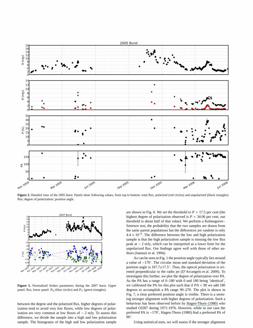
During our monitoring campaign, two major outbursts wereobserved, one in late 2005 and the other one in late 2007. Detailedplots of the two major outbursts are presented in Figures 2 (fulldata), 3 (Stokes parameters) for the 2005 burst and 4 (full data), 5(Stokes parameters) for the 2007 burst.

The first major outburst is observed in late 2005. We do notsee any exceptional behaviour before the ’summer gap’ in 2005.The flux is relatively low and the polarization is moderatelyhigh(P∼ 20 per cent). After the ’summer gap’, in late 2005, we see a

4 C. Villforth et al.

Table 1.The participating telescopes in the OJ287 campaign. The second column gives the observatory abbreviation used in the data tables and the third columnthe mirror diameter. The last columns give the number of photometric and polarimetric data points.

Observatory abbr. D NU NB NV NR NI NPol

[cm]

Athens, Greece ATH 40 79Calar Alto, Spain CA 220 118 110Canakkale, Turkey CO 40 3 12 5Grove Creek, Australia GC 30 8Heidelberg, Germany HEI 70 1Krakow, Poland KR 50 14 47 57 25MDM, USA MDM 240 34KVA, La Palma KVA 35 406 256NOT, La Palma NOT 256 45 34Osaka, Japan OSA 51 63 89 71SATUa, Trinidad SAT 1Mt. Suhora, Poland SUH 60 5 101 178 208 143Taurus Hill, Finland TH 30 49Trebur, Germany TRE 120 74Tuorla, Finland TUO 103 131

UAb, USA UA 40 2Xinglong, China XIO 90 159

Liverpool Telescope, La Palma LIV 200 24 24 38c 24d

Total 5 139 315 1511 268 400

a St. Augustine-Tuorlab University of Alabamac SDSS ’rd SDSS ’i

rather smooth increase in flux, the polarization is similarly high asbefore the burst. The main flare shows two major bursts of similarstrength, separated by about a month. The object stays in burst tillearly 2006, the variability after the two peaks is erratic. Asmoothdecline starts in spring 2006. In the end phase of the decline, whenthe flux almost reaches a normal level again, a short, highly po-larized outburst occurs. After this short flare, the source returns tonormal flux levels when the 2006 ’summer gap’ sets in.

As for the exact timing of the burst, we see two major flaresof similar strength in this burst. It is unclear which of the two isthe main flare. The first of the two flares is observed on 20 Octo-ber 2005 and the second flare is observed on 9 November 2005.The error in these values are in the order of days due to samplinglimitations.

This burst was predicted to happen in 2006 by bothLehto & Valtonen (1996) (2006 May 12) and Valtaoja et al. (2000)(2006 September 25). Thus, we can clearly say that our findingdis-agrees strongly with both existing predictions. The Lehto &Val-tonen model has an error of about six months, while the Valtaojamodel has an error of almost a year. The modified Lehto & Valto-nen model (Valtonen et al. 2006; Valtonen 2007) by definitionfitsthe burst in 2005 as it is based on the timing from that burst.

As for the appearance in polarization, only very few datapoints are available in polarization during the 2005 flare. No oneexpected a major burst at this point and thus few telescopes weremonitoring OJ287 in polarization. From the few data points wehave, it seems as if the whole burst was rather strongly polarized.Only two data points were observed during the flares, both showingrather high degrees of polarization. The position angle in those twodata points is around zero, which is rather close to the valueof ∼

170, which the position angle is observed to fluctuate around mostof the time.

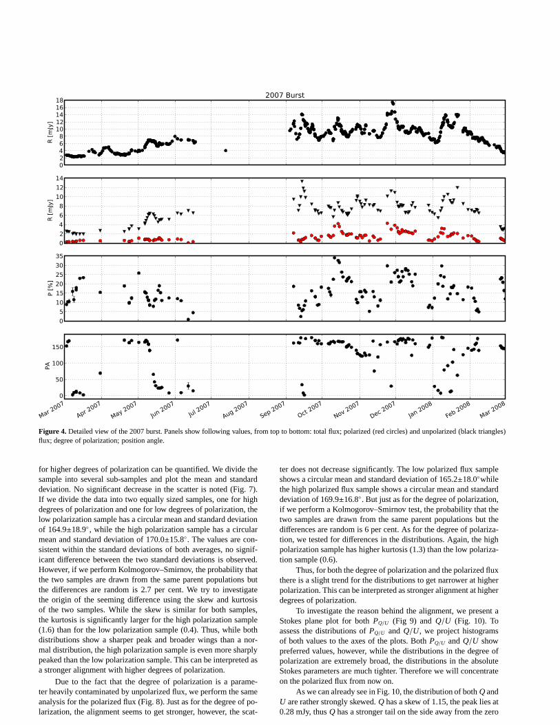
After the 2006 ’summer gap’, a moderately polarized, steepand short outburst is observed. Whereupon the light-curve is with-out prominent features, only showing smaller, rather erratic bursts.Already in early June 2007, the flux starts to increase rathersteeply,announcing the beginning of the second major outburst. The po-larization during this rise is extremely low, the increase in flux isnot smooth as for the 2005 burst, but overlaid with several smallerflares. After the ’summer gap’, in September 2007, the outburstreaches its peak, the polarization is high and the variability in flux iserratic. The plateau of the burst lasts till January 2008. During thistime, the flux stays on a constantly high level, superimposedwithcountless fast erratic flares. A smooth, rather steep decline begins inJanuary 2008. The decline is interrupted by a highly polarized, sud-den and steep flare, similar to the one observed after the 2005burst.However, after the second burst, OJ287 does not return to itsnor-mal state, another highly polarized, broad and strong burstbeginswhich lasts until the end of our monitoring campaign in summer2009. The ’third major burst’ is slightly less luminous (∼12 mJy)than the first (∼14 mJy) and second bursts (∼16 mJy). The burst isextremely chaotic, similar to the second burst in its plateau.

While the 2005 burst was a test for the ’old’ Lehto & Valtonen(1996) model and the Valtaoja et al. (2000) models, the 2007 burstwill only be used to test the ’new’ Lehto & Valtonen model(Valtonen et al. 2006; Valtonen 2007) as both other models did notpredict the first burst correctly. The ’summer gap’ poses a seriousproblem for the exact timing of the 2007 burst. We see a sharp riseof flux right before the ’summer gap’. When OJ287 is observableagain, the outburst is already in its plateau. Valtonen et al. (2008)identified the second flare after the summer gap as the major burst.

Variability and stability in blazar jets 5

02468

1012141618

R [

mJy

]

Photopolarimetric monitoring of OJ287 in 2005-2009

0

2

4

6

8

10

12

14

R [

mJy

]

0

5

10

15

20

25

30

35

P [

%]

Dec 2004

Jun 2005

Dec 2005

Jun 2006

Dec 2006

Jun 2007

Dec 2007

Jun 2008

Dec 2008

Jun 2009

0

50

100

150

PA

Figure 1. Full photopolarimetric light-curve for OJ287 in 2005–2009. Panels show following values, from top to bottom: total flux; polarized (red circles) andunpolarized (black triangles) flux; degree of polarization; position angle. Solid vertical lines show data bins for OPCvariability used in Section 3.2. Verticaldash-dotted lines show beginning and end of bubbles and swings as discussed in Section 3.3.

This burst is not the highest peak in the plateau, but it showsex-tremely low levels of polarization, as predicted by Valtonen (2007).It is not clear if another strong peak occurred shortly before OJ287returned from the ’summer gap’. A single, rather low photometricdata-point was observed during the summer gap on 12 July 2007.Thus we can assume that the highest peak did not occur shortlyafter that date. We assume that several flares must have occurredbefore OJ287 returned to high luminosities from such a dip. As thetime scale of the erratic flares is usually about a week, we concludethat the major outburst in 2007 has occurred no earlier than mid tolate August 2007. The first peak after the summer gap was observedon 2007 September 12. However, several flares of similar strengthare observed after that, the highest of those as late as December2007. Thus, we cannot clearly say which of those flares is the mainflare, it might have happened at any time between August and De-cember 2007. The second flare after the summer gap is well con-sistent with predictions from the modified Lehto & Valtonen model(Valtonen et al. 2006; Valtonen 2007), who predicted the burst tohappen in 2007 September 13. It is also practically unpolarized, aspredicted by Valtonen (2007).

As for the appearance of the burst in polarization, while thede-gree of polarization starts off rather low during the beginning of theburst, it rises to extremely high values in the first post-maximumpeak. The position angle stays relatively stable for the first two

peaks after the summer gap while a swinging behaviour is seenin the third peak after the summer gap after which the position an-gle falls back to the preferred value of∼170. In Fig. 5, we plotthe normalised Stokes parameters for the same time span, thetwonormalised Stokes parameters show similar evolution. Justas thephotometric light-curve, the polarimetric light-curves shows rathererratic behaviour.

3.2 Statistical properties of the polarimetric dataset

In this section, we will analyse the data using statistical methods.We will not consider single events in the light-curve, but the proper-ties of the entire data set. Whenever we calculate the mean orstan-dard deviation for the position angle, we use the circular mean andcircular standard deviation (Mardia & Jupp 1975). Throughout thisparagraph, we use the Fisher kurtosis, normalized to zero. For allstatistical tests we use the statistical packagesstatsandmorestatsfrom SciPy1.

First we would like to assess if the degree of polarization cor-relates with theR band flux. While there is no strong correlation

1 http://www.scipy.org/

6 C. Villforth et al.

02468

1012141618

R [

mJy

]

2005 Burst

0

2

4

6

8

10

12

14

R [

mJy

]

0

5

10

15

20

25

30

35

P [

%]

Dec 2004

Mar 2005

Jun 2005

Sep 2005

Dec 2005

Mar 2006

Jun 2006

0

50

100

150

PA

Figure 2. Detailed view of the 2005 burst. Panels show following values, from top to bottom: total flux; polarized (red circles) andunpolarized (black triangles)flux; degree of polarization; position angle.

02468

1012141618

R [

mJy

]

2007 Burst

Mar 2007

Apr 2007

May 2007

Jun 2007

Jul 2007

Aug 2007

Sep 2007

Oct 2007

Nov 2007

Dec 2007

Jan 2008

Feb 2008

Mar 2008

30

20

10

0

10

20

30

40

P [

%]

Figure 5. Normalised Stokes parameters during the 2007 burst. Upperpanel: flux, lower panel:PQ (blue circles) andPU (green triangles).

between the degree and the polarized flux, higher degrees of polar-ization tend to avoid very low fluxes, while low degrees of polar-ization are very common at low fluxes of∼ 2 mJy. To assess thisdifference, we divide the sample into a high and low polarizationsample. The histograms of the high and low polarization sample

are shown in Fig. 6. We set the threshold toP = 17.5 per cent (thehighest degree of polarization observed isP = 34.06 per cent, ourthreshold is about half of that value). We perform a Kolmogorov–Smirnov test, the probability that the two samples are drawnfromthe same parent populations but the differences are random is only4.4 × 10−8. The difference between the low and high polarizationsample is that the high polarization sample is missing the low fluxpeak at∼ 2 mJy, which can be interpreted as a lower limit for theunpolarized flux. Our findings agree well with those of other au-thors (Jannuzi et al. 1994).

As can be seen in Fig. 1 the position angle typically lies arounda value of∼170. The circular mean and standard deviation of theposition angle is 167.7±17.5 . Thus, the optical polarization is ori-ented perpendicular to the radio jet (D’Arcangelo et al. 2009). Toinvestigate this further, we plot the degree of polarization over PA.As the PA has a range of 0–180 with 0 and 180 being ’identical’,we calibrated the PA for this plot such that ifPA< 90 we add 180degrees to accomplish a PA range 90–270. The plot is shown inFig. 7, a clear preferred position angle is visible. There isa seem-ing stronger alignment with higher degrees of polarization. Such abehaviour has been observed before by Hagen-Thorn (1980) whostudied OJ287 during 1971-1976. However, while in our case thepreferred PA is∼170, Hagen-Thorn (1980) find a preferred PA of90.

Using statistical tests, we will assess if the stronger alignment

Variability and stability in blazar jets 7

02468

1012141618

R [

mJy

]

2007 Burst

0

2

4

6

8

10

12

14

R [

mJy

]

0

5

10

15

20

25

30

35

P [

%]

Mar 2007

Apr 2007

May 2007

Jun 2007

Jul 2007

Aug 2007

Sep 2007

Oct 2007

Nov 2007

Dec 2007

Jan 2008

Feb 2008

Mar 2008

0

50

100

150

PA

Figure 4. Detailed view of the 2007 burst. Panels show following values, from top to bottom: total flux; polarized (red circles) andunpolarized (black triangles)flux; degree of polarization; position angle.

for higher degrees of polarization can be quantified. We divide thesample into several sub-samples and plot the mean and standarddeviation. No significant decrease in the scatter is noted (Fig. 7).If we divide the data into two equally sized samples, one for highdegrees of polarization and one for low degrees of polarization, thelow polarization sample has a circular mean and standard deviationof 164.9±18.9 , while the high polarization sample has a circularmean and standard deviation of 170.0±15.8. The values are con-sistent within the standard deviations of both averages, nosignif-icant difference between the two standard deviations is observed.However, if we perform Kolmogorov–Smirnov, the probability thatthe two samples are drawn from the same parent populations butthe differences are random is 2.7 per cent. We try to investigatethe origin of the seeming difference using the skew and kurtosisof the two samples. While the skew is similar for both samples,the kurtosis is significantly larger for the high polarization sample(1.6) than for the low polarization sample (0.4). Thus, while bothdistributions show a sharper peak and broader wings than a nor-mal distribution, the high polarization sample is even moresharplypeaked than the low polarization sample. This can be interpreted asa stronger alignment with higher degrees of polarization.

Due to the fact that the degree of polarization is a parame-ter heavily contaminated by unpolarized flux, we perform thesameanalysis for the polarized flux (Fig. 8). Just as for the degree of po-larization, the alignment seems to get stronger, however, the scat-

ter does not decrease significantly. The low polarized flux sampleshows a circular mean and standard deviation of 165.2±18.0whilethe high polarized flux sample shows a circular mean and standarddeviation of 169.9±16.8. But just as for the degree of polarization,if we perform a Kolmogorov–Smirnov test, the probability that thetwo samples are drawn from the same parent populations but thedifferences are random is 6 per cent. As for the degree of polariza-tion, we tested for differences in the distributions. Again, the highpolarization sample has higher kurtosis (1.3) than the low polariza-tion sample (0.6).

Thus, for both the degree of polarization and the polarized fluxthere is a slight trend for the distributions to get narrowerat higherpolarization. This can be interpreted as stronger alignment at higherdegrees of polarization.

To investigate the reason behind the alignment, we present aStokes plane plot for bothPQ/U (Fig 9) andQ/U (Fig. 10). Toassess the distributions ofPQ/U and Q/U, we project histogramsof both values to the axes of the plots. BothPQ/U andQ/U showpreferred values, however, while the distributions in the degree ofpolarization are extremely broad, the distributions in theabsoluteStokes parameters are much tighter. Therefore we will concentrateon the polarized flux from now on.

As we can already see in Fig. 10, the distribution of bothQandU are rather strongly skewed.Q has a skew of 1.15, the peak lies at0.28 mJy, thusQ has a stronger tail on the side away from the zero

8 C. Villforth et al.

P>17.5%

0 2 4 6 8 10 12 14 16R band flux [mJy]

P<17.5%

Figure 6. Flux histogram for high (P > 17.5 per cent, upper panel) and lowpolarization (P < 17.5 per cent, lower panel).

point.U has a skew of -0.22, the peak lies at -0.15 mJy, thus just asQ, U has a stronger tail away from the zero point. To describe theshape of the distribution, we calculate the Fisher kurtosis. Q has akurtosis of 3.7,U has a kurtosis of 1.6. Thus both distributions haveextremely wide wings and sharp peaks,Q is even more stronglypeaked thanU.

We interpret this finding such that there is an underlying, sta-ble source of polarized emission, causing the peak, the optical po-larization core (OPC). Using this interpretation, we separate theemission into two components:

• the optical polarization core (OPC)• turbulent, chaotic jet emission

Due to the strong skew in the distribution, arithmetic meanor median are not suitable to determine the exact value of theOPC.We therefore determine the values from sigma-clipped data (σ=2, 5iterations). These estimates are plotted in Fig. 10 as solidlines, wesee that the values describe the peak of the distribution very well.The parameters of the OPC are:Q = 0.28 mJy,U = -0.15 mJy,total polarized flux= 0.32 mJy. For comparison, the flux distribu-tion peaks at around 2.5 mJy. Thus the polarized OPC emissionrepresents about 10 per cent of the quiescent total flux emission.Assuming that the OPC emission is maximally polarized (P = 70per cent), the total flux of the OPC isFOPC,total = 0.46 mJy. Thusfor a common flux of 2.5 mJy, the OPC emission contributes about20 per cent to the total flux.

Using the OPC values derived above, we calculate a core-subtracted polarized flux by subtracting the OPC vectorially fromevery data point. We then use the core-subtractedQ/U to calculatea core-subtracted polarized flux and position angle.

We use the core-subtracted position angle to assess if thealignment of the OPC persists in the turbulent jet emission.Fig.11 shows the comparison between the normal and core subtractedPA. The distribution of the core-subtracted PA is almost flat, wedo not see a clear preferred position angle as in case of the rawdata. The core subtracted position angle has a circular meanandstandard deviation of 9.4± 27.8, compared to 167.7±17.5 for theraw data. This is only a very weak alignment (no alignment wouldcorrespond to a standard deviation of∼60). The weak residual pre-ferred position angle agrees with the original preferred PAwithinthe errorbars.

Next, we will assess if the OPC shows an evolution during our

50 100 150 200 250 300PA

0

5

10

15

20

25

30

35

P [

%]

Figure 7. Degree of polarization versus position angle for data 2005-2009.Filled circles with bars represent the circular mean and standard deviationof binned data.

50 100 150 200 250 300PA

0.0

0.5

1.0

1.5

2.0

2.5

3.0

3.5

4.0

4.5

pola

rize

d f

lux [

mJy

]

Figure 8. Polarized flux versus position angle for data 2005–2009. Filledcircles with bars represent the circular mean and standard deviation ofbinned data.

30 20 10 0 10 20 30 40PQ [%]

30

20

10

0

10

20

30

PU [

%]

Figure 9.Stokes plane plot for polarimetric data 2005–2009. Histograms ofPQ/U are projected to the corresponding axes. Dashed lines indicatePQ/U =

0.

Variability and stability in blazar jets 9

3 2 1 0 1 2 3 4Q [mJy]

3

2

1

0

1

2

U [

mJy

]

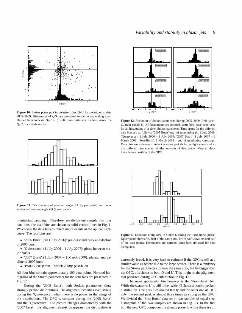
Figure 10. Stokes plane plot in polarized fluxQ/U for polarimetric data2005–2009. Histograms ofQ/U are projected to the corresponding axes.Dashed lines indicateQ/U = 0, solid lines estimates for best values forQ/U, for details see text.

100 150 200 250PA

Figure 11. Distributions of position anglePA (upper panel) and core-subtracted position anglePA (lower panel).

monitoring campaign. Therefore, we divide our sample into fourdata bins, the used bins are shown as solid vertical lines in Fig. 1.We choose the data bins to reflect major events in the optical light-curve. The four bins are:

• ’2005 Burst’ (till 1 July 2006): pre-burst and peak and declineof 2005 burst• ’Quiescence’ (1 July 2006 – 1 July 2007): phase between ma-

jor bursts• ’2007 Burst’ (1 July 2007 – 1 March 2008): plateau and de-

cline of 2007 burst• ’Post-Burst’ (from 1 March 2008): post-burst

All four bins contain approximately 100 data points. Normedhis-tograms of the Stokes parameters for the four bins are presented inFig. 12

During the ’2005 Burst’, both Stokes parameters showstrongly peaked distributions. The alignment becomes evenstrongduring the ’Quiescence’, when there is no power in the wings ofthe distributions. The OPC is constant during the ’2005 Burst’and the ’Quiescence’. The picture changes dramatically with the’2007 burst’, the alignment almost disappears, the distribution is

3 2 1 0 1 2 3 4Q [mJy]

2005 Burst

Quiescence

2007 Burst

Post-Burst

3 2 1 0 1 2U [mJy]

2005 Burst

Quiescence

2007 Burst

Post-Burst

Figure 12. Evolution of Stokes parameters during 2005–2009. Left panel:Q, right panel:U. All histograms are normed, same bins have been usedfor all histograms of a given Stokes parameter. Time spans for the differentdata bins are as follows: ’2005 Burst’ start of monitoring till 1 July 2006;’Quiescence’: 1 July 2006 – 1 July 2007; ’2007 Burst’: 1 July 2007 – 1March 2008; ’Post-Burst’: 1 March 2008 – end of monitoring campaign.Data bins were chosen to reflect obvious periods in the light curve and sothat different bins contain similar amounts of data points. Verticalblacklines denote position of the OPC.

1.5 1.0 0.5 0.0 0.5 1.0 1.5 2.0 2.5Q [mJy]

Figure 13.Evolution of the OPC in StokesQ during the ’Post-Burst’ phase.Upper panel shows first half of the data point, lower half shows second halfof the data points. Histograms are normed, same bins are usedfor bothhistograms.

extremely broad. It is very hard to estimate if the OPC is still at asimilar value as before due to the large scatter. There is a tendencyfor the Stokes parameters to have the same sign, but be biggerthanthe OPC, this shows in bothQ andU. This might be the alignmentthat persisted during OPC-subtraction in Fig. 11.

The most spectacular bin however is the ’Post-Burst’ bin.While the scatter inU is still rather wide,Q shows a double-peakeddistribution. One peak lies around 0 mJy and the other one at∼0.8mJy, the second peak is almost three times as strong as the OPC.We divided the ’Post-Burst’ data set in two samples of equal size,histograms of the two samples are shown in Fig. 13. In the firstbin, the new OPC component is already present, while there isstill

10 C. Villforth et al.

1975 1980 1985 1990 1995 2000 20050

20

40

60

80

100

120

140

160

180PA

Figure 14. Evolution of the optical position anglePA of OJ287 from∼1970 till today.

40302010 0 10 20 30 40PQ [%]

1975-1985

1985-1995

1995-2000

2005-2009

30 20 10 0 10 20 30PU [%]

1975-1985

1985-1995

1995-2000

2005-2009

Figure 15. Evolution of normalised Stokes parameters during 1975–2009.Left panel:PQ, right panel:PU . All histograms are normed, same bins havebeen used for all histograms of a given Stokes parameter. Solid vertical linesdenotePQ/U = 0 per cent.

a strong component at∼ 0 mJy. In the second bin however, thenew OPC component is fully dominant. We have thus detected astrengthening of the OPC directly after one of the double-peakedbursts. The component inQ almost tripled it’s strength.

Thus, during our monitoring campaign the OPC was stable,however, we did observe a sudden change in the OPC, directly afterthe second major burst in 2007. This raises the question how theOPC has evolved in the past.

A proper investigation of this subject would require long-termphotopolarimetric monitoring (i.e. polarization and flux measure-ments) in one well-calibrated filter. Such a dataset is not available.However, to get an idea of the evolution of the OPC, we can plotthePA over time. As the frequency dependence of the position angleis weak in blazars, we can even use multi-band data. In Fig. 14weplot the historic evolution of the position angle from the 1970s tillthe 90s. Those data are partially from literature, partially, they havebeen observed by Yuri Efimov with the 125 cm telescope at theCrimean Astrophysical Observatory (Ukraine), using the computercontrolledUBVRI Double Image Chopping Photopolarimeter, de-veloped at the Helsinki University Observatory by V. Piirola.

It is very clear from this plot that the OPC was not stable in thepast∼ 40 years. The most dramatic change happens around 1994,during one of the major double-peaked bursts: the preferredPAshows a swing, changing its orientation from∼ 90to ∼ 180. Thisis also the value that is observed during our monitoring campaign.

An interesting finding is the fact that all strong changes in the posi-tion angle seem to have happened shortly (∼ 1 yr) after one of themajor double-peaked bursts. This is very similar to the evolutionwe observe during our monitoring campaign, changes in the OPCseem to follow the double-peaked bursts.

To assess this further, we present a plot similar to Fig. 12,showing the evolution of the OPC. Due to the fact that the historicdata is simple polarimetric data without accompanying flux mea-surements, we cannot calculate the Stokes parameters, thus, we willwork with normalised Stokes parameters. Note that as discussedearlier in this Section, the normalised Stokes parameters are worsefor determining the OPC as they are contaminated by unpolarizedflux (see Fig. 9 compared to Fig. 10). We present the evolutionofthe OPC during the last 40 years in Fig. 15. We divide the data intobins using 1 January of the years 1985 and 1995. While the evolu-tion in U is rather mild, the evolution inQ shows a clear bulk mo-tion from∼ -10 per cent to∼ + 10 per cent during the last 40 years,the crossing of the zero point is most likely around∼ 1995. Thiscorresponds to a motion of the OPC in the Stokes plane from posi-tion angles of∼ 90 in the 1970s to a position angle of∼ 180 in thepresent. We will not further investigate these changes as our sam-pling is extremely uneven and most likely also concentratedaroundinteresting events in the light-curve. As we have seen before, Stokesplane plot look very different during quiescence or burst (Fig. 12).Therefore, we believe that binning the data into smaller bins willintroduce uncontrollable selection effects.

We studied statistical properties of the polarimetric datasetand found a strong alignment in position angle that originates ina strong peak in the distribution of values in the Stokes plane. Weinterpret this finding as a sign of an underlying source of constantpolarized flux. This emission dominates during quiescent phases,while during bursts chaotic emission dominates. During ourmoni-toring campaign, we observe a strengthening of the OPC afterthe2007 burst. We also study long-term evolution in the OPC and finda rather steady migration in the Stokes plane. Also for the long termevolution, the changes in the OPC seem to correlate with the majorbursts.

3.3 Reoccurring events in the polarimetric light-curve

While in Section 3.1 we only discussed events that show as strongrise in total flux, in this Section we aim to determine if re-occurringevents in the polarization exist. We also aim to classify those re-occurring events in a way that will make it possible for otherau-thors to identify similar events. A table with a list of all eventsdiscussed in the following paragraphs and their basic properties ispresented in Tab. 2.

To identify the ’reoccurring events’ we visually inspect the2005–2009 light-curve inPQ/U , Q/U, P andPAand compose a listof all remarkable events. We are aware that this method is some-what arbitrary, as the identification of the events is subjective. Weare also aware that we are heavily influenced by data gaps. How-ever, because optical polarization variability in blazarsis poorlyunderstood we believe that it can help to classify and discuss typ-ical events. The time of all those events is also shown in Fig.1,dash-dotted lines indicate the beginning and end of all events.

The first group of events with similar appearance are the ’Bub-bles’. In these events, bothPQ andPU start at low values, rise to amaximum simultaneously and then return to low values, enclosinga bubble. This eye-catching appearance in the plots lends this typeof events the name ’Bubble’. The prototype for this group of eventsis Bubble 1, a 25 d lasting event that occurred between JD 2453820

Variability and stability in blazar jets 11

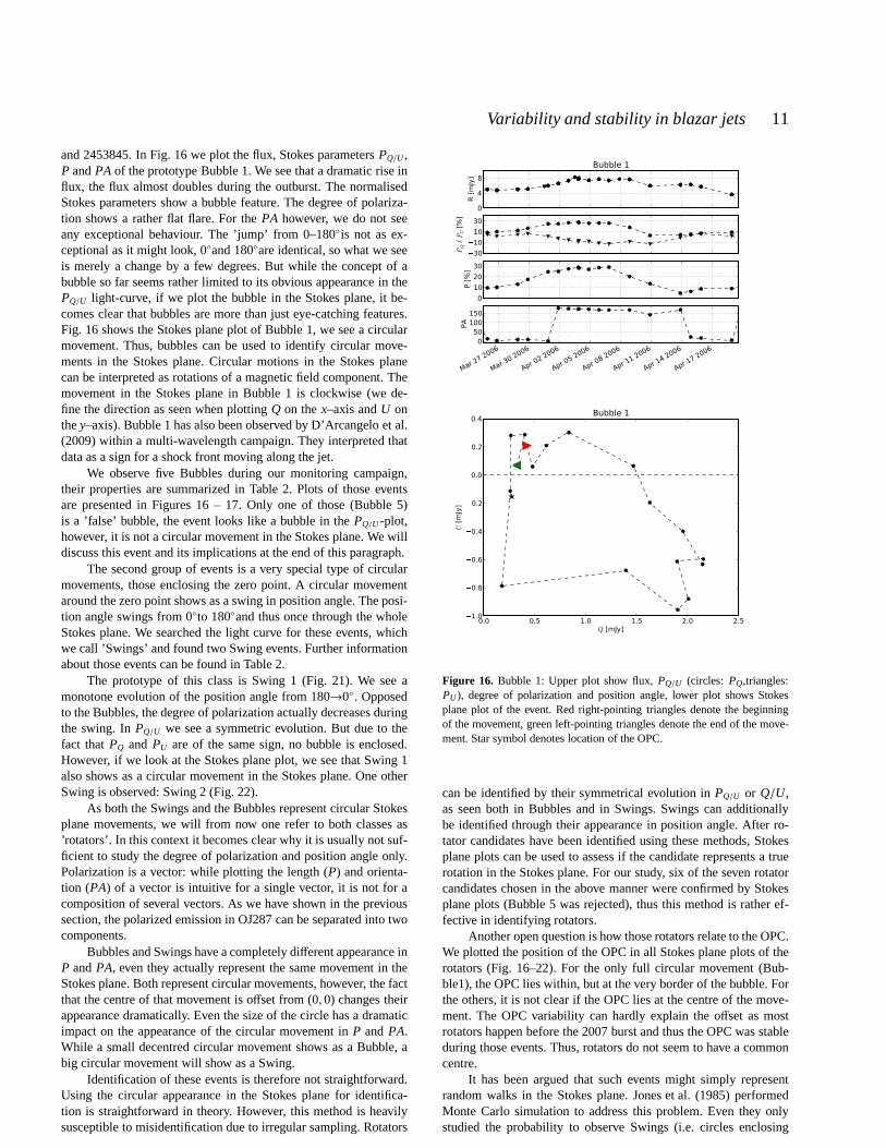
and 2453845. In Fig. 16 we plot the flux, Stokes parametersPQ/U ,P andPAof the prototype Bubble 1. We see that a dramatic rise influx, the flux almost doubles during the outburst. The normalisedStokes parameters show a bubble feature. The degree of polariza-tion shows a rather flat flare. For thePA however, we do not seeany exceptional behaviour. The ’jump’ from 0–180 is not as ex-ceptional as it might look, 0and 180are identical, so what we seeis merely a change by a few degrees. But while the concept of abubble so far seems rather limited to its obvious appearancein thePQ/U light-curve, if we plot the bubble in the Stokes plane, it be-comes clear that bubbles are more than just eye-catching features.Fig. 16 shows the Stokes plane plot of Bubble 1, we see a circularmovement. Thus, bubbles can be used to identify circular move-ments in the Stokes plane. Circular motions in the Stokes planecan be interpreted as rotations of a magnetic field component. Themovement in the Stokes plane in Bubble 1 is clockwise (we de-fine the direction as seen when plottingQ on thex–axis andU onthey–axis). Bubble 1 has also been observed by D’Arcangelo et al.(2009) within a multi-wavelength campaign. They interpreted thatdata as a sign for a shock front moving along the jet.

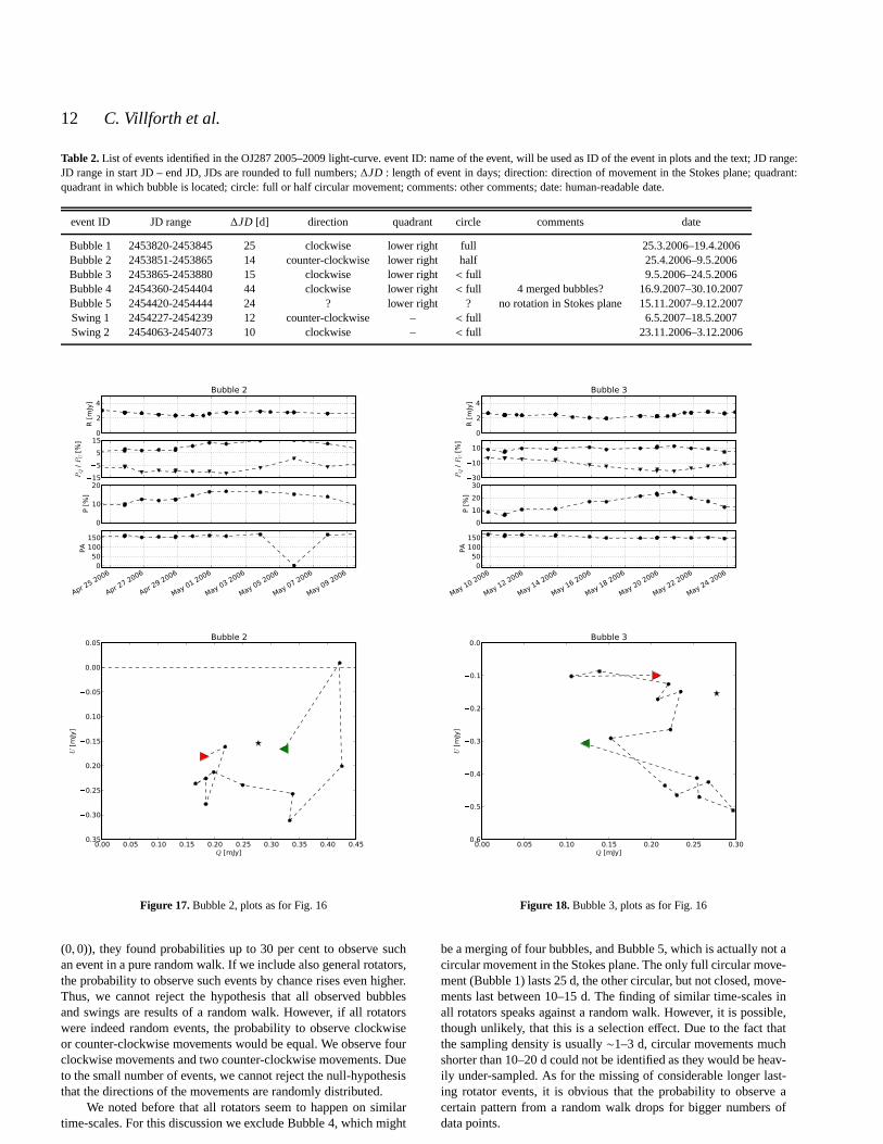
We observe five Bubbles during our monitoring campaign,their properties are summarized in Table 2. Plots of those eventsare presented in Figures 16 – 17. Only one of those (Bubble 5)is a ’false’ bubble, the event looks like a bubble in thePQ/U -plot,however, it is not a circular movement in the Stokes plane. Wewilldiscuss this event and its implications at the end of this paragraph.

The second group of events is a very special type of circularmovements, those enclosing the zero point. A circular movementaround the zero point shows as a swing in position angle. The posi-tion angle swings from 0to 180and thus once through the wholeStokes plane. We searched the light curve for these events, whichwe call ’Swings’ and found two Swing events. Further informationabout those events can be found in Table 2.

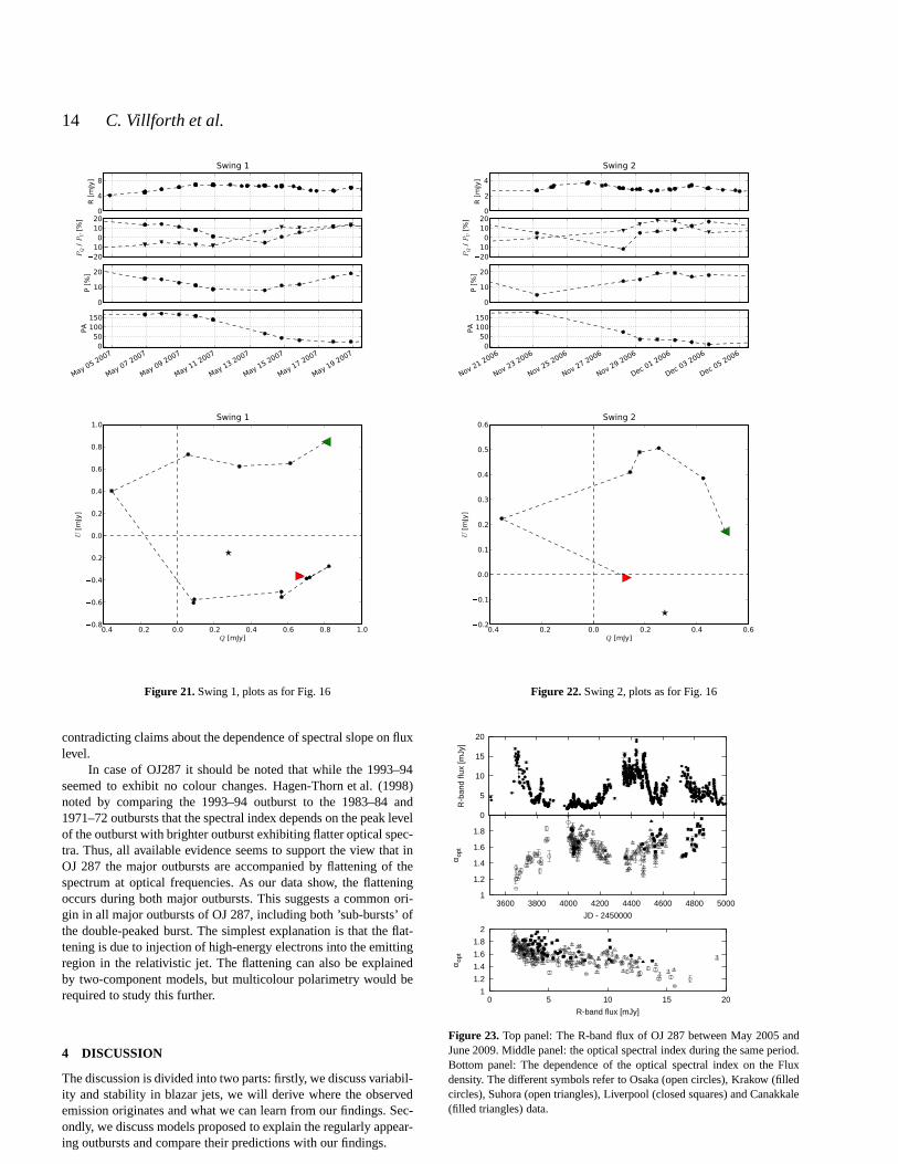
The prototype of this class is Swing 1 (Fig. 21). We see amonotone evolution of the position angle from 180→0 . Opposedto the Bubbles, the degree of polarization actually decreases duringthe swing. InPQ/U we see a symmetric evolution. But due to thefact thatPQ and PU are of the same sign, no bubble is enclosed.However, if we look at the Stokes plane plot, we see that Swing1also shows as a circular movement in the Stokes plane. One otherSwing is observed: Swing 2 (Fig. 22).

As both the Swings and the Bubbles represent circular Stokesplane movements, we will from now one refer to both classes as’rotators’. In this context it becomes clear why it is usually not suf-ficient to study the degree of polarization and position angle only.Polarization is a vector: while plotting the length (P) and orienta-tion (PA) of a vector is intuitive for a single vector, it is not for acomposition of several vectors. As we have shown in the previoussection, the polarized emission in OJ287 can be separated into twocomponents.

Bubbles and Swings have a completely different appearance inP andPA, even they actually represent the same movement in theStokes plane. Both represent circular movements, however,the factthat the centre of that movement is offset from (0, 0) changes theirappearance dramatically. Even the size of the circle has a dramaticimpact on the appearance of the circular movement inP andPA.While a small decentred circular movement shows as a Bubble,abig circular movement will show as a Swing.

Identification of these events is therefore not straightforward.Using the circular appearance in the Stokes plane for identifica-tion is straightforward in theory. However, this method is heavilysusceptible to misidentification due to irregular sampling. Rotators

0

4

8

R [

mJy

]

Bubble 1

30

10

10

30

PQ /

PU [

%]

0

10

20

30

P [

%]

Mar 27 2006

Mar 30 2006

Apr 02 2006

Apr 05 2006

Apr 08 2006

Apr 11 2006

Apr 14 2006

Apr 17 2006

050

100150

PA

0.0 0.5 1.0 1.5 2.0 2.5Q [mJy]

1.0

0.8

0.6

0.4

0.2

0.0

0.2

0.4

U [

mJy

]

Bubble 1

Figure 16. Bubble 1: Upper plot show flux,PQ/U (circles: PQ,triangles:PU), degree of polarization and position angle, lower plot shows Stokesplane plot of the event. Red right-pointing triangles denote the beginningof the movement, green left-pointing triangles denote the end of the move-ment. Star symbol denotes location of the OPC.

can be identified by their symmetrical evolution inPQ/U or Q/U,as seen both in Bubbles and in Swings. Swings can additionallybe identified through their appearance in position angle. After ro-tator candidates have been identified using these methods, Stokesplane plots can be used to assess if the candidate representsa truerotation in the Stokes plane. For our study, six of the seven rotatorcandidates chosen in the above manner were confirmed by Stokesplane plots (Bubble 5 was rejected), thus this method is rather ef-fective in identifying rotators.

Another open question is how those rotators relate to the OPC.We plotted the position of the OPC in all Stokes plane plots oftherotators (Fig. 16–22). For the only full circular movement (Bub-ble1), the OPC lies within, but at the very border of the bubble. Forthe others, it is not clear if the OPC lies at the centre of the move-ment. The OPC variability can hardly explain the offset as mostrotators happen before the 2007 burst and thus the OPC was stableduring those events. Thus, rotators do not seem to have a commoncentre.

It has been argued that such events might simply representrandom walks in the Stokes plane. Jones et al. (1985) performedMonte Carlo simulation to address this problem. Even they onlystudied the probability to observe Swings (i.e. circles enclosing

12 C. Villforth et al.

Table 2.List of events identified in the OJ287 2005–2009 light-curve. event ID: name of the event, will be used as ID of the event in plots and the text; JD range:JD range in start JD – end JD, JDs are rounded to full numbers;∆JD : length of event in days; direction: direction of movement in the Stokes plane; quadrant:quadrant in which bubble is located; circle: full or half circular movement; comments: other comments; date: human-readable date.

event ID JD range ∆JD [d] direction quadrant circle comments date

Bubble 1 2453820-2453845 25 clockwise lower right full 25.3.2006–19.4.2006Bubble 2 2453851-2453865 14 counter-clockwise lower righthalf 25.4.2006–9.5.2006Bubble 3 2453865-2453880 15 clockwise lower right< full 9.5.2006–24.5.2006Bubble 4 2454360-2454404 44 clockwise lower right< full 4 merged bubbles? 16.9.2007–30.10.2007Bubble 5 2454420-2454444 24 ? lower right ? no rotation in Stokes plane 15.11.2007–9.12.2007Swing 1 2454227-2454239 12 counter-clockwise – < full 6.5.2007–18.5.2007Swing 2 2454063-2454073 10 clockwise – < full 23.11.2006–3.12.2006

0

2

4

R [

mJy

]

Bubble 2

15

5

5

15

PQ /

PU [

%]

0

10

20

P [

%]

Apr 25 2006

Apr 27 2006

Apr 29 2006

May 01 2006

May 03 2006

May 05 2006

May 07 2006

May 09 20060

50100150

PA

0.00 0.05 0.10 0.15 0.20 0.25 0.30 0.35 0.40 0.45Q [mJy]

0.35

0.30

0.25

0.20

0.15

0.10

0.05

0.00

0.05

U [

mJy

]

Bubble 2

Figure 17.Bubble 2, plots as for Fig. 16

(0,0)), they found probabilities up to 30 per cent to observe suchan event in a pure random walk. If we include also general rotators,the probability to observe such events by chance rises even higher.Thus, we cannot reject the hypothesis that all observed bubblesand swings are results of a random walk. However, if all rotatorswere indeed random events, the probability to observe clockwiseor counter-clockwise movements would be equal. We observe fourclockwise movements and two counter-clockwise movements.Dueto the small number of events, we cannot reject the null-hypothesisthat the directions of the movements are randomly distributed.

We noted before that all rotators seem to happen on similartime-scales. For this discussion we exclude Bubble 4, whichmight

0

2

4

R [

mJy

]

Bubble 3

30

10

10PQ /

PU [

%]

0

10

20

30

P [

%]

May 10 2006

May 12 2006

May 14 2006

May 16 2006

May 18 2006

May 20 2006

May 22 2006

May 24 20060

50100150

PA

0.00 0.05 0.10 0.15 0.20 0.25 0.30Q [mJy]

0.6

0.5

0.4

0.3

0.2

0.1

0.0

U [

mJy

]

Bubble 3

Figure 18.Bubble 3, plots as for Fig. 16

be a merging of four bubbles, and Bubble 5, which is actually not acircular movement in the Stokes plane. The only full circular move-ment (Bubble 1) lasts 25 d, the other circular, but not closed, move-ments last between 10–15 d. The finding of similar time-scales inall rotators speaks against a random walk. However, it is possible,though unlikely, that this is a selection effect. Due to the fact thatthe sampling density is usually∼1–3 d, circular movements muchshorter than 10–20 d could not be identified as they would be heav-ily under-sampled. As for the missing of considerable longer last-ing rotator events, it is obvious that the probability to observe acertain pattern from a random walk drops for bigger numbers ofdata points.

Variability and stability in blazar jets 13

4

8

12

16

R [

mJy

]

Bubble 4

30

10

10

30

PQ /

PU [

%]

010203040

P [

%]

Sep 18 2007

Sep 21 2007

Sep 24 2007

Sep 27 2007

Sep 30 2007

Oct 03 2007

Oct 06 2007

Oct 09 2007

Oct 12 2007

Oct 15 2007

Oct 18 2007

Oct 21 2007

Oct 24 2007

Oct 27 2007

Oct 30 2007

050

100150

PA

0.5 0.0 0.5 1.0 1.5 2.0 2.5 3.0 3.5 4.0Q [mJy]

2.0

1.5

1.0

0.5

0.0

U [

mJy

]

Bubble 4

Figure 19.Bubble 4, plots as for Fig. 16

While the preference of clockwise movements and the similartime-scales point towards a physical reason behind the rotators, wecannot completely reject the possibility that some of the previouslydescribed events are a result of random walks. We will howeverdiscuss possible physical causes for such observations in Section4.1.

3.4 Optical spectral index variability

We investigate the variability of the spectral indexα (Fν ∝ ν−α) inthe optical by fitting power-law spectra to the observed multicolourdata. The multicolour data are not strictly simultaneous, but we useonly multicolour data where all filters were observed withinan hourfrom each other. Altogether 218 multicolour observations are usedfor the spectral fits.

For converting theBVRI magnitudes to linear fluxes we usedthe zero points given in Bessell (1979). The galactic absorption wascorrected using Schlegel et al. (1998). The flux of the host galaxyis ∼ 0.08 mJy in theR-band (see Section 4.2), which is∼ 3 percent of the total flux at the faintest flux levels reported in this paper.Thus we have made no correction for the host galaxy. The fits weremade in a logν - log Fν scale by fitting a straight line toVRI orBVRIdata using ordinary least squares (OLS) regression of y on x.In five cases we have alsoU-band data, but theU-band point lies inall cases∼ 10 per cent below the straight line delineated by otherbands. Since the drop-off in the spectrum is very sudden, we treated

48

121620

R [

mJy

]

Bubble 5

30

10

10

30

PQ /

PU [

%]

0

10

20

30

P [

%]

Nov 17 2007

Nov 20 2007

Nov 23 2007

Nov 26 2007

Nov 29 2007

Dec 02 2007

Dec 05 2007

Dec 08 2007

050

100150

PA

0.5 0.0 0.5 1.0 1.5 2.0 2.5 3.0 3.5 4.0Q [mJy]

3.0

2.5

2.0

1.5

1.0

0.5

0.0

U [

mJy

]

Bubble 5

Figure 20.Bubble 5, plots as for Fig. 16

it as a problem in the calibration rather than a true spectralfeatureand excluded theU-band from further analysis. We also excludedthe three cases where the error in the spectral index was larger than0.1.

In Fig. 23 we show the evolution of the optical spectral in-dex with time and its dependence on the optical flux. We see aclear dependence between the flux level and the spectral indexwith brighter flux levels corresponding to flatter optical spectra.The Spearman correlation coefficient of the flux–αopt correlation is−0.71 with> 99.9 per cent significance. This kind of ’bluer whenbrighter’ behaviour has been observed before in OJ287 and alsoin other blazars (e.g. Fiorucci et al. 2004), although a morecom-plex behaviour is sometimes observed (Raiteri et al. 2008).Alsonegative correlations between flux and bluer colours have been re-ported (e.g. Bottcher et al. 2009). During the 1993-94 outburst ofOJ 287 the optical colours were also reported to have been con-stant over a wide range of optical magnitudes (Sillanpaa et al. 1996;Hagen-Thorn et al. 1998).

If one looks at the flux -α plots in Fiorucci et al. (2004) itbecomes evident that the spectral slope changes are very subtle anda successful detection requires monitoring the target overa largeflux range and with high precision. For instance, in case of our data,the change inV–R colour is 0.06 mag over a magnitude range of2 mag. Thus in a short campaign covering a limited range in fluxthe spectral slope changes may go unnoticed leading to apparently

14 C. Villforth et al.

0

4

8

R [

mJy

]

Swing 1

2010

01020

PQ /

PU [

%]

0

10

20

P [

%]

May 05 2007

May 07 2007

May 09 2007

May 11 2007

May 13 2007

May 15 2007

May 17 2007

May 19 20070

50100150

PA

0.4 0.2 0.0 0.2 0.4 0.6 0.8 1.0Q [mJy]

0.8

0.6

0.4

0.2

0.0

0.2

0.4

0.6

0.8

1.0

U [

mJy

]

Swing 1

Figure 21.Swing 1, plots as for Fig. 16

contradicting claims about the dependence of spectral slope on fluxlevel.

In case of OJ287 it should be noted that while the 1993–94seemed to exhibit no colour changes. Hagen-Thorn et al. (1998)noted by comparing the 1993–94 outburst to the 1983–84 and1971–72 outbursts that the spectral index depends on the peak levelof the outburst with brighter outburst exhibiting flatter optical spec-tra. Thus, all available evidence seems to support the view that inOJ 287 the major outbursts are accompanied by flattening of thespectrum at optical frequencies. As our data show, the flatteningoccurs during both major outbursts. This suggests a common ori-gin in all major outbursts of OJ 287, including both ’sub-bursts’ ofthe double-peaked burst. The simplest explanation is that the flat-tening is due to injection of high-energy electrons into theemittingregion in the relativistic jet. The flattening can also be explainedby two-component models, but multicolour polarimetry would berequired to study this further.

4 DISCUSSION

The discussion is divided into two parts: firstly, we discussvariabil-ity and stability in blazar jets, we will derive where the observedemission originates and what we can learn from our findings. Sec-ondly, we discuss models proposed to explain the regularly appear-ing outbursts and compare their predictions with our findings.

0

2

4

R [

mJy

]

Swing 2

2010

01020

PQ /

PU [

%]

0

10

20

P [

%]

Nov 21 2006

Nov 23 2006

Nov 25 2006

Nov 27 2006

Nov 29 2006

Dec 01 2006

Dec 03 2006

Dec 05 2006

050

100150

PA

0.4 0.2 0.0 0.2 0.4 0.6Q [mJy]

0.2

0.1

0.0

0.1

0.2

0.3

0.4

0.5

0.6

U [

mJy

]

Swing 2

Figure 22.Swing 2, plots as for Fig. 16

0

5

10

15

20

R-b

and

flux

[mJy

]

1

1.2

1.4

1.6

1.8

3600 3800 4000 4200 4400 4600 4800 5000

α opt

JD - 2450000

1

1.2

1.4

1.6

1.8

2

0 5 10 15 20

α opt

R-band flux [mJy]

Figure 23. Top panel: The R-band flux of OJ 287 between May 2005 andJune 2009. Middle panel: the optical spectral index during the same period.Bottom panel: The dependence of the optical spectral index on the Fluxdensity. The different symbols refer to Osaka (open circles), Krakow (filledcircles), Suhora (open triangles), Liverpool (closed squares) and Canakkale(filled triangles) data.

Variability and stability in blazar jets 15

4.1 Variability and stability in the jet of OJ287

In the previous section we showed that the polarized emission fromOJ287 has a clear preferred position angle. We were able to di-vide the optical polarized emission into two separate components:the optical polarization core (OPC) and chaotic emission with aweak alignment along the direction of the OPC. The OPC rep-resents emission of polarized flux that is stable on time scales ofyears, but highly variable on time scales of decades. We observeda strengthening of the OPC during our monitoring campaign, thechange happened shortly after the 2007 burst. The chaotic emis-sion partially shows in so-called ’rotators’, which represent circularmovements in the Stokes plane. It is unclear if the circular move-ments are centred around the OPC. In this section we shall trytoderive where this emission originates and what we can learn fromour findings.

4.1.1 Where does polarized emission in blazar jets originate?

In general, polarization in blazars is caused by synchrotron emis-sion. Synchrotron emission is observed when charged particlesmove in a strong magnetic field. However, to result in high degreesof polarization, the magnetic field needs to be ordered, otherwisethe polarization in different directions cancels out. An obvious wayto align unordered magnetic fields is through shock fronts, whichare a very common feature in magneto-hydro-dynamical (MHD)jets. Shocks can compress an unordered magnetic field and pro-duce a strong, ordered magnetic field, oriented perpendicular to theflow direction (Hughes et al. 1989a,b; Marscher & Gear 1985).Asshocks naturally occur in jets and produce strong, linearlypolar-ized emission, relating the high degrees of polarization observed inblazar jets with shock fronts suggests itself.

So far, the shock front in jet model has been extremely suc-cessful in modelling flares in several blazars (e.g. Marscher & Gear1985; Marscher et al. 2008; D’Arcangelo et al. 2009). However,Gabuzda et al. (2004) pointed out that there is evidence thatpointstowards a global, helical magnetic field in the jet. With increasingresolution in VLBI maps, it has been found that the aligned mag-netic field covers extended areas, whereas shocks are compact. Ad-ditionally, the alignment of the magnetic field has been observedto stay intact even in the presence of bends and kinks. All theseobservations point towards a globally – not locally – aligned mag-netic field. Also, our finding of extremely weak correlation betweenhigh degrees of polarization and high fluxes points towards aglobalmagnetic field. If polarized emission would only be generated inshock fronts, it should always be related to outbursts in flux, this ishowever not observed.

Additionally, simulations support findings of a global mag-netic field. The importance of globally aligned magnetic fields forthe launching and collimation of outflows has been emphasizedrepeatedly (see e.g. Nakamura et al. 2001, Igumenshchev et al.2003). In addition, helical magnetic fields are produced rather nat-urally: if a global magnetic field is present in the accretiondisc,the accretion process will spin up the field lines, creating ahelicalmagnetic field that can carry the jet (Nakamura et al. 2001).

Another interesting observation is the alignment between op-tical and radio polarization. Gabuzda et al. (2006) studiedthe re-lation between the optical and radio polarization in a number ofblazar jets and found both values to be surprisingly well aligned.This might mean that the alignment of the magnetic field is a globalphenomenon. A global magnetic field would naturally align thepolarization in the same way in every region of the jet, and thus

through all wavelengths. Instabilities in the jet might cause smallerregions to show a different alignment. However, the finding thatradio and optical polarization are aligned does not prove the exis-tence of a global magnetic field. A ’common point of emission’forthe bulk of both the optical and radio data can also explain such astrong alignment.

4.1.2 How can changes in the OPC be explained?

In OJ287, the polarization vector is currently oriented perpendic-ular to the jet – pointing towards a longitudinal magnetic field –while in the past it has been oriented along the jet direction– point-ing towards a transverse magnetic field. Both the helical magneticfield and the shock front model however produce purely transversemagnetic fields. Thus, neither the helical magnetic field model northe shock front model can explain all the observations. But beforewe jump to any conclusions, let us discuss what could cause anapparent flip of the magnetic field direction.

The easiest and most obvious way to flip the PA is to flip themagnetic field. However, in shock fronts, the magnetic field is bydefinition aligned perpendicular to the jet flow. Thus, it is not pos-sible to flip the magnetic field in a shock front as the magneticfieldtakes a well-defined value. The same goes for the helical magneticin which the toroidal component is dominant due to beaming, caus-ing the observed magnetic field to be transverse.

Lyutikov et al. (2005) pointed out thatPA ⊥−→B is not strictly

valid in AGN jets. This relation only holds in the non-relativisticcase, which is a rather absurd approximation to make for AGNjets. Due to the beaming, certain components of the magneticfieldbecome more visible in the polarization than others. However, toachieve a 90flip, one would need to assume two components witha perpendicularly oriented magnetic field. While componentone isfully beamed and component two is de-beamed before the flip, thebeaming of the two components would need to reverse. It is veryhard to imagine a setup in which such an event would take place.

Another possibility for a flip of the magnetic field would be amovement of the jet itself. In case the jet would perform somekindof swinging motion, a swinging motion of the magnetic field wouldbe observed in polarization. Due to the fact that OJ287 has a rathersmall viewing angle, this might only require a movement of few de-grees or less. However, it is not clear how such a movement couldbe achieved. Corkscrew shaped jets are observed in several sources(Steffen et al. 1995), however, these jets perform a constant pre-cessing motion on time scales of years. For OJ287 one would haveto explain a single movement. With respect to the binary model,Valtonen et al. (2006) stated that a binary could push the disc in acertain direction at every orbit. OJ287 does not show a constantlymoving jet, but a single jump. Additionally, it is questionable if a’kick to the disc’ would show as such a sudden movement in thejet. Because the magnetic fields are assumed to be the ’framing’of the jet, it is unclear if a ’kick to the disc’ could be powerfulenough to move the entire magnetic field within only about a year.If the jet would have undergone such a traumatic change, it shouldalso be visible in VLBI maps. However, Gabuzda & Gomez (2001)published VLBI maps of OJ287 in which components with polar-ization vectors both transverse and longitudinal are observed, noremains of a perpendicularly oriented dead jet are visible,makingthe jet swing hypothesis even more unlikely.

The last option would be a change in the opacity, i.e. a changebetween optically thick and optically thin emission. In case of opti-cally thin emission the observed PA lies orthogonal to the magnetic

16 C. Villforth et al.

field while for optically thick emission, the observed PA lies par-allel to the magnetic field. Therefore a change of the regionsthatdominate the emission can cause a 90flip. Beaming could causesuch a change. If the beaming factor changes, the restframe wave-length of the emission we observe in the optical changes. If thechange between optically thick and optically thin emissionis closeto the restframe wavelength of the emission we observe as opti-cal. Thus a change of the beaming factor could explain the flip.However, the transition between optically thick and thin emissionusually lies in the radio frequencies (e.g. Gabuzda & Gomez2001).

Both the helical magnetic field and the shock front model can-not produce a naturally longitudinal field and thus cannot explainthe behaviour observed in OJ287. This raises the question ifit ispossible to produce anaturally longitudinal magnetic field in thejet. Longitudinal magnetic fields can be produced through shear atthe border of the jet that interacts with the surrounding medium,the shear-dominated area is called sheath. In this case, longitudinalfields are observed on the border of the jet and transverse fields areobserved in the spine of the jet (see e.g. Gabuzda 2003). Thishasbeen observed in some sources (see e.g. Gabuzda 2003). However,in OJ287 such a spine+ sheath structure is not visible. Addition-ally, it is questionable if the sheath could dominate over the spinefor a period of time, after which the spine dominates again.

D’Arcangelo et al. (2009) discussed the interesting findingthat the polarization in OJ287 – both in radio and optical – pointstowards a longitudinal magnetic field. They suggested that shearaligns the magnetic field longitudinally in the core. They arguedthat during the times in which the field was observed to be trans-verse, shocks aligned the field in a transverse direction temporarily.In contrast to these findings, Efimov et al. (2002) studied opticalphotometric monitoring data from 1994-1997 and found evidenceof a global helical magnetic field in the jet.

Poloidal magnetic fields provide a longitudinal magnetic fieldnaturally. In simulations, injected poloidal magnetic fields areneeded to produce powerful jets (see e.g. Igumenshchev et al.2003). However, due to the rotation in the accretion flow, thepoloidal components get spun up into a helical structure. Ifthemagnetic field structure is helical, beaming will enhance thetoroidal component strongly, this will be observed as atransversemagnetic field. If the rotation is minimal, most of the poloidalfield will be preserved and only a small toroidal component willbe produced. Normal accretion discs are rotating rapidly, it is thusunlikely that a standard thin accretion disc would produce apre-dominantly poloidal magnetic field. Radiatively inefficient accre-tion flows are candidates for Bondi-like and thus minimally ro-tating accretion flows (Igumenshchev & Abramowicz 2001). Ithasbeen suggested that BL Lac objects accrete through such flowsandnot standard thin accretion discs (Baum et al. 1995; Ghisellini et al.2009). Thus it is possible that OJ287 has accreted a predominantlypoloidal magnetic field.

If we assume that a poloidal magnetic field is causing the un-usual position angle currently observed in OJ287, we have toex-plain that the magnetic field used to be oriented transversely from1970–1994. One could argue that shock fronts dominated the emis-sion from 1970–1994, but that seems highly constructed. It alsodoes not explain the migration of the OPC through the Stokes plane(Fig. 15). Another way to explain the observations is through theaccretion of magnetic field lines. In an accretion process, not onlymatter, but also magnetic field accretes onto the black hole.Whileclosed field lines can be swallowed by the black hole, open fieldlines cannot. When open field lines accrete, they get caught nearthe black hole, building a poloidal magnetic field. In case the ac-

cretion of open field lines with the same orientation continues,the poloidal magnetic field grows stronger and stronger. Finally,the poloidal component gets so strong that it dominates and ’takesover’. Thus we can explain the PA flip observed in the 1990s asaccretion of poloidal field lines. In 1994, after a phase of massiveaccretion of both matter and magnetic field, the poloidal compo-nent got so strong that it started to dominate. The fact that the OPCstrengthened after the 2007 burst also suggests that the changes ofthe magnetic field are related to enhanced accretion events.

4.1.3 What is the origin of the OPC?

The question remains where the OPC originates. Two possibleex-planations for an optical polarization core exist: a globalmagneticfield and a common point of emission. If a global magnetic fieldexists, polarized emission is expected from the entire jet flow. Inthat case, the OPC can be interpreted as a sign of the ’quiescent jet’and therefore can be used to analyse the global magnetic fieldin thejet. By ’quiescent jet’ we mean the jet without any turbulences orshock fronts. The emission from the quiescent jet would naturallybe stable as it depends only on the strength and orientation of themagnetic field, the beaming factor and the accretion rate (ormoreprecisely, the rate at which matter flows through the jet). All ofthose parameters are not expected to change on small time scales.In case of a rapid change of the magnetic field, the changes prop-agate in the jet with the speed of light. Due to the high beamingfactor in OJ287, the change might be observed to propagate withsuperluminal speed. The fact that changes in the OPC are observedon time scales of about a year indicates that the bulk of the OPCemission originates in a part of the jet with a size of& 1 pc.

An alternative explanation is that there is a ’common point ofemission’, i.e. all OPC emission originates from a small area in thejet. It is not obvious why the ’common point of emission’, whichis presumably extremely small, would be stable on time-scales ofyears. This approach can explain the alignment between the radioand optical polarization, but has trouble explaining the flip in posi-tion angle. D’Arcangelo et al. (2009) argued that the position angleflip indicates a change between a normal and shear-dominatedstateof the jet. However, this would require a mechanism which wouldturn a stable ’normal’ jet into a stable shear-dominated jet.

As argued before, the OPC swing can most naturally be ex-plained assuming a global magnetic field. The stability of the OPCon time-scales is also more naturally explained by an extendedsource of emission. Therefore, we argue that the OPC traces thequiescent jet and can therefore be used to study the jet magneticfield in blazars.

4.1.4 Is the OPC commonly observed in blazars?

Another question is if a preferred position angle, as observed inOJ287, is a common feature in all blazars. Jones et al. (1985)observed 20 compact radio sources in different radio bandsand found a ’radio polarization core’, which they describedasscattering around a common value. Opposed to our findings,Jones et al. (1985) concluded that thePQ/U gave a better estimateof this value thanQ/U. They concluded from this that the mag-netic field is mostly tangled, only showing minor anisotropies.Angel & Stockman (1980) were the first ones to address this topicin the optical. They were able to divide a sample of 21 objects(all blazars or Seyfert galaxies with blazar-like SEDs) into twodistinct groups. Group one does not show any preferred PA, the

Variability and stability in blazar jets 17

data-points are ’all over the compass’. We will call these sourcesOPC-weak in the further discussion. The second group consists ofobjects in which repeated measurements show a restricted rangeof angles. These objects will be referred to as OPC-strong inthefurther discussion. Angel & Stockman (1980) already noted thatOJ287 belongs to both classes, depending on the time when it isobserved. During the 2005–2009 OJ287 was clearly OPC-strong,it was also OPC-strong during the monitoring campaign conductedby Hagen-Thorn (1980). In the 1980s however, OJ287 was OPC-weak. Angel & Stockman (1980) noted that all OPC-weak sourcesin their sample are rather bright, high-redshift objects, while theOPC-strong sources are at lower redshift and fainter.

We decided to compare the both groups, omitting OJ287.We found that the two groups, the OPC-weak and OPC-strongsources, show significant differences. Out of the eight OPC-weaksources, five are FSRQs, two are BL Lacs and one (3C279) is a BLLac/FSRQ transition object. On the other hand, out of the 12 OPC-strong sources, nine are BL Lacs, two are Seyfert galaxies and onlyone is a FSRQ. Even considering the fact that we are clearly lim-ited by low number statistics and some objects might have beenmisidentified due to limited amount of available polarization data,this is a truly fascinating finding. If this neat separation can be con-firmed for a larger sample, this would mean that that the jet emis-sion in BL Lac objects and FSRQs differs significantly. This is sup-ported by the findings of Jannuzi et al. (1994) which studied opticalpolarization variability in BL Lacs and found all of them to have apreferred position angle, showing in a similar manner as observedin OJ287.

This result indicates a difference in the ratio of turbulent (un-aligned) and quiescent (OPC/aligned) jet emission. In FSRQs, theturbulent jet emission seems to dominate, the OPC emission isweak compared to the normal level of the turbulent emission.Theposition angle is either unaligned or only weakly aligned. In BLLac objects, the OPC emission is strong compared to the levelsof the turbulent emission, the position angle is aligned. Assumingthat the OPC emission originates from the common point of emis-sion, this would indicate that the common point of emission (e.g. astanding shock front) in FSRQs is weaker compared to the restofthe jet emission than in BL Lacs. Assuming that the OPC is causedby quiescent jet emission in presence of a strong helical magneticfield, this would indicate that the magnetic field in FSRQ jetsmightbe weaker or that the jet emission is dominated by turbulent un-aligned emission. Thus, if the findings from Angel & Stockman(1980) would be confirmed for larger samples, this would indicatethat not only do FSRQs and BL Lacs show different accretion pro-cesses, but they also differ in the variability and properties of theirjets.

4.1.5 How can ’rotators’ be explained?

Another open question is the origin of the rotators we observed. Ro-tators are commonly observed in radio, Aller et al. (1981) first iden-tified these events calling them ’polarization rotators’. Jones et al.(1985) observed such rotators as well, however, he suggested thatthose might just be random walk events. As we discussed in Sec-tion 3.3, we cannot clearly reject the hypothesis that thoserotatorevents are indeed random events.

While one might expect that all rotators would be centredaround the OPC, this cannot be confirmed for our observations.The decentring of the bubbles cannot be explained assuming fastvariability in the OPC. This might either be explained by anothercomponent that is constant during the rotator and decentresthe ro-

tator from the OPC or by assuming that rotator are not rotatingaround the zero-point but another point in the Stokes plane.

Rotators could be interpreted as blobs moving along a helicaltrajectory inside the jet. However, there is a serious caveat to thisinterpretation. If the rotators were indeed signs of a blob movingalong a helical trajectory, all of them should have the same direc-tion as the orientation of the helical field will decide the orientationof the rotation. Clearly not all rotators have the same direction!One could argue that the rotators with the ’wrong orientation’ arerandom movements while the ones with the ’right orientation’ areblobs moving along the magnetic field. However, this is clearly nota convincing explanation.

A more natural explanation is to assume that the rotators areshock fronts moving backwards and forwards in the jet, swipingthrough the helical magnetic field. This would explain the differentrotation directions observed as well as the presence of rotators thatdo not represent full circles in the Stokes plane. Additionally, the’wobbling shock front’ seems to fit the bubble sequence consistingof Bubbles 1, 2 and 3. These bubbles follow each other with a verysmall time lag. Bubble 1 is clockwise, 2 counter-clockwise and 3clockwise again, this could be explained as a shock front wobblingback and forth. It can also explain a common time-scale for allrotator events in case the speed of the ’wobbling shock front’ isapproximately constant.

We are able to interpret our observations as a sign of a jet thathas two major components, the quiescent jet and turbulent emis-sion from wobbling shock fronts inside the jet. The quiescent jetcontributes considerably to the jet emission, even if we assume thatthe emission of the quiescent jet is maximally polarized (which israther unlikely), we find that in contributes∼20 per cent to the fluxin a quiescent state. We further argue that polarimetric monitoringcan be used to study the global magnetic field in the jet and as-sess if the jet is dominated by turbulent or quiescent emission. Wealso find differences between FSRQs and BL Lacs concerning thestrength of the quiescent jet component, our findings indicate thatFSRQ jets are dominated by turbulent emission while BL Lac jetsare dominated by quiescent jet emission. Further observations willhave to show if our findings hold for bigger samples.

4.2 OJ287: a blazar hosting a binary black hole?

This part of the discussion is dedicated to the mystery of theregu-larly appearing double-peaked outbursts observed in OJ287. Beforewe rate the different models proposed for OJ287, we compose a listof requirements for a successful model and use this list to system-atically assess each particular model.

4.2.1 A list of requirements for OJ287 models

While the light-curve of OJ287 has been studied excessively, lim-itations to the suggested models set by the objects itself have re-ceived little attention. It is clear that a successfully model wouldnot only have to describe the light-curve correctly but alsobe con-sistent with the properties of the object, including the black holemass. Before discussing prominent features of the light-curve, wetherefore discuss the limitations set by the fact that OJ287is a BLLac object and derive an estimate for the black hole mass.

BL Lacs are a special subclass of blazars. It is nowadayswidely believed that BL Lac objects are Fanaroff-Riley I (FR I) typeobjects with a jet pointed directly towards the observer (Baum et al.

18 C. Villforth et al.

1995). FR I objects are low-luminosity radio galaxies with ajet thatis luminous and relativistic near the core, while it decelerates tosub-relativistic speed on scales of∼ 100− 1000 pc.

Baum et al. (1995) systematically studied the differences be-tween FR II and FR I radio galaxies and found that the spectrumof FR Is is missing strong broad emission lines. They found the lu-minosity and ionization of narrow emission lines is consistent withbeing caused by ionizing radiation from the host galaxy and not theAGN. The weakness or absence of broad emission lines cannot beexplained using obscuration. Baum et al. (1995) were able toex-plain the line properties by assuming that FR Is accrete throughradiatively inefficient accretion flows (RIAFS). Therefore the ion-izing radiation from the accretion disc in FR Is is missing, caus-ing the weakness or absence of broad and narrow emission lines.Ghisellini et al. (2009) studiedγ-ray properties of a big sample ofBL Lacs and FSRQs and found a neat separation of the two blazartypes in theγ-ray luminosity vs spectral index plane. They wereable to explain this separation assuming that FSRQs accreteradia-tively efficiently while BL Lacs accrete radiatively inefficiently.

Baum et al. (1995) and Ghisellini et al. (2009) based theirstudies on completely different datasets, but reached the same con-clusions. Additionally, no other possible explanation forthe di-chotomy between FR I/ II radio galaxies and BL Lacs/ FSRQsexist to our knowledge. Thus, we can state that BL Lac objectsmost likely accrete through RIAFs. This statement raises the ques-tion if accretion through a RIAF instead of a standard thin accretiondisc would have any influence on the suggested models for OJ287.

Radiatively inefficient flows can appear in two regimes of ac-cretion: sub-Eddington accretion ( ˙m≪ 1) and super-Eddington ac-cretion (m ≫ 1). Both flows have a common feature: due to thefact that the flows are not radiating efficiently, the cooling is in-efficient. Thus, these flows are hot and geometrically thick. Overthe years, several analytical models for RIAFs were developed:such as the advection-dominated accretion flows (ADAF), adiabaticinflow-outflow solution (ADIOS), the convection-dominatedaccre-tion flow (CDAF) and convection dominated Bondi-flows (CDBF).For a full description of the analytical models see Igumenshchev(2004). In the last years, numerical viscous and MHD modelswere used to simulate radiatively inefficient accretion flows (e.g.Igumenshchev et al. 2003). From MHD simulations it became clearthat the properties of the flow depend strongly on the injected mag-netic field. Even the exact physics in these flows is not well under-stood yet, one point is clear, RIAFs are geometrically thick! Thelack of cooling ’puffs up’ the disc. A thick disc might be problem-atic for binary black hole models that associate the bursts with disccrossing. In case of a thin disc, the time it takes the secondary blackhole to cross the disc is short. In case of a geometrically thick discand a small orbit however, it might take the secondary a consid-erable percentage of the orbital period to cross the disc. Thus theburst would cover a longer timespan.

Therefore, we estimate if the assumed trajectory of the sec-ondary black hole lies within the simulation regime and thuswithinthe range in which the flow is geometrically thick. The simula-tions from Igumenshchev et al. (2003) reach out to a radius of256RS chwarzschild. Considering two example masses for the central super-massive black hole of 109/1010M⊙ this corresponds to∼ 8×1014/15

m. Using the third Kepler law, we can roughly estimate the semi-major axes of a possible binary black hole. We assume an orbitalperiod of 9 yr (in the restframe of the object). For the primary blackhole mass, we use the two example values of 109/1010M⊙. We fur-thermore assume thatMsecondaryBH ≪ MprimaryBH. This yields asemi-major axes for the 109M⊙ black hole of∼ 6 × 1014 m, for

the 1010M∼ black hole, we get a semi-major axes of∼ 1× 1015 m.These values lie inside, but in the outer part of the simulation box.Considering the newest version of the Lehto & Valtonen model, inwhich the secondary orbit is highly eccentric, the radii of the disccrossing lie at 1014−15 m and thus well within the simulation box.

Assuming that OJ287 is indeed powered by a radiatively inef-ficient, geometrically thick accretion flow, the outburst due to pierc-ing of the accretion disc by the secondary black hole lasts longer. Aclearly defined ’disc piercing’ no longer exists as the secondary isinside the disc for a considerable part of the orbit. However, OJ287is only observed to be ’in burst’ about ten percent of its time! Incase of the Lehto & Valtonen model the flare associated with thedisc piercing lasts only∼1 week! This corresponds to only<1 percent of the orbital period and is thus in clear contradictionto a ge-ometrically thick accretion flow.

Further limitations to possible models can be set by the massof the central black hole. Due to the fact that OJ287 is a BL Lacob-ject and does not show broad emission lines except in its extremelyfaint state (see e.g. Sitko & Junkkarinen 1985), determination ofthe mass of the central black hole is not feasible using reverber-ation mapping. Another method to determine the masses of cen-tral black holes is using relations between the host galaxy and themass of the central black hole (see Novak et al. 2006 for a summaryof these methods), this method can be used for OJ287 as the hostgalaxy properties have been studied. We summarize different re-sults of host galaxy studies in Tab. 3. We use the results to estimatethe mass of the central black hole.

For all publications apart from Hutchings et al. (1984), whereno apparent magnitudes are given, we calculate the absolutemag-nitude applying k-corrections from Bicker et al. (2004). Noevo-lutionary corrections are applied. If the preferred morphology isa disc model, we use k-corrections for a Sb galaxy, otherwiseweuse the k-corrections for an E galaxy. O’Dowd & Urry (2005) usedtheS T ISfilter F28x50LPfor which no k-corrections are available.This filter is a low pass filter with a cut-off frequency of∼5500Å.In this case, we use k-corrections for BesselR. Even the real trans-mission curve of this filter is much bluer than for a BesselR, we donot expect that this introduces big errors. For example the differ-ence between the k-correction forR andI at this redshift are only<0.1 mag.

A few things are notable when talking about the host galaxy ofOJ287. The first is the repeatedly mentioned decentring of the ex-tended emission (Yanny et al. 1997; Heidt et al. 1999; Nilsson et al.2003). The only mentioning of the amount of decentring is fromYanny et al. (1997), who found a value of 0.4 arcsec, correspond-ing to as much as 1.81 kpc. However, Yanny et al. (1997) mighthave had problems with the PSF and thus these results should betaken with caution. Decentring might be more of a sign that thehost was actually not resolved than a sign that there is actually atruly decentred nebulosity. Another noteworthy fact is theextremeoptical-NIR colour indicated by the different results. The measuredhost galaxy inK is about 3 mag more luminous than aL∗-galaxywhile the upper limits for the optical filter are around the values forL∗-galaxies. This implies an extremely red galaxy. Even ULIRGs,supposedly the reddest galaxies in the optical-NIR range, do notshow such extreme optical-NIR colours but a rather flat spectrum(see e.g. Kim et al. 1995). This leads us to assume that the detectionin NIR is most likely spurious, as already suspected by the authors(Wright et al. 1998). All in all, we think that it is safe to assume thatthe host galaxy of OJ287 is unresolved, however, several consistentand reliable upper limits exist. The values found in the optical arewell consistent with anL∗ elliptical galaxy. Thus we can use these

Variability and stability in blazar jets 19

Table 3. Properties of OJ287 host galaxy from different publications. Columns have following meanings: firstcolumn shows the publicationused; band: filter used;m: apparent host magnitude;M: absolute host magnitude;re[kpc]: effective radius of galaxy in kpc; morph.: morphology,if not specified, none given in the publication; dc?: decentring of host with respect to point source (yes, no, ? if not mentioned, values given inarcseconds);logMBH: log of the mass of the central black hole in solar masses.

band m M re[kpc] morph. dc? logMBH

Hutchings et al. (1984) R – >-23.1 – – ? <9.0Yanny et al. (1997) F814W 18.30±1.30 -23.05 – – 0.4´ 8.9Wright et al. (1998) K 12.0 -29.15 6.68 disc ? –Wright et al. (1998) K 12.2 -29.14 11.13 none preferred ? 10.4Heidt et al. (1999) R 18.41 -22.96 4.4 bulge yes 8.9Heidt et al. (1999) R 19.32 -22.00 10.2 disc yes –Urry et al. (2000) F702W >18.53 >-23.01 – – ? <8.9Pursimo et al. (2002) R 18.91 -22.79 4.5 bulge ? 8.8Nilsson et al. (2003) R >18.1 >-23.27 – – yes <9.0O’Dowd & Urry (2005) F28x50LP >18.53 >-23.02 – – ? <8.9

0

10

20

30

40

50

60

2410000 2415000 2420000 2425000 2430000 2435000 2440000 2445000 2450000 2455000

1900 1920 1940 1960 1980 2000

V-b

and

flux

/ mJy

JD

year

Figure 24. OJ287V-band flux from 1885-2009.R-band fluxes were con-verted toV-band fluxes usingV-R= 0.4 mag.

upper limits to estimate the upper limit for the mass of the centralblack hole.

We use relations published in Novak et al. (2006) to estimatethe mass of the central black hole. For theR band data we use therelation based on data from Bettoni et al. (2003). We use the samerelation for the filtersF814W, F702WandF28x50LPas the differ-ences between these bands are minimal and no colour-correctionsfor these filters are available. For theK band data, we use colourcorrections from Poggianti (1997) to transform the magnitude totheJ band, we use the relation based on data from Marconi & Hunt(2003) to derive the black hole mass.

Estimating the central black hole mass from the optical datagives values oflogMBH . 9. The results from the only availableNIR measurement gives a value oflogMBH ≈ 10. The big differ-ence is caused by the fact that combining the optical and NIR re-sults gives a colour that strongly deviates from colours of normalelliptical or disc galaxies at similar redshift. Note that relations aspresented in Novak et al. (2006) only hold for galaxies with normalSEDs. If the galaxy strongly deviates from a normal SED, blackhole masses derived using luminosities are no longer reliable. How-ever, upper limits for optical host galaxy luminosities andblackhole masses derived from optical data hold.

After discussing the properties of OJ287 not related to thelight-curve, we will continue by putting together a list of prominentproperties of the light-curve and finish by presenting a clear list of

requirements which we use to rate the different models. A plot ofthe entire flux monitoring data, from 1885 to 2009 is presented inFig. 24.

Exact timing has received a lot of attention, especially in theLehto & Valtonen model and its successors. However, in ordertobe able to calculate results from their models, all authors had tomake simplifications. Including all possible influences (i.e. MHDand general relativistic effects, warped disc...) would yield mod-els with too many adjustable parameters. Additionally, solving theproblem of a binary black hole together with an accretion flowwould require fully relativistic MHD simulations that alsocalcu-late the radiation transfer, this is not possible with current MHDmodels and computer power. Therefore, we do not believe thatitis possible to calculate the timing of the bursts with an accuracy inthe order of days. Additionally, the light-curve has ’holes’ causedby OJ287 being to close to the sun to be observed. As we discussedin Section 3.1, this can have the effect that the exact time of theoutburst can only be determined with an accuracy in the orderofweeks to months. Also, before∼1970 the sampling was too sparseto determine the exact time of the outbursts accurately, this effectsthe calculations for the models. Therefore we believe that neitherare exact timing predictions possible nor is it possible to derive ex-act outburst times from the light-curve. Due to this fact we will notput a lot of weight on high timing accuracy in this discussion. How-ever, we do discuss if models strongly deviate from the measuredtime of the outburst.

The ’pseudo-periodicity’: this rather awkward word describ-ing the light-curve of OJ287 was introduced to emphasize that theoutbursts in OJ287 appear regularly while deviating from periodic-ity. Particularly the 2005 burst strongly deviates from periodicity,being observed about a year earlier than expected for strictperi-odicity. It is true that strong, rather regularly appearingoutburstshave been observed from the 1970s till the present. However,thisrepresents only four cycles. We do not believe that earlier outburstscan clearly be established as the sampling was too sparse (see Fig.24). Especially as there are about 10 year long gaps in the data. Thefact that outbursts were observed around the time expected before1970 does not prove that there were periodic outbursts – not evenpseudo-periodic outbursts for that matter. For certainty,one canonly say that the data before the 1970s does not contradict regularlyappearing outbursts at∼ 12 yr intervals. Additionally, OJ287 maybe ’loosing’ its regularly appearing outbursts. The peak fluxes inthe double peaked outbursts have been declining significantly sincethe first well-sampled burst in the∼1970s (see Fig. 24). Between

20 C. Villforth et al.

the 1994–1995 burst and the present burst there was an additionaloutburst which was approximately as strong as the 2005–2007ma-jor outbursts (see Fig. 24). Also, a ’third major burst’ directly afterthe second major burst was observed during the 2005–2007 cam-paign. The current major bursts are by no means as exceptional asthe bursts observed in the 1970s and 1980s. While bursts are stillobserved near the expected time, and partially more than oneyearearlier than expected, additional bursts of similar strength are ob-served. A model would thus have to explain regularly appearingoutbursts every∼ 9 yr (in the object restframe) over' 3−4 cycles.

Double-peaked outburstsare observed in the 1970s, 80s and90s-bursts. The two bursts are of similar strength and separated by∼ 1 yr. The 2005/2007 burst might also be classified as a double-peaked burst. However, a third peak has been observed duringthisperiod, following the second peak almost with only a short delay.

The peak intensitiesin the major optical bursts have beendeclining from almost 60 mJy in the 1970s to only about 15 mJy inthe latest bursts. Both peaks show a similar evolution (see Fig. 24).If we include earlier, poorly sampled, bursts it seems like the peakintensities have been increasing from∼ 1900–1970 (see Fig. 24).However, as the sampling is too poor to draw clear conclusions, wewill neglect the evolution before 1970.

Radio counterparts are observed for some optical outburstswhile they are missing for others. There is no clear pattern for theoccurrence of radio counterparts. During the both the 1980sand1990s flaring, the first burst showed a radio counterpart while thesecond did not (Valtaoja et al. 2000). Sampling for the 1970sburstsis too sparse to draw clear conclusions (Valtaoja et al. 2000). Dur-ing the 2005–2007 period neither of the bursts showed a radiocoun-terpart (Merja Tornikoski & Anne Lahteenmaki, private communi-cation). While we are clearly limited by small number statistics,we can state that the first burst was never observed to have a radio-counterpart, while the second burst was observed both with andwithout radio-counterpart.

Strong changes in the optical polarization coreare observedfrom the 1970s till today (see Fig. 14). The strength of the OPC hasshowed both de- and increasing phases. A flip in the preferredPA ofabout 90has been observed in the 1990s (see Fig. 14). It seems thatstrong changes in the core polarization follow the double-peakedbursts with a delay of∼ 1 yr. However, the connection between thedouble-peaked outbursts and the OPC changes is not well estab-lished due to small number statistics.

The limitations set by the object itself: from host galaxydata, we can set an upper limit for the central black hole massof M <

= 109M⊙. Additionally, we know that OJ287 is a BL Lacobject and thus a FR I radio galaxy. Many observations point to-wards the fact that BL Lac objects are fed by radiatively inefficientand thus geometrically thick accretion flows (e.g. Baum et al. 1995,Ghisellini et al. 2009).

Thus a new model would have to explain the following obser-vations:

• regularly appearing outbursts in the optical light-curve with aperiod of∼ 9 yr over>= 3-4 cycles• double-peaked outbursts in at least three cases, both peaks

have comparable strength, the current double-peaked burstmightbe better classified as a triple-burst• the peak intensities undergo strong changes, from 1970–2007

the peak intensities have been abating, both peaks show a similarevolution• radio counterparts are observed in some bursts, never has one

of the first bursts been observed to show a radio counterpart,the

second bursts are observed both with and without radio counter-parts• the strength of the OPC changes, including a flip, changes are

possibly related to the double-peaked bursts• a black hole mass<= 109M⊙• a radiatively inefficient, geometrically thick accretion flow

In Tab. 4 we present a comprehensive and short summary ofthe different models using our list of requirements. Each model willbe discussed separately and in detail in the following paragraphs.

4.2.2 Lehto& Valtonen: a binary black hole, two disc piercings,gravitational waves

In this section we discuss both the original Lehto & Valtonenmodel (Lehto & Valtonen 1996) and the modified Lehto & Valto-nen model that was presented to fit the unexpectedly early outburstin 2005 (Valtonen et al. 2006; Valtonen 2007). Note that bothmod-els are almost identical, the differences are due to the addition of a’live disc’, a new fit to the data using the 2005 burst and changedtiming for earlier bursts. The basic properties of the modelhoweverare identical.

Before we compare this model to our list of requirements,we would like to discuss some properties and parameters of thismodel. One of the critical points in the Lehto & Valtonen modelis the question how the disturbance in the disc will affect the jet.Valtonen et al. (2009) estimated that the particles reach the jet afteronly a few days, producing a jet burst immediately after the firstthermal flare. The jet flare merges with the accretion disc flare, nodelay at all is observed between the two flares. Thus each observedburst actually consists of two flares: the accretion-disc-flare and thejet-response-flare. To achieve such a short delay, they assumed thatthe particles enter the jet flow as soon as they pass a radius of10RS chwarzschild, which is very close to the radius at which the sec-ondary black hole pierces the disc. Particles that get injected intothe jet become visible immediately. It is very likely that changingthis parameter would change the appearance of the bursts dramat-ically. As the short time delay between the accretion disc piercingand the jet response is so fundamentally important for this model,we will discuss this point in greater detail.

It is unclear why Valtonen et al. (2009) chose this particularradius. For comparison, the radius at which the accreting mate-rial plunges into the black hole, the innermost stable circular orbit(ISCO) isRISCO = 3 × RS chwarzschildfor a non-rotating black hole.The ISCO shrinks considerably if the black hole has a high spin.The ISCO is the smallest radius at which the accreting materialcould enter the jet. Additionally, Valtonen et al. (2009) did not takeviscosity and MHD effects into account. Viscosity and turbulenceplay a major role in accretion processes (Balbus & Hawley 1998)and thus estimations neglecting these effects might yield wrong re-sults.

Thus, we will estimate the time delay between the discpiercing and the jet response and compare it to the results fromValtonen et al. (2009). If we assume that the launching of thejethappens anywhere between the disc piercing and the ISCO, we cantry to estimate the time it takes the disturbance to become visiblein the jet. Estimating these time-scales is rather challenging. How-ever, we can use the viscous time scale at the radius of the discpiercing to get a lower limit for the time it takes for the disturbanceto reach the ISCO. The viscous time-scale for standardα-discs canbe calculated as follows (Czerny 2006):

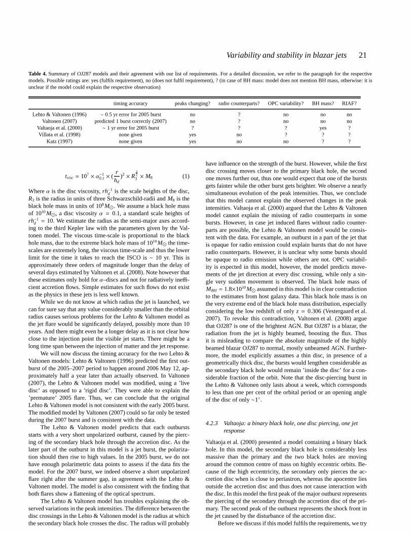
Variability and stability in blazar jets 21

Table 4. Summary of OJ287 models and their agreement with our list of requirements. For a detailed discussion, we refer to the paragraph for the respectivemodels. Possible ratings are: yes (fulfils requirement), no(does not fulfil requirement), ? (in case of BH mass: model does not mention BH mass, otherwise: it isunclear if the model could explain the respective observation)

timing accuracy peaks changing? radio counterparts? OPC variability? BH mass? RIAF?

Lehto & Valtonen (1996) ∼ 0.5 yr error for 2005 burst no ? no no noValtonen (2007) predicted 1 burst correctly (2007) no ? no no no

Valtaoja et al. (2000) ∼ 1 yr error for 2005 burst ? ? ? yes ?Villata et al. (1998) none given yes no ? ? ?

Katz (1997) none given yes no no ? ?

tvisc = 107× α−1

0.1 × (rhd

)2× R

323 × M8 (1)

Whereα is the disc viscosity,rh−1d is the scale heights of the disc,

R3 is the radius in units of three Schwarzschild-radii andM8 is theblack hole mass in units of 108M⊙. We assume a black hole massof 1010M⊙, a disc viscosityα = 0.1, a standard scale heights ofrh−1

d = 10. We estimate the radius as the semi-major axes accord-ing to the third Kepler law with the parameters given by the Val-tonen model. The viscous time-scale is proportional to the blackhole mass, due to the extreme black hole mass of 1010M⊙ the time-scales are extremely long, the viscous time-scale and thus the lowerlimit for the time it takes to reach the ISCO is∼ 10 yr. This isapproximately three orders of magnitude longer than the delay ofseveral days estimated by Valtonen et al. (2008). Note however thatthese estimates only hold forα–discs and not for radiatively ineffi-cient accretion flows. Simple estimates for such flows do not existas the physics in these jets is less well known.

While we do not know at which radius the jet is launched, wecan for sure say that any value considerably smaller than theorbitalradius causes serious problems for the Lehto & Valtonen model asthe jet flare would be significantly delayed, possibly more than 10years. And there might even be a longer delay as it is not clearhowclose to the injection point the visible jet starts. There might be along time span between the injection of matter and the jet response.

We will now discuss the timing accuracy for the two Lehto &Valtonen models: Lehto & Valtonen (1996) predicted the firstout-burst of the 2005–2007 period to happen around 2006 May 12, ap-proximately half a year later than actually observed. In Valtonen(2007), the Lehto & Valtonen model was modified, using a ’livedisc’ as opposed to a ’rigid disc’. They were able to explain the’premature’ 2005 flare. Thus, we can conclude that the originalLehto & Valtonen model is not consistent with the early 2005 burst.The modified model by Valtonen (2007) could so far only be testedduring the 2007 burst and is consistent with the data.

The Lehto & Valtonen model predicts that each outburstsstarts with a very short unpolarized outburst, caused by thepierc-ing of the secondary black hole through the accretion disc. As thelater part of the outburst in this model is a jet burst, the polariza-tion should then rise to high values. In the 2005 burst, we do nothave enough polarimetric data points to assess if the data fits themodel. For the 2007 burst, we indeed observe a short unpolarizedflare right after the summer gap, in agreement with the Lehto &Valtonen model. The model is also consistent with the findingthatboth flares show a flattening of the optical spectrum.

The Lehto & Valtonen model has troubles explaining the ob-served variations in the peak intensities. The difference between thedisc crossings in the Lehto & Valtonen model is the radius at whichthe secondary black hole crosses the disc. The radius will probably

have influence on the strength of the burst. However, while the firstdisc crossing moves closer to the primary black hole, the secondone moves further out, thus one would expect that one of the burstsgets fainter while the other burst gets brighter. We observea nearlysimultaneous evolution of the peak intensities. Thus, we concludethat this model cannot explain the observed changes in the peakintensities. Valtaoja et al. (2000) argued that the Lehto & Valtonenmodel cannot explain the missing of radio counterparts in somebursts. However, in case jet induced flares without radio counter-parts are possible, the Lehto & Valtonen model would be consis-tent with the data. For example, an outburst in a part of the jet thatis opaque for radio emission could explain bursts that do nothaveradio counterparts. However, it is unclear why some bursts shouldbe opaque to radio emission while others are not. OPC variabil-ity is expected in this model, however, the model predicts move-ments of the jet direction at every disc crossing, while onlya sin-gle very sudden movement is observed. The black hole mass ofMBH = 1.8×1010M⊙ assumed in this model is in clear contradictionto the estimates from host galaxy data. This black hole mass is onthe very extreme end of the black hole mass distribution, especiallyconsidering the low redshift of onlyz = 0.306 (Vestergaard et al.2007). To revoke this contradiction, Valtonen et al. (2008)arguethat OJ287 is one of the brightest AGN. But OJ287 is a blazar, theradiation from the jet is highly beamed, boosting the flux. Thusit is misleading to compare the absolute magnitude of the highlybeamed blazar OJ287 to normal, mostly unbeamed AGN. Further-more, the model explicitly assumes a thin disc, in presence of ageometrically thick disc, the bursts would lengthen considerable asthe secondary black hole would remain ’inside the disc’ for acon-siderable fraction of the orbit. Note that the disc-piercing burst inthe Lehto & Valtonen only lasts about a week, which correspondsto less than one per cent of the orbital period or an opening angleof the disc of only∼1.

4.2.3 Valtaoja: a binary black hole, one disc piercing, one jetresponse

Valtaoja et al. (2000) presented a model containing a binaryblackhole. In this model, the secondary black hole is considerably lessmassive than the primary and the two black holes are movingaround the common centre of mass on highly eccentric orbits.Be-cause of the high eccentricity, the secondary only pierces the ac-cretion disc when is close to periastron, whereas the apocentre liesoutside the accretion disc and thus does not cause interaction withthe disc. In this model the first peak of the major outburst representsthe piercing of the secondary through the accretion disc of the pri-mary. The second peak of the outburst represents the shock front inthe jet caused by the disturbance of the accretion disc.

Before we discuss if this model fulfils the requirements, we try

22 C. Villforth et al.

to estimate if a gap of∼ 1 yr between the first and the second burstis reasonable. We use the same formula and argument as in Section4.2.2 to estimate this time span. We assume a standard thin disc anda black hole mass of 109M⊙. Due to the fact that the orbit is highlyeccentric, we take a lower limit for the radius of 3RS chwarzschild. Thisyields a lower limit for the accretion time of∼ 3y. This is still inthe order of magnitude of the observed time gap. Note howeverthatthis value is the absolute lower limit. On the other hand, it is notclear how that estimate would change if one assumed a radiativelyinefficient instead of an standardα-disc.

As for the timing, the Valtaoja model assumes strict periodic-ity in the first peak. The delay between the first and second burstis assumed to be approximately 1 yr. However, due to the fact thatthe second peak represents the jet response to the disc crossing,which is obviously a very complex process, Valtaoja et al. (2000)do not provide a time prediction for the second burst. Using an or-bital solutions with a zero-point ofJD0 = 2449667 and a period ofP = 4324d, the primary outburst is expected in 2006 September 25(Valtaoja et al. 2000). Thus, the primary outburst happenedmorethan one year earlier than predicted.

In the Valtaoja model the first burst is a thermal flare, thus onewould not expect high degrees of polarization. The few data pointsobserved during the 2005 burst do show rather high degrees ofpo-larization, in contradiction to the model. The second burstin theValtaoja model is a jet burst and is therefore expected to be veryhighly polarized. Indeed, the 2007 outburst was very highlypolar-ized. The fact that both outbursts show a flattening of the opticalspectrum and thus most likely have the same origin speaks againstthe Valtaoja model.

As for the list of requirements: it is not evident if the Val-taoja model can explain the strong variability in the peak intensities.The first bursts is caused by a disc-crossing. Therefore considerablechanges in the strength of this bursts could either be explained bychanges in the radius at which the disc crossing occurs or by sig-nificant changes in the disc itself. However, if such a changeinthe intensity of the first burst would appear, one would also expectthe second burst to reflect these changes. This is indeed observed.Thus, the model might be able to explain the changes in the peakintensities. Valtaoja et al. (2000) based their models on the fact thatduring the double-peaked burst 1994–1995, the first peak didnothave a radio-counterpart, while the second peak also appeared inradio. During the 2005–2007 burst none of the peaks had a radiocounterpart. As for the Lehto & Valtonen model, the missing ofradio-counterparts could be explained if some burst happened inareas that are opaque to radio emission. Also, it is unclear if theValtaoja model could explain the OPC variability. As for theblackhole mass, Valtaoja et al. (2000) based his model on a 109

× M⊙black hole, which is the value estimated from host galaxy data. Ifwe assume that OJ287 is powered by a radiatively inefficient accre-tion flow, this could pose a problem for the Valtaoja model. Eventhe orbit is highly eccentric, a geometrically thick disc would con-siderably increase the time the secondary black hole spends’insidethe disc’ thereby increasing the length of the first burst. Because theexact orbit is not specified in the Valtaoja model, it is unclear howbig the effect would be. Also, the limitations by the geometricallythick accretion flow are not as severe as for the Lehto & Valtonenmodel as the disc-piercing-flare of the Valtaoja model lasts0.5–1yr as opposed to∼ 1 week for the Lehto & Valtonen model.

4.2.4 Villata: a binary black hole, two precessing jets, beamingevents

Villata et al. (1998) proposed a model containing a binary blackhole. Unlike in all other models, both supermassive black holes pro-duce relativistic jets. According to this model, both majoroutburstsare beaming events, each of the two bursts caused by one particularjet.

Due to the fact that this is a qualitative model, no exact timingpredictions are available. In this model, the peak intensities do un-dergo strong changes in a similar pattern as observed (Villata et al.1998). However, as Valtaoja et al. (2000) pointed out, this modelcannot explain the fact that some bursts have radio counterpartswhile others do not. For beaming events, one would expect allwavelength ranges to show enhanced emission, but this is notob-served. Due to the fact that in the Villata model the two jets ’windaround each other’, building a helical structure, it is not clear howthis would show in the OPC evolution. As mentioned above, themodel is qualitative, thus no statement about the black holemass ismade. The Villata model does not assume any particular accretionflow, thus, it is consistent with a RIAF.

4.2.5 Katz: a binary black hole, a precessing disc and jet

Katz (1997) proposed a precessing disc to be the cause for theob-served behaviour in OJ 287. A precessing disc would cause thejetto precess as well. In this model, the outbursts represent a sweepingof the jet through the line of sight. The double-peaked structure ofthe outbursts is thought to be caused by a nodding motion of the jetprecession.

As this is a qualitative model, no exact timing predictions areavailable. Due to the fact that both outbursts in this model arecaused by beaming events from the same jet, one would expectthat the strength of outbursts is variable in a pattern similar to theobservations. It might even be expected that the peak luminositiesundergo strong changes if the beaming factor changes between thedifferent bursts. This could show as an additional periodic variabil-ity in the peak intensities, which would be consistent with the data.Due to the fact that both bursts are ’beaming bursts’, this modelcannot explain the missing of radio counterparts in some bursts, aspointed out by Valtaoja et al. (2000). It is unclear if such a setupcould explain the observed OPC variations. The model is qualita-tive, and therefore does not specify the black hole mass. Themodelexplicitly assumes a thin accretion disc. It is questionable that aRIAF could show similar precession as RIAFs are not rotationallysupported.

4.2.6 Alternative explanations: accretion as a cause for regularbursts or better BBH models?

As we saw from the discussion in the previous section, noneof the existing models is able to explain all observations. Sev-eral models based on the assumption of a binary black hole havebeen developed (Lehto & Valtonen 1996; Katz 1997; Villata etal.1998; Valtaoja et al. 2000) and modified (e.g. Valtonen 2007;Valtonen et al. 2009). Parameters have been added, but still, noneof the models can explain all the observations.

Binary black hole models might profit from growing interestin understanding binary black hole mergers. For example, ithasbeen shown that binary black holes might show three disc systems,consisting of circum-black hole discs around the two black holesand a circum-binary disc around the whole system (Hayasaki et al.

Variability and stability in blazar jets 23

2007). However, those simulations were done for rather large sepa-rations, and it is unclear how such a system would look in a closerstage of its evolution. Perego et al. (2009) studied the interactionbetween binary black holes and the accreting material. Consideringsuch effects, current binary black hole models could be improved.

While gravitation based periodicity (i.e. two bodies circlingaround each other) is clearly the most obvious approach to explainregularity, it has been suggested that it is possible to achieve reg-ularity through resonance in accretion discs or jets (Ouyedet al.1997). The periodicity in simulated jets found by Ouyed et al.(1997) happened on time-scales of days and was strictly periodicand not abating. However, Ouyed et al. (1997) showed that op-posed to pictures of purely chaotic jets, reappearing, resonancebased events are possible in jets and accretion discs. For the case ofOJ287, Marscher (1997) argued that the properties of certain out-bursts suggest the jet as a source for the variations. Therefore, wewould like to discuss jet- and accretion-disc based approaches toexplain the observed behaviour in OJ287.

We base our discussion on our finding of the optical polar-ization core and its evolution during the last decades. We arguedin Section 4.1 that the observed behaviour in OJ287 is a sign ofa gradual strengthening of the poloidal magnetic field componentduring the last decades. The jet magnetic field used to be dom-inated by a toroidal component, while it is currently dominatedby a poloidal component. We also argued that due to the fact thatOJ287 is a BL Lac type object it is most likely powered by a radia-tively inefficient accretion flow (Baum et al. 1995; Ghisellini et al.2009). Those flows are minimally rotating (Igumenshchev 2004)and therefore make it possible that accreted poloidal field lines areonly minimally spun up and therefore preserve their poloidal com-ponent.

We argue that it would be rather astonishing to observe twoexceptional processes, namely regular bursts and changes in thejet magnetic field, going on in one object without any connectionbetween the two. We therefore suggest a casual connection betweenthe regular bursts and the OPC variability, with the OPC variabilitybeing the ’main symptom’ and the regular bursts being a ’after-effect’ of the changes in the jet.

We suggest that the bursts are related to the accretion of mag-netic field lines. We suggest that the regularly appearing flaresare signs that the accretion of the magnetic field happened inavalanches. Let us assume that at some point in the past, massiveaccretion of magnetic field caused strong disturbances in the mag-netic field of the accretion disc. This disturbance caused a reso-nance in the accretion disc, a ’magnetic breathing’ of the disc. Theresonance causes regularly appearing avalanche accretionof mag-netic field. We suggest that each double-peaked flare represents aphase of massive magnetic field accretion. As the central (poloidal)magnetic field strengthens, it starts to dominate the area near theblack hole. The strong central magnetic field starts to impede fur-ther accretion of magnetic field of the same orientation. Dueto this,the double-peaked flares are weakening over the course of time. Fi-nally, the strong central magnetic field will ’choke’ the resonance.

Based on this assumption, we interpret that the first episodeof avalanche accretion happened prior to the 1970s bursts. Thisevent caused the magnetic breathing. Phases of avalanche accre-tion were observed in the early 1970s, 1984–1985, 1994–1995and2005–2007, showing as gigantic double-peaked flares. In ourinter-pretation, the toroidal magnetic field component fully dominatedthe jet during the early phase of photopolarimetric monitoring. Thisshowed in a strong alignment of the OPC along the jet directionbetween the 1970s and 1980s bursts. The avalanche accretiondur-

ing the 1980s bursts caused a strengthening of the poloidal mag-netic field component. The poloidal and toroidal component wereof similar strength and thus the OPC was rather weak. The nextac-cretion during the big flaring around 1994 further strengthened thepoloidal component and it became dominant, causing the OPC toalign perpendicular to the jet. We interpret the abating of the peakintensities in the double-peaked flares as a sign of the strengtheningof the central poloidal magnetic field. The central field starts to re-pel further accretion of poloidal magnetic field lines and thereforethe strength of the double-peaked bursts weakens. According to ourinterpretation, the fact that the periodicity in OJ287 is lost and thestrength of the double-peaked bursts has reached the level of or-dinary outbursts can be interpreted such that the central poloidalmagnetic field has become so strong that the avalanche accretion ofmagnetic field lines of the same orientation is no longer possible.The resonance got choked by the strong central field. Therefore, wepredict that no more regularly appearing double-peaked outburstswill be observed in the future. Based on our assumptions, theseburst were caused by resonant avalanche accretion which is nowa-days impeded by the strength of the central magnetic field. Thisexplanation is also well consistent with our finding that theOPCstrengthened after the 2007 burst.

If this interpretation were true, the OPC in OJ287 would re-main strong and oriented perpendicular to the jet direction. Dueto the fact that no more accretion of open magnetic field linesofconsiderable strength is expected, the jet magnetic field, and thusthe OPC, should be stable and not show strong changes. Also, nofurther strong double-peaked bursts are expected based on this as-sumption as the central field has become so strong that avalancheaccretion is simply not possible any longer.

We are well aware that the suggested explanation is specu-lative. While it has been shown in simulations that setups astheone described in the ’magnetic breathing’ model are realistic (seee.g. Igumenshchev et al. 2003), some points are not fully clear. Itis not clear if a timespan of∼10 yr is realistic for such a resonancebehaviour. As argued earlier, time-scales of years are normal foraccretion processes around supermassive black holes, thuswe be-lieve the observed time-scale is realistic for resonance processes inthe accretion disc. The biggest caveat of this approach is the factthat it does not naturally explain the double-peaked bursts. We ar-gue that what we see is the accretion of magnetic field coupledtoaccreting matter. While the first bursts represents the accretion ofthe magnetic field, which can be observed instantaneously, the mat-ter needs time to reach the optical jet. The delay of about oneyearbetween the first and the second burst in this model would repre-sent the time it takes the matter to reach the visible jet. This wouldexplain that both bursts show a similar evolution in strength. How-ever, it does not explain the missing of radio-counterpartsin somebursts. It is not yet clear what decides if a disturbance in the jet willbe observed in radio, therefore it is unclear if the magneticbreath-ing model can explain the radio behaviour. The ’magnetic breath-ing’ approach does explain the OPC variability, it is consistent witha moderate black hole mass and a radiatively inefficient accretionflow.

With more advanced simulations, it will hopefully soon be-come possible to simulate both accretion processes and the launch-ing of the jet simultaneously. When those simulations become pos-sible, it will be interesting to assess if a setup as suggested in thissection is realistic. It will also be interesting to see if developmentsin the theoretical understandings of jets will bring new explana-tions. Further observations will also have to show if the strong reg-

24 C. Villforth et al.

ularly appearing outburst have indeed stopped. Till then, the caseof OJ287 will remain a mystery.

5 SUMMARY AND CONCLUSIONS

In this paper we present photopolarimetric monitoring of OJ287during the most recent major double-peaked outburst. We analysethe photopolarimetric light-curve, we describe the general appear-ance of the light-curve, analyse statistical properties and study theappearance of flares in polarization. We also compose a list of re-quirements for OJ287 models in which we also include propertiesof OJ287 not related to the light-curve. We use this list to compareall proposed models. We also discuss alternative explanations forOJ287. Our finding can be summarized as follows:

• During the 2005–2009 monitoring campaign, we observe twomajor outbursts. The first burst starts in summer 2005 and lasts tillearly summer 2006. The second burst starts in early summer 2007,it reaches its peak between mid August and 2007 September 12.The second burst is considerably longer lasting than the first one,covering an overall timespan of almost 2 years, as opposed toabout1 yr in the first burst. Both burst show strong polarization inboththe maximum and the declining phase.• The degree of polarization does not correlate with the flux, in

agreement with findings of other authors (Jannuzi et al. 1994).• We find a strong preferred position angle, caused by an under-

lying stable source of polarized emission: the optical polarizationcore (OPC). The OPC is stable on time scales, however, we did ob-serve a fast change in the OPC during our monitoring campaign.The change happened after the 2007 burst and strengthened theOPC considerably. We also found changes of the OPC during thelast decades, showing as a migration in the Stokes plane crossingthe zero point. Those changes are also correlated with the double-peaked bursts. We interpret that the OPC emission originates fromthe quiescent jet. Our observations indicate that a global magneticfield exists in blazar jets and can be observed as alignment oftheoptical polarization position angle. Based on former studies on thealignment of the optical polarization in blazars (Angel & Stockman1980; Jannuzi et al. 1994), we find a difference between the jets ofFSRQs and BL Lacs. In BL Lacs, the optical polarized emissionis dominated by the quiescent jet, while in FSRQs it is dominatedby the turbulent emission. Further observations will have to showif this holds for bigger samples.• We identify five events in the polarized emission that we clas-

sify as ’Bubbles’ and two events we classify as ’Swings’. BothBubbles and Swings are circular movements in the Stokes plane,generally known as rotators. No common centre for all rotators canbe identified, this cannot be explained through fast OPC variabil-ity. All rotators happen on similar time-scales and show a preferreddirection of rotation. We interpret these events as movements ofshock-fronts both up- and downstream the jet. Through theirmove-ment, the shock fronts swipe through different orientation of thehelical magnetic field, thereby producing swinging motions.• We study optical spectral index variations and find a ’bluer-

when-brighter’ trend in both flares. This is in agreement with otherstudies of OJ287 (Hagen-Thorn et al. 1998).• We compose a list of requirements for OJ287 models. The list

includes: regularly appearing double peaked outbursts, strong vari-ations in the peak intensities, differences between the bursts regard-ing the existence of radio counterparts, strong changes in the pre-ferred position angle (which we interpret as variability inthe OPC),

a black hole mass ofMBH . 109M⊙ and a radiatively inefficient,geometrically thick accretion flow.• We assess all models using the list of requirements. We con-

clude that none of the models can explain all items on the list.The original Lehto & Valtonen model (Lehto & Valtonen 1996) didnot predict the early 2005 outburst. Its successor, the new Lehto& Valtonen model (Valtonen et al. 2006; Valtonen 2007) is con-sistent with the timing of the 2007 burst. However, it cannotex-plain any of the other items on our list and is in contradiction withfour items on the list. The Valtaoja model (Valtaoja et al. 2000) didnot predict the early 2005 outburst, no modification to the modelwere made to fit the new observations. It is not clear if the Valtaojamodel can explain the other items on the list. Both the Villata model(Villata et al. 1998) and the Katz model (Katz 1997) cannot explainall items on the list.• We also discuss possibilities for alternative explanations. We

discuss a new approach based on the finding of violent variabilityof the optical core polarization in OJ287, observed since the 1970s.We argue that the optical polarization core is a sign of the quiescentjet and thus traces the jet magnetic field. Thus a change in thedirec-tion of the optical polarization core indicates a change of the direc-tion of the jet magnetic field. We suggest that this could havetakenplace in OJ287 through accretion of poloidal magnetic field lines.We suggest that a strong accretion event in the past caused reso-nance in the accretion disc. This resonance showed as avalancheaccretion of magnetic field lines every nine years in the object rest-frame, causing the double-peaked burst. According to our inter-pretation, the strength of the double-peaked outbursts is abating asthe central magnetic field strengthens and thereby repels accretingmagnetic field lines. We argue that the central magnetic fieldstartedto choke the resonance and therefore we expect no more regularlyappearing bursts. We also conclude that as long as this toy modelcannot be confirmed by simulations, the mystery of OJ287 willre-main unsolved.

ACKNOWLEDGEMENTS

The authors would like to thank the anonymous referee for hiscom-ments and suggestions. We would also like to thank Staszek Zola,Merja Tornikoski, Anne Lahteenmaki, the Metsahovi monitoringteam, Esko Valtaoja and Vilppu Piirola. Part of the data presentedhere are based on observations made with the Nordic Optical Tele-scope, operated on the island of La Palma jointly by Denmark,Finland, Iceland, Norway, and Sweden, in the Spanish Observa-torio del Roque de los Muchachos of the Instituto de Astrosicade Canarias. Part of the data presented here have been taken us-ing ALFOSC, which is owned by the Instituto de Astrofisica deAndalucia (IAA) and operated at the Nordic Optical Telescope un-der agreement between IAA and the NBIfAFG of the AstronomicalObservatory of Copenhagen. Based on observations collected at theCentro Astronomico Hispano Aleman (CAHA) at Calar Alto, op-erated jointly by the Max-Planck Institut fur Astronomie and theInstituto de Astrofısica de Andalucıa (CSIC). This work was partlysupported by the Polish MNiSW grant No. 3812/B/H03/2009/36.Jianghua Wu and Xu Zhou are supported by the Chinese NationalNatural Science Foundation grants 10603006 and 10633020.

Variability and stability in blazar jets 25

REFERENCES

Aller H. D., Aller M. F., Hodge P. E., 1981, Astronomical Journal,86, 325

Angel J. R. P., Stockman H. S., 1980, Annual Review of Astron-omy and Astrophysics, 18, 321

Balbus S. A., Hawley J. F., 1998, Reviews of Modern Physics, 70,1

Baum S. A., Zirbel E. L., O’Dea C. P., 1995, Astrophysical Jour-nal, 451, 88

Bessell M. S., 1979, Publications of the Astronomical Society ofthe Pacific, 91, 589

Bettoni D., Falomo R., Fasano G., Govoni F., 2003, Astronomyand Astrophysics, 399, 869

Bicker J., v. Alvensleben U. F., Moller C. S., Fricke K. J., 2004,Astronomy and Astrophysics, 413, 37

Bottcher M., Fultz K., Aller H. D., Aller M. F., Apodaca J.,Arkharov A. A., Bach U., Bachev R., Berdyugin A., Buemi C.,Calcidese P., Carosati D., Charlot P., Ciprini S., Paola A. D.,2009, Astrophysical Journal, 694, 174

Czerny B., 2006 Vol. 360, The role of the accretion disk in AGNvariability. p. 265

D’Arcangelo F. D., Marscher A. P., Jorstad S. G., Smith P. S.,Lar-ionov V. M., Hagen-Thorn V. A., Williams G. G., Gear W. K.,Clemens D. P., Sarcia D., Grabau A., Tollestrup E. V., BuieM. W., Taylor B., Dunham E., 2009, Astrophysical Journal, 697,985

Degl’Innocenti E. L., Bagnulo S., Fossati L., 2007 Vol. 364,Po-larimetric standardization. p. 495

Efimov Y. S., Shakhovskoy N. M., Takalo L. O., Sillanpaa A.,2002, Astronomy and Astrophysics, 381, 408

Fiorucci M., Ciprini S., Tosti G., 2004, Astronomy and Astro-physics, 419, 25

Gabuzda D. C., 2003, New Astronomy Review, 47, 599Gabuzda D. C., Gomez J. L., 2001, Monthly Notices of the RoyalAstronomical Society, 320, L49

Gabuzda D. C., Rastorgueva E. A., Smith P. S., O’Sullivan S. P.,2006, Monthly Notices of the Royal Astronomical Society, 369,1596

Gabuzda D. C., amonn Murray Cronin P., 2004, Monthly Noticesof the Royal Astronomical Society, 351, L89

Ghisellini G., Maraschi L., Tavecchio F., 2009, 0903.2043Gonzalez-Perez J. N., Kidger M. R., Martın-Luis F., 2001, Astro-nomical Journal, 122, 2055

Hagen-Thorn V. A., 1980, Astrophysics and Space Science, 73,263

Hagen-Thorn V. A., Marchenko S. G., Takalo L. O., Sillanpa¨a A.,Pursimo T., Boltwood P., Kidger M., Gonzalez-Perez J. N., 1998,Astronomy and Astrophysics Supplement Series, 133, 353

Hayasaki K., Mineshige S., Sudou H., 2007, Publications of theAstronomical Society of Japan, 59, 427

Heidt J., Nilsson K., Appenzeller I., Jager K., Seifert W.,SzeifertT., Gassler W., Hafner R., Hummel W., Muschielok B., NicklasH., Stahl O., 1999, Astronomy and Astrophysics, 352, L11

Holmes P. A., Brand P. W. J. L., Impey C. D., Williams P. M.,Smith P., Elston R., Balonek T., Zeilik M., Burns J., HeckertP.,Barvainis R., Kenny J., Schmidt G., Puschell J., 1984, MonthlyNotices of the Royal Astronomical Society, 211, 497

Hughes P. A., Aller H. D., Aller M. F., 1989a, Astrophysical Jour-nal, 341, 54

Hughes P. A., Aller H. D., Aller M. F., 1989b, Astrophysical Jour-nal, 341, 68

Hutchings J. B., Crampton D., Campbell B., 1984, AstrophysicalJournal, 280, 41

Igumenshchev I. V., 2004, Progress of Theoretical Physics Sup-plement, 155, 87

Igumenshchev I. V., Abramowicz M. A., 2001, astro-ph/0102482Igumenshchev I. V., Narayan R., Abramowicz M. A., 2003, As-trophysical Journal, 592, 1042

Jannuzi B. T., Smith P. S., Elston R., 1994, 428, 130Jones T. W., Rudnick L., Fiedler R. L., Aller H. D., Aller M. F.,Hodge P. E., 1985, Astrophysical Journal, 290, 627

Katz J. I., 1997, Astrophysical Journal, 478, 527Kim D., Sanders D. B., Veilleux S., Mazzarella J. M., Soifer B. T.,1995, Astrophysical Journal Supplement Series, 98, 129

Lehto H. J., Valtonen M. J., 1996, Astrophysical Journal, 460, 207Lyutikov M., Pariev V. I., Gabuzda D. C., 2005, Monthly Noticesof the Royal Astronomical Society, 360, 869

Marconi A., Hunt L. K., 2003, Astrophysical Journal, 589, L21Mardia K. V., Jupp P. E., , 1975, DirectionalStatistics, http://www3.interscience.wiley.com/cgi-bin/bookhome/119138576/

Marscher A., 1997, Conference Proceedings: ’OJ-94 AnnualMeeting 1997, An international Workshop on Multi-frequencymonitoring of Blazars’, pp 81–86

Marscher A. P., Gear W. K., 1985, Astrophysical Journal, 298,114

Marscher A. P., Jorstad S. G., D’Arcangelo F. D., Smith P. S.,Williams G. G., Larionov V. M., Oh H., Olmstead A. R., AllerM. F., Aller H. D., McHardy I. M., Lahteenmaki A., TornikoskiM., 2008, Nature, 452, 966

Nakamura M., Uchida Y., Hirose S., 2001, New Astronomy, 6, 61Nilsson K., Pursimo T., Heidt J., Takalo L. O., Sillanpaa A.,Brinkmann W., 2003, Astronomy and Astrophysics, 400, 95

Novak G. S., Faber S. M., Dekel A., 2006, Astrophysical Journal,637, 96

O’Dowd M., Urry C. M., 2005, Astrophysical Journal, 627, 97Ouyed R., Pudritz R. E., Stone J. M., 1997, Nature, 385, 409Perego A., Dotti M., Colpi M., Volonteri M., 2009, Astro-ph:0907.3742

Poggianti B. M., 1997, Astronomy and Astrophysics SupplementSeries, 122, 399

Pursimo T., Nilsson K., Takalo L. O., Sillanpaa A., Heidt J., PietilaH., 2002, Astronomy and Astrophysics, 381, 810

Raiteri C. M., Villata M., Larionov V. M., Gurwell M. A., ChenW. P., Kurtanidze O. M., Aller M. F., Bottcher M., CalcideseP.,Hroch F., Lahteenmaki A., Lee C., Nilsson K., 2008, Astronomyand Astrophysics, 491, 755

Schlegel D. J., Finkbeiner D. P., Davis M., 1998, AstrophysicalJournal, 500, 525

Sillanpaa A., Haarala S., Valtonen M. J., Sundelius B., Byrd G. G.,1988, Astrophysical Journal, 325, 628

Sillanpaa A., Takalo L. O., Pursimo T., Nilsson K., HeinamakiP., Katajainen S., Pietila H., Hanski M., Rekola R., KidgerM.,Boltwood P., Turner G. W., Robertson J. W., Honeycut R. K.,Efimov Y. S., 1996, Astronomy and Astrophysics, 315, L13

Simmons J. F. L., Stewart B. G., 1985, Astronomy and Astro-physics, 142, 100

Sitko M. L., Junkkarinen V. T., 1985, Publications of the Astro-nomical Society of the Pacific, 97, 1158

Steffen W., Zensus J. A., Krichbaum T. P., Witzel A., Qian S. J.,1995, Astronomy and Astrophysics, 302, 335

Turnshek D. A., Bohlin R. C., Williamson R. L., Lupie O. L.,Koornneef J., Morgan D. H., 1990, Astronomical Journal, 99,

26 C. Villforth et al.

1243Ulrich M., Maraschi L., Urry C. M., 1997, Annual Review of As-tronomy and Astrophysics, 35, 445

Urry C. M., Padovani P., 1995, Publications of the AstronomicalSociety of the Pacific, 107, 803

Urry C. M., Scarpa R., O’Dowd M., Falomo R., Pesce J. E., TrevesA., 2000, Astrophysical Journal, 532, 816

Valtaoja E., Terasranta H., Tornikoski M., Sillanpaa A., AllerM. F., Aller H. D., Hughes P. A., 2000, Astrophysical Journal,531, 744

Valtonen M. J., 2007, Astrophysical Journal, 659, 1074Valtonen M. J., Lehto H. J., Nilsson K., Heidt J., Takalo L. O.,Sillanpaa A., Villforth C., Kidger M., Poyner G., PursimoT.,Zola S., 2008, Nature, 452, 851

Valtonen M. J., Lehto H. J., Sillanpaa A., Nilsson K., Mikkola S.,Hudec R., Basta M., Terasranta H., Haque S., Rampadarath H.,2006, Astrophysical Journal, 646, 36

Valtonen M. J., Nilsson K., Villforth C., Lehto H. J., TakaloL. O.,Lindfors E., Sillanpaa A., Hentunen V., Mikkola S., Zola S.,Drozdz M., Koziel D., 2009, Astrophysical Journal, 698, 781

Vestergaard M., Fan X., Tremonti C. A., Osmer P. S., RichardsG. T., 2007, 0801.0243

Villata M., Raiteri C. M., Sillanpaa A., Takalo L. O., 1998,Monthly Notices of the Royal Astronomical Society, 293, L13

Villforth C., Nilsson K., stensen R., Heidt J., Niemi S., Pforr J.,2009, Monthly Notices of the Royal Astronomical Society, 397,1893

Wagner S. J., Witzel A., 1995, Annual Review of Astronomy andAstrophysics, 33, 163

Wright S. C., McHardy I. M., Abraham R. G., 1998, MonthlyNotices of the Royal Astronomical Society, 295, 799

Yanny B., Jannuzi B. T., Impey C., 1997, Astrophysical Journal,484, L113

All in-text references underlined in blue are linked to publications on ResearchGate, letting you access and read them immediately.