arX

iv:n

ucl-

th/9

8110

46v1

13

Nov

199

8

DOE/ER/40561-31-INT98

TRI-PP-98-27

KRL MAP-238

NT@UW-99-4

The Three-Boson System with Short-Range Interactions

P.F. Bedaquea, H.-W. Hammerb, and U. van Kolckc,d

aInstitute for Nuclear Theory

University of Washington, Seattle, WA 98195, USA

bedaque@mocha.phys.washington.edu

bTRIUMF, 4004 Wesbrook Mall

Vancouver, BC, V6T 2A3, Canada

hammer@triumf.ca

c Kellogg Radiation Laboratory, 106-38

California Institute of Technology, Pasadena, CA 91125, USA

vankolck@krl.caltech.edu

d Department of Physics

University of Washington, Seattle, WA 98195, USA

Abstract

We discuss renormalization of the non-relativistic three-body problem with

short-range forces. The problem is non-perturbative at momenta of the order

of the inverse of the two-body scattering length. An infinite number of graphs

must be summed, which leads to a cutoff dependence that does not appear

in any order in perturbation theory. We argue that this cutoff dependence

can be absorbed in one local three-body force counterterm and compute the

running of the three-body force with the cutoff. This allows a calculation of

the scattering of a particle and the two-particle bound state if the correspond-

ing scattering length is used as input. We also obtain a model-independent

relation between binding energy of a shallow three-body bound state and this

scattering length. We comment on the power counting that organizes higher-

order corrections and on relevance of this result for the effective field theory

program in nuclear and molecular physics.

I. INTRODUCTION

The three-body system provides non-trivial testground for ideas developed in two-bodydynamics, and as such has a long and venerable history. It is in general of very difficultsolution, but when all particles have momenta much smaller than the inverse of the range ofinteractions it simplifies considerably while still retaining some very rich universal features[1–3]. At such low energies, the two-body system can be attacked with many differenttechniques: effective range expansion, boundary conditions at the origin, etc.; a particularlyconvenient method for the extension to a many-body context is that of effective field theory(EFT) [4]. Here we use EFT to solve the three-body system with short-range interactionsin a systematic momentum expansion.

Generically the sizes of bound states made out of A particles of massm are all comparableto the range R of interactions. Similarly, the dimensionful scattering parameters — the two-body scattering length a2, the two-body effective range parameter r2, and so on— are alsoof the same order, R ∼ a2 ∼ r2 ∼ . . . The A-body amplitudes reduce at low energy k2/mto perturbative expansions in kR [5]. Less trivial is the case where the interactions arefine-tuned so that the two-body system has a shallow (real or virtual) bound state —thatis, a bound state of size ∼ a2 much larger than the range of the interactions R ∼ r2. This isa case of interest in nuclear physics, where the deuteron is large compared to the Comptonwavelength of the pion 1/mπ, and in molecular physics, where shallow molecules such asthe 4He “dimer” can be over an order of magnitude larger than the range of the interatomicpotential.

In this fine-tuning scenario, the A-body system still can be treated in a perturbativeexpansion in ka2 in the scattering region where all momenta are of order k ≪ 1/a2. Boundstates, however, correspond to k >∼ a2 and demand that a certain class of interactionsbe iterated an infinite number of times. In the two-body system, it can be shown [6,7]that one needs to sum exactly only two-body contact interactions which are momentumindependent. This resummation generates a new expansion in powers of kR where thefull dependence in ka2 is kept. Contact interactions with increasing number of derivativescan be treated as perturbative insertions of increasing order. First and second corrections,for example, are determined by the insertion of a two-derivative contact interaction, whichencodes information about the effective range; to these first three orders, all there is is S-wavescattering with an amplitude equivalent (up to higher-order terms) to the first two termsin an effective range expansion. The EFT for the two-particle systems is thus equivalent toeffective range theory [6–8]; it is valid even at k ∼ 1/a2 and, in particular, for bound statesof size ∼ a2.

There has been great progress recently in dealing with this problem in the two-bodycase [9]. Ultraviolet divergences appear in graphs with leading-order interactions and theirresummation contains arbitrarily high powers of the cutoff. A crucial point is that this cutoffdependence can be absorbed in the coefficients of the leading-order interactions themselves.All our ignorance about the influence of short-distance physics on low-energy phenomena isthen embodied in these few coefficients, and EFT has predictive power.

The question we want to answer in this paper is whether the leading two-body inter-actions are sufficient to approximately describe the three-body system in the same energyrange, or whether we also need to include three-body interactions in leading order. The

1

answer hinges on the relative size of three-body interactions, so this question is intimatelyrelated to the renormalization group flow of three-body interactions with the mass scaleintroduced in the regularization procedure. This flow, in turn, depends on the behavior ofthe sum of two-body contact contributions to three-body amplitude as function of the renor-malization scale, or equivalently, as function of the ultraviolet cutoff Λ. What makes thisproblem different from standard field theory examples is that it does not have a perturbativeexpansion in a small coupling constant, and thus from the start involves an infinite numberof diagrams.

The extension of the EFT program to three-particle systems in fact presents us with apuzzle [10]. The two-nucleon (NN) system has a shallow real bound state (the deuteron) inthe 3S1 channel (and a shallower virtual bound state in the 1S0 channel). Information aboutthe three-nucleon system is accessible in nucleon-deuteron (Nd) scattering, which proceedsvia two channels of total spin J = 3/2 and J = 1/2. Because of the Pauli principle weexpect smaller three-body contact forces in the quartet channel than in the doublet channel.Assuming three-body forces to have a size completely determined by R according to naivedimensional analysis, the J = 3/2 Nd amplitude only receives contributions of three-bodyforces at relative O((kR)6), so up to (and including) relative O((kR)2) the J = 3/2 Ndamplitude depends on the NN amplitude only [11,12]. At low energies, the J = 3/2 Ndamplitude can be obtained by solving a single integral equation. We have shown that itis ultraviolet convergent, and its low-energy end independent of the cutoff; moreover, withparameters entirely determined by NN data, it predicts low-energy phase shifts in excellentagreement with the experimental scattering length [11] and with an existing phase-shiftanalysis [12]. The J = 1/2 Nd amplitude constructed out of the NN amplitude to thesame order can be obtained from a pair of coupled integral equations. However, despitedescribing a sum of ultraviolet finite diagrams, numerical experimentation shows that itdoes not converge as the cutoff is increased. A system of three bosons exhibits a similarproblem in the easier context of a single integral equation. For simplicity, we limit ourselveshere to the latter case, which is of relevance to 4He molecular systems. Similar argumentsbut more cumbersome formulas apply to the J = 1/2 three-fermion amplitude, which wewill address in a later publication.

Our study concerns momenta such that all forces can be considered short-ranged, but itis also relevant to higher momenta where we start to resolve the short-range dynamics. Ingeneral, what we have been considering as short-range dynamics will itself have structureand consist of longer- and shorter-range components. The latter will still be described bycontact interactions in the new EFT appropriated to these higher energies. Elements ofthe discussion presented here will permeate this more complicated renormalization scenario.In the nuclear case, as we increase energy we start seeing effects of pion propagation, andinteractions have both pion-exchange and contact components of similar sizes [13]. It hasrecently been argued [7] that, because of fine-tuning, at moderate energies contact interac-tions are actually larger than pion effects by a factor of 2 or 3, so that pion interactionscan be treated as corrections. A number of applications show that deuteron physics can befruitfully dealt with this way [14]. The momentum where this power counting breaks downis currently matter of controversy [15]. Our results hold unchanged throughout the regionof validity of this power counting.

After setting up our formalism in Sect. II, we show in Sect. III that in general the sum

2

of two-body contact contributions to the particle/bound-state scattering amplitude, whilefinite, does not converge as the cutoff Λ is increased. We then present evidence in Sect. IVthat the leading-order cutoff dependence can be absorbed in a local three-body force withone single parameter Λ⋆. In particular, we derive an approximate analytic formula for thedependence of the bare three-body on the cutoff Λ. As a consequence, although input froma three-body datum is necessary, the EFT retains its predictive power. For example, if thethree-body scattering length a3 is used to determine Λ⋆, then the amplitude at (small) non-zero energies can be predicted and is cutoff independent. If Λ⋆ is such that there exists a(ground or excited) bound state large enough to be within the range of the EFT expansion,its binding energy B3 can be predicted as well. As an example, we consider the 4He trimer.In any such physical system, Λ⋆ is determined by the dynamics of the underlying theoryas a certain (possibly complicated) function of its parameters. Different models for theunderlying dynamics that are fit to the same two-body scattering data will correspond todifferent values for a3 and B3, and in principle could cover the whole plane B3 × a3. TheEFT, however, predicts that in leading order these models can be distinguished by onlyone number, Λ⋆, and therefore that they would lie on a curve B3 = B3(a3). Indeed, in anuclear context this has been observed, and is called the Phillips line [3]. We discuss boundstates and construct the corresponding bosonic line in Sect. V. In Sect. VI we discuss howcorrections to this leading order can be handled in a systematic fashion. In Sect. VII weoffer conclusions on our extension of the EFT program to three-particle systems with largetwo-body scattering lengths. Some of the results presented here were briefly reported in Ref.[16].

II. LAGRANGIAN AND INTEGRAL EQUATION

Particles with momenta much smaller than their mass m propagate as non-relativisticparticles. If momenta are also small compared to the range of interaction R, the (bare)interaction can be approximated by a sequence of contact interactions, with an increasingnumber of derivatives. This is true regardless of the fine details of the interaction; infor-mation about these details is encoded in the actual values of the coefficients of the contactinteractions. The most general Lagrangian involving a non-relativistic boson ψ and invariantunder small-velocity Lorentz, parity, and time-reversal transformations is

L = ψ†(i∂0 +~∇2

2m)ψ − C0

2(ψ†ψ)2 − D0

6(ψ†ψ)3 + . . . , (1)

where the ellipsis stand for terms with more derivatives and/or fields; those with morefields will not contribute to three-body amplitudes, while those with more derivatives aresuppressed at low momenta.

The scope of this EFT in the two-body sector is by now well understood [9]. Thetwo-body amplitude will contain, in addition to “analytic” terms from two-particle contactinteractions, also their iteration, which produces loops whose non-analytic terms are respon-sible for the unitarity cut. In leading order, one has to consider only the C0 term iterated toall orders, which is equivalent to the effective range expansion truncated at the level of thescattering length. The ultraviolet divergences found can all be absorbed in the parameter

3

C0. The renormalized value of this parameter is C0 = 4πa2/m. For a2 > 0 there is a realS-wave bound state at energy −B2 = −1/ma2

2. It can be further shown that the renormal-ized on-shell two-body amplitude forms an expansion in momenta that breaks down onlyat momenta of O(1/R) [6]. In the fine-tuning scenario we are interested in, for momentaof magnitude typical of the shallow S-wave bound state, k ∼ 1/a2, the expansion is in thesmall parameter R/a2 ≪ 1. We want here to extend this approach to the three-body systemand establish the order in the EFT expansion in which a three-body force first appears.

It is convenient [17] to rewrite this theory by introducing a dummy field T with quantumnumbers of two bosons, referred to from here on as “dimeron” (in analogy to dibaryon in thenuclear case). It is straightforward to show —for example, by a Gaussian path integration—that the Lagrangian Eq. (1) is equivalent to

L = ψ†(i∂0 +~∇2

2m)ψ + ∆T †T − g√

2(T †ψψ + h.c.) + hT †Tψ†ψ + . . . (2)

The arbitrary scale ∆ is included in (2) only to give the field T the usual mass dimensionof a heavy field. Observables will depend on the parameters appearing explicitly in Eq. (2)only through the combinations g2/∆ ≡ C0 and −3hg2/∆2 ≡ D0.

Two-particle contact interactions are thus replaced by the s-channel propagation of thedimeron field; the two-body amplitude is completely determined by the full dimeron self-energy, that is, by the dimeron propagator dressed by particle loops. Three-particle contactinteractions are likewise rewritten as particle-dimeron contact interactions, and so on.

Let us consider elastic particle/bound-state scattering. (Three-body bound states man-ifest themselves as poles at negative energy. Both the inelastic channel and three-nucleonscattering involve the same type of diagrams and can be obtained by a straightforward ex-tension of the following arguments.) We restrict ourselves to external momenta Q ∼ 1/a2

and energies Q2/m ∼ 1/ma22. In leading order in a low-momentum expansion, the (bare)

dimeron propagator is simply a constant i/∆, while the propagator for a particle of four-momentum p reduces to the usual non-relativistic propagator

iS(p) =i

p0 − ~p 2

2m+ iǫ

, (3)

with S = O(m/Q2).A few of the first (connected) diagrams in perturbation theory in the coupling constant

g are illustrated in Fig. 1. In second order in the coupling, there is a single, tree diagram, ofO(mg2/Q2). The second diagram is of fourth order and has one loop; it is power-countingconvergent and of O((mg2)2/4πQ∆). The third diagram is of sixth order and has two-loops; it is logarithmically divergent in the ultraviolet cutoff Λ and of O((mg2)3 ln(Λ/∆)/(4π∆)2). It is clear that increasing the order brings factors of mg2Q/4π∆, so the divergencesget progressively worse. At this point, one might jump to the conclusion that removal ofdivergences would require an increasing number of three-body force counterterms, startingwith h ∼ ((mg2)3/(4π∆)2) ln(Λ/∆).

However, there are other diagrams that appear in the same orders: besides the bare“pinball” diagrams of Fig. 1, we also have those which contain insertions of nucleon loopsin dimeron propagators, the first few of which are shown in Fig. 2. All but one of the

4

FIG. 1. Bare pinball diagrams up to O(g6). A single (double) line represents a particle (bare

dimeron) propagator.

diagrams of fourth and sixth orders, contribute to (off-shell) wave-function renormalization.The remaining sixth-order diagram is of the form of the fourth-order bare pinball. The extraloop contributes a linearly divergent integral. The divergent piece ∝ Λ can be absorbed ing2/∆, and for cutoffs Λ ∼ 1/R the convergent terms that go ∝ Q2/Λ and higher inversepowers of Λ are of the size of other already disregarded higher-order terms. This is justtwo-body renormalization at work in a three-body context: the net effect of a nucleon loopin the dimeron propagator is the remaining, non-analytic term of O(mg2Q/4π∆).

If we were interested in momenta much smaller than the typical bound-state momentum,this would be essentially the end of the story. Things are more interesting for Q ∼ 1/a2,in which case the coupling constant expansion is an expansion in mg2Q/4π∆ ∼ 1. In thetwo-body subsystem, all graphs built up from leading interactions are equally important.Whenever a bare dimeron propagator appears, so do all bubble insertions in it. It is notdifficult to show [6] that the two-body problem can still be renormalized by absorbing ing2/∆ the factors of Λ from more insertions of nucleon loops. (From here on g2/∆ refersto the sum of bare and loop contributions.) But what happens with the divergences in thegraphs of Fig. 1?

The three-body amplitude can now be reexpressed in terms of the graphs in Fig. 1 butwith the dressed dimeron propagator shown in Fig. 3,

i∆(p) =−i

−∆ + mg2

4π

√

−mp0 + ~p2

4− iǫ+ iǫ

, (4)

substituted for the bare propagator. The extra√

in the denominator improves ultraviolet

convergence: now pinball loops carry factors of mg2Q/4π(∆ + Q). All diagrams go as

FIG. 2. Pinball diagrams with bubbles up to O(g6).

5

...= + + +

FIG. 3. Dressed dimeron propagator.

1/Λ2 for Q ∼ Λ, i.e., are power counting finite. The resummation into a dressed propagatoraccounts for cancellations among divergences found in diagrams with bare propagators. Onecould expect, based on perturbation theory experience, that for Λ ≫ 1/a2 the low-energyend of this three-body amplitude is to a good approximation cutoff independent, and thatthe three-body amplitude converges as Λ → ∞.

Unfortunately, things are not so straightforward. Since all diagrams are of the sameorder, O(mg2Q/4π∆) ∼ 1, the three-body amplitude is actually the solution of an integralequation. This equation, including the three-body force, is depicted in Fig. 4. We choose thefollowing kinematics: the incoming particle and bound state are on-shell with four-momenta(k2/2m,−~k) and (k2/4m− B2, ~k), respectively. The outgoing particle and bound state areoff-shell with four-momenta (k2/2m− ε,−~p) and (k2/4m−B2 + ε, ~p); the on-shell point hasε = k2/2m − p2/2m and p = k. The total energy is E = 3k2/4m − B2. Denoting the blob

in Fig. 4 with this kinematics by it(~k, ~p, ε), we have

it(~k, ~p, ε) = −2g2iS(−k2/4m−B2 + ε, ~p+ ~k) + ih

+λ∫ d4q

(2π)4iS(k2/2m− ε− q0,−~q)

[

−2g2iS(−k2/4m−B2 + 2ε+ q0, ~p+ ~q) + ih]

i∆(k2/4m−B2 + ε+ q0, ~q) it(~k, ~q, ε+ q0). (5)

Here λ = 1 for the bosonic case we are considering. The same equation is valid in the case offermions, with different values of λ. In particular, for three nucleons in a spin J = 3/2 stateunder two-body interactions only, this equation holds with λ = −1/2 and h = 0. (For threenucleons in a spin J = 1/2 state a pair of coupled integral equations results, with propertiessimilar to the bosonic case.)

After performing the q0 integration we can set ǫ = k2/2m−p2/2m and, defining t(~k, ~p) ≡t(~k, ~p, k2/2m− p2/2m), we have

t(~k, ~p) =2mg2

k2

4+ p2 +mB2 + ~p · ~k

+ h

+8πλ∫

d3q

(2π)3

t(~k, ~q)

− 1a2

+√

3q2

4−mE

[

1

−3k2

4+mB2 + q2 + p2 + ~p · ~q

+h

2mg2

]

. (6)

Projection on the S-wave is obtained by integration over the angle between ~p and ~k, resultingin

t(k, p) =mg2

pkln

(

p2 + pk + k2 −mE

p2 − pk + k2 −mE

)

+ h

6

...

T+T

++ +

=

+

+

T =

+

...+++

FIG. 4. The amplitude T for particle/bound-state scattering as a sum of dressed pinball and

three-body-force diagrams (first and second lines) and as an integral equation (third line).

+2λ

π

∫ Λ

0dq

t(k, q)q2

− 1a2

+√

3q2

4−mE

[

1

pqln

(

p2 + pq + q2 −mE

p2 − pq + q2 −mE

)

+h

mg2

]

. (7)

The scattering amplitude T (k) is given by

T (k) =√Zt(k, k)

√Z, (8)

where Z is given by

Z−1 = i∂

∂p0(i∆(P ))−1

∣

∣

∣

∣

∣

p0=−B2

=m2g2

8π√mB2

. (9)

It is customary to define the function a(k, p),

a(k, p)

p2 − k2=ma2

8π

Zt(k, p)

− 1a2

+√

3p2

4−mE

, (10)

that on shell reduces to

a(k, k) =m

3πT (k). (11)

In particular, a(0, 0) = −a3. The equation satisfied by a(k, p) is

a(k, p) = M(k, p; k) +2λ

π

∫ Λ

0dq M(q, p; k)

q2

q2 − k2 − iǫa(k, q), (12)

with the kernel

7

M(q, p; k) =4

3

1

a2

+

√

3p2

4−mE

[

1

pqln

(

q2 + qp+ p2 −mE

q2 − qp+ p2 −mE

)

+h

mg2

]

. (13)

Eqs. (12) and (13) reduce to the expressions found in Refs. [18,10–12] when h = 0. Notethat the perturbative series shown in Fig. 4 corresponds to a perturbative solution of theintegral equation for small λ.

The solution of Eq. (12) is complex even below the threshold for the breakup of the two-particle bound state due to the iǫ prescription. To facilitate our discussion we will use belowthe function K(k, p) that satisfies the same Eq. (12) as a(k, p) but with the iǫ substitutedby a principal value prescription. K(k, p) is real below the breakup threshold. a(k, k) and,consequently, the scattering matrix can be obtained from K(k, p) through

a(k, k) =K(k, k)

1 − ikK(k, k). (14)

III. THE PROBLEM

In order to understand the ultraviolet behavior of the theory, let us first take h = 0.When p ≫ 1/a2 (but k ∼ 1/a2), the inhomogeneous term is small (O(1/pa2)), the maincontribution to the integral comes from the region q ∼ p, and the amplitude satisfies theapproximate equation

K(k, p) =4λ√3π

∫ Λ

0

dq

qln

(

q2 + pq + p2

q2 − pq + p2

)

K(k, q). (15)

Now, in the limit Λ → ∞ there is no scale left. Scale invariance suggests solutions of theform K(k, p) = ps, which exist only if s satisfies

1 − 8λ√3s

sin πs6

cos πs2

= 0. (16)

If K(k, p) is a solution, K(k, p2⋆/p) is also a solution for arbitrary p⋆. Because of this

additional symmetry, the solutions of Eq. (16) come in pairs.

For λ < λc = 3√

34π

≃ 0.4135, Eq. (16) has only real roots. For example, if λ = −1/2, thereare solutions s = ±2,±2.17, . . . In this case an acceptable solution of Eq. (15) decreasesin the ultraviolet, K(k, p ≫ 1/a2) = Cp−|s|. For finite cutoff, the solution should still havethis form as long as p ≪ Λ. The overall constant C = C(Λ) cannot be fixed from thehomogeneous asymptotic equation, but is determined by matching the asymptotic solutiononto the solution at p ∼ 1/a2 of the full Eq. (12). Because of the fast ultraviolet convergence,the full solution to Eq. (12) is expected to be insensitive to the choice of regulator, so thata well-defined limΛ→∞C(Λ) can be found. This behavior can indeed be seen in a numericalsolution of Eq. (12) [11,12].

For λ = 1, on the other hand, there are purely imaginary solutions: s = ±is0, wheres0 ≃ 1.0064. The solution of Eq. (15) as Λ → ∞ is

8

FIG. 5. Amplitude K(0, p) as function of the momentum p. Full, dashed, and dash-dotted

curves are for H = 0 and Λ = 1.0, 2.0, 3.0 × 104a−12 , respectively. Dotted, short-dash-dotted, and

short-dashed curves are for Λ = 1.0 × 104a−12 and H = −6.0, −2.5, −1.8, respectively.

K(k, p≫ 1/a2) = C cos

(

s0lnp

p⋆

)

. (17)

Again, for finite cutoff this should hold at least for p ≪ Λ, with p⋆ = p⋆(Λ) determined bythe cutoff. On dimensional grounds,

p⋆(Λ) = exp(−δ/s0) Λ, (18)

where δ is a dimensionless, cutoff independent number.There are now two constants C(Λ) and δ: the solution of Eq. (12) is not unique in

the limit Λ → ∞ [19]. The undetermined phase p⋆ arises from the symmetry K(k, p) →K(k, p2

⋆/p). When λ = −1/2 we can dismiss the solution that grows in the ultraviolet sincethe integral in the Eq. (12) will not converge, but in the λ = 1 case there is no way toselect a preferred oscillatory solution. The same problem exists for any λ that yields purelyimaginary solutions for s in Eq. (16). From now on, for definiteness we specialize to thecase of purely imaginary s.

Solutions K(0, p) of Eq. (12) for λ = 1 and finite Λ (but h = 0) are shown in Fig. 5. Wehave verified that in the region 1/a2 ≪ p≪ Λ the solutions indeed have the form (17), withs0 = 1.02 ± 0.01. The phase p⋆ was found approximately linear in the cutoff in accordancewith Eq. (18): δ = 0.76±0.01 is cutoff independent. We have also found that the amplitudeis

C = − γ

cos (s0 ln(p⋆a2) + ǫ)(19)

with γ = 1.50 ± 0.03 and ǫ ∼ 0.08, both cutoff independent. This generates the strikingmeeting points at pn = a−1

2 exp([(n + 1)π − ǫ]/s0) ∼ 0.92a−12 (22.7)(n+1), n an integer, that

can be seen in Fig. 5.

9

FIG. 6. Amplitude K(0, p) for Λ0,1,2,3, in the family of Λ0 = 5.72a−12 , corresponding to

H(Λn) = 0, for a3 = −2.0a2.

Apart from these meeting points, the amplitude does not show signs of converging asΛ → ∞. We are forced to conclude that terms that are O(Q/Λ) cannot be dropped, as it isusually done in calculations in finite orders in perturbation theory. The presence of theseterms determines a unique phase in the asymptotic region. The solution for small p is tobe matched at an intermediate scale to the large-p solution, so the cutoff dependence leaksinto the small-p region. Small differences in the asymptotic phase lead to large differencesin, for example, the particle/bound-state scattering length.

Since K(k, p ≫ 1/a2) is given by Eqs. (17)–(19), it is the same within a discrete familyof cutoffs Λn = Λ0 exp(nπ/s0) ≃ Λ0(22.7)n, n an integer. We expect that the low-energysolution will then be invariant for cutoffs in this family. If Λ0 is fixed in such a way thatthe three-body scattering length a3 is reproduced, then the same a3 should result from anyof the Λn’s in the same family. Moreover, the amplitude K(k, p) around p = k = 0 shouldbe similar as well. This is indeed what we find: in Fig. 6, we plot the low-energy solutionsfor cutoffs in the family of Λ0 = 5.72a−1

2 (Λ1 = 122.2a−12 ≃ 22.7Λ0, etc.) fitted to give

a3 = −2.0a2 (cf. Fig. 9). For the appropriate a3/a2, we find the same cutoffs as in Ref. [20].This generalizes the results of Ref. [20]: we see that a family of cutoffs determines not onlythe scattering length but also the (low-)energy dependence of the amplitude. As we varyfamilies (i.e., Λ0), however, the low-energy behavior of the amplitude shows strong cutoffdependence. This leakage of high-momentum behavior into the low-momentum physics isindication that we are not performing renormalization consistently with our expansion.

Note that if one were to truncate the series of diagrams in Fig. 4 at some finite numberof loops one would miss the asymptotic behavior of K(k, p) that generates this cutoff de-pendence. This is because s0 (and its expansion in powers of λ) vanish in a neighborhoodof λ = 0. The truncation of the series in Fig. 4 is equivalent to perturbation theory in λ,and cannot produce a non-vanishing s0. We are here facing truly non-perturbative aspectsof renormalization.

10

IV. THE SOLUTION

Faced with such a problem, the only way to eliminate this cutoff dependence is to modifyour leading order calculation, that is, to change our accounting of the higher-energy behaviorof the theory through the addition of at least one new interaction.

In order to do so, we can follow essentially two routes. One is to revise our systematicexpansion in the two-body system. The task in this case is to enlarge the EFT in order toincorporate higher-energy degrees of freedom that have so far been treated only in somethingakin to a multipole expansion. Generically, the next mass scale above 1/a2 is 1/r2, andincorporating momenta Q ∼ 1/r2 means that amplitudes certainly can no longer be treatedin a Qr2 expansion. With these new elements, a new small parameter has to be identified.The resulting, new leading-order two-body amplitude might very well exhibit sufficiently niceultraviolet behavior to guarantee the disappearance of the pronounced cutoff dependencefound above in the three-body amplitudes.

While this is a perfectly legitimate way to proceed, it is in most cases not a simple task.It demands a qualitative new understanding of the shorter-range dynamics of the systemunder study. It is also specific to that system since the dynamics at Q ∼ 1/r2 will have tobe treated in more detail; its consequences will not be common to all systems with a largea2. Moreover, the modifications of the leading-order two-body amplitude, if any, might notresolve the leakage problem in the three-body system. We follow here the other possibleroute. By construction, this approach preserves the expansion of the two-body amplitude;as such it is simple, model independent, and designed to function.

The observed cutoff dependence comes from the behavior of the amplitude in the ultravi-olet region, where the EFT Lagrangian, Eq. (2), is not to be trusted. When the low-energyexpansion is perturbative the cutoff-dependent contribution from high loop momenta can beexpanded in powers of the low external momenta and cancelled by terms in the Lagrangian,since those also give contributions analytic in the external momenta. Thus all uncertaintycoming from the high momentum behavior of the theory is parametrized by the coefficientsof a few local counterterms. The present case is complicated by the fact that the cutoffdependence of the amplitude is non-analytic around p = 0. This, however, does not meanthat the renormalization program in this low-energy EFT is doomed: a three-body forceterm of sufficient strength contributes not only at tree level, but also in loops dressed byany number of two-particle interactions. We want to show that the bare three-body forcecoefficient h(Λ) can be combined with the the problematic parameter p⋆(Λ) in order to pro-duce an amplitude K(k, p) which is cutoff independent, at least around p = k = 0. Becausethe cutoff dependence generated by the two-body amplitude is a somewhat complicatedoscillation, we expect a similar behavior of the h(Λ) that ensures cutoff independence. Inparticular, h(Λ) must be such that it vanishes for “critical” cutoffs Λn that belong to thefamily that gives the desired a3. For any other cutoff, h(Λ) must be non-vanishing.

So, let us now consider the effects of a non-zero h(Λ). It is convenient to rewrite thethree-body force as h(Λ) = 2mg2H(Λ)/Λ2. In the remainder of this paper we will referto H(Λ) as the bare three-body force. H(Λ) has to be at least big enough so as to give anon-negligible contribution in the p ∼ k ∼ Λ region. This means that the dimensionlessquantity H(Λ) has to be at least of O(1). We will look for a solution initially assuming a“minimal” ansatz H(Λ) ∼ 1; we subsequently show via an unbiased numerical analysis that

11

this assumption is justified.Such a three-body force has the feature that its contribution to the inhomogeneous term

is small compared to the contribution from the two-body interaction, as it is at most p/Λof the latter. When p ≫ 1/a2 (but k ∼ 1/a2), the amplitude satisfies a new approximateequation

K(k, p) =4λ√3π

∫ Λ

0

dq

q

[

ln

(

q2 + pq + p2

q2 − pq + p2

)

+ 2H(Λ)pq

Λ2

]

K(k, q). (20)

For p ∼ Λ the term proportional to H(Λ) becomes important and the solution K(k, p ∼ Λ)has a complicated form. In the range 1/a2 ≪ p≪ Λ, on the other hand, the three-body forceterm is suppressed by p/Λ compared to the logarithm and can be disregarded. Consequently,the behavior (17) is still correct in the intermediate region. The effect of a finite value ofH can be at most to change the values of the amplitude C and the phase δ, which becomedependent on H . As shown in Fig. 5, this feature is confirmed by numerical solutions: whiledifferent values of the three-body force H (at a fixed Λ) preserve the form of the solution,the phase (and amplitude) are changed. If H is chosen to be a function of Λ in such away as to cancel the explicit Λ dependence, we can make the solution of Eq. (12) cutoffindependent for all p ≪ Λ. In particular, the scattering amplitude that is determined bythe on-shell value K(k, k) with k ∼ 1/a2 will be cutoff independent as well. For this to bepossible C and δ must depend on the same combination of Λ and H . Thus H(Λ) must bechosen such that

− s0 ln Λ + δ(H(Λ)) ≡ −s0 ln Λ⋆, (21)

where Λ⋆ is a (cutoff independent) parameter fixed either by experiment or by matching witha microscopic model. Eq. (21) simply means that p⋆(h(Λ),Λ) = Λ⋆ is cutoff independent,and the 1/a2 ≪ p≪ Λ solution is

K(k,Λ ≫ p≫ 1/a2) = − γ

cos(s0 ln(Λ⋆a2) + ǫ)cos

(

s0lnp

Λ⋆

)

. (22)

Matching with the p ∼ 1/a2 solution should then determine the scattering length a3 = a3(Λ⋆)and the low-energy dependence of the amplitude.

For p ∼ 1/a2, Eq. (12) becomes

3

4

K(k, p)(

1a2

+√

3p2

4−mE

) =1

pkln

(

p2 + pk + k2 −ME

p2 − pk + k2 −ME

)

+2λ

πp

∫ µ

0dq ln

(

p2 + pq + q2 −ME

p2 − pq + q2 −ME

)

qK(k, q)

q2 − k2

+4λ

π

∫ Λ

µdq

[

1

q2+H(Λ)

Λ2

]

K(k, q), (23)

where µ is an arbitrary scale such that µ≪ Λ, and we have dropped terms which are smallerby powers of p/Λ or µ/Λ. We want K(k, p ∼ 1/a2) cutoff independent and determined

12

(b)(a)

TT

FIG. 7. Inhomogeneous terms of the integral equation (12): (a) two-body and (b) three-body

kernels.

completely by Λ⋆. Then all cutoff dependence contained in the µ-to-Λ integral —in theintegration limit, implicit in K(k, p ≫ 1/a2), and in H(Λ)— has to combine to produce aΛ-independent result. Achieving this means that K(k, p ∼ 1/a2) will depend only on Λ⋆ notjust at p = 0 but also for a range of p’s, because the high-momentum contributions fromparticle exchange and from the three-body force have the same momentum dependence. Thehigh-momentum modes in Fig. 7(a) can be absorbed in Fig. 7(b).

We can now obtain an approximate expression forH(Λ). For this purpose, let us considerEq. (23) for two different values of the cutoff Λ and Λ′ > Λ, whose solutions we denote byK(k, p) and K ′(k, p), respectively. The equation for K ′(k, p) will have the same form as theone for K(k, p) except for some extra terms:

4λ

π

{

∫ Λ′

Λdq

[

1

q2+H(Λ)

Λ2

]

K ′(k, q) +

(

H(Λ′)

Λ′2 − H(Λ)

Λ2

)

∫ Λ

µdq K ′(k, q)

}

. (24)

Assuming that K ′(k, p) has the same phase cos(s0 ln(p/Λ⋆)) as K(k, p) even for p ∼ Λ′, Eq.(24) becomes

4λ

π√

1 + s20

{ 1

Λ′ [sin(s0 ln(Λ′/Λ⋆) − arctg(1/s0)) +H(Λ′) sin(s0 ln(Λ′/Λ⋆) + arctg(1/s0))]

−(Λ′ → Λ)} , (25)

plus terms terms that are smaller by µ/Λ. We can make the terms in (25) vanish if

H(Λ) = −sin(s0 ln( Λ

Λ⋆

) − arctg( 1s0

))

sin(s0 ln( ΛΛ⋆

) + arctg( 1s0

)). (26)

Note that H(Λ) is periodic in Λ: H(Λn) = H(Λ) for Λn = Λ exp(nπ/s0) ≃ Λ(22.7)n, nan integer. In particular, the three-body force (26) vanishes at the critical cutoffs Λn =Λ0 exp(nπ/s0) with Λ0 = Λ⋆ exp(arctan(1/s0)), as anticipated. Clearly, H is periodic in Λ⋆

as well.Since with such H(Λ) the inhomogeneous equation for K ′(k, p) is nearly the same as the

equation for K(k, p), it follows that K ′(k, p) has also the same amplitude as K(k, p) in theintermediate region. That is, H(Λ) chosen like Eq. (26) exactly compensates any change incutoff, so that K ′(k, p) = K(k, p) for all values p≪ Λ (up to terms suppressed by p/Λ). Asa consequence, the on-shell K-matrix K(k, k) will be Λ independent as long as k ≪ Λ.

13

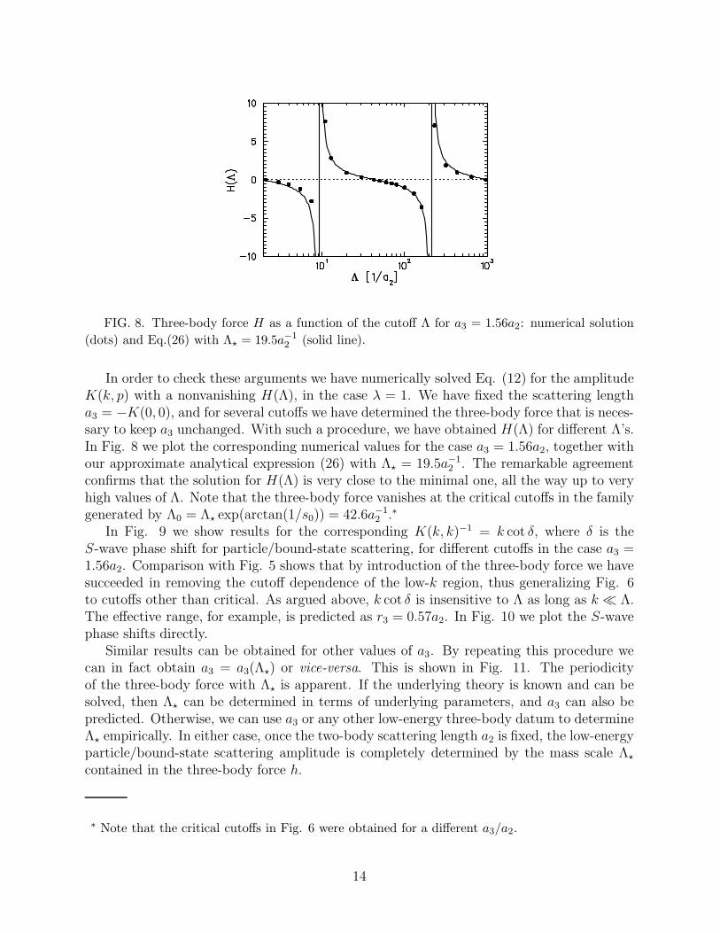
FIG. 8. Three-body force H as a function of the cutoff Λ for a3 = 1.56a2: numerical solution

(dots) and Eq.(26) with Λ⋆ = 19.5a−12 (solid line).

In order to check these arguments we have numerically solved Eq. (12) for the amplitudeK(k, p) with a nonvanishing H(Λ), in the case λ = 1. We have fixed the scattering lengtha3 = −K(0, 0), and for several cutoffs we have determined the three-body force that is neces-sary to keep a3 unchanged. With such a procedure, we have obtained H(Λ) for different Λ’s.In Fig. 8 we plot the corresponding numerical values for the case a3 = 1.56a2, together withour approximate analytical expression (26) with Λ⋆ = 19.5a−1

2 . The remarkable agreementconfirms that the solution for H(Λ) is very close to the minimal one, all the way up to veryhigh values of Λ. Note that the three-body force vanishes at the critical cutoffs in the familygenerated by Λ0 = Λ⋆ exp(arctan(1/s0)) = 42.6a−1

2 .∗

In Fig. 9 we show results for the corresponding K(k, k)−1 = k cot δ, where δ is theS-wave phase shift for particle/bound-state scattering, for different cutoffs in the case a3 =1.56a2. Comparison with Fig. 5 shows that by introduction of the three-body force we havesucceeded in removing the cutoff dependence of the low-k region, thus generalizing Fig. 6to cutoffs other than critical. As argued above, k cot δ is insensitive to Λ as long as k ≪ Λ.The effective range, for example, is predicted as r3 = 0.57a2. In Fig. 10 we plot the S-wavephase shifts directly.

Similar results can be obtained for other values of a3. By repeating this procedure wecan in fact obtain a3 = a3(Λ⋆) or vice-versa. This is shown in Fig. 11. The periodicityof the three-body force with Λ⋆ is apparent. If the underlying theory is known and can besolved, then Λ⋆ can be determined in terms of underlying parameters, and a3 can also bepredicted. Otherwise, we can use a3 or any other low-energy three-body datum to determineΛ⋆ empirically. In either case, once the two-body scattering length a2 is fixed, the low-energyparticle/bound-state scattering amplitude is completely determined by the mass scale Λ⋆

contained in the three-body force h.

∗ Note that the critical cutoffs in Fig. 6 were obtained for a different a3/a2.

14

FIG. 9. Energy dependence for Λ⋆ = 19.5a−12 : k cot δ as function of k for different cutoffs

(Λ = 42.6, 100.0, 230.0, 959.0 × a−12 ).

V. BOUND STATE

We can extend the preceding analysis to the three-body bound-state problem. In thiscase the relevant equation to be solved is Eq. (12) without inhomogeneous terms. The latterdid not play an important role in our ultraviolet arguments, so the same arguments hold forany bound state with binding energy B3 comparable with 1/ma2

2, i.e., for any bound statewith the dimensionless binding energy b3 = ma2

2B3 = O(1). Such bound states are shallow,having a size ∼ 1/

√mB3 = a2/

√b3 comparable to a2, and thus should be within range of

the EFT. In principle, all bound states with size larger than ∼ r2 should be amenable tothis EFT description. Their properties will be determined in first approximation by onlya2 and a3, or equivalently C0 and Λ⋆, while more precise information can be obtained in anexpansion in

√b3r2/a2.

In Fig. 12 we plot binding energies for a range of cutoffs, with the three-body forceadjusted to give a fixed scattering length a3 = 1.56a2. (With an appropriate a3, our resultsreduce to those of Ref. [20] when the cutoff is at one of the critical values Λn.) As we cansee, for this value of Λ⋆ there exists a shallow bound state at b3 ≃ 2 whose binding energy isindependent of the cutoff. This bound state has a size ∼ 0.7a2 and can thus be studied withinthe EFT. As we increase the cutoff, deeper bound states appear at Λn = Λ0 exp(nπ/s0) withn an integer and Λ0 ≃ 10, so that for Λn−1 ≤ Λ ≤ Λn there are n + 1 bound states. Thenext-to-shallowest bound state has b3 ≃ 70 and thus a size ∼ 0.1a2. If the underlying theoryis such that r2 <∼ a2/10, a cutoff Λ >∼ 1/r2 allows us to deal with the next-to-shallowestbound state. The next deeper bound state has b3 ≃ 4 × 104 and thus a size ∼ 0.01a2, andso on. These most likely lie outside the EFT.

Properties of the shallowest bound state, if within the EFT, are model independent andthus the most interesting. For a fixed a2, they are determined by Λ⋆. In Fig. 13 we plotthe binding energy B3 as function of Λ⋆. This should be compared with the behavior ofa3 = a3(Λ⋆) shown in Fig. 11. It is clear that at Λ⋆ ∼ 4a−1

2 a bound state appears at zeroenergy. As Λ⋆ increases, this state gets progressively more bound until at Λ⋆ ∼ 22.7× 4a−1

2

15

FIG. 10. S-wave phase shifts δ as function of energy E, as predicted by the EFT when

a3 = 1.56a2 (Λ = 42.6, 100.0, 230.0, 959.0 × a−12 ).

a new shallowest bound state appears; the picture repeats indefinitely. Whenever a boundstate is close to zero energy, a3 is large in magnitude, negative if the bound state is virtualand positive if real. This can be seen in Fig. 11.

Eliminating Λ⋆, we obtain an universal curve B3 = B3(a3), as in Fig. 14. Qualitativefeatures of this curve can be understood from Figs. 11 and 13. For a3 large in magnitude,small variations of Λ⋆ lead to large variations of a3 but small variations of B3, so the curveflattens out at both ends. For a3 large and positive, there is a shallow real bound state; fora3 large and negative, there is a shallow virtual bound state but the curve tracks the deeperreal bound state. For a3 ∼ a2, a3 and B3 vary with Λ⋆ at a similar rate, and the curveinterpolates between the two ends.

This curve is known in the three-nucleon case as the Phillips line [3]. It has been derivedbefore in the context of models for the two-particle potential that differed in their high-momentum behavior. Varying among two-particle potential models one could expect to fillup the B3×a3 plane. In the EFT, the high-momentum behavior of the two-particle potentialis butchered, which causes no trouble in describing two-particle scattering at low-energies,but —in the peculiar way described here— does require a three-body force. It is crucialthat the EFT does retain a systematic expansion, so that in leading order it requires only

one local three-body counterterm, determined by Λ⋆. Varying among two-particle potentialmodels is thus equivalent to varying the one parameter Λ⋆ of the three-body force. Thisspans a single curve B3 = B3(a3) in the B3 × a3 plane. Our argument suggests that thePhillips line is a generic phenomenon and provides a simple explanation of its origin.

VI. HIGHER ORDERS

The corrections to the calculations in the previous sections come from operators notexplicitly written in Eq. (1) and are suppressed by powers of kR orR/a2. The first correctioncomes from terms involving two derivatives and four nucleons fields [6]:

16

FIG. 11. Particle/bound-state scattering length a3 as function of the three-body force param-

eter Λ⋆.

− C2

8(ψ†ψ ψ†∇2ψ + . . .). (27)

They account for the effective range term in the effective range expansion of particle-particlescattering, and one finds C2 = πa2

2r2/m. As it was done before, (27) can also be generatedby integrating out the T field from Eq. (2) if the extra term

g2T†(i∂0 +

∇2

4m)T , (28)

where g2/∆ = 4mC2/C0, is added to Eq. (2). Indeed, integration over the auxiliary field Tgenerates, besides the terms shown in Eq. (1), also a four-nucleon term involving two spacederivatives or one time derivative. As usual, a nucleon-field redefinition involving the equa-tions of motion can be performed to trade the time derivative by two space derivatives. Thisfield redefinition does not change on-shell amplitudes. As far as observables are concerned,adding (28) to Eq. (2) is thus equivalent to adding (27) to Eq. (1).

The correction proportional to r2 is then given by the diagram in Fig. 15(a) (pluscorresponding wave function renormalization pieces) and includes one insertion of the kineticterm, Eq. (28). The contribution of this graph to t(k, p) is

g2

2π2

∫ ∞

0dq q2 it(q, p) (i∆(3k2/4m− 1/ma2

2 − q2/2m, ~q))2

(

3(k2 − q2)

4m− 1

ma22

)

it(k, q). (29)

As discussed above, t(k, p) behaves for large p as t(k, p) ∼ A(k) cos(s0 log(p/Λ⋆))/p, so thediagram is naively linearly divergent. The identity

1

a2

q2 − k2

(− 1a2

+√

3(q2−k2)4

+ 1a2

2

)2

=4

3

1 +

2a2

(√

3(q2−k2)4

+ 1a2

2

− 1a2

)

3(q2−k2)4

− 2a2

(√

3(q2−k2)4

+ 1a2

2

− 1a2

)

(30)

17

FIG. 12. Three-body binding energies B3 as functions of the cutoff Λ for Λ⋆ = 19.5a−12 .

can be used to rewrite Eq. (29) and it shows that the most divergent piece (the one dueto the constant on the right hand side of Eq. (30)) actually vanishes. This is becausein this term the integral can be closed in the complex plane without circling any pole.The only contribution comes from the second term in Eq. (30) but this term is furthersuppressed in the ultraviolet, resulting in a logarithmically divergent contribution from thediagram in Fig. 15(a). This divergent piece has a complicated dependence on the externalmomentum k since it is proportional to A2(k) (the dependence on k of the other termsincluded in the graph is unimportant in the ultraviolet). This is an unusual situation. Inperturbative calculations the divergent part is simply a polynomial in the external momentaand it can consequently be absorbed in a finite number of local counterterms appearingonly at tree level. Here the dependence on the external momenta is more complicated butthe counterterm appears in graphs with an arbitrary number of leading-order interactions.To see this, let us split the three-body force coefficient h into a leading order piece h(0)

(the same considered in the previous sections) and a sub-leading piece h(1) that will beincluded perturbatively. The inclusion of the sub-leading three-body force proportional toh(1) generates the three diagrams shown in Fig. 15(b,c,d). Simple power counting showsthat the graph in Fig. 15(d) is the most divergent of the three. The important point isthat the external momentum dependence of the most divergent part of the graph in Fig.15(d) is given by A2(k), again because the dependence on the external momentum k of thenucleon propagators in Fig. 15(d) can be discarded in the ultraviolet region. Since the kdependence of the divergent part is the same in Fig. 15(a) and Fig. 15(d), h(1) can bechosen as a function of the cutoff so as to make the sum of these two graphs finite. Asalways, the renormalization procedure leaves a finite piece in h undetermined that shouldbe fixed through the use of one experimental input. This conclusion seems to agree withRef. [21]. More details of the calculation of the range correction as applied to the case ofthree nucleons in the triton channel are left for a future publication.

18

FIG. 13. Binding energy B3 of the shallowest bound state as function of the parameter Λ⋆.

VII. DISCUSSION AND CONCLUSION

Our results should hold for 4He atoms. In fact, it has recently been established that thetwo-4He bound state (“dimer”) is very shallow, with an average size 〈r〉 = 62 ± 10 A [22],more than an order of magnitude larger than the range of the interatomic potential. The low-energy two-4He system should then be describable by contact two-body forces. In leadingorder, the measured size translates into a scattering length a2 = 124 A, which determinesthe strength of the contact interaction. Unfortunately, although the three-4He (“trimer”)has been observed [23], there seems to be no low-energy information on its properties noron 4He/dimer scattering. At least one three-body datum is needed to determine Λ⋆ and usethe EFT to make predictions.

Until such datum becomes available, we can only illustrate the method by using a phe-nomenological 4He-4He potential as a model of a microscopic theory. We select a potential[24] which is consistent with the recent measurement of the dimer binding energy. It gives forthe two-body system a2 = 124.7 A and r2 ≃ 7.4 A. Three-body calculations are much moredifficult to perform with such a phenomenological potential. An estimate for the 4He/dimerscattering length is a3 = 195 A. Ground and excited bound states have been reported; es-timates for the shallowest bound state place it in the range B3 = 1.04 − 1.7 mK, while adeeper state lies around B3 = 0.082− 0.1173 K. There exist a prediction for the low-energyS-wave phase shifts, albeit for a different potential, but r3 could not be determined.

Using such model we can estimate the range of validity of the EFT in momentum to be∼ 1/r2 ≃ 0.14 A−1, and the leading order to give an accuracy of ∼ r2/a2 ≃ 0.06, or about10%, at momenta Q ∼ 1/a2. Using this potential’s a3/a2 = 1.56 we can determine Λ⋆, andpredict both the energy dependence in 4He/dimer scattering and the trimer binding energy.In fact, in Figs. 9, 10, and 12, we have used exactly this value of a3. As a consequence,Fig. 9 represents our lowest-order prediction for k cot δ for atom/dimer scattering, fromwhich we can for the first time extract an effective range r3 = 71 A. Fig. 10 displays theS-wave phase shifts themselves, and is in qualitative agreement with the result of Ref. [24]

19

FIG. 14. Phillips line: binding energy B3 of the shallowest bound state as function of the

particle/bound-state scattering length a3.

for a similar potential, being obtained here at a negligible fraction of computer time. FromFig. 12 we predict a bound state at B3 = 1.2 mK, which is certainly within the EFT. Thenext-to-shallowest bound state is small enough to be at the border of EFT applicability. Fora sufficiently large cutoff, we find B3 = 0.057 K, but in the best case scenario correctionsfrom higher orders should be a lot larger than 10%, and very important.

Because of the similarity of the integral equations, our arguments should be relevant forsystems of three fermions with internal quantum numbers as well. We are in the process ofverifying this for the three-nucleon system in the J = 1/2 channel, where we will be ableto check our predictions against the energy dependence of existing phase shift analyses ofneutron-deuteron scattering and against the triton binding energy [25]. We also plan toextend our calculations to the four-and-more-body system and search for the existence ofother leading few-body forces.

These results will hold in an EFT where the pion has been integrated out, which isvalid for Q <∼ mπ. In an exciting new development, it has been argued in Ref. [7] thatthere is a region of momenta above mπ where, although pions have to be kept explicitly,their effects are sub-leading. The leading two-body operators are thus the same as in the

T T

(c) (d)

TT T

(a) (b)

FIG. 15. O(r2/a2) diagrams: (a) one insertion of (28) in the dimeron propagator, denoted by

a cross; (b,c,d) one insertion of a correction to the three-body force h, denoted by a circle.

20

“pionless” theory. A number of examples seem to corroborate this picture [14]. In this case,our leading-order results will be valid in this “pionful” theory as well, suggesting that ourbound-state calculation will provide a reasonable estimate of the triton binding energy.

In conclusion, we have provided analytical and numerical evidence that renormalizationof the three-body problem with short-range forces requires in general the presence in leadingorder of a one-parameter contact three-body force. This frames results obtained earlier withparticular models within a larger, model-independent picture. It opens up the possibilityof applying the EFT method to a large class of systems of three or more particles withshort-range forces.

AcknowledgmentsWe thank V. Efimov, H. Muller, and D. Kaplan for helpful discussions. HWH and UvK

acknowledge the hospitality of the Nuclear Theory Group and the INT in Seattle, wherepart of this work was carried out. This research was supported in part by the U.S. Depart-ment of Energy grants DOE-ER-40561 and DE-FG03-97ER41014, the Natural Science andEngineering Research Council of Canada, and the U.S. National Science Foundation grantPHY94-20470.

21

REFERENCES

[1] L.H. Thomas, Phys. Rev. 47 (1935) 903; S.K. Adhikari, T. Frederico, and I.D. Goldman,Phys. Rev. Lett. 74 (1995) 487.

[2] V.N. Efimov, Sov. J. Nucl. Phys. 12 (1971) 589; Phys. Rev. C47 (1993) 1876.[3] A.C. Phillips, Nucl. Phys. A107 (1968) 209.[4] G.P. Lepage, in “From Actions to Answers, TASI’89”, T. DeGrand and D. Toussaint

(editors), World Scientific, 1990; D.B. Kaplan, nucl-th/9506035; H. Georgi, Ann. Rev.

Part. Sci. 43 (1994) 209.[5] E. Braaten and A. Nieto, Phys. Rev. B56 (1997) 14745; Phys. Rev. B55 (1997) 8090.[6] U. van Kolck, in Proceedings of the Workshop on Chiral Dynamics 1997, Theory and

Experiment , A. Bernstein, D. Drechsel, and T. Walcher (editors), Springer–Verlag, 1998,hep-ph/9711222; in Ref. [9]; nucl-th/9808007.

[7] D.B. Kaplan, M.J. Savage, and M.B. Wise, Phys. Lett. B424 (1998) 390;nucl-th/9802075.

[8] J. Gegelia, nucl-th/9802038; nucl-th/9805008; M.C. Birse, J.A. McGovern, andK.G. Richardson, hep-ph/9807302; hep-ph/9808398; T.D. Cohen and J.M. Hansen,nucl-th/9808006.

[9] “Nuclear Physics with Effective Field Theory”, R. Seki, U. van Kolck, and M.J. Savage(editors), World Scientific, 1998.

[10] P.F. Bedaque, in Ref. [9], nucl-th/9806041.[11] P.F. Bedaque and U. van Kolck, Phys. Lett. B428 (1998) 221.[12] P.F. Bedaque, H.-W. Hammer, and U. van Kolck, Phys. Rev. C58 (1998) R641.[13] S. Weinberg, Phys. Lett. B251 (1990) 288; Nucl. Phys. B363 (1991) 3; Phys. Lett. B295

(1992) 114; C. Ordonez and U. van Kolck, Phys. Lett. B291 (1992) 459; C. Ordonez, L.Ray, and U. van Kolck, Phys. Rev. Lett. 72 (1994) 1982; Phys. Rev. C53 (1996) 2086;U. van Kolck, Phys. Rev. C49 (1994) 2932; J.L. Friar, D. Huber, and U. van Kolck,nucl-th/9809065.

[14] D.B. Kaplan, M.J. Savage and M.B. Wise, nucl-th/9804032; J.-W. Chen et al,nucl-th/9806080; M.J. Savage and R.P. Springer, nucl-th/9807014; D.B. Ka-plan et al, nucl-th/9807081; J.-W. Chen et al, nucl-th/9809023; J.-W. Chen,nucl-th/9810021.

[15] J. Gegelia, nucl-th/9806028; T.D. Cohen and J.M. Hansen, nucl-th/9808038; T.Mehen and I.W. Stewart, nucl-th/9809071; nucl-th/9809095.

[16] P.F. Bedaque, H.-W. Hammer, and U. van Kolck, nucl-th/9809025.[17] D.B. Kaplan, Nucl. Phys. B494 (1997) 471.[18] G.V. Skorniakov and K.A. Ter-Martirosian, Sov. Phys. JETP 4 (1957) 648.[19] G.S. Danilov and V.I. Lebedev, Sov. Phys. JETP 17 (1963) 1015;[20] V.F. Kharchenko, Sov. J. Nucl. Phys. 16 (1973) 173.[21] V.N. Efimov, Phys. Rev. C44 (1991) 2303.[22] F. Luo, C.F. Giese, and W.R. Gentry, J. Chem. Phys. 104 (1996) 1151.[23] W. Schollkopf and J. Peter Toennies, J. Chem. Phys. 104 (1996) 1155.[24] Y.-H. Uang and W.C. Stwalley, J. Chem. Phys. 76 (1982) 5069; S. Nakaichi-Maeda

and T.K. Lim, Phys. Rev. A28 (1983) 692; A.K. Motovilov, S.A. Sofianos, and E.A.Kolganova, Chem. Phys. Lett. 275 (1997) 168.

22

[25] P.F. Bedaque, H.-W. Hammer, and U. van Kolck, in progress.

23