Studying Short-Range Correlations with the 12C(e, e′pn) Reaction

A dissertation submitted

to Kent State University in partial

fulfillment of the requirements for the

degree of Doctor of Philosophy

by

Ramesh Raj Subedi

December, 2007

Dissertation written by

Ramesh Raj Subedi

B.Sc., Tribhuvan University, 1988

M.Sc., Tribhuvan University, 1994

Ph.D., Kent State University, 2007

Approved by

Dr. John W. Watson , Co-chair, Doctoral Dissertation Committee

Dr. Douglas W. Higinbotham , Co-chair, Doctoral Dissertation Committee

Dr. Bryon D. Anderson, Member, Doctoral Dissertation Committee

Dr. George Fai, Member, Doctoral Dissertation Committee

Dr. Christopher J. Woolverton, Member, Doctoral Dissertation Committee

Accepted by

Dr. Bryon D. Anderson, Chair, Department of Physics

Dr. Jerry Feezel, Dean, College of Arts and Sciences

ii

Table of Contents

List of Figures . . . . . . . . . . . . . . . . . . . . . . . . . . . . . . . . . . . x

List of Tables . . . . . . . . . . . . . . . . . . . . . . . . . . . . . . . . . . . . x

Acknowledgements . . . . . . . . . . . . . . . . . . . . . . . . . . . . . . . . . xi

Chapter

1 Introduction . . . . . . . . . . . . . . . . . . . . . . . . . . . . . . . . . 1

1.1 The Nucleon-Nucleon Interaction . . . . . . . . . . . . . . . . . . 2

1.1.1 The Shell Model in General . . . . . . . . . . . . . . . . . 3

1.1.2 The Shell Model for 12C . . . . . . . . . . . . . . . . . . . 4

1.1.3 Beyond the Shell Model . . . . . . . . . . . . . . . . . . . 4

1.2 Experiment Overview . . . . . . . . . . . . . . . . . . . . . . . . . 5

1.3 Previous Work . . . . . . . . . . . . . . . . . . . . . . . . . . . . . 9

2 Theory . . . . . . . . . . . . . . . . . . . . . . . . . . . . . . . . . . . . 11

2.1 Kinematic Variables . . . . . . . . . . . . . . . . . . . . . . . . . . 11

2.2 Short-Range Correlations . . . . . . . . . . . . . . . . . . . . . . . 14

2.2.1 Short-Range Correlations from A(e, e′) . . . . . . . . . . . 20

2.2.2 Short-Range Correlations from A(e, e′p) . . . . . . . . . . . 24

2.2.3 Short-Range Correlations from A(e, e′pN) . . . . . . . . . 26

3 Setup of the Experiment . . . . . . . . . . . . . . . . . . . . . . . . . . 29

3.1 Kinematic Settings . . . . . . . . . . . . . . . . . . . . . . . . . . 30

3.2 Jefferson Lab Hall A . . . . . . . . . . . . . . . . . . . . . . . . . 32

iii

3.3 The Target System . . . . . . . . . . . . . . . . . . . . . . . . . . 32

3.4 The High Resolution Spectrometers . . . . . . . . . . . . . . . . . 36

3.4.1 The Vertical Drift Chambers . . . . . . . . . . . . . . . . . 38

3.4.2 The Scintillator Planes . . . . . . . . . . . . . . . . . . . . 39

3.4.3 The Gas Cherenkov Detector . . . . . . . . . . . . . . . . . 41

3.4.4 The Pion Rejector . . . . . . . . . . . . . . . . . . . . . . . 42

3.5 Trigger . . . . . . . . . . . . . . . . . . . . . . . . . . . . . . . . . 44

3.6 The BigBite Spectrometer . . . . . . . . . . . . . . . . . . . . . . 46

3.6.1 The BigBite Detector Package . . . . . . . . . . . . . . . . 51

3.7 The Neutron Detector . . . . . . . . . . . . . . . . . . . . . . . . 52

3.7.1 The Neutron Detector Planes . . . . . . . . . . . . . . . . 54

3.7.2 The Veto plane . . . . . . . . . . . . . . . . . . . . . . . . 55

3.7.3 Electronics . . . . . . . . . . . . . . . . . . . . . . . . . . . 57

4 Neutron-Detection Efficiency . . . . . . . . . . . . . . . . . . . . . . . . 59

4.1 The Discriminator Thresholds . . . . . . . . . . . . . . . . . . . . 60

4.2 Efficiency . . . . . . . . . . . . . . . . . . . . . . . . . . . . . . . 62

4.3 Transmittance . . . . . . . . . . . . . . . . . . . . . . . . . . . . . 63

4.4 Detection Efficiency . . . . . . . . . . . . . . . . . . . . . . . . . . 68

4.5 Conclusion . . . . . . . . . . . . . . . . . . . . . . . . . . . . . . . 70

5 Data Analysis-I: The HRSs and BigBite . . . . . . . . . . . . . . . . . 73

5.1 Particle Identification in the HRSs . . . . . . . . . . . . . . . . . . 73

5.1.1 The Left High-Resolution Spectrometer (HRSL) . . . . . . 73

5.2 Coincidence Time . . . . . . . . . . . . . . . . . . . . . . . . . . . 77

5.3 Software Cuts . . . . . . . . . . . . . . . . . . . . . . . . . . . . . 79

5.4 Detection of Recoiling Protons . . . . . . . . . . . . . . . . . . . . 84

iv

6 Data Analysis-II: Neutron Analysis . . . . . . . . . . . . . . . . . . . . 86

6.1 Detector Calibration . . . . . . . . . . . . . . . . . . . . . . . . . 86

6.1.1 TDC Alignment . . . . . . . . . . . . . . . . . . . . . . . . 87

6.1.2 Bar-Length Alignment . . . . . . . . . . . . . . . . . . . . 88

6.2 Neutron Identification . . . . . . . . . . . . . . . . . . . . . . . . 90

6.3 Time-of-Flight . . . . . . . . . . . . . . . . . . . . . . . . . . . . . 92

6.3.1 The Time-Of-Flight for the Liquid-Deuterium Data . . . . 95

6.3.2 TOF Resolution . . . . . . . . . . . . . . . . . . . . . . . . 99

6.4 Momentum Reconstruction . . . . . . . . . . . . . . . . . . . . . . 102

6.4.1 Momentum Resolution . . . . . . . . . . . . . . . . . . . . 102

6.5 Event Rate . . . . . . . . . . . . . . . . . . . . . . . . . . . . . . . 105

6.6 Simulation . . . . . . . . . . . . . . . . . . . . . . . . . . . . . . . 107

6.6.1 GEANT4 . . . . . . . . . . . . . . . . . . . . . . . . . . . 107

6.6.2 MCEEP . . . . . . . . . . . . . . . . . . . . . . . . . . . . 107

7 Results and Discussion . . . . . . . . . . . . . . . . . . . . . . . . . . . 111

7.1 12C(e, e′pn) Result . . . . . . . . . . . . . . . . . . . . . . . . . . 111

7.2 Summary . . . . . . . . . . . . . . . . . . . . . . . . . . . . . . . 120

7.3 Conclusion . . . . . . . . . . . . . . . . . . . . . . . . . . . . . . . 123

Bibliography . . . . . . . . . . . . . . . . . . . . . . . . . . . . . . . . . . . . 125

Appendix ANeutron Detection Efficiency Determination . . . . . . . . . . . . . . . . . 130

A.1 The Threshold Determination . . . . . . . . . . . . . . . . . . . . 130

A.2 The Efficiency Data . . . . . . . . . . . . . . . . . . . . . . . . . . 133

Appendix BE01-015 Collaboration List . . . . . . . . . . . . . . . . . . . . . . . . . . . 141

v

List of Figures

1.1 A qualitative sketch of the NN-interaction. . . . . . . . . . . . . . . . 2

1.2 A generic shell-model diagram for the 12C nucleus. . . . . . . . . . . . 5

1.3 A simple reaction diagram for nucleon knockout in the A(e, e′pN)

reaction. . . . . . . . . . . . . . . . . . . . . . . . . . . . . . . . . . . 7

1.4 Diagrams for SRCs and two-body processes. . . . . . . . . . . . . . . 8

1.5 BNL Eva collaboration result for the 12C(p, ppn) reaction. . . . . . . 10

2.1 The kinematic layout for defining variables. . . . . . . . . . . . . . . . 13

2.2 Spectroscopic strength from the A(e, e′p) reaction. . . . . . . . . . . . 16

2.3 Theoretical nucleon-momentum distributions in 12C. . . . . . . . . . . 17

2.4 Plots of correlation functions in coordinate space and momentum space. 20

2.5 y-scaling plots. . . . . . . . . . . . . . . . . . . . . . . . . . . . . . . 22

2.6 SRC results from Hall B at Jefferson Laboratory . . . . . . . . . . . . 23

2.7 Missing energy (E2m) distribution from the 12C(e, e′pp) reaction. . . . 27

3.1 Schematic diagrams of the Jefferson Laboratory accelerator site and

Hall A . . . . . . . . . . . . . . . . . . . . . . . . . . . . . . . . . . . 33

3.2 Detector setup for experiment E01-015. . . . . . . . . . . . . . . . . . 34

3.3 The slanted Carbon Target showing its tilt with respect to the beam. 35

3.4 The high-resolution spectrometers in Hall A. . . . . . . . . . . . . . . 37

3.5 Schematic layout of the detectors for the HRSs. . . . . . . . . . . . . 38

vi

3.6 Schematic layout of the VDCs. . . . . . . . . . . . . . . . . . . . . . 40

3.7 Schematic layout of the HRSL pion rejector. . . . . . . . . . . . . . . 44

3.8 Layout of the BigBite spectrometer and the neutron detector with

respect to the beam line. . . . . . . . . . . . . . . . . . . . . . . . . . 48

3.9 CAD rendering of the BigBite magnet and the BigBite detector package. 49

3.10 Photograph of the BigBite spectrometer and the neutron detector. . . 50

3.11 Electronics block diagram for the BigBite detector. . . . . . . . . . . 53

3.12 Neutron detector configuration. . . . . . . . . . . . . . . . . . . . . . 54

3.13 Veto paddles (front view). . . . . . . . . . . . . . . . . . . . . . . . . 55

3.14 Electronics block diagram for the neutron detector. . . . . . . . . . . 58

4.1 Threshold plot for the Neutron Detector bars. . . . . . . . . . . . . . 61

4.2 Efficiency versus kinetic energy plots for the plastic scintillator bars. . 64

4.3 Neutron transmittance versus kinetic energy for different material

combinations. . . . . . . . . . . . . . . . . . . . . . . . . . . . . . . . 66

4.4 Detection efficiency versus kinetic energy plots for the Neutron De-

tector. . . . . . . . . . . . . . . . . . . . . . . . . . . . . . . . . . . . 69

4.5 Detection efficiency versus momentum plots. . . . . . . . . . . . . . . 72

5.1 The ADC sum for the gas Cherenkov detector in the HRSL. . . . . . 74

5.2 The pion rejector (preshower and shower detectors) signal. . . . . . . 75

5.3 Spectrum of β in the HRSR. . . . . . . . . . . . . . . . . . . . . . . . 76

5.4 Spectrum of the coincidence time for the CK3 kinematics. . . . . . . 78

5.5 Nominal acceptance of the HRSs. . . . . . . . . . . . . . . . . . . . . 80

vii

5.6 Two redundant cuts to remove events with pions and ∆’s in CK3

kinematics. . . . . . . . . . . . . . . . . . . . . . . . . . . . . . . . . 81

5.7 Shown on the top is a missing-energy plot. . . . . . . . . . . . . . . . 82

5.8 Missing momentum versus missing energy for the 12C(e, e′p) reaction. 83

5.9 The time-of-flight spectrum for particles detected with the BigBite

detector. . . . . . . . . . . . . . . . . . . . . . . . . . . . . . . . . . . 84

6.1 Alignment of the neutron counter TDCs. . . . . . . . . . . . . . . . 89

6.2 The y-position spectra of the scintillator bars of the fourth plane. . . 91

6.3 A schematic diagram showing how the scintillator bars immediately

in front of a hit-bar are used as a veto. . . . . . . . . . . . . . . . . . 93

6.4 The difference between the expected and observed time-of-flight (∆t)

for individual scintillator bars using low-energy liquid-deuterium data 94

6.5 The difference between expected and observed time-of-flight for each

plane using the low-energy liquid-deuterium data. . . . . . . . . . . . 96

6.6 The difference between the expected and the observed time-of-flight

for the neutron detector using the low-energy liquid-deuterium data. . 97

6.7 The difference between the expected and the observed time-of-flight

using the high-energy liquid-deuterium data at low missing momentum. 98

6.8 The measured TOF spectrum for the low-energy liquid-deuterium data.100

6.9 . . . . . . . . . . . . . . . . . . . . . . . . . . . . . . . . . . . . . . . 101

6.10 The spectrum of neutron momenta reconstructed from time-of-flight

information, using the low-energy (2.345 GeV) liquid-deuterium cal-

ibration data. . . . . . . . . . . . . . . . . . . . . . . . . . . . . . . . 103

6.11 The momentum resolution (∆p) obtained by plotting the difference

in measured momentum and expected momentum for the low-energy

liquid-deuterium data. . . . . . . . . . . . . . . . . . . . . . . . . . . 104

6.12 Event rates in the neutron detector at a beam current of 40 µA. . . . 106

viii

6.13 Neutrons and protons in the GEANT4 simulation for the E01-015

experiment. . . . . . . . . . . . . . . . . . . . . . . . . . . . . . . . . 108

6.14 Plot showing the extrapolation factor as a function of momentum for

the phase-space correction. . . . . . . . . . . . . . . . . . . . . . . . . 109

7.1 Two dimensional spectra for the 12C(e,e′p) coincidence time versus

time-of-flight plots for recoiling neutrons (top) and recoiling protons

(bottom) from the 12C(e,e′pN) reaction. . . . . . . . . . . . . . . . . 112

7.2 NIKHEF result for a triple-coincidence TOF. Shown is the recoil-

proton TOF for the 12C(e,e′pp) reaction versus the 12C(e,e′p) coinci-

dence time. . . . . . . . . . . . . . . . . . . . . . . . . . . . . . . . . 113

7.3 Time-of-flight neutron spectrum from the production runs for the12C(e, e′pn) reaction in the CK3 kinematics. . . . . . . . . . . . . . . 113

7.4 Spectrum of the cosine of the angle between the missing momentum

and the recoil-neutron momentum. . . . . . . . . . . . . . . . . . . . 114

7.5 Recoil-neutron momentum reconstruction spectra. . . . . . . . . . . . 116

7.6 Missing energy (E2m) plot for the 12C(e, e′pn) reaction in the CK3

kinematics. . . . . . . . . . . . . . . . . . . . . . . . . . . . . . . . . 117

7.7 The magnitude of center-of-mass momentum and the magnitude of

relative momentum of the 12C(e, e′pn) reaction. . . . . . . . . . . . . 118

7.8 The left plot is the measured cross-section ratio for 12C(e, e′pn)/12C(e, e′p)

and 12C(e, e′pp)/12C(e, e′p). The right plot is extrapolated cross-

section ratios using acceptance corrections, where the magenta is for12C(p, ppn)/12C(p, pp) from reference [1] while the blue and red are

for 12C(e, e′pn)/12C(e, e′p) and 12C(e, e′pp)/12C(e, e′p), respectively. . 121

7.9 The cross-section ratio for the 12C(e, e′pn)/12C(e, e′pp) reactions. . . . 122

A.1 Typical ADC spectrum from the hydrogen elastic run. . . . . . . . . 131

A.2 A typical ADC versus TDC spectrum from the 12C production runs. . 132

ix

List of Tables

3.1 Nominal values of kinematic variables. . . . . . . . . . . . . . . . . . 31

3.2 Configuration of the target ladder for the E01-015 experiment. . . . . 35

A.1 Efficiency of different scintillator bars. . . . . . . . . . . . . . . . . . 135

A.2 Removal cross section for Pb, Fe, C, H, plastic, and air. . . . . . . . . 136

A.3 Transmittance for Pb, Fe, air, and plastics. . . . . . . . . . . . . . . . 137

A.4 Transmittance for different combinations of materials. . . . . . . . . . 138

A.5 The detection efficiency of different planes. . . . . . . . . . . . . . . . 139

A.6 Final result for the neutron detector efficiency. . . . . . . . . . . . . . 140

x

Acknowledgement

This dissertation would not have been possible without help from various peo-

ple. First and foremost, I wish to express my deep gratitude to my advisors John

W. Watson and Douglas W. Higinbotham for giving me inspiration and guidance

during my research work. They are also thankful for investing a lot of time and

energy in my education. I would also like to thank other members of my disserta-

tion committee: Bryon Anderson, George Fai, and Christopher Woolverton for their

valuable comments on this dissertation.

I would like to thank John for supporting me financially, giving me a unique

opportunity by sending me to Jefferson Laboratory and allowing me to stay there

throughout my research, giving me a great deal of freedom in my work but never

lacking when help was needed. Whenever he came to Jefferson Laboratory, he used

to say, “You are making a good progress; I am happy with that.” That used to be a

great compliment and boost to my confidence. I am also grateful to him for carefully

editing my horribly written dissertation and turning it into a readable document.

I respect Doug’s superb ability to supervise students by always encouraging

them, being available to them, and taking care of them like a guardian. No matter

how silly you are, he always used to say, “Don’t worry; you will know it eventually.”

Well-versed in accelerator and Hall A equipment, he is a source of ideas in designing

and instrumenting experiments, and extracting the physics. I learned a lot from

you; thank you Doug.

I am grateful to Shalev Gilad, who always had well thought and balanced

comments, for driving the physics results to a meaningful conclusion. Thanks also

to Eli Piasetzky, who always has a hardworking nature- “Do it now, don’t wait until

tomorrow” - has been the leading driving force for the whole analysis, pushing us

xi

to extract the main physics results as quickly as possible.

I had a wonderful experience working with my fellow graduate students on

this experiment: Peter Monaghan and Ran Shneor. Your help in many aspects,

including data analysis, has been unabated; Peter used to be my next door neighbour

whom I could ask for help that I needed, including editing my English in numerous

documents. Thank you both of you.

It was Olivier Gayou who inspired and encouraged me to learn computer pro-

gramming and always believed in my work. Thank you Olivier. Robert Feuerbach

and Steve Wood were always ready to help me in computer programming and used

to be my resource person for troubleshoooting any computer hardware/software

problems that I used to have. Their suggestions on physics analysis were excellent.

Thank you both of you.

Several other people at Jefferson Laboratory and abroad with whom I worked

closely, spent significant time discussing various issues, and whose help in computer

programming, electronics hardware, and detector assembling was instrumental in

my learning are: Ole Hansen, Ru Igarashi, Eddy Jans, Vahe Mamyan, Kathy Mc-

Cormick, Bob Michaels, Bryan Moffit, Tigran Navasardyan, Yi Qiang, Bodo Reitz,

Brad Sawatzky, Albert Shahinyan, Paul Ulmer, Larry Weinstein, and Bogdan Wo-

jtsekhowski. I thank you all.

A sincere thanks goes to Hall A engineering staff (Paul, Al, Joyce, Susan,

and Ravi) for their support while preparing the experiment, accelerater people for

providing a high quality beam, Hall A technical staff (Ed, Jack, Mark, Gary, Heidi,

Scott, and Todd) for their support during the experiment running time, Hall A staff

scientists (Jian-Ping Chen, Eugene Chudakov, Javier Gomez, Ole Hansen, Douglas

Higinbotham, Kees De Jager, John LeRose, Bob Michaels, Sirish Nanda, Arun Saha,

and Bogdan Wojtsekhowski) and the Hall A collaboration for the help they provided

xii

various ways and, in particular, taking shifts during the data taking period of the

experiment.

Back at Kent State, I am grateful to the Physics Department faculty (Bryon

Anderson, George Fai, Jim Gleeson, Satyendra Kumar, Michael Lee, Mark Manley,

Elizabeth Mann, Makis Petratos, Khandker Quader, and John Watson) for giving

me a world class education, to the staff for providing sufficient administrative sup-

port, and my fellow graduate students for their valuable friendship. Thank you

Kim, Cindy and Loretta by helping me various ways and, particularly, answering

my numerous emails without delay.

I wish to thank my family, specially my mother, for raising me and showing

ways to get to this point of my life. Finally, I wish to thank my children (Anu and

Soniya) for their patience throughout this work, and my loving wife Nirmala for her

infinite selfless support.

August 17, 2007.

xiii

Chapter 1

Introduction

Nuclei are made of protons and neutrons, called collectively “nucleons”; the

standard notation is p, n, and N, respectively. Electron scattering off a single

particle predominately exchanges a single virtual photon. The particle can be a

whole nucleus, a group of nucleons, one nucleon, or even a single quark, depending

upon the amount of energy and momentum transferred in the process. At sufficiently

low energy and momentum transfer, scattering occurs leaving the whole nucleus

intact and in its ground state. This is called elastic scattering. Elastic scattering is

considered to be a surface reaction and no detailed information is obtained related

to the interior of the nucleus.

As the energy and momentum transfer increase, the constituent nucleons are

resolved and the scattering can occur elastically from a nucleon. This is called quasi-

elastic (or quasi-free) scattering. The cross-sectional peak is smeared due to the

Fermi motion of nucleons. Further increases in the energy and momentum transfer

allow for the excitation of nucleons to various resonances. For example, a proton,

having interacted with the scattered electron, becomes a ∆ particle which then

decays into a pion and a baryon. For high enough energy and momentum transfer,

the interaction probes an individual quark. This is deep-inelastic scattering.

Electron scattering is a well established process and a powerful tool for studying

nuclear structure. The Thomas Jefferson National Accelerator Facility (Jefferson

Laboratory) is an ideal place for electron-scatterring studies through coincidence

experiments, due to the availability of a continuous-wave electron beam.

1

2

V(r

) [M

eV]

r [fm]

repulsion

attraction

0

0

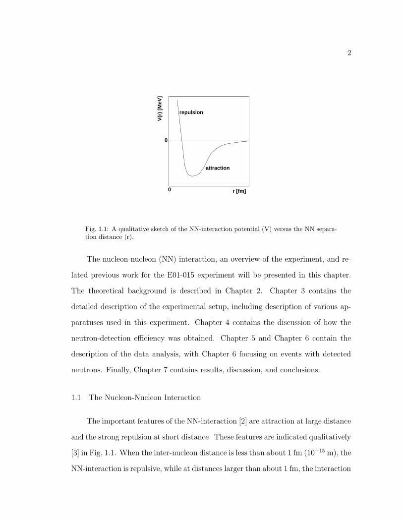
Fig. 1.1: A qualitative sketch of the NN-interaction potential (V) versus the NN separa-tion distance (r).

The nucleon-nucleon (NN) interaction, an overview of the experiment, and re-

lated previous work for the E01-015 experiment will be presented in this chapter.

The theoretical background is described in Chapter 2. Chapter 3 contains the

detailed description of the experimental setup, including description of various ap-

paratuses used in this experiment. Chapter 4 contains the discussion of how the

neutron-detection efficiency was obtained. Chapter 5 and Chapter 6 contain the

description of the data analysis, with Chapter 6 focusing on events with detected

neutrons. Finally, Chapter 7 contains results, discussion, and conclusions.

1.1 The Nucleon-Nucleon Interaction

The important features of the NN-interaction [2] are attraction at large distance

and the strong repulsion at short distance. These features are indicated qualitatively

[3] in Fig. 1.1. When the inter-nucleon distance is less than about 1 fm (10−15 m), the

NN-interaction is repulsive, while at distances larger than about 1 fm, the interaction

3

becomes attractive.

1.1.1 The Shell Model in General

The independent-particle shell model1 assumes that each nucleon moves inde-

pendently from the others in the attractive mean field created by all the other nu-

cleons. Neutrons and protons have independently-defined shell-model states. Even

though the shell model is a phenomenological model, it not only gives a good de-

scription of nuclear ground states, but also predicts the sequence, quantum numbers,

and relative positions of excited states.

Considering the nucleus of A nucleons as a non-relativistic quantum-mechanical

system with two-body interactions between the nucleons, the Hamiltonian (H) of

the system is given in terms of kinetic energy (T ) and the iteraction potential (v)

as

H = T +A∑

i<j=1

v(i, j). (1.1)

Introducing a one-body potential V (i), the mean field, in which the ith nucleon is

moving, we can rewrite the above equation as

H = T +A∑

i=1

V (i) +A∑

i<j=1

v(i, j) −A∑

i=1

V (i). (1.2)

With the notation of the shell-model Hamiltonian as Hsm and the residual interac-

tion as Vres, we get

H = Hsm + Vres (1.3)

1There are many nuclear models that use the shell structure of nuclear states. We donote the“independent particle shell model” as simply the “shell model” henceforth.

4

where

Hsm = T +A∑

i=1

V (i) (1.4)

and

Vres =A∑

i<j=1

v(i, j) −A∑

i=1

V (i) (1.5)

The main assumption of the shell model is the neglect of the residual interaction.

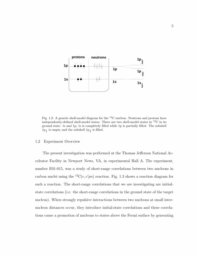
1.1.2 The Shell Model for 12C

Figure 1.2 shows the nucleon states for the 12C nucleus in its ground state.

There are two shell-model states in 12C in its ground state: 1s and 1p; 1s is com-

pletely filled while 1p is partially filled. The subshell 1p 12

is empty and the subshell

1p 32

is filled. In this scheme, the possible shell-model configurations of the NN-pairs

in the 12C nucleus can be (1p3/2)2, (1p3/2, 1s1/2), and (1s1/2)

2.

1.1.3 Beyond the Shell Model

The research described in this dissertation was a quest to observe physics be-

yond the shell model. The primary assumption of the shell model is that the nucleons

undergo independent motion in the nuclear mean field which is a reflection of the

attractive part of the NN interaction. What we were seeking in this project was to

observe and quantify, where possible, correlated motion. In particular, we were look-

ing for pairs of nucleon with roughly equal and opposite (“back-to-back”) momenta,

due to interaction through the short-range repulsive part of the NN interaction.

These short-range correlated pairs are called short-range correlations (SRCs).

5

1s

1p

protons neutrons

1p

2

12

32

1

1p

1s1s

1p

Fig. 1.2: A generic shell-model diagram for the 12C nucleus. Neutrons and protons haveindependently-defined shell-model states. There are two shell-model states in 12C in itsground state: 1s and 1p; 1s is completely filled while 1p is partially filled. The subshell1p 1

2

is empty and the subshell 1p 3

2

is filled.

1.2 Experiment Overview

The present investigation was performed at the Thomas Jefferson National Ac-

celrator Facility in Newport News, VA, in experimental Hall A. The experiment,

number E01-015, was a study of short-range correlations between two nucleons in

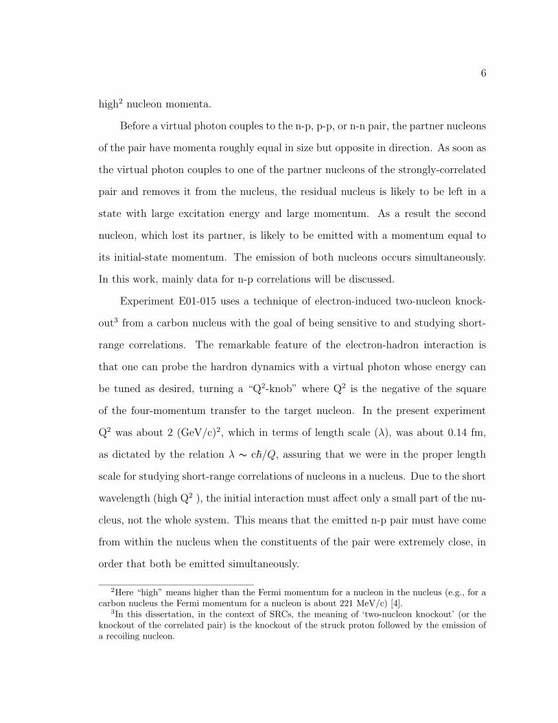
carbon nuclei using the 12C(e, e′pn) reaction. Fig. 1.3 shows a reaction diagram for

such a reaction. The short-range correlations that we are investigating are initial-

state correlations (i.e. the short-range correlations in the ground state of the target

nucleus). When strongly repulsive interactions between two nucleons at small inter-

nucleon distances occur, they introduce initial-state correlations and these correla-

tions cause a promotion of nucleons to states above the Fermi surface by generating

6

high2 nucleon momenta.

Before a virtual photon couples to the n-p, p-p, or n-n pair, the partner nucleons

of the pair have momenta roughly equal in size but opposite in direction. As soon as

the virtual photon couples to one of the partner nucleons of the strongly-correlated

pair and removes it from the nucleus, the residual nucleus is likely to be left in a

state with large excitation energy and large momentum. As a result the second

nucleon, which lost its partner, is likely to be emitted with a momentum equal to

its initial-state momentum. The emission of both nucleons occurs simultaneously.

In this work, mainly data for n-p correlations will be discussed.

Experiment E01-015 uses a technique of electron-induced two-nucleon knock-

out3 from a carbon nucleus with the goal of being sensitive to and studying short-

range correlations. The remarkable feature of the electron-hadron interaction is

that one can probe the hardron dynamics with a virtual photon whose energy can

be tuned as desired, turning a “Q2-knob” where Q2 is the negative of the square

of the four-momentum transfer to the target nucleon. In the present experiment

Q2 was about 2 (GeV/c)2, which in terms of length scale (λ), was about 0.14 fm,

as dictated by the relation λ ∼ c~/Q, assuring that we were in the proper length

scale for studying short-range correlations of nucleons in a nucleus. Due to the short

wavelength (high Q2 ), the initial interaction must affect only a small part of the nu-

cleus, not the whole system. This means that the emitted n-p pair must have come

from within the nucleus when the constituents of the pair were extremely close, in

order that both be emitted simultaneously.

2Here “high” means higher than the Fermi momentum for a nucleon in the nucleus (e.g., for acarbon nucleus the Fermi momentum for a nucleon is about 221 MeV/c) [4].

3In this dissertation, in the context of SRCs, the meaning of ‘two-nucleon knockout’ (or theknockout of the correlated pair) is the knockout of the struck proton followed by the emission ofa recoiling nucleon.

7

e’

eq

p

AA−2

N

Fig. 1.3: A simple reaction diagram for nucleon knockout in the A(e, e′pN) reaction.The small oval represents the interaction of a proton and a nucleon at small seperation,producing a correlated pair. The wavy line represents the virtual photon, which couplesto the correlated proton.

In order to access small inter-nucleon distances for a correlated pair, both nu-

cleons should be in a state of high relative momentum, ~prel = (~pn−~pm)/2, compared

to the Fermi momentum. Here ~pm and ~pn are the momenta of the initial-state pro-

ton, and the recoil (partner) neutron, respectively. In this definition of relative

momentum, the recoil neutron momentum is approximately equal to the the rel-

ative momentum. Furthermore, assuming that the virtual photon couples to the

proton of the n-p pair, the momentum of the ejected neutron and the reconstructed

initial-state momentum of the proton will be approximately equal and opposite.

Such a relative momentum forms the signature of NN short-range correlations. The

angle between the momentum directions of these two correlated partners can be

reconstructed and the value of this angle turns out to be about 180. This is, so

to speak, the back-to-back nature of the momenta of the correlated nucleons in the

pair. Small deviations from equal and opposite momenta of the correlated partners

8

N

N

N

N

A−2

A

A

A−2

A−2

A

N

N

.A−2

N

N∆

A

A−2

N

N

.

A

A−2

N

N

N

N

isobar deexcitation

seagull

SRCs

MECs

isobar excitation

ICs

MECs

FSIs

pion−in−flight

ICs

A

.

∆

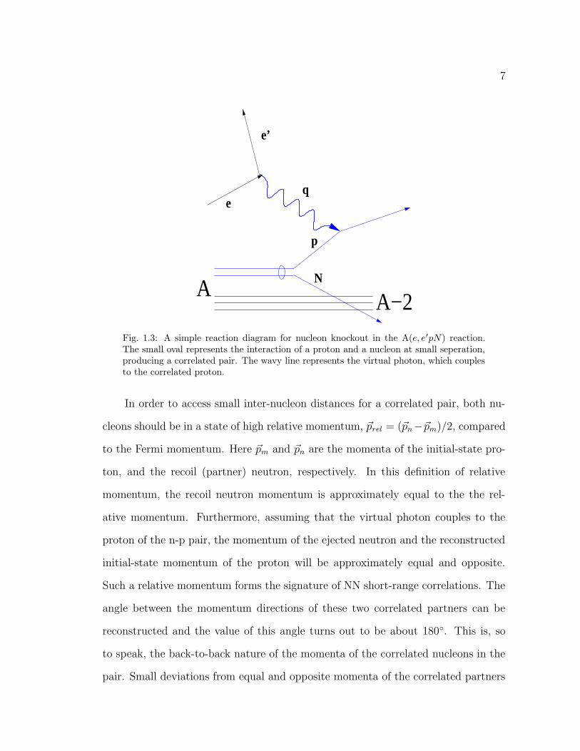
Fig. 1.4: Diagrams for SRCs and two-body processes.

are attributable to the motion of the center-of-mass of the pair within the target

nucleus.

The virtual photon can couple to the carbon nucleus via different processes. It

may be absorbed by one nucleon through a one-body hadronic current, or by many

nucleons through many-body hadronic currents. We detect the emitted two high-

momentum nucleons in the study of SRCs in this investigation. Because the virtual

photon couples to only one member of the SRC pair, the SRC is a one-body process,

even though it leads to the emission of two nucleons (see the top left diagram in

Fig. 1.4). On the other hand, all two-body processes (see Fig. 1.4), such as meson-

exchange currents (MECs), isobar currents (ICs), and final-state interactions (FSIs),

lead to the emission of two high energy nucleons. Hence the SRC must compete

with these two-body processes.

Though the complete elimination of MECs, ICs, and FSIs is impossible, they

9

are expected to be suppressed at high Q2 (Q2 is the negative of the square of the

4-momentum transfer, see Sect. 2.1 for detail) and high Bjorken x (denoted as xB)

[5]. For this reason, the kinematics of the present experiment are chosen in such a

way that it has high Q2 (2 GeV 2/c2) and high xB (1.2). We choose anti-parallel

kinematics to minimize FSIs between the two outgoing nucleons.

1.3 Previous Work

There have been numerous attemts to explore SRCs using either one-nucleon

emission methods, or two-nucleon emission methods. The one-nucleon knockout

experiments of the type A(e, e′p) have recently been investigated at Jefferson lab

in both Hall A [6, 7], and Hall C [8], and show strong evidence for the existence

of SRCs. The Hall C result, as reported in [8] for the 12C(e, e′p) reaction, shows

that the strength of the spectral function matches a theoretically predicted spectral

function which included the contribution of SRCs.

There were also many investigations of SRCs using two-nucleon emission re-

actions of the type A(e, e′pN) via triple-coincidence experiments, for example, at

NIKHEF [9, 10, 11, 12, 13, 14], and at Jefferson Lab Hall B [15, 16, 17]. Also at

Brookhaven National Laboratory (BNL), the Eva collaboration studied the 12C(p, ppn)

reaction [18, 19, 20] at beam momenta from 6-10 GeV/c.

The present investigation received inspiration from the experiment performed

at BNL by the Eva collaboration. One of the main findings from that project [20] is

shown in Fig. 1.5 for the 12C(p, ppn) reaction. Shown in the figure is the cosine of an-

gle γ between the reconstructed momentum of the struck proton and the momentum

of the recoiling neutron, versus the neutron momentum pn. The interesting finding

is that below the Fermi momentum kF (0.221 GeV/c for carbon [4]) the distribution

10

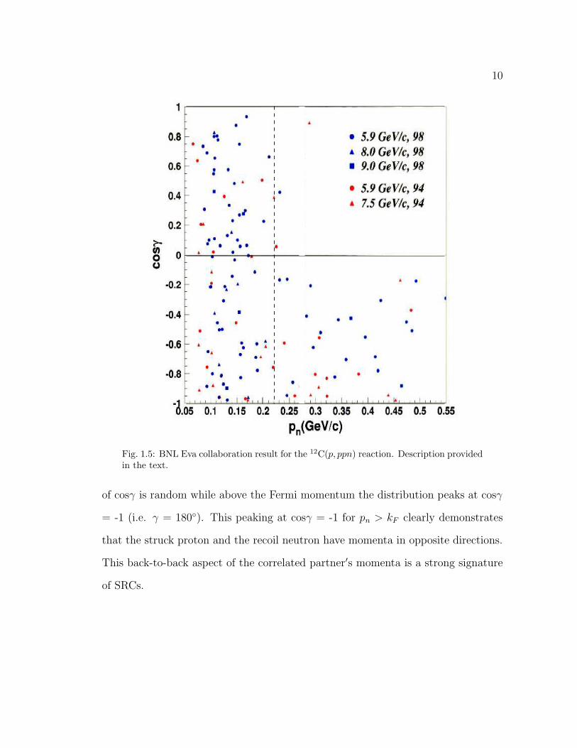
Fig. 1.5: BNL Eva collaboration result for the 12C(p, ppn) reaction. Description providedin the text.

of cosγ is random while above the Fermi momentum the distribution peaks at cosγ

= -1 (i.e. γ = 180). This peaking at cosγ = -1 for pn > kF clearly demonstrates

that the struck proton and the recoil neutron have momenta in opposite directions.

This back-to-back aspect of the correlated partner′s momenta is a strong signature

of SRCs.

Chapter 2

Theory

A brief theoretical introduction of short-range correlations is given in this chap-

ter by starting in the first section with the description of kinematic variables. In the

later sections, a brief conceptual introduction to SRCs is given, followed by descrip-

tions of reactions sensitive to SRCs. The mathematical formulation of SRCs, which

is beyond the scope of this thesis, is quite involved and is still in a developing stage.

There are many mathematical approaches, e.g., self-consistent Green’s function the-

ory, the correlated-basis-function approach [21, 22], variational technique [23], the

Ghent-model [24], etc., to describe the NN-interaction in ways which ultimately lead

to the same physics in the SRC regime.

2.1 Kinematic Variables

For the A(e, e′p) reaction, see Fig. 2.1 for a kinematic diagram, let q ≡ qµ =

(ω, ~q) denote the four-momentum transfer by the virtual photon to the target nu-

cleon, where ω is the energy transfer and ~q is the three-momentum transfer. The

four-momentum-transfer squared, using natural units (~ = c = 1), is given as

q2 = qµqµ = (ω,−~q).(ω, ~q′) = ω2 − ~q 2, (2.1)

where the incident electron of energy E has four-momentum K = (E, ~K), the

scattered electron of energy E ′ with scattering angle θ has four-momentum K ′ =

11

12

(E ′, ~K ′). These transfer quantities can also be written as

q = K −K ′, ω = E − E ′, ~q = ~K − ~K ′. (2.2)

Since we are dealing with an ultrarelativistic1 electron, we can ignore the electron

mass, me, compared to its energy. Hence E = | ~K| and E ′ = | ~K ′|, and as shown in

reference [25]

q2 = 2m2e − 2 ~K. ~K ′ ' −2 ~K. ~K ′ = −4EE ′sin2(

θ

2). (2.3)

The missing energy (Em) and missing momentum (~pm) of the (A− 1) system,

using conservation of energy and three-momentum, are given as

Em = ω − Tp − TA−1, (2.4)

~pm = ~pp − ~q, (2.5)

where Tp and TA−1 denote kinetic energy of scattered proton and recoiling (A− 1)

nucleus, respectively; ~pp is the momentum of struck proton after it was struck. It

is also important to note that the magnitude and direction of ~pm coincide with the

momentum (~k) of the scattered proton before it was struck, i.e., ~pm = ~k. (Unless

otherewise noted, the quantitiy k is |~k|.) Implicit in this statement is the “impulse

approximation”, where we assume that the absorption of the virtual photon and

removal of the proton does not disturb or rearrange the A-1 system on the time

scale of the reaction. Another important point here is that the kinematics diagram

1A particle of mass m, momentum ~p and energy E holding a relation E =√

~p2 + m2 is said tobe relativistic if m ∼ |~p| and ultrarelativistic if m |~p|.

13

e

e’

p

n q

θ

pm

θp

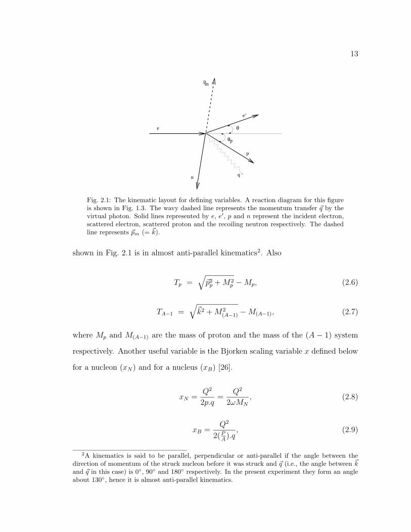
Fig. 2.1: The kinematic layout for defining variables. A reaction diagram for this figureis shown in Fig. 1.3. The wavy dashed line represents the momentum transfer ~q by thevirtual photon. Solid lines represented by e, e′, p and n represent the incident electron,scattered electron, scattered proton and the recoiling neutron respectively. The dashedline represents ~pm (= ~k).

shown in Fig. 2.1 is in almost anti-parallel kinematics2. Also

Tp =√~p2

p +M2p −Mp, (2.6)

TA−1 =√~k2 +M2

(A−1) −M(A−1), (2.7)

where Mp and M(A−1) are the mass of proton and the mass of the (A − 1) system

respectively. Another useful variable is the Bjorken scaling variable x defined below

for a nucleon (xN) and for a nucleus (xB) [26].

xN =Q2

2p.q=

Q2

2ωMN

, (2.8)

xB =Q2

2(PA).q, (2.9)

2A kinematics is said to be parallel, perpendicular or anti-parallel if the angle between thedirection of momentum of the struck nucleon before it was struck and ~q (i.e., the angle between ~k

and ~q in this case) is 0, 90 and 180 respectively. In the present experiment they form an angleabout 130, hence it is almost anti-parallel kinematics.

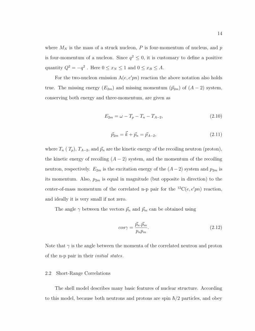
14

where MN is the mass of a struck nucleon, P is four-momentum of nucleus, and p

is four-momentum of a nucleon. Since q2 ≤ 0, it is customary to define a positive

quantity Q2 = −q2 . Here 0 ≤ xN ≤ 1 and 0 ≤ xB ≤ A.

For the two-nucleon emission A(e, e′pn) reaction the above notation also holds

true. The missing energy (E2m) and missing momentum (~p2m) of (A − 2) system,

conserving both energy and three-momentum, are given as

E2m = ω − Tp − Tn − TA−2, (2.10)

~p2m = ~k + ~pn = ~pA−2, (2.11)

where Tn ( Tp), TA−2, and ~pn are the kinetic energy of the recoiling neutron (proton),

the kinetic energy of recoiling (A − 2) system, and the momentum of the recoiling

neutron, respectively. E2m is the excitation energy of the (A− 2) system and p2m is

its momentum. Also, p2m is equal in magnitude (but opposite in direction) to the

center-of-mass momentum of the correlated n-p pair for the 12C(e, e′pn) reaction,

and ideally it is very small if not zero.

The angle γ between the vectors ~pn and ~pm can be obtained using

cosγ =~pn.~pm

pnpm

. (2.12)

Note that γ is the angle between the momenta of the correlated neutron and proton

of the n-p pair in their initial states .

2.2 Short-Range Correlations

The shell model describes many basic features of nuclear structure. According

to this model, because both neutrons and protons are spin ~/2 particles, and obey

15

the Pauli principle, the states below the Fermi-sea are fully occupied and the states

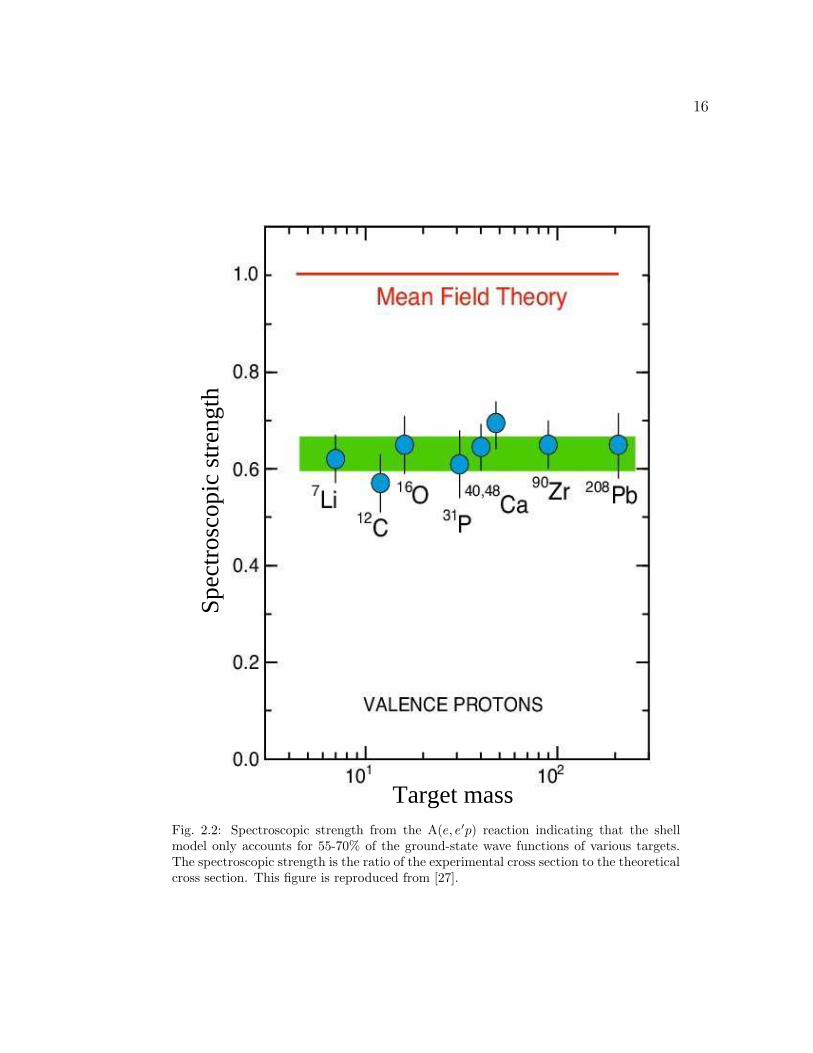
above it are totally empty. This is not what has been observed in A(e, e′p) ex-

periments, where the occupancy number below the Fermi-sea ranges approximately

from 55 to 75% [27, 28, 29, 30], see Fig. 2.2 for example. The possible explanation

for this shortcoming of the shell model, is the absence of nucleon-nucleon (NN) cor-

relations in the model. The main effect of NN correlations is to deplete states below

the Fermi level and make states above the Fermi level partially occupied.

Correlations in nuclei, i.e. deviation from independent-particle behaviour, are

generally classified into two types: long-range correlations (LRCs) due to the long-

range, attractive part of the NN interaction, and SRCs dominated by the short-

range, repulsive part of the NN interaction. LRCs are generally believed to produce

corrections and/or minor modifications to the shell-model picture of nuclear struc-

ture. SRCs generally lead to physics beyond the shell model.

The carbon nucleus is a quantum many-body system. In such a system inter-

actions between constituent nucleons play an important role in binding the nucleus.

The interparticle distance between nucleons inside the nucleus is of the order of the

nucleon size (∼1 fm). Short-range correlations are caused by hard collisions due to

a strong repulsive core of the NN interactions when nucleons are at distances less

than the nucleon size. In this case the strong short-range and tensor components

of NN interactions induce short-range correlations into the nuclear wave function.

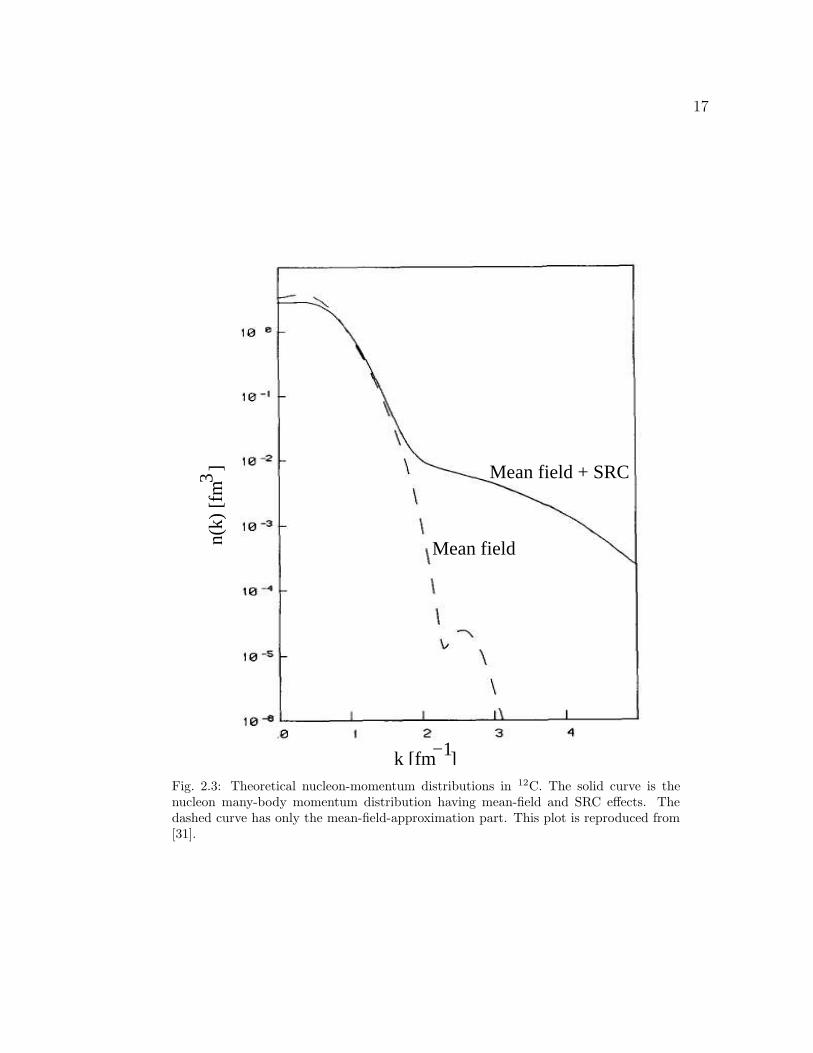
These correlations give rise to an enhancement in the momentum distribution at

higher momenta when compared to the mean field description of the nucleus. This

is depicted in Fig. 2.3 where the nucleon momentum distribution, n(k), for 12C is

plotted as a function of momentum (k). Although the concept of SRCs was intro-

duced in late 1950s by Gottfried [32], and intensive research was carried out in 1980s

and 1990s [33, 34, 28, 35, 36, 9, 37], SRCs are still an active field of research.

16

Spec

tros

copi

c st

reng

th

Target massFig. 2.2: Spectroscopic strength from the A(e, e′p) reaction indicating that the shellmodel only accounts for 55-70% of the ground-state wave functions of various targets.The spectroscopic strength is the ratio of the experimental cross section to the theoreticalcross section. This figure is reproduced from [27].

17

n(k)

[fm

]3 Mean field + SRC

Mean field

k [fm ]−1

Fig. 2.3: Theoretical nucleon-momentum distributions in 12C. The solid curve is thenucleon many-body momentum distribution having mean-field and SRC effects. Thedashed curve has only the mean-field-approximation part. This plot is reproduced from[31].

18

Studying correlations manifestly reveals the structure of nuclei since the inclu-

sion of such effects modifies the shape of the spectral function3 and changes the

spectroscopic factor. Here are a few points worth-noting.

1. The effects of short-range correlations should be independent of the nuclear sys-

tem, as these correlations are very localized and not sensitive to the global struc-

ture of the whole nuclear system. For this reason the effects of short-range

correlations should be similar for the nuclei 4He and 208Pb.

2. The momentum distribution n(k) is probe-independent. Hence whatever probe

we use, γ-rays, electrons, or protons, etc., we should be getting the same physics.

The form of the theoretical expressions for extracting the cross-sections remain

the same.

3. The long-range two-nucleon correlations arising from pion exchange, on the other

hand, could be sensitive to the whole nuclear system and exhibit different results

for different nuclei.

In the correlated-basis-function approach (for details see [38]) the correlated

wave functions ψ are constructed using the many-body correlation operator G, acting

on the uncorrelated wave function ψ obtained from a mean-field potential such that

|ψ >=G|ψ >√

< ψ|G†G|ψ >. (2.13)

The correlation operator is given as

G = S[ΠA

i<j=1

∑

p

f p(~rij)Opij

], (2.14)

3See Sect. 2.2.2 for definitions of the spectral function and spectroscopic factor.

19

where S is a symmetrization operator, f is correlation function, and ~rij = ~ri − ~rj.

Here ~ri refers to the coordinates of the ejected nucleon, and ~rj refers to the coordi-

nates of any of the remaining nucleons to which the ejected nucleon is correlated.

The following operators are usually retained in G:

Op=1ij = 1,

Op=2ij = ~σi,

Op=3ij = ~τi.~τj,

Op=4ij = (~σi.~σj)(~τi.~τj),

Op=5ij = Sij,

Op=6ij = Sij(~τi.~τj),

where Sij = [ 3r2ij

(~σi.~rij)(~σj.~rij) − ~σi.~σj] is the tensor operator, ~σi are Pauli matices

and ~τi are the isospin version of the Pauli matices. It is believed [23, 24, 39] that

the three components in G corresponding to p = 1, 4 and 6, which correspond

to the central (also called Jastrow), the spin-isospin, and the tensor components,

respectively, cause the biggest correlation effect, although compared to the central

correlations the spin-isospin and the tensor correlations are weak. In any event, all

such central, tensor or spin-isospin parts contribute their shares to the short-range

correlation effect. Hence, to a good approximation, the correlation operator can be

constrained to the central, tensor, and spin-isospin terms only, which is given as

G = S[ΠA

i<j=1

(fc(~rij) + ftτ (~rij)Sij~τi.~τj + fστ (~rij)Sij~σi~σj~τi.~τj

)]. (2.15)

The correlation function fc accounts for the strong repulsion that the two nucleons

experience when they approach each other. The two smaller correlation functions,

ftτ and fστ , account for the tensor and the spin-isospin correlations, respectively.

Plots of these functions [38] are shown in Fig. 2.4, both in coordinate space and

momentum space. The meaning of P12 in the figure is the same as k in our notation.

We shall return to the roles of these three functions in Chapter 7.

20

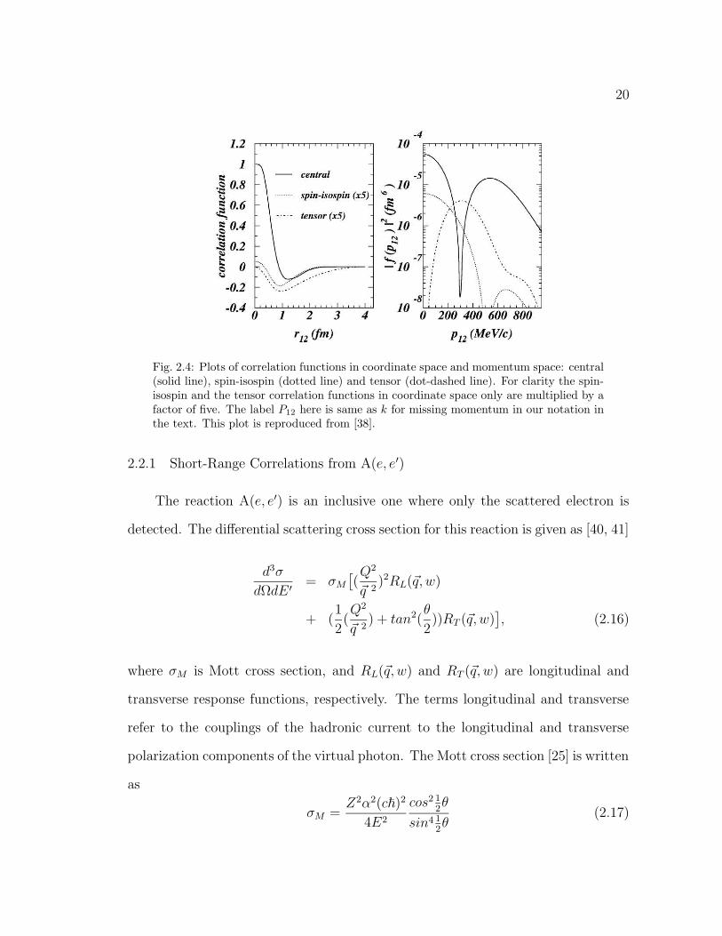
Fig. 2.4: Plots of correlation functions in coordinate space and momentum space: central(solid line), spin-isospin (dotted line) and tensor (dot-dashed line). For clarity the spin-isospin and the tensor correlation functions in coordinate space only are multiplied by afactor of five. The label P12 here is same as k for missing momentum in our notation inthe text. This plot is reproduced from [38].

2.2.1 Short-Range Correlations from A(e, e′)

The reaction A(e, e′) is an inclusive one where only the scattered electron is

detected. The differential scattering cross section for this reaction is given as [40, 41]

d3σ

dΩdE ′= σM

[(Q2

~q 2)2RL(~q, w)

+ (1

2(Q2

~q 2) + tan2(

θ

2))RT (~q, w)

], (2.16)

where σM is Mott cross section, and RL(~q, w) and RT (~q, w) are longitudinal and

transverse response functions, respectively. The terms longitudinal and transverse

refer to the couplings of the hadronic current to the longitudinal and transverse

polarization components of the virtual photon. The Mott cross section [25] is written

as

σM =Z2α2(c~)2

4E2

cos2 12θ

sin4 12θ

(2.17)

21

where α is the fine structure constant. The integrated strength of RL(~q, w) is given

by the Coulomb sum rule [41] SL(~q) such that

SL(~q) =1

Z

∫ ∞

w+el

dωSL(~q, ω), (2.18)

with

SL(~q, ω) ≡ RL(~q, ω)

|GEp(~q, ω)|2 , (2.19)

where Z is the number of protons in the nucleus and GEp is the electric form factor

(a function describing the charge distribution) of the proton. The lower limit ω+el of

the integration simply excludes the elastic electron-nucleus scattering contribution.

In the large momentum transfer limit (i.e., |~q| → ∞), SL(~q) → 1. It is believed

[42, 43] that SL(~q) is sensitive to short-range correlations due to NN-interactions.

The nucleon momentum distribution (see Figs.2.3 and 2.5) has been always

an interesting quantity for understanding SRCs. Inclusive electron-scattering ex-

periments (SLAC data [44], and Jefferson Laboratory Hall C data [45]) have been

performed, covering a wide |~q|-range appropriate for probing the nucleon momen-

tum distribution in the nucleus with the goal of observing y-scaling. The idea of

y-scaling is the following. In a quasielastic A(e, e′) scattering, the nuclear response

function S(~q, ω), which generally depends on both momentum (~q) and energy (ω)

transfers, exhibit scaling; i.e., it can be related to a function f(y) of only one kine-

matical variable y(~q, ω) such that f(y) = (|~q|/M)S(~q, ω) [47]. Here y (= ~k.~q/|~q|)

is the minimum momentum of the struck nucleon along the direction of the virtual

photon and M is the nucleon mass. Knowledge of f(y) can be used to obtain the

22

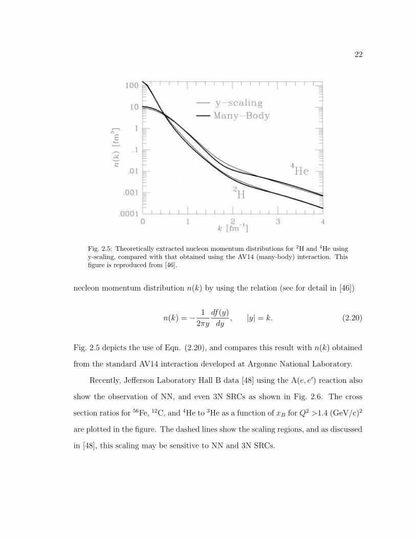
Fig. 2.5: Theoretically extracted nucleon momentum distributions for 2H and 4He usingy-scaling, compared with that obtained using the AV14 (many-body) interaction. Thisfigure is reproduced from [46].

necleon momentum distribution n(k) by using the relation (see for detail in [46])

n(k) = − 1

2πy

df(y)

dy, |y| = k. (2.20)

Fig. 2.5 depicts the use of Eqn. (2.20), and compares this result with n(k) obtained

from the standard AV14 interaction developed at Argonne National Laboratory.

Recently, Jefferson Laboratory Hall B data [48] using the A(e, e′) reaction also

show the observation of NN, and even 3N SRCs as shown in Fig. 2.6. The cross

section ratios for 56Fe, 12C, and 4He to 3He as a function of xB for Q2 >1.4 (GeV/c)2

are plotted in the figure. The dashed lines show the scaling regions, and as discussed

in [48], this scaling may be sensitive to NN and 3N SRCs.

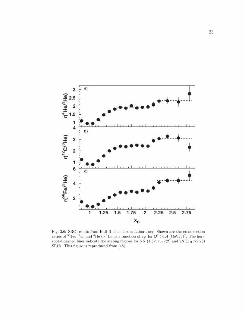
23

Fig. 2.6: SRC results from Hall B at Jefferson Laboratory. Shown are the cross sectionratios of 56Fe, 12C, and 4He to 3He as a function of xB for Q2 >1.4 (GeV/c)2. The hori-zontal dashed lines indicate the scaling regions for NN (1.5< xB <2) and 3N (xB >2.25)SRCs. This figure is reproduced from [48].

24

2.2.2 Short-Range Correlations from A(e, e′p)

The reaction A(e, e′p) is a semi-exclusive one in the sense that the scattered

electron and the knocked out proton are detected in coincidence, while the recoiling

nucleus is not detected. The A(e, e′p) reaction is potentially a rich source of informa-

tion about SRCs. For the present experiment (E01-015), data from the 12C(e, e′p)

channel are being analyzed by another student [49].

The six-fold differential cross section, σ(Em, k), of the semi-exclusive reaction

12C(e, e′p) is given as [38]

σ(Em, k) =d6σ

dΩe′dΩpdE ′dTp

(e, e′p)

=

∫dΩpdEA−2

d9σ

dTpdΩpdTpdΩpdE ′dΩe′

(e, e′pp)

+

∫dΩndEA−2

d9σ

dTndΩndTpdΩpdE ′dΩe′

(e, e′pn). (2.21)

The measurement of the cross section for the 12C(e, e′p) reaction can involve the

contribution from two-nuclon knockout, i.e. 12C(e, e′pN), which needs a triple-

coincidence measurement to be well charaterized, and is not the scope of the A(e, e′p)

experiment. Nevertheless two-nucleon-knockout information is already implicit in

the A(e, e′p) measurement. Also here in the notation (Em, k) both quantities Em

and k refer to the initial state quantities [50] (i. e., before being struck by a virtual

photon) of the struck proton; in the impulse approximation they are the missing

energy and missing momentum of the A(e, e′p) reaction, respectively.

The differential cross section for the A(e, e′p) reaction can also be written as

σ(Em, k) =d6σ

dΩe′dE ′dΩpdTp

(e, e′p) = KcσepS(Em, k) (2.22)

25

where Kc is a kinematical factor, σep is an off-shell (bound) electron-proton cross

section (in the prescription of T. de Forest [51]) and S(Em, k) is the spectral function

which gives the joint probability of finding a proton with missing energy Em and

missing momentum k (≡ |~pm|) inside the nucleus. The spectral function contains the

physics of the nuclear-structure information. There may be included a spectroscopic

factor in S so as to match the theoretical cross section to the experimental cross

section. Rewriting Eqn. (2.22) in a slightly different way, we get an expression for

the spectral function

S(Em, k) = (1

Kcσep

)d6σ

dΩe′dE ′dΩpdTp

(e, e′p). (2.23)

The spectral function S(Em, k) consists of two parts [28] given as

S(Em, k) = S0(Em, k) + S1(Em, k) (2.24)

where S0(Em, k) is the mean-field part and S1(Em, k) is the remainder (not including

the mean-field part). Another useful quantity is the momentum distribution n(k)

and can be written as [28]

n(k) = 4π

∫ ∞

Emin

dEmS(k,Em) (2.25)

with

n(k) = n0(k) + n1(k) (2.26)

in a similar manner to Eqn. (2.24). A typical nucleon momentum distribution was

shown in Fig. 2.3. The integral of the nucleon momentumvdistribution function in

the entire missing-momentum range is called the spectroscopic strength N . This N

26

can also have two parts in reasoning similar to equation (2.26) such that

N = N0 +N1. (2.27)

In general, N is unity; from the A(e, e′p) experiments such as [27] (see Fig. 2.2),

N0 is about 0.7 which accounts for the mean-field part and N1 is about 0.3 which

accounts for correlations, a major part of which comes from SRCs.

2.2.3 Short-Range Correlations from A(e, e′pN)

The reaction A(e, e′pN) is also a semi-exclusive one in the sense that the scat-

tered electron, the knocked-out proton and the recoiling nucleon are detected in

coincidence. The experiment performed in this way is a triple-coincidence experi-

ment. Due to the requirement that the three particles be detected at the same time,

the cross section is exceedingly small for triple-coincidence measurements.

The concepts presented in Sect.2.2.2 apply here also after modifying the ex-

pression for the spectral function as given below:

S(Em, k) = (1

KcσepN

)d9σ

dΩe′dE ′dΩpdTpdΩNdTN

(e, e′pN) (2.28)

where the notation is obvious. Although there has been considerable effort spent in

studying two-nucleon knockout reactions, as mentioned in Sect. 1.3, for example,

see references [7-18], the understanding of SRCs is still in a slowly-developing phase.

The missing-energy (E2m) and the missing-momentum (p2m) distributions as

defined in equations (2.10) and (2.11), respectively, can give an indication of the

knockout of the correlated pair. Such a distribution for the missing energy for the

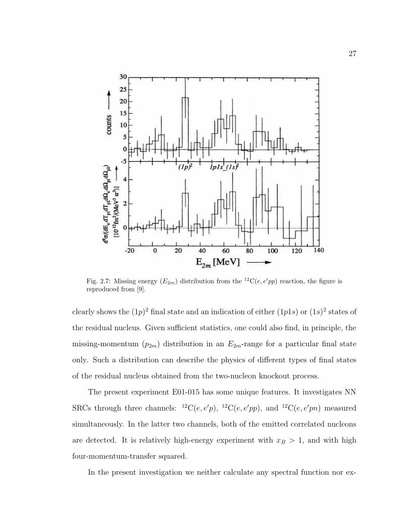
12C(e, e′pp) reaction is shown in Fig. 2.7 which is reproduced from [9]. The figure

27

Fig. 2.7: Missing energy (E2m) distribution from the 12C(e, e′pp) reaction, the figure isreproduced from [9].

clearly shows the (1p)2 final state and an indication of either (1p1s) or (1s)2 states of

the residual nucleus. Given sufficient statistics, one could also find, in principle, the

missing-momentum (p2m) distribution in an E2m-range for a particular final state

only. Such a distribution can describe the physics of different types of final states

of the residual nucleus obtained from the two-nucleon knockout process.

The present experiment E01-015 has some unique features. It investigates NN

SRCs through three channels: 12C(e, e′p), 12C(e, e′pp), and 12C(e, e′pn) measured

simultaneously. In the latter two channels, both of the emitted correlated nucleons

are detected. It is relatively high-energy experiment with xB > 1, and with high

four-momentum-transfer squared.

In the present investigation we neither calculate any spectral function nor ex-

28

tract any cross sections for the 12C(e, e′p) or 12C(e, e′pn) reactions. Instead we work

with the cross section ratio of the 9-fold differential cross section for the 12C(e, e′pn)

reaction to the 6-fold differential cross section for the 12C(e, e′p) reaction. Also we

give the cross section ratio of the 9-fold differential cross section of the 12C(e, e′pn)

reaction to the 9-fold differential cross section of the 12C(e, e′pp) reaction where the

6-fold differential cross section for the 12C(e, e′p) reaction for both cases remains the

same. By working with ratios, many of the factors that contribute to the uncertain-

ties of cross section determinations are eliminated from the final results.

Chapter 3

Setup of the Experiment

Experiments that require coincidence measurements at high momentum resolu-

tion, involving processes at high momentum transfer, are generally low cross section

measurements which result in low count rates. Obtaining adequate count rates gen-

erally requres a high luminosity1 and moderately large-acceptance detectors. Jeffer-

son Laboratory Hall A is a unique facility that fulfills these criteria for the coicidence

experiments due to the presence of two high-resolution spectrometers (HRSs). Ex-

periment E01-015, also known as the “SRC experiment”, is a triple-coincidence

experiment. It ran from January through April 2005. The main aim of the experi-

ment was to study simultaneously the 12C(e, e′p) reaction and the 12C(e, e′pp) and

12C(e, e′pn) reactions, as a tool to measure short-range nucleon-nucleon correlations

[52].

The primary equipment in Hall A [53] is two HRSs designed specifically for

A(e, e′p) measurements at beam energies of several GeV. Generally the left HRS

(HRSL) is instrumented for electron detection and the right HRS (HRSR) is in-

strumented for proton, or other heavy charged particle (π, K, 2H, etc.) detection.

Details on the two HRSs are given in Sect.3.4

We used both HRSs in a coincidence mode to record data for the 12C(e, e′p)

reaction; singles data from each spectrometer were also recorded in the datastream.

To measure protons or neutrons in coincidence with 12C(e, e′p) events, we employed

1The luminosity is a property of both the beam as well as the target material [25]. If L is theluminosity, dN

dtthe number of incoming beam particles per second, n the target particle density in

the scattering material, and d the target thickness, then L = nd dNdt

. The unit of L is cm−2s−1.

29

30

the newly comissioned third spectrometer consisting of the “BigBite” dipole magnet

[54, 55] along with its detector package, and a large neutron detector array.

For the production runs at 4.6275 GeV beam, the scattered electrons and struck

protons were detected in the HRSL and HRSR, respectively, whereas the recoiling

protons (neutrons) were detected in the BigBite detector (neutron detector). Both

the BigBite detector and the neutron detector, as described in Sect.3.6 and 3.7,

respectively, were made up of highly segmented layers of plastic scintillator detectors.

Also for calibration purposes, data from hydrogen and deuterium were taken. How

the experiment was set up will be described in this chapter.

3.1 Kinematic Settings

In the present experiment we had a variety of kinematical settings for three

purposes: (a) commissioning of the neutron detector, (b) commissioning of the

BigBite spectrometer, and (c) producing different sets of production runs. They are

summarized in Table 3.1, in which only the kinematics that were used in the data

analysis of this dissertation work are given. Following is a short description of these

various kinematical settings:

1. LH: Liquid hydrogen (4 cm target) elastic runs with 2-pass (2.345 GeV) beam

with electrons detected in the left HRS and protons detected in the neutron

detector array at -50 angle located 15 meters from the target. This kinematics

was dedicated to neutron-detector calibration.

2. LDK0: Liquid deuterium (15 cm target) runs with 2-pass beam where electrons

were detected in the right HRS and protons in the left HRS. In all other following

kinematics the HRSs’ polarity was opposite relative to this kinematics and the

incident electron beam was 4-pass (4.6275 GeV).

31

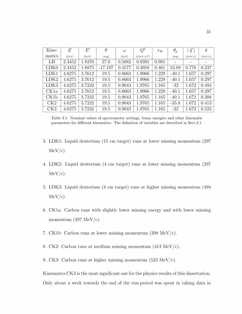
Kine- E E ′ θ ω Q2 xB θp | ~q | kmatics [GeV] [GeV] [deg] [GeV] [(GeV/c)2] [deg] [GeV/c] [GeV/c]

LH 2.3452 1.8370 27.0 0.5082 0.9391 0.985 - - -LDK0 2.3452 1.8875 -17.197 0.4577 0.3958 0.461 53.89 0.778 0.237LDK1 4.6275 3.7612 19.5 0.8663 1.9966 1.229 -40.1 1.657 0.297LDK2 4.6275 3.7612 19.5 0.8663 1.9966 1.229 -40.1 1.657 0.297LDK3 4.6275 3.7232 19.5 0.9043 1.9765 1.165 -32 1.672 0.494CK1a 4.6275 3.7612 19.5 0.8663 1.9966 1.229 -40.1 1.657 0.297CK1b 4.6275 3.7232 19.5 0.9043 1.9765 1.165 -40.1 1.672 0.308CK2 4.6275 3.7232 19.5 0.9043 1.9765 1.165 -35.8 1.672 0.413CK3 4.6275 3.7232 19.5 0.9043 1.9765 1.165 -32 1.672 0.523

Table 3.1: Nominal values of spectrometer settings, beam energies and other kinematicparameters for different kinematics. The definition of variables are described in Sect.2.1.

3. LDK1: Liquid deuterium (15 cm target) runs at lower missing momentum (297

MeV/c).

4. LDK2: Liquid deuterium (4 cm target) runs at lower missing momentum (297

MeV/c).

5. LDK3: Liquid deuterium (4 cm target) runs at higher missing momentum (494

MeV/c).

6. CK1a: Carbon runs with slightly lower missing energy and with lower missing

momentum (297 MeV/c).

7. CK1b: Carbon runs at lower missing momentum (308 MeV/c).

8. CK2: Carbon runs at medium missing momentum (413 MeV/c).

9. CK3: Carbon runs at higher missing momentum (523 MeV/c).

Kinematics CK3 is the most significant one for the physics results of this dissertation.

Only about a week towards the end of the run-period was spent in taking data in

32

this kinematic setting.

3.2 Jefferson Lab Hall A

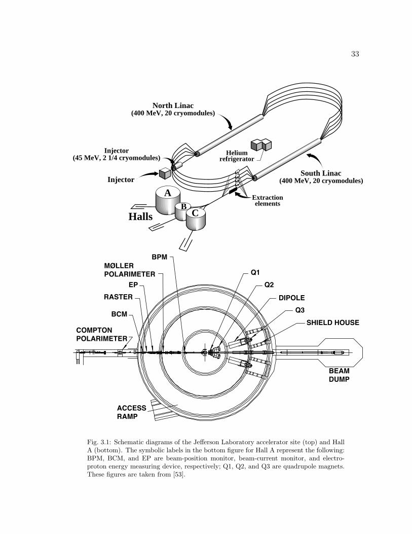
Shown in Fig. 3.1 is a schematic layout of the Jefferson Laboratory accelerator

site and Hall A. The electron beam is produced at the injector, then accelerated and

recirculated for the desired number of passes, and directed to any of the experiment

halls A, B, and C. The description of the Hall A detectors, along with the specific

detectors dedicated to this experiment, is presented in the following sections. The

schematic diagrams of the Jefferson Laboratory accelerator site and Hall A are shown

in Fig. 3.1, while the the detector setup is shown in Fig. 3.2.

3.3 The Target System

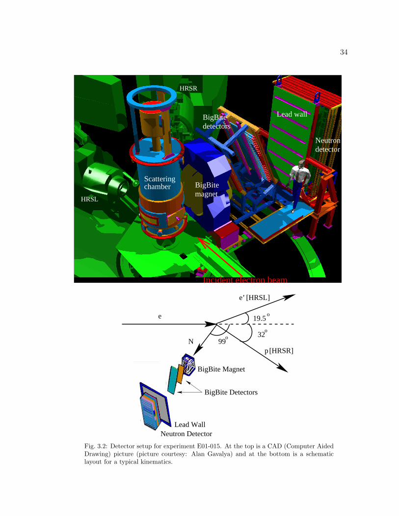
The configuration of the target system for the E01-015 experiment is given

in Table 3.2. The slanted carbon target was used for production runs, while the

liquid hydrogen and liquid deuterium targets were used for calibration runs. The

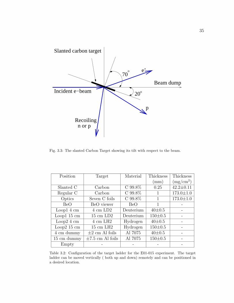
production carbon target was slanted because the expected recoiling particles in this

experiment were relatively low energy (less than 200 MeV) protons and neutrons.

In order to reduce the distance these recoiling particles had to travel in the target

we placed this carbon foil at an angle of 70 with respect to the incident electron

beam (see Fig. 3.3).

This experiment was the commissioning experiment for the BigBite spectrome-

ter. Part of the new equipment for use with BigBite was a specially designed target

chamber with exit windows matching the acceptances of both the HRSs and BigBite.

This chamber has an extra high window to match the large vertical acceptance of

the BigBite magnet in addition to the nominal window for the HRSL (the HRSR

33

AB

C

Heliumrefrigerator

Extractionelements

North Linac(400 MeV, 20 cryomodules)

Injector(45 MeV, 2 1/4 cryomodules)

Injector

Halls

South Linac(400 MeV, 20 cryomodules)

EP

RASTER

BCM

COMPTON

POLARIMETER

MØLLER

POLARIMETER

BPM

Q1

Q2

DIPOLE

Q3

SHIELD HOUSE

BEAM

DUMP

ACCESS

RAMP

Fig. 3.1: Schematic diagrams of the Jefferson Laboratory accelerator site (top) and HallA (bottom). The symbolic labels in the bottom figure for Hall A represent the following:BPM, BCM, and EP are beam-position monitor, beam-current monitor, and electro-proton energy measuring device, respectively; Q1, Q2, and Q3 are quadrupole magnets.These figures are taken from [53].

34

BigBitemagnet

BigBitedetectors

Lead wall

Neutrondetector

Incident electron beam

Scatteringchamber

HRSR

HRSL

oo

BigBite Detectors

N

e o

9932

19.5

p

BigBite Magnet

Lead WallNeutron Detector

e’ [HRSL]

[HRSR]

Fig. 3.2: Detector setup for experiment E01-015. At the top is a CAD (Computer AidedDrawing) picture (picture courtesy: Alan Gavalya) and at the bottom is a schematiclayout for a typical kinematics.

35

p

Recoiling n or p

Incident e−beam

e’70

o

Slanted carbon target

20o

Beam dump

Fig. 3.3: The slanted Carbon Target showing its tilt with respect to the beam.

Position Target Material Thickness Thickness(mm) (mg/cm2)

Slanted C Carbon C 99.8% 0.25 42.2±0.11Regular C Carbon C 99.8% 1 173.0±1.0

Optics Seven C foils C 99.8% 1 173.0±1.0BeO BeO viewer BeO 1 -

Loop1 4 cm 4 cm LD2 Deuterium 40±0.5 -Loop1 15 cm 15 cm LD2 Deuterium 150±0.5 -Loop2 4 cm 4 cm LH2 Hydrogen 40±0.5 -Loop2 15 cm 15 cm LH2 Hydrogen 150±0.5 -4 cm dummy ±2 cm Al foils Al 7075 40±0.5 -15 cm dummy ±7.5 cm Al foils Al 7075 150±0.5 -

Empty - - - -

Table 3.2: Configuration of the target ladder for the E01-015 experiment. The targetladder can be moved vertically ( both up and down) remotely and can be positioned ina desired location.

36

shared the same window as BigBite). The beam exit window towards BigBite had

vertical height of 38.1 cm while that for HRS was half this height. The window was

0.081 cm thick and made of 2024 T6 aluminium.

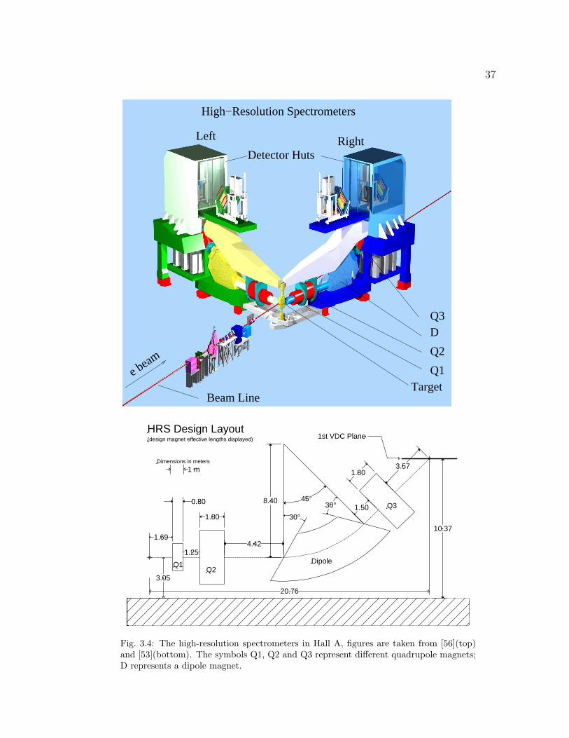
3.4 The High Resolution Spectrometers

Hall A has two high resolution spectrometers as shown schematically in Fig. 3.4

(top). The magnetic elements of the HRSs consist of three superconducting quadrupoles

(Q1, Q2, and Q3) and a super conducting dipole (D) in a QQDQ arrangement, see

Fig. 3.4 (bottom). Quadrupole Q1 focuses in the vertical plane whereas both Q2

and Q3 provide vertical defocusing. The 6.6 m long dipole, providing a vertical bend

of 45, has focussing entrance and exit polefaces and includes additionanl focussing

from the field gradient in the dipole. For details about the magnetic elements and

design of the HRSs see [53].

In this experiment, for the most of the production runs, HRSL was used as the

electron spectrometer and HRSR was used as the proton spectrometer. In some

of the kinematics, dedicated for calibration runs, we reversed their roles. In other

calibration runs, HRSR was not used at all.

The detector package in each spectrometer is housed within a shielding hut

and is located on top of the HRS structure immediately after Q3. The detector

package configuration is very flexible. What detector configuration to use, which

detector elements to add, keep or remove depends upon the need of the individual

experiment. In this experiment, in addition to two vertical drift chambers (VDC)

in both HRSs, the spectrometers had the following detector packages (schematic

layout shown in Fig. 3.5). The left HRS had scintillator planes S1 and S2, a Gas

Cherenkov detector, and a shower detector functioning as a pion rejector. The Gas

37

Q1

Q3

Target

Q2

D

Beam Line

Left RightDetector Huts

e beam

High−Resolution Spectrometers

1.80

1.80

4.42

3.57

1.50

1.25

0.80

1.69

45°30°

30°

8.40

10.37

3.05

HRS Design Layout(design magnet effective lengths displayed)

Q1Q2

Dipole

Q3

20.76

1st VDC Plane

Dimensions in meters

1 m

Fig. 3.4: The high-resolution spectrometers in Hall A, figures are taken from [56](top)and [53](bottom). The symbols Q1, Q2 and Q3 represent different quadrupole magnets;D represents a dipole magnet.

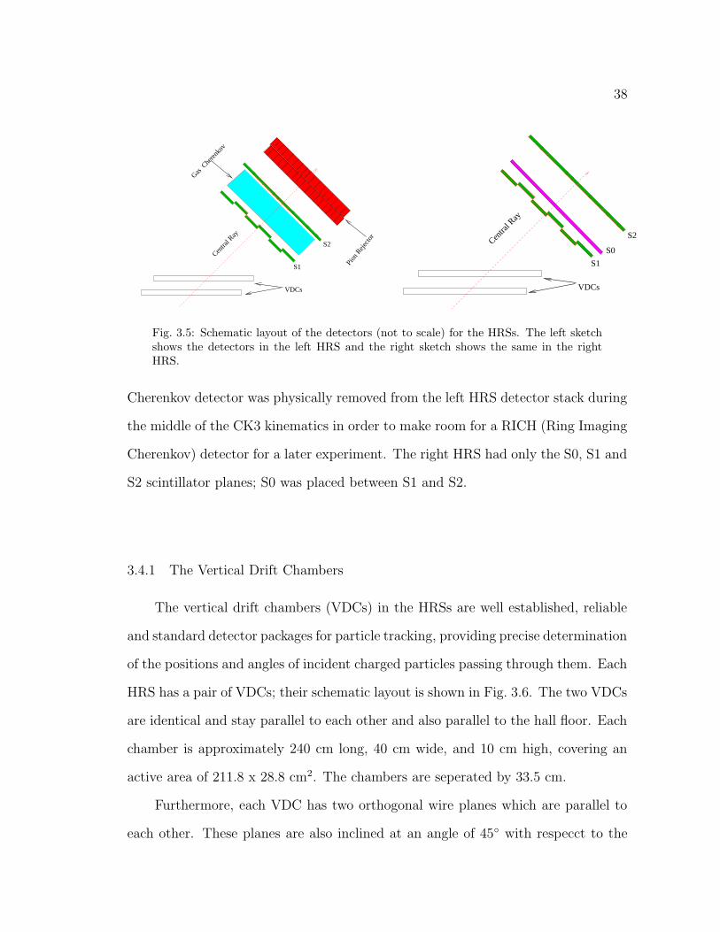
38

S1

S2

Gas C

heren

kov

Centra

l Ray

VDCs

Pion

Reje

ctor

S1

S2

S0Cen

tral R

ay

VDCs

Fig. 3.5: Schematic layout of the detectors (not to scale) for the HRSs. The left sketchshows the detectors in the left HRS and the right sketch shows the same in the rightHRS.

Cherenkov detector was physically removed from the left HRS detector stack during

the middle of the CK3 kinematics in order to make room for a RICH (Ring Imaging

Cherenkov) detector for a later experiment. The right HRS had only the S0, S1 and

S2 scintillator planes; S0 was placed between S1 and S2.

3.4.1 The Vertical Drift Chambers

The vertical drift chambers (VDCs) in the HRSs are well established, reliable

and standard detector packages for particle tracking, providing precise determination

of the positions and angles of incident charged particles passing through them. Each

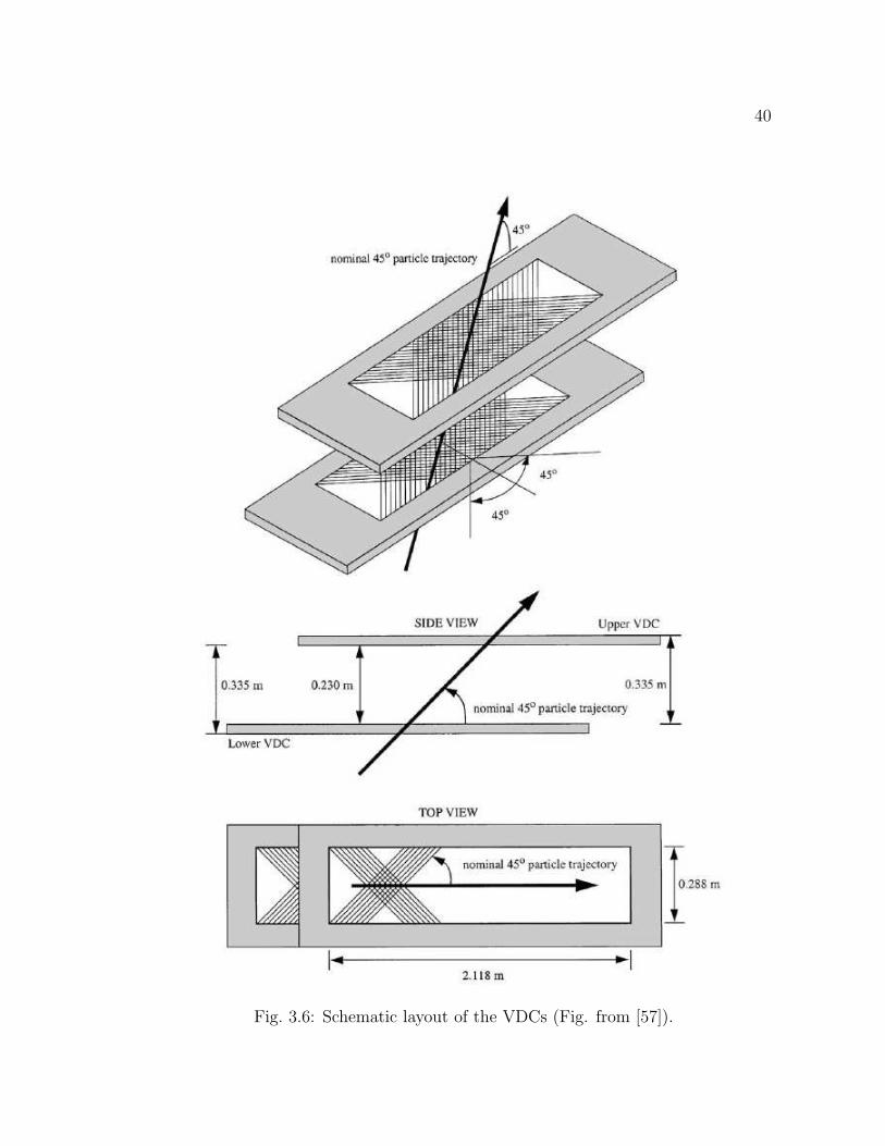
HRS has a pair of VDCs; their schematic layout is shown in Fig. 3.6. The two VDCs

are identical and stay parallel to each other and also parallel to the hall floor. Each

chamber is approximately 240 cm long, 40 cm wide, and 10 cm high, covering an

active area of 211.8 x 28.8 cm2. The chambers are seperated by 33.5 cm.

Furthermore, each VDC has two orthogonal wire planes which are parallel to

each other. These planes are also inclined at an angle of 45 with respecct to the

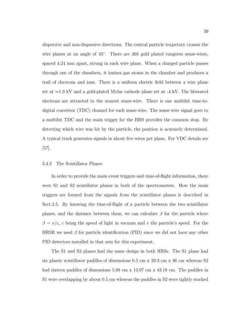
39

dispersive and non-dispersive directions. The central particle trajectory crosses the

wire planes at an angle of 45. There are 368 gold plated tungsten sense-wires,

spaced 4.24 mm apart, strung in each wire plane. When a charged particle passes

through one of the chambers, it ionizes gas atoms in the chamber and produces a

trail of electrons and ions. There is a uniform electric field between a wire plane

set at ∼1.9 kV and a gold-plated Mylar cathode plane set at -4 kV. The liberated

electrons are attracted to the nearest sense-wire. There is one multihit time-to-

digital convertor (TDC) channel for each sense-wire. The sense-wire signal goes to

a multihit TDC and the main trigger for the HRS provides the common stop. By

detecting which wire was hit by the particle, the position is acurately determined.

A typical track generates signals in about five wires per plane. For VDC details see

[57].

3.4.2 The Scintillator Planes

In order to provide the main event triggers and time-of-flight information, there

were S1 and S2 scintillator planes in both of the spectrometers. How the main

triggers are formed from the signals from the scintillator planes is described in

Sect.3.5. By knowing the time-of-flight of a particle between the two scintillator

planes, and the distance between them, we can calculate β for the particle where

β = v/c, c being the speed of light in vacuum and v the particle’s speed. For the

HRSR we used β for particle identification (PID) since we did not have any other

PID detectors installed in that arm for this experiment.

The S1 and S2 planes had the same design in both HRSs. The S1 plane had

six plastic scintillator paddles of dimensions 0.5 cm x 29.3 cm x 36 cm whereas S2

had sixteen paddles of dimensions 5.08 cm x 13.97 cm x 43.18 cm. The paddles in

S1 were overlapping by about 0.5 cm whereas the paddles in S2 were tightly stacked

40

Fig. 3.6: Schematic layout of the VDCs (Fig. from [57]).

41

without any overlap. Each paddle was viewed by two phototubes attached at its

ends. HRSR had an additional S0 plane consisting of a single paddle of dimensions

0.5 cm x 25 cm x 176 cm. The distance between S1 and S0 was 43.5 cm while that

between S1 and S2 was 202.2 (181.5) cm in the right (left) HRS.

3.4.3 The Gas Cherenkov Detector

The gas Cherenkov detector provides excellent particle identification for elec-

trons, by rejecting pions. The idea is to choose a certain gas such that it does not

emit Cherenkov radiation by pions of the momentum range of interest. Cherenkov

light is emitted when a charged particle in a material medium moves faster than the

speed of light in that medium. The speed of light in the medium is

v = c/n (3.1)

where n is the index of refraction. In order to emit Cherenkov light one should have

v = βc > c/n (3.2)

where βc is v, the speed of the particle. In this situation light is emitted in a

well-defined cone of half angle θ given by (see [58])

cosθ =1

βn. (3.3)

The Hall A gas Cherenkov tank utilezes CO2 gas at atmospheric pressure with

an index of refraction 1.00041. It has ten mirrors arranged in two rows, and each

mirror is viewed by one phototube. For details see [59] and for the position of the

Cherenkov detector in the detector stack see Fig. 3.5.

42

For electrons (β '1), n = 1.00041 translates to half-cone angle of 1.64 degrees,

hence the light is emitted in the forward direction. In order to calculate the threshold

momentum (pth) for Cherenkov light emission, we use the threshold relation from

Eqn.(3.2) by replacing βc with cn

in the following equation

E = γmc2 =√m2c4 + p2c2 (3.4)

where γ = 1/√

1 − β2 and obtain

pth =mc√n2 − 1

(3.5)

For electrons we find pth = 17.84 MeV/c, hence in experiment E01-015, electrons

always produced Cherenkov light since HRSL was always set for electron energies

> 1 GeV. On the other hand, for pions we find pth = 4888.51 MeV/c, hence pions

never produced Cherenkov light because the central momentum settings for the

spectrometers were never more than 3800 MeV/c.

In this experiment, although the electron signal from the Cherenkov detector

was very clean, any residual pion contamination was removed using the shower

detectors described in the next section.

3.4.4 The Pion Rejector

The pion rejector, consisting of a pair of shower detectors, is another PID detec-

tor, and is a miniature form of an electromagnetic calorimeter. An electromagnetic

calorimeter measures the energy deposited by charged particles when they travel

through it. Shower detectors are generally made of high Z materials, since the prob-

ability of forming an electromagnetic shower is a strong function of Z. The pion

43

rejector is made of lead glass.

When the energetic electrons are incident on a shower detector, an electromag-

netic shower consisting of electrons (e−), positrons (e+), and photons is formed.

Formation of such a cascade continues until the energy of the particles falls below

about 100 MeV, at which point dissipative processes, such as ionization and excita-

tion, occur. In principle, the energetic charged particles produce an electromagnetic

shower, and the photons in the shower appear as Cherenkov light which is collected

in the phototubes of the shower dector.

The absorption length or the mean-free path (the mean distance traveled before

a collision) of an electron is not the same as that of a pion . For example, a 15 cm

thick lead-glass is good enough for absorbing electrons while this thickness is too

short for pions since they have a long absorption length. The result is that we can

find a large energy deposition by electrons and only a small energy deposition by

pions.

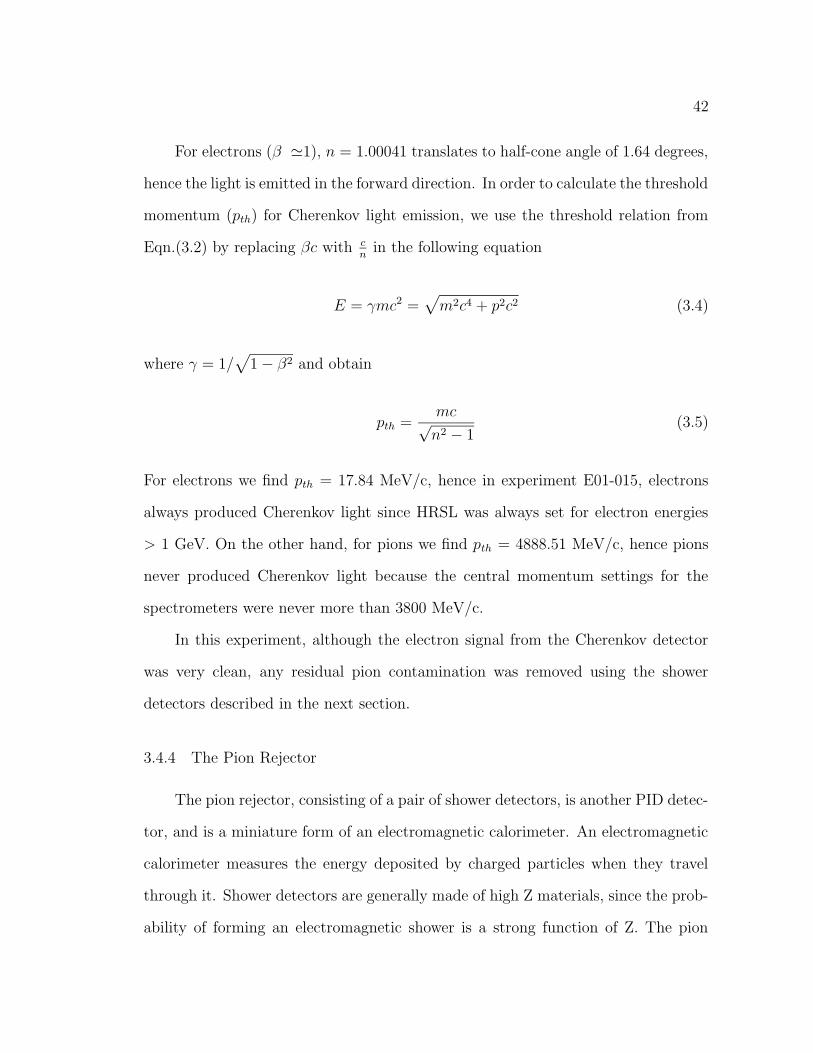
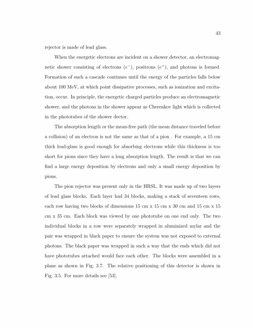
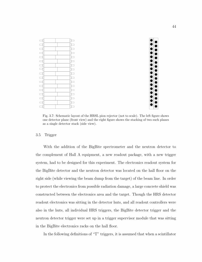
The pion rejector was present only in the HRSL. It was made up of two layers

of lead glass blocks. Each layer had 34 blocks, making a stack of seventeen rows,

each row having two blocks of dimensions 15 cm x 15 cm x 30 cm and 15 cm x 15

cm x 35 cm. Each block was viewed by one phototube on one end only. The two

individual blocks in a row were separately wrapped in aluminized mylar and the

pair was wrapped in black paper to ensure the system was not exposed to external

photons. The black paper was wrapped in such a way that the ends which did not

have phototubes attached would face each other. The blocks were assembled in a

plane as shown in Fig. 3.7. The relative positioning of this detector is shown in

Fig. 3.5. For more details see [53].

44

!!!!""""####$$$$

%%%%&&&&

''''((((

))))****

++++,,,,

----....

////0000

11112222

33334444

55556666

777788889999::::;;;;<<<<==

==>>>>????@@@@

AAAABBBBCCCCDDDD

Fig. 3.7: Schematic layout of the HRSL pion rejector (not to scale). The left figure showsone detector plane (front view) and the right figure shows the stacking of two such planesas a single detector stack (side view).

3.5 Trigger

With the addition of the BigBite spectrometer and the neutron detector to

the complement of Hall A equipment, a new readout package, with a new trigger

system, had to be designed for this experiment. The electronics readout system for

the BigBite detector and the neutron detector was located on the hall floor on the

right side (while viewing the beam dump from the target) of the beam line. In order

to protect the electronics from possible radiation damage, a large concrete shield was

constructed between the electronics area and the target. Though the HRS detector

readout electronics was sitting in the detector huts, and all readout controllers were

also in the huts, all individual HRS triggers, the BigBite detector trigger and the

neutron detector trigger were set up in a trigger supervisor module that was sitting

in the BigBite electronics racks on the hall floor.

In the following definitions of “T” triggers, it is assumed that when a scintillator

45

plane generates a signal, that signal was obtained from a logical OR of all of its

individual bar signals. The individual bar signal is a coicidence signal between the

two phototubes on a bar. The following triggers were registered into the datastream

when the following conditions were fulfilled.

• T1 trigger: both scintillator planes in the HRSR have signals in a timing window

of about 100 ns.

• T2 trigger: in HRSR, either the S1 or S2 scintillator plane has a signal and the

S0 scintillator plane has a signal.

• T3 trigger: both scintillator planes in HRSR have signals in a timing window of

about 50 ns.

• T4 trigger: in HRSL, only one of the scintillator planes and the Gas Cherenkov

detector have signals.

• T5 trigger: the logical AND of T1 and T3 in a timing window of about 100 ns,

and made earlier by 60 to 80 ns compared to all other triggers.

• T6 trigger (for detail see section 3.6.1): the trigger from the BigBite detector,

but not recorded in the datastream due to a very high rate in this trigger.

• T7 trigger (for detail see section 3.7): trigger from the neutron detector, but not

recorded in the datastream due to a very high rate for this trigger.

The Hall A data aquisition (DAQ) system can handle event rates up to about

2 kHz. In the E01-015 experiment, the DAQ system had event rate below 500 Hz,

in order to keep the electronic deadtime below 20%. A trigger determines whether

an event should be recorded by the DAQ system. This experiment had the seven

T triggers (defined above) and one timing trigger. There were only three main

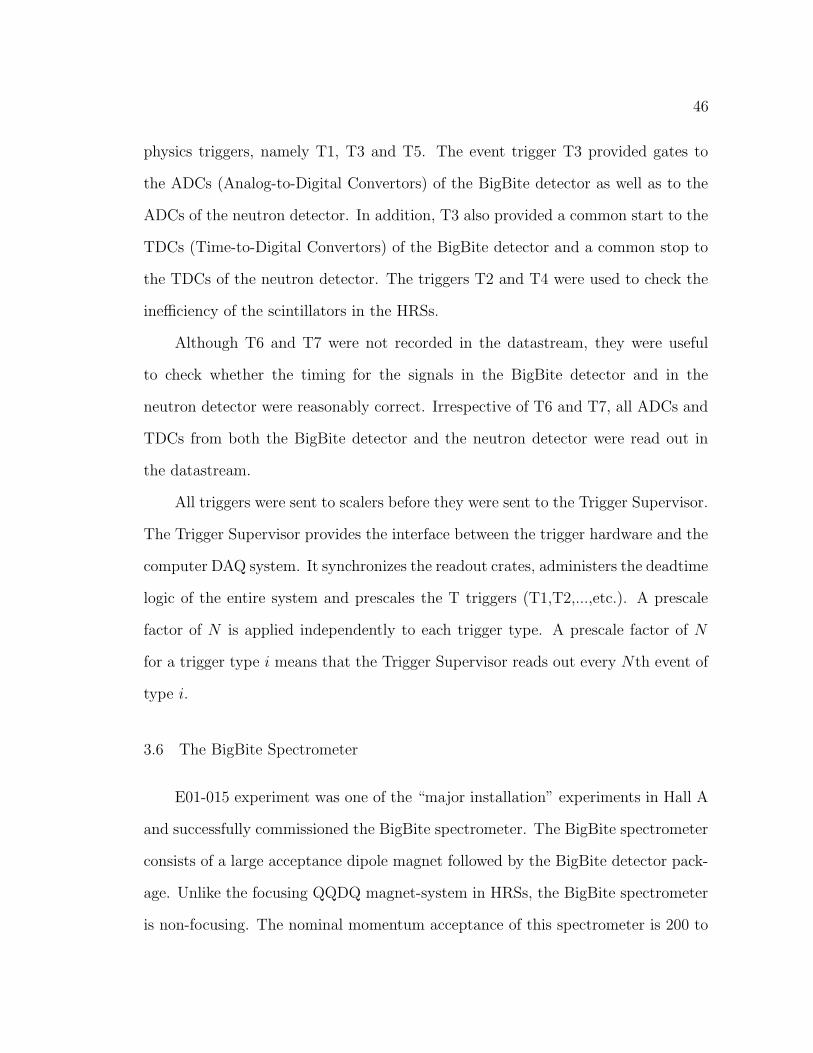
46

physics triggers, namely T1, T3 and T5. The event trigger T3 provided gates to

the ADCs (Analog-to-Digital Convertors) of the BigBite detector as well as to the

ADCs of the neutron detector. In addition, T3 also provided a common start to the

TDCs (Time-to-Digital Convertors) of the BigBite detector and a common stop to

the TDCs of the neutron detector. The triggers T2 and T4 were used to check the

inefficiency of the scintillators in the HRSs.

Although T6 and T7 were not recorded in the datastream, they were useful

to check whether the timing for the signals in the BigBite detector and in the

neutron detector were reasonably correct. Irrespective of T6 and T7, all ADCs and

TDCs from both the BigBite detector and the neutron detector were read out in

the datastream.

All triggers were sent to scalers before they were sent to the Trigger Supervisor.

The Trigger Supervisor provides the interface between the trigger hardware and the

computer DAQ system. It synchronizes the readout crates, administers the deadtime

logic of the entire system and prescales the T triggers (T1,T2,...,etc.). A prescale

factor of N is applied independently to each trigger type. A prescale factor of N

for a trigger type i means that the Trigger Supervisor reads out every Nth event of

type i.

3.6 The BigBite Spectrometer

E01-015 experiment was one of the “major installation” experiments in Hall A

and successfully commissioned the BigBite spectrometer. The BigBite spectrometer

consists of a large acceptance dipole magnet followed by the BigBite detector pack-

age. Unlike the focusing QQDQ magnet-system in HRSs, the BigBite spectrometer

is non-focusing. The nominal momentum acceptance of this spectrometer is 200 to

47

900 MeV/c [54, 55] and the angular acceptance when the magnet is 1.1 m from the

target is 96 msr. The horizontal and vertical openings of the magnet are 25 cm and

148 cm, respectively, which define the horizontal and vertical acceptances, respec-

tively. Figure 3.8 (and Fig. 3.2 as well) shows a schematic layout of this spectrometer

followed by the neutron detector, and Fig. 3.9 is a CAD rendering of BigBite and

its detector package. Figure 3.10 shows the photograph of these detectors in place

for the experiment.

There is a flood of proposals that wish to utilize BigBite. A partial list of

Hall A experiments that use or plan to use the BigBite spectrometer (though not

necessarily the SRC detector package) are listed here:

1. E01-015, This SRC experiment, BigBite detecting protons [52].

2. E02-013, GnE experiment, BigBite detecting electrons [60] (completed data tak-

ing).

3. E04-007: π0 threshold experiment, BigBite detecting protons [61].

4. E05-009: Resonance experiment, BigBite detecting K+s [62].

5. E05-102: 3He(e, e′d) experiment, BigBite detecting deuterons [63].

6. E06-010: Transversity experiment, BigBite detecting electrons [64].

7. E06-014: dn2 , BigBite detecting electrons [65].

8. E12-06-122: An1 at 12 GeV, BigBite detecting electrons [66].

9. E07-006: second generation SRC experiment, BigBite detecting protons [67].

Any charged particle entering into the BigBite magnetic field is deflected by

the magnetic field. Before and after the magnetic field, the particle trajectory is a

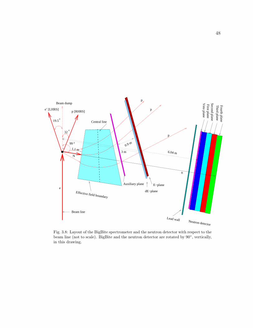
48

19.50

320

N

99 0

e’ [LHRS]p [RHRS]

Neutron detector

Veto plane

First planeSecond plane

Third plane

Fourth plane

Beam dump

0.9 m

e

Beam line

3 m

Central line

1.1 m

p

p

n

Effective field boundary

p

Lead wall

6.04 m

Auxiliary plane

dE−plane

E−plane

Fig. 3.8: Layout of the BigBite spectrometer and the neutron detector with respect to thebeam line (not to scale). BigBite and the neutron detector are rotated by 90, vertically,in this drawing.

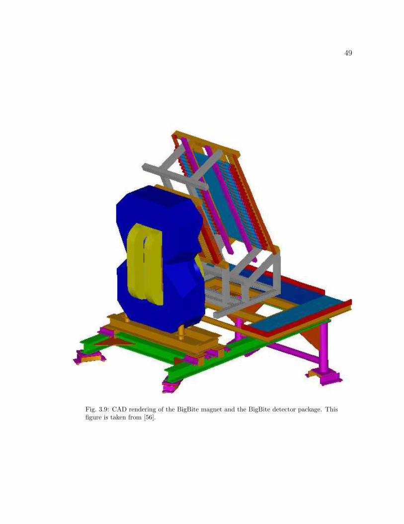
49

Fig. 3.9: CAD rendering of the BigBite magnet and the BigBite detector package. Thisfigure is taken from [56].

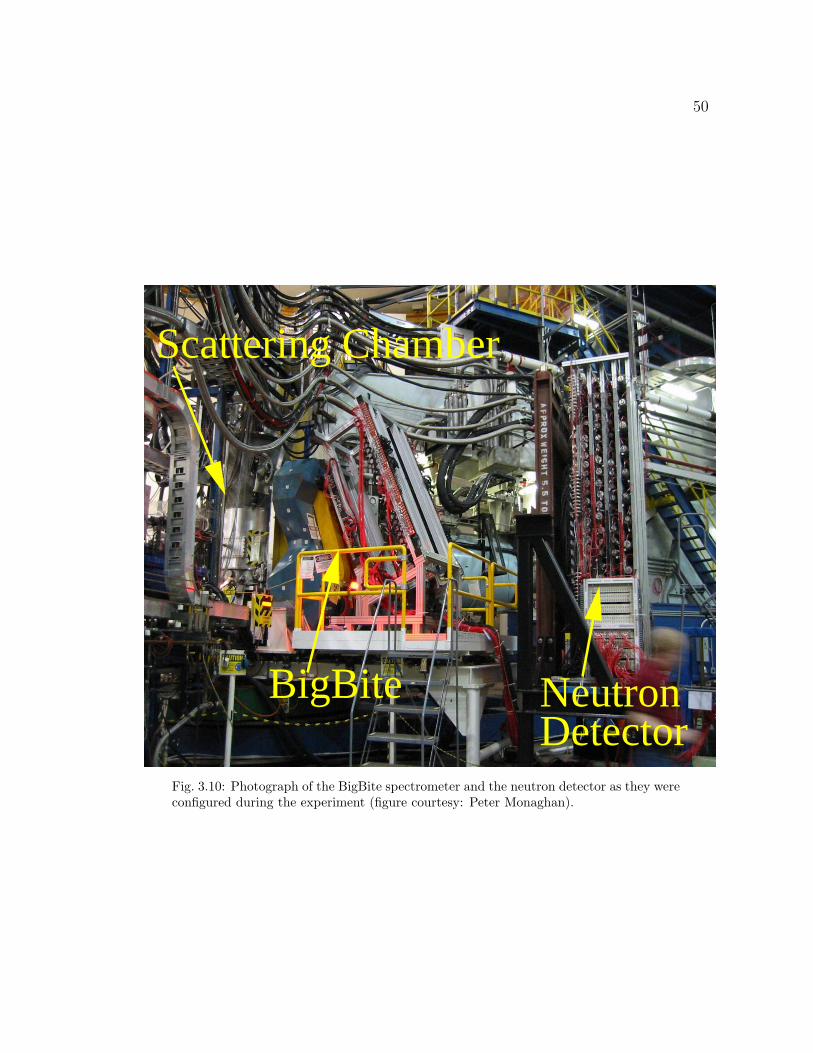
50

Scattering Chamber

BigBiteDetectorNeutron

Fig. 3.10: Photograph of the BigBite spectrometer and the neutron detector as they wereconfigured during the experiment (figure courtesy: Peter Monaghan).

51

straight line, while inside the field it is circular (see Fig. 3.8). The circular motion

is described by the equation ~F = q~v x ~B where ~F is Lorentz force experienced by a

particle of charge q with velocity ~v in the magnetic field of strength ~B.

A field strength of 0.93 T was used during the E01-015 experiment; the current

drawn by the BigBite magnet for this field was 518 A. Protons were deflected up-

wards inside the field and swept into the BigBite detector system. Neutrons passing

through BigBite were not affected by the BigBite field, and followed a straight line

path to the neutron detector.

The BigBite spectrometer was located at 99 right of the beam line during all

production runs. The distance between the target and the entrance to the BigBite

magnet was always 1.1 m.

3.6.1 The BigBite Detector Package

The BigBite detector package (see details in [68, 69]) consisted of three scintil-

lator planes: the auxiliary plane, the dE-plane and the E-plane as shown in Fig. 3.8

(and also in Fig. 3.9). The auxiliary plane had 56 thin scintillator paddles of di-

mensions 2.5 mm x 25 mm x 350 mm, each paddle being viewed by one phototube

on one end.

The dE- and E-planes both had 24 scintillator paddles, each 50 cm long and 8.6

cm wide. The thickness of a dE-counter was 3 mm while that of an E-counter was

30 mm. Each counter in the dE- and E-planes was viewed by two phototubes. The

dE-bars were thin so that protons lost only a negligible amount of energy, whereas

the E-bars were thick so that all or most of the proton kinetic energy was lost there.

The combination of the dE- and E-planes was called the trigger plane because they

formed the trigger for the particles (protons) to be detected by the BigBite detector.

The electronics block diagram for reading out each scintillator and sending the

52

signals to the DAQ system, is shown in Fig. 3.11. The phototube signals were first

amplified ten times using amplifiers giving two identical outputs. One output is

delayed by 500 nanoseconds and sent to the ADC module which digitizes the charge

accumulated over a specific interval (the time period of the gate). The other output

was sent without delay to a discriminator to produce a logic pulse. Again two

outputs were produced by the discriminator. One output was sent to form a trigger

(T6) for the BigBite detector. The other output was delayed by 500 nanoseconds

and sent to a CAMAC module which again produced two outputs. One output was

sent to a scaler module (VME) and the remaining output was sent to the TDC

module (VME).

The purpose of the high segmentation of each plane was to accomodate the

high count rates that were expected in these planes, and also to get better position

and momentum resolutions by track reconstruction. We utilized two methods for

track reconstructions. One method involved finding the time-of-flight between the

auxiliary plane and the trigger plane, where there is no magnetic field. The other

method involved finding the time-of-flight between the target and the trigger plane,

where the bending of the trajectory of the proton in the magnetic field is used. The

distance between the target and trigger plane was about 3 m whereas that between

auxiliary plane and the trigger plane was about 0.9 m. Details of the analysis of

proton events in the BigBite spectrometer can be found in [69].

3.7 The Neutron Detector

In the setup for production runs at high energy (4.6275 GeV), the neutron

detector was sitting downstream of the BigBite spectrometer. From a survey report

[70] (see also in internal report from P. Monaghan [71] for E01-015 experiment),

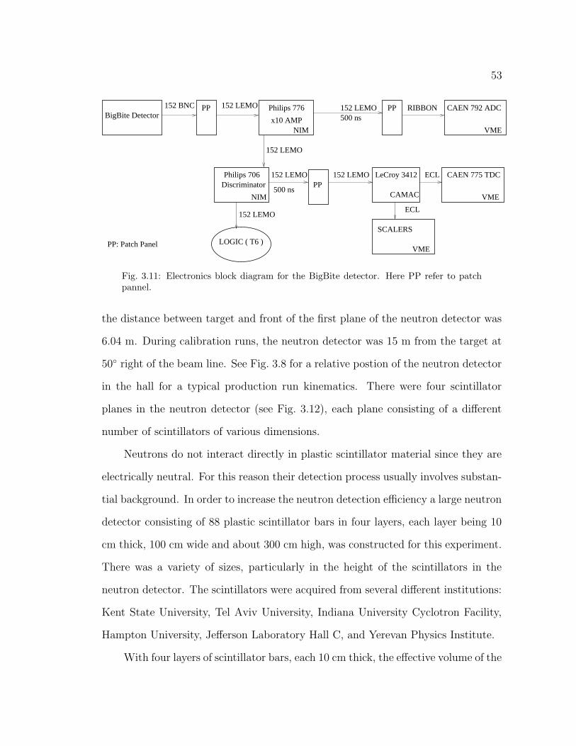
53

CAEN 792 ADC152 BNC RIBBONBigBite Detector

PP PP

VME

Philips 776

x10 AMPNIM

CAMAC

ECL

PPDiscriminatorPhilips 706

NIM

LOGIC ( T6 )

500 ns

500 ns

CAEN 775 TDCLeCroy 3412 ECL

PP: Patch Panel

SCALERS

VME

VME

152 LEMO 152 LEMO

152 LEMO

152 LEMO

152 LEMO

152 LEMO

Fig. 3.11: Electronics block diagram for the BigBite detector. Here PP refer to patchpannel.

the distance between target and front of the first plane of the neutron detector was

6.04 m. During calibration runs, the neutron detector was 15 m from the target at

50 right of the beam line. See Fig. 3.8 for a relative postion of the neutron detector

in the hall for a typical production run kinematics. There were four scintillator

planes in the neutron detector (see Fig. 3.12), each plane consisting of a different

number of scintillators of various dimensions.

Neutrons do not interact directly in plastic scintillator material since they are

electrically neutral. For this reason their detection process usually involves substan-

tial background. In order to increase the neutron detection efficiency a large neutron

detector consisting of 88 plastic scintillator bars in four layers, each layer being 10

cm thick, 100 cm wide and about 300 cm high, was constructed for this experiment.

There was a variety of sizes, particularly in the height of the scintillators in the

neutron detector. The scintillators were acquired from several different institutions:

Kent State University, Tel Aviv University, Indiana University Cyclotron Facility,

Hampton University, Jefferson Laboratory Hall C, and Yerevan Physics Institute.

With four layers of scintillator bars, each 10 cm thick, the effective volume of the

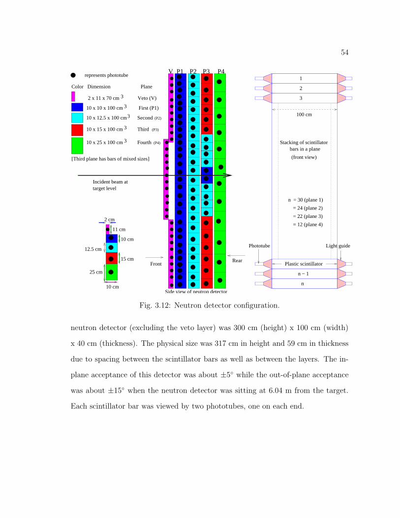
54

Incident beam attarget level

RearFront

represents phototube

[Third plane has bars of mixed sizes]

Side view of neutron detector

2 cm

10 cm

11 cm

10 cm

25 cm

12.5 cm

15 cm

Color Dimension Plane

3

3

3

3

100 cm

1

n − 1

2

n

3

= 22 (plane 3)

= 12 (plane 4)

= 24 (plane 2)

(front view)

Stacking of scintillatorbars in a plane

n = 30 (plane 1)

Phototube

Plastic scintillator

Light guide

3

10 x 10 x 100 cm First (P1)

10 x 12.5 x 100 cm Second

2 x 11 x 70 cm Veto (V)

(P2)

10 x 15 x 100 cm Third (P3)

10 x 25 x 100 cm Fourth (P4)

V P1 P2 P3 P4

Fig. 3.12: Neutron detector configuration.

neutron detector (excluding the veto layer) was 300 cm (height) x 100 cm (width)

x 40 cm (thickness). The physical size was 317 cm in height and 59 cm in thickness

due to spacing between the scintillator bars as well as between the layers. The in-

plane acceptance of this detector was about ±5 while the out-of-plane acceptance

was about ±15 when the neutron detector was sitting at 6.04 m from the target.

Each scintillator bar was viewed by two phototubes, one on each end.

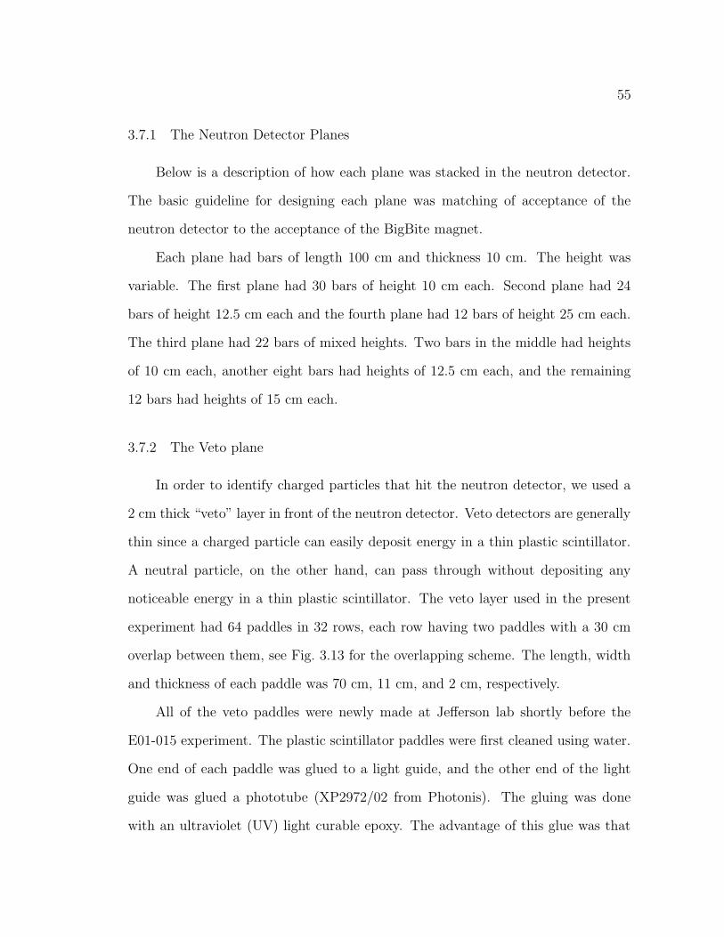
55

3.7.1 The Neutron Detector Planes

Below is a description of how each plane was stacked in the neutron detector.

The basic guideline for designing each plane was matching of acceptance of the

neutron detector to the acceptance of the BigBite magnet.

Each plane had bars of length 100 cm and thickness 10 cm. The height was

variable. The first plane had 30 bars of height 10 cm each. Second plane had 24

bars of height 12.5 cm each and the fourth plane had 12 bars of height 25 cm each.

The third plane had 22 bars of mixed heights. Two bars in the middle had heights

of 10 cm each, another eight bars had heights of 12.5 cm each, and the remaining

12 bars had heights of 15 cm each.

3.7.2 The Veto plane

In order to identify charged particles that hit the neutron detector, we used a

2 cm thick “veto” layer in front of the neutron detector. Veto detectors are generally

thin since a charged particle can easily deposit energy in a thin plastic scintillator.

A neutral particle, on the other hand, can pass through without depositing any

noticeable energy in a thin plastic scintillator. The veto layer used in the present

experiment had 64 paddles in 32 rows, each row having two paddles with a 30 cm

overlap between them, see Fig. 3.13 for the overlapping scheme. The length, width

and thickness of each paddle was 70 cm, 11 cm, and 2 cm, respectively.

All of the veto paddles were newly made at Jefferson lab shortly before the

E01-015 experiment. The plastic scintillator paddles were first cleaned using water.

One end of each paddle was glued to a light guide, and the other end of the light

guide was glued a phototube (XP2972/02 from Photonis). The gluing was done

with an ultraviolet (UV) light curable epoxy. The advantage of this glue was that

56

Two paddles overlap

11 cm

70 cm

30 cm

Individual paddles22 cm

2.9 cm

Plastic scintillator

Light guide

9.9 cm

Phototube (XP2972/02)

Fig. 3.13: Veto paddles (front view).

the glue would set as soon as it was exposed to the UV light. The paddle was then

ready for wrapping.

Each veto paddle was wrapped with aluminized mylar with its non-conducting

surface towards the surface of the paddle. Each paddle was then wrapped with

heavy black PVC plastic of thickness 0.5 mm to make the paddle light tight so that

no photons would enter the system from outside. Each paddle was then carefully

tested for light-tightness.

Light-tightness was tested by measuring the dark current of the phototube.

The dark current was measured at a high voltage (HV) of about 1.5 kV. This HV

was higher than the intended HV (1.1 kV) for the experiment for these paddles.

Generally, the higher the HV, higher the dark current. It was observed that the

dark current was almost always less than 40 nA. If the dark current was of the order

of 100 nA then the paddle was subject to a further investigation. The problem

could be in the wrapping, the gluing or both. There were several glued joints in

each paddle: the joint between scintillator and the light guide, between the light

guide and phototube, and even between the two parts (trapezoidal and cylindrical)

of the light guides. The dark current was also measured by covering the paddle with

a heavy thick black cloth on different positions of the paddle to see if there was any

57

variation before and after covering.

3.7.3 Electronics

The electronics block diagram for reading out the signals from each scintillator

bar, and sending those signals to DAQ system is shown in Fig 3.14. Below is

described how the electronics circuitry was setup. Each phototube signal, after being

delayed by 237 ns, was first amplified by a factor of ten, using an amplifier giving

two copies of the output. One copy was delayed by 500 nanosecond and sent to a

FASTBUS 1881 ADC module2. Another copy was sent to a LeCroy 4413 (CAMAC)

discriminator which was capable of giving two copies of its output. One copy was

sent to a VME scaler module and the remaining copy, after a 500 nanosecond delay,

was sent to a FASTBUS 1877 TDC module. In order to make the trigger (T7) from

the neutron-detector scintillators, the signal from the summing module was sent to

another LeCroy 4413 (CAMAC) discriminator with a threshold of 300 mV and the

output from this discriminator was fed into a logic unit forming the T7 trigger.

The FASTBUS 1887 TDC modules had a time-per-channel of 0.5 ns and were

operated in a common-stop mode. In this mode, an event such as a signal from the

neutron detector, started the timing in the TDCs. The TDC timing was stopped

by the T3 trigger for this event, and subsequently the event was readout in the

datastream. The FASTBUS 1881 ADC modules in this experiment were gated by

a gate period of 200 ns, and that gate was also provided by the T3 trigger.

2Before arriving at the ADC module, the signal went through two additional modules viz. asumming module, and a filter before the delay. These modules were part of the setup for anotherexperiment (Gn

E) [60], with which we shared electronics. They had no impact on our signalprocessing.

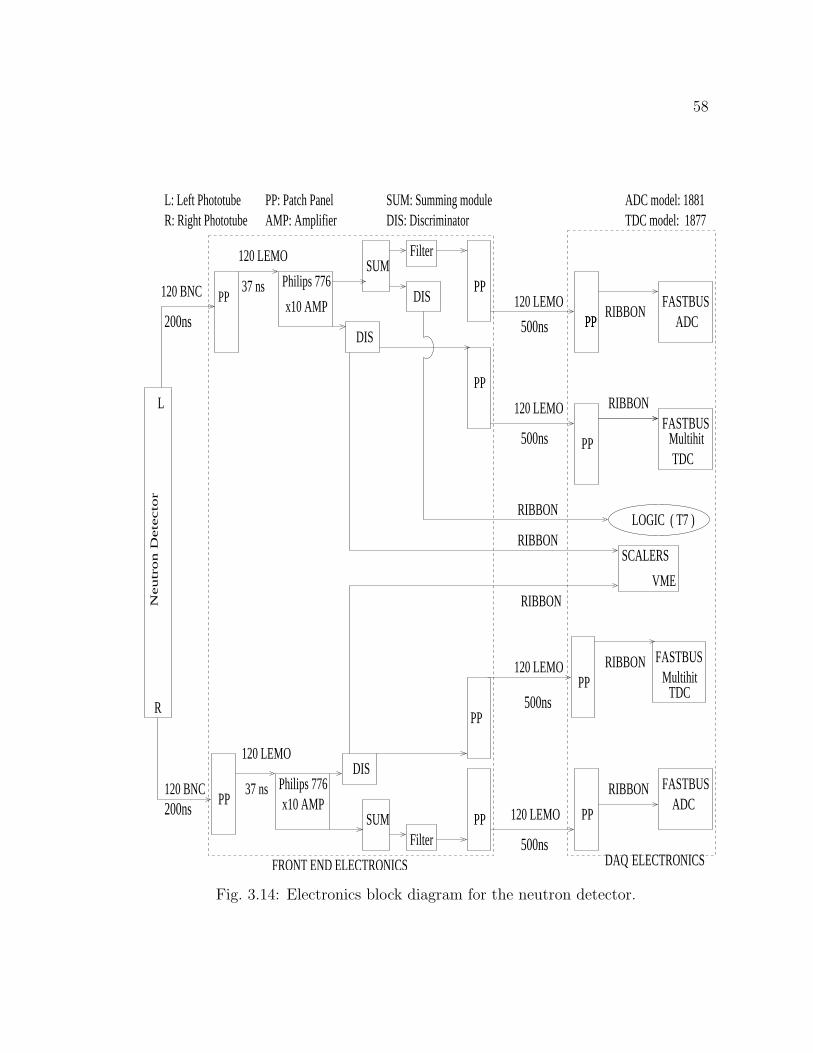
58

500ns

200ns

200ns

PP

500ns

500ns

500ns

PPPP

L

Neutr

on D

ete

cto

r

R

120 BNC

120 BNC

PP

SUMFilter

TDC

RIBBON

FASTBUSMultihit

FASTBUSADC

RIBBONPP

PP

PP

PP

37 ns Philips 776

x10 AMP

37 ns

DIS

Philips 776x10 AMP

SUM

DIS

FilterPP

PP

FASTBUSADC

PP

FASTBUSMultihit

TDC

RIBBON

LOGIC ( T7 )

VME

SCALERS

DIS

RIBBON

RIBBON

RIBBON

RIBBON

FRONT END ELECTRONICS

ADC model: 1881TDC model: 1877

SUM: Summing moduleDIS: DiscriminatorAMP: Amplifier

PP: Patch PanelR: Right PhototubeL: Left Phototube

120 LEMO

120 LEMO

120 LEMO

120 LEMO

120 LEMO

120 LEMO

DAQ ELECTRONICS

Fig. 3.14: Electronics block diagram for the neutron detector.

Chapter 4

Neutron-Detection Efficiency

The neutron-detection efficiency of a neutron detector is a crucial quantity for

interpreting signals obtained from the neutron detector. If the efficiency is ε, and

the signal without efficiency correction is S, then the signal with efficiency correc-

tion will be S/ε. Our primary determination of the neutron-detection efficiency

was exprimental. We used the 2H(e, e′p)n reaction in what is commonly called “the

associated particle” method. The 2H(e, e′p) measurement with the two HRSs is

“kinematically complete,” meaning that the direction and momentum of the asso-

ciated neutron is determined for each e-p coincidence, from conservation of energy

and momentum. The LDK0, LDK1, LDK2, and LDK3 kinematics were dedicated

to these associated-particle efficiency measurements.

The efficiency data from the 2H(e, e′p)n reaction measurements were of only

modest statistical accuracy in the neutron momentum range of interest. Therefore

we developed a model simulation of the efficiency that we adjusted to provide a good

description of the measured efficiency data. The basis of the simulation was a Monte-

Carlo neutron-detection efficiency code [72] developed at Kent State University by

R. Cecil, et al. The key parameter for extracting the efficiency from the code

is the pulse-height (light production) thresholds for the scintillator bars making

up the detector. Because our electronic signal processing did not correspond to

the assumptions in the Cecil code, we determined “effective thresholds” for the

simulation that provided a good description of our efficiency data. The simulation

then gave us a smooth curve of efficiency versus neutron momentum that we used

for the data analysis and interpretation.

59

60

The process of arriving at the final simulation is described in this chapter.

4.1 The Discriminator Thresholds

The neutron-detection efficiency depends on the discriminator thresholds for

phototube signals, which are set in the electronics. The descriminator thresholds

determine the minimum light output of the scintillator bars that is detectable. The

lower the threshold the higher the efficiency.

The following plot (Fig. 4.1) was used to extract the thresholds corresponding

to each scintillator bar in the various planes of the neutron detector. We used elastic

runs on the hydrogen target as well as cosmic ray data in order to produce this plot

(the procedure for obtaining these thresholds is described in Appendix A.1). Figure

4.1 shows that the first plane had an average threshold of 5.3 MeVee1, the second

had an average threshold of 4.4 MeVee, the third 4.7 MeVee, and the last plane had

an average threshold of 7.1MeVee.

From the 2H(e, e′p)n reaction at low energy (2.345 GeV), we know kinematically

that once the struck proton goes to the HRS, the recoil neutron must go to the

neutron detector. On the other hand, this is not the case for the 12C(e, e′pn) reaction,

since in addition to a recoiling neutron, there are additional reactions to share the

available momentum and energy. Hence we can only expect a small count rate in the

neutron detector from the 12C(e, e′pn) reaction. For this reason, we set different2

hardware thresholds for the neutron-detector discriminators for different run periods.

1MeVee: unit for light production in a scintillator; ee stands for “electron equivalent.” Forexample, 10 MeVee means light production equivalent to a 10 MeV electron. Electrons are used asa standard, because the relationship between energy loss and light production is linear for electrons.For protons and heavier particles it is non-linear, and unique to the particle species.

2The hardware threshold for the low energy 2H(e, e′p)n reaction runs was -100 mV, and thatfor all other production runs was -50 mV. The higher the magnitude of the hardware threshold,the lower the count rate.

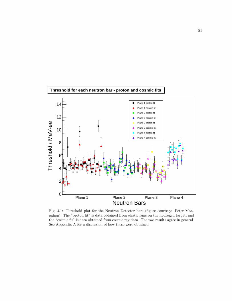
61

Neutron BarsPlane 1 Plane 2 Plane 3 Plane 4

Thr

esho

ld /

MeV

-ee

0

2

4

6

8

10

12

14

Threshold for each neutron bar - proton and cosmic fits

Plane 1 proton fit

Plane 1 cosmic fit

Plane 2 proton fit

Plane 2 cosmic fit

Plane 3 proton fit

Plane 3 cosmic fit

Plane 4 proton fit

Plane 4 cosmic fit

Fig. 4.1: Threshold plot for the Neutron Detector bars (figure courtesy: Peter Mon-aghan). The “proton fit” is data obtained from elastic runs on the hydrogen target, andthe “cosmic fit” is data obtained from cosmic ray data. The two results agree in general.See Appendix A for a discussion of how these were obtained

62

All high energy (4.627 GeV) data had the neutron-detector discriminator threshold

at -50 mV. The thresholds in MeVee mentioned above and plotted in Fig. 4.1 belong

to this part of the experimental data. All low energy (2.345 GeV) data on liquid

deuterium target were taken with a -100 mV hardware threshold.

4.2 Efficiency

We used a computer simulation code developed by R.Cecil et al [72] to model

the neutron-detection efficiency of a scintillator bar. Note that the neutron-detection

efficiency from the simulation assumes that the neutron flux is incident on the neu-

tron counter without any attenuation. But in the actual experiment we had various

materials between the target, where the neutrons are produced, and the neutron

detector. Hence we had to consider two things in order to use the simulation code

to get the efficiency: (1) neutron-detection efficiency with no transmittance correc-

tion and (2) the neutron transmittance for the materials present between the target

and the neutron counter. In practice, these two quantities are multiplied together

to give the overall neutron-detection efficiency.

When we ran the Cecil code [72] and considered the output corresponding to

the average thresholds discussed in Sect.4.1, the simulated efficiencies were substan-

tially larger than the measured ones. This is not surprizing, since the discriminator

thresholds do not really correspond to what is in the computer model. The problem

comes from the length of the scintillator bars. The light attenuation length in the

plastic scintillator is on the order of a couple of meters. This means that a small

signal near one end of a bar may produce a signal above threshold at that end, but

not at the other end. No such mechanisim is built in the Cecil code, which assumes

that all events “above threshold” produce recorded events. In practice, the Kent

63

State group has found that a software data replay threshold on the ADC signals,

close to twice the hardware thresholds, is required for measured detection efficiencies

to agree with calculated ones.

When comparing our measured efficiencies from the 2H(e, e′p)n reaction with

those calculated with the Cecil code, we found that good agreement was obtained

when “effective thresholds” were 80% larger than the hardware thresholds, and that

is what we have chosen to use. Thus the effective thresholds are 9.5, 7.9, 7.6, and

12.8 MeVee for planes 1, 2, 3, and 4 of the neutron detector, respectively.

Shown in Fig. 4.2 are typical efficiency plots obtained from the simulation code

for the effective thresholds. What is plotted here is the efficiency of a scintillator

bar versus the kinetic energy of the neutrons. The efficiency indicates how many

neutrons are detected out of the total incident neutron flux on the scintillator bar.

The peak between 40 to 60 MeV for the plots in Fig. 4.2 indicates the onset of

reactions on carbon. Below the peaks n-p elastic scattering dominates the efficiency

while above the peak 12C reaction channels open up and dominate the efficiency.

Note that the code does not care about the history of the neutron flight before it

hits the counter. This means that in order to know the history, for example, what

fraction of the neutrons were removed from the flux due to an absorbing material

present in front of the scintillator bar, one has to know the neutron transmittance

of the absorber as described below.

4.3 Transmittance

Determining how many neutrons are headed towards the neutron detector de-

pends upon what fraction of the neutrons are absorbed or scattered in the material

between the target and the neutron detector. The transmittance (T) of the neutron

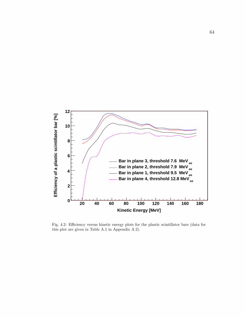
64

Kinetic Energy [MeV]

20 40 60 80 100 120 140 160 180

Eff

icie

ncy

of

a p

last

ic s

cin

tilla

tor

bar

[%

]

0

2

4

6

8

10

12

eeBar in plane 3, threshold 7.6 MeV

eeBar in plane 2, threshold 7.9 MeV

eeBar in plane 1, threshold 9.5 MeV

eeBar in plane 4, threshold 12.8 MeV

Fig. 4.2: Efficiency versus kinetic energy plots for the plastic scintillator bars (data forthis plot are given in Table A.1 in Appendix A.2).

65

flux through a specific material is given by the expression:

T = e−σnL (4.1)

where σ is removal cross section for a neutron in that material, n is number density

of the material, which is N.ρ/A, and L is the thickness of the material. Here N

is Avogadro number, ρ is density of the material, and A is atomic weight of the

material .

The “removal cross section” is the probability that a neutron will be removed

from the flux, i.e., the neutron will not be detected by the neutron detector. Re-

moval cross sections cannot be obtained directly from a cross section table since the

probability for removal depends on the distance of the detector from the target and

the intervening medium which can remove neutrons from the beam. If the medium

is close to the target and far from the detector then the total cross section can

contribute to the removal cross section. By contrast the space between the back

face of lead wall and the front face of neutron detector was only 56 cm and the

neutron detector was sitting 6.04 m from the target. Thus the total cross section

for neutrons in lead wall did not contribute to the removal cross section.

The total cross section is given as the sum of the elastic cross section and

the non-elastic cross section. The non-elastic cross section is not an inelastic cross

section in that it includes all the reaction channels. The elastic cross section peaks

strongly near 0 about the beam direction.

We define the removal cross section as the “non-elastic” cross section plus a

fraction of the elastic cross section appropriate to the location of a specific material

between the target and the detector. If the material is close to the detector (like

the lead wall) then almost all elastically scattered neutrons will strike the detector,

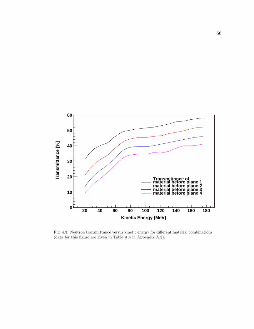
66

Kinetic Energy [MeV]

20 40 60 80 100 120 140 160 180

Tra

nsm

itta

nce

[%

]

0

10

20

30

40

50

60

Transmittance ofmaterial before plane 1material before plane 2material before plane 3material before plane 4

Fig. 4.3: Neutron transmittance versus kinetic energy for different material combinations(data for this figure are given in Table A.4 in Appendix A.2).

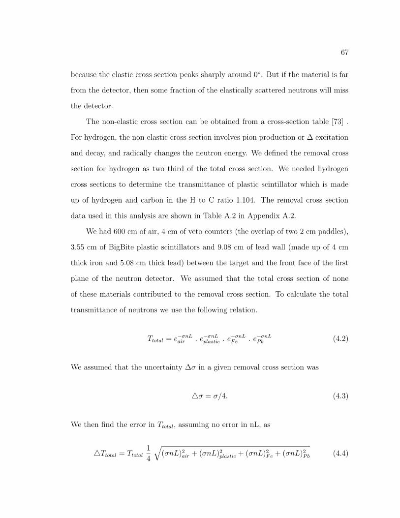
67

because the elastic cross section peaks sharply around 0. But if the material is far

from the detector, then some fraction of the elastically scattered neutrons will miss

the detector.

The non-elastic cross section can be obtained from a cross-section table [73] .

For hydrogen, the non-elastic cross section involves pion production or ∆ excitation

and decay, and radically changes the neutron energy. We defined the removal cross

section for hydrogen as two third of the total cross section. We needed hydrogen

cross sections to determine the transmittance of plastic scintillator which is made

up of hydrogen and carbon in the H to C ratio 1.104. The removal cross section

data used in this analysis are shown in Table A.2 in Appendix A.2.

We had 600 cm of air, 4 cm of veto counters (the overlap of two 2 cm paddles),

3.55 cm of BigBite plastic scintillators and 9.08 cm of lead wall (made up of 4 cm

thick iron and 5.08 cm thick lead) between the target and the front face of the first

plane of the neutron detector. We assumed that the total cross section of none

of these materials contributed to the removal cross section. To calculate the total

transmittance of neutrons we use the following relation.

Ttotal = e−σnLair . e−σnL

plastic . e−σnLFe . e−σnL

Pb (4.2)

We assumed that the uncertainty ∆σ in a given removal cross section was

4σ = σ/4. (4.3)

We then find the error in Ttotal, assuming no error in nL, as

4Ttotal = Ttotal1

4

√(σnL)2

air + (σnL)2plastic + (σnL)2

Fe + (σnL)2Pb (4.4)

68

Shown in Fig. 4.3 are typical plots showing the total transmittance of the various

materials between the target and the front face of different planes of the neutron

detector. The error in transmittance is about ± 5% due to an uncertainty of ±25%

[74] in the removal cross sections.

4.4 Detection Efficiency

We define a product of Transmittance (T ) and the calculated (Monte-Carlo

code [72]) efficiency (εb) of a scintillator bar in a plane of the neutron detector as

the neutron-detection efficiency (εp) for that plane :

εp = εb T, (4.5)

with uncertainty

4εp = εp .

√(4εb

εb

)2 + (4TT

)2. (4.6)

When we add this quantity for all four planes, this will be the neutron-detection

efficiency (ε) for the entire neutron detector:

ε = εp1 + εp2 + εp3 + εp4 (4.7)

with uncertainty

4ε =√ε2

p1 + ε2p2 + ε2

p3 + ε2p4 (4.8)

Shown in Fig. 4.4 as a green curve is detection efficiency of the neutron detector

as a function of neutron kinetic energy. The other curves are the efficiencies for the

individual planes. Data for this figure are presented in Table A.5 in Appendix A.2.

The procedure for calculation of detection efficiency as shown in Fig. 4.4 is the

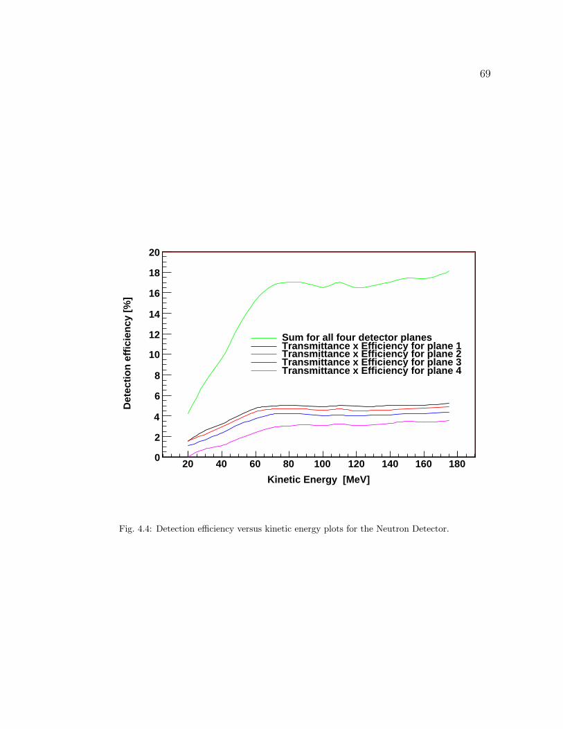
69

Kinetic Energy [MeV]

20 40 60 80 100 120 140 160 180

Det

ecti

on

eff

icie

ncy

[%

]

0

2

4

6

8

10

12

14

16

18

20

Sum for all four detector planesTransmittance x Efficiency for plane 1Transmittance x Efficiency for plane 2Transmittance x Efficiency for plane 3Transmittance x Efficiency for plane 4

Fig. 4.4: Detection efficiency versus kinetic energy plots for the Neutron Detector.

70

following.

1. Plane 1: Product of efficiency of one bar in plane 1 and the transmittance of air,

lead wall and plastic of thickness 7.55 cm (plastic from the BigBite bars + veto

paddles). The veto thickness is taken as 4 cm for this purpose due to the overlap

of two veto paddles, each 2 cm thick, in the middle.

2. Plane 2: Product of efficiency of one bar in plane 2 and the transmittance of air,

lead wall and plastic of thickness 17.55 cm (plastic from the BigBite bars + veto

paddles + a bar in plane 1).

3. Plane 3: Product of efficiency of one bar in plane 3 and the transmittance of air,

lead wall and plastic of thickness 27.55 cm (plastic from the BigBite bars + veto

paddles + a bar in plane 1+ a bar in plane 2).

4. Plane 4: Product of efficiency of one bar in plane 4 and the transmittance of air,

lead wall and plastic of thickness 37.55 cm (plastic from the BigBite bars + veto

paddles + a bar in plane 1+ a bar in plane 2 + a bar in plane 3).

The neutron-detection efficiency for the neutron detector is the sum of the values

obtained in the four steps mentioned above.

4.5 Conclusion

Shown in Fig. 4.5 are the data points for the measured efficiency plotted with the

smooth curves for the simulated efficiency calculated for the “effective” thresholds.

The data for these plots are given in Table A.6 in Appendix A.2. The blue data

points, and the green data points were obtained from the 2-pass (2.345 GeV), and

4-pass (4.6275 GeV) liquid deuterium runs, respectively. Similarly the blue, and the

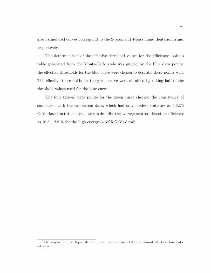
71

green simulated curves correspond to the 2-pass, and 4-pass liquid deuterium runs,

respectively.

The determination of the effective threshold values for the efficiency look-up

table generated from the Monte-Carlo code was guided by the blue data points:

the effective thresholds for the blue curve were chosen to describe these points well.

The effective theresholds for the green curve were obtained by taking half of the

threshold values used for the blue curve.

The four (green) data points for the green curve checked the consistency of

simulation with the calibration data, which had only modest statistics at 4.6275

GeV. Based on this analysis, we can describe the average neutron-detection efficiency

as 16.5± 2.8 % for the high energy (4.6275 GeV) data3.

3The 4-pass data on liquid deuterium and carbon were taken at almost identical kinematicsettings.

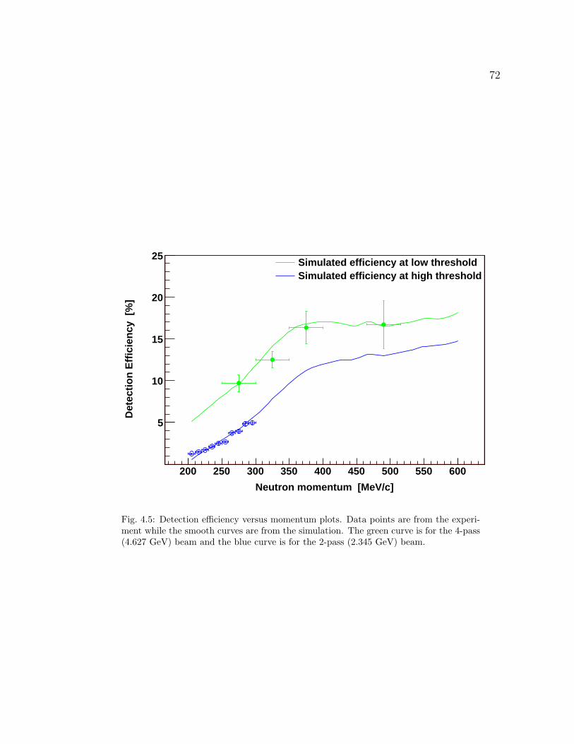
72

Neutron momentum [MeV/c]

200 250 300 350 400 450 500 550 600

Det

ecti

on

Eff

icie

ncy

[%

]

5

10

15

20

25Simulated efficiency at low thresholdSimulated efficiency at high threshold

Fig. 4.5: Detection efficiency versus momentum plots. Data points are from the experi-ment while the smooth curves are from the simulation. The green curve is for the 4-pass(4.627 GeV) beam and the blue curve is for the 2-pass (2.345 GeV) beam.

Chapter 5

Data Analysis-I: The HRSs and BigBite

In this and the next chapter we describe the data analysis methods used in

the present work. The data replay code used in this analysis was the C++-based

Hall A analyzer code [75] (henceforth called analyzer) which was based on CERN’s

ROOT-package [76]. We introduced the BigBite library into the analyzer in order

to incorporate newly added detectors such as the BigBite detector and the neutron

detector for this experiment.

In the HRSs, the particle tracks were measured in the focal plane. These

particle trajectories were traced back to the target to obtain the interaction vertex

(θtgt, φtgt, ytgt, δp/p) through the use of the VDC matrix elements incorporated in

database files of the analyzer. All physical quantities were described in terms of

the laboratory coordinate system.

5.1 Particle Identification in the HRSs

5.1.1 The Left High-Resolution Spectrometer (HRSL)

The electron signal was very clean in the HRSL. Only a coincidence time cut

and a spectrometer acceptance cut were required to identify electrons cleanly. For a

simple cross check, we used the pion rejector to reject pions and the gas Cherenkov

detector to identify electrons. The cuts for these detectors were not used for the

present analysis because they did not change the strength of the signal or back-

ground.

73

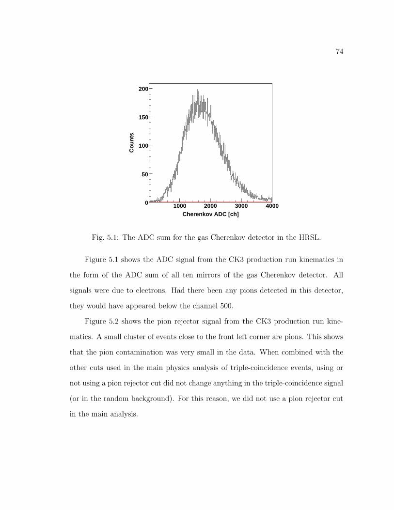
74

Cherenkov ADC [ch]1000 2000 3000 4000

Co

un

ts

0

50

100

150

200

Fig. 5.1: The ADC sum for the gas Cherenkov detector in the HRSL.

Figure 5.1 shows the ADC signal from the CK3 production run kinematics in

the form of the ADC sum of all ten mirrors of the gas Cherenkov detector. All

signals were due to electrons. Had there been any pions detected in this detector,

they would have appeared below the channel 500.

Figure 5.2 shows the pion rejector signal from the CK3 production run kine-

matics. A small cluster of events close to the front left corner are pions. This shows

that the pion contamination was very small in the data. When combined with the

other cuts used in the main physics analysis of triple-coincidence events, using or

not using a pion rejector cut did not change anything in the triple-coincidence signal

(or in the random background). For this reason, we did not use a pion rejector cut

in the main analysis.

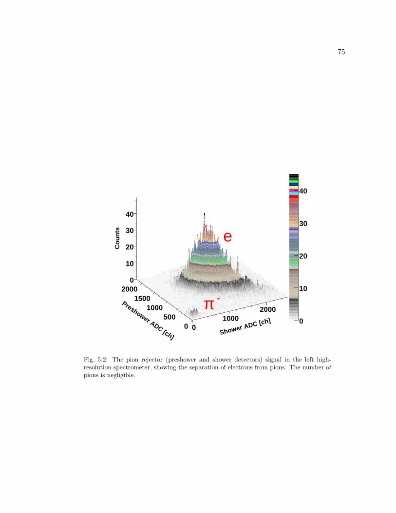
75

Shower ADC [ch]0

10002000

Preshower ADC [ch]

0500

10001500

2000

Co

un

ts

0

10

20

30

40

Co

un

ts0

10

20

30

40

e

- π

Fig. 5.2: The pion rejector (preshower and shower detectors) signal in the left high-resolution spectrometer, showing the separation of electrons from pions. The number ofpions is negligible.

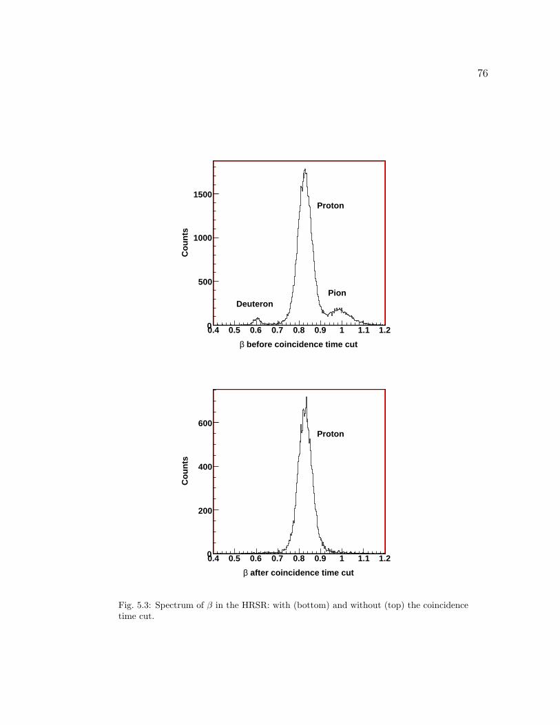
76

before coincidence time cutβ

0.4 0.5 0.6 0.7 0.8 0.9 1 1.1 1.2

Co

un

ts

0

500

1000

1500

Deuteron

Proton

Pion

after coincidence time cutβ

0.4 0.5 0.6 0.7 0.8 0.9 1 1.1 1.2

Co

un

ts

0

200

400

600Proton

Fig. 5.3: Spectrum of β in the HRSR: with (bottom) and without (top) the coincidencetime cut.

77

The Right High Resolution Spectrometer (HRSR)

The HRSR did not have any dedicated particle-identification detectors, so we

had to identify protons using the time-of-filght between the two scintillator planes

(S1 and S2). The time-of-flight was converted to β, the speed of a particle in

units of c, the speed of light. As seen on the top part of Fig. 5.3, signals due to

deuterons, protons and pions are clearly evident. A clean proton signal was obtained

after applying the coincidence time cut (Sect.5.2) which removed the deuterons and

pions (see the bottom part of Fig. 5.3). Thus after using the coincidence-time cut

we did not have to use a β-cut in the physics anaysis. The β plot in Fig. 5.3 is from

the CK3 kinematics. After using the coincidence-time cut, no pion or deuteron

contamination was observed in other kinematics either.

5.2 Coincidence Time

The time-of-flight difference for coincident particles in the HRSL and the HRSR

is called the coincidence time. A real coincidence event involves two particles emerg-

ing from the target at the same instant, thus producing a narrow peak in the time-

of-flight spectrum (see Fig. 5.4). An accidental coincidence event is caused by two

uncorrelated single-arm events which fall within the coincidence timing window con-

tributing to the continuous flat background in the time-of-flight spectrum in Fig. 5.4.

The coincidence time for double-coincidence A(e, e′p) events is the main basis

of the analysis of the triple-coincidence A(e, e′pn) reaction. For this reason we paid

special attention to calibrating the timing of the scintillator paddles of the two

scintillator planes in each HRS to get as narrow a coincidence time peak as possible.

The optimization tools for the HRS coincidence time have been well established [77]

due to the completion of numerous coincidence experiments in Hall A.

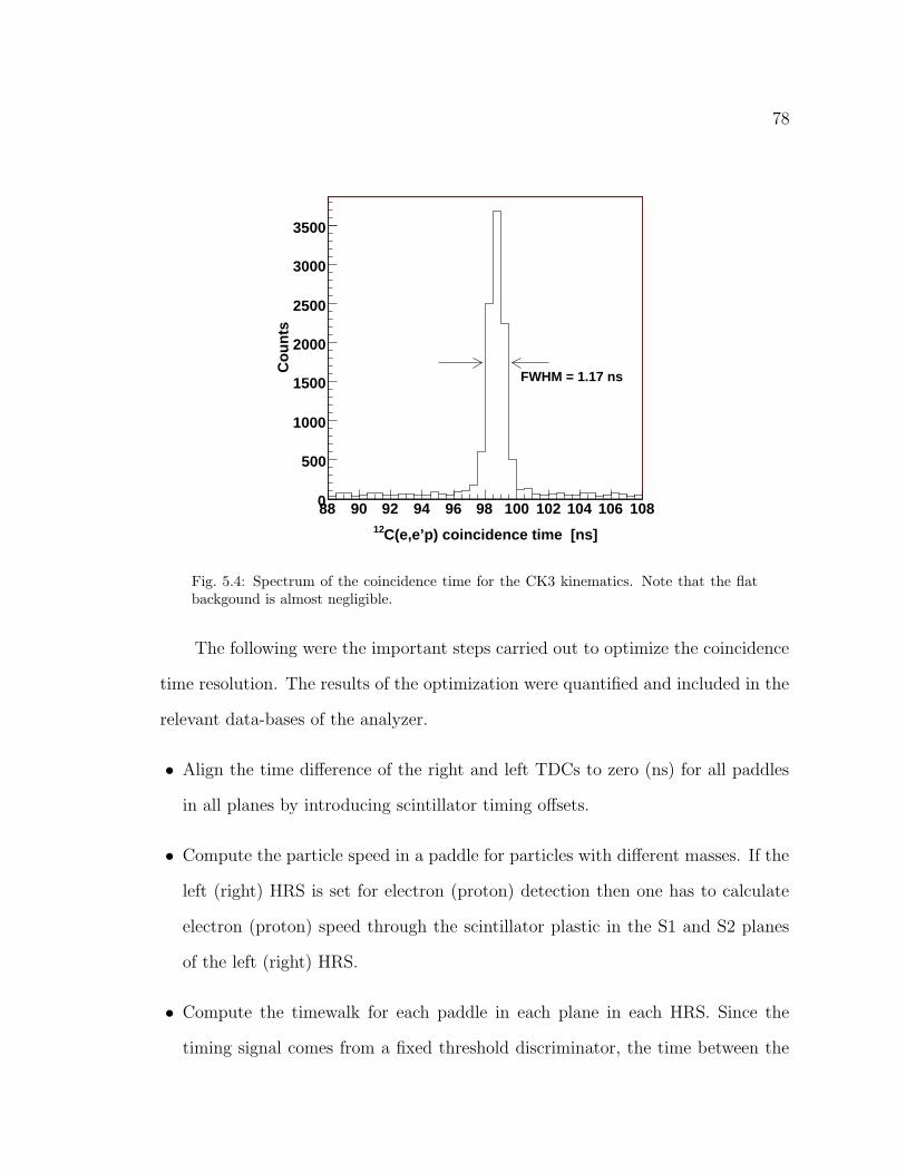
78

C(e,e’p) coincidence time [ns]12

88 90 92 94 96 98 100 102 104 106 108

Co

un

ts

0

500

1000

1500

2000

2500

3000

3500

FWHM = 1.17 ns

Fig. 5.4: Spectrum of the coincidence time for the CK3 kinematics. Note that the flatbackgound is almost negligible.

The following were the important steps carried out to optimize the coincidence

time resolution. The results of the optimization were quantified and included in the

relevant data-bases of the analyzer.

• Align the time difference of the right and left TDCs to zero (ns) for all paddles

in all planes by introducing scintillator timing offsets.

• Compute the particle speed in a paddle for particles with different masses. If the

left (right) HRS is set for electron (proton) detection then one has to calculate

electron (proton) speed through the scintillator plastic in the S1 and S2 planes

of the left (right) HRS.

• Compute the timewalk for each paddle in each plane in each HRS. Since the

timing signal comes from a fixed threshold discriminator, the time between the

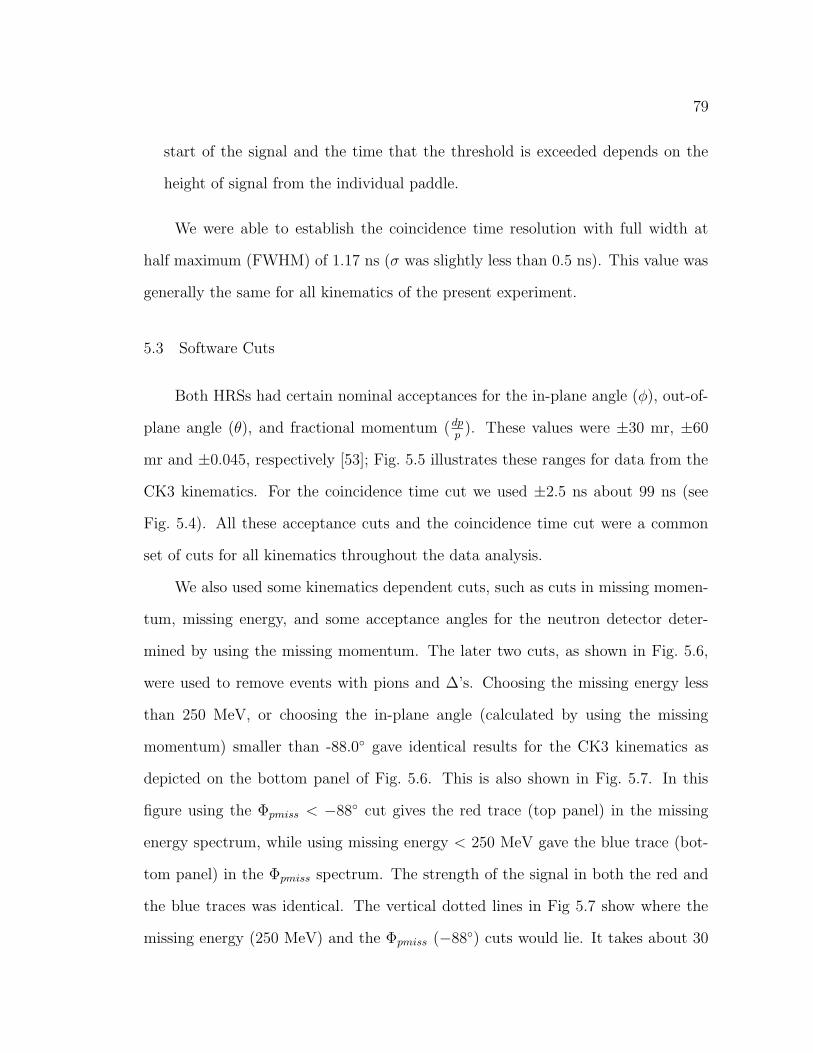
79

start of the signal and the time that the threshold is exceeded depends on the

height of signal from the individual paddle.

We were able to establish the coincidence time resolution with full width at

half maximum (FWHM) of 1.17 ns (σ was slightly less than 0.5 ns). This value was

generally the same for all kinematics of the present experiment.

5.3 Software Cuts

Both HRSs had certain nominal acceptances for the in-plane angle (φ), out-of-

plane angle (θ), and fractional momentum ( dpp). These values were ±30 mr, ±60

mr and ±0.045, respectively [53]; Fig. 5.5 illustrates these ranges for data from the

CK3 kinematics. For the coincidence time cut we used ±2.5 ns about 99 ns (see

Fig. 5.4). All these acceptance cuts and the coincidence time cut were a common

set of cuts for all kinematics throughout the data analysis.

We also used some kinematics dependent cuts, such as cuts in missing momen-

tum, missing energy, and some acceptance angles for the neutron detector deter-

mined by using the missing momentum. The later two cuts, as shown in Fig. 5.6,

were used to remove events with pions and ∆’s. Choosing the missing energy less

than 250 MeV, or choosing the in-plane angle (calculated by using the missing

momentum) smaller than -88.0 gave identical results for the CK3 kinematics as

depicted on the bottom panel of Fig. 5.6. This is also shown in Fig. 5.7. In this

figure using the Φpmiss < −88 cut gives the red trace (top panel) in the missing

energy spectrum, while using missing energy < 250 MeV gave the blue trace (bot-

tom panel) in the Φpmiss spectrum. The strength of the signal in both the red and

the blue traces was identical. The vertical dotted lines in Fig 5.7 show where the

missing energy (250 MeV) and the Φpmiss (−88) cuts would lie. It takes about 30

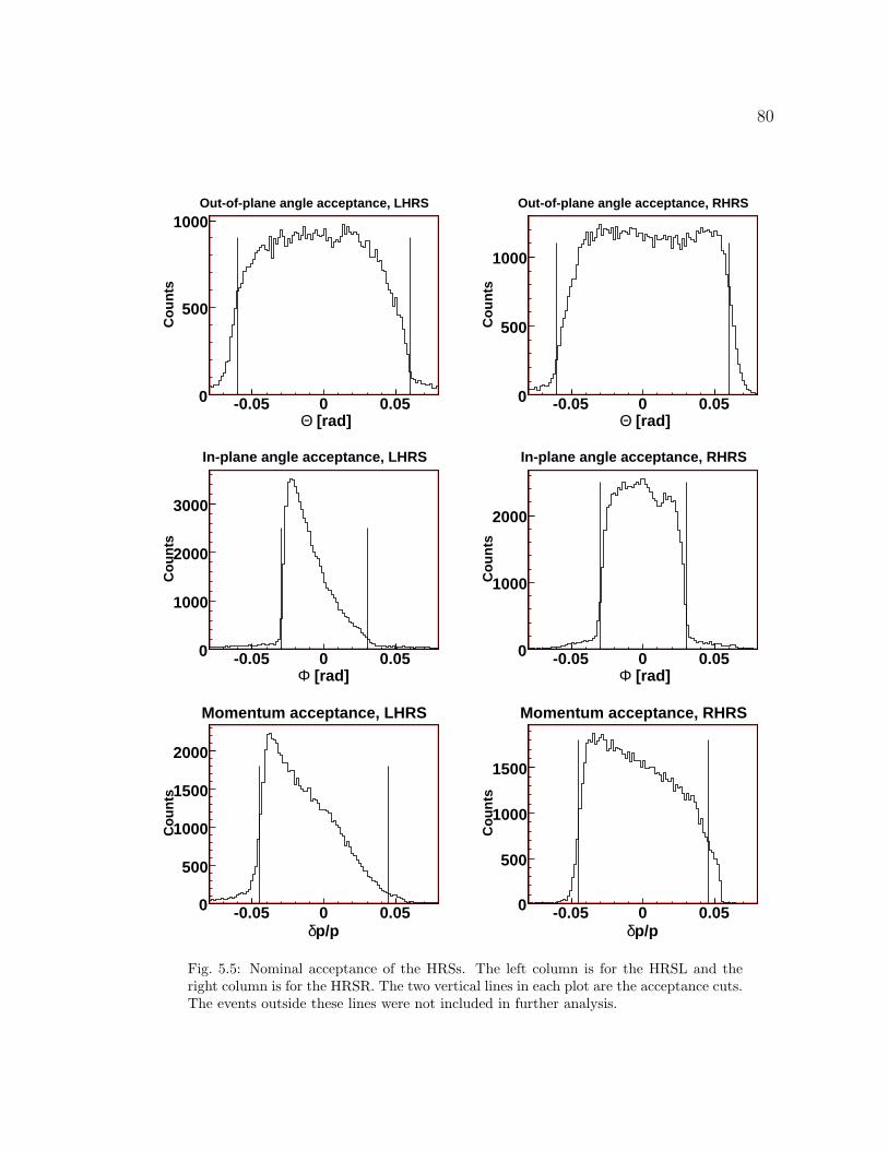
80

[rad]Θ -0.05 0 0.05

Co

un

ts

0

500

1000Out-of-plane angle acceptance, LHRS

[rad]Θ -0.05 0 0.05

Co

un

ts

0

500

1000

Out-of-plane angle acceptance, RHRS

[rad]Φ-0.05 0 0.05

Co

un

ts

0

1000

2000

3000

In-plane angle acceptance, LHRS

[rad]Φ -0.05 0 0.05

Co

un

ts

0

1000

2000

In-plane angle acceptance, RHRS

p/pδ-0.05 0 0.05

Co

un

ts

0

500

1000

1500

2000

Momentum acceptance, LHRS

p/pδ-0.05 0 0.05

Co

un

ts

0

500

1000

1500

Momentum acceptance, RHRS

Fig. 5.5: Nominal acceptance of the HRSs. The left column is for the HRSL and theright column is for the HRSR. The two vertical lines in each plot are the acceptance cuts.The events outside these lines were not included in further analysis.

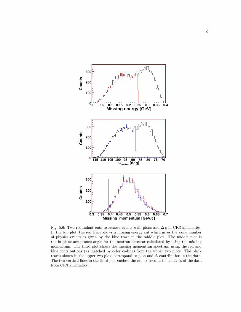
81

Missing energy [GeV]0 0.05 0.1 0.15 0.2 0.25 0.3 0.35 0.4

Co

un

ts

0

100

200

300

[deg]pmissΦ-115 -110 -105 -100 -95 -90 -85 -80 -75 -70

Co

un

ts

0

100

200

300

Missing momentum [GeV/c]0.3 0.35 0.4 0.45 0.5 0.55 0.6 0.65 0.7

Co

un

ts

0

100

200

300

Fig. 5.6: Two redundant cuts to remove events with pions and ∆’s in CK3 kinematics.In the top plot, the red trace shows a missing energy cut which gives the same numberof physics events as given by the blue trace in the middle plot. The middle plot isthe in-plane acceptance angle for the neutron detector calculated by using the missingmomentum. The third plot shows the missing momentum spectrum using the red andblue contributions (as matched by color coding) from the upper two plots. The blacktraces shown in the upper two plots correspond to pion and ∆ contribution in the data.The two vertical lines in the third plot enclose the events used in the analysis of the datafrom CK3 kinematics.

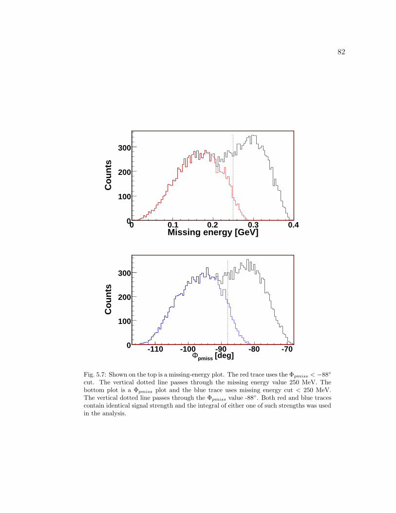
82

Missing energy [GeV]0 0.1 0.2 0.3 0.4

Co

un

ts

0

100

200

300

[deg]pmissΦ-110 -100 -90 -80 -70

Co

un

ts

0

100

200

300

Fig. 5.7: Shown on the top is a missing-energy plot. The red trace uses the Φpmiss < −88

cut. The vertical dotted line passes through the missing energy value 250 MeV. Thebottom plot is a Φpmiss plot and the blue trace uses missing energy cut < 250 MeV.The vertical dotted line passes through the Φpmiss value -88. Both red and blue tracescontain identical signal strength and the integral of either one of such strengths was usedin the analysis.

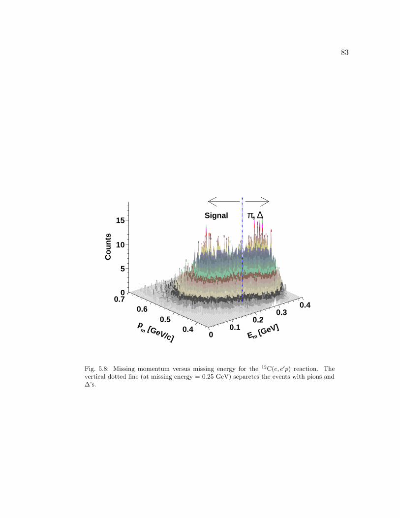
83

[GeV]mE0

0.10.2

0.30.4

[GeV/c]m

p0.4

0.50.6

0.7

Co

un

ts

0

5

10

15Signal ∆, π

Fig. 5.8: Missing momentum versus missing energy for the 12C(e, e′p) reaction. Thevertical dotted line (at missing energy = 0.25 GeV) separetes the events with pions and∆’s.

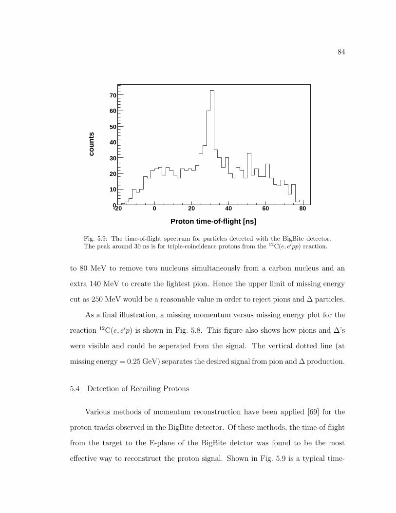
84

Proton time-of-flight [ns]

-20 0 20 40 60 80

cou

nts

0

10

20

30

40

50

60

70

Fig. 5.9: The time-of-flight spectrum for particles detected with the BigBite detector.The peak around 30 ns is for triple-coincidence protons from the 12C(e, e′pp) reaction.

to 80 MeV to remove two nucleons simultaneously from a carbon nucleus and an

extra 140 MeV to create the lightest pion. Hence the upper limit of missing energy

cut as 250 MeV would be a reasonable value in order to reject pions and ∆ particles.

As a final illustration, a missing momentum versus missing energy plot for the

reaction 12C(e, e′p) is shown in Fig. 5.8. This figure also shows how pions and ∆’s

were visible and could be seperated from the signal. The vertical dotted line (at

missing energy = 0.25 GeV) separates the desired signal from pion and ∆ production.

5.4 Detection of Recoiling Protons

Various methods of momentum reconstruction have been applied [69] for the

proton tracks observed in the BigBite detector. Of these methods, the time-of-flight

from the target to the E-plane of the BigBite detctor was found to be the most

effective way to reconstruct the proton signal. Shown in Fig. 5.9 is a typical time-

85

of-flight plot for recoiling protons from the 12C(e, e′pp) reaction . The pronuounced

peak at about 30 ns is due to the protons detected by BigBite in triple-coincidence

in the CK3 kinematics. This shows direct evidence of short-range correlations for

p-p pairs in the reaction 12C(e, e′pp). See [69] for further details about the study of

NN short-range correlations via 12C(e, e′pp) reaction based on experiment E01-015.

Chapter 6

Data Analysis-II: Neutron Analysis

The primary focus of the research for this dissertation is detection of the recoil-

ing neutrons, and the search for NN short-range correlations of such neutrons with

the struck-protons from the 12C(e, e′pn) reaction. In this section we describe how

we calibrated the neutron detector and used it to identify the recoiling neutrons and

measure their momenta.

6.1 Detector Calibration

Since neutrons are neutral particles, there are two aspects to their detection

that require considerable care. First, neutrons are not detected directly; we detect

secondary charged particles from their interactions with the H and C nuclei in the

scintillator bars. This means that the amount of energy deposited in a scintillator

bar, and the scintillation light produced, does not give a direct measure of the

energy (or momentum) of the neutron. Rather, a monoenergetic flux of neutrons

will produce a spectrum of light production, the maximum output corresponding to

when a neutron has transferred all of its energy to a proton. This will happen only in

a head on collision (180 scattering in the center-of-mass system) with the proton in

an 1H atom. The fraction of the light production spectrum that we capture depends

on the minimum light output that our electronics or software will accept from the

phototubes (PMTs). This fraction in turn is reflected directly in the detection

efficiency of a scintillator bar. Therefore, determination of the efficiency is essential

to obtaining meaningful physics results.

86

87

Second, we use plastic scintillator for neutron detectors because the time scale

of the scintillation-light production, on the order of 1 ns, allows us to determine the

time-of-flight (TOF) of a neutron from the target to the detector, and hence the

velocity, momentum, and kinetic energy of the neutron. But this “time-of-flight”

technique requires accurate knowledge of the time origin (“time zero”) for the TOF

spectrum. Every cable and every electronics module (even including PMT transit

times) that the signal from a PMT passes through introduces a delay in that signal,

hence accurate determination of “time zero” is essential.

To calibrate “time zero” and the efficiency of the neutron detector, we utilized

what is called the “associated particle” technique. In this technique, kinematics

dictate that for every particle detected in a primary detector (the HRSs for this

experiment) there must be, a priori, a particle passing through the neutron detector.

We used two reactions in this manner to calibrate the neutron detector: 1H(e, e′)p

(e-p elastic scattering), and the 2H(e, e′p)n reaction. The following sections describe

how we used these two reactions to calibrate the neutron detector. This involved

determining the gains and relative timing of the 176 PMTs for the 88 scintillator

bars.

6.1.1 TDC Alignment

The most important thing about neutron detection using the time-of-flight

method was to make sure that each scintillator bar in the neutron detector had

TDC-signals from both PMTs. To ensure this, we took a few 1H(e, e′)p elastic-

hydrogen runs (LH kinematics) making sure that the neutron detector was fully

illuminated by the recoiling protons; the scattered electrons went to HRSL. Using

data from such runs, we aligned the TDC spectra for each PMT by introducing an

offset in the raw TDC value, these offsets were placed in the data base of the analysis

88

code. The accuracy of the alignment of individual TDCs was not important, since

the time-of-flight measurement of the neutrons was not directly related to these off-

sets. The reason is that the sum of left and right TDCs went into the time-of-flight

expression. We had also to align the later quantity independent of the individual

TDC alignment. Hence we alligned each TDC to appear in a small time window

of a few nanoseconds. As an example, Fig. 6.1 shows the result of such alignment

for the right TDCs of plane four (all other planes show the similar result); all TDC

spectra are confined to a window of about 60 channels which corresponds to a time

window of 30 ns (a channel was equal to 0.5 ns for the neutron detector TDCs).

6.1.2 Bar-Length Alignment

The difference between the left and right TDCs is related to the length of a

scintillator bar (the y-position in a bar). Each bar in the neutron detector was one

meter long. The purpose1 of the alignment was to observe the y-position as one meter

by introducing appropriate offsets and scale parameters to the TDC difference of the

left and right PMTs, and to place all histograms in the same position (preferably a

zero position). These offsets and scale parameters were then recorded in the data

base of the analysis code.

Ideally the y-position is given [78] as

y =v

2(TL − TR) (6.1)

where v is light speed in the scintillator material and TL (TR) is the left (right) TDC

1We need y-position to calculate the distance between the target and the neutron-hit positionin the scintillator bar. This distance is necessary to reconstruct the neutron momentum from theneutron TOF.

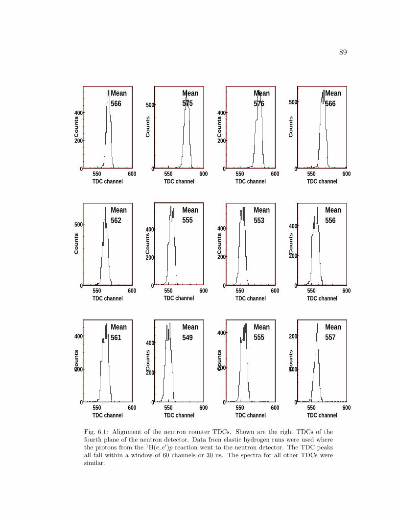
89

TDC channel550 600

Co

un

ts

0

200

400

Mean566

TDC channel550 600

Co

un

ts

0

500

Mean575

TDC channel550 600

Co

un

ts

0

200

400

Mean576

TDC channel550 600

Co

un

ts

0

500Mean566

TDC channel550 600

Co

un

ts

0

500

Mean562

TDC channel550 600

Co

un

ts

0

200

400

Mean555

TDC channel550 600

Co

un

ts

0

200

400

Mean553

TDC channel550 600

Co

un

ts0

200

400

Mean556

TDC channel550 600

Co

un

ts

0

200

400Mean561

TDC channel550 600

Co

un

ts

0

200

400

Mean549

TDC channel550 600

Co

un

ts

0

200

400Mean555

TDC channel550 600

Co

un

ts

0

100

200Mean557

Fig. 6.1: Alignment of the neutron counter TDCs. Shown are the right TDCs of thefourth plane of the neutron detector. Data from elastic hydrogen runs were used wherethe protons from the 1H(e, e′)p reaction went to the neutron detector. The TDC peaksall fall within a window of 60 channels or 30 ns. The spectra for all other TDCs weresimilar.

90

value. But due to various connecting wires and delays this equation turns out to be

y = S(v

2(TL − TR) + C) (6.2)

where C is a position-offset and S is a position-scale parameter. The parameter C

makes (v2(TL − TR) + C) centered at zero and the parameter S either expands or

contracts ( v2(TL −TR)+C) to make the y-position spectrum equal to the bar length

(1.0 m in this case).

When calibrating or measuring the position spectrum, v (the speed of light in

material = c/n) is never the correct value. It would be, if all scintillation photons

travelled straight to the PMT. But most of them are actually reflected at some

point, giving a longer path length. In essence, the product of S and v gives the

speed for a “light pulse” involving many photons, some direct and some reflected.

For y-positon alignment we could use any production runs since the TDC align-

ment had already been done using elastic hydrogen runs. An example of such align-

ment is shown in Fig. 6.2 and it can be observed from the figure that each histogram

is constrained to ± 50 cm, the physical length of the bar.

6.2 Neutron Identification

The pulse-height and timing of a neutron signal in a scintillator bar are not

sufficient to distinguish neutrons from charged particles. Neutrons do not produce

signals in a scintillator themselves; they scatter off of protons or react with a nucleus

yielding energetic protons or light ions. So an event in a scintillator bar can be

identified as a neutron candidate by the absence of any signal in the scintillators

that are between the neutron source (the target) and scintillator bar where the event

occured. For the first plane of scintillator bars, events in the veto layer served to

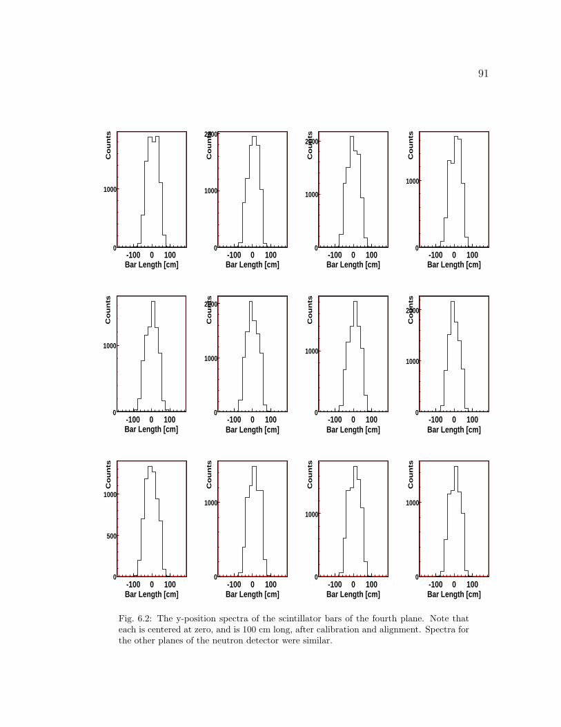
91

Bar Length [cm]-100 0 100

Co

un

ts

0

1000

Bar Length [cm]-100 0 100

Co

un

ts

0

1000

2000

Bar Length [cm]-100 0 100

Co

un

ts

0

1000

2000

Bar Length [cm]-100 0 100

Co

un

ts

0

1000

Bar Length [cm]-100 0 100

Co

un

ts

0

1000

Bar Length [cm]-100 0 100

Co

un

ts

0

1000

2000

Bar Length [cm]-100 0 100

Co

un

ts

0

1000

Bar Length [cm]-100 0 100

Co

un

ts0

1000

2000

Bar Length [cm]-100 0 100

Co

un

ts

0

500

1000

Bar Length [cm]-100 0 100

Co

un

ts

0

1000

Bar Length [cm]-100 0 100

Co

un

ts

0

1000

Bar Length [cm]-100 0 100

Co

un

ts

0

1000

Fig. 6.2: The y-position spectra of the scintillator bars of the fourth plane. Note thateach is centered at zero, and is 100 cm long, after calibration and alignment. Spectra forthe other planes of the neutron detector were similar.

92

identify non-neutron events. In the subsequent planes, the planes of bars closer to

the target constituted the “veto”.

Because of high rates in the scintillator bars and veto paddles, the segmentation

and timing capabilities were used to minimize accidental vetos. For each scintillator

bar, all bars in the next closer plane to the target that shadow some part or all of

the scintillator bar are deemed to be the “blocking bars” for that bar (see Fig. 6.3).

There were two to four blocking bars for a single bar. If an event occurs in one of

these blocking bars at the “same time” as the candidate neutron event, then the

event is vetoed. An event is defined to be at the “same time” as another event if

they occur within ±20 ns of each other.

While photons, being neutral, could also be identified as a neutron candidates,

mis-identification of a photon as a neutron was unlikely in the present set-up. Pho-

tons would typically produce e+-e− showers in the shielding in front of the neutron

detector. If some part of the shower got through the shielding, it would produce

signals in the veto detectors, vetoing any events in the bars. Photons should also

be easily identified as having β = 1 or 1v

=1c

= 3.3 ns/m.

In summary, a neutron was defined as requiring an event in a bar in a plane,

with no events in the two to four contiguous bars in front of it in an adjacent plane,

within a time window of ±20 ns, the reference of the time window being the time

of the candidate neutron event.

6.3 Time-of-Flight

Neutron time-of-flight (TOF) is the time required for the neutron to travel from

the target to the point of neutron detection (about 6 m from the target). This TOF

can be measured for one scintillator bar, for one plane, and for the whole neutron

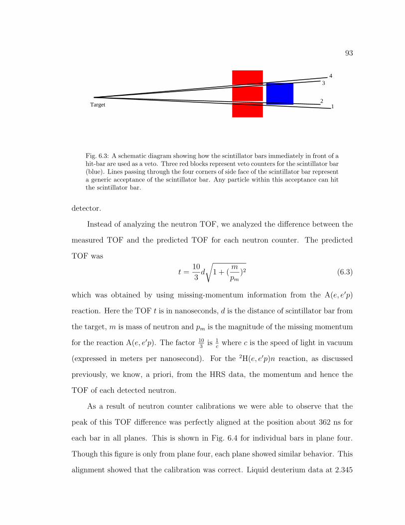
93

12

34

Target

Fig. 6.3: A schematic diagram showing how the scintillator bars immediately in front of ahit-bar are used as a veto. Three red blocks represent veto counters for the scintillator bar(blue). Lines passing through the four corners of side face of the scintillator bar representa generic acceptance of the scintillator bar. Any particle within this acceptance can hitthe scintillator bar.

detector.

Instead of analyzing the neutron TOF, we analyzed the difference between the

measured TOF and the predicted TOF for each neutron counter. The predicted

TOF was

t =10

3d

√1 + (

m

pm

)2 (6.3)

which was obtained by using missing-momentum information from the A(e, e′p)

reaction. Here the TOF t is in nanoseconds, d is the distance of scintillator bar from

the target, m is mass of neutron and pm is the magnitude of the missing momentum

for the reaction A(e, e′p). The factor 103

is 1c

where c is the speed of light in vacuum

(expressed in meters per nanosecond). For the 2H(e, e′p)n reaction, as discussed

previously, we know, a priori, from the HRS data, the momentum and hence the

TOF of each detected neutron.

As a result of neutron counter calibrations we were able to observe that the

peak of this TOF difference was perfectly aligned at the position about 362 ns for

each bar in all planes. This is shown in Fig. 6.4 for individual bars in plane four.

Though this figure is only from plane four, each plane showed similar behavior. This

alignment showed that the calibration was correct. Liquid deuterium data at 2.345

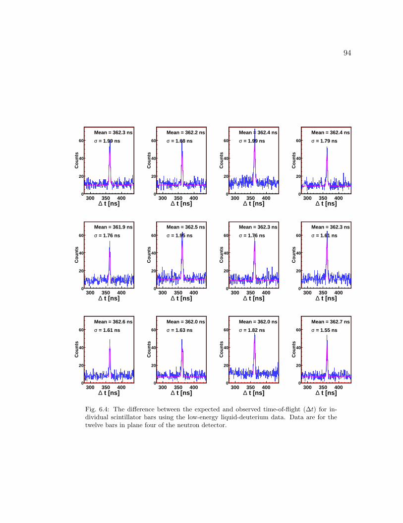
94

t [ns]∆300 350 400

Co

un

ts

0

20

40

60

Mean = 362.3 ns

= 1.99 nsσ

t [ns]∆300 350 400

Co

un

ts

0

20

40

60

Mean = 362.2 ns

= 1.68 nsσ

t [ns]∆300 350 400

Co

un

ts

0

20

40

60

Mean = 362.4 ns

= 1.99 nsσ

t [ns]∆300 350 400

Co

un

ts

0

20

40

60

Mean = 362.4 ns

= 1.79 nsσ

t [ns]∆300 350 400

Co

un

ts

0

20

40

60

Mean = 361.9 ns

= 1.76 nsσ

t [ns]∆300 350 400

Co

un

ts

0

20

40

60

Mean = 362.5 ns

= 1.95 nsσ

t [ns]∆300 350 400

Co

un

ts

0

20

40

60

Mean = 362.3 ns

= 1.76 nsσ

t [ns]∆300 350 400

Co

un

ts0

20

40

60

Mean = 362.3 ns

= 1.61 nsσ

t [ns]∆300 350 400

Co

un

ts

0

20

40

60

Mean = 362.6 ns

= 1.61 nsσ

t [ns]∆300 350 400

Co

un

ts

0

20

40

60

Mean = 362.0 ns

= 1.63 nsσ

t [ns]∆300 350 400

Co

un

ts

0

20

40

60

Mean = 362.0 ns

= 1.82 nsσ

t [ns]∆300 350 400

Co

un

ts

0

20

40

60

Mean = 362.7 ns

= 1.55 nsσ

Fig. 6.4: The difference between the expected and observed time-of-flight (∆t) for in-dividual scintillator bars using the low-energy liquid-deuterium data. Data are for thetwelve bars in plane four of the neutron detector.

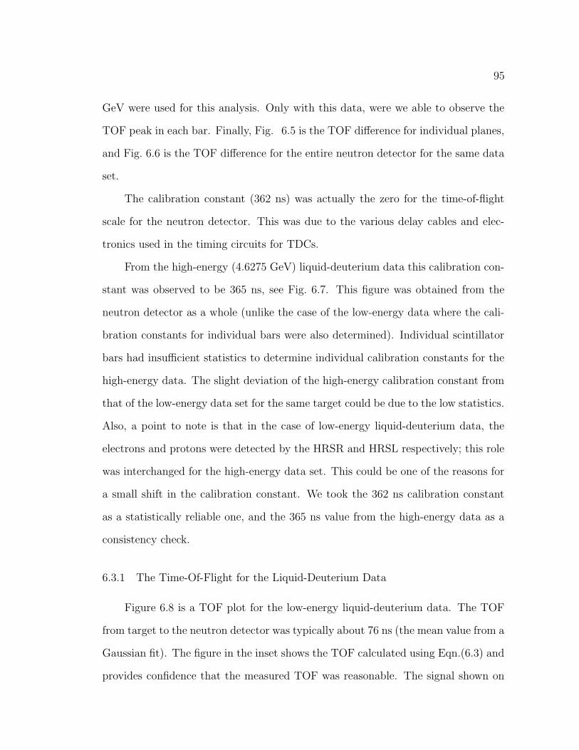
95

GeV were used for this analysis. Only with this data, were we able to observe the

TOF peak in each bar. Finally, Fig. 6.5 is the TOF difference for individual planes,

and Fig. 6.6 is the TOF difference for the entire neutron detector for the same data

set.

The calibration constant (362 ns) was actually the zero for the time-of-flight

scale for the neutron detector. This was due to the various delay cables and elec-

tronics used in the timing circuits for TDCs.

From the high-energy (4.6275 GeV) liquid-deuterium data this calibration con-

stant was observed to be 365 ns, see Fig. 6.7. This figure was obtained from the

neutron detector as a whole (unlike the case of the low-energy data where the cali-

bration constants for individual bars were also determined). Individual scintillator

bars had insufficient statistics to determine individual calibration constants for the

high-energy data. The slight deviation of the high-energy calibration constant from

that of the low-energy data set for the same target could be due to the low statistics.

Also, a point to note is that in the case of low-energy liquid-deuterium data, the

electrons and protons were detected by the HRSR and HRSL respectively; this role

was interchanged for the high-energy data set. This could be one of the reasons for

a small shift in the calibration constant. We took the 362 ns calibration constant

as a statistically reliable one, and the 365 ns value from the high-energy data as a

consistency check.

6.3.1 The Time-Of-Flight for the Liquid-Deuterium Data

Figure 6.8 is a TOF plot for the low-energy liquid-deuterium data. The TOF

from target to the neutron detector was typically about 76 ns (the mean value from a

Gaussian fit). The figure in the inset shows the TOF calculated using Eqn.(6.3) and

provides confidence that the measured TOF was reasonable. The signal shown on

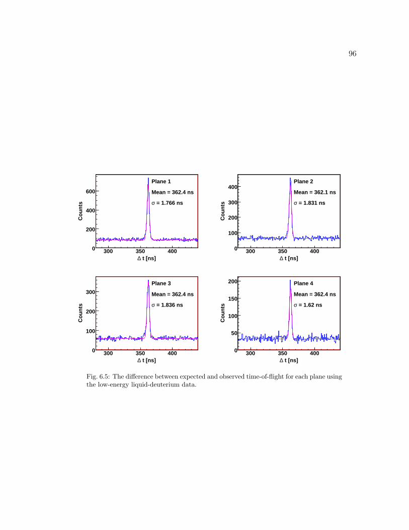
96

t [ns]∆300 350 400

Co

un

ts

0

200

400

600

Plane 1

Mean = 362.4 ns

= 1.766 nsσ

t [ns]∆300 350 400

Co

un

ts

0

100

200

300

400Plane 2

Mean = 362.1 ns

= 1.831 nsσ

t [ns]∆300 350 400

Co

un

ts

0

100

200

300

Plane 3

Mean = 362.4 ns

= 1.836 nsσ

t [ns]∆300 350 400

Co

un

ts

0

50

100

150

200 Plane 4

Mean = 362.4 ns

= 1.62 nsσ

Fig. 6.5: The difference between expected and observed time-of-flight for each plane usingthe low-energy liquid-deuterium data.

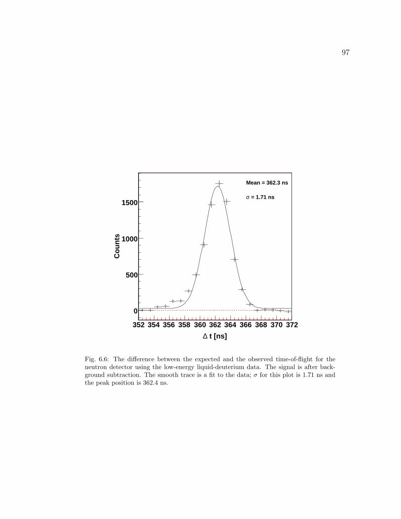
97

t [ns]∆352 354 356 358 360 362 364 366 368 370 372

Co

un

ts

0

500

1000

1500

Mean = 362.3 ns

= 1.71 nsσ

Fig. 6.6: The difference between the expected and the observed time-of-flight for theneutron detector using the low-energy liquid-deuterium data. The signal is after back-ground subtraction. The smooth trace is a fit to the data; σ for this plot is 1.71 ns andthe peak position is 362.4 ns.

98

t [ns]∆350 360 370 380 390

Co

un

ts

0

100

200

t [ns]∆200 300 400 500 600

Co

un

ts

0

100

200

300

400

Fig. 6.7: The difference between the expected and the observed time-of-flight using thehigh-energy liquid-deuterium data at low missing momentum. The smooth trace is afit to the data. The data have been background subtracted. The inset shows the databefore the background subtraction. The peak position is 365 ns.

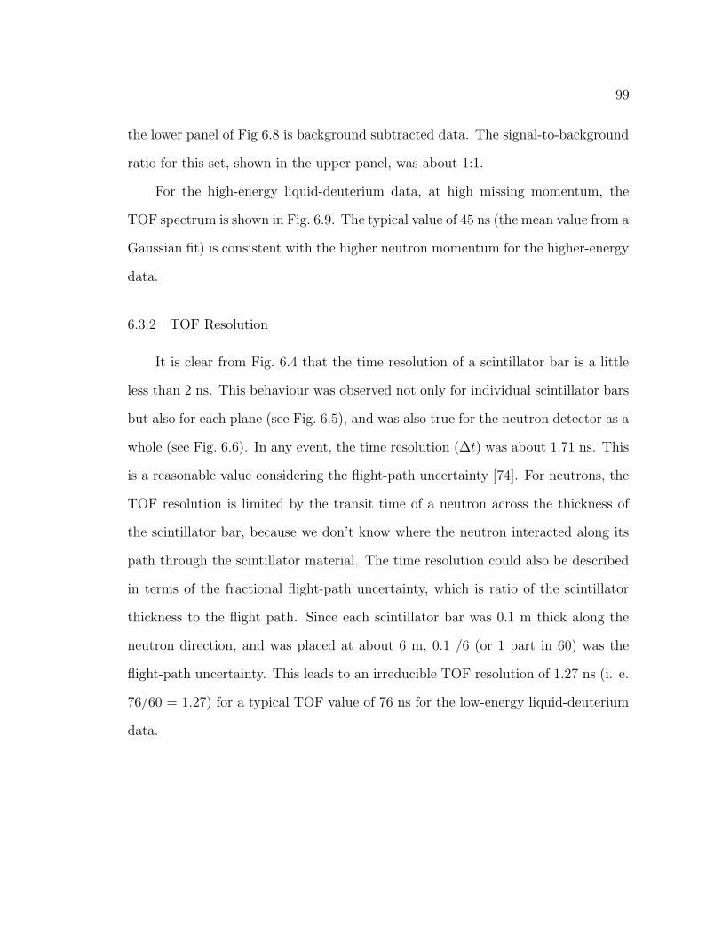
99

the lower panel of Fig 6.8 is background subtracted data. The signal-to-background

ratio for this set, shown in the upper panel, was about 1:1.

For the high-energy liquid-deuterium data, at high missing momentum, the

TOF spectrum is shown in Fig. 6.9. The typical value of 45 ns (the mean value from a

Gaussian fit) is consistent with the higher neutron momentum for the higher-energy

data.

6.3.2 TOF Resolution

It is clear from Fig. 6.4 that the time resolution of a scintillator bar is a little

less than 2 ns. This behaviour was observed not only for individual scintillator bars

but also for each plane (see Fig. 6.5), and was also true for the neutron detector as a

whole (see Fig. 6.6). In any event, the time resolution (∆t) was about 1.71 ns. This

is a reasonable value considering the flight-path uncertainty [74]. For neutrons, the

TOF resolution is limited by the transit time of a neutron across the thickness of

the scintillator bar, because we don’t know where the neutron interacted along its

path through the scintillator material. The time resolution could also be described

in terms of the fractional flight-path uncertainty, which is ratio of the scintillator

thickness to the flight path. Since each scintillator bar was 0.1 m thick along the

neutron direction, and was placed at about 6 m, 0.1 /6 (or 1 part in 60) was the

flight-path uncertainty. This leads to an irreducible TOF resolution of 1.27 ns (i. e.

76/60 = 1.27) for a typical TOF value of 76 ns for the low-energy liquid-deuterium

data.

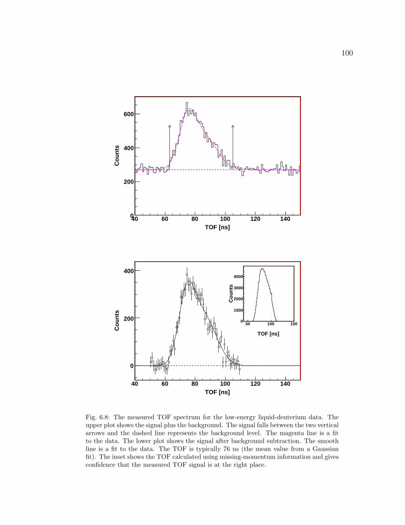
100

TOF [ns]40 60 80 100 120 140

Co

un

ts

0

200

400

600

TOF [ns]40 60 80 100 120 140

Co

un

ts

0

200

400

TOF [ns]

50 100 150

Co

un

ts

0

1000

2000

3000

4000

Fig. 6.8: The measured TOF spectrum for the low-energy liquid-deuterium data. Theupper plot shows the signal plus the background. The signal falls between the two verticalarrows and the dashed line represents the background level. The magenta line is a fitto the data. The lower plot shows the signal after background subtraction. The smoothline is a fit to the data. The TOF is typically 76 ns (the mean value from a Gaussianfit). The inset shows the TOF calculated using missing-momentum information and givesconfidence that the measured TOF signal is at the right place.

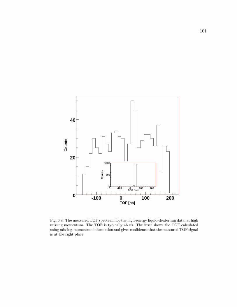
101

TOF [ns]-100 0 100 200

Co

un

ts

0

20

40

TOF [ns]-100 0 100 200

Co

un

ts

0

500

1000

Fig. 6.9: The measured TOF spectrum for the high-energy liquid-deuterium data, at highmissing momentum. The TOF is typically 45 ns. The inset shows the TOF calculatedusing missing-momentum information and gives confidence that the measured TOF signalis at the right place.

102

6.4 Momentum Reconstruction

It is useful to construct the momentum of detected neutrons using TOF infor-

mation. Replacing pm in Eqn.6.3 by simply pn, the reconstructed momentum of the

neutron, we get the following relation:

pn =m√

(0.3 td)2 − 1

(6.4)

Figure 6.10 shows this reconstructed momentum from the low-energy (2.345 GeV)

liquid-deuterium calibration data. The reconstructed neutron momentum ranged

from 200 to 320 MeV/c for this data set. The events are for the TOF peak (above

the background level) in Fig. 6.8.

6.4.1 Momentum Resolution

The time-of-flight resolution can be used to find the momentum resolution as

follows. The standard expression for β is

β =d

ct=

p

(m2 + p2)1/2(6.5)

where a particle of mass m in GeV/c2 with momentum p in GeV/c travels a distance

d in a time t (also called time-of-flight). From this one can express the time-of-flight

in terms of momentum

t =d(m2 + p2)1/2

cp(6.6)

or momentum in terms of time-of-flight

p =

√md2

c2t2 − d2. (6.7)

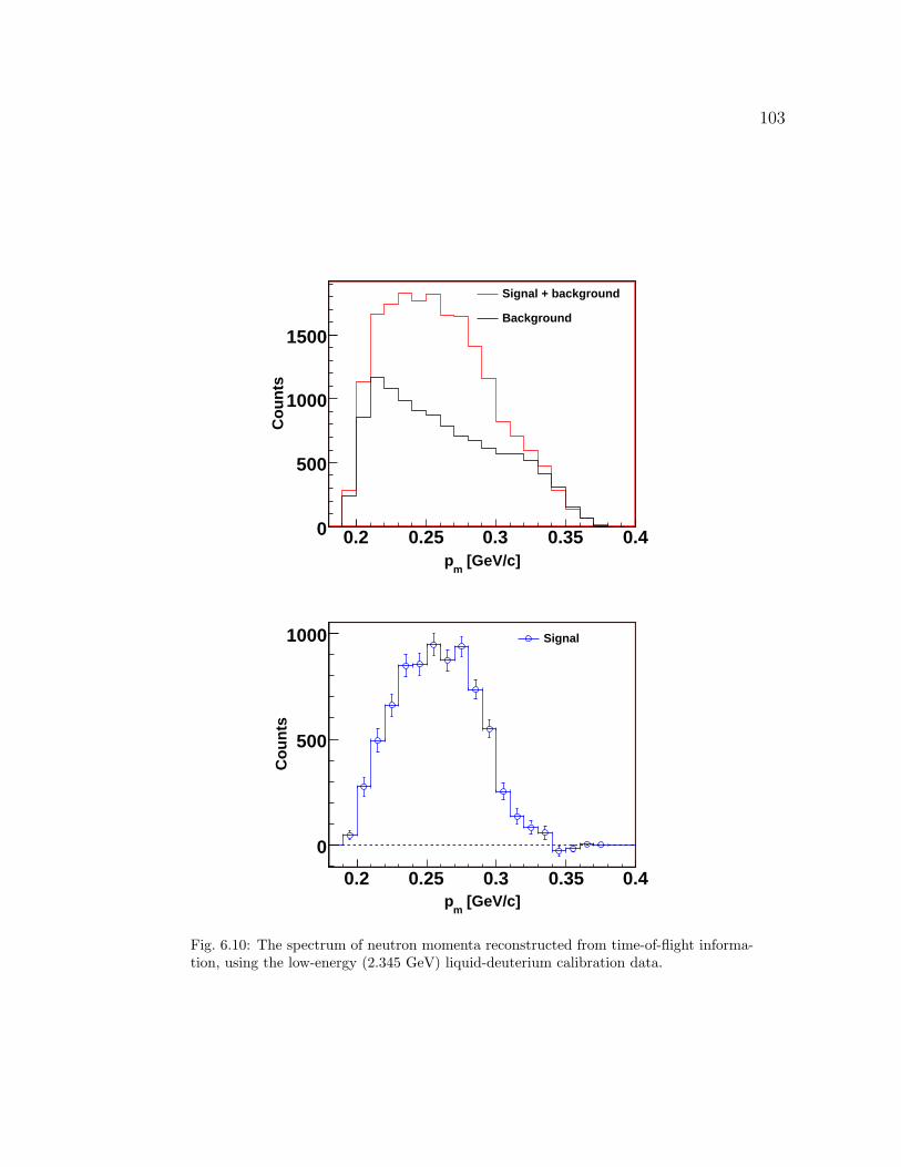
103

[GeV/c]m

p0.2 0.25 0.3 0.35 0.4

Co

un

ts

0

500

1000

1500

Signal + background

Background

[GeV/c]m

p0.2 0.25 0.3 0.35 0.4

Co

un

ts

0

500

1000 Signal

Fig. 6.10: The spectrum of neutron momenta reconstructed from time-of-flight informa-tion, using the low-energy (2.345 GeV) liquid-deuterium calibration data.

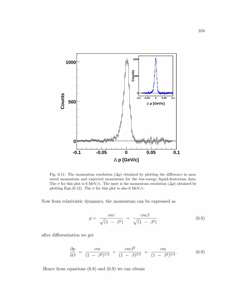
104

p [GeV/c]∆-0.1 -0.05 0 0.05 0.1

Co

un

ts

0

500

1000

p [GeV/c]∆

-0.1 -0.05 0 0.05 0.1

Co

un

ts

0

500

1000

Fig. 6.11: The momentum resolution (∆p) obtained by plotting the difference in mea-sured momentum and expected momentum for the low-energy liquid-deuterium data.The σ for this plot is 6 MeV/c. The inset is the momentum resolution (∆p) obtained byplotting Eqn.(6.12). The σ for this plot is also 6 MeV/c.

Now from relativistic dynamics, the momentum can be expressed as

p =mv√

(1 − β2)=

cmβ√(1 − β2)

(6.8)

after differentiation we get

∂p

∂β=

cm

(1 − β2)1/2+

cmβ2

(1 − β)3/2=

cm

(1 − β2)3/2. (6.9)

Hence from equations (6.8) and (6.9) we can obtain

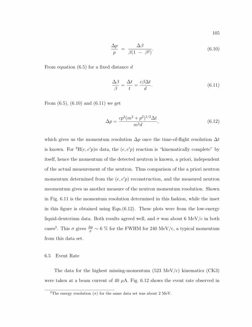
105

∆p

p=

∆β

β(1 − β2). (6.10)

From equation (6.5) for a fixed distance d

∆β

β=

∆t

t=cβ∆t

d. (6.11)

From (6.5), (6.10) and (6.11) we get

∆p =cp2(m2 + p2)1/2∆t

m2d, (6.12)

which gives us the momentum resolution ∆p once the time-of-flight resolution ∆t

is known. For 2H(e, e′p)n data, the (e, e′p) reaction is “kinematically complete” by

itself, hence the momentum of the detected neutron is known, a priori, independent

of the actual measurement of the neutron. Thus comparison of the a priori neutron

momentum determined from the (e, e′p) reconstruction, and the measured neutron

meomentum gives us another measure of the neutron momentum resolution. Shown

in Fig. 6.11 is the momentum resolution determined in this fashion, while the inset

in this figure is obtained using Eqn.(6.12). These plots were from the low-energy

liquid-deuterium data. Both results agreed well, and σ was about 6 MeV/c in both

cases2. This σ gives ∆pp

∼ 6 % for the FWHM for 240 MeV/c, a typical momentum

from this data set.

6.5 Event Rate

The data for the highest missing-momentum (523 MeV/c) kinematics (CK3)

were taken at a beam current of 40 µA. Fig. 6.12 shows the event rate observed in

2The energy resolution (σ) for the same data set was about 2 MeV.

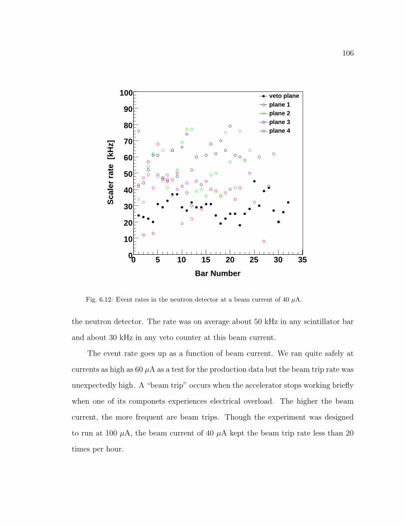
106

Bar Number

0 5 10 15 20 25 30 35

Sca

ler

rate

[kH

z]

0

10

20

30

40

50

60

70

80

90

100 veto planeplane 1plane 2plane 3plane 4

Fig. 6.12: Event rates in the neutron detector at a beam current of 40 µA.

the neutron detector. The rate was on average about 50 kHz in any scintillator bar

and about 30 kHz in any veto counter at this beam current.

The event rate goes up as a function of beam current. We ran quite safely at

currents as high as 60 µA as a test for the production data but the beam trip rate was

unexpectedly high. A “beam trip” occurs when the accelerator stops working briefly

when one of its componets experiences electrical overload. The higher the beam

current, the more frequent are beam trips. Though the experiment was designed

to run at 100 µA, the beam current of 40 µA kept the beam trip rate less than 20

times per hour.

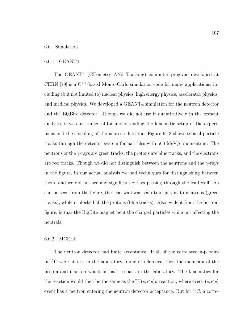
107

6.6 Simulation

6.6.1 GEANT4

The GEANT4 (GEometry ANd Tracking) computer program developed at

CERN [79] is a C++-based Monte-Carlo simulation code for many applications, in-

cluding (but not limited to) nuclear physics, high energy physics, accelerator physics,

and medical physics. We developed a GEANT4 simulation for the neutron detector

and the BigBite detector. Though we did not use it quantitatively in the present

analysis, it was instrumental for understanding the kinematic setup of the experi-

ment and the shielding of the neutron detector. Figure 6.13 shows typical particle

tracks through the detector system for particles with 500 MeV/c momentum. The

neutrons or the γ-rays are green tracks, the protons are blue tracks, and the electrons

are red tracks. Though we did not distinguish between the neutrons and the γ-rays

in the figure, in our actual analysis we had techniques for distinguishing between

them, and we did not see any significant γ-rays passing through the lead wall. As

can be seen from the figure, the lead wall was semi-transperant to neutrons (green

tracks), while it blocked all the protons (blue tracks). Also evident from the bottom

figure, is that the BigBite magnet bent the charged particles while not affecting the

neutrals.

6.6.2 MCEEP

The neutron detector had finite acceptance. If all of the correlated n-p pairs

in 12C were at rest in the laboratory frame of reference, then the momenta of the

proton and neutron would be back-to-back in the laboratory. The kinematics for

the reaction would then be the same as the 2H(e, e′p)n reaction, where every (e, e′p)

event has a neutron entering the neutron detector acceptance. But for 12C, a corre-

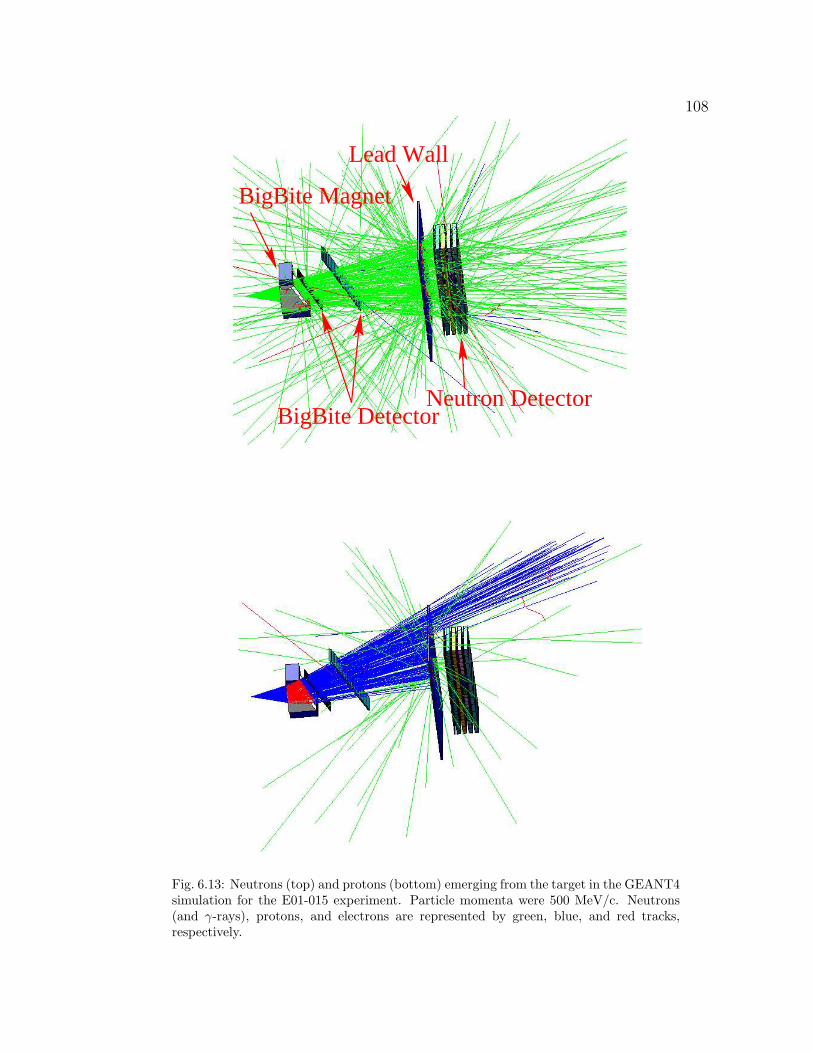
108

BigBite Magnet

BigBite DetectorNeutron Detector

Lead Wall

Fig. 6.13: Neutrons (top) and protons (bottom) emerging from the target in the GEANT4simulation for the E01-015 experiment. Particle momenta were 500 MeV/c. Neutrons(and γ-rays), protons, and electrons are represented by green, blue, and red tracks,respectively.

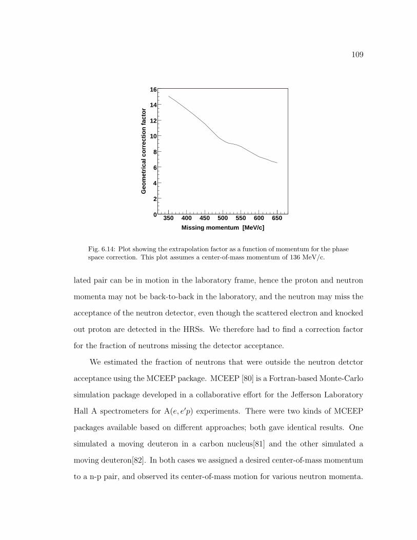
109

Missing momentum [MeV/c]

350 400 450 500 550 600 650

Geo

met

rica

l co

rrec

tio

n f

acto

r

0

2

4

6

8

10

12

14

16

Fig. 6.14: Plot showing the extrapolation factor as a function of momentum for the phasespace correction. This plot assumes a center-of-mass momentum of 136 MeV/c.

lated pair can be in motion in the laboratory frame, hence the proton and neutron

momenta may not be back-to-back in the laboratory, and the neutron may miss the

acceptance of the neutron detector, even though the scattered electron and knocked

out proton are detected in the HRSs. We therefore had to find a correction factor

for the fraction of neutrons missing the detector acceptance.

We estimated the fraction of neutrons that were outside the neutron detctor

acceptance using the MCEEP package. MCEEP [80] is a Fortran-based Monte-Carlo

simulation package developed in a collaborative effort for the Jefferson Laboratory

Hall A spectrometers for A(e, e′p) experiments. There were two kinds of MCEEP

packages available based on different approaches; both gave identical results. One

simulated a moving deuteron in a carbon nucleus[81] and the other simulated a

moving deuteron[82]. In both cases we assigned a desired center-of-mass momentum

to a n-p pair, and observed its center-of-mass motion for various neutron momenta.

110

The geometrical correction factor is the ratio of triple-coincidence neutrons without

and with the neutron detector acceptance.

Figure 6.14 shows the extrapolation (geometrical correction) factor as a function

of missing momentum that we had to use to convert the raw cross section ratio of

12C(e, e′pn)/12C(e, e′p) events to the corrected cross section ratio. For example at

510 MeV/c we had to multiply the raw cross section ratio of 12C(e, e′pn)/12C(e, e′p)

events by a factor of 9.0 in order to get the corrected cross section ratio3. The plot

is for a center-of-mass-momentum of 136 MeV/c for the n-p pair [83].

3The uncertainty in the geometrical correction factor is about 2%.

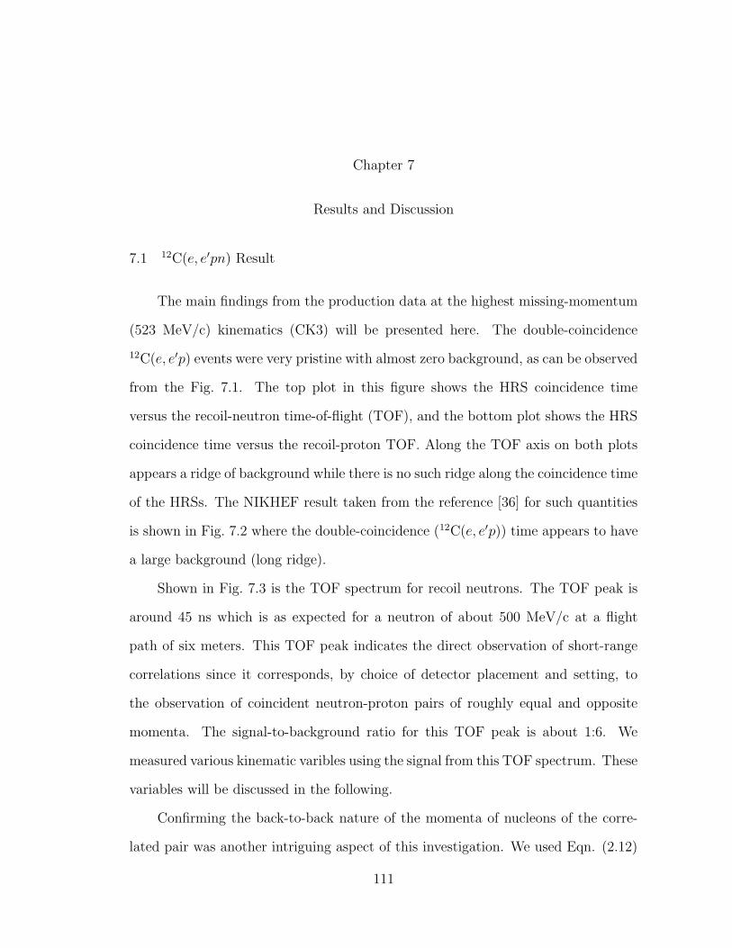
Chapter 7

Results and Discussion

7.1 12C(e, e′pn) Result

The main findings from the production data at the highest missing-momentum

(523 MeV/c) kinematics (CK3) will be presented here. The double-coincidence

12C(e, e′p) events were very pristine with almost zero background, as can be observed

from the Fig. 7.1. The top plot in this figure shows the HRS coincidence time

versus the recoil-neutron time-of-flight (TOF), and the bottom plot shows the HRS

coincidence time versus the recoil-proton TOF. Along the TOF axis on both plots

appears a ridge of background while there is no such ridge along the coincidence time

of the HRSs. The NIKHEF result taken from the reference [36] for such quantities

is shown in Fig. 7.2 where the double-coincidence (12C(e, e′p)) time appears to have

a large background (long ridge).

Shown in Fig. 7.3 is the TOF spectrum for recoil neutrons. The TOF peak is

around 45 ns which is as expected for a neutron of about 500 MeV/c at a flight

path of six meters. This TOF peak indicates the direct observation of short-range

correlations since it corresponds, by choice of detector placement and setting, to

the observation of coincident neutron-proton pairs of roughly equal and opposite

momenta. The signal-to-background ratio for this TOF peak is about 1:6. We

measured various kinematic varibles using the signal from this TOF spectrum. These

variables will be discussed in the following.

Confirming the back-to-back nature of the momenta of nucleons of the corre-

lated pair was another intriguing aspect of this investigation. We used Eqn. (2.12)

111

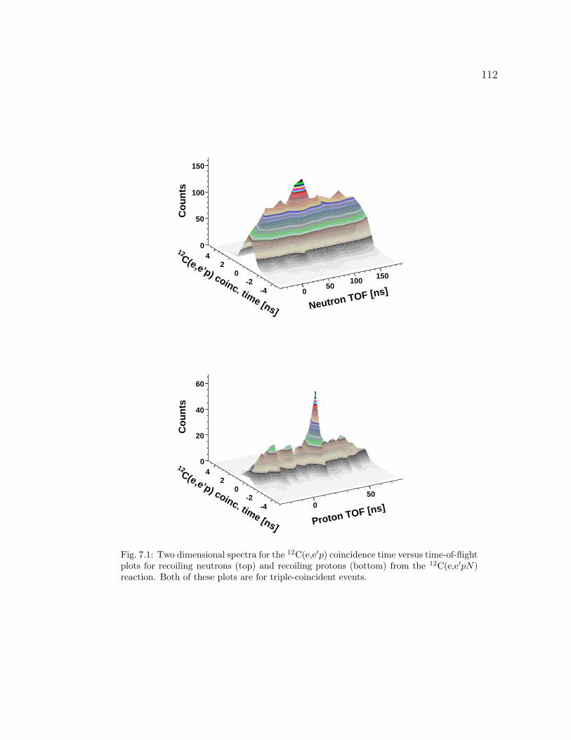
112

Neutron TOF [ns]050

100150

C(e,e’p) coinc. time [ns]

12

-4-2

02

4

Co

un

ts

0

50

100

150

Proton TOF [ns]050

C(e,e’p) coinc. time [ns]

12

-4-2

02

4

Co

un

ts

0

20

40

60

Fig. 7.1: Two dimensional spectra for the 12C(e,e′p) coincidence time versus time-of-flightplots for recoiling neutrons (top) and recoiling protons (bottom) from the 12C(e,e′pN)reaction. Both of these plots are for triple-coincident events.

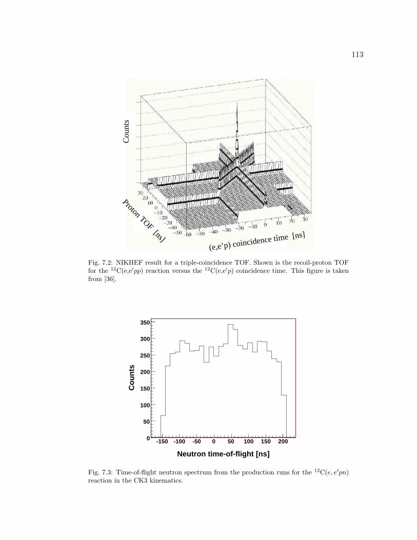
113

Proton TOF [ns](e,e’p) coincidence time [ns]

Cou

nts

Fig. 7.2: NIKHEF result for a triple-coincidence TOF. Shown is the recoil-proton TOFfor the 12C(e,e′pp) reaction versus the 12C(e,e′p) coincidence time. This figure is takenfrom [36].

Neutron time-of-flight [ns]

-150 -100 -50 0 50 100 150 200

Co

un

ts

0

50

100

150

200

250

300

350

Fig. 7.3: Time-of-flight neutron spectrum from the production runs for the 12C(e, e′pn)reaction in the CK3 kinematics.

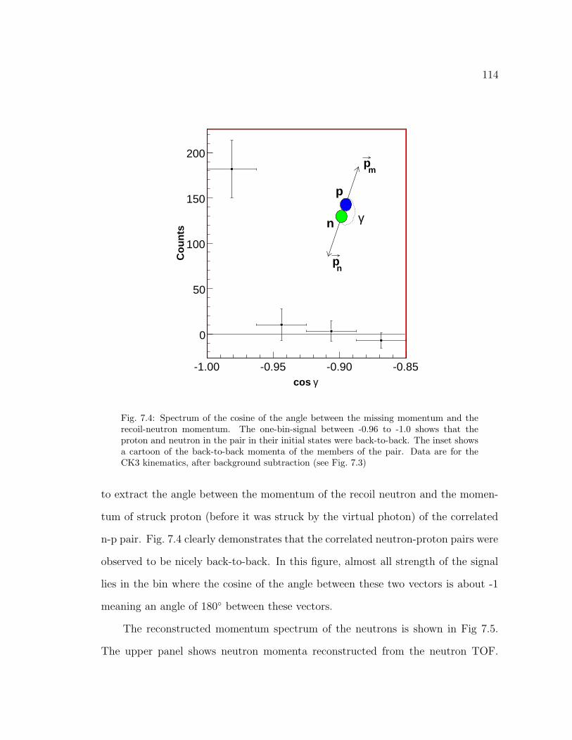
114

γcos -1.00 -0.95 -0.90 -0.85

Co

un

ts

0

50

100

150

200

p

n γ

pm

pn

Fig. 7.4: Spectrum of the cosine of the angle between the missing momentum and therecoil-neutron momentum. The one-bin-signal between -0.96 to -1.0 shows that theproton and neutron in the pair in their initial states were back-to-back. The inset showsa cartoon of the back-to-back momenta of the members of the pair. Data are for theCK3 kinematics, after background subtraction (see Fig. 7.3)

to extract the angle between the momentum of the recoil neutron and the momen-

tum of struck proton (before it was struck by the virtual photon) of the correlated

n-p pair. Fig. 7.4 clearly demonstrates that the correlated neutron-proton pairs were

observed to be nicely back-to-back. In this figure, almost all strength of the signal

lies in the bin where the cosine of the angle between these two vectors is about -1

meaning an angle of 180 between these vectors.

The reconstructed momentum spectrum of the neutrons is shown in Fig 7.5.

The upper panel shows neutron momenta reconstructed from the neutron TOF.

115

The lower panel shows neutron momenta computed from the (e, e′p) missing mo-

mentum, i.e. assuming that the n-p pair was stationary in the laboratory frame of

reference. We attribute the difference between these two spectra to the c.m. motion

of the pair which is clearly not zero (as assumed in the bottom panel). The final

result for the cross-section ratios discussed below was independent of the momentum

reconstruction.

The missing energy for the 12C(e, e′pn) reaction, calculated using Eqn.(2.10)

(also called E2m or double missing energy), is shown in Fig. 7.6. One has to have

recoil-neutron momentum information in order to produce such a plot. The upper

plot was produced using the neutron momentum derived from the measured TOF.

For the lower plot, the neutron momentum was assumed to be equal to the missing

momentum of the 12C(e, e′p) reaction. Though we do not see any structure on these

plots, the distribution is within an expected region [36] of about 30 to 80 MeV for

the emission of a nucleon-nucleon pair.

Another point of interest was to look at the center-of-mass momentum and the

relative momentum of the correlated n-p pair. The center-of-mass momentum is also

interpreted, by momentum conservation, as the momentum of the A − 2 residual

nucleus. The relative momentum of the n-p pair given by

~prel = 0.5(~pn − ~pp) (7.1)

can also be interpreted as the momentum of the recoiling neutron. Figure 7.7 shows

such momenta. The mean center-of-mass momentum is about 80 MeV/c and is a

very small quantity when compared to the relative momentum of the n-p pair (∼

500 MeV/c).

For quantitative results, we measured cross-section ratios for various reaction

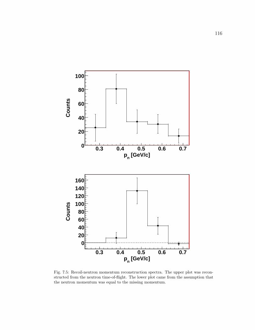
116

[GeV/c]n

p0.3 0.4 0.5 0.6 0.7

Co

un

ts

0

20

40

60

80

100

[GeV/c]n

p0.3 0.4 0.5 0.6 0.7

Co

un

ts

020406080

100120140160

Fig. 7.5: Recoil-neutron momentum reconstruction spectra. The upper plot was recon-structed from the neutron time-of-flight. The lower plot came from the assumption thatthe neutron momentum was equal to the missing momentum.

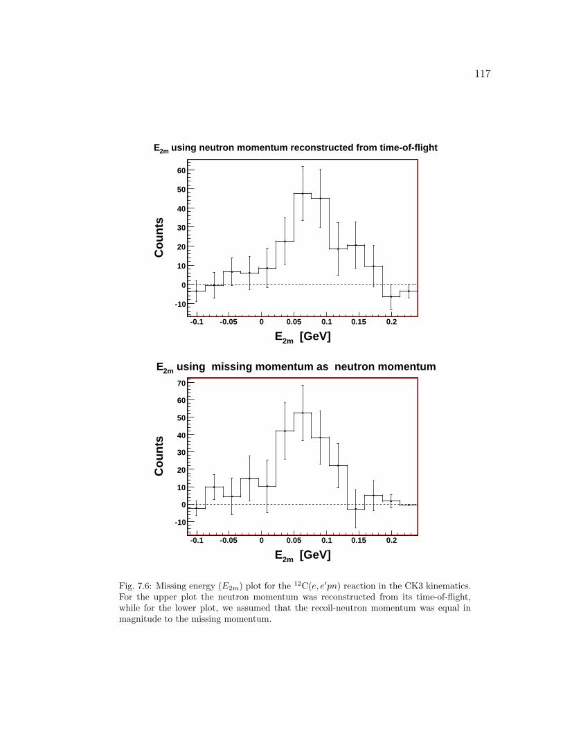
117

[GeV]2mE-0.1 -0.05 0 0.05 0.1 0.15 0.2

Co

un

ts

-10

0

10

20

30

40

50

60

using neutron momentum reconstructed from time-of-flight2mE

[GeV]2mE-0.1 -0.05 0 0.05 0.1 0.15 0.2

Co

un

ts

-10

0

10

20

30

40

50

60

70

using missing momentum as neutron momentum2mE

Fig. 7.6: Missing energy (E2m) plot for the 12C(e, e′pn) reaction in the CK3 kinematics.For the upper plot the neutron momentum was reconstructed from its time-of-flight,while for the lower plot, we assumed that the recoil-neutron momentum was equal inmagnitude to the missing momentum.

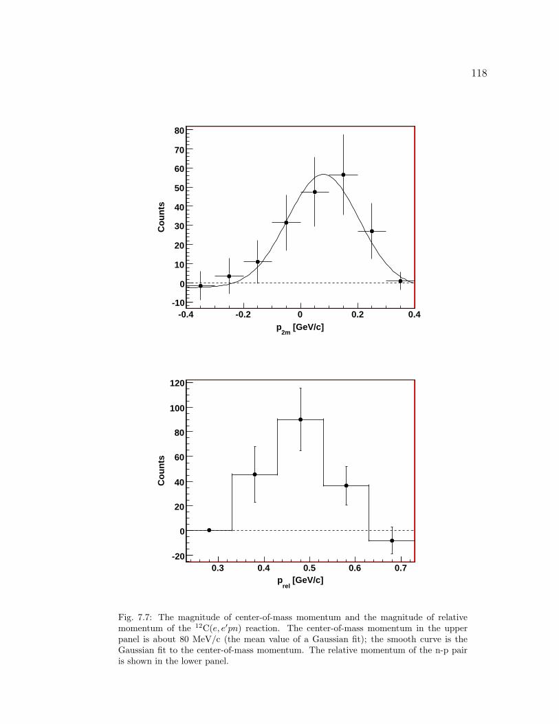
118

[GeV/c]2m

p-0.4 -0.2 0 0.2 0.4

Co

un

ts

-10

0

10

20

30

40

50

60

70

80

[GeV/c]rel

p0.3 0.4 0.5 0.6 0.7

Co

un

ts

-20

0

20

40

60

80

100

120

Fig. 7.7: The magnitude of center-of-mass momentum and the magnitude of relativemomentum of the 12C(e, e′pn) reaction. The center-of-mass momentum in the upperpanel is about 80 MeV/c (the mean value of a Gaussian fit); the smooth curve is theGaussian fit to the center-of-mass momentum. The relative momentum of the n-p pairis shown in the lower panel.

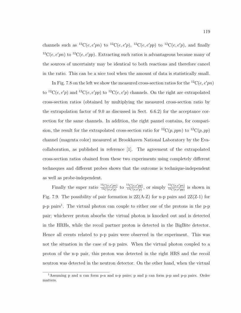
119

channels such as 12C(e, e′pn) to 12C(e, e′p), 12C(e, e′pp) to 12C(e, e′p), and finally

12C(e, e′pn) to 12C(e, e′pp). Extracting such ratios is advantageous because many of

the sources of uncertainty may be identical to both reactions and therefore cancel

in the ratio. This can be a nice tool when the amount of data is statistically small.

In Fig. 7.8 on the left we show the measured cross-section ratios for the 12C(e, e′pn)

to 12C(e, e′p) and 12C(e, e′pp) to 12C(e, e′p) channels. On the right are extrapolated

cross-section ratios (obtained by multiplying the measured cross-section ratio by

the extrapolation factor of 9.0 as discussed in Sect. 6.6.2) for the acceptance cor-

rection for the same channels. In addition, the right pannel contains, for compari-

sion, the result for the extrapolated cross-section ratio for 12C(p, ppn) to 12C(p, pp)

channel (magenta color) measured at Brookhaven National Laboratory by the Eva-

collaboration, as published in reference [1]. The agreement of the extrapolated

cross-section ratios obained from these two experiments using completely different

techneques and different probes shows that the outcome is technique-independent

as well as probe-independent.

Finally the super ratio12C(e,e′pn)12C(e,e′p)

to12C(e,e′pp)12C(e,e′p)

, or simply12C(e,e′pn)12C(e,e′pp)

is shown in

Fig. 7.9. The possibility of pair formation is 2Z(A-Z) for n-p pairs and 2Z(Z-1) for

p-p pairs1. The virtual photon can couple to either one of the protons in the p-p

pair; whichever proton absorbs the virtual photon is knocked out and is detected

in the HRHs, while the recoil partner proton is detected in the BigBite detector.

Hence all events related to p-p pairs were observed in the experiment. This was

not the situation in the case of n-p pairs. When the virtual photon coupled to a

proton of the n-p pair, this proton was detected in the right HRS and the recoil

neutron was detected in the neutron detector. On the other hand, when the virtual

1Assuming p and n can form p-n and n-p pairs; p and p can form p-p and p-p pairs. Ordermatters.

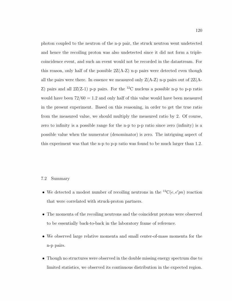
120

photon coupled to the neutron of the n-p pair, the struck neutron went undetected

and hence the recoiling proton was also undetected since it did not form a triple-

coincidence event, and such an event would not be recorded in the datastream. For

this reason, only half of the possible 2Z(A-Z) n-p pairs were detected even though

all the pairs were there. In essence we measured only Z(A-Z) n-p pairs out of 2Z(A-

Z) pairs and all 2Z(Z-1) p-p pairs. For the 12C nucleus a possible n-p to p-p ratio

would have been 72/60 = 1.2 and only half of this value would have been measured

in the present experiment. Based on this reasoning, in order to get the true ratio

from the measured value, we should multiply the measured ratio by 2. Of course,

zero to infinity is a possible range for the n-p to p-p ratio since zero (infinity) is a

possible value when the numerator (denominator) is zero. The intriguing aspect of

this experiment was that the n-p to p-p ratio was found to be much larger than 1.2.

7.2 Summary

• We detected a modest number of recoiling neutrons in the 12C(e, e′pn) reaction

that were correlated with struck-proton partners.

• The momenta of the recoiling neutrons and the coincident protons were observed

to be essentially back-to-back in the laboratory frame of reference.

• We observed large relative momenta and small center-of-mass momenta for the

n-p pairs.

• Though no structures were observed in the double missing energy spectrum due to

limited statistics, we observed its continuous distribution in the expected region.

121

Missing Momentum [GeV/c]

0.3 0.4 0.5 0.6

Cro

ss-S

ecti

on

Rat

io

0

0.02

0.04

0.06

0.08

0.1

0.12

0.14

C(e,e’p)12C(e,e’pn) / 12

C(e,e’p)12C(e,e’pp) / 12

Missing Momentum [GeV/c]

0.3 0.4 0.5 0.6

Cro

ss-S

ecti

on

Rat

io

0

0.2

0.4

0.6

0.8

1

C(e,e’p)12C(e,e’pn) / 12

C(p,pp)12C(p,ppn) / 12

C(e,e’p)12C(e,e’pp) / 12

Fig. 7.8: The left plot is the measured cross-section ratio for 12C(e, e′pn)/12C(e, e′p)and 12C(e, e′pp)/12C(e, e′p). The right plot is extrapolated cross-section ratios usingacceptance corrections, where the magenta is for 12C(p, ppn)/12C(p, pp) from reference[1] while the blue and red are for 12C(e, e′pn)/12C(e, e′p) and 12C(e, e′pp)/12C(e, e′p),respectively.

• We observed that there are many more n-p pairs than p-p pairs. The measured

cross-section ratio12C(e,e′pn)12C(e,e′p)

was 11.0 ± 2.5 % for n-p pairs and the measured

cross-section ratio12C(e,e′pp)12C(e,e′p)

was only 1.4 ± 0.2 % for p-p pairs.

• The measured value for the super ratio12C(e,e′pn)12C(e,e′p)

to12C(e,e′pp)12C(e,e′p)

, or simply12C(e,e′pn)12C(e,e′pp)

was 8.1 ± 2.2.

Taking into account the kinematical restriction of the measurement (the need

for a multiplication factor of 2 as explained in Sect.7.1), this super ratio becomes

16.1 ± 4.5. In addition, due to single charge-exchange reactions, like np –> pp,

more p-p pairs can be generated. The correction for the effect of single charge-

exchange reactions was found to be 11% [69]. After this correction, the n-p to p-p

ratio becomes 17.9 ±4.5.

122

Missing Momentum [GeV/c]

0.4 0.5 0.6

Cro

ss-S

ecti

on

Rat

io

0

2

4

6

8

10

C(e,e’pp)12C(e,e’pn) / 12

Fig. 7.9: The cross-section ratio for the 12C(e, e′pn)/12C(e, e′pp) reactions.

123

The finding that the n-p to p-p short-range correlated pair ratio as 17.9 ± 4.5

compared to a naively expected value of 1.2 was the outstanding discovery of this

SRC experiment. This large ratio could have far-reaching implications for modeling

and understanding cold dense nuclear matter such as neutron stars [5].

A theoretical calculation, according to the reference [84], which includes central,

tensor, and spin-isospin correlations, assumes that tensor correlations play a key role

in producing more n-p pairs than p-p pairs.

Based upon this investigation and other results of E01-015 experiment, there

is a newly approved experiment, E07-006 [67], that will investigate short-range cor-

relations using the 4He(e, e′pN) reaction in the missing momentum range from 400

to 875 MeV/c, using a setup similar to E01-015.

7.3 Conclusion

Correlations in nuclei are generally classified into two types: long-range cor-

relations due to the long-range, attractive part of the nucleon-nucleon interaction,

and short-range correlations due to the short-range, repulsive part of the nucleon-

nucleon interaction. We investigated electron-induced two-nucleon emission from

carbon with the goal of being sensitive to and studying short-range correlations us-

ing the 12C(e, e′pN) reaction in a triple-coincidence measurement. The kinematic

coverage was such that Q2 = 2 (GeV/c)2, xB = 1.2, and the missing momentum of

the 12C(e,e′p) reaction ranged from 250 to 650 MeV/c. Two existing high-resolution

spectrometers were used to detect the scattered electrons and and the struck protons

in the 12C(e,e′pn) reaction . On the other hand, the recoiling neutrons in the same

reaction were detected using the time-of-flight method by the large neutron detector

designed and constructed specially for this experiment. Since short-range correla-

124

tions can be emulated by various two-body effects such as meson-exchange currents,

isobar currents and final-state interactions, we chose anti-parallel kinematics with

high Q2 at xB >1 to minimize them.

We performed the analysis of the 12C(e, e′pn) reaction, and made direct ob-

servation of short-range correlated n-p pairs. From our analysis we conclude that

there are 17.9±4.5 times more n-p short-range correlated pairs than p-p short-range

correlated pairs.

Bibliography

[1] E. Piasetzky et al., Phys. Rev. Lett. 97, 162504 (2006).

[2] R. V. Reid, Ann. of Phys 50, 411 (1968).

[3] G. E. Brown and M. Rho, Phys. Today Feb, 24 (1983).

[4] E. J. Moniz et al., Phys. Rev. Lett. 26, 445 (1971).

[5] M. M. Sargsian et al., J. Phys. G29, R1 (2003).

[6] F. Benmokhtar, Ph. D. Thesis, Rutgers, The State university of New Jersey(2004).

[7] F. Benmokhtar et al., Phys. Rev. Lett. 94, 082305 (2004).

[8] D. Rohe et al., Phys. Rev. Lett. 93, 182501 (2004).

[9] L. J. H. M. Kester et al., Phys. Rev. lett. 74, 1712 (1995).

[10] A. Zondervan et al., Nucl. Phys. A 587, 697 (1995).

[11] C. J. G. Onderwater et al., Phys. Rev. Lett. 78, 4893 (1997).

[12] C. J. G. Onderwater et al., Phys. Rev. Lett. 81, 2213 (1998).

[13] G. Rosner, Prog. Part. Nucl. Phys 44, 99 (2000).

[14] D. G. Middleton et al., arXive:nucl-ex 0701053, v1 (2007).

[15] B. Zhang, Ph. D. Thesis, Massachusetts Institute of Technology (2003).

[16] R. Niyazov, Ph. D. Thesis, Old Dominion University (2003).

[17] R. A. Niyzov et al., Phys. Rev. Lett. 92, 052303 (2004).

125

126

[18] A. Tang, Ph. D. Thesis, Kent State University (2002).

[19] J. L. S. Aclander, Ph. D. Thesis, Tel-Aviv University, Israel (2001).

[20] A. Tang et al., Phys. Rev. Lett. 90, 042301 (2003).

[21] O. Benhar and V. R. Pandharipande, Nucl. Phys. A 473, 234 (1987).

[22] O. Benhar et al., Nucl. Phys. A 505, 267 (1989).

[23] S. C. Pieper et al., Phys. Rev. C 46, 1741 (1992).

[24] J. Ryckebusch et al., Nucl. Phys. A 624, 581 (1997).

[25] B. Povh, K. Rith, C. Scholz, and F. Zetsche, PARTICLE AND NUCLEI, AnIntroduction to the Physical Concepts, 3rd Ed., Springer-Verlag, (1999).

[26] A. Accardi et al., arXiv:nucl-th/0701024v2 (2007).

[27] L. Lapikas, Nucl. Phys. A553, 297c (1993).

[28] C. Ciofi degli Atti, and S. Simula, Phys. Rev. C 53, 1689 (1996).

[29] P. Grabmayr, Prog. Part. Nucl. Phys. 29, 251 (1992).

[30] W. H. Dickhoff and C. Barbieri, Prog. Part. Nucl. Phys. 52, 377 (2004).

[31] O. Benhar et al., Phys. Lett. B 177, 135 (1986).

[32] K. Gottfried, Nucl. Phys. 5, 557 (1957).

[33] L. I. Frankfurt and M. I. Strikman, Phys. Rep. 76, 215 (1981).

[34] L. Frankfurt and M. Strikman, Phys. Rep. 160, 235 (1988).

[35] S. C. Pieper, R. B. Wiringa, and V. R. Pandharipande, Phys. Rev. C 46, 1741(1992).

[36] L. J. H. M. Kester, Ph. D. Thesis, Free University Amsterdam (1993).

[37] J. Ryckebusch et al., Nucl. Instr. and Meth. 624, 581 (1997).

127

[38] S. Janssen et al., Nucl. Phys. A 672, 285 (2000).

[39] C. C. degli Atti and D. Treleani, Phys. Rev. C 60, 024602 (1999).

[40] O. Benhar and V. R. Pandharipande, Phys. Rev. C 47, 2218 (1993).

[41] O. Benhar, V. R. Pandharipande and S. C. Pieper, Rev. Mod. Phys. 65, 817(1993).

[42] R. Schiavilla, A. Fabrocini, and V. R. Pandharipande, Nucl. Phys. A 473, 290(1987).

[43] J. Carlson, R. Schiavilla, Rev. Mod. Phys. 70, 743 (1998).

[44] D. B. Day et al., Phys. Rev. Lett. 59, 427 (1987).

[45] J. Arrington et al., Phys. Rev. Lett. 82, 2056 (1999).

[46] C. Ciofi degli Atti, and G. B. West, Phys. Lett. B 458, 447 (1999).

[47] O. Benhar, Phys. Rev. Lett. 83, 3130 (1999).

[48] K. S. Egiyan et al., Phys. Rev. Lett. 96, 082501 (2006).

[49] P. Monaghan, Ph. D. Thesis, Massachusetts Institute of Technology (2007).

[50] P. K. A. de Witt Huberts, Nucl. Part. Phys. 16, 507 (1990).

[51] T. de Forest Jr., Nucl. Phys. A 392, 232 (1983).

[52] W.Bertozzi, E. Piasetzky, J. Watson, and S. Wood, Studying Short-RangeCorrelations in Nuclei at the Repulsive Core Limit via the Triple Coincidence(e,e’pN), Jefferson Lab Hall A Proposal E01-015, (2000).

[53] J.Alcorn, at al., Nucl. Instr. and Meth. A 522, 294 (2004).

[54] D.J.J. de Lange, at al., Nucl. Instr. and Meth. A 406, 182 (1998).

[55] D.J.J. de Lange, at al., Nucl. Instr. and Meth. A 412, 254 (1998).

[56] Jefferson Lab Hall A webpage, http://www.jlab.org/help/Ghelp/halla3d.html.

128

[57] K. G. Fissum, at al., Nucl. Instr. and Meth. A 474, 108 (2001).

[58] W. R. Leo, Techniques for Nuclear and Particle Physics Experiments, A How-toApproach, 2nd Ed., Springer-Verlag (1994).

[59] M. Iodice, at al., Nucl. Instr. and Meth. A 411, 223 (1998).

[60] G. Cates, K. McCormic, B. Reitz, and B. Wojtsekhowski, Measurement of theNeutron Electric Form Factor Gn

E at High Q2, Jefferson Lab Hall A ProposalE02-013, (2001).

[61] J. Annand, D. Higinbotham, R. Lindgren, V. Nelyubin, and B. Norum, Preci-sioin Measurement of the Electroproduction of Π0 Near Threshold: A Test ofChiral QCD Dynamics , Jefferson Lab Hall A Proposal E04-007, (2003).

[62] G. Cates, V. Nelyubin, and P. Reimer, High Resolution Study of the Resonancein nK+ System, Jefferson Lab Hall A Proposal E05-009, (2004).

[63] S. Gilad, D. Higinbotham, W. Korsch, B. Norum, and S. Sirca, Measurementsof Ax and Az Asymmetries in the Quasi-elastic 3He(e, e′d) Reaction , JeffersonLab Hall A Proposal E05-102, (2005).

[64] J. P. Chen, X. Jiang, J. c. Peng, Measurement of Single Target-Spin Asymmetryin Semi-Inclusive ~n(e, e′Π−) Reaction on a Transversely Polarized 3He Target,Jefferson Lab Hall A Proposal E06-010, (2005).

[65] S. Choi, X. Jiang, Z. E. Meziani, and B. Swatzky, Precision Measurements ofthe Neutron d2: Towards the Electric χE and Magnetic χB Color Polarizabili-ties, Jefferson Lab Hall A Proposal E06-014, (2005).

[66] W. Bertozzi, G. Cates, K. Grimm, N. Liyanage, Z. E. Meziani, G.Rosner, B.Wojtsekhowski, and Z. Zhang, Measurement of neutron asymmetry A1n in thevalence quark region using 8.8 GeV and 6.6 GeV beam energies and BigBitespectrometer in Hall A, Jefferson Lab Hall A Proposal E12-06-122, (2006).

[67] S. Gilad, D. W. Higinbotham, B. Moffit, E. Piasetzky, J. Watson, Studying theInternal Small-Distance Structure of Nuclei via the Triple Coincidence (e,e’pN),Jefferson Lab Hall A Proposal 07-006 (2007).

[68] R. Shneor, M. Sc. Thesis, Tel-Aviv University, Israel (2003).

[69] R. Shneor, Ph. D. Thesis, Tel-Aviv University, Israel (2007).

129

[70] Hall A Survey report (report numbers A969 and A987) for the experimentE01015, http : //hallaweb.jlab.org/news/minutes/Survey−Reports/Survey−Reports.html (2005).

[71] P. Monaghan, Survey Report posted onhttp : //hallaweb.jlab.org/experiment/E01−015/, Massachusetts Institute ofTechnology .

[72] R. A. Cecil, B. D. Anderson, and R. Madey, Nucl. Instr. and Meth. 161, 439(1979).

[73] V. McLane et al., Neutron Cross Section, Curves, Volume 2, Academic Press(1999).

[74] J. W. Watson, Private communication .

[75] Jefferson Lab Hall A analyzer, http://hallaweb.jlab.org/root/index.html .

[76] ROOT - An Object-Oriented Data Analysis Framework, http://root.cern.ch .

[77] N. Liyanage, Ph. D. Thesis, Massachusetts Institute of Technology (1999).

[78] R. Madey et al., Nucl. Instr. and Meth. 214, 401 (1983).

[79] GEANT4 simulation, http://geant4.web.cern.ch/geant4/ .

[80] P. E. Ulmer, MCEEP: Monte Carlo for electro-nuclear coincidence experiments,http://hallaweb.jlab.org/publications/Technotes/technote.html (1991).

[81] S. Wood, Private communication .

[82] R. Shenor, Private communication .

[83] R.Shneor et al., arXiv:nucl-ex/0703023 (2007).

[84] R. Schiavilla et al., Phys. Rev. Lett. 98, 132501 (2007).

[85] J. F. Janni, At. Data Nucl. Data Tables 27, 147 (1982).

Appendix A

Neutron Detection Efficiency Determination

In this Appendix we describe how the effective threshold was determined, which

is central for calculating the efficiency of the neutron detector.

A.1 The Threshold Determination

We used e-p elastic scattering (LH kinematics) to provide a proton flux of known

energy passing through the neutron detector. In this kinematics, all protons entering

the neutron detector were passing protons, which were not completely stopped. For

these passing protons, the energy loss in the scintillator Eloss is in a regime where

the light production in MeVee is equal to Eloss in MeV. In the hydrogen elastic

runs, scattered electrons went to the HRSL and the recoiling protons went to the

neutron detector. Neither the BigBite magnet nor the BigBite detector package

were between the target and the neutron detector. The neutron detector was sitting

15 m from the target, 50 right of the beamline (while viewing the beam dump from

the target). Hence the energy loss of proton occured only in the target chamber

materials and the materials (such as air and plastic scintillator bars) between the

target and the scintillator bar. In order to calculate the proton energy loss, we used

proton energy loss tables from [85]. Figure A.1 is a typical ADC plot for one PMT

of one bar from the elastic hydrogen run. The arrow indicates the peak channel, for

130

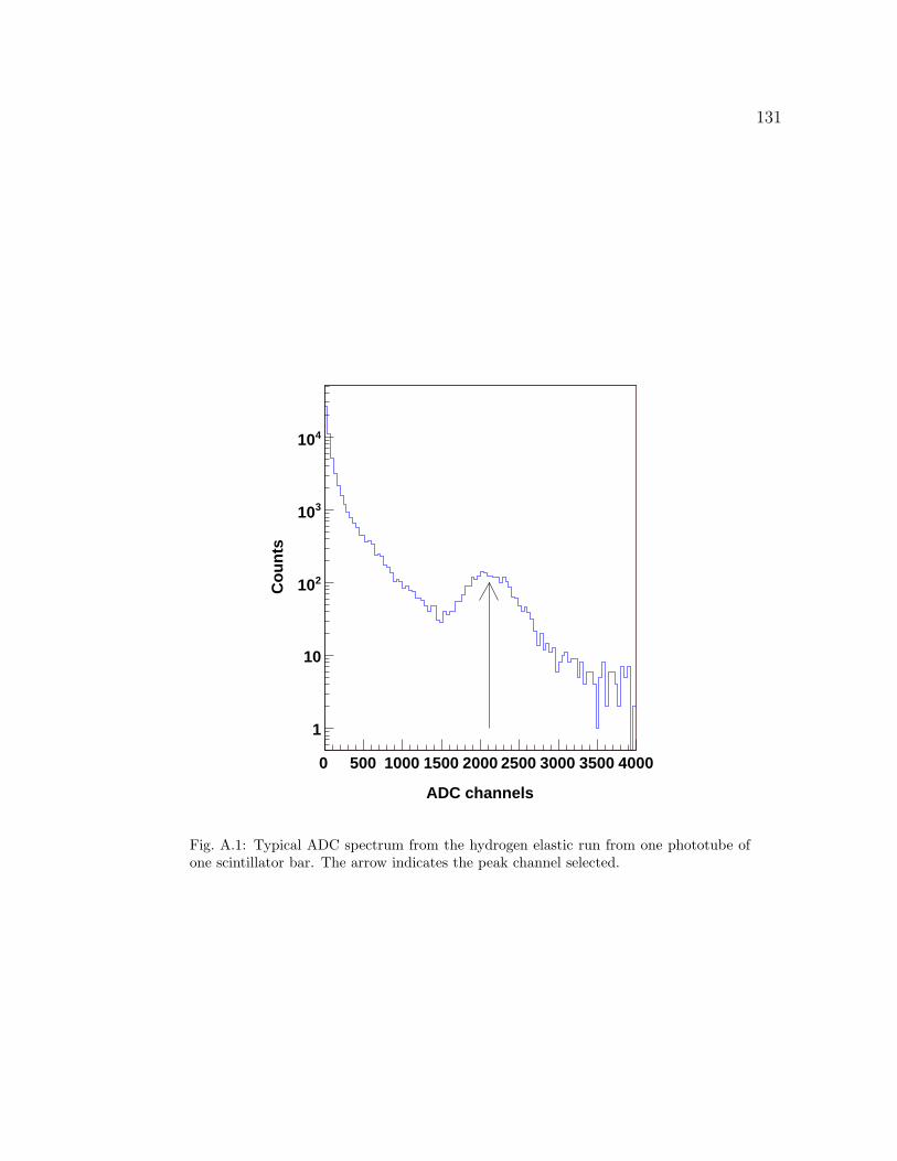
131

ADC channels

0 500 1000 1500 2000 2500 3000 3500 4000

Co

un

ts

1

10

210

310

410

Fig. A.1: Typical ADC spectrum from the hydrogen elastic run from one phototube ofone scintillator bar. The arrow indicates the peak channel selected.

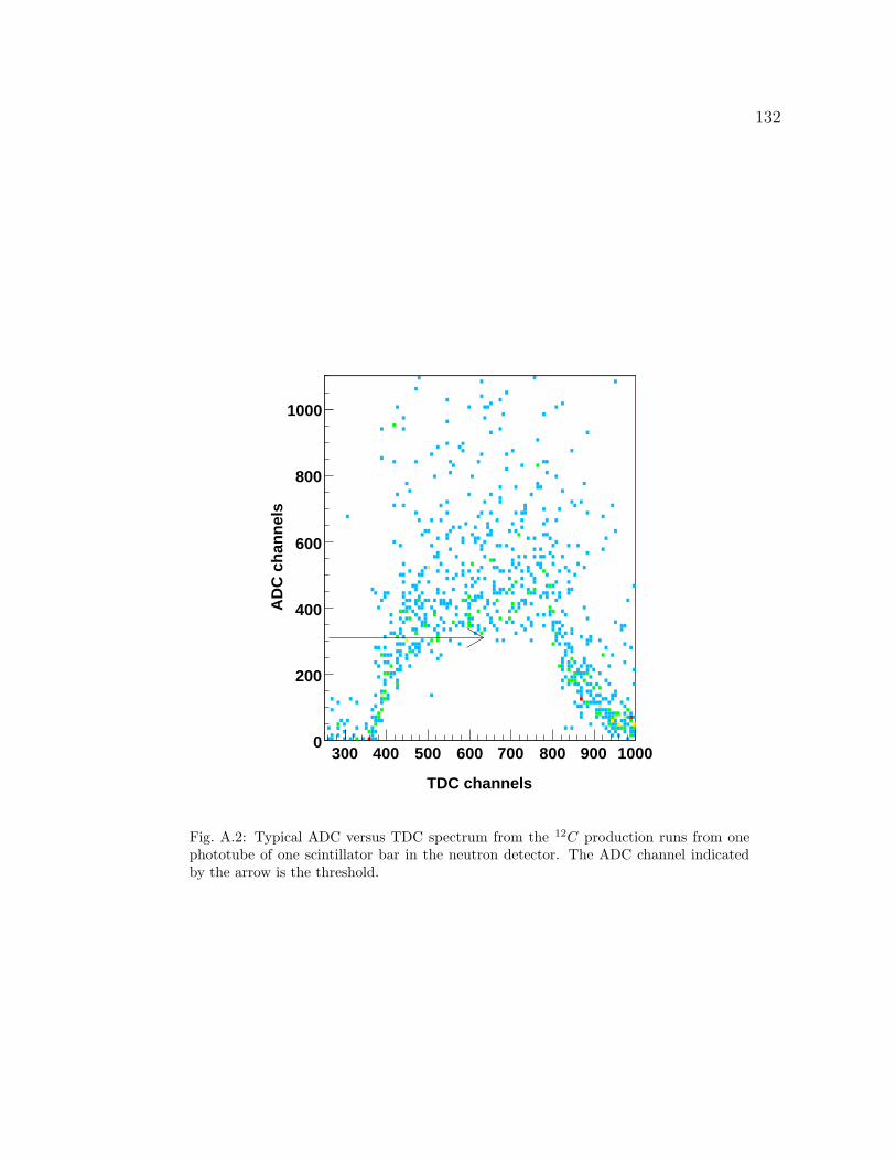
132

TDC channels

300 400 500 600 700 800 900 1000

AD

C c

han

nel

s

0

200

400

600

800

1000

Fig. A.2: Typical ADC versus TDC spectrum from the 12C production runs from onephototube of one scintillator bar in the neutron detector. The ADC channel indicatedby the arrow is the threshold.

133

which we know Eloss. The hydrogen elastic data give us a point of known energy

deposition and hence light output for each phototube. The next step is to determine

the electronic threshold for each phototube. This was accomplished by using the 12C

production data and observing the minimum ADC output. Figure A.2 is a scatter

plot of the ADC versus the TDC signals for production runs. Here one can clearly

see the ADC threshold in the TDC window: the ADC channel corresponding to

that threshold value (Fig. A.2) was then recorded. Note that all ADC values were

“pedestal subtracted” so the ADC scale has a true zero.

The proton elestic peaks (Fig. A.1) and ADC thresholds (Fig. A.2) were then

combined with the calculated Eloss for the protons to determine the ADC threshold

in MeVee for each phototube:

Threshold =ADCThreshold

ADC peakEloss (A.1)

The threshold value was determined for all individual scintillator bars and finally,

an average value for each plane was calculated.

A.2 The Efficiency Data

In this section, we present the complete set of the efficiencies that were used for

data analysis. Table A.1 shows the data plotted in Fig. 4.2. The simulation code

needs the height, length and thickness of a scintillator bar in its input file. Though

the length and the thickness of all scintillator bars were alike, the third plane had

134

bars of mixed heights. We used an average height of 12.5 cm in the input file of the

simulation code for a scintillator bar in the third plane.

The removal cross section (i.e., non elastic cross section) in barns for the relevant

elements and materials are given in Table A.2. Here the non-elastic cross section for

Pb, Fe and C were directly read from [73] and that for air was obtained from [74].

The removal cross section for plastic was calculated from information for C and H,

assuming that the plastic is made up of C and H only with the H to C ratio equal

to 1.104. Note that the removal cross section for H was taken as the two thirds of

the total cross section.

The table A.3 shows the transmittance data for the relevant materials. Note

that the following thicknesses for materials between the target and the front face of

the plane one of the neutron detector were used: air 600 cm, lead in the lead wall

5.08 cm, iron in the lead wall 4 cm, scintillator plastic in the three planes of the

BigBite detectors 3.55 cm, the two overlaping veto bars 4 cm. Also note that every

scintillator bar in the neutron detector had a thickness of 10 cm.

The number density (n), length (L) and n∗L for the relevant subtances were:

Lead: n = 0.03300∗1024 cm−3, L = 5.08 cm, nL = 0.16774∗1024 cm−2,

Iron: n = 0.08460∗1024 cm−3, L = 4.00 cm, nL = 0.33853∗1024 cm−2,

Plastic: n = 0.99784∗1023 cm−3, L = 7.55 cm, nL = 0.75336∗1024 cm−2,

Air: n = 0.00270∗1022 cm−3, L = 600.0 cm, nL = 0.01620∗1024 cm−2.

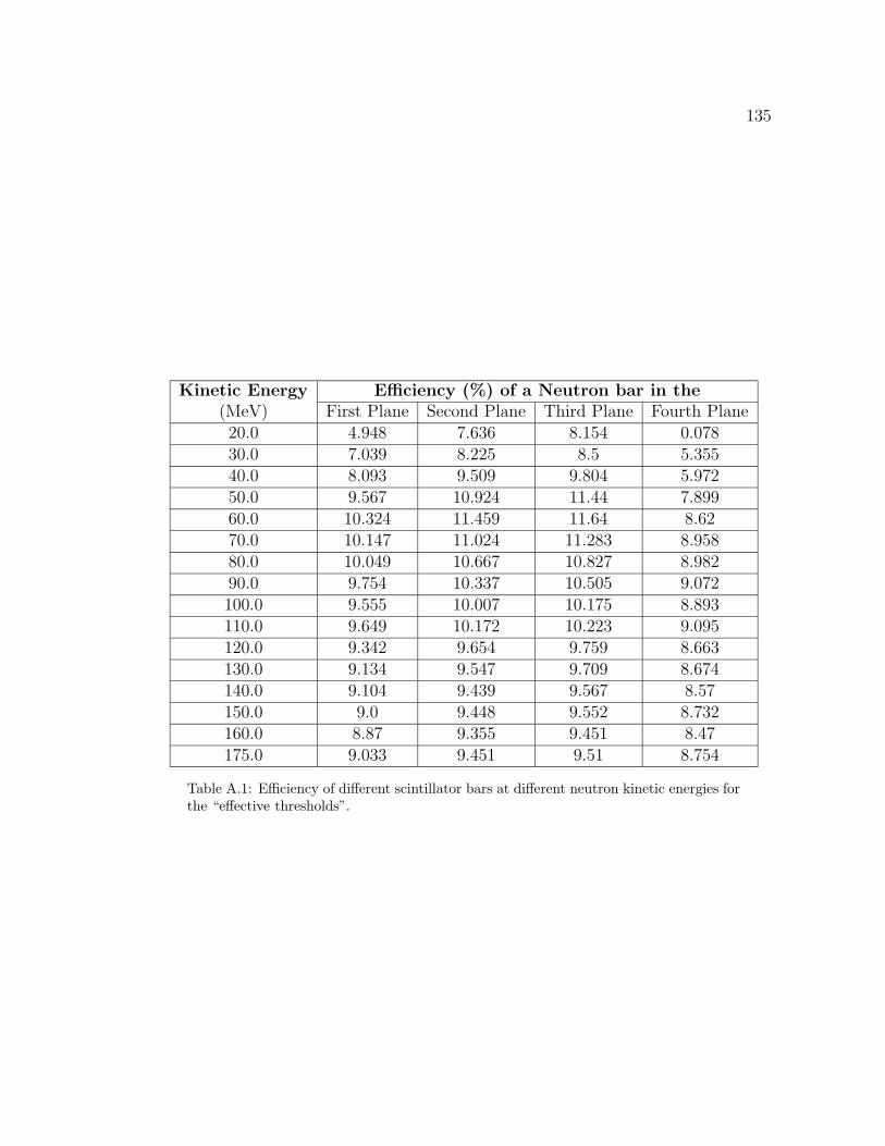
135

Kinetic Energy Efficiency (%) of a Neutron bar in the(MeV) First Plane Second Plane Third Plane Fourth Plane20.0 4.948 7.636 8.154 0.07830.0 7.039 8.225 8.5 5.35540.0 8.093 9.509 9.804 5.97250.0 9.567 10.924 11.44 7.89960.0 10.324 11.459 11.64 8.6270.0 10.147 11.024 11.283 8.95880.0 10.049 10.667 10.827 8.98290.0 9.754 10.337 10.505 9.072100.0 9.555 10.007 10.175 8.893110.0 9.649 10.172 10.223 9.095120.0 9.342 9.654 9.759 8.663130.0 9.134 9.547 9.709 8.674140.0 9.104 9.439 9.567 8.57150.0 9.0 9.448 9.552 8.732160.0 8.87 9.355 9.451 8.47175.0 9.033 9.451 9.51 8.754

Table A.1: Efficiency of different scintillator bars at different neutron kinetic energies forthe “effective thresholds”.

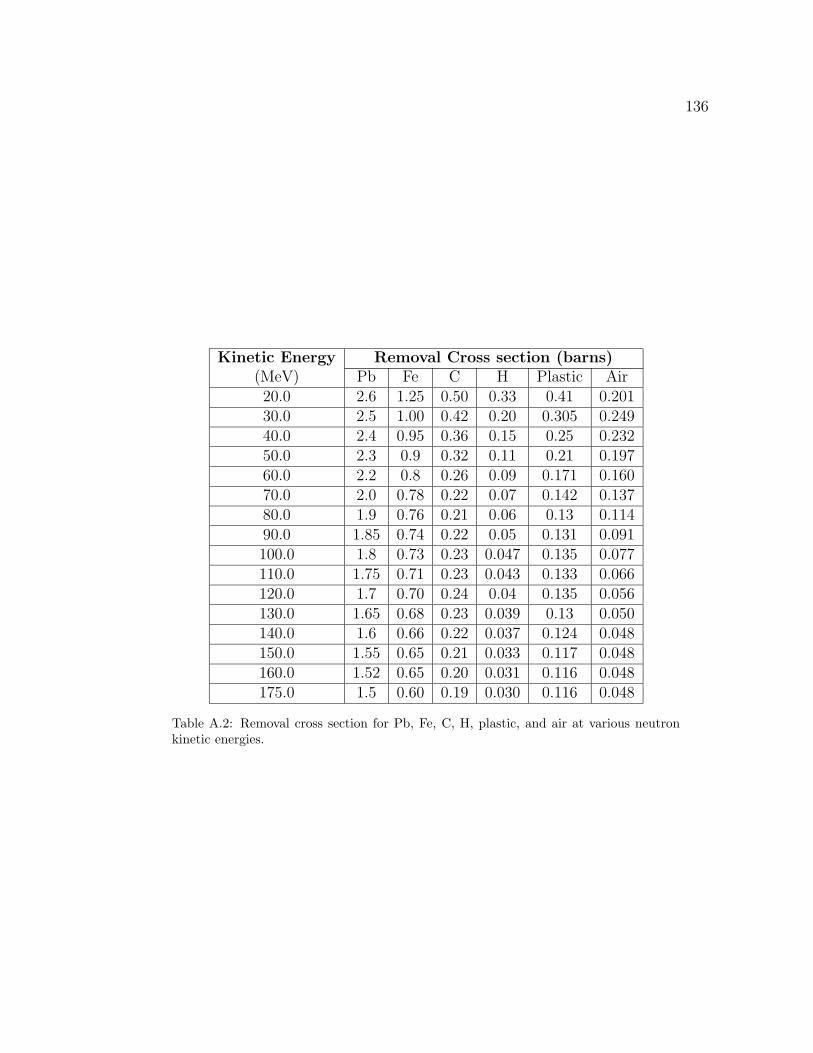
136

Kinetic Energy Removal Cross section (barns)(MeV) Pb Fe C H Plastic Air20.0 2.6 1.25 0.50 0.33 0.41 0.20130.0 2.5 1.00 0.42 0.20 0.305 0.24940.0 2.4 0.95 0.36 0.15 0.25 0.23250.0 2.3 0.9 0.32 0.11 0.21 0.19760.0 2.2 0.8 0.26 0.09 0.171 0.16070.0 2.0 0.78 0.22 0.07 0.142 0.13780.0 1.9 0.76 0.21 0.06 0.13 0.11490.0 1.85 0.74 0.22 0.05 0.131 0.091100.0 1.8 0.73 0.23 0.047 0.135 0.077110.0 1.75 0.71 0.23 0.043 0.133 0.066120.0 1.7 0.70 0.24 0.04 0.135 0.056130.0 1.65 0.68 0.23 0.039 0.13 0.050140.0 1.6 0.66 0.22 0.037 0.124 0.048150.0 1.55 0.65 0.21 0.033 0.117 0.048160.0 1.52 0.65 0.20 0.031 0.116 0.048175.0 1.5 0.60 0.19 0.030 0.116 0.048

Table A.2: Removal cross section for Pb, Fe, C, H, plastic, and air at various neutronkinetic energies.

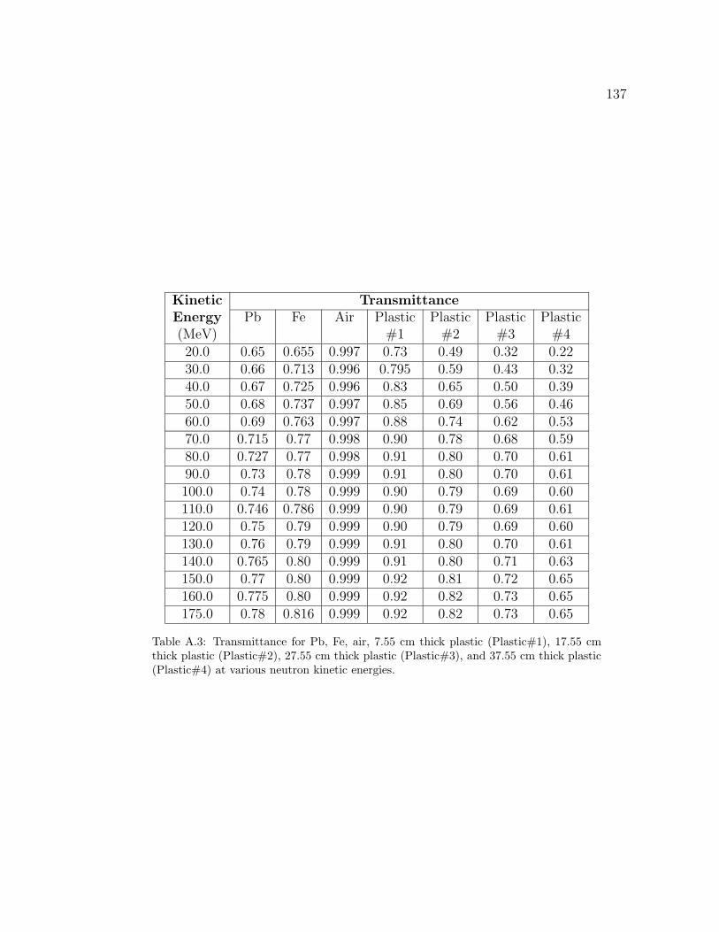
137

Kinetic TransmittanceEnergy Pb Fe Air Plastic Plastic Plastic Plastic(MeV) #1 #2 #3 #420.0 0.65 0.655 0.997 0.73 0.49 0.32 0.2230.0 0.66 0.713 0.996 0.795 0.59 0.43 0.3240.0 0.67 0.725 0.996 0.83 0.65 0.50 0.3950.0 0.68 0.737 0.997 0.85 0.69 0.56 0.4660.0 0.69 0.763 0.997 0.88 0.74 0.62 0.5370.0 0.715 0.77 0.998 0.90 0.78 0.68 0.5980.0 0.727 0.77 0.998 0.91 0.80 0.70 0.6190.0 0.73 0.78 0.999 0.91 0.80 0.70 0.61100.0 0.74 0.78 0.999 0.90 0.79 0.69 0.60110.0 0.746 0.786 0.999 0.90 0.79 0.69 0.61120.0 0.75 0.79 0.999 0.90 0.79 0.69 0.60130.0 0.76 0.79 0.999 0.91 0.80 0.70 0.61140.0 0.765 0.80 0.999 0.91 0.80 0.71 0.63150.0 0.77 0.80 0.999 0.92 0.81 0.72 0.65160.0 0.775 0.80 0.999 0.92 0.82 0.73 0.65175.0 0.78 0.816 0.999 0.92 0.82 0.73 0.65

Table A.3: Transmittance for Pb, Fe, air, 7.55 cm thick plastic (Plastic#1), 17.55 cmthick plastic (Plastic#2), 27.55 cm thick plastic (Plastic#3), and 37.55 cm thick plastic(Plastic#4) at various neutron kinetic energies.

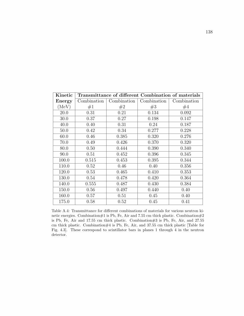
138

Kinetic Transmittance of different Combination of materialsEnergy Combination Combination Combination Combination(MeV) #1 #2 #3 #420.0 0.31 0.21 0.134 0.09230.0 0.37 0.27 0.198 0.14740.0 0.40 0.31 0.24 0.18750.0 0.42 0.34 0.277 0.22860.0 0.46 0.385 0.320 0.27670.0 0.49 0.426 0.370 0.32080.0 0.50 0.444 0.390 0.34090.0 0.51 0.452 0.396 0.345100.0 0.515 0.453 0.395 0.344110.0 0.52 0.46 0.40 0.356120.0 0.53 0.465 0.410 0.353130.0 0.54 0.478 0.420 0.364140.0 0.555 0.487 0.430 0.384150.0 0.56 0.497 0.440 0.40160.0 0.57 0.51 0.45 0.40175.0 0.58 0.52 0.45 0.41

Table A.4: Transmittance for different combinations of materials for various neutron ki-netic energies. Combination#1 is Pb, Fe, Air and 7.55 cm thick plastic. Combination#2is Pb, Fe, Air and 17.55 cm thick plastic. Combination#3 is Pb, Fe, Air, and 27.55cm thick plastic. Combination#4 is Pb, Fe, Air, and 37.55 cm thick plastic [Table forFig. 4.3]. These correspond to scintillator bars in planes 1 through 4 in the neutrondetector.

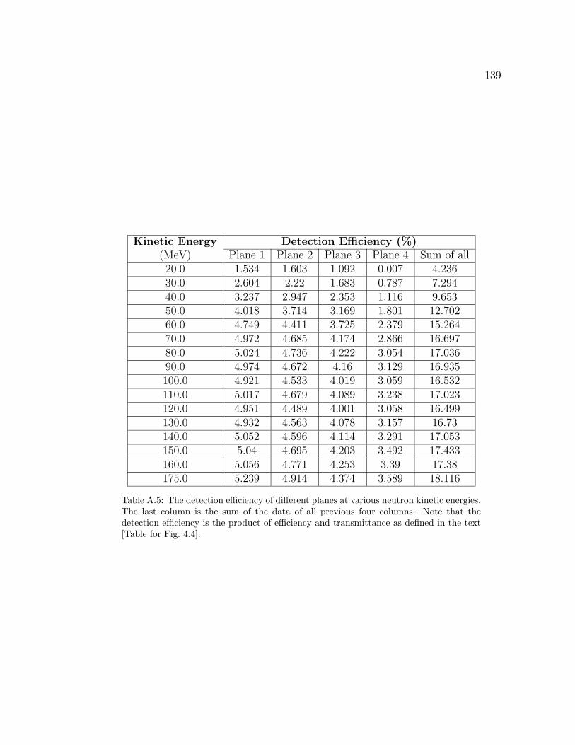
139

Kinetic Energy Detection Efficiency (%)(MeV) Plane 1 Plane 2 Plane 3 Plane 4 Sum of all20.0 1.534 1.603 1.092 0.007 4.23630.0 2.604 2.22 1.683 0.787 7.29440.0 3.237 2.947 2.353 1.116 9.65350.0 4.018 3.714 3.169 1.801 12.70260.0 4.749 4.411 3.725 2.379 15.26470.0 4.972 4.685 4.174 2.866 16.69780.0 5.024 4.736 4.222 3.054 17.03690.0 4.974 4.672 4.16 3.129 16.935100.0 4.921 4.533 4.019 3.059 16.532110.0 5.017 4.679 4.089 3.238 17.023120.0 4.951 4.489 4.001 3.058 16.499130.0 4.932 4.563 4.078 3.157 16.73140.0 5.052 4.596 4.114 3.291 17.053150.0 5.04 4.695 4.203 3.492 17.433160.0 5.056 4.771 4.253 3.39 17.38175.0 5.239 4.914 4.374 3.589 18.116

Table A.5: The detection efficiency of different planes at various neutron kinetic energies.The last column is the sum of the data of all previous four columns. Note that thedetection efficiency is the product of efficiency and transmittance as defined in the text[Table for Fig. 4.4].

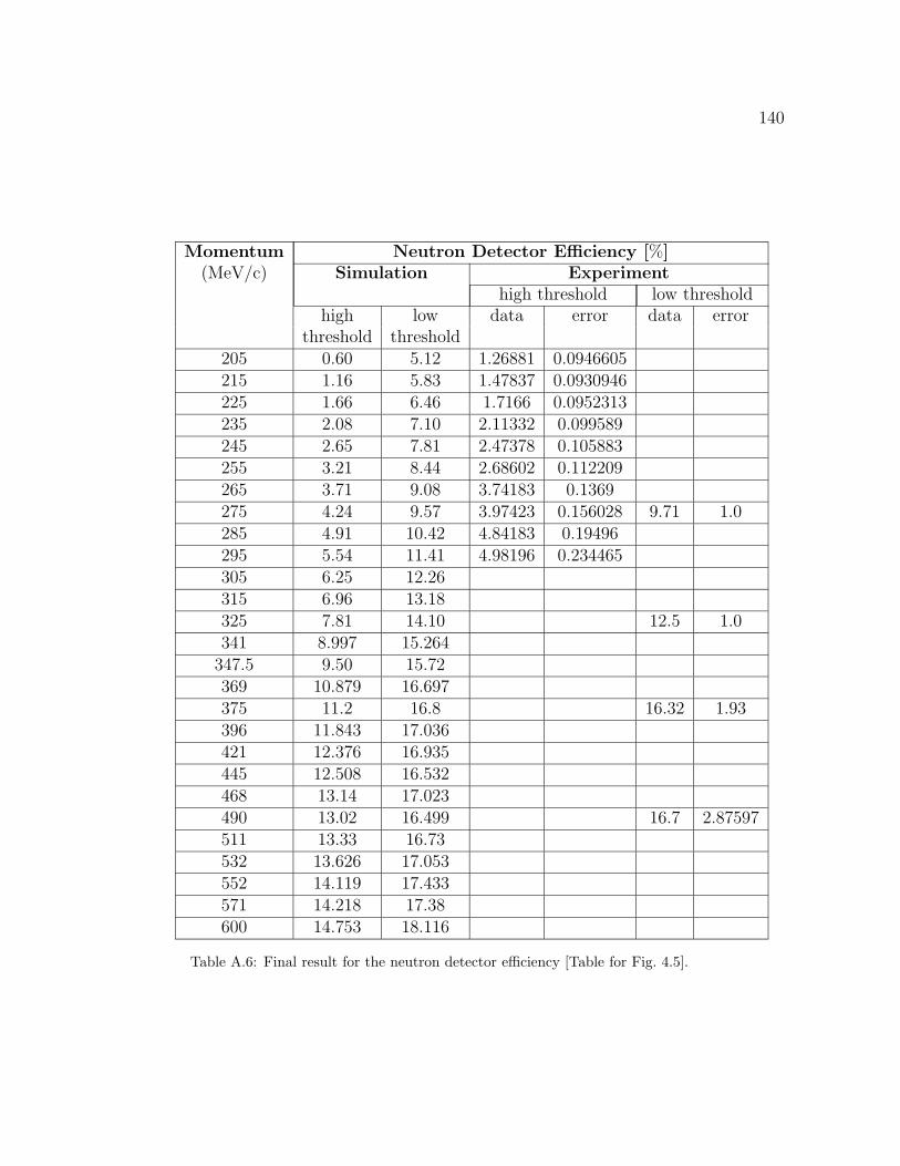
140

Momentum Neutron Detector Efficiency [%](MeV/c) Simulation Experiment

high threshold low thresholdhigh low data error data error

threshold threshold205 0.60 5.12 1.26881 0.0946605215 1.16 5.83 1.47837 0.0930946225 1.66 6.46 1.7166 0.0952313235 2.08 7.10 2.11332 0.099589245 2.65 7.81 2.47378 0.105883255 3.21 8.44 2.68602 0.112209265 3.71 9.08 3.74183 0.1369275 4.24 9.57 3.97423 0.156028 9.71 1.0285 4.91 10.42 4.84183 0.19496295 5.54 11.41 4.98196 0.234465305 6.25 12.26315 6.96 13.18325 7.81 14.10 12.5 1.0341 8.997 15.264

347.5 9.50 15.72369 10.879 16.697375 11.2 16.8 16.32 1.93396 11.843 17.036421 12.376 16.935445 12.508 16.532468 13.14 17.023490 13.02 16.499 16.7 2.87597511 13.33 16.73532 13.626 17.053552 14.119 17.433571 14.218 17.38600 14.753 18.116

Table A.6: Final result for the neutron detector efficiency [Table for Fig. 4.5].

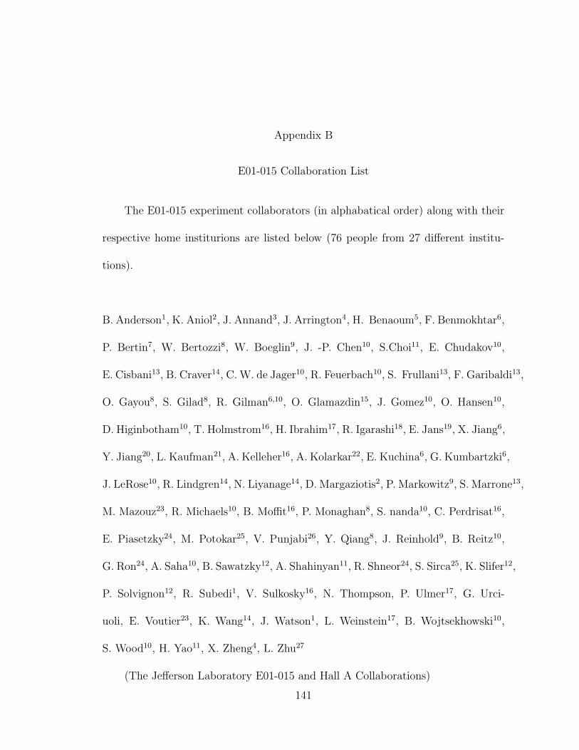
Appendix B

E01-015 Collaboration List

The E01-015 experiment collaborators (in alphabatical order) along with their

respective home institurions are listed below (76 people from 27 different institu-

tions).

B. Anderson1, K. Aniol2, J. Annand3, J. Arrington4, H. Benaoum5, F. Benmokhtar6,

P. Bertin7, W. Bertozzi8, W. Boeglin9, J. -P. Chen10, S.Choi11, E. Chudakov10,

E. Cisbani13, B. Craver14, C. W. de Jager10, R. Feuerbach10, S. Frullani13, F. Garibaldi13,

O. Gayou8, S. Gilad8, R. Gilman6,10, O. Glamazdin15, J. Gomez10, O. Hansen10,

D. Higinbotham10, T. Holmstrom16, H. Ibrahim17, R. Igarashi18, E. Jans19, X. Jiang6,

Y. Jiang20, L. Kaufman21, A. Kelleher16, A. Kolarkar22, E. Kuchina6, G. Kumbartzki6,

J. LeRose10, R. Lindgren14, N. Liyanage14, D. Margaziotis2, P. Markowitz9, S. Marrone13,

M. Mazouz23, R. Michaels10, B. Moffit16, P. Monaghan8, S. nanda10, C. Perdrisat16,

E. Piasetzky24, M. Potokar25, V. Punjabi26, Y. Qiang8, J. Reinhold9, B. Reitz10,

G. Ron24, A. Saha10, B. Sawatzky12, A. Shahinyan11, R. Shneor24, S. Sirca25, K. Slifer12,

P. Solvignon12, R. Subedi1, V. Sulkosky16, N. Thompson, P. Ulmer17, G. Urci-

uoli, E. Voutier23, K. Wang14, J. Watson1, L. Weinstein17, B. Wojtsekhowski10,

S. Wood10, H. Yao11, X. Zheng4, L. Zhu27

(The Jefferson Laboratory E01-015 and Hall A Collaborations)

141

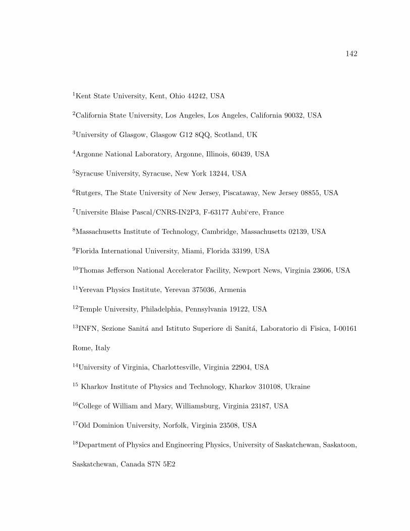
142

1Kent State University, Kent, Ohio 44242, USA

2California State University, Los Angeles, Los Angeles, California 90032, USA

3University of Glasgow, Glasgow G12 8QQ, Scotland, UK

4Argonne National Laboratory, Argonne, Illinois, 60439, USA

5Syracuse University, Syracuse, New York 13244, USA

6Rutgers, The State University of New Jersey, Piscataway, New Jersey 08855, USA

7Universite Blaise Pascal/CNRS-IN2P3, F-63177 Aubi‘ere, France

8Massachusetts Institute of Technology, Cambridge, Massachusetts 02139, USA

9Florida International University, Miami, Florida 33199, USA

10Thomas Jefferson National Accelerator Facility, Newport News, Virginia 23606, USA

11Yerevan Physics Institute, Yerevan 375036, Armenia

12Temple University, Philadelphia, Pennsylvania 19122, USA

13INFN, Sezione Sanita and Istituto Superiore di Sanita, Laboratorio di Fisica, I-00161

Rome, Italy

14University of Virginia, Charlottesville, Virginia 22904, USA

15 Kharkov Institute of Physics and Technology, Kharkov 310108, Ukraine

16College of William and Mary, Williamsburg, Virginia 23187, USA

17Old Dominion University, Norfolk, Virginia 23508, USA

18Department of Physics and Engineering Physics, University of Saskatchewan, Saskatoon,

Saskatchewan, Canada S7N 5E2

143

19Nationaal Instituut voor Kernfysica en Hoge-Energiefysica (NIKHEF)

20CCAST (World Laboratory), P.O. Box 8730, Beijing 100080, China

21University of Massachusetts Amherst, Amherst, Massachusetts 01003, USA

22University of Kentucky, Lexington, Kentucky 40506, USA

23Laboratoire de Physique Subatomique et de Cosmologie, 38026 Grenoble, France

24Tel Aviv University, Tel Aviv 69978, Israel

25Institute ”Jozef Stefan”, University of Ljubljana, Jamova 39, 1000 Ljubljana, Slovenia

26 Norfolk State University, Norfolk, Virginia 23504, USA

27University of Illinois at Urbana-Champaign, Urbana, Illinois 61801, USA