
PN ~ {)rcA - ~33 - USAID
295
PN {)rcA - S--z.. WATER SYSTEM DESIGN SEMINAR MAY 14 AND MAY 15, 1996 PRESENTERS: DANIEL GALLAGHER, P.E AND FRED ZOBRIST, P.E. SPONSORED BY: USAIDIWEST BANK AND GAZA AND UNDP JERUSALEM OFFICE CONTRACT NUMBER: HNE-0159-C-OO-3080-00 MANAGEMENT SYSTEMS INTERNATIONAL J l
-
Upload
khangminh22 -
Category
Documents
-
view
1 -
download
0
Transcript of PN ~ {)rcA - ~33 - USAID
PN ~ {)rcA - ~33q~g S--z..
WATER SYSTEM DESIGN SEMINAR
MAY 14 AND MAY 15, 1996
PRESENTERS:
DANIEL GALLAGHER, P.E
AND
FRED ZOBRIST, P.E.
SPONSORED BY:
USAIDIWEST BANK AND GAZA
AND
UNDP JERUSALEM OFFICE
CONTRACT NUMBER:HNE-0159-C-OO-3080-00
MANAGEMENT SYSTEMS INTERNATIONAL
Jl

WATER SYSTEM DESIGN SEMINAR
PART I
REPORT ON SEMINAR HELD ON
MAY 14 AND MAY 15
1996
AT
BEIR ZEIT UNIVERSITY
SPONSORED BY
USAIDI WEST BANK AND GAZA
AND
UNDP JERUSALEM OFFICE

PART I
CONTENTS
WATER SYSTEM DESIGN SEMINAR
Background Page 1
Participant Reactions 1
Software Programs 2
Pipe Materials and Costs 2
Materials Distributed 3
Conclusions and Recommendations 3
List ofAttendees Appendix A
Schedule B
Scope ofWork C

PART 11
CONTENTS
HAND OUT MATERIALS
TABEPANET users manual
InstaDing EPANET
Water Distribution System Seminar - Notes
Pipe Materials - Notes
AWWA PVC Pipe Design and Installation
Appendix A - AWWA Guidelines Criteria for 1/2 in. through 3 in. PE pipe
Indianapolis Water Company Goes to School (re. PEl
Fairfax County, Va., Public Facilities Regs. for Water and Fire (partial)
Fairfax County Water Authority Water Main Inst. Service Contracts
Plans - Notes
Cost Analysis - Notes
1
2
3
4
5
6
7
8
9
10
11

WATER SYSTEM DESIGN SEMINAR
Background
USAID is currently financing the construction ofwater networks for a number ofvillages andmunicipalities on the West Bank. Deficiencies were observed by USAID in recent water networkdesign related to hydraulic efficiency and the use of costly materials. Specific examples include:
- use ofcostly pipe materials has contributed to under sizing water mains andlaterals
- many undersized lines are classified as "service lines" and designated as branch linesrather than as elements ofa "looped" network grid
- concern about intermittent water flow has contributed to a practice ofdesigningreservoirs to "directly feed" rather than more efficient "floating" reservoirs
- inappropriate pipe materials contribute to high losses in the networks
- the hilly terrain in many areas often result in high system operatingpressures resulting in huge losses
- design drawings lack minimal basic data with which to evaluate theadequacy ofthe design
To assist with reducing these problems and improving the design process oflocal engineersUSAID and UNDP sponsored a two day seminar to introduce modem design practices andcomputerized hydraulic network design concepts. Included were alternative pipe uses and costconcepts. Appendix A provides a copy ofthe schedule and appendix C the target scope-of-work.
USAID provided a team oftwo senior engineers with broad experience in the water supplysector, while the UNDP provided for the training facilities and selected the participants. Beir ZeitUniversity was selected because ofits large computer laboratory.
A total of 19 participated in the seminar including USAID representatives. Each was given a diskwith a copy ofEPANET. A list ofthe attendees is included as appendix B.
Participant Reactions
The participants were very enthusiastic and involved during the seminar. A great number ofquestions were asked and discussions and dialog ensued. The participants were aware of some

ofthe topics presented, such as floating storage tanks and hydraulic modeling analysis. Classdiscussion involved how to implement these within the concerns and limitations ofwateravailability on the West Bank. Some ofthe concepts, such as pressure zones for hilly terrain,seemed new to the class. Discussion took place on how this approach could benefit their designs.
Software Programs
The main focus ofcomputer portion ofthe class was EPANET, the USEPA's dynamic hydraulicmodel. This program, including its on-disk manual was distributed to each ofthe participants.Complimentary programs also given out were NOTEBOOK, an improved text editor forEPANET data file creation, and ZIP and UNZIP, programs for compressing and expandinggroups offil~.
Besides the example data files that are packaged with EPANET, several more were prepared,distributed, and analyzed during the course. These were designed not only to illustrate EPANET,but also to point out appropriate design standards and practices. The data files included anexample ofpressure zones, an example ofhow storage tanks are implemented in EPANET, anexample offloating storage tank design, and a case study ofthe village ofFasiyal. This examplewas used to explain standards for headloss, velocity, and pressure that can be checked anddesigned for using hydraulic modeling. It was also used to illustrate the effects ofdifferent pipematerials on system hydraulics. A:final example was created during the class to ensure that theparticipants knew how to prepare EPANET data files.
A second design program BR2 was distributed and discussed in the course but not demonstrated.This program is for the optimal design ofbranched water distribution system and automaticallyselects pipe diameters to meet pressure constraints.
A briefdemonstration ofa GIS (geographic information system) was presented that included acomparison ofthis technology with CAD and the use ofGIS in planning.
A presentation ofAutoCad had been planned but was not conducted because ofcomputersoftware limitations and time constraints.
Pipe Materials and Costs
The session on alternative pipe use brought out strong prejudices against using plastics and poly's,although did appear to broaden their knowledge base. AWWA research materials andspecifications were provided on the uses ofthese types ofpipe. Also discussed were examplesand standards being used by u.S. utilities for pipe laying and system design. Also discussed wasthe requirements for basic construction drawings. Supporting handouts were also provided.
The review ofcosts showed an area ofweakness ofthe participants as life cycle costing and
2

alternative cost analyses are not currently being incorporated into their design and planningprocesses. However, they showed great interest and noted that they would like additional trainingon the subject.
Materials Distributed
In addition to the software listed above, the following copies were distributed to the participantsor provided to UNDP personnel for reference and later distribution as desired.
A paper copy ofthe EPANET manual (see part IT).The initial maps and data sets for the Fasiyal case study.Directions for installing EPANETCourse notes (see part IT)AWWA Manual 31: Distribution requirements for fire protectionAWWA Manual 32: Distribution network analysis for water utilitiesAutoCad for Dummies, lOG Press, ISBN 1-56884-141-4, 1996.Various related documents on alternate pipe, standards and costs (see part IT)
A copy ofeach ofthe materials provided as handouts to all participants is included in Part IT.
Conclusions and Recommendations
The USAID goals ofintroducing computerized network design concepts were fully met andaccepted by the participants. Participant feed back was positive and they, in general, expressedthe need for follow up and for additional seminars and workshops. This expression included theneed for more infonnation on cost analyses and consideration ofadditional subjects. They alsoexpressed a need for study tours to review more developed utilities and their practices.
The participants were provided background materials and software on EPANET a popular designtool among consultants and materials on alternative pipe materials, standards and constructiondrawing requirements. The handout materials were popular and well received. A copy ofthehandouts provided in the course are included as Part IT ofthis report.
It was clear that the majority ofthe class participants were interested in this technology and werewilling to think about using it in improving their current design practices. The seminar wassuccessful in generating this interest and whetting their appetite. There was not time to fully teachthe participants all they needed to know to implement hydraulic modeling analysis in theirstandard designs. Further training that works with the design engineers and implements acomplete design for one oftheir systems would be valuable - particularly a training session thatshows how hydraulic modeling can allow for numerous alternative designs to be examined withlittle effort and in a relatively short time.
3
1

The level ofbasic engineering skills ofthe participants was uniformly high. The level ofcomputerskills was more variable. Future seminars may want to limit participation to those comfortablewith computers or provide an optional session on basic computer training for those who need it.The lack ofadequate English among the participants was not apparent except in one or two cases.
Training in economic and financial analyses ofwater projects should also be included as costs,especially life cycle, have a major impact on design considerations.
4

8:30 - 9:00 am
9:00 - 9:30
9:30 -10:30
10:30 - 10:45
10:45 - 11:30
11:30 - 12:00
12:00 - 12:30 pm
12:30 - 1:30
1:30 - 3:00
3:00 - 3:15
3:15 - 4:30
WATER SYSTEM DESIGN SEMINAR
Day 1
Tuesday, May 14, 1996
Registration
Welcome and Overview
Hydraulic Analysis: headloss formulas, storage,valves
Break
Hydraulic Analysis: pumps, pump curves, distr.systems
Software Overview (computer lab)
Branched distribution system design (computerlab)
Lunch
EPANET: requirements, installation, anddemonstrations (computer lab)
Break
EPANET: case studies, design in hilly areas(computer lab)
q

8:30 -10:30 am
10:30 - 10:45
10:45 - 12:30
12:30 - 1:30
1:30 - 2:30
2:30 - 3:30
3:30 - 3:45
3:45 - 4:15
4:15 - 4:30
Day 2
Wednesday, May 15, 1996
EPANET: case studies, floating reservoirs(computer lab)
Break
EPANET: case studies (computer lab)
Lunch
Pipe materials
Cost analysis
Break
GIS demonstration
Miscellaneous and closeout

Qalqilia Municipality
Jerusalem Water Undertaking
UNDP
Palestinian Water Authority
Palestinian Water Authority
UNDP
West Bank Water Department
West Bank Water Department
West Bank Water Department
West Bank Water Department
West Bank Water Department
Hebron Municipality
Jenin Municipality
Jenin Municipality
UNDP
USAID
USAID
USAID
LIST OF PARTICIPANTS
PECDARMAZENNURI
NABIL BARHAM
NADAL KAHLIL
MUSAKHATIB
NADEL AL KHATEEB
YOUSIF HAMMAD
JOHNY THEODORY
MOHAMMAD JA'AS
ALIODEH
TAHER NASSEREDDIN
IBRAHIM AYESH
YUSIF HAMMAD
IMADAL-ZEC
WADDAH LABADI
WASFI IZZAT KABAHA
ABDUL MANEM SALEM
TOM STAAL
JOHN STARNES
CARL MAXWELL
11

•
SCOPE OF WORKWATER SYSTEM DESIGN SEMINAR
Background
USAID is presently financing the construction of water networksfor a number of villages and for one municipality in the WestBank. However, USAID/West Bank and Gaza is concerned thatexisting design practices in the West Bank result in theconstruction of water networks that are generally not costeffective. Among deficiencies observed in recent water networkdesigns are:
• The use of costly pipe materials has contributed to apractice of undersizing water mains.
• Extensive lengths of undersized pipeline are classified asIIservice lines ll and thus designed as branch lines ratherthan as essential elements of a IIlooped ll network grid.
• Concern about intermittent supplies has contributed to apractice of abandoning the use of reservoirs that IIfloat n onthe system in favor of costly IIdirect feedlines n toreservoirs.
• Inappropriate pipe materials, particularly for smallerdiameter lines, contribute to hugh losses in pipe networks.
• As a result of hilly terrain in many areas of the West Bank,system operating pressures often are excessive andcontribute to the huge losses in pipe networks.
• Design drawings lack minimal basic data with which toevaluate the adequacy of design --
o Design parameters such as per capita flows, assumedpipe friction coefficients, and peak factors areomitted.
o Information regarding pressure ranges at connections toexisting transmission mains and delivery capacities ofexisting well supplies are not provided.
o Horizontal and vertical controls for pipe networks arenot routinely provided. Often, neither pipelineprofiles are provided nor topographic maps included inthe design drawings.
Many of the noted design deficiencies are directly attributableeither to: 1) a lack of capacity within water departments toperform detailed hydraulic analyses of relatively complex pipenetworks or 2) lack of information on alternative materials of
I~

Scope of WorkWater System Design Seminar
construction.
Scope of Work
Summary Statement of Work
Two engineers with extensive experience in the design andconstruction of water systems will develop and conduct a 2-dayseminar covering the design of pipeline networks for village andmunicipal water systems.
Purpose
The primary purpose of the seminar is to develop an understandingamong water system designers in the West Bank of the importanceof properly sizing and interconnecting system components,including reservoirs, to maximizing flows while minimizing energyand materials costs.
Specific Tasks
Under the joint sponsorship of the United Nations DevelopmentProgram (UNDP) and USAID, a 2-day seminar developed by theconsultants will be held in the West Bank to introduce anddemonstrate computer-based tools for analyzing and designed waterpipe networks. The target audience of the seminar will be watersystem designers from the West Bank Water Department and thevarious municipalities. The seminar will cover the following:
•
•
•
••
•
Basic review of closed conduit hydraulics focusing on theHardy Cross procedure for analyzing looped pipe networks.
Presentation of typical basic design criteria for waternetworks.
Suggested formats for design drawings for pipelines.
Overview of both commonly used software for conductinghydraulic simulations of looped water distribution networksand a typical CADD system for designing networks.
Demonstration of "user friendly" software selected by theconsultants for introducing computer-based hydraulicanalyses to the West Bank Water Department and selectedmunicipal water departments. One licensed copy each (totalof five copies) of the selected software will be provided tothe West Bank Water Department, the UNDP, and threemunicipalities .

Scope of WorkWater System Design Seminar
Page 3
• Demonstration of CADD software recommended by theconsultants for designing water distribution systems. Ifapproved by USAID, one licensed copy of the recommendedsoftware will be provided to the West Bank Water Department.
• Application of selected software in case studies of WestBank village water networks. Preferably I these case studieswill be for systems either recently funded by USAID orproposed for funding by USAID.
• Comparison of floating reservoir and direct feedlinereservoir interconnections to pipe networks.
• Use of pressure reducing stations and other alternatives fordesigning water networks in hilly areas with substantialvariation in elevations between neighborhoods.
• Presentation of the advantages and disadvantages ofalternative materials for water mains, service connections I
and house connections. Particular emphasis shall be givento the use of polyvinyl chloride (PVC) pipe for water mainsand high density polyethylene (HDPE) pipe for service andhouse connections. Local availability and costs ofalternative pipe materials and accessories will be includedin the presentation.
• Suggested options for providing service connections inconjunction with mainline construction.
• Construction costs for various alternative network layoutsand pipe material options as well as lifecycle costing willbe addressed with emphasis on their impact on user fees.Additionally, the critical impact of water losses on thecost of water delivered shall be reviewed.
Technical Direction
The consultants will report directly to the Chief Engineer of theUSAIDjWest Bank and Gaza Mission and will coordinate allactivities with the Programme Management Officer of theUNDPjJerusalem.
Scheduling of Work
In order to develop and present the proposed 2-day seminar, it isenvisaged that the services of a Team Leader and a Water Expertwill be required per the following schedule:

Scope of WorkWater System Design Seminar
Page 4
Activity Team Leader Water Expert
Preparation of Course 5 person-days 2 person-daysMaterials and Procurement ofComputer Software in u.S.
Travel to Tel Aviv 1 person-day 1 person-day
Briefing of USAID in Tel Aviv 1 person-day 1 person-day
Set-Up for Seminar in West 1 person-day 1 person-dayBank
Presentation of 2-Day Seminar 2 person-days 2 person-daysin West Bank
Travel to u.S. 1 person-day 1 person-day
Note: This schedule is based on the assumption that the UNDP will arrange forthe seminar facilities.
Special Requirements
The consultants attention is directed to the following specialrequirements:
• The consultants will be required to procure not less thanfive (5) licensed copies of software for hydraulic analysesof closed conduit networks for distribution to the UNDP andothers identified by USAID.
• The consultants will be required to procure, if approved byUSAID, one (1) licensed copy of CADD software for the WestBank Water Department.
• It shall be the consultants' responsibility to provide notless than two computer systems to demonstrate the selectedsoftware.
• Course materials in the form of handouts shall be providedfor not less than 25 participants (5 from UNDP, 5 from theWest Bank Water Department, 10 from the municipalities, 3from USAID, and 2 others).
Note: It is assumed that UNDP will arrange for meals and refreshments to beprovided as part of the seminar.
Reports
There are two reports required for this assignment:
Scope of WorkWater System Design Seminar
Page 5
• Prior to purchasing any software, the consultant willcontact USAID to report the specifics, including price, ofthe selected software.
• The consultants shall provide both USAID and UNDP an end ofassignment report (in WordPerfect Version 5.2 on 3~-inch
disks) describing the contents of the seminar and gauging,based upon student feedback, the success of the seminar infulfilling its purpose.

Scope of WorkWater System Design Seminar
WATER SYSTEM DESIGN SEMINAR
FIRST DAY
Page 6
8:30 am
9:00 am
9:30 am
REGISTRATION - COFFEE
WELCOME REMARKS
USAID
UNDP
Instructor (program review)
PROBLEM AND REVIEW
Review of hydraulics, network design, pipingsystems and reservoir systems.
Include standard formulas including Hardy Cross,friction loss, reservoir types and purposes.
Present typical basic design criteria.
Introduce various suggested formats for designdrawings.
Present overview of CADD systems and other software forhydraulic analysis and design.
10:30 am BREAK
10:45 am DEMONSTRATION SOFTWARE
Review and explanation of selected demonstrationsoftware package.
12:30 pm LUNCH
1:30 pm CASE STUDIES
Demonstration of software using case studies oflocal examples of hydraulic analysis of a waternetwork.
Participants to be divided into subgroups.
•
3:00 pm BREAK
/1

•
Scope of WorkWater System Design Seminar
3:15 pm CASE STUDIES
4:00 pm CASE STUDY REPORTS
4:30 pm CLOSE
Page 7
Scope of WorkWater System Design Seminar
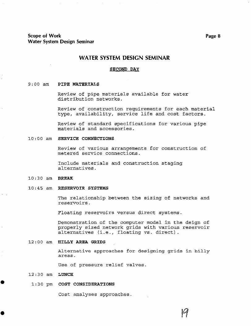
WATER SYSTEM DESIGN SEMINAR
SECOND DAY
Page 8
9:00 am PIPE MATERIALS
Review of pipe materials available for waterdistribution networks.
Review of construction requirements for each materialtype t availabilitYt service life and cost factors.
Review of standard specifications for various pipematerials and accessories.
•
•
10:00 am SERVICE CONNECTIONS
Review of various arrangements for construction ofmetered service connections.
Include materials and construction stagingalternatives.
10:30 am BREAK
10:45 am RESERVOIR SYSTEMS
The relationship between the sizing of networks andreservoirs.
Floating reservoirs versus direct systems.
Demonstration of the computer model in the deign ofproperly sized network grids with various reservoiralternatives (i.e. t floating vs. direct).
12:00 am HILLY AREA GRIDS
Alternative approaches for designing grids in hillyareas.
Use of pressure relief valves.
12:30 am LUNCH
1:30 pm COST CONSIDERATIONS
Cost analyses approaches .

•
•
Scope of WorkWater System Design Seminar
Lifecycle costing.
Basis for establishment of user fees.
Impact of various materials on costs/user fees.
Impact of network design on costs/user fees.
Impact of water loss on user fees.
2:30 pm DEMONSTRATION SOFTWARE CASE STUDY
Emphasize reservoir design alternatives.
3:15 pm BREAK
3:30 pm CASE STUDY (continuation)
4:15 pm SUMMARY
4:30 pm CLOSE
10
Page 9

Scope of WorkWater System Design Seminar
WATER SYSTEM DESIGN SEMINAR
EXAMPLE MODULE
Second Day -- 9:00-10:00 am
Objectives:
Page 10
•
•
•
1. Understand the various types of pipe available for waternetworks and service connections.
2. Understand the impacts of using various types of pipe oncosts, construction and life of system.
3. Understand the advantages and disadvantages of each type ofpipe.
Topics:
1. Definition of Pipelines
a. Trunk Mains
b. Distribution Mains
c. Service Lines
d. House Connections
2. Discussion of Pipe Materials
a. Asbestos Cement
b. Ductile Iron
c. Glassfibre Reinforced Plastic (GRP)
d. High Density Polyethylene (HDPE)
e. Polyvinyl Chloride (PVC)
f. Coated Steel
g. Galvanized
h. Other
3. Advantages and Disadvantages of Each

•
•
•
•
Scope of WorkWater System Design Seminar
4. Installation Criteria for Each
a. Excavation, Laying, and Backfilling Procedures
b. Joints and Fittings
c. Corrosion Protection
d. Testing
e. Repair and Hookup
5 . Maintenance
6. Availability
a. Local Production
b. Local Suppliers/Importers
7. Costs
8. Standards and Specifications
a. International Standards
b. Local Standards
c. Procurement Testing and Inspection
9. Mixing Pipe Materials
10. Summary and Suggestions for the Region
11. Questions and Comments
Page 11

•
•
•
•
WATER SYSTEM DESIGN SEMINAR
PART II
HANDOUT MATERIALS AT SEMINAR HELD ON
MAY 14 AND MAY 15
1996
AT
BEIR ZEIT UNIVERSITY
SPONSORED BY
USAIDI WEST BANK AND GAZA
AND
UNDP JERUSALEM OFFICE

PART 11
CONTENTS
HAND OUT MATERIALS
TAB
•
•
•
•
EPANET users manual
Installing EPANET
Water Distribution System Seminar - Notes
Pipe Materials - Notes
AWWA PVC Pipe Design and Installation
Appendix A - AWWA Guidelines Criteria for 1/2 in. through 3 in. PE pipe
Indianapolis Water Company Goes to School (re. PE)
Fairfax County, Va., Public FacBities Regs. for Water and Fire (partial)
Fairfax County Water Authority Water Main Inst. Service Contracts
Plans - Notes
Cost Analysis - Notes
1
2
3
4
5
6
7
8
9
10
11

~
EPANET USERS MANUAL
by
Lewis A. RossmanDrinking Waler Research Division
Risk Reduction Engineering LaboraloryCincinnali, Ohio 45268
RISK REDUCTION ENGINEERING LABORATORYOFFICE OF RESEARCH AND DEVELOPMENT
U.S. ENVIRONMENTAL PROTECTION AGENCYCINCINNATI.OH 45268
January 1994(Version 1.1)
DISCLAIMER
The information in this document has been funded wholly or in part by the U.S.Environmental Protection Agency (EPA). It has been subjected to the Agency's peer andadministrative review. Ind hiS been Ipproved for publication IS In EPA document.Mention of trade names or commercial products does no\ constitute endorsement orrecommendation for lise.
Allhough a reasonable effort has been made to assure that the resulls obtained are correct,the compuler programs described in this manual are experimental. Therefore the aUlhorand Ihe U.S. Environmental Protection Agency are not responsible and assume no liabilitywhatsoever for any resulls or any use made of Ihe resulls obtained from these programs,nor for auy damages or litigalion that result from the use of these programs for anypnrpose.
2

FOREWORD
Todays rapidly developing and changing technologies and induslrial products andpractices frequently carry with them the increased generation of materials Ihat, ifimproperly dealt With, can threaten both public health and Ihe environment. The U.S.Environmental Protection Agency (EPA) is charged by Congress with protecling theNation's land, air, and water resources. Under a mandate of national environmental laws,the Agency slrives to fonnulate and implement actions leading to a compatible balancebetween human activities and the ability of natural systems to support and nurture life..These laws direet the EPA to perform research to defme our environmental problems,measure Ule impacts, and search for solutions.
The Risk Reduction Engineering Laboratory is responsible for planning, implementing,and managing research, development, and demonstration programs to provide anauthoritative, defensible engineering basis in support of the policies, programs, andregulations of the EPA wilh respect to drinking water, wastewater, pesticides, toxicsubstances, solid and hazardous wastes, and Superfund-related activities. This pubticationis one of the products of that research and provides a vilal communication link betweenIhe researcher and the user community.
In order to meet regulatory requirements and customer eKpectalions, water utilities arefeeling a growing need to understand beller the movement and Iransformalion undergoneby treated water introduced into their distribution systems. EPANET is a computerizedsimulation model thai helps meet this goal It predicts the dynamic hydraulic and waterquality behaviQr within a drinking water distribution system operating over an extendedtime period. This manual describes the operation of the program and shows how it can beused to analyze avariety ofwater quality related issues in distribution systems.
E. Timothy Oppelt, DirectorRisk Reduction Engineering Laboratory
ABSTRACf
EPANET is a compuler program that performs extended period simulation of hydraulicand water quality behavior within drinking water distribution systems. It tracks the flowof water in each pipe, the pressure al each pipe junction, the height of water in eachslorage lank, and the concenlralion ofasubstance throughout a distribution system duringa multi-time period simulation. In addition to subslance concentrations, waler age andsource tracing can also be performed. The water quality module of EPANET is equippedto model such phenomena as reactions within the bulk flow, reactions at the pipe wall, andmass transport between the bulk flow and pipe wall. This manual describes how to use theEPANET program on a personal compuler under both DOS and Microsoft@ Windows"".Under Windows the user is able to edit EPANET input files, run a simulation, display Iheresults on acolor coded map of the distribution system and generate additional tabular andgraphical views of these results.
-2

FIGURES
Number ~
TABLES
Number ~
-tl
2.1 Node·Link Represenhtion ofaNetwork 32.2 Example ofaPump Characteristic CUlVe 62.3 Pump CUlVe Willi Extended Flow Range 72.4 Effect ofReialive Speed (n) on Pump CUlVe 82.5 Time Pattern for Water Usage II4.1 Example EPANBT Input Dala 244.2 Examples of Pump CUlVe Input Requirements 394.3 Definition ofTank Levels ,................................ 494.4 Example·Map File 555.1 Text Edilor Command Summary 655.2 Contents of EPANET4D.BAT 666.1 Example Contents of the EPANET4W Workspace 696.2 File Dialog Dox 716.3 Text Editor Command Summary 726.4 The Browser 766.5 Legend Dialog Box 796.6 Map Options Dialog Box 806.7 Table Search Dialog Box 816.8 Graph Options Dialog Box 836.9 Data to Link Willi aGraph 836.10 Graph With Linked Data 847.1 Nelwork for Example I...................................................... 887.2 Input Data for Example I 887.3 Portion ofOutput Report for Example I 917.4 Network for Example 2 947.5 Input Dala for Example 2 967.6 ObselVed (X) and Predicted Fluoride Levels at Node II
ofExample 2..................................................................... 987.7 Network for Example 3 997.8 Detail ofNetwork Around River Source 1007.9 Spatial Coverage ofWater From uke Source After
14 Hours 102
2.1 Pipe Head Loss Formulas 52.2 Rouglmess Coefficients for New Pipe 52.3 Loss Coefficients for Common Components 104.1 Summary ofDefault Parameter Values 584.2 Summary ofInput Parameter Units 59

TABLE OF CONTENTS
Disclaimer iiForeword iiiAbstract ivFigures viiTables viiiAcknowledgemcnts ix
I. Introduction ..
2. nle NClwork Modcl.............................................................. 3
2.1 Network Componcnls .. 32.2 Time Paltems 112.3 Hydraulic Simulation Model...................................... 122.4 Water Quality Simulation Model............................... 142.5 Reaction Rate Model............................................... 152.6 Water Age and Source Tracing 17
3. Installalion 18
3.1 System Requiremcnts 183.2 Installation for Doth Windows and OOS..................... 183.3 Installation for DOS Only.......................................... 193.4 Customizing Your Installation 20
4. Input Data Fonnats 22
4.1 Data Preparation 224.2 Input File Organizalion 234.3 Input File Fonnal........................................................ 264.4 Verification Filc Fonnat 544.5 Map File Fonnal........................................................ 554.6 Sununary ofDcfaull Values and Units 57
s
5. RUlltling BPANET Under OOS 60
5.1 GenmllnslnlctiOllS 605.2 Contents oCthe OUtput Report 615.3 The EPANET4D Program 63
6. RUl1tIing BPANET Under Windows 68
6.1 Ovcrview 686.2 Launching the Program 706.3 Operating Procedures 706.4 Summary oCMenu Commands 85
7. Example Applications 81
7.1 Introduction 877.2 Example 1- Chlorine Decay 817.3 Example 2- Fluoride Tracer Analysis 947.4 Example 3- Source Tracing 99
Appendix A. Files Installed by EPANET 103
Appen,dix B. Error and Waming Messages 105
Appendix C. The KYP2EPA Conversion Program 109
Appendix D. Troubleshooting 110
6
~

~
ACKNOWLEDGEMENTS
Special thanks are owed to Dr. Waller M. Grayman, Consulting Engineer, and to Dr. PaulF. Boulos of Montgomery Watson for the many suggestions and hours of testing theyprovided during the development of the EPANET program. Without their assistance, thequality ofthis product would be substantially less.
The efforts of Dr. Rolf Deininger and Kuo.Liang Lei of the University of Michigan, Dr.Charles N. Haas ofDrexel University, Eugene Mantchev ofthe Seallie Water Department,and Drs. Lindell Ormsbee and Srioivas Reddy of the University of Kentucky in beta·testing the EPANET program are also greatly appreciated. Gayle Smalley of the NorthMarin Water District and Rob Tull of Montgomery Watson supplied data for one of theexample networks in Chapter 7. Dr. James Uber of the University of Cincinnatj alongwith his students Cheryl Bush, Mao Fang, and Ken Hickey, provided Ihoughtful discussionon many key issues. The p,ublic domain text editor TE 2.61 used by EPANET wasdeveloped by John D. Haluska.
A fUlal note of acknowledgement goes to Dr. Robert M Clark, Director of RREL'sDrinking Water Research Division, whose pioneering work in modeling water qnality indistribution systems and personal encouragement inspired the development ofEPANET.
9
CHAPTER 1
INTRODUCTION
EPANET is a computer program that performs extended period simulation ofhydraulic and water quality behavior within pressurized pipe networks. Anetworkcan consist of pipes, nodes (pipe junctions), pumps, valves and storage tanks orreservoirs. EPANET tracks the flow of water in each pipe, the pressure at eachnode, the height of water in each tank, and the concentration of a substancethroughout the network during a multi·time period simulation. In addition tosubstance concentrations, water age and source tracing can also be simulated.
EPANET is designed to be a research tool for improving our understanding of themovement and fate ofdrinking water constituents within distribution systems. Thewater quality module of EPANET is equipped to model such phenomena asreactions within the bulk flow, reactions at the pipe wal~ and mass transportbetween the bulk flow and pipe wall. As we gain more experience and knowledgeof water quality behavior within distribution systems we intend to update andrefine EPANET to reflect this progress.
Another distinguishing feature of EPANET is ils coordinated approach tomodeling network hydraulics and water quality. The program can compute asimultaneous solution for both conditions together. Alternatively it can computeonly network hydraulics and save these results to a file, or use a previously savedhydraulics file to drive awater quality simulation.
EPANET can be used for many different kinds of applications in distributionsystem analysis. Sampling program design, hydraulic model calibration, chlorineresidual analysis, and consumer exposure assessment are some examples.EPANET can help assess alternative management strategies for improving waterquality throughout asystem. These would include:
• allering source utilization within multiple source systcms,
• altering pumping and tank filling/emptying schedules ,
• use ofsatellite treatment, such as re-chlorination at storage tanks,

• targeled pipe cleaning and replacement.
EPANET was coded in the C language and makes use of dynamically allocatedmemory. Thus (he only limits on network size are available memory. The versionof EPANET contained on the distribution disk is intended for use on IBMcompatible personal computers running under DOS. However it is a relativelysimple task to re-compile the source code to run on other machines, such as UNIXMlrkslations.
The EPANET package contains 1wo program modules. One is anetwork simulatorthat runs under DOS, receiving ils inpul from a file and writing its output toanother file. The user must use external programs 10 editlhe input file and view orprint the output file. (An optional DOS shell program is provided that interactivelyedits EPANET input, runs the simulator, and views or prints ils oulput according10 selections made from amenu). The second module is aMicrosoll@ WindowsTlA
lx program that allows one to edit EPANET input data, run the simulator, andgraphically display its resulls in a variety of ways on a map of the network. Thusthere are IWO different ways to run EPANET •• under DOS or under Windows.We believe that for most situations Ihe visualization power oflhe Windows versionis an essential aid in trying to comprehend the resulls of running EPANET andrecommend that this mode be used if your computer hardware and software cansllpport it.
Chapter 2 of Ihis manual describes how EPANET models water distributionsystems. Chapter 3 tells you how to install the EPANET system on your personalcomputer. Adetailed description of the program's input data fonnat is provided inalapter 4, while Chapters 5 and 6 give instructions for running EPANET underDOS and Windows, respectively. Finally, Chapter 7 illustrates different fealures ofthe program by running several example applications.
CHAPTER 2
THE NETWORK MODEL
2.1 Network Components
EPANET views a water distribution network as a collectio'n of links connectedtogether at their endpoints called nodes. Figure 2.1 illustrates a node-linkrepresentation ofasimple water network.
Clie'ckValve
Figure 1.1 Node-Link Representation ofa Network
As shown in the figure,links come in several varieties:
I. pipes
2. pumps
3. valves.
Besides being the junction point between connecting pipes, nodes can se,,'e as:
~
2
I. points ofwater consumption (demand nodes)
3

How EPANBT models the hydraulic behavior of each of these components will bereviewed next. For the sake of discussion we will express all flow rates in cubicfeet per second (cfs), although the program can also accept flow units in gallonsper minute (gpm), million gallons per day (mgd), or liters per second (Us).
=====================================--============--====Notes: C=Hazen·Williams roughness coefficient
E=Darcy-Weisbach roughness coefficient (ft)f =friction factor (dependent on E, d, and q)d=pipe diameter (ft)L=pipe length (ft)
2.
3.
points ofwater input (source nodes)
locations of tanks or reservoirs (storage nodes).
Chezy-Manning(full pipe flow)
4.66 n2d-H3 L 2
Pipes Table 2.1 Roughness Coefficients for New Pipe
where hL is the head loss in feel, q is the flow in cfs, a is a resistance coefficient,and bis a flow exponent.
Pipes convey water from one point to another. Flow direction is from the end athigher head (potential energy per pound of water) to that at lower head. The headlost to friction associated with flow through a pipe can be expressed in a generalfashion as:
BPANET can use one of three popular forms of Equation I: the Hazen-Williamsformula, the Darcy-Weisbach formula, or the Chezy.Manning formula. TheHazen-Williams formula is probably Ihe most popular head loss equation fordistribution systems, the Darcy-Weisbach formula is more applicable to laminarflow and to fluids other than water, while the Chezy-Manning formula is morecommonly used for open channeillow. Table 2.1 lists values of the resistancecoefficients and flow exponents for each formula. Note that each formula uses adifferent pipe roughness coefficient that must be determined empirically. Table 2.2lists general ranges of these coefficients for different types of new pipe materials.Be aware that apipe's rouglmess coefficient can change considerably with age.
Pipes can contain check valves in them that restrict flow to a specific direction.They can also be made to open or close at pre-set times, when tank le~els fallbelow or above certain set-points, or when nodal pressures fall below or abovecertain set-points.
======;=;================--===============--========----===
(2)
Manning'sn
0.015·0,017
0.011-0.015
0.015·0.017
0.013 - 0.0I5
0.012 -0.0 I5
0.012-0.017
0.5
0.005
0.15
0.85
1.0- 10
Darcy-WeisbachE,millifeet
120
140 ·150
140· ISO
110
130 -140
120 ·140
Hazen-WilliamsC
ho =bo· aqb
Material
A pump is a device that raises the hydraulic head of water. The relationshipdescribing the head imparted to a fluid as a function of ils flow rate through thepump is termed the pump characteristic curve. Figure 2.2 gives an example.EPANET represents pump curves with a function of the fonn:
=================================================--=====
Cast IronConcrete orConcrete LinedGalvanized IronPlasticSteelVitrified Clay
===~===================================================
Pumps
(I)hL =aqb
~
=======:;==============================----==============
=============--========--=======================--========
Table 2.1 Pipe Head Loss Fonnulas
Resistance Coefficient (a) Flow Exponent (b)
where ho is the head gain imparted by the pump in ft, q is the flow through thepump in cfs, ho is the shutoff head, a is a resistance coefficient, and b is a flowexponent. By supplying EPANET with the shutoff head ho and two other pointson the pump curve, the program is able to estimate values for aand b.
1.85
2
4.72 C-t.8S d-4.87 L
0.0252 Qe,d,q) d·S L
Formula
Hazen-Williams
Darcy·Weisbach
4 S

Anolher way 10 represent I pump when ils charaleristic cUlVe is unknown is toassume thai it adds energy to the water at I conslant rale. In Ihis case the equationof the pump cwve would be
where Hp is the pump horsepower. The Jailer quantity can be computed based onan initial estimate of the flow and head at which the pump will operate. This typeofpump cUlVe should only be used for steady-state, preliminary design studies.
Flow through a pump is unidirectional and pumps must operate within the headand flow limits imposed by their characteristic cUlVes. If the syslem conditionsrequire Ihal the pump produce more Ihan ils shutoff head, EPANET will allempl10 close the pump off and will issue a warning message. EPANET allows you tolurn pumps on or off at pre-set times, when tank levels fall below or above certainset-poinls, or when nodal pressures fall below or above certain sel-points. Variablespeed pumps can also be considered by specifYing that their speed selling bechanged under these same types of conditions. By defmition, the original pumpcurve supplied to the program has a relative speed selling of I. If the pump speeddoubles, then Ihe relalive selling would be 2; if run at half speed, the relativeselling is 0.5 and so on. Figure 2.4 illustrates how changing a pump's speedselling affects its characteristic cUlVe.
(3)ho =8.81 Hp/q
Figure 2.2 Example ofa Pump Characteristic Curve
floII'. tIs
400
300
:::,;
200".,X
100
00 3 6 9 12
Some pumps exhibit a different type of characteristic curve beyond their normalflow range. Figure 2.3 shows a pump with a linear head-flow relation in itsextended flow rang~. In this case EPANET can describe the pump's behavior withtwo equations, one for the normal flow range and another for its extended flowrange.
Figure 2.4 Effecl ofRelalive Speed (n) on Pump CUlVe
0100 , ,
SOD
::
i 200:r
"I
\ exto/lded100 t ,--
, Flow Range,,,,0' , , \
0 4 I 12 l'FloW, ct\
Figure 23 Pump CUlVe wilh Extended Flow Range
aDo
1100
:::,;
400...,X
200
00 A e
flow, cIs
12 1&
~
6 1

where K is a minor loss coefficient, q is flow rate in cfs, and d is diameter in ft.Table 2.3 gives values of Kfor several different kinds ofcomponents.
Minor head losses (also called local losses) can be associated with the addedturbulence that occurs at bends, junctions, meIers, and valves. The importance ofsuch losses will depend on the layout of the pipe network and the degree ofaccuracy required. EPANET allows each pipe and valve to have a minor losscoefficient associated with it. It computes the resulting head loss from thefollowing formula:
Valves
Aside from the valves in pipes that are either fully opened or closed (such as checkvalves), EPANET can a~o represent valves that control either the pressure or flowat specific points in 8 network. Such valves are considered as links of negligiblelength with specified upslresm and downstream junction nodes. The types ofvalves that can be modelled are:
I. Pressure Reducing Valves (PRVs)
2. Pressure Sustaining Valves (PSVs)
hL =0.0252 Kq2 d-4 (4)
3. Pres~ure Breaker Valves (PBVs)'Table 2.3 Loss Coefficients for Common Components=======================================4. Flow Control Valves (FCVs)Component Loss Coefficient
~
5. Throllie Conlrol Valves (TCVs)
PRVs limit the pressure on their downstream end to not exceed a pre·set valuewhen the upstream pressure is above the selling. If the upstream pressure is belowthe selling, t'hen flow through the valve is nnrestricted. Should the pressure on thedownstream end exceed that on the upstream end, the valve closes to preventreverse flow.
PSVs try to maintain a minimllm pressure on their npstream end when thedownstream pressure is below that value. If the downstream pressure is above theselling, then flow through the valve is unrestricted. Should the downstreampressure exceed the upstream pressure then the valve closes to prevent reversenow.
PBVs force a specified pressure loss to occur across the valve. Flow can be ineither direction through the valve.
FCVs limit the flow through avalve to aspecified amounl. The program producesa warning message if this flow callnot be maintained without having to addadditional head at the valve.
TCVs simulate a partially closed valve by adjusting the minor he~d loss coefficientof the valve. Arelationship between the degree to which the valve is closed andthe resulting head loss coefficicnt is usually available from the valve manufacturer.
Minor Losses
8
=======================================
Globe valve, fully open 10.0
Angle valve, fully open 5.0
Swillg check valve, fully open 2.5
Gale valve, fully open 0.2
Short·radillS elbow 0.9
Medium-radius elbow 0.8
Long.radillS elbow 0.6
45° elbow 0.4
Closed return bend 2.2
Standard tee • flow through run 0.6
Standard tee· flow through branch 1.8
Square entrance 0.5
Exit 1.0================--=======================
Nodes
All nodes should have their elevation above sea level specified so that thecontribution to hydraulic head due 10 elevation can be computed. Any waterconsumption or supply rates at nodes that are not storage nodes must be knownover the duration oftime the network is being analyzed. Storage nodes (i.e., tanksand reservoirs) are special types ofnodes where a free water surface exists and thehydraulic head is simply the elevation of water above sea level. Tanks aredistinguished from reservoirs by having their water surface level change as waterflows into or out ofthem •• reservoirs remain at a constant water level no mailer
9

2.2 Time Patterns
"'hat the now is. EPANET modcls the change in water level of a storage tankwith the following equation:
Thus EPANET needs to know the cross-sectional area as well as the minimum andmaximum pcrmissible water levels for storage tanks. Reservoir.type storage nodesare usually used to represent external water sources, such as lakes, rivers, or wellficlds. Storage nodes should not have an external water consumption or supplyrate associated wilh them.
EPANET assumes thai water usage rates, external water supply rales, andconstituenl source concentrations at nodes remain constant over a fIXed period oflime, but these quantities can change from one time period to another. The defaulltime period interval is I hour, but this can be set at any desired value. The value ofany ofthese quantities in a time period equals a baseline value mUlliplied by a timepattern factor for that pcriod. Figure 2.S illustrates a pattern of factors that mightapply to daily waler demands, where each period is of 2 hours duration. Differentpallems can be assigned to individual nodes or groups ofnodes.
"
......r-- -
r-- r--
r-- -- -
r-- -......
The hydraulic model used by EPANET is an extended period hydraulic simulatorthat solves the following set of equations for each storage node s (tank orreservoir) in the system:
2
o2 3 4 :l 0 7 8 9 10 11 12
PeriodFigure 2.5 Time Pattern for Water Usage
..ooGIU.
aJ0)IIIIII~
2.3 Hydraulic Simulation Model
(5)
change in water level, ftflow rate into (+) or out of(-) lank, cfscross·sectional area ofthe tank, ft2lime interval, sec
where Ay =qA =At
Ay =(qlA:) At
(6)'Oys/i1 =qsl As
~(7)qs =Ejqis- I:jqsj
(8)hs =Es + Y.
along with the following equations for each link (between nodes i and j) and eachnodek:
hj • hj = f(qij) (9)
Ijqik - Ijqkj - Ok = 0 (10)
where the unknown qlUlntities are:Y. = height ofwater stored at node s, ft
10 \I

Equation (6) expresses conservation of water volume at a storage node whileEquations (7) and (10) do the same for pipe junctions. Equation (9) represents theenergy loss or gain due to flow within alink. For known initial storage node levelsys at time zero, Equations (9) and (10) are solved for all flows qij and heads hiusing Equation (8) as a boundary condition. This step is called "hydraulicallybalancing" the network, and is accomplished by using an iterative technique tosolve lhe nonlinear equations involved.
(II)
concentration ofsubstance in link ij as afunction ofdistance and time (i.e., Cjj :: Cij(Xij,t)), mass/ft3distance along link ij, ftflow rate in link ij at time ~ cfscross-sectional area of link ij, ft2rate ofreaction ofconstituent within link ij, mass/ft3/day
::
::
::
Oeij lilt :: -(qij I Aij)(Oeij /axij) + 9(cij)
XijqijAijO(Cij)
Equation (II) must be solved with a known initial condition at time zero and Ihefollowing boundary condition at the beginning oflhe link, i.e., at node i where Xij ::0:
where cij
EPANET's dynamic water quality simulator tracks the fate of a dissolvedsubstance flowing through the network over time. It uses the flows from thehydraulic simulation to solve I conservation of mass equation for the substancewithin each link connecting nodes i and j:
::
::
q!qijhi
Es
Okf(')
flow inlo storage node s, cfsflow in link connecting nodes i and j, cfshydraulic grade line elevation at node i (eqll8lto elevationhead pins pressure head), ft
and !he known constants are:At :: cross-sectional area ofstorage node s (taken as infinite
forreservoirs~ ft2elevation ofnode s, ft ,flow consumed (+) or supplied (0) at node k, cfsfunctional relation between head loss and flow in a link
The summations are made over all links k,i that have flow into the head node (i) oflink ij, while Lki is the length of link k,L Mj is the substance mass introduced byany extental source at node ~ and Qsi is the source's flow rate. Observe that theboundary condition for link ij depends on the end node concentrations of all linksk,i that deliver flow to link ij. Thus Equations (II) and (12) form acoupled set ofdilferentiaUalgebraic equations over all links in the network.
EPANET solves these equations by I numerical scheme called the DiscreteVolume Element Method (DVEM) (Rossman, L.A., Boulos, P.F., and Allman, T.,"The Discrete Volume Element Method for Modeling Water Quality in PipeNetworks", Jour. Waler Resources Planning and Management, VoL 119, No.5,September/October 1993.). Within each hydraulic time period when flows areconstant, DVEM computes I shorter water qualily time step and divides each pipeinto a number of completely mixed volume segments. Within each water qualitylime step, the material contained in each pipe segment is ftrSt transferred to itsadjacent downstream segment. When the adjacent segment is I junction node, themass and flow entering the node is Idded to Iny mass and flow already receivedfrom other pipes. After this Iransport step is completed for III pipes, the resultingmixture concentration at each junction node is computed Ind released inlo thehead end segments ofpipes with flow leaving Ihe node. Then the mass within eachpipe segment is reacted. Tha sequence of steps is repeated until the time when I
13
~f
The method used by EPANET 10 solve Ihis system of equations is known as the"gradient algorithm" (Todin~ E. and Pilal~ S., "A gradient method for the analysisof pipe networks", International Conference on Computer Applications for WaterSupply and Distribution, Leicester Polytechnic, UK, September 8-10, 1987.) andhas several attractive features. Firsl,the system of linear equations to be solved ateach iteration of the algorithm is sparse, symmetric, and positive-defmile. Thisallows highly efficient sparse matrix techniques to be used for their solution·(George, A. and Lin, J. W·H., Compuler Solulion of Large Sparse PositiveDefinite Systems, Prentice-Hal~ Inc., Englewood Cliffs, NJ, 1981.) Second, themethod maintains flow continuity at all nodes after its ftrSt iteration. And third, itcan readily handle pumps and valves without having to change the structure of theequation matrix when !he slatus of!hese components changes.
After a netwo'rk hydraulic solution is obtained, flow into (or out of) each storagenode, qs is found from Equation (7) and used in Equation (6) to fmd new storagenode elevations after a time step dt. This process is then repeated for allsubsequent time steps for !he remainder of the simulation period.
The normal hydraulic time slep used in EPANET is I hour, but can be madeshorter if more accuracy is needed. Shorter time steps than normal can occurautomatically whenever pipe or pump controls are activated (e.g., a tank 1iI1s to thelevel that causes a pump to shul 011), or when a tank becomes either empty or full(causing the tank outlet/inlet line to be closed).
2.4 Water Quality Simulation Modelt2
rk IIki Ckj<LJd,t) +MjCij(O,t) =------
rkQki +Qsi(12)

new hydraulic condition occurs. The network is Ihen re-segmented and thecomputations are continued.
The water quality time steps used in the method are chosen to be as large aspossible without causing any pipe's flow volume to exceed its physical volume(i.e., have mass transported beyond the end of the pipe). Thus the water qualitytime step dtwq cannot be larger than the shortest time oftravelthrough any pipe inthe network, i.e.:
The flfst term in this equation models bulk flow reaction, while the second term,which includes a new unknown Cw, represenls the rate at which material istransported between the bulk flow and reaction siles on the pipe wall. Assumingthat the rate of reaction at the wall is fIrSt order with respect to Cw and that itproceeds at the same rate as material is transported to the wall (so that noaccumulation occurs), we can write the following mass balance for the wallreaction:
dtwq =Min (Vij /qjj) for all pipes ij (13)k«c-Cw) = kwew (16)
where kwis a wall reaction rate constant with units of filsec. Solving for Cw andsubstituting into Equation (IS) results in the following reaction rate expression:where Vij is the volume of pipe ij and qij is its flow rate. Pumps and valves are
not included in this determination since transport through them is assumed tooccur instantaneously. Under Ihis water quality time step, the number of volumesegments in each pipe (nij) is:
ll(c) =-Kc (17)
where INTlx] is the largest integer less than or equal to x. EPANET limits dtwq tobe no smaller Ihan a user-adjustable time tolerance, so that solution times and thenumber of segment volumes do not become excessive. The default value of Ihistolerance is 1110 the lenglh of the hydraulic time step. In addition, the user canspecify a maximum number ofvolume segments Ihat any single pipe can be dividedinto. The default value for this parameter is 100.
The above discussion pertains to substance decay, with mass transfer from Ihe bulkflow to the pipe wall. Dropping tbe negative sign in front of K in Equation (17)would model the growth of a substance, with mass transfer from the pipe wall tothe bulk 110w.
nij = INT (Vij / (qij dtwq)] (14)where K is an overall first order rate conslant equal to:
kwkeK =kb+---
RIrtkw+ kr)(18)
2.5 Reaction Rate Model
Equation (11) of EPANET's water quality model provides a mechanism forconsidering the loss (or growth) ofasubstance by reaction as it travels through thedistribution system. Reaction can occur both wilhin the bulk flow alld withmaterial along the pipe wall. EPANET models both types of reactions using flfstorder kinetics. In generaL within any given pipe, material in the bulk flow willdecrease at a ratc equal to:
To summarize,there are three coefficients used by EPANET to describe reactionswithin a pipe. The pipe's bulk rate constant kb and its wall rate constant kwmustbe determined empirically and supplied as input to the model. The mass transfercoefficicnt ke is calculated internally by EPANBT using the dimensionlessSherwood Number as follows <Edwards, O.K., Denny, V.B.• and Mills. A.F.,Transfer Processes. McGraw-Hili, New York, NY. 1976'>:
O(c) =-kbC - (kef RH)(C' ew) (IS)
kr = ShDfd
Sh = 0.023 ReO.S3 ScO.333 for Re t! 2300
(19)
(20)
~
where kbcke
RHCw
first-order bulk reaction rate constant, lIsecsubstance concentration in bulk flow. mass/ft3mass transfer coefficient belwecu bulk flow and pipewall, ftlsechydraulic radius ofpipe (pipe radius/2), ftsubstance concentration at the wall, mass/ft3
t4
Sh =3.6S +
where kr =ShRe =
0.668(dIL)Re Sc
I +.04[(dIL)Re ScJ.61forRe <2300
mass transfer coefficient, filsecSherwood NumberReynolds Number (q d/ Af II)
(21)
15

ScdLqAD =v
Sclunidt Number (v / D)pipe diameter, ftpipe length, ftflow rate, cfscross-sectional flow area ofpipe, ft2molecular diffusivity ofsubstance in fluid, ft2/seckinematic viscosity offluid, ft2/sec
CHAPTER 3
INSTALLATION
~
Equation (20) applies to turbulent flow where the mass transfer coefficient isindependent of the position along the pipe. For laminar flow, Equation (21)supplies an average value of the mass transfer coefficient along the length of thepipe.
2.6 Water Age and Source Tracing
In addition to chemical transport, EPANET can also model the changes in age ofwater over lime throughonta network. To accomplish this, the program interpretsthe variable c in Equation (II) as the age of water and sets the reaction term lI(c)in the equation to a constant value of \.0. During the simulation, any new waterentering the network from reservoirs or source nodes enters with age of zero.Water age provides a simple, non·specific measure of the overall quality ofdelivered drinking water. When the model is run under constant hydraulicconditions, the age of water at any node in the network can also be interpreted asthe time of travel 10 Ihe node.
EPANET can also track over time what percent of water reaching any node in thenetwork had ils origin at a particular node. In this case Ihe variable c in Equation(II) becomes the percentage of flow from the node in question and the reactionterm is set to zero. The c·value of the source node is kept at 100 percenttltrqugltouttlte duration of tlte simulation. The source node can be any node in thenetwork, including storage nodes. Source tracing is a useful tool for anaiyziugdistribution systems drawing water from two or more different raw water supplies.It can show to what degree water from a given source blends with that from othersources, and how the spatiaIpattern oftNs blending changes over time.
3.1 System Requirements
To install EPANET to run under both Windows and DOS requires the followiug:
an ffiM-compatible PC equipped with an 80286 or higher CPUMS·DOS or PC·DOS version 3.0 or laterMicrosoft Windows version 3.0 or laterat least 3megabytes of free disk space
To install EPANET for I)OS only requires a PC equipped with an 8088 or higherCPU running MS·DOS or PC·DOS version 3.0 or laler. Allhough not required, amath co-processor is highly recommended.
3.2 Installation For Both Windows and DOS
To iustall EPANETsotllat it willl\Ul under either Windows or DOS:
1. Place the distribution disk in a floppy disk drive (drive Aor B).
2a. IfWindows is not muning, enter the command
WIN A.·SETUP
at the DOS prompt (use IVlN B:SEI'UP instead if the distribution disk isin drive B).
2b. If Windows is already running, select Run from the FIle menu of theProgram Manager, type A:SETUP ill the Command Line box. and selectthe OK bullon. (Type B:SETUP instead if the distribution disk is in driveB).
3. Ifyou wish to install EPANET in a directory otlier than C:\EPANET enterthe full path name for your directory choice in the dialog box that appealS.
16 11

After a successful installalion, a new Program Group named EPANET will beadded to your Program Manager, with an EPANET icon in it.
••5.
Select the Continue bullon to resume the inslallalion.
When lhe installation is completed, a README.TXT file will bedisplayed in the Windows Notepad program informing you of anymodifications to the users manual and how to further customize yourinstallalion.
3.
4.
5.
When prompted, enter the full path name of your choice for an EPANETdirectory, or simply hit the Enter key to Iccept C:IEPANET.
Verify your choice ofan EPANET directory by hilling the y key. Hillingthe Escape key will cancel the installation, while any other key wiD ask youto re-specify In EPANET directory.
The relevant files will be copied from the installation disk to your EPANETdirectory.
Note: IfEPANET fails to install properly, try lhe following:
Shut down all other Windows applications that may be running (such as theClock) aud launch the setup program again from Program Manager.
Exit from Windows, change directories to the Windows directory (typicallyc:\windows), and repeat the installation procedure.
If using Windows for Workgroups, exit from Windows, re-start Windowsin Standard mode, and repeat the installation procedure.
Appendix Alists the various files that are installed on your system. If for somereason you need to re-install the entire EPANET system or only a portion of it,repeat the entire installation procedure as described above. Do not try to copyildividual files off of (he distribution disk since several of these files are in acompressed fonnat.
3.3 Installation For DOS Only
If your system is not equipped with Windows, you can install a version ofEPANET that will run only under DOS as follows:
Appendix Aalso lists those files installed for DOS operation only.
3.4 Customizing Your Installation
Running in 32·Bit Mode
EPANET's network simulator comes in both astandard version and 32-bit version.The Jailer works only on PC's equipped with an 80386 or higher CPU and whenrun under Windows, in Windows' 386 Enhanced mode. It runs simulations abouttwice as fast and makes all of the machine's extended memory available to theprogram. The standard version of the simulator can only use a maximum of 640kilobytes of conventional memory. Because the program size oflhe 32·bit versionof EPANET is about 260 kilobytes larger than the standard version, werecommend that you use it only if you have at least this amount of extendedmemory available on your machine.
If you want to run EPANET in 32-bit mode, you must modify theAUTOEXEC.BAT file in your root directory. Using any text editor or wordprocessor that saves its oUlput in ASCn format, add the following line to this file:
SET EPANET=JZ
(Note there are no spaces on either side of Ihe equal sign.) After re-booling yourmachine, EPANET will aulomatically run in 32·bil mode. To relurn 10 standardmode, simply remove Ihis line from your AUTOEXEC.BAT file and re·bool yourmachine.
I.
2.
Place the distribution disk in a floppy disk drive (eilher drive Aor B).
Enler the following command at the DOS prompt:
A:SETUND(or B:SETUND if the disk is in drive B).
\8
Using II Different Editor
The Windows version of EPANET comes wilh I public domain text editor that isused to edit input data files. It is a DOS program named TE.EXE Ihal EPANETruns within a DOS window. If you wish, you can substilule a different editor ofyour choosing. It can be either a DOS or Windows program that can accept the
19

name of the tile to edit on its command line, and is capable of editing large files.This would eliminate such programs as Ihe Windows Notepad which has a file sizelimit ofonly 32 kilobytes.
To replace the edilor that ships with EPANET with another DOS edilor (such asEDIT.COM that comes wilh MS·DOS 5.0 and later):
Use the Windows PIF Editor to change the sellings in the EDlTOR.PIF filein your EPANET directory. For example, to switch to the MS·DOS editorwhich resides ina directory named C:\DOS, use the following settings:
CHAPTER 4
INPUT DATA FORMATS
Program Filename:Window Title:Startup Directory:
C:IDOSlEDIT.cOMEDITOR
4.1 Data Preparation
Prior to running EPANET, the following inilial steps should be taken for thenetwork being studied:
~
To replace the default editor with aWindows editor:
Use any text editor to add the following section to the file EPANET.INI inyour Windows directory (ifthis file doesn\ exist then create it):,
IEDITORIProgralll=progralll name>Captioll=<window title>
where <program name> is the full path name ofthe editor program(e.g., C:IEDITORS\WINEDlIEXE) and <window title> is the
portion of the caption that always appears in the editor'smain window (e.g., WINED(1).
20
1. IdentifY all network components and their connections. Network componentsconsist of pipes, pumps, valves, storage tanks and reservoirs. The term "node"denotes ajunction where network components connect to one another. Tanksand reservoirs are also considered as nodes. The component (pipe, pump orvalve) cOlUlecting any two nodes is termed a "link".
2. Assign unique ID numben to all nodes. ID numbers must be between 1and2147483647, but need not be in any specific or~er nor be consecutive.
3. Assign an ID number to each link (pipe, pump, or valve). It is permissible touse the same ID number for both anode and a link.
4. Collect informalion on the following system parameten:a. diameter, length, rouglmess and minor loss coefficient for each pipe,b. characteristic operating curve for each pump.c. diameter, minor loss coefficient and pressure or flow setting for each
control valve.d. diameter and lower and upper water levels for each tanke. controllUles that determine how pump, valve and pipe settings
change with time, tank water levels, or nodal pressures,f. changes in water demands for each node over the time period being
simulatedg. initial water qll8lity at all nodes and changes in water qll8lity over
time at source nodes.
With Utis information in hand, you are now ready to construct an input file to usewith EPANET.
4.2 Input File Organization
2\

EPANET receives its input data from afile whose contents are divided into severaldifferent sections. Each section begins with aspecific keyword in brackets. Figure4.1 provides an example EPANET input file. (Any text appearing aller asemicolon is a comment added to enhance readability.) The keywords and thecategories of input data they represent are:
============--========--========(TITLE]EPANET Example Networl: 1
[JUNC'l'10NS]
i------------------------
The only mandatory sections are (JUNCTIONS), (TANKS), and (PIPES). Theorder of seclions is not important, except that whenever data in a sectionreferences a node, that node must have already been defmed in the (JUNCTIONS)or (TANKS) sections. The same holds true for any reference to a link (pipe, pumpor valve). To be safe then. you should place the (TITLE), (JUNCTIONS).ITANKS). (PIPES), (PUMPS), and (VALVES) sections first.
Each section ean contain one or more lines of dala. Blank lines may appearanywhere in the file and the semicolon (;) can be used to indicate that what followson the line is acomment, not data. Data items can appear in any column of a line,but a line cannot contain more than 80 characters. Observe how in Figure 4.1these features were used to create a tabular appearance for the data. complete witllcolumn headings. .
i------------------------
Figure 4.1 Example EPANET Input Data
%
o150150100150200150100100
710710700695700695690700710
101112132122233132
Elevation Demand; 10 it gpIII
===========================--====================
(TANKS]i--------------------------------------------
£lev. Init. Min. Max. Diam.; 10 it tevel Level Level it;----------------_.._-------------------------
2 850 120 100 150 50.59 800
(PIPES]i---- .. --........·-----..••• ..••• ..------------------ ..---; Head Tail Lengtb Diam. Rougb.;10 Node Node it in coeff.i------------------------·_·---------------------10 10 11 10530 18 10011 11 12 5280 14 10012 12 13 5280 10 10021 21 22 5280 10 10022 22 23 5280 12 10031 31 32 5280 6 100110 2 12 200 18 100111 11 21 5280 10 100112 12 22 5280 12 100113 13 23 5280 8 100121 21 31 5280 8 100122 22 32 5280 6 100
initial waler quality in networkbaseline contaminant source slrengthreaction rate coefficientsmiscellaneous analysis options
initial status ofselected linkslink control ntleswater demand and sonrce strengU. time paUemssimulation lime step parameters
changes in baseline water demandschanges in pipe roughness coefficients
signals end of input file
problem tiUejunction node informationtank/reservoir informationpipe informationpump informationvalve informationoulput report format
[TITLE)(JUNCTIONS)[TANKS)(PIPES)(PUMPS)[VALVES)[REPORT)
[STATUSI(CONTROLSI(PATTERNS)(TIMES)
[QUALITY)[SOURCES)[REACTIONS)(OPTIONS)
[DEMANDS)[ROUGHNESS)(END)
22 23

=============~==========~=======================
(PUMPS);-----------_ ..... __ ........._.........--_....
Keywords can appear in mixed lower and upper case. Unless specifically noted,the default wlits for all data are as follows:
;--_......------------- ...._---------; Head Tail Design H-Q;10 Node Node ft 9t:G
(CONTROLS)
9 9 10 250 1500
LengthPressureFlowConcentration
feetpounds per square inch (psi)gallons per minute (gpm)milligrams per liter (mgIL)
;_ - -_ _------------------_ ..LINK 9 OPEN IF NODE 2 BELOW 110LINK 9 CLOSED IF NODE 2 ABOVE 140
(PAmRNS);--..------_ _--_ - __ -------; ID Multipliers .....
An option is available in the (OPTIONS) section to change the flow units to eithercubic feet per second (cfs), million gallons per day (ntgd), or titers per second(Us). In the laller case, SI (metric) units would apply to all quantities, so lengthsand pressures would be expressed in meters (m). Concentration units can also bechanged in the [OPTIONS) section to any desired measure.
;---_ .. ------------ ...._.._..-..-....------_ ........---1 1.0 1.2 1.4 1.6 1.4 1.21 1.0 0.9 0.6 0.4 0.6 0.8 Steady.Stale
HydraulicsExtended PeriodHydraulics
Extended PeriodWater Quality
(QUALITY)
j-------- ..---_.._---_..........
i---------------- ............- .... - ...···-·..--- ..----- ..• ...----
;--------------_.._-------
(REACTIONS)
(TITLE)(JUNCTIONSI(TANKS)(pIPES)(PUMPS)(VALVES)(REPORT)····-_·_> (STATUS)
(CONTROLS)(PATIERNS)(TIMES)----->[QUALITY)
(SOURCES)[REACTIONS)(OPTIONS)
; Bulk decay coeff.; Wall decay coeff.
GLOBAL BULK - •5GLOBAL HALL -1
DURATION 24 ; 24 hour simulation periodPAmRN TIMESTEP 2 ; 2 hour pattern time period
2 32 O.S9 1.02 1.0
; Initial;Nodes Concen. mg/L
; ....._---------------_ .........._..------------------
(TIMES)
~-- (OPTIONS);_ ....._--_ .._---_ .._---------------_ .._------------- 4.3 Input File Format
QUALITY Chlorine ; Chlorine analysisMAP Net1.map; Hap coordinates file
(ENO)
Adetailed description of the data in each section ofthe input file will now be givenin alphabetical order. Each section begins on a new page. Mandatory keywordsare shown in boldface while optional items appear in parenlheses.
===============~=============================
Figure 4.1 Conlinued
24 25

SectMn: (CONTROLSI Secllon: (CONTROLSI (continued)
PUl'fOse:
Allows pump, valve and pipe seltings to change at specific times or whenspecific pressures or tank water levels are reached in the network.
Formats:
The first format implements the control at the designaled time. Times can beexpressed as hours:minutes or IS I decimal value. In the laller case, the defaultunits are hours.
The second format implements the control when a specified node drops below itsaclion level while the third format applies the control when the node rises abovethe aclion level.
LINK linklD setting AT TIME tvaille (llnils)LINK linklD setting IF NODE nodelD BELOW levelLINK linklD selling IF NODE nodelD ABOVE level
Paramelers:
linklDselling
IvailleIInils
nodeJDlevel
Remarks:
ID number ofa pump, vaIve or pipelink selting which can be:
•apump slahlS (either OPEN or CLOSED),•apump speed (relative to the speed used to define the
pump's characteristic cUlVe in the (PUMPSI section),•avalve setting (pressure, flow or loss coefficient)
or slalus (either OPEN or CLOSED)•apipe status (either OPEN or CLOSED)
time at which change in link selling appliesoptioualunits on control time which can be:
SECONDS (or SEC),MINUTES (or MIN),IIOURS(defaull),DAYS (or DAY)
ID ofcontrolling nodecontrol action level (either water level above tank bottomifcontrol node is a tank, ft (m), or pressure level ifcontrolnode is ajunction node, psi (m).
Sellings for constant-speed pumps are eilher OPEN (pump on) or CLOSED(pump oil). You can simulate I variable speed pump by specifying a speed factorfor its selling. When the factor is 0, the pump is off. When it is I, the pumpoperates on its original characterislic cUlVe. Olher speed faclor values shift theposilion of the characteristic curve as described in Chapler 2.
Conlrol valve sellings can be either numerical values or OPEN/CLOSED.
The only allowable seltings for pipes are OPEN or CLOSED. If. pipe is closed,EPANET assumes the existence of. valve somewhere in the line. DO NOTspecify avalve in the (VALVESI seclion to accomplish this purpose.
Examples:
;Open pllmp 23 when the waler level in the tank 01 node 45 drops;below 23fI andclose il when the level rises above 36fl.LINK 23 OPEN IF NODE 45 BELOW 23LINK 23 CLOSED IF NODE 45 ABOVE 36
;Close pipe 245 at 3.2 hollrs into the simulationLINK 245 CLOSED AT TIME 3.2
;Drop the speedo[pump 1to holfits normal level when the pressure at;node 10goes above 75psiLINK I 0.5 IF NODE 10 ABOVE 75
~.~
Use one line for c~ch control rule. Alink can be subject to more than one controlrule. Control can be based on time, on water levels in lanks (not elevations), or onpressures at junction nodes.
26 27

Section: (DEMANDS!
Purpose:
Provides an alternative 10 the [JUNCTIONS) section for entering baseline nodaldemand flows. '
Format:
MULTIPLY valuenode demand (pal/em)
Parameters:
SedIon: (JUNCTIONS!
Purpose:
Identifies elevations and, optionally, baseline demands and demand pallerns for alljllJlction nodes in the system.
Formats:
id elev (demand) (pal/em)
Parameters:
valuenodedemand
pal/em
Remarks:
multiplier valuenode IDbaseline demand flow allhe node (negative if there isexternal flow into the node)optional ID of time paUem defined in (PAITERNS! section
idelevdemand
pal/em
Remarks:
node IDnode elevation, ft (m)optional baseline demand flow (negalive for exlemal sourceflows inlo the node)optional ID of time paUem defined in (PAITERNS!section
~
The firsl formal multiplies each baseline demand specified previously in the[JUNCTIONS! section by a given amount. The second formal is used forindividual nodes whose demands are 10 be specified.
This optional seclion can be used 10 specify nodal demands and their time pallerns,inslead ofbolh elevation and demand as in lhe (JUNCTIONS! section. Any nodereferenced in this section musl have been previously defmed in Ihe [JUNCTIONS!seclion.
Unless explicilly specified either here or in the [JUNCTIONS! section. a node'sdemand is zero and it is assigned lime paUern I by default.
One line should appear for each junction node, excluding lanks and reservoirs.
If you wanl to specify a lime pallern ID for a node you must fust specify thebaseline demand ahead of it.
If not specified olherwise, anode's demand is zero and il is assigned time pallern Ibydefaull.
A[JUNCTIONS) section is required.
Elamples:
Storage nodes (tanks/reservoirs) should not have demands or external inflowsassigned to them.
E!ample:
12 245 3 ;Nodel2 hns abareline demand of245 gpm which varies, ;over time according to time pattern 3
34 -45 ;Node34 hns an external baseline i'!flow of450 gpm
28
101 124123 245 56
34 102 ·245 2
;Node 101 is at elevation of124ft.;Node 123 is at elevation of245 ft. and has abase;demandof56 gpm.o'Node 34 is at elevation of102ft. and has abase;inflow to the system of245 gpm which changes;with time according to pal/em number 2
29
Sedion: (OPTIONS' Sedlon: (OPTIONSI (continued)
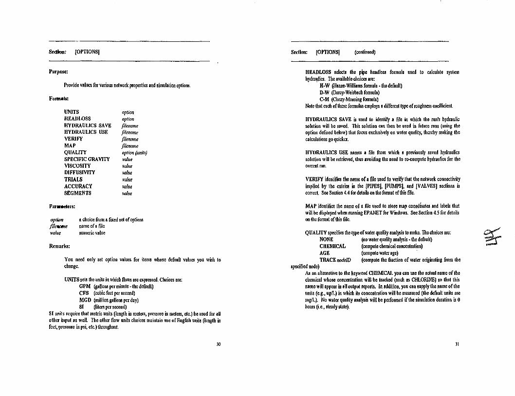
Purpose:
Provide values for various network properties and simulation options.
Fonnats:
UNITSHEADLOSSHYDRAULICS SAVEHYDRAULICS USEVERIFYMAPQUALITYSPECIFIC GRAVITYVISCOSITYD1FFUSMTYTRIALSACCURACYSEGMENTS
optionoptionfilenamefilenamefilenamefilenameoption (linits)vallievallievallievallievallievallie
HEADLOSS selects the pipe headloss fonnula used to calculate systemhydraylics. The available choices are:
H-W (Hazen-Williams fonnula - the default)D-W (Darcy.Weisbach fonnula)CoM (Chezy-Manning fonnula)
Note that each of these fonnulas employs adifferent type of roughness coefficient.
HYDRAULICS SAVE is used to identifY a file in which the run's hydraulicsolution will be saved. This solution can then be used in future runs (using theoption dermed below) that focus exclusively on water quality, thereby making thecalculations go quicker.
HYDRAULICS USE names a file from which a previously saved hydraulicssolution will be retrieved, thus avoiding the need to re-compute hydraulics for thecurrent run.
VERIFY identifies the name ofa file used to verify that the network connectivityimplied by the entries in the (PIPES), (PUMPS), and (VALVES) sections iscorrect. See Section 4.4 for details on the fonnat ofthis file.
Par.-.eters:
You necd only set option values for items whose defauU values you wish tochange.
UNITS sets the units in which flows are expressed. Choices are:GPM (gallons per minute -lhe defauU)CFS (cubic feet per second)MGD (million gallons per day)SI (liters per second)
81 unils require that metric unils (Ienglh in meters, pressure in meters, etc.) be used for allother input as well. The other flow units choices mainlain use of English units (length infce~ pressure in psi, etc.) throughout.
op/Ionflle_evallie
Remarks:
achoice from afixed set ofoptionsname ofa filenumeric value
MAP identifies the name of a file used to store map coordiilates and labels thatwill be displayed when running EPANET for Windows. See Section 4.5 for detailson Ihe fonnat ofthis file.
QUALITY specifies the type ofwater quality analysis to make. The choices are:NONE (no waler quality analysis· the defauU)CHEMICAL (compute chemical concentralion)AGE (compule water age) .TRACE nodelD (compute the fraction of water originating from Ihe
specified node)As an alteruative to the keyword CHEMICAL you can use the actual name oflhechemical whose concentration wiD be tracked (such as CHLORINE) so that thisname will appear in all oUlput reports. In addition, you can supply the name of lheunils (e.g., ugIL) in which i1s concentration will be measured (the default unils aremg/L). No waler quality analysis will be performed if the simulation duration is 0hours (i.e., steady slate).
~~
30 31

Seelion: (OPTIONS) (continued) Seelion: (PATTERNS)
SPECIFIC GRAVITY is the weight per unit volume of the fluid being modelledrelative to that ofwater. The default value is J.O.
VISCOSITY is the kinematic viscosity of the fluid at the temperature conditionbeing simulated. The units of viscosity are ft2/sec (or m2/sec for SI units). Thedefault value is 1.Ix10·S 112/sec, corresponding to water at 20 degrees C.Viscosity is used only when the Darcy.Weisbach headloss formula is employed orwhen apipe wall reaction mechanism is included in the water quality analysis.
Purpose:
Describes how water demands and external source concentrations change overtime.
Format:
pattern multl mult2 ....
D1FFUSIVITY is the molecular dilfusivity of the chemical being tracked. It hasEnglish units of ft2/sec and SI units of m2/sec. The default value is l.3x 10-8/12/soo. This is the dilfusivity of chlorine in water at 20 degrees C. Diffusivity isused only when pipe wall reactions are considered in the water quality analysis.
TRIALS is the maximum number of iterations that EPANET should employ whensolving Ihe network hydraulic equatious at each time step of the simulation. Thedefault value is 40.
Parameters:
patternnll/ltJ,mult2,etc.
Remarks:
pallern ID number
mullipliers applied to baseline values in consecutive timeperiods
-t:CS)
ACCURACY prescribes aconvergence criterion for the iterative method used tosolve the network's hydraulic equations. The iterations end when the sum ofabsolute flow changes in all links divided by the total flow in all links is less thanthe ACCURACY value. The default for this parameter is 0.001. EPANET willnot allow avalue smaller than IO-Sto be used.
SEGMENTS specifies the maximum number of segments that any pipe can bedivided into during the water quality analysis. The default value is 100. Thenllmber ofpipes reaching this limit can be reported on by asking for a status reportin the [REPORT) section.
Use as many lines as it takes to describe all time patterns. If a given timepattern requires more than one line, remember to start each new line with the lDnumber of the pattern.
A time pattern consists of a collection of multipliers that are applied to abaseline demand or souree concentration over a sequence of consecutive timeperiods. Within a time period, the demand (or source concentration) staysconstant at a level equal to the multiplier times the baseline value. The default timeperiod length is I hour, but this can be changed in the (TIMES) section.
Examples:
UNITS MGDHEADLOSS ().W
QUALITY TRACE 12HYDRAULICS SAVB test.hydACCURACY.OOOS,SEGMENTS 300
;MGDflow un;t!;Darcy·We;sbach head lou formula;Track%offlowfrom node J2;Save hydraulic result!;Jncreme the accuracy of;hydraulic and water quality results
32
There is no limit on the number of patterns or mullipliers per pattern. However,system memory is conserved ifyou number the patterns in order beginning with I.If the duration of a pattern wless than the total duration of the simulation. thepattern will repeat itself. For example. suppose you want to conduct a S·daysimulation where hourly demands repeat Ihemselves on a daily cycle. Then yourtime pattenlS need only contain 24 multipliers.
33

Sedlon: IPATIERNSJ (continued) SedIon: JPIPESJ
By defaull, all multipliers for all time periods in all paltems are I. Thus if you donot define any time paltems nor make any assignment of nodes to time paltems,demands and source concentrations will never change from their baseline levelsduring the course of the simulation.
Nodes are assigned to specific demand time pallems in the IJUNCTlONS) orIDEMANDS) sections, and to source concentration time pallems in theISOURCES! section. Unless assigned to a specific pallcm in one of thesesections, the default pallem associated with a node's demand is pallem I. Forcontaminant sources, the default is to have no paltem, meaning there will be notime variation in source strength.
Formats:
id nodel node2 length diam rcoefJ (lcoejJ) (CV)
linkIDID ofbeginning nodeID ofending nodepipe length, It (m)pipe diameter, inches (nun)roughness coefficient, unitless for Hazen-Williams orChezy-Manning headloss formulas, millifeet (nun) forDarcy-Weisbach formulaoptional minor loss coefficient (0 ifnot specified)used if the pipe contains acheck valve.
idnodelnode2lengthdiamrcoefJ
Provides adescription ofeach pipe in the network.
IcoefJCV
Parameters:
Purpose:
Remarks:
;Pa/lem 1 extends over S time periods with;multipliers ranging from .87 to 1.5
;Pa/lem 2 is I/sed to describe afire flow condition;that exists in time period2at a node that;otherwise wOl/ld not have any demand
I 1.1 1.3 1.5I 1.1 .87
2 0 ISO 0 0 0
Examples:
One line should appear for each pipe.
. Aheadloss formula can be specified in the IOPTlONS! section. The default is theHazen·Williams formula. Note that the units of a Darcy-Weisbach roughnesscoefficient are millifeet (or nun for SI unils).
~
A[PIPES) seclion is required.
Examples:
12 34 4S 1200 8 120 ;Pipe with Hazen-Williams roughness;coefficient
123 34 65 2500 10 .8 S ;Pipe with Darcy-Weisbach rOl/ghness and;minor loss coefficient
56 12 7 12008 120 CV ;Pipewithcheckvalvepreventingflow;from Node 7to 12
~ M

,/
Sedion: [PUMP~I
Purpose:
Describes each pump in the netwOlk and its characteristic curve.
Formats:
id nodel node2 hpid nodel node2 hI qlid nodel node2 hO hi ql h2 q2id nodel node2 hO hI ql h2 q2 q3
Sedion: [PUMPSI (continued)
The last format describes acharacteristic curve with an extended flow range. If q3equals q2. then the extended flow range begins at q2 and follows the slope of thepump curve at this point until zero head is reached. If q3 is greater than q2, thenthe extended cwve is astraight line between these two flows.
Graphical examples ofthe input requirements for the various types of pump curvesare shown in Figure 4.2 on the following page.
Unless modified in the [STATUS) or [CONTROLS) sections, all pumps areassumed to be operating throughout the simulation.
The program automatically prevents reverse flow through a pump, and issueswarning messages when a pump is operating out of its nonnal range.
Variable speed pumps can be modelled by establishing speed settings in the(STATUSI and [CONTROLS) sections. See descriptions of these sections fordetails.
-C~
Parameters:
id link IDnodeI ill ofnode on inlet side ofpumpnode2 ill ofnode on discharge side ofpumphp pump power rating, hp (kw)hO shutoffhead, II (m)hi. ql design head, II (m), and design flowh2, q2 head, II (m) and flow at upper end of nonnal operating flow rangeq3 maximum flow in extended flow range
Remarks:
One line of either format should appear for each pump.
The flfst format is used for pumps where the characteristic cnrve is unknown and aconstant power output is asswned.
The second fonnat is used for a "standard" pump curve with no extended ,flowrange, where the cutolfhead is 133% ofthe design head and the maximum flow istwice the design flow.
The dlird fonnat describes apnmp clllVe wilh no extended flow range.
36
Elamp/es:
101 1 2 200102 3 4 50 1200193 5 6 100 75 1000 50 1200 1500
;CollS/ant horsepowerpump;Standardpump curve;Cus/om curve with extended range
37

flO I ----... hI ,ql
la_u]~ I Custom CU've,J J No Exlended "h2,q2flowRqe
--'10"'low
Section: rQUAUTY/
Purpose:
Establishes the initial water quality level at network nodes at the start of asimulation.
Formats:
nodel (node2) quality
Flow
i:! ICustomClfYe,Slend6rd &terKledflowR8I1ge
node ID'sinitial qualily, (concentration for chemical constituents,hoUls for water age, or percent for sour'iC tracing)
nadel,node2quality
Parameters:
Remarks:q3
h2,q2
Flo"
flO
I ICustom ClfYe,CU!lom extendedflow Range
hl,qlflO
Figure 4.2 Examples ofPump Curve Input Requirements Use as many lines as needed to specitY the initial water quality throughout thenetwork.
Each tine can either specify water quality at asingle node or for arange ofnodes.
The units of water quality depend on the type of analysis to be performed:concentration ~ used for chemical propagation, hours are for water age, andpercent is used for source How tracing.
~~
Remember to change the entries in this section when you change the type of waterquality analysis being perfonned.
Ifnot set in this section, I nodes's initial water quality is assumed to be O.
Elamples:
I 23 I10.1
;Nodes 110 23 have initial quality ofI.;Node 10'3 initial quality iuhanged10.1.
38 39

Section: (REACTIONS) Seclion: (REACTIONS( (continued)
Purpose:
Specifies reacHon rate coefficients.
Formats:
Note that the bulk reaction coefficient has units of days·1 while the wall reactioncoefficient has units of ftlday (or m1day). One way to compare the relativemagnitude ofthese Iwo Iypes ofcoefficients is 10 divide the wall coefficient by thehydraulic radius oflhe pipe (ie.• 1/2 the pipe radius). The resulting quantity willhave the same tmils as the bulk coefficien~ days·l.
Default reaction rate coefficients are 0 for all pipes and tanks.
GLOBAL sets asingle coefficient for either bulk reactions or pipe wall reactionsthat applies Ihroughoulthe network.
Parameters:
GLOBAL BULKGLOBAL WALLBULKWALLTANK
Example 1:;Global bulk decay throllglwut network of.l/day.;modifiedto .S/dayforpipes 23 to 52,;andare.growth rate of.05/day in Tank 102;There is no wall reaction.
Remember to use negative signs on all reaction coefficients that representsubstance decay.
GLOBAL BULK·.1BULK 23 52 •.5TANK 102 .05
;Example2:GLOBAL BULK -.5 ;Global bulk decay throughout network of.Slday.GLOBAL \VALL·U;Global wall decay of1.5 flIday.WALL 32 ·2.0 ;Pipe 32 has wall decay of2j1fday.
EIamples:
bulkcoejJwallcoejJpipe] (pipe2) blllkcoejfpipe] (pipe2) wallcoejfnodel (node2) bulkcoejJ
bulk rate coefficient, days·1wall rate coefficienl.llIday (m/day)
tank ID's
pipeID's
bll/kcoejJwallcoejJpipel.pipe2nodel,node2
Remarks:
~~
BULK and WALL establish reaction coefficients for individual pipes. or groupsof pipes in the network. These will override any global coefficient.
I
TANK establishes a reaction coefficient for individuallanks or groups of lanks.This will override any global bulk coefficient.
40 41

Sedioo: (REPORT(Sedion: IREPORT( (continued)
Purpose:
Describes the conlents of the output report.
FOl11lals:
Remarks:
FILE specifies the name of a text file to which the output report will be wrilten.Normally this option would only be used when running under Windows sinceunder DOS, the output report file name is given on the command line. UnderWindows, the default is not to save the output report to afile.
Parallleters:
FILESTATUSPAGESIZENODESNODESLINKSLINKSvariable BELOWvariable ABOVE
PAGESIZE sets the number of lines written on each page of the output report.The default is 55.
The NODE and LINK lines specify which nodes and links should be included inthe output report. Use as many lines as it takes to include all of the items youwant reported. The default is to report on all nodes and links. Using NODENONE or LINK NONE eliminates any node or link oUlput, respectively.
~
;Report on Nodes 12 and:2i through 36, as well as;nodes with pressure below 30psi.;No links are reportedon.
NODE 12NODE 22 36PRESSURE BELOW 30LINK NONE
The last format tells EPANET to report on those nodes and links whose computedvariables meet a certain criterion. Multiple criteria are connected by OR's. Forexample, PRESSURE BELOW 30, PRESSURE ABOVE 100, and QUALITYBELOW I wiD report all nodes that meet one or more of these conditions. Thiswill be in addition to any nodes or links specified in the NODE and LINK lines.
STATUS is used to include or exclude system status reports from being generatedevery time hydraulic conditions change during the simulation. The default is toexclude these reports. A FULL status report includes information for eachsolution trial of the hydraulic equations and is normally used only for de-bugginghydraulically unbalanced networks.
Examples:
filenameoptionlinesnode/ (node2)NONElink} (link2)NONEvaluevalue
name of report fileYES. FULL or NOnumber oflines per page in oUlput report
node ill numbers
link ill numbersoutput variable name:
DEMAND (in (Jow units)ELEVATION(in ft or m)GRADE (in fl or m)PRESSURE (in psi or m)QUALITY (in concentration unils, hours. or %)DIAMETER (in inches ormm)FLOW (in (Jow unils)VELOCITY (in ftIsec or mlscc)
. IIEADLOSS (in Milo-fi or ill/kill)numerical valuevalue
filenameoptionlinesnode/.node2link/.link2variable
42 43

J
Section: [ROUGHNESS)
Purpose:
Provides an alternative to the [PIPES) seetion for easily adjusting roughnesscoefficients for groups of pipes,
Formats:
ADD value'MULTIPLY valuepipeI (pipe2) roughcoeff
Sedlon: [SOURCES)
Purpose:
Assigns baseline concentrations to nodes that serve. as sources of chemicalconstituents into the network.
Format:
Mde concen (pal/em)
Parameters:
Parameters:
valuepipe/,pipe2roughcoeff
adjustment value
pipe ID'srouglmess coefficien~ unitless for Hazen-Williams orChezy-Mauning headloss formulas, millifeet (rom) forDarcy·Weisbach fonnula
Mde source node IDconcen baseline concentration ofconstituent entering the node as
an external sourcepal/em optional ID of time pallem defined in [PATIERNS) section
Remarks:
Use one line for each node that serves as aconstituent source.
<r)--
Remal'ks:
The fust format adds agiven amount to each pipe's roughness coefficient. Use anegative value to reduce roughnesses.
The second formal multiplies each pipe's roughness coefficienl by a givenamount.
The third formal is used repeatedly for each pipe or group of pipes whoseroughness coefficients will be sello aspeeific value.
This seelion allows you 10 easily modi/}' roughness coefficients wilhout having tochange them individually in lhe [PIPES) seetion. This can prove espeeially usefuldnring calibralion runs.
Example:
The data in this seetion pertain only to water quality analyses for chemicals, not towater age or source tracing.
For junction nodes, if there is no external source inflow (negative demand)assigned to the node, then the quality at the node always equals the source quality.Use this feature to simulate satellile treatment such as chlorine boosler sIalions.
The oplional time paltern ID idenlifies which time paltern defmed in Ihe[PATTERNS) seetion will be used 10 vary Ihe source strength aboul its baselinelevel over time. Ifomilled, there is no variation in source strength over time.
Esample:
102 100 3 ;Node 102 has abaseline source strength of100 mglL;which varies over lime according to pal/em 3
ADD ·51252110
;Subtract 5from the roughness coefficient ofeachpipe.;Set roughness coefficient ofpipes 12 through 52 to / /0.
44 4S

Seu;on: ISTATUS)
Purpose:
Establishes initial selling ofselected links at the start ofthe simulation.
Format:
linkl (/ink2) selling
Parameters:
Seellon: ITANKS)
Purpose:
Describes each storage lank or rese1Voir in the network.
Formals:
node elev (ini/level minlevel maxlevel diam (minvol))
Parameters:
linkl. Iink2selling
Rel1llll'ks:
link lD'slink selling at the start of tile simulalion, which can be:
- a pump stalus (either OPEN or CLOSED).- apump speed (relative to Ihe speed used to define the
pump's characteristic curve in the IPUMPS) seclion).• avalve selling (pressure, flow or loss coefficient)
or status (eilher OPEN or CLOSED)• apipe statns (either OPEN or CLOSED)
nodeelevini/levelminlevelmaxleveldiamminvol
Renlarks:
nodeIDbollom elevation oftank where water level is zero. It (m)initial water level above tank bollom, ft (m)lowest allowable waler level, ft (m)highest allowable water level, ft (m)tank diameter, ft (m)volume ofwater below minimum level, ft3 (m3).,
Use one line for each link or range of links whose initial selling you wish tospecify.
Normally all pipes are open, all pumps are on (wilh a speed selling of 1), and allvalves are at their original pressure, flow or loss coefficient sellings at the start ofthe simulation. To change a link's status at some future point during thesimulation, you would use a rule in the ICONTROLS) section.
You cannot set the status ofapipe containing acheck valve.
Enmple:
One line should appear for each tank or reservoir.
For reservoirs you need only enter the node ID and elevation. By definition, thewater surface elevation in a reservoir remains fIXed while for tanks it varies as flowenters or leaves.
Waler surface elevation in tanks equals the bollom elevation plus water level.Tanks are assumed to be cylindrical between their minimum and maximum levels.Non-cylindrical haltom sections can be accommodated by supplying the volume ofthe section as the last parameter on the line (minvol). See Fig. 4.3 for adescription of tank levels. For non-circular tanks, use a diameter ClJualto 1.128times the square root of the area.
G
24 CLOSED1 4 1.2
;Close ofJpipe 24 a/the 5/011 of/he simulation;Begin the siml/lalion with pl/mps I /hrol/gh 4
. ;opera/ing at I.ltimes their Ilomzal speed
A ITANKSJ section is rClJuired.
Examples:
46
101 423 15 10 20 45
102 390
,'45ft diameter tank with variable water;surface level;Reservoir wi/hflXed water surface
47

Purpose:
Section: ITiMESI
Describes various time step parametelS used in the simulation.
value (unils)value (unils)value (unils)value (unils)value (unils)value (unils)value (unils)
DURATIONHYDRAUUC TlMESTEPQUALITY TIMESTEPMINIMUM TRAVELTIMEPATTERN TIMESTEPREPORT TIMESTEPREPORT START
Formats:
Maximum
Level
t 11t'tn"i"1 1 Elevation
MinimumVolume
Minimumlevel
Datum
Figure 4.3 Delinilion ofTank LevelsParameters:
value a time valueuniU optional time unils which can be:
SECONDS (or SEC)MINUTES (or MIN)HOURS (default)DAYS (or DAY)
'(jRemarks:
You need only specify those time parameters that will differ from their defaultvalues.
Use of time units is optional. The default units are hoUlS.
DURATION sets the length of the entire simulation (both hydraulic and waterquality). The default value is 0 hours, which implies that a steady state run will bemade. No water quality analysis will be performed for steady state runs.
48 49

Stdiln: ITIMES) (CQntinued)
HYDRAUUC TIMESTEP determines how ollen a new hydraulic slale of thenelwOlk is computed. The default time step is 1hour.
QUAUTY TIMESTEP fIXes the time step that will be used 10 track waterquality changes through Ihe network. If not supplied, Ihe program uses aninternally compuled lime step based on Ihe smallest lime of travel through any pipein the nelwork. I(you ask for astatus report in the IREPORT) seclion, a listing ofIhe quality lime sleps used throughout the simulation will appear in EPANET'soutput report.
MINIMUM TRAVELTIME establishes the smallest time of travel through apipe recognized by EPANEr. Travel limes smaller than this number are set equalto it. (Travel times through pumps and valves are instantaneous and are nolaffected by this limit.) The default minimum travel time is 1110 the hydraulic timeslep.
PATIERN T1MESTEP determines the lenglh ofa time pallem period (i.e., Iheperiod of lime over which water demands and constiluent source strengths remainconslanl). EPANET will adjusl your HYDRAULIC TlMESTBP to be no greaterthan your designated PATTERN TIMESTEP. The default time paltem period is 1hour.
REPORT TIMESTEP detennillcs the interval of time between which networkconditions are reported on. Ifneed be, BPANET will reduce your HYDRAULICT1MESTEP so that it is no greater than the REPORT TIMESTEP. The defaultvalue is 1hour.
REPORT START specifies al what time into Ihe simulalion results should beginto be reported. The default value is O.
Examples:
Section: ITITLE)
Purpose:
Altaches adescriplive tille 10 the problem being analyzed.
Format:
Up to three lines of 80 or less characters CQntaining the title of Ihe problem beinganalyzed.
Remarks:
The ITITLEI seclion is oplional.
tb
DURATION 120QUALITY TlMESTEP 2MINPAITERN T1AJESTEP 2
REPORT TIMESffiP 2HOURSREPORT START WAYS
;120 hOllr (5 day) simulationperiod:2 minllte water quality lime step;2 hOllr interval betll'eell changes in;demands;ReporlS are generatedeve/)' 2;holll'$ beginning on day 2
so 51

4.4 Verification File FormatSeelion: (VALVES(
The verification lite provides an optional means ofchecking that the links specifiedin the input file connect the correct pair of nodes together. If you choose to use a
Purpose: verification file, its name should appear in the (OPTIONS) section of the input fileusing aline that reads:
Describes each control valve in !he network.VERIFY filename
Format:where filename is the name of the verification file.
id nodeJ node2 diam type selling ~osscoeff)The verification file cousists ofasingle section whose format is:
Parameters:
losscoeff
idnodeJnode2diamtype
Format:
node linkJ link2 ...
ID's ofall links connected to node.
node IDnodelinkJlink2, etc.
Remarks:
Verifies network nodellink connectivity.
Purpose:
Parameters:
Section: (VERlFICATlON(
IinkIDID of node on upstream side ofvalveID of node on downslream side ofvalvevalve diameter, inches (mm)type ofvalve:
PRV for pressure reducing valve,PSV for pressure sustaining valve,PBV for pressure breaker valve,FCV for Dow control valve,Tev for throtlle control valve,
selling pressure selling for PRVs, PSVs and PBVs in psi (m), flowselling for FCVs, or loss coefficient for TCVsminor loss coefficient for fully opened valve (0 ifnotspecified)
One line should appear for each control valve. Check valves are identified ill the[PIPES) section, not here.
Remarks:qControl valves should not be COlUlected direclly to tanks or reservoin.
Include one line for each node in the network.Note that pressure sellings for valves are pressures and not total head (or hydraulicgrade line elevation).
Examples:
301 12 34 8 PRY 7S ;ValveJOJ ;s an 8"PRY Ihal keeps the:prenure al Node 34 below 75 psi.
The file can cOlltain blank lines and it treats the semicolon (;) as a signal that therest of the line is a comment. EPANET will report an error message if anyinconsistencies between the connections established in the input file and those inthe verification file are found. Awarning message will be issued if all nodes arenot listed in the verification file.
52 53

4.6 Map File Format
The Windows version of EPANET allows you to view simulation results on a mapof the network being analyzed. To use this feature you must frrst create a file thatcontains the X·Ycoordinates ofthe network nodes included in the map. The nameof this file should appear in the [OPTIONS) section of the EPANET input fileusing a line that reads:
MAP filename
Sedlon: (COORDINATES)
Purpose:
Assigns map coordinates to network nodes.
Format:
node Xcoord Ycoordwhere filename is Ihe name of the map file. This will cause the map to bedisplayed automatically aller a successlill simulation. If you do not specify a mapin an EPANET input file or you wish to change to another map, you can use amenu option in the Windows version of EPANET to specify Ihe uame of the mapfile to be displayed (see Section 6.3).
TIle contents of the map file are divided into Ihe following sections:
Parameters:
nodeXcoordYcoord
node IDhorizontal coordinatevertical coordinate
The file can contain blank lines and it treats the semicolon (;) as a signallhat therest of the line is a comment An example map file is shown in Figure 4.4. Thefollowing pages describe Ihe formats of the (COORDINATES) and (LABELS)sections.
(COORDINATES)ILABELSI(END)
specifies uodal X·Ycoordinatesspecifies location and text of labelssignals eud of map file
Remarks:
Include one line for each node displayed on the map.
The coordinates represent the distance from the node to an arbitrary origin at thelower left of the map. Any convenient units of measure for this distance can beused.
;---- -_....._..........-_ ..-----------..........
=================================[COOlUllNATES]INode X-coord Y·coord
There is no requirement that all nodes be included in the map, and their locationsneed not be to actual scale (such as when trying to depict a cluster of nodes thatare close to one another). ~
2 50 909 10 70
10 20 7011 30 70
[LABELS]IX·coord Y·coord Label;----------------------------------
o1255
(END]
706890
"Source""Pump""Tank"
::.=============================Figure 4.4 Example Map File
'4 s,

~
Seelion: [LABELS)
Purpose:
Assigns map coordinates to text labels.
Format:
Xeoord reoord "/abel" (node)
Parameters:
Xeoord horizontal coordinateYeoord vertical coordinate"/abel" label text (in double quotes)node ID ofoptional anchor node
Remarks:
Include one line for each label on lhe map.
TIle coordinates refer to the upper tell comer ofllte label.
The optional anchor node anchors tlte label to the node when the map is re-scaledduring zoom-in operations.
4.6 Summary of Default Values and Units
Tlte only mandatory sections required in an EPANET input file are tlte[JUNCTIONS), [TANKS), and [PIPES) sections. Table 4.1 summarizes thedefault values used by EPANET in lieu of specific instructions supplied in otherinput sections. Table 4.2 lists the units in which the various input parameters mustbe expressed. The "now unils" in this table can correspond to either gallons perminute (the default), cubic feet per second, million gallons per day, or liter persecond, depending what option is specified for UNITS in the [OPTIONS) section.SI (melric) unils apply only ifSI is designal~ for UNITS.
56
Table 4.1 Sununary ofDefault Parameler Values
====================----====;=====================--====Parameter Default Value Relevant Section=======-- --==--======
Nodal Demands Ogpm [JUNCTIONS)[DEMANDS)
mitial Quality 0 [QUALITY]Source Quality 0 [SOURCES)Time Pallem Multipliel1 I for all pallents [PATIERNS)Demand Time Patterns Paltem I for all nodes [JUNCTIONS)
[DEMANDS)Source Time Patterns NoPallem [SOURCES)Time Pallem Time Step I hour [TIMES)Simulation Duration ohours (steady state) [TIMES)Hydraulic Time Step I hour [TIMES)lIeadloss Fonnula Hazen-Williams [OPTIONS)FlowUnils GPM [OPTIONS)Hydraulic Trial Limit 40 [OPTIONSIHydraulic Accuracy .001 [OPTIONS)Specific Gravity 1.0 [OPTIONS)Viscosity I.1xlO-5ft2/sec [OPTIONS)Dilfusivity I.3x 10-8 ft2/sec [OPTIONS)Water Quality Analysis None [OPTIONS)Reaction Rates 0 [REACTIONS)Pipe Segment Limit 100 per pipe [OPTIONS)Minimum Travel Time Hydraulic Step /10 [TIMES)Reporting Start Time ohoUl1 [TIMES)Reporting Time Step I hour (TIMES)Lines per Report Page 55 [REPORT)Nodes Reported On All [REPORT)Links Reported On All [REPORT)Status Reports Generated No [REPORT)=--====== - - -- ---
51

Table 4.2 Sununary of Input Parameter Units
CHAPTER 5
Paramtltr English Unlla 51 (llftlrlc) Unlla
Junction Elevation feet meters
Junction Demand Oowunits Oowunits
Tank IJollom Elevation feet meters
Tank Levels feet above bollom meters above bollom
Tank Diameter feet meters
Tank Minimwn Volwne cubic feet cubic meters
Junctionffank QualityOJemical milligramslliter same
(or uscr·supplied) asAge houl! EnglishSource Trace percent
Pipe Length feet meters
Pipe Diameter inches millimeters
Pipe RouglmesslIazen·Williant.l none noneDarcy·Weisbach millifeet millimetersOJezy-Manning none none
Minor Loss Coefficient none none
Pump Power Rating horsepower kilowatts
Pumpllead feet meters
Pump Flow flow units flow units
Pwnp Speed Selling none none
Valve Diameter inches millimeters
Valve Pressure Selling pounds per square inch meters
Valve Flow Selling Oowunits Oowunits
Bulk Reaction Coeff. days-. days'·
Wall Reaction Coeff. feet/day meters/day
Specific Gravity none none
Viscosity square feel per second square meters per second
DiO'usivity square feet per second square meters per second
S8
RUNNING EPANET UNDER DOS
5.1 Generallnstructions
Step I. Create an Input File
To run EPANET under DOS you fust create an input file that describes thenelwork being simulated. This file must be created wilh an edilor or wordprocessor thaI saves its text in ASCII formal. The fonnat of the input file has beendescribed in Chapter 4. You might also want to prepare a verification file.following Ihe format described in Chapler 4. thai will verify Ihe nodal conneclionsconlained in Ihe input file.
Step 2. Invoke the EPANET Simulator
Assuming thai your current direclory is the same one in which the EPANET fileswere inslalled, the command issued from the DOS prompl for running anEPANET simulation is:
EPANET inpfl1e rptfl1e
where inpfile is the name of the input file and rptfile is the name ofa file that willcontain the oUlput report wilh the simulation resulls. Nole that if either of thesefiles resides in. different direclory than the EPANET files, then their names mustinclude their full directory paths.
You might prefer to keep your network data files in different directories than yourEPANET program files, esp~ially if you will be working on many differentnetwork analyses. To avoid the need to supply full path names for your dala filesyou can add the EPANET directory to the path variable that DOS maintains, andthen launch the program directly from any directory you choose. Consult yourDOS manual for instructions on selling up your path.
Step 3. View the Output Report
S9
~

the water surface elevation of each storage node and whether it isfilling or emptying
the status (OPEN or CLOSED) ofeach pump and valve
S. Utose pipes which have been closed off.
4.
3.
If a waler quality analysis is being made, a second. type of stalus table, theSYSTEM WATER QUAlJTY STATUS lable will appear next. For eachhydraulic time slep, this table displays the water quality time step and the numberofpipes Ihat required more Utan Ute maximum allowable number ofsegments.
where rplflle is the name ofyour EPANET outpul report file. Then use Ihe allowkeys 10 move through Ihe file one line al a lime, or use Ihe Page Up and PageDown keys 10 move one page at a time. You exit the viewer by pressing theEscape key. In addition, you can be print the output report by issuing the DOSPRINT command as follows:
BROWSE rptfde
To view the oulput report over the video display you can employ a file viewerprogram capable of handling large files. Such a program, BROWSE.COM, hasbeen installed in your EPANET directory. To use it, simply enler Ute command
PRINT rptfde The third type oftable presents NODE RESULTS at each reporting period oflhesimulation. Unless chauged in Ihe [TIMES) section of the input file, the reportinginterval is I hour. For each node that has been flagged for reporting (the default isto report on all nodes) the following information is produced:
5.2 Contents of the Output ReportI. NodeID
EPANET's oUlput report consists offour differenl types of tables. Iflhe STATUSoption was set to YES or FULL in the [REPORT) section of the input file, aSYSTEM HYDRAULIC STATUS table will be produced at the start of everyhydraulic time step or whenever one of Ute followiug events occurs first:
2.
3.
Elevation
Demand flow (negative values denote source flow)
I. afilling tank reaches its maximum level or an emptying tankreaches its minimum level,
4.
S.
Hydraulic grade (elevation +pressure head)
Pressure
~
2. the control time for a pump, valve or pipe is reached or thecontrol level ofalank is reached,
3. areporting period occurs.
6. Chemical concentration, age of water or percent of flowfrom a given source, depending on the type of water qualityanalysis being made (only for non·steady state runs).
If a full status report was requested, each System Hydraulic Status table will bepreceded by a listing of the accuracy achieved at each iteration of the method usedto hydraulically balance Ihe network and will show which links are changing status(e.g., opening and closing) during these iterations. Normally this level ofdetail isneeded only to debug systems that fail to converge hydraulically.
For tank nodes, a positive value for demand flow means thaI water flows into thetank, while a negative value means that water flows oul of the tank. The[REPORT) section oflhe input file allows you to limit output to only those nodesbelow or above specific Iimils on the above variables. This helps reduce theamount ofoutput produced and focus in on critical points in Ute network.
The SYSTEM HYDRAULIC STATUS table itselfdisplays the following items:
The fmal type of lable presents lJNK RESULTS at the end of each reportingperiod. Each link flagged for output reporting (the default is to report on all links)has the following items listed:
I. whether the system is hydraulically balanced or not, the number ofiterations required and the accuracy achieved, I. Link ID
2. Ute total water demand exerted by Ute system 2. Head and tail nodes
60 61

3.
4.
Diameter
Flow rate (negative iffrom tail node to head node)
5-Quit
and prompts you to enter the number of the choice you wish to select
5. Velocity
6. Headloss per 1000 ft (or rn) ofpipe
For valves the headloss reported is the actual change in head across the valve,while for pumps, it is the negative of the head supplied by the pump. Pumps alsohave their power consumption displayed. As with nodes, the link listing can belimited to those links whose output variables meet crileria specified in the(REPORT) section ofthe input file.
5.3 The EPANET4D Program
EPANET4D is a DOS batch program lhatlets you interactively edit an BPANBTinput file, run the file through BPANET, and then view or print the results all fromwithin a single program. EPANET4D comes supplied wilh its own liIe editor andviewer, but you can substitule your own choices for these ifyou like.
You nm EPANET4D by issuing the following command from lhe DOS prompt:
EPANET40 Inpfile rptfile
where inptile and rptlile are lhe names of an input and report file. If you arerunuing EPANET4D from the BPANET directory, then make sure that the fullpath names are included with the input and report file names if Ihey reside in adifferent directory. Alternalively, you can launch the program from any directoryyou choose as long as the EPANET dircctory is included in your DOS palh.
After the program loads itself, it displays amenu with the following choices:
EPANEr MENU:;=================--=
I •Edit input file
.2·RunEPANET
3•View report file
4•Print report liIe
62
Choice I executes I text editor program in which you can enter and change thecontents of the EPANET input file. The editor is very simple to use and has anon-line help facility which can be accessed by pressing the FI key. The commandsused by the editor are summarized in Figure 5.1. To exit the editor, you press theF4 key. After exiting, you are returned to the menu screen.
Reminder: When exiting the editor, you must respond with Y(for yes) when itasks if you wish to save the changes you made to the file if youwant EPANET to ~ecognize these changes.
Choice 2 executes the EPANET simulator. After execution, you are prompted tohit any key which then returns you to the menu screen.
Choice 3 allows you to browse through the EPANET report file after a run hasbcen made. You use the keyboard arrow keys to move up or down through thefile a line at a time. The Page Up and Page Down keys will move you a page at atime. You exit the file browser by pressing the Escape (ESC) key.
Choice 4 prints the contents of the report file by calling on the DOS PRINTcommand. The menu screen re-appears allerwards.
Choice 5exits Ule EPANET4D program and returns you to DOS.
63
~

...... _ _ .. .. t
, ... ... ....... _ ..._ .._ ....... _ .... .... _ ... .. _t
• - _oo ----_._--_ _ - - .._ ··oo oo .. oo oo .oo '"
Cur.or Movement
hoho off
r ...
r -- lPAIlEUD.8AT IDOS B.toh Fil. to Inpl....nt EPAllU llenu PrO'jr...1r ...
if "\2" - "" goto errt
if "\1" - ....2" goto err2
if not ..itt U copy tenphte U
if ••itt \2 del \2
: .tart
ellecho.
echo.
echo IPANET WENU
.eho ------- _
echo.
echo 1 - Bdit input fil. \1
echo..cho 2 - Run IPAllEr
echo.
.oho !. Vi.v report fill \2
echo.
echo ,- Print repo.t fil. \2
echo.
echo 5 - Quit
echo.echo ------- _
echo.
echo Type the nUirber of your nlection:gotdgt
if errodevel 6 goto .tart
if errorlevel 5 goto qUit
if errorlevel .4 goto printout
if errorlevel 3 goto viw
if errorlevel 2 goto run
if errortovel 1 goto edit
goto ltort
If you don~ care for the file editor and viewer that comes wilh EPANET4D youcan substitute your own choices for these programs. The programs you use muslbe able to accept the name of an input file on the command line and the viewermust be capable of handling large files, since the output from a long tennsimulation ofalarge network can be quite considerable in size.Figure S.2lisls the contents of the EPANET4D.BAT file. Ifyou would like to useanother text editor, replace the word "te.exe" that appears below the ".......Launch file editor line with the name of the new editor. To useallother file viewer, replace the word "browse.com" below the " Launchfile viewer •••••••••" line with the name of the new file viewer. Note that ifthese programs reside in a different directory than the EPANET directory, youmust include the full path name for the program.:~==========================================----======
c- Ctrl .- Shft .- Alt
Dioplay IlIIII'tlIry of T••t IdUor _nd.
Find phralo (1-31 oha..1 in fil. o. block
Pind/replace ph.... 11-31 ch• ." in ftl. or block 0
Frint file oc- block to LPft, LP1'2, or Ln3
ASCII cod. IlI'I • 32-255 on keypad
rhon .-Xi-'" on kOVPld for AllCn Ill' • 1-31rOlll' return to DOS. Baol: to U: IXIT
SIt loft/right Nrgin" pag. longth
Po....t p.ragraph to left/right IIIrgin.
n IP.thllFilell.....1
._-_ oo oo .. oo.oooo - _ _- •
Block
.. e-S, Left Chu left • o-os, Home Line b~in
• o-D, Rt Char right t c-QD, End Line end
II a-A, a-Left PreY Yord t o"QI, c-Home Screen top
I a-V I a-Rt N~lIlt word • a-OX, c-Ind Screen bot.tom
• 0-1, Up Prey line • c-QR, o-PgUp File .t,ut" a-X, Dn Neat line • c-QC, c-PgDn File end
II e-W Scroll up II c"QD To block. .tart •
II a-Z Scroll down ill o.. QK To block. end
• a-R, P9Up Up 23 linn II hb Next word, pc-ev line II
, e-e, (1900 On 23 linn II ,-Tab PreY word, prey line'
'0-Q4 To .pecified line • c-Kn Set line muk. n-0-3 •
t c-QP On p~ge len linn II o"On To Une JDark. n-0-3t _oo_ .._.._. __ 11
Innrt/Delete
o-J(l), o-KII," Ia.. ftl. and quit editor
c-Kl, i'2 Save and/or load another fil.
uxr EDITOR 2.6 C<HlAND SUlOIARY
Hi.cellaneou.
• ~ .. __ .. __ .._ .. __ _ _t
,tl.
o rI
o o-gF
• c-llAill c-KP,'5
• a-Xa-Y.-I
• coop• o-kl,'3• cooQM
• a-B
..............................................................................................._ -----_.
11 .. oooo_ ...__ ........ oo_ .. oooo•• .... .. •
, c-V, In. In.ert/Replace · c-H, BkSp Delete left char, !ntr Split/lnoert Un. · o"G, Del Del char/join line·, c-H, F9 In.ert Une · o-T Del next vord, c-Y, rl0 Delete line • cog( D.I to .nd Uno.- -------- .. --..oo-----------------_ _oo _oo oo_ __ .
._------------------------------------------_ __ .
·~ --_..-_..- _- -..- _------------"
~., c-KB, F1 lUrk block .tart · c-Ke Cop!' block
· o-K!(, F8 lUrk block Ind • o-K\' Del.t. block
~ · 0-101 Hido/dilplay block • o-Itv IIovI block0 o-I(! Block right I char 0 c-KR Read block frOll ditk •0 c·1<IJ Block loft I char 0 0-1(11 Write block to diok .
===,=-=-====,Figure 5.1 Text Editor Command Swmnary Figure S.z ContenlJ ofEPANET4D.BAT (Continued on Next Page)
64 6S

===================================================:.ditr_
rem ......... Launch editor program .........
t •.••• \1,oto .tart
:run
010
if ·~ep.n.t~·-·32· goto nn32ep.n.t16.••• ~I ~2 ~3
pau••
goto .tart
:run32
let DOS4IG-quiet
echo Running 32·bit verdon of IPANlf •••
do.41gv epanet32.eKe ..1 \2 ..3
.et DOS4o-
paule
. qoto .tart
:vitv
ell
U' not edit \2 goto err3
r.11Irem UtitUti Launch file viever .... ttttt
brov.e. com \2
goto .tart
:printout
ell
if not ~xilt \2 goto err3print \2
goto .tart
:errl
echo Correct synbx i.: lPANtr4D inpfile rptfile
echo where inpfile ia the name of an input file
echo ilnd tptfile it the name of a report file.
echo.
goto end
:..r2
echo Cannot Ule tame name for input and report filel.
echo.
goto end
:err3echo Report file \2 ha. not been created yet.
echo.
pau.e
goto .tart
:quit
ell
:end
Figure 5.2 Continued
66
CHAPTER 6
RUNNING EPANET UNDER WINDOWS
6.1 Overview
The Windows version of EPANET. referred to as EPANET4W, provides agraphical user interface for running network simulations and viewing their results.II allows you to edit EPANET input files, execute EPANET's network simulator,and view EPANET's output in avariety offormats that include:
•color-coded network maps
• time series plots
• tabular reports.
This chapter assumes that you have a basic understanding of how to work withWindows applications, and are familiar with the different parts ofa window (suchas the menll bar, the control·menu box, and the minimize and maximize billions)and with mouse operations.
Figure 6.1 shows how Ihe EPANET4W workspace might appear at some pointduring a run. /I gives examples ofthe different types ofwindows that the programcan generate. These include:
I. awindow lisling the netwoik's input data2. aBrowser window that controls what aspect of Ihe networksimulation results should be viewed3. awindow with • map of the netwoik4. windoW! that display output results in tabular form5. windoW! that display time series graphs ofoulput results.
The figure also shows the program's menu har across the top of the workspace.Using the windows version of EPANET involves making a repeated sequencc ofchoices from this menll to select, edit and run al\ EPANET input file (or select apreviously saved output file), and view the results in the form ofmaps, graphs, andtables. 11lc following paragraphs explain these various prQl:edures.
67
~~

Figure 6.1 Example Contenls ofthe EPANET4W Workspace
;-----------------
;-----------------
Method I. Double click the EPANET icon in the EPANET program groupwithin Program Manager.
Method 2. From the Program Manager, select File from the main menu, andthen select the Run option under it. When prompted for thecommand line to use, enter path\EPANET4W where path is thefull path name ofyour EPANET directory (e.g., C:IEPANEn.
EPANET4W comes wilh a complete Help facility that functions the same as otherWindows Help systems. You access it by selecting an option from the Help menuor by pressing the FI key. From the Help menu you can choose to view thesystem's table of contents, go directly to the section dealing with input dataformals, or search for help on aspecific topic.
Getting Help
6.3 Operating Procedures
Opening an Input File
20.10. 15.Time. lui
IIDeAgpPl
£leuft
EPANET Example Network 1
I
i 10
[JUHCTlOHS)
~VNote: EPANET4W allows you to keep multiple windows loaded in its workspace
at one time. To conserve system resources, it is recommended that youclose windows when they are no longer needed by double-clicking thecontrol·menu boK in their upper left comer.
After EPANET4W begins, your first operation should be to open an input tile (orpreviously saved output tile) for processing. To open an input tile, select OpenInput from the File menu. Atile dialog box will appear as shown in Figure 6.2.You can change drives, directories, or tile name pallems within this window (thedefault file name pallem for input tiles is *.INP). To specify a new tile that doesnot currently exist, type its name into the File Name box. Press the Enter key orclick the OK bullon to load your selected file. Click the Cancel bullon (or pressthe Escape key) to cancel the operation. After a file has been selected, its namewill appear in the tille bar ofEPANET4W's main window.
6.2 Launching the Program
EPANET4W can be slarted either from DOS or from within Windows. To start itfrom DOS, issue the command:
WIN pathlEPANET4W
where path is Ihe full path name ofyour EPANET directory (e.g., C:IEPANET).
There are two different ways to start up EPANET4W if you are already in theWindows environment:
68 69

:;~ Open Input File UIlT 10nOR 2.' CllIK\HI) I1MWlY
·········..------..·---····· - ··..-· ·.·r·· -_ .File Hllme:
l-.inp IInel1.inp IIInet2.1npnet3.inp
Ilirectories:
e:\epllnel
lOe:\
I.-t-II IPathllPUtlI_1
o·lCD, o-KG, FI
o-lel. n
0- ctrl •• IhCt a- AIt
ruo
lave fUo and quit editor
Savo and/or load anothor fUo
Cur.or Movement
Lino beginLine ondScr..n topScr..n bott...File .tart
,Uo endfo block .tart
To block ond
Neat word, preY line
Prev WE'd, preY line
set Uno ..rk _-3To Une Nrk 0-0-3
a-OS, Home
a-QD, Ind
a-Ol, a-HotM
e-gX, a-Ind
c-gR, o-'gUp
e-QC, a-PgDn
o-gB
c-gK
Tab.·fab
c·J(nc·gn
0-1. !.eft Ch.. l.rtc-D # Rt Ch,ar d~ht
c-A, c·Left Prev word
c-F, c-Rt Next word
coo!, Up Prev Une
c-X, Dn NeKt Une
CoN Icroll up
0-1 Scroll dovn
o-R. 'gUp Up 23 Un..o-c, PgDn Dn 23 11n..
o-gl To ",tellied Unoo-g, On pogo Ion Une.
Drives:
Ii
I~c: mgIinput files r.inp) 111List files 01 Jype:
~
Figure 6.2 File Dialog Box
Viewing the Input File In.ort/Oeloto
c-KB, F7 Ilark block .tart o-Ke Copy blockc-KK, F8 Ilart block end o-K'i Deloto block
c-KIt Nlde/dioplay block o-1lY IIovo block
c-KI Block right 1 ohar o-KR Read block Cr... diokb-m Block 10ft 1 char c-IQI Nolto block to diok
Dl",lay .......'1' oC rort Idltor _nd.
Find phrue It-31 charel in fUo or block
Find/replace phrue 11-31 chau, In CUo or blockPrint fUo or block to un, LM2, or LPr3Alcn ClOd. XVI • 32·255 on kowad
rhen a-Xa'Y on tOWad Cor Alcn XV • 1-31
Teop roturn to DOS. lack to TI: UII
lot 10ft/right ...rgin.. page longth
Fo....t p..agraph to loCt/right 1IIH'91n.
Hl.oellal1OO\l.
Block
$
Delete left char
Del char/join UneDel neKt vord
Del to end line
a-H, Skip
e-G, Del
c-f
o'llY
In.ert/ReplaceIpUt/lnnrt UneIn.ert line
Delete line
c-V, Ina
Entr
c-N, Fea-V, FlO
F1
o-g,
c-g~
o-K!'. F5
a-h-Ya-I
0-'o-KB. F3
o-QH
o-B
After you first open an input file ils contents will be displayed in a non-editablereport window. This window can be moved, resized, and closed when no longerneeded. If you are using a new file that has just been created, ils conlenls willconlain seelion headings for Ihe input file formals described in Chapler 4. If youneed 10 view your inpul file at any olher lime during an EPANET4\v session,simply selecllnput Data from the Repon menu.
To edillhe conlenls ofthe inpul file, selecllnput Data from Ihe Edit menu. Thiswill load and di<lplay your inpul file in a lexl edilor. The commands used 10operale Ihe defaull edilor Ihal ships wilh EPANET are summarized in Figure 6.3.To exil Ihe edilor, you press Ihe F4 key. Be sure 10 answer yes (Y) when Iheedilor asks ifyou wanllo save your changes ifyou wanllhem 10 be recognized byEPANET4\V. If during an editing session you decide to do some olher operationwilhin EPANET4\V,snch as consull ils Help facilily to review an input fonnal,lheedilor window will disappear underneath Ihe EPANET4W window. In Ihis caseyou can always gel back 10 the edilor by selecling Input Data from Ihe Edit menuonce again.
Editing the Input File
Figure 6J Text Edilor Conunand Summary
70 71

Hints: You can subslitute a different DOS or Windows file editorprogram for the one supplied with BPANBT. Consult Chapter 3for instruclions on how to do this.
If you are using a DOS file editor, then pressing the ALTENTER key combination will toggle the editor between appearingin awindow and in full-screen mode.
As an alternalive 10 opening an input file for editing and analyzing with BPANBT,you can choose to view results generated from aprior session ofEPANET4W thatwere saved to a file. To do this, select Open Output from the FIle menu. Afiledialog box will appear from which you can select the output file to view. Allerselecting the file, its name will appear in the title bar of EPANET4W's mainwindow. EPANET4W will then display ils Browser window and, ifa map file isassociated with the output file, will draw a map of the network. The program willnot be able to display any status reports or warning messages that were generatedwhen this network was first simulated.
~
Editing Other Files
At times you might Hnd it necessary to edit other files, such as the map andverification files. There are two ways to do this. One is to invoke theEPANET4W editor for your input file as described earlier, and then from wilhinthe editor switch to the file you want 10 edit. Hitting the F2 key in the editorsupplied with EPANET will allow you to do this. Be sure to save your file aftermaking any changes to it. Asecond approach is to switch back to ProgramManager and launch any editor you normally use as a new task to edit your choiceof files. TIten switch back to EPANET4W.
Running the Input File
Use Ihe Run menu 10 request that the current input file be processed by IheEPANET's network simulator. Selecting Windowed will run ihe simUlator in awindow so that you can observe its progress. If you select Minimized Ihesimulator will appear as an icon until it is done processing. Select Cancel tocancel the request.
If the run was unsuccessfu~ EPANET4W will display the error messagesgenerated by the simulator in a report window explaining what went wrong. Atthis point you could invoke Ihe editor once again to fIX your mistakes, leaving thereport window displayed on the screen so that you can see where in the input filethe errors occurred.
If the run was successfu~ EPANET4W will display its Browser window and willalso draw amap of the network in ils Map window, providing that the name of amap file was included in the input dala. Instructions on using the Browser windowto view different aspects of the output are given below. Ifthere were any warningmessages generated, an Output Summary for the run will also be displayed in areport window which will scroll down to the line containing the first warningmessage. See Viewing an Output Summary below for details.
Opening an Output File12
Note: The output file referred to here is not the same as the report file producedwhen EPANET is run under DOS as described in Chapter S. It is possibleto run EPANET under DOS and have it generate an EPANET4W oulputfile by adding a third file name to the command line as follows:
EPANET fnpfile rpfflle oufflte
where inptile is the name of input data file, rptlile is the name ofthe reportfile that can be viewed or printed, and outfile is the name of the oulput filethat can be accessed under BPANBT4W. The BPANET simulator tends toexecute about twice as fast when run directly under DOS (and not in aDOS session under Windows). Allhough it might be more efficient togenerate simulation results in this way, you loose the advantage of beingable to interactively make changes to the network and quickly visualizetheir impact.
Opening aMap File
Ifno map file was specified in the current input data file (or output resulls file), orthe specified map was incorrect, or you simply want to switch to a different map ofthe network, you can select Open Map from the File menu. This will open up afile dialog box from which anew map file can be selected.
Aller viewing the map you might fmd that it needs to be modified. For example,text labels might need to be re-Iocated. You can use the editor to make thesechanges to the map file as described earlier under the Editing Other Files, andthen use the Open Map option of the File menu to load the updated map.
Saving the Current Output
13

Select Save Output from the File menu to save the resulls obtained from thelalest EPANET simulation to a liIe. This allows you to eome back toEPANET4W at a laler time to view the resulls of the current simulation withouthaving to re·run il all over again. Enter the name under which you want to savethe current oulput resulls in the File Name field of the file dialog box that appCllrs.The suggested file extension to use for oulpul resulls is ".oul". You ean use thedrive and directory boxes to select new choices for the liIe's path.
Viewing an Output Summary
A summary report of the current output resulls can be generated by selectingOutllut Summary from the Report menu. At a minimum, Ihe fepoft willsummarize the nature of the nelwork being analyzed (e.g., number of nodes andlinks, head loss equalion used, type of watef quality analysis performed, etc.). Inaddilion, if the results were generated from running an input liIe, the report willinclude any warning messages produced by EPANET (such as pumps opcratingout of range) and, if requested in the (REPORT) section of the input liIe, a stalusreport on ClIch tank, pump, and valve throughout Ihe duration of the simulalion.This type of infonnation will not be listed if you have selected an oUlput liIe forviewing. The output summary window can be moved, resized, and closed when nolonger needed.
Using the Browser Figure 6.4 The Browser
1lle Bfowser window (Figure 6.4) allows you to control how Ihe EPANET olllplllis viewed. 1llis window is IIsed 10:
a) selecla node view variable from among:i. Noneii. Demandiii. E1cvalioniv. Hydraulic Gradev. Pressurevi. Water Quality (non·steady state runs only)
b)
c)
select a link view variable from among:i. Noneii. Diameteriii. Flowiv. Velocilyv. Headlossvi. Average Water Quality (non·steady slate runs only)
view the value ofllie node Ind link variables for specific nodes and links
~
74
d) select atime period for viewing
Functions (a), (b), and (c) are accomplished by making selections from thedropdown list boxes in the Browser's Nodes and Links panels. The upper boxes ineach panel contain the list of node and link /D's, respectively. The lower boxescontain node and link view variable choices. The list boxes are activated byclicking on their arrows. Alist ofoptions will appear from which you click on thedesired choice. Whenever I choice on Iny of these items is made, the followingevenls will occur:
75

'S
a) The values of the view variables displayed in the Browserwill be updated. '
b) The network map wiD be color·coded corresponding to thecurrent selections for node and link view variables. Nodes arerepresented as colored circles (tanks/reservoirs are squares) andlinks as lines between nodes. Alegend indicating what value rangesthe colors represent can be displayed by selecting Legend from theMap menu.
c) After a specific node or link is selected from the Browser,its location on the map is highlighted.
Whenever you click the mouse on anode or on the midpoint ofa link displayed inthe map, that node or link is highlighted and the value of ils current view variableis displayed in the Browser.
The Links panel contains a bullon labelled Info. Clicking on this bullon willoverwrite the panel with alisting of Ihe input information for Ihe currently selectedlink. For pipes, this information includes diameter, length, roughness coefficienl,minor loss coefficient, and reaction rate coefficients. For pumps it includes theequation oflhe pump curve. The listing also contains the current status of the link(e.g., open or closed). When you are done viewing this information, simply clickanywhere in the listing 10 reslore lhe Links panel to its original slate.
To change the current lime period being viewed, you move Ihe slider bar in IheBrowser's Time panel. To move forward one time period, click Ihe righl arrow onthe slider bar. To move backwards, click the left arrow. Whenever the time ischanged, the values in the Node and Link panels are updated and Ihe map is reocolored to reflect changed conditions within the network. You can simulate a timeanimation of the map by keeping the mouse bullon depressed over one oflhe sliderbar arrows. If a steady state run was made, no slider bar will appear in the Timepanel.
As with any other window generated by EPANET4W, you can move the Browserto another location by moving the mouse into its title bar, pressing the left bullonwhile moving the window to a new location, and then releasing Ihe bUllon. Youcan also minimize Ihe Browser window to an icon by clicking ils Minimize bUllonin Ihe upper right oflhe window. To restore the window, simply double·click onUle icon. You cannot close lhe Browser window.
Viewing the Map
The appearance oCthe network map can be modified by making choices from theMap menu. The choices and lheir resulling actions are as follows:
76
c)
a) Zoom In •• allows you to magnify a portion of the map bydefming a zoom window. The area bounded by the zoom windowwill be drawn 10 fdl the enlire Map window. To defme the zoomwindow, move the mouse within the Map window to where youwant a comer of Ihe zoom window to begin, then click the leftmouse bUllon. Nexl move thee mouse until the outline boxdisplayed encompasses the area you wish to zoom in on. Thenclick the left mouse button once again. Clicking the right mousebullon cancels the zoom operation.
b) Zoom Out •• restores the map to a state that existed priorto the last zoom in
Redraw - redraws the map at its original scale.
d) Display Legend •• toggles the display of a node or linklegend on and off. The legend can be dragged to a differentlocation on the map by moving the mouse with the left bullon helddown. Double-clicking the left mouse button in the legend willremove it from the map. Clicking the right mouse bullon within thelegend allows you 10 modify the legend as described nex!.
e) Modify Legend •• displays adialog box for your choice ofnode or link legend that lets you derme what numerical rangescorrespond 10 aparticular color on the map for the current node orlink variable. It also lets you change the colors used for lhe legend(see Figure 6.S). The Default Values bulton restores Ihe ranges 10their internally computed values while Ihe Default Colors bullondoes the same for colors. Modifying the legend can give you aquick picture of where in the network a certain condition holds.For example, the legend shown in Figure 6.5 will display all nodeswhere Ihe pressure is below 20 psi in the filSt color.
77

Node Pressure
0....-------._.120
,-
.1-10 ,_
.Iso 11_
.100 I[M_Figure 6.5 Legend Dialog Box
I) Options •• displays a dialog box for map labelling and stylechoices (see Figure 6.6). You can elect 10 label nodes and linkswilh their !D's and valnes of the current view variable, change thesize of nodes and thickness of links, have flow direction arrowsdrawn on the links, have pump and valve symbols drawn on thelinks. change the map's background color, or change the way inwhich objects on the map are highlighted. (Point highlightingaccents the individual object while area highlighting highlights aregion around the object)
Map Options
Nodes Unks
DiaplllY: Diapilly:
DID's DID's
OVlltU9S DVlllues
181 Text oArrows
Size: OSymbalsOSmllll Style:
@Lorge @!Thinl
oThickBllckground - I
@Block fH;'"''''''''oGrlly oPain!
oWhile @Arell
--Figure 6.6 Map OptioIlS Dialog Box
When the mouse is posilioned over the map, the following keyboard·mousecombinatioIlS can be used as shoJ1culs to implement operations on the Map menu:
Shift·Left Mouse BullonClrI·Left Mouse BullonAII·Left Mouse BullonAIl·Right Mouse Bulton
-> Zoomln-> Zoom Out-> Redraw-> OplioIlS
~
78
In addition to the options offered by the Map menu, the horizontal and verticalscrollbars on the Map window can be used to pan across the map either horizontally or vertically. The Map window can also be moved, minimized, and resized,but it can not be closed.
Generating Tables
The Report menu can be used ta display two types of tables of output resulls.Selecting Cumnt Time from the Report menu produces a table showing thevalnes of all variables at the current time period for either all nodes or alllinb in
79

the network. Selecting Time Series from the same menu creates a tablecontaining the values ofall variables for all time periods for eilher the current nodeor current link. Recall that the Browser window establishes the current time,current node, and current link. Multiple tables can be displayed in EPANET4W'sworkspace at one time. These windows can be moved, resized, and, when nolonger needed, closed.
Searching Tables
Vou can search for entries in a table that meet a specified criterion by selectingSearch from the Report menu. The lable you wish to search must be thecurrently active window in the EPANET4W workspace (i.e., have its title barhighlighted -. tee Switching Between Windows below). Adialog box like theone in Figure 6.7 will appear where you can defme your search criterion. Alleryou specify your criterion, EPANET4W will report on the number of items thatmeet it and will ask if you want to show only those items in the table or not. Ifyou answer yes, then any subsequent searches on the table will be made fromamong its remaining entries. To reslore the table to its original full contents, selectRestore from the Report menu.
Select O(lllons from the Graph menu to customize a graph whose window iscurrently active (i.e., has its title bar highlighted -- see Switching BetweenWindows below). Adialog box will appear as shown in Figure 6.8. The lowerportion of the box lets you customize the appearance of the V-Axis (the verticalaxis) ofthe graph. If the Auto Scale box is checked, EPANET4W will choose itsown axis scaling for you. The Data File box at the top allows you to link a datafile containing observed data to the graph. Vou can either type in the name of thefile you wish to use or click on the button to the right of the box to bring up a filedialog box. Each line in the file linked to the graph should contain an X-value(time) and a V·value to be plolled on the graph. Figures 6.9 and 6.10 display thecontents of a typical time series data file and how a graph would look after thesedata are linked to it. This feature should prove especially useful for modelcalibration.
Options for Node 19 Graph
Doto File
IC;\EPANET\NET2-NI9.DAT III
Generating Graphs
~
DiameterFlowVeloci
:uIil.i
Chlorine
Search of Links at 0.00 hrs --IIs I---Figure 6.7 Table Search Dialog Box
V-Axis i
Title
IFluoride lor Node 19. mg/l IMinimum Moximum
10.07 I 11.04 ITic lnteNol
I I I8J Auto Scole
.. 1-To produce a graph showing how the value of the current view variable for thecurrent node in the Browser window changes over time, select Current Nodefrom the Graph menu. Select Current Unk to produce a similar plot for thecurrent link. If the current link is apump, selecting Pump Curve from the Graphmenu will produce a plot of the pump's characteristic operating curve. Multiplegraphs can be displayed within the EPANET4W workspace, and their windowscan be moved, resized, and closed when no longer needed.
Customizing Graphs
80
Figure 6.8 Graph Options Dialog
8t

================0.25 1.042.75 1.045.70 1.088.60 1.00
12.00 0.8113.25 0.9514.73 1.0217.77 1.0120.52 0.8723.53 0.2827.17 0.9829.87 0.8533.92 0.1235.67 0.1738.48 0.6442.08 0.7944 .68 0.8747.50 0.1651.17 0.5653.45 0.70
The copied data or image can then be pasted into other Windows applications.When copying from I table you can fUlt select the range ofdata to copy. Clickingon the upper-left grayed ceU in the table will select the entire table. Clicking onany column's top label will select the entire column. Data copied from tables arestored as text in the Clipboard, while map and graph images Ire stored as bitmaps.
Printing
Select Print from the File menu to print the contents of any active window(except the Browser) in the EPANET4W workspace to your Windows defauUprinter. If the active window is a graph or the map,' then a dialog box will appearin which you can speciIY a title for the plot and the page margins to use. SelectingPrinler Selup from the File menu will open up a dialog box from which you canselect a different printer and alter certain printer seUings, such as printing inportrait or landscape mode.
Switching Between Windows================
Ifthe currently active window is a map, table, report, or graph, selecting Copy ToClipboard from the Edit menu will copy its contents to the Windows Clipboard.
82
Select Exit from the File menu to exit BPANET4W.
6.4 Summary of Menu Commands
~
83
Opens an input dala file for processingOpens apreviously saved output file for processingOpens amap file and displays its contentsSaves the cwrent oUlput results to I filePrints the contents ofthe currently active windowSelects aprinter and its featuresExits the program
The Window menu offers a convenient means for switching between the windowscnrrenlly displayed in the BPANET4W workspace. This menu lists the titles of allopen windows in the workspace. The currently active window will have a checkmark next to it on this list and will appear on top of any other windows in theworkspace wilh its tille bar highlighted. To make adilTerent window active simplyclick on its name in the Window menu. Another way to make a currently visiblewindow active is to click anywhere within it.
Exiting EPANET4W
FileOpen InputOpenOntpn!Open MapSaveOlltputPrintPrinter SetupExit
60.50.30. 40.Time. tw.
Figure 6.9 Data to Link With aGraph
Figure 6.10 Graph With Linked Dala
1.00
Copying to the Clipboard

EditCopy to Clipboard
Input Data
RunWindowedMinimizedCancel
ReportInput DataOutput SummaryCurrenl Time
Time Series
Search
Restore
GraphCurrent Node
~ Current Link-Pump CurveOptions
MapZoom InZoom OutRedrawDisplay LegendModify Legend
Options
Copies the contents of the currently active windowto !be Windows clipboardEdils !be current input data file
Runs !be EPANET simulator in awindowRuns the EPANET simulator as an iconCancels the run request
Displays listing of input dataDisplays listing ofoutput summaryDisplays table of all node or link resulls for currenttime periodDisplays table of resulls for the current node or linkfor all time periodsSearches currently active table for enlries meeting aspecified criterionRestores currently active table to its original state
Displays time series graph for current view variableat the current nodeDisplays time series graph for current view variableal the current linkDisplays pump curve if the current link is apumpLinks observed data (in a file) to the current graphand customizes its Y-axis scaling
Zooms in on aselected area ofthe map displayRestores map to state prior to last zoom inRedraws map at its original scaleToggles display of node orlink legend on and offModifies colors and scale ranges for displaying nodeor link values on the mapChanges appearance of the map (e.g., ,adds labels,adds flow direction arrows, changes node/link size,changes backgronnd color)
84
WindowWindow List
HelpContentsInput FormatsSearch for Help OnAbout EPANET
Activates selected window
Displays help system's table ofcontentsProvides help on input data formatsProvides help on aspecific topicDisplays EPANET version number
8S

Tank 2
nturwoll g
CHAPTER 7
to 11 12 13
EXAMPLE APPLICATIONS Pump~
to
111
11
112
t2
113
22
7.1 Introduction 2121
22 23
This chapter presents three example applications of the EPANET program. Thedata sets for each example are provided on the EPANET dislribution disk andshould already reside in your EPANET directory if you followed the installationinstructions in Chapter 3. TIle liIe names of the data sets are:
121 122
31
31 32
Figure 7.1 Network for Example 1
7.2 Example 1• Chlorine Decay
Figure 7.1 depicts a small distribution system that will be used to illustrate howEPANEr can model chlorine decay. Pump 9takes water from a reservoir at Node9 and feeds it into a system containing a storage tank at Node 2. The operation ofthe pump is controlled by the level in Tank 2. A 24 hour simulation of chlorinetransport will be made assuming a first order decay of chlorine in the bulk 1lowoccurs with arate constant of-O.5/day and afirst order wall reaction occurs wilh arate conslant of ·1 ftIday. The input data for this problem appears in Figure 7.2(comments have been added throughout the data set to enhance its readability -use ofsuch comments is purely optional).
: ------------------------
:-----------_.-----------
~
100 150 50.5
o150
150
100
ISO
200
150
100
100
ft 9P"
110
110
100
195
100
195
190
100
110
Elev~tion Demand
2 850 1208 800
10
1112
13
21
22
23
31
32
(TnUI
IP~IT IKaJll'le Network 1
IJIlHCTIOIlSI
I
I 10
: --_ ..- - -_ -..-- ..
IT~Il:SJ
,--------------------------------------------Ilev. Init. llin. Max. Dlall.
,10 ft Level Level Level ft
(Input data for Example I)(Map coordinates for Example I)(Input dala for Example 2)(Map coordinates for Example 2)(Node 11 sampling resulls for Example 2)(Node 19 sampling results for Example 2)(Node 34 sampling results for Example 2)(Input data for Example 3)(Map coordinates for Example 3)
NETl.INPNETl.MAPNET2.INPNET2.MAPNET2-NII.DATNET2-NI9.DATNET2·N34.DATNETlINPNETlMAP
Figure 7.2 Input Data for Example I (Continued on Next Page)
u ~

(PIPEsl,-----_......_-_ ......_--_.._---_ ...._------_ .._-_ ......._- _.._-
Head !aH Length 01.... Rough.
;10 Node Node ft In Coeff.,---_......_-_.........._........_---_ ................._-_ .... _..................
10 10 11 10530 IS 100
11 11 12 52S0 14 100
12 12 13 5280 10 100
21 21 22 5280 10 100
22 22 23 5280 12 100
31 31 32 5280 , 100
110 2 12 200 18 100
III 11 21 5280 10 100
112 12 22 5280 12 100
113 13 23 52S0 8 100
121 21 ]1 5280 8 100
122 22 ]2 52S0 , 100
DURATION 24 I 24 hour .lmbtion period
PAtTSRN TlIlISTIP 2 I 2 hour pattern ti.. period
(OPTIONS I:--- - __ ----------- _..~ALITY' Chlorine ; Chlorine Auly.t.
NAP NeU._ I Nap coordlnat.. fHo
ISNDI
Figure 7.2 Ccnlinued
These dala also appear in the fIle NETl.INP in your EPANET directory. You canrun Ihe program on this data several different ways:
(PUMPSIa) from DOS, issue the command:
~(?
: .. -- --------- .. ----------- ------Head !.ail Design H-Q
; 10 Node Node ft VP":------------ -- --- .... _-_ ........_---
10 250 1500
(CONTROLS)
:--------------------_.._- ----_.....-.....-.......LINK B OPSN IP NODE 2 SELIllI 110
LINK B CLOS!D IF NODE 2 ASOV! 140
(PAtTERN81:.. -_ - - - .. __ .. _--_ ---I 10 Hultiplie.......: -- --_._--- _- -_ .
1.0 1.2 1.1 1.1 1.1 1.2
1.0 O.S 0.' 0.1 0.' 0.8
(QUALITYI
b)
EPANET NET1.INP NET1.RPT
and use a file viewer to view the contents of NBll.RPI orhave it prinled,
from DOS, issue the command:
EPANET4D NET1.INP NET1.RPT
and select 10 run EPANET from the menu and then view orprint the output file NETl.RPT,
c) if you've installed EPANET for Windows, then launch iI,open the NETI.INP file, run the lite through EPANBT, and thenlook at the results using EPANBT4Ws various view optious.
:- _ _ _---; Initial
;Nodel Conoen. ~JL
Aportion ofthe output file, NETI.RPT, produced by methods (a) and (b) above isshown in Figure 7.3.
; ..........._---_ .... -.._.._..._--============================]2 0.5
1.0
1.0 Pago I Thu Jul 28 OB:48'12 UB]
: _--- - __._ ...(RUCtIONS I
GLOBAL BULK ·.5OLOBAL IlALL -I
(!tillS)
I Bulk dooay _rr.I Wall decay _ff.
ill ill ill ill. ill ill ill ill ill ill. ill t tt ill ill ill ill. ill U ill ill ill. ill t ill ill ill •• ill ill ill t ill iIIt ill t tt. t ill t •• ill •••••• ill ill. ill tt ill
EPANIT
~raulio and lIator Quality
Analyd. for Pipo Notwork.
Verdon 1.1It It It It It It It It It tit It. It It t t t t t tt.t tt. t. t t •••• t t •• t t ••••••• t •••••••• t tt•• tt t t
; --- .. _ -_..----88 89

EPAHIT lJIarrpl. Network 1
===========~==========================================
=======================================================
_......- ............_._ ... -------------_..... _---------------_ ..- ..- ........_......._.. __ .._---10 110.00 0.00 1004.50 121.61 0.50
11 110.00 150.00 P85.31 11P.2P 0.50
12 700.00 150.00 nO.01 111.02 0.50
13 U5.00 100.00 UO.06 118.66 0.50
21 700.00 150.00 Pll.55 111.66 0.50
22 U5.00 200.00 Ut.01 110.15 0.50
23 UO.OO 150.00 P60.63 120.13 0.50
31 700.00 100.00 P61.35 115.04 0.50
32 110.00 100.00 965.n 110." 0.50
2 050.00 165.06 no.oo 52.00 1.00 Tank
, 000.00 -1865.06 800.00 0.00 1.00 Re.e:rvoir
~
Start Ind Dialnlter Flow Velocity Headlo..
Link Nod. Nod. in !lI'a fp. 11000lt
--------_ .._- .............-----------------....__ .....................-----------10 10 11 18.00 18'5.06 2.35 1.02
11 11 12 14.00 1233.51 2.51 2.8'
12 12 13 10.00 12'.41 0.53 0.23
21 21 22 10.00 If0.11 0.18 0.41
22 22 23 12.00 120.5' 0.36 0.08
31 31 32 6.00 60.11 0.46 0.33
110 2 12 10.00 -165.06 O.U 0.35
111 11 21 10.00 481.68 1.01 2.61
112 12 22 12.00 10'.11 0.56 0.1f
113 13 23 0.00 2'.41 O.lf 0.06
121 21 31 8.00 160.11 O.PO o.n122 22 32 6.00 58.23 0.61 0.65, , 10 1865.06 '6 hp -206.50 PIlII'p
Node Retultl at 1:0 tlu:_..._---~--- .._-----_.-......................_......._....... __ .._--------,-------
!lev. Demand Grade Prellure Chlorine
Nod. It !lI'm ft pal "9/L....._--------------_...- ...... _---_ .. _-_ .._.._._--------_ ..._---------------
10 110.00 0.00 1006.82 120.65 1.00
11 110.00 150.00 P88.05 120.48 0.45
12 100.00 150.00 P73.13 118.35 0."
13 685.00 100.00 P71.n llf.'8 0."
21 700.00 150.00 874.4P 110.'6 0.43
22 U5.00 200.00 P72.IO 120.01 0.46
23 6PO.00 150.00 P71. 66 122.04 0.65
31 100.00 100.00 P70.32 111.13 0.61
32 110.00 100.00 P68.63 112.06 0.60
2 850.00 761.57 P13.06 53.32 o.n '.Ink, 800.00 -1861.51 800.00 0.00 1.00 Ruervoir
Link R••ult. at 1:00 hn:-----_.................._-----_ ......_-----------_.._........_............__._- ...-.
Start Ind Diameter Flow Velocity N..dlo"
Link Nod. Hode in !lI'a rp. IIOOOrt.. _----------_.._---....._................._........._----_... -_........._...----------
10 10 11 10.00 186"1.40 2.33 l.n
11 11 12 16.00 121f.02 2.56 2.83
12 12 13 10.00 130.If 0.53 0.23
21 21 22 10.00 181.26 0.16 0.65
22 22 U 12.00 lU.81 0.36 0.00
31 31 32 6.00 60.42 0." 0.32
110 2 12 18.00 -161.40 0.P4 0.36
III 11 21 10.00 617.68 1.95 2.51
======:;:=====--=====--===--=========Figure7J Panel20f3=======================================================
"9/L
BPANET Example N.twork 1
p.lft
Grade Pre..ure ChlorineDemand
qpm
Portion ofOlIlput Report for Example I(Panel I of3)
Eltv.
ftNode
Input Data rl1•................... net1. inp
VerificaUon FUe .
Hydraulic. FU. • .
IIap FU :............... lI.t1. p
lIunber of Pipe. 12
lIunb.r of lIod.. 11
Nunber of Tanka 2
Nunber of PIlII'p' 1
Nurrber of Valve 0
KUdlo.. Fot1l'lJla Hnen-Hll1iarnt
Hydraulio Tim..tep 1.00 hn
Hydraulic Accuracy ..•.•••••••••••• 0.001000
IIad Tdalt 40
Quality Analyti Chlorin.
Kinimum Travel Time 6.00 min
IIadlllDll Segmentt p.r Pipe ..•••••.• 100
Specific Oravlty 1.00
1<in....U. Vhco.lty ...•••••••••••• 1.10.-005 .q ft/ •••
Ch.mical Oiffulivity 1.30e-000 .q tt/.ecfotal Dur~tion .•.••••••••••••••••• 24.00 hr.
Reporting Criteria:All Nod..
All Link.
Poage 2
Node Ruultt at 0:00 hr.t
Figure7J
Link Relulh at 0:00 hr.: Page 3 IPAlfIT lJIampl. Hetvork 1
90 91

112 12 22 12.00 182.14 0.55 0.20113 13 23 B.OO 30.18 0.18 0.05121 21 31 B.OO 140.42 0.00 0.10122 22 32 6.00 5B.5B 0.68 0."
B B 10 IBC7.48 nhp -206. B2 PWl1'
Elev. Demand Grade Friliurl Chlorine
Hode ft 91'11 ft poi ""l/L
-----------_ .. _-_ ..--_......_..-.......... __...----------------------------10 710.00 0.00 100B.43 I2B.31 1.0011 110.00 IBO.OO iBi.11 121.22 0.8112 100.00 IBO.OO 116.08 I1B.63 0.8113 6B5.00 120.00 814.02 120.BO 0.3121 100.00 IBO.OO 115.H 110.34 0.1622 6B5.00 240.00 813.81 120.81 0.3B23 680.00 IBO.OO 113.33 122.11 0.4031 100.00 120.00 BU.B6 116.B8 0.3432 710.00 120.00 B68.13 111.B5 0.312 B50.00 516.44 816.06 54.62 0.84 Tank.
B 800.00 -IB36.44 BOO.OO 0.00 1.00 Ruervoir
Link Re.ultl at 2:00 hrt:
--------------- ..-----------------------------_ .. _-- .._--_ ...._..-..-..Start End Diameter Plow Velocity Heaello..
Link. Node Node in gpm fpI 1I000ft---------------_._--_._--_.._...._---------....._-- ....._............-....--_...
10 10 II 18.00 1836.44 2.32 1.1111 11 12 14.00 1163.11 2.43 2.5012 12 13 10.00 113.00 0.71 0.3B21 21 22 10.00 150.41 0.61 0.3022 22 23 12.00 121.00 0.36 O.OB31 31 32 6.00 42.20 0.48 0.35
110 2 12 IB.OO -516.44 0.65 0.11111 11 21 10.00 482.n 2.01 2.12112 12 22 12.00 284.33 0.83 0.43113 13 2! 8.00 51.00 0.34 0.13121 21 31 8.00 112.20 1.04 1.03122 22 32 6.00 11.80 0.88 1.08
B B 10 1836.44 nhp -208.43 'WI1'
============--====--=====================================Figure7J Panel 3of3
~
~
Link Ruult. at 1:00 hu: (continued)
Start End Di~ter
Link. Node Node in
Node Relultl ,at 2:00 hn:
Plow Velocity Headlo..
91'11 fpI /1000ft
92
7.3 Example 2•Fluoride Tracer Analysis
Our second example shows how EPANET ean be used in conjunction with trBcerstudies to calibrate distribution system hydraulics. Figure 7.4 displays a portion ofan actual distribution system which was subjected to a fluoride tracer test.Fluoride addition at the treatment plant feeding the network was lurned off, andperiodic fluoride measurements were laken at several points in the network for 55hours thereafter. Three of these sampling points are. Nodes II, 19, and 34.Although it was possible 10 compute hourly lolal demand variation in the networkover this lime period from pump station records and recorded tank elevations, nodirect measurements were made of either nodal demands or flow velocities. TheEPANET model was used to adjust values of individual nodal baseline demands sothat predicted fluoride measuremenls eame as close as possible to observed values.
Figure 7.4 Netwotk for Example 2
Figure 7.5 displays fhe fmal calibrated input data set for this example, which iscontained in the file NET2.lNP in your EPANET directory. Note that in the(PATTERNS) section of the input, Ihree time palterns are defmed. Pallern Ipertains to Ihe nodal d~llland flows (all nodes are assigned to time paltern I bydefault). Pallern 2 is for the flow entering Ihe network from the pump slation atNode 1. (The pump station is represented u ajunction node with external sourceflow rather than a true pump.) Paltern 3 defUles how the fluoride concentration
93

(TANKS): -..---_.._---_..--_ ..
; ----------_ ..__ _-_..------_ ..
nev. Inlt. IIIn. 110.. 01....
/ 10 ft. Level Level Level ft.
5070
29 110 1
30 130 3
31 190 11
32 110 \1
33 180 1.5
34 190 1.5
35 110 0
35 110 I
(QUALITYI
26 235 56.1 50
The NET2.1NP data can be run either with EPANET under DOS or underWindows. Three text files have becn supplied that contain the observed fluoridevalues at nodes II, 19 and 34. They are named NET2·NII.DAT. NET2·NI9.DAT, and NET2·N34.DAT, respectively. Each line in the files contains atime value and measured fluoride concentration value. If you run the Windowsversion of EPANET, you can use its time series graph feature to compare thepredicted and observed fluoride values at each of the three sampling locations.(See the instructions on page 82.) As an example, Figure 7.6 shows lhe resultsoblaiued al Node II.
level entering Node I died off aller it was shut off at the treatment plant. AlsoIICte that in the [REPORT) section we only ask for output at three nodes (wherefluoride samples. were collected) and that there is no [REACTION) sectionmuse fluoride is aeonseiValive substance.
: .. ---_.- _ - --
\,0
(PIPESI
ISOURCESI
: --_ .._--- ..- - ----_..
~,Pattern
TaU Length 01.... Rough.
Hod. ft. In. Coeff.
rrq/L
Fluoride Source
Head
Hod.
1 1 2 2400 12 100
2 2 5 800 12 100
3 2 ! 1300 B 100
4 3 4 1200 S 100
5 4 5 1000 12 100
6 5 6 1200 12 100
1 6 1 2700 12 100
8 1 B 1200 12 140
9 1 9 400 12 100
10 8 10 1000 8 140
11 • 11 100 12 100
12 11 12 noo 12 100
13 12 U 600 12 100
14 13 14 400 12 100
15 14 15 300 12 100
/10
Figure 7.5 Input Data for Example 2(panel I of3)
; .._------------------------------------_ _ ..
: _--_ - -----_ ..
: 10
; Fjut Lut Fluoride
: Node Nod. ft9/L/ .
I 36 1.0
: ,. _ _.._------------_.._---_ .._----..-- -
(TITU)
!PANE! hanple Network 2
IJIlNCflOOSI; ......... oo __ ....... _ ...............-- .... -_ .......
nev. Demand Dern.and
/ 10 ft. qpm htt..rn: ---_ .. --_ .. -- ----_.. -_ ............ --.
I 50 -5'4.4
2 100 8
3 60 14
4 60 8
5 100 0
6 125 5
7 160 4
0 110 9
9 180 1410 130 5
11 185 34.78
12 210 16
13 210 2
II 200 2
15 190 2
16 150 20
11 100 20
18 100 20
19 150 5
20 110 19
21 150 16
22 200 10
23 230 8
24 190 1125 230 6
21 130 8
20 110 0
94 95

Figure 7.6 Observed (X) and Predicted Fluoride Levels at Node 11 Of~. 2
97
•
Ilo/l
.......... -;. -~ ..
Panel 3of3
......... .. ~. ~ "_~I. ·1- ..
Figure 7.5
(SliD)
(fllI!S)
OURAflOII 55
10PflOIIB)
QUALIfY Fluorid.
lIAI' IIU2.lIAI'
node 11
nod. I'nod. 34
linte none
0.000. 10. 20. 30. 40. 50. 60.Time. hll
0.40
0.20'" 00"""
0.60
0.80
It
16 13 16 1588 0 100
17 15 17 1588 8 100
18 If n 688 8 100
19 n 18 188 12 180
20 18 32 350 12 100
21 If 10 !l88 8 180
22 If 28 1100 12 100
23 20 21 1300 8 100
24 21 22 1380 • 100
25 28 22 1388 8 108
26 24 23 680 12 100
21 15 24 258 12 100
29 23 25 300 12 108
29 25 26 200 12 100
30 25 31 600 12 100
31 31 21 400 9 100
32 21 29 408 9 108
34 29 20 180 9 100
35 22 33 1888 9 100
36 33 34 480 9 100
31 32 19 580 9 108
30 29 35 580 9 100
39 35 30 1088 8 100
40 20 35 108 9 100
U 29 36 308 9 100
Figure 7.5 Panel2of3-
(PATTSRN91
:Oemnd p"ttern
1.261.04 .91 .91 .Be 1.10 1.29
.61 .61 1.34 2.46 .91 .92 .69
I.U .61 .31 .19.31.611.261.56
1.1' 1.26 .n.1 1.03 .13
.991.06 .99 1.12 1.12 1.34 1.12
---J I .91 1.04 1.15 .91 .61 .n .46
I .51 .14 1.12 1.34 1.26 .91 .92
~ I 1.31 1.03 .91 .99 .91 .91
; Pwtp flov pattern
2 .96 .96 .94 .96 .96 .16 .62 0 0 0 0 0 .8 I I
2 I I .15 0 8 0000 .55 .12 .92 .92 .92 .9
2 .9 .45 8 8 0 0 8 .1 1 1 1 I .2 0 0
2 OOOO.U.92.92.92.92.92
:Pluoride .ource pattern3 .90 1.02 1.05 .91 .&4 .46 .35 .35
3 .35 .35 .35 .35 .17 .17 .13 .13 .13 .15
3 .15.15.15.15.15.15.15.12.1 .~
3 .11 .~.~.".".".~.~.~
3 .~.~.~.~.~.".~.~.~
3 .01 .Ot .Ot .08 .35 .12 .82 .92 1
IRiPORf)%

7.4 Example 3•Source Tracing
This Ihird example is one Ihal uses EPANET 10 delennine Ihe coverage achievedby one particular raw waler source in a two-source distribulion syslem. Figure 7.7is a map of Ihe network being sludied. It represenls only a portion of a largersyslem inlo which it feeds. There are two raw waler sources •• one thai is usedconlinuously from high quality river waler and anolher used for a portion of theday Ihal comes from lower quality lake waler. In order to design an effeclivesampling program we would like to determine how far inlo Ihe dislribulion syslemthe lake water source penetrates under average water demand conditions.
off. When Ihe pump is off Ihe pipe is opened. The slalemenls in!he (CONTROLS) seclion lhallccomplish Ibis are:
(CONTROLS]LINK 336 OPEN IF NODE 1BELOW 17.1LINK 336 CLOSED IF NODE 1ABOVE 19.1LINK 330 CLOSED IF NODE 1BELOW 17.1LINK 330 OPEN IF NODE 1ABOVE 19.1
RESERVOIR 4i
60
Figure 7.8 Delail ofNelwork Around River Source(Not to Scale)
un
•
Figure 7.7 Nelwork for Example 3
PUMP 335
~
The inpul dala for Ihis example is conlained in the file NET3.INP and because ofits size, will not be reproduced here. Some noteworthy fealures of Ihis dala sciare:
1. Node 4, Ihe river source, feeds Ihe system conlinuouslythrough either Pump 335 or Pipe 330. (See Figure 7.8 for a blowup map oflhis portion ofthe system.) The pump is controlled bylite waler level in Tank 1. When Ihe pump is on, Pipe 330 is valved
98
2. Pump 10. which supplies waler from Ihe lake source (Node5), operales only during hours 1to IS oflhe simulalion (9:00 am 1011:00 pm for !his example).
3. Connections 10 olher portions of Ihe syslem not conlainedin Ihe nelwork occur II Nodes IS, 35, 123, and 203. The baselinedemlnds for these nodes are sel 10 1.0 Ind Ihe aclual hourlydemands appear in time pllleros 3, 4, 2, Ind 5, respeclively, IS
defined in !he [PATTERNS) seclion.
99

4. The [OPTIONS) section indicates that our water qualitysimulation wililrace the percentage of flow originating from thelake source, Node 5, over a24·hour period.
5. The (REPORT) section turns off any tabular oUlput forlinks.
Advisory: If you run Ihis dala set as is with EPANET under DOS. the outputreport produced will run some 57 pages.
APPENDIX A
FILES INSTALLED BY EPANET
An installation for both Windows and DOS will place the following files in yourEPANET directory:
:i
figure 7.9, jenerated by the EPANET4W program. shows the extent to whichlake water propagates through the network after 14 hours of simulation. Afterthis, when the lake waler is turned off. ils coverage begins to recede. Note that itwould be very difficult using the tabular output data from EPANET itself tovisualize the spatial reach of Ihe lake water over time.
EPANETl6.EXEEPANET32.EXEDOS4GW.EXEEPANET4W.EXEEPANET.HLPEPANET.BATEPANET4D.BATSOLVER.BATSOLVER.PIFEDITOR.PIFTEMPLATETE.EXEBROWSE.COMGETDOT.COMKYP2EPAEXENETl.1NPNETl.MAPNET2.1NPNET2.MAPNET2-NII.DATNET2-NI9.DATNET2-N34.DATNETlINPNETlMAPREADME.TXT
standard (16.bit) version of the network simulator32-bit version of the network simulatorDOS extender used with EPANET32.EXEEPANET program for Windows
Windows Help file for EPANETIUJ\S EPANET simulator from DOSmenu program for running EPANET from DOSIUJ\S EPANETsimulator from EPANET4WProgram Information File for SOLVER.BATProgram Information File for EPANET4W editortemplate file for input datatext editor programfile viewer programutility program used by EPANET4D.BATtranslates KYPIPE input to EPANET inputinput data for example network Imap coordinates for example network Iinput data for example network 2map coordinates for example network 2fluoride data from node 11 ofnetwork 2fluoride data from node 19 ofnetwork 2fluoride data from node 34 ofnelwork 2input data for example network 3map coordinates for example network 3latest information abont EPANET
Figul'e 7.9 Spatial Coverage of Water From Lake Source After 14 Hours
tOO
In addition. the following dynamic link library files will be installed in yourWindows \sYSTEM directory unless amore recent version already exists:
COMMDLG.DLLVBRUN200.DLL
\01

VfiR.DLLCMDIALOG.VBXGRID.VBXTEXTVIEW.VBX
(If you are are running a shared version of Windows over a network, then thesefiles will be placed in your local Windows directory.)
An inslallalion for DOS only will copy the following files 10 your EPANETdirectory:
APPENDIX B
ERROR AND WARNING MESSAGES
EPANETl6.EXEDOS4GW.EXEfiPANET4D.BATTE.EXEGETDGT.COMNETl.1NPNET2.1NPNET2-NII.DATNET2-N34.DATNET3.MAP
EPANET32.EXEEPANET.BATTEMPLATEBROWSE.COMKVP2EPA.EXENETl.MAPNEn.MAPNEn-NI9.DATNETlINPREADME.TXT
102
Error Number
10
II
12
13
14
15
Error Number
101
102
Descriplion
Error in trying to open a lemporary scratch file used byEPANET 10 save hydraulics results. May be caused by diskbeing full.
Error in Irying to open the file conlaining hydraulics resultsfrom aprevious run. Mosllikely caused by an incorrect filename used in the HYDRAULICS USED line of the[OPTIONS) section in the input data file.
The hydraulics file specified in the [OPTIONS) section ofIhe inpUI data does not appear 10 malch the nelworkdescribed in the input.
Cannol read data from the hydraulics file. Most likelycaused by specifying a file Ihal does not contain hydraulicsdata.
Cannot wrile results to the outpul report file. Could be due10 an illegal file name or the disk being full.
Error in trying 10 open the network verification file. Mostlikely caused by an incorrecl file name in theVERlFlCAnON line of the (OPTIONS) section of theinput file.
Description
Not enough memory to store nelwoIk data.
Not enough memory for hydraulic analySis.103
-<€P

103
104
200
201
202
203
204
205
206
207
208
209
210
~ 211-212
EnorNwnber
213
214
215
Not enough memory for water quality analysis.
Not enough memory to write the output report.
One or more enors were delected in the input file.
Fonuat enor in input line.
Node defined in input line was previously defined.
Link defined in input line was previously defined.
blput line refers to an undefined node.
Input line refers to an undefined link.
Incorrect pump curve data (e.g., the pump curve is notconcave or does not have decreasing head with increasingflow).
Inpulline refers to an undefined lime pallem index;
blpUt line contains an illegal numerical value.
Input line contains illegal pipe data (e.g., values less Ihan orequal to zero).
Tauk levels are mis-specified (e.g., a minimum level wasgrealer than the maximum level).
There are no tanks or reservoirs in the network.
One end ofacontrol valve is atank or reservoir.
Description
An unconnected node was detected. The node ID isdisplayed.
The verification file indicates a different set of linksconnectiug 10 anode than are found in the input file.
There are not enough nodes in the network.
t04
216
217
218
300
400
Warning Message
Pump calmot deliver head.
Pump calmot deliver flow.
Flow conlrol valve calmotdeliver flow.
System unbalanced I.
An illegal slalus was set for a check valve (e.g., OPEN orCLOSED).
The reporting slart time is greater than the simulationduratiolt
The input line contains more than 80 characters.
The network hydraulic equations become ill-conditionedand cannot be solved. The program indicates which node iscausing the problem and prints a stalus table for thenetwork at this point in time.
The water quality transport equations could not be solved.
Suggested Action
Use apump with a larger shutolfhead.
Use apump with a larger flow capacity.
Reduce the flow selling on the valve orprovide additional head at Ihe valve.
Use the STATUS RJLL command in the[REPORT) section of the input to identify any linkswhose status keeps switching back and forthbetween iterations of the network hydraulicequations.
105

ISituations that produce this condition might include inconsistent pressure control levelsand closed-otT tanks or links that isolate a portion of the network from any source.Computational resulls produced from an unbalanced network are not physicallymeaningful. If the condition persists over several time periods, it could result in an illconditioned set ofhydraulic equations that calUlot be solved.
106
APPENDIX C
THE KYP2EPA CONVERSION PROGRAM2
KYP2EPA is aprogram that takes a Kentucky Pipes (KVPlPE) input data set andconverts it into an EPANET input data sel. The KVPIPE data set is assumed to
adhere to the format specified in the KVPIPE User's Manual3. KYP2EPA is runfrom the DOS prompt with the following command:
KYP2EPA kypfile epafile
where kypfile is the name of an existing KVPIPE file and epafile is the name ofthe EPANET file to be produced.
KYP2EPA supports all of the KVPIPE modeling features except it ignores pipeparameter changes and external inflows to tanks (Cards 4a-C. 4b-C and SoC).Each pipe in the KYPIPE file that contains a pump or valve is converted into twolinks in the EPANET file; a new pump or valve link at the head end of the pipe(including a new end node) followed by the original pipe. The program alsoassigns node numbers to all tanks and reservoirs in the KVPIPE file. Thesemodifications are summarized by comment lines placed at the head of theEPANETfile.
An EPANET verification file will be generated if the geometric verification optionis included in the KVPIPE file. The verification file has the same prefIX IS theEPANET input file and a .VER extension. Newly created nodes and nodesconnected to newly created links will not be included in the file. This will causeEPANET to issue a warning message when it is run unless these data are editedinto the .VER file by the user.
2rhis program was co-authored by Dr. Paul F. Boulos of the Computer AidedEngineering Department of Montgomery Watson, Pasadena, California. Its developmentwas partially supported by the American Water Works Association Research Foundationunder Project #815, "Characterization and Modeling of Chlorine Decay in DistributionSystems". '
3Wood•OJ. "Computer Analysis of Flow 01 Pipe Networks Including Extended PeriodSimulations", University ofKentucky. Lexington, KY, 1980 (1986 edition).
107
~

~
APPENDIX D
TROUBLESHOOTING
EPANET fails to install correctly under Windows.
Try one or more of!be following:
I. Shut down all oilier Windows applications that may be running (such as theClock) and launch the selup program again from Program Manager.
2. Exit from Windows, change directories to the Windows directory (typicallyc:\windowsl, and repeal the installation procedure.
3. If using Windows for Workgroups, exit from Windows, re-start Windowsin Standard mode, and repeat the installation procednre.
When running under Windows, a message appears saying that theEditor or the Simulator cannot be found.
Make sure that the files EDlTOR.PIF and SOLVER.PIF reside in your EPANETdirectory. If you have replaced the default editor that comes with EPANET,thenmake sure that you have modified the EDlTOR.PIF file correctly (if using a DOSeditor) or have modified the EPANET.INI file correctly (if using a Windowseditor). See Seclion 3.4 for instruclions on modifying !bese files.
The EPANET simulator returns with one of the Not EnoughMemory error messages.
Try one or more ofthe following:
I. Use the 32-bit version ofthe simulator ifyou have an 80386 or higher CPUwilh extended memory on your PC. See Section 3.4 for instructions onhow to run EPANET in 32·bit mode.
t08
2. If the error message occurs when running under Windows, try running thesame input file under the DOS version of EPANET. By adding a third filename to command line that launches EPANET under DOS, you can viewIhe results of the run at a later time under Windows. After slarting upEPANET for Windows again, select that file to load under the OpenOutput option of!be File menu.
3. If the error message refers to a water quality analysis (error number 103),Ihen make sure that your QUALITY TlMESTEP parameter in the(OPTIONS) section of the input file is not too small and that yourSEGMENTS parameter is not too large.
An EPANET run produces a System Unbalanced warningmessage.
This condition typically occurs when a pump or valve keeps switching its statusback and forth between successive iterations of solving the hydraulic equations forthe network thus causing the system to fail to converge to a solution. Possiblecauses for this are a pair of pressure controls that tum a pump on and off whosepressure sellings are too close together, or a collection of pressure regulatingvalves whose pressure sellings influence the status of one another. You canspecify the STATUS FULL option in the (REPORTI section of the input toidentify those links that might be behaving in this manner and then modify theirpressure sellings to avoid this situation. Another option would be to use a slightlylarger value for the ACCURACY parameler in the (OPTIONS) section of theinput and see ifthis solves !be problem.
An EPANET run produces obviously incorrect results (e.g., largenegative pressures) or stops running with Error Message 300(Cannot Solve Network Hydraulic Equations).
First check your input data to make sure !bal:
I. all parameters are in their correct units (e.g., inches (or millimeters) for linkdiameters, millifeet (or millimeters) for Darcy-Weisbach roughnesscoefficients, psi (or meters) for valve pressure sellings),
2. parameters Bre entered in the right order (e.g., pipe length precedes pipediameter, the node ID on the suction side precedes the node ID on thedischarge side for pumps),
tOO

3. lank levels are specified as heighl above Ihe elevalion of Ihe lank bollom(and nolas lotal elevation).
Then check your output for Ihe following condilions Ihal will cause a portion ofIhe nelwork 10 become isolated from any source ofsupply:
I. pumps Ihal are shul down because Ihey cannot deliver Ihe required head(try using apump with a larger shulolfhead),
2. valves that close to prevenl reverse flow (eilher modify the pressure sellingfor the valve or provide more head on its upslream side),
3. lanks Ihal reach their minimum water level (eilher reduce Ihe minimumlevel or have supply pumps online before this condition is reached).
Nole Ihal il is possible for several oflhese couditions to exisl allhe same lime.
110
$

Installing EPANET
EPANET is usually provided in a zipped or compressed format. This makes it easier to tranport by floppydisk and to transmit over phone lines. To install EPANET, you need to unzip or e"'"Pand out the files andrun the setup program. A typical set of instructions, assuming you are installing to drive C: is givenbelow.
Boot the computer. At the C:> prompt, typemd epatemp.J
Where.J indicates pressing the Return key. Place the floppy containing EPANETZIP and UNZIP.EXEor PKUNZIP.EXE in drive A, then copy these files to C; by typing
, copy a:*.* c:\epatemp.JMove to the epatemp directory and expand the files by typing
cd epatemp.Junzip epanet.zip.J
Note that if you were provided pkunzip.exe instead ofunzip.exe, you should instead typecd epatemp.Jpkunzip epanet.zip.J
The unzip program will expand EPANETZIP out into a large number of files.
At this point, you are ready to run Windows. Typewin.J
Finally, you need to run the SETUP.EXE program located in the epatemp directory to install EPANET.Go to the File menu in windows and select Run. For the program name type c:\epatemp\setup.exe. (Notethat there is a setup4d.xe program as well. This is for installing the DOS version of EPANET, which isnot as powerful.)
The setup program should start. It will ask for a directory to install EPANET The default isC:\EPANET. This is usually acceptable, although you can change it if necessary. Type the Return key,and after a few minutes the EPANET icon will appear. This indicates that EPANET is successfullyinstalled.
The editor that is provided with EPANET is antiquated and hard to use. The EPANET manual providesinstructions for changing the default editor. Make sure that the editor is capable of working with largefiles (>64k). This limitation generally excludes NOTEPAD.EXE, which is supplied with Windows.There are a number of suitable shareware editors available. including NOTEBOOK.EXE.

Water Distribution System Seminar
by
Daniel Gallagher
and
Fred Zobrist
Sponsored ~_
USAID and UNDP
May 14-15, 1996

Table of Contents
I. Hydraulic equations 5A. Bernoulli's Energy Equation " 5B. Hazen Williams 5
·C. Manning 6D. Darcy-Weisbach 6E. Minor losses 7
11. Pumps .7A. Pump head _capacity curve : 7
III. Valves 8A. check 8B. pressure reducing - 8C. pressure sustaining 8D. pressure breaker valves 8E. flow control valves 8F. throttle control valves 8G. gate valves 8H. butterfly valves 8I. air vacuum and air relief valves 8J. Altitude-control valves ~ 9K. globe and angle valves 9
IV. Storage -:: = 9A. Types ofwater storage facilities 9
1. types of service 9a) operating storage 9b) emergency storage 10
2. configuration 10a) tanks 10b) standpipes IIc) reservoirs 11d) pneumatic tanks 11
3. Construction material II4. Location 1]
B. "Floating" storage tanks 11V. Hydraulic modeling 11
A. Notation and data requirements 12I. Water System Inventory 12
a) inventory existing facilities 12(1) pipe location and diameter, length, type, age, present condition : 12(2) storage facilities: capacity, location, availability, dimensions, water surfaceelevations, connections to system 12(3) design and operation features of service and booster pumps, including capacity,system head, elevation 12(4) control and regulatory valves elevation, operation, pressure setting, purpose 12(5) service areas and pressure zone boundaries 12
b) review operating records and interview staff 12(I) diurnal and seasonal treated water production records 12(2) service and booster pump flows and pressures 12
2

(3) clearwell and storage level variations for different demand situations 12(4) system operation criteria for pump stations, storage, source pumps 12(5) system operating pressures determined from past testing or monitoring 13(6) power consumption records, costs, and rate structure 13(7) observed low pressure areas indicating system deficiencies 13(8) observed fire flow capabilities 13
c) review water consumption records ,13(l) total water sales (billing records) 13(2) service population , ,13(3) number and types of connections : 13(4) consumption by major users 13(5) peaking factors , 13(6) system diurnal demand curves 13 -
d) develop water demands using consumption records and population and land useprojections. Existing and projected demands should be established for the total system, subareas within the system, and major users 13
(1) average annual day demands 13(2) maximum day demands 13(3) peak hour demands 13(4) fire flow demands : 13(5) minimum hour demands or maximum storage -replenishment rate 13(6) other site specific demand features 13
e) establish background information for power management and operationaLimprovementprograms 14
(1) plot pump characteristic curves vs system head curves 14(2) establish average maximum day pumping rate from the developed diurnal demandcurve '" -.' 14(3) determine whether system storage or auxiliary power can be used to reduce peakpumping rate to or below the average of the maximum day demand 14(4) check the piping arrangements to storage complexes for replenishment constraints .. 14(5) examine pump curves vs system head curve conditions to determine optimaloperation sequence based on system demands 14
2. Required physical data 14a) pipe segments 14
(I) assign ID numbers 14(2) establish length between nodes 14(3) determine pipe diameter, roughness coefficient (age and pipe material) 14
b) nodes : 14(1) assign ID numbers 14(2) establish ground surface elevations of each node 14
c) supply pumps and booster pumps 15(I) assign ID numbers (EPANET treats as links, other programs as nodes) 15(2) determine multiple points on pump curve 15(3) define on/off control levels based on system pressure or tank elevations) 15(4) determine ground surface elevation for each pump 15(5) assign valve or adjust pump curve for minor losses 15
d) control valves and pressure regulating valves , 15(1) assign ID number (EPANET treats as links, other programs as nodes) 15(2) determine downstream pressure setting for each PRV 15
3

(3) determine control pressures for flow control valves 15(4) establish ground surface elevations 15
e) reservoirs and storage facilities 15(1) assign ID number (treated as nodes) 15(2) define capacity, dimensions, flow rate, and operating range 15(3) establish ground surface and water surface elevations 15
B. Branched distribution systems 15C. L,ooped distribution systems 20
1. continuity equations / conservation offlow 212. flow equations around loops ~ 2 r3. solution techniques 21
a) unknown flows 21(1) single link flow adjtlStment 22(2) simultaneous flow adjustment 22(3) linear method 22
b) unknown heads 22(1) single head adjustment.. 23(2) simultaneous head adjustment 23
c) Hardy Cross 23d) Method Comparison 25
D. Peaking factors 26E. Model initialization for limiting conditions 26F. EPANET :-:- 27
I. Installation 272. Data Files 273. Analyzing EPANET Results 30
G. Model Output Analysis : 30VI. Maps and Drawings 30
A. Comprehensive map (or wall map) 30B. Sectional maps or plat 31C. Valves and hydrant maps 31D. Plan and profile drawings 31E. Supplemental maps 31F. Card records 31
VII. Design Standards (by Donald Lauria, University ofNorth Carolina) 32A. Introduction 32B. Levels of Service 32C. Design Periods ' 34D. Design Flows : 36E. Pipelines, Networks and Tanks 37
4
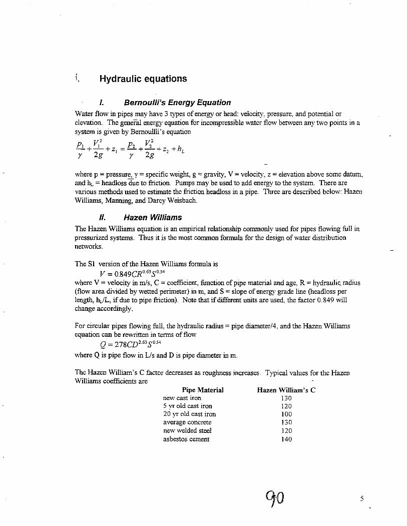
i. Hydraulic equations
I. Bernoulli's Energy EquationWater flow in pipes may have 3 types of energy or head: velocity, pressure, and potential orelevation. The general energy equation for incompressible water flmv between any two points in asystem is given by Bemoullli' s equation
V2 V2
EJ...+_I_+ Zj =P2 +_2_+ Z2 +hLr 2g r 2g
where p =pressure, Y =specific weight, g =gravity, V =velocity, z =elevation above some datum,and hL = headloss due to friction. Pumps may be used to add energy to the system. There arevarious methods used to estimate the friction headloss in a pipe. Three are described below: HazenWilliams, Manning, and Darcy Weisbach.
II. Hazen WilliamsThe Hazen Williams equation is an empirical relationship commonly used for pipes flowing full inpressurized systems. Thus it is the most common formula for the design of water distributionnetworks.
The SI version of the Hazen Williams formula isV = O.849CRo.63SO.54
where V = velocity in mis, C =coefficient, function ofpipe material and age, R =hydraulic radius(flow area divided by wetted perimeter) in m, and S = slope of energy grade line (headloss perlength, hdL, if due to pipe friction). Note that if different units are used, the factor 0.849 willchange accordingly.
For circular pipes flowing full, the hydraulic radius =pipe diameter/4, and the Hazen Williamsequation can be rewritten in terms of flow
Q = 278CD 2.63S054
where Q is pipe flow in Lis and D is pipe diameter in m.
The Hazen William's C factor decreases as roughness increases. Typical values for the HazenWilliams coefficients are
Pipe Materialne\\' cast iron5 yr old cast iron20 yr old cast ironaverage concretenew welded steelasbestos cement
Hazen William's C130120100130120140
5

/II. ManningMore commonly used for open channel flow such as sewers, although some engineers also use itpressurized systems. The SI units Manning equation is
V =~R%SJ,2n
where V = velocity in mis, n =coefficient of roughness, R = hydraulic radius in m, and S = slopeof energy grade line.For circular pipes flowing full, the hydraulic radius = pipe diameter/4, and the Manning equationcan be rewritten in terms of flow
0= 312 D%S7~- nwhere Q is pipe flow in LIs and D is pipe diameter in m.
Manning's n increase as roughness increases. Typical values are given below.
Materialconcretecast-iron pipevitrified claybrickcorrugated metal pipebituminous concreteuniform firm sodded earth
Manning n0.0130.0150.0140.0160.0220.0150.025
IV. Darcy-WeisbachMore fundamental than the other equations. Friction factor varies with turbulent/laminar flowcondition.
LV 2
hL =f--2Dg
where hL = head loss, L = pipe length, D =pipe diameter, f= friction factor, V = velocity. thefriction factor fis a function of relative roughness ofpipe (pipe material and age) and Reynoldsnumber. It is usually determined from a Moody diagram.
The Darcy Weisbach formula can be rearranged to yieldIi
v =(2gDS) /2
f
Notice that for a given pipe, all of these equations have the formhL =K Qa
where K = a coefficient for a given pipe and depends upon its length, diameter, age, material, etc.K is a constant for the Hazen Williams and Manning equations but varies with Q (through theReynolds number) for the Darcy Weisbacha =constant exponent that depends on the formula used
C\\ 6

v. Minor lossesMinor losses for turbulent flow conditions are generally expressed as a function ofY:/2g thevelocity head. For long pipes, pipe friction headloss usually predominates and minor losses can beneglected. For shorter pipes such as those in treatment plant, minor losses can be important.
y~ Pumps
Capacity of a pump is expressed as flow delivered. The head required to overcome losses in a pipe _system is termed system head. The total dynamic head is the head against which the pump mustwork when water is being pumped. This is the head added to the system by the pump and can becalculated as the difference in head using Bernoulli's equation between the discharge and suctionnozzle ofthe pump_.
The power input for a pump is a function ofthe flow, head, and efficiency ofthe pump. Typicalefficiencies range from 60-90%. -
E = pump output =r QHr
P power P
I. Pump head - capacity curveThe head that a constant speed pump can produce as flow changes called pump head - capacitycurve or pump characteristic curve. The system curve is the plot ofthe total dynamic head(sum ofthe static lift + kinetic energy losses).
system curve
capacity
The operating point for the pump is defined by the intersection of the pump head curve and thesystem curve.
7

..;.;. Valves
I. checkCheck valves permit flow in only one direction. Commonly used to prevent flow reversal of flowwhen pumps are shit off. Check valves, termed foot valves, can be installed on the suction side ofpump to prevent loss of prime. Check valves are installed on the discharge side of pump to reducehammer force.
II. pressure reducingPressure reducing valves maintain a set pressure on the downstream end. Operate by using theupstream pressure to throttle the flow through an op.ening similar to globe valve. The throttlingvalve will open or close until the downstream pressure reaches the preset value.
III. pressure sustainingPressure sustaining valves attempt to maintain a minimum pressure on the upstream end when thedownstream pressure is below that value. If the downstream pressure is above the setting, flow isunrestricted. If the downstream pressure is above the upstream pressure, valve will close toprevent reverse flow.
IV. pressure breaker valves- Pressure breaker valves for a speqfied pressure loss across the valve.
V. flow control valvesFlow control valves to limit the flow through a valve to set amount, providing sufficient head isavailable.
VI. throttle control valvesThrottle control valves simulate a partially closed valve by adjusting the minor loss coefficient ofthe valve.
VII. gate valvesMost commonly used for on-off service. Relatively inexpensive and offer positive shutoff.Located throughout a distribution system at regular intervals so that breaks in the system can beisolated. Valves should be accessible through manhole of valve box. Generally must be installedin vertical position. Large gate valves frequently include small bypass valve to equalize pressureon the main valve and reduce potential for water hammer.
VIII. butterfly valvesLess expensive and easier to operate than gate valves. Not suitable for liquids that contain solidsand light prevent complete closure.
IX. air vacuum and air relief valvesUsed in long pipes at high points to prevent negative pressure from building up if lines are drainedor to allow accumulated air to be released. Operate automatically.
8

X. Altitude-control valvesA type of diaphragm-valve used to control level of water in a tank supplied from a pressure .system. Two types are used: single acting and double acting. Single acting used only for filling thetanks. The tank discharges through a separate lined or through a check valve in a bypass linearound the altitude valve. A double acting altitude valve allows water to flow both to and from thetank. When the tank becomes full, the valve closes to prevent overflow. When the distributionpressure drops below the pressure exerted by the full tank, the valve opens to discharge water tothe distribution system.
XI. globe and angle valvesNot commonly used in water distribution system. Primary application is household plumbing.
~. Storage
Storage is provided to equalize supply and demand, level out pumping requirements, provide waterduring source or pump failure, provide water to meet fire demands, provide surge relief, and toblend water sources. With adequate storage, water can be treated and pumped from the treatmentplant to the distribution system at a rate equaling the maximum day demand and pumps can beoperated at their rated capacity. Storage can also be used if the treatment plant operates for only aportion of a day.
I. Types of water storage facilities
1. types of service
i) operating storageOperating storage generally floats on the system with the reservoir filling when demand is low andemptying when demand exceeds supply. A mass balance can be used to size the operating storage.
9

Given the following demand rates, find the required operational:storage assuming 24 hr pumping. I
! II I i iI I
I i i i;
Time Interval IDemand IHourly IHourly iSupply - Demandstart lend Rate IDemand Supply ito !from
I gpm gal gal istorage !storageI12:00 AMI 1:00 AM 1900 114000 280460 1664601 0
1:00 AM 2:00 AM 1800 108000 280460 1724601 02:00AM 3:00AM 1795 107700 280460 172760: 03:00 AM 4:00 AM 1700 102000 280460 178460: 04:00 AM 5:00AM 1800 108000 2804601 1724601 05:00 AM 6:00AM 1910 114600 280460 165860: 06:00 AM 1-:00 AM 3200 192000 2804601 884601 07:00 AM 8:00AM 5000 300000 280460 OJ -195408:00 AM 9:00AM 5650 339000 280460 oj -585409:00 AM 10:00 AM 6000 360000 280460 O! -79540
10:00 AM 11:00 AM 6210 372600 280460 o! -9214011:00 AM 12:00 PM 6300 378000 280460 O! -9754012:00 PM 1:00 PM 6500 390000 280460 Of -109540
1:00 PM 2:00 PM 6460 387600 280460 01 -1071402:00 PM 3:00 PM 6430 385800 280460 01 -1053403:00 PM 4:00 PM 6500 390000 280460 0: -1095404:00 PM 5:00 PM 6700 402000 280460 01 -1215405:00 PM 6:00 PM 71191 427140 280460 01 -1466806:00 PM 7:00 PM 9000 540000 280460 01 -2595407:00 PM 8:00 PM 8690 521400 280460 01 -2409408:00 PM 9:00 PM 5220 313200 280460 01 -327409:00 PM 10:00 PM 2200 132000 280460 1484601 0
10:00 PM 11:00 PMI 2100 126000 2804601 154460! 011:00 PM 12:00 AM 2000 120000 280460 1604601 0
I I,
Sum: I 6731040 6731040 15803001 -1580300I I I
I
Average hourly pumping: 16,731,040/24 = ! 280460:I I ! I
Required storage: I I 1580300 I I
ii) emergency storage
Designed to be used only in exceptional situations such as fires or source failures.
2. configuration
i) tanks
Generally refers to any structure used for containing water. Elevated tanks are supported on steelor concrete tower. Ground level tanks are less expensive to build and operate, but may require abooster pump to provide adequate pressure.
10

ii) standpipesTank resting on the ground \vith a height greater than its diameter. Gencrally only thc upperportion has enough pressure to be used in the distribution system. The lower portion can be usedfor emergency storage.
iii) reservoirsReservoirs generally refers to very large storage facilities. Can be ponds, lakes, etc. Morecornrilon to use reservoirs for raw water storage rather than treated water.
ivy pneumatic tanksUsed in very high or remote areas with few customers. Consists of steel pressure tank partiallyfilled vvith pressurized air. The compressed air on top of the water provides necessary pressure tothe area. A small booster pump is located on the intake side ofthe tank. The pump is only turnedon 1rllen the pressure in the tank drops below a set level. The maximum amount of water that maybe withdrawn at any time is approximately 1/3 the total tank volume.
3. Construction materialTanks can be made from steel or concrete with an appropriate liner.
4. LocationTo minimize pipe diameters, elevated storage facilities are usually located in regions of the serviceareas where pressure is low, i.e. as close to the center of demand as reasonable. The water level inthe reservoir must be at a sufficient elevation to permit gravity flow at an adequate pressure.Reduced pipe diameters can be used near a reservoir because the water will flow in all directionsaway from the tank when it is supply water. Elevated storage facilities near the treatment plantgenerally do not allow for reduced pipe diameters. Decentralized storage with several smallertanks in different parts of the distribution system are usually preferred compared to one large tank.
Ground-level storage with booster pumps is often used when the system has several pressure zones.Storage is located at the boundaries of these pressure zones. Water from the lower pressure zoneflows into the reservoir and is pumped to the higher pressure zone.
II. UFloating"storage tanksDuring periods oflow flow, usually in late evening, the heads in the distribution system are lowand the storage tank is filled automatically. Altitude control valves can be used to shut offfIowwhen the storage tank is full. As the demand increases during the day, the head in the distributionsystem falls and the entire capacity of the treatment pumps is used to meet demands. As demandincreases further, the excess demand is met from the storage tank and the tank begins to empty.
c. Hydraulic modeling
Pressures (heads) should be adequate for consumers and fire fighting. This influences thediameters chosen. Ifhelp is needed to maintain pressure, in-line booster pumps and elevatedstorage tanks can be used. Typical pressures in residential areas of the US range from 40 to 50psig (90 to 115 feet ofhead). Pipe sizes should be large enough to avoid excessively high or lowvelocities. Generally 3 to 4 feet per second is considered desirable. The National Board of Fire
II

Underwriters requires a minimum of 8 in diameter pipe, although 6 inch diameter pipe can be usedin the grid system.
Hydraulic models for distribution systems should be analyzed for conditions that exist now as wellas for conditions that exist at the end of the_design period. Headlosses are expected to increase aspipc::s age.
I. Notation and dflta requirementsDistribution systems are generally based on a link-node framework. Links are use to represent thepipes. Nodes represent locations where flows enter or leave the system or where links jointogether. Nodes should be placed wherever pipe characteristics (e.g. diameter or material) changeor to provide sufficient resolution for water demands. Demands are typically not modeled at thelevel of individual households - rather a group ofhouseholds are clumped together and thedemands are located at one common point.
1. Water System Inventory
i) inventory existingfacilities
(1) pipe location and diameter, length, type, age,present condition
(2) storage facilities: capacity, location, availability,dimensions, water surface elevations, connectionsto system
(3) design and operation features of service andbooster pumps, including capacity, system head,elevation
(4) control and regulatory valves elevation, operation,pressure setting, purpose
(5) service areas and pressure zone boundaries
ii) review operating records and interview staff
c(\
(1 )
(2)
(3)
(4)
diurnal and seasonal treated water productionrecords
service and booster pump flows and pressures
c1earwell and storage level variations for differentdemand situations
system operation criteria for pump stations,storage, source pumps
12

(5) system operating pressures determined from pasttesting or monitoring
(6) power consumption records, costs, and ratestructure
(7) observed low pressure areas indicating systemdeficiencies
(8) observed fire flow capabilities
iii) review water consumption records
(1) total water sales (billing records)
(2) service population
(3) number and types of connections
(4) consumption by major users
(5) peaking factors
(6) system diurnal demand curves
ivy develop water demands using consumption records andpopulation and land use prl?,;ections. Existing andprojected demands should be establishedfor the totalsystem, sub areas within the system, and major users.
(1) average annual day demands
(2) maximum day demands
(3) peak hour demands
(4) fire flow demands
(5) minimum hour demands or maximum storage replenishment rate
(6) other site specific demand features
13

l~ establish background information for power managementand operational improvement programs
(1) plot pump characteristic curves vs system headcurves
(2) establish average maximum day pumping ratefrom the developed diurnal demand curve
(3) determine whether system storage or auxiliarypower can be used to reduce peak pumping rate toor below the average of the maximum daydemand.
(4) check the piping arrangements to storagecomplexes for replenishment constraints
(5) examine pump curves vs system head curveconditions to determine optimal operationsequence based on system demands
2. Required physical data
i) pipe segments
(1) assign 10 numbers
(2) establish length between nodes
(3) determine pipe diameter, roughness coefficient(age and pipe material)
ii) nodes
(1) assign ID numbers
(2) establish ground surface elevations of each node
If read from contour map, 1 m contours desirable, 3 m contours acceptable ifno other data. Errorsarise from interpolated contours. (Note 1 ft error =:: 0.43 psi.) Generally, ground surfaceelevations are used, not the elevations of the buried pipe.
Accurate data needed for pressure control points - points where system pressure fixed or open toatmosphere - and pressure regulated discharge points. Other node elevations can be estimated.
14

iii) supply pumps and booster pumps
(1) assign 10 numbers (EPANET treats as links, otherprograms as nodes)
(2) determine multiple points on pump curve
(3) define on/off control levels based on systempressure or tank elevations) .
(4) determine ground surface elevation for each pump
(5) assign valve or adjust pump curve for minor losses
iv) controll'alves andpressure regulating valves
(1) assign 10 number (EPANET treats as links, otherprograms as nodes)
(2) determine downstream pressure setting.Jor eachPRV
(3) determine control pressures for flow control valves
(4) establish ground surface elevations
v) resen'oirs and storagefacilities
(1) assign 10 number (treated as nodes)
(2) define capacity, dimensions, flow rate, andoperating range
(3) establish ground surface and water surfaceelevations
/I. Branched distribution systemsThere are 2 general classes ofpiped distribution systems: branched and looped. A branchednenvork contains no closed circuits or loops. Pipes can simply dead end. Branched nenvorks arcfound on the outskirts of many tovvns, in rural communities, in irrigation systems, and frequently invillages in developing countries. Branched distribution systems have a structure similar to a tree.A trunk line provide the major source of water. Service mains and submains branch off the trunkline. Branched distribution systems have several limitations: stagnation in the dead ends may allowfor bacterial growths and sedimentation, disinfectant residuals are hard to maintain in the deadends, repairs will shut down service for all connections beyond the repair point, the pressure at theend of the line may become undesirable low as additional corrections are made.
15

~ : ~ : ~\ ~ : : : :1 : : : : :1 : : ~ : :1 : ~..,/ --,..IJ ..I~.J..I...,1..,/...I~..IJ..IJ.J ~-I...I.J..I-I~"'/.J
(a) (b)Examples ofbranched distribution systems
On the other hand, branched distributions are simple to design and construct, and are less costlythan looped systems. When branched networks are used, the cost of the network is often of majorconcern. Branched networks use less pipe than looped networks, and therefore cost significantlyless:- An interesting problem is to design a branched distribution network that has minimum costfor a specified layout. Once the layout is established, the major factors affecting cost are thediameters used throughout. These must be chosen to maintain necessary heads at each point in thedistribution system. This problem requires an understanding ofboth fluid flow in pipes andoptimization techniques. As stated, the problem can be formulated as a linear programmingproblem. A linear program optimizes a linear objective function that is subject to a series of linearequality and inequality constraints. The problem will be illustrated through the use of an example.Given the example network below
11081,",<jj LPS
LJ,; jljElev=60m
Link 1071000m
11061 q jj LPS
Elev=55m L\,. @J,;jljm HGL
Link 1044000 m
Elev=60m
~j~y LPS'·· @~jjy<jj m HGLA
1 LPSElev=10m
Link 106
4000 mLJ,; jlj Link 105
700 m
Link 1032000 m
LPS
Lj,;jjjE1 e v= 6 Om
Elev=90m' <jj~j~y LPS
<,.. < ' , I ~ & ~ ~ ~ & ~ ~ " ~ " " & " " "" ~ ,," ~ fl."" fI. ,. ,. " & ,. ~ fI. ,. & ,. " ,. &" I ", II II ,." II •• II • II II .... iii II II II • ••1' . "'" 'IJ ' 'J ' 'J 'JJ .. II •• II .\ \ • \ II •
J~ JJJJJJ"'/...IJJJJ.JJ..IJJ ~ ..IJ ..1...1 J JJJJJJ JJ LPS
3 LPS LJ,;jjj
Elev=60m
Link 102
1000 m
LJ,;jjj Link 101
1000 m
Lj,; jjjElev=60m
16

The example network consists of 7 pipe segments or links which arc connected by 8 nodes. Eachnode is a point of water input or demand or a junction between two pipes. The network containsno closed loops, hence it is a branched network and the link flows may be easily detennined fromthe mass balance equations alone. Inputs to the network occur at nodes 104 and 106. These inputshave knovvn hydraulic grade line elevations. All other nodes are either demand or junction nodes.Two links, 105 and 106, are existing, 'with 10 cm diameters. It is assumed that link 105 willremain unchanged, while link 106 will be paralleled with new pipe if necessary. All other links willbe designed using new pipe.
The design objective is to select pipes for the links in such a manner that the t-otal construction costis minimized subject to certain design constraints. Both the objective and the constraints can bewritten as linear equations or inequalities. The resulting problem is called a linear program. Themathematical trick that pennits th~ fonnulation ofthe problem as a linear program is that pipelength, rather than pipe diameter, is treated as the unknown or decision variable. Thus, theengineer proposes commercially available pipe diameters as candidates for each link, and the linearprogramming algorithm selects from these candidates the optimal combination. Different sets ofpipe diameters for different links are allowed. The optimal combination of pipes for each linkwould then be laid in series along the link.
The candidate pipe diameters for the example network are 5 cm, 10 cm, and 20 cm. The decisionvariables are:
Xl = the length of 5 cm pipe to be used in link 101X2 = the length of 10 cm pipe to be used in link 101X3 = the length of 20 cm pipe to be used in link 101X4 = the length of 5 cm pipe to be used in link 102Xs = the length of 10 cm pipe to be used in link 102X6 = the length of 20 cm pipe to be used in link 102X7 = the length of 5 cm pipe to be used in link 103X8 = the length of 10 cm pipe to be used in link 103Xg = the length of 20 cm pipe to be used in link 103XlO = the length of 5 cm pipe to be used in link 104Xll = the length of 10 cm pipe to be used in link 104Xl2 = the length of20 cm pipe to be used in link 104XJ3 = the length of 10 cm pipe to be used in link 105X14 = the length of 10.8 cm pipe to be used in link 106"XlS = the length of 14 cm pipe to be used in link 106"Xl6 = the length of 23.7 em pipe to be used in link 106"Xl? = the length of 5 cm pipe to be used in link 107x18 = the length of 10 cm pipe to be used in link 107X19 = the length of 20 em pipe to be used in link 107
"These are equivalent diameter pipes. Xl4 is the equivalent diameter of the existing 10 cmand the candidate 5 em. Similarly, XlS is the equivalent of the existing 10 em and thecandidate 10 em, and xl6is the equivalent of the existing 10 cm and the candidate 20 cm.
The installed costs per unit length of the candidate pipe are $15/m for the 5 cm pipe, $50/m for the10 em pipe, and $1 OOlm for the 20 cm pipe. Installed pipe has an associated cost of $O/m,regardless of its diameter. The construction cost is thus
17

COST = I5xl +50X2+ IOOx3+ 15 '4+50x~+ lOOx(,+15 X7 + 50 Xg + 100 X9 + 15 XIO + 50 Xll + 100 Xl2 +aXu + 15 Xl4 + 50 Xl5 + 100 XJ6 + 15 X17 +
50 Xl8 +)00 XJ9
The constraints on the design variables consist ofboth equalities and inequalities. Theseconstraints impose_both headloss and length restrictions on the decision variables. There are 3 typeof headloss ~onstraints that may be imposed at each node. The first type says that the residualhead at the node must be greater than or equal to some specified head. This is used to insure thatthere is minimum positive pressure at the specified nodes. An alternative constraint is that theresidual head must be less than or equal to some specified head. This type of constraint are used inhilly terrains to prevent exceeding the allowable pipe pressure 000 prevent excessive pressures atnodes. The final type of constraint is that the residual head is equal to some known head. Thisconstraint is used-in networks with more than one input node to insure that the headloss along thepath from the two nodes is equal to the difference in the hydraulic grade lines (HGL). Paths arereferenced from a specified input node called the reference node. This last type of constraint mustbe imposed where more than one input occurs. The other constraints may be imposed as needed.In general, minimum pressure constraints are imposed at the e:\.1:remities of the network, i.e. theterminal or end nodes. Maximum pressure constraints are imposed at low elevation points on hillyterrain. The linear programming technique automatically adds constraints that all the decisionvariable be nonnegative. Since theses variable represent lengths in this problem, these additionalconstraints are not a difficulty. If the minimum allowable head is 1 meter, and this constraint is tobe applied to nodes 101, 102, 103, and 108, and node 104 is taken as the reference node, theconstraints can be \"ritten as
hL lO3 + hL102 <= 100 - 60 - 1 = 39hL lO3 <= 100 - 90 - 1 = 9hL103 + hL lO1 <= 100 - 60 - 1 = 39hL106 + hL lO7 <= 100 - 60 - 1 = 39
where the subscripts on the headloss refer to the links, 100 is taken from the HGLofthe reference node, 60 and 90 are the ground elevations of the constrainednodes, and I is the minimum residual head.
If the head at node 107 is constrained not to exceed 55 m, then its constraint can be written as
hL106 >= 100 - 10 - 55 = 35
Since there are two input nodes, with fixed HGL's, an additional constrain must be written
hLIOS + hL104 = 100 - 110 =-10
Nodes 104 and 105, as interior nodes, probably do not need to be constrained on the first design.If the initial results suggest that constraints are necessary, they may be added and second designperformed.
The headlosses are calculated for each of the candidate pipes using one of the flow equations,typically the Hazen Williams equation. The headloss can be calculated from
\(f) 18

hL'J = (Q/kiCl8S Dt87LJ
where hLi] =headloss in pipe j in link iQ; =flow in link iki =constant for link i that depends on unitsC; = Hazen Williams coefficient In link iDj =diameter ofpipe j
For example, in link 101, three different diameter pip~s may be used to make the link.
Additional constraints must be added to insure that the lengths of the candidate diameters match theneeded total length of each pipe. These constraints are
Xl + X2 + X3 =1000X4 + Xs + X6 =1000X7 + X8 + X9 =2000XlO + XII + Xl2 =4000XJ3 = 700Xj4 + XIS + Xl6 =4000X17 + XI8 + XI9 = 1000
The linear programming automatically adds the constraints that
Xi >=0 i = 1,...,19
The problem, then, is to choose the xi's that minimize the cost, but meet all of the constraints. Acomputer program, BRANCH, that sets up and solves this type of problem is included along withuser instructions. The basic solution from the linear programming algorithm is
Link # Diameter (cm) Length (m)101 5 129.6
10 870.4102 5 129.6
10 870.4103 10 231.1
20 1768.9104 10 115.9
20 884.1105 10 700.0106 10.8 1883.9
14.0 2116.1107 10 607.9
20 392.1
These diameters and lengths just meet each of the constraints that '\Tere imposed, using as much ofthe smaller, less expensive diameter pipe as possible.
Pipes are assumed to be laid in order of decreasing diameter in the downstream direction. Thus forlink 104, the 20 cm pipe should be laid from node 106 (the upstream node) and then the 10 cm pipe
19

used to complete the distance to node 105 (the downstream node). This ensures that thedownstream nodes exceed the minimum pressures when such constraints arc used.
It may not be possible to meet all the constraints with any combination of the candidate diameters.In this case the algorithm will return with a solution labeled infeasible. For example, the headlossfrom the reference node to a node with a minimum pressure constraint may be greater thanallowable to meet the constraint even when the largest candidate diameter is used for the entire linleThe problem would then be infeasible. To attempt to correct this situatio~ make larger diameterpipes available on paths subject to minimum head constraints, smaller diameter pipes available onpaths with maximum head constraints, and both larger and smaller diameters available on pathslink nodes with known hydraulic grade lines.
III. Looped distribution systems
A distribution system with loops or circuits can provide the reliability that a branched networkcannot. If a break occurs, water is able to flow through the remaining pipes in the loop and movedownstream. Since flow occurs in all pipes, the water quality should not have sufficient time todeteriorate if the network is designed properly. Typical loop patters include a grid pattern with acentral feeder line that nonnaIIy carries the bulk of the flow (Figure 2a) or a grid pattern with amain looped feeder (Figure 2b).
I~~~~~~~...,...~
I
( a)
(b)
Figure 2. Examples of Looped Distribution Systems
The pressures and flows in looped distribution systems are solved by ''''Titing a series of nonlinearequations based on conservation of flow and energy.
20

1. continuity equations / conservation of flowThere are two type of equations that are used to detennine the flows in the links. The first type isbased on conservation of mass, sometimes called a mass balance. It simply states that the sum ofthe flO\'i'S entering a node must equal the sum ofthe flows leaving a node. Thus at each junction
I: Qinjlow = I:Qou!fIow
2. flow equations around loopsThe second type of equation is based on the conservation of energy. It states that the sum of thesigned head losses around a loop equals the energy input from any pumps on the loop. If there areno pumps, the headlosses must sum to zero. In other words, the energy at a node is the same nomatter what direction the node is approached from.
I:hi = I:E p (for each primary loop)
where Ep =energy added to water by pumpsNote that a sign convention must be adopted to properly sum the headlosses. Typically, flows in aclockwise direction around a loop are considered positive. For example, for the loop and the flowdirections given
i i
A second type of energy equation can be written for any two fixed grade nodes, which says that thesum of the headlosses along any path connecting the fixed head nodes must equal the difference inheads between the nodes.
3.
( for each R - I pair of fixed head reservoirs)
solution techniques
i) unknown flows
If the flows in each pipe are treated as unknown, then L equations must be written to solve forthese flows. N of the equations are the mass balance equations at the nodes, P are energy balanceequations around each primary loop, and R-l equations are the energy balance between fixed head
21

reservoirs. The mass balance equations are linear in terms of the flows. The energy equations arcwritten in terms of the flow in the pipe using anyone of the flow equations discussed above, e.g.the Hazen Williams equation. The resulting energy equations are nonlinear in terms ofthe flO\vs.Thus, a system ofL nonlinear equations must be solved to provide the flows. Three methods areavailable:
(1) single link flow adjustment
This method was developed by Hardy Cross and is one ofthe most commonly used. It is suitablefor hand calculation. The technique requires an initial estimate of the flows that satisfy the massbalances at each node. Given these flows, a flow adjustment factor for each loop is calculatedbased on the energy equations. This adjustment factor is added to the flows in the pipes in theappropriate loop, resulting in an updated estimate ofthe flows. The process is repeated using thecurrent flow estimates until the adjustment factors fall below some specified criterion. An exampleand a computer program for the Hardy Cross solution of looped networks is given below.
(2) simultaneous flow adjustment
This technique solves the system on nonlinear equations based on Newton's method or one of itsvariations. Again, an initial estimate of flows is required. A flow adjustment factor is calculatedfor each pipe simultaneously, resulting in improved flow estimates. This process is repeated untilthe adjustment factors fall below some specified criterion.
(3) linear method
This method approximates the energy equations with linear relationships in terms of approximateflows
hL = [K"Q(O)"-J] Qwhere Q(O) =the initial or previous estimate ofthe flow
Q =the current estimate ofthe flow, i.e. the unknown to be solved for
This formulation results in a system of L linear equations which can easily be solved for the newflow estimates. The process is iterated until the changes in flows between any successive iterationsfalls below some specified criterion.
ii) unknown heads
Methods which treat the heads at nodes as unknown require N independent equations. These areprovid~d by the mass balance equations written in terms of heads between adjacent nodes. Forexample, the flow in the link with nodes I and 2 as end nodes can be calculate from
Writing each ofthe mass balances with the above equation substituting for each flow results in asystem on N nonlinear equations to be solved. Since there are generally less nodes than there arelinks, this solution technique requires less space on a computer. Two methods are available forsolution.
22

(1) single head adjustment
This method was also described by Hardy Cross, but is not as widely used. Initial heads at each ofthe nodes are first assumed. Head adjustment factors are calculated based on the mass balance atthe node. This process is repeated until the adjustment factors are less than the convergencecriterion.
(2) simultaneous head adjustment
This technique solves the system of nonlinear equations based on Newton's method or one of itsvariations. Again, an initial estimate of heads in required. A head adjustment factor is calculatedfor each node simultaneously, resulting in improved head estimates. This process is repeated untilthe adjustment factors fall below some specified criterion.
iii) Hardy Cross
The Hardy Cross method was used for may years. It is suitable for simple net\vorks and can besolved by hand. The method calculates successive flow corrections to the pipes in a primary loop.Hardy Cross is not recommended if alternative computer solutions are available, as Hardy Crossdoes exhibit convergence problems at times. The approach is
I) Assume flow distribution within each pipe. Flow continuity must be established at each junctionnode. The headloss equations do not have to be satisfied. However, the closer the initial flowdistribution is to the actual flows, the more quickly the method will converge.
2) Choose a direction around a loop that will be considered positIve. Traditionally, clockwisedirection is chosen.
3) For each primary loop, determine the headloss in each pipe, using one of the hydraulic equationsdiscussed above (e.g. Hazen Williams). A sign is given to the headloss based on the direction offlow and the sign convention.
4) Sum the signed headlosses and sum the signed headlosses divided by flow.5) Calculate the flow correction for the loop by
Z}L!lQloop = h
1.85L /7'Q(Note the minus sign in the formula.)
6) Apply the correction to the assumed flow in each pipe in the loop.
7) Repeat steps 3-6 for the other primary loops8) Iterate steps 3-7 for each primary loop until each calculated correction is sufficiently small. Ifthe initial flows were approximately correct, the Hardy Cross method will usually converge in 3iterations.
Note that in applying corrections to pipes common to two loops the corrections for both loops aremade to the common pipes. This is required to maintain flow continuity at junctions.
\(fb 23

Example: Solve for the flows in the following network. Use Hazen Williams to calculate headloss.All the nodes have elevation O. All the pipes have a C = 100.
B2000',6"
C~m "-/
200
/.1' ........gpm
2000',6"
~ ~2000',6"
1000 600gpm G
2000',6" gpm2000',6" ---+-A - D..--ilQUgpm :/'; ~ <3QUgpm
~600
J~2000',6"gpm
2000',6"
, .''v
400 400gpm m I) gpm'-F
2000',6"E~
ITERATION 1 I--
ILink IDiam Length Flow hL/L IhL hL/Q new flow
lin 1ft gpm ftlft ft Iftlgpm gpmAS I 8 1000 50 0.000116 0.11602 0.00232 60.4BC I 6 2000 50 0.000471 0.942024 0.018841 60.4CD I 6 10001 -150 -0.0036. -3.60238 0.0240161 -139.6DG I 6 1000 300 0.0130031 13.00327, 0.043344 310.4GA 1 6 1000 -300 -0.0131 -13.0033 0.043344! -289.6
1 Isum i -2.544341 0.1318651I I delta flow ! 10.42972 iI I i
I
iAG I 6 1000 289.6 0.0121791 12.17853 0.042057 301.3GD I 6 1000 -310.4 -0.013851 -13.8528 0.044625 -298.7DE ! 41 1000 150 0.025955! 25.95491 0.1730331 161.7EF i 6 20001 -250 -0.00928! -18.5546 0.0742181 -238.3FA
I
8 10001 -650 -0.013411 -13.4089 0.0206291 -638.3Isum I -7.68281 0.3545621i
1 Idelta flow' 11.71268 I
24

ITERATION 2 I i !
Link !Diam Length IFlow IhL/L IhL !hL/Q inew flowin ft gpm ftlft ift lft/gpm jgpm
AB 1 8 1000 60.4 0.000165 0.164781 0.0027271 67.9i
BC i 6 2000 60.4 0.0006691 1.33793 0.022141 67.9CD I 6 1000 -139.6 -0.00315 -3.15232 0.022586 i -132.1DG 6 1000 298.7 0.01291 12.90048 0.043186: 306.2GA I 6 1000 -301.3 -0.01311 -13.1064 0.043502: -293.8
sum _. -1.85557 0.134141 iI delta flow 7.477255 I
I IAG I 6 10001 293.8 0.01251 12.51045 0.0425811 295.5GD 6 1000 -306.2 -0.0135 -13.5048 0.0441051 -304.5DE 4 1000 161.7 0.029832 29.83236 0.1844781 - 163.4EF 6 2000 -238.3 -0.00849 -16.977 0.0712461 -236.6FA 8 1000 -638.3 -0.01296 . -12.9649 0.0203121 -636.6
sum· -1.10384 0.3627211delta flow 1.644983 I
ITERATION 3 I ILink IDiam Length Flow hL/L IhL hL/Q inew flow
lin ft gpm ftlft ft ftlgpm gpmAB i 8 1000 67.9 0.000205 0.204516 0.003012 68.9I
BC 6 2000 67.9 0.00083 1.6605621 0.024453, 68.9CD 6 1000 -132.1 -0.002851 -2.84673 0.0215511 -131.1DG 6 1000 304.5 0.013371 13.37079 0.0439041 305.6GA 6 1000 -295.5 -0.012641 -12.6405 0.0427841 -294.4
! sum -0.251341 0.135703I , delta flow 1.0011371 i
!,
AG 6 1000 294.4 0.0125611 12.561271 0.04266j 294.7GD I 6 1000 -305.6 -0.013451 -13.4523 0.0440261 -305.3DE i 4 1000 163.4 0.0303971 30.39676 0.1860751 163.6EF I 6 2000 -236.6 -0.00838i -16.7606 1 0.070827 [ -236.4i
FA i 8 1000 -636.6 -0.01291 -12.903 0.0202671 -636.4I sum -0.15788 0.363855!I I delta flow I 0.234545 l
il~ Method ComparisonWhenever working with systems of nonlinear equations, the reliability of the solution technique isimportant. All of the methods described above require initial estimates of the unknov.ns to start thesolution process. If these estimates are very different from the correct values, the techniques maynot converge to the correct answer. Studies have shown that the simultaneous flo,,,' adjustmentmethod and the linear method are the most likely to accurately converge. The other threetechniques can exhibit convergence problems. The Hardy Cross method appears more likely to failwhen the energy equations contain some links with very high headlosses and some links with verysmall headlosses.
25
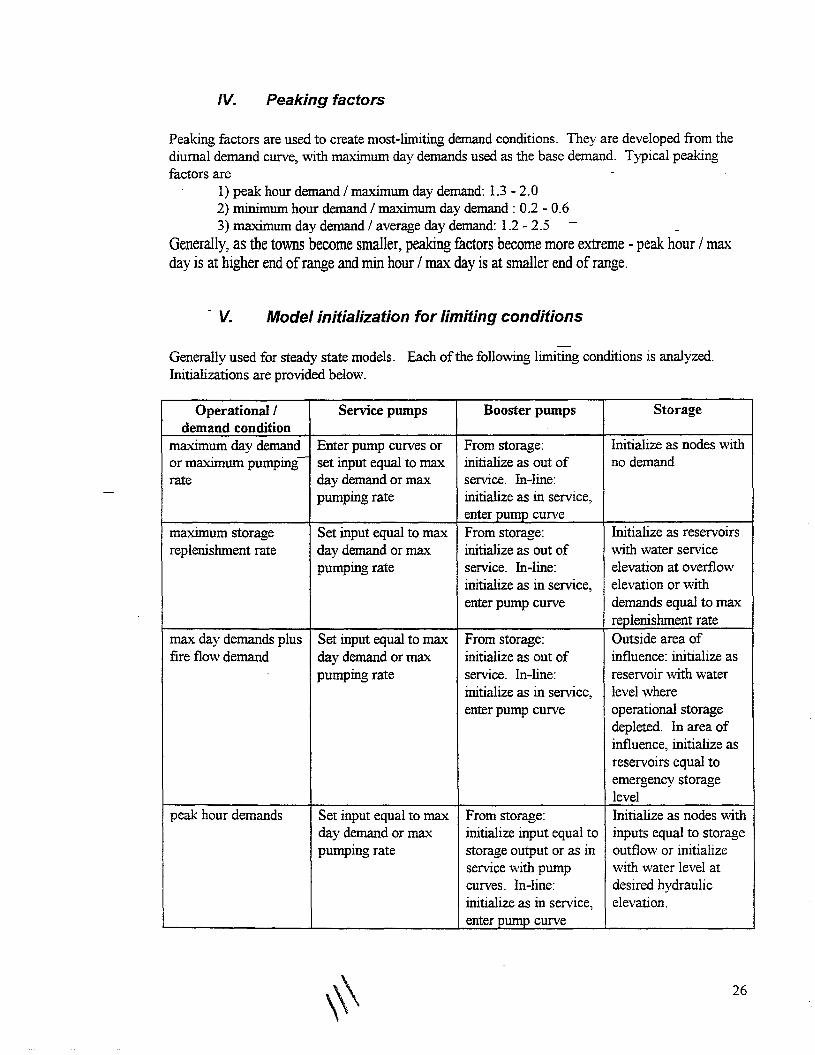
IV. Peaking factors
Peaking factors are used to create most-limiting demand conditions. They are developed from thediurnal demand curve, with maximum day demands used as the base demand. Typical peakingfactors are
I) peak hour demand / maximum day demand: 1.3 - 2.02) minimum hour demand / maximum day demand: 0.2 - 0.63) maximum day demand / average day demand: 1.2 - 2.5
Generally, as the towns become smaller, peaking factors become more extreme - peak hour / maxday is at higher end of range and min hour / max day is at smaller end of range.
- V. Model initialization for limiting conditions
Generally used for steady state models. Each of the following limiting conditions is analyzed.Initializations are provided below.
Operational! Service pumps Booster pumps Storagedemand condition
maximum day demand Enter pump curves or From storage: Initialize as nodes with. . -
set input equal to max initialize as out of no demandor maxunum pumpmgrate day demand or max service. In-line:
pumping rate initialize as in service,enter pump curve
maximum storage Set input equal to max From storage: Initialize as reservoirsreplenishment rate day demand or max initialize as out of with water service
pumping rate service. In-line: elevation at overflowinitialize as in service, elevation or withenter pump curve demands equal to max
replenishment ratemax day demands plus Set input equal to max From storage: Outside area offire flow demand day demand or max initialize as out of influence: initialize as
pumping rate service. In-line: reservoir with waterinitialize as in service, level whereenter pump curve operational storage
depleted. In area ofinfluence, initialize asreservoirs equal toemergency storagelevel
peak hour demands Set input equal to max From storage: Initialize as nodes vvithday demand or max initialize input equal to inputs equal to storagepumping rate storage output or as in outflow or initialize
service with pump with water level atcurves. In-line: desired hydraulicinitialize as in service, elevation.enter pump curve
26

VI. EPANETDeveloped by USEPA as hydraulic model coupled with contaminant transport model. Flow modelis dynamic, capable of tracking conditions under varying flows and demands. Model runs underboth DOS and Windows, although the Windows model contains more graphics and can handlelarger system. System size is limited by amount of RAM memory - there is no fixed limit. Modelwill simulate flows and pressures, several types ofvalves, including check and PRY, reservoirs,storage tanks, and pumps.
1. InstallationIf the program is provided in a compressed format, you vvill need to expand it prior to installation.Typically, the program is provided in '! ZIP format. You will need PKUNZIP or similar programto expand. Copy EPANET.ZIP t a temporary subdirectory and type
PKUNZIP EPANET.ZIP(PKUNZIP is frequently renames to just UNZIP. Type the name ofwhichever program willdecompress the file.)
Start Windows. From the File Manager, run SETUP.EXE. This will install EPANET to its ownsubdirectory and create an icon for its use.
Although not necessary, running Windows in enhanceamode allows for a larger system to bemodeled and improves the model run times. Add the following line to your AUTOEXEC.BAT file
SET EPAN:IT=32Note that there are no spaces around the =sign. For advanced users, editing the SOLVER.PIF fileto force SOLVER.EXE to run in full screen mode, rather than 'windowed mode, will also increasethe speed of the program.
The text editor that is supplied with EPANET is DOS based. Ifyou wish to change it to aWindows based editor or spreadsheet, add the following lines to the EPANET.INI file found in theWindows subdirectory:
[EDITOR]Program=<progname>Caption=<window title>
where the names in <> should be filled in appropriately. The editor or spreadsheet must be set toproduce pure ASCII text files. Select an editor capable of working 'Vvith files> 64K. Thisexcludes NOTEPAD.
The full manual is provided on disk (usually in ZIP format) as several files in WindO\vs WRITEformat (which comes with Windows). Each file can be loaded into WRITE and printer.
2. Data Files
One input file is required to run EPANET. An additional map and verification files are notrequired but are recommended. The input file is an ASCII text file divided into sections labeledwith [], e.g. [PIPES]. Comments can be added starting with a semicolon. Lines are limited to 80characters in length.
27

The specifications within each section are given in the EPANET manual and the help file. Input isfree fonn, the entries do not need to appear in specific columns of a line. The minimum sectionsrequired for a hydraulic model are [JUNCTIONS] [PIPES] and [TANKS]. Note that junctions(nodes and tanks) and pipes (pipe segments, pumps, and valves) must be defined before any otherreference. The standard section listing in order for a steady state hydraulics analysis is:
[TITLE][JUNCTIONS][TANKS][PIPES][PUMP-S][VALVES]
. [REPORT)If a dynamic analysis is used, then the following sections are added
[STATUS][CONTROLS][PATTERNS][TIMES]
If a water quality analysis is used, then the following sections are added:[QUALIIT][SOURCES][REACTIONS]
An [OPTIONS] section is usually placed at the end ofthe file.Among other things, the [OPTIONS] section can be used to set the units used for the simulation.SI units are liters/sec for flow, meter for length and head, and mm for diameters.
Two optional files can also be used and are recommended. They are specified in the [OPTIONS].. section. The first is a map file which lists each node and corresponding x,y location in a
[COORDINATES] section. Optional teA'! labels can be included in the [LABELS] section. Thex,y measurements can be in any arbitrary scale. They are used for display purposes only, and donot affect the hydraulic calculations.
The second auxiliary file is a verification file. It lists each node with all the links that are attachedto the node. Because numbering and transcribing the nodes and links is usually where most ofthemodeling errors are made, using a verification files will help identify data entry problems.
Very brief summaries of each section type are provided below. Full details are available from theEPANET manual or help file.
[TITLE]Used to identify the model run. Up to 3 lines oftext.
[JUNCTIONS]Used to ID junction nodes and corresponding elevations and demands. Use negative demands forfixed inputs. An optional pattern id can also be specified for dynamic models.
[TANKS]For reservoirs, an ID and elevation are entered. For tanks, an ID, the bottom elevation of the tanlethe initial water level above the bottom ofthe tank, the lowest water level above the bottom of the
28

tank, the highest level above the bottom of the tank, and the tank diameter are entered. Tanks areassumed to be cylindrical by EPANET.
[PIPES]The pipe 10, head and tail nodes, length, diameter, and roughness coefficient are entered. Minorloss coefficients can be listed here. Check valves are also specified here.
[PUMPS]EPANET treats pumps as links in the model. A pump 10, head and tail node, and a description ofthe pump characteristic curve are entered.
[VALVES]EPANET treats valves (other than check valves) as links in the model. A valve ID, the head andtail nodes, the diameter, the valve type (pressure reducing, pressure sustaining, pressure breaker,flow control, or throttle control), the setting for the valve, and a minor loss coefficient are entered.
[REPORT]Describes the output report to be created. Specific nodes or links can be examined.
[STATUS]Used to initialize the settings oflinks at the start of the simulation. Pumps can be open or closed.Relative pump speed can be given. Valve (PRV, PSV, FCV, TCF) settings can be open or closed.A pipe can be open or closed, which is used to simulate gate valves in the system.
[CONTROLS]Allows pumps, valves, and pipe setting to change at given times or when specific pressures or tankwater levels are reached.
[PATTERNS]Specifies how water demands and sources vary with time. A pattern 10 is provided along with aseries of multipliers to be applied to the demands. The default time period is I hr, and this can bechanged in the [TIMES] section. As many patterns as needed can be specified.
[TIMES]Sets the time step parameters for the simulation, including the duration of the simulation and thehydraulic, pattern, and report timesteps.
[OPTIONS]Sets values for network properties and simulation options including units, headloss formula, theverify and map file names.
Other sections which provide alternative entry formats include
[DEMANDS]Alternative to the [JUNCTION] section for entering baseline demands.
[ROUGHNESS]Provides an alternative to the [JUNCTION] section for altering roughness coefficients for groupsof pipes.
29

water sourcescaleorientation arrowdate last correctedpressure zone limits (may change)closed valves at pressure zone limits
3. Analyzing EPANET ResultsAs a Windows program, EPANET presents results in a number ofdifferent Windows. TheBrowser window allows for the simulation time, node, and link to be selected. Node informationincludes demand, elevation, hydraulic grade, pressure, and water quality. Link informationincludes diameter, flow, velocity, headloss/length, and average water quality. If a map is visible,the var~able will be color coded on the map and the specific node or link will be highlighted.
The Report menu can generate spreadsheet-like tables for the current time ofall nodes or links or atime series for the current node or link.
The graph menu can generate a time series plot ofthe current node or link.
VII. Model Output AnalysisThe model output can be used to test for system deficiencies. Deficiencies an a water distributionsystem are generally indicated by inadequate pressure. The model is useful in evaluating the causesand analyzing corrective actions.
Check that major trunk mains are able to meet the necessary storage replenishment rate. If any ofthe following conditions occur in a pipe segment, they are generally considerea' deficient and shouldbe corrected:
1) velocities greater than 1.5 m/s ( up to 3 m/s may be acceptable, but high headloss canresult and the potential for water hammer is greater)
2) headlosses greater than 10m / 1000 m3) large diameter pipes (16 inch or greater) with headlosses greater than 3 m / 1000 m
The general solution to each ofthese deficiencies is to increase pipe diameters. These conditionsshould be treated as general guidelines, not as finn rules.
Pumps should be checked that they deliver adequate flows over full range of system demands.,including average day demands. Conservative practice in multiple pump facilities is to providemaximum day flows with the largest pump out of service.
c. Maps and Drawings
I. Comprehensive map (or wall map)Map of entire distribution system used by system manager. Generally does not display all details.Typically includes:street nameswater mainssizes of mainsfire hydrantsvalvesreservoirs and tankspump stations
30

Typical scales ranging between 500 and 1000 ft to an inch.Update once or twice a year or after major system extension.
-II. Sectional maps or plat
Provides detailed picture of section of distribution system. Used for day-to--day operation. Severalmaps are required to-eover the entire srstem. Typically includessection designation or number water account numbersadjacent section number measurements to service linesstreet names distances main to curb boxmains and sizes distances to angle pointsmaterials of mains distances to fittingsdate ofmain installation dead ends and measurementsdistance from property line date last correctedfire hydrants and numbers orientation or north arrowvalves and numbers scalevalve sheet designation sho\\'l1 in margin closed valves at pressure zone limitsintersection number service limitsblock numbers tanks and reservoirslot numbers pump stationshouse numbers pressure zone limits
Typical scales are 50 to 100 ft to an inch.
Sectional maps should not overlap but should butt up against each other to avoid confusion. Eachshould be indexed, with the comprehensive map used as a base. Sectional maps must be updatedmore frequently than comprehensive maps, typically monthly or quarterly.
III. Valves and hydrant mapsPinpoint valves and hydrants throughout the distribution system. Provide measurements frompermanent reference points to each valve in system. Should include direction to open, number ofturns to open, model, type, date installed. last date tested or repaired. May either be similar to asectional map with a corresponding table, or an intersection map at a very large scale (20 to 30 ftto an inch)
IV. Plan and profile drawingsShovi' pipe depth, pipe location (both horizontal and vertical displacement), and the correct distancefrom a starting reference point.
V. Supplemental mapsSome large systems keep an arterial map at a 2000-4000 ft to an inch scale of large mains (>= 8inches) for use in system analysis. Pressure zone maps or leak frequency maps can also be useful
VI. Card recordsMost systems maintain card or database records for pipes, valves, hydrants.
31

(.. Design Standards (by Donald Lauria, University of North
Carolina)
I Introduction
Most developing countries have several different agencies engaged in the planning and design ofcommunity water and sanitation systems. It is common for each agency.to have its ovm set ofdesign standards. Frequently, the standards are'based on nonns of industrialized countries andthus result in systems that are very expensive. When this occurs, problems usually results.
If the beneficiaries ofwater and sanitation systems cannot afford them because they are tooexpensive, then there may be inadequate funds for operation, maintenance, repairs, and expansion. The systems may fall into disrepair, resulting in deterioration of service over time. Neededexpansions may not take place. The inevitable result is excessive community dependence ongovernment for subsidies and assistance, which frequently are unavailable.
To avoid this unfortunate condition, it is desirable that each community be responsible for payingthe costs of its own system. This means tailoring the level ofwater and sanitation service to eachcommunity's ability to pay. This in tum may require a separate set of design standards for eachsystem instead of a single set of identical standards for all systems. Almost without exception,standards based on less e,,-1ravagant levels of service are needed to achieve the goal of financial selfsufficiency than those currently in use.
It is usually difficult to develop an appropriate set of design standards for each community. Suchstandards need to be adopted on the basis oftrial and error, with the planner/designer investigatingsuccessively lower standards until a satisfactory and affordable design emerges. This is a timeconsuming process that few planning agencies are willing to undertake.
II Levels ofService
In selecting an appropriate level of service and corresponding set of design standards for water andsanitation systems, the main goal is financial self sufficiency for the community so that it will notbe excessively dependent on others and can therefore control its own destiny. This means that thecosts associated with paying for and running the system must not exceed the community's ability topay.
A second important principle in selecting the level of service is that the community itself should betlle major decision maker. Service and design standards that are imposed on a community withoutconsulting its members are frequently doomed to failure. This means holding public meetings toinfonn the community ofalternatives, their associated costs, and to detennine the willingness of thecommunity to pay them.
In selecting a level ofwater supply service, it is almost always necessary to provide a level higherthan the one that already exists~ furthennore, the level need not be very much higher than theexisting one. For example, consider a community in which most houses have their own wells",,,hich have become polluted, necessitating the construction ofa new system. If the selected servicelevel for the new system consists ofpublic taps, they may not be used because people may prefer
32

the convenience oftheir wells, even though they are polluted. Public taps might also beinappropriate for a community where vendors are delivering water to each house because they arcless convenient than the existing service level. On the other hand, public taps probably areappropriate for places where people are presently having to walk long distances to fetch water. Insuch communities, individual house connections probably provide a level of sen/ice that is too highbecause they far exceed the users' expectations.
The level of service for sanitation must be consistent with that for water supply. Clearly, it wouldbe inappropriate to provide a piped sewer system in a community where water supply is by publictaps. Correspondingly, pit privies and latrines maybe inappropriate for houses' with individualconnections and multiple taps.
Four of the major types ofwater supply service for piped systems in ascending order of servicelevel are 1) public taps, 2) yard/patio connections, 3) single house taps (sanitary core), andmultiple taps (conventional). Each type provides greater convenience than the previeus level. Thesanitation levels associated with these are 1) pit privies/latrines, 2) pour-flush latrines, 3) septictanks or latrines with drainfields or soakaways, and 4) piped sewerage. A fifth level of watersupply would provide fire protection.
With each level of service, the cost per capita increases by a factor between 1.5 and 2.0. Forexample, conservatively estimated, the cost per capita for public tap system is in the order of US$15; a yard tap system costs about US$ 30; a single-house tap system costs about US$ 45; andconventional water supply costs about US$ 75. Hence, a conventional system is about six timesmore expensive than a public tap system. Roughly the same applies to sanitation. Note that themajor jump in convenience benefits results in providing water on the premises (yard tap) instead ofat a public tap in the street. A sanitary core provides greater convenience than a yard tap, andmultiple taps provide greater convenience than a sanitary core, but the marginal increases in theseconvenience benefits are not nearly as great as those associated with using yard taps instead ofpublic taps.
In selecting the level of service, consideration needs to be given to upgrading over time. Initially,public taps might be provided which, in a period of, say,S years, can be upgraded to yard taps orconnections.
In developing countries, it is unusual to provide the same level of service for an entire community.More commonly, part of a community may receive house connections while the rest is served withpublic taps. Sometimes, population or housing density is used as a guide for proposing the mix ofconnections and public taps. The standards proposed by COPECAS in Guatemala, which seemreasonable, are as follows:
Connections% Lcd*
100
100 40 100
CommunityLevel Population
I Dispersed
II 100-500
III 500-2,000
IV 2,000- I 0,000
50
60
100
150
Standposts% Lcd
50 40
40 50
Latrines%
50
40

V
VI
10,000-50,000
>50,000
* liters per capita per day
IlL Design Periods
70 200
85 225
30 50
15 50
30
15
-A design period is the future period for which a system is intended to have excess capacity. If adesign period of, say, 10 years is selected for a water treatment plant, this means that the engineerwants the plant to be able to meet demands for 10 years beyond the time when it is constructed. Ofcourse, the plant may be able to meet demands for longer (or shorter) than 10 years if the actualrate at which demand grows is different than the rate anticipated by the designer. Plant capacitydepends, then, on two factors, the selected design period and the anticipated gwwth in demand.Normally, different design periods are used for the major components of water and sanitationsystems.
In projecting or estimating future demands, it is common to assume linear or geometric rates ofgrO\vth. A rate of, say, 2% per year is an example ofgeometric growth, and a rate of, say, 20persons per year (or 20 persons per year per 1000 initial population) is..an example of lineargrowth. A gwwth rate of 2% per year for water demand is higher than that found in mostindustrialized countries; it is not unusual for developing countries. Doubling time is roughly equalto 70 divided by the growth rate in percent. Hence, a community whose population is growing at2% per year would be expected to double its population every 35 years; a 3% rate implies doublingevery 23 years. A linear groV\1:h rate of, say, 20 persons per year per 1000 initial population isequivalent to 2 persons per year per 100 or about 2% per year. Hence, a groV\1:h of 40 persons peryear per 1000 is about 4%, which is very high.
Probably the main reason for selecting a design period and providing excess capacity in facilitiesdepends on the concept of economies of scale. Other reasons include the concept of useful life andrapidly increasing costs due to inflation. Economies of scale exist if average costs decrease asscale increases. Most consumer products and most components ofwater/sanitation systems haveeconomies of scale. Consider a commodity that costs 100 for a quantity of 10; the average cost is100/10 = 10. Assume this same commodity costs 160 for a quantity of 20; the average cost is 8.Hence, average cost decreased as scale increased. Therefore, economies of scale exist and it isprobably economical to buy the giant economy size; that is, to buy more than one presently needsin order to capture the economies of scale.
In all cases where there is a set-up cost, economies of scale exist, and it is preferable to provideexcess capacity. For example, moving equipment onto a construction site incurs a set-up costbefore any work is done; similarly, traveling to a store to make a purchase incurs a cost before anypurchase is made. In these cases, it is best to capture economies of scale by purchasing more thanis immediately needed. It is seldom optimal to select a design period of zero; that is, to meet onlypresent demands. This can usually be justified for only two reasons: (I) it will be a long time, ifever, before the excess quantity is ever used, or (2) sufficient funds are not available to enablepurchasing ahead ofdemand.
34

The larger the portion of total cost represented by the set-up cost, in general, the longer should bethe design period. Projects with large set-up costs usually have large economies of scale.
The economy of scale factor (b) measures the magnitude of economies of scale and hence can beused to select an optimal design period. This factor denotes the percentage increase in cost per onepercent increase in scale or capacity. Consider the example in para. 3.3: cost increased by 60%(from 100 to 160), the scale increased by 100% (from 10 to 20). Hence, the economy of scalefactor is 601100 = 0.6. A small, economy of scale factor, say 0.3, implies only a 30% increase incost if scale or capacity doubles. It follows that small economy of scale factors denote largeeconomies of scale for which the design period should be relatively long. For b = 1.0, costincreases 100% for a 100% increase in scale. In this case, there are no economies of scale and thedesign period, if greater than zero, should be based on uther considerations.
A value of b can be estimated for different water and sanitation components by fitting the costmodel C =aXb to cost (C) and capacity (X) data for each component. Ordinary least squares canbe used to estimate b by regressing log C against log X.
Treatment plants, pumping stations and water supply facilities often have a value ofb of about0.7; pipelines and networks usually have a value of b of about 0.5; and storage tanks have b ofabout 0-.6. These values can differ substantially from one country to another or from one region toanother within the same country.
A large tecbnicalliterature exists-on the use ofb for determining the qptimal design period x* (seefor example Lauria et al., Jour. ofEnvironmental Engineering Division, April 1977). Equationsin this literature must be used with caution; they are only guides to judgement, and they do notcover all situations.
All the equations for determining optimal design periods that are in the literature cannot berepeated here. However, a few guidelines may be helpful. If a system has an initial deficit incapacity instead of demand and capacity being exactly in balance, s* should be larger than what isobtained by using the equation above. For example, the design period for a new system in acommunity with no existing facilities or with facilities that are meeting only a small fraction of theexisting demand should probably be 50% larger than the value obtained from the above equation.
It is seldom possible to make an infinite number of expansions of the same facility, which makes itinappropriate to use equations like the one above. If a facility is not likely to be expanded anymore than 2 or 3 times, then a special economical analysis would have to be made to determine theoptimal design period.
After taking account of all the things that make use of the above equation for x* invalid (such aslimitations on the number of expansions, initial deficits, budget constraints, and restriction onfuture opportunities to plan and construct facilities), it may be roughly correct to use a designperiod of between 5 and 10 years for components 'with equipment (treatment plants, pumpingstations and tanks), and not more than 20 years for pipes and networks. In any event, ability topay may be the determining factor of the amount of excess capacity the community can afford toinclude in its facilities.
35

IV. Design Flows
Design flows are usually obtained by multiplying the expected population at the end of the designperiod by an assumed per capita flow. Normally, a peaking factor is used to convert the averagedesign flow to a maximum daily or maximum hourly value, depending on the component to bedesigned. To the domestic flows must be added quantities for commercial, industrial and publicuse plus an allowance for unaccounted losses.
Average per capita design flows depend on several factors, level of service perhaps being mostimportant. For public standposts, an average flow of between 25-and 50 led is usually assumed.While 25 led is an adequate quantity of water per person, this value could be unrealistically low fordesign purposes. For example, if each standpost were designed for, say, 100 persons with a peakhourly factor of, say, 1-.5, then the peak hourly design flow per standpost would be only 2.6 IImin.which is too low. At this rate, it would take 6 minutes to fill a bucket. Furthermore, if thepressure at the tap were 5 m or more, a typical faucet would probably deliver at least 4 or 5 timesthis flow. Hence, the selected design flow for public taps should take account of the number ofpersons per tap. With 200 persons per tap, an average flow of 25 led is probably satisfactory, butwith fewer than 200, a higher average flow is more realistic.
Typical average per capita design flows for yard taps, single house taps and multiple house tapsare in the order of 50, 100 and 200 lcd, respectively. Hence, at each successively higher level ofservice, the average flow doubles. These flows are probably minimum values. Some standardsrecommend flows based on population density. The EMPAGUA standards for Guatemala City,for example, recommend an average value of 100 led for places with density of 600 persons per ha,increasing to 350 led for low densities of 100 personslha.
In small communities, commercial and other water demands are frequently ignored, which isprobably acceptable. However, larger towns with commercial establishments need to take accountofthese flows. In all cases, a reasonable value for unaccounted losses in newly constructedsystems is between 20 and 25%.
Some design standards recommend fire flows, even for small to",'11S, which is unreasonable. It isnot uncommon to find recommendations for 2 or even 3 fire flows simultaneously, and one set ofstandards in Peru recommends that fire protection should be provided at any point in the network,which is uncalled for.
To design for fire flows in places that do not have fire fighting equipment is unreasonable. It is arate small town that has equipment for-even one fire flow much less 2 or 3. Furthermore, to even.consider fire flows unless the network is to be designed using a computer program is absurd. Sincethe location of the fire flow is uncertain, the flow must be moved to different locations in designingthe network. This essentially requires use ofa computer. Also, to provide fire protection at alllocations would result in all pipes of the network being oversized to handle such flows. Fewcommunities can afford such a luxury; rather, fire protection is usually restricted to high-valuedistricts of the community. The COPECAS standards for Guatemala recommend no fireprotection for places smaller than 20,000 persons; where protection is provided, the design flow is5 Ips. These values seem reasonable.
36

Peaking factors playa critical role in design since most hydraulic facilities must be sized to handlepeak flows. Typical peaking factors for maximum daily flows are between 1.2 and 1.5 (maxday/average), and peak hour factors are usually between 2.0 and 3.0 (max hour/average).Unfortunately, few studies have been conducted to actually measure peaking factors, in part due tothe lack ofmetering equipment. It is important to recognize that peaking factors are higher insmall communities than in larger ones.
In water-systems, source works, transmission mains to conduct water to the community, andtreatment plants are usually designed for maximum daily values because such demands may persistfor e},,1ended periods of time. Networks and pumping stations are usually designed for peak hourlyflows because these facilities must have sufficient capacity to meet instantaneous demands.Storage tank volumes are usually based on average flows. In wastewater systems, pipelines,networks and pumping stations are usually designed to handle peak hourly flows, and treatmentplants are sized for average values.
V. Pipelines, Networks and Tanks
The sizes of pipelines that deliver flows by gravity depend on the available hydraulic gradient andthe design flow. This applies to both open channel and pressure systems. The sizes of pipelinesthat delivery pumped flows usually depend on a design velocity which is assumed to be economicalor optimal; a value ofabout 1.5 mls is typical.
Some standards require the designed to make a cost analysis to determine optimal design velocity:In most cases, this is unnecessary. The optimal design velocity depends on the relative prices ofpower and pipeline construction. If power is relatively expensive compared to construction costs,it may be optimal to enlarge the pipe; that is, to design for a velocity lower than 1.5 mls.Conversely, ifpower is relatively cheap compared to pipe construction, a velocity higher than 1.5mls may be optimal. In most countries, however, ifpower is expensive, so too is pipe, in whichcase a design velocity of about 1.5 mls should be acceptable.
For network design, use ofthe computer is strongly recommended. Networks, whether for water orsewage, are very expensive, and the computer enables the designer to select sizes that minimizecost. Also, networks are complicated and hard to design; the computer ensures that they willfunction as intended.
In most networks, pipe length is the principal determinant of cost; it is usually more critical thandiameter. This is because there are large economies of scale with respect to diameter but none withrespect to length. For this reason, great care is needed in making network layouts so as to keeppipe length as short as possible.
Branched networks are usually less expensive than ones with loops. However, they are lessreliable; a break in one pipe will interrupt service to all downstream users. Branched networksmay be nearly as expensive as looped ones in linear communities where houses are stretched outalong a main road. Branched networks are particularly appropriate for use v,,'ith public tapsystems; for communities v,rith individual house connections or public taps that serve at most onlya few houses, it is generally necessary to place pipes on all the streets where houses are located,resulting in a looped system.
37

Branched networks are much easier to design than ones with loops. Computer programs that uscoptimization techniques such as those distributed by the World Bank make branched net\vorkdesign relatively simple and ensure minimum cost. Looped networks must be designed by trial anderror to seek a least cost solution, \vhich essentially requires use of a computer program like thoseavailable from the World Bank.
If the level of service is to be upgraded over time from, say, public taps to house connections, itmay be preferable to design the initial bFanched network for the taps with sufficient capacity sothat it.can serve as the primary network in the looped system when it is finally upgraded to housecOIUlections.
Most standards recommend minimum diameters for water networks; 100 mm for primary networksand 50 mm for secondary are typical values. While such guidelines can be useful, th~1 should beflexible. A community in very hilly terrain, for example, might benefit by using smaller minimumsizes to avoid eX1:remely high pressures-at points of low elevation.
Minimum pressure standards for water networks are usually in the range of 5 m to 15 m. If acomputer is used for design, its ability to accurately simulate the pressures in a network underdifferent flow conditions enables selection of lower minimum pressures may be needed as an addedfactor of safety to account for inaccuracies in design. Seldom is it necessary or desirable to specifyminimum pipeline velocities in a network.
Occasionally, design standards recommend the use of individual house tanks for storage rather thana central tank for the system on the assumption that this will enable the network to be designed formaximum daily instead of peak hourly flows. Unless each house tank is fitted \\~th a flowrestrictor on its inlet, the network may still need to be designed for peak hourly flows. In anyevent, individual tanks are usually more expensive, less reliable, and more risky to health than acentral tank for the system.
In Latin America, it is common to provide a separate line from the source works to the storage tankand to operate the tank on a fill and draw basis. Such systems are relatively easy to operate anddesign since they have only a single source ofwater input to the network. However, they can bemuch more expensive than systems which use floating storage tanks where the network itself isused to transmit water from the source to the tank, thus eliminating a separate transmission line.However, the network must have sufficient capacity to fill the tank; this usually requires sizing atleast some network pipes under minimum demand conditions (nighttime) while the rest of the pipesmust be sized for peak demands. Also, during periods of peak demand, the network has two pointsof water input, one from the tank and the other from the source of supply. The increaseddifficulties in the design and operation offloating tank systems are usually more than offset bysavings in cost.
Some standards recommend different storage tank volumes depending on whether floating or filland-draw systems are used. There is little rationale for such differences. The required volume ofstorage tanks cannot be precisely determined ~thout accurate information on demand variationsthroughout the day; tanks are needed, after all, to meet peak hourly demands. The commonstandard of making tank volume equal to 25% of average daily design flow is reasonable; morethan this in most cases would simply provide reserve in the event ofpump failure at the source.
38

Recent developments in the design of small-bore sewers may make this an attractive alternative toconventional sewage. Small diameters are possible because sewage solids are removed inindividual septic tanks at each house. The cost savings in smaller pipes must be weighed againstproviding individual septic tanks and, more importantly, in maintaining them so that sewers do notclog. The World Bank distributes computer programs to assist the design of both conventional andsmall-bore sewers.
I~ 39

PIPE MATERIALS
OB.JECTIVES
1. REVIEW THE VARIOUS TYPES OF PIPESAVAILABLE FOR WATER NETWORKS ANDSERVICE
2. REVIEW THE IMPACT OF USING VARIOUSTYPES·OF PIPE
3. DISCUSS ADVANTAGES ANDDISADVANTAGES OF VARIOUS TYPES OFPIPE
1

DEFINITION OF PIPELINES
TRUNK MAINS
•
•
•
CONVEYS WATER FROM SOURCE TOTREATMENT; TREATMENT TORESERVOIR; RESERVOIR TO RESERVOIR
HISTORICALLY THESE HAVE BEENOWNED BY MEKOROT
DO NOT USUALLY HAVECONNECTIONS
DISTRIBUTION MAINS
•
•
•
•
FORM THE DISTRIBUTION NETWORK
HAVE MANY CONNECTION SUCH AS THESERVICE LINES
VARY IN SIZE FROM 2 u (50mm) TO t 8 II
(450mm) AND LARGER
TYPICAL SIZES LOCALLY ARE 3, 4, &INCH (75mm, 100mm, .. 150MM)INSIDE DIAMETER
2
\'W

SERVICE LINES
• CONVEY WATER FROM DISTRIBUTIONMAIN INTO CONSUMERS PROPERTY
• GENERALLY 1/2 INCH FOR RESIDENTIALPROPERTY, BUT CAN BE MUCH LARGERFOR INDUSTRIAL SITES
• METERS ARE GENERALLY AT THE ENDOF THE SERVICE LINE
HOUSE CONNECTIONS
• FROM POINT OF METER THIS IS THEOWNERS RESPONSIBILITY
3

PIPE MATERIALS
1. ASBESTOS CEMENT
-•
GENERALLY OUT OF FAVOR
SOME LOCAL USE (RAFAH)
2. DUCTILE IRON
• STANDARD OF MANY UTILITIES
3. GLASSFIBER REINFORCED PLASTIC (GRP)
4. STEEL PIPE
• ELECTRIC RESISTANCE WELDED
.. SPIRALLY WELDED
.. CAN BE BLACK, GALVANIZED, LINEDAND COATED (COATINGS AND LININGSDISCUSSED LATER)
s. POLYVINYL CHLORIDE (PVC)
6. POLYETHYLENE (PE)
.. LOW DENSITY (LDPE)
.. MEDIUM DENSITY (MDPE)
.. HIGH DENSITY (HDPE)
4

STEEL PIPE COATINGS AND PROTECTION
INTERNAL LINING
• CEMENT MORTAR LINING (AWWA)(CENTRIFICALLV APPLIED)
EXTERNAL COATING
• POLVETHYLENE TAPE (AWWA)
• SYNERGY (POLYKEN TECH)THREE LAVERS CHEMICALLY FUSEDTOGETHER
• COMPRESSION COAT (AWWA)A CONCRETE COATING REINFORCEDWITH WIRE MESH
INTERNAL & EXTERNAL COIVU31NATiCNS
SiZES
• 1/2 TO 80 INCH LOCALLY
5

ADVANTAGES OF COATED PIPE
• OFFERS LONG LIFE UNDERAGGRESSIVE SOILS AND WATERCONDITIONS
• STEEL PIPE PROVIDES ENGINEERS AHIGH LEVEL OF COMFORT AND A BELIEFTHAT PRODUCT WILL LAST
• WILL TAKE ROUGH HANDLING ANDPOOR WORKMANSHIP DURINGINSTALLATION
DISADVANTAGES OF COATED PIPE
•
•
•
-
HIGH COST ON MATERIALS ANDPLACEMENT
COATINGS NEED ATTENTION AT dOINTS
COATINGS CAN BE DAMAGED WITHROUGH HANDLING WHICH CAN LEAD TOEARLY DETERIORATION AND LEAKAGE
REQUIRES HEAVY EQUIPMENT TOASSIST WITH PLACEMENT OF LARGERLINES
6

RIGID POLYVINYL CHLORIDE
GENERAL USE
• SUCCESSFUL HISTORY OF USE OF PVCPIPE SYSTEMS FOR WATER SUPPLY,SEWAGE, INDUSTRY AND AGRICULTURE
• A"WWA STANDARDS FOR PVCMANUFACTURE, DESIGN ANDINSTALLATION
LOCAL AVAILABILITY
• AVAILABLE IN SIZES OF 75 TO 630 mmFOR BELL SOCKETS AND 20 TO 1 1 0mm FOR CEMENTED dOINTS
• PIPE AVAILABLE IN OPERATINGPRESSURES OF S, S, 1 0, 12.5 AND 1 &BARS
ADVANTAGES·
• NONCORROSIVE AND CHEMICALRESISTANT
- SMOOTH INNER SURFACE RESISTSSCALE ACCUMULATION
- LIGHT WEIGHT, EASY TO INSTALL
- LOW COST
- LONG LIFE
7

• FLEXIBLE, AD"USTABLE TO SOILMOVEMENT
DISADVANTAGES
• LONG TERM EXPOSURE TOULTRAVIOLET RADIATION CAN CAUSEDAMAGE
• REQUIRES CAREFUL HANDLING ANDSTORAGE TO PREVENT DAMAGE
• REQUIRES CAREFUL INSTALLATION
INSTALLATION. TESTING AND MAINTENANCEAND SERVICE CONNECTIONS GUIDELINES AREINCLUDED IN THE HANDOUT
8

POLYETHYLENE PRESSURE PIPE
GENERAL USE
- AWWA INITIALLY APPROVEDSTANDARDS FOR 1/2 INCH THROUGH 3INCH FOR WATER SERVICE IN 1978
- AWWA APPROVED STANDARDS FOR 4INCH THROUGH 63 INCH FOR WATERDISTRIBUTION IN 1 992
LOCAL AVAILABILITY
- MANUFACTURED FROM THREE TYPESOF POLYETHYLENE: LOW-DENSITY(LDPE); MEDIUM DENSITY (MDPE); &HIGH DENSITY (HDPE)
• AVAILABLE IN 4, 6, AND 1 0 BARS WITHSPECIAL ORDERS OF 1 & BARS
- SUPPLIED IN STRAIGHT LENGTHS,COILS (HUNDREDS OF METERS) ANDREELS (THOUSANDS OF METERS)
ADVANTAGES
• LOW COST
- LIGHT WEIGHT AND EASY TO HANDLE
- LOW COEFFICIENT" OF FRICTION
• HIGHLY FLEXIBLE
• RESISTANT TO CORROSION (INTERNAL
9

•AND EXTERNAL)EASY TO INSTALL AND MAINTAIN
DISADVANTAGES
•
•
•
REQUIRES SPECIAL HANDLING ANDINSTALLATION TO PREVENT DAMAGE
SCRATCHES AND NICKS CAN CAUSELATER FAILURES
POOR INSTALLATION AND KINKINGHAVE BEEN MA.JOR REASONS OF PASTFAILURES
.JOINING
SEVERAL METHODS ARE USED
•
•
•
THERMAL BUTT-FUSION - COMMON ONLARGE DIAMETER PIPE
FLANGED ..JOINING
MECHANICAL AND COMPRESSIONDEVICES
10

COSTS
VARIOUS PIPE TYPES/SIZES(DOLLARS/METER)
DIA. PROT. PROT. PVC LDPE HDPEINCH STEEL STEEL
EST 1 EST 2
3 14.81 1&.&3 1.87 •• 2.62
4 18.18 20.42 3.30 •• 5.64
5 •• 21.97 •• • • ••
6 23.05 25.S9 7.00 •• ••
8 28.87 32.42 13.50 •• ••
10 35.80 40.20 21.15 •• ••
12 40.83 45.86 26.93 •• ••
1 •• •• • • 0.32
NOTES
- PVC AND HDPE COSTS ARE BASED ONA W/P OF 10 BARS
- LDPE IS BASED ON & BARS
- THE PROTECTED STEEL ESTIMATES AREBASED ON INTERIOR CONCRETE LININGAND PLASTIC WRAPPING
• PRICES DO NOT INCLUDE VAT
11

1 11 =3 11 =4
11 =6" =8 11 =1011 =1211 =
25 mm75 mm110 mm1&Omm225mm280mm315mm
CONVERSIONS
(approximate)
PRESSURE
Ibs/sq in feet head Bars metershead
0.4335 1 0.0299 0.305
1 2.30& 0.0&89 0.703
1.42 3.28 0.0981 1
14.5 33.5 1 10.2
FLOW
1 GALLON PER MIN = 0.075 LITERS PER SEC
1 LITER PER SEC = 1 3. 1 9 GAL PER MIN
1 GALLON = 4.546 LITERS
12

AVtlVVA
PVC PIPE
DESIGN AND INSTALLATION
• INSTALLATION
• TESTING AND MAINTENANCE

Chapter 7
Installation
This chapter discusses the installation of PVC pipe in trenches, the use of casings,the joining of PVC pipe, the selection and installation of appurtenances, and the useof thrust blocking.
·7-1. Installation in Trenches
With all pipe products, proper installation procedures are essential to successfulpipe performance. Although recommended installation procedures for PVC pipedo not vary substantially from procedures used with other pipe products, anunderstanding of significant differences is important. Terminology commonly usedin PVC piping installation practice is shown in Figure 15.
The following installation recommendations, where properly implemented,should ensure trouble-free, long-term performance in buried PVC piping systemsdesigned for pressure applications.
Alignment and GradeAll pipe should be laid to, and maintained at, the established lines and grades.
Fittings, valves, air vents, and hydrants should be installed at the required locationswith valve and hydrant stems plumb.
Trench ConstructionStockpiling excavated material. All excavated material should be stockpiled in
a manner that will not endanger the work or obstruct sidewalks and driveways.Hydrants under pressure, valve-pit covers, valve boxes, curb-stop boxes, fire andpolice call boxes, and other utility controls should be kept accessible.
63

64 PVC PIPE - DESIGN AND INSTALLATIONl
I
•COVER6'" to 12"
(150 to 300 .. )
PIPE SPRINGLINE
J_E
_
EXCAVATED TRENCH ~IOTH
PIPE WIDTH
FINAL3ACKF I LL
-lUNCH I NG!. ~
... ---f- :~. 5EDb r N:'i
~----r-'~UNDA T; ON
'1014 r IIOT BE REQU IREO)
Figure 15. Trench Cross-Section Showing Terminology
Trench width. Trench width at the ground surface may vary depending ondepth, type of soiL and position of surface structures. The minimum clear width ofthe trench. sheeted or unsheeted. measured at the springline of the pipe should be Ift (300 mm) greater than the outside diameter of the pipe. The maximumrecommended clear width of the trench at the top of the pipe is equal to the pipeoutside diameter plus 2 ft (600 mm). If the maximum recommended trench widthmust be exceeded or if the pipe is installed in a compacted embankment, then pipeembedment should be compacted to a point of at least 212 pipe diameters from thepipe on both sides of the pipe or to the trench walls. whichever is less.
Dewatering. Where conditions are such that running or standing water occursin the trench bottom or the soil in the trench bottom displays a "quick" tendency,the water should be removed by pumps and other suitable means (such as wellpoints or pervious underdrain bedding) until the pipe has been installed and thebackfill has been placed to a sufficient height to prevent flotation of pipe.Generally, a depth of backfill over the top of the pipe equal to I~ pipe diameters issufficient to prevent flotation·.
Preparation of trench bottom. The trench bottom should be constructed toprovide a firm, stable, and uniform support for the full length ofthe pipe. Bell holesshould be provided at each joint to permit proper assembly and pipe support. Anypart of the trench bottom excavated below grade should be backfilled to grade andshould be compacted as required to provide firm pipe support. When an unstablesubgrade condition is encountered that could provide inadequate pipe support,
1"

INSTALLATION 65
additional trench depth should be excavated and refilled with suitable foundationmaterial. Ledge rock, boulders, and large stones should be removed to provide 4 in.(100 mm) of soil cushion on all sides of the pipe and accessories.
Laying of pipe. To prevent damage, proper implements, tools, and equipmentshould be used for placement of the pipe in the trench. Under no circumstancesshould the pipe or accessories be dropped into the trench. All foreign matter or dirtshould be removed from the pipe interior. Pipe joints should be assembled withcare. When pipe laying is not in progress, open ends of installed pipe should beclosed to prevent entrance of trench water, dirt, foreign matter, or small animalsinto the line.
Reaction or thrust blocking. Concrete reaction or thrust blocking should beprovided at each hydrant, valve, bend, tee, and at reducers or fittings where changesoccur in pipe diameter or direction. Anchorage may also be made to the water-mainpipe with rods and clamps. Thrust blocking is discussed in detail in Section 7-5, atthe end of this chapter.
Pipe embedment. PVC pipe should be installed with proper bedding providinguniform longitudinal support under the pipe. Backfill material should be workedunder the sides of the pipe to provide satisfactory haunching. Initial backfillmaterial should be placed to a minimum depth of 6 in. (150 mm) over the top of thepipe. All pipe embedment material should be selected and placed carefully,avoiding stones (over l'h in. in size), frozen lumps, and debris. Sharp stones andcrushed rock (larger than * in.), which could cause significant scratching orabrasion of the pipe, should be excluded from the embedment material. Propercompaction procedures should be exercised to provide soil densities as specified bythe design engineer.
Final backfill. After placement and compaction of pipe embedment materials,the balance of backfill materials may be machine placed. The material shouldcontain no large stones or rocks, frozen material, or debris. Proper compactionprocedures should be exercised to provide required densities.
7-2. Casings
Where PVC water pipe is installed under highways. runways. or railways, casingsmay be required for the following reasons:
• To prevent damage to structures caused by soil erosion or settlement in case ofpipe failure or leakage,
• To permit economical pipe removal and placement in the future,• To accommodate regulations or requirements imposed by public or private
owners of property in which the pipe is installed. or• To permit boring rather than excavation where open excavation would be
impossible or prohibitively expensive.When PVC pipe is installed in casings, skids must be used to prevent damage to
the pipe and bell during installation and to provide proper long-term line support.PVC pipe in casings should not rest on bells. Skids should properly position thePVC pipe in the casing. Figure 16 shows a typical skid arrangement on PVC pipe.
l~O

66 PVC PIPE - DESIGN AND INSTALLATION
A
~STRAPPING
/
"SKID
.POSITIONBRACE
12" aUNDER - 4 SKIDSFigure 16. PVC Pipe Casing Skids
Table 18Table of Casing Sizes
Casing Size Maximum SkidNominal Pipe Size (Inside Diameter) Support Spacing
(Diameter. in.) in mm It m
4 8-10 203-254 4.7 1.46 10-12 254-305 6.3 1.98 14-16 356-406 7.4 2.3
10 16-18 406-457 8.5 2.612 18-20 457-508 9.6 2.9
Skids may extend for the full length of the pipe. with the exception of the bell andspigot portion required for assembly, or may be spaced at intervals. Skids mustprovide sufficient height to permit clearance between bell joint and casing wall.Skids should be fastened securely to pipe with strapping, cables, or clamps.
Table 18 provides recommendations on casing size required for different sizes ofPVC pipe and maximum skid support spacings. Casings are normally sized toprovide an inside clearance which is at least 2 in. (50 mm) greater than themaximum outside diameter of the pipe bell, pipe skids, or cradle runners.
Pipe may be installed in the casing using (I) winch drawn cable or (2) jacking. Inboth methods, exercise care to avoid damage to pipe or belljoints. Use oflubricant(flax soap or drilling mud) between skids and casing can ease installation.
CAUTION: Do not use petroleum products (for example, oil or grease)prolonged exposure to these products can cause damage to some elastomericgaskets. Life of wooden skids can be extended by treatment with woodpreservatives; do not use creosote treated wood, as creosote can weaken PVC pipethrough chemical corrosion.
Upon completion of pipe insertion, backfilling in accordance with designrequirements can be accomplished. During backfilling, exercise care to preventfloating the PVC pipe out of proper position. Do not use wedges to lock pipe intoposition during backfill position. When pressure grouting is used for backfilling,exercise caution that excess grout pressure does not distort or collapse the pipe.

INSTALLATION
7-3. Pipe Joint Assembly
67
The joining of one pipe to another may be performed using various methods.Gasketed joints and solvent cement joints are covered in the following paragraphs.
Assembly of Gasketed JointsThe assembly of the gasketed joint should be performed as recommended by the
pipe manufacturer. The elastomeric gaskets may be supplied separately in packagesor prepositioned in the bell joint or coupling at the factory. Note that some jointdesigns provide permanent factory-installed gaskets. When gaskets are colorcoded, it is important that the pipe manufacturer or the manufacturer's literature beconsulted for the significance. In all cases, clean the gasket, the bell or couplinginterior, especially the groove area (except when gasket is permanently installed),and the spigot area, using a rag, brush, or paper towel to remove any dirt or foreignmaterial before the assembling. Inspect the gasket, pipe spigot bevel, gasket groove,and sealing surfaces for damage or deformation. When gaskets are not factoryinstalled, use only gaskets that are designed for and supplied with the pipe. Insertgaskets as recommended by the manufacturer.
Lubricant should be applied as specified by the pipe manufacturer. Damage tothe gaskets or the pipe may result from the use of unapproved lubricants. Use onlylubricant supplied by the pipe manufacturer for use with gasketed PVC pipe inpotable water systems.
After lubrication. the pipe is ready to be joined. Correct alignment of the pipe isessential for ease of assembly. Align the spigot to the bell and insert the spigot into
2x4BlOCK
PUSH
I II I
( I
'JFigure 17. Bar and Block Assembly

68 PVC PIPE - DESIGN AND INSTALLATION
the bell until it contacts the gasket uniformly. Do not swing or "stab" the joint~ thatis, do not suspend the pipe and swing it into the bell.
The pipe should be pushed into th'e bell or coupling either by hand or with the useof bar and block (Figure 17). Construction machinery should be used only at thedirection of the manufacturer. The reference mark (a distinct circumferential line)is placed on the pipe's spigot end by the manufacturer to indicate the correct depthof spigot penetration into the pipe's gasket joint. If undue resistance to insertion ofthe pipe end is encountered, or if the reference mark does not position properly,disassemble the joint and check the position of the gasket. If the gasket is twisted orpushed out of its seat ("fishmouthed"), inspect components, repair or replacedamaged items, clean the components, and repeat the assembly steps. Be sure bothpipe lengths are in concentric alignment. If the gasket is not out of position, verifyproper location of the reference mark. Relocate the reference mark if it is out ofposition. Few fittings allow as much spigot insertion length as do pipe bells andcouplings. '
To join field-cut pipe, it is first necessary to prepare the pipe end. A square cut isessential for proper assembly. The pipe can be cut easily with a hacksaw, handsaw,or a power handsaw with a steel blade or abrasive disc. It is recommended that thepipe be marked around its entire circumference prior to cutting to ensure a squarecut. Use a factory-finished beveled end as a guide for beveling in field~ ensure properbevel angle, correct depth of bevel, and proper marking of the insertion referencemark. The end may be beveled using a pipe beveling tool or wood rasp that will cutthe correct taper. A portable sander or abrasive disc may also be used to bevel thepipe end. Round off any sharp edges on the leading edge of the bevel with apocketknife or a file.
Assembly of Solvent Cement JointsIn special applications, solvent cemented joints may be required. Solvent
cemented joints should be made in accordance with manufacturer'srecommendations or in accordance with ASTM D 2855, "Standard RecommendedPractice for Making Solvent-Cemented Joints with Poly (Vinyl Chloride) (PVC)Pipe and Fittings." Proper training of installation crews in the technique of solventcementing is advised to ensure reliable joints. Techniques must be modified toaccommodate significant changes in the environment. (For example, wind,moisture, dust, and temperature require proper consideration.)
Solvent cements used in assembly of PVC pipe should meet requirementsestablished by ASTM D 2564, "Solvent Cements for Poly (Vinyl Chloride) (PVC)Plastic Pipe and Fittings." When making solvent cement joints, safety proceduresshould be followed as established in ASTM F 402, "Safe Handling of SolventCements Used for Joining Thermoplastic Pipe and Fittings."
7-4. Appurtenances
Piping systems include pipe and various appurtenances required in the control,operation, and maintenance of the systems. Proper design, installation, andoperation of PVC piping systems must relate to appurtenances as well as pipe.

INSTALLATION 69
System RequirementsControl valves. Control valves (gate or butterfly) must be provided in the
system to permit isolation of anyone line within the system. Secondary lines arevalved from main feeder lines. In high value commercial and industrial areas,control valves are normally located at intervals no greater than 500 ft (152 m). Inother areas, control valve interval recommended is normally 800-1200 ft (244-366m).
Safety valves. Pressure relief valves are important in long pipelines for surgecontrol. Air relief valves are desirable at high points in pressure lines where otherrelief is not available. Blow-off valves are used at low system elevations and deadends to permit line emptying or flushing when necessary. Vacuum relief valves areused to prevent complications caused by negative pressures.
Fire hydrants. Fire hydrants are normally spaced to provide maximum fireprotection coverage of 40000-160000 sq ft (3700-14900 sq m), depending uponthe needed fire flow. The distribution lines servicing fire hydrants are normallyprovided in 6-in. (150-mm) nominal diameter or larger. Hydrant connections frommain lines should be valved.
Fittings. Fittings are required for changes in line direction or size and branchconnections (for example, tee and cross fittings). Fittings are available in a varietyof designs and materials. Cast-iron fittings are generally used with CI (cast-iron)dimensioned PVC water main pipe.
Appurtenance InstallationControl valves. Valve weight should not be carried by PVC pipe. The valve
should be supported by a concrete cradle or concrete block with anchors. Valvesshould connect directly with PVC pipe using elastomeric gaskets supplied by thevalve manufacturers. Control valves in pressurized systems may require anchorage,reaction, or thrust blocking to prevent movement from thrust when the valve isclosed. Control valves in a pressurized system should be checked to ensure thatsufficient resistance to thrust is available when the valve is closed. In some designs,butterfly valves will not function properly on certain sizes of PVC pipe withoutspecial nipple adapters.
Safety valves. Valve weight should not be carried by PVC pipe. Heavy valvesshould be supported by concrete cradles. Lightweight valves (for example, 4 and 6in., 100 and 150 mm) may be supported by properly compacted soil. Valves shouldconnect directly with PVC pipe using elastomeric gaskets provided by the valvemanufacturers.
Fire hydrants. Hydrant weight should not be carried by PVC pipe. Hydrantweight, hydrant lead valve, fittings, and branch tee should be supported by aconcrete cradle or cradles. The concrete foundation for the fire hydrant serves as
• Reaction or thrust blocking,• Anchorage preventing frost heave, and• Foundation preventing wash out.
(See Figure 18, Fire Hydrant Foundation.)Fittings. Weight of cast-iron and metallic fittings should not be carried by PVC
pipe. Cast-iron fitting weight should be supported by a concrete block or cradle.

70 PVC PIPE - DESIGN AND INSTALLATION
... :o ._ •..'
.,-:"-0,.: ..... .. ,
When fittings are used in a hydrant runout asingle length can be used to connect twofitti ngs ..
POUR THE BASEArTER HYDRANTHAS BEEN SET
- PLAN - 0 0' ..
...... .II. ~ .. , :" •
This type of hydrant foundation acts as a thrust-block.as an anchorage against frost-heave and eliminateswashouts from waste-water drain.
('ourtesy of Johns-Manville Sales Corp.
Figure 18. Fire Hydrant Foundation
PVC fittings may be supported with properly compacted bedding. Some fittings inpressurized systems require reaction or thrust blocking to prevent movement due tolongitudinal line thrust.
7-5. Reaction or Thrust Blocking
Water under pressure exerts thrust forces in piping systems. Thrust blocking shouldbe provided as necessary to prevent movement ofpipe or appurtenances in responseto thrust. Thrust blocking is required whenever the pipeline
• Changes direction (for example, tees, bends, elbows. and crosses),• Changes size such as at reducers,• Stops such as at dead ends, or• Connects to valves and hydrants, at which thrust develops when closed.
Size and type of thrust blocking depends on• Maximum system operating pressure or test pressure,• Pipe size,• Appurtenance size,• Type of fitting or appurtenance,• Line profile (for example, horizontal or vertical bends), and• Soil strength.Figure 19 displays standard types of thrust blocking used in pressurized water
systems. Table 19 shows the approximate thrust developed at fittings andappurtenances for each 100 psi (0.69 MPa) of either test or operating pressure.Thrusts from greater or lesser pressures may be proportioned accordingly.
There are numerous design methods and nomographs available for sizing thrustblocks. One method used assumes soil-bearing values. Table 20 gives approximate

INSTALLATION
Table 19
Thrust Developed per 100 psi Pressure, lb force (N)
Pipe Size Fitting Fitting Valves, Teesin. (mm) 90-deg Elbow 45~deg Elbow Dead Ends
4 (100 mm) 1,800 ( 8,007) 1,100 ( 4,893) 1,300 ( 5,783)6 (150 mm) 4,000 (17,793) 2,300 (10,231) 2,900 (12,900)8 (200 mm) 7,200 (32,027) 4,100 (18,238) 5,100 (22,686)
10 (250 mm) 11,200 (49,820) 6,300 (28,024) 7,900 (35,141)12 (300 mm) 16,000 (7 1,172) 9,100 (40,479) 11,300 (50,265)
Table 20Estimated Bearing Load
71
Soil Type
Muck, peat, etc.Soft claySandSand and gravelSand and gravel with claySand and gravel cemented
with clayHard pan
fbi sq ft
o500
1,0001,5002,000
4,0005,000
Nlm2
o23,94047,88171,82195,761
191523239,403
allowable bearing load for various types of soil. The bearing loads are estimated forhorizontal thrusts when depth of saturated soil cover exceeds 2 ft (0.6 m). It isemphasized that safe bearing loads in project soils must be established in systemdesign. When doubt exists, soil-bearing tests should be conducted.
If thrust block design has not been specified by the project engineer, the design ofthrust blocking can be calculated using Tables 19 and 20and Figure 19, as shown inthe following example. The selection of thrust block also can be made with thewidely used nomograph given in Figure 20.
Example: Determine the design of thrust block required at an 8-in. 90-degelbow. Maximum test pressure equals 200 psi; soil type is sand.
(1) Calculate thru3t: From Table 19, thrust on 8-in. 90-degelbowequals 7200 lb perlOO psi operating pressure.
Total thrust = 2(7200) = 14.400 1bs
(2) Calculate thrust block size: From Table 20, safe bearing load for sand equals1000 lb/ sq ft.
14.400Total Thrust Support Area = = 14.4 sq [t
1000
(3) Select type of thrust block: From Figure 19, select type 3.
Thrusts also can be effectively resisted by commercially available joint clamps ordesigned tie rod and clamp systems. It should be noted that clamps and tie rods mayrequire corrosion protection.

72 PVC PIPE - DESIGN AND INSTALLATION
If thrusts, due to high pressure, are expected, anchor valves asbelow. At vertical bends, anchor to resist outward thrusts.
1. Thru line connection, tee2. Thru line connection, cross used as tee3. Direction change, elbow4. Change line size, reducer5. Direction change, tee used as elbow
6. Direction change, cross used as elbow7. Direction change8. Thru line connection, wye9. Valve anchor .
10. Direction change vertical, bend anchor
Courtesy of Johns-Manville: Sales Corp.
Figure 19. Types of Thrust Blocking

PIPE 10.o,.
'B
.,
'B
'0
,.
'0
fOACEf
'M''DO
'00
.0
'0
THRUSTT,.....
'00
'DO
.0
'0
PRESSUREP
."'DO
'BO
THRUST BLOCK SECTION
THRUST BLOCKBEARING ARE A
•tq.h.
'DO
.0
SOil CLASSIFICATIONSTANOAliDPi'NEiRATION
blo ... llt.
CLAVEY IGflANULAR
YUTLOOst.-
Ylltyson
-,Loon
'OF'
ALLOWA!L!
BEARINGPRESSURE
0,IOhl/lqfl
o.t)~
D.'
0.'
0.'
DIMENSIONfACTOR.,
CL'-VEV IGA,6.NULAR
'0'0
uSESINGLE I ZPOIN, en
1, ,;rr
USE}>
A,I>ItGa:I..-Art -lTHIIU" 8l0CIC 6
...IW>!l1=.1L.. ZII(VISf: lltIALA$ IIIlQUIIIIlD
0.'
10
SOlllOEl'HIFICATION CHARACTERISTICSCLAYEY SOIL
VERY SOFT-EXTRUDES 8ETWEEN flliGERS WHENsouEEZ£D l~ HAND
~-MOLDEO By LIGHT f1NG£R PRESSUREHlPIU.. - MOLDED BY STRONG fiNGER PRE SSUAESTIff-INDENTED BY THUMBVEAY STIFF-lhOf:HTEO BY THU"l! NAILHARD-OIFFICUl T TO INDEhT BY THU"'B NAil
GRAHiili R SOil--VfRTLOOSi - US'LY PUSH ROO IN stV£R/IIl FHT
UiQS[:iASii't [XCAYATfD WITH SHOVELWEOIUW-DlffIGUL T TO EXCAVATE ¥fIT" SttOVELQ!.!!!!-PICIC REQUIRED TO [)(CAYAT[
30--
"lOIU"
OUSf:
'0
.0-
..
,.
.0
'0VlillY
Stl"
" .... 0 40
SflF'
----16
'0-32
'0--e
'BlOWS TO DRIVE .'/,IN.I.D.SPLIT SPOON SA""PL[R ONEfT. WIfH 140 lBS HAMMERFALLING 30 IN.
'.
lli
'0
SOIL
'0
..
~4. AUOWABL,E OEARING PRESSURE-
CLAYEY SOIL ~ COIolPUTED FROM SHEAR STRENGTHOf SOIL. SAf[TV FACTOR. ;J.
Gf!!!t~IJ:.- COMPUTED 0'" Ilf,uUolUIroI [lASTlCCOIllPfI[SSIO" OF 50lL EQUAL to 1/2INCt4.
~ fOR HORIZONtAL OR DOWNWARD THRUST ONLY. po NOT USEFOR UPWARD THRUST.
30
'0
'0
'I'
,"./.
'Il
,0
I. THRUST BLOCK 15 CONSIDERED TO ACT AS ASPREAD fOOTING. THEREFORE. HEIGHT or BLOCK!llUST BE EQUAL TO OR LESS TIiAN 1/2 THE DEPTHFROM THE GROUND SURfACE TO THE BLOCKS BASE.
2. THRUST IILOGK BEARINQ ,.AC[ IS -,P'ROXI1ll4T£LY SOUARE.3. GROUND W4TER LEvEl ASSO"'t.O TO 8£ ABovE
fHE THRUST BLOCK.
'0
"
16
~
Source: Morrison. E.B. Nomographs for the Design of Thrust Blocks. Civil Enf{.• 39:6:50 (June 1969).
Figure 20. Thrust Block Nomograph-...JW

Chapter 8
Testing and Maintenance
This chapter contains testing procedures for leakage and pressure, proceduresrequired for disinfection before PVC potable water piping is placed in service, andprocedures for thawing and locating installed PVC piping.
8-1. Testing and DisinfectionTo prevent floating of the pipe, sufficient backfill should be placed prior to fillingpipe with water and subsequent field testing. Where local conditions require thatthe trenches be backfilled immediately after the pipe has been laid, the testing maybe carried out after backfilling has been completed, but before placement ofpermanent surface.
At least seven days should elapse after the last concrete thrust or reactionblocking has been cast with normal (Type I) portland cement. The elapsed time maybe reduced to three days with the use of a high-early-strength (Type III) portlandcement. It is suggested that testing be conducted first on short lengths of installedpipe line, thereby permitting the installer to verify that proper installation and jointassembly techniques have been employed.
Filling, Drainage, and Air Relief of MainsWater mains should be drained through drainage branches or blowoffs.
Drainage branches and blowoffs should be provided with valves and should belocated at low points and dead ends. Drainage branches or blowoffs must not beconnected to any sewer, submerged in any stream, or be installed in any othermanner that can permit back siphonage into the distribution system. Permanent airvents should be installed at all high points. If permanent air vents are not requiredat all high points, the installer should install corporation cocks at all such points to
75
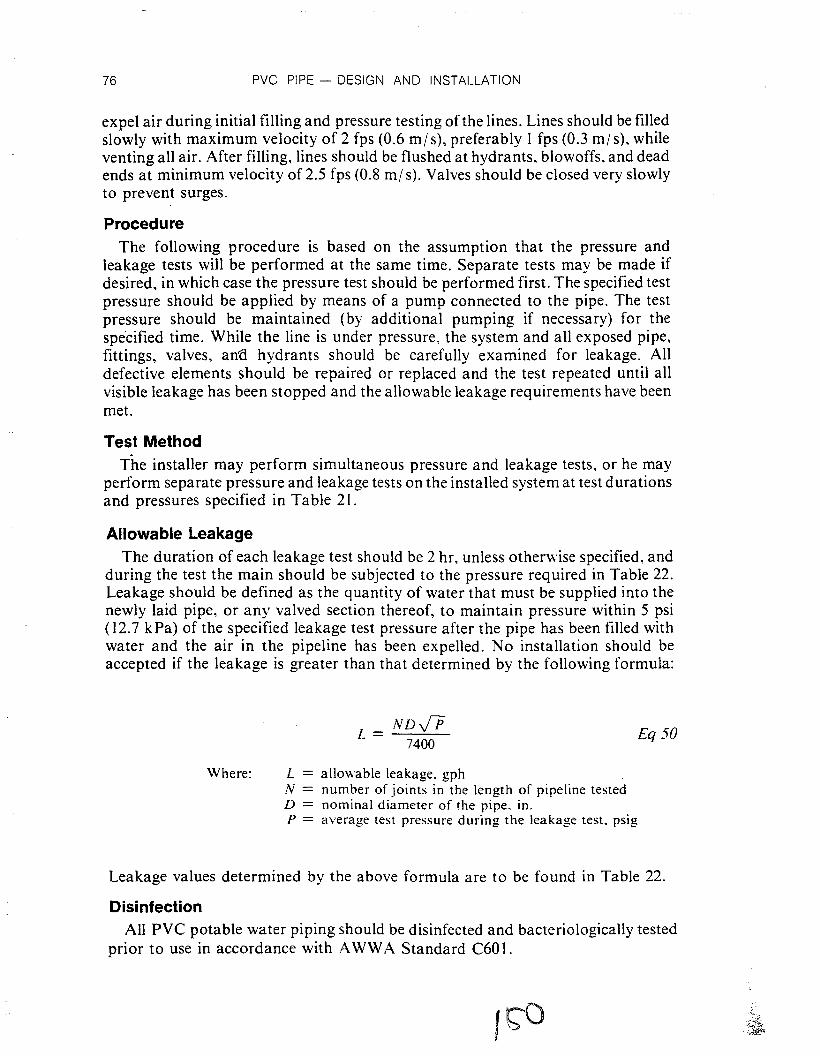
76 PVC PIPE - DESIGN AND INSTALLATION
expel air during initial filling and pressure testing of the lines. Lines should be filledslowly with maximum velocity of 2 fps (0.6 m/ s), preferably I fps (0.3 m/ s), whileventing all air. After filling, lines should be flushed at hydrants, blowoffs, and deadends at minimum velocity of 2.5 fps (0.8 m/ s). Valves should be closed very slowlyto prevent surges.
ProcedureThe following procedure is based on the assumption that the pressure and
leakage tests will be performed at the same time. Separate tests may be made ifdesired, in which case the pressure test should be performed first. The specified testpressure should be applied by means of a pump connected to the pipe. The testpressure should be maintained (by additional pumping if necessary) for thespecified time. While the line is under pressure, the system and all exposed pipe,fittings, valves, an'Cl hydrants should be carefully examined for leakage. Alldefective elements should be repaired or replaced and the test repeated until allvisible leakage has been stopped and the allowable leakage requirements have beenmet.
Test MethodThe installer may perform simultaneous pressure and leakage tests, or he may
perform separate pressure and leakage tests on the installed system at test durationsand pressures specified in Table 21.
Allowable LeakageThe duration of each leakage test should be 2 hr, unless otherwise specified, and
during the test the main should be subjected to the pressure required in Table 22.Leakage should be defined as the quantity of water that must be supplied into thenewly laid pipe, or any valved section thereof, to maintain pressure within 5 psi(12.7 kPa) of the specified leakage test pressure after the pipe has been filled withwater and the air in the pipeline has been expelled. No installation should beaccepted if the leakage is greater than that determined by the following formula:
Where:
L = NDJP7400
L = allowable leakage. gphN = number of joints in the length of pipeline testedD = nominal diameter of the pipe. in.P = average test pressure during the leakage test. psig
Eq 50
Leakage values determined by the above formula are to be found in Table 22.
DisinfectionAll PVC potable water piping should be disinfected and bacteriologically tested
prior to use in accordance with AWWA Standard C60 I .
'i';.: .•
.:,~

Procedure
TESTING AND MAINTENANCE
Table 21
System Test Methods
Pressure Test Duration
77
Separate pressuretest
Simultaneous pressureand leakage tests
150% of working pressure atpoint of test, but not lessthan 125% of normal workingpressure at highest elevation150% of working pressure at pointof test, but not less than 125o/cof normal working pressure athighest elevation
Separate leakage 150% of normal average workingtest pressure of segment tested
2 hr
I hr
2 hr
Source: Recommended Standard for the Installation of Polninvl Chloride (PVC)Pressure Pipe. U~)-B-3. Uni-Bell Plastic Pipe Association. . -
Table 22
Allowable Leakage for AWWA PVC Pipe
Nominal Average Test Pressure in Line. psiPipe Size 50 I 100 I 150 I 200 I 250
in. Allowable Leakage Per 1000 Ft or 50 Joints. gal/ hr (L/ hr)
4 .19 (.72) .27 (1.02) .33 (1.25) .38 (1.44) .43 (1.63)6 .29 (I. 10) .41 (1.55) .50 (1.89) .57 (2.16) .64 (2.42)8 .38 (1.44) .54 (2.04) .66 (2.50) .76 (2.88) .85 (3.22)
10 .48 (1.82) .68 (2.57) .83 (3.14) .96 (3.63) 1.07 (4.05)12 .57 (2.16) .81 (3.07) .99 (3.75) 1.15 (4.35) 1.28 (4.84)
8-2. Maintenance
Thawing. Frozen PVC water lines may be thawed by hot-water or steaminjection. Torches and other direct-heating devices should not be used to thawfrozen lines.
Locating. The high dielectric strength (insulating property) of PVC pipeprevents location of buried pipe with electric current type metal detectors unless atracer has been buried with the pipe during installation. If location duringmaintenance and future construction is to be accomplished using these types ofdetectors, a low-cost inductive or conductive tracer should be buried with the pipe(for example, metallic ribbon or low-cost metal wire). Location also may beaccomplished using buried pipe detection apparatus designed to locate nonmetallicburied pipe lines (such as asbestos-cement and plastic). Such devices operate in amanner similar to a simple seismograph and have proven to be effective. Probingwith metal bars is not recommended.
\~

Chapter 9
Service Connections
Service connections vary in size from small services supplying individual homes tolarge outlets for industrial users. Service lines are connected to PVC water mainsusing the following methods:
• Tapping through service clamps or saddles,• Tapping sleeves and valves for larger service connections, and• Direct tapping (AWWA C900 PC 150 and PC 200 only, 3/4- and I-in.
corporation stops).
Service Clamps or SaddlesService connections may be made using a service clamp or saddle. Maximum
outlet size recommended with service clamps or saddles is 2 in. (50 mm). Whenmaking this type of connection with the line under pressure, equipment is usedwhich attaches to the corporation stop and permits a cutting tool to be fed throughthe corporation stop to cut a hole in the pipe. Cutting tools should be sharp andshould not apply excessive pressure. No threading of the pipe wall is required sincethe corporation stop is threaded into the service clamp. Service clamps or saddlesused with PVC water pipe should
• Provide full support around the circumference of the pipe, and• Provide a bearing area of sufficient width along the axis of the pipe, 2 in. (50
mm) minimum, ensuring that the pipe will not be distorted when the saddle istightened.
Service clamps should not• Have lugs that will dig into the pipe when the saddle is tightened,• Have a U-bolt type of strap that does not provide sufficient bearing area, or• Have a clamping arrangement that is not fully contoured to the outside
diameter of the pipe.
79 IbU

80 PVC PIPE - DESIGN AND INSTALLATION
A number of tapping machines are available that will drill through a corporationstop. It is important that the cutting tool be a shell-type cutter (hole cutter) that willretain the coupon and that is designed to accommodate walls as heavy as DR 14(Pressure Class 200. AWWA e900). Many shell cutters are designed only for thinwalled PVC; they do not have sufficient throat depth to handle the heavier walledpipe.
Service clamps and saddles should be installed in accordance withmanufacturer's recommendations.
Tapping Sleeves and Valves
Tapping sleeves and valves are used when service connections larger than 2 in. (50mm) must be made in PVC water main. Tapping sleeves may be used for makinglarge taps under pressure.
When tapping sleeves are ordered from the manufacturer. the outside diameterof the pipe being tapped. the size of the outlet desired, and the working pressureshould be specified to ensure that the sleeve furnished will be satisfactory. Leadjoint sleeves should not be used.
Tapping sleeves should be assembled in accordance with the manufacturer'sdirections. Drilling equipment can be purchased or rented from sleevemanufacturers. who will also furnish instructions and! or instructors trained inmaking such taps. (Contractors who specialize in this type of work are alsoavailable in some areas.)
Tapping sleeves should be well-supported independently from the pipe duringthe tapping. Support used should be left in place after tapping. Thrust blocksshould be used as with any other fitting or appurtenance.
Table 23 lists recommended minimum lengths of tapping sleeves for the variousmain and tap sizes for AWWA PVC pressure pipe.
Table 23
Minimum Tapping Sleeve Length
Main & Tap(in. nominal)
Minimum Laying Lengthin. mm
4 X 2, 4 X 3, 4 X 46 X 2, 6 X 3, 6 X 4, 6 X 68 X 2, 8 X 3, 8 X 4, 8 X 68x810 X 2, 10 X 3, 10 X 4, 10 X 610 X 8, 10 X 1012 X 2, 12 X 3, 12 X 5, 12 X 612 X 812 X 10, 12 X 12
,(7
161819211923192125
406457483533483584483533635

SERVICE CONNECTIONS 81
Direct TappingFor some sizes of AWWA C900 PVC pipe, service connections may be made by
the direct tapping of pipe wall and the insertion of a corporation stop. PVC pipemanufactured in accordance with AWWA C900 in nominal sizes 6-12 in. ( 150-300mm), Pressure Classes 150 and 200, is being successfully direct tapped in the field.For 4 in. (100 mm) nominal size, Pressure Class 150 and 200, and for all sizes inPressure Class 100, service clamps or saddles should be used. In direct tapping,proper use of specified direct tapping equipment, corporation stops,polytetrafIuoroethylene (for example, Teflon®) thread sealant tape, and a torquewrench is recommended. Do not use liquid thread sealants. This procedure shouldbe used with proper direction and instructions from the manufacturer of the PVCpipe and the manufacturer of the direct tapping equipment.
Connecting Service LineIn common practice. service connections (service clamps. saddles. and direct
taps) are installed with the outlet at an angle of 45 deg above horizontal. It isrecommended that direct taps be placed on the horizontal (at springline) tominimize potential for breakage and, in cold climate regions. to prevent the serviceline from being appreciably closer to the ground surface than the water main. Abend, or "gooseneck," in the service line should always be provided to ensureflexibility and to accommodate the effects of load due to settlement, expansion,and/ or contraction. Proper soil consolidation should be provided in the area oftheservice connection..

Appendices
Appendix A. Approximate Pipe Weights
Weight of Belled Pipe Lengths, Lb/20 ft length (Kg/6.1 m)(Weights are approximate only and are for a gUide in selection of handling equipment.)
Nominal Size, in. Pressure Class 100 Pressure Class 150 Pressure Class 200
4 37 (17) 51 (23) 64 (29)6 77 (35) 105 (48) 132 (60)8 132 (60) 180 (82) 227 (103)
10 199 (90) 271 (123) 342 (155)12 281 (128) 383 (174) 484 (220)
NOTE: The above approximate weights per 20-ft length of pipe are calculated on cast iron (GI) equivalent00 dimensions. Pipe with steel pipe (IPS) equivalent 00 dimensions will be slightly less.
Appendix B. Notes to the Engineer and Owner
In specifying a total project, it is necessary that the following items be consideredin the special conditions of the contract documents.1. Special provisions for excavation and trenching requirements. Special
excavation provisions-open trench, sheeting, trench width, sheeting removal.2. Special provisions for conflicting utilities and responsibility for their location,
relocation, and repair.3. Removal and replacement of roadways, pavements, and other improved
surfaces and surface features.4. List of materials to be furnished by owner.5. Special trench foundations.6. Special trench backfill.7. Special provisions for testing, including responsibility for furnishing and
conveying water for testing and disinfection. Responsibility for furnishing ofequipment for testing. Required records and inspection of test. Stipulateddesign system operating pressure and required test pressure.
8. Enumeration of applicable plans, drawings, specifications, and other contractdocuments.
9. Special provisions for method of disinfection.
83
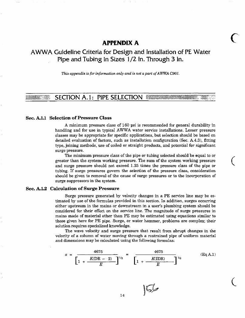
APPENDIX AAWWA Guideline Criteria for Design and Installation of PE Water
Pipe and Tubing in Sizes 1/2 In. Through 3 In.
This appendix is for information only and is not a part ofAWWA C901.
SECTION A.l: PIPE SELECTION
Sec. AI.I Selection of Pressure Class
A minimum pressure class of 160 psi is recommended for general durability inhandling and for use in typical AWWA water service installations. Lesser pressureclasses may be appropriate for specific applications, but selection should be based ondetailed evaluation of factors, such as installation configuration (Sec. A.4.3), fittingtype, joining methods, use of coiled or straight products, and potential for significantsurge pressure.
The minimum pressure class of the pipe or tubing selected should be equal to orgreater than the system working pressure. The sum of the system working pressure (and surge pressure should not exceed 1.25 times the pressure class of the pipe ortubing. If surge pressures govern the selection of the pressure class, considerationshould be given to removal of the cause of surge pressures or to the incorporation ofsurge suppressors in the system.
Sec. AI.2 Calculation of Surge Pressure
Surge pressure generated by velocity changes in a PE service line may be estimated by use of the formulas provided in this section. In addition, surges occurringeither upstream in the mains or downstream in a user's plumbing system should beconsidered for their effect on the service line. The magnitude of surge pressures inmains made of material other than PE may be estimated using equations similar tothose given here for PE pipe. Surge, or water hammer, problems are complex; theirsolution requires specialized knowledge.
The wave velocity and surge pressure that result from abrupt changes in thevelocity of a column of water moving through a restrained pipe of uniform materialand dimensions may be calculated using the following formulas:
4675 4675(EqA.1)a = =
[1 +K(DR - 2) ] 1/2 [1 +
K(lDR) ] 1/2
E E
}(;£,(
14

PE PRESSURE PIPE AND TUBING 15
'C'" Ps =aV
2.31g(EqA.2)
Where:
IDR =Ps =V =
=
wave velocity, in feet per secondbulk modulus ofwater =294,000 Ib/in.2
dimension ratio, outside-diameter basis (Sec. 1.2.6)modulus of elasticity of pipe material, in pounds per square inch.E varies by material used, as follows:
For PE 2406, E = 80,000 psiFor PE 3406, E = 115,000 psiFor PE 3408, E = 115,000 psi
dimension ratio ofpipe, inside-diameter basis (Sec. 1.2.7)surge pressure, in pounds per square inch gaugevelocity change, in feet per second, occurring within thecritical time 2Lla
Where:L = pipe length, in feet
gravitational acceleration = 32.2 ft IsIs
=
=
=
g
aKDR =E
Table Al shows surge pressures resulting from an instantaneous change invelocity ofl ft Is, as calculated from the above equations.
:,r'\ Table A.l Calculated Surge Pressures for an Instantaneous Change in Velocity of 1 ft/s in PE Pipe
or Tubing
Dimension RatiosOD Based (DR) ID Based (IDR)
Surge Pressurespsi
21.0 19.017.0 15.013.5 11.511.0 9.0
9.0 7.07.3 5.3
8.39.3
10.612.013.515.4
Sec. A.l.3 Temperature Effects
The pressure classes of pipe and tubing in AWWA C90I are based on watertemperatures of 73.4°F (23°C). Polyethylene piping intended for use where servicetemperatures may exceed this value for prolonged periods should have a hydrostaticdesign basis established for the specified temperature or higher. The elevatedtemperature pressure class is calculated using either Eq 1 or Eq 2 (Sec. 1.2.13) andthe elevated-temperature hydrostatic design basis or the interpolated elevatedtemperature hydrostatic design basis in accordance with ASTM D2837.

16 AWWA C901-88
SEOlON A.2: DESIGN CRITERIA
Sec. A.2.1 Hydrostatic Design Basis
Hydrostatic design basis values for a temperature of 73.4'1' (23°C) for thematerials covered in this standard are given in Table A2.
Sec. A.2.2 Hydrostatic Design Stress
For PE materials covered by this standard, the values of the hydrostatic designstresses (hydrostatic design basis multiplied by the design factor, which, in this standard, is 0.5) are given in Table A2. These values are for service temperatures of73.4°F (23°C) and should be modified for higher service temperatures (see Sec. Al.3).
Table A.2 Hydrostatic Design Basis and Hydrostatic Design Stress for PE Pipe and Tubing
•
Standard PE Code
PE2406PE 3406PE 3408
Hydrostatic Design Basisat 73.4~ (23°C)
psi
125012501600
Hydrostatic Design Stressat 73.4~ (23°C)
psi
630630800
Sec. A.2.3 Design. Factor •
Because the strength of PE materials depends on the duration of application ofloading, the effective safety factor that corresponds to a design factor of 0.5 will varywith actual end-use conditions. For the PE materials covered by this standard, the effective safety factor under hydrostatic pressure ranges from at least 3 for short-termloading to approximately 2 for long-term (100,000 h) sustained loading at the maximum recommended system working pressure and service temperature. The designfactor is also intended to account for unknown local effects, such as ovalling and longitudinal bending, that occur in properly installed buried pipe.
SECTION A.3: EXTERNAL LOADS
Sec. A.3.1 Earth Loads
For properly installed small-diameter conduit, the effects of distributed earthloads can usually be disregarded.
Sec. A.3.2 Live Loads
Tubing or pipe should be installed to preclude construction loads and subsequenttraffic loads. If the installation is to be subjected to surface traffic, a minimum coverof 24 in. should be provided, and trench backfill in the pipe zone should be compactedto at least 90 percent of the laboratory maximum density of the backfill soil as determined in accordance with ASTM D698.
J06
•

•
•
'.
PE PRESSURE PIPE AND TUBING 17
Sec. A.3.3 Concentrated Loads
Pipe and tubing installations should be designed and constructed to preclude localized concentrated,loadings such as point contact with stones; the effects of differential earth settlement, particularly at points of connection with rigidly anchored fittings; and excessive bending due to installation configuration, especially at fittings.
It"'_ SECTION A.4: INSTALLATION
Sec. A.4.1 Storage and HandlingPolyethylene pipe, tubing, and fittings should be stored in a way that prevents
damage due to crushing or piercing, excessive heat, harmful chemicals, or exposure tosunlight for prolonged periods. The manufacturer's recommendations regardingstorage should be followed.
Polyethylene is not subject to breakage during normal handling. However, it issubject to damage by hard objects with a cutting edge. Therefore, handling operationsand trench installation and backfill should be performed with reasonable care toprevent scratches, nicks, and gouges in the conduit.
Practices such as dragging coils of pipe or tubing over rough ground and installing by pulling through auger or bore holes containing sharp-edged material should beavoided to prevent damage by excessive abrasion and cutting. Uncoiling and otherhandling should be done without kinking. If pipe is excessively cut (to a depth greaterthan 10 percent of its wall thickness) or kinked, the damaged portion should beremoved, discarded, and replaced.
Sec. A.4.2 Bending
Bends in PE pipe and tubing should not be permitted to occur closer than 10diameters from any fitting or valve. The recommended minimum radius of curvatureis 30 diameters, or the coil radius when bending with the coil. Furthermore, bendingof coiled pipe against the coil should not go beyond straight. Polyethylene pipe ortubing that becomes kinked during handling or installation should not be used, andcare should be taken to ensure that kinking does not develop after installation.
Sec. A.4.3 Joining Methods and Fittings
The use offittings that are not covered by a recognized standard is subject to thejudgment and discretion ofthe purchaser. Each such fitting should be qualified beforeuse by investigation and by tests when necessary to determine that the fitting issuitable and safe for the intended service.
Polyethylene pipe or tubing can be joined to other PE pipe or fittings or to pipeor appurtenances of other materials using one or more joining systems. The purchaser should verify with the pipe and fittings manufacturer that fittings are capableof restraining PE pipe or tubing from pullout, especially for larger-diameter productswith thicker walls. Pressure classes for pipe and fittings should be the same or compatible. Further information and specific procedures may be obtained from the pipeand fittings manufacturers.
A.4.3.1 Insert fittings. Insert fittings are available for PE pipe in a variety ofstyles, including couplings, tees, ells, and adapters. Pipe ends should be prepared forsuch fittings by cutting the pipe square using a cutter designed for cutting plastic
,t:f!\

18 AWWA C901-88
pipe. Two all-stainless-steel clamps are slipped over the end of the pipe. The end ofthe pipe is forced over the barbs of the fitting until it makes contact with the shoulderof the fitting. (The end of the pipe may be softened by immersing in hot water to permit the pipe to slip on more easily.) The clamps are then tightened to provide a leaktight connection. Care should be taken to see that the clamp screw positions are offsetapproximately 180°.
For PE pipe products in pressure classes of 160 psi or greater and withdiameters of1 1/2 in. or larger, special, heavy-duty tightening clamps that can developthe necessary pipe-tightening force to preclude pullout from insert fittings should beused. The pipe should be softened by immersing in hot water to facilitate a tight sealaround the insert under the compressive force of the clamp. Only metal insert fittingsthat can resist creep deformation, which may lead to loss of seal and reduction ofjointpull-out resistance, should be used. To ensure that such joints have been properlymade, the joints should be pressure tested before being covered. When joining suchheavier wall pipe, the use of alternate techniques, such as heat fusion and speciallydesigned mechanical fittings, should be considered.
A.4.3.2 Flared fittings. Recommendations for flaring are contained in ASTMD3140. Flared fittings should be used only on recommendation of the pipe manufacturer.
A.4.3.3 Mechanical fittings. Mechanical fittings provide either a pressure sealalone or a pressure seal and varying degrees of resistance to pullout, including thosethat hold beyond the tensile yield of the PE pipe. Mechanical fittings may requiretightening of a compression nut, tightening of bolts, or merely inserting properlyprepared pipe or tubing to the proper stab depth in the fitting. Pipe and fittingmanufacturers' recommendations for installation should be followed.
Internal stiffeners that extend beyond the clamp or coupling nut should not beused. It is recommended that a solid tubular metal stiffener be used. The pipe shouldbe cut square using a cutter designed for cutting plastic pipe. It is further recommended that the outside ends of the pipe be chamfered to remove sharp edges thatcould gouge or cut the gasket when being installed. Chamfering or bevelling is a partof the recommended installation procedure for stab fittings.
A.4.3.4 Heat-fusion connections. Joints can be made either pipe end to pipe end,pipe end to fitting, or between a saddle fitting and pipe by heat-fusion methods. Thesemethods involve preparation of surfaces, heating of the surfaces to proper fusiontemperatures, and bringing the surfaces together in a prescribed manner to effect thefusion bond. ASTM D2657 describes the heat-joining practice.
Special tools to provide proper heat and alignment are required for heat-fusionconnections. These are available from several equipment manufacturers, who can alsoprovide joining procedures. Detailed written procedures and visual aids that can beused to train personnel are available from various pipe and fittings manufacturers.Specific recommendations for time, temperature, and pressure must be obtained fromthe pipe and fittings suppliers.
Sec. A.4.4 Embedment of Pipe and Tubing
In underground installations, the PE pipe and tubing should be installed intrench bottoms that provide continuous support and are uniform and free from rocks,stones, and debris (see ASTM D2774). The initial backfill, from 3 in. below thepipeline to 4-6 in. above the pipe, should be sand or other materials, as allowed inASTM D2774. In order to prevent freezing in the water lines, the pipe should be installed below the frost line.
•
•
•

•PE PRESSURE PIPE AND TUBING 19
Sec. AA.5 TestingThe installation should be tested for leakage in accordance with the applicable
code or engineering standard prior to acceptance by the owner.
SECTION'A.5: WATER SYSTEM DISINFECTION
Polyethylene pipe and tubing should be disinfected in accordance with AWWAC651-86, Standard for Disinfecting Water Mains.
SECTION A.6: SQUEEZE-OFF
•
•-
The use of squeeze-off techniques for emergency shut-off should be performedonly on materials, wall thicknesses, and pipe diameters and with tools and methodsas recommended by the pipe manufacturer.
SECTION A.7: REFERENCES
The latest edition of the following documents are incorporated by reference inthis appendix. They form a part of this appendix to the extent specified. In any case ofconflict, the requirements of the appendix shall prevail. These references are providedfor information only and are not a part ofAWWA C901.
ASTM* D698-Standard Test Methods for Moisture-Density Relations of Soilsand Soil-Aggregate Mixtures Using 5.5-lb (2.49-kg) Rammer and 12-in. (305-mm)Drop.
ASTM D2657-Standard Practice for Heat-Joining of Polyolefin Pipe and Fittings.
ASTM D2774-Standard Recommended Practice for Underground InstallationofThermoplastic Pressure Piping.
ASTM D2837-Standard Method for Obtaining Hydrostatic Design Basis forThermoplastic Pipe Materials.
ASTM D3140-Standard Practice for Flaring Polyolefin Pipe and Tubing.AWWA C651-86-Standard for Disinfecting Water Mains.
*American Society for Testing and Materials, 1916 Race St., Philadelphia, PA 19103.
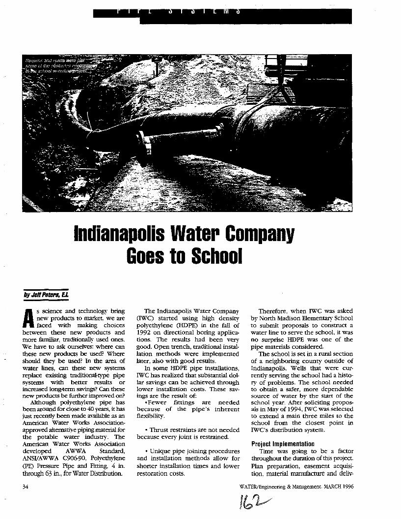
Indianapolis Water CompanyGoes to School
by J,gP'IBI'B, E.L
WATERIEngineering & Management. MARCH 1996
As science and technology bringnew products to market, we arefaced with making choices
between these new products andmore familiar, traditionally used ones.We have to ask ourselves: where canthese new products be used? Whereshould they be used? In the area ofwater lines, can these new systemsreplace existing traditional-type pipesystems with better results orincreased long-term savings? Can thesenew products be further improved on?
Although polyethylene pipe hasbeen around for dose to 40 years, it hasjust recently been made available as anAmerican Water Works Associationapproved alternative piping material forthe potable water industry. TheAmerican Water Works Associationdeveloped AWWA Standard,ANSI!AWWA C906-90, Polyethylene(PE) Pressure Pipe and Fitting, 4 in.through 63 in., for Water Distribution.
34
The Indianapolis Water Company(!WC) started using high densitypolyethylene (HDPE) in the fall of1992 on directional boring applications. The results had been verygood. Open trench, traditional installation methods were implementedlater, also with good results.
In some HDPE pipe installations,IWC has realized that substantial dollar savings can be achieved throughlower installation costs. These savings are the result of:
•Fewer fittings are neededbecause of the pipe's inherentflexibility.
• Thrust restraints are not neededbecause every joint is restrained.
• Unique pipe joining proceduresand installation methods allow forshorter installation times and lowerrestoration costs.
Therefore, when IWC was askedby North Madison Elementary Schoolto submit proposals to construct awater line to serve the school, it wasno surprise HDPE was one of thepipe materials considered.
The school is set in a rural sectionof a neighboring county outside ofIndianapolis. Wells that were currently serving the school had a history of problems. The school neededto obtain a safer, more dependablesource of water by the start of theschool year. After soliciting proposals in May of 1994,!We was selectedto extend a main three miles to theschool from the closest point inIWC's distribution system.
Project ImplementationTime was going to be a factor
throughout the duration of this project.Plan preparation, easement acquisition, material manufacture and deIiv-

WATER/Engineering & Management. ~1ARCH 1996
)\,For more information on this SUbject,
circle 911 on the reader service card.
'"',~ .-...----------35
About the Author:Jeff Peters is an Assistant Design Engineer withIndianapolis Water Company, Indianapolis, IN.
lessonsMuch has been learned about
HOPE pipe from this large project.Problems encountered have beenresolved. We will continue to learnand develop methods and productsthat solve the problems we havetoday. The gas industry has alreadyproven that this technology works.Adapting HOPE pipe systems to thewater industry is the challenge thatwe are now stepping up to.
line would not be achieved. With acontingency plan in place to supplywater to the school, construction continued uninterrupted. On August 25(Friday of the first week of school), allthe 24 in. HOPE pipe, hydrants, valvesand fittings had been installed. Themain was filled in eight hours and sterilization began at 6 a.m. on the following morning. Sun., August 27, theline was flushed and the first sampleof water was sent to IWC's labs fortesting. On Tues., August 29, after twosuccessive successful water sampleswere taken, the main was placed inservice. This was one week later thanthe original target date.
The successful completion of thisproject was achieved through thededication of EJP, PLEXCO andBowen Engineering, who illustratedwhat can be achieved in light ofalmost insurmountable odds.
.._-~
pouring in over the next two weeks.Bowen unloaded the 51 ft longpieces of pipe at four staging areasalong the project route by using afront-end loader equipped with lifting forks.
On July 18, Bowen began fusingpipe above ground with the help ofPLEXCO field service representativeGary Breazeale. Each joint, from thetime the pipe was placed into thefusion machine, faced off, heated,joined under pressure, allowed tocool, and removed, took approximately 45 minutes. Bowen was givena rule of thumb of two minutes fusiontime for every inch of pipe diameterto make an acceptable joint.
After a week of fusing pipe, several 500 ft runs ofpipe were ready to bejoined together and installed.Without any underground obstructions, Bowen was able to install 4,000ft of pipe in just the first week.
With the production rate achievedin the first week of construction, afeeling of confidence was beginningto spread at the project site.However, the easy part was done.What lay ahead was a race againsttime. There were five streams tocross, 2,500 ft of heavily wooded terrain to clear and excavate, fourasphalt paved county roads to opencut and cross, and 7,500 ft of residential area with over 40 homes topass in front of.
With only four weeks left beforeschool opened, !WC asked Bowen tothrow everything they could at thisproject to try to meet the completion date. An additional crew wasbrought in and Bowen began working 10 hr days, seven days a week.
Three days before the start ofschool, it was apparent that our dead-
ery, and construction all had to becompleted in 10 weeks in order to getwater to the school by the time itopened in late August. When theschool accepted IWC's proposal for3.5 miles of24 in. HOPE pipe, a working set of plans was almost ready forbidding. Since !We had neverinstalled HDPE pipe of this sizebefore, several concerns needed to beaddressed:
• Are thrust restraints required atbends or other fused fittings?
• How can large diameter taps (6in. or larger) be made?
• How would the thermal expansion/contraction characteristics ofpolyethylene effect the project?
• How will polyethylene bejoined to traditional materials likeductile iron?
• How can large diameter butterfly valves be incorporated in the IPSsized HOPE pipe?
Working with Everett]. Prescott,Inc. (EJP) and a large U.S. polyethylene pipe manufacturer, PLEXCOPerformance Pipe Division - ChevronChemical Company, Bensenville, IL,we were able to work out thesetypes of constructability questionsand move on.
Because over 15,000 ft of 24 in.SOR 13.5 (rated with a continuousworking pressure of 125 psi) pipeneeded to be manufactured in lessthan 25 days, all parties needed towork together to meet the demanding deadline for this project. Thetask of manufacturing and shippingall the required pipe and fittings wasaccomplished by the four weekdelivery deadline.
ConstructionInvitations to construction bid
ders were sent out on June 28 anddue back by July;. The scheduledstart of construction was July 11.This meant the successful biddingcontractor had seven days, includingthe 4th of July weekend, to preparea competitive bid. Then they had sixmore days to mobilize equipmentand manpower to the project siteafter notification of being the successful bidder. Bowen EngineeringCorp., Fishers, Ind., was hired forthe project and entrusted to meetthese deadlines.
Pipe began arriving at the job siteon July 11. Twenty-one semi-truckloads, 816 ft of pipe at a time. came

SUMMARY OF KEY STANDARDS
FAIRFAX COUNTY
- WATER MAINS TO BE LOCATED 8 FEETNORTH OR EAST OF STREET CENTERLINE
- GAS MAINS TO OPPOSITE
- SEWER LINES WILL BE LOCATED WITHIN AFIVE FOOT RIGHT-OF-WAY ALONG THESTREET CENTERLINE
- WATER CUTOFFS (VALVES) SHALL BELOCATED IN UTILITY STRIP BETWEEN CURBAND GUTTER.
- WATER SERVICE LINES SHALL BECONSTRUCTED INTO LOT PRIOR TOSIDEWALK CONSTRUCTION
- ALL WATER MAINS SHALL HAVE A 4 FOOTCOVER UNLESS OTHER WISE APPROVED
- NO UNDERGROUND ELECTRIC, TELEPHONE,TELEVISION OR OTHER UTILITIES SHALL BEINSTALLED IN THE PUBLIC WATER SUPPLYEASEMENT PARALLEL TO THE WATERMAIN
- PLANS AND PROFILES ARE REQUIRED FORALL UTILITY CROSSING,.
- MAINS 3 11 THROUGH 1 2 11 ARE TO BEDUCTILE IRON

- CORROSION PREVENTION AND CONTROLMEASURES ARE TO BE USED ON ALLBURIED UTILITY CROSSINGS
- CASING PIPE CROSSINGS (REQUIRED FORMA.JOR HIGHWAYS AND RAILROADS) ARETO HAVE CATHODIC PROTECTION
- AD.JACENT STORM AND SANITARY SEWERSARE TO nE CONSTRUCTED AND ACCEPTEDPRIOR TO WATER MAIN INSTALLATION
- SERVICE TO THREE OR MORE RESIDENCESREQUIRES A 3 11 MINIMUM LINE
- COMMERCIAL FACILITIES REQUIRING AFIRE LINE SHALL HAVE SEPARATE FIRE ANDDOMESTIC SERVICE LINES
- MAINS SHALL BE INSTALLED IN TRAVELAREAS WHERE POSSIBLE
- PROFILES ARE REQUIRED FOR ALL MAINSIN OPEN AREAS, AT ROAD CROSSINGS ANDFOR ALL MAINS IN EXCESS OF 12 INCHES
- FIRE HYDRANTS REQUIRE A SII MINIMUMMAIN

9-0000 WATER AND FIRE REGULATIONS- TABLE OF CONTENTS
9-0100 PUBLIC WATER SUPPLY9-0101 General Requirements9-0102 Pl1bIic Water Supply Agency Data9-0103 Fire Hydrants
9-0200 FIRE MARSHAL REQUIREMENTS9-0201 General Data9-0202 Construction Requirements
9-0300 PLATES
STANDARD PLATE DESCRIPTION SECTIONDESIGNA- NO.TION
FH-l 1-9 Location of Fire Hydrants 9-0103FH-2 2-9 Standard Fire Hydrant Island Parking Areas 9-0103FH-3 3-9 Standard Fire Hydrant Island Parking Areas 9-0103FH-4 4-9 Standard Fire Hydrant Island Parking Areas 9-0103FH-5 5-9 Fire Hydrant Protection in Area Where Island 9-0103
Cannot be ConstructedFH-7 6-9 Fire Lanes 9-0202
9-0400 TABLES
STANDARD TABLE DESCRIPTION SECTIONDESIGNA- NO.TION
N/A 9.1 Fire Flow 9-0202.2F(1)N/A 9.2 Fire Flow Coefficient 9-0202.2G(1)N/A 9.3 Maximum Fire Flow 9-0202.2G(2)N/A 9.4 Exposure Surcharges 9-0202.2G(6)N/A 9.5 Occupancy Reductions 9-0202.2G(8)
3"$'95
1995 PFM Page 9-1
/U,

9-0000 WATER AND Fm.E REGULATIONS
9-0100 PUBLIC WATER SUPPLY
9-0101 General Requirements:
9-0101.1 A public water supply approved by theappropriate agencies shall be provided to servesubdivision lots of less than 20,000 ft2 in size.
9-0101.2 Subdivisions containing 3 or more lotswhich are at least 20,000 £t2 in size, but not greaterthan 74,999 £t2 in size, shall be served by an approved public water supply.
9-01013 All extensions of public water supply systems required by § 9-0100 et seq. shall conform tothe requirements established by § 70-1-13 of theCode and § 9-0200 et seq.
9-0101.4 In residential developments containing20or fewer lots which are 20,000 £t2 in size or greaterand in which the nearest boundary is located morethan an average of 125' per loe from the nearestexisting water main:
9-0101.4A The County Executive may waive therequirements set forth in § 9-0101.2 & 3 and §70-1-13 of the Code which requires that watercapacity for fire flow comply with Insurance ServicesOffice standards, and that water storage capacity of30,000 gallons be provided.
9-0101.4B The County Executive may refuse togrant such a waiver if he determines from the plansand plats submitted to the County for approval thatsubstantial development is anticipated for the areassurrounding the proposed development.
9-0101.4C Wherever such waiver is granted:
9-0101.4C(1) Either a central well water supplysystem, with all necessary water mains and facilitiesor individual wells and dry water mains with allnecessary appurtenances, shall be installed as required by the approved water supply agency or the
3/15/95
County; and
9-0101.4C(2) Requisite fIre hydrants shall be furnished or payment equal to the value of said hydrants at time of waiver, and an installation feetherefore shall be paid to the approved water supplyagency; provided, however, that where the CountyExecutive determines that, based on the adoptedComprehensive Plan and capital improvementsprogram of the County, the installation of a publicwater main within an average of 125' per loe fromthe nearest boundary of the proposed developmentis not expected within the next 10 years, individualwells may be installed without providing dry watermains and fIre hydrants.
9-01015 In residential developments with lots75,000 if in size or greater, when the developerelects to install a central well water supply systemwith all necessary appurtenant water facilities, therequirements that water capacity for fIre flowcomply with Insurance Services Office standards,and that water storage capacity of 30,000 gallonsneed not be provided.
9-0101.6 All requests for the above waivers shallbe submitted in writing to the appropriate SiteReview Branch of OEM.
9-0102 Public Water Supply Agency Data
9-0102.1 Any person contemplating the construction of an extension of a water supply system shall,at the time of submitting subdivision plans, profJjesand specifications, agree by written contract approved by the appropriate public water supplyagency that, upon completion of the construction of
ISuch footage shall be computed as follows: distance between nearest existing water main andnearest boundary of the proposed developmentdivided by number of proposed lots shall equalmore than 125'.
1995 PFM Page 9-2

the extension of such water system and the approvaland acceptance thereof by the proper official, thewater system so constructed shall become theproperty of the appropriate public water supplyagency.
9-0102.2 All water mains, their sizes, valves andfIre hydrants, and their relationship to gas lines shallbe shown as indicated below:
9-0102.2A In subdivision streets on tangent sections, the water main shall be located 8' north oreast of the street centerline, and the gas main shallbe located 8' south or west of the centerline.
9-0102.2B On loop streets the water main shall belocated 8' north or east of the predominate centerline of the street. The gas main shall be located 8'south or west of the predominate centerline of thestreet. The water and gas mains shall then continueon the same side of the centerline as determinedabove for their entire length of the streets.
9-0102.2C Due to the complexity of design oftownhouse streets, it is not feasible to specify theside of the street on which the water line should belocated. Developers of townhouse sites shall conferwith the public water supply agency and the Washington Gas Light Company. These agencies willassist the developers at this stage in effecting asatisfactory location for water and gas mains andeliminating the need for revisions to the fInisheddrawings for the development.
9-0102.20 Water service cut-offs shall be locatedin the utility strip between the curb and gutter andsidewalk unless otherwise permitted by the Director.The water service line shall be constructed into thelot prior to the placing of any concrete sidewalk.
9-0102.2E Dry water mains shall be shown on theplans. House and other building connections mustbe stubbed to the property line before the streetpaving section is constructed.
9-0102.3 Guideline Criteria:
311Sros
9-0102.3A All water main construction shallcomply with the requirements of the standardspecifIcations and plans of the public water supplyagency serving the location.
9-01023B All water mains shall have a minimumcover of 4' unless otherwise designated.
9-0102.3C The developer shall request inspectionby the public water supply agency 3 days prior tocommencing construction of any water mains.
9-010230 No underground electric, telephone,television cable, gas, chilled water lines or any otherunderground utilities shall be installed within thepublic water supply easement parallel to the proposed water main. Plan and profiles of all utilitycrossings of water mains within the easements shallbe submitted to the public water supply agency forapproval prior to construction.
9-0102.3E Any relocation of existing water mainsdue to development shall be provided for by thedeveloper.
9-01023F No water main valves are to be closedprior to notification of the appropriate water supplyagency.
9-01023G Water mains shall not be installed on asite until easements are recorded and the developerhas furnished proper forms for water main installation.
9-01023H All water mains 3" through U" shall beClass 52, Ductile Iron Water Main unless otherwisedesignated.
9-010231 The developer is requested to submitunit prices for oversize water mains and appurtenances as shown on the plans for approval byFCWA prior to ordering materials or commencingconstruction of any oversize water mains.
9-010231(1) Approval by FCWA will require aperiod of approximately 90 days.
1995 PFM Page 9-3

9-0102.31(2) This approval is contingent uponobtaining approval by the Fairfax County PlanningCommission and, if necessary, by the Board underthe provisions of § 15.1-456 of the Va. Code, asamended. Where applicable, a statement regardingthis approval shall be shown on the plans.
9-0102.3J All hydrant, water service, fire line andstub-out valves shall be strapped. Swivel fittings areoptional in lieu of strapping.
9-0102.3K The developer shall notify the publicwater supply agency prior to the installation ofinterior plumbing to determine the location of thewater meter and any pre-wiring for remote register.
9-01023L When the property is located in areaswhere the pressure is less than 30 PSI, boosterpumps shall be required to provide adequate pressure.
9-0102.3M The developer shall make provision fordischarge of water as required by the public watersupply agency for water meter repairs and testingwith proper arrangements for E&S control duringdischarge.
9-0102.3N The working pressure shall be shown onthe plans. In accordance with the VUSBC, a pressure regulating valve must be installed by theproperty owner in the building plumbing systemwhere the working pressure exceeds 80 PSI in orderto eliminate water hammer and unnecessary wastageof water.
9-0102.30 The approximate location of watermeters shall be shown on the plans by symbol.
9-0102.3P All water meters above I" shall belocated inside in an accessible location and shall notbe installed under existing piping or close to otherfacilities.
9-0102.3P(1) Meter installations shall be inspected,and the bypass valve, if required, shall be sealed bythe appropriate public water authority.
311 5/95
9-0102.3P(2) The remote register shall be installedon the outside of the building.
9-0102.3P(3) The developer shall notify OEM,Public Utilities Branch, prior to the commencementof any construction or line testing.
9-0102.30 The developer shall agree to assumecomplete responsibility and all costs for the installation of the mains and appurtenances and for anyadjustments in alignment and grade, location,repairs, and maintenance which may be requiredprior to finish grading and surfacing of streetsand/or easements and fmal acceptance of thefacilities. Final acceptance shall not be considereduntil after the streets have been surfaced or theeasements finally graded.
9-0102.3R Corrosion prevention and control measures shall be used to protect water mains when awater main crosses another buried utility line.
9-0102.3S Cathodic Protection of Casing Pipe.
9-0102.3S(1) Anodes need not be affIXed to casingpipes that are not under the influence of impressedcurrent from another source. Casings shall be filledwith bluestone dust after the installation of thecarrier pipe.
9-010235(2) Casing pipe crossings of all railroadsand interstate highways shall be protected by theinstallation of two 17 lb anodes, 1 to be installed ateach end of the casing pipe.
9-0102.3S(3) Where construction excavations(boring portals) require the use of temporaryrestraining tie rods from the carner pipe to thecasing pipe during the testing operations, these tierods shall be severed and bent away to preventelectrical continuity. These tie rods shall not besevered until installation of the required concreteblocking. However, if the tie rods cannot be removed, no additional cathodic protection shall berequired to protect the casing pipe.
1995 PFM Page 9-4

9-0102.3S(4) Anodes placed in rock shall be installed using the following procedures:
9-0102.3S(4)a Anodes shall be placed approximately 10' from the water main adjacent to thetrench at a depth that can be dug without specialblasting required for that purpose; or
9-0102.3S(4)b When rock is close to or at theground surface, the anode shall be placed in thepipe trench at least to the depth of the crown of thepipe and can be laid horizontally.
9-01023T Prior to any water main installation allrequired sanitary sewers, including laterals, andstorm sewers must be installed, their ditches compacted for full depth according to current requirements, the sanitary sewer accepted for service byOEM, and the streets and/or easements roughgraded to meet current standards.
9-0102.4 Use of the public water supply as asource of water for temporary construction washracks.
9-0102.4A All subdivision and site plans shall showthe location in detail for a temporary wash rack forthe cleaning of trucks and construction equipmentleaving the site. The means by which water isprovided and the area of temporary ponding forsettling of water shall be shown. The public watersupply may be used to provide wash water.
9-0102.4B If the extent of the site is so limited asnot to warrant a wash rack, alternate provisions forcleaning shall be shown.
9-0102.5 Service Connections
9-0102.5A More than 2 pipestem lots shall requirea 3" water main installation for water service.
9-0102.5B Water meters 11/2" and larger shall belocated inside; a bypass is required for all 3" metersand above.
311$'°5
9-0102.5C Commercial development, office buildings, warehouses, churches, etc., that require a fireline to the building shall have separate fire anddomestic lines for service.
9-0102.6 Design Guidelines
9-0102.6A When connecting to existing watermains, the locations of existing valves requiringoperation shall be indicated on plans.
9-0102.6B Where feasible, loops to water mainsshould be considered.
9-0102.6C All water mains shall be installed intravel areas where possible. Profiles are requiredfor all water mains in open areas, at road crossingsand for all water mains 12" and larger.
9-0102.60 The separation between sanitary sewermains and laterals and water mains shall be inaccordance with the Commonwealth of VirginiaWaterworks Regulations.
9-0102.6E Air releases and blow-offs shall be installed on all mains U" and larger. Hydrants shouldbe utilized for this purpose where feasible.
9-o102.6F All valves 16" and larger shall be butterfly valves.
9-0102.6G 2" blow-offs shall be installed on allwater mains.
9-0102.6H When utilities are proposed in closeproximity to an existing water main, or when gradechanges are proposed above an existing water main,test holes shall be required.
9-0102.61 Depending upon test hole results, sheeting or bracing may be required when other facilitiescross an existing water main.
9-0102.6J Corrosion control is required for casingpipe. Corrosion control measures on pipe crossingstreams and utilities with bonded joints and im-
1995 PFM Page 9-5

pressed current shall be coordinated with the watersupply agency.
9-0102.7 Miscellaneous Notes
9-0102.7A Easement plats shall be included as partof the fmal plan submission (off- and on-site).
9-0102.7B Plan approval by the FCWA may besubject to developer acceptance of satisfactoryagreement for the installation of off-site or oversizefacilities.
9-0102.7C New proposal requests, or requestsrequiring engineering analysis, shall include a fee.A fee shall be required for all requests to updateprevious proposals.
9-0102.70 FCWA approval may be contingentupon the installation of water mains in other sections or subdivisions and connections thereto.
9-0103 Fire Hydrants
9..Q103.1 A permit for the installation of fire hydrants shall be obtained from the Director.
9-01032 Fire hydrants shall be of 3 way class, withone 4 1/2" pumper outlet and two 2 1/2" hoseoutlets all with National Standard fire hose couplingthreads.
9-0103.3 Fire hydrants shall conformto the American Waterworks Association Specifications,C-502.64, and will be provided a 6" connection tothe main with a minimum 5 1/4" valve opening.The center of the hydrant shall be a maximum of24" from the top of face of curb. The closest partof the hydrant (4 1/2" nozzle cover) shall be a minimum 12" from top face of curb.
9-0103.4 Fire hydrants placed on streets withoutcurb and gutter shall be in accordance with thestandard and the terms of the permit. The 2 1/2"hose connection shall have a minimum clearance of5' from the side slopes.
3 "5/95;
9-0103.5 The bottom of the safety flange shall be2 1/2" above the elevation of the edge of the shoulder on streets without curb and gutter and abovethe elevation of curb on streets with curb andgutter.
9-0103.6 A suitable sump must be provided toallow draining of the hydrant.
9-0103.7 The location of all fire hydrants shall beshown on the plans for the improvements.
9-0103.8 The hydrant shall be located so that thethrust block is placed in undisturbed soil. In thosecases where this is not practical, the soil beneathand surrounding the thrust block shall be compactedto 95% of maximum density in accordance withVDOT Sections 523.03, 302, 303.10 and 200.02.
9-0103.9 Fire hydrant branch connections placedin fill material shall be installed using restrainedjoint pipe or tie rods as approved by the engineerfor the public water supply agency. Retainer glandsshall not be permitted.
9-0103.10 The 4 1/2" nozzle shall face the street,travel lane, service drive or normal vehicular travelway, whichever applies.
9-0103.11 All fire hydrants on public or privatestreets and in easement areas shall be installed inaccordance with the current County design andconstruction standards.
9-0103.12 All water mains and fIre hydrants shallbe installed in accordance with current specificationsof the FCWA.
9-0200 FIRE MARSHALREQUIREMENTS
9-0201 General Data. In accordance with §62-2-4 et seq. (Fire Prevention Code) of the Code:
9-0201.1 No person shall use, tamper with, damage or destroy any fire hydrants, valves, or watermains within the County; except that a fxre depart-
1995 PFM Page 9-6
\~\

ment may use such hydrants for fire fighting andtraining purposes. Also a person who has obtaineda permit for use from the public water authority orutility having proper jurisdiction over said items mayuse the items.
9-0201.2 When use is by a person under permitfrom the authority having jurisdiction, the user shallcomply with all policies that are outlined on saidpermit or application.
9-0202 Construction Requirements 1
9-0202.1 Fire Hydrant Information
9-0202.lA All fire flow requirements shall bedetermined by the Fire Marshal.
9-0202.1B Fire flow waivers shall be requestedthrough DEM (§ 9-0100 et seq.).
9-0202.1C Sidewalks shall be warped around hydrants in areas where the grass area is shown as 2'or less.
9-0202.1D Easements shall be required for hydrants located on ditch section streets where thereis less than 5' clearance from hydrant to the property line. Show typical installation.
9-0202.1E Hydrants shall not be placed in concreteareas.
9-0202.1F If hydrants are to be located in an areaof possible guardrail construction, plans should bechecked for notes regarding possible obstruction.
9-0202.1G Hydrants shall be installed either 5'from the point of curvature of curb returns or onthe property line in subdivisions.
ISee § 9-0103 and Plates 1-9 through 5-9 for firehydrant details.
3/15'95
9-0202.1H Steel posts shall be installed aroundhydrants as needed for industrial and commercialdevelopment where curbs are not available.
9-0202.11 All fire hydrants shall be located aminimum of 50' from all buildings.
9-0202.U No plantings or other obstructions shallbe made within 4' of any fire hydrant, or within 10'of a siamese connection.
9-0202.1K Where standpipes or sprinkler systemsare required within buildings, a fire hydrant will belocated within 100' of the fire department connection.
9-0202.1L All fire hydrants shall be located inaccordance with the following schedule (distancemeasured from the hydrant to the most remotepoint of vehicular access on the site): IndustrialBuildings - 250'; School Buildings - 300'; Commercial, Churches and Office Buildings - 350'; Apartments, Multi-family and Townhouses - 350'; Singlefamily dwellings - 500'.
9-0202.2 Guideline Criteria
9-0202.2A All hydrant branches shall have a minimum cover of 3' at the ditch line.
9-0202.2B All fire hydrant locations shall be reviewed by the County for conformity to the FairfaxCounty Standards as shown in Plates 1-9 thru 5-9.
9-0202.2C It has been requested by the FireMarshal's Office that all site plans submitted forreview include the following information:
9-0202.2C(1) Use group classification (defined bythe VUSBC).
9-0202.2C(2) Type of construction (defined by theVUSBC).
9-0202.2C(3) Existing and proposed water mains.
1995 PFM Page 9-7

TABLE 9.1 FIRE FLOW9-0202.2C(4) Existing and proposed fIre hydrants.
9-02022C(5} Water main size.
9-0202.2C(6) Available water pressure and flowcapability, static pressure, residual pressure, flow inGPM.
9-0202.2C(7) Type of fIre suppression or detectionequipment to be provided; e.g., sprinklers, standpipes, smoke or heat detectors. (See current editionof the VUSBC for requirements).
Minimum ExposureDistance
0' - 10'11' - 30'31' and greater
Fire Flow (GPM.)
1500 - 20001000 - 15001000
9-0202.2C(8) Location and size of underground fIrelines.
9-0202.2C(9) Location of fire department siameseconnections (street front of building).
9-0202.2C(10) Height of building in feet andstories.
9-02022C(1l) Breakdown of building interiorssuch as firewalls, tenant separations, etc.
9-020220 H a fixed fIre suppression or detectionsystem is to be provided, the type of system shall beclearly indicated. The installation shall be subject tothe applicable section of the VUSBC.
9-02022E Private bridges must have a design satisfactory to the Director to carry fIre equipmentwhere necessary. AASHTO "Standard SpecifIcations for Highway Bridges" and the VDOT BridgeEngineer will be consulted for guidance on a caseby case basis.
9-0202.2F Fire Flow Requirements
9-0202.2F(1) One and two-family dwellings minimum exposure distances.
3PS195
9-0202.2F(2) Townhouses or multiplex units - residential or professional 2500 GPM.
9-0202.2F(3) Other uses - fIre flow requirementsestablished by the procedures and formulas delineated below.
9-0202.2G FireFlowRequirement Determination1;
9-0202.2G(1) DefInitions (for this determinationonly):
Required Fire Flow: Fire flow water to the siterequired for fire fIghting for any and all structuresand appurtenances on the site.
Floor level: Any occupiable level of a structurewhether above or below grade.
F: Required fire flow in GPM.
C : Coefficient related to the type of construction(see Table 9.2).
A: The total area of all floor levels in the structurebeing considered. (Gross floor area of the wholestructure.)
lAll required fire flow shall be calculated at aminimum 20 PSI residual pressure remaining on thepublic water or central well system to be in conformance with Commonwealth of Virginia WaterworksRegulations.
1995 PFM Page 9-8

TABLE 9.2 FIRE FLOW COEFFICIENT
C TYPE OF CONSTRUCTION
1.5 for wood construction (1993 VUSBC, typesSA, SB)
9-02022G(4) Complete automatic sprinkler protection reduction - Value obtained from the formulagiven below may be reduced 50% only if the structure or structures under consideration are completely covered with a sprinkler system. Partial protection will not be allowed for any -reduction in fireflow.
1.0
0.9
0.8
0.6
for ordinary construction (1993 VUSBC,types 3A, 3B)
for heavy timber construction (1993VUSBC, type 4)
for noncombustible construction (1993VUSBC, types 2A, 2B, 2C)
for fire resistive construction (1993VUSBC, types lA, lB)
9-0202.2G(5) Calculation formula: F = 18 C (A).5where F, C, A are defined in § 9-0202.2G(1). Thisformula must be applied sequentially to each structure on the site. The largest fIre flow calculatedthen applies.
9-0202.2G(6) Exposure surcharges - The valuecalculated in the above formula shall be increasedby a percentage for exposure of other structureswithin 150' of the structure under consideration.The percentage increase for anyone side shall be:
TABLE 9.4 EXPOSURE SURCHARGES9-0202.2G(2) Maximums - Fire flow required shallnot exceed the following maximums (before anyreductions are taken): Separation (ft) Percentage (%)
TABLE 9.3 MAXIMUM FIRE FLOW
GPM TYPE OF CONSTRUCTION
8000 Wood, heavy timber or ordinary construction
6000 Noncombustible or fire-resistive construction
9-02022G(3) Minimums - Fire flow required shallnever be less than 500 GPM for a structure. Fireflow required for single-family detached dwellingsshall never be less than 1000 GPM. Both values areabsolute minimums after all reductions are taken.
0-10 2510.1-30 2030.1-60 15
60.1-100 10100.1-150 5
Total exposure surcharge shall be the sum of thepercentages for all sides of the building but shallnot exceed 75%.
9-0202.2G(7) Special consideration - The abovecalculation procedure does not apply to: high hazardstructures; lumber yards or lumber storage; petroleum storage; refineries; chemical plants; grainstorage; power generating facilities; hazardousmanufacturing processes; and paint storage, highpiled combustible storage, flammable liquids storage, etc. All of the above require special consideration and direct consultation with the Fire Prevention Division regarding fIre flow requirement.
1995 PFM Page 9-9

9-0202.2G(8) Occupancy reductions - The followingpercentage reductions to the value calculated by theabove formUla may be taken:
TABLE 9.5 OCCUPANCY REDUCTIONS
Type Occupancy % Type Occupancy %
Asylums 15 Prisons 10Churches 15 Public Buildings 10Clubs 10 Rooming Houses 10Dormitories 25 Schools 15Hospitals 20 Open Parking 25Hotels 10 Structures (standNursing Homes 15 alone, not underOffice Buildings 10 buildings
9-0202.2G(9) Procedure for Calculation of Required Fire Flow:
9-0202.2G(9)a Determine type ofconstruction andhence "C."
9-0202.2G(9)b Determine the gross floor area(A).
9-Q202.2G(9)c Determine the occupancy reductions, if any.
9-0202.2G(9)d Apply the sprinkler reduction, iffully covered by a sprinkler system.
9-02022G(9)e Determine the total surcharge forexposures.
9-0202.2G(9)f Perform the following multiplication:
9-0202.2G(9)f(l) F = 18 C (A).5
9-0202.2G(9)f(2) (F) (occupancy reduction)(sprinkler reduction) (exposure surcharge) equalstotal required fire flow for the structure underconsideration.
3 (]5 f95,
Note: Occupancy reduction is 100% - % given inTable 9.5. Sprinkler reduction is 50%. Exposuresurcharge is 100% + % given in Table 9.4.
9-0202.2H Central Well Systems.
9-0202.2H(1) Central well systems apply to one andtwo-family developments where public water is notavailable within specified distances required forpublic water main extension.!
9-0202.2H(2) Central well systems shall be designedfor a minimum 30,000 gallon storage capacity withadequate pressure for fIre fIghting activities.
9-020221 Fire Protection Waiver Procedures.
9-0202.21(1) The following information is to beprovided when requesting a modification or waiverof any fire protection requirement of the PPM.
9-0202.21(2) All requests must be submitted andaddressed to the appropriate Site Review Branch ofDEM and include the following:
9-0202.21(2)a A plan or sketch showing the proposed location of all improvements on the site andthe type of construction involved.
9-0202.21(2)b The address, tax map reference number and the proposed use of the property.
9-o202.2I(2)c The current zoning classification ofthe property and if recently rezoned, the rezoningnumber and the date of approval by the Board.
9-o202.21(2)d Copies of any required special exception or special permit with date of approval.
!Specified distance required equals US times thenumber of proposed lots to the nearest boundaryline of the proposed development.
1995 PFM Page 9-10

9-0202.2I(2)e Specific item requested to be waivedor modified.
9-0202.2I(2)f Length of time for which the waiveris requested.
9-0202.2I(2)g Any proposed alternate form of fireprotection.
9-0202.2I(2)h The name, address and telephonenumber of the person making the request.
9-0202.2I(2)i The County assigned number for siteand subdivision plans and waiver requests associatedwith the property.
9-0202.2J Fire Department Access
9-0202.2J(1) Access for emergency vehicles shallbe provided to within 100' of the main or principalentrance of every building. The access shall beprovided by a public or private street or parking lot.
9-0202.2J(2) When buildings are more than 5stories or 50' in height, ladder truck access shall beprovided to both the front and rear of the building.
9-0202.2J(3) The access to the rear may be provided by either a street, parking lot, or fxre lane.
9-0202.2J(4) The inner surface of the ladder truckaccess way shall be no less than 15' and no morethan 30' from the exterior building wall.
9-0202.2J(5) Where required, fue lanes shall havea minimum width of 24'.
9-0202.2J(6) Required fIre department access waysover 100' in length shall have provisions for turningapparatus around (Plate 7-7 should be consulted fordesign guidance).
9-0202.2J(7) A U' wide access lane to within 50' ofthe edge of swimming pools, with an 8' personnelgate in the fence at the point of access is required
3 '15/95
except for individually owned pools located onsingle family lots.
1995 PFM Page 9-11

FAIRFAX COUNTY PUBLIC FACILITIES MANUAL
26" max.
Seenote
at right
NOTE:The closest part of the hydrantshall be 14" min. from the flowline of the curb. No hydrantswill be installed so that anypart of the barrel is withinthe sidewalk.
Ref sec 9-01039-2-92!leY 8-10-94
2-fS-95
LOCATION OFFIRE HYDRANTS
PLATE NO srD NO
1-9 FI-I-l

FAIRFAX COUNTY PUBLIC FACILITIES MANUAL
Type of curb & gutterwill be determined bygrading in parking area.
" " " " " " " " " " " " " " " " "I" "" I 2 '2"... ... ... ... ... ... ... ... ... ... ... ... .. .. ... ... • ... .. .. .. i.. ... ... ... .. ... .. .. .. .. ... ... .. .. .. ... .. .. ... ... ... ...~
• " " " " " " " " • • " " " " ':. " • " " I"" " " " • " " • " " " • C")' " • • .: •
::::::::::::::::::::::::::::::::J::::::::'C::"• • • " " " " • '.' S o-d . " " •~ -"-!H::HH>-"-l
• • • • • • • • LD' • • ., •••••.. .. .. .. ...••••••••••••••••• a:l••••••••••• '. • • • • • .1 •
18'
(I)
::.-
standard parkingspace
18'
Standard parkingspace
Ref Sec 9-0I 034-8-93Rev 8-10-94
STANDARD FIRE Hy-DRANTISLAND-PARKING
AREA
PLATE NO STD NO
2-9 FH-2

FAIRFAX COUNTY PUBLIC FACILITIES MANUAL
.. .. .. .. .. ... ... . .. .. .. .. ... ..
. . . .. .. ... ... .. ... .. .. .. .. .. .. .. .. . .. .. .. .. .. .. .. .. .. .. .. .. .. .. .. .. .. ..
.. .. .. .. .. .. .. .. .. .. .. .. .. .. .. .. .. .. .. .. .. .. .. .. .. .. .. .. .. .. .. .. .. .. .. .. .. .. .. .. .. .. .. .. .. ..
8.5'
CG6R-C&G
Standard parkingspace
t:-:·:·:-:-:««<~.>:.:-:-:<.>~<-:.:. •••. ' ....• ' • '4'3'" •
I !. Fire. . . , . • . .1 "hydrant ....••
\ '.. . . . . , . . . . .\ ' .
\ . . . . . . . . . .\ .
CG6R-C&G
!,
18'
.. .. .. .. .. .. .. .. .. ..)------,...----,-------------, ! •••••••••••••••••••••r. . . . . . . . . . .
~ . . . . . . . . . .~~:::: .:. :.:.:.:.:r.:.:~. :•:.:.:.:.:.r· . . . . . . . . . .r • . . . . • . . . .I' • • • Sod • . • . •
Ir«?fK1[ - - .I •.•••...•••••••.••••••
1
······-···············......•..• ·&.5~ ...•.•••
Type of curb & gutterin island will be determined by grading ofparking area.
Ref Sec 9-01034-8-93Rev 8-10-94
2-6-95
STANDARD FIREHYDRANT ISLANDPARKING AREAS
PLATE NO STD NO
3-9 FH-3

FAIRFAX COUNTy- PUBLIC FACILITIES MANUAL
.... ... ... .. ...
... ... .. ... ... ... ...... ...
... ... ... ... ... ... ... ... ... .. ..... ... ... ... ... ... ... ... ... ... ... ... ... ... ... .. ... ... ... ... .. ... ... ...
... ... ... ... ... ... ... ... ... ... ... ... ... ... ... ... ... ... .. ... ... ... ... ... ... ...... ... ... ... ... ... ... ... ... ... ... ... ... ... ... ... ... ... ... ... ... ... ... ... ... ... ... ... .. .• ..
... ...... .. ... ... ... .. ... ... ... .. ... ... ... .. ... ... .. ... ..
... ... ... ... ... ... ... ... ... ... ... ... ... .. ... ... ... ... .. ... .. ... ... .. ... ... ... ... ... ... ... ... ... ... ... ... ... ... ... ... .. ... ... ... ...... ... ... ... ... ... ... ... ... .. .. ... ... ... .. ... ... ... .. ... ... .. ... ... ... ... ... ... ... ... ... ... ... ... ... ... ... ... ... ... ... ... .. ... ... ...
CG6
6'
8.5' 8.5'-'-............................................................ .1
12'
......../..: ~........... ~.••••••••.••.•••••.••. J• •••••••••••••••••••• I
• • • • • 8.5' • • • -I 8.5'
~ / Flow line
L.Type of curb &gutter in islandwill be determinedby grading of parking lot
•••••••••• -1• • • • • • • • • • • I
. . • Sod . . . . . 1
U·········.rt4'.. '4: 3;,·1... ... ~ ..... I.. .......-!...... ..
\~.. :.:.:.:.;:.>: '.'~' ./, Fire Hydrant•••••• ·..rr \ri:'. • ./ / /
• • ""-\\.:Ur .?-.. A... ... ."'l::~ ......
• '.'.' • 2' 2"
18'Standard parkingI_~S--space--z..--
.
PLATE NO STD NORef Sec 9-01034-7-93Rev 8-10-94
2-6-95
STANDARD FIRE HYDRANTISLAND - PARKING 4-9 FH-4

FAIRFAX COUNTY PUBLIC FACILITIES MAKUAL
I(
PLATE NO STn NORef Sec 9-01039-2-92Rev 8-10-94
2-6-95
FIRE HYDRANT PROTECTIONIN AREA WHERE ISLAND
CANNOT BE CONSTRUCTED 5-9 FH-5I

FAIRFAX COCNTY PUBLIC FACILITIES MANUAL
4" in yellow stripes extend12' for DO parking or parallelparking. 18' for perpendicularparking.
W= Width of fire lane
FIRE LANE STANDARD-NOTES
posts filledconcrete
Parking - Firelane"signs
1. Subject to approval of the Fairfax County Fire Marshal, where building entrances are not accessible within100' of public or private street or parking area, a min. paved width of 24' shall be provided.
2. Where entrances to swimming pools (other than pools located on single family lots and individually owned)are not accessible within 50' of a public or private street or parking area. a min. paved width of12' shall be provided.
3. Where a developer is applying for a tabular increase in the size of a building because of excess street frontage,a min. paved width of 24' shall be provided around the entire building and to a public or privatestreet. The entire building perimeter shall have an unoccupied space of not less than 30'.
4. See Fire Lane requirements.
5. Access to rear of building more than 5 stories or 50' in height.
Fire lane markings, types of signs, locations, etc., shall be subject to the approval of the Office of the FireMarshal.
Ret Sec 9-02024-7-93Rev 8-10-94
2-6-9~FIRE LANES
PLATE NO
6-9
STD 1\'0
FH-7

FAIRFAX COUNTY WATER AUTHORITY
WATER MAIN INSTALLATION AND SERVICECONTRACTS
SELECTED SECTIONS
• CORROSION CONTROL
• WATER DISTRIBUTION
• THRUST RESTRAINTS
• LEAKAGE TESTS
.. STANDARD DETAILS

Contractor has the required experience to perform the work in theopinion of the NACE Certified Corrosion Specialist and a certificate isissued in accordance with Paragraph B. of this section.
B. The Company shall issue a certificate of compliance indicating that allcorrosion control measures comply with the Specifications.
C. Testing shall be witnessed, at their option and discretion, by a designatedrepresentative of the Authority.
D. Test results shall be recorded in a standard, uniform format approved bythe Authority and shall be retained for review on request by same at anytime. These documents shall be made a permanent record of the pipelineinstallation and shall be submitted at the completion of the Work.
E. As-Built drawings:1. Provide marked-up Drawings indicating the "as-built" location of each
key cathodic protection item, including the following:a. Test stationsb. Test station wire routing
2. Provide detailed field sketches showing the location of all test stationswith respect to existing physical features, including three ties wherepossible. Identify each test station by test station number and pipelinestation number.
PART 2 PRODUCTS
2.01 MANUFACTURERS
A. Beckman Industrial Corporation, Brea, CA
B. Biddle Instruments, Blue Bell, PA
C. CP Test Services, Inc., Harrison, NJ
D. Central Plastics Company, Shawnee, OK
E. Continental Industries, Inc., Tulsa, OK
F. Denso North America Inc., Houston, TX
G. Erico Products, Inc., Cleveland, OH
H. G.e. Electronics, Rockford, IL
WMISC-95 02655-2

SECTION 02655
CORROSION CONTROL
PART 1 GENERAL
1.01 SECTION INCLUDES
A. Bonded Joints
B. Cathodic Protection Coatings
C. Insulated Joints
D. Magnesium Anodes
E. Test Stations
F. Miscellaneous Cathodic Protection Work
1.02 UNIT PRICES
A. Refer to Section 01025 - Measurement and Payment.
1.03 QUALITY ASSURANCE
A. Subcontractor Qualifications1. Employ an independent Cathodic Protection Company (Company) to
install, test and certify the cathodic protection system. This systemincludes bonded joints, test stations and field-applied coating materials.Said Company shall have the following qualifications:a. Continuously engaged in the field of corrosion control installations
and electrical/corrosion control testing.b. Not less than 5 years experience in the installation and testing of
cathodic protection systems for underground pipelines of similartype and equal complexity as the system specified and indicated.
c. Completed at least three successful corrosion control systems forunderground pipelines of similar type and equal complexity as thesystem specified and indicated.
d. Employ a National Association of Corrosion Engineers(NACE)Certified Corrosion Specialist.
2. Consideration will be given to allow the general contractor to performthe installation work under the direct supervision of the Company if the
WMISC-95 02655-1

I. Gas Electronics, Seymour, MI
J. Gerome Manufacturing Company, Inc., Uniontown, PA
K. Harco Corporation, Medina, OH
L. Lietz, Overland Park, KS
M. Multicore Solders, Westburg, NY
N. PSI Industries, Burbank, CA
O. Pipeline Seal & Insulator, Inc. Houston, TX
P. Royston Laboratories, Inc., Pittsburgh, PA
Q. Thomas and Betts Corporation, Raritan, NJ .
R. Tinker and Raso, San Gabriel, CA
S. Trenton Corporation, Ann Arbor, MI
T. 3M Company, St. Paul, MN
2.02 MATERIALS
A. Magnesium Anodes: Furnish Type H-1 Grade III packaged magnesiumanodes as manufactured by Harco Corporation.1. Anode Material: Bare anode weights shall be 17 pounds for 17 pound
anodes and 32 pounds for 32 pound anodes. Composition by weightshall be as follows:
WMISC-95
ELEMENT
AluminumManganeseZincSiliconCopperNickelIronOtherMagnesium
PERCENT
5.3 to 6.70.15 Minimum2.5 to 3.50.10 Maximum0.02 Maximum0.002 Maximum0.003 Maximum0.30 MaximumRemainder
02655-3
J

2. Wire: Provide 20 feet of No. 12 AWG solid copper wire, type TWinsulation, black color unless otherwise specified.
3. Anode assembly: Anodes shall be packaged in a permeable cloth bagwith approximately 25 pounds of prepared backfill for 17-pound anodesand 38 pounds of prepared backfill for 32-pound anodes. The prepared
.backfill shall have the following composition by weight:
MATERIAL
Ground hydrant gypsumPowdered Wyoming bentoniteAnhydrous sodium sulfate
PERCENT
75205
B. Cleaning solvent: Provide Chloro-kleen as manufactured by GC Electronicsor PC-81 as manufactured by Multicore Solders.
C. Electrical Coating Compound: Provide Scotchkote as manufactured by the3M Company.
D. Insulated Flange Materials: Provide insulating materials which includean insulating gasket, insulating sleeves and washers as manufactured byPSI Industries.1. Insulating Gasket:
a. Type nEn Neoprene-faced phenolicb. Gasket shall protrude 1/16-inch into the pipe to prevent bridging of
the gap by foreign conducting material in the pipe.c. Gasket seal shall be nitrile (buna N)
2. Insulating Sleeves:a. G-10 EpoxyIGlass
3. Insulating Washers:a. G-10 Epoxy/Glass - provide two washers for each bolt.
4. Steel Washers:a. 1/8-inch thick plated hot rolled steel - provide two washers for each
bolt.
E. Insulated Union Materials: Provide insulating materials composed of nylonas made by Central Plastic Company.
F. . Electrical Tape: Provide Scotch 130C vinyl plastic electrical tape andScotch 88 rubber splicing tape.
G. Terminal Boxes: .1. Buried Service: Provide Model NM-5 terminal boxes as manufactured
by CP Test Services. Shaft length shall be 18 inches. The lettersnFCWAft shall be cast into the cover for each terminal box.
WMISC-95
\l{\02655-4

2. Vaults: Provide Testox Model 1003 terminal boxes as manufactured byGerome Manufacturing Company, Inc. Terminal boxes shall be 8 terminal,aluminum casting, double hub with slip fit for 1 1/4-inch pipe and theletters "FCWAn shall be cast into the cover.
H. Terminal Lugs and Connectors:1. Terminal lugs: Provide one hole non-insulated terminal lugs for 1/4-inch
bolt size Series 54100 and Model C10-14 as manufactured by Thomasand Betts.
2. Butt Splices: Provide non-insulated butt splices, Series 54500 andModel 2C10 manufactured by Thomas and Betts.
I. Solder: Provide .062 inch diameter 60/40 Solder with 3.5 percent typeRMA rosin core.
J. Copper Wire: With the exception of wire purchased as part of themagnesium anode assembly, provide stranded copper wire of the AWGwire sizes and .color shown on Standard Details.1. Wire for bonded joints: All wire for joint bonding shall be single
conductor, stranded copper with high molecular weight polyethylene(HMWPE) insulation.
2. Wire for test stations: All wire for test stations shall be singleconductor, stranded copper wire with 600-volt THWN, THHN or THWinsulation.
K. Thermite Weld Coating Materials: Provide weld coating materials asmanufactured by Royston Laboratories Inc.1. Primer: Roybond 747 primer2. Weld Coating: Royston Handy Cap 2
L. Field-applied Pipe Coating: Petrolatum system for underground service asmanufactured by Denso Incorporated or Wax-Tape as manufactured by theTrenton Corporation.
M. Brass Survey Markers: 2-inch flat survey monument, model no. 8134-03,as manufactured by Lietz.
N. Reference Electrodes: Provide a permanent copper-copper sulfatereference electrode with a 2" x a" long schedule ao PVC body, an overallpackage size of 8" x 16" long and a weight of 15 pounds. Referenceelectrodes shall be supplied prepackaged in a permeable cloth bah withspecial copper-copper sulfate reference electrode backfill. Lead wire shallbe a minimum of 25 feet long of No. 14 AWG stranded copper wire withhigh molecular weight polyethylene(HMWPE) insulation. The lead wire
WMISC-95 02655-5

shall be attached to the electrode core with the manufacturer's standardconnection. The connection shall be stronger than the wire.
2.04 EQUIPMENT
A. Thermite Welding Equipment: Provide Cadweld or Thermoweld Thermitewelding equipment as manufactured by Erico Products Inc. and ContinentalIndustries, Inc. respectively.1. Refer to the following table for the equipment required for making the
attachment of copper wire to ductile iron pipe.
Equipment for Attachment of Copper Wire to Ductileor Cast Iron Pipe and Fittings
CADWELD THERMOWELDAWGWire Mold Alloy Adapter Mold PCI AdapterSize No. Charge Sleeve No. Charge Sleeve
12 CAHBA-1G-* CA25XF-19 CAB-133-1H M-156-* 25 A-2008 CAHBA-1G-* CA25XF-19 M-156-* 256 CAHBA-1H-* CA25XF-19 M-157-* 254 CAHBA-1L-* CA45XF-19 M-159-* 452 CAHBA-1V-* CA45XF-19 M-161-* 45
*Specify pipe size
2. Refer to the following table for the equipment required for makingthe attachment of copper wire to Steel Pipe.
Equipment for Attachment of Copper Wire to Steel Pipe
CADWELD THERMOWELDAWGWire Mold Alloy Adapter Mold PCI AdapterSize No. Charge Sleeve No. Charge Sleeve
12 CAHAA-1G CA15 CAB-133-1H M-100 15 A-2008 CAHAA-1G CA15 M-100 156 CAHAA-1H CA15 M-102 154 CAHAA-1L CA15 M-106 152 CAHAA-1V CA32 M-112 32
B. Field Test Equipment: The following equipment is required for testingcomponents of the corrosion control system.
WMISC-95

1. 1 each, Model 601 or 702 Insulation Checker, as manufactured by GasElectronics Company.
2. 1 each, HD100 Series, Digital Multimeter, with case and test leads asmanufactured by Beckman Industrial Corporation.
3. 2 each, Model 68 Copper/Copper Sulfate Reference Electrodes asmanufactured by Tinker And Raso.
4. 1 quart Copper Sulfate Anti-Freeze Solution.5. 1/2 lb. Copper Sulfate Crystals.6. 1 Model 247001 Digital Low Resistance Ohmmeter as manufactured by
Biddle Instruments.7. 1 Model 242011 Duplex Helical Current and Potential Hand Spikes,
length of cables as required, as manufactured by Biddle Instruments.8. 1 Model 249004 Calibration Shunt rated at 0.001 ohm, 100 amperes
as manufactured by Biddle Instruments.
PART 3 EXECUTION
3.01 INSTALLATION
A. Bonded Joints: Bond water main joints including pipe, fittings, valves andhydrants at locations indicated on the Drawings. Bonded joints shall beinstalled by Thermite Welding as specified herein.
B. Thermite Welding: Wires shall be attached to the pipe by the thermiteweld process.1. Preparation: Prepare a 2-inch square area along the top of the pipe or
fitting prior to making each thermite weld.a. Remove all mill coating, dirt, grime, and grease from weld area by
wire brushing and the use of suitable safety solvents.b. Clean the weld area to a bright shiny surface by the use of a
mechanical grinder or file.c. Copper wire shall be dry, free from dirt, grease, corrosion by
products and other foreign matter.d. Cut wire in a manner which does not damage strands and position in
accordance with the Drawings.e. Use adapter sleeves, on 12AWG wire to build up the wire diameter
to fit the opening of the larger size welders. Extend wire 1/4-inchbeyond the end of the sleeve.
2. Installation: Install thermite welds in accordance with the Drawingsand manufacturer recommended procedures.
3. Testing Welds: After weld has cooled remove all slag and test weld inaccordance with Article 3.02 Tests, herein.
4. Cleaning Molds: Clean mold and mold covers after completing eachweld to assure that no slag will penetrate into next weld.
WMISC-95 02655-7

5. Coating Thermite Welds: Coat all thermite welds with Roybond 747Primer and a Royston Handy Cap 2.a. Preparation: Clean all mud, dirt grease, oil and other from the
completed weld area.b. Primer: Apply a coat of primer and allow to dry to a non-glossy
appearance.c. Caps:
1) Remove the release paper from the bottom of the cap.2) Position the dome of the cap over the weld and the tunnel over
the lead wire.3) Push the dome of the cap firmly into the weld area, lift the lead
wire away from the pipe and squeeze the black rubber compoundcompletely around and underneath the wire.
4) Reposition the lead wire back down on the pipe and press theblack rubber compound into firm contact with the pipe over theentire area. Ensure that all bare wire is covered.
C. Magnesium Anodes: Install magnesium anodes as shown in the Drawingsand where designated on the Drawings.1. Preparation: Remove the paper-shipping bag from the anode prior to
installation.2. Anode and Wire Location: Install anode such that the uppermost part
of the anode is at least as deep as the bottom of the pipe it isprotecting.a. Provide a minimum of 3 feet of cover for the anode lead wire.
Increase the cover to 4 feet within 10 feet of a test station toprovide adequate clearance between the wire and the guard posts.
3. Anode installation in rock areas: If solid rock is encountered at a depthwhich will not accommodate normal installation of the anode,investigate the immediate area to determine if anode can be installed atthe specified depth somewhere in the immediate area.a. If the Contractor is unable to find a place in the immediate area of
the specified anode location where the anode can be installed to thespecified depth, install anode closer to the surface, with a minimumcover of 3 feet over the top of the anode. All deviations fromstandard anode installation must be approved in advance by theEngineer.
4. Anode Backfill: Backfill anode with clean earth, free from large rocksand organic material.a. Do not backfill anodes with sand.
D. Insulated Flanges: Install insulating gaskets between pipe flanges withwire leads attached to the pipe on both sides of the flange as shown in theDrawings.
WMISC-95 02655-8

1. Preparation: Clean all mud, dirt, grease, oil and other contaminantsfrom all flange surfaces. Check the flange face and bolt hole tolerancesand verify clearances prior to installing insulating gasket materials.
2. Installation: Install insulated flange gasket, sleeves and washers inaccordance with the Drawings and the manufacturer's recommendedprocedures. Care shall be taken during assembly to ensure electricalisolation between the opposing flange faces. Coat flanges withcathodic protection coating as shown on the Drawings. Wire leadsshall be attached to both sides of the insulated flange as shown on theDrawings.
E. Insulated Unions: Install insulated unions between two threaded pipe endsas shown on the Drawings.
F. Wire Connectors and Terminations:1. All wire leads into a terminal box shall be soldered to a one-hole
terminal lug. The copper wire must be dry and free from dirt, grease,corrosion byproducts and foreign matter. Clean the copper wire with asolvent prior to soldering.
2. When wire splicing is required, the conductors shall be placed in a buttsplice connector, crimped, soldered, and insulated as shown on theDrawings. Clean wire as described above prior to soldering. Splicesshall be insulated by spirally wrapping (minimum 50 percent overlap)with two layers of high voltage rubber splicing tape and two layers ofvinyl electrical tape.
3. No splices will be allowed in joint bond wires.
G. Test Stations: Test station installations are comprised of a terminal box,concrete pad, guard post, 2-inch brass survey marker, and wire leads, inaccordance with the Drawings. Test stations vary only in the number andsize of wire leads associated with each installation. The type of teststation, number, size, and color of wire leads are shown on the Drawings..1. Test Station Wire Leads: Route test station wire leads with the same
cover as required for anode leads.a. Tape wire leads at 10 foot intervals.b. When multiple anode leads are terminated in a test station, splice a
different color anode lead to each anode for identification.c. Use thermite weld process "to attach test station lead wires to pipe.
2. Test Station Guard Posts: Test station guard posts shall be primedwith a polyamide epoxy primer and top coated with 2 coats of apolyurethane enamel. Paint system dry film thickness shall be 8.0 milsminimum. The top coat color shall be OSHA Federal Safety Blue.Apply paint in accordance with the paint manufacturer'srecommendations.
WMISC-95 02655-9

H. Field-applied Pipe Coating: Coat pipe, fittings and appurtenances withDenso Petrolatum Tape, or Wax-Tape, in accordance with theManufacturer's instructions, in the locations indicated on the Drawings.
I. Reference Electrodes:1.· Install a reference electrode at test stations as indicated on the
Drawings and specified herein. The reference electrode shall beinstalled 6 inches from the water main between the foreign pipeline andwater main. Backfill in accordance with the requirements formagnesium anodes.
2. Prior to installation, the clear plastic cover shall be removed from thepackage. The cloth bag containing the special backfill shall remainintact.
3.02 TESTS
A. Field Testing - General:1. Test equipment shall be as specified in PART 2 PRODUCTS.2. Bonded Joints shall be tested prior to coating thermite welds and
backfilling.3. The following tests shall be performed upon completion of the water
main and corrosion control system installation:a. Continuity Testb. Insulated Joint Effectiveness Testc. Casing Insulator Effectiveness Test
4. Construction defects located during testing shall be corrected by theContractor.
B. Bonded Joint Test Procedure:1. Conduct electrical resistance tests on each bonded joint. Measure the
resistance of each bonded joint with a low resistance ohmmeter instrict accordance with the manufacturer's operating instructions. Usethe probes to contact the pipe on each side of the joint, withouttouching the thermite weld connection or wire. The contact area shallbe cleaned to bright metal by filing and grinding prior to testing if thetest surface exhibits any rusting or oxidation. Probe connections to thebond wire or thermite welds shall not be acceptable. Record themeasured bonded joint resistance.
WMISC-95 02655-10

2. Maximum allowable resistance (ohms) per bonded joint is as follows:
BOND TYPE #2 AWG #4 AWG #6 AWG
Pipe Joint(push on, mechanical or flanged) 0.000165 0.000265 0.000420
Coupling/Sleeve 0.000260 0.000425 0.000670
3. Replace any joint bonds that exceed the allowable resistance and·retest.
4. Protect the completed joint bond during the backfilling operation.
C. Continuity·Test Procedure:1. Conduct an overall continuity test at the end of the work. The
longitudinal pipe resistance shall be measured by impressing a DC testcurrent between a pipe test wire at consecutive test stations. DCvoltage shall be simultaneously measured while impressing the DCcurrent. The resulting span resistance shall be calculated and presentedto the Engineer for review and approval.
2. Acceptable· span resistance: The maximum acceptable span resistanceshall be the summation of the following:
a) Number of pipe joints multiplied by the theoretical resistance of ajoint bond.
b) Number of pipe segments multiplied by the resistance per pipesegment (resistance per pipe segment to be certified by the pipefabricator).
3. Defective joint bonds, discovered during the testing shall be located,uncovered, and repaired.
D. Insulated Joint Effectiveness Test Procedure1. The effectiveness of all dielectric insulating flanges shall be tested
utilizing a Gas Electronics Insulator Tester Model 601 or 702 inaccordance with the manufacturer's operating instructions.
E. Casing Insulator Effectiveness Test Procedure1. The effectiveness of all casing insulators shall be tested by utilizing a
Gas Electronics Insulator Tester Model 702 in accordance with themanufacturer's operating instructions.
END OF SECTION
WMISC-95 02655-11

SECTION 02660
WATER DISTRIBUTION
PART 1 GENERAL
1.01 SECTION INCLUDES
A. Water Main Construction: This Section includes the requirements toconstruct and test piping, fittings, valves and appurtenances for a watersupply and distribution system.
B. Connections to Existing System: Connections to the existing Cast GrayIron, Ductile Iron, Prestressed Concrete Cylinder Pipe (PCCP), Steel andAsbestos-Cement water piping for extensions, repairs or relocations ofexisting Water Distribution System.
C. Service and Other Connections: Copper service and air-release/blow-offconnections to new and existing water distribution piping.
1.02 UNIT PRICES
A. Refer to Section 01025 - Measurement and Payment
1.03 REFERENCES
A. AWWA/ANSI C110/A21.10 American National Standard for Ductile Ironand Gray-Iron Fittings, 3-inch through 48-inch, for Water and OtherLiquids.
B. AWWA C115/A21.15 American National Standard for Flanged Ductile IronPipe with Threaded Flanges.
C. ANSI Standard B16.1 Cast Iron Pipe Flanges and Flanged Fittings.
D. AWWA eGOO Installation of Ductile Iron Water Mains and Appurtenances.
E. AWWA/ANSI C153/A21 .53 Ductile Iron Compact Fittings, 3-inch through16-inch, for Water and Other Liquids.
F. AWWA/ANSI C1 53/A21.4 American National Standard for Cement MortarLining for Ductile Iron Pipe and Fittings for Water.
WMISC-95 02660-1

G. AWWA/ANSI C151.A21.51 American National Standard for Ductile IronPipe Centrifugally Cast in Metal Molds or Sand Lined Molds for Water orOther Liquids.
H. AWWA C206 Field Welding of Steel Water Pipe.
I. ASTM A325 Specification for High Strength Bolts for Structural SteelJoints.
J. AWWA C500 Gate Valves for Water and Sewerage Systems.
K. AWWA C504 Rubber Seated Butterfly Valves.
L. AWWA C502 Dry Barrel Fire Hydrants.
M. Commonwealth of Virginia/State Board of Health, Waterworks Regulations
N. Fairfax County Water Authority, "Approved Product List".
1.04 SUBMITTALS
A. Shop Drawings: Submit for the following in accordance with Section01300:1. Pipe, fittings, and specials2. Adapters3. Mechanical couplings"4. Temporary bulkheads5. Connections to other mains6. Valve or other water main closures7. Other items required by the Contract Documents or requested by
Engineer.
B. Letter of Certification From Contractor: Contractor shall submit a lettercertifying that valves, pipe, fittings and related items to be supplied by theContractor shall be from the FCWA "Approved Product List" wheneverapplicable.
C. Laying Schedules: Furnish laying schedules for ductile iron water mains 30inches in diameter and larger.
D. Proposed Methods and Procedures: Submit for the following in accordancewith Section 01300.1. Equipment, materials, and procedures for handling pipe, fittings and
specials at the site.2. Pipe closure methods and procedures.3. Wrapping for buried flanges.
WMISC-95 02660-2

E. Fabrication Procedures: Submit the following in accordance with Section01300.1. Welded Outlets: Submit a detailed explanation of the weld process
including the items listed under welding, below, before approval by theEngineer.
2. Welding: equipment, materials and procedures, typical or guaranteedmechanical properties of the weldment, limitations of applications, andquality control procedures.
F. Manufacturer's Certification: Submit the following in accordance with01300.1. Copper coupling: Submit records of chemical analysis, certified test
reports stating conformance with the specifications.
G. Test Results: Submit the following in accordance with Section 01300.1. Radiographs of welds
1.05 QUALIFICATIONS
A. Welders: Welders shall be qualified in accordance with the requirements ofAWWA C206.
1.06 REGULATORY REQUIREMENTS
A. Commonwealth of Virginia/State Board of Health: Water main installationshall be in accorda~qe with the Waterworks Regulations of the State Boardof Health.
1.07 DELIVERY, STORAGE AND HANDLING
A. Ductile Iron Pipe: Loading, unloading, handling, inspection and storage ofductile iron and gray iron pipe, fittings, valves and accessories andappurtenances shall be performed in accordance with AWWA C600 andthe following:1. Delivery of Pipe supplied by the Authority or the Contractor shall be
scheduled and coordinated with the pipe manufacturer by theContractor.
2. Each piece shall be examined for defects by a representative of theAuthority. Defective pieces shall be duly marked "DEFECTIVE -- DONOT USE."
3. All defective pieces shall be returned to the manufacturer at hisexpense. If defective materials are not removed from the project sitewithin 30 days following written notification by the Authority, they willbe removed by the Authority at the expense of the supplier. No pieceshall be laid which is known to be defective. If any piece is discoveredto be defective after having been laid, it shall be removed and replaced
WMISC-95 02660-3 Jb}1

with a sound one in a satisfactory manner by the Contractor at his ownexpense.
B. Coated Steel Pipe: Transportation and handling of coated pipe shall be inaccordance with AWWA C214 and in the following manner to protect thepipe and coating from damage.1. When the pipe arrives at the job site, the Contractor shall inspect the
pipe with a holiday detector before unloading. Any damaged coatingsshall be repaired by the pipe manufacturer. After accepting the pipeand just prior to installation of the pipe, the Contractor shall at hisexpense inspect all exterior coatings on pipe, fittings, specials, andclosures for holidays and other defects. Field inspection of the exteriortape- wrap coating system shall be by a low amperage, adjustablevoltage, pulse type holiday detector, Model E-P as manufactured byTinker and Rasor Company, San Gabriel, California, or approved equal.The test shall be conducted at a minimum of 8000 volts. All holidaysand defects shall be repaired by the Contractor at his expense inaccordance with the coating manufacturer's recommendations, asdetailed hereinbelow, and to the satisfaction of·the Engineer.
2. At the project site the pIpe shall only be handled with slings. Metalchains, cables, tongs, forklifts or other equipment likely to causedamage to the coating shall not be permitted. Web slings shall be atype that will not damage the coating. Use a minimum of 2 web slingswhen handling pipe. Slings shall be 18 inches wide. Slings shall notpass through the pipe. Hooks on the end of the pipe will not beallowed. If possible, the pipe shall be handled from cutback ends.Stringing and storing the coated pipe shall be done using padded 4inches wide (minimum) skids or select loam or sand berms, orsuspended or cutback ends where possible. In urban areas pipe shallbe suspended on padded skids or skids placed at cutback area. Whereskid chucks are used in contact with coated pipe they shall be paddedwith several layers of coating tape. Padded chucks shall be placedsuch that coated pipe is nested on skid rather than the chuck. Coatedpipe shall not be laid on pavement without benefit of padding atcontact points. In preparation for transporting pipe, use web slings fortie downs.
3. If cables or chains are used during transportation, they must beproperly padded with approved suitable material as required to protectthe coating from damage while in transit. Spiral welded pipe must be"square stacked" only. Use of a padded horizontal separator stripbetween successive rows of pipe is necessary to prevent damage tothe pipe coating; i.e., rug material with coating tape strips over it for allcontact areas where pipe will rest.
4. At all times during construction of the pipeline, every precaution shallbe taken to prevent damage to the protective coating. No metal toolsor heavy objects shall be permitted to come into contact unnecessarily
WMISC-95 02660-4

with the finished coating. Workmen shall not be permitted to walkupon the coating except when absolutely necessary and approved bythe Engineer, in which case they shall wear shoes with rubber orcomposition soles and heels or other suitable footwear which will notdamage the coating.
5.Pipe shall be hoisted from the trench side to the trench by means ofslings.
C. Prestressed Concrete Cylinder Pipe (PCCP): Transportation and handling ofPCCP, specials, fittings, and other accessories shall be in accordance withthe following:1. The Contractor shall use extreme care while unloading and handUng.
The Contractor shall assume full responsibility for inspecting all PCCPwhen it arrives on site. Verification of the bills of lading, packing lists,and materials received shall be the responsibility of the Contractor.Material damaged, lost, or stolen following acceptance by theContractor shall be his responsibility.
2. Pipe, specials, fittings and other accessories shall be properly handledat the job site in storage and installation. All pipe units shall be keptfrom ;:;:.mtact with adjacent units in handling, hauling, and storage. Allpipe, specials, and fittings shall be handled by slings located betweenthe ends of the piece being handled. Under no condition shall a slingpassed through the pipe or hooks on the joint rings be used for handlingpipe and accessories.
3. If pipe or special is damaged by the Contractor, the damage will beinspected by the Engineer and the pipe manufacturer, at the expense ofthe Contractor. Damage to the structural strength, joint rings, internallining or protective coating of the pipe, which in the opinion of the pipemanufacturer and the Engineer can be repaired in the field, shall bepromptly and efficiently repaired to the satisfaction of the Engineer andthe pipe manufacturer at the expense of the Contractor. If suchdamage is severe in the opinion of the pipe manufacturer or theEngineer, the pipe shall be rejected and replaced at the expense of theContractor.
D. Asbestos-Cement Pipe shall be handled in accordance with AWWA CG03.
1 .08 HANDLING MATERIALS FURNISHED BY THE AUTHORITY
A. Obtaining Materials: The Contractor shall arrange for obtaining materialssupplied by the Authority in the following manner unless specifiedotherwise•
. 1. The pipe and pipe fittings shall be delivered to the project site by theAuthority's pipe manufacturing contractor unless the materials arealready in stock at one of the Authority's property yards. In theseinstances the Contractor shall unload and string such material at no
WMISC-95 02660-5

additional cost to the Authority. Included in this operation is amaximum waiting period of 2 hours for the arrival of the pipe deliverytrucks to the project site. If the pipe materials cannot be strung outalong the pipeline route, the Contractor shall arrange for theirstockpiling within approved areas and shall furnish all necessary plant,labor and equipment required to relocate and string the pipe and fittingswhere required, at no additional cost to the Authority.
2. All other material furnished by the Authority shall be secured by theContractor from the Authority's storage yards located at 2220 FairfaxTerrace, Alexandria, Virginia, 4400 Henninger Court, Chantilly, Virginia,and at 8001 Cinderbed Road, Newington, Virginia.
3. The Contractor shall carefully inspect all material at the time of deliveryand shall note any missing, damaged or defective material on thepacking list accompanying the shipment prior to accepting deliverythereof.a. Any missing, damaged or defective material found after the
Contractor has accepted delivery of the material shall be replaced bythe Contractor at no additional cost to the Authority.
b. Only-one complete valve box shall be furnished for each valvesupplied by the Authority. Should the Contractor damage the valvebox prior to having the Work accepted by the Authority, he shallfurnish an equal replacement at his own expense. Occasionally usedvalve of hydrants may be furnished, in which case the Contractorshall cooperate with the Authority in placing them in operation.
4. The Contractor shall be responsible for supplying all labor, equipmentand other facilities required to load and deliver such items to the Projectsite with the exception of equipment and one operator for loadingmaterial at the property yards which will be provided by the Authority.Before loading such items at the storage yard(s), the Contractor shallinspect the same and report any evidence of damage or imperfection tothe Engineer. Any damaged or imperfect item noted at that time will bereplaced by the Authority. Any item damaged by the Contractor duringloading or delivery to the Project site shall be replaced by theContractor.
B. Returning Unused Materials: All materials shall remain the property of theAuthority.1. All unused items shall be returned to the Authority's property yard(s) by
the Contractor at his expense (excluding pipe which will be paid forseparately) .
2. Any excess material on hand upon the completion of the Project shallbe free of mud, loaded, delivered and unloaded at such Authoritystorage yard listed below or as may be designated by the Engineer.Payment will be made in accordance with Section 01025 Contract, fortransporting pipe to and from the Authority's property yard.
WMISC-95 02660-6

C. Salvage: All materials such as hydrants, valves, valve boxes, pipe andfittings, damaged or removed by the Contractor, shall remain the propertyof the Fairfax County Water Authority and shall be returned to one of theAuthority's storage yards as directed by the Engineer, or if the Engineer sodirects, materials shall be disposed of by the Contractor at his expense.
PART 2 PRODUCTS
2.01 MANUFACTURERS
A. The Authority publishes an "Approved Products List" which lists, bycategory, manufacturer's products approved for use in the Authority'ssystem. Manufacturer's products covered by the categories included inthis document which are not specifically listed are not approved for use.Copies of this document are available from the Authority's PurchasingDepartment. Manufacturers not covered under categories included in theApproved Product List are listed herein.
B. Paint Coatings:1. KopCoat Company
C. Gasket Lubricants:1. Davis and Young Soap Co.
2.02 MATERIALS
A. Materials Furnished by the Authority1. Unless otherwise specified, the Authority will furnish the following
materials at no additional cost to the Contractor for Authority-financedprojects:a. Mechanical and push-on joint Gray Iron or Ductile Iron Pipe, fittings
and the following appurtenances:1) Glands, including restraining glands, gaskets, nuts and bolts for
mechanical joints.2) Gaskets and lubricants for push-on joints.
b. Fire hydrants and the following appurtenances:1) 6-inch diameter connecting pipe.
c. Mechanical Joint Valves1) Mechanical joint gate valves and valve boxes for diameters 4
inches through 14 inches.2) Mechanical joint butterfly valves and valve boxes for direct
buried valves 16 inches and greater in diameter.d. Flanged valves for installation in vaults or direct bury.
1) Gaskets and bolts are not supplied by the Authority.e. Tapping sleeves and valves.
WMISC-95 02660-7

f. Copper pipe and the following appurtenances for serviceconnections:1) Meter boxes and covers2) Curb boxes3) All other necessary materials with the exception of concrete and
gravel.g. Steel water pipe, fittings and specials.
1) Steel casing pipe will not be supplied by the Authority.2. The Contractor shall furnish all other required materials not included on
the preceding list at his expense unless otherwise specified.
PART 3 EXECUTION
3.01 EXAMINATION
A. Verify existing field conditions.
B. Perform test pits at all known utility crossings and as required on theDrawings.
C. Inspect water main materials for cleanliness and absence of damage.
3.02 PREPARATION
A. Ductile Iron Pipe and Fittings:1. Push-on Joints
a. Thoroughly clean the groove and bell socket and insert the gasket,making sure that it faces the proper direction and is correctlyseated.
b. After cleaning any dirt or foreign material from the plain end, applylubricant in accordance with the pipe manufacturer'srecommendations.
c. When pipe is cut in the field, bevel the plain end with a heavy file oran air-driven grinder to remove all sharp edges.
2. Mechanical Joints: The socket and plain end shall be wiped clean of allsand and dirt and any excess coating in the bell shall be removed. Theplain end, bell socket and gasket shall be washed with a soap solution.
3. Flanged Joints: Rust-prevention grease shall be removed from theflanges using a solvent-soaked rag. The flanges and gasket shall thenbe wiped clean of all dirt and grit.
3.03 DUCTILE IRON PIPE INSTALLATION
A. Excavating, Trenching and Backfilling: shall be in accordance with Section02220.
WMISC-95 02660-8

1. All Work under this Contract shall be constructed in accordance withthe lines and grades shown on the Drawings. The full responsibility forestablishing and maintaining alignment and grade shall rest upon theContractor.
2. The Contractor shall lay all pipe in trenches in accordance with the pipemanufacturer's approved laying schedule, when applicable, and therequirements of Section 02220 and this Section.
B. Pipe Laying:1. Proper and suitable tools and appliances for the safe and convenient
cutting, handling and laying of the pipe and fittings shall be used. Thepipe and fittings shall be thoroughly cleaned by power washing beforethey are laid and shall be kept clean until they are accepted in thecompleted Work. Special care shall be exercised to avoid leaving bitsof wood, dirt and other foreign particles in the pipe. If any suchparticles are discovered before final acceptance of the Work, they shallbe removed and the pipe, valves and fittings replaced at theContractor's expense. All mains shall be' kept absolutely clean duringconstruction. In matters not covered by these Specifications, laying ofductile iron pipe shall meet the requirements of AWWA Standard C600.Exposed ends of uncompleted lines shall be capped or otherwisetemporarily sealed with approved watertight bulkheads at all timeswhen pipe laying is not actually in progress.
2. Pipe laid in excavations shall be laid on good foundation, trimmed toshape and, when required, secured against settlement. At joints,enough depth and width shall be provided to permit the making of thejoints and the inspection of the bottom half of the joint. All elbows andtees shall be properly backed up and anchored so that there will be nomovement of the pipe in the joints due to internal or external pressure.Pipes shall have solid bearing throughout their entire length.
3. The Contractor shall lay all pipe in strict accordance with themanufacturer's recommended procedures. The laying schedule forcurves or other pipe deflections shall have a maximum joint deflectioneighty per cent of the value shown in the approximate tables in AWWAC600, except in the case of bevel pipe, where the maximum deflectionshall be as marked on the pipe. An absolute minimum of three feet ofcover in localized areas shall be permitted when approved by theEngineer. Under normal laying conditions, the depth of cover shall be 4feet.
4. Where pipe is laid in rock trenches, a minimum space of 6 inches belowthe outside bottom of the pipe shall be filled with selected material inaccordance with Section 02220 before the pipe is laid.
5. When special beddings are shown on the Drawings or are ordered bythe Engineer, they shall conform to the requirements of Section 02220of these Specifications.
WMISC-95 02660-9

6. Temporary bulkheads shall be installed at the ends of sections whereadjoining water mains have not been completed. All such bulkheadsshall be removed when the need for them has passed or when orderedby the Engineer.
C. Joining Pipe and Fittings:1. When joining pipes and fittings, the Work shall be done in strict
accordance with the requirements of AWWA C600, the manufacturer'sprinted instructions, approved submittals and these Specifications.
2. Push-on joints shall be assembled with general procedure to be asfollows:a. Prepare pipe and joint as described in this specification Section.b. Push the plain end into the bell of the pipe. Keep the joint straight
while pushing. Make deflection after the joint is assembled.3. Mechanical joints shall be assembled with general procedure to be as
follows:a. Prepare the socket and plain end as described in this specification
section.b. Place the gland on the plain end with the lip extension toward the
plain end of the pipe, followed by the gasket with the narrow edgeof the gasket toward the end of the pipe.
c. The pipe shall be pushed into the bell socket and the gasket pressedfirmly and evenly around the entire socket. The gland is thenpushed up to the bell and centered on the pipe. Glands may requirea wedge under the top side to assist in centering the gland lipagainst. the gasket.
d. The bolts shall then be inserted and tightened with the fingers untilall are even. A ratchet wrench shall be used to complete thetightening of the bolts, care shall be exercised to tighten theopposite nuts to keep the gland square with the socket and the boltstress evenly distributed. The following torque shall be applied:
Bolt Size Torque
5/S-inch3/4-inch1-inch1 1/4-inch
45-60 Ft. Lb.75-90 Ft. Lb.
100-120 Ft. Lb.120-150 Ft. Lb.
-4. Flanged joints: shall be assembled with general procedure to be asfollows:a. Prepare flanges in accordance with the requirements of this
specification Section.b. The flanges shall be accurately aligned, using a spirit level, and pipe
properly supported before the gasket and bolts are inserted. Therubber gasket shall be carefully placed to ensure full flow and propersealing of the joint.
WMISC-95 02660-10

c. Bolt threads shall be given a light coat of thread lubricant and theninserted and the nuts turned up by hand. Bolts shall then be pulledup with a wrench employing the crossover method. Applied torquesshall be in strict accordance with the manufacturer's requirements.
5. Mechanically Coupled Joints: Mechanical couplings shall be installed instrict accordance with the manufacturer's instruction and in a mannerto ensure permanently tight joints under all reasonable conditions ofexpansion, contraction, shifting and settlement. Mechanical couplingsand harnessed mechanically coupled joints installed underground shallbe coated as specified in this Section.
D. Ductile Iron Pipe on Supports:1. Whenever pipe is laid on supports, the saddle angle of the support shall
not be less than 120 degrees.2. Whenever pipe is laid on supports, the minimum axial bearing length of
the supports shall be in accordance with the following table:
Pipe Diameter
3 - 8 inch10 - 14 inch30 - 54 inch
Axial Bearing Length
6 inches12 inches18 inches
E. Pipe Cradles and Encasements: Where concrete cradles or encasementsare required, they shall be constructed in accordance with Section 03300of these specifications, and the Drawings.
F. Thrust Restraints: Thrust Restraints including anchors, strapping or otherapproved restraining devices shall be in accordance with Section 02669 ofthese specifications, and the Drawings.
G. Coatings: The exterior surfaces of all buried bolts, nuts, couplings,harness tie rods, saddles and special anchorage materials shall be cleanedand coated with two coats of KopCoat Bitumastic No. 50, 15 mils per coatfor a total thickness of 30 mils. The first coat shall be spray applied, thesecond coat may be spray or brush applied.
H. Temporary Bulkheads: At the ends of sections where adjoining pipelineshave not been completed and are not ready to be connected, installtemporary, externally braced test plugs approved by the Engineer. All suchexternally braced test plugs shall be removed when the need for them haspassed or when ordered by the Engineer.
I. Pipe Installed Within Structures and Concrete Encasements: Wheretemporary support are used, they shall be sufficiently rigid to prevent
WMISC-95 02660-11

shifting of the pipe. No reinforcing in structure or concrete encasementsshall touch the pipe.
J. Sanitary Sewer Crossings:1. Maintain required separation between water and sewer facilities in
. accordance with Virginia State Board of Health "Water WorksRegulations" •
2. Provide concrete pier supports for existing Sanitary sewer pipe crossingover the water main in accordance with the Drawings.
K. Surface Water Crossing: Install surface water crossings in accordancewith the Virginia State Board of Health "Water Works Regulations" and thefollowing:1. No above-water crossings will be permitted.
3.04 VALVES AND HYDRANTS
A. Joints: Joints shall be made up in accordance with the proceduresoutlined in this specification Section.
B. Valves:1. Valves shall be carefully erected in their respective positions free from
distortion and strain with operators vertical unless otherwise shown onthe Drawings. The valves shall be placed and left in satisfactoryoperating condition. Restrain valves as required.
2. Unless otherwise shown or specified, direct burial valves and valves invaults or manholes shall have 2-inch square operating nuts. If theoperating nut is 4 feet or more below grade, it shall be provided withextended shafts and 2-inch operating nuts extending to 3 feet belowgrade.
3. Natural rubber seat rings shall be coated with an approved opaquematerial which shall protect the rubber from attack by ozone and otherdeleterious materials.
4. Rubber seated valves, which are to be stored for longer than threemonths shall be partially opened to prevent damage or permanentdeformation to the seat ring.
5. Valve boxes shall be adjusted with the tops at the proper grade. Valveboxes in unpaved areas shall be installed with concrete in accordancewith the Drawings. The top section of the valve box will overlap thelower section with a minimum lap of 2 inches.
C. Hydrants: Hydrants shall stand plumb and shall have their hose nozzlesparallel to the water main and their pumper nozzles facing the street or asdirected by the Engineer. The hydrant shall to be turned on its base inorder to have the pumper nozzles facing the street.
WMISC-95 02660-12

3.05 CONNECTIONS TO THE WATER SYSTEM
A. General: The Contractor shall connect the pipelines to existing watermains and make provisions for future connections, as shown on theDrawings. If system shutdown is necessary, the Contractor shall give theEngineer sufficient notice before these operations are to be performed sothat advance notice may be given to the affected customers.
B. The Authority will close all valves in making shutdown and open all valvesin restoring pressure to the existing main and initiating pressure in the newinstallation. Connections to water mains shall be made by the Contractoronly after complete preparation for such Work has been made, in orderthat the duration of the shutdown may be as short as possible.
C. Make connections to existing mains in accordance with approvedsubmittals.
D. Where existing mains are provided with fittings for the purpose ofconnecting to the new main, the Contractor shall remove the plugs orbulkheads, clean the ends, prepare them for connection to the newpipeline, and make the new joint.
E. The water released by cutting or opening existing mains shall be removedand the excavation kept dry until all necessary Work within the excavationhas been completed.
3.06 SERVICE, AIR RELEASE AND BLOW OFF CONNECTIONS
A. Service Connections: 1-inch service connections shall be installed by theContractor in the Authority's retail service area as required by theDrawings or the Engineer.1. The connections shall be made by tapping the water main with a 1-inch
corporation stop at the top center position on the pipe. A 1-inch elbowshall be attached thereto and the 1-inch copper tube connected to theelbow. Allowance for any possible movement of the water main orservice piping at the tap shall be accomplished by making a half loop inthe copper tube and firmly compacting the backfill under this loop. Thetube shall be extended to the concrete curb which the tube shall bepassed under and terminated at a 1-inch curb stop or meter assemblyas directed by the Engineer. Care shall be used to prevent the tubefrom crimping, binding or twisting. The concrete curb shall not beremoved or damaged. Where required, a curb box shall be placedvertically and aligned over a curb stop for proper access and, whererequired, a meter box shall be placed around a meter assembly asshown on the Drawings.
2. A minimum of 3 feet of cover shall be placed over the service tube.
WMISC-95 02660-13

B. Air Release or Blowoff Connections: All requirements for the installation ofservice connections are required for manual air release or blowoffconnections, 2 inches in diameter or smaller. Copper tube for air releaseconnections shall terminate at a curb stop with a curb box.
C. Provide approved tapping saddles where pipe walls are insufficient toembed three threads in metal.
3.07 LEAKAGE TESTS
A. Perform leakage tests in accordance with Section 02676. Make necessaryrepairs and repeat tests until required results are obtained.
3.08 DISINFECTION
A. Disinfect finished water mains and appurtenances in accordance withSection 02675. Repeat disinfection and testing until required results areobtained.
3.09 DISPOSAL OF ASBESTOS CEMENT PIPE MATERIALS
A. The Contractor shall double bag or wrap asbestos contaminated material,seal and mark containers and dispose of material at an authorized disposalsite in accordance with federal, state and local requirements. TheContractor shall provide the Engineer with signed manifest or other proofthat asbestos contaminated material has been disposed of legally.
END OF SECTION
02660-14

SECTION 02669
THRUST RESTRAINTS
PART 1 GENERAL
1.01 SECTION INCLUDES
A. Concrete Thrust Anchors
B. Concrete Thrust Collars
C. Mechanical Joint Restraints
1.02 PRODUCTS FURNISHED BUT NOT INSTALLED UNDER THIS SECTION
A. Restraining Glands
1.03 SUBMITTALS
A. Submit material lists and calculations for thrust restraints not shown ordifferent from that shown on the Drawings.
B. Submit description and installation instructions for restraining glands.
1.04 UNIT PRICES
A. Refer to Section 01025 - Measurement and Payment
1.05 REFERENCES
A. ASTM A325 Specification for High Strength Bolts for Structural SteelJoints
B. ASTM A536 Specification for Ductile Iron Castings.
C. AWWA C111 Rubber Gasket Joints for Ductile Iron Pressure Pipe andFittings.
D. AWWA C153 Ductile Iron Compact Fittings, 3 Inch through 16 Inch, forwater and other liquids.
WMISC-95 02669-1

PART 2 PRODUCTS
2.01 MANUFACTURERS
A. EBAA Iron, Inc.
2.02 MANUFACTURED UNITS
A. Restraining Glands: Mechanical joint restraint shall be provided in thedesign of the follower gland and shall include a restraining mechanismwhich, when actuated, imparts multiple wedging action against the pipe,increasing its resistance as the pressure increases. Flexibility of the jointshall be maintained after burial. Glands shall be manufactured of ductileiron conforming'to ASTM A536. Restraining devices shall bemanufactured of ductile iron, heat treated to a minimum hardness of 370BHN. Dimensions of the gland shall be such that it can be used with thestandardized mechanical joint bell and tee-head bolts conforming toAWWA C111 and AWWAC153. Twist-off nuts shall be used to ensureproper actuating of the restraining devices. The mechanical jointrestraining device shall have a working pressure of at least 250 psi with aminimum safety factor of 2:1 and shall be EBAA Iron, Inc., MEGALUG™.
2.03 MIXES
A. Concrete for Thrust Collars: Provide concrete in accordance with therequirements of Section 03300.
B. Concrete for Thrust Anchors: Provide concrete in accordance with therequirements of Section 03300.
PART 3 EXECUTION
3.01 INSTALLATION
A. Provide thrust restraints shown or otherwise necessary to resist movementin new or existing water mains.
3.02 CONCRETE THRUST ANCHORS
A. Provide concrete thrust anchors at all bends, tees, plugs, caps, andhydrants, and welded outlets.
B. Dimensions: Refer to the Drawings for dimensions of thrust anchors.
WMISC-95 02669-2

C. Installation: Bearing area for thrust anchors shall be against undisturbedearth. The face of the excavation shall be flat and at the proper angle tothe fitting.a. Install thrust anchors such that pipe and fitting joints are accessible for
. repair.b. Brace the bowl of each hydrant against the required area of
unexcavated earth at the end of the trench with concrete thrust anchor.
3.03 CONCRETE THRUST COLLARS
A. Provide concrete thrust collars at the locations shown on the Drawings.
B. Dimensions: Refer to the Drawings for the dimensions of thrust collars.
C. Reinforcement: Provide reinforcing steel where shown on the Drawingsand in accordance with Section 03300.
D. Installation: Provide and place concrete in accordance with requirementsof Section 03300.
3.04 CONCRETE
A. Curing: Cure all concrete thrust anchors and thrust collars for a minimumof seven days prior to pressure testing.
B. Backfilling: Backfill around concrete thrust collars and concrete thrustanchors according to the requirements of Section 02220 - Excavating,Backfilling and Compacting, and the following:1. Do not backfill thrust collars or thrust anchors until a minimum of four
hours has elapsed.
3.05 RESTRAINING GLANDS
A. Install mechanical joint restraint in accordance with the manufacturer'sinstructions.
END OF SECTION
WMISC-95 02669-3

SECTION 02675
DISINFECTION OF WATER DISTRIBUTION SYSTEMS
PART 1 GENERAL
1.01 SECTION INCLUDES
A. Disinfection: Disinfection of potable water distribution and transmissionsystems.
B. Testing: Testing and reporting results.
1.02 UNIT PRICES
A. Disinfection: No separate payment shall be made for disinfection of watermains and appurtenances.
1.03 REFERENCES
A. AWWA B300 - Standard for Hypochlorites.
B. AWWA B301 - Standard for Liquid Chlorine.
C. AWWA C651 - Standards for Disinfecting Water Mains.
D. Waterworks Regulations - Commonwealth of Virginia/State Board ofHealth.
1.04 SUBMITTALS
A. Test Reports: Indicate results comparative to specified requirements.
1.05 PROJECT RECORD DOCUMENTS
A. .Record Documents: Submit under provisions of Section 01700, ContractCloseout.1. Disinfection report; record:
a. Type and form of disinfectant used.
WMISC-95 02675-1

b. Date and time of disinfectant injection start and time of completion.c. Test locations.d. Initial and 24 hour disinfectant residuals in ppm.e. Date and time of flushing start and completion.f. Disinfectant residual after flushing in ppm for each outlet tested.
2. Bacteriological report; record:a. Date issued, project name.b. Time and date of water sample collection.c. Name of person collecting sample.d. Test location, sample source.e. Initial and 24 hour disinfectant residuals in ppm.f. Coliform bacteria test results.g. Certification that water conforms, or fails to conform, to bacterial
standards of Virginia Department of Health and the Authority.
1.06 QUALITY ASSURANCE
A. Performance Standard: Work shall be performed in accordance with theVirginia State Board of Health "Water Works Regulations",AWWA C651,and as modified herein.
B. Bacteria Tests will be performed by the Authority laboratory.
PART 2 PRODUCTS
2.01 DISINFECTION CHEMICALS
A. Chemicals: AWWA B300 Hypochlorite, AWWA B301 Liquid Chlorine.
2.02 OTHER PRODUCTS
A. Corporation Stops: Mueller H-1 0013 Corporation Stops
PART 3 EXECUTION
3.01 EXAMINATION
A. Cleaning and Inspection: Verify that the water main has been cleaned andinspected.
3.02 DISINFECTION
A. Disinfection of Water Mains Under 20 Inches: Disinfect water mains inaccordance with AWWA C651 and the Commonwealth of Virginia/StateBoard of Health Waterworks Regulations.
WMISC-95 02675-2

1. Filling Gnd Contact: When installation has been completed, the mainshall be filled with water at a rate such that water within the main willflow at a velocity no greater than 1 ft/s. The Authority requires abouttwo turns of the source valve. The Engineer will be present during thisprocedure to verity that the Contractor is adhering to this requirement.
B. Disinfection of Water Mains 20 Inches and Greater: Disinfection of watermains 20 inches and greater in diameter shall be performed in thefollowing manner:1. Continuous Feed Method: For water mains 20 inches and greater in
diameter, the Contractor shall follow the requirements ofCommonwealth of Virginia/State Board of Health WaterworksRegulations and AWWA Standard C651 for the continuous feedmethod except that the method shall give a 24 hour chlorine residual ofnot less than 25 mg/I.
C. Disinfectant Level: Disinfectant level should be checked and maintained inthe following manner:1. Chlorine Residual: A chlorine residual shall be taken at the farthest
point from the location where water is introduced when the new watermain is charged. The minimum reading is to be 25 mgll, which isrequired for proper disinfecting. If less than 25 mg/I are present, anadditional chlorine solution is to be added to obtain the 25 mg/I beforethe water main is pressure tested.
2. Disinfection Time: Allow the 25 mg/I to sit for a minimum of 24 hoursbefore pressure testing, but no longer than 5 days. The Engineer willverity this.
3. Precautions: Precautions shall be taken to assure that air pockets areeliminated. This water shall remain in the pipe for at least 24 hours. Ifthe water temperature is less than 41 F(5C), the water shall remain inthe pipe for at least 48 hours. Valves shall be positioned so that thestrong chlorine solution in the main being disinfected shall not flow intowater mains in active service.
D. Leakage Testing: Pressure test water main in accordance with Section02676.
E. Flushing: After a satisfactory pressure test is performed, the water main isto be flushed as shown in the Drawings and in the following manner:1. General: Let water flow at the maximum rate possible until it is clear
(< 1.0 NTU) and a chlorine residual is obtained which is comparable tothe source water. The Engineer will advise the Contractor on how longto flush.
WMISC-95 02675-3

a. The Engineer will be present at the start of the flushing process toverify procedures and to notify the Authority of the location offlushing.
2. Flushing from fire hydrants:a. Open fire hydrant valve, street valve and source valve completely
for free discharge. Use the diffuser if necessary.b. If a fire hydrant cannot provide for a free discharge even with a
diffuser, either install a hand control valve on the 2 1/2-inch hoseconnection (with fire hose if necessary) or use the fire hydrant streetvalve to control flow. Do not use the fire hydrant valve to controlflow.
3. Flushing from Blow-Ofts: For blow-offs, insert the 2-inch connectorpipe with adapter and attach hose if required, and open blow-off valveto control flow.
4. Time Requirements: If over a week has elapsed between the pressuretest and sampling, there should be very thorough flushing. If the timeperiod has been in excess of a month or transported water was utilizedfor pressure testing, special procedures may be required at no additionalcost to the Authority.
3.03 QUALITY CONTROL
A. Water Samples: In accordance with the Virginia State Board of Health"Water Works Regulations", bacteriological samples shall be collected atregular intervals not to exceed 2000 feet. Two negative (passing)samples collected at least 24 hours apart for each sample location arerequired for acceptance of the water main.1. Scheduling: After the water main has been pressure tested, the
Engineer, while the Contractor's representative is present, willcontact the Authority's Construction Branch to schedule thesamples. Samples will not be scheduled in advance of the pressuretest.
2. Cancellations: Cancellations or sample failures will be scheduled inturn with original samples.
3. Unsatisfactory Sample: If the samples fail, the Contractor shallreschedule and repeat the flushing and sampling process.
4. Additional Disinfection: If the second set of samples fail, the watermain shall be disinfected again with a chlorine solution and shall beallowed to sit for a minimum of 24 hours. The flushing andsampling process shall then be repeated.
B. Failure to Meet Quality Standards1• Water Quality: Should the initial treatment, as determined by the
laboratory tests, fail to result in a water comparable in quality to thewater served to the public from the existing water supply system,
WMISC-95 02675-4

disinfection and flushing shall be repeated until satisfactory resultsare obtained.
2. Cost of Additional Disinfection: Any labor, materials or equipmentneeded to rechlorinate or reflush water main shall be furnished bythe Contractor at no additional cost to the Authority.
3.04 PROTECTION
A. Discharge of Disinfected Water:1. Discharge: Neutralize chlorinated water prior to discharging.
Disinfected water with a free chlorine residual in excess of 2.0 mg/lshall not be introduced into the Authority's distribution system.
2. Controls: The Contractor shall provide siltation control as requiredto protect against soil erosion in accordance with Section 02270Erosion Control.
3. Responsibilities: The Contractor shall be responsible for anydamage to vegetation, trees, streams, ponds, and lakes caused bythe discharge of chlorinated water. Damages or injury to customersserved by the Authority resulting from introduction of disinfectedwater into the system shall be the responsibility of the Contractorand shall be remedied at his expense. Guidelines for dechlorinationare explained in AWWA Standard C651 - "Disinfecting WaterMains. n
END OF SECTION
WMISC-95 02675-5

SECTION 02676
LEAKAGE TESTS
PART 1 GENERAL
1.01 SECTION INCLUDES
A. Hydrostatic pressure and leakage tests
1.02 UNIT PRICES
A. No separate payment shall be made for hydrostatic pressure and leakagetesting
1.03 SUBMITTALS
A. Submit detailed description of testing program including but not limited tothe following:1. Schedule of test sections and piezometric test elevations if different
from that shown on the Drawings.2. Type and location of bulkheads; provisions for thrust restraint.3. Proposed sources of water and points of introduction into the pipeline.4. Proposed equipment and methods for admitting test water and filling
and dewatering the pipeline.5. Proposed sequence of activities.6. Proposed methods and details for testing pipe, joints, closures, etc.,
installed after completion of hydrostatic tests.
PART 2 PRODUCTS
2.01 MEASURING DEVICES
A. The Authority will furnish meters and gauges for testing purposes.
PART 3 EXECUTION
3.01 GENERAL
A. The water mains shall be tested for leakage by the Contractor at his ownexpense in the presence of the Engineer. All tests shall be conducted in amanner to minimize as much as possible any interference with the
WMISC-95 02676-1

Contractor's Work or progress. A maximum of 2,500 linear feet of watermain may be tested at one time.
B. Each section of water main between adjacent butterfly valves shall betested separately. The maximum differential pressure across any butterflyvalve during testing shall not exceed the test pressure specified by theEngineer.
C. The Contractor shall notify the Engineer when the Work is ready for testingand tests shall be made as soon thereafter as practicable under thedirection of the Engineer. Personnel for reading meters, gauges or othermeasuring devices will be furnished by the Engineer, but all other labor,equipment, water and materials shall be furnished by the Contractor,unless otherwise specified.
D. Testing of the pipelines shall not be made until at least 7 days haveelapsed after all concrete thrust blocking has been installed.
E. The Authority reserves the right to check the completed pipeline forvertical alignment prior to filling with water and testing. The Contractorshall not allow water in any pipelines without the express writtenpermission of the Engineer.
F. All air valves shall be installed as indicated on the Drawings andindividually checked for proper operation prior to filling the water main fortesting. If for any reason it is necessary to drain the water main, theContractor staall take all precautions required to ensure the safety ofpersonnel entering and inspecting the water main. When draining thewater main, all air valves shall be rechecked for proper operation. This isrequired to avoid the formation of a vacuum lock which could prevent thewater from properly draining and become a hazard to men working withinthe pipeline if released. Pipelines containing large orifice valves shall befilled at a maximum rate of 1 foot-per-second.
G. Perform disinfection and bacteriological sampling in accordance withSection 02675.
3.02 TESTING
A. The pipeline shall be filled with water in accordance with Section 02675for a minimum of 24 hours immediately prior to testing for leakage.
B. The piping shalf be tested under the greater of a hydrostatic pressure of150 psi or 125% of the maximum expected working pressure at the highpoint of the line unless otherwise shown or directed by the Engineer. Air
WMISC-95 02676-2

shall be purged from the pipeline through taps in the pipe prior to testing.The test pressure shall be applied to the piping by means of a hand pumpor other approved method and shall be maintained for minimum of twohours. The test pressure shall not vary by more than plus or minus 5 psi.
C. The leakage as determined by the above test shall not exceed theallowable leakage as given by the following formula:
L= SO (P)o.s133,200
In this formula "L" equals the allowable leakage, in gallons per hour; liS" isthe length of pipe tested in feet; liD" is the diameter of the pipe, in inches;and lip" is the average test pressure during the leakage test, in psi gauge.(By this formula, the allowable leakage is 3.31 gallons per hour or 6.62gallons for a two-hour test period on a 24-inch pipeline 1500 feet in lengthat 150 psi test pressure).
3.03 REPAIRING LEAKS
A. When leakage occurs, defective pipe, valves, fittings, appurtenances orjoints shall be located and repaired at the expense of the Contractor. If thedefective portions cannot be so located, the Contractor, at his ownexpense, shall remove and reconstruct as much of the original Work asnecessary to obtain a water main that does not exceed the allowableleakage upon retesting.
END OF SECTION
WMISC-95 02676-3

SECTION 02930
LAWNS AND GRASSES
PART 1 GENERAL
1.01 SECTION INCLUDES
A. Seeding and Fertilizing
B. Sodding
1.02 UNIT PRICES
A. Refer to Section 01025 - Measurement and Payment and the following:
B. Limits for Payment: Payment for sodding and for seeding and fertilizingshall be made to the limits shown on the Drawings, or the following:1. 4-inch through 20-inch diameter water mains: Payment shall be
limited to the area within lines equidistant and parallel to the watermain centerline encompassing a total width 48 inches greater than theinside diameter of the water main. .
2. 24-inch through 36-inch diameter water main: Payment shall belimited to the area within lines equidistant and parallel to the watermain centerline, encompassing a total width 60 inches greater thanthe inside diameter of the water main.
3. Vaults, manholes, and other special structures: Payment shall belimited to an area 18 inches beyond the outside limits of the structure.
4. Payment limits in easement areas if different than the preceding willbe determined by the Engineer at the time of Construction.
1.03 REFERENCES
A. Erosion and Sediment Control Manual of Fairfax County, Virginia.
1.04 SUBMITTALS
A. Certified Analysis: Provide a certified analysis of fertilizer proposed for use.
WMISC-95 02930-1

1.05 REGULATORY REQUIREMENTS
A. Seeding and Mulching Requirements: Seeding and mulching proceduresshall conform with the applicable provisions of the Erosion and SedimentControl Manual of Fairfax County.
1.06 STORAGE AND PROTECTION
A. Sod: Store sod in piles of tight rolls or layers laid grass to grass or roots toroots. Sprinkle sad piles with water and cover with straw or moist burlap.Keep sad moist. Sad which is allowed to dry out will be rejected by theEngineer.
PART 2 PRODUCTS
2.01 MATERIALS
A. Seed: Provide grass seed mixture composed of 70% Kentucky 31 tallFescue and 30% common Kentucky Blue Grass. Under no circumstancesshall rye grass be added to the grass mixture. Seed shall be mixed by theseedman to the satisfaction of the Engineer. Seed analysis shall be markedon the containers. The seed components shall be free of noxious weedseeds and shall have not less than the following purity and germination:
Kentucky Blue GrassKentucky Fescue
PercentPurity
8598
PercentGermination
7590
B. Sad: Sad shall be well rooted, healthy, pasture type sod, reasonably freefrom weeds and selected from areas approved by the Engineer. Cut sadinto square or rectangular sections of equal width and of a size that willpermit them to be lifted without breaking. Cut to a depth approximatelyequal to the depth of the roots, but in no case shall the depth be less than1 inch.1. Sad may be provided by the Contractor in place of seeding at no
additional cost to the Authority.
C. Fertilizer: Provide a commercial fertilizer mixture for use on lawn areaswhich provides a complete plant food and which contains nitrogen,phosphorus and potash in the proportions of 5% water soluble nitrogen,10% available phosphorous, and 5% water soluble potash.
WMISC-95 02930-2

D. Topsoil: Strip suitable topsoil from excavations and stockpile for reuse inaccordance with Section 02220. Supply additional material required at nocost to the Authority. This soil shall be friable loam, and shall be obtainedfrom naturally well-drained areas. It shall be free from subsoil, clay lumps,stones, stumps, roots, brush, weeds, litter, trash or other harmful material.
PART 3 EXECUTION
3.01 PREPARATION
A. Topsoil: Upon completion of construction in the area to be seeded orsodded, spread a uniform layer of topsoil over the compacted subgrade.1• Depth of Topsoil: Provide a minirrwm 4-inch topsoil layer for areas to
be seeded and a minimum 3-inch layer of topsoil for areas to besodded.
2. Finish grading of topsoil: Compact topsoil with an approved rollerweighing between 250 and 750 pounds.a. Provide finished surface without irregularities to the grade shown
on the Drawings or, if not shown, the grade which conforms tothe existing finished grade.
b. In areas to be sodded, loosen soil to a minimum depth of 2inches, restore to a uniform grade and sprinkle with water.
B. Fertilizer: Spread fertilizer uniformly, by means of a mechanical spreader,at the rate of 50 pounds per 1000 square feet. Apply fertilizer at least 24
.~~)Urs prior to seeding or sodding.
3.02 INSTALLATION
A. Seeding: Grass seed shall be sown by a mechanical seeder operated intwo directions. Total application shall be 5 pounds to 1,000 square feet.Rake seed lightly into the surface and roll with a light, hard rolier. Sprinkleseeded areas with a fine spray in such a manner as not to wash out theseed. Use care in raking not to destroy the finished grade nor to disturbuniform distribution of seed. Perform seeding on a still day and only withthe approval of the Engineer.
B. Hydroseeding: Application of seed, lime or fertilizer by Hydroseeder will bepermitted.
WMISC-95 02930-3

C. Sodding: Provide sod where shown on the Drawings. Place sod by handwith close joints. Do not overlap. Fill all gaps with sod and after thesections are set, fill all joints with loamy topsoil. Following soddingoperation, sprinkle area with water and roll or tamp to incorporate sod withsod bed in order to assure a tight joint between strips.1. Sodding on Slopes: Anchor sod placed on slopes steeper than a 2:1
in place by stakes driven flush with the surface after the tamping androlling have been completed. Stakes shall be at least 8 inches longand have a cross-sectional area not less than 1 square inch and shallbe placed in such a manner as to hold the sod securely in place.
3.03 PROTECTION
A. General: The Contractor shall be responsible for protecting and maintainingsodded and seeded areas until acceptance by the Authority.
B. Protection against Washouts: Protect seeded areas against washouts bycovering the area with burlap or straw or by other approved means.Regrade and reseed washouts until a good sod is established, to theEngineer's satisfaction.
C. Watering: Keep sodded or seeded areas sufficiently moist in order tomaintain and promote life and growth of the sod or seed until the Work isaccepted.
END OF SECTION
WMISC-95 02930-4

APPENDIX AFAIRFAX COUNTY WATER AUTHORITY
STANDARD DETAILS
List of Drawings
1 Sanitary Sewer Protection - Water Main Crossing under Sewer
2 Sanitary Sewer Protection - Water Main Crossing over Sewer
3 Concrete Thrust Anchor
4 Standard Hydrant Installation
5 Air Release and Blow-Off Piping - Ductile Iron Pipe 20" and Larger
6 Standard Hydrant (Greater than 8' Bury)
7 Methods of Flushing Fire Hydrants and Blow-Ofts
8 Hydrant Protection - Guard Posts Detail
9 1" - 2" Air Release w/Guard Posts Detail
10 2" Blow-Oft Detail
11 1" Service Connection with Water Meter
12 Corrosion Control Thermite Welds
13 Corrosion Control Bonded Joints
14 Corrosion Control Miscellaneous Detail
15 Corrosion Control Test Station Installation
16 Corrosion Control Test Station Wiring Type T - Standard,Type I - Insulated Flange
17 Corrosion Control Test Station Wiring Type F - Foreign PipelineCrossing
18 Corrosion Control Test Station Wiring Type C - Trenchless Crossing
19 Trenchless Crossing Installation
WMISC-95

APPROVALS REVISIONSINITIALS DATE NO. DESCRIPTION INITIALS DATE
CHECKED BY RJZ 12/20/94CHECKED BYAPPROVED BY
MIS
RJE12/20/9412/20/94
SUPPORT AT NEAREST JOINTOF PIPE - EACH SIDE
~ ~6" MIN. (TYP.)
.;
WATER MAIN1'-0 MIN. (TYP.)
SANITARY SEWER(SIZE VARIES)
CLASS D CONCRETE PIER
r _A-----..,.------"'------f-----,.,.
/'/-,&...---'-,.....
INSTALL SUPPORT IN JUNDISTURBED EARTH
ELEVATION
~I (TYP.)
o-,..~-+---+-
8"
SANITARY SEWER(SIZE VARIES)
CLASS 0 CONCRETE PIER
SECTION A-A
CONCRETE PIER DETAIL
401
1SANITARY SEWER PROTECTION
WATER MAIN CROSSING UNDER SEWERCONTRACT ITEM 3
FAIRFAX COUNTY WATER AUTHORITY SCALE
I:===========ST=A=ND=A=RD===DET.=A=ILS============~ NOT TO SCALEDRAWING NO.

CHECKED BY
APPROVALSINITIALS
RJZDATE NO.
12/20/94
REVISIONSDESCRIPTION INITIALS DATE
CHECKED BYAPPROVED BY
MIS
RJE12/20/9412/20/94
CLASS DCONCRETE PIER
12" CLEARANCE MIN.
1. 30'.11~l
SANITARY SEWER 5'-0" MIN.(SIZE VARIES)
ELEVATION
WATER MAIN
CLASS D CONCRETE PIER
~c .. .. b MIN.
I •VARIES
NOTE:PROPOSED PIERS TO BE BUILTON UNDISTURBED EARTH
SECTION A-A
CONCRETE PIER DETAIL
WATER MAIN
SANITARY SEWER(SIZE VARIES)
FAIRFAX COUNTY WATER AUTHORITYSTANDARD DETAILS
SANITARY SEWER PROTECTIONWATER MAIN CROSSING OVER SEWER
CONTRACT ITEM 3

APPROVALS REVISIONSINITIALS DATE NO. DESCRIPTION INmALS DATE
CHECKED BY RJZ 12/20/94CHECKED BY MIS 12/20/94APPROVED BY RJE 12/20/94
PIPE DEGREE MINIMUM CONCRETE ANCHOR BLOCK DIMENSIONS-fEET VOLUMEWORKING PRESSURE OF
SIZE OF 75 PSI 100 PSI 125 PSI 150 PSI 175 PSI CONCRETEINCHES BEND
L H L H L H L H L H CU. YD. (n90 2.5 1.0 2.5 1.5 2.0 2.0 2.5 2.0 3.0 2.0 0.24
6 45 1.5 1.0 2.0 1.0 2.0 1.0 2.5 1.0 2.0 1.5 0.1322 1/2 1.0 1.0 1.0 1.0 1.0 1.0 1.5 1.0 1.5 1.0 0.0690 2.0 2.0 2.5 2.5 3.0 2.5 4.0 2.0 4.0 2.5 0.40
8 45 2.5 1.0 2.0 1.5 2.0 2.0 2.5 2.0 2.5 2.0 0.1922 1/2 1.5 1.0 1.5 1.0 2.0 1.0 2.5 1.0 2.0 1.5 0.1090 3.0 3.0 4.0 3.0 5.0 3.0 5.0 4.0 5.5 4.0 0.78
12 45 2.5 2.0 3.5 2.0 4.0 2.5 4.0 2.5 4.0 3.0 0.4522 1/2 2.5 1.0 2.5 1.5 2.5 2.0 2.5 2.0 3.0 2.0 0.2490 5.0 3.5 5.5 4.0 6.0 4.5 7.5 4.5 7.5 5.0 1.43
16 45 4.0 2.5 4.0 3.0 5.0 3.0 5.0 3.5 5.0 4.5 0.7822 1/2 2.5 2.0 3.0 2.0 3.0 2.5 3.0 3.0 4.0 3.0 0.3990 5.5 4.5 6.5 5.5 7.5 5.5 8.5 6.0 9.5 6.0 1.99
20 45 4.0 3.5 5.0 4.0 5.5 4.0 6.0 4.5 7.0 4.5 1.1122 1/2 3.0 2.5 3.5 3.0 4.0 3.0 4.5 3.0 5.5 3.0 0.5890 6.5 5.5 8.0 6.0 9.5 6.5 11.0 6.5 13.0 6.5 2.37
24 45 5.0 4.0 5.5 5.0 7.5 4.5 7.0 5.5 9.0 5.0 1.3622 1/2 3.5 3.0 4.0 3.5 5.0 3.5 5.0 4.0 6.0 4.0 0.69
(1) Approximate volume of concrete required for various size bends at 100 psi working pressure and minimumblock thicknesses of 1'-9" for 0', ~, 12", and 10' pipe, 1'-0' for 2r!' pipe, and 1'-4- for 24- pipe.
t 45' MAX. .... gO". 45' ORg-x1'x~~1 I ~~~" 1'-r!'± I oW t UNDISTURBEDCONC. BL9-f~ • ..\.... ij) ~:l"
. 22 lIZ BEND1 ~12'-{]"± EARTH '" .~.'; ,,~:.u. -I ..~ ,~~14 =-.<
-b---- -{- t~J,.~ I ;.::..
l-~'~·~ ~l'/ --q- .'/.~. ~-~1'-r!' -:'"r - . ~.L'. :.. -.... l.- I ~ .1. H ···.Vf~4JV :;: ICONC.AACHOR~ ~/-- V- I ,4S
At.IAX. TEE..../ I AB-! BLOCK (lYP) . •. MIN. BLOCK
L ~ J . THICKNESS (TYP~I
45' Llc_~ PLAN SECTION B-B PLAN
2'-r!'±
I~~~GENERAL NOTES
H -~~~ -( --q- A. The above table is based on 2000 pst soil bearing capacity, R=2PA sin '/2and for a test pressure = 1.5 x working pressure.
'. 'f· 'e B. Concrete Anchor Block dimensions for tees to be same as for 90' bends.
L ·~..L PLUG C. Anchor Block Design for pipe larger than 2.( shall be reviewed on an individual
45'..;"'"- SECTION A-Abasis by the Authority's engineer.Height of Concrete Anchor Block abave pipe centerline is 1/3 the H dimension.
~FAIRFAX COUNTY WATER AUTHORITY SCALE
STANDARD DETAILS NOT TO SCALE
1~i-·l~1DRAWING NO.
CONCRETE THRUST ANCHOR 3°u47Y W~¢"ttCONTRACT ITEM 24 -1....,/1 FILE: SD9403-
'" £.. i

CHECKED BYCHECKED BYAPPROVED BY
APPROVALSINITIALS
RJZMISRJE
DATE
12/20/9412/20/9412/20/94
REVISIONSDESCRIPTION INITIALS DATE
SOLID CONC. BLOCKENCASED IN CONC.
9 CUBIC FEET OF GRAVEL(MAX. SIZE 2", MIN. SIZE 3/4")COVERED WITH 2 LAYERS OF15# TAR PAPER
EX. GRADE
"
",,0' MIN.
\
\\
WATER MAIN ~
4'-0" MIN.
NOTE:HYDRANT LOCATION IN REGARDTO FACE OF CURB. SEEFAIRFAX COUNlY STANDARDS.(PUBLIC FACIUTIES MANUAL)
V EXCAVATION TRENCH
I
CONCRETE THRUSTANCHOR (SIZE ASSPECIRED IN CONC.THRUST ANCHORDETNL &TABLE ORAS SHOWN ON THEDRAWINGS)
OFFSET TEE OR TAPPING ASSEMBLYFOR LARGE DIA. PIPE SEE DRAWING 5
CONCRETE PAD1.5' X 1.5' X 0.5'
0' DIA. BRANCH
NOTES:1. IF SWIVEL TEE IS NOT USED, VALVE MUST BE RESTRNNED TO TEE WITH
MEGALUG RETAINING GlANDS.
FAIRFAX COUNTY WATER AUTHORITYSTANDARD DETAILS
STANDARD HYDRANT INSTALLATION
CONTRACT ITEM 11

APPROVALS REVISIONS
CHECKED BYINITIAlS
RJZDATE
12/20/94NO. DESCRIPTION INITiAlS DATE
CHECKED BYAPPROVED BY
MISRJE
12/20/9412/20/94
[
45' M.J. X M.J. BEND
DIP PE X PE NIPPLE2'-0" LONG
I r M.J. X M.J. VALVE
fLilul1~lni--i-')
I ~--mr--C1-I r CONCRETE PAD
r-':"-'-'----s--u..l.""'"1.5' X 1.5' X 0.5'
NOTE:CONCRffi PAD DIMENSIONS, APPURTENANTSIZES AND LAYOUT SHALL BE IN ACCORDANCEWITH THE CONTRACT DRAWINGS.
"4 ....
RESTRAIN WITH RESTRAINING GLANDS
D.I.P. WITH M.J. ---~...4-_BOSSED OUTLEr
CONCRffi THRUSTANCHOR (SIZE ASSPECIFIED IN .....-~.....,
CONCRErETHRUST ANCHORDETAIL & TABLEOR AS SHOWN .,',.. .ON THE DRAWINGS • '.. :
....~. .....
BLOW-OFF FOR DUCTILE IRON PIPE 20" & LARGER
M.J. X M.J. VALVE,
~_JlJ1.~'l t-tl-lt--.
-Q_-Irr~l. -( I I ../"'\:: I:\ iH~:H~~HI---.
CONCRETE PAD • i ,.' ' • '."
1.5' X 1.5' X 0.5'
4, M.J. X M.J. BEND~DIP PE X PE NIPPLE 2'-0" LONG
NOTE:HYDRANT INSTALlATION FOR AIR RELEASEOR BLOW-OFF SHALL BE IN ACCORDANCEWITH STANDARD HYDRANT INSTALlATION.
.---RESTRAIN WITH RESTRAINING GLANDS
D.I.P. WITH M.J. BOSSED OUTLET
CONCRETE THRUSTANCHOR (SIZE ASSPECIFIED INCONCRETE THRUSTANCHOR DETAIL &TABLE OR AS SHOWNON THE DRAWINGS
.. . - ..... '~~
AIR RELEASE PIPING FOR DUCTILE IRON PIPE 20" & LARGER
FAIRFAX COUNTY WATER AUTHORITYSTANDARD DErAILS
AIR RELEASE AND BLOW-OFF PIPINGDUCTILE IRON PIPE 20" & LARGER
CONTRACT ITEM 17-19 & 24
SCALENOT TO SCALE
DRAWING NO.

APPROVALS REVISIONSINITIALS DATE NO. DESCRIPTION INITIALS DATE
CHECKED BY RJZ 12/20/94CHECKED BY MIS 12/20/94
SEE lYPlCAl HYDRANTINSTALLATION DITAlL
APPROVED BY RJE 12/20/94
ALIGN HYDRANT NOZZLE SO DISCHARGEFLOWS DOWNSTREAM
EX. GRADE
VARIES4' - 8' BURY
RESTRAIN WiTH--MEGALUG RESTRAINING GLANDS
---""'-0 DJ.P. P.E. X P.E.
_____--t-o - 45' M.J. X M.J. BEND
f) DJ.P. P.E. X P.E.
0' - 90" M.J. X M.J. BEND(ROTATE UP 45')
STD. THRUST BLOCK
SIDE ELEVATION
o D.LP. PoE. X P.E.
ff' M.J. X MoJ. VALVE
NOTE: RESTRAIN ALL PIPINGFROM WATER MAIN TOHYDRANT BARREL.
STD. VALVE BOX wiVALVE STEM EXTENSION
b - 45'--""",,M.Jo X M.Jo BEND
SEE 1YPICAL HYDRANTINSTALLATION DETAILEX. GRADE
f)' DJ.P. P.E. X P.E.
o - gO" M.Jo X MoJo BEND(ROTATE UP 45')
STDo THRUST BLOCK ~==:t:-~=~ J TO WATER MAIN
~t=::1~~=;---- CONCRETE PAD...:.R=ES=TRA.:.:::.::..:.IN~W..:..:.:I.:.:.TH~ME~G~AL=U.:::..G ....:.:R=ES=TRAl=N~GLA=N~D=S_-+-_-+-_ 2'-0" x 2'-0" x 0'-0
FRONT ELEVATION
DRAWING NO.
SCALE
NOT TO SCALEFAIRFAX COUNTY WATER AUTHORITY
STANDARD DETAILS
STANDARD HYDRANT (GREATER THAN 8' BURY) 6CONTRACT ITEM 11. 14. 24

APPROVALS REVISIONS
CHECKED BYCHECKED BY MIS 12/20/94APPROVED BY RJE 12/20/94
URB & GUTTER
c.J
SIDEWALK?
DRAIN HOSE TODROP INLET
2" BLOW-OFF
,. A
.J
~WATER MAIN
DRAIN HOSE TO DROP INLETSOURCE VALVES STREET VALVES
PLAN
HAND CONTROL VN...VE
DROP INLET
HYDRANT BARREL
CURB &GUTTER
HYDRANT~ERo /CURB &
GUTTERI I
HYDRANT BARREL
SECTION A-A SECTION B-B
DROP INLET
VALVE BOXPLUG
EX. WATER MAIN
PIPE CONNECTION
'-----2" BLOW-OFF ASSEMBLY
NOTE:DISCHARGE END OFDRAIN HOSE SHALLNOT BE SUBMERGEDAND SHALL REMAINOPEN TO AIR.
SECTION C-C
7METHODS OF FLUSHING FIRE HYDRANTS
AND BLOW-OFFSCONTRACT ITEM 13 - 19
FAIRFAX COUNTY WATER AUTHORITY SCALE
I~=========S1=AN=D=AR=D=D=ET=A=IL=S========:=::; NOT TO SCALEDRAWING NO.

CHECKED BY
APPROVALS REVISIONS_______---4--::..IN;;.;.IT;:.,;;IAL=S-+_--=DA.;.:.:TE=__~~N.:..::O..:..j. ....:D:.=E:::.;SC:.:..R:::.IP...:.:TI.::.;ON~__--t:.:..IN:..:..:.IT.::...:IALS=+----.':::DA~T.::..E--J
RJZ 12/20/94CHECKED BY MIS 12/20/94
10I
C\I
10I..
C\I
.+
b----4------1- I
L{)
2'-6'"2'-6"
~--------I:
5'-0"
RJE 12/20/94
GUARD POST (lYP.)-----.(PAINT IN ACCORDANCEWITH SECTION 9800)
WATER MAIN
HYDRANT BRANCH
APPROVED BY
GUARD POST
WATER MAIN
PLAN
()ELEVATION
HYDRANT BARREL
bI
n
bI
n
NOTE:GUARD POSTS ARE USED TO PROTECT A HYDRANT IN AREAS WHERE VEHICULAR OR EQUIPMENT TRAmcMAY BE ENCOUNTERED. THE DRAWING OR ENGINEER TO SPECIFY THE INSTALlATION OF GUARD POSTS.
8CONTRACT ITEM 11
HYDRANT PROTECTION - GUARD POSTS
FAIRFAX COUNTY WATER AUTHORITY SCAlE
:==========ST=A=N=DA=R=D==D=ET:=A1=LS==========~ NOT TO SCAlEDRAWING NO.
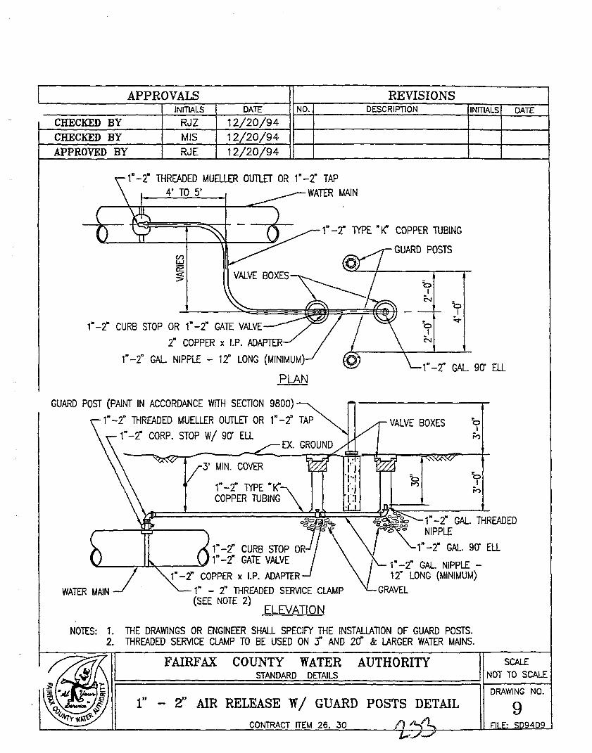
APPROVALS REVISIONS
CHECKED BYINITIALS
RJZDATE NO.
12/20/94DESCRIPTION INITIALS DATE
CHECKED BYAPPROVED BY
MISRJE
12/20/9412/20/94
bI~
,.. - 2" GAL. gO" ELL
bI
N
bI
N
,. - 'l' 1YPE •K" COPPER TUBING
GUARD POSTS
,.-t THREADED ~4UaLER OUTLET OR ,. - t TAP4' TO 5' WATER MAIN
,.-2" CURB STOP OR 1" -2" GATE VALVE
2" COPPER x I.P. ADAPTER
,.' -2" GAL NIPPLE - 12" LONG (MINIMUM)
PLAN
bI
r-,
bI
r-,
1" -2" GAL THREADEDNIPPLE
VALVE BOXES
1"-2" CURB STOP OR1"-2" GATE VALVE___--.,.....,&.,L::~--",
,. -2" COPPER x I.P. ADAPTER
1" - 2" THREADED SERVICE CLAMP(SEE NOTE 2)
ELEVATION
NOTES: 1. THE DRAWINGS OR ENGINEER SHALL SPECIFY THE INSTALlATION OF GUARD POSTS.2. THREADED SERVICE CLAMP TO BE USED ON 3" AND 2Cf' & LARGER WATER MAINS.
GUARD POST (PAINT IN ACCORDANCE WITH SECTION 9800)
,.' -2" THREADED MUELLER OUTLEr OR "'-2" TAP
1"-2" CORP. STOP WI 90' ELL
DRAWING NO.
FAIRFAX COUNTY WATER AUTHORITYSTANDARD DETAILS
f' - 2" AIR RELEASE W/ GUARD POSTS DETAIL 9CONTRACT ITEM 26. 30

APPROVALS REVISIONSINITIALS DATE NO. DESCRIPTION INITIALS DATE
CHECKED BY RJZ 12/20/94CHECKED BY MIS 12/20/94APPROVED BY RJE 12/20/94
WATER MAIN (SIZE VARIES)
A
L ."PLAN
... ~ .. ' 4 .
CLASS .. 0" CONCRETE
. " '
UNDISTURBED GROUND
2" DIA. GALVANIZEDNIPPLE
LEVEL WITHTOP OF W/M
...•
l' GALVANIZED ELL2" x 1'-0" GALVANIZED NIPPLE
FINISHED GRADE
WATER MAIN(SIZE VARIES)
t' GATE VALVE OR CURB STOP WISCREWED ENDS, wi l' SQUARE NUT
ECCENTRIC TAPPED PLUG ------,12" & LARGER Cl TAPPED 4"-5'
l' x 1'-0" BRASS OR COPPER NIPPLECLASS .. 0" CONCRETE
SECTION A-ANOTE:1. BLOCKING SHALL EXTEND BEYOND THE WATER MAIN TO UNDISTURBED GROUND.2. PER YOOT REQUIREMENTS, BLOW-OFF VALVE BOXES TO BE INSTALLED NO CLOSER
THAN 5'-0" TO EDGE OF PAVEMENT IN CUL-DE-SAC INSTALLATIONS.
10CONTRACT ITEM 26
2" BLOW-OFF DETAIL
FAIRFAX COUNTY WATER AUTHORITY SCALESTANDARD DETAILS NOT TO SCALE
I:=========:=::::::::::::::::====:::::::::::::::::==========~ DRAWING NO.

APPROVALS REVISIONSINITIALS DATE NO. DESCRIPTION INITIALS DATE
CHECKED BY RJZ 12/20/94CHECKED BY MIS 12/20/94APPROVED BY RJE 12/20/94
STANDARD 1Er METER BOX
COUPLINGS:PLASTIC TO COPPER(BY OTHERS)
~~D=:=:J
1" TYPE "K" COPPER PIPECONCRETE CURB & GUTTER
3/4" x ," THREADEDCORPORATION STOP OR 1" TAP AND gO" ELL
MEASUREMENT FOR PAYMENTWATER MAIN
PLAN
STANDARD METER BOX COVERTO BE FLUSH WITH EX. GROUND
FINISHED GRADE
WATER MffiR
STANDARD 18"METER BOX
1*\'"~-MmR YOKE SEE NOTE
COMMON BRICK ATQUARTER POINTS
COUPLINGS:PLASTIC TO COPPER(BY OTHERS)
18"
10N
ELEVATION
CONCR8E CURB &GUTIIR
PAVEMENT~
," TYPE "K" COPPER PIPE
NOTES:
,. NO PlASTIC TUBING TO BE USED INSIDE METER BOX.2. METER BOX, METER BOX COVER, 5/ff' x ," MffiR YOKE TO BE F.C.WA STANDARD TYPE.3. THREADED SERVICE CLAMP TO BE USED ON S' AND 2Cf' & LARGER WATER MAINS.
3/4" x 1" THREADEDCORPORATION STOPAND geT ELL
DRAWING NO.
SCALENOT TO SCALE
FAIRFAX COUNTY WATER AUTHORITYSTANDARD DETAILS
1" SERVICE CONNECTION WITH WATER METER 11CONTRACT ITEM 30

APPROVALS REVISIONSINITIALS
CHECKED BY RJZ
CHECKED BY DAWAPPROVED BY RJE
DATE j-.:..N:.::.O~. ....':D:.=.ES=..:C~R::.:...tP..:..:.TIO::..:.N~ __+IN:.:.:.IT.:..:IALS=t---=.;DA~J=-E-I
12/20/9412/20/9412/20/94
GRAPHITE MOLD
TOP OF PIPE OR FITTING
TAP HOLE
1/2"
END OF CABLE SHOULD NOT PASSCENTER LINE OF MOLD
PACKING MATERIAL\(IF REC'D) \
CABLE \
MOLD & WIRE POSITION
THERMITE WELD COATING
COMPLETED WELD
NOTE:
1. REFER TO SPECIRCATION SECTION 02655 FOR MOLD, WELD METAL,AND THERMITE WELD COATING INFORMATION.
12CONTRACT ITEM 29
CORROSION CONTROL THERMITE WELDS
FAIRFAX COUNTY WATER AUTHORITY SCALESTANDARD DETAILS NOT TO SCALE
I:===================::::::::==========~ DRAWING NO.

APPROVALS REVISIONS_______--+_IN_ITIALS-=--+_---7'-DA......T=E:--_II_N......O-+. D_E_SC_R_IPT_IO-N----+-IN......IT......IALS=+-......;;;,;DA......T.=..E--I
CHECKED BY RJZ 12/20/94CHECKED BY DAW 12/20/94APPROVED BY RJE 12/20/94
THERMITE WELD
....../ (TYPICAL)
P./
~ ~
- -I ~ ~
'-'
TYPICAL PIPE JOINT BOND
+-£-+VALVE. REDUCER. SOLID SLEEVE MECHANICAL SLEEVE
THERMITE WELD(TYPICAL)
BEND TEE
NOTES: TYPICAL BONDING FOR FITTINGS
1. THERMITE WELD BONDING WIRES TO TOP OF PIPE OR FITTINGS.
2. WIRE SIZE FOR BONDING JOINTS SHALL BE AS FOLLOWS:1t' & SMALLER - i6 AWG16" TO 36" - 4 AWG42" & lARGER - 2 AWG
3. BOND WIRE LENGTH SHALL BE KEPT TO A MINIMUM FOR FITTINGS.MAXIMUM BOND WIRE LENGTH FOR PIPE JOINT SHALL BE 18 INCHES.
FAIRFAX COUNTY WATER AUTHORITYSTANDARD. DETAILS
CORROSION CONTROL BONDED JOINTSCONTRACT ITEM 29
SCALE
NOT TO SCALE
DRAWING NO.
13

CHECKED BYCHECKED BYAPPROVED BY
APPROVALSINITIALS
RJZDAWRJE
DATE
12/20/9412/20/9412/20/94
NO.
REVISIONSDESCRIPTION INITIALS DATE
ELECTRICAL COATINGCOMPOUND
1~ 1" 1"TYP. TYP. TYP.
CRIMP THE BUTT SPLICE ANDSOLDER
WIRE
RUBBER SPLICING TAPE
VINYL PLASTIC ELECTRICALTAPE
TYPICAL WIRE SPLICE
FAIRFAX COUNTY WATER AUTHORITYSTANDARD DETAILS
CORROSION CONTROLMISCELLANEOUS DETAIL
CONTRACT ITEM 29
14

APPROVALS REVISIONSINITIAlS DATE NO. DESCRIPTION INITIALS DATE
CHECKED BY RJZ 12/20/94CHECKED BY DAW 12/20/94
A
TERMINAL BOX
24" SQUARE CONCRffiPAD FOR TEST STATION
<t TO BE PARALLELTO WATER MAIN
SINGLE TERMINAL BOX TEST STATION
A
LA
J
t' BRASS SURVEYMARKER (FLAT HEAD)
RJE 12/20/94
..
3'-0"
18"lYP.
....-i----+-....wr." -:-r-
~
APPROVED BY
A
LTERMINAL BOX
36" SQUARE CONCRffiPAD FOR TEST STATION
<t TO BE PARALlEL TO WATER MAINDOUBLE TERMINAL BOX TEST STATION
(lYPE F-FOREIGN PIPELINE CROSSING TEST STATION ONLY)
PLAN
TERMINAL BOX
WIRE LEADS(NUMBER VARIES PERlYPE OF INSTALLATION)
TAPE WIRE lEADS TOGETHERAT 10' INTERVALS
GUARD POSTS
SECTION
. I .
10'
'b.1Cl..
- i=....,
b·1Cl..
- i=....,
'bI~
I::NOTES:
1. LOCATE SURVEY MARKER IN NORTHEAST CORNER OF CONCRETE PAD.2. GUARD POSTS SHALL BE PRIMED AND PAINTED AS SPECIFIED IN
SECTION 02655 - CORROSION CONTROL
15CORROSION CONTROL
TEST STATION INSTALLATIONCONTRACT ITEM 29
FAIRFAX COUNTY WATER AUTHORITY SCALE
I~=========ST=AN=D=AR=D=D=ET=A='LS==========: NOT TO SCAlEDRAWING NO.

APPROVALS REVISIONSINITIALS DATE NO. DESCRIPTION INITIAlS DATE
CHECKED BY RJZ 12/20/94CHECKED BY DAW 12/20/94APPROVED BY RJE 12/20/94
TERMINAL BLOCK -INSIDE FLUSH MOUNTEDTERMINAL BOX
WATER MAIN
#12 AWGANODE LEAD WIRE WHEN SPECIFIED (TYP.)
#10 AWG WHITE
THERMITE WELD (TYPICAL)
1YPE T - STANDARD
DOWNSTREAM - GREENWIRE INSULATION
#10 AWG#10 AWG
TERMINAl BLOCK
I I ~WATER~FLOW
'-IN-SU-l.A-TE-D-F-LA-N-GE---L~.....J-1--1-;---;-II .--:1~2"~(lYP.)
OR COUPLING -I 1-12" (lYP.)
WATER MAIN
UPSTREAM - WHITEWIRE INSULATION
1YPE I - INSULATED FLANGE
NOTE:1. WHEN MULTIPLE ANODE LEADS ARE ATTACHED TO A TERMINAL BLOCK,
PROVIDE A DIFFERENT COLOR FOR EACH.
FAIRFAX COUNTY WATER AUTHORITYSTANDARD DETAILS
CORROSION CONTROL TEST STATION WIRINGTYPE T - STANDARD, TYPE I - INSULATED FLANGE
CONTRACT ITEM 29
16

DAW 12/20/94CHECKED BYCHECKED BY
APPROVALS REVISIONS_______--i---.;.;.IN.;.;.;IT..;;..IA=Ls~-___::_D.;.,;.;AT=E_::___;~N;...;;,.0_4. -:;D=E;;..;SC;.;.;R;;;..IP..;.;.TIO;;.;.N~__~IN.:,..;.ITI~AL::;;;S4_.=.;.DA...;.;.TE=__I
RJZ 12/20/94
APPROVED BY RJE 12/20/94
TO PERMANENT REFERENCEELECTRODE LOCATE fi' BELOWPROPOSED WATER MAIN ANDABOVE FOREIGN LINE
A
.J
32LB. MAGNESIUM ANODE (TYP.)
(2) TERMINAL BOXES (SEE NOTE 2)
FOREIGN LINE
A
L
PIPE COATING
WATER MAIN
PLAN
PIPE COATING. SEE SPECIFICATIONS.SECTION 02655 (TYP.)
WATER MAIN
--- PERMANENT REFERENCE ELECTRODE
~-~- (2) - 32LB. MAGNESIUM ANODES100'
FOREIGN LINE SEE NOTE 1 _I_-===~-L-Jlt-.......
TERMINAL BLOCK (TYP.)INSIDE FLUSH MOUNTEDTERMINAL BOX # BLUE
14 AWG RED# 4 AWG --if++!--+ +--- # 4 AWG
WHITE L....f---j-~....:-- --, # 10 AWG# 10 AWG _--+1
SECTION A-A
NOTES:1. CONNECTIONS TO FOREIGN UNE BY FOREIGN UNE OWNER.2. IN COLUMBIA GAS R-O-W INSTALL SINGLE TERMINAL BOX WITHOUT BOLLARD
ADJACENT TO PROPOSED COLUMBIA GAS TEST STATION. CONTRACTOR SHALLCOORDINATE INSTALLATION WITH COLUMBIA GAS.
FAIRFAX COUNTY WATER AUTHORITYSTANDARD DETAILS
CORROSION CONTROL TEST STATION WIRINGTYPE F - FOREIGN PIPELINE CROSSING
CONTRACT ITEM 29

APPROVALS REVISIONS
CHECKED BYINITIALS
RJZDATE
12/20/94NO. DESCRIPTION INITIALS DATE
CHECKED BY DAW 12/20/94APPROVED BY RJE 12/20/94
THERMITE WELD (lYP.)
WATER MAIN 1.
CASING PIPE 11 u_)...__:---__~-._ ---~:::L_~__\_ (2) - 32LB. MAGNESIUM ANODES
BONDED JOINTS (SEE NOTE 1)
PLAN
WHITE
TERMINAL BLOCK (TYP.)INSIDE FLUSH MOUNTEDTERMINAL BOX
WATER MAIN
CASING PIPE
TO TEST STATION
THERMITE WELD (TYP.)
ELEVATION OF TOP OFMAGNESIUM ANODE BELOWELEVATION OF BOTTOMOF CASING PIPE
.. \-_-- 32LB. MAGNESIUM ANODE (INSTALLAT EACH END OF CASING PIPE)
SECTION
NOTE:1. PROVIDE ELECTRICAL CONTINUITY BETWEEN TYPE C - TRENCHLESS CROSSING TEST STATIONS, MINIMUM.
FAIRFAX COUNTY WATER AUTHORITYSTANDARD DETAILS
CORROSION CONTROL TEST STATION WIRINGTYPE C - TRENCHLESS CROSSING
CONTRACT ITEM 23 & 29
SCALENOT TO SCALE
DRAWING NO.
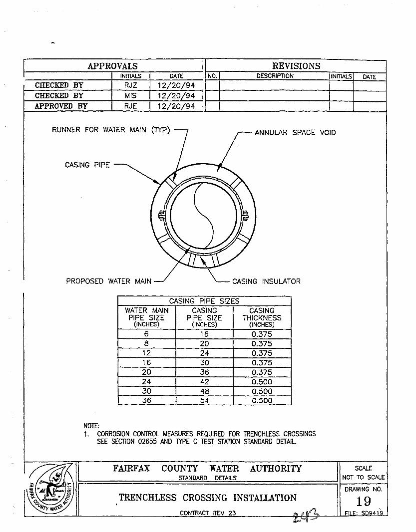
APPROVALS REVISIONSDESCRIPTION INITIALS DATEDATE NO.
I---+-----------+-....;......;~-...::;;....:.:.=...--I
12/20/94INITIALS
RJZCHECKED BYCHECKED BY MIS 12/20/94APPROVED BY RJE 12/20/94
RUNNER FOR WATER MAIN
CASING PIPE
PROPOSED WATER MAIN
ANNULAR SPACE VOID
CASING INSULATOR
CASING PIPE SIZESWATER MAIN CASING CASINGPIPE SIZE PIPE SIZE THICKNESS
(INCHES) (INCHES) (INCHES)
6 16 0.3758 20 0.37512 24 0.37516 30 0.37520 36 0.37524 42 0.50030 48 0.50036 54 0.500
NOTE:1. CORROSION CONTROL MEASURES REQUIRED FOR TRENCHLESS CROSSINGS
SEE SECTION 02655 AND lYPE C TEST STATION STANDARD DETAIL
FAIRFAX COUNTY WATER AUTHORITYSTANDARD DETAILS
TRENCHLESS CROSSING INSTALLATION
CONTRACT ITEM 23
SCALE
NOT TO SCALE
DRAWING NO.
19

PLANS
PURPOSE
•
•
•
OBTAIN APPROVAL FROM REGULATORYAND FINANCING AGENCIES
PROVIDE A BASIS FOR CONSTRUCTION
SERVE AS A PERMANENT RECORD OFFACILITIES
INCLUDE SHEETS FOR
• TITLE AND INDEX
• SITE/LOCATION PLAN
• TOPOGRAPHY (ON PLAN SHEETS)
• PLAN AND PROFILES
• CROSS SECTIONS
• DETAILS
TITLE BLOCKS
- DATES; APPROVAL & REVISIONS
- NAMES OF DESIGN/APPROVALENGINEERS
- IDENTIFICATION OF PRO~ECTAND DATAON SHEET

LEGEND
•
•
•
•
NOTES
SCALES (INCLUDE BAR CHART)
NORTH ARROW
SYMBOLS EXPLANATION
ABBREVIATIONS
• EXPLANATIONS AND CLARIFICATIONS
• CONTRACTOR GUIDANCE (NOT INTECHNICAL SPECIFICATIONS)
• KEY DESIGN ASSUMPTIONS
• REFERENCES

COST ANALYSIS
PURPOSE
- REVIEW IMPACT OF COSTS ONDESIGNING WATER SYSTEMS
- REVIEW HOW DESIGN DECISIONSRELATE TO USER FEES
CAPITAL BUDGETING TECHNIQUES
- CAPITAL BUDGETING INVOLVESPLANNING FOR THE BEST SELECTIONSAND FINANCING OF LONG TERMINVESTMENTS
- TWO STANDARD APPROACHES USED TOANALYZE ALTERNATIVES OFTEN USEDARE:
1 • NET PRESENT VALUE (NPV)
2 - INTERNAL RATE OF RETURN
1. NET PRESENT VALUE
NPV =PVi - PVo
NPV - NET PRESENT VALUE
PVi - PRESENT VALUE OF INCOMEFROM PRo.JECT
PVo - PRESENT VALUE OF CASHOUTFLOW FROM PRo.JECT

NPV APPROACH USES INTEREST RATESFACTORS BASED ON CURRENT OR PR~ECTED
COSTS OF CAPITAL
NPV MUST BE ZERO OR POSITIVE TO ASSURETHAT COSTS WILL BE MET.
THE PVi FOR A WATER UTILITY MUST COMEPRIMARILY FROM USER FEES
2. INTERNAL RATE OF RETURN (IRR)
THE IRR METHOD SE I S THE NPV AT ZEROWHILE THE INTEREST RATE IS CALCULATEDBASED ON A TRIAL AND ERROR METHOD.
THESE APPROACHES ARE TYPICALLY USED BYECONOMISTS ANALYZING THE ECONOMICFEASIBILITY OF A PRo.JECT AND AREGENERALLY REQUIRED BY FINANCIALINSTITUTIONS AND DONOR AGENCIES DURINGTHE PRo.JECT EVALUATION PROCESS.

ALTERNATIVE ANALYSIS
PRESENT WORTH
-•
-
ALL COSTS ARE CAPITALIZED TO THEIRVALUE TODAY
USE STANDARD DISCOUNT ORPRESENT WORTH FACTORS
DIFFERENT ALTERNATIVES CAN BEREDUCED TO THEIR PRESENT WORTHVALUE AND COMPARED ON AN EQUALBASIS
ANNUAL COSTS
•
-
--
ALL COSTS ARE SPREAD OUT TO THEIREQUIVALENT VALUE IF PAID ON ANANNUAL BASIS
USE CAPITAL RECOVER FACTORS
AGAIN, DIFFERENT ALTERNATIVES CANBE REVIEWED BY COMPARING THEIRANNUAL COSTS

EXAMPLE
ASSUME A VILLAGE OF 20,000 PEOPLEREQUIRING THE FOLLOWING
PIPE SIZE PROT STEEL PVC HDPE
MATERIAL DOLLARS PER METERSI. 25 7 10
3" 1& 2 3
1 I' 5 1 1
INSTALLATION&11 50 40 30
3 1• 40 30 25
111 10 10 10
TOTAL/M&11 75 47 40
3" 5S 32 28
1" 15 1 1 1 1
TOTAL SYSTEM COSTS IN DOLLARS
5000M-6" 375,000 235,000 200,000
10,000M- 5S0,000 320,000 280,0003"
2000M-1 11 30,000 22,000 22.000
TOTAL $965,000 $577,000 $502,000
NUMBERS ARE ILLUSTRATIVE

•
EXAMPLE 1
DETAILS
ITEM PROT PVC HDPESTEEL
NETWORK $9&5,000 $577,000 $502,000INSTALLED
LIFE IN 40 50 30YEARS
SALVAGE 0 0 0VALUE
SERVICE -- -- --FOR 20,000
ANNUAL COSTS
O&M -- -- --PIPE $10,000 $20,000 $30,000REPAIR
RECOVERY 0.1022& 0.1008& 0.10&08FACTOR10%
CAPITAL $98,&80 $58,19& $53,252RECOVERY
TOTAL $108,680 $78,19& $83,252
COST PER CUM WATER
DESIGN $.19 $.13 $.14-
80% $.23 $.17 $.18DESIGN

EXAMPLE 2
DETAILS
ITEM PROT PVC HDPESTEEL
NETWORK $965,000 $577,000 $502,000INSTALLED
LIFE IN 40 50 30YEARS
SALVAGE 0 0 0VALUE
SERVICE •• .. ••FOR 20,000
ANNUAL COSTS
O&M .. .. ..PIPE $10,000 $20,000 $30,000REPAIR
RECOVERY 0.20014 0.20002 0.20085FACTOR20%
CAPITAL $193,135 $115,411 $100,826RECOVERY
TOTAL $203,135 $135,411 $130,826
COST PER CUM WATER
DESIGN $.35 $.23 $.22
80% $.43 $.29 $.28DESIGN
~\

•
•
EXAMPLE 3
DETAILSITEM PROT PVC HDPE
STEELN£lWORK $965,000 $577,000 $502,000INSTALLED
LIFE IN 50 25 20YEARS
SALVAGE 0 0 0VALUE
SERVICE -- -- --FOR 20,000
ANNUAL COSTS
O&M -- -- --PIPE -- -- --REPAIR
RECOVERY 0.10086 0.11017 0.11746FACTOR10%
CAPITAL $97,323 $63,568 $58,965RECOVERY
TOTAL
COST PER CUM WATER
DESIGN $0.17 $0.11 $0.10
80% 0.21 0.14- 0.13DESIGN
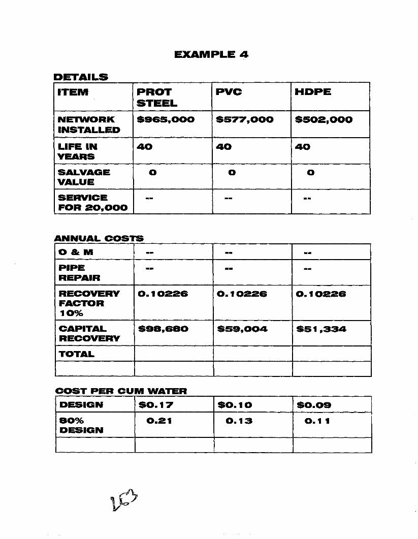
EXAMPLE 4
DETAILS
ITEM PROT PVC HDPESTEEL
NElWORK $965,000 $577,000 $502,000INSTALLED
LIFE IN 40 40 40YEARS
SALVAGE 0 0 0VALUE
SERVICE •• .. ..FOR 20,000
ANNUAL COSTS
oaM .. .. ••
PIPE •• .. ..REPAIR
RECOVERY 0.10226 0.10226 0.10226FACTOR10%
CAPITAL $98,680 $59,004 $51,334RECOVERY
TOTAL
COST PER CUM WATER
DESIGN $0.17 $0.10 $0.09
80% 0.21 0.13 0.1 1DESIGN

•
•
•
•
EXAMPLE 5
DETAILS
ITEM PROT PVC HDPESTEEL
NETWORK $9&S,000 $S77,000 $S02,000INSTALLED
LIFE IN 20 20 20YEARS
SALVAGE 0 0 0VALUE
SERVICE -- -- --FOR 20,000
ANNUAL COSTS
oaM -- -- --PIPE -- -- --REPAIR
RECOVERY 0.1174& 0.1174& 0.1174&FACTOR10%
CAPITAL $113,348 $&7,774 $Se,9&SRECOVERY
TOTAL
COST PER CUM WATER
DESIGN SO.19 $0.12 $0.10
80% 0.24 0.15 0.13DESIGN

EXAMPLE & (BOT)
DETAILS
ITEM PROT PVC HDPESTEEL
NE'lWORK $965,000 $577,000 $502,000INSTALLED
LIFE IN 12 12 12YEARS
SALVAGE 0 0 0VALUE
SERVICE -- -- --FOR20,000
ANNUAL COSTS
O&M -- -- --PIPE -- -- --REPAIR
RECOVERY 0.18448 0.18448 0.18448FACTOR15%
CAPITAL $178,023 $106,445 $92,609RECOVERY
TOTAL
COST PER CUM WATER
DESIGN $0.30 $0.18 $0.16
80% 0.38 0.23 0.20DESIGN

•
•
•
•
NOTE OF INTEREST
THE HEAD LOSS DIFFERENCE BETWEENPLASTIC AND STEEL PIPES IS 59 METERSPER KILOMETER
• FOR A 2 1/2 INCH PIPE CARRYING 1/2CUM/MIN (approx 1 00 gal/min)
THIS TRANSLATES TO A PUMPING COST OF$S067/KM/YEAR OR 2 CENTS PER CUM OFWATER
• IF ELECTRICITY COSTS 10 CENTS PEAKWH, PUMP EFFICIENCY IS 70% ANDMOTOR EFFICIENCY IS 90%

WATER SYSTEM DESIGN SEMINAR
MAY 14 AND MAY 15, 1996
(pART Ill)
PRESENTERS:
DANIEL GALLAGHER, P.E
AND
FRED ZOBRIST, P.E.
SPONSORED BY:
USAIDIWEST BANK AND GAZA
AND
UNDP JERUSALEM OFFICE
CONTRACT NUMBER:HNE-0159-C-OO-30S0-00
MANAGEMENT SYSTEMS INTERNATIONAL

INTRODUCTION
This is Part III of a three part report on the Water System Design Seminar conducted at Beir ZeitUniversity on May 14 and May 15, 1996. Parts I and II of the report were printed earlier andare included in a single volume. For additional information on the seminar contact the USAIDengineering office in Tel-Aviv.

Table of Contents
I. Hydraulic equations , 1A. Bernoulli's Energy Equation 1B. Hazen Williams 1C. Manning 1D. Darcy-Weisbach 2E. Minor losses 2
II. Pumps 3A. Pump head - capacity curve , 3
III. Valves , 3A. check 3B. pressure reducing......•......................................................................................................... 4C. pressure sustaining 4D. pressure breaker valves 4E. flov" control valves 4F. throttle control valves 4G. gate valves 4H. butterfly valves 4I. air vacuum and air reliefvalves 4J. Altitude-control valves 4K. globe and angle valves 5
IV. Storage 5A. Types ofwater storage facilities 5
1. types of service 5a) operating storage 5b) emergency storage 6
2. configuration 6a) tanks 6b) standpipes 7c) reservoirs 7d) pneumatic tanks 7
3. Construction material 74. Location 7
B. "Floating" storage tanks 7V. Hydraulic modeling 7
A. Notation and data requirements 81. Water System Inventory 82. Required physical data 10
B. Branched distribution systems 11C. Looped distribution systems 16
1. continuity equations / conservation offlow 162. flo\v equations around loops 163. solution techniques 17
a) unkno\vn flo\vs 17b) unknO\vn heads.......................................................................................................... 18c) Hardy Cross l~
d) Method Comparison 21D. Peaking factors 22

E. Model initialization for limiting conditions : 22F. EPANET 23
1. Installation 232. Data Files 233. Analyzing EPANET Results 26
G. Model Output Analysis 26VI. Maps and Dra\vings 26
A. Comprehensive map (or wall map) 26B. Sectional maps or plat 27C. Valves and hydrant maps 27D. Plan and profile drawings 27E. Supplemental maps 27F. Card records 27
VII. Design Standards (by Donald Lauria, University ofNorth Carolina) 28A. Introduction 28B. Levels of Service .. '" , 28C. Design Periods 30D. Design Flo\vs 32E. Pipelines, Net\vorks and Tanks 33
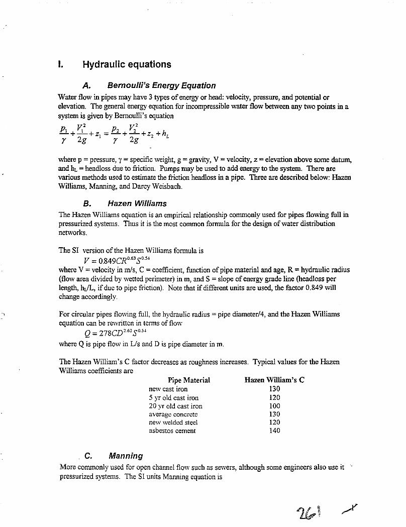
I. Hydraulic equations
A. Bernoulli's Energy EquationWater flow in pipes may have 3 types ofenergy or head: velocity, pressure, and potential orelevation. The general energy equation for incompressible water flow between any two points in asystem is given by Bernoulli's equation
v.2 V?!!.L+_1_+ Z = P2 +-L+ z +hr 2g I r 2g 2 L
where p = pressure, y = specific weight, g = gravity, V = velocity, z =elevation above some datum,and hL =headloss due to friction. Pumps may be used to add energy to the system. There arevarious methods used to estimate the friction headloss in a pipe. Three are described below: HazenWilliams, Manning, and Darcy Weisbach.
B. Hazen WilliamsThe Hazen Williams equation is an empirical relationship commonly used for pipes flowing full inpressurized systems. Thus it is the most cornmon formula for the design ofwater distributionnetworks.
The SI version of the Hazen Williams formula isV = O.849CRo.63SO.54
where V = velocity in mis, C = coefficient, function of pipe material and age, R = hydraulic radius(flow area divided by wetted perimeter) in m, and S =slope ofenergy grade line (headloss perlength, hdL, if due to pipe friction). Note that if different units are used, the factor 0.849 willchange accordingly.
For circular pipes flowing full, the hydraulic radius = pipe diameter/4, and the Hazen Williamsequation can be rewritten in terms of flow
Q = 278CD263S054
where Q is pipe flow in Lis and D is pipe diameter in m.
The Hazen William's C factor decreases as roughness increases. Typical values for the HazenWilliams coefficients are
Pipe Materialnew cast iron5 yr old cast iron20 yr old cast ironaverage concretenew welded steelasbestos cement
Hazen William's C130120100130120140
C. ManningMore commonly used for open channel flow such as sewers, although some engineers also use itpressurized systems. The SI units Manning equation is

v = .!.R%S~n
where V = velocity in mis, n = coefficient ofrougimess, R = hydraulic radius in In, and S = slopeofenergy grade line.For circular pipes flowing full, the hydraulic radius = pipe diameter/4, and the Manning equationcan be rewritten in terms offlow
Q= 312 D%S~n
where Q is pipe flow in LIs and D is pipe diameter in m.
Manning's n increase as rougImess increases. Typical values are given below.
Materialconcretecast-iron pipevitrified claybrickcorrugated metal pipebituminous concreteuniform firm sodded earth
Manningn0.0130.0150.0140.0160.0220.0150.025
D. Darcy-WeisbachMore fundamental than the other equations. Friction factor varies with turbulentllaminar flowcondition.
h =jLV2
L 2Dgwhere hL = head loss, L = pipe length, D = pipe diameter, f= friction factor, V = velocity. thefriction factor f is a function of relative rouglmess ofpipe (pipe material and age) and Reynoldsnumber. It is usually determined from a Moody diagram.
The Darcy Weisbach formula can be rearranged to yield
v=eg~st
Notice that for a given pipe, all of these equations have the formhL =K Qa
where K = a coefficient for a given pipe and depends upon its length, diameter, age, material, etc.K is a constant for the Hazen Williams and Manning equations but varies with Q (through theReynolds number) for the Darcy Weisbacha = constant exponent that depends on the formula used
E. Minor lossesMinor losses for turbulent flow conditions are generally expressed as a function ofV2/2g the .velocity head. For long pipes, pipe friction headloss usually predominates and minor losses can beneglected. For shorter pipes such as those in treatment plant, minor losses can be important.
2

II. PumpsCapacity of a pump is expressed as flow delivered. The head required to overcome losses in a pipesystem is termed system head. The total dynamic head is the head against which the pump mustwork when water is being pumped. This is the head added to the system by the pump and can becalculated as the difference in head using Bernoulli's equation between the discharge and suctionnozzle ofthe pump.
The power input for a pump is a function ofthe flow, head, and efficiency ofthe pump. Typicalefficiencies range from 60-90%.
E = pump output =r QHt
P power P
A. Pump head - capacity curveThe head that a constant speed pump can produce as flow changes called pump head - capacitycurve or pump characteristic curve. The system curve is the plot of the total dynamic head(sum ofthe static lift + kinetic energy losses).
system curve
capacity
The operating point for the pump is defined by the intersection ofthe pump head curve and thesystem curve.
III. Valves
A. checkCheck valves permit flow in only one direction. Conunonly used to prevent flow reversal of flowwhen pumps are shit off. Check valves, termed foot valves, can be installed on the suction side ofpump to prevent loss of prime. Check valves are installed on the discharge side ofpump to reducehanuner force.

B. pressure reducingPressure reducing valves maintain a set pressure on the downstream end. Operate by using theupstream pressure to throttle the flow through an opening similar to globe valve. The throttlingvalve will open or close until the downstream pressure reaches the preset value.
c. pressure sustainingPressure sustaining valves attempt to maintain a minimum pressure on the upstream end when thedownstream pressure is below that value. Ifthe downstream pressure is above the setting, flow isunrestricted. If the downstream pressure is above the upstream pressure, valve will close toprevent reverse flow.
D. pressure breaker valvesPressure breaker valves for a specified pressure loss across the valve.
E. flow control valvesFlow control valves to limit the flow through a valve to set amount, providing sufficient head isavailable.
F. throttle control valvesThrottle control valves simulate a partially closed valve by adjusting the minor loss coefficient ofthe valve.
G. gate valvesMost commonly used for on-off service. Relatively inexpensive and offer positive shutoff.Located throughout a distribution system at regular intervals so that breaks in the system can beisolated. Valves should be accessible through manhole ofvalve box. Generally must be installedin vertical position. Large gate valves frequently include small bypass valve to equalize pressureon the main valve and reduce potential for water hammer.
H. butterfly valvesLess expensive and easier to operate than gate valves. Not suitable for liquids that contain solidsand light prevent complete closure.
I. air vacuum and air relief valvesUsed in long pipes at high points to prevent negative pressure from building up iflines are drainedor to allow accumulated air to be released. Operate automatically.
J. Altitude-control valvesA type of diaphragm-valve used to control level of water in a tank supplied from a pressuresystem. Two types are used: single acting and double acting. Single acting used only for filling thetanks. The tank discharges through a separate lined or through a check valve in a bypass linearound the altitude valve. A double acting altitude valve allows water to flow both to and from thetank. When the tank becomes full, the valve closes to prevent overflow. When the distributionpressure drops below the pressure exerted by the full tank, the valve opens to discharge water tothe distribution system.
4

K. globe and angle valvesNot commonly used in water distribution system. Primary application is household plumbing.
IV. StorageStorage is provided to equalize supply and demand, level out pumping requirements, provide waterduring source or pump failure, provide water to meet fire demands, provide surge relief, and toblend water sources. With adequate storage, water can be treated and pumped from the treatmentplant to the distribution system at a rate equaling the maximum day demand and pumps can beoperated at their rated capacity. Storage can also be used ifthe treatment plant operates for only aportion ofa day.
A. Types of water storage facilities
1. types of service
aj operating storageOperating storage generally floats on the system with the reservoir filling when demand is low andemptying when demand exceeds supply. A mass balance can be used to size the operating storage.

Given the following demand rates, find the required operationalstorage assuming 24 hr pumping.
Time Interval Demand Hourly Hourly Supply - Demandstart end Rate Demand Supply to from
gpm gal gal storage storage12:00 AM 1:00 AM 1900 114000 280460 166460 0
1:00AM 2:00AM 1800 108000 280460 172460 02:00AM 3:00AM 1795 107700 280460 172760 03:00AM 4:00AM 1700 102000 280460 178460 04:00AM 5:00AM 1800 108000 280460 172460 05:00AM 6:00 AM 1910 114600 280460 165860 06:00AM 7:00AM 3200 192000 280460 88460 07:00AM 8:00AM 5000 300000 280460 0 -195408:00AM 9:00AM 5650 339000 280460 0 -585409:00AM 10:00 AM 6000 360000 280460 0 -79540
10:00 AM 11:00 AM 6210 372600 280460 0 -9214011:00 AM 12:00 PM 6300 378000 280460 0 -9754012:00 PM 1:00 PM 6500 390000 280460 0 -109540
1:00 PM 2:00 PM 6460 387600 280460 0 -1071402:00 PM 3:00 PM 6430 385800 280460 0 -1053403:00 PM 4:00 PM 6500 390000 280460 0 -1095404:00 PM 5:00 PM 6700 402000 280460 0 -1215405:00 PM 6:00 PM 7119 427140 280460 0 -1466806:00 PM 7:00 PM 9000 540000 280460 0 -2595407:00 PM 8:00 PM 8690 521400 280460 0 -2409408:00 PM 9:00 PM 5220 313200 280460 0 -327409:00 PM 10:00 PM 2200 132000 280460 148460 0
10:00 PM 11:00 PM 2100 126000 280460 154460 011:00 PM 12:00 AM 2000 120000 280460 160460 0
Sum: 6731040 6731040 1580300 -1580300
Average hourly pumping: 6,731,040 124 = 280460
Required storage: 1580300
b) emergency storage
Designed to be used only in exceptional situations such as fires or source failures.
2. configuration
a) tanks
Generally refers to any structure used for containing water. Elevated tanks are supported on steelor concrete to\ver. Ground level tanks are less expensive to build and operate, but may require abooster pump to provide adequate pressure.
6

b) standpipesTank resting on the ground with a height greater than its diameter. Generally only the upperportion has enough pressure to be used in the distribution system. The lower portion can be usedfor emergency storage.
c) resen'oirsReservoirs generally refers to very large storage facilities. Can be ponds, lakes, etc. Morecommon to use reservoirs for raw water storage rather than treated water.
d) pneumatic tanksUsed in very high or remote areas with few customers. Consists of steel pressure tank partiallyfilled with pressurized air. The compressed air on top ofthe water provides necessary pressure tothe area. A small booster pump is located on the intake side ofthe tank. The pump is only turnedon when the pressure in the tank drops below a set level. The maximum amount ofwater that maybe withdrawn at any time is approximately 1/3 the total tank volume.
3. Construction materialTanks can be made from steel or concrete with an appropriate liner.
4. LocationTo minimize pipe diameters, elevated storage facilities are usually located in regions ofthe serviceareas where pressure is low, i.e. as close to the center ofdemand as reasonable. The water level inthe reservoir must be at a sufficient elevation to permit gravity flow at an adequate pressure.Reduced pipe diameters can be used near a reservoir because the water will flow in all directionsaway from the tank when it is supply water. Elevated storage facilities near the treatment plantgenerally do not allow for reduced pipe diameters. Decentralized storage with several smallertanks in different parts of the distribution system are usually preferred compared to one large tank.
Ground-level storage with booster pumps is often used when the system has several pressure zones.Storage is located at the boundaries of these pressure zones. Water from the lower pressure zoneflows into the reservoir and is pumped to the higher pressure zone.
B. "Floating" storage tanksDuring periods of low flow, usually in late evening, the heads in the distribution system are lowand the storage tank is filled automatically. Altitude control valves can be used to shut offflowwhen the storage tank is full. As the demand increases during the day, the head in the distributionsystem falls and the entire capacity of the treatment pumps is used to meet demands. As demandincreases further, the excess demand is met from the storage tank and the tank begins to empty.
V. Hydraulic modelingPressures (heads) should be adequate for consumers and fire fighting. This influences thediameters chosen. Ifhelp is needed to maintain pressure, in-line booster pumps and elevatedstorage tanks can be used. Typical pressures in residential areas ofthe US range from 40 to 50psig (90 to 115 feet of head). Pipe sizes should be large enough to avoid excessively high or lowvelocities. Generally 3 to 4 feet per second is considered desirable. The National Board ofFire
7

Underwriters requires a minimum of 8 in diameter pipe, although 6 inch diameter pipe can be usedin the grid system.
Hydraulic models for distribution systems should be analyzed for conditions that exist now as wellas for conditions that exist at the end ofthe design period. Headlosses are expected to increase aspipes age.
A. Notation and data requirementsDistribution systems are generally based on a link-node framework. Links are use to represent thepipes. Nodes represent locations where flows enter or leave the system or where links jointogether. Nodes should be placed wherever pipe characteristics (e.g. diameter or material) changeor to provide sufficient resolution for water demands. Demands are typically not modeled at thelevel of individual households - rather a group ofhouseholds are clumped together and thedemands are located at one common point.
1. Water System Inventory
a) inventory e"istingfacilities
(1) pipe location and diameter, length, type, age,present condition
(2) storage facilities: capacity, location, availability,dimensions, water surface elevations, connectionsto system
(3) design and operation features of service andbooster pumps, including capacity, system head,elevation
(4) control and regulatory valves elevation, operation,pressure setting, purpose
(5) service areas and pressure zone boundaries
b) review operating records and inten,jew staff
(1) diurnal and seasonal treated water productionrecords
(2) service and booster pump flows and pressures
(3) clearwell and storage level variations for differentdemand situations
(4) system operation criteria for pump stations,storage, source pumps

(5) system operating pressures determined from pasttesting or monitoring
(6) power consumption records, costs, and ratestructure
(7) observed low pressure areas indicating systemdeficiencies
(8) observed fire flow capabilities
c) review water consumption records
(1) total water sales (billing records)
(2) service population
(3) number and types of connections
(4) consumption by major users
(5) peaking factors
(6) system diurnal demand curves
d) develop water demands using consumption records andpopulation amI land use projections. Existing andprojected demands should be establishedfor the totalsystem, sub areas within the system, and major users.
(1 ) average annual day demands
(2) maximum day demands
(3) peak hour demands
(4) fire flow demands
(5) minimum hour demands or maximum storage -replenishment rate
(6) other site specific demand features
'.
9

e) establish background information for power managementand operational improvementprograms
(1) plot pump characteristic curves vs system headcurves
(2) establish average maximum day pumping ratefrom the developed diurnal demand curve
(3) determine whether system storage or auxiliarypower can be used to reduce peak pumping rate toor below the average of the maximum daydemand.
(4) check the piping arrangements to storagecomplexes for replenishment constraints
(5) examine pump curves vs system head curveconditions to determine optimal operationsequence based on system demands
2. Required physical data
a) pipe segments
(1) assign lD numbers
(2) establish length between nodes
(3) determine pipe diameter, roughness coefficient(age and pipe material)
b) nodes
(1) assign ID numbers
(2) establish ground surface elevations of each nodeIf read from contour map, 1 m contours desirable, 3 m contours acceptable ifno other data. Errorsarise from interpolated contours. (Note 1 ft error =0.43 psi.) Generally, ground surfaceelevations are used, not the elevations of the buried pipe.
Accurate data needed for pressure control points - points where system pressure fixed or open toatmosphere - and pressure regulated discharge points. Other node elevations can be estimated.
'1;10 10

c) supply pumps and booster pumps
(1 ) assign 10 numbers (EPANET treats as links, otherprograms as nodes)
(2) determine multiple points on pump curve
(3) define on/off control levels based on systempressure or tank elevations)
(4) determine ground surface elevation for each pump
(5) assign valve or adjust pump curve for minor losses
d) control valves andpressure regulating valves
(1) assign lD number (EPANET treats as links, otherprograms as nodes)
(2) determine downstream pressure setting for eachPRV
(3) determine control pressures for flow control valves
(4) establish ground surface elevations
e) resen'oirs and storagefacilities
(1) assign ID number (treated as nodes)
(2) define capacity, dimensions, flow rate, andoperating range
(3) establish ground surface and water surfaceelevations
B. Branched distribution systemsThere are 2 general classes ofpiped distribution systems: branched and looped. A branchednetwork contains no closed circuits or loops. Pipes can simply dead end. Branched networks arefound on the outskirts ofmany to\VJ1S, in rural communities, in irrigation systems, and frequently invillages in developing countries. Branched distribution systems have a structure similar to a tree.A trunk line provide the major source of water. Service mains and submains branch offthe trunkline. Branched distribution systems have several limitations: stagnation in the dead ends may allowfor bacterial growths and sedimentation, disinfectant residuals are hard to maintain in the deadends, repairs will shut down service for all connections beyond the repair point, the pressure at the-end of the line may become undesirable low as additional corrections are made.

--1----t---(~ ~)
Examples ofbranched distribution systems
On the other hand, branched distributions are simple to design and construct, and are less costlythan looped systems. When branched networks are used, the cost ofthe network is often ofmajorconcern. Branched networks u~e less pipe than looped networks, and therefore cost significantlyless. An interesting problem is to design a branched distribution network that has minimum costfor a specified layout. Once the layout is established, the major factors affecting cost are thediameters used throughout. These must be chosen to maintain necessary heads at each point in thedistribution system. This problem requires an understanding ofboth fluid flow in pipes andoptimization techniques. As stated, the problem can be formulated as a linear programmingproblem. A linear program optimizes a linear objective function that is subject to a series of linearequality and inequality constraints. The problem will be illustrated through the use ofan example.Given the example network below
~-> 3 LPS 11061<- 4 LPSElev=60m Elev=55m~@ 110m HGL
I II II Link 107 I Link 104I 1000 m 4000 m
I Elev=60m I~ 8 LPS-> r-----, @100 m HGL .L-,
<-1107 1-1---------11041---------111051-> 1 LPS
~l~;:'::' L~~~O1~6 T L~~~ ~05 '---'Elev=60m
I Link 103I 2000 m
Ir-----, Elev=90m~-> 1 LPS ~
<-1101 t-I---------111031t-----------11102 1-> 3 LPS3 LPS L-.-.J Link 102 L-.-.J Link 101 L-.-.J Elev=60mElev=60m 1000 m 1000 m
The example network consists of 7 pipe segments or links which are connected by 8 nodes. Eachnode is a point of water input or demand or a junction between two pipes. The network containsno closed loops, hence it is a branched network and the link flows may be easily determined fromthe mass balance equations alone. Inputs to the network occur at nodes 104 and 106. These inputshave knO\vn hydraulic grade line elevations. All other nodes are either demand or junction nodes. ".Two links, 105 and 106, are existing, with 10 em diameters. It is assumed that link 105 will
rtltV 12

remain unchanged, while link 106 will be paralleled with new pipe ifnecessary. All other links willbe designed using new pipe.
The design objective is to select pipes for the links in such a manner that the total construction costis minimized subject to certain design constraints. Both the objective and the constraints can bewritten as linear equations or inequalities. The resulting problem is called a linear program. Themathematical trick that permits the formulation ofthe problem as a linear program is that pipelength, rather than pipe diameter, is treated as the unknown or decision variable. Thus, theengineer proposes commercially available pipe diameters as candidates for each link, and the linearprogramming algorithm selects from these candidates the optimal combination. Different sets ofpipe diameters for different lin!<s are allowed. The optimal combination ofpipes for each linkwould then be laid in series along the link.
The candidate pipe diameters for the example network are 5 em, 10 em, and 20 cm. The decisionvariables are:
XI = the length of 5 cm pipe to be used in link 101X2 = the length of 10 cm pipe to be used in link 101X3 = the length of20 em pipe to be used in link 101X4 = the length of 5 em pipe to be used in link 102Xs = the length of 10 cm pipe to be used in link 102Xli = the length of 20 cm pipe to be used in link 102X7 = the length of 5 cm pipe to be used in link 103Xs = the length of 10 em pipe to be used in link 103X9 = the length of20 em pipe to be used in link 103XIO = the length of 5 cm pipe to be used in link 104Xu = the length of 10 em pipe to be used in link 104XI2 = the length of 20 em pipe to be used in link 104XI3 = the length of 10 cm pipe to be used in link 105XI4 = the length of 10.8 cm pipe to be used in link 106·XIS = the length of 14 cm pipe to be used in link 106·X 16 = the length of 23.7 cm pipe to be used in link 106·XI7 = the length of 5 cm pipe to be used in link 107XIS = the length of 10 em pipe to be used in link 107XI9 = the length of20 cm pipe to be used in link 107
• These are equivalent diameter pipes. XI4 is the equivalent diameter of the existing 10 emand the candidate 5 em. Similarly, XIS is the equivalent of the existing 10 cm and thecandidate 10 em, and xl6is the equivalent of the existing 10 em and the candidate 20 em.
The installed costs per unit length ofthe candidate pipe are $15/m for the 5 em pipe, $50/m for the10 cm pipe, and $1OOlm for the 20 em pipe. Installed pipe has an associated cost of $O/m,regardless of its diameter. The construction cost is thus
COST = 15 XI + 50 X2 + 100 X3 + 15 X4 + 50 Xs + 100 Xli +15 X7 + 50 Xs + 100 X9 + 15 XIO + 50 Xu + 100 X12 +oXl3 + 15 X14 + 50 XIS + 100 XI6 + 15 X17 +
50 XIS + 100 XI9
'11) 13

The constraints on the design variables consist ofboth equalities and inequalities. Theseconstraints impose both headloss and length restrictions on the decision variables. There are 3 typeofheadloss constraints that may be imposed at each node. The first type says that the residualhead at the node must be greater than or equal to some specified head. This is used to insure thatthere is minimum positive pressure at the specified nodes. An alternative constraint is that theresidual head must be less than or equal to some specified head. This type ofconstraint are used inhilly terrains to prevent exceeding the allowable pipe pressure or to prevent excessive pressures atnodes. The final type ofconstraint is that the residual head is equal to some known head. Thisconstraint is used in networks with more than one input node to insure that the headloss along thepath from the two nodes is equal to the difference in the hydraulic grade lines (HGL). Paths arereferenced from a specified input node called the reference node. This last type ofconstraint mustbe imposed where more than one input occurs. The other constraints may be imposed as needed.In general, minimum pressure constraints are imposed at the extremities ofthe network, i.e. theterminal or end nodes. Maximum pressure constraints are imposed at low elevation points on hillyterrain. The linear programming technique automatically adds constraints that all the decisionvariable be nonnegative. Since theses variable represent lengths in this problem, these additionalconstraints are not a difficulty. lfthe minimum allowable head is 1 meter, and this constraint is tobe applied to nodes 101, 102, 103, and 108, and node 104 is taken as the reference node, theconstraints can be written as
hLI03 + hL102 <= 100 - 60 - 1 = 39hL103 <= 100 - 90 - 1 = 9hLI03 + hLI01 <= 100 - 60 - 1 = 39hLJ06 + hLI07 <= 100 - 60 - 1= 39
where the subscripts on the headloss refer to the links, 100 is taken from the HGLof the reference node, 60 and 90 are the ground elevations of the constrainednodes, and 1 is the minimum residual head.
lfthe head at node 107 is constrained not to exceed 55 m, then its constraint can be written as
hLI06 >= 100 - 10 - 55 = 35
Since there are two input nodes, with fixed HGL's, an additional constrain must be written
hLI05 + hL104 = 100 - 110 =-10
Nodes 104 and 105, as interior nodes, probably do not need to be constrained on the first design.lfthe initial results suggest that constraints are necessary, they may be added and second designperformed.
The headlosses are calculated for each of the candidate pipes using one ofthe flow equations,typically the Hazen Williams equation. TIle headloss can be calculated from
hLij =(Q/kiCi)J.sS nt·S7 Ljwhere hLij =headloss in pipe j in link i
Qi = flow in link iki =constant for link i that depends on unitsCi =Hazen Williams coefficient in link i
".
14

Dj =diameter of pipe jFor example, in link 101, three different diameter pipes may be used to make the link.
Additional constraints must be added to insure that the lengths ofthe candidate diameters match theneeded total length ofeach pipe. These constraints are
Xl + X2 + X3 = 1000X4 + Xs + X6 = 1000X7 + Xl! + X9 =2000XIO + XII + XI2 =4000XI3 = 700 _X14 + XIS + X16 =4000X17 + XI8 + X19 = 1000
The linear programming automatically adds the constraints that
Xj>=O i = 1,...,19
The problem, then, is to choose the xi's that minimize the cost, but meet all ofthe constraints. Acomputer program, BRANCH, that sets up and solves this type ofproblem is included along withuser instructions. The basic solution from the linear programming algorithm is
Link # Diameter (cm) Length (m)101 5 129.6
10 870.4102 5 129.6
10 870.4103 10 231.1
20 1768.9104 10 115.9
20 884.1105 10 700.0106 10.8 1883.9
14.0 2116.1107 10 607.9
20 392.1
These diameters and lengths just meet each of the constraints that were imposed, using as much ofthe smaller, less expensive diameter pipe as possible.
Pipes are assumed to be laid in order of decreasing diameter in the downstream direction. Thus forlink 104, the 20 cm pipe should be laid from node 106 (the upstream node) and then the 10 cm pipeused to complete the distance to node 105 (the dO\VI1stream node). This ensures that thedownstream nodes exceed the minimum pressures when such constraints are used.
It may not be possible to meet all the constraints ,,"ith any combination of the candidate diameters.In this case the algoritlun will return with a solution labeled infeasible. For example, the headloss..from the reference node to a node with a minimum pressure constraint may be greater thanallowable to meet the constraint even when the largest candidate diameter is used for the entire link.
15

The problem would then be infeasible. To attempt to correct this situation, make larger diameterpipes available on paths subject to minimum head constraints, smaller diameter pipes available onpaths with maximum head constraints, and both larger and smaller diameters available on pathslink nodes with known hydraulic grade lines.
C. Looped distribution systems
A distribution system with loops or circuits can provide the reliability that a branched networkcannot. If a break occurs, water is able to flow through the remaining pipes in the loop and movedownstream. Since flow occurs in all pipes, the water quality should not have sufficient time todeteriorate if the network is designed properly. Typical loop patters include a grid pattern with acentral feeder line that normally carries the bulk of the flow (Figure 2a) or a grid pattern with amain looped feeder (Figure 2b).
I
~I===l===l===I
( a)
Ii Ii
=il!:::======t====!lll
I ....L.-__...JI
(b)
Figure 2. Examples of Looped Distribution Systems
The pressures and flows in looped distribution systems are solved by writing a series ofnonlinearequations based on conservation of flow and energy.
1. continuity equations I conservation of flowThere are two type of equations that are used to determine the flows in the links. The first type isbased on conservation of mass, sometimes caIled a mass balance. It simply states that the sum ofthe flows entering a node must equal the sum of the flows leaving a node. Thus at each junction
L QinJlow =L Qoutf/ow
2. flow equations around loopsThe second type of equation is based on the conservation ofenergy. It states that the sum ofthesigned head losses around a loop equals the energy input from any pumps on the loop. If there areno pumps, the headlosses must sum to zero. In other words, the energy at a node is the same nomatter what direction the node is approached from.
'Lhl = IEp (for each primary loop)
where Ep =energy added to water by pumps
16

Note that a sign convention must be adopted to properly sum the headlosses. Typically, flows in aclockwise direction around a loop are considered positive. For example, for the loop and the flowdirections given
A second type ofenergy equation can be written for any two fixed grade nodes, which says that thesum ofthe headlosses along any path connecting the fixed head nodes must equal the difference inheads between the nodes.
3.
( for each R - 1 pair of fixed head reservoirs)
solution techniques
a) unknown flowsIf the flows in each pipe are treated as unknown, then L equations must be written to solve forthese flows. N of the equations are the mass balance equations at the nodes, P are energy balanceequations around each primary loop, and R-l equations are the energy balance between fixed headreservoirs. The mass balance equations are linear in terms ofthe flows. The energy equations arewritten in terms of the flow in the pipe using anyone ofthe flow equations discussed above, e.g.the Hazen Williams equation. The resulting energy equations are nonlinear in terms ofthe flows.Thus, a system of L nonlinear equations must be solved to provide the flows. Three methods areavailable:
(l) single link flow adjustment
This method was developed by Hardy Cross and is one of the most commonly used. It is suitablefor hand calculation. The technique requires an initial estimate ofthe flows that satisfy the massbalances at each node. Given these flows, a flow adjustment factor for each loop is calculatedbased on the energy equations. This adjustment factor is added to the flows in the pipes in theappropriate loop, resulting in an updated estimate of the flows. The process is repeated using the '.
'J;11 17

current flow estimates until the adjustment factors fall below some specified criterion. An exampleand a computer program for the Hardy Cross solution of looped networks is given below.
(2) simultaneous flow adjustment
This technique solves the system on nonlinear equations based on Newton's method or one of itsvariations. Again, an initial estimate offlows is required. A flow adjustment factor is calculatedfor each pipe simultaneously, resulting in improved flow estimates. This process is repeated untilthe adjustment factors fall below some specified criterion.
_ (3) linear method
This method approximates the energy equations with linear relationships in tenns ofapproximateflows
hL = [K Q(ot-I] Q
where Q(O) = the initial or previous estimate ofthe flowQ =the current estimate ofthe flow, i.e. the unknown to be solved for
This fonnulation results in a system of L linear equations which can easily be solved for the newflow estimates. The process is iterated until the changes in flows between any successive iterationsfalls below some specified criterion.
b) unknown heads
Methods which treat the heads at nodes as unknown require N independent equations. These areprovided by the mass balance equations written in tenns ofheads between adjacent nodes. Forexample, the flow in the link with nodes I and 2 as end nodes can be calculate from
h - 'IY-o - 1 "2-1-2 - k
1-2
Writing each of the mass balances with the above equation substituting for each flow results in asystem on N nonlinear equations to be solved. Since there are generally less nodes than there arelinks, this solution technique requires less space on a computer. Two methods are available forsolution.
(1) single head adjustment
This method was also described by Hardy Cross, but is not as widely used. Initial heads at each ofthe nodes are first assumed. Head adjustment factors are calculated based on the mass balance atthe node. This process is repeated until the adjustment factors are less than the convergencecriterion.
(2) simultaneous head adjustment
This technique solves the system of nonlinear equations based on Newton's method or one of itsvariations. Again, an initial estimate ofheads in required. A head adjustment factor is calculatedfor each node simultaneously, resulting in improved head estimates. This process is repeated untilthe adjustment factors fall below some specified criterion.
18

c) Hartly CrossThe Hardy Cross method was used for may years. It is suitable for simple networks and can besolved by hand. The method calculates successive flow corrections to the pipes in a primary loop.Hardy Cross is not recommended if alternative computer solutions are available, as Hardy Crossdoes exhibit convergence problems at times. The approach is
1) Assume flow distribution within each pipe. Flow continuity must be established at each junctionnode. The headloss equations do not have to be satisfied. However, the closer the initial flowdistribution is to the actual flows, the more quickly the method will converge.
2) Choose a direction around a-loop that will be considered positive. Traditionally, clockwisedirection is chosen.
3) For each primary loop, determine the headloss in each pipe, using one ofthe hydraulic equationsdiscussed above (e.g. Hazen Williams). A sign is given to the headloss based on the direction offlow and the sign convention.
fj.Q/oop = - hL /
1.85L 7Q(Note the minus sign in the formula.)
4) Sum the signed headlosses and sum the signed headlosses divided by flow.5) Calculate the flow correction for the loop by
LhL
6) Apply the correction to the assumed flow in each pipe in the loop.
7) Repeat steps 3-6 for the other primary loops8) Iterate steps 3-7 for each primary loop until each calculated correction is sufficiently small. Ifthe initial flows were approximately correct, the Hardy Cross method will usually converge in 3iterations.
Note that in applying corrections to pipes common to two loops the corrections for both loops aremade to the common pipes. This is required to maintain flow continuity at junctions.
Example: Solve for the flows in the following network. Use Hazen Williams to calculate headloss.All the nodes have elevation O. All the pipes have a C = 100.
19

62000',6"
~
A
2000',6"
2000',6".----C~~m~~---1'C~I v 200
gpm
B
1000gpm
--+A
2000',6"
2000'; 6"
WUgplD >G
-"'"~
600gpm
2000',6"
~ JOugpm
600gpm
D..-
2000',6"
400gpm
..-Fm::>
2000',6"
400gpmE~
ITERATION 1,
Link Diam Length Flow hL/L hL hdQ newf)owin ft gpm ftlft ft ftlgpm gpm
AS 8 1000 50 0.000116 0.11602 0.00232 60.4BC 6 2000 50 0.000471 0.942024 0.01884 60.4CD 6 1000 -150 -0.0036 -3.60238 0.024016 -139.6DG 6 1000 300 0.013003 13.00327 0.043344 310.4GA 6 1000 -300 -0.013 -13.0033 0.043344 -289.6
sum -2.54434 0.131865delta flow 10.42972
AG 6 1000 289.6 0.012179 12.17853 0.042057 301.3GO 6 1000 -310.4 -0.01385 -13.8528 0.044625 -298.7DE 4 1000 150 0.025955 25.9549 0.173033 161.7EF 6 20001 -250 -0.00928 -18.5546 0.074218 -238.3FA 8 1000 -650 -0.01341 -13.4089 0.020629 -638.3
sum -7.68281 0.354562delta flow 11.71268

ITERATION 2Link Diam Length Flow hdL hL hL/Q new flow
in ft gpm ftlft ft ftlgpm gpmAB 8 1000 60.4 0.000165 0.16478 0.002727 67.9BC 6 2000 60.4 0.000669 1.33793 0.02214 67.9CD 6 1000 -139.6 -0.00315 -3.15232 0.022586 -132.1DG 6 1000 298.7 0.0129 12.90048 0.043186 306.2GA 6 1000 -301.3 -0.01311 -13.1064 0.043502 -293.8
sum -1.85557 0.134141delta flow 7.477255
AG 6 tOOO 293.8 0.01251 12.51045 0.042581 295.5GO 6 1000 -306.2 -0.0135 -13.5048 0.044105 -304.5DE 4 1000 161.7 0.029832 29.83236 0.184478 163.4EF 6 2000 -238.3 -0.00849 -16.977 0.071246 -236.6FA 8 1000 -638.3 -0.01296 -12.9649 0.020312 -636.6
sum -1.10384 0.362721delta flow 1.644983
ITERATION 3Link Diam Length Flow hL/L hL hdQ new flow
in ft gpm ftlft ft ftlgpm gpmAB 8 1000 67.9 0.000205 0.204516 0.003012 68.9BC 6 2000 67.9 0.00083 1.660562 0.024453 68.9CD 6 1000 -132.1 -0.00285 -2.84673 0.021551 -131.1DG 6 1000 304.5 0.013371 13.37079 0.043904 305.6GA 6 1000 -295.5 -0.01264 -12.6405 0.042784 -294.4
sum -0.25134 0.135703delta flow 1.001137
AG 6 1000 294.4 0.012561 12.56127 0.04266 294.7GO 6 1000 -305.6 -0.01345 -13.4523 0.044026 -305.3DE 4 1000 163.4 0.030397 30.39676 0.186075 163.6EF 6 2000 -236.6 -0.00838 -16.7606 0.070827 -236.4FA 8 1000 -636.6 -0.0129 -12.903 0.020267 -636.4
sum -0.15788 0.363855delta flow 0.234545
d) Method ComparisonWhenever working with systems ofnonlinear equations, the reliability ofthe solution technique isimportant. All of the methods described above require initial estimates ofthe unknowns to start thesolution process. If these estimates are very different from the correct values, the techniques maynot converge to the correct answer. Studies have shown that the simultaneous flow adjustmentmethod and the linear method are the most likely to accurately converge. The other threetechniques can exhibit convergence problems. The Hardy Cross method appears more likely to failwhen the energy equations contain some links with very high headlosses and some links with verysmall- headlosses.
".
21

D. Peaking factors
Peaking factors are used to create most-limiting demand conditions. They are developed from thediurnal demand curve, with maximum day demands used as the base demand. Typical peakingfactors are
1) peak hour demand / maximum day demand: 1.3 - 2.02) minimum hour demand / ma-cimum day demand: 0.2 - 0.63) maximum day demand / average day demand: 1.2 - 2.5
Generally, as the to\vns become smaller, peaking factors become more extreme - peak hour / maxday is at higher end ofrange and min hour / max day is at smaller end ofrange.
E. Model initialization for limiting conditions
Generally used for steady state models. Each ofthe following limiting conditions is analyzed.Initializations are provided below.
Operational I Service pumps Booster pumps Storagedemand condition
maximum day demand Enter pump curves or From storage: Initialize as nodes withor maximum pumping set input equal to max initialize as out of no demandrate day demand or max service. In-line:
pumping rate initialize as in service,enter numn curve
maximum storage Set input equal to rna'\. From storage: Initialize as reservoirsreplenishment rate day demand or rna'\. initialize as out of with water service
pumping rate service. In-line: elevation at overflowinitialize as in service, elevation or withenter pump curve demands equal to max
reolenishmcnt ratemax day demands plus Set input equal to max From storage: Outside area offire flow demand day demand or rna'\. initialize as out of influence: initialize as
pumping rate service. In-line: reservoir with waterinitialize as in service, level whereenter pump curve operational storage
depleted. In area ofinfluence, initialize asreservoirs equal toemergency storagelevel
peak hour demands Set input equal to max From storage: Initialize as nodes withday demand or max initialize input equal to inputs equal to storagepumping rate storage output or as in outflow or initialize
service with pump with water level atcurves. In-line: desired hydraulicinitialize as in service, elevation.enter pump curve ".
'l;~~" 22

F. EPANETDeveloped by USEPA as hydraulic model coupled with contaminant transport model. Flow modelis dynamic, capable of tracking conditions under varying flows and demands. Model runs underboth DOS and Windows, although the Windows model contains more graphics and can handlelarger system. System size is limited by amount ofRAM memory - there is no fixed limit. Modelwill simulate flows and pressures, several types ofvalves, including check and PRY, reservoirs,storage tanks, and pumps.
1. InstallationIf the program is provided in a compressed format, you will need to expand it prior to installation.Typically, the program is provided in a ZIP format. You will need PKUNZIP or similar programto expand. Copy EPANET.ZIP t a temporary subdirectory and type
PKUNZIP EPANET.ZIP(PKUNZIP is frequently renames to just UNZIP. Type the name ofwhichever program willdecompress the file.)
Start Windows. From the File Manager, run SETUP.EXE. This will install EPANET to its ownsubdirectory and create an icon for its use.
Although not necessary, running Windows in enhanced mode allows for a larger system to bemodeled and improves the model run times. Add the following line to your AUTOEXEC.BAT file
SET EPANET=32Note that there are no spaces around the = sign. For advanced users, editing the SOLVER.PIF fileto force SOLVER.EXE to run in full screen mode, rather than windowed mode, will also increasethe speed of the program.
The text editor that is supplied with EPANET is DOS based. Ifyou wish to change it to aWindows based editor or spreadsheet, add the following lines to the EPANET.INI file found in theWindows subdirectory:
[EDITOR]Program=<progname>Caption=<window title>
where the names in <> should be filled in appropriately. The editor or spreadsheet must be set toproduce pure ASCII text files. Select an editor capable ofworking with files> 64K. Thisexcludes NOTEPAD.
The full manual is provided on disk (usually in ZIP format) as several files in Windows WRITEfonnat (which comes with Windows). Each file can be loaded into WRITE and printer.
2. Data Files
One input file is required to run EPANET. An additional map and verification files are notrequired but are recommended. The input file is an ASCII te,,1: file divided into sections labeledwith n, e.g. [PIPES]. Comments can be added starting with a semicolon. Lines are limited to 80characters in length.
23

The specifications within each section are given in the EPANET manual and the help file. Input isfree fonn, the entries do not need to appear in specific colunms ofa line. The minimum sectionsrequired for a hydraulic model are [JUNCTIONS] [PIPES] and [TANKS]. Note that junctions(nodes and tanks) and pipes (pipe segments, pumps, and valves) must be defined before any otherreference. The standard section listing in order for a steady state hydraulics analysis is:
[TITLE][JUNCTIONS][TANKS][PIPES][PUMPS][VALVES][REPORT]
If a dynamic analysis is used, then the following sections are added[STATUS][CONTROLS][PATTERNS][TIMES]
If a water quality analysis is used, then the following sections are added:[QUALITY][SOURCES][REACTIONS]
An [OPTIONS] section is usually placed at the end of the file.Among other things, the [OPTIONS] section can be used to set the units used for the simulation.SI units are liters/sec for flow, meter for length and head, and mm for diameters.
Two optional files can also be used and are recommended. They are specified in the [OPTIONS]section. The first is a map file which lists each node and corresponding x,y location in a[COORDINATES] section. Optional text labels can be included in the [LABELS] section. Thex,y measurements can be in any arbitrary scale. They are used for display purposes only, and donot affect the hydraulic calculations.
The second auxiliary file is a verification file. It lists each node with all the links that are attachedto the node. Because numbering and transcribing the nodes and links is usually where most ofthemodeling errors are made, using a verification files will help identify data entry problems.
Very brief summaries of each section type are provided below. Full details are available from theEPANET manual or help file.
[TITLE]Used to identify the model run. Up to 3 lines oftext.
[JUNCTIONS]Used to ID junction nodes and corresponding elevations and demands. Use negative demands forfixed inputs. An optional pattern id can also be specified for dynamic models.
[TANKS]For reservoirs, an ID and elevation are entered. For tanks, an ID, the bottom elevation of the tankl
the initial water level above the bottom of the tank, the lowest water level above the bottom ofthe
24
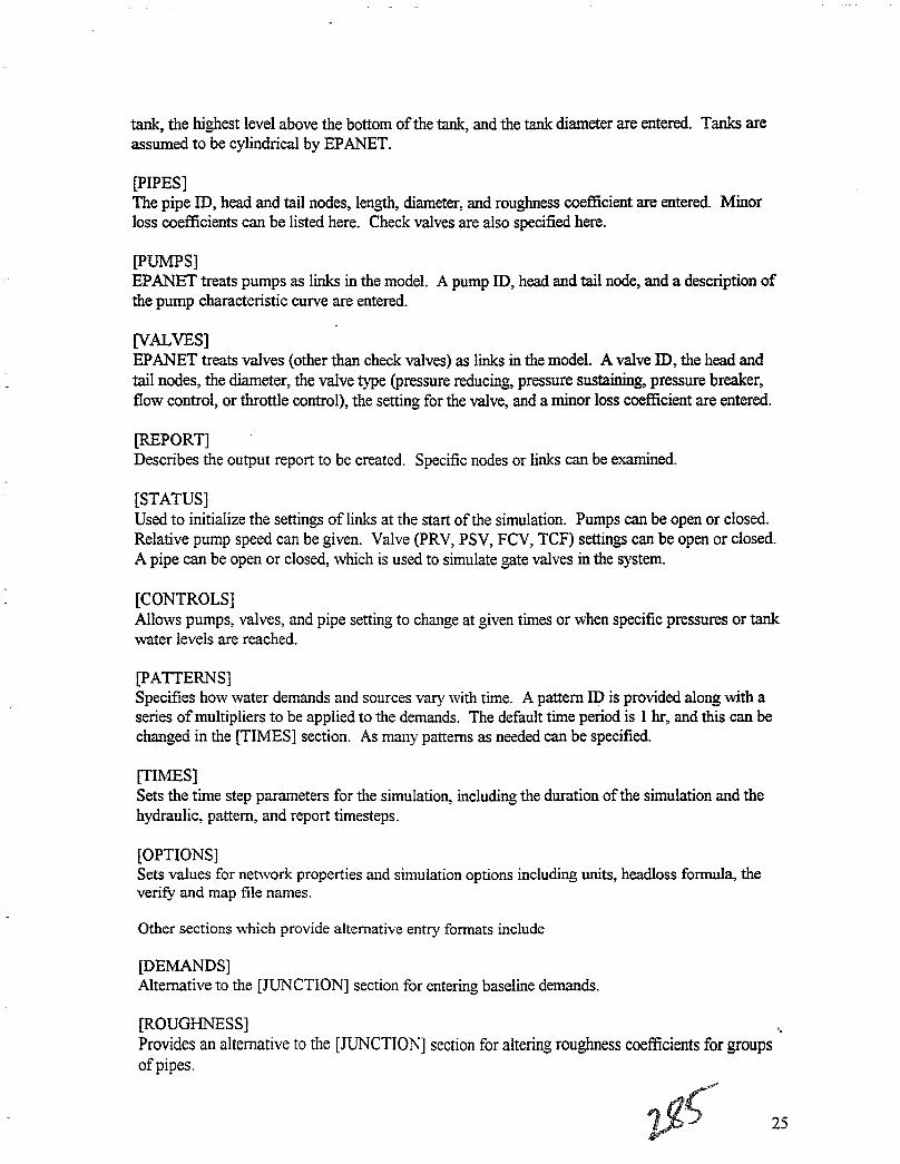
tank, the highest level above the bottom ofthe tank, and the tank diameter are entered. Tanks areassumed to be cylindrical by EPANET.
[PIPES]The pipe ID, head and tail nodes, length, diameter, and roughness coefficient are entered. Minorloss coefficients can be listed here. Check valves are also specified here.
[PUMPS]EPANET treats pumps as links in the model. A pump In, head and tail node, and a description ofthe pump characteristic curve are entered.
[VALVES]EPANET treats valves (other than check valves) as links in the model. A valve ill, the head andtail nodes, the diameter, the valve type (pressure reducing, pressure sustaining, pressure breaker,flow control, or throttle control), the setting for the valve, and a minor loss coefficient are entered.
[REPORT]Describes the output report to be created. Specific nodes or links can be examined.
[STATUS]Used to initialize the settings oflinks at the start of the simulation. Pumps can be open or closed.Relative pump speed can be given. Valve (PRV, PSV, FCV, TCF) settings can be open or closed.A pipe can be open or closed, which is used to simulate gate valves in the system.
[CONTROLS]Allows pumps, valves, and pipe setting to change at given times or when specific pressures or tankwater levels are reached.
[PATTERNS]Specifies how water demands and sources vary with time. A pattern ID is provided along with aseries of multipliers to be applied to the demands. The default time period is I hr, and this can bechanged in the (TIMES] section. As many patterns as needed can be specified.
[TIMES]Sets the time step parameters for the simulation, including the duration ofthe simulation and thehydraulic, pattern, and report timesteps.
[OPTIONS]Sets values for network properties and simulation options including units, headloss formula, theverify and map file names.
Other sections which provide alternative entry formats include
[DEMANDS]Alternative to the [JUNCTION] section for entering baseline demands.
[ROUGHNESS] '.Provides an alternative to the [JUNCTION] section for altering roughness coefficients for groupsof pipes.
25

3. Analyzing EPANET ResultsAs a Windows program, EPANET presents results in a number ofdifferent Windows. TheBrowser window allows for the simulation time, node, and link to be selected. Node informationincludes demand, elevation, hydraulic grade, pressure, and water quality. Link informationincludes diameter, flow, velocity, headloss/length, and average water quality. Ifa map is visible,the variable will be color coded on the map and the specific node or link will be highlighted.
The Report menu can generate spreadsheet-like tables for the current time ofall nodes or links or atime series for the current node or link.
The graph menu can generate a time series plot of the current node or link.
G. Model Output AnalysisThe model output can be used to test for system deficiencies. Deficiencies an a water distributionsystem are generally indicated by inadequate pressure. The model is useful in evaluating the causesand analyzing corrective actions.
Check that major trunk mains are able to meet the necessary storage replenishment rate. Ifany ofthe following conditions occur in a pipe segment, they are generally considered deficient and shouldbe corrected:
1) velocities greater than 1.5 m/s (up to 3 m/s may be acceptable, but high headloss canresult and the potential for water hammer is greater)
2) headlosses greater than 10m /1000 m3) large diameter pipes (16 inch or greater) with headlosses greater than 3 m /1000 m
The general solution to each of these deficiencies is to increase pipe diameters. These conditionsshould be treated as general guidelines, not as firm rules.
Pumps should be checked that they deliver adequate flows over full range ofsystem demands.,including average day demands. Conservative practice in multiple pump facilities is to providemaximum day flows with the largest pump out of service.
VI. Maps and Drawings
water sourcescaleorientation arrowdate last correctedpressure zone limits (may change)closed valves at pressure zone limits
A. Comprehensive map (or wall map)Map of entire distribution system used by system manager. Generally does not display all details.Typically includes:street nameswater mainssizes of mainsfire hydrantsvalvesreservoirs and tankspump stations
--.
26

Typical scales ranging between 500 and 1000 ft to an inch.Update once or twice a year or after major system extension.
B. Sectional maps or platProvides detailed picture ofsection of distribution system. Used for day-to-day operatiOl. Severalmaps are required to cover the entire system. Typically includessection designation or number water account numbersadjacent section number measurements to service linesstreet names distances main to curb boxmains and sizes distances to angle pointsmaterials ofmains distances to fittingsdate ofmain installation dead ends and measurementsdistance from property line date last correctedfire hydrants and numbers orientation or north arrowvalves and numbers scalevalve sheet designation shown in margin closed valves at pressure zone limitsintersection number service limitsblock numbers tanks and reservoirslot numbers pump stationshouse numbers pressure zone limits
Typical scales are 50 to 100 ft to an inch.
Sectional maps should not overlap but should butt up against each other to avoid confusion. Eachshould be indexed, with the comprehensive map used as a base. Sectional maps must be updatedmore frequently than comprehensive maps, typically monthly or quarterly.
C. Valves and hydrant mapsPinpoint valves and hydrants throughout the distribution system. Provide measurements frompermanent reference points to each valve in system. Should include direction to open, number ofturns to open, model, type, date installed. last date tested or repaired. May either be similar to asectional map with a corresponding table, or an intersection map at a very large scale (20 to 30 ftto an inch)
D. Plan and profile drawingsShow pipe depth, pipe location (both horizontal and vertical displacement), and the correct distancefrom a starting reference point.
E. Supplemental mapsSome large systems keep an arterial map at a 2000-4000 ft to an inch scale oflarge mains (>= 8inches) for use in system analysis. Pressure zone maps or leak frequency maps can also be useful
F. Card recordsMost systems maintain card or database records for pipes, valves, hydrants.
• 27

VII. Design Standards (by Donald Lauria, University of NorthCarolina)
A. Introduction
Most developing countries have several different agencies engaged in the planning and design ofcommunity water and sanitation systems. It is common for each agency to have its own set ofdesign standards. Frequently, the standards are based on noons of industrialized countries andthus result in systems that are very expensive. When this occurs, problems usually results.
If the beneficiaries ofwater and sanitation systems cannot afford them because they are tooexpensive, then there may be inadequate funds for operation, maintenance, repairs, and expansion.The systems may fall into disrepair, resulting in deterioration ofservice over time. Neededexpansions may not take place. The inevitable result is excessive community dependence ongovernment for subsidies and assistance, which frequently are unavailable.
To avoid this unfortunate condition, it is desirable that each community be responsible for payingthe costs of its own system. This means tailoring the level ofwater and sanitation service to eachcommunity's ability to pay. This in tum may require a separate set of design standards for eachsystem instead of a single set of identical standards for all systems. Almost without exception,standards based on less extravagant levels of service are needed to achieve the goal offinancial selfsufficiency than those currently in use.
It is usually difficult to develop an appropriate set of design standards for each community. Suchstandards need to be adopted on the basis of trial and error, with the planner/designer investigatingsuccessively lower standards until a satisfactory and affordable design emerges. This is a timeconsuming process that few planning agencies are willing to undertake.
B. Levels ofService
In selecting an appropriate level of service and corresponding set of design standards for water andsanitation systems, the main goal is financial selfsufficiency for the community so that it will notbe excessively dependent on others and can therefore control its own destiny. This means that thecosts associated with paying for and running the system must not exceed the community's ability topay.
A second important principle in selecting the level of service is that the community itself should bethe major decision maker. Service and design standards that are imposed on a community withoutconsulting its members are frequently doomed to failure. This means holding public meetings toinform the community of alternatives, their associated costs, and to determine the willingness ofthecommunity to pay them.
In selecting a level of water supply service, it is almost always necessary to provide a level higherthan the one that already exists; furthermore, the level need not be very much higher than theexisting one. For example, consider a community in which most houses have their own wellswhich have become polluted, necessitating the construction ofa new system. If the selected servic~
level for the new system consists of public taps, they may not be used because people may preferthe convenience of their wells, even though they are polluted. Public taps might also be
28

inappropriate for a conununity where vendors are delivering water to each house because they areless convenient than the existing service level. On the other hand, public taps probably areappropriate for places where people are presently having to walk long distances to fetch water. Insuch communities, individual house connections probably provide a level ofservice that is too highbecause they far exceed the users' expectations.
The level of service for sanitation must be consistent with that for water supply. Clearly, it wouldbe inappropriate to provide a piped sewer system in a community where water supply is by publictaps. Correspondingly, pit privies and latrines may be inappropriate for houses with individualconnections and multiple taps.
Four of the major types ofwater supply service for piped systems in ascending order of servicelevel are 1) public taps, 2) yard/patio connections, 3) single house taps (sanitary core), andmultiple taps (conventional). Each type provides greater convenience than the previous level. Thesanitation levels associated with these are 1) pit privies/latrines, 2) pour-flush latrines, 3) septictanks or latrines with drainfields or soakaways, and 4) piped sewerage. A fifth level ofwatersupply would provide fire protection.
With each level of service, the cost per capita increases by a factor between 1.5 and 2.0. Forexample, conservatively estimated, the cost per capita for public tap system is in the order ofUS$15; a yard tap system costs about US$ 30; a single-house tap system costs about US$ 45; andconventional water supply costs about US$ 75. Hence, a conventional system is about six timesmore expensive than a public tap system. Roughly the same applies to sanitation. Note that themajor jump in convenience benefits results in providing water on the premises (yard tap) instead ofat a public tap in the street. A sanitary core provides greater convenience than a yard tap, andmultiple taps provide greater convenience than a sanitary core, but the marginal increases in thcseconvenience benefits are not nearly as great as those associated with using yard taps instead ofpublic taps.
In selecting the level of service, consideration needs to be given to upgrading over time. Initially,public taps might be provided which, in a period of, say, 5 years, can be upgraded to yard taps orconnections.
In developing countries, it is unusual to provide the same level of service for an entire community.More conunonly, part of a community may receive house connections while the rest is served withpublic taps. Sometimes, population or housing density is used as a guide for proposing the mix ofconnections and public taps. The standards proposed by COPECAS in Guatemala, which seemreasonable, are as follows:
Connections% Lcd*
100
100 40 100
CommunityLevel Population
I Dispersed
II 100-500
III 500-2,000
IV 2,000-10,000
50
60
100
150
Standposts% Lcd
50 40
40 50
Latrines%
50
40
29

V 10,000-50,000 70 200 30 50 30
VI >50,000 85 225 15 50 15
* liters per capita per day
C Design Periods
A design period is the future period for which a system is intended to have excess capacity. Ifadesign period of, say, 10 years· is selected for a water treatment plant, this means that the engineerwants the plant to be able to meet demands for 10 years beyond the time when it is constructed. Ofcourse, the plant may be able to meet demands for longer (or shorter) than 10 years if the actualrate at which demand grows is different than the rate anticipated by the designer. Plant capacitydepends, then, on nvo factors, the selected design period and the anticipated growth in demand.NonnaIly, different design periods are used for the major components ofwater and sanitationsystems.
In projecting or estimating future demands, it is common to assume linear or geometric rates ofgrowth. A rate of, say, 2% per year is an example ofgeometric growth, and a rate of, say, 20persons per year (or 20 persons per year per 1000 initial population) is an example of lineargrowth. A growth rate of 2% per year for water demand is higher than that found in mostindustrialized countries; it is not unusual for developing countries. Doubling time is roughly equalto 70 divided by the growth rate in percent. Hence, a community whose population is growing at2% per year would be expected to double its population every 35 years; a 3% rate implies doublingevery 23 years. A linear growth rate of, say, 20 persons per year per 1000 initial population isequivalent to 2 persons per year per 100 or about 2% per year. Hence, a growth of40 persons peryear per 1000 is about 4%, which is very high.
Probably the main reason for selecting a design period and providing excess capacity in facilitiesdepends on the concept of economies of scale. Other reasons include the concept ofuseful life andrapidly increasing costs due to inflation. Economies of scale exist if average costs decrease asscale increases. Most consumer products and most components ofwaterIsanitation systems haveeconomies of scale. Consider a commodity that costs 100 for a quantity of 10; the average cost is100/10 = 10. Assume this same commodity costs 160 for a quantity of 20; the average cost is 8.Hence, average cost decreased as scale increased. Therefore, economies of scale exist and it isprobably economical to buy the giant economy size; that is, to buy more than one presently needsin order to capture the economies of scale.
In all cases where there is a set-up cost, economies of scale exist, and it is preferable to provideexcess capacity. For example, moving equipment onto a construction site incurs a set-up costbefore any work is done; similarly, traveling to a store to make a purchase incurs a cost before anypurchase is made. In these cases, it is best to capture economies of scale by purchasing more thanis immediately needed. It is seldom optimal to select a design period ofzero; that is, to meet onlypresent demands. This can usually be justified for only nvo reasons: (1) it will be a long time, ifever, before the excess quantity is ever used, or (2) sufficient funds are not available to enablepurchasing ahead of demand. '.
30

The larger the portion oftota! cost represented by the set-up cost, in general, the longer should bethe design period. Projects with large set-up costs usually have large economies ofscale.
The economy ofscale factor (b) measures the magnitude ofeconomies ofscale and hence can beused to select an optimal design period. This factor denotes the percentage increase in cost per onepercent increase in scale or capacity. Consider the example in para. 3.3: cost increased by 60%(from 100 to 160), the scale increased by 100% (from 10 to 20). Hence, the economy ofscalefactor is 601100 =0.6. A small, economy of scale factor, say 0.3, implies only a 30% increase incost if scale or capacity doubles. It follows that small economy of scale factors denote largeeconomies of scale for which the design period should be relatively long. For b = 1.0, costincreases 100% for a 100% increase in scale. In this case, there are no economies of scale and thedesign period, ifgreater than zero, should be based on other considerations.
A value ofb can be estimated for different water and sanitation components by fitting the costmodel C =aXb to cost (C) and capacity (X) data for each component. Ordinary least squares canbe used to estimate b by regressing log C against log X.
Treatment plants, pumping stations and water supply facilities often have a value ofb ofabout0.7; pipelines and networks usually have a value ofb of about 0.5; and storage tanks have b ofabout 0.6. These values can differ substantially from one country to another or from one region toanother within the same country.
A large technical literature exists on the use ofb for determining the optimal design period x* (seefor example Lauria et aI., Jour. ofEnvironmental Engineering Division, April 1977). Equationsin this literature must be used with caution; they are only guides to judgement, and they do notcover all situations.
All the equations for determining optimal design periods that are in the literature cannot berepeated here. However, a few guidelines may be helpful. If a system has an initial deficit incapacity instead of demand and capacity being exactly in balance, s* should be larger than what isobtained by using the equation above. For example, the design period for a new system in acommunity with no existing facilities or with facilities that are meeting only a small fraction of theexisting demand should probably be 50% larger than the value obtained from the above equation.
It is seldom possible to make an infinite number of expansions ofthe same facility, which makes itinappropriate to use equations like the one above. If a facility is not likely to be expanded anymore than 2 or 3 times, then a special economical analysis would have to be made to determine theoptimal design period.
After taking account of all the things that make use of the above equation for x* invalid (such aslimitations on the number of expansions, initial deficits, budget constraints, and restriction onfuture opportunities to plan and construct facilities), it may be roughly correct to use a designperiod ofbetween 5 and 10 years for components \,rith equipment (treatment plants, pumpingstations and tanks), and not more than 20 years for pipes and networks. In any event, ability topay may be the determining factor of the amount of excess capacity the community can afford toinclude in its facilities.
31

D. Design Flows
Design flows are usually obtained by multiplying the expected population at the end ofthe designperiod by an assumed per capita flow. Normally, a peaking factor is used to convert the averagedesign flow to a ma."'rimum daily or maximum hourly value, depending on the component to bedesigned. To the domestic flows must be added quantities for commercial, industrial and publicuse plus an allowance for unaccounted losses.
Average per capita design flows depend on several factors, level ofservice perhaps being mostimportant. For public standposts, an average flow ofbetween 25 and 50 led is usually assumed.While 25 led is an adequate quantity ofwater per person, this value could be unrealistically low fordesign purposes. For example, ifeach standpost were designed for, say, 100 persons with a peakhourly factor of, say, 1.5, then the peak hourly design flow per standpost would be only 2.6 l/min,which is too low. At this rate, it would take 6 minutes to fill a bucket. Furthermore, ifthepressure at the tap were 5 m or more, a typical faucet would probably deliver at least 4 or 5 timesthis flow. Hence, the selected design flow for public taps should take account ofthe number ofpersons per tap. With 200 persons per tap, an average flow of25 led is probably satisfactory, butwith fewer than 200, a higher average flow is more realistic.
Typical average per capita design flows for yard taps, single house taps and multiple house tapsare in the order of50, 100 and 200 lcd, respectively. Hence, at each successively higher level ofservice, the average flow doubles. These flows are probably minimum values. Some standardsrecommend flows based on population density. The EMPAGUA standards for Guatemala City,for example, recommend an average value of 100 led for places with density of600 persons per ha,increasing to 350 led for low densities of 100 personslha.
In small communities, commercial and other water demands are frequently ignored, which isprobably acceptable. However, larger towns with commercial establishments need to take accountofthese flows. In all cases, a reasonable value for unaccounted losses in newly constructedsystems is between 20 and 25%.
Some design standards recommend fire flows, even for small towns, which is unreasonable. It isnot uncommon to find recommendations for 2 or even 3 fire flows simultaneously, and one set ofstandards in Peru recommends that fire protection should be provided at any point in the network,which is uncalled for.
To design for fire flows in places that do not have fire fighting equipment is unreasonable. It is arate small to\\'n that has equipment for even one fire flow much less 2 or 3. Furthermore, to evenconsider fire flows unless the network is to be designed using a computer program is absurd. Sincethe location of the fire flow is uncertain, the flow must be moved to different locations in designingthe network. This essentially requires use of a computer. Also, to provide fire protection at alllocations would result in all pipes of the network being oversized to handle such flows. Fewcommunities can afford such a luxury; rather, fire protection is usually restricted to high-valuedistricts of the community. TIle COPECAS standards for Guatemala recommend no fireprotection for places smaller than 20,000 persons; where protection is provided, the design flow is5 Ips. These values seem reasonable.
...
32
Peaking factors playa critical role in design since most hydraulic facilities must be' sized to handlepeak flows. Typical peaking factors for maximum daily flows are between 1.2 and 1.5 (maxday/average), and peak hour factors are usually between 2.0 and 3.0 (max hour/average).Unfortunately, few studies have been conducted to actually measure peaking factors, in part due tothe lack ofmetering equipment. It is important to recognize that peaking factors are higher insmall communities than in larger ones.
In water systems, source works, transmission mains to conduct water to the community, andtreatment plants are usually designed for maximum daily values because such demands may persistfor extended periods oftime. Networks and pumping stations are usually designed for peak hourlyflows because these facilities must have sufficient capacity to meet instantaneous demands.Storage tank volumes are usually based on average flows. In wastewater systems, pipelines,networks and pumping stations are usually designed to handle peak hourly flows, and treatmentplants are sized for average values.
E. Pipelines, Networks and Tanks
The sizes ofpipelines that deliver flows by gravity depend on the available hydraulic gradient andthe design flow. This applies to both open channel and pressure systems. The sizes ofpipelinesthat delivery pumped flows usually depend on a design velocity which is assumed to be economicalor optimal; a value of about 1.5 mls is typical.
Some standards require the designed to make a cost analysis to determine optimal design velocity.In most cases, this is unnecessary. The optimal design velocity depends on the relative prices ofpower and pipeline construction. If power is relatively expensive compared to construction costs,it may be optimal to enlarge the pipe; that is, to design for a velocity lower than 1.5 mls.Conversely, if power is relatively cheap compared to pipe construction, a velocity higher than 1.5mls may be optimal. In most countries, however, ifpower is expensive, so too is pipe, in whichcase a design velocity ofabout 1.5 mls should be acceptable.
For network design, use of the computer is strongly recommended. Networks, whether for water orsewage, are very expensive, and the computer enables the designer to select sizes that minimizecost. Also, networks are complicated and hard to design; the computer ensures that they willfunction as intended.
In most net\''Vorks, pipe length is the principal determinant ofcost; it is usually more critical thandiameter. This is because there are large economies of scale with respect to diameter but none withrespect to length. For this reason, great care is needed in making network layouts so as to keeppipe length as short as possible.
Branched networks are usually less expensive than ones with loops. However, they are lessreliable; a break in one pipe will interrupt service to all downstream users. Branched networksmay be nearly as expensive as looped ones in linear communities where houses are stretched outalong a main road. Branched networks are particularly appropriate for use with public tapsystems; for communities with individual house connections or public taps that serve at most onlya few houses, it is generally necessary to place pipes on all the streets where houses are located,resulting in a looped system. ".
33

Branched networks are much easier to design than ones with loops. Computer programs that useoptimization techniques such as those distributed by the World Bank make branched networkdesign relatively simple and ensure minimum cost. Looped networks must be designed by trial anderror to seek a least cost solution, which essentially requires use ofa computer program like thoseavailable from the World Bank.
Ifthe level of service is to be upgraded over time from, say, public taps to house connections, itmay be preferable to design the initial branched network for the taps with sufficient capacity sothat it can serve as the primary network in the looped system when it is finally upgraded to houseconnections.
Most standards recommend minimum diameters for water networks; 100 rom for primary networksand 50 rom for secondary are typical values. While such guidelines can be useful, they should beflexible. A community in very hilly terrain, for example, might benefit by using smaller minimumsizes to avoid extremely high pressures at points oflow elevation.
Minimum pressure standards for water networks are usually in the range of5 m to 15 m. Ifacomputer is used for design, its ability to accurately simulate the pressures in a network underdifferent flow conditions enables selection of lower minimum pressures may be needed as an addedfactor of safety to account for inaccuracies in design. Seldom is it necessary or desirable to specifyminimum pipeline velocities in a network.
Occasionally, design standards recommend the use of individual house tanks for storage rather thana central tank for the system on the assumption that this will enable the network to be designed formaximum daily instead of peak hourly flows. Unless each house tank is fitted with a flowrestrictor on its inlet, the network may still need to be designed for peak hourly flows. In anyevent, individual tanks are usuallymore expensive, less reliable, and more risky to health than acentral tank for the system.
In Latin America, it is common to provide a separate line from the source works to the storage tankand to operate the tank on a fill and draw basis. Such systems are relatively easy to operate anddesign since they have only a single source ofwater input to the network. However, they can bemuch more expensive than systems which use floating storage tanks where the network itself isused to transmit water from the source to the tank, thus eliminating a separate transmission line.However, the network must have sufficient capacity to fill the tank; this usually requires sizing atleast some network pipes under minimum demand conditions (nighttime) while the rest ofthe pipesmust be sized for peak demands. Also, during periods ofpeak demand, the network has two pointsofwater input, one from the tank and the other from the source of supply. The increaseddifficulties in the design and operation of floating tank systems are usually more than offset bysavings in cost.
Some standards recommend different storage tank volumes depending on whether floating or filland-draw systems are used. There is little rationale for such differences. The required volume ofstorage tanks cannot be precisely determined without accurate information on demand variationsthroughout the day; tanks are needed, after all, to meet peak hourly demands. The commonstandard of making tank volume equal to 25% of average daily design flow is reasonable; morethan this in most cases would simply provide reserve in the event of pump failure at the source.
34

Recent developments in the design ofsmall-bore sewers may make this an attractive alternative toconventional sewage. Small diameters are possible because sewage solids are removed inindividual septic tanks at each house. The cost savings in smaller pipes must be weighed againstproviding individual septic tanks and, more importantly, in maintaining them so that sewers do notclog. The World Bank distributes computer programs to assist the design ofboth conventional andsmall-bore sewers.
-'.
35