N A.,.,A / CP--------2(}(}].----2].l l 4.1

The Te_ath Thermal and. FIu.id.s

Analysis Workshop

Co£?p,,es °

Marsl'_a/I Space Night Cente_ Ma_shafi Space F/igl}t Center, Alsbsms

N ASA MarsP_&tl}Space }£IiSPKCerK(o,l:T}:_:l:ma] arid Fklids

Group a_d heSd _:_:@c, Sc,v_11C_>_K_H",{.Is_b,/ersky ot'/k_aba_mt

Js_ {R_r_CsvJHe,Alabama.. September" 13.---.17,1999.

duJy 200 {

The NASA STI Program Office...in Profile

Since its founding, NASA has been dedicated tothe advancement of aeronautics and spacescience, rll_e NASA Scientific and Technical

Intbrmation (STI) Program Office plays a keypart in helping NASA maintain this importantrole.

The NASA STI Program Office is operated by

I.angley Research Center, the lead center forNASA's scientific and technical information. The

NASA STI Program Office provides access to the

NASA STI Database, the largest collection ofaeronautical m_d space science STI in the world. The

Program Office is also NASA's institu tional

mechanism for disseminating tt_e results of itsresearch and development activities. "Iltese results

are published by NASA in the NASA STI Report

Series, which includes the following report types:

TECHNICAL F'UBI.ICATION. Reports of

completed research or a major significant phaseof research that present the results of NASA

programs and include extensive data or

fl_eoretical analysis. Includes compilations ofsignificant scientific and technical data and

information deemed to be of continuing referencevalue. NASA's counterpart of peer-reviewed

formal professional papers but has less stringent

limitations on manuscript length and extent ofgraphic presentations.

TECHNICAl, MEMORAND[ IM. Scientific and

technical findings tidal are preliminary or of

specialized interest, e.g., quick release reports,

working papers, and bibliographies that containminimal annotation. Does not contain extensive

analysis.

CONTRACTOR REPORT. Scientific and

technical findings by NASA-sponsored

contractors and grantees.

CONFERENCE PUBLICA_IlON. Collected

papers from scientific and technical conferences,symposia, seminars, or other meetings sponsored

or cosponsored by NASA.

SPECIAL PI JBLICATION. Scientific, technical,

or historical information from NASA programs,projects, and mission, often concerned with

subjects having substantial public interest.

TECHNICAl, TRANSLATION.

English-language translations of foreign scientific

and technical material pertinent to NASA'smission.

Specialized services that complement the STIProgram Office's diverse offerings include creating

custom thesauri, building customized databases,

organizing and publishing research results...evenproviding videos.

For more fifformafion about the NASA STI ProgramOffice, see the following:

. Access tl_e NASA STI Program Home Page at

http://www.sti.nasa.gov

° E-mail your question via fl_e Internet to

help@ sti.nasa.gov

° Fax your question to the NASA Access ttelp

Desk at (301) 621----0134

° Telephone the NASA Access ttelp Desk at (301)621-0390

Write to:

NASA Access ftelp Desk

NAS A Center for AeroSpace Information7121 Standard Drive

Hanover, MD 21076---1320

(301)621-0390

NASA / CP--------.2001----211141

The Tenth Thermal and Fluids

Analysis WorkshopAlok Majumdar, Compiler

Marshafl Space Flight Center, Marshall Space Flight Center, Alabama

N ational Aeronautics and

Space Administration

Marshall Space F].ight Center * MSFC, Alabama 3581.2

July 2001

NASA Center for AeroSpace Information7121 Standard Drive

Hanover, MD 21076 1320(301) 621 0390

Available hom:

National rR:chnical Inff_rmation Sm_'ice

5285 Port Royal RoadSpringfield, VA 22161

(703) 487 4650

FOREWORD

This yearly workshop focuses on applications of thermal and fluids analysis in the

aerospace field. Its purpose is to bring industry, academia, and government together to

share information and exchange ideas about analysis tools and methods. Originating

from the Glenn Research Center, this was the first year the Thermal Fluids and Analysis

workshop was held at the Marshall Space Flight Center.

While each workshop contains short courses, hands-on classes, and product

overview lectures, only the technical papers and presentations are included in thisdocument.

The organizers of this year's workshop consider it a privilege to participate in

such an event. We would like to thank all the authors, presenters, and industry

representatives who contributed to this year's success.

James W. Owen Sheryl L. Kittredge

TABLE OF CONTENTS

THERMAL SPACECRAFT/PAYLOADS PAPER SESSION

Space Science Payloads Optical Properties Monitor (OPM) Mission Flight

Anomalies Thermal Analyses

Craig P. Schmitz, AZ Technology, Inc.

Shuttle and Transfer Orbit Thermal Analysis and Testing of the Chandra

X-Ray Observatory Charged-Coupled Device Imaging SpectrometerRadiator Shades

John R. Sharp, NASA MSFC

Thermal Analysis of a Finite Element Model in a Radiation DominatedEnvironment

Arthur T. Page, NASA MSFC

An Overview of the Thermal Challenges of Designing Microgravity Furnaces

Douglas G. Westra, NASA MSFC

Evaluation of the Use of Optical Fiber Thermometers for Thermal Controlof the Quench Module Insert

Matthew R. Jones, University of Arizona, Jeffrey T. Farmer, NASA MSFC,

and Shawn P. Breeding, TecMasters, Inc.

Characterization of the Heat Extraction Capability of a Compliant, Sliding,

Thermal Interface for Use in a High Temperature, Vacuum MicrogravityFurnace

Jenny Bellomy-Ezell, Sverdrup Tech., Inc., Jeff Farmer, NASA MSFC,

Shawn Breeding and Reggie Spivey, TecMasters, Inc.

On the Application of ADI Methods to Predict Conjugate Phase Changeand Diffusion Heat Transfer

Dean S. Schrage, Dynacs Engineering Company, Inc.

THERMAL PROPULSION/VEHICLES PAPER SESSION

Reusable Solid Rocket Motor Nozzle Joint-4 Thermal Analysis

J. Louie Clayton, NASA MSFC

Thermal/Pyrolysis Gas Flow Analysis of Carbon Phenolic Material

J. Louie Clayton

LOX System Prestart Conditioning on X-34Brian K. Goode, NASA MSFC

STS-93SSMENozzleTubeRupture InvestigationW.DennisRomine,RocketdynePropulsionandPower,BoeingCorporation

Zero Gravity Cryogenic Vent System Concepts for Upper Stages

Robin H. Flachbart, James B. Holt, and Leon J. Hastings, NASA MSFC

Thermal Analysis of the Fastrac Chamber/Nozzle

Darrell Davis, NASA MSFC

INTERDISCIPLINARY PAPER SESSION

Method Improvements in Thermal Analysis of Mach 10 Leading Edges

Ruth M. Amundsen, NASA LaRC

A Steady State and Quasi-Steady Interface Between the Generalized Fluid

System Simulation Program and the SINDA/G Thermal Analysis Program

Paul Schallhorn, Alok Majumdar, Sverdrup Tech., Inc., and Bruce Tiller,NASA MSFC

A Collaborative Analysis Tool for Thermal Protection Systems for Single

Stage to Orbit Launch Vehicles

Reginald Alexander, NASA MSFC, Thomas Troy Stanley, International

Space Systems, Inc.

Computation of Coupled Thermal-Fluid Problems in Distributed MemoryEnvironment

H. Wei, H. M. Shang, and Y. S. Chela, Engineering Sciences, Inc.

Multi-Disciplinary Computing at CFDRC

W. J. Coirier, A. J. Przekwas, and V. J. Harrand, CFD Research Corporation

FLUIDS PAPER SESSION

Fluids 1a (Group Overviews)

Overview of Fluid Dynamic Activities at MSFC

Roberto Garcia, Lisa Griffin, and Ten-See Wang, NASA MSFC

Aerothermodynamics at NASA - Langley Research Center

K. James Weilmuenster, NASA LaRC

Fluidslb (VehiclesandRBCC)

Computational Aerodynamic Design and Analysis of a Commercial ReusableLaunch Vehicle

M. R. Mendenhall, H. S. Y. Chou, and J. F. Love, Nielsen EngineeringResearch

A Parallel Cartesian Approach for External Aerodynamics of Vehicles

With Complex Geometries

M. J. Aftosmis, NASA Ames Research Center, M. J. Berger,

and G. Adomavicis, Courant Institute

Parallelization of the Flow Field Dependent Variation Scheme for Solving

the Triple Shock/Boundary Layer Interaction Problem

Richard Gregory Schunk, NASA MSFC, T. J. Chung, Universityof Alabama in Hunstville

Integration of RBCC Flowpath Analysis Tools

D. G. Messitt, Gencorp Aerojet

Ongoing Analyses of Rocket Based Combined Cycle Engines by the Applied

Fluid Dynamics Analysis Group at Marshall Space Flight Center

Joseph H. Rut', James B. Holt, and Francisco Canabal, NASA MSFC

Fluids 2a (Combustion)

Overview of the NCC

Nan-Suey Liu, NASA Glenn Research Center

An Unstructured CFD Model for Base Heating Analysis

Y. S. Chen, H. M. Shang, and Jiwen Liu, Engineering Sciences, Inc.

Optimization of a GO2/GH2 Impinging Injector Element

P. Kevin Tucker, NASA MSFC, and Wei Shyy and Rajkumar

Vaidyanathan, University of Florida, Gainesville

Raman Spectroscopy for Instantaneous Multipoint, Multispecies Gas

Concentration and Temperature Measurements in Rocket Engine Propellant

Injector Flows

Joseph A. Wehrmeyer, Vanderbilt University, and Huu Phuoc Trinh,NASA MSFC

Fluids2b(Acoustics)

FastracGas Generator Testing

Tomas E. Nesman and Jay Dennis, NASA MSFC

Computational Aeroacoustic Analysis System Development

A. Hadid, W. Lin, E. Ascoli, S. Barson, and M. Sindir, Boeing/Rocketdyne

An Overview of Computational Aeroacoustic Modeling at NASA Langley

David P. Lockard, NASA Langley Research Center

Fluids 2c (Fluid Network and Thermal Environments Modeling)

Numerical Modeling of a Helium Pressurization System of Propulsion Test

Article (PTA1)

Todd Steadman, Alok Majumdar, Sverdrup Technologies, Inc.,

Kimberly Holt, NASA MSFC

Analytical Assessment of a Gross Leakage Event Within the International

Space Station (ISS) Node 2 Internal Active Thermal Control System (IATCS)

James M. Holt, NASA MSFC and Stephen E. Clanton, Sverdup

Technology, Inc.

Fluids 3 (Turbomachinery)

Time-Accurate Solutions of Incompressible Navier-Stokes Equations

for Potential Turbopump Applications

Cetin Kiris, MCAT Institute and Dochan Kwak, NASA AmesResearch Center

Unshrouded Centrifugal Turbopump Impeller Design Methodology

George H. Prueger, Morgan Williams, Wei-chung Chen, John Paris,

Boeing/Rocketdyne, and Robert Williams and, Eric Stewart, NASA MSFC

Water Flow Performance of a Superscale Model of the Fastrac Liquid

Oxygen Pump

Stephen Skelly, Thomas Zoladz, NASA MSFC

The Performance of Annular Diffusers Subject to Inlet Flow Field Variationsand Exit Distortion

David Japikse, Concepts ETI

Rotor Design for the SSME Fuel Flowmeter

Bogdan Marcu, Boeing/Rocketdyne

MaximizingMultistageAxial GasTurbine EfficiencyOver a Rangeof Operating Conditions***

George S. Dulikravick, University of Texas at Arlington, Milan V. Petrovic,

University of Belgrade, and Brian H. Dennis, Pennsylvania State University

The Off-Design Performance of a Carefully Instrumented Radial InflowTurbine

David Japikse, Concepts ETI

Overview of Turbine Aerodynamic Analysis and Testing at MSFC***

Lisa W. Griffin, Susan T. Hudson, and Thomas F. Zoladz, NASA MSFC

3D Unsteady CFD Analysis of a Supersonic Turbine***

Daniel Dorney, Virginia Commonwealth University

INVITED FLUID LECTURE SESSION

Turbine Aerodynamic Design: An Overview of the Evolution of the Processand the Impact Computational Capability has Made on the End Item***

Frank W. Huber, Independent Consultant

Modeling Approximations for Multistage Flows in Turbomachinery***

Daniel J. Dorney, Virginia Commonwealth University and Douglas Sondak,

Boston University

Liquid Rocket Injector Effects on Combustion Chamber Heat Flux***

Steven C. Fisher, Boeing/Rocketdyne Propulsion and Power

To Make It Fast - Make It Local***

Lynn Lewis, Silicon Graphics Incoporated, Global Professional Services

Marked papers were not available in electronic form. Please contact authors for a

copy.

SPACE SCIENCE PAYLOADS

OPTICAL PROPERTIES MONITOR (OPM)

MISSION FLIGHT ANOMALIES THERMAL ANALYSES

Craig P. Schmitz

AZ Technology, Inc.

Huntsville, Alabama

ABSTRACT

The OPM was the first space payload that measured in-situ the optical properties of materials and had data

telemetered to ground. The OPM was EVA mounted to the Mir Docking Module for an eight-month stay where

flight samples were exposed to the Mir induced and natural environments. The OPM was comprised of three optical

instruments; a total hemispherical spectral reflectometer, a vacuum ultraviolet spectrometer, and a total integrated

scatterometer. There were also three environmental monitors; an atomic oxygen monitor, solar and infrared

radiometers, and two temperature-controlled quartz crystal microbalances (to monitor contamination).

Measurements were performed weekly and data telemetered to ground through the Mir data system. This paper will

describe the OPM thermal control design and how the thermal math models were used to analyze anomalies which

occurred during the space flight mission.

BACKGROUND

In 1986, the National Aeronautics and Space Administration (NASA) Office of Aeronautics and Space

Technology (OAST) released an Announcement of Opportunity (AO) under the In-Space Technologies Experiment

Program (IN-STEP). This AO was issued to seek new experiments for space flight that were under development by

contractors or new experiments that were unable to be developed because of cost constraints. In response to this

AO, the OPM experiment was proposed as an in-space materials laboratory to measure in-situ the effects of the space

environment on thermal control materials, optical materials, and other materials of interest to the aerospace

community. The OPM was selected and funded.. The Marshall Space Flight Center (MSFC) in Huntsville, Alabama

managed the proj ect.

The OPM was launched on STS-81 on January 12, 1997. Mounted in a SpaceHab Double Rack, the OPM

was Intravehicular Activity (IVA) transferred into the Mir Space Station on January 16, 1997. It was stowed for two

and one-half months before deployment and powered up on the Mir Docking Module by the first joint Russian-

American Extravehicular Activity (EVA) on April 29, 1997. On June 25, 1997, the OPM lost power because of the

Progress collision into Mir's Spektr module and did not regain operational status until September 12, 1997. The

OPM continued operation until January 2, 1998 when the OPM was powered down in preparation of the

January 8, 1998 EVA to retrieve the OPM. After a successful Russian EVA retrieval, the OPM was later transferred

IVA into the Shuttle (STS-89) and returned to Kennedy Space Center (KSC) on January 31, 1998.

A detailed description of the OPM Experiment including an overview of the system design and mission

performance is provided in the "Optical Properties Monitor (OPM) System Report" [1]. Figure 1 is a photograph of

the deployed OPM. The OPM is seen near the 2 o'clock position on the Docking Module. Figure 2 illustrates the

OPM mounting orientation on the Mir Space Station. The baseline layout of the internal hardware is illustrated in

Figure 3. This layout shows the locations of the electronics boxes, experiment subsystems, and sample carousel.

Figure 1: OPM on MIR (Docking Module End View).

Figure 2: OPM Mounting Orientation on the Mir.

TIS

SUBSYSTEM

(2)

EVA HANDRAIL (2)

828.7 mm _ CAROUSEL DRIVE

_ 32.63 in.

POWER/DATA INTERFACE BASEPLATE

Figure 3: Layout of the Internal Hardware of the OPM.

OPM THERMAL CONTROL

The OPM experiment was modeled using SINDA'85/FLUINT [21 and TRASYS TM to calculate the

conduction and radiation heat transfer between the internal OPM components as well as its external environment. Toassist in the accuracy of the model predictions, the OPM was added to the integrated Mir/Docking Module thermalmodels obtained from NASA/JSC [4'5]. The results of the predicted thermal values dictated how the OPM thermal

design was achieved for hot, cold, and nominal operating conditions. Further, the OPM timeline was analyzed tominimize peak input power requirements (kilowatts [kW], not kilowatt-hour [kWh]) and assess the internaltemperature fluctuations to the OPM. These predicted thermal extremes were not to exceed the component minimum

and maximum operating temperatures. Indeed, the OPM timeline was changed to modify the proposed measurementsequence which decreased the component temperature extremes and peak power (kW). However, the measurementssequence duration increased, increasing the total kWh.

Based on model predictions and the modified weekly timeline, the OPM was designed for passive thermal

control with active heaters to maintain a minimum temperature of 0°C. The heaters maintained thermal controlduring the quiescent periods of operation when the OPM was operating in monitor mode (i.e. not performingmeasurements). During the measurement sequence, the heaters were switched off and the external thermal control

coatings coupled with the thermal capacitance of the OPM provided sufficient thermal control. The OPM heatersystem design, located on the emissivity plate, consisted of two heater circuits with two 15-watt heater elementsmounted in parallel in each circuit. Heater control was effected by using thermistors on this plate to thermostatically

control their operation. Heater setpoints were selected approximately at 4°C (on) and 7°C (off). Thermal controlwas evaluated for materials exposed directly to the space environment as well as those not exposed. For exposed

surfaces, the temperature control was achieved by the combination of various types of thermal control coatings, somehaving low solar absorptance or high solar reflectance coupled with either low thermal emittance (AZT customcoating) or high thermal emittance (white coating) in order to control absorption of direct solar irradiance andreflected solar irradiance from Mir and/or the earth (albedo). Low thermal emittance coatings were used to minimize

radiation from selected OPM panels while high thermal emittance coatings were used on other panels to maximizethe thermal radiation. The unexposed surfaces were covered with MLI to minimize heat transfer. The combinationof materials provided the necessary thermal control to match the measurement sequence and overall timeline with the

expected Mir environment.

The _Thermal Data Book for the OPM Experiment" _61documents the details of the OPM thermal control

system design including the TRASYS geometric math models, the S1NDA thermal math models, the design analyses,

and the thermal vacuum test program which was used to verify the math models. The _Mission Thermal Data Book

for the OPM" [7]documents the OPM thermal flight data including the use of the thermal math models to evaluate the

flight anomalies. A typical thermal profile, predicted by the models for the measurement sequence and compared to

flight data, is shown in Figure 4.

I I I I

...... _1_1_ Math Modal Node 4502 - Refleet_let_ •

2 4 6 8 10

Thne lu's

Figure 4: OPM Reflectometer Thermal Profile for the Measurement Sequence

INSTRUMENTATION

The OPM thermal instrumentation consisted of 31 thermistors. Each of the 31 thermistors is either epoxied

directly to the OPM structure or epoxied into an aluminum-mounting block mechanically attached to the OPM

structure. Table 1 provides a description of the 31-thermistor mounting locations.

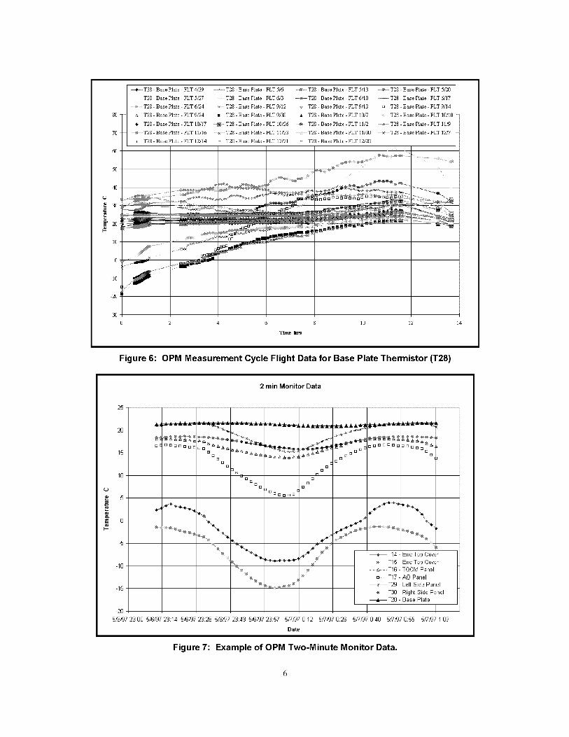
Temperature data was recorded for each of the 31 thermistors throughout each of the 27 OPM measurement

sequences/timelines. The nominal OPM measurement cycle timeline is shown in Figure 5. Figure 6 shows the

combined set of 27 measurement cycle temperature profiles for Thermistor T28 located on the OPM Base Plate.

Temperature data was recorded for each of the 31 Thermistors throughout the mission while in the

monitoring mode. Temperature monitor data was recorded using two different time intervals. For one two-hour

period each day the monitor data was recorded using two-minute intervals. Figure 7 is an example of the two-minute

monitor data for May 6-7 1997. This data provides information on the temperature variations that occur during a

single 90-minute orbit. For the remainder of the day the monitor data was recorded using a two-hour time interval.

This data provides information on the temperature variations that occur over a twenty-four hour period (sixteen

orbits). The two-minute and two-hour monitor data have been combined into a single overall monitor data set.

All of the critical electronic components are mounted on either the Base Plate or the Emissivity Plate.

During the monitoring mode (non-measurement cycle) all of the component temperatures are driven by one of these

two locations. Figure 8 presents the temperature monitor data for the OPM Base Plate Thermistor (T28) and

Emissivity Plate Thermistor (T09) for the month of June 1997.

Table 1: OPM Thermistor Mounting Locations.

Thermistor

#

TOO

T01

T02

T03

T04

T05

T06

T07

T08

T09

T10

Tll

T12

T13

T14

T15

Description Location Thermistor Description Location#

Thermistor VR1 Carousel Tray 6 T 16 Top Panel- TQCM SideThermistor VR2 Carousel Wheel 6 T17

Encl. Top Panel #1

Encl. Top Panel #2Reflectometer # 1

Top Panel - AO SideThermistor VR3 Carousel Wheel 7 T 18 Flex Mirror Mount

Thermistor VR4 Carousel Tray 7 T19 Reflectometer #2 Monochromator MotorMount

Thermistor VR5 Carousel Tray 8 T20 VUVCarousel Wheel 8Thermistor VR6

Carousel Tray 1Carousel Wheel 1

E-Plate

T21

T22

T23

Thermistor VR7

T24

TIS #1

TIS #2

AO

DAC S

Thermistor VR8

E-Plate T25 PSC

E-Plate T26 PAC

E-Plate T27 TQCMCarousel Motor Enc. Base Plate

Main Support Bracket

Green LASER (532 nm)

Emissivit_ Plate #1

Emissivit_ Plate #2

Emissivit_ Plate #3

Emissivit_ Plate #4Carousel Motor #1

IR LASER (1064 nm)AO Motor Mount

T28

Carousel Motor #2 Carousel Motor T29 Enc. Side Panel Left Left Side Panel

Encl. Top Cover # 1

Encl. Top Cover #2

Top Cover Top Rib

Top Cover FrontRib

T30 Enc. Side Panel Right

DACS Mountin_ Flange

PSC Top Cover

PAC Top Cover

TQCM Mountin_ PlateBase Plate

Right Side Panel

40 -.

3O

m,

2O

10

TIS

f

V]fV Reflectometer Calorimeter

:

I°ac hermst°rI i

ii °

=l

F,' I I I I I -' I I I I

3 4 5 6 7 g 9 10 11

'°• I'N

- I I'

12 13

MeasurementCycleTimehrs

Figure 5: Nominal OPM Measurement Cycle Timeline.

gO

70

T2g - Base Plate-FLT 4129

T28 - B asePlate-FLT 5/27

--.x----T2gBasePlate FLT6_24

ex T2g - Base Plate - FLT W24

• T2g- Base Plate-FLT 10/17

----_---T2g - Base Plate-FLT 11/16

...._----T2g - Base Plate-FLT 12/14

........T2g- Base Plate- FLT 5/6 ---_---T2g -Base Plate-FLT 5/13 _ T2g -Base Plate-FLT Ji20

T28- Base Plate- FLT 6/3 _ T28 -Base Plate-FLT 6£10 ...._ T2g -Base Plate-FLT 6£17

× T2g BasePlate FLT9/12 <> T2g BasePlate FLT9/13 [] T2g BasePlate FLTg/14

--t-- T2g - Baae Plate - FLT 9/30 ---*b--T2g - Baae Plate - FLT 10/7 ---.:::---T2g- Ba_e Plate - FLT 10/10

--:_ T2g - Base Plate - FLT 10f26 e T2g - Base Plate - FLT 11f2 .... _----T2g - Base Plate - FLT 11/9

•--:&---T2g - Base Plate - FLT 11/23 ---_---T2g - Base Plate - FLT 11/30 ---_---.T2g - B as e Plate - FLT 12/7

....... T2g - Base Plate - FLT 12/21 -- T2g - Base Plate - FLT 12/2g

6O

._ .......... ?._.xx_ ................... [ : " "OTTI'7""_- .._

_,_4 ''_° _....... _-___-_,_!?_:.-_ :'_#__............ "=-

-30 1

0 i0 12 14

Time hrs

Figure 6: OPM Measurement Cycle Flight Data for Base Plate Thermistor (T28)

2 min Monitor Data

E

F--

25

20

I0

5

0

-I0

-15

OOO[:oD

Io

OOODD

.....................

on

[]

[]

,*.,__ K,k ,_ ,.

_._A "_ _'_-._,.

- Enc TopCoverEnc Top Cover

- TQCM Panel

- AO Panel

- Left Sicle Panel

Right Side Panel- Base Plate

I I

----_--_ T14

-_ T15

-- _.--.T16

[] T17

...... _----- ]29

• - T30

---_-_ T28

-2o I9E_J7 23:00 5_J7 23:14 5_J7 23:28 5_J7 23:43 5_J7 23:57 5/7,97 0:12 5/7497 0:28 5/7?97 0:40 5/7/97 0:55 5/7/97 1:09

Date

Figure 7: Example of OPM Two-Minute Monitor Data.

7O

6O

5O

4O

u

3O

0_2O

0

-10

20

-30

6/1/97 O:OE

Monitor Datafor June 1997

Base Plate

:_ ,_'_. ,:._. , _ ,,,

E -Plate

iiii_ii /i;iiiiiiii

iiiiiiii f-_ im , ,",

iiii_iii

iiiiiiiiii iii_' _ '_ " 'iiii_iii i_

iiiiiiii i

iIi

6/8/97 O:OC 6/15/97 0:00 6/92/97 C:O0 B_9/97 0:00

Date

Figure 8: OPM Temperature Monitor Data for June 1997

OPM THERMAL VACUUM TEST

The OPM was designed for passive thermal control with supplemental active resistance heating to maintain

an internal thermal environment between 0 and 40°C. The anticipated and documented Mir attitude orientation was

gravity gradient for seventy to eighty percent of the time. To simulate this environment, the OPM was placed in a

thermal vacuum chamber. Heat lamps were used to simulate the incident solar energy on the OPM. Based on

thermal analyses for the OPM mounted on the Mir Docking Module, minimum and maximum operating temperatures

were predicted for the "mission." These thermal set points corresponded to OPM Base Plate temperatures of -5 and

+5°C at the beginning of a measurement cycle. Multiple thermal cycles were conducted while at vacuum with

functional tests performed at the minimum and maximum set points. Figure 9 illustrates the OPM Thermal Vacuum

Test Cycles. Figure 10 is the OPM in the thermal vacuum chamber.

OPM Thermal Tests

i. Thermal Vaetm_ Test (4 C_les)

C_A)3.15

MaxJmmn

(45"C)

ii

i

iii

Maximmm

ii

TEIVlP (2s) (7.8) :Ambimt 3.2 S.3 :

(-15"C)

iiiiii

3A

(2S)

Sm_va] Test(Non-Oporto.)

(t_/A)3.5

iiiiii

....' 3.7i

iiii

, (1st Cycle) :

i

(28) 02) 02 ) 02 )

3.8 3.10 3.12 3.14/IAm •

iiii, (28)i

.,ii

l3.9 3._1 m :3.13

(23) (23) (23)

[Nomluelvol_geleve@shownlnparenthes_]

TIME

iii

v - Ba;mout _ = Fow_ Off

_, - Z238Tat _J_ -StopTem

Figure 9: OPM Thermal Vacuum Test Cycles.

Figure 10: OPM in the Thermal Vacuum Chamber.

The thermal vacuum test began with a functional test at ambient pressure and temperature to ensure the

OPM systems were setup and working properly• The chamber was evacuated to test pressure of at least lxl04 Torr

(typically 3x10 -_ Torr) and a second functional test conducted to check experiment operation at vacuum prior to

beginning testing• The OPM was subjected to hot and cold survival temperatures, while non-operational, followed

by a functional test at ambient temperature• Four thermal cycles were conducted, with the first concurrent with a

thermal balance check to calibrate the thermal analyses to the actual hardware performance• Figure 11 is an example

of the thermal balance temperature comparison between the thermistors located on the Reflectometer instrument and

the OPM thermal models• The criterion for acceptable thermal balance was agreement within 5°C. The OPM proto-

flight hardware successfully passed the thermal vacuum tests•

25

2_

5

0

-10

!Thermal Balance Functional Test 3.7

i REFL Flip Motor [

i -- REFL Monochromator

i ........... Thermal Model (Node 5201)

i ......... Thermal Model (Node 4502)' L.......................................................................................... :

z

Figure 11: Thermal Balance Temperature Comparison for OPM Reflectometer Instrument.

OPM MISSION THERMAL DATA

For most space systems the primary purpose for development of thermal models is as a design tool.

However, as the OPM program demonstrates, the thermal models in conjunction with flight temperature data can be

extremely useful tools for evaluating the system performance and health•

One of the primary features of the OPM thermal control system is the use of Kapton-backed etched-foil

electric heaters to maintain temperatures above the minimum limit temperature of 0°C. Figure 12 shows a typical

temperature profile for the emissivity plate during two cycles of heaters "On" and "Off." The OPM heater "On" set

point is 6500f2 that converts to 4.2°C. The OPM heater "Oft _' set point is 6000f2 which converts to 6.7°C. Note that

the average of the emissivity plate thermistors T08 and T09 are used for controlling the heaters• The Figure 12 data

is used as evidence that the heater system functioned within the design criteria•

10

9 ,--_ I

2 Minute Monitor Data for September 11, 1997

,, Heaters,_,_,_'__,_"_,__.,__- ,_1_', Se :Point = 6.7 C

Avg(-1"08,T09) _ _ _/ ,_

Heaters "On" Set Point = ,.2 C

4

3

2

1

0

9/11,97 18:48

I I I I

I I I I

9/11,97 17:18 9/11,97 17:48 9/11,97 18:14 9/11,97 18:4.3 9/11,97 19:12

Time of Day

9/11,97 19:40

Figure 12: Typical OPM Heater Thermal Performance

In addition to evaluating specific components of the thermal control system, like the heater elements, the

thermal data obtained from the OPM flight has been used to characterize the overall thermal performance of the

OPM Thermal Control System. Figure 13 is an example of the temperature monitor data for the month of

May, 1997. During this first month of deployment the system temperatures, represented by the base plate and

emissivity plate thermistor data, was maintained between design limits (0-40°C). Figure 8, which summarizes the

monitor data for June, shows the base plate temperature exceeds 40°C on June 3rd.

The thermal event on June 3 resulted in an anomaly investigation of the orbital attitude of the Mir space

station. Figure 14 is an example of how the OPM thermal data was used to characterize the orbital attitude effects on

OPM System temperatures. The 38 °C rise in base plate temperature on June 3r4 is directly related to the attitude

change of Mir. In this example the solar vector changed from 120 degrees from vertical, which is 30 degrees below

the plane of the OPM sample carousel, to 25 degrees from vertical. In addition, this thermal event occurs during the

four day period from June 3r4 to June 7 th during which the Mir orbit is 100 percent in the Sun (no Earth shadow).

This set of orbital conditions describes the worst case hot orbital environment experienced by OPM. The preflight

Mir attitudes used for design of OPM were Mir X-axis gravity gradient (70%), Mir X-axis solar inertial (20%) and

undefined (10%). Since this attitude falls within the 10% undefined, the OPM design criteria was to maintain system

temperatures below the maximum limit temperature (40°C) for a duration of 2.4 hours (10% of 1 day). The OPM

base plate temperature after 2.4 hours is approximately 35°C which is below the design limit (40°C). The actual Mir

attitude change lasted for 7.6 hours which exceeds the preflight design criteria and results in base plate temperatures

of 60°C. Although the OPM base plate temperatures exceeded the design criteria on eight occasions (6/2, 6/13,

6/24, 11/3, 11/4, 11/27, 12/25, and 12/26) during monitoring mode and on three occasions (5/20, 6/3, and 6/24)

during measurement cycles the only known temperature/external environment related failures of OPM hardware

during the Mir mission is the radiometer sensor which failed on June 3ra.

10

Monitor Data for May 1997

_J

==

=E

Base Plate

,i ,t, _'i

i%=:: _,:, ,_} ! _,

E-Plate

r F _1 F F

e

m

e

F_

eI_ :'4 " ......... I I

I

1

4;29;97 0:00 5_FJ7 0:00 5/13/97 0:00 5;20;97 0:00 5;27;97 0:00

Date

Figure 13: OPM Temperature Monitor Data for May 1997

140

120

100

,= :#

&_ so

4O

2O

Solar //

Elevation /"

Base Plate

Temperature

\\

\

_leasurement {

_imeline 8

,, ,,

,, ,,,, ,,

{ ..: '; !

_' :.',

I ', i',

, -_.,, ,,,, ,,

,, ,,

0

5;31/97 12:00 6/I/97 000 6/1/97 12:00 6/2,97 0:00 6.,2,97 12:00 6.,3,97 000 6/3/97 12:00 6;4,97 0:00 6/4,97 12:00 6/5,97 000

Date (DMT)

Figure 14: OPM Thermal Response to Mir Attitude Change on June 2, 1997

ll

The first significant mission anomaly was the failure of the VUV instrument. The first indication of an

anomaly with the VUV instrument occurred upon review of the first data transfer from Mir on April 30, 1997. This

first data set included raw data from the measurement timeline which occurred on April 29. Included in this data

were the raw data from the VUV instrument. This data was not within the expected measurement range.

Immediately a fault analysis, and fault analysis tree were performed to determine possible causes for failure and

possible courses of action for correcting the problem. The resulting fault tree resulted in a large number of possible

causes for failure including bad detectors, VUV lamp sources, carousel position, data management software, etc. No

direct evidence of the cause of the VUV failure was available real time during the mission. Visual inspection was

the only methodology for evaluating many of the possible failure modes. However, the thermal data proved to be a

very convincing indirect source of evidence pointing at the Deuterium Lamp as the most probably cause for failure.

Figure 15 is a comparison of the OPM April 29 th Flight Data Thermistor T20 with parametric temperature

profiles generated using the OPM SINDA thermal math model. Three parametric models were generated using

S1NDA. The first model assumes that the VUV was fully functional (20W lamp, 10W lamp heater and 4.5W stepper

motors), the second model assumes that the lamp was not functional (10W lamp heater and 4.5W stepper motors),

the third option assumes that both the lamp and the lamp heater are not functional (4.5W stepper motors). The

model with both the lamp and lamp heater not functional shows excellent agreement with the flight data. This data

was included in the VUV anomaly fault analysis which was performed during the OPM mission prior to retrieval.

This thermal evidence was one of the key factors that identified the lamp as the most probable cause of the VUV

anomaly. Post flight inspection of the OPM VUV confirmed that the lamp did not function due to a broken lampheater element.

30

OPM SINDA TM1VI

1

1 1

I I

', vuV ',

!Wan aup i

', i

,1¢i

1

VIIV 1

1

11

1

1

I I I

..... _-----5701 TMM D2 Lamp(20W_, Heater (10Vq_, Step (4.5Vq_

5701 TMM D2 Lamp (0V¢), Heater (10W_, Step (4.JW_

......::----- 5701 TMM D2 Lamp OW_. Heatet_/?vq_. Step (45W_

T20- VUV Filter Motor Flight - FLT 4¢29

_'4_.:<_-.___

0 2 4 6 g i0 12 14 16

Time hrs

Figure 15: Typical VUV Thermal Profile.

The other major OPM mission anomaly was the loss of Mir power. This anomaly affected OPM in two

significant ways. The first is the loss of power to OPM itself. The second is the resulting reduction in attitude

control of Mir which continued to occur throughout the remainder of the OPM Mir mission.

12

TheOPMexperimentwasflownonMir withoutarealtimeclock.Missionelapsedtimewasrecordedusinganelapsedtimeclock.Theresultisthatsignificanterrorsbetweenthemissionelapsedtimeandrealtimewereproducedduringeachof theOPMpowerlosses.Themostsignificantof thesepowerlossesresultedfromtheProgresscollisionwith Spektr on June 25 th. The collision occurred on June 25, 1997 on the Mir Station while

practicing manual rendezvous procedures. Upon collision, the crew reacted quickly to seal off the leaking Spektr

module and to conserve power. The OPM power was then severed in order to conserve battery power. The power

remained off until September 12, 1997, when the OPM was officially repowered. Later, the OPM Team discovered

the OPM power was not shut down by turning the power breaker to the "Ofl _' position in the Docking Module and/or

in the Krystal module. Instead, once the Krystal module was repowered, the power to OPM began cycling. In fact,

the OPM experiment was powered up when the Mir Station entered the sunlight, and went off (unpowered) when it

went beyond the terminator. When this was realized, the OPM was powered down at the power breaker until ready

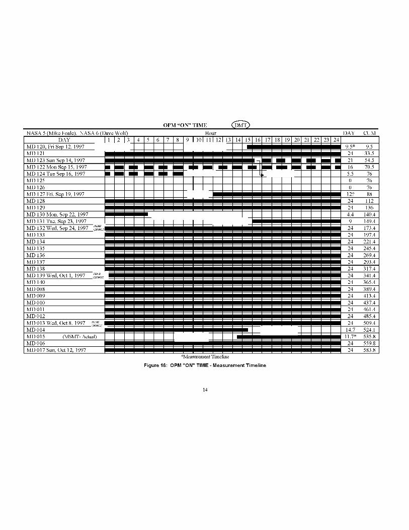
for official power up. Figure 16 shows the estimated power on/off status chart for the period between September 12

and October 12, 1997. The OPM did not have a real-time clock, only an elapsed timer so the exact times cannot be

determined. The time is given in Decreed Moscow Time (DMT) - the time used by the Mir crew.

The OPM temperature data combined with the Mir attitude data (Figure 17) and the OPM _ON" timeline

(Figure 16) obtained from the Mir daily activity reports has been used to adjust the OPM mission elapsed time to a

best estimate of real time. Table 2 summarizes the correction factors which have been applied to the mission elapsed

time beginning with the powering _ON" of OPM on September 9, 1997. No correction has been applied to the

period between September 9 and 15 due to a lack of significant Mir attitude events or accurate OPM Power status

information. Figure 18 is an example of how the OPM base plate responded to Mir attitude changes on November 6

- 11, 1997. This data incorporates the seven-hour correction to the timeline as shown in Table 2. Note that _loss of

power" is an anomaly that was beyond the scope of the OPM mission. The OPM design was shown to be capable of

fully recovering from this condition. Sufficient thermal data was recorded to allow a reconstruction of the mission

timeline within the accuracy of the 2-hour monitoring data. No science data was lost or rendered unusable due to the

inaccuracy of the reconstructed mission timeline.

The OPM experiment lost Mir power on several occasions after the June 25th collision. On at least six

occasions the OPM was restarted from a "Cold Soak" condition (Base Plate below -10°C). Four of the restarts were

immediately followed by an OPM measurement cycle (9/12, 9/14, 9/24, and 11/23). Two of the restarts occurred

during monitoring mode (-9/9 and 10/21). Figure 19 shows the rate at which the OPM recovers to nominal

temperatures after a cold restart on October 21, 1997. Both the base plate and the emissivity plate are above 0°C

within five hours of restart. Note that "loss of power" is an anomaly which was beyond the scope of the OPM

mission. However, the OPM design was shown to be fully capable of recovering from this condition.

13

OPM "ON" TIME

NASA 5 (Mike Foale), NASA 6 ([ rave Wo]

DAY 1 2 3

MD 120, Fri Sep 12, 1997

MD 121

MD 123 Sun Sep 14, 1997

MD 122Mon Sep 15, 1997 • BB

MD 124Tue Sep 16, 1997 • BB

MD 125

MD 126

MD 127 Fri, Sep 19, 1997MD 128

MD 129

MD 130 Mon, Sep 22, 1997

MD 131 Tue, Sep 23, 1997

MD 132 Wed, Sep 24, 1997MD 133

MD 134

MD 135

MD 136

MD 137

MD 138

MD 139 Wed, Oct 1, 1997 PLND(MSMT)

MD 140

MD 008

MD 009

MD 010

MD011

MD 012

MD 013 Wed, Oct 8, 1997 PL_(MSMT)

MD 014

MD 015 (MSMT- Actual)

MD 016

MD 017 Sun, Oct 12, 1997

Hour

*Measurement Timeline

Figure 16: OPM "ON" TIME - Measurement Timeline

DAY CUM

9.5* 9.5

24 33.5

21 54.5

16 70.5

5.5 76

0 76

0 76

12? 88

24 112

24 136

4.4 140.4

9 149.4

24 173.4

24 197.4

24 221.4

24 245.4

24 269.4

24 293.4

24 317.4

24 341.4

24 365.4

24 389.4

24 413.4

24 437.4

24 461.4

24 485.4

24 509.4

14.7 524.1

11.7" 535.8

24 559.8

24 583.8

14

200

OPM/Mir Attitude Data for November, 1997

180 -

160 -

140 -

120

v 100

._o 80 -

> 60-

L_ 40-

20-

c9 0

l lJ , Ji i i i

10/28/97

4OO

350 -

300

250-

200 -

150 -

E•_ 100 -

<_ 50-m

0--50

11/4/97 11/11/97 11/18/97 11/25/97 12/2/97

lil+ +i

10/28/97 11/4/97 11/11/97 11/18/97 11/25/97 12/2/97

Date (DMT)

Figure 17: OPM/MirAttitude Data for November, 1997.

Table 2: OPM Mission Elapsed Time Correction.

MET Correction Corrected Timeline

Start End hrs :min: sec Start End

9/9/97 17:15 9/15/97 17:18 0:00:00 9/9/97 17:15 9/15/97 17:18

9/22/97 1:41 9/22/97 3:41 56:00:00 9/24/97 9:41 9/24/97 11:41

9/23/97 1:10 9/28/97 23:18 36:00:00 9/24/97 13:10 9/30/97 11:18

10/1/97 0:18 10/10/97 1:37 -10:53:00 9/30/97 13:25 10/9/97 14:44

10/10/97 21:05 10/19/97 15:13 14:00:00 10/11/97 11:05 10/20/97 5:13

10/19/97 15:13 10/20/97 23:15 56:22:00 10/21/97 23:35 10/23/97 7:37

10/23/97 1:16 10/24/97 21:33 8:22:00 10/23/97 9:38 10/25/97 5:55

10/25/97 11:33 11/21/97 18:03 7:00:00 10/25/97 18:33 11/22/97 1:03

11/22/97 11:55 12/31/97 15:22 42:23:00 11/24/97 6:18 1/2/98 9:45

15

_a

140

128

IO0

r t •

Solar

Elevation

iii_r-ilrii-r ,r__._.__,_LLLJ.... I......k J L.... .....U

;Measurement_l_Timeline 20 _

Base Plate

Temperature

\

___J L__JF--.

LiJ:- i11/8/9712:80 11._/970:00 11.,7/9712:00 11/9/970:00 11/9/9712:00 11/9/970:00 11/9/9712:0011/10/978:00 11/10/97

12:00

Dale (DMT)

11/11/97 0:00

Figure 18: OPM Thermal Response to Mir Attitude change on November 6-11, 1997.

Monitor Data for October 1997

Base PlateThermistor - 128

10/21/97

12:00

10/21/97 10/22,97 10/22,97 10/22,97 10/22,97 10/23/97 10/23/97 10/23/97 10/23/97 10/24/97

18:00 0:00 6:00 12:00 18:00 O:OO 8:OO 12:00 10:00 O:OO

Date

Figure 19: OPM Restart Temperature Response on October 21, 1997.

]6

SUMMARY AND CONCLUSIONS

A thermal control system was designed for the OPM Experiment. Detailed S1NDA and TRASYS models

were developed for the OPM which were used to evaluate system health and performance. Thermal flight data and

thermal analysis techniques were demonstrated to be critical sources of information in the evaluation of flightanomalies.

ACKNOWLEDGEMENTS

The author wishes to acknowledge the contributions of Donald Wilkes/OPM Principal Investigator and Leigh

Hummer/OPM Chief Engineer of AZ Technology, Inc., NASA/MSFC for overall management and test support,

NASA/HQ for primary funding support, and NASA/JSC for funding, Mir, and EVA support.

REFERENCES

1. _Optical Properties Monitor (OPM) System Report," AZ Technology, Report Number 91-1-118-164,

February 3, 1999 (Draft).

2. _SINDA/FLU1NT, Systems Improved Numerical Differencing Analyzer and Fluid Integrator, Version 2.2,"

MCR-86-594, Martin Marietta Corporation, Denver Aerospace, September 1988.

3. _Thermal Radiation Analysis System (TRASYS II)," COSMIC Program #MSC20448 and #MSC21030,

June 1983.

4. _Mir Geothermal and Thermal Math Models," SSD93D0366A, Rockwell International, Rev. A, April 1994.

5. _Mir-2 Docking Module Geometries and Thermal Math Model Descriptions," SSD94D0365, Rockwell

International, Dec. 1994.

6. Schmitz, Craig P., "Thermal Data Book for the Optical Properties Monitor (OPM) Experiment,"

AZ Technology, Report Number 91-1-118-145, April 22, 1997.

7. Schmitz, Craig P., _Mission Thermal Data Book for the Optical properties Monitor (OPM) Experiment,"

AZ Technology, Report Number 91-1-118-166, February 18, 1999 (Draft).

17

THERMAL ANAL YSIS OF A FINITE ELEMENT MODEL

IN A RADIATION DOMINATED ENVIRONMENT

Arthur T. Page

National Aeronautics And Space Administration

George C. Marshall Space Flight Center

MSFC, AL 35812

ABSTRACT

This paper presents a brief overview of thermal analysis, evaluating the University of Arizona mirror design, for theNext Generation Space Telescope (NGST) Pre-Phase A vehicle concept. Model building begins using ThermalDesktop TM, by Cullimore and Ring Technologies, to import a NASTRAN bulk data file from the structural model ofthe mirror assembly. Using AutoCAD ® capabilities, additional surfaces are added to simulate the thermal aspects ofthe problem which, for due reason, are not part of the structural model. Surfaces are then available to acceptthermophysical and thermo-optical properties. Thermal Desktop TM calculates radiation conductors using MonteCarlo simulations. Then Thermal Desktop TM generates the SINDA input file having a one-to-one correspondencewith the NASTRAN node and element definitions. A model is now available to evaluate the mirror design in theradiation dominated environment, conduct parametric trade studies of the thermal design, and provide temperaturesto the finite element structural model.

INTRODUCTION

The NGST, Figure 1, is NASA's planned successor to the Hubble Space Telescope. NGST is being designed as alarge imaging and spectroscopic instrument capable of observing sources in the near infrared (IR) wavelengths.Marshall Space Flight Center's (MSFC) role in this evolving program includes feasibility studies and technologydevelopment demonstrations for the optical telescope assembly (OTA). MSFC's Thermal Control Systems Groupalso supports the program office at Goddard Space Flight Center (GSFC) as a member of the integrated analysisteam. The University of Arizona (UofA) is one of several participants in the NGST Mirror System Demonstratorcontracts developing technology for large, lightweight optics. Each of the participant's mirror designs willeventually be evaluated for relative performance by the integrated analysis team using a baseline Telescope designcommonly referred to as the "yardstick" design.

Figure 1: GSFC Pre-Phase A NGST conceptual design 1

TELESCOPE DESCRIPTION

The NGST Telescope is composed of four major subsystems, Figure 2, which include the Sunshade, Primary Mirror(PM) Assembly, Secondary Mirror (SM) with mast, and the Integrated Scientific Instrument Module (ISIM). TheSunshade is a deployable structure basically acting as multi-layer insulation (MLI) to block direct solar energy fromthe OTA. The PM assembly is also a deployable structure too large to launch in a fixed position. The central petalis fixed and surrounded by deployable petals. Once deployed, the PM assembly has a diameter of approximately 8.5meters. The SM is mounted at the end of a composite mast attached to the central petal of the PM.

>>>>>>>>>>>>>>>>>>>>>>>>>>>>

Since the Telescope investigates near IR sources, the primary mirror must be maintained at stable temperatures near35 Kelvin. The NGST baseline orbit is at the 'L2' Lagragian point, Figure 3. The L2 point is located at an altitudeof approximately 3 times the distance from the earth to the moon. It remains on the anti-sun side of the earth. Thisorbit, along with the Sunshade, provides a cold environment at very stable conditions

Figure 3: Lagrangian Points relative to the sun and earth orbit 1

The NGST attitude is defined relative to the solar vector. Figure 4 shows how the attitude changes from having the

Sunshade normal to the solar vector, which is the hottest attitude, by slewing to as much as +/- 27 ° off axis, which isthe coldest attitude.

i !i':

::i!i: i ?iiii:

Figure 4: NGST slew maneuver

Figure 5 shows the UofA demonstrator mirror design for a single petal. The mirror is hexagonal shaped. Structural

models of this mirror are scaled up to about 3 m flat-to-flat to fit the "yardstick" Telescope design. The front mirror

surface is glass approximately 2 mm thick. The glass is held in place by a complex assembly of linkages attached to

the backside of the mirror on one end and the actuators on the other end. Behind the glass mirror is the Reaction

Structure. The Reaction Structure is an open-cell honeycomb composite. It includes a front and back face but

remains open-cell as an assembly. Actuators are mounted inside the cells of the reaction plate.

Glass

Reaction

Structure

Figure 5: University Of Arizona NGST Demonstrator Mirror 2

ANALYTICAL OBJECTIVES

Mirror temperature effects are integrated into stress analysis, along with dynamic loading. The combined effects are

inputs to the optical analysis which evaluates performance of the individual petals and overall assembly. This

integrated analysis effort is used to compare relative performance of the various mirror designs, requirements for

individual components such as the actuators, and effects of other subsystem conceptual designs such as the SM mast

and ISIM. This effort also evaluates the necessity for cryo-figuring, effects of material selection, and effects of

mounting techniques.

More specifically, the first objective for the thermal analysis is to determine the maximum mirror temperatures

during the hot case attitude. This data is used to determine mirror deformations from ambient conditions and

evaluate the requirement for cryo-figuring. The second major objective is to determine the mirror temperature

response to a slew maneuver from the hot case attitude to the cold case attitude. This data is used to evaluate mirror

performance following the slew to determine when perturbations to the optical performance stabilize. The data is

also used to determine the required travel for actuators to correct for thermal deformations. Another major objective

is to compare temperatures and eventually stress magnitudes, dynamic response, and optical performance between

the detailed petal and the corresponding simplified petal. This data is used to determine the amount of surface detail

necessary in the integrated model to accurately evaluate overall performance criteria among the various disciplines.

In order to meet these objectives, the thermal analysis process follows a simple path. Sunshade temperatures are

provided as boundary conditions from GSFC for the hot and cold attitudes. The NASTRAN FEM model is

imported into Thermal Desktop TM and converted to thermal entities. Thermophysical properties, thermo-optical

properties, and surface thicknesses are defined. Surfaces/solids are added as necessary. The SINDA thermal

network is constructed and radiation conductors calculated. Temperatures are calculated using SINDA. Steady-

state temperatures are calculated at the hot attitude and then the boundary conditions are changed to reflect the slew

maneuver and a transient solution is completed. Temperatures are exported back to the NASTRAN FEM with a

one-to-one correspondence between calculated temperatures and grid points. Although this is a simple path, the

analytical process is not without significant challenges. These are discussed in the next section.

ANALYTICAL CHALLENGES

NGST performance and environmental requirements pose challenges to the integrated analysis effort that only a few

years ago would have been insurmountable. Previous telescopes, with strict optical performance requirements, often

chose to maintain mirror elements near ambient conditions with strict requirements on the thermal control system

(TCS) design. Optical performance can then rely on stable temperatures that remain near manufacturing conditions

of the mirror elements. Likewise, mirror elements are usually mounted inside a spacecraft structure allowing TCS

designs to dampen temperature excursions due to environmental changes. Such luxuries are not afforded NGST.

Due to NGST IR imaging requirements, optical elements must be near 35 K during operation, thereby making

thermal effects over a large temperature span play a major role in optical performance. NGST also requires a large

mirror assembly which necessitates lightweight, deployable elements. Mirror elements are too large to be enclosed

in a spacecraft structure. The thin surfaces, naturally, have large temperature gradients. In summary, integration

analysis and most notably thermal analysis becomes much more important for the NGST design and performanceevaluation.

Integration analysis passes thermal and dynamic responses to stress models which combine the various loads into

final mirror deformations. The deformations are then passed on to optical models to evaluate final performance.

Therefore, the stress model serves as the primary gateway of data sharing among disciplines. Several challenges

exist for this integration. First, there must be a routine interface between the stress FEM and the thermal model to

evaluate changing designs. There are many mirror designs, optical assembly designs, TCS designs, etc. Likewise,

the use of structural FEM in thermal analysis almost always dictates a large number of surfaces and grid

points/nodes. Second, the thermal model must evaluate temperatures of surfaces with specular optical properties,

driven by a radiation dominated environment.

Historically,thermalsoftwarepackagesthatinterfacewithFEM'scannotperformfullradiationanalysistocalculateradiationconductors,orbitalheating,andaddsurfacesaspartoftheTCSdesign.Somedonotprovideameanstocalculatenon-lineartemperatureresponses.In addition,mostof thesepackagesdonotprovideaninterfacetoS1NDAwhichremainsthetriedandtrueworkhorseofthermalanalyststhroughoutNASA.Thepackagesthatdoprovideaninterfacearesometimesnotviableforcontinuouslychangingdesignsordesignsdrivenbyradiation.Therefore,agapresultswhichgreatlyhindersintegratedthermalanalysis.

Withinrecentyearsaveryfewsoftwarepackageshaveevolvedthatdoprovide,toonedegreeoranother,interfacestoFEM'susedbyotheranalyticaldisciplines,interfacestoCADpackagesusedbydesigners,andfinally,theyarecapableof fullthermalanalysiswithradiation.ThermalDesktopTM, which runs within AutoCAD ® , is one of the

most notable developments that does provide these capabilities. Thermal Desktop TM is used for NGST because of

its capability to import NASTRAN FEM's, calculate radiation conductors for a very large number of surfaces, add

thermal design features, quickly change material properties and geometry, evaluate surfaces with specular

properties, and post-process temperatures for direct export back to NASTRAN. There are many other features

within the package that are not used for NGST analysis. Some of the more notable features are the capability to

evaluate articulating surfaces and the capability to reduce the number of surfaces in the model while maintaining the

original interface to FEM's grid points.

THERMAL/STRUCTURAL MODEL

With the Sunshade added, the NASTRAN FEM has 2,015 elements (surfaces) and 1,466 grid points (nodes) once

imported into Thermal Desktop TM, Figure 6. The detailed mirror has 785 elements (surfaces) while the simplified

mirrors have only 26 elements (surfaces) per petal. The FEM includes the Sunshade, PM Petals, SM Mast, and SM.

The FEM also includes the Reaction Structure for the detailed petal. This NASTRAN FEM serves as the basic

model used to share data among the various disciples conducting integrated analysis. Post-processed results from

the thermal analysis provide temperatures for each of these grid points in the NASTRAN FEM. The ISIM is not

included in this model because the baseline model used for comparison had no ISIM. This model does not include

elements for the Reaction Structure behind the simplified petals.

_:..?<2: -.: :5

_r:::........._.;.. i]:g[Q ::_i)_'_.i--i:!i...........:::i

Figure 6: NASTRAN FEM of NGST with the UofA mirror design

Thermal analysis must consider radiation between the mirror petals and Reaction Structure and between the

Reaction Structure and Sunshade, Figure 7. Modeling the open-cell structure is discussed below. Using AutoCAD ®

features, the simplified petal surfaces are copied and translated behind the mirror providing new surfaces for a

simplified Reaction Structure with identical detail, Figure 8. Using Thermal Desktop TM the new surfaces are put in a

separate submodel. Once the simplified Reaction Structure is added, the thermal model has 2,219 surfaces and

1,689 nodes.

Figure 7: Radiation interchange toward the backside of the Mirror

Figure 8: Reaction Structure surfaces added to the thermal model

The next step in developing the thermal model is defining thicknesses and material properties of the various planersurfaces. Thicknesses and material properties are used to calculate nodal thermal capacitance and linear conductorsto adjacent nodes. Surfaces are selected using a multitude of options within either AutoCAD ® or ThermalDesktop TM. The PM is borasilicate glass while the Reaction Structure and SM Mast are laminated composites.

Properties are given in Tables 1 & 2. If material properties near 30 K are available they are used. Otherwise,properties are set to those used in the "yardstick" analysis. The PM surfaces are set to the actual glass thickness of 2mm. The SM Mast surfaces are set to the actual thickness of 3 mm. The Reaction Structure surfaces are set to the

actual thickness of the single facesheet toward the PM which is 0.76 mm. This simplifies the honeycomb assemblyand provides conservative predictions on lateral temperature gradients. However, the material density of theReaction Structure is increased to include the total thermal capacity of the two facesheets and honeycomb webs.This maintains accuracy for the transient analysis.

............S_ac_............I ................I_a_n_ .............I_m_s_i_'!iyS_shaa_ , , 0,03

0.03

C_mP_Si_e@_0_ 04

Table l: Thermophysical Properties Table 2: Surface Emissivity

The next step before beginning calculations is selecting the necessary surfaces to be included in the radiationanalysis and defining optical properties for those surfaces. This is a simple task for all structures except one. Adifficult situation exists with the honeycomb Reaction Structure. The structure is open-cell. Therefore, the backsideof the PM glass "sees" through the Reaction Structure to the Sunshade, Figure 7. A detailed model of eachindividual cell would require too many surfaces to handle in the radiation analysis. As a common alternative,simplifying assumptions are used. Optical properties for this structure include 11% transmissivity in the IRwavelength. The transmissivity value is determined by importing design drawings of the facesheet. Again, usingAutoCAD ® techniques, the relative surface area of the open-cells to facesheet is calculated.

Radiation conductors are now calculated and a S1NDA network file is generated. The final analysis uses a total of414,945 radiation conductors and 5,179 linear conductors.

RESULTS

As a checkout procedure, the temperatures are first calculated using only the radiation network. In this case only thefront mirror surface is active. This helps evaluate the radiation network and gives a quick comparison of thedetailed petal, to the left, and simplified petal, to the right. Mirror temperatures, Figure 9, show symmetry across thePM assembly along a vertical axis as expected. It also shows good agreement between the detailed and simplifiedpetal. There is a shadow of the SM Mast toward the top of the PM assembly as it blocks radiation from the warmerSunshade below.

}35

iiii_i_i_i_i_........ _i_i_i_i_iiiiiii3S

iiii iiiiils2

"::::::::::::::::::::::::

? i

iii o:::::::::::::::::::::::::::::::::::::::::::::::::_8 _

iiiiiiiiiiiiiiiiiiiiiiiiiiiiiiiiiiiiiiiiiiiiiiiiiiii ¸¸I¸¸7

iiiiiiiiiiiiiiiiiiiiiiiiiiiiiiiiiiiiiiiiiiiiiiiiiiiii__

iii<s

Figure 9: Results from a checkout run with radiation only

With the checkout complete the conduction network is added to the S1NDA model. Calculations for the hot case

attitude show a maximum mirror temperature around 32 K, Figures 10 & 11. The temperature gradient across the

PM assembly is about 10 K. The central petal has the largest gradient of any single petal.

2222222222222222}}}i_};,

ii!!i_ii!iiiiiiiiiiiiiiiiiiiiiiiiiiiiiiiiiiiiiii__

iiiii!ii}iiiiiiiiiiiiiiiiiiiiiiiiiiiiiiiiiiiiiii':::::::::::::::::::::::::::::::::::::::_i_5

:::::::::::::::::::::::::::::::::::::::_:::::::::::::::::::::::::::::::::::::::

i_ililililililililililililililili_ili_i__?_

iiiiiiiiiiiiiiiiiiiiiiiiiiiiiiiiiiiiiiiiiiiiiiiii_ii

Figure 10: Final hot case results- isometric view

N iii!iii_il

.... iiiiiiiiiiiiiiiiiiiiiiiiiiiiiiiiiiiiiiiiii iiiiiiiiiiiiiiiiiiiiiii

.......iiiiiiiiiiiiiiiiiiiiiiiiiiiiiiiiiiiiiiiiiiiiiiii_iii_iiiiiiiiiiiiiiiii_iiiiiiiiiiiiiiiiiiiiiiiiiiiiiiiiiiiiiiiiiiiiiiiiiii_iiiiiiiiiiiii_iiiiiiiiiiiii__

® !!!!! iiiii i iiii!iiiii!i!i!ii i ii!i!iiiiiiiii `iiiiiiiiiiiiiiiiiiiiiiiiiiiiiiiiiiiiiiii `% iiiiiiiiiii iiiiiiiiiiiiiii i iiiii i i i iiii i

iiiiii_iii

Figure 11: Final hot case results- front view

There is a large gradient at the interface between petals. Eventually, latches and/or hinges will be included that may

have significant effects on these gradients. It should be noted that these temperatures are not considered the best

possible with the UofA mirror design. Future analysis, to improve performance, should consider options to

eliminate direct radiation from the backside of the Mirror to the Sunshade. Gradients can be easily reduced with the

addition of insulation, for example. Temperatures for the entire vehicle are given in Figure 12.

............................................til_

iiiiiiiiiiiiiiiiiiiiiiiiiiiiiiiiiiiiiiiiiiii

iiiiiiiiiiiiiiiiiiiiiiiiiiiiiiiiiiiiiiiiiiiiiiiiii__iiiiiiiiiiiiiiiiiiiiiiiiiiiiiiiiiiiiiiiiiiii__

iiiiiiiiiiiiiiiiiiiiiiiiiiiiiiiiiiiiiiiiiiii_

Figure 12: Final hot case results- entire vehicle

During the maximum slew maneuver Sunshade temperatures decrease about 2 K on average. Figure 13 shows how

the Mirror and OTA structure respond to the different environment. Although the Mirror is lightweight, the

radiation coupling to the Sunshade is small. Therefore, Mirror temperatures continue to decrease for a long time

following the slew. Transient temperatures are used in the stress analysis to provide thermal deformations over a

period of time following the slew. This information is used to determine when optical stability is achieved.

Although Mirror temperatures continue to change many days following the slew, the rate of temperature change

decreases a great deal after about 36 hours, Figure 14.

0.0

-0.2

_" -0.4

i-0.6

'_ -0.8

-1.0

\

Sunshidd

Mirror Front Smface

-1.2 -

0 240 480 720 960

Thne (hrs)

Figure 13 Slew Maneuver- Temperature Change From Initial Conditions

Figure14:SlewManeuver-Rateof TemperatureChange

CONCLUSIONS

Initial calculations show that the L2 orbit combined with the Sunshade design result in Mirror temperatures at orbelow 32 K. Temperatures of the simplified petal show the same degree of fidelity in gradients as the detailed petal.Therefore, the simplified petals do reflect the required amount of detail to accurately evaluate temperatures. Mirrortemperatures continue to decrease many days following a 27 ° slew maneuver. As a result of this effort, a thermalmodel now exists to conduct parametric trade studies that evaluate various design changes to reduce gradients andimprove the optical performance. The thermal model can be quickly modified to reflect design changes as the

project matures.

This effort also demonstrates that Thermal Desktop TM is a useful tool to perform thermal analysis on FEM models inan environment dominated by radiation interchange. The release of Thermal Desktop TM is a major advancement in

tools available to the thermal analysis. Thermal analysis can now play a more active role in the integrated analysisand concurrent engineering design effort.

REFERENCES

[1] National Aeronautics and Space Administration, Goddard Space Flight Center, Next Generation SpaceTelescope Internet Home Page.

[2] University Of Arizona, Next Generation Space Telescope Mirror System Demonstrator Critical DesignReview.

10

AN OVERVIEW OF THE THERMAL CHALLENGESOF DESIGNING MICROGRAVITY FURNACES

Douglas G. WestraNASA Marshall Space Flight Center

ABSTRACT

Marshall Space Flight Center is involved in a wide variet_ of microgravity projects that require furnaces,with hot zone temperatures ranging from 300 °C to 2300 C, requirements for gradient processing and rapid

quench, and both semi-condutor and metal materials. On these types of projects, the thermal engineer is a

key player in the design process.

Microgravity furnaces present unique challenges to the thermal designer. One challenge is designing a

sample containment assembly that achieves dual containment, yet allows a high radial heat flux. Another

challenge is providing a high axial gradient but a very low radial gradient.

These furnaces also present unique challenges to the thermal analyst. First, there are several orders of

magnitude difference in the size of the thermal %onductors" between various parts of the model. A second

challenge is providing high fidelity in the sample model, and connecting the sample with the rest of the

furnace model, yet maintaining some sanity in the number of total nodes in the model.

The purpose of this paper is to present an overview of the challenges involved in designing and analyzing

microgravity furnaces and how some of these challenges have been overcome. The thermal analysis tools

presently used to analyze microgravity furnaces and will be listed. Challenges for the future and a

description of future analysis tools will be given.

INTRODUCTION

Marshall Space Flight Center (MSFC) is the Lead Center for NASA's Microgravity Research Program and

manages microgravity research projects at Marshall and other NASA Centers. One of the disciplines that

Marshall is responsible for managing is materials science. A fundamental goal of microgravity materials

science research is to better understand how buoyancy driven convection and sedimentation affect the

processing of the materials. By suppressing these gravity driven phenomena in the microgravity

environment of low earth orbit (LEO), other phenomena normally obscured by gravity may be investigated.

Studying the phenomena normally obscured by gravity allows the gravity driven phenomena to be betterunderstood as well.

Scientists from the academic and research communities apply to NASA to become Principal Investigators in

various materials science disciplines. The materials science discipline that is discussed here is directional

solidification processing of metals and semi-conductors. This specific discipline requires high temperature

furnaces that must meet challenging thermal requirements. These thermal requirements include providing a

large thermal gradient in the sample, a rapid quench at the end of processing, and very stringent isothermal

specifications within certain sections of the sample, to name a few. While meeting these thermal

requirements, containment of (sometimes-hazardous) materials and all other safety requirements must be

met. Many times, meeting the safety requirements makes meeting the thermal requirements extremely

difficult. Temperature measurement and other types of instrumentation issues are also significant furnace

design challenges.

Thermalmathematicalmodelingisveryimportantinthedesignofthesehightemperaturefurnaces.Thermalmathematicalmodelingisusedinthepreliminarydesignofthefurnace,aidsinthedesignprocess,andisusedtodiagnosetestdatafromthefurnace.ThethermalmathematicalmodelsmustincludethenumericalrepresentationofthePI'ssampleaswellasthefurnaceinordertoassessthesample'simpactonthethermalperformanceofthefurnace.Thispresentsmanychallengesaswell:adequatelycharacterizingthesamplewithoutgeneratingahugeamountofnodes,severalordersofmagnitudedifferencebetweenthermalconductorsinthemodel,anddealingwithfurnacecontrolissues.

Themainfocusofthispaperistodiscusstheabovereferencedchallenges.Asanintroductiontomicrogravitymaterialsscienceprocessingofmetalsandsemiconductors,twotypesoffurnaceswill be

described. Following, some examples of sample systems and their containment will be described. Next,

furnace processing and control will be outlined. Then, the challenges associated with furnace design and

analysis will be discussed. Solutions that have been implemented and that are being considered will be

included. Finally, conclusions will be discussed.

DESCRIPTION OF TWO TYPES OF MICROGRAVITY FURNACES

There are a wide variety of furnaces that are used for materials processing. However, there are two types

that have been used for most of the furnaces designed and built by Marshall for metal and semi-conductor

processing. These two furnaces are related: 1) Bridgman-Stockbarger and 2) Bridgman furnaces.

Figure 1 shows a cutaway view of a Bridgman-Stockbarger furnace. This particular furnace operates in an

inert gas environment; however, Bridman-Stockbarger furnaces may also be designed to operate in a

vacuum environment.

There are three main zones in this furnace: a hot zone, an adiabatic zone, and a cold zone. The hot zone is

designed to add heat to the sample radially such that the sample melts. Heat is radially extracted from the

sample in the cold zone such that the sample re-solidifies. Ideally, there is no radial heat transfer in the

adiabatic zone. The temperature difference between the hot zone and cold zone produces the required axial

gradient in the sample. The optimally designed furnace will operate such that the location of the solid-

liquid interface is located in the gradient zone. This is normally the gradient specified by the PI. It is

desirable that this gradient is in the adiabatic zone for the following reason: since there is (ideally) no radial

heat transfer in the adiabatic zone, the shape of the solid-liquid interface is flattest in the adiabatic zone.

Since the furnace is designed so that the design gradient is located in the adiabatic zone, this zone is also

commonly called the gradient zone.

A Bridgman-Stockbarger furnace has a "heated" cold zone as a distinguishing characteristic. The cold zone

is only "cold" relative to the hot zone. That is, the required axial thermal gradient is achieved by operating

the hot zone at temperatures on the order of 1200 - 2200 C, while the cold zone operates on the order of

400 - 1000 °C. Bridgman-Stockbarger furnaces are typically used for semi-conductor directional

solidification processing.

Figure 2 shows a Bridgman furnace design. This furnace operates in an inert gas environment. As with a

Bridgman-Stockbarger, a Bridgman furnace may also be designed to operate in a vacuum environment. The

Bridgman furnace has the same main components as the Bridgman-Stockbarger furnace: a hot zone, a

gradient or adiabatic zone, and a cold zone. However, a Bridgman furnace has an actively cooled cold

zone. The cold zone extracts heat from the sample at temperatures slightly warmer than ambient or cooler if

necessary. There are other features on the particular furnaces shown: a quench block is on both and a

vacuum block is shown on the furnace in Figure 2. On this Bridgman furnace, a water spray is used to

quench or rapidly cool the sample. The vacuum block is used to remove the water and steam mixture that

results when water is sprayed at a hot surface.

TFAWS 99 2

Figure 1 Bridgman-Stockbarger Furnace that operates in an inert gas environment.

• " Quench Block

Close Out Plate _ _,

Guide RodBearing _ _.,_l._

i

Vacuum Block

Chill Block

, Gradient Block

i \/1

Close Out Plate

Figure 2: Bridgman Furnace that operates in an inert gas environment.

TFAWS 99 3

EXAMPLES OF SAMPLE CONTAINMENT ASSEMBLIES (SCA)

Figure 3 shows two sample containment assemblies (SCAs). The one on the left is that of a double-

contained system. The sample is contained directly within an ampoule. Common ampoule materials are

ceramics such as aluminum oxide (alumina), aluminum nitride, and graphite. The outer container is called

the cartridge, normally constructed of metals. There is a gap between the ampoule and the cartridge. The

materials or design of this gap will be explained in detail later on in this paper. The cartridge is affixed to

the support structure of the SCA.

The right side of Figure 3 shows a single-contained SCA, or simply, a crucible. The crucible is made of the

same materials as ampoules: ceramics such as aluminum nitride, etc. The SCA support structure is attachedto the crucible material in this case.

Figure 3: Two different Sample Container Assembly (SCA) Designs.

TFAWS 99 4

FURNACEPROCESSING AND CONTROL

Furnace processing normally begins by inserting the sample into the hot zone such that the entire sample is

melted. The sample is left to %oak" in the hot zone for several hours so that it is of uniform temperature

and composition. This is especially important with alloy materials.

After the soak period, the furnace is translated with respect to the sample so that in effect, the sample is

_removed" from the furnace. Note, translating the furnace rather than the SCA is preferred so that the

furnace, not the sample, absorbs any disturbances associated with this translation. The translation rate is on

the order of millimeters per minute. As the sample is translated into the gradient (adiabatic) zone and then

into the cold zone, the molten sample material solidifies. There are transients due to end effects, but the

translation rate is often slow enough such that heat transfer can be characterized as a quasi-steady-state

process. Some scientists will vary the translation rate during one sample run, which then produces a break

in the quasi-steady-state process.

The structure and morphology of the solid-liquid front is very dependent on the material, the magnitude of

the gradient, and the translation speed. An entire paper could be written on this subject, but this is beyond

the scope of this paper. The phenomenon occurring at the solid-liquid interface and the resulting

microstructure are what the PI controls via his science requirements. A point should be made that in alloys,

the phase change is not isothermal. That is, the phase change takes place over a finite temperature range.

Therefore, there is not a distinct spatial solid-liquid interface. Rather, there is a finite length of sample over

which the phase change takes place. The length of the sample that contains both liquid and solid

components is known as the mushy zone.

The characteristics of the solid-liquid interface or mushy zone cannot be seen while it is being processed.

The nature of the solid-liquid interface or mushy zone may be predicted from the solidified microstructure

after processing, but it cannot be known exactly. Therefore, it is desirable to take a snapshot of what is

going on at the solid-liquid interface or mushy zone. This can be accomplished via rapid cooling or quench.

When a quench occurs, the materials at the solid-liquid interface do not have time to change into their

equilibrium morphology. The rapidness of the quench determines the quality of this snapshot. Therefore, it

is desirable to make this quench as rapid as physically possible.

Refer back to the Bridgman-Stockbarger furnace, Figure 1. Notice that within the hot zone, there are four

heaters shown: the hot guard heater, the main and redundant heaters, and the booster heater. The main and

redundant heaters occupy most of the axial length of the hot zone, with the main heater radially inside the

redundant heater. The redundant heater, as its name implies, is available in case the main heater fails.

However, to lengthen the life of the main heater, both main and redundant are often operated

simultaneously. With the redundant heater on, the main heater can operate at a lower power level, thus

increasing its expected operating life.

The guard heater, located on the bottom or cold end of the hot zone, is designed to operate at a higher

power density than the main/redundant heater. This helps to _guard" the sample from cooling due to heat

losses out the end of the furnace. The higher power density that the guard heater provides helps keep the

temperature profile at the end of the sample equal with the rest of the sample.

The booster heater, located adjacent to the gradient (adiabatic) zone, is also designed for a high power

density. By _boosting" the heat going into the sample, the axial gradient in the sample may be increased

exactly where it's needed.

The cold zone in the Bridgman-Stockbarger furnace shown has main and redundant heaters and a guard

heater, for the same reason as in the hot zone. A booster heater is not necessary in the cold zone. The

main/redundant heater setpoint can be adjusted for optimum thermal gradient.

TFAWS 99 5

AlthoughthislevelofdetailisnotshowninFigure2,thehotzoneofmostBridgmanfurnacesisdesignedwithaguardheater,amainandredundantheaterset,andaboosterheater.TheactivelycooledcoldzoneonBridgmanheatersobviouslycontainsnoheaters.ThereispresentlyaBridgmanfurnacebeingdesignedwithtwoseparatelycontrolledboosterheaterstoallowforevenbettercontrolandoptimizationofthethermalgradientinthesample.

FURNACEAND SCA DESIGN CHALLENGES

The design and operation of the furnace and SCA are very interdependent. Therefore, this section includes

challenges associated with SCA design as well as furnace design.

FURNACE DESIGN CHALLENGES

There are several furnace design challenges that are critical to meeting the science requirements outlined by

the PI. The challenges listed here are hot zone design, gradient (adiabatic) zone design, cold zone design,

quench system design, control of multiple heaters in the hot zone, and temperature measurement.

Hot Zone Design

The purpose of the hot zone is to add heat to the sample radially to effect melting of the sample. There are

two major challenges to this. The first is to control the hot zone inner diameter temperature so that the

sample is driven to the temperature profile required by the PI. This issue is addressed below. The second

challenge is to achieve the required temperature profile with as little power as possible. Therefore,

sophisticated insulation design is required. Gas furnaces are insulated with high performance ceramic

insulation such as Zirconium Oxide. The best performing insulation will often not withstand the extreme

temperatures at the center of the hot zone. Therefore, a lower performing high temperature insulation is

used in the center, with the higher performing (lower maximum temperature) towards the outside of the

furnace. Refer back to Figure 1 to see the different insulation layers in the hot zone of an inert gas furnace.

Vacuum furnaces require high performance radiation shields, and many layers of them. Multiple shields

with a low emissivity are used to restrict radiation heat transfer. Structural mechanisms for the heater

substrate and for the radiation shields must be designed to minimize the thermal conduction path as well asto minimize radiation heat transfer.

Gradient (Adiabatic Zone) Design

The gradient zone should be designed to optimize the location and shape of the solid-liquid interface.

Obviously, the gradient zone also serves as an insulation barrier between the hot zone and cold zone.

Design features beside thermal insulation have been added to some furnaces at Marshall. For instance, in

the Crystal Growth Furnace (CGF), a thermal shunt was used. The gradient zone had load-bearing structure

within it; therefore, it could not be made entirely of low conductivity insulation. The thermal shunt

conducted heat out radially, decreasing the cooling load of the cold zone. This shunt gave the furnace

flexibility to accommodate multiple PIs with varying thermal requirements.

Cold Zone Design

The cold zone has the role of removing heat from the sample so that solidification occurs and so that the

gradient requirement may be met.

TFAWS 99 6

ThecoldzonesetpointtemperatureinaBridgman-Stockbargerfurnaceisusuallyhighenoughthatradiationheattransferiseffective.Therequiredgradientmaybeachievedbyloweringorraisingthecoldzonesetpointtemperature.

ABridgmanfurnacecoldzoneusuallyoperatesatmuchcoolertemperaturesthanaBridgman-Stockbargerfurnace.Waterisaneffectiveandcommoncoolantforthecoldzone.Radiationheattransferattheselowertemperaturesisineffective;therefore,itcannotberelieduponformeetinggradientrequirements.ConductionheattransferisthemosteffectivemeansoftransferringheatfromtheSCAtothecoldzoneattheserelativelylowtemperatures.

OnemeansofeffectingconductionheattransferfromtheSCAtothecoldzoneistodesignthefurnacesuchthataverysmallgapexistsbetweentheoutsidediameteroftheSCAandtheinsidediameterofthecoldzone.Theentirefurnaceisthenoperatedinaninertgassuchashelium.TheheliumservesastheconductionpathinthesmallannulargapbetweentheSCAandcoldzone.Heliumgasisanattractivechoicebecauseamonginertgases,ithasoneofthehighestthermalconductivities(otherthanhydrogen,whichisnotusedforobviousreasons).However,aheliumgasenvironmenthasthedisadvantageofseverelydegradingthethermalpropertiesofhotzoneinsulation.Therefore,anothersolutionhasbeenimplementedinanumberofBridgmanfurnacesatMarshall.Thissolutionistouseeitheranargongasenvironmentoravacuumenvironmentwithvel-therminthecoldzone.Vel-thermprovidesaslidingthermalcontactinterface.It iscompliantandreliable.Argongaswiththevel-thermthermalinterfaceprovidesaslightlybetterthermalconductancethanheliumgasbyitself.Usingargonratherthanheliumresultedin50%savingsinpowerappliedtothehotzoneofaparticularBridgmanfurnaceatMarshall.

Quench System Design

This is one of the most challenging design issues. The goal of a quench system is to radially remove as

much heat as possible from the outside surface of the SCA. There are a number of quench systems that

have been used. Others are being considered. Table 1 lists these systems, along with their

advantages/disadvantages and their nominal heat transfer rate.

Water spray has a high surface heat transfer rate, however, this high heat transfer rate occurs when the

surface temperature is between the boiling point and the leidenfrost temperature of the coolant. The

leidenfrost temperature is the temperature at which the cooling mechanism transforms to nucleate boiling: a

very effective means of phase change cooling. The initial surface temperature of the quenched section will

be centered at the phase change temperature of the sample material, well above the leidenfrost temperature

for most PI materials (approximately 200 C for water). At temperatures well above leidenfrost, a vapor

barrier will form around the SCA surface, which is the reason for the severe degradation in heat transfer

rate. Marshall has funded a Small Business Innovation Research (SBIR) Contract to optimize water spray

characteristics and overcome some of the degradation that occurs at high temperatures. The SBIR

contractor has made significant progress by optimizing water spray pattern, water droplet size, and water

droplet velocity, such that the water droplets penetrate the steam barrier. Through these efforts, the heato

transfer coefficient can be increased at temperatures well above 200 C by raising the leidenfrost

temperature. Despite these efforts, water spray still has some inherent problems: the water/steam must be

recovered, there are concerns about water coming in contact with the furnace heater core, and issues with

material contamination.

With a high-pressure gas quench, gas is stored at high pressure in a container outside the furnace enclosure.

The gas is released into the annulus between the SCA and its enclosure. The high pressure and small cross-

sectional area cause the gas to achieve sonic velocity in the annulus. This heat transfer rate achieved is up

to 10,000 W/mA2-K. Gas quench is very attractive, not only because it has less operating problems than

water, but also because it has the potential of operating in-situ. That is, rather than translating the SCA

TFAWS 99 7

(orfurnacerelativetotheSCA)sothatthesolid-liquidfront/mushyzoneisinthecoldzoneoraseparatequenchzone,thesampleisquenchedinplace.Thesolid-liquid/mushyzoneislocatedinthegradientzoneandthequenchingmechanismisbroughttoit,inthegradientzone.Doingawaywiththepre-quenchtranslationavoidsatimedelayandthevibrationthatmaycompromisetheintegrityofthemorphologytobepreservedwith the quench.

Clamp-on devices have also been investigated. The basic concept is to press down on the quenched surface

with a device that has a high heat capacity. One example is a collett mechanism made of copper. Thus far,

clamp-on devices without a phase change material have not resulted in high enough surface heat transfer

rates. The challenge is to effect an adequate heat transfer path between the clamp-on device and the

quenched surface (the SCA outer diameter) without damaging the quenched surface or introducing

excessive vibration. Plans are under way to improve the design of these devices using compliant materials

that also allow adequate heat transfer from the clamp-on device to the quenched surface.

MSFC is also testing clamp-on devices that use a phase change material to serve as the thermal interface

mechanism between the clamp-on device and the quenched surface. The phase change material becomes

compliant to offer low thermal resistance as it changes phase from solid to liquid. In addition, the phase

change material absorbs much of the heat, right at the quenched surface. At high initial quench surface

temperatures such as in metal solidification processing, liquid metals are the only materials that can

withstand the temperatures. On-going tests show that these devices hold a lot of promise.

TFAWS 99 8

Multi-Heater Control

As mentioned earlier, a hot zone has up to five separately controlled heaters: one or two boosters, a set of

main and redundant heaters, and a guard heater. A cold zone may have up to three heaters. These heaters

are coupled to each other. For example, if more heat is applied to the booster heater, the control

measurement of the main heater will be affected as well as the booster heater. Therefore, very sophisticated

heater control is necessary. In addition, tight isothermal requirements in the hot zoneo

(r 1 C) can make heater control even more difficult.

Temperature Measurement

Temperature measurement is very critical in microgravity furnaces. Two examples are heater control

temperature measurement and furnace / sample performance characterization to assure that science

requirements are met. Problems and solutions are discussed here.

Thermocouples are the most common measurement device for heater control. Control thermocouples can

be stressed due to thermal expansion and exposure to high temperature over long periods of time.

Thermocouples can lose calibration over time, especially at high temperatures. Therefore, heater control

temperature measurement should have at least one level of redundancy; this allows continued operation if

one of the control thermocouples fails. An alternative to using thermocouples is optical fiber thermometers,

which transport and analyze the blackbody radiation being absorbed by a probe placed at the desired

temperature measurement location. This method of temperature measurement also has its challenges,

including having to be very careful about placement of the optical fiber.

Sample measurement can be extremely difficult. Depending on the sample, a thermocouple can be

destroyed when it reacts with the sample. Liquid aluminum, for example, is extremely corrosive and can

destroy a thermocouple after a relatively short exposure time. On double-contained SCA configurations,

thermocouples can be placed in the annular gap between the ampoule and the cartridge, with the

thermocouple bead bonded to the ampoule. This type of measurement provides good steady state or quasi-

steady-state temperature measurement but is very limited for transient temperature measurement of the

sample. Thermal analysis is often used to correlate the temperatures measured on the outside of the

ampoule to the desired temperature measurement within the sample.

SCA DESIGN CHALLENGES

The design of the SCA is probably one of the most important and challenging design considerations for

furnace design. Its design will affect the quality and magnitude of the gradient and even more so, the

success of the quench.

Effect of SCA Gap on Gradient

Figure 4 shows a detailed cross-section of a two containment level SCA design. The thermal heat path

down the SCA in the axial direction affects the thermal gradient in the sample. If the axial conductance of

the SCA is on the order of or higher than that of the sample, more heat will flow from the hot zone to the

cold zone through this path, and the magnitude of the axial thermal gradient will be reduced significantly.

The quality of the thermal axial gradient can also be affected by the thermal properties of the SCA. If the

thermal conductance through the SCA is much greater than that of the sample, the solidification front will

be closer to the cold zone near the wall than in the sample center. The opposite effect will occur if the

TFAWS 99 9

thermalconductanceoftheSCAismuchlessthanthatofthesample.ThethermalconductanceoftheSCAcannotbematchedexactlytothatofthesample,butmeasuresshouldbetakentominimizethiseffect.

Effect of SCA Gap on Quench Rate

The SCA thermal conductance affects quench rate significantly. Here, the conduction path in the radial

direction is very important. Referring back to Figure 4, there are three major resistances between the

quench medium on the outside of the cartridge to the sample: the cartridge wall, the filler gap, and the

ampoule wall. The major challenge is the gap between the inside of the cartridge and the outside of the

ampoule. Figure 5 shows the overall thermal conductance versus the gap heat transfer coefficient for three

different ampoule materials. The figure shows that up to a gap heat transfer coefficient of 1000 W/mA2-K,

the ampoule material is irrelevant. That is, for a gap thermal conductance of 1000 W/mA2-K or below, the

thermal resistance of the cartridge wall and of the ampoule wall are insignificant compared to that of the

gap between them.

Figure 4: Sample Container Assembly (SCA) Cross-section.

Marshall has investigated the use of liquid metals such as certain indium alloys or crushed powers like

alumina or boron nitride as heat transfer "filler" in the SCA gap. However, implementation of these

design solutions has been impractical. Problems with thermal expansion of the liquid metals and too low of

an effective thermal conductivity with the ceramic powders have been problems thus far.

Applying a metal coating to a ceramic ampoule material via Vacuum Plasma Spray (VPS) is an option

being investigated. The metal coating has the purpose of holding the SCA together in case of ceramic

failure during quench or other stress causing events. Whether this type of system meets safety requirements

for hazardous materials is still being assessed.

TFAWS 99 10

--, 5.0

®_ 4.0Ua_ _ 3.5

3.0•_ ,-m

0 ',_ 2.5ta_.

2.0

1.5

• 1.0,_I e_

u 0.5or_k,,i,., 0.0

T 1

• ArgonGas Gap (AmpouleMat_ed_Irrele_nt)

I. HeliumGas Gap (AmpouleMatedatIn'ele*,ent)

--x-- AluminumNLtddeAmpoule

_ __ GraphiteAmpoule

--I.- AluminaAmpoule

.........I0 I00 1,000 I0,000

/

, , • , ,,"i

I00,000

Gap Heat TEansfe¢ Coefflclnt (W/mA.2-K)

Figure 5: SCA Conductance vs. Gap Heat Transfer Coefficient for a 1.0 mm Gap.

FURNACE THERMAL ANALYSIS DESIGN CHALLENGES

Bridgman and Bridgman-Stockbarger furnaces have a cylindrical geometry, which lends itself to two-

dimensional (2-D) axisymmetric thermal models. Figure 6 shows an example of a 2-D axisymmetric model

of a Bridgman furnace.

A 2-D axisymmetric model has the advantage of requiring much fewer nodes than a 3-D model. Obviously,

this type of model assumes isothermality in the theta (0) direction. Even though most furnace and sample

components are cylindrical and therefore axisymmetric, even the best-designed furnace will have some non-

axisymmetric features (i.e., heater wire connections, thermocouples, water lines, structural components,

insulation split down the middle for ease of construction, etc.). Assumptions and simplifications must be

made to account for these deviations from axisymmetry. A 3-D model of some or the entire furnace may be

necessary to assess the effect of these deviations on isothermality in the theta direction.

MULTI-HEATER CONTROL

Thermal analysis plays a key role in heater control. The cross coupling of heaters with each other can be

modeled. The design setpoints can be programmed into the thermal model and the power required by each

heater may be predicted. Accurate representations of the heater winding locations and heater winding

density are critical for accurately predicting the power drawn by each heater. Thermal contact resistance

between heater winding substrates and thermal properties are very important for accurate thermal modeling.

FINE MESH IN SAMPLE

Oftentimes, Principal Investigators depend on accurate and detailed predictions of their samples' operating

temperatures. Therefore, a high level of fidelity is required in the sample. The modeled representation of

the furnace may not require as much fidelity. Therefore, to avoid an enormous model, methods must be

TFAWS 99 11

Mare Heater

Re dwld _lt Heater

®um-d Heat_"

iiiiiiiiiii..........

_c mtr dgi e

_SACA Gap

._ _a.poule

_s plam e

_n

- 2 D Axisynunetric

- Radiation mid Convection to the Environnlent

- 9760 Nodes, 8810 Elements

- Analyzed via PATRAN-Gen _-at ed SINDA Model

- Intenlal Radiation Analyzed with TRASYS

- 40,100 L.lem" Conductoi_

- 22,300 Radiation Conductoi_

Stainless Steel

Figure 6: A Thermal 2-D Axisymmetric Model of a Bridgman Furnace.

employed to reduce the node spacing from sample to furnace level in the thermal model. Most modern

mathematical modeling tools have mesh generators that allow either a gradual change in model fidelity or

discontinuities in the mesh, with internal interpolation schemes communicating across the discontinuous

interface.

An alternative to modeling the sample in detail in the furnace model is to model the sample at the lower

fidelity of the furnace, and also in a separate more detailed model. Boundary conditions from the

furnace/sample model are used as input for the more detailed sample model. This modeling scenario does

allow one to run smaller furnace/sample models but has the disadvantage of requiring a lot of data

manipulation. Iterations may be required so that the two models converge to one solution.

LARGE ORDER OF MAGNITUDE DIFFERENCE IN THERMAL "CONDUCTORS"

The nature of an axisymmetric thermal model contributes to large geometric variations between thermal

conductors in the center of the model versus those near the outer diameter. The variation of thermal

properties between the sample and the furnace insulation and the general practice of high fidelity modeling

TFAWS 99 12

of the sample (in the center of the model) and lower fidelity modeling of the furnace insulation (near the

outer diameter of the model), adds to the problem.

THERMAL PROPERTIES

Thermal properties for samples, particularly alloys, are notoriously hard to come by. In fact, the purpose of

some investigations is to determine thermal properties. In addition, there is often a large change in

properties between liquid and solid with the mushy zone properties very hard to come by.

The thermal properties of ceramic insulation are often hard to find, or are defined only at one or two

temperatures. In vacuum furnaces, the surface thermal properties are often very temperature dependent but

known only at one or two temperatures. Manufacturing processes of ceramics (pyrolitic graphite vs.

_normal" graphite) can also make for huge differences in thermal properties.

THERMAL TOOLS FOR MICROGRAVITY FURNACE: PAST, PRESENT, AND FUTURE

The most common thermal modeling tool used for microgravity furnaces is the Systems Improved

Numerical Differencing Analyzer (SINDA), both S1NDA _85 and GASKI S1NDA. Graphical interfaces to

SINDA, such as Thermal Desktop have improved its use and flexibility. Thermal Radiation Analysis

System (TRASYS) is still used, but is giving way to better, more modem tools. RADCAD is an example.

PATRAN has become popular as a furnace design tool in the last few years. It has the advantage of being

very quick for modeling simple furnaces or individual furnace components, yet allows a high degree of

sophistication and detail when necessary. PATRAN has its own thermal (including radiation) modeler, but

also has S1NDA and TRASYS interfaces.

FIDAP has some of the advantages of PATRAN, but also has fluid analysis capabilities, allowing the user

to model sample liquid convective flows. FIDAP also has excellent pre-processing and post-processing

capabilities.

A tool that is going to be implemented for furnace design soon is ProCAST. ProCAST has been developed

by the metal casting industry, and will allow transient modeling of a sample/furnace system as the sample is

translated out of the furnace. ProCAST was developed for the metal casting industry and includes much of

the detailed calculations that metallurgists are interested in.

CONCLUSIONS

Microgravity furnace design and analysis present unique challenges to the thermal designers. Particularly,

the high temperatures, steep science requirements, and stringent safety requirements make the job of the

thermal designer very difficult. This paper explains some of these challenges and presents some solutions.

However, there is much to be done and much to be learned.

ACKNOWLEDGEMENTS

The author wishes to acknowledge the assistance of many fellow furnace designers. These include Jeff

Farmer, Myscha Crouch, Monica Hammond, Ed Carrasquillo, and Chris Coppens at Marshall Space Flight

Center; Scott Gilley, Barry Battista, Reggie Spivey, Shawn Breeding, and Mark Griffen at Tec-Masters,

Inc; Bill Patterson at Pace and Waite; and Jermy Bellomy-Ezell and Stu Nelson at Sverdrup Technology,

Inc. Without the camaraderie, advice, and shared experiences from these engineers over the last six years,

this paper would not have been possible. Many others, from safety engineers to test engineers to project

management to design are too numerous to mention.

TFAWS 99 13

REFERENCES

1. _HighGradientFurnaceWithQuench(HGFQ)PhaseA/BFinalReport."PreparedbyHGFQProductDevelopmentTeam.July1996.

2. NationalAeronauticsandSpaceAdministration._MarshallSpaceFlightCenterFiscalYear1998AnnualReport."

3. Flemings,M.C._SolidificationProcessing."1973.

4. Totten,G.E.;Bates,C.E.;andClinton,N.A._HandbookofQuenchantsandQuenchingTechnology."1993.

TFAWS99 14

EVALUATION OF THE USE OF OPTICAL FIBER THERMOMETERS

FOR THERMAL CONTROL OF THE QUENCH MODULE INSERT

Matthew R. Jones

Department of Aerospace and Mechanical Engineering

The University of Arizona

Jeffrey T. Farmer

Marshall Space Flight Center

NASA

Shawn P. Breeding

Tec-Masters, Inc.

ABSTRACT

Issues regarding the use of optical fiber thermometers to control heater settings in a microgravity vacuumfurnace are addressed. It is desirable to use these probes in environments such as the International SpaceStation, because they can be operated without re-calibration for extended periods. However, the analysispresented in this paper shows that temperature readings obtained using optical fiber thermometers can becorrupted by emissions from the fiber when extended portions of the probe are exposed to elevatedtemperatures.

INTRODUCTION

The Quench Module Insert (QMI) is a platform for conducting solidification experiments in a microgravityenvironment. Current plans call for the installation of the QMI in the Microgravity Science Research Rank# 1 on the International Space Station. The design of the QMI is similar to that of a Bridgman furnace andconsists of a heater core, insulation jacket, instrumentation, coolant loop components, and a quenchsystem. The QMI hot zone assembly is shown in Figure 1. The heater core contains four heated zones:Booster 1, Booster 2, Main and Guard. The sensor plate is cooled in order to maintain the optical fiberthermometers (OFT) and other instrumentation at acceptable operating temperatures The quenching occursin a water-cooled chill block (not shown) which is located adjacent to Booster 1. This design produces thehigh thermal gradients required for directional solidification processing experiments.

Precise thermal control is necessary to perform the candidate experiments for the QMI, and there is concernthat thermocouples will drift due to exposure to cyclical thermal environments during the extended periodof time it is planned to have the QMI in orbit. This concern led to the inclusion of OFT in the design ofthe QMI. Preliminary designs call for the installation of Accufibers with sapphire blackbody sensors.Accufibers are a brand of OFT manufactured by LUXTRON Corporation. Product literature available fromLUXTRON indicates that Accufibers have an accuracy of 0.2% at 1000 C and a resolution of 0.01 C. In

addition,Accufibersdemonstrateexcellentlong-termstabilityandareimmuneto electromagneticinterference.IntheproposedQMIdesign,thesapphirefiberisalignedwiththeaxisoftheQMIandanextendedportionofthefiberisexposedtoelevatedtemperatures.TheanalysispresentedinthispaperindicatesthatOFTreadingswillbecorruptedundertheseconditions.ResultsobtainedfromathermalmodeloftheQMIareusedtopredictthetemperaturereadingsofanOFTprobe.ThesepredictionsareconsistentwithreadingsobtainedduringthetestingofaQMIprototype.

• W_i_i_)iiiiiiiiiiiiiiiiiiiiiiiiiiiiiiiiiiiiiiiiiiiiiiiiiiiiiiiiiiiiiiiiiiiiiiiiiiiiiiiiiiiiiiiiiiiiiiiiiiiiiiiiiiiiiiiiiiiiiiiiiiiiiiiiiiiiiiiiiiiiii¸

iiiiiiiiiiiiiiiiiiiiiiiiiiiiiiiiiiiiiiiiiiiiiiiiii!i_i_×-,ar_

: iFigure 1: QMI Hot Zone (Heater Elements) Assembly.

OVERVIEW OF OPTICAL FIBER THERMOMETRY

This section summarizes the basic principles of OFT 2. An Accufiber sapphire blackbody sensor isillustrated in Figure 2. The probe consists of a sapphire (A1203) fiber whose sensing tip is given a metalliccoating. The sensing tip of the fiber is essentially an isothermal cavity, so the emission from this cavitywill be approximately equal to the emission from a blackbody. The other end of the fiber is attached to theOFTdetection system.

To 1,91 L P,.I

Figure 2: Schematic diagram for an Accufiber sapphire blackbody sensor. The sensing tip (z=0) is coatedwith a thin metallic film to create a small isothermal cavity at a temperature of To. The radiative fluxemitted by the cavity, E_(0), is approximately equal to the spectral emissive power of a blackbody, Eb)_(To).

Modeling the sapphire fiber as a non-scattering medium, the radiative flux propagating along the fiber isgoverned by

TFAWS 99 2

whereE_isthespectralradiativeflux(W/m2btm), Ka_ is the spectral absorption coefficient (mm -1) andEb_.(T(z)) is the spectral emissive power of a blackbody at a temperature of T(z). If the spectral absorptioncoefficient is independent of temperature, it is convenient to use the optical depth as the independentvariable

tx = K_xz (2)

Eq. (1) then becomes

dE--_ + E;v = Etx(T(t;v )dtx

(3)

Assuming that the sensing tip of the probe emits like a blackbody, the appropriate boundary condition forEq. 3 is

Ex(0)= Ebb(To ) (4)

The solution to Eq. 3, subject to the boundary condition given by Eq. 4 is

t_L

Ebb(To )= Ex(tzs)exp{txL}- I Eb_(T0)_))exp{t)_ }dtx0

(5)

where t_ = KarL. The spectral radiative flux measured by the Accufiber detection system, M_, is related tothe spectral radiative flux at the end of the sapphire fiber.

MX = Ex(tzs)A;_C (6)

where A;_ is the width of the band pass filter used by the Accufiber probe and C is a correction factor toaccount for various losses in the detection system. Substitution of Eq. 6 into Eq. 5 gives

Ebg(To)= MKet_ txLA;_C - I Ebx(T(tx))exp{tx} dtx0

(7)

The integral on the right hand side of Eq. 7 represents the portion of the measured spectral radiative fluxthat is due to emission by the fiber. This integral can be neglected if sapphire is a poor emitter at thewavelengths of interest (K_x << 1) or if the fiber is at a low enough temperature to ensure that the emissionby the fiber is negligible at the wavelengths of interest (T(tx) << To).

The spectral emissive power of a blackbody at a temperature of T is given by Planck's equation.

Etx(T) - Cl

Ks[exp{Cy£_T}- 1]

(8)

where the radiation constants are c 1= 3.7413x108 Wgm 4/m 2 and c2 = 14388blmK 3. For the wavelengths

used by the Accufiber probe (;_1 = 0.80btm, ;_2 = 0.95btm) and the temperature range of interest (400 - 1700

K), the exponential term is much larger than one. Therefore, Eq. 8 is well approximated using Wein'slimit.

Etx(T) - cl;_5exp{CtT } (9)

TFAWS 99 3

ThetemperaturereadingobtainedbytheAccufiberprobe,Tin,iscalculatedbyneglectingtheintegralinEq.7. SubstitutionofEq.9intoEq.7thengives

exp{--_Tm} = ;_M_et_L (10)ClA;_C

Using the measurements at two wavelengths and Eq. 10, the following ratio can be formed.

exp{- C_lT m} = ( _.._.)5(C A;2) ](_

exp{--/k_2Tm } _ ;22J _,CA;21J_M)_2 e tz_

Assuming that A;_l = A;_2and that the losses in the

wavelength, Tm is given by

Tm = caFr \7

' _l Mxl e t_'lL _/

(11)

Accufiber detection system do not depend on

(12)

ANALYSIS OF ERRORS DUE TO EMISSION BY THE FIBER

Clearly, temperatures obtained using Eq. 12 will only be accurate when the approximations employed inthe derivation are satisfied. In particular, emission by the fiber will change the value of the radiative fluxmeasured by the OFT detection system and result in inaccurate measurements when large portions of thesapphire fiber are at elevated temperatures.

RELATIONSHIP BETWEEN To AND Tm

Recall that the measured temperature is the temperature obtained when the integral in Eq. 7 is neglected.The relationship between the measured spectral radiative flux and the measured temperature is

M)_etzL ClA;_C - ;_5exp{ -cSTm } (13)

Substituting Eq. 13 into Eq. 7 and solving for Tm gives

Tm = l+xp{ - C_lT0} + f(;_l,T(tal))]- ln[exp{- _2To} + f(_,T(t _2))] (14)

where

_5 t zi_

=- (f(_,T(t;_)) ;Eb; _ T(t;_ ex t)_ t)_ (15)

c 1 o

and T(tx) is the temperature profile along the sapphire fiber.

TFAWS 99 4

InordertoevaluateEq.14andassestheerrorsduetoemissionbythefiber,it isnecessarytoknowthetemperatureprofilealongthefiberandtheabsorptioncoefficientofA1203 at the wavelengths of interest.The following sections address these matters.

TEMPERATURE PROFILE ALONG THE OPTICAL FIBER THERMOMETER

The OFT probes are inserted in a boron nitride sleeve that surrounds the heated core of the QMI. Theprobes are coupled radiatively to the sleeve in which they are housed. There is also a conduction pathalong the fibers to the sensor mounting plate. A SINDA model of the thermal environment of each fiberwas developed to estimate the temperature profile along the fiber. A description of the geometry of the QMIand the SINDA thermal model is given elsewhere 1.

The SINDA model was used to calculate simulated OFT readings for the probes that are aligned with theBooster 1, Booster 2 and Main heating elements for the six cases listed in Table 1. The set points refer tothe temperatures settings of the heating elements. Since the sensing tips of the OFT are positioned in theboron nitride sleeve and away from the heating elements, the set points are 10 to 40 C higher than thetemperatures of the sensing tips. Figures 3 - 5 show the estimated temperature profiles for each of the threeOFT probes.

Table 1. OMI Heater Set Points

Case Booster 1

Set Point (C)

Booster 2

Set Point (C)

Main

Set Point (C)

Guard

Set Point (C)

1 600 600 600 600

2 600 600 650 6503 900 900 900 900

4 900 900 950 950

5 1100 1100 1100 11006 1200 1150 1100 1100

1200 .... , .... , .... , .... , .... , ....

.-.: .-'..:= ....... ._,_i000 _ _ _

"_ "__":-"::-" -'-"-" -" _."2,"....... 'X

800 _,,_ ,_

%,.T(C) 600 ...... '--,,-, g '_.

400 _'.,o . _'_._- -- Case 3 .... Ca_ 5

200 ----Caselcase 2 --_- "_''-" _ "_

0 .....

0 50 100 150 200 250 300

0 )Z nlnl

Figure 3: Estimated temperature profiles for Probe 1.

TFAWS 99 5

1200 .....

.-'_." ."T. : .-:'. _ _ _ "_. ,_lOOO _ _ •

soo , _":-"-" -" -"2"-"U -"-" ...... 7.'_\

T(C) 6oo ...... _A.

400 _.-- Case 1 -- -- Case 3 .... Ca_ 55 _'_2OO

-- Case 2 .... Case 4 -- - Ca_

0 .............................

0 50 100 150 200 250 300

(, )Z nlnl

Figure 4: Estimated temperature profiles for Probe 2.

1200 .... , .... , .... , ....

1000 ml _'" _" _'" %" _ .

--. .... . -..._.._ ".._

_-----____..'''_. . •

soo " "" _.'. k

w<c,6oo "\400 _ _'*_ _2..'\

200 -- Casel -- -- Case 3 .... __.. •

-- Case9-- - - _ -- - Case 6

0 ...................

0 50 _00 ) 150 200Z nlnl

Figure 5: Estimated temperature profiles for Probe 3.

OPTICAL PROPERTIES OF SAPPHIRE

Brewster 3 lists values for the real and imaginary parts of the refractive index a function of wavelength. At 1

btm, the imaginary part of the refractive index is k = 6 x 10 -8. Assuming that the refractive index does not

vary significantly with wavelength, the absorption coefficients at 0.80 and 0.95 btm can be calculated.

4gk _ 9.42x10_ 4_]in_l (16)Ka£1- _1

4rgc = 7.94x10_ 4mm- 1 (17)

These values are consistent with the data published by Gryvnak and Burch 4 as shown in Figure 6.

TFAWS 99 6

Figure6: Spectralabsorptioncoefficientofsinglecrystalsapphire(A1203)atelevatedtemperatures4.

COMPARISONOFToANDTm

UsingtheestimatedtemperatureprofilesshowninFigures3- 5andthespectralabsorptioncoefficientsgivenbyEq.16andEq.17,theintegralinEq.15wasevaluatednumerically.EstimatesforTmwerethencalculatedforeachoftheOFTtemperatureprofiles.ThesevaluesarecomparedwiththetemperatureatthesensingtipoftheOFTinTable2.

Table2. ComparisonofOFTReadingsandSensingTipTemperaturesProbe ] Case ] OFTReadings(C) ] OFTSensin_TipTemperature(C)

1 1 598 5941 2 616 6041 3 900 8901 4 916 8961 5 1102 10871 6 1171 11672 1 595 5922 2 621 6122 3 898 8912 4 920 9032 5 1100 10872 6 1145 11423 1 563 5613 2 618 6163 3 869 8663 4 924 9203 5 1075 10713 6 1085 1080

ComparisonofthepredictedOFTreadingswiththeestimatedsensingtiptemperaturesindicatesthaterrorsduetofiberemissionincreaseasthelengthoffiberexposedtoelevatedtemperaturesincreases.Theseresultsalsoshowthattheerrorsincreaseastemperaturesincrease.

TFAWS99 7

COMPARISON OF PREDICTED AND MEASURED OFT TEMPERATURES

A prototype version of the QMI was tested at various heater settings, and the OFT readings were obtained

for the six cases listed in Table 1. These measured values are compared with the predicted values in Table3.

Table 3. Predicted and Measured OFT Temperature Readings

Probe I Case I Predicted OFT Temperature Readin_ (C) I Measured OFT Temperature Readin_ (C)

1 1 598 586

1 2 616 591

1 3 900 873

1 4 916 879

1 5 1102 1064

1 6 1171 1132

2 1 595 612

2 2 621 639

2 3 898 910

2 4 920 938

2 5 1100 1115

2 6 1145 1146

3 1 563 576

3 2 618 620

3 3 869 857

3 4 924 904

3 5 1075 1052

3 6 1085 1059

The agreement between the measured and predicted OFT readings is somewhat imprecise. The

measurements obtained from probe 1 are consistently lower than the predicted values. Measurements

obtained using probe 2 are consistently higher than the predicted values. Since the temperatures in the

boron nitride sleeve vary considerably, these results indicate that the location of the probe's sensing tips

in the QMI prototype may differ from their location in the SINDA model. In addition, uncertainties

regarding the thermal coupling between the OFT probes and their environment in the SINDA model make

a precise interpretation of these results difficult.

SUMMARY AND CONCLUSIONS

The analysis presented in this paper demonstrates that an elevated temperature profile along the fiber will

increase the temperature read by an OFT system due to radiative emission by the fiber. An expression that

quantifies the errors due to fiber emission has been derived. The results presented in this paper show that

the difference between the measured and tip temperatures decreases as the length of fiber exposed to elevated

temperatures decreases. Also, the errors generally increase as temperatures increase.

Predictions of the OFT readings based on a SINDA model of the probes thermal environment were

compared with OFT readings obtained during the testing of a prototype of the QMI. The agreement

between the predicted and measured values is not exact, but is consistent with uncertainties regarding the

exact position of the sensing tips of the probes and the thermal coupling between the probes and their

surroundings. Efforts to more accurately characterize the thermal environment of the OFT are currently

being made.

TFAWS 99 8

ACKNOWLEDGMENTS

MRJ wishes to acknowledge the support of NASA - Marshall Space Flight Center through anIntergovernmental Personnel Act Assignment Agreement.

REFERENCES

1. NASA-MSFC, Tec-Masters, Inc., Sverdrup Technologies 1999 Thermal Design Data Book, QuenchModule Insert, Preliminary Design Review.

2. Dils, R. R. 1983 "High-temperature optical fiber thermometry," Journal of Applied Physics, Vol. 54(3), pp. 1198-1201.

3. Brewster, M. Q. 1992 Thermal Radiative Tran@r & Properties, John Wiley & Sons, New York.4. Gryvnak, D. A. and Burch, D. E. 1965 "Optical and Infrared Properties of A1203 at Elevated

Temperatures," Journal of the Optical Society of America, Vol. 55 (6)pp. 625-629.

TFAWS 99 9

Characterization of the Heat Extraction Capability of a Compliant, Sliding, Thermal Interface

for Use in a High Temperature, Vacuum, Microgravity Furnace

Jenny Bellomy-Ezell

Sverdrup Technologies Inc., Huntsville, AL

Jeff Farmer

NASA Marshall Space Flight Center

Shawn Breeding, Reggie Spivey

TecMasters Inc., Huntsville, AL

ABSTRACT

A compliant, thermal interface material is tested to evaluate its thermal behavior at elevated temperatures, in

vacuum conditions, and under varying levels of compression. Preliminary results indicate that the thermal

performance of this polymer fiber-based, felt-like material is sufficient to meet thermal extraction requirements

for the Quench Module Insert, a Bridgman furnace for microgravity material science investigation. This paper

discusses testing and modeling approaches employed, gives of a status of characterization activities and provides

preliminary test results.

Introduction

A common type of furnace used in Microgravity material science investigations is a Bridgman furnace consisting

of hot zone for melting a long, thin, cylindrical sample (typically a metal alloy), and a cold zone for extracting

heat from the sample to resolidify it. The primary function of this configuration is to induce a large temperature

gradient along the length of the sample at approximately the location of the interface of the solid and liquid

regions of the sample. Additionally, this furnace translates relative to the sample such that the translation rate of

the furnace is equal to the rate at which the solid liquid interface moves (this corresponds to the solidification

rate). An example of this type of furnace, currently being developed, is the Quench Module Insert (QMI), [Ref].

The QMI furnace will be installed as part of the Microgravity Science Research Facility (MSRF); one of the first

science facilities planned to fly aboard the International Space Station (ISS).

In the current QMI design, the cold zone consists of the water-cooled outer section surrounding a conical shaped

insert. On the inner diameter of this insert is a felt or velvet-like material that serves as the primary thermal

interface with the sample assembly.

Figure 1. Schematic of Replaceable Cold Zone.

This felt is composed of carbon polymer fibers, which are perpendicularly attached to a substrate, which is then

affixed to the replaceable cold zone insert. This material is a product called Vel-Therm and is produced by a

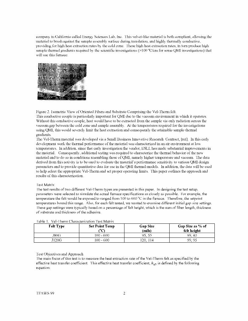
companyinCaliforniacalledEnergySciencesLab,Inc.Thisvelvet-likematerialisbothcompliant,allowingthematerialtobrushagainstthesampleassemblysurfaceduringtranslation,andhighlythermallyconductive,providingforhighheatextractionratesbythecoldzone.Thesehighheatextractionrates,inturnproducehighsamplethermalgradientsrequiredbythescientificinvestigations(>100°C/cmforsomeQMIinvestigations)thatwillusethisfurnace.

iii!iiiii _i). ?

ii_ii...... ".: ,:i_ii_i=_[iiiiii?i!i!i_ililili_il)i:i!

Figure 2. Isometric View of Oriented Fibers and Substrate Comprising the Vel-Therm felt.

This conductive couple is particularly important for QMI due to the vacuum environment in which it operates.

Without this conductive couple, heat would have to be extracted from the sample via only radiation across the

vacuum gap between the cold zone and sample assembly. At the temperatures required for the investigations

using QMI, this would severely limit the heat extraction and consequently the attainable sample thermal

gradients.

The Vel-Therm material was developed via a Small Business Innovative Research Contract, [ref]. In this early

development work the thermal performance of the material was characterized in an air environment at low

temperatures. In addition, since that early investigation the vendor, ESLI, has made substantial improvements in

the material. Consequently, additional testing was required to characterize the thermal behavior of the new

material and to do so in conditions resembling those of QMI, namely higher temperature and vacuum. The data

derived from this activity is to be used to evaluate the material's performance sensitivity to various QMI design

parameters and to provide quantitative data for use in the QMI thermal models. In addition, the data will be used

to help select the appropriate Vel-Therm and set proper operating limits. This paper outlines the approach and

results of this characterization.

Test Matrix

The test results of two different Vel-Therm types are presented in this paper. In designing the test setup,

parameters were selected to simulate the actual furnace specifications as closely as possible. For example, the

temperature the felt would be exposed to ranged from 100 to 600 °C in the furnace. Therefore, the setpoint

temperatures bound this range. Also, for each felt tested, we wanted to examine different initial gap size settings.

These gap settings were typically based on a percentage of felt height, which is the sum of fiber length, thickness

of substrate and thickness of the adhesive.

Table 1. Vel-Therm Characterization Test Matrix

Felt Type

J80G

Set Point Temp(°C)

100 - 600

Gap Size

(mils)95, 55

Gap Size as % of

felt height

99, 40

J120G 100 - 600 120, 114 99, 95

Test Objectives and Approach

The main focus of this test is to measure the heat extraction rate of the Vel-Therm felt as specified by the

effective heat transfer coefficient. This effective heat transfer coefficient, h_d; is defined by the following

equation:

TFAWS 99 2

heft --O-//A(THo,_ Too,d)

Where Q is the heat extracted by cold zone through the felt interface; A is the area of the felt interface; T;qotandTColdare the temperatures of the hot and cold surfaces, respectively, being coupled via the felt. More

importantly, Thor simulates the temperatures seen by the sample assembly and Tcolasimulates the chill blocktemperatures.The primary means of establishing the power being conducted through the felt was to measure the energy

transferred to the water passing through the cold side assembly. Consequently, the effective heat transfer in termsof the measured parameters is given in the following equation.

heft = thCp(T°ut - T_n)A(T>m - Tcozd)

Where fil and Cp are the mass flow rate and the specific heat, respectively, of the cooling water. To,t and Tin arethe outlet and inlet temperatures of the cooling water. A is the surface area over which the Vel-Therm felt isapplied. T_ot is the average temperature of the hot (or heated) surface and TColdis the average temperature of thecold (or cooled) surface. This assumes that the heat lost to the surroundings, either through conduction or

radiation, from the cold surface is negligible. It was assumed, and confirmed via analysis, that each surface wasapproximately isothermal under the specific test conditions.Test Fixture

Again, we wanted to measure the temperature delta across the water as our means of characterizing the heat

transfer performance of the Vel-Therm. Therefore, the test fixture was designed to measure the heat transferredfrom the top surface of the hot side assembly, to the bottom surface of the chill block, which is actively cooled bya helical fluid loop just under the surface. Both the hot side assembly and the chill block are made of copper.

The hot side assembly temperature was targeted to represent those typical of QMI sample assembly and the chillblock was controlled to temperatures typical of the QMI cold zone. The two surfaces are coupled with the Vel-Therm, which is bonded to the chill block surface. The gap between the Hot Side Assembly and the Cold SideAssembly was positioned by a scissor-supported plate, which supports the Cold Side Assembly from above.

_._/Top Base Platef/

Cold Side Mount _ __ _" _

PAN Interface -'_ L-_

_C____S_ Cold Side Assembly

Hot Side Assembly-__

Hot Side ASS.I.Y Support

Bottom Base Plate_

Figure 3. Isometric View of VEL-THERM Test Setup (not to scale)

We also wanted to minimize heat transfer to the chill block in areas other than the Vel-Therm interface.

Therefore, to reduce heat loss from the bottom and sides of the Hot Side Assembly, a 6-layer molybdenum

radiation shield was constructed around the circumference of the Hot Side Assembly. Additionally, the mating

TFAWS 99 3

surfaces of the chill block and hot copper were highly polished in order to minimize radiative coupling between

the two surfaces. Furthermore, aluminized tape was adhered to the chill block's circumference to help prevent

radiative gains in the chill block thereby further reducing inaccuracies in measured heat load.

Lastly, appropriate instrumentation was applied and the whole assembly was housed in a bell jar and vacuum

conditions (P< 10-4mbar) imposed. Temperatures of the test assembly were monitored by twelve Type K

thermocouples. RTD's were used to measure the water inlets and outlet temperatures.

Thermal Model

While some initial thermal analysis was performed via spreadsheet based hand calculations, the bulk detailed

analysis is being performed using PATRAN and P3Thermal. P3Thermal is a geometry-based thermal analysis

tool that uses PATRAN as the geometry modeler and mesh generator. P3Thermal accommodates conductive,

radiative, and convective transfer in solids and also provides capabilities to assess advective heating of the

coolant flow. Details of the PATRAN and P3Thermal are provided in reference 7. The geometric model of the

test apparatus is depicted in Figure 4. The molybdenum shields are not shown so that the hot and cold copper

assemblies may be viewed.

Figure 4. Isometric View of 3D Test Apparatus Test PATRAN/P3THERMAL Model without Radiation Shields.

A number of boundary conditions were applied to the model to simulate the important heat flow paths and

thermal sinks. Using P3Thermal, we were able to use multiple enclosures to capture the radiative exchange andheat loss. The area where the VEL-THERM felt is adhered to the chill block and in contact with the heated

copper has a convection between regions boundary condition imposed. To accurately simulate the heat transfer

to the chill block's helical fluid loop an advective boundary condition was imposed.

The main focus of this on-going analysis is to predict the heater power levels and losses, water cooling rates and

temperatures at key locations throughout the test apparatus. This model was also used to validate the

isothermality of the chill block area where the Vel-Therm is applied.

TFAWS 99 4

Results and Error Assessment

JSOGVeI-Therm Heat Transfer Coefficient

_" 350

._ 300_. 250

=_ 2oo

_- 150

z 100

>

5o

00

I : ..2222L:1_;.:.............

1O0 200 300 400 500 600 700

Hot Side Temperature (°C)

]

...._----,55 mils Gap Setting /195 mils Gap Setting

Figure 5. J80O VEL-THERM Heat Transfer Coefficient vs. Hot Side Surface Temperature

The data for the J80G is presented as a function of the hot side temperature and initial gap size. Data was

recorded at four temperatures, ranging from 100 to 600°C. The cold surface temperature was maintained between

35 and 40°C. In the first run (55 mil gap size), the fibers are bent to conform to a gap size that is almost half of

the fibers' length. It was supposed that increasing the compression could theoretically result in an increase in

effective heat transfer coefficient. As the gap shrinks relative to the fiber length, more of the fiber is bent over.

The result would be increased surface contact between the fiber the hot side surface and possibly increased

contact pressure due to bending the fibers. This increased area and pressure could increase contact conductance.

Results for the 55 mil gap size case, however, were actually lower than the second run which had a larger gap

size, indicating that h might actually increase with an increasing gap size. The 55 mil gap could have been

excessive, damaging some of the fibers.

The gap size for the second run was set to 95 mils such that the fibers were in contact with the hot copper but not

bent to the naked eye. Both cases show significant dependence on temperature. This fact could have arisen from

increased radiation at elevated hot surface temperatures.

The following sets of curves summarize the results obtained for the second VEL-THERM type tested, the J120G.

Figure 6. J80G VEL-THERM Heat Transfer Coefficient vs. Hot Side Surface Temperature

J120G Vel Therm Heat Transfer Coefficient

300

250

200

- 1oo I*6

50LLI

0

0

__l.._ _°_

100 200 300 400 500

Hot Side Temperature (°C)

]

120 mils Gap Setting /

J.....@-----.114 m s Gap Setting

600 700

'FAWS 99 5

Now,wecanseethatthedataindeedshowsatrendindicatingthattheeffectiveheattransfercoefficientincreasesasgapsizeincreases.It isnotintuitivewhythisishappeningandfurthertestingisneededtoinvestigatethistrend.Again,theresultsindicatetemperaturedependence.ComparingthedifferentVel-Thermtypes,theJ80G'sperformanceissuperior.

ErrorAssessmentToprovideanerrorassessment,theheattransfermeasuredacrossthewaterwascomparedtotheheatprovidedbythepowersupply.Attemptsweremadetoquantifytheheatlossfromtheheaterthatoccurredinplacesotherthanthefeltinterface.TheonlysignificantconductionheatpathswerethosefromtheheaterleadsandtheHotSideSupportStructure.Handcalculationsweredonetoquantifytheheatlossinthisarea.TheJ80Gfat600°Crunwaschosenforcomparisonasaworstcasescenario.Comparingthewattagefromthepowersupplytotheqintothewater,theheaterpowerwas119Whigher.Theheattransferdownthetwoheaterleadsaccountedfor27W.Theheattransferdownthefoursupportrodsaccountedforanother30W.TheonlysignificantradiationheattransferwasthatemittedbytheHotSideAssembly.ThetestsetupconfigurationemploysmolybdenumradiationshieldstoinsulatetheHotSideAssembly.Inaddition,thecopperblockencasingtheheaterelementwaspolishedreducingtheemissivityandtheradiativelossesfurther.Radiationfromthehotcopper,supportrodsandshieldswascalculatedusingtheequationforinfiniteconcentric

q12=_Ai_(T__I4- T_24)

[1/gl + 1-g2/g2] (rl/r2)

cylinders. This identified another 19 W of heat loss.

The heater leads were encapsulated with insulation to exclude interference with the base plate. This insulation

provided a heat leak that accounts for 6W. Another possible source of heat loss is into the copper tubing that

connects the fluid loop to the flexible tubing of the water pump. Also, radiation from the exposed portions of the

surfaces of the copper cylinder where the VEL-THERM is applied may contribute. This accounted for

approximately 5 W. This still leaves approximately 30 watts unaccounted for. A possible explanation may be

error associated with the measurement devices, either measuring the water flow or the heater output. The

unidentified heat loss is less than 10% of the calculated heat transfer into the water. This error may relate to the

curve discussed earlier which indicates that heff actually increases as gap size increases. This issue is under

investigation.

In addition to the hand calculations, the modeling effort is on going to investigate this heat loss. The test setup is

well instrumented, therefore, we are looking at temperatures at various locations to find where the energy loss is

occurring. Insights gained from this error assessment will aid in a redesign of the test setup.

Conclusions

Overall, the performance J80G VEL-THERM was in performance, as it had been in the room environment

testing. Also, significant temperature dependence was observed in both Vel-Therm types. The results do seem to

suggest that the effective heat transfer coefficient increases as gap size increases. Therefore, lower compression

rates would be recommended. This trend is not fully understood and will be investigated further. One benefit of

utilizing lower compression rates is decreasing the possibility of damaging the fibers. Another benefit of using

the lower compression rates is avoiding the misalignment problems caused between the interior surface of the

furnace bore and the exterior surface of the SACA during the high processing temperatures when material

properties change and expansion occurs.

A possible explanation of the surprising results is the lack of fiber density control. The fiber packing fraction

would impact performance by affecting the amount of contact area provided. If it varies from one batch to

another more than slightly, the ability to repeat earlier performance is lost. This raises the question of how to

control or test each batch before accepting it into inventory. This is an important area of concern and will require

future work to resolve.

A great deal of work remains to be done to characterize the heat extraction capability of VelTherm. Namely,

resolving the energy balance problem and possibly redesigning the test fixture. Also, examination of the trend

indicating that h increases with gap size, since this is not intuitive.

TFAWS 99 6

ACKNOWLEDGEMENTSTheauthor(s)wishtoacknowledgethecontributionsof PhillipBryant,KevinBurks,MyschaCrouchandDougWestraoftheMarshallSpaceFlightCenter.

REFERENCESQuenchModuleInsertPreliminaryDesignReviewThermalDesignDataBook,NASA-MSFC,TecMasterInc.,SverdrupTech.,Huntsville,A1,March1999FundamentalsofHeatandMassTransfer,SecondEdition,FrankP.Incropera& DavidP.DeWitt,PurdueUniversity,1985ThermophysicalPropertiesofHighTemperatureSolidMaterials,Vol.1:Elements,PurdueUniversity,TheMacMillanComVel-Thermy,NewYorkIntroductiontoThermalAnalysisUsingMSC/THERMAL,PAT312,ExerciseWorkbook,Release7.5,April,1998SatelliteThermalControlHandbook,DavidG.Gilmore,TheAerospaceCorporationPress,E1Segundo,California,1994SampleAmpoule-CartridgeAssemblyForMicrogravityCrystalGrowth,ESLI,SanDiego,CA

TFAWS99 7

Inthispaper,theprocessofphasechangeheattransferisinvestigated.Tosimplifytherepresentationoftheinterfacebetweenphases,astandardphase-qualitybasedmethod(equivalenttoanenthalpymethod)isimplementedtodescribetheenergyconservationprocess.Thisequationdescribesanequivalenceofthetime-rateofchangeofthecontinuousphase-qualityx to the diffusive energy transport via a Laplacian of the continuous temperature field T.

Because of the mixture of terms (x, T), relaxation techniques are usually employed to solve the descretization of the

energy equation for a continuous geometry. In this manner, the quality is solved iteratively and applied to a constitutive

relationship for temperature in order to survey the temperature field and reveal the diffusive heat flow term. In the

present study these equations are extended for implementation of alternating direction implicit (ADI) techniques in a

direct solution with the main goal of decreasing computational wall-clock time. The formulation allows a descretized

model to possess both phase change nodes and solid diffusion nodes, the former defaulting to basic diffusion above and

below the melt point of the material in question. This expands the utility in conjugate heat transfer modelling, e.g. as in

heat exchangers employing phase change materials. In the present study, one set of equations is used to represent all

diffusion nodes. By relating the temperature to the phase quality with two coefficients which adjust as a function ofx

and physical properties, the descretized equations are converted to the form A x = f where x is the phase quality

vector, thus producing the sought-after conversion from a temperature solution to a quality based solution. The equations

are developed for both the 3D splitting and 3D Brian ADI methods. Because the overall heat transfer process involves

transient solidification or melting, the time-space variations in the quality field cause the diagonals of A to change in

time. In this fashion, the tri-diagonal matrix that is extracted from the thermal diffusion network of laterally connected

nodes in a sweep direction must be computed at every time step. This forces and additional LDU decomposition at each

time step. These incremental expenses of an ADI implementation can be significant; however, for the case study

presented, the overall ADI technique is nearly x30 faster than conventional relaxation methods. The current method is

validated against analytical solutions of 2D flat and cylindrical solidification front propagation. A pseudo code is

presented to assist the reader in algorithmic implementation.

NOMENCLATURE

A,B

Ci

hj._

phj._

r

ro

r

t

t

T

AT

linear temperature coefficients

heat capacity, specific to phase for g

latent heat of fusion

specific latent heat of fusion p h fg = log hg - p f h f

radius of solidification front

radius of solidification front, time initial value

radius of solidification front, nondimensional F --F

Fo

heat generation applied to node

time

atime, nondimensional, I -- I for cylindrical geometry and --

2

Fo

temperature

two phase equilibrium temperature

temperature conversion function

AT*

x (n-l), U, V

An

x, Ez

X

(_ vi

a

AX 2I for fiat front geometry

subcooling

ATsubcooling, nondimensional, /_ T* -

Tjg

succession of intermediate states applied in ADI equation splitting en route to solution x (_)

node thickness, n = X,, Y, Z

Cartesian coordinate directions

phase quality, X = 0 implies 100 % phasef X = 1 implies 100 % phase g

volume of node i

GREEK

a

6

effective thermal diffusivity, 19/ --

thickness of solidification front

k, Tjg

P hj_

thickness of solidification front, nondimensional _ --

p density

5

AX

VECTORS AND TENSORS

A tri-diagonal coefficient matrix

fG

q

r

7"

X

p,

forcing vector

conductance tensor

heat flux vector

spatial domain

temperature in spatial domain

phase quality in spatial domain

gradient operator

1. INTRODUCTIONPhasechangeheattransferprocessesarecommoninmanyindustrialapplications.Generallyspeaking_phase-

changeprocessesdonotproceedunconstrained.Rather_ they occur in contact with some solid structure such as a heat

exchanger case or conductive fin. These solid diffusive structures can be thought of a thermal shunt which brings the

boundary conditions to bear on the phase change materials. These diffusive components interact with the phase change

material creating a conjugate heat transfer process - conjugate in the sense that there is a coupling between diffusive-

diffusive and diffusive-phase-change mechanisms. The need for efficient numerical techniques to simulate t]ae conjugate

heat transfer processes has stimulated the development of many models. These are reviewed in [1]. In many cases_ the

complexities of tracking the interface can be collapsed by adopting a homogeneous model and applying a phase quality to

represent the fractional content of a two-phase region. This is more commonly referred to as the enthalw-porosity

method and appears to have established a satisfactory level of acceptance within the thermal community.

There are several forms to the discrete enthalw-porosity equations. The energy equations can be parabolized

with temperature as the primary state_ carrying along phase quality to apply to a logical model to assess the heat capacity

in the field. As the temperature penetrates a narrow bandwidth around the discrete melting point_ the heat capacity of a

control volume is set to near infinite values_ hence emulating the nature of latent energy takeup (e.g. see [2_ 3]). In

another form_ the continuous enthal W field is parabolized and the time-rate of the quality field is carried as a source term_

activated with a Heaviside operator on the quality (e.g. see [4]). These discretized forms are cumbersome to work with

because of the multiplicity of states_ variables and logical elements in assessing thermal properties and switched source

terms for each node. A residual form is usually applied to represent each thermal control volume. The residual describes

an excess energy content of the node_ basically an numerical energy imbalance which is driven to near-zero values

through the application of successive over relaxation (SOR) methods. The functional dependence of the phase change

aspect can be coded quite readily with this approach and tends to reinforce a marriage between enflaalpy-porosity models

and iterative solution methods.

In most instances_ the application of SOR methods for large node-count 3D problems incurs slow transient

solution rates_ and the addition of phase change phenomenon degrades matters worse_ if only through the additional

computations described above. The emergence of direct inversion techniques such as alternating direction implicit (ADI)

methods would appear to be an attractive approach. However_ it is not entirely clear how ADI methods_ which require

the discretized equations in vector form AX = f with a single definitive state x for which to solve_ are to be adopted

to the enthalw-porosity model. Indeed_ relevant studies of ADI adaptations to phase change heat transfer are uncommon

in comparison to ADI treatments of diffusion transport alone. Voller [4] presented a discretized enthal W representation

which was solved with a tri-diagoual matrix algorithm. Voller describes the regeneration ofmatrixA at each time step;

however_ the particular algorithm_ whether splitting_ conventional_ Douglas etc_ was not specified. Mampaey [5]

described a Peachman and Rachford ADI method to predict multidmensional solidification. The temperature field was

parabolized and phase change was modelled by adjusting the specific heat of the melt at the onset of solidification.

Temperature oscillations were observed at the onset of a prediction_ thought to be the effect of extreme temperature

gradients between a melt and a sand casting boundary; this lead to the development of a revised scheme for 3D

simulations which was effective in predicting total solidification times for a casting. More recently Ismail and Goncalves

[1] describe the application of an ADI method to enthalw-based equations to predict the performance of a cylindrical

phase change storage unit. The specific method_ equations and implementation were not presented_ the paper_ instead_

focusing on parametric results.

Rationale and Approach

An ADI implementation to predict phase change heat transfer appears to be practical but within these studies,

the following deficiencies are noted. First, the matrix inversion routine requires a single target state; the selection of this

state, be it phase quality x or other variable, and subsequent modification of the conservation equations is not well

described. Second, the coefficient matrix A will adjust when a thermal node transfigures from a single-phase to a two-

phase and back to a single-phase state; the algorithmic approach to the reconfiguration induced by these regime shifts is

not described systematically. Third, the unconditional solution stability obtained with a diffusionally-designed ADI

method may be compromised by these regime shifts; the extent or existence of this stability degradation has not been

studied. Fourth with the ensemble of ADI methods available, there is little mention of a best method to use. Fifth, a

systematic validation of an ADI-derived phase-change simulation is lacking. Sixth, the motivation for ADI

implementation - computational expedience compared to relaxation methods - has not been established in a practical

application study.

The objectives of the present study echo these. The descretized energy equation is derived in §2 and using a

temperature conversion function derived in §2.1, is converted to a quality-based equation in §2.4. This equation is

adapted to both 3D splitting and 3D Brian ADI methods in §3, further summarized by extracting the tri-diagonals and

forcing coefficients in §3.1. A pseudo-code is presented in §3.2, along with a discussion of regime-shift stability issues

and a suggested approach to recomputation of the coefficient matrixA, the forcing vectorf The solutions derived with

the 3D splitting method is compared to analytical solutions of flat front solidification in both one and two dimensions,

and to a cylindrical two dimensional solidification in §4.1 and §4.2, respectively. The computational performance of the

both ADI methods is compared to a SOR-derived solution of a 3D conjugate heat transfer problem in §5.

2. GOVERNING EQUATIONS

In this paper, the terms control volume and node are synonymous. Each describes a fixed geometric volume, a

Cartesian-based six sided parallel-piped, which exchanges energy with adjoining nodes through Fourier-originated

thermal diffusion. A enthalw-quality method will be adopted to predict the transient energy content in a thermal node.

The primary state will be the phase quality x which will range continuously from negative to positive values. The energy

equation for a node i is written as an equivalence between the substantial derivative of enthalpy, to thermal diffusion and

-q*dA+ gidv= /9 h- dv+ phV.dACS CS

a source heating term:

Neglecting the advection of enthalpy by a velocity field V, kinetic and potential energy changes, and assuming the

material to be incompressible, the energy equation for a node of fixed volume is simplified:

Iqji O dAj At- Si = pi 6vi -

CS] &

where the left side terms read as the total heat flow by diffusion into node i and the source heating. The integration of the

heat flux vector qji over the control surfaces residing about node i can be rewritten as a heat flow into node i:

b'Q,=- SqjiedAjCSj

Next, the enthalpy is referenced to a continuous function of the phase quality and the f-phase enthalpy and latent heat of

fusion:

h= hi + x hi.

where Diand Digare understood to depend on pressure through a coexistence curve. Taking the time-partial derivative

_t _t(hi+xhi.)

and observing the compressiblity constraint:

_x= hfg --

_t

p, hi. 6v, -6Q,+s,_t

which when combined with the heat flow rate and the original expression, yields:

2.1 Temperature Conversion Function

The phase quality is related to temperature through the conversion function 7'(X). To derive this function, a

range of constraints must be observed. The function must return the unique equilibrium melting temperature

T(X) = Tfg for 0 _ x _ 1. Outside this quality range, the function must return subcooled and superheated

hi + C_(T- Ti.)= hi + x hi.

temperatures. In the subcooled region (X % 0 ) the temperature follows the approximation:

h. + C_. (T - T i.) = hi + x hi.

and in the superheated region ( X > 1):

which upon combining and inverting yields the following linear relationship:

T (x, i) = Ai x + Bi

Ai z

(x < 0"hjg

CPi

0 O<x<l

x>l

j

Bi z

hfgTfg -m

Cp_

x<O

x>l

)

for which the coefficients are defined:

Coefficients A and B are subscripted with the node index number, indicating they are unique for each node. These vary

in two ways. First, a model may possess different phase change materials; each node may be associated with a different

set of phase change properties Tfg, hfg, Cp s , Cp_ 1. Second, during the course of a thermal simulation, the quality

field will evolve naturally and A and B will change from node to node, reflected by the composite nature of the function.

2.2 Diffusion Term

The thermal diffusion between adjoining nodes is specified by a thermal conductance, itself determined by

thermal conductivity of the material in question and the geometry of the two nodes. As described in Appendix A, the

conductance between two adjoining nodes is determined by the geometric mean of the respective half-node conductances,

enabling nodes of dissimilar thermal conductivity to be modelled. The heat flux vector is determined by a product of a

conductance tensor G (made up of these values) and a unit vector, either +ex, +ey, +ez, proportional to the temperature

difference between respective nodes:

1Because both phase-change and conventional diffusion nodes can be grouped and solved together, the ADI solution requires that each

node have a defined set of phase change properties. For conventional diffusion nodes, these properties are meaningless, basically reflecting the fact

that the phase change process is out of reach of the temperature penetrating the node. In this case, the values Tfg, hfg, Cp i , Cpx can be

set to 1. Practical experience show-s that this has no effect on the solution.

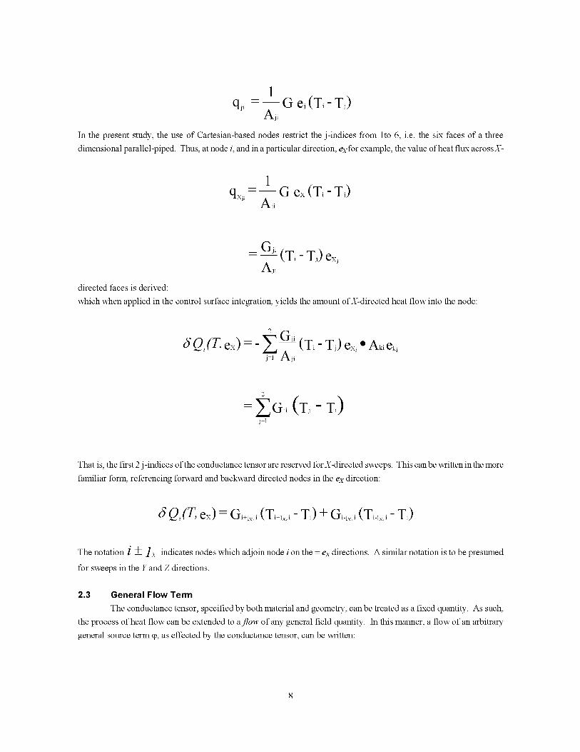
1qji - G ej (Ti- Tj)

aji

In the present study, the use of Cartesian-based nodes restrict the j-indices from lto 6, i.e. the six faces of a three

dimensional parallel-piped. Thus, at node i, and in a particular direction, exfor example, the value of heat flux acrossX-

1q×j,- G ex (Ti- Tj)

Aji

_ Gji (Ti- Tj) e×jAji

directed faces is derived:

which when applied in the control surface integration, yields the amount of X-directed heat flow into the node:

aQi(T, e×) =- (Zi - Zj) exj • Aki ekj

2

= Eaji (Zj -- Zi)

j=l

That is, the first 2 j-indices of the conductance tensor are reserved forX-directed sweeps. This can be written in the more

familiar form, referencing forward and backward directed nodes in the ex direction:

Qi(T, e×) = Gi+l×,i (Ti+l×,i - Ti) q- Gi_l×,i (Ti_l×,i - Ti)

The notation i -}- 1x indicates nodes which adjoin node i on the 4- ex directions. A similar notation is to be presumed

for sweeps in the Y and Z directions.

2.a General Flow Term

The conductance tensor, specified by both material and geometry, can be treated as a fixed quantity. As such,

the process of heat flow can be extended to aflow of any general field quantity. In this manner, a flow of an arbitrary

general source term % as effected by the conductance tensor, can be written:

2 4

_Qi(_, en) = ex'en _aji (_j - _i) + eY'en _aji

j=l j=3

6

(_j -- _i) + ez" en E;

j<;

That is, field property q_induces a net flow into node i, in the en direction. As presented below, this convention will

allow the basic ADI equations to be streamlined and simplified for the various methods. As described below, the flow

termwill operate onthe temperature coefficients A, B. Thus, flowterms willbe presented in the form _ Qi(B, ex)

which read as the flow caused by the coefficient B, affected and controlled by the conductance tensor, directed in the ex

direction. The form of these terms and there operative direction depend ultimately on the sweep direction and the

specific ADI method.

2.4 Discretized Quality Equation

Upon collecting the above equations, the final form of the discrete energy equation at node i is given by the

following:

P, hx. 6 v,- -_t

- 6Q,(T,e×)+ _Qi(T, ey) + _Qi(T, ez) + Si

As discussed above, this equation is a function of both T and x, not of a form suitable for the ADI implementation. By

referencing heat flow terms through the temperature conversion function, this equation can be rewritten:

P, hi. 6 v, c_x, _ 6 Q,(T(x), e×) + c_Qsubi(T(x), eY) + 6 Qi (r(x), e_) + Si?t

with the phase quality now appearing throughout the left and right hand sides. Because the diffusion function _Qi is a

linear operator, the conversion to a quality-based equation is made by combining this equation with the linear temperature

conversion function (9):

p, hxgcYv, - 6Q,(A,x,,e×.eY.e_)+ 6Qi(Bi.e×.e_.e_)+_3ic_t

While the coefficients A, B themselves depend on the quality state, the goal of isolating a single target state is achieved

with this equation. It is this basic equation which will be adapted to the various methods.

3. ADI IMPLEMENTATION

The basic ADI equations are adapted from the Chang et al. [6] paper which describes the splitting and Brian

ADI methods (in addition to conventional, Douglas and modified splitting methods). In the following equations, as

identified in the nomenclature, three successive ADI sweep levels operate on the intermediate quality states,

(n-l)X ,/_jr V, en route to the solution of the future-time quality, x (").

AtSplitting Method: The splitting method operates on time levels offset by-- . In Equation 19, the source

3

term is combined with the diffusive transport of the B coefficient. The diffusive transport of the quality term is then split

into respective X,, Y, Z components creating the three implicit equations:

(X - Sweep) Pi hjg 6 vi(n-I)

U_ - x_

At

3

3 6.Q_(A_U. ex)=6.Qi(Bi,ex,eY,ez)+_;i

(Y-Sweep) /3i h_ 6 Vi --

Vi - Ui

At

3

3 6.Qi(Ai Vi, eY) = 6.Qi(Bi, ex, eY, ez) + Si

(Z - Sweep) Pi hfgb"Vi

(n)Xi - Vi

At

3

3 6. Qi(Ai Vi, ez) = 6. Qi(Bi, ex, eY, ez) + Si

AtBrian Method: The Brian method operates on levels of --. As opposed to splitting the diffusion of the

2

quality, the Brian method applies the intermediate quality states in the following manner:

10

(X - Sweep) Pi hjg 6 vi(n-I)U_ - x_

At

2

5Q_(A_U.e×)=SQi(Ai (n-l_Xi , eY, e2

(Y - Sweep) Pi hf_6 vi

(n-l)gi - xi

At

2

-_Qi(Ai Vi, e,:)= _ Qi(Ai Ui, ex) q- _Qi(Ai

(n)

(Z - Sweep) Pi hfg6 vi xi - ViAt

2

_ Qi (Ai xi(n), ez) = _Qi(Ai Ui, ex) _1_ _Qi( A

3.1 Coefficient Extraction

A general tri-diagonal sweep equation can be extracted from each of these sweep equations:

b,_,_,_,+a,_,_,+ci_,_,+,= f, forn=X, KZ

where g represents either U, V,,x (n),respective toX, Y, Z sweep directions. Table 1 summarizes the coefficient extraction

ofA andf for each sweep direction, method-specific. The convention ()Lr reads, the coefficient value O at node i, in

sweep directionX. Similarly, the indexing notation i-lx reads as the west-facing node connecting node i, while i-lr reads

as the south-facing node connecting node i, and so forth.

Method

- 3 G_-;x,__ - 3 Gi+;x,_pSw h_g,+ 3 A_(G__;.

At�3

PSwh_, + 3 Ai(G__;_.At�3

pSv_h_, + 3 A_(G__;_.At�3

-3 Gi+;.

-3Gi+lz.i

P6 w h_, (n-l) 2Si + x_ +3At�3 1

• Si +

p6 w h_,At/3 Ui + 3 _C

1

p6 v, h_gAt/3 ' V, + 3 _G

1

11

I I I I

- Gilx,i Ai

- Gil_,iAi

- Gilz,i Ai

p6v_h_, + A_(G___,_At�2

p6v_ h_, + A_(G___,__At�2

- G_+_,_A_

P6w h_, + A_(G___,__At�2

- G_+_,_A_

- Gi+lz,iAi

p6 w h_, (_-_)x_ + _-'_G

At�26

(_-1)

3

6

At�2 x_ + ,

2

1

6

+ -5

6

pd w h_, _-'GslAt�2 V, + ,

2

1

4

3

Table 1. Summary of coefficient extraction for general sweep matrix equation.

12

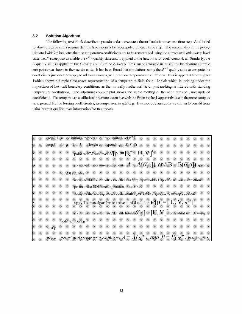
3.2 Solution Algorithm

The following text block describes a pseudo code to execute a thermal solution over one time step. As alluded

to above, regime shifts require that the tri-diagonals be recomputed on each time step. The second step in the p-loop

(denoted with _) indicates that the temperature coefficients are to be recomputed using the current available sweep level

state, i.e. X-sweep has available the x (n-v quality state and is applied to the functions for coefficientsA, B. Similarly, the

U quality state is applied in the Y-sweep and Vfor the Z-sweep. This can be arranged in the coding by creating a simple

sub-pointer as shown in the pseudo code. It has been found that simulations using the x (n-v quality state to compute the

coefficients just once, to apply to all three sweeps, will produce temperature oscillations. This is apparent from Figure

lwhich shows a simple time-space representation of a temperature field for a 1D slab which is melting under the

imposition of hot wall boundary conditions, as the normally isothermal field, post melting, is littered with standing

temperature oscillations. The adjoining contour plot shows the stable melting of the solid derived using updated

coefficients. The temperature oscillations are more extensive with the Brian mefllod, apparently due to the more complex

arrangement for the forcing coefficientsfi in comparison to splitting. Even so, both methods are shown to benefit from

using current quality level information for the update.

66mP i6temp aiur ) ffii6 ti A{O[p])and B BfO[p])i ifi)f6_i sub{ eve {

rnp )f 0 ihe fo __i_ _ve _ __ ffie ient _f )_ _N O!_ )e _ifi _i _we 0pair 0_i

pply T hpmaS a!gp_it _ive_ AI)_lutm _[p] X ]

6a_numb_iSg

13

4. VALIDATION of ADI METHOD

The ADI phase change model is validated by comparing the numerical simulation to an analytical solution of

freezing fronts in two simple geometries. Table 2 presents the details for the numerical-analytical model comparisons.

The analytical models are derived by simplifying the transient solidification-diffusion process by assuming a non-

capacitvie diffusion process across the accumulating solidified region. Under these conditions, a control volume

formulation can be applied to predict the time-dependent size of the solidification region as a function of an effective

thermal diffusivity a and the subcooled temperature of the boundary. As derived in Appendix B, the transient

* *d = AT*t

propagation of the flat and a cylindrical solidification fronts is determined, respectively:

1 ln(r*) 1(/2 1)=AT.t.-ffF - -

solidification front: geometry and thermal physical

properties

material water

h>i_ 333.7 x 10 a J/kg K

C 4220J/kg K •

k>; kg 0.566 W/m C •

T>i: 273.15 K

p 1000 kg/m 3

• both phases set equal for comparison to analytical model

- note this is for convenience only and not required by the

method

numerical simulation model

/_/_y node size 1 cm

At 2000 s

t>- 5x10 5

x(r, O) initial quality field set to 1.0, corresponding to

saturated liquid

T(r, O) initial temperature field set to 273.15 K

T(O, 0 cold wall boundary temperature maintained at

AT = 10 °C below Te,

x_,t node represents solidification front when

xi<0.5

ADI scheme 3D splitting method applied in respective 2D

domains, Z-direction split included in solution

Table 2. Description of parameters applied in numerical prediction of solidification front and

comparisons to analytical models.

14

4.1 Flat-Front Solidification

The flat-front geometries applied in the simulation are depicted in Figure 2. The fundamental geometry is a one-

dimensional mesh. A two-dimensional variation is created by rotating the 1D mesh by 45 degrees. Figure 3 presents a

comparison of the ADI-numerical and analytical solutions for these model variants. The linear 1D and rotated 2D node

configurations should yield the identical numerical prediction of the advance of the solidification front. However, the

rotated mesh invokes diffusion in both directions, testing the solutions of the intermediate quality states at the time levels

t +/-At, t + X-At. asshown, the results compare to within 5 percent ofthe flat front analytical solution. The

3 3

numerical predictions fall below the predictive line, suggested to result from including finite capacitance in the

solidifying regions in the numerical model which retards the discharge of the energy accumulated in the solid to the cold

wall boundary condition. Equivalently speaking, the analytical model predicts a higher propagation rate because

capacitance in the solid phase is nullified. The quality field for the rotated slab is presented in Figure 4. The adiabatic

edges of the slab model and notched descretization creates a slight disturbance which causes the solidification front,

expectantly flat, to exhibit a slight curvature near the adiabatic boundaries.

4.2 Cylindrical-Front Solidification

The cylindrical front simulation is performed by approximating a cylinder with a select number of Cartesian

nodes. Figure 5 illustrates the Cartesian node geometry applied to the vary node densities. The corresponding predictive

comparison is presented in Figure 6. As shown, the ADI model predicts the position of the solidification front to within 5

percent, despite the apparently crude descretization of the initial cylinder forming the cold wall boundary condition.

In contrast to retardation of the growth for the flat front (owed to neglect of capacitance in the analytical model),

the cylindrical front data lie above the predictive line and are explained on the basis of the conversion of the descrete

field problem from a linear to a cylindrical geometry with increasing node density. Basically, in the limit of one center

node, the numerical model nearly represents a flat front solidification, however, not exactly because diffusion still occurs

in bothX, Y directions. With increasing node density, the quasi-flat front solidification is incrementally converted to a

cylindrical expanse. With this incremental conversion, the data form increasingly better comparisons with the analytical

predictions. Eventually, at some point, the capacitive terms retained in the numerical prediction tend to offset this aspect

as is the case in the flat front prediction. The quality field is presented in Figure 7, displaying a sharp transition from

solid to liquid across the solidification front and showing the expected circular expanse of solidification.

5. APPLICATION STUDY

Figure 8 illustrates the geometry applied in this conjugate problem, which consists of an aluminum-cased phase

change module (PCM) which is coupled between a simulated electronics heat source and a temperature boundary

condition. The boundary condition varies sinusoidally from +10 °C above and below the melting point of 0 °C with a

period of 10 seconds. The simulated electronics apply a total of 9 Watts over the 9 nodes. A quarter-symmetry section is

modeled with each node described by a cube, measuring 2 mm on edge. Figure 9 describes the evolution of wall clock

time versus the simulation time. The wall clock time is normalized using the end-value of wall clock time measured with

the ADI-Brian method in order to offer results of a general nature which are to an extent, independent of processor speed

and coding techniques. The ADI simulation proceeds at about a factor of x30 faster than the SOR-derived solution.

Figure 10 shows the time-temperature trace of several points in the solution domain and also the temperature field at time

t = 100 s, derive with the ADI-Brian method. These results indicate the computational savings offset the expense of

recomputing A andfby a significant factor.

15

16

6. CONCLUSION

The present study presents an adaptation of the splitting and Brian ADI methods to effect a direct solution oft_e

quality-based conservation equations to predict phase change heat transfer. It has been shown that the equations can be

constructed with a single target state. The application of a temperature conversion function allows both conventional

diffusion nodes and phase change nodes to be mixed in a simulation with no special considerations or restrictions. The

method appears to be numerically stable for 3D simulations, compares well with analytical solutions and is significantly

faster than conventional relaxation methods. The incremental expenses introduced by the quality representation, i.e.

matrix recomputation, LDU decomposition, can be readily forfeited given a near two order of magnitude increase in

algorithmic speed obtained with the new method.

REFERENCES

Ismail, K. A. R., and Goncalves, M. M., _Thermal Performance of a PCM Storage Unit," Energf Conversion

and Management, Vol. 40, pp 115-138, 1999.

Runnels S. R., and Cary, G. F., _¢Finite Element Simulation of Phase Change Using Capacitance Methods,"

NumericalHeat Transfer, PartB, Vol. 19, pp 13-30, 1991.

Busko, W., and Gross, I. R., _¢New Finite Element Method for Multidimensional Phase Change Heat Transfer

Problems," Numerical Heat Transfer, Part B, Vol. 19, pp 31-48, 1991.

Voller, V. R., _¢Fast Implicit Finite-Difference Methods for the Analysis of Phase Change Problems," Numerical

Heat Transfer, PartB, Vol. 17, pp 155-169, 1990.

Mampaey, F., _A Stable Alternating Direction Method for Simulating Multi-Dimensional Solidification

Problems," International Journal for Numerical Methods in Engineering, Vol. 30, pp 711-728, 1990.

Chang, M. J., Chow, L. C., and Chang, W. S., _Improved Alternating-Direction Implicit Method for Solving

Transient Three Dimensionional Diffusion Problems, _ NumericalHeat Transfer, PartB, Vol. 19, pp 69-84,

1991.

17

Appendix A

Determination of Thermal Conductance Values

From Figure B. 1, the thermal conductance between two nodes is determined by the following half-node

ki Ayz

Gi,i+_o- c_xi

2

conductance values:

The half-node conductance values for any two connecting nodes are combined in a geometric average to represent the

overall thermal conductance between nodes:

G2,1 z

1

1 1

Gl, l+%o GZ2-%o

18

Appendix B

Analytical Model of Propagation of Solidification Front

In this analysis, a transient control volume is used to capture the energy conservation of an expanding

solidification front. As illustrated in Figure B. 1, the control volume encompasses and expands with the solidified region.

c_,I-q'dA=ac! /P)-/?t I/9 h- dv+ phV.dA

CS

The energy equation can be expressed as:

For simplification the following constraints and stipulations are placed: the density is constant across the two phases; the

substances are incompressible; the capacitance of the accumulating solid phase is neglected in the time-partial integral.

Because the control volume contains the entire solid region, the enthalpy flux is determined by the portion of the liquid

IphV,dA:-phgA(t)_CS

phase advecting into the surface:

The energy equation can be simplified applying a Fourier term for the heat flux vector:

As shown below, the final solution to the cylindrical front degenerates to the flat front when the initial radius is made very

large. Exploiting this generality, the analysis will proceed specific to the cylindrical geometry to avoid the redundant

- H 2 zcr ?at

analysis. The time-partial of volume can be simplified:

kj AT(r --_ ro) 2 _ ro = p hjg 2 _ r?

which when combined with the energy equation, produces the following ODE:

Prior to separating and integrating this equation, the temperature gradient at ro, i.e. the gradient imposed by the

cold wall boundary condition. As stipulated that the solid or f-phase is non-capacitive, the temperature distribution

throughout the solid must be conducive to preserving the total heat flow through the differential rings which comprise the

cylinder. A simple analysis will show that the contraction of the the cross sectional area nearing the inner cold wall

cylinderforcesthetemperatureprofileto followa logarithmicdistributionoftheformT(r) = m ln(r) b.+

Applying the two boundary conditions across the extent of the solid phase yields two equations which with to solve for m

and b:

19

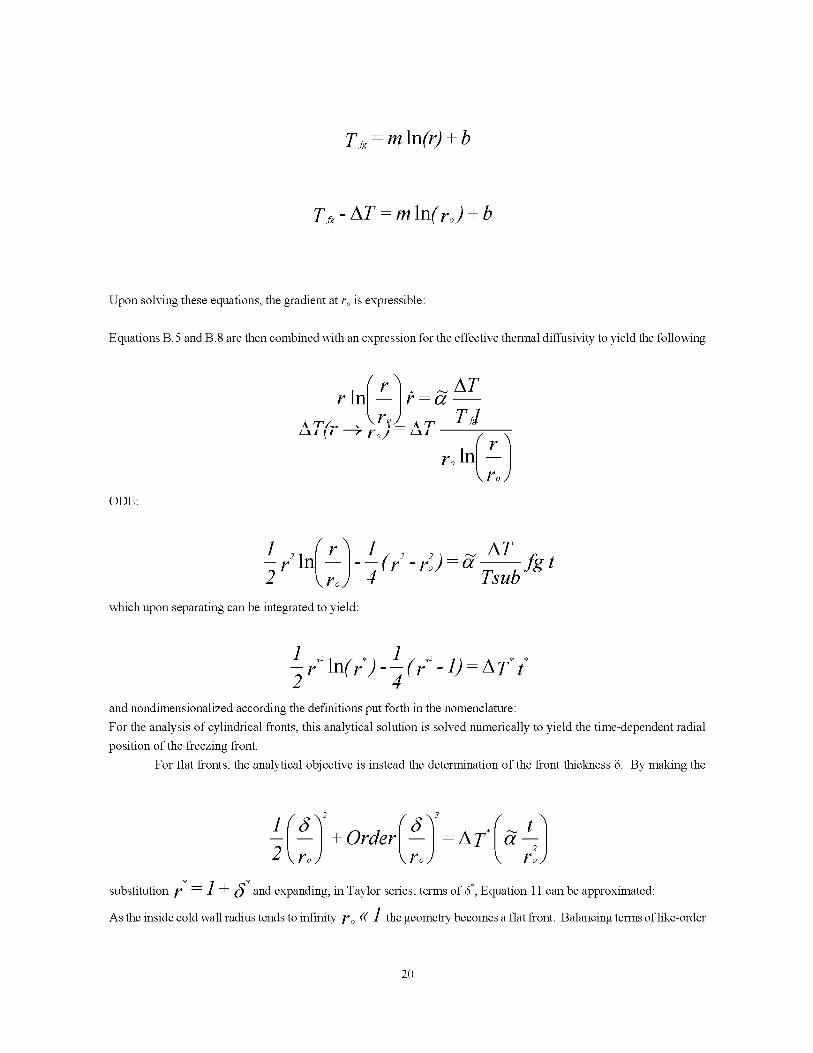
Ti_ = m ln(r) + b

Ti_-AT=mln(ro)+b

Upon solving these equations, the gradient at ro is expressible:

Equations B. 5 and B. 8 are then combined with an expression for the effective thermal diffusivity to yield the following

ODE:

ATr In/r/_ =

AT�_ . _ J\r_±AT Tit_1 If --7 Yo,I -- _1 ro'n(rl

\ro/

7 roj--4(/-r ):eTT-db fxtwhich upon separating can be integrated to yield:

l .2 l t*_r ln(r*)-_(r*2-1)=AT *

and nondimensionalized according the definitions put forth in the nomenclature:

For the analysis of cylindrical fronts, this analytical solution is solved numerically to yield the time-dependent radial

position of the freezing front.

For flat fronts, the analytical objective is instead the determination of the front thickness 8. By making the

+Order =AT* _ t

substitution F -- 1 + ¢_*-- and expanding, in Taylor series, terms of 8*, Equation 11 can be approximated:

As the inside cold wall radius tends to infinity Fo (( 1 the geometry becomes a flat front. Balancing terms of like-order

2O

requires that ¢2_

6_/2_AT*t

N_- and the front thickness 8 can therefore be approximated:

21

The flat front solution (in the absence of a convection boundary condition) lacks a characteristic length scale

suitable for the nondimensionalization. Thus, in the flat front simulations and data comparisons, the removal of length

solution with A B coefficients derived

with current sweep level pointer e[p]A

A = A (e[p])A

B = B (e[p])

,[time

I

solution with A B coefficients derived

with first sweep level pointer 1t[1]

A = A (x (n-l))t,.

B = B (x (n-1) )

produces spatial temperature variations-- which emanate from front and rebound

\\, continuously off boundaries\

\,\

2 outer boundaries maintained atsuper-melt temperatures

//

/

1 D Slab initially //

at melt temperature T fg

and time units is affected by applying the discrete node thickness AN- used in the simulation, producing the following

expression:

18

Tfg ......................................i

T C ATsc

solid phase liquid phase

_- interface

_iiiiiiiiiiiiiiiiiiiiiiiiiiiiiiiiii)_

slab (1D): solidification front propogates in

e x direction only

slab (1 D) rotated (45 degrees) creates 2D

grid, solidification front propogates in e x and

e y directions

]9

20

quality x

-0.13 0.01 0.15 0.29 0.43 0.58 0.72 0.86 1

21

iiiiiiiiiiiiiiiiiii ',:::::::::::::::::::

......... //

/ iiiiiiiiiiiiiiiiii_iiiiiiiiiiiiiiiiiiii_iiiiiiiiiiiiiiiiiiiii_iiiiiiiiiiiiiiiiiiiiIiiiiiiiiiiiiiiiiiiii_k

1.5.An

.....iiiiiiiiiiiiiiiiiiIiiiiiiiiiiiiiiiiiii1iiiiiiiiiiiiiiiiiiiii_iiiiiiiiiiiiiiiiiiiiIiiiiiiiiiiiiiiiiiiii_/

..........iiiiiiiiiiiiiiiiiiliiiiiiiiiiiiiiiiiiiiliiiiiiiiiiiiiiiiiiiF__"

3.5-An

....._iTiiiTiiTil_iiiiiiiiiiiiiiiiiiTl_TiiTiiTiii_"iiiiiiiiiiiii iiiiiiiiiiiiiiiiii iiiiiiiiiiiiiiiiiii iiiiiiiiiiiiiiiiiii iiiiiiiiiiiiiiiiii iiiiiiiiiiiiiiiiiii ::::::::::::::::::_

___!iiiiiiiiiiiiiii!iiiiiiiiiiiiiiiiiiii!iiiiiiiiiiiiiiiiiiii!iiiiiiiiiiiiiiiiiiiii!iiiiiiiiiiiiiiiiiiii!iiiiiiiiiiiiiiiiiiii!iiiiiiiiiiiiiiiiiiii!iiiiiiiiiiiiiiiiiiiii!iiiiiiiiiiiiii!!

_.:+:+:+:+ :+:+:+:<+ +:+:+:+:+:+:+:+:+:< :+:+:+:<+ +:+:+:+:+:+:+:+:+-

::::::::::::::::::::::::::::::::::::::::i:::::::::::::::::::

.........iiiiiiiiiiiiiiiiiiiliiiiiiiiiiiiiiiiiiiiliiiiiiiiiiiiiiiiiii............._ii!i_i_i_ii i_i_i_i_i_i_i_i_i_iii_ii_i_!i_ii¸

4.5"An

22

23

quality x

_iI_I_iliiiiiiiiiiiiiiiiiiiiiiiiiii:.iii:.iiilli:iiiiiiiiiiiiiiiiiii_iiiiiiiiiiiiiiiiiiiiiiii!iiiii!iii!!!i!_!iiiiiiiiiiiiiiiiiiiiiiiiiiiiiiii_iiiiiii_!iiiiii_iiiii!_iiiiiiiiiiiiiiiiiiiiiiiiiiiiiiiii_

-0.13 0.01 0.15 0.29 0.43 0.58 0.72 0.86 1

24

iiiiiiiiiiiiiiiiiiiiiiiiiiiiiiiiiiiiiiiiii

iiiiiiiiiiiiiiiiiiiiiiiiiiiiiiiiiiiiiiiiiiiiiiiiiiiiiiiiiiiiiiiiiiiiiiiiiiiiiiiiiiiiiiiiiiiiiiiiiiiiiiiiiiiiiiiiiiiiiiiiiiiiiiiiiiiiiiiiiiiiiiiiiiiiiiiiiiiiiiiiiiiiiiii

[] Heater Nodes

l_[ 9 W total

[] Aluminum Casing Nodes[] Phase Change Nodes

[] Boundary (T) Nodes

Phase Change Nodes

k = 1.080 W/m C

p = 1000 kg/m3C = 1000 J/kgC

Tfg = 273.15 K

h fg = 70.26E3 J/kg

25

t wall clock

t extent ADI

nominal x30 faster100]

58

30 ...........................

28 _ . ...............................................

1.0 .....................

5 ...."" ....

3 ........

2

• 5 ,_' ........................................................

.2 ..- ........... "

.1 _.-"" "

.05 .' .....

.03 ."

.02 .S

• 0051

• 003_

•88=1• 881/

SORAt = 0.5

ADI- BrianAt = O.5

t Local Simulation (s)

26

t = 100

290

280

iiiii_i_i_iiiiiiiii_i_i_i_iiiiiii_i_i_i_iiiiiiiii_iiiiiiiiiiiiiiiiiiiiiiiiiii!j_i_#_....._._

_i!iiiiiiiii!i_i!ii;iiiiiiii,ili,iiiiiii_i_i_i_iiiiiiiiiiiiiiiiiiiiiiiiiIII_

__x%.`_ii_iiiIIiiiiiiiiiiiiiiiiiiiiiiiiiiiiiiiiiiiiiiiiiiiiiiiiiiiiiiiiiiiiiiiiiiiiiiiii?iiiii_i_iii_iiiiiii!!!!!}_i_

.iII_[_i.i.i.i.i.i.i.i.i.i.i.i.i.i.i.i.i.i.i.i.i.i.i.i.i.i.i.i.i.i._iiiiii;iii_iiiiiiiiiiiiiigiii_i.i_iiIIiii_iiiiiiiiiiiiiiiiiiiiiiiiiiiiiiiiiiiiiiiiiiiiiiiiiiiiiiiiiiiiiiiiiiiiiiii_i_i_iiiiiiiiiiiiiiiiiiiii_ii_

ii_iiM_i_iiiii-iiiiii_i_i_iiii_i_iiiiiiiiiiiiiii

I I I I

/z¢

570/ i,''v

260 I I0 20 40

,,I60 go

time (s)

2?

r(t)

ro

Iconduction into cold wall

i enthalpy flux at interface

-- I, I t I/Z

28

REUSABLE SOLID ROCKET MOTOR NOZZLE JOINT -4

THERMAL ANALYSIS

J. Louie Clayton

National Aeronautics and Space Administration

Marshall Space Flight Center

Huntsville, Alabama

Abstract

This study provides for development and test

verification of a thermal model used for prediction

of joint heating environments, structural

temperatures and seal erosions in the Space

Shuttle Reusable Solid Rocket Motor (RSRM)

Nozzle Joint-4. The heating environments are a

result of rapid pressurization of the joint free

volume assuming a leak path has occurred in the

filler material used for assembly gap close out.

Combustion gasses flow along the leak path from

nozzle environment to joint O-ring gland resulting

in local heating to the metal housing and erosion

of seal materials. Analysis of this condition was

based on usage of the NASA Joint Pressurization

Routine (JPR) for environment determination and

the Systems Improved Numerical Differencing

Analyzer (S1NDA) for structural temperature

prediction. Model generated temperatures,

pressures and seal erosions are compared to hot

fire test data for several different leak path

situations. Investigated in the hot fire test

program were nozzle joint-4 O-ring erosion

sensitivities to leak path width in both open and

confined joint geometries. Model predictions

were in generally good agreement with the test

data for the confined leak path cases. Worst case

flight predictions are provided using the test-

calibrated model. Analysis issues are discussed

based on model calibration procedures.

List of Symbols

A normal surface area

C specific heat

D passage hydraulic

e Euler constant

f Moody friction factor

gc gravitational constanth convection film coefficient

H enthalpy

L flow path length

M molecular weight

m mass

p pressure

Q heat rate

R gas constant

T temperature

U internal energyt time

V volume

W work

Greek

A difference operator

Subscripts

g gasi inlet

o outlet

p constant pressurew wall

v constant volume

Summars!

First, an overview of the RSRM nozzle

joint-4 configuration and process history will be

presented. JPR 1 methodology fundamentals are

covered next by providing a cursory look at

governing equations and modeling techniques

used for computation of heating environments.

Incorporation with S1NDA 2 as a finite element

thermal solver is briefly discussed. Results ofmodel calibration with data obtained from test

program "ETP-1385 Joint-4 Hot Gas Test" 3 are

discussed. Finally, the test calibrated joint-4

model will be used for prediction of worst case

flight results using nozzle joint-4 boundary

conditions and current gland geometry. In

closing analysis issues, results and conclusions

are presented.

Introduction

Nozzle Joint-4 Information

RSRM Nozzle Joint-4, Fig. 1, is located aft

of the throat in the supersonic region of thenozzle. Liner materials at this location are a

carbon phenolic ablator backed by glass phenolic

insulator, which is secondarily bonded to a steel

housing. Operational environments are estimated

to be -150 psia static pressure at a local recovery

temperature of-5100°R. The primary O-ring is a

face seal housed in a glass phenolic gland and the

opposing sealing surface is the aft end of the steel

throat assembly. The joint-4 secondary O-ring is

a bore seal and contained entirely in the aft end of

the throat housing structure.

Contributions to joint free volume come

from the primary and secondary gland, the

chamfer region and assembly gaps in the liner

materials. After the housings are bolted together,

the assembly gaps are back-filled with room

temperature vulcanizing silicon (RTV). The RTV

is injected radially penetrating the length of the

assembly gap typically with depth irregularities

adjacent to the primary O-ring gland. Post-flight

observation of typical RTV penetration depths has

allowed for an average assembly gap volumecontribution to be estimated at -0.5 in 3. Nominal

primary gland volume is -2.2 in 3, chamfer region

is estimated at 5.5 in 3 and secondary gland has a

nominal volume of -4.2 in 3. As an assembly aid

HD-2 grease is applied to mating surfaces and has

the effect of a volume filler. Based on the post-

flight data, about one cubic inch of grease

typically occupies joint volume. Accounting for

all individual contributions, total joint-4 freevolume on a nominal basis is about 11.4 in 3 .

Carbon Cloth

Phenolic

Glass Cloth Throat Inlet

Phenolic Assembly

Forward Exit Cone

- Assembly

Secondary

O-ring

Fig. 1. RSRM Nozzle Joint-4 Cross Section

Nozzle Joint Back-Fill Process

There are two ways of dealing with

assembly gaps that can potentially communicate

motor environments with joint sealing surfaces.

The first is to vent the joint. No back-fill

materials are used in the gaps. Pressurization of

the primary gland is rapid and heating to the

sealing surfaces a result of compression of the

gases at the stagnation point. This design is used

in many solid rocket motor joints with perhaps

addition of a permeable "slag barrier" to trap hot

particulate matter. The second method fills the

assembly gaps with a "filler" material, which is

the process used in the RSRM program. Early in

the motor program, application of RTV was a

one-step procedure involving radial injection into

the assembly gap. The procedure had the

characteristic of producing "tail voids" at the

circumferential location where the injection

process began. It was determined voids were a

result of the close- out phase of the back-fill

process. When the injection process clocked 360

degrees and was "closing-out", air was being

trapped and compressed. Over time the trapped

air would work its way out of the joint through

the uncured RTV. Tail voids are formed

extending from gland inboard to flame surface.

If the void terminates before it reaches the free

surface, it has potential for being exposed during

motor operation. For this scenario, a confined

leak path pressurizes the primary gland usually

resulting in local heat affects and seal erosion.

This specific anomaly happened in nozzle joint-3

of motor flight sets 44 and 45 where minor

amounts of primary seal erosion occurred.

Programmatic evolution of the back-fill

process has led to qualification of a two-step

procedure. The joint gaps are filled, partially

excavated, and then re-filled. Due to the

geometry involved in joint-4, the excavation (a

digging process) is performed to the first turn.

The excavated portion of the gap is then re-filled

with RTV. A vacuum close-out procedure is

used to minimize trapped air. This process

change transpired on RSRM-48 nozzle flight set

and since that time, there has been no evidence

of gas penetration into the joints as a result of atail void.

A problem with the current procedure is that

excavation can only be performed in the first leg

to the inflection point. If a void exists in the

second leg of the assembly gap, there is a finite

chance of exposure resulting in a confined jet

pressurization of the primary gland. Based on

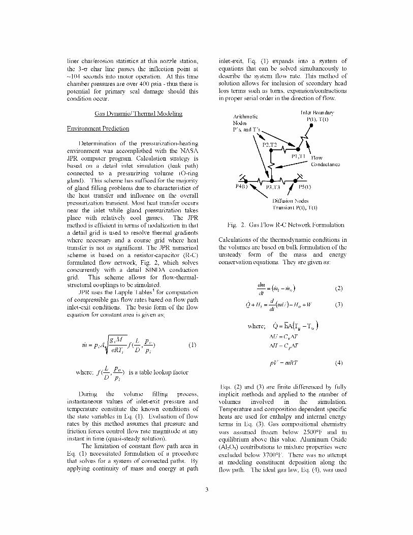
linerchar/erosionstatisticsatthisnozzlestation,the3-c_charlinepassestheinflectionpointat-104secondsintomotoroperation.At thistimechamberpressuresareover400psia-thusthereispotentialfor primarysealdamageshouldthisconditionoccur.

Gas Dynamic/Thermal Modeling

Environment Prediction

Determination of the pressurization-heating

environment was accomplished with the NASA

JPR computer program. Calculation strategy is

based on a detail inlet simulation (leak path)

connected to a pressurizing volume (O-ring

gland). This scheme has sufficed for the majority

of gland filling problems due to characteristics ofthe heat transfer and influence on the overall

pressurization transient. Most heat transfer occurs

near the inlet while gland pressurization takes

place with relatively cool gasses. The JPR

method is efficient in terms of nodalization in that

a detail grid is used to resolve thermal gradients

where necessary and a course grid where heat

transfer is not as significant. The JPR numerical

scheme is based on a resistor-capacitor (R-C)

formulated flow network, Fig. 2, which solves

concurrently with a detail SINDA conduction

grid. This scheme allows for flow-thermal-

structural couplings to be simulated.

JPR uses the Lapple Tables 4 for computation

of compressible gas flow rates based on flow path

inlet-exit conditions. The basic form of the flow

equation for constant area is given as;

_ __L Po,

m=pi V -7?7J 7,7 ) (1)

where; f(L,__o. ). is atable lookup factor

During the volume filling process,

instantaneous values of inlet-exit pressure and

temperature constitute the known conditions of

the state variables in Eq. (1). Evaluation of flow

rates by this method assumes that pressure and

friction forces control flow rate magnitude at any

instant in time (quasi-steady solution).

The limitation of constant flow path area in

Eq. (1) necessitated formulation of a procedure

that solves for a system of connected paths. By

applying continuity of mass and energy at path

inlet-exit, Eq. (1) expands into a system of

equations that can be solved simultaneously to

describe the system flow rate. This method of

solution allows for inclusion of secondary head

loss terms such as turns, expansion/contractions

in proper serial order in the direction of flow.

Inlet BoundaryArithmetic

P(t), W(t)

PN(&Ld T_ P

\ ] el,T1 Flow

_¢_ Conductance

Z,--a2g-v=,a-

Diffusion Nodes

Transient P(t), T(t)

Fig. 2. Gas Flow R-C Network Formulation

Calculations of the thermodynamic conditions inthe volumes are based on bulk formulation of the

unsteady form of the mass and energy

conservation equations. They are given as:

dm _ (,i,dt-v i-rho) (2)

Q+H i =d(mU)+Ho+W (3)

where; (_ = hA(Tg -Tw)

AU = CvAT

AH = C pAT

pV = mRT (4)

Eqs. (2) and (3) are finite differenced by fully

implicit methods and applied to the number of

volumes involved in the simulation.

Temperature and composition dependent specific

heats are used for enthalpy and internal energy

terms in Eq. (3). Gas compositional chemistry

was assumed frozen below 2500°F and in

equilibrium above this value. Aluminum Oxide

(Al203) contributions to mixture properties were

excluded below 3700°F. There was no attempt

at modeling constituent deposition along the

flow path. The ideal gas law, Eq. (4), was used

to relatetotalpressureto volumetricmassandbulktemperature.Equivalentmolecularweightswereusedintheevaluationofthegasconstant.

JPRinternallysolvesfor volumetricheatlossby usingconvectiveboundaryconditionscoupledtoa 1-Dconductiongrid. Thebuilt-inconductiongridallowsforefficientcalculationofheatlossinglandregionsawayfromtheleakpathinlet. Detailsof JPRcomputationalproceduresarefoundinRef.[1].

Detail Temperature Prediction

A feature of JPR is the concurrent solution

of a detail conduction grid describing heat transfer

along the inlet leak path. For this study a 3-D

finite element grid, Fig. 3., was constructed using

MSC/PATRAN 5. The grid region contained

thermal mass sufficient to capture the heat transfer

events associated with joint pressurization. Along

the inlet to the primary gland, heat losses to the

lateral sides were sub-modeled with a finite

difference grid. Lateral heat transfer (z-direction)

was accounted for and a numerically simplified

treatment of flow path ablation easily

implemented. Given path rectangular aspect

ratio's and duration of a typical filling event,

conduction comer effects have a second order

influence on gas temperature prediction.

Leak Path Inlet Leak

Le Path

Leak Patl_Leg-3

condaryGland _,

Leak Path

Leg- 1

PrimaryGland

Fig. 3. Nozzle Joint-4 Finite Element Grid

Conductivity and heat capacitances for

liner materials were temperature and density

dependent. The material was assumed to be fully

charred at temperatures above 1000°F and no

accounting for kinetic decomposition rate wasconsidered. Directional conductivites were used

and ply angles fixed at 45 ° from nozzle centerline.

Steel and O-ring material properties were input as

functions of temperature. The O-ring material is

elastomeric fluorocarbon (V1115) and has an

ablation temperature of-805°F. Surface erosionrates have been measured _ and correlated in

terms of heat transfer coefficient. Model

predictions of O-ring erosion are performed on a

fine grid sub-model using internally calculatedenvironments and the 1-D surface erosion data.

Jet Spreading and Computational Fluid

Dynamics (CFD) Sub-Modeling

Several test configurations include regions

where the leak path is not confined. The flow is

free to spread laterally before entering an O-ring

gland. Several of the primary gland tests were

configured with leg-3 open over the length of the

article. Gas flows along a confined rectangular

path in legs-1 and -2 and enters the unconfined

leg-3 where a partial free jet forms. The width of

the jet increases and centerline velocitydecreases in the direction of flow z. There is a

generally a reduction in centerline mass velocity

accompanied by lower gas temperatures at the

impingement point.

For the secondary gland cases, jet

spreading occurs in the chamfer region outboard

of the primary seal. Leakage past the primary

seal will result in pressurization of both chamfer

and secondary gland. Assuming flow past a

leaking primary is localized, flow enters the

chamfered region and spreads laterally before

entering the secondary gland. It was determined

by CFD analysis most of the flow traverses the

chamfer paths before entering the secondary

groove. Three-dimensional CFD models of both

leg-3 and joint chamfer-secondary regions were

constructed using the Finite Difference Navier-

Stokes (FDNS 3-D) code. 8

An approximate method of quantifyingrelative amounts of flow involved in heat transfer

in a spreading region was devised and based on

CFD sub-modeling. The rate of gland

pressurization and inlet mass flow can be

sufficiently calculated with traditional 1-D

internal flow equations. Spreading regions are

treated as a secondary loss (sudden expansion) in

the global flow solution. The globally computed

mass flow, temperature and pressure of gas

entering a spreading region provide in-flow

boundary conditions for a CFD sub-model. The

technique involves capturing time slices of the

inlet conditions and performing steady CFDsolutions of the flow field. Results are tabulated

where the dependent variable is the ratio of

centerline mass velocity versus mass flow rate

anddistancefromoriginofjet. ThismethodofcorrelationisincorporatedintoatransientS1NDAthermalmodelto determinetimebasedflowfractionsusedin specificlocationsof theconductiongrid.

Results

WorkperformedunderEngineeringTestPlan(ETP)-1385_TortuousPathThermalTestBed"generatedusableresultsfor mosttestingperformed.Earlytestsweredevelopmentalinnatureandresultsconsiderednothighlyreliable.Fig.4 depictsa crosssectionof thetestarticleshowingcenterlinemeasurementlocations.

P 1 ,P2

T1,T2

gas thermochemistry was considered comparable

to flight. Details of hardware, measurements and

results are found in Ref. [3].

The following section provides a brief

description of the test configuration followed by

a comparison of analysis results versus testmeasured data.

Configuration- 1

The leak path was machined and width

fixed at 150 mils confined to the primary gland.

Gaps along the path ranged from 50-60 mil, at

the entrance, to 30-40 mils adjacent to the gland.

Total volume was -3.8 in 3. Shown in Fig. 5-7

are predicted and measured pressures,

temperatures and erosion.

P1 1,Tll T15

Fig. 4. Test Article Measurement Locations

The assembly measured eight inches in the lateral

direction and to simulate O-ring glands of a flight

joint, 55-mil ID tubes were attached to the sides

of the test article. This set-up allowed for flow

impingement inside the detail section of the

assembly and traversal of gas flow in two lateral

directions. The tubes were 5 feet long, made of

stainless steel, and had fill bottles attached to the

end. The fill bottles contained the additional free

volume necessary to match the free volume

contained in a flight-configured joint-4. Original

intent of the tubing was to simulate flow friction

and heat transfer associated with a pressurizing

gland.Delivered environments were consistent

with inlet pressure measurements averaging -200

psia. Several attempts were made at measurement

of inlet gas temperature but were generally

considered unsuccessful. The test article grain

was cast from shuttle propellant TP-H1148 thus

theoretical flame temperatures and combustion

250

200

_ 150

100

50

P6 predic*_i i-- Pd test

- -)I[- - bottle predicted ."

0

0 0.5 1 1.5 2 2.5 3 3.5

time, s econds

Fig. 5. Configuration-l, Leak Path and Fill

Bottle Pressure Comparison

3000

2500

2000

1500

1000

500

0

0

i - -X- - T6 ies_ i

'1"16test i

0.5 1 1.5 2 2.5 3 3.5

time, seconds

Fig. 6. Configuration-l, Leak Path Gas and

Metal Temperature Comparison

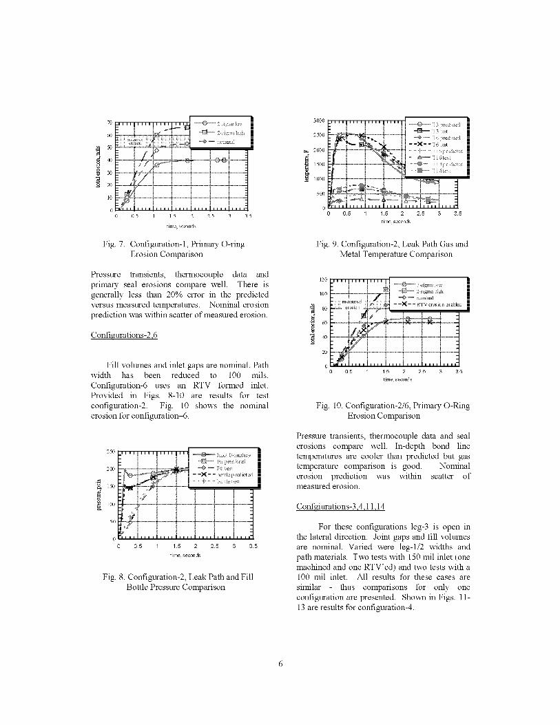
70

60

50

40

30

20

10

0

0

|

0.5 1 1.5 2 2.5 3 3.5

time, secoilds

Fig. 7. Configuration-l, Primary O-ringErosion Comparison

Pressure transients, thermocouple data andprimary seal erosions compare well. There isgenerally less than 20% error in the predictedversus measured temperatures. Nominal erosion

prediction was within scatter of measured erosion.

Configurations-2,6

Fill volumes and inlet gaps are nominal. Pathwidth has been reduced to 100 mils.

Configuration-6 uses an RTV formed inlet.Provided in Figs. 8-10 are results for testconfiguration-2. Fig. 10 shows the nominalerosion for configuration-6.

250

20O

150

10O

50

I •-'' ''I''' 'I'''' I'''i _h2.e_>c_md_v i

i _ _ i _ P6 predict_ " i1 1 ' i

.......... _-.............. i ........... ' --._ _ -- i'6 _e< i

• i_"': .......... }"""'-- --bottlepreclicted

!._ ! ! 1

........:_.............i..............t.............-..............i..............-..........

0_ .............................................

0 0.5 1 1.5 2 2.5 8 8.5

time, seconds

Fig. 8. Configuration-2, Leak Path and FillBottle Pressure Comparison

3000

2500

I_ 2000

i 1500

1000

500

0

0 0.5 1 1.5 2 2.5 3 3.5

time, seconds

Fig. 9. Configuration-2, Leak Path Gas andMetal Temperature Comparison

120

100

s0_ 60

4o

2O

0

0 0.5 1 1.5 2 2.5 3 3.5

time, seconds

Fig. 10. Configuration-2/6, Primary O-RingErosion Comparison

Pressure transients, thermocouple data and sealerosions compare well. In-depth bond linetemperatures are cooler than predicted but gastemperature comparison is good. Nominalerosion prediction was within scatter ofmeasured erosion.

ConfAiurations-3,4,11,14

For these configurations leg-3 is open inthe lateral direction. Joint gaps and fill volumesare nominal. Varied were leg-l/2 widths andpath materials. Two tests with 150 mil inlet (onemachined and one RTV'ed) and two tests with a100 mil inlet. All results for these cases are

similar thus comparisons for only oneconfiguration are presented. Shown in Figs. 11-13 are results for configuration-4.

250

200

150

100

50

00

|' ' ' I ' ' ' ' I ' ' q F_ess_ueI

1 '_ % P6 predicted

........ 1 _ -- }'6 me_nr_x!

- -_- - bottle p redicted

,_ 1 i l 1 i

2ii:::ii::i:i:i::ii:i::i:i:i::iii::ii:i:i:J0.5 1 1.5 2 2.5 3 3.5

time, seconds

Fig. 11. Configuration-4, Leak Path and FillBottle Pressure Comparison

2000

1500

1000

5OO

-'' ''1' '''1' '''1 ''''i _'_l"'_':'rcd_"d

ii "=_=== T6 meas:,_red

¢" _ _a_ _ 1 --)(--T14measltred _.

...........................i..............}...........Y_. '- " _ .._:_:'-;T " ..'-...........

",,,I,,,,I,,,,I,,,,I,,,,I,,,,i,,,,

05 1 15 2 25 3 35

time, seconds

Fig. 12. Configuration-4, Leak Path Gas andMetal Temperature Comparison

2O

15

-_ 10

_ 5

!

._1_1[ .... [ .... [ .... [ ...... _...... 2__i i....... |

_- _-- _ -_- _-_o_,-........... 7 ........... !.............. _.............. I •

iii...... -ed iiiiiiiiiiii._

............77..........Ui771777 0.5 1 1.5 2 2.5 3 3.5

time, seconds

Fig. 13. Configuration-4, Primary O-RingErosion Comparison

For the unconfined cases predicted bottlepressures compare well, implying that computedmass flow rates are accurate. Centerline pressuresin leg-3 did not compare well. Temperaturepredictions were generally lower than measured

by 20-40%. The lower 2-c_ erosion prediction isthe best match with the measured data.

Secondary Gland Filling Cases

Four tests were conducted with a flawed

primary seal, allowing pressurization of thechamfer and secondary gland. Results forconfiguration-8 are presented. Geometry issimilar to a flight-configured joint-4 andmeasurable secondary O-ring erosion wasproduced. Configuration-8 had a confined 150mil machined path to the primary. The primaryseal had a _dog-bone" defect aligned with theinlet path. Fill volume for the primary gland wasnominal. The chamfer contained _5.41 in3 and

secondary --4.21 in3. Leading into the secondarygland, the metal gap measured 5 mils. Shown inFigs. 14-17 are comparisons for bottle pressures,inlet gas/metal housing temperatures andsecondary O-ring erosion.

[]

250 _ _ IJrima;?, b_ttlepredJ_ed

i_.2"_'__---_ -- d/am fer bottle predicted

•_ i I " _'.'%.""" q., ;it<i:::" %,,'@ ._:.,{iq}e.{

150 _ J

[ 100

5O

00 1 2 3 4 5 6 7

time, seconds

Fig. 14. Configuration-8, Secondary Gland CaseFill Bottle Pressure Comparison

3000

2500

2000

500

0 1 2 3 4 5

time, seconds

Fig. 15. Configuration-8, Secondary Gland CaseGas Temperature Comparison

1dO0 I-' ' ' ' I ' ' ' ' I ' ' ,i ""_@""'1 t_r_r.i_,i

1200 _--F'_""_ ....................!..............i _- Tl6:)r:dicled

::::::::::::::::::::::::................600E___. =_ ...................: :_®_ ._:. _x.._x,_.,, ,.........:g:4-'...................."................-

0

0 1 2 3 4

time, seconds

Fig. 16. Configuration-8, Secondary Gland Case

Metal Temperature Comparison

g

10

0 0.5 1 1.5 2 2.5 3

tittle, seconds

Fig. 17. Configuration-8, Secondary Gland Case

Secondary O-ring Erosion Comparison

Flight Configured Joint Modeling

To account for differences between the test

article and full-scale joint, the following modeling

modifications were made. Effective joint-4 gland

flow areas, hydraulic diameters, flow path lengths

and volumes were calculated using current

configuration data. These calculations accounted

for curvature of a seated O-ring and effect of

assembly grease. Full-scale nozzle environments

adjusted for the joint-4 location were used. Early

in motor operation static pressures at the joint are

-150 psia. A temperature of 5100°R was assumed

for gas available for pressurization. Standard

chamber data was used for adjustment of local

pressure and temperature as a function of time.

Two cases were investigated. The first

assumes a pre-existing leak path to the secondary

at motor ignition. Geometry of the leak path was

the same as test configuration-8. For this case,

pressures, temperatures and secondary seal total

erosion is presented. The second case deals with

the smart void scenario. Analysis begins at 104

seconds when the char line has penetrated the first

turn and exposes a smart void. For this case,

pressures, temperatures and primary seal erosions

are presented for various leak path widths.

.4

_2

Provided in Figs. 18-20 are results for the

secondary gland pressurization. The analysis

assumes a 150 mil leak path and 150 mil dog-

bone in the primary at motor ignition.

160

140

120

100

80

60

40

20

0

0 0.5 1.5 2 2.5 3

time, seconds

Fig. 18. Leak Path to Secondary @ Ignition

Flight Case Gland Pressures

1200

1000

8OO

600

4OO

200

0

0 0.5 1.5 2 2.5 3

time, seconds

Fig.

6

g

2

19. Gas Path to Secondary @ Ignition

Flight Case Temperatures

i •

=----_t_ 2--sigma k,w

! !

: !

0.5 1 1.5 2 2.5 3

time, secoMs

Fig. 20. Gas Path to Secondary @ Ignition

Secondary O-ring Erosion

Gland pressure response is similar to test results.

The joint volume fill time is -3 seconds. Metal

surface temperatures adjacent to the gas path

range from 1100°F next to the primary to 600°F

in the secondary metal gap. Outboard surfaces

remainambient. Secondarysealerosionispredictedtobe5mils.

ShowninFigs.21-23areparametricresultsforprimaryglandpressurizationassuminga30,50and100mil smartvoid. Inletpressuresareapproximately80psia.Fillingoftheglandoccursin lessthantwosecondsfor all cases.Peakhousingtemperaturesaregenerallylessthan500°Ffor all cases.Maximumprimarysealerosionof20milsispredictedwitha50milleakpath.

90 i _ J.J++tt.,_,,7 |

80 "_ -- pI_Ilary, 50 rail m

-- --X-- -- plimary, 30 mil []70

"_ 60

! 50_i. 4o

3O

2O

10

103 104 108 109105 106 107

time, secoMs

Fig. 21. Smart Void Case, Predicted Primary

Gland Pressures

3o®E......... ! _..+++_,+_ ++,100_+ i2500 _'- ............. l"_"""'l""'i '--_-- iiilpiilgertleilt gas, 50 irlil

lE i I /_ _ - -)4[-- - impingmlent gas, 30 mflI-

;_.- 2000 _-. ............. +..j_.-._ -.....+, .............. ,................. _ ................ _ ............. -_

15130 L ............. i._....-.:' ' -..-.i.. -._............. i................. [ ................ [ ............. -_

10+t+I + + 1_ .............+..×_.+..-....v-.._.;:..........+................+.............!, i ! ,. ! !+ooB.............ii.. :":, .............-.]

2" +_ •

01_,,,, P,, +_,M4_+W_,_,,, ,_I103.5 104 104.5 105 105.5 106 106.5

time, seconds

Fig. 22. Smart Void Case, Predicted Gas

And Metal Temperatures

l "===+D_ erc+io+k 100 **NI i

25'' ''1' '''1 ''''11

- : : :1 _+ er:x,].]l 0 mJJ! ! !i

20 .............. i ................. [':m_""_ --0--erosior 30mil

"g'+ +"i+- i+ i

15.............................+................i.................................................10 .............. +...... ¢-1- -_---------- ,.':,_-.......... +_---+--------+_------+..............

5 +++ -t-+t+io103.5 104 104.5 105 105.5 106 106.5

tittle, seconds

Fig. 23. Smart Void Case, Predicted PrimarySeal Erosion

Conclusions

Based on results presented in this study, the

following conclusions / observations are made;

(1) Test configurations-1,-2 provided calibration

benchmarks for inlet gas temperature. By

machining the leak path, flow areasremained constant over time. There was no

flow spreading to be accounted for in

determination of mass velocities at the jet

origin. These configurations provided the

least amount of guesswork in quantifying

the effect of impingement gas temperature

on seal erosion. Inlet gas temperature of

_5100°R gave the best fit to erosion and

thermocouple data.

(2) Methodologies used for prediction of fill

bottle pressurization rates were accurate

without use of empirically derived factors to

account for comparison mismatches. The

gas flow network global method of solution

provided good estimates of total mass flow

and hence a solid basis for the sub-model

procedures used.

(3) Temperature comparisons were acceptable

given the nature of the measurements, e.g.,

large gradients, tiny gaps and millisecond

time scales. Gas temperature measurements

were difficult to match and required sub-

modeling of the thermocouple junction. Sub-

model results indicate gas temperatures may

be in error as much as 1000°F during peak

flow rate conditions.

(4) Seal erosion predictions were in good

agreement for the confined jet cases.

Erosion coefficients for a planar jet 9 best fit

the measured data. Nominal predictions

usually were bounded within the scatter of

the data. The impingement film coefficient

relationships contained in Ref. [6] were

slightly modified to account for 2-D velocity

decay dependencies.

(5) Largest comparison inaccuracies occurred in

non-confined geometry where the flow field

is multidimensional and CFD sub-modeling

required. The analysis tendency was to

over-predict seal erosions with CFD

computed flow fractions. Based on nominal

geometry, the fractions were reduced by afactor of 2-3 to best fit the data. Parametric

CFD analyses shows that varying the

secondarymetalgapfromthenominal5milsto 3 mils yieldsapproximatelythe rightmagnitudefortheflowfraction.Theover-predictiontendencymaybeanartifactofassemblytolerancesor soot/ condensable

deposition all of which contribute to off-

nominal geometry.

(6) Primary O-ring erosion for all _unconfined"

configurations ranged between 5 and 12 mils.

Model results suggest that venting leg-3

complete circumference and adding this

volume back into total system volume would

result in double the primary erosion (10-25

mil range). Model response indicated peak

flow rate magnitudes remained about the

same, occurred at the same time but fill times

increased. The time increase was

proportional to the volume increase, which

was proportional to the erosion increase

(about double). Recall the 100 mil confined

test produced seal erosion on the order of 90-

100 mils, about 10 times the erosion amount

of the spreading cases. This observation

suggests that a vented leg-3 is more tolerantof seal erosion in the worst case scenarios.

(7) The issue of inlet leak path width and what is

considered _worst case" was assessed. For

the smart void case, it was determined that a

maximum primary seal erosion of 20 mils

occurred with a 40-50 mil initial leak path

size. Below this threshold, total erosions

decreased as a function of decreased width.

Albeit fill times are longer, decreasing

impingement gas temperatures are controlling

seal erosion rates at the smaller gas pathwidths.

(8) Test results provided in ETP-1385 are

conservative due to the following; test free

volumes were larger, gland geometry more

constrictive and source pressures were high.The results are non-conservative due to the

lack of testing at smaller leak path widths.

Parametrics were performed to evaluate the

relationship between inlet leak path width and

secondary seal erosion. Findings indicate a

maximum secondary erosion of 16 mils

occurs at path widths of 40-50 mils. Again,

as path widths decrease below 40 mils, gas

temperature reduction effects on seal erosionrate control total erosion and not the overall

fill time.

2.

3.

4.

5.

6.

7.

8.

9.

References

_Joint Pressurization Routine (JPR)

Theoretical Development and Users

Manual", J. Louie Clayton, NASA-MSFC

Internal Memorandum, ED66 (95-01), 1995

Systems Improved Numerical Differencing

Analyzer (S1NDA), J.D. Gaski, Network

Analysis Associates Inc., Version 1.8

"Tortuous Path Thermal Analysis Test Bed

ETP-1385", Thiokol Corporation final

report TWR-66623, Mar-04, 1999

"Isothermal And Adiabatic flow of

Compressible Fluids", C.E. Lapple,

American Institute of Chemical Engineers,

1963

MSC/PATRAN, Version 7.5, McNeal

Scheinidler Corporation, Cosa Mesa

California, 1998

"O-Ring2: Volume Filling And O-ring

Prediction Code, Improved Model

Description And Validation, Part I Improved

O-ring Erosion Model", M. O'Mally,

Thiokol Corporation TWR--17030, 1988

"Boundary Layer Theory", Herman

Schlichting, Seventh Edition, McGraw Hill

Book Company, 1979

Finite Difference Navier-Stokes (FDNS3D),

CFD code, Y.S. Chen, NASA contract

NAS8-37408, 1990

"Prediction of Pressurization and Erosion of

the SRB O-Rings During Motor Ignition

(Part II): Parametric Studies of Field and

Nozzle Joints, M. Salita, Thiokol

Corporation TWR- 15186, July 1985

10

Thermal / Pyrolysis Gas Flow-Analysis of Carbon Phenolic Material

J. Louie Clayton

Thermodynamics and Heat Transfer Group

Marshall Space Flight Center / NASA

Redstone Arsenal, Alabama

ABSTRACT

Provided in this study are predicted in-depth temperature and pyrolysis gas pressure distributions for carbon

phenolic materials that are externally heated with a laser source. Governing equations, numerical techniques and

comparisons to measured temperature data are also presented. Surface thermochemical conditions were determined

using the Aerotherm Chemical Equilibrium (ACE) program. Surface heating simulation used facility calibrated

radiative and convective flux levels. Temperatures and pyrolysis gas pressures are predicted using an upgraded form of

the SINDA/CMA program that was developed by NASA during the Solid Propulsion Integrity Program (SPIP). Multi-

specie mass balance, tracking of condensable vapors, high heat rate kinetics, real gas compressibility and reduced

mixture viscosity's have been added to the algorithm. In general, surface and in-depth temperature comparisons are

very good. Specie partial pressures calculations show- that a saturated water-vapor mixture is the main contributor to

peak in-depth total pressure. Further, for most of the cases studied, the water-vapor mixture is driven near the critical

point and is believed to significantly increase the local heat capacity of the composite material. This phenomenon if

not accounted for in analysis models may lead to an over prediction in temperature response in charring regions of the

material.

NOMENCLATURE

A -area

B' -dimensionless mass loss rate

CH -Stanton Number, Heat Transfer

CM -Stanton Number, Mass Transfer

C -specific heat

E -activation energy

F - 1st generic coefficient

O -2 nd generic coefficient

h -enthalpy

J -mass source/sink rate

k -thermal conductivity

K -permeability

m -mass

lay -mass flow- rate

mf -mass fraction

n -number of reactions

M -Molecular weight

P -total pressure

Q -heat transfer rate

R -gas constant-recession rate

S -source term

t -time

T -temperature

u -velocityV -volume

w -weight fraction

x -spatial coordinate

z -compressibility factor

Z -difthsional driving potential

c_ -surface total absorptivity

!3 -pre-exponential factor

-surface total emissivity

F -resin volume fraction

-dynamic viscosity

d_ -porosity

p -density

_/ -coefficient for Forchiemer extension

Subscripts:

c -carbon

cn -condensation

e -edge

f -final

g -gas

i,j -free indices

o -original

p -constant pressure

r -recovery

rad -radiation

s -solid material

sc -solid conduction

t -total

v -virgin

vp -vaporization

w -wall

INTRODUCTION

TheSpaceShuttleReusableSolidRocketMotors(RSRM)havenowprovidedthemainpropulsionsourceforover95missions.Duringthistimeaveryextensivedatabaseofmotoroperationalperformancehasbeenamassedwhichincludesparameterssuchasnozzleinsulationerosionrates.Thesedataareunderstoodstatisticallytotheextentthatvariationsontheorderoftenthsofaninchareindicatorsthatachangehasoccurredineithermaterialsa_d/orprocessesusedintheirrefurbishment.ThelefthandnozzleoftheRSRM-56flightsetdisplayedanomalouserosion(pocketing)aftofthethroat(Fig.1)affectingthefullcircumferenceofthemotorandmeasuringasmuchas0.5"deeperthanexpectedmeanvalues.Basedonstatistics,theeventwasapproximatelya6-_occurrenceandthuscouldnotbediscardedwithoutfurtherunderstanding.

Fig.1.RSRMNozzleShowingPocketingRegion

Thedegradedmaterialperformancewasbelievedtobeattributabletothe"pocketing"phenomenonthatisdistinctlydifferentfromtypicallyoccurringthermochemicalerosion.Atthislocationinthenozzlethroatringmaterialplyanglesare45° to motor centerline and about 70 ° to the conducted isotherms. It is known that in-pla_e (with ply)

fibers oriented orthogonal to the isotherms are more likely to pocket. It was therefore suspected that for the RSRM-56

nozzle, process variation had produced fiber orientations approaching 90 ° to the flame surface and was likely the

primary cause of the increased erosion. Additionally, other factors related to materials and/or process variation were

considered potential contributors thus it was decided to initiate a comprehensive test program aimed at gaining a better

understanding of material thermostructural behavior.

The resources of the Laser Hardened Material Evaluation Laboratory (LHMEL) facility were utilized to examine

pocketing activity as a function of fiber orientation and other material variations such as resin content, moisture content

and ply distortions. LHMEL has the major advantages of a relatively large spatially flat surface heating distribution of

precise magnitude, rapid turn-around test time and direct measurement of surface temperature. Disadvantages of the

LHMEL are total pressures, thermochemistry and surface recession does not compare well with the actual RSRM.

Average recession rates are about one-forth of that experienced in the RSRM nozzle at the location of interest. There is

some debate and conflicting data [1] that seems to suggest that the effect of active surface thermochemistry may be

important in terms of suppression of pocketing. Notwithstanding these data, the decision was made to test at LHMEL

based on the belief that pocketing is an "in-depth" phenomena and not strongly dependent on surface recession.

The following provides a description of modifications incorporated into the SINDA/CMA computer code which

was developed by the author [2] during the Solid Propulsion Integrity Program (SPIP). Upgrades include multi-specie

mass balance, real gas equation of state using generalized compressibility data, reduced mixture viscosity, resin

weight fraction Arrhenius formulation, high rate TGA coefficients and a condensation/vaporization simulation for

vapors in the pyrolysis gas mixture. Basic formulations of the energy and momentum equations remain essentially

unchanged but will be covered for completeness.

GoverningEquations

In-depthtemperatureandpyrolysisgaspressurecalculationsarebasedonsimultaneoussolutionof1-Dconservationequationsformass,momentumandenergyalongwitharealgasequationofstateandkineticrateequation.Thefollowingbasicassumptionswereincorporatedintothemathmodel:

1)Local thermal equilibrium exists between pyrolysis gas and solid thus one energy equation can

describe thermal response of both.

2) Pyrolysis gas motion is governed by the Darcy-Forcheimer equation. Permeability and porosity data

was correlated as a function of degree of char. Data was assembled from Clayton TMand Stokes [4].

3) Temperature and pressure gradients are 1-dimensional thus material aaaisotropy can be simulated by

use of effective properties. Rule of mixtures was used for determination of properties in the charring

region.

4) Transport of condensable species through the pore network occurs in the vapor phase. Liquid

occupying pore volumes was assumed to be stationary and in equilibrium with its respective vapor in

the mixture. Condensation and vaporization rates are governed by the amount of a specie that can be

thermodynamically accommodated in the mixture relative to saturation over a given time step.

5) Condensed phase species residing together in a pore volume are assumed not to interact with each

other chemically or physically. Gas phase permeability remains unchanged due to the presence of

liquid in the pore volumes.

6) Mixture specie concentrations, in the pore free volumes, were determined by "origin" generation,

condensation/vaporization rates and upstream advection. Equilibrium and/or kinetic rate reactions

within the gas and reactions with the char layer are currently not modeled.

Surface Energy Balance

Surface heating conditions are determined by consideration of combined convective, radiative and

thermochemical loading. The LHMEL is unique, and different from the RSRM in that surface response is driven by

the incident radiation emitted from a CO2 laser and is convectivly cooled by air flow-. Oxidation of carbon in the char

layer is present and averages about one mil/sec depending on incident heat rate and location on the sample.

Components of the surface heat flux are depicted in Fig. 2.

thermochemically N_

eroding surface

boundary

layer edge

net chemical

/\

incident

radiation re-radiation

backside in-depth

advected conduction

fluxes

Fig. 2. Thermochemically Eroding Surface Boundary Conditions

During testing, surface radiometer data was collected and used for model calibration of surface optical properties.

Backfitting model response to measured data across the range of incident flux levels, surface absorptivity was found to

be independent of temperature while re-radiated energy levels were controlled by a temperature dependent emissivity.

The backfit suggested that c_ - 0.97 and _ was - 0.85 @ 3000°F and increased linearly to _ 0.96 @ 5000°F. Forced

convective cooling of the sample was imposed by a 0.5 Mach air flow-directed parallel to the heated surface. Facility

airflow- calibration data was used for determination of convective heat and mass transfer coefficients and average values

of these quantities input into the SINDA/CMA model. Surface oxidation rate was correlated in familiar b-prime table

format and estimated by an ACE [5] solution for standard air environment. Surface recession rates average about one

mil/secandvarysubstantiallyalongtheheatedsurfacewiththeleadingedgehavingthegreatesterosion.ArithmeticsummationofrespectivefluxesidentifiedinFig.2.givesthefollowingexpressionforthesurfaceenergybalance:

PeUeCH(hr-hew)+PeUeCM['_(Zi*-Z_w}1Tw-B'hw]+mchc+riaghg

+°_wqrad- F°'gwT; - qsc=0(1)

Termslefttorightareidentifiedasfreestreamconvection,surfacethermochemical,backsideadvectivefluxes,radiationincident/emittedandconductionintothematerial.Numericalsolutionforthesurfaceenergybalance[2]isimplicitwithrespecttotemperaturecalculationsbutexplicitintimerelativetomassflow-calculatedquantities.Netfluxvaluesareloadedintothesourcetermofthesurfacenodeduringiterativeconvergenceoftheglobaltemperatureandpressurecalculations.ThisnumericalmethodisdifferentfromthestandardCMAapproachbutthetwomethodscomparewellwithadifferenceoflessthan1/2%incomputedsurfacetemperature[2].

In-Depth Thermal Solution

Invoking the assumption of gas-solid equilibrium, leads to the standard CMA [6] formulation for energy

conservation given by Eq. 2. For this study an additional term that accounts for pyrolysis gas capacitance has been

added to the equation per the general formulation provided by Keyhani [7]. Inclusion of gas capacitance has heretofore

been considered unnecessary due to order of magnitude considerations however based on findings presented in this

study, it is believed this term can become significant in charring regions of the material. Terms left to right are energy

storage, conduction, decomposition, grid movement, pyrolysis gas flow- and latent phase change rates. The last two

terms were added to account for the phase energy of saturated water and phenol compounds.

(PsC s ,_T s 1 k(kA_T/+(hg__)__+_pC _T ' Iilg _hg .... Qvp+ _)9gCg) _ - Ac_x\ c_x) 'a v _ ± -A-_ -- ± v_cn

(2)

A finite element scheme was used for discretization of the energy equation. The computational grid consist of

one dimensional first order elements with applied front/back face boundary conditions, Fig. 3.

front face

11 ] ] ] ] ]ntl_lement] backface

net external //[ [ [ [ [ [ boundary

heat flux "''tl_+_ I_ _ _ _ _ _ conditions

"////// pl In

Fig. 3. One Dimensional Finite Element Grid

Surface recession is accommodated by movement of the grid relative to a fixed coordinate and applying a

correction term to account for the induced advected energy into the element(s). As with the baseline CMA technique,

the last element (furthest from the heated surface) shrinks to accommodate surface recession. If eroded total depth

exceeds elemental thickness it is dropped from the active network and the adjacent element now absorbs the recession

and so on. Determination of the elemental "stiffness" matrix is based on trapezoidal rule numerical quadrature which

evaluates material heterogeneous and temperature dependencies explicitly in time. Temperature and pressure elemental

integration points are coincident with a density field "nodlet" grid. Use of a nodlet grid for the density calculations is

similar to the CMA technique and is generally necessitated by the exponential behavior of the Arrhenuis equation.

In-Depth Pyrolysis Gas Pressure Solution

Pyrolysis gas pressure distributions are calculated using a Darcy-Forcheimer form of the momentum equation

substituted into the conservation of mass equation. Real gas effects for the mixture are simulated by application of a

generalized compressibility factor to the ideal gas law-. Pseudocritical temperatures and pressures Is] are calculated for

the mixture based on mole fractions and the individual specie data. These "reduced" properties are used as

independent variables for table lookup to determine the z factors. Mixture viscosity calculations [9] incorporate the

effects of pressure, temperature and molecular polarity and are functions of mole fraction data and the pseudocritical

reduced properties. Expression of gas properties in terms of mixture equivalents, i.e., gas constant, viscosity's, etc.,

permits use of Darcys equation for computation of total gas pressures. Specie partial pressures are simple functions of

the mole fraction data which result from the multi-component mass balance. Terms left to right in Eq. (3) are

functionally identified as gaseous mixture storage, total diffusive mass flux, total rate of pyrolysis gas generation,

coordinate set movement correction, total multi-specie vaporization and condensation.

cgt\ zRT )=_ _ (pg)A-_- -AOG+a _x vp cn(3)

Eq. (3), the "pressure" equation, is analogous in formulation to the energy equation and is thus numerically solvable by

the same finite element techniques used for temperature calculation. Assembly of the pressure elemental stiffness

matrix relies on explicit quadrature of spatially dependent properties using the same procedure derived for the thermal

calculations. Details of discretization of the diffusive term, treatment of source/sink terms and numerical degree of

coupling are developed and discussed in Ref. [2].

In-Depth Kinetic Decomposition

A resin based weight fraction formulation of the Arrhenius equation was employed for the in-depth material

decomposition simulation. Kinetics coefficients were developed by Clayton [1°] and computed from high rate TGA data

derived by Southern Research Institute (SoRI). The weight loss curve fit considered three reactions and was based on

the 3000°C/minute data. The Arrhenius relationship used in the SINDA/CMA code has the following form:

g i

dw i n 1 ni( w )ni[_ieR _- (4)-- , i -- Wf idt i=_-w°

A thermal decomposition "nodlet" grid was implemented for refined description of variation in material density

along the 1-D coordinate. This grid is fixed and contains time based composite material density resulting from

integration of Eq. (4). A simple Euler scheme was applied in which integration time steps are set equal to the transient

solution time step for the temperature and pressure calculations. Updating of temperature in the calculation occurs

explicitly and the resultant pyrolysis gas flow-rates are used explicitly in temperature and pressure calculations (loosely

coupled). Quadrature involved in evaluation of stiffness matrices assumes a piecewise linear distribution of density

described by integration of Eq. (4) at the fixed nodlet sites. Conversion of resin weight fraction data to composite

density was based on the following relationship

os= ov(i wi)+ (5)

Multi-Component Mass Balance

A multi-component mass balance allows for tracking of individual molecular species evolved during the in-depth

thermal decomposition process. The procedure utilizes a control volume aligned with elements in the pressure grid,

Fig. 4. Total rate of decomposition and thus pyrolysis gas generation is determined by Eq. (4) and is assumed strictly a

function of temperature and local char state. Mole fraction data that describes molecular species evolved as a function

ofdegreeofchartakenfromClaytonTMwasusedtodeterminethe"origin"generationrate.Atotalofeightmolecularspecieswereconsidered;water,carbondioxide,carbonmonoxide,methane,hydrogen,phenol,cresolandxylenol.Oftheseeight,waterandphenolhavecriticaltemperatureshighenoughandoccurinsufficientconcentrationsthatcondensationandvaporizationhastobeconsideredifaccuratetotalpressuremagnitudesaretobecalculated.

Pi+l m fijr}l t[ outPi-1

Fig. 4. Multi-Component Mass Balance

At the boundaries of the control volume are the advected fluxes of the individual species. Depending on computed

direction of flow- upstream contributions contribute to a weighted average type calculation of pore volume specie

concentration. Equivalent molecular weights, gas constants, mixture viscosity's, specific heats are all functions of the

mixture mole fraction calculations. Tracking partial pressures of individual species allows for simulation of

condensation and vaporization. The computational procedure involves comparing specie partial pressure to its

saturation pressure for the local temperature, Fig. 5. Below- critical temperatures for the given specie, if its partial

pressure tries to exceed the saturation pressure, an instantaneous rate of condensation is calculated that will keep the

specie partial pressures equal to its saturation pressure (T_ to T 3 ). Time integration of the rate of condensation gives

the total amount of liquid that has accumulated in the open pore volumes. This liquid is available for vaporization

when conditions are such that the mixture can thermodynamically accommodate its presence. Vaporization rates are

computed based on the premise that the gas mixture remains saturated until all the liquid in the pore volume is

removed(T_ to T 5 ). Above critical temperatures gas mixture PVT behavior is described by the ideal gas law-using

generalized compressibility factors. The technique employed is similar to that used by Clayton TM.

partial

pressure

critical

T'_ t _ point

saturation T3 _ ] _ T6boundary _ /[ ] _ j

\ /'1 A 1____---_T_ T;

T3

__"_l conT3nsation vaporization

I2 m ij =0 I 12(Jn-Jvp) At 12(Jn-Jvp) At 12 m ij =0

temperature

Fig. 5. Condensation and Vaporization Simulation

NUMERICAL SOLUTION

As previously discussed, discretization of energy and mass conservation equations was based on a finite element

formulation employing a nodlet grid for integration of the Arrhenius equation. Time integration of the non-steady

behavior of the diffusion equations, i.e., pressure and temperature, was performed by a Crank-Nicholson procedure.

Eqs. (2) and (3), are cast into the following generic form:

(5)

where; • is temperature or total pressure

Eq. (5) is solved by iteration for the dependent variable A_ i. A successive point (Gauss-Seidel) scheme is

applied which uses dependent and source term damping. Coupling is fully implicit between pressure, temperature and

surface energy balance meaning that all quantities are converged together along with their respective coefficients and

source terms at every time step. The Arrhenius equation is not iterated with temperature and pressures. A simple

explicit updating is performed using "old" time step data values. The global method of solution is described in detail

by Clayton [2] but will be summarized here to include the phase change logic. The overall numerical procedure goes as

follows:

1) Initialize temperature, pressure, density and nodal coordinates. Compute coefficients in Equation (5).

2) Increment boundary information and solve for temperatures and pressures by iteration.

3) Using converged data in Variables 2, interpolate temperatures onto density grid and integrate Arrhenuis

equation across the time step. Store decomposition data into an array versus position.

4) Recalculate coefficients in Eqn. (5) based on new-properties data, i.e., conductivity' s, permeability' s, mass-

energy source and sink rates, coordinate system location, etc...

5) Perform nodal mass balance as function of converged flow-conditions for current time step. Compute mass

and mole fractions, partial pressures, mixture equivalent properties.

6) Compare partial pressures with saturation pressure @ temperature for condensable species. If partial pressure

is greater, using real gas law- compute amount of mass removal necessary to make the two equal. Accumulate

this mass as liquid in the control volume. If partial pressure is less than saturation, using real gas law- compute

amount of mass necessary to saturate mixture and vaporize accumulated liquid (if there is any). Adjust mass

source terms in pressure network to reflect local rates of condensation/vaporization.

7) Perform grid movement logistics, if current time is less than end time return to step #2

Steps #3-#7 are performed in Variables 2 of the SINDA/CMA model thus all procedures described in these steps are

explicitly coupled in time to the pressure and temperature calculations in step #2.

RESULTS

Spatial distributions for in-depth temperature and pyrolysis gas pressure for various incident radiant heating rates

are presented in Figs. 6-14. For these cases ply angles are fixed at 90 ° and time slices at 3, 10 and 20 seconds are

provided. For clarity, partial pressures of only major contributors such as water vapor, carbon dioxide and monoxide

are presented. For the 300 Watt case, surface temperatures range from 2900°-3700°F and increase monatonically

during the test. Peak total pressures range from 140-180 atmospheres with the maximum occurring at the 10 second

time slice. Water vapor is the dominant pyrolysis gas specie in the charring regions of the material with mixture mole

fractions approaching 99%. Gas flow-s are driven in-depth and to the heated surface depending on proximity relative to

the peak pressure location. In the cooler material, carbon dioxide becomes the dominant specie. As the mixture is

driven in-depth, the water vapor is condensed out leaving only species with critical temperatures low- enough to exist as

a gas at the given total pressure and temperature. For the 500 Watt cases, Figs. 9-11, surface temperatures range from

3600°-4300°F, increasing during the test. Peak total pressures range from 130-190 atmospheres with the maximum

occurring at 3 seconds (earlier in test compared to 300 Watts). Specie distributions followthe same general trends.

Looking at the 1000 Watt cases, Figs. 12-14, surface temperatures now- vary from 4600°-5100°F and increase during

the test. Peak total pressures range from 200-220 atmospheres with the maximum occurring at 10 seconds. Clearly

observable trends in Figs. 6-14 are overall increase in material temperatures and total pressures with increasing surface

heat flux.

3000

2500

2000

1500

1000

500

00

i i

0.2 0.3 0.4 0.5 0.6 0.7

depth, inches

Fig. 6. Temperature and Pressure Distributions @ 3 Seconds

300 Watt Case, 90 ° Ply

140

120

100

80

60

40

20

0

-20

0.8

S

350O

3000

2500

2000

1500

1000

5OO

0

0

...._'i'"'"_

-._ -_ -_, -_ -_._= ._. :_ _

0,1 0.2 0.3 0.4 0.5 0.6 0.7

depth inches

Fig. 7. Temperature and Pressure Distributions @ 10 Seconds

300 Watt Case, 90 ° Ply

200

150

100_

50

e'_

4000

3500

3000

2500

2000

1500

1000

500

0

150

E _',i i '/':.....................i............l! .....................i __+_ __ _,ro_,<.,_O2100

..............__i_i ......................i.......................i....................

....................i.......................i...................i.....:..._.............i......................i..................._ ........[....................

7 ........... .........o-50

0.1 0.2 0.3 0.4 0.5 0.6 0.7 0.8

depth, inches

Fig. 8. Temperature and Pressure Distributions @ 20 Seconds

300 Watt Case, 90 ° Ply

e'_

4000

3500

3000

2500

2000

1500

1000

5OO

0

0

,," ' " I " " ' ' | " " " ' I ' " ' ' | ' " ' ' " ' ' " ' " ' " " " " "

....._..._.................................................[......................i......................[.......................[....................;: i_;° _._-- i i i i :-....................._.,.............................L:....i._......_...........i......................i.......................i..................-i'°}i['\ i i i _.._. i i :

.:..........""i:-v:i ....................± ..................i......................i............._ ................i.....................

0.1 0.2 0.3 0.4 0.5 0.6 0.7 0.8

depth, inches

Fig. 9. Temperature and Pressure Distributions @ 3 Seconds

500 Watt Case, 90 ° Ply

200

150

100

50 _"

0

-50

5000

4000

3000

2000

1000

00 0.1 0.2 0.3 0.4 0.5 0.6 0.7

depth, inches

Fig. 10. Temperature and Pressure Distributions @ 10 Seconds

500 Watt Case, 90 ° Ply

200

150

5OOO

4000

3000

2000

1000

00

\

- total pressme

- -X - - partial pressure, CO

o + _ - partia_ Uessuco C02

a io+.

o _ -

0.1 0.2 0.3 0.4 0.5 0.6 0.7

depth, inches

Fig. 11. Temperature and Pressure Distributions @ 20 Seconds

500 Watt Case, 90 ° Ply

140

120

100

80

60O

.g

40

20

g.

5000

4000

3000

2000

1000

,T............................................................°..............._ i

°'1 i"

" - v.._-----_'_-=--_-l_ --t_-'=_ •

250

200

150

100

50 _

0.1 0.2 0.3 0.4 0.5 0.6 0.7

depth, inches

Fig. 12. Temperature and Pressure Distributions @ 3 Seconds

1000 Watt Case, 90 ° Ply

©

6000

5OOO

4000

3000

2000

1000

00

250

.... I .... I .... ! .... ! .... _ .... t .... _ .... Ill" I I i i ---.-I3 - .>*al prcss13re II

i i .... _ii_i=-i_i'_ ;_',I>-a_'_,IL_C' 1200

.._'.j._£'"'"i .......................i............_ '"'"'i......................._'"l - -* - - partial pressure, CO

" "%j i -% i I = "" ..% i , _i i . - .................._ -.1 150.............. .-"'"X.........................._'"'_............................?......................_......................?..... -I g

i [ t i i ......1.......... _ i..................-,I 100

: _i " =r

, , , , i , , , , t , , __'_", _\...... 2 " -50

0.1 0.2 0.3 0.4 0.5 0.6 0.7 0.8

depth, inches

Fig. 13. Temperature and Pressure Distributions @ 10 Seconds

1000 Watt Case, 90 ° Ply

!

6000

5000

4000

3000

2000

1000

i _ - w;tal presst_re

'_ - -X - - partial pressure, CO

250

\i i[:<t

....................i.......................i................................. ...................

0.1 0.2 0.3 0.4 0.5 0.6 0.7

depth, inches

Fig. 14. Temperature and Pressure Distributions @ 20 Seconds

1000 Watt Case, 90 ° Ply

200

0 -500 0.8

150 p_

I

100 1O

-I:5"

50 _

Provided in Figs. 15 and 16 are comparisons of predicted material thermal response to the laboratory measured

data. Surface temperature data was obtained by radiometry while in-depth measurements were gathered by secondarily

bonded thermocouples. Thermocouple depths were 0.125, 0.250 and 0.375 inches; a constant spacing of one-eighth

inch. Adjustment of surface optical properties, per the discussed procedure, allowed for very good correlation in

predicted response to the measured data. A good temperature match at the surface is a necessary starting point for

understanding comparisons made at the in-depth locations. In general, the in-depth calculated quantities compare well

with measured data and some discernible trends were evident. For the 300 Watt case at the 0.25" location, the

measurement strays from the prediction at _10 seconds. Comparisons at locations on both sides of this thermocouple

are very good thus it is believed that the measurement may be inaccurate to some extent. High surface heating rate

(1000 Watt case) comparisons are provided in Fig. 16. Unfortunately, lower capability thermocouples were used for

this test and the in-depth measurements fail at _2100°F. A general tendency for this test, and others in a series of

_1100 tests, is that model predictions lead measurements in the 700-1500°F range. Laboratory measured specific

heats, for virgin and char material, were used for results presented in Figs. 15 and 16 to demonstrate this over

prediction trend. Addition of saturated water pressure and temperature dependent specific heats into the energy

equation would produce a better temperature comparison at the in-depth locations.

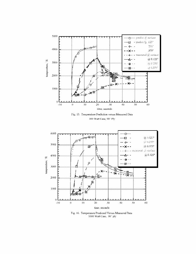
!I.I

5000

4000

3OOO

2000

1000

i

0

-10 0 10 20 30 40 50 60

time, seconds

Fig 15 Temperature Prediction versus Measured Data

300 Watt Case, 90 ° Ply

!

6000

5OOO

4000

3000

2000

1000

0

-10

........................'"...................... '".........._'" ( ......................i ................... - -X -- @ 0.375"

........................_ .................... "'_"_ ...............i ................... ""_- - @ 0.125"

I n i = i.x--L-'-__ ii/ i,_ i " -_ i

................................................1_]" _i_ ...............--:_.........................._}.........................._i.......................

I_ _/i i .............i........................................................................__ ....................................................

• i i i " i i

",, ,,i .... i .... i .... i .... i .... i ....

0 10 20 30 40 50 60

time, seconds

Fig. 16. Temperature Predicted Versus Measured Data

1000 Watt Case, 90 ° ply

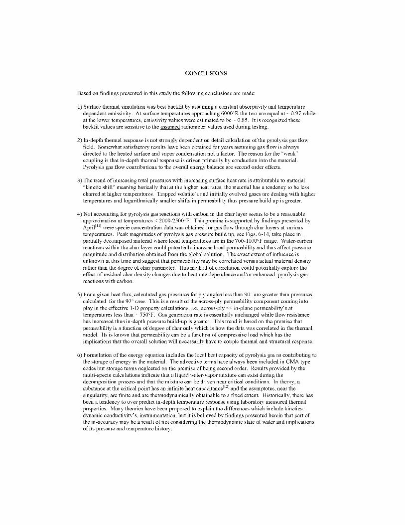
CONCLUSIONS

Based on findings presented in this study the following conclusions are made:

1) Surface thermal simulation was best backfit by assuming a constant absorptivity and temperature

dependent emissivity. At surface temperatures approaching 6000°R the two are equal at - 0.97 while

at the lower temperatures, emissivity values were estimated to be - 0.85. It is recognized these

backfit values are sensitive to the assumed radiometer values used during testing.

2) In-depth thermal response is not strongly dependent on detail calculation of the pyrolysis gas flow-

field. Somewhat satisfactory results have been obtained for years assuming gas flow- is always

directed to the heated surface and vapor condensation not a factor. The reason for the "weak"

coupling is that in-depth thermal response is driven primarily by conduction into the material.

Pyrolysis gas flow- contributions to the overall energy balance are second order effects.

3) The trend of increasing total pressures with increasing surface heat rate is attributable to material

"kinetic shift" meaning basically that at the higher heat rates, the material has a tendency to be less

charred at higher temperatures. Trapped volatile's and initially evolved gases are dealing with higher

temperatures and logarithmically smaller shifts in permeability thus pressure build up is greater.

4) Not accounting for pyrolysis gas reactions with carbon in the char layer seems to be a reasonable

approximation at temperatures < 2000-2500°F. This premise is supported by findings presented by

April [11] were specie concentration data was obtained for gas flow- through char layers at various

temperatures. Peak magnitudes of pyrolysis gas pressure build up, see Figs. 6-14, take place in

partially decomposed material where local temperatures are in the 700-1100°F range. Water-carbon

reactions within the char layer could potentially increase local permeability and thus affect pressure

magnitude and distribution obtained from the global solution. The exact extent of influence is

unknown at this time and suggest that permeability may be correlated versus actual material density

rather than the degree of char parameter. This method of correlation could potentially capture the

effect of residual char density changes due to heat rate dependence and/or enhanced pyrolysis gas

reactions with carbon.

5) For a given heat flux, calculated gas pressures for ply angles less than 90 ° are greater than pressures

calculated for the 90 ° case. This is a result of the across-ply permeability component coming into

play in the effective 1-D property calculations, i.e., across-ply << in-plane permeability's at

temperatures less than _ 750°F. Gas generation rate is essentially unchanged while flow- resistance

has increased thus in-depth pressure build-up is greater. This trend is based on the premise that

permeability is a function of degree of char only which is how-the data was correlated in the thermal

model. Its is known that permeability can be a function of compressive load which has the

implications that the overall solution will necessarily have to couple thermal and structural response.

6) Formulation of the energy equation includes the local heat capacity of pyrolysis gas as contributing to

the storage of energy in the material. The advective terms have always been included in CMA type

codes but storage terms neglected on the premise of being second order. Results provided by the

multi-specie calculations indicate that a liquid water-vapor mixture can exist during the

decomposition process and that the mixture can be driven near critical conditions. In theory, a[12]substance at the critical point has an infinite heat capacitance and the asymptotes, near the

singularity, are finite and are thermodynamically obtainable to a fixed extent. Historically, there has

been a tendency to over predict in-depth temperature response using laboratory measured thermal

properties. Many theories have been proposed to explain the differences which include kinetics,

dynamic conductivity' s, instrumentation, but it is believed by findings presented herein that part of

the in-accuracy may be a result of not considering the thermodynamic state of water and implications

of its pressure and temperature history.

REFERENCES

1Ross R., Strobel F., Fretter E., 1992, "Plasma Arc Testing and Thermal Characterization of NARC FM5055

Carbon-Phenolic", Document Number HI-046F1.2.9, Prepared For NASA Sponsored by the Solid

Propulsion Integrity Program Nozzle work Package.

2Clayton J.L., 1992, "SINDA Temperature and Pressure Predictions of Carbon-Phenolic in Solid Rocket Motor

Environment", in the Proceedings of the JANNAF Rocket Nozzle Technology Subcommittee Meeting, CPIA

publication.

3Clayton F.I., 1992, "Influence of Real Gas effects on the Predicted Response of Carbon Phenolic Material

Exposed to Elevated Temperature and Pressure Environments", in the Proceedings of the JANNAF Rocket

Nozzle Technology Subcommittee Meeting, CPIA publication.

4 Stokes Eric, 1997, "Room Temperature As-Cured In-Plmae Permeability of MX4926 From Several Post Fired

RSRM Throat Rings", Southern Research Corporation, SRI-ENG-97-281-9115.16

5 Powers, Charles and Kendal, Robert, "Aerothermal Chemical Equilibrium Program (ACE)", May 1969,

Aerotherm Corporation, Mountain Valley California

6 Strobel, Forest and Ross, Robert, "CMA90S Input Guide and Users Manual, December 1990, Aerotherm

Corporation, Huntsville Operations, Huntsville, Alabama

7 Keyhani, Majid and Krishnan, Vikran, "A One-Dimensional Thermal Model with Efficient Scheme for Surface

Recession", in the Proceedings of the JANNAF Rocket Nozzle Technology Subcommittee Meeting, CPIA

publication, Mechmaical And Aerospace Engineering Department University of Tennessee.

7 Clayton, F.I., 1992, "Predictions of the Thermal Response of the SPIP 48-2 MNASA Ground Test Nozzle

Materials", in the Proceedings of the JANNAF Rocket Nozzle Technology Subcommittee Meeting, CPIA

publication

8 Van Wylen and Sontag, " Introduction to Thermodynamics: Classical mad Statistical", John Wiley and Sons,

Inc., 1970

9 Bird, Stewart and Lightfoot, "Transport Phenomena", Department of Chemical Engineering, University of

Wisconsin, John Wiley and Sons, Inc. 1960.

10 Clayton, F.I., 1994, "Derivation of New Thermal decomposition Model For Carbon-Phenolic Composites",

Science Applications International Corporation, DN. HI-065F/1.2.9, Contract Number NAS8-37801,Subtask:3.1.1.2

11 April, G., Pike R. and Valle, E., "Modeling Reacting Gas Flow-in the Char Layer of an Ablator", Louisimaa

State University, Baton Rouge, La., AIAA Journal Vol. 9, No. 6, June 1971

12 Eckert, E.R.G. mad Drake, R.M., "Analysis of Heat mad Mass Transfer", Hemisphere Publishing Corporation,1987

LOX SYSTEM PRESTART CONDITIONING ON X-34

Brian K. Goode

Marshall Space Flight Center

ED25 Thermodynamics and Heat Transfer Group

ABSTRACT

The X-34 is a reusable launch vehicle that will be carried underneath an airplane to altitude of 35000 feet

where it will be launched. It utilizes a single Fastrac 60K rocket engine for propulsion. This engine burns

RP-1 and Lox as propellants and has a single shaft Lox and RP-1 turbopump. With these features there are

three important requirements that must be met during the prestart thermal conditioning of this engine and

feed system. First, the Lox temperature prior to starting the engine must be cold enough to be in the

predefined start box at that pressure. Second, the RP-1 in the single shaft turbopump in close proximity to

the lox must not freeze significantly where it effects turbopump or engine operation. Third, the chill phase

of the prestart countdown has been allocated 7001b of Lox which if exceeded starts to effect mission

performance. Extensive testing and analysis has been performed to evaluate the chill characteristics of the

Fastrac Engine as well as test facilities and X-34 Lox feed and bleed systems.

INTRODUCTION

The captive carry phase of the X-34 launch is the period that the X-34 is attached to the L 1011 aircraft and

the aircraft is airborne. During development of the Fastrac engine, it has been thermally conditioned before

start, using many different procedures and with many different facility configurations. None of which have

exactly duplicated the X-34 captive carry flight conditions. The X-34 feed line is smaller than any in the

ground test program. The flight environment as well as the helium supply to the turbopump buffer seal is

expected to be much colder. A thermal model is being developed to assist in determining the flight chill

procedure and to show that the requirements can be met given the vehicle configuration and the colder

conditions.

Experiments have been performed to characterize the RP-1 freezing hazard and to determine Lox and LN2

boiling heat transfer coefficients. A thermal model using SINDA has been created that simulates the chill

down of all the mass in the feed system, turbopump, and bleed system. An integral flow model of the Lox is

included to get the transient flow rate through the system. Logic is included which will simulate each of the

ground test facilities and X-34, Lox or LN2, and with actual valve sequences and tank pressure profiles.

FUNDAMENTAL TESTING

RP-1 FREEZING CHARACTERISTICS

Simple tests were performed to provide an experimental basis for some aspects of this problem. All that

was known of frozen RP-1 was the freezing temperatures listed in text books and property books. RP-1 was

frozeninanaluminumtrayusingliquidnitrogenandastheRP-1thawedthetemperaturewasmeasuredandphysicalpropertieswereobserved.Theresultsindicatedthatthereisno freezingtemperaturebutatransitionthatoccursbetweenthetemperaturesof400Rand350R.Astemperatureisreducedbelow350Rthesolidwaxincreasesinhardness.Thesetemperaturesareapproximatebecauseduringthawthereweremanyphases,andtemperaturesexistingsimultaneouslyinthetray.Thistestshowedconclusivelythat400Rwouldbeasafelowerlimit,andthat335Rrepresentsasignificantrisktoturbopumpoperation.RP-1isshownin figure1withatemperatureof373R(-87F). Table1liststhetemperaturesandcorrespondingphysicalobservations.

Figure1:FreezingRP-1InaTray Figure2:FreezingRP-1onTubeWall

A secondtestwasperformedto determinehowmuchfrozenRP-1wouldaccumulateona coldwallsubmergedinwarmRP-1.LN2flowedthroughthetube,andthewalltemperaturewasmeasuredtobe160R. Againtherewasnosolidliquidboundarybutatransitionthatoccurredasthedistancefromthewallincreased.Thismadethicknessmeasurementsrathersubjective.Thistestshowedthatif bulkRP-1temperaturesremainedwarmnosignificantbuildupofsolidRP-1cantakeplace.Aconservativeapproachtocalculatingfrozenthicknesswasdeveloped.Figure2showsathicknessmeasurementbeingtakeninthisexperimentandtable2showsthevaluesforfourseparatemeasurementsandanaverage.

Table 1: Frozen RP-1 Observations Table 2: Steady State Thickness Values

Temperature Description Measurement Value302 R Hard wax A. .044 inches

335 R Solid wax, softening some B. .082 inches

350 R Soft wax C. .074 inches

355 R Gel D. .024 inches

380 R Gel, thick liquid, rapid warm up average .056 inches

420 R Liquid RP-1 with some solid present

TFAWS 99 2

BOILINGHEATTRANSFERCOEFFICIENTS

Twoexperimentswereperformedto investigateBoilingHeatTransferCoefficients(HTC).Thefirsttestmeasured17impellersurfacesasit waschilledinliquidnitrogen.Figure3showsachilledimpellerinaverticalorientation.Figure4 showstheimpellerbeingsubmergedin liquidnitrogenin ahorizontalorientation.Thesecondtestmeasuredthesurfacetemperaturesoftwosteelplateschilledinliquidoxygen.Figure5showstheplatesinloxandfigure6showstheinstrumentedplatesonthetable.AonedimensionalthermalmodelwasusedtoderivetheboilingHTCasafunctionofsurfacetemperaturefromthemeasureddata.Theimpellertestshowednosignificantvariationwithorientation.ThistestshowsthatwhenLN2envelopestheimpellerthatallsurfaceswerechilledin140seconds.Figure7showsthemeasureddatafromanimpellertest.Figure8showspredictedimpellersurfacetemperaturesformetalof differentthicknessusingthederivedLN2boilingHTCcurve.Figure9showsthederivedcurvesforLoxandit isanaverageof theseloxcurvesthatisusedinthethermalmodel.ThecriticalboilingcharacteristicsapparentfromtestingwerethefilmboilingHTCandthetransitionregionfromminimumtomaximumheatflux.

Figure3:ChilledLoxImpeller Figure4:ChillingLoxImpellerinLN2

Figure5:ChillingSteelPlatesinLox Figure6:InstrumentedSteelPlates

TFAWS99 3

IJ_

o_

E

I--

1oo

-lOO

-2oo

-300

-400

Impeller in LN2

Measured Surface Temperatures

' ' ' I ' ' ' ' ' ' I ' ' ' ' ' ' ' ' ' I ' ' ' I ' ' '

" i L . . . .: _ . ..'_L_--_ :: i _ T7 "

_._'*'e,, ,"_ i + T2 i

---i"%1_2'_: ....... [- -_4_- -i ............. [ ............ ].......... ] --*-- T10 |-

, "1_ _" : : _ : : i- _ T12 |I II * _ ', _ ', i - - T13 '

.......... :'_.} _ Z ___ ___ _ _ _-Z _=_ _ _ ............. }_ ...... i .......... _,i i i i __

- \ :', ,,_= _ = --. = = =!,', , ! ",..,____ ! __ ! !

i t. ",,'.__ __. "-----',-. i_-_ i i, ==.;.. _ .:'___ \== ==

........-t---4-4-:........i..........._---_-_--i ........z_.-"_:--,.-i ............i............i _: i i m_,,,' i '_ iI = . = ', ', ', -_ !

I : _ I 'I II II _ II Ii ," _ I

_ : I' II Ill _ II Ii _ _ II

..........z$.'-........_:,._:;_-_:2;-_--_ ....._ ............._-_ .....:

:

, , , I , , , I , , , I , , , I , , , I , , , I , , , I , , ,

0 20 40 60 80 100 120 140 160

ich01 .kgTime (seconds) 12/g/g7

Figure:7: Measured Surface Temperatures, LN2 Impeller Test

v

Q_

Q_e_

EQ_

Predicted Temperatures Using Derived Curves

for Boiling Heat Transfer Coefficient

600 !

Thickness

!_L inches500 ..................... ',::, ................ *,,,..................... ',"................. 41 - 0.90 | ....

i', ', i -l_ 0.70% i400 'il )l" . . . . ::_1£_;_I '_ l---X-- -- 0"35..........................................................--+--oo7

, . , ! _51.",_

3OO

l l

100 , , , , I , , , , I , , , , I , , , , I , , , ,

-50 0 50 100 150 200

ich02_kg

Time (seconds) 12110/97

Figure 8: Predicted Impeller Surface Temperatures from Derived HTC Curve

TFAWS 99 4

o•?c-

"3-

C_

O4

25OO

2OOO

1500

1000

5OO

-5OO

IO0

Derived Heat Transfer Coefficient Curves

For Lox Boiling Test

i ! !

i._ Film Boiling H Ranges 25 to 40

............. a-_ ............................. Transition Begins 240 R .........

_i _i', Peak H is approximate 1800

............._---_ ..................................................................................

............ -_- - l'_i ................ , ..................... ,..................... . ....................

.................... _............... ........ -_-_. .......................................... a; ...... ._ _._.;_ .......

200 300 400 500 600

IbO4_kg

Wall Temperature (R) _2_0_g7

Figure 9: Derived HTC Curves from Steel Plates in Lox

COMPONENT AND ENGINE TESTING

The first component test series had the turbopump only with an upper lox line bleed and a turbopump bleed

for thermal conditioning prior to start. There were many pressure and temperature measurements in the lox

system and on the external surfaces of the turbopump. There was no flow meter installed which could

measure the low bleed flow rates during chill. The first attempt to chill through the turbopump bleed was

much to slow so an alternate plan to chill through the Lox throttle valve was incorporated. This valve at

40% open and a 4.5 inch diameter line simulates the main oxidizer valve on the engine. There was a

temperature probe installed in the fuel bearing coolant line to measure the fuel temperature behind the

impeller. Many changes were made to the model after this first series. The tests revealed that the 9 tooth

Kel-F labyrinth seal ring and the warm helium are important in maintaining warm fuel temperatures.

External thermocouples on the IPS housing matched well with the model predictions.

The first engine level testing occurred on the Horizontal Test Facility. This series provided the first flow

rate data through the engine bleed which was critical information for model correlation. This facility also

had many pressures and temperatures measured in the lox system. The 9 tooth labyrinth seal ring material

changed to nickel 200 which had a larger operating clearance than the Kel-F. To maintain warm fuel

temperatures helium cavity pressure was raised in the Inter Propellant Seal (IPS). Another significant chill

test was performed on HTF where the engine and lower feed line were chilled with flow through the main

oxidizer valve only. The actual flow rate was 43 lbm/sec which was lower than expected. There was an

unexpected 30 psi pressure drop between pump inlet and discharge which happened when the pump spun to

TFAWS 99 5

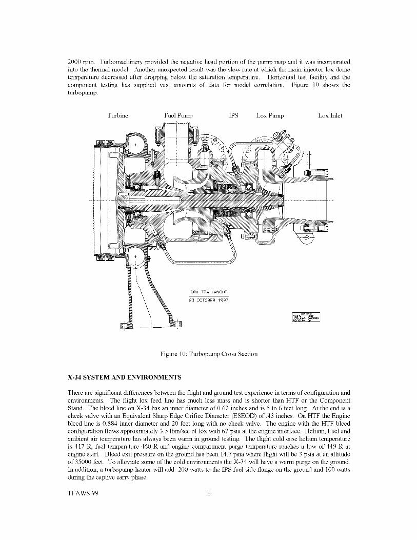
2000rpm.Turbomachineryprovidedthenegativeheadportionofthepumpmapandit wasincorporatedintothethermalmodel.Anotherunexpectedresultwastheslowrateatwhichthemaininjectorloxdometemperaturedecreasedafterdroppingbelowthesaturationtemperature.Horizontaltestfacilityandthecomponenttestinghassuppliedvastamountsof datafor modelcorrelation.Figure10showstheturbopump.

Turbine FuelPump IPS LoxPump LoxInlet

60K TPA LAYOUT

23 OCTOBER 1997

Figure 10: Turbopump Cross Section

X-34 SYSTEM AND ENVIRONMENTS

There are significant differences between the flight and ground test experience in terms of configuration and

environments. The flight lox feed line has much less mass and is shorter than HTF or the Component

Stand. The bleed line on X-34 has an inner diameter of 0.62 inches and is 5 to 6 feet long. At the end is a

check valve with an Equivalent Sharp Edge Orifice Diameter (ESEOD) of .43 inches. On HTF the Engine

bleed line is 0.884 inner diameter and 20 feet long with no check valve. The engine with the HTF bleed

configuration flows approximately 3.5 lbm/sec of lox with 67 psia at the engine interface. Helium, Fuel and

ambient air temperature has always been warm in ground testing. The flight cold case helium temperature

is 417 R, fuel temperature 460 R and engine compartment purge temperature reaches a low of 449 R at

engine start. Bleed exit pressure on the ground has been 14.7 psia where flight will be 3 psia at an altitude

of 35000 feet. To alleviate some of the cold environments the X-34 will have a warm purge on the ground.

In addition, a turbopump heater will add 200 watts to the IPS fuel side flange on the ground and 100 watts

during the captive carry phase.

TFAWS 99 6

LowerFeedlineBleed

UpperFeedlineBleed

LowerFeedline

LoxPump FuelPump

Engine--InterfacePanel

CheckValve

Prevalve

®Engine Bleed Valve

GG Oxidizer

Valve

Figure 11: Typical Lox Feed and Bleed System

Oxidizer

Valve

Cox

Seal

Drain

THERMAL MODEL

A thermal model was created to determine the important parameters that drive the thermal conditioning of

the turbopump prestart. It encompasses the feed line, bleed lines, and most of the turbopump. There is

detailed modeling of the lox also since transient flow rates and lox quality are such important aspects of this

problem. The approach taken is to model the ground test hardware, environments, valve sequences,

pressures and correlate the model. Only then can the X-34 condition be predicted with confidence. As more

test data has been produced the model has evolved to be more complex to match the data. The following

major changes to the model have taken place in chronological order. The first improvement was the

detailed modeling of the Inter Propellant Seal to match the warm fuel seal drain temperature that was seen

on the component stand. These changes include a variable clearance in the 9 tooth labyrinth seal and fluid

nodes with heat transfer for the helium. Then heaters were added along with logic to simulate the flight

designed thermostat set points and tolerances. Then the necessary logic to model all facilities with all the

flow circuits was added with the capability to run complicated pressure and valve position profiles.

Properties and lox temperatures are determined from calculated enthalpy to better model the saturated and

subcooled fluid and the heat transfer occuring in the lox system.

INTEGRAL FLUID MODEL

The fluid in the lox feed and bleed system has been divided in to approximately 60 nodes. At each location

the state of the lox is dependent on the energy balance including the stored energy, energy in and out from

mass flow, and the convective energy transferred to the fluid in the volume. The enthalpy is calculated and

TFAWS 99 7

usedtodeterminethefluidproperties.Fornodeswhichcontainsaturatedliquidandvapor,allpropertiesarecalculatedbasedonvolumefractionofvapor,andsaturatedvaporandliquidproperties.Theapproachtocalculatingheattransfercoefficient(HTC)is tocalculateavaporandliquidHTCandthenaveragethetwobasedonthevaporfractionbyvolume.Theflowratecalculationhasproventobethemostdifficult.ThefirstapproachwassimpleandusedlossfactorsandBemoulli'sequationtoiterateonaflowrateineachbleedpath.ThedifficultyhascomefromthefactthattherearelargevariationsindensityandHTCthatoccur,causingtheflowratepredictiontobeunstable.Atapressureof50psiasaturatedliquidis77timesmoredensethanvapor.NucleateboilingHTCis ashighas1800btu/ft2/hr/Fandfilm boilingHTCis aslowas20btu/ft2/hr/F.Theflowcalculationwasstabilizedanda goodcorrelationwasachievedforanenginebleedonlychillonHTF.CorrelationtotheMOVchillonHTFhoweverhasbeendifficult.Thecurrentversionofthechillmodelhasamorecomplicatedsolutionthatincludesconductorsforchokedflowandcavitation.It isincompleteatthistime.

HARDWARETEMPERATUREPREDICTIONS

All themasswhichmustbechilledorthatmaytransferheattoanyoftheloxflowcircuitsisincludedinthemodel.Theturbopumpis modeledin greaterdetailin orderto addressthefuelsidetemperaturerequirementsaswellasmatchanyIPSandturbopumpsurfacetemperaturesmeasuredin thegroundtestprogram.Thefeedlinesandbleedlinesaremodeledsimplywithapproximately60nodes,eachwith the

correct surface area and mass. External heat transfer is included or disabled if the line is insulated.

RESULTS FOR HTF AND X-34

The results presented in this paper are from a version of the model which correlated well with an engine

bleed test on HTF and then was used to predict the X-34 chill. This version of the model did not correlate

well with the HTF test where the engine, feed and bleed system were chilled through the Main Oxidizer

Valve (MOV). The results presented here are for illustration of what the model capabilities are, recognizing

that more features are required to match all the test data.

On HTF the chill sequence typically involves a low pressure chill of the upper feed line through the upper

feed line bleed. When cold liquid is evident upstream of the prevalve, the prevalve is opened beginning the

chill of the lower feed line through the lower feed line bleed and engine bleed. Shortly after prevalve

opening the upper feed line bleed is closed and the tank is pressurized taking the engine interface pressure

from 18 psia to 68 psia. Figures 12 shows the predicted mass flow rate. The first hump in this curve is the

low pressure upper feed line chill. The second hump is lower feed line chill with both lower valves open

and engine interface pressure at 80psia. Flow rate drops in half to 4.5 lbm/sec when the lower lox line

bleed is closed. The next drop in flow rate occurs when the tank is vented. While vented the lower lox line

bleed is opened again and at approximately -1700 seconds the tank is pressurized to 68 psia. Shortly after

pressurization the lower lox line bleed is closed again. Figures 13 and 14 show analysis and test data

respectively for engine interface temperature and how it compares to saturation temperature at that pressure.

Figures 15 and 16 show predicted and measured gallons of lox in the tank. Figures 17 and 18 show

predicted and measured fuel seal drain temperature. It is interesting to note how this temperature rises at -

3200 seconds when tank pressure is reduced and how it drops again at -1700 seconds when the tank

pressure is increased again.

The X-34 analysis is much more simple in terms of tank pressurization and valve sequences. Tank pressure

starts at 13 psia and the prevalve and engine bleed are opened at 0 seconds. Soon the tank pressure is

ramped to 58 psia which is the start pressure for the engine. Figure 19 shows the engine interface

temperature as well as the saturation temperature at the interface pressure. The plot shows the engine

interface temperature constraint being met at 410 seconds. The lox consumption curve is shown in figure

TFAWS 99 8

20andwiththischillprocedureshows700lbconsumedat710seconds.Thestartwindowthenwilloccurbetween410and710seconds.Figure21showsthatinthiswindowthefuelsealdraintemperatureatanacceptablelevelandconsistentwiththegroundtestexperienceof400R. Figure22showsthepredictedtransientflowratefortheX-34bleedlineatthelowexitpressure.

FUTURETESTINGANDANALYSIS

ThereisaplannedtestonHTFwithasimulatedX-34bleedline. DownstreamoftheEngineInterfacePaneltherecurrentlyisableedline20feetlongwith inner diameter of ..884 inch. The last 5.5 feet of thisline is to be modified to inner diameter of .62 inch and with an orifice at the end with diameter of .43 to

simulate a check valve which is in the X-34 bleed line. The X-34 vehicle itself is scheduled to ground

tested with an engine firing included so there will be chill data for the flight feed and bleed system prior to

first flight.

The thermal model is currently being modified to include flow conductors to calculate choked flow and

cavitating flow for valves and orifices in the lox feed and bleed system. Once that version is operational

and predicting stable flow rates, correlation to test data will begin.

c

w

12

10

Analysis, HTF Test, Lox Mass Flowrate

-2 '

-6000

.... I .... I .... I .... ! .... I .... I ....

: [ [ = --T1411

.............. i............................. ".............. "............... i...... xp2_cd_htf05

I I I I I I I I I I I I I I I I I I I I I I I I I I I I

-5000 -4000 -3000 -2000 -1000 0 1000

Time (seconds)

Figure 12: Predicted Feed line Flow rate

TFAWS 99 9

R

Analysis, HTF Test, Engine Interface Temperature

550 .... I .... I .... I .... I .... I .... I ' ' '

I i ! i i :.............._____.........j..............._..............!...............!__[-- TT-3S,51_500 _ ! i i _.....TSATE'FI

450 .............. i----- t- ...... ] .............................. !............... [___.xp6_ccl_htf05 ....

400 ............................ _............................................. _............... _..............

350 ............................................................ _-.............. _.............................

300 ........................................... _.............. _.............................................

250 .............. ; ........ t ..... I............... ',-

: i ............................... ! ..............1

200 ....................... /_v v,4,...... -i--i ............... i ----; --:- --:----.i- -:--:- - --:--:-4L..............', t i : i ] :

........ i i i i150 ' ' ' ' ' ' ' ' , , , , I , , , , , , , , , , , , , , , ,

-6000 -5000 -4000 -3000 -2000 -1000 0 1000

Time (seconds)

Figure 13 : Predicted Engine Inlet Temperature

500-

400

300

........ _1........ ' ............... -_........ "_........

: I : I

: I

i I

.................................................................................. _........................ 4 --

200 , x , k _ , / , _"

"................................. +....... " :'" I *'\ : " I /\

: I : I: I : I

1O0 ..................................._..................................+......................................................................_..................................+..................................-6000 -5000 -4000 -3000 -2000 -1000 0

-rIME *Averaged to 1000 Points12:58FM August 31, 1999

Figure 14: Measured Engine Inlet Temperature

TFAWS 99 l0

Sn

Ge

m

x

P

Analysis, HTF Test, Lox Volume Gallons

45OO

4000

35OO

3000

2500

2000

1500

-6000

.... I .... I .... I .... ! .... I .... I ....

mT 451

i i i i i i i i i i i i i i i i i i i i I i i i i J i i i i

-5000 -4000 -3000 -2000 -1000 0 1000

Time (seconds)

Figure 15: Predicted Lox Volume in Gallons

--X--b2fl h045.100 6208 GAL LT3S02-LO4400- V'_lnRot v3.'l 0

4000

3600

3200-

28OO

24OO

2000-

160C

I I I I II I J I

I I I I II I I I I

I J I I II I I I I

I I I I II I I J I

I I I I II I I I I

I I I I...................... I....................... I...................... I......................... I .......................... I .........................

I I I I II I I J I

I I I I II I I I

I J I I II I I I

I I I I I

I I I J II I I I I

I I I I I

I

................ I......... I.................. I........J I I

I I II I I

I I I

I I I

TFAWS 99

-6000 -5000 -4000 -3000 -2000 -1000 0

TIME *Averaged to 1000 Points10:43AM Augu_ 31,1999

Figure l 6: Measured Lox Volume in Gallons

ll

R

m

f

Analysis, HTF Test, Fuel Seal Drain Temperature

52o 500 ....i..............i......................................i i x;e---c-_--h#O_

480

460

440

420

400

-6000 -5000 -4000 -3000 -2000 -1000 0 1000

Time (seconds)

Figure 17: Predicted Fuel Seal Drain Temperature

--X-- b2fl h045.100520

500- ...............................----__--

6344 DEGRIPS FL ISLDR]MPV_nRot _G 10

480 i ....I

I

I

I

460- ................ iI

I

I

I

440- _ _ _ iI I I i

i

I I I i

420 ............... i- - T ............ I......... i

I I i

I I i

400 ....I I I

I I I I

I I I I

380_ _ _ t-6000 -5000 -4000 -3000 -2000 -1000 0

to 00TIME *Averaged ,:1_,__o_o_!_§

Figure 18: Measured Fuel Seal Drain Temperature

TFAWS 99 12

R

m

Analysis, X-34 Cold Case, Engine Interface Temperature

220 I I I !

i i j, --TT_S,_,_,210 ......................................................................... _ .... TSATEIF |

1 1 1

200 ................... i .................... i ..................... ! ............. xp6_cd_x34cold---

190 ....', ] ', ,, ,,

1

18o ...................._.....................i.....................i ....................4....................

, a1 1,, ,,

170 ;-_................. _.................... Start Box 163 N at 410' seconds .....

. I 1 _ 1

160 ,, ,, ',1

11

1

_o....................i....................i.....................i..........................................140 , , , i , , , i , , , I , , , I , , ,

0 200 400 600 800 1000

Time (seconds)

Figure 19: Predicted X-34 Engine Inlet Temperature

n

m

n

8

TFAWS 99

1200

1000

800

6OO

400

200

Analysis, X-34 Cold Case, Lox Consumption

......... i, ; T_46'-I ''/_.........................................................__

200 400 600 800 1000

Time (seconds)

Figure 20: Predicted X-34 Lox Consumption

13

R

m

Analysis, X-34 Cold Case, Fuel Seal Drain Temperature

55O

5OO

45O

400

35O

'l&' ' .......... ! ' ' '

___=P,o6344I

xp6_cd_x34col d

! _ ,, 3_8_! ;'iI "_.i 710sec El

....................L...... _ .....i.....................

I I I I I I I I I I I I I I I

0 200 400 600 800 1000

Time (seconds)

Figure 21: Predicted X-34 Fuel Seal Drain Temperature

1.5

c

1

w

0.5

Analysis, X-34 Cold Case, Lox Flowrate

I i !

Steady Liquid Flowrate 1.7 Ibm/sec

..................................._ .......i--,--------;-i_i-ii-

,,, i,,, i,,, i,, p2'_cdx3co,ld

0 200 400 600 800 1000

Time (seconds)

Figure 22: Predicted X-34 Lox Flowrate

TFAWS 99 14

CONCLUSIONS

Current analysis indicates that all the prestart thermal conditioning requirements can be met although the

exact procedure and timing for the start window can't exactly be determined. There is some flexibility in

the procedure in that the MOV can be opened to accelerate the opening of the start window. Also, once the

liquid starts flowing in the bleed line the tank pressure can be reduced to reduce consumption and delay the

closing of the window.

ACKNOWLEDGEMENTS

The author wishes to acknowledge the contributions of the following people and orgainizations.

Richard Cooper and the component test team for performing the work necessary in the RP-1 Tray freezing

test, the Impeller chill test in LN2 and the modifications performed on the component test stand as well as

special chill tests on the component test stand for the purpose of model correllation.

Phil Hall for performing the work necessary in the lox boiling heat transfer coefficient testing.

Bruce Tiller and Wayne Gamwell for performing the work necessary for the RP-1 freezing on the cold tube

wall testing.

Mike Ise, Tom Byrd and the Fastrac Engine Horizontal Test Facility team for hardware modifications and

dedicated chill testing with the engine.

TFAWS 99 15

STS-93 SSME NOZZLE TUBE RUPTURE INVESTIGATION

W. Dennis Romine, Senior Engineering Specialist

Rocketdyne Propulsion & Power

Space & Communications Group

Boeing Corporation

INTRODUCTION

STS-93 was launched on July 23, 1999. There was an anomaly at the end of the

launch in that the Space Shuttle Main Engines (SSME) shut down 0.16 second early

because sensors detected a low level of oxidizer in the LOX tank (actually the duct from

the tank to the vehicle). This resulted in a cutoff velocity for the vehicle that was 16

ft/sec low. It should have been 25872 ft/sec. An investigation was immediately initiatedinto the cause of this LOX tank low level cutoff.

It was noticed during the launch that the turbine temperatures for Main Engine 3

(E2019) were approximately 100°F higher than the preflight prediction. Linear Engine

Model matching of the data indicated that a nozzle leak best fit the data. Post launch

review of the data showed, that at approximately five seconds into the start, numerous

parameters indicated small anomalous shifts. These shifts were all consistent with a

rupture of nozzle tubes.

Post launch review of the films showed that just after SSME ignition and just

prior to liftoff a streak is seen in the exhaust plume of E2019. Just after liftoff the streak

can be seen emanating from the nozzle wall. This photo confirmed that a leak was

coming from the nozzle tubes. Based on the photo, the axial location of the leak wasestimated to be 28" from the aft end of the nozzle. The streak continued to be visible

during the launch (Figure 1).

Almost immediately upon landing a visual inspection was made of the nozzle. It

was confirmed that three nozzle tubes were ruptured at the suspected location (Figure 2).

The focus then turned to the cause of the tube ruptures. Prior to landing, a hardware

review revealed that two main injector LOX posts had been deactivated prior to the

flight. This is done by inserting pins in the orifices located in the interpropellant plate of

the main injector (Figure 3). Therefore, once the engine was available, a high priority

was to inspect for these pins. Indeed one of two pins was missing. A pin is

approximately 0.9" long by 0.1" in diameter, weighs 1.5 grams, and is gold plated. Also,

there was a ding in the Main Combustion Chamber (MCC) in line with this post at a

location 2.5" upstream of the MCC throat. The tube ruptures are located approximately

30 ° in the azimuthal direction from the post with the missing pin.

The ruptured tubes were sectioned from the nozzle and subjected to an evaluation

in the Materials laboratory. The overall length encompassed by the tube ruptures was

consistent with the size of a deactivation pin. The key finding from this investigation was

thatthediscolorationnotedattheruptureswasindeedgoldandhadachemicalcompositionidenticalwith thatof thegoldplatingusedonthepins. Thesamegoldwasalsofoundatthedentin theMCCwall. Theothersignificantfindingwasthattherupturingof thetubesoccurredduringtheimpactandwasnota delayedevent.Thisevaluationconfirmedthattheejectedpin causedthetuberuptures.

As aresultof thisconclusion,thefollowingaerothermalquestionsweregeneratedwith regardtothepin.

• Whatis thetrajectoryof thepin?

• Whatis thevelocityof thepin asit impactsthenozzle?

• Whatis theprobabilitythatanejectedpin will impactthenozzle?

• Whatis theprobabilitythatthepin will damagethenozzleif it hitsthenozzle?

• Wasthistheworstdamagethatthepin couldcause?• Wouldthepinhit thenozzleif it is ejectedfrom adifferentlocationonthefaceof

theinjector?

• How muchdamagecanthepin dototheMCC?

At first it wouldseemtobeadifficult taskto answerthesequestionsfor aseeminglyrandomevent.However,it wasfoundthatarelativelysimplecomputermodelusingbasicflow principlescouldbedevelopedto providereasonablefirst orderanswersto thesequestions.

TRAJECTORYCALCULATIONMETHODOLOGY

In orderto attemptanytypeof trajectoryanalysisfor thepin,thecombustiongasflow field mustbedefined.Thisinformationwasgeneratedwhenthechamberandnozzlecontourswereinitially developed.Theseparametersare

• Thecombustionchamberandnozzlecontourprofiles.

• ThecombustiongasMachnumber.

• Thecombustiongasvelocity.

• Thecombustiongasstaticpressure.

• Thecombustiongasstatictemperature.

• Thecombustiongasdensity.

trajectory.thepin.

With this information,asimplemodelcanbesetup for calculatingthepinThefundamentalequationfor thismodelis theequationfor thedragforceon

F = CD*AN* p(VG-Vp)2/2

Using this fundamental equation, the following procedure is used to calculate the

axial component of the pin traj ectory.

1. The initial coordinates of the pin are selected (axial and radial location).

2. An initial pin velocity (speed and angle or, equivalently axial and radial components

of velocity) is selected.

3. Values for the axial and radial drag coefficients are selected.

4. Values for the pin area normal and parallel to the combustion chamber axis aredetermined.

5. An incremental axial position is selected (initial X + _).

6. The combustion gas density and axial speed are determined for the average axial

position (initial X + _/2).

7. An initial guess is made for the pin axial speed after it has traversed the axial lengthincrement.

8. The average axial speed of the pin for the axial increment is calculated by taking the

average of the starting and ending speeds.

9. From the relative axial speed and the density, the pressure [p(gGx-gpx)2/2] acting on

the pin in the axial direction is calculated.

10. The average axial force over the axial length increment is calculated from the axial

pressure acting on the pin, the drag coefficient, and the pin area normal to thechamber axis.

11. From the initial axial speed, the average force, the pin mass and the axial length

increment, the time for the pin to traverse the axial length increment is determined.

12. From the initial axial speed, the time increment, the mass of the pin, and the average

axial force on the pin, the axial speed of the pin at the end of the axial increment iscalculated.

13. Using this axial speed at the end of the axial increment, Steps 8 through 12 are

repeated until the axial speed converges.

14. Steps 5 through 13 are repeated until the desired final axial position is reached.

Once the axial component of the trajectory has been calculated, the radial

component can be calculated using the following similar procedure.

1. Starting at the initial position of the pin and the initial axial increment, the average

radial component of the combustion gas velocity is determined.

An initial guess is made for the pin radial speed after it has traversed the axial lengthincrement.

3. The pin radial speed at the average axial position is calculated by averaging the

starting and ending radial speeds.

From the relative radial speed and the density, the pressure [p(VG_-Vp_)2/2] acting on

the pin in the radial direction is calculated.

.

.

5. The average radial force over the axial length increment is calculated from the radial

pressure acting on the pin, the drag coefficient, and the pin area parallel to thechamber axis.

6. From the initial radial speed, the time increment, the mass of the pin, and the average

radial force on the pin, the radial speed of the pin at the end of the axial increment iscalculated.

7. Using this radial speed at the end of the axial increment, Steps 3 through 6 are

repeated until the radial speed converges.

8. Using the average radial speed and the time for traversing the axial increment, the

change in radial position is calculated and added to the radial position at the start of

the increment to get the radial position at the end of the increment.

9. Steps 1 through 8 are repeated until the desired final axial position is reached.

Using this procedure, starting parameters can been iterated to determine the

values required to impact the nozzle as a specific location.

DRAG COEFFICIENT

To make the above calculations, the drag coefficients for the pin in both the axial

and radial directions must be determined. The drag coefficient is a function of the Mach

number, the Reynolds number, the object shape, and the orientation of the object within

the flow field. The Reynolds number for the pin as it travels in the combustion gas flowfield is calculated to be in the range from 103 to 10 5. The two extreme positions for the

pin orientation are for the pin axis to be either normal or parallel to either the axial or

radial component of the combustion gas velocity.

For the pin axis normal to the flow field, the pin can be approximated as a

cylinder in cross flow. The drag for this configuration has been studied extensively for

an infinitely long cylinder and is available as a function of Reynolds number in standard

texts. For this configuration in the Reynolds number range of interest, the drag

coefficient is between 0.9 and 1.2. For a cylinder of finite length the drag coefficient will

be lower. For a cylinder with an aspect ratio of 9:1 (approximately that of the pin), the

drag coefficient is approximately 2/3 that for an infinitely long cylinder. Applying this

ratio to the infinitely long cylinder results gives a drag coefficient range from 0.6 to 0.8.

The area of the pin normal to its axis is approximately 0.09 in 2. This will result in a

maximum drag coefficient times area of 0.072 in 2.

For the pin axis parallel to the flow field, the pin can be approximated as either a

square ended cylinder or a projectile depending on which way the pin is oriented. The

projectile will have the lower drag coefficient. The minimum drag coefficient for a

projectile is 0.2. Multiplying this by the pin approximate cross sectional area of 0.015 in 2

gives a minimum drag coefficient times area of 0.003 in 2.

Thepin couldalsoberotatingand/ortumbling.Rotationcancreatelift.However,calculationsindicatethatthepin wouldhaveto developasignificantrotationrateto generateanappreciablelift. It is notexpectedto dothis. Anytumblingwill causethedragcoefficienttimesareavalueto varywith time. Thecalculatedrangeof valuesfor thedragcoefficienttimesarea(0.003in2to 0.072in2)areintendedto provideageneralrangeof thevaluesthatcanbeexpectedfor thepin asit is travelingthroughthecombustiongasflow field.

TRAJECTORYTOMCCIMPACT

Oncethepin dislodgesfromtheorificeit will traveldowntheLOX postuntil itexitstheinjector.FromtheLOX pressureandthegeometry,theforceonthepin canbeestimatedandthevelocitycalculated.FromtheMaterialsevaluationit isknownthatthetubesrupturedwhenthepinhit them. Thedataindicatesthatthetubesrupturedatapproximatelyfive secondsafterignition,whichis onesecondinto100%powerleveloperation.Therefore,thepin wasdislodgedduring100%powerleveloperation.Fromanumberof calculationsit wasdeterminedthatareasonableestimatefor thevelocityof thepin asit exitsthepostis 100ft/sec.Thepin initial radialpositionwill beapproximately0.4" fromtheMCC wall. Mostlikely it will betravelingwith thepin axisparallelto theflow. Itsdragcoefficienttimesareain theaxialdirectionshouldbeclosetotheminimumcalculatedvalue0.003in2. In thenormaldirectionit will becloseto themaximumvalueof 0.072in2.

A parametricanalysiswasmadeto determinetheconditionsrequiredfor thepinto impacttheMCC ata location2.5"forwardof thethroat. Parametersvariedweretheaxialdragcoefficienttimesarea,radialdragcoefficienttimesarea,initial velocity,andexit anglefromLOX post. Thefollowingconclusionsweremadefromthisparametricanalysis.

• Themostsignificantresultwasthattheminimuminitial trajectoryanglefor thepinhadtobeapproximately10° in orderfor thepinto impact2.5" forwardof thethroat.Thisminimumanglewasindependentof thecombinationof otherconditionsrequired.Any anglelessthan10° will causethepin to impactmoreforwardof thethroat.

• Foraninitial velocitylessthan100ft/sec,theaxialdragcoefficienttimesareabecomessmallerthanwhatappearsto beaminimumrealisticvalue. Thiswouldimply thatthe100ft/secis areasonablevaluefor theinitial speedof thepin whenitexitstheLOX post.

• A pin in oneof theoutertworowsof elements(rows12or 13,whicharemostlikelyto haveapin)of themaininjectorwill haveahighprobabilityof strikingtheMCC.

• Theimpactangleof thepin relativeto theMCC wall is shallow(lessthan10° with atypicalvalueof 5°). Thisis consistentwith theobserveddamageto theMCC.

• Thevelocityof thepin whenit hits theMCC isprimarilyafunctionof theinitialvelocity. This isbecausetheaccelerationof thepin isrelativelysmallupto thetime

it hitstheMCC. Theaxialvelocityatimpactis lessthan50ft/secgreaterthantheinitial velocityfor therangeof conditionsanalyzed.

Thetimefromexpulsionof thepinto impactwith theMCC will beafunctionof theaxialvelocitywhich,in turn,isaprimarilyafunctionof theassumedinitial velocity.Foraninitial velocityof 100ft/sec,thetimeis approximately10milliseconds.

TRAJECTORYFORNOZZLEIMPACT

After thepin impactstheMCC,it continuestravelingin thecombustiongasflowfield until it impactsthenozzleata location28" forwardof theaftmanifold. It isnotknownpreciselyhowtheimpactof thepin with theMCCaffectsthepin trajectory.Itcanbeexpectedtherewill beareductionin thepinvelocityasaresultof it hittingtheMCC. Theshallowimpactanglesuggeststhatthepin trajectoryanglewhenit leavestheMCC will besimilarto thatof theMCC wall atthepointof impact(25°). It isknownthatthepin impactedthenozzleatanazimuthalangle30° from the MCC impact point.

This could imply that the impact with the MCC gave the pin a velocity component in theazimuthal direction.

A parametric analysis was also made for the trajectory of the pin from when it

grazed the MCC to when it impacted the nozzle. Parameters varied were the axial drag

coefficient times area, radial drag coefficient times area, initial speed and angle after

grazing the MCC. The following conclusions were made from this analysis.

• For reasonable values of the initial speed and angle after grazing the MCC, these

parameters do not significantly affect the trajectory (Figure 4).

• The pin velocity at impact is on the order of 700 to 900 ft/sec depending on the

assumed set of conditions. This is roughly an order of magnitude less than the

combustion gas velocity. A structural analysis estimated that an axial component of

the velocity of 300 ft/sec and a radial component of 600 ft/sec are required to produce

the observed damage to the nozzle tubes. This is equivalent to a pin velocity of about700 ft/sec. The calculated velocities are consistent with this structural evaluation.

• The pin impacts the nozzle at an angle of typically 13° to 15 ° relative to the nozzlewall.

• The time from impact with the MCC to impact the nozzle is on the order of 20 to 30

milliseconds depending on the assumed set of conditions.

PROBABILITY OF PIN HITTING THE NOZZLE

Using the trajectory calculation model, the combination of conditions required for

the pin to hit the nozzle can be determined. This is done by first determining the

combination of conditions (radial and axial drag coefficient time area) that will result in

the pin hitting at the aft end of the nozzle. This set of conditions represents the dividing

line between impacting and not impacting the nozzle (Figure 5). Any combination of

axialdragcoefficienttimesareaandradialdragcoefficienttimesareabelowthelinewillresultin thepin hittingthenozzle.

Next therangeof axialdragcoefficienttimesareaandradialdragcoefficienttimesareathatcanoccurfor thepin canbedetermined.Thiswasdiscussedearlier.Theminimumaxialdragcoefficienttimesareathatcanbeexpectedis0.003in2. Forthisconditiontheradialdragcoefficienttimesareawouldbeatits maximumvalueof 0.072in2. Themaximumvaluefor axialdragcoefficienttimesareawouldbethe0.072in2value.Forthisconditiontheradialdragcoefficienttimeareacouldrangefromtheminimumof 0.003in2tothemaximumof 0.072in2dependingonthepin orientation.Theserangesresultin atriangularregionof possibleaxialandradialdragcoefficienttimesareas(Figure5). If thereisanequalprobabilityof anypointwithin thetriangle,thentheprobabilityof thepin hittingthenozzleis theratioof thehit areaof thetriangleto thetotalareaof thetriangle.Thisratiois 12%,whichis equivalentto aonein eightchanceof thepin hittingthenozzle.

However,ratherthananequalprobabilityof anyconditionwithin thetriangleoccurring,it is expectedthattherewill beaprobabilitydistributionfor boththeaxialandradialcomponents.Thepin shouldwantto alignits axisgenerallyto thatof thenozzlecenterline.Thiswouldcauseaskewedprobabilitydistributionwheretheaxialdragcoefficienttimesareawouldmostprobablybeatthelow endof itsrangeandtheradialdragcoefficienttimesareawouldmostprobablybeatthehighendof its range.

A lognormaldistributionappliedto boththeaxialdragcoefficienttimesareaandtheradialdragcoefficienttimesareacanbeusedto approximatethisexpectedskewness(Figure4). Whentheseprobabilitydistributionsarefactoredintothecalculation,theprobabilityof thepin hittingthenozzleincreasesto 64%orapproximatelytwo in three.

PROBABILITYOFPIN RUPTURINGA NOZZLETUBE

Startingwith asetof conditionsthatresultsin thepin impactingthenozzleattheaft end,theaxialdragcoefficienttimesareacanbeincrementallyreducedto resultin thepin impactingfartherandfartherforwardin thenozzle.Thevelocityof thepin atthevariousimpactlocationsisapartof thetrajectorycalculation.As expected,theimpactvelocityof thepin decreasesastheimpactlocationmovesforward.Thekineticenergyofthepin asit impactsthenozzleis expectedto betheprimaryfactorin determiningif thepin will ruptureanozzletube. Simplistically,sincethesquareof thevelocityisproportionaltothekineticenergyof thepin, thereshouldbeaminimumpin velocityrequiredto causeatubeto rupture.In reality,otherfactorsneedto beconsideredsuchaspin orientationatimpact,theradialandaxialcomponentsof thevelocity,thetubegeometryatthe impactlocation(tubediameterandwall thicknessdecreasesgoingforwardin thenozzle),andthetubetemperature(increasesgoingforwardin thenozzle).

Linesof constantvelocitycanbedeterminedandthenoverlaidontheparametricanalysisresults(Figure5). Theareawithin thetrianglebetweenaconstantvelocityline

andthelineof demarcationbetweenhittingandnothittingthenozzle,is thesetofconditionsthatwill resultin thepin impactingator greaterthanagivenvelocity.Assuminganequalprobabilityfor anypoint,theprobabilityof thepin hittingatorgreaterthanagivenvelocityis theratioof areas.Again,theprobabilitydistributionscanalsobefactoredin. Theseprobabilitiescanthenbeplottedasafunctionof velocity(Figure6).

Thestructuralevaluationindicatedthatminimumrequiredpin velocityto causetherupturesisontheorderof 700ft/sec. Applyinga50ft/secuncertaintyto thiscalculationresultsin arangefrom650ft/secto 750ft/sec.Thehotfire experienceis thatonein eighteen(5.6%)ejectedpinscausedaruptureof nozzletubes.Becauseof thesmallsample,the95%confidencelimits for thisstatisticare1.4%to 27%. Thisboxofconditionscanbeoverlaidonthecalculation(Figure6). Fromthis it canbeseenthat,despitethesimplificationsandassumptionsthatwentinto themodel,themodelcanmakereasonableprobabilityassessments.

CONCLUSIONS

In summary,asimplegenericmodelfor determiningthetrajectoryandotherconditionsof anobjectin thecombustionchamberandnozzlehotgasflow field of arocketenginehasbeendeveloped.Thismodel(process)canbeusedfor anyanalysisof arocketenginewhereit is desiredto estimatetheimplicationsof asolidcontaminantthathasbeenintroducedinto thecombustiongasflow field.

Forthespecificcaseof theLOX postdeactivationpin thatwasejectedduringthelaunchof STS-93,it wasfoundthattheresultsof themodelwereconsistentwith thehardwareobservations.Additionally,themodelwasusedto makeprobabilitypredictions,whichwerealsoconsistentwith thehot fire experience.

NOMENCLATURE

AN z

CD =

F =

LOX =

MCC =

SSME =

STS =

go =

VGR ----

VGX --

gp =

VpR --

gpx --

X =

Area normal to flow

Drag coefficient

Force

Liquid oxygen

Main Combustion Chamber

Space Shuttle Main Engine

Space Transportation System

Velocity of combustion gas

Component of combustion gas velocity in radial direction

Component of combustion gas velocity in axial direction

Velocity of particle

Component of particle velocity in the radial direction

Component of particle velocity in the axial direction

Axial position

AX = Axial position increment

p = Density

Figure 1. Nozzle Leak During Launch

lO

Figure2. NozzleTubeRuptures

11

Powerhead _

Combustion

Chamber Main Injector

LOX Post

Orifice

Gold

Pin

LOXPosts

(600)

_X Post

Figure 3. SSME Main Injector LOX Post Deactivation

12

50

40

_E" 30

,m"1o(_ 20

n_

10

0

-20

Approximately to scale

Nozzle _ ____lm pact

Contour _.._._,....-"""- ;.>-"-_" " Point, .;.;; ;""

..:>.:.:I

• -''•>

.-'"" J'_ Vo = 20 ft/sec

I I I I I I

0 20 40 60 80 100

Axial Distance from STMCC Throat (in)

120

Figure 4. Example Pin Trajectories

13

0.10

A

,m

-X

¢.)

O

O03

¢-t

X

0.08

0.06

0.04

0.02

0.00

0.00

\\

%%

%\

\%

\ Impact Vel.

",,,, (ft/sec) _ _

I I I I

0.02 0.04 0.06 0.08 0.10

Radial Drag Coefficient * Area (in 2)

Figure 5. Flow Conditions for Pin Impacting Nozzle

14

,-- 70

v

(9.Q

I--

03

O.

n_

"10

(9

O

=mm

"R.QO

EL

60

50

40

30

20

10

0

400

normal distribution

Equal distribution :: _ Uncertainty box

500 600 700 800 900

Impact Velocity Required to Cause Tube Rupture (ft/sec)

1000

Figure 6. Probability of Tube Rupture

15

ZERO GRAVITY CRYOGENIC VENT SYSTEM

CONCEPTS FOR UPPER STAGES

Robin H. Flachbart

James B. Holt

Leon J. Hastings

Space Transportation Directorate

NASA- Marshall Space Flight Center

ABSTRACT

The capability to vent in zero gravity without resettling is a technology need that involves practically all

uses of sub-critical cryogenics in space, and would extend cryogenic orbital transfer vehicle capabilities.

However, the lack of definition regarding liquid/ullage orientation coupled with the somewhat random

nature of the thermal stratification and resulting pressure rise rates, lead to significant technical challenges.

Typically a zero gravity vent concept, termed a thermodynamic vent system (TVS), consists of a tank mixer

to destratify the propellant, combined with a Joule-Thomson (J-T) valve to extract thermal energy from the

propellant. Marshall Space Flight Center's (MSFC's) Multipurpose Hydrogen Test Bed (MHTB) was used

to test both spray-bar and axial jet TVS concepts. The axial jet system consists of a recirculation pump heat

exchanger unit. The spray-bar system consists of a recirculation pump, a parallel flow concentric tube heat

exchanger, and a spray-bar positioned close to the longitudinal axis of the tank. The operation of both

concepts is similar. In the mixing mode, the recirculation pump withdraws liquid from the tank and sprays

it into the tank liquid, ullage, and exposed tank surfaces. When energy extraction is required, a small

portion of the recirculated liquid is passed sequentially through the J-T expansion valve, the heat exchanger,

and is vented overboard. The vented vapor cools the circulated bulk fluid, thereby removing thermal energy

and reducing tank pressure. The pump operates alone, cycling on and off, to destratify the tank liquid and

ullage until the liquid vapor pressure reaches the lower set point. At that point, the J-T valve begins to

cycle on and off with the pump. Thus, for short duration missions, only the mixer may operate, thus

minimizing or even eliminating boil-off losses.

TVSperformancetestingdemonstratedthatthespray-barwaseffectiveinprovidingtankpressurecontrolwithina6.89kPa(lpsi)bandforfill levelsof90%,50%,and25%.Completedestratificationoftheliquidandullagewasachievedatthesefill levels.Theaxialjetwaseffectiveinprovidingtankpressurecontrolwithin the same pressure control band at the 90% fill level. However, at the 50% level, the system reached

a point at which it was unable to extract enough energy to keep up with the heat leak into the tank. Due to a

hardware problem, the recirculation pump operated well below the axial jet design flow rate. Therefore, it

is likely that the performance of the axial jet would have improved had the pump operated at the proper

flow rate. A CFD model is being used to determine if the desired axial jet performance would be achieved

if a higher pump flow rate were available. Testing conducted thus far has demonstrated that both TVS

concepts can be effective in destratifying a propellant tank, rejecting stored heat energy, and thus,

controlling tank pressure.

NOMENCLATURE

CdA

h

Lohm

P

0S

T

t

U

X

ziP

equivalent flow area

heat of vaporization

enthalpy

viscojet flow resistance

mass flow rate

pressure

heat leak rate

specific gravity at viscojet inlet

temperature

time

internal energy

viscojet exit quality

pressure drop across viscojet

INTRODUCTION

The development of high-energy cryogenic upper stages is essential for the efficient delivery of large

payloads to various destinations envisioned in near term chemical propulsion programs. Also, many

advanced propulsion systems, including solar thermal and nuclear fission, use hydrogen as a working fluid.

Some of these systems are intended for long duration missions. A key technology challenge for all of these

applications is cryogenic fluid management (CFM) advanced development, specifically, the long term

storage of cryogens in space. In response to this challenge, MSFC has initiated an advanced

TFAWS 99 2

development/technologyprogramtobroadentheCFMexperience/database.Duetothecostof,andlimitedopportunitiesfor,orbitalexperiments,groundtestingisbeingemployedtothefullestextentpossible.Therefore,amajorobjectiveoftheMSFCprogramhasbeentoperformgroundbasedadvanceddevelopmenttestingonCFMsystemsforspacetransportationapplications.

A significantchallengeassociatedwithlongtermstorageofcryogensinspaceismaintainingpropellanttankpressurecontrolwhileminimizingpropellantboiloffloss.Auxiliarythrustersaretraditionallyusedtosettlethepropellantsinordertoaccomplishtankventing.Suchsystemsincurincreasingweightpenaltiesassociatedwith the propellant and hardware required to perform the settling burns. In addition, tank

venting may become necessary at an inopportune time in the mission timeline. The thermodynamic vent

system (TVS) concept enables tank pressure control through venting without resettling. A TVS typically

includes a Joule-Thompson expansion device, two-phase heat exchanger, and a mixing pump to destratify

and extract thermal energy from the tank contents without significant liquid losses.

However, TVS implementation has been constrained by the lack of opportunities for on-orbit experience,

mainly due to funding constraints. Analytical modeling of such systems is difficult due to the complex

combination of micro-gravity heat transfer, thermodynamic, and fluid mechanic phenomena involved, and is

further complicated by the lack of on-orbit data to correlate with the models.

SPRAY-BAR CONCEPT

The spray-bar TVS concept, developed by Boeing (Reference 1), was the first TVS concept tested in

MSFC's Multipurpose Hydrogen Test Bed (MHTB) (Reference 2). An illustration of spray-bar TVS

concept is provided in Figure 1. One advantage of this concept is that the active components (J-T

expansion valve, subsystem pump, and isolation valve) are located outside of the tank. Such an approach

simplifies component installation and enables modification or changeout of TVS components without

entering the tank. Also, this configuration supports feed line and engine thermal conditioning during micro-

gravity coast. The second, and perhaps more important advantage, is the longitudinal spray-bar, which is

used to achieve both liquid bulk and ullage gas thermal destratification through mixing. Since the liquid

bulk and ullage are destratified regardless of position, and the self induced heat transfer mechanisms are

based on forced convection, the spray-bar concept lends itself to verification in normal gravity. Therefore,

there is the potential for minimizing the dependence on costly micro-gravity experimentation.

TFAWS 99 3

JT Valve

Pump

Figure 1: Spray-Bar TVS Concept

In the mixing mode, fluid is withdrawn from the tank by the pump and flows back into the tank through a

spray-bar positioned along (or near) the tank longitudinal axis. The fluid is expelled radially back into the

tank through the spray-bar, which forces circulation and mixing of the tank contents regardless of liquid and

ullage position, assuring destratification and minimum pressure rise rate. For missions lasting from a few

days to weeks, depending on the insulation performance, tank mixing may be sufficient to control the tank

pressure with no propellant loss. When pressure control can no longer be achieved with mixing alone, a

portion of the circulated liquid is passed through the J-T valve, where it is expanded to a lower temperature

and pressure, passed through the heat exchanger element of the spray-bar, and finally is vented to space.

Therefore, the vented fluid removes thermal energy from, and thus cools, the bulk fluid circulated through

the mixing element of the spray-bar.

In an orbital propellant transfer scenario the spray-bar concept can be used to assist tank refill. By filling

through the spray-bar/heat exchanger, the in-flowing fluid can be cooled and used to mix the tank contents,

thus resulting in a "no-vent fill" process with minimal propellant losses. Additionally, if capillary liquid

acquisition devices (LAD) are used for micro-gravity propellant expulsion, the liquid within the LAD can

be conditioned by the spray-bar TVS. By withdrawing liquid from the capillary liquid acquisition device,

TFAWS 99 4

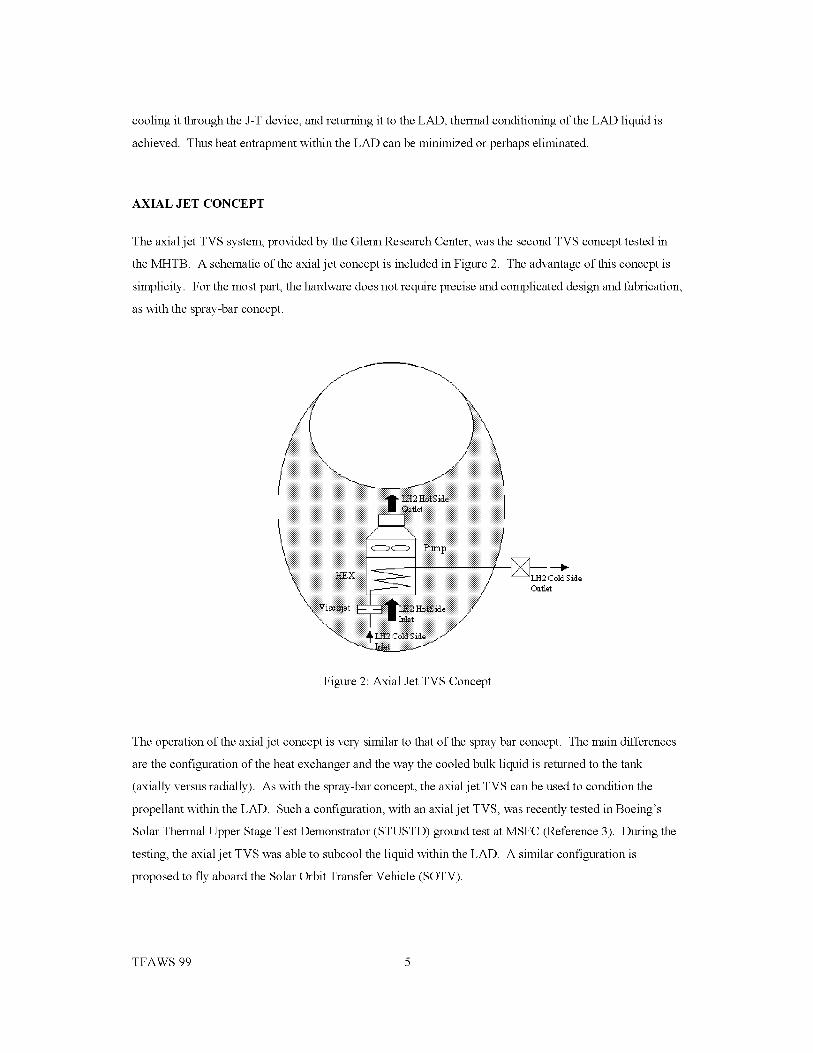
coolingit throughtheJ-Tdevice,andreturningittotheLAD,thermalconditioningoftheLADliquidisachieved.ThusheatentrapmentwithintheLADcanbeminimizedorperhapseliminated.

AXIAL JET CONCEPT

The axial jet TVS system, provided by the Glenn Research Center, was the second TVS concept tested in

the MHTB. A schematic of the axial jet concept is included in Figure 2. The advantage of this concept is

simplicity. For the most part, the hardware does not require precise and complicated design and fabrication,

as with the spray-bar concept.

Figure 2: Axial Jet TVS Concept

The operation of the axial jet concept is very similar to that of the spray bar concept. The main differences

are the configuration of the heat exchanger and the way the cooled bulk liquid is returned to the tank

(axially versus radially). As with the spray-bar concept, the axial jet TVS can be used to condition the

propellant within the LAD. Such a configuration, with an axial jet TVS, was recently tested in Boeing's

Solar Thermal Upper Stage Test Demonstrator (STUSTD) ground test at MSFC (Reference 3). During the

testing, the axial jet TVS was able to subcool the liquid within the LAD. A similar configuration is

proposed to fly aboard the Solar Orbit Transfer Vehicle (SOTV).

TFAWS 99 5

TESTSETUP

Themajortestarticleelementsconsistof thetesttankandenvironmentalshroudwithsupportingequipment,cryogenicinsulationsubsystem,andtestarticleinstrumentation.Thetechnicaldescriptionofeachoftheseelementsispresentedinthefollowingsections.

TESTTANKANDSUPPORTINGEQUIPMENT

TheMHTBaluminumtankiscylindricalwithaheightof 3.05m,adiameterof 3.05mand2:1ellipticaldomesasshowninFigure3. It hasaninternalvolumeof 18.09m3 and a surface area of 34.75 m 2. The

tank is ASME pressure vessel coded for a maximum operating pressure of 344 kPa and was designed to

accommodate various CFM concepts. The low heat leak composite legs and other tank penetrations are

equipped with LH2 heat guards so that more accurate measurement of the tank insulation performance can

be made.

Lin °n __ !

Figure 3: MHTB Tank and Support Equipment

The tank is enclosed within an environmental shroud which contains a ground hold conditioning purge,

(similar to a payload bay) and imposes a range of uniform temperatures on the insulation external surfaces

during orbit hold simulations. The shroud is 4.57 m high with a diameter of 3.56 m, and contains a purge

ring for distributing dry nitrogen.

TFAWS 99 6

CRYOGENICINSULATIONSUB-SYSTEM

TheMHTBinsulationconsistsofa%pray-on"foam/multilayercombination.Thefoamelementenablestheuseofapayloadbaytypepurgeduringgroundholdperiodsandthe45layermultilayerinsulation(MLI)providesthermalprotectionwhileatvacuumconditionsin orbit. Asreportedin Reference4, whichdescribestheinsulationperformanceinmoredetail,thecombinedeffectsoftheMLIvariabledensity,largeventholepattern,andinstallationtechniqueyieldsubstantialperformanceimprovements.However,inthisapplication,theinsulationsystemiscompromisedbytheTVShardwareinstallationandtaken_asis"aspartoftheMHTBtankconfiguration.

INSTRUMENTATION

Thetankinstrumentationconsistsprimarilyofthermocoupleandsilicondiodestomeasureinsulation,fluid,andtankwalltemperatures.TheMLIinterstitialpressureismeasuredattheSOFI/MLIinterfaceusingathinwalledprobethatpenetratestheMLI.Theprobeisalsoequippedwithaportforbothdewpointandgasspeciessampling.Twoofthefourcompositelegs,thevent,fill/drain,pressurization,pressuresensorprobe,andmanholepump-outpenetrationsareinstrumentedtodeterminethesolidconductioncomponentof heatleak.Thetankis internallyequippedwith two silicon diode rakes, which provide temperature

gradient measurements within both ullage and liquid. The TVS systems are instrumented with pressure and

temperature measurements throughout, in order to determine the pump flow rate, gas state in the vent lines,

and vent gas mass flow rate. These measured values are used to quantify the performance of the two TVS

concepts.

TEST FACILITY

Testing was performed at the MSFC East Test Area thermal vacuum facility, Test Stand 300. The

cylindrical vacuum chamber has usable internal diameter of 5.5 meters and height of 7.9 meters. The

chamber pumping train consists of a single stage gaseous nitrogen (GN2) ejector, three mechanical roughing

pumps with blowers, and two 1.2 meter diameter oil diffusion pumps. Liquid nitrogen cold walls surround

the usable chamber volume providing cryopumping and thermal conditioning. The facility and test article

-8

shroud systems in combination enabled simulation of orbital conditions (vacuum levels as low as 10 torr

and insulation surface temperatures ranging from 80 to 300 K).

A key facility capability was the test article pressure control subsystem used to maintain the steady-state

tank ullage pressure necessary during the boiloff tests, which are described in the next section. The

subsystem was composed of several flow control valves (located in the MHTB vent line), each of which

TFAWS 99 7

wasregulatedthroughaclosedloopcontrolsystem.Thiscontrolsystemadjustedthevalvepositionsbasedonacomparisonbetweenthemeasuredtankullagepressureandadesiredsetpoint.

TESTPROCEDURES

Two types of tests were performed with the TVS system in the MHTB. The first type was referred to as the

boiloff test, and the second was the TVS performance test. A more detailed description of each type of test

is provided in the following subsections.

BOILOFF TESTING

Boiloff testing was conducted to determine the ambient heat leak into the MHTB tank and to set up

consistent initial conditions for each of the TVS tests. The first test series was conducted with the vacuum

chamber LN2 cold walls operating to produce a minimum heat leak condition. The second series was run

without the LN2 cold walls, thereby providing a high ambient heat leak condition. Details relating to the

performance of boiloff testing were reported in Reference 4. Maintenance of constant ullage pressure and

steady state insulation temperatures was necessary during this test. The boiloff vent flow rate was typically

recorded for 6 hours after steady state was achieved.

The ambient heat leak is expressed as an energy balance across the tank boundary where the boiloff heat

transfer is equal to the sum of the heat transfer through the insulation, the tank penetrations, and the rate of

energy storage, if any, as seen in the following equation:

: + Q e.etra o.,+ --A Usystem

At

The terms Qboiloff and Qpe,_traao,_,, are defined using the test data. Specific calculation of these parameters

can be found in Reference 4. The thermal storage term AU_y_,t_m / At represents the energy flow into or out

of the test tank wall, insulation, and fluid mass. It is driven by the fluid saturation temperature, which varies

as ullage pressure varies. Since the ullage pressure is held within a tight control band (+/- 0.0069 kPa), this

term is considered negligible. The Qi,_,ul_ao, term can then determined using the defined quantities listed

above.

TFAWS 99 8

TVSPERFORMANCETESTING

Thespray-barwasevaluatedat90%,50%,and25%fill levelsinthefirsttestseries.Inthesecondseries,boththespray-barandaxialjetconceptsweretestedat90%and50%fill levels,butwithanelevatedheatleakcondition.TheambientheatleakwaselevatedduringSeries2duetotheaxialjetTVShardwareaddition,andbecausethefacilitycoldwallswerenotoperated.

Foreachfill level,afterboilofftestingwascomplete,thetankwaslockedupandallowedtoselfpressurizeuntiltheullagepressure(P4)reachedthemaximumtankpressuresetpointof138kPa.Uponreachingthispressure,therecirculationpumpwasturnedon,andmixingcontinueduntiltheullagepressurereached131kPa,thetankminimumsetpoint.Uponreachingtheminimumsetpoint,thepumpwasturnedoffandthetankwouldselfpressurizeforthenextcycle.Thisautomatedoperationcontinueduntilthetankliquidsaturationpressure(PSA1)reachedthelowerpressuresetpoint.Atthispoint,theJ-Tdevicewasusedtoextractheatenergyfromtheliquidwheneverthepumpoperated.BothTVSsystemconceptsoperatedinthismanneruntilthetestsconcluded.ThisTVScontrollogicisillustratedinFigure4.

...................... MAX PRESSURE

TANK PRESSURE-- -- MIN PRESSURE

VAPOR PRESSURE

ON

P =OP==TlONIIIllIIIIlo,,

ON

Figure 4: TVS Control Logic Illustration

RESULTS AND DISCUSSION

The baseline heat leak, mixing or destratification performance, and thermal energy removal, for both TVS

concepts, are discussed in the following sections.

TFAWS 99 9

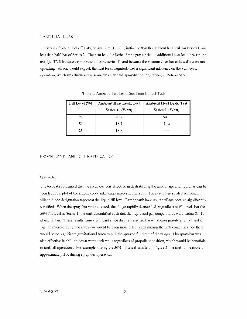
TANKHEATLEAK

Theresultsfromtheboilofftests,presentedinTable1,indicatedthattheambientheatleakforSeries1waslessthanhalfthatofSeries2. TheheatleakforSeries2wasgreaterduetoadditionalheatleakthroughtheaxialjetTVShardware(notpresentduringseries1),andbecausethevacuumchambercoldwallswerenotoperating.Asonewouldexpect,theheatleakmagnitudehadasignificantinfluenceontheventcycleoperation,whichwasdiscussedinsomedetail,forthespray-barconfiguration,inReference5.

Table1:AmbientHeatLeakDataFromBoiloffTests

FillLevel (%)

90

50

25

Ambient Heat Leak, Test

Series 1, (Watt)

20.2

18.7

18.8

Ambient Heat Leak, Test

Series 2, (Watt)

54.1

51.0

PROPELLANT TANK DESTRATIFICATION

Spray-Bar

The test data confirmed that the spray-bar was effective in destratifying the tank ullage and liquid, as can be

seen from the plot of the silicon diode rake temperatures in Figure 5. The percentages listed with each

silicon diode designation represent the liquid fill level. During tank lock-up, the ullage became significantly

stratified. When the spray-bar was activated, the ullage rapidly destratified, regardless of fill level. For the

50% fill level in Series 1, the tank destratified such that the liquid and gas temperatures were within 0.4 K

of each other. These results were significant since they represented the worst case gravity environment of

1-g. In micro-gravity, the spray-bar would be even more effective in mixing the tank contents, since there

would be no significant gravitational force to pull the sprayed fluid out of the ullage. The spray-bar was

also effective in chilling down warm tank walls regardless of propellant position, which would be beneficial

in tank fill operations. For example, during the 50% fill test illustrated in Figure 5, the tank dome cooled

approximately 2 K during spray-bar operation.

TFAWS 99 10

q<

o

<o

P,

--p263968k300/954 / +p263968k300/+p263968k.300 TD3 79.2% +p263968k.300 TD4 70.1%+p263968k.300 TD5 61.1% "_'---p263968k.300 TD6 52.0%--_-p263968k.300 TD7 42.9% _--_-p263968k.300 TD8 33.9%-"_-'-. p263968k.300 TD9 (24.8%) _--'_'G---p263968k.300 TD10 (15.8%)

p263968k.300 TD11 (7.6%) _ p263968k.300 TD12 C1.8%)

T_4S° _- • i, _I-.TVS" i w,"_Op#1Operati_n,_, -_ "_ Tank Lock-Up

:30 sic22.5 i ::

_.'Z.,.,_2 .... dl_ _-.

21.044000 46000 48000 50000 52000

ation

TIME(sec)

54000

Figure 5: Plot Illustrating Tank Stratification/Destratification for the Spray-Bar, 50% Fill, Series 1

Axial Jet

The axial jet did not appear to destratify the ullage as can be seen by the plots in Figures 6 and 7. However,

there was not a significant rise in temperature during the tank lock-up between TVS cycles. One

explanation for the lack of destratification was that the liquid jet did not penetrate the liquid/ullage

interface, and thus was unable to cool the ullage. However, due to a hardware problem, the axial jet

recirculation pump operated at approximately 38 lpm, one third of its rated flow rate of 114 lpm. A CFD

model of the axial jet was constructed in order to investigate whether or not, the higher flow rate would

have significantly improved the axial jet performance. Preliminary results from that model are discussed

later in this paper.

One observation that was counter-intuitive, was the tank lock-up time between TVS cycles, for the axial jet

versus the spray-bar. The tank lock-up time for the axial jet was expected to be less than for the spray-bar

since it was not as effective in cooling the ullage as the spray-bar. It was expected that the warm, stratified

ullage would lead to a pressure rise rate much greater than for the cool, destratified ullage created by the

spray-bar. However, the tank lock-up times for the axial jet were actually longer for both fill levels tested in

Series 2. Some potential causes for this phenomenon have been identified, and are being investigated.

Potential causes include: larger ullage volume (lower fill level) during axial jet tests, evaporation of liquid

deposited on tank surfaces by the spray bar, and less efficient destratification of the tank liquid by the spray-

TFAWS 99 11

bar compared to the axial jet. CFD models planned for both TVS concepts will clarify this phenomenon,

and the results of these analyses will be published at a later date.

o

---N-- p263981j.300 p4 (Ullage Pressme, kPa)

----_--p2639811.300 TD2/88.1%/

+p2639811.300 TD4 70.1%

___p2639811.300 TD6 52.0%p2639811.300 TD8 33.9%

----zS--p2639811.300 TD10 (15.8%)

140---N---p2639811.300 TD12 (1.8%)

120

lOO

40

+p263981j3ooTDl/954 /----7---p2639811.300 TD3 79.2%----_-p2639811.300 TD5 61.1%---EB--p2639811.300 TD7 42.9%--4Z--p2639811.300 TD9 24.8%---N-- p263981J.300 TDll (7.6%)

-_ ____X_T_X__._._._-,-_ ---x--r-'-'x"ank Lock-Up _

TVS TVS

Operation

20132000 136000 140000 144000 148000

TIME (sec)

O )eration

_ Ullage Temps

-- Liquid Temps152000 156000

Figure 6: Plot of Tank Stratification for Axial Jet, 50% Fill, Series 2

TD1 95.4%----N--- p263981j.300 TD3/79.2% /p2639811.300--_b-- p2639811.300 TD5 61.1%)

+v263981_300_9/248o_o/@p2639811.300 TD7 42.9%

36 _ p2639811.300 TD11 (716%

34

"_ 32

"_ 30

o 28

26

_24

22

i _ALiii

_WTIHi

+p263981 300To2/881 /----7---p2639811.300 TD4 70.1%----_-p2639811.300 TD6 52.0%+p2639811.300 TD8 33.9%--4Z--p2639811.300 TD10 (15.8%)_-N--- p2639811.300 TD12 (1.8%)

ii iiiiJiiiii

Nm mMIIHIII illllll|lll

I ill lUllilillllll

lum_n_uu

iiiiiiiiiiiiiiiiiiiUii'_

m, !_llrmllfrIIllllI

..;,_,, Ji

20

_LiquidTemps

132000 136000 140000 144000 148000 152000

TIME(sec)156000

Figure 7: Enlarged Plot of Tank Temperatures in Figure 6

TFAWS 99 12

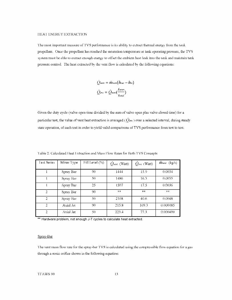
HEATENERGYEXTRACTION

ThemostimportantmeasureofTVSperformanceisitsabilitytoextractthermalenergyfromthetankpropellant.Oncethepropellanthasreachedthesaturationtemperatureattankoperatingpressure,theTVSsystemmustbeabletoextractenoughenergytooffsettheambientheatleakintothetankandmaintaintankpressurecontrol.Theheatextractedbytheventflowiscalculatedbythefollowingequations:

• _, , lopen,Qave = {]vent(--)

[total

Given the duty cycle (valve open time divided by the sum of valve open plus valve closed time) for a

particular test, the value of vent heat extraction is averaged ( Qav¢ ) over a selected interval, during steady

state operation, of each test in order to yield valid comparisons of TVS performance from test to test.

Table 2: Calculated Heat Extraction and Mass Flow Rates for Both TVS Concepts

Test Series Mixer Type Fill Level (%) Ovent (Watt) Oa_¢ (Watt) /h_em (kg/s)

1 Spray Bar 90 1444 15.9 0.0034

1 Spray Bar 50 1486 16.3 0.0035

1 Spray Bar 25 1507 17.5 0.0036

2 Spray Bar 90 ** ** **

2 Spray Bar 50 2108 40.6 0.0048

2 Axial Jet 90 215.8 109.3 0.000485

2 Axial Jet 50 223.4 77.3 0.000499

** Hardware )roblem, not enough J-T cycles to calculate heat extracted.

Spray-Bar

The vent mass flow rate for the spray-bar TVS is calculated using the compressible flow equation for a gas

through a sonic orifice shown in the following equation:

TFAWS 99 13

O.14( CdA ) P

mvent --

The assumption that gas was flowing through the orifice was verified with the test data, which indicated that

the heat exchanger completely vaporized the two-phase mixture exiting the J-T valve.

Table 2 summarizes the average heat extraction rates for all of the spray-bar tests conducted, both in 1996

and 1998. When comparing Q_e values to the ambient heat leak values for the same test, in all cases, the

Qaw value is lower than the corresponding ambient heat leak value. The maximum difference, 21%,

occurred in test Series 1 at the 90% fill level. In reality, the thermal energy removed by the TVS equaled

the ambient heat leak into the tank. Otherwise, the tank pressure would not have remained within the

prescribed pressure control band and the liquid saturation pressure would have continued to rise.

Potential sources for the difference between the heat extraction rate and the ambient heat leak were

investigated. One source considered, but ruled out, was instrumentation uncertainties. The error in

measured quantities would had to have been much larger than the instrumentation uncertainties to yield the

additional enthalpy necessary to raise the heat extraction rate to the ambient heat leak value. The small

magnitude of the vent mass flow rate and its calculation sensitivities made it the most likely candidate to

account for any difference between the ambient heat leak and the TVS heat extraction calculation.

Axial Jet

The vent flow rate for the axial jet was calculated using an the following equation for the mass flow rate

through the viscojet:

10000&v_nt = 0.9(-7---7_, )(AP * S) 1/2(1- X).

LOHm

Further detail on this flow rate equation is supplied in Reference 6. The comparison of the heat extraction

calculations for the axial jet in Table 2, to the ambient heat leak values in Table 1, reveals a 102%

difference for the 90% fill case, and a 52% difference for the 50% fill case. These differences are even

greater than those observed for the spray-bar configuration. As with the spray-bar tests, the most likely

candidate for these differences lies again in the vent mass flow rate calculation. The equation was originally

formulated for a liquid or two phase mixture flowing through the viscojet. Temperature and pressure data at

TFAWS 99 14

the viscojet exit indicated that the state was a gas, the quality of which is X=I. Since at X=I, the vent flow

rate becomes zero, the (1 -X) term was discarded and the vent flow rate was calculated based on a liquid

state. This would lead to a much larger calculation for mass flow rate, and thus a greater heat extraction

rate. As with the spray-bar cases, the heat extraction calculation is irrelevant if the TVS is able to maintain

the propellant tank pressure within the subscribed control band. One can conclude that the TVS is able to

remove heat energy at a rate equal to the ambient heat leak. Such was the case for the axial jet at the 90%

fill level. However, at the 50% fill level, the TVS was unable to remove enough heat energy to maintain the

tank ullage pressure within the control band. As the TVS continued to operate, tank ullage pressure

continued to increase.

CFD MODELING

Since the axial jet concept, due to a hardware problem, ran at less than its designed capacity, any

comparison of the test data alone is incomplete. In order to gain a more valid comparison of the two

concepts, a CFD model of the axial jet configuration was assembled. The tool used was CFX-4, a CFD

code distributed by AEA Technology, Inc. In addition to the fluid dynamics modeling, CFX is capable of

modeling ambient heat leak into, as well as heat and mass transfer within, a system.

Two CFX cases were modeled, at the 50% fill level, with pump flow rates of 114 lpm (30 gpm) and 38 lpm

(10 gpm). Ambient heat leak and mass transfer within the tank were not taken into account. The initial

temperature conditions for each case were identical and based on actual test data. Temperature contours

from the two cases were included in Figures 8 and 9. The preliminary results show that the liquid jet barely

penetrated the liquid/ullage interface for the 38 lpm case, as seen in Figure 8. The temperature contour

indicated a stratified ullage, which is unaffected by the jet. This was confirmed by the ullage temperature

data, which remained stratified and almost constant, as shown in Figure 7. For the case run at the rated flow

rate of 114 lpm, the liquid jet penetrated the liquid/ullage interface and hit the tank dome, as shown in

Figure 9. The temperature contour indicated that some ullage cooling took place, although the very top of

the ullage was still quite warm. Therefore, it is reasonable to assume that the axial jet performance would

have been improved had the mixer been able to run at the rated flow rate. However, the performance

cannot be quantified at this time since the CFD case modeled the fluid dynamics only. Results with ambient

heat transfer and mass transfer effects will be published at a later date.

TFAWS 99 15

_.._95_i094

.....iiiiiiiiiiiiiiiii_ i .3_2 i

:1:1:1:18

iiiiiiiiiiiiiiiiiiiiii::::::::::::::::::::::iiiiiiiiiiiiiii23.7774

iii:_%i

i_o 0_00

(K)i0 gal/rain

iiiiiiiiiiiiiiiiiiiiiiiiiiiiiiiiiiiiiiiiiiiiiiiiiiiiiiiiiiiiiiiiiiiiiiiiiiiiiiiiiiiiiiiiiiiiiiiiiiiiiiiiiiiiiiiiiiiiiiiiiiiiiiiiiiiiiiiiiiiiiiiiiiiii

iiiiiiiiiiiiiiiiiiiiiiiiiiiiiiiiiiiiiiiiiiiiiiiiiiiiiiiiiiiiiiiiiiiiiiiiiiiiiiiiiiiiiiiiiiiiiiiiiiiiiiiiiiiiiiiiiiiiiiiiiiiiiiiiiiiiiiiiiiiiiiiiiiiii

iiiiiiiiiiiiiiiiiiiiiiiiiiiiiiiiiiiiiiiiiiiiiiiiiiiiiiiiiiiiiiiiiiiiiiiiiiiiiiiiiiiiiiiiiiiiiiiiiiiiiiiiiiiiiiiiiiiiiiiiiiiiiiiiiiiiiiiiiiiiiiiiiiiiiiiiiiiiiiiiiiiiiiiiiiiiiiiiiiiiiiiiiiiiiiiiiiiiiiiiiiiiiiiiiiiiiiiiiiiiiiiiiiiiiiiiiiiiiiiiiiiiiiiiiiiiiiiiiiiiiiiiiiiiiiiiiiiiiiiiiiiiiiiiiiiiiiiiii

iiiiiiiiiiiiiiiiiiiiiiiiiiiiiiiiiiiiiiiiiiiiiiiiiiiiiiiiiiiiiiiiiiiiiiiiiiiiiiiiiiiiiiiiiiiiiiiiiiiiiiiiiiiiiiiiiiiiiiiiiiiiiiiiiiiiiiiiiiiiiiiiiiiii

iiiiiiiiiiiiiiiiiiiiiiiiiiiiiiiiiiiiiiiiiiiiiiiiiiiiiiiiiiiiiiiiiiiiiiiiiiiiiiiiiiiiiiiiiiiiiiiiiiiiiiiiiiiiiiiiiiiiiiiiiiiiiiiiiiiiiiiiiiiiiiiiiiiii

iiiiiiiiiiiiiiiiiiiiiiiiiiiiiiiiiiiiiiiiiiiiiiiiiiiiiiiiiiiiiiiiiiiiiiiiiiiiiiiiiiiiiiiiiiiiiiiiiiiiiiiiiiiiiiiiiiiiiiiiiiiiiiiiiiiiiiiiiiiiiiiiiiiii

iiiiiiiiiiiiiiiiiiiiiiiiiiiiiiiiiiiiiiiiiiiiiiiiiiiiiiiiiiiiiiiiiiiiiiiiiiiiiiiiiiiiiiiiiiiiiiiiiiiiiiiiiiiiiiiiiiiiiiiiiiiiiiiiiiiiiiiiiiiiiiiiiiiiiiiiiiiiiiiiiiiiiiiiiiiiiiiiiiiiiiiiiiiiiiiiiiiiiiiiiiiiiiiiiiiiiiiiiiiiiiiiiiiiiiiiiiiiiiiiiiiiiiiiiiiiiiiiiiiiiiiiiiiiiiiiiiiiiiiiiiiiiiiiiiiiiiiiii:

Figure 8: Temperature Contour in Tank, Axial Jet, 50% Fill, 10 gpm

Temperature (K)

30 gal/rain ...........

30.6015

::::::

20 _o00

Figure 9: Temperature Contour in Tank, Axial Jet, 50% Fill, 30 gpm

TFAWS 99 16

CONCLUSIONS

The test data dramatically illustrate that the spray-bar TVS configuration was very effective in destratifying,

and removing heat energy from, the propellant tank contents. This was evidenced by the fact that the spray-

bar maintained ullage pressure within the prescribed control band, for all fill levels and heat leak values

tested. The axial jet was ineffective in destratifying the tank ullage, and failed to maintain the tank ullage

pressure within the control band for the 50% fill case. Preliminary CFD models indicated that the hardware

problem limiting the mixer flow rate to almost 1/3 of its rated value, was a factor in the reduced

performance of the axial jet. Had the mixer liquid jet penetrated the ullage, some de stratification would

have taken place. Unfortunately, that amount of destratification is difficult to quantify at this time.

However, future CFD modeling with heat and mass transfer should provide some insight into whether or not

the axial jet would have performed nominally at the rated mixer flow rate.

ACKNOWLEDGEMENTS

The authors would like to thank the MSFC East Test Area personnel, especially Kevin Pedersen, for their

dedicated work in testing both the spray-bar and axial jet concepts. The authors would like to extend their

appreciation to Tibor Lak and Han Nguyen at Boeing for the spray-bar design, hardware delivery, and test

support. The authors would also like to thank personnel at Glenn Research Center for providing the axial

jet hardware and test support.

REFERENCES

1. Lak, Tibor; Wood, Charles, _Zero-G Thermodynamic Vent System Final Report", Rockwell Aerospace

Report Number: SDD 94M0038, Contract Number: NAS8-39202, 1994.

2. Fox, E. C.; Kiefel, E. R.; McIntosh, G.L.; Sharpe, J. B.; Sheahan, D. R.; Wakefield, M. E.;

_Multipurpose Hydrogen Test Bed System Definition and Insulated Tank Performance, Final Report",

Martin Marietta Astronautics, Contract Number: NAS8-39201, July 1993.

Olsen, A.D.; Cady, E.C.; Jenkins, D.S.; Hastings, L. J.; _Solar Thermal Upper Stage Cryogen System

thEngineering Test", AIAA/SAE/ASME/ASEE 35 Joint Propulsion Conference and Exhibit, June 20-

23, Los Angeles, CA, 1999.

TFAWS 99 17

4. Hastings, Leon J., Martin, James J., _%xperimental Testing of a Foam/Multilayer Insulation (FMLI)

Thermal Control System (TCS) For Use On a Cryogenic Upper Stage", 1st Conference on Orbital

Transfer Vehicles, Space Technology and Applications International Forum (STAIF), 1998.

Flachbart, Robin H.; Hastings, Leon J.; Martin, James J., _Testing of a Spray-Bar Zero Gravity

Cryogenic Vent System For Upper Stages", AIAA/SAE/ASME/ASEE 35 th Joint Propulsion

Conference and Exhibit, June 20-23, Los Angeles, CA, 1999.

6. Papell, Stephen S.; Nyland, Ted W.; Saiyed, Naseem H., _Liquid Hydrogen Mass Flow Through a

Multiple Orifice Joule-Thomson Device", 27 th AIAA Thermophysics Conference, July 6-8, Nashville,

TN, 1992.

TFAWS 99 18

THERMAL ANALYSIS OF THE FASTRAC

CHAMBER/NOZZLE

Darrell Davis

Marshall Space Flight Center

ABSTRACT

This paper will describe the thermal analysis techniques used to predict temperatures in the film-cooled

ablative rocket nozzle used on the Fastrac 60K rocket engine. A model was developed that predicts char

and pyrolysis depths, liner thermal gradients, and temperatures of the bondline between the overwrap and

liner. Correlation of the model was accomplished by thermal analog tests performed at Southern Research,

and specially instrumented hot fire tests at the Marshall Space Flight Center. Infrared thermography was

instrumental in defining nozzle hot wall surface temperatures. In-depth and outboard thermocouple data

was used to correlate the kinetic decomposition routine used to predict char and pyrolysis depths. These

depths were anchored with measured char and pyrolysis depths from cross-sectioned hot-fire nozzles. For

the X-34 flight analysis, the model includes the ablative Thermal Protection System (TPS) material that

protects the overwrap from the recirculating plume. Results from model correlation, hot-fire testing, and

flight predictions will be discussed.

INTRODUCTION

The Fastrac program provides a low-cost, 60,000 lb (60K) thrust, rocket engine to the aerospace

community. Part of this low-cost design is an ablative chamber/nozzle assembly that is actively film-cooled

with RP1. The chamber/nozzle is designed for one time use only and will be replaced after every flight.

The baseline chamber/nozzle consists of a tape-wrapped silica phenolic liner with a filament-wound carbon

epoxy overwrap added for extra strength. A filament wound glass phenolic overwarp is also being tested as

part of a parallel verification effort. The flight nozzles will have a 30:1 area ratio. However, most of the

nozzles that have been ground tested have a 15:1 area ratio since the 30:1 nozzle is underexpanded at sealevel.

The concerns during the design phase included: effects of the film cooling, degree of surface recession and

the ability to maintain the liner to overwrap bondline below 300 F. The insulative properties of the silica

phenolic protect the bondline during firing (typically 150 seconds), however the "soakback" effect causes

the bondline to exceed the limit after shutdown and to potentially create a debond. The soakback effect was

mentioned as a design problem at the Preliminary Design Review. To address this, as well as the other

desing concerns, extra tests were added to the test plan to assist in gathering data to refine the thermal

model. As the design progressed, it was obvious that the liner had to be thicker to protect the bondline.

This was an undesirable solution since it increased the weight of the nozzle. The solution was to thicken the

liner as much as possible only at the attach rings and add to shear pins to distribute the load into the nozzle

in case the rings still came loose. This resulted in the baseline configuration shown in Figure 1. Table 1

presents the design thicknesses at key locations.

x/"

15:1 Exit Plane

1

i Afk_ng

1Attach Ring

Chamber

_-'_ _ i Nozzle Thin

........... -,_x__ i Section

T_oat 1

Nozzl_'Near-Throat

30:1 Exit Plane

Figure 1: Fastrac Chamber/Nozzle Baseline Configuration.

Silica Phenolic Graphite Epoxy

Thickness Thickness

Chamber 0.987 0.253

Throat 0.850 0.807

Nozzle Near-Throat 0.852 0.316

Attach Ring 1.349 0.123

Nozzle Thin Section 0.801 0.072

Aft Ring 1.194 0.062

Table 1 Fastrac Chamber/Nozzle Design Thickness.

TFAWS 99 2

MODELDESCRIPTION

A one-dimensional SINDA model was developed to predict in-depth temperature response and bondline

temperatures for ground tests and for flight conditions. The S1NDA model consisted of 45 finite element

nodes across the thickness of the silica phenolic liner and 5 nodes through the graphite epoxy overwrap. A

non-linear grid was used to capture the high gradients near the surface while minimizing the overall number

of nodes. Material properties for the virgin and charred silica phenolic were obtained through testing at

Southern Research, Inc. (SORI) in Birmingham, AL. Preliminary hot gas temperature predictions were

provided by the CFD group at the Marshall Space Flight Center. SINDA/CMA 1, a kinetic decomposition

routine, based on the Arrhenius equation, was added to account for the effect of material decomposition and

pyrolysis gas formation. Cork was added to the external nozzle surfaces to protect the graphite epoxy from

the plume recirculation environments during flight. ABL 2, an in-house developed code that can be coupled

with S1NDA, was used to size the cork. ABL uses a empirically derived recession rate versus heat rate

curve to calculate surface recession of the cork while tracking thermal capacitance and conduction path

lengths to calculate heat transfer through the receding material. This is the first model generated at MSFC

that has incorporated SINDA/CMA and ABL to account for material decomposition of two different

materials experiencing two different environments.

Thermal Curtain

Aft Compartment

Purge

Bondline

radiation Q

T gas, inside

T gas vs time, outside

h vs time

Radiation Q

- Aft of Thermal Curtain

Graphite Epoxy Overwrap

Silica Phenolic Liner

Char/Pyrolysis Zone

Figure 2: Schematic Representation of SINDA Model

TESTING

Preliminary material testing was performed at MSFC's Improved Hot Gas Facility (IHGF) and Wright

Patterson Air Force Base's Laser Hardened Material Evaluation Laboratory (LHMEL). These tests did not

provide much data that could be used to validate the in-depth model predictions, however they verified the

assumption that the surface would not recede at the expected hot-fire conditions. The first data used to

correlate the model came from Thermal Analog tests performed at SORP. The test provided one-

dimensional heating of a 2.0" x 2.0" x 0.85" coupon of silica phenolic/graphite epoxy lay-up by exposing

the coupon surface to a resistively heated graphite heater. The coupon surface was heated at rates that

simulated actual engine firings. A schematic of the basic facility is shown in Figure 3.

TFAWS 99 3

TestFrame

TestSpe_Heater

LoadRod

SteelFixture

SupportBlock

Figure3:SchematicofSORIAnalogTests

Atotalofthreesamplesweretested.Thefirsttwotestsrunswerefor150secondsandthethirdwasfor230seconds.Temperatureof the surface,backside,andfive in-depthlocationswererecordedwiththermocouples.DepthsoftheimbeddedthermocouplesweredeterminedbyCTtechniques.Therecordedsurfacetemperaturewasusedasaninputto theS1NDAmodelandtemperatureswerepredictedatthemeasuredthermocoupledepths.Becauseofuncertaintyin thecharproperties,andtheunknownmaterialpropertiesinthepyrolysisregion,materialpropertieswereadjusteduntiltheS1NDAmodelresultsmatchedtheresultsfromtheThermalAnalogTests.Charandheat-affecteddepthswerealsotakenfromthesesamples.Thisdatawasusedtoanchorthekineticdecompositionroutine.

2500

2000

1500

1000

5OO

Thermal Analog Test #2 ResultsSolid lines represent test results

Dotted lines represent model results

?_ Numbers represe, depth treasured,r _ _ ', _ . .- _ , : ; ,.-,,\ : fromsurface -

L i Surface i i i i :i

- i i 0.13" _iZS>_ _ _! \_,! -

i-. _ ' -" ' ' • -_ ';_J ..... +_+' ..... 4

,-- _,_s' 0.25-_+ , ,£._--_-<, , i, _, _-- 0.38 s .......r j , _/___,>.i;J" ,,.,.c<.,.;-:S _*_ 0.50"

- ,/,, .:/_?<.i - _ ;f __'C] 0.63

I_ , , _+ .. _j+_. l--It_ +_ I _ ]

0 50 100 150 200 250

Time (sec)

Figure 4: Model Comparison to SORI Analog Tests

TFAWS 99 4

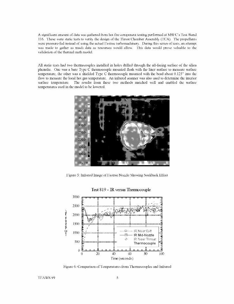
A significantamountofdatawasgatheredfromhotfirecomponenttestingperformedatMSFC'sTestStand116.ThesewerestaticteststoveritythedesignoftheThrustChamberAssembly(TCA).Thepropellantswerepressure-fedinsteadofusingtheactualFastracturbomachinery.Duringthisseriesoftests,anattemptwasmadeto gatherasmuchdataasresourceswouldallow.Thisdatawouldprovevaluableto thevalidationofthethermalmathmodel.

All statictestshadtwothermocouplesinstalledinholesdrilledthroughtheaft-facingsurfaceofthesilicaphenolic.OnewasabareTypeCthermocouplemountedflushwiththelinersurfacetomeasuresurfacetemperature,theotherwasashieldedTypeCthermocouplemountedwiththebeadabout0.125"intotheflowtomeasurethelocalhotgastemperature.Aninfraredscannerwasalsousedtodeterminetheinteriorsurfacetemperature.Theresultsfromthesetwomethodsmatchedwell andenabledthesurfacetemperaturesusedinthemodeltobelowered.

Figure5:InfraredImageofFastracNozzleShowingSoakbackEffect

Test 819 - IR versus Thennocouple

3OOO

15oo ..... .......... .......... .......... ........ !

N , _ , j .........0 .......... IR N_car E×it _._

lOOOF7 ........ _.......... t-

- ' : t _ IR Mid-No_le

_ : * _ 1R Near TiTroat500 _ ........ • .......... _-

i-_ , : ..... Thermocouple "

r ; : _ :

0 20 40 60 80 100

Titre(seconds)

Figure 6: Comparison of Temperatures from Thermocouples and Infrared

TFAWS 99 5

Intwooftheearlytests,designated60K#1and60K#2,thermocoupleplugswereusedtomeasurein-depthtemperatureresponse.ThisprocesswasdevelopedduringearliertechnologydevelopmentprogramsatMSFC.Theplugswere0.25"silicaphenoliccylindersintowhichwereimbeddedthreethermocouples.

ThermocoupleLeads

RTV

ThermocouplePlug

GraphiteEpoxy

SilicaPhenolic

FlameSurface

Figure7:SchematicofThermocouplePlug

Theplugswerelaidupinthesamemannerasthelinermaterial.Carehadtobetakenduringinstallationtoensureproperplacementofthethermocoupleleadswithintheplug.A holewasdrilledintothesilicaphenoliclinerfromthebacksidetowithin a nominal 0.100" from the surface and the plugs were installed

into these holes. Plugs were placed at four axial locations and two radial locations for each axial location.

_-_ Type C thermocouples

Thermocouple Plug Locations

Figure8: Thermocouple locations on 60K # 1 and 60k #2

TFAWS 99 6

All of the thermocouples in the A plugs were Type S while the B plugs used a combination of Type K and

Type S. Because of the low conductivity of the silica phenolic, a steep thermal gradient exists in the linerand it was necessary to know the exact depths of the thermocouples. Depths of these thermocouples wereagain obtained by using CT techniques. However, the Type K thermocouples were invisble to CT. TheType K thermocouple data also tended to have more noise in the data and tended to open during the firing.

Therefore the data from the Type S thermocouples in the A plugs was used in model verification. In the60K # 1 test, two Type S thermocouples failed, and during the 60K #2 test, a leak path developed aroundplug 2A and invalidated the thermocouple readings from that plug. Both tests were planned 150 secondduration tests, however due to test anomalies, 60K # 1 ran for 28 seconds and 60K #2 ran for 130 seconds.

Thermocouple measurements versus model predictions are presented in the figures below

60K 771 Plug 1A

Solid lines represent test results

Dotted lines represent model predictions

4r

O 2_ TC1-Depth=0.291"

150 "_ .... _ ..... : -'-i.,......... : .............. : ............................. M

i i, \ i'°°k7-......................... i

Ji _ TC3- Depth = 0.504" ,___ ."50 E7i _<" ! ! : :

i" "i N .... i

_Z : Note: TC2 failed duringtest0 r-! • • • | _ , • • ! , • • • ! , • • • _ , • o • !

0 100 200 300 400 500

Titre (sec)

Figure 9: Model versus Test Data for Test 60K # 1, Plug 1A

60K 771 Plug 2A

Solid lines represent test results

Dotted lines represent model predictions200

150

100

50

TC - Depth = 0.370"l_ Ill ' _

b .... l - r_;_: _"-_'- -" ..................... " ........J

.... _,s , : _ . ', __JU-i 7 ...... :................ ,.............. '-_::-, ......... -ir II _ • ' ', __, ' _ "1<i- _ TC3- Depth = 0.420" , -__

[ ii7 : , : ]t IN _ , _ ', I1i_ - i_4 ........................... " .......... ; ........ _iL i_: ', Ji _ ; |

Note: IC_ failed duringtest 4

Figure

0 100 200 300 400 500

Titre (sec)

10: Model versus Test Data for Test 60K # 1, Plug 2A

TFAWS 99 7

f

400

60K#1Plug3ASolidlinesrepresenttestresults

Dottedlinesrepresentmodelpredictions

350_--_ "7-_---.......... : .......... ; ...................1- : _, _.TC1 - Depth - 0.251

300 _-- 1.-_f__-r-__,_....... :........... :........... :.........

250 _ ;_e*"::._ '_, 'TC2-Depth=0.332"._; ...........

L-i;g: ..........i.........200_ _g/:: ::150 _:_

__ -. ,_,-__.qj21 TC3 - Depth = 0.386" : :

100__...-_-'_....i..........:...........i...........i.........

00 100 200 300 400 500

Titre (sec)

Figure 11 : Model versus Test Data for Test 60K # 1, Plug 3A

60K #1 Plug 4A

Solid lines represent test resultsDotted lines represent model predictions

TC1 - Depth = 0 264" _350 " "" ' ' ; "_

i- ql :,,. : :

i ,g : _'_1. TC2 - Depth = 0.302" :250 _- - 'N --_0_-,_,_,,-_ .......... _...................

15o_--_i_,/-_ .......... i...... __g _.Y TC3-Depth=0.406 ....

100 N_-ve_ig._ ..... ',_.............. ','.................. i_................. :_............... _2

0 0 100 200 300 400 500

Time (sec)

Figure 12: Model versus Test Data for Test 60K # 1, Plug 4A

TFAWS 99 8

60K #2 Plug 1ASolid lines represent test results

Dotted lines represent model prediction

1200 _ .... , .... , .... , .... , .... i_- 2£)_ TC1-Depth = 0.167"

1000 j__ ,.-.; ::

../" _ */::_._ TC2- Depth = 0.252"!

i-f ......................................Ji-- 4 /2¢ !_. _ ! --i

400 L- ;#-- Lj'-: ................ __=,.-_ .................... J

r _)_ TC3 - Depth'= 0.310'___ -i

200 i_Y" i i i i _

0 100 200 300 400 500

Time (sec)

Figure 13: Model versus Test Data for Test 60K #2, Plug 1A

f

1500

60K #2 Plug 3ASolid lines represent test results

Dotted lines represent model prediction

_ TC1 - Depth = 0.145" ._'_

1000 _ ..... ,_- --: _%-_ ................................. =_

_" d# g':// "<_"._ TC2-Depth=0.212" -i

500 _,-#-7 -2Z ......... ] .......... 7"_Z2 .......

_' I _<__,*" TC3 Depth = 0.330" '. "_

00 100 200 300 400 500

Time (sec)

Figure 14: Model versus Test Data for Test 60K #2, Plug 3A

TFAWS 99 9

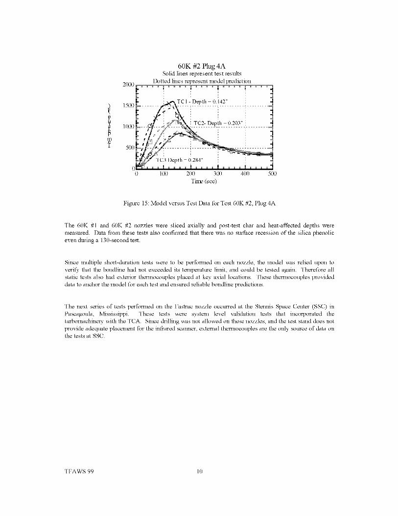
60K#2Plug4ASolidlinesrepresenttestresults

2000

_ TC1-Depth=0i42" i -_1500_-_............_----_,......................_.............i............

! : _f)._ ' TC2- Depth = 0 203" '

k e i%_+±500 _.:/_-j-_-¢_ .......... 4- - ....

b_#_ ;J TC3 Depth = 0.284" !

0 100 200 300 400 500

Titre (sec)

Figure 15: Model versus Test Data for Test 60K #2, Plug 4A

The 60K #1 and 60K #2 nozzles were sliced axially and post-test char and heat-affected depths were

measured. Data from these tests also confirmed that there was no surface recession of the silica phenolic

even during a 130-second test.

Since multiple short-duration tests were to be performed on each nozzle, the model was relied upon to

verify that the bondline had not exceeded its temperature limit, and could be tested again. Therefore all

static tests also had exterior thermocouples placed at key axial locations. These thermocouples provided

data to anchor the model for each test and ensured reliable bondline predictions.

The next series of tests performed on the Fastrac nozzle occurred at the Stennis Space Center (SSC) in

Pascagoula, Mississippi. These tests were system level validation tests that incorporated the

turbomachinery with the TCA. Since drilling was not allowed on these nozzles, and the test stand does not

provide adequate placement for the infrared scanner, external thermocouples are the only source of data onthe tests at SSC.

TFAWS 99 10

2,0"

Figure 16: Thermocouple Placement on the H2 Series Tests at SSC

The H2 series tests were performed on a 15:1 nozzle with a glass phenolic overwrap. Results from thermal

analysis and test data showed that the glass phenolic and graphite epoxy overwraps would perform very

similarly thermally. Test H2A-2B and Test H2B-2 both ran for the planned full duration of 24 and 155

second, respectively• Comparison of model results with exterior thermocouple data is presented in the

figures below• The model predictions tend to agree well with the thermocouple data. Most of the

disagreements are caused by purges on the test stand cooling the nozzle surface after shutdown. While the

model can account for this effect, the timeline and temperatures of these purges are not easily obtained•

200

180

160

140

120

100

80

60

H2 Series Tests at SSC - Chamber

Solid lines represent test results

Dotted lines represent model predictions..... T____________r _____.-____________T____r ............ r-----T-----T---N---_-T_=.L_. --_,--az-r_--;_----z:_;----T-

, ,_ _ f: 'Test H2B-2_ i_ :

............. _.......... _-_-_ .... _ .... i

............... .......... .......... :........., i Test H2A-2B

.......... ; - - --- _- -- ; .... _ .... + .... <;_-_ _ _'°-_ -4_- --=

_ '. _ _ i : -.-. ...... '. •

_---.rr_'-_-_: _"i _-_ , ; :

...._..... _ ,'4 ............ ,,.................. _................. ,................._2__ , :

....2__J______________L__L__L:__L_L:__L_L__:__L_L_L___L_L__....0 200 400 600 800 1000

Titre (sec)

Figure 17: Fastrac Chamber Model Results versus Test Data for H2 Series Testing

TFAWS 99 11

?

H2 Series Tests at SSC - Nozzle Near ThroatSolid lines represent test results

Dotted lines represent model predictions300 i::....1......T......;......1......T......:......l......T......;......r....._......i......1......_......r......]......_......r......r...::]

J-- ', : : : 4- .... d

250 ,,'7-.................... 'L.... @__.-_v__ ;_z__-, .....

. . ¢ _;_[-_: - : ,:-_Test H2B-2_ , _ _ , , --,

200 .......... _..... i "- - _f - .... "_-- - !.......... ! dq

, -_'/ i :TestH2A-2B

15o ]:.................i / '_ .....2 _:-:_-'____F- , _ ¢ ._ "CJ _'._' ' ' q

50 "----,------,------,-------'------,------,-------,------'------,-------,------,------'-------,------,------,-------'------,------,-------,----"0 200 400 600 800 1000

Timo (sec)

Figure 18: Fastrac Nozzle Near-Throat Model Results versus Test Data for H2 Series Testing

?

H2 Series Tests at SSC - Attach Ring

Solid lines represent test results

Dotted lines re _resent model predictions250 ' ' ' i ' ' ' ' ' ' i ' ' ' i ' ' ' _

200 @ ; " _ °-_; ........ ,.........-_-Ne-- : ............... l

Test H2B-2 ¢ J "e_

1so .......... ;....... :__:____._s._.._i .......... i ........ -# , eg , , -

i _ ¢_./_ _._')_JU" Test H2A-ZB100 .......... -.___ __.._<C: ........ ,_.......... '_........ --

i i -- _'_ : : -I

5O i , i i , , i J , i , l i , , i , , i]

0 200 400 600 800 1000

Timo (sec)

Figure 19: Fastrac Attach Ring Model Results versus Test Data for H2 Series Testing

TFAWS 99 12

?

H2 Series Tests at SSC - 15:1 Exit Plane

Solid lines represent test results

Dotted lines represent model predictions400 _ ' ' _ [ ' _ ' i _ _ ' _ ' ' ' ' _ 4

_- '. mJ

350 i............................... _.......................... --_ ......................

Test H2B-2 (-;_ Z_ _"_"-4Z_-_ _ _ _ -_-,300 i................................................ _,_................. _,-- _- _--_--J

250 ........... _-*"......................................i-- ,_j _ ' ; ; 4- , _ g , , q__ ,¢ / . _j

200 _-......... _-_ ..................... Test H2A-2B ..... -4- _',i .<'_.._'_'._-_ ... : j

P _ .... q

100 _- -.._............. !.............. !..................!...................

50 "----'------'------'-------'------'------'-------'------'------'-------'------'------'-------'------'------'------'------'------'-------'----"0 200 400 600 800 1000

Titre (sec)

Figure 20: Fastrac Exit Plane Model Results versus Test Data for H2 Series Testing

These nozzles are also instrumented with strain gauges to allow structural analysts to verify their models.Data from these strain gauges can show where a debond has occurred. Figure 19 shows strain gauge andthermocouple data plotted together at the exit plane, where a visual examination confirmed a debond.

Test H2B-2

Temperatures and Strain At Nozzle Exit Plane

400 _ .... I .... i .... I_' ' ' _ I .... _ 200kChangein slope of temperature :!i Debond :

350 _ corresponds with strain peak. !_i......... !---_ 0

,';..................:.........._- -,-'....... 200

400200 _ ......... ,.................... !..................... _ -600

150 _ .... \----:---_ .... : ....... _ -800

F- " " "O, r,, : ' ' ' qi50 -- ........ _...... _--_--: .................. :-........ -4 -1200

0 Vi i , , I i i i, i'l i , , J i i i, I i i i ,4 -14000 100 200 300 400 500

Titre (sec)

Figure 21: Thermocouple and Strain Gauge Data From Test H2B-2

The spike in the strain gauge data indicates a debond occurred at that time. At the same time, thethermocouple data changes slope. This is also an indication of a debond. When the graphite epoxyoverwrap debonds from the liner, the conduction path from the liner to overwrap is broken. The overwrapis then more heavily influenced by convective cooling from the ambient temperature than by the radiant

heating now produced by the liner. This causes a change in slope in the thermocouple response.

TFAWS 99 13

The nozzle near-throat region is an area of concern for potential debonding. In this section, the overwrap is

becoming thinner due to an increase in local area ratio and the liner is not as thick as it is further

downstream at the attach ring. Visual obselvations cannot reveal a debond in this region, and on-pad non-

destructive evaluation (NDE) methods have not been developed to a point where they are feasible to use in

small, tight spaces. Strain gauge data from the near-throat region of Test H2B-2 seems to indicate a

debond. When the thermocouple data is plotted alongside the strain gauge data, Figure 20, it may also show

indications of a debond by the change of slope in the temperature trace.

Test H2B-2

Temperatures and Strain At Nozzle Near-Throat

300 i_. , ..... i,,, i,,, i , , _ _

Debond? _ i ! NozzlelSkin Tempt250 _ ......... !---'_--i ........ =__:--_

150 ) .............. _ .... - ...................... Strain 0 deg

:150 -- ........ 71- 7 ...... !-- Strain 90 deg ..... :i........

0

200

0

-200

-400

-600

-800

-1000200 400 600 800 1000

Tirre(sec)

Figure 22: Thermocouple and Strain Gauge Data from Test H2B-2

Post test laboratory NDE could not positively declare a debond at this location, but did reveal a low-density

area. It is possible that this configuration of thermocouples and strain gauges could be used for health

monitoring of the nozzle during ground tests.

THERMAL PREDICTIONS FOR STRUCTURAL ANALYSIS

Once the model had been proven reliable and able to match test results, it was used to provide two-

dimensional thermal distributions to structural analysts. The kinetic decomposition routine could not be

adapted to a two-dimensional grid. Since there was very little difference in local plume temperatures and

therefore no AT to drive axial conduction, it was determined that an interpolation of 1-D results would

provide the necessary data. The analytical nozzle was separated into 28 1-D slices as shown in Figure 21.

TFAWS 99 14

\ 79 ou

1 7 _ 9"1QI_31518_123_24_830_334

I 100 1069,"

Figure 23: Locations of 1-D Slices Used to Generate 2-D Thermal Distributions

Each slice was run with its corresponding gas temperature, heat transfer coefficient, silica phenolic

thickness, graphite epoxy thickness to provide a thermal gradient profile at that location. The results were

interpolated onto a 2-D PATRAN finite element mesh. Results provided for structural analysis included hot

and cold extremes for both ground and flight.

MSC 9ATRAN Version7.5 O5-Nar-99 13:18 25

Fnng_ TIME: 600.00 SECONDS no d.eluge, ltrO asd01 Temperature, (NON LAYERED

z

[g......X

575 C

543 !

511 !

479

448 :

415 !

384 l

35Z !

321.

289

257 ;

225 !

194

152 !

130 ;

default F_lgeMax $75.0 @Nd37_4

Mm_ 00 _Nc_5

Figure 24: Example of Two-Dimensional Thermal Distribution

FLIGHT PREDICTIONS

During flight, the overwrap forward of the heat shield will be exposed to environments generated inside the

aft compartment. The nozzle itself will contribute to this environment, especially post-firing. Flight

exterior nozzle temperatures were provided to Oribital Sciences Corporation for inclusion to their aft

compartment model. Aft of the heat shield, the nozzle will be exposed to recirculation of the plume.

MSFC's CFD group provided plume recirculation environments. ABL, an in-house code that runs

concurrently with S1NDA, was used to size the thermal protection system (TPS) materials. Two materials

were selected for analysis; cork, Marshall Convergent Coating (MCC-1). MCC-1 is a sprayable ablator

developed at MSFC containing cork, glass ecospheres and an epxoy resin. It is currently used as the main

acreage TPS on the Solid Rocket Boosters. Results from the analysis showed that 0.25" of either material

would protect the graphite epoxy overwrap to 300 F. Since MCC-1 is sprayable, it requires the

TFAWS 99 15

programming of a computer to follow the specific geometry of the nozzle. This made the MCC-1 more

expensive for a short production run, so the program decided to use cork as the external TPS material. RT-455, a K5NA substitute, will be used as a closeout material and the entire TPS system will be covered withAcrymax paint.

400

Bondline Temperatures

Flight - Hot Day

- ' ' ' ! " ' ' .'.-.--'-.............. "-"-.i--..-..L...! ' ' " -.r ' .-"' _............. i

300 _- :, -

200 L ......... ',7:........ .>'°"__':-'--',-- ::_-"-"----', .........

P ..S--- . ................2,-+-_ .....:i ' "

100•"_-".... __ @Throat

...... .... i _ N.'°_l-eNiar Thr°atL,,,.-_..)<i : :,0 _>_ ................. ,...... ,! . ,-" _, ,

.-- ' ', ',i ............i............No2;_(-,'--[_]I_l_,'._-)c+Io[l

_100 = , , , = , , , , , , , ..0 200 400 600 800 1000

-15me (sec)

Figure 25: Flight Predictions

CONCLUSIONS

Because of an extensive test program that generated data used to correlate the model, the model can be

trusted to give reliable results. These results indicate that during a 150-second engine bum, all bondlineswill remain below 150F. However, this bondline limit will be violated during the soakback and willpotentially cause a debond.

ACKNOWLEDGEMENTS

The author wishes to acknowledge the contributions of Louie Clayton for help with the S1NDA/CMAroutine, Donald Bryan for help with the infrared imaging, and Bruce Tiller for guidance.

REFERENCES

1. "SINDA Temperature and Pressure Predictions of Carbon-Phenolic in a Solid Rocket Motor NozzleEnvironment", 1992 JANNAF Conference, Moffat Field, Palo Alto, CA, J. Louie Clayton

2. "S1NDA/ABL Solution Routine Updates", J. Louie Clayton, NASA Internal Memorandum, ED63(25-96), 1996

TFAWS 99 16

3. _Thermal Analog Testing of Fastrac MX2600 Silica Phenolic, Final Report to MSFC", Michael D.

Johns, SRI-ENG-98-26-8657.15, 1998

TFAWS 99 17

METHOD IMPROVEMENTS IN THERMAL ANALYSIS

OF MACH 10 LEADING EDGES

Ruth M. Amundsen

National Aeronautics and Space Administration

Langley Research Center

Hampton VA 23681-2199

ABSTRACT

Several improvements have recently been made in the thermal analysis methods for leading edges of a

hypersonic vehicle• The leading edges of this vehicle undergo exceptionally high heat loads that

incorporate extreme spatial gradients as well as severe transients. Due to the varying flight conditions,

complex geometry, and need for thermal loads at many points along the trajectory, full computational fluid

dynamics (CFD) analysis of the aeroheating loads is not feasible• Thus, engineering methods must be used

to determine the aeroheating on the vehicle surfaces, and that must be utilized in the thermal analysis• Over

the last year, the thermal analysis of a hypersonic vehicle has been enhanced in several ways. Two different

engineering codes are used to predict aeroheating loads: one over the curve near the stagnation point, and

the other on flat surfaces downstream of the leading edge. These two are matched together at the

intersection point using a method that allows closer approximation of CFD results• User-developed

FORTRAN, which is part of the thermal solver PATRAN Thermal, is used to accomplish this. The

customizable FORTRAN code also allows use of many different time- and space-dependent factors,

interpolation of the heat load in time and space, and inclusion of both highly swept and unswept grid

structures• This FORTRAN is available to other PATRAN users who may want to accomplish a similar

objective in analysis• Flux, rather than convective coefficient, is used to define heat loads, which allows

more accurate analysis as well as better application of margins• Improvements have also been made in more

efficient utilization of imported CAD geometry, by creating faces on solids to facilitate load application•

INTRODUCTION

Earlier work by the author in the thermal analysis of hypersonic leading edges has been described

elsewhere. 1,2 This paper will describe improvements in the methodology that have been made recently.

Several hypersonic leading edges of varying geometries have been analyzed. The thermal solver used is

MSC/PATRAN Thermal. The aeroheating loads for the hypersonic trajectory are generated in other

software, and output in a text file format. The challenge is to import these aeroheating loads into PATRAN,

interpolate in time and space to allow application to the PATRAN thermal model, and apply factors to the

loads that are both time and spatially dependent. The main improvements that have been made in the last

year are: to import and interpolate heat flux rather than the convective coefficient and recovery temperature;

add flexibility so that the code can correctly interpolate from swept grid structures with varying

directionality; incorporate time- and space-dependent factors; and alter the aeroheating loads at specific

points on the geometry. The method for applying heat loads on the leading edge that are dependent on

nodal temperature has been fully developed. Also, the method for verifying the interpolation has been

optimized.

HEATFLUXIMPORT

Achangewasmadeintheinterpolationsoftwaretoimportaeroheatingflux,ratherthantheconvectivecoefficienthcandthefluidtemperature.Thiswasdoneforseveralreasons.First,thefluxisthevalueactuallycalculatedbytheaeroheatingsoftware.Theothertwovaluesweredeterminedfromflux,introducingpossibleinaccuracies.ThefluidtemperatureisofquestionablevalueattherangeofMachnumbersencounteredinthisanalysis.Second,thefluxdependsnotonlydirectlyonthenodaltemperature(asitalsowasintheoriginalmethodusinghc),butalsoindirectly.Thisindirectorsecond-orderdependenceoffluxonthenodaltemperaturewasnotfullyhandledbyimportinghcandcomputingfluxbasedonatemperaturedifference.Third,thequestionofapplyingfactorstothefluxbecomesmorecomplexwhenh_wasused.Whenhcwasthevalueimported,anyuncertaintyfactorscouldonlybeappliedtoh_.Thiswouldleadtodifferenttemperaturesatlatertimesthanwhenrunwithoutfactors,andthustoadifferent(lower)flux.Thus,thefactorwasnotreallybeingappliedtothetotalinputflux.Whenfluxistheimportedvalue,anyfactorappliedisactuallyincreasingthefluxbythecorrectamountatanygiventime.Inordertoimportfluxratherthanhc,adifferentsubroutineinthePATRANulibfileswasrequired.Theuhval.fsubroutinewasusedforimportofhcandfluidtemperature.Forimportofflux,theumicro,fsubroutinewasutilized.Thelogicinthetwosubroutinesisverysimilar.However,differentvariablesarepassedto,andusedwithin,thetwosubroutines.Inumicro.f,manyoftheinternalPATRANvariablesandarrays,suchasITLIST,IFLIST,andMFID,mustbeinitializedwith the correct sizes. Then, within

umicro.f, the solution time and nodal position are evaluated and used for the time and spatial interpolation.

A separate subroutine is called to perform the interpolation. Since the interpolation is based only on the

nodal position in PATRAN, this method can be applied equally well to structured (brick) or unstructured

(tetrahedral) meshes. It can also be applied to surface meshes.

Since the aeroheating flux is dependent on the temperature of the surface, surface temperatures at each time

point must be output to the aeroheating program for calculation of flux. With new predicted fluxes, the

PATRAN thermal solution is re-run, and temperatures again transferred for new calculation of aeroheating.

This iteration normally only requires about three cycles to achieve closure (matching of input and output

temperatures).

IMPORT GRID PARAMETERS

The interpolation from one grid set to another would be fairly simple if the grids were both orthogonal to

the same axes, and the gradients were small relative to the grid spacing. However, in the aeroheating grid,

there are several parameters that make interpolation difficult.

First, the leading edge is sometimes swept at a severe angle, by as much as 70 degrees from normal to the

flow. The vehicle is normally modeled with one axis parallel to the flow, and thus the leading edge is not in

general parallel with an axis, but can be at a large angle to an axis. The grid of the aeroheating model

usually follows the vehicle lines, and thus is swept with the leading edge, although the sweep angle is not

constant and decreases substantially toward the aft end of the part. The steep gradient in heating that occurs

on a hypersonic leading edge is normal to the line of the leading edge: i.e., the fall-off in heat flux is very

abrupt in the direction directly away from the leading edge. If interpolation were done directly on the

spatial coordinates of x and y, the flux could be interpolated incorrectly, since the gradient is dependent on

the distance from the leading edge and not specifically on x or y. The sweep also makes it difficult to select

the correct set of grid points to interpolate between. Using either x or y alone to select the grid point is not

sufficient. It is also not enough to base it on the closest aeroheating point, since the point that is physically

closest may have a very different flux based on its distance from the leading edge. In the software, an

iterative set of equations is used to find the correct starting point in the aeroheating grid. Then, effective

coordinates based on the distance from the leading edge are used for interpolation.

An example mesh is shown in Figure 1. The aeroheating grid is represented by closed circles, and two

example nodes in the PATRAN mesh by open circles. The PATRAN mesh is mush denser than the

aeroheating grid, so for clarity only two example nodes are shown. The solid lines indicate the lines of

TFAWS 99 2

nodesintheaeroheatinggrid.Onecanseethatforanygivenlineofypoints,thevaluesarenotconstant,andforanygivenlineofxpoints,thevalueschangesubstantiallyforeachchangeiny. LookingatexamplePATRANnodeA,onecanseethatgoingonlybythexcoordinatewouldresultinselectingagridlinemuchfartherfromtheleadingedgethaniscorrect.LookingatexamplePATRANnodeB,onecanseethattheycoordinatecannotbeusedasthesolecriteriaeither.Infact,duetotherelativecoarsenessandsweepangleoftheaeroheatinggrid,thepositionofeachPATRANnodemustbedeterminedbasedonanequivalentline,paralleltotheaeroheatinggridatthatpoint.ThedashedlineinthefigureindicatesthisequivalentlinefornodeA. Then,thetruegridcellcontainingthenodecanbedetermined,andtheinterpolationcanbeperformedbasedontheequivalentposition.

Y• Aeroheatiw,node i_

!O ExamDlePATRANnodesI

lx _

Figure 1. Example interpolation mesh (viewed in 2D).

Second, the aeroheating gridding does not follow a prescribed physical direction. The grid is ordered in the

aeroheating program so as to conform to the sweep angle. On a part where part of the leading edge is swept

back along positive z, and the other swept along negative z (as illustrated below in Figure 3), the physical

ordering of the grid when brought into PATRAN will not be constant. The grid may be ordered such that

the array increases in x and decreases in y, or the other way around. Or both values may increase or

decrease together in the array. In the y axis (normal to the swept lines), the lines are close to constant value,

but not quite. A line of nodes at some given position in the array (say, at the second value ofy in each row)

may not even be monotonic in y. The FORTRAN needs to be flexible enough to handle these changes in

directionality.

Also, the aeroheating grid may not be oriented with the same x and y, and may not have the origin in the

same place as the PATRAN model. The software handles changes in the axis orientation and origin

position by modifying the values read in from the array, before they are used for interpolation.

ALTERATIONS TO HEAT FLUX

The umicro.f subroutine is where factors can be applied to the heat flux value. There are several different

conditions where factors are required. Effects on trailing edges, outer edges, coves, and gap regions, are all

not completely predicted by the aeroheating code. Thus, factors must be applied to the loads in these

regions to achieve an accurate thermal prediction. Regions that will all receive the same factor can be

grouped, and a separate boundary condition applied. Then, the identification number of the boundary

condition is used as the flag in umicro.f to trigger application of a given factor. The position in any of three

axes can be used as a trigger for applying a set factor, or as a variable in calculating a spatially dependent

factor to apply. The time in a transient solution can also be used as a trigger for changing factors.

In some cases, the region where a factor is required is not a discrete part of the solid geometry. In most

cases, the solid geometry is electronically imported from Pro/Engineer. There are often cases where a

region is not broken out as a geometric entity on the solid that is imported, but due to aerodynamic

considerations it must be treated with a separate factor. This can be done by manually selecting the affected

elements, or by setting up a complex logic network of the spatial variables to define the region in question.

These methods are somewhat cumbersome and time-consuming. A more straightforward method is to break

the base geometry according to the surfaces that are desired. The base geometry will still exist as a solid,

and can be handled as such for application of loads and boundary conditions. Faces may be added to the

solid that facilitate loads application. One way to accomplish this is by breaking the solid (for example,

with a plane), but this leaves multiple solids instead of the original one. A more elegant method is to break

TFAWS 99 3

thesolidintoitsconstituentsurfaces,andsplitwhicheversurfacesarenecessaryforefficientloadapplication.Thesolidcanthenbere-assembledfromthedesiredsurfaces,leavingasinglesolidcontainingalltherequiredfacesforloadsapplication.Theaeroheatingfluxpredictionisnotreliableatthefolwardtangencypointwheretheflatsectionmeetstheroundoftheleadingedge.AmethodwasdevelopedtomakethisfluxmoreconsistentwithCFDpredictions.Forsectionswheretheaeroheatinggridextendstotheforwardleadingedge,thevalueofeachpointalongthetangencylinewasreplacedbyavaluecalculatedusingFay-Riddellmethods.Thissubstitutionisdoneusinglogicinthesubroutinewherethearrayisreadin.

LEADING EDGE METHOD

The leading edge heating requires another method entirely, since the aeroheating code used for the flat

acreage sections is not used on the leading edge. The value of heating is dependent on the trajectory, the

leading edge geometry, the angular position on the leading edge, and on the temperature at the leading edge.

The code uses basic Fay-Riddell methods to calculate stagnation heating, then modifies those values by the

specified sweep angle and body angle. See Figure 2 for an illustration of the angular position (body angle).

The Fay-Riddell calculation must be done for each time point in the trajectory. For swept leading edges, the

temperature of all nodes at a given angular position may not be constant. Thus, in order to use a correct

heat flux for all nodes, the heat flux must be altered based on the local temperature.

0 ° body angle

-'------_ " 45°1angency ;_]ndtY angle

Figure 2. Body angle definition.

For nodes other than the reference node used to calculate heat flux, the flux into the node was factored using

the following:

,tag- Lode_no& :Qr_f _ _ [1]

where Tnode and Qnode are the temperature of and flux into the given node, and Tref and Qref are the

temperature of and flux into the node whose temperature is used for heat flux calculation. This was done in

PATRAN by making the heat into the leading edge nodes a product of three functions:

[21

VERIFICATION OF FLUX INTERPOLATION

The verification of the interpolation of the flux would at first seem to be a simple matter of evaluating the

flux in PATRAN versus the flux from the text formatted input file. However, a difficulty arises in that

PATRAN Thermal does not plot flux as one of the standard parameters. The parameter that can be plotted

directly from the nodal results file is nodal heating, which is the heat per node. This can be changed to flux

TFAWS 99 4

bydividingbythenodalsub-area.Toaccomplishthis,onefirstneedstogenerateafileofthenodalsub-areasforeachnodethatreceivesheating.Onesimplewaytodothisistoimporttheqmacro.datfileintoanyspreadsheetprogram,suchasMicrosoftExcel.Thefilecanbereformattedtogiveonlynodenumberandnodalsub-area.Then,nodesthatreceiveheatingviamorethanoneboundaryconditionmustbesummedtofindtheirtotalsub-area.Oncethisisdone,thefilecanbefilteredsothateachnodeappearsonlyonce.TheheatpernodecanbeoutputfromPATRANintoatextfilebydoingaCreate_ReportfromtheResultsmenu,ononlythesurfacenodes(thosereceivingaerodynamicheating).Thistextfilecanthenbepulledintothesamespreadsheetdescribedabove.Oncethenodesareinthesameorder,it isasimplemattertocalculatefluxbydividingtheheatbythenodalsub-area.ThesheetofnodenumberversusheatfluxcanbesavedasatextfileandpulledintoPATRANviaPATRAN'ssharewarespreadsheetfunction.Aresultcasecanbecreatedfromthespreadsheetdata,andthefluxplottedonthemodel.Thefluxfromtheoriginaltext-formattedaeroheatingfilecanbecomparedgraphicallybyplottingit inTecplotorasimilarplottingprogram.ThefluxonanexamplePATRANmodelisshowninFigure3. Thismodelutilizes12separateboundaryconditionsforacreageheatflux,tocapturethediscreteregionsonthegeometry,aswellasfiveregionsforleadingedgeheatflux.ThemeshonthePATRANmodelisnotshownsinceit issuchadensemeshthatit wouldcompletelyobscurethefluxcontours(inthismodeltherearemorethan45,000nodes).Thefluxdirectlyfromtheaeroheatingcode,plottedinTecplot,isshowninFigure4. Theunitsandscalearewithheldduetoconcernswithdataexport;however,whentheplotsareevaluatedintheiroriginalcolorformat,onthesamescaleandunits,theinterpolationandfactorapplicationcanbedirectlyverified.

Outeredge

Trailingedge

region

gap

Directgapwithblockage(highfactor)

Z

Figure 3. Flux interpolated onto PATRAN model, with factors applied.

TFAWS 99 5

Z

Figure 4. Aeroheating load on original grid.

The flux can also be evaluated versus x, y and z, to obtain a quantitative comparison. The flux from the

original file and as interpolated within PATRAN can be output versus x, y and z. Differences between the

two can be determined, versus each variable, to assess the interpolation. Exact comparisons of the

interpolation can be performed in this manner.

CONCLUSIONS

The prediction of thermal behavior of hypersonic leading edges using PATRAN has been accomplished by

development of the user-customizable FORTRAN available. Performance of accurate thermal analysis

requires consideration of many factors. Interpolation of the heating loads from an aerodynamic code must

be done carefully due to the highly swept and directional nature of the grid, as well as the steep gradients in

heat flux away from a leading edge. Interpolation of heat flux, rather than convective coefficient, has been

found to make the aeroheating prediction more accurate, as well as facilitating the application of factors.

Leading edges with various sweep angles, grid directionality, and grid orientation are all handled by the

FORTRAN developed for this interpolation. Factors that are constant, spatially dependent or time

dependent can be applied to discrete areas of the geometry. Discrete areas for load application can be

created as needed by breaking the original geometry prior to meshing or load application. A method for

robust application of the stagnation point heating at the leading edge has been developed. A method for

verifying the flux interpolation by plotting flux on the PATRAN model has been established.

ACRONYMNS AND SYMBOLS

CFD

hc

Qref, node

Tstag, ref, node

computational fluid dynamics

convective coefficient

Flux at a reference node, and at a given node, respectively

Temperature at the stagnation point (fluid), at a reference node, and at a given node,

respectively

TFAWS 99 6

ACKNOWLEDGEMENTS

The author wishes to acknowledge the contributions of Phil Yarrington in providing the original software,

Chuck Leonard and Vince Cuda for assistance with aeroheating, and Mike Lindell for general modeling

assistance.

REFERENCES

1. Ruth M. Amundsen, _Comparison of Integrated Analysis Methods for Two Model Scenarios," Ninth

Conference, Workshop and Product Presentation on Thermal and Fluids Analysis Tools and Methods,

Cleveland, Ohio, August 31--September 4, 1998.

2. R.M. Amundsen, A. O. Torres, C. P. Leonard, Thermal Analysis Of The Hyper-X Research Vehicle

Wing: Mach 7 Design, 1997 Joint Army NAVY NASA Air Force (JANNAF), West Palm Beach,

Florida, October 30, 1997.

TFAWS 99 7

A STEADY STATE AND QUASI-STEADY INTERFACE

BETWEEN THE GENERALIZED FLUID SYSTEM

SIMULATION PROGRAM AND THE SINDA/G

THERMAL ANALYSIS PROGRAM

Paul Schallhorn and Alok Majumdar

Sverdrup Technology, Inc.

Huntsville, Alabama

Bruce Tiller

NASA Marshall Space Flight Center

MSFC, Alabama

ABSTRACT

A general purpose, one dimensional fluid flow code is currently being interfaced with the thermal analysis

program S1NDA/G. The flow code, GFSSP, is capable of analyzing steady state and transient flow in a

complex network. The flow code is capable of modeling several physical phenomena including

compressibility effects, phase changes, body forces (such as gravity and centrifugal) and mixture

thermodynamics for multiple species. The addition of GFSSP to SINDA/G provides a significant

improvement in convective heat transfer modeling for SINDA/G. The interface development is conducted

in multiple phases. This paper describes the first phase of the interface which allows for steady and quasi-

steady (unsteady solid, steady fluid) conjugate heat transfer modeling.

INTRODUCTION

Accurate conjugate heat transfer predictions for complex situations require both proper modeling of the

solid and flow networks and realistically modeling the interaction between these networks. Proper

modeling of the solid network can be easily performed using either classical analytical techniques or with

established numerical model tools, such as SINDA/G. Proper modeling of the flow network, however,

requires a numerical tool that account for multiple different flow paths, a variety of flow geometries, an

ability to predict flow reversal, the ability to account for compressibility effects and ability to predict phase

change.

THERMAL CODE

SINDA/G 1 (S_S_S__stemsImproved Numerical Differencing Analyzer / G__aski) is a code that solves the diffusion

equation using a lumped parameter approach. The code was developed as a general purpose thermal

analysis program which uses a conductor-capacitor network to represent a physical situation; however,

SINDA can solve other diffusion type problems. The code consists of two components: a preprocessor and

a library. The library consists of a series of subroutines necessary to solve a wide variety of problems. The

preprocessor converts the input model deck into a driver FORTRAN source code, complies and links with

the library, then executes the model and generates an output file. One of the main advantages of S1NDA

overotherthermalcodesis thatit acceptsFORTRANstatements,developedbytheuser,intheinputdeckwhichallowtheusertotailorthecodeto suitaparticularproblem.It is thisabilitytoaddFORTRANcodingtotheS1NDAinputdeckwhicheasilyallowsforaninterfacewithothercodes,specificallyinthecaseathand,ageneralpurposefluidnetworkflowcode.

FLUID CODE

CODE

The Generalized Fluid System Simulation Program 2 (GFSSP) was developed for the Marshall Space Flight

Center's Propulsion Laboratory for the purpose of calculating pressure and flow distribution in a complex

flow network associated with secondary flow in a liquid rocket engine turbopump. The code was developed

to be a general purpose, one-dimensional flow network solver so that generic networks could be modeled.

Capabilities of the GFSSP are summarized below:

Modeling flow distributions in a complex network;

Modeling of compressible and incompressible flows;

Modeling real fluids via embedded thermodynamic and thermophysical properties routines and

tables;

Mixing calculation of real fluids;

Phase change calculation of real fluids;

Axial thrust calculations for turbopumps;

Calculation o f buoyancy driven flows;

Calculation of both steady and unsteady flows (both boundary conditions and geometry can vary

with time);

Choice of first or second law approach to solving the energy equation.

The GFSSP uses a series of nodes and branches to define the flow network. Nodes are positions within the

network where fluid properties (pressure, density, etc.) are either known or calculated. Branches are the

portions of the flow network where flow conditions (geometry, flow rate, etc.) are known or calculated.

The code contains 18 various branch options to model different geometries. These branch options include

classical pipe flow with and without end losses, flow with a loss coefficient, non-circular duct, thick orifice,

thin orifice, square expansion, square reduction, face seal, labyrinth seal, valves and tees, pump using pump

characteristics, pump using horsepower and efficiency, and a Joule-Thompson device.

The GFSSP has additional options including the ability to model gravitational effects, rotation, fluid

mixture, a turbopump assembly, the ability to add mass, momentum and heat sources at any appropriate

point in the model, and the ability to model multidimensional flow (two and three dimensional flow field

calculation).

The GFSSP uses a finite volume approach with a staggered grid. This approach is commonly used in

computational fluid dynamics schemes (Patankar 3, Patankar and Karki4).

OVERVIEW OF SOLID/FLUID INTERFACE

In order to run the two codes concurrently, GFSSP was converted into a subroutine called from an interface

subroutine. Figure 1 schematically illustrates the interface call sequence. This interface subroutine, called

from S1NDA, uses the surface temperature and area of the adjacent solid node along with the flowrate and

upstream temperature of the adjacent fluid branch to calculate the heat exchange between the solid and

fluid. The interface routine calculates, or has specified, the convective heat transfer coefficient (h). The

interface subroutine calculates and distributes the heat back to the solid node and to the downstream fluid

node using a technique called "upwinding." Upwinding models the effect of heat addition to the fluid

TFAWS 99 2

manifesting downstream of the point of the addition, from a bulk flow perspective. This technique is

commonly used in CFD codes to model fluid inertia. Figure 2 illustrates the convective heat transfercalculation scheme.

SINDA/GCalls InterfaceSubroutine InVARIABLES1

Figure 1 S1NDA - GFSSP Interface

........ _ ................ _ ............... / QFi -- -QSi

Legend

--Fluid Internal Node F_ --Solid Internal Node

tin-q--Fluid Boundary Node-- Solid Boundary Node

-- Fluid Branch

Figure 2: Convective Heat Transfer Scheme Within The S1NDA - GFSSP Interface

From the point of view of the two codes involved, therefore, only heat sources/sinks are added at discretenodes and these heat sources/sinks are updated with every S1NDA iteration.

The interface is generalized so that the solid and fluid models can have different levels of discretization,resulting in three different scenarios: multiple solid nodes for a given fluid branch, one solid node for agiven fluid branch, and one solid node for multiple fluid branches. These three scenarios are illustrated in

Figure 3.

TFAWS 99 3

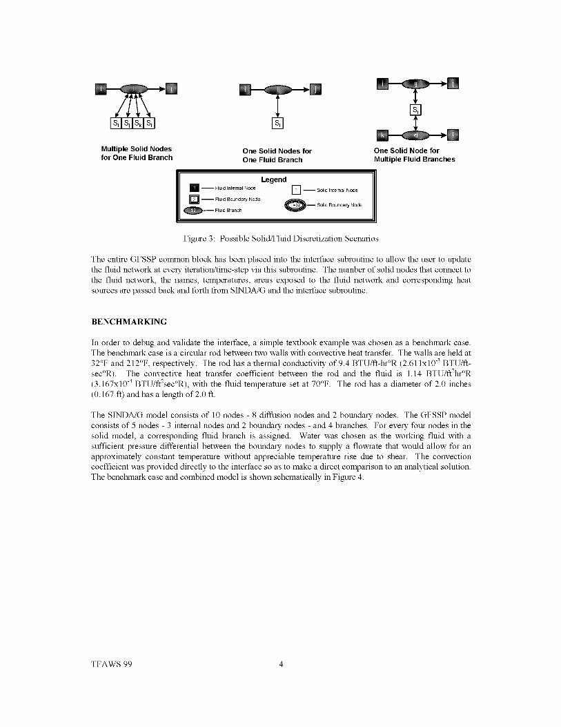
Multiple Solid Nodesfor One Fluid Branch

One Solid Nodes forOne Fluid Branch

Legend

-- Fluid Internal Node [] -- Solid Internal Node

tin-q--Fluid Boundary Node-- Solid Boundary Node

_ Fluid Branch

One Solid Node for

Multiple Fluid Branches

Figure 3: Possible Solid/Fluid Discretization Scenarios

The entire GFSSP common block has been placed into the interface subroutine to allow the user to update

the fluid network at every iteration/time-step via this subroutine. The number of solid nodes that connect to

the fluid network, the names, temperatures, areas exposed to the fluid network and corresponding heat

sources are passed back and forth from S1NDA/G and the interface subroutine.

BENCHMARKING

In order to debug and validate the interface, a simple textbook example was chosen as a benchmark case.The benchmark case is a circular rod between two walls with convective heat transfer. The walls are held at

32°F and 212°F, respectively. The rod has a thermal conductivity of 9.4 BTU/ft-hr°R (2.61 lxl0 -3 BTU/ft-

sec°R). The convective heat transfer coefficient between the rod and the fluid is 1.14 BTU/ft2hr°R

(3.167x10 -4 BTU/ft2sec°R), with the fluid temperature set at 70°F. The rod has a diameter of 2.0 inches

(0.167 ft) and has a length of 2.0 ft.

The SINDA/G model consists of 10 nodes - 8 diffusion nodes and 2 boundary nodes. The GFSSP model

consists of 5 nodes - 3 internal nodes and 2 boundary nodes - and 4 branches. For every four nodes in the

solid model, a corresponding fluid branch is assigned. Water was chosen as the working fluid with a

sufficient pressure differential between the boundary nodes to supply a flowrate that would allow for an

approximately constant temperature without appreciable temperature rise due to shear. The convection

coefficient was provided directly to the interface so as to make a direct comparison to an analytical solution.

The benchmark case and combined model is shown schematically in Figure 4.

TFAWS 99 4

32°F

70°F

Benchmark Case

212°F

1121314151617181-

Benchmark SINDA-GFSSP Model

Legend

I_-- Fluid Internal Node [] -- Solid Internal Node

-- Fluid Boundary Node 1___Solid Boundary Node

I_D_ Fluid Branch

Figure 4: S1NDA/G - GFSSP Benchmark Case

The closed form solution of the benchmark case is given in Equation 1, below, and derived in the ThermalAnalysis Workbook 5.

T(x) = Zfluid -I- 4.653e 1714× - 42.650e 1.714x (1)

where, x = distance from the cold wall in feet and

Tfluid = 70°F.

The results of the benchmark combined models are shown with the analytical solution in Figure 5 below.As Figure 5 illustrates, the S1NDA/G - GFSSP interfaced prediction lies on the curve of the analyticalsolution, thus providing a first level validation of the interface.

25O

o

E

200

150

100

5O

--Analytical Solution

SINDA/G-GFSSP Interfaced Solution

I I I

05 1 15

Distance from Cold Wall (x, ft)

Figure 5: Benchmark Case Results for SINDA/G-GF SSP Model with Analytical Solution

TFAWS 99 5

ADDITIONAL TEST CASES

In order to exercise the interface between S1NDA/G and GFSSP, three additional test cases were identified

which exploit different aspects of the interface.

The goal of the first of the additional test cases (the second test case) was to predict phase change in the

fluid model due to heat transfer to the solid. In this case, steam at 215°F and 14.705 psia enters a flow path

and flows over a solid bar and exits at 14.700 psia. The back face of the bar is held at 32°F. For simplicity,

the convective heat transfer coefficient is set in the interface at a constant value (3.167x10 -3 BTU/ft2sec°R,

an order of magnitude higher than the benchmark case). It should be noted that. Figure 6 illustrates the

physical situation and the S1NDA/G - GFSSP combined models. The results of the modeling effort for case

2 is shown in Figures 7 and 8. Figure 7 illustrates the temperature profile for both the solid and the fluid.

Note that the temperature of the fluid remaining constant during the phase change. Figure 8 illustrates the

quality of the fluid as a function of location downstream of the inlet. The fluid temperature is superimposed

on this figure to show the constant temperature during the phase change.

Steam In ..................................... Water Out

(T_u,d inlet 215 F)

32°F

Physical SituationCase 2 SINDA-GFSSP Model

Legend

I_-- Fluid Internal Node [] -- Solid Internal Node

Q_ Fluid Boundary Node

-- Solid Boundary Node

-- Fluid Branch

Figure 6: Test Case Two - Physical Situation and Combined Models

TFAWS 99 6

220

200

A180

o

"_ 160

Q,,E

140I--

120

IO0

Fluid

Solid

i i i i i i i i

1 2 3 4 5 6 7 8

Position (Relative to Solid Node Numbers)

Figure 7: Test Case Two - Temperature vs. Location for both Solid & Fluid Models

1 250

>,

1

O

200

I.I.0.7 o

0.6 150

0.5 _.

E0.4 1001_

"O.1

0.3 '_1I.I.

0.2 _ Quality 50

Temperature0.1

0 ,0

100 200 300 400 500 600 700 800 900

Node Number

Figure 8: Test Case Two - Fluid Quality vs. Location

The goal of the second of the additional test cases (the third test case) was to control the area of an orificeusing a temperature supplied by S1NDA/G. In this case, a metal bar is bounded by two fluid streams (onecold, the other hot) in steady state operation as illustrated in Figure 9, below. The bar is 0.25 feet thick,with a thermal conductivity of 18.8 BTU/ft-hr°R (5.22x10 -3 BTU/ft-sec°R). The bar has been descretized

into 35 solid nodes. The cold fluid stream consists of water entering at boundary node 1 with boundaryconditions of 70°F and 45.5 psia, and exiting at boundary node 8 with a boundary pressure of 45.0 psia.

TFAWS 99 7

Thecoldstreamentrancebranch(branch12)isanorificewithacross-sectionalareaof0.25squareinchesandlosscoefficientof0.6.Theremainderofthecoldstreamhasacross-sectionalareaof0.5squareinches.Thehotstreamconsistsof steamenteringatboundarynode11withboundaryconditionsof 250°Fand14.75psia,andexitingatboundarynode18withaboundarypressureof 14.70psia.Thehotstreamentrancebranch(branch1112)isanorificewhoseareaisafunctionofthetemperatureoftheadjacentsolidnode(node105).Thefunctionalrelationshipbetweentheorificecross-sectionalareaandsolidnodetemperatureisprovidedinEquation2,below.

Ao_i_ce=0.15+[0.01*(Tsolid155.0)]where,A=Areainsquareinches

T=Temperaturein°F

T1 = 70°F D

FlowArea is a Function

of Surface Temperature

101 102 103 104 105

106 107 108 109 110

(2)

T11 = 250°F

Branch 1112 is

a Function of

Temperature of

Solid Node 105

111 112113114115

116 117 118 119 120

121 122 123 124 125

126127128129130

131 132133134135

Physical SituationCase 3 SINDA-GFSSP Model

Figure 9: Test Case Three - Physical Situation and Combined Models

For simplicity, the heat transfer coefficient for each stream was set at a constant value: 5.0x10 -3

BTU/ft2sec°R for the cold stream and 2.5x10 -3 BTU/ft2sec°R for the hot stream. The results of the modelingeffort for case 3 are shown in Figures 10 and 11. Figure 10 illustrates the temperature profile in the bar atthe fluid entrance location (solid nodes 101-105), midline (solid nodes 116-120) and fluid exit location

(solid nodes 131-135). Figure 11 illustrates the convergence characteristics of the area for fluid branch1112 as a function of the solid model iteration.

TFAWS 99 8

o

EI--

17o

165

16o

155

15o

145

14o

135

13o

125

12o

-105)

_ ................... ,...m....Midline (Solid Nodes 116-120)

Fluid Exit (Solid Nodes 131-135)

I I I I

0.05 0.1 0.15 0.2

Distance from Cold Stream (ft)

Figure 10: Test Case Three - Temperature Profile in the Solid at Three Locations

0.25

0.35

,m

6-&

m

0.3

0.25

0.2

o.15

o.1 I I I I I I I I

50 1O0 150 200 250 300 350 400 450

Solid Model Iteration

Figure 11 Test Case Three - Fluid Branch 1112 Orifice Area vs. Solid Model Iteration

TFAWS 99 9

The final additional test case (test case four) had the goal of a "quasi-steady" operation in which the S1NDA

model is run in an unsteady mode, and the time step controls the boundary conditions of the fluid loopoperating in steady state mode. The physical situation modeled is nearly identical in geometry to test casethree, except that the fluid networks' geometries remain constant (i.e. area of branch 1112 is 0.15 in2 andnot a function of the temperature of solid node 105). The metal bar is initially at an uniform temperature of

155°F. The cold fluid stream boundary node 1 is initially at 70°F and 45.5 psia; whereas, the cold fluidstream boundary node 8 pressure is set at 45.0 psia. The hot fluid stream boundary node 11 is initially at250°F and 14.75 psia; whereas, the hot fluid stream boundary node 18 pressure is set at 14.70 psia. The

thermal conductivity and convective heat transfer coefficients are the same as used in test case three. Thetotal model run time is 20 hours, with the first 10 hours used to establish a steady state prediction. After 10hours, the inlet temperature of the two fluid boundary nodes (fluid nodes 1 and 11) become a function oftime. Equations 3 and 4 provide the functional relationship between temperature and time for fluid nodes 1

and 11, respectively. Figure 12 illustrates the physical situation and combined models.

= _ 70 °FT1 _10t (oF)

(3)

Yll =

250°F

280 - 4t (° F) (4)

where, T = Temperature in °Ft = time in hours

TI( < 10 hours) = 70°F

TI( > 10 hours) = 10 (°F)

_J H T11( < 10 hours) = 250°FBoundary temperatures at_ _ TII(E > 10 hours) = 2804 (°F)fluid nodes I & 11 are

/

functions of solid model time--

101 102 103 104 105

106 107 108 109 110

111112113114115

116 117 118 119 120

121 122123124 125

126127128129130

131 132 133 134 135

PhysicalSituationCase4 SINDAGFSSPModel

Figure 12: Test Case Four - Physical Situation and Combined Models

The results of the modeling effort for case 4 are shown in Figures 13 and 14. Figure 13 illustrates thetemperature/time profile for three solid nodes (116, 118, and 120) and the two inlet fluid boundary nodes.

TFAWS 99 10

Figure14illustratesthetemperatureprofileinthebarforsolidnodes116- 120atseveraltimesteps.Thesefiguresillustratethesolidtemperaturefollowingtheinletfluidtemperature.

26O

240

220

200

o180

160

Q.

E 140

h-

120

100

"1

Fluid Node 11 _"_

Solid Node 120 __......¢... _

Solid Node 118 _-_

Solid Node 116

Fluid Node 1

5 10 15

Time (hr)

2O

180

Figure 13: Test Case Four - Temperature vs. Time

170

160

o 150

140

(2.E

130t--

120

110

100 I I I I

0.05 0.1 0.15 0.2

Distance From Cold Stream (ft)

Figure 14: Test Case Four - Midline Temperature Profile

0.25

TFAWS 99 11

IMPLEMENTATION STATUS

To date, the interface subroutine has been developed to allow for modeling of steady state flow networks

with steady or unsteady solid modeling. Development is currently underway for fully unsteady modeling in

which the time step for the fluid model may be different than that of the solid model.

CONCLUSIONS

A general purpose fluid network code has successfully been interface with a general purpose thermal

analysis code for steady state flow models and both steady and unsteady thermal models. A benchmark

case was identified, combined models were constructed and executed. The predictions from the combined

benchmark models provided an accurate prediction of the temperature profile in the solid when compared to

the analytical, closed form solution. Three additional cases demonstrated fluid phase prediction and control

of the fluid model by the solid model's information via the interface subroutine. A status of the

implementation was also provided.

ACKNOWLEDGEMENTS

The authors wish to acknowledge the contributions of Mr. Randy Lycans of Sverdrup Technology and Dr.

Barry Battista of Tec-Masters.

This work was performed for the George C. Marshall Space Flight Center under contract NAS8-40386,Task Directive 661-007.

REFERENCES

1. Behee, R.: SINDA/G User's Guide, Version 1.81, Network Analysis, Inc., 1998.

2. Majumdar, A.K.; Bailey, J.W.; Schallhom, P.A.; Steadman, T. :A Generalized Fluid System Simulation

Program to Model Flow Distributions in Fluid Networks, (User's Manual) SvT Report No. 331-201-

97-005, NASA MSFC Contract No. NAS 8-40836, October 1997.

3. Patankar, S., Numerical Heat Transfer and Fluid Flow, Hemisphere Publishing Co., New York, 1980.

4. Patankar, S., Karki, K., Documentation of COMPACT-2D Version 3.1, (User's Manual) Innovative

Research, Inc., 1993.

5. Owen, J.W. (ed.): ThermalAnalysis Workbook, NASA TM-103568, p.1-3-2, January 1992.

TFAWS 99 12

A COLLABORATIVE ANALYSIS TOOL FOR

THERMAL PROTECTION SYSTEMS FOR SINGLE

STAGE TO ORBIT LAUNCH VEHICLES

Reginald Alexander

NASA/Marshall Space Flight Center

MSFC, AL USA 35812

Thomas Troy Stanley

International Space Systems, Inc.

Huntsville, AL USA 35816

ABSTRACT

Presented is a design tool and process that connects several disciplines which are needed in the complex

and integrated design of high performance reusable single stage to orbit (SSTO) vehicles. Every system is

linked to all other systems, as is the case with SSTO vehicles with air breathing propulsion, which is

currently being studied by the National Aeronautics and Space Administration (NASA). In particular, the

thermal protection system (TPS) is linked directly to almost every major system. The propulsion system

pushes the vehicle to velocities on the order of 15 times the speed of sound in the atmosphere before pulling

up to go to orbit which results in high temperatures on the external surfaces of the vehicle. Thermal

protection systems to maintain the structural integrity of the vehicle must be able to mitigate the heat

transfer to the structure and be lightweight. Herein lies the interdependency, in that as the vehicle's speed

increases, the TPS requirements are increased. And as TPS masses increase the effect on the propulsion

system and all other systems is compounded. To adequately calculate the TPS mass of this type of vehicle

several engineering disciplines and analytical tools must be used preferably in an environment that data is

easily transferred and multiple iterations are easily facilitated.

INTRODUCTION

Developing the next generation of launch vehicles is a primary focus of the National Aeronautics and Space

Administration (NASA). Several concepts have been proposed, many of which are fully reusable single

stage to orbit (SSTO) vehicles. Lowering the cost of placing a payload into orbit drives this idea of a fully

reusable vehicle.

Analysis of these concepts is essential to determining which to carry forward into more detail design.

According to Malone [1] in the current development process, 90% of the cost is committed in the first 10%

of the development cycle. Thus, more design knowledge is needed in the design process to minimize

changes. Also, the fidelity of the analyses is critical due to the strong interaction between each of the

systems (Figure 1). This interaction is most notable in the SSTO concepts that involve air-breathing

propulsion. In these concepts the thermal protection system (TPS) is a critical system. The TPS must

protect the air frame structure of a vehicle which flies at 15 to 20 times the speed of sound in the

atmosphere before the vehicle pulls up and goes into orbit. The TPS mass affects the mass of the vehicle

which affects the propulsion system, the vehicle's ascent trajectory, structure, aerosurfaces and other vehicle

subsystems. The TPS can not just be added to vehicle but must be an integral part of the vehicle's missionscenario definition.

l 1.InteractionofVehicleFigure Systems

THERMAL ANALYSIS

Several engineering disciplines are involved in vehicle analysis and design. This work will focus on the

thermal protection system (TPS) analysis. Directly involved in TPS sizing are trajectory analysis and

aerothermal heating analysis. To begin assessing the TPS mass requirements for a vehicle the trajectory

analyst generates a trajectory that delivers the required payload to the specified orbit. Similarly the analyst

calculates the trajectory required for a vehicle's reentry from orbit. Next the aerothermal analyst calculates

the convective heating rates on defined _body points" of the vehicle. TPS materials are selected based on

the surface temperatures due to the heating on each defined surface. Finally the thermal analyst calculates

the thickness of the TPS material and derives a mass. This process is iterated as often as necessary (time

allowing) to achieve an optimum design.

TOOLS

Several disciplines (on different computing platforms and maybe even in different locations) use tools

specific to their disciplines to provide input to the analysis process. The Program to Optimize Simulated

Trajectories (POST) is used to calculate trajectories and vehicle ascent and reentry performance. The

output of this code is a single large text file containing the numerical results for the run. The Miniature

Version of the JA70 Aerodynamic Heating Computer Program (MINIVER) is used to calculate aerothermal

heating. Its output also is a large set of data containing various information relative to understanding the

heating environment of a launch vehicle. The program Systems Improved Numerical Differencing Analyzer

(S1NDA) is used to calculate the TPS thickness at each body point. It is a numerical solver used to

calculate the temperatures of a thermal network of nodes set-up by the user. All of these programs are

UNIX based although there are personal computer (PC) versions of SINDA. Other tools used are text

editors and spread sheet programs used on desktop PC' s.

PROCESS

The problem with the process described is that those codes often reside on different computing platforms,

and have output formats that are not compatible with the data input format required by other tools. Figure 2

shows the process used in the Preliminary Design Office at NASA Marshall Space Flight Center. The

vehicle's ascent or reentry trajectory is generated using POST. Data specifically needed for input into the

aeroheating model is extracted and passed via e-mail or by hand to the aeroheating analyst. The

aerothermal heating analyst receives this data and uses a spreadsheet program to remove any unnecessary

data points. Once this is completed the data is formatted (in the spreadsheet) and transferred from the PC to

a UNIX based machine using a File Transfer Protocol (FTP) program. This part of the process is important

since

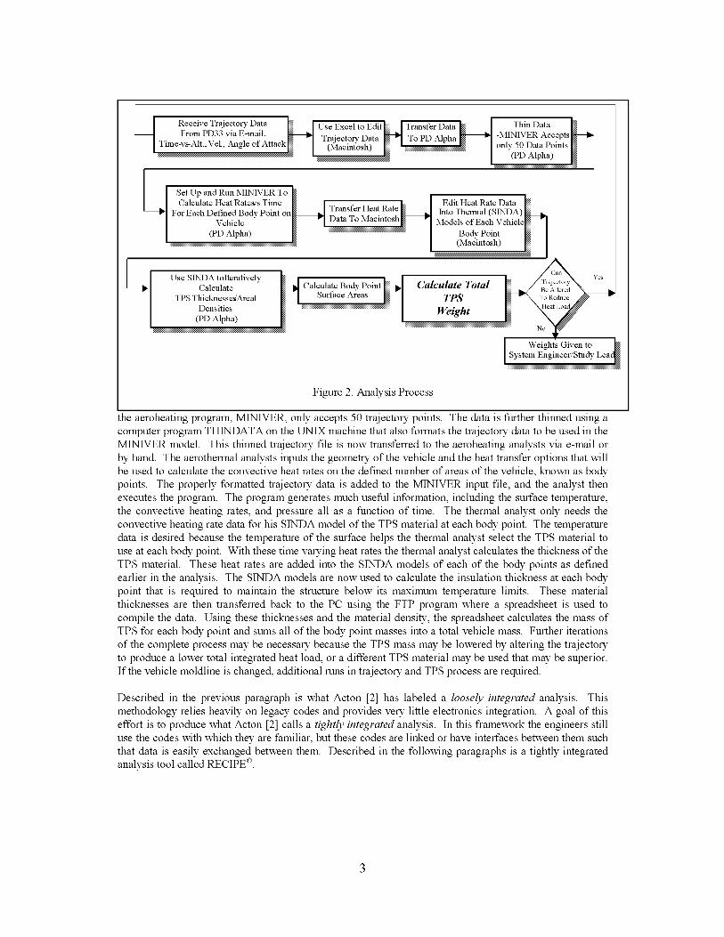
Receiverr jectoryData L IUseExceltoEditLJrransf rDataL rhinDataFrom PD33 via E-mail. _ (Macintosh) _ , _\\\\\\\\\\\\\\\\\,_ only 50 Data PointsTime-vs-Alt.,Vel., Angle of Attack_ ] Trajectory Data [_ -] To PD Alpha _ -MINIVER Accepts

_\\\\\_\\\\\\\\\_ ' _\\\\\\\\\\\\\\\\\,_, (PD Alpha)

_1 Set Up and Run MINIVER ToI Calculate Heat Rateses Time _ ! L Edit Heat Rate Data [_For Each Defined Body Point on_ j Transfer Hea! Rate _ Into Thermal (SINDA) L

Vehicle _ Data To Macmtosh_ r Models of Each Vehicle_ F]

I (PD Alpha) __\\\\\\\\\\\\\\'_ Body Point _ I

I I UseSINDAtolteratively N , , k _._. -, Yes

Calculate _ Calculate Body Point _ Calculate Total _/_;*°'e_

TPS ThicknessegAreal _ I Surface Areas _l TPS _x T_Densities l_ _\\\\\\\\\\\\\\\\\'_ w_r • -- k%_2, \Heat boadLx%%"

(PD Alpha) ] wetgttt

_\\\\\\\\\\\\\\\\\,_ _ _ _x,.

Figure 2. Analysis Process

Weights Given toSystem Engineer/Study Lea__\\\\\\\\\\\\\\\\\\_

the aeroheating program, MINIVER, only accepts 50 trajectory points. The data is further thinned using a

computer program TH1NDATA on the UNIX machine that also formats the trajectory data to be used in the

MINIVER model. This thinned trajectory file is now transferred to the aeroheating analysts via e-mail or

by hand. The aerothermal analysts inputs the geometry of the vehicle and the heat transfer options that will

be used to calculate the convective heat rates on the defined number of areas of the vehicle, known as body

points. The properly formatted trajectory data is added to the MINIVER input file, and the analyst then

executes the program. The program generates much useful information, including the surface temperature,

the convective heating rates, and pressure all as a function of time. The thermal analyst only needs the

convective heating rate data for his S1NDA model of the TPS material at each body point. The temperature

data is desired because the temperature of the surface helps the thermal analyst select the TPS material to

use at each body point. With these time varying heat rates the thermal analyst calculates the thickness of the

TPS material. These heat rates are added into the S1NDA models of each of the body points as defined

earlier in the analysis. The S1NDA models are now used to calculate the insulation thickness at each body

point that is required to maintain the structure below its maximum temperature limits. These material

thicknesses are then transferred back to the PC using the FTP program where a spreadsheet is used to

compile the data. Using these thicknesses and the material density, the spreadsheet calculates the mass of

TPS for each body point and sums all of the body point masses into a total vehicle mass. Further iterations

of the complete process may be necessary because the TPS mass may be lowered by altering the trajectory

to produce a lower total integrated heat load, or a different TPS material may be used that may be superior.

If the vehicle moldline is changed, additional runs in trajectory and TPS process are required.

Described in the previous paragraph is what Acton [2] has labeled a loosely integrated analysis. This

methodology relies heavily on legacy codes and provides very little electronics integration. A goal of this

effort is to produce what Acton [2] calls a tightly integrated analysis. In this framework the engineers still

use the codes with which they are familiar, but these codes are linked or have interfaces between them such

that data is easily exchanged between them. Described in the following paragraphs is a tightly integrated

analysis tool called RECIPE ©.

A COLLABORATIVETOOL

CollaborationbetweenthesedisciplinesisessentialtoadequatelysizetheTPSforthistypeofvehicle.Toincreasethefidelityof themodelsandreducecycletimefordesignthevehicle,theremustbebetterinteractionandexchangingof data.Thedevelopmentof atoolthatinterfaceswithallof thetoolsandprovidestheoutputintheformatnecessarytobeusedbytheothercodesisdesired.Thistoolwouldenabletheusageof legacytoolssuchasSINDA,MINIVER,andPOST.Thesecodesarewellunderstoodbyengineersandhavebecomestandardsintheindustry.Thatis importantwhentryingto establishaverycohesivecollaborativeenvironment.Thistoolwouldalsohavetobecross-platform,meaningthatit wouldbeusableonandcantransferdatabetweenUNIX-based,PC,andMacintoshmachines.Thisisagainessentialbecauseallengineershavedifferentcomputingplatformsandtoolsthattheyuseintheiranalysis.

A solutiontotheaforementionedproblemisRECIPE©. Thissoftwaretoolisacross-platformapplicationcapableofhostinganumberofengineersanddesignersacrosstheInternetfordistributedandcollaborativeengineeringenvironments.It providesaninterfacebetweentheengineeringtoolsofaparticulardisciplineandtheothertoolsthatneedthedatathatitprovides.Thedataisprovidedintheinputformatrequiredbythedesignatedreceivingtool(s).Theprogramallowstheusertoselectfromasuiteofstand-aloneprogramsthatwouldbeusedforthedesiredanalysis.Forexample,inthecaseoftheTPSanalysisdescribedabove,theusersmaychoosePOSTasthetrajectoryanalysistool.But,if anyothertrajectoryprogramshavebeenintegratedintotothesuiteofprograms,theusermaychooseit. Oncehehasexecutedhisprogramandissatisfiedwith his results he can publish the data to be used by the analyst who is producing the aerothermal

results.

According to Stanley [3] the user interfaces for the RECIPE © framework preserve the standard user

interaction with the legacy codes while also providing the ability to use the Intemet to exchange data and

work in collaborative environments. This framework allows the single user to optimize his results from

within his discipline and then "publish" them for the world to use in their models. The user interface

consists of a graphical user interface (GUI) to direct a portion of the design process. Shown in Figure 3 is

the RECIPE © executive GUI.

_i_ :_ _ _iiiiiiiiiiiiiiiiiiii°_iiiiii°°_iiii::i_iiiiiiiiiiiiiiiiiiiii_iiiiiiiiiiiiiiiiiiiiiii°°_`_°_iiiiiiiiiiiiiiiiiiiiiiiiiiii

........................................................................._,_

_1997-lggg Intem_enal Sp_ Sy_em_, Inc

Figure 3. RECIPE © Executive GUI

To determine its effectiveness in saving time and achieve a collaborative environment, a Thermal Analysis

Test Bed (TATB) was developed that connected only the trajectory analysis, the aeroheating analysis and

the thermal analysis. The goal of this activity was to demonstrate the effectiveness of the collaborative

environment and show the time savings attained by eliminating much of the data manipulation performed by

the users of the programs mentioned.

IntheTATB,RECIPE©willbeperformingallofthefunctionsthattheuserwouldhavetoperformwiththeexceptionof "building"theinitialanalyticalmodels.Thatfunctionis lefttotheanalyst.Figure4isasimplifiedschematicof theTATBanalysisprocess.All of thefunctionsin theboxesareRECIPE©functions,whilethecirclesareentrypointswheretheusercanassessthecalculationsoftheanalysiscodes.Theseentrypointsarenotnecessaryexcepttoensurethattheinputsarebeingusedproperlyandthattheengineerhasconfidencethatdatabeinggeneratedarecorrect.OnceaniterationiscompletedandtheTPSmasseshavebeencalculated,thisprocessmaybeiteratedtoapproachanoptimumdesign.Forexample,ifthemassesareexcessiveandposeathreattothevehiclefeasibilitychangesmaybemade.Oneoftheseisalteringthetrajectory;anothermaybeselectingamoretechnologicallyadvancedTPSmaterial.Using the

previously outlined process, another iteration would likely be too time consuming and labor intensive. But,

using this collaborative tool much of the labor has been removed making iterations more attractive. So

several trajectories may be analyzed considering the thermal implications, and several different TPS

materials may be analyzed to examine the technology implications.

Review Data

Sets-Up SINDA

Model(S)

D RECIPE © Function

I User Function

I Figure 4. TATB Simplified

PROGRAM EXECUTION/TEST CASE

New TPS MaterialNew Traj ectorr_

Review Data

A sample analysis of an SSTO vehicle TPS was performed to determine the effectiveness of the TATB

process. The object of this test was to compare the actual time required to complete the analyses described

earlier. The vehicle uses air-breathing propulsion to help it achieve its mission requirements. As stated

earlier, this requirement puts a severe burden on the TPS not only during reentry from orbit, but also on

ascent where the vehicle may accelerate up to speeds 15 times the speed of sound before going to orbit. For

this test case the computer platforms are a UNIX-based DEC ALPHA (on which MINIVER, S1NDA,

TH1NDATA and the RECIPE © server were run) and an Apple Power Macintosh 9600 (on which the

RECIPE © client and spreadsheet were run).

FirstabaselineanalysistimewasestablishedusingtheprocessshowninFigure2. Asstatedearlierthisprocessisverylaborintensiveandrequiresconsiderableinteractionfromtheanalyststomanipulatethedatatobeusedbythespecifiedtools.NexttheprocessshowninFigure2wasexecuted.Figure3showstheExecutiveGraphicalUserInterface(GUI)forRECIPE©.InthisExecutiveGUIunderthermalthebutton_%ditThermal"wasselected.AnothersetofGUI'sisnowavailable.OneinwhichtheMINIVERmodelsmaybesetupandeditedandanotherwheretheS1NDAmodelsaresetupandedited.

In theMINIVERGUIthePOSTtrajectorydatathatwill beusedisselected.RECIPE©retrievesthespecifieddataandexecutesthethinningprogram.Thisprogramrequiredsomeinteractionfromtheusertodeterminethedegreeofthinningrequiredtominimizethedatato50sets.FromthispointintheprocesstheMINIVERmodelissetupandrun. Theengineeris in full controlof whereandhowthedatawillbeexecutedandused.RECIPE©providesmodelconnectivity,filetransfer,anddatamanipulation.Intheprocessof runningMINIVER,thevehicleis dividedin40bodypoints,20leewardand20windward.

There will be a separate output file of convective heat rates and radiation equilibrium temperature both as

functions of time. The TATB database enables the correlation of the MINIVER output files with the

S1NDA models of each body point TPS for which these output files will be input. As is shown in Figure 5

of the MINIVER GUI there is a number of text files that contain the heat rate data for each particular

project. The database allows the user to store several projects' output files. The user next selects the

SINDA GUI. The desired MINIVER output file is selected and the corresponding SINDA model is

selected. With the MINIVER data edited into the S1NDA model program can be executed and the TPS

thickness for the selected body point can be calculated. Each body point SINDA model is executed until all

of the TPS thicknesses are calculated. For these test cases the S1NDA models of each body point will be

run in series as the MINIVER data is linked to the S1NDA models and the user selects _Run" in the S1NDA

GUI (Figure 6). Later versions of the code will enable the user to link all of the MINIVER output with theSINDA models and the models will be run with no user interaction.

Finally with all of the TPS sized for the whole vehicle the mass is calculated using a spreadsheet. The

output from each of the SINDA runs is linked directly in the spreadsheet and the vehicle TPS mass is

calculated based on the area that is represented by the body point and the density of the TPS material.

................................................................... ---=h==:Fh: ................................................ -----

i .............. __ _._ ............... " ............... ;_';_'" ..............

:::::::::::::::::::::::::::::::::::::::::::::::::::::::::: ?

i .............. _c_s:' ............. i _;-_N2_-_;-_ _a ........................ _r ...............::: .::::::::::::::::::::::::::::::::::::::::::==========================================================================================

! ii

I Figure 5 MINIVER ogI I

................................. i ' _,2.' _ _;_

.-'.................... f2_':_" ,_

I Figure 6. SINDA GUI I

RESULTS/COMPARISON

A benchmarkwasestablishedbyexecutingtheprocessasdescribedinFigure2 andmeasuringthe time

required to complete each step. For this work the process was executed once with no extra iterations. The

process is now well understood and can be performed more easily now than in the initial runs when the

process was being developed. The data shown in Table 1 is the amount of time required to complete the

TPS conceptual analysis of a vehicle before the TATB. The length of time to complete the initial analysis

was probably 3 to 4 times the values shown in the tables. But as the users became more familiar with the

tools for data manipulation, the length of time to complete the processes became shorter.

The results of using the RECIPE © code in the first steps of the TATB process shows that there is about a

20% reduction in the time taken to complete the steps to edit the POST data and to thin it. This reduction is

due mainly to the decrease in the time required to move and format data for each of the analysis tools. This

tool does not remove the responsibility of the analysts to utilize the legacy codes, but it enables them to

integrate the tools to achieve a better set of results more quickly. An even greater reduction in the total time

to complete the analysis is expected when file management system portion of the code is completed which

will be used to connect the aeroheating data to the thermal models. A conservative estimate of 50% is the

anticipated reduction in the analysis cycle time.

:i:i:i:i:i:i:i:i:i:i:i:i:i:i:i:i:i:i:i:i:i:i:i:i:i:i:i:i:i:i:i:i:i:i:i:i:i:i:i:i:i:i:i:i:i:i:i:i:i[:i:i:i:i:i:i:i:i:i:i:i:i:i:i:i:i:i:i:i:i:i:i:i:i:i:i:i:i:i:i:i:i:iMian_zt_.:i:i:i:i:i:i:i:i:i:i:i:i:i:i:i:i:i:i:i:i:i:i:i:i:i:i:i:i:i:i:i:i:

Ea it _j ___ _ I _3 I _Ti._:i_i:i:i:i:i:i:i:i:i:i:i:i:i:i:i:i:i:i:i:i:i:i:ili:i:i:i:i:i:i:i:i:i:i:i:i:i:i:i_i:i:i:i:i:i:i:i:i:i:i:i:i:i:i:ili:i:i:i:i:i:i:i:i:i:i:i:i:i:i:i:i:i:i:i:i_oi:i:i:i:i:i:i:i:i:i:i:i:i:i:i:i:i:i:i:i:i:Ex:_:_u_l.gi:M:_E_:i:i:i:i:i:i:i:i:i:ili:i:i:i:i:i:i:i:i:i:i:i:i:i:i:i_i:i:i:i:i:i:i:i:i:i:i:i:i:i:i:ili:i:i:i:i:i:i:i:i:i:i:i:i:i:i:i:i:i:i:i:i_7i:i:i:i:i:i:i:i:i:i:i:i:i:i:i:i:i:i:i:i:i::E¢i_: :M:N:YE:O:u_

:Ex:_:_:u_:¢:i_:_:_ie_i.i:i:i:i:i:i:i:i:i:i:i:i:i_iii_i:i:i:i:i:i:i:i:i:i:i:i:i:ili:i:i:i:i:i:i:i:i:i:i:i:i:i:i:i:i:i:i:i:i_i:i:i:i:i:i:i:i:i:i:i:i:i:i:i:i:i:i:i:i:i:

BENEFITS

I Table 1. Time to Complete TPS Analysis Benchmark I

The benefits of this type of tool in concept design are numerous. First, because the tool is cross-platform

the designers may use the type computers with which they are most familiar. The information is easily

exchanged between disciplines regardless of the platform. The tools will eliminate mistakes in the transfer

of input and output files. Also several engineers may be accommodated in the collaborative environment.

Thus better designs may be attained sooner. Design/analysis time will be reduced due to increased

communication and reduced efforts by the engineers to format the data and pass it on the next user of the

information. These factors should enable the team to perform more design iterations thereby reaching an

optimum design. Finally it allows the engineer to concentrate on engineering rather that data manipulation.

Thus more time can be spent considering the design of the thermal protection system of the vehicle rather

than developing the models or formatting the data.

CONCLUSION

Wurster [4] states that the TPS of the entry vehicle, as much as any other vehicle component, requires

integrated design at the vehicle system level. The TATB is a demonstration of such a system level tool that

will allow users to evaluate TPS concepts, trajectories, structure and how they interact and affect the

feasibility and cost ofa SSTO vehicle. It is important to note that this test bed is only a part or module in a

suite of tools that may be integrated to be used for vehicle design and analysis. Having these integrated

these tools gives engineers the ability to collaborate on designs and analyses can only make for higher

fidelity designs and analyses that should eventually lead to better and lower cost designs. It has been shown

that integrating the tools reduces the amount of time to complete a discipline iteration. This implies that

giventheoriginalamountoftimeforanalysesmoreiterationsshouldbecompletedwhichhelpthedesignersoptimizeavehicledesign.

REFERENCES

[1] Malone,JohnB.,'_IntelligentSynthesisEnvironment."_:/Tise.larc.nasa._

[2] Acton,D.E.,Olds,J.R.,_ComputationalFrameworksforCollaborativeMultidisciplinaryDesignofComplexSystems."AIAA98-4942,SymposiumonMultidisciplinaryAnalysisandOptimizationSept.2-4,1998.

[3] Stanley,ThomasT., Christenson,R. L., _IntegratedDesignModelingin a Design-to-CostEnvironment."ThePennsylvaniaStatePropulsionEngineeringResearchCenter10th AnnualSymposium,NASA/MSFC,October26-27,1998.

[4] Wurster, Kathryn E.,"Lifting Entry Vehicle Mass Reductionthrough Integrated

Thermostructural/Trajectory Design." Journal of Spacecraft, Vol. 20, No. 6 Nov.-Dec. 1983.

COMPUTATION OF COUPLED THERMAL-FLUID

PROBLEMS IN DISTRIBUTED MEMORY ENVIRONMENT

H. Wei, H. M. Shang, Y. S. Chen

Engineering Sciences Inc., Huntsville, AL

Phone: (256) 883-6233, fax: (256) 883-6267, e-mail: hwei@esi-al.com

ABSTRACT

The thermal-fluid coupling problems are very important to aerospace and engineering applications. In stead of

analyzing heat transfer and fluid flow separately, this study merged two well-accepted engineering solution

methods, S1NDA for thermal analysis and FDNS for fluid flow simulation, into a unified multi-disciplinary thermal-

fluid prediction method. A fully conservative patched grid interface algorithm for arbitrary two-dimensional and

three-dimensional geometry has been developed. The state-of-the-art parallel computing concept was used to couple

S1NDA and FDNS for the communication of boundary conditions through PVM (Parallel Virtual Machine) libraries.

Therefore, the thermal analysis performed by S1NDA and the fluid flow calculated by FDNS are fully coupled to

obtain steady state or transient solutions. The natural convection between two thick-walled eccentric tubes was

calculated and the predicted results match the experiment data perfectly. A 3-D rocket engine model and a real 3-D

SSME geometry were used to test the current model, and the reasonable temperature field was obtained.

INTRODUCTION

Modeling of the thermal-fluid coupling effects plays an important role in the design and problem diagnostics of

liquid rocket engine systems and the sub-systems, such as combustion chamber regenerative cooling channels

compatibility, cryogenic fluid management with passive recirculation, etc. The heat transfer between different

material and fluid media is also commonly encountered in the engineering practices. The applications include the

cooling of electric equipment, material processing and compact heat exchangers. Conventional approach for the

thermal-fluid coupling solution very often requires two separate analyses that involve different ways of practice and

complexity in each discipline. This study is to merge two well-accepted engineering solution methods, SINDA and

FDNS, into a unified multi-disciplinary thermal-fluid analysis method with the aid of patched grid and parallel

computing techniques. In the resulting method, the thermal simulating by S1NDA and the flow fields calculating by

FDNS are fully coupled to get the steady state or transient solutions.

S1NDA (Systems Improved Numerical Differencing Analyzer) [1] is a widely accepted thermal analysis software

for simulating solid components energy balance using method of conductor-capacitor networks. Other models such

as wall radiation heat transfer and one-dimensional fluid flow equations are used to provide boundary conditions for

complex systems. On the other hand, many practical applications in rocket engine flow analysis require CFD

models, such as the FDNS (Finite Difference Navier-Stokes) code [2], for better predictions of the flow fields which

can not be modeled properly with the simplified method used in SINDA. Therefore, merge of these two disciplines

into one unified analytical model will enhance the productivity and prediction capability of the thermal-fluid design

community.

Since the grids for CFD and SINDA are generated independently, the grid lines of two adjoining regions may align

(continuous grids) or may not align (discontinuous grids) with each other. Generally, the CFD model requires finer

grids to accurately predict flow fields than the grids used for thermal analyses. So, the grid lines are mostly

discontinuous at the interface for most applications. The boundary solution translation procedure must be

conservative, stable, and robust for the integrated system. The patched grid approach [3] was used for interface

linkage between S1NDA and FDNS. We keep all the grid lines and collect the smallest cells. When the heat flux or

temperature are exchanged across the interface, the local energy conservation is achieved by integrating upon cell

areas. In the iterative procedure, SINDA and FDNS communicate and exchange boundary conditions through the

boundary heat transfer coefficient and temperature.

A uniquefeatureofthismethodis theusageofimplicitcouplingofSINDAandFDNSbytheparallelcomputingtechnique.It makesthismethodbetterefficiencyandstability,andapplicableforbothsteadystateandtransientsolutions.In theintegratedS1NDAandFDNSsystemusingthePVMlibrary[4],S1NDAisrunasthemaster(parent)process,andcaninitializeseveralFDNScopiesfortheslave(children)processes.BothSINDAandFDNSarerunwiththeirowninputandcontroldata,andarecommunicatingandexchangingboundaryconditionswitheachotherthroughPVM.

Thedevelopednumericalmethodis firsttestedbyabenchmarkproblem.A 2-Dcaseof thenaturalconvectionbetweentwothick-walledeccentrictubeshasbeensimulated.Thepredictedresultsmatchtheexperimentdataperfectly.Then,a3-Drocketenginemodelandareal3-DSSMEgeometryareusedtotestthecurrentmodel.Thenozzleflow,thesolidwallandthecoolingchannelflowareallcoupledtogetherduringthecomputation.

NUMERICAL METHODS

A FULLY CONSERVATIVE PATCHED GRID INTERFACE ALGORITHM

For 2-D cases, the interface boundary is determined by all of the face grid points of both adjoining zones as shown

in Fig. 1. This enables that all the individual points from both zones lie in the interface line and then the interface is

unique and accurate.

For 3-D cases, the cell elements are defined using the original grid points in both zones plus the intersection points.

So, all of the grid points are used to construct the interface surface. The intersection point of these two set of grid

meshes is defined as the intersection of one grid mesh with the image of the nearby cells of another grid mesh on it.

For higher accuracy, the finer mesh is selected as the base mesh and the image of the other mesh is calculated based

on every cell of the base mesh. If the interface is planar surface, the image can be calculated only once based on the

base surface.

Figure 2 shows that a planar surface structured mesh intersect with another unstructured mesh. We keep all the grid

lines and collect the resulting cells. They may be no longer quadrilaterals or triangular, but polygons with the edge

number less than eight (the maximum edge number of a polygon is eight in the case of two structured grids mesh

interface). The polygon doesn't need to be triangulated under the memory and speed consideration. Figure 3 is a

cylinder face as a simple example of curved interface in 3-D application. The 6x6 mesh (dark lines) is the base mesh

and the 4x4 mesh (light lines) is projected based on every cell of the base mesh to construct the interface mesh.

We use the unstructured grid data format to manage cell element at the interface. The surface in 3-D domain should

first be translated into x-y plane by translation and rotation processes. Then cell elements (polygon) are detected.

The process includes calculating the intersect point, determining the vortex of polygon, calculating the cell area,

defining a pointer to indicate its corresponding cell ID in the original interface meshes of two zones respectively.

When communicating across the interface, the local mass and energy conservation is enforced through integration

upon cell areas.

ACCELERATE PATCH GRID GEOMETRIC SEARCH BY USING B1NARY SEARCH TREE ALGORITHM

In order to construct interface elements, every cell in one mesh must be checked with every cell in another mesh to

see if they have intersections. The number of search is the first mesh cell number times the second mesh cell

number, nlxn2. However, if we build a binary tree [5] to organize the geometric domain of one mesh, and search

the intersected cell by using tree traverse technique, the search effort will be tremendously reduced. Assume every

terminal node of the tree holds five cells, then the comparison times needed for one cell in mesh 1 to get the

interested cell group in mesh 2 is only log2(n2/5) .

Here we use the two end points coordinates of the block diagonal as the key to build the geometric binary search

tree. First find out minimum and maximum x, y, z over all the grids in mesh 2. The root represents the cube A(min

x, min y, min z)-B(max x, max y, max z). This block is bisected across the x axis and the region for which

Xa<X<(Xa+Xb)/2 is assigned to left son and the region for which (Xa+Xb)/2<X<Xb is assigned to the right son.

Zone1 one2

Interface

Figure1.Interfaceisdefinedbyallofthegridpointsin2-Dcase

grid1 grid2

' ................,_#..............._ _ _L ":_'L::"_¸ _, _ ,,, _ ......

k i ):¢.. "

overlap of grid 1, 2 interface

Figure 2 • Patched grid planar surface interface

":_}'V:-'.v_:;4"C_:s.2.;._.. .........

grid mesh 1 and 2

?"'_:_"h _-----:'d_-_....:_.,,

.............L ._g,i...--.--!-_---;,----':_

interface

Figure 3. Patched grid curve surface interface

A/

Pz A A C

Level 1 Level 2

i i O

d -_ '_ .... H_] _-T _-i 7"TNI

)E ..n L E i i.._jZ2_.._12.21

7A C A C

Level 3 Level 4

KF AL ID EJ MH CN LB OO

Tree structure

Figure 4. Geometric binary search tree structure.

For each of the node, repeat the process across Y-axis, and then do it across Z-axis. The process is continued by

choosing X Y Z in cyclic order. Figure 4 shows the procedure.

Since the region represented by son node is covered by the region represented by its parent, so if a cell is not

overlapped with a region represented by a node, the complete set of the regions stored in the sub tree of this node

can be disregarded from the search. The geometric search algorithm can be displayed by a recursive procedure as:

1. Check if the cell overlapped with the region represented by the root.

2. If the cell overlapped with the left sub region, search the left tree.

3. If the cell overlapped with the right sub region, search the right tree.

Thebinarysearchtreeis implementedbyusingC++languageandcoupledwiththepatchgridsubroutineinFORTRAN.Forthe3-Dnozzlecase,thereexisttwointerfacesbetweennozzleflowandsolidwall.Oneinterfaceis231cellsinfluidsideand56cellsinsolidside,anotherinterfaceis891cellsinfluidsideand56cellsinsolidside.OnIRISworkstation,theCPUtimeusedforconstructingtheinterfaceis2.13swithbinarysearchtreeand4.08swithoutbinarysearchtree.Thepatchedgridprocessisgreatlyspeedup,andthelargerthegridsize,themoreefficientofthismethod.

S1NDA/EDNSPRE-PROCESSOR

ThecomprehensiveCFDtechniquesincludinggeometrymodeling,gridgeneration,flowsolverandpost-processorhavebeenwelldevelopedatEngineeringSciences.FortheS1NDAinputfile,it generallyrequirestedioushandcalculationsof nodalcapacitanceandconductance.TocoupleCFDmodelwithS1NDA,apreprocessormustbedevelopedfirst to generatea S1NDAinputdeckfor subsequentfinitedifferenceanalyses.Wedevelopedapreprocessorthathastwomaintasks.ThefirsttaskistodetachinterfaceboundarygridsfromSINDAdomaingridstoprepareboundarygriddataforthepatchedgridmanipulationasdescribedabove.ThesecondtaskistogenerateS1NDAinputfile,whichincludescalculationof nodalcapacitanceandconductanceforS1NDAnetworkmodel,settingboundaryconditions,takingtheCFD-SINDAcommunicationsubroutinesandfinally,writingouttheSINDAinputfileaccordingtoitsrequiredformat.Ourpreprocessorcantakebothstructuredandunstructuredgrids.It canalsotakethegridandboundaryinformationdirectlyfromthePATRANneutralfiletogeneratetheS1NDAinputfile.And,thepost-processorcanprintoutS1NDAtemperaturefieldinplot3dformat,tobeviewedthroughtheCFDpost-processor.

S1NDAANDFDNSCOUPLL1NGWITHPVM

ThecommunicationbetweenS1NDAandFDNSwillbeachievedthroughparallelcomputingapproach.IntheintegratedS1NDAandFDNSsystemusingPVMlibraries,S1NDAwill runasmaster(parent)process,andcaninitializeseveralFDNScopiesasotherslave(children)processes.BothSINDAandFDNSrunwiththeirowninputandcontroldata,andcommunicateandexchangeboundaryconditionseachotherthroughPVM.S1NDAcalculatestheconductionheatfluxandtemperaturewithinthewallnodes,basedontheboundaryheattransfercoefficientprovidedbytheCFDmodel.Ontheotherhand,theCFDmodelusestheS1NDA-calculatedwalltemperaturesasfixedboundarytemperatures,andsolvestheenergyequationtocalculatethefluidtemperatures,heatfluxandheattransfercoefficientattheboundary.Thisprocessiscoupledandrepeatedforsteadystateortransientsolutions.

TheprogramcommunicationsbetweenSINDAandFDNSareshowninFig.5. AfterstartingPVMdaemon,executingS1NDAcodewill automatically start FDNS. The whole process will stop when the iteration number for

steady state solution or time progressing for transient calculation exceed the specified values.

ENHANCEMENT OF THERMAL-FLUID COUPLING

In the iterative procedure, S1NDA and FDNS communicate and exchange boundary conditions through the boundary

heat flux or temperature. We have experienced convergence problem when passing heat flux directly from fluid

side to solid side if the thermal conductivity is very small compared to fluid side' s effective thermal conductivity.

The temperature fields close to solid-fluid interface oscillate during the iteration procedure unless small time step is

used. It is found that the numerical stability can be enhanced if we pass the heat transfer coefficient and temperature

instead of heat flux.

The heat flux calculated in fluid side can be expressed as:

and

q = h(ry r_)

q = k(ry r_)/A_,

where q is the heat flux, h is the heat transfer coefficient, Tf is the fluid temperature at the grid adjacent to the wall,

T,_ is the wall temperature, k is the thermal conductivity and Am is the normal distance between the grid and wall. Sothe heat transfer coefficient of laminar flow can be calculated as

h =k/A s

where, for turbulent flow, h is given by the turbulence model.

Call initpvm I

Call recvnb <

1I UpdateQ I

Pass h, T

_ [Start FDNS I

Calculate h, T ]

[Callsendnb ]

Call sendnb ] • Call recvnb ]

1 ,L[ UpdateT ]

Pass T

Check /

N_______ < C°nvergeni_ -

Yes

I Output I I Output I

No

Figure 5. Communication between S1NDA and FDNS

NUMERICAL RESULTS

THICK-WALLED ECCENTRIC TUBES CONJUGATE HEAT TRANSFER

The conjugate heat transfer between eccentric tubes is calculated by the integrated CFD-S1NDA model, where the

FDNS code is used to solve the natural convection and S1NDA is used to solve the tube wall heat conduction. Figure

6 gives the geometry and the boundary conditions for this problem. The inner surface of the inner tube and the outer

surface of the outer tube are kept at different fixed temperatures, Ti and To. The flow between the tubes is induced

through the buoyancy force caused by temperature gradient. According to the experiments conducted by Kuehn and

Goldstein [6], the Prandtl number of the fluid is 0.7, the Rayleigh number based on the length scale (Roi-Rio) and the

temperature difference (Ti-To) is taken to be 4.93x104.

Two types of grid systems denoted as Grid 1 and Grid 2 are used. In Grid 1, the grid mesh is 41x21 for the fluid and

4 lx6 for inner and outer tube walls respectively. The grid lines are continues at the interface. In Grid 2, the grid size

is 41x21 for the fluid but 15x6 is used for the solid walls. The grid lines at the interface are discontinuous for Grid 2

and the patched grid technique is utilized.

For very large conductivity ratio C between solid and fluid (i.e. C=104 for copper: air), the tubes are indicated to be

isothermal. The numerically predicted temperature distributions at d?=0 ° and d?=180 ° are compared with the

experimental data of Kuehn and Goldstein [6] in Fig. 7. _/represents the distance from the innermost tube wall,

which is normalized by the distance between the outermost and the innermost walls. The dimensionless temperature

is defined as (T-To)/(Ti-To). From the figure we can see that the Grid 2 can give same results as Grid 1 and all are in

good agreement with experimental data.

We simulated two different conductivity ratio cases, one for C equals to 1 and another for C equals to 104, the latter

one corresponding to copper and air. Figure 8 shows the streamlines and the temperature contours. It is clear that

the bigger the conductivity ratio the smaller the temperature gradient across the wall. When the C value is very

large, the Bi number (defined as thermal conductivity ratio of solid to fluid) is very small and the wall is almost

isothermal. That is the case for copper and air. This is verified in both Fig. 7 and Fig. 8 for different conductivity

ratios. For the case of C=I, the transient solutions at t=ls, 5s, 10s are shown in Fig. 9.

\

To

Roi/Rio=2.6, Rii/Rio=0.6,

Roo/Rio=3.0, e/(Roi-Rio)=0.623

Figure 6. Geometry and Grid 2 for thick-walled

eccentric tubes conjugate heat transfer.

8

1.0

0.8

0.6

0.4

0.2

0.0o.o 1.0

'7 , , i .... i .... i ....

_'_ phi _[l, ffri dl[] phi =0, gri d_

k ._ phi =O exp.phi =180, gri dl

ax phi =1gO, exp.

k_

.... I .... I .... /_

0._ 0.4 0,6 0.8

Figure 7. The dimensionless temperature vs.

normalized distance between the tube walls for d?=0 °and 180 °.

tt=ls

(a) C=IO 4

t=5s

(b) C=I

Figure 8. Computed temperature contours andstreamline patterns.

t=10s

Figure 9. Flow pattern and temperature fielddeveloping transient process for C= 1.

3-D ROCKET ENGINE

Development of the algorithm for running multiple copies of FDNS for flow fields with a S1NDA model for heat

conduction is the solid component. The 3-D rocket engine model is selected as a test case. As shown in Fig. 10, this

model consists of a hot gas flow part for FDNS nozzle flow model, a solid metal wall part for S1NDA thermal model

and two outer flow passages for FDNS cooling channel model. The nozzle gas flow is a compressible flow, and the

cooling channel water flow is an incompressible flow. The grid size and initial conditions for each model are shown

in Fig. 10. For better observation, solid wall and cooling channel is showed apart from the nozzle.

S1NDA runs with two copies of FDNS simultaneously. SINDA and each copy of FDNS use their own input and

control data. S1NDA runs as a master process and initialize two FDNS children processes. Figure 11 (a) shows the

overall view of the temperature field including the hot gas nozzle flow solved by FDNS, the solid wall block solved

by SINDA, and the outer cooling channel flow solved by FDNS. Enlarged views near location b, c, and d, indicated

in Fig. ll(a), are shown in Fig. 1 l(b), 1 l(c), and ll(d) respectively. The gapes shown in Fig. 11 are caused by the

differences in grid densities between the FDNS model and the S1NDA model. Computationally, there is no gapes

between these two models. The patched grid interface model enforces the energy conservation across arbitrarily

patched interface grids between FDNS model and SINDA model. Reasonable temperature contours and variations

across the fluid-solid interfaces are observed in Fig. 11.

FDNS CoolingChannel Model

SINDA

Thermal Model

FDNS Nozzle

Flow Model

M=0.2

T=3600K

Zone 1

Zone 2 .,_

...._'_-,_,_,_,_,_%%% __'j Zone 2

Zone l _=5m/s _ _e_

_T=285 K _,,fy Zone 2.,

Zonel j<_ _ i _

•

Grid

Zone 1:3 lx5x6

Zone 2:15x5x6

Zone 1 : 15x4x5

Zone 2:15x4x5

Zone 1: 21x31xll

Zone 2: 81x31xll

Figure 10: SSME nozzle and coolant channel flow configuration

(b)

(a). Full view.

(a)

(c) (d)

Figure 11: Temperature field of a 3-D SINDA/FDNS coupled solution.

(b) (c) (d): Coolant, solid and main flow interfaces at different sections.

3-D SSME

A real geometry SSME nozzle flow with coolant channel flow and channel solid heat conduction is calculated using

the new developed S1NDA/multiple-FDNS simulation tool. Figure 12 shows the system configuration and grid mesh

distribution. The coolant channel is showed apart from the SSME nozzle for clear observation. The hot gas flows in

at uniform velocity with the Mach number of 0.2 and temperature of 3600K. Liquid hydrogen enters the coolant

channel at velocity of 0.5 lm/s, which results in the coolant mass flow rate of 29.451b/s for the 550-charmel design.

The hydrogen properties at pressure of 5000 psia and temperature of 54K are used in the calculations.

Figure 13 shows the temperature fields of 3-D SSME hot gas flow, coolant flow and coolant channel wall heat

conduction by S1NDA/multiple-FDNS coupled solution. Where, Fig. 13(a) is the full view in the middle cut of x-y

plane. Fig. 13(b) gives the enlarged view of coolant, solid and main flow interfaces at the location (b) indicated in

Fig. 13(a). Fig. 13(c) is the cross section temperature contours (in y-z plane) at the location (c). Due to the grid

lines are discontinuous at the interfaces of coolant flow and channel wall, the temperature contour lines also show

some discontinuity by the graphics package. The gape between hot gas flow and the channel wall is because of the

x-location of the hot gas cross section and x-location of the channel wall and coolant flow cross section are not

exactly the same.

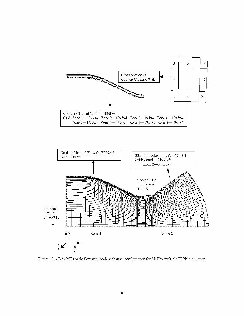
CrossSectionof

antChannelWall

1 4

CoolantChannelWallforS1NDAGrid:Zone1--19x4x4Zone2--19x5x4

Zone5--19x5x4Zone6--19x4x4Zone3--1x4x4Zone4--19x5x4Zone7--19x4x5Zone8--19x4x4

7

61

Hot Gas:

M=0.2

T=3600K

Coolant Channel Flow for FDNS-2

Grid: 21x7x7 SSME Hot Gas Flow for FDNS-1Grid: Zonel--3 lx3 lx9

l Zone 2--3 lx3 lx9

__!_ Coolant H2:_ _. u=0.51m/s_ _ =

_Y

J

zk x

i

Zone 1 Zone 2

Figure 12.3-D SSME nozzle flow with coolant channel configuration for SINDA/multiple-FDNS simulation.

10

(a)

.... _ ' i_i_iiili!_!_;i_i__i/i_L_!i_!;ii_ii_:_ii_i_!_'_ili_i_!'_"i

(b) (c)

Figure 13: Temperature fields of 3-D SSME hot gas flow, coolant flow and coolant channel wall heat conduction by

S1NDA/multiple-FDNS coupled solution.

(a) Full view. (b) Coolant, solid and main flow interfaces. (c) cross section temperature contours

CONCLUSIONS

The integrated SINDA-FDNS model can effectively solve the coupled thermal-fluid problems. The fully conserved

patched grid algorithm can ensure the energy conservation across the solid-fluid interfaces. The state-of-art parallel

computing technique makes S1NDA and FDNS rurming and exchanging information every time step. The successful

implementation of S1NDA model starting multiple copies of FDNS completed the entire model building. The

resulted thermal-fluid model will be used for typical liquid rocket engine thermal-fluid analysis. It can serve as a

reliable modeling tool in the aerospace and civil engineering industry.

11

ACKNOWLEDGMENT

This work is performed under the support from NASA Marshall Space Flight Center with the contract NAS8-98066.

The authors would like to acknowledge the technical suggestions from Dr. T. S. Wang of NASA Marshall.

REFERENCES

1. S1NDA/FLU1NT-Systems Improved Numerical Differencing Analyzer and Fluid Integrator, Version 2.6,

NASA/Cosmic Library.

2. Y.S. Chen: "FDNS-a General Purpose CFD Code, User's Guide, Version 3.0," ESI-93-01, May 1993.

3. G. H. Klopfer and G. A. Molvik: "Conservative Multizonal Interface Algorithm for the 3-D Navier-Stokes

Equations," AIAA-91-1601.

4. Geist, A., Beguelin, A., Dongarra, J., Jiang, W., Manchek, R., and Sunderam, V., "PVM: Parallel Virtual Machine

- A Users' Guide and Tutorial for Networked Parallel Computing," The MIT Press, Cambridge, MA, 1994.

5. J. Bonet and J. Peraire: "An Alternating Digital Tree (ADT) Algorithm for 3D Geometric Searching and

Intersection Problem," International Journal for Numerical Methods in Engineering, Vol. 31, pp. 1-17, 1991.

6. Kuehn, J.H., and Goldstein, R.J., "An Experimental Study of Natural Convection Heat Transfer in Concentric

Horizontal Cylindrical Annuli," Journal of Heat Transfer, Vol. 100, pp. 635-640, 1978.

12

MULTI-DISCIPLINARY COMPUTING AT CFDRC

W.J. Coirier, A.J. Przekwas, and V.J. Harrand

_._{jc@cfdrc,com: ajp@cfdrc.com; vjh@cfdrc.com

CFD Research Corporation

215 Wynn Dr.

Huntsville, AL 35805

ABSTRACT

This paper describes two methodologies to perform Multi-Disciplinary simulations involving coupled fluid,

thermal, structural, and electromagnetical interactions. The two approaches taken, termed tightly-coupledand loosely-coupled, yield two very different numerical and resultant software implementations. Thetightly-coupled approach follows a more traditional integration strategy, where the different applicationmodules (flow, heat, structures) are bound tightly together in a single package. This approach has distinct

advantages for problems that are computationally stiff and require a more tightly-coupled/implicit solutionstrategy. The loosely-coupled approach defines a heterogeneous, distributed computing framework withinwhich the different applications operate, allowing not only data exchange, but also invocation offimctionality amongst the different applications. Unique interfacing procedures permit the rapid

introduction of new applications into the framework, and allow independent, multi-disciplinary integrationof different vendor-supplied software. Both approaches are being actively pursued at CFD ResearchCorporation. This paper briefly describes the two approaches and presents example applications of both to

Aerospace and Micro-Electro-Mechanical Systems (MEMS).

SECTION I. INTRODUCTION

It is becoming widely recognized that Multi-Disciplinary Analysis, Design and Optimization is necessary to

extract the highest possible performance for Aerospace vehicles [Goldin, et al., 1998; Singhal, et al., 1999].This also holds true for a number of other areas, such as Automotive products, Bio-Medical devices, andespecially for Micro-Electro-Mechanical Systems (MEMS) [Stout et al., 1999; Przekwas, et al. 1999]. Due

to the explosive increase in computing power and resultant decrease in cost, computationally intensiveapplications unrealizable just a few years ago are now viable. Work in the improvement of algorithms foruni-disciplines will always be important and necessary, but the near term growth in the application ofscientific computing based analysis will be through the software integration of existing technologies. This

paper describes two approaches being taken to perform Multi-Disciplinary simulations involving coupledfluid, thermal, structural, and electromagnetical interactions. The two approaches, loosely termed tightly-coupled and loosely-coupled, yield two very different numerical and resultant software implementationstrategies.

The tightly-coupled approach, used in the CFD-ACE+ system, follows a more traditional integrationstrategy, where the different application modules (flow, heat, structures) are bound tightly together in asingle package. This approach has distinct advantages for problems that are computationally stiff/ill-

conditioned, and require a more tightly-coupled/implicit solution strategy.

The loosely-coupled approach, used in the Multi-Disciplinary Integrated Computing Environment

(MDICE), defines a distributed computing framework within which the different applications operate,allowing not only data exchange, but also invocation of functionality amongst the different applications.This permits the rapid introduction of new applications into the framework, and allows independent, multi-disciplinary integration of different vendor-supplied software.

BothapproachesarebeingactivelypursuedatCFDResearchCorporation.Thispaperbrieflydescribesthetwoapproachesandpresentsexampleapplicationsofbothto AerospaceandMicro-Electro-MechanicalSystems(MEMS).

SECTION II. TIGHTLY-COUPLED ANALYSIS: CFD-ACE+

The tightly-coupled approach to solving Multi-Disciplinary problems is represented by the CFD-ACE+system. This system solves the governing equations for a variety of physical processes, including:• Mass and Momentum Transfer

• Heat Transfer

• Structural Mechanics

• Electrostatics

• Electromagnetics

Each of these phenomena are represented by different governing equation sets, and exhibit elliptic,

parabolic and hyperbolic characteristics. Therefore, dependent upon the particular discipline, differentdiscretization strategies are taken, including Finite-Volume, Finite-Element and Boundary-Elementmethods. Coupling between the different disciplines is implicit when they share the same discretizationstrategy, and is explicit for those disciplines that do not. In this context, explicit coupling employs a

relaxation (steady state), or sub-iterative (unsteady) procedure. Implicit coupling, also called tight coupling,then implies a fully-coupled approach, which by necessity, also means discretization scheme. For example,conductive heat transfer problems are solved fully coupled to fluids problems, as they both share the samefinite-volume formulation, and hence, can share the same algorithmic implementations. For fluids-structures

interactions, the coupling is based upon a sub-iterative procedure for temporally varying solutions, and is arelaxation-based coupling for steady problems. The key to the tightly-coupled approach is the use ofcommon data representations as well as functionality within the core solver.

The CFD-ACE+ system is built around a collection of core physics solvers, using the CFD-DTF commonfile format as a persistent storage mechanism and static data transfer path (Data Bus). The CFD-DTFcommon file format and library defines a common set of data definitions and access mechanisms useful for

Finite-Volume (FVM), Finite-Element (FEM) and Boundary-Element Methods (BEM)-based scientificapplications. This allows the complete definition of most CFD and CSD problems by providing sufficientlycomplete data definitions and their corresponding file access mechanisms. The library and accompanyingcommon file format permit such features/data as:

• Structured, Unstructured, Polyhedral Grids

• Extensible Boundary and Volume Condition Data

• Platform Independent Data Exchange

• Consistent, Complete and Efficient Connectivity independent of grid type

• Fortran, Fortran90, C and C++ interfaces

The CFD-ACE+ system is comprised of a geometry modeler/mesh generator, graphical based pre-processor/model setup, physics solvers and graphical post processor. These modules are:

• CFD-GEOM: A geometry modeler, mesh generator

• CFD-GUI: A graphical user interface for pre-processing the solver

• CFD-ACEU: A parallel, pressure-based, polyhedral unstructured solver

• CFD-VIEW: A visualization package/post-processing tool.

These application modules are all integrated via the CFD-DTF common file format and library. This

publicly available common file format/library enables many important features in the unstructured flowsolver, allowing the treatment of multiple-domained grids containing structured, unstructured andpolyhedral-unstructured meshes in a fully implicit manner, as if they were consolidated into a single"virtual" zone. Figure 1 illustrates the components of this system showing the data transfer mechanism

(CFD-DTF) that allows the model definition, preprocessing, solver and postprocessing to be procedurallyintegrated.

TFAWS 99 2

Figure1.CFD-ACE+SoftwareSystem

Thegeometrymodeler/meshgenerator,coupledtothegraphicalpreprocessorandpostprocessorpackageviatheCFD-DTFcommonfileformatandlibraryisanopensimulationarchitectureapplicabletoawidevarietyofothersolutionmodules.BymakingasolvermoduleDTF-compliant,it canleveragethepre-andpost-processingcapabilitiesavailablewith theCFD-ACE+system.A completedescriptionof eachcomponentofthesystemisbeyondthescopeofthispaper;Figure2illustrateseachofthecomponentsofthesystembyshowinga snapshotofthegraphicalinterfacesforthegeometrymodeling,pre-andpost-processingmodules.

CFD-GEOM(geometry,grid)

::::':Ni:i

CFD-VIEW (visualization)

CFD-GUI (model setup)Figure 2: Sample Screenshots for Micro-Pump Analysis showing CFD-GEOM, CFD-GUI and CFD-VIEW

TFAWS 99 3

Thecorephysicssolveriscomprisedof3separateapplications:• CFD-ACE(U):FVMflow,heat,masstransfermodule• CFD-FastBEM:AfastBEMsolver• CFD-FEMSTRESS:AFEMstructuralanalysispackage

Eachoftheseisdescribedbrieflybelow.

SECTIONIIA.CFD-ACE(U)

CFD-ACEU is a finite-volume, pressure-based, unstructured transport equation solver. It supportsconservation volumes comprised of arbitrary polyhedra, including the more commonly used types, such as

hexahedra, tetrahedra, prisms, quadrilaterals and triangles. It uses a fully implicit procedure based upon theSIMPLE/PISO algorithm, and employs first-, second- and third-order spatial discretizations, as well as first-

and second-order temporal schemes. In addition to the traditional Reynolds Averaged Navier-Stokesequations, it is used to solve a wide variety of transport/conservation equations, including:

• Two- and One-equation Turbulence Models

• Multi-component Diffusion of reacting and non-reacting dilute gases, including PDF models.

• Surface Chemistry.

• Radiation and Conjugate Heat Transfer

Discretization of the equations is made using a finite-volume formulation, which relates the conservation-law form of the Navier-Stokes equations to a collection of flux integrations over the surfaces of a set of

discrete control volumes, or cells. The equations are solved sequentially and implicitly, meaning that eachequation, such as say a momentum equation, is linearized about the current time/iteration level. The physicssolver has been parallelized upon distributed and SMP architectures using the MPI message passing library.The parallelization of the code has been performed in such a manner that the convergence rate and

robustness of the code is not degraded relative to the serial mode of operation.

Figure 3. Parallel Computations of Selected Aerospace, Automotive and Defense-Related Problems usingCFD-ACE+

TFAWS 99 4

TheFinite-Volumeformulationusedindevelopingthephysicssolverallowsit tobeappliedtomeshesofarbitrarypolyhedra,permittingthesolutiononallmeshtypes,including• structuredgrids• unstructuredgridsoftriangles,quads,tetrahedra,pyramids,prismsandhexahedra• polyhedralgrids,obtainedviacartesianmesh,andmeshrefinement.

Figure3showsanillustrationofrecentapplicationsofCFD-ACE+torotorcraftaerodynamics,underhoodcoolingandcombatvehicleexhaust/gun-fumemodeling.

SECTIONliB. CFD-FEMSTRESS

FEMSTRESSis a finite-elementstructuralanalysisdevelopedat CFDRC.It solvesthestructuralmechanicsequationsinfinite-elementformderivedfromtheprincipleofvirtualwork.Inthisapproach,abalanceis formedbetweentheexternallyappliedloadsandtheinternallygeneratedloads.Convergenceisobtainedwhenthestressfieldresultingfromthecalculateddeformationsissuchthattheexternallyappliedloadsarebalanced.Forlinearproblems,thisresultsin thestandardlinearequationsobtainedusingtheGalerkinor Energyformulations.Forlineartransientproblems,amodalanalysisoptionisalsoavailable.Fornonlinearproblems,aNewton-Rhapsoniterativeschemeusingthetangentstiffnessmatrixisusedtoconvergetothebalanceof externalandinternalforces.

Inputto FEMSTRESSconsistsof surfaceforces(e.g.pressureloads)andbodyforces(e.g.gravity,thermoelasticity),aswellasthefixedboundaryconditionsandthesolidproperties.Outputincludesdisplacementsofallthenodepoints,theCartesianstresstensor,andtheprincipalstresses.

ThecurrentcapabilitiesofFEMSTRESSinclude:• staticanddynamicanalysis• modalanalysis• thermolasticity• materialandgeometricnonlinearity• plasticity• anisotropy• elastic/rigidandelastic/elasticcontact

TheelementssupportedbyFEMSTRESSare:2D Elements

(plane stress, plane strain, andaxisymmetric):

• 3-node triangle

• 6-node triangle

• 4-node quadrilateral

• 8-node quadrilateral

3D Elements:

• 4-node Tetrahedral

• 10-node Tetrahedral

• 6-node Prism (wedge)

• 15-node Prism (wedge)• 8-node hexahedral

• 20-node hexahedral

Special Elements

• Rectangular Beam

• 3-node triangluar shell

• 6-node triangluar shell

• 4-node quadrilateral shell

• 8-node quadrilateral shell

SECTION IIC. CFD-FASTBEM

CFD-FastBEM is a Boundary Element Method (BEM) solver that is may be used to solve such problems as:• Electrostatics

• Low Re Fluid Flows

• Acoustics/EM Waves

The BEM solver is capable of solving different equation types including Laplace/Poisson, Navier, Stokes,

and Hemholtz at low frequency. Boundary conditions BEM supports include Dirichlet, Neumann, and third

TFAWS 99 5

kind(convectiveforLaplaceandspringsupportforNavier).Multi-domains,eachwithdifferentsetofproperties,aresupported.Continuityoftheprimaryvariable(temperature,electricpotential,displacement)aswellasthesecondaryvariable(fluxesandtractions)areautomaticallyhandledacrosstheinterface.Anewmethod(developedwithinCFDRC)isusedtoevaluatetheboundaryintegrals.Themethodissimilartothemultipolemethod,but is applicableto anyboundaryintegralequation,includingthe3-DNavierequation.Sourcesterms(termstypicallyplacedontheright-handsideof theequationsandarenotafunctionof theprimaryvariablesolved)areapproximatedbyparticles.Fastsummationsof thesourcestermsareused.ThetimecomplexityisO(logM)foreachsummationofthecontributionofMparticles.A"matrixless"generalizedminimalresidual(GMRES)methodisusedtosolvethelinearequationsystemsiteratively.A diagonalpreconditionerisusedeverywhereexceptontheinterfaces,wherea2x2submatrixpreconditionerisused.TheoveralltimecomplexityisO(N)withoutsourcesandO(NlogM)withsourcesforeachiteration.Thetotaltimealsodependsonthenumberofiterationsof theGMRESmethod.Thisnumberisinturnproblemdependentandpreconditionerdependent.Ingeneral,aboutN°°5~°25iterationsareneeded.Therefore,thetimedependenceis roughlyO(N 1"°5~1"25) or O(N 1"°5~1"25 log M). The spatial

dependence is O(N+M). For small problems (with up to a few hundred elements), conventional O(N 2) BEMcan be faster than accelerated BEM. The conventional BEM solver can be activated by a simple parameter

setting. The BEM libraries are accessible through C function calls. The user can print the results inCFD-VIEW format or VRML.

SECTION IID. EXAMPLES OF MULTI-DISCIPLINARY ANALYSIS USING CFD-ACE+

CFD-ACE+ has recently been used to investigate a variety of micro-scale devices that must be modeledusing Multi-Disciplinary analysis. The following shows a subset of some of the devices being analyzed,indicating the different analysis modules being used to perform the analysis.

Micropump (Unsteady, fluid-structure-electrostatics)This illustrates the unsteady flow-structures-electrostatics interaction present for the modeling of a micro-scale pump. This pump is piezo-electrically activated, which when the voltage is applied, draws the pumpmembrane (see Figure 4) up. This membrane is modeled as a plate fixed at both ends, which deforms

according to the electrostatically applied voltage. Upon voltage application, this membrane deflectsupwards, imposing a pressure gradient, which pulls fluid from the inlet reservoir (on left), filling the volumecreated by the deflection of the upper membrane. Once the voltage is turned off, the membrane returns to its

original shape, pumping fluid out of the outlet membrane, on right. Figure 4 shows two snapshots in time ofthis unsteady process. The grid, model setup and post-processing for this problem are illustrated in Figure2.

...................... i2_ ..................................... ,,,,,,,21.........................i

iiiiiiiiiiiiiiiiiiiiiiiiiiiiiiiiiiiiiiiiiiiiiiiiiiiiiiiiiiiiiiiiiiiiiiiiiiiiiiiiiiiiiiiiiiiiiiiiiiiiiiiiii_i_i_iii_i_iiiiiii¸

i:

Figure 4. Micropump Simulation using Coupled Fluid-Structures-Electromagnetic Disciplines

Accelerometor (Electrostatics)This problem simulates an electrostatically driven accelerometer. The electrostatic model calculates theelectrostatic pressure force on the elastic beam. The structural model is used to calculate the stresses,strains, and displacements on the elastic beam. As seen in Figure 5 when 10 V is applied to the upper beam

TFAWS 99 6

thedeflectiontowardtherigidbodyissmall,withamaximumdisplacementof0.055gmatbeamcenter.Withanappliedvoltageof20Vthebeamdeformsontotherigidbody.

fixedend.................................................................................................................................e!astic ...........................................± .........................................

fixed end ..................... ,_ .......................... :_ : .............................. , .....

t0 am 80 um ...................................................................................................................................................................................................................

10V 20V

Figure 5. Doubly Clamped Beam Under an Electrostatic Load, with an Applied Voltage 0o 10 or 20 V

Another problem shown in Figure 6(a) is an electrostatically loaded plate. This is an example of anaccelerometer. A large plate with an applied voltage of 20 V is clamped by four beams. The whole upperelastic structure has a Young's Modulus of 1.69 x l 09Pa, Poisson's Ratio of 0.3, and no residual stress. The

upper plate is 2.0 _tm above a ground plane. Figure 6(b) shows the calculated displacement contours on theupper plate due to the electrostatic load. With 20 V applied to the upper plate a maximum deflection in the

center of the plate of 1.83 _tm toward the ground plane is calculated.

20.0

(a) (b)Figure 6. Accelerometer Under an Electrostatic Load. (a) The geometric dimensions and problem set-up.

(b) The calculated displacement of the plate due to the electrostatic load. The displacement of the plate

toward the ground plane is maximum (1.83 gm) at the center of the upper plate.

Fluidiclv-damped Beam under Electrostatic Load (Fluid-Structures-Electrostatics)The coupled thermal-fluid-structural-electrostatic capability in CFD-ACE+MEMS was tested on a simple

demonstration problem. The problem setup is shown in Figure 7. The geometry consists of a closedchamber, 5 man high and 70 man long, which contains a compressible gas of viscosity equal to 0.0171 Pa-sat an initial pressure Po 10 Pa and temperature To 300 K. The chamber is bounded at the top by a

flexible beam clamped at each edge, and by adiabatic walls on the other three sides. The beam is 1 manthick, and has a modulus of elasticity of 4000 Pa. From symmetry considerations, half of the geometry ismodeled, with symmetry conditions applied to the left edge.

TFAWS 99 7

5 mm gas

_ Vo sinmt_ ca

• 35 mm •

..... :. :. :. : : : :.................................. _'"'";' . . , _ , '. :_ :'. _- -k _: -_ 5-:_ :._ :_.- 2:2_::::-_ ............. ;.--'-'2 --2.7.2- ¢-_ 22. 22 :5- 2: 2 2- ; ;

t { a t _ {, -_ C_ _:_ _? _ _ ::av;::*'-.;'=.__-e_-,v:::=:aa--a=:-----:::__"a=r_:::::=:_:c--:------ .......... ------¢ ........

............................................._ . , , ,. , , . _--__

............................................ z__ .;:v.. :_=_ ....... :=x_-_---2_a-'-2_:_-_--'_2:---5 %:: 5; "-_' 2:' _ 2: _- :- ...... :....7---.'7Z: ": -...... -- : ; : : :27-, _2 .... _'7. Lq _ ...........

_ _;_ "-"_-:_ ........... :::::::::::::::::::::::--' =- : : : : : i : ' ' '

...................................._:_:_i_i_i_i_i_i_i_i_i_iiiiiiiiiiiiiiiiiiiiiiiiiiiiiiiiiiiiiiiiiiiiiiiiiiiiiiiiiiiiiiiiiiiiiiiiiiiiiiiiiiiiiiiiiiiiiiiii_i_i_i_i__ ...........................................-_._=_ :_ ._ .._ S. S.... _ 2 .: :: ; : i

.....'....... .-___-_ -,:___- _'W-_'_'_'_---_--"_"-"_--"-"'-'--_--_2_-_--@_=_:2--'--""*"722--'_2* 0:=....::.;........:: : :: :

, ----_a----_*----_ ........ _-'&-Z---_--_2_ ........................ :-- :_- "= ': : :

==========================================='-_====---Z-_.:.-_ _ 0_15l!! _:::=_::iE:[:?-_-2_:'_4 "--_i_ _:: -ii ii :i ! ! :

Po = 10 Pa

Figure 7. Doubly Clamped Fluid Damped Beam Under a Sinusoidal Electrostatic Load. Shown is a time

sequence of the beam displacement, fluid velocity field (vectors), and normal axial stress (contours onbeam) for the Po 10 Pa case.

A sinusoidal voltage is applied (12000 sin 5_t V) to the bottom wall, and the beam on top of the chamber isgrounded. The sinusoidal varying electrostatic force deflects the beam downward compressing the gas. Asthe gas is compressed, the pressure increases, applying an upward force to the beam to counteract the

electrostatic force. At each time step the resulting deformation is obtained from a balance of theelectrostatic, pressure, and inertial forces.

The result of the analysis was to determine the transient response of the fluid pressure, temperature,

electrostatic field, and the deflection and stresses of the beam. To accomplish this, the governing equationsfor the four models (flow, heat, electrostatic, and structural analysis) are coupled and solved implicitly ateach time step. The time sequence of Figure 7 shows the deflection of the beam, the gas flow as vectors, and

the normal axial stress as contours on the beam. The snapshots were taken before, at, and after the voltagemaximum. As the beam moves downward the gas is forced into the clamped comer pushing the elastic beamupward. The energy equation was also solved but the temperature increases were minimal (only 0.1 K) dueto the small number of cycles simulated.

Buoyancy-Driven Flow of a Conductive Fluid (Flow-ElectromaRnetics)The Lorentz force is demonstrated by the calculation of buoyancy driven flow of a conducting fluid in auniform magnetic field. The bottom boundary rotates with a specified angular velocity and has a uniform

temperature. The inner part of the top boundary rotates in the opposite direction of the lower boundary andhas a uniform temperature lower than that of the bottom boundary. The outer part of the top boundary is a

TFAWS 99 8

freesurface.Thetemperaturedifferencebetweentheboundariescreatesabuoyancy-drivenflowpatterninadditiontotherotationimposedbythewalls.A uniformmagneticfieldin theoppositedirectionofgravitydampstheflowthroughtheLorentzforce.Figure8showscontoursofthetemperatureandvelocityintheverticaldirectionwithandwithoutthemagneticfield.Thevelocitymagnitudeismuchsmallerwhenthemagneticfielddampstheflow.

i ii iiiiiiiiiiN,ii!iiiiiiii

no B

'_B (a)

B !iiiiiiiiiiii!i!ii_i_;_no B

(b)Figure 8. (a) Temperature and (b) Vertical Velocity Contours for Coupled Flow/Magnetics Solution. Right

Half is without the Magnetic Field, Left Half is with the Magnetic Field

Electro-Osmosis (Fluid-Elect roma_netics)Electroosmosis techniques are widely used for transport of charged fluids in microfluidic systems. Shown

in Fig. 9 is a cross channel device used for sample injection and separation. The flow of material in thedevice is controlled by static fields. Depending on the voltage Vs applied to the upper and lower reservoirof the cross channels, the flow of charged specie can be suppressed (0V), flowed into (37.5V), or flowedout of(135V) the cross channels.

iiiiiiiiiiiiiiiiiiiiiiiiiiiiiiiiiiiiiiiiiiiiiiiiiiiIi3iiSiiiiVi

TFAWS 99 9

flow

velocity

i_i_:̧:._ii_iiii

Figure 9. Electric Potential in Flow Velocities for a Cross Channel Device

SECTION III. MDICE: MULTI-DISCIPLINARY INTEGRATED COMPUTING ENVIRONMENT

The Multi-Disciplinary Integrated Computing Environment (MDICE) provides a distributed computingframework that is suitable for Multi-Disciplinary analysis, design and optimization. This approach allowsseparately developed and maintained analysis packages to be integrated within a dynamic, distributed and

heterogeneous computing environment. The MDICE architecture allows not only data exchange amongstapplications, but also functionality exchange: Applications may invoke certain functions in otherapplications through the MDICE environment. The different applications communicate through a rich set ofpre-defined, MDICE supplied interfaces, which perform all necessary data manipulations as well as

interface specific function invocation. This environment is constructed of three separate components: acentral controller, a library of MDICE communication and control functions, and lastly, the MDICE-compliant application modules themselves, which include a variety of structural, fluid and heat transfersolvers.

The central controlling process provides network and application control, serves as an object repository,executes remote procedure calls and coordinates and synchronizes the execution of the application modules.It communicates via a message passing library (PVM), and provides the overall control via a Graphical

User Interface and strongly typed scripting language. Figure 10 shows the GUI for the MDICE-AE(AeroElastic) controller.

The next component, the MDICE library, provides an extensible object definition that is used to define and

instantiate all data passed to and from the application modules. This library also contains the interfaceobjects, which perform the very necessary data exchange and data manipulations between the applicationmodules. The development of a rich set of interface objects is crucial to the application of the MDICE

environment to a wide variety of Multi-Disciplinary problems. Contained within this environment are:

Fluid/Structure Interfaces:

• Conservative and Consistent interfacing (force and virtual work conservation)

• Arbitrary grid coupling and alignment (e.g. structured to unstructured grids)

• Multi-Dimensional coupling (e.g. structural beam models coupled to three-dimensional fluids flowmodels)

Fluid/Fluid Interfaces

• Arbitrary grid coupling and alignment (e.g. structured to unstructured grids)

• Multi-Dimensional coupling (e.g. axisymmetric-3D or 2D to 3D)

• Mixing Plane interfacing (circumferential averaging)

TFAWS 99 10

iiiiiiiiiiiiiiiiiiiiiiiiiiiiiiiiiiiiiim iiiiiiiiiiiiiiiiiiiiiiiiiiiiiiiiiii_l_i_iiiiiiiiiiiiiiiiiiiiiiiiiiiiiiiiiiii iiiiiiiiiiiiiiiiiiiiiiiiiiiiiiiiiiiii_

iliiiiiiiiiiiiiiiiiiiiiiiii_iiiiiiiiiiii_iiiiiiiiiiiiii iiiIiiiiiiii

iiiiiiiiiliiii_ii_!_iiiiiiiiiii_i iiiii!i_iiiiiiiii

iIiiii_iiiiiiiiiiiiiii_:_:_iiiiiiiiiiiiiil_iiiiiiiiiiiiiiiiiiiiiiiiiiiiiiiiiiiiii iiiiiiiiiiiiiiii_i_iiiii_iiiiiiiiiiiiiiiiii_iiii

Figure 10. MDICE-AE Users Interface Structures Interface Panel

Overset/Chimera Interfaces

• Automated hole cutting for structured, unstructured, polyhedral grids• Automatic Data Conversion

• Units, Axes, dimensionality

These interfaces allow different fidelity models to communicate across different disciplines. This allows, forexample, a beam structural model to be used with a three-dimensional Reynolds Averaged Navier-Stokes(RANS) solver, or a two-dimensional RANS to be coupled with a three-dimensional structural analysismodule. Since the interfaces provide self describing data exchange, applications such as visualization

packages may also be driven within the environment. As an example, consider Figure 11, which shows acircumferential averaging interface for turbomachinery applications, and Figure 12 showing a 2D/3Dinterface used for gas turbine combustor calculations.

In the context of tight and loose coupling procedures, the MDICE environment uses a loose couplingapproach, but since it is operating in a heterogeneous/distributed environment, the modules may run inparallel. For instance, for a fluid structures interaction problem, the structural analysis modules and flowsolver modules are computing simultaneously, and are synchronized by the central controlling MDICE

process. This also allows parallel physics solvers, such as CFD-ACE+, to perform independently threadedparallel calculations while being treated as a single module in the MDICE environment (multi-levelparallelization).

Each application module in the environment communicates to others through the interface objects, allowinga wide variety of module combinations to be constructed to approach a given Multi-Disciplinary problem.

TFAWS 99 11

Thisallowstheretrofittingof legacyapplicationsintoa Multi-Disciplinaryenvironment,permittingdisciplinespecifictoolstobeusedwheretheyarebest.Asanexample,foranorganizationthatmightbeveryexperiencedusing,say,MSC/NASTRAN,butnotexperiencedusingCFD,thisenvironmentwouldbeideal.In thiscase,nocorporateexperienceandconfidencegainedwiththestructuralanalysispackagewouldbelost,whilefunctionalityto performhigh-fidelityaero-structuralinteractionproblemswouldbegained.

Figure11.IllustrationofCircumferentialAveragingInterface(Left,forturbomachinery)

;iii:Figure12.2D/3DInterface(forGasTurbine

CombustorSwirlertoDomeInterface)

Presently,therearea widevarietyof applicationsandorganizationsusingtheMDICEenvironment,primarilyforaero-structuralinteractionproblems.Recently,directinterfacestoparametricCADpackages,suchasPro/Engineerhavebeenmade,andworkisunderwayintegratingotherdisciplinesintotheMDICEenvironment.Table1showsalistofDisciplinesandOrganizations/ApplicationsthatareusingtheMDICEframework.

Table1.Discipline Code

ParametricComputerAidedDesign(CAD)Pro-Engineer(ParametricTechnology)UniGraphics(UniGraphics)CATIA(IBM)

GeometricModeling/MeshGeneration CFD-GEOM(CFDRC)

ComputationalFluidDynamics

FiniteElementAnalysis(FEA),LinearStructuresSolvers(Modal,InfluenceCoeff.)BeamModels

CFD-ACE(CFDRC)CFD-ACE+(CFDRC)CFD-FASTRAN(CFDRC)GCNSfv(Northrop-Grumman)NISTAR(Pratt& Whitney)NASTAR(Pratt&Whitney)Corsair(Pratt&Whitney/NASA-Lewis)NPARC(NASAGlenn)Cobalt(AFRL)(CFD)ENS3D-AE(ARFL)Splitflow(Lockheed-Martin)ADPAC(NASA-Glenn)LSS(CFDRC)NGLSS(Northrop-Grumman)MSC/NASTRANANSYSCFD-FEMSTRESS(CFDRC)

3DGraphicalVisualization CFD-VIEW(CFDRC)LinePlottingPackage XMGR(PublicDomain)ScreenSnapping/MovingMaking ImageMagick(PublicDomain)

TFAWS99 12

SECTION IIIB. SAMPLE MDICE EXAMPLES

Two examples of the Multi-Disciplinary Integrated Compuing Environment are shown here for solving

coupled aero-structural interaction problems. Also, an example is shown illustrating Chimera meshcapability coupled with CFD-ACE+ to perform a moving body, 6DOF, fluid-structures low speed flow.

F-16 Win_/BodyThis example shows MDICE being applied to compute the steady state aeroelastic deflections of a F-16wing/body structural/aero model. The LSS solver was used for the structural model, which consisted of arigid fuselage and strake, and flexible wing. The aerodynamics model was constructed using the CFD-

FASTRAN compressible flow solver. The flight conditions correspond to a Mach number of 1.2 and anangle of attack of 5.116 degrees.

The computed wing tip deflection (65 mm) compared favorably to the experimentally measured deflection

(68 ram).

Figure 12:F-16 Wing/Body Deformation due to Aero Loads

Twin-Tail Buffet

This example shows how the MDICE environment has been used to compute the unsteady, coupled, aero-structural response of a twin tail delta wing configuration at angle of attack. This configuration canexperience an unsteady buffeting caused by interaction of the wing leading edge vortex with the flexiblevertical stabilizers. For this subsonic flow, the tail deflections cause pressure perturbations to the flow field

that are fed upstream, altering the vortex structure. The results computed here [Sheta, et al., 1999] havebeen compared favorably with experimental data in [Washburn, et al., 1993].

The fluids model used is the CFD-FASTRAN flow solver, coupled to the LSS structural module. The flowequations solved are the compressible RANS equations using a 2nd-order upwind scheme, with a lst-ordertemporal scheme. The structural model used is a beam model, where the tails are modeled as cantileveredbeams, fixed at the root, and allowed to oscillate in both bending and torsional modes. The MDICE

interface for this run is shown in Figure 13. This configuration was run at 4 angles of attack, and the resultscompared to experimental data. Figure 14 shows a selection of the computed results at the 4 angles ofattack, illustrating the asymmetrical, unsteady vortex breakdown, interacting with the tail torsional/bendingmodes.

TFAWS 99 13

Figure 13: MDICE Control of Coupled Fluid/Structures Interaction Problem

o_ = 26 °c_ = 30 °

c_ = 34 ° c_ = 38 °

Figure 14: Unsteady, Coupled Aero-Structural Analysis of Twin-Tail Buffetting using MDICE-AE

TFAWS 99 14

As seen in these figures, at the lowest angle of attack, the leading edge vortices are symmetric, and do not

burst until past the vertical stabilizers. At 30 degrees, some asymmetry is noted, and the vortices are seen toburst near the tails. This asymmetry causes an unsteady pressure load on the tails, causing (asymmetric)bending and torsional modes of vibration. These unsteady modes then feed upstream, further coupling withthe asymmetric behavior of the vortex structure. At higher angles of attack, this asymmetric, unsteady

behavior is fitrther excited, as shown by the contours at 34 and 38 degrees. The computed bendingmoments, torsional moments and frequencies compared very well with the experimental data, and are shownmore completely in [Sheta, et al., 1999].

Transient Analysis of a Butterfly Valve Closure (MDICE + CFD-ACE+)For this example, the unsteady flow and solid stresses induced during the closing of a butterfly valve aresimulated. The MDICE environment is used to drive CFD-ACE+ (flow-structures), along with the MDICElibrary's Chimera mesh module and interfaces, as well as MDICE's 6 Degrees-of-Freedom (6DOF) module

and interfaces. This unsteady calculation begins with the steady solution of the valve in the open position,and progresses to fully closed in 3 seconds. The valve motion is defined via the 6DOF model, and theMDICE environment generates the unsteady results, viewed in real time. Figure 15 shows the overset mesh,

the initial (steady) conditions at fully opened, and the a snapshot of the transient simulation near closing,showing the induced stresses in the valve.

overset mesh initial condition

Figure 15. Transient Butterfly Valve Closing Process: Unsteady, Overset, Fluid-Structures usingMDICE+CFD-ACE+

SECTION IV. CONCLUSIONS

Two approaches suitable for Multi-Disciplinary Analysis have been presented, and the correspondingsoftware suites described. For each of these approaches, a limited selection of examples have been shown,illustrating the different disciplines and ranges of applicability. These two approaches have been termed

"tightly-coupled" and "loosely-coupled". The tightly-coupled approach has been represented by the CFD-ACE+ system, while the loosely-coupled approach has been represented by the Multi-DisciplinaryIntegrated Computing Environment. A brief description of the CFD-ACE+ system has been given,describing the implicit coupling procedures used for like discretization schemes, relaxation-based couplingfor dissimilar discretization schemes, the common data access mechanisms via the CFD-DTF common file

format and library, and the different modules that make up the system. A limited set of examples of thisapproach have been shown. The loosely-coupled approach has been represented by the MDICE

TFAWS 99 15

environment.Thedifferentcomponentsthatmakeupthisheterogeneouslydistributed,Multi-Disciplinaryenvironmenthavebeendescribed,theinterfacingtechnologyaddressed,anda numberof sampleapplicationsshown.

SECTION V. ACKNOWLEDGEMENTS

The authors would like to acknowledge a number of very important contributors to the capability that hasbeen outlined in this paper. For the CFD-ACE+ system, we would like to particularly acknowledge thecontinuous support and encouragement of Dr. Ashok Singhal/President CFDRC, as well as the entire CFD-

ACE+ development team, including; Milind Talpallikar, Dr. H.Q. Yang, Dr. Yu Jiang, Dr. MaheshAthavale, Dr. Philip Stout, and Dr. Giridharan. For the MDICE environment, external support viaAFRL/VA and NASA GRC is greatly appreciated, as well the internal support via CFDRC IR&D. Inparticular, we would like to thank Dr. Vijiyan Parthasarthy, Dr. Essam Sheta and Dr. Charles Warren fortheir contributions to the development and further application of the MDICE environment.

REFERENCES

Goldin, D.S., Venneri, S.L. and Noor, A., (1998), "NASA's ISE (Intelligent Synthesis Environment),"

presentation.Przekwas, A.J., Yang, H.Q. and Athavale, M.M., (1999), "Computational Design of Membrane Pumps with

Active/Passive Values for Microfluidic MEMS," SPIE, Paris, France.Sheta, E.F., Siegel, J.M., Golos, F.N., and Harrand, V.J., (1999), "Twin-Tail Buffet Simulation Using a

Multi-Disciplinary Computing Environment," NASA/CP- 1999-209136,CEAS/AIAA/ICASE/NASA Langley International Forum on Aeroelasticity and StructuralDynamics, Williamsburg, VA, June 22-25.

Singhal, A.K., Parthasarathy, V., Siegel, J.M., and Reich, A., (1999), "Coupled Fluid-Structural-ThermalSimulations of Industrial Problems; Requirements, Approaches and Examples - Keynote Lecture,"Keynote Lecture ASME, Pressure Vessels and Piping Conference, August 1-5, 1999, Boston, MA.

Stout, P.J., et al., (1999) "A CAD System for Simulation and Modeling ofMEMS,: SPIE, Paris, France.

Washburn, A.E., Jenkins, L.N., Ferman, M.A., (1993), "Experimental Investigation of Vortex FinInteraction," AIAA-93-0050.

TFAWS 99 16

Overview of Fluid Dynamic Activities

At the Marshall Space Flight Center

Roberto Garcia

Lisa Griffin

Ten-See Wang

Applied Fluid Dynamics Group

Presented at:

The 10th Thermal and Fluids Analysis Workshop

Huntsville, AL

September 13-17, 1999

Overview

• Organizational Changes at MSFC

• Recent Program Support & Technology Development

- Analysis & cold flow testing

- Fastrac, X-34, X-33, RLV, LFBB

• Ongoing Activities

- RLV focused technology, RBCC concepts development,methodology & code development

• Future Activities and Direction

- Hardware design and development

- Tools Development

• Concluding remarks

- Constraints, cooperation, opportunities

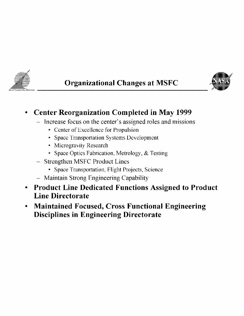
Organizational Changes at MSFC

• Center Reorganization Completed in May 1999

- Increase focus on the center' s assigned roles and missions

• Center of Excellence for Propulsion

• Space Transportation Systems Development

• Microgravity Research

• Space Optics Fabrication, Metrology, & Testing

- Strengthen MSFC Product Lines

• Space Transportation, Flight Projects, Science

- Maintain Strong Engineering Capability

• Product Line Dedicated Functions Assigned to ProductLine Directorate

• Maintained Focused, Cross Functional Engineering

Disciplines in Engineering Directorate

Organizational Changes at MSFC

• Fluid Dynamics in Space Transportation Directorate

- Discipline primarily supports space transportation product line

- TD63: Fluid Physics and Dynamics Group (bldg. 4203)

• Acoustics, aerothermal analysis, dynamic data reduction and analysis,

plume induced environments, cold-flow testing PIs

- TD64: Applied Fluid Dynamics Analysis Group (bldg. 4203)

• Develop and apply computational fluid dynamics (CFD) analysis

- TD74: Experimental Fluid Dynamics Group (bldg. 4732)

• Maintain, operate, & develop cold-flow experimental facilities

• Other Disciplines (Thermal, Stress, etc.) in EngineeringDirectorate

- Support broadly distributed among product lines

Recent Program Support & Tech. Dev.

Fastrac Low-Cost Engine Technology Demonstrator

- Primary propulsion for X-34 vehicle

- Hydrodynamic design and analysis of both pumps

• All the primary flow paths in the LOX and RP- 1 pumps

• Water flow test of LOX pump

- Verify non-cavitated performance, determine suction capability

- Steve Skelley presentation Tuesday morning (Fluids 3a)

- Aerodynamic design and analysis of the turbine

• Single stage supersonic turbine w/exit guide vanes

• First time accurate, full NS, rotor stator analysis

- Lisa Griffin presentation Tuesday morning (Fluids 3b)

- TCA and GG performance and environments predictions

• Injector patternization water tests

• Finite rate combustion devices analysis

- CFD baselined as performance prediction method

Recent Program Support & Tech. Dev.

Fastrac Turbopump Cross-sectionhllet Manifold

L©X _ Diffuser & Volute

RP Pumo

Inducer-Impeller

RP Pump Diffuser & Volute

2/27/97layout

Recent Program Support & Tech. Dev.

Pump flow path design and analysis

Turbine flowpath design and time accurate analysis

-r

Frequency - Hz

Recent Program Support & Tech. Dev.

Fastrac LOX pump

cold flow testing

Stage Head Coefficient vs Normalized Flow/Speed Ratio

0.55 ,4

°.5° t

'_,0.,,5l= o.4o_

_ 0.25t

@ Measured

.... _ ...... + Pred cted

0.20 I .... I .... I .... I .... I .... I .... I .... I .... I .... I .... I .... I ....

40 50 60 70 80 90 100 110 120 130 140 150 160

Normalized Flow/Speed (%)

Recent Program Support & Tech. Dev.

........_i_iiiiiiiiiiiiiiiiiiiiiiiiii_i_i_i_iiiii_i_i_i_i_iiiiiiiiiiiiiiiiiiiiiiiiiiiiiiiiiiiiiiiiiiiiiiiiiiiiiiiiiiiii_i_i_i_i_iiiii_i_i_iiiiiiiiiilililililiiiiii!i!i!i!i!ii

Fastrac TCA performance prediction with 15:1 nozzle

=======================================......................

Pattemization tests and

performance prediction

Fastrac TCA performance prediction with 30:1 nozzle

ii....................... ........................................_....

Recent Program Support & Tech. Dev.

• X-34 Pathfinder Vehicle Design Support

- Propulsion system feedlines flow analysis

• Assure pump inlet flow distortion within acceptable limits

- Plume induced heating on the vehicle

• Initial predictions refined with component test data

- Sonic boom prediction for environmental impact statement

• X-33 /RLV Vehicle Design Support

- Assessment of 3 phase-1 concepts: lifting body, winged body,

Delta-Clipper

- Extensive wind tunnel tests for aerodynamic configuration

development

• Critical impact on resolving transonic pitching moment issue

Recent Program Support & Tech. Dev.

_i_ii_iiiii!i!!i!iii!iiiiiiiiiii_i_iiiiiiiiiiiiiiiiiiiiiiiiiiiiiiiiiiiiiii_i_

X-34 and X-33 feedline analysisRLV Phase-1 Concepts

:: J i s_,2'-x " , I .J

o _gl_of_ck _ph_10 IS

X-33 and RLV Aerodynamic Testing

Recent Program Support & Tech. Dev.

• X-33 /RLV Vehicle Design Support (continued)

- Ascent loads with and without plume

• Aerodynamics load benchmark with LaRC jet-effects tests

• Plume induced thermal loads

- CFD used to supplement empirical data base

• Base heating hot-fire short duration tests

- LH2 feedline hydrodynamic design, analysis, & cold flow test

• Tight packaging, close-coupled valve, J-2 turbomachinery

- X-33 sonic boom prediction for environmental impact statement

• Liquid Fly-Back Booster Wind Tunnel Tests

- Fly-back, liquid propulsion boosters under consideration forShuttle upgrades

- Support aerodynamic configuration development

• Using wind tunnel data for CFD code assessment

Recent Program Support & Tech. Dev.

:::::::::::::::::::

i!i!i!i!i!i!ili_iill¸

iiiiiiiiiiiiiiiiii4_::::::::::::::::::iiiiiiiiiiiiiiiiiiii

iiiiiiiiiiiiiiiiiiii_i:i:i:i:i:i:i:i:i:ii

CFD External Pressures

....<!!_ii]ii_.... _iii]i_

OInterpolate CFD onto

Finite Element Model

iiiiiii!

External Applied CFD Pressures

onto Finite Element Model

Recent Program Support & Tech. Dev.

Linear Aerospike Plume-Induced X-33 Base-Heating

Sea level, no bleedAt an altitude of 3.7km w/base bleed

Short Duration hot-fire of base flows

Ongoing Activities

• RLV Focused Technology

- Awarded two tasks to develop RLV turbomachinery technology

- Turbine optimization task

• Eliminate dependence on availability of composites &/or increase Isp

- Daniel Dorney presentation Tuesday morning (Fluids 3a)

- Unshrouded impeller technology development task

• Increase stage loading without sacrificing efficiency

- George Prueger presentation Tuesday morning (Fluids 3a)

• Rocket Based Combined Cycle Concepts Development

- Trailblazer LOX-LH2 and DRACO LOX-Hydrocarbon concepts

- Code benchmark for ejector mode operation

- Joe Ruf presentation later this morning (Fluids lb)

Ongoing Activities

RLV Focused Technology

Turbine Optimization

RLV Focused Technology

Unshrouded Impeller Tech.

Ongoing Activities

Ejector concept parametrics25

20It,-

'-,1

L,.

0.10

-40

PSU RBCC Top Wall Pressure

Comparison

'_ ..........._ 20# *"" * 15_

/ 10.._B_

0

-20 0 20 40 60 80 100

x (in)

• T06199920

• T06189921

............ 2D

--3D

_Geom etry

Trailblazer nozzle

concept assessment

Ejector mode code benchmark

Using Penn State data

Ongoing Activities

• Methodology and Code Development

- Assessing & developing codes to support advanced propulsion

concepts

• Pulse detonation wave engine code assessment

• Laser-light craft performance prediction code development

• Defining requirements for high temperature, ionized flows

- Demonstrating coupled fluids-thermal analysis capability in

support of RBCC concept development

- Assessing available unstructured grid generation capability

- Developing optimization techniques

- Kevin Tucker presentation this afternoon (Fluids 2a)

- Assessing and demonstrating CART3D

• Inviscid, Cartesian vehicle aerodynamic code

- Michael Aftosmis presentation later this morning (Fluids lb)

Ongoing Activities

Performance Modeling of Laser Light Crafts

T

5o _i_ro s xoo _o 2oo _o s

NASA[MSFC]ED32 Laser Lightcraft Thermo._uid Field S@uhtion

Ongoing Activities

7--/.

/

LFBB used for CART3D Assessment .....'

-2 0

Mach 1.3, Beta=0,BJCVW configuration

::::::::::::::::::::::::::::::::::::::::::::::::::::::::::::::-:-:-:-:-:-:-:

:i:i:i:i:i:i:i:::i:i:i:i:i:i:::i:i:i:i:i:i:i:i:i:i:i:__:::::;:;:;:;:;.........:.:.:.:.:.:.:.:..:.:.:.:.:.:..:.:.:.:.:.:.:.:_:_:::_: ::::::::::::::::::::::::::::::::

............ +>>>>>>.>>>>>>>:............._ _::_:_:_:_:_::::::::::::::::::::::::::::::::::::::::::::::::

4 6 _ 10 12 14 16 18

_n_e of Attack _de_

Future Activities and Direction

• Hardware Design and Development

- RLV engine preliminary design (next 12 months)

• Aerodynamic design and cold flow tests

• Propulsion system environments

- Support detail design of RBCC concepts (next 3 years)

• DRACO flow path development and flight experiment

• Trailblazer detail design

• Combustion devices and turbomachinery supporting technologies

Long life, wide flow range capabilities, low weight

- Spaceliner 100 Technology Roadmap

• 5, 10, and 20 year goals

• Hardware and supporting code technology

• RBCC part of roadmaps 10 year goals

• Laser light crafts part of 20 year goals

Future Activities and Direction

• Tools Development

- Fast, efficient incompressible flow analysis code (Pearl)

- Time accurate, rotor-stator incompressible flow analysis capability

- Cetin Kiris presentation Tuesday morning (Fluids 3a)

- Improvements to hydrocarbon combustion modeling capability

• Increase code efficiency, expand physics

- Increase flexibility and capability at cold flow test facilities

• On-rotor measurements, broader speed range for pump testing, allownearly simultaneous testing of turbine and nozzle test facility

- Unstructured, full NS code development w/finite rate capability

- Y. S. Chen presentation this afternoon (Fluids 2a)

- Advanced Engineering Initiative (AEI)

• Code improvements, automation, & integration into design system

• Develop, demonstrate, and implement MDO capability

Future Activities and Direction

Unstr ucturedi full N S code d evelo p m en t w/fi n it e r at e ca p a b i lity

Concluding remarks

• Constraints

- Budget situation currently tenuous

• New starts will suffer if budget cuts not addressed

• Cooperation

- Leveraging from each others activities necessary

• Maximum benefits from invested funds, builds political support

• Opportunity

- Future hardware development becoming more reliant on high

fidelity analysis

• Required to achieve the necessary system operational characteristics

• Budget constraints, public relations (political) consequences of failure

- In the midst of major leap forward in fluid analysis capabilities

Aerothermodynamics At NASA - Langley Research Center

K. James Weilmuenster

Senior Research Engineer

Aerothermodynamics Branch

NASA Langley Research Center

Hampton, VA

INTRODUCTION

The Aerothermodynamics Branch at NASA - Langley Research Center is tasked with

developing, assessing and applying aerothermodynamic technologies to enable the

development of hypersonic aircraft, launch vehicles, and planetary/earth entry systems.

To accomplish this mission, the Branch capitalizes on the synergism between the

experimental and computational facilities/tools which reside in the branch and a staff that

can draw on five decades of experience in aerothermodynamics.

The Aerothermodynamics Branch is staffed by 30 scientists/engineers. The staff, of

which two-thirds are less than 40 years old, is split evenly between experimentalists and

computationalists. Approximately 90 percent of the staff work on space transportation

systems while the remainder work on planetary missions. The Branch manages 5

hypersonic wind tunnels which are staffed by 14 technicians, numerous high end work

stations and a SGI Origin 2000 system. The Branch also utilizes other test facilities

located at Langley as well as other national and international test sites. Large scale

computational requirements are met by access to Agency resources.

AEROTHERMODYNAMIC PROCESS

Aerothermodynamics is a blend of aerodynamic forces and moments, pressure/shear

loading, heating and fluid dynamics across the speed range. This information is obtained

from ground based experiments, engineering/computational analysis and flight test results

and becomes the basis for the aerothermodynamic process.

The aerothermodynamic process is the road map that defines the steps necessary to turn

mission requirements into a flight vehicle. A systems analysis, based on mission

requirements, will define an initial concept. The configuration is then screened using

parametric ground-based testing to determine whether or not the vehicle is flyable

(aerodynamics) and survivable (aeroheating) throughout the reference trajectory. If the

vehicle passes this test, then the flight characteristics of the vehicle are optimized using

detailed ground based testing and CFD codes. Ultimately, the outer mold lines are frozen.

At this point,hight fidelity testingand"benchmark"CFDcodesareusedto developaflight databookandestablishaerodynamic/aeroheatingflightmargins.

This processhasbeendevelopedand refined throughLangley's involvementin thedesignand analysisof hypersonicvehiclesbeginningwith the X-15 andcurrentlytheNASA family of X planes.During that time, the Branchhasdealtwith blunt to veryslendervehiclessuchasthehighenergyJovianentryvehicle,Galileo,theShuttleOrbiter,DODmissileprograms,Marsmicroprobes,NASP,HyperX andtheX-33.

ANALYSIS TOOLS

Up until the mid 1980's, aerothermodynamic analysis was based on engineering tools,

data obtained from ground based facilities and a very limited amount of flight data. At

this time, Computational Fluid Dynamics (CFD) began to contribute to the knowledge

base, primarily as a tool to characterize real-gas effects at flight conditions. As CFD has

matured, it has taken on an increasingly larger role in the analysis of hypersonic vehicles.

Currently, for a given vehicle, CFD accounts for approximately 25% of the aerothermal

data base. In another decade that percentage should double due to increased computer

speed/size, radical improvements in surface modeling/grid generation and improved

solution techniques. However, ground based facilities will always be a major contributor

to the aerothermodynamic data base due to their ability to quickly generate large amountsof data.

Ground Based Testin_

The Aerothermodynamic Facilities Complex 1 (AFC) represents all of NASA's

experimental aerothermodynamic testing capability via conventional-type (as opposed to

impulse-type) hypersonic blowdown-to-vacuum wind tunnels. The five facilities of the

AFC provide a Mach number range from 6 to 20 using three different test gases. The 20-

Inch Mach 6 Air Tunnel can provide unit Reynolds numbers from 0.5 to 8 million per

foot in perfect air (i.e. 7 = 1.4 in the freestream and within the model shocklayer) via

reservoir stagnation pressures from 30 to 500 psia at a temperature of approximately 950

°R. The 15-Inch Mach 6 Hi Temp Tunnel provides essentially the same Reynolds number

in air, but at an increased total temperature capability (to 1500 °R). The 20 -Inch Mach 6

CF4 Tunnel simulates real-gas effects at Mach 15 - 20 by using a gas three times heavier

than air which provides a relatively low value of 7 within the shocklayer of the model;

thereby simulating the low 7 aspect of a dissociated gas.. The 31-Inch Mach 10 Tunnel

can provide unit Reynolds numbers of .5 to 2 million per foot at reservoir stagnation

pressures of 350 to 1450 psia at a temperature of 1850 °R. The 22-Inch Mach 15/20 He

Tunnel provides a high Mach number test capability using an unheated gas as helium can

be expanded from ambient temperature to Mach 26 without liquification. Over the past

decade, these facilities have been upgraded to improve data quality and to implement a

common instrumentation and data acquisition system among the facilities.

Standard measurement and visualization techniques, strain gauge balances to obtain

aerodynamics, oil-flow for surface streamlines, thin film resistance gauges for discreet

surface temperature/heat flux measurements, electronically scanned pressure models and

schlierenare available.In addition,Langley hasdevelopedphosphorthermography2technologyto obtainglobalsurfaceheattransfermeasurements.Work is continuingtoenhancethequalityof the experimentaldataby implementingrapidmodel fabrication3and3-dimensionalopticalscanning4QA processesto reducetime from designto testaswell asimprovedmeasurementanddataanalysistechniques.Modelcoatings5capableofprovidingsimultaneousglobaltemperatureandpressuredistributionswill undergotunneltestingby theendof thisyear.In addition,a technique6designedto rapidlyextrapolategroundbasedheatingdatato flight surfacetemperatureshasshowngreatpromise.CFD and Grid Generation

Grid Generation: One of the major impediments to the timely inclusion of CFD analysis

in the design process has been the long lead time required to generate grids. The

Aerothermodynamics Branch has made a large investment in the development of a state-

of-the-art, robust grid generation process based on commercial and in-house developedsoftware for both structured 7 and unstructured 8 grid generation. Given a surface

definition, block decomposed, viscous, structured grids can be generated in 1-5 days

depending on the complexity of the configuration while parametric geometry changes

and regriding can take as little as ½ day. Currently, the Branch's unstructured gridgeneration is based on the FELISA 9 system and limited to grids for inviscid flow. A

viscous capability based on the VGRID 1° software is being developed. In general, the

unstructured grid generation is less cumbersome than the structured grid generation and it

is much easier to handle parametric geometry changes. It is still time consuming due to

required initial preprocessing of the surface geometry. Limited grid adaptation for

structured grids is imbedded in the flow solver with some additional refinement

capability available through the grid generation tools while unstructured grid adaptation

resides in the grid generator.

Computational Tools: The Branch has several codes at its disposal. Some are designed

for specific tasks or flow regimes while others are general in nature.

The Langley Approximate Three-dimensional Convective Heating 11 (LATCH) and

Solution of the Axisymmetric Boundary Layer Equations 11 (SABLE) are engineering

codes designed to quickly assess a vehicle's thermal environment. LATCH can rapidly

compute the approximate heating along inviscid surface streamlines on complex three-

dimensional vehicles based on the axisymmetric analog for 3D boundary layers. The

SABLE code computes axisymmetric and two-dimensional boundary layer flows on

reentry vehicles and can be interfaced with the LATCH code to compute approximate 3D

boundary layer solutions along streamlines on complex vehicles. Each of these codes has

a turbulent option and can handle perfect gas, CF4 and equilibrium air chemistry flows. In

each code, edge conditions are obtained from an existing 3D inviscid flowfield solution.

LATCH can work with solutions on both structured and unstructured grids while SABLE

is currently restricted to working with structured grids. Both of these codes can compute

the global heating in a matter of minutes on a SGI R10000 work station.

The FELISA 9 code is an inviscid flow solver for unstructured grids that is multigrid

accelerated for subsonic/supersonic flows, TVD upwinded for hypersonic flows and can

handleperfectgas,CF4andequilibriumair chemistryflows.Thecodeis usedextensivelyfor parametricaerodynamicanalysisandtradestudiesandto generateinputsolutionsforthe LATCH code.The LangleyAerothermodynamicUpwind RelaxationAlgorithmn

(LAURA) code also has an inviscid option for structured grid computations.

The LAURA code is the "benchmark" flow solver used by the Branch. It is a finite-

volume code based on Roe's averaging and TVD limiters. It has options for chemical and

thermal nonequilibrium flow in Earth and Mars atmospheres, laminar or turbulent flow

and finite catalytic wall models. This code has been extensively validated against ground

based and flight data and has been the workhorse CFD code in the development of Mars

entry vehicles and the NASA's current family of X planes. The commercially available

GASP code was also used in parts of the X33 and X34 programs.

The Viscous Shock Layer 13 (VSL) code provides the Branch with a tool to quickly assess

high energy entry flows over axisymmetric bodies using detailed thermodynamic and

chemistry models and accounting for surface ablation, radiation and shock slip.

The Direct Simulation Monte Carlo TM (DSMC) method is based on the statistical

simulation of molecules as they collide with themselves and a vehicle moving through a

fluid. DSMC is used to simulate flows under highly rarified conditions where

conventional continuum methods such as Navier-Stokes analysis are not valid. The

applications can range from RCS jet interactions to on orbit contamination studies.

With the exception of the VSL code, all of the flow solvers used by the Branch have a

vector and MPI implementation. The codes are routinely run on C-90 and SGI Origin

2000 mainframes as well as single and clustered workstations. The Branch is also

investigating a shared memory multi-level parallel implementation of the LAURA code

on a 256 processor Origin 2000.

CFD is still a maturing technology which offers many opportunities for large productivity

gains. The Aerothermodynamics Branch is looking to the following areas to elevate the

quality and timeliness of CFD in the aerothermodynamic design process. The grid

generation process can still be improved. In particular, by tying the grid generator

directly to the configuration's CAD representation. This can improve the structured grid

generation process, but the big impact is on the time required to generate an unstructured

grid, which can be reduced by an order of magnitude, and at the same time improve the

quality of the surface grid. The Branch has a prototype for such a system working and

will continue the development of this software. To take advantage of this enhanced

unstructured grid generation capability, the Branch is building a new "benchmark" flow

solver based on unstructured grids the will maintain all of the functionality of the current

LAURA code and include grid adaptation based on error estimates from the adjoint

equations. In addition, the Branch will continue to search for improved engineering

prediction technology that will speed the analysis process over the hypersonic portion of

a trajectory and the rapid integration of flight thermal environments with TPS sizing

programs.

FLIGHT DATA

Hypersonic flight data is very scarce, but it represents a unique opportunity to benchmark

prediction techniques, both experimental and computational, against flight values.

Historically, the Branch has utilized all available flight data in this manner. For example,

confidence in the Branch's analysis tools being used in today's X plane programs is

directly linked to Shuttle Orbiter flight data which is almost 20 years old. There will soon

be new opportunities for benchmarking against flight data as the X planes begin to fly.

These vehicles represent new configurations and TPS systems relative to vehicles that

have flown in the past. Also, on board measurements should be of a higher quality than

those available in the past and there is also a potential to get global surface temperatures

from ground based measurements. As with the Orbiter flight data, this new set of data

will drive significant improvements in both experimental and computational

aerothermodynamic analysis tools.

FUTURE PROGRAMS

With the emphasis on space transportation systems and reduction in the cost of access to

space, aerothermodynamics is in the critical path of NASA's high profile programs.While the X-33/X-34 programs are nearing flight status, The X-37, 2 nd generation

RLV(Lockheed Martin) and 3 rd generation space transportation system programs are

being initiated. An exciting growth area for aerothermodynamics is the renewed interest

in high energy planetary entry probes such as the Mars Sample Return, Comet Sample

Return and Human Exploration and Development of Space (HEDS) programs.

SUMMARY

The Aerothermodynamics Branch has developed a well defined process for

aerothermodynamic analysis and design based on five decades of experience. As NASA's

lead Center for aerothermodynamics, the Branch has the personnel, experimental

facilities and computational tools to effectively carry out its mission while continuously

upgrading its analysis capabilities. NASA's current focus on access to space activities

will keep aerothermodynamics in the critical path of these programs. However, renewed

interest in high energy planetary entry missions is a growth area for this discipline.

1. Michael DiFulvio, (757) 864-5229, m:..dif_.uj.._iQ.C@.itgcb.A_._.gb.g£_y

2. Norman R. Merski, Jr., (757) 864-7539, n.r.merski(_larc.nasa.eov

3. Norman R. Merski, Jr., (757) 864-7539, r_.r.merski_larc.nasa.,_.,.ov

4. Gregory M. Buck, (757) 864-5240, g:.r!b.[Luck!_-_lgff..f::.r_!_.:gg..._

5. Gregory M. Buck, (757) 864-5240, _@,larc.nasa._

6. Norman R. Merski,Jr., (757) 864-7539, n.r merski_),larc nasa._

7. Steve J. Alter, (757) 864-7771, s.j.alter @larc.nasa.gov

8. K. James Weilmuenster, (757) 864-4363, _.weihnuer_s_er@arc.nasa._

9. KarenL. Bibb,(757)864-8005,..k..:..1.:..._2.i._2_2:[_.[_k_i_:.._!g_.._:.g9210.ShahyarZ.Pirzadeh,(757)864-2245,_la_c._lasa.e:ov11.H. HarrisHamilton,II, (757)864-4365h hhamilton_i!larc.nasa12.PeterA. Gnoffo,(757)864-4380,__arc.nasa._13.RoopN. Gupta,(757)864-4385,_larc.nasa._14.JamesN. Moss,(757)864-4379,,[,n,moss(&larc.nasa,_ov

COMPUTATIONAL AERODYNAMIC DESIGN AND

ANALYSIS OF A COMMERCIAL REUSABLE

LAUNCH VEHICLE

M. R. Mendenhall, H. S. Y. Chou, and J. F. LoveNielsen Engineering & Research

ABSTRACT

Aerodynamic analysis tools ranging from semiempirical engineering methods to Euler and Navier-Stokes CFD

methods have been used with wind turmel tests in an integrated design approach to accomplish the aerodynamic

design and analysis of the Kistler Aerospace K-1 reusable launch vehicle. It was shown that traditional engineering

missile aerodynamic prediction methods are not adequate for this unconventional RLV design, and it was necessary

to rely heavily on applied CFD for the aerodynamic characteristics over a wide range of Mach numbers and angles of

attack. The practical and economical uses of computational aerodynamic results for performance, stability and

control, stage separation, trajectory simulations, and structural analysis are described.

NOMENCLATURE

CN Normal force coefficient

D Reference diameter

LAP Launch Assist Platform

OV Orbiter vehicle

p Static pressure

q Dynamic pressure

Xcp Center of pressure location, positive aft

(inf) Free stream value

INTRODUCTION

The need for commercial satellite launches is due in no small part to the large Low-Earth-Orbit constellations of

communications satellites. 1 The projected launch needs for the next ten years far exceeds the current capabilities.

As a consequence, the scarcity of future launch vehicles is encouraging new launch service providers to enter themarket with new vehicles.

Kistler Aerospace is in the midst of the commercial development of a fully reusable launch vehicle, and NEAR has

been tasked to provide the computational and experimental aerodynamic analyses to assist in the development of this

unique vehicle. The K-1 vehicle is a two-stage RLV in which both stages are returned to the launch point; stage one

immediately after separation from stage two, and stage two after a trip to orbit to release its payload. 2 To further

TFAWS 99 1

complicatetheaerodynamicanalysis,thisreal-worldcommercialventureisdefinedbyacompresseddevelopmentschedulewithcostplayinganimportantrole. In aneffortto tailortheaerodynamicanalysisto theoveralldevelopmentprogram,it wasnecessarytoaccomplishtheaerodynamicanalysisusingbothcomputationalmethodsandwindtunneltestinginanefficientintegratedapproach.

Engineeringmethods,CFD,andwindtunneltestingwereusedinacoordinatedefforttoprovidethevariouslevelsofaerodynamicdetailrequiredbythevariousdisciplinesinvolvedin thedesign.Thepurposeof thispaperis todocumentsomeexperiencesusingcomputationalaerodynamicmethodsfor theK-1 launchvehicleanalyses.Evaluationsof empirical,engineering,andCFDmethods,theirrelativeusefulness,theiravailability,andtheirreliabilityaredescribed,andadiscussionofpracticalproblemsinvolvingcomputationalaerodynamicsfortheK-1vehiclearepresented.

BACKGROUND

NEAR has provided aerodynamic support for a variety of commercial launch vehicles, including the Kistler K-1

RLV, Orbital's Pegasus 3 and Taurus, and the Beal BA-2. Each of these projects required the selection of appropriate

prediction methods. Factors of cost and schedule were considered along with accuracy and reliability when selecting

the aerodynamic prediction methods. The objective is to minimize uncertainties in the aerodynamics, but the analyst

must always consider what solution is adequate for each specific requirement to avoid using higher level methods

than necessary thus increasing the analysis costs.

Depending on the design phase, conceptual, preliminary, or detailed, selection of the level and type of computational

method to use is dictated by the type of results needed and the acceptable margins and error bounds for the results.

This process has been accomplished at each step of the analysis to maintain control of the analysis costs while

providing the best possible results to the disciplines using the aerodynamic characteristics. For example, general

aerodynamic forces and moments are required over a wide range of Mach numbers and flow angles for use in

performance and trajectory analyses as well as GN&C system design. Detailed pressure distributions are required at

a more limited set of flight conditions for structural design and analysis and other studies such as venting and access

door loads.

MISSION REQUIREMENTS

The general characteristics of the K-1 mission profile are shown in Figure 1. At launch (]. in Fig. 1) , the stack

configuration is similar to traditional launch vehicles, and detailed analysis has been accomplished with both wind

tunnel tests and computational methods. After stage 1 separation (2 in Fig. 1), the aerodynamic requirements for the

booster stage are unique because of the innovative flight requirements and unconventional configuration. The first

stage shown in Figure 2(a) must rotate and fly at a very high angle of attack (5< > 90 =_) in the wake of the orbiter

vehicle (2 in Fig. 1) in preparation for the return to the launch site. During the reentry phase, the first stage rotates

180 degrees and reenters the atmosphere with the nozzles forward.

The orbiter vehicle (OV) shown in Figure 2(b) continues the ascent into orbit where it deploys its payload (_ in Fig.

1). During reentry, the computational aerodynamic challenges begin again. As part of the aerodynamic design and

analysis of the OV, aerodynamic characteristics for a wide range of Mach numbers (subsonic, supersonic, and

hypersonic) and a high angle of attack range (0 to 25 deg) are required. Because of the critical nature of the trim

characteristics, it is important that the lift, drag, and center of pressure be known to a high degree of accuracy. In

addition, the OV will deploy parachutes; therefore, the wake characteristics of the OV must be known to reasonable

accuracy for parachute design.

TFAWS 99 2

TECHNICALAPPROACH

The aerodynamic design and analysis of the K-1 configurations described above require creative use of analytical

methods, CFD, and wind tunnel testing in an integrated design effort. Many different prediction methods are

available for application to launch vehicles, ranging from engineering methods 4'5 to CFD. 6'7'8 Those described herein

are not the only codes available, but they are the methods that have been validated at NEAR, and there is an

experience base to provide some confidence about the accuracy and reliability for specific flow conditions. It is also

important to understand the influence of configuration characteristics on the resulting aerodynamics so that the

proper code selection is made for the specific configuration of interest. Because of the compressed schedule

dictated by the commercial effort, it is important that results be available on a timely basis and that the accuracy of

the individual results be assessed. As noted above, it is important that the analytical results be _good enough'

without being _too good' because of the additional time and costs associated with using a higher-level prediction

method than necessary.

The initial technical approach was to obtain preliminary aerodynamic characteristics with an engineering prediction

method. 4'5 Because of the critical nature of the center of pressure on the orbiter vehicle, it was soon determined that

the engineering methods were not adequate to this task. It was determined that Euler 6 solutions were the minimum

acceptable level of prediction method which would provide the required accuracy in center of pressure for the range

of Mach numbers of interest. Consequently, as the configuration changed during preliminary design, the

aerodynamic characteristics were updated through iteration between Euler solutions and wind tunnel tests. As the

configuration converged, solutions of the Navier-Stokes equations were used to provide detailed aerodynamic

characteristics for those conditions for which viscous effects are important. As part of the CFD effort, grids and

solutions from independent sources 7'8 were used to evaluate the quality of the predicted results.

PRELIMINARY DESIGN

For purposes of this discussion, many codes with varying levels of fidelity have been classified as preliminary design

methods. In earlier work, this classification was reserved for semiempirical and lower level engineering methods,

and engineering and panel methods were classified as higher fidelity methods. However, with the advances in

computer power and the use of higher fidelity methods during preliminary design, all of these methods have been

grouped under preliminary design. They will be discussed in order of increasing fidelity.

M3HAX 5 is a semiempirical method which uses a combination of theoretical models and an experimental database

for tail fin loads. The method emphasizes high angles of attack and transonic speeds, and M3HAX has been

validated extensively by comparison with measured aerodynamic characteristics for a wide range of configurations.

Unfortunately, the extremely blunt nose of the K-10V and the absence of control surfaces dictate that M3HAX

would not be adequate for this analysis.

Missile DATCOM 4 was developed specifically for preliminary design applications and it has also been validated by

numerous comparisons with experimental data. It is a body buildup method which uses prediction methods for each

component of the configuration.

INVISCID CFD

OVERFLOW 6 is usually run as a Navier-Stokes viscous solver; however, it can also be run in Euler mode for

inviscid solutions using a coarser grid. The Euler solutions discussed in the Results section are from this code unless

otherwise noted.

TFAWS 99 3

VISCOUSCFD

OVERFLOW6isaNavier-StokesCFDsolverdevelopedatNASA/AmesResearchCenter•It hasbecomeveryefficientforlargenumbersofCFDsimulationsofdifferentconfigurationslikethosediscussedinthispaper•It isaveryflexibleCFDtoolforlaunchvehicledesign•ThecentraldifferenceschemewithdissipationinspacewasusedthroughouttheKistlerprojectfor K-1CFDanalysis,andall CFDrunswereobtainedoneitherSUNor HPworkstations•

CFL3D7is aNavier-Stokesflowsolverfor multi-blockandstructuredgrids,developedat theNASA/LangleyResearchCenter•Itutilizesefficientmultigridandmeshsequencingrelaxationschemesforthesteady-statesolutions•CFL3Dprovidesthemostcomprehensivelistofturbulencemodels,including0-equation,1-equation,and2-equationmodels•CFL3Dwasusedasacross-checkingtoolforotherCFDsolutionsintheK-1analysis•

LAURA8isaNavier-StokescodedesignedforhypersonicviscousflowsimulationdevelopedatNASA/LangleyResearchCenter•In particular,LAURAhascomprehensivecapabilitiesforbothchemicalequilibriumandnon-equilibriumflowsimulations•It wasusedintheCFDanalysisoftheK-1configurationforMachnumbersgreaterthan6.NASALangleyResearchCenter9 produced the solutions shown from this code.

RESULTS

The Kistler K-1 orbiter vehicle (OV) has been studied with wind tunnel tests and a number of computational

methods at all levels• The special requirements for this vehicle must always be considered when looking at the

computational results; that is, it must return from orbit, be stable through the hypersonic and supersonic Mach

regimes, and maintain reasonable trim characteristics until the landing parachutes can be deployed• The K-10V

configuration with its blunt nose, long cylindrical body, and aft flare proved to be a challenge for all the prediction

methods investigated• CFD solutions were used to tailor the nose bluntness to move the center of pressure aft for

increased static stability at low supersonic speeds• These results were then verified in wind tunnel tests•

Aerodynamic forces and moments were obtained using all levels of methods, including Missile DATCOM and CFD

solutions for both Euler and Navier-Stokes equations. The version of M3HAX available during the preliminary

design phase was not capable of handling the OV flare with reliability, so it was not considered for this analysis•

Wind tunnel data were also available for the range 0.8 < M < 20 for use in validation of the methods• As the design

evolved, the results from the computational methods could _e used with greater confidence and reduced uncertainties

based on the comparisons between experiment and computations for the previous configurations.

The geometry and mass characteristics of the K- 10V are such that the vehicle trims at a positive angle of attack over

the entire Mach range• The normal force coefficient and the longitudinal center of pressure at a constant c_ = 8 deg is

shown as a function of Mach number in Figure 3. In this figure, the wind tunnel results shown are from several

different test programs and different tunnels. The data for M > 6 are from NASA/Langley Research Center. l°

Though there is some roughness in the data from the tests at M_ _ 4-.4, the general character of the data for the entire

Mach range is consistent•

The predicted normal force coefficients from the different computational methods are shown in Figure 3. The

Missile DATCOM results are greater than the measurements, and the agreement seems to deteriorate at the higher

supersonic Mach numbers• This may be caused by a problem with the aerodynamic contribution of the flare and the

inability to handle nonlinear effects The Euler solution is not available for M < 1 but above Mach 3 the results are• . ". . _ . ' . ' .

in good agreement with the experiments to about Mach 10. Finally, the viscous Navler-Stokes solutions from

OVERFLOW through the transonic range and the supersonic range to about Mach 2.5 are in very good agreement

with the experimental data.

TFAWS 99 4

ResultsfromtheLAURAaerothermodynamicsCFDcodewereprovidedbyNASA/Langley.1°ThedifferencesbetweentheLAURAandtheOVERFLOWresultshavebeenattributedtotheuseofrealgaseffectsandaslightlycoarsergridfortheLAURAcalculations•CFL3DandOVERFLOWprovidenearlyidenticalresultsforcalculationsonthesamegrid.

BecauseoftheimportanceofthestaticstabilityonthereturnflightoftheOV,thecentersofpressurefortheaboveflightconditionsarealsoshownin Figure3 for thewindtunneldataandthecomputationalresults•ThesecomparisonsdemonstratethatMissileDATCOMisnotabletoproduceacceptableresultsforlongitudinalcenterofpressureAtM < 1 DATCOMpredictsthecenterofpressuretobeforwardofthatmeasuredinthewindtunnelbyapproximately0.2D.Thisisaconservativeresultinthatit indicateslessstaticstabilitythanthewindtunneldata.Atsupersonicspeeds,DATCOMpredictsthecenterofpressuretobeapproximately0.2Daftofthatmeasuredinthewind tunnel. This is an unconservative result that indicates more static stability than the wind tunnel data. While an

error of 0.2D in the center of pressure is often acceptable for slender tactical missile configurations, it is not

acceptable for a vehicle like the K-10V.

Both Euler and Navier-Stokes CFD solutions for center of pressure are in reasonable agreement at supersonic Mach

numbers• At hypersonic Mach numbers, the predicted center of pressure is nearly 0.2D forward of that measured in

the wind tunnel, but there is some uncertainty about the validity of the measurements at M = 20 in the He tunnel at

LaRC. The real gas results from the LAURA code and the perfect gas results from the OVERFLOW code are not in

as good agreement as expected• The normal force distributions on the OV from both solutions show similar results,

but the real gas effects change the loading on the flare and have a large impact on the vehicle center of pressure.

The traditional approach to analyzing vehicle aerodynamics is to look at the variation of normal force and center of

pressure as a function of angle of attack at a constant Mach number• The results of the comparison of measurements

and predictions for the OV at Mach 2.0 are shown in Figure 4. The predicted normal force on the OV is in good

agreement for all levels of computational results, further verification that normal force is relatively easy to predict

using lower level methods•

The center-of-pressure results in Figure 4 illustrate the challenge in the selection of a computational method for

preliminary aerodynamics design• The engineering method, DATCOM, produced very optimistic stability results at

low angles of attack, but above 20 degrees, these results are in reasonable agreement with the wind tunnel results•

The inviscid Euler results are much closer to the experimental results, and at low angles of attack where the

agreement is poorest, the predicted results are conservative in that they indicate less static stability than exhibited by

the vehicle• The viscous results are in good agreement over the entire angle range•

Another interesting application of CFD for the K-10V analysis was to define the details of the flow in the wake at

supersonic Mach numbers• The LAP must fly in the OV wake for a short time after separation, and a drogue chute

will be deployed from the OV at low supersonic Mach numbers• Data for CFD validation purposes are not available

at the Mach numbers of interest, but appropriate wake data are available at a higher Mach number; therefore,

validation of the computations was conducted at a higher supersonic Mach number to build confidence in the

solutions at the lower Mach numbers• These results are shown in Figures 5 and 6.

In Figure 5, the predicted variation of local Mach number and pressure on the centerline of the OV is compared with

measurements in the wake of a similar flared body. 11 These viscous solutions were obtained at Mach 4.4. Although

the data measurements are sparse, the agreement is quite reasonable•

In Figure 6, the predicted dynamic pressure profiles across the OV wake are shown at several downstream locations•The wind tunnel measurements were obtained from measurements of the axial force on the LAP as it was traversed

through the wake. The dynamic pressure ratio was assumed to be the ratio of the axial force in the wake to the axial

force in the free stream• The predicted details of the wake are in very good agreement with the experiments,

including the location of the bow and flare shocks• The locations of these shocks were also validated with

shadowgraph measurements during the wind tunnel test.

TFAWS 99 5

CONCLUSIONS

Applied CFD has been used extensively during the preliminary design of a reusable launch vehicle. Euler solutions

have proved to be useful as a practical design method, and Navier-Stokes solutions have been used for selected

conditions for which high accuracy and detailed flowfield results were needed. Wind tunnel data were used to

validate the analytical results and assess the aerodynamic uncertainties.

One of the lessons learned in the aerodynamic design and analysis effort is that advanced CFD methods can be used

routinely for the prediction of aerodynamic characteristics on unusual and unconventional flight vehicles. It was

shown that these methods can provide aerodynamic information on a timely basis while keeping to the cost and

schedule of a commercial program.

Though a number of different aerodynamic tools are required for the successful computational aerodynamic design

and analysis of advanced launch vehicles, some care must be applied before using the results, particularly if test data

are not available. The user must understand the limits and uncertainties involved with the different methods and

approaches. Codes should be validated and grids must be examined carefully for convergence, but it is often

tempting to accept without question the aerodynamic results from the methods without exercising a bit of healthy

skepticism. It is difficult to be critical when caught up in the euphoria of getting a computational solution on a

complex configuration. Application of the prediction methods to selected sample cases on similar configurations for

which wind tunnel data are available is highly recommended to build up some experience in the use of the individualcodes.

Wind tunnel tests are important in the validation of prediction methods, but if they are not available, the

aerodynamics analyst should consider the use of multiple independent codes to test the results for consistency.

However, even if this is accomplished, the analyst must have a basic understanding of the applicability of the

different levels of computational methods before accepting the predicted aerodynamic characteristics. For example,

engineering methods usually predict normal force, but they have problems with center of pressure. Xcp is usually

forward of the actual location for the simpler methods. Euler solutions provide the same level of quality in normal

force predictions, but the center of pressure is generally better. Viscous solutions will provide the best normal force

results, and the center of pressure is much more reliable; however, the major disadvantage is the cost required to

achieve good solutions.

ACKNOWLEDGEMENTS

The authors acknowledge Kistler Aerospace Corporation for their willingness to use computational aerodynamics in

the design and analysis of the K-1 RLV and for permission to discuss the aerodynamics of the K-1 vehicle. Richard

Petersen and Ryan Curtis of Kistler worked closely with the authors on the aerodynamics analyses, and they had the

difficult task of making practical use of the aerodynamic information produced by the authors. The authors also wish

to thank Peter Gnoffo and Frank Greene of the NASA/Langley Research Center for the LAURA CFD and wind

tunnel results on the Kistler orbiter vehicle. In addition, many other staff members at NASA/Langley made valuable

contributions to the understanding of the aerodynamics of the K-1 vehicle.

REFERENCES

1. Beardsley, T., AThe Way to Go in Space,@ Scientific American, Feb. 1999, pp.80-97.

2. Proctor, P., "Kistler Seeks to Create cUPS of Space,'" Aviation Week & Apace Technology, Jun. 30, 1997.

pp. 53-55.

TFAWS 99 6

3.

4.

5.

6.

7.

8.

9.

10.

11.

Mendenhall, M. R., Lesieutre, D. J., Whittaker, C. H., Curry, R. E., and Moulton, B., "Aerodynamic

Analysis of Pegasus - Computations vs Reality," AIAA 93-0520, Jan. 1993.

Burns, K. A., Deters, K. J., Vukelich, S. R., and Blake, W. B., "Missile DATCOM: User's Manual -

Revision 6/93," WL TR-93-3043, Wright Lab., Wright-Patterson AFB, OH, Jun. 1993.

Lesieutre, D. J., Love, J. F., and Dillenius, M. F. E., "M3HAX Aerodynamic Analysis for Firmed Vehicles

with Axisymmetric Bodies," NEAR TR 493, Nielsen Engineering & Research, Mountain View, CA, Nov.

1996.

Buning, P. G. et al, "OVERFLOW User's Manual, Version 1.6be," Feb. 2, 1996.

Krist, S. L., Biedron, R. T., and Rumsey, C. L., "CFL3D User's Manual, Version 5.0", NASA TM-1998-

208444, Jun. 1998.

Gnoftb, P. A., "LAURA User's Manual, Version 4.1," NASA document, 1998.

NASA/LaRC CFD analysis of K-10V, Frank Greene and Peter Gnoffo private communications.

NASA/LaRC hypersonic wind tunnel tests of K-10V, Frank Greene private communication.

Heinrich, H. G. and Hess, R. S., "Pressure Distribution in the Wake of Two Bodies of Revolution at

Transonic and Supersonic Speeds," ASD TDR 62-1104, 1963.

TFAWS 99 7

Figure1.-KistlerK-1FlightProfile

TFAWS99 8

Figure 2(a).- Kistler Aerospace K-1 Stage 1 Booster

Figure 2(b).- Kistler Aerospace K-1 Orbiter Vehicle

TFAWS 99 9

Figure3.-Measuredandpredictedaerodynamiccharacteristicsof theK-10V atAOA=8deg.

0.8

K-10V

Alpha=8 deg.

0.7

0.6

0.5

0.4

0.3

0.2

0.1

O

[] Vought Wind Tunnel Data

E__..., O LaRC Wind Tunnel Data

_ - Euler Solutions

_ Navier-Stokes Solutions

m mNavier_Stokes (LAURA)

_ ,M ss e DATCOM

_ , - ....... i-._ ..... _-:-_-2..z_

2 4 6 8 10 12 14 16 18 20 22

Mach Number

24

2.00

K-10V

Alpha=8 deg.

1.90

1.80

1.70

1.60

13

_- 1.50.

1.40

1.30

1.20 •

1.10

1.00

DI

E"

E

41

O LaRC Wind Tunnel Data

/ D VoughtWind Tunnel Data

"_ _ _ EulerSolutions

_ -"_ Navier-Stokes Solutions

_ _Navier-Stokes (LAURA)

_"_.f L_ _ 'Missile DATCOM

o

I

t

2 4 6 8 10 12 14 16

Mach Number

18 20 22 24

TFAWS 99 10

Figure 4.- Measured and predicted aerodynamic characteristics of the K-10V at Mach 2.

3.0

2.5

2.0

CN 1.5

1.0

0.5

0.0

0

+Wind Tunnel Data

................Missile DATCOM

....... Euler Solution

Navier-Stokes Solution(Overflow)

I I I I

5 10 15 20 25 30

Alpha

2.0

1.8

1.6

Xcp/D1.4

1.2

1.0 t t t i [

0 5 10 15 20 25 30

Alpha

TFAWS 99 11

Figure 5.- Measured and predicted K-1 Orbiter wake characteristics

3.00

K-1 Orbiter Wake Characteristics

Mach 4.4, Alpha = 0

E

e-U

2.50

2.00

1.50

1.00

0.50

0.00

0 2 4 6 8 10

X/D

K-1 Orbiter Wake Characteristics

Mach 4.4, Alpha = 0

1.40

1.2o

1 .oo

0.80

0.60

0.40

0.20

0.00

I--B-- Experiment

0 2 4 6 8 10

X/D

TFAWS 99 12

Figure 6.- Measured and predicted K-10V wake dynamic pressure profiles

4.5

OV Wake Characteristics, Mach 4.6X/D=2

4

3.5

3

2.5

2

1.5

1

0.5

0

0

I I t I I

0.2 0.4 0.6 0.8 1 1.2

q/q(inf)

OV Wake Characteristics, Mach 4.6X/D=4

4.5

4

3.5

3

2.5

2

1.5

1

0.5

0

-- W/T Data Solution

....... Nav er-Stokes

22 -",

I I I I I

0.2 0.4 0.6 0.8 1 1.2

q/q(inf)

.4

OV Wake Characteristics, Mach 4.6

X/D=6

4.5_

a

4 ÷

3.5+

3+

2.5 +

2+

1.5+

1+

0.5 +

O,

0

I I I I

0.2 0.4 0.6 0.8 1

q/q(inf)

1.2 1.4

TFAWS 99 13

A PARALLEL CARTESIAN APPROACH FOR

EXTERNAL AERODYNAMICS OF VEHICLES

WITH COMPLEX GEOMETRY

M. J. Aftosmis

Mail Stop T27BNASA Ames Research Center

Moffett Field, CA 94404

afiosmis@nas, nasa.gov

M. J. Berger and G. AdomaviciusCourant Institute

12 Mercer St.

New York, NY 10012

berger@c#ns.nyu.edu

ABSTRACT

This workshop paper presents the current status in the development of a new approach for the solution of theEuler equations on Cartesian meshes with embedded boundaries in three dimensions on distributed andshared memory architectures. The approach uses adaptively refined Cartesian hexahedra to fill the computa-

tional domain. Where these cells intersect the geometry, they are cut by the boundary into arbitrarily shapedpolyhedra which receive special treatment by the solver. The presentation documents a newly developed

multilevel upwind solver based on a flexible domain-decomposition strategy. One novel aspect of the workis its use of space-filling curves (SFC) for memory efficient on-the-fly parallelization, dynamic re-partition-

ing and automatic coarse mesh generation. Within each subdomain the approach employs a variety reorder-

ing techniques so that relevant data are on the same page in memory permitting high-performance on cache-based processors. Details of the on-the-fly SFC based partitioning are presented as are construction rules for

the automatic coarse mesh generation. After describing the approach, the paper uses model problems and 3-D configurations to both verify and validate the solver. The model problems demonstrate that second-order

accuracy is maintained despite the presence of the irregular cut-cells in the mesh. In addition, it examinesboth parallel efficiency and convergence behavior. These investigations demonstrate a parallel speed-up inexcess of 28 on 32 processors of an SGI Origin 2000 system and confirm that mesh partitioning has no effect

on convergence behavior.

INTRODUCTION

Recent years have witnessed the rapid maturation of embedded-boundary Cartesian approaches. The work inreferences [1]-[7] (among many others) demonstrate that the approach can be used to robustly compute

flows around vehicles with a high degree of geometric complexity. This strength is largely due to the under-lying observation that cells in these meshes are purely Cartesian (away from geometry) or arbitrarily shapedpolyhedra (where initially Cartesian hexahedra are clipped against the body's surface). Figure 1 illustrates

the types of cells found in these meshes. Note that cut-cells as shown in fig. lb may be split into any numberof unconnected regions by the geometry, such split-cells imply that the index space of the Cartesian hexahe-

dra will not, in general, be the same as that of the control volumes integrated by the solver.

The observation that cells in a Cartesian mesh are either cut or un-cut has important implications for both

mesh generation and solver efficiency. Since cut-cells are assumed to be arbitrarily shaped, the geometriccomplexity of a particular configuration does not impact the mesh generation process, and thus mesh gener-

A PargM CartesianApproachforExtemg Aerodynamicsof Vehicleswith ComplexGeometry

a. c.

Figure 1: Types of cells in Cartesian meshes with embedded boundaries: a) a volume cell, b) a cut-cell,c) a split-cell cut into two polyhedra.

ation systems like those in [2], [4], and [6] can be fully automated. Moreover since the vast majority of the

domain is discretized with simple hexahedra, the process can be extremely fast. As an example, the meshgenerator in ref. [2] produced approximately 1 x 106 cells/minute on moderately powered desktop worksta-tions in 1997 [2].

Advocates of Cartesian approaches often note that solvers which take advantage of these meshes may usesimplified discretization formulae in the pure Cartesian cells off-body and yet still take extra care to accu-

rately integrate the cut-cells which have embedded geometry. Such arguments note that un-cut cells fill thevolume of space around the geometry. Thus, while a typical mesh may contain O(N 3) off-body cells, onlyO(N 2) cut-cells actually intersect the body itself. Following this reasoning, one sees that since a simplified

form of the spatial discretization operator is applied to the vast majority of the cells in the domain. The net

savings in operation count can be dramatic. In addition, throughout much of the domain, the solver operateson pure Cartesian meshes. Without mesh skewing or stretching to hinder performance or stability, the solver

therefore may achieve its full order of accuracy in cells with purely Cartesian stencils.

While Cartesian mesh generators have largely overcome an important obstacle in the CFD process, solvers

which take full advantage of the approach have been less convincingly documented. Moreover, removal ofthe mesh generation bottleneck from the analysis cycle places a renewed emphasis on flow solver efficiency.

The current research explores the issues of accuracy and efficiency. The approach uses domain-decomposi-tion to target the current crop of shared and distributed memory computing platforms, and multilevelsmoothing to enhance convergence. Wherever possible, the solver uses an appropriately simplified operator

for the spatial discretization of the pure Cartesian cells. In this workshop paper, we present a brief outline ofthe finite-volume discretization and multigrid scheme before shifting focus to the domain decomposition and

coarse mesh generation. Results are presented for a variety of model problems and 3-D configurations, andthese provide a basis for a preliminary assessment of the accuracy and efficiency of the solver.

SPATIAL AND TEMPORAL DISCRETIZATION

Embedded boundary Cartesian approaches discretize the computational domain with either "volume cells"

which are the adaptively Cartesian hexahedra filling the space away from boundaries, and "cut-cells" whichare formed by the Cartesian cells which actually intersect the surface. As shown by Figure 1, volume cellsalways have six coordinate aligned faces, while cut-cells are considered to be arbitrarily shaped polyhedra.

"Split-cells" refers to a subset of cut-cells which are actually split into multiple, non-communicating, flowpolyhedra by the geometry. The solver uses a cell-centered finite-volume scheme for the spatial discretiza-

tion with the state vector stored at the cell-center of each of the Cartesian hexahedra. In boundary cut-cells,these quantities are stored at the centroid of the actual polyhedron formed by the intersection of the Carte-

sian cell with the body. The fact that some cut-cells may indeed be split-cells indicates that the index space

of the control volumes is not necessarily the same as that of the set of Cartesian hexahedra from which themesh was constructed.

Within each control volume, the spatial integration scheme proceeds by traversing a face-based data struc-

ture to reconstruct a piecewise linear polynomial distribution of each state variable within the cell as in the

TFAWS 99 2

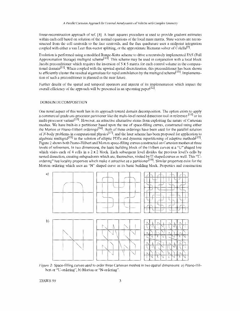
A ParallelCartesianApproachforExternal Aerodynamicsof Vehicleswith ComplexGeometry

linear-reconstruction approach of ref. [8]. A leas_squares procedure is used to provide gradient estimateswithin each cell based on solution of the normal equations of the local mass matrix. State vectors are recon-

structed from the cell centroids to the face centroids, and the flux quadrature uses a midpoint integrationcoupled with either a van Leer flux-vector splitting, or the approximate Riemann solver of Colella [9].

Evolution is performed using a modified Runge-Kutta scheme to drive a recursively implemented FAS (FullApproximation Storage) multigrid scheme [1°]. This scheme may be used in conjunction with a local block

Jacobi preconditioner which requires the inversion of 5 x 5 matrix for each control volume in the computa-tional domain [11]. When coupled with the upwind spatial discretization, this preconditioner has been shownto efficiently cluster the residual eigenvalues for rapid annihilation by the multigrid scheme [13]. Implementa-

tion of such a preconditioner is planned in the near future.

Further details of the spatial and temporal operators and aspects of its implementation which impact theoverall efficiency of the approach will be presented in an upcoming paper [12].

DOMAIN DECOMPOSITION

One novel aspect of this work lies in its approach toward domain decomposition. The option exists to applya commercial grade uni-processor partitioner like the multi-level nested dissection tool in reference [141or its

multi-processor variant [15[. However, an attractive alternative stems from exploiting the nature of Cartesian

meshes. We have built-in a partitioner based upon the use of space-filling curves, constructed using eitherthe Morton or Peano-Hilbert orderings [16[. Both of these orderings have been used for the parallel solutionof N-body problems in computational physics [17[, and the later scheme has been proposed for application to

algebraic multigrid [181in the solution of elliptic PDEs and dynamic repartitioning of adaptive methods [19[.

Figure 2 shows both Peano-Hilbert and Morton space-filling curves constructed on Cartesian meshes at threelevels of refinement. In two dimensions, the basic building block of the Hilbert curves is a "U" shaped line

which visits each of 4 cells in a 2 x 2 block. Each subsequent level divides the previous level's cells bynested dissection, creating subquadrants which are, themselves, visited by U shaped curves as well. This "U-ordering" has locality properties which make it attractive as a partitioner [19[. Similar properties exist for the

Morton ordering which uses an "N" shaped curve as its basic building block. Properties and construction

a)

..... ......... ...... .\\

: : " _',_ --_,--,_ _ ,_',,_4 " ._,-J.,.......,......................... _ _._ \ ........ ,, \..i ..7.,,r"

i i i i _............. _-......................i "....

" i i _ _ :............. _'--, ..-............ _ --_"--.--- i.................. i ---..""' -_ ---"_ _ --_- ----i --'.-- --_'-4

_,.......! .......... k...., i _'

.......................... _ f ....... i ......,i......... : _ -_'_ ----_ --_ -------i --_ -_,-M

i i _ k ........... _..... _ .......... _ ....." i i

b)

i ...._ k\ _i) _.................. <_ .................\ : ......................................., __ ! ;:_KI

_ _,_ :,,,i,_i

Figure 2: Space-filling curves used to order three Cartesian meshes in

bert or "U-ordering", b) Morton or "N-ordering".

two spatial dimensions: a) Peano-Hil-

TFAWS 99 3

A ParallelCartesianApproachforExternal Aerodynamicsof Vehicleswith ComplexGeometW

rules for these space-filling curves are discussed in refs. [20] and [21]. For the present, we note only thatsuch orderings have 3 important properties.

1. Mapping 9_d -+ U : The U and N orderings provide a unique mappings from the d-dimensionalphysical space of the problem domain 9_d to a one-dimensional hyperspace, U, which one traverses

following the curve. In the U-order, two cells adjacent on the curve remain neighbors in this one-dimensional hyperspace.

2. Locality: In the U-order, each cell visited by the curve is directly connected to two face-neigh-boring cells which remain face-neighbors in the one dimensional hyperspace spanned by the curve.Locality in N-ordered domains is almost as good [16].

3. Compactness: Encoding and decoding the Hilbert or Morton order requires only local informa-tion. Following the integer indexing for Cartesian meshes outlined in ref. [2], a cell's 1-D index inUmay be constructed using only that cell's integer coordinates in 9_d and the maximum number ofrefinements that exist in the mesh. This aspect is in marked contrast to other partitioing schemesbased on recursive spectral bisection or other multilevel decomposition approaches which requirethe entire connectivity matrix of the mesh in order to perform the partitioning.

To illustrate the property of compactness, consider the position of a cell i in the N-order. One way to con-

struct this mapping would be from a global operation such as a recursive lexicographic ordering of all cellsin the domain. Such a construction would not satisfy the property of compactness. Instead, the position of i

in the N-order may be deduced solely by inspection of cell i's integer coordinates (xi, Yi, zi).

Assume (_ci, _i, 5¢) is the bitwise representation of the integer coordinates (xi, Yi, zi) using m-bit integers. The

bit sequence {_c_5_ } denotes a 3-bit integer constructed by interleaving the first bit ofxi, Yi and z i. One canthen immediately compute cell i's position in Uas the 3m-bit integer {_c_5_c_?_. _m_m_m•"xi Yi zi } • Thus, sim-ply by inspection of a cell's integer coordinates, we are able to directly calculate its position in the one-

dimensional space U without any additional information. Similarly compact construction rules exist for theU-order[21].

Figure 3 illustrates these mapping and locality properties for an adapted two-dimensional Cartesian mesh,partitioned into three subdomains. The figure demonstrates the fact that for adapted Cartesian meshes, the

hyperspace U may not be fully populated by cells in the mesh. However, since cell indices in U may beexplicitly formed, this poses no shortcoming.

The quality of the partitioing resulting from U-ordered meshes have been examined in Ref.[19]. and were

found to be competitive with respect to other popular partitioners. Weights can be assigned on a cell-by-cellbasis. One advantage of using this partitioning strategy stems from the observation that mesh refinement or

2-D physical space ,art 2

pa.rt1 part 3

L

iI,a • ....

1-D hyperspace

part 1 part 3, part 2.........•,........... ,_............... _&............................

,,...... "........................................................................."v..............._ ............",,'....................... "_

a b c d e f g h ijklmnop q r s

Figure 3: An adapted Cartesian mesh and associated space-filling curve based on the U-ordering of9_2 --+ U with the U-ordering illustrating locality and mesh partitioing in two spatial dimensions. Par-

titions are indicated by the heavy dashed lines in the sketch

TFAWS 99 4

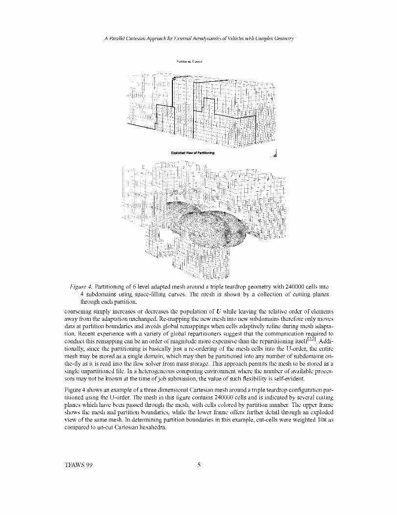
A ParalM Cartesian Approach for External Aerodynamics of Vehicles with Complex Geometry

i•iii:

Partitioned Domain

Exploded View of Partil_oning _

i:>ih

Figure 4: Partitioning of 6 level adapted mesh around a triple teardrop geometry with 240000 cells into

4 subdomains using space-filling curves. The mesh is shown by a collection of cutting planes

through each partition.

coarsening simply increases or decreases the population of U while leaving the relative order of elements

away from the adaptation unchanged. Re-mapping the new mesh into new subdomains therefore only movesdata at partition boundaries and avoids global remappings when cells adaptively refine during mesh adapta-

tion. Recent experience with a variety of global repartitioners suggest that the communication required toconduct this remapping can be an order of magnitude more expensive than the repartitioning itselt f221. Addi-

tionally, since the partitioning is basically just a re-ordering of the mesh cells into the U-order, the entiremesh may be stored as a single domain, which may then be partitioned into any number of subdomains on-

the-fly as it is read into the flow solver from mass storage. This approach permits the mesh to be stored as asingle unpartitioned file. In a heterogeneous computing environment where the number of available proces-

sors may not be known at the time of job submission, the value of such flexibility is self-evident.

Figure 4 shows an example of a three dimensional Cartesian mesh around a triple teardrop configuration par-

titioned using the U-order. The mesh in this figure contains 240000 cells and is indicated by several cuttingplanes which have been passed through the mesh, with cells colored by partition number. The upper frameshows the mesh and partition boundaries, while the lower frame offers further detail through an exploded

view of the same mesh. In determining partition boundaries in this example, cut-cells were weighted 10x ascompared to un-cut Cartesian hexahedra.

TFAWS 99 5

A PargM Cartesian Approach for Extemg Aerodynamics of Vehicles with Con@ex Geometi 7

SUBDOMAIN CONNECTIVITY MATRIX LOCALITY

Figure 5 illustrates the cell adjacency matrix

within a typical subdomain after applying the U-

ordering. Each cell face in the subdomain results

in a point on this graph whose coordinates are the

indices of the neighboring cells. As indicated on

the figure, this matrix is block structured, and the

regions stemming from the various cell types in

the subdomains are labeled. Computation of the

residual occurs in the two diagonal blocks labeled

"volume cells" and "cut-cells", while the overlap

regions are updated via data-exchange with neigh-

boring subdomains. Examination of the structure

of these diagonal blocks indicates high total band-

width requirements. The face list within each sub-

domain is sorted by the lowest cell index which

the face connects to, and thus a loop over the face

lists of either the volume or cut-cells accesses data

in these two blocks row-by-row, from the top

down. However, since the cells are clustered into

"arms" off the main diagonal, memory pages

loaded to access one cell will be subsequently hit

Pec_no H_ilbert Order_ing

--_.............................................._..._....................,,'...................:._,_._.............

_\,._......................... +iFlo.,:!I} e>:es ..................... .,',_.,k\,\, _:_. :_tit(_e_; 1. _,.\_"

JO:,,}_:FI<,_,:;_OL:;_,,C_t

Figure 5: Connectivity matrix of a typical subdomain

after partitioning with the U-ordering. Various

cell types within the subdomain are labeled.

many times as other nearby cells are requested by subsequent faces. Despite this, further bandwidth reduc-

tion and diagonal dominance may still be advantageous on some cache-based computing architectures or for

use with some matrix inverters or preconditioners. The standard technique for alleviating this shortcoming is

further reordering within each of these blocks [231.

Provision is included for applying a RCM reordering [231 to the diagonal blocks in this matrix which pro-

duces a matrix with substantially reduced bandwidth. For cache-based machines, further re-ordering is also

possible by coloring the data on any given cache-line so that data-dependencies are avoided when loading

the data pipes on pipelining architectures, or for constructing short vectors on processors which support

short vector processing.

AUTOMATIC CONSTRUCTION OF COARSE GRIDS

A central issue in the implementation of multigrid smoothers on unstructured meshes is the construction of a

series of coarse grids for the smoother to act upon. However, since adaptively refined Cartesian grids are

based upon successive refinements of an initial coarse grid, there is a natural path for coarse grid construc-

tion. A variety of approaches have been suggested in the literature, however, the asymptotic coarsening ratio

in some of these has been insufficient to ensure that the method will extract the full benefit of multigrid.

Moreover, the approach in ref. [2] permits the cells to divide anisotropically and therefore, we revisit the

issue of efficient coarse mesh generation.

In contrast to coarse grid generation problems on unstructured (general) hexahedral, tetrahedral, or mixed

element meshes, coarse cells in Cartesian meshes can be designed to nest exactly (i.e. cells on the coarse

mesh are the precise boolean addition of cells on the fine mesh). In addition, the cells can be organized such

that any cell in the mesh may be located uniquely by a set of integer indices [21. The combination of these two

facts lead to an novel coarse mesh generation algorithm for adaptively refined Cartesian meshes. The asymp-

totic complexity of this algorithm is O(Nlog N), where Nis the number of cells in the fine mesh. This result

stems from the fact that the central operation is a standard quicksort routine 1, and all other operations may

1. This result could be improved upon through the use of a radix sort, or other sort which has a better time-bound, however, quicksort is fast enough in most cases.

TFAWS 99 6

A ParalM CartesianApproachforExternal Aerodynamicsof Vehicleswith ComplexGeometry

Figure 6: (Left) A two dimensional adaptively refined Cartesian mesh. Cut-cells are shown shaded.

(Right) The same mesh, after reordering with a specially designed comparison operator in prepara-tion for coarsening.

be performed in constant time.

Figure 6 displays a two dimensional, directionally refined Cartesian mesh which illustrates the coarse mesh

generation strategy. The mesh shown (left) is the input or "fine mesh" which the algorithm coarsens. Theboundary of a hypothetical body is indicated, and the crosshatching indicates where there are no cells in the

mesh. Gray shaded cells denote cut-hexahedra. To the right of this figure lies a second view of the mesh after

it has been sorted using a specially designed comparison operator. The cell indices in this mesh indicate thesorted order, which is further illustrated by a partial sketch of the path shown through cells 9 16.

The comparison operator basically performs a recursive lexicographical ordering of cells which can coarsen

into the same coarse cell. Adaptively refined Cartesian meshes are formed by repeated subdivision of an ini-tial coarse mesh (referred to as the level 0 mesh), therefore any cell, i, is traceable to an initial "parent cell"

in the level 0 mesh. Similarly, if cell i has been refined R times, it will have parent cells at levels 0 through(R 1). If a cell has never been divided, then it is referred to as a "level 0 cell" and is identical to its level 0

parent.

1. Cells on the level 0 mesh are sorted in lexicographic order using the integer coordinates of theirlevel 0 parents as keys.

2. If a cell has been subdivided, recursively sort its children lexicographically.

This algorithm can be implemented with a single quicksort which uses a comparison operator which exam-

ines the integer indices of two input cells on a bit-by-bit basis (see ref. [12]). As noted above, its asymptoticcomplexity is proportional to that of the sorting method used.

After sorting the fine mesh, coarsening proceeds in a straightforward manner. Cells are processed by a singlesweep through the sorted order. If a contiguous set of cells are found which coarsen to the same parent theyare coalesced into that parent. Cells which do not meet this criteria are "not coarsenable" and are injected tothe coarse mesh without modification.

Figure 7 (left) shows the coarse mesh resulting from one application of the coarsening algorithm, note that

fine grid cells on the level-0 mesh arefidly coarsened and do not coarsen beyond their initial size. The right

7

3

6 8

41 3 6 15

38 40

2 S 2 S 14

37 39

: 4 z 4 13

113 12 22 24 33 _5

Figure 7: Left: Adapted Cartesian mesh from Figure 6 after one coarsening. Outline of geometry is indi-

cated, and cut-cells are shown in grey. Right: Same mesh after one additional application of thecoarsening algorithm

TFAWS 99 7

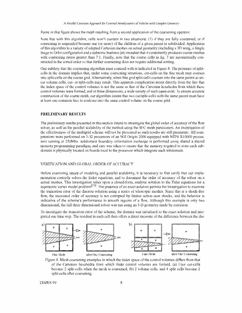
A PargM CartesianApproachforExtemg Aerodynamicsof Vehicleswith ComplexGeometry

frame in this figure shows the mesh resulting from a second application of the coarsening operator.

Note that with this algorithm, cells won't coarsen in two situations: (1) if they are fully coarsened; or if

coarsening is suspended because one (or more) of the children of a given parent is subdivided. Application

of this algorithm to a variety of adapted Cartesian meshes on actual geometry (including a 3D wing, a SingleStage to Orbit configuration and a subsonic business jet) revealed that it consistently produces coarse meshes

with coarsening ratios greater than 7:1. Finally, note that the coarse cells in fig. 7 are automatically con-structed in the sorted order so that further coarsening does not require additional sorting.

One subtlety that the coarsening algorithm must contend with is indicated in Figure 8. The presence of split-

cells in the domain implies that, under some coarsening situations, cut-cells on the fine mesh may coarseninto split-cells on the coarse grid. Alternatively, when fine grid split-cells coarsen into the same parent as un-

cut volume cells, cut- or split-cells may result. This apparent complication stems directly from the fact thatthe index space of the control volumes is not the same as that of the Cartesian hexahedra from which these

control volumes were formed, and in three dimensions, a wide variety of such cases exist. To ensure accurateconstruction of the coarse mesh, our algorithm insists that two cut/split-cells with the same parent must have

at least one common face to coalesce into the same control volume on the coarse grid.

PRELIMINARY RESULTS

The preliminary results presented in this section intend to investigate the global order of accuracy of the flow

solver, as well as the parallel scalability of the method using the SFC mesh partitioners. An investigation ofthe effectiveness of the multigrid scheme will not be presented as such results are still premature. All com-

putations were performed on 1-32 processors of an SGI Origin 2000 equipped with MIPS R10000 proces-sors running at 250Mhz. subdomain boundary information exchange is performed using shared a shared

memory programming paradigm, and care was taken to ensure that the memory required to store each sub-domain is physically located on boards local to the processor which integrate each subdomain.

VERIFICATION AND GLOBAL ORDER OF ACCURACY

Before examining issues of modeling and parallel scalability, it is necessary to first verify that our imple-mentation correctly solves the Euler equations, and to document the order of accuracy of the solver on a

actual meshes. This investigation relies upon a closed-form, analytic solution to the Euler equations for asupersonic vortex model problem [241. The presence of an exact solution permits the investigation to examine

the truncation error of the discrete solution using a series of telescopic meshes. Since this is a shock-freeflow, the measured order of accuracy is not corrupted by limiter action near shocks, and the behavior is

indicative of the scheme's performance in smooth regions of a flow. Although this example is only twodimensional, the full three dimensional solver was run using an 3-D geometry made by extrusion.

To investigate the truncation error of the scheme, the domain was initialized to the exact solution and inte-grated one time step. The residual in each cell then offers a direct measure of the difference between the dis-

a)- __],,__ _'+ _ _/ b) _e -- +__t_ _ __,_,,-,x

FineMesh after OneCoarsening Fine Mesh after One Coarsening

Figure 8: Mesh coarsening examples in which the index space of the control volumes differs from thatof the Cartesian hexahedra from which these control volumes are formed. (a) Four cut-cells

become 2 split-cells when the mesh is coarsened, (b) 2 volume cells, and 4 split cells become 2

split-cells after coarsening.

TFAWS 99 8

A ParalM Cartesian Approach for External Aerodynamics of Vehicles with Complex Geometry

exact solution."

p(r) = Pi{

1

7 + 1M2[- 1 _ '

Figure 9: Overview of supersonic vortex model problem from ref. [24] used

to investigate the order of accuracy of the solver. Mesh sequence at right

shows series of 5 telescoping meshes used in the investigation, at condi-tions:Min 2.25,pin 1/% Pin 1, r i 1, ro 1.384.

crete scheme and the governing equations, including the effects of boundary conditions.

Figure 9 presents an overview of the investigation. The sketch at the left shows the inviscid flow between

two concentric circular arcs, while the frame at the right shows the sequence of 5 Cartesian meshes used inthe investigation. The meshes were created by nested subdivision and while the coarsest of these grids had105 cells in a 2D slice, the finest had over 21000 cells at the same station.

Figure 10 contains a plot of the L2 norm of density error resulting from this analysis. The error plot isremarkably linear over the first 4 meshes, but shows signs of a slight tailing-off on the final mesh. Over the

first 4 meshes, the average order of accuracy is 1.88. If the finest mesh is included, this estimate drops to avalue of 1.82. Both of these slopes are comparable to those in the investigation of reconstruction schemes on

body-fitted unstructured meshes in ref. [24], and we note that the absolute magnitude of error in the present(Cartesian) scheme is more than a factor of two lower than was reported in that investigation. The slight tail-

ing-off of the results for mesh 5 is believed to be a result of round-off error in computation of the error normis not surprising considering the extremely low levels of error measured on this mesh. This hypothesis, how-

ever, is still under investigation.

10-2

LU

*dc

EbZ

10-3

10-4

10-50 1 2 3 4 5 6

No. of Mesh Refinements

Figure 10." L2 norm of density truncation error for sequence of refined meshes shown

in fig. 9.

TFAWS 99 9

A ParalM Cartesian Approach for External Aerodynamics of Vehicles with Complex Geometry

The results shown in fig. 10 were generated using the Colella flux function, however, results with the vanLeer option are essentially identical.

CONVERGENCE ON PARTITIONED

DOMAINS10 _

10 _

1@

Adopting the domain decomposition with a single lo0

overlap cell permits a formulation which ensures to _

that the residuals computed within each cell at ,, to2every timestep with one partitioning match those _ to3

for any other partitioning. Figure 11 illustrates this 5 to 4property by documenting convergence of the maxi-

_ 10 _

mum residual of density for the supersonic vortex _ lo _×

problem using a 250,000 cell mesh partitioned into _ lo7

1, 2, 4, and 8 subdomains. All histories in this fig- looure collapse to the same line to within machine pre- loocision. As the legend indicates, this test was

10 0

performed using both the machine's default arith- lometic (SGI Origin 2000, cc option -OfitsO and lo'IEEE-754 compliant arithmetic.

2nd Order(3 1) _h_ne nolimiter........ i........ i......... i........ i......... i......... i........ i......... i.........

o\

H 1 padilion

< 1 part IEEE

: 2 parts

+ + 2 prociEEE

4parts

< 4parts IEEE

*= * 8 parts

\

\\

\

\

....... , ........ , ......... , ........ , ......... , ......... ,........ , ......... , .........

200 400 600 800 1000 1200 1400 1600 1800

Iterations (3-stage R-K)

Figure 11: Comparison of convergence history using

ONERA M6 WING 1, 2, 4, and 8 subdomains using both default (SGIOrigin 2000, cc option -OfitsO and IEEE-754

With the preliminary verification complete, focus compliant arithmetic.

shifts to a three dimensional example of an ONERA M6 wing which has been widely cited in the literature.This transonic M_ 0.84, cz 3.06 ° case is often used in the validation of inviscid solution techniques. Thistest was performed at a relatively high Reynolds number (based on root chord) of 12 x 106125[, which mini-

mizes effects of the displacement thickness making accurate comparisons of sectional pressure distributions

possible. Other viscous effects in the experimental data are limited to a slight separation filling in the Cp dis-tribution behind the lambda shock on the lee surface.

Simulation of this test was conducted using the geometry of a wing in free air, with the far-field boundarylocated 30 chords from the wing. The final mesh contained 525000 control volumes, with 25000 cut-cells

and 528 split-cells. The mesh was partitioned into 8 subdomains using the Peano-Hilbert ordering described

iiiiiiiiiiiiiiiiiiiiiiiiiii iiiiiiiiiiiiiiiiiiiiiiiiiiiiiiiiiiiiiiiiiiiiiiiiiiiiiiiiiiiiiiiiiiiiiiiiiiiiiiiiiiiiiiiiiiiiiiiiiiiiiiiiiiiiiiiiiiiiiiiiiiiiiiiiiiiiiiiiiiiiiiiiiiiiiiiiiiiiiiiiiiiiiiiiiiiiiiiiiiiiiiiiiiiiiiiiiiiiiiiiiiiiiiiii

Figure 12." Partitioned mesh and Cp contours for the ONERA M6 wing example. The mesh contains525000 cells at 9 levels of refinement, mesh partitions are shown by color-coding and outlined in

heavy lines. Cp contours are plotted using a cell-by-cell reconstruction of the discrete solution.M_ = 0.84, cz = 3.06, van Leer flux.

TFAWS 99 10

A Parallel Cartesian Approach for External Aerodynamics of Vehicles with Complex Geometry

in the preceding section. Figure 12 displays this mesh by three cutting planes. Cells on each cut plane are

color coded by subdomain. Along side the mesh, fig. 12 presents C)) contours on the wing surface, and sym-

metry plane resulting from a simulation using the van Leer flux option. This image clearly displays the well-

known lambda shock structure on the upper surface of the wing. Contours in this image were constructed

cell-by-cell, using the computed gradients within each cell. This method of plotting gives a more accurate

picture of the discrete solution, since fluxes are formed with this same reconstruction. The slight breaks in

the contour lines in some high gradient regions are a by-product of this cell-by-cell plotting. These solution

shown was converged 6 orders of magnitude (L 1 norm of density) using the van Leer flux option.

Figure 13 provides a quantitative assessment of the solution quality through pressure profiles at six spanwise

stations. This figure displays @ vs. x/c at spanwise stations at 20, 44, 65, 80, 90, and 95% span. The inboard

stations correctly display the double-shock on the upper surface, while stations at 90 and 95% confirm accu-

rate prediction of the merging of these shocks. The experimental data at stations 20 and 44% indicate that

the rear shock is followed by a mild separation bubble triggered by the shock-boundary layer interaction. As

is typical in such cases, the inviscid discrete solution locates this rear shock slightly behind its experimental

counterpart.

1

0.5

0

0.5

I

Span Station 20% Span Station 44%

1

0.5 14 ::: "_ ::_-:::::_

0. :

0 020.2 0.4 06 0.8 1 1.2 1.2

•:: :+

Span Station 65%

1

0.5

0

0.5

Span Station 80%

:::::::::::::::::::::::

02 0.4 0.6 0.8 1 1.2

1

0.5

o

o.5

1

Span Station 95%

:S;::_ / ========================

0.2 0.4 06 0.8 1 1.2 02 0.4 0.6 0.8 1 1.2

Figure 13: Cp vs. x/c for ONERA M6 wing example at six spanwise locations. M_ = 0.84, cz = 3.06 °.

Experimental data from ref. [25] shown as symbols, inviscid discrete solution shown with solid

line.

TFAWS 99 11

A PargM Cartesian Approach for Extemg Aerodynamics of Vehicles with Con@ex Geomet W

PARALLEL SCALABILITY AND PERFORMANCE

Figure 14 contains preliminary results from

scalability testing. Tests were conducted on

from 1 to 32 processors on an Mips R10000

based SGI Origin 2000. The mesh in this test

contained 525000 cells. Each processor of this

machine has a 4Mb Level 2 cache, and two

processors on each board share the same local

memory. Examination of this plot shows gen-

erally good scalability, however, communica-

tion does appear to slow this particular

computation on 4 and 8 processors when the

problem initially gets spread over several

boards within the machine. On 32 processors

the timings show a "cache bubble" evidenced

by the fact that the results on 32 processors are

more than a factor of two faster than the tim-

ings on 16 processors. Table 1 shows the per-

processor execution rate and parallel speed-up

for this example. Results in this table clearly

show a 4% increase in per-processor execution

35 . . . , . . . , . . . , . . . , . . . , . . . , . . . , . . . , . . .

-- _, Measured (Origin 2000, 250Mhz) /

30 ---- Ideal /

25 / /

/

_15 /

5 /:,_/_'*"

°_" ;_ _ 1'2 1'_ 2'0 A A 3'2 '3_No. of Processors

Figure 14: Preliminary investigation of parallel scalabil-

ity of single mesh (no-multigrid) case. Data reflect

average results from 3 runs with each partitioning.

rate on 32 processors as each processor's L2 cache was very nearly sufficient to store the entire subdomain.

The table demonstrates no substantial decrease in performance with larger numbers of subdomains, and the

communication/computation ratio afforded by the partitioning does not appear to be uncompetative. Results

in Table 1 and in Figure 14 were obtained by averaging the results of 3 separate sets of tests since timings on

this machine are known to vary by as much as 10%.

Table 1: Parallel scalability and processing rate per processor. Results for each partitioning

reflect average of three runs. 525000 control volumes, 200 iterations _er test.

No. of CPUtime/CPUParallel Speed-up Mflops/CPU a Ideal Speedup

Processors (sec.)

1 2559 1 81.4 1

2 1315 1.94 81.9 2

4 865 2.96 72.77 4

8 383 5.76 77.57 8

16 188 13.61 78 16

32 90 28.37 82 32

a. Mflops counted using R10000 hardware counters on optimized code, with single cycle MADD

instruction disabled. Floating-point multiply, add, and divide each counted as one flop.

CONCLUSIONS AND CURRENT WORK

This paper presented preliminary verification and validation of a new, parallel, upwind solver for Cartesian

meshes. Comparison of the scheme's one-step truncation error with an analytic solution demonstrated an

achieved order of accuracy between 1.82 and 1.88. Preliminary validation by direct comparison to experi-

mental results on a three dimensional wing configuration was also performed, demonstrating that the dis-

crete solutions were competitive with other solution procedures. Preliminary documentation of a new on-

the-fly SFC based partitioning strategy was also presented. This strategy enables reordered meshes to be pre-

TFAWS 99 12

A PargM CartesianApproachforExtemg Aerodynamicsof Vehicleswith ComplexGeometry

sorted and stored as a single domain. This mesh can then be partitioned into any number of partitions at runtime. Investigations demonstrated that this decomposition strategy produces a parallel speed-up in excess of

28 on 32 processors with no net decrease in processing rate. Details of a new coarse mesh generation algo-rithm for multilevel smoothers on Cartesian meshes were also presented. This algorithm generally achieves

mesh coarsening ratios in excess of 7 on adaptively refined meshes.

Development of this method continues, and examples on complex configurations at elevated Mach numbers

are planned in the immediate future. An investigation of multigrid efficiency for flows with complex geome-try at a variety of Mach numbers is on-going.

ACKNOWLEDGMENTS

The authors would like to extend thanks to R. L6hner for pointing to literature on the use of space-filling

curves as potentially useful reorderers and partitioners. M. Berger and G. Adomavicius were supported inpart by AFOSR Grant F49620-97-1-0322 and DOE Grant DEFG02-92ER25139. Some of this work was

performed while M. Berger was at RIACS and this support is gratefully acknowledged.

REFERENCES

[1 ] Melton J. E., Berger, M. J., and Aftosmis, M. J., "3D Applications of a Cartesian grid Euler method,"

AIAA Paper 95-0853-CP, Jul. 1993.

[2] Aftosmis, M.J., Berger, M.J., Melton, J.E.: "Robust and efficient Cartesian mesh generation for com-

ponent-based geometry." AIAA Paper 97-0196, Jan. 1997.

[3] Charlton, E. F., and Powell, K. G., "An octree solution to conservation-laws over arbitrary regions."

AIAA Paper 97-0198, Jan. 1997.

[4] Wang Z.J., "An automated viscous adaptive Cartesian grid generation method for complex geome-

tries." in Proceedings' of the 6th International Conf on Numerical Grid Generation in Computational

Field Simulations; Eds. Cross, M. et al., Univ. Greenwich, UK., 1998.

[5] Day, M. S., Colella, R, Lijewski, M. J., Rendleman, C. A., and Marcus, D. L., "Embedded boundary

algorithms for solving the Poisson equation on complex domains," Lawrence Berkeley National Lab-

oratory, LBNL-41811, May, 1998.

[6] Karman, S. L., "SPLITFLOW: A 3D unstructured Cartesian/prismatic grid CFD code for complex

geometries." AIAA Paper 95-0343, Jan. 1995.

[7] Forrer, H., "Second order accurate boundary treatment for Cartesian grid methods." Seminar for

Angewandte Mathmatic, ETH Ztirich, ETH Research Report 96-13, 1996.

[8] Barth, T.J., and Jespersen, D.C., "The design and application of upwind schemes on unstructured

meshes." AIAA Paper 89-0366, Jan. 1989.

[9] Colella P, Ferguson, R., and Glaz, H., "Multifluid algorithms for Eulerian finite difference methods".

Preprint 1996.

[10] Hackbusch, W., and Trottenberg, U., (eds.), Lecture Notes in Mathematics: Multigrid Methods',

Springer-Verlag Berlin, Heidelberg, ISBN 0-387-11955-8, 1982.

TFAWS 99 13

A ParallelCartesianApproachforExternal Aerodynamicsof Vehicleswith ComplexGeometry

[11] Riemslagh, K., and Dick, E., "A multigrid method for steady Euler equations on unstructured adap-

tive grids." Proceedings' ofthe 6th Copper Mountain Conj. on Multigrid Methods, NASA Conference

publication 3224, pp. 527-542. 1993.

[12] Aftosmis, M. J., Berger, M J., and Adomavicius, G. "A domain-decomposed multi-level method for

adaptively refined Cartesian grids with embedded boundaries." AIAA Paper 2000-0808, Jan. 2000.

[13] Allmaras, S. R., "Analysis of semi-implicit preconditioners for multigrid solution of the 2-D com-

pressible Navier-Stokes Equations"., AIAA Paper 95-1651-CP, fun., 1995.

[14] Karypis, G., and Kumar, V., "METIS: A software package for partitioned unstructured graphs, parti-

tioing meshes, and computing fill-reducing orderings of sparse matrices." University of Minn. Dept.

of Comp. Sci., Minneapolis, MN., Nov. 1997

[15] Schloegel, K., Karypis, G., and Kumar, V., "Parallel Multilevel Diffusion Schemes for Repartitioning

of Adaptive Meshes." Tech. Rep. #97-014, University of Minn. Dept. of Comp. Sci., 1997.

[16] Samet, The design and analysis ofspatial data structures. Addison-Wesley Series on Computer sci-

ence and information processing, Addison-Wesley Publishing Co., 1990.

[17] Salmon, J.K., Warren, M.S., and Winckelmans, G.S., "Fast parallel tree codes for gravitational and

fluid dynamical N-body problems." Internat. Jol.for Supercomp. Applic. 8:(2), 1994.

[18] Griebel, M., Tilman, N., and Regler, H., "Algebraic multigrid methods for the solution of the Navier-

Stokes equations in complicated geometries." Int. J. Numer. Methods for Heat and Fluid Flow 26,

pp. 281-301, 1998, also as SFB report 342/1/96A, Institut ffir Informatik, TU Mfinchen, 1996.

[19] Pilkington, J.R., and Baden, S.B.,"Dynamic partitioning of non-uniform structured workloads with

spacefilling curves." Jan 1995.

[20] Schrack, G., and Lu, X., "The spatial U-order and some of its mathematical characteristics." Proceed-

ings' of the IEEE Pacific Rim Conj. on Communications, Computers and Signal Processing. Victoia

B.C, Canada, May, 1995.

[21] Liu, X., and Schrack, G., "Encoding and decoding the Hilbert order." Software-Practice andExperi-

ence, 26(12), pp. 1335-1346, Dec. 1996.

[22] Biswas, R., Oliker, L., "Experiments with repartitioning and load balancing adaptive meshes." NAS

Technical Report NAS-97-021, NASA Ames Research Ctr., Moffett Field CA., Oct. 1997.

[23] L6finer, R., "Renumbering strategies for unstructured-grid solvers operating on shared-memory,

cache-based parallel machines." AIAA Paper 97-2045-CP, fun., 1997.

[24] Aftosmis, M. J., Gaitonde, D., and Tavares, T. S., "Behavior of linear reconstruction techniques on

unstructured meshes." AIAA J., 33(11), pp. 2038-2049, Nov. 1995.

[25] Schmitt, V., and Charpin, F., "Pressure distributions on the ONERA-M6-Wing at transonic Mach

numbers." Experimental Data Base for Computer Program Assessment, AGARD Advisory Report

AR-138, 1979.

TFAWS 99 14

PARALLELIZATION OF THE FLOW FIELD

DEPENDENT VARIATION SCHEME FOR SOLVING

THE TRIPLE SHOCK/BOUNDARY LAYER

INTERACTION PROBLEM

Richard Gregory Schunk

NASA/Marshall Space Flight Center

T. J. Chung

University of Alabama in Huntsville

ABSTRACT

A parallelized version of the Flowfield Dependent Variation (FDV) Method is developed to analyze a

problem of current research interest, the flowfield resulting from a triple shock#ooundary layer interaction.

Such flowfields are often encountered in the inlets of high speed air-breathing vehicles including the NASA

Hyper-X research vehicle. In order to resolve the complex shock structure and to provide adequate

resolution for boundary layer computations of the convective heat transfer from surfaces inside the inlet,

models containing over 500,000 nodes are needed. Efficient parallelization of the computation is essential

to achieving results in a timely manner. Results from a parallelization scheme, based upon multi-threading,

as implemented on multiple processor supercomputers and workstations is presented.

INTRODUCTION

The Flowfield Dependent Variation (FDV) Method is utilized to analyze a problem of current research

interest, the flowfield produced from a triple shock#ooundary layer interaction. Flow fields of this nature

are often encountered in the inlets of high speed vehicles such as the scramjet engine of NASA's Hyper-X

research vehicle. For this analysis, the numerical results are compared to experimental wind tunnel

measurements made by Garrison, Settles, and Horstman [1,2]. The objective of the FDV analysis is to

resolve the major flowfield structures observed during the experiment while demonstrating an efficient

parallelization scheme based upon multi-threaded programming.

FLOWFIELD DEPENDENT VARIATION (FDV) THEORY

The original idea of FDV methods began from the need to address the physics involved in shock wave

turbulent boundary layer interactions [3-5]. In this situation, transitions and interactions of inviscid/viscous,

compressible/incompressible, and laminar/turbulent flows constitute not only the physical complexities but

also computational difficulties. This is where the very low velocity in the vicinity of the wall and very high

velocity far away from the wall coexist within a domain of study. Transitions from one type of flow to

another and interactions between two distinctly different flows have been studied for many years both

experimentally and numerically. Traditionally, incompressible flows were analyzed using the pressure-

basedformulationwiththeprimitivevariablesfortheimplicitsolutionoftheNavier-Stokessystemofequationstogetherwith the pressure Poisson equation. On the other hand, compressible flows were

analyzed using the density-based formulation with the conservation variables for the explicit solution of the

Navier-Stokes system of equations. In dealing with the domain of study which contains all speed flows with

various physical properties where the equations of state for compressible and incompressible flows are

different, and where the transitions between laminar and turbulent flows are involved in dilatational

dissipation due to compressibility, we must provide very special and powerful numerical treatments. The

FDV scheme has been devised toward resolving all of these issues.

To this end, let us consider the Navier-Stokes system of equations in conservation form,

_U _ _F_ + _G______- B

& _x i _xi

In expanding U n+l in a special form of Taylor series about If, we introduce the variation parameters S 1 and

s 2 for the first and second derivatives of U with respect to time, respectively

where

_LJ f/+S1 At 2 d2U"+'2U "+1 = U" + At-

2 _2

8U "--SI 8U" 8AU "--]

-- +S 1-- 0_<Sl_<l& & &

&2 &2

with AIf +1 = If+l _ If. Substituting (3) into (2),

AU "+1 = At + s 1--

_2AUn+I

Jr s 2 c_t2 o _<S 2 --<1

Notice that S1, associated with the first time derivative, is intended to provide variations as appropriate to

the convection and diffusion processes of the flowfield, whereas s 2 , involved in the second time derivative,

is to control adequate application of artificial viscosity as required in accordance with the flowfield.

In the conservation form of the Navier-Stokes system of equations, Fi and B are functions of U, and Gi is a

function of U and its gradient U k. Thus, by the chain rule of calculus, the first and second derivative of U

with respect to time may be written as follows:

_U #E _Gi- +B

& c_xi c_xi

We denote the convection Jacobian a_, the diffusion Jacobian b_, the diffusion gradient Jacobian c_k, and

the source Jacobian d as

(1)

(2)

(3a)

(3b)

(4)

(5a)

(5b)

TFAWS 99 2

Forthepurposeof generality,weassumeherethatthesourcetermsarisefromadditionalequationsforchemicalspeciesequations.

Thesecondderivativeof U withrespectto timemaynowbewrittenin termsof theseJacobiansbysubstitutioninto(5b),

d2U_ d (a i+bi)|_+_Bc32 &i / &j &j ) +--cik - d -- + -- -

&_&k /&j &j ) \&j &j

Substituting (5a) and (6) into (4), and assuming the product of the diffusion gradient Jacobian with third

order spatial derivatives to be negligible, we have

The variation parameters s 1and s 2 which appear in (7) may be accorded with appropriate physical roles by

calculating them from the flowfield-dependent quantities. For example, if s 1 is associated with the

temporal changes (A terms, henceforth called fluctuations, not meant to be turbulent fluctuations) of

convection, it may be calculated from the spatial changes of Mach number between adjacent nodal points so

that $1= 0 would imply no changes in convection fluctuations. Similarly, if s 1is associated with the

fluctuations of diffusion, then it may be calculated from the spatial changes of Reynolds number or Peclet

number between adjacent nodal points such that $1= 0 would signify no changes in diffusion fluctuations.

Therefore, the role of s 1 for diffusion is different from that of convection. Similarly, the role of s 1 for the

fluctuation of the sources (such as reaction rates and heat generation) should be different from convection

and diffusion. For example, we may define the fluctuation quantities associated with s 1 as

AB n+l c_AFn+I i c_AGn+I i ABn+ 1Slc I-Sld Sls

8x _ 8x i

2 2 n+l

4]_/m ax--]_/min _AF= +

Mmi n 63xi

4Re2ax-Re2mi n _mGn; 1 _ 4Dam2ax-Da2min ABn+,

Re mi_ _x _ Dami n

(6)

(7)

(8)

TFAWS 99 3

whereit isseenthatthevariationparameters 1 originally adopted as a single mathematical or numerical

parameter has now turned into multiple physical parameters such as the changes of Mach numbers,

Reynolds numbers (or Peclet numbers), and Damkohler numbers (Da), between adjacent nodal points.

The magnitudes of fluctuations of convection, diffusion, and source terms are dictated by the current

flowfield situations in space and time. Similar assessments can be applied to the variation parameter s 2 as

associated with its corresponding fluctuation terms of convection, diffusion, and source. Thus, in order to

provide variations to the changes of convection, diffusion, and source terms differently in accordance with

the current flowfield situations, we reassign s 1 and s 2 associated with convection, diffusion and source terms

as follows:

slAG i _sldAGi= s3AG i , slAB _sl,AB_= ssAB

s2AG i _s2dAGi= s4AG i , s2AB _S2sAB = s6AB

with the various variation parameters defined as

s lc = s1 = first order convection variation parameter

s 2c-- s2 = second order convection variation parameter

sld = s 3 = first order diffusion variation parameter

s2d = s 4 = second order diffusion variation parameter

s is-- s5 = first order source term variation parameter

s 2s-- s6 = second order source term variation parameter

The first order variation parameters S1, $3, and s 5 are flowfield-dependent, whereas the second order

variation parameters s2, s4, and s 6 are exponentially proportional to the first order variation parameters, and

mainly act as artificial viscosity.

EXPERIMENTAL MEASUREMENTS

The analytical results are compared to experimental measurements for a triple shock interaction obtained by

Garrison, Settles, and Horstman [1,2]. The wind tunnel model used to produce the triple shock#ooundary

layer interaction consists of two vertical fins and a horizontal ramp as shown in Figure 1. The angle of

attack for the fins is 15 ° and the ramp is inclined at an angle of 10 ° with respect to the inlet flow. The inlet

flow is at Mach 3.85 with a stagnation temperature and pressure of 295K and 1500 kPa, respectively. The

fins are 82.5 mm high and are separated by a distance of 96.3 mm. The leading edge of the model is located

21 cm in front of the ramp inlet and produces a turbulent boundary layer with a thickness of 3.5 mm at the

inlet to the model. Flow through the model is characterized by three oblique shocks originating from the

leading edges of the ramp and the fins. Above the oblique ramp shock, the two inviscid fin shocks intersect

and reflect as shown in the figure. For the purposes of this analysis, the ramp is assumed to be 120 mm in

length, the distance at which the reflected inviscid fin shocks are just incident upon the exit comers of each

fin. According to inviscid flow theory, the fin shocks should intersect approximately 92 mm from the

combined ramp and fin entrance. Measurements of the flowfield structure in the x-y plane are made via the

Planar Laser Scattering (PLS) technique at various depths upstream of, coincident with, and behind the

inviscid fin shock intersection [2].

TFAWS 99 4

., "15°. "

Fins/__

Flow

---) Shocks "_< ReflectedFin.__ Shocks

/

Figure 1 Inviscid Fin Shock Reflection (Top View, X-Z Plane)

Of particular interest in this analysis is the complex shock#ooundary layer interaction produced in the x-y

planes perpendicular to the flow direction. Upstream of and coincident with the inviscid ramp shock

intersection, the fin and ramp shocks are reflected and interact with the fin and ramp boundary layers to

produce the shock structures contained in the PLS images of Figure 2. Upstream of the shock intersection

(left), the flow is characterized by the inviscid fin and ramp shocks reflecting to form a corner shock. Slip

lines separating the shock induced flow regions are also visible in the image. The flow separation from the

ramp underneath the embedded fin shock is also visible in the image. At the shock intersection (right), the

inviscid fin shocks merge, the ramp shock dissapears, and the comer shock is reflected to form the structure

shown. The curvature of the fin shocks become more pronounced and a large separation region is observed

underneath the reflected comer shocks. This is attributed to the curvature of the inviscid shocks to the finite

height of the fins (i.e. there would be no shock curvature with fins of "infinite" height) [1].

TFAWS 99 5

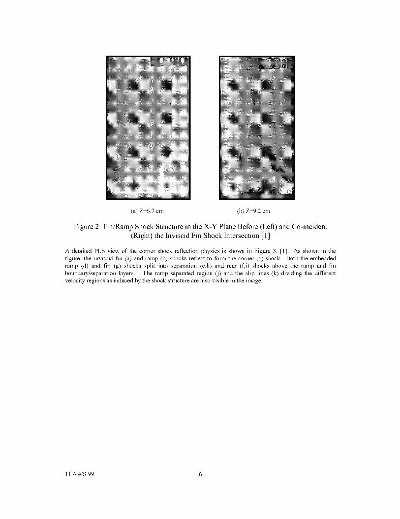
(a)Z=6.7cm (b)Z=9.2cm

Figure 2: Fin/Ramp Shock Structure in the X-Y Plane Before (Left) and Co-incident

(Right) the Inviscid Fin Shock Intersection [1]

A detailed PLS view of the comer shock reflection physics is shown in Figure 3. [1]. As shown in the

figure, the inviscid fin (a) and ramp (b) shocks reflect to form the comer (c) shock. Both the embedded

ramp (d) and fin (g) shocks split into separation (e,h) and rear (f,i) shocks above the ramp and fin

boundary/separation layers. The ramp separated region (j) and the slip lines (k) dividing the different

velocity regions as induced by the shock structure are also visible in the image.

TFAWS 99 6

PLS Image of Corner Flow

C

j ""'-..'J

Corresponding Flowfield Structure

a

d e

Figure 3: Fin/Ramp Shock Structure in the X-Y Plane [ 1 ], a) Inviscid Fin Shock, b)

Comer Shock, c) Inviscid Ramp Shock, d) Embedded Ramp Shock, e) Ramp Separation

Shock, f) Ramp Rear Shock, g) Embedded Fin Shock, h) Separation Fin Shock, i) Rear

Fin Shock, j) Separated Region, k) Sliplines

COMPUTER MODEL

Since the two fins are symmetric about the centerline, only half of the wind tunnel model is included in the

computational model. Two finite difference computational grids, varying in resolution, are developed forthe FDV analysis. The coarse grid model, consisting of a non-uniform nodal resolution of 31 x 41 x 55 (inthe x, y, and z directions) is shown in Figure 4. The viscous grid is clustered close to the fin and rampsurfaces. Results from the coarse grid analysis are used as the starting condition for the fine grid model.

The fine grid model is obtained by interpolating the flow variables against the coarse mesh. Doubling thenumber of grid points in each direction produces a fine grid with over 538,000 nodal points (61 x 81 x 109).Recall that the most important aspect of the FDV theory is that the shock capturing mechanism and thetransition and interaction between compressible/incompressible, viscous/inviscid, and laminar/turbulent

flows are incorporated into the FDV formulation. No special treatments are required to simulate thesephysical phenomena. Thus, the finite difference discretization requires no special schemes. Simple centraldifferences can be used to discretize the FDV.

TFAWS 99 7

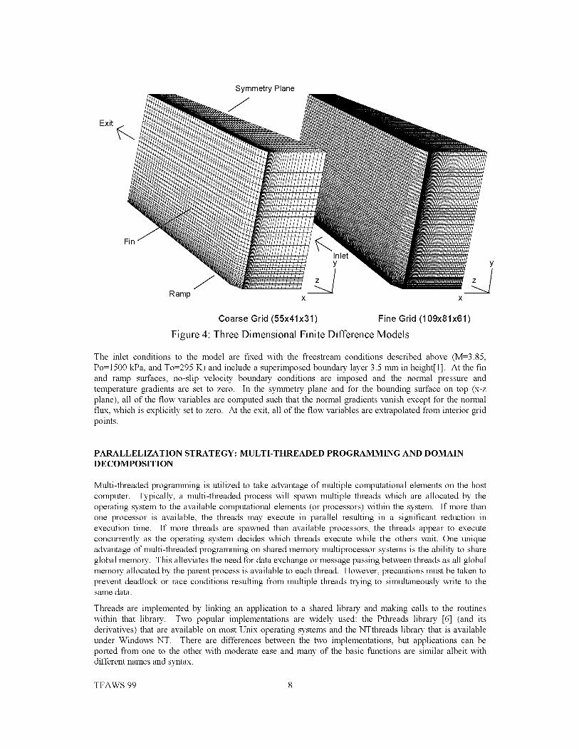
Symmetry Plane

Exit

Fin

Ramp

InletY

JX

Coarse Grid (55x41x31) Fine Grid (109x81x61)

Figure 4: Three Dimensional Finite Difference Models

The inlet conditions to the model are fixed with the freestream conditions described above (M=3.85,

Po=1500 kPa, and To=295 K) and include a superimposed boundary layer 3.5 mm in height[l]. At the fin

and ramp surfaces, no-slip velocity boundary conditions are imposed and the normal pressure and

temperature gradients are set to zero. In the symmetry plane and for the bounding surface on top (x-z

plane), all of the flow variables are computed such that the normal gradients vanish except for the normal

flux, which is explicitly set to zero. At the exit, all of the flow variables are extrapolated from interior grid

points.

PARALLELIZATION STRATEGY: MULTI-THREADED PROGRAMMING AND DOMAIN

DECOMPOSITION

Multi-threaded programming is utilized to take advantage of multiple computational elements on the host

computer. Typically, a multi-threaded process will spawn multiple threads which are allocated by the

operating system to the available computational elements (or processors) within the system. If more than

one processor is available, the threads may execute in parallel resulting in a significant reduction in

execution time. If more threads are spawned than available processors, the threads appear to execute

concurrently as the operating system decides which threads execute while the others wait. One unique

advantage of multi-threaded programming on shared memory multiprocessor systems is the ability to share

global memory. This alleviates the need for data exchange or message passing between threads as all global

memory allocated by the parent process is available to each thread. However, precautions must be taken to

prevent deadlock or race conditions resulting from multiple threads trying to simultaneously write to thesame data.

Threads are implemented by linking an application to a shared library and making calls to the routines

within that library. Two popular implementations are widely used: the Pthreads library [6] (and its

derivatives) that are available on most Unix operating systems and the NTthreads library that is available

under Windows NT. There are differences between the two implementations, but applications can be

ported from one to the other with moderate ease and many of the basic functions are similar albeit with

different names and syntax.

TFAWS 99 8

Domaindecompositionmethods[7]canbeusedinconjunctionwithmulti-threadedprogrammingtocreateanefficientparallelapplication.Thesub-domainsresultingfromthedecompositionprovideaconvenientdivisionoflaborfortheprocessingelementswithinthehostcomputer.Inthisapplication,anAdditiveSchwarzdomaindecomposition[7]methodisutilized.Themethodisillustratedbelow(Figure5)foratwodimensionalsquaremeshthatisdecomposedintofoursub-domains.Thenodesbelongingtoeachofthefoursub-domainsaredenotedwith geometric symbols while boundary nodes are identified with bold

crosses. The desire is to solve for each node implicitly within a single sub-domain. For nodes on the edge

of each sub-domain this is accomplished by treating the adjacent node in the neighboring sub-domain as a

boundary. The overlapping of neighboring nodes between sub-domains is illustrated in Figure 6. Higher

degrees of overlapping, which may improve convergence at the expense of computation time, are also used.

,N ;

<_ @ Sub-domain 1

+ Sub-domain 2

Sub-domain 3

+ Sub-domain 4

_ BoundaryNode

Figure 5: Multiple Subdomains

01% 01% 0"_ 0"_Nodes shaded in

white are solved

implicitly within in "*"

each sub-domain.

.&

.&

Nodes from neighboring

.;. sub-domains (shaded)

are treated as boundary

nodes and allowed to lag

_:" "_i_:" / one timestep.

/.& .::. .:. .:.

Figure 6: Domain Decomposition

In a parallel application, load balancing between processors is critical to achieving optimum performance.

Ideally, if a domain could be decomposed into regions requiring an identical amount of computation, it

would be a simple matter to divide the problem between processing elements as shown in Figure 7 for four

threads executing on an equal number of processors.

TFAWS 99 9

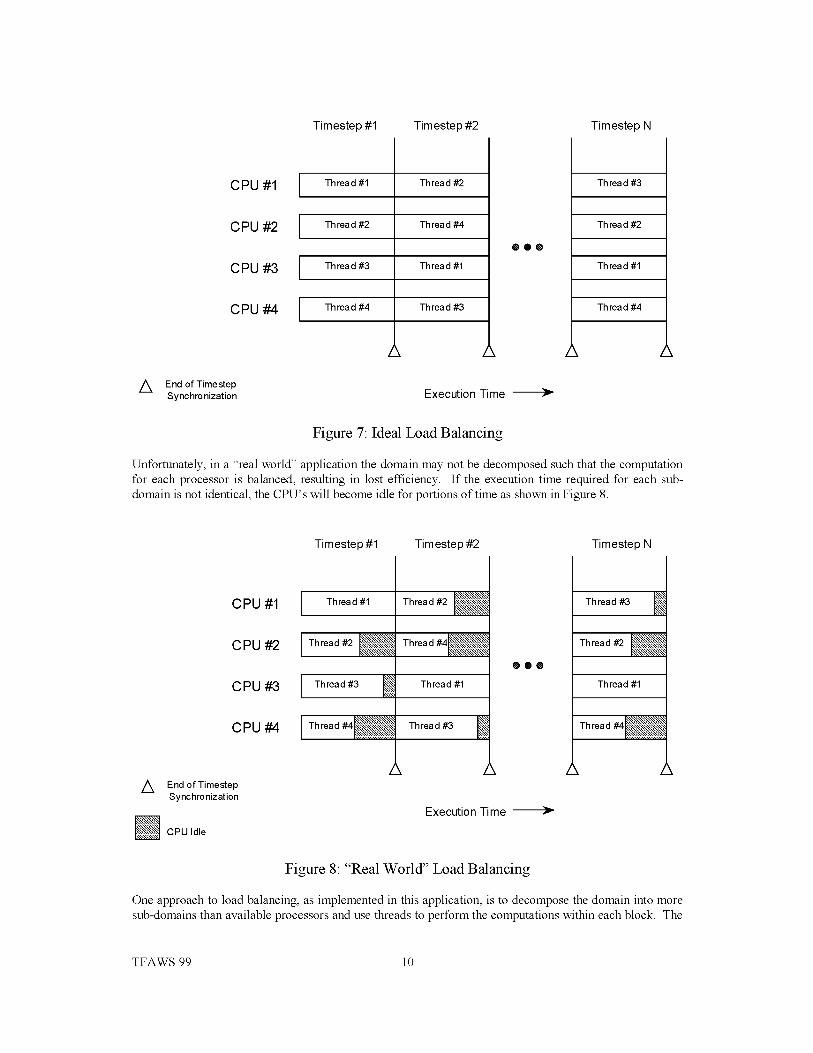
Timestep #1 Timestep #2 Timestep N

/_ End of TimestepSynchronization

CPU #1

CPU #2

CPU #3

CPU #-4

Thread #1 Thread #2

Thread #2 Thread #4

Thread #3 Thread #1

Thread #4 Thread #3

00O

/X

Execution Time

Thread #3

Thread #2

Thread #1

Thread #4

Figure 7: Ideal Load Balancing

Unfortunately, in a "real world" application the domain may not be decomposed such that the computation

for each processor is balanced, resulting in lost efficiency. If the execution time required for each sub-

domain is not identical, the CPU's will become idle for portions of time as shown in Figure 8.

CPU #1

Timestep #1 Tim estep #2

Thread #1 Thread #2 _'._q_£\\N

CPU #2 Thread#2 _\_q-q-_q-q-_Thread#4I_-.\\\\\\\\\\\\\'_

C PU #3 Thread #3 __ Thread #1

CPU #4 Thread #4 ._ Thread #3 _

/_ End of TimestepSynchronization

N CPU Idle

000

Execution Time

Timestep N

Thread #3 kit

Thread #2 _\<_£q_£_

Thread #1

Figure 8: "Real World" Load Balancing

One approach to load balancing, as implemented in this application, is to decompose the domain into more

sub-domains than available processors and use threads to perform the computations within each block. The

TFAWS 99 10

finer granularity permits a

shown in Figure 9.

CPU #1 I #1

more even distribution of work amongst the available processing elements as

opus2 I

opus3 l

CPU #-4

CPU #1

CPU #2

CPU #3

CPU #-4

I #1 I #2

I #6Ii

X

Execution Time --

J

>- 4 Sub-domains

> 8 Sub-domains

/_ End of TimestepSynchronization

N CPU Idle

Figure 9: Domain Decomposition Improves Parallelism

In this approach, the number of threads spawned is equal to the number of available processors with each

thread marching through the available sub-domains (which preferably number at least two times the numberof processors), solving one at a time in an "assembly-line" fashion. A stack is employed where each threadpops the next sub-domain to be solved off of the top of the stack. Mutual exclusion locks are employed toprotect the stack pointer in the event two or more threads access the stack simultaneously. Each thread

remains busy until the number of sub-domains is exhausted. If the number of sub-domains is large enough,the degree of parallelism will be high although decomposing a problem into too many sub-domains mayadversely affect convergence. This approach is illustrated in Figures 10 and 11.

TFAWS 99 11

iiiiii

1) Decompose the domain 2) Push each sub-domain onto a software stack

Figure l O: Decompose the Domain and push onto Stack

Stack Pointer

_iiiNiiiiiiiiiiiiiiiiiiiiiiiiiii_iiiiiiiii__iiiiii_iiiiiiiiiiiiiii _iiiiiii_iiiiiii_iiiiiii

:_:_:_:_:_:_:_:_ :: ::::::::::::::::::::::::::::::::::::: :::::::::::::::::::::::::::::::::::::: _:_:_:_:_:_:_:_:_:_:_:_:_:_:_:_:_:_:_:

3) Spawn threads and execute until stack is exhausted

Figure 11: Allow Threads to Process each Sub-domain

The coarse mesh computations were performed on a four processor Alpha TM based workstation located atthe University of Alabama in Huntsville and on a dual processor Pentium TM II workstation located at theMarshall Space Flight Center. The fine mesh computations were conducted on SGITM Origin 2000 andPower Challenge XL supercomputers (each containing twelve processors) located at the Marshall Space

TFAWS 99 12

Flight Center. The FDV application solver is based upon the Generalized Minimum Residual (GMRES)

algorithm described by Shakib [8]. The application is coded to be multi-threaded to take advantage

parallelism in the host computer. The number of threads is specified at run time and is based upon the

expected number of available CPU's. The results for three different architectures are provided in Table 1.

Typical utilizations (defined as CPU time/elapsed time) range from 180% to 380% for two to eight threads.

It should be noted that both the number of threads and number of processors impose theoretical limits on

the maximum performance gain. Obviously, the normalized performance increase can not exceed the

number of threads and, aside from tertiary performance issues (such as on processor cache), nor can the

normalized performance increase exceed the number of processors. For the coarse mesh model, actual

speed increases range from 1.77 to 3.44 for 2 to 4 processors. The results are encouraging when

considering the CPU contention between multiple users on the host machines. For the coarse mesh model

on a dual processor Pentium II workstation (with no other users) a CPU utilization of 196% is observed

with a real time speedup of 1.92. The four processor machine did exhibit a significant amount of overhead

when moving beyond a single thread. Utilizing four threads for the fine mesh model resulted in CPU

utilizations of 357% and 370% for a domain decomposed into 27 and 64 regions, respectively. The fine

mesh model was not run with a single processor or thread so no relative speed-up data is available. The

CPU utilization is encouraging considering the high CPU contention on the twelve processor machine.

Table 1. Computational Performance Summary

Threads Grid Decomposition

55x41x31 4x4x4

55x41x31 4x4x4

55x41x31 4x4x4

55x41x31 4x4x455x41x31 4x4x4

55x41x31 4x4x4

55x41x31 4x4x4

109x81x61 3x3x3

109x81x61 4x4x4

CPU Time Elapsed Time

(hours)5.0_

5.12

4.6_

5.1_5.3C

5.3C

5.1E

37.4C

52.7E

CPU Utilization

(hours)5.05

2.62

4.72

2.661.42

1.40

1.37

10.47

14.25

Speed-up

100%

196%

99%

195%373%

378%

377%

357%

370%

1.00

1.93

1.00

1.773.32

3.36

3.44

NA

NA

Processor

Pentium II

Pentium II

Alpha

Alpha

Alpha

Alpha

Alpha

R10000

R10000

Number of Proc

12

12

Density contours for the inviscid shock interaction (x-z plane, as viewed from above the wind tunnel model)

are shown in Figure 12. The 15 ° fins produce inviscid shocks that are predicted to intersect and reflect

approximately 92 mm from the ramp entrance. The reflected shock does not intersect with the exit comer

of the ramp as expected. Two cross sections, located at 67 mm and 92 mm, respectively, from the entrance

are noted on the plot.

TFAWS 99 13

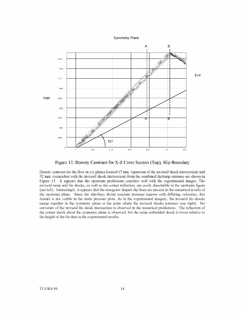
Inlet 0.025

...

0.02 _

O.Ol S __ f

..... /0 0.02 0.04 0.06

Symmetry Plane

A B

, /SU/I

, s:_ /I J, 4:_ _

S j''::;::/ II

" III

I

II

I

I

II

II

II

I

I

I

I

II

II

II

Exit

Figure 12: Density Contours for X-Z Cross Section (Top), Slip Boundary

Density contours for the flow in x-y planes located 67 mm (upstream of the inviscid shock intersection) and

92 mm (coincident with the inviscid shock intersection) from the combined fin/ramp entrance are shown in

Figure 13. It appears that the upstream predictions correlate well with the experimental images. The

inviscid ramp and fin shocks, as well as the comer reflection, are easily discernible in the upstream figure

(see left). Interestingly, it appears that the triangular shaped slip lines are present in the numerical results of

the upstream plane. Since the slip-lines divide constant pressure regions with differing velocities, this

feature is not visible in the static pressure plots. As in the experimental imagery, the inviscid fin shocks

merge together in the symmetry plane at the point where the inviscid shocks intersect (see right). No

curvature of the inviscid fin shock intersection is observed in the numerical predictions. The reflection of

the comer shock about the symmetry plane is observed, but the ramp embedded shock is lower relative to

the height of the fin than in the experimental results.

TFAWS 99 14

Plane A-A (Ahead of the 15° Fin Shock Intersection)

13_

E

(D

P

I I

I II I

• L

_1 _ P IiI I

iI Ih I

[I I

ii I[I I

[I I

[I Iil I

/ [I II I

I I

L 2t •::iii [I I

I ilili i I I

' U]'- ................. r- _. :.:......:...._.::..:.:.:......:..:.<_:.:.-..,::.I !:: I'_{ " '1.......... 1 ......... J

ii!',li!i!] i"-.'" i ____ i iz _:_ _ ____"_ ,_____.... ',_i_:- _ _'..

' ii!_'_ ' ' "'_'-_I lil!_;i:i_ I I I

lu _u 3u 4_

m[3-

E

E

#

Plane B-B (At the 15° Fin Shock Intersection)

il I I I

il I I I

il I I I1• L I •

il I I I

il I I Iil I I I,, , , ,iq, f t iii I I I

il I I Iii I I I

h _ _it I /

I I I

ii t I

Figure 13 Density Contours for Y-Z Cross Section, Slip Boundary

CONCLUSIONS

The comparison of the FDV method to the actual measured flowfield for the triple shock interaction is

encouraging. Many of the flowfield features observed in the experimental imagery are resolved in the

computation including the inviscid shock corner reflections. Particularly good results are obtained for the

shock structure in the cross sectional x-y planes upstream of the inviscid shock intersection. The numerical

results did not exhibit the shock curvatures evident in the experimental images, but this may be rectified

through increased grid resolution or a different boundary condition for the top surface (x-z plane) may be

required. It is concluded that the multi-threaded domain decomposition approach provides an efficient

strategy for parallelizing the FDV code and it is expected to be implemented on problems of increasing size

in the future.

ACKNOWLEDGEMENTS

The authors wish to acknowledge Professor Krishna Kavi and members of the "Crash" group at the

University of Alabama in Huntsville Electrical and Computer Engineering Department for their support.

REFERENCES

Garrison, T. J., Settles G. S., Naranyanswami, N., Knight D. D., and Horstman, C. C., "Flowfield

Surveys and Computations of a Crossing Shock Wave/Boundary Layer Interaction", AIAA Paper 94-

2273, June 1994.

2. Garrison, T. J., Settles G. S., and Horstman, C. C., "Measurements of Triple Shock Wave/Turbulent

Boundary Layer Interaction", AIAA Paper 94-2274, June 1994.

TFAWS 99 15

4.

6.

7.

8.

Yoon, K. T.and Chung, T. J., _Three-dimensional mixed explicit-implicit generalized Galerkin

spectral element methods for high-speed turbulent compressible flows", Computer Methods in

Applied Mechanics and Engineering, 135,343 -367 (1996)

Yoon, K. T., Moon, S. Y., Garcia, G. A., Heard, G. W., and Chung, T. J., _Flowfield dependent mixed

explicit-implicit (FDMEI) methods for high and low speed and compressible and incompressible

flows", Computer methods in Applied Mechanics and Engineering, 151, 75-104 (1998)

Chung, T. J., _Transitions and interactions of inviscid/viscous, compressible/incompressible and

laminar/turbulent flows", Int. J. Numer. Meth. Fluids, in press.

Nichols B., Buttlar D., and Farrell J., _Pthreads Programming", O'Reilly and Associates, Inc., (1996).

Demmel, J.W., _Applied Numerical Linear Algebra", SIAM, Philadelphia, 347-351, (1997).

Shakib, F., Hughes, T., and Zdenek J.,"A Multi-element Group Preconditioned GMRES Algorithm for

Non-symmetric Systems Arising in Finite Element Analysis", Computer Methods in Applied

Mechanics and Engineering (1989).

TFAWS 99 16

INTEGRATION OF RBCC FLOWPATH

ANALYSIS TOOLS

D.G. Messitt

Gencorp Aeroj etP.O. Box 13222

Sacramento, CA 95813

ABSTRACT

A framework for integration of RBCC flowpath analysis tools is presented which allows for increased

modeling flexibility, incorporation of improved engine component models, and integration of disparate

computer codes. The interfaces between the engine components are abstracted with a construct which hides

the details of the data passing between modules, presenting a standard interface to each component model.

This framework facilitates application of different levels of fidelity for analysis of each engine component,

which may reflect differing levels of maturity in the component design.

INTRODUCTION

Efforts aimed at integration of flowpath analysis tools have historically resulted in the construction of

monolithic codes which contain models of the entire flowpath, from inlet to nozzle. These codes, such as

RAMSCRAM, 1 RJPA, 2 and SRGULL, 3 have become industry standards, and have been accepted through

an extensive database of established results. They are poorly documented, and careful verification data,

where they exist, are not generally available. The models of individual engine components, such as the

combustor and nozzle, are tightly integrated within the code framework, cf. Fig. 1. This can make it difficult

to add a new model or to analyze a radically different engine design.

The thermodynamic model is usually provided by a version of the CEA code, 4 although the NOTS routines

are used by RJPA, and other codes use custom routines, e.g., SCREAM. 5 The thermodynamic models are so

tightly integrated with the component models, cf. Fig. 1, that it is impossible to update them, or to replacethem in order to standardize on a common set of routines.

Routines overlap, share data,

and share memory

In let

Model

Isolator

Model

Combustor

Model

Nozzle

Model

Thermodynamic Routines

Figure 1 Subroutines share data and cannot be easily improved, replaced, or individually verified.

INTEGRATEDFLOWPATH ANALYSIS TOOL

A typical RBCC flowpath may be broken into several parts, as illustrated in Fig. 2. The interface locations

are somewhat arbitrary, and are chosen based upon the availability of existing data, or the suitability of

available models for the flow processes. Each component has an interface where fluid enters or leaves.

Inlet

IsolatorCombustor

Figure 2 Illustration of RBCC engine flowpath component modelling

A flowpath analysis environment constructed with this philosophy has the ability to use different levels of

fidelity for different engine components. This concept is illustrated in Fig. 3, where a 2D inlet simulation

provides the inflow properties for the isolator, which is modeled in 1D based upon an experimental

correlation. This capability is enabled by the realization that the inlet and isolator interact by the flow of a

fluid at the interface. It is important to note that there can sometimes be feedback upstream, as illustrated in

Fig. 4, a CFD simulation of inlet unstart.

Inlet2-D CFD Model

i i 1

Oas Object

Isolator

ExperimentalCorrelation

• |•_ p

Figure 3 The inlet and isolator interface consists of a gas object which knows the fluid properties atthe interface.

TFAWS 99 2

Unstarted

Started

Figure 4 CFD Simulation of an inlet unstart demonstrated feedback from the isolator at Mach 5.

Communication between engine component models is abstracted by using the concept of a gas object. The

gas object at the inlet and outlet of each component contains all of the information required to specify the

state of the fluid at that point. A conceptual diagram of a gas object may look something like Fig. 5. The gas

at the interface has certain properties, such as average pressure, velocity, etc. for a gas generated by a 1D

model. The properties may be instead 2D profiles or 3D surfaces, if they were generated by a model with

higher fidelity. They may be stored only in the computer memory, and thus be transient, or be persistent,

such as a CFD code output file. The data may even physically reside on a different computer and a different

operating system.

Gas Object Abstracts Module Interface

Gas Properties

Average p, V, etc.Composition

2DCFD: i-o 3D

19

Routinesto Convert

and ReportProperties

1D--1_2D

3D_ID

etc.

Figure 5 Interface between engine components isolates results from component model details.

The gas object also has the ability to report its properties when queried. For example, the isolator in Fig. 3

needs to obtain the 1D average inflow properties from the product of the 2D inlet CFD analysis. The

isolator does this by invoking a subroutine contained in the definition of the gas object, essentially asking

the gas "please give me your average pressure, velocity, etc." The gas object gets the appropriate CFD data

file from the network, and then invokes a suitable averaging method for the CFD data. The results of the

averaging are reported to the isolator.

TFAWS 99 3

In this example, the isolator model has no knowledge of the details of how the properties at the inlet exit

were obtained. This important feature is what enables improved or updated component models to be easilyincorporated into the overall flowpath analysis procedure. It facilitates the incorporation of experimentaldata, when the component interfaces can be suitably defined.

The individual conducting the flowpath analysis defines which component models are used and how theyare linked together. The interface is abstracted through the use of the gas object concept, outlined above.

The framework allows for strongly coupled engine component models, such as a single routine whichmodels the isolator and combustor, cf. Fig. 6. The technique also allows flexibility in assembling enginecomponents to analyze other engine cycles, such as the Dual Combustion Ramjet (DCR) 6model illustrated

in Fig. 7.

Inlet

Simple 1DFortran

Code

Spreadsheetetc.

2D CF DEuler

N-S

Exp. DataCorrelation

Raw Data

3D CF DEulerN-S

Isolator

I Simple 1D

I Exp. Data

I 2D CFD I

I 3OCFOI

Combined Inlet

and Isolator

Model

Combustor

Figure 6 Engine components encapsulate the analysis method.

Scam Inlet

Ram Inlet _,

Fuel ¢

Isolator _

Combustor

GasGene rator

t

_I Nozzle I

Figure 7 Schematic of a DCR engine analysis using distributed engine component models.

The key benefit of this framework is that the individual component models are isolated from the details ofthe techniques used to analyze the other engine components. Different engine components may be analyzedto different levels of fidelity, by choosing the appropriate analysis technique for each individual enginecomponent, e.g., 1-D combustor analysis which flows into a 3-D nozzle CFD code.

TFAWS 99 4

Distributed computing is also supported. Continuing the example of Fig. 3, the CFD analysis could be

conducted on High Performance Computing (HPC) resources, with the subsequent components analyzed on

a PC and/or Unix workstations, cf. Fig. 8. The details of the interfaces between the engine component

models are hidden by the abstraction of the gas object, which obtains required data from the network

transparently.

l Gas ObjectInterface

HPCII' 3D CFD

Inlet, nozzle

t N. j4!_ ..":3

Integ rated FlowpathAnalysis

Gas ObjectInterface

U n ix Wo rkstatio nIsolator, combustor

Figure 8 Distributed analysis of RBCC engine flowpath.

INTEGRATION FRAMEWORK ISSUES

There are many important issues which impact the implementation of the flowpath analysis integration

framework. The most important of these is the construction of the structure which allows for the building of

an engine model from the available component simulation routines. The most straightforward method

involves assembling the available component models into a predefined sequence, similar to the existing

monolithic codes. The advantages of fidelity zooming, distributed computation, individual model

verification and validation, and integration of otherwise incompatible tools (e.g., linking spreadsheets with

Fortran code) still exist, but the full potential of the framework is not realized.

INTEGRATION ARCHITECTURE

A better solution would involve constructing an architecture which would allow the graphical layout of

engine component models on a canvas, in a manner similar to the schematic of Fig. 7. The architecture

would link the models using the gas object abstraction, and collect and store output data for later inspection.

This capability does not yet exist for current RBCC engine analysis tools.

Feedback between models, illustrated by inlet unstart in Fig. 4, requires special provisions in the code

which assembles the engine component models into a flowpath simulation. The reduction in the level of

integration between the component models may increase the time required to obtain a solution in cases

where feedback is important.

TFAWS 99 5

TRACEABILITY

Anotherveryimportantissueconcernstraceabilityof thedatageneratedbytheflowpathanalysis.Theindividualcomponentmodelsareverifiedandvalidatedagainstaccepteddata,providingconfidenceintheresultsofanewanalysis.It is alsoveryimportantto taginputandoutputfileswithinformationwhichidentifiesthecomponentmodelsused,includingversioninformationandmodelassumptions.Thiscapabilityis includedasapropertyofthegasobjectswhichencapsulatetheflowfieldinformationgeneratedbyeachmodel.It mustalsobeincludedinanysupplementaryinformationobtainedfromthemodel,suchasoutputfilescontainingpressuredistributionsorotherinternalinformationnotencapsulatedinthegasobjectwhichrepresentsthemodelinfloworoutflow.

CONCLUSIONS

A framework for integration of RBCC flowpath analysis tools has been presented which allows for

increased flexibility, incorporation of improved engine component models, and integration of disparate

computer codes. The interfaces between the engine components are abstracted with a construct which hides

the details of the data passing between modules, presenting a standard interface to each component model.

This abstraction of the model interfaces reduces the complications for implementing heterogeneous

distributed computing.

ACKNOWLEDGEMENTS

The author wishes to acknowledge the contributions of Mel Bulman and Dick Johnson.

REFERENCES

2.

4.

6.

Burkardt, L.A., and Franciscus, L.C., "RAMSCRAM - A Flexible Ramjet/Scramjet Engine Simulation

Program," NASA Technical Memorandum 102451, June, 1990.

Pandolfini, P.P., Billig, F.S., Corpening, G.P., Corda, S., and Friedman, M.A., "Analyzing Hypersonic

Engines Using the Ramjet Performance Analysis Code," APL Technical Review, Vol. 2, No. 1, 1990,

pp. 34-45.

Pinckney, S.Z., Walton, J.T., "Program SRGULL: An Advanced Engineering Model for the Prediction

of Airframe-Integrated Subsonic/Supersonic Hydrogen Combustion Ramjet Cycle Performance,"

NASP TM 1120, Jan., 1991.

Gordon, S., and McBride, B.J., "Computer Program for Calculation of Complex Chemical Equilibrium

Compositions and Applications I. Analysis," NASA RP-1311, Oct., 1994.

Bradford, J.E., and Olds, J.R., "SCCREAM v.5: A Web-Based Airbreathing Propulsion Analysis

Tool," AIAA Paper 99-2104, June, 1999.

Billig, F.S., Waltrup, P.J., and Stockbridge, R.D., "Integral-Rocket Dual-Combustion Ramjets: A New

Propulsion Concept," Journal of Spacecraft and Rockets, Vol. 17, Sept.-Oct., 1980, pp. 416-424.

TFAWS 99 6

ONGOING ANALYSES OF ROCKET BASED COMBINED CYCLE

ENGINES BY THE APPLIED FLUID DYNAMICS ANALYSIS

GROUP AT MARSHALL SPACE FLIGHT CENTER

Joseph H. Ruf, James B. Holt, Francisco Canabal

Marshall Space Flight Center

ABSTRACT

This paper presents the status of analyses on three Rocket Based Combined Cycle (RBCC) configurations

underway in the Applied Fluid Dynamics Analysis Group (TD64). TD64 is performing computational fluid

dynamics (CFD) analysis on a Penn State RBCC test rig, the proposed Draco axisymmetric RBCC engine

and the Trailblazer engine. The intent of the analysis on the Penn State test rig is to benchmark the Finite

Difference Navier Stokes 1 (FDNS) code for ejector mode fluid dynamics. The Draco analysis was a trade

study to determine the ejector mode performance as a function of three engine design variables. The

Trailblazer analysis is to evaluate the nozzle performance in scramjet mode. Results to date of each

analysis are presented

NOMENCLATURE

As = Secondary Flow Area

Ap = primary thruster exit flow area plus thruster base area

A5 = mixer inlet area, A_ + Ap

As = ram burner area

D = mixer diameter at mixer inlet

L = mixer length

R = radius

y = local radius

rh = mass flow rate

SUMMARY

Three analyses related to RBCC concepts are underway in TD64 at MSFC. Each analysis is described in its

own section of this paper. The first two analyses deal with the first mode of the RBCC engines or the

_ejector' mode. The ejector mode occurs at Mach numbers less than one while the primary thruster exhaust

entrains or _ejects' air through the engine.

The first analysis is a benchmark of the FDNS CFD code for RBCC ejector mode fluid physics. Penn State

University (PSU) is in the process of completing a benchmark quality laboratory experiment of an RBCC

configurationinejectormode.ThisbenchmarkwilldeterminehowbesttouseFDNStopredictejectormodeperformanceofRBCCengineconcepts.

ThesecondanalysisusedFDNStopredicttheejectormodeperformanceofanearlyconfigurationoftheDarcoRBCCengine.A tradestudyof27engineconfigurationswasperformed.DracoisaneartermRBCCaxisymmetricengineintendedtoair-breatheupthroughtheramjetmode.

ThethirdanalysisisusingFDNStodeterminethenozzleperformancefortheTrailblazervehicleinthescramjetmode.Thecomputationaldomainbeginsinsidetheengineandincludesthefreestreamflowfortheinstalledperformanceeffects.TheTrailblazervehicleissingle-stage-to-orbitRBCCconceptwiththreesemi-axisymmetricengines.

FDNSEJECTORFLOWBENCHMARKING

INTRODUCTION

The PSU RBCC hardware is a two-dimensional design (figure 1) with variable geometry to enable studies

of RBCC mixing and secondary combustion phenomena. Gaseous hydrogen and oxygen were used as

propellants. The ejector mode configuration had a simple two-dimensional inlet and exhausted to

atmospheric pressure. The ejector mode test included measurements for wall static pressure, wall heat flux

and overall thrust. Additionally, optical and laser based diagnostics were employed to evaluate mixing and

secondary combustion during testing. A primary objective of the PSU ejector mode test was to provide

high quality benchmark data for CFD code validation.

OBJECTIVE

The objective of this analysis is to benchmark the FDNS CFD code for RBCC ejector mode operation. The

key physical process of interest is the shear layer interaction between and mixing of the primary thruster

exhaust with the secondary (air) flow. This process has a significant affect on the amount of secondary flow

entrained and, therefore, the performance of the RBCC's ejector mode.

APPROACH

The test conditions modeled are for the primary thruster at 500 psi and an oxidizer-to-fuel (O/F) ratio of

eight. The afterburner has a small amount of gaseous hydrogen injected. A semi-3D domain is currently

being used to model the test hardware. The symmetry in the hardware allows the domain to contain only

1/4 th of the hardware flowpath. The semi-3D domain is fairly dense in the axial and vertical directions, but

is coarse in depth. The depth is incorporated to enable the afterburner fuel injection. The analysis is steady

state and implements finite-rate chemistry and thermodynamics and the standard k-_ turbulence model.

STATUS

The only test data currently available is the upper wall static pressures for two runs. The complete data

should be available with a few weeks. The wall pressures from the current solution are compared to the test

data in figure 2. The semi-3D results match the test data very well. The slight drop in pressure in the

afterburner is due to the hydrogen injection and afterbuming. All hydrogen is consumed before the gases

exit the nozzle.

FUTURE WORK

Future work will involve refining the three-dimensional grid and then comparing to the complete

experimental data set for O/F of eight. Further benchmarking will be pursued by modeling the same

hardware with the primary thruster at an O/F of four.

TFAWS 99 2

DRACO EJECTOR/MIXER TRADE STUDY

INTRODUCTION

The first or _ejector' mode of the Draco engine will have a significant impact on the overall engine cycle

performance. By their very nature the one-dimensional RBCC cycle performance codes used for RBCC

conceptual design do not capture the multidimensional fluid dynamic interactions that may have significant

effects on the ejector mode performance. If CFD can be integrated into the design process early the RBCC

cycle performance codes would benefit from information on the three-dimensional effects and engine

designers would gain additional understanding of RBCC internal fluid dynamics.

An early Draco configuration was chosen to start the CFD trade study on ejector/mixer performance even

though significant changes in the Draco design were likely. This trade study was used to get all the CFD

related tools in place, working and streamlined so future ejector/mixer configuration trade studies could be

tackled much quicker.

OBJECTIVE

The first objective to this analysis was to determine the Draco ejector/mixer performance trends for

quiescent freestream for a matrix of engine design variables. The second objective was to get the CFD and

related analysis tools in place, working and streamlined for quick turn-around of ejector/mixer configuration

trade studies.

APPROACH

The Draco flowpath configuration for this analysis was axisymmetric with a single primary thruster on the

engine centerline (figure 3). The primary thruster was housed in a centerbody that created an annular

constant area inlet. On the front of the centerbody was an inlet compression spike.

Figure 3 defines some of the Draco design variables. The ejector/mixer inlet plane is defined to be the exit

plane of the primary thruster. The mixer length (L) was a function of two of the trade space variables, L/D

and AJAp. The mixer diameter (D) was defined as its diameter at the inlet plane. A_ is the area of the

secondary flow area and Ap is the area of the primary thruster exit area plus any base area surrounding the

thruster. A5 is the total flow area at the ejector/mixer inlet plane (A_ + Ap) and As is the flow area of theram burner.

The engine design variables that defined the trade space were: ejector/mixer L/D; AJAp, the ratio of

secondary to primary flow areas; and As/As, ratio of ram burner to ejector/mixer inlet areas. Each variable

had three values so that the trade space included 27 cases as shown in table 1. Several of the engine

configurations are shown in figure 4.

The performance of the ejector/mixer was measured with the following figures of merit (FOM): By-pass

ratio, the ratio of secondary flow to primary flow; ejector compression ratio (ECR), the ratio of total

pressure at ejector/mixer exit to total pressure of secondary flow; ejector/mixer thrust efficiency, thrust at

the exit divided by thrust at the mixer inlet; ejector/mixer mixing efficiency as defined below.

Mixer Mixing Efficiency - 1 -I/_i_irideal-/_air @ Ylmi ..... it

ERz_'_ I/_ak --/_air @Ylmixerinlety =0 ideal

The mixing efficiency was defined as a measure of how well the mixer achieved perfectly mixed

homogeneous flow at the ejector/mixer exit. The mass flow distribution of secondary flow (air) was used to

TFAWS 99 3

calculatethemixingefficiency.Thedifferencebetweenhomogeneousflowandtheair massflowdistributionthatexistedattheejector/mixerinletwasdeterminedandnormalizedtorepresentzeromixing.A valueof 1wouldoccuronlyif theentrainedairwasperfectlymixedwiththeprimaryflowandtheresultingmixedflowhadnogradients(_plug'flow). Valuesof lessthanzerowerepossibleif theejector/mixerincreasedthestriationoftheprimaryandsecondaryflows.

Thegeometricdefinitionofthe27caseswasextractedfromanenginedesignspreadsheet.Thisgeometrywaspassedto Gridgen5to generatethegrids.All gridscontainedthesamenumberof nodesin thefreestream,inlet,ramburnerandnozzleportionsofthedomain.Thenumberofnodesintheaxialdirectionof theejector/mixervariedbecauseof theirdifferentlengths.A consistentaxialdelta-swasusedintheejector/mixerregion.Thegridscontainedapproximately33k,38kand44knodesfortheL/D=I,2,and3configurations,respectively.OncetheGridgentemplatewasinplaceforeachL/Dgridsthe24subsequentgridscouldbegeneratedinlessthanfiveminuteseach.

TheFDNSCFDcodewasimplementedwithatwo-speciemodel:airanda specieof averagehot-gasproperties.Thisanalysiswasnon-reactingbutfutureanalysiswill include finite rate reaction as necessary.

The standard k-_ turbulence model was implemented. The benchmarking effort above will indicate if

another turbulence model is more appropriate for future work.

The freestream far field boundaries were set to conserve total pressure of one atmosphere. All engine

surfaces were set to no-slip adiabatic walls and the centerline of the engine was set to an axisymmetric

boundary condition. Primary thruster mass flow rates were the same for all configurations but each AJAp

ratio resulted in a different primary thruster area ratio, therefore, a different primary thruster exit pressure.

The AJAp=I had the lowest exit pressure and AJAp=3 had the highest exit pressure. The primary thruster

exit flow properties were calculated with the Reacting and Multiphase Program 4. These thruster exit flow

properties were defined as fixed inlet conditions for the ejector/mixer analysis.

The solution procedure was highly automated by using a series of Unix scripts. The scripting automatically

acquired the appropriate grid and initialized the grid and solution in FDNS format. The scripts then ran the

solution 15 thousand iterations through a series of CFD inputs increasing the time step while decreasing the

damping. The grid was then adapted based on flow field gradients with Self-Adaptive Grid Code 5, the

solutions were run 15 thousand more iterations, and post processed for the FOMs. Subsequent

configurations used previously converged restart files where possible. All 27 configurations were run 15k

iterations before and after adaptation even though most all were converged much sooner. This scripting

procedure allowed the matrix of cases to be run in a _submit and forget' mode from the end of grid

generation to the point of looking at the final post processed answers.

The solutions were run on single processors of an SGI R10000 16-processor computer. Each configuration

required about 44 processor hours from start to finish. The 27 cases were submitted on a Friday afternoon

with staggered start times over the weekend. The last case was completed on the following Tuesday.

RESULTS

Figure 5 shows Mach number and air mass fraction contours of the Draco internal flow path for two

configurations, L/D=I, AJAs=I.5 and AJAp=I and 3. The Mach number contours of the AJAp=3

configuration indicate the primary flow attached to the mixer wall sooner and incurred significantly stronger

shocks than the As/Ap=l configuration. The shocks were caused by the primary flow's interaction with the

secondary flow and the mixer wall. The Mach contours in the inlet show the AJAp=I configuration had a

higher secondary flow rate.

In figure 5 the mixer exit plane is approximately one-third of the distance between the primary thruster exit

and the engine exit. The air mass fraction contours indicate that at the mixer exit plane the AJAp=I

configuration had slightly better mixing of the primary and secondary flows.

TFAWS 99 4

Figure6 indicatesthelargestdriverin theby-passratiowasAJAp.Thiswasaresultof thedifferentprimarythrusterarearatiosand,therefore,exitpressures.FortherangeofAJApstudiedthelowestprimarythrusterexitpressure(As/Ap=l)pumpedthemostsecondaryflow.BothL/DandAJA5hadlessdramaticbutyetsignificanteffectsonby-passratio.

TheECR(figure7)waslowestatAJAp=Ibecausethehighsecondaryflowratedilutedtheaveragetotalpressureoftheresultantmixedflow.ECRalsowaslowestforthelargestL/D. Thisresultedfromtheincreasednumberofshocksthatoccuredinthelongermixers.

Themixingefficiency(figure8)showsthattheAs/Ap=lconfigurationhadthebestmixedflowatthemixerexit.TherewasnosignificantdifferencebetweenL/D=2and3. AJA5didnotsignificantlyeffectmixingefficiency.Figure9plotsthemixingefficiencyforallconfigurationsfromthemixerinlettothemixerexitplane.TheAJAp=2and3 decreasedthemixingbecauseof thehigherprimarythrusterexitpressurescompressedthesecondaryflowagainstthemixerwalls.

In figure10themixerthrustefficiencyisshownversusaxialstationfortheL/D=3configurations.Themixerdegradedthrustforall configurations.NotethatAJA5hasa significanteffectonmixerthrustefficiency,especiallyforAs/Ap=l.

CONCLUSIONS

In thistradestudytheAJAp=Iconfigurationclearlyhadthehighestby-passratiosandmixermixingefficiencies.TheadditionallengthofL/D=3overL/D=2didnotsignificantlyenhancethemixermixingefficiency.TheAJAs=1.5configurationshadthehighestmixerthrustefficiencies.

TheCFDandrelatedanalysistoolsareinplace,workingandstreamlinedforquickturn-aroundofDracoejector/mixerconfigurationtradestudies.

FUTUREWORK

If thePSUejectorbenchmarkdeterminesthatthereisabetterturbulencemodelforejectorflowsthanthek-gmodelthese27configurationswillbere-runwiththemoreappropriateturbulencemodel.

Responsesurfacemethodology6willbeincorporatedintothesolutionprocedureto determineoptimumejector/mixerconfigurations.

TRAILBLAZER

INTRODUCTION

The Trailblazer 7 is a reusable, single-stage-to-orbit vehicle concept, intended to reduce the cost of space

access by making optimum use of air-breathing propulsion. The Trailblazer is a hydrogen-oxygen fueled

vertical take-off/horizontal landing vehicle with 130,0001b gross lift-off weight and 3001b payload. Figure

11 shows the Trialblazer reference vehicle. The propulsion system operates in four modes including ramjet,

scramjet, and rocket modes from lift-off to orbit. A full description of the Trailblazer concept can be found

in reference 7.

In scramjet mode the effective specific impulse is very sensitive to the expansion process efficiency,

especially approaching the maximum air-breathing Mach number of about 10. To determine the expansion

nozzle efficiency the Applied Fluid Dynamics Group is performing CFD analysis of the Trailblazer engine

flowpath for the scramjet mode.

OBJECTIVE

TFAWS 99 5

Theprimaryobjectiveof thisstudyis to provideestimatesof theexpansionprocessefficiencyof theTrailblazernozzleconfigurationinscramjetmode.Thedominantlossmechanismsaretobeidentifiedandquantifiedinordertoguiderefinementsinthenozzledesign.

APPROACH

TheanalysisisbeingperformedwiththeFDNSCFDcode.Finite-ratechemistryandthermodynamicsandstandardk-aturbulencemodelareimplemented.Thefree-streamflowisincludedtoaccuratelymodelthealtitudecompensatingeffectof theaft-body.Effectsof vehicleangleof attackandyawareneglected.Symmetryisassumedaboutaplaneparalleltothevehicleaxisthatbisectstheengineflowpathsuchthatonehalfof anengineand1/6thofthevehicleaftendarein thedomain.Figure12showstheexternalportionof thecomputationaldomain.Theengineinletboundaryconditionsforthescramjetmodewereprovidedbyaone-dimensionalengineperformancecode.ThefreestreamvelocityissettoMach10.Theexpansionprocessefficiencywill be determined by post-processing the three-dimensional CFD solution of

the nozzle flowfield

STATUS

Preliminary results are presented in terms of pressure contours in figures 13 through 15. Figure 13 shows

the pressure contours along the plane of symmetry. Figures 14 and 15 show surface pressure contours in the

neighborhood of the primary thruster and ramp respectively.

FUTURE WORK

After completion of the current scramjet mode analysis two additional engine modes will be analyzed; the

ejector mode and the rocket mode. The primary objective will again be to determine the expansion process

efficiency of the Trailblazer configuration.

ACKNOWLEDGEMENTS

The authors would like to thanks Dr. C. Trefny and Mr. M. D'Agostino for their assistance with this work.

REFERENCES

1. Chen, Y. S., _FDNS - A General Purpose CFD Code, Version 4.0", Engineering Sciences, Inc., ESI-

TR-97-01, Huntsville, AL., May 1997.

2. Lehman, M., Pal, S., Broda, J. C. and Santoro, R. J., "Raman Spectroscopy Based Study of RBCC

Ejector Mode Performance," AIAA-99-0090, 37th AIAA Aerospace Sciences Meeting, Reno, NV,

January 11-14, 1999.

3. Gridgen Version 13 user manual, http://pointwise.com/

4. Smith, S.D., _High Altitude Supersonic Flow of Chemically Reacting Gas-Particle Mixtures - Volume

1, LMSC-HREC TR D867400-1, Lockheed Missile and Space Company, Huntsville, AL., October

1984.

5. Davies, C. B. and Venkatapathy, E., _ The Multidimensional Self-Adaptive Grid Code, SAGEv2",

NASA TM 110350, April 1995.

TFAWS 99 6

6.

7.

Myers, R. H. and Montgomery, D. C., Response Surface Methodology-Process and Product

Optimization Using Designed Experiments, John Wiley & Sons, 1995.

Trefny, C., "An Air-Breathing Launch Vehicle Concept for Single-Stage-to-Orbit", AIAA Paper 99-

2730, June, 1999.

TFAWS 99 7

A8/A5= 1.5

A8/A5=2.

A8/A5=2.5

L/D=1 L/D=2 L/D=3

As/Ap=l As/Ap=2 As/Ap=3 As/Ap=l As/Ap=2 As/Ap=3 As/Ap=l As/Ap=2 As/Ap=3

1.1.15 1.2.15 1.3.15 2.1.15 2.2.15 2.3.15 3.1.15 3.2.15 3.3.15

1.1.20 1.2.20 1.3.20 2.1.20 2.2.20 2.3.20 3.1.20 3.2.20 3.3.20

1.1.25 1.2.25 1.3.25 2.1.25 2.2.25 2.3.25 3.1.25 3.2.25 3.3.25

Table 1. Draco Ejector Cases

Figure 1. Penn State RBCC Ejector Mode Experimental Hardware

Top Wall Pressure Comparison25 20

10

/-30 -15 0 15 30 45 60 75 90

1816

_ 14._12_--10-_

6 -v-4

20

x (in)

& T0619992qo T061899211

Figure 2. Comparison of FDNS and Test Data Upper Wall Pressures for Ejector Mode

TFAWS 99 8

(D

c¢

A5, DA8

Axial Station

As Secondary Flow Area, Constant Area Inlet

Ap Primary Thruster Exit Area + Thruster Base Area

As/Ap 1,2or3

L Mixer Length

D Mixer Diameter at Inlet

L/D 1,2 or 3

A5 Mixer Inlet Area

A8 Ram Burner Area

A8/A5 1.5,2.0, or 2.5

Figure 3. Draco Engine Layout

TFAWS 99 10

L/D= 1, As/Ap= 1

i I_ A8/A5=2.0 [ j i i i i i J

,.,..,,.,,.--

o9

rr"

As/Ap= 1, A8/A5= 1.5

L L -- ,/D=I i L L L L i L i ii i _ LID=2 i i i i i i i i i

........... LID=3: : L L ........ ;

i i i i i i i i i i i i i

i i i i i i i i i i i i i

......_.:,--,._..,.--,--_.-_.!.,..,b,_,.,_.,___: -.-! !L L ...... -_ L L L L L L i L i i

L/D= 1, A8/A5= 1.5

iiiiiiiiiiiiiiiiiii As,Ao=I" • As/Ap=2

........... As/Ap=3: : : ...... J

i i i i i i i i i i

.._.,.,.- , , , , _ , , ,

Axial Station

Figure 4. Examples of Engine Layouts in Trade Study

?,

<

TFAWS 99 12

Figure6. By-PassRatiovs.As/As

g

3

8k_

_L/D=3, A8/AS=2 0L/D=3 A8/AS=2 5

A_/Ap

Figure 7. Ejector Compression Ratio vs. AJAp

2O

As/Ap

TFAWS 99 13

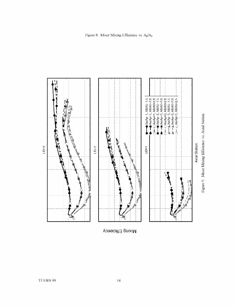
Figure 8. Mixer Mixing Efficiency vs. AJA5

_oue!oNq 6u!X!lAl

II II II II II II II II II

<<<<<<<<<

<<<<<<<<<<<<<<<<

°T_I_I__r-

._o

©

_2

TFAWS 99 14

L/D=3

EI

u_

OI I O_OAs/Ap=I, A8/A5=15O" 4As/Ap=I, AS/A5=2 0

u_ @,_As/Ap=I, A8/A5=2 5

W_,,_ As/Ap=2, AS/A5=15

,'_ As/Ap=2, AS/A5=2 0

_As/Ap_3, AS/A5=15_,_ As/Ap=2, AS/A5=2 5

,._.-, ,_.As/Ap_3, A8/A5=2 0

i i i i

Axial Station

Figure 10. Mixer Thrust Efficiency vs. Axial Station for L/D=3 Configurations

......_iiii_!'i¸¸i_iiiiiiiiiiiiiiiiiiiiiiiii

....._.iiiiiiiiiiiiiiiiiiiiiiiiiiiiiiiiiiiiii_:iiiiiiiiiiiiiiiiiiiiiiiiiiiiiiiiiiiiiiiiiiiiiiii__

::::::::::::::::::::::::::::::::::::::::::::::::::::

........ii;iijiiiiiiiiiiiiiiiiiiiiiiiiiiiiiiiiiiiiiiiiiiiiiiiiii__

:::::::::::::::::::::::::::::::::::::::::::::::::::::::::::::::::

,.iiiiiiiiiiiiiiiiiiiiiiiiiiiiiiii?i?iiiiiiiiiiiiiiiiiiiiiiiiiiiiiiii_iii

.... i/_i!iiiiiiiiiiiiiiiiiiiiiiiiiiiiiiiiiiiiiiiiiiiii!!il¸¸?i:i:i:i::

Figure 11. Trailblazer Reference Vehicle

TFAWS 99 15

TFAWS 99 16

Figure12.ComputationalDomainforTrailblazerNozzleAnalysis

TFAWS99 17

'iiiiiiiiiiiiiiiiiii!i!i;_io_

Figure 13. Pressure Contours on Symmetry Plane

PreSsure; contour

TFAWS 99 18

Figure14.PressureContoursNearInletandPrimaryThruster

Figure15.PressureContoursontheAftRamp

TFAWS99 19

OVERVIEW OF THE NCC

Nan-Suey LIU

(216)433-8722, nan-suey.liu@grc.nasa.govNASA Glenn Research Center

A multi-disciplinary design/analysis tool for combustion systems is critical for optimizing the

low-emission, high-performance combustor design process. Based on discussions between then

NASA Lewis Research Center and the jet engine companies, an industry-government team was

formed in early 1995 to develop the National Combustion Code (NCC), which is an integrated

system of computer codes for the design and analysis of combustion systems. NCC has

advanced features that address the need to meet designer's requirements such as "assured

accuracy", "fast turnaround", and "acceptable cost". The NCC development team is comprised

of Allison Engine Company (Allison), CFD Research Corporation (CFDRC), GE Aircraft

Engines (GEAE), NASA Glenn Research Center (LeRC), and Pratt & Whitney (P&W).

The "unstructured mesh" capability and "parallel computing" are fundamental features of NCC

from its inception. The NCC system is composed of a set of"elements" which includes grid

generator, main flow solver, turbulence module, turbulence and chemistry interaction module,

chemistry module, spray module, radiation heat transfer module, data visualization module,

and a post-processor for evaluating engine performance parameters. Each element may have

contributions from several team members. Such a multi-source multi-element system needs to

be integrated in a way that facilitates inter-module data communication, flexibility in module

selection, and ease of integration.

The development of the NCC beta version was essentially completed in June 1998. Technical

details of the NCC elements are given in the Reference List. Elements such as the baseline flow

solver, turbulence module, and the chemistry module, have been extensively validated; and

their parallel performance on large-scale parallel systems has been evaluated and optimized.

However the scalar PDF module and the Spray module, as well as their coupling with the

baseline flow solver, were developed in a small-scale distributed computing environment. As a

result, the validation of the NCC beta version as a whole was quite limited. Current effort has

been focused on the validation of the integrated code and the evaluation/optimization of its

overall performance on large-scale parallel systems.

Acknowledgements

The NASA High Performance Computing and Communications Program (HPCCP) and the

Smart Green Engine Program (SGE) have supported this effort.

REFERENCES

[1] Stubbs, R.M., and Liu, N.-S., "Preview of National Combustion Code," AIAA Paper 97-

3114, July 1997.

[2] Harrand, V.J., Siegel, J.M., Singhal, A.K., and Whitmire, J.B., "Key Components and

Technologies for the NCC Computing Framework," AIAA Paper 98-3857, July 1998.

[3] Ryder, R.C., "The Baseline Solver for the National Combustion Code," AIAA Paper 98-

3853, July 1998.

[4] Brankovic, A., Ryder, R.C., and Syed, S.A., "Mixing and Combustion Modeling for Gas

Turbine Combustors Using Unstructured CFD Technology," AIAA Paper 98-3854, July 1998.

[5] Chen, K.-H., Norris, A.T., Quealy, A., and Liu, N.-S., "Benchmark Test Cases for the

National Combustion Code," AIAA Paper 98-3855, July 1998.

[6] Chen, K.-H., and Liu, N.-S., "Evaluation of A Non-Linear Turbulence Model Using Mixed

Volume Unstructured Grids," AIAA Paper 98-0233, January 1998.

[7] Shih, T.-H., and Liu, N.-S., "A k-epsilon Model for Wall-Bounded Shear Flows," AIAA

Paper 98-2551, June 1998.

[8] Shih, T.-H, Chen, K.-H., and Liu, N.-S., "A Non-Linear k-epsilon Model for Turbulent

Shear Flows," AIAA Paper 98-3983, July 1998.

[9] Nikj oo, M., and Mongia, H.C., "Study of Non-Linear k-epsilon Model for Turbulent

Swirling Flows," AIAA Paper 98-3984, July 1998.

[10] Raju, M.S., "Extension of the Coupled Monte-Carlo-PDF/SPRAY/CFD Computations to

Unstructured Grids and Parallel Computing," AIAA Paper 97-0801, January 1997.

[11] Anand, M.S., James, S., and Razdan, M.K., "A Scalar PDF Combustion Model for the

National Combustion Code." AIAA Paper 98-3856, July 1998.

[12] Kundu, K.P., Penko, P.F., and Yang, S.L., "Simplified Jet-A/Air Combustion Mechanisms

for Calculation of NOX Emissions," AIAA Paper 98-3986, July 1998.

[13] Norris, A.T., "Automated Simplification of Full Chemical Mechanisms: Implementation in

National Combustion Code," AIAA paper 98-3987, July 1998.

[14] Raju, M.S., "Combined Scalar-Monte-Carlo-PDF/CFD Computations of Spray Flames on

Unstructured Grids with Parallel Computing," AIAA Paper 97-2969, July 1997.

[15 ] Raj u, M.S., "LSPRAY-A Lagrangian Spray Solver-User' s Manual," NASA CR-97206240,November 1997.

[16] Kumar, GN., Mongia, H.C., and Moder, J.P., "Validation of Radiative Heat Transfer

Computations Module for National Combustion Code," AIAA Paper 98-3985, July 1998.

[17] Liu, N.-S., Quealy, A., Kundu, K.P., Brankovic, A., Ryder, R.C., and Van Dyke, K.,

"Multi-Disciplinary Combustor Design System and Emissions Modeling," NASA CDCP-

20011, Proceedings of the 1996 Computational Aerosciences Workshop, May 1997, pp. 49-54.

[18] Liu, N.-S., Quealy, A., "NCC-A Multi-Disciplinary Design/Analysis Tool for Combustion

Systems," NASA Computational Aerosciences Workshop 98, August 1998.

[19] Liu, N.-S., and Chen, K.-H., "FLUX: An Alternative Flow Solver for the National

Combustion Code," AIAA Paper 99-1079, January 1999.

[20] Guo, Y., He, G., Hsu, A. T., Brankovic, A., Syed, S., and Liu, N.-S., "The Development of

a Variable Schmidt Number Model for Jet-in Crossflows Using Genetic Algorithms," AIAA

Paper 99-0671, January, 1999.

TFAWS 99 2

AN UNSTRUCTURED CFD MODEL FOR

BASE HEATING ANALYSIS

Y. S. Chen, H. M. Shang and Jiwen Liu

Engineering Sciences Inc., Huntsville, AL

Phone: (256) 883-6233, fax: (256) 883-6267, e-mail: ychen@esi-al.com

ABSTRACT

This paper summarizes the technical development and findings of a research project for launch vehicle base-heating

analysis. An integrated design tool using unstructured grid method with solution-adaptation and parallel computing

strategy is employed to predict the base heating and plume radiation. The CFD flow field with solution-adaptation

and viscous/turbulence effects is employed for the heat transfer and fluid flow analyses. The present unstructured

grid method imports geometry data from computer aided design (CAD) data base and simplifies the grid generation

and grid adaptation procedures in the numerical simulation of flow field around complex geometries. Computational

efficiency is highly enhanced through parallel computing using multiple CPUs or networked computers. Test cases

of fluid flow and radiative heat transfer problems under limited conditions are investigated in this effort. Benchmark

base flow test cases are also investigated. Comparisons of the base heating data show reasonably good agreements

between the present model and the measured data. Discrepancies in data comparisons can be attributed to the effects

of heat loss, fuel mixing and air aspiration that need to be further investigated by using a more complete numerical

model. This study also shows the effects of the differences between the subscale model and the real nozzle design.

Complex three-dimensional analysis, the solution-adaptation procedure and user friendly graphics interface will be

fully integrated with CAD systems in future study. The basic study and development of the present unstructured grid

CFD method will enhance the cost effectiveness in the design and evaluation of fluid flow and heat transfer

processes of launch vehicles.

INTRODUCTION

With the advent of powerful computers and the development of efficient numerical modeling technology, it is highly

feasible to use the advanced computational fluid dynamics (CFD) models as an effective engineering design and

analysis tool before the first test program is conducted. One of the critical design issues that must be addressed is the

evaluation of the flow conditions in the based region of the launch vehicle during the ascent phase of its trajectory.

The engine compartment and aft control surfaces will experience radiative heating due to the hot exhaust plume. At

certain flight conditions, the nozzle exhaust gas from the engine may impinge on the aft aerodynamic control

surfaces and recirculate within the engine compartment causing a rise in the convective heating. The analysis of

radiative base heating from rocket exhaust plumes has attracted considerable attention during the past few decades,

since the base has to be protected against radiative heating from rocket exhaust plumes. Theoretically, the properties

of gases and particles within exhaust plumes influence the thermal radiation process through absorbing, emitting and

scattering characteristics. Therefore, models as well as methods for predicting rocket plume base heating are in high

demand.

The Radiative Transfer Equation (RTE) is an integro-differential equation whose exact analytical solution is only

possible for very simple and specific settings. The situation worsens even further when this equation is coupled with

the energy equation in order to solve for other forms of energy transfer. The resulting expression, under these

circumstances has the added difficulty of non linearity. This intrinsic difficulty in the solution of the RTE has

resulted in the development of several approximated models such as the zone method, Monte Carlo method, flux

method, discrete ordinates method (DOM), finite volume method (FVM) etc. These models have been reviewed,

with different degrees of detail, by several authors [ 1-3]. Currently, two of the most widely used methods in radiative

transfer simulation are the DOM and FVM. In the DOM and FVM, the RTE is directly solved numerically along

discrete directions or control angles that approximate the angular intensity distribution. As a result, these two

methodsarerelativelyeasytocode;theyprovideaccurateresultsbyusinghigher-orderapproximations;theycanaccountfor spectralabsorptionby gasesandscatteringby particlesandtheyarecompatiblewithnumericalalgorithmsforsolvingtransportequations[1,4].However,theFVMhastwosalientfeaturesthattheDOMdoesnothave.Oneisthefreedomofselectionofcontrolangleandanotheristheguaranteeofconservationofradiantenergy.Liuetal. [5]comparedthesolutionsfromthesetwomethodsandfoundthattheresultsfromtheFVMweremoreaccurate.TheGRASPcode[6],developedatEngineeringSciences,Inc.(ESI)isaveryaccurateandefficientcodecomparedtootherexistingcodes,it maystilltakealargeamountof CPUtimeto simulatemostofthepracticalproblemsonserialprocessorsdueto thecharacteristicsof theRTE.Whilenumericalaccuracy,computationalefficiencyandproblemsolvingrobustnessthroughparallelprocessinghavebeenthekeyemphasesinthetoday'sdevelopmentof generalpurposeCFDcodes,therehasbeenlackof activeexplorationof highperformancecomputingforsolvingRTE.It isthisurgentneedthatmotivatesustoproposethisproject.Successofthisprojectwill enable us to solve many complex radiative heat transfer problems that are still very challenging today.

The traditional structured grid CFD codes and RTE solvers with multi-zone body-fitted coordinates take the

advantage of automatic indexing and are efficient for many applications. However, for very complicated domains,

the men-power spent in the grid generation is often the largest portion of the entire effort spent in problem analyses.

The CFD applications for complex geometries have achieved significant successes by using unstructured grid (finite

element mesh) methods [7-9]. The unstructured grid method has the advantages of automated grid generation in very

complex domains and flexible mesh adaptation in high gradient region over structured grid method.

An integrated design tool using unstructured grid method with solution-adaptation and parallel computing strategy is

employed in this research project to predict the base heating and plume radiation. CFD solution methods with

solution-adaptation and viscous/turbulence effects are used for the heat transfer and fluid flow analyses. The present

unstructured grid method imports geometry data from computer aided design (CAD) data base, and simplifies the

grid generation and grid adaptation procedures for the numerical simulation of flow field around complex

geometries. Computational efficiency is highly enhanced through parallel computing using multiple CPUs or

network computers. Test cases of fluid flow and radiative heat transfer problems under specific conditions are

investigated in the present study. Complex three-dimensional analysis, the solution-adaptation procedure and user

friendly graphics interface will be fully integrated with CAD systems in the follow-on study. The basic study and

development of the present unstructured grid CFD method will be used by the designers to enhance the cost

effectiveness in the designs and evaluation of fluid flow and heat transfer environment of launch vehicles.

NUMERICAL APPROACH AND IMPLEMENTATION

The procedure of predicting the base-heating environment involves the generation of computational mesh and the

solutions of the plume flow and radiative heat transfer equations. The integrated process is illustrated in Figure 1.

The governing equations, numerical methodologies, grid generation, solution-adaptation and parallel strategy are

described in the following sections.

MATHEMATICAL FORMULATIONS FOR RADIATIVE TRANSFER EQUATION (RTE)

Consider the RTE in a Cartesian coordinate system as shown in Fig. 2a. The balance of energy passing in a specified

direction _ through a small differential volume in an absorbing-emitting and scattering medium can be written as

[10,111:

(f_-V)I4(r,f_) =-(_c 4 +o-4)I4(r,f_)+_c4Ib4(r)+ °-4 fI4(r,f_')%(f_'_f_)df_' (1)

where the subscript X represents the wave-number; 14 (r, f_) is the spectral radiative intensity, which is a function

of position and direction; I b,4 (r) is the blackbody radiative intensity at the temperature of the medium; K x and crx

are the spectral absorption and scattering coefficients, respectively; and qb4(_'--+ _) is the scattering phase

function from the incoming _"]' direction to the outgoing direction {-]. The term on the left hand side represents the

gradient of the intensity in the direction _'-]. The three terms on the right hand side represent the changes in intensity

due to absorption and out-scattering, emission and in-scattering, respectively.

Grid Generation _ UNIC-MESH I

1i I 1 I II Diffusive Boundary I---_IRTE Solver !' _!Fl°w Solver _J Turbulence Equation I

+Figure 1. Processes involved in the base-heating analysis.

If the wall bounding the medium emits and reflects diffusely, then the radiative boundary condition for Eq. (1) is

given by

<1-_,) jrfI,(r,,n-)n'n-L4n-/.(r.,n +) = ed, .(r.) + -- (2)' 7_

n4_ <0

where _+ and _- denote the leaving and arriving radiative intensity directions, respectively; gz is the spectral wall

emissivity; n represents the unit normal vector on the wall.

Equation (1) is a complex integro-differential equation whose exact analytical solution is only possible for very

simple and specific settings. This intrinsic difficulty has resulted in the development of several approximated models.In this project, the finite volume method (FVM) will be used to solve the RTE and the their numerical analysis

procedures are briefly described here. In the following analysis, subscripts )v are dropped for the sake of brevity andthey will be added whenever necessary.

In the FVM, the spatial and angular domains are divided into a finite number of control volumes and control angles,

respectively. Then Eqs. (1) and (2) are integrated over each control volume and control angle. Since the FVM sharesthe same computational grid as the CFD approach, the considered spatial domain will be divided into MA controlvolumes and surfaces by a grid generator. For numerical analysis of the FVM, a representative control volume

resulted from the spatial domain division is shown in Fig. 2b. By referring to the division practice for the spatial

domain, the angular domain (see Fig. 2c) at a node centered in a control volume is divided into N0xN,=MB control

angles with No and N, representing numbers of control angle in polar angle 0 and azimuthal angle _ directions,respectively. These MB discrete solid angles are nonoverlapping and their sum is 4n. Unlike the selection of aquadrature scheme in the discrete ordinates method (DOM), there is no specific restriction in selecting control angles

in the FVM. However, the control angles are usually chosen in a manner that best captures the physics of a givenproblem. This is analogous to the selection of control volumes.

x

(a)

N _T

J's• Node

x tnt_m_nn Point

(b)

"---?><L .... --:!_j-

(c)

Figure 2. (a) Coordinate system for radiative transfer equation, (b) a representative

control volume, and (c) a representative control angle.

GOVERNING EQUATIONS FOR FLUID DYNAMICS

The continuity equation and the Navier-Stokes equation, under the isotropic turbulent viscosity hypothesis, can bewritten in a Cartesian tensor form:

dp d f _ 0 (3)

+U x._j "°uYud--d% + dxy (4)dt

where 9 is the fluid density, u_ is the i th Cartesian component of the velocity, and p is the static pressure. The shear

stress _j can be expressed as:

,(du c3_j 2c3_ _ 2

where p is the fluid viscosity and/4 is the turbulent viscosity defined as:k 2

p, = C p-- (6)g

The energy equation for total enthalpy, hi, is written as:F/

c? pht + c?

pu ht) = c_x; L/ Prjc?xj_ dtdt 7ff]x_( _ d 2+p_/drl+dp+@ (7)

where A is the thermal conductivity, Prt is the turbulent Prandtl number, T is the fluid temperature, _ is the energydissipation function.

The species conservation equation is expressed as:

(8)

where Yi is the ith species mass fraction, D is the mass diffusivity, @ is the turbulent Schmidt number, and O) i is the

chemical reaction rate for species i respectively.

The standard two-equation k-_ model with wall function is employed, and the transport equations are

d d /4 3k

3t oxj- - oxjL\ %joxjj

OIQE__ +_-XJ '/OujO[ E) = __Xj -/jL/+ __/__Xj 1 + ]Q_ (C1/OC2E)_[_- _"_/'4 _E E (10)

where P is the rate of production of turbulence kinetic energy and the model constants are C_=0.09, CI=1.44, C2=1.92,

_k=1.0 and cr_=l.3.

The cell-centered scheme is employed here because the control volume surface can be represented by the cell surface

and coding structure can be much simplified. The transport equations can also be written in integral form as

d I_p_df_+4fi,.fidF=_Scdf_ (11)dt

where f2 is the domain of interest and F is the surrounding surface; n is the unit normal ofF in outward direction. A

two-dimensional control volume is shown in Figure 3.

2D UNSTRCTURED CELLS

o Main Point

[] Boundm'y Point1,2,.. Node Point

F Flux

S Cell Surface

Figure 3. Cell centered control volume for two-dimensional unstructured girds.

The flux function /_ contains the inviscid and the viscous flux vector,

fc=p_¢-/+V¢ (12)

The finite volume formulation of flux integral can be evaluated by the summation of the flux vectors over each face,

_/?-ddr = Z F_,j AFj (13)j k(i)

where k(i) is a list of faces of cell i, Fi,j represents convection and diffusion fluxes through the interface between

cell i and j, and AFj is the cell-face area.

A general implicit discretized time-marching scheme for the transport equations can be written as below,

_1 NB (p_p)" (14)A "+1- _-'_A 6_n+l+ +S+ p _p -- _ m _m_At ) m=l At ¢

where NB means the neighbor cells of cell P. The high order differencing term and cross diffusion term are treated

using known quantities and retained in the source term and updated explicitly.

In an extended SIMPLE [12-14] family pressure-correction algorithm, the pressure correction equation is

formulated using the perturbed equation of state, momentum and continuity equations. The simplified formulations

can be written as:

p' , , uk+l = uk pk+l lok +p,u, = - D. Vp + it' = (15)P'= RT

/7 _ _ k57+v(.ip)+v( .i)= (16)where Du is the pressure-velocity coupling coefficient. Substituting Eq.(15) into Eq.(16), and considering

Ap=,o k+l ,on=(,o k+l pk)+(pk pn)= p'+(pk pn), the following all-speed pressure correction equation is

obtained,

RT At R--_P ..... (17)

where the superscripts n and k represent the last time step and iterative values respectively. The entire pressure

correction step is repeated 2 or 3 times such that the mass conservation condition is enforced.

The momentum equations are solved implicitly at the predictor step. Once the solution of pressure correction

Eq.(17) is obtained, the velocity, pressure and density fields are updated using Eq.(15). The scalar equations such as

mass fraction, turbulence and energy equations, will be solved sequentially. Then the solution procedure will march

to the next time level for transient calculation or global iteration for steady calculation.

LINEAR MATRIX SOLVER

The discretized finite-volume equations can be represented by a set of linear algebra equations, which are non-

symmetric matrix system with arbitrary sparsity patterns. Due to the diagonal dominates for the matrixes of the

transport equations, they can converge even through the classical iterative methods. However, the coefficient matrix

for the pressure-correction equation may be ill conditioned and the classical iterative methods may break down or

converge slowly. Since satisfaction of the continuity equation is of crucial importance to guarantee the overall

convergence, most of the computing time in fluid flow calculation is spent on solving the pressure-correction

equation by which the continuity-satisfying flow field is invoked.

The preconditioned Bi-CGSTAB matrix solver is used to efficiently solve the linear algebra equations [15] resulting

from transport equations. An algebraic multigrid method [16] will be used to solve the algebra equation resulting

from the pressure correction equation. The algorithm of AMG method is fully introduced in [16].

There are two types of fixed cycle multi-grid sequences, V cycle and W cycle. W cycle is more efficient because

each grid level has the chance to pass its residual down to the coarse grid level twice and receive the corrections

twice. The paths of V cycle and W cycle are shown in Figure 4, where the restriction process goes down at "d",

reach the bottom at "b" and then the prolongation process goes up at "u". In this research, W cycle is used and the

coarse grid level is set to no more than six. The bottom level is reached when the mesh cell number is less than 100

or the level is number 6 whichever comes first. The Incomplete Lower Upper (ILU) factorization scheme is used to

solve the linear equations. It takes two sweeps in down processes and 3 sweeps in the up processes. At the bottom,

GMRES method is used to ensure the accurate solution at the coarsest grid level. Several cycles may be needed to

reduce the residual by two orders of magnitude in each time step. For all the calculation in this study, the cycle

number is less than 10 and mostly around 5.

V cycle W cycle

Figure 4. V and W cycle diagram.

GRID GENERATION

The unstructured grid type varies from triangular to quadrilateral for 2D problems and tetrahedral, prism, pyramid, to

hexahedral for 3D problems. Grid considered can include either single type or mixed types of grid. The unstructured

grids can be generated using PATRAN or VGRID [17]. The former one is a commercial package with CAD

capability and the latter one is developed at NANA/LaRC and available in public domain. These grid generation

packages are user friendly and can generate high quality unstructured grids. The present unstructured grid method

also reads structured grids. Hence, any structured grid generators, such as GRIDGEN, and UNIC-MESH, can also be

used to build the base-heating model.

DOMAIN DECOMPOSITION

To implement a parallel computation strategy, the computational domain needs to be partitioned into many sub-

domains. Each sub-domain then occupies one processor of a parallel computer. Many partitioning algorithms have

been developed to partition an unstructured grid. These algorithms include Recursive Coordinate Bisection (RCB),

Recursive Spectral Bisection (RSB), and Recursive Graph Bisection (RGB) methods. A public available package

developed at University of Minnesota, METIS [18], can partition high quality unstructured meshes efficiently. Grids

with 1 million vertices can be partitioned in 256 parts in under 20 second on a Pentium Pro personal computer.

PARALLEL IMPLEMENTATION

In a parallel computation, the governing equations are solved in all sub-domains, which are assigned to different

computer processors [19]. Exchange of data between processors is necessary to enforce the boundary conditions at

the divided interfaces. The communication overhead must be kept well below the computational time. Currently,

many communication software packages, such as PVM and MPI, have been developed for distributed computing.

The Parallel Virtual Machine (PVM) software system [20] is developed at the University of Tennessee and Oak

Ridge National Laboratory (ORNL). It is a standard massage passing interface and enables distributed computing

across a wide variety of computer types, including massively parallel processors (MPPs). It is built around the

concept of a virtual machine which is a dynamic collection of (homogenous or heterogeneous) computational

resource managed as a large single parallel computer. PVM is implemented for data communication among

processors in this project.

MPI stands for Message Passing Interface[21]. The goal of MPI, simply stated, is to develop a widely used standard

for writing message-passing programs. As such interface attempts to establish a practical, portable, efficient, and

flexible standard for message passing. The main advantages of establishing a message-passing standard are

portability and ease-of-use. In a distributed memory communication environment in which the higher level routines

and/or abstractions are build upon lower level message passing routines the benefits of standardization are

particularly apparent. Furthermore, the definition of a message passing standard provides vendors with a clearly

defined base set of routines that they can implemented efficiently, or in some cases provide hardware support for,

thereby enhancing scalability.

VALIDATIONS

VALIDATIONS FOR THE UNSTRUCTURED RADIATION MODEL

Based on the theoretical and numerical analyses described earlier, a computer code has been developed which iscapable of modeling multi-dimensional radiative heat transfer using structured, unstructured, or hybrid grids. Toinvestigate the accuracy of the present unstructured method, six selected benchmark problems were investigatedwhich included 2D planar, axisymmetric, and 3D geometries. To test the sensitivity of the unstructured method on

the grid, a structured grid and an unstructured grid were used for each problem, and their corresponding solutionswere compared against the available other solutions and they were labeled as the unstructured solution and structuredsolution in the following figures. For a 2D problem, the volume cell type is quadrilateral for a structured grid and

triangular for an unstructured grid. For a 3D problem, the volume cell type is hexahedral for a structured grid andprism for an unstructured grid. In each problem, the angular domains for the structured and unstructured grids weredivided by the same strategy which was either the Sn-type discretization or azimuthal discretization. All computationwas conducted on the IBM RISC/6000 machine and the numerical solution was considered to be convergent when

the relative incident radiation change was less than 0.01%. The iteration numbers for different grids were the samefor each problem, and they were equal to two for the cases with black walls and not more than ten for other caseswith scattering medium or gray walls.

2D PLANAR GEOMETRY NO. 1

The first problem examined is a quarter of a circle with a rectangular region added to the top as shown in Fig. 5a.

The curve wall is hot and black and it has an emissive power of unity, while the rest walls are cold and black. Themedium is cold and it is transparent for the first case and purely absorbing with K=I.0 m -1 for the second case. The

Monte Carlo method [22] has been used to investigate this problem before and its solution was used to test againstthe present solutions.

Figure 5b and 5c show the structured and unstructured grids used in the calculation, respectively. The azimuthal

discretization strategy was employed for the both grids in which the angular domain was discretized into

N0xN,=4x20 control angles with uniform A0 and Ad?. The results for the radiative heat flux on the right wall fromdifferent solutions are presented in Fig. 6. At each case, the structured, unstructured, and Monte Carlo solutions areseen to have a very good agreement, and their maximum difference is within 2%. At the location close to the curve

hot wall, the predicted values of radiative wall flux for all solutions are high and they are gradually decreased as thedistance from the hot wall is increased.

(a) (b) (c)Figure 5. 2D planar geometry No. 1: (a) schematic; (b) structured grid; (c) unstructured grid.

Figure6.

1.0 , , , i • , , i , , , i , , • i , . , i

0.8 _.

0.6

0.4

0.2

0.0 ' ' ' ' " ' ' ' " ' ' ' ' ' " ' ' ' "

0.00 0.20 0.40 0.60 0.80 1.00

y(m)

Comparison of radiative wall heat flux distributions on the right wall.

2D PLANAR GEOMETRY NO. 2

The schematic of the second problem is showed in Fig. 7a. The top wall is located at y=l.0 m. The bottom wall

varies according to the following function

½y = [tanh(2 - 3x) - tanh(2)]0 < x <--3

The bottom black wall is maintained at 1000 K while the other black walls are kept at 0 K. The medium is cold (0 K)

and it is purely isotropically scattering with c_=1.0 m -1 for the first case and purely absorbing with K=I.0 m -1 for the

second case. Chai et al [23] considered this problem with the FVM and their solution was used to validate thepresent solutions.

Figure 7a also shows the structured grid used in the calculation while the unstructured grid is presented in Fig. 7b.

The angular domain was discretized using the $8 quadrature scheme. The results of interest are the radiative wallfluxes on the top wall and they are demonstrated in Fig. 8. Both the unstructured and structured solutions are foundto be in good agreement with Chai et al's solution. Maximum difference occurs in the left end region of the wall

where the structured results are slightly higher for the case with K=1.0 m -1.

_AAAAAAAAAAAAAAAAA_L

.AI_AAAAAA__

"-AA;_I_;',,_AAAAAAAAAA/

(a) (b)

Figure 7. 2D planar geometry No. 2: (a) structured grid; (b) unstructured grid.

?'_ ' ''l'''t'''t'''t'''t'''t'''

2O

15

10

Ic--O.O. _=1.0

//'°

o eh_ _t _.(m94) _.

0 ,,. i , . , i . , , i . , . i , , , i , ,, i , , ,

0.0 0.5 1.0 1.5 2.0 2.5 3.0 3.5

X, m

Figure 8. Comparison of radiative wall heat flux distributions on the top wall.

2D AXISYMMETRIC CYLINDRICAL GEOMETRY

The third problem examined is a 2D axisymmetric cylindrical enclosure and its schematic is plotted in Fig. 9a. The

radius of cylinder is 1 m and the height is 2m. The enclosure is filled with an absorbing-emitting medium which is

maintained at an emissive power of unity. The selected medium absorption coefficient K varies from 0.1, 1.0 to 5.0

m -1. All enclosure walls are cold and black. This benchmark problem is studied frequently because an exact solution

[24] for radiative flux on the lateral wall is available.

Radiative transfer in a 2D axisymmetric geometry is a 3D process but it can be treated in 2D coordinates. Figure 9b

and 9c show the 2D computational domains with a structured grid and an unstructured grid, respectively. It is noted

that the bottom line of the domain corresponds to the axisymmetric line of the cylinder and the symmetric boundary

condition was imposed along this line in the computation. The angular domain discretization was carried out using

the $8 quadrature scheme. Currently, the artifice developed by Carlson and Lathrop (Eq. (6)) has been only used in

the Cartesian grid as seen in Fig. 9b, and the curvature coefficients for angular redistribution %+1/2 are the same for

all volume cells. However, with the use of the general formulation of %_1/2 (Eq. (8)) for irregular shape of volume

cell as seen in Fig. 9c, the values of %+1/2 will be different at different volume cells. This will slightly increase the

computational memory of the problem. Figure 10 shows the radiative wall flux distributions along the lateral wall.

Both the structured and unstructured solutions are seen to match the exact solution very well for various opticalthicknesses.

Uml

(b) (c)

Figure 9. 2D axisymmetric cylindrical enclosure: (a) schematic; (b) structured grid; (c) unstructured grid.

10

1.2 , • • i • • • i • • • i • • • i • •

1.0

0.8

0.6

0.4

_'=5.0 m -1

-%-- UnsLracLured

........ Structured

O Exact

0.2 r=0.1 m-1

• v o v v 0

0.0 ...................1.0 1.2 1.4 1.6 1.8 2.0

X, 1T1

Figure l 0. Comparison of radiative wall heat flux distributions on the side wall of a cylindrical enclosure.

2D AXISYMMETRIC TRIANGULAR TOROID

The fourth problem examined is a 2D axisymmetric triangular toroid and Fig. 1la shows the schematic of a cross

section of the problem. The length of each equilateral wall is 1 m. The medium in the toroid is maintained at an

emissive power of unity and it is assumed to be absorbing-emitting with K=1.0 m -1. All walls are cold and black. This

problem was investigated before and the exact solution [25] for radiative wall flux along the lateral wall is available

for the present comparison.

Figure 1 lb and 1 lc show the structured and unstructured grids used in the calculation, respectively. Unlike the

previous problem which used the Sn-type scheme, the azimuthal discretization strategy with N0xN,=4x20 was

employed to discretize the angular domain in this problem. The artifice developed by Carlson and Lathrop (Eq. (6))

has been mainly applied by the DOM to treat 2D axisymmetric problems. In fact, this artifice can also be used by the

FVM which employs azimuthal discretization strategy to discretize the angular domain. One of objective of this

problem is to validate the application of Eq. (6) with the azimuthal discretization strategy. Figure 12 presents the

radiative wall flux distributions along the lateral wall. It is obvious that the structured and unstructured solutions

demonstrate very good agreement with the exact solution. This agreement is consistent with the expectation. The

application of the FVM with the artifice shown in Eq. (6) represents a significant simplification over the

conventional treatment for FVM where a 2D axisymmetric problem has to be modeled in a way similar to a 3D

problem.

(a) (b) (c)

Figure 11. 2D axisymmetric triangular toroid: (a) schematic; (b) structured grid; (c) unstructured grid.

11

0.5

0.4

0.3

0.2

0.1

0.00.0

• , . i . . . i . . . i . . . i . . .

0.2 0.4 0.6 0.8 1.0

S (In)

Figure 12. Comparison of radiative wall heat flux distributions on the lateral wall.

3D IDEALIZED FURNACE

The fifth problem examined represents a 3D idealized furnace proposed by Menguc and Viskanta [26] as shown inFig. 13a. The dimensional size of the geometry is 2)<2)<4 m. The furnace is filled with a gray gas with /¢=0.5 m -1

and or=0. The uniform internal heat sources are q=5.0 kW/m 3.The six walls are gray walls and their emissivities and

temperatures are: g2=0.85, T2=1200 K for wall 2; g5=0.70, T5=400 K for wall 5; El=E3=E4=E6=0.7,

Tl=T3=T4=T6=900 K for walls 1, 3, 4 and 6. Due to the internal heat source, this problem requires an iterativesolution procedure with the energy equation. Several authors have used the discrete ordinates [27], spherical andzone [28] methods to solve this problem. Different models have predicted similar results. Only zone solution wasselected to test against the present results.

Figures 13b and 13c show the structured and unstructured grids used in the calculation. The angular domain wasdivided using the $8 quadrature scheme. For the clarity of comparison, the results for temperature and radiative wallflux distributions are only presented along several lines as seen in Figs. 14 and 15. In Fig. 14, the temperature

distributions are shown along a line (x-axis direction) with y=1.0 m for three different z locations. At the z locationsof 0.4 m and 2.0 m, the predictions from the structured and unstructured solutions are found to be in very goodagreement with the zone solution. At the z location of 3.6 m, the unstructured results are slightly higher while thestructured results are little lower in comparison with the zone results. However, their maximum difference is not

more than 1.5%. Figure 15 demonstrates the net radiative wall heat flux distributions along a line (x-axis direction)with y=l.0 m on the hot wall (wall 2) and cold wall (wall 5). Again, the structured and unstructured solutions areseen very close to the zone solution on each wall.

(a) (b) (c)Figure 13. 3D idealized furnace: (a) schematic; (b) structured grid; (c) unstructured grid.

12

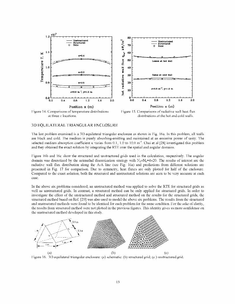
×10 31.2 ..

0

0in,

0

E-I

1.1

1.0

0.9

, • , , , • , , ,

-- Unstructured

........ Structured

0 Zone

z=0.4

z=2.0

_......_ ............... 9. .............. _ .......

z=3.5

---------___ /.... .o. o G ................... _ ............... _ ...............................

e=0.5 m -1, y=t.O m

80

_. 70

60

N 50

40

ao

;_ 20

10

z

• , , • , , , , ,

-- Unstructured........ S+.ruetured

0 Zone

...... 2 ............. R .............. '2......

Losses a t. hot wall

Gains at cold wall

z=0.5 m -l, y:l.O m

0.8 ' ' ' ' ' ' ' ' ' ' ' ' ' ' ' ' ' ' ' 0 " " " ' " " " ' " " " ' ' " " ' ' " "0.0 0.4 0.8 1.2 1.6 2.0 0.0 0.4 0.8 1.2 1.6 2.0

Position x (m) Position x (m)

Figure 15. Comparisons of radiative wall heat flux

distributions at the hot and cold walls.

Figure 14. Comparisons of temperature distributions

at three z locations.

3D EQUILATERAL TRIANGULAR ENCLOSURE

The last problem examined is a 3D equilateral triangular enclosure as shown in Fig. 16a. In this problem, all walls

are black and cold. The medium is purely absorbing-emitting and maintained at an emissive power of unity. The

selected medium absorption coefficient K varies from 0.1, 1.0 to 10.0 m -1. Chai et al [28] investigated this problem

and they obtained the exact solution by integrating the RTE over the spatial and angular domains.

Figure 16b and 16c show the structured and unstructured grids used in the calculation, respectively. The angular

domain was discretized by the azimuthal discretization strategy with N0xN,=4x20. The results of interest are the

radiative wall flux distribution along the A-A line (see Fig. 16a) and predictions from different solutions are

presented in Fig. 17 for comparison. Due to symmetry, heat fluxes are only plotted for half of the enclosure.

Compared to the exact solution, both the structured and unstructured solutions are seen to be very accurate at each

case.

In the above six problems considered, an unstructured method was applied to solve the RTE for structured grids as

well as unstructured grids. In contrast, a structured method can be only applied for structured grids. In order to

investigate the effect of the unstructured method and structured method on the results for the structured grids, the

structured method based on Ref. [29] was also used to model the above six problems. The results from the structured

and unstructured methods were found to be identical for each problem for the same condition. For the sake of clarity,

the results from structured method were not plotted in the previous figures. This identity gives us more confidence on

the unstructured method developed in this study.

(a) (b) (c)Figure 16. 3D equilateral triangular enclosure: (a) schematic; (b) structured grid; (c) unstructured grid.

13

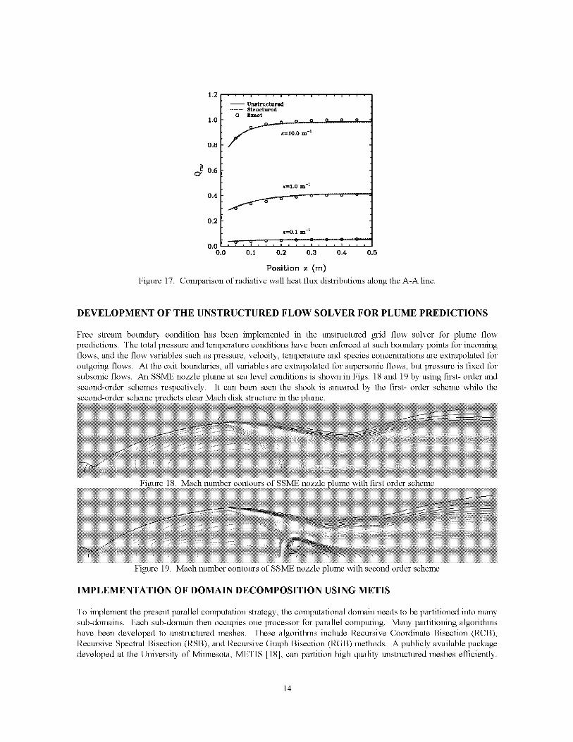
Figure17.

0.8

0._O'

1.2 • , • i , • • i • , • i

-- Unstructured

........ Structured

0 Exact

1.0 .__o o

_'1__10 0 m 1

_'=1.0 m -I

0.4 __.,_--_ - ,_

0.2

• =0.1 m -I

o o ___o......

v j-- G

0.0 _ ' Y ' _" ' T . = . -':, .---:-----------"_.. , . . .......0.0 0.1 0.2 0.3 0.4 0.5

PosiLion z (m)

Comparison of radiative wall heat flux distributions along the A-A line.

DEVELOPMENT OF THE UNSTRUCTURED FLOW SOLVER FOR PLUME PREDICTIONS

Free stream boundary condition has been implemented in the unstructured grid flow solver for plume flow

predictions. The total pressure and temperature conditions have been enforced at such boundary points for incoming

flows, and the flow variables such as pressure, velocity, temperature and species concentrations are extrapolated for

outgoing flows. At the exit boundaries, all variables are extrapolated for supersonic flows, but pressure is fixed for

subsonic flows. An SSME nozzle plume at sea level conditions is shown in Figs. 18 and 19 by using first- order and

second-order schemes respectively. It can been seen the shock is smeared by the first- order scheme while the

second-order scheme predicts clear Mach disk structure in the plume.

iiiiiiiiiil !i!iii!iii!iiiii!iii!iiiii!iii!iii!i!,_._,_,_,_._,'_:_:_'_:_:_:

!iiiii!!iii

iiiiiiiiiii_

!ii!_ii

iiiiiiii!iiiii!iiiii!iiiiiii!iiiii!iii_

iiiiiiiii!iiiii!iiiiiiiiiiiii!iiiii!iiiiiii!iiiiiiiii

iiiiiiiiiiiiiiiiiiiiiii iiiiiiiiiiiiiiiiiiiiiiiiiiiiiiiiiiiiii_i_i_i_i_ii̧iiiiiiiiili_i_!_i_!_!_i_!_i_!_!_i_!_i_!_!_i_!_i_

iliiiiiiiiiiiiiiiiiiiiiiiiiiiiiiiiiiil

iiiiiiiiiiiiiiiiiiiiiii:!:i:!:i:i:!:i:!:i:i:!:i:!:i:i:!:i:!:;:::::::

Figure 19.

ii!!iiiii!!ii_

....... :+:+:+:::::: ......

Mach number contours of SSME nozzle plume with second order scheme

IMPLEMENTATION OF DOMAIN DECOMPOSITION USING METIS

To implement the present parallel computation strategy, the computational domain needs to be partitioned into many

sub-domains. Each sub-domain then occupies one processor for parallel computing. Many partitioning algorithms

have been developed to unstructured meshes. These algorithms include Recursive Coordinate Bisection (RCB),

Recursive Spectral Bisection (RSB), and Recursive Graph Bisection (RGB) methods. A publicly available package

developed at the University of Minnesota, METIS [18], can partition high quality unstructured meshes efficiently.

14

Gridswith1millionverticescanbepartitionedinto256partsin lessthan20secondonaPentiumPropersonalcomputer.Figs.20-21present10partitioneddomainsfor amulti-airfoilgridandthepredictedMachnumbercontoursrespectively.Thepartitioneddomainsurfaceandthepredictedpressurecontoursareshownfor a3-DBoeing747gridinFigs.22and23. Aboutequalgridsizeshavebeenpartitionedforeachdomain,andthetotaldimensionforthezonalinterfacesareminimizedtoreducetheglobalcommunicationtime.

NN

N_

Fili_rei_i20ii_i_i_iPa_itlonedig_ids i_ifo:i_iaimulliiiiiaii:foil mesh

Figure 22. Partitioned domain surface for a

three-dimensional Boeing 747 grid.

Figure 21. Predicted Mach Number contours.

Figure 23. Predicted pressure contours for Boeing 747.

IMPLEMENTATION OF PARALLEL COMPUTING ALGORITHM

Numerical solution has been performed for a turbulent incompressible two-dimensional cascade flow. A four-block

grid partition (Fig. 24) was created using METIS. With the explicit block coupling, the solution may diverge in

some cases. When the implicit block coupling is used in the algebraic multi-grid (AMG) method, both serial (single

CPU) and parallel computing require about the same number of global iterations or time steps to reach a converged

solution. Fig. 25 shows the converged pressure contours and Fig. 26 presents the convergence history vs. time steps.

Due to the small grid size used in this test case, the parallel efficiency only reaches 60%. The efficiency can be

expected to be much higher for large three-dimensional applications.

ii}

Figure 24. Grid partitions for cascade flow.

ii__iiii!ii_iiiiiii_iiiiiiiiiiiii_iiiiiiiii_iiiiiiii_i!iiii_;iiiii_iiii_i__iiiiiiiiiiiiiiiiiiiii;iii_i_ii!iii_i!i_iiiiii_iii_iiiiii!_!_!i!i_i!iiiii!iiiiiiii_i_i_i_i_iii_ii_iiiii_i_i_i!i_i_i_i_i_iiiiiii_iii_ii_ii_ii_ii_iii;

Figure 25. Predicted pressure contour

15

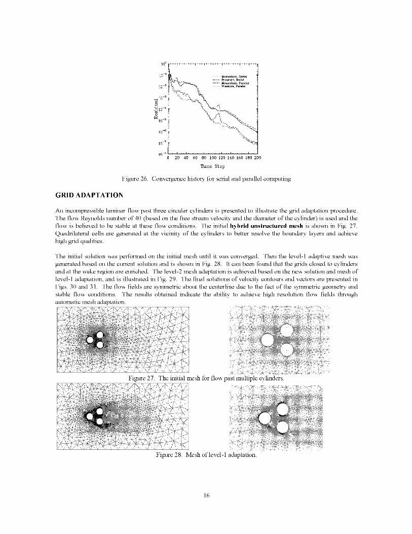
10 0

10 1

lO-Z

_ 10 -3

lO-_

tZ 10- 5

10-6

i0 -7

10 -s

-- Momentum, Scrim....... Pressure, Serial..... Moment_, P_elel.... Pressure, Parelel

[

..,...,...,...,...,..._... ,...,...,..._

20 40 60 80 100 120 140 160 180 200

Time Sfiep

Figure 26. Convergence history for serial and parallel computing

GRID ADAPTATION

An incompressible laminar flow past three circular cylinders is presented to illustrate the grid adaptation procedure.

The flow Reynolds number of 40 (based on the free stream velocity and the diameter of the cylinder) is used and the

flow is believed to be stable at these flow conditions. The initial hybrid unstructured mesh is shown in Fig. 27.

Quadrilateral cells are generated at the vicinity of the cylinders to better resolve the boundary layers and achieve

high grid qualities.

The initial solution was performed on the initial mesh until it was converged. Then the level-1 adaptive mesh was

generated based on the current solution and is shown in Fig. 28. It can been found that the grids closed to cylinders

and at the wake region are enriched. The level-2 mesh adaptation is achieved based on the new solution and mesh of

level-1 adaptation, and is illustrated in Fig. 29. The final solutions of velocity contours and vectors are presented in

Figs. 30 and 31. The flow fields are symmetric about the centerline due to the fact of the symmetric geometry and

stable flow conditions. The results obtained indicate the ability to achieve high resolution flow fields through

automatic mesh adaptation.

Figure 27. The initial mesh for flow past multiple cylinders.

Figure 28. Mesh of level-1 adaptation.

16

Figure 29. Mesh of level-2 adaptation.

",.",_ I ,!! i ................\ ! ii "........... / /'.......•........ ......

P

' _" "".... ' ii 'i "i ........\ ...................

Figure 30. Velocity contours for level-2 mesh adaptation. Figure 31. Velocity vectorsnear the cylinders.

NUMERICAL SIMULATION OF QUALIS/MSFC 2.25% X-33 BASE HEATING MODEL

The model selected jointly by Qualis and NASA MSFC [30], is a 2.25% simulation of the aft third of the X-33 flightdemonstration vehicle currently under joint development by NASA and Lockheed Martin Skunk Works, Palmdale,California. The model matches the X-33 propulsion system parameters and produces exhaust gas constituents and

external plumes that designed to be a close simulation to the X-33 flight plume shapes and thermodynamicproperties. The model is instrumented primarily to monitor propulsion system performance, but also was equippedwith base heating instrumentation to measure the base region environments as a secondary objective.

The X-33 vehicle has two rows of rectangular nozzle thrusters; 20 nozzles along the upper aerospike surface and 20nozzles along the lower aerospike surface respectively. In the current CFD model, only a half of a nozzle regionalong the upper or lower spike surface is modeled due the cyclic arrangement of the nozzles. This model represents

the flow conditions near the center plane of the aerospike engine by ignoring the lateral entrainment effects. Fig. 32ashows the flow domain and grids used in CFD simulations. A patch grid interface is used to connect the nozzle roundand square intersection (see Fig. 32b), which is not the exact nozzle geometry of the X-33 design. The grids with168,000 point are generated by ESI's UMESH package.

The test case of Run 1, 12/03/98, and a latest test case of 669 Psia chamber total pressure are simulated in the presentstudy. For the first case, total pressure of 450 Psia (_30.62 atm) and total temperature of 3456 K have been used asthe inlet conditions. The O/F ratio is 5.823 for both cases with equilibrium species concentration specified at the

thruster inlet. Numerical solutions are obtained in 5,000 time steps for each case using 10 CPUs at MSFC's PowerChallenge and spent 6.1 hours clock time with an average of 75% CPU time fully used. The predicted nozzlepressure, temperature, and Mach number contours of the first case are shown in Fig. 33-35.

17

Nozzle

Nozzle ExitThruster

Conical Section "

Base Slot Section ....ii_!'i!i_iiiiiiiiiiiiiiiiiiiiiiiiiiiiiiiiiiiiiiiiiiiiiiii_,_i_,,_Rampi_i_iiiiiiiiiiiiiiiiiiiiiiiiiiiiiiiiiiiiiiiiiiiiiiiiiiii_,dk---"

(a) The Entire Flow Domain (b) Near Patched-Grid Interface

Figure 32. The flow domain and patched-grid used by the CFD model.

.............................................i_!:ii!i_i_i.................................................

Fig. 33. Predicted pressure (atm). Fig. 34. Predicted temperature (K). Fig. 35. Predicted Mach number.

The CFD predictions of the velocity vectors, Mach number contours, and temperature contours, on the nozzle

symmetry plane, are shown in Figs. 36-38 respectively. A recirculation zone is shown in Fig. 36 near the base region

with temperature around 2,100K in the same region (Fig. 38). The predicted convective heat flux near the base

center region is around 65 Btu/sft-s, which is over-predicted compared to the measurement heat flux of 51.2 But/sft-

S.

In the second test case, the entrainment effects and the strength of the recirculating base flow are increased due to the

increased chamber pressure and the nozzle flow momentum. The overall plume Mach number is also increased that

results in higher flow temperature and convective heat flux in the base region. Figs. 39-41 show the predicted Mach

number, Temperature and H20 mass fraction contours respectively (also on the nozzle symmetry plane). The

predicted convective heat flux near the base symmetry plane is around 162 Btu/sft-s. The measured heat flux for this

case is about 119 Btu/sft-s. Again, the current model has over-predicted the heat flux. The reasons for this

discrepancy can be attributed to:

(1) the heat loss in the combustion chamber, thruster, along the ramp and base surfaces;

(2) the fuel/oxidizer mixing and combustion efficiency that may affect the total temperature at the thruster inlet,

whereas equilibrium chemistry conditions are used in the CFD model; and

(3) the heat flux reduction due to the effect of air aspiration from the sides of the linear aerospike engine, which thecurrent numerical model does not consider.

iiiiiiiiiiiiiiiiiiiiiiiiiiiiiiiiiiiiiiiiiiiiiiiiiiiiiiiii_ii_i_iiii__iiii________!!!!

Figure 36. Predicted velocity vectors

(450 psia Pc).

Figure 37. Predicted Mach number contours

(450 psia Pc).

18

Figure.38.Predictedtemperaturecontours(K)(450psiaPc).

Figure.39.PredictedMachnumbercontours(669psiaPc).

Figure40.Predictedtemperaturecontours(K)(669psiaPc)

Figure41.PredictedH20contours(669psiaPc).

Finally,thereisonemoreimportantissueconcerningtheappropriatenessofusingthesubscalemodelinsimulatingtheX-33baseflows.Asindicatedin Qualis'subscalemodel,thenozzlegeometrydownstreamof thethroatisapproximatedbyaconicalsectionandaconstantheightslot,insteadofanozzlegeometrywithsmoothtransitionfromacircularthroattoarectangularexit(asin theX-33design).Thisapproximatednozzlegeometrycreatesanobliqueshockdownstreamofthestepjumpandobstructstheflowexpansiondownstreamofthestep.Figs.42-43showtheMachnumberandtemperaturecontoursneartheregionofthestepjump.Asaresult,thenozzleflowisnotfullyexpandedwith substantial total pressure loss at the nozzle exit. This may have large effects on the base

pressure and base heating levels. One must be very cautious about simulating full-scale launch vehicles using

subscale models. Any misrepresented detail may have significant impact on important base flow performance data

(such as base pressure and base heating data). These effects could have been discovered using detailed CFD

analyses (such as the current model) early on for the subscale model design. Their impact on the base flow

performance data can be assessed with confidence before the subscale testing is planned and conducted.

Figure 42. Predicted Mach number contours

near the step jump region (669 psia Pc).

Figure 43. Predicted temperature contours (K)

near the step jump region (669 psia Pc).

19

CONCLUSIONS

The current study has been successfully conducted and established that an integrated design tool using unstructured

grid method with solution-adaptation and parallel computing strategy can become a practical analysis tool to predict

base heating and plume radiation. An unstructured finite volume method for radiative heat transfer has been

developed and they are applicable to any 2D planar, axisymmetric, or 3D problems with unstructured grids. Six

benchmark problems, which cover a wide range of geometries and radiative property conditions, have been

examined. The present solutions based on a structured grid and an unstructured grid are very close and they all have

a very good agreement with available reference solutions. The present study indicates that not only is the developed

unstructured radiation model flexible in treating problems with complex geometries but also it is very accurate andefficient.

For plume predictions, free stream (entrainment) boundary condition and plume exit boundary condition have been

successfully implemented. Solutions have been obtained for SSME nozzle plume flows and Mach disk has been

clearly shown with a flux limited second-order upwind scheme.

To implement a parallel computation strategy, the computational domain needs to be partitioned into many sub-

domains. Each sub-domain then occupies one processor of a parallel computer. The domain decomposition using

METIS has been implemented in the current flow solver for parallel computing applications.

The parallel-computing algorithm based on domain decomposition has been accomplished in this study. Algebraic

multi-grid matrix solver has been paralleled to accelerate the convergence rate of pressure correction equation.

Same global convergence rate has been demonstrated for single CPU (domain) and multi-CPU (domain)

calculations.

The grid adaptation algorithm based on flow solution has been demonstrated for two-dimensional problem and

shows the flexibility of unstructured grid method for solution adaptation. Further extension to three-dimensional

applications will be implemented in future study.

Numerical simulation of Qualis/MSFC 2.25% X-33 base heating model has been performed using a sub-domain

CFD model with 168,000 grid points and parallel computation. Numerical solution is obtained within 5,000 time

steps using 10 CPUs at MSFC's Power Challenge spent 6.1 hours clock time with an average of 75% CPU time fully

used. The current CFD model over predicts the base heat flux for two cases with chamber total pressure of 450 psia

and 669 psia. Comparisons of the base heating data show reasonably good agreements between the present model

and the measured data. Discrepancies in data comparisons can be attributed to the effects of heat loss, fuel mixing

and air aspiration that need to be further investigated by using a more complete numerical model.

The present study also reveals the effects of a major difference between the subscale model and the X-33 design in

the nozzle geometry. The simplification in the nozzle geometry of the subscale model has been shown to create an

oblique shock system in the nozzle, which may have caused obstruction to the nozzle flow expansion and substantial

total pressure loss to the nozzle flow. This may have significant impact on the base flow performance data such as

the base pressure and the base heat flux. These effects can be investigated using the current CFD model before the

design of the subscale model to assess their impact on the base flow performance data.

REFERENCES

1. Viskanta, R. and Menguc, M. P., "Radiation Heat Transfer in Combustion Systems," Progress in Energy and

Combustion Science, Vol. 13, No. 2, 1987, pp. 97-160.

2. Howell, J. R., "Thermal Radiation in Participating Media: The Past, the Present, and Some Possible Futures,"

ASME Journal of Heat Transfer, Vol. 110, No. 4, 1988, pp. 1220-1229.

3. Modest, M. F., Radiative Heat Transfer, McGraw-Hill, New York, 1993.

4. Chai, J. C., Lee, H. S., and Patankar, S. V., "Finite-Volume Method for Radiative Heat Transfer," Journal of

Thermophysics andHeat Transfer, Vol. 8, No. 3, 1994, pp. 419-425.

2O

5. Liu,J.,Shang,H.M.,Chen,Y.S.,andWang,T.S.,_PredictionofRadiativeTransferinGeneralBody-FittedCoordinates,"AIAAPaper97-0811,Jan.1997;Alsoto bepublishedin Numerical Heat Transfer, Part B:Fundamentals.

6. Liu, J., Shang, H. M., Chen, Y. S., and Wang, T. S., _GRASP: A General Radiation Simulation Program,"

AIAA Paper 97-2559, June, 1997.

7. Shang, H.M., and Chen, Y.S., _Unstructured Adaptive Grid Method for Reacting Flow Computation," AIAA

Paper 97-3183.

8. Shang. H.M., Shih, M.H., Chen, Y.S., and Liaw, P., _Tlow Calculation On Unstructured Grids With a Pressure-

Based Method," Proc. of6thlnt. Sym. on CFD, Lake Tahoe, NV, Sep. 4-8, 1995.

9. Shang, H.M., Chen, Y.S., Liaw, P., and Chen, C.P., _A Hybrid Unstructured-Grid Method for Fluid Flow

Computation," Numerical Developments in CFD Symposium of the Joint ASME/JSME Fluids Engineering

Conference, Hilton Head Island, SC, Aug. 13-18, 1995.

10. Liu, J., Shang, H. M., Chen, Y. S., and Wang, T. S., _GRASP: A General Radiation Simulation Program,"

AIAA Paper 97-2559, June, 1997.

11. Liu, J., Shang, H. M., Chen, Y. S., and Wang, T. S., _Prediction of Radiative Transfer in General Body-Fitted

Coordinates," Numerical Heat Transfer, Part B: Fundamentals, Vol. 31, No. 4, 1997, pp. 423-439.

12. Patankar, S.V., NumericalHeat Transfer and Fluid Flow. Hemisphere, Washington, D.C., 1980.

13. Shang. H.M., Shih, M.H., Chen, Y.S., and Liaw, P., _Tlow Calculation On Unstructured Grids With a Pressure-

Based Method," Proc. of6thlnt. Sym. on CFD, Lake Tahoe, NV, Sep. 4-8, 1995.

14. Shang, H.M., Chen, Y.S., Liaw, P., and Chen, C.P., _A Hybrid Unstructured-Grid Method for Fluid Flow

Computation," Numerical Developments in CFD Symposium of the Joint ASME/JSME Fluids Engineering

Conference, Hilton Head Island, SC, Aug. 13-18, 1995.

15. Shang, H.M., and Chen, Y.S., _Numerical Calculation of Fluid Flow Problems Using Efficient Matrix Solver

for Pressure-Correction Equation," Proceedings of the 1997 ASME Fluids Engineering Division Summer

Meeting, Paper FEDSM97-3508, June 22-26, 1997, Vancouver, British Columbia, Canada.

16. Raw, M., _Robustness of Coupled Algebric Multigrid for the Navier-Stkoes Equations," AIAA Paper 96-0297,

January 1996.

17. Parikh, P., Pirzadeh, S., and Lohner, R., _A Package for 3-D Unstructured Grid Generation, Finite-Element

Flow Solutions, and Flow-Field Visualization," NASA CR- 182090, September, 1990.

18. Karypis and V. Kumar, _METIS, A Software Package for Partitioning Unstructured Graphs, Partitioning

Meshes, and Computing Fill-Reducing Orderings of Sparse Matrices," Version 3.0.3, November 5, 1997.

19. Shang, H.M., and Chen, Y.S., _Development of parallel computing algorithm for A pressure-based flow solver, "

Proceedings of FEDSM'98 ASME Fluids Engineering Division Summer Meeting, FEDSM98-4927,

Washington, DC, June 21 - 25, 1998

20. Geist, A., Beguelin, A., Dongarra, J., Jiang, W., Manchek, R., and Sunderam, V., _'PVM: Parallel Virtual

Machine - A Users' Guide and Tutorial for Networked Parallel Computing," The MIT Press, Cambridge, MA,

1994.

21. W. Gropp, E. Lusk, and A. Skjellum, _'Using MPI", published by MIT Press, ISBN 0-262-57104-8.

22. G. Parthasarathy, H. S. Lee, J. C. Chai, and S. V. Patankar, ASME HTD-Vol. 276, pp. 191-199, 1994.

23. J. C. Chai, H. S. Lee, and S. V. Patankar, Num. Heat Transfer, PartB, 26, 225-235 (1994).

24. S. S. Dua andP. Cheng, Int. Jr. HeatMass Transfer, 18, 245-259 (1975).

25. J. Y. Murthy and S. R. Mathur, Num. Heat Transfer, PartB, 33, 397-416 (1998).

26. M. P. Menguc and R. Viskanta, J_£J_T, 33, 533-549 (1985)

27. W. A. Fiveland, d. Tkermopkys. 2, 309-316 (1988).

28. J. C. Chai, J. P. Moder, and G. Parthasarathy, AIAA Paper 96-1889 (1996).

29. J. Liu, H. M. Shang, and Y. S. Chen, Num. Heat Transfer, PartB, 31,423-439 (1997).

30. C. D. Engel, R. L. Bender, B. A. Engel and J. M. Sebghati, _'NASA SBIR 95-1 Phase II Aerospike Plug Base

Heating Model Development Final Report," NASA Contract NAS8-97020, December 31, 1998, Qualis

Corporation

21

OPTIMIZATION OF A GOjGH2 IMPINGING

INJECTOR ELEMENT

P. Kevin Tucker

NASA

Marshall Space Flight Center, AL 35812

Wei Shyy and Rajkumar Vaidyanathan

Department of Aerospace Engineering, Mechanics & Engineering Science

University of Florida

Gainesville, Florida 32611

ABSTRACT

An injector optimization methodology, method i, is used to investigate optimal design points for a gaseous

oxygen/gaseous hydrogen (GOJGH2) impinging injector element. The unlike impinging element, a fuel-

oxidizer-fuel (F-O-F) triplet, is optimized in terms of design variables such as fuel pressure drop, APf

oxidizer pressure drop, APo, combustor length, Lcomb, and impingement half-angle, _z, for a given mixture

ratio and chamber pressure. Dependent variables such as energy release efficiency, ERE, wall heat flux, Qw,

injector heat flux, Qinj, relative combustor weight, Wrel, and relative injector cost, Crel, are calculated and

then correlated with the design variables. An empirical design methodology is used to generate these

responses for 163 combinations of input variables. Method i is then used to generate response surfaces for

each dependent variable. Desirabilitiy functions based on dependent variable constraints are created and

used to facilitate development of composite response surfaces representing some, or all, of the five

dependent variables in terms of the input variables. Three examples illustrating the utility and flexibility of

method i are discussed in detail. First, joint response surfaces are constructed by sequentially adding

dependent variables. Optimum designs are identified after addition of each variable and the effect each

variable has on the design is shown. This stepwise demonstration also highlights the importance of

including variables such as weight and cost early in the design process. Secondly, using the composite

response surface which includes all five dependent variables, unequal weights are assigned to emphasize

certain variables relative to others. Here, method i is used to enable objective trade studies on design issues

such as component life and thrust to weight ratio. Finally, specific variable weights are further increased to

illustrate the high marginal co st of realizing the last increment of injector performance and thruster weight.

NOMENCLATURE

Symbols

A

B

C

D

E

ERE

H

minimum acceptable value

target value

target value

composite desirability (joint response)

maximum acceptable value

energy release efficiency

height

NOMENCLATURE(Con't)L

MR

O/F

P

d

m

u

o_

AP

length

momentum ratio

oxidizer to fuel mass ratio

pressure

diameter or desirability

mass flow rate

velocity

impingement half-angle

pressure drop

Subscripts

C

comb

f

f_

impinge

inj

ni

0

rel

W

chamber

combustor

fuel

freestream

impingement

injector

normalized injection

oxidizer

relative

wall

Superscripts

S

t

desirability function weight

desirability function weight

INTRODUCTION

In order to meet future launch program goals, the Spaceliner 100 Technology Roadmap I specifies very

aggressive system goals for safety, life and cost per pound of payload launched into Earth orbit. Spaceliner

100 safety goals would decrease catastrophic events from the current 1 in 200 to 1 in 1,000,000 in 15 years.

The life goal would be increased from the current 200 manned missions per year to 2000-5000 per year

over the same time period. Concurrently, the cost goal aims to reduce the cost of delivering payloads to

Earth orbit from the current $10,000 per pound to $1000 per pound in 10 years and to $100 per pound in 15

years and ultimately to $10 per pound.

NEED FOR IMPROVED INJECTOR DESIGN METHODOLIGIES

Design and development of advanced propulsion systems will be crucial to meeting these goals. Propulsion

systems which meet these requirements must not only have high thrust to weight ratios, but also achieve

higher operability and maintainability standards than in previous or current programs. Combustor designs,

and injector designs in particular, will be key issues in meeting these goals. The injector design determines

performance and stability, and is, therefore, the key factor governing injector face and chamber wall heat

transfer/compatibility issues. Injector design also affects engine weight, cost, operability and

maintainability.

The injector design methodologies used successfully in previous programs were typically based on large

TFAWS 99 2

subscaledatabasesandtheempiricaldesigntoolsderivedfromthem2'3'4'5'6.Thesemethodologieswereoftenguidedbyextensivesub-andfull-scalehot-firetestprograms.Currentandplannedlaunchvehicleprogramshaverelativelylowbudgetsandaggressiveschedules;neitherof whichis conduciveto thelargetestprogramsofthepast.Also,newrequirementsforoperabilityandmaintainabilityrequirethattheinjectordesignberobust.Hence,variablesnotpreviouslyincludedintheinjectordesignnowmeritconsiderationforinclusionin thedesignprocess.Thesenewprogramswithcompressedschedules,lowerbudgetsandmorestringentrequirementsmakethedevelopmentof broaderandmoreefficientinjectordesignmethodologiesanworthygoal.

METHOD I

This work demonstrates a new design methodology called method i 7'8(.Methodology for Optimizing the

Design of Injectors) which seeks to address the above issues in the context of injector design. Simply put,

method i is used to generate appropriate design data and then guide the designer through the information

toward an optimum design subject to his specified constraints. Since the information generated by method i

is not linked to any information type or source, it potentially affords the designer the ability to consider any

relevant combination of design variables for a wide variety of injector types and propellant combinations.

This generality also allows method i to use information at varying levels of breadth (i.e., scope of design

variables) and depth (i.e., detail of design variables). Hence, method i could be useful for both element

selection and the preliminary design phase. Once injector selection and preliminary designs are

accomplished, method i can be used to optimize the injector design. Since method i is structured so that any

pertinent information source can be used, design data can be obtained from existing databases and empirical

design methodologies. If required, new data can be generated with modern experimental techniques or

appropriate CFD models.

As implied above, method i is comprised of two discrete entities. The first element is the tool used to

generate the design data--in this work, an empirical design methodology for GO2/GH2 injectors. Injector

designs using GO2/GH2 propellants serve as a good point for the initial evaluation of method i for a number

of reasons. First, the physics of the system are relatively simple. Atomization and vaporization do not

complicate matters as they do when a liquid propellant is present. Also, an experimental database developed

by Calhoon et al. 9 exists along with an empirical design methodology 1° derived from the data. Finally,

should additional information be required, both modern laser-based diagnostic techniques 11'12'13'14and CFD

modeling 14'15have been successfully applied to injector elements using GO2/GH2 propellants.

The second entity in method i is a group of optimization techniques. It is the optimization capability that

extends method i beyond previous injector design methodologies. Historically, injectors have been

designed, fabricated and tested based on experience and intuition. As the hardware was tested, designers

proposed modifications aimed at obtaining an improved design. Despite their experience and skill, these

efforts were unlikely to produce the optimal design in a short time frame. Also, as more design variables are

considered, the design process becomes increasingly complex and it is more difficult to foresee the effect of

the modification of one variable on other variables. Use of an optimization approach to guide the design

addresses both of these issues. The optimization scheme allows large amounts of inter-related information

to be managed in such a way that the extent to which variables influence each other can be objectively

evaluated and optimal design points can be identified with confidence. Method i currently uses the

Response Surface Method (RSM) 16 to facilitate the optimization. The RSM approach is to conduct a series

of well-chosen experiments (i. e., numerical, physical, or both) and use the resulting function values to

construct a global approximation (i. e., response surface) of the measured quantity (i. e., response) over the

design space. A standard constrained optimization algorithm is then used to interrogate the response surface

for an optimum design.

DEVELOPMENT APPROACH AND STATUS

The approach used to develop and demonstrate this new methodology can be divided into three main tasks.

Task 1 can be viewed as a proof of concept where the basic methodology is developed and demonstrated on

TFAWS 99 3

singleelementinjectors.Thistaskinvolvesdemonstrationofmethod i in the element selection/preliminary

design process. Design data from empirical methodologies is to be generated for three major element

types--shear coaxial, swirl coaxial and impinging elements. In addition to the typical design output

variable such as performance and heat flux, a goal is to enable the inclusion of additional parameters such

as cost and weight early in the design process. This work for the shear coaxial element is essentially

complete 7 and the work for the impinging element is presented below. Generation of design data for the

swirl coaxial element will finish the empirical database for Task 1. Then a swirl coaxial element will be

optimized in a process similar to what has been done with the other two elements. Finally, to complete Task

1, all the design data, along with the optimization techniques developed to date, will be demonstrated in an

element selection/preliminary design process.

Also, any potential "show stoppers" are to be identified and addressed in Task 1. Empirical design

methodologies, such as found in Calhoon et al, may allow the designer to generate large quantities of data

within a design space. However, due to their empiricism, these methodologies are often sufficiently accurate

only over the range of variables for which test data was taken to develop the methodology. For some

injector types, propellant combinations or design conditions, this limitation may require that more relevant

data be generated to ensure confidence in the design. Historically, this data has been generated in sub- and

full-scale test programs. More recently CFD analysis from validated models has been used to augment the

test data. The data from test programs and CFD analysis are expensive and time consuming to obtain.

Recognition of this fact has direct implications for the usefulness of optimization techniques in injector

design methodologies. Although the optimization scheme must be capable of efficiently organizing large

amounts of design information generated from empirical design methodologies, it must also be able to make

effective use of the relatively small amounts of data available in some cases. An optimization scheme that

requires large amounts of data to generate meaningful results will be marginally useful, if at all, when only

small amounts of data are available for use. This potential shortcoming was addressed by using Neural

Networks to augment the design optimization process 8. In a process that simulated a case where only a

limited amount of design data was available, a radial basis neural network was trained on the available data

and then used to generate additional design data. The accuracy of the new data proved to be sufficient to

allow it to be used reliably in the design optimization process.

Task 2 involves replacing/augmenting the empirical data with data from physical and numerical

experiments (i.e., test data and validated CFD analyses). CFD models will be further validated and applied

to selected cases already represented by data from the empirical methodology. Allowance in the

optimization process will be made for the differences in depth and breadth of the different types of

information since data from physical and numerical experiments are multi-dimensional and allow more

design variables to be examined and included in the process. Also, in general, the numerical and physical

experiments should be more accurate than the empirical data used to date. The different levels of accuracymust therefore be addressed in Task 2.

Task 3 involves using CFD analyses and empirical methods to design a multi-element injector consisting of

7-12 elements. Optimization will be done in the context of single element variables plus element pattern,

element spacing, film cooling, etc.

SCOPE OF CURRENT EFFORT

This paper presents the design optimization of a impinging injector--the second element to be evaluated in

Task 1. The first element to be evaluated in Task 1 was a shear coaxial GO2/GH2 element. Here, an F-O-F

triplet element is chosen for the demonstration. This element type is widely used and is capable of operating

at high efficiency levels. A schematic of an F-O-F element is shown in Fig. 1.

The empirical design methodology of Calhoon et al uses the oxidizer pressure drop, APo, fuel pressure

drop, APj, combustor length, Lco_, and the impingement half-angle, c_ as independent variables. For this

injector design, the pressure drop range is set to 10-20% of the chamber pressure due to stability

considerations. The combustor length, defined as the distance from the injector to the end of the barrel

portion of the chamber ranges from 2-8 inches. The impingement half angle is allow to vary from 15-50 °.

TFAWS 99 4

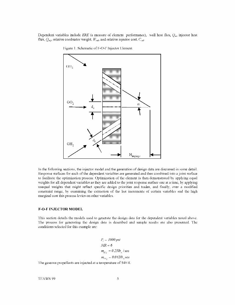
DependentvariablesincludeERE (a measure of element performance),

flux, Qinj, relative combustor weight, V/tel, and relative injector cost, Crel.

Figure 1. Schematic of F-O-F Inj ector Element

GH 2

wall heat flux, Q,_, injector heat

GO 2

GH 2

Himpinge

In the following sections, the injector model and the generation of design data are discussed in some detail.

Response surfaces for each of the dependent variables are generated and then combined into a joint surface

to facilitate the optimization process. Optimization of the element is then demonstrated by applying equal

weights for all dependent variables as they are added to the joint response surface one at a time, by applying

unequal weights that might reflect specific design priorities and trades, and finally, over a modified

constraint range, by examining the extraction of the last increments of certain variables and the high

marginal cost this process levies on other variables.

F-O-F INJECTOR MODEL

This section details the models used to generate the design data for the dependent variables noted above.

The process for generating the design data is described and sample results are also presented. The

conditions selected for this example are:

Pc = lO00psi

MR=6

m_,o, = 0.251b /sec

m_,_2 = 0.0421b sec

The gaseous propellants are injected at a temperature of 540 R.

TFAWS 99 5

MODELSFORDEPENDENTVARIABLES

Asnotedabove,theempiricaldesignmethodologyusedtocharacterizetheERE and Q,_ was developed by

Calhoon et al. This methodology uses a quantity called the normalized injection momentum ratio to

correlate the mixing at the different design points for the triplet element. They define this quantity as

MR.,- 23rn°ur_ (1)mfu f sina

The maximum mixing, and thus maximum ERE, occurs at an MRni of 2.0. Since the propellant mass

flowrates are fixed, only the propellant velocities and the impingement half-angle influence the normalized

injection momentum ratio. The velocities are proportional to the square root of the respective pressure

drops across the injector, AP o and APe For the flow conditions and variable ranges considered in this

problem, MRni ranges from 3.2 to 17.8. Accordingly, lowering APo, raising APy, increasing c_, or somecombination of these actions will increase ERE.

The wall heat flux is correlated with the propellant momentum ratio as defined by

MR = _ (2)mf uf

For the F-O-F triplet element, the maximum wall heat flux occurs at a momentum ratio of approximately

0.4. High heat flux is the result of over-penetration of the fuel jet which produces a high O/F in the wall

region. For the flow conditions and variable ranges considered in this effort, MR ranges from 1.06 to 2.11.

Hence, increasing the value of this ratio by either increasing AP o or decreasing AP/ lowers the wall heatflUX.

The heat flux seen by the injector face, Q*_2, is qualitatively modeled by the impingement height, H,m/_ge.

The notion being that, as the impingement height decreases, the combustion occurs closer to the injector

face, causing a proportional increase in Q*_2 Thus, for the purposes of this exercise, Qi_2 is modeled as the

reciprocal of the H,m/nge. Impingement height is a function of c_ and zlP/Reference to Fig. 1 shows that as

c_ is increased, Him/_g_ is shortened. The dependence of Him/_g_ on the fuel orifice diameter, dy, and thus,

APy; results from making the freestream length of the fuel jet, If,, a function of dy17. For each APy; If, was

set to six times df for an impingement half-angle of 30 °. So, as df increases (corresponding to decreasing

APy), If, increases, as does Him/_g _.

The models for V/r_1 and Crel are simple but represent the correct trends. V/_I is a function only of Loo,_, the

combustor length from injector face to the end of the chamber barrel section. The dimensions of the rest of

the thrust chamber assembly are assumed to be fixed. So, as Loomb increases, V/_I increases accordingly. The

model for C_I is based on the notion that smaller orifices are more expensive to machine. Therefore, C_I is a

function of both propellant pressure drops. As the zlP's increase, the propellant velocity through the injector

increases and the orifice area decreases. So, as either, or both, APo and AP/increase, Crel increases.

GENERATION OF DESIGN DATA

The system variables given above and independent variables (constrained to the previously noted ranges)

are used to generate the design data for element optimization studies. Since propellant momentum ratio is

an important variable in the empirical design methodology, a matrix of momentum ratios was developed

over the 100-200 psi propellant pressure drop range. The matrix of 49 combinations of fuel and oxidizer

pressure drops is shown in Table 1 where momentum ratios range from 1.06 to 2.11. Nine pressure drop

combinations, eight around the border and one in the middle, were selected for use in populating the design

data base. These nine points are highlighted in Table 1 in bold type.

TFAWS 99 6

Table 1. Propellant Momentum Ratio as a Function of Propellant Pressure Drops.

iiiiiiiiiiiiiiiii_OOiiiiiiiiiiiiiiiiiiiiiiiiiiii

iiiiiiiiiiiiiiiii_i_0iiiiiiiiiiiiiiiiiiiiiiiiiiii

iiiiiiiiiiiiiiiii_i_0iiiiiiiiiiiiiiiiiiiiiiiiiiii

1.49

1.57

1.67

1.73

1.79

1.93

2.11

1.42

1.50

1.59

1.64

1.70

1.83

2.00

1.33

1.41

1.50

1.54

1.60

1.72

1.89

1.30

1.37

1.45

1.49

1.55

1.67

1.83

1.25

1.32

1.40

1.44

1.50

1.61

1.77

1.16

1.22

1.30

1.34

1.39

1.50

1.64

1.06

1.11

1.18

1.22

1.27

1.37

1.49

Detailed design results for the case with both APo and APj- at 200 psi are shown in Table 2. Similar datawas generated for the other eight pressure drop combinations. There are 20 combinations of Lco_ and c_for

each zip combination, making a total of 180 design points selected. Seventeen of these were outside the

database embodied by the empirical design methodology, resulting in 163 design points actually being

evaluated. The data trends are as expected. ERE, for a given AP combination, increases with increasingLco,,_ and c_. The increased L_o_ provides more residence time for the propellants to mix and burn.

Increasing c_increases the radial component of the injected fuel, thus providing better mixing. The wall heat

flux is constant for a given AP combination. Impingement height increases with increasing c_. Relative

combustor cost increases with increasing L_o,,_ and the relative injector cost is constant for a given zipcombination.

Table 2. Design Data for APo and APf= 200 psi.

iiiiiiiiiiiiiiiiiiiii_i_i_iiiiiiiiiiiiiiiiiii:iiiiiiiiiiiiiiiiiiiiNN_iiiiiiiiiiiiiiiiiiiiiiiiiiiiiiiiiiii_i_iiiiiiiiiiiiiiiiiiiiiiiiiiiiiiiiiiiiiiiii_iiiiiiiiiiiiiiiiiiiiiiiiiiiiiiiiiiiiiiiiiiiiiiENEiiiiiiiiiiiiiiiiiiiiiiiiiiiiiiiiiiiiiiiii_iiiiiiiiiiiiiiiiiiiii0.923 1.0830.923 1.0830.923 1.0830.923 1.083

0.923 1.083

200 200 2 15 NA 0.85 0.84200 200 2 20 85 0.85 0.62200 200 2 30 92.8 0.85 0.39200 200 2 45 95.4 0.85 0.23

200 200 2 50 95.8 0.85 0.19

200 200 4 15 91 0.85 0.84 1 1.083200 200 4 20 95.2 0.85 0.62 1 1.083200 200 4 30 96.8 0.85 0.39 1 1.083200 200 4 45 98.1 0.85 0.23 1 1.083200 200 4 50 98.4 0.85 0.19 1 1.083

200 200 6 15 95.6 0.85 0.84 1.077 1.083200 200 6 20 97.8 0.85 0.62 1.077 1.083200 200 6 30 98.5 0.85 0.39 1.077 1.083200 200 6 45 99.2 0.85 0.23 1.077 1.083200 200 6 50 99.4 0.85 0.19 1.077 1.083

200 200 8 15 98.3 0.85 0.84 1.154 1.083200 200 8 20 99.1 0.85 0.62 1.154 1.083200 200 8 30 99.4 0.85 0.39 1.154 1.083200 200 8 45 99.6 0.85 0.23 1.154 1.083200 200 8 50 99.7 0.85 0.19 1.154 1.083

TFAWS 99 7

RESPONSE SURFACE GENERATION

In this effort, method i uses the Response Surface Method (RSM) to find optimal values of ERE, Q,,, Qi,j,

V/tel and Crel for acceptable values of APo, APj, Lcomb and c_. The approach of RSM is to perform a series of

experiments, or numerical analyses, for a prescribed set of design points, and to construct a response surface

of the measured quantity over the design space. In the present context, the five responses of interest are

ERE, _w, _inj, _frel and C_I. The design space consists of the set of relevant design variables APo, ziP/, Lco_

and c_. The response surfaces are fit by standard least-squares regression with a quadratic polynomial using

the JMP 18 statistical analysis software. JMP is an interactive, spreadsheet-based program which provides a

variety of statistical analysis functions. A backward elimination procedure based on t-statistics is used to

discard terms and improve the prediction accuracy 19.

INDIVIDUAL RESPONSE SURFACES

When the JMP software is used to analyze the 163 design points, five individual full response surfaces for

the variables in the design space are approximated by quadratic polynomials that contain 15 terms each.

Using the t-statistics approach noted above and detailed in Tucker et al 7, unnecessary terms in each equation

can be eliminated to give the reduced surfaces shown below in equations 3-7.

ERE: O.O028Loom_APo -O.O043.__om_AP f -0.2248Loomb 2 + O.O0024APo_z -O.O0051JPf_z --O. 044&_or_b_Z (3)

_?.O06_z 2 - 0.031 ldPo + O.0547APf + 5.268Loomb + 0.814_z + 63.344

Q_ : O.000017APoo 2 _ O.00002 lJ PooAP, + 0.0000075dP,2 _ O.O04NPo + O.O029AP, + O. 959 (4)

H ........ : O.O000034NPf 2 + O.O00028dPfa + 0.00058_ 2 -O.O027APf - 0.061a + 1.924 (5)

_e, = O.038,qoomb + 0.846 (6)

C,e, : q).OOOOO3,NPo 2 + O.O00006,NP_ - O.O043APo - O.O0096JP, + 0.845 (7)

A SUlvey of the reduced response surfaces indicates that the equations reflect the functionality used to

construct the models for the dependent variables.

JOINT RESPONSE SURFACES

In the current study, it is desirable to attempt to maximize ERE and while simultaneously minimizing _,_,

Q_,j, V/_ I and C_I. One method of optimizing multiple responses simultaneously is to build from the

individual responses a composite response known as the desirability function. The method allows for a

designer's own priorities for the response values to be built into the optimization procedure. The first step

in the method is to develop a desirability, d, for each response. In the case where a response should be

maximized, such as ERE, the desirability takes the form:

=\ B- A ) (8)

where B is the target value and A is the lowest acceptable value such that d 1 for any ERE > B and d 0

for ERE < A. The power value s is set according to one's subjective impression about the role of the

response in the total desirability of the product. In the case where a response is to be minimized, such as

_,_, the desirability takes on the form:

LC - E/

TFAWS 99 8

whereC is the target value and E is the highest acceptable value such that d = 1 for any Q,_ < C and d = 0

for Q,_ > E. Choices for A, B, C, and E are chosen according to the designer's priorities or, as in the present

study, simply as the boundary values of the domain of ERE and Q,_.

Figure 2. Desirability Function for Various

Weight Factors, s. Response Value

A B

1.0 1.0

0.8 0.8

0.6 0.6 G

0.4 0.4

0.2 0.2

0.0 0.0

A B

Choices for s and t are more difficult, but plots such as Figure 2 can be instructive. Figure 2 shows the

appearance of the desirability function for the case of maximizing a response. Desirabilities with s<<l

imply that a product need not be close to the response target value, B, to be quite acceptable. But s 8,

say, implies that the product is nearly unacceptable unless the response is close to B.

A single composite response is developed which is the geometric mean of the desirabilities of the individual

responses. The composite response is defined as:

D= (d 1 .d 2 .d 3 ...din) Ym (10) The

complete joint response surface for the present case is given by:

# )'

OPTIMIZATION RESULTS & DISCUSSION

Three set of results are presented below to demonstrate the capability of method i for the current injector

design. These three examples illustrate the effect of each variable on the optimum design, the trade-offs

between life and performance issues, and the effect on the design of extracting the last increment of

performance.

EFFECT OF EACH VARIABLE ON THE DESIGN USING ORIGINAL CONSTRAINTS & EQUAL

WEIGHT S

TFAWS 99 9

The results in this section were obtained by building the joint response surface with the addition of one

dependent variable at a time. The results are shown in Table 3. Since current non-optimizer based designmethods yield high-performing injector elements, simply maximizing the ERE is not a challenge.

Accordingly, the initial results (Case 1) are obtained with a joint ERE and Q,_ response surface. The resultsin Case 2 have the impingement height added, Case 3 adds the relative chamber weight and the relative cost

is added in Case 4. All results are obtained using the original independent variable constraints and alldependent variables have equal weights of one. The results for Case 1 show that ERE is at its maximum and

Q,_ is very near its minimum desirability limit. Minimizing _,_ requires a small APf relative to APo asevidenced by the values of 100 psi and 183 psi, respectively. Maximum ERE values are found at the longest

chamber length, Lcomb=8 inches. Even with the relatively high value of 183 psi for AP o and low value of APfof 100 psi, ERE is maximized to 99.9% with an impingement half-angle of 33.1 °.

Table 3. Effect of Each Variable on the Design--Optimal Designs for Original Constraints & Equal Weights

iiiiiiiiiiiiiiiiiiiiiiiiiN_i_NNiiiiiiiiiiiiiiiiiiiiiiiiiiiii.....................................................iiiiiiiiiiiiiiiiiiii_Niiiliiiiiiiiiiiiiiiiiiiiiiiiiiiiiiiiiiiiiiiiiiiii_ii_iiiiiiiiiiiiiiiiiiiiiiiiiiiiiiiiiiiiiiiiiiiiiiiN_iiiliiiiiiiiiiiiiiiiiiiiiiiiiiiiiiiiiiiiiiiiiiii_N_iiliiiiiiiiiiiiiiiiiiiiiiiiiii

APo 100-200 183 183 179 100

APr 100-200 100 132 149 100

Lcomb 2-8 8.0 8.0 6.6 6.5

(_ 15-50 33.1 18.9 22.3 24.0

ERE

Qw

Himpinge

Wrel

95.0-99.9

0.7-1.3

0.2-1.0

99.9

0.74

98.3

0.76

0.75

98.0

0.79

0.61

98.0

0.86

0.63

0.9-1.2 -- -- 1.1 1.1

Crel 0.7-1.1 -- -- -- 0.93

Addition of the impingement height to Case 2 to model the injector face heat flux, _,j, forces c_lower toincrease hr_p_,g_ and decrease _,j. This decrease in the radial component of the fuel momentum has an

adverse affect on ERE. This effect is mitigated to a degree by increasing the APfby 32 psi to 132 psi. ERE

is still reduced by 1.6%. Also, the increase in APf causes increased penetration of the fuel jet which resultsin a slightly higher _,_.

Case 3 adds the relative combustor weight to the list of dependent variables modeled. Since V/_I is only afunction of Lcomb, minimizing V/_I shortens the combustor length from 8 to 6.6 inches. The shorter L_o,,_

tends to lower ERE. This effect is offset to a large degree by increases in APf and c_,both of which increasethe radial component of the fuel momentum. The increase in APf also causes a slight increase in Q,_. The

increase in c_causes a significant decrease in H_p_,g_ which increases the injector face heat flux.Finally, the relative cost of the injector is added in Case 5. Since C_I is only a function of propellant

pressure drops, both AP o and APf are driven to their respective minimum values. This and a slight increasein c_allow ERE to be maintained at 98%, even with a slight decrease in L_o,,_. The largest effect of this fairly

dramatic decrease in propellant pressure drops is on _,_. Even though the values for APo and APf fell, APfincreased relative to AP o causing _,_ to increase by almost 9%. Impingement height and relative combustor

weight are essentially unchanged.Although several of the variables included in this exercise are qualitative, an important conclusion can still

be drawn. The sequential addition of dependent variables to an existing design results in changes to both theindependent and dependent variables in the existing design. The direction and magnitude of these changes

depends on the sensitivity of the variables, but the changes may well be significant. The design in Case 4 is

TFAWS 99 10

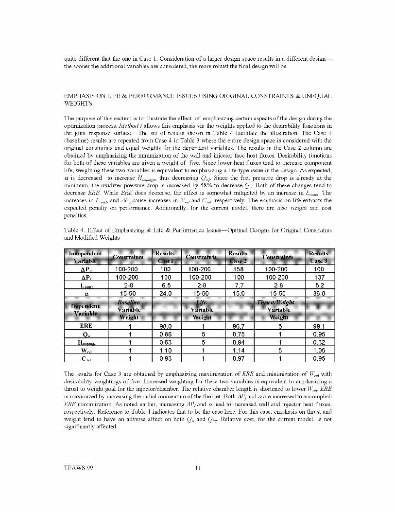
quitedifferentthattheoneinCase1.Considerationofalargerdesignspaceresultsinadifferentdesign--thesoonertheadditionalvariablesareconsidered,themorerobustthefinaldesignwillbe.

EMPHASISONLIFE& PERFORMANCEISSUESUSINGORIGINALCONSTRAINTS& UNEQUALWEIGHTS

Thepurposeofthissectionistoillustratetheeffectof emphasizingcertainaspectsofthedesignduringtheoptimizationprocess.Method i allows this emphasis via the weights applied to the desirability functions in

the joint response surface. The set of results shown in Table 4 facilitate the illustration. The Case 1(baseline) results are repeated from Case 4 in Table 3 where the entire design space is considered with the

original constraints and equal weights for the dependent variables. The results in the Case 2 column areobtained by emphasizing the minimization of the wall and injector face heat fluxes. Desirability functions

for both of these variables are given a weight of five. Since lower heat fluxes tend to increase componentlife, weighting these two variables is equivalent to emphasizing a life-type issue in the design. As expected,

c_ is decreased to increase //impinge, thus decreasing Qinj. Since the fuel pressure drop is already at theminimum, the oxidizer pressure drop is increased by 58% to decrease Q,_. Both of these changes tend to

decrease ERE. While ERE does decrease, the effect is somewhat mitigated by an increase in Lcomb. The

increases in Lcomb and AP o cause increases in Wrel and Cr_1, respectively. The emphasis on life extracts theexpected penalty on performance. Additionally, for the current model, there are also weight and cost

penalties.

Table 4. Effect of Emphasizing & Life & Performance Issues--Optimal Designs for Original Constraintsand Modified Weights

iiiiii iiiiiiiiiiiiiiiiii iiiiiiiiiiiiiiiii iiiiiiiiiiiiiiiii_NNiiiiiiiiiiiiiiiiiiiiii iiiiiiiiiii_:_fiiiiiiiiiiiiii

APo

APf

Lcomb

100-200 100

100-200 100

2-8 6.5

15-50 24.0

iiiiiiiiiiiiiiiii_l_iiiiiiiiiiiiiiiiiiiiiiii...........................................................iiiiiiiiiiiiiiiii_iNiiiiiiiiiiiiiiiiiiiiii.............................

iiiiiiiiiiiiiiiiiiiii_N_

iiiiiii__i_iiiiiiiiiiiiiiiii

100-200

100-200

2-8

15-50

iiiiiiiiiiiiiiiiiiiiiiiiiiiii_=._*iiiiiiiiiiiiiiiii_l{_iiiiiiiiiiiiiiiiiiiiiiii

iiiiiiiiiiiiiiiiiiiii_i

iiiii_lNiiiiiiiiiiii

iiiiiiii_iii2iiiiiiiiiiiiii

158

100

7.7

15.0

iiiiiiiiiiiiiii__iiiiiiiiiiiiiiiiiiiiiiiii

100-200

100-200

2-8

15-50

.............................iiii_N_

iiiiii_iiiiiiiiiiiii

iiiiiiii_iii_iiiiiiiiiiiiii

100

137

5.2

36.0

_ii_iiiiiiiiiiiiiiiiiiiiiiiiiiiiiiiiiiiiiiiiiiiiiiiiiiiiiiiiiiii

ERE 1 98.0 1 96.7 5 99.1

Q,_- 1 0.86 5 0.75 1 0.95

Himpinge 1 0.63 5 0.94 1 0.32Wrel 1 1.10 1 1.14 5 1.05

Crel 1 0.93 1 0.97 1 0.95

The results for Case 3 are obtained by emphasizing maximization of ERE and minimization of W_z with

desirability weightings of five. Increased weighting for these two variables is equivalent to emphasizing athrust to weight goal for the injector/chamber. The relative chamber length is shortened to lower W_z. ERE

is maximized by increasing the radial momentum of the fuel jet. Both APf and c_are increased to accomplishERE maximization. As noted earlier, increasing APf and c_lead to increased wall and injector heat fluxes,respectively. Reference to Table 4 indicates that to be the case here. For this case, emphasis on thrust and

weight tend to have an adverse affect on both _,_ and _nj. Relative cost, for the current model, is notsignificantly affected.

TFAWS 99 11

EXTRACTIONOFLASTPERFORMANCE& WEIGHTINCREMENTS(MODIFIEDCONSTRAINTS& UNEQUALWEIGHTS)

Here,thehighmarginalcostof realizingthelastincrementof thrusttoweightis shown.Thissectionillustratesthecapabilitytomodifytheconstraintsontheindependentvariablesanduseunequalweightsonthedependentvariablesatthesametime.TheresultsforCase3inTable4arecarriedovertoCase1inTable5asthebaselineforthisexample.HeretheoriginalconstraintsareusedbutincreasedweightshavebeenappliedtoemphasizeERE and V/tel. Cases 2 and 3 modify the constraints on the propellant pressure

drops, raising the minimum pressure drop from 100 psi to 150 psi. For Case 2, both APo and APf are now atthe minimum level for the modified constraints. Lco,_ is increased slightly to maintain ERE. The decrease of

APf relative to APo causes a decrease in Q,_. The slightly higher pressure drops also cause Crel to increasesomewhat. Other variables are not changed appreciably.

Table 5. Effects of Realizing the Last Increments of Performance & Weight--Optimum Designs for

Modified Constraints and Unequal Weights

iiiiii__iiiiiiiiii iiiiiiiiiiiiiiiiiii_!iiiiiiiiiiiiiiiiiiiiiiiiiiiiii_i_iiiiiiiiiiiiiiiiM_i_aiiiiiiiiii_iiiiiiiiiii_l_iiiiiiiiiiiiiiiiiiiiiiii_a_iiiiiiiiii_iiiiiiiiiiiiii_iiiii_iiiiiiiiiiii_

APo 100-200 100 150-200 150 150-200 150

,,_Pf 100-200 137 150-200 150 150-200 200

Lo,.b 2-8 5.2 2-8 5.4 2-8 4.4

15-50 36.0 15-50 35.6 15-50 44.8

_i_i_i_i_i__iiiiiiiiiiiiiiiiiiiiiiiiiiiiiiii_lfl_iiiiiiiiiiiiiiiiiiiiii______________________________________________________________________________________________________________________iiiiiiiiiiiiiiiii_l[_iiiiiiiiiiiiiiiiiiiiiii _lfl_iiiiiiiiiiiiiiiiiiiiiiiiiiiiiiiiiiiiiiiiiiiiiiiiiiiiiiiiiiii

ERE 5 99.1 5 99.0 10 99.1

Q,_- 1 0.95 1 0.84 0.1 0.95

H_,.p_._ 1 0.32 1 0.31 0.1 0.21W_d 5 1.05 5 1.05 10 1.01

C_d 1 0.95 1 1.00 0.1 1.07

For Case 3, ERE and V/_z are further emphasized by increasing their desirability weights to 10 while

decreasing the other weights to 0.1. Lcom_ is shortened to respond to the increased emphasis on weight

minimization. Maintaining the high level of ERE requires large increases in APf and c_to increase the radial

component of the fuel jet momentum. The increase in APf causes over-penetration of the fuel jet which

results in an increase in wall heat flux. The large increase in a yields the expected decrease in hr_e_,_ whichincreases the injector face heat flux. The additional emphasis on ERE and C_z yields essentially no increase

in ERE in this range of zip 's, although a small weight savings is seen. These marginal improvements are

offset by fairly large increases in C_z and Q*-2

SUMMARY

An unlike impinging GO2/GH2 injector element design has been employed to facilitate optimization studies.Starting with propellant pressure drops, combustor length, and impingement half-angle, an empirical design

methodology was used to calculate the dependent variables for 163 design points. The dependent variableswere energy release efficiency, chamber wall and injector face heat fluxes, relative chamber weight, and

relative injector cost. The response surface methodology was used to fit the results with quadraticpolynomials. Desirability functions were used to create joint response surfaces which were used in the

optimization studies.

TFAWS 99 12

Three sets of results were generated to illustrate the capability of method i in the context of injector design

and optimization. The first set of results started with a design optimized for ERE and Q,_, then added the

other three dependent variables to the design one at a time. Each sequential optimal design was different

than previous designs with the final design being quite different than the initial design. The result

qualitatively showed the importance of including as many variables as possible early in the design. The

optimization techniques embodied in method i facilitate this early inclusion by allowing efficient

management of large amounts of data.

The second set of results focuses on the inherent design trade-offs between performance and component life

issues. Different weights were applied to emphasize variables related to performance (ERE and Wrel). While

the thrust to weight ratio was improved, the adverse affect on variables related to component life (Q,_ and

Qi_) were clearly shown. Conversely, when Q,_ and Qinj were emphasized, the toll on the performance

variables was clear. These techniques can be used to identify both qualitative trends and to examine the

quantitative trade-offs present in this and other design processes.

Finally, a third set of results was used to illustrate the effect on the over all design of different degrees of

emphasis on certain variables. Over a narrower range of some of the independent variables, ERE and Wrel

were weighted over the other variables by a factor of 5 and then by a factor of 100 in the composite

desirability function. As the emphasis on ERE and W_I was increased, the resulting marginal improvements

were shown to be offset by the fairly large adverse effects on the other variables. Method i allows the

designer to objectively evaluate these adverse effects as he seeks to improve the design.

The flexibility and utility of method i have been demonstrated in this effort. Use of method i can allow an

injector designer to confidently and efficiently manage large amounts of data to conduct a range of design

optimization studies. Constraints on independent variables can be modified to allow optimum designs to be

sought in specific portions of the parameter space. Also, individual or specific groups of dependent

variables can be emphasized to reflect a designer's priorities in the design optimization process.

A similar study will be conducted for a GO2/GH2 swirl coaxial injector element. Then, the data and

response surfaces generated for the shear coaxial, swirl coaxial, and impinging elements will be used to

demonstrate the ability of method i to select an optimum element type based on a range of constraints and

design priorities.

REFERENCES

1. Personal Communication with Garry Lyles.

2. Rupe, J. H., "An Experimental Correlation of the Nonreactive Properties of Injection Schemes and

Combustion Effects in a Liquid Rocket Engine," NASA TR 32-255, 1965.

3. Pieper, J. L., "Oxygen/Hydrocarbon Injector Characterization," PL-TR 91-3029, October, 1991.

4. Nurick, J. H., "DROPMIX - A PC Based Program for Rocket Engine Injector Design," JANNAF

Propulsion Conference, Cheyenne, Wyoming, 1990.

5. Dickerson, R., Tate, K., Nurick, W., "Correlation of Spray Injector Parameters with Rocket Engine

Performance," AFRPL-TR-68-11, January, 1968.

6. Pavli, A. L., "Design and Evaluation of High Performance Rocket Engine Injectors for Use with

Hydrocarbon Fuels," NASA TM 79319, 1979.

7. Tucker, P. K., Shyy, W, Sloan, J. G., "An Integrated Design/Optimization for Rocket Engine Injectors,"

34 th AIAA/ASME/SAE/ASEE Joint Propulsion Conference and Exhibit, July 13-15, 1998, AIAA 98-3513,

Cleveland, OH.

8. Shyy, W, Tucker, P. K. and Vaidyanathan, R., "Response Surface and Neural Network Techniques for

Rocket Engine Injector Optimization," 35 th AIAA/ASME/SAE/ASEE Joint Propulsion Conference and

Exhibit, June 20-23, 1999, AIAA 99-2455, Los Angeles, CA.

9. Calhoon, D., Ito, J. and Kors, D., "Investigation of Gaseous Propellant Combustion and Associated

Injector-Chamber Design Guidelines," Aerojet Liquid Rocket Company, NASA CR-121234, Contract

NAS3-13379, July 1973.

10. Calhoon, D., Ito, J. and Kors, D., "Handbook for Design of Gaseous Propellant Injectors and

Combustion Chambers," NASA CR- 121234, Contract NAS3-13379, July 1973

TFAWS 99 13

11.Foust,M. J., PalS.,andSantoro,R. J. _GaseousPropellantRocketStudiesUsingRamanSpectroscopy,"AIAA96-2766,32ndAIAA/ASME/SAE/ASEEJointPropulsionConference,July1-3,1996,LakeBuenaVista,FL.12.Moser,M.D.Pal,S.andSantoroR.J.,_LaserLightScatteringMeasurementsin aGO2/GH2Uni-ElementRocketChamber,"AIAA95-0137,33rdAerospaceSciencesMeetingandExhibit,January9-12,1995,RenoNV.13.Santoro,R. J., _AnExperimentalStudyof CharacteristicCombustion-DrivenFlowfor CFDValidation,"FinalReportforNASAContractNAS8-38862,October,1997.14.Tucker,P.K.,Klem,M.D.,Smith,T.D.,Farhangi,S.,Fisher,S.C.,andSantoro,R.J.,_DesignofEfficientGO2/GH2Injectors:A NASA,IndustryandUniversityEffort,"AIAA 97-3350,33rdAIAA/ASME/SAE/ASEEJointPropulsionConference,July6-9,1997,Seattle,WA.15.Schley,C.A.,Hagemarm,G.,Tucker,P.K.,Venkateswaran,S.andMerkle,C.L.,_ComparisonofComputationalCodesforModelingHydrogen-OxygenInjectors,"AIAA97-3302,33rdAIAA/ASME/SAE/ASEEJointPropulsionConference,July6-9,1997,Seattle,WA.16.Myers,R.H.andMontgomery,D.C.,Response Surface Methodolo_-Process and Product

Optimization Using Designed Experiments, John Wiley & Sons, 1995.

17. Gill, G. S., and Nurick, W. H., _Liquid Rocket Engine Injectors," NASA SP-8089, March, 1976.

18. SAS Institute Inc. (1995). JMP version 3. Cary, NC.

19. Microsoft Corporation. (1985-1996). Microsoft Excel 97

TFAWS 99 14

RAMAN SPECTROSCOPY FOR INSTANTANEOUS MULTIPOINT, MULTISPECIES GASCONCENTRATION AND TEMPERATURE MEASUREMENTS IN ROCKET ENGINE

PROPELLENT INJECTOR FLOWS

Joseph A. WehrmeyerResearch Associate Professor

Mechanical Engineering Department

Vanderbilt University

Huu Phuoc Trinh

Combustion Devices Group

Subsystem and Component Development Department

Space Transportation Directorate

Abstract

Propellent injector development at MSFC includes experimental analysis using optical

techniques, such as Raman, fluorescence, or Mie scattering. For the application of spontaneous

Raman scattering to hydrocarbon-fueled flows a technique needs to be developed to remove the

interfering polycyclic aromatic hydrocarbon fluorescence from the relatively weak Raman

signals. A current application of such a technique is to the analysis of the mixing and

combustion performance of multij et, impinging-j et candidate fuel injectors for the baseline Mars

ascent engine, which will burn methane and liquid oxygen produced in-situ on Mars to reduce

the propellent mass transported to Mars for future manned Mars missions. The present technique

takes advantage of the strongly polarized nature of Raman scattering. It is shown to be

discernable from unpolarized fluorescence interference by subtracting one polarized image from

another. Both of these polarized images are obtained from a single laser pulse by using a

polarization-separating calcite rhomb mounted in the imaging spectrograph. A demonstration in

a propane-air flame is presented.

Introduction

Technology development associated with advanced space transportation propulsion

systems includes design and analysis of new types of propellent injectors. An effort exists at

NASA-Marshall to include experimentally-obtained reactant/product mixing/combustion

information as part of the injector analysis. Hardware associated with this effort includes an

optically-accessible high pressure combustion chamber sized for single-element fuel injectors

(unielement test article) and a newer, larger modular combustion test article (MCTA) that can

accommodate multi-element fuel injector configurations and that is also optically-accessible.

Optical accessibility allows laser-based methods, such as laser Mie scattering, fluorescence, and

spontaneous Raman scattering, to be applied. Raman spectroscopy has been used to analyze an

oxygen-rich gaseous hydrogen/liquid oxygen (GHz/LOx) injector flow in the unielement test

article (1) and most recently is being considered for use in the MCTA to analyze the mixing and

combustion performance of multij et, impinging-j et candidate fuel injectors for the baseline Mars

ascent engine (2). This engine will bum methane (CH4) and LOx produced in-situ on Mars to

reduce the propellent mass transported to Mars for future manned Mars missions (3).

Applicationof Ramanspectroscopyto hydrocarbon-fueledcombustionbringstheissueofinterferenceof theweakRamanscatteringlight signalswith stronglaser-inducedfluorescence.Thefluorescenceinterferencecanbefrom polycyclicaromatichydrocarbons(PAH's)whichareexcitedandfluoresceacrosstheultravioletandvisiblespectrum(4) andwhenusingultravioletlaserscanbedueto thehydroxylradical(OH)andto vibrationally-excited02,bothof whicharepresentin combustionreactionzones(5). By takingadvantageof thepolarizationpropertiesofRamanscattering,it is possibleto discriminatetheRamansignalfrom interferingfluorescenceinterferenceand hence apply Raman scatteringto the analysisof hydrocarbon-fueledcombustion.Thiscanbedoneby obtainingtwo Ramanimages,oneusingaverticallypolarizedlaserandoneusingahorizontally-polarizedlaser,andthensubtractingtheintensityof oneimagefrom anotherto obtaina netRamansignal(6). A secondmethodthatlendsitselfto single-pulse(andhenceinstantaneous)measurementsis to obtaintwo simultaneousRamanimagescreatedfrom thesamelaserpulse. Oneof theseimagesis thevertically-polarizedsignalandoneis forthehorizontally-polarizedsignal. ThedifferencebetweentheseimagesprovidesthenetRamansignal, freeof fluorescenceinterference.This techniquehasbeendemonstratedfor a time-averagedapplication(7) andthispaperdescribesasingle-pulseapplicationof thetechnique.

Background

Raman scattering is a weak light scattering process that can be understood by realizing

that molecular internal energy can be stored in several modes, including: electronic (quantum

mechanical energy level described by the labels X, A, B, etc.), vibration (v -- 0, 1, etc.), and

rotation (J = 0, 1, etc.), and that light energy is quantized into photons and the energy of each

photon is inversely proportional to wavelength. A Stokes Q-branch Raman scattering process

involves an absorption of one laser photon at the laser wavelength )_I_ASEaand a subsequent

emission of a photon with less energy at a longer wavelength. The Raman wavelength )_aaMAN

depends on the vibrational energy level spacing of the laser and hence is different for each

molecule. The Raman scattering signals are linearly related to the density of each molecular

species and are all relatively weak compared to other light scattering processes, such as Rayleigh

scattering and fluorescence. To increase Raman signal strength a UV laser can be used because

Raman signal strength for a given laser power increases with a decrease in laser wavelength (5).

For the present work a pulsed UV laser, in particular a pulsed, narrowband, tunable KrF excimer

laser is used which produces light in a 0.001 nm bandwidth that is tunable from 248 to 249 nm

and is pulsed up to 50 Hz with a pulse energy of 400 mJ and a pulse length of 20 nsec. Using a

pulsed laser allows rejection of continuous flame emission by gating the light detection system

on only during the laser pulse. A narrowband, tunable laser is used to minimize the problem of

laser-induced OH and 02 fluorescence by tuning the laser bandwidth between fluorescence

excitation lines (5), at least for atmospheric pressure flames, but for high pressure flames

pressure broadening becomes so prevalent that some OH and 02 is to be expected (1).

Figures la and lb shows simulated Raman spectra, using RAMSES (8) for 300 K

reactants in the baseline Mars ascent engine (CH4 and 02) for the baseline O/F ratio of 3. Figure

lb shows the expected Raman spectrum at adiabatic equilibrium and a chamber pressure of 250

psia. These spectra show how Raman scattering can reveal both the extent of mixing of

propellents near the injector face (by the amount of simultaneous occurrence of CH4 and 02) and

the extent of reaction (by the relative amounts of reactants and products detected). The signal

strength of Raman scattering depends on two molecular invariants, the square of the mean

polarizability (a') 2 and the square of the anisotropic polarizability (7') 2. These are used in an

equationfor a constant_, that canbe consideredastheRamanscatteringcrosssectionfor asinglemolecule.Thevalueof • alsodependsonthepolarizationof the incidentlaserbeam,thepolarizationof thedetectedRamansignal,andtheangleof detectedRamansignalwith respecttoincominglaserbeam.For a 90° collectionangleandfor theRamanandlaserbeamsbothin ahorizontalplane,thevalueof • for verticallypolarizedRamansignalis (9):

• = (a') 2+ 1/45(r') 2

and for horizontally polarized Raman signal qb is:

qb = 1/60 (]/,)2

Usually a '2 and 7 '2 are similar in magnitude and thus the vertically polarized light is

almost two orders of magnitude greater than the horizontally polarized light. Thus the Raman

scattering signal essentially retains the polarization of the incoming laser beam. However a

fluorescence light emission process does not retain the laser polarization because of the relatively

long time the molecule exists in the excited state before fluorescing. During this time the

molecule rotates, eliminating any correlation between the polarization of absorbed and emitted

photons.

The difference in polarization properties between Raman and fluorescence is exploited in

the experimental system shown schematically in Fig. 2. It represents a typical UV Raman

system in that a pulsed, narrowband KrF UV laser is used as the light source and an imaging

spectrograph coupled to a gated, intensified CCD camera is used as the detection device. The

intensifier and laser are triggered simultaneously using a Princeton Instruments PG200

programmable pulser. The laser is focused to a beam waist of 250 btm using a 500 mm focal

length lens. The unique feature of this system is the insertion of a calcite rhomb just behind the

entrance slit of the spectrograph. This optical element displaces the horizontally polarized

Raman image about 5 mm from the vertically polarized Raman image, which travels directly

straight through the rhomb. The length of the entrance slit is limited to 4 mm to keep the two

polarized images from overlapping. Figure 3 shows a typical single-pulse image obtained from

the experimental system, and this image shows the relative strength of vertically polarized signal

compared to horizontally polarized signal. The H20 Raman signal (from air humidity) is almost

completely polarized, while the N2 signal is slightly depolarized and the 02 signal is more

depolarized than N2. This corresponds to others' experimental observations (6,10).

Spatially-integrated single-pulse Raman spectra are shown in Fig. 4, obtained from a

slightly premixed C3Hs-air bunsen flame. One of these spectra is the vertically polarized

Raman-fluorescence signal. The horizontally polarized signal shows essentially only the

fluorescence signal, which has two contributions. A broadband component is caused by PAH

fluorescence, extending from below 255 nm to above 275 nm. A second contribution to the

fluorescence background is the OH fluorescence from about 265 to 270 nm, caused by tuning the

laser slightly onto a strong OH transition. This is done to demonstrate the ability of the

technique to simultaneously measure Raman spectra and OH fluorescence. Before subtracting

the horizontally polarized signal from the vertical it is first multiplied by a factor of 2.22 to

account for the ratio in transmission efficiency (for the specctrometer/calcite rhomb) between the

vertically and horizontally polarized signals. The net signal shows a fluorescence-free Raman

spectrum that shows the simultaneous occurrence of CO2 and H20 (products of combustion), CO

andH2(intermediateproducts),andunburnedC3H8. Information about the spatial structure of

the flame can be revealed in the single-pulse image of Fig. 5. This image shows unburned C3H8

occurring near the 0 mm position. The cooler, denser unburned gas mixture also provides a

stronger N2 Raman signal near that location. At -1.5 mm the C3H8 pyrolizes into other

hydrocarbons, including PAH's that cause a strip of broadband fluorescence to appear at this

location. Farther into the flame chemical reactions involving oxidation take place, creating the

OH intermediate. This shows up in Fig. 5 by the replacement of PAH fluorescence with OH

fluorescence at flame positions greater than -2.5 mm. By subtracting the scaled upper part of

Fig. 5 (horizontally polarized fluorescence signal) from the bottom part (vertically polarized

signal), and by summing the net Raman signal for each location (wavelength integration) a

qualitative picture of the structure of the flame can be discerned, as in Fig. 6. This figure shows

the drop in C3H8 signal and the concurrent increase in H20 signal, showing the formation of that

product occurring close to the fuel zone. In the same region the H2 and CO signals are generally

higher than in the fuel zone or in the OH reaction zone past 2.5 mm.

Summary and Conclusions

Taking advantage of the strongly polarized nature of Raman scattering, it can be

discerned from unpolarized fluorescence interference by subtracting one polarized image from

another. Both of these polarized images can be obtained from a single laser pulse by using a

polarization-separating calcite rhomb mounted in the imaging spectrograph. This reduces the

imaged laser beam length from 12.5 mm down to 4 mm but allows fluorescence-free Raman

measurements in propane-air flames. In the pyrolysis zone of these flames considerable PAH

fluorescence exists and in a separate flame zone there exists considerable OH fluorescence.

However the polarization separation technique is robust enough to allow simultaneous Raman

and OH fluorescence measurements to be obtained, which can provide even more informationabout flame chemical reaction zones.

References

1. Wehrmeyer, J. A., J. M. Cramer, R. H. Eskridge, and C. C. Dobson, _UV Raman Diagnostics for Rocket Engine

Injector Development," AIAA Paper 97-2843, 1997.

2. Mueller, P. J., D. W. Plachta, T. Peters, J. C. Whitehead, "Subscale Precursor to a Human Mars Mission Using

In-Situ Propellent Production," AIAA Paper 98-3301, 1998.

3. Kos, L., "The Human Mars Mission: Transportation Assessment," Space Technology and Applications

International Forum Conference, Abuquerque, N.M., Conference Proceedings Part III, p. 1211, Jan. 1998.

4. Smyth, K., Combustion andFlame, 1999.

5. Wehrmeyer, J. A., T.-S. Cheng, and R. W. Pitz, "Raman Scattering Measurements in Flames Using a Tunable

KrF Excimer Laser, Applied @tics 31: pp. 1495-1504, 1992.

6. Granefeld, G., V. Beuhausen, and P. Andresen, "Interference-Free UV-Laser-Induced Raman and Rayleigh

Measurements in Hydrocarbon Combustion Using Polarization Properties," Applied Physics B 61: pp. 473-478.

7. Hartfield, R., C. Dobson, R. Eskridge, and J. Wehrmeyer, "Development of a Technique for Separating Raman

Scattering Signals from Background Emission with Single-Shot Measurement Potential," AIAA Paper 97-

3357, 1997.

8. Hassel, E. P., "Ultraviolet Raman Scattering Measurements in Flames Using a Narrowband Excimer Laser,"

Applied Optics 32, 1993.

9. Long, D., "Raman Spectroscopy," McGraw-Hill, 1977.

10. Permey, C. M., L. M. Goldman, M. Lapp, "Raman Scattering Cross Sections, " Nature Physical Science 235:

pp. 110-112.

!

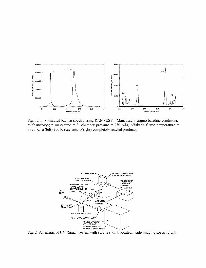
c_

' \....__i '___J

W_VELEN_TH, _'_

J

ol ,_scO,_:L.____.... .j i,..4,._t

Fig. 1a,b. Simulated Raman spectra using RAMSES for Mars ascent engine baseline conditions:

methane/oxygen mass ratio = 3, chamber pressure = 250 psia, adiabatic flame temperature =

3390 K. a (left) 300 K reactants, b(right) completely reacted products.

TO COMPUTER _ DIGITAL CAMERA WITH

/ GATED INTENSIFIER

0.3 m IMAGING r_(//

SPECTROGRAPH . I I I / TRIGGER FOR

50 mm DIA. 250 mm X _ LASER AND' CAMERA

FOCAL LENGTHOUART_DOUBLET_ I_-_ I--''_NS'F',_RBEAM LENSES_ "_ I I _DUMP _/'_J_ I I I_'>< _1 _1

BEAM WAIST [_ _

P_OPA"E_'RFLA"E/ I ''_ I

PULSED UV LASER "_ I I

400 mJ/PULSE _ I I

NARROWBAND: 0.001 nm _ I /

TUNABLE_48 to 249 nm

Fig. 2. Schematic of UV Raman system with calcite rhomb located inside imaging spectrograph.

__iiiii_iiiii_ii_ii_iiiiiiiiiiiiiiiiiiiiiiiiiiiiiiiiii__iiiiiiiiii_

O,_

-am_o

I--N

oI255 WAVELENGTH, nm

Fig. 3. Single-pulse, polarization-resolved

Raman image in humid air.

]

277

1_

Fig 4 Single-pulse, polarization-resolved

Raman spectra in propane-air flame.

B_

...i ¢_

____uI"-N

W_

I

255 WAVELENGTH, nm

Fig 5 Single-pulse, polarization-resolved

Raman image in propane-air flame.

I

277

500°0

_ g "" _- k_.m_ "_,_ "_%

_: . . _'_ s -\ _'_:_<:i? "_-'_, _ "_ _ .....

Fig. 6. Net wavelength-integrated Ramansi__al vs. position for image of Fig. 5.

FASTRAC GAS GENERATOR TESTING

Tomas E. Nesman and Jay Dennis

Subsystem and Component Development Department

Space Transportation Directorate, NASA, MSFC

ABSTRACT

A rocket engine gas generator component development test was recently conducted at the Marshall Space Flight

Center. This gas generator is intended to power a rocket engine turbopump by the combustion of Lox and RP-1.

The testing demonstrated design requirements for start sequence, wall compatibility, performance, and stable

combustion. During testing the gas generator injector was modified to improve distribution of outer wall coolant

and the igniter boss was modified to investigate the use of a pyrotechnic igniter. Expected chamber pressure

oscillations at longitudinal acoustic mode were measured for three different chamber lengths tested. High amplitude

discrete oscillations resulted in the chamber-alone configurations when chamber acoustic modes coupled with feed-

system acoustics modes. For the full gas generator configuration, which included a turbine inlet manifold, high

amplitude oscillations occurred only at off-design very low power levels. This testing led to a successful gas

generator design for the Fastrac 60,000 lb thrust engine.

NOMENCLATURE

D diameter

L length

x axial station downstream of injector

f frequency

P pressure

p' fluctuating pressureO/F oxidizer to fuel mixture ratio

SUBSCRIPTS

g turbulence generator

c combustion chamber

INTRODUCTION

A gas generator for a 60,000 pound thrust rocket engine was tested at the Marshall Space Flight Center (MSFC) test

stand 116 (Figure 1) in 1997 and 1998. This was a Fastrac approach to design and development which required a

robust design, success oriented schedule, and minimal testing. The gas generator is a small cylindrical chamber

where Lox and RP-1 were injected and burned at a low oxidizer to fuel (O/F) mixture ratio. The gas generator

chamber was tested alone and in combination with a turbine inlet manifold (TIM). In the engine configuration, the

hot gas discharges from the gas generator into the turbine inlet manifold which is an annular volume where small

nozzles direct the flow into the turbine blade rows to power the Fastrac turbopump. In the initial component test

configuration, the hot gas discharges from the gas generator through a small nozzle into ambient atmosphere. In the

final component test configuration, the hot gas discharges into a turbine inlet manifold before exiting to the

atmosphere.

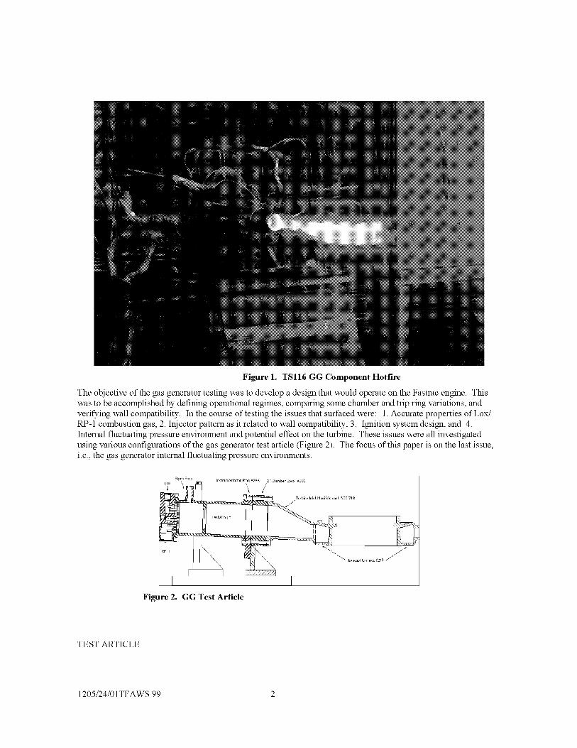
Figure1. TSll6 GG Component Hotfire

The objective of the gas generator testing was to develop a design that would operate on the Fastrac engine. This

was to be accomplished by defining operational regimes, comparing some chamber and trip ring variations, and

verifying wall compatibility. In the course of testing the issues that surfaced were: 1. Accurate properties of Lox/

RP-1 combustion gas, 2. Injector pattern as it related to wall compatibility, 3. Ignition system design, and 4.

Internal fluctuating pressure environment and potential effect on the turbine. These issues were all investigated

using various configurations of the gas generator test article (Figure 2). The focus of this paper is on the last issue,

i.e., the gas generator internal fluctuating pressure environments.

Figure 2. GG Test Article

TEST ARTICLE

1205/24/O1TFAWS 99 2

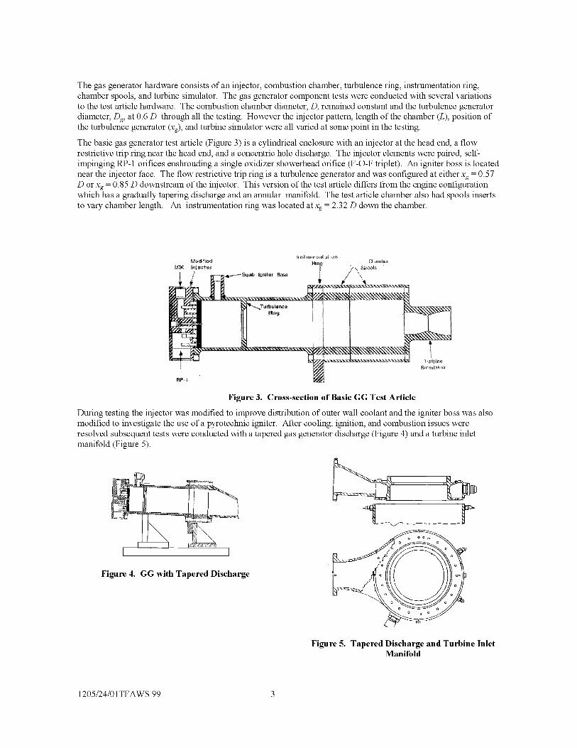
Thegasgeneratorhardwareconsistsofaninjector,combustionchamber,turbulencering,instrumentationring,chamberspools,andturbinesimulator.Thegasgeneratorcomponenttestswereconductedwithseveralvariationstothetestarticlehardware.Thecombustionchamberdiameter,D, remained constant and the turbulence generator

diameter, Dg, at 0.6 D through all the testing. However the injector pattern, length of the chamber (L), position of

the turbulence generator (xg), and turbine simulator were all varied at some point in the testing.

The basic gas generator test article (Figure 3) is a cylindrical enclosure with an injector at the head end, a flow

restrictive trip ring near the head end, and a concentric hole discharge. The injector elements were paired, self-

impinging RP-1 orifices enshrouding a single oxidizer showerhead orifice (F-O-F triplet). An igniter boss is located

near the injector face. The flow restrictive trip ring is a turbulence generator and was configured at either xg = 0.57

D or xg = 0.85 D downstream of the injector. This version of the test article differs from the engine configuration

which has a gradually tapering discharge and an annular manifold. The test article chamber also had spools inserts

to vary chamber length. An instrumentation ring was located at xg = 2.32 D down the chamber.

Figure 3. Cross-section of Basic GG Test Article

During testing the injector was modified to improve distribution of outer wall coolant and the igniter boss was also

modified to investigate the use of a pyrotechnic igniter. After cooling, ignition, and combustion issues were

resolved subsequent tests were conducted with a tapered gas generator discharge (Figure 4) and a turbine inlet

manifold (Figure 5).

[-I

Figure 4. GG with Tapered Discharge

Figure 5. Tapered Discharge and Turbine InletManifold

1205/24/01TFAWS 99 3

INSTRUMENTATION

Thegasgeneratortestarticlewasdesignedwitharingthatcouldbeinsertedintothechamberbodywithafullarrayofinstrumentation.Theinstrumentationringcontainedahighfrequencypressuretransducerandseveralthermocouples.Fivethermocoupleswereinsertedintothechamberthroughtheinstrumentationringwithvaryingdepthsofpenetration.Selectedgasgeneratormeasurementswererecordedontheteststand116highsampledatasystem(Table1).Typicallyfrom11to14ofthesemeasurementswererecordedonanyonetest.Thehighsampletestdatawerelowpassfilteredat10,000Hzandthensampledat40,000samplespersecond.Onedynamicpressuretransducerwasclose-mountedtothechamberinnerwallbuttheotherpressuremeasurementsweresusceptibletosenselineresonancewithlimitedusefulnessforevaluatingfluctuatingpressureamplitudes.

Table 1. High Sample Data Instrumentation

MSID NOMENCLATURE UNIT S

P3001 GG Pc dynamic pressure PSI

P3004 GG Pc pressure # 1 PSI

P3005 GG Pc pressure #2 PSI

P8307 GG Pc upstream turb ring PSI

A3001 Axial accel injector G PK

A3002 Radial accel G PK

A3003 Injector inlet

GG Lox injection

G PK

P2305 PSI

P4304 GG TEA injection pressure PSI

P7350 Turbine inlet manifold simulator PSI

P8306 Fuel manifold pressure # 1 PSI

P8307 Fuel manifold pressure #2 PSI

P8308 GG fuel inlet at RP1 filter PSI

DP8309

T7301Fuel iniection AP

__ GG temp. at instr, rin_

1/4dia. GG temp. at instr, ringTC7302

PSI

mV

mV

TEST RESULTS

Four series of gas generator hotfire tests were conducted at test stand 116. Thirty seven component hotfire tests

in all were completed during the gas generator development. Series 1 consisted of tests 1 through 8 which

were conducted in summer of 1997. These tests featured the modified triplet element injector with film coolant

holes and the baseline gas generator combustion chamber. The eight tests were conducted with chamber

pressures, at the injector end, ranging from 505 to 705 psia and oxidizer-to-fuel mixture ratios ranging from

0.25 to 0.36. The gas generator chamber was exhausted through a 1.1" diameter nozzle. Test duration varied

from 64 seconds to 154 seconds (flight duration).

Series 2 consisted of tests 9 through 24 conducted in fall 1997. Tests 9 through 12 had the gas generator

exhausting through outer nozzles, and tests 13 through 15 went back to the first nozzle configuration. Power

spectral density analysis (PSD) showed an anomalous 1600 - 1870 Hz frequency in the chamber fluctuating

pressure and accelerometers. This frequency appears to coincide with a broader acoustic mode frequency early

on in test 13, the end of test 21, and throughout test 22. The oscillation showed up at a discrete 1660 Hz, with

harmonics, on test 23 (Figure 6). The pressure oscillations produced vibrations of around 26 G rms (Figure 7).

1205/24/01TFAWS 99 4

Figure 6. Chamber Pressure PSD Figure 7. Accelerometer PSD's

The gas generator was inspected after series 1 and again after the first few series 2 tests• Some bluing of the

chamber plus erosion damage to the turbulence generator was noted• The damage is a result of the pressure

drop in the fuel manifold (from top to bottom)• The external thermocouples also showed there is an asymmetry,

with a temperature of 1500 ° F measured at the top and 800 ° at the bottom• The bluing problem was eliminated

by two changes to the gas generator• The first change was to increase the diameter of the RP-1 line into the fuel

manifold from 3/4,, to 1" to create a more uniform flow into the manifold and subsequently the AP across the

injector. The second change was to drill outer wall coolant holes in the injector on the side where high

temperatures were a problem•

Series 3 consisted of Tests 25 through 30 conducted in early 1998. The objectives of these tests were to

develop a pyrotechnic igniter start sequence and demonstrate acceptable operation of the flight configuration

hardware• The hardware was configured with a pyrotechnic igniter, barrel chamber, gradually tapering exhaust

duct, and fuel turbine inlet manifold• This is flight configuration hardware with the exception of drilled holes in

the turbine inlet manifold instead of nozzles. The series 3 tests show that the high amplitude discrete 1870 Hz

frequency is no longer present (Figure 8). A low amplitude resonant condition does occur at the start of someof these tests however•

160

Frequency (Hz)

Figure 8. Dynamic Chamber Pressure Spectragram of Test 30

8,000

-18000

-36000

-54000

-72000

-90000

1205/24/01TFAWS 99 5

Series4consistedof tests31through37infallof1998.Thisseriescompletedtheplannedgasgeneratorcomponentdevelopmenttestprogram.Theprimaryobjectivesofthisseriesoftestsweretorepeatedlydemonstrateproperignitionofthegasgeneratorusinganewpyrotechnicigniterandoperationat40-50%powerlevel•AdditionalobjectivesweretogatherthermalenvirorLmentdataonthecastturbineinletmanifoldanddemonstrategoodignitionwithaheliumatmosphereinthegasgenerator•All testobjectivesweremetandthenewignitersperformedwell.Onthesetests,however,thegasgeneratorexhibitssignificantchamberpressureoscillationsatchamberpressuresbelow260psia(47%ofnominal)•Aninterestingexampleofthisoccurredontest34wherea'_jump"tohigheroscillationlevels(Figure9)wascoincidentwitha"shift"inchamberhotgastemperature(Figure10)andsomechamberoscillationfrequencieschangedfromnarrowbandrandompeaks(Figure11)tohighamplitudediscretepeaks(Figure12).

PSI RMS

0-i0,000 HzComposite

.50,9

25,0

20,0

15,0

10,'3

5,'3

....,_:"" p3159834.116 P2305 PSIG GG LOX INJECTION :: p3159834.116 P300S PSIS GG PC PRESS #2

"_p3159834.116 P830S PSIG GG FUEL/RP-I INLET

400 : :% : :

300 i :

200 : .....

,u<....100

i0TIME SECONDS

0 10 30 40

Test: P03159834.116Engine:Shutdown: 32.621

2:36PM October 01, 1998

Figure 9. Low Pc Test "Jump" in Oscillation Amplitude

.... N'"" p31sge34 116 T7301 DEGF HOT GAS RaKE TEMP #1 12:

.... _---- pSZSgSS4 116 TTS04 DEGF HOT GAS aAKE TEMP #4 S:0

..... _;:b••• pSZSgSS4 116 TTS06 DEGF HOT GAS aAKE TEMP #6 11:ii00

.... h-- pSZSgSS4 116 TTS02 DEGF HOT GAS aAKE TEMP #2 4:O.... _---- pSZSgSS4 116 TTS0S DEGF HOT GAS aAKE TEMP #S 9:O

1000

9S0

9OO ¸

SS0

S00

Test:Engine:Shutdown:

i

/ £,,._ .........................._,'_-_-:,,:,_........... _h / f_ .......... --_-_-4--_ =..-=,>._,..

..................... ...........................!.i..........2O 3O

TIME SECONDS

p3159834 1160

3262i 9:07AM October O5, i998

Figure 10. Low Pc Test "Shift" in Hot Gas Temperatures

1205/24/01TFAWS 99 6

0 1000 2000 _,00 4000 5000 0 4000FREO(Hzl

50,:)O

Figure 11. Low Pc Test "Before-Jump" PSD Figure 12. Low Pc Test "After-Jump" PSD

GENERAL RE SULT S

Based on the general characteristics of gas generator chamber oscillations several oscillation mechanisms were

postulated. Acoustic waveguides of the fluid systems were postulated as the resonators and fluid mechanisms

as exciters. The acoustic modes of the gas generator were of prime importance. The chamber axial dimensions

and oxidizer to fuel mixture ratio (O/F) were two of the key parameters affecting acoustics that were varied

during Fastrac gas generator component testing. Three different gas generator chamber lengths, L, were tested.

The range of test mixture ratios varied from a low O/F = 0.18 to a high O/F = 0.37. Table 2 shows the gas

generator test numbers in a matrix of chamber length versus mixture ratio. The outlined test numbers in Table 2

indicate the use of turbulence ring at xg = 0.85 D downstream of the injector instead ofxg = 0.57 D.

Table 2. Test Matrix

Test Numbers

(O/F) L = 11" L = 15" GG +TIM

LowMR i[0, ]i[, 12, 13, 15, 16, 17, 18, 2&29

(. 18- .26)

Nominal MR 3, 4, 5, 6, 7, 8, 9, 19, 21, 23 26, 27, 30, 31, 34

(.27- .32)

High MR 14, 20, 22, 24 25, 32, 33, 35, 36, 37

(.33 - .37)

1205/24/01TFAWS 99 7

ACOUSTICANALYSIS

ThepropertiesoftheLox/ RP- 1 hot gas at mixture ratios of around 0.3 are difficult to determine. The best

source of this information is a set of data and curve fits resulting from an Aerojet study.1 Estimates of sound

speed using equilibrium equations were higher than measured in the Aerojet study. An empirical analysis

combining both sound speed estimations and measured hot gas temperature and pressure led to a nominal

average chamber sound speed of 1441 ft/s. Furthermore, computational fluid dynamic analysis 2 showed sound

speed varying from around 700 ft/s near the injector to 1000 ft/s at the turbulence generator and increasing

towards the nozzle. The nominal fluid properties for the oxidizer and fuel are shown in Table 3 along with the

hot gas properties at three different mixture ratios.

Table 3. Fluid Properties

Component

Fluid Flow rate

(lbm/s)

GG chamber O/F=0.25 8.1

O/F=0.31 7.2

O/F=0.36 6.4

Oxidizer Inlet Lox 1.7

Fuel Inlet RP- 1 5.46

I Temp(OR) I press(psia) I Density(lb/ft 3)

1,470 551 1.350

1,616 542 0.970

1,706 532 0.717

211 686 63.03

523 630 49.5

Since the gas generator is a long cylinder, standing acoustic waves were expected as in an organ pipe. Even

with the turbine inlet manifold ring attached a variety of standing wave pressure patterns can be envisioned

(Figure 13). For acoustic waves in the chamber, the injector will provide a near rigid termination as will the

nozzle end for the gas generator alone configurations. The turbulence ring will serve to block some axial gas

oscillation and will also generate downstream shear layer oscillations. The acoustic modal patterns can be

checked for consistency with measured relative phase from available high frequency measurements.

iP8307i

Figure 13. GG+TIM Acoustic Mode (typical)

Estimates were made of the gas generator test article acoustic mode frequencies where a constant sound speed

of 1440 ft/s was assumed and the gas generator combustion chamber was modeled as a closed-closed pipe

element. The GG + TIM frequencies were estimated determining the stem and top resonance frequencies of a

T-tube pipe element) The physical system was approximated by assuming static (no flow) hot gas within a T-

tube having all pipe radii equal. Various top and stem standing wave combinations were determined.

The major peaks from measured gas generator chamber dynamic pressure spectra were compiled for most tests.

The spectral peaks occur in integer multiples as would be expected from longitudinal acoustic modes of the gas

generator chamber. The measured peak frequency divided by integer multiple was plotted versus sound speed

(Figure 14). This plot shows the data divides into three distinct linear trends based on the chamber length.

1205/24/01TFAWS 99 8

1200

Table 4. Acoustic Mode Frequencies (Hz)

Mode GG 11

1 T 2,952

2 T 4,897

1 R 5970

1 L 786

2 L 1,572

3 L 2,358

4 L 3,144

TIM 1T --

TIM 2T --

I GG 151 GG+ TIM

2,952 2,952

4,897 4,897

5970 5970

576 252

1,153 511

1,729 758

2,306 1023

-- 765

-- 1275

1000

800

= 600

g

400

200

•. & ,&- .&............... ,_

0 .... I .... I .... I .... I .... I ....

1100 1200 1300 1400 1500 1600 1700

Sound Speed (ft/s)

o Avg fi/i _ Avg fi/i _._ Avg fi/i

--GG 11" L modes --GG 15" L modes ....... GG+TIM L modes

Figure 14. Measured GG Oscillation Frequencies

The instrumentation ring was well situated for measuring chamber pressure fluctuations, however, it would not

be available on the gas generator used in turbopump and engine testing. For those tests the chamber pressure

was measured at a boss located in the chamber wall between the injector and the turbulence ring. Some of the

last gas generator component tests were conducted with dynamic pressure transducers located in the new

location and in the instrumentation ring. The new transducer was able to detect most of the discrete spectral

peaks from the chamber acoustic modes, however, the magnitudes were significantly lower than measured at

the instrumentation ring (Figure 15).

S+60 lOO% pr

, ",'i_,

Figure 15. Measurement Location Change Figure 16. TPA and GG Pc Log PSD's

The turbopump assembly (TPA) was tested several times with a gas generator to power the turbine• On these

tests the gas generator chamber fluctuations were measured at the boss between the injector and the turbulence

generator. A comparison of the chamber fluctuations from the gas generator on the turbopump assembly to the

gas generator component test (Figure 16) shows that in the former the acoustic modes are not excited.

1205/24/01TFAWS 99 9

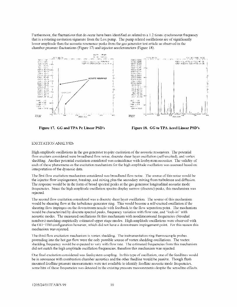
Furthermore,thefluctuationsthatdooccurhavebeenidentifiedasrelatedtoa1.2timessynchronousfrequencythatisarotatingcavitationsignaturefromtheLoxpump.Thepumprelatedoscillationsareofsignificantlyloweramplitudethantheacousticresonancepeaksfromthegasgeneratortestarticleasobservedinthechamberpressurefluctuations(Figure17)andinjectoraccelerometers(Figure18).

S2fL'> 5 _: :_<:)?,

55" £s 5:5_9F

;:!27i ;J _ _i: -i);:?

................... 'i i i

K_

Figure 17. GG and TPA Pc Linear PSD's Figure 18. GG to TPA Accel Linear PSD's

EXCITATION ANALYSIS

High amplitude oscillations in the gas generator require excitation of the acoustic resonators. The potential

flow exciters considered were broadband flow noise, discrete shear layer oscillation (self-excited), and vortex

shedding. Another potential excitation considered was coincidence with feedsystem acoustics. The validity of

each of these phenomena as the excitation mechanism for the high amplitude oscillation was assessed based on

interpretation of the dynamic data.

The first flow excitation mechanism considered was broadband flow noise. The source of this noise would be

the injector flow impingement, breakup, and mixing plus the secondary mixing from turbulence and diffusion.

The response would be in the form of broad spectral peaks at the gas generator longitudinal acoustic mode

frequencies. Since the high amplitude oscillation spectra display narrow (discrete) peaks, this mechanism was

rejected.

The second flow excitation considered was a discrete shear layer oscillation. The source of this mechanism

would be shearing flow at the turbulence generator ring. This would become a self-excited oscillation if the

shearing flow impinges on the downstream nozzle with feedback to the flow separation point. The mechanism

would be characterized by discrete spectral peaks, frequency variation with flow rate, and "lock-in" with

acoustic modes. The measured oscillations fit this mechanism with nondimensional frequencies (Strouhal

numbers) matching empirically estimated upper stage modes. High amplitude oscillations were observed with

the GG+TIM configuration however, which did not have a downstream impingement point. For this reason this

mechanism was rej ected.

The third flow excitation mechanism is vortex shedding. The instrumentation ring thermocouple probes

protruding into the hot gas flow were the only possible source of vortex shedding oscillations. The vortex

shedding frequency would be expected to vary with flow rate. The estimated frequencies from this mechanism

did not match the high amplitude oscillation frequencies, therefore this mechanism was rejected.

One final excitation considered was feedsystem coupling. In this type of oscillation, one of the feedlines would

be in resonance with combustion chamber acoustics and the other feedline would be passive. Though flush

mounted feedline pressure measurements were not available to identify feedline acoustic mode frequencies,

some hint of these frequencies was detected in the existing pressure measurements despite the senseline effects.

1205/24/01TFAWS 99 10

Inaddition,frequencyresponsefunctionsshowedsomecorrelationbetweenfeedlinemeasurementsandchambermeasurementsduringhighamplitudeoscillations.Ontest34,forexample,basedoncoherence(Figure19)it appearsthattheloxfeedlineisapassiveelementinthehighamplitudeoscillationresonance.thissametesthowever,thefuelfeedsystem(Figure20)andtheturbineinletmanifold(Figure21)appeartoparticipateintheacousticresonanceofthechamber.

On

P3001 GG Pc DYNAMIC PRESSURE X P2305 GG LOX INJECTION I

w 0.8u

0.60.4

Oo 0.2

0 500 1000 1500 2000 2500 3000 3500 4000 4500 5000

Frequency (Hz)

1

w 0.8u

0.6

0.4Oo 0.2

Figure 19. Lox Feedline to Chamber Coherence

I ..............P3001 GG Pc DYNAMIC PRESSURE X P8306 FUEL MANIFOLD #1 I

0 500 1000 1500 2000 2500 3000 3500 4000 4500 5000

Frequency(Hz)

Figure 20. Fuel Feedline to Chamber Coherence

I - P3001 GG Pc DYNAMIC PRESSURE X P7350 T/S MANIFOLD I

8

t0.4

0.2

0

0 500 1000 1500 2000 2500 3000 3500 4000 4500 5000

Frequency (Hz)

Figure 21. TIM to Chamber Coherence

1205/24/01TFAWS 99 11

CONCLUSIONS

Component testing was performed at MSFC to develop a gas generator design that would operate on the Fastrac

engine. This was accomplished by performing 37 tests to address several design issues that surfaced. The gas

generator internal fluctuating pressure environment was one of these issues. In early testing, it was observed

that Fastrac gas generator chamber pressure oscillations occurred at or near longitudinal acoustic mode

frequencies. The gas generator oscillations were shown to be dependent on gas generator length and hot gas

sound speed, consistent with longitudinal acoustic modes of the gas generator. Three different Fastrac gas

generator lengths were tested and with each configuration high amplitude chamber acoustic mode oscillations

were observed under certain operating conditions. Elimination of the gas generator component test feedsystem,

i.e., turbopump component testing, eliminated the high amplitude oscillations. Because of this last observation,

and because of the high coherence between feedline and chamber pressures, the high amplitude oscillations

observed in testing were attributed to acoustic modes of the gas generator in resonance with the acoustic modes

of the feedsystem.

ACKNOWLEDGEMENTS

The design of the Fastrac gas generator was accomplished by the following team: Design Lead/Jay Dermis;

Structural and Loads Analysis/Leigh Ann Perkins and Cynthia Stewart; Mechanical Design/John Price and

Andy Hissam; Thermal Analysis/Hai Nguyen and Bruce Tiller; Pyrotechnic Igniter/Eric Taylor; Combustion

Physics/Marvin Rocker, Huu Trinh, and John Hutt; Fluid Dynamics/Francisco Canabal; Component Test/Tim

Sanders, Johnny Heflin, Cynthia Lee, and Matt Hammond; and Materials/Tina Malone, Doug Wells, and

Wayne Gamwell.

REFERENCES

1.

2.

3.

Hemandez, R., Ito, J. I., and Niiya, K. Y., "Carbon Deposition Model For Oxygen-Hydrocarbon

Combustion'', Interim Final Report 2427-IFR for contract NAS8-34715, 1987

Canabal, F., Fastrac 601£ Engine CDR CFD Analysis: Gas Generator, from Fastrac 60K Critical Design

Review, NASA- Marshall Space Flight Center, March 1997

Merkli, P. "Acoustic Resonance Frequency for a T-tube," J. Applied Math. & Physics (ZAMP), vol 29,

1978, pp 486-498

1205/24/O1TFAWS 99 12

COMPUTATIONAL AEROACOUSTIC ANALYSIS

SYSTEM DEVELOPMENT

A. Hadid, W. Lin, E. Ascoli, S. Barson, and M. Sindir

Rocketdyne Propulsion & Power

The Boeing Company

Canoga Park, CA 91309-7922

ABSTRACT

Many industrial and commercial products operate in a dynamic flow environment and the aerodynamically

generated noise has become a very important factor in the design of these products. In light of theimportance in characterizing this dynamic environment, Rocketdyne has initiated a multiyear effort todevelop an advanced general-purpose Computational Aeroacoustic Analysis System (CAAS) to addressthese issues. This system will provide a high fidelity predictive capability for aeroacoustic design and

analysis. The numerical platform is able to provide high temporal and spatial accuracy that is required foraeroacoustic calculations through the development of a high order spectral element numerical algorithm.The analysis system is integrated with well-established CAE tools, such as a graphical user interface (GUI)through PATRAN, to provide cost-effective access to all of the necessary tools. These include

preprocessing (geometry import, grid generation and boundary condition specification), code set up(problem specification, user parameter definition, etc.), and postprocessing.

The purpose of the present paper is to assess the feasibility of such a system and to demonstrate theefficiency and accuracy of the numerical algorithm through numerical examples. Computations of vortexshedding noise were carried out in the context of a two-dimensional low Mach number turbulent flow past asquare cylinder. The computational aeroacoustic approach that is used in CAAS relies on coupling a base

flow solver to the acoustic solver throughout a computational cycle. The unsteady fluid motion, which isresponsible for both the generation and propagation of acoustic waves, is calculated using a high order flowsolver. The results of the flow field are then passed to the acoustic solver through an interpolator to map the

field values into the acoustic grid. The acoustic field, which is governed by the linearized Euler equations,is then calculated using the flow results computed from the flow solver.

NOMENCLATURE

c Speed of sound

f forcing function

L characteristic length

M Mach number

m number of equations

p pressureRe Reynoldsnumbert non-dimensional time (L/c)

__u solution vector

u, v velocities in x and y-directions respectively

x, y Cartesian coordinates

p density

& time step

INTRODUCTION

Many aerospace and commercial products are operated in a dynamic flow environment. The structuralintegrity, performance and development costs of these products are affected by the unsteady flow fields they

encounter. In a rocket propulsion system, dynamic loads are attributed as the cause of many life limitingand failure mechanisms. Unsteady flows can also be a very effective sound generating mechanism; George[1] states that the aerodynamically generated noise increases approximately as velocity to the 6th power.

Sound may be generated whenever a relative motion exists between two fluids or between a fluid and asurface. Examples of flow-induced noise in an aerospace or automotive environment are numerous.Airplanes, helicopters, jet engines, turbomachinery and rockets all exhibit undesirable noise characteristics.In all these applications the common physical processes that are responsible for noise generation includeturbulent fluid motion, structural vibration and unsteady aerodynamics. This coupled unsteady fluid

dynamics and acoustic environment is poorly understood and engineering tools are required to analyze thisphenomenon. In light of the importance in characterizing the dynamic flnid-acoustic environment,Rocketdyne has initiated a multi-year effort to develop a general-purpose computational fluid dynamics

based analysis system for dynamic fluid-acoustic prediction. This is a fully integrated system that willprovide high fidelity predictive capability through the development of a novel and accurate numericalalgorithm. The numerical algorithm is a high order method based on the least squares spectral elementmethod (LSSEM), which provides the required capability to accurately model complex geometries and

rapidly varying flow and acoustic fields.

In what follows, we describe the coupled computational aeroacoustic system that is developed and thenumerical method used with a demonstration of the accuracy and effectiveness of this method.

CAAS SYSTEM DEVELOPMENT

CAAS is an integrated general-purpose analysis tool for aeroacoustic engineering and design. It is intendedto provide a detailed temporal description of an acoustic field in terms of signal intensity, frequency

distribution, and propagation pattern. Numerical simulation of an acoustic field generally requires hightemporal and spatial resolution. CAAS employs a highly accurate numerical algorithm based on the least-squares spectral element method. The code developed, Unstructured implicit F!ow solver (UniFlo), is a

high-order accurate numerical platform needed for acoustics calculations and is an expanded version of theoriginal algorithm proposed by Chan [2]. It can accurately resolve the acoustic effects at the near and midfields that are covered with a suitable mesh. The CAAS system consists of five basic components: a GUI, apreprocessor, an analysis code, a postprocessor, and a data base management system (DBMS). At the heartof the system is the analysis code that will actually carry out the aeroacoustic calculations. The other four

components interface and work efficiently with the analysis code. The GUI provides the primary interfacefor users to interact with the system and perform the necessary code setup (boundary and initial conditions,

TFAWS 99 2

etc.). Thepre-andpostprocessorsdefinethedesigngeometry,constructthecomputationalmodeltofacilitateanalysis,andgraphicallypresenttheresultsofthecalculations.TheDBMSmanagesthevarioussystemdatabasesandprovidesdataaccess.ThecommercialsoftwarePATRANfromtheMacNeal-SchwendlerCorporation(MSC)isusedastheplatformfortheGUI,pre-andpostprocessing,andDBMSsystemmodules.Thenumericalalgorithmwillbedescribedindetailsinsection3. However,theothermajorsystemlevelfeaturesaredescribedbelow.

GRAPHICALUSERINTERFACE(GUI)

TheGUIisconstructedtopresenttheuserwithinformationneededtoperformoperations,duringanystepoftheanalysiscycle.Thesystemwillprompttheuserforinputstosetupinitialandboundaryconditionsforexample.It incorporatesahighdegreeoflogictoprompttheuserforinputsorit will fill relevant defaultvalues when none is selected. The system will also guide the user toward a faster setup and better codeperformance. There is also a set of tutorials for new users to get started through sample problems in a step

by step fashion. A 'help' button is also available to provide the user with relevant information for the taskat hand and access to online manuals.

PREPROCESSING

Preprocessing includes all steps needed to define the problem to be solved prior to executing thecomputational solver. This includes the ability to import or create the geometric description, generate a

suitable computational mesh, and provide the required code inputs. The standard PATRAN capability hasbeen enhanced to generate spectral elements of arbitrary order from finite elements (quads and hex) usingspecial translator and grid generation tools. These tools support conversion from quadrilateral and

hexahedral elements to a conforming spectral element grid of arbitrary order. Graphical display tools areprovided to visualize both the geometry and the mesh generated together with the capability to manipulateand change the geometry and mesh for effective modeling of the design hardware. GUI panels also includecode setup parameters such as fluid properties, control inputs and boundary conditions.

POSTPROCESSING

CAAS provides the user with the capability to extract and visualize results in different forms, from simpleline plotting to 3D surface and vector plots. Transient flow visualization with animation schemes can alsobe employed. Graphics may be stored or exported in different forms, such as postscript, RGB, raster, gif ortif.

DATABASE MANAGEMENT SYSTEM (DBMS)

The CAAS database contains all of the preprocessing information (grid, setup parameters, boundary andinitial conditions), solution files (stored at specified time intervals), and postprocessed information for boththe flow and acoustic fields. The approach is to utilize existing PATRAN database which includes basicgeometry information and other code setup together with a second database that is specific to aeroacoustic

solutions. The spectral order computational grid will be stored in this database along with the solutionvariables at each specified time step. The two databases are linked and will appear as one to the user.

Other nongraphical system features are also available and are needed for effective use in a real designenvironment. These include "session file" that saves all meaningful keystrokes and mouse interactions

TFAWS 99 3

whichwillallowtheuserto quicklyrecovertheworkcompletedduringaworkingsessionincaseofanunplannedinterruption(e.g.powerfailure)withoutrepeatingallofthecommands.Thesystemalsoallowstheuserto createa scriptincludingall desiredoperationsandthenrunthescriptbyexecutingasinglecommand.Templatesforageneralclassoffproblemscanalsobesetuptoavoidmanyredundantstepsintheproblemsetup.

NUMERICALMETHOD

Thenumericalplatformforboththeflowandacousticsolversisbasedontheleast-squaresspectralelementmethod(LSSEM)operatingexclusivelyinphysicalspacein orderto handlecomplexgeometryandavarietyofboundaryconditions.Themethodhaslowdispersiveanddissipativeerrorswhichrendersit idealforpredictingsignalpropagationsuchasacousticwaves.TheunsteadyfluidmotionwhichisgovernedbytheincompressibleNavier-Stokesequationsareresponsibleforboththegenerationandpropagationofacousticwaveswhicharegovernedby thelinearizedEulerequationsderivedfromtheperturbationexpansionaboutMachnumberinthesubsonicregime.TheLSSEMisanextensionofthefiniteelementmethodproposedbyJiangetal.[3]whocastthegoverningequationsasasetoffirstordersystemas

Lfi =f (1)

L is a first order partial differential operator given as;

nd o_Lfi = _ A i -- + Aofi (2)

i=l O_Xi

nu 2 or 3, depending on the spatial dimensions, xi's are the Cartesian coordinates, _ is an n-dimensional

solution vector of the dependent variables, j7 is the forcing function. A's are m x n matrices, which

describe the characteristics of the system of equations being solved, m is the number of equations in the

system. The idea behind LSSEM is to minimize the residual function, /_ such that /_ = L_- j7 and

construct a least squares functional as

I(a) : _- (La-f)2d_2 (3)

Isoparametric mapping is employed to transform the equations from the Cartesian (x,y) system to a

generalized (_,r/) coordinate system (in two-dimensions for example). The dependent variable _ isapproximated as;

M M

U(_l'_m) = Z Z _1i (_l)(_)J(_m){au } (4)

i j

Where _i (_l) and _Pj (tlm) are one-dimensional linearly independent shape functions. {a_} are the

unknown expansion coefficients for the dependent variables and M is the total number of basis functions (or

degree of freedom) in each direction of an element. The basis fimctions used in the present study are theLagrangian interpolant based on Legendre polynomials of the independent variables. Substituting Eq. (4)into Eq. (1), forming the residual and applying the method of least squares [4] with respect to the expansion

TFAWS 99 4

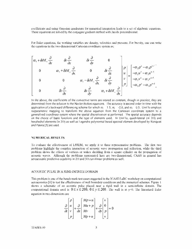
coefficientsandusingGaussianquadraturefornumericalintegrationleadstoasetofalgebraicequations.TheseequationsaresolvedbytheconjugategradientmethodwithJacobipreconditioner.

ForEulerequations,theworkingvariablesaredensity,velocitiesandpressure.Forbrevity,onecanwritetheequationsinthetwo-dimensionalCartesiancoordinatesystemas;

al + StM 3 5t 3 5t 3)x )x oN

80 al + 5tM --

&

0 0

08x

80 &--

8x

8 8a_ + 5tM -- 5t-

ax oN,9 8

5t + a_ + 5tm --go2

-___2p n __ _3p n-1-

--_2 un -- _3 un-1

--_2 vn -- _3 vn-1

--a2p n -- a3p n-1

In the above, the coefficients of the convective terms are treated as constant, though in practice, they aredetermined from the solution to the Navier-Stokes equations. The accuracy is second order in time with the

application of a backward differencing scheme for which tzl 1.5, tz2 -2.0, and tz3 0.5. UniFlo employsisoparametric mapping to transform the above equation from the Cartesian coordinate system to a

generalized coordinate system where the spatial discretization is performed. The spatial accuracy dependson the choice of basis functions and the type of elements used. In UniFlo, quadrilateral (in 2D) andhexahedral elements (in 3D) as well as Legendre polynomial based spectral element developed by Ronquist

and Patera [5] are used.

NUMERICAL RESULTS

To evaluate the effectiveness of LSSEM, we apply it to three representative problems. The first twoproblems highlight the complex interaction of acoustic wave propagation and reflection, while the third

problem shows the effects of vortices or wakes shedding from a square cylinder on the propagation ofacoustic waves. Although the problems represented here are two-dimensional, CAAS in general hasaeroacoustic predictive capability in 2D and 3D curvilinear problems as well.

ACOUSTIC PULSE IN A SEMI-INFINITE DOMAIN

This problem is one of the bench mark test cases suggested in the ICASE/LaRC workshop on computationalaeroacoustics [6] to test the effectiveness of wall boundary conditions and the numerical schemes. Figure 1shows a schematic of an acoustic pulse placed near a rigid wall in a semi-infinite domain. The

computational domain used is 0 -< )c _<200, 0 -< y -< 200. The wall is at y 0. The linearized Euler

equation in two-dimensions are

c3 Pu c3 [ Mu + p [ c3 0

Lmp+uj P

=o

TFAWS 99 5

Mis the Mach number 0.5. The initial condition is

at time t = 0,u = v = 0 andp = p = exp -(ln2) x° + (Yo - 25) 225

where Xo 100, yo 25 are the coordinates of the initial pulse.

Figure 2 shows time history plots of an acoustic pulse reflected from a hard wall in a uniform flow at Mach

0.5 at times, t 15, 45, 60, 90, 100 and 150 respectively. The lower boundary is a reflecting wall while theother boundaries are non-reflecting out-going wave boundaries. This problem was used to test theeffectiveness of wall boundary condition and out-going wave conditions devised in the acoustic solver.Figure 3 shows a comparison of the computed acoustic pressure with the exact solution along the line x_ at

times t 75, 90 and 100 respectively. The computed results show good agreement with the exact solution.

As seen from figure 2, the acoustic pulse expands at the speed of sound and travels with the base flow atMach 0.5. The downstream wave travels at Mach 1.5, three times faster than the upstream wave, andreaches the downstream boundary early and exits. The pulse reflects from the lower wall, as seen in the red

spots, and expands as the original pulse does. Both original and reflected waves continue to expand andtravel with the base flow, and then exit the right, left, and upper sides of the domain. The computed resultsshow that both wall reflection and out-going wave conditions work very well, except at t 150 there is avery tiny reflection of the reflected wave at the downstream boundary.

YT NONREFLECTING ._

Io ................... 7r'¢

M = 0._ // I

Z_ _ I(DPUL AT t it" I

r ,__,,o, ,o

,u4,LL LLLLI ILL I

',oZ f j/ I Z

JJ I I[

HARD WALL

Figure 1. Problem Schematic for an Acoustic Pulse in a Semi-Infinite Domain

TFAWS 99 6

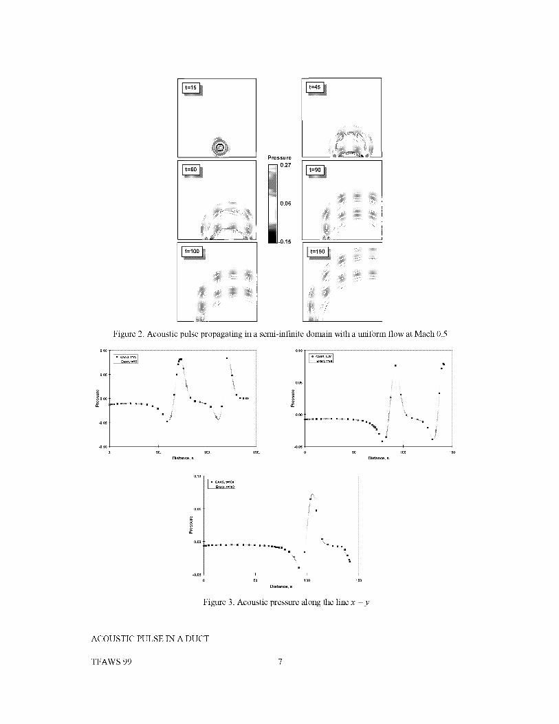
=o.oo

o..

_i!_ii;!!i!_', _ _;_ii!!!_iiiiii_

Pressure

0.27

0.06

-0.15

!.....

_,_,_Z_;::!_ _i _ ,_ _:::_>:__,i:,_

iiiiiiiiii'_ii:

Figure 2. Acoustic pulse propagating in a semi-infinite domain with a uniform flow at Mach 0.5

O.lO ............................................................................................................... ,

O.O5" - _:

i¸ ' ,

i_ ¸_¸=¸= _ _ = m _ =

-O.lO i i

o. 50. 100. 150.

Distance, s

0.10 ...............................................................................................................

0.05

==

==o.

o.oo

¸=¸=¸''¸,% i¸

i

=

i m,= _:

_: i ¸

i

50 lOO 15o

Distance, s

0.05 -

®

==

o.oo -

m

ii_ _i

I=

I

50 100 150

Distance, s

Figure 3. Acoustic pressure along the line x y

ACOUSTIC PULSE IN A DUCT

TFAWS 99

Figure 4 shows a schematic of an acoustic pulse placed at the center of a duct. Figure 5 shows time history

plots of the acoustic pulse traveling in a 2D duct with reflecting walls and a uniform flow at Mach 0.5. This

example simulates the propagation of sound waves generated in the inlet and exhaust ducts of an internal

combustion engine such as in an automobile. The problem is also used to test the effectiveness of hard wall

conditions and nonreflecting (out-going wave) conditions. Initially the sound source is created by some

mechanism in the center of the duct. It expands at the speed of sound, travels with the base flow at Mach

0.5, and forms waveguide patterns in the duct.

I

M = 0.5 I

I

I

I

I

I

I

HARD WALL

t=o

@bPULSE

Z

HARD WALL

Figure 4. Problem schematic for acoustic pulse in a duct

t=35 t=50

J

t = 75 t = 100

IIll_!iiiiiiiiiiiiiiiiiii_i_i_iiiii_iiiii_l

J,,n,L

[_iiiiiiiiiiiiiiiiiiii!_iiii_iiiii_i

Figure 5. Acoustic pulse propagating in a duct

AEROACOUSTICS OF A 2D VORTEX SHEDDING FROM A RECTANGULAR CYLINDER

The sound generated by a viscous flow past a square cylinder at Re 14,000 is predicted using the linearized

Euler equations approach. The time-dependent mean flow is calculated using a separate flow solver that is

based on a second order accurate finite-volume method. Time accuracy of the flow solver is assured using

the PISO methodology [7], which is essentially noniterative. The solution process is split into a series of

steps whereby operations on pressure are decoupled from those on velocity at each time step. The

avoidance of iterations substantially reduces the computational effort compared with that required by

iterative methods such as in UniFlo.

Calculations are performed for the turbulent flow around a square obstacle of height H in a domain

extending about 20H downstream and 2.5H upstream. The calculations using the two-equation k-e

turbulence model captured the vortex shedding phenomenon. The Reynolds number based on the inlet

TFAWS 99 8

velocity and the obstacle height is 14,000 with an assumed 6% turbulence intensity. The upper and lowerboundaries were treated as free stream and a zero gradient outflow boundary condition was used at the exit.

The computational domain is resolved by a fine grid of 250x80 cells with clustering at the obstacle walls. Atime step of 0.1 msec was used in the calculations. Once an oscillatory periodic solution was obtained, theflow solver was coupled with the UniFlo acoustic solver to calculate the sound generated by the periodicallyshedding flow. Figure 6a, shows a marker particle trace, which illustrates the shedding pattern. Figure 6b,

confirms the oscillating periodic nature of the flow with a single predominant frequency of about 4.7 Hz

which is in agreement with the experimental results of Dur_o et al. [8]. Figure 7, shows contours of the

sound pressure generated by the vortex shedding behind the square cylinder at three instants of time. Thelong-time behavior is to focus the acoustic pressure signal along the centerline of the flow axis. High soundpressure levels are generated close to the cylinder where the strength of vortices is highest.

0.1

0.00,0 0'. I 0j, 2 0r,3

×

Figure 6a. Streak line plot

.:,."]

"s

0°t

o_- f

JIflz_

Figure 6b. Power spectrum of the vortex shedding

TFAWS 99 9

t = 0.02 s

t = 0.10 s

t = 0.20 s

p, dB

57

0

-57

-66

80

73

0

-72

-79

78 I

0

-78

-85

CONCLUSIONS

A computational aeroacoustic analysis system (CAAS) has been developed. CAAS is a complete system

that enables aeroacoustic analysis from a PATRAN-based graphical user interface (GUI). Significant

customization of the PATRAN GUI was completed as was the development of several peripheral tools (e.g.,

spectral element grid generators, interpolators).

An acoustic module, based on the least squares spectral element method (LSSEM) has been developed and

demonstrated on a variety of acoustic and aeroacoustic test cases, including the fully coupled solution of

vortex shedding, sound generation, and sound propagation. Preliminary comparisons of flow and acoustic

results show qualitatively good behavior, but further comparisons with benchmark test data are required to

fully verify the current predictive capability.

ACKNOWLEDGMENTS

The authors would like to recognize a number of additional contributors. Funding for the CAAS program

has been provided by NASA and three industry partners, Boeing/Rocketdyne, Ford Motor Company, and

MacNeal-Schwendler (MSC). Further, a majority of the PATRAN GUI customization and database

management was performed by MSC personnel.

REFERENCES

1. Albert R. George, "Automobile aerodynamic noise", SAE Transactions, 99(6): 434-457, 1990.

2. D. Chan, "A least squares spectral element method for incompressible flow simulation", Proceedings of

the Fifteenth International Conference on Numerical Methods in Fluid Dynamics, 1996.

TFAWS 99 10

3. B. Jiang, T. Lin and L. Povinelli, "Large scale computation of incompressible viscous flow", Comput.Meth. Appl. Mech. Eng., 114 : 213-231, 1994.

4. D.S. Burnett, "Finite element analysis: from concept to application", Addison-Wesley, 1987.

5. E. Ronquist and A. Patera, "A Legendre spectral element method for the Stefan problem", Int. J. Num.

Meth. Eng., 24 : 2273-2299, 1987.

6. ICASE/LaRC Workshop on Benchmark Problems in Computational Aeroacoustics (CAA), Editors, J.C. Hardin, J. R. Ristorcelli and C. K. W. Tam, 1995, NASA-CP 3300.

7. R. Issa, "Solution of the implicitly discretized fluid flow equations by operator-splitting", J. Comput.Phys., 62 : 40-, 1986.

8. D. Durao, M. Heitor and J. Pereira, "Measurements of turbulent and periodic flows around a square

cross-section cylinder", Experiments in Fluids, 6 : 298 - 304, 1988.

TFAWS 99 11

AN OVERVIEW OF COMPUTATIONAL AEROACOUSTIC MODELINGAT NASA LANGLEY

DAVID P. LOCKARD

Aerodynamics; Aerothermodynamics; and Acoustics Competency

NASA Langley Research CenterHampton, VA 23681-2199, U.S.A

ABSTRACT

The use of computational techniques in the area of acoustics is known as computational aeroacoustics and hasshown great promise in recent years. Although an ultimate goal is to use computational simulations as a virtual wind

tunnel, the problem is so complex that blind applications of traditional algorithms are typically unable to produceacceptable results. The phenomena of interest are inherently unsteady and cover a wide range of frequencies and

amplitudes. Nonetheless, with appropriate simplifications and special care to resolve specific phenomena, currentlyavailable methods can be used to solve important acoustic problems. These simulations can be used to complement

experiments, and often give much more detailed information than can be obtained in a wind tunnel. The use ofacoustic analogy methods to inexpensively determine far-field acoustics from near-field unsteadiness has greatly

reduced the computational requirements. A few examples of current applications of computational aeroacoustics atNASA Langley are given. There remains a large class of problems that require more accurate and efficient methods.Research to develop more advanced methods that are able to handle the geometric complexity of realistic problems

using block-structured and unstructured grids are highlighted.

INTRODUCTION

Computational aeroacoustics is a very broad field that encompasses research that uses numerical simulations tobetter understand aerodynamic noise. There is a large computational effort at NASA Langley Research Center aimed

at predicting and reducing aircraft noise, and this paper only attempts to give an overview of a representative fractionof that work. The problem is very difficult because the geometry and physics involved are often quite complex. It has

taken 30 years to achieve significant noise reduction for jet engines. Although great strides have been made in thereduction of jet noise through the use of high-bypass ratio engines, there is a lack of understanding of thefundamental noise sources in subsonic jets. Today, tonal noise from large inlet fans is also important. There is a

general theory for fan noise, but calculations are still somewhat limited. Extensive research is ongoing in the areas of

duct and liner acoustics[ 1]. Furthermore, the engines are not the only noise source that must be considered.Reductions in jet noise have made the airframe a significant, and in some cases dominant source during landing. Theflaps, slats, and landing gear are all important contributors to the sound field. To achieve significant noise reduction,

these three maj or landing systems and the engines must all be quieted commensurately.

The physics behind the unsteadiness that generates noise is also very complicated. Fluctuations tend to grow in

shear layers and vortical structures. Resolving these features in a mean flow calculation can be difficult. Trying tocapture the unsteadiness growing in them is even more challenging. Separated regions, instabilities, and large and

small scale turbulence structures can all contribute to the sound field. Furthermore, the energy that is radiated asnoise is typically only a small fraction of the total energy near the source. This is part of the scale disparity between

acoustic and hydrodynamic fluctuations. The human ear is able to distinguish between signals with vastly varyingamplitudes, so it is typical to use a logarithmic scale to describe them. The sound pressure level (SPL) is given by

/

SPL = 20 log(_) (1)

with units of decibels (dB). The reference pressure Pref = 20 × 10 .6 Pa is the threshold of human hearing, and rmsmeans root mean square. The ratio of pressure amplitudes between a quiet conversation, 60 dB, and a rock concert,120 dB, is 1000. In addition, atmospheric pressure is 3500 times greater than the pressure amplitude of a 120 dB

signal. At 120 dB, one starts feeling discomfort and experiences a ringing in the ears. Although this level is very loud

tohumans,it issosmallthatatypicalcomputationalfluiddynamics(CFD)simulationveryeasilylosesthesoundwavesamongthelargehydrodynamicfluctuations.Simultaneouslyresolvingthehydrodynamicfluctuationsandthewiderangeofacousticsignalsisverydifficult.

Acousticiansalsohavetodealwithverydisparatelengthandtimescales.Mostlypeoplecanhearfairlywellbetweenfrequenciesof100Hzand10kHz.Thiscorrespondstowavelengthsof0.11ft (0.034m)and11ft (3.4m),respectively.Tryingtohaveenoughgridpointsinthedomaintoresolvetheveryshortwavelengthwhilehavingadomainlargeenoughtoencompassthelongwavelengthresultsinenormousgrids.Oneisalsofacedwiththechallengeoftryingtopropagatethesignaltoobserverslocatedatgreatdistancesfromthesources.A similarscaleproblemoccurstemporally.ThewavelengthAofanacousticwaveisrelatedtothetemporalperiodT by A = cT

where c is the speed of sound. The periods for 100 Hz and 10 kHz are 0.0001 s and 0.01 s, respectively. Hence, oneneeds many time steps for the short period, and long run times to get a significant sample of the long period. This

problem is usually exacerbated by initial transients in numerical solutions which must decay sufficiently before onecan start sampling the acoustics. Even when using sampling techniques developed for experimental work, it isdifficult to run codes long enough to get statistically significant samples of pseudo-random phenomena. Furthermore,

the disparity between different acoustic waves is only part of the problem. One also has to compare the acousticscales with those of other fluid phenomena and the geometry.

Faced with these challenges, one must inevitably make simplifying assumptions. However, computational methodsare often able to relax those used in the past. The basic goal is to obtain an understanding of the underlying physics of

the noise sources. One needs to know the strength, location, frequency, wavelength, and nature of the disturbances.With this information one can develop prediction methods that are general across different configurations that have

similar source mechanisms generating the noise. Furthermore, one can begin attacking the sources in systematicways that are more likely to lead to significant noise reduction. To get at the physics, we are using currently availabletools and developing new ones to do bigger problems in the future. To reduce the complexity, most calculations

concentrate on a small frequency range rather than trying to resolve all of the relevant frequencies at once. In

addition, one can solve equations linearized about the mean flow[2, 3] to separate out the acoustic and hydrodynamicscales. Using these simplifications makes many problems tractable to modern methods. Furthermore, numericalapplications of acoustic analogy methods have matured significantly, and they allow far-field acoustics to be

calculated from unsteady fluctuations in the vicinity of the sources. This greatly reduces the computational effort andprovides a means of finding the noise where the observers are actually located.

The remainder of the paper discusses some of the acoustic problems that have been solved using combinations ofavailable methods. First, the CFD code CFL3D is described. It was used in many of the example computations. The

acoustic analogy is explained in slightly more detail because it is key to most of the calculations and is less widelyknown. At the end of the paper, examples of several new technologies under development are discussed. These

include high-order methods for block-structured and unstructured grids. Because of the great scale disparities inacoustics, one either needs high-accuracy methods that resolve waves with a minimal number of

points-per-wavelength or standard methods with fine grids. Such comparisons[4, 5] have shown that high-ordermethods are more efficient at resolving acoustic phenomena than traditional methods with extremely fine grids.However, high-order methods often suffer from robustness problems for realistic configurations, and these new

efforts are aimed at overcoming this difficulty.

COMPUTATIONAL TOOLS

THE COMPUTER CODE CFL3D

The computer code CFL3D [6, 7] is a robust, workhorse code used to compute both steady and unsteady flowfields. The CFL3D code was developed at NASA Langley Research Center to solve the three-dimensional,

time-dependent, thin-layer (in each coordinate direction) Reynolds-averaged Navier-Stokes (RANS) equations usinga finite-volume formulation. The code uses upwind-biased spatial differencing for the inviscid terms and flux limitingto obtain smooth solutions in the vicinity of shock waves. The viscous derivatives, when used, are computed by

second order central differencing. Fluxes at the cell faces are calculated by flux-difference-splitting. An implicitthree-factor approximate factorization method is used to advance the solution in time. Patched grid interfaces, overset

grids, and slides zones are available for use at zone boundaries.

The time-dependent version of CFL3D uses subiterations to obtain second order temporal accuracy. In the _- - TS

subiteration option [8], each of the subiterations is advanced with a pseudo-time step. This approach facilitates a

TFAWS 99

more rapid convergence to the result at each physical time step. The steady-state version of the code employs full

multigrid acceleration.

ACOUSTIC ANALOGY

An acoustic analogy is a rearrangement of the governing equations of fluid motion such that the left-hand side

consists of a wave operator in an undisturbed medium, and the right-hand side is comprised of acoustic source terms.The solution to the equation can be written as the convolution of the source terms with the Green function for the

wave operator. Hence, if one can obtain the strengths of the source terms in the regions where they are significant,one can determine the acoustic signal at any point in the flow, including locations at long distances from the sources.

Lighthill[9] was the first to propose this approach. Although this concept is relatively simple, extensive manipulationshave been required to put the equations in the most useful forms for analytic and numerical applications.

The Ffowcs Williams and Hawkings [10] equation is the most general form of the Lighthill acoustic analogy andwhen provided with input of unsteady flow conditions, is appropriate for numerically computing the acoustic field.

The equation is derived directly from the equations of conservation of mass and momentum. Following Brentner andFarassat [ 11], the FW-H equation may be written in differential form as

02

[72c2p'(x, t) - OxiOxj [TijH(f)] - _[LiS(f)] + _[QS(f)] (2)

°_ V 2 is the wave operator, c is the ambient speed of sound, t is observer time, p' is thewhere: [7 2 ---- 12 Ot 2

perturbation density, Po is the ambient density, f = 0 describes the integration surface, f < 0 being inside theintegration surface, 5(f) is the Dirac delta function, and H(f) is the Heaviside function. The quantities Q, Ui and Li

are defined by

O = (_oU_), c_ = (1 - _)v_ + _"_noand C_ = P_ji_j + _._(_.._- v,_). (3)

In the above equations, p is the total density, fl_i, is the fluid momentum, vi is the velocity of the integration surfacef = 0, and Pi3 is the compressive stress tensor. For an inviscid fluid, Pij = P't_ij where p' is the perturbation

pressure and 5ij is the Kronecker delta. The Lighthill stress tensor is given by Tii. The subscript n indicates thecomponent of velocity in the direction normal to the surface.

An integral solution to the FW-H equation (2) can be written in terms of the acoustic pressure p' = c2p ' in the

region f > 0. Utilizing formulation 1A of Farassat [12, 13], the integral representation has the form

where

;'(x,t) = p_(x,t) + p_(x,t) +;b(x,t) (4)

47rp_(x,t) : / [PQ(y,T)lr_tdS , 47rp_(x,t)= / [PL(y,T)]r_tdS.and (5)f o f o

47cp_r(x,t) = / [Pr(Y,_-)]r_tdl/\ (6)

f o

The subscript ret means that the quantities must be evaluated at the appropriate retarded or emission time T. The

kernel functions PT, PL, PQ are combinations of flow quantities and geometric parameters. For many numericalsimulations it is desirable to let the integration surface be permeable and place it within the flow. However, when thesurface coincides with a solid body, the terms take on simple meanings. The Q term is known as the thickness

contribution and represents the noise generated by the unsteady displacement of fluid by the body. The L terminvolves the noise caused by the fluctuating loading on the body. The term P_r accounts for all quadrupoles outside of

the integration surface (i.e., f > 0). Quadrupole contributions include nonlinear effects and refraction. In most work,p_r is small and can be neglected. This is important because the quadrupole term involves a volume integration,

whereas p_ and p_ only require an integration over the surface. All quadrupole contributions that are within thesurface are accounted for by the surface integrations. Hence, the far-field pressure at any instance in time can usuallybe calculated by integrating the near-field flow quantities over a surface. This allows for very rapid calculations of

noise a great distance away from the source region where the integration surface is typically placed.

TFAWS 99

e

e

,m

O

<

2O

10

-10

(a) (b)

Time

m..o

._1Q.(/)

110.0

100.0

90.0

80.0

70.0

60.0

50.00

(c)

5 10 15 20 25 30 35 40

Harmonic number

Figure 1. Comparison of measure and computed noise for a four-bladed Sikorsky model rotor. The microphone

locations was nominally 25 deg. below the rotor plane on the advancing side, 1.5 rotor radii from the rotor hub. This isa descent condition. (a) Measure time history; (b) predicted time history; (c) spectral comparison (-- measured;

predicted)

Rotorcraft acoustics is an area where the FW-H equation has been utilized with great success. The codeWOPWOP[ 13] has been used extensively by industry and researchers to predict helicopter noise. Even for complex

phenomena such as blade vortex interaction (BVI), WOPWOP correctly predicts the acoustic signature when it isgiven accurate pressure data as inputs. As an example, figure 1 compares the experimentally observed and computed

acoustic signals[ 14] when experimentally measured surface pressures from a four bladed rotor where used as input toWOPWOR The spectral comparison in figure 1 shows the agreement is good up to the 32nd harmonic. Similar

comparisons using CFD data as input do not yield such good results. This underscores the importance of havingaccurate input data on the integration surface. The acoustic theory is mature enough for such complicated problems,but more accurate CFD is needed.

SAMPLE APPLICATIONS

Although there are many problems that cannot be solved with conventional methods, appropriate assumptions canmake many realistic problems tractable. This section provides several examples where current methods were

successfully used to simulate important acoustic phenomena.

ROTOR NOISE

Rumsey et a/.[15] used the Navier-Stokes code CFL3D to predict one of the ducted-fan engine acoustic modes that

results from a rotor-wake/stator-blade interaction. A patched-sliding-zone interface was employed to passinformation between the moving rotor-row and the stationary stator row. Figure 2 shows the geometry and 2.7 million

point grid used in the calculation. The code produced averaged aerodynamic results downstream of the rotor that arein good agreement with a widely used average-passage code. The calculation was designed to capture a single

acoustic mode, and the code successfully generated and propagated that mode upstream with minimal attenuationinto a region of nearly uniform flow as shown in figure 3(a). Two acoustic codes were used to find the far-field noise.

Propagation in the duct was computed by Eversmann's wave envelope code, which is based on a finite-elementmodel. Propagation to the far field was accomplished by using the Kirchhoff formula for moving surfaces. The

Kirchhoffmethod is used in a similar fashion to acoustic analogy methods, but is less general. Comparison ofmeasured and computed far-field noise levels are in fair agreement in the range of directivity angles (20-40 deg.)where the peak radiation lobes are observed for the mode under investigation. Figure 3 compares the experimental

and computed results. Although only a single acoustic mode was targeted in this study, it provided a proof ofconcept: Navier-Stokes codes can be used to both generate and propagate rotor-stator acoustic modes through and

engine, where the results can be coupled to other far-field noise prediction codes.

TFAWS 99

E

cOOr"

0.24-

0.00

16 rotor blades

__0stator vanes / acoustic signals

--

-0,12

torward -pro pagating

-0.04 0.04 0.12

Axial distance, m

(a) Geometry.

I

0.20

M=0.2

(b) 2.7 million point grid.

Figure 2. Geometry and grid for rotor-wake/stator-blade interaction problem.

L

LCZ

240

160

80

0

80

160

0.00

time = •

time = T + 0.75

_, theo£y Ax theoI?/

, I , I , I , I

0.04 0.08 0.12 0.16

Axial distance, m

(a) Near-field pressure.

, I

0.2C

120

100EL

0O4 80

6o[33X]

4O

0_09 2O

.O""

Q _----_--.._ ......Q _.eQ /"b'

..." k -. ', /

__ ref plane at .08 m....... ref plane at .14 m...._ ..... experiment

I _ I _ I _ I _ I

20 40 60 80 1O0

microphone angle, deg

(b) Far-field noise.

Figure 3. Near-field pressure computed by CFL3D and far-field pressure computed by Eversmann's wave envelope

code and a Kirchhofftechnique.

TFAWS 99

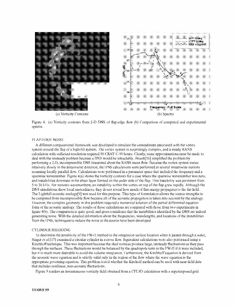
Figure 4.spectra.

(a) Vorticity Contours

(a) Vorticity contours from 2-D DNS of flap-edge flow (b) Comparison of computed and experimental

FLAP-EDGE NOISE

A different computational framework was developed to simulate the unsteadiness associated with the vortexsystem around the flap of a high-lift system. The vortex system is surprisingly complex, and a steady RANS

calculation with sufficient resolution required 50 CRAY C-90 hours. Clearly, some approximations must be made todeal with the unsteady problem because a DNS would be intractable. Streett[ 16] simplified the problem byperforming a 2-D, incompressible DNS linearized about the RANS mean flow. Because the vortex system varies

relatively slowly in the streamwise direction, the DNS calculations were performed at several streamwise stationsassuming locally parallel flow. Calculations were performed in a parameter space that included the frequency and a

spanwise wavenumber. Figure 4(a) shows the vorticity contours for a case where the spanwise wavenumber was zero,and instabilities dominate in the shear layer formed on the under side of the flap. This instability was persistent from

5 to 30 kHz. For nonzero wavenumbers, an instability within the vortex on top of the flap grew rapidly. Although theDNS simulations show local unsteadiness, they do not reveal how much of that energy propagates to the far-field.

The Lighthill acoustic analogy[9] was used for this purpose. This type of formulation allows the source strengths tobe computed from incompressible flow because all of the acoustic propagation is taken into account by the analogy.

However, the complex geometry in this problem required a numerical solution of the partial differential equationform of the acoustic analogy. The results of those calculations are compared with those from two experiments infigure 4(b). The comparison is quite good, and gives confidence that the instabilities identified by the DNS are indeed

generating noise. With the detailed information about the frequencies, wavelengths, and locations of the instabilitiesfrom the DNS, techniques to reduce the noise at the source have been developed.

CYLINDER SHEDDING

To determine the sensitivity of the FW-H method to the integration surface location when it passes through a wake,

Singer et al.[17] examined a circular cylinder in a cross flow. Equivalent calculations were also performed using aKirchhofftechnique. This was important because the shed vortices produce large, unsteady fluctuations as they passthrough the surfaces. These fluctuations would be balanced by the quadrupole term in the FW-H if it were included,

but it is much more desirable to avoid the volume integration. Furthermore, the Kirchhoff equation is derived fromthe acoustic wave equation and is strictly valid only in the region of the flow where the wave equation is the

appropriate governing equation. This problem tested whether the Kirchoffmethod can be used with near-field datathat includes nonlinear, non-acoustic fluctuations.

Figure 5 renders an instantaneous vorticity field obtained from a CFL3D calculation with a superimposed grid

TFAWS 99

Figure 5. Vorticity field computed from CFD. FW-H integration surfaces are at r = 0.5D, r = 1.5D, r = 2.5D, andr = 5.1D

distribution on the lower portion of the figure. The positions of the FW-H integration surfaces are indicated in theupper portion of the figure. Figure 6(a) shows the computed pressure signals at the observer for the different

integration surfaces using a Kirchhoff formulation, and figure 6(b) shows the the results obtained with theFW-H formulation. The use of an integration surface that cuts through the cylinder wake does not appear to adversely

affect the results obtained with the FW-H formulation. However, these variations are very small compared with theresults of Figure 6(a), in which the pressure computed with a standard Kirchhoff formulation for the same problem

with the same integration surfaces varies wildly. This result clearly demonstrates that the FW-H should be usedinstead of the Kirchhoffmethod. Furthermore, there is very little difference in the computational effort required forthe two approaches.

TRAILING-EDGE SCATTERING

Calculation methods for acoustic fields that include trailing-edge noise currently are largely empirical [18]. Singer

et al. [17]. investigated the feasibility of directly computing the acoustic field generated by flow over a sharp trailingedge. A hybrid computational approach was taken wherein the CFL3D solver was used to accurately calculate the

unsteady fluid dynamics over a relatively small region near the surface, and an acoustics code based on the FfowcsWilliams and Hawkings [10] (FW-H) equation computed the acoustic field generated by the previously calculated

unsteady near flow field. To investigate edge scattering, an airfoil with vortices convecting past its trailing edge wassimulated. A 2.6% thickness NACA 00 series airfoil was placed in a flow with a small, flat plate introducedperpendicular to the flow at 98% chord. In the presence of flow, vortices roll up just downstream of the flat plate,

alternately near the plate's top and bottom edges.

Figure 7 shows vorticity magnitude contours in the vicinity of the trailing edge at a single time step. The circular

concentrations of vorticity indicate the individual vortices that constitute the unsteady Karman vortex streetdownstream of the vortex-generator plate. Cases were run with Mach numbers ranging from 0.2 to 0.5 that produced

regular Strouhal shedding at the plate. The frequency of the vortices convecting past the trailing edge is less distinctbecause the vortices shed from the vortex-generator plate often pair and interact with neighboring vortices, as shown

in figure 7.

The FW-H code computed the acoustic field generated by the unsteady aerodynamic flow field. The far-field

signals were obtained at several observer locations. Figure 8(a) shows spectra of the acoustic signals for severalobserver positions. The angular measurements are increasingly positive for counterclockwise rotations, with 0

degrees being directed downstream. The figure shows greatly reduced noise radiation directly upstream and directlydownstream. Integration of each acoustic spectrum over the frequencies provides the mean square acoustic pressure.

Variation of the mean square acoustic pressure as a function of Mach number is plotted in Figure 8(b). The symbolsshow the data, and the lines are linear least-squares fit to the logarithm of the data. For an observer at 30 degrees, themean square pressure varies as the 5.2 power of Mach number. Accounting for the actual rms fluctuating velocity in

the calculations, a theoretical scaling of M 5a_ is implied, which is in close agreement with the computationallyobserved scaling of M 52. These computations have helped to verify that the hybrid approach is valid and capable of

accurately predicting fairly complicated, broadband, acoustic phenomena.

TFAWS 99

2OO

lOO

p', Pa

80

(a) [ (b)60

It

ii

40 !_ _

, 20-10 i

iu_.i p', Pa

2oo ,: ',--2

--300

--40

-4000.008 0.009 0.010 0.011 0.012 0.008 0.009 0.010 0.011 0.012

t, sec t, sec

(a) Computations with Kirchhoff scheme. (b) Computations with FW-H scheme.

Figure 6. Acoustic signals computed for various integration surfaces that correspond to those indicated in Figure 5.

Integration surfaces at-- r = 0.5D, r = 1.5D, - ..... r = 2.5D, - ........ r = 5.1D.

U

Figure 7. Instantaneous vorticity magnitude contours in vicinity of trailing edge for M = 0.2 case. Approximately

2% of aft portion of airfoil is shown.

TFAWS 99

,j 40

¢0

70 I .......... _'""

60 "" °°°°"" ;:"% : :

50[-- X i . _:r _l;;:'._l,_l

" '

2O

10 i i i i I I I I I Ill10000 20000 30000

f, Hz

a.

2

g

7060

50

40

30

20

10

tO/

//

/

//

, _ , , , , I , ,, I , , , , I , ,I,,,,

0.2 0.25 0.3 0.35 0.4 0.45

Mach

(a) (b)

Figure 8. (a) Spectra of acoustic signals (referenced to 20#Pa) for observers located 10C from trailing edge of airfoil;

on-airfoil-body integration surface used, M = 0.2. Observers located at: 0 deg., 45 deg.,...... 90 deg., •..... 135 deg., -- -- -- 180 deg. (b) Variation in mean square acoustic pressure versus Mach

number; [] data for 30 deg., -- least-squares fit for 30 deg., <>data for 45 deg., least-squares fit for45 deg.

HIGH-LIFT CONFIGURATION

A cooperative test involving NASA's High-Lift Program Element and NASA's Airframe Noise Team wasconducted in NASA Langley Research Center's Low-Turbulence Pressure Tunnel (LTPT). The model tested in the

tunnel is known as the Energy Efficient Transport (EET) model. The EET model tested includes a full-spanleading-edge slat and a part-span trailing flap. To obtain acoustic data, members of Boeing Commercial Airplane

Company designed and built a microphone array that was installed in the wind tunnel. The microphone array and thesubsequent data processing followed techniques developed earlier at Boeing [19].

Figure 9(a) illustrates one unexpected feature of the experimental data. For a slat deflection of 6_ = 30 degrees, avery large amplitude peak was observed in the acoustic spectrum in the vicinity of 50 kHz. This peak rises almost 20dB above the signal observed for the case in which the slat is deflected 20 degrees. During the course of the

experiment, efforts to eliminate the high-frequency peak by altering the overhang of the slat were largelyunsuccessful. Only for cases in which the overhang became unrealistically large was a significant change in the

high-frequency acoustic peak observed. Increasing the configuration's angle-of-attack from 10 to 15 degrees, reducedthe amplitude of the high-frequency peak by approximately 10 dB. For some time, no consistent explanation of the

observed phenomena was available.

Khorrami et al [20] provides details of unsteady, two-dimensional (2D), Reynolds-averaged Navier-Stokes

(RANS) calculations designed to mimic the experimental conditions. In particular, the RANS computation wasspecially designed to properly incorporate and resolve the small, but finite trailing-edge thickness of the slat.

Extremely small grid cells were used in the vicinity of the slat trailing edge and the time step was chosen to ensuremore than 120 time steps per period of a 50 kHz signal. Slat deflections of both 30 and 20 degrees were simulated.

These calculations clearly show vortex shedding from the slat trailing edge for the case with a 30 degree slatdeflection. Figure 9(b) shows a snapshot of the pressure fluctuations produced in the flow field. The vortex sheddingvirtually disappears for the case of a 20 degree slat deflection.

Singer et al. [21] discuss the aeroacoustic analysis of the unsteady data. As a first approximation, the codedeveloped by Lockard[22] for computing the 2D acoustic field from 2D CFD data was used to predict the sound field.

Figure 10(a) shows computed spectra based on 1/12 th octave bins for an observer located at 270 degrees. Clearly thecomputed noise also has a significant peak in the spectra in the same frequency range as the experiment. This

confirmed that the fluctuations from the slat vortex shedding weren't just hydrodynamic fluctuations, but also

TFAWS 99

95 t- .......................................................................................r .........................._............... " "" "r""";'-- "_'" _

SlatAngle i i i i i

A 85 ...................................................................................i ..........................i............... .i.

80 ................................_,..........................._,.................... _,.

75

70 [ _,,_,_,_

Frequency (kHz)

(a) (b)

Figure 9. (a) Acoustic spectrum based upon 1/12th octave bins with array focussed on slat region. Configuration

angle of attack is 10 deg., Reynolds number is 7.2 million, Mach number is 0.2. (b) Instantaneous fluctuation pressure,in vicinity of leading-edge slat, from CFD calculation. Slat deflection is 30 deg.

90 I

I6O

55 I

f, kHz

-I¢n¢n

O.

-IO"¢n

c-

o

E I

I

I

!

/

,--I--T,--,I,,,,I,,,,I,,,,I,,,,I

streamwise coordinate

(a) (b)

Figure 10. (a) Spectra for observer positioned at 270 deg. with 30 deg. slat deflection. (b) Comparison of squaredacoustic pressure at individual microphones to that predicted computationally. Microphone positions and values are

shown with squares; dashed line indicates computationally predicted values.

TFAWS 99

10

producednoise.Althoughtheacousticarrayusedintheexperimentwasnotintendedtoprovideanydirectivityinformation,thehigh-frequencyacousticsignalwassoloudthatitoverwhelmedtheintrinsicwind-tunnelnoiseandcanbeidentifiedfromthespectrumofsomeoftheindividualmicrophonesusedintheacousticarray.Therelativeamplitudesofthemeansquarefluctuatingpressureinafrequencyrangearound50kHzfromasubsetofmicrophoneshavingapproximatelythesamecross-streamlocationarecomparedwithcomputedvaluesinFig.10(b).Themaximumamplitudeofthemicrophonedataisscaledwiththemaximumamplitudeofthecalculation.Thenon-zeromicrophoneresponsefar-upstreamisassociatedwiththewall-pressurefluctuationsoftheturbulentboundarylayeralongthewind-tunnelceiling.ThesefluctuationsarenotincludedaspartoftheCFDcalculations.Slightlyupstreamoftheslatleadingedge,thenoiselevelrises.Themaximumamplitudeoccursinthemid-chordregionfollowedbyasharpdropinamplitude.Thequalitativefeaturesofthecomputationsagreeremarkablywellwiththemicrophonedata,andthedirectivityresultsaidedintheredesignoftheacousticarrayforasubsequentwind-tunneltest.

ADVANCEDTOOLS

Althoughgreatstrideshavebeenmadeinsimulatingacousticphenomena,thecostsassociatedwithsomeofthecalculationsareclearlylimiting.TheunsteadyRANScalculationofthe2-Dslatsheddingrequiredover100CRAYhours.Theprojectionfora3-Dproblemisenormous.It isunlikelythatadvancesincomputerpoweralonewillmakealloftheneededcalculationsfeasible.Tohelpbridgethegapbetweenavailableresourcesandneededsimulations,someadvancedmethodologiesarebeingdevelopedthataremuchmoreefficientandaccuratethantraditionalmethods.Twomainpathsarebeingexplored.Mostgridsusedtodayarestillblock-structured,andthemacro-elementtechniqueisbeingdevelopedtoprovidemoreaccurateinterfaceconditionsthatcanberetrofittedintocurrentcodesandusedinnewcodeswithhigh-orderfinite-differencespatialoperators.TheothertechniquebeingdevelopedisthediscontinuousGalerkinwhichprovideshigh-orderonunstructuredgrids.

DISCONTINUOUSGALERKINTheprocessofgeneratingablock-structuredmeshwiththesmoothnessrequiredforhigh-accuracyschemesisa

time-consumingprocessoftenmeasuredinweeksormonths.Unstructuredgridsaboutcomplexgeometriesaremoreeasilygenerated,andforthisreason,methodsusingunstructuredgridshavegainedfavorforaerodynamicanalyses.However,theyhavenotbeenutilizedforacousticsproblemsbecausethemethodsaregenerallylow-orderandincapableofpropagatingwaveswithoutunacceptablelevelsofdissipationanddispersion.Attemptstoextendfinite-differenceandfinite-volumemethodsforunstructuredgridstohigh-orderbyincreasingthestencilsizehaveintroducedstorageandrobustnessproblems.

ThediscontinuousGalerkinmethod[23,24]isacompactfinite-elementprojectionmethodthatprovidesapracticalframeworkforthedevelopmentofahigh-ordermethodusingunstructuredgrids.Higher-orderaccuracyisobtainedbyrepresentingthesolutionasahigh-degreepolynomialwhosetimeevolutionisgovernedbyalocalGalerkinprojection.Thisapproachresultsinacompactandrobustmethodwhoseaccuracyisinsensitivetomeshsmoothness.ThetraditionalimplementationofthediscontinuousGalerkinusesquadraturefortheevaluationoftheintegralprojectionsandisprohibitivelyexpensive.AtkinsandShu[25]introducedthequadrature-freeformulationinwhichtheintegralsareevaluateda-prioriandexactlyforasimilarityelement.Theapproachhasbeendemonstratedtopossesstheaccuracyrequiredforacousticsevenincaseswherethegridisnotsmooth.Otherissuessuchasboundaryconditionsandthetreatmentofnon-linearfluxeshavealsobeenstudiedinearlierwork[26,27].

A majoradvantageofthediscontinuousGalerkinmethodisthatitscompactformreadilypermitsanon-heterogeneoustreatmentofaproblem.Thatis,theshapeofelementsused,thedegreeofapproximation,eventhechoiceofgoverningequations,canbeallowedtovaryfromelementtoelementwithnolossofrigorinthemethod.Totakeadvantageofthisflexibility,anobject-orientedC++computerprogramthatimplementsthediscontinuousGalerkinmethodhasbeendevelopmentandvalidated.However,manyoftheapplicationshaveinvolvedbenchmarkproblemsforaeroacoustics[5]withrelativelysimpletwo-dimensionalgeometriesandlinearizedequationswithuniformmeanflows.Recentworkhasbeenaimedataddingandvalidatingadditionallycapabilitythatisessentialtotheaeroacousticanalysisoflargecomplexconfigurations.

Currentapplicationsofthemethodinvolvethree-dimensionalproblems,thetreatmentofnonuniformmeanflows,viscousflows,andtheefficientuseofparallelcomputingplatforms.Withthesenewcapabilities,thistoolwillenablerapidaeroacousticanalysesofrealisticaircraftconfigurations.Whencoupledwithcurrentlyavailablegridgeneratorsandlargeparallelcomputers,theentireprocessofmeshgeneration,problemsetup,andcalculationcanbeperformed

TFAWS99

11

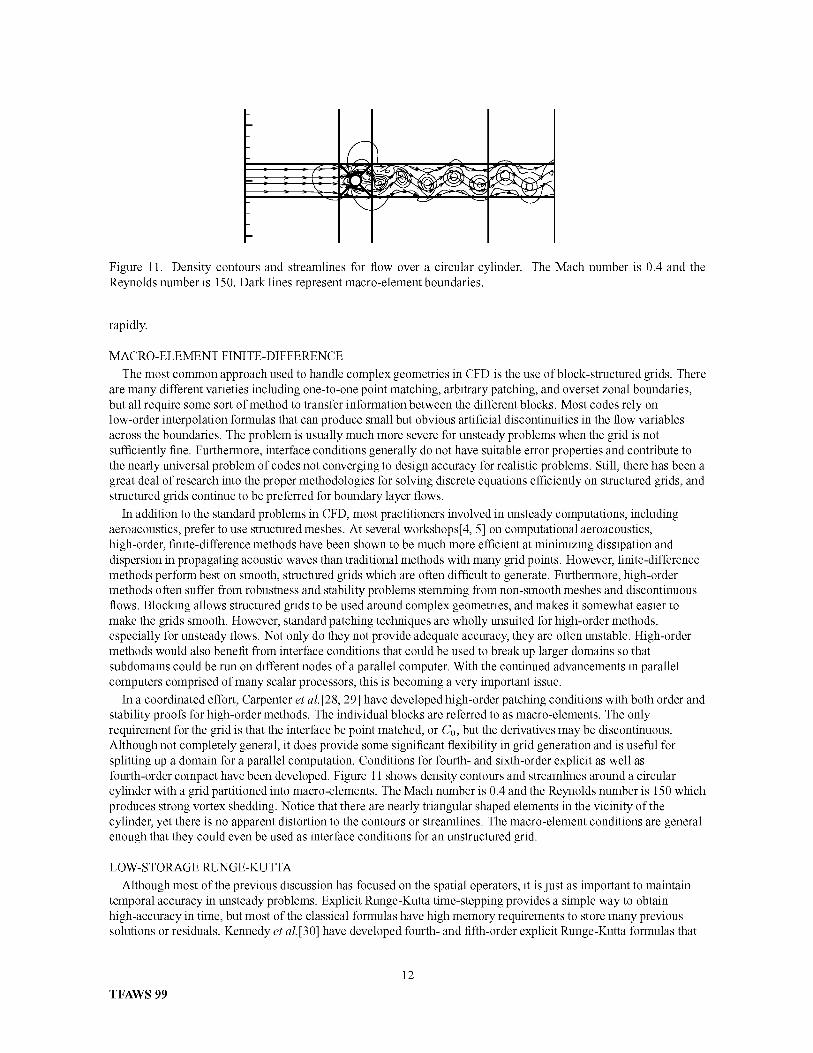
" " _/t

Figure11.Densitycontoursandstreamlinesforflowoveracircularcylinder.TheMachnumberis0.4andtheReynoldsnumberis150.Darklinesrepresentmacro-elementboundaries.

rapidly.

MACRO-ELEMENTFINITE-DIFFERENCEThemostcommonapproachusedtohandlecomplexgeometriesinCFDistheuseofblock-structuredgrids.There

aremanydifferentvarietiesincludingone-to-onepointmatching,arbitrarypatching,andoversetzonalboundaries,butallrequiresomesortofmethodtotransferinformationbetweenthedifferentblocks.Mostcodesrelyonlow-orderinterpolationformulasthatcanproducesmallbutobviousartificialdiscontinuitiesintheflowvariablesacrosstheboundaries.Theproblemisusuallymuchmoresevereforunsteadyproblemswhenthegridisnotsufficientlyfine.Furthermore,interfaceconditionsgenerallydonothavesuitableerrorpropertiesandcontributetothenearlyuniversalproblemofcodesnotconvergingtodesignaccuracyforrealisticproblems.Still,therehasbeenagreatdealofresearchintothepropermethodologiesforsolvingdiscreteequationsefficientlyonstructuredgrids,andstructuredgridscontinuetobepreferredforboundarylayerflows.

InadditiontothestandardproblemsinCFD,mostpractitionersinvolvedinunsteadycomputations,includingaeroacoustics,prefertousestructuredmeshes.At severalworkshops[4,5]oncomputationalaeroacoustics,high-order,finite-differencemethodshavebeenshowntobemuchmoreefficientatminimizingdissipationanddispersioninpropagatingacousticwavesthantraditionalmethodswithmanygridpoints.However,finite-differencemethodsperformbestonsmooth,structuredgridswhichareoftendifficulttogenerate.Furthermore,high-ordermethodsoftensufferfromrobustnessandstabilityproblemsstemmingfromnon-smoothmeshesanddiscontinuousflows.Blockingallowsstructuredgridstobeusedaroundcomplexgeometries,andmakesit somewhateasiertomakethegridssmooth.However,standardpatchingtechniquesarewhollyunsuitedforhigh-ordermethods,especiallyforunsteadyflows.Notonlydotheynotprovideadequateaccuracy,theyareoftenunstable.High-ordermethodswouldalsobenefitfrominterfaceconditionsthatcouldbeusedtobreakuplargerdomainssothatsubdomainscouldberunondifferentnodesofaparallelcomputer.Withthecontinuedadvancementsinparallelcomputerscomprisedofmanyscalarprocessors,thisisbecomingaveryimportantissue.

Inacoordinatedeffort,Carpenteret al. [28, 29] have developed high-order patching conditions with both order andstability proofs for high-order methods. The individual blocks are referred to as macro-elements. The onlyrequirement for the grid is that the interface be point matched, or Co, but the derivatives may be discontinuous.

Although not completely general, it does provide some significant flexibility in grid generation and is useful for

splitting up a domain for a parallel computation. Conditions for fourth- and sixth-order explicit as well asfourth-order compact have been developed. Figure 11 shows density contours and streamlines around a circularcylinder with a grid partitioned into macro-elements. The Mach number is 0.4 and the Reynolds number is 150 which

produces strong vortex shedding. Notice that there are nearly triangular shaped elements in the vicinity of thecylinder, yet there is no apparent distortion to the contours or streamlines. The macro-element conditions are general

enough that they could even be used as interface conditions for an unstructured grid.

LOW-STORAGE RUNGE-KUTTA

Although most of the previous discussion has focused on the spatial operators, it is just as important to maintain

temporal accuracy in unsteady problems. Explicit Runge-Kutta time-stepping provides a simple way to obtainhigh-accuracy in time, but most of the classical formulas have high memory requirements to store many previous

solutions or residuals. Kennedy et al. [30] have developed fourth- and fifth-order explicit Runge-Kutta formulas that

TFAWS 99

12

onlyrequire2NstorageforN unknowns. This can be a substantial savings in memory, and can also be very

beneficial in the run time on cache-based computers which are often limited by memory access. Furthermore, some ofthe new Runge-Kutta methods have embedded lower-order formulas that allow for automated time-stepping by using

the solutions from the two orders to determine if there is too much error and the time step needs to be decreased.

A difficulty with explicit time stepping for unsteady problems is that the time step must be chosen to keep the

smallest cell in the entire grid stable. In boundary layer flows with strong clustering towards walls, this can result in atime-step orders of magnitude smaller than what is needed for temporal accuracy. Research is ongoing into different

implicit methods that can be used in regions where the grid spacing is extremely small.

SUMMARY

Despite the simplifications used in the examples, the cost of performing many of the acoustic calculations was stillvery high. Just obtaining a highly resolved mean flow for a high-lift flap system required 50 CRAY C-90 hours, and

an unsteady RANS of a two-dimensional slat problem required over 100 hours. Nonetheless, some significant insighthas been gained by applying currently available computational techniques to problems of interest. Typically, the

calculations concentrated on resolving certain frequency ranges rather than trying to solve for all of the scalessimultaneously. Because many important noise sources are narrow band, this approach is appropriate. The noise

generated from vortex-shedding at a slat trailing edge is a good example in which this approach was taken, and apreviously unknown noise source was identified. There remain many problems that cannot be solved today, and someof the efforts at NASA Langley to develop advanced tools that will enable the next generation of acoustic simulations

have been highlighted.

ACKNOWLEDGMENTS

The author would like to thank the members of the Computational Modeling and Simulation Branch at NASALangley Research Center for their significant contributions to this paper.

REFERENCES

1. W. R. WATSON, M. G. JONES, S. E. TANNER and T. L. PARROTT 1996AIAA Journal34(3), 548 554.

Validation of a numerical method for extracting liner impedance.

2. P. J. MORRIS, Q. WANG, L. N. LONG and D. P. LOCKARD 1997AIAA PaperNo. 97-1598. Numericalpredictions of high-speed jet noise.

3. J. C. HARDIN and D. S. POPE 1994 Theoretical and ComputationalPhysics 6(5-6). An acoustic/viscous

splitting technique for computational aeroacoustics.

4. J. C. Hardin and M. Y. Hussaini, editors 1993 Computational Aeroacoustics. Springer-Verlag. (Presentations at

the Workshop on Computational Aeroacoustics sponsored by ICASE and the acoustics division of NASA LaRCon April 6-9.)

5. C. K. W. Tam and J. C. Hardin, editors 1997 Second ComputationalAeroacoustics (CAA) Workshop onBenchmark Problems. NASA CP-3352. (Proceedings of a workshop sponsored by NASA and Florida State

University in Tallahassee, Florida on Nov. 4-5, 1996.)

6. C. RUMSEY, R. BIEDRON and J. THOMAS 1997 TM 112861. NASA. (presented at the Godonov's Method forGas Dynamics Symposium, Ann Arbor, MI.) CFL3D: Its history and some recent applications.

7. S. L. KRIST, R. T. BIEDRON and C. RUMSEY 1997. NASA Langley Research Center, Aerodynamic and

Acoustic Methods Branch. CFL3D User _' Manual (Version 5).

8. C. L. RUMSEY, M. D. SANETRIK, R. T. BIEDRON, N. D. MELSON and E. B. PARLETTE 1996 Computersand Fluids' 25(2), 217 236. Efficiency and accuracy of time-accurate turbulent Navier-Stokes computations.

9. M. J. LIGHTHILL 1952 Proceedings' of the Royal Society A221, 564 587. On sound generated

aerodynamically, I: general theory.

TFAWS 99

13

10.J.E.FFOWCSWILLIAMSandD.L. HAWKINGS1969Philosophical Transactions of the Royal Society

A264(1151), 321 342. Sound generated by turbulence and surfaces in arbitrary motion.

11. K. S. B RENTNER and F. FARAS SAT 1998 AIAA Journal 36(8), 1379 1386. An analytical comparison of theacoustic analogy and kirchhoff formulation for moving surfaces.

12. F. FARASSAT and G. P. SuccI 19883 Vertica 7(4), 309 320. The prediction of helicopter discrete frequencynoise.

13. K. S. B RENTER 1986. NASA Langley Research Center. (NASA TM 87721.), Prediction of Helicopter DiscreteFrequency Rotor Noise A Computer Program Incorporating Realistic Blade Motions and AdvancedFormulation

14. K. S. BRENTNER and F. FARASSAT 1994 Journal of Sound and Vibration 170(1), 79 96. Helicopter noise

prediction: The current status and future direction.

15. C. L. RUMSEY, R. BIEDRON, F. FARASSAT and P. L. SPENCE 1998 Journal ofSoundand Vibration 213(4),643 664. Ducted-fan engine acoustic predictions using a Navier-Stokes code.

16. C. L. STREETT 1998AIAA PaperNo. 98-2226. Numerical simulation of a flap-edge flowfield.

17. B. A. SINGER, K. S. BRENTNER, D. L. LOCKARD and G. M. LILLEY 1999AIAA PaperNo. 99-0231.

Simulation of acoustic scattering from a trailing edge.

18. S. WAGNER, R. BAREISS and G. GUIDATI 1996 Wind Turbine Noise. New York: Springer.

19. J. R. UNDERBRINK and R. P. DOUGHERTY 1996 NOISECON 96. Array design for non-intrusive measurmentsof noise sources.

20. M. R. KHORRAMI, M. E. BERKMAN, M. CHOUDHARI, B. A. SINGER, D. L. LOCKARD and K. S.

BRENTNER 1999AIAA PaperNo. 99-1805. Unsteady flow computations of a slat with a blunt trailing edge.

21. B. A. SINGER, D. L. LOCKARD, K. S. BRENTNER, M. R. KHORRAMI, M. E. BERKMAN andM. CHOUDHARI 1999 AIAA Paper No. 99-1802. Computational acoustic analysis of slat trailing-edge flow.

22. D. P. LOCKARD. (to appear in journal ofsound and vibration.) An efficient, two-dimensional implementationof the Ffowcs Williams and Hawkings equation.

23. C. JOHNSON and J. PITKARATA 1986 Mathematics of Computation 46(176), 1 26. An analysis of thediscontinuous Galerkin method for a scalar hyperbolic equation.

24. B. COCKBURN and C.-W. SHU 1998 SIAM Journal of Numerical Analysis 35, 2440 2463. The local

discontinuous Galerkin method for time-dependent convection-diffusion systems.

25. H. L. ATKINS and C. W. SHU 1997 AIAA Journal36(5), 775 782. Quadrature-free implementation ofdiscontinuous Galerkin method for hyperbolic equations.

26. H. L. ATKINS 1997. AIAA Paper-97-1581. (Third Joint CEAS/AIAA Aeroacoustics Conference, May 12-14.)Continued development of the discontinuous Galerkin method for computational aeroacoustic applications.

27. H. L. ATKINS 1997. AIAA Paper 97-2032. (13th AIAA computational fluid dynamics conference, Snowmass

Village, Colorado, June 29-July 2.) Local analysis of shock capturing using discontinuous Galerkinmethodology.

28. M. H. CARPENTER, J. NORDSTROM and D. GOTTLEIB 1999 Journal of ComputationalPhysics 148,

341 365. A stable and conservative interface treatment of arbitrary spatial accuracy.

29. M. H. CARPENTER and J. NORDSTROM 1999 Journal of ComputationalPhysics 148, 621 645. Boundary andinterface conditions for high-order finite-difference methods applied to the Euler and Navier-Stokes equations.

30. C. A. KENNEDY, M. H. CARPENTER and R. LEWIS. (to appear in applied numerical mathematics'.)

Low-storage explicit Runge-Kutta schemes for the compressible Navier-Stokes equations.

TFAWS 99

14

NUMERICAL MODELING OF HELIUM

PRESSURIZATION SYSTEM OF PROPULSION TEST

ARTICLE (PTA)

Todd Steadman and Alok Majumdar

Sverdrup Technology

Huntsville, AL

Kimberly Holt

Marshall Space Flight Center

Huntsville, AL

ABSTRACT

A transient model of the Propulsion Test Article (PTA) Helium Pressurization System was developed using the

Generalized Fluid System Simulation Program (GFSSP). The model included feed lines from the facility interface

to the engine purge interface and Liquid Oxygen (LOX) and Rocket Propellant 1 (RP-1) tanks, the propellant tanks

themselves including ullage space and propellant feed lines to their respective pump interfaces. GFSSP's capability

was extended to model a control valve to maintain ullage pressure within a specified limit and pressurization

processes such as heat transfer between ullage gas, propellant and the tank wall. The purpose of the model is to

predict the flow system characteristics in the entire pressurization system during 80 seconds of lower feed system

priming, 420 seconds of fuel and LOX pump priming and 150 seconds of engine firing. Subsequent to the work

presented here, the PTA model has been updated to include the LOX and RP-1 pumps, while the pressurization

option itself has been modified to include the effects of mass transfer. This updated model will be compared withPTA test data as it becomes available.

INTRODUCTION

The Propulsion Test Article (PTA) provides a test bed environment to evaluate low cost solutions to booster

technology. PTA consists of Liquid Oxygen (LOX) and Rocket Propellant 1 (RP-1) tanks with a total useable

propellant load of 44000 lbs. The pressurization system is one of the major PTA subsystems. This system provides

helium to the propellant tanks for pressurization, to valves for actuation, and to the engine for purges. A model was

built to verify by analysis that the Main Propulsion System (MPS)/engine helium system requirements are met.

The pressurization system of PTA consists of a LOX tank and an RP-1 tank that are both pressurized by helium. A

mathematical model was required to predict the ullage and propellant conditions for PTA during pressurization for

lower feed system priming, pump priming, and engine firing. The model prediction will ensure that the helium

system can provide adequate helium flow to both propellant tanks and the engine, the temperature levels inside the

tanks remain within acceptable limits, and the propellant interface pressure satisfies the Net Positive Suction

Pressure (NPSP) requirements of its respective pump. The pressurization of a propellant tank is a complex

thermodynamic process with heat and mass transfer in a stratified environment. Ring[l] described the physical

processes and heat transfer correlation in his monograph. Epstein and Anderson[2] developed an equation for the

prediction of cryogenic pressurant requirements for axisymmetric propellant tanks. Recently, Van Dresar[3]

improved the accuracy of Epstein and Anderson's correlation for liquid hydrogen tanks. A computer program[4]

was also developed for Marshall Space Flight Center to simulate pressurization sequencing for the LOX and

hydrogen tanks in the Technology Test Bed. This program employs a single node thermodynamic ullage model to

calculate the ullage pressure based on ideal gas law, heat transfer and mixing. McRight[5] estimated the helium

requirementandsizedtheflowcontrolorificesbasedonchokedflow assumptionsfor thePTAHeliumPressurizationSystem.

Theobjectiveofthepresentworkis todevelopanintegratedmathematicalmodelfromthefacilityheliumsupplyinterfacetothePTA/engineinterfacestomodelpressurizationpriortoandduringengineoperation.Themodelhasfourprimaryfunctions.Theyare:

a. ToverifybyanalysisthattheMPS/enginerequirementsaremet.b. TopredicttheflowrateandpressuredistributionoftheheliumsupplylinefeedingboththeLOXand

RP-1tanks,c. Topredicttheullageconditionsconsideringheatandmasstransferbetweentheullage,propellantand

thetankwall,d. Topredictthepropellantconditionsleavingthetank.

TheGeneralizedFluidSystemSimulationProgram(GFSSP)[6]hasbeenusedtodevelopthismodel.GFSSPisageneralpurposefluidflowsimulationprogramformodelingsteadystateandtransientflowdistributioninafluidnetwork.ThetransientcapabilityofGFSSPhasrecentlybeenextended[7]tomodelthepressurizationprocessinapropellanttank.A simple5-nodemodelwasdevelopedtotestthenumericalstabilityandphysicalsensitivityoftheformulation.ThepredictedpressurantrequirementwasalsoverifiedbycomparingwithEpsteinandAnderson's[2]correlation.

ThispaperdescribesanintegratedGFSSPmodeloftheHeliumPressurizationSystemofPTA.Themodelextendsfromfacilityinterfacetoenginepurgeandpumpinterfaces.It includesallpiping,fittings,orificesandvalves.BothRP-1andLOXtanksareincludedinthemodel.Eachpropellanttankhasadiffuserandcontrolsystem.Pressureandtemperaturearespecifiedattheinterfaces.Thepurposeofthemodelistopredictthepressureandflowratedistributionin theentiresystem.GFSSPpredictionsof heliumrequirementshavealsobeencomparedwith

McRight's[5] analysis.

GFSSP MODEL

An integrated GFSSP model of the Helium Pressurization System of PTA is shown in Figure 1. The model consists

of 61 nodes and 60 branches. The model contains six boundary nodes, which are listed along with the interface they

represent in Table 1.

Table 1. PTA Boundary Node Locations

Boundary Node

1

61

Interface

Facility

Engine (Purge)

53 Ullage-propellant (LOX Tank)

55 LOX Pump

30 Ullage-propellant (RP- 1 Tank)

32 RP- 1 Pump

It may be noted that the nodes representing the ullage-propellant interface (Node 53 and 30) are pseudo-boundary

nodes. The code uses the calculated ullage pressure at the previous time step instead of pressures provided by the

user through history files. Helium enters into the system from the facility interface through 1.5 inch outside

diameter (OD) tubing. From this main line, helium is distributed into three parallel branches. The first branching

takes place after 128 inches of tubing. This branch supplies helium to the engine for engine purges through 0.75

inch OD tubing. The second branching takes place 305 inches downstream of the first branch. This branch supplies

helium to the LOX tank using 1.0-inch OD tubing. The remainder of the helium line is routed to pressurize the RP-1

tank using 0.75-inch OD tubing. All tubing sizes have a wall thickness of 0.109 inches. The lines leading to the

LOX and RP-1 tanks each have two parallel legs, one of which remains closed during a given operation. The left leg

of the circuit is used to pressurize the tank during lower feed system priming and pump priming operations while the

right leg of the circuit is used to pressurize the tank just prior to and during engine firing. In the model discussed in

thispaper,settingahighresistanceintheappropriatebrancheseliminatedtheflowtothelegnotbeingusedforthatparticularrun.

MODEL RESULTS

The GFSSP model shown in Figure 1 was broken into six separate runs that covered a period of 650 seconds,

beginning at -500 seconds before engine start and continuing to +150 seconds after engine start using a time step of

0.1 second. The first three runs represent the lower feed system priming, the next two runs represent the pump

priming and the final run represents the engine firing. The model was broken into multiple runs to accurately model

the various propellant flow rates required at different stages of operation. These flow rates were achieved by

altering the orifice sizes in branches 1054 and 1031 of Figure 1 until GFSSP predicted the calculated flow rate for

that particular period of operation.

The first run is a steady state analysis, which is used exclusively to obtain an initial solution for use in the first

transient run. Each run thereafter uses the previous run's final time step solution as its initial condition. The second

run begins at -500 seconds and runs for one second to -499 seconds. During this time there is no flow leaving either

the LOX or RP-1 tank. The ullages of each tank are initially at a pressure of 14.7 psia with their respective ullage

pressure control set points set to a nominal pressure of 20 psia with a plus or minus 3 psi control band. The third run

lasts for 79 seconds, beginning at -499 seconds and ending at -420 seconds. The ullage pressure control remains at a

set point of 20 psia while there is now a 0.12 lbm/s propellant bleed flow from the LOX tank and a 0.1 lbm/s

propellant bleed flow from the RP-1 tank. During a test, the RP-1 system is primed before the LOX system, but for

simplicity, both propellant systems are primed at the same time during the analysis.

The fourth run covers a 60 second duration from -420 seconds to -360 seconds. At the beginning of this run the

ullage pressure control set points increase to 67 psia for the LOX tank and 50 psia for the RP-1 tank with a plus or

minus 3 psi control band. The propellant bleed flow rates see an increase to 1 lbm/s for the LOX tank and 0.25

lbm/s for the RP-1 tank. At the end of this run the RP-1 bleed is closed and the system is considered primed. The

fifth run encompasses the remaining 360 seconds before engine start from -360 seconds to 0 seconds. The ullage

pressure control set points remain the same for the first 240 seconds of this run. At -120 seconds prepress occurs

and the set points for each tank rise by 5 psi, resulting in nominal set points of 72 psia for the LOX tank and 55 psia

for the RP-1 tank with a plus or minus 3 psi control band. The propellant bleed flow rate for LOX remains at 1

lbm/s and there is no RP-1 propellant bleed flow during this time.

The sixth and final run covers the 150 second engine firing period from 0 seconds to +150 seconds. Initially, the

ullage pressure control set points remain at their prepress values, but after 3 seconds they drop 5 psi to the run

pressure of 67 psia for the LOX tank and 50 psia for the RP-1 tank with a plus or minus 3 psi control band.

Propellant flow to the engine is 139 lbm/s for LOX and 64 lbm/s for RP-1.

PRESSURE

Figure 2 shows the predicted pressure history of the RP-1 ullage, RP-1 tank bottom, LOX ullage and LOX tank

bottom pressures. The difference in pressure between the tank bottom and ullage is the gravitational head, which

slowly reduces as propellant is drained from the tank. The saw tooth nature of the pressure profiles is due to the

control valves that are set to close or open as the ullage pressures rise above or fall below the prescribed control

band. This is especially evident in the LOX pressure predictions, where the propellant bleed flow and the ullage

thermal characteristics cause enough pressure drop in the tank to cycle the control valve repeatedly. On the other

hand the RP-1 propellant bleed flow is low enough that once the control valve closes there is not enough subsequent

pressure drop in the tank to open the valve again until the next change in the ullage pressure control set point. Thus,

the RP-1 pressure predictions appear as a series of straight lines prior to engine start.

Valve cycling is quite pronounced in both the LOX and RP-1 tank pressure predictions once the engine starts. The

pressure predictions show that during engine firing the maximum tank bottom pressure in the RP-1 tank is 61.5 psia

while the LOX tank bottom pressure achieves a maximum value of 83.5 psia. These maximum values are seen

duringthefirstthreesecondsofenginefiringwhentheullagepressurecontrolsetpointsarestillattheirprepresslevels.It isalsoobservedthatthefrequencyofpressureoscillationis largerin theLOXtankthantheRP-1tank.ThisobservationisattributabletothehighervolumetricflowratesandtheullagethermalcollapseassociatedwiththeLOXtankascomparedtothoserequiredfortheRP-1tank.

TEMPERATURE

Figure3showsthepredictedullagetemperaturehistoryintheRP-1tank.Initiallywallandpropellanttemperatureswereassumedequalat70°F.HeattransferbetweentheullagegasandwallisnotverysignificantintheRP-1tankandasaresultthetankwalltemperatureremainsapproximatelyconstantoverthe500secondsbeforeenginestartandrisesonlytwodegreesduringthe150secondenginefiring.Ullagetemperature,ontheotherhand,experiencestwosignificanttemperaturespikesinthe500secondsbeforeenginestart.Thesespikesareassociatedwithincreasesin theullagepressuresetpoints(-493sec,-416sec)andtheassumptionthattheheliumentersat 120°F. Thesecond,andlargest,spikepeaksat96°Fbutullagetemperaturedropsdownto71°Fbeforeenginestart.Duringenginefiring,ullagetemperatureincreasesbyabout28°Fduetomixingandpressurization.Ullagetemperaturediminishesslightlyduringtheperiodofvalveclosure.Thisisduetoheattransferfromtheullagegastothewall.

Thepredictedullagetemperaturehistoryin theLOXtankisshowninFigure4.TheLOXullagetemperatureisassumedtobeinitiallyat-260°Fwhilethetankwalltemperatureisassumedtobeinitiallyat-300°F. ThetankwalltemperatureriseismorepronouncedintheLOXtankthantheRP-1tank,rising43°Foverthecourseofthe650-secondrun.UnlikeRP-1,LOXullagetemperaturefluctuatesthroughoutthe500secondsbeforeenginestartdueto valvecycling.Duringthistime,temperaturespikessimilarto thosediscussedwith RP-1, which are

associated with increase in the ullage pressure set points (-494 sec, -417 sec), are evident. The largest LOX ullage

temperature spike peaks at a value of -88 °F but drops back to -255 °F at engine start. During engine firing, the

temperature rise is 173 °F. The higher temperature rise in the LOX tank is primarily due to the fact that the LOX

ullage is initially assumed to be at -260 °F and mixes with helium at 120 °F. On the other hand, the initial

temperature difference between the RP-1 ullage and the helium pressurant is much smaller. The other contributing

factor is the higher helium flow rate into the LOX tank.

MASS FLOW RATE

Figure 5 shows the helium flow rates. Helium flow rate varies over time due to the opening and closing of the

control valves. The flow from the facility interface is distributed to three branches. A nearly constant flow rate

(about 0.4 lbm/sec) is predicted to the engine purge interface for engine purges. The maximum flow rates to the

LOX and RP-1 tanks are about 0.34 lbm/sec and 0.085 lbm/sec, respectively. Table 2 shows a comparison of

GFSSP helium flow predictions with McRight's[3] pressurization analysis model.

Facility0.825

Table 2. Comparison between GFSSP and MeRight's[3] Helium Flow Rates

GFSSP McRight

(lbm/sec) (lbm/sec)

LOX RP-1 l Purge Facility LOX [RP-1 Purge0.34 0.085 0.4 1.00 0.35 0.1 0.55

The comparison shown in Table 2 appears reasonable considering that McRight's analysis did not consider pressure

loss in lines and fittings and choked flow rate through the orifice was calculated based on a facility pressure of 765

psia. GFSSP calculates pressure drop through the line, therefore the choked flow rate at lower pressure is evidently

less than McRight' s prediction.

The propellant flow rates from RP-1 and LOX tanks are shown in Figure 6. Figure 7 shows the RP-1 and LOX

propellant flow rates in the period prior to engine start. All flow rates were achieved by altering the restrictions

downstream of the LOX and RP-1 tanks to match the flow rates required at that point in time. This was done

because of a lack of proper flow geometry information downstream of the propellant tanks. The observed

oscillationinflowrateisduetotheullagepressurecontrolband.It shouldbenotedthatthismodelisbasedonprescribedpressuresatinletandoutletboundary.Thisoscillatingflowpredictioncanbeeliminatedbyextendingthemodelfurtherdownstreamtoincludethepumpsandappropriateresistancesthepumpsmustovercomeinthesystem.

SUMMARYOFRESULTS

TheGFSSPmodelofthePTApressurizationsystempredictsthefollowingflowsystemcharacteristicsduringthe150-secondengineoperationperiodoftherunexceptwherenoted.

AverageLOXullagepressure=67.2psiaAverageLOXtankbottompressure=73.0psiaLOXtemperature= 160RAverageLOXflowratetotheengine=139.0lbm/secTotalLOXsupplyinthecomplete650secondrun=324ft3LOXullagetemperatureriseinthecomplete650secondrun=173R

AverageRP-1ullagepressure=50.1psiaAverageRP-1tankbottompressure=52.6psiaRP-1temperature=530RAverageRP-1flowratetotheengine=62.4lbm/secTotalRP-1supplyinthecomplete650secondrun= 198ft3RP-1ullagetemperatureriseinthecomplete650secondrun=29R

MaximumHeliumflowratetoLOXtank=0.34lbm/secMaximumHeliumflowratetoRP-1tank=0.085lbm/secAverageHeliumflowratetoEngineInterface=0.4lbm/secMaximumHeliumflowratefromFacilityInterface=0.825lbm/sec

CONCLUSIONS

A detailednumericalmodelofapressurizationsystemconsistingofLOXandRP-1tankswasdevelopedusingtheGeneralizedFluidSystemSimulationProgram.GFSSP'spressurizationcapabilitywasfurtherextendedbydevelopinganumericalmodelforsimulatingacontrolsystemformaintainingullagepressurewithinaspecifiedlimit.GFSSP'spredictedpressurehistoryshowstheevidenceofopeningandclosingofvalvesduringthedrainingofpropellantfromthetank.Themodelalsopredictsthevariationof valvecyclingfrequencydueto changesin theflowrate,ullagevolumeandheattransfer.FutureworkwillincludeaddingtheLOX andRP-1pumpsto themodelfor a morerealisticpredictionof systemcharacteristicsaswellasmodifyingthepressurizationoptionto accountfortheeffectsofmasstransferfrompropellanttotheullage.Modelpredictionswill be compared with measured data from PTA tests.

ACKNOWLED GEMENT

This work was performed under the Task Directive entitled "Propulsion System Analysis" for MSFC

Science and Engineering Contract NAS 8-40836 with Dr. Charles Schafer of Marshall Space Flight Center

as Task Initiator. The authors would like to acknowledge Mr. Tom Beasley of Sverdrup Technology for his

suggestions and review.

REFERENCES

1. Ring,Elliot,"RocketPropellantandPressurizationSystems",PrenticeHall,1964.2. Epstein,M.,andAnderson,R.E.,"AnEquationforthePredictionof CryogenicPressurantRequirementsfor

AxisymmetricPropellantTanks,"Advances in Cryogenic Engineering, Vol. 13, Plenum, New York, 1968, pp.

207-214.

3. Van Dresar, Neil T., "Prediction of Pressurant Mass Requirements for Axisymmetric Liquid Hydrogen Tanks",

Journal of Propulsion andPower, Vol. 13, No. 6, 1997, pp. 796-799.

4. A Computer Program entitled "TTBSIM" for simulating Tank Pressurization for Technology Test Bed at

Marshall Space Flight Center, June 1997.

5. McRight, P., "Pressurization Analysis- A Visual Basic Computer Program to calculate mass flow rate of

compressible sonic flow", Marshall Space Flight Center, November 14, 1997

6. Majumdar, A, Bailey, J. W., Schallhom, P., Steadman, T., "A Generalized Fluid System Simulation Program to

Model Flow Distribution in Fluid Networks", Sverdrup Technology Report No. 331-201-97-005, Contract No.

NAS8-40836, October 1997.

7. Majumdar, A and Steadman, T., "Numerical Modeling of Pressurization of a Propellant Tank", Paper No.

AIAA 99-0879, 37 th AIAA Aerospace Sciences Meeting Conference and Exhibit, January 11-14, 1999, Reno,

Nevada.

Pipe SV7 Tee, FloT[a_ Pipe SV3 Pipe Tee, FloT[a_ Reduction Pipe SV4

L=128 in. CL =0.6 Kl=200 L=17 in. CL=0.6 L=288 in. Kl_200 D1=1.3 in. L_221 in. CL=0.6

Facility Interface "__ _ln_

P=765 psia

T 0-120F Pipe

SV2 Pipe L=12 in

CL=0.6 L=19 in. D=0.53 "in.

I

Reduction _1 Tee, Elbow Tee, Elbow

D1=1.3 in. SV5 Pipe Kl=500 Kl=500 PipeCL=0.6 L=14 in. K2=0.7 K2=0.7 I L=7.5 in.

D2=0.53 in. = . • 2 D=0.53 in D=0.53 in.

Tee, Elbow Tee, Elbow SV12Pipe Pipe Kl=500 Kl=500 Pipe SV13

L=143 in. L=ll in. K2=0.7 K2=0.7 L=28 in. CL=0.6 I CL=0.6

D 0.53 in. D 0.78 ir D 0.78 in. A 0.00001 in A 0.2827 in 2

Flex Tube SV15 SV14 Pipe 3F13 OF12 Pipe

L=28 in. CL=0.6 CL=0.6 L=14 in. CL=0.6 CL=0.6 I L=9 in.

D=0.53 in. A=0.00001 in A=0.63617 in 2 D=0.53 ir A=0.00785 hi2 A=0.02895 i D=0.53 in.

Engine Interface . Tee Elbow

t_615 - 815 psia Pipe OF15 OF14 Pipe K_=500 FM1

L=18 in. CL =0.6 Cy0.6 L=15 in. K2=0 7 CL=0"83056

D=0.78 ir A_'01767in2 A_.10179h[ D_).78in.

Tee Ebow _¢,v_ _ Pipe

.... K1500 FM2 Expmls on Pipe CV8For stainless steel tubing it is assumed r.l _oo gl ;--7,..... . Pipe .' K2K20.707 ¥ ATCL=0"77371u']_I _ "_'D1=0.53 In. L=14 m. _,v_JCL=0.6 D=0.53L=14in..

that e=0.0008 in. For steel flex tubing, _1. 0_35/1ir_n2 _,_158 inSr]nin.

this roughness is multiplied by four. _ t__/

Expansion Pipe CV9 Pipe . Recovet3_ V_n=15 ii 3 Vv,=285 it 3

_f4 inlD1=0"78 in" L=21 in" CL=0.6 L=103781"in. ACL 7_.)'i06858 in_ V_ls #_]__<_ V_'_ 5fl_....

V_ 25fl _ V_w_475 fl_ RP1 Diffuser RP1 Surface RP1 FeedlineRLec 0v(_I_ " AC=3(_.6991 in s C:!]_L] _ C d_:'@e to1;e°rnat io n

_L( X Dfl._e_LOX'_e_ c lit ec_j InterfaceRP1 Pump

C_0.6 CL 0.0 CL dependent on Interface

A 37.6991 in s A 4015. in s stage of operation

A 14.25 in s

Figure 1. GFSSP Model of the PTA Pressurization System

9.00E+01

8.00E+01

7.00E+01

6.00E+01

'_ 5.00E+01v

.=4.00E+01

3.00E+01

2.00E+01

1.00E+01

-- LOX Tank Bottom

" " " LOX Ullage

...... RP-1 Tank Bottom

.... RP-1 Ullage

0.00E+00

-500 -450 -400 -350 -300 -250 -200 -150 -100

Time (sec)

Figure 2. Propellant Tank Pressure History

-50 0 50 100 150

1.10E+02

1.05E+02

1.00E+02

-- Ullage- - TankWall

9.50E+01

9.00E+01

8.50E+01

8.00E+01_

7.50E+01 4

7.00E+01 ................................

-500 -450

_...__

-400 -350 -300 -250 -200 -150 -100 -50 0

Time (sec)

50 100 150

Figure 3. RP-1 Temperature History

OIOOE+O0 I

-500E+01-- Ullage

I --- TankWall I

-100E+02

-1150E+02

©k

I

-200E+02

-250E+02 k _

-3 00E+02 .........

-500

!

-450 -400 -350 -300 -250 -200 -150 -100 -50

Time (see)

0 50 100 150

Figure 4. LOX Temperature History

5.00E-01

4.50E-01

4.00E-01

3.50E-01

3.00E-01

2.50E-01

2.00E-01:

:

1.50E-01 ::

:

1.00E-01 I

5.00E-02 i !

0.00E+00 1_ ., ,

-500 -450

................. f .................. [.................. I ..................................

i I --EnginePurgelnterface I_J ........... LOX Tank Interface I

........ RP-1 Tank Interface Ii

-_--_-- _--

Ill I t

_l; I 1

=-lr....._

k

="_r "=- --t_

i I _ I i

i I I ! _ i

-400 -350 -300 -250 -200 -150 -100 -50 0Time (sec)

_=__II¢,_ _ l i q_l ',;_i Iii

50 100 150

Figure 5. Helium Flow Rate History

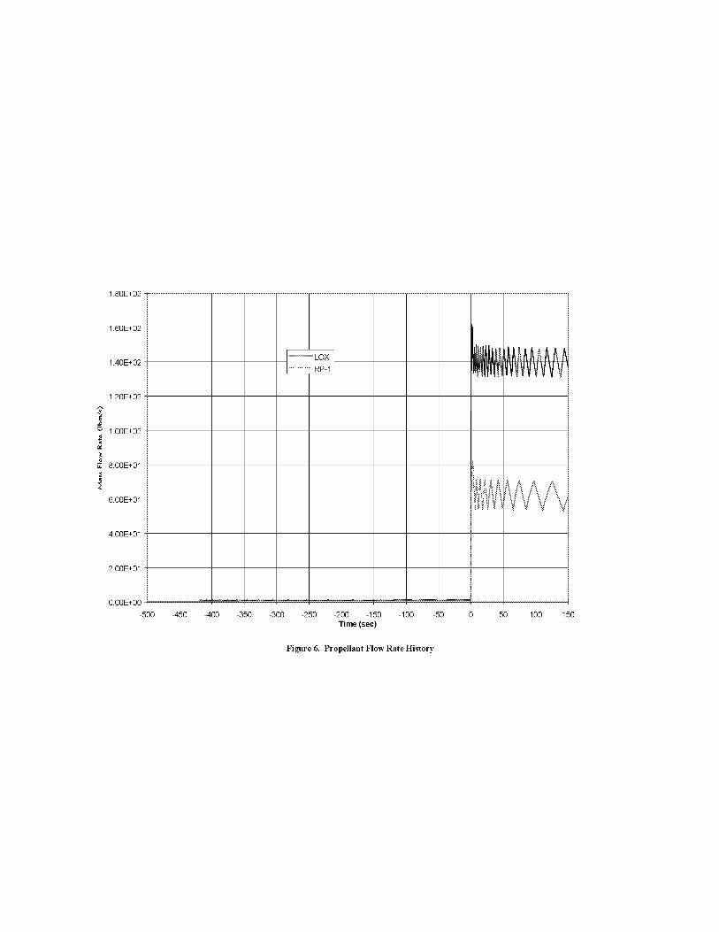
1.80E+02

1.60E+02

1.40E+02

1.20E+02

v 1.00E+02

8.00E+01

6.00E+01

4.00E+01

2.00E+01

O.OOE+O0

-500 -450 -400 -350 -300 -250 -200 -150 -100 -50 0

Time(see)

50 100 150

Figure 6. Propellant Flow Rate History

1.40E+00

1.20E+00

1.00E+00

8.00E-01

6.00E-01

4.00E-01

2.00E-01

0.00E+00

-500 -45O -400 -350 -300 -250 -200 -150 -100 -50

Time (sec)

Figure 7. Propellant Bleed Flow Rate History Detail

ANALYTICAL ASSESSMENT OF A GROSS LEAKAGE

EVENT WITHIN THE INTERNALTIONAL SPACE

STATION (ISS) NODE 2 INTERNAL ACTIVE THERMAL

CONTROL SYSTEM (IATCS)

James M. Holt

National Aeronautics and Space Administration

Marshall Space Flight Center

MSFC, AL 35812

Stephen E. Clanton

Sverdrup Technology, Inc.

MSFC Group

Huntsville, AL 35806

ABSTRACT

Results of the International Space Station (ISS) Node 2 Internal Active Thermal Control System (IATCS)

gross leakage analysis are presented for evaluating total leakage flow rates and volume discharge caused by a

gross leakage event (i.e. open boundary condition). A Systems Improved Numerical Differencing Analyzer

and Fluid Integrator (S1NDA85/FLU1NT) thermal hydraulic mathematical model (THMM) representing the

Node 2 IATCS was developed to simulate system performance under steady-state nominal conditions as well

as the transient flow effect resulting from an open line exposed to ambient. The objective of the analysis was

to determine the adequacy of the leak detection software in limiting the quantity of fluid lost during a gross

leakage event to within an acceptable level.

INTRODUCTION

Within the pressurized elements of the International Space Station (ISS), requirements exist to ensure a safe,

habitable environment for the crew. Internal Active Thermal Control Systems (IATCS), typically pumped

coolant loops utilizing a non-hazardous working fluid, have constraints on touch temperature, maximum

design pressure and leakage. This paper addresses "gross" leakage, or leakage that is much greater than

normal, specification leakage. Node 2 is required to limit the internal heat transport fluid leakage to no

greater than one gallon per gross leakage event 1.

The quantity of fluid expelled during a gross leakage event is clearly defined, however the duration is only

bounded in general terms by the "event." Node 2 utilizes software to control IATCS functions, and thus,

hardware and software response times must be taken into account to quantify the leakage "event." The

applicable software time constraints for gross leakage failure detection, isolation and recovery (FDIR) are as

follows2:

Time Averaged Accumulator Quantity Sensor Data

Data Transfer Latency to INTSYS

1NTSYS Command to Node 2 Latency

Pump Package Assembly (PPA) Response

1.7 seconds

1.0 seconds

2.0secoMs

0.5secoMs

Total Time 5.2 seconds

Therefore,an"event"of 5.2secondsmustbeanalyzedto determinecomplianceof theNode2 IATCShardwareandsoftware(FDIR)designswiththegrossleakagerequirement•ThispaperpresentsananalysisofagrossleakageeventfortheNode2IATCS.

NODE2 IATCS DESCRIPTION

The Node 2 IATCS consists of two separate single-phase, water coolant loops• The function of the IATCS is

to provide heat rejection for subsystem avionics equipment, for the environmental control system and for

subsystems and payloads within elements attached to Node 2. The two IATCS loops consist of a Low

Temperature Loop (LTL), that provides coolant temperatures in the range of 38-43 °F, and a Moderate

Temperature Loop (MTL), that provides coolant temperatures in the range of 61-65 °F. The Node 2 IATCS

is schematically shown in Figure 1.

LOW TEMPERATURE LOOP

l;STBD NAD

RACK RACK

MODERATE TEMPERATURE LOOP

<

JEM,

I I I

>

Figure 1. Node 2 IATCS

Each loop contains a Pump Package Assembly (PPA), capable of providing a mass flow rate of 3000 lbm/hr,

and a System Flow Control Assembly (SFCA) that maintains a constant differential pressure across the

system• Thermal control components include an ammonia/water heat exchanger, a Three-Way Mix Valve

(TWMV), which controls the water supply temperature to subsystems and attached elements, and a

regenerative heat exchanger (LTL only)•

The PPA contains a centrifugal pump and an accumulator that maintains sufficient pressure at the pump inlet

to avoid cavitation• The bellows within the accumulator is pressurized by gaseous nitrogen, actively

controlled by a Nitrogen Interface Assembly (NIA). As will be presented, the accumulator plays a significant

role, in addition to the pump, to the total fluid leakage during a gross leakage event• The accumulator has a

gas side maximum design pressure of 35 psia, and a nominal operational pressure in the range of 18 to

30 psia. The accumulator has a fluid capacity of 680 in 3 + 30 in 3 (2.8 gal. to 3.1 gal.) 3. An accumulator

TFAWS 99 2

quantitysensorindicatesthelevelof waterwithintheaccumulator,andat59%,promptsthesoftwaretoinitiatetheshutdownprocedure4.

SINDA85/FLUINTTHERMALHYDRAULIC MATHMATICAL MODEL

The gross leakage analysis is based on the Node 2 Design Review 1 (DR1) S1NDA85/FLU1NT IATCS

Thermal Hydraulic Mathematical Model (THMM) developed by Alenia Aerospazio 5. In order to analyze the

transient, gross leakage event, a plenum at ambient pressure was added downstream of the leakage location,

and inertia effects were added for all fluid lines. The most significant change to the model was logic added to

simulate the transient pressure within the accumulator.

The mathematical model fluid network is constructed of "lumps" and "paths" and a set of governing equations

are developed and solved within SINDA85/FLUINT. Three types of "lumps" exist within

S1NDA85/FLU1NT: tank, junction and plenum. The Node 2 IATCS model primarily consists of tanks (finite

volume) and junctions (zero volume), with a plenum _infinite volume) added to provide a "pressure" sink for

the leakage location.

The algebraic forms of the mass and energy conservahon equations for junctions are:

Zm=O

Eh;+6--0where:

m mass flow rate

h donor enthalpy

(_ lump energy source or sink term.

Similarly, the governing equations for tanks are differential forms of the mass and energy conservation

equations:

__m - dMdt

_--_hm+Q-P V+ VC =--_-

where:

M

P

VV

C

U

lump mass

lump pressure

volumetric flow rate

lump volume

tank wall compliance factor

lump internal energy term.

TFAWS 99 3

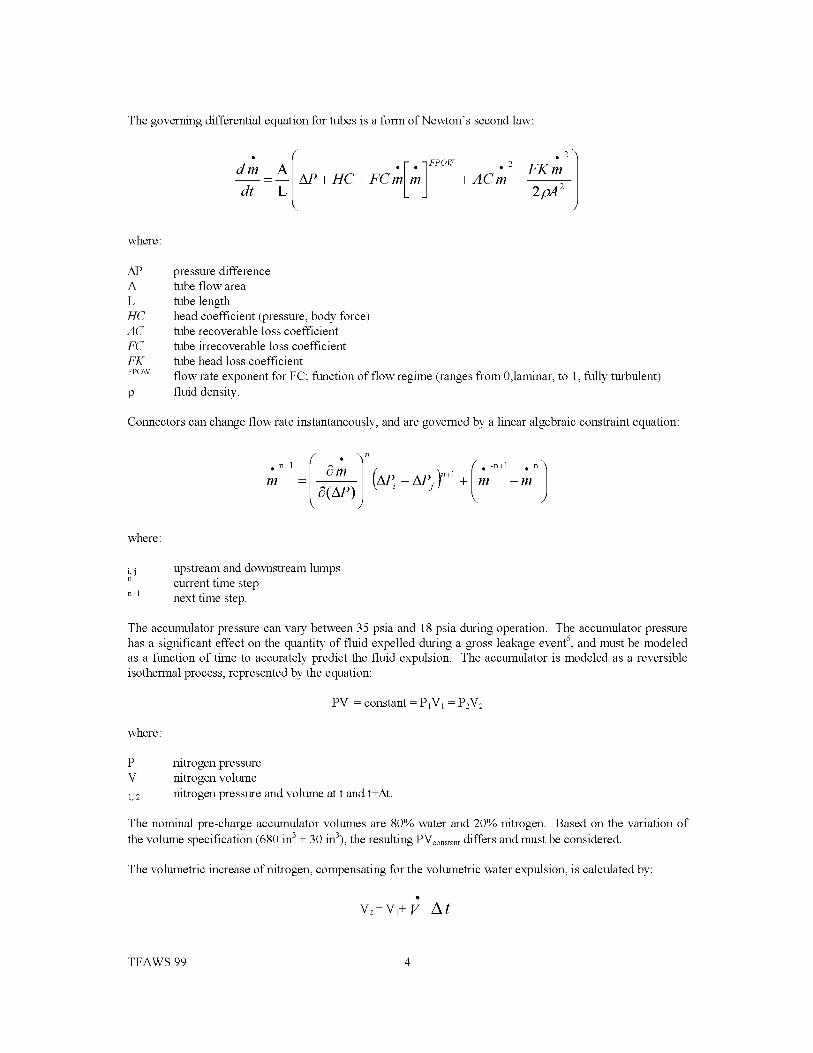
ThegoverningdifferentialequationfortubesisaformofNewton'ssecondlaw:

dm A

dt L hJ .2•F" -]ppo_ 2

AP + HC + FC m m +ACre FK m2pA 2

where:

AP pressure differenceA tube flow area

L tube length

HC head coefficient (pressure, body force)

AC tube recoverable loss coefficient

FC tube irrecoverable loss coefficient

FK tube head loss coefficient

vPOW flow rate exponent for FC; function of flow regime (ranges from 0,laminar, to 1, fully turbulent)

p fluid density.

Connectors can change flow rate instantaneously, and are governed by a linear algebraic constraint equation:

, / /• n+l _ m -n+l • n

m : A_i- Ap j n+l+ m

where:

i, j upstream and downstream lumps

n current time step

n+l next time step.

The accumulator pressure can vary between 35 psia and 18 psia during operation. The accumulator pressure

has a significant effect on the quantity of fluid expelled during a gross leakage event 6, and must be modeled

as a function of time to accurately predict the fluid expulsion. The accumulator is modeled as a reversible

isothermal process, represented by the equation:

PV = constant = Pig1 : P2V2

where:

P

V

1,2

nitrogen pressure

nitrogen volume

nitrogen pressure and volume at t and t+At.

The nominal pre-charge accumulator volumes are 80% water and 20% nitrogen. Based on the variation of

the volume specification (680 in 3 + 30 in3), the resulting PVconsta_t differs and must be considered.

The volumetric increase of nitrogen, compensating for the volumetric water expulsion, is calculated by:

V2 = Vl-}- V A t

TFAWS 99 4

where:

V

Atvolumetric flow rate of water expelled from the system

computational time step.

The transient nitrogen pressure is then calculated by:

P2 = PVconstant/V2

ANALYSIS

Leakage scenarios were developed for both the MTL and LTL. These scenarios assume a critical Quick

Disconnect (QD) seal failure at the Node 2 to attached element(s) IATCS interface. The scenarios analyzed

were:

• Leakage at Node 2 to CAM MTL supply interface

• Leakage at CAM to Node 2 MTL return interface

• Leakage at Node 2 to MPLM LTL supply interface

• Leakage at MPLM to Node 2 LTL return interface

• Leakage at Node 2 to CAM LTL supply interface

• Leakage at CAM to Node 2 LTL return interface.

Steady state and transient simulations were performed for each leakage scenario. FASTIC and STDSTL

solution routines were used to establish nominal, steady-state conditions prior to analyzing the gross leakage

event. The FWDBCK solution routine was used for the transient analysis of the event. The computational

time step was limited to no greater than 0.1 seconds 7.

S1NDA85/FLUINT analysis results for the aforementioned scenarios showed that the "leakage at Node 2 to

CAM MTL return interface" provided the most severe leakage path in which to assess the IATCS system 6.

This scenario was considered for the purpose of this paper.

LEAKAGE AT CAM TO NODE 2 MTL RETURN INTERFACE

This scenario assumes that leakage occurs at the Quick Disconnect (QD) located on the Node 2 side of the

CAM MTL return line. The QD on the CAM side of the return line is assumed to "seal" upon disconnection.

Figure 2 depicts the IATCS MTL nodal network and leakage area. At the onset of the leakage event, nominal

flow through the CAM from the supply line is "shut off" due to the sealed QD on the return line. The leakage

area for the failed QD is calculated based on 100% exposure of the line cross-sectional area (0.3872 in2). The

failed QD is exposed to an ambient pressure of 14.25 psia which coincides with the U. S. Laboratory (USL)

module nitrogen introduction threshold.

TFAWS 99 5

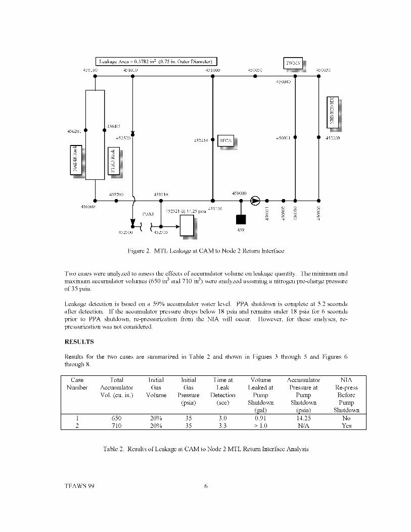
456201

Q

I LeakageArea=0"3782ins(0"75in'OuterDiameter) I

456100 451010 451000

_L

q l56401

452520 452410

T 455200 451110 450000

456500

452521@14.25 psia 451100CA

452500 452505459

450050

450040

450011 | I

Figure 2. MTL Leakage at CAM to Node 2 Return Interface

450030

Q452200

Two cases were analyzed to assess the effects of accumulator volume on leakage quantity. The minimum and

maximum accumulator volumes (650 in 3 and 710 in 3) were analyzed assuming a nitrogen pre-charge pressure

of 35 psia.

Leakage detection is based on a 59% accumulator water level. PPA shutdown is complete at 5.2 seconds

after detection. If the accumulator pressure drops below 18 psia and remains under 18 psia for 6 seconds

prior to PPA shutdown, re-pressurization from the NIA will occur. However, for these analyses, re-

pressurization was not considered.

RESULTS

Results for the two cases are summarized in Table 2 and shown in Figures 3 through 5 and Figures 6

through 8.

Case Total Initial Initial Time at Volume Accumulator NIA

Number Accumulator Gas Gas Leak Leaked at Pressure at Re-press

Vol. (cu. in.) Volume Pressure Detection Pump Pump Before

(psia) (sec) Shutdown Shutdown Pump

(gal) (psia) Shutdown

1 650 20% 35 3.0 0.91 14.25 No

2 710 20% 35 3.3 > 1.0 N/A Yes

Table 2. Results of Leakage at CAM to Node 2 MTL Return Interface Analysis

TFAWS 99 6

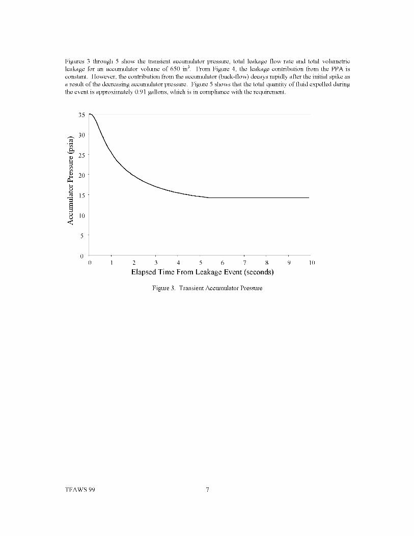
Figures3 through5 showthetransientaccumulatorpressure,totalleakageflowrateandtotalvolumetricleakageforanaccumulatorvolumeof650in3. FromFigure4,theleakagecontributionfromthePPAisconstant.However,thecontributionfromtheaccumulator(back-flow)decaysrapidlyaftertheinitialspikeasaresultofthedecreasingaccumulatorpressure.Figure5showsthatthetotalquantityoffluidexpelledduringtheeventisapproximately0.91gallons,whichisincompliancewiththerequirement.

35

3O

&o 25

r_r_O

20

oN 15

o 10e,.,)

<

0 1 2 3 4 5 6 7 8

Elapsed Time From Leakage Event (seconds)

Figure 3. Transient Accumulator Pressure

10

TFAWS 99 7

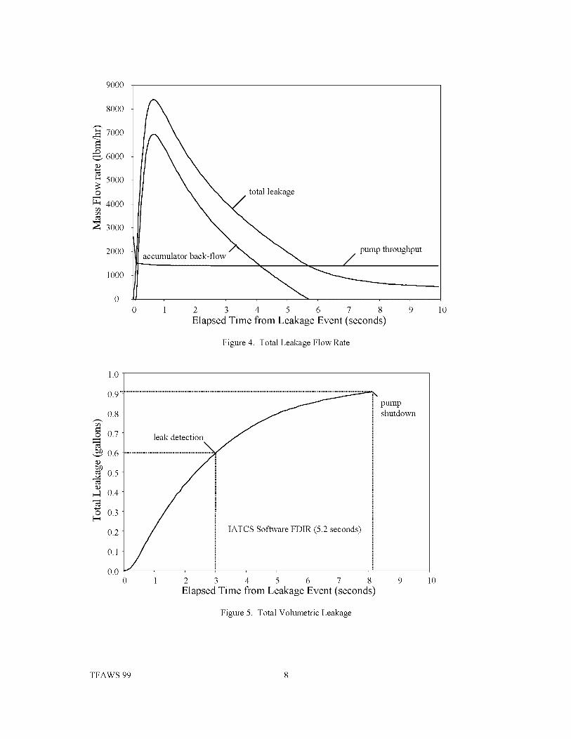
9000

8000

7000.0"-- 6000

5000

o

4000

3000

2000

1000

total leakage

accumulator back-flowpump throughput

0 1 2 3 4 5 6 7 8

Elapsed Time from Leakage Event (seconds)

Figure 4. Total Leakage Flow Rate

10

1.0

0.9

0.8

o 0.7

_ 0.6(D

_ 0.5

0.4

_6 0.3

0.2

0.1

0.0

IATCS Software FDIR (5.2 seconds)

2 3 4 5 6 7 8

Elapsed Time from Leakage Event (seconds)

Figure 5. Total Volumetric Leakage

pumpshutdown

10

TFAWS 99 8

Figures6 through8 showthetransientaccumulatorpressure,totalleakageflowrateandtotalvolumetricleakageforanaccumulatorvolumeof710in3.Asfromthepreviousresults,thetrendsareidentical.FromFigure6,theleakagecontributionfromthePPAisconstant.Again,thecontributionfromtheaccumulator(back-flow)decaysrapidlyaftertheinitialspikeasaresultofthedecreasingaccumulatorpressure.Figure8showsthatthetotalquantityof fluidexpelledduringtheeventis approximately0.92gal,whichis incompliancewiththerequirement.However,fromFigure6,theaccumulatorpressureisbelow18psiaformorethan6secondspriortoPPAshutdownandre-pressurizationoftheaccumulatormustoccur.If re-pressurizationhasbeenaccountedfor,thetotalquantityoffluidexpelledwouldexceed1.0gal.

4O

35

._30

25

20

15e,...)

e,...)

"< lO

0 1 2 3 4 5 6 7 8 9 10

Elapsed Time from Leakage Event (seconds)

Figure 6. Transient Accumulator Pressure

TFAWS 99 9

9000

8000

7000-

_6000,.Q

5000

o,..- 4000-

3000

2000

1000

accumulator back-flow

total leakage

pump throughput

0 1 2 3 4 5 6 7 8 9 10

Elapsed Time from Leakage Event (seconds)

Figure 7. Total Leakage Flow Rate

1.0_

0.9

0.8"Do 0.7

0.6(D

0.5

2 0.4i

_6 0.3

0.2

0.1

0.0

0

i hutd°wn

leak detection l _ i

1 2 3 4 5 6 7 8 9 10

Elapsed Time from Leakage Event (seconds)

Figure 8. Total Volumetric Leakage

TFAWS 99 10

CONCLUSIONS

For an accumulator pre-charge ratio of 80% water and 20% nitrogen and a pressure of 35 psia, an

accumulator of 650 in 3 (minimum hardware specification) is in compliance with the gross leakage

requirement with the current FDIR software. However, for the same pre-charge conditions, an accumulator of

710 in 3 (maximum hardware specification) does not satisfy the requirement. Since the accumulator volume

variation is a consequence of the manufacturing process, either the pre-charge water volume (80%) or the

software leak detection threshold (59%) must be altered to insure that the requirement is not violated.

ACKNOWLEDGEMENTS

The authors wish to thank Giuseppe Valenzano and Silvia Lombardi of Alenia Aerospazio for development

of the Node 2 IATCS THMM, and for their dedication not only to this problem, but to the many challenges of

developing hardware and systems for the ISS. We also wish to thank Robert Hartung of Boeing-Huntsville,

Darryl Gaines of NASA-MSFC and Deborah Kromis of Quality Research for their help with the software

details of this problem.

REFERENCES

1. SSP 50290, Node 2 Prime Item Development Specification (PIDS)

2. Node 2 SSR/PDR

3. 2353866G, Prime Item Development Specification, Type B1, Pump Package Assembly, AlliedSignal

Aerospace Company, Aerospace Equipment Systems.

4. Node 2 Software Requirements Specification

5. N2-TN-AI-0012, N2 IATCS Thermal-Hydraulic Analysis, Alenia Aerospazio, January 30, 1998.

6. 661-017-98-009, Node 2 IATCS Gross Leakage Analysis, Sverdrup Technology, September 23, 1998.

7. Systems Improved Numerical Differencing Analyzer and Fluid Integrator (S1NDA85/FLU1NT),

Cullimore and Ring Technologies, Inc.

TFAWS 99 11

TIME-ACCURATE SOLUTIONS OF INCOMPRESSIBLE NAVIER-STOKES

EQUATIONS FOR POTENTIAL TURBOPUMP APPLICATIONS

Cetin Kiris

MCAT, Inc.

Dochan Kwak

NASA Ames Research Center

Mail Stop T27B-1

Moffett Field, CA 94035

Abstract

Two numerical procedures, one based on artificial compressibility method and the

other pressure projection method, are outlined fbr obtaining time-accurate solutions of

the incompressible Navier-Stokes equations. The perfbrmance of the two method are com-

pared by obtaining unsteady solutions fbr the evolution of twin vortices behind a fiat plate.

Calulated results are compared with experimental and other numerical results. For an un-

steady flow which requires small physical time step, pressure projection method was found

to be computationally efficient since it does not require any subiterations procedure. It was

observed that the artificial compressibility method requires a fast convergence scheme at

each physical time step in order to satisfy incompressibility condition. This was obtained

by using a GMRES-ILU(0) solver in our computations. When a line-relaxation scheme

was used, the time accuracy was degraded and time-accurate computations became very

expensive.

Introduction

The primary objective of this research is to support the design of liquid rocket sys-

tems fbr the Advanced Space Transportation System. Since the space launch systems in

the near future are likely to rely on liquid rocket engines, increasing the efficiency and

reliability of the engine components is an important task. One of the major problems in

the liquid rocket engine is to understand fluid dynamics of fuel and oxidizer flows from

the fuel tank to plume. Turbopumps in liquid rocket engines are one of the biggest source

of vibrations. Understanding the flow through the entire turbopump geometry through

numerical simulation will be of significant value toward design. This will help to improve

safety of future space missions. One of the milestones of this effort is to develop, apply and

demonstrate the capability and accuracy of 3D CFD methods as efficient design analysis

tools on high perfbrmance computer platforms. In order to achieve flange-to-flange entire

turbopump simulations, moving boundary capability and an efficient time-accurate inte-

gration method should be build in the numerical procedure. This paper, in particular, is

concerned with the time integration procedure of incompressible Navier-Stokes equations.

The incompressible Navier-Stokes equations pose a special problem of satisfying the

mass conservation equation because it is not coupled to the momentum equations. To

satisfy incompressibility various procedures can be selected depending on the choice of for-

mulations, variables, discretization and iterative schemes. In this paper, two fbrmulations

areconsidered,the first onebasedon an artificial compressibilitymethod and the secondone on a pressureprojection method. The artificial compressibilitymethodI takes ad-vantageof the advancesmadein conjunctionwith compressibleflow computations. Thisapproachrelaxesthe requirementof enforcingmassconservationequation rigorously ateachtime iteration, however,at the expenseof introducing anartificial wavephenomenon.This approachcanbeviewedasa specialcaseof apreconditionedcompressibleflow tbrmu-lation. However,the computationalefficiencyis in generalbetter than that of compressibleflow solversat the incompressiblelimit. This approachhasbeenshownto bevery robustin a wide rangeof applications2-4.

The first primitive variablemethod for incompressibleflow wasdevelopedby Harlowand Welch5 usingpressureprojection. Numerousvariantshavebeendevelopedsince. Inthis method,the pressureis usedasamappingparameterto satisfythecontinuity equation.The usualcomputationalprocedureinvolveschoosingthe pressurefield at the current timestep suchthat continuity is satisfiedat the next time step. The time step is advancedinmultiple steps(fractional step) which is computationally convenient.However,governingequationsare not coupledasin an artificial compressibilityapproach.This will affect therobustnessand linfit the maximum allowabletime stepsize. Sincethis approachis timeaccurate,therearecaseswherethe fractional stepsolveris computationallymoreefficientcomparedto the artificial compressibilitymethod5-9.

Various numerical algorithms associatedwith thesemethods have been developedalongwith accompanyingflow solvers. In the presentpaper, it is intendedto outline thetime integration proceduresof the two methodsdiscussedabove. A new time integrationschemeis alsopresentedfor pressureprojection method. Numericalresultsfrom both for-mulationsfor the developmentof the twin vorticies1°'11behindthe fiat plate arepresentedin computedresults section.

Artificial Compressibility Formulation

The artificial compressibility algorithm introduces a time-derivative of the pressure

term into the continuity equation; the elliptic-parabolic type partial differential equations

are transtbrmed into the hyperbolic-parabolic type. The artificial compressibility method

by Chorin (1967) can be written as

10p---+ -o (1)fl Ot Ox_

Op- + hi = -ri (2)

Ot Ox_

where t is time, xi the Cartesian coordinates, ui the corresponding velocity components,

p the pressure, /3 artificial compressibility, and h_ contains both convective and viscous

terms. At steady state the pressure term in continuity equation drops out and thus in-

compressibility is recovered. For time accurate computations, this has to be repeated at

each time level to maintain incompressibility at each time step.

In the present study, the time derivatives in the momentum equations are differenced

using a second-order, three-point, backward-difference fbrmula.

3un+l -- 4Un q- Ha-1 = --r n+l (3)2At

where u and r denote the dependent variable vector and the right hand side vector tbr the

momentum equations, respectively. After the discretization in time, the pseudocompress-

ibilty term and pseudo-time level (rn) are introduced to equations.

1

AT (prt+l,rn+l _ pn+l,rn) = --/iV" U n+l'rn+x

1.5

Z_t (Unq-l'rnq-1 -- UrZq-l'rn) = --rnq-l'rnq-1-- (4)

3un+l,rn _ 4U n q- U rz-1

2At

Here At, At, n, and m denote physical time step, pseudo-time step, physical time level,

and subiteration time level, respectively. The equations are iterated to convergence in

pseudo-time fbr each physical time step until the divergence of the velocity field has been

reduced below a specified tolerance value. This typically requires 10 to 30 subiterations.

The matrix equation is solved iteratively by using a nonfactored Gauss-Seidel type

line-relaxation scheme, 12 which maintains stability and allows a large pseudo-time step to

be taken. Details of the numerical method can be tbund in Ret_. 2-3. GMRES scheme has

also been utilized tbr the solution of the resulting matrix equation la. Computer memory

requirement for the corresponding flow solver (INS3D-UP code) with line-relaxation is

35 times number of grid points in words, and with GMRES-ILU(0) scheme is 220 times

number of grid points in words. Extensive memory requirement tbr GMRES scheme makes

the code unpractical tbr three-dimensional applications. Writing a matrix-free GMRESsolver renmains to be one of the items tbr future enhancemets.

The original version of the INS3D code 2 with pseudocompressibility approach utilized

the Beam-Warming 14 approximate factorization algorithm and central differencing of the

convective terms. Since the convective terms of the resulting equations are hyperbolic,

upwind differencing can be applied to these terms. The current versions of the INS3D-UP

code use flux-difference splitting based on the method of Roe. 15 Chakravarthy 16 outlines a

class of high-accuracy flux-differencing schemes tbr the compressible flow equations. The

third and fifth-order upwind differencing used here is an implementation of these schemes

tbr the incompressible Navier-Stokes equations. The upwind differencing leads to a more

diagonal dominant system than does central differencing and does not require a user-

specified artificial dissipation. The viscous flux derivatives are computed by using central

differencing.

Time-accurate artificial compressibility tbrmulation has been used successfully for un-

steady calculations. The only drawback of this tbrmulation is the computational cost due

to subiteration procedure.

Pressure Projection Method

The time integration scheme is based on operator splitting, which can be accomplished

in several ways by combining the pressure, convective, and viscous terms in the momentum

equations.The tractional stepmethodis basedon the decompositionof vector field into adivergencefreecomponentand gradientof a scalarfield. The commonapplicationof thismethod is donein two steps.The first step is to solvetbr an auxiliary velocity field usingthe momentumequations. In the secondstep,the velocity field is correctedby using thepressurewhich can map the auxiliary velocity onto a divergencetree velocity field. Themomentumequationsare discretizedin time using a second-orderimplicit Runga-Kuttamethod (RK2) which can alsobe viewedasa predictor-correctormethod.

1 Op _'

At (_ -- _) -- Oxi + h(u_) (5)

and a corrector step

2 / n-b1 0P n-b1 n+l _ __ _}_ h(?t_) ) (6)

where u_ denotes the auxiliary velocity field. The h term in the momentum equations

includes the convective and viscous terms. By using equation (5), equation (6) can bewritten as

_i (?t_+ 1 * Op n+l 1n+l

- _) - o_ + h(_ ) - at(_ - _) (7)

By subtracting equation (5) from equation (7), we obtain

2 (o n+l ' n-t-1

At,. _ -_) =-v_ + h(_ )- h(_) (8)

where p' = p_,+l _ p_. At n + 1 time level, the velocity field has to satisfy the incompress-

ibility condition which is the continuity equation.

V" U n-}-I = 0 (9)

This incompressiblity condition is entbrced by using a Poisson equation tbr pressure.

' Zv.u* (10)V2P = At

The Poisson equation tbr pressure is obtained by taking the divergence of equation (8) and

using equation (9). The only assumption is made in this procedure is that h(u_ _+1) -h(u_')

term in equation 8 is considered small. If the corrector step was explicit, this term wouldvanish.

In equations (5) and (7), both convective and viscous terms are treated implicitly.

The residual term at the (,) and (n + 1) level is linearized giving the tbllowing equationsin delta tbrm

+ _ (_* - _) - o_ + h(_') (11)

2I Oh (_t n+l _t* -_- h(_t_)- _?) (12)+ _ - ) - Ox, Xi (_ -

where I is the idendity matrix. Equation (12) can also be written in more familiar fbrm

of fractional-step method by substituting equation (5) in equation (12).

[ ()*]2/ Oh (?/nq-1 0/)' (13)27 + _ -_*)- 0xi

Equations (11), (10), and (12) give the proposed time integration procedure of the pressure

projection method.

The algorithm tbr the pressure projection method is based on a finite-volume formu-

lation and uses the pressure in the cell center and the mass fluxes across the faces of each

cell as dependent variables. The discretization of the mass conservation equation in finite

volume tbrmulation gives

(S_ •u)j+l,k,_ - (S_ •u)j_+,k,_+

(S_ •u)_,k++,_ - (S_ •u)j,__+,_+

(S_ • u)j,k,_+_ - (S_ •u)j,k,__l = 0

(14)

where S is the surface area vector. The mass conservation equation is evaluated over the

faces of a computational Each term in equation (14) approximates the mass flux over the

corresponding cell face. If the mass fluxes are chosen as unknowns, the continuity equation

is satisfied automatically in generalized coordinate systems. The mass fluxes over the _, _!

, and _ faces of the computational cell are

U _ =S _ • u

U _ =S _ • u

U _ =S ¢ • u

(15)

The continuity equation with this choice of the dependent variables takes a tbrm identical

to the Cartesian case. Theretbre, the mass fluxes are considered as the 'natural' depen-

dent variables tbr projection methods in curvilinear coordinates. The mass conservation

equation with new dependent variables in a generalized coordinate system becomes

- - vj,k-½,l @

U_¢,k,l+½ ¢- 1 = 0(16)

Treating the mass fluxes as dependent variables in finite volume tbrmulation is equivalent

to using contravariant velocity components, scaled by the inverse of the transtbrmation

Jacobian, in a finite-difference tbrmulation. This choice of mass fluxes as dependent vari-

ables complicates the discretization of the momentum equations. In order to replace u

by the new dependent variables U l, the corresponding area vectors are dotted with the

momentum equations. Then the integral momentum equation is evaluated on different

computational cells tbr each unknown U z. Each cell has the dimensions of A_ x A_j x AC,1

1 /g,l) (j,/_ q- _,l), and (j,k,l + ½) tbr g e, U r_, gildbut the centers are located at (j + _, ,

U c momentum equations, respectively. The staggered grid orientation eliminates pressure

checker-board-like oscillations in pressure and provides more compact stencils. The deriva-

tion of momentum equations and the solution procedure is outlined in reference 9. Since

each equation is solved in a segregated fashion, memory requirements for GMRES solver

in INS3D-FS is not as big as INS3D-UP code. Required memory fbr INS3D-FS is 70 times

number of grid poins in words.

Computed Results

In this section, numerical results tbr the time evolution of twin vortices behind a fiat

plate are presented in order to verify the time-dependent features of the two algorithms.

In order to investigate different features of the algorithms, several cases are needed to

run with various code related parameters. To speed up this process, a two dimensional

test case is selected here. It should be noted that associated flow solvers, INS3D-UP

fbr artificial compressibility method and INS3D-FS fbr pressure projection method, are

written fbr three-dimensional applications. With this numerical experiment, it is intended

to give some basis fbr selecting a method fbr large three-dimensional unsteady applications

where computing resources become a critical issue.

Computed results from both methods are compared with the experimental data by

Taneda and Honji 1°. The experiment has carried out in a water tank 40 cm wide. A thin

test plate of size H = 3cut immersed in the water was started from the rest impulsively at

the velocity U = 0.495c_/s. Reynolds number tbr this case is 126 based on U = 0.495cut/s

velocity and the plate height H. Computational grid with with size of 181x81x3 is presented

in figure 1. Since INS3D-FS is written in finite volume staggered grid fbrmulation, it

requires one additional ghost cell in each direction. Figure 2 shows calculated velocity

vectors obtained from INS3D-FS at various times. The flow separates the plate at each

edge and fbrms a vortex pair. The twin vortices become longer in the flow direction withtime.

The calculated time history of the stagnation point is compared with experimental

results and other numerical results in figure 3. Symbols represent experimental mea-

surements, solid line and dashed line represent results from INS3D-UP and INS3D-FS,

respectively. Dotted line show the numerical results from finite element tbrmulations of

Yoshida and Nomura 11. The interval fbr time integration was 0.5 sec, which corresponds

to nondimensional value of 0.0825, tbr all computations in figure 3. Eventhough the plate

started impulsively in the experiment, the computations presented in figure 3 have a slow

start procedure. Figure 4 shows prescribed velocity tbr an impulsive start (4a) and tbr

a slow start (4b) used in INS3D-UP and INS3D-FS calculations. Reference 11 also used

same slow start procedure in their calculations. When nondimensional time step of 0.0825

was used with an impulsive start, large discrepancies were observed between numerical

results and the experimental mesurements. This can be seen in figure 5a. When the time

step is decreased, fairly good agreement was observed between numerical results and the

measurements as seen in figure 5b. For the slow start case, the velocity profile shown in

figure 4b is prescribed and the origin of time of calculation is appropriately shiRed from

the time of experiment. This unsteady computations with INS3D-FS (At = 0.0825) was

completed in two hours of CPU time on single processor Cray-J90.

INS3D-UP computationswith line-relaxationschemeis presentedin figure 6. Vari-ousartificial compressibilityparametersand numberof subiterationswereused.Figure 6showsthe effectsof numberof subiterationsand the effectsof usingtwo differentartificialcompressibilityparameters/d. When the incompressibility conditions is not satisfied at

each physical time step, numerical results can be erronous in time-accurate computations.

With line-relaxation scheme, INS3D-UP calculations required between 4 hours of CPU

time (10 subiterations at each physical time step) and 14 hours (40 subiterations) on a

single processor Cray-J90 computer. Our observation tbr the time-accurate computations

from this numerical example is that the artificial compressibility method requires a fast

convergence scheme at each physical time step in order to satisfy incompressibility condi-

tion. If this is not satisfied as seen in line-relaxation scheme, the time accuracy is degraded

(see figure 6). In addition, artificial compressibility method with line relaxation scheme

can be expensive tbr 3D time-accurate computations. In figure 7, INS3D-UP results with

GMRES-ILU(0) solver are presented. These results were obtained less than 4 hours on a

Cray-J90 computer. Fairly good agreement was obtained between the computed results

and experimental data. With GMRES-ILU(0) solver, the mass flow ratio between inflow

and exit was always satisfied. In addition, the discrepancies between numerical results

are very small when two different values of artificial compressibility parameter were used.

Figure 8 shows the results from artificial compressibility method with and without Poisson

equation correction tbr the pressure. In artifical compressibility method, after the first

sub-iteration, the Poisson equation is employed tbr the pressure correction. Chain-dashed

line in figure 8 represents the results from this new procedure. With the Poisson equation

correction, the line relaxation results compare well with experimental data and the GM-

RES results with 10 subiterations. With this new procedure, both computing time and

memory requirement are substantially reduced (at least three times).

Concluding Remarks

Unsteady computations were perfbrmed using two different solution algorithms, which

are artificial compressibility method and pressure projection method. When a fast converg-

ing scheme, such as GMRES-ILU(0) solver, was incorparated in artificial compressibility

method, fairly good agreement was obtained between computed results and experimental

data. Our numerical experiment showed that incompressiblity condition was satisfied in

10 subiterations at each physical time step. Memory requirement of this scheme is the

major drawback tbr three-dimensional large applications. However, memory requirement

may not be an issue on the paralel platfbrms, such as SGI Origin 2000. The line-relaxation

scheme in artificial compressibility method becomes very expensive and results in erronous

solution tbr time-accurate computations. For an unsteady flow which requires small physi-

cal time step, pressure projection method was tbund to be computationally efficient since it

does not require any subiterations procedure. However, governing equations are not fully

coupled as in the artificial compressibility approach. This may affect the robustness and

limit the maximum allowable time step size. A new method is developed by combining

pressure projection method with artificial compressibility method. With Poisson solver

correction,the numberof subiteration wasreducedto two iterations at eachphysicaltimestep.

Acknowledgments

Computer time was provided by the Numerical Aerodynamic Simulation (NAS) Fa-

cility and the Central Computing Facility at NASA Ames Research Center.

References

1. Chorin, A., J., "A Numerical Method tbr Solving Incompressible Viscous FlowProblems," orournal of" Computational Physics, Vol. 2, pp. 12-26, 1967.

2. Kwak, D., Chang, J. L C., Shanks, S. P., and Chakravarthy, S., "A Three-Dimensional Incompressible Navier-Stokes Flow Solver Using Primitive Variables," AIAA

Journal, Vol. 24, No. 3, pp. 390-396, 1977.

3. Rogers, S. E., Kwak, D. "Upwind Differencing tbr the Time-Accurate Incompress-ible Navier-Stokes Equations," AIAA orournal, Vol. 28, No. 2, pp. 253-262, 1990.

4. Rogers, S. E., Kwak, D. and Kiris, C., "Numerical Solution of the IncompressibleNavier-Stokes Equations tbr Steady and Time-Dependent Problems," AIAA orournal, Vol.

29, No. 4, pp. 603-610, 1991.

5. Harlow, F. H., and, Welch, J. E., "Numerical Calculation of Time-DependentViscous Incompressible Flow with Free Surface," Phys. Fluids , Vol. 8, No. 12, pp.

2182-2189, 1965.6. Kim, J. and Moin, P., "Application of a

Fractional-Step Method to Incompressible Navier-Stokes Equations," or. Comp. Phys. ,

Vol. 59, pp. 308-323, 1985.Y. Choi, H., and Moin, P., "Effects of the Computational Time Step on Numerical

Solutions of Turbulent Flow," or. Comp. Phys., Vol. 113, pp. 1-4, 1994.8. Rosenfeld, M., Kwak, D., and Vinokur, M., "A Fractional-Step Method tbr the

Unsteady Incompressible Navier-Stokes Equations in Generalized Coordinate Systems,"

AIAA Paper No. 88-0718, 1988.or. Comp. Physics, Vol. 94, No. 1, pp. 102-137, 1991.

9. Kiris, C., and Kwak, D., "Numerical Solution of Incompressible Navier-StokesEquations Using a Fractional-Step Approach,"AIAA Paper No. 96-2089, 1996.

10. Taneda, S., and Honji, H., "Unsteady Flow Past a Flat Plate Normal to the

Direction of Motion," Y. Phys. Soc. orapan, Vol. 30, pp. 262-273, 1971.11. Yoshida, Y., and Nomura, T., "A Transient Solution Method tbr the Finite

Element Incompressible Navier-Stokes Equations," Int. Y. N'um. Methods in Fluids ,Vol. 5, pp. 873-890, 1985.

12 MacCormack, R., W., "Current Status of Numerical Solutions of the Navier-Stokes

Equations,"AIAA Paper No. 85-0032, 1985.

13. Rogers, S. E., "A Comparison of Implicit Schemes tbr the Incompressible Navier-Stokes Equations and Artificial Compressibility," AIAA orournal, Vol. 33, No. 10, Oct.1995

14 Beam, R. M., Warming, R. F., " An Implicit Factored Scheme tbr the CompressibleNavier-Stokes Equations," AIAA orournal, Vol 16, pp. 393-401, 1978.

15 Roe, P.L., "Approximate Riemann Solvers, Parameter Vectors, and DifferenceSchemes," Journal of Computational Physics, Vol. 43, pp. 357-372 1981

16 Chakravarthy, S. R., Osher, S., "A New Class of High Accuracy TVD Schemes tbrHyperbolic Conservation Laws," AIAA Paper No. 85-0363, 1985.

Figure 1 : Computational grid forthe flow past a 90-degree flat plate.

(plate tickness = 0.03H)

VELOCITY VECTORS AND MAGNITUDE CON]'oURS .(!NS3D--FS)

l-' ....... Finite Elem. Sol. (ref. 11)/

0 ½ 4 6'

Time

Figure 3 : Calculated time history

of the stagnation point.

VELOCITY VECTORS AND MAGNITUDE CONTOURS (INS3D-FS)

Figure 2a : Velocity vectors at vari-

ous non-dimensional times (INS3D-FS).

i

iii::_iii iiiiiii:_ii::i_ _i_i_i_i_!!i_!!_a:!::_:::::_:::_::::_::_:::_:::_............................................. "............. _"_i::i:;::_i

::ill..... _Ni_igii:ig_?;?ili_;i_i gg;i_gii_i_iigsi_gii;iiiiziigi?"ii;_iii iii_:ii21:2i_ii_ii ....iiii_ N_iiiiiiiiiigiiiiiiiiiiiiii_igiigiii_i_ii;ii_ii_iii_ii_sii_iikQ_,iii_zii)iiiii_Ai_sii;ii;ii ;i ii_si_iii; ;i ii; iA i iii::_.....

Figure 2b : Velocity vectors at vari-

ous non-dimensional times (INS3D-FS).

impulsive start 4-a

slow start 4-b

l u = U (l-cos(_t/T))/2

Figure 4 : Prescribed velocity foran impulsive start (a) and for a slow

start(b).

• / • EXP. (Taneda, 1971),, -- DT=0.0825, SLOW START

.... DT=0.0825, IMPULSIVE START

0 ½ 4 6'

Time

Figure 5a : Effects of starting pro-cedure.

H or,)* "--"

= y • EXP (Taneda, 1971)

_-55 (fine glid)

/ -.- DT 0.0103125

0 ½ 4 6'

Time

Figure 5b: Effects of time-step size

for impulsive start.

1'0 2'0 3'0 40

Time (sec)

Figure 6 : Evaluation movement of

stagnation point from INS3D-UP cal-culation with line-relaxation scheme.

H - .._...._..........._...'" !'"""

" ...'..."2 _=;"

;=

1

• .... BETA=100, SLOW START

I." ....... BETel0, IMPULSIVE START

0 0 _ _ 6Time (sec)

Figure 7 : Evaluation movement of

stagnation point from INS3D-UP cal-

culation with GMRES-ILU(0) scheme.

32-

1 •x_ / INS3D-UP/DT 0.0825

• ,/,' / • EXP. (Tmleda, 1971)

• // ," -- LINE-RELAXATION, NSUB=10• J" / _/ION_NSoUB 10

J _oIsS_oN SOL, NSUB 2

i _ 6'Time

Figure 8 : Artificial compressibilityresults with and without Poisson equa-tion correction.

UNSHROUDED CENTRIFUGAL TURBOPUMP

IMPELLER DESIGN METHODOLOGY

George H. Prueger, Morgan Williams, Wei-chung Chen, John Paris

Boeing / Rocketdyne Propulsion and Power

Robert Williams, Eric StewartNASA - MSFC

ABSTRACT

Turbopump weight continues to be a dominant parameter in the trade space for reduction of engine weight.

Space Shuttle Main Engine weight distribution indicates that the turbomachinery make up approximately

30% of the total engine weight. Weight reduction can be achieved through the reduction of envelope of the

turbopump. Reduction in envelope relates to an increase in turbopump speed and an increase in impeller

head coefficient. Speed can be increased until suction performance limits are achieved on the pump or due

to alternate constraints the turbine or bearings limit speed. Once the speed of the turbopump is set the

impeller tip speed sets the minimum head coefficient of the machine. To reduce impeller diameter the head

coefficient must be increased. A significant limitation with increasing head coefficient is that the slope of

the head-flow characteristic is affected and this can limit engine throttling range.

Unshrouded impellers offer a design option for increased turbopump speed without increasing the impeller

head coefficient. However, there are several issues with regard to using an unshrouded impeller: there is a

pump performance penalty due to the front open face recirculation flow, there is a potential pump axial

thrust problem from the unbalanced front open face and the back shroud face, and since test data is very

limited for this configuration, there is uncertainty in the magnitude and phase of the rotordynamic forces

due to the front impeller passage. The purpose of the paper is to discuss the design of an unshrouded

impeller and to examine the hydrodynamic performance, axial thrust, and rotordynamic performance. The

design methodology will also be discussed. This work will help provide some guidelines for unshrouded

impeller design.

INTRODUCTION

Unshrouded impellers are used commonly in compressors and some industrial turbopumps. In rocket

engine applications unshrouded impellers are successful employed on the Pratt & Whitney RL-10 upper

stage engine. The current impetus to unshrouded impellers is the ability to increase impeller tip speed

limits, which in some turbopump designs limit the operating speed of the machine. This would limit the

speed at which the turbopump could operate and consequently set the lower bound for turbopump weight.

The use of shrouded impellers in rocket turbopumps is based on the need to maintain performance levels at

all required operating points in the design. The performance of an unshrouded impeller degrades as the tip

clearance is increased, reference 1. This affects both the discharge pressure capability and the efficiency of

the machine. High discharge pressure, cryogenic, turbopumps typically have substantial variation in

impeller tip clearance from assembly, to chill, to operation. This is due to differences in materials between

housing and rotor materials, as well as deflections in the housings due to pressure loads. The application of

advanced computational fluid dynamic tools to design impellers which are less sensitive to tip clearance is

one of the goals of the NRA8-21 Unshrouded High Performance Impeller Technology Project. Johannes

Lauer, et. al, reference 2, conducted an experimental study on compressor impellers to ascertain what the

design parameter drivers were for sensitivity to tip clearance. The study was not conclusive probably due

to the variation in design parameters investigated, but lead to some insight into potential mechanisms for tip

clearancesensitivity.Thetoolswillalsobeusedtopredictaxialthrustandrotordynamiccoefficientsofanunshroudedimpeller.

DESIGN METHODOLOGY

The design speed was previously set by a conceptual evaluation of the tip speed capability of an

unshrouded titanium impeller. The selection of head coefficient of 0.53 was selected to success at

achieving wide operating range. Thus, the diameter was calculated to be 15.75 inches. Table 1 lists the

design parameters.

Table 1: Impeller Design Point Parameters

Parameter l Value

-.P_-_m_--_.¢.-°.-d.-._P_-...........................................................................................l................................................................?.2.._.0................................................................

..................................................................1....................................................................................................................................Impeller Head Coefficient I 0.53

Rocketdyne's LOSSISOLATION program was used to define the blade angles required to achieve the

required head. Rocketdyne's centrifugal detail geometry through analysis tool, eTANGO, was used to

develop the impeller contours, blade definition, initial pressure loading, and grids for subsequent

iiiiii iiiii i iiiiii

:+:,=================.......

iiiiiiiiiiiiiiiiiiiiiiiii_!i_:ei:_iii_!i_i:iiii_i_iiiiiiil{{{{{{

/

ii x_.w=np COORD_NAT__NO._NALSYSTEMii_ "YTP:TIP SLOP IN NEW SYSTEM SICE SIGULAR IN ORIGINAL SYSTEM

:::::: MERIDIANAL=MERI DISTANCE:::::: XTNF,'YTNF,XTF, YTF ARE FINAL COORDINATE OF EQUAL DISTANCE

iii XTN YTN XT YT YTP(S SLOP] MERIDIANAL:::::: TIP CONTOUR

i:_1 2.00110 3.4641 0.0000 4.OBO0 -0.5,,3 O.O000 :i:i:i:;

::::::L 2.1 G25 3.3851 0.1802 4.0128 0.3959 0.1800 _::

Figure 1: eTANGO Design / Analysis Interface

computational fluid dynamic (CFD) analysis of the geometry. Since Rocketdyne's typical impellers are

shrouded, eTANGO was upgraded to incorporate tip clearance regions for the CFD analysis.

Figure1showstheeTANGOenvironmentwiththecontoursandbladedescriptionfora6+6impeller.Theuseofthisdesigntoolallowedtherapidgenerationofalltheimpellerdesignsrequiredcompletingtheongoingtradesstudy.Theinterfaceisintuitiveandallowsthedesignengineertointeractivelymakechangestothedesignvariablesandseetheimpactonthepressureloading.ThereisdirectoutputfromthistooltoaPro/ENGINEERgenericmodelforrapidgenerationoftheimpellersolidmodelshowninfigure2,fora6+6impeller.

Figure2: Generic Pro/ENGINEER Solid Model

DESIGN TRADES

Decreased performance sensitivity to tip clearance is a necessity to allow for incorporation of unshrouded

impeller technology into rocket engine turbopumps. Based on literature review and tip clearance modeling

assumptions, it was decided that the primary design parameters of interest are:

1. Blade solidity2. Blade number

3. Blade wrap

4. Axial length5. Diffusion factor

6. Cant angle

7. B2-width

8. Exit blade angle9. Head coefficient

Further review of these parameters indicated that three were fixed due to engine balance constraints or need

to minimize changes to the tester. These are:1. Head coefficient

2. Axial length (shroud contour)

3. B2-width

With the above two parameters fixed, blade solidity, blade wrap, diffusion factor, and exit blade angle are

all varied with change in blade number. This leaves blade number, and cant angle as the remaining

parameters to study. Cant angle is most likely a second order affect on performance and was eliminated

from the study. Although, cant could have a significant impact on structural design to meet increased tip

speed.

The design parameter, which was held for further study, was the blade number. The following bladenumbers were selected for further evaluation: 5+5, 6+6, and 8+8. Table 2 documents the final designparameters for each design.

Table 2 : Impeller Trade Study Design ParametersBlade Number

Parameter 5+5 I 6+6 I 8+8

Fiend (2c_ef'f'i_ient 0 q'_ 0 q'_ 0 q'_

Exit Flow Coefficient 0.128 0.118 0.117Diffusion Factor 0.80 0.60 0.43

._.I_etB!__d_.e_s!_e_..Res._ee_..@___ _.................................................................._ .........................................22.........................................22....................

._.IOft _}!@_.?_._H..e.!ght,ii!f .h................................................................................................1:.6.......................................1:6.......................................1._..6...................

._.T.!.P_._.P.!_m_terd.n__.h............................................................................................................._.5.:.8.....................................1__:.8.....................................1.__:.8.................B2-Width, Inch 0.58 0.58 0.58Exit Blade Angle, Degrees 74 49 38

...._[_!a.!.B! ad.e WYa!?_I_.?g_?e_.......................................................................................................................52 ...................................................?_}..........................................................120 ...........................

W2 / W1 (Relative Velocity Ratio) 0.88 0.90 0.90

The impeller grid distribution is shown in table 3, with a typical grid shown in the meridional and blade-to-blade planes in figure 3.

Table 3: Im _eller Grid DistributionNodes

Zone ID (Meridional x Radial x Blade-to-Blade)

1 7xllx332 llxllx29

3 17xllx134 17xllx135 5x29x33

6 23xllx337 33x5x33

UNSHR©UD IMPELLER DESIGN2 (5 _5) BkAD_; TO BLADE OFD GR_D

8

uJ

5

< 6

_g

_ds

4

L NSHROUD hAPELLER DESIGN2 (545) MERID_ONAL C}:D GRID10 , , , ,

'2 I I I I I

AXIAL DISTANCEj NC_-[[S2 4 6 8

(a)Figure 3: (A) Blade to blade plane, (B) Meridional Plane

I I

2 3

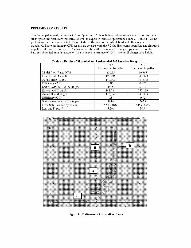
PRELIMINARY RESULTS

The first impeller analyzed was a 7+7 configuration. Although this configuration is not part of the trade

study space, the results are indicative of what to expect in terms of tip clearance impact. Table 4 lists the

performance variables evaluated. Figure 4 shows the locations at which head and efficiency were

calculated. These preliminary CFD results are consists with the J-2 Oxidizer pump open face and shrouded

impeller test results, reference 3. The test report shows the impeller efficiency drops about 10 points

between shrouded impeller and open face with axial clearance of 10% impeller discharge vane height.

Table 4 : Results of Shrouded and Unshrouded 7+7 Impeller Designs

7+7

Unshrouded Impeller

7+7

Shrouded Impeller

Model Flow Rate, GPM 20,295 19,667

Euler Head (A-B), ft 128,486 141,379

Actual Head (A-B), ft 110,362 137,642

Efficiency (A-B) 0.86 0.974

Static Pressure Rise (A-B), psi 1975 2601

Euler Head(C-D), ft 141,014 153,169

Actual Head(C-D), ft 113,252 141,333

Efficiency (C-D) 0.8 0.92

Static Pressure Rise (C-D), psi 1976 2633

Flow Split (suction / pressure) 52% / 48% 51% / 49%

Leakage Flow, % 5.5% N/A

Figure 4 : Performance Calculation Planes

ROTORDYNAMIC ASSESSMENT

Stable turbomachinery operation depends on the damping of the rotor motion. Currently, rotordynamic

stability parameters are estimated by using bulk flow theories and small perturbation (quasi-steady)

assumptions. A well-established experience base with unshrouded impeller rotordynamic coefficients does

not exist.

To help understand the unshrouded impeller's rotordynamic performance, Enigma's computational

rotordynamic methodology was applied to the unshrouded impeller. This method directly simulates the

rotor whirling motion (no quasi-steady assumptions) and can be, in principle, applied to large eccentricity

whirl problems.

For Navier-Stokes based rotordynamic calculations, the impeller shaft/hub moves with an imposed whirling

harmonic motion, figure 5, and the flow equations are integrated time-accurately until reaction force time

periodicity is observed. The fluid reaction force vector time history is calculated; the force history can then

be post-processed and decomposed into normal and tangential components. Because of the direct

simulation of the moving hub, the flow model must consist of the complete three-dimensional geometry

(full 360 degrees in circumference). A similar approach to access the rotordynamic fluid forces on seals has

been fully described in reference 4.

_y

F_:::aema _il_)_'ce(_t mi aim_m_e eafaece)

F, t

Z

Figure 5: Whirling impeller rotor (hub)

Four whirl cases were computed: forward and backward synchronous, and forward and backward super

synchronous. The effect of whirl ratio on the housing fluid forces are shown in figure 6. Using this

calculation methodology rotordynamic coefficients can be supplied to the rotordynamics community to

evaluate the impact on stability of the machine at all required operating points.

F/Fref

20.0

10.0

0.0

-10.0

''''l''''l''''l''''l''''l''''l''''l''''

.... l .... l .... l .... l .... l .... l .... l,,,

-1.5 -I.0 -0.5 0.0 0.5 1.0 1.5 2.0

_/_

Figure 6: Computed normal and tangential forces

CONCLUSIONS

Performance degradation due to impeller tip clearance is well documented in literature. Two methods are

available to combat this issue. Maintain tight tip clearances at all operating points or design an impeller

with tip clearance insensitivity. The former is difficult to achieve in a high pressure turbopump due to

housing deflections and material growth and shrink due operating speeds and cryogenic fluid temperatures.

Literature review indicated that blade number variations could decrease tip clearance sensitivity. A trade

study has been undertaken to evaluate blade number impact on performance with varying tip clearance.

Rotordynamic assessment of turbopump stability is of great concern for rocket engine turbopumps. This is

due to the inability to provide high levels of damping in the system at will. A method has been described

for evaluating these forces with unshrouded impellers.

REFERENCE

1. Y. Senoo and M. Ishida, _Deterioration of Compressor Performance Due to Tip Clearance of

Centrifugal Impellers," Journal of Turbomachinery, January 1987, Vol. 109, pp. 55-61

2. Johannes Lauer, et. al., _Tip Clearance Sensitivity of Centrifugal Pumps with Semi-Open Impeller,"

1997 ASME Fluids Engineering Division Summer Meeting, FEDSM97-3366.

3. Hoshide, R. K. And C. E. Nielson, _Final Report, Study of Blade Clearance Effects on Centrifugal

Pumps", NASA CR-12081, R-8806, November, 1972.

4. Williams, M., W. Chen, L. Brozowski, A. Eastland, _Three-Dimensional Finite Difference Method for

Rotordynamic Fluid Forces on Seals" AIAA Journal, Volume 35, Number 8, Pages 1417-1420, August

1997.

WATER FLOW PERFORMANCE OF A SUPERSCALE MODEL OF THE

FASTRAC LIQUID OXYGEN PUMP

Stephen Skelleyand

Thomas Zoladz

Fluid Physics and Dynamics Group

Subsystem and Component Development Department

Space Transportation Directorate

Marshall Space Flight Center

ABSTRACT

As part of the National Aeronautics and Space

Administration's ongoing effort to lower the cost of

access to space, the Marshall Space Flight Center has

developed a rocket engine with 60,000 pounds ofthrust for use on the Reusable Launch Vehicle

technology demonstrator slated for launch in 2000.

This gas generator cycle engine, known as the Fastrac

engine, uses liquid oxygen and RP-1 for propellants

and includes single stage liquid oxygen and RP-1

pumps and a single stage supersonic turbine on a

common shaft. The turbopump design effort

included the first use and application of new suction

capability prediction codes and three-dimensional

blade generation codes in an attempt to reduce the

turbomachinery design and certification costs

typically associated with rocket engine development.

To verify the pump's predicted cavitation

performance, a water flow test of a superscale model

of the Fastrac liquid oxygen pump was conducted to

experimentally evaluate the liquid oxygen pump's

performance at and around the design point.

The water flow test article replicated the flow path of

the Fastrac liquid oxygen pump in a 1.582x scale

model, including scaled seal clearances for correct

leakage flow at a model operating speed of 5000

revolutions per minute. Flow entered the 3-blade

axial-flow inducer, transitioned to a shrouded, 6-

blade radial impeller, and discharged into a vaneless

radial diffuser and collection volute. The test article

included approximately 50 total and static pressure

measurement locations as well as flush-mounted,

high frequency pressure transducers for complete

mapping of the pressure environment. The primary

objectives of the water flow test were to measure the

steady-state and dynamic pressure environment of the

liquid oxygen pump versus flow coefficient, suction

specific speed, and back face leakage flow rate.

Initial results showed acceptable correlation between

the predicted and experimentally measured pump

head rise at low suction specific speeds. Likewise,

only small circumferential variations in steady-state

impeller exit and radial diffuser pressure distributions

were observed from 80% to 120% of the design flow

coefficient, matching the computational predictions

and confirming that the integrated design approach

has minimized any exit volute-induced distortions.

The test article exhibited suction performance trends

typically observed in inducer designs with virtually

constant head rise with decreasing inlet pressure until

complete pump head breakdown. Unfortunately, the

net positive suction head at 3% head fall-off occurred

far below that predicted at all tested flow coefficients,

resulting in a negative net positive suction head

margin at the design point in water. Additional

testing to map the unsteady pressure environment

was conducted and cavitation-induced flow

disturbances at the inducer inlet were observed. Two

distinct disturbances were identified, one rotating and

one stationary relative to the fixed frame of reference,

while the transition from one regime to the next

produced significant effects on the steady state pump

performance. The impact of the unsteady phenomena

and the corresponding energy losses on the

unexpectedly poor pump performance is also

discussed.

INTRODUCTION

Marshall Space Flight Center (MSFC) has developed

a 60,000 pound thrust rocket engine for use on the

Reusable Launch Vehicle Technology Demonstrator

vehicle (X-34). The gas generator cycle engine, also

called the Fastrac engine, uses liquid oxygen and RP-

1 for propellant. The turbopump integrates a single

stage liquid oxygen pump, a single stage RP-1 pump,

and single stage supersonic turbine into a compact

assembly on a common shaft. A cross section of the

turbopump appears in figure 1.

Figure1. Fastrac Turbopump Cross Section

The engine was designed entirely by MSFC

personnel and the turbopump design included the first

use and application of new suction capability

prediction methods and three-dimensional blade

generation codes. In response to previous

experiences with liquid oxygen pumps, a water flow

test to evaluate the suction capability and head

performance of the liquid oxygen pump was

proposed. Using a superscale model of the pump, a

test was conducted in MSFC's Inducer Test Loop

during the first half of 1999 to evaluate the test article

performance at scaled operating conditions in water.

This document is intended to summarize the results

from the experimental water flow test.

TEST FACILITY DESCRIPTION

The Inducer Test Loop is a closed loop water flow

test facility with manual set point control of flow

rate, shaft speed, water temperature, and test article

inlet pressure. In operation flow leaves the 300

gallon stainless steel reservoir through an 8 inch line,

transitions to 6 inch line, passes through a flow

straightener section, and enters the test article. High

pressure discharge flow exits the test article, passes

through a 6 inch turbine type flow meter, and returns

to the reservoir. A 6 inch quiet valve provides

remote back pressure control for flow rate

adjustment. Test article inlet pressure is controlled

by pressurizing or evacuating the small air volume at

the top of the reservoir. This reservoir ullage

pressure, coupled with the line losses between the

reservoir and test article inlet and the height of the

water in the reservoir itself, is used to set a wide

range of inlet pressures - from 165 down to 3 pounds

per square inch absolute. The test loop

accommodates flow rates up to 4000 gallons per

minute and is constructed primarily of schedule 40

and schedule 80 PVC. An auxiliary loop removesdissolved air from the test fluid and maintains water

temperatures between 70 and 100 degrees Fahrenheit.

The driveline consists of a 3-phase, 150 horsepower

motor with a variable speed controller and belt driven

bearing box. Design limit speed is approximately

6000 revolutions per minute, but higher speeds are

obtainable by changing the pulley ratio and belt

material. Bearing temperatures, shaft speed, test

article inlet pressure, flow rate, water temperature,

and discharge pressure are monitored at the facility

operator's control panel and an Orbiscope dissolved

oxygen sensor is used to measure the water dissolved

oxygen content. For all testing water dissolved

oxygen content was maintained at or below 4 parts

per million.

TEST ARTICLE DESCRIPTION

The test article was a superscale (1.582X) model of

the Fastrac liquid oxygen pump and replicated the

primary flow path including the front and rear

leakage cavities. Bearing coolant flow, or back face

leakage, was collected metered, and returned to the

pump inlet through 2 external lines. A cross section

and front view of the test article appears in figure 2.

Figure 2. Test Article Cross Section and Front

View

The stainless steel inducer-impeller shown in figure 3

was fabricated by Turbocam, Inc. and included 3 full

length blades and 3 splitters, resulting in 6 shrouded

flow passages at the impeller discharge. No back

face pumping vanes were included on the test article

inducer-impeller although the prototype includes this

design feature. The stainless steel inducer-impeller

was a replacement for the original aluminum inducer-

impeller which was damaged after approximately 20

hours of testing. High cycle fatigue resulted in the

loss of the tips of each of the 3 inducer blades. The

steelinducer-impellersufferednofatigueorcavitation-induceddamageduringtesting.

Inducer-Impeller Assembly

Impeller discharge flow was guided through a

vaneless, constant width radial diffuser, rectangular

cross section volute, and conical exit diffuser and

directed away from the pump perpendicular to theaxis of rotation. Table 1 summarizes the scaled and

as-built geometric parameters for the test article.

Table 2 summarizes the prototype and test article

design point operating conditions.

Table 1. Test Article Geometric Parameters

Number of Blades

Inlet Tip DiameterInlet Hub Diameter

Reference Blade Length (Hub to

Tip)

Leading Edge Tip Thickness

Inlet Blade Angle at TipInducer Radial Clearance

Exit Tip Diameter

Exit Blade Height

Exit Blade AngleRadial Diffuser Inner Diameter

Radial Diffuser Outer Diameter

Radial Diffuser Passage WidthVolute Throat Area

Exit Diffuser Cone Angle

Exit Diffuser Cone Length-to-InletRadius RatioExit Diffuser Cone Exit Diameter

3+6

5.177 inch

1.973 inch

1.736 inch

0.019 inch

10.5 degrees0.021 inch

7.056 inch

0.682 inch

26.5 degrees7.147 inch

9.487 inch

0.684 inch

6.660 sq inch

6.00 degrees5.00

4.182 inch

Table 2. Proto_pe andll

Parameter

Fluid

Fluid Temperature

Shaft Speed

Inlet Flange Flow- Rate

Impeller Flow- Rate

Inlet Flange TotalPressure

Back Face LeakageRate

Net Positive Suction

Head

Inlet Tip FlowCoefficient

Suction Specific Speed

(rpm, gpm, fi)

Test Article Design PointPrototype Test

Article

LiquidOxygen

166 deg R

20,000 rpm

880.4 gpm

923.7 gpm

46.0 psia

25.6 gpm

59.2 fi

0.135

27820

Water

90 deg F

5000 rpm

870 gpm

913 gpm

4.7 psia

25.3 gpm

9.2 ft

0.135

27820

All test article hardware except the inducer-impeller

was fabricated of anodized 2219 aluminum by

Dynamic Engineering, Inc. The test article design

inlet pressure, shaft speed, and discharge pressure

were 40 pounds per square inch absolute, 6000

revolutions per minute, and 165 pounds per square

inch absolute, respectively.

INSTRUMENTATION

Steady-state measurements acquired during testing

were used to confirm set point conditions, evaluate

pump performance, and monitor test article health.

Surface static pressure taps were distributed

throughout the test article and grouped into 12 axial

measurement planes. Total pressure probes at the

inlet and discharge flanges were used to establish

flange-to-flange pressure rise and a flow direction

probe at the impeller discharge further defined pump

performance. Flush-mounted high frequency

response transducers were also located at 3 axial

planes in the test article and at 4 locations in the

facility piping for recording of system and pump

pressure oscillations. Accelerometers on the test

article were used to resolve motion of the stationary

components. The approximate locations, types, and

numbers of these measurements appear in figure 4.

Figure 4. Test Article Measurement Locations,

Types, and Numbers

TEST PLAN

The objectives of the experimental water flow testwere to

1. Measure the steady-state pump suction

performance versus flow coefficient and back

face leakage flow rate.

2. Measure the pump steady-state head

performance versus flow coefficient and back

face leakage flow rate.

3. Measure the pump dynamic pressure

environment versus flow coefficient, suction

specific speed, and back face leakage flow rate.

4. Measure pump intra-stage pressures for

verification of design code predictions.

An implied objective was to provide a safe and

inexpensive test article to support potential failure

investigations or redesign efforts. The original test

plan included pump operation as low as 50% of the

design flow coefficient. Following the failure of the

aluminum inducer-impeller, all testing and operation

with the replacement steel inducer-impeller was

confined to a range of 80% to 120% of the design

flow coefficient. Likewise, the installed back face

leakage routing lines included too much resistance,

so operation with higher than the nominal scaled

leakage flow rate was not possible. Test variables

included flow coefficient, suction specific speed, and

back face leakage flow rate. The test article set point

variables were then water temperature, inlet flange

flow rate, inlet flange total pressure, shaft speed, and

back face leakage rate. The as-tested ranges of each

of the test variables appear in table 3 for a shaft speed

of 5000 revolutions per minute.

Table 3.

Back Face

Leakage Rate

Nominal

Completed Test MatrixPercent Suction Specific Speed

Design FlowCoefficient

80%

90%

100%

110%

120%

6340 29010

5670 28680

5550 27580

5780 26260

5770 25170

90% 8030 24560

HalfNominal 100% 5660 26000

110% 7530 24700

90% 7820 28200

Zero 100% 7470 27830

110% 8030 26620

STEADY STATE PERFORMANCE

The overall stage total and static pressure rise as well

as the total and static pressure rise of the inducer-

impeller appear in figure 5 versus percent design

flow coefficient. Pressure rise data in figure 5 are

values corresponding to a suction specific speed at or

below 10000 for the nominal back face leakage flow

rate. Data has been non-dimensionalized by the

impeller tip speed and the predicted performance

curve included for reference. The trends are as

expected with steadily decreasing pressure rise with

increasing flow rate. The water flow test article

appeared to underperform slightly at and below the

design flow coefficient with head rise at the higher

flow rates much closer to the predicted. Expressed in

terms of degree of reaction, or the ratio of impeller

static head rise to stage total head rise, the

experimental value at the design flow coefficient was

0.83, indicating excellent conversion of available

dynamic head to static pressure.

Figure 5. Stage and Inducer-Impeller Head

Coefficient versus Percent Design Flow Coefficient0s0

0 4s

040

8

0?s

050

Dm_n Fiow ceffive_t = o I s5Speed = 5000 rpmS_c_i0_ Specific Speed, 10000

0250 70 OSO

_&_,_ _ stage Total

_ Sta_o StaticI_ducer I_peller ma

_ -- Pr edic_ed, st_e Tot_l

O90 lOCI II0 120 150

Per6ent Design Flow Ceeffi6ient

The experimental pump stage suction performance

appears in figure 6 with stage head coefficient versus

inlet flange suction specific speed. The individual

curves correspond to flow coefficients from 80% to

120% of the design flow coefficient. The trends are

as expected with inducer-impeller designs with

virtually constant head coefficient with decreasing

inlet pressure. The small reduction in steady state

head rise at a suction specific speed of approximately

17000 to 21000 was attributed to the transition of a

rotating, cavitation disturbance at the inlet to a

synchronous, uniform cavity oscillation. Complete

head breakdown soon follows. The approximate

range of the inlet rotating disturbance was from a

suction specific speed of 11500 to 17000 and further

discussion of the observed unsteady phenomena

appears in a later section. The pump design point and

calculated 3% head loss curve are included for

reference. As this curve illustrates, the test article

failed to achieve the desired suction performance in

water at the design flow coefficient with a calculated

margin on net positive suction head of-9% between

the demonstrated and required capability. The

measured variation in head coefficient at the 110%

design flow coefficient was attributed to electrical

contamination of the stage pressure rise measurement

during those set points. All other data included in

this document remained unaffected.

Figure 6. Stage Head Coefficient versus Suction

Specific Speed and Percent Design FlowCoefficient

O5O

;___ ;------__- ..... _" 2 __ .Y,, "e*

Design FI0_ C0effieiem - 0 155 &spe*d = 5000 rpm *

Suotion_peoifto_peed ba_edon inletflangetotalpressure

025

5OOO

040

OSS

I0000 15000 20000 25000 _0000

Inlet Flange Suction S_eclflC S_eeO

For comparison the inducer-impeller head coefficient

is plotted versus suction specific speed and percent

design flow coefficient in figure 7. No variation is

observed in the 110% design flow coefficient data.

Figure 7. Inducer-Impeller Head Coefficient

versus Suction Specific Speed and Percent Designflow Coefficient

0ss

O4O

0_5

A primary design objective was to minimize the

impeller discharge distortion and thereby minimize

the fluid-induced pump sideloads. Figure 8 shows

the measured static pressure distribution at the

impeller discharge versus percent design flow

coefficient. A view slightly further downstream

appears in figure 9 with the static pressuredistribution at the exit of the radial diffuser. Each

location shows increasing influence of the volute

cutwater - located at 24 degrees - with the least

pressure variation at each location at the design flow

coefficient. In each plot the static pressure

coefficient is defined as the local pressure divided by

the plane average static pressure and divided by the

calculated dynamic pressure.

Figure 9. Static Pressure Distribution at the

Radial Diffuser Discharge

_,_.._

i.....

/...J_ i

The final check on inducer-impeller performance was

via a single flow direction probe located slightly

downstream of the impeller discharge in the center of

the radial diffuser. Total pressure, static pressure,

and probe-relative flow angle was then derived from

the sensed pressures and the probe calibration results.

The impeller discharge flow angle relative to impeller

tangential versus percent design flow coefficient

appears in figure 10. The predicted discharge flow

angle at the design flow coefficient was 14 degrees

relative to impeller tangential.

Figure 10. Impeller Discharge Flow Angle versus

Percent Design Flow Coefficient

The majority of data was collected at a back face

leakage rate corresponding to the nominal condition.

However, limited performance data was collected at

half the nominal leakage rate and with the external

leakage metering lines closed. The effect of reducing

the leakage rate on stage head rise appears in figure

11 for suction specific speeds at or less than 10000.

As expected the stage head rise increases with

decreasing leakage rate as work previously expended

on the leakage flow is applied to the throughflow.

The inducer actually operates at a slightly lower flow

coefficient as the leakage flow is reduced at constant

pump flow rate and thereby contributes a small

amount to the increase in stage performance.

Figure 11. Stage Head Coefficient versus Percent

Design Flow Coefficient and Leakage Rate

i

Although a small effect on suction performance

appears in the leakage rate comparison in figure 12,the calculated differences are of the same order as the

experimental uncertainty at these values of suction

specific speed. No conclusion should then be drawn

from these results. Figure 11 is then included to

illustrate the repeatability of the small drop in stage

performance, which appears for each configuration

near a suction specific speed of 17000. This

performance drop, as will be seen in the following

section, corresponds to the highest amplitude of the

synchronous cavity oscillation at the inducer inlet.

Figure 12. Stage Head Coefficient versus Suction

Specific Speed and Leakage Rate at Design FlowCoefficient

i

UNSTEADY PERFORMANCE

Figure 13 shows the progression of unsteady

oscillations versus time as the pump inlet pressure

was steadily reduced at a constant shaft speed of

5000 revolutions per minute (83.3 Hertz) at the

design flow coefficient. At low suction specific

speeds, the oscillation at 3 times shaft speed (3N)

wasmostprominentaswasassociatedwiththewakesfromthe3inducerblades.Assuctionspecificspeedapproached11000at88.5secondsthe3Noscillationtransitionedtoarotatingdisturbancemovingatapproximately1.2timestheshaftspeed(1.2N)asviewedfromastationaryobserver.Thisrotatingdisturbancewasidentifiedasasinglecavitationcellmovingoppositethedirectionofshaftrotation.Furtherreductionininletpressurecausesthesingle-cellrotatingdisturbancetotransitiontoastationaryoscillationwithafrequencyequaltotheshaftspeed.Simultaneouslyahigheramplitudeoscillationappearedwithafrequencyveryclosetothefundamentalfrequencyofthetestfacilitypiping-approximately10Hertz.Theselowfrequencyandsynchronousoscillationspersistedasinletpressurewasreducedandheadbreakdownwasreached.Thepotentialfordynamiccouplingbetweenthefacilityandpumpwasrecognizedandattemptsweremadetobetterisolatethepumpfromthefacility.Allwereunsuccessfulandthelowfrequencyoscillationappearedto_%ck-in"with the facility harmonic at all

tested flow coefficients.

Figure 13. Oscillation Amplitudes versus

Frequency and Time at Constant Speed andDesign Flow Coefficient

e Mode

Cavitation

Time (sec)

The dynamic coupling between the test article and

facility, combined with the presence of cavitation,

suggested the occurrence of auto-oscillation, if only

for a brief period. Brermen 1 noted severe steady state

performance deficits due to the energy dissipation

during auto-oscillation and the magnitude of the head

loss at the design flow coefficient was approximately

3%. The nondimensional amplitudes of the

oscillations noted in figure 13 and stage head

coefficient appear in figure 14 versus suction specific

speed. Oscillation amplitudes have been normalized

by the dynamic pressure based on impeller tip speed

while head coefficient has been normalized by the

non-cavitated value. For comparison the

corresponding normalized amplitudes from recent

component testing in liquid oxygen are included.

Figure 14. Oscillation Amplitudes versus Suction

Specific Speed

i 0srlllah0n

5._ " _umance a,ltUn

-,

p_

Auto-oscillation is typically characterized by high

amplitude, system-wide oscillations in pressure and

flow rate. As seen in figure 13, pressure oscillations

during auto-oscillation were highest at the onset of

the phenomena. These oscillations appeared in

conjunction with noticeable facility piping

displacements and low frequency, shock-like

vibrations. However, the period of these high

intensity vibrations and pressure oscillations was

brief and occupied only a very narrow band of

suction specific speed values. The relationship

between the synchronous oscillation and the

appearance of auto-oscillation is still under review,

but the transition of a rotating cavitation disturbance

to a fixed number of cavitation cells oscillating inunison has been observed in other inducer

performance investigations. Rosenmarm: and

others _'4 observed the transition of a rotating

disturbance to a _unidirectional" or synchronous

oscillations with frequency equal to the shaft speed

just before head breakdown. The relationship

between the uniform cavity or synchronous

oscillation and the corresponding system dynamic

response and the subsequent onset of auto-oscillation

requires further investigation. Regardless, the pump

and system dynamic interaction appears to have

contributed to the inability of the test article to

achieve the expected suction capability. Although

beyond the scope of this document, the significance

of the data in figure 14 for the prototype pump

operating in liquid oxygen should be noted. Despite

the difference in test facility configurations, the

prototype exhibited similar unsteady performance

characteristics with the appearance of a synchronous

oscillation at high suction specific speeds. This may

suggestasensitivityofthepumptodynamicsysteminteractions.

UNCERTAINTYANALYSISAnuncertaintyanalysisincorporatingtheexperimentalprecisionandbiaserrorsusingtheroot-sum-squaremethodwasperformedtoquantifytheworstcaseuncertaintiesassociatedwiththemeasuredandcalculatedquantities.A95%confidencelevelwasassumed.Theestimateduncertaintiesforeachoftheparameterspresentedherearesummarizedintable4. Sincetheestimateduncertaintyassociatedwithsuctionspecificspeedisadominatedbythenonlinearfunctionofpressure,thequoteduncertaintyforsuctionspecificspeedintable4correspondstoasuctionspecificspeedof27000.

Table 4. Estimated Uncertainties

Parameter Uncertainty

Stage Head Coefficient

Impeller Head Coefficient

Percent Design Flow Coefficient

Suction Specific Speed

Pressure Coefficient

Impeller Discharge Flow Angle

+ 0.005

+ 0.007

+ 0.05

+ 800

+ 0.04

+ 1.2 degree

CONCLUSIONS

Although this document is intended to merely

summarize the experimental performance of the

superscale water flow test, a few general conclusions

regarding the Fastrac liquid oxygen pump

performance can be made:

1. Steady state stage head rise was lower than

predicted for 80% to 100% of the design flow

coefficient. At 120% of the design flow

coefficient, steady state stage head rise exceeded

the predicted performance.

2. Suction performance in water failed to meet the

desired capability with a margin on net positivesuction head of-9%.

3. Three regimes of unsteady oscillations were

observed, identified, and tracked versus pump

operating parameters, including a brief period ofauto-oscillation.

4. The appearance of auto-oscillation corresponded

to drops in the steady state stage head rise of

approximately 3% at the design flow coefficient.

5. The onset of auto-oscillation was unaffected by

reduction in the pump back face leakage flow

rate.

ACKNOWLEDGEMENTS

The authors gratefully acknowledge Jeff Moore and

Teddy Stephens of the Experimental Fluid Dynamics

Group for their operation of the experimental test

facility and assistance with test article andinstrumentation installation. The measurement

systems were designed, integrated, and maintained by

Drew Smith and Herb Bush, also of the Experimental

Fluid Dynamics Group. Richard Branick of Sverdrup

was responsible for test article assembly. The

authors would also like to recognize Stephen Fritz of

Cortez III for his incredible electrical troubleshootingskills.

REFERENCES

1 Brermen, C. E., Hydrodynamics of Pumps,

Concepts ETI, Inc. and Oxford University Press,

Norwich, 1994.

2 Rosenmarm, W., "Experimental Investigation of

Hydrodynamically Induced Shaft Forces with a Three

Bladed Inducer," Symposium on Cavitation in Fluid

Machinery, ASME Winter Annual Meeting, Chicago,

IL, Nov. 7-11, 1965.

3 Kamijo, K., Yoshida, M., and Tsujimoto, Y.,

"Hydraulic and Mechanical Performance of LE-7

LOX Pump Inducer," Journal of Propulsion and

Power, vol. 9, no. 6, 819-826, 1993.

4 Kamijo, K., Shimura, T., and Watanabe, M., "A

Visual Observation of Cavitating Inducer Instability,"

National Aerospace Lab (Japan) Report NAL TR-

598T, 1980.

THE PERFORMANCE OF ANNULAR DIFFUSERS

SUBJECT TO INLET FLOW FIELD VARIATIONS

AND EXIT DISTORTION

Dr. David Japikse

Concepts ETI, Inc.

217 Billings Farm Road

White River Junction, Vermont 05001-9486

ABSTRACT

A series of studies has been conducted to evaluate the performance of annular diffusers subject to the influence of

inlet swirl, boundary layer thickness, and distortion typical of turbine operation. Exit distortion, as imposed by an

exit collector or hood has also been studied. Both a moderate length and a very short length annular diffuser have

been included in this series of evaluations. Guidelines for design are presented as well as suggestions for CFD

utilization in future designs.

NOMENCLATURE

AR

B

BL

C1, B2

Cp(0_2)

CP(1-2)

@_l-p;GGcE

L,£

L/Ar

M

-'P2

PpR/B1

R, r

rlt- rlh

SLC

g

%, q_2

72

C2

Subscripts:

Area ratio

Aerodynamic Blockage

Boundary Layer Method

Specific diffuser names

Static pressure recovery from upstream to exit stations

Static pressure recovery from inlet to exit stations

Static pressure recovery from inlet to plenum stations

Static pressure recovery (Pexit - Pin)/(PO, in - Pin)

Static pressure recovery along convex wallRelative eccentricity, e/(r3-r2) -see Figure 19 for symbols

Length scales see Figure 16a or Figures 19 and 20.

Diffuser non-dimensional length

Mach number

Average static pressure at diffuser exit

Average static pressure in exit plenum

See Figure 11

Radius, see Figures 16a, 19 and 20.

Inlet span

Streamline curvature method

Swirl angle measured from meridional direction

Eccentricity, see Figure 19

See Figure 19

Passage exit mean angle with respect to a radial lineAverage diffuser exit velocity

0 - upstream station

1 - inlet station

2 - exit station

1. INTRODUCTION

The performance of annular diffusers is important to inter-stage and last-stage elements of many turbomachines.

Recovering excessive kinetic energy in the form of a static pressure rise significantly improves stage efficiency. This

conversion process, however, is influenced by diverse fluid dynamic phenomena as the flow adjacent to walls is

decelerated and also by inlet and exit distortions. Designing and perfecting annular diffusers can be a complex

process. Consequently, a series of consortia projects was organized and led by the author during a 1975 - 1981

period with specific project management and contributions by Japikse (1977, 1978, 1981), Goebel (1981), and Patel

(1977). These results are now available by sponsors' consent and are gratefully acknowledged.

Prior contributions to the diffuser technical literature are numerous and are surveyed by Japikse (1984) and Japikse

and Baines (1998). A short synopsis for turbine design is given by Japikse (1999). Several useful references are

cited herein to provide data comparisons or trends. These include data from Sovran & Klomp (1967) giving the first

annular diffuser map, Stevens & Williams (1980) showing an influence of inlet conditions, Takehira (1977) showing

the influence of wall curvature, and Deych et.al. (1970) showing the influence of flow distortion from an exhaust

hood.

Sovran and Klomp (1967), as shown in Figure 1 prepared early maps of diffuser performance. It should be

understood that the Sovran and Klomp map is a composite of many different tests of their own and tests from other

investigators. The details of those tests may be found in the appendix of the Sovran and Klomp reference. By way

of illustration, several example points are taken from the appendix and overlaid in Figure 2. It may be observed that

these particular overlays are in rough agreement with the general contours, but definitely not

in precise agreement. This variance is to be expected when a generalized map is made as a composite of many

individual or specific results from different investigators. Hence the map should be used for general guidance; for

specific results, one should consider the specific test conditions of specific studies as referenced in the appendix to

the Sovran and Klomp investigation.

i I I

tc , [ --

!,-o,1

"_IAR,

Figure 1 : Annular diffuser performance chart,

B_ = 0.02 (Sovran and KIomp ] 967).

•76 8

zo "

lO

o5

2 io 2o

Figure 2: Sovran and KIomp map showing

several original test points.

The investigation of this present study looked at all of the parameters discussed in the technical literature and

evaluated annular diffusers under extreme conditions of geometric restriction as well as more generous design

configurations. Figure 3 shows the geometric environment in which these diffusers were considered. Case 1 was

the restricted length design frame which was a very tight configuration indeed (essentially permitting one to design a

conveying passage as opposed to a diffuser passage). With extension plates, more radius could be employed and

some additional diffusion might be achieved. The Case 2 design frame permitted a moderate length diffuser to be

designed following more conventional norms of the diffuser literature and technology. Principle results for the

Case 2 configuration are shown in Figure 4. It may be observed that good performance all the way up to a swirl

angle of 40 ° has been achieved and that an exhaust hood (discussed later) has been utilized with no more than one

point of pressure recovery penalty. Similar results for the B2 diffuser, which was optimized for the Case 1 restricted

length design, are shown in Figure 5. For this B2 case, the compromise is quite severe, although 22% pressure

TFAWS 2

Radial Position

From Centerline r2/rlt = 1.5

(1.8 in)

Case 1

With Exten-

sion Plates

Case 1

Restricted

Length

Design

Frame

rlt (1.2 in)

B2tlh (U.13 i_

Case 2

Moderate Length

Design Frame

C1

L/tlt = 0.5 (0.6") L/tlt = 2.0 (2.4")

x=O

Figure 3a: Selected design frames.

-o._ o 0.2 o.4 0.6 o.s 1.e 1.2 1.4 t._ l.s 2.0 2.2 2.4

Figure 3b: C1 diffuser configuration showing quasi-orthogonalnumbers for computation.

0.t

0.S I

0.S

0.4

cp(1-p)

0.3

0.2

o.1

0

1 I !

_-,

['I Diffuser Alon(

0 Diffuser With-Single Exit

Hood

m

I I t

lO 20 30 40

Inlet SwirI

Figure 4: System pressurerecovery coefficient as a function ofinlet swirl angle for an optimallydesigned single exit hood and theC1 (moderate design frame)exhaust diffuser.

l¢

0,9

o

06

o,s

Cp(1-2)

o.2

i .... i ..... , I i i t

dump :o_f_qur_ti_n, LO*

o!_ o!, o!_ i.... o!, o_ o._

Figure 5a: Cp(0_2/ recovery for the B2diffuser.

1.o

0.9

O.B

0.7

0.6

0.5

CP(t-2_

0.4

0.3

0.2

0.1

o

i i i i i i i

o shroud pl.te o.ly,

AR - ].31 _ 20o1°"

dump configuration. _ 30"

I I I I I I Io.1 o._ o._ o,4 o.s o._ o._ o.i

_eh _umber

Figure 5b: Cp(__2) recovery for the B2diffuser.

TFAWS 3

recoveryhasbeenachievedontheoverallbasis.Figure6 showsa setof wallstaticpressurecalculationsandmeasurementsforthisdesignproblem;it isevidentthatverylargelocalpressurerecoverieshavebeenforcedduetothestrongbendingofthisflowfieldandtheresultantpressuregradients(whichfollowtheEuler-nequation).

-5

-10

-15

$ (P-PVu;IPGG

-20

TEST NUMBER 71

: '. : : : ', : : : : : : ,

x

IIo x

-25

o

-30 o o

8

-35 , , .......

xx x

x

x xP

o

o

o

o

-I00 -50 O 50 I0(% MERIDIORAL DISTANCE FROM INLET

x = HUB B2 DIFFUSER

o : SHHOUD AREA RATIO= 1.31

P = PLENUM SWIRL ANGLE= 0

Figure 6:B2 wall pressure survey without shroud

extension plate, AR : 1.31, M : 0.59, _x: 0°.

2. INLET VARIATIONS (DISTORTION)

Test results for the C1 diffuser, as a function of the inlet aerodynamic blockage, are shown in Figure 7. It will beobserved that the trend follows that of a simple boundary layer calculation to a reasonable first approximation. It isalso clear that pressure recovery drops off substantially with inlet fluid dynamic blockage. One can safely concludethat fluid dynamic blockage is a first order aerodynamic parameter. This parameter, over a modest variance, candrop the pressure recovery coefficient by at least ten points.

Figure 8 shows an additional test of the C1 diffuser with the optimum hood (as described later) as tested behind anactual operating turbine. The inlet velocity profiles to the

x

Figure 7: Measuredrecovery levels.

! iiiBo und2;, Lay_er Modeling

and predicted annular diffuser

.9

•j

.3

E , ' , ' , i , i

Tr_z_• _)r ,_co s,,,ili _:onve_tionnl it.let hound_r/ Sawer

• Data points for dlttuser operation bohinc turbine staqe.

_ 6& , Is 10, 1_, I, I14 1G '18 I

]nlet ,:l_ckaqc. "

I2O

Figure 8: Comparison of diffuser recovery withconventional inlet boundary layer blockage and withoperation behind an axial turbine.

TFAWS 4

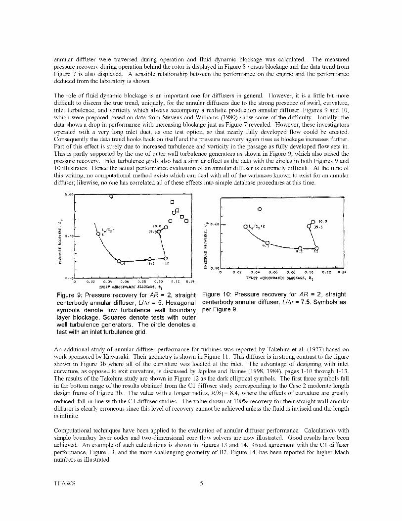
annular diffuser were traversed during operation and fluid dynamic blockage was calculated. The measured

pressure recovery during operation behind the rotor is displayed in Figure 8 versus blockage and the data trend from

Figure 7 is also displayed. A sensible relationship between the performance on the engine and the performance

deduced from the laboratory is shown.

The role of fluid dynamic blockage is an important one for diffusers in general. However, it is a little bit more

difficult to discern the true trend, uniquely, for the annular diffusers due to the strong presence of swirl, curvature,

inlet turbulence, and vorticity which always accompany a realistic production annular diffuser. Figures 9 and 10,

which were prepared based on data from Stevens and Williams (1980) show some of the difficulty. Initially, the

data shows a drop in performance with increasing blockage just as Figure 7 revealed. However, these investigators

operated with a very long inlet duct, as one test option, so that nearly fully developed flow could be created.

Consequently the data trend hooks back on itself and the pressure recovery again rises as blockage increases further.

Part of this effect is surely due to increased turbulence and vorticity in the passage as fully developed flow sets in.

This is partly supported by the use of outer wall turbulence generators as shown in Figure 9, which also raised the

pressure recovery. Inlet turbulence grids also had a similar effect as the data with the circles in both Figures 9 and

10 illustrates. Hence the actual performance evaluation of an annular diffuser is extremely difficult. At the time of

this writing, no computational method exists which can deal with all of the variances known to exist for an annular

diffuser; likewise, no one has correlated all of these effects into simple database procedures at this time.

,GO

O

d_O_

O

Figure 9: Pressure recovery for AR = 2, straight

centerbody annular diffuser, L/Ar = 5. Hexagonal

symbols denote low turbulence wall boundary

layer blockage. Squares denote tests with outer

wall turbulence generators. The circle denotes a

test with an inlet turbulence grid.

,2

o

_3, CZ

Figure 10: Pressure recovery for AR = 2, straight

centerbody annular diffuser, L/Ar = 7.5. Symbols as

per Figure 9.

An additional study of annular diffuser performance for turbines was reported by Takehira et al. (1977) based on

work sponsored by Kawasaki. Their geometry is shown in Figure 11. This diffuser is in strong contrast to the figure

shown in Figure 3b where all of the curvature was located at the inlet. The advantage of designing with inlet

curvature, as opposed to exit curvature, is discussed by Japikse and Baines (1998, 1984), pages 1-10 through 1-13.

The results of the Takehira study are shown in Figure 12 as the dark elliptical symbols. The first three symbols fall

in the bottom range of the results obtained from the C1 diffuser study corresponding to the Case 2 moderate length

design frame of Figure 3b. The value with a longer radius, R/B1 = 8.4, where the effects of curvature are greatly

reduced, fall in line with the C1 diffuser studies. The value shown at 100% recovery for their straight wall annular

diffuser is clearly erroneous since this level of recovery cannot be achieved unless the fluid is inviscid and the lengthis infinite.

Computational techniques have been applied to the evaluation of annular diffuser performance. Calculations with

simple boundary layer codes and two-dimensional core flow solvers are now illustrated. Good results have been

achieved. An example of such calculations is shown in Figures 13 and 14. Good agreement with the C1 diffuser

performance, Figure 13, and the more challenging geometry of B2, Figure 14, has been reported for higher Machnumbers as illustrated.

TFAWS 5

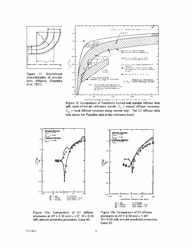
Figure 11: Geometricalcharacteristics of annular

bent diffusers (Takehiraet al. 1977).

0,9

0.S

0.7

o.s

o.5

u

9.4

o,]

o.2

o.1

convex Surface Streamline Length, s/_" and Straight Diffuser Effective Length, L/d"

Figure 12: Comparison of Takehira's curved wall annular diffuser data

with state-of-the-art reference bands. C_ = overall diffuser recovery,

C_c = local diffuser recovery along convex wall. The C1 diffuser datafalls above the Takehira data in the reference band.

A

-8 --

-lO

-12

-i00

I I I_od Recovtr

Cpl_2 = 0.62

Cpl_p = 0.64

_ rQdictad P_cover ._Cpi.2 - 0.748

?

I l l-50 0 50 I00

/_ • Hub Cl Diffuser

O = Shroud Area Ratio. Z.30

[] = Plen_= Swirl Angle - 0

Figure 13a: Comparison of C1 diffuser

pressures at AR = 2.30 and _ = 0°, M = 0.30with annular predicted pressures, Case 90.

-5

-i0

i [ I

_surqPd l_I_very

Cpi.2 - 0.60

Cpl.p - 0.62

_ P rsdictld RIco_,

Cp1_2 - 0.770

I I I-30

-i00 -5.0 0 50 I0(

• M_ridiohal OfLJt_cs rt_ Inlet

/_ = Hub C1 Diffuser

O - Shroud Area Ratio = 2.30

[] - Plen_ Swirl AngEl - 40

Figure 13b: Comparison of C1 diffuserpressures at AR = 2.30 and _ = 40 °.

M = 0.50 with annular predicted pressures,Case 93.

TFAWS 6

-I_ -50 0 5O tO0

c5 - L I I 1-5

I.....

_15 " _ _15

f_ .....

Measu=ed Re=overy

%1 " O.36

%1 = O.4O

-3O Y -30

"i II-35cpl-2 I -3_

-1o0 -5O 0 50 i00

% m from inlet

Figure 14a: Comparison of B2 diffuser pressuresatAR=1.31 ands=0 °,M=0.59withSLC+BLpredicted pressures, Case 71.

oo 020

o

I I I

Measured Recovery

cpi_2 = 0.35

Cpl_p = 0.38

P redieted Recovery

Cpl_2 " 0.498

-35 ; I I I-ioo -50 0 50 IOO

% Meridional Distance fr_ Inlet

- Hub B2 Diffuser_0 = Shroud Area Ratio = 1.31

[] = PlenUm Swirl Angle = 40

Figure 14b: Comparison of B2 diffuser pressuresat AR = 1.31 and _ = 40 °, M = 0.56 withSLC + BL predicted pressures, Case 76.

_ __ _ ...... ii__ .

"_'"i_"""_:..... ? l:_iii _ :::__.'::;!'_

_ "... ._. :!i: : .....

_ .....

Figure 15: Measured and CFD coupled wall static pressures for the C1 annular diffuser. Case a isbelieved to be fully turbulent flow; cases b and c are believed to have transitory flow.

TFAWS 6

Obviously, modern designers prefer to use CFD codes; Figure 15 shows some CFD results with good agreement at

high Mach number (top figure). However, as the Mach number is reduced, the agreement becomes less satisfactory.

This problem is due to the transitional behavior of the flow and at lower Mach numbers lower Reynolds numbers

also exist which correspond to transitional wall shear layers. CFD can be done only in fully turbulent flows, and can

be used to study sensible system phenomena such as the effect of velocity profile and swirl distribution leaving a last

turbine blade row and entering an annular diffuser. If desired, a complete exhaust hood can be modeled so that the

complete coupling effects can be evaluated. System studies of this type are highly recommended for CFD

examination at the present time. However, transitional boundary layers still elude the modem CFD modeling

specialists.

3. HISTORICAL HOOD STUDIES

Frequently, it is necessary to collect the fluid exiting from an exhaust diffuser and turn it by approximately 90 °. An

extreme pressure distortion can therefore be expected under certain design conditions and with various turbine

performance penalties associated. If an exhaust diffuser is employed, the performance of the diffuser can be

4":

r'h _* tie 0',9K

:I* " rlh

r_h/rl_ - hub _ip _tio - 0.8K- I

Cp 0.7tlt _ rlh

L 4

_4 " _It - rlh 0.6

L 5

_5" rl_ - :lh

_ =rlh/Tlt+l

1.2 % k -lo

u%oO -, 8

g

°.6-0.4 I I , I , _'--" I

2 3 4 5 6

£4=£4/rlt-rlh

Figure 16c: Variation in the total loss factor

1-Cp depending on axial hood dimension / 4 and

K for annular diffusers with a hood. Cp includes

the diffuser plus hood. (Deych et al. 1970)

Increas&ng rlh/rl_

0.5 I ' _ I

4 6 8 ,13

. Zlh/rlt,.-" 1 . tlh ,, rt._

, - rlh/r_t r,t - r,h

Figure 16b: Cp versus K for straight annular

diffuser (Deych et al 1970 )

0°_

0.6

L)I

0°._

0o>0 2 3 4 5 6

g4

Figure 16d: Effect of radial hood dimension

L 5 = Ls/(rlt- rlh ) on the efficiency of exhaust

ducts (Deych et al 1970)

TFAWS 7

adverselyimpactedbyaninappropriateexitdevice.Figure16showssomeofthekeyresultsfromDeychetal.(1970)for straight-wallannulardiffuserswithexhausthoodsof variousdimensions.Clearly,highlevelsofrecoverycanbeachieved.Conversely,recoverycanbereadilydestroyedif theflowstatesarenotcarefullyevaluated.

FurtherexamplesofexhaustdiffuserperformanceareevidencedinFigures17and18fromthestudybyJapikseandPampreen(1979).Inthatstudy,flowvisualizationwasconductedtodeterminethebasicflowpatternsasshowninFigure18.Comervorticeshavedevelopedwhichconvectthefluidfromthebottomofthecollectoralongthesidesandontothecollectordischarge.

06 ; , '. ..... ".' i

>." /-

4 /I / Z /

Q= O B //////

_.,,11._ l/Ill/

i _1¢ 2./I/'///

- // _ll_. / / !

J 0,2 I '4 I O_O I j OPENdNG /.J

0 ± ! . _ I ....... '0 4_ _(_ 17_(3 I_0 200 24Q 2_Q 32(3 "_g

Figure 17: Angular distribution of shroud exit static pressure recovery

based on mean-inlet conditions; exhaust diffuser with single exitcollector, (Japikse and Pampreen, 1979)

Figure 18: Flow patterns in the exhaust diffuser with a single-exit exhaust collector. The hub surface, lefthand view, shows collector induced streamline distortion at the diffuser discharge and a complex vortex

rising along the R.H.S.; the diffuser inlet is undistorted. The collector bottom region, right-hand view,

reveals evidence of a three-dimensional vortex structure at the bottom and implies complex flow pathlines

away from the surface.

TFAWS 8

4. EXIT HOODS AND DISTORTION

A further, and highly diverse, investigation of both single and double exit hoods, was planned by Japikse and Patel

(circa 1976-1977) and conducted and reported by Patel (1978), with supporting notes by Japikse (1978). This

investigation used the annular diffusers presented previously by Japikse (1977) was extended by and Goebel and

Japikse (1981). The diffusers are different from those covered by Deych, above, in that they were designed to

recover rotor exit swirl, and hence had substantial radial extent, as noted above. This study of hood performance,

consequently, considered the effect of flow field swirl as well as other important fluid dynamic parameters.

The basic hood geometry is shown in Figure 19 (Figures 19-29 are from Patel, 1978) with various designations for

important hood geometry, including eccentricity which is denoted by _. The direction of flow field swirl (+c0, as

utilized during the test program, is also shown in Figure 19. Geometry for the double exit discharge hood is shown

in Figure 20 and this configuration has much less variance than the Figure 19 geometry. Principle experimental

results for the single exit discharge are shown in Figures 21 and 22 for the concentric spacing of the single exit

discharge, but with various values of L 4 and R 3. The Figure 21 configuration corresponds to a centered discharge,

from an axial perspective, whereas Figure 22 corresponds to the alignment of the diffuser hub wall with the back

wall of the hood. Although it was noted in the investigation that the latter configuration gave the highest pressure

recovery for the diffuser itself, the overall system pressure recovery is slightly impaired as a comparison of these

two figures reveals. The important geometric variables covered in these two figures are the radius R 3 and the hood

width L 4. By achieving a hood width of at least 2.0, the effect ofR 3 is no longer significant and once a value ofL 4

of approximately 3 is achieved, one has obtained nearly the asymptotic limit corresponding to a full plenum

discharge. The reference line of 0.64 shown in these figures corresponds to the prior tests of the diffuser alone with

flow discharge into a simple plenum. These figures provide substantial guidance for the appropriate sizing of anexhaust hood and allow sensible economic tradeoff studies to be conducted.

Figure 19: Nomenclature for the single exit hood.f

R3 = I"3/I"2 L4 = Z4/Zl

L2 = _2/gl L6 = g6/r2

L7 = _/r2

Figure 20: Nomenclature forthe double exit hood.

TFAWS 9

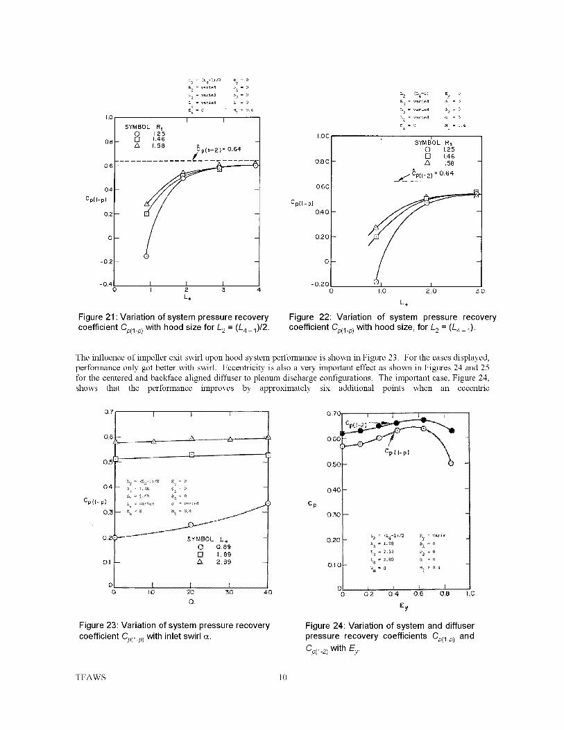
1.0

0.8

O,6--

OA

Cp(I-p)

0.2-

0 -

-0.2-

-0.40

L 2 = (L4-I)/2 Ey _ O

R 3 = varied '_i = 0

L 3 = varied _2 _ O

L 4 = varied _ = 0

E x - 0 M 1 _ 0.4

I

SYMBOL R_0[3ZX

I I

11251.461.58 ^

p(i-2) 0.64

I I II 2 3

L4

Figure 21 : Variation of system pressure recovery

coefficient Cp(I_p)with hood size for L2 = (L4_ 1)/2.

I'OO /

elfCp(I-p)

0.40

0.20

0--

-0.200

L 2 - (L4-z) Sy = o

R 3 = varied _i = 0

L 3 = varied _2 = 0

L 4 = varied _ - 0

E x = 0 M 1 = 0.4

I SYM BlO L R3 /0 1.25 t[] 1.46

A 1.58

_:po-a) =0.64/

1.0 2.0 5.0

L4

Figure 22: Variation of system pressure recovery

coefficient Cp(I_p)with hood size, for L2 = (L4_1).

The influence of impeller exit swirl upon hood system performance is shown in Figure 23. For the cases displayed,performance only got better with swirl. Eccentricity is also a very important effect as shown in Figures 24 and 25

for the centered and backface aligned diffuser to plenum discharge configurations. The important case, Figure 24,shows that the performance improves by approximately six additional points when an eccentric

0.7

0.6

02

04

O

O 0 20 50 4 0

Q

o.7oI_ _ i !_

o.oo "-,\

0,40

O,SO

0.20

O.iO

0

0

t 3 = 2._2 @_ = e

0 2 0 4 0.6, 0.8 I ,C

Ey

Figure 23: Variation of system pressure recovery

coefficient Cp(l_p)with inlet swirl o_.

Figure 24: Variation of system and diffuser

pressure recovery coefficients Cp(__p) and

Cp(1-2) with Ey.

TFAWS 10

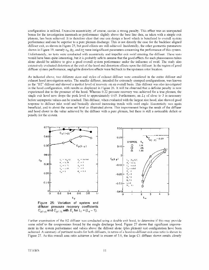
configuration is utilized. Excessive eccentricity, of course, carries a strong penalty. This effect was an unexpected

bonus for the investigation inasmuch as performance slightly above the base line data, as taken with a simple exit

plenum, has been achieved. It is therefore clear that one can design a hood which is beneficial to overall system

performance and can be superior to a pure plenum discharge. This is not directly the case for the backface aligned

diffuser exit, as shown in Figure 25, but good effects are still achieved. Incidentally, the other geometric parameters

shown in Figure 19, namely _x, _ 1, and _2 were insignificant parameters concerning the performance of this system.

Unfortunately, no tests were conducted with eccentricity and impeller exit swirl entering the diffuser. These tests

would have been quite interesting, but it is probably safe to assume that the good effects for each phenomenon taken

alone should be additive to give a good overall system performance under the influence of swirl. The study also

extensively evaluated distortion at the exit of the hood and distortion effects upon the diffuser. In the region of good

diffuser system performance, negligible distortion effects were fed back to the upstream rotor location.

As indicated above, two different sizes and styles of exhaust diffuser were considered in the entire diffuser and

exhaust hood investigation series. The smaller diffuser, intended for extremely cramped configurations, was known

as the "B2" diffuser and showed a modest level of recovery on an overall basis. This diffuser was also investigated

in the hood configuration, with results as displayed in Figure 26. It will be observed that a definite penalty is now

experienced due to the presence of the hood. Whereas 0.22 pressure recovery was achieved for a true plenum, the

single exit hood now drops the peak level to approximately 0.05. Furthermore, an L 4 of close to 5 is necessary

before asymptotic values can be reached. This diffuser, when evaluated with the largest size hood, also showed good

response to diffuser inlet swirl and basically showed increasing trends with swirl angle. Eccentricity was again

beneficial, and to about the same net level as illustrated above. This improvement brings the result of the diffuser

and hood closer to the value achieved by the diffuser with a pure plenum, but there is still a noticeable deficit or

penalty for the system.

0 70

O.40

Cp

0.30

0.20

0 A 0

00

E,_ _ ,'2" _% _ _,_t

.......I _ m i0,;_ 0,4 0,6 08 ,

Ey

Figure 25: Variation of system and

diffuser pressure recovery coefficients

Cp(l_p) and Cp(1_2) with Ey for L 2 = (L 4 - 1).

0,30

0,20

0,10

O

cpo-p)

-0,10

-0.20

-0.50

-0.40O

I I I I

--_,\ .............Cp[ I-2) = 0.22

SYMBOL R a

0 t.14FI 1.26

I,

[_

L2=(L4-1)/2

R 3 = varied

L 3 = valied

L 4 = valied

E x = 0

Ey = 0

_1=0

0_2 = 0

c_=0

M 1 =0.4

I I I Ii 2 3 4 ,5

L4

Further examination of the B2 diffuser was conducted using a double exit hood, to determine if this may provide

some relief to the compromises forced by the single discharge hood. Figure 27 shows that significant improve-

ment in the system performance and values above the diffuser alone (plus plenum) test configuration have been

achieved. A summary of pertinent results for both diffusers, in terms of a hood-to-diffuser exit area ratio is shown in

Figure 27. As this overall area ratio achieves a level in excess of 3.0, the large C1 diffuser shows results closely

TFAWS 11

approachingtheplenumtestvalueforthatdiffuser.Ofcoursetestswithaneccentricdiffuserwouldexceedthisreferencelevel.Inthesamefigure,thepertinentresultsfortheB2diffuseraredisplayedandit isclearthatit isnotpossible,withasingleexithood,tomatchthelevelsoftheB2diffuserwith a plenum discharge. However, when

using two exit ports, levels of performance above that of the B2 diffuser with collector are displayed.

It is important to assure minimum area ratio, as Figure 27 suggests. The area ratio for these hoods and diffusers maybe defined as follows:

z43_ 1

Hood exit acea 2r3l 4 R3 * L 4

Diffuser exit area 2er r211cos 72 2- cos 72

1.00

0.80

0.60

0.40

Cp(I-p)0.20

0

-0.20

-0.400

Figure 27: System pressure

function of area ration AR 1.

I I I I i I I I

0 CI W/SINGLE EXIT HOOD

[3 B2 W/SINGLE EXIT HOOD ^

8 B2W/DOUBLEEXITHOOD Cp(]-2)FOR THE CI

DIFFUSER

_-_-

/ J2 -% .....FORTHAI2/rl = vori<d _* = 3

I. varied 7 = 3

['4 - ,,aricd = [)

I I I I I

0.4 0.8 1.2 1.6 2.0 2.4 2.8 3.2 5.6

AR_

recovery coefficient Cpo_p) as a

For the particular diffusers utilized, 72 equals 54 ° for the C1 diffuser and 0 ° for the B2 diffuser. A further area ratio,

which is of benefit to this analysis, can be defined by concentrating on the critical area in the hood, which would

occur either at 90 ° or the 270 ° location for a single exit hood (see Figure 20). In the case of no eccentricity, this area

is simply (r 3 - r2) 14. Forming an area ratio between the area at 90 ° and the sector of diffuser exit area from 0 ° to

90 ° , one obtains the following:

AR 2 lilA90o / _rea of the 0 ° to 90 ° sector at diffuser exit

which can also be rewritten as:

_-r2g 2_ - lgr

mh: ]/4brr2/l_OSr2g 7_osr--7

This area ratio is a local area ratio in contrast to the AR 1 given above which is an overall hood area ratio. By plotting

principle results in terms of this local area ratio, as shown in Figure 28, it is discovered that there is a minimum AR 2

of approximately 0.8 which is necessary to avoid serious penalties in the performance of the hood. In fact, a value

TFAWS 12

somewhathigherwouldberecommendedwheneverpossible.Finally,ahood(static)pressurelosscoefficientcanbedefinedasfollows:

P2 - PpLhood -- __1 --2

_-PC 2

The value of the diffuser exit velocity C 2 must be estimated knowing the pressure recovery coefficient of the

diffuser alone. When this is done, a hood loss coefficient as shown in Figure 29 is obtained. Interestingly, the data

for each diffuser falls essentially on the same curve! It may be hypothesized that the effects of diffuser exit or hood

inlet dynamic head have now been scaled out and that this parameter is controlled substantially by the area ratio. As

with Figure 27, it appears that an area ratio on the order of two is preferable to obtain minimum system losses.

I I

0.80

0.60

0_0

Cp(I-p)

0.20

0

-0.20

-040

0

L 2 = (L4-ii/2 Ey = 0

R 3 = v_ried _i = 0

L = varied ,_ = 0

L 4 = varied a = 9

Ex = o M 1 : o. 4

E]_//D j [] B2 W/SINGLE EXIT ROOD

I q I I I [

0.4 0.8 1.2 1.6 2.0 2.4

AR 2

Figure 28: System pressure recovery coefficient

vO-(1-p)as a function of the area ratio AR 2.

Lhood

2,20

2.00

1.80

1.60

1.40

1.20

1.00

0.80

0.60

0_0

0,20

0

0.20

0

I

0.4

o Cl W/$rNGLEEXll HOOD

[] B2 W/SINGLE EXIT HOOD

z4 = v_J.ea _ - ,J

Ex = e n 1 - _.4

El

I, I I I I I I

0,8 1,2 1.6 2.0 2.4 2,8 3.2 _,6

AR,

Figure 29: The hood loss coefficient Lhood as a

function of the area ratio AR 1.

Further tests were conducted by using a splitter plate as displayed in Figure 30 or a boat-tail strut as shown in

Figure 31. Neither of these devices had any significant impact on the best performing configurations discussed

previously. Occasionally, they had some positive effect on some of the lower performing geometric configurations.

Hence, these are options for strengthening a hood structure.

These hood results, drawing largely on the reference work of Patel (1977) and the cited supporting work, greatly

augment the database supplied by Deych (1970). It is clear that the designer must take great care in laying out an

exhaust hood for a high-performance exhaust diffuser system, but it is equally clear that good data are available to

guide an intelligent choice of these design parameters.

TFAWS 13

:_':OODB

-4-

\

Di:FFGSER:y

Figure 30: Schematic of the single exit hood with

a hood splitter plate.

DIFFUSEREXITCONTOUR I

= o _ 19

Figure 31 Schematic of the single exit hood witha "boat-tail" strut.

5. CONCLUSIONS

A series of annular diffusers has been designed subject to available technology and then tested according to

influences of inlet boundary layer variations, passage curvature, inlet swirl and exit collector (hood) distortion

effects. The following has been noted:

1. overall performance compares sensibly with the findings of Sovran & Klomp (1967);

2. performance changes dramatically with inlet boundary layer thickness, much as found for conical and channel

diffusers, and strongly with means of artificial boundary layer thickening (trips, vortex generators, etc.) which

cannot be predicted today;

3. curvature late in a passage is worse than curvature early in a passage;

4. swirl can help the performance of an annular diffuser if it is sensibly distributed and helps to unload the wall

curvature effects;

5. the key to exhaust hood design is either very large collector size or a very special combination of design

parameters, which should always be checked experimentally;

6. core flow and boundary layer calculations have successfully modeled bulk design effects such as gross

blockage, passage shape, and inlet swirl; and,

7. fine scale CFD modeling has clarified some gross flow phenomena but cannot resolve many detailedobservations.

6. ACKNOWLEDGEMENTS

The author wishes to acknowledge the important contributions of his co-workers, Messrs. Goebel and Patel. Mr. Jay

Goebel served as project engineer for the studies with inlet blockage variations and Dr. Patel served as project

director for the hood studies. Each made vital contributions to the totality of the work presented herein.

TFAWS 14

REFERENCES

Deych,M.Ye.,andZaryan_n,A.Ye.,"DynamicsofDift_sersandExhaustDuctsofTurbomachines,"NTISAD745470,1970.

2. Goebel, J. H., and Japikse, D., "The Performance of an Annular Diffuser Subject to Various Inlet Blockage

and Rotor Discharge Effects," Creare TN-325 and Concepts ETI, Inc. TM-1, February 1981

3. Japikse, D., "The Design and Evaluation of Restricted Length Annular Exhaust Diffusers," Creare Inc. TN-

257, May 1977.

4. Japikse, D., "The Use of Boat Tail Struts in Single Discharge Hoods," Appendix C, Creare Inc., TN-277,

Hanover, NH, 1978.

5.

6.

Japikse, D., "Turbomachinery Diffuser Design Technology," Concepts ETI, Inc., Wilder, VT, 1984.

Japikse, D., "Exhaust Energy Recovery," Axial and Radial Turbine Technology Course, Concepts ETI, Inc.,

Wilder, VT, April 19-23, 1999.

7. Japikse, D., Baines, N., "Diffuser Design Technology," Concepts ETI, Inc., Wilder, VT, 1998.

8. Japikse, D., Pampreen, R., "Annular Diffuser Performance for an Automotive Gas Turbine," Journ Engfor

Power 101: 358-372.

9. Patel, B., "Evaluation of the Performance of Single and Double Exit Hoods for Annular Exhaust Diffusers,"

Creare Inc., TN-277, Hanover, NH, 1978.

10. Sovran, G., Klomp, E. D., "Experimentally Determined Optimum Geometries for Rectilinear Diffusers with

Rectangular, Conical or Annular Cross-Section," Fluid Dynamics of Internal Flow, Elsevier Publishing Co.,

Amsterdam, 1967.

11. Stevens, S. J, Williams, G. J., The influence of inlet conditions on the performance of annular diffusers.

Trans ASME Journ Fluids Eng 102: 357-363. 1980

12. Takehira, A., et al., "An Experimental Study of the Annular Diffusers in Axial-Flow Compressors and

Turbines," Paper No. 39, Tokyo Joint Gas Turbine Congress, 1977, also Paper No. 39, Japan Society of

Mechanical Engineers, 1977.

TFAWS 15

ROTOR DESIGN FOR THE SSME FUEL FLOWMETER

Bogdan Marcu

Boeing

Rocketdyne Propulsion and Power

ABSTRACT

The present report describes the process of redesigning a new rotor for the SSME Fuel Flowmeter. The

new design addresses the specific requirement of a lower rotor speed, which would allow the SSME

operation at 115% rated power level and above. A series of calculations combining fleet flowmeters test

data, airfoil fluid dynamics and CFD simulations of flow patterns behind the flowmeter's hexagonal

straightener has led to a blade twist design c_ = c_(radius) targeting a kfconstant of 0.8256. The kfconstant

relates the fuel volume flow to the flowmeter rotor speed, for this particular value 17685 GPM at 3650

RPM. Based on this angle distribution, two actual blade designs were developed. A first design using the

same blade airfoil as the original design targeted the new kfvalue only. A second design using a variable

blade chord length and variable airfoil relative thickness targeted simultaneously the new kfvalue and an

optimum blade design destined to provide smooth and stable operation and a significant increase in the

blade natural frequency associated with the first bending mode, such that a comfortable margin could be

obtained at 115% RPL. The second design is a result of a concurrent engineering process, during which

several iterations were made in order to achieve a targeted blade natural frequency associated with the first

bending mode of 1300 Hz. Water flow tests preliminary results indicate a kfvalue of 0.8179 for the first

design, which is within 1% of the target value. The second design rotor shows a natural frequency

associated with the first bending mode of 1308 Hz, and a water-flow calibration constant oflC = 0.8169.

NOMENCLATURE

U

Ca

W

i

CD, eL

P

b

Kf

Kfw

blade tangential velocity

fluid axial velocity

fluid relative velocity

blade stagger angle

angle of relative fluid velocity

flow incidence angle on the blade

drag and lift coefficients

fluid density

blade chord length

flow meter calibration constant for engine operation

flow meter calibration constant determined from water flow test

1.INTRODUCTION

TheSpaceShuttleMainEngineusesaturbinetypeflowmeter[3]tocontroltheamountoffueldeliveredtotheengineandthemixtureratiobetweenthefuelandoxidizer.Theflowmeterislocatedinaductbetweenthelowpressurefuelpumpdischargeandtheintaketothehighpressurepump.Themetertranslatesthevolumeflowoftheliquidhydrogenbasedonitsrotorspeedandacalibrationconstant,denominatedasKfwhichrelatesthefuelvolumeflowratetotherotor'srotationalspeedKf= 4*RPM/GPM,whereRPMistherotorspeedinrotationsperminuteandGPMthefuelvolumeflowrateingallonsperminute.Theoriginalflow-meterdesignemployedaflowstraightenerwithasetofvanesformingchannelswith a

square section, a configuration referred to as the _egg-crate" housing. This straightener was replaced by

another design, with vanes forming a set of channels with hexagonal cross-section. In this new

configuration, the flow meter rotor is mounted closer to hexagonal vanes, at approximately 1 inch distance

(previously, in the egg-crate straightener housing it was mounted at approximately 2 inch distance). Over

the years of SSME operation, a certain behavior was observed in the flow-meter operation [1]: at certain

regimes, an apparent shift seems to occur in the Kf value, without a real change in the volume flow rate.

The Kf shift phenomenon also appears to be associated with a fluctuation in the rotor's speed. Such

fluctuation may be of high frequency, but since the rotation is only measured 4 times per one complete

revolution, some aliasing phenomenon appears to occur in the measurements. Hence, the term of _aliasing"

has been associated with the rotor speed fluctuations, occurring simultaneously with the Kf shifting.

Extensive work has been done to investigate these phenomena [2]. It was found that when the blade passes

one of the wakes in the flow pattern generated behind the hex flow straightener, there is a momentary stall

flow regime on the blade which slows down the rotor. The occurrence of successive stalls may produce the

Kf shifting phenomenon, associated with a high frequency oscillation in the rotor speed reffered to as

_aliasing". The rotor wake interaction is stronger for the new hex housing due to the proximity of the rotor

with respect to the straightener exit.

Another issue of concern generated by the new hex housing is a strong symmetry pattern in the flow field

behind it, especially 12N and 18N symmetry patterns. Such symmetry patterns generate a blade excitation

with frequencies approaching the flow meter rotor blade natural frequency associated with the first bending

mode (-830 Hz) if the rotor speed is approaching 4000 RPM. For this reason, the fleet flow meters have a

limitation in speed at 3800 RPM in order to maintain a safety frequency margin. In many cases, this

limitation precludes the SSME reaching 115% Rated Power Level.

2. DESIGN REQUIREMENTS

The hexagonal housing is being modified by cutting the back face of the straightener vanes at a 21 degree

angle. In this manner, the spacing between the vanes and the rotor is increased from 1.05 inches to 1.95

inches at the tip of the blade, while remaining 1.05 inch at the hub. Also, the flow meter rotor is re-

designed in a manner destined to achieve a lower rotational speed. The requirement is to achieve a

maximum rotational speed of 3650 RPM at 115% SSME rated power level, for which the nominal fuel

volume flow rate is 17,685 GPM. For this regime, the flow calibration constant must have the value Kf =

0.8256. A slightly lower value is admissible.

This report addresses the rotor re-design effort.

TFAWS 99 2

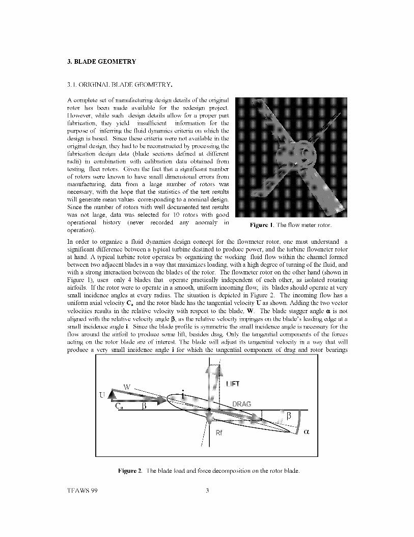
3. BLADE GEOMETRY

3.1. ORIGINAL BLADE GEOMETRY.

A complete set of manufacturing design details of the original

rotor has been made available for the redesign project.However, while such design details allow for a proper partfabrication, they yield insufficient information for the

purpose of inferring the fluid dynamics criteria on which thedesign is based. Since these criteria were not available in theoriginal design, they had to be reconstructed by processing thefabrication design data (blade sections defined at differentradii) in combination with calibration data obtained from

testing fleet rotors. Given the fact that a significant numberof rotors were known to have small dimensional errors from

manufacturing, data from a large number of rotors was

necessary, with the hope that the statistics of the test resultswill generate mean values corresponding to a nominal design.Since the number of rotors with well documented test results

was not large, data was selected for 10 rotors with good

operational history (never recorded any anomaly inoperation).

Figure 1. The flow meter rotor.

In order to organize a fluid dynamics design concept for the flowmeter rotor, one must understand asignificant difference between a typical turbine destined to produce power, and the turbine flowmeter rotor

at hand. A typical turbine rotor operates by organizing the working fluid flow within the channel formedbetween two adjacent blades in a way that maximizes loading, with a high degree of turning of the fluid, andwith a strong interaction between the blades of the rotor. The flowmeter rotor on the other hand (shown inFigure 1), uses only 4 blades that operate practically independent of each other, as isolated rotating

airfoils. If the rotor were to operate in a smooth, uniform incoming flow, its blades should operate at verysmall incidence angles at every radius. The situation is depicted in Figure 2. The incoming flow has auniform axial velocity Ca and the rotor blade has the tangential velocity U as shown. Adding the two vector

velocities results in the relative velocity with respect to the blade, W. The blade stagger angle _ is not

aligned with the relative velocity angle 13,as the relative velocity impinges on the blade's leading edge at asmall incidence angle i. Since the blade profile is symmetric the small incidence angle is necessary for the

flow around the airfoil to produce some lift, besides drag. Only the tangential components of the forcesacting on the rotor blade are of interest. The blade will adjust its tangential velocity in a way that willproduce a very small incidence angle i for which the tangential component of drag and rotor bearings

U

LIFT

I Rf/t

i

TFAWS 99

Figure 2. The blade load and force decomposition on the rotor blade.

3

friction resistance Rf will be compensated by the tangential component of lift. This model leads to a

variable blade stagger angle which varies with the blade radius in a proportional manner if the small

incidence angle is neglected, therefore we are seeking a relation of the form c¢ = _(R), where R is the

blade radius. This relation depends on the required rotor speed at a given volume flow, and on the necessary

incidence angle i at each blade radius. If we take under consideration the boundary layer development on

the shroud and hub end walls, the incidence angle i then depends on the incoming flow axial velocity

distribution with radius Ca =Ca(R). Things are complicated more by considering the presence of the wakes

in the incoming flow, which add a tangential dependency Ca=Ca(R,0), where 0 is a tangential angular

coordinate. Such dependency further generates transient features that render the analysis too complex to

obtain immediate useful results.

Therefore, let us consider an upstream flow that is characterized by a uniform axial velocity and no swirl.

Based on this assumption, one could calculate a volume flow and a rotational speed of the original design

rotor, at which the flow incidence i on the rotor blade is zero or close to zero at each radius. Is such a

rotational speed is found for any given volume flow, the calculation verifies a free-vortex blade design.

However, such calculation does not imply a stable rotation at the rotational speed calculated and no

equilibrium of forces on the blade is assumed. This topic will be discussed in the next section.

By processing the original design blade profiles given at four radii, the blade stagger angles were obtained

and used for the aforementioned calculation. The results show indeed a free vortex blade twist, with a

theoretical flow calibration constant of Kf = 0.8777, and close to zero incidence angles, as indicated in the

following table, third column.

Table 1.

Blade Radius

(% of blade height)

8.6

38.3

68.0

97.7

Blade angle

(degs)

4.9

9.06

13.13

17.06

Flow incidence angle i

(for idealized, uniform

_pstream flow - des_)

-0.0049

0.0016

-0.0011

0.0044

Apparent flow incidence

angle i (see Fig. 4)

(calibration data - de_)

0.04

0.07

0.10

0.13

In operation, the upstream flow is not perfectly uniform, but distorted by wakes behind the hexagonal flow

straightener, which together with the end-walls boundary layers generate an unsteady character of the

incoming flow Ca=Ca(R,0,t), in both tangential 0, and radial r directions. A good way to obtain an average

flow calibration constant is to use all data points available from the calibration of the selected fleet rotors,

and compute a calibration constant based on the mean square linear fit through the data. Figure 3 show this

computation: the horizontal axis indicates the rotor speed measured in pips per second (a pip is a passage of

one blade through a magnetic field of a sensor, hence 4 pips per rotation), while the vertical axis shows the

liquid hydrogen volume flow through the meter, in gallons per minute. The dark line on the plot is a linear

fit through the data points, yielding a flow calibration constant of Kf = 0.8708, while the light colored line

corresponds to the idealized case of perfectly uniform flow upstream and zero flow incidence on the blade

at all radii, for which the calibration constant value is Kf = 0.8777 as explained.

The difference between the two lines in figure 3 is very small, corresponding to calculated flow incidence

angles shown in the fourth column of table 1. The largest flow incidence angle is calculated at 97.7%

radius, a value of 0.13 °. It is necessary to emphasize the fact that the flow incidence angles indicated in

column 4 of Table 1 are not actual physical flow angles with respect to the blade, since the flow field at the

blade leading edge is distorted by wakes and end-wall boundary layers as explained already. These

incidence angles represent a model based on the forces and velocity diagram shown on Figure 2, a model

intended to be used for redesign. The rationale behind these values is as follows: A dimensional average of

the selected fleet rotors is very close to the original rotor nominal design, as the possible small

TFAWS 99 4

xlO_1.8

Fuel Flow

.,., /1.7........................................_...........".omT-o'..._,o...l-o'.Ooooo;i."oo......................i........................._ ...........1.6........................................I---..3;est."_ata..line.-..i...........................................J........................................J......................

i i i i i : :_:!_ .... i

........................................J...........................................i...........................................i...........................................i......................................_::2..................i..................................1_ i i i i ..........yf::i i

p i i i #:i_ i ii i i ...........,_ i i i

M 1.3........................................i...........................................i...........................................i_:_:_'::i........................................i...................................t..................................

i i ?:_:: i J Ji._........................................j...........................................i......................

i i i i i

1.1........................................i............................7 i__:_:................................i...........................................i........................................i...................................i..................................

1.................................i._: i i i i i .............0.9 /i i i i i i

120 140 160 180 299 229 249 269

F/M Speed (pips/sec)

Figure 3. Calibration hot fire test data from fleet rotors, and linear fit of the

data (dark line). The light colored line corresponds to the ideal case of uniform

flow- and zero flow- incidence on the blade.

se

eD

TFAWS 99

97.7% radius

O.6F....T..----II.............!--:---T ...............::--T!--T_::::::: .... '!...............................

I,_----,.:_-:.........:+-:,.........._¢_..........i,__..........._.......... .........

'- ..............i- ..............................'- ..............- ...............1-...............:...........'" .................i68.0% radius

O_F:- ...............[--_ ...............I--T............--i.''' ....7..............................!oL ...........":............L ..... _ L_0...10..3...7. i:: : ......... ........ i

38.3% radius

0.6[............................I.................._ ............................I........................-I-[;[;[..... l..............................]

8.6% radius

0.2F....I......................[i................_...............ii..,F.i...........i..._........::::::::.... 7..............................loL..-.:.::.:::::'''::@_'::_.........::':_..........F_.............¢...........i&.0.....0...4....4...3..._2_:_.::_:...::i!_:::::_:.:...]..:!::::_::............ i

_o._/.....:..............:!--"::............._..............:.....::............." .............:_T""-'::::".................i140 160 180 200 220 240 260

F/M Speed (pips/sec)

Figure 4. Apparent flow- incidence angles at the radii where nominal blade

design of the original rotor is specified. The line indicates a mean square linear

fit through the data at each radius, while the numbers represent the average.

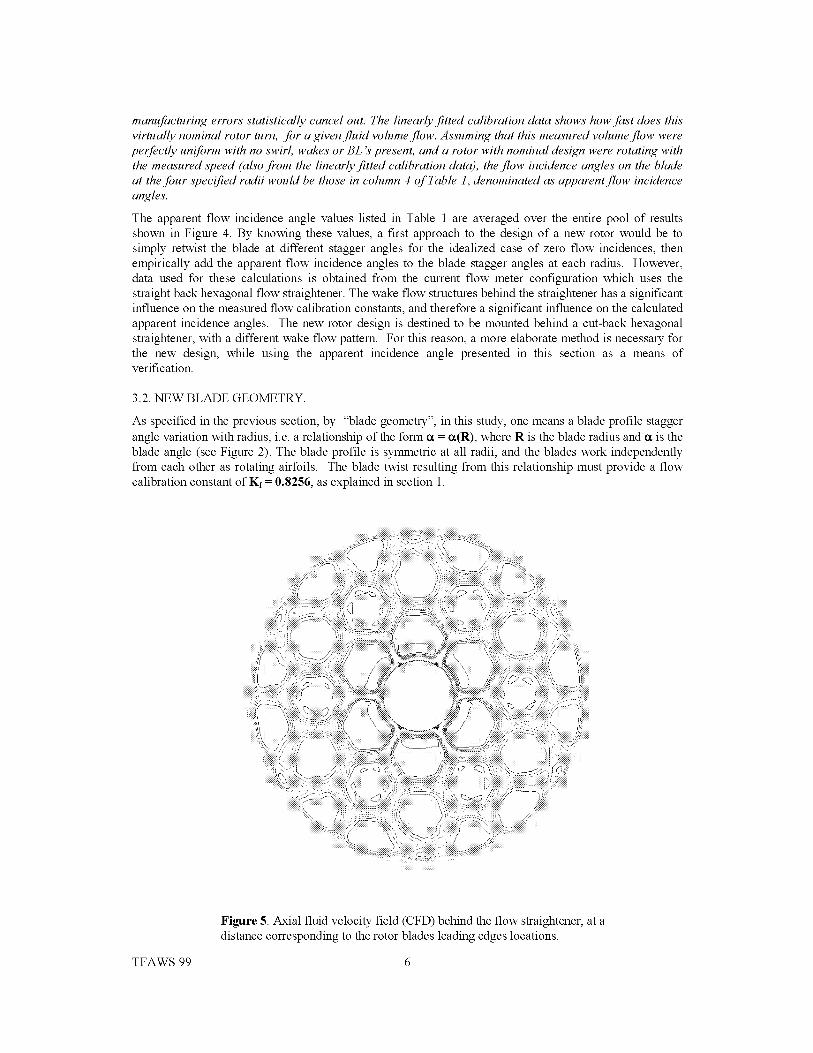
manufacturing errors statistically cancel out. The linearly fitted calibration data shows how fast does this

virtually nominal rotor turn, for a given fluid volume flow. Assuming that this measured volume flow were

perfectly uniform with no swirl, wakes or BL 's present, and a rotor with nominal design were rotating with

the measured speed (also from the linearly fitted calibration data), the flow incidence angles on the blade

at the four specified radii would be those in column 4 of Table 1, denominated as apparent flow incidence

angles.

The apparent flow incidence angle values listed in Table 1 are averaged over the entire pool of results

shown in Figure 4. By knowing these values, a first approach to the design of a new rotor would be to

simply retwist the blade at different stagger angles for the idealized case of zero flow incidences, then

empirically add the apparent flow incidence angles to the blade stagger angles at each radius. However,

data used for these calculations is obtained from the current flow meter configuration which uses the

straight back hexagonal flow straightener. The wake flow structures behind the straightener has a significant

influence on the measured flow calibration constants, and therefore a significant influence on the calculated

apparent incidence angles. The new rotor design is destined to be mounted behind a cut-back hexagonal

straightener, with a different wake flow pattern. For this reason, a more elaborate method is necessary for

the new design, while using the apparent incidence angle presented in this section as a means of

verification.

3.2. NEW BLADE GEOMETRY.

As specified in the previous section, by "blade geometry", in this study, one means a blade profile stagger

angle variation with radius, i.e. a relationship of the form _ = _(R), where R is the blade radius and _ is the

blade angle (see Figure 2). The blade profile is symmetric at all radii, and the blades work independently

from each other as rotating airfoils. The blade twist resulting from this relationship must provide a flow

calibration constant of Kf = 0.8256, as explained in section 1.

Figure 5. Axial fluid velocity field (CFD) behind the flow straightener, at a

distance corresponding to the rotor blades leading edges locations.

TFAWS 99 6

Thedifficultyinchoosingthenew_=_(R)designcomesfromthecomplexflowpatterngeneratedbehindthehexagonalflowstraightener.Differentstudies[1,2]haveshownthattheproximityof theflowstraightenertotherotorbladeleadingedgesoftengeneratesanomaliesinoperations,suchasshiftsintheflowcalibrationconstantassociatedwithaliasing.DetailedCFDanalysis[2]hasshownthecomplexityoftheupstreamflowpatternsandexplainedtheKfshiftasresultingfromaperiodicalquasi-stallphenomenoninducedbythestronginteractionbetweenthewakesattheexitofthehexagonalflowstraightenerandtherotorblades. Suchinteractionswereshownto diminishsignificantlywith the spacing between the

straightener and the rotor. For these reasons, the design of a new rotor has been conceptualized in

conjunction with a modification of the hexagonal straightener, whose exit plane is being cut back at a 21 °

angle, increasing the distance from its exit to the blade from 1.05 to 1.95 inches at the tip of the blade. At

the rotor hub, the 1.05 inch distance is maintained. Therefore the new blade design must account for the

flow pattern behind the new straightener configuration in order to obtained a proper blade twist and

provide the reduced rotor speed required.

The calculations presented in section 3.1 have shown that the original rotor blade design is essentially a

free-vortex design. However, in order to obtain a precise rotor speed at a given volume flow, the designer

must allow for a small alteration of the free-vortex blade twist, in order to account for the effects generated

by the flow non-uniformity. Such effects are quantified by the apparent flow incidence angles also

presented in section 3.1. In order to obtain such quantification for the cut-back straightener configuration

both water-flow rotor test data with a prototype hex housing and CFD computations are used.

Figure 5 shows a CFD generated flowfield behind the cut-back hex straightener in the form of axial fluid

velocity distribution C,=C,(R,0), shown in the transversal plane containing the rotor blades' leading edges.

axial fluid Velocity. f t/see

Figure 6. Radial distribution of the fluid axial velocity, plotted every 2.5 degrees for

a 120 degrees sector. Data is extracted from the flow field shown in figure 5. The

thick dotted line represents an average per one rotation in the tangential direction.

TFAWS 99 7

In this simulation, the rotor and its influence on the

upstream flow is removed. Figure 6 shows, superimposed,several plots of the axial flow velocity distributions in theradial direction extracted every 2.5 degrees in thetangential direction from the flow field in figure 5.

Basically these are the axial flow patterns that are "seen"successively by the rotor blade as it sweeps the flow fieldin its rotation. The average per one rotation in the

tangential direction of the axial fluid velocity Ca = Ca(R )

is represented in Figure 6 by the thick dotted line . Byexamining this radial distribution of velocity one canunderstand that for a rotor blade twisted according to the

free-vortex law, at any given instance, there are significantvariations in fluid flow incidence angles i along thetangential direction, and at all radii. The incidence angle i

can have positive as well as negative values within onecomplete rotation. Thus, at every moment, there aresections of the blade producing tangential forces in thedirection of rotation, and other sections producingresistance. At each of these instances the flow around the

entire blade is very complex, requiring significantresources to be resolved by real time CFD. The prohibitive

cost of such resources in both equipment and man hoursrequires a different more practical approach.

Figure 7 summarizes a calculation model that combinesthe aerodynamic principles expressed in Figure 2 with the

b

dR

R

Figure 7. Force balance calculation on arotor blade.

available CFD data, and anchors them using test data. The rotor blade is divided in 32 horizontal bins as

shown in the figure. Each bin produces, locally, either positive or resistive tangential force dFT, which, inturn, produces a positive or negative torque

dT= dFT R (1)

The localized bin tangential force dFT, is a projection of the local drag and lift forces along the tangentialdirection (as shown in Figure 2) and a portion of the resistant bearings friction torque, which is small andcan be neglected.

dFT = lpbdRW2 x [CL(R)cos(13(R))- {CD(R)sin(13(R)) ] (2)

Here, b is the blade's width, R is the radius of the local bin, dR is the bin's radial width, _(R) is the blade

stagger angle, CL and CD are the local lift and drag coeficients -- which depend on the local relative fluid

velocity W(R) and local incidence angle i(R) -- and 13 is the fluid density. For a given axial velocitydistribution Ca=Ca(R), a relative velocity distribution W=W(R) results by vectorial addition with the

tangential velocity U(R) = R x co, where co is the rotor's rotational speed which achieves a stable, constant

value when equilibrium is achieved on the blade:

Rtip

dT = 0 (3)Rhub

The model is anchored for the Ca=Ca(R) distribution indicated by the average velocity profile in Figure 6,and the rotation resulting from several water flow tests of a cut-back hex straightener using three separaterotors which indicate a Kf value of 0.871. The NACA 0016-64 airfoil CL and CD coefficient values are

used in this calculations, since this NACA profile is closest to the original rotor blade profile from theavailable literature. It is important to note that in the model anchoring process one must account

TFAWS 99 8

empirically for several details associated with the physics of the problem at hand which are not accounted

for in the model. Such details are: i) the nature of the working fluid is different from the fluid for which

standard CL and CD are known, ii) the incident flow is characterized by intense fluctuations which alter the

aerodynamic performance, iii) the three-dimensional character of the flow is neglected, locally, for each bin.

The factor g in equation (2) is the anchoring factor. The choice of placing this factor in association with

the drag force term is based on the consideration that, given the flow fluctuations, it is to be expected that

the drag on the blade profile be actually larger that the literature indicates, while lift forces will be smaller.

CFD analysis [2] of the Kr shifting phenomenon seems to be indicating the same trend. However, _ values

do not reflect a quantification of drag amplification, and must be regarded as purely empirical values

destined to anchor a model and be used in the design process.

Using the average Ca=Ca(R) velocity distribution in Figure 6, the measured Kr = 0.871 flow coefficient

is matched by choosing _ = 32.0. Simulations show a very small sensitivity of the calculated Kr value with

respect to _ , and therefore a good tuning capability of this parameter. Using g = 32.0, the new blade

stagger angle _ = _(R) distribution is calculated based on a free-vortex blade twist altered by a small

incidence angle distribution i = i(R), found by repeated iterations. Figure 8 shows the new blade stagger

angle design, plotted together with the original blade stagger angle design for comparison. The difference

between the old and the new design is small: only 0.84 degrees at the blade tip.

...... originai design _ .......... new design .,,,/-/ .....

14 ........... .,i _/": 'S

m .... _ = i i i

Z 2/" :ie-

t ,

_._,,_.....S'ii i

/,5 ,_

0,6 08 1 ! .2 !4 1:6 1.8 2 2_2 2.4 2:6blade radius, inches

Figure 8. Blade stagger angle distribution

TFAWS 99 9

3.3.ROTORDESIGNCONCEPT1

Havingdeterminedthenewbladeradialtwist,thefirstdesignconceptusestheoriginalbladeprofileinshapingupanewbladeusingthenewstaggerangledistributionshowninFigure8. Theoriginalbladedesignisgiveninthespecificationsatfourradialstations(expressedinpercentagesofbladeheightinTable1 by coordinatepointsx, y. Thedatahasbeenprocessednumericallyandtheprofilehasbeenmathematicallyreconstructedbasedoncircleelements(0.016inchradiusand0.005inchradiusfortheleadingandtrailingedgesrespectively.) andsetsof thirdorderpolynomials.Figure9 showsthereconstructedprofile,whichhasachordlengthof 0.747inches,andamaximumthicknessof 16%(relativethicknessexpressedinpercentsofthechordlength)at40%ofthechordlength.Forcomparison,theNACA0016-64profileisplottedinthesamefigure.

O.05F ....:22_ _-_ ....... " . ..... q

0 .......................................

-0.05

0 0.1 0.2 0.3 0.4 0.5 0.6 0.7

NACA 0016-64Actual rotor blade

Figure 9. Rotor concept 1 and NACA 0016-64 airfoils. The rotor blade has been

mathematically reconstructed from the x,y coordinates given in the original designdocumentation.

For the concept 1 rotor, the new blade natural frequency associated with the first bending mode is

approximately 830 Hz. For a successful design, the rotor must not exceed 3650 RPM at a fuel volume flow

of 17,685 GPM--which defines the regime at 115% SSME Rated Power Level--thus allowing for a 12%

frequency margin with respect to the 12N symmetry excitation mode associated with the wake flow

structures behind the hexagonal straightener. The 3650 RPM is a slow speed for such high volume flow,

rendering the design calibration coefficient Kf = 0.8256 very sensitive to any alteration in the blade stagger

angle. For 3650 RPM, at the blade mean diameter the relative flow velocity has an average angle of 9.6 °,

while the blade's stagger angle is 9.9 °. Given the blade profile accepted tolerance field for the original

design of +0.003 inches, a biased manufacturing within the 0.006 inch tolerance band as shown in Figure

10 can produce a stagger angle error of 0.46 °, i.e. an error of 4.7%. This possible error places the rotor

speed value in the 3475-3825 RPM range, which, for the right end of the range, not only reduces the

frequency margin to 7.8%, but also exceeds the 3800 RPM limit. For these reasons, the flow of

information from the design concept to the manufacturing of the hardware must be carefully controlled.

Such control is exerted by following the path of essential design information and ensure that minimum or no

iiiiiiiiiiiiiiiiiiiiiiiiiiiiiiiiiiiiiiiiiiiiiiiiiiiiiiiii

D Actual airfoil D Tolerance field

Figure 10. Stagger angle error due to biased manufacturing of the rotor airfoil, within the

accepted tolerance band.

TFAWS 99 10

alterationoftheoriginalconceptualdesigngeometryoccurs.ThebladegeometryisimportedintothesolidmodelingsoftwareviaASCIItranslationfiles.Theairfoilgeometryisthereforemaintainingit's originalmathematicaldefinition.Furthermore,airfoiltolerancebandisdecreasedfrom+0.003 to +0.002. The solid

model of the rotor is further translated into an IGES ASCII translation file, and imported into the CNC

software for manufacturing. Once in the manufacturing phase, information control of the geometry is

weaker, and depends on the quality of the supplier's technology. For this reason, a feed-back loop into the

information control is organized by extracting inspection-specific geometry data from the solid model, and

inspect the final product. In this manner, the solid model becomes a process reference element to which the

final product is compared. The details of this information loop will be the subject of a future report.

The rotor concept 1 has been manufactured and water-flow tested, in conjunction with three types of flow

straighteners: i) the original egg-crate straightener, ii) the current design hex straightener and iii) the cut-

back hex straightener. The water-flow calibration constants obtained are listed in Table 2.

Table 2. Rotor Concept 1 water-flow test results.

Type of upstream straightener Water-flow calibration coefficient

Egg-crate 0.8180 + 0.94%

Current design hex 0.8456 + 0.7%

Cut-back hex 0.8179+0.18%

The water-flow calibration coefficient obtained for the cut-back hex straightener is Kfw = 0.8179, which is

approximately 1% lower that the targeted value of 0.8256. Since the calculations were made for

incompressible volume flows, this value should remain the same for engine operation . Nevertheless, in

operation, the changes in Re number (a five fold increase) and nature of the fluid will slightly increase the

value of the calibration constant, as the fleet testing experience shows. A quantification of this increase is

difficult to predict.

3.3. ROTOR DESIGN CONCEPT 2.

The second design concept follows the same radial twist

additional objectives:

for the blade geometry, while targeting two

• An increase in the blade natural frequency associated with the first bending mode to 1300 Hz. For this

frequency, at 115% RPL there is a 16% frequency margin above the excitation frequency associated

with the 18N wake flow symmetry behind the hex straightener. Since 18N is the highest symmetry

number, the blade natural frequency is above all excitation frequencies associated with the upstream

flow in operation.

• An optimization of the flow around the blade in a manner that minimizes the effects of the strong wake

structures at the hub-- where there is only 1 inch separation between the rotor and the cut back hex

straightener---and increases the role played by the flow around the upper half of the blade, located in a

less perturbed flow field.

Both objectives are to be achieved by a tapered design of the blade geometry employing a variable blade

chord length and a variable airfoil relative thickness from hub to tip. The design uses the modified NACA

Four-digit series of airfoils whose relative thickness varies linearly from 24% at the hub to 13% at the tip.

The chord length varies also linearly with radius, scaling the original design chord length by 109% at the

hub and 100% at the tip. Figure 11 shows 8 radial sections of this design, by comparison to the original

profile. The final design was obtained after 14 iterations, each iteration consisting of a mathematical model,

translation and import into a solid modeling software, followed by export into a stress and natural frequency

TFAWS 99 11

analysissoftware.Themanufacturedrotortestedonly5Hz differencefromthepredicted1308Hznaturalbladefrequencyassociatedwiththefirstbendingmode.

012 ......... 04 0i6 08

0 02 0i4 0:6 0:8

0;1 .....

01 k: __> .....

0 02 0:4 0.6 0.8

0 0:2 0:4 0i6 08

,0:10 01:2 0:4- :0i6 018

0 :02 0.4 0!6 0:8

0 02 Oi# 0i6 08

0 0_2 0i4 0:6 0:8

Figure 11. Rotor Concept 2 blade geometry shown at 8 equally spaced radial sections. The blade chord

length varies linearly from 109% of the original chord length at the hub to 100% original chord length at

the tip. Airfoil relative thickness varies linearly from 24% at the hub to 13% at the tip. Airfoils are modified

NACA Four-digit series.

TFAWS 99 12

Atthetimeofwritingthisreport,onlypreliminarywaterflowtestsofthesecondrotordesignareavailable.TheresultsareshowninTable3.

Table 3. Rotor Concept 2 water-flow test results.

Type of upstream straightener Water-flow calibration coefficient

Egg-crate 0.8154 + 0.44%

Current design hex 0.8436 + 0.1%

Cut-back hex 0.8169 + 0.1%

The numbers are very similar to the results obtained for rotor concept 1, slightly slower. The same

observations made at the previous section regarding the change in flow regime for engine operation should

be noted here as well. Preliminary real-time measurements from the magnetic detectors show a very smooth

rotation for concept 2 rotor.

CONCLUSIONS

A new rotor design has been conceptualized for the SSME fuel flowmeter, in conjunction with a

modification of the hexagonal flow straightener destined to increase the spacing between the straightener

vanes and the rotor's blades at the rotor's blade tip. The design requirement, essentially a slower speed,

will allow operation of the SSME at 115% rated power level and beyond. The new design is obtained by a

retwist of the rotor blades, following a calculated radial distribution of the blade stagger angle c_=c_(R).

Based on the same stagger angle radial distribution, two design concepts have been finalized, prototyped

and water-flow tested. The first concept follows the new blade twist using the same blade profile as the

original design. The second concept uses a tapered blade design which increases the blade natural frequency

associated with the first bending mode to 1308 Hz, while optimizing the flow around the blade, generating a

smooth operation. The water flow tests indicate a flow calibration constant within 1% of the targeted value.

ACKNOWLEDGEMENTS

The author wishes to acknowledge the contributions of William Bowling-Jr for the innovative solid

modeling of the rotor geometry. Mr. Bowling's feed back and contribution to the control of the design

information is essential to this project. The formulation of design requirements, management of design

iterations, stress and blade dynamics feed back to the author is due to John Ubowski. The team efficient

management and coordination as well as scheduling of the intensive water flow tests is due to Hem-y

Loureiro.

Special thanks to Dr. Edward D. Lynch for providing the CFD flow field data behind the hexagonal

straightener, and for the interesting discussions regarding the flow regimes and instabilities past the meter

rotor blades.

TFAWS 99 13

REFERENCES

1. Fox.T.H.,"PossibleMechanismforFlometerOscillationsSeenonSTS-8",MashallSpaceFlightCenterLetter,April9,1984

2. Ascoli,E.et.al._ApplicationofCFDtoExplainStallBehavioroftheSSMEFlowmeter",AIAApaper99-2458,presentedatthe35 th AIAA/ASME/SAE/ASEE Joint Propulsion Conference and Exhibit.

3. J.T. France, _The Measurement of Fuel Flow", AGARD Flight Test Instrumentation Series, Volume 3,

NATO publication, 1972.

4. Schlichting, H. _Boundary Layer Theory", McGraw Hill, 1979

5. Abbot, I.H. and von Doenhoff, A. E.," Theory of Wing Sections", Dover, 1949.

TFAWS 99 14

THE OFF-DESIGN PERFORMANCE OF A CAREFULLY

INSTRUMENTED RADIAL INFLOW TURBINE

Dr. David Japikse

Concepts ETI, Inc.

217 Billings Farm Road

White River Junction, Vermont 05001-9486

ABSTRACT

The performance of a common radial inflow turbine, operating with a nozzle-less inflow volute and an exhaust

diffuser, has been evaluated. Experimental techniques are discussed and test problems are reviewed. Internal data

have been acquired for each sub-component. Fundamental questions about data interpretation are addressed.

Suggested parameters for sub-component and overall data correlation are given. Important trends of basic loss and

diffusion parameters are presented. Suggestions for additional studies are offered.

NOMENCLATURE

A

b

Co

ef

fi2

L

LC, K

ill

N

P

Po

Qf

To

GU

Area

Passage height (span)

Isentropic expansion velocity based on enthalpy and Equation 13 or 16

Expansion ratio, P00 / P4 or Poo / P4

Multiplicative loss adjustment factor

Impeller incidence

Length

Loss coefficient, see Figure 7Mass flow rate

Rotational Speed

Static pressure

Total pressure

Heat flux

Radius

Total temperature

Operating clearance

Wheel speed; usually U 2 by implication

GREEK SYMBOLS

a4

q

0

Absolute swirl angle

average of four core probes in Figures 9 and 10

Radial and circumferential average in Figures 14 and 15

Blade angle; degrees from meridional surface

efficiency, also diffuser effectiveness (Cp/Cp, ideal)

Blade angle, degrees from meridional

TFAWS 1

STATIONSANDSUBSCRIPTS

0 Upstreamstagnation,throat1 Voluteexitstate2 Impellerinletstate3 Impellerexitstate4 DiffuserexitstateD Diffuser exit state

r referred state; also _corr'

ts total-to-static

1. INTRODUCTION

The radial inflow turbine is an essential element of every low cost automotive turbocharger, produced in the level of

three to five million copies per year around the globe. It is also used for small gas turbines and cryogenic expanders.

It has received some extensive investigation over the past 50 years but receives very little research at the present

time. Modeling of the radial inflow turbine is achieved with moderate accuracy, but as shown below, numerous

questions concerning the fundamental performance of radial turbines still exist and have not been dealt with in the

technical literature. This investigation establishes the base of current understanding for radial inflow turbines and

presents extensive data from one thorough investigation of a radial inflow turbine including internal fluid dynamic

and thermodynamic measurements as well as accurate overall measurements. This paper is presented with the

permission of original consortium sponsors, which is appreciated.

2. PAST TECHNICAL CONTRIBUTIONS

A large number of technical contributions to the radial inflow turbine technology have been presented in various

forms. These have been reviewed in detail by Japikse (1982) [1] and the literature survey has largely been

incorporated in subsequent presentations by Baines (1999) [2] and others. Highlights of the original literature

survey are summarized. The technical literature for radial flow turbines was found to fall almost exclusively into

four categories, as follows:

1.

2.

3.

4.

Investigations by NASA

Investigations by American Industry:

Various English contributions, principally from Universities, and,

A useful variety of Japanese contributions.

The principal driving force for conducting these investigations was to study the radial inflow turbine for small gas

turbine application (up to helicopter size engines), for turbochargers, and for space power applications. The

strongest consistent industrial requirement, throughout the past decades and up to the present time, has clearly been

the turbocharger application.

The reported survey of the technical literature revealed several significant observations:

1.

2.

3.

4.

Most of the reported measurements concerned overall power absorbed, and hence efficiency, plus

referenced flow versus expansion ratio.

The most common internal measurement was a single impeller exit radial survey with a three-hole probe

where total pressure and swirl angle were measured.

Other internal measurements were virtually non-existent in nearly all studies.

Most studies concentrated on simple design difference investigations such as changing operating clearance,

changing blade number, changing axial length, or some other simple direct design variation.

The four preceding observations can be readily reconfirmed by the interested reader upon reviewing the literature

surveys referenced above. Due to the absence of detailed internal data, all of the prediction models have failed to

confirm their integrity by comparison to station-by-station velocity triangle, loss, and recovery measurements.

TFAWS 2

Instead,variousadjustmentfactorswithinthe_models'havebeenmanipulatedat will to obtaingoodoverallagreementonflowrateandefficiencywiththehopethattheadjustmentin internalcoefficientsmighthavesomebasisinrealityandmightsuggestagreaterlevelofunderstanding.Nonetheless,lackingdetailedinternaldata,thereisnobasisuponwhichtheinternalmodelscanberigorouslyconfirmedorrefuted.A particularlycurioussituationexistsintheexitsurveyswhichhavebeenreportedinthepaststudies.All thesurveysshowedsignificantvariationsinexitswirlangle.Thesevariationsweredistinctlydifferentfromwhatmighthavebeenexpectedfromflowcodeswhichwereavailableatthetimeof theinvestigations.In allcases,however,noeffortwasmadetomeasurethestaticpressuredistributionattheimpellerexitandfundamentalunderstandingof aswirlingflowshouldleadaninvestigatortounderstandtheneedformeasuredstaticpressurevariationstoaccompanytheswirlanglevariation.

3. RESEARCH OBJECTIVES

The objectives of the present investigation were to learn how to obtain good, reliable measurements inside a radial

inflow turbine and to establish recommendations for future investigations. Additionally, it was desired to actually

obtain a good set of measurements and interpret the measurements into fundamental modeling parameters for a

single turbine stage.

To meet the objectives set forth, a radial inflow turbine was obtained and developed into a test facility. Figure 1

shows a contour outline of the radial inflow turbine showing the principal meanline dimensions. The impeller was

comprised of radial elements and has a 0 ° inlet blade angle. Only the exhaust diffuser was modified slightly from

the original configuration; specifically, the surface of the diffuser was machined to conform to exactly the

dimensions shown in the figure, so that a proper machined surface would be available to facilitate repeatable

measurements in the future (in other words, the rough cast surface was removed and replaced by a reliable,

machined surface). Figure 2 displays the test facility created for the purpose of this investigation. Flow was

delivered to the turbine test rig from a combustor in which kerosene was burned with compressed air. Inlet

temperature could be controlled over a wide range of temperatures, as discussed below. The inlet state was found,

by several casual traverses, to be quite uniform and well mixed-out. A set of three different inlet total pressure and

three different inlet total temperature measurements were made as well as static pressure and flow rate. Rotational

speed was measured as well. The entire turbine assembly was carefully insulated to minimize heat loss from the test

TFAWS

Figure 1. Principal one-dimensional geometry specification, not to scale.

3

rig. Several different options for exit flow field traversing were considered. Initial consideration was for traversing

close to the impeller exit, but mechanical interference with the hub attachment (a common nut) ruled out this

possibility and subsequently it was decided to traverse downstream of the exhaust diffuser. Four different

circumferential positions were traversed giving a total of 8 different radii representing the exit flow field. Total

pressure and absolute flow angle were initially measured (following the common technical literature of the day) and

subsequently static pressure was also measured, as discussed below. In order to get a good exit total temperature,

three elements of a Koch mixer were used as shown in the figure. This allowed a 99+% mixing completion to be

achieved with a very uniform total temperature at the discharge. By using this total temperature (actually an average

of six shielded probes), and the inlet total temperature, plus appropriate calibrations, a very accurate measurement of

temperature drop could be achieved.

/

Figure 2. Radial turbine instrumentation.

In order to confirm the adequacy of the techniques utilized, a heat loss calibration was conducted. After removing

the impeller and replacing it with a stationary hub flow deflector, the inlet and outlet temperatures were measured

over a period of time. It was found that thermodynamic equilibrium could be achieved with all temperatures

stabilized within approximately two hours. Additionally, a small drop in temperature from the inlet to the outlet was

measured which was attributed principally to heat conduction down the shaft and through the bearing housing and

also through the insulated walls. These tests were conducted while maintaining a steady flow of oil to the bearings

(not rotating) at typical oil temperatures. The major results are shown in Figure 3. It should be mentioned that

similar tests had been previously conducted on a different test rig (although principally to determine the flux of heat

from the turbine into a compressor which was being tested). The results showed (not at all surprisingly) that a very

linear relationship of the temperature difference, as suggested in Figure 3, would be achieved. For the present test,

data was recorded at only two temperatures. The 800°R gas temperature corresponds to the lowest temperature

which could be held with the combustor operating stably. The 580°R temperature corresponds to no combustor

operation and simply the discharge temperature of the compressed gas leaving the supply compressors. Based on

the prior data, a simple linear interpolation between these two conditions was used to estimate the amount of

correction. Prior tests have also revealed that hot turbine operations should not be considered: the heat loss would

be too great and the correction factor would amount to a significant percentage of the measured temperature drop

through the turbine. By controlling operating temperatures in the lower range suggested by Figure 3, and carefully

scheduling the tests, the maximum correction was usually held at less than 0.5 ° and the resultant uncertainty is

probably no more than plus/minus one or two tenths of a degree Rankin. Consequently, the thermal adequacy of the

test rig was reasonably demonstrated. It should also be mentioned that the temperature measuring probes were all

half shielded thermocouples which have a known calibration characteristic for recovery factor and, consequently,

good corrections for local Mach number were readily possible.

TFAWS 4

\ ,_ tt

Figure 3. Turbine housing thermal calibration with

impeller removed (zero on ordinate is no heat loss).

Figure 4. Turbine supplier's performance

map and scoping calculations of this study.

Prior to conducting tests, careful sensitivity calculations were made in an attempt to discern which parameters might

be of greater significance for detailed investigation. Figure 4 shows a set of measured results from the manufacture

of the turbine with scoping calculations conducted by the author. The calculations used an early meanline

performance code using common modeling techniques referred to later. The investigations clearly illustrated an

unexpected sensitivity: small changes (not revealed in Figure 4) to the exit modeling conditions could significantly

change the interpretation of the velocity triangle at the impeller inlet. In other words, by considering alternative

models at the impeller exit, one could introduce a variety of different possible interpretations at the rotor inlet. This

sensitivity had simply been overlooked in prior investigations since little attention had been given to station-by-

station measurements and nearly exclusive attention was placed on the overall performance characteristics while

taking great liberty to adjust any internal parameters desired (usually the rotor inlet conditions with indifference to

the exit conditions).

Additional instrumentation included three-hole probes fixed at a location just upstream of the impeller inlet at mid-

passage. These were located at four different circumferential positions corresponding to different sectors of the

volute. It was originally desired to traverse the flow field at this location, but inadequate consortium sponsorship

limited the degree to which measurements could be made at this location. Consequently, the four fixed probes were

utilized in an effort to determine core, and possibly maximum, values of flow parameters at this location. This

proved to be an exceedingly difficult measurement as noted below.

With these issues in focus, the test hardware was built and taken through a shakedown evaluation. The original

shakedown evaluation of two hours produced data which reflected most of the expected trends and conditions for the

planned test. However, strange signals from the fixed total pressure/yaw angle probes upstream of the impeller

required careful examination. This examination revealed that the probes had simply been destroyed by particulate

erosion in the two hours of testing with a small amount of damage to the impeller and volute. Consequently,

significant efforts were expended to remove particulates from the test field. This required a startup period for the

combustor with hot gas discharge bypassing the turbocharger for a startup transient of one or two hours and then the

flow was brought into the impeller. Additionally, a particle separator was introduced upstream of the test rig. The

resultant flow was much cleaner and a new rotor and volute housing showed only limited distress after many, many

hours of operation. Additionally, the four fixed probes were replaced with Inconel probes (the original being

TFAWS 5

stainlesssteel)andtheselastedthroughoutmostof theresultanttestprogram(althoughoneor twoprobesdideventuallyfailneartheendoftheproject).Theshakedowntestswithunexpectedbutessentialmodifications,didestablishthemeansforobtainingaccurateandreliabledatawhichcouldbeusedforgoodmodelbuilding.

Samplesofkeydataarepresentednext.Figure5displaysstaticpressuremeasurementsconductedatkeystationsthroughandaroundtheradialinflowturbine.Thesamedataaremeasuredateverysingletestpointfortheentireinvestigation;onlyoneispresentedhere.Thehighestpressureistheinlettotalpressurefollowednextbytheinletstaticpressure.Beneaththisaretwolevelsof staticpressure,showninacircumferentialvariation,whicharetakenaroundthevolute(orscroll).Thehighervalueisontheoutersurfaceofthescroll,wherethestaticpressureshouldbehighestbytheEuler-nequation,andthenextoneisonthesidewallof thevolute.Thesevaluesarenotcompletelyuniformshowingthatthevolutedoesnothavetotallyuniformstaticpressureinacircumferentialsense,ataskwhichwouldbeextremelyhardtoeffectinanyvolutedesign.At theimpellertip thereisaverycarefulmeasurementof staticpressurewithtapsatevery45°, andmorecloselyspacednearthetongueofthevolute.Adefinitevariationofthestaticpressureatthislocationcanbeobservedandthisisaresultofdistortionfromthevolute.At theimpellerexit,thestaticpressureis measuredalongtheshroudsurfaceanddisplayedwiththexsymbol.It isthelowestcasingpressurerecordedandfallsbelowthedownstreampressure(whichhasalsobeenusedtonormalizeall thepressuresofthisplot). It thereforeappearsthatthereis,in fact,astaticpressurerisethroughthediffuser,atleastalongtheshroudstreamlineasthesetapswouldindicate.

Onemustbecarefulin interpretingthevariationof staticpressurein thevoluteparticularlyconcerningthesuddendropinstaticpressurealongtheoutersurfaceassuggestedatthelocationof90°. A carefulexaminationofthisparticulartapwasmadeandit wasobservedthatthepressuretapfellintoapocketof castingporosityalongtheinsidesurface.This,ofcourse,wouldintroducenoticeableerror,severalpercentof dynamicheadatleast,andthereforewouldgivelargeruncertaintyinthismeasurementthaninothermeasurements.Thevoluteouterpressuremeasurementsaresubjecttothisuncertaintysincetherewasnowaytoenterintothevoluteandsmoothoutthesurface.However,theimpellertipandexitpressureswereextremelyaccuratepressuretapsdrilledintoamachinedsurface;hencethesemeasurementscanbeconsideredtobeofcommonaccuracy(+0.05-0.08psia).

Figure6displaysasampleofimpellercoverstaticpressuredata.Inallcases,asmoothaccelerationwasnotedwithnegligiblecircumferentialvariationsinpressure.

tt:l.

i

l.ll

i

i.It

tg

I ! i I i: i 4

1 i , ! t ! j:

iT-! ,, i i i

--= : :: _ "i 4s_-- ._ :r.= .......... 2_.....

1 :! ! i ]

"Io oo,,:- .....] - I

i Ill

tl

l+

it

1,i

lli

lt, tl

] } i i '

i 1 _ , !

t1

, • . _ t

I t} ' I _ '<

ii t'! 111 ,¢ $¢ .1_ ;'l i. _ lit,

Figure 5. Circumferential pressure

measurements at various key stations

(divided by p4).

Figure 6. Impeller cover static pressure variation.

TFAWS 6

It wasdesiredtolearnasmuchabouttheflowangleatthevolutedischarge,thatis theimpellerinlet,aspossible•Unfortunately,onlycorevaluescouldbemeasuredbutthesearestillverybeneficial•Thecorelosscoefficientwasconsequentlycalculatedforthevolute(whilemakingnocommentsaboutthehigherlosseswhichmustbefoundclosertothewalls)asdisplayedinFigures7and8. ThesecondfiguregivesanearlyconstantvariationwithrespecttoU/C0,butforreasonswhicharenotimmediatelyobviousfromtheseplots,thereisamaximumin lossattheexpansionratioof2.2withadrop-offatthehigherexpansionratioof2.8.It isclearthatthecoreflowfromthevoluteinletflangeuptotheimpellerinletisnotisentropicbutthatsmalllossesontheorderof2%to4%oftheinletstagnationpressureareevident•Lossesnearthewallswouldlikelybemuchhigherduetolocalboundarylayereffects•Thus,eventhoughthisvoluteservesasanozzlewithcontinuouslyacceleratingflow,thedevelopmentofstrongboundarylayers(withskewedorsecondaryflow)alongthesidewallsissubstantialandreachesallthewayacrosstothecoreregionoftheflowfieldgivinglossesineachofthefourmeasuredlocations•Noneoftheprobesshowedanisentropiccoreunderanyoperatingconditions•

• $

,4

Figure 7. Volute core loss _-_ versus U/C0.• ]_02 /)2 --

• ;,:)

_-_ 2,1 ¸

G

Figure 8. Volute core loss (Apo/Poo) versus U/C o.

TFAWS 7

Additionally,themeasured(coreregion)swirlanglesaredisplayedin Figures9 and10. Theanglevariationproceedsfromapproximately69.5°atlowexpansionratiouptoapproximately73.5°atthehighestexpansionratiowithatendencytoincreaseinanearlymonotonicform.However,themeasureddatadoshownoticeablevariationwithU/C0. Figure10givesareasonablefirstestimateof thegeneraltrendsonanaveragebasis.Thestrongvariationathighvaluesofexpansionratiowouldsuggestfurtherinvestigations.

i

73

_2

71,

]To

6g

_,lL_lllj;ll'llli_ j

I I[ ) T I I ; I I I i i I I I r I I I Io._ o.e

oJ%

?3

72

7o

69 I I I Is.L I I

Figure 9. Volute exit swirl angle versus U/C o . Figure 10. Volute exit core swirl angle

versus stage expansion ratio.

Impeller exit flow field traverses were conducted for a set of six different operating points (discussed below) and

required more than one week of continuous testing to log these data. Clearly, said data was not recorded for every

single testing point, but only the select points due to economic limitations. It was felt that these data were important

to anchor the results of the entire investigation. After the investigations were conducted, which unfortunately

followed the current practice of the industry of recording swirl angle and total pressure, it became clear during data

processing that an important link was missing: the static pressure must also be measured. Consequently, one test

case was repeated as shown in Figures 11, 12 and 13 presenting the total pressure, the flow angle and the static

pressure. These data clearly show that the static pressure is not constant but drops substantially toward the

centerline of the test facility as a consequence of the strong swirl distribution. The static pressure variation is clearly

important and must be at least recognized if proper data processing is to be achieved. To obtain this particular

measurement, the three-hole probe was used in reverse and was calibrated for base pressure. Knowing this basic

trend, corrections could be made for the comprehensive traverses conducted at the selected six operating points.

TFAWS 8

i

I

i

Figure 11. Radial turbine exhaustsurvey - total pressure.

Figure 12. Radial turbine exhaust

survey - flow angle.

Figure 13. Radial turbine exhaust survey

- static pressure.

TFAWS 9

Figure14showsanexitstaticpressurecorrectionfactorthatwasdevelopedforthediffuserexitasafunctionofexitswirl.Thisvaluewasachievedbyadjustingthelevelof staticpressureusedintheintegrationofthetotalpressureandswirlangleinformationfromthetraverseswhilesatisfyingthelocalmeasuredmassflowrate.Theinvestigationoftheexitflowfieldviathetraversingshowedthattheoneoversight,inpastinvestigationsandinitiallyin thisinvestigation,wasthelackofattentiontothestaticpressuredistributionintheexitpipe.Whenthisparameterwassensiblyadjusted,massflowagreementwasobtainedandarationalcorrectiontothestaticpressurewasimplied.Thisalsoresultedin improvedvaluesof exitswirlangledistributionsincetheweightingof themassaverageparametersisconsequentlyaffected.

TheFigure14correctionfactorwasusedwiththesixtraversepointsasindicatedand,additionally,everyothertestpointonthemaphadasinglepointrecordedusingthestation4cobra(traverse)probeinaJTxedradialposition.Thefixedpositionhadbeencarefullyselectedto beaveryrepresentativepointoftheflowfieldwhichverynearlyreplicatedthemassaveragevaluefromthesixtraverses.Onlytheslightestcorrectionwasnecessarysincethelocationforthefixedprobewaswellchosen.Asaconsequence,allofthedataforboththefixedprobeandforthedetailedtraverses,givingadiffuserexitswirlangle,aredisplayedinFigure15. It canbeobservedthattheswirldistributionatthediffuserexithasbeensensiblymapped.Thesixdifferenttraversepointsindicatedtrendswithin+3 °, an error which is quite modest on a trigonometric basis. Incidentally, it should be mentioned that the six

traverse points were conducted at four different expansion ratio levels and, at the design expansion ratio of 2.2, also

at three different values of U/C 0 varying from 0.65 to 0.72 to 0.81. Due to the particular style of load control in the

test rig, it was possible to independently control U/C 0 while testing at a particular expansion ratio.

+1.0 I

u/e =. 8

o 0Is:%.... _" ......I-,°

er=2.8

,C

er=2.2

U/Co=. 7 2

10 20 30

I_l

Figure 14. Possible diffuser exit static pressure

correction factor as a function of _ and U/C 0.

2_

I0

I0

-20

Figure 15. Deduced impeller exit flow angles as a

function of U/C o and er.

TFAWS 10

4. DATA EVALUATION

Using the data obtained from this investigation, a series of loss calculations and flow state calculations were

prepared. These, of course, required certain modeling equations as discussed now. Figure 16 shows a Mollier

diagram that reveals the isentropic incremental basis for conducting loss calculations. This is one of the cleanest and

most consistent methods of evaluating internal state changes for a radial flow turbomachinery stage. Table 1 shows

the related equations. The denominator of incremental loss expressions is shown as equation 12 and the increments

are based on the isentropic enthalpy or temperature at each intermediate state of the expansion process. Of

particular note is the state 2m which corresponds to a mixed-out state at the impeller inlet. Equation 7 reveals part

of the modeling picture: Mizumachi (1960) [3] suggested that a fraction of the kinetic energy associated with the

velocity component normal to the blade would be lost irreversibly and would manifest itself as a total pressure loss

and a static enthalpy gain. Other investigators assumed that 100% of this component was lost. At a later time, it

was suggested that the component under consideration was not the component associated with the approach

incidence but rather an effective incidence which would represent the difference between the gas angle and some

special optimum flow angle. A reasonable deduction of the optimum flow angle might be the condition under which

the blade tip is unloaded with the use of substantial approach (usually negative) incidence. The origin of this

suggestion is no longer clear, but it may have started indirectly from an approach by Todd and Futral (1969) [4] or

in a presentation by Japikse (1981 and 1986) [5,6]. Hence this model involves two parameters, the value _opt and the

'f' coefficient from Mizumachi. Modeling Station 2 can also be effected substantially by understanding properly the

value of P02 at the volute exit. Recognizing that a substantial velocity distribution exists at this location in the

absolute frame, and that this distorted profile may not produce a full measure of useful work extraction in the

relative frame, it is quite possible that a substantial mixing loss is implied by the character of the velocity profile at

the volute exit. Thus, for purposes of evaluation, it can be hypothesized that a mixing calculation should be

conducted at the volute exit to represent the degradation of the velocity profile at this location. Of course, the true

profile has not been measured (or computed), but the core value has been modeled in a simple sudden expansion

mixing calculation. Thus a classic Borda-Carnot mixing calculation can be made to obtain a value of P02,m which

reflects profile mixing as well as the core loss. Other efficiency definitions are shown in Table 2.

Figure 16.

Total State..... Static State

P00 P02 P02....P2

/ S/,_ ,f f

Basis for isentropic incremental loss calculations.

TFAWS 11

TABLE 1

STRATEGY 1 INCREMENTAL ISENTROPIC CHANGES

l)" Anscroli = (T0:0-T02,S):/X

2) &_rotor, tot = (T02,S-T03,S "(T02"TO3))/X

3) &_ =_incideece (To2,S'T02_, S)/X

4) A_rotor

5) &_4iffu_er

where

6) r02,S

7) T2m

= (T02_,s-To3,s-(To2-TO3))/X

= (TO3,s-To4,s)/X

) (k-l) Ik= T00 (PozlP00

: T2 + f W2 _ sin_(i ) k-',l2k:_8

(f_l.O, 0.75, 0.5)

8) P02m,S

9) Y02m,8

I0) Y03,S

ii) T04,S

12) X

i = _-6opt

= P2/(T2 /T00)k/(k-1)

T00(P0_m,S/PO0__ , (k-l)/k

= _ , l , (k-l)/kZOO _POY P00 )

Too'P04" P00)< I (k_l) Ik

= T00-T04,S

TABLE 2

STRATEGY 2 ISENTROPIC EXPANSION BASIS

Scroll:

13) nscroil _

14) nrotor =

15)

16)

_'2ZC2s (TOO-T2,S) k-l'

(k-l)Ik

T2, S = T00fP2/P00)

3,S = k-:i (T2-T3,S) "2 _2 _3

. (k-l)Ik

T3, $ = T00(P3tP02)

TFAWS 12

An additional challenge is manifest in obtaining good values for Station 3. Although Station 4 has been reasonably

well documented by full flow field traversing, it is necessary to back calculate from Station 4 to Station 3. This was

initially done by assuming a fixed value of diffuser effectiveness and then was subsequently modified by using

conservation of mass, conservation of angular momentum, conservation of energy and a simple density relationship.

This allowed a simple back calculation from Station 4 to Station 3. Although a small amount of angular momentum

is surely destroyed between Stations 3 and 4, testing of a wide variety of swirl producing and swirl controlling

devices suggests that the angular momentum destruction over this short distance would be limited to simply 1% or

2% and might be neglected. (If desired, bracketing calculations could be conducted to reconsider this small

variation.)

It is important to maintain a proper work balance across the impeller. The work balance must reflect the measured

enthalpy drop on the one hand and the change in UC(_ on the other hand. The value of UC(_ at the impeller exit is

distinctly smaller than the value at the impeller inlet, but not at all negligible. Fortunately, a good understanding of

the C(_ values at Station 4 is available from the six traverses plus Figure 15 and reasonable estimates at Station 3 can

consequently be rendered with only a small residual uncertainty. This allows closure on the value of C(_2. It was

quickly found that this value was noticeably different from the value of C(_2 which might be estimated from the

swirl angle measured at the central or core location at volute exit. This is not surprising since the core value might

only be indicative of one extreme value of swirl angle at the volute exit and would not reasonably be expected to

reflect a true average. Consequently, the value of C(_ 2 was computed from the work input (measured to better than

1%) and the exit angular momentum. One of the most fundamental differences between this investigation and all

prior radial inflow turbine studies is the careful attention given to issues involved at the rotor exit before an attempt

was made to establish a value of C(_ 2.

With the preceding concepts established, it is now possible to present a wide variety of measured results. Results

are presented in plots against stage reaction and sometimes U/C 0 . Both reaction and U/C 0 were frequently used

throughout this investigation, but better data trends were usually obtained with reaction rather than U/C 0 . It is

recognized that the latter has been frequently employed in radial turbine literature and that reaction has only

occasionally been used; nonetheless, the present study established a definite, although slight, preference for reaction

as a plotting parameter.

Figure 17 shows a first comparison. Efficiency is shown plotted versus reaction and U/C 0. In Case A the results are

based on just a simple calculation from inlet flange to stage exit flange using the exit static pressure along the exit

pipe wall. In other words, no attention was paid to detailed internal stage parameters. In Case B, however, all the

aforementioned considerations were rendered and for this particular plot, the influence of exit static pressure

correction is reflected in the data, meaning that a corrected core value of exit static pressure, based on the swirl

profile, has been utilized. This changes both the value of calculated reaction (slightly) and the efficiency

(modestly). In some cases, it lowered the efficiency slightly and in other cases it raised the efficiency slightly.

Probably the most profound observation is the shift of the very high to much higher values of reaction. Indeed, the

high expansion ratio data have always been a little unusual throughout this entire study and the one parameter which

seems to shed some light on this set of data is reaction. This is the highest reaction data of the present investigation.

Although many investigations of other radial inflow turbines present efficiency as one simple trend line as a function

of U/C0, this was never found in the present study and always some variation with expansion ratio was found from

one er line to the next. There is, of course, no fundamental reason why this cannot occur in a true compressible flow

problem for a highly loaded turbine stage. Also shown in Figure 17b are the same results plotted versus U/C 0 and it

may be noted that the high expansion ratio data falls in a strange location relative to the other trends.

TFAWS 13

iiii!iiiiill!ii!iii!ii!!ili;......2....i,!_-_ 4o a.....:..4.............

_E_CTION

Figure 17a. Measured turbine efficiency,total-to-static versus reaction. Case A.

u')

[.8

F

|._ I i=.s _6 J._ mi8 _._

WHEEL SPEEOISPOUTING VE.OC[TY

Figure 17b. Measured turbine efficiency,total-to-static versus U/C0. Case A.

_ ,'- ! i i _ .....

!iii ill} _,

i l i i!i i! 11} i!'_i i i i i {,e i i ! i !

! ! i i i_'_! i?i _!!.....?.,,,.r,_-_.!.--,.?,,_o_-''-"._._........._.,T,~...:_, T^..._......_......

i ! i::i _i ! i i i _i i

i! i} ! i !i_ :, i'll:i ! :i ! i i _ i i

REACT _0t_

Figure 17c. Measured turbine efficiency, total-to-

static, versus reaction. Case B.

TFAWS 14

Measuredflowversusspeeddataatvariouslevelsof expansionratioareplottedinFigure18,followingaformcommonlyusedbythemanufacturerofthisparticularturbinerotor•It is insensibleagreementwithdatatakenbythemanufactureraswell.

Figure 18. Measured turbine flow characteristic.

The isentropic incremental loss for the volute or scroll is shown in Figure 19. In the first case (Fig. 19a), only the

simplest method of calculation was employed where the static pressure at the volute exit plus a velocity based on

continuity and the core flow angle was used to close the set of calculations• By contrast, a much more careful

calculation, where the core conditions at the volute exit were used to establish a blockage value with a subsequent

Borda-Carnot sudden expansion mixing loss are used to establish the Case B total pressure loss for the volute• In

this case, all four sets of data form a very sensible loss bucket with minimum values at a reaction level at a range of

0.65 to 0.7. Higher and lower levels of reaction show distinctly higher loss levels• The fundamental difference in

the Case A and Case B presentation, of course, is a reflection of the detailed consideration given to the interpretation

of data through sensible modeling• The second case is far more plausible• Figures 19b and 19c suggest that reaction

is better than U/C 0 for correlating.

TFAWS 15

_, : ,, .

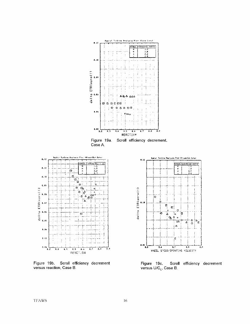
i _ i : i......

0e c__ :ee ! _

.....! : : : i 2.

F{EI_CT Irm

Figure 19a. Scroll efficiency decrement,Case A.

:,:. 1,33 .

........................................... _ ......... 7.__..:._,. _.,-, T ,_ !

_._ .................................:,.,_..._ .:..............L__'4...o.;.......;.....

L_7

: : • i ! i !

_'_ ...................................... : ......... _ "'" " "T" ''' ''_'' "'' --7" '_ A V " ' "_"

5 • .

IREAET I0_'_

_y

! i ia_, + i i :. |

.................................;'..........C_ :...... i

Figure 19b. Scroll efficiency decrementversus reaction, Case B.

Figure 19c. Scroll efficiency decrementversus U/Co, Case B.

TFAWS 16

Likewise, interpretation of impeller losses can be made using the core values of Station 2 for Case A and including

the diffuser with the impeller for the Case A calculation, as shown in Figure 20a. With the more detailed

investigation, where Station 3 is carefully back calculated from Station 4 and Station 2 includes the mixing

calculations, a more definitive rotor loss bucket is achieved as displayed for Case B (see Fig. 20b). This loss bucket

is now quite tight and the two intermediate levels of expansion ratio define the bottom of the bucket whereas the

highest and lowest expansion ratios define the wings of the bucket. The minimum occurs at a reaction of

approximately 0.65. The same information can be presented in terms of approach incidence with the same modeling

conditions as previously given; see Figure 21. Case B, of course, is preferred due to the careful attention given to

splitting out detailed losses. It appears that the optimum performance falls at an approach incidence of

approximately -40 °, a condition where the blades may very well be substantially unloaded and rotor secondary flows

may be minimal. However, the high expansion ratio data has not collapsed to the same low level as the other three

cases.

oo

o4-0

(-

I--UA

O4-

"U

g.2O

lB. IS

1_.18

|.1_5

e.ee i _ iO.Z 0.3 |.4

Rodio[ ;vrb;ne Anoly_lo Plot (Co.t Oo?o)

_z];i;i

_YMBOL EXP_blCN _.d

* Z.8

+

: + : • i _ "

.................._ 0....... _........... _....................A_

!

i. z:i:_!! !

' ' J' 2 ' ' ' J 'g$ _6 |.7 e8 e,9

RERCTION

A

04-

C_

@

i i : ............i2g

i i i i: i i

i!!! i i!ii i i i i!i " i i

i!!i _ii!! !i i !_ i :_ i i i i i i i ! ! i

'"' r 2 _!._2_Z.2__,e! _,L.2_2..._.,L...,,i......i ; i i ; i i i' i_ i :!

i i i i iel i i i i ;! "

_ :. i : i :iei*! /i i ;

R;E_CT I 0 N

Figure 20a. Total efficiency decrementfor the rotor versus reaction, Case A.

Figure 20b. Total efficiency decrement for

the rotor versus reaction, Case B.

TFAWS 17

.............i..........._...........i............._:LZ_L__iiJ1

" im i i 5 iO

m#

i i+ " i

_,, .........i........................i..............._e............................_.............i..............' i i° *N:,

"_ ...................................i..........._........................_'""'_"i'_

.................................?...............................'_.............i..................:............

)

Figure 20c. Total efficiency decrement for therotor versus U/C o, Case B.

o4.-

(._o

0

0

+

+

+_

Figure 21a. Efficiency decrement for the rotorversus approach incidence, Case A.

o,4.--

o[..

0

i i _,z i_ ! _--_

. !

m_

Figure 21b. Efficiency decrement for the rotorversus approach incidence, Case B.

TFAWS 18

A separate incidence loss can be computed based on the historical approach used by Benson, Mizumachi, NASA

and others based on the perpendicular component of relative kinetic energy. For both Case A and Case B modeling

these results are shown in Figures 22a and 22b. This is strictly an analytical estimate of what others have suggested

could be an incidence loss, or perhaps an incidence effect on impeller internal secondary flow losses• If this full

component (which is hypothetical) is removed from the rotor loss, than a revised rotor efficiency is achieved. The

results are shown in Figures 22c and 22d as a resulting rotor loss coefficient• Clearly, there is a problem in this

modeling• For Case B, the values go negative and the correction is overstated• Case A should not be considered a

preferable condition since it is artificially high by ignoring the mixing losses in the volute and including the loss of

the diffuser in with the impeller• The same results can be observed, as a function of approach incidence, in

Figure 23a and 23b for Case A and Case B, respectively• The fact that the rotor loss has not been flattened out by

removing the incidence for Case B is suggestive of the fact that not only is the correction overstated, but may be

inappropriately applied• This issue is returned to later•

@f.)c

UC

&--LLI

@"0

l.ll

If.IS

I.II

I.IS

I.II$.Z

Figure 22a. Full 1/2W2n efficiency decrement

(i.e., secondary flow portion) as a function of

reaction, Case A.

ig@

¢2

{ _ i i _, i :i i i iai

! _, i i ! i i _ i i " i

i i ! i i ii_ i i i i i i i _

i i i i i ! i i ! i + ' i

RE_CT_O_

Figure 22b. Full 1/2W2n efficiency

decrement (i.e., secondary flow portion)

as a function of reaction, Case B.

TFAWS 19

°..........o

R[_CTI_N

Figure 22c. Rotor (passage) efficiency

decrement (i.e., with full 1/2W2n secondary flowcomponent removed) as a function of reaction,Case A.

o

+L_

i,_ ................_........._. ..........:.........!.....; .

i

{. 1;J •o .....TN__ _...................;...............................................

v

S

-.,, ..............................................................i............].......

i

!

Figure 23a. Rotor (passage) efficiency

decrement (i.e., with full 112_12 n secondaryflow component removed). Note the overcorrection at high-incidence, Case A.

-_'=_-_-_-_-,1,1 _._ I

_- -'] ! ! i :: ! i i _i ) i i

i i i i i i i i _ i ! _ !

i i i]! _ i i _ i i i )

t_E_CT[ ON

Figure 22d. Rotor (passage) efficiency

decrement (i.e., with full 1/2W2n secondaryflow component removed) as a function ofreaction, Case B.

0

-|_|$

_-t _---?--_i"-i:.--_ii i i i ! i i

i i÷ ! _i i i.___ _ ,

! i i i 'i _! ! ! l

_! i i ) i; }

Figure 23b. Rotor (passage) efficiency

decrement (i.e., with full 1/2W2n secondaryflow component removed). Note the overcorrection at high-incidence, Case B.

TFAWS 20

The issue of rotor modeling can be extended by looking at the two variables in the historical incidence loss model of

Equation 7. Observing that a f3op t of approximately -40 ° is sensible, a series of calculations were made with this

value included. The resulting rotor efficiency (Equation 14) is shown in Figures 24a, 24b and 24c plotted versus

reaction, U/C 0 and incidence, respectively. In this case, a very sensible rotor efficiency relationship is found with a

peak at approximately 0.6 to 0.65 on reaction or approximately 0.72 - 0.75 for U/C 0. These trends are encouraging

as a fairly tight data variance is observed and the optimum corresponds with values expected from various turbine

studies in the past. Plotting efficiency versus incidence, as shown in Figure 24c, shows a peak at approximately -40 °

which may well be the condition of the unloaded blade tip. Once the isentropic efficiency increment is computed

and displayed versus incidence (see Figure 25), it may be observed that a tight variance is obtained, but not a truly

flat characteristic. In order to flatten this trend, a different value of f3op t at each expansion ratio would be required.

Further studies were conducted resulting in the data of Figure 26 where nearly constant trends are observed for two

of the expansion ratios with the third one falling quite high. In this case, f3op t was varied at each expansion ratio

line and an optimum value could not be found for er = 1.5, a value -55 ° was found for er = 1.8, a value -50 ° was

found for er = 2.2 and a value for -45 ° was found for er = 2.8. Initial studies to change the coefficient of the term

(labeled as f in Equation 7) did not yield meaningful results due to a lack of sensitivity in the data. This should be

re-examined with additional data from other cases as this may be an important variable to bring all the trends

together.

Figure 24a. Rotor efficiency versus reaction,Case B.

Figure 24b. Rotor efficiency versus U/C o,

Case B.

TFAWS 21

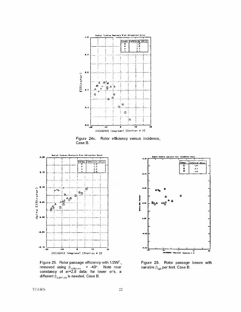
Figure 24c. Rotor efficiency versus incidence,Case B.

w

..........i........i _-,_---mi -_--_-..................i.........................: i _ !

................i...............i.................................................................:......g

Figure 25. Rotor passage efficiency with 1/2W2n

removed using I_optimum = -40 °. Note nearconstancy of er=2.8 data; for lower er's, a

different I_op_imumis needed, Case B.

11_1_:t1_1_l_ _t_ll_*.l _*L4_I._ _1_

Figure 26. Rotor passage losses with

variable I_opt per text, Case B.

TFAWS 22

I,!$0

_L-SL------'_--"2Zi2Z::_-%2_"-.2:--t_ i _4 i,:

_.ll_ " ".......r---_H ........ _---_------r----_--.-_----_---74Z::_.._Z_

i_ .-_,-._ ....... _) _r'_ "_"

:-__-s_-.. :;:::.:_:2=-:_'_:c::,/:============================....

Figure 27. Computed exhaust diffuser eNciency

decrement; Case B. Note that there is no Case A

by definition.

In turn, the exhaust diffuser losses are computed and only the Case B results can be displayed (by definition Case A

ignored the question)• It will be observed that estimated losses through the exhaust diffuser are between

approximately two and four points of stage efficiency• This is a modest loss and corresponds to a rather short

diffuser. The leaving kinetic energy from the diffuser is displayed, in terms of stage efficiency, in Figure 28 for

Case A and Case B. In this case, the results are understandably quite close together• Approximately two points of

stage efficiency exist in kinetic energy at the diffuser exit. This does not mean that the diffuser performed well.

Additional studies were made to understand the performance of the exhaust diffuser. After correcting the static

pressure distribution at Station 4 to a realistic level based on the existence of swirl, and back calculating to a sensible

average value at Station 3, both static pressure recovery and total pressure loss for the diffuser could be computed•

These are shown in Figures 29 and 30, respectively, plotted versus the swirl angle• A tight data variation is obtained

and it is reasonably consistent with good diffuser performance as a function of inlet swirl (see Japikse (1999) [7]).

Parameters can be plotted versus each other in a very important relationship where total pressure loss is related to

static pressure recovery following the relationship of K = @i - @ (see Japikse, 1984 [8]). These data are shown in

Figure 31 for the present diffuser• Lines of constant diffuser effectiveness are shown as rays emanating from the

virtual origin and three lines corresponding to 0.2, 0.33 and 0.5 for diffuser effectiveness are shown• It is clear that

this diffuser has an effectiveness between approximately 0.2 and 0.4. Based on the carefully measured values of p3

and P4 with deduced corrections for the static pressure profile across the flow field, it appears that reasonable

pressure levels have been established and sensible calculations of @ have been achieved. It may be definitely

concluded that the diffuser is recovering, even with the very erratic inlet total pressure distribution (see Fig. 11),

static pressure, and swirl angle distribution• However, the very low diffuser effectiveness, 0.2 to 0.4, is surely

amongst the lowest levels of diffuser recovery of any common industrial diffuser (note: a classic Borda-Camot

sudden expansion mixing has a peak diffuser effectiveness of 0•667)•

TFAWS 23

II,l_ ................................................

..........;.....:._..;...i _...............

: : - . _

.,.2 .......

4-4"

RE_CT[SN

Figure 28a. Diffuser leaving loss(difference of stage total and staticefficiencies), Case A.

t)3

d_J

d

i _ i _ i _ " -

i i i i i i • _._'-

i i li i i l

?ii iiiil-i -iiiilli i _ ! i i i _,! i i ii i i I _ i i _ i ! ;.

.....i-i-?? i__N_ia,_i !.........

Figure 28b. Diffuser leaving loss(difference of stage total and staticefficiencies), Case B.

¢,_

.................._ _ _

i i ! _ : '

e,_ ......... ! ....... _......... ! ......... :i..._!.a .i_.. e ) ......... ........

:, ! i ! i : i :

..........._..........]_..,.,,,_............_..........:.......:!.........!......._.......!

.&

.......i........_........$ ......._ _ Z_

.........f..............._,,-_ ......._.........i........i........._........i._' .o _i ! i i i

.........i:--i........i.........!---_--i....._----i.............

,,, .....!__i........!..........._!____!..........L_.__I..........!i.........

iliii i

Figure 29. Diffuser pressure recovery

versus _3, Case B.

Figure 30. Diffuser loss coefficient versus

_3, Case B.

TFAWS 24

0

_CP

Figure 31. Exhaust diffuser loss

recovery, Case B.

versus

The determination of aerodynamic blockage at several key points in the stage was an important outcome of the

present investigation. In order to calculate the sudden expansion Borda-Carnot mixing loss at Station 2, the local

static pressure, total pressure, swirl angle (for the core flow) plus conservation of mass and total temperature were

used to close the continuity equation and obtain a local blockage factor. This has been done for Case B as shown in

Figures 32a and 32b. In Case A, only the blockage was calculated without any mixing calculation; in Case B the

actual mixing calculation was conducted. It would be observed that the level of estimated blockage is definitely

affected by the modeling approach employed and that the blockage is on the order of 50%, a result which is not too

surprising when one considers the general character of this flow field. It is interesting, however, that there is a

minimum at a reaction of approximately 0.65. The same results were also considered with blockage versus flow

angle as shown in Figures 33a and 33b for Cases A and B, respectively. Although no definitive trend is shown, an

examination of the Case B results suggest that perhaps there could be some parametric variation implied as a family

of trend lines through the data sets. This has not been ascertained as yet, but would be an area for further

investigation.

TFAWS 25

o

N

C3

_3

Rodlo| Turbine Rnolyolo Plot ([are Oato)

JJ,_

.............. I _ I._*"_ " -t

_:E _ _,_ff_ .................

4 a_.4"

_E_CTION

Figure 32a. Volute exit blockage, Case A.

JJ

.[......... .¢

: ....

77

.>3

g4-*O

tj

_J

i

i ............... i. !. ..... _ _.: : ...._.-, ............

: i i ? i : ;

RE_C T ION

Figure 32b. Volute exit blockage, Case B.

Figure 33a. Volute exit blockage as afunction of volute exit swirl angle, Case A.

o

_J

.--'-_ , _'_ ,_ _;_ -1i i ! ,* _._

! i i i i i ! l

!i5

i i

g9 ?| 7'I _$ ??

Figure 33b. Volute exit blockage as afunction of volute exit swirl angle, Case B.

TFAWS 26

The efficiency of the volute alone can also be computed and is displayed in Figures 34a and 34b as a function of

reaction and U/Co, respectively. As with other parameters, optimum values at approximately 0.6 and 0.72,

respectively, have been observed. Again, reaction gives a better overall correlation of the variables. Likewise, a

swirl coefficient can be defined for the volute as shown in Figures 35a and 35b when reaction and U/C o are used as

plotting parameters. Once again, reaction has given a slightly superior modeling parameter.

{ev

ii iii iio! i iiiiil }

RE#C? l 0_

Figure 34a. Scroll efficiency versus

reaction, Case B.

o1_o

@.9

|.!

0,5

Figure 34b.

Case B.

Rodl:l f_,,bl_e RneTynl| _lle (lllled-@w_ 0oto)

} i ISYMSQL CXP_'$1tJN _TIO

{ I = S

i ; i ,, 8i i i • z.z

i i°i

................; .........._ i'_ ...........................i..............

................_.........._............._.............,=................i ; ÷ '

..................... i ................... i

' ' ' J ' i '@.6 I_ ? I} @ _.9

NNEEI_ SPEEO/SPOUTING VELOCITY

Scroll efficiency versus U/C o ,

@

2

t_

z

! i i _-__

....,J..2.2.o2_L2....i.._i...Z....:..2__......

! i ! i }{ ; i; _ i ;_

i _ i ! ; i i i i i ! _-!i[!; i_i!:

...... :..--.? .................. :.............. ...-..........:w.. ................. . ...........

i !i i ii,o ! ! _ !!

........__?-T: ! T _! i" ....................i......

REACTION

Figure 35a. Scroll swirl coefficient versusreaction. Case B.

@

11

@

........L......i........!..........!............_............i.............i.........

i i '

..............................i..............T-_: .................................

! ÷ i+÷ 14- i i

_ZEL $_ZZ,G/Sg'OUT_,_G VZL{)C! rY

Figure 35b. Scroll swirl coefficient

versus U/C o, Case B.

TFAWS 27

Finally,it is interestingto compareimportantmodelingparametersfrombeforetheinvestigationwithrevisedestimatesaftertheinvestigation.Figure4showedthetrialcalculationsthatweremadebeforetestswereconductedinordertoestimateimportanttrendsforfuturestudy.Table3displaysafewoftheimportantmodelingparameterswhichwereusedbothbeforeandafterthetestseriestomodelthestage.Itmaybeseenthattheoriginalestimatesofmanytestparameterswereonlynominallycorrectbasedonpriorexistingtechnicaldata.Indeed,havingcarefullymeasuredinternalparametersandthenrefiningthelevelsof rotorefficiency,diffuserpressurerecovery,swirlcoefficientandotherparametersforcedustorealizetheimportanttrade-offbetweenthedifferentvariablesandthenecessityofmeasuringinternalflowstatesinordertodefinethesewith reasonable rigor.

TABLE 3

BASIC STAGE MODELING PARAMETER

Parameter

r}scroll

Measured Value

0.825 + 0.025

Original "Estimate"

(Before Testing)N/A

SC 0.90 + 0.02 0.85

B 1 0.06 + 0.02 0.20

_2 optimum

i] rotor

-45 ° to -55 °

0.725 + 0.025

0.20 + 0.05CpD

-10 ° to -20 °

0.82 to 0.98

0.30

5. CONCLUSIONS

Based on the work presented herein, a number of important conclusions have been reached for this study. They maybe summarized as follows:

]. Accurate measurements of stage and component performance can be achieved by thorough instrumentation

of a radial inflow turbine stage including flow field traverses at the impeller inlet, and the impeller or

diffuser discharge, supplemented with static pressure taps at impeller tip, the impeller exit, and the diffuser

exit, as well as the inlet station, augmented with inlet total pressure total temperatures upstream of the

volute inlet and downstream total temperatures following a Koch mixer. By operating in sensible ranges of

inlet temperatures, very accurate measurements of the work input can be achieved with a thermally

calibrated rig.

2. Traversing the rotor exit requires measuring the static pressure distribution as well as the total pressure

distribution and the yaw angle pressure distribution. At least six circumferential positions arerecommended.

Reaction serves as an excellent correlating parameter for the various overall and internal parameters

characterized in the performance of this radial inflow turbine stage. The alternative parameter, U/Co, is

also an excellent parameter that did not collapse data as well as reaction level.

4. Breaking the component losses into isentropic incremental efficiency decrements is a good way to examine

sub-component performance.

5. The historical incidence loss model, which debits the impeller for a loss in proportion to the normal

component of inlet relative velocity-based kinetic energy, offset by some optimum angle, appears to work

sensibly for an important part of the impeller loss process. However, a preferred value of _optimum has not

been established and values for _opt vary substantially, easily in the range of -40 ° to -60 ° for this study.

Further investigations concerning the condition of unloading the impeller blade at inlet need to be

conducted, both experimentally and analytically with CFD.

TFAWS 28

6.

7.

The volute can be well modeled with a nominal isentropic efficiency of 0.825 +0.025 with a modest

variation with reaction or U/C o. It also has a swirl coefficient of approximately 0.9 + 0.02. These

modeling parameters could likewise be deduced for a number of other stages if good data are taken and

overall modeling parameters could consequently be correlated with additional geometric variations

considered in the database. Inlet blockage for the volute is approximately 6 +2%.

The exhaust diffuser definitely recovers and shows a pressure recovery coefficient of approximately

0.2 + 0.05. This diffuser performance corresponds to a very low effectiveness of 20% to 40%. The

diffuser is operating with some useful effect even though the inlet profiles are highly distorted, even

including reversed flow at inlet under certain operating conditions.

REFERENCES

2.

4.

5.

6.

7.

8.

Japikse, D., "The Comprehensive Performance Evaluation of a Radial Inflow Turbine,"

Creare R&D, Inc. TN-348, and Concepts ETI, Inc. TM 5, Nov. 1982.

Baines, N.C., "The Aerodynamic of Radial Turbines," Axial and Radial Turbines, Course Lecture Notes,

Concepts ETI, Inc., Wilder, VT 1999.

Mizumachi, N., "A study of Radial Gas Turbines," Translation done at University of Michigan,

Industry Program of the College of Engineering, IP-476, Nov. 1960.

Todd, C. A., Futral, S. M., "A Fortran IV Program to Estimate the Off-Design Performance

of Radial-Inflow Turbines," NASA TN D-5059, March 1969.

Japikse, D., "Rotor Inlet Modeling For Radial Inflow Turbines," Design Data Sheet No. 3,

Turbomachinery Design Digest, March 2, 1981.

Japikse, D., "Radial Turbine Design and Performance," Course Lecture Notes,

Concepts ETI, Inc., Wilder, VT 1986.

Japikse, D. "Exhaust Energy Recovery," Axial and Radial Turbines, Lecture on Diffuser Performance,

Course Lecture Notes, Concepts ETI, Inc., Wilder, VT 1999.

Japikse, D. (ed.), "A New Diffuser Mapping Technique - Studies in Component Performance:

Part 1," ASME Paper No. 84-GT-237, Amsterdam, June 1984.

TFAWS 29

REPORT DOCUMENTATION PAGE Form ApprovedOMB No, 0704-0188

Public reporting burden for this collection of information is estimated to average 1 hour per response, including tile time for reviewing instructions, searching existing data sources,

gathering and maintaining the data needed, and completing and reviewing the collection of in[ormafion. Send comments regarding this burden estimate or arty other aspect of this

collection of information, including suggestions for reducing this burden, to Washington Headquarters Services, Directorate for Information Operation and Reports, 1215 Jefferson

Davis Highway, Suite 1204. Arlington, VA 22202-4302, and to the Office of Management and Budget, Paperwork Reduction Project (070,1-0188), Washington, DO 20503

1, AGENCY USE ONLY (Leave Blank) 2, REPORT DATE 3, REPORT TYPE AND DATES COVERED

July 200l Conference Pllblication4, TITLE AND SUBTITLE 5, FUNDING NUMBERS

The Tenth Thermal and Fluids Analysis Workshop

6, AUTHORS

Alok Majumdar, Compiler

7, PERFORMING ORGANIZATION NAMES(S) AND ADDRESS(KS) 8. PERFORMING ORGANIZATIONREPORT NUMBER

George C. Marshall Space Flight Center M-1022Marshall Space Flight Center, AL 35812

9. SPONSORING/MONITORING AGENCY NAME(S) AND ADDRESS(aS) 10. SPONSORING/MONITORINGAGENCY REPORT NUMBER

National Aeronautics and. Space Administration

Washington, DC 20546-----0001 NAS A/CP----2001-----211141

11. SUPPLEMENTARY NOTES

Proceedings of a workshop held at NASA Marshall Space Flight Center, September 13-17, 1999.Workshop organizers: Jim Owen and Sheryl Kittredge of Marshall Space Flight Center. Prepared

for Structures, Mechanics, and Thermal Department, Engineering Directorate •12a. DISTRIBUTiON/AVAILABILITY STATEMENT 12b. DISTRIBUTION CODE

Unclassified-Unlimited

Subject Category 34Standard Distribution

13. ABSTRACT (Maximum 200 werds)

The Tenth Thermal and Fluids Analysis Workshop (TFAWS 99) was held at the Bevill Center, University ofAlabama in tluntsville, Huntsville, Alabama, September 13-17, 1999. The theme for the hands-on trainingworkshop and conference was '"]bols and Techniques Contribuling to Engineering Excellence". Forty-seven

technical papers were presented in four sessions. The sessions were: (1) Thermal Spacecraft/Payloads,(2) Thermal Propulsion/Vehicles, (3) Interdisciplinary Paper, and (4) Fluids Paper. Forty papers were

published in these proceedings. 31_e remaining seven papers wre nol available in electronic format at thetime of publication. In additon to the tedmical papers, there were (a) nine hands-on classes on thermal and

flow analyses softwares, (b) twelve short courses, (c) thirteen product overview lectures, and (d) threekeynote lectures. 311e workshop resulted in participation of 171 persons representing NASA Centers,

GovelTunent agencies, aerospace industries, academia, software providers, and private corporations.

14. SUBJECT TERMS 15, NUMBER OF PAGES

thermal analysis, computational fluid dynamics, numerical heat transfer, 542

network flow analysis, thermal protection system, interdisciplinary analysis _6. PmCECODE

17. SECURITY CLASSiFICATiON 18, SECURITY CLASSIFICATION 19. SECURITY CLASSiFICATiON 20, LIMITATION OF ABSTRACTOF REPORT OF THIS PAGE OF ABSTRACT

Unclassified Unclassified Unclassified Unlimited

NSN 7540-01-280-5500 Standard Form 298 (Rev. 2-89)Prescribed by ANSI Std. 239-18298-102