The Scope of Dimensional Analysis in Qualitative Reasoning

Computational Intelligence, Volume 10, Number 2, 1994

THE SCOPE OF DIMENSIONAL ANALYSIS IN QUALITATIVE REASONING

JAYANT KAL,AGNANAM

MAX HENRION

ESWARAN SUBRAHMANIAN

Department of Engineering and Public Policy, Carnegie Mellon University, Pittsburgh, PA 1.5213, U.S.A.

Engineering Design Research Center; Carnegie hlellon University, Pittsburgh, PA 1.5213, U.S.A.

Dimensional analysis, traditionally used in physics and engineering to identify quantitative relationships, has recently been applied to qualitative reasoning of physical 'systems. We illustrate some problems of this approach. In the light of this, we reexamine the fundamentals of dimensional analysis in order to more precisely characterize its scope and limitations as a tool in qualitative reasoning. We also explore its relationship to state equation representations of physical systems. In particular, we describe its value in providing a set of constraints to reduce the ambiguity that bedevils qualitative reasoning schemes. We argue that dimensional analysis should not be seen as a substitute for knowledge about the physics but rather a supplement to other sources of knowledge,

Key words: dimensional analysis, qualitative reasoning, comparative statics.

1. INTRODUCTION

Dimensional analysis is a technique widely used in physics and engineering for helping to identify and check quantitative relationships between variables describing physical processes. Simple examination of the dimensions of the relevant variables is sometimes sufficient to determine the functional form of a physical law. On initial exposure to dimensional analysis, the fact that consideration of something as apparently mundane as the dimensions of the variables can be sufficient to determine the entire functional form of a complex physical law without the need for substantive physical knowledge of the phenomenon often seems suspiciously like magic to the beginning physics or engineering student. In fact, cases in whch dimensional analysis can entirely determine the form of the relationship down to a single constant of proportionality are comparatively rare outside textbooks. But nevertheless, dimensional analysis does provide some useful constraints on the form of relationships in other cases.

In a recent paper, Bhaskar and Nigam (1990) make the interesting suggestion of using dimensional analysis for qualitative reasoning about physical systems. In some cases it provides a simple way to determine qualitative relations between variables based on purely dimensional considerations. They use this method convincingly to solve a number of problems from the A1 literature. However, they leave the exact scope and limitations of the technique unexplored. In fact, the approach they propose can sometimes give incorrect answers, as we shall illustrate by the consideration of a problem in heat transfer (condensation in a vertical

In this paper, we use this problem as a starting point for an investigation of the foundational principles of the method of dimensional analysis to identify the scope and limits of the technique. We present some new theorems which identify more precisely the scope of its application to qualitative reasoning. Finally we link dimensional analysis to the standard state equation formulation widely used for modeling physical systems. For a given physical system, any state variable can be written as a function of the exogenous variables in an explicit form. The number of exogenous variables can be in general larger than the number of dimensions required to describe all the variables of interest. This observation is the key which provides

pipe).

@ 1994 Blackwell Publishers, 238 Main Street, Cambridge, MA 02142, USA, and 108 Cowley Road, Oxford, OX4 1JE UK.

118 COMPUTATIONAL INTELLIGENCE

a way to link a system of equations to the dimensional characteristics of its variables and hence identify the limits of dimensional analysis for qualitative reasoning. While this perhaps removes some of the magic of dimensional analysis as an apparent substitute for physical knowledge in qualitative reasoning, it also provides a deeper characterization of its potential as a useful source of constraints for reducing the ambiguity that bedevils schemes for qualitative reasoning.

2. AN EXAMPLE: CONDENSATION IN A VERTICAL PIPE

We start out with an illustrative example, applying dimensional analysis to a standard physics problem, to wit the condensation of vapor in a vertical pipe. We will use it to point out the restrictions implicit in the assumptions made by Bhaskar and Nigam (1990) in operationalizing dimensional analysis for qualitative reasoning. These problems motivate the theoretical analysis of the scope and limitations of dimensional analysis developed in the rest of the paper. This example is adapted from Langhaar (1951).

A condenser is a key component of many devices involving heat transfer, including refrigerators, air conditioners, and distillation columns. It generally consists of one or more pipes in which the vapor condenses, transferring heat from the refrigerant fluid to the pipe wall. In this case we consider a vertical pipe. The condensate forms a layer of liquid which runs down inside the pipe. The heat released by the vapor condensing on the inner surface of the layer (the latent heat of vaporization) is conducted across this layer into the pipe wall. A key issue in designing a condenser is estimating the rate of condensation, which is controlled by the rate of heat transfer from the vapor-liquid interface to the pipe wall. Hence a key parameter for the engineer is the average heat transfer coefficient, h , that is the heat transfer per unit surface area of pipe per unit time per unit of temperature difference between the vapor and the pipe wall.

Careful examination of the physical processes identifies the following exogenous quantities as affecting the average heat transfer coefficient, h: The temperature difference A0 between the vapor, assumed to be at saturation temperature (boiling point) and the pipe wall; the length of the pipe L ; the latent heat of vaporization per volume of the liquid ph; its specific weight (gravitational force per volume) p g ; and its thermal conductivity (heat flux per unit area per unit time per temperature gradient) k .

To conduct a dimensional analysis of the process we must start by selecting our set of fundamental dimensions. We will use the traditional ones: mass M , length L, time T , and temperature 0. Below are the dimensions for each of the quantities expressed in terms of this set of fundamental dimensions.

h = heat transfer coefficient [ M T - 3 @ - ' ]

L = length of pipe [ L ]

k = thermal conductivity of condensate [ M L T - 3 0 - 1 ]

p = viscosity [ML- 'T - ' I

At? = temp. diff. bet. vapor and wall [0]

ph = heat of vaporizationhit volume [ M L-' T-']

pg = specific weight [ML-2T-']

THE SCOPE OF DIMENSIONAL AKALY SIS IN QUALITATIVE REASONING 119

In general, we may express the relation between the variables of interest as follows:

f (h, A@, L , ph, k , p g , F ) = 0 (1)

In 191 6, Nusselt theoretically derived the following functional relationship for heat transfer in a vertical condenser pipe:

Nusselt’s derivation was based on a number of simplifying assumptions, including:

0 The thermal conductivity ( k ) , viscosity (p), and specific weight (p ) of the liquid are constant throughout the liquid layer.

0 The latent heat of condensation at the liquid-vapor interface is equal to the heat carried away by conduction through the liquid film (energy conservation).

0 The temperature of the vapor and the vapor-liquid surface is equal to the saturation temperature 0.

0 The temperature of the pipe wall is uniformly 0 - A@. 0 The flow in the liquid layer is laminar and the horizontal component of the velocity is

small, so convection can be neglected as a source of heat transfer. 0 Liquid flow is in equilibrium with the condensation, resulting in a film thickness that

does not vary over time.

For a more detailed exposition of the assumptions and derivation see Sedov (1959). Based on this characterization of the physical phenomena, we apply dimensional analysis to reason qualitatively about changes in the dependent variables for changes in independent variables.

The dimensional matrix for the quantities in the relationship specifies the power of each fundamental dimension in the dimensions for each quantity:

h A0 L ph k pg p

M l O O 1 1 1 1 L 0 0 1 - 1 1 - 2 - 1 T -3 0 0 -2 -3 -2 -1 0 - 1 1 0 0 - 1 0 0

The rank of this matrix is Y = 4. The number of quantities is n = 7. This implies that the structural relation in Es. (2) can be characterized by n - r = 7 - 4 = 3 independent

1 . , dimensionless numbers. They are

hh n , = -. k g ’

By the Buckingham n theorem, Eq. (1) can be rewritten as

(3)

Now let us consider a qualitative reasoning question; e.g., how does the average heat transfer rate change if the latent heat of vaporization, A, increases (for example by substituting

1 20 COMPUTATIONAL INTELLIGENCE

a different refrigerant fluid), all other variables remaining constant. From the relation (2) it immediately follows that

Throughout this discussion we assume that all the quantities are. positive with no loss in generality, and so,

ah * - - > o ah

Hence we conclude that an increase in the latent heat of vaporization, h, would produce an increase in the average heat transfer coefficient, h. So such a change might allow a smaller condenser.

On the other hand, if we were to adopt the methodology used by Bhaskar and Nigam ( 1990), it would follow that

This answer is in obvious contradiction with Eq. (6). The problem arises from their implicit assumption that n 1 is constant even though h is

changing. This arises from their following assumption that is made in their paper: By Hall's theorem, it is possible to construct dimensionless numbers ni such that each ni contains exactly one variable that does not belong to the basis. By assuming that a particular ni can be held constant, it is possible to see how each variable of interest is related to the other variables in the basis.

However in this problem, the assumption is not valid. We can show this combining Eqs. (2) and (4) as

0.943 n l = (n=n3)'/4

From Eq. (3), the product (n2lJ3) 'I4 varies as h-5/4, and any changes in h will also affect Ill. Therefore

This clearly illustrates how the methodology suggested by Bhaskar and Nigam (1990) does not provide the correct answers because of the implicit assumption that al71/ah = 0.

Having discovered this, we next ask the question as to whether we can in general specify when anl/aA. = 0, without explicitly deriving a relation between all the variables.

From the above observation three obvious sets of conditions suggest themselves, such that if they are satisfied then the methodology of Bhaskar and Nigam (1990) can be used.

THE SCOPE OF DIMENSIONAL ANALYSIS IN QUALITATIVE REASONING 121

They are:

1. For a given set of variables, there exists only one independent dimensionless number, or 2. If n2, H3 are such that they do not contain the variable h, or 3 . If I l 2 , l73 are related in such a way that the variable of interest does not appear in the final

functional relation. This is more concisely stated as a f ( l ' I 2 , l73)/ah = 0. This implies that l22, l l 3 are related in such a way that A. cancels out.

It is important to point out that these conditions are not satisfied in the above example. The goal of this paper is to state these conditions in general terms for a physical system modeled by a set of state equations.

3. THE METHOD OF DIMENSIONAL ANALYSIS

In this section we will provide a brief overview of the method of dimensional analysis designed to bring out the way it reduces the degrees of freedom in a relation between physical quantities. We will provide informal explanations of the key terms, and introduce the principle of dimensional homogeneity and Buchngham's ll theorem. We will illustrate these ideas with an example. The reader interested in more detail is referred to classic expositions (Bridgman 1931; Langhaar 1951; Focken 1953). We follow this by some cautionary remarks about the dependence of the method on physics knowledge in selecting relevant exogenous quantities. This overview is provided as a preliminary to reexamining the role of dimension analysis in qualitative reasoning.

3.1. Basic Concepts

A guantiq is a measurable characteristic of the world such as the length of a piece of string or the speed of light. Most real-valued quantities have dimensions, such as length or velocity, which characterize the type of quantity. Some quantities have no dimensions, such as the slope of a road or the Reynold's number for fluid flow in a pipe. A dimensional quantity is measured in some unit of the same dimension. Units of length include centimeters, furlongs, and lightyears. The magnitude of a quantity is its numerical value in a given unit. The magnitude of the speed of light is approximately 299,792 in units of kilometers per second (Henrion and Fischhoff 1986).

As illustrated in the condenser example, dimensional analysis requires a set of dimensions to be selected as fundamental. The conventional choice of fundamental dimensions includes length, L , mass, M , time, T , and temperature, 0. But in fact the choice is arbitrary subject to two conditions, that the set be complete (for the problem) and independent. A set of dimensions is complete for the application at hand iff the dimensions of every quantity of interest in the process can be fully expressed as some combination (product of powers) of the dimensions. A set of dimensions is independent iff no dimension in the set can be expressed as a combination (product of powers) of the other dimensions in the set. For example, M , L , T , and 0 are complete for the set of quantities mentioned above for the condenser, but charge needs to be added for an electrical problem. Force F , velocity V, frequency Q, and temperature 0 form a set that is independent and complete for the condenser problem, and, in principle, equally useful. The conventional preference for M , L , T , and 0 seems to be because those dimensions are generally easiest to measure, and we see no advantage in bucking tradition on this point.


Given a set of fundamental dimensions, all other dimensions are termed derived since they can be expressed as a unique combination (product of constant powers) of the fundamental dimensions. Similarly, we can refer to fundamental quantities, being quantities whose dimensions are fundamental, and derived quantities, whose dimensions are derived. A key axiom is that the ratio of two quantities of the same dimensions, whether fundamental or derived, is independent of the units they are measured in (provided both use the same units). From this can be shown an important result, that any derived quantity, x , can be expressed as a product of constant powers of fundamental quantities, M I , u2, . . . .

x = k U a U b u c . . 1 2 3 . (8)

where k , a , b, c, . . . are constants. The proof for this result can be found in Bridgman (1931).

3.2. The Principle of Dimensional Homogeneity

Physical laws or equations relating physical quantities are of two lunds:

1. Definitions of derived quantities 2. Empirical relationships between quantities, subject to experimental test

Examples of definitions include the definitions of velocity, v , acceleration, a, and force, f , in terms of distance, d , time, t , and each other:

U f = m a

1 t t

v = -, a = -, (9)

Note that each derived quantity is definable in terms of fundamental quantities. Examples of empirical relationships include Nusselt’s law for heat transfer in a vertical condenser pipe in Eq. (2), or Boyle’s law.

The basis of all dimensional analysis is the principle of dimensional homogeneity. This states that each term in an equation must have the same dimensions. This principle provides strong constraints on what kinds of relationships make sense. In some cases this is sufficient to determine the functional form of a relationship within a constant of proportionality. This also provides a basis for certain kinds of qualitative analysis of the direction of the effect on one quantity of a perturbation in another.

For example, consider the following relation giving quantity x as a product of constant powers of quantities u 1 , u2, . . . , u,:

If the dimensions of (x, u1, u2, , . . , u,) are represented by the following dimensional matrix:

x U ] u2 . ’ . un

M a a1 a2 . . . a, L b bl b2 . . . b, T c C ] c2 . . . Cn

then the relation is dimensionally homogeneous ifs

alkl + a2k2 f . . - + ankn = a blkl + b2k2 + - . . + b,k, = b clkl + ~ 2 k 2 + . . . + c,k, = c

THE SCOPE OF DIMENSIONAL ANALYSIS IN QUALRATIVE REASONING 123

For the relation to be dimensionally homogeneous, the exponents (kl , k2, . . ~ , k,) must satisfy the above equations. If we do not know the exponents then we can use these equations to constrain the set of possible values. Without dimensional analysis there are n degrees of freedom in constructing a relationship as the product of constant powers of n quantities (ignoring the constant of proportionality k ) . The principle of dimensional homogeneity eliminates r degrees of freedom, where r is the rank of the dimensional matrix. If n = r then the exponents and the relationship are completely determined down to the constant of proportionality. If n > r , then there remain n - r = p degrees of freedom in the specification of the relationship.

3.3. The Buckingham n Theorem

Let us return to the explicit form equation shown in Eq. (9). If x = f ( u 1 , uz, . . . , u,) is a dimensionally homogeneous equation and if x is not dimensionless, then there exists a product of powers of the ui that has the same dimension as x. If we divide the equation by this product, then this gives a dimensionless number on the left-hand side, and reduces the equation to the following form:

n = F(u1 , u2, . . . , u,)

The remaining degrees of freedom can be characterized by p dimensionless numbers n, for i = 1, . . . , p, where each n, is a different combination (product of powers) of the quantities. According to Buckingham's fl theorem there will always be p such dimensionless numbers, and the original relationship can always be rewritten in terms of an arbitrary product of powers of these dimensionless numbers:

(1 1)

These results are proved in Langhaar (195 1). The powers of the ni represent the undetermined degrees of freedom. The l 7 i represent particular combinations of subsets of the quantities which have particular physical significance.

n = F ( n l , n2,. . . , nP) where p = n - r

3.4.

The example presented here is based on the phenomenon of heat transfer that takes place through convection when a fluid is forced through a pipe (Brown and Marco 1958). The fluid is assumed to be turbulent. A thin film of the fluid that adheres to the surface of the pipe serves as the heat transfer surface. The heat coefficient of surface convection is dependent on the thermal conductivity and thickness of the film. The factors influencing the conductance of the film based on the laws of fluid flow and heat transfer are surface and size of the surface (diameter of the pipe), thermal conductivity of the fluid, specific heat, viscosity, density of the fluid, and velocity of the stream.

An Example: Forced Fluid Flow through a Pipe

The heat transfer coefficient for forced convection, h,, can be expressed as

h, = f(D> u , P , P > c p , k) (12)

where

h , = convection heat transfer coefficient [MT-3@- '] D = diameter of pipe [Ll V = velocity of stream [ L TI

I24 COMPUTAITONAL INTELLIGENCE

p = viscosity [ M L - ' T - ' I p = density of fluid [AIL3]

cp = specific heat [L'T-'0]

k = thermal conductivity of fluid [ M L T - 3 0 - ' ]

To compute dimensionless products for the phenomenon under consideration, the following dimensional matrix can be generated for the above variables:

h , c , V p ,Y D k

M l O O l l O I L 0 2 1 - 3 - 1 2 1 T -3 -2 -1 0 -1 -2 0 0 - 1 - 1 0 0 0 - 1 0

The rank r of the dimensional matrix is 4. The number of dimensionless products that can be generated are n - r = 7 - 4 = 3. Any product n of these variables is of the form

n = ha1 c$Z Va3pa4~aS Da6kal

Therefore, the dimensional equation, where [x] denotes the dimensions of x, is

[ n] = [M T - 3 0- ' I a 1 [ L2 T-*@Ia2 [ L T-'Ia3 [ ML3]'4 [ M L - ' T - ' 1"' [ LIa6 [ML TP3(3-' 1"'

If I3 is required to be dimensionless, the exponents of M, L, T , 0 must all be zero.

Since the number of variables is 7 and the rank of the system is 4, we have three independent solutions which provide the three dimensionless products. In Eq. (13) we can assign any values to three variables, and these will determine the rest. Therefore choosing three different sets of values for a ' , a2, a3, we have

Therefore, the three dimensionless numbers are

Using the results of dimensional analysis and the Buclungham theorem we can restate Eq. (12) as


Experimental examination of the phenomenon confirms the relationship and gives us numerical estimates for the constant of proportionality and the exponents

n 1 is generally known as Nusselt’s number, while l72 and II3 are known as Reynold’s number and Prandtl’s number.

3.5. Dimensional analysis draws information about relationships between physical quantities

solely from the principle of dimensional homogeneity. The results obtained depend on the correctness of assumptions about what exogenous variables are relevant to the endogenous variables of interest. It is important to note that dimensional analysis does not answer the question, “On what quantities does the result depend?” but rather “How does the result depend on those quantities known to be relevant?’

In their conclusion, Bhaskar and Nigam (1990) state, “The technique is useful primarily because it can be applied when no knowledge of the physical laws of a device is available.” This reflects some standard rextbook presentations of dimensional analysis, but it is important not to be misled into the impression that it can ever entirely substitute for physical knowledge. Even in the standard cases presented in the textbooks and by Bhaskar and Nigam, considerable knowledge of physics is required to apply dimensional analysis, as will be attested by any student who attempts to apply it in exercises.

It is often a hard problem to identify the relevant exogenous variables. In a few cases dimensional analysis can tell you that an apparently relevant variable is actually not relevant: It produces an exponent of zero. For example, in the law giving the period of a pendulum, dimensional analysis reveals that the mass of the bob is irrelevant. (Mass is not a dimension present in the period, nor in any other exogenous variable.) But in most cases, adding irrelevant exogenous variables will render dimensional analysis inconclusive. Adding any variable with the same dimensions as another will reduce the usefulness of the technique. For example, in the vertical condenser pipe, adding any variable with dimensions a power of length only, such as the diameter of the pipe [ L ] or its cross-sectional area [L2], would render the analysis inconclusive, (We illustrate this later in the shell and tube heat exchanger.) It could not distinguish the role of any such Variables, which are actually irrelevant assuming they are large enough, from that of the length of the pipe, which is relevant. Substantial physical knowledge about the process is required to establish which of these are relevant and which not.

In fact, to reduce the number of exogenous variables so that dimensional analysis can exert its full power frequently requires considerable ingenuity in devising exogenous variables that are actually combinations of variables. Again in the condenser example, the use of the temperature difference A0 as a single variable, rather than the temperature of the vapor 8 and the pipe wall 8 - A8 as two exogenous variables is needed to make the analysis tractable. Physical knowledge is required to understand that it is only the difference that is relevant. Similarly, the use of the heat of vaporization per unit volume ph and the specific weight pg, instead of the three variables p , A, and g , reveals cunning use of physical knowledge about how these factors enter into the process, for example that gravity only acts through the density of the liquid.

Dimensional Analysis and Physics Knowledge


4. IMPLICATIONS FOR QUALITATIVE REASONING

As mentioned earlier, this discussion is motivated by our desire to evaluate the direction of change in endogenous variables for a perturbation in a given exogenous variable (comparative statics). However, the exact functional relationship between the endogenous and exogenous variables is not always available. In these cases, the comparative statics problem has to be solved qualitatively, where only the sign of the first partials of the functional relations are assumed to be known. The qualitative method for comparative statics while providing a means to generate qualitative solutions, does not ensure a unique solution. Since the Buckingham I7 theorem characterizes how functional relations are constrained by dimensional considerations, we now address the question of the usefulness of this information toward filtering the number of solutions to the qualitative comparative statics problem.

In the following subsection, we first characterize the qualitative comparative statics problem in standard mathematical terms. Using this characterization, we explicate the solution method and the associated problem of multiple solutions. Then we present four propositions which characterize conditions under which dimensional considerations are useful for reducing the number of qualitative solutions. These propositions circumscribe the scope of dimensional analysis in solving the qualitative comparative statics problem.

4.1. Qualitative Comparative Statics

two exogenous variables (u1, ~ 1 2 ) by the following equilibrium relations: We start with the simple case of two endogenous variables (XI, x2) which are related to

f i ( x l , X 2 , U l r u 2 ) = 0 , i = l , 2

If the exogenous variable is perturbed, then the change in the endogenous variables is given by

0 0

fd, (2) + fd2 (2) = -t;, 0 fx: (2) + s,: ($)O = -s;,

where f:j = df ' /axj. Now let us assume that the functional relations f ' are not known but the signs of their partials are known and are

The solutions to the vector of partials (a.xl/aul, axZ/aul ) can take one of the values from the set [(+ +>, (- -j, (+ -), (- +>I. The solution method uses the constraints of the sign matrix in (17) to eliminate some of these values. For example, the solution (-, -) can be eliminated since substituting it in the first equation of (17) leads to contradiction. The solution set, however, is not unique and is given by [(+, -), (-, +>I. The qualitative comparative statics problem can be generalized as we demonstrate in the following paragraphs. This generalization is based on the discussion in Samuelson's book (1 947).

At the equilibrium point, a system with n endogenous variables x, and m exogenous variables u j is described by these sets of equations:

THE SCOPE OF DIMENSIONAL ANALYSK IN QUALITATIVE REASONING 127

In order to determine the changes in the endogenous variables x, for a change in an exogenous variable. say U I about the equilibrium point we need to solve the following set of linear algebraic equations:

Notice that the coefficients f j , are evaluated at the equilibrium point and hence are constants. If the values of f:, and f;, , i = 1, . . . , n, are known, then the set of equations in (19) can be solved for the partials axi/auk using Gauss elimination methods. However, when the values of fj, 's and fd, 's are not characterizable numerically, but can be specified in terms of (+, 0, - ), the need to reason qualitatively arises. The discrete-interval-based characterization of functional forms, results in a nonunique set of solutions for the vector of partials of the state variables. In general, the possible number of qualitative solutions to the vector of partials ( a x ~ / d u l , ax2/aul . . . . , ax,/aul) is 2", out of which 2n - I can be eliminated based on the constraints presented in Eq. ( 19).

This situation has been well recognized in qualitative reasoning literature and some work has been done in an attempt to characterize the conditions under which a unique solution can be found. An overview of this work can be found in the survey paper by Maybee and Quirk ( 1969). The approach taken in this paper is different in that we investigate the usefulness of incorporating the information regarding the dimensions of variables in reducing the number of solutions.

Let us examine how dimensional analysis can be applied to reduce the number of qualitative solutions. In principle, by the implicit function theorem, each state variable can be written as an explicit function of the input variables.

xi = gi(u1, u2, . . . 1 u,) (20) In general, if the explicit form of Eq. (20) can be determined, i.e., the functional form gi is known then the partial axi/auk can be readily evaluated. As we show later, dimensional considerations allow us to sometimes to determine the explicit form without actually solving Eqs. (1 8). For each partial that can be determined by dimensional considerations the number of qualitative solutions can be reduced by a factor of 2. The conditions under which this is possible are derived in Section 4.2.

4.2.

In this section we prove four propositions that characterize the conditions under which the Buckingham ll theorem is able to sufficiently constrain the functional relationship so that the explicit form of Eq. (20) can be determined. We state the following theorem which will prove useful later in proving the propositions introduced. Theorem 1. If x is not dimensionless, a product of the form x = ~ 1 ~ 2 ~ 3 . . . u, exists, iff, the dimensional matrix of the variables ( u 1 , u2, . . . , u,) has the same rank as the dimensional matrix of the variables ( x , u 1, UZ. . . . , urn ).

Some Results Based on Dimensional Analysis

I28 COMPUTATIONAL INTELL~GENCE

The proof is given in Langhaar (1 95 1 , Chap. 4).

Proposition 1. Consider an equation f ( x , u1, u2, . . . , urn) = 0 where (u1, u2, . . . , u,) are independent variables, and the rank of the dimensional matrix of (x, u1, z.42, . . . , u,) is m, and the rank of the dimensional matrix of (u1, u2, . . . , u,) is also m , then the set of variables (x, u1, u2, . . . , u,) form exactly one dimensionless product n which is a constant.

Proof. Given that the rank of the dimensional matrix of (u 1, up, . . . , urn) and (x, u1,u2, . . . , urn) is the same, we know from Theorem 1 that x can be written in terms of the independent variables (u 1 , u2, . . . , u,). Since this 1 is the unique functional relation forthe set of variables (x, u1, u2, . . . , u,) we now use the Buckingham II theorem. The number of variables in the set (x, u1, up, . . . , urn) is m + 1 and the rank of the dimensional matrix of this set is given as m ; therefore the number of independent dimensionless products is 1 . So we rewrite f as follows:

f ( l 7 ) = 0 or l7 = const

Hence the dimensionless product is a constant.

Proposition 2. Given a function of the form f (x , u1, u2, . . . , u,) = 0 and that the rank of the dimensional matrix of (x, U I , ~ 2 , . . . , u,) and ( ~ 1 , 1 4 2 , . . . , u,) is rn, then the signs of the partials of x w.r.t. (u 1 , up, . . . , urn) can be unambiguously determined.

Proof. Given that the rank of the dimensional matrix of (x, u 1,242, . . . , u,) and (u1, u2, . . . , urn) is the same, by Theorem 2 there exists exactly one dimensionless quantity n. Therefore

f ( n ) = o j n = constant =+ xu;I'ui' . . . u z = const

From this relation, the sign of the ax/auk can be unambiguously determined, if the constant rn at the equilibrium value and ak are known.

Example. Flow in a pipe: Consider a flow in a pipe where we are interested in the critical velocity at which the flow becomes turbulent.

fWU, D, PI CL) = 0

where

v,, = critical velocity [LT- ' I D = diameter of pipe [ L ] p = mass density of fluid [ M L 3 ] p = viscosity of fluid [ML-IT- ' ]

Since n = 4, r = 3 there exists one dimensionless product. Therefore

The change in the critical velocity for a change in any of the other variables can be unambiguously determined in terms of signs.

THE SCOPE OF DIMENSIONAL ANALYSIS IN QIJALITATIVE REASONING 129

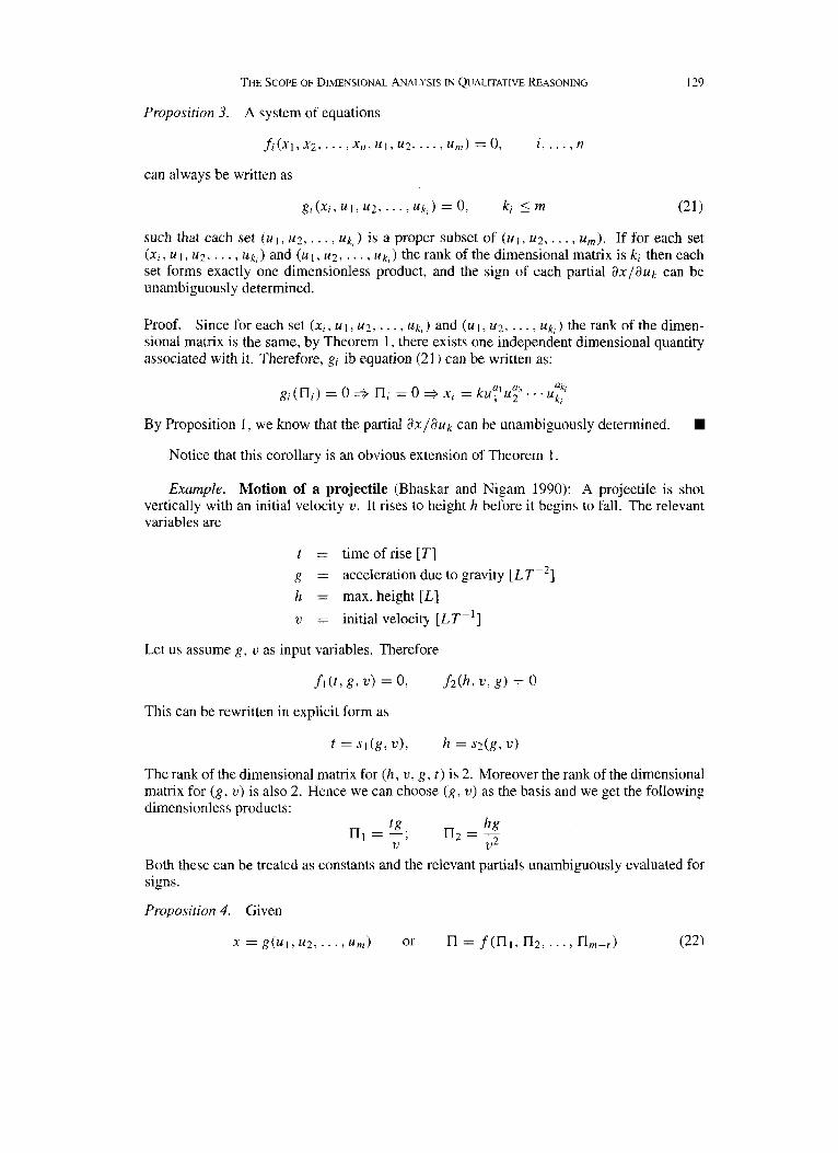
Proposition 3. A system of equations

can always be written as

gi(x, , ul, u?, . . . , u k , ) = 0, kj 5 m (21)

such that each set ( U I , u2, . . . , UR,) is a proper subset of ( U I , u2, . . . , urn). If for each set ( X i , u i , u2. . . . , U k , ) and (u1, u2 , . . . , Uk,) the rank of the dimensional matrix is ki then each set forms exactly one dimensionless product, and the sign of each partial ax/auk can be unambiguously determined.

Proof. Since for each set (x , , u 1, u2, . . . , U k , ) and ( u l , u2, . . . , uk , ) the rank of the dimensional matrix is the same, by Theorem 1, there exists one independent dimensional quantity associated with it. Therefore, g, ib equation (21) can be written as:

g, (n,) = 0 3 n, = o =+ x , = kU;lU;7 . . . Unhi k,

By Proposition 1, we know that the partial a x / a u k can be unambiguously determined.

Notice that this corollary is an obvious extension of Theorem 1 .

Example. vertically with variables are

Motion of a projectile (Bhaskar and Nigam 1990): A projectile is shot an initial velocity v. It rises to height h before it begins to fall. The relevant

t = time of rise [7] g = acceleration due to gravity [ L T F 2 ] h = max. height [I,] v = initial velocity [ L T - ' ]

Let us assume g , v as input variables. Therefore

This can be rewritten in explicit form as

t = si(g, u), h = S?(g, v)

The rank of the dimensional matrix for (h , v , g , t ) is 2. Moreover the rank of the dimensional matrix for ( g , v) is also 2. Hence we can choose (g, v) as the basis and we get the following dimensionless products:

Both these can be treated as constants and the relevant partials unambiguously evaluated for signs.

Proposition 4. Given


where ( u 1, u2, . . . , u,) are independent variables, and !3 is defined as

If the rank of the dimensional matrix of ( x , u1, u2, . . . , u,) is r such that Y 5 m then the partial of the dependent variable x w.r.t. one of the independent variables ( u l , u2, . . . , u,) can be unambiguously determined iff one the following conditions hold:

1. a n l / a u k = 0 for 1 = 1, . . . , m - r . 2. sign(akukf) = sign (a f /auk ) . 3. a f /auk =o .

Proof. We rewrite x from Eq. (23) as

Therefore from Eq. (24)

Consider the second term in Eq. (25):

Case 1. If dl l l /auk = 0 for all 1 = 1 , . . . , m - r , then af/auk = 0, from Eq. (26). Therefore ax/auk can be unambiguously determined provided ak and f are known.

Case 2. Notice that, from Eq. (251, the signs of both the terms on the right-hand side are exactly the same by condition 2 of the theorem. Therefore, for the purposes of evaluating the sign of ax/auk, we need consider only one term; i.e., we may treat n as a constant.

Case 3. If condition 3 of the theorem holds then the second term in Eq. (25) is 0. Therefore the sign of ax/auk can be unambiguously determined provided ak and f are known in terms of their signs about the equilibrium point.

Now in order to prove the only if part, assume that none of the above three cases is true. Then from Eqs. (25), (26) none of the terms are zero and in general they can be of opposite signs and hence the partial is indeterminate.

Notice that case 2 is interesting in that it requires the knowledge of the sign of the function f and the partial a f /auk. This information might not be available in general since the explicit form g is not easy to determine in most cases. Similarly, case 3 requires the knowledge of the exact functional form of f in Eq. (22) which is once again not easily determined. However, if the condition enumerated in case 1 is satisfied, then we have a sufficient condition for determining the sign of the partial ax/uk.


4.3. Dimensional Analysis and Systems of Equations

The conditions discussed above may seem quite stringent and their applicability restricted. Nevertheless, the approach can be valuable when solving a large system of equations for qualitative solutions. Consider a system of n equations with n unknown variables as shown in Eq. (19). Since we are interested in evaluating the partial ax,/auk, i = 1, . . . , n, we potentially have 2" possible combinations of signs (f, f, . . . , &) as solutions to the vector of partials. If one of the equations fi satisfies the conditions of Propositions 2-4, then we can evaluate the sign of the partial axi/auk unambiguously. This reduces the number of combinations from 2" to 2"-'.

Consider another possibility, where the system of n x n equations can be partitioned into a self-contained subset of m x m which satisfies the conditions laid down in Proposition 3. In this case, we can determine the partials 2, i = 1, . . . , m, for m variables. This implies that the number of possible solutions can be reduced by a factor of 2*, from 2" to 2"-". If it is possible to identify more than one such subset then further reductions are possible. Thus, although the cases discussed in the previous section may look fairly noncommittal, they can in fact lead to substantial reductions in the possible qualitative solutions to systems of equations.

4.4. Related Concepts

Kokar has used the theory of dimensional analysis in the context of qualitative reasoning (Kokar 1987a; 1987b) and machine learning (Kokar 1986a; 1986b). In this subsection we describe Kokar's work briefly and outline the similarities and differences in comparison to the work presented in this paper.

Qualitative simulation of processes is based on variables which take nominal values corresponding to intervals on the real line. In order to gain insights from a qualitative simulation, the boundaries between intervals (called "landmark points" in the A1 literature) should delineate qualitatively different outcomes for the simulation. However, for most physical processes, qualitatively different behaviors are not marked by single variables but rather by specific constraints between several variables (e.g., the point at which water begins to boil is given by a relationship between pressure and temperature). Kokar calls these constraints or boundaries critical hypersu@uces and uses the theory of dimensional analysis to identify them. Kokar analyzes the set of relevant variables and available data for completeness and generates the set of dimensionless numbers corresponding to a basis. The critical value corresponding to such dimensionless numbers is derived based on the sign of the first derivates and they define the critical hypersurface. The focus of Kokar's work is on identifying numerically the boundaries in the space of variables (for a process of interest) which delineate qualitatively different behaviors. In contrast the work presented in this paper is concerned with the question of mahng explicit the conditions under which the principle of dimensional homogeneity is sufficient to determine the sign of the first partial derivates between variables.

Kokar has also developed a method called COPER which uses the theory of dimensional analysis for discovering functional formulae among a set of relevant variables for a physical process. COPER exploits the scientific methodology used to discover physical laws by grouping the variables into dimensionless numbers for a given choice of basis variables and generates a functional formula over these transformed variables. Additionally, since the choice of basis is not unique, the search for a functional relationship is conducted over the set of all possible basis variables. This particular use of dimensional analysis in A1 is related to machine learning. Although the work presented in this paper is not directly focused on discovering functional formulae, conditions regarding the sign of the first partials developed here can be used to constrain the search for functional formulae.


5. DISCUSSION

Bhaskar and Nigam have used the method of dimensional analysis to solve a number of examples from the qualitative reasoning literature in AI. Their approach has essentially consisted of identifying an “appropriate basis” and using this basis to derive the dimensionless numbers for each example. They subsequently assume these dimensionless numbers as constants and evaluate the sign of the partials. We have illustrated how this approach sometimes provides incorrect answers with the example of condensation in a vertical pipe. However, the question arises whether we get incorrect answers because we might have cho- sen an “inappropriate basis.” In this section, we solve the same example with a different basis which seemingly provides the correct answers. We show that the failure of Bhaskar and Nigam’s method to provide the correct solution has nothing to do with the selection of an “appropriate basis”; rather it is related to the fact that no single dimensionless number captures the relationship between h and A.

Consider the following basis: h, p, L , A@. This basis yields 4 dimensionless quantities:

, .3=- , x 4 = - hA0 L k A8

n1= ------, n2 = - FA Fh EL. ?L

pLh“2 g L

Based on these dimensionless numbers we can rewrite the relationship between 511 and the rest of the n’s as follows:

Now let us consider the sign of the partial of h w.r.t. h. The relationship between h and the other variables can be written in terms of n1.

ah - ah = (&)n1+(g-)$

Evaluating anllah using (27), we get

This equation indicates that the sign of the partial is positive simply because the first term is larger than the second term. Notice that if one were to restrict one’s attention to the first term in the equation (which is equivalent to assuming that the dimensionless l7 is constant) we will still get the correct answer. But this is a coincidence rather than a consequence of the choice of an appropriate basis!

6. CONCLUSIONS

We have investigated some of the foundational principles of dimensional analysis in an attempt to understand its scope and limitations for qualitative reasoning. Our results characterize a set of conditions under which dimensional analysis can provide useful information


to guide qualitative reasoning. While these conditions may appear severely limiting, we have argued that there are many situations in systems described by sets of state equations in which dimensional analysis can provide substantial reduction in ambiguity. That is, it can significantly reduce the space of possible qualitative solutions.

Dimensional analysis is no magic substitute for physics knowledge. In particular, physics knowledge is essential in identifying which exogenous variables may be relevant, and in combining them in physically meaningful ways so as to reduce the number of independent variables in the dimensional analysis. Nevertheless, it is a useful source of constraints on the set of physically meaningful relationships. It should not be ignored as a useful supplement to other sources of knowledge to reduce the ambiguities prevalent in schemes for qualitative reasoning.

ACKNOWLEDGMENTS

This work was supported by the National Science Foundation under grant IRI-8807061 to Carnegie Mellon and by the Rockwell International Science Center, Palo Alto Laboratory. Thanks are also due to Yumi Iwasaki and Herbert A. Simon for some valuable discussions of these issues.

REFERENCES

BHASKAR, R., and A. NIGAM. 1990. Qualitative physics using dimensional analysis. Artificial Intelligence, 4573-

BRIDGMAN, P. W. 193 1. Dimensional analysis. Yale University Press, New Haven, CT. BROWN, A. I., and S. M. MARCO. 1958. Introduction to heat transfer. McGraw-Hill, New York. FOCKEN, C. M. 1953. Dimensional methods and their applications. Edward Arnold, London. HENRION, M., and B. FISCHHOFF. 1986. Assessing uncertainty in physical constants. American Journal of Physics,

KOKAR, M. M. 1986a. Discovering functional formulas through changing representation base. In Proceedings of

KOKAR, M. M. 1986b. Determining arguments of invariant functional descriptions. Machine Learning, 1:403-422. KOKAR, M. M. 1987a. Critical hypersurfaces and the quantity space. In Proceedings of AAAI-87, Seattle, 616-

KOKAR, M. M. 1987b. Generating qualitative representations of continuous physical processes. In Methodologies

LANGHAAR, H. L. 1951. Dimensional analysis and theory of models. Wiley, New York. MAYBEE, J., and J. QUIRK. 1969. Qualitative problems in matrix theory. SIAM Review, l l(1). SAMUELSON, P. A. 1947. Foundations of economic analysis. Harvard University Press. SEDOV, L. I. 1959. Similarity and dimensional methods in mechanics. Translated from Russian by M. Holt.

111.

54(9):791-798.

AAAI-86, Philadelphia, 455-459.

620.

for intelligent systems. Edited by Z. W. Ras and M. Zemankova. North-Holland, New York.

Academic Press.

The Scope of Dimensional Analysis in Qualitative Reasoning

Documents

Transcript of The Scope of Dimensional Analysis in Qualitative Reasoning