Noname manuscript No.(will be inserted by the editor)

Qualitative Spatial Reasoning with ConceptualNeighborhoods for Agent Control

Frank Dylla, Jan Oliver Wallgrün

SFB/TR 8 Spatial Cognition, Universität Bremen, Bibliothekstr. 1, 28359 Bremen, Ger-many, e-mail:{dylla,wallgruen}@sfbtr8.uni-bremen.de

Received: date / Revised version: date

Abstract Research on qualitative spatial reasoning has produced a variety of cal-culi for reasoning about orientation or direction relations. Such qualitative abstrac-tions are very helpful for agent control and communication between robots andhumans. Conceptual neighborhood has been introduced as a means of describingpossible changes of spatial relations which e.g. allows action planning at a highlevel of abstraction. We discuss how the concrete neighborhood structure dependson application-specific parameters and derive corresponding neighborhood struc-tures for theOPRAm calculus. We demonstrate that conceptual neighborhoodsallow resolution of conflicting information by model-based relaxation of spatialconstraints. In addition, we address the problem of automatically deriving neigh-borhood structures and show how this can be achieved if the relations of a calculuscan be modeled in another calculus for which the neighborhood structure is known.

1 Introduction

Qualitative spatial reasoning (QSR) is an established field of research investigat-ing qualitative representations of space that abstract from the details of the physicalworld together with reasoning techniques that allow predictions about spatial re-lations, even when precise quantitative information is not available [2]. QSR istypically realized in form of calculi over sets of spatial relations (e.g.left-of ornorth-of). These calculi are well-suited to serve as simple and efficient abstrac-tions of the world, e.g. for robot navigation [6] or communication purposes [17].

A multitude of spatial calculi has been proposed during the last two decades,focusing on different aspects of space (mereotopology, orientation, distance, etc.)and dealing with different kinds of objects (points, line segments, extended objects,etc.). The two main research directions in QSR are topological reasoning aboutregions [26,8,29] and positional reasoning about configurations of point objects

2 Frank Dylla, Jan Oliver Wallgrün

[11,9,16,19,28] or line segments [21,31,6]. Calculi dealing with such informationhave been well investigated over the recent years and provide general and soundreasoning mechanisms. An overview is given in [3].

An important concept in the context of robot navigation and agent control—and the main topic of this text—is the notion of conceptual neighborhood betweenspatial relations. Conceptual neighborhood has been introduced as a means of de-scribing possible changes of spatial relations which e.g. allows action planning ata high level of abstraction.

As we will show in this text the concrete neighborhood structure, however, de-pends very much on application-specific parameters like what kind of continuoustransformations have to be considered for the objects involved (e.g. locomotion,deformation, etc.), whether objects can be transformed simultaneously, or whethertwo objects can occupy the same space or not. The exemplary calculus we willinvestigate in this text is the Oriented Point Relation Algebra (OPRAm) with ad-justable granularity [19,18] for reasoning about the orientation relations betweenoriented points. We will analyze its conceptual neighborhood structures as theyarise under different conditions in the context of robot navigation.

After this analysis, we will demonstrate one way in which conceptual neigh-borhoods can be beneficially employed for controlling mobile robots, namely theapplication of conceptual neighborhoods for a model-based resolution of conflictsin spatial information stemming from different knowledge sources. Standard con-straint satisfaction techniques for relational constraints [15] will be used to checkfor consistency, while the conceptual neighborhoods will be used to incrementallyrelax the spatial constraints until an optimal consistent relaxation is found withrespect to an application-dependent cost or distance function.

Since conceptual neighborhood structures depend on the given scenario and,in addition, qualitative spatial calculi themselves are often developed or adaptedfor a specific task, methods for automatically deriving or verifying properties likecomposition tables and neighborhood structures for new calculi are required [7].We address this problem by showing that neighborhood structures for two otherorientation calculi, the FlipFlop calculus [16] and the fine-grained Dipole RelationAlgebra [6], can be automatically computed by first modeling the relations of thesecalculi inOPRAm, then generating neighboring configurations inOPRAm, andfinally translating the consistent ones back into the original calculus.

The text is structured as follows: We begin by briefly introducing the mostrelevant concepts with respect to QSR and in particular theOPRAm calculus inSection 2. In the next section, we present the notion of conceptual neighborhoodstructures and investigate the different neighborhood structures ofOPRAm. Sec-tion 4 is concerned with the application of conceptual neighborhoods for resolvingconflicting information by relaxation. And in Section 5, we address the problemof deriving conceptual neighborhood structures automatically.

2 Qualitative Spatial Reasoning and theOPRAm Calculus

In this section, we give a brief overview on spatial calculi and qualitative spatialreasoning and introduce the Oriented Point Relation Algebra (OPRAm), which

Qualitative Spatial Reasoning with Conceptual Neighborhoods for Agent Control 3

will accompany us through the rest of the text. TheOPRAm calculus has beenchosen as it is algebraically well defined and thus well qualified for being inte-grated into robot control architectures.

2.1 Qualitative Spatial Calculi

A qualitative spatial calculus defines operations on a finite setR of spatial rela-tions, like left-of, north-of, overlap, etc. The spatial relations are defined over ausually infinite set of spatial objects, the domainD (e.g. points, line segments, re-gions, etc.). In this text, we will mainly considerbinary calculiin whichR consistsof binary relationsR ⊆ D ×D.

The set of relationsR of a spatial calculus is typically derived from a jointlyexhaustive and pairwise disjoint (JEPD) set ofbase relationsBR so that each pairof objects fromD is contained in exactly one relation fromBR. Every relationin R is a union of a subset of the base relation. Since spatial calculi are typicallyused for constraint reasoning and unions of relations correspond to disjunction ofrelational constraints, it is common to speak of disjunctions of relations as welland write them as sets{B1, ..., Bn} of base relations.R is then either taken to bethe powerset2BR of the base relations (all unions of base relations) or a subset ofthe powerset. In order to be usable for constraint reasoning,R should contain atleast the base relations, the empty relation∅, the universal relationU = D × D,and the identity relationId = {(x, x)|x ∈ D}. R also needs to be closed underthe operations defined in the following.

As the relations are subsets of tuples from the same Cartesian product, the setoperations union, intersection, and complement can directly be applied:

Union: R ∪ S = { (x, y) | (x, y) ∈ R ∨ (x, y) ∈ S }Intersection:R ∩ S = { (x, y) | (x, y) ∈ R ∧ (x, y) ∈ S }Complement:R = U \R = { (x, y) | (x, y) ∈ U ∧ (x, y) 6∈ R }whereR andS are relations fromR.

In addition, two more operations are defined which allow derivation of newfacts from given information,conversionandcomposition:

Converse:R` = { (y, x) | (x, y) ∈ R }Composition:R ◦ S = { (x, z) | ∃y ∈ D : ((x, y) ∈ R ∧ (y, z) ∈ S) }

The composition operation is especially important for constraint reasoningsince it describes what relations may hold between objectsA andC given what isknown about the relation betweenA andB and the relation betweenB andC. Forinstance, from knowing thatA is north-of B andB is north-of C it follows thatAis north-of C as well. The composition operation is often given in form of look-uptables calledcomposition tables.

2.2OPRAm: A Calculus for Reasoning about Oriented Points

The domain of the Oriented Point Relation Algebra (OPRAm) [19,18] is theset of oriented points (points in the plane with an additional direction parameter).

4 Frank Dylla, Jan Oliver Wallgrün

1

3

2

5

7

0 76

51

0

4

4A

B

(a)m = 2: A 2∠17 B

0

23

4

67 9 10

5

1

13

0 15 1413

1211

109

7

3

8

8

A B

(b) m = 4: A 4∠313 B

AB

0

1

2

34

5

6

7

(c) case whereA andBcoincide:A 2∠1 B

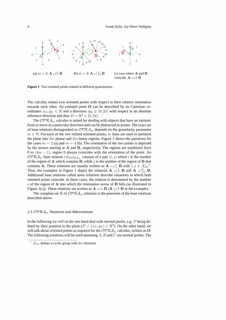
Figure 1 Two oriented points related at different granularities.

The calculus relates two oriented points with respect to their relative orientationtowards each other. An oriented pointO can be described by its Cartesian co-ordinatesxO, yO ∈ R and a directionφO ∈ [0, 2π] with respect to an absolutereference direction and thusD = R2 × [0, 2π].

TheOPRAm calculus is suited for dealing with objects that have an intrinsicfront or move in a particular direction and can be abstracted as points. The exact setof base relations distinguished inOPRAm depends on the granularity parameterm ∈ N. For each of the two related oriented points,m lines are used to partitionthe plane into2m planar and2m linear regions. Figure 1 shows the partitions forthe casesm = 2 (a) andm = 4 (b). The orientation of the two points is depictedby the arrows starting atA andB, respectively. The regions are numbered from0 to (4m − 1), region 0 always coincides with the orientation of the point. AnOPRAm base relationrelOPRAm

consists of a pair(i, j) wherei is the numberof the region ofA which containsB, while j is the number of the region ofB thatcontainsA. These relations are usually written asA m∠j

i B with i, j ∈ Z4m1.

Thus, the examples in Figure 1 depict the relationsA 2∠17 B andA 4∠3

13 B.Additional base relations calledsame relationsdescribe situations in which bothoriented points coincide. In these cases, the relation is determined by the numbers of the region ofA into which the orientation arrow ofB falls (as illustrated inFigure 1(c)). These relations are written asA 2∠s B (A 2∠1 B in the example).

The complete setR ofOPRAm relations is the powerset of the base relationsdescribed above.

2.3OPRAm Notations and Abbreviations

In the following we will on the one hand deal withnormal points, e.g.P being de-fined by their position in the plane (P = (xP , yP ) ∈ R2). On the other hand, wewill talk aboutoriented pointsas required for theOPRAm calculus, written asO.The following notations will be used assumingA,B andC are normal points: The

1 Z4m defines a cyclic group with4m elements.

Qualitative Spatial Reasoning with Conceptual Neighborhoods for Agent Control 5

directionφBC is defined as the direction fromB towardsC. We writeABC forthe oriented point((xA, yA), φBC). It has the same position as the normal pointA and the directionφBC . We just writeA if the direction is unknown or unspeci-fied, e.g. if we want to define an oriented point that coincides withA but can havean arbitrary direction. Note thatAAB , AAC , andA are three different orientedpoints coinciding in position but possibly differing in orientation. Additionally,we want to emphasize that oriented point names likeAAC are only identifiers weuse for making their role intuitively comprehensible. The knowledge that one ori-ented point either coincides with or is oriented towards another has to be explicitlyrepresented by respective relations.

As mentioned, we will speak about disjunctions of base relations instead ofunions and write them as sets. We will use the abbreviationA m∠{k−l}

{i−j} B withi, j, k, l ∈ Z4m for the disjunction

j∨a=i

l∨b=k

A m∠ba B.

A ∗ abbreviates all members0 to (4m − 1) of Z4m and{i, j} a disjunction ofiandj such that for exampleA m∠∗{i,j} B denotes(

4m−1∨b=0

A m∠bi B

)∨

(4m−1∨b=0

A m∠bj B

).

2.4 Constraint Reasoning with Spatial Calculi

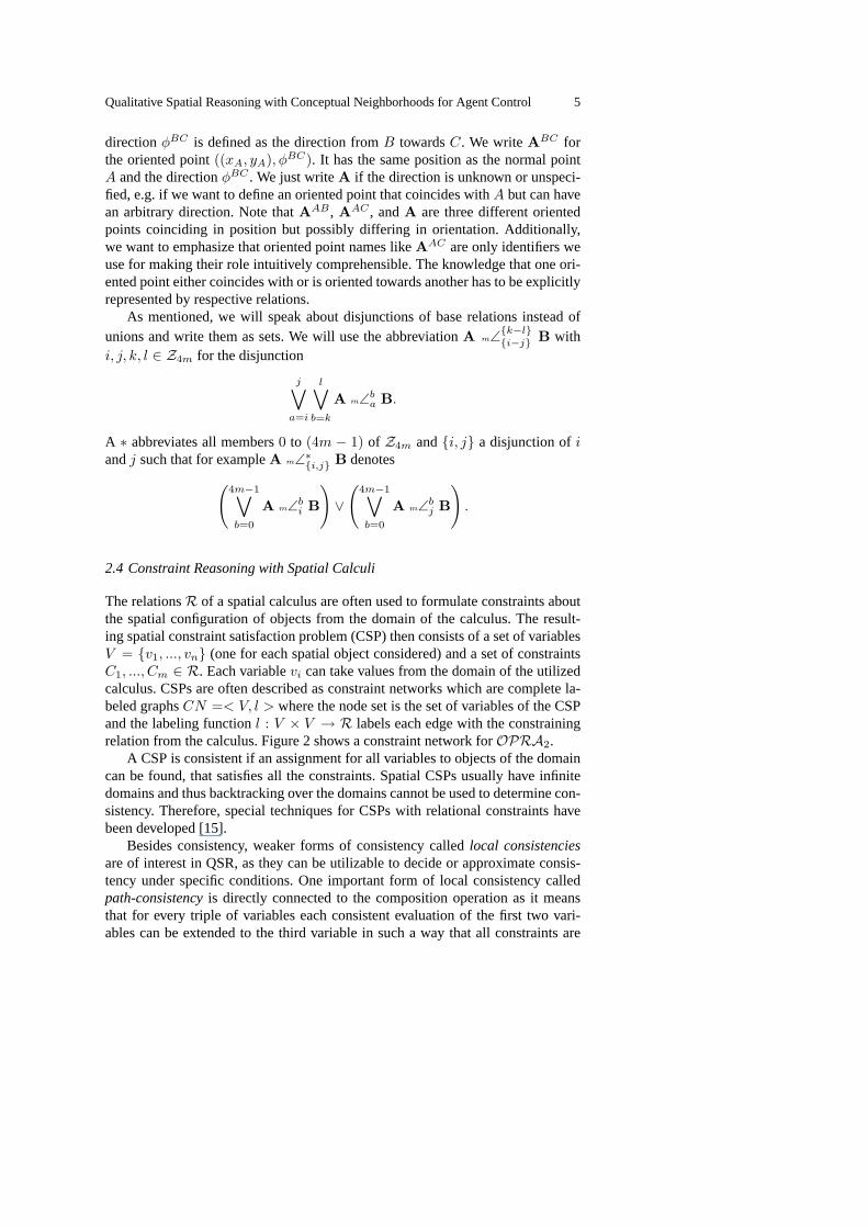
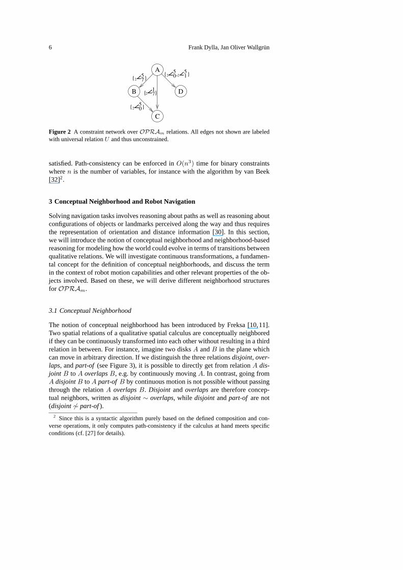
The relationsR of a spatial calculus are often used to formulate constraints aboutthe spatial configuration of objects from the domain of the calculus. The result-ing spatial constraint satisfaction problem (CSP) then consists of a set of variablesV = {v1, ..., vn} (one for each spatial object considered) and a set of constraintsC1, ..., Cm ∈ R. Each variablevi can take values from the domain of the utilizedcalculus. CSPs are often described as constraint networks which are complete la-beled graphsCN =< V, l > where the node set is the set of variables of the CSPand the labeling functionl : V × V → R labels each edge with the constrainingrelation from the calculus. Figure 2 shows a constraint network forOPRA2.

A CSP is consistent if an assignment for all variables to objects of the domaincan be found, that satisfies all the constraints. Spatial CSPs usually have infinitedomains and thus backtracking over the domains cannot be used to determine con-sistency. Therefore, special techniques for CSPs with relational constraints havebeen developed [15].

Besides consistency, weaker forms of consistency calledlocal consistenciesare of interest in QSR, as they can be utilizable to decide or approximate consis-tency under specific conditions. One important form of local consistency calledpath-consistencyis directly connected to the composition operation as it meansthat for every triple of variables each consistent evaluation of the first two vari-ables can be extended to the third variable in such a way that all constraints are

6 Frank Dylla, Jan Oliver Wallgrün

A

C

D

2 05

2 15

2 75

2 05

2 71B

{ , }{ }

{ }

{ }

Figure 2 A constraint network overOPRAm relations. All edges not shown are labeledwith universal relationU and thus unconstrained.

satisfied. Path-consistency can be enforced inO(n3) time for binary constraintswheren is the number of variables, for instance with the algorithm by van Beek[32]2.

3 Conceptual Neighborhood and Robot Navigation

Solving navigation tasks involves reasoning about paths as well as reasoning aboutconfigurations of objects or landmarks perceived along the way and thus requiresthe representation of orientation and distance information [30]. In this section,we will introduce the notion of conceptual neighborhood and neighborhood-basedreasoning for modeling how the world could evolve in terms of transitions betweenqualitative relations. We will investigate continuous transformations, a fundamen-tal concept for the definition of conceptual neighborhoods, and discuss the termin the context of robot motion capabilities and other relevant properties of the ob-jects involved. Based on these, we will derive different neighborhood structuresfor OPRAm.

3.1 Conceptual Neighborhood

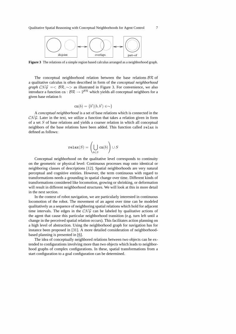
The notion of conceptual neighborhood has been introduced by Freksa [10,11].Two spatial relations of a qualitative spatial calculus are conceptually neighboredif they can be continuously transformed into each other without resulting in a thirdrelation in between. For instance, imagine two disksA andB in the plane whichcan move in arbitrary direction. If we distinguish the three relationsdisjoint, over-laps, andpart-of (see Figure 3), it is possible to directly get from relationA dis-joint B to A overlapsB, e.g. by continuously movingA. In contrast, going fromA disjointB to A part-of B by continuous motion is not possible without passingthrough the relationA overlapsB. Disjoint andoverlapsare therefore concep-tual neighbors, written asdisjoint∼ overlaps, while disjoint andpart-of are not(disjoint 6∼ part-of).

2 Since this is a syntactic algorithm purely based on the defined composition and con-verse operations, it only computes path-consistency if the calculus at hand meets specificconditions (cf. [27] for details).

Qualitative Spatial Reasoning with Conceptual Neighborhoods for Agent Control 7

disjoint part−ofoverlaps

Figure 3 The relations of a simple region based calculus arranged as a neighborhood graph.

The conceptual neighborhood relation between the base relationsBR ofa qualitative calculus is often described in form of theconceptual neighborhoodgraph CNG =< BR,∼> as illustrated in Figure 3. For convenience, we alsointroduce a functioncn : BR → 2BR which yields all conceptual neighbors for agiven base relationb:

cn(b) = {b′|(b, b′) ∈∼}

A conceptual neighborhoodis a set of base relations which is connected in theCNG. Later in the text, we utilize a function that takes a relation given in formof a setS of base relations and yields a coarser relation in which all conceptualneighbors of the base relations have been added. This function calledrelax isdefined as follows:

relax(S) =

(⋃b∈S

cn(b)

)∪ S

Conceptual neighborhood on the qualitative level corresponds to continuityon the geometric or physical level: Continuous processes map onto identical orneighboring classes of descriptions [12]. Spatial neighborhoods are very naturalperceptual and cognitive entities. However, the term continuous with regard totransformations needs a grounding in spatial change over time. Different kinds oftransformations considered like locomotion, growing or shrinking, or deformationwill result in different neighborhood structures. We will look at this in more detailin the next section.

In the context of robot navigation, we are particularly interested in continuouslocomotion of the robot. The movement of an agent over time can be modeledqualitatively as a sequence of neighboring spatial relations which hold for adjacenttime intervals. The edges in theCNG can be labeled by qualitative actions ofthe agent that cause this particular neighborhood transition (e.g. turn left until achange in the perceived spatial relation occurs). This facilitates action planning ona high level of abstraction. Using the neighborhood graph for navigation has forinstance been proposed in [31]. A more detailed consideration of neighborhood-based planning is presented in [6].

The idea of conceptually neighbored relations between two objects can be ex-tended to configurations involving more than two objects which leads to neighbor-hood graphs of complex configurations. In these, spatial transformations from astart configuration to a goal configuration can be determined.

8 Frank Dylla, Jan Oliver Wallgrün

Modeling the relations from a naive point of view, i.e. by keeping track ofall relations between all objects, leads to combinatorial explosion, as for exampleshown in [25]. This can be seen as an allocentric approach. One way to reducethese complexity issues is to shift to an egocentric perspective by only consideringneighborhoods of relations to a selected set of reliably recognizable objects [6].

3.2 Continuous Transformation

The termcontinuous transformationis a central concept in the definition of con-ceptual neighborhood. Detailed investigations on different aspects of continuityhave been presented in [1,4,14,13,22]. The original definition of conceptual neigh-borhood originates from work on time intervals and therefore only the continuoustransformations shortening and lengthening of intervals were considered. Whentransferring conceptual neighborhood to spatial relations, only vague discrimina-tions were made between different types of transformations, e.g. between transfor-mations in size or transformations in position, although different types of neigh-borhoods were already mentioned in [11]. For navigation and action planning itis crucial that theCNGs reflect the capabilities of the agent so that neighborhoodinduces direct reachability in the physical world.

Overall, three main aspects affect the neighborhood structure for a given spatialcalculus in the context of robot navigation:

– the robot kinematics (motion capabilities)– whether the objects may move simultaneously– whether objects may coincide in position or not (superposition)

Restrictions in motion capabilities and number of objects moving will affectwhich relations are connected in theCNG. To give an example, let us assume thatOPRA2 relationA 2∠7

7 B holds between an agentA and some static objectB.The orientations correspond to the intrinsic fronts of both objects (cf. Figure 4). Ifour robot is equipped with an omnidrive allowing it to drive sideways, it can reachconfigurationA 2∠0

0 B directly by moving to the right side. A robot only outfittedwith a differential drive has to traverse (notated as ) other configurations beforereaching the desired configuration, e.g.A 2∠7

7 B A 2∠70 B A 2∠7

1 B A 2∠0

1 B A 2∠00 B.

In contrast, if the related objects cannot take the same position (no superpo-sition), for instance because they are both solid physical objects, then relationswhich represent such configurations are not feasible and thus are missing in theCNG. To simplify matters, we will talk about solid and non-solid objects in theremainder of the text, though the reasons for not allowing superposition can bedifferent.

In the following, we will systematically derive the neighborhood structures fortheOPRAm calculus starting out with very simple robot kinematics and endingwith the most general case of the neighborhood structure for objects which canmove in arbitrary direction. The considered situations are the following:

1. one object moving, rotation only

Qualitative Spatial Reasoning with Conceptual Neighborhoods for Agent Control 9

0

2

3

1

5

6B

7

4

1

3

2

5

7

0

4

A6

(a)A 2∠77 B

0

2

3

1

6B

4

1

3

2

5

0

4

A6

7

7

5

(b) A 2∠00 B

Figure 4 Possible conceptual neighborhood structures regarding different motion capabil-ities of agentA with respect to a static objectB. Direct transition is possible from 4(a)to 4(b) if agentA is able to move sidewards (dotted line), whereas several neighborhoodtransitions are necessary if not (dashed line).

2. two objects moving, rotation only3. two objects moving, translation only, solid objects4. two objects moving, translation only, non-solid objects5. two objects moving,either translationor rotation, non-solid objects6. two objects moving, unconstrained motion, non-solid objects

3.3 Neighborhood Structure ofOPRAm

For understanding the neighborhood structures ofOPRAm, we start by consider-ing the simplest case in which only one of the two related solid objects is allowedto rotate while the other does not move at all.

3.3.1 Single Rotating ObjectImagine a robotR represented by the oriented pointR standing in a room together with a stable object with a fixed intrinsic front, e.g.a locker (L). Rotating on the spot will lead to a change in relative position of thelocker compared to the robot’s own intrinsic front, but the robot’s relative positionto the locker does not change. Therefore, theOPRAm relation representing thesituation (R m∠j

i L) only changes ini. Turning left results in a decrease ofi byone, and a right turn in an increase by one. This means that for alli, j ∈ Z4m,cn(m∠j

i ) = {m∠ji−1, m∠j

i+1} 3. Reversing the roles ofL andR entails the same

changes inj: cn(m∠ji ) = {m∠j−1

i , m∠j+1i }. Figure 5(a) illustrates this neighbor-

hood structure with the involved actions ofR annotated to the edges. If we allow

3 Note, thatZ4m is defined as acyclicgroup so that no modulo operation is required.

10 Frank Dylla, Jan Oliver Wallgrün

A left rot

A right rot

B right rotB left rotij

i−1j

i+1j

ij+1

ij−1

(a) Only one object is able to ro-tate.

B left rot

A left rot

B right rot

A right rot

A & B left rot

A & B right rot

A left

&

B ri

ght r

ot

B

left

rot

A righ

t &

ij

i−1j−1

i+1j−1

i−1j+1

i−1j

i+1j

ij+1

ij−1

i+1j+1

(b) Both objects are able to ro-tate.

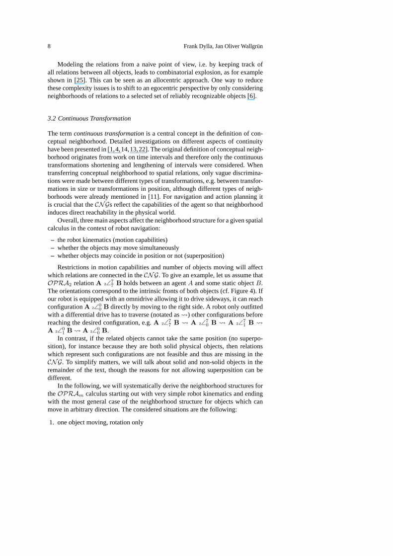
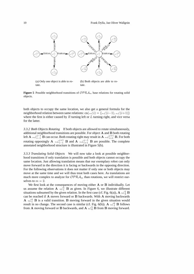
Figure 5 Possible neighborhood transitions ofOPRAm base relations for rotating solidobjects.

both objects to occupy the same location, we also get a general formula for theneighborhood relation between same relations:cn(m∠i) = {m∠(i−1), m∠(i+1)}where the first is either caused byR turning left orL turning right, and vice versafor the latter.

3.3.2 Both Objects RotatingIf both objects are allowed to rotate simultaneously,additional neighborhood transitions are possible. For objectA andB both rotatingleft A m∠j−1

i−1 B can occur. Both rotating right may result inA m∠j+1i+1 B. For both

rotating opposinglyA m∠j+1i−1 B andA m∠j−1

i+1 B are possible. The completeannotated neighborhood structure is illustrated in Figure 5(b).

3.3.3 Translating Solid ObjectsWe will now take a look at possible neighbor-hood transitions if only translation is possible and both objects cannot occupy thesame location. Just allowing translation means that our exemplary robot can onlymove forward in the direction it is facing or backwards in the opposing direction.For the following observations it does not matter if only one or both objects maymove at the same time and we will thus treat both cases here. As translations aremuch more complex to analyze forOPRAm than rotations, we will restrict our-selves tom = 2.

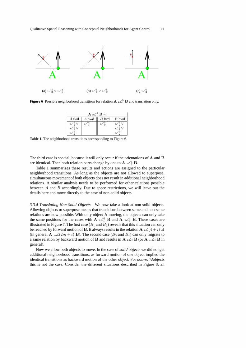
We first look at the consequences of moving eitherA or B individually. Letus assume the relationA 2∠5

1 B as given. In Figure 6, we illustrate differentsituations subsumed by the given relation. In the first case (cf. Fig. 6(a)),A 2∠5

2 Bcan be reached ifA moves forward orB backwards. WithA moving backwardsA 2∠4

1 B is a valid transition.B moving forward in the given situation wouldresult in no change. The second case is similar (cf. Fig. 6(b)).A 2∠6

1 B followsfrom A moving forward orB backwards, andA 2∠5

0 B from B moving forward.

Qualitative Spatial Reasoning with Conceptual Neighborhoods for Agent Control 11

B

A(a) 2∠5

2 ∨ 2∠41

B

A(b) 2∠6

1 ∨ 2∠50

B

A(c) 2∠6

2

Figure 6 Possible neighborhood transitions for relationA 2∠51 B and translation only.

A 2∠51 B ∼

A fwd A bwd B fwd B bwd2∠5

2 ∨ 2∠41 2∠5

0 2∠52 ∨

2∠61 ∨ 2∠6

1 ∨2∠6

2 2∠62

Table 1 The neighborhood transitions corresponding to Figure 6.

The third case is special, because it will only occur if the orientations ofA andBare identical. Then both relation parts change by one toA 2∠6

2 B.Table 1 summarizes these results and actions are assigned to the particular

neighborhood transitions. As long as the objects are not allowed to superpose,simultaneous movement of both objects does not result in additional neighborhoodrelations. A similar analysis needs to be performed for other relations possiblebetweenA andB accordingly. Due to space restrictions, we will leave out thedetails here and move directly to the case of non-solid objects.

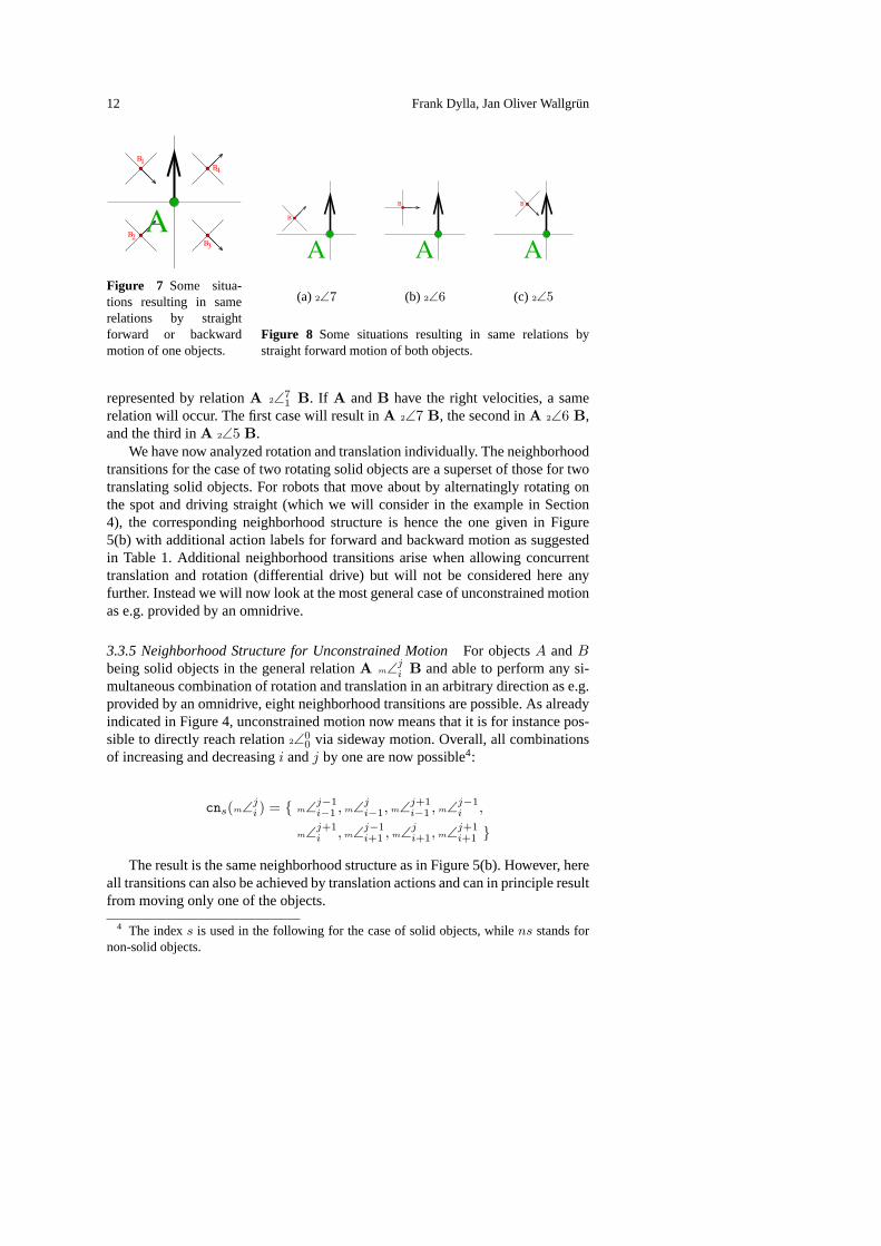
3.3.4 Translating Non-Solid ObjectsWe now take a look at non-solid objects.Allowing objects to superpose means that transitions between same and non-samerelations are now possible. With only objectB moving, the objects can only takethe same positions for the cases withA 2∠0

i B andA 2∠4i B. These cases are

illustrated in Figure 7. The first case (B1 andB2) reveals that this situation can onlybe reached by forward motion ofB. It always results in the relationA 2∠(4 + i) B(in generalA m∠(2m + i) B). The second case (B3 andB4) can only migrate toa same relation by backward motion ofB and results inA 2∠i B (or A m∠i B ingeneral).

Now we allow both objects to move. In the case ofsolid objects we did not getadditional neighborhood transitions, as forward motion of one object implied theidentical transitions as backward motion of the other object. Fornon-solidobjectsthis is not the case. Consider the different situations described in Figure 8, all

12 Frank Dylla, Jan Oliver Wallgrün

B1

B2B3

B4

A

Figure 7 Some situa-tions resulting in samerelations by straightforward or backwardmotion of one objects.

B

A

(a) 2∠7

B

A

(b) 2∠6

B

A

(c) 2∠5

Figure 8 Some situations resulting in same relations bystraight forward motion of both objects.

represented by relationA 2∠71 B. If A andB have the right velocities, a same

relation will occur. The first case will result inA 2∠7 B, the second inA 2∠6 B,and the third inA 2∠5 B.

We have now analyzed rotation and translation individually. The neighborhoodtransitions for the case of two rotating solid objects are a superset of those for twotranslating solid objects. For robots that move about by alternatingly rotating onthe spot and driving straight (which we will consider in the example in Section4), the corresponding neighborhood structure is hence the one given in Figure5(b) with additional action labels for forward and backward motion as suggestedin Table 1. Additional neighborhood transitions arise when allowing concurrenttranslation and rotation (differential drive) but will not be considered here anyfurther. Instead we will now look at the most general case of unconstrained motionas e.g. provided by an omnidrive.

3.3.5 Neighborhood Structure for Unconstrained MotionFor objectsA andBbeing solid objects in the general relationA m∠j

i B and able to perform any si-multaneous combination of rotation and translation in an arbitrary direction as e.g.provided by an omnidrive, eight neighborhood transitions are possible. As alreadyindicated in Figure 4, unconstrained motion now means that it is for instance pos-sible to directly reach relation2∠0

0 via sideway motion. Overall, all combinationsof increasing and decreasingi andj by one are now possible4:

cns(m∠ji ) = { m∠j−1

i−1 , m∠ji−1, m∠j+1

i−1 , m∠j−1i ,

m∠j+1i , m∠j−1

i+1 , m∠ji+1, m∠j+1

i+1 }

The result is the same neighborhood structure as in Figure 5(b). However, hereall transitions can also be achieved by translation actions and can in principle resultfrom moving only one of the objects.

4 The indexs is used in the following for the case of solid objects, whilens stands fornon-solid objects.

Qualitative Spatial Reasoning with Conceptual Neighborhoods for Agent Control 13

If we have non-solid objects, same relations can be reached as well and samerelations can either change into different same relations or back to non-same rela-tions:

cnns(m∠ji ) = {m∠(i− 1), m∠(i + 1), m∠(−j), m∠(2m− j),

m∠i, m∠(2m + i)} ∪ cns(m∠ji )

cnns(m∠s) = {m∠(s + 1), m∠(s− 1), m∠s∗, m∠2m−s

∗ , m∠∗s, m∠∗2m+s}

We have now derived the neighborhood structures of theOPRAmcalculus fordifferent scenarios. As briefly discussed above, these neighborhood structures canfor instance be employed for qualitative action planning. In the following, we willaddress another application of conceptual neighborhoods, namely the model-basedresolution of conflicts in spatial information.

4 Dealing with Conflicting Information: Relaxing Constraint Networks

As suggested in [20], conceptual neighborhoods offer a suitable way to deal withconflicting information. In the following, we will demonstrate this by showinghow they can serve as a domain-specific heuristic to resolve contradictions. Thedistance between two relations in the neighborhood graph can be used to formulateappropriate distance measures between constraint networks which allows search-ing for the minimal relaxation of the inconsistent information. We start out by firstillustrating the problem with a small example and by defining what we mean by re-laxation. We then proceed by showing how conceptual neighborhood relations canbe used to formulate application-specific distance functions and finally address theproblem of determining the minimal relaxation with respect to a chosen distancefunction.

4.1 Inconsistent Information and Relaxations

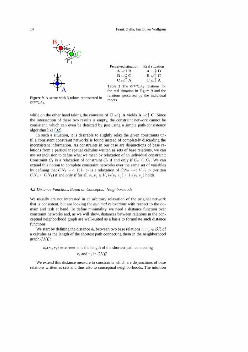
Let us consider a small example involving three robots as illustrated in Figure 9.The robotsA,B,C are solving some task as a team and all have a limited viewangle (indicated by the dashed lines) which in this case means thatA only seesB,B only seesC andC only seesA. They represent information about the currentsituation in the form of qualitative spatial relations from theOPRA2 calculus andhave the ability to communicate with each other to exchange information on whatthey currently perceive. This results in a common world model including informa-tion not available to the individual robot (e.g. the information about the other robotthat is currently outside their view). However, the combined world model does notneed to be consistent. In our case, due to slight errors in the perception of robotB,the relations perceived by the robots could be as shown in Table 2.

The corresponding constraint network is inconsistent as the configuration de-scribed by these three relations is not satisfiable in the domain of oriented points.For instance, the composition ofA 2∠5

7 B andB 2∠50 C yieldsA 2∠{5−7}

{5−7} C,

14 Frank Dylla, Jan Oliver Wallgrün

B

C

AFigure 9 A scene with 3 robots represented inOPRA2.

Perceived situation Real situationA 2∠5

7 B A 2∠57 B

B 2∠50 C B 2∠5

7 CC 2∠7

1 A C 2∠71 A

Table 2 The OPRA2 relations forthe real situation in Figure 9 and therelations perceived by the individualrobots.

while on the other hand taking the converse ofC 2∠71 A yieldsA 2∠1

7 C. Sincethe intersection of these two results is empty, the constraint network cannot beconsistent, which can even be detected by just using a simple path-consistencyalgorithm like [32].

In such a situation, it is desirable to slightly relax the given constraints un-til a consistent constraint networks is found instead of completely discarding theinconsistent information. As constraints in our case are disjunctions of base re-lations from a particular spatial calculus written as sets of base relations, we canuse set inclusion to define what we mean by relaxation of an individual constraint:ConstraintC1 is a relaxation of constraintC2 if and only if C2 ⊆ C1. We canextend this notion to complete constraint networks over the same set of variablesby defining thatCN1 =< V, l1 > is a relaxation ofCN2 =< V, l2 > (writtenCN2 ⊆ CN1) if and only if for all vi, vj ∈ V , l2(vi, vj) ⊆ l1(vi, vj) holds.

4.2 Distance Functions Based on Conceptual Neighborhoods

We usually are not interested in an arbitrary relaxation of the original networkthat is consistent, but are looking forminimal relaxationswith respect to the do-main and task at hand. To define minimality, we need a distance function overconstraint networks and, as we will show, distances between relations in the con-ceptual neighborhood graph are well-suited as a basis to formulate such distancefunctions.

We start by defining the distancedb between two base relationsri, rj ∈ BR ofa calculus as the length of the shortest path connecting them in the neighborhoodgraphCNG:

db(ri, rj) = x ⇐⇒ x is the length of the shortest path connecting

ri andrj in CNG

We extend this distance measure to constraints which are disjunctions of baserelations written as sets and thus also to conceptual neighborhoods. The intuition

Qualitative Spatial Reasoning with Conceptual Neighborhoods for Agent Control 15

behind this extension is that the distance should correspond to the number of timeswe have to apply therelax operation from Section 3.1 to one of the sets untilthe result contains all the relations from the other set. This corresponds to takingthe symmetric Hausdorff distance between the two sets based ondb. We thereforedefine the distancedc(S, R) between two sets of base relationsS, R ∈ 2BR as:

dc(S, R) = max{h(S, R), h(R,S)}

where

h(S, R) = maxs∈S

(minr∈R

db(s, r))

How this distance function for individual constraints should be extended toconstraint networks over the same set of variables is dependent on the concrete ap-plication considered since the resulting distance function describes what we con-sider similar in the given context. Things that one might want to minimize in agiven application could for example be the following:

– the number of corresponding constraints that differ in constraint networksCN1

andCN2:

ConstraintsChanged(CN1, CN2) = | {(vi, vj) | vi, vj ∈ V ∧l1(vi, vj) 6= l2(vi, vj)} |

– the maximal distance between corresponding constraints as given bydc:

MaxChangedDistance(CN1, CN2) = maxvi,vj∈V

dc (l1(vi, vj), l2(vi, vj))

– the overall sum of distances between corresponding constraints as given bydc:

SumOfDistances(CN1, CN2) =∑

vi,vj∈V

dc (l1(vi, vj), l2(vi, vj))

Such measures can be arbitrarily combined to define an overall distance func-tion dCN over the space of constraint networks over the same set of variables andthe same set of relational constraints, for example by taking the weighted sum:

dCN (CN1, CN2) = α ConstraintsChanged(CN1, CN2)+ β MaxChangedDistance(CN1, CN2)+ γ SumOfDistances(CN1, CN2)

16 Frank Dylla, Jan Oliver Wallgrün

4.3 Minimal Relaxations

Finding the minimal relaxation means that we have to solve a combinatorial opti-mization problem in which the cost function is given by our distance functiondCN

with respect to the original constraint network. We assume that all constraints inour original network are conceptual neighborhoods. Relaxed constraint networksare constructed by applying therelax function to individual constraints so thatthey are replaced by the next bigger conceptual neighborhood.

LetRCCN be the set of all constraint networks which are relaxations of a givenconstraint networkCN and consistent:

RCCN = { N | CN ⊆ N ∧ N is consistent}

The goal of the relaxation process now is to find a constraint networkCN∗ ∈RCCN that is closest toCN according to the distance functiondCN chosen. Wecall such a network aminimal consistent relaxationof CN 5:

CN∗ = argminN∈RCCN

dCN (N,CN)

The number of possible relaxations isnl wheren is the number of constraints(which is proportional to|V |2) andl is the diameter of the constraint graph whichmeans a constraint can be relaxed at mostl times. If the distance to the originalnetwork grows monotonically whenever therelax operator is applied to a con-straint, a general algorithm similar to Dijkstra’s shortest path algorithm can beused to find a minimal relaxation. Constraint networks would then be stored in apriority queue sorted by increasing distance from the original constraint network.In every step the first network is taken from the queue and checked for consistency.If it is not consistent several new networks are generated by applyingrelax to oneof the constraints of the current network. These new networks are then sorted intothe queue. If the inspected network is consistent, it has to be a minimal consistentrelaxation.

However, for certain distance functions it is possible to directly enumerate therelaxations in order of increasing distance without the need of keeping multipleconstraint networks stored in a queue. Provided we have such an enumerationfunction generateRelaxation(N) that generates the next relaxation from thecurrently considered relaxationN with respect to the distance function, and wehave a functionconsistency(N) that decides the consistency of networkN ,we can define a recursive functionmcr(CN) that computes a minimal consistentrelaxation of a given networkCN as follows:

mcr(CN) ={

CN : if consistent(CN)mcr(generateRelaxation(CN)) : otherwise

5 Note, thatCN∗ is not well-defined, as several minimal consistent relaxations may exist.

Qualitative Spatial Reasoning with Conceptual Neighborhoods for Agent Control 17

In our example case, we are dealing with noisy sensor information. Therefore,we want our overall distance functiond to combineMaxChangedDistance andSumOfDistances in a way thatMaxChangedDistance is given precedence overSumOfDistances. This means, that given two different relaxationsCN1, CN2 ofCN , MaxChangedDistance(CN1, CN) > MaxChangedDistance(CN2, CN)implies d(CN1, CN) > d(CN2, CN). Only if MaxChangedDistance is thesame forCN1 andCN2, SumOfDistances would be used to decide which one iscloser toCN . Employing this distance is very appropriate for our application sinceit prefers relaxations with multiple small changes over few large changes while,as a second criterion, minimizing the overall sum of changes. In applications inwhich few large outliers are more likely than many small changes, a combina-tion of ConstraintsChanged andSumOfDistances would have been the betterchoice.

For many applications, a reasonable distance function will give strict prece-dence of one criterion over another. In principal, these can still be formulated asa weighted sum by choosing the weights accordingly. Moreover, in most cases itshould be possible to formulate direct enumeration algorithms. The enumerationfunction we used for our example together with the networks considered can befound on our website6. For simplicity we assume that our robots can either rotateon the spot or move straight in the direction they are facing and employ the cor-responding neighborhood structure as discussed in Section 3.3.4. The result is oneof the following two possible minimal consistent relaxations:

A 2∠57 B A 2∠5

7 BB 2∠5

7 C and B 2∠67 C

C 2∠71 A C 2∠7

1 A

The original situation is correctly described by the first of these two solutionsbut the other would have been just as likely given the inconsistent information.Even if the agents follow a conservative policy and only accept what holds in allminimal consistent relaxations, they still are able to determine the position of therobot not visible to them, just not the exact orientation ofC with respect toB.

Even though we can generate relaxations in order of increasing distance to theoriginal constraint network, the huge number of possible relaxations means thatonly for problems in which the minimal consistent relaxations are rather close tothe original network can be relaxed in appropriate time. In our case, it would bereasonable to assume that no perceived relation will be further from the actual re-lation by more than 2 with respect todb. Therefore, if no corresponding consistentrelaxation withMaxChangedDistance ≤ 2 would have been found, the relaxationprocess could have been stopped, as obviously something unexpected must havehappened.

To summarize, as we have shown conceptual neighborhoods can serve as ameaningful and well-defined basis for optimizing the relaxation process in con-straint networks. Minimal relaxation can be defined based on minimal neighbor-hood distance. However, as a prerequisite the adequate neighborhood structure for

6 http://www.sfbtr8.uni-bremen.de/project/r3/relaxation/

18 Frank Dylla, Jan Oliver Wallgrün

l

A BC

b ir

fes

Figure 10 The reference frame for the FlipFlop Calculus.

the application at hand needs to be known. Since manually deriving neighbor-hood structures can be a very tedious process, tools to automate the derivation arerequired. We will now present a method that exploits the formalization of the rela-tions of a new calculus in another calculus with known neighborhood structure toautomatically deduce the neighboring structure of the new calculus.

5 Deriving Conceptual Neighborhoods for Qualitative Calculi inOPRAm

Since not always adequate calculi are available for specific tasks, new ones haveto be developed. Determing the operations and properties of a new calculus is anerror-prone and time-consuming process. Modeling one spatial calculus in anotherone has been shown to be helpful for determining the properties and operations ofa new calculus. In [23,24] the Dependency Calculus is presented and its propertiesare derived by mapping it onto the Region Connection Calculus [26]. In [7] it isshown howOPRAm representations of other orientation calculi can be utilizedto automatically compute composition tables.

This section proceeds in a similar way. We introduce two more orientation cal-culi, then show how to model their base relations inOPRAm, and finally usethese models and our knowledge aboutOPRAm neighborhood structures to de-rive the neighborhood relations of the two calculi. The calculi considered are theFlipFlop calculus (FFC) and the fine-grained Dipole Relation Algebra (DRAf ).

5.1 The FlipFlop Calculus (FFC)

The FlipFlop calculus proposed in [16] describes the position of a pointC (thereferent) in the plane with respect to two other pointsA (the origin) andB (therelatum) as illustrated in Figure 10. FFC relations are only defined forA 6= B. Thefollowing base relations are distinguished:C can be to theleft or to ther ight of theoriented line going throughA andB, or C can be placed on the line resulting inone of the five relationsinside,front,back,start (C = A) or end (C = B) resultingin 7 base relations overall. A FFC relationrelFFC is written asA,B relFFC C,e.g.A,B r C as depicted in Figure 10.

5.2 Encoding the FlipFlop Calculus inOPRAm

To encode the seven ternary FlipFlop base relationsA,B relFFC C in OPRA1

based on the three normal pointsA, B, andC, we use the two oriented pointsAAC

Qualitative Spatial Reasoning with Conceptual Neighborhoods for Agent Control 19

A, B rFFC C AAC rOPRA1 BBC AAC rOPRA1 C BBC rOPRA1 C

front AAC1∠2

0 BBC AAC1∠∗0 C BBC

1∠∗0 Cend AAC

1∠∗0 BBC AAC1∠∗0 C BBC

1∠∗ Cinside AAC

1∠00 BBC AAC

1∠∗0 C BAC1∠∗0 C

start AAC1∠0∗ BBC AAC

1∠∗ C BBC1∠∗0 C

back AAC1∠0

2 BBC AAC1∠∗0 C BBC

1∠∗0 Cleft AAC

1∠13 BBC AAC

1∠∗0 C BBC1∠∗0 C

r ight AAC1∠3

1 BBC AAC1∠∗0 C BBC

1∠∗0 C

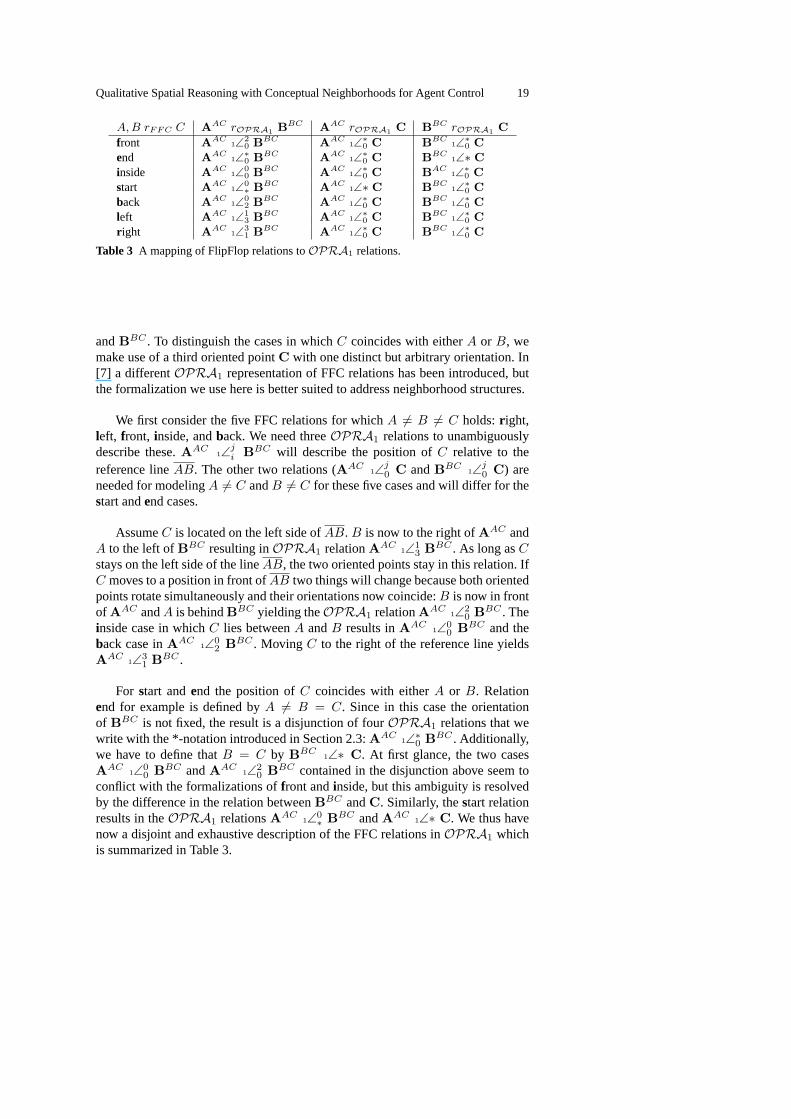
Table 3 A mapping of FlipFlop relations toOPRA1 relations.

andBBC . To distinguish the cases in whichC coincides with eitherA or B, wemake use of a third oriented pointC with one distinct but arbitrary orientation. In[7] a differentOPRA1 representation of FFC relations has been introduced, butthe formalization we use here is better suited to address neighborhood structures.

We first consider the five FFC relations for whichA 6= B 6= C holds:r ight,left, front, inside, andback. We need threeOPRA1 relations to unambiguouslydescribe these.AAC

1∠ji BBC will describe the position ofC relative to the

reference lineAB. The other two relations (AAC1∠j

0 C andBBC1∠j

0 C) areneeded for modelingA 6= C andB 6= C for these five cases and will differ for thestart andend cases.

AssumeC is located on the left side ofAB. B is now to the right ofAAC andA to the left ofBBC resulting inOPRA1 relationAAC

1∠13 BBC . As long asC

stays on the left side of the lineAB, the two oriented points stay in this relation. IfC moves to a position in front ofAB two things will change because both orientedpoints rotate simultaneously and their orientations now coincide:B is now in frontof AAC andA is behindBBC yielding theOPRA1 relationAAC

1∠20 BBC . The

inside case in whichC lies betweenA andB results inAAC1∠0

0 BBC and theback case inAAC

1∠02 BBC . Moving C to the right of the reference line yields

AAC1∠3

1 BBC .

For start andend the position ofC coincides with eitherA or B. Relationend for example is defined byA 6= B = C. Since in this case the orientationof BBC is not fixed, the result is a disjunction of fourOPRA1 relations that wewrite with the *-notation introduced in Section 2.3:AAC

1∠∗0 BBC . Additionally,we have to define thatB = C by BBC

1∠∗ C. At first glance, the two casesAAC

1∠00 BBC andAAC

1∠20 BBC contained in the disjunction above seem to

conflict with the formalizations offront andinside, but this ambiguity is resolvedby the difference in the relation betweenBBC andC. Similarly, thestart relationresults in theOPRA1 relationsAAC

1∠0∗ BBC andAAC

1∠∗ C. We thus havenow a disjoint and exhaustive description of the FFC relations inOPRA1 whichis summarized in Table 3.

20 Frank Dylla, Jan Oliver Wallgrün

endstartback frontinside

left

right

Figure 11 The conceptual neighborhood structure of the FlipFlop Calculus.

5.3 Deriving theCNG for FFC

Now we derive the general neighborhood structure of FFC from the general neigh-borhood structure ofOPRA1 described in Section 3.3.5. SinceA andB are notallowed to coincide in the FFC definition, we can restrict ourselves to considercases in which onlyC is allowed to move. Nevertheless, the corresponding ori-ented pointC is part of all three relations in theOPRA1 formalization and thusall three relations can change simultaneously.

The general idea of the algorithm for deriving theCNG is to combine theindividual conceptual neighbors of the threeOPRA1 relations and check theresulting constraint networks for consistency to find out whether the generatedformalizations describe valid FFC relations. We abbreviate theOPRA1 modelAAC S1 BBC ∧ AAC S2 C ∧ BBC S3 C of a FCC relation (as providedby Table 3) as a triple(S1, S2, S3) where theSi again are sets of base relations.The set of combinations that need to be checked for a given triple(S1, S2, S3) canthen be specified with the help of therelax function (defined in Section 3.1) as(relax(S1)× relax(S2)× relax(S3)) \ (S1 × S2 × S3).

For the FFC relationfront, we check all combinations from the following threesets except those which are combinations of base relations already contained inS1,S2, andS3:

relax(S1) = relax({1∠20}) = {1∠2

0,1∠13, 1∠2

3, 1∠33, 1∠1

0, 1∠30, 1∠1

1, 1∠21, 1∠3

1}relax(S2) = relax(S3) = relax(1∠∗0) = {1∠∗01∠∗3, 1∠∗1, 1∠∗}

From all these combinations that were checked for consistency with the SparQtoolbox [5], all consistent networks fall into one of three classes from Table 3.These are(1∠1

3, 1∠∗0, 1∠∗0) for left, (1∠31, 1∠∗0, 1∠∗0) for r ight, and(1∠∗0, 1∠∗0, 1∠∗)

for end. These three FFC relations are indeed the correct conceptual neighbors ofthefront relation. Applying this method to the other base relations yields theCNGshown in Figure 11.

5.4 The Fine-Grained Dipole Relation Algebra (DRAf )

A dipole is an oriented line segment as e.g. determined by a start and an endpoint. We will write dAB for a dipole defined by start pointA and end pointB.

Qualitative Spatial Reasoning with Conceptual Neighborhoods for Agent Control 21

A B

C

D

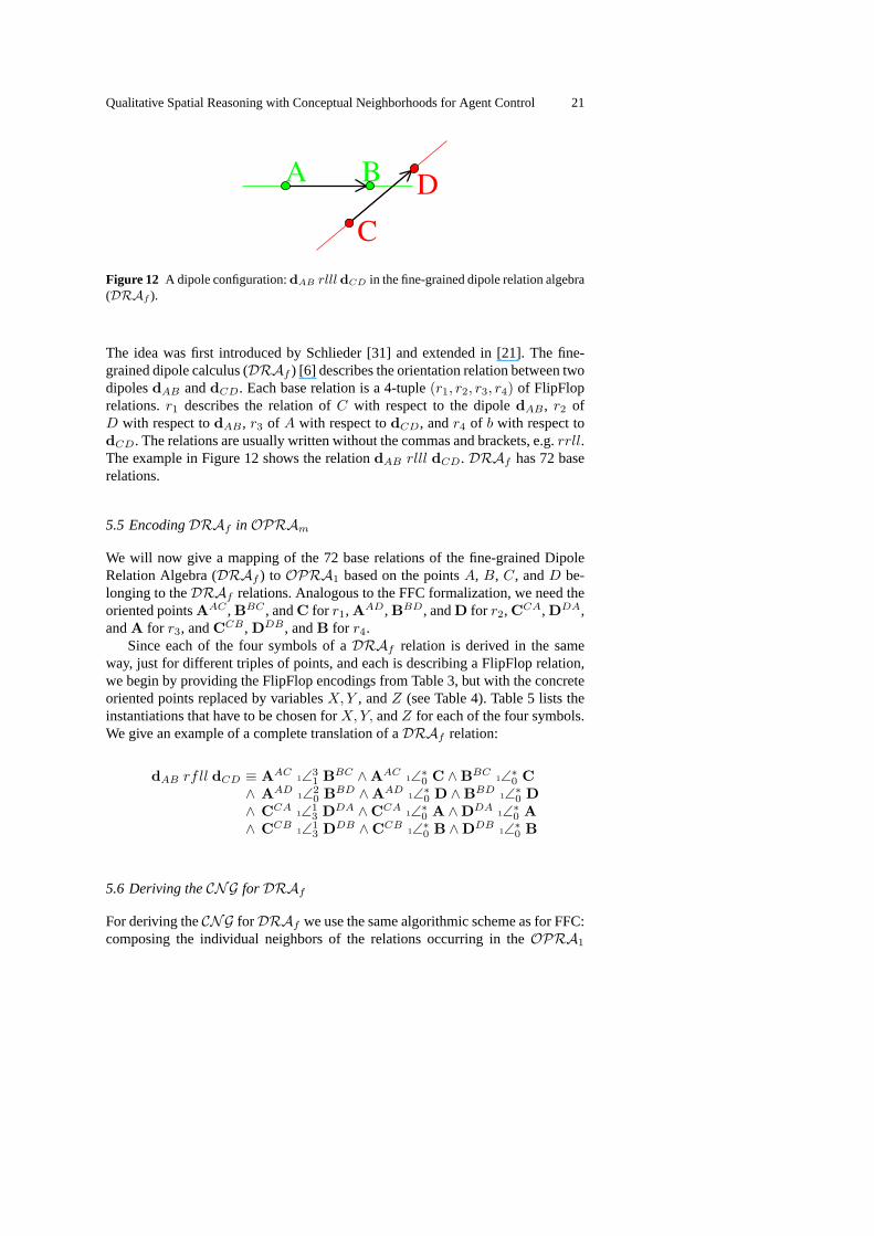
Figure 12 A dipole configuration:dAB rlll dCD in the fine-grained dipole relation algebra(DRAf ).

The idea was first introduced by Schlieder [31] and extended in [21]. The fine-grained dipole calculus (DRAf ) [6] describes the orientation relation between twodipolesdAB anddCD. Each base relation is a 4-tuple(r1, r2, r3, r4) of FlipFloprelations.r1 describes the relation ofC with respect to the dipoledAB , r2 ofD with respect todAB , r3 of A with respect todCD, andr4 of b with respect todCD. The relations are usually written without the commas and brackets, e.g.rrll.The example in Figure 12 shows the relationdAB rlll dCD. DRAf has 72 baserelations.

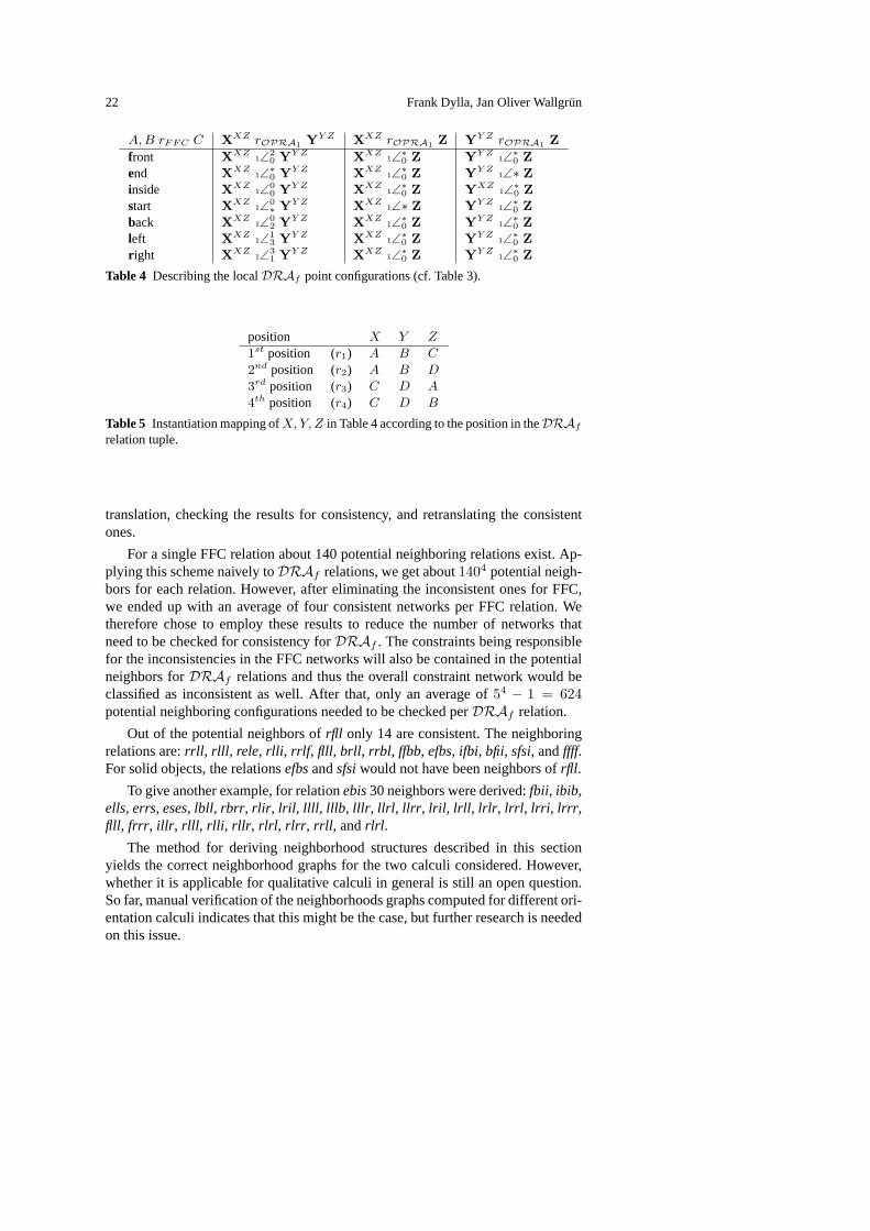
5.5 EncodingDRAf in OPRAm

We will now give a mapping of the 72 base relations of the fine-grained DipoleRelation Algebra (DRAf ) to OPRA1 based on the pointsA, B, C, andD be-longing to theDRAf relations. Analogous to the FFC formalization, we need theoriented pointsAAC , BBC , andC for r1, AAD, BBD, andD for r2, CCA, DDA,andA for r3, andCCB , DDB , andB for r4.

Since each of the four symbols of aDRAf relation is derived in the sameway, just for different triples of points, and each is describing a FlipFlop relation,we begin by providing the FlipFlop encodings from Table 3, but with the concreteoriented points replaced by variablesX, Y , andZ (see Table 4). Table 5 lists theinstantiations that have to be chosen forX, Y, andZ for each of the four symbols.We give an example of a complete translation of aDRAf relation:

dAB rfll dCD ≡ AAC1∠3

1 BBC ∧AAC1∠∗0 C ∧BBC

1∠∗0 C∧ AAD

1∠20 BBD ∧AAD

1∠∗0 D ∧BBD1∠∗0 D

∧ CCA1∠1

3 DDA ∧CCA1∠∗0 A ∧DDA

1∠∗0 A∧ CCB

1∠13 DDB ∧CCB

1∠∗0 B ∧DDB1∠∗0 B

5.6 Deriving theCNG for DRAf

For deriving theCNG forDRAf we use the same algorithmic scheme as for FFC:composing the individual neighbors of the relations occurring in theOPRA1

22 Frank Dylla, Jan Oliver Wallgrün

A, B rFFC C XXZ rOPRA1 YY Z XXZ rOPRA1 Z YY Z rOPRA1 Z

front XXZ1∠2

0 YY Z XXZ1∠∗0 Z YY Z

1∠∗0 Zend XXZ

1∠∗0 YY Z XXZ1∠∗0 Z YY Z

1∠∗ Zinside XXZ

1∠00 YY Z XXZ

1∠∗0 Z YXZ1∠∗0 Z

start XXZ1∠0∗ YY Z XXZ

1∠∗ Z YY Z1∠∗0 Z

back XXZ1∠0

2 YY Z XXZ1∠∗0 Z YY Z

1∠∗0 Zleft XXZ

1∠13 YY Z XXZ

1∠∗0 Z YY Z1∠∗0 Z

r ight XXZ1∠3

1 YY Z XXZ1∠∗0 Z YY Z

1∠∗0 Z

Table 4 Describing the localDRAf point configurations (cf. Table 3).

position X Y Z

1st position (r1) A B C

2nd position (r2) A B D

3rd position (r3) C D A

4th position (r4) C D B

Table 5 Instantiation mapping ofX, Y, Z in Table 4 according to the position in theDRAf

relation tuple.

translation, checking the results for consistency, and retranslating the consistentones.

For a single FFC relation about 140 potential neighboring relations exist. Ap-plying this scheme naively toDRAf relations, we get about1404 potential neigh-bors for each relation. However, after eliminating the inconsistent ones for FFC,we ended up with an average of four consistent networks per FFC relation. Wetherefore chose to employ these results to reduce the number of networks thatneed to be checked for consistency forDRAf . The constraints being responsiblefor the inconsistencies in the FFC networks will also be contained in the potentialneighbors forDRAf relations and thus the overall constraint network would beclassified as inconsistent as well. After that, only an average of54 − 1 = 624potential neighboring configurations needed to be checked perDRAf relation.

Out of the potential neighbors ofrfll only 14 are consistent. The neighboringrelations are:rrll , rlll , rele, rlli , rrlf , flll , brll , rrbl , ffbb, efbs, ifbi, bfii, sfsi, andffff.For solid objects, the relationsefbsandsfsiwould not have been neighbors ofrfll .

To give another example, for relationebis30 neighbors were derived:fbii, ibib,ells, errs, eses, lbll , rbrr , rlir , lril , llll , lllb , lllr , llrl , llrr , lril , lrll , lrlr , lrrl , lrri , lrrr ,flll , frrr , illr , rlll , rlli , rllr , rlrl , rlrr , rrll , andrlrl .

The method for deriving neighborhood structures described in this sectionyields the correct neighborhood graphs for the two calculi considered. However,whether it is applicable for qualitative calculi in general is still an open question.So far, manual verification of the neighborhoods graphs computed for different ori-entation calculi indicates that this might be the case, but further research is neededon this issue.

Qualitative Spatial Reasoning with Conceptual Neighborhoods for Agent Control 23

6 Conclusion

In this paper, we investigated the idea of conceptual neighborhood in the context ofrobot control tasks and world modeling. We have shown that conceptual neighbor-hoods are well-suited to provide information about how the world might developon a high level of abstraction. Using the example of theOPRAm calculus, westudied how neighborhood structures are affected by such task and environment-specific parameters like robot motion capabilities, the dynamic of the objects in-volved, and whether objects are able to superpose or not. As an exemplary appli-cation of conceptual neighborhoods, we showed how these structures can be ex-ploited for resolving conflicting knowledge about the world, e.g. as arising throughnoisy sensor readings.

As often no adequate calculus is available for a specific task, new ones have tobe developed and methods to automate this are needed. We showed that expressingthe relations of a new calculus in a different well-specified calculus is one way inwhich this automation can be achieved.

TheOPRAm calculus is a very suitable calculus for formalizing other orien-tation calculi as it is expressive enough to unambiguously describe the relationsof most other orientation calculi as configurations of a rather small number of ori-ented points. We presented theOPRAm formalizations for the FlipFlop Calculusand the fine-grained Dipole Relation Algebra, and will continue to do so for otherspatial calculi.

Other benefits of the mappings between different calculi still need to be investi-gated. In addition, the idea of complex neighborhood graphs that represent possiblechanges of spatial relations for more than two objects needs further investigation.In principle, the approach presented in Section 5 computes neighboring configura-tions forOPRAm configurations of more than two objects. We intend to continuework in this direction in order to improve the applicability of neighborhood-basedplanning in complex dynamic situations.

AcknowledgementsThe authors would like to thank Lutz Frommberger, DiedrichWolter, Reinhard Moratz, and Christian Freksa for fruitful discussions and impulses. Ourwork was supported by the DFG Transregional Collaborative Research Center SFB/TR 8Spatial Cognition.

References

1. B. Bennett and A. P. Galton. A unifying semantics for time and events.ArtificialIntelligence, 153(1-2):13–48, March 2004.

2. A. G. Cohn. Qualitative spatial representation and reasoning techniques. In G. Brewka,C. Habel, and B. Nebel, editors,KI-97: Advances in Artificial Intelligence, 21st AnnualGerman Conference on Artificial Intelligence, Freiburg, Germany, September 9-12,1997, Proceedings, volume 1303 ofLecture Notes in Computer Science, pages 1–30,Berlin, 1997. Springer.

3. A. G. Cohn and S. M. Hazarika. Qualitative spatial representation and reasoning: Anoverview.Fundamenta Informaticae, 46(1-2):1–29, 2001.

24 Frank Dylla, Jan Oliver Wallgrün

4. E. Davis. Continuous shape transformation and metrics of shape. InFundamentaInformaticae, volume 46, pages 31–54. May 2001.

5. F. Dylla, L. Frommberger, J. O. Wallgrün, and D. Wolter. SparQ: A toolbox for qualita-tive spatial representation and reasoning. InProceedings of the Workshop on Qualita-tive Constraint Calculi: Application and Integration at KI 2006, pages 79–90, Bremen,Germany, June 2006.

6. F. Dylla and R. Moratz. Exploiting qualitative spatial neighborhoods in the situationcalculus. In C. Freksa, M. Knauff, B. Krieg-Brückner, B. Nebel, and T. Barkowsky,editors,Spatial Cognition IV. Reasoning, Action, Interaction: International ConferenceSpatial Cognition 2004, volume 3343 ofLecture Notes in Artificial Intelligence, pages304–322. Springer, Berlin, Heidelberg, 2005.

7. F. Dylla and J. O. Wallgrün. On generalizing orientation information inOPRAm.In Proceedings of the 29th German Conference on Artificial Intelligence (KI 2006),Bremen, Germany, June 2006.

8. M. J. Egenhofer. A formal definition of binary topological relationships. In3rd In-ternational Conference on Foundations of Data Organization and Algorithms, pages457–472, New York, NY, USA, 1989. Springer.

9. A. Frank. Qualitative spatial reasoning about cardinal directions. InProceedings ofthe American Congress on Surveying and Mapping (ACSM-ASPRS), pages 148–167,Baltimore, Maryland, USA, 1991.

10. C. Freksa. Conceptual neighborhood and its role in temporal and spatial reasoning. InM. G. Singh and L. Travé-Massuyès, editors,Proceedings of the IMACS Workshop onDecision Support Systems and Qualitative Reasoning, pages 181–187, North-Holland,Amsterdam, 1991. Elsevier.

11. C. Freksa. Using orientation information for qualitative spatial reasoning. In A. U.Frank, I. Campari, and U. Formentini, editors,Theories and methods of spatio-temporalreasoning in geographic space, pages 162–178. Springer, Berlin, 1992.

12. C. Freksa. Spatial Cognition – An AI Prespective. InProceedings of 16th EuropeanConference on AI (ECAI 2004), 2004.

13. A. Galton. Continuous motion in discrete space. In A. Cohn, F. Giunchiglia, and B. Sel-man, editors,Proc. 7th Internat. Conf. on Principles of Knowledge Representation andReasoning (KR2000), pages 26–37. Morgan Kaufmann, San Francisco, CA, 2000.

14. A. Galton.Qualitative Spatial Change. Oxford University Press, 2000.15. P. Ladkin and A. Reinefeld. Effective solution of qualitative constraint problems.Arti-

ficial Intelligence, 57:105–124, 1992.16. G. Ligozat. Qualitative triangulation for spatial reasoning. In A. U. Frank and I. Cam-

pari, editors,Spatial Information Theory: A Theoretical Basis for GIS, (COSIT’93),Marciana Marina, Elba Island, Italy, volume 716 ofLecture Notes in Computer Sci-ence, pages 54–68. Springer, 1993.

17. R. Moratz. Intuitive linguistic joint object reference in human-robot interaction. InProceedings of the Twenty-First National Conference on Artificial Intelligence (AAAI),Boston, Massachusetts, 2006. to appear.

18. R. Moratz. Representing relative direction as a binary relation of oriented points. InECAI 2006 Proceedings of the 17th European Conference on Artificial Intelligence,2006. to appear.

19. R. Moratz, F. Dylla, and L. Frommberger. A relative orientation algebra with adjustablegranularity. InProceedings of the Workshop on Agents in Real-Time and DynamicEnvironments (IJCAI 05), 2005.

20. R. Moratz and C. Freksa. Spatial reasoning with uncertain data using stochastic re-laxation. In W. Brauer, editor,Fuzzy-Neuro Systems 98, pages 106–112. Infix; SanktAugustin, 1998.

Qualitative Spatial Reasoning with Conceptual Neighborhoods for Agent Control 25

21. R. Moratz, J. Renz, and D. Wolter. Qualitative spatial reasoning about line segments. InW. Horn, editor,Proceedings of the 14th European Conference on Artificial Intelligence(ECAI), Berlin, Germany, 2000. IOS Press.

22. P. Muller. A qualitative theory of motion based on spatio-temporal primitives. In A. G.Cohn, L. Schubert, and S. C. Shapiro, editors,KR’98: Principles of Knowledge Repre-sentation and Reasoning, pages 131–141. Morgan Kaufmann, San Francisco, Califor-nia, 1998.

23. M. Ragni and A. Scivos. Dependency calculus: Reasoning in a general point relationalgebra. InProceedings of the 28th German Conference on Artificial Intelligence (KI2005), pages 49–63, Koblenz, Germany, Sept. 2005.

24. M. Ragni and A. Scivos. Dependency calculus reasoning in a general point relationalgebra. In L. P. Kaelbling and A. Saffiotti, editors,IJCAI-05, Proceedings of the Nine-teenth International Joint Conference on Artificial Intelligence, Edinburgh, Scotland,UK, July 30-August 5, 2005, pages 1577–1578. Professional Book Center, 2005.

25. M. Ragni and S. Wölfl. Temporalizing spatial calculi—on generalized neighborhoodgraphs. InProceedings of the 28th German Conference on Artificial Intelligence (KI2005), Koblenz, Germany, Sept. 2005.

26. D. A. Randell, Z. Cui, and A. Cohn. A spatial logic based on regions and connection.In B. Nebel, C. Rich, and W. Swartout, editors,Principles of Knowledge Representa-tion and Reasoning: Proceedings of the Third International Conference (KR’92), pages165–176. Morgan Kaufmann, San Mateo, California, 1992.

27. J. Renz and G. Ligozat. Weak composition for qualitative spatial and temporal rea-soning. InPrinciples and Practice of Constraint Programming - CP 2005, 11th Inter-national Conference, CP 2005, Sitges, Spain, October 1-5, 2005, Proceedings, volume3709 ofLNCS, pages 534–548. Springer, 2005.

28. J. Renz and D. Mitra. Qualitative direction calculi with arbitrary granularity. InC. Zhang, H. W. Guesgen, and W.-K. Yeap, editors,PRICAI 2004: Trends in ArtificialIntelligence, 8th Pacific RimInternational Conference on Artificial Intelligence, Auck-land, New Zealand, Proceedings, volume 3157 ofLecture Notes in Computer Science,pages 65–74. Springer, 2004.

29. J. Renz and B. Nebel. On the complexity of qualitative spatial reasoning: A maximaltractable fragment of the region connection calculus.Artificial Intelligence, 108(1-2):69–123, 1999.

30. T. Röfer. Route navigation using motion analysis. In C. Freksa and D. M. Mark,editors,Spatial Information Theory: Foundations of Geographic Information Science.Conference on Spatial Information Theory (COSIT), pages 21–36. Springer, Berlin,1999.

31. C. Schlieder. Reasoning about ordering. InSpatial Information Theory: A TheoreticalBasis for GIS (COSIT’95), volume 988 ofLecture Notes in Computer Science, pages341–349. Springer, Berlin, Heidelberg, 1995.

32. P. van Beek. Reasoning about qualitative temporal information.Artificial Intelligence,58(1-3):297–321, 1992.