the relationship between imf broad based index of financial ...
27
PREPRINT 1 THE RELATIONSHIP BETWEEN IMF BROAD BASED INDEX OF FINANCIAL DEVELOPMENT AND INTERNATIONAL TRADE: EVIDENCE FROM INDIA Ummuhabeeba Chaliyan Doctoral Candidate, Department of Economics and Finance, Birla Institute of Technology and Science Pilani Hyderabad campus (Email: [email protected]) Mini P. Thomas Assistant Professor, Department of Economics and Finance, Birla Institute of Technology and Science Pilani Hyderabad campus (Email: [email protected])
-
Upload
khangminh22 -
Category
Documents
-
view
1 -
download
0
Transcript of the relationship between imf broad based index of financial ...
PREPRINT
1
THE RELATIONSHIP BETWEEN IMF BROAD BASED INDEX OF
FINANCIAL DEVELOPMENT AND INTERNATIONAL TRADE:
EVIDENCE FROM INDIA
Ummuhabeeba Chaliyan
Doctoral Candidate,
Department of Economics and Finance,
Birla Institute of Technology and Science Pilani Hyderabad campus
(Email: [email protected])
Mini P. Thomas
Assistant Professor,
Department of Economics and Finance,
Birla Institute of Technology and Science Pilani Hyderabad campus
(Email: [email protected])
PREPRINT
2
THE RELATIONSHIP BETWEEN IMF BROAD BASED INDEX OF
FINANCIAL DEVELOPMENT AND INTERNATIONAL TRADE:
EVIDENCE FROM INDIA
Ummuhabeeba Chaliyan Mini P. Thomas
Abstract
This study investigates whether a uni-directional or bi-directional causal relationship exists
between financial development and international trade for Indian economy, during the time
period from 1980 to 2019. Three measures of financial development created by IMF, namely,
financial institutional development index, financial market development index and a composite
index of financial development is utilized for the empirical analysis. Johansen cointegration,
vector error correction model and vector auto regressive model are estimated to examine the long
run relationship and short run dynamics among the variables of interest. The econometric results
indicate that there is indeed a long run association between the composite index of financial
development and trade openness. Cointegration is also found to exist between trade openness and
index of financial market development. However, there is no evidence of cointegration between
financial institutional development and trade openness. Granger causality test results indicate the
presence of uni-directional causality running from composite index of financial development to
trade openness. Financial market development is also found to Granger cause trade openness.
Empirical evidence thus underlines the importance of formulating policies which recognize the
role of well-developed financial markets in promoting international trade.
Key words: Financial Development, Financial Market Development, Financial Institutional
Development, Trade openness, Cointegration, VEC, VAR
JEL Classification: F14, G1, C01
PREPRINT
3
Introduction
Financial development and international trade are key drivers of the economic growth
performance of a country. India has a strongly diversified financial sector comprising
commercial banks, insurance companies, non-banking financial companies, cooperatives,
pension funds and mutual funds. Financial sector reforms initiated in India in the 1990s, based
on the report by Narasimhan Committee, mainly focused on banking system and capital market.
The reforms aimed at putting an end to the then prevailing regime of financial repression, enable
price discovery by the market determination of interest rates, and maintain financial stability
even in the face of domestic or external shocks (RBI 2007). Financial development, measured as
domestic credit to private sector as percentage of GDP, rose from 20.5 in 1980 to 50.15 in 2019
for Indian economy. It peaked at 52.4 percent in 2013. Interestingly, banks have provided more
than 50 percent of the domestic credit requirement of private sector in India since 2010 (World
Bank 2019). The state of development of financial sector varies across countries. Consequently,
there has been rigorous debate about the desirable mode of financial system. At the same time,
international trade liberalization achieved through the adoption of several trade liberalization
policies in different years. An important wave in this respect was the implementation of 5 years
Export Import (EXIM) policy in 1992.For India, Trade openness to GDP ratio stood at 15.4
percent in 1980, after which it steadily rose and attained a peak of 55.8 percent in 2012. It has
exhibited a declining trend ever since and stood to 40.01 in 2019 (World Bank 2019).
Financial development is increasingly becoming an important contributor to the economic
growth of countries. Seminal work by (Goldsmith 1969), (McKinnon 1973) and (Shaw 1973) have
analyzed the role of financial intermediaries in boosting long run growth of economies. Other
theoretical studies also contributed to the debate in the successive years, which include (Levine
1997, 702, Levine and Zervos 1998, 550); (Levine, Loayza, and Beck2000, 40) and (Luintel and
Musahid 1999, 399). Another work (Murinde and Eng 1994, 400) is examining the country specific
study about Singapore for the period 1979 - 1999, finds the causality from financial development
to economic growth. Evidence obtained from the study in Turkey for the period 1989- 2007,
supports the bidirectional causality exists between financial development, trade openness and
growth (Yucel 2009). (Santana 2020, 10) found that financial liberalization negatively impacted
PREPRINT
4
upon the relationship between financial development and economic growth in Latin America,
due to the emergence and recurrence of banking crises.
Studies which examined the role of financial development in economic growth of countries are
numerous and well established in the literature, compared to studies which unravel the link
between financial development and international trade. The present study aims to examine
whether a unidirectional or bi-directional relationship exists between financial development and
international trade in case of Indian economy, by using time series techniques. This study brings
in a new dimension to existing studies on this subject, by resorting to the broad based measure of
financial development created by IMF, to account for all possible variations in the financial
system. Since financial development is a complex multidimensional variable, the typical proxies
such as ratio of private credit to GDP or stock market capitalization can’t fully account for the
concept. Broad financial development index of IMF encompasses three dimensions of efficiency,
access and depth, with respect to both financial institutions and financial markets (Svirydzenka
2016).
Literature Review
The Heckscher Ohlin and Vanek theory of international trade states that factor content of a
commodity is most important for trade. It postulates that a country well-endowed with a
particular factor will engage in the production and trade of that commodity which intensively use
the abundant factor. (Kletzer and Bardhan 1987, 65) was the first study to link credit markets to
international trade patterns. They postulated that countries with identical technology and
endowments may still differ in terms of comparative cost advantages, because of credit market
imperfections, arising from moral hazard considerations and asymmetric information. Path
breaking work by (Beck 2001, 120) theoretically modeled the role of financial intermediaries in
boosting large scale, high return projects, and proved that countries with a higher state of
financial development have a comparative advantage in manufacturing. The model was validated
using a panel dataset for 30 years for 65 countries. Trade in manufactured goods was specified as
a function of private credit as a share of GDP and other control variables such as initial level of
real per capita GDP, black market premium, real per capita capital, population and growth rate of
terms of trade. The estimation was carried out using Ordinary Least squares and Instrumental
Variable Technique. After controlling for country specific effects and possible reverse causality,
PREPRINT
5
the study found that financial development does exert a significant causal impact on two
measures of international trade, namely the level of exports and the trade balance of
manufactured goods.
Few studies (Beck 2002, 120) and (Vlachos and Svalryd 2005, 114) have analyzed the link between
financial development and international trade, from the point of view of economies of scale.
They found that financial sector can facilitate trade immensely. A well developed financial sector
can source savings to private sector and assist entrepreneurs to engage in more business
activities, thereby overcoming credit constraints. Since manufacturing sector exploits increasing
economies of scale, it can reap higher profit coupled with the high level of financial development
associated with manufacturing sector. In every country, the sector which faces demand shock has
to protect from risk. This implies that international trade patterns are highly dependent on
differences in financial development, with a highly developed financial system permitting the
country to specialize in risky goods (Baldwin 1989, 145). Availability of trade credit is determined
by the level of financial health and width of network of issuing banks. These factors can
positively contribute to the flexibility and liquidity of funding and supply of trade credit (Jain,
Gajbhiye, and Tewari 2019).
(Do and Levchenko 2004) built a theoretical model wherein international trade boosts growth of
financially dependent sectors and financial system in a wealthy country. The poor country begins
to import the financially dependent good from the rich country rather than produce it
domestically, implying a decline of the domestic financial system and demand for external
finance. The model was empirically validated using a panel dataset of 77 countries, from 1965 to
1995. Financial development was specified as a function of trade openness and control variables
such as initial level of private credit to GDP, initial per capita GDP, a measure of human capital
(average years of secondary schooling in the population), as well as legal origin dummies.
Financial development was measured using three alternative indicators, namely, the ratio of
private credit to GDP, the ratio of liquid liabilities to GDP, and claims of deposit money banks
on nonfinancial domestic sectors as share of GDP. This study thus provides theoretical and
empirical basis for direction of causality running from trade openness to financial development.
As trade finance is an important factor determining flow of imports and exports, financial
development is always positively correlated with volume of trade (Liston and McNeil 2013, 13).
PREPRINT
6
Studies carried out using multi industry approach found that financial development and ratio of
export to domestic sales is positively associated in capital intensive industries, whereas the trade
share is much lower in labour intensive industries. But the net effect can be offset at the
aggregate level (Leibovici 2018). Empirical studies indicate positive short run and negative long
run association between financial development and international trade, along with unidirectional
causality running from financial development to international trade (Bilas, Bosnjak, and Novak
2017, 84). Economic growth is linked to international trade through the medium of financial
development, whereby economic growth increases financial development and thus enhances
trade participation of countries (Kar, Nazlioglu, and Agir. 2013, 139).
Countries that trade manufactured commodities can elevate the financial system of that country
because such economies demand more external finance, which leads to greater financial
development of country (Samba and Yu 2009, 65). Export oriented firms demand more external
finance to meet high fixed cost. Therefore, destabilizing financial conditions affect export
oriented firms more than it affects domestic oriented ones (Feng and Lin2013, 44). Another
interesting inter-relationship between financial development and international trade is found via
the linkage between imports and debt financed consumption. Higher domestic demand is
financed by inflow of foreign loans. Both the appreciation of domestic currency due to higher
imports and inflow of foreign loans resulted in current account deficit in European transition
countries (Aristovnik 2008; Zakharova 2008; Bakker and Gulde 2010, 120). When developing and
developed countries were analyzed separately for the period between 1961 and 2020 to assess the
linkage between financial development and international trade, financial development was found
to be a key factor which promotes trade participation of countries. The direction of causality
varied among countries, depending on their level of economic development (Kiendrebeogo 2012).
Financial development (private credit and money supply) has a positive influence on trade
volume by increasing productivity and technology up gradation through efficient allocation of
financial resources (Kaushal and Pathak 2015, 10). Another empirical study investigated the
relationship between exports, financial development and GDP growth in Pakistan by applying
the Bound testing approach to cointegration and vector error correction model (VECM) based
Granger causality test, and found the existence of the long run relationship among the variables
(Shabaz and Rahman 2014, 164). Johansen multivariate approach to cointegration found no
significant long run relation among economic growth, financial development and international
PREPRINT
7
trade for Nigeria during the time period from 1970 to 2005 (Chimobi 2010). (Arora and
Mukherjee 2020, 285) examined the nexus between financial development and trade
performance of Indian Economy using annual data from 1980 to 2016. The study resorted to the
time series technique of the Auto regressive distributed lag bound testing approach to check for
the presence of cointegration. Financial development was measured using the widely used
indicator of private credit as a percentage of GDP. International trade performance was measured
using three alternative indicators, namely, manufactured exports as a percentage of GDP,
manufactured imports as a percentage of GDP and net manufactured exports as a percentage of
GDP. International trade in primary goods and services were not covered in this study. They
found the existence of a long run equilibrium relationship between international trade in
manufactured goods and financial development and existence of unidirectional causality from
financial development to net exports of manufactured goods. Empirical evidence indicated
absence of reverse causality from international trade to financial development in case of Indian
economy.
Based on the above literature review, it is found that that there is no conclusive evidence with
regard to the direction of causality between the state of financial development and international
trade of a country. The present study is trying to contribute to this growing literature by
analyzing the linkage between financial development and international trade specifically for
Indian economy. There is a dearth of Indian studies which have examined the relationship
between financial development and international trade in aggregate (inclusive of agriculture,
manufacturing and services). This paper also adds a new dimension to the existing studies by
measuring financial development using the broad based index created by IMF. This indicator is
definitely superior to ratio of private credit to GDP, as a proxy for financial development. This
study also throws light on the nature of relationship between trade openness and two of the sub-
indices of IMF index of financial development, namely, financial market development and
financial institutional development.
Data and Methodology
The empirical model to estimate the relationship between financial development and
international trade in India is specified as given in equations (1), (2) and (3).
TRADE = f (FD, LGDP, REER) (1)
PREPRINT
8
TRADE = f (FID, LGDP, REER) (2)
TRADE = f (FMD, LGDP, REER) (3)
The term TRADE in the equations (1), (2) and (3) denote trade openness, measured as the sum of
exports and imports of a country, expressed as a percentage of GDP. FD, FID and FMD in
equations (1), (2), and (3) denote financial development, financial institutional development and
financial market development indices respectively. The term LGDP in all the three equations
represents log of GDP per capita and the term REER in all the three equations represent the real
effective exchange rate. GDP and REER are taken as control variables in the model
specification.
Annual data representing GDP per capita and trade openness are taken from World Development
Indicators database of World Bank. Annual time series data on financial development, financial
institutional development and financial market development are obtained from the Financial
Development Index Database of IMF. Time series data on India’s real effective exchange rate is
taken from RBI’s Handbook of statistics on Indian economy. The time span of the study ranges
from 1980 to 2019.
The main aim of the paper is to test whether a one way or two way causal relationship exists
between financial development and international trade for Indian economy. Time series
econometric techniques are utilized for this purpose. Unit root tests are used to examine the
stationarity properties and identify the order of integration of the above mentioned
macroeconomic variables, since most of the economic and financial time series data tend to be
non stationary. Second step of analysis involves testing for cointegration to check for the
existence of a long run relationship amongst the variables of interest. Since all the variables are
of the order of integration of one, Johansens cointegration technique (1988), which is based on
maximum likelihood method, is most suitable for this study. After cointegration between the
variables is established, the VEC Model is estimated to study the short run dynamics and
direction of causality among the variables.
In the absence of cointegration for any of the equations (1), (2) and (3), VAR (Vector
Autoregression) Model is estimated. The causality test is employed as any cointegrated system
establishes an error correction mechanism that restricts the variable to deviate from its long run
PREPRINT
9
equilibrium. In applied econometric literature, the direction of causal relationship can be
examined by using the well known Granger causality test (1988). In every step, the dependent
variable is regressed on past values of itself and other independent variables. The optimum lag
length for the model is chosen based on Akaike Information Criteria.
VECM representation for the equations 1 and 3 are as follows:
∆TRADEt= β0 +∑ θk ∆TRADEt-j + ∑ γk ∆FDt-j +∑ τk ∆LGDPt-j + ∑ φk ∆REERt-j + λ
[TRADEt-1- α0^ - α1 FD-1 –α2^ LGDP-1 – α3^ REER-1] + εt (4)
∆TRADEt= β1 +∑ δk ∆TRADEt-j + ∑ χk ∆FMDt-j +∑ σk ∆LGDPt-j + ∑ ηk ∆REERt-j + ρ
[TRADEt-1- α4^ - α5 FMD-1 –α6^ LGDP-1 – α7^ REER-1] + πt (5)
Here, ∆ indicates first difference operator, λ and ρ are representing speed of adjustment to attain
long run equilibrium and εt and πt are error terms.
Vector Auto regression framework for equation 2 is as follows:
TRADEi,t= П11 TRADEi,t-k + П12 FIDi,t-k + П13 LGDPi,t-k + П14 REERi,t-k + εδi,t (6)
FIDi,t= П21 FIDi,t-k + П22 TRADEi,t-k + П23 LGDPi,t-k + П24 REERi,t-k + ετi,t (7)
LGDPi,t= П31 LGDPi,t-k + П32 TRADEi,t-k + П33 FIDi,t-k + П34 REERi,t-k + εγi,t (8)
REERi,t = П41 REERi,t-k + П42 TRADEi,t-k + П43 LGDPi,t-k + П44 FIDi,t-k + εφi,t (9)
Afterwards, regression diagnostic tests are carried out to check for serial autocorrelation,
multicollinearity, heteroscedasticity, normality of residuals and specification error. Breusch
Godfrey LM Test, Variance Inflation Factor, White heteroskedasticity test and Jarque-Bera test
and RAMSEY RESET Test are implemented to ensure that the estimated model does not suffer
from the above problems. The presence of structural breaks in the model is detected with the
help of a sequential Bai-Perron test (2003).
Empirical Results
Countries across the world are experiencing greater integration of their domestic economies with
the world economy. Economic growth of a country is influenced to a great extent by the growth
of its financial sector along with other factors such as international trading environment.
PREPRINT
10
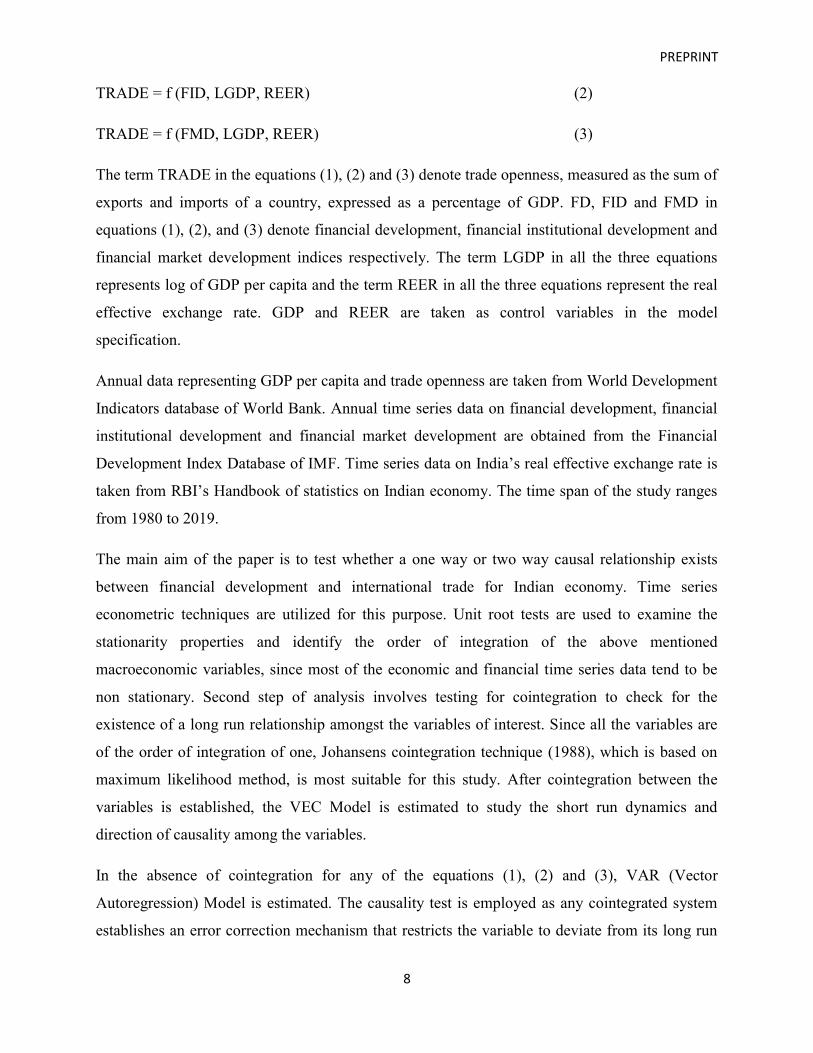
Figure 1: Growth trend of Broad based Index of Financial Development
Source: IMF, 2019
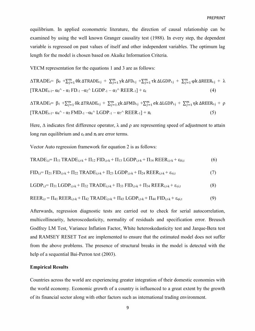
Figure 2: Growth Trend of Financial Institutional Development
Source: IMF, 2019
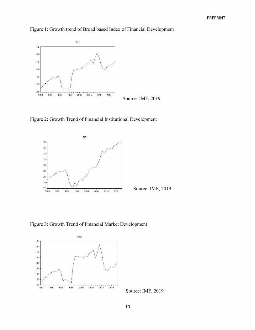
Figure 3: Growth Trend of Financial Market Development
Source: IMF, 2019
PREPRINT
11
Figure 1 plots the growth trend of the broad-based index of financial development created by
IMF. Figures 2 and 3 are showing the growth trend of the sub-indices of financial market
development and financial institutional development of IMF. While comparing the graphical
plots, it is found that the growth trend of the financial development index exhibits the exact same
pattern as the financial market development index. Financial institutional development is found
to register a slightly different growth trajectory compared to the other two indicators.
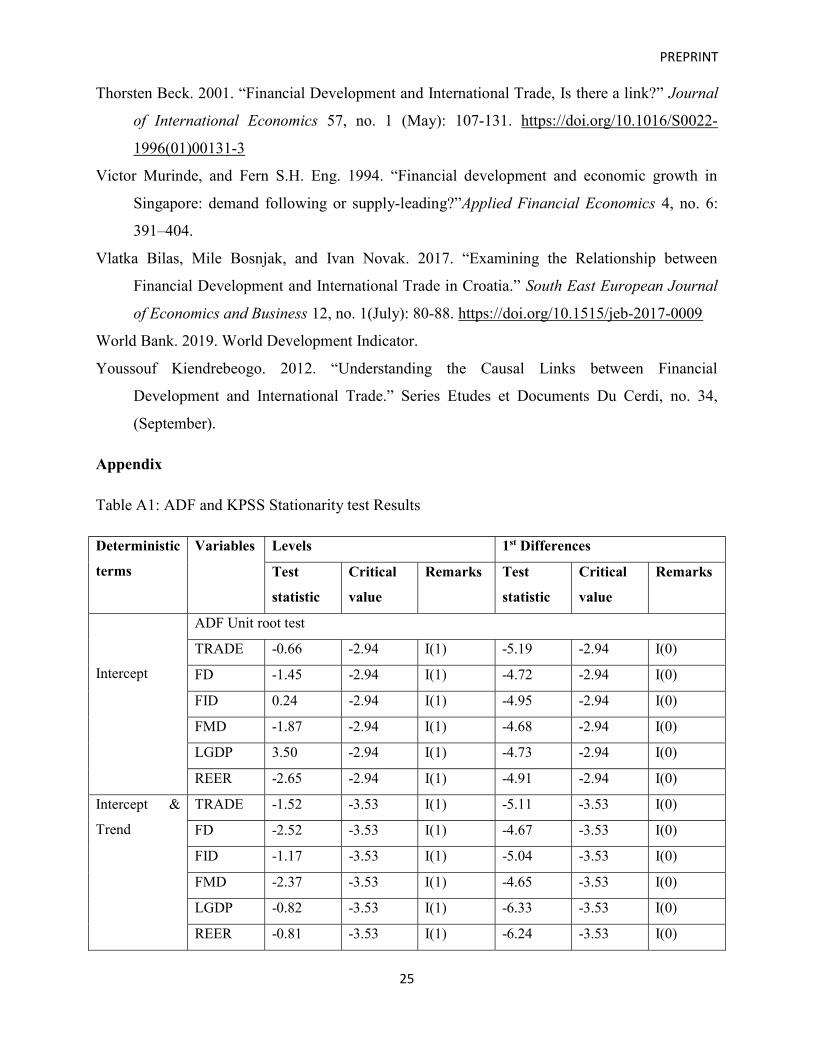
In order to examine the long term relationship between the two macroeconomic variables of
interest, it is important to test for stationarity and order of integration. Hence the standard unit
root tests such as ADF (Dickey and Fuller 1979) and KPSS tests (Kwiatkowski, Phillips,
Schmidt and Shin 1992) are initially carried out. Since the paper is considering macroeconomic
variables, it is wise to use a stationarity test which allows for unknown structural breaks as it
avoids the possibility of spurious regression. Moreover, the sequential Bai-Perron (2003) test
claims for the presence of structural breaks in the series (Table A3, Appendix). In the current
study, Perron test (1997), which allows for endogenous structural breaks used in order to identify
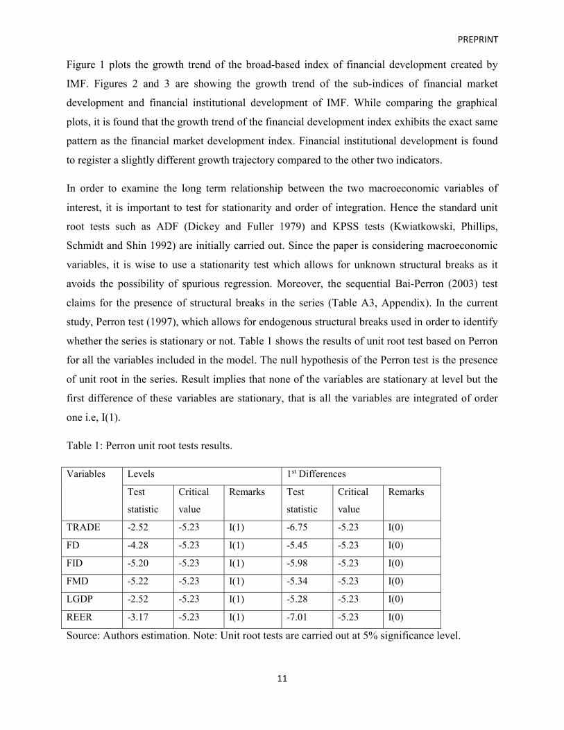
whether the series is stationary or not. Table 1 shows the results of unit root test based on Perron
for all the variables included in the model. The null hypothesis of the Perron test is the presence
of unit root in the series. Result implies that none of the variables are stationary at level but the
first difference of these variables are stationary, that is all the variables are integrated of order
one i.e, I(1).
Table 1: Perron unit root tests results.
Variables Levels 1st Differences
Test
statistic
Critical
value
Remarks Test
statistic
Critical
value
Remarks
TRADE -2.52 -5.23 I(1) -6.75 -5.23 I(0)
FD -4.28 -5.23 I(1) -5.45 -5.23 I(0)
FID -5.20 -5.23 I(1) -5.98 -5.23 I(0)
FMD -5.22 -5.23 I(1) -5.34 -5.23 I(0)
LGDP -2.52 -5.23 I(1) -5.28 -5.23 I(0)
REER -3.17 -5.23 I(1) -7.01 -5.23 I(0)
Source: Authors estimation. Note: Unit root tests are carried out at 5% significance level.
PREPRINT
12
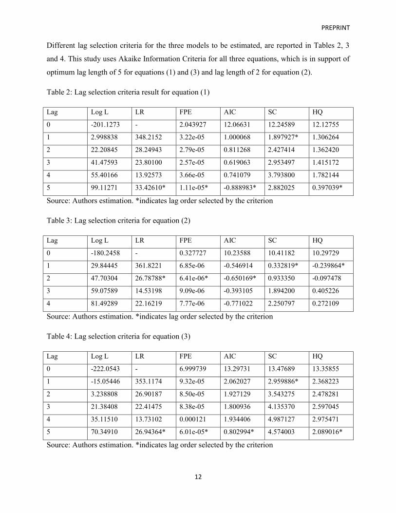
Different lag selection criteria for the three models to be estimated, are reported in Tables 2, 3
and 4. This study uses Akaike Information Criteria for all three equations, which is in support of
optimum lag length of 5 for equations (1) and (3) and lag length of 2 for equation (2).
Table 2: Lag selection criteria result for equation (1)
Lag Log L LR FPE AIC SC HQ
0 -201.1273 - 2.043927 12.06631 12.24589 12.12755
1 2.998838 348.2152 3.22e-05 1.000068 1.897927* 1.306264
2 22.20845 28.24943 2.79e-05 0.811268 2.427414 1.362420
3 41.47593 23.80100 2.57e-05 0.619063 2.953497 1.415172
4 55.40166 13.92573 3.66e-05 0.741079 3.793800 1.782144
5 99.11271 33.42610* 1.11e-05* -0.888983* 2.882025 0.397039*
Source: Authors estimation. *indicates lag order selected by the criterion
Table 3: Lag selection criteria for equation (2)
Lag Log L LR FPE AIC SC HQ
0 -180.2458 - 0.327727 10.23588 10.41182 10.29729
1 29.84445 361.8221 6.85e-06 -0.546914 0.332819* -0.239864*
2 47.70304 26.78788* 6.41e-06* -0.650169* 0.933350 -0.097478
3 59.07589 14.53198 9.09e-06 -0.393105 1.894200 0.405226
4 81.49289 22.16219 7.77e-06 -0.771022 2.250797 0.272109
Source: Authors estimation. *indicates lag order selected by the criterion
Table 4: Lag selection criteria for equation (3)
Lag Log L LR FPE AIC SC HQ
0 -222.0543 - 6.999739 13.29731 13.47689 13.35855
1 -15.05446 353.1174 9.32e-05 2.062027 2.959886* 2.368223
2 3.238808 26.90187 8.50e-05 1.927129 3.543275 2.478281
3 21.38408 22.41475 8.38e-05 1.800936 4.135370 2.597045
4 35.11510 13.73102 0.000121 1.934406 4.987127 2.975471
5 70.34910 26.94364* 6.01e-05* 0.802994* 4.574003 2.089016*
Source: Authors estimation. *indicates lag order selected by the criterion
PREPRINT
13
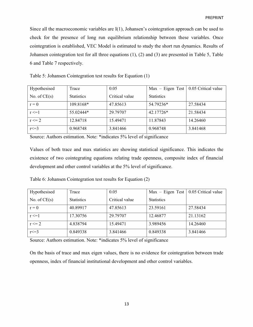
Since all the macroeconomic variables are I(1), Johansen’s cointegration approach can be used to
check for the presence of long run equilibrium relationship between these variables. Once
cointegration is established, VEC Model is estimated to study the short run dynamics. Results of
Johansen cointegration test for all three equations (1), (2) and (3) are presented in Table 5, Table
6 and Table 7 respectively.
Table 5: Johansen Cointegration test results for Equation (1)
Hypothesised
No. of CE(s)
Trace
Statistics
0.05
Critical value
Max – Eigen Test
Statistics
0.05 Critical value
r = 0 109.8168* 47.85613 54.79236* 27.58434
r <=1 55.02444* 29.79707 42.17726* 21.58434
r <= 2 12.84718 15.49471 11.87843 14.26460
r<=3 0.968748 3.841466 0.968748 3.841468
Source: Authors estimation. Note: *indicates 5% level of significance
Values of both trace and max statistics are showing statistical significance. This indicates the
existence of two cointegrating equations relating trade openness, composite index of financial
development and other control variables at the 5% level of significance.
Table 6: Johansen Cointegration test results for Equation (2)
Hypothesised
No. of CE(s)
Trace
Statistics
0.05
Critical value
Max – Eigen Test
Statistics
0.05 Critical value
r = 0 40.89917 47.85613 23.59161 27.58434
r <=1 17.30756 29.79707 12.46877 21.13162
r <= 2 4.838794 15.49471 3.989456 14.26460
r<=3 0.849338 3.841466 0.849338 3.841466
Source: Authors estimation. Note: *indicates 5% level of significance
On the basis of trace and max eigen values, there is no evidence for cointegration between trade
openness, index of financial institutional development and other control variables.
PREPRINT
14
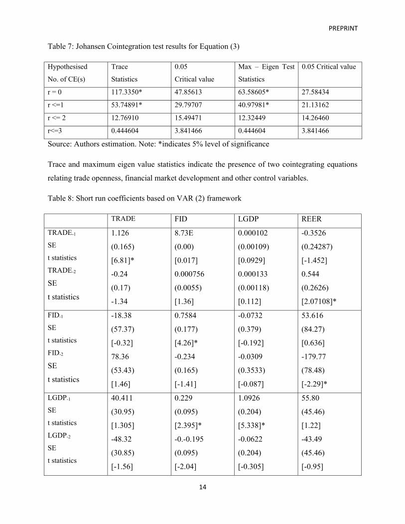
Table 7: Johansen Cointegration test results for Equation (3)
Hypothesised
No. of CE(s)
Trace
Statistics
0.05
Critical value
Max – Eigen Test
Statistics
0.05 Critical value
r = 0 117.3350* 47.85613 63.58605* 27.58434
r <=1 53.74891* 29.79707 40.97981* 21.13162
r <= 2 12.76910 15.49471 12.32449 14.26460
r<=3 0.444604 3.841466 0.444604 3.841466
Source: Authors estimation. Note: *indicates 5% level of significance
Trace and maximum eigen value statistics indicate the presence of two cointegrating equations
relating trade openness, financial market development and other control variables.
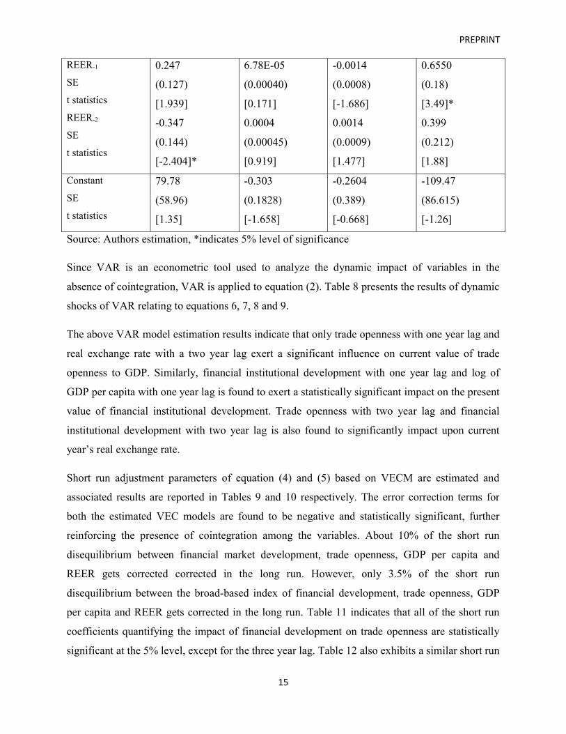
Table 8: Short run coefficients based on VAR (2) framework
TRADE FID LGDP REER
TRADE-1
SE
t statistics
TRADE-2
SE
t statistics
1.126
(0.165)
[6.81]*
-0.24
(0.17)
-1.34
8.73E
(0.00)
[0.017]
0.000756
(0.0055)
[1.36]
0.000102
(0.00109)
[0.0929]
0.000133
(0.00118)
[0.112]
-0.3526
(0.24287)
[-1.452]
0.544
(0.2626)
[2.07108]*
FID-1
SE
t statistics
FID-2
SE
t statistics
-18.38
(57.37)
[-0.32]
78.36
(53.43)
[1.46]
0.7584
(0.177)
[4.26]*
-0.234
(0.165)
[-1.41]
-0.0732
(0.379)
[-0.192]
-0.0309
(0.3533)
[-0.087]
53.616
(84.27)
[0.636]
-179.77
(78.48)
[-2.29]*
LGDP-1
SE
t statistics
LGDP-2
SE
t statistics
40.411
(30.95)
[1.305]
-48.32
(30.85)
[-1.56]
0.229
(0.095)
[2.395]*
-0.-0.195
(0.095)
[-2.04]
1.0926
(0.204)
[5.338]*
-0.0622
(0.204)
[-0.305]
55.80
(45.46)
[1.22]
-43.49
(45.46)
[-0.95]
PREPRINT
15
REER-1
SE
t statistics
REER-2
SE
t statistics
0.247
(0.127)
[1.939]
-0.347
(0.144)
[-2.404]*
6.78E-05
(0.00040)
[0.171]
0.0004
(0.00045)
[0.919]
-0.0014
(0.0008)
[-1.686]
0.0014
(0.0009)
[1.477]
0.6550
(0.18)
[3.49]*
0.399
(0.212)
[1.88]
Constant
SE
t statistics
79.78
(58.96)
[1.35]
-0.303
(0.1828)
[-1.658]
-0.2604
(0.389)
[-0.668]
-109.47
(86.615)
[-1.26]
Source: Authors estimation, *indicates 5% level of significance
Since VAR is an econometric tool used to analyze the dynamic impact of variables in the
absence of cointegration, VAR is applied to equation (2). Table 8 presents the results of dynamic
shocks of VAR relating to equations 6, 7, 8 and 9.
The above VAR model estimation results indicate that only trade openness with one year lag and
real exchange rate with a two year lag exert a significant influence on current value of trade
openness to GDP. Similarly, financial institutional development with one year lag and log of
GDP per capita with one year lag is found to exert a statistically significant impact on the present
value of financial institutional development. Trade openness with two year lag and financial
institutional development with two year lag is also found to significantly impact upon current
year’s real exchange rate.
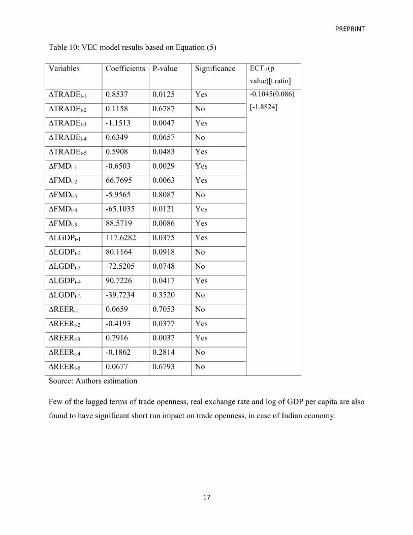
Short run adjustment parameters of equation (4) and (5) based on VECM are estimated and
associated results are reported in Tables 9 and 10 respectively. The error correction terms for
both the estimated VEC models are found to be negative and statistically significant, further
reinforcing the presence of cointegration among the variables. About 10% of the short run
disequilibrium between financial market development, trade openness, GDP per capita and
REER gets corrected corrected in the long run. However, only 3.5% of the short run
disequilibrium between the broad-based index of financial development, trade openness, GDP
per capita and REER gets corrected in the long run. Table 11 indicates that all of the short run
coefficients quantifying the impact of financial development on trade openness are statistically
significant at the 5% level, except for the three year lag. Table 12 also exhibits a similar short run
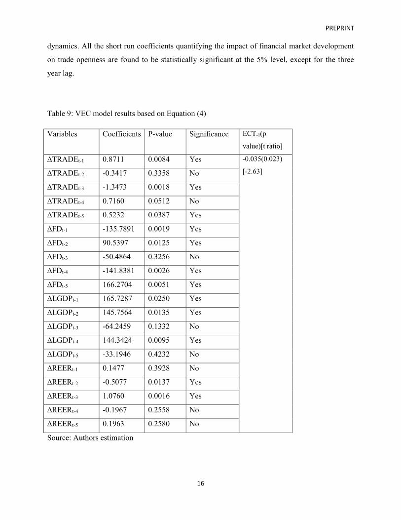
PREPRINT
16
dynamics. All the short run coefficients quantifying the impact of financial market development
on trade openness are found to be statistically significant at the 5% level, except for the three
year lag.
Table 9: VEC model results based on Equation (4)
Variables Coefficients P-value Significance ECT-1(p
value)[t ratio]
∆TRADEt-1 0.8711 0.0084 Yes -0.035(0.023)
[-2.63] ∆TRADEt-2 -0.3417 0.3358 No
∆TRADEt-3 -1.3473 0.0018 Yes
∆TRADEt-4 0.7160 0.0512 No
∆TRADEt-5 0.5232 0.0387 Yes
∆FDt-1 -135.7891 0.0019 Yes
∆FDt-2 90.5397 0.0125 Yes
∆FDt-3 -50.4864 0.3256 No
∆FDt-4 -141.8381 0.0026 Yes
∆FDt-5 166.2704 0.0051 Yes
∆LGDPt-1 165.7287 0.0250 Yes
∆LGDPt-2 145.7564 0.0135 Yes
∆LGDPt-3 -64.2459 0.1332 No
∆LGDPt-4 144.3424 0.0095 Yes
∆LGDPt-5 -33.1946 0.4232 No
∆REERt-1 0.1477 0.3928 No
∆REERt-2 -0.5077 0.0137 Yes
∆REERt-3 1.0760 0.0016 Yes
∆REERt-4 -0.1967 0.2558 No
∆REERt-5 0.1963 0.2580 No
Source: Authors estimation
PREPRINT
17
Table 10: VEC model results based on Equation (5)
Variables Coefficients P-value Significance ECT-1(p
value)[t ratio]
∆TRADEt-1 0.8537 0.0125 Yes -0.1045(0.086)
[-1.8824] ∆TRADEt-2 0.1158 0.6787 No
∆TRADEt-3 -1.1513 0.0047 Yes
∆TRADEt-4 0.6349 0.0657 No
∆TRADEt-5 0.5908 0.0483 Yes
∆FMDt-1 -0.6503 0.0029 Yes
∆FMDt-2 66.7695 0.0063 Yes
∆FMDt-3 -5.9565 0.8087 No
∆FMDt-4 -65.1035 0.0121 Yes
∆FMDt-5 88.5719 0.0086 Yes
∆LGDPt-1 117.6282 0.0375 Yes
∆LGDPt-2 80.1164 0.0918 No
∆LGDPt-3 -72.5205 0.0748 No
∆LGDPt-4 90.7226 0.0417 Yes
∆LGDPt-5 -39.7234 0.3520 No
∆REERt-1 0.0659 0.7053 No
∆REERt-2 -0.4193 0.0377 Yes
∆REERt-3 0.7916 0.0037 Yes
∆REERt-4 -0.1862 0.2814 No
∆REERt-5 0.0677 0.6793 No
Source: Authors estimation
Few of the lagged terms of trade openness, real exchange rate and log of GDP per capita are also
found to have significant short run impact on trade openness, in case of Indian economy.
PREPRINT
18
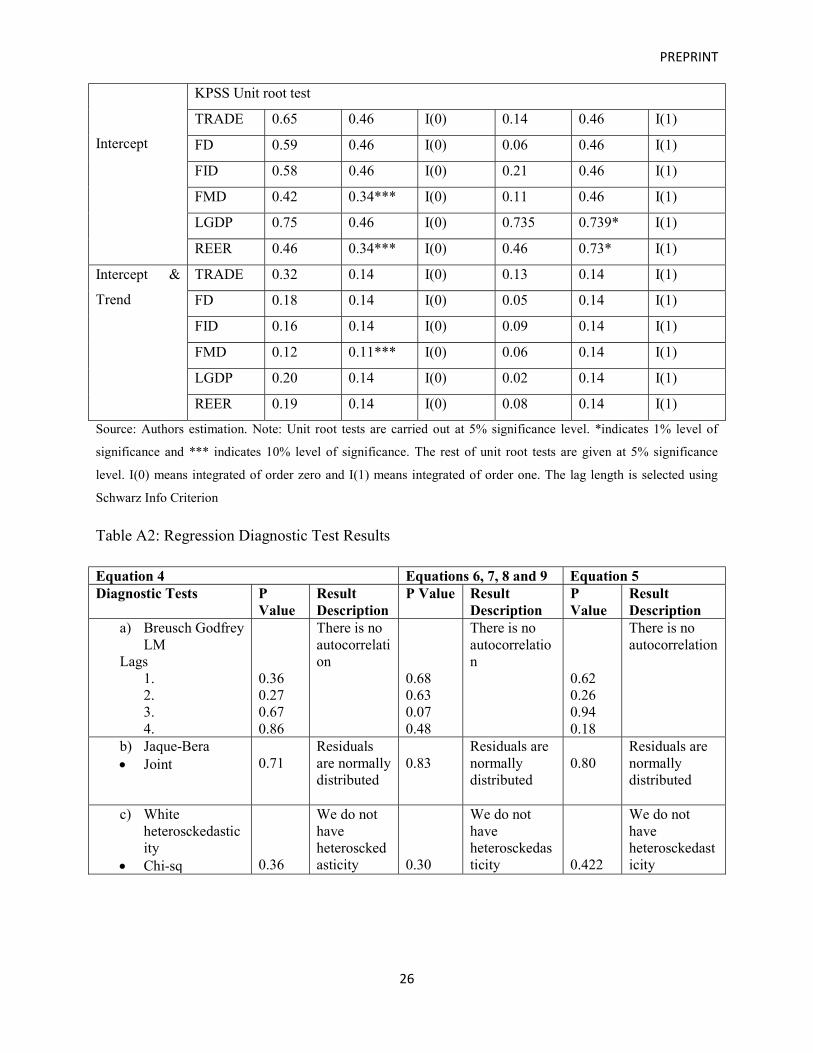
It is necessary to check the statistical and operational quality of the model, with the help of
regression diagnostic tests. Since the study uses financial and economic variables, it aggravates
the chance for collinearity between explanatory variables. However, the significance of
regression coefficients and lower variance inflation factor rule out the possibility of high
multicollinearity in the model. Therefore, no serious remedial measures are required to treat it.
Other tests on residuals ensure that the model is adequately robust and does not suffer from serial
autocorrelation, non-normality and heteroscedasticity. The Ramsey RESET (1969) test was
conducted to check whether the functional form of model is correct or not. Result shows all three
estimated models have correct functional form (see Table A2 in Appendix).
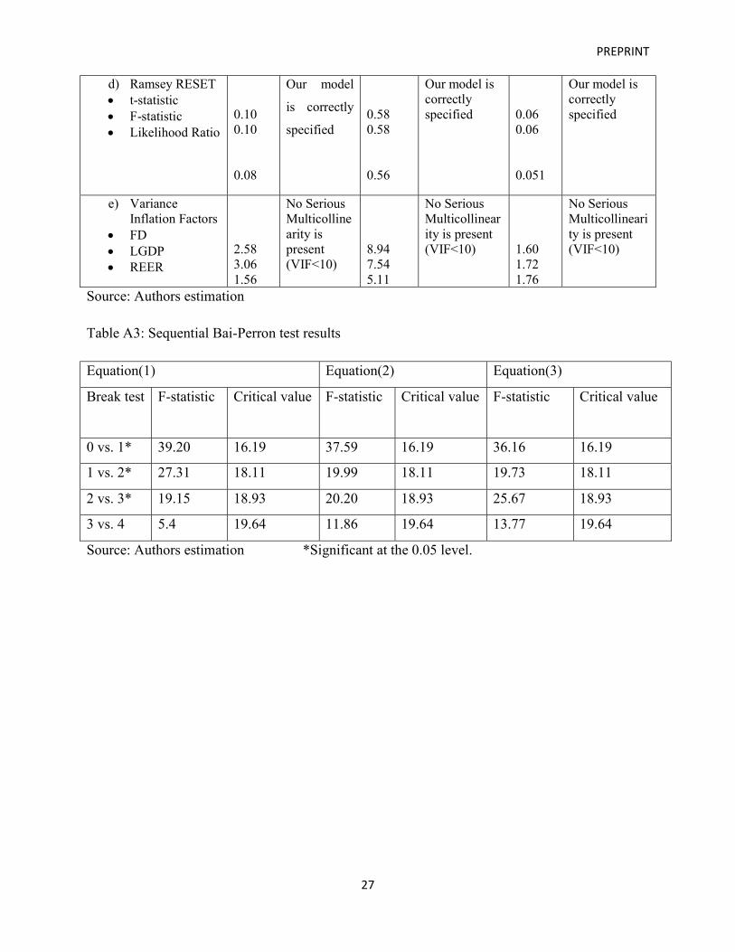
The presence of structural breaks is identified by using sequential Bai-Perron (2003) test and F
statistics spotted three structural breaks in the series, results of which are reported in Table A3 of
Appendix. Bai Perron Test indicates multiple structural breaks in 1998, 2008 and 2014, and these
can be explained as follows: Introduction of second generation banking sector reforms based on
Narasimham Committee 2 in 1998, global financial recession in 2008 and the initiation of the fall
in the rate of economic growth in 2014 respectively. The validity of model is not affected by the
presence of structural breaks because all the macroeconomic variables entering the model are
stationary at their first difference based on both the results of traditional unit root tests (ADF and
KPSS) and Perron unit root test with structural breaks.
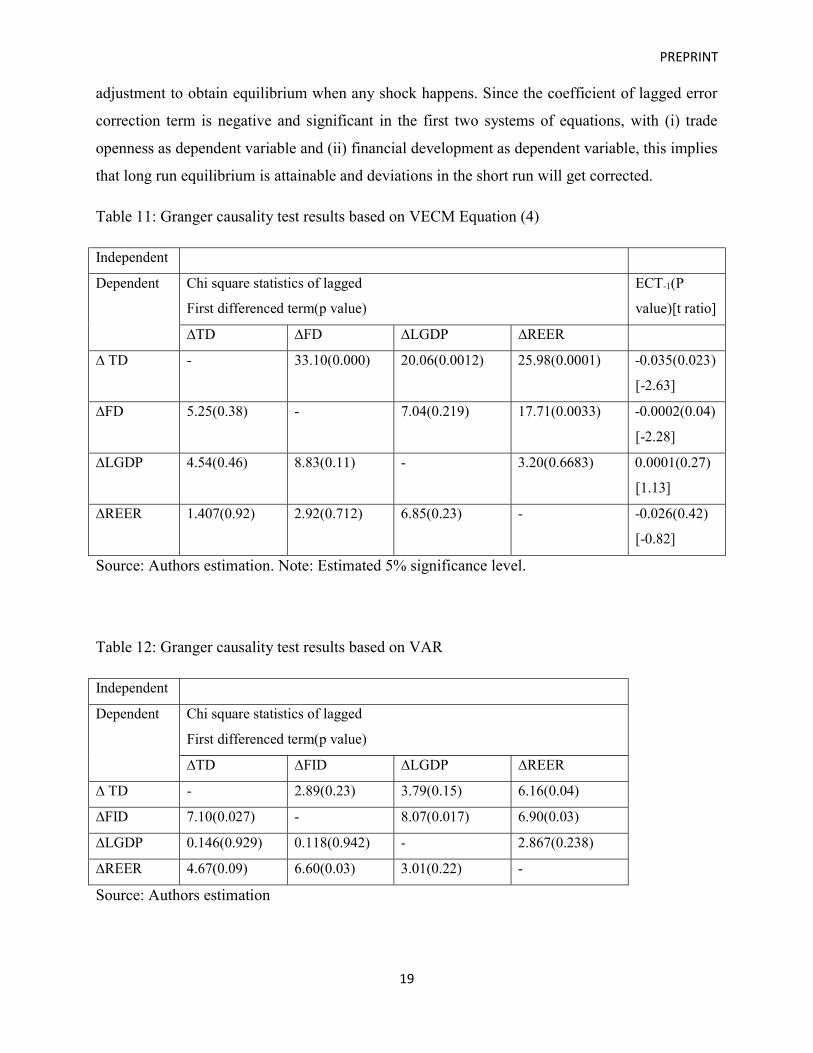
The presence of cointegration among variables hints at the presence of unidirectional or
bidirectional Granger causality among variables. Short run causality can be obtained from Chi-
square (χ2) value of lagged difference of independent variables and long run causality can be
examined through t statistics on coefficients of lagged values of error correction terms (ECTt-1).
The results of Granger causality test based on first differenced variables are shown in the table
below.
The test results reject null hypothesis that financial development does not granger cause trade
openness, log of GDP per capita does not granger causes trade openness, and real exchange rate
does not granger causes trade openness. Unidirectional short run causality is found to run from
financial development to trade openness, log of GDP per capita to trade openness and real
exchange rate to GDP per capita. Empirical evidence also indicates one way causality from real
exchange rate to financial development. The coefficient on ECT-1, measure the speed of
PREPRINT
19
adjustment to obtain equilibrium when any shock happens. Since the coefficient of lagged error
correction term is negative and significant in the first two systems of equations, with (i) trade
openness as dependent variable and (ii) financial development as dependent variable, this implies
that long run equilibrium is attainable and deviations in the short run will get corrected.
Table 11: Granger causality test results based on VECM Equation (4)
Independent
Dependent Chi square statistics of lagged
First differenced term(p value)
ECT-1(P
value)[t ratio]
∆TD ∆FD ∆LGDP ∆REER
∆ TD - 33.10(0.000) 20.06(0.0012) 25.98(0.0001) -0.035(0.023)
[-2.63]
∆FD 5.25(0.38) - 7.04(0.219) 17.71(0.0033) -0.0002(0.04)
[-2.28]
∆LGDP 4.54(0.46) 8.83(0.11) - 3.20(0.6683) 0.0001(0.27)
[1.13]
∆REER 1.407(0.92) 2.92(0.712) 6.85(0.23) - -0.026(0.42)
[-0.82]
Source: Authors estimation. Note: Estimated 5% significance level.
Table 12: Granger causality test results based on VAR
Independent
Dependent Chi square statistics of lagged
First differenced term(p value)
∆TD ∆FID ∆LGDP ∆REER
∆ TD - 2.89(0.23) 3.79(0.15) 6.16(0.04)
∆FID 7.10(0.027) - 8.07(0.017) 6.90(0.03)
∆LGDP 0.146(0.929) 0.118(0.942) - 2.867(0.238)
∆REER 4.67(0.09) 6.60(0.03) 3.01(0.22) -
Source: Authors estimation
PREPRINT
20
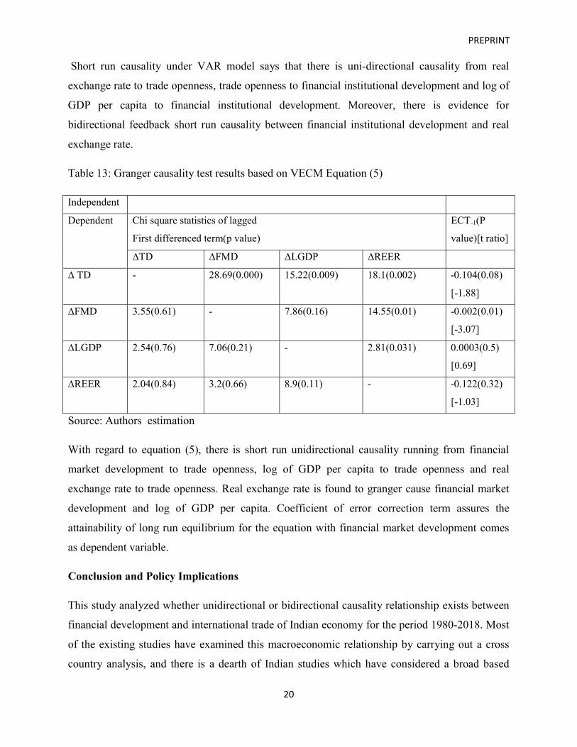
Short run causality under VAR model says that there is uni-directional causality from real
exchange rate to trade openness, trade openness to financial institutional development and log of
GDP per capita to financial institutional development. Moreover, there is evidence for
bidirectional feedback short run causality between financial institutional development and real
exchange rate.
Table 13: Granger causality test results based on VECM Equation (5)
Independent
Dependent Chi square statistics of lagged
First differenced term(p value)
ECT-1(P
value)[t ratio]
∆TD ∆FMD ∆LGDP ∆REER
∆ TD - 28.69(0.000) 15.22(0.009) 18.1(0.002) -0.104(0.08)
[-1.88]
∆FMD 3.55(0.61) - 7.86(0.16) 14.55(0.01) -0.002(0.01)
[-3.07]
∆LGDP 2.54(0.76) 7.06(0.21) - 2.81(0.031) 0.0003(0.5)
[0.69]
∆REER 2.04(0.84) 3.2(0.66) 8.9(0.11) - -0.122(0.32)
[-1.03]
Source: Authors estimation
With regard to equation (5), there is short run unidirectional causality running from financial
market development to trade openness, log of GDP per capita to trade openness and real
exchange rate to trade openness. Real exchange rate is found to granger cause financial market
development and log of GDP per capita. Coefficient of error correction term assures the
attainability of long run equilibrium for the equation with financial market development comes
as dependent variable.
Conclusion and Policy Implications
This study analyzed whether unidirectional or bidirectional causality relationship exists between
financial development and international trade of Indian economy for the period 1980-2018. Most
of the existing studies have examined this macroeconomic relationship by carrying out a cross
country analysis, and there is a dearth of Indian studies which have considered a broad based

PREPRINT
21
measure of financial development and aggregate international trade inclusive of agricultural
goods, manufacturing goods and services. This study added a new dimension to previous studies
by estimating three distinct econometric models using the three indices of financial development
created by IMF. Using Johansen cointegration, the study found that there is existence of long run
equilibrium relationship between trade openness and the composite index of financial
development. It was further established that cointegration also exists between trade openness and
index of financial market development. However, no significant long run association was found
between trade openness and index of financial institutional development. The direction of
causality between the variables of interest is analyzed using VEC based Granger causality test.
The causality test results indicate uni-directional causality running from the composite financial
development index to trade openness. Uni-directional causality was also found to run from
financial market development index to trade openness. There is short run uni-directional
causality from trade openness to financial institutional development index and bi-directional
short run causal relationship is found between financial institutional development and real
exchange rate.
Results indicate that development of financial sector can positively impact upon volume of
international trade in India. Since IMF financial development index is composed of financial
market development and financial institutional development, results implies that financial market
development is exerting bigger influence on financial development when it comes to accelerate
trade openness as there is more pronounced financial market development effect on increase of
trade openness. So, it can be suspected that trading industries are using more external finance or
few collateralizable assets. Hence, standalone trade liberalization policies are not advisable for
India. Moreover, the trade promotion policies should encompass the productivity and
accessibility aspects of external finance to the export oriented industries. India’s foreign trade
policy should also ensure that access to finance does not become a hurdle for small and medium
sized enterprises to enter and flourish in trade related activities. Since financial development can
contribute to overall trade performance of India, there is indeed a need for further financial sector
reform to further drive economic prosperity of Indian economy.
Empirical evidence also indicates small positive impact of financial institutional development on
trade openness as well. Trade openness is also found to reverse cause the development of
financial institutions. As international trade mature, more financial services and insurance will
PREPRINT
22
be demanded in response to increased domestic production. It helps in efficient allocation of
savings and further expansion of financial system. The study underlines the importance of
financial development, and specifically policies targeted at development of financial markets, in
accelerating the trade openness of Indian economy. Engaging in international trade is also found
to promote development of Indian financial institutions, which puts forth a case for greater
integration of Indian economy with the world economy.
Acknowledgment
The authors are grateful for the valuable feedback received from the participants of the 31st
Annual Conference of International Trade and Finance Association, held from May 28-29, 2021.
Bibliography
Alejandro Santana. 2020. “The relationship between Financial Development and Economic
Growth in Latin American Countries: The Role of Banking Crises and Financial
Liberalization”. Global Economy Journal 20, no. 4(December): 1-26.
DOI:10.1142/S2194565920500232.
Aleksander Aristovnik. 2008. “Short Term Determinants of Current Account Deficit: Evidence
from Eastern Europe and the Former Soviet Union.” Eastern European Economics, 46,
no. 1(January): 24-42.
Bas B. Bakker, and Anna Marie Gulde. 2010. “The Credit Bottom in the EU New Member
States: Bad Luck or Bad Policies?” IMF Working Paper, no. 130 (May): 1-44.
Daniel Perez Liston, and Lawrence McNeil. 2013. ‘The Impact of Trade Finance on International
Trade: Does Financial Development Matter?’ International Journal Economics and
Business Research 8, no. 1 (January):1-19.
Daria V. Zakharova. 2008. “One-Size-Fits-One: Tailor-Made Fiscal Responses to Capital Flows.” IMF Working Paper, no. 269 (December):1-27.https://doi.org/10.5089/9781451871272.001
PREPRINT
23
Edward S. Shaw. 1973. “Financial Deepening in Economic Development.” The Journal of
Finance 29, no. 4 (September).
Fatih Yucel. 2009. “Causal Relationships between Financial Development, Trade Openness and
Economic Growth: The case of Turkey.”Journal of Social Sciences 5, no. 1 (January):33-
42. 10.3844/jssp.2009.33.42
Fernando Leibovici. 2018 “Financial Development and International Trade” FRB St. Louis
Working Paper, no, 15 (August): 1-50
Jonas Vlachos, and Helena Svalryd. 2005. “Financial Markets, the Pattern of Specialization and
Comparative Advantage. Evidence from OECD countries.”European Economic Review 49,
no. 1 (January):113-144. 10.1016/S0014-2921(03)00030-8
Katsiaryna Svirydzenka. 2016. “Introducing a New Broad based Index of Financial
Development.”IMF Working Paper, no. 16 (January):1-43
Kenneth Kletzer and Pranab Bardhan. 1987. “Credit markets and patterns of international trade”.
Journal of Development Economics 27, no. 1 (October): 57-70. DOI:
10.1142/S2194565920500232
Kul B. Luintel, and Musahid. 1999. “A Quantitative Reassessment of the FinanceGrowth Nexus:
Evidence from a Multivariate VAR.”Journal of Development Economics 60, no. 2
(December): 381-405.
Leena Ajit Kaushal, and Neha Pathak. 2015. “The Causal Relationship among Economic Growth
Financial Development and Trade Openness in Indian Economy.”International Journal of
Economic Perspectives 9, no. 2 (June): 5-22.
Ling Feng, and Ching Yi Lin. 2013. “Financial shocks and Exports.”International Review of
Economics and Finance 26, no.4 (April): 39-55. 10.1016/j.iref.2012.08.007
Michele Cyrille Samba, and Yan Yu. 2009. “Financial Development and International Trade in
Manufactures: An Evaluation of the Relation in Some Selected Asian
Countries.”International Journal of Business and Management 12, no. 12 (December):52-
69.
Muhammad Shabaz, and Mohammad Mafizur Rahman. 2014. “Exports, Financial Development
and Economic Growth in Pakistan.”International Journal of Development Issues 13, no. 2
(July): 155-170. 10.1108/IJDI-09-2013-0065
Muhsin Kar, Saban Nazlioglu, and Huseyin Agir. 2013. “Trade Openness, Financial
Development, and Economic Growth in Turkey: Linear and Nonlinear Causality
PREPRINT
24
Analysis.”Proceedings of International Conference of Eurasian Economies, Petersburg,
Russia: 133-143.
Omoke Philip Chimobi. 2010. “The Causal Relationship among Financial Development, Trade
Openness and Economic Growth in Nigeria.” International Journal of Economics and
Finance 2, no. 2: 137-147. 10.5539/ijef.v2n2p137
Puneet K. Arora and Jaydeep Mukherjee. 2020. “The nexus between financial development and
trade performance. Empirical evidence from India in the presence of endogenous structural
breaks”. Journal of Financial Economic Policy 12, no. 2: 279-291.
Quoy Tan Do, and Andrei A. Levchenko. 2004. “Trade and Financial Development.” World
Bank Working, no. 3347. http://www-wds.worldbank.org/external/default/WDSC ...
ered/PDF/wps3347.pdf.
Rajeev Jain, Dhirendra Gajbhiye, and SousmasreeTewari. 2019. “Cross Border Trade Credit: A
post Crisis Empirical Analysis for India.” RBI Working Paper, no.
02.https://rbidocs.rbi.org.in/rdocs/Publications/PDFs/WPS022019CBTCCC06C3A2CF6F4
26EBA4590C599B38369.PDF.
Raymond W. Goldsmith. 1969. Financial Structure and Development. New Haven, CT: Yale
University Press.
RBI, “Report on Currency and Finance.” May 31, 2007.
https://www.rbi.org.in/scripts/PublicationsView.aspx?id=9237
Richard E. Baldwin. 1989. Exporting the capital markets: comparative advantages and capital
markets imperfections. North Holland: The convergence of international and domestic
markets: Amsterdam. 135-152.
Ronald I. McKinnon. 1973. Money and Capital in Economic Development. Washington, D.C:
Brookings Institution Press.
Ross Levine, and Sarah Zervos. 1998. “Stock Markets, Banks, and Economic Growth.”
American Economic Review 88, no. 3 (June): 537-558.
Ross Levine, Norman Loayza, and Thorsten Beck. 2000. “Financial Intermediation and Growth:
Causality and causes.”Journal of Monetary Economics 46, no. 1 (August):31-77.
Ross Levine. 1997. “Financial Development and Economic Growth: Views and
Agenda.”Journal of Economic Literature 35, no. 2 (June): 688-726.
PREPRINT
25
Thorsten Beck. 2001. “Financial Development and International Trade, Is there a link?” Journal
of International Economics 57, no. 1 (May): 107-131. https://doi.org/10.1016/S0022-
1996(01)00131-3
Victor Murinde, and Fern S.H. Eng. 1994. “Financial development and economic growth in
Singapore: demand following or supply-leading?”Applied Financial Economics 4, no. 6:
391–404.
Vlatka Bilas, Mile Bosnjak, and Ivan Novak. 2017. “Examining the Relationship between
Financial Development and International Trade in Croatia.” South East European Journal
of Economics and Business 12, no. 1(July): 80-88. https://doi.org/10.1515/jeb-2017-0009
World Bank. 2019. World Development Indicator.
Youssouf Kiendrebeogo. 2012. “Understanding the Causal Links between Financial
Development and International Trade.” Series Etudes et Documents Du Cerdi, no. 34,
(September).
Appendix
Table A1: ADF and KPSS Stationarity test Results
Deterministic
terms
Variables Levels 1st Differences
Test
statistic
Critical
value
Remarks Test
statistic
Critical
value
Remarks
Intercept
ADF Unit root test
TRADE -0.66 -2.94 I(1) -5.19 -2.94 I(0)
FD -1.45 -2.94 I(1) -4.72 -2.94 I(0)
FID 0.24 -2.94 I(1) -4.95 -2.94 I(0)
FMD -1.87 -2.94 I(1) -4.68 -2.94 I(0)
LGDP 3.50 -2.94 I(1) -4.73 -2.94 I(0)
REER -2.65 -2.94 I(1) -4.91 -2.94 I(0)
Intercept &
Trend
TRADE -1.52 -3.53 I(1) -5.11 -3.53 I(0)
FD -2.52 -3.53 I(1) -4.67 -3.53 I(0)
FID -1.17 -3.53 I(1) -5.04 -3.53 I(0)
FMD -2.37 -3.53 I(1) -4.65 -3.53 I(0)
LGDP -0.82 -3.53 I(1) -6.33 -3.53 I(0)
REER -0.81 -3.53 I(1) -6.24 -3.53 I(0)
PREPRINT
26
Intercept
KPSS Unit root test
TRADE 0.65 0.46 I(0) 0.14 0.46 I(1)
FD 0.59 0.46 I(0) 0.06 0.46 I(1)
FID 0.58 0.46 I(0) 0.21 0.46 I(1)
FMD 0.42 0.34*** I(0) 0.11 0.46 I(1)
LGDP 0.75 0.46 I(0) 0.735 0.739* I(1)
REER 0.46 0.34*** I(0) 0.46 0.73* I(1)
Intercept &
Trend
TRADE 0.32 0.14 I(0) 0.13 0.14 I(1)
FD 0.18 0.14 I(0) 0.05 0.14 I(1)
FID 0.16 0.14 I(0) 0.09 0.14 I(1)
FMD 0.12 0.11*** I(0) 0.06 0.14 I(1)
LGDP 0.20 0.14 I(0) 0.02 0.14 I(1)
REER 0.19 0.14 I(0) 0.08 0.14 I(1)
Source: Authors estimation. Note: Unit root tests are carried out at 5% significance level. *indicates 1% level of
significance and *** indicates 10% level of significance. The rest of unit root tests are given at 5% significance
level. I(0) means integrated of order zero and I(1) means integrated of order one. The lag length is selected using
Schwarz Info Criterion
Table A2: Regression Diagnostic Test Results
Equation 4 Equations 6, 7, 8 and 9 Equation 5 Diagnostic Tests P
Value Result Description
P Value Result Description
P Value
Result Description
a) Breusch Godfrey LM
Lags 1. 2. 3. 4.
0.36 0.27 0.67 0.86
There is no autocorrelation
0.68 0.63 0.07 0.48
There is no autocorrelation
0.62 0.26 0.94 0.18
There is no autocorrelation
b) Jaque-Bera Joint
0.71
Residuals are normally distributed
0.83
Residuals are normally distributed
0.80
Residuals are normally distributed
c) White heterosckedasticity
Chi-sq
0.36
We do not have heterosckedasticity
0.30
We do not have heterosckedasticity
0.422
We do not have heterosckedasticity
PREPRINT
27
d) Ramsey RESET t-statistic F-statistic Likelihood Ratio
0.10 0.10 0.08
Our model
is correctly
specified
0.58 0.58 0.56
Our model is correctly specified
0.06 0.06 0.051
Our model is correctly specified
e) Variance Inflation Factors
FD LGDP REER
2.58 3.06 1.56
No Serious Multicollinearity is present (VIF<10)
8.94 7.54 5.11
No Serious Multicollinearity is present (VIF<10)
1.60 1.72 1.76
No Serious Multicollinearity is present (VIF<10)
Source: Authors estimation
Table A3: Sequential Bai-Perron test results
Equation(1) Equation(2) Equation(3)
Break test F-statistic Critical value F-statistic Critical value F-statistic Critical value
0 vs. 1* 39.20 16.19 37.59 16.19 36.16 16.19
1 vs. 2* 27.31 18.11 19.99 18.11 19.73 18.11
2 vs. 3* 19.15 18.93 20.20 18.93 25.67 18.93
3 vs. 4 5.4 19.64 11.86 19.64 13.77 19.64
Source: Authors estimation *Significant at the 0.05 level.