The pitfalls of ecological forecasting

The pitfalls of ecological forecasting

TOM H. OLIVER* and DAVID B. ROY

NERC Centre for Ecology and Hydrology, Wallingford, Oxfordshire, OX10 8BB, UK

Received 23 December 2014; revised 21 April 2015; accepted for publication 21 April 2015

Ecological forecasting is difficult but essential, because reactive management results in corrective actions that areoften too late to avert significant environmental damage. Here, we appraise different forecasting methods with aparticular focus on the modelling of species populations. We show how simple extrapolation of current trends instate is often inadequate because environmental drivers change in intensity over time and new drivers emerge.However, statistical models, incorporating relationships with drivers, simply offset the prediction problem,requiring us to forecast how the drivers will themselves change over time. Some authors approach this problemby focusing in detail on a single driver, whilst others use ‘storyline’ scenarios, which consider projected changesin a wide range of different drivers. We explain why both approaches are problematic and identify a compromiseto model key drivers and interactions along with possible response options to help inform environmentalmanagement. We also highlight the crucial role of validation of forecasts using independent data. Although theseissues are relevant for all types of ecological forecasting, we provide examples based on forecasts for populationsof UK butterflies. We show how a high goodness-of-fit for models used to calibrate data is not sufficient for goodforecasting. Long-term biological recording schemes rather than experiments will often provide data for ecologicalforecasting and validation because these schemes allow capture of landscape-scale land-use effects and theirinteractions with other drivers. © 2015 The Linnean Society of London, Biological Journal of the LinneanSociety, 2015, 115, 767–778.

ADDITIONAL KEYWORDS: butterfly monitoring – density dependence – environmental drivers –prediction – predictive modelling – weather.

WHY ATTEMPT TO FORECAST?

Two very different masters teach [man] his lesson:experience and foresight. Experience teaches effi-ciently but brutally. . .I should prefer, in so far aspossible, to replace this rude teacher with a moregentle one: foresight (Fr�ed�eric Bastiat, 1848)

Predicting the future is notoriously difficult. Manygreat thinkers have tried, and spectacularly failed.For example, in 1895, Lord Kelvin, a Scottish mathe-matician and physicist is famous to have forthrightlystated to have ‘not the smallest molecule of faith’ inaerial flight beyond ballooning, just 8 years beforethe Wright brothers put together the first successfulfixed wing aeroplane. Similarly, in a 1961 interviewT.A.M. Craven the US Federal Communicationscommissioner of the time famously predicted: ‘There is

practically no chance communications space satelliteswill be used to provide better telephone, telegraph,television or radio service inside the United States’.Only a few years later, satellites were in spaceperforming all the above services. So perhaps it is bestto keep our heads below the parapet and not makepredictions that, in retrospect, appear foolhardy?

In many fields of research, however, forecasting –prediction of future states based on past events, isessential. Forecasts allow us to alter our behaviours inresponse to likely realisations of future events in orderto reduce costs or maximise benefits. In the environ-mental sciences, for example, weather forecasts,which have improved greatly in recent decades, pro-vide huge overall benefit to society. In the longer term,climatological forecasts provide critical guidance tohelp steer our socioeconomic systems away fromunsustainable and self-destructive pathways. Thereare still many dangers associated with ‘getting itwrong’ (as UK weather forecaster Michael Fish*Corresponding author. E-mail: [email protected]

767© 2015 The Linnean Society of London, Biological Journal of the Linnean Society, 2015, 115, 767–778

Biological Journal of the Linnean Society, 2015, 115, 767–778. With 3 figures.

famously did in 1987 when he told people not to worryabout a hurricane just hours before winds reaching122 mph hit southern England). However, hidingaway from making forecasts is often not an option,because this path leads to greater overall costs thanmaking predictions that are occasionally wrong.

In ecological science, forecasting is also essential.It forms part of a set of tools, including horizon scan-ning (Sutherland et al., 2008; Roy et al., 2014) andrisk assessments (Mace et al., 2008; Thomas et al.,2011), that enable us to anticipate future changesand respond appropriately. Reactive responses tonew environmental impacts caused through changesin socioeconomic systems (e.g. adoption of new tech-nologies), may often be too late to avert significantenvironmental damage.

For example, the pesticide DDT caused substantiallosses to bird populations before it was finallybanned (US Environmental Protection Agency, 1975;Pimentel, 2005). In Europe, agricultural subsidies,paid to farmers to increase food production and secu-rity, have led to increased loss of natural or semi-natural habitats, and have been a primary cause ofEuropean biodiversity decline (Van Swaay et al.,2010; UK NEA, 2011; Inger et al., 2014). Theresponses to mitigate these environmental impactsand others have mostly been reactive, in that theyoccurred only when damage had begun. In contrast,risk assessments based on experimental evidence ofpesticide toxicity along with ecological modelling topredict potential impacts on species populations atlarger spatial scales could have enabled proactivepreventative measures to be taken.

In many cases, due to slow decision making andpolicy implementation, significant damage has beendone before ameliorative actions are in place. Theslow progress to develop co-operative global actionsto halt climate change may turn out to be anothersuch example, with potentially very large conse-quences for the environment and society (IPCC,2014). In other cases, policy responses may be rap-idly formulated based on hastily gathered evidence.In both situations there are strong benefits of earlyevidence gathering, ecological modelling and riskassessment to inform timely and evidence-based pol-icy decisions. It should be recognised, however, thatit will never be possible to foresee all ecological prob-lems and some environmental management will haveto be reactive.

In understanding the chain of events leading toenvironmental impacts, the ‘DPSIR’ (driver, pressure,state, impact, response) framework can be usefuland is widely used (Fig. 1; European EnvironmentAgency, 2007; United States Environmental Protec-tion Agency, 2014). This framework illustrates thecausal links between the ultimate drivers of environ-

mental degradation (e.g. population growth), the prox-imate pressures (e.g. food production) on the state ofthe environment (e.g. biodiversity) and their finalimpacts on humans (e.g. loss of well-being throughdegradation of ecosystem services that are under-pinned by biodiversity). Societal responses may thenbe put in place to ameliorate these impacts. Thesemay tackle the ultimate drivers (e.g. campaigns toeducate on the environmental impacts of populationgrowth) or proximate pressures (e.g. sustainable foodproduction) or try to address the state of the environ-ment directly without addressing drivers and pres-sures (e.g. improving the quality of semi-naturalhabitats that are known to support a high diversity ofspecialised species). However, the key problem withthe DPSIR framework is that following it sequen-tially, as described above, amounts to reactive man-agement practices that are often too late to avertsignificant environmental damage. It would be far bet-ter, as the quotation at the start of this article sug-gests, to be able to look forwards and predict possibleimpacts so that they can be averted. Thus, there isgreat need to forecast the impact of environmentaldrivers and pressures on the state of the environment.

EXTRAPOLATION OF TRENDS – THESIMPLEST WAY TO FORECAST

By far the most straightforward way of predictingfuture states of the environment is to identify pasttrends in state over time and extrapolate these for-wards using some kind of statistical model. Forexample the Global Biodiversity Outlook 4 report(GBO-4; Secretariat of the Convention on BiologicalDiversity, 2014) includes indicator-based extrapola-tions of recent and current trends to 2020. Thereport states ‘The assessment of progress towardsthe Aichi Biodiversity Targets in GBO-4 is informedby recent trends in 55 biodiversity-related indicatorsand their statistical extrapolation to 2020’. Extrapo-lation can sometimes work well. For example, as

Figure 1. The ‘DPSIR’ framework with an example of

drivers, pressures, state and impacts in capitalised font.

© 2015 The Linnean Society of London, Biological Journal of the Linnean Society, 2015, 115, 767–778

768 T. H. OLIVER and D. B. ROY

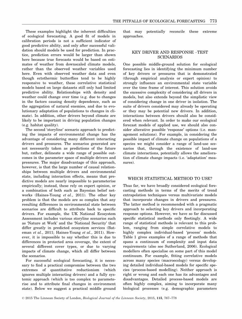
shown in Figure 2A and B for the butterfly speciesAphantopus hyperantus, a linear trend fitted toa national population index from 1980 to 2000adequately predicts abundances for the subsequent13 years (mean absolute error = 0.076). In othercases, extrapolation does a poor job at predicting thefuture state of an environmental variable. This situa-tion might be due to several reasons: (1) there is sub-stantial error in our measurement of the systemstate; (2) our statistical model is inadequate (e.g. fit-ting a linear trend when there is significant curva-ture); (3) there is a high degree of short-termvariability in the system state about some trend(sometimes called ‘stochasticity’); or (4) the ‘rules’that govern the system state change over time (i.e.

the drivers and pressures change). Examples ofunsuccessful extrapolations are shown for the butter-fly species Euphydryas aurinia (Fig. 2C, D; meanabsolute error = 0.217) and Hesperia comma(Fig. 2E, F; mean absolute error = 0.421). In thesecases, neither linear models, nor second or thirdorder polynomials, fitted to 1980–2000 data are ableto adequately predict population indices in the subse-quent 13 years.

Why are extrapolations so poor for these species?The population indices are collated from a reason-ably large number of sites (mean number of sites peryear for each species � standard error: A. hyperan-tus = 324.7 � 32.3; E. Aurinia = 62.5 � 5.24; Hespe-ria comma = 25.8 � 1.9) and so any measurement

1980 1985 1990 1995 2000 2005 2010

01

23

4

Year

1980 1985 1990 1995 2000 2005 2010Year

1980 1985 1990 1995 2000 2005 2010Year

Log

abun

danc

e in

dex

01

23

4

Log

abun

danc

e in

dex

01

23

4

Log

abun

danc

e in

dex

A

2002 2004 2006 2008 2010 2012

0.0

0.2

0.4

0.6

0.8

1.0

Year

2002 2004 2006 2008 2010 2012Year

2002 2004 2006 2008 2010 2012Year

Pre

dict

ion

erro

r

0.0

0.2

0.4

0.6

0.8

1.0

Pre

dict

ion

erro

r0.

00.

20.

40.

60.

81.

0

Pre

dict

ion

erro

r

B

C D

E F

Figure 2. Extrapolations of population abundance for three butterfly species: the Ringlet Aphantopus hyperantus (A,

B); Marsh Fritillary Euphydryas aurinia (C, D); and Silver Spotted Skipper Hesperia comma (E, F). Left hand panels

show the UK national log collated index of abundance with a linear trend fitted to the data from 1980 to 2000 and used

to predict abundance from 2001 onwards (open circles). The right hand panel shows the absolute difference between pre-

dicted and observed values.


THE PITFALLS OF ECOLOGICAL FORECASTING 769

errors should cancel each other out and have negligi-ble effect. With regards to the statistical model, foreach species three different models were compared(linear and second and third order polynomials) andin both cases the linear model was the best fit to the1980–2000 data. In the case of E. aurinia (Fig. 2C,D), the interannual population variability is verylarge, and although the linear model is a better fitcompared with models with curvature, the predictedvalues of the population index are often poor esti-mates. This factor may be problematic if accurateannual predictions are necessary; for example, if wewere aiming to predict the abundance of a pest spe-cies in order to inform prophylactic pesticide applica-tion. It may be possible to predict some of theinterannual variability in population abundanceswith models incorporating the factors that drive pop-ulation dynamics (see next section), but there willoften remain variation left over that we are unableto explain (e.g. resulting from demographic stochas-ticity). Despite this outcome, it is notable that errorsin our predictions do not necessarily get markedlyworse the further on in time a prediction is made(e.g. Fig. 2D; regression of absolute error by year:F1,11 = 0.42, P = 0.53). Therefore, if accurate annualpredictions are not so important, but we are rathermore interested in broad forecasts of future popula-tion trends, e.g. to allocate conservation fundingappropriately, then large interannual population var-iability may not be such an issue (Roy et al., 2001).The exception here would be for special cases inwhich stochasticity itself changes over time (e.g.changing environmentally induced stochasticity aspopulations move towards – or away – from the edgeof their fundamental niche space as the climatechanges; Oliver, Brereton & Roy, 2013; Oliver et al.,2014).

Our third example (Hesperia comma; Fig. 2E, F),is also a poor forecast from extrapolation, but in thiscase the interannual population variability is rela-tively low (Bennie et al., 2013). Instead, the lineartrend, which is a good fit to the population indicesbetween 1980 and 2000, is a poor fit to the data from2001 onwards, with the predictions getting notice-ably worse the further ahead we try to predict(Fig. 2F; regression of absolute error by year:F1,11 = 18.2, P = 0.001). The population trajectoryhas changed direction, presumably because density-dependent processes are beginning to operate orbecause the primary drivers that affect populations(e.g. climate, habitat quality, habitat extent) havechanged over the duration of the monitoring period.This problem is critical for extrapolation methods,because by using data only on the system state wecannot account for changes in drivers. Instead, theyare assumed to be constant; an assumption that is

very often contravened. For example, Mason et al.(2015) consider rates of distribution change (north-ern range margin shift) in four different animalgroups over two time intervals (from 1970 to 2010)and find that rates of change in the first time inter-val are poor predictors of rates of change in the sub-sequent time interval. What are these changes indrivers that underlie species responses?

The UK National Ecosystem Assessment (UKNEA, 2011) was the first comprehensive review ofdrivers of change in biodiversity and other ecosystemservices. It assessed the historic impact of drivers,but also their expected future impact. It is notablethat the magnitude of drivers often changes overtime. For example, habitat loss and pollution havebeen the primary causes of biodiversity loss in theUK over the last century, but the impacts of thesedrivers are expected to lessen, with climate changeand invasive species becoming the major new driversof change (UK NEA, 2011). Similar patterns arelikely to be occurring across other heavily modifiedtemperate landscapes. For example, Carvalheiroet al. (2013) suggest that pollinator declines in anumber of northwest European countries may haveslowed, probably due to a peak in the conversion ofland use to intensive agriculture. In addition tochanges in the magnitude of existing drivers, newdrivers may emerge with the advent of new technolo-gies (August et al., 2015). For example, a recent hori-zon scanning exercise by Sutherland et al. (2008)identified nanotechnology and geoengineering asfields with a large potential to impact biodiversity.Finally, drivers of change also interact in their envi-ronmental impacts, leading to non-linearity inresponses (Brook, Sodhi & Bradshaw, 2008). Forexample, climate and land-use change can interacton biodiversity through a wide range of mechanismsaffecting processes from demography to metapopula-tion structure and community interactions (Oliver &Morecroft, 2014). All these changes in drivers meanthat simple extrapolations of system state are often apoor method of forecasting, especially over longertimescales. Instead, statistical models are neededthat can incorporate the impact of drivers and howthese may change in the future.

FORECASTING CHANGES IN DRIVERS ANDPRESSURES

In order to incorporate the impact of pressures onthe state of environmental systems we need tounderstand their functional relationships (e.g. whatis the relationship between weather variables and aspecies’ population size), and also anticipate howpressures are likely to change in the future (e.g.



what will future weather be like under climatechange). Effects may be direct (e.g. weather impactson demographic rates) or indirect (e.g. mediatedthrough impacts on other species that interact withthe focal species). The former task of understandingcausal relationships can be achieved through experi-mentation (e.g. Tilman et al., 1994) or throughobservation of ‘natural experiments’ (i.e. using long-term monitoring of system state and relating this tonaturally occurring changes in drivers and pres-sures; Baker et al., 2012; Eglington & Pearce-Hig-gins, 2012; Roy et al., 2001). Both these methods arecostly and time consuming, but the experimentaldesigns (e.g. split-plot field experiments, long-termmonitoring networks) and statistical analysis tech-niques needed (e.g. multivariate regressions, hierar-chical mixed modelling and structural equationmodelling) are well versed in the ecological sciences.In contrast, the latter task of anticipating futurechanges in drivers and pressures is more difficultand less practiced. One technique would be to useextrapolative techniques to predict how drivers andpressures may change based on past temporaltrends. For example the GBO-4 report (Secretariatof the Convention on Biological Diversity, 2014) usesextrapolations of trends in human population size,gross domestic product, intensity of resource use,agricultural subsidies and surplus nitrogen in theenvironment. However, the problems with extrapola-tion of the state of the environment outlined abovealso hold true for extrapolation of pressures affectingsystem state – the pressures themselves are affectedby multiple other factors (drivers) that may havenon-linear trends over time. These more proximatedrivers are themselves affected by other drivers, andso on. For example, nitrogen deposition is affectedby both the cost of petrochemical fertilisers and priceof crops in the world market, these factors them-selves are affected by other more ultimate driverssuch as population growth and development of alter-native resource extraction and food production tech-nologies. Suddenly we are faced with an enormoustask: to forecast how a given pressure might changewe need to understand the whole chain of causalityaffecting that pressure (the ‘infinite regress of driv-ers’ dilemma). Much ecological science, and indeedscience in general, has tended to be reductionist inits approach, focusing on specific causal relation-ships, but more systematic ways of thinking are evi-dent in ancient eastern world views (e.g. theBuddhist concept of ‘Prat�ıtyasamutp�ada’) thatstrongly emphasises the interdependency of entitiesand multiple causal linkages between them, and alsofeature in ‘systems ecology’ approaches (Odum, 1983;Schellnhuber, 1999; Evans et al., 2013). Yet, thereare clear practical limitations to understanding

changes to specific pressures by tracing causal linksacross the entire socio-ecological-economic system;effectively, this relies on a statistical model of theentire world!

At this point, one might be tempted to throw inthe towel and give up trying to forecast future envi-ronmental states. However, returning to our originalreason for attempting forecasting – that without itwe rely on reactive management that is often too lateto avert significant environmental damage – we arereminded that forecasting, although difficult, is verynecessary. What is needed is a practical way forwardthat still remains as rigorous as possible. Pragmaticapproaches to the problem so far have tended toeither focus on one specific chain of causality affect-ing the environmental state (e.g. how climate changewill affect local temperatures and how these willaffect species populations; Thomas et al., 2004), or toadopt a ‘storyline’ scenario approach where variouspossible socioeconomic scenarios are described andthen a deliberative approach used to translate howchanges in more ultimate drivers (such as populationsize, climate, new technologies) will impact on proxi-mate pressures that affect environmental states.This latter approach is adopted by the MillenniumEcosystem Assessment (2005) and also in UKNational Ecosystem Assessment (UK NEA, 2011) inorder to explore how different socioeconomic scenar-ios might affect the state of the environment and theecosystem services it provides. Both approaches haveadvantages but also some key problems.

The first approach that focuses on a single ‘chain’of causality can afford more detailed quantitativeanalysis, but because this approach is more reduc-tionist it ignores the importance of other interactingdrivers and pressures on the system state. This maybe warranted where there is good evidence for anoverwhelmingly strong influence of one driver, whichexplains a large proportion of variance in the systemstate. For example, Figure 3 illustrates predictivecorrelative models for the abundance of three butter-fly species, whose population dynamics are driven byannual weather and density dependence to varyingextents. The first species, Melanargia galathea (Aand B), shows a reasonably good fit between pre-dicted and observed abundance in the model calibra-tion period (R2 = 0.68 with density dependenceeffects incorporated in models, R2 = 0.53 without),and also in the model validation (mean absoluteerror [MAE] = 0.14–0.15) and the ‘forecasting’ peri-ods (MAE = 0.10–0.11). In contrast, for the speciesCelastrina argiolus (C and D) even though goodness-of-fit for the model incorporating density dependenceis greater than the one without (R2 = 0.72 comparedwith 0.54) and there is little apparent differencein model fit in the validation period (MAE = 0.21



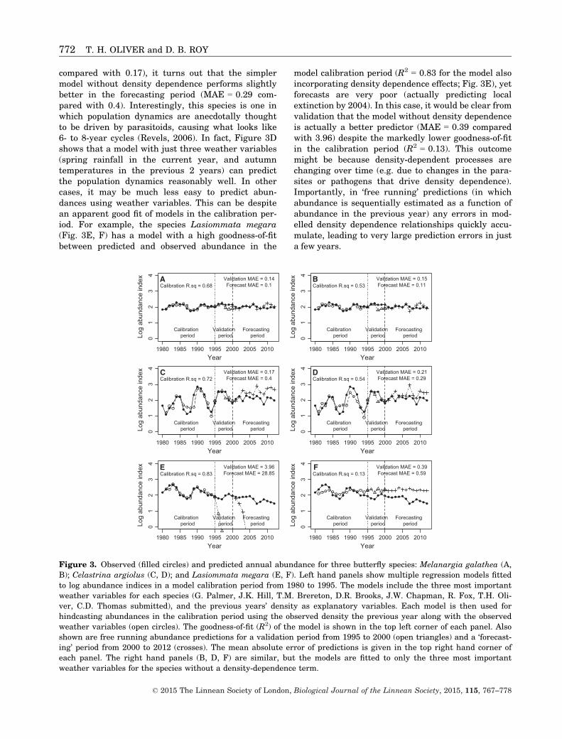
compared with 0.17), it turns out that the simplermodel without density dependence performs slightlybetter in the forecasting period (MAE = 0.29 com-pared with 0.4). Interestingly, this species is one inwhich population dynamics are anecdotally thoughtto be driven by parasitoids, causing what looks like6- to 8-year cycles (Revels, 2006). In fact, Figure 3Dshows that a model with just three weather variables(spring rainfall in the current year, and autumntemperatures in the previous 2 years) can predictthe population dynamics reasonably well. In othercases, it may be much less easy to predict abun-dances using weather variables. This can be despitean apparent good fit of models in the calibration per-iod. For example, the species Lasiommata megara(Fig. 3E, F) has a model with a high goodness-of-fitbetween predicted and observed abundance in the

model calibration period (R2 = 0.83 for the model alsoincorporating density dependence effects; Fig. 3E), yetforecasts are very poor (actually predicting localextinction by 2004). In this case, it would be clear fromvalidation that the model without density dependenceis actually a better predictor (MAE = 0.39 comparedwith 3.96) despite the markedly lower goodness-of-fitin the calibration period (R2 = 0.13). This outcomemight be because density-dependent processes arechanging over time (e.g. due to changes in the para-sites or pathogens that drive density dependence).Importantly, in ‘free running’ predictions (in whichabundance is sequentially estimated as a function ofabundance in the previous year) any errors in mod-elled density dependence relationships quickly accu-mulate, leading to very large prediction errors in justa few years.

1980 1985 1990 1995 2000 2005 2010

01

23

4

Year1980 1985 1990 1995 2000 2005 2010

Year

1980 1985 1990 1995 2000 2005 2010Year

1980 1985 1990 1995 2000 2005 2010Year

1980 1985 1990 1995 2000 2005 2010Year

1980 1985 1990 1995 2000 2005 2010Year

Log

abun

danc

e in

dex

01

23

4

Log

abun

danc

e in

dex

01

23

4

Log

abun

danc

e in

dex

01

23

4

Log

abun

danc

e in

dex

01

23

4

Log

abun

danc

e in

dex

01

23

4

Log

abun

danc

e in

dex

Calibration period

Validation period

Forecasting period

Calibration R.sq = 0.68Validation MAE = 0.14Forecast MAE = 0.1

A

Calibration period

Validation period

Forecasting period


B

Calibration period

Validation period

Forecasting period


C

Calibration period

Validation period

Forecasting period


D

Calibration period

Validation period

Forecasting period


E

Calibration period

Validation period

Forecasting period


F

Figure 3. Observed (filled circles) and predicted annual abundance for three butterfly species: Melanargia galathea (A,

B); Celastrina argiolus (C, D); and Lasiommata megara (E, F). Left hand panels show multiple regression models fitted

to log abundance indices in a model calibration period from 1980 to 1995. The models include the three most important

weather variables for each species (G. Palmer, J.K. Hill, T.M. Brereton, D.R. Brooks, J.W. Chapman, R. Fox, T.H. Oli-

ver, C.D. Thomas submitted), and the previous years’ density as explanatory variables. Each model is then used for

hindcasting abundances in the calibration period using the observed density the previous year along with the observed

weather variables (open circles). The goodness-of-fit (R2) of the model is shown in the top left corner of each panel. Also

shown are free running abundance predictions for a validation period from 1995 to 2000 (open triangles) and a ‘forecast-

ing’ period from 2000 to 2012 (crosses). The mean absolute error of predictions is given in the top right hand corner of

each panel. The right hand panels (B, D, F) are similar, but the models are fitted to only the three most important

weather variables for the species without a density-dependence term.



These examples highlight the inherent difficultiesof ecological forecasting. A good fit of models incalibration periods is not a sufficient indicator ofgood predictive ability, and only after successful vali-dation should models be used for prediction. In prac-tice, prediction errors would be larger than shownhere because true forecasts would be based on esti-mates of weather from downscaled climate models,rather than the observed weather variables usedhere. Even with observed weather data and eventhough ectothermic butterflies tend to be highlyresponsive to weather, these correlative statisticalmodels based on large datasets still only had limitedpredictive ability. Relationships with density andweather could change over time (e.g. due to changesin the factors causing density dependence, such asthe aggregation of natural enemies, and due to evo-lutionary adaptation of populations to changes in cli-mate). In addition, other drivers beyond climate arelikely to be important in driving population changes(e.g. habitat quality).

The second ‘storyline’ scenario approach to predict-ing the impacts of environmental change has theadvantage of considering many different interactingdrivers and pressures. The scenarios generated arenot necessarily taken as predictions of the futurebut, rather, delineate a wide range of possible out-comes in the parameter space of multiple drivers andpressures. The major disadvantage of this approach,however, is that the large number of causal relation-ships between multiple drivers and environmentalstate, including interaction effects, means that pre-dictive models are nearly impossible to parameteriseempirically; instead, these rely on expert opinion, ora combination of both such as Bayesian belief net-works (Haines-Young et al., 2011). The other keyproblem is that the models are so complex that anyresulting differences in environmental state betweenscenarios are difficult to attribute back to specificdrivers. For example, the UK National EcosystemAssessment includes various storyline scenarios suchas ‘Nature at Work’ and the ‘National Security’ thatdiffer greatly in predicted ecosystem services (Bat-eman et al., 2011; Haines-Young et al., 2011). How-ever, it is impossible to say whether this is due todifferences in protected area coverage, the extent ofseveral different cover types, or due to varyingimpacts of climate change, which all differ betweenthe scenarios.

For successful ecological forecasting, it is neces-sary to find a practical compromise between the twoextremes of quantitative reductionism (whichignores multiple interacting drivers) and a fully sys-temic approach (which is too complex to paramete-rise and to attribute final changes in environmentstate). Below we suggest a practical middle ground

that may potentially reconcile these extremeapproaches.

KEY DRIVER AND RESPONSE –TESTSCENARIOS

One possible middle-ground solution for ecologicalforecasting lies in identifying the minimum numberof key drivers or pressures that is demonstrated(through empirical analysis or expert opinion) tostrongly influence an environmental state variableover the time frame of interest. This solution avoidsthe excessive complexity of considering all drivers inmodels, but also extends beyond the simplistic viewof considering change in one driver in isolation. Thesuite of drivers considered may already be operatingor they may be potential new drivers. In addition,interactions between drivers should also be consid-ered when relevant. In order to make our ecologicalforecast models of applied use, we should also con-sider alterative possible ‘response’ options (i.e. man-agement solutions). For example, in considering thepossible impact of climate change on populations of aspecies we might consider a range of land-use sce-narios that, through the existence of land-useclimate interactions, potentially allows the ameliora-tion of climate change impacts (i.e. ‘adaptation’ mea-sures).

WHICH STATISTICAL METHOD TO USE?

Thus far, we have broadly considered ecological fore-casting methods in terms of the merits of trendextrapolation techniques versus multivariate modelsthat incorporate changes in drivers and pressures.The latter method is recommended with a pragmaticapproach to selecting key drivers and incorporatingresponse options. However, we have so far discussedspecific statistical methods only fleetingly. A widerange of statistical methods is relevant to this prob-lem, ranging from simple correlative models tohighly complex individual-based ‘process’ models.Table 1 gives examples of a range of methods thatspans a continuum of complexity and input datarequirements (also see Sutherland, 2006). Ecologicalmodellers often specialise on some part of this modelcontinuum. For example, fitting correlative modelsacross many species (macroecology) versus develop-ing detailed individual-based models for specific spe-cies (process-based modelling). Neither approach isright or wrong and each one has its advantages anddisadvantages. Detailed process-based models areoften highly complex, aiming to incorporate manybiological processes (e.g. demographic parameters



that vary in different environments, interspecificinteractions and evolutionary processes). As such,they are more biologically realistic representationswith the potential for more accurate predictions.However, the cost of this complexity is that manymore parameters need to be estimated, requiring sig-nificantly more data to calibrate models. When oneconsiders the total numbers of species that one couldpotentially be interested in for conservation ecology(e.g. c. 70 000 in the UK, which is a relatively spe-cies-poor country; UK Species Inventory, 2014; Gur-ney, 2015), then it becomes clear that such data-hungry models are impractical, unless they can beshown to produce general responses that are repre-sentative of many other species. At the other end ofthe spectrum, extrapolative techniques or simple cor-relative models, which consider species responses toa single driver, may be too simplistic and ignore keyinteractions between drivers. This lack of mechanis-tic understanding behind species responses can meanthat predictions are inaccurate if drivers change innon-linear ways over time. To identify a practicalway forward, again, the theory of the ‘middle way’may help up to reconcile these extremes. Methodsare needed that balance the complexity needed tomake robust predictions with the feasibility of modelparameterisation given data availability. The threemethods in the middle rows of Table 1 are mostlikely to achieve this balance and produce reliableforecasts of environmental change for many speciesin order to inform conservation responses. Theseinclude phenomenological models and mechanisticmodels. In practice, successful models may contain acombination of both the above approaches, with well

known biological processes specified by mechanisticrelationships but with flexibility for unknown rela-tionships to be estimated from the observed data(Dormann et al., 2012).

RIGOUR IN PREDICTIVE MODELLING

In addition to selecting the most appropriate statisti-cal modelling framework, the modelling approachmust be as rigorous as possible, in order to ensureaccurate predictions. This situation is especiallyimportant if our forecasts are used as evidence toimplement prophylactic management to avert envi-ronmental damage. Such management options mayhave substantial costs and therefore need to be wellevidenced. For example, setting aside semi-naturalhabitats to maintain pollinating insects under cli-mate change has costs in terms of reduced land forcropping and so strong evidence is needed to con-vince stakeholders of the best land managementsolution.

To select the most appropriate statistical model,the goodness-of-fit to historic data of alternativemodels is usually assessed. But this criterion alonecan lead to over-parameterised models that are poorat predicting future environmental states. Instead,model validation is necessary using data indepen-dent of that used for model fitting. For example, Fig-ure 3 shows how 20 years of historic monitoring datacan be split into 15 years for model fitting (of abun-dance changes in relation to weather variables) andfive for model testing. This approach can preventoverfitting and allow better predictions of subsequent

Table 1. Different statistical methods for ecological forecasting

Forecasting method Description Example

Extrapolation Descriptive statistical model of trend in

system state variable

Predicting species geographic range margins from

past rates of change

Simple

correlative models

Statistical relationship between driver or

pressure variable(s) and sytem

state variable

Predicting species distribution from relationships

between occurrence and climate variables

Phenomenological

models*

Statistical relationship between driver or

pressure and intermediate demographic

processes that combine to determine state

Predicting species abundance from climate impacts

on population growth, mortality and dispersal

Mechanistic model* Relationship between driver or pressure and

intermediate demographic processes based

on prior biological understanding

Predicting species abundance under climate

changes based on physiological relationships

between development rates and lethal

temperatures

Individual-based

models

Behavioural rules used to model individual

decisions, often in combination with

phenomological components relating to

demography

Predicting impacts of climate change on

individual movements and how this scales up

to species range margin shifts

*Note that this dichotomy is not strict and some models combine both phenomenological and mechanistic components.



abundance (demonstrated here by hindcasting to themost recent 13 years of data). In the absence of timeseries data, space-for-time substitutions are the nextbest option to validate models; for example, usingthe model fitted to data in one area to predict envi-ronmental state in a different area. There can beproblems with this approach, however, as a numberof different correlated variables may change acrossspatial gradients (White & Kerr, 2006; Isaac et al.,2010).

Despite the importance of validation, yet becauseof its difficulty, several current modelling frame-works are being used to predict future environmentalstates with limited validation of the models. Thisapproach is especially evident in the recently emerg-ing field of ecosystem service modelling (e.g. Nelsonet al., 2009, 2010; UK NEA, 2011; Bateman et al.,2013). There is clearly a danger in implementingmanagement options with limited evidence. Undersuch circumstances an adaptive managementapproach is highly appropriate, in which the man-agement actions predicted as most suitable are takenbut with regular monitoring to assess their effective-ness. Past environmental policies have often tendedto be inflexible, however, leading to ‘lock-in’ to a setof options with little consideration of adaptive man-agement. For example, agri-environment schemesput in place in the UK to prevent biodiversitydeclines in agricultural landscapes were based onsynthesis of the evidence base for the effectiveness ofdifferent management options. Over £400 M per yearis spent on these schemes in England (Natural Eng-land, 2009), yet the budget to monitor the effective-ness of these schemes (and validate the predictionsof their effectiveness) is a very small percentage ofthis (< 1%). With this and many other environmentalpolicies, when seen in the context of ecological fore-casting and its validation, there is a strong argumentfor rebalancing spending on action versus monitoringand analysis.

DATA FOR PREDICTIVE MODELS AND THEIMPORTANCE OF BIOLOGICAL RECORDING

As discussed above, a wide range of environmentaldrivers can impact species. Models of these causalrelationships (and the potential interactions betweendrivers) will necessarily have several estimatedparameters, even when reduced to the subset of driv-ers with the largest impacts. Therefore, substantialdatasets on species populations and measured valuesof drivers are needed for model calibration and vali-dation. These data may come from mesocosm or fieldexperiments, or ‘natural experiments’ comprisingthe monitoring of natural populations over broad

environmental gradients. Mesocosm experimentsconsider responses to a limited range of manipulatedvariables under controlled conditions. They areuseful for testing theory and stimulating furtherresearch (Benton et al., 2007), although the ability ofthese systems to produce species responses similar tothose in the real world is questionable (Carpenter,1996). Field experiments comprise a selected rangeof treatments to consider the effects of different driv-ers but at a larger scale and in more realistic set-tings subject to ‘noise’ from other unmeasuredenvironmental drivers (Carpenter, 1998). Experimen-tal manipulation is the ideal way to test ecologicaltheories (including those pertaining to relationshipsbetween drivers and population responses), but fieldexperiments are very time consuming and expensive.In addition, even in large-scale experiments, the lim-ited spatial and temporal scale means that patternsoperating at large scales may be missed (e.g. Wiens,Rotenberry & Van Horne, 1986). The alternative todesigned experiments is to exploit natural environ-mental gradients and large-scale perturbations(Carpenter, 1990). This approach requires monitoringof species responses, ideally with high levels ofspatial and temporal replication that are necessaryto maintain statistical power in the face of combinedvariability across wide range of environmental vari-ables. Examples of such large-scale monitoringinclude the collection of biological records (georefer-enced records of species presences), such as thoseheld by the Biological Records Centre (Pocock et al.,2015), the broad utility of which is demonstrated bythe articles within this issue (Chapman et al., 2015;Gillingham et al., 2015; Mason et al., 2015; Powney& Isaac, 2015; Purse & Golding, 2015; Roy, 2015;Roy et al., 2015; Sutherland, Roy & Amano, 2015).Abundance data such as that represented in speciesmonitoring schemes (e.g. the UK Butterfly Monitor-ing Scheme data used in this paper), are even moreuseful in allowing forecasts of abundance rather thanjust species presence, although there is evidence thatdistribution data can predict abundance to a limiteddegree (Elmendorf & Moore, 2008; VanDerWal et al.,2009; Oliver et al., 2012a,b). Monitoring data providea crucial resource for ecological forecasting becauseof the large spatial and temporal extent that theycan cover. This resource is facilitated by the use oftrained volunteers that help to reduce the total costsof monitoring schemes. Experimental approaches,although much better for well controlled tests of the-ory and testing management techniques, are oftentoo limited in their spatial coverage to adequatelyinform ecological forecasts, at least beyond the loca-tion of the experiment. For example, speciesresponses to weather conditions (a major driver ofpopulation variation across most species) can be



assessed using data from national monitoringschemes (Roy et al., 2001; Wallis De Vries, Baxter &Van Vliet, 2011; Eglington & Pearce-Higgins, 2012).In addition, because weather effects are modified bytopography and habitat type not just at the local scalebut also by the structural composition of surroundinglandscapes (Oliver et al., 2010, 2012a, 2013), then it isnecessary to empirically model these effects in orderto make general forecasts beyond the responses of asingle site. Fortunately, some countries have wellestablished species monitoring schemes (e.g. the longhistory of natural history recording in Britain), andprotocols for a number of currently unstudied speciesgroups and new monitoring schemes in other coun-tries are currently under development. Internationalinitiatives are also at work to synthesise monitoringdata (e.g. the global Biodiversity ObservationNetwork, GEOBON).

CONCLUSION

Overall, this review has highlighted the necessity ofecological forecasting in order to avert environmentaldamages that would occur under a solely reactivemanagement approach. Extrapolating from historicenvironmental states will often be unsuccessfulbecause drivers and pressures themselves change innon-linear ways and interact in their impact. Newpressures on systems, such as those from emergingtechnologies, may also arise. The complexity of causalpathways between drivers, pressures and environ-mental state is effectively endless, so a pragmaticapproach is needed to focus on a subset of pathwaysthat have the greatest impact on system state. Addi-tionally, incorporating possible response options inour models will allow us to assess the effectiveness ofpotential solutions to environmental damage. In termsof modelling techniques, a compromise between com-plexity (and potential biological realism) and feasibil-ity given data availability will be necessary, but thereis also a key importance in validating models toensure that forecasts can be made with reasonableconfidence. Although ecological forecasting is verydifficult, it is also highly necessary. Much ecologicalscience has tended to focus on understanding currentand historic patterns and trends. However, there is aclear need to step out of our comfort zones and developecological forecasts in order to inform enviromentalmanagement effectively.

ACKNOWLEDGEMENTS

We are grateful to the UK Butterfly MonitoringScheme (UKBMS) volunteers and scheme co-ordinators

for providing the data used in the forecasting exam-ples in this paper. The UKBMS is funded funding bya multi-agency consortium led by the Department forEnvironmental Food and Rural Affairs, and includ-ing the Natural Resources Wales, Natural England,Forestry Commission, and Scottish Natural Heritage.The Biological Record Centre, of which the UKBMSis part, receives support from the Joint Nature Con-servation Committee and the Natural EnvironmentResearch Council (via National Capability funding tothe Centre for Ecology & Hydrology, projectNEC04932).We thank Mike Morecroft and ChrisPreston for helpful comments that improved thismanuscript.

REFERENCES

August T, HarveyM, Lightfoot P, Kilbey D, Papadopoulos

T, Jepson P. 2015. Emerging technologies for biological

recording. Biological Journal of the Linnean Society 115:

731–749.

Baker DJ, Freeman SN, Grice PV, Siriwardena GM.

2012. Landscape-scale responses of birds to agri-environ-

ment management: a test of the English Environmental

Stewardship scheme. Journal of Applied Ecology 49: 871–

882.

Bateman IJ, Abson D, Andrews B, Crowe A, Darnell A,

Dugdale S, Fezzi C, Foden J, Haines-Young R, Hulme

M, Munday P, Pascual U, Paterson J, Perino G, Sen A,

Siriwardena G, Termansen M. 2011. Chapter 26: valuing

changes in ecosystem services: scenario analyses. In: The UK

national ecosystem assessment: technical report. Cambridge:

UNEP-WCMC. Available at: http://uknea.unep-wcmc.org/Link

Click.aspx?fileticket=m%2BvhAV3c9uk%3D&tabid=82.

Bateman IJ, Harwood AR, Mace GM, Watson RT, Abson

DJ, Andrews B, Binner A, Crowe A, Day BH, Dugdale

S, Fezzi C, Foden J, Hadley D, Haines-Young R, Hul-

me M, Kontoleon A, Lovett AA, Munday P, Pascual U,

Paterson J, Perino G, Sen A, Siriwardena G, van So-

est D, Termansen M. 2013. Bringing ecosystem services

into economic decision-making: land use in the United

Kingdom. Science 341: 45–50.

Bennie J, Hodgson JA, Lawson CR, Holloway CTR, Roy

DB, Brereton T, Thomas CD, Wilson RJ. 2013. Range

expansion through fragmented landscapes under a variable

climate. Ecology Letters 16: 921–929.

Benton TG, Solan M, Travis JMJ, Sait SM. 2007. Micro-

cosm experiments can inform global ecological problems.

Trends in Ecology & Evolution 22: 516–521.

Brook BW, Sodhi NS, Bradshaw CJA. 2008. Synergies

among extinction drivers under global change. Trends in

Ecology and Evolution 23: 453–460.

Carpenter SR. 1990. Large-scale perturbations: opportuni-

ties for innovation. Ecology 71: 2038–2043.

Carpenter SR. 1996. Microcosm experiments have limited

relevance for community and ecosystem ecology. Ecology

77: 677–680.



Carpenter SR. 1998. The need for large-scale experiments to

assess and predict the response of ecosystems to perturbation.

In: Pace M, Groffman P, eds. Successes, limitations, and fron-

tiers in ecosystem science. New York: Springer, 287–312.

Carvalheiro LG, Kunin WE, Keil P, Aguirre-Guti�errez

J, Ellis WN, Fox R, Groom Q, Hennekens S, Van

Landuyt W, Maes D, Van de Meutter F, Michez D,

Rasmont P, Ode B, Potts SG, Reemer M, Roberts

SPM, Schamin�ee J, WallisDeVries MF, Biesmeijer JC.

2013. Species richness declines and biotic homogenisation

have slowed down for NW-European pollinators and plants.

Ecology Letters 16: 870–878.

Chapman D, Bell S, Helfer S, Roy DB. 2015. Unbiased

inference of plant flowering phenology from biological

recording data. Biological Journal of the Linnean Society

115: 543–554.

Dormann CF, Schymanski SJ, Cabral J, Chuine I, Gra-

ham C, Hartig F, Kearney M, Morin X, R€omermann C,

Schr€oder B, Singer A. 2012. Correlation and process in

species distribution models: bridging a dichotomy. Journal

of Biogeography 39: 2119–2131.

Eglington S, Pearce-Higgins JW. 2012. Disentangling the

relative importance of changes in climate and land-use

intensity in driving recent bird population trends. PLoS

ONE 7: e30407.

Elmendorf SC, Moore KA. 2008. Use of community-compo-

sition data to predict the fecundity and abundance of spe-

cies. Conservation Biology 22: 1523–1532.

European Environment Agency. 2007. The DPSIR frame-

work used by the EEA. Available at: http://ia2dec.e-

w.eea.europa.eu/knowledge_base/Frameworks/doc101182.

Evans MR, Bithell M, Cornell SJ, Dall SRX, D�ıaz S,

Emmott S, Ernande B, Grimm V, Hodgson DJ, Lewis

SL, Mace GM, Morecroft M, Moustakas A, Murphy E,

Newbold T, Norris KJ, Petchey O, Smith M, Travis

JMJ, Benton TG. 2013. Predictive systems ecology. Pro-

ceedings of the Royal Society B: Biological Sciences 280.

Gillingham PK, Bradbury RB, Roy DB, Anderson BJ,

Baxter JM, Bourn NAD, Crick HQP, Findon RA, Fox

R, Franco A, Hill JK, Hodgson JA, Holt AR, Morecroft

MD, O’Hanlon NJ, Oliver TH, Pearce-Higgins JW,

Procter DA, Thomas JA, Walker KJ, Walmsley CA,

Wilson RJ, Thomas CD. 2015. The effectiveness of pro-

tected areas in the conservation of species with changing

geographical ranges. Biological Journal of the Linnean

Society 115: 707–717.

Gurney M. 2015. Gains and losses: recent colonisations and

extinctions in Britain. Biological Journal of the Linnean

Society 115: 573–585.

Haines-Young R, Paterson J, Potschin M, Wilson A,

Kass G. 2011. Chapter 25: The UK NEA Scenarios: Devel-

opment of Storylines and Analysis of Outcomes. In: The UK

national ecosystem assessment: synthesis of the key findings.

Cambridge: UNEP-WCMC. Available at: http://uknea.

unep-wcmc.org/LinkClick.aspx?fileticket=m%2BvhAV3c9uk

%3D&tabid=82

Inger R, Gregory R, Duffy JP, Stott I, Vor�ı�sek P,

Gaston KJ. 2014. Common European birds are declining

rapidly while less abundant species’ numbers are rising.

Ecology Letters 18: 28–36.

IPCC. 2014. Working Group II Contribution to the IPCC

Fifth Assessment Report. Climate Change 2014: Impacts,

Adaptation, and Vulnerability.

Isaac NJB, Girardello M, Brereton T, Roy D. 2010. But-

terfly abundance in a warming climate: patterns in space

and time are not congruent. Journal of Insect Conservation

15: 233–240.

Mace GM, Collar NJ, Gaston KJ, Hilton-Taylor C,

Akc�akaya HR, Leader-Williams N, Milner-Gulland EJ,

Stuart SN. 2008. Quantification of extinction risk: IUCN’s

system for classifying threatened species. Conservation

Biology 22: 1424–1442.

Maes D, Isaac NJB, Harrower CA, Collen B, van Strien

AJ, Roy DB. 2015. The use of opportunistic data for IUCN

Red List assessments. Biological Journal of the Linnean

Society 115: 690–706.

Mason SC, Palmer G, Fox R, Gillings S, Hill JK, Thomas

CD, Oliver TH. 2015. Geographical range margins of many

taxonomic groups continue to shift polewards. Biological

Journal of the Linnean Society 115: 586–597.

Millennium Ecosystem Assessment. 2005. Ecosystems

and Human Well-being: Opportunities and Challenges for

Business and Industry. Washington, DC: World Resources

Institute.

Natural England. 2009. Agri-environment schemes in Eng-

land 2009: a review of results and effectiveness: Natural

England Report (NE194).

Nelson E, Mendoza G, Regetz J, Polasky S, Tallis H,

Cameron D, Chan KMA, Daily GC, Goldstein J, Kareiva

PM, Lonsdorf E, Naidoo R, Ricketts TH, Shaw M. 2009.

Modeling multiple ecosystem services, biodiversity conserva-

tion, commodity production, and tradeoffs at landscape scales.

Frontiers in Ecology and The Environment 7: 4–11.

Nelson E, Sander H, Hawthorne P, Conte M, Ennaanay

D, Wolny S, Manson S, Polasky S. 2010. Projecting global

land-use change and its effect on ecosystem service provision

and biodiversity with simple models. PLoS ONE 5: e14327.

Odum HT. 1983. Systems Ecology: An Introduction. Wiley-

Interscience.

Oliver T, Roy DB, Hill JK, Brereton T, Thomas CD.

2010. Heterogeneous landscapes promote population stabil-

ity. Ecology Letters 13: 473–484.

Oliver TH, Roy DB, Brereton T, Thomas JA. 2012a.

Reduced variability in range-edge butterfly populations

over three decades of climate warming. Global Change Biol-

ogy 18: 1531–1539.

Oliver TH, Gillings SG, Girardello M, Rapacciuolo G,

Brereton T, Siriwardena GM, Roy DB, Pywell RF,

Fuller RJ. 2012b. Population density but not stability can

be predicted from species distribution models. Journal of

Applied Ecology 49: 581–590.

Oliver TH, Brereton T, Roy DB. 2013. Population resilience

to an extreme drought is influenced by habitat area and frag-

mentation in the local landscape. Ecography 36: 579–586.

Oliver TH, Morecroft MD. 2014. Interactions between cli-

mate change and land use change on biodiversity: attribu-



tion problems, risks, and opportunities. Wiley Interdisci-

plinary Reviews: Climate Change 5: 317–335.

Oliver TH, Stefanescu C, Paramo F, Brereton T, Roy

DB. 2014. Latitudinal gradients in butterfly population

variability are influenced by landscape heterogeneity. Ecog-

raphy 37: 863–871.

Pocock MJO, Roy HE, Preston CD, Roy DB. 2015. The

biological records centre: a pioneer of citizen science. Bio-

logical Journal of the Linnean Society 115: 475–493.

Powney GD, Isaac NJB. 2015. Beyond maps: a review of

the applications of biological records. Biological Journal of

the Linnean Society 115: 532–542.

Purse B, Golding N. 2015. Tracking the spread and impacts

of diseases with biological records and distribution model-

ling. Biological Journal of the Linnean Society 115: 664–677.

Pimentel D. 2005. Environmental and economic costs of the

application of pesticides primarily in the United States.

Environment, Development and Sustainability 7: 229–252.

Revels R. 2006. More on the rise and fall of the Holly blue.

British Wildlife 17: 419–424.

Roy DB, Rothery P, Moss D, Pollard E, Thomas JA.

2001. Butterfly numbers and weather: predicting historical

trends in abundance and the future effects of climate

change. Journal of Animal Ecology 70: 201–217.

Roy HE, Peyton J, Aldridge DC, Bantock T, Blackburn

TM, Britton R, Clark P, Cook E, Dehnen-Schmutz K,

Dines T, Dobson M, Edwards F, Harrower C, Harvey

MC, Minchin D, Noble DG, Parrott D, Pocock MJO,

Preston CD, Roy S, Salisbury A, Sch€onrogge K,

Sewell J, Shaw RH, Stebbing P, Stewart AJA, Walker

KJ. 2014. Horizon scanning for invasive alien species with

the potential to threaten biodiversity in Great Britain.

Global Change Biology 20: 3859–3871.

Roy HE, Rorke SL, Beckmann B, Botham MS, Brown

PMJ, Noble D, Sewell J, Walker KJ. 2015. The contribu-

tion of volunteer recorders to our understanding of biologi-

cal invasions. Biological Journal of the Linnean Society

115: 678–689.

Schellnhuber HJ. 1999. ‘Earth system’ analysis and the

second Copernican revolution. Nature 402: C19–C23.

Secretariat of the Convention on Biological Diversity.

2014. Global Biodiversity Outlook 4: Montr�eal.

Sutherland WJ, Roy DB, Amano T. 2015. An agenda for

the future of biological recording for ecological monitoring

and citizen science. Biological Journal of the Linnean Soci-

ety 115: 779–784.

Sutherland WJ. 2006. Predicting the ecological conse-

quences of environmental change: a review of the methods.

Journal of Applied Ecology 43: 599–616.

Sutherland WJ, Bailey MJ, Bainbridge IP, Brereton T,

Dick JTA, Drewitt J, Dulvy NK, Dusic NR, Freckleton

RP, Gaston KJ, Gilder PM, Green RE, Heathwaite AL,

Johnson SM, Macdonald DW, Mitchell R, Osborn D,

Owen RP, Pretty J, Prior SV, Prosser H, Pullin AS,

Rose P, Stott A, Tew T, Thomas CD, Thompson DBA,

Vickery JA, Walker M, Walmsley C, Warrington S,

Watkinson AR, Williams RJ, Woodroffe R, Woodroof

HJ. 2008. Future novel threats and opportunities facing

UK biodiversity identified by horizon scanning. Journal of

Applied Ecology 45: 821–833.

Thomas CD, Cameron A, Green RE, Bakkenes M,

Beaumont LJ, Collingham YC, Erasmus BFN, Ferre-

ira de Siqueira M, Grainger A, Hannah L, Hughes L,

Huntley B, van Jaarsveld AS, Midgley GF, Miles L,

Ortega-Huerta MA, Peterson AT, Phillips OL,

Williams SE. 2004. Extinction risk from climate change.

Nature 427: 145–148.

Thomas CD, Hill JK, Anderson BJ, Bailey S, Beale CM,

Bradbury RB, Bulman CR, Crick HPQ, Eigenbrod F,

Griffiths H, Kunin WE, Oliver TH, Walmsley CA,

Watts K, Worsfold NT, Yardley T. 2011. A framework

for assessing threats and benefits to species responding to

climate change. Methods in Ecology and Evolution 2: 125–

142.

Tilman D, Dodd M, Silvertown J, Poulton P, Johnston

A, Crawley M. 1994. The park grass experiment-insights

from the most long-term ecological study. In: Leigh RA,

Johnston AE, eds. Long-term Experiments in Agricultural

and Ecological Science. Wallingford, Oxon. Wallingford,

Oxon, UK: CAB International, 287–303.

UK NEA. 2011. The UK national ecosystem assessment: syn-

thesis of the key findings. Cambridge: UNEP-WCMC.

UK Species Inventory. 2014. Natural History Museum.

Available at: http://www.nhm.ac.uk/research-curation/scien-

tific-resources/biodiversity/uk-biodiversity/uk-species/about-

the-species-inventory/index.html.

United States Environmental Protection Agency. 2014.

Tutorials on Systems Thinking using the DPSIR Frame-

work. Available at: http://www.epa.gov/ged/tutorial/.

US Environmental Protection Agency. 1975. DDT: A !

review of scientific and economic aspects of the decision to

ban its use as a pesticide. EPA-540/1-75-022: Washington

DC.

Van Swaay CAM, Van StrienAJ, Harpke A, Fontaine B,

Stefanescu C, Roy D, Maes D, K€uhn E, ~Ounap E,

Regan E, �Svitra G, Heli€ol€a J, Settele J, Warren MS,

Plattner M, Kuussaari M, Cornish N, Garcia Pereira

P, Leopold P, Feldmann R, Jullard R, Verovnik R,

Popov S, Brereton T, Gmelig MeylingA, Collins S.

2010. The European Butterfly Indicator for Grassland spe-

cies 1990–2009. Report VS2010.010, De Vlinderstichting,

Wageningen.

VanDerWal J, Shoo LP, Johnson CN, Williams SE.

2009. Abundance and the environmental niche: environ-

mental suitability estimated from niche models predicts the

upper limit of local abundance. The American Naturalist

174: 282–291.

Wallis De Vries MF, Baxter W, Van Vliet AJH. 2011.

Beyond climate envelopes: effects of weather on regional

population trends in butterflies. Oecologia 167: 559–571.

White P, Kerr J. 2006. Contrasting spatial and temporal

global change impacts on butterfly species richness during

the 20th century. Ecography 29: 908–918.

Wiens JA, Rotenberry JT, Van Horne B. 1986. A lesson

in the limitations of field experiments: shrubsteppe birds

and habitat alteration. Ecology 67: 365–376.



The pitfalls of ecological forecasting

Documents

Transcript of The pitfalls of ecological forecasting