Technical Report

TR-2011-012

The Physics of Communicability in Complex Networks

by

Ernesto Estrada, Naomichi Hatano, Michele Benzi

Mathematics and Computer Science

EMORY UNIVERSITY

1

The Physics of Communicability in Complex Networks

Ernesto Estrada1

Department of Mathematics and Statistics, Department of Physics, SUPA, and Institute of

Complex Systems, University of Strathclyde, Glasgow G1 1XQ, UK.

Naomichi Hatano

Institute of Industrial Science, University of Tokyo, Komaba, Meguro, Tokyo 153-8505,

Japan.

Michele Benzi

Department of Mathematics and Computer Sciences, Emory University, Atlanta, Georgia

30322, USA

1 Corresponding author. E-mail: ernesto.estrada@strath.ac.uk

2

ABSTRACT

A fundamental problem in the study of complex networks is to provide quantitative measures

of correlation and information flow between different parts of a system. To this end, several

notions of communicability have been introduced and applied to a wide variety of real-world

networks in recent years. Several such communicability functions are reviewed in this paper.

It is emphasized that communication and correlation in networks can take place through

many more routes than the shortest paths, a fact that may not have been sufficiently

appreciated in previously proposed correlation measures. In contrast to these, the

communicability measures reviewed in this paper are defined by taking into account all

possible routes between two nodes, assigning smaller weights to longer ones. This point of

view naturally leads to the definition of communicability in terms of matrix functions, such

as the exponential, resolvent, and hyperbolic functions, in which the matrix argument is either

the adjacency matrix or the graph Laplacian associated with the network.

Considerable insight on communicability can be gained by modeling a network as a system

of oscillators and deriving physical interpretations, both classical and quantum-mechanical,

of various communicability functions. Applications of communicability measures to the

analysis of complex systems are illustrated on a variety of biological, physical and social

networks. The last part of the paper is devoted to a review of the notion of locality in

complex networks and to computational aspects that by exploiting sparsity can greatly reduce

the computational efforts for the calculation of communicability functions for large networks.

3

CONTENTS

I. INTRODUCTION ............................................................................................................................... 4

A. Overview: interaction and correlation ............................................................................................ 4

B. Correlation function ....................................................................................................................... 8

C. Plan of the article .......................................................................................................................... 10

II. COMMUNICABILITY IN NETWORKS ....................................................................................... 10

A. Combinatorial definition .............................................................................................................. 10

B. Some combinatorial formulae ...................................................................................................... 15

III. PHYSICAL ANALOGIES ............................................................................................................. 17

A. Oscillator Networks ..................................................................................................................... 17

B. Network Hamiltonians ................................................................................................................. 18

C. Network of Quantum Oscillators ................................................................................................. 20

D. Network of Classical Oscillators .................................................................................................. 26

IV. COMPARING COMMUNICABILITY FUNCTIONS .................................................................. 29

A. Study of a social conflict ........................................................................................................... 30

B. Study of biomolecular networks ............................................................................................... 35

V. COMMUNICABILITY AND THE ANALYSIS OF NETWORKS ............................................... 39

A. Microscopic analysis of networks ................................................................................................ 40

B. Mesoscopic analysis of networks ................................................................................................. 42

C. Macroscopic analysis of networks ............................................................................................... 47

D. Multiscale analysis of networks ................................................................................................... 52

E. Communicability at negative absolute temperature ..................................................................... 55

VI. COMMUNICABILITY AND LOCALIZATION IN COMPLEX NETWORKS ......................... 59

A. Generalities ............................................................................................................................... 59

B. Exponential decay in communicability ........................................................................................ 62

VII. COMPUTABILITY OF COMMUNICABILITY FUNCTIONS .................................................. 66

A. Analytical results .......................................................................................................................... 66

B. Numerical experiments ................................................................................................................ 73

VIII. CONCLUSIONS AND PERSPECTIVES ................................................................................... 74

REFERENCES ..................................................................................................................................... 77

4

I. INTRODUCTION

A. Overview: interaction and correlation

In social system studies it is frequently found that agents belonging to the same

group tend to behave similarly (Manski, 2000). Social scientists use the term „interaction‟ to

explain this empirical regularity and use terms such as “social norms”, “peer influences”,

“neighborhood effects”, “conformity”, “imitation”, “contagion”, “epidemics”, “bandwagons”

or “herd behavior” to refer to them (Merton, 1957; Granovetter, 1979; Manski, 2000). In

physics, one is often warned (but not as often heard) that interaction and correlation are two

different concepts. Consider a solid, for example. Each atom in a solid interacts with

neighboring atoms mostly, and perhaps with next- and second-next neighboring ones at most.

However, if we hit one end of a solid bar, the effect of the action propagates to the other end,

which is a manifestation of the fact that an atom on the one end of solid is correlated with an

atom on the other end. Correlation is indeed the driving force of most phase transitions of

many-body systems. When a substance undergoes successive phase transitions from gas to

liquid on to solid, the interaction range of each atom does not change much but the

correlation range grows singularly and becomes macroscopic eventually when the body is

solidified. It is not difficult then to realize that the term „interaction‟ widely used in social

sciences actually refers mostly to the „social correlation’ that is produced by the networked

characteristic of social systems (for a review on the statistical physics of social dynamics see:

Castellano et al., 2009). One illustrative example of macroscopic (global) correlation is the

cell-phone adoption during the 1990s; it was a “contagion” effect that induced many to buy

phones simply because their friends and colleagues were buying them, which then propagated

in a correlated way across Europe (Michard and Bouchard, 2005) and the world.

The atomic/social metaphor has been widely used in both social and physical

sciences. Some of the pioneers of statistical physics, like Maxwell and Boltzmann, were

5

inspired by the works of social scientists Buckle and Quetelet; see (Ball, 2004). More

recently, the metaphor of a „social atom‟ and the tools of statistical mechanics were used to

explain the structure and dynamics of social and economic systems (Buchanan, 2007), giving

rise to the fields of socio- and econophysics (Mantegna and Stanley, 1999; Chakrabarti et al.,

2006). This analogy functions very well when the properties studied depend mainly on the

networked structural properties of the system analyzed. A good example is a linear chain in

which the i th node is connected to the (i 1) th one. It has been proven that a purely one-

dimensional system never becomes a solid (Peierls, 1936; Ruelle, 1969). It is roughly

explained as follows. In one dimension, correlation could grow only along the chain. A

disturbance at only one point of the chain, destroying correlation locally, results in the global

destruction of the correlation between the atoms on both ends. However, social networks are

much more complex than a linear chain and the analogy with a three-dimensional atomic

system is more illuminating. In the three-dimensional system, we know very well that the

global correlation can overcome the local disturbance, such as the removal of one atom, to be

a solid at low temperatures. This is because there are many more paths along which the

correlation can grow than in one dimension. In other words, there is a topologically more

complex networked structure in these systems and the complexity of the structure promotes

the growth of correlation throughout the systems.

It is clear that not only atomic and social systems display network-like structures.

Complex networks are also ubiquitous in many biological, ecological, technological,

informational, and infrastructural systems (Albert and Barabási, 2002; Barabási and Oltvai,

2003; Caldarelli, 2007; da Fontoura Costa et al., 2011; Dorogovtsev and Mendes, 2003;

Newman, 2003; 2010; Strogatz, 2001; Watts, 2003). A complex network is a representation of

a complex system in which the nodes niVvi ,1, of a graph ,G V E represent the

entities of the systems and the interactions between pairs of entities are accounted for by the

6

links ,i jv v E of the graph. (In graph theory, a node is also called a vertex and a link an

edge.) Consequently, global correlation effects are also observed in a variety of complex

networks. For instance, it is well documented that the extinction of one species in an

ecological system produces a “cascade” of effects that propagate well beyond the nearest

neighbors of the extinguished species (Dunne et al., 2002; Jordán and Scheuring, 2002). In a

biological cell where protein-protein interactions form biomolecular networks, it is well

documented that „perturbing‟ one protein can trigger a cascade of effects that change or

modify the synthesis and folding of several other proteins not necessarily directly interacting

with the targeted one (Zotenko et al., 2008). For infrastructural network scenarios, the

cascade of local failures in power grids that have produced mass blackouts such as the one in

eleven USA states and two Canadian provinces on 14th

August 2003 affecting 50 million

people, or those in London, U.K., Sweden-Denmark, and Italy, are palpable examples of

correlation effects in complex networks (Makarov et al., 2005). Finally, the propagation of

crisis effects in a world-wide networked economy (Count and Bouchard, 2000; Eguíluz and

Zimmermann, 2000) alerts us about the importance of the study of correlation in complex

networks as a tool of great relevance to understand the structure and functioning of many

complex systems in nature and society. It is then essential to understand what topology

indeed promotes the growth of correlation and what disturbs it in such systems.

Unfortunately, the term „correlation‟ is frequently used in other sciences under

different meanings than the one in physics. For instance, the term “correlated effects” is used

in social sciences to refer to “interactions” in which “agents in the same group tend to behave

similarly because they have similar individual characteristics or face similar institutional

environments” (Manski, 2000). In other contexts it mainly refers to the linear

interdependence of two or more variables in the statistical sense as measured by a correlation

7

coefficient. Subsequently, in the context of complex networks we have proposed the use of

the term “communicability” to refer to the situations in which a perturbation on one node of

the network is „felt‟ by the rest of the nodes with different intensities. The concept of network

communicability was introduced by Estrada and Hatano (2008). The intuition behind this

concept is that in many real-world situations the communication between a pair of nodes in a

network does not take place only through the optimal shortest-path routes connecting both

nodes, but through all possible routes connecting both nodes, the number of which can be

enormous in the complex topology of the systems. The information can also go back and

forth before arriving at the end node of a given route. The network communicability

quantifies such correlation effects in the communication between nodes in complex networks.

The most important point that we would like to stress in the present paper is that the number

of routes along which the correlation can grow is crucial in the analyses of the structures of

complex networks.

There have been other proposals of indices for the communication through complex

networks. These indices are mainly used to quantify the self-communicability of a given node

in the form of a centrality measure. The most characteristic of these indices are the closeness

(Freeman, 1979) and betweenness centrality (Freeman, 1979) and some of their modifications

like the information centrality (Stephenson and Zelen, 1989), and betweeness accounting not

only for shortest paths (Freeman et al., 1991; Newman 2005; Estrada et al., 2009). In some

way the eigenvector centrality introduced by Bonacich (1972; 1989), which is the principal

eigenvector of the adjacency matrix of the network, can be considered as a self-

communicability function. In this context, we can consider the number kN i of walks of

length k starting at node i (see further for proper definition) of a non-bipartite connected

network. If 1

1

n

k k k

j

s i N i N j

, for k , the vector 1 , 2 ,

T

k k ks s s n

8

tends towards the eigenvector centrality (Cvetković et al., 1997). This means that the

eigenvector centrality of node i represents the ratio of the number of walks of length k that

departs from i to the total number of walks of length k in a non-bipartite connected network

when the length of these walks is sufficiently large.

In the present review, we will analyze four other kinds of communicability indices. It

is important to note that it is not a matter of deciding which index is the „correct‟ one to

indicate the communication. There is indeed no standard that we can refer to in judging the

„correctness‟ of an index. It is a matter of which index is more appropriate to a specific

problem than others. In judging the appropriateness, we will have to resort to our intuition

and experience. Typically, we would make predictions from various indices and compare

them with the result of analyzing actual datasets or sometimes even with a plausible guess. In

the present review, we therefore show various specific examples where one index is more

appropriate than others.

B. Correlation function

Correlation effects can be quantified by the correlation function. The definition of

the correlation function depends on the problem under study, but the general idea is to

measure how a tiny disturbance at one point of the system propagates to another point of the

system; hence the aliases, the propagator and the Green‟s function. For a general reference on

this topic the interested reader is referred to Landau and Lifshitz (1980). In quantum

mechanics, the system with the Hamiltonian H evolves in time according to the time-

evolution operator

expi

U t Ht

. (1)

(For some readers, the form

9

1

G E E H

, (2)

may be more familiar. Indeed, Eq. (2) is simply the one-sided Fourier transform of Eq. (1)

(Sakurai, 1985).) Then, the typical definition of the propagator may be given as

†

0, vac vacrC r t a U t a , (3)

where vac denotes the vacuum state and †

0a denotes the particle creation operator at the

origin 0, whereas ra denotes the particle annihilation operator at the distance r from the

origin. Equation (3) describes how the impact of creating a particle at the point 0 propagates

over the distance r and affects the point r after the time t . Obviously, the correlation is

strong if there are many paths on which the effect can propagate.

In equilibrium statistical physics, the thermal disturbance is important. Instead of the

real-time dynamics in Eq. (3), we then often consider the thermal correlation function, or the

thermal Green‟s function, which may be given in the form

†

0, vac vacrC r a a , (4)

where

1 expZ H , (5)

is the density operator of the Gibbs equilibrium distribution, where expZ tr H

is the

partition function. We will take full advantage of the thermal Green‟s function (4) throughout

the paper. It describes the propagation of disturbance through the system in a thermal bath at

the inverse temperature 1/ kT , where k here is the Boltzmann constant. The thermal

Green‟s function (4) is indeed the analytic continuation of the Green‟s function (3) onto the

imaginary time axis /it .

10

C. Plan of the article

We will define the communicability in Sec. II, presenting several definitions. Section

III elaborates the analogy between the communicability of complex networks and the

correlation of physical systems. We will show that classical and quantum statistical

calculations with the adjacency-based and Laplacian-based models result in four different

versions of the communicability. Then in Sec. IV we compare the four versions in two

specific examples. Section V presents a variety of usages of the communicability in analyses

of various complex networks, namely analyses at the microscopic level, the mesoscopic level,

the macroscopic level, and the multi-scale level. We also present an interesting application of

the communicability with a negative temperature to the analysis of bipartite networks. We

discuss the locality of the communicability in Sec. VI, showing instances of exponential

decay and slow decay of the communicability, or the correlation function. We finally review

recent advances in computing the communicability of large networks. It is a heavy task to

compute the communicability as an exponentiated operator. Taking advantage of the sparsity

of the adjacency matrix can greatly improve the computational efficiency. The final section is

devoted to conclusions.

II. COMMUNICABILITY IN NETWORKS

A. Combinatorial definition

In this section we introduce the concept of communicability in networks by using a

graph-theoretic (combinatorial) approach. In general, we will refer to simple graphs

,G V E in which there are no self-loops or multiple-links. When directionality or weights

of the links are considered it is explicitly stated; otherwise, we will refer to undirected and

unweighted graphs. The concept of network communicability briefly described in the

Introduction of this work immediately invokes the concept of walks in networks. A walk of

11

length k is a sequence of (not necessarily distinct) nodes 0 1 1, , , ,k kv v v v such that for each

1,2 ,i k there is a link from 1iv to iv (Cvetković et al., 1997). Using the concept of walk

we define the communicability between two nodes as follows. The communicability between

the nodes p and q in a network is the weighted sum of all walks starting at node p and

ending at node q , in which the weighting scheme gives more weight to the shortest walks

than to the longer ones.

Mathematically, the communicability function can be expressed as follows (Estrada and

Hatano, 2008):

0

k

pq kpq

k

G c A

, (6)

where A is the adjacency matrix, which has unity in the ,p q -entry if the nodes p and q

are linked to each other and has zero otherwise. In Eq. (6), we have used the fact that the

,p q -entry of the k th power of the adjacency matrix, k

pqA , gives the number of walks of

length k starting at the node p and ending at the node q (Harary and Schwenck, 1979). The

terms 0

k

pp kpp

k

G c A

represent the self-communicability of a node and they provide a

centrality measure known as the node subgraph centrality (Estrada and Rodríguez-Velazquez,

2005a).

Centrality measures were originally introduced in social sciences (Freeman, 1979;

Wasserman and Faust, 1994) and are now widely used in the whole field of complex network

analysis (Newman, 2010). The coefficients kc need to fulfill the following requirements: (i)

making the series (1) convergent, (ii) giving less weight to longer walks, and (iii) giving real

positive values for the communicability. Then, assuming a factorial penalization we obtain

the following communicability function:

12

0 !

k

pqEA A

pqpq

k

A

G e

k

, (7)

where Ae is a matrix function that can be defined using the following Taylor series (Higham,

2008):

2 3

2! 3! !

kA A A A

e I A

k

. (8)

Note that the inclusion of the identity matrix in the expansion (8) does not affect neither the

subgraph centrality nor the communicability between pairs of nodes since in the first case it

only adds a constant to every value of the centrality measures and in the second case the off-

diagonal entries are unchanged. Using the spectral decomposition of the adjacency matrix,

the communicability function can be expressed as:

,

, ,

1

j A

nEA

pq j A j A

j

G p q e

, (9)

where 1, 2, ,A A n A are the eigenvalues of the adjacency matrix in a non-increasing

order and ,j A p is the p th entry of the j th eigenvector which is associated with the

eigenvalue ,j A of the adjacency matrix.

It is straightforward to realize that the shortest paths connecting any pair of nodes

always make the largest contribution to the communicability function. That is, if l

rsP is the

number of shortest paths between the nodes r and s having length l and k

rsW is the number

of walks of length k l connecting the same nodes, the communicability function is given

by

13

! !

l k

EA rs rsrs

k l

P WG

l k

, (10)

which indicates that EA

pqG accounts for all channels of communication between two nodes,

giving more weight to the shortest path connecting them. Therefore, the name of

„communicability‟ has been proposed to designate this function.

We can generalize the concept of communicability in three different ways. First, the

analogy of the communicability with the thermal Green‟s function in statistical physics

motivates us to introduce the temperature T , or its inverse as a weighting parameter:

0 !

k k

pqEA A

pqpq

k

A

G e

k

, (11)

where

2 3

2! 3! !

k

AA A A

e I A

k

. (12)

The „physical meaning‟ of this parameter will be evident in the next sections of this paper.

An interesting way of utilizing the parameter is to consider the negative

temperature. The communicability function of a network can be separated into the

contributions coming from walks of even and odd lengths. For instance, for the case of EA

pqG

we can write

, , , , , ,

1 1

cosh sinh

even odd

n nEA

pq j A j A j A j A j A j A

j j

EA EA

pq pq

G p q p q

G G

(13)

We can separate these two contributions as

14

1

even

2

EA EA EA

pq pq pqG G G

,

1

odd

2

EA EA EA

pq pq pqG G G

.

For a network having link weights ijw , the communicability function is obtained

by using the weighted adjacency matrix ijn n

W w

as

0 !

k

pqEA W

pqpq

k

W

G e

k

. (14)

In this case it has been proposed to normalize the weighted adjacency matrix in order to avoid

the excessive influence of links with higher weights in the network (Crofts et al., 2009). The

normalization used so far transforms the weighted adjacency matrix as: 1/2 1/2W K WK ,

where K is a diagonal matrix of weighted degrees.

The third useful generalization of the communicability function is obtained by

considering other penalization coefficients ck in the expression (6), which can give rise to

different matrix functions. For instance, let 11/ and let us take k

kc in Eq. (6)

(Estrada and Higham, 2010). Then, we obtain the following communicability function:

1

0 0

RA k k k

pq kpq pq

k k

G c W W I W

, (15)

where we have replaced the adjacency matrix in (6) by its weighted version. The index RA

pqG

was introduced as early as 1953 by Katz (1953) as a centrality measure for the nodes in social

networks.

15

Another extension of the communicability function makes use of a strategy to increase

or decrease the contribution of longer walks to the communicability between two nodes. For

instance, indices zooming-in around a node give rise to the so-called t A matrix functions

(Estrada 2010a). In a similar way we can zoom out around a node by penalizing less the long

walks from one node to another (Estrada 2010a).

The sum of the subgraph centralities for all nodes in the network represents a global

index for the network (Estrada, 2000; Estrada and Rodríguez-Velazquez, 2005), which is

nowadays known as the Estrada index of a network (de la Peña et al., 2007; Deng et al.,

2009; Gutman et al., 2010):

,

1

j A

nA

j

EE G tr e e

. (16)

B. Some combinatorial formulae

Most of the combinatorial analysis of communicability in networks has been devoted to

the so-called Estrada index, for which several bounds and analytic expressions have been

proposed. The interested reader is referred to the recent reviews of Deng et al. (2009) and

Gutman et al. (2010). Here we reproduce some expressions that can be useful for

understanding these indices when analyzing complex networks. The Estrada index of a path

or linear chain having n nodes is given by (Gutman and Graovac, 2007)

2cos 2 / 1

1

nr n

n

r

EE P e

. (17)

Intuitively, the communicability between the two nodes at the end of a linear path should tend

to zero as the length of the path tends to infinity. We can write the expression for rsG for the

path nP (Estrada and Hatano, 2008):

16

2cos

11cos cos

1 1 1

j

EA n

rs n

j

j r s j r sG P e

n n n

. (18)

Then it is straightforward to realize by simple substitution in (18) that 0EA

rs nG P for the

nodes at the end of a linear path as n .

The Estrada index of a complete graph of n nodes nK , i.e., one having 1 / 2n n

links, is given by:

1 11n

nEE K e n e , (19)

and the communicability between any pair of nodes in the complete network nK is given by

(Estrada and Hatano, 2008)

1 1

1

2

1 11

n nnEA n

rs n j j

j

e eG K e r s e

n n ne ne

. (20)

This means that EA

rsG as n , which perfectly agrees with our intuition of what the

communicability should mean in a network. For an Erdös-Rényi random graph with n nodes

and probability p , ,n pG Shang (2011a) has found that the Estrada index is given by:

, 1 1 np

n pEE G o e

, (21)

almost surely, as n .

In a regular graph with n nodes of degree 1d q , the mean Estrada index

, , /meanEE G EE G n was found by Ejov et al. (2007) to be

2 2

2 /22 12

41 1, 2 ,

2 1 2

q

s

mean klklkq

lq sqEE G e ds I q

q s n

(22)

17

where runs over all (oriented) primitive geodesics in the network, l is the length of ,

and mI z is the Bessel function of the first kind

2

0

/ 2

! !

n r

m

r

zI z

r n r

. (23)

These authors (Ejov et al., 2007) have observed a pattern of self-similarity named by

them as filars when the average of the Estrada index is plotted against the variance of the

same index. As displayed (Ejov et al., 2007) for cubic graphs, the mean-variance plot form

thread-like clusters with similar slopes and distances between consecutive clusters. It was

shown that the graphs belonging to each cluster have the same number of triangles, and these

numbers strictly increase from the left-most cluster to the right-most, starting from zero.

Consequently, the mean-variance plot for regular graphs constitutes a way of characterizing

the structure of these kinds of graph. Ejov et al. (2009) have demonstrated that this self-

similar pattern is also observed for the mean-variance plot of the resolvent-like version of the

Estrada index, which is derived from Eq. (12).

III. PHYSICAL ANALOGIES

A. Oscillator Networks

In the Introduction, we emphasized the analogy between the concept of correlation in

physical systems and the communicability in network sciences. Here we explore the analogy

more precisely, relating abstract complex networks with a physical oscillator model. In the

present section, we consider every node as a ball of mass m and every link as a spring with

the spring constant 2m connecting two balls. We consider that the ball-spring network is

submerged into a thermal bath at the temperature T . Then the balls in the complex network

oscillate under thermal disturbances. How do the thermal disturbances propagate through the

18

network? This physical analogy indeed gives the communicability of the complex network.

For the sake of simplicity, we assume that there is no damping and no external forces are

applied to the system. The coordinates chosen to describe a configuration of the system are ix ,

1,2, ,i n , each of which indicates the fluctuation of the ball i from its equilibrium point

0ix . Similar models have been previously used by Kim et al. (2003), who introduced the

term netons to refer to phonons in a complex network in order to differentiate the underlying

topological structure of these systems, which is not the usual periodic lattice.

B. Network Hamiltonians

Let us start with a Hamiltonian of the oscillator network of the form

2 2 2 2 2

,

,

2 2 2

i iA i ij i j

i i j

i j

p m x mH K k A x x

m

(24)

where ik is the degree of the node i (the number of links that are connected to the node i )

and K is a constant satisfying maxi iK k . The second term of the right-hand side is the

potential energy of the springs connecting the balls, because i jx x is the extension or the

contraction of the spring connecting the nodes i and j . The first term in the first set of

square parentheses is the kinetic energy of the ball i , whereas the second term in the first set

of square parentheses is a counter term that offsets the movement of the network as a whole

by tying the network to the ground. We add this term because we are only interested in small

oscillations around the equilibrium; this will be explained below again.

The Hamiltonian (24) is expanded as follows:

19

2 2 2

22 2

, , ,

2 2

2 .2

i iA i

i

ij i ij j ij i j

i j i j i ji j i j i j

p m xH K k

m

mA x A x A x x

(25)

We can rewrite the first and second terms in the second set of square parentheses as

2 2

,

,ij i i i

i j i

i j

A x k x

(26)

while the third term can be rewritten as

, ,

.ij i j i ij j

i j i j

i j

A x x x A x

(27)

Therefore, the final form of Eq. (25) is given by

2 2 22

,

.

2 2 2

iA i i ij j

i i j

p Km mH x x A x

m

(28)

Note that the term (26) cancels the ik -dependent part of the counter term in Eq. (24).

Let us next consider the Hamiltonian of the oscillator network in the form

2 2 2

2 2

iL ij i j

i

p mH A x x

m

(29)

instead of the Hamiltonian AH in Eq. (24). Because the Hamiltonian LH lacks the springs

that tie the whole network to the ground (the second term in the first set of parentheses in the

right-hand side of Eq. (24)), this network can undesirably move as a whole. We will deal with

this motion shortly.

The expansion of the Hamiltonian (29) as in Eqs. (25)-(28) now gives

20

2 2 22

,

2 2

,

2 2 2

,2 2

iL i i i ij j

i i j

ii ij j

i i j

p m mH k x x A x

m

p mx L x

m

(30)

where ijL denotes an element of the network Laplacian L . The network Laplacian is given

by L D A , where D is a diagonal matrix with ii iD k , and is often used in analyzing

diffusion phenomena on complex networks. That is why we referred to Eq. (30) as LH .

C. Network of Quantum Oscillators

We start by considering the quantum-mechanical counterpart of the Hamiltonian AH in

Eq. (24). In this case the momenta jp and the coordinates ix are not independent variables

but they are operators that satisfy the commutation relation,

,i j ijx p i

. (31)

We use the boson creation and annihilation operators defined by

† 1

2i i i

ia x m p

m

, (32)

1

2i i i

ia x m p

m

, (33)

or

†

2i i ix a a

m

, (34)

†

2i i ip a a

m

, (35)

21

where /K m . The commutation relation (31) yields

†,i j ija a

. (36)

With the use of these operators, we can recast the Hamiltonian (24), or equivalently Eq. (28),

into the form

2

† † †

,

1.

2 4A i i i i ij j j

i i j

H a a a a A a a

(37)

Since A is symmetric, we can diagonalize it by means of an orthogonal matrix O as in

,TO KI A O (38)

where is the diagonal matrix with the eigenvalues of KI A on the diagonal. This

generates a new set of boson creation and annihilation operators as

T

i i ii

i i

b O a a O

, (39)

† † † T

i i ii

i i

b O a a O

, (40)

or

T

i ii

a O b b O

, (41)

† † †T

i ii

a O b b O

. (42)

Applying the transformations (39)-(42) to the Hamiltonian (37), we can decouple it as

AH H

, (43)

22

with

2 2† †

2 2 2† † † †

2 2 2 2† †

2

1

2 4

1

2 4

11 .

2 2 4

H b b K b b

b b K b b b b b b

K b b K b b

(44)

In order to go further, we now introduce an approximation in which each mode of

oscillation does not get excited beyond the first excited state. In other words, we restrict

ourselves to the space spanned by the ground state (the vacuum) vac and the first excited

states † vacb . Then the second term in the last line of the Hamiltonian (44) does not

contribute and we thereby have

2

†

2

11

2 2

H K b b

(45)

within this approximation. This approximation is justified when the energy level spacing

is much greater than the energy scale of external disturbances, (specifically the temperature

fluctuation 1/Bk T , in assuming the physical metaphor that the complex network is

submerged into a thermal bath at the temperature T ), as well as than the energy of the

network springs , i.e. 1 and . This happens when the mass of each

oscillator is small, when the springs to the ground, 2m ,

are strong, and when the network

springs 2m are weak. Then an oscillation of tiny amplitude propagates over the network.

We are going to work in this limit hereafter. The thermal bath represents here an „external

situation‟ which affects all the links in the network at the same time, e.g., economic crisis,

social agitation, extreme physiological conditions, etc. After equilibration, all links in the

23

network are weighted by the parameter 1

Bk T

. The parameter is known as the

inverse temperature and Bk is the Boltzmann constant. This is exactly the same parameter as

the one that we have introduced in the previous section as a weight for every link in the

network.

We are now in a position to compute the partition function as well as the thermal

Green‟s function quantum-mechanically. As stated above, we consider only the ground state

and one excitation from it. Therefore we have the quantum-mechanical partition function in

the form

2

2

vac vac

vac vac

exp 1 .2 2

AHA

H

Z e

e

K

(46)

The diagonal thermal Green‟s function is given in the framework of quantum mechanics by

†1vac vac ,AHA

pp p pG a e aZ

(47)

which indicates how much an excitation at the node p propagates throughout the network

before coming back to the same node and being annihilated. The transformations (39)-(42) let

us compute the quantity (47) as

24

†

,

†

†

2

2

2

1vac vac

1vac vac vac vac

vac vac

vac vac

exp 12

exp ,2

AHA T

pp pA p

H HT

pA p

H

T

pHp

T

pp

pp

G O b e b OZ

O b e b O eZ

b e bO O

e

O K O

e A

(48)

where we have used Eq. (38) in the last line. Similarly, we can compute the off-diagonal

thermal Green‟s function as

2

exp .2

A

pq

pq

G e A

(49)

Then, if we compare Eq. (49) with Eq. (7) we see that

EA A

pq pqG e G

with the identification 2 2 . Note that the constant K affects only the proportionality

constant through /K m in the expression (49). This means that when the temperature

tends to infinite, 0 , there is absolutely no communicability between any pair of nodes.

That is, 00 0EA

pq pqpqG e I . An analogous situation to consider is that there is no

way for the information to go from one node to another when all links in the network have

been suppressed. If we consider the case when the temperature tends to zero, , then

there is an infinite communicability between every pair of nodes, i.e.,

A

pq pqG e .

25

The same quantum-mechanical calculation by using the Hamiltonian HL in Eq. (29)

(instead of the Hamiltonian HA in Eq. (24)) gives

2

0

2

2 2 20

lim exp

2

1 lim exp ,

2

L

pq

pq

p q

G L

O O

(50)

where 2 is the second eigenvalue of the Laplacian matrix. This gives the communicability

function 1EA

pqG upon setting 2 2 . Obviously, the term +1 added to the

communicability function in the previous line does not have any effect for the practical use of

this network measure. The reason why the second eigenvalue emerges in Eq. (50) is because

the Laplacian matrix of a connected network has a zero eigenvalue as its first eigenvalue.

This zero eigenvalue represents the mode where all nodes move in the same direction.

Because the network represented by HL is not tied to the ground, nothing prevents the

movement of the network as a whole. Since we are only interested in small oscillations

around the equilibrium, we remove the mode of the zero eigenvalue from the above

consideration and hence have the second eigenvalue in Eq. (50) as the first non-trivial

eigenvalue.

In closing we have that:

The communicability functions EA

pqG and EL

pqG of a network correspond to the

thermal Green‟s function of a network of quantum harmonic oscillators.

26

D. Network of Classical Oscillators

Let us now consider the classical-mechanical version of the Hamiltonian AH in Eq. (24). In

classical mechanics, the momenta pi and the coordinates xi are independent variables. In

statistical mechanics of classical systems, the integration of the factor

2

exp

2

ip

m

(51)

over the momenta ip reduces to a constant term, not affecting the integration over ix . We

will therefore leave out the kinetic energy for the moment and consider the Hamiltonian of

the form

2 22

,

2

2 2

,

2

A i i ij j

i i j

T

Km mH x x A x

mx KI A x

(52)

where 1 2, , ,T

nx x x x and I is the nn identity matrix.

Let us calculate the partition function Z and the thermal Green‟s function pqG in the

framework of classical statistical mechanics. The partition function is given by

2

exp ,

2

AH T

i

i

mZ e dx dx x KI A x

(53)

where the integral is n -fold. We can carry out this n -fold integration by diagonalizing the

matrix A . Now, we can use the same diagonalization as in Eq. (28). By taking a sufficiently

large value of the constant K , we can make all eigenvalues positive. By defining a new

set of variables y as y Ox and Tx O y , we can transform the Hamiltonian (52) in the

form

27

22 22 20 .

2 2 2

T

A

mm mH y y y y

(54)

On the other hand, the integration measure of the n -fold integration in Eq. (53) is

transformed as i

i

dx dy

, because the Jacobian of the orthogonal matrix O is unity.

Therefore, the multi-fold integration in the partition function (53) is decoupled to give

22exp

2

mZ y dy

(55)

2

2.

m

(56)

We can rewrite this in terms of the original matrix A in the form

/2

22 1.

det

n

Z

m KI A

(57)

Since we have made all the eigenvalues of KI A positive, its determinant is positive.

The centrality index may be given in the framework of classical mechanics by

2 21.AH

pp p p i

i

G x x e dx

Z

(58)

The same transformation as in Eqs. (54)-(58) yields

2

1.AHT

ppp

G O y e dy

Z

(59)

28

In the integrand, odd functions with respect to y vanish. Therefore, only the terms of 2

y

survive after integration in the expansion of the square parentheses in the integrand. This

gives

222

22 2 2

22

1exp

2

1exp

2

exp .

2

pp p

p

mG O y y dy

Z

mO y y dy

Z

my dy

(60)

Comparing this expression with Eq. (55), we have

2 2

2 2

32

/22

2 2

/2

2

2

2

1

2

1

2

2

2

1

1/ .

m y

pp p pm y

p

pp

pp

my e dyG O O

e dy

m

O

m

KI A

m

I A K

mK

(61)

Likewise, the communicability measure may be given by the thermal Green‟s function in the

framework of classical mechanics as

1

,AH

pq p q p q i

i

G x x x x e dx

Z

, (62)

which results in

29

1

2

1/ .pq

pq

G I A K

Km

(63)

This represents a correlation between the node displacements in a network due to small

thermal oscillations (Estrada and Hatano, 2010a; b). Comparing the last expression with Eq.

(21), we arrive at

2RA

pq pqG mK G

with the identification 1/ K .

The same calculation using the Hamiltonian (29) gives

2

1D

pq pqG L

m

(64)

where L is the Moore-Penrose generalized inverse of the Laplacian. This is due to the fact

that the Laplacian matrix of a connected network has a nondegenerate zero eigenvalue. Based

on similar considerations to those described below Eq. (50), we remove the mode of the zero

eigenvalue from the above consideration and hence have (64).

Then, we conclude that:

The communicability functions RA

pqG and D

pqG of a network correspond to the

thermal Green‟s function of a network of classical harmonic oscillators.

IV. COMPARING COMMUNICABILITY FUNCTIONS

In the previous sections we have defined four communicability functions, two based on

networks of quantum harmonic oscillators EA

pqG and EL

pqG , and two on networks of classical

harmonic oscillators RA

pqG and D

pqG . As was emphasized in Section I.C, there is not a

systematic way of selecting one communicability function for a particular problem; the use of

30

one or another of these functions relies on the particular problem under study. Consequently,

we give here a couple of examples to illustrate the use of these communicability functions in

different scenarios.

A. Study of a social conflict

The first example consists of a small social network studied by Thurman (1979) as a

result of 16 months of observation of office politics. The office was an overseas branch of a

large international organization and consisted of 15 members. Thurman studied an informal

network of friendship ties among the members, which was not a part of the official structure of

the office. During Thurman‟s study a conflict arose in the office as two members, identified as

Emma and Minna, were the targets of a leveling coalition formed by 6 members of the staff,

identified as Ann, Amy, Katy, Pete, Tina, and Lisa. The attacking coalition is formed by some

of the best connected members of the office. However, Emma, who is one of the targets of the

attacks has as many connections as Pete and Ann, which are in the coalition. On the other

hand, Minna has the same number of ties as Andy and Bill, which are not the objective of the

coalition.

Let us consider the average communicability for a given node defined as

1

1

n

p pqq pG G

n

.

In FIG. 1a we illustrate the social network of the overseas office in which the targets of the

coalition are drawn in black and the members of the coalition in gray. In FIG. 1b we plot the

values of the normalized average communicability for every individual in the office for the

four different kinds of communicability previously defined. The quantum and classical

communicabilities are in general linearly related to each other. For instance, the Pearson

correlation coefficient between EA

pG and RA

pG is 0.97. In this example we have not

31

systematically varied the value of the empirical parameter in 1

RA

pq

pq

G I A

, which

is a necessary but time consuming part of the use of resolvent-like communicability. Here we

have used 0.1 , which fulfills the condition 11/ .

FIG. 1. (color online). a) Diagrammatic representation of the social network of friendship ties

in the office of an overseas branch of a large international organization according to Thurman

(1979). Members of the coalition are drawn in gray, and targets in black. b) Values of the

relative communicability (see text) for every member of the social network represented in a).

The values of the average communicabilities are as follows: squares EL

pG , circles EA

pG ,

diamonds RA

pG , triangles 1/ D

pG . Note that D

pG increases as the other indices decrease,

for which we have plotted 1/ D

pG instead.

The main difference between the four communicability measures is that EA

pG ( 1 )

is the only one that ranks the six members of the coalition as the ones having the largest

average communicability among all members of the office (FIG. 1b). The highest

communicability is observed between Pete and Lisa, Pete and Ann as well as Ann and Lisa.

Pete has been recognized by Thurman as the center of the social circle in the office, which

32

also involves Lisa, Katy and Amy. Pete was coming to the office from the central office and

was known to have dated both Katy and Amy. He was also the one who arranged for Ann to be

assigned to this office. Emma, who is one of the targets of the attacks, occupies the position

immediately below the coalition and displays a good communicability with the President. It

was known that Emma played an important role in the office as she was promoted to the

administrative manager, where she has direct control of the drivers, the bookkeeping section,

the secretarial pool and a variety of other services. Then, it is plausible that the members of the

coalition see Emma as a threat, making her the target of their attacks. On the other hand, her

relatively large communicability with all members of the organization makes her less

vulnerable to the attacks of the coalition (see FIG. 2a). At the end of the day she was able to

resist the attacks and consolidate her position in the office; as Thurman has put the case, “she

could mobilize a defense against a leveling coalition though a counter-attack”.

The situation of Minna was quite different. She is placed by the average

communicability index EA

pG at the bottom of the ranking together with Peg and Mike. She

was new at the office as she came from another field office. Despite that she had over 20 years

of experience, Pete and the president had been warned of Minna‟s “over enthusiasm”, which

might interrupt the smooth working of the office. Her lack of communicability makes her a

very vulnerable target of the attacks. She was very much affected by this situation as “she

could not use her reticulum to mobilize effective support in a conflict situation”.

The analysis of this social conflict is very much complemented by the study of the node

displacement correlation D

pqG among members of the office. Let us consider that the office as

a whole has been „shaken‟ by the conflict that has arisen there. Every member of the office

will be affected, having some displacements D

ppG from their equilibrium position. The most

robust members will be less affected and they will display only small displacements in

33

comparison with more vulnerable ones. The sign of the term D

pqG will tell us whether two

members of the office are „correlated‟ in their displacements or not. That is, if two members

of the office have the same sign for D

pqG we can assume that they are responding in a

coordinated way to the „thermal oscillations‟ of the network as a whole. Then, we have seen

that the members of the coalition not only display small values of D

ppG indicating their robust

position in the office but also that their displacements are positively correlated (see FIG. 2b).

Emma again has the most robust position in the office according to her very low value

of D

ppG , which can explain why she was so resilient to the attacks. However, the most

revealing thing is provided by the values of D

pqG between Emma and the members of the

coalition. As can be seen in FIG. 2b Emma is anticorrelated with the members of the

attacking coalition and Minna is anticorrelated with all other members of the office. Emma is

positively correlated with the president and with some of the weakest members (according to

their communicability) of the office. These results indicate that it is not only important to

have a robust position in the office but also to be positively coordinated with the important

members of the office to avoid possible attacks of leveling coalitions. The current analysis

could provide some support to the arduous labor of sociologists in their field work, in

particular for the quantitative analysis of the effects producing conflicts in social systems.

34

FIG. 2 (color online). Average communicability between members of the office according to

EA

pqG (a) and to D

pqG (b). The members of the office are numbered as: 1: Ann, 2: Amy, 3: Katy,

4: Pete, 5: Tina, 6: Lisa, 7: Minna, 8: Emma, 9: President, 10: Bill, 11: Andy, 12: Mary, 13:

Rose, 14: Mike, 15: Peg.

An important advantage of the consideration of the communicability based on a

network of quantum harmonic oscillators is that we can explore the effect of the

„temperature‟ on the process under study. That is, while for the networks of classical

oscillators the communicability changes linearly with the temperature (see Eqs. (63) and

(64)), for the network of quantum oscillators the change of temperature affects non-trivially

the structure of the network (see Eqs. (49) and (50)). Then, if we study EA

pG for the

members of the overseas office we can observe some important changes that give important

information about the evolution of the conflict in the office. For instance, as the temperature

increases from 1 to 0.5 it can be seen that the gap in communicability between

Emma and the leveling coalition decreases significantly as can be seen in FIG. 3. As the

temperature increases to 0.1 Emma becomes one of the best communicated persons in

35

the office only surpassed by Pete and Ann (see FIG. 3). The increase of temperature here can

be understood as the increase of the tensions in the office and the relative increase of

communicability of Emma can explain quantitatively the findings of Thurman that during the

crisis Emma was able to consolidate her position in the office and even gaining more status.

FIG 3 (color online). Relative average communicability for each member of the overseas

office studied by Thurman (1979) at three different temperatures.

B. Study of biomolecular networks

As a second example of the use of communicability functions in complex networks we

illustrate the study of atomic motion in biomolecular systems. In this case there is an

experimental measure that accounts for the displacement of atoms in such molecules due to

the thermal oscillations. Such an experimental measure is provided by X-ray experiments as

36

the so-called B-factor or the temperature factor, which represents the reduction of coherent

scattering of X-rays due to the thermal motion of the atoms. The B-factors are very important

for the study of protein structures as a measure of their dynamical behavior (Soheilifard et al.,

2008). For instance, regions with large B-factors are usually more flexible and functionally

important. Bahar et al. (1997) used the atomic displacements D

ppG to describe thermal

fluctuations in proteins.

Here we consider the protein lipase B from Candida antarctica (1tca) (Uppernberg,

1994) represented as a complex network in which the nodes represent amino acids, centred at

their C atoms, with the exception of glycine for which C is used. Two nodes are then

connected if the distance ijr between both C atoms of the residues i and j is not longer

than a certain cutoff value 7.0Cr Å. In FIG. 4 we illustrate the values of the experimental

B-factors (bottom) and those of the Laplacian-based atomic displacements obtained from

consideration of the protein as a network of classical D

ppG (middle) and of quantum EL

ppG

(top) harmonic oscillators (Estrada, 2010b). It can be seen that the atomic displacement D

ppG

shows better correlation with the experimental values of the B-factor than EL

ppG . However, in

both cases, D

ppG and EL

ppG , the region around the amino acid number 250 appears like the most

flexible one, in contrast with the experimental results that show the region around the residue

220 as the one having the largest atomic displacements. Also the atomic displacements of the

amino acids 70 and 124 appear exaggeratedly large (see FIG. 4). In fact, both

communicability indices are linearly related with a Pearson correlation coefficient equal to

0.95.

37

FIG. 4 (color online). Relative atomic displacement for the residues in the lipase B from

Candida antarctica (1tca). Bottom curve: experimental B factors, middle curve: D

ppG , top

curve: EL

ppG . The values of D

ppG and EL

ppG are displaced 0.5 and 1.0 units up in order to provide

better visibility.

As we have seen in the analysis of the social network in the previous section the use of

communicabilities based on networks of quantum harmonic oscillators gives the advantage of

exploring the effects of the temperature on the processes under study. In FIG. 5 we plot the

38

values of EL

ppG for the residues in the protein 1tca at four different temperatures. As we

can see, as soon as the temperature decreases the region around the amino acids 70, 124 and

250 start to lose their flexibility in comparison with that of the residue 220. At the same time

the linear correlation coefficient between the experimental B-factors and the communicability

increases from 0.66 for 1 to 0.75 for 8 , which is even better than the value (0.71)

obtained by using D

ppG . For 8 , the relation between the experimental and the calculated

values of B-factors becomes non-linear.

39

FIG. 5 (color online). Relative atomic displacement for the residues in the lipase B from

Candida antarctica (1tca) at three different temperatures. From bottom to top: Exp., 4 ,

8 , 10 , 12 . The values of the communicability are displaced up 0.5 units each in

order to provide better visibility.

The two examples analyzed so far in this section, the social conflict and atomic

displacements in proteins, have shown that in general communicabilities based on quantum

and classical harmonic oscillators are linearly related to each other. This is repeated in many

complex networks not analyzed in this review. As we have seen in these two examples, the

non-trivial variation of the quantum-based communicabilities with the temperature and the

necessity of using an empirical parameter for the classical one gives some advantages to the

quantum communicability. However, there are situations, not analyzed so far in this review,

in which the communicabilities based on classical oscillators are the appropriate choice. This

is for instance the study of networks that evolve in time (Grindrod et al., 2011). In this case

the use of the classical communicability produces the right penalization of walks that evolve

not only in one snapshot of a network, but also in a sequence of times. In the next section we

will provide more general examples of the application of communicability functions for the

analysis of a variety of processes in complex networks.

V. COMMUNICABILITY AND THE ANALYSIS OF NETWORKS

We consider here the analysis of a complex network in three different scales: micro-,

meso- and macroscopic. What we understand here as a „microscopic‟ analysis of a complex

network is the consideration of its local topological properties, such as those derived from the

analysis of close environments around individual nodes and links. An extension of this

environment allows us to analyze a „mesoscopic‟ level of organization in which nodes and

links group together forming some kind of clusters characterized by properties which are

40

more or less independent of the properties of individual nodes and those of the network as a

whole. The „macroscopic‟ properties of complex networks refer to their global topological

properties. That is, those properties that characterizes the network as a whole. There have

been several works analyzing the role of communicability and self-communicability at these

three different scales (Bradonjić et al., 2011; Crofts and Higham, 2009; Crofts et al., 2011; da

Fontoura Costa et al., 2008; Došlić, 2005; Estrada 2007a; b; 2010b; Estrada and Bodin, 2008;

Estrada and Hatano, 2009a; b; Estrada et al., 2009; Jungsbluth et al., 2007; Koponen and

Pehkonen, 2010; Li et al., 2010; Ma et al., 2010; MacArthur et al., 2010; Malliaros and

Megalooikonomou, 2011; Ren et al., 2011; Tordesillas et al., 2010; Shang, 2011b; Wang and

Qin, 2010; Walker and Tordesillas, 2010; Ying and Wu, 2008). We present here some

illustrative examples to give a flavor of the relevance of these approaches.

A. Microscopic analysis of networks

An example of the use of communicability for analyzing the microscopic structure of

networks is the identification of essential proteins in protein-protein interaction (PPI)

networks. An essential protein is one that when knocked out renders the cell unviable. After a

pioneering work of Jeong et al. (2001) a method was designed to identify essential protein in

silico using the topological information provided by the PPI network (Estrada, 2006a, b). The

method consists of ranking the proteins in the PPI network according to a given centrality

measure. Then, it is expected that the top proteins in such ranking are essential to this

organism. The proof-of-concept for this method was provided by the analysis of a small

dataset of the yeast PPI network consisting of 2,224 proteins and 6,604 interactions (von

Mering et al., 2002). In this experiment the self-communicability (subgraph centrality) of a

protein emerged as the best predictor for protein essentiality among 6 centrality measures

(Estrada, 2006a). For instance, for the selection of the top 100 proteins EA

ppG identifies 54% of

the essential proteins, while the degree identifies 43% and the random selection identifies

41

25%. More recent results have shown how to improve these percentages and more

importantly how false positives affect the discovery of essential proteins by using centrality

measures. Li et al. (2010) used three datasets with different levels of confidence which

consists of 2,455, 11,000 and 45,000 interactions, respectively. They showed that lower

percentages of essential proteins are identified by any centrality measures when the method is

applied to less confidence datasets. Then, Li et al. (2010) used a strategy consisting of giving

a weight to each interaction in the PPI network of yeast, which represents the probability of

this interaction being a true positive. This confidence score for each interaction was assigned

on the basis of two criteria: (1) observing experimental evidences for the interaction; (2)

evaluating the function similarity of the pair of proteins using gene ontology (GO) semantic

similarity. Li et al. (2010) studied a PPI network of yeast consisting of 4,746 proteins and

15,166 interactions and its high reliability core formed by 2,373 proteins and 5,283

interactions. In all the cases analyzed, the weighted subgraph centrality produced the best

performance in identifying essential proteins. For instance, by selecting 10% in the total PPI

network the weighted subgraph centrality identifies 53% of the existing essential proteins

versus 44% identified by its non-weighted version. The second highest percentages are

observed for the weighted versions of the information (Stephenson and Zelen, 1989) and

eigenvector (Bonacich, 1972; 1987) centralities which identify 47% of essential proteins.

When the experiment is carried out for the core of high reliability proteins, the weighted

subgraph centrality identifies 55% of essential proteins versus 52% of its unweighted version.

One characteristic of PPI networks is that many proteins are grouped together in

functional modules in which most of the proteins share some functionality (see further).

Consequently, a microscopic analysis of the network is not enough for identifying essential

proteins. For instance, if a protein has many links with other proteins which are in different

modules, the knocking out of such protein will make many protein complexes disconnected

42

with a consequent loss of different functionalities in the cell. This can be interpreted as a

plausible cause for essentiality of that protein. Using this reasoning Ren et al. (2011) have

modified the subgraph centrality to include the participation of a protein in protein

complexes. This kind of approach can be considered as a combination of micro- and

mesoscopic scales for the analysis of a network. They considered the number of links that a

protein i has with other proteins in a complex C , ,k i C . Then, the values of ,k i C are

summed for all complexes in which the protein i takes place giving the number of links that

the protein i has in different protein complexes, imC . The so-called harmonic centrality is

now defined as:

max max

1/ /

2

EA EA

i ii iHC G G mC mC , (65)

where the subscript „max‟ indicates the maximum value among all nodes of the network. The

factor ½ in the expression was determined empirically. Using this approach Ren et al. (2011)

studied two PPI networks from DIP database (Xenarios et al., 2000), one in which protein

complexes are identified by experimental methods (YGS_PC) and another in which they are

identified by the CMC algorithm (YCMC_PC). The first includes 1,042 proteins and 209

complexes, while the second is formed by 1,538 proteins and 623 complexes. The results

obtained by using this approach show that the iHC method reaches an impressive 70% of

good classification for the top 200 ranked proteins.

B. Mesoscopic analysis of networks

Protein complexes are examples of a mesoscopic type of organization existing in

complex networks. This organization consists of several clusters of tightly connected nodes

forming distinguishable communities which are relatively poorly connected to each other.

The detection of communities in complex networks has become one of the most intensive

43

areas of interdisciplinary research in this field (Fortunato, 2010; Fortunato and Barthélemy,

2007; Newman, 2004; 2006a; b; von Luxburg, 2007). Estrada and Hatano (2008) have

proposed to reveal the community structure of complex networks by using the sign separation

of the communicability function:

1,

, ,

, ,

1, 1,

, , , ,

2 2

, , , ,

2 2

,

A

j A j A

j A j A

EA

pq A A

j A j A j A j A

j n j n

j A j A j A j A

j n j n

G p q e

p q e p q e

p q e p q e

(66)

where represents the summation over the terms with both , ( )j A p and , ( )j A q

positive, represents the summation over the terms with both , ( )j A p positive and

, ( )j A q negative, and so on.

In the vibrational approach in which the communicability is identified as the thermal

Green‟s function of the network, the first term corresponds to the „translational‟ movement of

the network with all nodes vibrating in the same direction. The second term is identified with

the coordinated vibrations of a pair of nodes which vibrates in the same direction. The third

term corresponds to the „discoordinate‟ vibration of the pairs of nodes in which one is moved

in one direction and the other moves in the contrary one. Notice that the third term is

negative. Therefore, the communicability function can be written as:

tras coord discEA EA EA EA

pq pq pq pqG G G G . Then, we say that two nodes p and q are in the

same cluster if their contribution to the communicability coming from coordEA

pqG is larger

than that coming from discEA

pqG . In other words, two nodes are in the same community if

they are more „coordinated‟ in their vibrations than „discoordinated‟. Consequently it is

natural to call the second term of (66) the intra-cluster communicability and the third term as

44

the inter-cluster one (Estrada and Hatano, 2008). Mathematically, the difference between

intra- and inter-cluster communicability is written as:

1,

, ,

1, 1,

intracluster intercluster

, , , ,

2 2

A

j A j A

EA EA

pq pq A A

j A j A j A j A

j j

G G p q e

p q e p q e

(67)

A community is then defined based on the communicability as a subset of nodes C V

in the network ( , )G V E for which the intracluster communicability is larger than the

intercluster one for most of the nodes in C , which are then grouped according to a given

quantitative criterion (Estrada and Hatano, 2008; 2009a; Estrada 2011). Several approaches

have been proposed for identifying communities on the basis of the communicability function.

For instance, the network can be transformed into a communicability graph, where two nodes

are connected if and only if 0EA

pqG . Then, overlapped communities are identified as the

cliques of this graph (Estrada and Hatano, 2008; 2009a). In FIG. 7a we illustrate the

friendship network of a karate club studied by Zachary (1977) and its communicability graph

(FIG. 6b). The method described before detected five communities (See FIG. 6c), three of

which are highly overlapped ones. This may be one of the main drawbacks of this approach,

which in general produces a large number of highly overlapped communities. This situation

can be resolved in different ways, such as by considering hierarchical approaches based on the

similarity between the communicability of pairs of nodes (Estrada, 2011) (see FIG 6d).

However, when hierarchical methods as the ones proposed in (Estrada, 2011) are used the nice

feature of having overlapped communities is lost.

a) b)

45

c) d)

FIG. 6 (color online). Diagrammatic representation of the Zackary karate club network (a) and

its communicability graph (b). c) Overlapped communities in the network represented in (a)

and (d) the similarity among nodes used to detect hierarchical communities (see text).

The divorce between hierarchical and overlapping communities appears to be solved in

a recent paper by Ma, Gao and Yong (2010), who present a new approach to community

detection based on the communicability. The algorithm that they propose allows one to

identify the overlapping and hierarchical community structure in complex networks more

precisely than with other approaches presented in the literature, such as eigenvector-based

methods or the nonnegative matrix factorization (NMF). The algorithm in (Ma et al., 2010)

uses several tunable factors, including the inverse temperature in the matrix exponential

Ae, an upper bound for the length of a short cycle, and the threshold for the density of cycles

46

in a community. An appropriate choice of parameters seems to be crucial for obtaining good

results, and it remains an open question how to select "good" parameters automatically.

Another important issue is how to exploit sparsity in the adjacency matrix so as to

improve on the generic time complexity of 3O n for a network with n nodes (see next

section). Ma and Gao (2011) have compared several non-traditional spectral clustering

methods for the detection of communities in complex networks. They have determined that

the communicability-based approach achieves the best performance but is the slowest one

(see further section on computability for an analysis).

Using their algorithm Ma et al. (2010) discovered several protein complexes in the yeast

PPI. They identified many of these modules with functional categories included into MIPS

(Mews et al., 2002) and classified their complexes according to the number of functions the

proteins in them share. For instance, in FIG. 7 we reproduce their results of modules, in which

most of the proteins are involved in one, two and three functions.

47

FIG. 7 (color online). Modules of the PPI network of yeast as found by the algorithm

according to Ma et al. (2010). (A) Most proteins in these modules involve transportation; (B)

proteins having two functions: transcription and protein binding; (C) a large module in which

proteins have three functions: metabolism, DNA processing, and cell rescue. The figure is

courtesy of Ma et al. (2010).

C. Macroscopic analysis of networks

Moving now on to the macroscopic analysis of complex networks, we find many

examples of the use of the communicability, in particular for studying the robustness of

complex networks in different contexts. The network robustness is a measure of the resilience

of the network as a whole to the loss of nodes and links. The so-called „natural connectivity‟

has been used to study the robustness of several classes of artificial and real-world networks

(Wu et al., 2010a; b) using various strategies for removing links. The natural connectivity

corresponds to the logarithm of the average Estrada index for a network:

ln /EE G n . (68)

It has been concluded that this index “has strong discrimination in measuring the

robustness of complex networks and exhibits the variation of robustness sensitively, even for

disconnected networks” (Wu et al., 2010a). The interpretation of this index is straightforward

in the context of statistical mechanics of the vibration of networks. For instance, it was

pointed out that the entropy ,S G , the total energy ,H G and Helmholtz free energy

,F G of the network are given by (Estrada and Hatano, 2007)

, ln ,B j j

j

S G k p EE

(69)

48

1

, ,n

j j

j

H G p

(70)

1, ln ,F G EE (71)

where /jE

jp e EE

is the probability that the network is found in a vibrational state of

energy ,j j AE . Here we have used G,EE EE . Then, the so-called „natural

connectivity‟ of a network (Wu et al., 2010a; b) can be rewritten for 1 as

ln ln nn EE G F K F G

, (72)

where nK stands for the complement of the complete graph, i.e., a graph with n nodes and

no link. This means that is the change of free energy of a hypothetical reaction in which all

links of a given network are removed. We recall that final initialF F F . In other words it is

the free energy gained by a network by having the connectivity pattern that it actually has.

A topic which can also be related to the network robustness is the identification of

structural changes that produce significant disturbances in the functioning of the complex

systems represented by networks. This is extremely important, for instance, in the science of

complex materials where the challenge is to decipher their inherent structural design

principles as they deform in response to external loads. Todesillas et al. (2010) have

pioneered the study of dense granular materials represented as complex networks. Walker and

Tordesillas (2010) have used the fact that when a force is applied to a material, the number of

small cycles within the contact network decreases and longer cycles appear. They studied

these transformations in granular materials represented by contact networks, using several

network measures, including the subgraph centrality and a measure of bipartivity based on it.

The spectral measure of bipartivity is the ratio of the self-communicability of a node based

49

only on even closed walks to the total self-communicability of this node (Estrada and

Rodríguez-Velazquez, 2005b):

,

1

( ) cosh / exp cosh / .n

S j A

j

b G tr A tr A EE G

(73)

Walker and Todesillas (2010) have found that the average subgraph centrality and the

network bipartivity reflect the changes in the topology of the granular materials produced by

the external strain (see FIG. 8a). The authors then studied a weighted version of the self-

communicability by considering the magnitude of the normal force component between two

particles as the weight of the corresponding link in the network. They determined that the

behavior of the weighted subgraph centrality follows closely that of the shear stress and that

the drops in this quantity coincide with the increase in the dissipation energy (Walker and

Tordesillas, 2010). An example of the evolution of a buckling force chain on a small cluster

as followed by the weighted subgraph centrality is shown in FIG. 8b. All in all, Walker and

Tordesillas showed that the weighted subgraph centrality “correlates strongly with nonaffine

deformation and dissipation, spatially and temporally, and at both the mesoscopic and

macroscopic level”.

50

51

FIG. 8 (color online). (top panel) Average self-communicability (subgraph centrality) based

on the exponential of the adjacency matrix for the global contact network for shear band

particles normalized between 0 and 1. The shear stress is shown as a dotted line and the

subgraph centrality as a solid one. (bottom panel) Evolution of a buckling force chain event.

Configuration of the force chain and its confining neighbors, contact network and weighted

subgraph centrality. The figure is courtesy of D. M. Walker and A. Tordesillas.

Another area that has attracted much attention in the study of complex networks is the

study of anatomical and functional brain networks (Bullmore and Sporn, 2009; Johansen-

Berg et al., 2010; Sporn, 2011). A weighted communicability measure based on the

normalized adjacency matrix was recently used by Crofts and Higham (2009) to study

anatomical networks of human brains divided into 48 cortical and 8 subcortical regions. The

networks were built from structural diffusion-weighted imaging data for 9 stroke patients at

least six months following first, left hemisphere, subcortical stroke, and 10 age-matched

control subjects. When considering data from the stroked hemisphere they discriminated

stroke patients from controls in an effective way, which is “expected given the presence of a

lesion and widespread degeneration in this hemisphere.” However, in a further work, Crofts

et al. (2011) studied 9 chronic stroke patients and 18 age-matched controls for whom brain

networks were built by using diffusion MRI tractography. This time the communicability

function was able to differentiate both groups by using information from the contralesional

hemisphere, despite the absence of gross structural pathology in it. They found reduced

communicability in brain regions surrounding the lesions in the affected hemisphere and

around remote, but interconnected, homologue locations in the contralesional hemisphere

(see FIG. 9).

52

FIG. 9 (color online). Illustration of stroke lesions in human brains (red) and regions with

reduced communicability. Reduced communicability is represented in blue and regions with

increased communicability are represented in green. The figure courtesy of J. J. Crofts,

reproduced with permission from Crofts et al. (2011).

D. Multiscale analysis of networks

A characteristic feature of complex systems is the difficulty in determining the

borderlines of the system. The communicability function has been used to study the

properties of networks known as good expansion, which allows determining whether a

network is homogeneous enough as for „expanding‟ its properties from a small sampling to

the whole system. In order to explain this concept, let us consider a network in which we

select an arbitrary subset of nodes containing no more than half the total number of nodes.

Then, suppose that the number of links between nodes in the subset is approximately equal to

the number of links between nodes in and out the subset. If this situation is repeated for any

subset of the nodes in the network we say that the network is an expander or it has good

expansion (GE) properties. This kind of networks does not contain structural bottlenecks; a

bottleneck is a link or a node that after removal leaves the network disconnected. GE

networks (GENs) have found many applications in a variety of fields (Hoory et al., 2006).

53

A method of determining whether a network has GE properties has been designed on

the basis of the self-communicability of a node (Estrada 2006c, d). The spectral scaling

method uses the odd subgraph centrality oddEA

ppG , which is written in the following way:

22

1 ,

2

odd sinh sinh ,EA

pp j A j

j

G EC p p

(74)

where 1,AEC p p is the p th component of the principal (Perron-Frobenius)

eigenvector A,1 corresponding to the largest eigenvalue 1,A of the network, which is also

known as the eigenvector centrality of the node p . Then, if a network has GE properties we

can assume 2 2

1 ,

2

sinh sinhj A j

j

EC p p

. That is, if the network has GE

properties the translational movement of the network dominates over all vibrational states,

which divides the network into many different communities as we have previously seen. In

the case of a k -regular network it is known that a large spectral gap, i.e., the difference

between the first and second largest eigenvalues of the adjacency matrix ( 1 2 ), implies

good expansion properties (Alon, 1986; Alon and Milman, 1985). In that case we can asume

that the spectral gap is large enough so that: 2 2

1 ,

2

sinh sinhj A j

j

EC p p

.

Therefore, in the general case a GEN has odd-subgraph centrality that can be written as

2

1odd sinh .EA

ppG EC p (75)

This means that the principal eigenvector of the network is directly related to the subgraph

centrality in GENs according to the following spectral power-law scaling relationship:

odd ,EA

ppEC p A G

(76)

where 0.5

1sinhA

and 0.5 . This expression can be written in a log-log scale as

54

log log log odd .EA

ppEC i A G (77)

Consequently, in a GEN a log-log plot of EC p vs. oddEA

ppG displays a perfect straight

line fit with slope 0.5 and intercept log A . Networks that do not possess GE properties

will display large deviations from this perfect fit. This method has been used to classify

complex networks into different universal structural classes (Estrada, 2007c) and has allowed

the generation of algorithms for constructing networks that reproduce some of these structural

classes (van Kerrenbroeck and Marinari, 2008). The problem of determining whether a

network displays GE properties is of relevance in sampling networks. For instance, GENs are

characterized by a large structural homogeneity across the scales of the network. Then, by

sampling a relatively small part of the network we can make a good estimation of the general

properties of the network as a whole.

Furthermore, the investigation of these properties is also important for generating

realistic models of networks, for searching in networks as well as for the analysis of rumour

spreading in networks. Recently, Malliaros and Megalooikonomou (2011) have studied

several large social networks, three of them corresponding to collaboration networks and 6

online social networks with up to 1,134,890 nodes and 2,987,624 links. They have found that

most of these social networks have GE properties according to the spectral scaling method

but the two smallest networks display bad expansion properties (see FIG. 10). They have

argued that these GE properties can be due to the large sizes of these systems, where it is

difficult to find subsets of nodes that can be easily isolated. Another possibility is the fact that

most of these networks are created over online social networking, which can facilitate the

establishment of „social‟ relationships between the agents (see for instance Dumbar, 1998). It

is known for instance that online social networks differ in the connectivity patterns from

those of more „classical‟ collaboration networks (Hu and Wang, 2009).

55

FIG. 10 (color online). Expansion properties of large social networks in which the principal

eigenvector is plotted versus the self-communicability (subgraph centrality) in log-log scale

and the values of the standard deviation G from perfect scaling are shown. The left plot

corresponds to the collaboration network of co-authorship in the field of high-energy physics

and the right one to the social network from Youtube site. The figure is courtesy of Mallarios

and Megalooikonomou.

E. Communicability at negative absolute temperature

In all the previous examples the parameter has been assigned real positive values.

That is, we have studied the behavior of the communicability functions at positive absolute

temperatures. However, an interesting situation arises when we study the communicability

function at negative absolute temperatures. The reader not accustomed to the concepts of

thermal physics can find the use of negative absolute temperatures strange. Therefore, we

provide here a short introduction to this concept based on the accounts of Ramsey (1956) and

Baierlain (1999). The thermodynamic definition of the temperature for a system in

equilibrium at a constant volume is given by:

,

1

V N

S

T U

, (78)

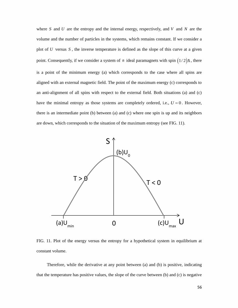
56

where S and U are the entropy and the internal energy, respectively, and V and N are the

volume and the number of particles in the systems, which remains constant. If we consider a

plot of U versus S , the inverse temperature is defined as the slope of this curve at a given

point. Consequently, if we consider a system of n ideal paramagnets with spin 1/ 2 , there

is a point of the minimum energy (a) which corresponds to the case where all spins are

aligned with an external magnetic field. The point of the maximum energy (c) corresponds to

an anti-alignment of all spins with respect to the external field. Both situations (a) and (c)

have the minimal entropy as those systems are completely ordered, i.e., 0U . However,

there is an intermediate point (b) between (a) and (c) where one spin is up and its neighbors

are down, which corresponds to the situation of the maximum entropy (see FIG. 11).

FIG. 11. Plot of the energy versus the entropy for a hypothetical system in equilibrium at

constant volume.

Therefore, while the derivative at any point between (a) and (b) is positive, indicating

that the temperature has positive values, the slope of the curve between (b) and (c) is negative

S

U

T > 0 T < 0

(a)Umin

(c)Umax

0

(b)U0

57

and so is the temperature. Then, the absolute temperature runs from cold to hot as:

0 , , 300 , , , , , , 300 , , 0K K K K K K , which means that absolute negative

temperatures are hotter than positive ones.

In order to study the communicability function at negative absolute temperatures, let us

start by writing it in the following form:

0 0 0

j j j

j j j

EA

pq j j j j j jG p q e p q e p q e

. (79)

While the eigenvectors associated with positive eigenvalues make contributions to the

partition of the network into communities or quasi-cliques, the eigenvectors associated with

negative ones make contributions to the partition of the network into quasi-bipartite clusters.

Then, for 0 , the first term of (79) makes the largest contribution to the communicability,

such that (Estrada et al., 2008):

0

0 j

j

nEA

pq j jG p q e

, (80)

which means that for 0EA

pqG the network is partitioned into quasi-bipartite clusters. This

can be easily seen by considering

2 3

2! 3!

AA A

e I A

, (81)

which can be expressed in terms of the hyperbolic functions as

cosh sinhA

e A A

. (82)

58

As we have previously seen, the term coshpq

A

represents the weighted sum of

the number of walks of even length connecting nodes p and q in the network. Similarly,

sinhpq

A

represents the weighted sum of the number of walks of odd length

connecting nodes p and q . Then, if we consider a bipartite graph in which p and q are

nodes which are in two different partitions of the network, it is straightforward to realize that

there are no walks of even length starting and p at ending at q in the graph. Consequently,

0 sinh 0EA

pqpq

G A . (83)

On the other hand, if p and q are in the same partition of a bipartite network we can

see that there is no walk of odd length connecting them due to the lack of odd cycles in the

bipartite graph, which makes

0 cosh 0EA

pqpq

G A . (84)

Thus, it is possible to adapt the methods and algorithms previously described to identify

communities in networks in order to identify network bipartitions. These methods have been

used for undirected networks (Estrada et al., 2008) in which bipartitions have been detected

for a variety of real-world systems. For instance, in FIG. 12 we illustrate the two main

partitions detected by using the communicability function at a negative absolute temperature

for the PPI network of the archae bacterium A. fulgidus. The study of bipartitions in complex

directed networks was also accomplished by using a modification of the communicability

function (Crofts et al., 2010).

59

FIG. 12 (color online). Bipartition of the PPI network of A. fulgidus obtained by means of the

communicability function at a negative absolute temperature. The nodes in one partition are

represented by squares and those in the other as circles. Inter-partition links are represented

by solid lines and the only one intra-partition link is represented as a discontinuous line.

VI. COMMUNICABILITY AND LOCALIZATION IN COMPLEX NETWORKS

A. Generalities

Locality is an important property of a large class of physical systems. For example, in

quantum chemistry and solid-state physics, the locality (also known as nearsightedness, see

(Des Cloizeaux, 1964; Kohn, 1996; Le Bris, 2005)) can be interpreted as the lack of long-

range correlations between the components of the system, which can be modeled by sites

connected by bonds in a more or less regular lattice. This means that with high probability, a

60

small perturbation at one site of the lattice will only be felt locally (i.e., by sites in a small

neighborhood).

Mathematically, this property manifests itself as fast off-diagonal decay in the density

matrix describing the system at hand; see, e.g., (Benzi et al., 2010). The locality is present in

insulators as well as in metallic systems at sufficiently high electronic temperatures. One

important consequence of the locality is that it enables the development of )(nO algorithms

for electronic structure computations, i.e., algorithms the asymptotic complexity of which

scales linearly in the size of the system (Goedeker, 1999). Note that traditional algorithms

based on diagonalization of the Hamiltonian, in contrast, scale like 3n .

The locality is also of great importance in the area of quantum information theory,

where it has been used, for example, to establish area laws for the entanglement entropy; see,

e.g., (Cramer and Eisert, 2006; Cramer et al., 2006; Hastings, 2004; Hastings and Koma,

2006; Schuch, 2007; Schuch et al., 2006) and especially (Eisert et al., 2010) for a

comprehensive survey.

Conversely, the absence of locality can be thought of as the presence of long-range

correlations throughout the system. In such a system, a small local perturbation will be felt

globally. In quantum chemistry this happens for conductors, e.g., metallic systems at zero or

very low electronic temperatures. In these systems, the entries of the density matrix decay

very slowly.

It should be obvious that the locality (or the lack of it) is also very important in the

study of complex networks. In this section we apply general results on exponential decay in

matrix functions (Benzi et al., 2010; Benzi and Golub, 2009; Benzi and Razouk, 2007) to the

study of a type of locality in complex networks. Specifically, we use the communicability as

a way to measure the correlations between nodes in a network. Thus, fast decay in He

(see

61

below for details) will be interpreted as a sign of localization, meaning the absence of strong

long-range correlations among the nodes; conversely, slow decay in He (or the lack of

decay) will be interpreted as a sign of a strongly connected network, in which even small

disturbances propagate easily to the entire network. Here H may denote either the adjacency

matrix or the graph Laplacian of the network.

Just as in the case of electronic structure computations, the locality is not only

conceptually important but may also lead in some cases to greatly reduced computational

effort, for instance in computing communicabilities or other network properties expressible as

matrix functions. It is, however, important to realize that such decay properties will be

present only in some networks, but not in others. For instance, in a small-world network we

cannot expect most communicabilities to be negligibly small, generally speaking. On the

other hand, other types of networks, such as regular lattices or highway networks can be

expected to exhibit strong locality. The actual rate of decay is affected by properties such as

the maximum degree of a node in the network and the inverse temperature .

Let us consider for instance the 1997 version of the Internet at Autonomous System

(AS) formed by 3015 nodes and 5156 links. Despite this network is sparse, the maximum

communicability EA

pqG between a pair of nodes is

13~10 . The minimum communicability is,

however, only 3.1. Then, by normalizing the communicability matrix it is easy to realize that

the minimum communicability is negligibly close to zero, i.e., 13~10

and can be excluded

from the calculations. The average normalized communicability in this version of the AS

Internet is 44.07 10 ; 16.7% of the pairs of nodes have a communicability smaller than

610 .

There are networks where the number of negligible entries is more significant than this;

in the network of 616 injecting drug users (IDUs) in Colorado Spring, 610EA

pqG for almost

62

30% of the pairs of nodes. We remark that there are some networks in which this situation is

not found at all; in the network of 1586 corporate directors of the top 500 US corporations,

only 0.4% of the pairs of nodes have communicability below 610. These cases of „locality‟

(or lack thereof) of the communicability in a group of nodes in the network are telling us

something about the structure of these networks. For instance, in the case of the IDU network

there is a central core dominating most of the communicability of the network as can be seen

in FIG. 13. These individuals are central in the communication with the rest of the network

and could be important targets of educational or health campaigns.

FIG. 13 (color online). Illustration of the normalized communicability between pairs of

individuals in a network of IDUs in Colorado Spring. Individuals are identified by numbers

in the x and y axes and their communicability is given as the values of the z axis.

63

B. Exponential decay in communicability

In the case of a symmetric matrix M with the spectrum contained in 1,1I and

for a matrix function f which is analytic on a region containing I , it has been proved that

the off-diagonal entries of this matrix function are bounded as

pqd

pqf M Ce

for all p q , (85)

where 0C , 0 and pqd denotes the shortest-path distance between the nodes p and q

in the undirected and unweighted graph associated with M . This result reveals the same

information as we have analyzed in section 2 of this work (see Eq. (20) for instance) for the

special case of the path graph. Basically, as the shortest-path separation between two nodes in

a network increases, their communicability vanishes. Note, however, that the actual decay is

not monotonic in general.

Now, let us consider the adjacency matrix A of an undirected network and let maxk be

the maximum degree of the network. Then, we can normalize the adjacency matrix as we

have done previously producing 1

maxA k A which has spectrum contained in the interval

1,1I . Then, we can obtain decay bounds for the exponential of A by computing

bounds for the matrix function maxk Af A e . The bounds are of the form

pqdEA

pqG Ce

for all p q , (86)

where now C and depend only on maxk . We will show later that a larger value of maxk

results in a larger constant C , and therefore a slower decay.

64

A shift and scaling is needed for the Laplacian to have spectrum in the interval

1,1I . We start by denoting

max,

2

L

L L I

(87)

the shifted and scaled Laplacian. Observing that

max, max,

2 2

L LL L I

, (88)

we immediately have

ˆmax, max,/2/2L LLe e e

. (89)

Thus, in order to obtain bounds on EL

pqG we compute bounds for the matrix function

max,

2

LA

f A e

, and then multiply the bounds by the constant factor

max,

2

L

e

.

Consider now the particular matrix function tAf A e , where 0t and A has

spectrum in 1,1I . Applying the bounds (85) and (86) to this function leads to the upper

bound

pqdtA

pq

e C t e

, ,p q (90)

where (Benzi and Golub, 1999)

12

1

te

C t

, 2ln . (91)

65

Here 2

1 2 1 1 1 , where 1 1 and

2 0 are the semi-axes of an ellipse

with foci at the points −1 and +1. The matrix function f is analytic on the interior of and

continuous on it. The bound (90) can be explicitly evaluated for any given value of 11 .

Note that if 0t , the factor 1te

in (91) is replaced by 1te

. Also note that owing to the

presence of the factor 1te in (91), the bounds for the entries of Ae are larger for a larger

value of maxk (just take maxt k ).

If we consider the inverse temperature we can obtain the following bound for the

Laplacian-based communicability function

pqdEL

pqG C e

, ,p q (92)

where

max, 1 1 /22

1

LC e

, 2ln . (93)

Note that C increases to infinity as 0T , and decreases to 1 as T . In the zero-

temperature limit the bound deteriorates and no decay is observed, which is consistent with

the observations above. In the limit T the right-hand side in the bound (90) tends to

2

1

pqde

, (94)

where 2ln and 1 is arbitrary. Taking sufficiently large, the above quantity can

be made smaller than any prescribed 0 , showing that in the limit T the off-diagonal

entries of e L are all zero: therefore, our bounds capture the correct limiting behavior for

both 0T and T .

In a similar way we can obtain the bound for the adjacency-based communicability,

66

pqdEA

pq AG C e

, p q (95)

with

max 12

1

k

AC e

, 2ln . (96)

As one would expect, the bound increases upon increasing maxk and increasing (or

decreasing the temperature). In the limit T we again find 0EA

pqG .

VII. COMPUTABILITY OF COMMUNICABILITY FUNCTIONS

A. Analytical results

Communicability functions have been incorporated into some computational tools for

the analysis of complex networks. For instance, a Hub Objects Analyzer (Hubba) (Lin et al.,

2008) designed as a web-based service for exploring important nodes in an interactome

network and BrainNetVis (Christodoulou et al., 2011), a tool for both quantitative and

qualitative network measures of brain interconnectivity, incorporate the subgraph centrality

as a standard measure for the analysis of nodes in networks. A more general computational

toolbox, CONTEST (Taylor and Higham, 2009), contains a series of Matlab utilities for

generating and analyzing various types of networks and incorporates several

communicability-based functions for the analysis of complex networks.

When implementing communicability functions for large complex networks a

fundamental question that arises is the efficiency of the algorithm selected for computing the

matrix functions. As a consequence it has been stated here and there that the subgraph

centrality and the communicability are difficult to compute for large networks. There have

been approaches as the ones described in the previous section based on the truncation of the

eigenvalues of the adjacency matrix for which we do not know the error of the

67

approximation. We present in this section a critical review of these computational approaches

to give the reader a better understanding of what to do and what not to do when computing

communicability functions in large complex networks.

Several approaches are available for computing the matrix exponential. Use of the

power series expansion (8) to find approximations to Ae in general cannot be recommended;

see (Moler and van Loan, 1978; 2003). A frequently used approach is based on the

eigendecomposition (9); see, e.g., (Dronen and Lv, 2011). This approach requires 2( )O n

space and 3( )O n arithmetic operations for a graph with n nodes; furthermore, the sparsity in

A is not exploited in this approach.

One of the most efficient and accurate available methods is the one based on the Padé

approximation combined with the scaling and squaring method (Higham, 2005; 2008). This

method, implemented in Matlab by the expm function, is nowadays the most widely used

one. Its complexity is also 2( )O n storage and

3( )O n arithmetic operations, and the sparsity

in A does not appear to be exploited in available implementations. (The sparsity in A is

exploited in codes that compute the action of the matrix exponential on a vector: Av e b ;

however, this problem is somewhat different from the one that we are interested in here.)

It is important to note that in many applications, it is not required to compute all entries

in the matrix exponential (or in other functions of A or L ). In particular, for computing the

graph centralities of the nodes in a graph (or the Estrada index) only the main diagonal of Ae

is required. However, neither the diagonalization (eigendecomposition) approach, nor the

scaling and squaring method are able to take advantage of this to reduce computational costs.

Moreover, for very large networks it is generally not feasible to compute all the

communicabilities; instead, one may be interested in computing only the average

68

communicability of each node in the network, or of a subset of nodes. Again, this can be

easily done without computing all the entries in Ae , as we show below.

Efficient and accurate methods of bounding and estimating arbitrary entries in a matrix

function ( )f A have been developed by Golub, Meurant and collaborators (see Golub and

Meurant, 2010 and references therein) and were first applied to problems of network analysis

by Benzi and Boito (2010) (see also Bonchi et al., 2011). Here we give a brief description of

these methods, referring the reader to (Benzi and Boito (2010)) for further details. Consider

the eigendecomposition TA Q Q and ( ) ( ) Tf A Qf Q , where 1[ , , ]nQ . Given the

vectors u and v , we have

1

( ) ( ) ( ) ( ) ( ) ( ),n

T T T T

i

i

u f A v u Qf Q v w f z f w i z i

(97)

where Tw Q u and

Tz Q v . In particular, for ( ) Af A e we obtain

1

( ) ( ).n

T A

i

i

u e v e w i z i

(98)

Choosing pu v e (the vector with the p th entry equal to 1 and all the remaining

ones equal to 0 ) we recover the well-known expression for the subgraph centrality of node

p :

2

1

( ) ( ) .n

T

p p i i

i

EE p e e e e p

A (99)

Likewise, choosing pu e and qv e we obtain the usual expression for the

communicability between node p and node q :

1

( ) ( ) .j

nT

pq p q j j

j

G e e e p q e

A (100)

69

Let now 1 denote the column vector with all entries equal to 1. The average

communicability for the node p can be computed as

1( ) 1 .

1

T T

p p pC p e e e e e

n

A A (101)

This shows that this quantity can be evaluated once the two bilinear forms 1T A

pe e and

T A

p pe e e have been computed.

Hence, the problem is reduced to evaluating bilinear expressions of the form ( )Tu f A v .

The key insight is that such bilinear forms can be thought of as Riemann- Stieltjes integrals

with respect to a (signed) spectral measure:

11

11

0, if ,

, , if ,

, if .

b niT

i ijna

j

a

u f A v f d w j z j

w j z j b

(102)

This integral can be approximated by means of a Gauss-type quadrature rule:

1 1

( ) ( ) ( ) ( ) [ ],r s

b

j j k ka

j k

f d c f t v f R f

(103)

where the nodes r

jjt 1}{ and the weights r

jjc 1}{ are unknown, whereas the nodes s

kk 1}{ are

prescribed. We have

0s for the Gauss rule,

1s , 1 a or 1 b for the Gauss-Radau rule,

2s , 1 a and 2 b for the Gauss-Lobatto rule.

For certain matrix functions, including the exponential and the resolvent, these

quadrature rules can be used to obtain lower and upper bounds on the quantities of interest;

70

adding quadrature nodes leads to tighter and tighter bounds, which converge to the true

values. The evaluation of these quadrature rules is reduced to the computation of orthogonal

polynomials via a three-term recurrence, or, equivalently, to the computation of entries and

spectral information on a certain tridiagonal (Jacobi) matrix via the Lanczos algorithm. Here

we briefly recall how this can be done for the case of the Gauss quadrature rule, when we

wish to estimate the i th diagonal entry of ( )f A . It follows from (103) that the quantity of

interest has the form 1 ( )rj j jc f t . The nodes and weights can be efficiently computed using

the Golub and Welsch QR algorithm, see (Golub and Meurant, 2010). Alternatively, one can

use the following relation (Theorem 3.4 in (Golub and Meurant, 2010)):

1 1

1

rT

j j r

j

c f t e f J e

, (104)

where

1 1

1 2 2

2 1 1

1

r

r r r

r r

J

(105)

is a tridiagonal matrix whose eigenvalues are the Gauss nodes, whereas the Gauss weights

are given by the squares of the first entries of the normalized eigenvectors of rJ . The entries

of rJ are computed using the Lanczos algorithm. The initial vectors are 1 0x and 0 ix e .

The iteration goes as follows:

1 1 2

1 1

1/2

( ) , 1,2,

,

.

j j j j j j j

T

j j j

T

j j j j

x r A I x x j

x Ax

r r r

(106)

71

In practice, a slightly different implementation due to Paige is preferred for numerical

reasons, see (Golub and Meurant, 2010).

For small r , i.e., for a small number of Lanczos steps, computing the (1,1) entry of

( )rf J is inexpensive. The main cost in estimating one entry of ( )f A with this approach is

associated with the sparse matrix-vector multiplies in the Lanczos algorithm applied to the

adjacency matrix A . If only a small, fixed number of iterations is performed for each

diagonal element of ( )f A , as is usually the case, the computational cost (per node) is at most

)(nO for a sparse graph, resulting in a total cost of 2( )O n for computing the subgraph

centrality of every node in the network. This theoretical worst case applies for instance to

small-world networks; for networks the diameter of which is not small, a careful sparse-

matrix-sparse-vector implementation leads to an ( )O k complexity per node, where k is the

average degree of a node in the network. This translates to an overall cost of )(nO for

computing all the subgraph centralities for a sparse network. The prefactor in the )(nO and

2( )O n estimates may be large, meaning that the quadrature rule-based approach will be faster

than traditional 3( )O n methods only for sufficiently large n . The break-even point will

depend on the particular type of network being considered, but in our experience it can occur

for n as small as a few hundreds. Of course, the larger n , the greater the savings realized

with the quadrature rule-based approach.

Furthermore, since each subgraph centrality can be computed independently of the

others, parallelization of the computation will result in a drastic reduction of computing

times, thus enabling the analysis of huge networks on massively parallel systems, at least in

principle. We are not aware of any other approach to computing subgraph centralities with

similar characteristics.

72

The case vu can be handled either by the nonsymmetric Lanczos process (Golub and

Meurant, 2010), or by means of the following polarization identity:

1

( ) ( ) ( ) ( ) .

2

TT T Tu f A v u v f A u v u f A u v f A v

(107)

For the case ( ) Af A e , pu e and qv e we obtain the following expression for the

communicability between nodes p and q :

1( ) ( ) ,

2

T

pq i j i jG e e e e e EE p EE q

A (108)

showing that once the subgraph centralities have been computed, only one additional

quadratic form must be evaluated in order to compute pqG . Hence, the cost of computing the

communicability between a pair of nodes is of the same order as that of computing the

subgraph centrality of a node.

For a very large network, computing the communicabilities between all pair of nodes

would likely be too expensive. In this case computing the average communicabilities may be

sufficient, depending on the problem; in other cases it may be sufficient to compute the

communicabilities for a subset of nodes, or only those communicabilities that are not a priori

known to be below a certain threshold (see discussion on decay).

As already mentioned, computing the average communicability for node p requires

evaluating the bilinear form 1T A

pe e . This can be computed with the nonsymmetric Lanczos

process, or alternatively with the symmetric Lanczos process via the alternative polarization

identity

11 1 1 1 1 .

4

T TT A

p p p p pe e e e e e e e

A A (109)

73

Hence, the cost of computing the average communicability of a node is of the same order as

computing the subgraph centrality of a node. We note that all the average communicabilities

can also be computed in parallel.

B. Numerical experiments

Here we present the results of computations on a set of small-world networks generated

using the CONTEST toolbox (Taylor and Higham, 2009). The networks are obtained from an

underlying regular lattice consisting of a ring, in which each node is connected to four

neighbors (two on each side). A shortcut to a randomly chosen node in the network is added

to each node in turn with probability 1.0p , with self-links and repeated links removed at

the end of the process.

First we consider a set of networks of n nodes with 1000 4000n , with increments

of 200. We compute the subgraph centralities of all nodes in the networks and then sum them

to obtain the Estrada index. The results are shown in FIG. 14. As expected, the computational

times with the eigendecomposition and with the Matlab function expm scale roughly like 3n .

Even without a sophisticated implementation, our results show that the quadrature rule-based

approach is systematically faster for networks of size greater than 2000n . In this graph the

time for the quadrature rule-based calculations appear to scale roughly linearly with n , rather

than with the expected (quadratic) complexity. This is probably due to the fact that for such

relatively small sparse problems, the computational time is dominated by non-floating point

operations (including indexing, memory references, etc.), which scale roughly linearly for the

range of problems of sizes considered here. This is confirmed by the plot in inset of FIG. 14,

where we present results for 1000,5000,10000n . This plot indicates a quadratic growth in

computing times for sufficiently large graphs.

74

FIG. 14 (color online). (Main) Plot of the time in seconds ( y -axis) for computing the Estrada

index of small world matrices of increasing size. The number of nodes N is on the x -axis. In

blue we show the time for the Matlab „expm‟ function, in black the time using the

eigendecomposition, and in red the time for estimating the trace using five iterations of the

Lanczos algorithm for each node. (Insert) Plot of the time in seconds for computing the

Estrada index of small world matrices of size 1000,5000,10000n .

VIII. CONCLUSIONS AND PERSPECTIVES

In recent years, the notion of communicability has become increasingly important in

the analysis of complex networks. It plays a prominent role in understanding network

properties at the micro-, meso-, and macroscopic level, as well as across multiple scales.

Measures of the communicability between nodes, or sets of nodes, can be used to construct

community detection algorithms, to quantify graph bipartivity, to analyze the spread or

rumors, to identify bottlenecks, to reveal the dynamics between agents in a social conflict,

75

and so forth. Moreover, centrality measures based on self-communicability (i.e., subgraph

centrality) have proved useful in analyzing the structure of complex networks arising in a

variety of fields. A few of these applications have been reviewed here, as well as

generalizations and improvements by a number of researchers.

Physical models based on oscillator networks can help justifying and understanding

the communicability functions of networks. A variety of models have been analyzed and

discussed in this paper, including classical and quantum-mechanical ones. Calculations with

these models can provide useful insights on the notion of communicability in various

situations; for instance, the use of negative absolute temperatures readily admits an elegant

interpretation in the context of complex network analysis.

All the communicability measures reviewed in this paper are expressed in terms of

walks between nodes in the graph representing the network. Counting these walks and

assigning weights to them so as to penalize longer walks naturally leads to matrix power

series and hence to analytic functions of graph matrices such as the adjacency or the

Laplacian matrix. A wealth of mathematical and algorithmic knowledge on matrix functions

can be utilized to compute communicability functions efficiently in the case of large and

sparse networks. Moreover, existing bounds for the entries of matrix functions can be directly

applied to investigate the locality (or its absence) in the network communicability. Interest in

communicability based on matrix functions has grown very rapidly since the initial proposal

(Estrada and Hatano, 2008) and is now an active area of research worldwide. There are still

several open questions that have been mentioned or analyzed in this review. Others will

appear from the systematic use of the communicability functions in the different application

fields. All of them will guarantee the continuity of research in this topic for the next few

years.

76

In closing, the communicability is likely to become an essential ingredient in both the

theoretical and the practical analysis of networks, and exciting developments will surely take

place in the years ahead.

Acknowledgement

NH and EE are partially supported by Aihara Innovative Mathematical Modeling Project, the

Japan Society for the Promotion of Science (JSPS) through the "Funding Program for World-

Leading Innovative R&D on Science and Technology (FIRST Program)," initiated by the

Council for Science and Technology Policy (CSTP). EE was also partially support by EPRSC

grant “MOLTEN: Mathematics Of Large Technological Evolving Networks”. MB was

supported by National Science Foundation grants DMS-0810862 and DMS-1115692.

77

REFERENCES

Albert, R., A-L. Barabási, 2002, “Statistical mechanics of complex networks,” Rev. Mod.

Phys. 74, 47-97.

Alon, N., 1986, “Eigenvalues and expanders,” Combinatorica 6, 83–96.

Alon, N., and V. D. Milman, 1985, “λ1, isoperimetric inequalities for graphs, and

superconcentrators,” J. Combin. Theory Ser. B 38, 73–88.

Bahar, I., A. R. Atilgan, and B. Erman, 1997, “Direct evaluation of thermal fluctuations in

proteins using a single-parameter harmonic potential,” Fold. Des. 2, 173-181.

Baierlein, R., 1999, Thermal Physics (Cambridge University Press, Cambridge).

Ball, P., 2004, Critical Mass. How One Thing Leads to Another (Arrow Books, London).

Barabási, A-L., and Z. N. Oltvai, 2003, “Network biology: Understanding the cell‟s

functional organization,” Nature Rev. Genet. 5, 101-113.

Benzi, M., and G. H. Golub, 1999, “Bounds for the entries of matrix functions with

applications to preconditioning,” BIT, 39, 417-438.

Benzi, M., and N. Razouk, 2007, “Decay rates and )(nO algorithms for approximating

functions of sparse matrices,” Electr. Trans. Numer. Anal., 28, 16-39.

Benzi, M., and P. Boito, 2010, “Quadrature rule-based bounds for functions of adjacency

matrices,” Linear Algebra Appl., 433, 637-652.

Benzi, M., P. Boito, and N. Razouk, 2010, “Decay Properties of Spectral Projectors with

Applications to Electronic Structure,” Math/CS Technical Report TR-2010-025, Emory

University.

78

Bonacich, P., 1972, “Factoring and weighting approaches to status scores and clique

identification,” J. Math. Sociol. 2, 113–120.

Bonacich, P., 1987, “Power and centrality: A family of measures,” Am. J. Soc. 92, 1170-1182.

Bonchi, F., D. F. Gleich, C. Greif, and L. V. S. Laksmanan, 2011, “Fast matrix computations

for pair-wise and column-wise commute times and Katz scores,” Internet Math., to

appear.

Bradonjić, M., A. Hagberg, and F. Pan, 2011, “Performance of wireless sensor networks

under random node failure,” Preprint Los Alamos National Laboratory,

http://math.lanl.gov/~hagberg/Papers/bradonjic-2011-performance.pdf.

Buchanan, M., 2007, The Social Atom: Why the Rich get Richer, Cheats get Caught and your

Neighbor Usually Looks Like You (Cyan Books and Marshall Cavendish).

Bullmore, E. and O. Sporns, 2009, “Complex brain networks: graph theoretical analysis of

structural and functional system,” Nature Rev. Neurosc., 10, 186-198.

Caldarelli, G., 2007, “Scale-Free Networks. Complex Webs in Nature and Technology,”

Oxford University Press, Oxford.

Castellano, C., S. Fortunato, and V. Loreto, 2009, “Statistical physics of social dynamics,”

Rev. Mod. Phys. 81, 591-646.

Chakrabarti, B. K., A. Chakraborti, and A. Chatterjee, 2006, Econophysics and Sociophysics:

Trends and Perspectives (Wiley VCH, Berlin).

Christodoulou, E. G., V. Sakkalis, V. Tsiaras, and I. G. Tollis, 2011, “BrainNetVis: An Open-

Access Tool to Effectively Quantify and Visualize Brain Networks,” Comput. Intell.

Neurosci., 747290.

79

Count, R., and J.-P. Bouchard, 2000, “Herd behavior and aggregate fluctuations in financial

markets,” Macroecon. Dyn. 4, 170-196.

Cramer, M., and J. Eisert, 2006, “Correlations, spectral gap and entanglement in harmonic

quantum systems on generic lattices,” New J. Phys., 8, 71.

Cramer, M., J. Eisert, M. B. Plenio, and J. Dreissig, 2006, “Entanglement-area law for

general bosonic harmonic lattice systems,” Phys. Rev. A, 73, 012309.

Crofts, J. J., E. Estrada, D. H. Higham, and A. Taylor, 2010, “Mapping directed networks,”

Elec. Trans. Num. Anal. 37, 337-350.

Crofts, J. J., and D. J. Higham, 2009, “A weighted communicability measure applied to

complex brain networks,” J. Roy. Soc. Interface 6, 411-414.

Crofts, J. J., D. J. Higham, R. Bosnell, S. Jbabdi, P. M. Matthews, T. E. J. Behrens, and H.

Johansen-Berg, 2011, “Network analysis detects changes in the contralesional

hemisphere following stroke,” Neuroimage 54, 161-169.

Cvetković, D., P. Rowlinson, and S. Simić, 1997, Eigenspaces of Graphs (Cambridge

University Press, Cambridge).

da Fontoura Costa, L., O. N. Oliveira Jr., G. Travieso, F. A. Rodrigues, P. R. Villas Boas, L.

Antiqueira, M. P. Viana, and L. E. Correa Rocha, 2011, “Analyzing and modeling real-

world phenomena with complex networks: a survey of applications,” Avd. Phys. 60,

329-412.

da Fontoura Costa, L., M. A. Rodrigues Tognetti, and F. Nascimento Silva, 2008, “Concentric

characterization and classification of complex network nodes: Application to an

institutional collaboration network,” Physica A 387, 6201-6214.

80

de la Peña, J. A., I. Gutman, and J. Rada, 2007, “Estimating the Estrada index,” Lin. Alg.

Appl. 427, 70-76.

Deng, H., S. Radenković, and I. Gutman, 2009, “The Estrada index”, in: Cvetković, D.,

Gutman I., 2009, Applications of Graph Spectra (Math. Inst., Belgrade, 2009), pp. 123–

140.

Des Cloizeaux, J., 1964, “Energy bands and projection operators in a crystal: analytic and

asymptotic properties,” Phys. Rev., 135, A685-A697.

Dorogovtsev, S. N., and J. F. F. Mendes, 2003, Evolution of Networks: From Biological Nets

to the Internet and WWW (Oxford University Press, Oxford).

Došlić, T., 2005, “Bipartivity of fullerene graphs and fullerene stability,” Chem. Phys. Lett.

412, 336-340.

Dronen, N., and Q. Lv, 2011, “Return probability and k-step measures,” arXiv:1105.4479v1.

Dumbar, R., 1998, Grooming, Gossip, and the Evolution of Language (Harvard University

Press).

Dunne, J. A., R. J. Williams, and N. D. Martinez, 2002, “Network structure and biodiversity

loss in food webs: robustness increases with connectance,” Ecol. Lett., 5, 558-567.

Eguíluz, V. M., and M. G. Zimmermann, 2000, “Transmission of information and herd

behavior: An application to financial markets,” Phys. Rev. Lett. 85, 5659-5662.

Eisert, J., M. Cramer, and M. B. Plenio, 2010, “Colloquium: Area laws for the entanglement

entropy,” Rev. Mod. Phys., 82, 277-306.

Ejov, V., J. A. Filar, S. K. Lucas, and P. Zograf, 2007, “Clustering of spectra and fractals of

regular graphs,” J. Math. Anal. Appl. 333, 236-246.

81

Ejov, V., S. Friedlan, and G. T. Nguyen, 2009, “A note on the graph‟s resolvent and the

multifilar structure,” Lin. Alg. Appl. 431, 1367-1379.

Estrada, E., 2000, “Characterization of 3D molecular structure,” Chem.Phys. Lett. 319, 713-

718.

Estrada, E., 2006a, “Virtual identification of essential proteins within the protein interaction

network of yeast,” Proteomics 6, 35-40.

Estrada, E., 2006b, “Protein bipartivity and essentiality in the yeast protein-protein

interaction network,” J. Proteome Res. 5, 2177-2184.

Estrada, E., 2006c, “Spectral scaling and good expansion properties in complex networks,”

Europhys. Lett. 73, 649-655.

Estrada, E., 2006d, “Network robustness. The interplay of expansibility and degree

distribution,” Eur. Phys. J. B, 52, 563-574.

Estrada, E., 2007a, “Characterization of topological keystone species. Local, global and

“meso-scale” centralities in food webs,” Ecol. Complex. 4, 48-57.

Estrada, E., 2007b, “Food web robustness to biodiversity loss: The roles of connectance,

expansibility and degree distribution,” J. Theor. Biol. 244, 296-307.

Estrada, E., 2007c, “Topological structural classes of complex networks,” Phys. Rev. E, 75,

016103.

Estrada, E., 2010a, “Generalized walks-based centrality measures for complex biological

networks,” J. Theor. Biol. 263, 556-565.

Estrada, E., 2010b, “Universality in protein residue networks,” Biophys. J. 98, 890-900.

82

Estrada, E., 2011, “Community Detection based on Network Communicability,” Chaos 21

016103.

Estrada, E., and Ö. Bodin, 2008, “Using network centrality measures to manage landscape

connectivity,” Ecol. Appl. 18, 1810-1825.

Estrada, E., and N. Hatano, 2007, “Statistical-mechanical approach to subgraph centrality in

complex networks,” Chem. Phys. Let. 439, 247-251.

Estrada, E., and N. Hatano, 2008, “Communicability in complex networks,” Phys. Rev. E 77,

036111.

Estrada, E., and N. Hatano, 2009a, “Communicability graph and community structures in

complex networks,” Appl. Math. Comput. 214, 500-511.

Estrada, E., and N. Hatano, 2009b, “Returnability in complex directed networks (digraphs),”

Lin. Alg. Appl. 430, 1886-1896.

Estrada, E. and N. Hatano, 2010a, “A Vibrational Approach to Node Centrality and

Vulnerability in Complex Networks,” Physica A 389, 3648-3660.

Estrada, E. and N. Hatano, 2010b, “Topological Atomic Displacements, Kirchhoff and

Wiener Indices of Molecules,” Chem. Phys. Lett. 486, 166-170.

Estrada, E., and D. J. Higham, 2010, “Network Properties Revealed Through Matrix

Functions,” SIAM Rev. 52, 696-714.

Estrada, E., D. J. Higham, and N. Hatano, 2008, “Communicability and multipartite structure

in complex networks at negative absolute temperatures‟” Phys. Rev. E, 78, 026102.

Estrada, E., D. J. Higham, and N. Hatano, 2009, “Communicability betweenness in complex

networks,” Physica, A, 388, 764-774.

83

Estrada, E., and J. A. Rodríguez-Velázquez, 2005a, “Subgraph centrality in complex

networks,” Phys. Rev. E 71, 056103.

Estrada, E., and J. A. Rodríguez-Velázquez, 2005b, “Spectral measures of bipartivity in

complex networks,” Phys. Rev. E 72, 046105.

Fortunato, S., 2010, “Community detection in graphs,” Phys. Rep. 486, 75-174.

Fortunato, S., and M. Barthélemy, 2007, “Resolution limit in community detection,” Proc.

Natl. Acad. Sci. USA 104, 36-41.

Freeman, L. C., 1979, “Centrality in networks: I. Conceptual clarification,” Social Networks

1, 215–239.

Freeman, L. C., S. P. Borgatti, and D. R. White, 1991, “Centrality in valued graphs: A

measure of betweenness based on network flow,” Social Networks, 13, 141-154.

Goedeker, S. 1999, “Linear scaling electronic structure methods,” Rev. Mod. Phys., 71, 1085-

1123.

Golub, G. H., and G. Meurant, 2010, Matrices, Moments and Quadrature with Applications

(Princeton University Press, Princeton, NJ).

Granovetter, M., 1979, “Threshold models of collective behavior,” Am. J. Soc. 83, 1420-

1443.

Grindrod, P., D. J. Higham, M. C. Parsons, and E. Estrada, 2011, “Communicability across

evolving networks,” Phys. Rev. E 83, 0146120.

Gutman, I., H. Deng, and S. Radenković, 2010, “The Estrada index: an updated survey,” in:

D. Cvetković and I. Gutman, 2011, Selected Topics on Applications of Graph Spectra

(Math. Inst., Beograd), pp. 155–174.

84

Harary, F., and A. J. Schwenk, 1979, “The spectral approach to determining the number of

walks in a graph,” Pacific J. Math, 80, 443-449.

Hastings, M. B., 2004, “Locality in quantum and Markov dynamics on lattices and

networks,” Phys. Rev. Lett., 93, 140402.

Hastings, M. B., and T. Koma, 2006, “Spectral gap and exponential decay of correlations,”

Comm. Math. Phys., 265, 781-804.

Higham, N., 2005, “The scaling and squaring method for the matrix exponential revisited,”

SIAM J. Matrix Anal. Appl., 26, 1179-1193.

Higham, N., 2008, Function of Matrices. Theory and Computation (Society for Industrial and

Applied Mathematics, Philadelphia, PA).

Hoory, S., N. Linial, and A. Wigderson, 2006, “Expander Graphs and their applications,”

Bull. Am. Math. Soc. 43, 439-561.

Hu, H.-B., and X.-F. Wang, 2009, “Disassortative mixing in online social networks,”

Europhys. Lett. 86, 18003.

Jeong, H., S. P. Manson, A.-L. Barabási, and Z. N. Oltvai, 2001, “Lethality and centrality in

protein netwoks,” Nature, 411, 41-42.

Johansen-Berg, H., J. Scholz, and C. J. Stagg, 2010, “relevance of structural brain

connectivity to learning and recovery from stroke,” Frontiers Syst. Neurosc. 4, article

146.

Jordán, F., and I. Scheuring, 2002, “Searching for keystones in ecological networks,” Oikos

99, 607-612.

85

Jungsbluth, M., B. Burghardt, and A. Hartmann, 2007, “Fingerprints networks: correlations

of local and global network properties,” Physica A 381, 444-456.

Katz, L., 1953, “A new status index derived from sociometric analysis,” Psychometrica, 18,

39-43.

Kim, B. J., H. Hong, and M. Y. Choi, 2003, “Netons: vibrations of complex networks,” J.

Phys. A: Math. Gen. 36, 6329-6336

Kohn, W., 1996, “Density functional and density matrix method scaling linearly with the

number of atoms,” Phys. Rev. Lett., 76, 3168-3171.

Koponen, I. T., and M. Pehkonen, 2010, “Entropy and energy in characterizing the

organization of contact maps in learning science,” Entropy 12, 1653-1672.

Landau L. D., and E. M. Lifshitz, 1980, Statistical Physics, 3rd edition, Part

1 (Pergamon, Oxford).

Le Bris, C., 2005, “Computational chemistry from the perspective of numerical analysis,”

Acta Numerica 363-444.

Li, M., J. Wang, H. Wang, and Y. Pan, 2010, “Essential proteins discovery from weighted

protein interaction networks,” Lect. Notes Comput. Sci. 6053, 89-100.

Lin, C.-Y., C.-H. Chin, H.-H. Wu, S.-H. Chen, C.-W. Ho, and M.-T. Ko, 2008, “Hubba: hub

objects analyzer–a framework of interactome hubs identification for network biology,”

Nucl. Acids. Res. 36, W438-W443.

Ma, X., and L. Gao, 2011, “Non-traditional spectral clustering algorithms for the detection of

community structure in complex networks: a comparative analysis,” J. Stat. Mech.:

Theor. Exp. P05012.

86

Ma, X., L. Gao, and X. Yong, 2010, “Eigenspaces of networks reveal the overlapping and

hierarchical community structure more precisely,” J. Stat. Mech.: Theor. Exp. P08012.

MacArthur, B. D., R. J. Sánchez-García, and A. Ma‟ayan, 2010, “Microdynamics and

criticality of adaptive regulatory networks,” Phys. Rev. Lett. 104, 168701.

Makarov, Y. V., V. I. Reshetov, A. Stroev, and I. Voropai, 2005, “Blackout prevention in the

United States, Europe and Russia,” Proc. IEEE 93, 1942 – 1955.

Malliaros, F. D., and V. Megalooikonomou, 2011, “Expansion properties of large social

graphs,” Lect. Notes Comput. Sci. 6637, 311-322.

Mantegna, R. N., and E. H. Stanley, 1999, Introduction to Econophysics: Correlations and

Complexity in Finance (Cambridge University Press).

Manski, C. F., 2000, “Economic analysis of social interactions,” J. Econ. Persp. 14, 115-136.

Merton, R., 1957, Social Theory and Social Structure (Glencoe: the Free Press).

Mewes, H. W., D. Frishman, U. Güldener, G. Mannhaupt, K. Mayer, M. Mokrejs, B.

Morgenstern, M. Münsterkötter, S. Rudd, and N. Weil, 2002, “MIPS: a database for

genomes and protein sequences,” Nucl. Acids Res. 30, 31-34

Michard, Q., and J.-P. Bouchard, 2005, “Theory of collective opinion shifts: From smooth

trends to abrupt swings,” Eur. Phys. J. B 47, 151-159.

Moler, C. and C. V. Loan, 2003, “Nineteen dubious ways to compute the exponential of a

matrix, twenty-five years later,” SIAM Rev. 45, 3-49.

Moler, C., and C. F. van Loan, 1978, “Nineteen dubious ways to compute the exponential of a

matrix,” SIAM Rev., 20, 801-836.

87

Newman, M. E. J., 2003, “The structure and function of complex networks,” SIAM Rev. 45,

167-256.

Newman, M. E. J., 2004, “Fast algorithm for detecting community structure in networks,”

Phys. Rev. E 69, 066133.

Newman, M. E. J., 2005, “A measure of betweenness centrality based on random walks,”

Social Networks 27, 39-54.

Newman, M. E. J., 2006a, “Finding community structure in networks using the eigenvectors

of matrices,” Phys. Rev. E 74, 036104.

Newman, M. E. J., 2006b, “Modularity and community structure in networks,” Proc. Natl.

Acad. Sci. USA 103, 8577-8582.

Newman, M. J. E., 2010, Networks. An Introduction (Oxford University Press, Oxford).

Peierls, R., 1936, “On Ising‟s model of ferromagnetism,” Proc. Camb. Phil. Soc. 32, 477-481.

Ramsey, N. F., 1956, “Thermodynamics and statistical mechanics at negative absolute

temperatures,” Phys. Rev. 103, 20-28.

Ren, J., J. Wang, M. Li, H. Wang, and B. Liu, 2011, “Prediction of essential proteins by

integration of PPI network topology and protein complexes information,” Lect. Notes

Comput. Sci. 6674, 12-24.

Ruelle, E., 1969, Statistical Mechanics. Rigorous Results (Benjamin, New York).

Sakurai, J. J., 1985, Modern Quantum Mechanics (Benjamin/Cummings, California), Section

7.11.

88

Schuch, N., 2007, “Quantum Entanglement: Theory and Applications,” PhD thesis,

Department of Physics, Technischen Universität München, Munich, Germany.

Schuch, N., J. I. Cirac, and M. M. Wolf, 2006, “Quantum states on harmonic lattices,” Comm.

Math. Phys., 267, 65-92.

Shang, Y., 2011a, “The Estrada index of random graphs,” Scientia Magna 7, 79-81.

Shang, Y., 2011b, “Perturbation results for the Estrada index in weighted networks,” J. Phys.

A: Math. Theor. 44, 075003.

Soheilifard, R., D. E. Makarov, and G. J. Rodin, 2008, “Critical evaluation of simple network

models of protein dynamics and their comparison with crystallographic B-factors, Phys.

Biol. 5, 026008.

Sporn, O., 2011, Networks of the Brain (MIT Press, Cambridge, Massachusetts).

Stephenson, K., and M. Zelen, 1989, “Rethinking centrality: methods and examples,” Social

Networks 11, 1–37.

Strogatz, S. H., 2001, “Exploring complex networks,” Nature 419, 268-276.

Taylor, A., and D. J. Higham, 2009, “CONTEST: A Controllable Test Matrix Toolbox for

MATLAB,” ACM Trans. Math. Software, 35, 26:1-26:17.

Thurman, B., 1979, “In the office: Networks and coalitions,” Social Networks 2, 47-63

Tordesillas, A., P. O‟Sullivan, D. M. Walker, and Paramitha, 2010, “Evolution of functional

connectivity in contact and force chain networks: Feature vectors, k-cores and minimal

cycles,” Comp. Rend. Mecan. 338, 556-569.

89

Uppernberg, J., M. T. Hansen, S. Patkar, and T. A. Jones, 1994, “The sequence, crystal

strucyure determination and refinement of two crystal forms of lipase B from Candida

antartica. Structure 2, 293-308.

Van Kerrenbroeck, V., and E. Marinari, 2008, “Ranking vertices and edges of a network by

loops: A new approach,” Phys. Rev. Lett. 101, 098701.

von Luxburg, U., 2007, “A tutorial on spectral clustering,” Stat. Comput. 17, 395-416.

von Mering, C., R. Krause, B. Snel, M. Cornell, S. G. Oliver, S. Fields, and P. Bork, 2002,

“Comparative assessment of large-scale data sets of protein-protein interactions,”

Nature 417, 399-403.

Walker, D. M., and A. Tordesillas, 2010, “Topological evolution in dense granular materials:

A complex networks perspective,” Int. J. Solids Struct. 47, 624-639.

Wang, G.-X., and T.-G. Qin, 2010, “Impact of community structure on network efficiency

and communicability,” ICICTA, vol. 2, pp.485-488, 2010 International Conference on

Intelligent Computation Technology and Automation.

Wasserman, S., and K. Faust, 1994, Social Network Analysis (Cambridge University Press,

Cambridge).

Watts, D. J., 2003, Small Worlds: The Dynamics of Networks between Order and Randomness

(Princeton University Press).

Wu, J., H. Deng, and Y. Tan, 2010a, “Spectral measure of robustness for Internet topology,”

3rd IEEE International Conference on Computer Science and Information Technology

(ICCSIT), 9-11 July 2010, pp. 50-54.

90

Wu, J., M. Barahona, T. Yue-Jin, and D. Hong-Zhong, 2010b, “Natural connectivity of

complex networks,” Chin. Phys. Lett. 27, 078902.

Xenarios, I., D. W. Rice, L. Salwinski, M. K. Baron, E. M. Marcotte, and D. Eisenberg, 2000,

“DIP: the Database of Interacting Proteins,” Nucl. Acids Res. 28, 289-291.

Ying, X., and X. Wu, 2008, "Randomizing Social Networks: a Spectrum Preserving

Approach," Proceedings of the 8th SIAM Conference on Data Mining (SDM08),

Atlanta, Georgia, April 24-26, 2008, pp. 739-750.

Zachary, W., 1977, “An information flow model for conflict and fission in small groups,” J.

Anthropol. Res. 33, 452-473.

Zotenko, E., J. Mestre, D. P. O‟Leary, and T. M. Przytycka, 2008, “Why do hubs in yeast

protein interaction network tend to be essential: reexamining the connection between

the network topology and essentiality,” PLoS Comput. Biol. 4, e1000140.