Particle Competition in Complex Networks forSemi-Supervised Classification

Fabricio Breve, Liang Zhao, and Marcos Quiles

Institute of Mathematics and Computer Science, University of Sao Paulo, Sao CarlosSP 13560-970, Brazil,

{fabricio,zhao,quiles}@icmc.usp.br,

Abstract. Semi-supervised learning is an important topic in machinelearning. In this paper, a network-based semi-supervised classificationmethod is proposed. Class labels are propagated by combined random-deterministic walking of particles and competition among them. Differentfrom other graph-based methods, our model does not rely on loss func-tion or regularizer. Computer simulations were performed with syntheticand real data, which show that the proposed method can classify arbi-trarily distributed data, including linear non-separable data. Moreover, itis much faster due to lower order of complexity and it can achieve betterresults with few pre-labeled data than other graph based methods.

Key words: semi-supervised learning, particle competition, complexnetworks, community detection

1 Introduction

Complex networks is a recent and active area of scientific research, which studieslarge scale networks with non-trivial topological structures, such as computernetworks, telecommunication networks, transportation networks, social networksand biological networks [1, 2, 3]. Many of these networks are found to be dividednaturally into communities or modules, thus discovering of these communitiesstructure became one of the main issues in complex network study [4, 5, 6, 7, 8].Recently, a particle competition approach was successfully applied to detectcommunities modeled in non-weighted networks [9].

The problem of community detection is also related to the machine learningfield, which is concerned with the design and development of algorithms and tech-niques that allow computers to “learn”, or improve their performance throughexperience [10]. Machine learning algorithms usually falls in one of these twocategories: supervised learning and unsupervised learning. In supervised learn-ing, the algorithm learns a function from the training data, which consists ofpairs of samples and their respective labels, so after having seen a number oftraining examples the algorithm can predict the labels of unseen data. On theother hand, in unsupervised learning the samples are unlabeled and the objectiveis to determine how the samples are organized. One form of unsupervised learn-ing is clustering, which is the partitioning of a data set into subsets (clusters), so

2 Fabricio Breve, Liang Zhao, Marcos Quiles

that the data in each cluster share some characteristics. The algorithm proposedin [9] to detect communities belongs to the unsupervised learning category.

With the emergence of the complex networks field and the study of largernetworks, it is common to have large data sets in which only a small subset ofsamples are labeled. That happens because unlabeled data is relatively easy tocollect, but labeling samples is often an expensive, difficult or time consumingtask, since it often requires the work of humans specialists. Supervised learningtechniques cannot handle this kind of problem because they require all sampleslabeled before the training process. Unsupervised learning techniques cannot beapplied to solve this kind of problem either because they ignore label informa-tion of samples. In order to solve these problems a new class of machine learningalgorithms arose, the semi-supervised class. Semi-supervised learning is halfwaybetween supervised and unsupervised learning, it address these problems by com-bining a few labeled samples with a lot of unlabeled samples to produce betterclassifiers while requiring less human effort [11, 12]. For example, consider Fig.2a, it is a toy data set with 2000 samples, but only 20 of them are labeled (redcircles and blue squares), a supervised algorithm would learn from only these20 samples and it would probably misclassify a lot of unseen samples, while anunsupervised algorithm would consider all the 2000 samples without any dis-tinction, thus not taking advantage of the labeled ones. On the other hand, asemi-supervised algorithm can learn from both labeled and unlabeled samples,probably producing a better classifier. Semi-supervised methods include genera-tive models [13, 14], cluster-and-label techniques [15, 16], co-training techniques[17, 18], low-density separation models, like Transductive Support Vector Ma-chines (TSVM) [19], and graph-based methods, like Mincut [20] and Local andGlobal Consistency [21].

Traditional semi-supervised techniques, such as Transductive Support VectorMachine (TSVM) [19], can identify data classes of well defined form, but usuallyfail to identify classes of irregular form. Thus, assumptions on class distribu-tion have to be made and unfortunately it is usually unknown a priori. On theother hand, since most graph based methods have high order of computationalcomplexity (O(n3)), it makes their use limited to small data sets [11]. This isconsidered as a serious shortage because semi-supervised learning techniques areusually applied to data sets with large amount of unlabeled data. Also, manygraph based methods can be viewed as regularization frameworks, they are sim-ilar to each other, basically differing only in the particular choice of the lossfunction and the regularizer [22, 20, 21, 23, 24, 25].

In this paper we present a new kind of network-based semi-supervised clas-sification technique, by using particle walking and competition. We extend themodel proposed in [9] to handle weighted networks and to take advantage ofpre-labeled data. The main contributions of this new method are:

– unlike most other graph-based models, it does not rely on loss functions orregularizers;

– it can classify arbitrarily distributed data, including linear non-separable data;

Particle Competition in Complex Networks 3

– it is much faster than other graph-based methods due to its low order ofcomplexity and thus it can be used to classify large data sets;

– it can achieve better results than other graph-based methods when a smallnumber of data samples is labeled.

This paper is organized as follows: Section 2 describes the model in details.Section 3 shows some experimental results from computer simulations, and inSection 4 we draw some conclusions.

2 Model Description

Our model is an extension of the particle competition approach proposed by[9]. Their model is used to detect communities in networks, represented by non-weighted networks. There are several particles walking in a network, competingwith each other for the possession of network nodes, and rejecting intruder par-ticles. In this way, after a number of iterations, each particle will be confinedwithin a community of the network, so the communities can be divided by ex-amining the nodes ownership.

In this paper, we have changed the nodes and particles dynamics, and someother details that will follow, so the new model is not only suitable to conductsemi-supervised learning, but also can represent weighted networks (weights rep-resent pair-wise similarity between data samples). The model is described asfollows:

Given a data set X = {x1, x2, . . . , xn} ⊂ Rm and a label set L = {1, 2, . . . , c},some samples xi are labeled as yi ∈ L and some are unlabeled as yi = ∅. Thegoal is to provide a label to these unlabeled samples.

First, we define a graph G = (V,E), with V = {v1, v2, . . . , vn}, and eachnode vi corresponds to a sample xi. An affinity matrix W [21, 26] defines theweight between the edges in E as follows:

Wij = exp−||xi − xj ||2/2σ2 if i 6= j, (1)Wii = 0, (2)

where Wij defines the pair-wise relationship between xi and xj , with the diagonalbeing zero, and σ is a scaling parameter which controls how quickly the affinityWij falls off with the distance between xi and xj .

Then, we create a set of particles P = (ρ1, ρ2, . . . , ρc), in which each particlecorresponds to a label in L. Each particle ρj has three variables ρvj (t), ρ

ωj (t) and

ρτj (t). The first variable, ρvj (t) ∈ V , is used to represent the node vi being visitedby particle ρj at time t. The second variable, ρωj ∈ [ωmin ωmax] is the particlepotential characterizing how much the particle can affect a node at time t, inthis paper we set the constants ωmin = 0 and ωmax = 1. The third variable,ρτj (t) ∈ V , represents the target node by particle ρj at time t, sometimes theparticle will be accepted by the node, so ρτj (t) = ρvj (t), and some times it willbe reject, thus ρτj (t) 6= ρvj (t), as we will explain later.

4 Fabricio Breve, Liang Zhao, Marcos Quiles

Each node vi have two variables: vρi (t) and vωi (t). The first, vρi (t) ∈ P registerthe particle that owns node vi at time t. The second variable is a vector vωi (t) ={vω1i (t), vω2

i (t), . . . , vωci (t)} of the same size of L, where each element vωj

i (t) ∈[ωmin ωmax] corresponds to the level of ownership by particle ρj over node vi.So, at any given time t the particle ρj that owns vi is defined as:

vρi (t) = arg maxjvωj

i (t). (3)

Also, the following equations always holds:

c∑j=1

vωj

i = ωmax + ωmin(c− 1). (4)

We begin the algorithm by setting the initial level of ownership vector vωi byeach particle ρj as follows:

vωj

i (0) =

ωmax if yi = jωmin if yi 6= j and yi 6= ∅

ωmin + (ωmax−ωminc ) if yi = ∅

, (5)

which means the nodes corresponding to labeled samples already starts withtheir ownership set to the corresponding particle with maximum strength, whilethe other nodes starts with all particles ownership levels equally set.

The initial position of each particle ρvj (0) is set to one of the nodes thatthey already owns (corresponding to pre-labeled samples) as set in Eq. 5, so thefollowing holds:

ρvj (0) = {vi|yi = j}. (6)

The initial potential of each particle is set as:

ρωj (0) = ωmax. (7)

We kept the concept of random moving and deterministic moving from theoriginal model, where random moving means the particle will try to move toany neighbor randomly chosen, and deterministic moving means the particlewill visit a node that it already owns. Here we extended these rules to handleweighted networks as follows: in random moving the particle ρj will try to moveto any neighbor vi randomly chosen with probability defined by:

p(vi|ρvj ) =Wki∑nq=1Wqi

, (8)

where k is the index of the node stored in ρvj , so Wki represents the weight ofthe edge connecting nodes ρvj and vi. In deterministic moving the particle ρj willtry to move to any neighbor vi randomly chosen with probability defined by:

p(vi|ρvj ) =Wkiv

ωj

i∑nq=1Wqiv

ωj

i

, (9)

Particle Competition in Complex Networks 5

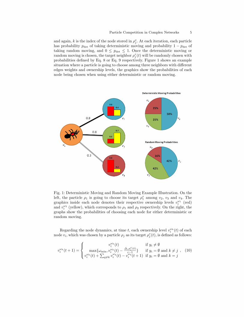
and again, k is the index of the node stored in ρvj . At each iteration, each particlehas probability pdet of taking deterministic moving and probability 1 − pdet oftaking random moving, and 0 ≤ pdet ≤ 1. Once the deterministic moving orrandom moving is chosen, the target neighbor ρτj (t) will be randomly chosen withprobabilities defined by Eq. 8 or Eq. 9 respectively. Figure 1 shows an examplesituation where a particle is going to choose among three neighbors with differentedges weights and ownership levels, the graphics show the probabilities of eachnode being chosen when using either deterministic or random moving.

Fig. 1: Deterministic Moving and Random Moving Example Illustration. On theleft, the particle ρ1 is going to choose its target ρτ1 among v2, v3 and v4. Thegraphics inside each node denotes their respective ownership levels vω1

i (red)and vω2

i (yellow), which corresponds to ρ1 and ρ2 respectively. On the right, thegraphs show the probabilities of choosing each node for either deterministic orrandom moving.

Regarding the node dynamics, at time t, each ownership level vωki (t) of each

node vi, which was chosen by a particle ρj as its target ρτj (t), is defined as follows:

vωki (t+ 1) =

vωki (t) if yi 6= ∅

max{ωmin, vωki (t)− ∆vρ

ωj (t)

c−1 } if yi = ∅ and k 6= j

vωki (t) +

∑q 6=k v

ωq

i (t)− vωq

i (t+ 1) if yi = ∅ and k = j

, (10)

6 Fabricio Breve, Liang Zhao, Marcos Quiles

where 0 < ∆v ≤ 1 is a parameter to control the ownership levels changing speed.If ∆v takes a low value, the node ownership levels change slowly, while if it takesa high value, the node ownership levels change quickly. Each particle ρj willincrease their corresponding ownership level vωj

i of the node vi they are targetingwhile decreasing the ownership levels (of this same node) that corresponds tothe other particles, always respecting Eq. 4. So if the particle already owns thenode its targeting, it will reinforce it, else it will increase its own ownership level,possibly becoming the new owner. However, vωi is fixed when yi 6= ∅ (particlevisiting a pre-labeled sample), so their ownership levels never change.

Regarding the particle dynamics, at time t, each particle potential ρωj (t) isset as:

ρωj (t+ 1) = vωj

i (t+ 1) with vi(t+ 1) = ρτj (t+ 1), (11)

which means every particle ρj have their potential ρωj set to the value of its own-ership level vωj

i from the node it is currently targeting. This way, a particle will bestrong as it is walking in its own neighborhood, but it will become weak if it tryto invade another neighborhood. Notice that to handle semi-supervised learningwe have made vωi fixed when yi 6= ∅, so a particle ρj can always “recharge” theirpotential to the maximum (ρωj = ωmax) when visiting nodes vi correspondingto pre-labeled samples of its own class (yi = j). Meanwhile, particles ρj cannotvisit or change ownership levels of nodes vi corresponding to pre-labeled samplesof other class (yi 6= j and yi 6= ∅) no matter how hard they try, and they willbecome weak (ρωj = ωmin) every time they try.

Finally, the particle position at time t is defined as follows:

ρvj (t+ 1) ={ρτj (t+ 1) if vρi (t+ 1) = ρjρvj (t) if vρi (t+ 1) 6= ρj

, (12)

with vi = ρτj (t + 1), which means that after raising its own ownership level onthe target node ρτj , the particle ρj will move to it if it already owned it or ifit became the new owner after that ownership level increase, else, it will staywhere it was. Notice that the node owner vρi at any time is defined by Eq. 3.

We have also introduced a “reset” mechanism to take the particles back to oneof the nodes corresponding to pre-labeled samples after a pre-defined amount ofsteps, so the particles could walk around all the pre-labeled nodes. This way, aftereach r steps, the particles are reset using Eq. 6, and their respective potentialsare set to the maximum by Eq. 7.

So, in summary, our algorithm works as follows:

1. Build the affinity matrix W by using Eq. 1,2. Set nodes ownership levels by using Eq. 5,3. Set particles initial positions and potentials by using Eq. 6 and Eq. 7 respec-

tively,4. Repeat steps 5 to 11 until convergence or for a pre-defined number of steps,5. Select between deterministic moving or random moving,6. Select the target node for each particle by using Eq. 8 or Eq. 9 for determin-

istic moving or random moving respectively,

Particle Competition in Complex Networks 7

7. Update nodes ownership levels by using Eq. 10,8. Update nodes ownership flags by using Eq. 3,9. Update particles potentials by using Eq. 11,

10. Update the particles positions by using Eq. 12,11. If r steps are reached, reset particles positions and potentials using Eq. 6

and Eq. 7 respectively.

3 Computer Simulations

In this section, we present the simulation results of some semi-supervised clas-sification tasks by using the proposed model with synthetic and real data sets.We also compare our method with the Global and Local Consistency Method[21] for both results accuracy and execution time. For our method, the followingparameters were held constant: pdet = 0.6 and ∆v = 0.1. The other parameters(σ and r) were set to their optimal values for each experiment. For the Consis-tency Method, the parameter α = 0.99 was held constant, as the authors did intheir original article [21], and σ was set to its optimal value for each experiment.

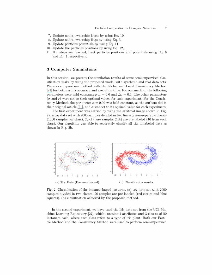
The first experiment was carried by using the artificial image shown in Fig.2a, a toy data set with 2000 samples divided in two linearly non-separable classes(1000 samples per class), 20 of these samples (1%) are pre-labeled (10 from eachclass). Our algorithm was able to accurately classify all the unlabeled data asshown in Fig. 2b.

−10 −8 −6 −4 −2 0 2 4 6

−10

−8

−6

−4

−2

0

2

4

6

(a) Toy Data (Banana-Shaped)

−10 −8 −6 −4 −2 0 2 4 6

−10

−8

−6

−4

−2

0

2

4

6

(b) Classification results

Fig. 2: Classification of the banana-shaped patterns. (a) toy data set with 2000samples divided in two classes, 20 samples are pre-labeled (red circles and bluesquares). (b) classification achieved by the proposed method.

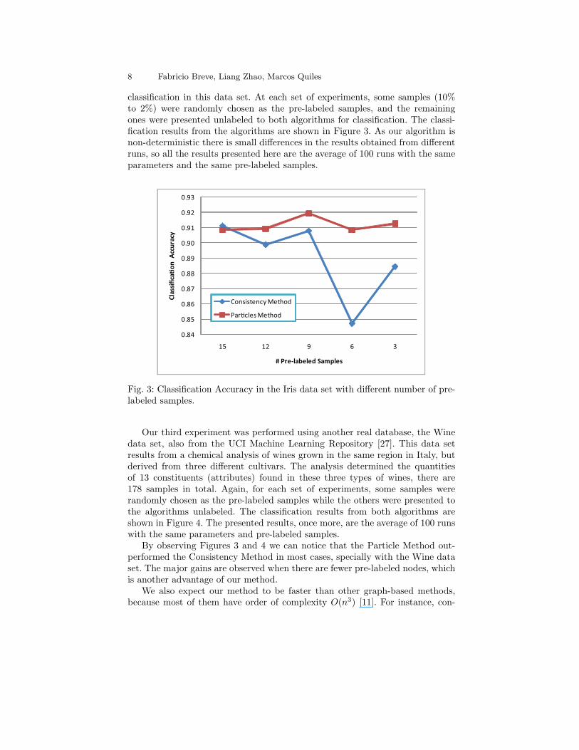
In the second experiment, we have used the Iris data set from the UCI Ma-chine Learning Repository [27], which contains 4 attributes and 3 classes of 50instances each, where each class refers to a type of iris plant. Both our Parti-cle Method and the Consistency Method were used to perform semi-supervised

8 Fabricio Breve, Liang Zhao, Marcos Quiles

classification in this data set. At each set of experiments, some samples (10%to 2%) were randomly chosen as the pre-labeled samples, and the remainingones were presented unlabeled to both algorithms for classification. The classi-fication results from the algorithms are shown in Figure 3. As our algorithm isnon-deterministic there is small differences in the results obtained from differentruns, so all the results presented here are the average of 100 runs with the sameparameters and the same pre-labeled samples.

0.84

0.85

0.86

0.87

0.88

0.89

0.90

0.91

0.92

0.93

15 12 9 6 3

Classifica!on Accuracy

# Pre-labeled Samples

Consistency Method

Par!cles Method

Fig. 3: Classification Accuracy in the Iris data set with different number of pre-labeled samples.

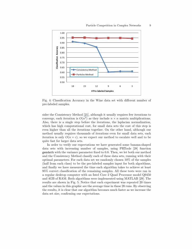
Our third experiment was performed using another real database, the Winedata set, also from the UCI Machine Learning Repository [27]. This data setresults from a chemical analysis of wines grown in the same region in Italy, butderived from three different cultivars. The analysis determined the quantitiesof 13 constituents (attributes) found in these three types of wines, there are178 samples in total. Again, for each set of experiments, some samples wererandomly chosen as the pre-labeled samples while the others were presented tothe algorithms unlabeled. The classification results from both algorithms areshown in Figure 4. The presented results, once more, are the average of 100 runswith the same parameters and pre-labeled samples.

By observing Figures 3 and 4 we can notice that the Particle Method out-performed the Consistency Method in most cases, specially with the Wine dataset. The major gains are observed when there are fewer pre-labeled nodes, whichis another advantage of our method.

We also expect our method to be faster than other graph-based methods,because most of them have order of complexity O(n3) [11]. For instance, con-

Particle Competition in Complex Networks 9

0.50

0.55

0.60

0.65

0.70

0.75

0.80

0.85

0.90

0.95

1.00

18 15 12 9 6 3

Classifica!on Accuracy

# Pre-labeled Samples

Consistency Method

Par!cles Method

Fig. 4: Classification Accuracy in the Wine data set with different number ofpre-labeled samples.

sider the Consistency Method [21], although it usually requires few iterations toconverge, each iteration is O(n3) as they include n × n matrix multiplications.Also, there is a single step before the iterations, the laplacian normalization,which has high computational cost, for small data sets the cost of this step iseven higher than all the iterations together. On the other hand, although ourmethod usually requires thousands of iterations even for small data sets, eachiteration is only O(n × c), so we expect our method to escalate well and to bequite fast for larger data sets.

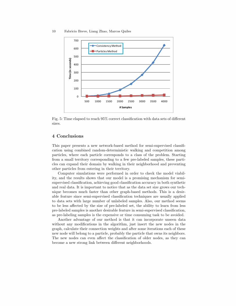
In order to verify our expectations we have generated some banana-shapeddata sets with increasing number of samples, using PRTools [28] functiongendatb with the variance parameter fixed to 0.8. Then, we let both our methodand the Consistency Method classify each of these data sets, running with theiroptimal parameters. For each data set we randomly chosen 10% of the samples(half from each class) to be the pre-labeled samples input for both algorithms,and finally we have measured the time each algorithm takes to achieve at least95% correct classification of the remaining samples. All these tests were ran ina regular desktop computer with an Intel Core 2 Quad Processor model Q9450and 4GB of RAM. Both algorithms were implemented using MATLAB [29]. Theresults are shown in Fig. 5. Notice that each experiment was repeated 20 timesand the values in this graphic are the average time in these 20 runs. By observingthe results, it is clear that our algorithm becomes much faster as we increase thedata set size, confirming our expectations.

10 Fabricio Breve, Liang Zhao, Marcos Quiles

0

100

200

300

400

500

600

700

500 1000 1500 2000 2500 3000 3500 4000

Tim

e (

in s

eco

nd

s)

# Samples

Consistency Method

Par!cles Method

Fig. 5: Time elapsed to reach 95% correct classification with data sets of differentsizes.

4 Conclusions

This paper presents a new network-based method for semi-supervised classifi-cation using combined random-deterministic walking and competition amongparticles, where each particle corresponds to a class of the problem. Startingfrom a small territory corresponding to a few pre-labeled samples, these parti-cles can expand their domain by walking in their neighborhood and preventingother particles from entering in their territory.

Computer simulations were performed in order to check the model viabil-ity, and the results shows that our model is a promising mechanism for semi-supervised classification, achieving good classification accuracy in both syntheticand real data. It is important to notice that as the data set size grows our tech-nique becomes much faster than other graph-based methods. This is a desir-able feature since semi-supervised classification techniques are usually appliedto data sets with large number of unlabeled samples. Also, our method seemsto be less affected by the size of pre-labeled set, the ability to learn from lesspre-labeled samples is another desirable feature in semi-supervised classification,as pre-labeling samples is the expensive or time consuming task to be avoided.

Another advantage of our method is that it can incorporate unseen datawithout any modifications in the algorithm, just insert the new nodes in thegraph, calculate their connection weights and after some iterations each of thesenew node will belong to a particle, probably the particle that owns its neighbors.The new nodes can even affect the classification of older nodes, as they canbecome a new strong link between different neighborhoods.

Particle Competition in Complex Networks 11

5 Acknowledgements

This work is supported by the State of Sao Paulo Research Foundation (FAPESP)and the Brazilian National Council of Technological and Scientific Development(CNPq).

References

1. Newman, M.: The structure and function of complex networks. SIAM Review 45,pp. 167–256. Society for Industrial and Applied Mathematics (2003)

2. Dorogovtsev, S., Mendes, F.: Evolution of Networks: From Biological Nets to theInternet and WWW. Oxford University Press (2003)

3. Bornholdt, S., Schuster, H.: Handbook of Graphs and Networks: From the Genometo the Internet. Wiley-VCH (2006)

4. Newman, M., Girvan, M.: Finding and evaluating community structure in networks.Physical Review E 69, 026113 (2004)

5. Newman, M.: Modularity and community structure in networks. In: Proceedings ofthe National Academy of Science of the United States of America 103, pp. 8577-8582(2006)

6. Duch, J., Arenas, A.: Community detection in complex networks using extremaloptimization. Physical Review E 72, 027104 (2005)

7. Reichardt, J., Bornholdt, S.: Detecting Fuzzy Community Structures in ComplexNetworks with a Potts Model. Physical Review Letters 93(21), 218701 (2004)

8. Danon. L, Dıaz-Guilera, A., Duch, J., Arenas, A.: Comparing community structureidentification. Journal of Statistical Mechanics: Theory and Experiment 9, P09008(2005)

9. Quiles, M., Zhao, L., Alonso, R., Romero, R.: Particle competition for complexnetwork community detection. Chaos 18, 033107 (2008).

10. Mitchell, T.: Machine Learning. McGraw Hill (1997)11. Zhu, X.: Semi-Supervised Learning Literature Survey. Technical Report, Computer

Sciences, University of Wisconsin-Madison (2005)12. Chapelle, O., Scholkopf, B., Zien, A.: Semi-Supervised Learning. MIT Press, Cam-

bridge (2006)13. Nigam, K., McCallum, A., Thrun, S., Mitchell, T.: Text classification from labeled

and unlabeled documents using EM. Machine Learning 39, pp. 103-134 (2000)14. Fujino, A., Ueda, N., Saito, K.: A hybrid generative/discriminative approach to

semi-supervised classifier design. In: AAAI-05, Proceedings of the Twentieth Na-tional Conference on Artificial Intelligence, pp. 764–769 (2005)

15. Demiriz, A., Bennet, K., Embrechts, M.: Semi-supervised clustering using geneticalgorithms. In: Proceedings of Artificial Neural Networks in Engineering, pp. 809–814. ASME Press (1999)

16. Dara, R., Kremer, S., Stacey, D.: Clustering unlabeled data with SOMs improvesclassification of labeled real-world data. In: Proceedings of the World Congress onComputational Intelligence (WCCI), pp. 2237-2242 (2002)

17. Blum, A. Mitchell, T.: Combining labeled and unlabeled data with co-training.In: COLT: Proceedings of the Workshop on Computational Learning Theory, pp.92–100 (1998)

18. Mitchell, T.: The role of unlabeled data in supervised learning. In: Proceedings ofthe Sixth International Colloquium on Cognitive Science (1999)

12 Fabricio Breve, Liang Zhao, Marcos Quiles

19. Vapnik, V.: Statistical Learning Theory. Wiley, New York (2008)20. Zhu, X., Ghahramani, Z., Lafferty, J.: Semi-supervised learning using Gaussian

fields and harmonic functions. In: Proceedings of the Twentieth International Con-ference on Machine Learning, pp. 912–919. Morgan Kaufmann, San Francisco (2003)

21. Zhou, D., Bousquet, O., Lal, T., Weston, J., Scholkopf, B.: Learning with localand global consistency. Advances in Neural Information Processing Systems 16, pp.321–328. MIT Press, Cambdridge (2004)

22. Blum, A., Chawla, S.: Learning from labeled and unlabeled data using graph min-cuts. In: Proceedings of the Eighteenth International Conference on Machine Learn-ing, pp. 19–26. Morgan Kaufmann, San Francisco (2001)

23. Belkin, M., Matveeva, I., Niyogi, P.: Regularization and semisupervised learningon large graphs. In: Conference on Learning Theory, pp. 624–638. Springer (2004)

24. Belkin, M., Niyogi, P., Sindhwani, V.: On manifold regularization. In: Proceedingsof the Tenth International Workshop on Artificial Intelligence and Statistics (AIS-TAT 2005), pp. 17–24. Society for Artificial Intelligence and Statistics, New Jersey(2005)

25. Joachims, T.: Transductive learning via spectral graph partitioning. In: Proceed-ings of International Conference on Machine Learning 2003, pp. 290-297. AAAIPress (2003)

26. Ng, A., Jordan, M., Weiss, Y.: On spectral clustering: analysis and an algorithm.Advances in Neural Information Processing Systems 14, pp. 849–856. MIT Press(2001)

27. Asuncion, A., Newman, D.: UCI Machine Learning Repository. Univer-sity of California, Irvine, School of Information and Computer Sciences,http://www.ics.uci.edu/∼mlearn/MLRepository.html (2007)

28. PRTools: The Matlab Toolbox for Pattern Recognition, http://prtools.org29. MATLAB, http://www.mathworks.com/products/matlab/