Semi-supervised Margin-based Feature Selection for Classification
223
HAL Id: tel-02489733 https://tel.archives-ouvertes.fr/tel-02489733 Submitted on 24 Feb 2020 HAL is a multi-disciplinary open access archive for the deposit and dissemination of sci- entific research documents, whether they are pub- lished or not. The documents may come from teaching and research institutions in France or abroad, or from public or private research centers. L’archive ouverte pluridisciplinaire HAL, est destinée au dépôt et à la diffusion de documents scientifiques de niveau recherche, publiés ou non, émanant des établissements d’enseignement et de recherche français ou étrangers, des laboratoires publics ou privés. Semi-supervised Margin-based Feature Selection for Classification Samah Hijazi To cite this version: Samah Hijazi. Semi-supervised Margin-based Feature Selection for Classification. Artificial Intelli- gence [cs.AI]. Université du Littoral Côte d’Opale; Université Libanaise, école doctorale des sciences et technologies, 2019. English. NNT : 2019DUNK0546. tel-02489733
-
Upload
khangminh22 -
Category
Documents
-
view
1 -
download
0
Transcript of Semi-supervised Margin-based Feature Selection for Classification

HAL Id: tel-02489733https://tel.archives-ouvertes.fr/tel-02489733
Submitted on 24 Feb 2020
HAL is a multi-disciplinary open accessarchive for the deposit and dissemination of sci-entific research documents, whether they are pub-lished or not. The documents may come fromteaching and research institutions in France orabroad, or from public or private research centers.
L’archive ouverte pluridisciplinaire HAL, estdestinée au dépôt et à la diffusion de documentsscientifiques de niveau recherche, publiés ou non,émanant des établissements d’enseignement et derecherche français ou étrangers, des laboratoirespublics ou privés.
Semi-supervised Margin-based Feature Selection forClassification
Samah Hijazi
To cite this version:Samah Hijazi. Semi-supervised Margin-based Feature Selection for Classification. Artificial Intelli-gence [cs.AI]. Université du Littoral Côte d’Opale; Université Libanaise, école doctorale des scienceset technologies, 2019. English. �NNT : 2019DUNK0546�. �tel-02489733�

THÈSE de doctorat en CotutellePour obtenir le grade de Docteur délivré par
L’Université du Littoral Côte d’OpaleL’Ecole Doctorale SPI - Université Lille Nord-De-France
etL’Université Libanaise
L’Ecole Doctorale des Sciences et Technologie
Discipline : Sciences et Technologies de l’Information et de la
communication, Traitement du Signal et des Images
Présentée et soutenue publiquement par
Samah HIJAZI
le 20 Décembre 2019
Sélection d’Attributs Basée Marge pour la Classificationdans un Contexte Semi-Supervisé
Membre du Jury:
M. Fadi DORNAIKA Professeur de Recherche à l’Université du Pays Basque RapporteurM. Ali MANSOUR Professeur à l’Université ENSTA Bretagne RapporteurM. Kifah TOUT Professeur à l’Université Libanaise PrésidentM. Ghaleb FAOUR Directeur de Recherche au CNRS-Liban ExaminateurMme. Marwa EL BOUZ Enseignante-Chercheuse à Yncréa-Ouest ExaminateurM. Denis HAMAD Professeur à l’Université du Littoral Côte d’Opale Directeur de thèseM. Ali KALAKECH Professeur à l’Université Libanaise Directeur de thèseMme. Mariam KALAKECH Maître de Conférences à l’Université Libanaise Encadrante de thèse

Cotutelle PhD THESISsubmitted in partial fulfillment for the degree of Doctor of Philosophy
from the University of the Opal CoastDoctoral School SPI - University of Lille- North France
andthe Lebanese University
Doctoral School of Science and Technology
Specialty : Information and Communication Sciences and
Technologies, Signal and Image Processing
Publicly defended by
Samah HIJAZIon December 20, 2019
Semi-supervised Margin-based Feature Selection forClassification
Committee Members:
Mr. Fadi DORNAIKA Research Professor at the University of the Basque Country ReviewerMr. Ali MANSOUR Professor at the University of ENSTA Bretagne ReviewerMr. Kifah TOUT Professor at the Lebanese University PresidentMr. Ghaleb FAOUR Research Director at CNRS-Lebanon ExaminerMrs. Marwa EL BOUZ Teacher-Researcher at Yncréa-Ouest ExaminerMr. Denis HAMAD Professor at the University of the Littoral Opal Coast Thesis DirectorMr. Ali KALAKECH Professor at the Lebanese University Thesis DirectorMrs. Mariam KALAKECH Senior Lecturer at the Lebanese University Thesis Supervisor

Contents
Acknowledgment i
Notations iii
Abbreviations v
Introduction 7
1 Score-Based Feature Selection 131.1 Introduction . . . . . . . . . . . . . . . . . . . . . . . . . . . . . . . . . . . 141.2 Dimensionality Reduction . . . . . . . . . . . . . . . . . . . . . . . . . . . 141.3 Data and Graph Representation . . . . . . . . . . . . . . . . . . . . . . . . 17
1.3.1 Graph Data Representation . . . . . . . . . . . . . . . . . . . . . . 171.3.2 Graph Laplacian Matrices . . . . . . . . . . . . . . . . . . . . . . . 21
1.4 Feature Selection with Contextual Knowledge . . . . . . . . . . . . . . . 221.4.1 Types of Supervision Information . . . . . . . . . . . . . . . . . . 24
1.5 General Procedure of Feature Selection . . . . . . . . . . . . . . . . . . . . 251.5.1 Subset Generation . . . . . . . . . . . . . . . . . . . . . . . . . . . 261.5.2 Evaluation Criterion of Performance . . . . . . . . . . . . . . . . . 271.5.3 Stopping Criterion . . . . . . . . . . . . . . . . . . . . . . . . . . . 291.5.4 Result Validation . . . . . . . . . . . . . . . . . . . . . . . . . . . . 29
1.6 Ranking Feature Selection Methods based on Scores . . . . . . . . . . . . 321.6.1 Unsupervised Scores . . . . . . . . . . . . . . . . . . . . . . . . . . 331.6.2 Supervised Scores . . . . . . . . . . . . . . . . . . . . . . . . . . . 351.6.3 Semi-supervised Scores with Pairwise Constraints . . . . . . . . . 36
1.7 Feature Redundancy Analysis . . . . . . . . . . . . . . . . . . . . . . . . . 391.7.1 Redundancy Performance Evaluation Metrics . . . . . . . . . . . 41
1.8 Conclusion . . . . . . . . . . . . . . . . . . . . . . . . . . . . . . . . . . . . 42

2 Relief-Based Feature Selection 452.1 Introduction . . . . . . . . . . . . . . . . . . . . . . . . . . . . . . . . . . . 452.2 The Original Relief Algorithm . . . . . . . . . . . . . . . . . . . . . . . . . 46
2.2.1 Strengths and Limitations . . . . . . . . . . . . . . . . . . . . . . . 492.3 Basic Variants and Extensions of Relief with Probabilistic Interpretation 51
2.3.1 Robustness . . . . . . . . . . . . . . . . . . . . . . . . . . . . . . . 522.3.2 Incomplete Data . . . . . . . . . . . . . . . . . . . . . . . . . . . . 532.3.3 Multi-Class Problems . . . . . . . . . . . . . . . . . . . . . . . . . 54
2.4 Concept of Change Interpretation . . . . . . . . . . . . . . . . . . . . . . . 562.5 Margin Notion in Relief-Based Feature Selection . . . . . . . . . . . . . . 58
2.5.1 Margin General Definition and Types . . . . . . . . . . . . . . . . 582.5.2 Mathematical Interpretation . . . . . . . . . . . . . . . . . . . . . . 602.5.3 Instance Weighting in RBAs . . . . . . . . . . . . . . . . . . . . . . 71
2.6 Statistical Interpretation . . . . . . . . . . . . . . . . . . . . . . . . . . . . 732.6.1 STatistical Inference for Relief (STIR) . . . . . . . . . . . . . . . . 74
2.7 Conclusion . . . . . . . . . . . . . . . . . . . . . . . . . . . . . . . . . . . . 75
3 An Approach based on Hypothesis-Margin and Pairwise Constraints 793.1 Introduction . . . . . . . . . . . . . . . . . . . . . . . . . . . . . . . . . . . 803.2 Hypothesis-Margin in a Constrained Context For Maximizing Relevance 81
3.2.1 General Mathematical Interpretation . . . . . . . . . . . . . . . . . 823.2.2 Relief with Side Constraints (Relief-Sc) . . . . . . . . . . . . . . . 843.2.3 ReliefF-Sc: A Robust version of Relief-Sc . . . . . . . . . . . . . . 883.2.4 Iterative Search Margin-Based Algorithm with Side Constraints
(Simba-Sc) . . . . . . . . . . . . . . . . . . . . . . . . . . . . . . . . 893.3 Feature Clustering in a Constrained Context for Minimizing Redundancy 91
3.3.1 Feature Space Sparse Graph Construction . . . . . . . . . . . . . . 933.3.2 Agglomerative Hierarchical Feature Clustering . . . . . . . . . . 953.3.3 Proposed Feature Selection Approach . . . . . . . . . . . . . . . . 97
3.4 Experimental Results . . . . . . . . . . . . . . . . . . . . . . . . . . . . . . 983.4.1 Experimental Results on Relief-Sc: Selection of Relevant Features 993.4.2 Experimental Results on FCRSC: Selection of Relevant and Non-
redundant Features . . . . . . . . . . . . . . . . . . . . . . . . . . . 1073.5 Conclusion . . . . . . . . . . . . . . . . . . . . . . . . . . . . . . . . . . . . 118
4 Active Learning of Pairwise Constraints 1214.1 Introduction . . . . . . . . . . . . . . . . . . . . . . . . . . . . . . . . . . . 1214.2 Related Work . . . . . . . . . . . . . . . . . . . . . . . . . . . . . . . . . . 124

4.2.1 Constraints Selection . . . . . . . . . . . . . . . . . . . . . . . . . . 1244.2.2 Constraints Propagation . . . . . . . . . . . . . . . . . . . . . . . . 125
4.3 Active learning of Constraints . . . . . . . . . . . . . . . . . . . . . . . . . 1284.3.1 Using Graph Laplacian . . . . . . . . . . . . . . . . . . . . . . . . 1284.3.2 Active Constraint Selection . . . . . . . . . . . . . . . . . . . . . . 129
4.4 Propagation of Actively Selected Constraints . . . . . . . . . . . . . . . . 1344.5 Complexity Analysis . . . . . . . . . . . . . . . . . . . . . . . . . . . . . . 1414.6 Experimental Results . . . . . . . . . . . . . . . . . . . . . . . . . . . . . . 141
4.6.1 Used Benchmarking Feature Selection Methods . . . . . . . . . . 1414.6.2 Datasets Description and Parameter Setting . . . . . . . . . . . . . 1424.6.3 Performance Evaluation Measures . . . . . . . . . . . . . . . . . . 1444.6.4 Performance Evaluation Results . . . . . . . . . . . . . . . . . . . 146
4.7 Conclusion . . . . . . . . . . . . . . . . . . . . . . . . . . . . . . . . . . . . 160
Conclusion and Perspectives 163
Bibliography 167
Publications 184
List of Tables 185
List of Figures 186
Abstract 191
Résumé 193
Résumé Étendu de la Thèse 195


Acknowledgment
First and foremost, praises and thanks to the God, the Almighty, for His showers ofblessings throughout my travel and research journey.
Special thanks to the University of the Littoral Opal Coast (ULCO), Agence Uni-versitaire de la Francophonie (AUF), and the National Council For Scientific Research(CNRS-L) for supporting this work with a scholarship grant as a part of ARCUS E2D2project.
I would like to express my deep and sincere gratitude to my thesis director, Pro-fessor Denis HAMAD for giving me the opportunity to do research and providinginvaluable guidance throughout this research. I would also like to thank Professor AliKALAKECH, my thesis co-director, and Dr. Mariam KALAKECH, my thesis super-visor, for their valuable advices during my thesis work. It was a great privilege andhonor to work under their guidance.
I would also like to express my special thanks to Professor Fadi DORNAIKA andProfessor Ali MANSOUR for their precious time and effort to review my work. Specialthanks to Professor Kifah TOUT, Professor Ghaleb FAOUR, and Dr. Marwa El BOUZas well for examining my thesis.
To my friends and research colleagues, Emna CHEBBI, Hiba AL ASSAAD, PamelaAL ALAM, Aya MOURAD, Ali DARWICH, Rim TRAD, Mohammad HARISSA, Ghi-daa BADRAN, Tarek ZAAROUR, Ragheb GHANDOUR, Rasha SHAMSEDDINE, andMohammad Ali ZAITER, thank you all for your constant support. I am also extremelythankful to the amazing Dr. Vinh Truong HOANG for his efforts and advices. Specialthanks to Mahdi BAHSOUN, I wouldn’t have known about this opportunity withoutyour help.
i

To my parents and life coaches, Zakaria HIJAZI and Amal WEHBI, no words canexpress my feelings of gratitude. Thank you for being there every moment, shower-ing me with love, support, encouragement, sincere prayers, and care. I am extremelygrateful for all the sacrifices you have done for making my future brighter. To my sis-ter, Sahar HIJAZI simply thank you for being you. I am extremely lucky to be yourlittle sister.
Final words to my partner and supporter Ali REBAIE. Thank you for your patienceand for listening to me every single day, to my smallest and simplest problems, to myfears and worries. Thank you for understanding the long silent nights. I owe it all toyou.

Notations
X Data matrix X = {xn}Nn=1
yl Data Labels vectorN Number of data pointsNc Number of points in class cF Number of featuresC Number of classesxn n-th data pointyn Label of data point xn
xni Value of n-th data point on i-th featureAi i-th featureAin Value of i-th feature on the n-th data pointµAi Mean of the i-th featureµc
AiMean of i-th feature for points of class c
S Similarity matrixD Degree diagonal matrixML Pairwise must-link constraints setCL Pairwise cannot-link constraints setSML Similarity matrix defined on MLSCL Similarity matrix defined on CLSkn Similarity matrix defined on ML and nearest neighborsDML Degree diagonal matrix defined on MLDCL Degree diagonal matrix defined on CLDkn Degree diagonal matrix defined on ML and nearest neighborsL Laplacian matrix with L = D− SLsym Normalized symmetric Laplacian matrixLrw Normalized asymmetric Laplacian matrixLML Laplacian matrix with LML = DML − SML
iii

LCL Laplacian matrix with LCL = DCL − SCL
Lkn Laplacian matrix with Lkn = Dkn − Skn
I Identity matrixV Set of nodes in a graphVn Graph node corresponding to data point xn
E Set of edges in a graphG = (V, E) Undirected graph constructed over XVi Variance Score of a particular feature Ai
LSi Laplacian Score of a particular feature Ai
Fi Fisher Score of a particular feature Ai
CS1i Constraint Score-1 of a particular feature Ai
CS2i Constraint Score-2 of a particular feature Ai
CS3i Constraint Score-3 of a particular feature Ai
CS4i Constraint Score-4 of a particular feature Ai
CLSi Constrained Laplacian Score of a particular feature Ai
K Number of nearest neighborsKNN(xn) Set of the K-nearest neighbors to xn
w Weight vector spanning F featureswi Weight of feature Ai
H(xn) Nearhit of point xn
M(xn) Nearmiss of point xn
T Number of iterationsKH(xn) K-nearhits of point xn
KM(xn) K-nearmisses of point xn
KM(xn, c) K-nearmisses of point xn from different class cρ(xn) Hypothesis-margin of point xn
z Hypothesis-margin vector of length Fρ(xn, xm) Hypothesis-margin of a cannot-link constraintρ((xn, xm),w) Weighted Hypothesis-margin of a cannot-link constraint∆(p1, p2) General distance function between any two data points∆(Ai, p1, p2) General distance function between any two data points on a specific feature∆w(p1, p2) General weighted distance function between any two data points
Abbreviations
RBAs Relief-Based AlgorithmsRelief-Sc Relief with Side ConstraintsACS Active Constraint SelectionRCG Random Constraint GenerationPACS Propagation of Actively Selected ConstraintsFCRSC Feature Clustering Relief-ScSimba Iterative Search Margin-Based AlgorithmSimba-Sc Simba with Side ConstraintsMI Mutual InformationmRMR Minimum Redundancy-Maximum RelevanceK-NN K- Nearest NeighborUCI University California IrvineSVM Support Vector MachinesNB Naive BayesC4.5 Decision TreeCSi Constraint Score-iCLS Constrained Laplacian ScoreFLDA Fisher Linear Discriminant AnalysisPCA Principal Component AnalysisMDS Multidimensional ScalingLLE Local Linear EmbeddingSPCA Supervised Principal Component Analysist-SNE t-distributed Stochastic Neighbor EmbeddingPCC Pearson Correlation CoefficientFCBF Fast Correlation-Based FilterSFS Sequential Forward SelectionSBS Sequential Backward Selection
v

STIR STatistical Inference for ReliefSVDD Support Vector Data DescriptionSDP Semi-Definite ProgrammingMTPs Meta-PointsLPP Locality Preserving ProjectionsMLPP-CLP Multiple Locality Preserving Projections with Cluster-based Label Propagation

Introduction
With the rapid growth of modern technologies, the limitless number of computer andInternet applications has caused an exponential increase in the amount of generateddata in a variety of domains. For instance, in domains such as social media, healthcare,marketing, bioinformatics and biometrics, the data provided such as image, video,text, voice, gene expression microarrays, and other kinds obtained from social rela-tions and the Internet of Things may not only be huge in terms of the data samples,but also in terms of feature dimensionality. This imposes many challenges on effectiveand efficient data management.
Therefore, the use of data mining and machine learning techniques becomes a ne-cessity for automatically extracting knowledge and uncovering hidden patterns fromdata. In fact, according to the contextual knowledge and the way of identifying datapatterns, these techniques can be broadly categorized into classification, regression (orprediction), and clustering. Data classification, the problem of identifying to which ofa set of pre-defined categories a data point should belong, can model many real-worldapplications. Indeed, datasets are usually represented by two-dimensional matriceswhere the rows correspond to data samples and columns correspond to the featurescharacterizing them. In this regard, some of the available features characterizing thedata may not provide any useful information or even express noise with respect to acertain relevance evaluation criterion (e.g. class discrimination), others may be corre-lated or redundant which makes the learning process complex, expensive in terms ofstorage and computation, ineffective, less generalizable and difficult to interpret.
As a solution, finding narrower data matrices that can successfully summarize theoriginal ones can be considered. The latter process is known as dimensionality reduc-tion which is a major step in data pre-processing. It can be mainly applied in twodifferent approaches: feature extraction and feature selection. Feature extraction con-
7

verts the initial input space into a new one of lower dimensions by combining theoriginal features, thus, changing their meaning. Whereas, feature selection simplychooses a small subset of features that best describes a dataset out of a larger set ofcandidate features with the aim of producing a lower-dimensional space without anycore changes to the meaning of features. Consequently, feature selection costs less thanfeature extraction in terms of computational cost and model interpretability.
Generally speaking, individual feature selection can be generalized into featureweighting/scoring/ranking, by which, each feature is individually assigned a soft rel-evance score instead of just a binary one. Indeed, the process by which this score isevaluated changes with the change of contextual knowledge. Therefore, in an un-supervised context where no labeling information is available at all, feature selec-tion methods resort to using data similarity and local discriminative information ap-proaches to measure the ability of features in discriminating data groups. On the otherside, in a supervised context where data is fully labeled, feature selection methods as-sign higher scores to features having high correlation measures with class labels. Therealso exists a whole family of feature selection algorithms that use a margin-based scorein order to evaluate and rank features. These are known as Relief-Based Algorithms(RBAs) and were initially suggested in the supervised context for two-class problems.They assign bigger weights for features that best contribute to enlarge a distance met-ric called hypothesis-margin. This margin is calculated as the difference between thedistance from a point to its nearmiss (nearest point having a different label) and thedistance to its nearhit (nearest data point having the same label). RBAs proved to gen-erally perform well regardless of the problem specifications. They have low bias filteralgorithms (independent of classifiers), considered relatively fast, capable of detectingfeature interaction, robust and noise-tolerant in addition to their ability to capture datalocal dependencies [1, 2].
However, in many real-world applications, there usually exist few labeled datapoints and lots of unlabeled ones, by which, both supervised and unsupervised fea-ture selection algorithms cannot fully take advantage of all data points in this scenario.Thus, it was wise to use semi-supervised methods to feat both labeled and unlabeledpoints. Actually, compared to class labels, pairwise constraints are another type ofsupervision information that can be acquired more easily. These constraints simplyspecify whether a pair of data points belongs to the same class (must-link constraint)or to different classes (cannot-link constraint) without specifying the classes them-selves. Many constraint scores use these two notions to rank features, however, they
8

still neglect the information provided by unconstrained and unlabeled data.
This led us to suggest a new framework for semi-supervised constrained margin-based feature selection that handles the two core aspects of feature selection: relevancyand redundancy. It consists of, (1) a constrained margin-based feature selection algo-rithm that utilizes pairwise cannot-link constraints only and benefits from both the lo-cal unlabeled neighborhood of the data points as well as the provided constraints, (2) amethod for actively selecting constraints based on matrix perturbation theory appliedon the similarity matrix in addition to the propagation of these constraints throughdecomposing the problem into a set of independent label propagation subproblems,and (3) a feature clustering method that combines sparse graph representation of thefeature space with margin maximization.
In order to compare the performance of our suggested methods with other score-based supervised, unsupervised and constrained feature selection methods, experi-ments will be initially carried out on well-known benchmark UCI (University Califor-nia Irvine [3]) and high-dimensional gene expression datasets.
Contributions
The core of this thesis is semi-supervised constrained feature selection for high-dimen-sional data. As feature selection aims at finding a small subset of relevant and non-redundant features that can successfully summarize the original feature space, ourworkflow was to focus first on tackling the problem of constraint-relevant feature se-lection followed by handling redundancy. Throughout this work our contributionscan be summarized as follows:
• We provide a comprehensive and concise literature review of Relief-based Al-gorithms from their four interpretations, called probabilistic [4], comprehensible[5], mathematical [6], and statistical [7]. We highlight their strengths, limita-tions, variants and extensions, in addition to representing the original Relief as amargin-based algorithm.
• We suggest the semi-supervised margin-based constrained algorithms Relief-Sc(Relief with Side Constraints) and its robust version ReliefF-Sc. They integratethe modification of hypothesis-margin when used with cannot-link constraints,with the analytical solution of the supervised Relief algorithm from its optimiza-
9

tion perspective. They utilize cannot-link constraints only to solve a simple con-vex problem in a closed-form providing a unique solution.
• We suggest an active method for pairwise constraints selection called ActiveConstraint Selection (ACS). The output of this method is used by Relief-Sc andReliefF-Sc. ACS is based on the matrix perturbation theory, specifically on theFirst-Order Eigenvector Perturbation theorem. It systematically chooses whichpairs of data are more effective in reducing uncertainty. Accordingly, only thesepairs are queried for constraints from human-experts, thus, decreasing humanlabor-cost and avoiding noisy constraints and any ill interactions between a ran-dom constraint set and our objective function. In addition, a method for Prop-agating these Actively Selected Constraints (PACS) to their neighborhood wasalso suggested.
• We propose extending our semi-supervised feature selection method into a novelcombination of feature clustering and hypothesis margin maximization. Thismethod, called Feature Clustering ReliefF-Sc (FCRSC), aims to allow redundancyelimination as part of our overall suggested framework.
Structure of thesis
This thesis is structured as follows:
In the first chapter, we introduce the definitions of dimensionality reduction, fea-ture extraction, feature selection, feature relevancy, and feature redundancy. We alsopresent the main data notations and knowledge representation together with graphdata construction methods. In addition, we categorize the feature selection processaccording to the availability of supervision information (class labels and pairwise con-straints) and according to the evaluation criterion of performance while presentingsome of the well-known state-of-the-art score-based ranking methods.
In the second chapter, we provide a survey of the most popular filter-type Relief-Based Algorithms and show their implicit margin-based core. Mainly, the originalsupervised Relief algorithm is explained thoroughly focusing on its strengths, limita-tions, and applications in different contexts as a context-aware algorithm. Also, wecover all variants, and extensions of Relief that were suggested to handle problemswith noisy, incomplete, and multi-class data. The chapter is divided into four majorsections each of which expresses Relief from a different possible interpretation (prob-
10

abilistic, comprehensible, mathematical, and statistical).
In the third chapter, we first suggest Relief-Sc and its robust version ReliefF-Sc.Their goal is effectively reducing data high dimensionality by finding a unique rel-evant feature subset in a closed-form. This is to be obtained in a semi-supervisedcontext using side pairwise cannot-link constraints. Therefore, we first explain thechange in the main notions of a margin (nearhit and nearmiss) from the supervised tothe constrained context. We also formulate the constrained Relief-Sc under the math-ematical interpretation of RBAs. In addition, we present the only other constrainedmargin-based algorithm (Simba-Sc) that is mainly used in our comparisons of Relief-Sc’s performance. On the other side, we present our FCRSC method for redundancyelimination or minimizing redundancy with its main three building blocks: (1) sparsegraph construction to represent feature similarities, (2) hierarchical clustering uponthe latter, (3) combining margin maximization with the output of feature clusteringwhich results in maximizing relevancy while minimizing redundancy. Finally, we ex-perimentally validate the efficiency of Relief-Sc, ReliefF-Sc, and FCRSC on multipleUCI machine learning and two high dimensional gene-expression datasets in compar-ison with supervised, unsupervised and semi-supervised state-of-the-art filter featureselection methods.
In the fourth chapter, we present our active constraint selection and propagationmethods with briefing their related work. In fact, we divide the chapter into two mainparts. The first one explains our core contribution i.e. the process of selecting pairwiseconstraints to be used by the constrained margin-based feature selection algorithmRelief-Sc. The second one is the augmentation of supervision information by prop-agating these constraints called PACS. Finally, extensive experiments are applied onUCI [3] benchmark datasets and two high-dimensional gene expression ones to vali-date the performance of our methods in addition to showing the effect of randomlygenerated constraints (RCG) vs. actively selected constraints (ACS) in the process ofconstrained feature selection.
Finally, we highlight our contributions and conclude the thesis while pointing outour future perspectives.
11

Chapter 1Score-Based Feature Selection
Contents1.1 Introduction . . . . . . . . . . . . . . . . . . . . . . . . . . . . . . . . . . 14
1.2 Dimensionality Reduction . . . . . . . . . . . . . . . . . . . . . . . . . 14
1.3 Data and Graph Representation . . . . . . . . . . . . . . . . . . . . . . 17
1.3.1 Graph Data Representation . . . . . . . . . . . . . . . . . . . . . 17
1.3.2 Graph Laplacian Matrices . . . . . . . . . . . . . . . . . . . . . . 21
1.4 Feature Selection with Contextual Knowledge . . . . . . . . . . . . . 22
1.4.1 Types of Supervision Information . . . . . . . . . . . . . . . . . 24
1.5 General Procedure of Feature Selection . . . . . . . . . . . . . . . . . . 25
1.5.1 Subset Generation . . . . . . . . . . . . . . . . . . . . . . . . . . 26
1.5.2 Evaluation Criterion of Performance . . . . . . . . . . . . . . . . 27
1.5.3 Stopping Criterion . . . . . . . . . . . . . . . . . . . . . . . . . . 29
1.5.4 Result Validation . . . . . . . . . . . . . . . . . . . . . . . . . . . 29
1.6 Ranking Feature Selection Methods based on Scores . . . . . . . . . . 32
1.6.1 Unsupervised Scores . . . . . . . . . . . . . . . . . . . . . . . . . 33
1.6.2 Supervised Scores . . . . . . . . . . . . . . . . . . . . . . . . . . 35
1.6.3 Semi-supervised Scores with Pairwise Constraints . . . . . . . . 36
1.7 Feature Redundancy Analysis . . . . . . . . . . . . . . . . . . . . . . . 39
1.7.1 Redundancy Performance Evaluation Metrics . . . . . . . . . . 41
1.8 Conclusion . . . . . . . . . . . . . . . . . . . . . . . . . . . . . . . . . . 42
13

1.1. Introduction
1.1 Introduction
When feeding high dimensional data to the “model” of traditional learning techniqueswithout any proper preprocessing, unsatisfactory learning performance can be ob-tained due to a critical problem known as the curse of dimensionality [8]. The latterrefers to a phenomenon by which data becomes sparser in high dimensional spacesleading to over-fitting the learning algorithm [9]. In addition, many of the features de-scribing the original feature space in real-world applications might be irrelevant andredundant.
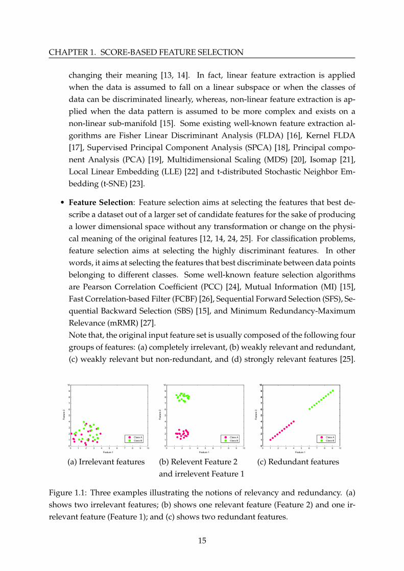
To clearly explain the notions of relevancy and redundancy, we use two featuresto present three different examples as can be seen in Figure (1.1). The first examplepresented in Figure (1.1a) shows the case when both Feature 1 and Feature 2 are con-sidered irrelevant, this is due to their inability to discriminate data points of the twodifferent classes (clusters). In the second example, presented in Figure (1.1b), Feature 1is considered irrelevant; whereas, Feature 2 can clearly separate Class A from Class B,thus, it is considered relevant. Note that, usually a feature that best describes a datasetaccording to a specific relevance evaluation criterion is said to be relevant, which is inthis example, the capability of class separation (classification problems). On the otherside, the third example, presented in Figure (1.1c), is the case when Feature 1 andFeature 2 are redundant. In such cases, the information provided by the features isstrongly correlated. Eliminating irrelevant and redundant features can decrease datadimensionality without any negative impact on the learning performance, on the con-trary, it is said to enhance it.
1.2 Dimensionality Reduction
It is well-known that the presence of irrelevant and redundant features can penalizethe performance of a machine learning algorithm, increase its storage requirements,elevate its computational costs and make data visualization and model interpretabilitymuch harder. In order to mitigate such problems, dimensionality reduction as a datapreprocessing strategy is one of the most powerful tools to be used. By its turn, it canbe mainly divided into two different groups, feature extraction and feature selection[10–12].
• Feature Extraction: projects the initial input space onto a new one of lower di-mension by combining the original features either linearly or non-linearly, thus,
14
CHAPTER 1. SCORE-BASED FEATURE SELECTION
changing their meaning [13, 14]. In fact, linear feature extraction is appliedwhen the data is assumed to fall on a linear subspace or when the classes ofdata can be discriminated linearly, whereas, non-linear feature extraction is ap-plied when the data pattern is assumed to be more complex and exists on anon-linear sub-manifold [15]. Some existing well-known feature extraction al-gorithms are Fisher Linear Discriminant Analysis (FLDA) [16], Kernel FLDA[17], Supervised Principal Component Analysis (SPCA) [18], Principal compo-nent Analysis (PCA) [19], Multidimensional Scaling (MDS) [20], Isomap [21],Local Linear Embedding (LLE) [22] and t-distributed Stochastic Neighbor Em-bedding (t-SNE) [23].
• Feature Selection: Feature selection aims at selecting the features that best de-scribe a dataset out of a larger set of candidate features for the sake of producinga lower dimensional space without any transformation or change on the physi-cal meaning of the original features [12, 14, 24, 25]. For classification problems,feature selection aims at selecting the highly discriminant features. In otherwords, it aims at selecting the features that best discriminate between data pointsbelonging to different classes. Some well-known feature selection algorithmsare Pearson Correlation Coefficient (PCC) [24], Mutual Information (MI) [15],Fast Correlation-based Filter (FCBF) [26], Sequential Forward Selection (SFS), Se-quential Backward Selection (SBS) [15], and Minimum Redundancy-MaximumRelevance (mRMR) [27].Note that, the original input feature set is usually composed of the following fourgroups of features: (a) completely irrelevant, (b) weakly relevant and redundant,(c) weakly relevant but non-redundant, and (d) strongly relevant features [25].
(a) Irrelevant features (b) Relevent Feature 2and irrelevent Feature 1
(c) Redundant features
Figure 1.1: Three examples illustrating the notions of relevancy and redundancy. (a)shows two irrelevant features; (b) shows one relevant feature (Feature 2) and one ir-relevant feature (Feature 1); and (c) shows two redundant features.
15
1.2. Dimensionality Reduction
Completely Irrelevant features
Weakly Relevant and
Redundant features
Weakly Relevant but
Non- Redundant features
Strongly Relevant features
Optimal feature subset
(a) (b) (c) (d)
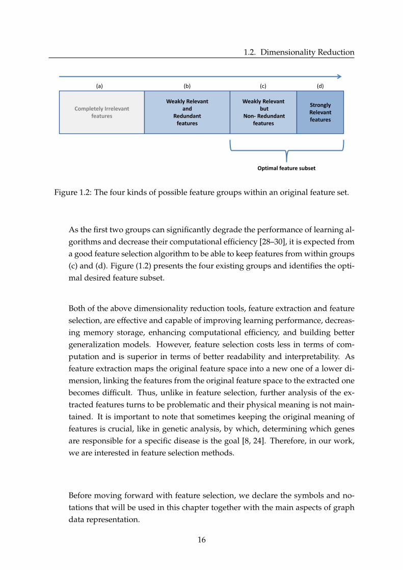
Figure 1.2: The four kinds of possible feature groups within an original feature set.
As the first two groups can significantly degrade the performance of learning al-gorithms and decrease their computational efficiency [28–30], it is expected froma good feature selection algorithm to be able to keep features from within groups(c) and (d). Figure (1.2) presents the four existing groups and identifies the opti-mal desired feature subset.
Both of the above dimensionality reduction tools, feature extraction and featureselection, are effective and capable of improving learning performance, decreas-ing memory storage, enhancing computational efficiency, and building bettergeneralization models. However, feature selection costs less in terms of com-putation and is superior in terms of better readability and interpretability. Asfeature extraction maps the original feature space into a new one of a lower di-mension, linking the features from the original feature space to the extracted onebecomes difficult. Thus, unlike in feature selection, further analysis of the ex-tracted features turns to be problematic and their physical meaning is not main-tained. It is important to note that sometimes keeping the original meaning offeatures is crucial, like in genetic analysis, by which, determining which genesare responsible for a specific disease is the goal [8, 24]. Therefore, in our work,we are interested in feature selection methods.
Before moving forward with feature selection, we declare the symbols and no-tations that will be used in this chapter together with the main aspects of graphdata representation.
16

CHAPTER 1. SCORE-BASED FEATURE SELECTION
1.3 Data and Graph Representation
In our work, we consider a data matrix X ∈ RN×F where N is the number of datapoints and F is the number of features. To be clear, it is possible to consider this matrixX from two perspectives:
• The data points perspective, where the data matrix X is represented as follows:
X =
x1
· · ·xn
· · ·xN
=
x11 · · · x1i · · · x1F
· · · · · · · · · · · · · · ·xn1 · · · xni · · · xnF
· · · · · · · · · · · · · · ·xN1 · · · xNi · · · xNF
(1.1)
Each of the N rows of matrix X represents a data point1 xn ∈RF. Thus, xni is thevalue of the n-th data point over the i-th feature Ai.
• The features perspective, where the data matrix X is represented as follows:
X =(
A1 · · · Ai · · · AF
)=
A11 · · · Ai1 · · · AF1
· · · · · · · · · · · · · · ·A1n · · · Ain · · · AFn
· · · · · · · · · · · · · · ·A1N · · · AiN · · · AFN
(1.2)
Each of the F columns of matrix X above represents a feature2Ai ∈ RN. Notethat, Ain is equivalent to xni and holds the same value. It can be also read as thevalue of the i-th feature over the n-th data point xn.
Throughout the report, italic letters are used to denote scalars and bold letters areused to denote vectors or matrices (e.g. xn1, xn, X).
1.3.1 Graph Data Representation
Liu and Zhang [31] have claimed that by constructing a graph using the data in theoriginal feature space, some of the data’s intrinsic properties are reflected. In otherwords, the graph structure reveals the inherent characteristics of the original data.Therefore, it is assumed that finding a smaller set of features that can best preserve the
1also known as an instance, example or observation.2 also known as a variable or attribute.
17

1.3. Data and Graph Representation
graph structure, is said to have the most informative and important features.
Generally, a very fundamental step in graph-based methods is graph construction.The latter is divided into graph adjacency determination and graph weight assign-ment. Regarding the graph adjacency determination, a set of well-known methodslike K-nearest neighbor, ε-ball based, and fully connected graph are widely used [32].On the other side, for graph weight assignment, another set of well-known methodsis used, some of which are Gaussian kernel, inverse Euclidean distance, and cosinesimilarity [33, 34].
In addition, according to graph theory, the structure information of a graph can beobtained from its spectrum [35]. Thus, spectral graph theory [36] represents a solidtheoretical framework, by which, multiple powerful existing feature selection meth-ods depend on [35, 37–40]. Therefore, we decided to brief the corresponding basicgraph aspects.
For the training set X with N points, let G = (V, E) be the undirected graph con-structed from X, where V= {V1, . . . ,VN} is the set of vertices and E is the set of edges.Each vertex Vn in this graph represents a data point xn and each edge connectingtwo vertices Vn and Vm carries a non-negative weight snm ≥ 0. The graph weightsare represented by an NxN similarity matrix S = (snm)n,m=1,...,N holding the pairwisesimilarities between all data points as follows:
S =
0 s12 . . . s1N
s21 0 · · · s2N...
... . . . ...sN1 sN2 · · · 0
(1.3)
G is an undirected graph, snm = smn, which means, the similarity matrix is symmetric.Also, note that each pairwise similarity snm is within the range 0≤ snm ≤ 1.
According to von Luxburg [32], there are several approaches to build a graph outof a given dataset with known pairwise similarities snm between its data points. Beforewe get to brief the most common similarity graph-building methods, it is importantto note that their main aim is modeling the local pairwise neighborhood relationshipsbetween data points.
• ε-neighborhood graph: In this type of graph, every two vertices that are asso-ciated with two data points having a distance less than a threshold ε, are con-
18

CHAPTER 1. SCORE-BASED FEATURE SELECTION
nected. In other words, a circle of radius ε and center xn defines which verticesare connected to the vertex Vn corresponding to xn. Since the distances betweenconnected points will all be within the same range (maximum ε), there is noneed for weighting the edges. Instead, an edge only exists between two ver-tices when their corresponding data points are considered neighbors yielding anunweighted graph (the weight of an edge is either 0 or 1).
• K-nearest neighbor graph: In this type of graph, the goal is to connect vertexVn with vertex Vm if xm is among the K-nearest neighbors of xn. Since in thisdefinition the neighborhood relationship might not be mutual (e.g xn is in theK-nearest neighbors of xm, however, not vice versa), it outputs a directed graph.
Two ways can be used to make this graph undirected:
– The normal K-nearest neighbor graph: built through ignoring the direc-tions of the edges, which means, connecting two vertices Vn and Vm withan undirected edge if xn is among the K-nearest neighbors of xm or xm isamong the K-nearest neighbors of xn.
– The mutual K-nearest neighbor graph: built through connecting two ver-tices Vn and Vm if both of their corresponding data points are among theK-nearest neighbors of each other.
In both cases, the edges are weighted by the similarity value between their end-points.
• Fully connected graph: In this type of graph, all data points with positive sim-ilarity to each other are connected and each edge is weighted by snm. As it isexpected from the graph to represent the local neighborhood relationships ofdata, this type of graph construction is usually only chosen if the similarity func-tion itself models local neighborhoods.
In fact, there are some well-known similarity functions that can be used for theconstruction of a graph such as:
– The Gaussian similarity function evaluated as follows:
snm = e−‖xn−xm‖2
2σ2 (1.4)
where the parameter σ is a user-defined constant that controls the width ofthe neighborhood and ‖xn − xm‖ denotes the distance between xn and xm.
19
1.3. Data and Graph Representation
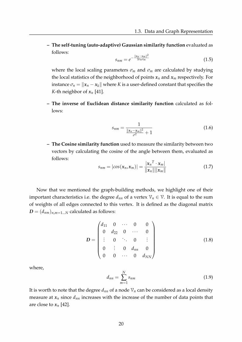
– The self-tuning (auto-adaptive) Gaussian similarity function evaluated asfollows:
snm = e−‖xn−xm‖2
2σnσm (1.5)
where the local scaling parameters σm and σm are calculated by studyingthe local statistics of the neighborhood of points xn and xm respectively. Forinstance σn = ‖xn− xk‖where K is a user-defined constant that specifies theK-th neighbor of xn [41].
– The inverse of Euclidean distance similarity function calculated as fol-lows:
snm =1
‖xn−xm‖2
σ2 + 1(1.6)
– The Cosine similarity function used to measure the similarity between twovectors by calculating the cosine of the angle between them, evaluated asfollows:
snm = |cos(xn, xm)| =|xn
T · xm|‖xn‖‖xm‖
(1.7)
Now that we mentioned the graph-building methods, we highlight one of theirimportant characteristics i.e. the degree dnn of a vertex Vn ∈ V. It is equal to the sumof weights of all edges connected to this vertex. It is defined as the diagonal matrixD = (dnm)n,m=1...N calculated as follows:
D =
d11 0 · · · 0 00 d22 0 · · · 0... 0 . . . 0
...
0... 0 dnn 0
0 0 · · · 0 dNN
(1.8)
where,
dnn =N
∑m=1
snm (1.9)
It is worth to note that the degree dnn of a node Vn can be considered as a local densitymeasure at xn since dnn increases with the increase of the number of data points thatare close to xn [42].
20

CHAPTER 1. SCORE-BASED FEATURE SELECTION
1.3.2 Graph Laplacian Matrices
Based on the definitions of the similarity matrix S and degree matrix D of the previoussection, the unnormalized Laplacian matrix can be determined as follows:
L = D− S (1.10)
where S and D are defined in Equations (1.3) and (1.8) respectively. The Laplacianmatrix L satisfies the properties of being symmetric, positive semi-definite, and thebelow Equation (1.11).
For every vector v ∈RN:
vT Lv =12
N
∑n,m=1
snm(vn − vm)2 (1.11)
Typically, we denote the eigenvalues of the Laplacian matrix L, sorted in their increas-ing order, by λ1 ≤ λ2 ≤ ... ≤ λN and their corresponding eigenvectors v1,v2,...,vN
satisfying Lv = λv.It is important to note that the data separation information according to the graphLaplacian actually starts being available from the second eigenvector and on, this issince λ1 = 0 and its associated vector v1 = (1/
√N)1 always holds, where 1 is a vector
of size N such that 1 = (1,1, ...,1)T.
Note that, the diagonal elements of the similarity matrix S do not affect or changethe unnormalized graph Laplacian. Thus, each similarity matrix which coincides withS on all off-diagonal positions yields the same unnormalized graph Laplacian. In par-ticular, self-edges in a graph do not change the corresponding graph Laplacian. There-fore, these are generally set to zero (snn = 0).
On the other side, there are two normalized Laplacian matrices, by which, one issymmetric and the other is asymmetric (random walk) [32].
• The normalized symmetric Laplacian matrix of the graph is defined as follows:
Lsym = D−1/2LD−1/2 = I − D−1/2SD−1/2 (1.12)
where D1/2 is the diagonal matrix defined upon D1/2nn =
√dnn. Thus, D−1/2
nn =1√dnn
with the assumption that dnn , 0 and Lsym also satisfies the properties ofbeing symmetric, positive semi-definite, and the below Equation (1.13).
21
1.4. Feature Selection with Contextual Knowledge
For every vector v ∈RN:
vT Lsymv =12
N
∑n,m=1
snm(vn√dnn− vm√
dmm)2 (1.13)
Also, the smallest eigenvalue is given by λ1 = 0 and its associated eigenvectorv1 = ( 1√
∑n dnn)D1/21 where 1 is a vector of size N such that 1 = (1,1, ...,1)T.
• The normalized asymmetric Laplacian matrix, also known as random walk [32],of the graph is defined as follows:
Lrw = D−1L = I − D−1S (1.14)
where D−1 is the diagonal matrix defined upon D−1nn = 1
dnnwith the assumption
that dnn , 0 and the eigenvector v1 of Lrw is equal to v1 =1√N
1 knowing that thesmallest eigenvalue λ1 = 0.
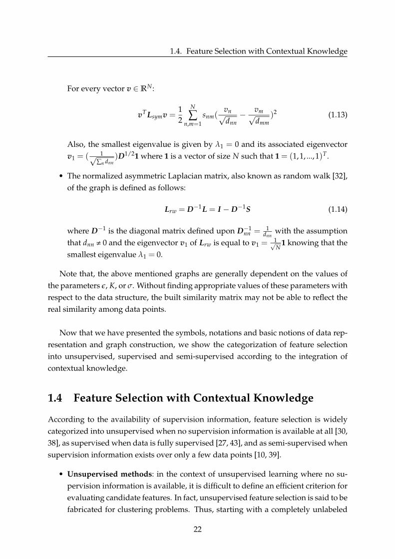
Note that, the above mentioned graphs are generally dependent on the values ofthe parameters ε, K, or σ. Without finding appropriate values of these parameters withrespect to the data structure, the built similarity matrix may not be able to reflect thereal similarity among data points.
Now that we have presented the symbols, notations and basic notions of data rep-resentation and graph construction, we show the categorization of feature selectioninto unsupervised, supervised and semi-supervised according to the integration ofcontextual knowledge.
1.4 Feature Selection with Contextual Knowledge
According to the availability of supervision information, feature selection is widelycategorized into unsupervised when no supervision information is available at all [30,38], as supervised when data is fully supervised [27, 43], and as semi-supervised whensupervision information exists over only a few data points [10, 39].
• Unsupervised methods: in the context of unsupervised learning where no su-pervision information is available, it is difficult to define an efficient criterion forevaluating candidate features. In fact, unsupervised feature selection is said to befabricated for clustering problems. Thus, starting with a completely unlabeled
22

CHAPTER 1. SCORE-BASED FEATURE SELECTION
training set, it utilizes all data points that are available in the feature selectionphase for the sake of finding robust criteria to define feature relevance. Multi-ple unsupervised methods for selecting features were proposed in the literature.These tend to use various evaluation criteria like the ability to preserve dataneighborhood graph, exploiting data similarity, maximizing feature variances,and the ability to preserve local discriminative information [24, 30, 35, 38, 44–48].
• Supervised methods: on the contrary to the unsupervised context, supervisedfeature selection methods are generally fabricated for classification and regres-sion problems [13]. As for classification, feature selection aims at finding thefeatures that can best discriminate data points of different classes. For example,a feature can be selected as relevant if it is highly correlated with the vector ofclass labels [9]. In this context, first a feature subset is selected using one of theavailable feature selection methods applied on the training data [27, 43, 49–51].Afterward, the learning algorithm is trained over the selected subset of features.Then, the built model is applied to unseen data (an unlabeled testing set de-scribed by the same set of features) for predicting class labels. Note that, the costof labeling data points by domain human experts is very high in terms of timeand effort and may not always be error-free (some data might be labeled falsely[52]).
• Semi-supervised methods: in brief, while traditional supervised feature selec-tion methods work when the data is fully labeled, unsupervised ones work with-out any supervision information. However, in many real-world applications, theamount of supervision information (e.g. the number of labeled data) might belimited providing insufficient supervision information to supervised feature se-lection methods. Similarly, unsupervised feature selection methods can be effec-tive using unlabeled data only, however, without the ability to benefit from theavailable supervision information. Hence, it is preferable to use semi-supervisedmethods that can evaluate the relevance of features taking into account both la-beled and unlabeled data [10, 53–56].
Therefore, in a training set X of N data points we may have two subsets dependingon the label availability: X l = {x1, x2, . . . , xl}l,0 with the class label corresponding toeach data point and Xu = {xl+1, xl+2, . . . , xl+u}u,0, which are unlabeled. When l = 0,all data points are unlabeled and the learning context is said to be unsupervised. Whenu = 0, all data points are labeled and the learning context is said to be supervised.However, in real world problems, where we typically have only few labeled and many
23

1.4. Feature Selection with Contextual Knowledge
unlabeled data points (l << u) the context is said to be semi-supervised. Note that,N = l + u.
1.4.1 Types of Supervision Information
Generally, class labels are the first to come to mind when mentioning supervision in-formation. These specify which class each data point should belong to. Accordingly,supervised and semi-supervised feature selection methods are usually explained interms of the available amount of class labels. However, in real-world applications,there exists a cheaper kind of supervision information i.e. pairwise constraints. On thecontrary to class labels, these constraints only specify whether a pair of data pointsshould belong to the same group (must-link constraint) or different groups (cannot-link constraint) without identifying the groups themselves.
1.4.1.1 Class Labels
As can be seen in Figure (1.3), in supervised or semi-supervised contexts, feature se-lection utilizes fully or partially labeled data respectively. In both cases, it aims atevaluating the relationship between the features and their provided class label infor-mation. Thus, considering that in the training set X each data point xn is associatedwith a class label yn, we denote by yl the vector of labels defined as follows:
yl =
y1
...yn
...yN
(1.15)
where yn ∈ {1, .., c, ...,C} and C is the number of classes of the data. Having Cclasses, we denote by Nc the number of data points in each class c.
1.4.1.2 Pairwise Constraints
Pairwise constraints are a cheaper kind of prior knowledge. They guide learning al-gorithms and allow multiple unsupervised ones to improve their performance [57]. Itis easier for a user to specify whether some pairs of data points belong to the sameclass or not, in other words, similar or dissimilar, than it is to specify class belongings.In fact, class labels can be directly transformed into must-link and cannot-link con-straints, however, constraints cannot be transformed into class labels. This is straight-
24

CHAPTER 1. SCORE-BASED FEATURE SELECTION
forward since the amount of information provided by class labels is superior. Hence,one way of building the must-link and cannot-link constraint sets is directly from theclass labels by connecting the data points that share the same label with a must-linkand connecting the data points that have different labels with a cannot-link [53, 58, 59].Another way is to find these sets by directly adding them to data points using ActiveLearning as will be suggested and discussed in chapter 4.
The sets of must-link and cannot-link constraints consisting of pairs of data pointsfrom the training set X, denoted by ML and CL respectively, are defined as follows:
• ML = {(xn, xm) | xn and xm belong to the same group}
• CL = {(xn, xm) | xn and xm belong to different groups}
Pairwise constraints are used to evaluate the relevance of each feature accordingto its constraint preserving ability. In the context of spectral theory, two graphs GML
and GCL can be constructed to represent them by using the data points of ML and CLrespectively. Accordingly, an edge is created between two nodes of the graph GML (orGCL) when their corresponding data points are must-linked (or cannot-linked). Thus,the similarity matrices holding the edge weights between every two nodes in GML andGCL are defined as follows:
sMLnm =
1 if (xn, xm) ∈ ML
0 otherwise(1.16)
sCLnm =
1 if (xn, xm) ∈ CL
0 otherwise(1.17)
In the three mentioned learning contexts: supervised, unsupervised, and semi-supervised, the process of feature selection follows a general workflow. The latter isillustrated in Figure (1.3) and will be detailed in the following section.
1.5 General Procedure of Feature Selection
By following the flow chart of the general procedure of feature selection presentedin Figure (1.3), there are typically four basic steps [12]. These are known as subsetgeneration, subset evaluation, stopping criterion and result validation [11].
25
1.5. General Procedure of Feature Selection
Original data
Unsupervised Supervised
Class labels
Data reconstruction
Subset generation by search strategy
Subset evaluation of performance
Stopping criterion
?
Feature Selection
result Result validation
Elimination of irrelevant and
redundant features
Semi-supervised
Pairwise constraints
Partially labeled
Partially constrained
False
True
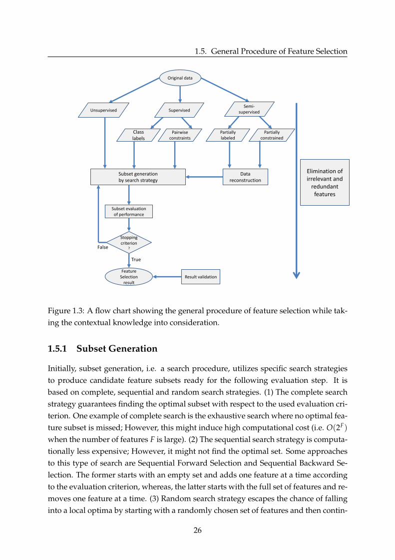
Figure 1.3: A flow chart showing the general procedure of feature selection while tak-ing the contextual knowledge into consideration.
1.5.1 Subset Generation
Initially, subset generation, i.e. a search procedure, utilizes specific search strategiesto produce candidate feature subsets ready for the following evaluation step. It isbased on complete, sequential and random search strategies. (1) The complete searchstrategy guarantees finding the optimal subset with respect to the used evaluation cri-terion. One example of complete search is the exhaustive search where no optimal fea-ture subset is missed; However, this might induce high computational cost (i.e. O(2F)
when the number of features F is large). (2) The sequential search strategy is computa-tionally less expensive; However, it might not find the optimal set. Some approachesto this type of search are Sequential Forward Selection and Sequential Backward Se-lection. The former starts with an empty set and adds one feature at a time accordingto the evaluation criterion, whereas, the latter starts with the full set of features and re-moves one feature at a time. (3) Random search strategy escapes the chance of fallinginto a local optima by starting with a randomly chosen set of features and then contin-
26

CHAPTER 1. SCORE-BASED FEATURE SELECTION
uing either with sequential search or with simply other random feature sets.
1.5.2 Evaluation Criterion of Performance
At this step, each of the candidate feature subsets is examined with respect to its pre-ceding best subset by a particular evaluation criterion. If the evaluation’s output con-firms that the new subset is better than the one before, the former replaces the latter.As can be seen in Figure (1.4), feature selection can be categorized into three mainmethods according to the evaluation criterion of performance. These methods are:filter methods [38, 40], wrapper methods [60, 61] and embedded methods [62, 63]. Fil-ter methods are also known as independent methods since they are independent ofany learning algorithm, while, wrapper and embedded methods are known as depen-dent ones since they utilize the performance of a learning algorithm in the process ofselecting features [11, 12].
Feature Selection Based on Evaluation Method
Filter Methods Embedded Methods Wrapper Methods
Classifier
Original features
Selected features
Search algorithm
Feature evaluation
Filter
Feature subset
Original features
Selected features
Search algorithm
Feature evaluation
Wrapper
using Classifier
Performance feedback
Feature subset
Original features
Selected features
Final selected features
Filter Step
Wrapper Step
Classifier
Classifier
Search algorithm
Feature evaluation
Filter
Feature subset
Search algorithm
Feature evaluation
Wrapper
using Classifier
Performance feedback
Feature subset
Figure 1.4: The broad categorization of feature selection into filter, wrapper and em-bedded methods based on the evaluation criterion.
27
1.5. General Procedure of Feature Selection
1.5.2.1 Filter methods
Filter methods measure the goodness of generated feature subsets by relying on theintrinsic characteristics of the data training set independently from any learning algo-rithm. Hence, although filter methods are said to be computationally efficient, theirselected feature subsets might not be optimal for the used learning algorithm. This iscaused by the fact that no specific learning algorithm is guiding the process of featureselection. Generally, any filter method works in two consecutive steps. Step 1, con-sists of ranking the features in the order of their importance with respect to a specificevaluation criterion. This criterion is further divided into univariate [38, 64] and mul-tivariate schemes [27, 65]. In the former, each feature is evaluated individually andindependently from other features, whereas, in the latter, multiple features are evalu-ated and ranked together in a batch mode. Step 2 consists of filtering out the featuresof lowest ranks, thus, obtaining the final selected subset.
Some of the well-known filter evaluation criteria are:
• Measures of features discriminative ability to separate classes (also known asdistance, divergence and separability measures) [37, 66, 67].
• Measures of features correlation with class labels (also known as dependencymeasures) [24, 68].
• Information based measures that typically evaluate the information gain from afeature [27, 69, 70].
• Measures of features manifold structure preserving ability [35, 38, 71].
• Measures of features ability in reconstructing the original data [45, 72].
1.5.2.2 Wrapper methods
Wrapper methods require a predefined learning algorithm, by which, the process offeature selection is wrapped around. In fact, wrapper methods utilize the performanceof this predetermined learning algorithm to evaluate the importance of features. Gen-erally, superior performance and optimal feature subsets are guaranteed with suchmethods as they focus on choosing the features that best improve the predictive accu-racy of a specific learning algorithm, however, they also tend to be computationallymore expensive. To sum up, after deciding on the learning algorithm, a typical wrap-per method performs two steps. In step 1, it searches for a subset of features. In step
28

CHAPTER 1. SCORE-BASED FEATURE SELECTION
2, it evaluates the selected subset using the chosen learning algorithm. Steps 1 and 2are repeated until the stopping criterion (section 1.5.3) is reached [60, 73].
1.5.2.3 Embedded methods
For the sake of a more efficient feature selection, embedded methods are a trade-offbetween both filter and wrapper methods. By which, they generally try to find a fea-ture subset that maintains good performance of learning algorithms while keepingcomputational cost in an acceptable range. For instance, one may consider a filter ap-proach to remove low ranked features in terms of relevance or importance, and thenapply a wrapper method on the selected subset to find the best features from within[46, 65, 74].
Out of these three widely used feature selection approaches, we are interested infilter methods as they are considered simple, fast and efficient. Moreover, they can beapplied as an independent preprocessing step before any mining algorithm.
1.5.3 Stopping Criterion
The stopping criterion decides when the process of feature selection should be termi-nated. In fact, both the generation and evaluation steps are repeated until the stoppingcriterion is met. The latter can be determined by:
• The subset generation step, where the process can be stopped either when a spe-cific number of selected features or a maximum number of iterations is reached.
• The evaluation step, where feature selection termination can be determined bythe stability of performance, which means, adding or removing features wouldnot impose any performance change or improvement. It can also be determinedby obtaining a sufficiently good feature subset, in other words, a subset thatobtains an evaluation measure, i.e. greater than an acceptance threshold.
1.5.4 Result Validation
Finally, the selected feature subset (i.e. considered the best compared to all other gen-erated subsets) has to be validated. Accordingly, result validation can be done bysimply evaluating the selected subset using domain prior knowledge. For example,by monitoring the change in the classification performance of a classifier with respectto the change in the feature subsets. For instance, if the classification accuracy rate
29

1.5. General Procedure of Feature Selection
records a greater value using the selected subset than using the original feature space,the result is considered good.
Note that, data classification is the problem of automatically determining to which cat-egory, out of a given set of categories, a new data point belongs. This is done througha process of two consecutive phases. (1) Building a model using a data training set,by which, the category or class membership of each data point is a priori known. (2)Testing the built model using a data testing set, by which, the category or class mem-bership of each data point is unknown. An example of a classification problem isautomatically deciding whether a person is healthy or diseased based on his observedmedical characteristics (features like: age, gender, family history, blood pressure, etc).In fact, some well-known classification algorithms usually used for this type of vali-dation are as follows:
• K-Nearest Neighbor (K-NN) [75]: a simple non-parametric method that can achievehigh performance when the number of data points is sufficiently big. It uti-lizes only the spatial distributions of empirical samples without any previousassumptions about their class distributions, where a new data point is classifiedby the class of the majority of its K-nearest points.
• Support Vector Machines (SVM) [76]: a set of well-known general learning meth-ods that have become very popular in the last few decades. A SVM classifiermaps data points into another space such that, a gap (called sample-margin) be-tween the mapped points of different classes is maximized. Accordingly, newdata points are mapped into that same space and classified based on which sideof the gap they fall. Basically, multi-class SVM can be done by dividing a multi-class problem into a set of two-class ones (e.g. one-against-one and one-against-all methods). Besides, different kernel functions like linear, sigmoid, polynomialand radial basis function (RBF) can be used.
• Naive Bayes (NB) [77]: a probabilistic classifier based on Bayes theorem. It ap-plies classification with a naive (strong) independence assumption among fea-tures. In other words, it considers that given the class labels, features are condi-tionally independent of each other.
• Decision Tree (C4.5) [78]: a well-known classifier that applies an entropy-basedcriterion on a set of training data to build the decision tree. For instance, the datapoints can be split into smaller subsets by using a feature as the decision rule.For this purpose, the algorithm measures the information gain at each split.
30

CHAPTER 1. SCORE-BASED FEATURE SELECTION
1.5.4.1 Relevancy Performance Evaluation Metrics
There exist multiple supervised performance evaluation metrics that are related todata classification and can be obtained after applying a classifier on the selected setof features. Three widely used metrics are accuracy, precision, and recall. To clearlyexplain them, we consider having two classes, a positive class and a negative class tobuild the confusion matrix. It holds the four different combinations of predicted andactual values of these two classes as can be seen in Figure (1.5).
1. True Positives (TP): the total number of correct predictions that are positive,which means, were predicted to be positive knowing that they actually belongto the positive class.
2. False Positives (FP): the total number of incorrect predictions that are positive,which means, were predicted to be positive knowing that they actually belongto the negative class.
3. True Negative (TN): the total number of correct predictions that are negative,which means, were predicted to be negative knowing that they actually belongto the negative class.
4. False Negative (FN): the total number of incorrect predictions that are negative,which means, were predicted to be negative knowing that they really belong tothe positive class.
TP
(True Positive)
FP
(False Positive)
FN
(False Negative)
TN
(True Negative)
Predicted Positive
Predicted Negative
Actual
Positive
Actual
Negative
Figure 1.5: The confusion matrix, a table of the four different combinations of pre-dicted (rows) and actual (columns) class values. It is very useful for understandingand measuring the accuracy, precision, and recall.
• Classification Accuracy: a well-known evaluation metric defined as a percentageof correct predictions. Thus, it evaluates how many data points were correctly
31

1.6. Ranking Feature Selection Methods based on Scores
classified using the selected features by classifiers like the ones presented in 1.5.4.
Accuracy =TP + TN
TP + TN + FP + FN(1.18)
• Precision and Recall: another two well-known evaluation metrics usually usedtogether and can be applied in the context of classification. Precision answersthe question of what proportion of positive predictions was actually correct.Whereas, recall, also called sensitivity, answers the question of what proportionof actual positives was identified correctly.
Precision =TP
TP + FP(1.19)
Recall =TP
TP + FN(1.20)
1.6 Ranking Feature Selection Methods based on Scores
In feature selection, filter methods can be broadly categorized as relying on subsetevaluation or individual evaluation. Subset evaluation depends on some search strat-egy to evaluate the relevance of candidate feature subsets. On the other side, individ-ual evaluation, also known as feature ranking/weighting, aims at sorting the featuresin either the increasing or decreasing order of a particular weight or score that is as-signed to each of them [2]. For that, unlike subset evaluation, it assesses the degree ofrelevance of each feature individually.
As our work is focused on feature ranking methods, in this section, we briefly re-view eight of the well-known ranking methods that are based on scores and will beused throughout the upcoming chapters. Later on, also a detailed and concise reviewof a filter-type feature ranking family that is based on feature weights is presented inchapter 2.
The eight well-known score-based ranking methods that are briefly reviewed inthis section are divided into unsupervised, supervised and semi-supervised as pre-sented in Figure (1.6).
32

CHAPTER 1. SCORE-BASED FEATURE SELECTION
Filter Methods
Score-based algorithms
Unsupervised Supervised Semi-supervised
Laplacian score
Variance Score
Fisher score
Class labels Pairwise
constraints Partially labeled
Partially constrained
Constraint score-1 (CS1)
Constraint score-2 (CS2)
Constraint score-4 (CS4)
Constrained Laplacian
Score (CLS)
Constraint score-3 (CS3)
Figure 1.6: Score-based feature selection methods categorized according to the differ-ent learning contexts.
1.6.1 Unsupervised Scores
• Variance Score [64]: generally known as the simplest unsupervised feature eval-uation method. It uses the variance along a specific feature to reflect its repre-sentative power. Hence, the features with the maximum variance are selectedassuming that a feature with higher variance contains more information and ismore relevant. This means that the features are ranked in the decreasing orderof their assigned Variance scores Vi.Variance score depends on the following equation to evaluate features:
Vi =1N
N
∑n=1
(Ain − µAi)2 (1.21)
where N is the number of data points, Ain is the value of feature Ai on a datapoint xn and µAi =
1N ∑N
n=1 Ain.Variance score can be also interpreted as a global graph preserving method asfollows [31]:
Vi =1N
ATi
(I − 1
N11T)
Ai (1.22)
33

1.6. Ranking Feature Selection Methods based on Scores
where I is the identity matrix and 1 ∈RN is a vector of all ones.
• Laplacian Score [38]: a well-known unsupervised feature selection method whichdoes not only depend on selecting the features of larger variances and higherrepresentative power but also considers their locality preserving ability. Its keyassumption is that data points within the same class should be close to each otherand far otherwise. In other words, a feature is said to be "good" when two neardata points in the original space are also near to each other on this particular fea-ture, which means, it has the ability to preserve the local geometrical structure ofthe data. Note that, the smaller Laplacian score is the better, i.e., the features areranked in the increasing order of their assigned Laplacian scores LSi.The Laplacian score is calculated according to the following equation:
LSi =∑xn,xm∈X(Ain − Aim)
2snm
∑xn∈X(Ain − µAi)2dnn
(1.23)
where dnn is defined in Equation (1.9) and D is a diagonal matrix holding dnn inits diagonal defined in Equation (1.8). S is neighborhood matrix between datapoints expressed as follows:
snm =
e−‖xn−xm‖2
σ2 if xn and xm are neighbors
0 otherwise(1.24)
where σ2 is a user-defined constant and "xn and xm are neighbors" means that ei-ther xn is in the K-nearest neighbors of xm or xm is among the K-nearest neighborsof xn.In addition, Equation (1.23) can be represented under the framework of the spec-tral graph theory as follows:
LSi =AT
i LAi
ATi DAi
(1.25)
where L is defined as in Equation (1.10) and Ai is defined as:
Ai = Ai −AT
i D11TD1
1 (1.26)
and 1 ∈RN is a vector of all ones.
34
CHAPTER 1. SCORE-BASED FEATURE SELECTION
1.6.2 Supervised Scores
1.6.2.1 Using Class Labels
• Fisher Score [64]: a well-known supervised feature selection method that seeksfeatures with best discriminant ability. It is based on maximizing the distancesbetween data points of different classes and minimizing the distances amongpoints of the same class. To rank the features in the order of their relevancy, theyare sorted in the decreasing order of their obtained fisher score Fi. Thus, as thevalue of an assigned score to a feature increases, its importance also increases.The Fisher score is calculated according to the following equation:
Fi =∑C
c=1 Nc(µcAi− µAi)
2
∑Cc=1 Nc(σc
Ai)2
(1.27)
where, Nc is the number of data points in class c, µAi denotes the mean of the i-thfeature over all data points, and µc
Aiand (σc
Ai)2 are the mean and the variance of
class c upon the i-th feature Ai respectively.Also, it is possible to compute Fisher score using the global graph-preservingmethod [31]. This can be done by writing Equation (1.27) as follows:
Fi =AT
i (Sw − Sb)Ai
ATi (I − Sw)Ai
(1.28)
where Sw = ∑Cc=1
1Nc
ececT is the summation of the weight matrices of C within-
class graphs knowing that ec is an F-dimensional class indicator vector that holdsec(n) = 1 if xn is in class c or 0 otherwise. In each of these within-class graphs,all data points are connected with an equal weight 1/Nc. Sb = 1
N eeT, on theother side, is the weight matrix of between-class graphs, by which, each edgeconnecting different classes is assigned a weight of 1/N. Note that, e is an F-dimensional between-class indicator vector.
1.6.2.2 Using Pairwise Constraints
• Constraint Scores [40]: two supervised constrained feature selection methodsthat utilize pairwise constraints (must-links and cannot-links) only to evaluatethe relevance of features. Their key idea is to select features having the highestconstraint preserving ability. This means that a "good" feature is the one thatcorrectly reflects that two data points are close to each other when they are con-nected by a must-link constraint and that they are far from one another when
35
1.6. Ranking Feature Selection Methods based on Scores
they are connected by a cannot-link constraint.The two introduced score functions are: Constraint Score-1 (CS1) and ConstraintScore-2 (CS2). Both score functions are to be minimized, which means, a lowerscore corresponds to a more relevant feature.
CS1 is calculated according to the following equation:
CS1i =∑(xn,xm)∈ML(Ain − Aim)
2
∑(xn,xm)∈CL(Ain − Aim)2 (1.29)
CS2, a variant of CS1, is calculated according to the following equation:
CS2i = ∑(xn,xm)∈ML(Ain − Aim)2 − λ ∑(xn,xm)∈CL(Ain − Aim)
2 (1.30)
Where ML and CL are the sets of must-link and cannot-link constraints definedin section 1.4.1.2 and λ is a regularization coefficient used to balance the contri-bution of the first and second terms of Equation (1.30). This is since the distancebetween points belonging to different classes is usually larger than the distancebetween points of the same class, thus, λ needs to be relatively small. The defaultvalue of λ, set by the authors, is 0.1 [40].
Note that, CS1 and CS2 can also be expressed under the framework of spectraltheory according to the following equations:
CS1i =AT
i LML Ai
ATi LCL Ai
(1.31)
CS2i = ATi LML Ai − λAT
i LCL Ai (1.32)
where, the matrices LML and LCL define the constraint Laplacian matrices cal-culated as: LML = DML − SML and LCL = DCL − SCL where DML and DCL arethe degree matrices defined by dML
nn = ∑Nm=1 sML
nm and dCLnn = ∑N
m=1 sCLnm having the
similarity matrices SML and SCL defined by Equations (1.16) and (1.17) respec-tively.
1.6.3 Semi-supervised Scores with Pairwise Constraints
• Constraint Score-3 (CS3) [79]: a semi-supervised feature selection method thatis fundamentally based on spectral graph theory and manifold learning. It aims
36

CHAPTER 1. SCORE-BASED FEATURE SELECTION
at selecting the most locality sensitive discriminant features. For that, it tries tofind both the local geometrical structure and the discriminant structure of databy utilizing unlabeled data and pairwise constraints respectively. In this method,a nearest neighbor graph3 (Gkn) is built using the set of must-link constraints MLand the data set X. Another graph4 (GCL) is built as defined in section 1.4.1.2.The edges of these two graphs are weighted using their corresponding similaritymatrices Skn and SCL respectively. This score is to be minimized by which a lowerscore means a more relevant feature.CS3 can be calculated as follows:
CS3i =∑(xn ,xm)∈X (Ain−Aim)
2sknnm
∑(xn ,xm)∈X (Ain−Aim)2sCLnm
(1.33)
where,
sknnm =
γ if xn and xm ∈ ML
1 if xn and xm are unlabeledbut xn ∈ KNN(xm) or xm ∈ KNN(xn)
0 otherwise
(1.34)
Note that, KNN(xn) denotes the set of the K-nearest neighbors to xn. γ and kwere set empirically to the values of 100 and 5 respectively [79].
As a graph-based method, the equation of CS3 can be also given by:
CS3i =AT
i Lkn Ai
ATi LCL Ai
(1.35)
where Lkn = Dkn− Skn defines the Laplacian matrix of graph Gkn, and the degreematrixDkn is defined by dkn
nn = ∑Nm=1 skn
nm.Due to the large value of γ, although CS3 is semi-supervised, it is consideredvery similar to CS2 that neglects unlabeled data points [53].
• Constraint Score-4 (CS4) [53]: a semi-supervised constrained feature selectionmethod that not only utilizes pairwise constraints to evaluate the relevance offeatures but also uses the intrinsic idea of the unsupervised Laplacian Score tobenefit from the available unlabeled data. Consequently, this score is consideredless sensitive to the user-defined constraint sets. It applies a simple multiplica-
3Also known as the within-class graph.4known as the between-class graph.
37

1.6. Ranking Feature Selection Methods based on Scores
tion of the unsupervised Laplacian Score from Equation (1.23) with the super-vised CS1 from Equation (1.30). This score is to be minimized by which a lowerscore means a more relevant feature. CS4 is calculated according to the followingequation:
CS4i =∑xn ,xm∈X (Ain−Aim)
2snm
∑xn∈X (Ain−µAi )2dnn
. ∑(xn ,xm)∈ML(Ain−Aim)2
∑(xn ,xm)∈CL(Ain−Aim)2 (1.36)
Note that, CS4 can also be expressed under the framework of spectral theory asit is also a graph-based method. The equation is given by:
CS4i =Ai
T LAi
AiT DAi
. ATi LML Ai
ATi LCL Ai
= LSi .CS1i
(1.37)
• Constrained Laplacian Score (CLS) [54]: a semi-supervised feature selection methodthat evaluates the relevance of a feature according to both of its locality and con-straints preserving abilities. It aims at selecting the most discriminative and in-formative features for data analysis and initially originates from constraining theknown Laplacian score. This score considers that a relevant feature should be theone, by which, two data points that are neighbors or connected by a must-linkconstraint, are close to each other. In addition, it should be the feature of highvariance, by which, two cannot-linked data points are well separated. This scoreis to be minimized. It is calculated according to the following equation:
CLSi =∑xn,xm∈X(Ain − Aim)
2sknnm
∑n ∑m|∃l,(xl ,xm)∈CL(Ain − αAinm)2dnn
(1.38)
where,
sknnm =
e−‖xn−xm‖2
σ2 if xn and xm are neighbors or (xn, xm) ∈ ML
0 otherwise(1.39)
and
αAinm =
Aim if (xn, xm) ∈ CL
µAi otherwise(1.40)
Hindawi [59] also derived CLS in the spectral graph-based representation as fol-lows:
CLSi =AT
i Lkn Ai
ATi LCLDkn Ai
(1.41)
38

CHAPTER 1. SCORE-BASED FEATURE SELECTION
1.7 Feature Redundancy Analysis
As detailed in section 1.6, a common practice of score-based filter-type feature selec-tion methods is to simply rank the features in the order of their assigned scores at theend of the individual evaluation process [59]. Then, a subset of the top-ranked fea-tures, e.g. a group of the first 10 features if the desired subset size is 10, is consideredas the final selected feature subset [80]. One drawback of this straightforward rank-ing approach is that the selected subset might hold features that are correlated to oneanother. This is also known as feature redundancy. In fact, redundant features mayincrease dimensionality unnecessarily [81] and degrade learning performance whenfacing a shortage of data [82]. Therefore, multiple pieces of research suggested en-hancing the representative power of the feature subset by demanding that the selectedfeatures are maximally dissimilar to each other [27, 54, 80, 83–85].
Feature-Relevance Analysis
Feature-Redundancy Analysis
Original features Selected
Features
Final Selected features
Figure 1.7: The general two-step framework of classical feature selection methods thathandle maximizing the relevancy of features with respect to a specific problem whileminimizing their redundancy with respect to each other.
Classical methods remove redundancy among features by generally depending onEuclidean distance, Pearson correlation and information measures [25]. Figure (1.7)shows the general procedure of such methods. For instance, one widely used methodis the "Minimum Redundancy-Maximum Relevance" called (mRMR) [27]. It is a su-pervised multivariate feature selection method that is said to output a feature subsethaving the most diverse features (as non-correlated to each other as possible) whilestill having a high correlation with the class label.
For that, mRMR method uses two criteria that are based on mutual information.
• A maximal relevance criterion, by which, the features of high mutual informa-tion with the vector of class labels are selected as follows:
maxRelevancy(Fs,yl) =1
card(Fs)∑
Ai∈Fs
I(Ai;yl)
39

1.7. Feature Redundancy Analysis
where Fs is the selected subset of features, card(Fs) is the number of features inFs, and yl is the vector of class labels.
• A minimum redundancy criterion, by which, the features of low mutual infor-mation with other features are selected as follows:
minRedundancy(Fs) =1
(card(Fs))2 ∑Ai,Aj∈Fs
I(Ai; Aj)
I(x;y) denotes the mutual information between elements x and y defined interms of their probabilistic density functions as follows:
I(x;y) = ∑x
∑y
P(x,y) logP(x,y)
P(x)P(y)
On the other side, there exists another non-classical framework for obtaining a subsetof representative and diverse features, i.e. feature clustering. Figure (1.8) shows thegeneral framework of applying clustering for the sake of maximizing diversity amongfeatures. Methods under this framework follow the below three-step process:
Clustering offeatures
Choosing representative
features
Selected feature subset of maximum relevance
and maximum diversity
Figure 1.8: A general framework for clustering-based feature selection methods.
• Step 1: A suitable distance measure is chosen for evaluating the similarity ordissimilarity between features.
• Step 2: An appropriate clustering method is applied for grouping similar fea-tures.
• Step 3: An appropriate evaluation criterion is applied for choosing the most rep-resentative feature out of each cluster.
In [86], Dhillon et al. suggested a global criterion for word (feature) clustering andapplied it to text classification. It is a novel information theoretic divisive algorithmthat minimizes the “within-cluster Jensen-Shannon divergence” while simultaneously
40

CHAPTER 1. SCORE-BASED FEATURE SELECTION
maximizing the “between-cluster Jensen-Shannon divergence”. Another supervisedmethod that hierarchically clusters the features (using Ward’s method), was proposedby Ienco and Meo [87]. It uses a hybrid method to evaluate the feature subset obtainedat each level of the dendrogram5. In fact, at each level, a class-distribution preservingmeasure (Goodman-Kruskal τ [88]) is used to select the most representative featuresfrom within each cluster before a classifier evaluates the goodness of the feature sub-set.In addition, many clustering-based feature selection methods using information the-ory were proposed [51, 89, 90]. For instance, one method that uses agglomerativehierarchical clustering builds its own kind of similarity space between features usingan information theoretic measure i.e. mutual information [91]. Whereas, Sotoca andPla [43] build their features dissimilarity space using conditional mutual information.On the other side, Zhao [92] combines the usage of the maximal information coeffi-cient measure with the affinity propagation clustering method to find similar features.
Note that, a feature clustering-based method might select an irrelevant feature asthese features are often clustered together. Thus, it is preferable to remove them beforefeature clustering.
1.7.1 Redundancy Performance Evaluation Metrics
• Representation Entropy (RE) [30, 44]: is an unsupervised metric used to com-pare the redundancy in obtained feature subsets. It obtains a maximum valuewhen all the eigenvalues become equally important, which means, the level ofuncertainty becomes maximum. This indicates that information is evenly dis-tributed among all the principal directions. On the contrary, it obtains a value ofzero only when all the information is present along the single principal coordi-nate direction (all eigenvalues are equal to zero except one).
The RE of a d-sized feature subset, denoted by HR, is calculated as follows:
HR = −d
∑j=1
λjlogλj
5A multi-level tree diagram called dendrogram. Cutting this dendrogram on a specific level resultsin one of the possible feature clustering solutions.
41

1.8. Conclusion
where
λj =λj
∑dj=1 λj
and λj is one eigenvalue of the d× d covariance matrix of the respective featurespace.
• Redundancy [59, 82]: another very well-known unsupervised metric that is basedon the linear correlation coefficient. It quantifies the strength of pairwise linearrelationship between two features. When there is no correlation between twofeatures, then the values of features do not tend to increase or decrease in tan-dem. It is not ensured that two uncorrelated features are independent, this issince some kind of nonlinear relationship might exist.
The redundancy measure, denoted by RED, of a feature subset Fs can be calcu-lated as follows:
RED(Fs) =1
card(Fs)(card(Fs)− 1) ∑Ai,Aj∈Fs,i>j
corr(Ai, Aj)
where card(Fs) is the number of features in Fs and corr(Ai, Aj) is linear correla-tion coefficient between features Ai and Aj calculated as follows:
corr(Ai, Aj) =∑n(Ain − µAi)(Ajn − µAj)√
∑n(Ain − µAi)2√
∑n(Ajn − µAj)2
where µAi and µAj are the means of the feature vectors Ai and Aj respectively.A large value of RED(Fs) means that many of the selected features have strongcorrelation and accordingly it is expected to have redundancy in Fs.
1.8 Conclusion
In this chapter, we introduced the general procedure of feature selection as a dimen-sionality reduction tool. For that, we first had to present the data notations and knowl-edge representation together with graph data construction and representation.Afterward, we started by defining the original feature space that can hold relevant,irrelevant, and redundant features, by which, the latter two feature-types are wellknown to degrade the performance of learning algorithms. As a solution, we high-lighted the importance of dimensionality reduction while broadly categorizing it into
42

CHAPTER 1. SCORE-BASED FEATURE SELECTION
feature extraction and feature selection methods. As our focus is on feature selectionmethods, we only provided a brief overview of some of the widely used feature extrac-tion methods. On the other side, we illustrated the problem of feature selection in theunsupervised, supervised, and semi-supervised learning contexts by detailing a set ofrepresentative state of the art score-based ranking methods. In addition, we reviewedthe categorization of feature selection into filter, wrapper, and embedded methods ac-cording to the evaluation criterion of performance. Finally, we explain the main ideaof feature redundancy analysis and state some of its performance evaluation metrics.
As our contribution field is focused on filter-type methods, the next chapter is a de-tailed review of a powerful family of these methods called Relief-Based Algorithms,by which, we will modify in the later chapters to effectively solve the problem of con-strained semi-supervised feature selection.
43


Chapter 2Relief-Based Feature Selection
Contents2.1 Introduction . . . . . . . . . . . . . . . . . . . . . . . . . . . . . . . . . . 45
2.2 The Original Relief Algorithm . . . . . . . . . . . . . . . . . . . . . . . 46
2.2.1 Strengths and Limitations . . . . . . . . . . . . . . . . . . . . . . 49
2.3 Basic Variants and Extensions of Relief with Probabilistic Interpre-tation . . . . . . . . . . . . . . . . . . . . . . . . . . . . . . . . . . . . . . 51
2.3.1 Robustness . . . . . . . . . . . . . . . . . . . . . . . . . . . . . . 52
2.3.2 Incomplete Data . . . . . . . . . . . . . . . . . . . . . . . . . . . 53
2.3.3 Multi-Class Problems . . . . . . . . . . . . . . . . . . . . . . . . 54
2.4 Concept of Change Interpretation . . . . . . . . . . . . . . . . . . . . . 56
2.5 Margin Notion in Relief-Based Feature Selection . . . . . . . . . . . . 58
2.5.1 Margin General Definition and Types . . . . . . . . . . . . . . . 58
2.5.2 Mathematical Interpretation . . . . . . . . . . . . . . . . . . . . . 60
2.5.3 Instance Weighting in RBAs . . . . . . . . . . . . . . . . . . . . . 71
2.6 Statistical Interpretation . . . . . . . . . . . . . . . . . . . . . . . . . . . 73
2.6.1 STatistical Inference for Relief (STIR) . . . . . . . . . . . . . . . 74
2.7 Conclusion . . . . . . . . . . . . . . . . . . . . . . . . . . . . . . . . . . 75
2.1 Introduction
As elaborated in the previous chapter, the data used in many machine learning andpattern recognition applications is provided with a very large number of features.
45
2.2. The Original Relief Algorithm
Some of which can be irrelevant or redundant. This can lead to over-fitting the learn-ing algorithm, penalizing its performance, and increasing its computational cost. Tomitigate such problems, feature selection can be used as a data preprocessing step.
Remembering that according to the evaluation criterion of performance, there arethree main categories for feature selection: filter methods [12, 93], wrapper methods,and embedded methods. We are particularly interested in filter Relief-based methodsthat are simply based on ranking features according to a specific assigned weight. Thisis motivated by the fact that compared to wrapper methods, Relief avoids any exhaus-tive combinatorial search and learning algorithm-dependency, hence, it is more effi-cient. Moreover, it usually performs better than other filter feature selection methodsdue to the performance feedback of a non-linear classifier when searching for relevantfeatures [94]. At the same time, Relief-based methods are context-aware, taking intoaccount local information to detect dependencies and interactions between featuresthemselves while still providing a global view to select useful features [37].
Therefore, in this chapter, we first explain the original Relief algorithm in section2.2. Then, by highlighting its strengths and limitations, we show its main variants andextensions in section 2.3. Also, Relief is presented by its four possible interpretations,that are, probabilistic, comprehensible, mathematical and statistical in sections 2.3, 2.4,2.5 and 2.6 respectively. In addition, Relief is introduced as a margin-based algorithmfollowed by a set of consequent extensions in section 2.5. Finally, we conclude thechapter in section 2.7.
2.2 The Original Relief Algorithm
Relief was suggested in 1992 by Kira and Rendell [49, 66] as a solution for the problemof selecting a small subset of features that ideally is necessary and sufficient to de-scribe some specific target concept1 in a supervised context. It is said to be an efficient,simple and practical feature selection solution for two-class real-world classificationproblems that involve feature interaction without the need of explicitly trying combi-nations of features.In addition, Relief that was inspired by instance based-learning [95, 96], calculates aproxy statistic for each feature in order to estimate its "quality" or "relevance" to thetarget concept. Hence, it is a statistical method that avoids heuristic search. In fact,
1 A target concept is the endpoint of a specific problem, e.g., it is the class label in classificationproblems and the predicted value in regression.
46

CHAPTER 2. RELIEF-BASED FEATURE SELECTION
in order to calculate these feature statistics, Relief introduced two very important no-tions, that are, the nearhit and the nearmiss of a data point. To explain them clearly, weconsider the training set X = [x1, ..., xn, ..., xN] ∈ RN×F, where xn = {xn1, ..., xni, ..., xnF}is the n-th data point in X of N data points characterized by F features with yn beingits corresponding class label.
Definition 2.1. The nearhit of a data point xn, denoted by H(xn), is defined as itsnearest point from the same class and the nearmiss of a data point xn, denoted byM(xn), is defined as its nearest point from a different class. Figure (2.1a) illustratesthese two notions.
Definition 2.2. The feature-statistics, referred to as the features "weights" or "scores"[2], are denoted by a weight vector w = (w1, ...,wi, ...,wF)
T spanning over the F fea-tures, where wi is the relevancy weight corresponding to the i-th feature.
The pseudo-code of Relief is presented below in Algorithm 2.1.
Algorithm 2.1 Relief
Input:
• Labeled Training set X of N data points and F features
• Number of iterations T
Output: Relevance vector
1. Initialize the weight vector to zero w = (0,0, ...,0)
2. For t = 1, ..., T
(a) Pick randomly a data point xn from X
(b) Find H(xn) and M(xn)
(c) For i = 1, ..., F, calculatewnew
i = woldi + ∆(Ai, xn, M(xn))2 − ∆(Ai, xn, H(xn))2
End For
End For
3. Relevance = w/T
4. The chosen feature set is {i|Relevancei > τ} where τ is a fixed threshold.
47

2.2. The Original Relief Algorithm
As summarized in Algorithm 2.1, Relief iterates over multiple random data points.At each iteration t of T, it selects a data point xn randomly and without replacement,where T is a user-defined parameter. Then, for the chosen xn, Relief finds the nearhitH(xn) and nearmiss M(xn) using squared Euclidean distance. It then updates thevalue of each feature weight wi by the value of the difference between the distancefrom xn to H(xn) and from xn to M(xn) over this specific feature. For instance, a rele-vant feature is expected to induce a different value between xn and M(xn), thus, whenthis is true, its corresponding relevancy weight wi is increased by the value of the dif-ference it induced. Conversely, it is expected from a relevant feature to induce a verysimilar value (no difference) between xn and its nearhit H(xn), therefore, any recordeddifference, is subtracted from the corresponding relevancy weight wi. By meaning,Relief evaluates the relevancy of each feature by calculating its ability to discriminatebetween near points of two different classes. Hence, a feature that contributes more tothis data discrimination is considered more relevant.
The ∆ function used in step (c), i.e. the weight-updating step of Algorithm 2.1,given by ∆(Ai, p1, p2), calculates the distance between any two data points p1 and p2
on a specific feature Ai.
Definition 2.3. For quantitative features, ∆ can be calculated as:
∆(Ai, p1, p2) =|value(Ai, p1)− value(Ai, p2)|
max(Ai)−min(Ai)∈ [0,1] (2.1)
Similarly, for qualitative features, ∆ can be calculated as:
∆(Ai, p1, p2) =
{0, if value(Ai, p1) = value(Ai, p2)
1, otherwise(2.2)
Where value(Ai, p) is the value of the data point p over the i-th feature. The maxi-mum and minimum values of Ai denoted max(Ai) and min(Ai) are evaluated overthe whole set of data points. This normalization ensures that all ∆ values are scaledinto the interval [0,1] for both qualitative and quantitative features. Note that, thesame ∆ function is also used to find the nearest neighbors of a considered data point.In fact, the distance between any two data points is simply the sum of their ∆ functionsover all features.
Figure (2.1) illustrates an example of the weight-updating step with continuousfeatures. In this example, we consider a set of 10 data points divided equally on two
48
CHAPTER 2. RELIEF-BASED FEATURE SELECTION
classes (A and B) and defined by two features (Feature 1 and Feature 2) each. The ta-ble presented in Figure (2.1b) shows these data points with their feature values, classassignment, and the maximum and minimum values of each feature used for max-min normalization. Figure (2.1a) also shows the 2D plot of these data points withx5 as the considered data point, x4 as its nearhit and x7 its nearmiss. Accordingly,Figure (2.1c) shows how the weights w1 and w2, corresponding to Feature 1 and Fea-ture 2 respectively, are updated upon considering the data point x5, its nearhit and itsnearmiss; when the value of a feature is different between x5 and its nearhit, this fea-ture loses and its corresponding weight is penalized by the value of the difference
(e.g.
w1− = (3−2)2
(max(feature1)−min(feature1))2
). On the other side, when the value of a feature is
different between x5 and its nearmiss, this feature wins and its corresponding weightis increased by the value of the difference
(e.g. w1+ = (3−7)2
(max(feature1)−min(feature1))2
).
Finally, after finishing the T iterations, the output (named Relevance in step (3) ofthe original Relief algorithm) is a weight vector w divided by T, obtaining an averageof the accumulated weight wi corresponding to each feature Ai. This guarantees thatall final weights are normalized within the interval [−1,1]. Then, each feature havinga Relevancei greater than a given threshold τ is selected. According to the theoreticdemonstration by kira and Rendell [49], the value of τ can be statistically evaluatedbased on Chebyshev’s inequality, such that, the probability of choosing an irrelevantfeature is as small as possible. However, instead of specifying the threshold value τ,it is often more practical to a priori specify the desired size of feature subset (a num-ber) based on the functional, computational, or run time limitations of the learningalgorithms to be applied after that. This can be done by ranking the features in thedescending order of their weights and then choosing the first 10 features if 10 was thedesired feature subset size.
Note that, although the original Relief [66] used Euclidean distance rather than Man-hattan distance, later experiments by Kononenko et al. [97] showed no significantdifferences between both distances in the context of Relief, thus, the simplified de-scription using Manhattan distance became a standard [2].
2.2.1 Strengths and Limitations
Notably, since Relief avoids heuristic search and does not look for an optimal mini-mum feature subset size, it is said to be efficient [66]. For instance, compared to thetime complexity of an algorithm that does an exhaustive search for detecting interac-
49

2.2. The Original Relief Algorithm
M (x5)H (x5)
(a) 2D Data Plot
Data point Feature 1 Feature 2 Class
X 1 2 3 A
X 2 1 4 A
X 3 3 4 A
X 4 2 5 A
X 5 3 6 A
X 6 8 6 B
X 7 7 5 B
X 8 9 5 B
X 9 7 4 B
X 10 9 4 B
Feature max 9 6
Feature min 1 3
Normalization (max-min)
8 3
Considered Data point
Nearhit
Nearmiss
(b) A Data table showing the feature values of theconsidered data point, its Nearhit and its Nearmiss
3 6 A
2 5 A
X5
H(x5)
M(x5)
Features Class
w1 -= 1/64
w1 +=16/64
X5
w2 +=1/9
3 6 A
7 5 B
w2 -= 1/9
(c) Weight Updates
Figure 2.1: An illustration of one weight-updating step by Relief over continuous fea-tures. (a) Shows the 2D plot of the data points with x5 as the considered data point,x4 as its nearhit and x7 its nearmiss. (b) Shows the data points table with the maxi-mum and minimum value of each feature used for max-min normalization. (c) Showshow the weights w1 and w2 corresponding to Feature 1 and Feature 2 respectively areupdated.
50
CHAPTER 2. RELIEF-BASED FEATURE SELECTION
tions between all feature pairs i.e. O(2F), Relief has a time complexity of O(TNF),or O(NF) whenever T < N. Thus, it requires linear time in terms of the number offeatures and training data points. In addition, Relief is non-parametric, which means,it ranks the features without making any assumptions regarding the population dis-tribution or sample size [2]. Moreover, Relief can be seen as an any-time ranking al-gorithm. This means that it can be stopped at any iteration and obtain a relevancy-ranking of features, yet, with more time or data its results can be improved. Reliefhas been also categorized as non-myopic, which means it can evaluate the relevanceof features in the context of other features (detects feature interactions) [98].However, the original Relief is basically limited to two-class classification problems.Although, Kira and Rendell [66] suggested that, as future work, the algorithm can beeasily extended to solve multi-class classification problems by splitting them into a se-ries of two-class problems, this solution was considered unsatisfactory and inefficient[99]. Relief also has no mechanism to work with missing data or feature redundancy.In fact, the original Relief analysis suggests that its performance might be penalizedby insufficient training iterations (i.e. not a large enough T). Most importantly, in 1994,Kononenko identified that Relief was susceptible to noise interfering with the selectionof nearest neighbors [4].
2.3 Basic Variants and Extensions of Relief with Proba-
bilistic Interpretation
Now that we detailed the aspects and notions of the basic original Relief algorithm,it is important to note that it gained a big deal of interest between filter-type featureselection methods leading to a series of extensions, interpretations, and modifications.In this section, we go through a concise review of the Relief-Based Algorithms, knownrecently as RBAs [2].
Initially, in the context of instance-based learning, kononenko [4] derived a proba-bilistic interpretation of the feature weights obtained by Relief.
Definition 2.4. The probabilistic interpretation considers that a good feature Ai
should:
• induce a high probability of having a different value over a data point xn and itsown nearmiss M(xn).
• induce a low probability of having a different value over a data point xn and its
51
2.3. Basic Variants and Extensions of Relief with Probabilistic Interpretation
own nearhit H(xn).
Thus, the weight wi of the feature Ai is obtained as an approximation of the differencebetween the above probabilities:
wi = P(
value(Ai, xn) , value(Ai, M(xn))
)−P(
value(Ai, xn) , value(Ai, H(xn))
) (2.3)
However, from this probabilistic point of view, it is considered that a larger numberof iterations T, i.e the number of data points used for approximating probabilities,provides a more reliable approximation. At the same time, T should not exceed thenumber of data points available in X, i.e T ≤ N.
2.3.1 Robustness
By following the drawbacks of Relief, Kononenko stated that the selection of near-est neighbors with respect to important features is one of the most important steps inRelief [4]. However, when selecting them in a context of irrelevant (redundant andnoisy) features, the process can become unreliable and negatively affect the probabil-ity estimations. Therefore, kononenko proposed the first modification of Relief, calledReliefA, as a solution. It is an extended more robust version of Relief that aims at in-creasing the reliability of probability approximations. For that, ReliefA searches forK-nearhits and K-nearmisses instead of only one nearhit and one nearmiss. In fact,ReliefA can be seen as a functionality-based extension, i.e, averaging the contributionsof K-nearhits/misses.
Definition 2.5. The K-nearhits of xn from the same class are denoted by KH(xn) :{H1(xn), H2(xn), ..., HK(xn)} and the K-nearmisses of xn from the opposite class ina two-class problem are denoted by KM(xn) : {M1(xn), M2(xn), ..., MK(xn)}. WhereK is a user defined parameter representing the number of closest points to xn to beconsidered.
However, the number of considered nearest neighbors K should be kept relativelysmall. This is due to the fact that as K increases from 1 approaching N, the conditionof using the "near" data points for feature weight estimation is eliminated. This wasderived by Robnik-Sikonja and Kononenko [37] who showed that without the "near"requirement, Relief weights might lose their ability to consider local information andhence the ability to detect feature interaction. In fact, the power of RBAs lies in their
52

CHAPTER 2. RELIEF-BASED FEATURE SELECTION
ability to efficiently exploit information locally while still being able to provide a globalview with context awareness.
It was noted that using ReliefA instead of Relief improves the estimates of featuresfor both free of noise and noisy datasets, however, a more significant improvement isobtained when the data is noisy [4].
2.3.2 Incomplete Data
Following the usage of K-nearest neighbors, five extensions were proposed to ReliefAto deal with missing values and multi-class problems, known as ReliefB through Reli-efF [4]. Three of these extensions that are ReliefB, ReliefC, and ReliefD, were proposedin order to deal with incomplete data or missing values.In fact, ReliefB handles missing values by modifying the output of the corresponding∆ function as follows:
• if at least one of the two data points has an unknown value on a specific featureAi:
∆(Ai, p1, p2) = 1− 1#o f valuesAi
where #o f valuesAi is the number of possible values for feature Ai.
On the other hand, ReliefC differs from ReliefB by disregarding the contributions ofthe differences that are calculated from data points of at least one unknown value on aspecific feature through suitable normalization. This is done with the assumption thatwhen enough training data is provided, the resulting feature weights should convergeto their correct estimate values.
However, experiments showed that ReliefD performed the best in the context of in-complete and noisy data. For that, when ReliefD encounters an unknown value of adata point on a specific feature, it replaces the output of the corresponding ∆ functionby the class-conditional probability that these two data points have different valuesover this specific feature as follows:
• if one data point of the two has an unknown value (e.g. value of p1 over Ai isunknown):
∆(Ai, p1, p2) = 1− P(value(Ai, p2)|class(p1))
53

2.3. Basic Variants and Extensions of Relief with Probabilistic Interpretation
• if both of the data points p1 and p2 have unknown values over Ai:
∆(Ai, p1, p2) = 1−#o f valuesAi
∑valueAi
P(valueAi |class(p1))× P(valueAi |class(p2))
Where #o f valuesAi is the number of possible values for feature Ai and the valuesof conditional probabilities are approximated using the relative frequencies over thetraining data.
On the contrary, Relieved-F suggested by kohavi et al. [100] handles missing databy simply setting the difference between two unknown values to 0 and the differencebetween an unknown and any other known value to one.
2.3.3 Multi-Class Problems
Kira and Rendell [49, 66] proposed that the original Relief algorithm can be appliedin the context of three or more classes through splitting the domain or problem into aseries of two-class ones. However, this was proved to be inefficient and unsatisfactory[97]. Therefore, as more practical solutions, the two other extensions, namely ReliefEand ReliefF, were proposed following ReliefD to efficiently deal with the problem ofhaving more than two classes [4]. As for ReliefE, the straightforward generalization ofRelief, it simply modifies the definition of nearmiss to be the one nearest point fromany "other" class with respect to a data point xn.
On the other side, ReliefF that includes both of the suggested modifications appliedin ReliefA and ReliefD, is the most common and well-known variant of the originalRelief algorithm nowadays. For instance, in order to deal with multi-class problems,ReliefF finds a nearmiss from each different class instead of finding only one nearmissfrom the opposite class in the case of two-class problems or from any different classas in ReliefE in case of multi-class problems. Then, the contributions of each nearmissfrom each "other" class are averaged based on the prior probability of each class andused to update weight estimates. By meaning, the algorithm evaluates the ability offeatures to separate all pairs of classes regardless of their number and regardless ofwhich two classes are the closest to each other. Moreover, as the capabilities of ReliefFinclude those of ReliefA, it can also choose K-nearmisses from each ‘different’ classand K-nearhits from the same class of a considered data point.
54

CHAPTER 2. RELIEF-BASED FEATURE SELECTION
Definition 2.6. The K-nearhits of xn from the same class are defined as in the pre-vious definition Definition 2.5 without being changed. However, the K-nearmissesof xn from each "other" class are now denoted by KM(xn, c) : {M1(xn, c), M2(xn, c), ...MK(xn, c)}. Where K is a user defined parameter representing the number of closestpoints to xn to be considered and c denotes the class to which each nearmiss belongs.
Finally, kononenko [4] concluded that as the number of iterations or considereddata points, i.e. T, approaches the total number of data points N, the quality of theweight estimates becomes more reliable. Hence, it became the default to set T = N,where each data point is considered once without replacement. In this regard, theRelieved-F [100], mentioned before, can be seen as a very straightforward extension toReliefF. It is a deterministic algorithm that uses all data points and all possible nearhitsand possible nearmisses of each point. For instance, if there is a tie between two pointson being equally "near" to a considered data point, their contributions are averaged in-stead of choosing one of them randomly. Kohavi et al. [100] claimed that although thisway requires only as much time as the standard Relief algorithm with T = N, it wouldprovide the result expected when it is allowed to run for an infinite amount of time.
Definition 2.7. The weight updating step in ReliefF can be given by:
wnewi = wold
i −1
(T·K) ∑Kj=1 ∆(Ai, x, H j)+
1(T·K) ∑c,class(x)
[ P(c)1−P(class(x)) ∑K
j=1 ∆(
Ai, x, M j(c))] (2.4)
Where P(c) represents the prior probability of class c (estimated from the train-ing set) and 1− P(class(x)) represents the sum of probabilities for the misses’ classes.Note that, the normalization using these prior class probabilities is a necessity. Thisis due to the fact that using K-nearmisses from each "other" class would tend to un-reliably reflect an exaggerated influence of classes with a small number of elements.Accordingly, the pseudo-code of ReliefF is presented below in Algorithm 2.2.
Note that, later in 1996, Kononenko et al. [99] suggested an adaptation of ReliefFto regression problems called RReliefF. In such cases where the target concept (i.e adiscrete variable in classification problems) is a continuous variable (real-valued func-tion), the notions of nearhit and nearmiss cannot be explicitly used. This is due to theimpossibility of realizing the exact knowledge of whether two data points belong tothe same class or not. Thus, the probability that the predicted value of two data pointsis different was introduced instead [101].
55

2.4. Concept of Change Interpretation
Algorithm 2.2 ReliefF
Input:
• Labeled Training set X of N data points and F features• Number of iterations T
Output: Weight vector w
1. Initialize the weight vector to zero w = (0,0, ...,0)
2. For t = 1, ..., T
(a) Pick randomly a data point x from X
(b) Find K-nearhits KH(x)
(c) For each class c , class(x)find K-nearmisses KM(x)End For
(d) For i = 1, ..., F, calculatewnew
i = woldi −
1(T·K) ∑K
j=1 ∆(Ai, x, H j) +
1(T·K) ∑c,class(x)
[ P(c)1−P(class(x)) ∑K
j=1 ∆(
Ai, x, M j(c))]
End For
End For
3. The chosen feature set is {i|wi > τ} where τ is a fixed threshold
2.4 Concept of Change Interpretation
So far, the probabilistic interpretation of Relief weights was well suited to hold andexplain a set of statistical and class-discriminative properties and extensions of RBAs.However, it fails when trying to find a human-comprehensible explanation of Equa-tion (2.3). For instance, subtraction of probabilities and the negated feature similarity(different values on a feature) are difficult to understand by human experts in real-world applications. Therefore, another interpretation (based on a theoretical analysis)of the Relief’s weights or estimates was introduced by Robnik-Sikonja and Kononenko[5]. It is said to be more understandable and comprehensible than the probabilistic one.
56

CHAPTER 2. RELIEF-BASED FEATURE SELECTION
In fact, Robnik-Sikonja and Kononenko suggested that the feature weights, as-signed by Relief, can be interpreted as their ability to explain a change in the valueof the endpoint (class or predicted value). However, this interpretation is proposedin the context of a problem space that is densely covered with data points to analyzethe behavior of Relief. By meaning, it assumes that when the number of data pointsapproaches infinity, Relief’s weights (quality estimates of each feature) converge andcan be interpreted as the ratio between the number of explained changes in the classlabels2 and the number of considered data points. If it is possible to explain a certainchange in the endpoint value in multiple different ways, all of these ways share creditfor it in the feature weight. Also, if two or more features are involved in one of theexplanation ways, all of these features gain the same credit to their relevancy weight.
An example which illustrates the "concept of change interpretation" was detailedin [37] and [5]. We use the same example to better explain the idea. Thus, Table 2.1shows a boolean domain where the predicted value (class) of a data point is deter-mined by the following expression: Class=(A1 · A2) + (A1 · A3).
Table 2.1: A table showing the data points and the responsibility of each feature inchanging the outcome of the boolean problem defined by Class = (A1 · A2) + (A1 ·A3). Example proposed by Robnik-Sikonja and Kononenko [5, 37].
Data pointFeatures
Class Features holding Responsibilty of Class ChangeScore
A1 A2 A3 A1 A2 A3
x1 1 1 1 1 A1 1/8 0 0x2 1 1 0 1 A1 or A2 0.5/8 0.5/8 0x3 1 0 1 1 A1 or A3 0.5/8 0 0.5/8x4 1 0 0 0 A2 or A3 0 0.5/8 0.5/8x5 0 1 1 0 A1 1/8 0 0x6 0 1 0 0 A1 1/8 0 0x7 0 0 1 0 A1 1/8 0 0x8 0 0 0 0 A1 and A2 or A1 and A3 1/8 0.5/8 0.5/8
Total Score 0.75 0.1875 0.1875
By analyzing the first row of Table 2.1, we can say that A1 takes the responsibilityof changing the value of the class label. This is clear since changing its value alonefrom 1 to 0 affects the value of the class similarly. Whereas, changing the value ofA2 or A3 alone leaves the class value unaltered. In addition, by analyzing the secondrow, it can be noticed that changing the values of either A1 or A2 can be responsiblefor altering the class label. Thus, in this case, changing A1 and changing A2 represent
2An explained change of concept is a change in the class label that can be justified by a feature valuechange.
57

2.5. Margin Notion in Relief-Based Feature Selection
two possible ways of "change in concept" and they share the responsibility for that.It is also possible to similarly analyze rows three to seven to decide which feature isresponsible for the class change. However, the analysis of the eighth row shows thatchanging only one feature is not enough for a class change. Nevertheless, changingA1 and A2 or A1 and A3 changes the class label. Hence, a minimum of two changesis required to change the class and the responsibility score goes to both of the featurepairs A1 and A2 or A1 and A3. Since there are 8 data points in this example and they allhave an equal probability of occurrence, each responsibility score is divided by 8. Forinstance, when feature A1 alone was responsible for the class change (rows 1, 5, 6 and7) it gains a value of 1/8 for each. On the other side, when it shares the responsibilitywith another feature each of them gets a score of 0.5/8. Finally, as can be seen in theTotal Score row of Table 2.1, feature A1 gets a total score of 0.75 and both A2 and A3
get a score of 0.1875 each.
To validate this conceptual example, Robnik-Sikonja and Kononenko [5] addedfive random binary features next to the three relevant ones that were discussed above.Then, they empirically showed that the feature weights obtained by Relief and ReliefFfor this problem converge to 0.75 for A1 and 0.187 for A2 and A3 when the number ofdata points is large. Also, a detailed analysis, derivation, and proof of this interpre-tation is presented in [5] with a complete description of how it differs between Reliefand ReliefF.
2.5 Margin Notion in Relief-Based Feature Selection
In 2004, Gilad-Bachrach et al. [102] presented the Relief-family weight updating func-tion as a "Maximal Margin" or "Large Margin" objective function to be optimized.
2.5.1 Margin General Definition and Types
Intuitively speaking, the margin is a geometric measure that evaluates the confidenceof a classifier when making its decision. Moreover, it plays a crucial role in the machinelearning and pattern recognition domains and similarly to other tools and techniquesin such domains, the margin was initially defined in the supervised context [103–105].It was also noted that it can be used for theoretic generalization bounds and as guide-lines for algorithmic design [104]. Two approaches were declared for defining themargin of a data point with respect to a classification rule [106]:
• The sample-margin, i.e. the more common approach, measures the distance be-
58

CHAPTER 2. RELIEF-BASED FEATURE SELECTION
tween a data point and the decision boundary induced by a specific classifier. Forexample, Support Vector Machines [76] include a classification algorithm thatrepresents data examples as points in space, mapped so that the data points be-longing to different classes are separated by a clear gap (sample-margin) that isas wide as possible. Figure (2.2a) shows how the sample margin quantifies thedistance a data point can travel before it hits the decision boundary.
• The hypothesis-margin, i.e. the alternative definition, requires a distance mea-sure between data points. It defines the margin as the difference between thedistance from a data point to its nearest point of alternative class (defined by Re-lief as nearmiss) and the distance to its nearest point of the same class (definedby Relief as nearhit).Figure (2.2b) provides an illustration of the hypothesis-margin. By meaning, itis the largest distance a data point can travel within the feature space withoutaltering the dataset’s labeling structure, and thus without affecting the label pre-diction of a new arriving point. This is done, such that, drawing a circle of aradius equal to the margin (denoted ρ) around each data point and allowingeach of these points to freely change its position within its corresponding cir-cle, does not alter the assigned label to the new data point. This shows that thehypothesis-margin measures the stability to trivial changes in the data pointslocations.
Although using the sample-margin looks initially more natural, it was shown in[106] that it can be unstable when using the first nearest neighbor (1-NN) margin.This is due to being very sensitive to the smallest relocations of the data points (asmall position-change can lead to a dramatic alteration in the decision boundary of thesample-margin). Moreover, it was proved that the hypothesis-margin lower boundsthe sample-margin and has a lower computational cost for high-dimensional datasets [106, 107]. Which means, in the case of 1-NN, a large hypothesis-margin ensuresa large sample-margin in addition to being simple and easy to compute.Therefore, noticing the resemblance between the nearest neighbor notions of the weight-updating rule (proposed in the original Relief) and the hypothesis-margin definition,made it natural to utilize margin maximization in feature selection. This is appliedunder the assumption that a feature’s ability to discriminate between data points withrespect to a specific classification rule can be measured by its contribution to the max-imization of this hypothesis-margin [102].
59

2.5. Margin Notion in Relief-Based Feature Selection
𝜌
Decision boundary
Sample Margin
(a) Sample-Margin
M(𝒙𝑛)
𝜌
𝒙𝑛
H(𝒙𝑛)
(b) Hypothesis-Margin
Figure 2.2: The two types of nearest neighbor margin denoted by ρ. We show howto measure the margin (radius of dotted circles) with respect to a new data point con-sidering a set of labeled data points; (a) The sample-margin i.e. the distance betweenthe considered data point and the decision boundary. (b) The hypothesis-margin i.e.the maximum distance the data points can travel without altering the label of the newdata point.
2.5.2 Mathematical Interpretation
Inspired by the work done in [102] where the margin notion was introduced to Relieffamily and the maximization of the averaged margin was empirically observed, Sunand Li [6] proposed a mathematical interpretation of Relief from its optimization pointof view. Before we get to show Relief from its optimization perspective, we generallydefine the margin and the weighted-margin independently of any specific distancemeasure.
Definition 2.8. The hypothesis-margin of a data point xn denoted by ρ(xn) withrespect to the training data X is the difference between the distance from xn to itsnearmiss and the distance from xn to its nearhit3 given by:
ρ(xn) = ∆(xn, M(xn))− ∆(xn, H(xn)) (2.5)
where ∆(p1, p2) is defined as the generalized distance function between any two datapoints p1 and p2 calculated in the space of all features F with p ∈ R and ∆(Ai, p1, p2)
3Recalling that the nearhit and nearmiss notions are declared in Definition 2.1 and illustrated inFigure (2.1a).
60

CHAPTER 2. RELIEF-BASED FEATURE SELECTION
from Definition 2.3 as follows:
∆(p1, p2) =
( F
∑i=1|∆(Ai, p1, p2)|
p) 1
p
(2.6)
Note that, ρ(xn) is only positive when xn is correctly classified by 1-NN classifier,which means, when the distance from xn to its nearmiss is larger than the distancefrom xn to its nearhit.
Thus, the overall hypothesis-margin over the training set X can be computed as:
ρ(X) =N
∑n=1
ρ(xn) (2.7)
As the ability of a feature to discriminate between data points can be evaluated byhow much it contributes to the margin’s maximization, this contribution can be rep-resented and quantified by the same weight vector w = (w1, ...,wi, ...,wF)
T spanningover the F features defined in Definition 2.2 [102]. Thus, one natural idea is to scaleeach feature by a non-negative vector w to obtain a weighted feature space such that amargin-based function in this induced feature space is maximized [6, 102]. Note that,applying margin-based feature selection in a weighted space is motivated by the factthat the nearest neighbors in the original space are highly unlikely to be the same inthe weighted feature space [6, 108].
Definition 2.9. Considering a weight vector w = (w1, ...,wi, ...,wF)T, the weighted
hypothesis-margin of a data point xn with respect to the training set X is given by:
ρ(xn,w) = ∆w(xn, M(xn))− ∆w(xn, H(xn)) (2.8)
where ∆w(p1, p2) is defined as the generalized distance function between any two datapoints p1 and p2 calculated in the weighted space of all features in F with p ∈ R asfollows:
∆w(p1, p2) =
( F
∑i=1|wi∆(Ai, p1, p2)|
p) 1
p
(2.9)
According to Equations (2.8) and (2.9), each time the margin is calculated withrespect to a data point xn of F features, the weight vector w contributes to this cal-culation. Taking (2.8) into account, it can be generalized to calculate the weightedhypothesis-margin over all the given data points. Consequently, the final weight vec-tor of dimension F shows the impact of each feature in enlarging the margin, which is
61
2.5. Margin Notion in Relief-Based Feature Selection
considered the relevancy score of the feature in terms of original Relief notions.
Thus, the weighted hypothesis-margin over the training set X is computed as:
ρ(X,w) =N
∑n=1
ρ(xn,w) (2.10)
It is clear that Equation (2.10) is the summation of the weighted hypothesis marginsover the whole training set. So, the key idea is that as a feature contributes more inenlarging the overall weighted margin, it gets higher weights, and will consequentlyhave a higher chance of being selected.
Changing the value of p in Equations (2.6) and (2.9) defines different margin-basedfeature selection algorithms. If it is set to 1 i.e l1-norm, deriving Manhattan distance,the standardized Relief algorithm is obtained [6, 50, 94]; if p is set to 2 i.e l2-norm de-riving Euclidean distance, the resulting algorithm is Simba [102]; also, if p is set to 2but the squared Euclidean distance is used, the resulting algorithm is the original Re-lief initially defined in [66].
As a side note, in the context of face recognition, where an enhanced block-basedface descriptor is used to represent face images, Moujahid and Dornaika [109] pro-posed a modified Relief algorithm (m-RELIEF) that uses a weighted χ2 distance toselect features (i.e. in this case histograms) instead of using the classical Euclideandistance.
2.5.2.1 Optimization Approach to Relief Algorithm
Sun and Li pointed out that the reason behind widely depending on heuristic-searchapproaches for feature selection is the difficulty of defining an objective function, bywhich, well-established optimization techniques can optimize [6, 50, 94]. However,they noticed that although Relief is a feature-weighting algorithm that allows work-ing with soft feature-weights4, it did not have a clearly defined objective function tobe optimized. Therefore, they defined the standardized Relief from its optimizationpoint of view over a margin-based objective function using Manhattan distance (i.ep = 1 in Equations (2.6) and (2.9)). This new interpretation enabled viewing Relief asan online feature-weighting algorithm. The latter makes use of the performance of a
4Soft weights means that weights assigned to each feature are real-valued instead of being binaryindicators of whether a feature is selected or not. The problem of defining an optimizable objectivefunction in feature selection can be somehow mitigated by using feature-weighting strategies [8].
62
CHAPTER 2. RELIEF-BASED FEATURE SELECTION
highly non-linear nearest neighbor classifier to learn discriminant information locallywith the aim of identifying useful features. For that, it solves a simple convex problemin a closed-form5 which justifies its simplicity and effectiveness.
Accordingly, the hypothesis-margin of a data point xn denoted by ρ(xn) is definedas:
ρ(xn) = |xn −M(xn)| − |xn − H(xn)| (2.11)
Where the used distance function | . | is the l1-norm (or Manhattan distance) definedas:
|v| =F
∑i=1|vi| = |v1|+ ... + |vi|... + |vF| (2.12)
The weighted hypothesis-margin of xn with respect to X is:
ρ(xn,w) = |xn −M(xn)|w − |xn − H(xn)|w (2.13)
where,
|v|w = |w ◦ v| =F
∑i=1
wi|vi| = w1|v1|+ ... + wi|vi|+ ... + wF|vF| (2.14)
Knowing that w ≥ 0 and ◦ is the Hadamard product.
Definition 2.10. The margin-based objective function from the optimization pointof view is obtained by scaling each feature such that the averaged hypothesis-marginin the weighted feature space can be maximized as follows:
maxw
∑Nn=1 ρ(xn,w)
= maxw
∑Nn=1
(∑F
i=1 wi|xni −M(xn)i| −∑Fi=1 wi|xni − H(xn)i|
)s.t. ‖w‖2
2 = 1 and w ≥ 0
(2.15)
where the weight vector w ≥ 0 ensures that it induces a distance measure. In fact, it isintuitive that the chosen weight vector should induce a positive value when featuresare relevant. Also, ||w||22 = 1 ensures that the vector is not maximized without bounds.
Definition 2.11. Let z = (z1, ...,zi, ...,zF)T be a vector that holds the hypothesis-
5An equation is said to be a closed-form solution if it solves a given problem in terms of functionsand mathematical operations from a given generally-accepted set. For example, an infinite sum wouldgenerally not be considered a closed-form [110].
63

2.5. Margin Notion in Relief-Based Feature Selection
margin induced by each feature when considering all data points in X as follows:
zi =N
∑n=1|xni −M(xn)i| − |xni − H(xn)i| (2.16)
For clarity, we express z in the following notation:
z =N
∑n=1
|xn1 −M(xn)1|
...|xnF −M(xn)F|
− |xn1 − H(xn)1|
...|xnF − H(xn)F|
=
z1
...zF
(2.17)
Definition 2.12. Considering z, the simplified margin-based objective function to bemaximized is given by:
maxw
wTz, s.t. ‖w‖22 = 1, w ≥ 0 (2.18)
By using the Lagrangian function on (2.18), the equation can be expressed as:
L(w,λ,µ) = −wTz + λ(wTw− 1)− µTw (2.19)
where λ > 0 and µ ≥ 0 are the Lagrangian multipliers.Now by taking the derivative of L with respect to w we obtain:
∂L
∂w= −z + 2λw− µ (2.20)
And satisfying stationarity condition by solving ∂L∂w = 0 we get:
∂L
∂w= 0 =⇒ w =
12λ
(z + µ) (2.21)
To derive a closed-form solution for w, it is assumed that there exists an i : 1 ≤ i ≤ Fwhere zi > 0, when this assumption is not true, i.e, when z ≤ 0, the distance betweena data point and its nearhit is simply greater than the distance between it and itsnearmiss, which negatively affects the performance of neighborhood-based learningalgorithms. However, using this assumption it can be proved by contradiction thatλ > 0. Consider the case when λ < 0 while holding the assumption that zi > 0, thenzi + µi > 0. It is then obtained that wi < 0 which contradicts with the initial constraintw ≥ 0.
According to Sun and Li [6], the Karush Kuhn Tucker (KKT [111]) complementarity
64
CHAPTER 2. RELIEF-BASED FEATURE SELECTION
condition: µTw = 0 is used to verify the three following cases:
1. zi = 0⇒ µi = 0⇒ wi = 0.
2. zi > 0⇒ zi + µi > 0⇒ wi > 0⇒ µi = 0.
3. zi < 0⇒ µi > 0⇒ wi = 0⇒ zi = −µi.
Finally, the optimal solution can be calculated in a closed-form as follows:
w∗ = w/‖w‖2 = (z)+/‖(z)+‖2
where, z is given by Equation (2.17)and (z)+ = [max(z1,0), ...,max(zF,0)]T
(2.22)
By comparing the latter expression of w with the update rule of Relief, Sun and Li[6] concluded that Relief is an online solution to the optimization scheme in Equation(2.15) and they claimed that this is always true except for irrelevant features i.e whenw∗i = 0 for zi ≤ 0.
2.5.2.2 Iterative Search Margin-Based Algorithm (Simba)
As mentioned in section 2.5.2, the Simba algorithm, proposed by Gilad-Bachrach etal. [102], is obtained when using the l2-norm with this mathematical interpretation. Itis an iterative search algorithm that uses a stochastic gradient ascent to maximize itsmargin-based evaluation function. It is a slightly modified Relief with the major ad-vantage of re-evaluating the margin with respect to the updated weight vector at eachprevious iteration. It is also said to deal with correlated or redundant features [102].
Definition 2.13. The hypothesis-margin of xn denoted by ρ(xn) is given by half thedifference between the distance from a data point to its nearmiss and the distance toits nearhit. However, we omit the half 6 obtaining the following:
ρ(xn) = ‖xn −M(xn)‖ − ‖xn − H(xn)‖ (2.23)
Where the used distance function ‖ .‖ is the l2-norm (or Euclidean distance) definedas:
‖v‖ =
√√√√ F
∑i=1
vi2 =
√v2
1 + ... + v2i + ... + v2
F (2.24)
6In order to maintain the coherence of the hypothesis-margin definition with previous ones, we omitthe multiplication by 1
2 from the definition used in [102] i.e. ρ(xn) =12(‖xn −M(xn)‖− ‖xn − H(xn)‖
).
65

2.5. Margin Notion in Relief-Based Feature Selection
Definition 2.14. The weighted hypothesis-margin of xn using the weight vector w =
(w1, ...,wi, ...,wF)T spanning over F features with respect to X is given by:
ρ(xn,w) = ‖xn −M(xn)‖w − ‖xn − H(xn)‖w (2.25)
where,
‖v‖w = ‖w ◦ v‖ =
√√√√ F
∑i=1
wi2vi
2 =√
w21v2
1 + ... + w2i v2
i + ... + w2Fv2
F (2.26)
Note that, since for any scalar λ, the weighed margin ρ(xn,λw) = |λ|ρ(xn,w), theauthors introduced a natural normalization factor, i.e. to require max(w2
i ) = 1. Thisguarantees that ‖v‖w ≤ ‖v‖.The building blocks of Simba’s evaluation function are the weighted margins of eachdata point known to us as ρ(xn,w).Definition 2.15. Considering the training set X and the feature weights denoted bythe vector w, Simba’s evaluation function is given by:
ρ(X,w) =N
∑n=1
ρ(xn,w) (2.27)
Thus, as ρ(X,w) is smooth almost everywhere, a gradient ascent can be used to maxi-mize it as follows:
∂ρ(X,w)∂wi
= ∑Nn=1
∂∂wi
(‖xn −M(xn)‖w − ‖xn − H(xn)‖w)
= ∑Nn=1
∂∂wi
(‖q‖w − ‖v‖w)
= ∑Nn=1
∂∂wi
(√∑F
i=1 w2i q2
i
)− ∂
∂wi
(√∑F
i=1 w2i v2
i
)
= ∑Nn=1
(2 wiq2
i
2√
∑Fi=1 w2
i q2i
)−(
2 wiv2i
2√
∑Fi=1 w2
i v2i
)
= ∑Nn=1 wi
(q2
i√∑F
i=1 w2i q2
i
− v2i√
∑Fi=1 w2
i v2i
)
= ∑Nn=1
[(xni−M(xn)i)
2
‖xn−M(xn)‖w− (xni−H(xn)i)
2
‖xn−H(xn)‖w
]wi
(2.28)
Where M(xn)i and H(xn)i denote the values of the nearmiss of xn and the nearhitof xn on a specific feature Ai respectively.
66

CHAPTER 2. RELIEF-BASED FEATURE SELECTION
Then, Simba algorithm presented in Algorithm 2.3 uses the following weight up-dating equation:
wnewi = wold
i +[(xni−M(xn)i)
2
‖xn−M(xn)‖w− (xni−H(xn)i)
2
‖xn−H(xn)‖w
]wold
i (2.29)
Algorithm 2.3. Simba
Input:
• Labeled Training set X of N data points and F features• Number of iterations T
Output: Weight vector w
1. Initialize w = (1,1, ...,1)
2. For t = 1, ..., T
(a) Pick randomly a data point x from X
(b) Calculate M(xn) and H(xn) with respect to X\{xn}and the weight vector w
(c) For i = 1, ..., F calculate
∆i =
((∆(Ai ,xn,M(xn)))2
∆w(xn,M(xn))− (∆(Ai ,xn,H(xn)))2
∆w(xn,H(xn))
)wi
End For
(d) w = w + ∆
End For
3. w←w2/∥∥w2
∥∥∞
where, w2 = (w12, ...,wi
2, ...,wF2) and
∥∥w2∥∥
∞ = max(w12, ...,wi
2, ...,wF2)
Although Gilad-Bachrach et al. claimed that Simba is superior to Relief as it eval-uates distances between data points according to the weight vector w at each itera-tion, Sun and Li [50], showed that is inferior to ReliefF and highlighted that a majordrawback of Simba is its implementation. In fact, its optimization returns many localmaxima. Although Simba alleviated this problem by restarting the algorithm multipletimes from different starting points, it still cannot guarantee obtaining a global max-imum. Moreover, as a constrained non-linear optimization problem, Simba cannot
67
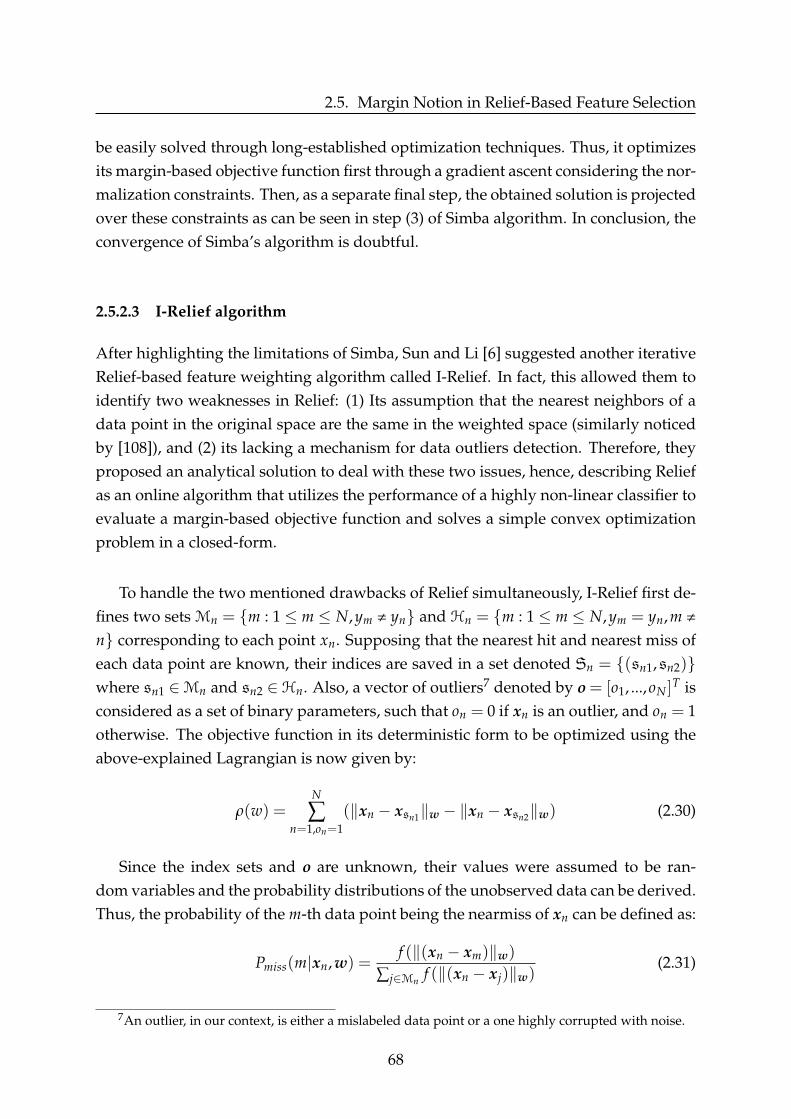
2.5. Margin Notion in Relief-Based Feature Selection
be easily solved through long-established optimization techniques. Thus, it optimizesits margin-based objective function first through a gradient ascent considering the nor-malization constraints. Then, as a separate final step, the obtained solution is projectedover these constraints as can be seen in step (3) of Simba algorithm. In conclusion, theconvergence of Simba’s algorithm is doubtful.
2.5.2.3 I-Relief algorithm
After highlighting the limitations of Simba, Sun and Li [6] suggested another iterativeRelief-based feature weighting algorithm called I-Relief. In fact, this allowed them toidentify two weaknesses in Relief: (1) Its assumption that the nearest neighbors of adata point in the original space are the same in the weighted space (similarly noticedby [108]), and (2) its lacking a mechanism for data outliers detection. Therefore, theyproposed an analytical solution to deal with these two issues, hence, describing Reliefas an online algorithm that utilizes the performance of a highly non-linear classifier toevaluate a margin-based objective function and solves a simple convex optimizationproblem in a closed-form.
To handle the two mentioned drawbacks of Relief simultaneously, I-Relief first de-fines two sets Mn = {m : 1 ≤ m ≤ N,ym , yn} and Hn = {m : 1 ≤ m ≤ N,ym = yn,m ,n} corresponding to each point xn. Supposing that the nearest hit and nearest miss ofeach data point are known, their indices are saved in a set denoted Sn = {(sn1,sn2)}where sn1 ∈Mn and sn2 ∈Hn. Also, a vector of outliers7 denoted by o = [o1, ...,oN]
T isconsidered as a set of binary parameters, such that on = 0 if xn is an outlier, and on = 1otherwise. The objective function in its deterministic form to be optimized using theabove-explained Lagrangian is now given by:
ρ(w) =N
∑n=1,on=1
(‖xn − xsn1‖w − ‖xn − xsn2‖w) (2.30)
Since the index sets and o are unknown, their values were assumed to be ran-dom variables and the probability distributions of the unobserved data can be derived.Thus, the probability of the m-th data point being the nearmiss of xn can be defined as:
Pmiss(m|xn,w) =f (‖(xn − xm)‖w)
∑j∈Mn f (‖(xn − xj)‖w)(2.31)
7An outlier, in our context, is either a mislabeled data point or a one highly corrupted with noise.
68

CHAPTER 2. RELIEF-BASED FEATURE SELECTION
Similarly the probability of the m-th data point being the nearhit of xn is given by:
Phit(m|xn,w) =f (‖(xn − xm)‖w)
∑j∈Hn f (‖(xn − xj)‖w)(2.32)
Where f (.) is a kernel function that can be denoted as f (d) = exp(−d/σ), and the ker-nel width σ is a user defined parameter.
Likewise the probability of an outlier is defined as:
Po(on = 0|X,w) =∑j∈Mn f (‖xn − xj‖w)
∑xj∈X\xn f (‖(xn − xj)‖w)(2.33)
And the probability of not an outlier is defined as:
γn = 1− Po(on = 0|X,w(t)). (2.34)
where t denotes an iteration and w(t) denotes the value of w at a specific iteration t.
Therefore, upon the latter definitions, the iterative algorithm I-Relief was derivedby adopting the idea of the EM algorithm [112] in order to treat unobserved data asrandom variables, however, the objective function of Equation (2.35) is not a likeli-hood.Thus, changing the deterministic ρ(w) into its estimated form as follows:
Step-1: After the t-th iteration, the Q function is calculated as:
Q(w|w(t)) = E{S,o}[ρ(w)]
= ∑Nn=1 γn(∑m∈Mn αm,n‖xn − xm‖w −∑m∈Hn βm,n‖xn − xm‖w)
= ∑Nn=1 γn
(∑i wi ∑m∈Mn αm,nMi
n,m −∑i wi ∑m∈Hn βm,nHin,m
)= wT ∑N
n=1 γn(Mn − Hn)
= wTv
(2.35)
Where superscript i denotes the i-th feature, Mn,m = |xn − xm| if m ∈ Mn, Hn,m =
|xn − xm| if m ∈Hn, αm,n = Pmiss(m|xn,w(t)), and βm,n = Phit(m|xn,w(t)).Step 2 : the re-estimation of w in the (t + 1)-th iteration is :
w(t+1) = argmaxw∈W
Q(w|w(t)) = (v)+/‖(v)+‖2 (2.36)
69

2.5. Margin Notion in Relief-Based Feature Selection
Where, W= {‖w‖2 = 1,w ≥ 0}. Eventually, I-Relief is presented in Algorithm 2.4.
Algorithm 2.4. I-Relief
Input:
• Labeled Training set X of N data points and F features
• Number of iterations T
• Kernel width σ , and stopping criterion φ
Output: Converged closed-form solution of the weight vector w
1. Initialize w = (1/F,1/F, ...,1/F)
2. For t = 1, ..., T
(a) Calculate pairwise distances d(xn, xm|w(t−1)),∀xn, xm ∈ X
(b) Calculate Pmiss, Phit and Po as in (2.31), (2.32) and (2.33) respectively.
(c) Update the weights in w as in Equation (2.36)
(d) If ‖w(t) −w(t−1)‖ ≤ φ, Break , End For
End For
2.5.2.4 Extensions of I-Relief to Multi-class and Semi-supervised Contexts
In the same work, I-Relief algorithm was also extended to a handle multi-class prob-lems in two different versions. The first one, called I-Relief-1, combined the mathemat-ical interpretation with ReliefF’s way of handling multi-class problems using the be-low straightforward integration of ρ = ∑c,class(x)
P(c)1−P(class(x)) |x−M(x, c)| − |x−H(x)|
into Equation (2.15), where P(c) is the prior probability of class c and 1− P(class(x))represents the sum of probabilities for the misses’ classes. However, it was noted thatobtaining a positive margin from such a combination does not necessarily mean that acorrect classification occurred. Therefore, I-Relief-2 was suggested to regain this char-acteristic using the below-defined margin:
ρ = min{c,class(x)}|x−M(x, c)| − |x− H(x)|= min{xm∈X\Xclass(x)}|x− xm| − |x− H(x)|
(2.37)
where Xclass(x) is a subset of X containing all data points belonging to the class of x.
70
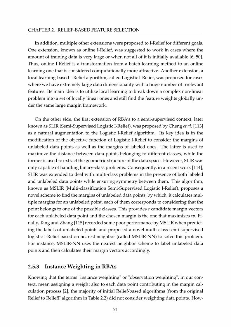
CHAPTER 2. RELIEF-BASED FEATURE SELECTION
In addition, multiple other extensions were proposed to I-Relief for different goals.One extension, known as online I-Relief, was suggested to work in cases where theamount of training data is very large or when not all of it is initially available [6, 50].Thus, online I-Relief is a transformation from a batch learning method to an onlinelearning one that is considered computationally more attractive. Another extension, alocal learning-based I-Relief algorithm, called Logistic I-Relief, was proposed for caseswhere we have extremely large data dimensionality with a huge number of irrelevantfeatures. Its main idea is to utilize local learning to break down a complex non-linearproblem into a set of locally linear ones and still find the feature weights globally un-der the same large margin framework.
On the other side, the first extension of RBA’s to a semi-supervised context, laterknown as SLIR (Semi-Supervised Logistic I-Relief), was proposed by Cheng et al. [113]as a natural augmentation to the Logistic I-Relief algorithm. Its key idea is in themodification of the objective function of Logistic I-Relief to consider the margins ofunlabeled data points as well as the margins of labeled ones. The latter is used tomaximize the distance between data points belonging to different classes, while theformer is used to extract the geometric structure of the data space. However, SLIR wasonly capable of handling binary-class problems. Consequently, in a recent work [114],SLIR was extended to deal with multi-class problems in the presence of both labeledand unlabeled data points while ensuring symmetry between them. This algorithm,known as MSLIR (Multi-classification Semi-Supervised Logistic I-Relief), proposes anovel scheme to find the margins of unlabeled data points, by which, it calculates mul-tiple margins for an unlabeled point, each of them corresponds to considering that thepoint belongs to one of the possible classes. This provides c candidate margin vectorsfor each unlabeled data point and the chosen margin is the one that maximizes w. Fi-nally, Tang and Zhang [115] recorded some poor performance by MSLIR when predict-ing the labels of unlabeled points and proposed a novel multi-class semi-supervisedlogistic I-Relief based on nearest neighbor (called MSLIR-NN) to solve this problem.For instance, MSLIR-NN uses the nearest neighbor scheme to label unlabeled datapoints and then calculates their margin vectors accordingly.
2.5.3 Instance Weighting in RBAs
Knowing that the terms "instance weighting" or "observation weighting", in our con-text, mean assigning a weight also to each data point contributing in the margin cal-culation process [2], the majority of initial Relief-based algorithms (from the originalRelief to ReliefF algorithm in Table 2.2) did not consider weighting data points. How-
71

2.5. Margin Notion in Relief-Based Feature Selection
ever, under the umbrella of instance weighting, this can be explained as using binaryweights where nearest points contribute with a weight of 1 and all other points get aweight of 0 (i.e no contribution).
For classification problems, Draper et al. [108] suggested the first iterative Relief-based approach, called Iterative Relief, with the aim of removing the bias of ReliefFagainst non-monotonic features8. After claiming that ReliefF’s distance measure canturn to be irrelevant when dealing with non-monotonic features, it was normal to as-sign higher weights to monotonic features as they are considered more relevant withrespect to non-monotonic ones. Thus, in order to find a distance measure that caneffectively choose similar nearhits and misses in the feature space, they proposed in-stance weighting using a "radius", by which, all data points within are included in thecalculation of feature weights instead of using an integer number K of nearhits andnearmisses. Moreover, the contribution of a data point decreases as it moves fartherfrom the target point within the radius circle.
Also, the methods suggested by I-Relief algorithms for calculating probability setsfor all hits and misses implicitly replaces the whole idea of a specific number K of hitsand misses by instance weighting [6, 50, 94, 117]. Where, in fact, a data point with ahigher probability of being the nearmiss or nearhit is the one having the smallest dis-tance from the target point.
On the other hand, similarly to I-Relief and its successors, a set of variants thathad their main focus on instance weighting were suggested. These are explained thor-oughly by the review of Urbanowiz et. al [2] and known as SURF (Spatially Uni-form ReliefF), SURF* (* indicates opposite), SWRF* (Sigmoid Weighted ReliefF Star),MultiSURF* (Multiple Threshold SURF*), and MultiSURF (Multiple Threshold SURF).The latter five algorithms could only handle discrete-valued features and binary classproblems since they are application driven9.
8The bias of ReliefF was declared by (Bins and Draper, 2001) especially when the data has morenoisy features [116], Knowing that a non-monotonic feature is a feature that is neither non-decreasingnor non-increasing with respect to the predicted value. These features can position the data points ofthe same class into different parts of the feature space even when they are relevant. In other words, ithas an internal optima.
9These algorithms were suggested for feature selection in genomics problems with single nucleotidepolymorphisms (SNPs). In such an application, features can have one of three discrete values (0, 1, or2) and a binary class representing sick or healthy patients.
72
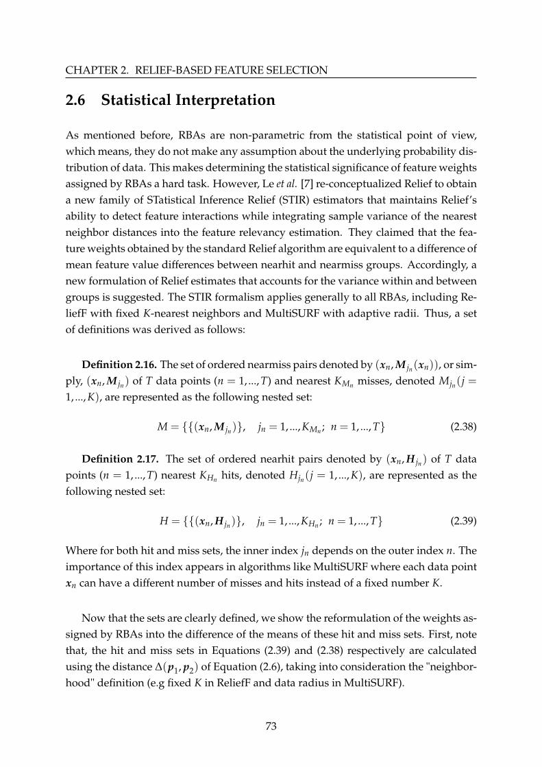
CHAPTER 2. RELIEF-BASED FEATURE SELECTION
2.6 Statistical Interpretation
As mentioned before, RBAs are non-parametric from the statistical point of view,which means, they do not make any assumption about the underlying probability dis-tribution of data. This makes determining the statistical significance of feature weightsassigned by RBAs a hard task. However, Le et al. [7] re-conceptualized Relief to obtaina new family of STatistical Inference Relief (STIR) estimators that maintains Relief’sability to detect feature interactions while integrating sample variance of the nearestneighbor distances into the feature relevancy estimation. They claimed that the fea-ture weights obtained by the standard Relief algorithm are equivalent to a difference ofmean feature value differences between nearhit and nearmiss groups. Accordingly, anew formulation of Relief estimates that accounts for the variance within and betweengroups is suggested. The STIR formalism applies generally to all RBAs, including Re-liefF with fixed K-nearest neighbors and MultiSURF with adaptive radii. Thus, a setof definitions was derived as follows:
Definition 2.16. The set of ordered nearmiss pairs denoted by (xn, M jn(xn)), or sim-ply, (xn, M jn) of T data points (n = 1, ..., T) and nearest KMn misses, denoted Mjn(j =1, ...,K), are represented as the following nested set:
M = {{(xn, M jn)}, jn = 1, ...,KMn ; n = 1, ..., T} (2.38)
Definition 2.17. The set of ordered nearhit pairs denoted by (xn, H jn) of T datapoints (n = 1, ..., T) nearest KHn hits, denoted Hjn(j = 1, ...,K), are represented as thefollowing nested set:
H = {{(xn, H jn)}, jn = 1, ...,KHn ; n = 1, ..., T} (2.39)
Where for both hit and miss sets, the inner index jn depends on the outer index n. Theimportance of this index appears in algorithms like MultiSURF where each data pointxn can have a different number of misses and hits instead of a fixed number K.
Now that the sets are clearly defined, we show the reformulation of the weights as-signed by RBAs into the difference of the means of these hit and miss sets. First, notethat, the hit and miss sets in Equations (2.39) and (2.38) respectively are calculatedusing the distance ∆(p1, p2) of Equation (2.6), taking into consideration the "neighbor-hood" definition (e.g fixed K in ReliefF and data radius in MultiSURF).
73

2.6. Statistical Interpretation
Definition 2.18. The mean of ∆ function (defined in Equation (2.1)) of a featureAi averaged over all pairs of nearmisses (M Equation (2.38)), denoted Mi, can be ex-pressed as:
Mi =1T
T
∑n=1
1KMn
KMn
∑jn=1
∆(Ai, xn, M jn) (2.40)
where Mjn is the j-th nearest miss of the data point xn, and KMn is the number ofnearmisses of xn. The scaling by 1
KMnensures a consistent neighborhood average
weighting for different RBAs like MultiSURF, SURF and ReliefF.
Definition 2.19. The mean of ∆ function (defined in Equation (2.1)) of a feature Ai
averaged over all pairs of nearhits (H Equation (2.39)), denoted Hi, can be expressedas:
Hi =1T
T
∑n=1
1KHn
KHn
∑jn=1
∆(Ai, xn, H jn) (2.41)
where, similarly, Hjn is the j-th nearest hit of the data point xn, and KHn is the numberof nearhits of xn.
Definition 2.20. The importance score assigned by RBAs to each feature Ai can bethen expressed as the averaged z presented in Equation (2.17) as follows:
zi = Mi − Hi (2.42)
This formulation applies to all RBAs [7]. Accordingly, Equation (2.42) was usedlater as the basis to compute the permutation p-values for the sake of comparison.Then, for computing the statistical significance of features with computational effi-ciency, Equation (2.42) was extended to develop a Relief-based pseudo t-test.
2.6.1 STatistical Inference for Relief (STIR)
The new type of Relief-based algorithm is then presented as an incorporation of thepooled standard deviations about the mean hit and miss ∆ functions to transform theRelief-based feature importance scores zi into a pseudo t-statistic [7]. Note that, thepooled standard deviation presented below allows for unbalanced variances betweenhit and miss nearest neighbor ∆ functions and allows for a different number of these∆ functions in the hit and miss groups themselves.
Definition 2.21. The STIR weight (or STIR score) is constructed from the Reliefdifference of means (zi in Equation (2.42)) in the numerator and the standard error in
74

CHAPTER 2. RELIEF-BASED FEATURE SELECTION
the denominator as follows:
wSTIRi =Mi − Hi
σpool[M, H]√
1/|M|+ 1/|H|(2.43)
Where |H| = ∑Tn=1 KHn and |M| = ∑T
n=1 KMn are the total number of hit and missneighbors over all the data points in X. And the pooled standard deviation denotedby σpool is given by:
σpool[M, H] =
√(|M| − 1)σ2
Mi+ |H| − 1)σ2
Hi
|M|+ |H| − 2(2.44)
And the group variances are given by:
σ2Mi
=1T
T
∑n=1
1KMn
KMn
∑jn=1
(∆(Ai, xn, M jn)− Mi)2 (2.45)
σ2Hi
=1T
T
∑n=1
1KHn
KHn
∑jn=1
(∆(Ai, xn, H jn)− Hi)2 (2.46)
According to [7], wSTIRi score shown in Equation (2.43) approximately follows at-distribution from which they compute p-values. For that, a degree of freedom df =|M|+ |H| − 2 is used in calculating the p-value. It was concluded that STIR can recordthe statistical significance of RBA scores by a pseudo t-test that stands for variance inthe mean difference of hit and miss nearest neighbor ∆ functions.
2.7 Conclusion
As we were interested in Relief-based methods, in this chapter, we concisely reviewedthe set of well-known efficient filter-type RBAs. For that, we started with a clear ex-planation of the original Relief algorithm while highlighting its strengths and limita-tions. Afterward, we presented the main variants and extensions of Relief that weresuggested to handle problems with noisy, incomplete, and multi-class data. This wasdone while generally categorizing RBAs according to their four broad possible inter-pretations. These are, the probabilistic, the comprehensible, the mathematical and thestatistical interpretations. Most importantly, Relief was introduced as a margin-basedfeature selection algorithm which will be the base of the following chapters.
75

2.7. Conclusion
Table 2.2: Summary of the main Relief-based algorithms covered in this chapter. Eachalgorithm is followed by its reference, main contribution, learning context, time com-plexity, and other capabilities mentioned explicitly in their original publications. C, l,and u used in the semi-supervised algorithms denote the number of classes, labeleddata points and unlabeled data points respectively. Some parts of the table are adaptedfrom [2].
Algorithm /Reference(s)
Focus / ContributionLearningContext
AsymptoticTime
Complexity
Con
tinu
ous
Feat
ures
Inst
ance
Wei
ghti
ng
Mul
ti-C
lass
Prob
lem
sR
egre
ssio
nPr
oble
ms
Mis
sing
Dat
a
Noi
se-t
oler
ant
Feat
ure-
Red
unda
ncy
Iter
ativ
eA
ppro
ach
Out
lier
Det
ecti
on
Relief [66]
First filter-type feature selectionmethod capable of dealing with
feature interactions(dependencies) in a simple and
efficient way.
Supervised O(TNF) x
ReliefA [4]
Using k-nearest hits/missesinstead of only one to increase the
reliability of probabilityapproximations and featureweights when data is noisy
Supervised O (TNF) x x
ReliefB-D [4]Handling missing data with
ReliefD being the best variantSupervised O (TNF) x x x
ReliefE-F [4]Dealing with multi-class
problems with ReliefF becomingthe standard algorithm.
Supervised O (TNF) x x x x
RReliefF [99, 101]
Adapting ReliefF to work withcontinuous class labels.
Introducing instance weightingby distance-from-target.
Supervised O (TNF) x x x x x
Relieved-F [100]Choosing the nearest points forscoring in a deterministic way.
Handling missing data.Supervised
T = N =⇒O(N2F)
x x x x
Iterative Relief [108]
Introducing the first iterativeapproach. Improving ReliefF by
removing its bias againstnon-monotonic features.
Replacing k-nearest neighbors byradius-circle around the target
point. Using distance-from-targetinstance weighting.
Supervised O(TN2F) x x x x
76

CHAPTER 2. RELIEF-BASED FEATURE SELECTION
Table 2.2 Continued
Algorithm /Reference(s)
Focus / ContributionLearningContext
AsymptoticTime
Complexity
Con
tinu
ous
Feat
ures
Inst
ance
Wei
ghti
ng
Mul
ti-C
lass
Prob
lem
sR
egre
ssio
nPr
oble
ms
Mis
sing
Dat
a
Noi
se-t
oler
ant
Feat
ure-
Red
unda
ncy
Iter
ativ
eA
ppro
ach
Out
lier
Det
ecti
on
Iterative SearchMargin-based
Algorithm (Simba)[102]
Introducing the first marginconcept to Relief-based
algorithms. Considering scoringin the weighted space. Using
gradient ascent optimization on amargin-based objective function.
Supervised O (TNF) x x x x
I-Relief [6, 50]
Introducing Relief from itsoptimization perspective.
Replacing the idea of definedK-nearest neighbors by
probabilities of being a hit or amiss and using them for instance
weighting. Introducing outlierdetection.
Supervised O (TN2F) x x x x x
I-Relief-1 andI-Relief-2 [6, 50]
Extending I-Relief to deal withmulti-class problems.
Supervised O (TN2F) x x x x x
Online I-Relief [6, 50]
Dealing with huge amounts ofdata or data not completely
available initially through onlinelearning (not batch mode).
Supervised O (TNF) x x x x x
Logistic I-Relief (LIR)[94, 117]
Handling extremely large datadimensionality with a large
number of irrelevant features inan efficient way through local
learning. Introducing a logisticmargin-based objective function
with a sparse solution.
Supervised O (TN2F) x x x x x
Semi-supervisedLogistic I-Relief
(SLIR) [113]
Modifying the objective functionof LIR to consider margins of
both labeled and unlabeled datapoints.
Semi-supervised
Margin oflabeled:O(Fl2).
Margin ofunlabeled
O(Flu)
x x x
77

2.7. Conclusion
Table 2.2 Continued
Algorithm /Reference(s)
Focus / ContributionLearningContext
AsymptoticTime
Complexity
Con
tinu
ous
Feat
ures
Inst
ance
Wei
ghti
ng
Mul
ti-C
lass
Prob
lem
sR
egre
ssio
nPr
oble
ms
Mis
sing
Dat
a
Noi
se-t
oler
ant
Feat
ure-
Red
unda
ncy
Iter
ativ
eA
ppro
ach
Out
lier
Det
ecti
on
Multi-classificationSemi-supervisedLogistic I-Relief
(MSLIR)[114]
Modifying the objective functionof SLIR to consider margins of
both labeled and unlabeled datapoints in multi-class problems.
Semi-supervised
Margin oflabeled:O(Fl2).
Margin ofunlabeledO(CFlu)
x x x x
Multi-classSemi-supervisedLogistic I-Reliefbased on nearest
neighbor(MSLIR-NN) [115]
Using the nearest neighborscheme to label unlabeled pointsand then calculating their margin
vectors accordingly.
Semi-supervised
Margin oflabeled:O(Fl2).
Margin ofunlabeled
O(Flu)
x x x x
STatistical InferenceRelief (STIR) [7]
Re-conceptualizing Relief toobtain a new family of STatisticalInference Relief (STIR) estimators
while maintaining its ability todetect feature interactions
through integrating samplevariance of the nearest neighbor
distances into the featurerelevancy estimation.
Supervised φ x x x
78

Chapter 3An Approach based onHypothesis-Margin and PairwiseConstraints
Contents3.1 Introduction . . . . . . . . . . . . . . . . . . . . . . . . . . . . . . . . . . 80
3.2 Hypothesis-Margin in a Constrained Context For Maximizing Rele-vance . . . . . . . . . . . . . . . . . . . . . . . . . . . . . . . . . . . . . . 81
3.2.1 General Mathematical Interpretation . . . . . . . . . . . . . . . . 82
3.2.2 Relief with Side Constraints (Relief-Sc) . . . . . . . . . . . . . . 84
3.2.3 ReliefF-Sc: A Robust version of Relief-Sc . . . . . . . . . . . . . 88
3.2.4 Iterative Search Margin-Based Algorithm with Side Constraints(Simba-Sc) . . . . . . . . . . . . . . . . . . . . . . . . . . . . . . . 89
3.3 Feature Clustering in a Constrained Context for Minimizing Redun-dancy . . . . . . . . . . . . . . . . . . . . . . . . . . . . . . . . . . . . . . 91
3.3.1 Feature Space Sparse Graph Construction . . . . . . . . . . . . . 93
3.3.2 Agglomerative Hierarchical Feature Clustering . . . . . . . . . 95
3.3.3 Proposed Feature Selection Approach . . . . . . . . . . . . . . . 97
3.4 Experimental Results . . . . . . . . . . . . . . . . . . . . . . . . . . . . 98
3.4.1 Experimental Results on Relief-Sc: Selection of Relevant Features 99
3.4.2 Experimental Results on FCRSC: Selection of Relevant and Non-redundant Features . . . . . . . . . . . . . . . . . . . . . . . . . . 107
3.5 Conclusion . . . . . . . . . . . . . . . . . . . . . . . . . . . . . . . . . . 118
79

3.1. Introduction
3.1 Introduction
The concept of a hypothesis-margin was initially suggested in the supervised learningcontext by [66] as an algorithm called Relief, it is a filter-type method for individual-evaluation feature selection. Being aware of the contextual supervision informationand capable of calculating a weight value for each feature, Relief proved its ability tosuccessfully rank features in the order of their relevance to a specific problem like clas-sifying new data points. This importance measure is referred to as feature weights. Bymeaning, the hypothesis-margin is the largest distance a data point can travel withinthe feature space without altering the dataset’s labeling structure, and thus withoutaffecting the label prediction of a new arriving point.
However, as explained in Chapter 2, in many real-world applications, there usu-ally exist few labeled data points and lots of unlabeled ones, by which both supervisedand unsupervised feature selection algorithms cannot fully take advantage of all datapoints in this scenario. Thus, it was wise to use semi-supervised methods [39, 54] tofeat both labeled and unlabeled data points. In fact, compared to class labels, pairwiseconstraints are another type of supervision information that can be acquired more eas-ily. These constraints simply specify whether two data points are similar and there-fore should be in the same category (a must-link constraint) or dissimilar and thereforeshould be in different categories (a cannot-link constraint) without the need to identifytheir class labels.
In this chapter, we suggest to integrate the modification of hypothesis-margin whenused with cannot-link constraints, with the analytical solution of the supervised Re-lief algorithm [50, 66]. This means we conjugate hypothesis-margin concept used in[107] with Relief algorithm from its optimization perspective. The proposed methodis a semi-supervised margin-based feature selection algorithm called Relief-Sc. It isa modification of the well-known original Relief algorithm from its optimization per-spective. It utilizes cannot-link constraints only to solve a simple convex problem ina closed form giving a unique solution. Besides, a slightly modified Relief-Sc into amore robust version with respect to noisy data, called ReliefF-Sc algorithm, is alsopresented and generally applied instead in our experiments.
80

CHAPTER 3. AN APPROACH BASED ON HYPOTHESIS-MARGIN ANDPAIRWISE CONSTRAINTS
In addition, we propose to extend our semi-supervised feature selection methodinto a novel combination of feature clustering and hypothesis margin maximizationcalled FCRSC. This approach aims at handling the two core aspects of feature selec-tion (relevance and redundancy) and is divided into three steps. First, the similarityweights between features are represented by a sparse graph by which it is assumedthat each feature can be reconstructed from the sparse linear combination of the oth-ers. Second, features are then hierarchically clustered identifying groups of the mostsimilar ones. Finally, our semi-supervised margin-based objective function is opti-mized to select the most data discriminative feature from within each cluster, hence,maximizing relevance while minimizing redundancy (maximizing diversity) amongfeatures. Eventually, we experimentally validate our proposed approach on multiplewell-known UCI [3] benchmark datasets.
This chapter is divided into two main sections. The first main one, i.e. section3.2, provides the introduction and explanation of the notions and concepts of thehypothesis-margin in a semi-supervised learning context with a general mathematicalinterpretation (section 3.2.1) and three feature selection algorithms descending fromit. These are Relief-Sc, ReliefF-Sc and Simba-Sc presented in sections 3.2.2, 3.2.3, and3.2.4 respectively. The second main section 3.3 presents the feature selection frame-work that deals with feature redundancy in addition to feature relevance. It includessections 3.3.1, 3.3.2, and 3.3.3 that present building the sparse graph, hierarchical clus-tering upon it, and the combination of feature clustering with constrained margin-based feature selection respectively. On the other side, in section 3.4, we present theexperimental results to validate the proposed approaches. Experiments are achievedon multiple well-known UCI machine learning datasets [3]. Finally, we conclude insection 3.5.
3.2 Hypothesis-Margin in a Constrained Context For Max-
imizing Relevance
In this section, we present a concise explanation of the constrained hypothesis-marginunder a general mathematical interpretation similarly to that of Chapter 2. We alsopresent the proposed margin-based feature selection algorithm Relief-Sc. In addition,we explain Simba-Sc [107] as a state of the art algorithm that applies feature selectionin a way that is similar to ours.
81

3.2. Hypothesis-Margin in a Constrained Context For Maximizing Relevance
3.2.1 General Mathematical Interpretation
Hypothesis-margin plays an important role in feature selection, just like sample-margindoes in Support Vector Machines (SVM) [94]. As hypothesis-margin lower boundsthe sample margin [102, 106], it was stated by Yang and Song [107] that in the caseof a 1-Nearest Neighbor (1-NN) large hypothesis-margin, a large sample-margin isguaranteed with ease of computation. In cases where the only available supervisioninformation is in the form of pairwise constraints, especially cannot-link ones [107],we consider using these constraints to calculate the constrained hypothesis-margin.Knowing that a cannot-link constraint specifically indicates that each data point ofthe considered data pair should belong to a different cluster, it is necessary to mod-ify the supervised notions of nearmiss and nearhit in order to find the constrainedhypothesis-margin. Thus, for pedagogical purposes, all the following definitions andequations are adapted from Chapter 2.
Definition 3.1. Let CL = {(xn, xm)} be a set of cannot link constraints and (xn, xm)
be one cannot-link constraint in it. For instance, as can be seen in Figure (3.1), in theconstrained context, the nearhit of xm denoted H(xm) is considered equivalent to thenearmiss M(xn) of xn (that is usually used in a supervised context with class labels),thus, it replaces it. On the other side, the nearhit of H(xn) represents the nearhit of xn
as it is usually. Also, the number of constraints card(CL) is equal to a user-predefinedvalue T.
Note that, according to the local cluster assumption, the nearhit of a point is sim-ply its nearest neighbor without any class information. In fact, this assumption meansthat nearby points are assigned to the same class or in other words have the same la-bel. Accordingly, the constrained hypothesis-margin was first mentioned in [107].
Definition 3.2. The constrained hypothesis-margin is calculated as the differencebetween the distance from the data point xn to the nearhit of xm denoted H(xm) andthe distance from the data point xn to its own nearhit H(xn).
ρ(xn, xm) = ∆(xn, H(xm))− ∆(xn, H(xn)) (3.1)
recalling that ∆(p1, p2) is defined in Chapter 2 as the generalized distance function be-tween any two data points p1 and p2 over all the features F with p ∈R and ∆(Ai, p1, p2)
defined in Definition 2.3.
82

CHAPTER 3. AN APPROACH BASED ON HYPOTHESIS-MARGIN ANDPAIRWISE CONSTRAINTS
M (xn)
Xn
H (xn)
(a) The original notions of nearmiss and nearhit used in the supervised margin calcu-lation (see Figure 2.1a). The nearmiss of a point xn represented by M(xn) is its nearestpoint from a different class and the nearhit of a point xn represented by H(xn) is itsnearest point from the same class.
Xm
Xn
H(xn)
H(xm)
(b) The modified notions of nearmiss and nearhit used in the constrained margin cal-culation, where the dashed line represents the cannot-link constraint between a couple(xn,xm). H(xm) represents the nearmiss M(xn) of xn and H(xn) represents the nearhitof xn.
Figure 3.1: The evolution of the nearmiss and nearhit notions from the supervisedcontext to the semi-supervised constrained one.
83

3.2. Hypothesis-Margin in a Constrained Context For Maximizing Relevance
Therefore, the overall constrained hypothesis-margin with respect to the set ofcannot-link constraints CL and the training set X can be computed as:
ρ(X) = ∑(xn,xm)∈CL
ρ(xn, xm) (3.2)
Similarly to the supervised context, we consider the weighted hypothesis-marginusing the weight vector w defined in Definition 2.2, however, in a semi-supervisedconstrained context. The latter can be calculated as follows:
ρ((xn, xm),w) = ∆w(xn, H(xm))− ∆w(xn, H(xn)) (3.3)
Each time the margin is calculated with respect to a data point xn of F features, theweight vector w contributes to this calculation. Taking Equation (3.3) into account, itcan be generalized to calculate the weighted hypothesis-margin over all the given datapoints. Consequently, the final weight vector of length F shows the impact of each fea-ture in enlarging the margin, which is considered the score/weight of the feature.
Then, the weighted constrained hypothesis-margin with respect to the set of cannot-link constraints CL and the training set X can be computed as:
ρ(X,w) = ∑(xn,xm)∈CL
ρ((xn, xm),w) (3.4)
It is then clear that Equation (3.4) is the summation of the weighted constrained hy-pothesis margins over the whole cannot-link constraints set. So, the feature subset thatcontributes the most in enlarging this overall margin has a weight vector of higher val-ues, and is consequently selected.
Similarly to the supervised context, changing the value of superscript p in Equa-tions (2.6) and (2.9) defines different constrained margin-based feature selection algo-rithms. If the l1-norm is used, deriving Manhattan distance, our proposed constrainedRelief-Sc algorithm is obtained [118]. However, if the l2-norm is used, deriving Eu-clidean distance, the resulting algorithm is the constrained Simba-Sc [107].
3.2.2 Relief with Side Constraints (Relief-Sc)
We consider the interesting mathematical interpretation that was suggested by Sunand Li [6] to view the margin from an optimization perspective. It was stated that thisinterpretation not only takes advantage of the performance of a highly nonlinear clas-
84

CHAPTER 3. AN APPROACH BASED ON HYPOTHESIS-MARGIN ANDPAIRWISE CONSTRAINTS
sifier to calculate a margin-based objective function, but also solves a simple convexproblem in a closed-form and obtains a unique solution. Thus, we modified this for-mulation into a constrained one called Relief-Sc that obtains its solution by calculatingthe margin over all the constraints in CL in a batch mode.Definition 3.3. The constrained hypothesis-margin of a cannot-link constraint (xn, xm)
denoted by ρ(xn, xm) under Relief-Sc is defined as:
ρ(xn, xm) = |xn − H(xm)| − |xn − H(xn)| (3.5)
Where the used distance function | . | is the l1-norm (or Manhattan distance) defined inEquation (2.12).
Accordingly, the weighted constrained hypothesis-margin of the cannot-link con-straint (xn, xm) with respect to X is:
ρ((xn, xm),w) = |xn − H(xm)|w − |xn − H(xn)|w (3.6)
where |v|w is defined in Equation (2.14).
Therefore, we focus on the constrained environment using pairwise constraints, es-pecially cannot-link ones as they are considered more important than must-link con-straints from margin’s perspective [107]. As a result, we found it axiomatic to integratethe usage of constrained hypothesis-margin with a more simple and computationallyefficient algorithm like Relief from its optimization point of view. Since constrainedalgorithms are penalized by the choice of constraints, the unique solution provided byoptimized Relief-Sc allows it to be effectively analyzed when given a fixed set of con-straints. Thus, the optimization method (gradient ascent) used in [107] was replacedby the analytical solution suggested in [6] producing a new version of Relief algorithmfrom an optimization view point.
Definition 3.4. The weighted constrained margin-based objective function to beoptimized by Relief-Sc is given by:
maxw
∑(xn,xm)∈CL
ρ((xn, xm),w)
= maxw
∑(xn,xm)∈CL
(∑F
i=1 wi|xni − H(xm)i| −∑Fi=1 wi|xni − H(xn)i|
)
s.t. ‖w‖22 = 1 and w ≥ 0
(3.7)
85

3.2. Hypothesis-Margin in a Constrained Context For Maximizing Relevance
It is intuitive that the weight vector w ≥ 0 should have positive values for relevantfeatures since it is a distance metric, and ||w||22 = 1 prevents the vector from beingmaximized without bounds [6].
Definition 3.5. To simplify and combine Equations (3.6) and (3.7), we show thei-th element (corresponding to the i-th feature) of the constrained margin vector z. Itis evaluated over all the available cannot-link constraints in CL with respect to thetraining set X as follows:
zi = ∑(xn,xm)∈CL
|xni − H(xm)i| − |xni − H(xn)i| (3.8)
For clarity, we express the margin vector z in the following notation:
z = ∑(xn,xm)∈CL
|xn1 − H(xm)1|
...|xnF − H(xm)F|
− |xn1 − H(xn)1|
...|xnF − H(xn)F|
=
z1
...zF
(3.9)
Definition 3.6. Considering the constrained margin vector z, the simplified weightedconstrained margin-based objective function to be optimized by Relief-Sc can be for-mulated as follows:
maxw
wTz, s.t. ‖w‖22 = 1, w ≥ 0 (3.10)
Now, using the Lagrangian function the Equation (3.10) can be expressed as:
L(w,λ,µ) = −wTz + λ(wTw− 1)− µTw (3.11)
where λ > 0 is the Lagrange multiplier and µ ≥ 0 is the Karush Kuhn Tucker (KKT)multiplier vector satisfying complementarity condition: µTw = 0.
Now by calculating the derivative of L with respect to w we obtain:
∂L
∂w= −z + 2λw− µ (3.12)
and we satisfy the stationarity condition by solving ∂L∂w = 0 to obtain w as follows:
∂L
∂w= 0 =⇒ w =
12λ
(z + µ) (3.13)
86

CHAPTER 3. AN APPROACH BASED ON HYPOTHESIS-MARGIN ANDPAIRWISE CONSTRAINTS
As mentioned in section 2.5.2.1, Sun and Li [6] used the Karush Kuhn Tucker (KKT[111]) complementarity condition: µTw = 0 to verify the three following cases thatalso hold in Relief-Sc:
1. zi = 0⇒ µi = 0, wi = 0.
2. zi > 0⇒ zi + µi > 0⇒ wi > 0⇒ µi = 0
3. zi < 0⇒ µi > 0⇒ wi = 0⇒ zi = −µi
This leads to: {wi
}F
i=1=
zi+
2λ if zi > 0
0 if zi ≤ 0(3.14)
Finally, the optimal solution can be calculated in a closed-form as:
w∗ = w/‖w‖2 = (z)+/‖(z)+‖2
where, z is given by Equation (3.9)and (z)+ = [max(z1,0), ...,max(zF,0)]T
(3.15)
In summary, Relief-Sc uses the cannot-link constraint set CL to calculate the averagedmargin z that the features induce using the nearhits of xn and xm. Finally, it calculatesw directly as shown in step 3 of Algorithm 3.1.
Algorithm 3.1 Relief-Sc
Input: Training data X, Set of cannot-link constraints CLOutput: Weight vector w
1. Calculate H(xn) and H(xm) for each cannot-link constraint in CL with Respect to X
2. For i = 1, ..., F,zi = ∑(xn,xm)∈CL ∆(Ai, xn, H(xm))− ∆(Ai, xn, H(xn))
end For
3. w = (z)+/||(z)+||2where, (z)+ = [max(z1,0), ...,max(zF,0)]T
87

3.2. Hypothesis-Margin in a Constrained Context For Maximizing Relevance
3.2.3 ReliefF-Sc: A Robust version of Relief-Sc
However, in ReliefF [4], the hypothesis-margin is calculated over a group of K-nearestneighbors (K-NN) for each selected data point which leads to considering ReliefF asthe robust supervised version of the original Relief algorithm with respect to noisydata. Thus, we similarly enhance Relief-Sc. For instance, when considering a cannot-link constraint (xn, xm), instead of taking only one nearhit to xn and one nearhit toxm, we now consider K-nearhits to xn and K-nearhits to xm denoted by KH(xn) :{H1(xn), H2(xn), ..., HK(xn)} and KH(xm) : {H1(xm), H2(xm), ..., HK(xm)} respectively,where K is a user defined parameter representing the number of closest points to xn
and xm to be considered. In this way, the margin evaluation is averaged over a largerneighborhood and thus is less vulnerable to erroneous data. Consequently, the i-thelement (corresponding to the i-th feature) of the margin vector z is given by:
zi = ∑(xn,xm)∈CL
1K
K
∑j=1
(∆(Ai, xn, H j(xm))− ∆(Ai, xn, H j(xn))
)(3.16)
Therefore, in the context of a robust constrained hypothesis margin over K-NN, weapply Relief-Sc as stated in Algorithm 3.2. To sum up, it uses a cannot-link constraintset to calculate the average margin zi that each feature induces over the K-nearest hitsof xn and xm. Finally, it calculates w directly as shown in step 3 of Algorithm 3.2.
Algorithm 3.2. ReliefF-Sc
Input: Training data X, Set of cannot-link constraints CL, and Number of Nearest NeighborsKOutput: Weight vector w
1. Calculate KH(xn) and KH(xm) for each cannot-link constraint in CL with Respect to X
2. For i = 1, ..., F,
zi = ∑(xn,xm)∈CL1K ∑K
j=1
(∆(Ai, xn, H j(xm))− ∆(Ai, xn, H j(xn))
)end For
3. w = (z)+/||(z)+||2where, (z)+ = [max(z1,0), ...,max(zF,0)]T
88

CHAPTER 3. AN APPROACH BASED ON HYPOTHESIS-MARGIN ANDPAIRWISE CONSTRAINTS
3.2.4 Iterative Search Margin-Based Algorithm with Side Constraints(Simba-Sc)
As mentioned in section 3.2.1, the Simba-Sc algorithm, proposed by Yang and Song [107],is obtained when using the l2-norm with this mathematical interpretation. It is amodification of Simba algorithm (detailed in section 2.5.2.2 of chapter 2) into a semi-supervised margin-based algorithm that iteratively utilizes pairwise constraints specif-ically cannot-link ones to evaluate the ability of features in discriminating data points.It also uses a gradient ascent method to maximize its margin-based objective function.Thus, a higher score means a more relevant feature. Note that, Simba-Sc has a mech-anism to deal with redundancy, however, it may still choose correlated features onlywhen this contributes positively to the overall performance.
Definition 3.7. The constrained hypothesis-margin of a cannot-link constraint (xn, xm)
denoted by ρ(xn, xm) is given by half the difference between the distance from the datapoint xn to the nearhit of xm and the distance to its own nearhit. However, similarly toEquation (2.23), we also omit the half obtaining the following:
ρ(xn, xm) = ‖xn − H(xm)‖ − ‖xn − H(xn)‖ (3.17)
where the used distance function ‖ .‖ is the l2-norm (or Euclidean distance) defined asin Equation (2.24).
Definition 3.8. By considering a training set X, a cannot-link constraint (xn, xm),and the weight vector w, the weighted hypothesis-margin of (xn, xm) is given by:
ρ((xn, xm),w) = ‖xn − H(xn)‖w − ‖xn − H(xn)‖w (3.18)
where ‖v‖w is defined in Equation (2.26).
Definition 3.9. Considering the training set X and the feature weights denoted bythe vector w, the evaluation function of Simba-Sc is given by:
ρ(X,w) = ∑(xn,xm)∈CL
ρ((xn, xm),w) (3.19)
By analyzing Equation (3.19), the authors declared that a natural normalizationconstraint is required on w, i.e., max (w2
i ) = 1 [107]. Besides, similarly to Simba, theyignore this normalization constraint during the calculation of w since for any scalar λ,
89
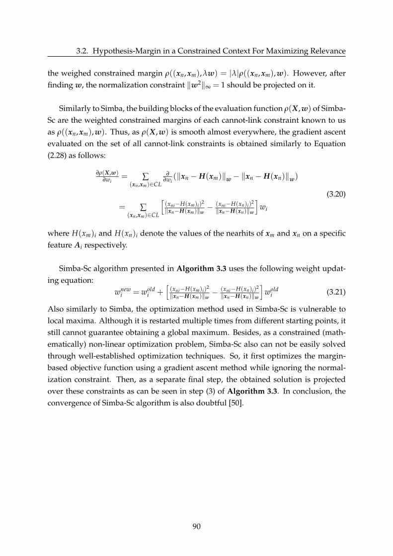
3.2. Hypothesis-Margin in a Constrained Context For Maximizing Relevance
the weighed constrained margin ρ((xn, xm),λw) = |λ|ρ((xn, xm),w). However, afterfinding w, the normalization constraint ‖w2‖∞ = 1 should be projected on it.
Similarly to Simba, the building blocks of the evaluation function ρ(X,w) of Simba-Sc are the weighted constrained margins of each cannot-link constraint known to usas ρ((xn, xm),w). Thus, as ρ(X,w) is smooth almost everywhere, the gradient ascentevaluated on the set of all cannot-link constraints is obtained similarly to Equation(2.28) as follows:
∂ρ(X,w)∂wi
= ∑(xn,xm)∈CL
∂∂wi
(‖xn − H(xm)‖w − ‖xn − H(xn)‖w)
= ∑(xn,xm)∈CL
[(xni−H(xm)i)
2
‖xn−H(xm)‖w− (xni−H(xn)i)
2
‖xn−H(xn)‖w
]wi
(3.20)
where H(xm)i and H(xn)i denote the values of the nearhits of xm and xn on a specificfeature Ai respectively.
Simba-Sc algorithm presented in Algorithm 3.3 uses the following weight updat-ing equation:
wnewi = wold
i +[(xni−H(xm)i)
2
‖xn−H(xm)‖w− (xni−H(xn)i)
2
‖xn−H(xn)‖w
]wold
i (3.21)
Also similarly to Simba, the optimization method used in Simba-Sc is vulnerable tolocal maxima. Although it is restarted multiple times from different starting points, itstill cannot guarantee obtaining a global maximum. Besides, as a constrained (math-ematically) non-linear optimization problem, Simba-Sc also can not be easily solvedthrough well-established optimization techniques. So, it first optimizes the margin-based objective function using a gradient ascent method while ignoring the normal-ization constraint. Then, as a separate final step, the obtained solution is projectedover these constraints as can be seen in step (3) of Algorithm 3.3. In conclusion, theconvergence of Simba-Sc algorithm is also doubtful [50].
90
CHAPTER 3. AN APPROACH BASED ON HYPOTHESIS-MARGIN ANDPAIRWISE CONSTRAINTS
Algorithm 3.3. Simba-Sc
Input:
• Training data X
• Set of cannot-link constraints CL
• Number of iterations T
Output: Weight vector w
1. Initialize w = (1,1, ...,1)
2. For t = 1, ..., T
(a) Pick randomly a cannot-link constraint (xn, xm) from CL
(b) Calculate H(xm) and H(xn) with respect to X\{xn}and the weight vector w
(c) For i = 1, ..., F calculate
∆i =
((∆(Ai ,xn,H(xm)))2
∆w(xn,H(xm))− (∆(Ai ,xn,H(xn)))2
∆w(xn,H(xn))
)wi
End For
(d) w = w + ∆
End For
3. w←w2/∥∥w2
∥∥∞
where w2 = (w12, ...,wi
2, ...,wF2) and
∥∥w2∥∥
∞ = max(w12, ...,wi
2, ...,wF2)
3.3 Feature Clustering in a Constrained Context for Min-
imizing Redundancy
Feature relevance is not the only aspect of a good feature selection method. In fact, thefeature space can be composed of the following four groups of features [25]: (a) com-pletely irrelevant, (b) redundant and weakly relevant, (c) non-redundant but weaklyrelevant, and (d) strongly relevant features. As the first two groups can significantlydegrade the performance of learning algorithms and decrease their computational ef-ficiency [29, 30], it is expected from a good feature selection method to be able to keep
91

3.3. Feature Clustering in a Constrained Context for Minimizing Redundancy
features from within groups (c) and (d).
However, we noticed that a drawback in Relief-Sc, inherited from its basic super-vised precursor Relief algorithm [66], is that it lacks the ability to deal with redundancyamong features. Nevertheless, it is well known that eliminating redundant features isalso an important aspect of feature selection.
Generally, in supervised and unsupervised contexts, multiple researches appliedfeature clustering with the aim of selecting a non-redundant and relevant feature sub-set. However, they tended to build their similarity matrices between features usinginformation theoretic measures like mutual information [91], conditional mutual in-formation [43] and maximal information coefficients [92]. It was also considered easyto transfer traditional data clustering methods to work for feature clustering, however,the challenge was in finding a suitable and meaningful definition of similarity notionbetween features [119].
Therefore, we propose to extend our semi-supervised feature selection method by anovel combination of feature clustering with hypothesis-margin maximization (Relief-Sc 3.2.2) to obtain a non-redundant feature subset, by which, its features are ranked inthe order of their relevance to a target concept. For that, we benefit from the charac-teristics of non-parametrized sparse representation where it is possible to reconstructeach feature by the sparse linear combination of others [120]. This is done throughsolving a L1-minimization problem. In fact, we may treat these sparse coefficients assimilarity weights to build our features similarity matrix on top of which we applyclustering. For instance, we adopt an agglomerative single-link hierarchical clusteringmethod. It clusters features progressively into larger groups forming a multi-level treediagram called dendrogram. Cutting this dendrogram on a specific level, results inone of the possible clustering solutions by which the features within the same cluster(or group) play important roles in reconstructing each other and are thus assumed tobe redundant in our scenario.
On the other side, multiple ways were used to select the most representative fea-ture from each cluster like using lasso-type penalty factors [121], feature-class associ-ation measures [87] or simply selecting the cluster’s centroid [92]. However, in ourapproach, we aim at representing each cluster by the feature that best maximizes apairwise constraint-relevancy margin-based objective function. This maximization isquantized by assigning bigger weights to features that best contribute to enlarging a
92

CHAPTER 3. AN APPROACH BASED ON HYPOTHESIS-MARGIN ANDPAIRWISE CONSTRAINTS
semi-supervised distance metric called constrained hypothesis-margin. Besides, theoverall approach aims at maximizing relevancy while minimizing redundancy, and tothe best of our knowledge, no work has previously done that by combining featureclustering upon sparse representation with the constrained hypothesis-margin. To beprecise, Simba-Sc [107] that is detailed in section 3.2.4 deals differently with redun-dancy, this will be illustrated in our experimental comparisons.
In the following sections, we detail each step of the proposed approach. For in-stance, in section 3.3.1, we explain how to represent the relationships between featuresto be used in clustering and in section 3.3.2, we explain the used hierarchical clusteringmethod in our context. Finally, in section 3.3.3, we present the overall semi-supervisedfeature selection approach that combines both feature clustering and hypothesis mar-gin maximization.
3.3.1 Feature Space Sparse Graph Construction
Sparse graph representation has received a great deal of attention in recent years [31,122, 123], this is due to its ability to find the most compact representation of the orig-inal data and to preserve its underlying discriminative information [47]. In fact, thesparse representation model generally aims at representing a data point using as fewas possible other data points within the same dataset (over-complete dictionary). Con-ventionally, some recent work utilized sparse theory to build the similarity matrixamong data points by assuming that each point can be reconstructed by the sparselinear combination of other points [120, 124, 125]. On the contrary, in our work, thesimilarity graph adjacency structure and the corresponding graph weights are builtsimultaneously among features instead of data points [126, 127]. While computing thesparse linear coefficients by solving a L1-norm regularized least squares loss problem,the most similar features as well as their estimated similarity weights to the recon-structed feature are identified. Hence, we obtain the feature-wise sparse similaritymatrix that will be used in grouping features.It is important to note that the main advantages of using the L1-graph are the follow-ing:
• It can lead to a sparse representation which can enhance the efficiency and therobustness to noise in learning algorithms [47].
• While many clustering algorithms [32, 128] are very sensitive to some parame-ters when building their similarity graphs (like the performance of traditional
93

3.3. Feature Clustering in a Constrained Context for Minimizing Redundancy
spectral clustering that is heavily related to the choice of the parameter sigma inGaussian kernel), our graph construction is parameter free.
• It obtains both the graph adjacency structure and the corresponding similarityweights by L1-optimization, while L2-graphs usually separate them into twosteps.
To mathematically formalize the problem, we consider the data matrix from itsfeature’s perspective as presented in Equation (1.2). Therefore, to reconstruct eachfeature (attribute) Ai using as few entries of X as possible, we set X i = X/Ai =
[A1, ..., Ai−1, Ai+1, ..., AF] and then we solve an L0-norm optimization problem as fol-lows:
minsi‖si‖0 s.t. Ai = X isi (3.22)
where ‖.‖0 denotes the L0-norm, which is equal to the number of non-zero compo-nents in si, si = [si1, ..., si,i−1,0, si,i+1, ..., siF]
T is a F-dimensional coefficients vector inwhich the ith element is equal to zero (implying that Ai is removed). The element sij
(i , j) denotes the contribution of any other feature Aj in reconstructing Ai.
Note that, the solution of Equation (3.22) is NP-hard. Thus, a sparse vector si canbe approximately estimated by the following L1-minimization problem [125]:
minsi≥0‖si‖1 s.t. Ai = X isi, 1Tsi = 1 (3.23)
where ‖.‖1 denotes the L1-norm and 1 ∈RF is a vector of all ones values.
In fact, due to the presence of noise, the constraint Ai = X isi in Equation (3.23) doesnot always hold. Thus, Liu and Zhang [31] mentioned a modified robust extension(invariant to translation and rotation) to mitigate this problem. It can be defined asfollows:
minsi≥0‖si‖1 s.t. ‖Ai − X isi‖2 < ξ, 1Tsi = 1 (3.24)
where ξ represents a given error tolerance. The sparse vector si is computed foreach feature Ai. The optimal solution of Equation (3.24) for each data point Ai is asparse vector si, this vector allows building the sparse re-constructive similarity matrixS = (si,j)F×F, defined by:
S = [s1, ..., si, ..., sF]T (3.25)
Note that, the obtained S is usually asymmetric, so we force symmetry using S =
(ST + S)/2.
94

CHAPTER 3. AN APPROACH BASED ON HYPOTHESIS-MARGIN ANDPAIRWISE CONSTRAINTS
The L1-minimization problem of Equation (3.24) can be solved in polynomial time bystandard linear programming methods [120] using publicly available packages suchas SLEP (Sparse learning with efficient projections) package [129]. As the vector si
is sparse (a lot of its components have zero values and few have non-zero ones), thefeatures in the dataset which are far from each other will have very small (zero or nearzero) coefficients. This solution can reflect the intrinsic geometric properties of featurespace. Algorithm 3.4 summarizes the graph construction.
Algorithm 3.4. Sparse Graph Construction
Input: Training data XOutput: Feature Similarity matrix SInitialize S = 0
1. For each feature Ai
(a) Eliminate Ai from X as
X i = X/Ai = [A1, ..., Ai−1, Ai+1, ..., AF]
(b) Solve Equation (3.24) to obtain si
(c) Iff the j-th entry of si denoted si,j , 0
set the weight Sij = |si,j|, 1≤ i, j ≤ F
2. Force symmetry by S = (ST + S)/2
3.3.2 Agglomerative Hierarchical Feature Clustering
As we mentioned before, a good feature selection algorithm is expected to find fea-tures that are most relevant in terms of discriminating data points between differentclasses while being least correlated to each other. The latter is similar to the generalassumption of clustering where the data is partitioned such that points within thesame cluster are as similar as possible to each other and as different as possible frompoints in other clusters [91]. Focusing on the idea of finding the least redundant (mostdiverse) features brought up clustering the features themselves instead of clusteringdata points [43, 89]. For instance, this minimized-redundancy among features can be
95

3.3. Feature Clustering in a Constrained Context for Minimizing Redundancy
obtained by grouping them into different groups according to a similarity criterionthen choosing one or multiple features to represent each group.Among the four primary clustering categories that are hierarchical, density-based, sta-tistical and centroid-based [130], we were interested in hierarchical clustering. It is use-ful when the structure of the dataset can hold nested clusters and does not require apredefined number of clusters as this algorithm outputs a tree diagram called dendro-gram. The dendrogram that records the sequence of merges of clusters (features) intolarger clusters, presents a multi-level grouping of these features [121]. Hence, depend-ing on the cutoff level of the dendrogram, the number of obtained clusters can varybetween 1 and F. Intuitively, at lower levels of the dendrogram we have the clustersof most redundant features that were first to be grouped. Thus, cutting on low lev-els, results in a higher number of clusters and therefore more cluster representativesi.e. a bigger output feature subset. However, cutting the dendrogram on higher lev-els results in a smaller number of clusters and thus fewer cluster representatives i.e. asmaller output feature subset. Hence, although choosing a high level of clustering en-sures eliminating more redundancy, it could still cause more information loss. As aresult, a good quality of clustering is closely related to the problem-adequate choice ofthe cutoff level. Therefore, we decided to cutoff when merging distances become largeenough to create a second-level hierarchy, which means when clusters of features startbeing merged together instead of merging individual features. This is explained byour goal of reducing redundancy among features to a certain level without excessivecompression that might lead to some information loss.
In summary, hierarchical clustering can have multiple methods for computing thedistance between clusters (ward, complete, median, centroid, single and others), how-ever, as we are working with features clustering and as we wish to merge the clusterson the most similar features (not their average nor on the farthest two features within acluster i.e complete linkage), the agglomerative single-linkage hierarchical clusteringwas applied. It takes as input the F× F feature-wise similarity matrix denoted by S ob-tained from section 3.3.1. This algorithm initially assigns each feature to its own clus-ter, then finds the largest element sij remaining in S, after that the corresponding twomost similar clusters (or features) are merged based on sij. After each merging step,the similarity matrix is updated by replacing the two grouped clusters (or features) bythe newly formed cluster in S. This update can be expressed as sh,ij = max
s{shi, shj}
Where sh,ij is the similarity between the cluster newly obtained by merging clusters(features) Ai and Aj and another cluster Ch (or feature Ah). shi and shj are the respec-tive similarities between cluster (or feature) pairs.
96

CHAPTER 3. AN APPROACH BASED ON HYPOTHESIS-MARGIN ANDPAIRWISE CONSTRAINTS
3.3.3 Proposed Feature Selection Approach
Our proposed approach that combines feature clustering with ReliefF-Sc, called (FCRSC),is a filter-type feature selection method as it does not depend on the performance ofany learning algorithm while obtaining its ranked feature subset. In addition, one veryimportant advantage of our method is that it is non-parametric, which means its per-formance is not vulnerable to being closely related to any tuned parameter. Moreover,we do not specify the number of clusters to be obtained from hierarchical clustering,but instead, we state a mechanism that choses the cutoff automatically such that noexcessive compression nor trivial solutions are obtained.
To sum it up, first, we build the feature similarity graph on top of which we applyagglomerative hierarchical clustering. This graph is obtained through sparse coding,where the assigned similarity weights between features are in fact sparse coefficientsindicating how much each feature contributes in reconstructing the other. It is veryimportant to find a clustering solution C where features compression is not exagger-ated (obtain very few clusters) nor underestimated (obtaining the trivial solution: eachfeature in its own cluster). Meanwhile, a weight is also assigned to each feature byReliefF-Sc as it maximizes the semi-supervised margin-based objective function.
The significance of this approach lies in the last but most important algorithmcalled FCRSC. It starts with the two available ingredients, i.e., the clustering solutionC obtained by hierarchical clustering and the weight vector w obtained by ReliefF-Sc.Then, for each of the clusters Cl in C, the number of features within Cl is evaluated.When a cluster has one and only one feature (considered not redundant at all), it is di-rectly added to the chosen feature subset Fs. However, when more than one feature isassigned to Cl, the features within Cl are sorted in the descending order of their corre-sponding margin weights given in w. Thus, the feature with the highest weight (mostrelevant) is added to the feature set Fs and the rest are eliminated as they are judgedto be redundant. After getting the representative feature from each cluster, these aresorted again in the descending order of w leading to the optimization of a two-foldobjective problem, i.e, (1) minimizing redundancy between features in Fs and (2) max-imizing relevancy between the features and the cannot-link constraints in CL. Thus,we obtain the ranked feature subset rankedFs. Note that, the number of features inrankedFs will be equal to the number of obtained clusters denoted card(Cl).
97
3.4. Experimental Results
Algorithm 3.5. FCRSC
Input:
• Set of Clusters C obtained by Hierarchical clustering• Weight vector w obtained by Algorithm 3.2
Output: Ranked Feature Subset rankedFs
Initialize: Feature set Fs = φ,
1. For each cluster Cl in C
if card(Cl) = 1
Fs← Fs ∪ Current f eature
end if
if card(Cl) > 1
Sorted← sort (features ∈ Cl , descending w)
Current f eature← Sorted( f irst row)
Fs← Fs ∪ Current f eature
end if
end For
2. rankedFs ← sort (Fs, descending w)
3. return rankedFs
3.4 Experimental Results
We present the experimental results of this chapter in two separate sections. The firstsection focuses on comparing Relief-Sc with the margin-based Simba-Sc algorithm interms of classification accuracy and their relation with the set of provided constraints.On the other hand, the second section uses a different data experimental setup to com-pare ReliefF-Sc and FCRSC with other well-known filter algorithms in terms of theability to select relevant features (expressed by classification accuracy) and the abilityto choose a less redundant feature subset while maintaining accuracy.
98

CHAPTER 3. AN APPROACH BASED ON HYPOTHESIS-MARGIN ANDPAIRWISE CONSTRAINTS
3.4.1 Experimental Results on Relief-Sc: Selection of Relevant Fea-tures
In this section, we compare the classification accuracy obtained by the nearest neigh-bor classification algorithm after feature selection using our proposed Relief-Sc algo-rithm and other classical feature selection algorithms: Fisher score (supervised), Lapla-cian score (unsupervised), and Simba-Sc (semi-supervised).
3.4.1.1 Datasets Description
For fair evaluation, we use four well-known numeric UCI machine learning datasets[3] that were used in [40] and [107], including Sonar, Soybean, Wine and Heart. Wealso use another two high dimensional gene-expression datasets: ColonCancer [131]and Leukemia [132].ColonCancer and Leukemia datasets aim at specifying the presence or absence of can-cerous tumors, they are characterized by a very small number of data points comparedto the number of features they possess. These two gene-expression datasets are an ob-vious example of a dataset suffering from the "curse of dimensionality".
Table 3.1 summarizes the main characteristics of each dataset. The second columnof this table shows the number of data points, the third column shows the data di-mension and the fourth column shows the number of classes. Also, the fifth columnspecifies the number of points in each class in order to allow observing whether theclasses are balanced or not and the last column presents the number of constraintsused by constrained algorithms. Before analyzing the results, we note that a datasetcan have features lying within different ranges, this affects the performance of fea-ture selection algorithms leading to unreliable outcomes. Thus, similarly to [30], wenormalize the features of each dataset using min-max criterion to scale their valuesbetween zero and one. Besides, similarly to [40], we partition the datasets into two
Table 3.1: Datasets and their characteristics
Dataset #points #features #classes #points per class #constraintsSonar 208 60 2 97, 111 10
Soybean 47 35 4 10, 10, 10, 17 8Wine 178 13 3 59, 71, 48 20Heart 270 13 2 150, 120 20
ColonCancer 62 2000 2 40, 22 10Leukemia 72 5147 2 47, 25 10
99

3.4. Experimental Results
halves, the first half of data points from each class is considered for training, and thesecond half is considered for testing.Feature selection is applied on the training subset, it allows ranking the features ac-cording to their assigned scores by different algorithms. Afterward, the classificationaccuracy of each ranked set of features is then measured by applying a classifier on thetesting subset defined by these same features. As in [40, 107], we use 1-NN classifierwith Euclidean distance for this purpose.
The comparison results between the two constrained algorithms Simba-Sc and ourproposed Relief-Sc are averaged over 10 runs. This means that at each run Simba-Scand Relief-Sc are applied on different cannot-link constraints (randomly generated).Since these constraints are considered more important than must-link ones from theview point of margin, the latter two algorithms utilized them. To be clear, in each runthese constraints are generated as follows: we randomly choose a pair of data pointsfrom the training set, then we check to which class each point belongs, if it appearsthat these two points belong to different classes, they are considered the end points ofa cannot-link constraint. This operation is repeated until we reach the desired numberof constraints. This number was specified similarly to [107] for the datasets Sonar,Soybean, Wine and Heart as 10, 8, 20 and 20 respectively. We also use 10 constraintsfor both ColonCancer and Leukemia datasets as can be seen in the last column of Table3.1.
3.4.1.2 Comparison of Classification Performances on UCI Machine Learning Datasets
Figure (3.2) shows the plots of classification accuracies vs. the desired number of fea-tures selected by our considered algorithms on the UCI datasets: Figure (3.2a) is forSonar, Figure (3.2b) is for Soybean, Figure (3.2c) is for Wine and Figure (3.2d) is forHeart.
As a reminder, the unsupervised Laplacian Score uses data discriminative powerand locality preserving ability to select features instead of any supervision informa-tion, unlike supervised Fisher Score that uses full class labels, yet both Laplacian andFisher Scores still have to access the whole training data to calculate feature scores. Infact, semi-supervised Relief-Sc and Simba-Sc use supervision information a bit morethan Laplacian Score, but much less than Fisher Score. This supervision informationtakes the form of few cannot-link constraints. The latter was reflected in Figure (3.2),where we can see that the classification accuracies of Relief-Sc and Simba-Sc gener-ally lies between the classification accuracies of Fisher and Laplacian Scores respec-
100

CHAPTER 3. AN APPROACH BASED ON HYPOTHESIS-MARGIN ANDPAIRWISE CONSTRAINTS
0 10 20 30 40 50 600.5
0.55
0.6
0.65
Ranked Features
Cla
ssifi
catio
n A
cura
cy 1
−N
N
Fisher ScoreLaplacian ScoreSimba−ScRelief−Sc
(a) Sonar
5 10 15 20 25 30 350.5
0.6
0.7
0.8
0.9
1
Ranked Features
Cla
ssifi
catio
n A
cura
cy 1
−N
N
Fisher ScoreLaplacian ScoreSimba−ScRelief−Sc
(b) Soybean
2 4 6 8 10 120.6
0.65
0.7
0.75
0.8
0.85
0.9
0.95
1
Ranked Features
Cla
ssifi
catio
n A
cura
cy 1
−N
N
Fisher ScoreLaplacian ScoreSimba−ScRelief−Sc
(c) Wine
2 4 6 8 10 120.5
0.55
0.6
0.65
0.7
0.75
0.8
Ranked Features
Cla
ssifi
catio
n A
cura
cy 1
−N
N
Fisher ScoreLaplacian ScoreSimba−ScRelief−Sc
(d) Heart
Figure 3.2: Classification accuracy vs. different number of selected features on 4 UCIdatasets: (a) Sonar; (b) Soybean; (c) Wine; (d) Heart. The number of constraints usedfor each dataset is presented in Table 3.1.
101

3.4. Experimental Results
Table 3.2: The highest classification accuracy rates Acc (in %), with d representing thedimension of the considered selected feature space and F representing the originalfeature space.
Simba-Sc Relief-Sc Without SelectionAcc d Acc d Acc F
Sonar 58.65 3 60.29 5 50.96 60Soybean 98.26 13 99.57 14 95.65 35
Wine 97.6 11 97.9 11 96.59 13Heart 76 9 75.78 8 74.81 13
tively. Sometimes, the constrained algorithms can even reach close classification ac-curacies to that of supervised scores. Since the accuracy curves achieved by Relief-Scand Simba-Sc are very comparable, we record their highest accuracy rates Acc and thecorresponding dimension d of their selected feature subset in Table 3.2. We also showin this table the rates obtained by using the original feature space without performingfeature selection.
From Table 3.2, we can first notice that the highest classification accuracy rates Accachieved when applying the two constrained selection algorithms are greater than therates achieved without selection (i.e. on the original feature space). This confirms theimportance of feature selection in improving the classification results. Indeed, this isdue to the fact that only few of the initially available features are usually highly rel-evant and not noisy with respect to the desired objective (e.g. classifying a person ashealthy or diseased). From this table, we can also see that Relief-Sc was superior to itsconstrained competitor Simba-Sc almost always, this is true except on Heart dataset.Also, when Relief-Sc recorded higher accuracies, the selected feature space was verysmall compared to the size of the original space, especially for Sonar (5 out of 60) andSoybean (14 out of 35). Note that, the decrease in accuracy for Heart dataset (Fig-ure (3.2d)) is caused by the presence of hybrid features. Qualitative features havingnominal values contributed more to the margin calculation than the other quantitativefeatures even if they are not really more relevant. A ramp function was suggested as asolution to this problem, by which, ∆ is set to 0 (or 1) if the difference between values ofcontinuous features is equal to or below (above) a user-predefined minimum (or max-imum). In between these two boundaries, a function of the distance from them is used[37, 133]. However, in practice, it may be challenging to apply such an approach sinceit requires a problem-specific optimization of two additional user-defined parameters[2].
102

CHAPTER 3. AN APPROACH BASED ON HYPOTHESIS-MARGIN ANDPAIRWISE CONSTRAINTS
3.4.1.3 Comparison of Classification Performances on High Dimensional Gene-Expression Datasets
Figure (3.3) shows the plots of classification accuracies vs. the desired number of fea-tures selected by the considered algorithms on these datasets: Figure (3.3a) is forColonCancer and Figure (3.3b) is for Leukemia. Also similarly to Table 3.2, we recordthe highest accuracy rates Acc and the corresponding dimension d selected by Relief-Sc and Simba-Sc on these two gene-expression datasets in Table 3.3.
For instance, Table 3.3 shows that Relief-Sc achieved a maximum accuracy of 76.45%on a set of 658 features out of 2000, unlike Simba-Sc that provided its highest accuracyof 76.13% on a set of 1008 features. This means the feature space can be reduced bymore than half using Relief-Sc and still provide fair classification accuracy. On theother side, Figure (3.3b) shows the Leukemia dataset where the classification perfor-mance of Relief-Sc was not only comparable to the other constrained Simba-Sc algo-rithm but also to the supervised Fisher Score. The accuracy curve achieved by FisherScore is close to that reached by Relief-Sc, i.e., 89.41% using only 52 features. Results
Table 3.3: The highest Classification Accuracy Rates Acc (in %), with d representingthe dimension of the considered selected feature space and F representing the originalfeature space.
Simba-Sc Relief-Sc Without SelectionAcc d Acc d Acc F
ColonCancer 76.13 1008 76.45 658 70 2000Leukemia 87.94 33 89.41 52 79 5147
on both UCI and gene-expression datasets show that integrating supervision informa-tion in the form of few cannot-link constraints only, can still be very useful for featureselection especially for the Relief-Sc algorithm. The classification performance of thisalgorithm generally lies between that of Fisher and Laplacian Scores respectively dueto the amount of supervision information available for each algorithm, yet it provedthat it can significantly reduce the size of the feature space while preserving goodclassification performance.
103

3.4. Experimental Results
0 500 1000 1500 20000.65
0.7
0.75
0.8
0.85
0.9
Ranked Features
Cla
ssifi
catio
n A
cura
cy 1
−N
N
Fisher ScoreLaplacian ScoreSimba−ScRelief−Sc
(a) ColonCancer
0 1000 2000 3000 4000 50000.65
0.7
0.75
0.8
0.85
0.9
Ranked Features
Cla
ssifi
catio
n A
cura
cy 1
−N
N
Fisher ScoreLaplacian ScoreSimba−ScRelief−Sc
(b) Leukemia
Figure 3.3: Classification Accuracy vs. different number of selected features on 2 highdimensional gene-expression datasets using 1NN: (a) ColonCancer; (b) Leukemia. Thenumber of constraints used for each dataset is presented in Table 3.1.
3.4.1.4 Comparison of Obtained Solutions on a Fixed Set of Cannot-link Con-straints
As explained in section 3.2.4, Simba-Sc uses a gradient ascent optimization method tofind a weight vector w that maximizes the hypothesis margin. It is then important tonote that in order to mitigate the problem of local optima, Simba-Sc chooses multiplestarting points and runs the whole algorithm for each of them. The output of each loop(starting point) is the margin calculated over the features of our cannot-link constraintsin CL. Thus, for each starting point another permutation of constraints is chosen bySimba-Sc and consequently we obtain a different margin. Finally, the margin havingthe largest sum is the chosen solution and its corresponding w is assigned as featureweights. Therefore, it is then clear that Simba-Sc is vulnerable to be trapped in localmaximum. This is because no random solution can guarantee that the algorithm triedall possible constraint permutations.
Consequently, on a fixed constraint set, Relief-Sc has the advantage of achievinga unique solution compared to Simba-Sc. In other words, it always obtains the samesolution whereas Simba-Sc fluctuates between multiple local maximum. In order tovalidate this advantage, Figure (3.4a) and Figure (3.4b) show the classification resultson four different successive runs of Relief-Sc and Simba-Sc on Wine and Heart datasetswhile fixing the set of cannot-link constraints. The unique solution provided by Relief-
104

CHAPTER 3. AN APPROACH BASED ON HYPOTHESIS-MARGIN ANDPAIRWISE CONSTRAINTS
2 4 6 8 10 120.6
0.65
0.7
0.75
0.8
0.85
0.9
0.95
1
Ranked Features
Cla
ssifi
catio
nAcu
racy
1−
NN
Simba−Sc 1st runSimba−Sc 2nd runSimba−Sc 3rd runSimba−Sc 4th runRelief−Sc
(a) Wine
2 4 6 8 10 120.5
0.55
0.6
0.65
0.7
0.75
0.8
Ranked Features
Cla
ssifi
catio
nAcu
racy
1−
NN
Simba−Sc 1st runSimba−Sc 2nd runSimba−Sc 3rd runSimba−Sc 4th runRelief−Sc
(b) Heart
Figure 3.4: Classification Accuracies after successive runs of Relief-Sc and Simba-Sc on(a) Wine; (b) Heart with a fixed set of cannot-link constraints.
Sc can be clearly stated compared to the alternating Simba-Sc solutions between betterand worse. This confirms that Relief-Sc is the only constrained algorithm that exploitsthe potential of a highly nonlinear classifier (1-NN) to find the closed-form solution ofa simple convex problem.
3.4.1.5 Comparison in terms of Running Time and Constraints number
In terms of computational complexity, the original supervised Relief [49] and Simba[102] are equivalent, their complexity is calculated as O(TNF) where T is the numberof iterations, N is the number of points and F is the number of features. However,when iterating over all training data points, i.e. when T = N, the complexity becomesO(N2F), this is why some works considered decreasing the size of used data pointsby smart selection of training instances [134]. Similarly, the constrained Relief-Sc andSimba-Sc have equivalent computational complexity but in our case T = card(CL),where card(CL) is the number of cannot-link constraints. When card(CL) is high, onecan also consider smart selection of constraints to prevent a high computational cost.
As we mentioned above, Simba-Sc chooses multiple starting points and re-evaluatesthe whole algorithm for each of them. It then compares their results, the one that ob-tains the margin of the largest sum, is the chosen solution. Although the number ofstarting points is a constant that is not considered in the big O notation of computa-tional complexity, re-running and comparing multiple runs to find the best solution
105

3.4. Experimental Results
Table 3.4: The average running time (in ms) for each of Relief-Sc and Simba-Sc vs. thenumber of cannot-ink constraints. Maximum number of constraints is 220 for Colon-Cancer and 297 Leukemia. Starting points fixed to default = 5 set by authors [107].
ColonCancer Leukemia#Constraints Relief-Sc Simba-Sc Relief-Sc Simba-Sc
5 27.4 103.7 129.8 329.615 33.3 252.9 134.7 590.925 39.3 393.4 152.8 880.735 45.4 551 168.6 1176.1
Max 149.3 3893.3 548.4 9297.2
affects the over all running time. It is clear that Simba-Sc is vulnerable to be trapped inlocal maximum. This is because no random solution can guarantee that the algorithmtried all possible constraint permutations. If this was the case, the computational com-plexity of Simba-Sc would increase and the algorithm might become intractable.For validation, we measure the running time of our proposed Relief-Sc and of Simba-
Table 3.5: The average running time (in ms) for Relief-Sc and Simba-Sc versus thenumber of starting points. Maximum number of cannot-link constraints is 220 forColonCancer and 297 Leukemia.
ColonCancer Leukemia#StartPoints Relief-Sc Simba-Sc Relief-Sc Simba-Sc
5 27.4 103.7 129.8 329.615 27.4 226.6 129.8 516.125 27.4 336.2 129.8 745.935 27.4 457.2 129.8 980.2
Max 27.4 2582.3 129.8 6852.1
Sc on the two high dimensional datasets (ColonCancer and Leukemia). The results areshown in Tables 3.4 and 3.5 where Relief-Sc appears scalable in terms of the number ofconstraints considered, whereas the running time of Simba-Sc increases linearly withthe number of constraints and starting points. For instance, on ColonCancer, when thenumber of training data points available is 31, having 20 in class 1 and 11 in class 2,a total of maximum 220 cannot-link constraints can be obtained. If we wish to try allpossible solutions and find the global maximum, Simba-Sc should also set the numberof starting points to 220. During this process, the elapsed time and randomness makeSimba-Sc intractable although our training data is small. Table 3.6 shows how the run-ning time of Simba-Sc increases when tested on both ColonCancer and Leukemia with
106

CHAPTER 3. AN APPROACH BASED ON HYPOTHESIS-MARGIN ANDPAIRWISE CONSTRAINTS
their corresponding maximum constraints and starting points. Note that from Table3.7 we can see that the running time of Relief-Sc is near to that of the unsupervisedLaplacian Score and even when it uses all possible constraints it still takes less timethan Fisher Score.
Table 3.6: The Running time (in ms) for Simba-Sc when considering the maximumnumber of cannot-link constraints and the maximum number of starting points i.e. 220for ColonCancer and 297 for Leukemia. Each constraint is randomly selected withoutreplacement.
#StartPoints = #Constraints ColonCancer Leukemia220 1.7 ×10⁵ -297 - 5.6 ×10⁵
Table 3.7: The Running times (in ms) for each of Fisher and Laplacian Scores averagedover 20 runs on the two high dimensional datasets.
ColonCancer LeukemiaFisher 687.6 1708.8
Laplacian 43.4 110.9
3.4.2 Experimental Results on FCRSC: Selection of Relevant and Non-redundant Features
In this section, we compare the performance of our proposed FCRSC approach withsome of the well-known state of the art feature selection methods. This comparison isapplied in terms of classification accuracy, redundancy-removal ability, and executiontime. The used datasets, feature selection methods, and classifiers are detailed in thefollowing sections.It is very important to note that, in this section, ReliefF-Sc is used, which means, thealgorithm considers K-nearhits (sections 3.2.2 and 3.2.3 show the difference betweenRelief-Sc and ReliefF-Sc).
3.4.2.1 Datasets Description
To evaluate the proposed approach, in this section, six well-known benchmark datasetsrepresenting a variety of problems were used. These datasets include Wine and Sonarcommon with the previous experiments in section 3.4.1, and Breast Cancer Wisconsin
107

3.4. Experimental Results
(Diagnostic) Data Set (WDBC), Ionosphere, Spambase, and Arrhythmia as additionaldatasets also from the UCI machine learning repository [3]. We summarize the maincharacteristics of each dataset in Table 3.8.We use the same normalization min-max method mentioned in 3.4.1.1 to keep the fea-tures within the same scale. Also for Arrhythmia dataset where some of the featurevalues are missing, similarly to [30] we replace them with the average of all availablevalues of the same corresponding feature. In addition, in the following experiments
Table 3.8: Datasets and their characteristics
Dataset #points #features #classes #points per class #constraintsWine 178 13 3 59, 71, 48 20
WDBC 569 30 2 357, 212 40Ionosphere 351 34 2 225, 126 20Spambase 4601 57 2 1813, 2788 100
Sonar 208 60 2 97, 111 20Arrhythmia 452 279 13 245, 44, 15, 15, 13, 25, 3, 2, 9, 50, 4, 5, 22 20
we partition each dataset into 2/3 for training and 1/3 for testing. This process isrepeated independently for 10 times and only the averaged results are recorded. Ineach run, feature selection followed by classifiers learning are applied on the trainingsubset to allow ranking the features according to their assigned scores by differentalgorithms and then training the classifier on these same ranked feature sets. The clas-sification accuracy that can be obtained by each ranked set of features (each featureselection method) is then measured by applying the learned classifier on the testingsubset defined by these same features.
3.4.2.2 Used Feature Selection methods, Classifiers, and Parameter Setting
We use the Variance and Laplacian scores as they are widely-used well-known un-supervised filter methods for comparison [30, 40]. We also choose to compare withthe supervised mRMR method since it aims at optimizing the same two-fold objectiveproblem. ReliefF, Simba-Sc and ReliefF-Sc, on the other side, are all margin-based,similarly to the proposed FCRSC.In addition, as the three semi-supervised constrained algorithms Simba-Sc, ReliefF-Scand the proposed FCRSC are dependent on cannot-link constraints, these constraintsare generated in each run (similarly to [107]) as explained in section 3.4.1.1. Regard-ing the number of constraints, we considered them relatively to the number of datapoints available in each dataset. Thus, it was set to 20 for Wine, Ionosphere, Sonarand Arrhythmia, 40 for WDBC, and 100 for Spambase dataset. Moreover, the number
108

CHAPTER 3. AN APPROACH BASED ON HYPOTHESIS-MARGIN ANDPAIRWISE CONSTRAINTS
of starting points for the nonlinear optimization method (gradient ascent) in Simba-Sc is set to its default value by the authors i.e 5. Also for fair comparisons, commonparameters between different algorithms were set to the same values. For instance,Laplacian score, ReliefF, ReliefF-Sc and FCRSC had their neighborhood size set to 10in all experiments (similarly to [30]) except for Spambase, which was set to 60 due toits large sample size. We also set the number of features in the subset obtained bymRMR to be equal to the number of clusters obtained by FCRSC.
We use more than one classifier of different decision-making natures and learningprocesses in order to provide a fair evaluation of used filter feature selection methodsindependently of the applied classification rules. These classifiers are: Nearest Neigh-bor classifier, SVM, Naive Bayes, and C4.5. Besides, these experiments can also beeye-opening on which classifier can be best used with the proposed feature selectionmethod.
3.4.2.3 Performance Evaluation in terms of Classification Accuracy and Feature setRedundancy for Constrained Algorithms
According to the previously detailed experimental setup, we first compare the perfor-mance of the proposed FCRSC method with that of the constrained feature selectionmethods stated in section 3.4.2.2. As these algorithms belong to the same supervisioncontext of the proposed method and depend on an evaluation function of similar na-ture, we chose to closely compare with them at first. Therefore, the comparison isapplied in terms of two important aspects: the classification accuracy a ranked featureset can bestow and the amount of redundancy that this set possesses. In fact, we aimat showing how FCRSC improves the performance of its precursor ReliefF-Sc and howit generally outperforms Simba-Sc in both of these aspects. In addition, C4.5 classifierwas used as it can not detect feature interactions [135], a capability that the comparedRelief-based algorithms has [97].
Hence, Figures (3.5) and (3.6) show the averaged accuracy rates obtained by the C4.5classifier on the ranked feature sets obtained by the constrained filter methods (Simba-Sc, ReliefF-Sc and the proposed FCRSC) on Wine, WDBC, Ionosphere, Spambase,Sonar and Arrhythmia datasets over 10 independent runs. In fact, each two figuresin a row correspond to one of the datasets. The figure on the left shows the averagedclassification accuracy and the figure on the right shows the corresponding averagedrepresentation entropy (i.e. an unsupervised metric used to compare redundancy inobtained feature subsets (section 1.7.1)).
109

3.4. Experimental Results
For instance, from Figures (3.5) and (3.6) we can see that generally FCRSC was alwaysable to obtain a feature subset that provides a better classification accuracy while be-ing less redundant. This was true except for Spambase in Figures (3.6a) and (3.6b),where the three algorithms performed approximately the same in terms of accuracyand redundancy and for Ionosphere in Figures (3.5e) and (3.5f), where FCRSC out-performed ReliefF-Sc and competed with Simba-Sc. On the other side, FCRSC provedthat it can significantly improve the classification performance of its constrained an-tecedent ReliefF-Sc (e.g. Ionosphere, Sonar and Arrhythmia) through compromisingbetween maximum relevancy and minimum redundancy in order to compose a sub-set that holds either weakly relevant but non-redundant features or strongly relevantones.Thus, from Figure (3.5a) on Wine dataset, we can see that FCRSC outperformed bothconstrained algorithms. Although, Figure (3.5b) showing Representation Entropy (RE)on Wine, shows that Simba-Sc had chosen less redundant features as the first threeones, still FCRSC outperformed it in terms of classification accuracy. In addition, theresults on WDBC dataset were interesting, by which, Figures (3.5c) and (3.5d) showthat FCRSC was better than ReliefF-Sc and Simba-Sc in both classification accuracyand redundancy reduction. For instance, FCRSC allowed a maximum classificationaccuracy of 94.60% after only 12 features out of 30 in the original space. Knowingthat similarly to FCRSC, Simba-Sc also has a mechanism to remove redundancy, it isimportant to note that it keeps redundant features only when they still enlarge themargin. This means that Simba-Sc can still choose redundant features which explainswhy FCRSC generally obtains higher representation entropy among the chosen fea-ture subsets (Figures (3.5) and (3.6)). Since the presence of redundant features candecrease learning performance, removing them allowed FCRSC to obtain higher accu-racy rates as stated in Figure (3.5c) on WDBC. Moreover, FCRSC on Sonar dataset, ascan be seen in Figures (3.6c) and (3.6d), outperformed Simba-Sc and ReliefF-Sc fromthe first few features until it reached its maximum of 75.94% on only 19 features outof 60 in the original space. However, later on, starting from the 27th chosen feature,Simba-Sc and ReliefF-Sc performed slightly better, although FCRSC maintained lessredundant feature subsets throughout all of its ranked features.Finally, as can be seen in Figures (3.6e) and (3.6f) on Arrhythmia, FCRSC clearly out-performed Simba-Sc which was not able to detect a feature subset that can at leastprovide a classification accuracy equivalent to the one obtained without feature selec-tion. In fact, ReliefF-Sc was able to find such a subset, however, its performance waslagging behind that of FCRSC. The latter was able to find a smaller feature subset withbetter classification accuracy and less redundancy among its features.
110

CHAPTER 3. AN APPROACH BASED ON HYPOTHESIS-MARGIN ANDPAIRWISE CONSTRAINTS
2 4 6 8 10 12Ranked Features
60
65
70
75
80
85
90
95
100
Cla
ssifi
catio
n A
ccur
acy
with
C4.
5 (%
)
Simba-Sc
ReliefF-Sc
FCRSC
(a) Wine
2 4 6 8 10 12Ranked Features
0
0.5
1
1.5
2
2.5
3
Rep
rese
ntat
ion
Ent
ropy
(b) Wine
5 10 15 20 25 30Ranked Features
90
91
92
93
94
95
Cla
ssifi
catio
n A
ccur
acy
with
C4.
5 (%
)
(c) WDBC
5 10 15 20 25 30Ranked Features
0
0.5
1
1.5
2
2.5
3R
epre
sent
atio
n E
ntro
py
(d) WDBC
5 10 15 20 25 30Ranked Features
75
80
85
90
95
Cla
ssifi
catio
n A
ccur
acy
with
C4.
5 (%
)
(e) Ionosphere
5 10 15 20 25 30Ranked Features
0
0.5
1
1.5
2
2.5
3
3.5
4
Rep
rese
ntat
ion
Ent
ropy
(f) Ionosphere
Figure 3.5: The averaged classification accuracy rates using C4.5 classifier vs. the num-ber of ranked features obtained by the constrained algorithms: Simba-Sc, Relief-Sc andthe proposed FCRSC over 10 independent runs on (a) Wine, (c) WDBC, and (e) Iono-sphere datasets. The averaged Representation Entropy (RE) of each dataset is alsoshown in (b), (d), and (f) respectively.
111

3.4. Experimental Results
10 20 30 40 50Ranked Features
75
80
85
90
95
Cla
ssifi
catio
n A
ccur
acy
with
C4.
5 (%
)
Simba-Sc
ReliefF-Sc
FCRSC
(a) Spambase
10 20 30 40 50Ranked Features
0
1
2
3
4
5
6
Rep
rese
ntat
ion
Ent
ropy
(b) Spambase
10 20 30 40 50 60Ranked Features
50
55
60
65
70
75
80
Cla
ssifi
catio
n A
ccur
acy
with
C4.
5 (%
)
(c) Sonar
10 20 30 40 50 60Ranked Features
0
0.5
1
1.5
2
2.5
3
3.5
4R
epre
sent
atio
n E
ntro
py
(d) Sonar
100 150 200 250Ranked Features
50
55
60
65
70
Cla
ssifi
catio
n A
ccur
acy
with
C4.
5 (%
)
(e) Arrhythmia
50 100 150 200 250Ranked Features
0
1
2
3
4
5
6
Rep
rese
ntat
ion
Ent
ropy
(f) Arrhythmia
Figure 3.6: The averaged classification accuracy rates using C4.5 classifier vs. the num-ber of ranked features obtained by the constrained algorithms: Simba-Sc, Relief-Sc andthe proposed FCRSC over 10 independent runs on (a) Spambase, (c) Sonar, and (e) Ar-rhythmia datasets. The averaged Representation Entropy (RE) of each dataset is alsoshown in (b), (d), and (f) respectively.
112

CHAPTER 3. AN APPROACH BASED ON HYPOTHESIS-MARGIN ANDPAIRWISE CONSTRAINTS
3.4.2.4 Performance Evaluation in terms of Classification Accuracy using MultipleClassifiers for the Unsupervised, Supervised, and FCRSC Algorithms
For the sake of generality, in this section, we compare the classification performanceof the proposed constrained FCRSC method with that of the unsupervised and su-pervised methods mentioned in 3.4.2.2 using three different classifiers. We use thewell-known K-NN, SVM and NB classifiers, each depending on a different decisionrule nature, to show the general positioning of FCRSC performance with respect tosome of the well-known feature selection state of the art algorithms. This also showswhether a performance degradation or improvement is classifier-dependent or is re-ally imposed by the chosen feature subset.
For instance, each of the Figures (3.7) through (3.12) corresponds to a dataset withthe classification accuracies obtained by three different classifiers upon the featuresubsets ranked by Variance score, Laplacian score, ReliefF, mRMR and the proposedFCRSC.
From these figures, we can see that in general FCRSC was always able to obtain ahigher accuracy curve compared to the unsupervised Variance and Laplacian scoresexcept on WDBC where the five feature selection algorithms showed interfering andfluctuating accuracy curves from the first few ranked features as can be seen in Figure(3.8). Also, FCRSC was sometimes able to compete with supervised methods as can beseen in Figure (3.7) on Wine, Figure (3.11) on Sonar and Figure (3.12) on Arrhythmia.
For instance, Figure (3.7) shows that using the three different classifiers on Winedataset, FCRSC performed better than the unsupervised Variance score on all of themfrom the first few features. It also outperformed the Laplacian score, however, the lat-ter chose a better starting feature. In addition, as mentioned before, FCRSC competedwith the supervised ReliefF and mRMR as can be seen in Figures (3.7a) and (3.7b),where in fact, FCRSC and mRMR performed approximately the same. This can be dueto their similar behavior in compromising between maximizing relevancy or minimiz-ing redundancy.
Also, FCRSC on Ionosphere, as can be seen in Figure (3.9), clearly outperformedthe unsupervised methods on the three classifiers in a very similar manner. Again,Figures (3.9a) and (3.9b) show a close classification accuracy values recorded by thesupervised mRMR and the constrained FCRSC.
113
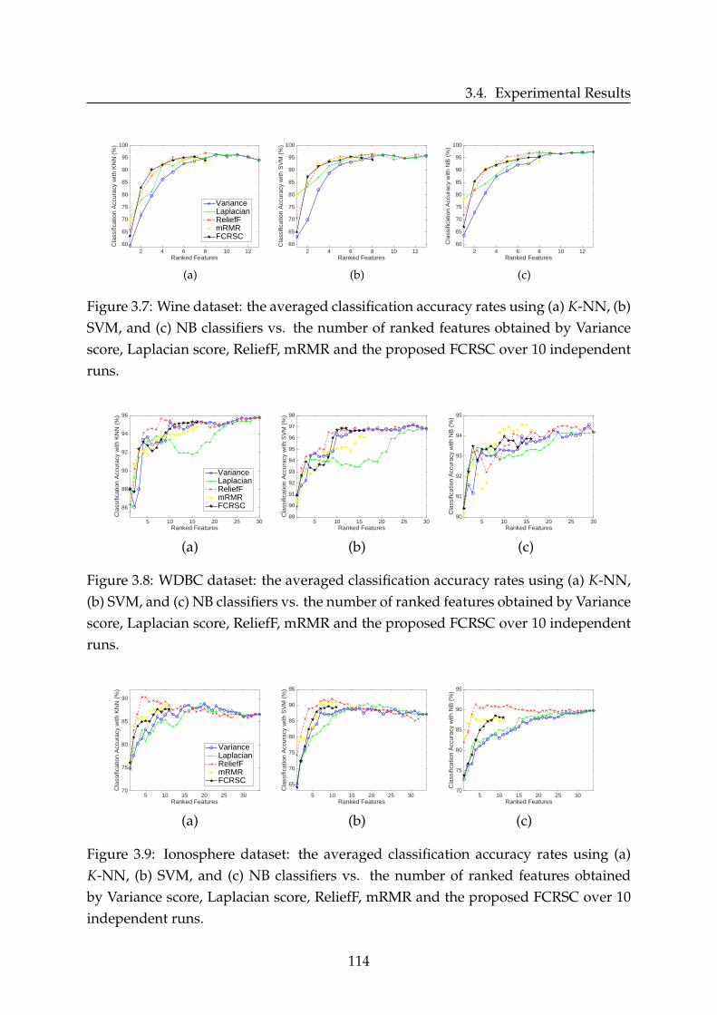
3.4. Experimental Results
2 4 6 8 10 12Ranked Features
60
65
70
75
80
85
90
95
100
Cla
ssifi
catio
n A
ccur
acy
with
KN
N (
%)
VarianceLaplacianReliefFmRMRFCRSC
(a)
2 4 6 8 10 12Ranked Features
60
65
70
75
80
85
90
95
100
Cla
ssifi
catio
n A
ccur
acy
with
SV
M (
%)
(b)
2 4 6 8 10 12Ranked Features
60
65
70
75
80
85
90
95
100
Cla
ssifi
catio
n A
ccur
acy
with
NB
(%
)
(c)
Figure 3.7: Wine dataset: the averaged classification accuracy rates using (a) K-NN, (b)SVM, and (c) NB classifiers vs. the number of ranked features obtained by Variancescore, Laplacian score, ReliefF, mRMR and the proposed FCRSC over 10 independentruns.
5 10 15 20 25 30Ranked Features
86
88
90
92
94
96
Cla
ssifi
catio
n A
ccur
acy
with
KN
N (
%)
VarianceLaplacianReliefFmRMRFCRSC
(a)
5 10 15 20 25 30Ranked Features
89
90
91
92
93
94
95
96
97
98
Cla
ssifi
catio
n A
ccur
acy
with
SV
M (
%)
(b)
5 10 15 20 25 30Ranked Features
90
91
92
93
94
95
Cla
ssifi
catio
n A
ccur
acy
with
NB
(%
)
(c)
Figure 3.8: WDBC dataset: the averaged classification accuracy rates using (a) K-NN,(b) SVM, and (c) NB classifiers vs. the number of ranked features obtained by Variancescore, Laplacian score, ReliefF, mRMR and the proposed FCRSC over 10 independentruns.
5 10 15 20 25 30Ranked Features
70
75
80
85
90
Cla
ssifi
catio
n A
ccur
acy
with
KN
N (
%)
VarianceLaplacianReliefFmRMRFCRSC
(a)
5 10 15 20 25 30Ranked Features
65
70
75
80
85
90
95
Cla
ssifi
catio
n A
ccur
acy
with
SV
M (
%)
(b)
5 10 15 20 25 30Ranked Features
70
75
80
85
90
95
Cla
ssifi
catio
n A
ccur
acy
with
NB
(%
)
(c)
Figure 3.9: Ionosphere dataset: the averaged classification accuracy rates using (a)K-NN, (b) SVM, and (c) NB classifiers vs. the number of ranked features obtainedby Variance score, Laplacian score, ReliefF, mRMR and the proposed FCRSC over 10independent runs.
114
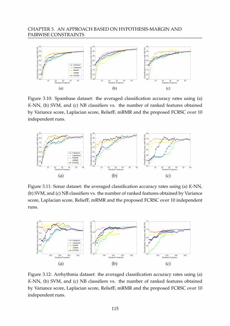
CHAPTER 3. AN APPROACH BASED ON HYPOTHESIS-MARGIN ANDPAIRWISE CONSTRAINTS
10 20 30 40 50Ranked Features
60
65
70
75
80
85
90
95
Cla
ssifi
catio
n A
ccur
acy
with
KN
N (
%)
Variance
Laplacian
ReliefF
mRMR
FCRSC
(a)
10 20 30 40 50Ranked Features
60
65
70
75
80
85
90
95
Cla
ssifi
catio
n A
ccur
acy
with
SV
M (
%)
(b)
10 20 30 40 50Ranked Features
60
65
70
75
80
85
90
95
Cla
ssifi
catio
n A
ccur
acy
with
NB
(%
)
(c)
Figure 3.10: Spambase dataset: the averaged classification accuracy rates using (a)K-NN, (b) SVM, and (c) NB classifiers vs. the number of ranked features obtainedby Variance score, Laplacian score, ReliefF, mRMR and the proposed FCRSC over 10independent runs.
10 20 30 40 50 60Ranked Features
50
55
60
65
70
75
80
85
Cla
ssifi
catio
n A
ccur
acy
with
KN
N (
%)
VarianceLaplacianReliefFmRMRFCRSC
(a)
10 20 30 40 50 60Ranked Features
50
55
60
65
70
75
80
85
Cla
ssifi
catio
n A
ccur
acy
with
SV
M (
%)
(b)
10 20 30 40 50 60Ranked Features
50
55
60
65
70
75
80
Cla
ssifi
catio
n A
ccur
acy
with
NB
(%
)
(c)
Figure 3.11: Sonar dataset: the averaged classification accuracy rates using (a) K-NN,(b) SVM, and (c) NB classifiers vs. the number of ranked features obtained by Variancescore, Laplacian score, ReliefF, mRMR and the proposed FCRSC over 10 independentruns.
100 150 200 250Ranked Features
46
48
50
52
54
56
Cla
ssifi
catio
n A
ccur
acy
with
KN
N (
%)
VarianceLaplacianReliefFmRMRFCRSC
(a)
100 150 200 250Ranked Features
55
60
65
70
Cla
ssifi
catio
n A
ccur
acy
with
SV
M (
%)
(b)
100 150 200 250Ranked Features
55
60
65
70
75
Cla
ssifi
catio
n A
ccur
acy
with
NB
(%
)
(c)
Figure 3.12: Arrhythmia dataset: the averaged classification accuracy rates using (a)K-NN, (b) SVM, and (c) NB classifiers vs. the number of ranked features obtainedby Variance score, Laplacian score, ReliefF, mRMR and the proposed FCRSC over 10independent runs.
115

3.4. Experimental Results
On the other side, on Spambase dataset, as can be seen in Figure (3.10), feature se-lection was generally not significant by all algorithms (the best accuracy was obtainedon the original feature set) except for ReliefF and mRMR with NB classifier shownin Figure (3.10c). However, the performance of FCRSC was generally stable with thethree used classifiers. It lies between the supervised and unsupervised methods exceptfor SVM classifier presented in Figure (3.10b) where both the unsupervised methodstogether with FCRSC outperformed mRMR. In addition, the results on Sonar and Ar-rhythmia were interesting, where as can be seen in Figure (3.11a) on Sonar dataset,both Variance and Laplacian scores reached their highest accuracy rates (82.03%) onthe full feature space of Sonar dataset i.e 60 features, whereas FCRSC obtained an ac-curacy of 83.04% over only 37 features. This shows that, in this case, Variance andLaplacian scores could not obtain a smaller feature subset that can provide a similaror better classification than the original one. It is important here to note that, the per-formance degradation of FCRSC that appeared between approximately the 27th and37th features on Sonar with C4.5 classifier (analyzed in the previous section and pre-sented in Figure (3.6c)) was classifier-related since a good performance was obtainedfor the same features using K-NN, SVM and NB classifiers.
On the other hand, Figure (3.12) on Arrhythmia, also shows that FCRSC outper-forms the unsupervised algorithms and competes with the supervised ones. In fact, itwas also able to obtain either a similar or a higher classification accuracy compared tothe one obtained by the full feature space with approximately only half the number offeatures. For example, an accuracy of 55.3% on 117 feature was recorded using FCRSCwith KNN (Figure (3.12a)) compared to 52.93% on 279 features without feature selec-tion and 55.5% on 141 features using ReliefF and mRMR.
In conclusion, FCRSC aims at finding a relevant and non-redundant feature subsetthat is said to either maintain the classification accuracy obtained on the full featurespace or provide an enhanced accuracy performance (through removing the irrelevantand noisy features). It is important to note that although FCRSC chooses a final subsetof features (size(Fs) < F), it is still a ranking feature selection method, which means,similarly to the other feature selection methods mentioned in this paper, subsets thatare also smaller than Fs can be obtained. Moreover, as FCRSC utilizes the ReliefF-Sc algorithm for its margin maximization objective, it was clear from the results thatremoving redundant features in addition to irrelevant ones allows better classificationperformance. Finally, using more than one classifier with different decision-makingnatures provided a fair evaluation of the used filter feature selection methods and
116

CHAPTER 3. AN APPROACH BASED ON HYPOTHESIS-MARGIN ANDPAIRWISE CONSTRAINTS
proved the general independence between them and the classifiers.
3.4.2.5 Comparison in terms of Running Time
In this section, we consider the different supervised, unsupervised and semi-supervisedfeature selection methods from the execution time perspective. Thus, Table 3.9 presentsthe average execution time (in ms) of each feature selection method over 10 indepen-dent runs.
Table 3.9: Average execution time (in ms) of the different Unsupervised, Supervised,and Semi-supervised feature selection methods over 10 independent runs.
Dataset
Feature Selection method
Unsupervised Supervised Semi-supervised
Variance Laplacian ReliefF mRMR Simba-Sc ReliefF-Sc FCRSC
Wine 0.41 9.06 71.62 13.66 569.04 1.70 9.61WDBC 0.81 73.68 205.70 43.25 3166.88 5.97 47.31
Ionosphere 0.34 29.66 128.20 28.39 1032.83 2.50 41.80Spambase 1.92 5408.62 15290.15 342.65 67081.99 755.62 1905.42
Sonar 0.59 16.06 108.83 35.76 694.99 2.73 89.55Arrythmia 2.46 93.64 4727.31 446.71 1336.32 5.47 1463.52
Average 1.09 938.45 3421.97 151.73 12313.67 129.00 592.87
For instance, from this table we can see that, Variance score, as expected, had theleast execution time with the least differences between datasets since it is the simplestmethod among all. However, Laplacian, ReliefF and Simba-Sc appeared to have agreat increase in execution time as the number of data points increase significantly aswas the case between Spambase (4601 data points) and Sonar (208 data points) withapproximately equal number of features. Although ReliefF-Sc and FCRSC also had asignificant increase in the latter case, this increase was less steep.
Noting that Simba-Sc, ReliefF-Sc and FCRSC are all dependent on constraints andare provided with the same number on each dataset, we declare that Simba-Sc con-sumes much more time due to it being repeated from 5 different starting points (gradi-ent ascent method) to optimize its objective function. On the other side, as the numberof features increase significantly between 13 for Wine and 60 for Sonar (having closenumber of data points and same number of provided constraints i.e 20) the executiontime by all the algorithms increased reasonably, however, ReliefF-Sc increased verylittle compared to FCRSC, and this is due to the time needed by FCRSC to apply the
117

3.5. Conclusion
steps of feature clustering and cluster-representative choosing.
Hence, the overall average execution time for each method on all datasets, as can beseen in the last row of Table 3.9, shows that FCRSC was generally faster than Laplacian,ReliefF, and Simba-Sc. Thus, in terms of computational complexity, we can say thatFCRSC is mainly related to the following:
• the number of cannot-link constraints card(CL)
• the number of data points N
• the dimension of feature space F
In big O notation, the constrained ReliefF-Sc can be calculated in O(card(CL)× NF).Also, the ranking step that is used within all ranking feature selection methods needsO(F × log(F)). The proposed FCRSC is divided into multiple steps some of whichcan be done in parallel (clustering the features and calculating their margin weights).For instance, the construction of the sparse graph costs O(F2) [47], the single linkagehierarchical clustering of features also needs O(F2). Hence, the overall computationalcomplexity by FCRSC can be calculated as O(Max(card(CL)× NF, F2, F× log(F))).
3.5 Conclusion
To deal with data high dimensionality in a semi-supervised context, we discussedmargin-based feature selection algorithms with side pairwise constraints. Consider-ing only cannot-link constraints due to their conceptual importance from the margin’sperspective and their ease of acquirement, we suggested Relief-Sc algorithm. It uti-lizes the cannot-link constraints to assign weights to different features according totheir contribution in maximizing the hypothesis-margin. Relief-Sc is capable of find-ing a unique relevant feature subset in a closed-form. Experimental results on multi-ple UCI machine learning and two high dimensional gene-expression datasets provedthat Relief-Sc can obtain comparable performances with supervised Fisher Score usingfull class labels on the entire training set, and has better performance than the otherconstrained Score Simba-Sc. Note that in [107], they concluded that Simba-Sc had bet-ter performance than Constraint Score-1 and Constraint Score-2, this means Relief-Scalso has better performance than these two scores. Moreover, Relief-Sc can work onlyon few constraints from the training set, which ensures computational advantage overother algorithms when dealing with high dimensional data. A robust version of Relief-Sc, called ReliefF-Sc, was also suggested.
118

CHAPTER 3. AN APPROACH BASED ON HYPOTHESIS-MARGIN ANDPAIRWISE CONSTRAINTS
In addition, a novel combination of feature clustering upon a sparse graph witha margin-based objective function called FCRSC was proposed. This approach issaid to handle the two core aspects of feature selection (relevancy and redundancy)in three main building blocks where it first constructs the similarity matrix betweenfeatures through sparse representation. Secondly, on top of the latter, feature clus-tering is applied simultaneously with the application of the margin-based algorithmReliefF-Sc. Finally, FCRSC obtains its final feature subset by choosing the featurethat most enlarges the margin from each cluster of features, hence, maximizing rel-evancy while minimizing redundancy. The efficiency of this approach was comparedto supervised, unsupervised and semi-supervised filter feature selection methods us-ing four different classification schemes on six UCI well-known benchmark machinelearning datasets. The results showed the satisfactory performance of FCRSC that out-performed the unsupervised and semi-supervised methods on most datasets and alsocompeted with the supervised ones.
119


Chapter 4Active Learning of Pairwise Constraints
Contents4.1 Introduction . . . . . . . . . . . . . . . . . . . . . . . . . . . . . . . . . . 121
4.2 Related Work . . . . . . . . . . . . . . . . . . . . . . . . . . . . . . . . . 124
4.2.1 Constraints Selection . . . . . . . . . . . . . . . . . . . . . . . . . 124
4.2.2 Constraints Propagation . . . . . . . . . . . . . . . . . . . . . . . 125
4.3 Active learning of Constraints . . . . . . . . . . . . . . . . . . . . . . . 128
4.3.1 Using Graph Laplacian . . . . . . . . . . . . . . . . . . . . . . . 128
4.3.2 Active Constraint Selection . . . . . . . . . . . . . . . . . . . . . 129
4.4 Propagation of Actively Selected Constraints . . . . . . . . . . . . . . 134
4.5 Complexity Analysis . . . . . . . . . . . . . . . . . . . . . . . . . . . . . 141
4.6 Experimental Results . . . . . . . . . . . . . . . . . . . . . . . . . . . . 141
4.6.1 Used Benchmarking Feature Selection Methods . . . . . . . . . 141
4.6.2 Datasets Description and Parameter Setting . . . . . . . . . . . . 142
4.6.3 Performance Evaluation Measures . . . . . . . . . . . . . . . . . 144
4.6.4 Performance Evaluation Results . . . . . . . . . . . . . . . . . . 146
4.7 Conclusion . . . . . . . . . . . . . . . . . . . . . . . . . . . . . . . . . . 160
4.1 Introduction
As explained in the previous chapter, our proposed algorithms Relief-Sc, ReliefF-Scand FCRSC are all constrained semi-supervised algorithms that particularly utilize
121

4.1. Introduction
cannot-link constraints. As a reminder, pairwise constraints are a cheaper kind ofsupervision information that does not need to reveal the class labels of data points.Initially, constraints were suggested to augment the performance of traditional clus-tering algorithms by increasing the semantic meaningfulness of the resulting clusters[136]. Accordingly, many algorithms used them to enhance clustering tasks [137–141],but only few considered using them for feature selection (e.g. [107, 142]).
However, in most current methods, pairwise constraints are said to be providedpassively and generated randomly over multiple algorithmic runs by which the resultsare averaged. This leads to the need for a large number of constraints that might be re-dundant, unnecessary, and under some circumstances even inimical to the algorithm’sperformance. It also masks the individual effect of each constraint set and introducesa human labor-cost burden. Although it was assumed by the machine learning com-munity that adding constraints as supervision information will guide and improveclustering performance, Davidson et al. [57] stated that the latter can still be degradedeven when constraints are random but directly generated from data labels. It is thenexpected that the used constraints can affect the performance of constrained featureselection methods just like they affect constrained clustering.
Therefore, in this chapter, we suggest a framework for actively selecting and thenpropagating these constraints for feature selection. This framework has three maincomponents. (1) The feature selection algorithm that utilizes constraints (detailed insections 3.2.2 and 3.2.3, (2) our core contribution i.e. the process of selecting these con-straints, and (3) the augmentation of supervision information through propagatingthem. In this chapter, we introduce the second two components:
• First, we target the process of systematically and actively selecting the constraintsbased on the idea of matrix perturbation [143]. Accordingly, we benefit from thespectral characteristics of the graph Laplacian which by turn is defined on thesimilarity matrix. The impact of each data couple (pairwise constraint) on thismatrix can be reflected by the change it can cause to the graph Laplacian, espe-cially to its eigensystem. When a small perturbation in the similarity value of acouple is able to perturb the graph Laplacian leading to a more well-separatedform of the second eigenvector, this couple is definitely considered more impor-tant and significant as a constraint. Therefore, we propose an Active ConstraintSelection (ACS) method based on a second-eigenvector sensitivity criterion. Itaims at seeking those data couples with the highest ability to change the posi-tion of the most uncertain points (i.e. near zero) on the second eigenvector to
122

CHAPTER 4. ACTIVE LEARNING OF PAIRWISE CONSTRAINTS
one of the two certain groups, thus, dividing the data into two well-separatedgroups. The latter couples will be the only ones queried for constraints, hence,reducing the cost of queries. In fact, these constraints that can decrease uncer-tainty and enhance class-separation, allow the selection of relevant features withthe highest class-discriminative ability.
• Second, as we aim to query an oracle for the constraints, we are able to ask onlya specific number of questions before this process gets inefficient and not user-friendly. Furthermore, for the family of margin-based algorithms, a sufficient setof points is needed to calculate the margin [2]. Thus, we adapt an exhaustivepropagation method that allows spreading the constraints to the neighborhoodof our initially instance-level selected ones. As this propagation produces softconstraints between data points, we also suggest thresholding for pruning theresults and avoiding noisy constraints.
These two components together with ReliefF-Sc (section 3.2.3) form our pro-posed framework of active constraint selection and propagation for feature se-lection.
In order to validate our framework, we apply a series of experiments. First, we com-pare the classification accuracies of our proposed ReliefF-Sc with random constraintsgeneration (RCG) to itself but with active constraint selection (ACS). Then, the latter iscompared to Relief-Sc with the propagation of active constraint selection (PACS). Sec-ond, we compare the accuracies obtained by different well known supervised, unsu-pervised, and constrained feature selection algorithms when utilizing RCG and ACS.These experiments are applied on multiple well-known UCI machine learning datasetsand two high-dimensional gene expression ones.
This chapter is structured as follows: in section 4.2, we explain some related workto constraints selection and propagation. In section 4.3, we explain our active con-straint selection method while providing the needed background. In section 4.4, wedetail our adaption of the constraint propagation method. Section 4.5 discusses thecomputational complexity of our method. The experimental results on the perfor-mance of feature selection after constraint selection and propagation are discussed insection 4.6. Finally, we conclude in section 4.7.
123

4.2. Related Work
4.2 Related Work
Since it is much easier to obtain pairwise relations between data points than to obtaintheir class labels, many pieces of research considered solving real-life problems usingthem instead. As a result, it was important to navigate through available methods tounderstand how a more beneficial constraint set can be chosen.
4.2.1 Constraints Selection
Davidson et al. [57] suggested two measures namely "informativeness" and "coher-ence" of constraints in order to measure their utility, they also stated that the degradedperformance after using a constraint set is not due to noisy or erroneous constraintsbut instead due to the interaction between this set and specifically the characteristicsof the used algorithm. Although the two latter suggested notions were tailored to aclustering framework, they could be applied as two standalone measures indepen-dently of the learning model. Therefore, Benabdeslem and Hindawi [54] adopted thenotion of "coherence" to measure the utility of constraints for their feature selectionconstrained Laplacian Score. Note that "informativeness" and "coherence" ensured"Direct constraint satisfaction" by which a must-link constraint is treated in a way thatits two endpoints are close to each other and a cannot-link constraint is treated in away that its two endpoints are ensured to be well-separated.
Furthermore, instance-level constraints can be generated from background knowl-edge given by an expert i.e querying an oracle, or by acquiring them from a set oflabeled data [138, 144]. The second way of generating constraints was more actuallyused except when actively choosing constraints is the goal [139]. In fact, whatever waywe choose to acquire constraints, measuring their utility is a good practice. Abin andBeigy [140] measured constraints utility actively using two assumptions. The first onestates that a constraint is considered more informative if it is a cannot-link constraintjoining two close data points, whereas the second assumption states that a constraint isconsidered more informative if it is a must-link constraint joining two far data points.The latter two assumptions give important spatial information about the data. More-over, they used a Support vector data description (SVDD) to find the support vectorsin the dataset and then generate constraints only from the points that are on the bound-ary, thus shaping the data. To make the best of the chosen constraints, they avoidedinformation redundancy by choosing distant constraints. This means that when twoconstraints of the same type are available in the same vicinity, only one of them is con-sidered.
124

CHAPTER 4. ACTIVE LEARNING OF PAIRWISE CONSTRAINTS
Similarly, [145] suggested active spectral clustering method "Access" that examinesthe eigenvectors of the graph Laplacian. It uses the theoretical properties of spectraldecomposition to identify data items that are located on the boundaries of clusters(boundary points and sparse points). It aimed to reduce the human interaction bur-den by actively obtaining constraints on these particular boundary points. However, itwas closely related to the assumption of having data with very close clusters or over-lapping boundaries and that the only reason for degraded performance is boundarypoints.
Another significant approach proposed by Wauthier et al. was to actively guide aspectral clustering algorithm to incrementally measure similarities that are most likelyto reduce uncertainty [141]. Particularly, they study the trade-off between desired clus-tering quality and the amount of available information about the data. This trade-offis studied in the framework of spectral clustering by which not all pairwise similar-ity measurements are available initially. For that, they maintain estimations of truesimilarities as baselines. Then, they iteratively query an external black-box (e.g. a hu-man expert) on points that show the highest uncertainty in the clustering task. It wasstated that most realistic pairwise similarity matrices do exhibit some clustering struc-ture even when incomplete. However, the selection of the most uncertain data pair, inthis case, can be seen as a constraints selection problem by showing that the utility ofhaving information of this particular couple is high.
4.2.2 Constraints Propagation
Generally, as the number of constraints is quadratically related to that of data points,it is only feasible to query for a small proportion of all possible constraints before theprocess turns to be resource-expensive, even when we utilize an inexpensive oracle[146]. Thus, in real-life scenarios, we might not be able to ask for a large number ofqueries and might have to work with the minimum but sufficient amount of data fromthe "constraint selection" step.
In [147], kamvar et al. just trivially modified the values of the similarity matrixto 1 and 0 where a must-link or a cannot-link constraint is present respectively. Thismethod barely affects spectral clustering results because only similarities between con-strained pairs are changed. In order to allow pairwise constraints to exert a strongereffect on spectral clustering, Lu and Ip [148] presented an exhaustive and efficientmethod for constraint propagation. They applied propagation by decomposing the
125
4.2. Related Work
process into sub-propagation-problems and then solving each of the subproblems in-dependently based on local K-NN graphs. It was noted that this method was thefirst to tackle constraint propagation to the entire dataset with computational effi-ciency. Moreover, as propagation is a pre-step done independently from the clusteringmethod, it can be used with different constrained clustering methods only by adjust-ing the affinity matrix accordingly. This method is not limited to two-class problems,allows soft constraints, and results in a closed-form solution.
From a different point of view, Klein et al. [144] tackled space-level informationgiven by constraints instead of only satisfying individual instance-level constraints,which means, a cannot-link constraint not only tells that its endpoints should be indifferent clusters, but also their nearby points should be similarly separated. Theyalso propagated must-link constraints by modifying the actual distance or similaritygraph and then applying unsupervised clustering on the modified graph. This implic-itly holds the neighborhood-based constraints information. However, they stated thatit was harder to maintain cannot-link constraints and used a proximity-based cluster-ing algorithm to propagate their information.
On the other hand, Lu and Carreira-Perpinan [137] also researched constraint prop-agation and suggested a method for affinity propagation that utilizes the limited avail-able pairwise constraints to change their corresponding values within the affinity ma-trix according to their positions through a Gaussian process. This method deals withmulti-class problems through applying an heuristic search over the different cannot-link constraints. Another idea was to extend an exemplar-based clustering algorithm[149] to work in a semi-supervised context with propagating instance-level constraints[150]. This method modified the factor-graph to include meta-points (MTPs) that cantake the role of exemplars. For instance, by enforcing constraints on these MTPs andthen changing the similarities between points accordingly, affinity propagation is ob-tained. Furthermore, a semi-definite programming problem (SDP) that is also not lim-ited to two-class problems was used by [151] to apply such constraint propagation butincurring a high computational cost.
When working in a semi-supervised context consistency is an important assump-tion. It means that points in the same neighborhood or on the same manifold areconsidered belonging to the same cluster. The latter, also known as cluster assump-tion, takes two different levels. When a neighborhood-based algorithm is used, thelevel is said to be local, whereas when the algorithm is structure-based, the level is
126
CHAPTER 4. ACTIVE LEARNING OF PAIRWISE CONSTRAINTS
said to be global. For instance, Zoidi et al. [152] modified the method suggested in[153] to handle propagating pairwise constraints within a "Multiple Locality Preserv-ing Projections with Cluster-based Label Propagation" (MLPP-CLP) framework, a newmethod for propagating person identity labels on facial images, this method used twotypes of knowledge: a projection matrix that holds the locality information from mul-tiple image representations and a priori pairwise must-links and cannot-links. Duringthe projection phase, both the propagated constraints and the Locality Preserving Pro-jections (LPP) are used to find a projection matrix that respects pairwise constraints,maps data to a space of reduced dimensionality and retains the locality information ofdata. For instance, data that are must-linked should be mapped close to each other anddata that are cannot-linked must be mapped far away from each other. To propagateconstraints, they modified the smooth iterative graph-based label propagation func-tion that utilizes an initial set of given labeled points to predict the labels of unlabeledones. The input of the function was changed to be the initial constraint matrix insteadof the initial label matrix, thus, the output is a neighborhood of propagated constraintsinstead of a matrix of predicted labels. It finally converges to a closed-form solution offully propagated constraints. Nevertheless, this method finds application when thereare multiple representations of data such as the case of multi-view camera systems.
From a different perspective, Wang et al. [154] answered the question of how to learnconstraints through self-learning, thus transforming the work from expert teaching toself-teaching. The latter transition tackles the problem of incrementally polling an ora-cle for new constraints and minimizes the number of queries needed from the humanexperts. Briefly, they suggested extending the objective function of spectral clusteringsuch that new constraints can be self-taught according to the graph affinity matrix andthe few available prior knowledge (constraints). This work is considered as "transfer-ring knowledge" since unconstrained data is gaining information through augmentedconstraints. But unlike other transfer learning settings, this framework has one do-main only (affinity graph) and one task (clustering). It was claimed that this frame-work was the first to combine graph min-cut with matrix completion into an iterativeself-teaching process. As they explained, spectral clustering had many advantagesover other clustering schemes like its simple objective function, its easy implementedclosed-form solution, and its ability of modeling arbitrarily shaped clusters. Yet, itgreatly depends on the completeness and correctness of the data graph.
127

4.3. Active learning of Constraints
4.3 Active learning of Constraints
Since feature selection by ReliefF-Sc closely depends on the used constraint set, weextend to study thoroughly the systematic and active selection of the constraints thatwill be used by this algorithm. Accordingly, we focus on cannot-link constraints asthey are considered more important than must-link constraints from the margin’s per-spective.
As we mentioned before, pairwise constraints were mostly used in constrained clus-tering problems to actively improve and guide clustering [139, 144, 145, 155]. Onlyfew used them similarly in feature selection [107, 142]. As mentioned before, utiliz-ing pairwise constraints does not necessarily improve clustering performance in thesense of increased agreement between the estimated clusters and the actual ones [57].Even when some constraint sets are generated from data labels directly, they can stilldecrease clustering performance. Moreover, Davidson et al. [57] proved that the per-formance degradation or stability is not always due to false constraints, but sometimesdue to ill interactions between a chosen constraint set and the objective function of theclustering algorithm used. Later, many pieces of research aimed at understandinghow a more beneficial constraint set can be chosen [58, 140, 141].
Therefore, in the following sections, we first give a brief background on how we usegraph Laplacian in 4.3.1 and then we detail the process of selecting constraints basedon the graph Laplacian eigen-decomposition for feature selection instead of clusteringin 4.3.2.
4.3.1 Using Graph Laplacian
This section closely depends on the definitions in section 1.3.2. For instance, for thedataset X with N points, we have an NxN symmetric similarity matrix S that holdspairwise similarities between all data points as defined in Equation (1.4). Simply, eachpairwise similarity, denoted snm, is within the range 0 ≤ snm ≤ 1: n,m = 1, ..., N andsince self-edges do not alter the graph Laplacian matrix, we set snn = 0. This similar-ity matrix is computed in some problem-specific manner using the self-tuning (auto-adaptive) method by [41] that utilizes a user-specified parameter representing a num-ber of the nearest-points to each data point to be considered for calculating the disper-sion parameter automatically for evaluating the Gaussian Kernel (Equation (1.5)).
Let D be the degree diagonal matrix defined in Equations (1.8) and (1.9). In our work,
128
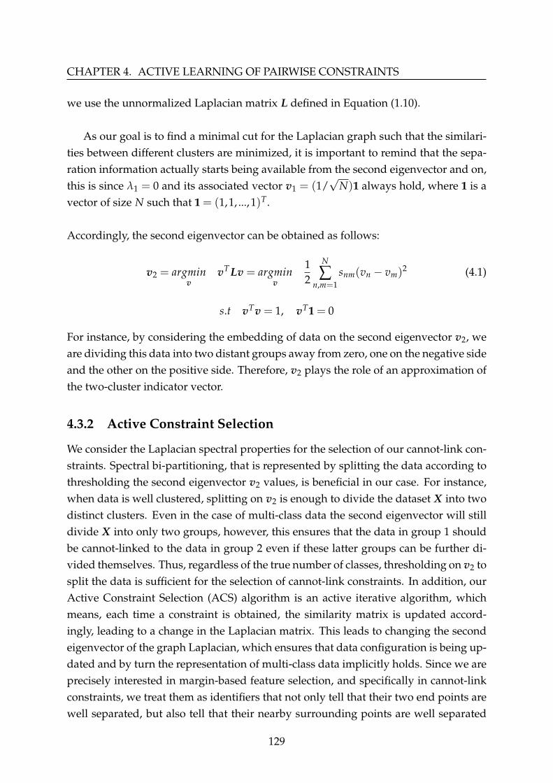
CHAPTER 4. ACTIVE LEARNING OF PAIRWISE CONSTRAINTS
we use the unnormalized Laplacian matrix L defined in Equation (1.10).
As our goal is to find a minimal cut for the Laplacian graph such that the similari-ties between different clusters are minimized, it is important to remind that the sepa-ration information actually starts being available from the second eigenvector and on,this is since λ1 = 0 and its associated vector v1 = (1/
√N)1 always hold, where 1 is a
vector of size N such that 1 = (1,1, ...,1)T.
Accordingly, the second eigenvector can be obtained as follows:
v2 = argminv
vT Lv = argminv
12
N
∑n,m=1
snm(vn − vm)2 (4.1)
s.t vTv = 1, vT1 = 0
For instance, by considering the embedding of data on the second eigenvector v2, weare dividing this data into two distant groups away from zero, one on the negative sideand the other on the positive side. Therefore, v2 plays the role of an approximation ofthe two-cluster indicator vector.
4.3.2 Active Constraint Selection
We consider the Laplacian spectral properties for the selection of our cannot-link con-straints. Spectral bi-partitioning, that is represented by splitting the data according tothresholding the second eigenvector v2 values, is beneficial in our case. For instance,when data is well clustered, splitting on v2 is enough to divide the dataset X into twodistinct clusters. Even in the case of multi-class data the second eigenvector will stilldivide X into only two groups, however, this ensures that the data in group 1 shouldbe cannot-linked to the data in group 2 even if these latter groups can be further di-vided themselves. Thus, regardless of the true number of classes, thresholding on v2 tosplit the data is sufficient for the selection of cannot-link constraints. In addition, ourActive Constraint Selection (ACS) algorithm is an active iterative algorithm, whichmeans, each time a constraint is obtained, the similarity matrix is updated accord-ingly, leading to a change in the Laplacian matrix. This leads to changing the secondeigenvector of the graph Laplacian, which ensures that data configuration is being up-dated and by turn the representation of multi-class data implicitly holds. Since we areprecisely interested in margin-based feature selection, and specifically in cannot-linkconstraints, we treat them as identifiers that not only tell that their two end points arewell separated, but also tell that their nearby surrounding points are well separated
129

4.3. Active learning of Constraints
too. In our case, this local consistency hypothesis is respected and assumed to betrue. Accordingly, we follow the logic of spectral analysis and benefit from the spec-tral properties of the graph Laplacian of data.
As we mentioned in section 4.3.1, upon embedding the data on v2, they are pro-jected as two distant groups away from zero, one on the negative side and the otheron the positive side, hence, v2 plays the role of an approximation of the relaxed clusterindicator vector. For instance, Equation (4.1) shows that any point with approximatelyequal similarities snm : n,m = 1, ..., N to all other points, will be embedded close to theaverage of all the points locations on v2, which means, it will be embedded near zeroand considered an uncertain point. Nevertheless, using v2, we are not working on thereal feature space, but on an equivalent projected one. Therefore, we iteratively utilizethe perturbation analysis theory to actively find the couple in input space that has thegreatest first order derivative with respect to this minimum point on v2 [156, 157].
Theoretically speaking, our method initially starts with a complete matrix of sim-ilarities and then mainly captures the point of minimum magnitude on the estimated|v2| denoted v2(i∗) where i∗ = argmini∈{1...N}|v2(i)|. This point is considered the onewith highest uncertainty. The method then measures the sensitivity of v2(i∗) to thechange in snm, once it finds the similarity couple (xn, xm) that is most able to changethe embedding location of v2(i∗) on v2, only this couple is queried for a constraintand its corresponding similarity snm is amended accordingly. For instance, an externalsource of knowledge (e.g. an expert or a human oracle) is asked to observe the couple(x∗n, x∗m) and provide an answer about whether it should be a cannot-link or a must-linkconstraint. If it appears that the queried couple should be a cannot-link (or must-link)constraint then snm is changed to 0 (or 1). Finally, v2 is calculated again and the processiterates until finding the required number of constraints.
Similarly to [143] and [141], we search for the couple of highest impact on v2 using:
(xn∗ , xm∗) = argmax(n,m)
∣∣∣∣dv2(i∗)
dsnm
∣∣∣∣ (4.2)
where Equation (4.2) is evaluated according to the First-Order Eigenvector Perturba-tion theorem [156] as follows:∣∣∣∣dv2(i∗)
dsnm
∣∣∣∣ = ∣∣∣∣ N
∑p>2
vT2 [∂L/∂snm]vp
λ2 − λpvp(i∗)
∣∣∣∣ (4.3)
130
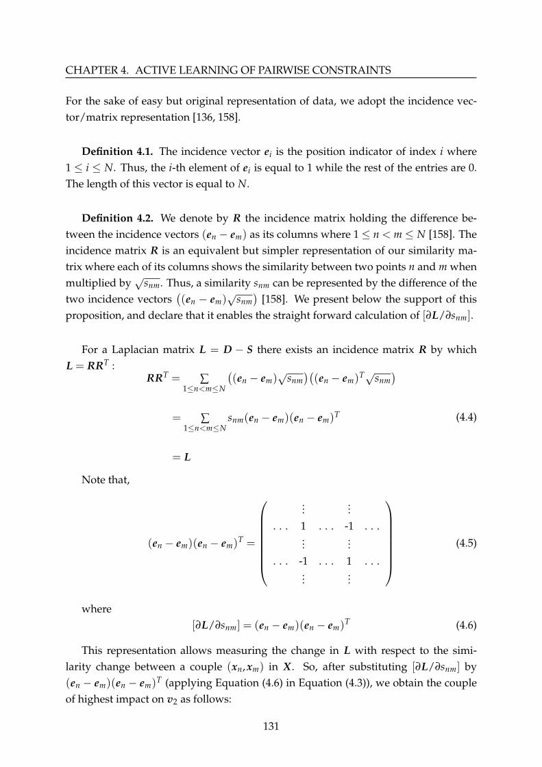
CHAPTER 4. ACTIVE LEARNING OF PAIRWISE CONSTRAINTS
For the sake of easy but original representation of data, we adopt the incidence vec-tor/matrix representation [136, 158].
Definition 4.1. The incidence vector ei is the position indicator of index i where1 ≤ i ≤ N. Thus, the i-th element of ei is equal to 1 while the rest of the entries are 0.The length of this vector is equal to N.
Definition 4.2. We denote by R the incidence matrix holding the difference be-tween the incidence vectors (en − em) as its columns where 1≤ n < m ≤ N [158]. Theincidence matrix R is an equivalent but simpler representation of our similarity ma-trix where each of its columns shows the similarity between two points n and m whenmultiplied by
√snm. Thus, a similarity snm can be represented by the difference of the
two incidence vectors((en − em)
√snm)
[158]. We present below the support of thisproposition, and declare that it enables the straight forward calculation of [∂L/∂snm].
For a Laplacian matrix L = D − S there exists an incidence matrix R by whichL = RRT :
RRT = ∑1≤n<m≤N
((en − em)
√snm)((en − em)T√snm
)= ∑
1≤n<m≤Nsnm(en − em)(en − em)T
= L
(4.4)
Note that,
(en − em)(en − em)T =
......
. . . 1 . . . -1 . . ....
.... . . -1 . . . 1 . . .
......
(4.5)
where[∂L/∂snm] = (en − em)(en − em)
T (4.6)
This representation allows measuring the change in L with respect to the simi-larity change between a couple (xn, xm) in X. So, after substituting [∂L/∂snm] by(en − em)(en − em)T (applying Equation (4.6) in Equation (4.3)), we obtain the coupleof highest impact on v2 as follows:
131

4.3. Active learning of Constraints
(xn∗ , xm∗) = argmax(n,m)
∣∣∣∣∑Np>2
vT2 [(en − em)(en − em)T]vp
λ2 − λpvp(i∗)
∣∣∣∣ (4.7)
Note that, since an uncertain couple is either uncertain due to having uncertainty onboth of its points or due to having at least one of them considered uncertain, it is pos-sible and common to have the point of minimum value on v2 as one of the points ofthe most sensitive couple (xn∗ , xm∗). The latter can be considered with the aim of de-creasing the search space to be N instead of N2.
Finally, once we have found the couples to be queried for constraints, we applyour feature selection method presented in Algorithm 3.2 on these constraints. It isimportant to note that when solving the hardest form of a specific problem, you im-plicitly solve the easier versions of it. Which means, selecting the most discriminativefeatures using the most confusing constraints implicitly holds feature selection on anyother true but random constraint. Algorithm 4.1 shows the detailed steps of our con-straint selection method.
Example:
To illustrate this method and highlight the significance of constraint selection, wepresent a toy example in Figure (4.1).
As can be seen in Figure (4.1a), the dataset is composed of 6 data points charac-terized by 3 features each. The scatter plot of these data points is presented in Figure(4.1b) where points 1, 2 and 3 are assigned to the first cluster and points 3, 4 and 5 areassigned to the second one. We also show the projection of these data points on thefirst feature A1, second feature A2 and third feature A3 in Figures (4.1c), (4.1d) and(4.1e) respectively. It is thus clear that the third feature A3 is the only one that can per-fectly assign the data points to their true clusters successfully. So, it is expected froman efficient feature selection method to identify feature A3 as the most relevant one.
When we first considered an unsupervised feature selection method, i.e the Lapla-cian score, it failed to identify the most relevant feature A3, instead, it chose A1 whichis known to be irrelevant as presented in Figure (4.1h). With the aim of improving fea-ture selection, we used our constrained margin-based semi-supervised method pre-sented in Algorithm 3.2 and called ReliefF-Sc.
132

CHAPTER 4. ACTIVE LEARNING OF PAIRWISE CONSTRAINTS
We first applied ReliefF-Sc on two randomly generated cannot-link constraints aspresented in Figure (4.1f), but surprisingly, the ranking of features did not change andA3 was still not identified as the most relevant feature correctly. Therefore, we consid-ered actively choosing the couples to be queried using Algorithm 4.1 before applyingReliefF-Sc again.
Figure (4.1i) shows the change in v2 during the process of selecting these constraints.It is divided into two steps. Step 1 shows that point 5 was the closest to zero on v2,hence it was considered the point with the highest uncertainty, i.e. i∗ = 5. As men-tioned before, a point is uncertain when it is not clear to which cluster it should beassigned. Accordingly, after evaluating the sensitivity of i∗ = 5 with respect to thedata couples, the couple (5, 2) was chosen to be queried for a constraint. The latterwas obtained from class labels in this example leading to a cannot-link constraint. Thesimilarity matrix is updated accordingly (s(5,2)=0) and the Laplacian matrix is recalcu-lated obtaining a different v2. Later, the updated v2 appears in the second graph of(4.1i) where the closest point to zero appeared to be point 3. Thus, as can be seen inStep 2 the second constraint (3, 6) was chosen similarly to Step 1. Finally, the selectedconstraints can be seen in Figure (4.1g) and the last update of v2 after finding the twoconstraints can be seen in the third graph of (4.1i) by which it appears that the twoclusters were well separable.The ranking of the constrained feature selection method ReliefF-Sc and the super-vised method ReliefF were identical as presented in Figure (4.1h). A3 was success-fully ranked as the most relevant feature, A1 the second, and the least relevant featureA2 was ranked the last as expected. Being able to reach the same ranking by ReliefF(supervised) using ReliefF-Sc (constrained) with active constraint selection (ACS) andnot with random constraint generation (RCG), shows the significance of choosing con-straints systematically.
One of the known drawbacks of the Relief family margin-based algorithms is thatdue to their initial supervised context, they need a set of points that is sufficientlybig to calculate the margin [2]. However, even inexpensive oracles can turn to beresource-expensive and impose high costs when queried for a large number of con-straints. Therefore, in our scenario, we should deal with a relatively small numberof constraints due to the nature of the this "Active Constraint Selection (ACS)" step.Hence, in the next section, we present a method that allows the automatic propaga-tion of these selected constraints to their unconstrained neighborhood.
133
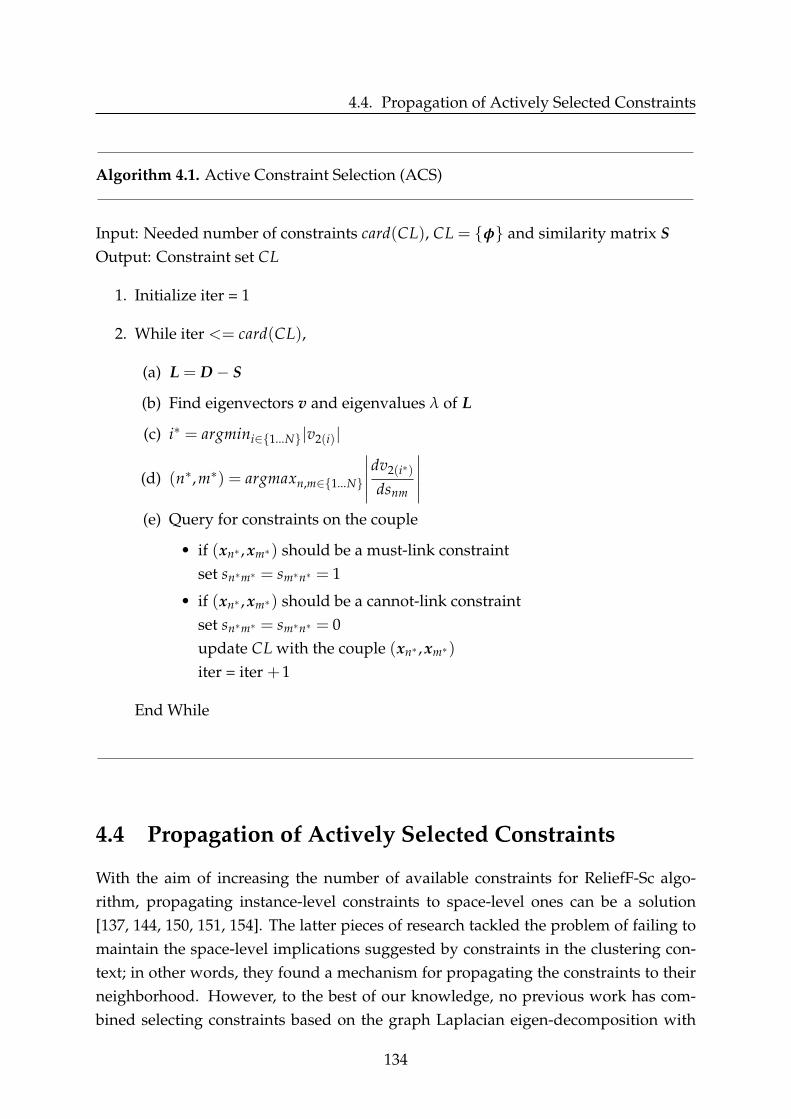
4.4. Propagation of Actively Selected Constraints
Algorithm 4.1. Active Constraint Selection (ACS)
Input: Needed number of constraints card(CL), CL = {φ} and similarity matrix SOutput: Constraint set CL
1. Initialize iter = 1
2. While iter <= card(CL),
(a) L = D− S
(b) Find eigenvectors v and eigenvalues λ of L
(c) i∗ = argmini∈{1...N}|v2(i)|
(d) (n∗,m∗) = argmaxn,m∈{1...N}
∣∣∣∣∣dv2(i∗)
dsnm
∣∣∣∣∣(e) Query for constraints on the couple
• if (xn∗ , xm∗) should be a must-link constraintset sn∗m∗ = sm∗n∗ = 1
• if (xn∗ , xm∗) should be a cannot-link constraintset sn∗m∗ = sm∗n∗ = 0update CL with the couple (xn∗ , xm∗)
iter = iter +1
End While
4.4 Propagation of Actively Selected Constraints
With the aim of increasing the number of available constraints for ReliefF-Sc algo-rithm, propagating instance-level constraints to space-level ones can be a solution[137, 144, 150, 151, 154]. The latter pieces of research tackled the problem of failing tomaintain the space-level implications suggested by constraints in the clustering con-text; in other words, they found a mechanism for propagating the constraints to theirneighborhood. However, to the best of our knowledge, no previous work has com-bined selecting constraints based on the graph Laplacian eigen-decomposition with
134

CHAPTER 4. ACTIVE LEARNING OF PAIRWISE CONSTRAINTS
(a) Dataset (b) 3D-scatter of data points
(c) Data projected on featureA1
(d) Data projected on featureA2
(e) Data projected on featureA3
(f) Random Constraint Gener-ation (RCG)
(g) Active Constraint Selection(ACS) by Algorithm 4.1
(h) Feature ranks by different Methods
Step 1:
i*=5 Obtained: (xn*, xm*)=(5,2) Query oracle for constraint Reply : cannot-link
⟹ Update S(5,2) = 0
⟹ Updated 𝒗𝟐 Step 2:
i*=3 Obtained: (xn*, xm*)=(3,6) Query oracle for constraint Reply : cannot-link
⟹ Update S(3,6) = 0
⟹ Updated 𝒗𝟐
(i) Changes in v2 during the process of Active Con-straint Selection where the x-axis holds the indexes ofdata points and the y-axis represents the values of thesedata points on v2
Figure 4.1: Three-dimensional Example Dataset: (a) Dataset, (b) 3D-scatter of datapoints; (c),(d),(e) Data projected on features A1, A2, A3 respectively; (i) shows changesin v2 during ACS; (g) shows the ACS by Algorithm 4.1; (f) shows RCG and (h) showsthe results of features ranked by different methods.
135

4.4. Propagation of Actively Selected Constraints
space-level constraints propagation for the sake of better feature selection.
To explain how propagation can affect feature selection, we show that while thefeatures selected in a constrained environment are consistent with the instance-levelconstraints themselves, they might not be consistent with the natural global implica-tions of these constraints. For example, in Figure (4.2) the true data partitioning isgiven in (4.2c) and Feature 2 should be selected, however, the two instance-level con-straints shown in (4.2b) might not be enough to select this feature based on Relief algo-rithm, on the contrary, Feature 1 is selected. When a stronger space-level propagationoccurs, it can change the results to clearly select Feature 2 as the data discriminatingfeature. Note that, the set of points in (4.2b) satisfies the cannot-link constraints, butFigure (4.2c), after propagation, shows a more intuitive partitioning for correct featureselection. Therefore, not only should points that are cannot-linked be in different clus-ters, but also their neighboring ones.
We thus explain the method we adapted to our scenario for propagating constraintsto the neighboring points surrounding our previously obtained ones using Algorithm4.1. It is intuitive to assume that if two points are cannot-linked, their nearest neigh-bors should also be cannot-linked due to neighboring point similarity rule. One mainobstacle known about propagating cannot-link constraints is that they are not transi-tive. On the contrary to working with a must-link propagation, if xm, xn are cannot-
(a) Data (b) Instance-levelcannot-link constraints
(c) Propagatedinformation
Figure 4.2: The effects of propagating cannot-link constraints to the data in (a): know-ing that the true partitioning is shown in (c) and that Feature 2 should be selected, twoinstance-level constraints only may be not enough to select Feature 2 based on Relieffamily distance-based feature selection (b); Whereas, a stronger space-level propaga-tion changes results to clearly select Feature 2 as the data discriminative feature (c).
136

CHAPTER 4. ACTIVE LEARNING OF PAIRWISE CONSTRAINTS
linked and xn, xj are cannot-linked we can’t derive the conclusion that xm, xj are alsocannot-linked. Therefore, we decide to generalize the cannot-link constraints that weinitially have to include neighboring points. This is done through an iterative proce-dure that is not limited to two-class problems, allows soft constraints, and convergesto a closed form solution with computational efficiency.To increase the number of pairwise constraints with the aim of exerting a stronger ef-fect on the constrained learning process, in [148], they presented an exhaustive andefficient method for constraints propagation. Since this propagation method is usu-ally applied as a pre-step independently from clustering, it is possible to use it beforeany other constrained learning method to be enhanced; just like filter-type methods infeature selection.
Definition 4.3. We denote by Q = {Qnm}N×N the initial indicator sparse matrix ofcannot-link constraints obtained by Algorithm 4.1 as:
Qnm =
{1, if (xn, xm) ∈ CL0, otherwise
(4.8)
Note that, in this paper, we are interested in propagating our actively chosen cannot-link pairwise constraints in order to provide more information to Relief-Sc for apply-ing margin-based feature selection, this is why the indicator matrix Qnm holds onlycannot-link constraints.
Although the method by [152] is capable of applying vertical constraint propa-gation, i.e along the columns of the initial constraint matrix Q, sometimes a columnmight not contain any pairwise constraint, this means that all the cells of this columnmight have the value of zero and therefore no vertical constraint propagation can beobtained for this particular column. Thus, [148] not only modified the label propaga-tion method to a constraint propagation one, but also solved empty constraint columnproblem by two exhaustive and efficient vertical and horizontal propagation steps.The latter step is usually applied after finishing vertical propagation in an iterativeapproach, and leads to a full matrix that contains a constraint between every two datapoints in X.
Similarly to [148] and [153], we use the normalized similarity graph to propagatethe constraints in a data-specific manner. For that, we denote by {Pnm}N×N the neigh-
137

4.4. Propagation of Actively Selected Constraints
borhood matrix calculated as follows:
P = D−12 SD−
12 (4.9)
where P is a symmetric matrix having real valued entries between data points. Notethat, unlike [148] we use a fully connected symmetric similarity graph instead of theK-NN graph to build S.
Definition 4.4. Let G = {Gnm}N×N : |Gnm| ≤ 1 be the matrix that holds the propa-gated constraints at each iteration of the algorithm while retaining initial informationfrom Q.The t-th iteration for a vertical propagation is given by:
Gv(t + 1) = aPGv(t) + (1− a)Q (4.10)
And it converges to [148]:
G∗v = (1− a)(I − aP)−1Q (4.11)
The t-th iteration for a horizontal propagation is given by:
Gh(t + 1) = aGh(t)P + (1− a)G∗v (4.12)
Similarly, it converges to [148]:
G∗h = (1− a)G∗v(I − aPT)−1 (4.13)
where a is a regularization parameter between [0,1], it regulates the amount of infor-mation a data point receives from its neighbors graph P and its initial state Q. It wasinitially set to 0.99 by [153] The convergence analyses of vertical and horizontal prop-agations are stated by [153] and [148] respectively.Finally, from Equations (4.11) and (4.13) the over all closed-form solution can be cal-culated in a quadratic time O(kN2) as:
G∗ = G∗h= (1− a)2(I − aP)−1Q(I − aP)−1 (4.14)
At the end of this propagation method a full matrix of soft pairwise constraints is ob-tained. Lu and Ip dealt with these values as confidence scores that are thresholdedupon zero leading to the adjustment of their similarity matrix accordingly. However,
138

CHAPTER 4. ACTIVE LEARNING OF PAIRWISE CONSTRAINTS
since our aim is not constrained spectral clustering but constrained feature selection,we need to find an appropriate threshold τ to filter the propagated constraints. Ac-cordingly, any couple corresponding to a cell in G∗ that has a value less than τ will bedisregarded and any couple corresponding to a cell in G∗ that has a value greater thanor equal to τ will be considered a cannot-link constraint in the new set of propagatedconstraints CL∗. Thus, we calculate the threshold τ as the mean of the maximum val-ues obtained from each row of G∗.Then,
CL∗ ={
(xn, xm) if G∗nm ≥ τ } (4.15)
We show our overall method step by step to reach constraint propagation in Al-gorithm 4.2. Note that the below standalone constraint propagation algorithm can beapplied prior to feature selection independently from any feature selection algorithm.
Algorithm 4.2. Standalone Constraint Propagation
Input: Actively Chosen Constraint set CL by Algorithm 4.2Output: Updated Constraint set CL∗ by Propagated constraints
1. Initialize the constraint matrix Q from CL using (4.8)
2. Calculate the normalized similarity graph P using (4.9)
3. Apply the Vertical constraint propagation using (4.11)
4. Apply the Horizontal constraint propagation using (4.13)
5. Calculate the threshold τ = Mean (Maximum o f each row in G∗)
6. Obtain CL∗ using (4.15)
Finally, Figure (4.3) shows the results of propagating the initial constraints ob-served in Figure (4.1) using Algorithm 4.2. As expected, ReliefF-Sc with PACS justmaintained the correct rank of features since ReliefF-Sc with only ACS was also ableto correctly rank them. However, Figure (4.3c) shows that the false rank by ReliefF-Scwith RCG was fortunately corrected upon applying propagation (PRCG). This is dueto augmenting supervision information although point 5 was left without a constraintas can be seen in Figure (4.3a).
139
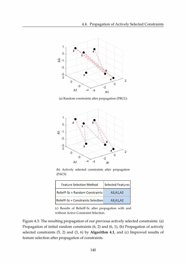
4.4. Propagation of Actively Selected Constraints
(a) Random constraints after propagation (PRCG)
(b) Actively selected constraints after propagation(PACS)
(c) Results of ReliefF-Sc after propagation with andwithout Active Constraint Selection.
Figure 4.3: The resulting propagation of our previous actively selected constraints: (a)Propagation of initial random constraints (6, 2) and (6, 1), (b) Propagation of activelyselected constraints (5, 2) and (3, 6) by Algorithm 4.1, and (c) Improved results offeature selection after propagation of constraints.
140
CHAPTER 4. ACTIVE LEARNING OF PAIRWISE CONSTRAINTS
4.5 Complexity Analysis
As for computational complexity of ReliefF-Sc, it is calculated as mentioned in theprevious chapter, O(card(CL)× NF), knowing that card(CL) is the number of cannot-link constraints, N is the number of data points and F is the dimension of featurespace. Under the ACS framework, the computational complexity by ReliefF-Sc is notthe problem since we aim to actively select as few as possible good constraints. How-ever, this selection of constraints using Algorithm 4.1 can turn to have a very high-costoverhead when the number of data points N is relatively large. This is due to the ne-cessity of calculating Equation (4.7) each time we want to find the sensitivity matrix.The latter holds all the sensitivities of all data couples to the minimum point i∗ onv2. Thus, Equation (4.7) that costs O(N3) has to be repeated as long as we still needmore constraints. Therefore, the overall computational complexity of Algorithm 4.1 iscalculated as O(card(CL)× N3). This is an issue to most of the pair-based constraintsselection algorithms due to the nature of the pair selection problem that needs to rankO(N2) candidate pairs during each of its searching iterations [136].
4.6 Experimental Results
We first describe the experimental setup, where we aim at comparing the classifica-tion accuracy obtained by the different supervised, unsupervised and semi-supervisedconstrained feature selection algorithms listed in section 4.6.1. We specify the useddatasets in section 4.6.2 and the performance evaluation measures in section 4.6.3.
In our experiments, we seek to show that our framework with active constraint se-lection replacing random constraint generation can significantly improve constrainedfeature selection algorithms especially our margin-based ReliefF-Sc. Note that, ACS isalgorithm-independent, which means that unlike other constraint selection methods[138, 139, 147], our method can be used to actively choose constraints regardless of theused constrained feature selection method. We also show the significance of propa-gating constraints and its effect on the classification accuracy curves. The comparisonresults are detailed in section 4.6.4.
4.6.1 Used Benchmarking Feature Selection Methods
To evaluate our feature selection framework using the proposed active constraint se-lection and propagation methods, we benchmark with the following well-known fea-ture selection methods including our own: Fisher score, ReliefF, Laplacian score, Con-
141

4.6. Experimental Results
straint score-1 (CS1), Constraint score-2 (CS2) (where λ is set to the default value givenby authors i.e 0.1 [40]), Simba-Sc (Start points parameter is set to its default value i.e5 [107]), Constraint score-4 (CS4), Constrained Laplacian score (CLS), and ReliefF-Scthe proposed semi-supervised margin-based constrained feature selection method de-tailed in section 3.2.3.In the following, ReliefF-Sc is applied in three versions: (1) alone with RCG denotedReliefF-Sc+RCG, (2) after applying ACS presented in Algorithm 4.1 denoted ReliefF-Sc+ACS, and (3) as a combination of Algorithms 3.2, 4.1 and 4.2 that is detailed insection 4.4. The latter is denoted as ReliefF-Sc+PACS.
4.6.2 Datasets Description and Parameter Setting
We evaluate our proposed active constraint selection and propagation framework onfive well-known numeric UCI machine learning datasets [3], including Soybean, Wine,Heart, Sonar and Image Segmentation. We also test on another two high dimen-sional gene-expression datasets: ColonCancer [131] and Leukemia [132]. Note that,our experiments are divided according to their goal into two parts. The first part,including sub-sections 4.6.4.1 and 4.6.4.2, focuses on highlighting the effect of Ac-tive Constraint Selection in comparison to Random Constraint Generation and Con-straint Propagation and is applied on Soybean, Wine, Heart, Sonar, ColonCancer andLeukemia datasets using the 1-NN classifier. The second part, including sub-sections4.6.4.3 and 4.6.4.4, focuses on the comparison with other feature selection methodsand is applied on Wine, Image Segmentation and ColonCancer using the 1-NN andSVM classifiers. Image Segmentation dataset was used in the second part in order tovalidate the results over a dataset with a greater number of classes.
Table 4.1 summarizes the main characteristics of each dataset mentioned in the firstcolumn. The second, third, and fourth columns show the number of data points, thedata dimension, and the number of classes respectively. Also, the fifth column speci-fies the number of points in each class in order to allow observing whether the classesare balanced or not and the last column indicates the number of queried constraints.Before recording the results, and for the sake of a fair comparison between differentmethods, we normalize all features to be between zero and one. Also, the similaritybetween data points is computed in some problem-specific manner, generally, we usethe self-tuning (auto-adaptive) method by [41] that takes only a user-specified param-eter representing the number of the nearest points to each data point and calculatesthe dispersion parameter automatically for evaluating the Gaussian Kernel.
142

CHAPTER 4. ACTIVE LEARNING OF PAIRWISE CONSTRAINTS
Table 4.1: Datasets and their main characteristics
Dataset #data points #features #classes #points per class #constraintsSoybean 47 35 4 10, 10, 10, 17 3
Wine 178 13 3 59, 71, 48 20Heart 270 13 2 150, 120 20Sonar 208 60 2 97, 111 10
Segmentation 210 19 7 30, 30, 30, 30, 30, 30, 30 10ColonCancer 62 2000 2 40, 22 8
Leukemia 72 5147 2 47, 25 10
In these experiments, we divide our datasets into training and testing sets definedby the same features, the first half of data points from each class is considered as thetraining set and the second half is considered as the testing set. We were also carefulthat no testing data is seen by either the feature selection algorithm or the classifierduring the learning process.
Regarding constraints, it is important to know that they can be generated frombackground knowledge given by an expert, i.e querying an oracle, or acquired exper-imentally from a set of labeled data [138]. In our experiments, since we compare theeffect of random constraints to the effect of constraint selection, we average the resultsover 100 runs for the random constraint sets. At each run, random constraints aregenerated as follows: a pair of data points is randomly picked from the training set,then its class assignment is checked if it turns to be that these two points belong todifferent classes they are considered a cannot-link constraint couple. This operationis repeated until the desired number of constraints is met. While for actively selectedconstraints, we select them using Algorithm 4.1 where the user only provides infor-mation about the couple considered most uncertain. Since cannot-link constraints areconsidered more important than must-link ones from the viewpoint of margin, Algo-rithm 3.2 (ReliefF-Sc) utilizes them only. Note that, we set the same value of K (numberof nearest neighbors) for both ReliefF and ReliefF-Sc on each dataset according to itscharacteristics. This value was set to 5 for Wine, Heart, Sonar and Leukemia and 3 forSoybean and Segmentation, however, only for ColonCancer we kept it equal to 1 sincewe experimentally noticed that this value provided the highest accuracy curve for thisparticular dataset.
Also, our criteria to choose the number of pairwise constraints to be queried is asfollows: we check the approximate number of points around zero on the second eigen-vector v2, and we consider it as the minimum supervision information needed. Hence,
143

4.6. Experimental Results
we use the number of cannot-link constraints specified by [107] for the datasets Wine,Heart, and Sonar i.e 20, 20 and 10 respectively since they fit our criteria, we also use10 constraints for Image Segmentation similarly to [53], however, for Soybean, Colon-Cancer and Leukemia datasets we assign 3, 8 and 10 constraints respectively. Notethat, for the algorithms that use both must-link and cannot-link constraints, for exam-ple, CS1 and CS2, we provide half the number of constraints as cannot-link and halfas must-link (chosen in the same manner when using ACS or RCG). This is to ensureproviding the same amount of supervision information to all algorithms.
4.6.3 Performance Evaluation Measures
After applying feature selection, we evaluate its performance using three evaluationmeasures: one is related to the data classification accuracy obtained by applying a clas-sifier on the selected set of features, and two others are directly related to measuringthe quality of the selected feature set, i.e., Precision and Distance measures [159].
1. Classification Accuracy: is defined as a percentage of correct predictions. Thus,we evaluate how many data points were correctly classified using the chosenfeature subset. It is defined in Equation (1.18) of section 1.5.4.1 as follows:
Accuracy =TP + TN
TP + TN + FP + FN
In our experiments, we evaluate the classification accuracy of each ranked set offeatures by applying two well known classifiers: the Nearest Neighbor (1-NN)classifier with euclidean distance and the SVM classifier with linear kernel func-tion (default configurations in Matlab-stats toolbox are used). For this purpose,first the feature selection is applied on the training set, this provides the rankingof features according to their assigned scores by different algorithms. Then, clas-sification using the selected features is applied on the testing set.
2. Precision (Pr) [159]: is here calculated as the number of features present in twolists: Target Tr that represents the first s features present in the optimal featureranking list Sopt and Rs that represents the first s features found in a selected setof features resulting from the feature selection method, divided by the numberof features in Tr denoted by card(Tr) (i.e card(Tr) = s):
Pr =card(Tr ∩ Rs)
card(Tr)(4.16)
144

CHAPTER 4. ACTIVE LEARNING OF PAIRWISE CONSTRAINTS
Figure 4.4: Relationship between the terms used in the Performance measures: Preci-sion and Distance.
This measure is between zero and one, knowing that Pr = 1 when the subsetsTr and Rs contain the same features and Pr = 0, when there is no intersectionbetween them. The higher precision the better result. For clarity we presentthe relations between all terms in Figure (4.4). Note that, Precision (Pr) here isdifferent from the one presented in Equation (1.19).
3. Distance [159]: since Precision cannot consider the order of features between Tr
and Rs, we also use Distance Dt. This measure is defined based on the sum ofdistances between the intersecting features of Tr and Rs. We calculate the dis-tance of each feature by comparing its position in Tr and Rs.Let us consider S
′opt the reverse of Sopt to calculate the maximum possible dis-
tance Dtmax between two lists having the same features as:
Dtmax = ∑∀Ai∈Sopt
|position(Ai ∈ Sopt)− position(Ai ∈ S′opt)| (4.17)
Where Dtmax is used to keep distance Dt between zero and one, knowing that Dtis at its best when it is zero with the two lists having identical ranking and largerthan zero otherwise.
Finally, Dt is calculated as follows:
Dt =∑∀Ai∈Tr |position(Ai ∈ Tr)− position(Ai ∈ R)|
Dtmax(4.18)
145

4.6. Experimental Results
4.6.4 Performance Evaluation Results
In this section, we first compare the classification accuracy obtained after applyingAlgorithm 3.2 (ReliefF-Sc with RCG) to the classification accuracy obtained after ap-plying the same algorithm but with active constraint selection (ReliefF-Sc with ACS)in section 4.6.4.1. We then propagate the selected constraints and compare the clas-sification accuracy obtained after applying ReliefF-Sc on these constraints to the clas-sification accuracy obtained without propagation in section 4.6.4.2. Then, in sections4.6.4.3 and 4.6.4.4, we compare supervised (Fisher, ReliefF), unsupervised (Laplacian),and semi-supervised constrained feature selection algorithms (ReliefF-Sc, Simba-Sc,CS1, CS2, CS4, CLS) also with RCG and ACS.
4.6.4.1 ReliefF-Sc with Random Constraint Generation (RCG) vs. ReliefF-Sc withActive Constraint Selection (ACS)
Figures (4.5a–4.5f) show the plot of classification accuracies vs. the desired numberof features ranked by ReliefF-Sc on Soybean, Wine, Heart, Sonar, ColonCancer, andLeukemia respectively. We also record the highest accuracy rates Acc and the corre-sponding dimension d of the selected feature subset obtained by ReliefF-Sc with andwithout constraint selection in Table 4.2.
As can be seen in Figure (4.5), it is generally always the case that the classificationaccuracy while using the constraints chosen by Algorithm 4.1 is better than the accu-racy using the same number of random constraints. For instance, Figures (4.5a) and(4.5b) show that with constraints selection we were able to reach the optimal classifica-tion of data points using only a few selected features. Moreover, it can be noticed thatgenerally, ReliefF-Sc with ACS obtains higher classification accuracies from the firstranked feature as can be seen in Figures (4.5b), (4.5d), (4.5e), and (4.5f), which meansthat applying feature selection on actively selected constraints is able to enhance fea-ture selection and identify the most discriminative feature earlier.
Note that, the results of ReliefF-Sc with RCG are averaged over 100 runs, whichmeans, their results implicitly hold more information, this masks the steep curve fluc-tuations through accuracy-averaging. Whereas ReliefF-Sc with ACS is deterministicand only applied once, this is due to the closed-form solutions obtained by both Al-gorithm 4.1 and ReliefF-Sc. In fact, we get the same selected constraints and the sameselected features regardless of the number of times we repeat a run. Moreover, notethat the applicability of a proposed method is a very important issue. For instance, ap-plying feature selection algorithms using randomly selected constraints might some-
146

CHAPTER 4. ACTIVE LEARNING OF PAIRWISE CONSTRAINTS
times obtain higher classification accuracies, but it is not logical nor feasible to queryfor the required number of random constraints in some real-world situations (e.g. 8constraints for ColonCancer requested for 100 times in order to average their results),it might then be less expensive to label the data than to query for 800 constraints. Thisissue reduces the applicability of RCG although it is usually used.
Moreover, from Table 4.2 we can see that feature selection by ReliefF-Sc with ACSon Wine and Soybean boosted classification accuracy to reach 100%, which means thatwith actively selected constraints, ReliefF-Sc was able to successfully select the featuresthat can provide an optimal classification of data by choosing only 9 features out of 35on Soybean and 5 features out of 13 on Wine, unlike the results of RCG that requiredchoosing 4 additional features in order to reach its highest accuracy rate i.e. 98.22%on Soybean and choosing 6 additional features to reach 97.75% on Wine. In addition,although the result on Sonar presented in Figure (4.5d) was problematic, this table alsoshows that ReliefF-Sc with ACS was still able to enhance the highest possible accuracyrate to become 62.50% on 29 which is 4.85% higher with a dimension that is smaller by1 feature.
Furthermore, we insist on the impressive result obtained on the high-dimensionalgene expression ColonCancer dataset, where ReliefF-Sc with selected constraints wasable to reach its highest accuracy from the first chosen feature, this shows that the al-gorithm was able to directly decide the most significant feature in the dataset usingour constraints. Whereas, it had to choose 1316 features to reach its highest accuracyusing random constraints. Finally, for Leukemia dataset, Table 4.2 shows that after se-lecting only 198 features out of 5147 the highest classification accuracy reached 91.18%using ACS, which is 7.74% higher than the accuracy using RCG i.e 83.44% with 388selected features.
Therefore, the significance of choosing the data couples to be queried for con-straints and then to be used for feature selection is here verified. Also, as the accu-racy rates achieved without feature selection on the original feature space were alwayslower than the accuracy rates achieved with feature selection, thus the importance offeature selection in improving the classification results is also confirmed.
As we mentioned before, one of the known drawbacks of the Relief family algo-rithms is that they might need a sufficiently big set of points to calculate the margin.Hence, since we care for asking the oracle as few questions as possible and for main-taining feasibility, we might sometimes obtain a very small number of constraints. As a
147

4.6. Experimental Results
5 10 15 20 25 30 35Ranked Features
0.4
0.5
0.6
0.7
0.8
0.9
1
Cla
ssifi
catio
n A
ccur
acy
with
1-N
N
ReliefF-Sc+RCGReliefF-Sc+ACS
(a) ReliefF-Sc with RCG and ACS on Soybean
2 4 6 8 10 12Ranked Features
0.6
0.65
0.7
0.75
0.8
0.85
0.9
0.95
1
Cla
ssifi
catio
n A
ccur
acy
with
1-N
N
ReliefF-Sc+RCG
ReliefF-Sc+ACS
(b) ReliefF-Sc with RCG and ACS on Wine
2 4 6 8 10 12Ranked Features
0.5
0.55
0.6
0.65
0.7
0.75
0.8
Cla
ssifi
catio
n A
ccur
acy
with
1-N
N
ReliefF-Sc+RCG
ReliefF-Sc+ACS
(c) ReliefF-Sc with RCG and ACS on Heart
10 20 30 40 50 60Ranked Features
0.45
0.5
0.55
0.6
0.65
Cla
ssifi
catio
n A
ccur
acy
with
1-N
N ReliefF-Sc+RCGReliefF-Sc+ACS
(d) ReliefF-Sc with RCG and ACS on Sonar
500 1000 1500 2000Ranked Features
0.6
0.65
0.7
0.75
0.8
0.85
Cla
ssifi
catio
n A
ccur
acy
with
1-N
N
ReliefF-Sc+RCG
ReliefF-Sc+ACS
(e) ReliefF-Sc with RCG and ACS on Colon-Cancer
1000 2000 3000 4000 5000Ranked Features
0.75
0.8
0.85
0.9
Cla
ssifi
catio
n A
ccur
acy
with
1-N
N ReliefF-Sc+RCGReliefF-Sc+ACS
(f) ReliefF-Sc with RCG and ACS on Leukemia
Figure 4.5: Accuracy rates using 1-NN classifier vs. different number of selected fea-tures obtained by ReliefF-Sc+RCG and ReliefF-Sc+ACS on 4 UCI datasets: (a) Soybean;(b) Wine; (c) Heart; (d) Sonar; and on 2 high dimensional gene-expression datasets: (e)ColonCancer; (f) Leukemia.
148
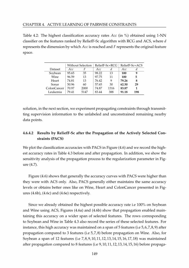
CHAPTER 4. ACTIVE LEARNING OF PAIRWISE CONSTRAINTS
Table 4.2: The highest classification accuracy rates Acc (in %) obtained using 1-NNclassifier on the features ranked by ReliefF-Sc algorithm with RCG and ACS, where drepresents the dimension by which Acc is reached and F represents the original featurespace.
Without Selection ReliefF-Sc+RCG ReliefF-Sc+ACSDataset Acc F Acc d Acc dSoybean 95.65 35 98.22 13 100 9
Wine 96.59 13 97.75 11 100 5Heart 74.81 13 76.42 9 79.26 8Sonar 50.96 60 57.65 30 62.50 29
ColonCancer 70.97 2000 74.87 1316 83.87 1Leukemia 79.41 5147 83.44 388 91.18 198
solution, in the next section, we experiment propagating constraints through transmit-ting supervision information to the unlabeled and unconstrained remaining nearbydata points.
4.6.4.2 Results by ReliefF-Sc after the Propagation of the Actively Selected Con-straints (PACS)
We plot the classification accuracies with PACS in Figure (4.6) and we record the high-est accuracy rates in Table 4.3 before and after propagation. In addition, we show thesensitivity analysis of the propagation process to the regularization parameter in Fig-ure (4.7).
Figure (4.6) shows that generally the accuracy curves with PACS were higher thanthey were with ACS only. Also, PACS generally either maintains the same accuracylevels or obtains better ones like on Wine, Heart and ColonCancer presented in Fig-ures (4.6b), (4.6c) and (4.6e) respectively.
Since we already obtained the highest possible accuracy rate i.e 100% on Soybeanand Wine using ACS, Figures (4.6a) and (4.6b) show that propagation enabled main-taining this accuracy on a wider span of selected features. The rows correspondingto Soybean and Wine in Table 4.3 also record the series of these selected features. Forinstance, this high accuracy was maintained on a span of 5 features (i.e 5,6,7,8,9) afterpropagation compared to 3 features (i.e 5,7,8) before propagation on Wine. Also, forSoybean a span of 12 features (i.e 7,8,9,10,11,12,13,14,15,16,17,18) was maintainedafter propagation compared to 8 features (i.e 9,10,11,12,13,14,15,16) before propaga-
149
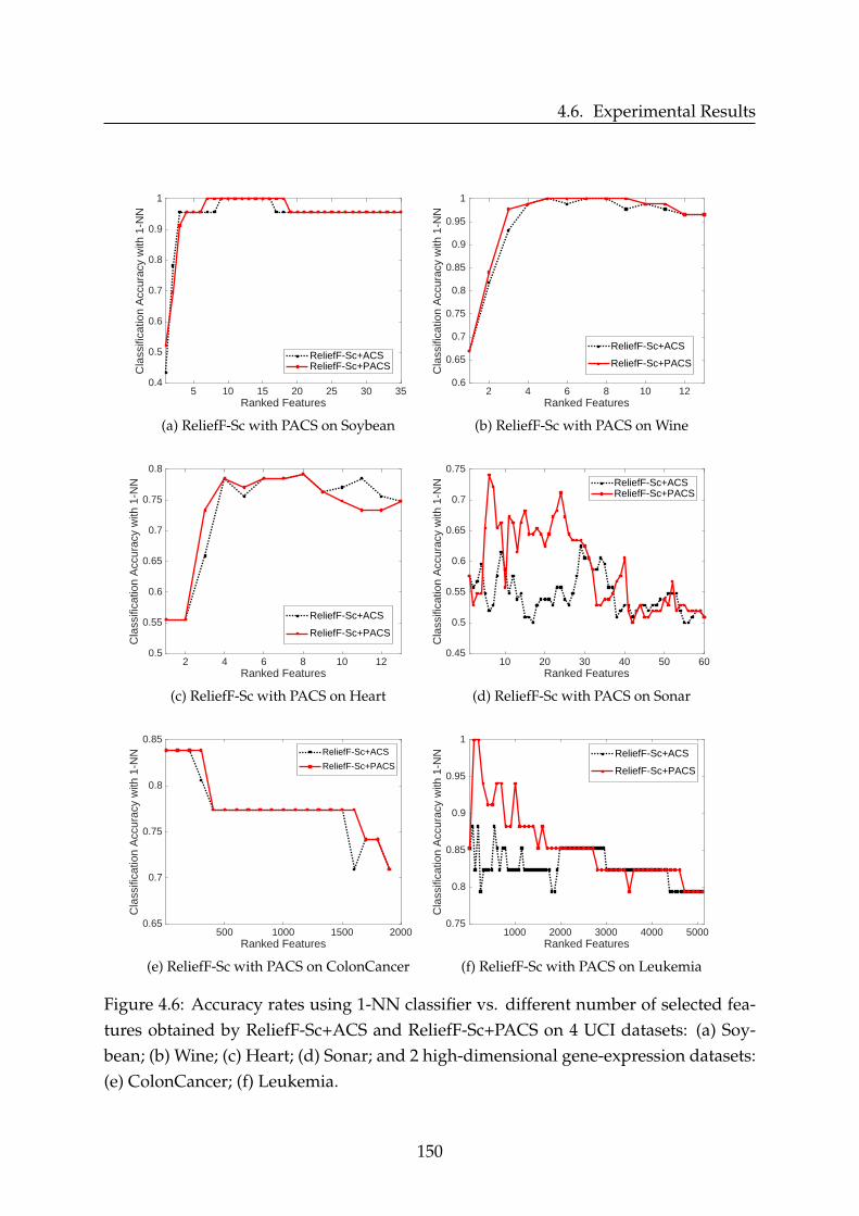
4.6. Experimental Results
5 10 15 20 25 30 35Ranked Features
0.4
0.5
0.6
0.7
0.8
0.9
1
Cla
ssifi
catio
n A
ccur
acy
with
1-N
N
ReliefF-Sc+ACSReliefF-Sc+PACS
(a) ReliefF-Sc with PACS on Soybean
2 4 6 8 10 12Ranked Features
0.6
0.65
0.7
0.75
0.8
0.85
0.9
0.95
1
Cla
ssifi
catio
n A
ccur
acy
with
1-N
N
ReliefF-Sc+ACS
ReliefF-Sc+PACS
(b) ReliefF-Sc with PACS on Wine
2 4 6 8 10 12Ranked Features
0.5
0.55
0.6
0.65
0.7
0.75
0.8
Cla
ssifi
catio
n A
ccur
acy
with
1-N
N
ReliefF-Sc+ACS
ReliefF-Sc+PACS
(c) ReliefF-Sc with PACS on Heart
10 20 30 40 50 60Ranked Features
0.45
0.5
0.55
0.6
0.65
0.7
0.75
Cla
ssifi
catio
n A
ccur
acy
with
1-N
N ReliefF-Sc+ACSReliefF-Sc+PACS
(d) ReliefF-Sc with PACS on Sonar
500 1000 1500 2000Ranked Features
0.65
0.7
0.75
0.8
0.85
Cla
ssifi
catio
n A
ccur
acy
with
1-N
N ReliefF-Sc+ACS
ReliefF-Sc+PACS
(e) ReliefF-Sc with PACS on ColonCancer
1000 2000 3000 4000 5000Ranked Features
0.75
0.8
0.85
0.9
0.95
1
Cla
ssifi
catio
n A
ccur
acy
with
1-N
N ReliefF-Sc+ACS
ReliefF-Sc+PACS
(f) ReliefF-Sc with PACS on Leukemia
Figure 4.6: Accuracy rates using 1-NN classifier vs. different number of selected fea-tures obtained by ReliefF-Sc+ACS and ReliefF-Sc+PACS on 4 UCI datasets: (a) Soy-bean; (b) Wine; (c) Heart; (d) Sonar; and 2 high-dimensional gene-expression datasets:(e) ColonCancer; (f) Leukemia.
150

CHAPTER 4. ACTIVE LEARNING OF PAIRWISE CONSTRAINTS
0.1 0.2 0.3 0.4 0.5 0.6 0.7 0.8 0.9Regularization parameter (a)
0.4
0.5
0.6
0.7
0.8
0.9
1
Acc
urac
y R
ate
SoybeanWineHeartSonar
Figure 4.7: Accuracy rates over the first 50% ranked features using 1-NN classifier vs.different values of the regularization Parameter a ranging in ]0,1[.
tion. It is also worth the note that the problematic result on Sonar was significantlyenhanced obtaining a much higher accuracy curve as can be seen in Figure (4.6d),which ensures a better feature selection process. Moreover, ReliefF-Sc with PACS onLeukemia was able to obtain 100% of accuracy from the first few ranked features ascan be seen in (4.6f) although with ACS (that was in its turn significantly higher thanthe accuracy using RCG) it was able to reach 91.18% maximum. Table 4.3 insists onthe latter. For instance, ReliefF-Sc with PACS on Leukemia reached this highest accu-racy on only 74 features after it had to choose 198 with ACS alone. Also, it shows thatthe highest classification accuracy on Sonar increased from 62.50% before constraintspropagation to 74.07% with only 6 selected features out of 60 in the original space.
Note that, the regularization parameter a = 0.99 ([153]) can be experimentallytuned to better fit each dataset. For Soybean, we keep a = 0.99. However, we ex-perimentally set a to the value of 0.6 for Wine, 0.37 for Heart, 0.47 for Sonar, 0.46 forColonCancer, and 0.75 for Leukemia dataset. In order to analyze the sensitivity of theconstraints propagation process to the regularization parameter a, we present Figure(4.7). It shows the fluctuation in accuracy on the first 50% ranked features when fea-ture selection is applied on propagated constraints. For example, Sonar dataset has 60features in the original feature space, we show the change in accuracy on exactly thefirst 30 selected features upon using all the possible values of a ranging between 0 and1 exclusively.
This Figure shows that for Soybean and Heart datasets the obtained sets of propa-gated constraints are less sensitive to the regularization parameter than those of Wine
151

4.6. Experimental Results
and Sonar. In fact, since Soybean already has a very small number of training datapoints (i.e. 24 points) the effect of constraints remained the same on feature selectionuntil the regularization parameter reached the last few values (that are greater than0.9). This means that more information is considered from the neighborhood graphand less is considered from the initial constraint matrix Q, which allows more prop-agation to the neighborhood leading to a considerable number of propagated con-straints with respect to the size of data (23 constraints on 24 data points). However,due to the noisy Sonar data, it was harder to follow the behavior with respect to a onit as the fluctuation was generally over all the analysis curve. It was also interestingas we noticed that using a value of 0.47 the number of propagated constraints reached102 remembering that we have only 104 training data points and noting that the initialset of actively chosen constraints before propagation had only 10 constraints. Hence,for Sonar we decided to use a = 0.47.
In conclusion, we do not expect the propagation to be independent of its only pa-rameter a; However, Figure (4.7) shows a great deal of stability even while a big changeappears in the value of a (like moving from a = 0.1 to a = 0.7 on Heart). There is al-ways some critical value of a by which the accuracy differs obviously (like a = 0.78 onHeart and a = 0.6 on Wine) except for Sonar. Therefore, we can analyze the data, if itssimilarity graph possess some kind of structure to the data by itself, then we can in-crease the value of a to consider more information from the neighborhood graph andallow higher levels of propagation. On the other side, when no clear structure of thedata is provided by the similarity graph, then we keep the value of a in small ranges inorder to consider more information from the matrix of chosen constraints and to keeplow levels of propagations (propagate only to very close neighboring points).
Table 4.3: The highest classification accuracy rates Acc (in %) obtained using 1-NNclassifier on the features ranked by ReliefF-Sc before and after constraints propagation,with d representing the dimension where Acc is reached. Initial constraints beforepropagation obtained systematically using Algorithm 4.1.
Without Selection ReliefF-Sc+ACS ReliefF-Sc+PACSDataset Acc F Acc d Acc dSoybean 95.65 35 100 9 –> 16 100 7 –> 18
Wine 96.59 13 100 5, 7, 8 100 5 –> 9Heart 74.81 13 79.26 8 79.26 8Sonar 50.96 60 62.50 29 74.07 6
ColonCancer 70.97 2000 83.87 1 83.87 1Leukemia 79.41 5147 91.18 198 100 74
152

CHAPTER 4. ACTIVE LEARNING OF PAIRWISE CONSTRAINTS
After detailing the performance results using ReliefF-Sc alone with RCG, ACS andPACS, in the next section, we wish to compare the algorithms detailed in section 4.6.1with RCG and ACS on Wine, Segmentation and ColonCancer datasets using both 1-NN and SVM classifiers.
4.6.4.3 Classification Accuracies by Different Constrained Feature Selection Meth-ods with Random Constraints Generation (RCG) vs. with Active ConstraintsSelection (ACS)
This section aims at benchmarking the different supervised, unsupervised, and semi-supervised constrained feature selection algorithms. It also aims at showing that theprocess of active constraint selection is independent of the constrained feature selec-tion algorithm and can enhance the chosen set of features regardless of the algorithmto be used. For that, we plot the accuracy curves obtained by 1-NN and SVM classi-fiers after feature selection using Fisher, ReliefF, Laplacian and the constrained margin-based ReliefF-Sc and Simba-Sc algorithms on Wine, Segmentation and ColonCancer inFigure (4.8). For these latter accuracies, Table 4.4 further presents the highest accuracyrates Acc and their corresponding dimensions d obtained by all the algorithms de-tailed in section 4.6.1 with and without constraint selection.
Moreover, in Figure (4.9) of this section, we also provide a comparison of thechange in accuracies using 1-NN and SVM classifiers after applying ReliefF-Sc andSimba-Sc with ACS and RCG vs. varying the number of provided constraints.
From Figure (4.8), we can see that generally both the constrained algorithms ReliefF-Sc and Simba-Sc were significantly improved when applied with ACS. We can also seethat our ReliefF-Sc was not only improved with ACS to outperform its self when ap-plied with RCG, but also to outperform Simba-Sc with ACS on the first few rankedfeatures as can be seen in Figures (4.8a) and (4.8b) although both methods reached thesame highest accuracy rate and on the same dimension on Wine dataset using 1-NNclassifier. ReliefF-Sc with ACS was also able to compete with the supervised ReliefFand Fisher scores as can be seen in Figures (4.8c), (4.8d) and (4.8f). Note that, Fisherand ReliefF utilize full class labels and being able to compete with their performancesonly with few selected constraints is very interesting. In addition, from Figures (4.8c)and (4.8d) we can see that ReliefF-Sc and Simba-Sc with ACS both obtained prominentresults on Segmentation, where they approximately maintained having higher accu-racy curves over the whole set of ranked features compared to the supervised algo-
153
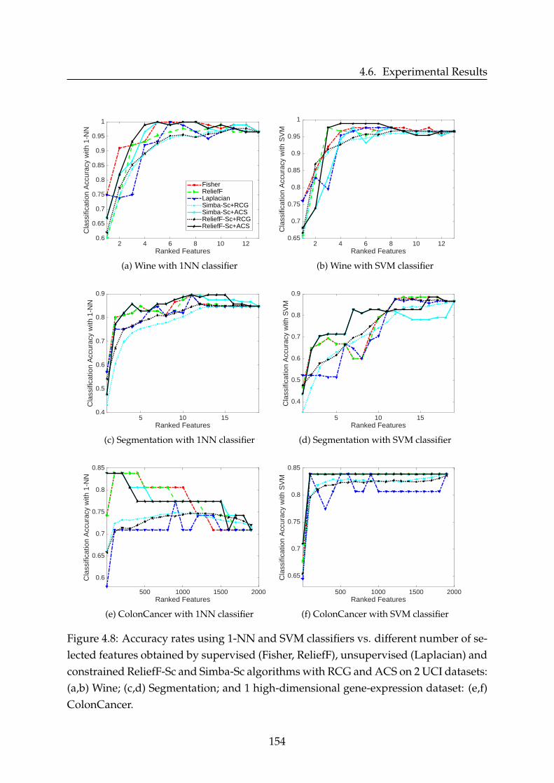
4.6. Experimental Results
2 4 6 8 10 12Ranked Features
0.6
0.65
0.7
0.75
0.8
0.85
0.9
0.95
1
Cla
ssifi
catio
n A
ccur
acy
with
1-N
N
FisherReliefFLaplacianSimba-Sc+RCGSimba-Sc+ACSReliefF-Sc+RCGReliefF-Sc+ACS
(a) Wine with 1NN classifier
2 4 6 8 10 12Ranked Features
0.65
0.7
0.75
0.8
0.85
0.9
0.95
1
Cla
ssifi
catio
n A
ccur
acy
with
SV
M
(b) Wine with SVM classifier
5 10 15Ranked Features
0.4
0.5
0.6
0.7
0.8
0.9
Cla
ssifi
catio
n A
ccur
acy
with
1-N
N
(c) Segmentation with 1NN classifier
5 10 15Ranked Features
0.4
0.5
0.6
0.7
0.8
0.9C
lass
ifica
tion
Acc
urac
y w
ith S
VM
(d) Segmentation with SVM classifier
500 1000 1500 2000Ranked Features
0.6
0.65
0.7
0.75
0.8
0.85
Cla
ssifi
catio
n A
ccur
acy
with
1-N
N
(e) ColonCancer with 1NN classifier
500 1000 1500 2000Ranked Features
0.65
0.7
0.75
0.8
0.85
Cla
ssifi
catio
n A
ccur
acy
with
SV
M
(f) ColonCancer with SVM classifier
Figure 4.8: Accuracy rates using 1-NN and SVM classifiers vs. different number of se-lected features obtained by supervised (Fisher, ReliefF), unsupervised (Laplacian) andconstrained ReliefF-Sc and Simba-Sc algorithms with RCG and ACS on 2 UCI datasets:(a,b) Wine; (c,d) Segmentation; and 1 high-dimensional gene-expression dataset: (e,f)ColonCancer.
154
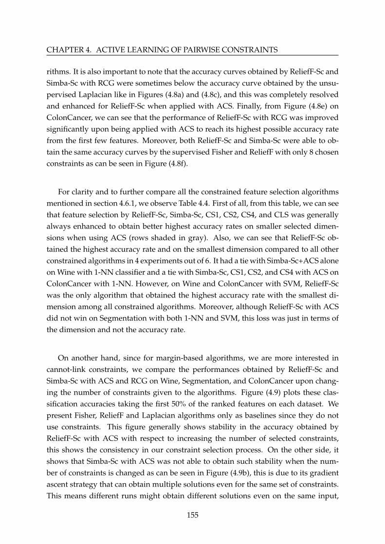
CHAPTER 4. ACTIVE LEARNING OF PAIRWISE CONSTRAINTS
rithms. It is also important to note that the accuracy curves obtained by ReliefF-Sc andSimba-Sc with RCG were sometimes below the accuracy curve obtained by the unsu-pervised Laplacian like in Figures (4.8a) and (4.8c), and this was completely resolvedand enhanced for ReliefF-Sc when applied with ACS. Finally, from Figure (4.8e) onColonCancer, we can see that the performance of ReliefF-Sc with RCG was improvedsignificantly upon being applied with ACS to reach its highest possible accuracy ratefrom the first few features. Moreover, both ReliefF-Sc and Simba-Sc were able to ob-tain the same accuracy curves by the supervised Fisher and ReliefF with only 8 chosenconstraints as can be seen in Figure (4.8f).
For clarity and to further compare all the constrained feature selection algorithmsmentioned in section 4.6.1, we observe Table 4.4. First of all, from this table, we can seethat feature selection by ReliefF-Sc, Simba-Sc, CS1, CS2, CS4, and CLS was generallyalways enhanced to obtain better highest accuracy rates on smaller selected dimen-sions when using ACS (rows shaded in gray). Also, we can see that ReliefF-Sc ob-tained the highest accuracy rate and on the smallest dimension compared to all otherconstrained algorithms in 4 experiments out of 6. It had a tie with Simba-Sc+ACS aloneon Wine with 1-NN classifier and a tie with Simba-Sc, CS1, CS2, and CS4 with ACS onColonCancer with 1-NN. However, on Wine and ColonCancer with SVM, ReliefF-Scwas the only algorithm that obtained the highest accuracy rate with the smallest di-mension among all constrained algorithms. Moreover, although ReliefF-Sc with ACSdid not win on Segmentation with both 1-NN and SVM, this loss was just in terms ofthe dimension and not the accuracy rate.
On another hand, since for margin-based algorithms, we are more interested incannot-link constraints, we compare the performances obtained by ReliefF-Sc andSimba-Sc with ACS and RCG on Wine, Segmentation, and ColonCancer upon chang-ing the number of constraints given to the algorithms. Figure (4.9) plots these clas-sification accuracies taking the first 50% of the ranked features on each dataset. Wepresent Fisher, ReliefF and Laplacian algorithms only as baselines since they do notuse constraints. This figure generally shows stability in the accuracy obtained byReliefF-Sc with ACS with respect to increasing the number of selected constraints,this shows the consistency in our constraint selection process. On the other side, itshows that Simba-Sc with ACS was not able to obtain such stability when the num-ber of constraints is changed as can be seen in Figure (4.9b), this is due to its gradientascent strategy that can obtain multiple solutions even for the same set of constraints.This means different runs might obtain different solutions even on the same input,
155

4.6. Experimental Results
Table 4.4: The highest accuracy rates Acc (in %) and their corresponding dimensionsd using 1-NN and SVM classifiers vs. different numbers of selected features obtainedby supervised (Fisher, ReliefF), unsupervised (Laplacian) and constrained ReliefF-Sc,Simba-Sc, CS1, CS2, CS4 and CLS algorithms with RCG and ACS on 2 UCI datasets:Wine; Segmentation; and 1 high-dimensional gene-expression dataset: ColonCancer.
1-NN Classifier SVM Classifier
Wine Segmentation ColonCancer Wine Segmentation ColonCancer
Acc d Acc d Acc d Acc d Acc d Acc d
Without Selection 96.59 13 84.76 19 70.97 2000 97.73 13 86.67 19 83.87 2000Fisher 100 5 89.52 11 83.87 5 97.72 5 88.57 13 83.87 11ReliefF 98.86 10 89.52 11 83.87 6 97.72 3 88.57 13 83.87 20
Laplacian 100 6 89.52 11 77.42 8 97.72 6 87.61 12 83.87 49
ReliefF-ScRCG 97.75 11 85.73 12 74.87 1316 96.72 9 87.54 12 83.87 1945ACS 100 5 89.52 11 83.87 1 98.86 4 88.57 16 83.87 19
Simba-Sc RCG 97.47 11 84.76 19 74.9 884 96.59 13 86.67 19 83.87 1926ACS 100 5 89.52 11 83.87 1 97.72 5 86.67 19 83.87 27
CS1 RCG 97.34 11 85.54 14 79.97 141 96.5 13 87.04 17 83.87 1878ACS 98.86 5 89.52 11 83.87 1 98.86 5 88.57 15 83.87 42
CS2 RCG 97 12 86.72 15 78.87 221 96.89 12 86.87 18 83.87 1913ACS 98.86 10 89.52 7 83.87 10 97.72 12 88.57 16 83.87 66
CS4 RCG 97.66 11 85.91 11 78.32 144 96.69 11 87.29 17 83.87 1892ACS 98.86 6 89.52 11 83.87 1 97.72 4 88.57 15 83.87 55
CLSRCG 97.82 10 85.1 14 78.81 182 96.65 7 87.38 15 83.87 1823ACS 98.86 5 89.52 10 83.87 27 97.72 5 88.57 13 83.87 112
unlike the closed-form solution that ReliefF-Sc provides. Also it is important to notethat when using ReliefF-Sc or Simba-Sc with RCG some added random constraints de-creased the performance as can be seen in Figures (4.9d), (4.9e) and (4.9f), this provesthat random constraints might introduce ill effects. In addition, (4.9a) shows thatReliefF-Sc and Simba-Sc with RCG obtained fluctuating accuracies that were generallybelow the supervised Fisher and ReliefF. On the other side, Figures (4.9c) and (4.9d)show that for all the number of constraints, ReliefF-Sc with ACS obtains stable andhigher accuracies than those of the supervised Fisher and ReliefF. In addition, Figures(4.9e) and (4.9f) on ColonCancer similarly show that ReliefF-Sc with ACS had an ac-curacy equal to the one obtained by Fisher on all constraint numbers. This experimentshows the sensitivity of the feature selection process to the input constraints. Usingmore constraints does not mean higher accuracy, on the contrary, the quality of theconstraints is what matters.
To sum up, Figure (4.8) and Table 4.4, highlight two very important findings. First,they clearly show that ACS is an algorithm-independent method since it was appliedwith multiple constrained feature selection algorithms and it was able to generally en-hance and improve them. Second, they also prove that the combination of our ReliefF-Sc algorithm and our ACS method is able to outperform constrained and unsupervisedfeature selection methods and compete with the supervised ones. On the other side,
156

CHAPTER 4. ACTIVE LEARNING OF PAIRWISE CONSTRAINTS
10 20 30 40 50Constraints Number
0.85
0.9
0.95
1
Cla
ssifi
catio
n A
ccur
acy
with
1-N
N
FisherReliefFLaplacianSimba-Sc+RCGSimba-Sc+ACSReliefF-Sc+RCGReliefF-Sc+ACS
(a) Wine with 1NN classifier
10 20 30 40 50Constraints Number
0.88
0.9
0.92
0.94
0.96
0.98
Cla
ssifi
catio
n A
ccur
acy
with
SV
M
(b) Wine with SVM classifier
10 20 30 40 50Constraints Number
0.74
0.76
0.78
0.8
0.82
0.84
0.86
0.88
0.9
Cla
ssifi
catio
n A
ccur
acy
with
1-N
N
(c) Segmentation with 1NN classifier
10 20 30 40 50Constraints Number
0.7
0.72
0.74
0.76
0.78
0.8
0.82
0.84
0.86
0.88C
lass
ifica
tion
Acc
urac
y w
ith S
VM
(d) Segmentation with SVM classifier
10 20 30 40 50Constraints Number
0.66
0.68
0.7
0.72
0.74
0.76
0.78
0.8
0.82
Cla
ssifi
catio
n A
ccur
acy
with
1-N
N
(e) ColonCancer with 1NN classifier
10 20 30 40 50Constraints Number
0.79
0.8
0.81
0.82
0.83
0.84
0.85
Cla
ssifi
catio
n A
ccur
acy
with
SV
M
(f) ColonCancer with SVM classifier
Figure 4.9: Accuracy rates obtained on the first 50% ranked features by the margin-based constrained ReliefF-Sc and Simba-Sc algorithms with RCG and ACS followedby 1-NN and SVM classifiers vs. different number of constraints on 2 UCI datasets:(a,b) Wine; (c,d) Segmentation; and 1 high-dimensional gene-expression dataset: (e,f)ColonCancer. Fisher, ReliefF and Laplacian do not use constraints and are used assupervised and unsupervised baselines.
157

4.6. Experimental Results
Figure (4.9) shows the importance of choosing the constraints systematically, provesthe consistency provided by ACS, and points out the sensitivity of feature selection tothe quality of inputted constraints.
In the following section, we further benchmark the same semi-supervised con-strained algorithms with RCG and ACS but this time using the two feature-relatedperformance measures (Precision and Distance).
4.6.4.4 Precision and Distance measures by Different Constrained Feature Selec-tion Methods with Random Generated Constraints (RCG) vs. with ActivelySelected Constraints (ACS)
In this section, we compare the precision and distance measures obtained by the con-strained feature selection algorithms. We use the ranked list of the supervised Fisherscore as the reference (optimal) list in our comparisons as it generally obtained thehighest accuracy rates in the above experiments and since it ranks features accordingto their correlation with the class labels directly. Thus, we consider it as the baselineby which we compare the ability of different semi-supervised algorithms to select thesame features (precision) and in the same order (distance). Note that, we use the firsthalf of the ranked lists by all algorithms in the calculation of these two measures as-suming that this ensures the removal of irrelevant features (e.g. for ColonCancer weselect first 1000 ranked features out of 2000 features in the original space). Also notethat since for the RCG method the results are averaged over 100 repeated runs, wecalculate the precision and distance measures for each run (on each subset we obtain)and we finally present the mean and standard deviations of these measures.
Figure (4.10) shows the bar graphs of precision and distance using the constrainedalgorithms with RCG and with ACS on Wine, Segmentation, and ColonCancer. Itshows that generally, the ranked feature lists by constrained algorithms with activeconstraint selection obtained higher precision when compared to the supervised rankedfeature list (by Fisher) with lower distances as can be seen in Figures (4.10e) and (4.10f)on ColonCancer. This means, even the order of selecting features tends to act in asupervised manner when constraints are selected actively. Also, the results on Seg-mentation in Figure (4.10c) show that constrained algorithms with ACS improved toidentically act like a supervised feature selection algorithm with full class labels onlywith 10 selected constraints.For instance, ReliefF-Sc, Simba-Sc, CS1, CS4, and CLS reached a precision value of 1 onthis dataset. In such a case, when precision is maximum, even if the distance measure
158
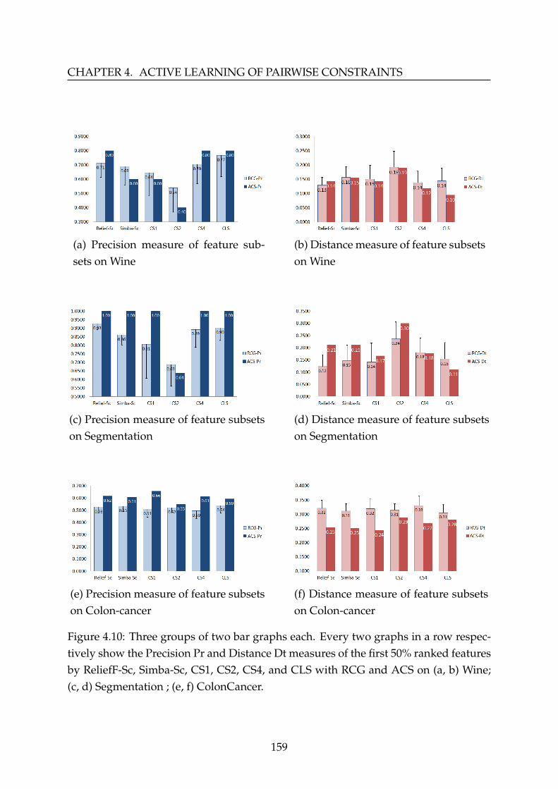
CHAPTER 4. ACTIVE LEARNING OF PAIRWISE CONSTRAINTS
(a) Precision measure of feature sub-sets on Wine
(b) Distance measure of feature subsetson Wine
(c) Precision measure of feature subsetson Segmentation
(d) Distance measure of feature subsetson Segmentation
(e) Precision measure of feature subsetson Colon-cancer
(f) Distance measure of feature subsetson Colon-cancer
Figure 4.10: Three groups of two bar graphs each. Every two graphs in a row respec-tively show the Precision Pr and Distance Dt measures of the first 50% ranked featuresby ReliefF-Sc, Simba-Sc, CS1, CS2, CS4, and CLS with RCG and ACS on (a, b) Wine;(c, d) Segmentation ; (e, f) ColonCancer.
159
4.7. Conclusion
increases like for ReliefF-Sc and Simba-Sc with ACS in Figure (4.10d), this increasedoes not mean a performance degradation at all. It only means that the algorithmsselected the optimal feature subset in another order. Although Simba-Sc, CS1, andCS2 showed a lower precision bar with ACS on Wine, it is important to notice thatthe standard deviation from the mean for RCG method is large enough to show that alower precision is always possible and the high precision cannot be ensured. Similarly,in (4.10b) the standard deviation of the distance measure of RCG shows that it can in-crease to be higher than the fixed distance value obtained by our ACS method. On theother side, note that the precision obtained by ReliefF-Sc with ACS outperformed thatof Simba-Sc, CS1, and CS2, whereas it was similar to that of CS4 and CLS on Wine.Also, all the constrained algorithms were competitive in terms of feature subsets’ pre-cision on Segmentation and ColonCancer except for CS2 that was lagging behind.
Finally, these experiments prove the significance of actively selecting constraintson the subset of selected features directly in addition to its importance and effect onthe classification accuracy. As we have explained, Fisher is a supervised feature selec-tion method that uses full class labels, thus, when ACS is able to enhance constrainedfeature selection algorithms to obtain similar feature subsets, it proves that only withfew but well-chosen queries, constrained algorithms can obtain results that are able tocompete with supervised ones.
4.7 Conclusion
In this chapter, we suggested a framework for actively selecting and propagating con-straints for feature selection using graph Laplacian. In fact, we highlighted two maincomponents: (1) our core contribution, i.e. the process of selecting pairwise constraintsto be used by the constrained margin-based feature selection algorithm ReliefF-Sc and(2) the augmentation of supervision information by propagating these constraints. Fo-cusing on the constraint selection process, we assumed that when a small perturba-tion in the similarity value of a data couple is able to perturb the similarity matrixand lead to a more well separated form of the second eigenvector of the graph Lapla-cian, this couple is definitely considered a more important and significant constraint.Thus, obtaining supervision information on such data couples is able to improve theperformance of constrained feature selection algorithms. Moreover, for the sake ofincreasing supervision information without engaging the resource-expensive humanoracle, we then propagated the selected constraints to their unlabeled neighborhood.This allowed the margin-based ReliefF-Sc to perform better with a sufficiently big set
160

CHAPTER 4. ACTIVE LEARNING OF PAIRWISE CONSTRAINTS
of couples as it requires. Finally, experimental results showed how crucial constraintselection can be to the performance of constrained feature selection algorithms.
161


Conclusion and Perspectives
In this thesis, we provided a semi-supervised margin-based constrained feature selec-tion framework that is capable of handling the main two aspects of feature selection:maximizing relevancy with respect to a target concept and minimizing redundancy.The latter is done for the sake of dimensionality reduction.
As we were interested in individual filter-type feature weighting/ranking, we pro-vided a comprehensive review of a whole family of feature selection algorithms thatuse a margin-based score in order to evaluate and rank features in the order of theirrelevance. These are known as Relief-Based Algorithms (RBAs) and proved to gen-erally perform well regardless of the problem specifications, they have a low bias,are considered relatively fast, are capable of detecting feature interaction, are robustand noise-tolerant in addition to being able to capture data local dependencies [1, 2].These algorithms were initially suggested in the supervised context and extended tothe semi-supervised one with class labels. However, feature selection became morechallenging with the “small labeled-sample” problem, in which the amount of datathat is unlabeled is much larger than the amount of labeled data taking into consider-ation the high cost of data labeling. Thus, we were interested in the semi-supervisedconstrained context where a cheaper kind of supervision information, i.e. pairwiseconstraints is used. These only specify whether two data points should be in the samegroup (must-link constraint), or in different groups (cannot- link constraint). So, wereviewed in details several recent works which have attempted to use pairwise con-straints in both supervised and semi-supervised contexts.
With our interest in exploiting the strengths of margin-based feature selection withinthe semi-supervised constrained environment, we discussed margin-based feature se-lection with side pairwise constraints. We also demonstrated the change in the notionof margin from the supervised to the constrained context and provided its mathe-
163

matical interpretation. Accordingly, we suggested our constrained margin-based fea-ture selection algorithm called Relief with Side constraints (Relief-Sc) and its robustversion ReliefF-Sc. Focusing only on cannot-link constraints due to their conceptualimportance from the margin’s perspective, we showed how Relief-Sc utilizes thesecannot-link constraints to assign weights to different features according to their con-tribution to maximizing the hypothesis-margin and finds a unique relevant featuresubset in a closed-form. Experimental results proved that Relief-Sc is competitive tosupervised scores using full class labels and can outperform other constrained andunsupervised ones. Moreover, we showed how it can provide good results with onlya few pairwise constraints, which ensures computational advantages over other algo-rithms when dealing with high dimensional data.
Although the importance of constraints is practically proven, some constraints candegrade the learning performance. Thus, we suggested an Active Constraint Selectionmethod (ACS) that depends on perturbation theory analysis to find a constraint set ofhigher utility. For that, we first discussed some of the most important related workon constraint selection. Then, we detailed the proposed method, by which, we findthe data couple that is capable of reducing uncertainty in terms of spectral analysis.In other words, we find the couple that when supplied with background knowledgeimposes the highest utility. Thus, we actively query the human oracle for information(pairwise constraint) on this particular chosen couple only.
Since we can only ask a small number of questions before the process becomesresource-expensive, we also presented a method for propagating the actively selectedconstraints into their unlabeled neighborhood, called PACS. In this regard, we showedhow PACS can increase supervision information and enhance feature selection with-out requiring higher costs of human-labor.
On the other side, we suggested a novel combination of feature clustering upona sparse graph with our margin-based objective function called Feature ClusteringRelief-Sc (FCRSC). The efficiency of this combination was validated in comparison tosupervised, unsupervised and semi-supervised filter feature selection methods usingfour different classifications schemes. The experimental results showed that eliminat-ing redundant features can considerably improve the learning process.
164
Perspectives
Based on the outcomes presented in this thesis, we highlight several future researchdirections.
• In our work, Relief-Sc utilizes cannot-link pairwise constraints only. Thus, itmight ignore valuable information carried by must-link constraints. Therefore,we can improve our work through finding a way to integrate must-link con-straints in our constrained margin-based objective function.
• In ACS, we have focused on finding a constraint set of high utility with respectto our objective function. However, when a considerable number of points arenear zero on the second eigen-vector (v2), the process of selecting constraints cantend to be random. Therefore, we can mitigate this weakness by considering thesensitivity of the couples with respect to multiple eigenvectors instead of onlythe second eigenvector. Then, the couple of highest sensitivity on multiple eigen-vectors is chosen. The number of the eigenvectors to be considered can be equalto the number of classes if known. In case not, we can either use all eigenvectorsas can be seen in Equation (4.7) or use some method to automatically estimatethe number of classes like eigengap [32] and density peaks [160].
• In ACS, we have focused on the First-Order Eigen-vector Perturbation Theoryto choose the most significant couple. There is also some work that chooses fea-tures based on the eigenvalue sensitivity analysis [71]. It would be interesting toexperiment whether eigenvalue sensitivity analysis could provide better perfor-mance in selecting our constraints.
• Our framework includes some computationally expensive subroutines such ascalculating the sparse graph of the feature space when the number of featuresis very large and calculating eigenvector sensitivity when the number of datapoints increases significantly. Therefore, working on the scalability of our frame-work can be of great importance. For example, parallelization of the process ofcalculating eigenvector sensitivity matrix can be considered. The process can benaturally split into several independent tasks.
• Relief-Sc is a semi-supervised algorithm. Although it exploits unlabeled data inthe neighborhood of a constraint, it is still closely related to the chosen constraintset. To decrease this effect, ensemble learning can be used where some othersimple unsupervised algorithm that focuses on the intrinsic structure of data canbe also used along with Relief-Sc. Each algorithm in the ensemble ranks the
165

features alone, at the end, some voting system finds the best in the combinedresults. Which means, the features ranked on top by both algorithms are theones that will be considered.
• Application to Image analysis domain e.g. face recognition, texture.
166

Bibliography
[1] Verónica Bolón-Canedo, Noelia Sánchez-Maroño, and Amparo Alonso-Betanzos. Recent advances and emerging challenges of feature selection in thecontext of big data. Knowledge-Based Systems, 86:33–45, September 2015.
[2] Ryan J. Urbanowicz, Melissa Meeker, William LaCava, Randal S. Olson, andJason H. Moore. Relief-based feature selection: introduction and review. Journalof Biomedical Informatics, 85:189–203, September 2018.
[3] Dheeru Dua and Casey Graff. UCI Machine Learning Repository. School ofInformation and Computer Sciences, University of California, Irvine, USA, 2019.http://archive.ics.uci.edu/ml.
[4] Igor Kononenko. Estimating attributes: analysis and extensions of RELIEF. InProceedings of the European Conference on Machine Learning (ECML’94), pages 171–182, Catania, Italy, 6-8 April 1994.
[5] Marko Robnik-Šikonja and Igor Kononenko. Comprehensible interpretation ofrelief’s estimates. In Proceedings of the 18th International Conference on MachineLearning (ICML’01), pages 433–40, Williamstown, Massachusetts, USA, 28 June -1 July 2001.
[6] Yijun Sun and Jian Li. Iterative RELIEF for feature weighting. In Proceedings ofthe 23rd International Conference on Machine Learning (ICML’06), pages 913–920,Pittsburgh, Pennsylvania, USA, 25-29 June 2006.
[7] Trang T. Le, Ryan J. Urbanowicz, Jason H. Moore, and Brett A McKinney. STa-tistical Inference Relief (STIR) feature selection. Bioinformatics, 35(8):1358–1365,April 2019.
167
[8] Huan Liu and Hiroshi Motoda. Computational methods of feature selection. DataMining and Knowledge Discovery Series. Chapman & Hall/CRC, Boca Raton,Florida, USA, October 2007.
[9] Jiliang Tang, Salem Alelyani, and Huan Liu. Feature selection for classification:A review. In Data Classification: Algorithms and Applications, chapter 2, pages37–64. Chapman & Hall/CRC, Boca Raton, Florida, USA, January 2014.
[10] Razieh Sheikhpour, Mehdi Agha Sarram, Sajjad Gharaghani, and MohammadAli Zare Chahooki. A survey on semi-supervised feature selection methods.Pattern Recognition, 64:141–158, April 2017.
[11] Manoranjan Dash and Huan Liu. Feature selection for classification. IntelligentData Analysis, 1(1-4):131–156, March 1997.
[12] Huan Liu and Lei Yu. Toward integrating feature selection algorithms for clas-sification and clustering. IEEE Transactions on Knowledge and Data Engineering,17(4):491–502, April 2005.
[13] Jundong Li, Kewei Cheng, Suhang Wang, Fred Morstatter, Robert P. Trevino, Jil-iang Tang, and Huan Liu. Feature selection: A data perspective. ACM ComputingSurveys (CSUR), 50(6):94, December 2017.
[14] Jianyu Miao and Lingfeng Niu. A survey on feature selection. Procedia ComputerScience, 91:919–926, December 2016.
[15] Benyamin Ghojogh, Maria N. Samad, Sayema Asif Mashhadi, Tania Kapoor,Wahab Ali, Fakhri Karray, and Mark Crowley. Feature selection and featureextraction in pattern analysis: A literature review. Computing Research Repository(CoRR), abs/1905.02845, May 2019.
[16] Ronald A. Fisher. The use of multiple measurements in taxonomic problems.Annals of Eugenics, 7(2):179–188, September 1936.
[17] Sebastian Mika, Gunnar Ratsch, Jason Weston, Bernhard Scholkopf, and Klaus-Robert Mullers. Fisher discriminant analysis with kernels. In Neural Networks forSignal Processing IX: Proceedings of the 1999 IEEE Signal Processing Society Work-shop (Cat. No.98TH8468), pages 41–48, Madison, Wisconsin, USA, 25 August1999.
168
[18] Elnaz Barshan, Ali Ghodsi, Zohreh Azimifar, and Mansoor Zolghadri Jahromi.Supervised principal component analysis: Visualization, classification and re-gression on subspaces and submanifolds. Pattern Recognition, 44(7):1357–1371,July 2011.
[19] Karl Pearson. LIII. on lines and planes of closest fit to systems of points in space.The London, Edinburgh, and Dublin Philosophical Magazine and Journal of Science,2(11):559–572, June 1901.
[20] Michael A.A. Cox and Trevor F. Cox. Multidimensional scaling. Chapman &Hall/CRC, Boca Raton, Florida, USA, 2008.
[21] Joshua B. Tenenbaum, Vin De Silva, and John C. Langford. A global geomet-ric framework for nonlinear dimensionality reduction. Science, 290(5500):2319–2323, December 2000.
[22] Sam T. Roweis and Lawrence K. Saul. Nonlinear dimensionality reduction bylocally linear embedding. Science, 290(5500):2323–2326, December 2000.
[23] Laurens van der Maaten and Geoffrey Hinton. Visualizing data using t-SNE.Journal of Machine Learning Research (JMLR), 9:2579–2605, November 2008.
[24] Isabelle Guyon and André Elisseeff. An introduction to variable and featureselection. Journal of Machine Learning Research (JMLR), 3:1157–1182, March 2003.
[25] Jie Cai, Jiawei Luo, Shulin Wang, and Sheng Yang. Feature selection in machinelearning: A new perspective. Neurocomputing, 300:70–79, July 2018.
[26] Lei Yu and Huan Liu. Feature selection for high-dimensional data: A fastcorrelation-based filter solution. In Proceedings of the 20th International Con-ference on Machine Learning (ICML’03), pages 856–863, Washington, District ofColumbia, USA, 21-24 August 2003.
[27] Hanchuan Peng, Fuhui Long, and Chris Ding. Feature selection based on mutualinformation criteria of max-dependency, max-relevance, and min-redundancy.IEEE Transactions on Pattern Analysis and Machine Intelligence, 27(8):1226–1238,June 2005.
[28] Yun Li, Tao Li, and Huan Liu. Recent advances in feature selection and its ap-plications. Knowledge and Information Systems, 53(3):551–577, December 2017.
169

[29] Jiye Liang, Feng Wang, Chuangyin Dang, and Yuhua Qian. A group incrementalapproach to feature selection applying rough set technique. IEEE Transactions onKnowledge and Data Engineering, 26(2):294–308, February 2014.
[30] Parham Moradi and Mehrdad Rostami. A graph theoretic approach for unsuper-vised feature selection. Engineering Applications of Artificial Intelligence, 44:33–45,September 2015.
[31] Mingxia Liu and Daoqiang Zhang. Sparsity score: A novel graph-preservingfeature selection method. International Journal of Pattern Recognition and ArtificialIntelligence, 28(04):1450009, June 2014.
[32] Ulrike Von Luxburg. A tutorial on spectral clustering. Statistics and Computing,17(4):395–416, December 2007.
[33] Shuicheng Yan, Dong Xu, Benyu Zhang, Hong-Jiang Zhang, Qiang Yang, andStephen Lin. Graph embedding and extensions: A general framework for di-mensionality reduction. IEEE Transactions on Pattern Analysis & Machine Intelli-gence, 29(1):40–51, January 2007.
[34] Corinna Cortes and Mehryar Mohri. On transductive regression. In Proceedingsof the 19th International Conference on Neural Information Processing Systems, pages305–312, Vancouver, British Columbia, Canada, 4-7 December 2006.
[35] Zheng Zhao and Huan Liu. Spectral feature selection for supervised and unsu-pervised learning. In Proceedings of the 24th International Conference on MachineLearning, pages 1151–1157, Corvalis, Oregon, USA, 20-24 June 2007.
[36] Fan R.K. Chung and Fan Chung Graham. Spectral graph theory, volume 92. Amer-ican Mathematical Society, USA, 1997.
[37] Marko Robnik-Šikonja and Igor Kononenko. Theoretical and empirical analysisof ReliefF and RReliefF. Machine Learning, 53(1-2):23–69, October 2003.
[38] Xiaofei He, Deng Cai, and Partha Niyogi. Laplacian score for feature selection.In Proceedings of the 18th International Conference on Neural Information ProcessingSystems, volume 18, page 507–514, Vancouver, British Columbia, Canada, 5-8December 2005.
[39] Zheng Zhao and Huan Liu. Semi-supervised feature selection via spectral anal-ysis. In Proceedings of the 7th SIAM International Conference on Data Mining, pages641–646, Minneapolis, Minnesota, USA, 26-28 April 2007.
170

[40] Daoqiang Zhang, Songcan Chen, and Zhi-Hua Zhou. Constraint score: A newfilter method for feature selection with pairwise constraints. Pattern Recognition,41(5):1440–1451, May 2008.
[41] Lihi Zelnik-Manor and Pietro Perona. Self-tuning spectral clustering. In Proceed-ings of the 17th International Conference on Neural Information Processing Systems,pages 1601–1608, Vancouver, British Columbia, Canada, 13-18 December 2004.
[42] Zheng Alan Zhao and Huan Liu. Spectral Feature Selection for Data Mining (OpenAccess). Data Mining and Knowledge Discovery Series. Chapman & Hall/CRC,Boca Raton, Florida, USA, December 2011.
[43] José Martínez Sotoca and Filiberto Pla. Supervised feature selection by cluster-ing using conditional mutual information-based distances. Pattern Recognition,43(6):2068–2081, June 2010.
[44] Saúl Solorio-Fernández, J. Ariel Carrasco-Ochoa, and José Fco Martínez-Trinidad. A review of unsupervised feature selection methods. Artificial In-telligence Review, pages 1–42, January 2019.
[45] Ahmed K. Farahat, Ali Ghodsi, and Mohamed S. Kamel. An efficient greedymethod for unsupervised feature selection. In Proceedings of the 11th IEEE In-ternational Conference on Data Mining (ICDM), pages 161–170, Vancouver, BritishColumbia, Canada, 11-14 December 2011.
[46] Yun Li, Bao-Liang Lu, and Zhong-Fu Wu. A hybrid method of unsupervised fea-ture selection based on ranking. In Proceedings of the 18th IEEE International Con-ference on Pattern Recognition (ICPR’06), volume 2, pages 687–690, Hong Kong,China, 20-24 August 2006.
[47] Mingxia Liu, Dan Sun, and Daoqiang Zhang. Sparsity score: A new filter fea-ture selection method based on graph. In Proceedings of the 21st IEEE InternationalConference on Pattern Recognition, pages 959–962, Tsukuba, Japan, 11-15 Novem-ber 2012.
[48] V. Madhusudan Rao and V.N. Sastry. Unsupervised feature ranking based onrepresentation entropy. In Proceedings of the 1st IEEE International Conference onRecent Advances in Information Technology (RAIT), pages 421–425, Dhanbad, India,15-17 March 2012.
171

[49] Kenji Kira and Larry A Rendell. The feature selection problem: Traditionalmethods and a new algorithm. In AAAI, pages 129–134, San Jose, California,USA, 12-16 July 1992.
[50] Yijun Sun. Iterative relief for feature weighting: algorithms, theories, and appli-cations. IEEE Transactions on Pattern Analysis and Machine Intelligence, 29(6):1035–1051, June 2007.
[51] Qin Liu, Jingxiao Zhang, Jiakai Xiao, Hongming Zhu, and Qinpei Zhao. A su-pervised feature selection algorithm through minimum spanning tree cluster-ing. In Proceedings of the 26th IEEE International Conference on Tools with ArtificialIntelligence (ICTAI), pages 264–271, Limassol, Cyprus, 10-12 November 2014.
[52] Vinh Truong Hoang. Multi color space LBP-based feature selection for texture classi-fication. PhD thesis, Université du Littoral Côte d’Opale, 15 February 2018.
[53] Mariam Kalakech, Philippe Biela, Ludovic Macaire, and Denis Hamad. Con-straint scores for semi-supervised feature selection: A comparative study. Pat-tern Recognition Letters, 32(5):656–665, April 2011.
[54] Khalid Benabdeslem and Mohammed . Efficient semi-supervised feature selec-tion: constraint, relevance, and redundancy. IEEE Transactions on Knowledge andData Engineering, 26(5):1131–1143, May 2014.
[55] Yintong Wang, Jiandong Wang, Hao Liao, and Haiyan Chen. An efficient semi-supervised representatives feature selection algorithm based on informationtheory. Pattern Recognition, 61:511–523, January 2017.
[56] Xu-Kui Yang, Liang He, Dan Qu, and Wei-Qiang Zhang. Semi-supervised mini-mum redundancy maximum relevance feature selection for audio classification.Multimedia Tools and Applications, 77(1):713–739, January 2018.
[57] Ian Davidson, Kiri L. Wagstaff, and Sugato Basu. Measuring constraint-set util-ity for partitional clustering algorithms. In Proceedings of the European Confer-ence on Principles of Data Mining and Knowledge Discovery (PKDD), pages 115–126,Berlin, Germany, 18-22 September 2006.
[58] Mohammed Hindawi, Kais Allab, and Khalid Benabdeslem. Constraintselection-based semi-supervised feature selection. In Proceedings of the 11th IEEEInternational Conference on Data Mining (ICDM), pages 1080–1085, Vancouver,British Columbia, Canada, 11-14 December 2011.
172

[59] Mohammed Hindawi. Feature selection for semi-supervised data analysis in deci-sional information systems. PhD thesis, INSA de Lyon, 21 February 2013.
[60] Md. Monirul Kabir, Md. Monirul Islam, and Kazuyuki Murase. A new wrap-per feature selection approach using neural network. Neurocomputing, 73(16-18):3273–3283, October 2010.
[61] Ali El Akadi, Aouatif Amine, Abdeljalil El Ouardighi, and Driss Aboutajdine. Atwo-stage gene selection scheme utilizing MRMR filter and GA wrapper. Knowl-edge and Information Systems, 26(3):487–500, March 2011.
[62] Zhigang Ma, Yi Yang, Feiping Nie, Jasper Uijlings, and Nicu Sebe. Exploiting theentire feature space with sparsity for automatic image annotation. In Proceedingsof the 19th ACM International Conference on Multimedia, pages 283–292, Scottsdale,Arizona, USA, 28 November - 1 December 2011.
[63] Caijuan Shi, Qiuqi Ruan, and Gaoyun An. Sparse feature selection basedon graph laplacian for web image annotation. Image and Vision Computing,32(3):189–201, March 2014.
[64] Christopher M. Bishop. Neural Networks: A Pattern Recognition Perspective. Ox-ford University Press and IOP Publishing, New York, USA, Handbook of NeuralComputation edition, 1996.
[65] Manoranjan Dash and Huan Liu. Feature selection for clustering. In Proceedingsof the Pacific-Asia Conference on Knowledge Discovery and Data Mining, pages 110–121, Kyoto, Japan, 18-20 April 2000.
[66] Kenji Kira and Larry A. Rendell. A practical approach to feature selection. InProceedings of the 9th International Workshop on Machine Learning, pages 249–256,Aberdeen, Scotland, 1-3 July 1992.
[67] Yi Yang, Heng Tao Shen, Zhigang Ma, Zi Huang, and Xiaofang Zhou. L2,1-norm regularized discriminative feature selection for unsupervised. In Proceed-ngs of the 22nd International Joint Conference on Artificial Intelligence (IJCAI’11),Barcelona, Catalonia, Spain, 16-22 July 2011.
[68] Mark Andrew Hall. Correlation-based feature selection for machine learning. PhDthesis, University of Waikato, Hamilton, New Zealand, April 1999.
[69] Pablo A. Estévez, Michel Tesmer, Claudio A. Perez, and Jacek M. Zurada. Nor-malized mutual information feature selection. IEEE Transactions on Neural Net-works, 20(2):189–201, February 2009.
173
[70] Huawen Liu, Jigui Sun, Lei Liu, and Huijie Zhang. Feature selection with dy-namic mutual information. Pattern Recognition, 42(7):1330–1339, July 2009.
[71] Yi Jiang and Jiangtao Ren. Eigenvalue sensitive feature selection. In Proceedingsof the 28th International Conference on Machine Learning (ICML’11), pages 89–96,Bellevue, Washington, USA, 28 June - 2 July 2011.
[72] Mahdokht Masaeli, Yan Yan, Ying Cui, Glenn Fung, and Jennifer G. Dy. Convexprincipal feature selection. In Proceedings of the 10th SIAM International Conferenceon Data Mining (SDM), pages 619–628, Columbus, Ohio, USA, 29 April - 1 May2010.
[73] Sebastián Maldonado and Richard Weber. A wrapper method for feature se-lection using support vector machines. Information Sciences, 179(13):2208–2217,June 2009.
[74] Saúl Solorio-Fernández, J. Ariel Carrasco-Ochoa, and José Fco Martínez-Trinidad. A new hybrid filter–wrapper feature selection method for clusteringbased on ranking. Neurocomputing, 214:866–880, November 2016.
[75] Thomas Cover and Peter Hart. Nearest neighbor pattern classification. IEEETransactions on Information Theory, 13(1):21–27, January 1967.
[76] Nello Cristianini and John Shawe-Taylor. An introduction to support vector ma-chines and other kernel-based learning methods. Cambridge University Press, Cam-bridge, UK, 2000.
[77] George H. John and Pat Langley. Estimating continuous distributions inbayesian classifiers. In Proceedings of the 11th Conference on Uncertainty in ArtificialIntelligence, pages 338–345, Montreal, Quebec, Canada, 18-20 August 1995.
[78] Ross Quinlan. C4.5: Programs for Machine Learning. Morgan Kaufmann Publish-ers, San Mateo, California, USA, September 1993.
[79] Jidong Zhao, Ke Lu, and Xiaofei He. Locality sensitive semi-supervised featureselection. Neurocomputing, 71(10-12):1842–1849, June 2008.
[80] Chris Ding and Hanchuan Peng. Minimum redundancy feature selection frommicroarray gene expression data. Journal of Bioinformatics and Computational Bi-ology, 3(02):185–205, May 2005.
[81] Michael J. Kearns and Umesh V. Vazirani. An Introduction to Computational Learn-ing Theory. MIT Press, USA, December 1994.
174

[82] Zheng Zhao, Lei Wang, and Huan Liu. Efficient spectral feature selection withminimum redundancy. In Proceedings of the 24th AAAI Conference on ArtificialIntelligence, pages 673–678, Atlanta, Georgia, USA, 11-15 July 2010.
[83] Jason Weston, André Elisseeff, Bernhard Schölkopf, and Mike Tipping. Use ofthe zero-norm with linear models and kernel methods. Journal of Machine Learn-ing Research, 3:1439–1461, March 2003.
[84] Lei Yu and Huan Liu. Efficient feature selection via analysis of relevance andredundancy. Journal of Machine Learning Research, 5:1205–1224, December 2004.
[85] Zheng Zhao, Lei Wang, Huan Liu, and Jieping Ye. On similarity preservingfeature selection. IEEE Transactions on Knowledge and Data Engineering, 25:619–632, October 2011.
[86] Inderjit S. Dhillon, Subramanyam Mallela, and Rahul Kumar. A divisiveinformation-theoretic feature clustering algorithm for text classification. Jour-nal of Machine Learning Research, 3:1265–1287, March 2003.
[87] Dino Ienco and Rosa Meo. Exploration and reduction of the feature space byhierarchical clustering. In Proceedings of the 8th SIAM International Conference onData Mining, pages 577–587, Atlanta, Georgia, USA, 24-26 April 2008.
[88] Leo A. Goodman and William H. Kruskal. Measures of association for crossclassifications III: Approximate sampling theory. Journal of the American Statisti-cal Association, 58(302):310–364, June 1963.
[89] Wai-Ho Au, Keith C.C. Chan, Andrew K.C. Wong, and Yang Wang. Attributeclustering for grouping, selection, and classification of gene expression data.IEEE/ACM Transactions on Computational Biology and Bioinformatics, 2(2):83–101,April 2005.
[90] Qinbao Song, Jingjie Ni, and Guangtao Wang. A fast clustering-based fea-ture subset selection algorithm for high-dimensional data. IEEE Transactions onKnowledge and Data Engineering, 25(1):1–14, August 2011.
[91] Huawen Liu, Xindong Wu, and Shichao Zhang. Feature selection using hierar-chical feature clustering. In Proceedings of the 20th ACM International Conferenceon Information and Knowledge Management (CIKM ’11), pages 979–984, Glasgow,Scotland, UK, 24-28 October 2011.
175

[92] Xi Zhao, Wei Deng, and Yong Shi. Feature selection with attributes clusteringby maximal information coefficient. Procedia Computer Science, 17:70–79, January2013.
[93] Huan Liu and Hiroshi Motoda. Feature extraction, construction and selection: Adata mining perspective. The Springer International Series in Engineering andComputer Science. Springer Science & Business Media, New York, USA, 1998.
[94] Yijun Sun, Sinisa Todorovic, and Steve Goodison. Local-learning-based featureselection for high-dimensional data analysis. IEEE Transactions on Pattern Anal-ysis and Machine Intelligence, 32(9):1610–1626, September 2010.
[95] David W. Aha. Incremental constructive induction: An instance-based ap-proach. In Machine Learning Proceedings, pages 117–121. Elsevier, Evanston, Illi-nois, USA, June 1991.
[96] James P. Callan, Tom Fawcett, and Edwina L. Rissland. CABOT: An adaptiveapproach to case-based search. In Proceedings of the 12th International Joint Con-ference on Artificial Intelligence (IJCAI), volume 2, pages 803–808, Sydney, NewSouth Wales, Australia, 24-30 August 1991.
[97] Igor Kononenko, Edvard Šimec, and Marko Robnik-Šikonja. Overcoming themyopia of inductive learning algorithms with relieff. Applied Intelligence, 7(1):39–55, January 1997.
[98] Huan Liu and Hiroshi Motoda. Non-myopic feature quality evaluation with(R)relieff. In Computational Methods of Feature Selection, pages 169–191. Chapmanand Hall/CRC, New York, USA, October 2007.
[99] Igor Kononenko, Marko Robnik-Sikonja, and Uros Pompe. ReliefF for estima-tion and discretization of attributes in classification, regression, and ILP prob-lems. Artificial Intelligence: Methodology, Systems, Applications, pages 31–40,September 1996.
[100] Ron Kohavi and George H. John. Wrappers for feature subset selection. ArtificialIntelligence, 97(1-2):273–324, December 1997.
[101] Marko Robnik-Šikonja and Igor Kononenko. An adaptation of Relief for at-tribute estimation in regression. In Proceedings of the 14th International Conferenceon Machine Learning (ICML’97), pages 296–304, Nashville, Tennessee, USA, 8-12July 1997.
176

[102] Ran Gilad-Bachrach, Amir Navot, and Naftali Tishby. Margin based featureselection-theory and algorithms. In Proceedings of the 21st International Conferenceon Machine Learning, pages 43–50, Banff, Alberta, Canada, 4-8 July 2004.
[103] Robert E. Schapire, Yoav Freund, Peter Bartlett, and Wee Sun Lee. Boosting themargin: A new explanation for the effectiveness of voting methods. The Annalsof Statistics, 26(5):1651–1686, 1998.
[104] Isabelle Guyon, Steve Gunn, Masoud Nikravesh, and Lofti A Zadeh. Featureextraction: foundations and applications. Springer, Berlin, Heidelberg, Germany,2008.
[105] Bernhard E. Boser, Isabelle M. Guyon, and Vladimir N. Vapnik. A training algo-rithm for optimal margin classifiers. In Proceedings of the 5th Annual Workshop onComputational Learning Theory, pages 144–152, Pittsburgh, Pennsylvania, USA,27-29 July 1992.
[106] Koby Crammer, Ran Gilad-Bachrach, Amir Navot, and Naftali Tishby. Marginanalysis of the LVQ algorithm. In Proceedings of the 15th International Confer-ence on Neural Information Processing Systems, pages 462–469, Vancouver, BritishColumbia, Canada, 9-14 December 2002.
[107] Ming Yang and Jing Song. A novel hypothesis-margin based approach for fea-ture selection with side pairwise constraints. Neurocomputing, 73(16-18):2859–2872, October 2010.
[108] Bruce Draper, Carol Kaito, and José Bins. Iterative relief. In Proceedings of theIEEE Computer Society Conference on Computer Vision and Pattern Recognition Work-shop, volume 6, pages 62–67, Madison, Wisconsin, USA, 16-22 June 2003.
[109] Abdelmalik Moujahid and Fadi Dornaika. Feature selection for spatially en-hanced LBP: application to face recognition. International Journal of Data Scienceand Analytics, 5(1):11–18, February 2018.
[110] Christopher Stover and Eric W. Weisstein. Closed-form solution. http://
mathworld.wolfram.com/Closed-FormSolution.html. Accessed: 2019-4-13.
[111] Edwin K.P. Chong and Stanislaw H. Zak. An introduction to optimization. Wileyseries in discrete mathematics and optimization. John Wiley & Sons, Canada,fourth edition, January 2013.
177
[112] Geoffrey McLachlan and Thriyambakam Krishnan. The EM algorithm and ex-tensions. Wiley Series in Probability and Statistics. John Wiley & Sons, Canada,second edition, April 2007.
[113] Yubo Cheng, Yunpeng Cai, Yijun Sun, and Jian Li. Semi-supervised feature se-lection under Logistic I-Relief framework. In Proceedings of the 19th InternationalConference on Pattern Recognition (ICPR), pages 1–4, Tampa, Florida, USA, 8-11December 2008.
[114] Baige Tang and Li Zhang. Semi-supervised feature selection based on logistic I-RELIEF for multi-classification. In Proceedings of the 15th Pacific Rim InternationalConference on Artificial Intelligence, pages 719–731, Nanjing, China, 28-31 August2018.
[115] Baige Tang and Li Zhang. Multi-class semi-supervised logistic I-RELIEF featureselection based on nearest neighbor. In Proceedings of the 23rd Pacific-Asia Con-ference on Knowledge Discovery and Data Mining, pages 281–292, Macau, China,14-17 April 2019.
[116] José Bins and Bruce A. Draper. Feature selection from huge feature sets. InProceedings of the 18th IEEE International Conference on Computer Vision (ICCV’01),pages 159–165, Vancouver, British Columbia, Canada, 7-14 July 2001.
[117] Yijun Sun, Sinisa Todorovic, and Steve Goodison. A feature selection algorithmcapable of handling extremely large data dimensionality. In Proceedings of the 8thSIAM International Conference on Data Mining, pages 530–540, Atlanta, Georgia,USA, 24-26 April 2008.
[118] Samah Hijazi, Mariam Kalakech, Denis Hamad, and Ali Kalakech. Feature selec-tion approach based on hypothesis-margin and pairwise constraints. In Proceed-ings of the IEEE Middle East and North Africa Communications Conference (MENA-COMM), pages 1–6, Jounieh, Lebanon, 18-20 April 2018.
[119] Catherine Krier, Damien François, Fabrice Rossi, and Michel Verleysen. Fea-ture clustering and mutual information for the selection of variables in spectraldata. In Proceedings of the 15th European Symposium on Artificial Neural Networks(ESANN), pages 157–162, Bruges, Belgium, 25-27 April 2007.
[120] Jun Jiao, Xuan Mo, and Chen Shen. Image clustering via sparse representation.In Proceedings of the 16th International Conference on Multimedia Modeling, pages761–766, Chongqing, China, 6-8 January 2010.
178

[121] Daniela M. Witten and Robert Tibshirani. A framework for feature selection inclustering. Journal of the American Statistical Association, 105(490):713–726, June2010.
[122] Xiaojuan Huang, Li Zhang, Bangjun Wang, Zhao Zhang, and Fanzhang Li. Fea-ture weight estimation based on dynamic representation and neighbor sparsereconstruction. Pattern Recognition, 81:388–403, September 2018.
[123] Yonghua Zhu, Xuejun Zhang, Ruili Wang, Wei Zheng, and Yingying Zhu. Self-representation and PCA embedding for unsupervised feature selection. WorldWide Web, 21(6):1675–1688, November 2018.
[124] Lishan Qiao, Songcan Chen, and Xiaoyang Tan. Sparsity preserving projectionswith applications to face recognition. Pattern Recognition, 43(1):331–341, January2010.
[125] Jin Xu, Guang Yang, Hong Man, and Haibo He. L1 graph based on sparse codingfor feature selection. In Proceedings of the 10th International Symposium on NeuralNetworks, pages 594–601, Dalian, China, 4-6 July 2013.
[126] Xiaofeng Zhu, Xuelong Li, Shichao Zhang, Chunhua Ju, and Xindong Wu. Ro-bust joint graph sparse coding for unsupervised spectral feature selection. IEEETransactions on Neural Networks and Learning Systems, 28(6):1263–1275, June 2017.
[127] Chenping Hou, Feiping Nie, Xuelong Li, Dongyun Yi, and Yi Wu. Joint em-bedding learning and sparse regression: A framework for unsupervised featureselection. IEEE Transactions on Cybernetics, 44(6):793–804, June 2014.
[128] Andrew Y. Ng, Michael I. Jordan, and Yair Weiss. On spectral clustering: Anal-ysis and an algorithm. In Proceedings of the 14th International Conference on Neu-ral Information Processing Systems, pages 849–856, Vancouver, British Columbia,Canada, 3-8 December 2001.
[129] Jun Liu, Shuiwang Ji, and Jieping Ye. SLEP: Sparse learning with efficient pro-jections. https://github.com/divelab/slep/, 2009.
[130] Tom Ronan, Zhijie Qi, and Kristen M Naegle. Avoiding common pitfalls whenclustering biological data. Science Signaling, 9(432):re6–re6, June 2016.
[131] Uri Alon, Naama Barkai, Daniel A. Notterman, Kurt Gish, Suzanne Ybarra,Daniel Mack, and Arnold J Levine. Broad patterns of gene expression revealed
179

by clustering analysis of tumor and normal colon tissues probed by oligonu-cleotide arrays. Proceedings of the National Academy of Sciences, 96(12):6745–6750,June 1999.
[132] Todd R. Golub, Donna K. Slonim, Pablo Tamayo, Christine Huard, MichelleGaasenbeek, Jill P. Mesirov, Hilary Coller, Mignon L. Loh, James R. Downing,and Mark A. Caligiuri. Molecular classification of cancer: class discovery andclass prediction by gene expression monitoring. Science, 286(5439):531–537, Oc-tober 1999.
[133] Se June Hong. Use of contextual information for feature ranking and discretiza-tion. IEEE Transactions on knowledge and Data Engineering, 9(5):718–730, October1997.
[134] Huan Liu, Lei Yu, Manoranjan Dash, and Hiroshi Motoda. Active feature selec-tion using classes. In Proceedings of the 7th Pacific-Asia Conference on KnowledgeDiscovery and Data Mining, pages 474–485, Seoul, Korea, 30 April - 2 May 2003.
[135] Arvind Kumar Shekar, Tom Bocklisch, Patricia Iglesias Sánchez,Christoph Nikolas Straehle, and Emmanuel Müller. Including multi-feature in-teractions and redundancy for feature ranking in mixed datasets. In Proceedingsof the Joint European Conference on Machine Learning and Knowledge Discovery inDatabases, pages 239–255, Skopje, Macedonia, 18-22 September 2017.
[136] Caiming Xiong, David M. Johnson, and Jason J. Corso. Active clustering withmodel-based uncertainty reduction. IEEE Transactions on Pattern Analysis andMachine Intelligence, 39(1):5–17, January 2017.
[137] Zhengdong Lu and Miguel A. Carreira-Perpinan. Constrained spectral cluster-ing through affinity propagation. In Proceedings of the IEEE Computer Society Con-ference on Computer Vision and Pattern Recognition (CVPR), pages 1–8, Anchorage,Alaska, USA, 24-26 June 2008.
[138] Kiri Wagstaff, Claire Cardie, Seth Rogers, and Stefan Schrödl. Constrained k-means clustering with background knowledge. In Proceedings of the 18th Interna-tional Conference on Machine Learning (ICML’01), pages 577–584, Williamstown,Massachusetts, USA, 28 June - 1 July 2001.
[139] Pavan Kumar Mallapragada, Rong Jin, and Anil K. Jain. Active query selec-tion for semi-supervised clustering. In Proceedings of the 19th IEEE InternationalConference on Pattern Recognition (ICPR), pages 1–4, Tampa, Florida, USA, 8-11December 2008.
180

[140] Ahmad Ali Abin and Hamid Beigy. Active selection of clustering constraints: asequential approach. Pattern Recognition, 47(3):1443–1458, March 2014.
[141] Fabian L. Wauthier, Nebojsa Jojic, and Michael I. Jordan. Active spectral cluster-ing via iterative uncertainty reduction. In Proceedings of the 18th ACM SIGKDDInternational Conference on Knowledge Discovery and Data Mining, pages 1339–1347, Beijing, China, 12-16 August 2012.
[142] Khalid Benabdeslem, Haytham Elghazel, and Mohammed Hindawi. Ensem-ble constrained laplacian score for efficient and robust semi-supervised featureselection. Knowledge and Information Systems, 49(3):1161–1185, December 2016.
[143] Gilbert W. Stewart and J-G. Sun. Matrix perturbation theory. Academic Press.,1990.
[144] Dan Klein, Sepandar D. Kamvar, and Christopher D. Manning. From instance-level constraints to space-level constraints: Making the most of prior knowledgein data clustering. Technical report, Stanford, 2002.
[145] Qianjun Xu, Marie desJardins, and Kiri L. Wagstaff. Active constrained clus-tering by examining spectral eigenvectors. In Proceedings of the 8th InternationalConference on Discovery Science, pages 294–307, Singapore, 8-11 October 2005.
[146] Zhenyong Fu and Zhiwu Lu. Pairwise constraint propagation: A survey. Com-puting Research Repository (CoRR), abs/1502.05752, February 2015.
[147] Sepandar D. Kamvar, Dan Klein, and Christopher D. Manning. Spectral learn-ing. In Proceedings of the 18th International Joint Conference of Artificial Intelligence,page 561–566, Acapulco, Mexico, 9-15 August 2003.
[148] Zhiwu Lu and Horace HS Ip. Constrained spectral clustering via exhaustive andefficient constraint propagation. In Proceedings of the 11th European Conference onComputer Vision, pages 1–14, Crete, Greece, 5-11 September 2010.
[149] Brendan J. Frey and Delbert Dueck. Clustering by passing messages betweendata points. Science, 315(5814):972–976, February 2007.
[150] Inmar Givoni and Brendan Frey. Semi-supervised affinity propagation withinstance-level constraints. In Proceedings of the 12th International Conference on Ar-tificial Intelligence and Statistics, pages 161–168, Clearwater Beach, Florida, USA,16-18 April 2009.
181

[151] Zhenguo Li, Jianzhuang Liu, and Xiaoou Tang. Pairwise constraint propagationby semidefinite programming for semi-supervised classification. In Proceedingsof the 25th International Conference on Machine Learning, pages 576–583, Helsinki,Finland, 5-9 July 2008.
[152] Olga Zoidi, Anastasios Tefas, Nikos Nikolaidis, and Ioannis Pitas. Personidentity label propagation in stereo videos. IEEE Transactions on Multimedia,16(5):1358–1368, August 2014.
[153] Denny Zhou, Olivier Bousquet, Thomas N. Lal, Jason Weston, and BernhardSchölkopf. Learning with local and global consistency. In Proceedings of the 16thInternational Conference on Neural Information Processing Systems, pages 321–328,Vancouver, British Columbia, Canada, 8-13 December 2003.
[154] Xiang Wang, Jun Wang, Buyue Qian, Fei Wang, and Ian Davidson. Self-taughtspectral clustering via constraint augmentation. In Proceedings of the 14th SIAMInternational Conference on Data Mining, pages 416–424, Philadelphia, Pennsylva-nia, USA, 24-26 April 2014.
[155] Sugato Basu, Arindam Banerjee, and Raymond J. Mooney. Active semi-supervision for pairwise constrained clustering. In Proceedings of the 4th SIAM In-ternational Conference on Data Mining, pages 333–344, Lake Buena Vista, Florida,USA, 22-24 April 2004.
[156] Yi Jiang and Jiangtao Ren. Eigenvector sensitive feature selection for spectralclustering. In Proceedings of the Joint European Conference on Machine Learning andKnowledge Discovery in Databases, pages 114–129, Dublin, Ireland, 10-14 Septem-ber 2011.
[157] Ling Huang, Donghui Yan, Nina Taft, and Michael I. Jordan. Spectral clusteringwith perturbed data. In Proceedings of the 21st International Conference on Neu-ral Information Processing Systems, pages 705–712, Vancouver, British Columbia,Canada, 8-11 December 2008.
[158] Huazhong Ning, Wei Xu, Yun Chi, Yihong Gong, and Thomas S Huang. In-cremental spectral clustering by efficiently updating the eigen-system. PatternRecognition, 43(1):113–127, January 2010.
[159] Huan Liu, Hiroshi Motoda, and Lei Yu. A selective sampling approach to activefeature selection. Artificial Intelligence, 159(1-2):49–74, November 2004.
182

[160] Alex Rodriguez and Alessandro Laio. Clustering by fast search and find of den-sity peaks. Science, 344(6191):1492–1496, June 2014.
[161] Suresh Balakrishnama and Aravind Ganapathiraju. Linear discriminantanalysis-a brief tutorial. Institute for Signal and information Processing, 18:1–8,March 1998.
183

Publications
During this PhD thesis, two articles have been presented and published in interna-tional conferences. Also, two original articles were submitted to international journals.
International Conferences:
1. Hijazi, S., Kalakech, M., Hamad, D. and Kalakech, A. Feature selection approachbased on hypothesis-margin and pairwise constraints. In IEEE Middle East andNorth Africa Communications Conference (MENACOMM), Jounieh, Lebanon,18-20 April 2018, pp. 1-6.
2. Hijazi, S., Fawaz, R., Kalakech, M., Kalakech, A. and Hamad, D. Top develop-ment indicators for middle eastern countries. In IEEE Sixth International Confer-ence on Digital Information, Networking, and Wireless Communications (DINWC),Beirut, Lebanon, 25-27 April 2018, pp. 98-102.
Accepted and submitted Articles to International Journal:
1. Hijazi, S., Hamad, D., Kalakech, M. and Kalakech, A. Active learning of con-straints for weighted feature selection. Journal of Advances in Data Analysisand Classification. 40 pages. Accepted with revision, 2019.
2. Hijazi, S., Hamad, D., Kalakech, M. and Kalakech, A. A constrained feature selec-tion approach based on feature clustering and hypothesis margin maximization.International Journal of Data Science and Analytics. 27 pages. Submitted on 12,January, 2020.
184

List of Tables
2.1 A table showing the data points and the responsibility of each feature inchanging the outcome of the boolean problem defined by Class = (A1 ·A2)+ (A1 · A3). Example proposed by Robnik-Sikonja and Kononenko[5, 37]. . . . . . . . . . . . . . . . . . . . . . . . . . . . . . . . . . . . . . . . 57
2.2 Summary of the main Relief-based algorithms covered in this chapter.Each algorithm is followed by its reference, main contribution, learningcontext, time complexity, and other capabilities mentioned explicitly intheir original publications. C, l, and u used in the semi-supervised algo-rithms denote the number of classes, labeled data points and unlabeleddata points respectively. Some parts of the table are adapted from [2]. . . 76
3.1 Datasets and their characteristics . . . . . . . . . . . . . . . . . . . . . . . 99
3.2 The highest classification accuracy rates Acc (in %), with d representingthe dimension of the considered selected feature space and F represent-ing the original feature space. . . . . . . . . . . . . . . . . . . . . . . . . . 102
3.3 The highest Classification Accuracy Rates Acc (in %), with d represent-ing the dimension of the considered selected feature space and F repre-senting the original feature space. . . . . . . . . . . . . . . . . . . . . . . . 103
3.4 The average running time (in ms) for each of Relief-Sc and Simba-Sc vs.the number of cannot-ink constraints. Maximum number of constraintsis 220 for ColonCancer and 297 Leukemia. Starting points fixed to de-fault = 5 set by authors [107]. . . . . . . . . . . . . . . . . . . . . . . . . . 106
3.5 The average running time (in ms) for Relief-Sc and Simba-Sc versus thenumber of starting points. Maximum number of cannot-link constraintsis 220 for ColonCancer and 297 Leukemia. . . . . . . . . . . . . . . . . . . 106
185

3.6 The Running time (in ms) for Simba-Sc when considering the maximumnumber of cannot-link constraints and the maximum number of startingpoints i.e. 220 for ColonCancer and 297 for Leukemia. Each constraintis randomly selected without replacement. . . . . . . . . . . . . . . . . . 107
3.7 The Running times (in ms) for each of Fisher and Laplacian Scores av-eraged over 20 runs on the two high dimensional datasets. . . . . . . . . 107
3.8 Datasets and their characteristics . . . . . . . . . . . . . . . . . . . . . . . 1083.9 Average execution time (in ms) of the different Unsupervised, Super-
vised, and Semi-supervised feature selection methods over 10 indepen-dent runs. . . . . . . . . . . . . . . . . . . . . . . . . . . . . . . . . . . . . 117
4.1 Datasets and their main characteristics . . . . . . . . . . . . . . . . . . . . 1434.2 The highest classification accuracy rates Acc (in %) obtained using 1-
NN classifier on the features ranked by ReliefF-Sc algorithm with RCGand ACS, where d represents the dimension by which Acc is reachedand F represents the original feature space. . . . . . . . . . . . . . . . . . 149
4.3 The highest classification accuracy rates Acc (in %) obtained using 1-NN classifier on the features ranked by ReliefF-Sc before and after con-straints propagation, with d representing the dimension where Acc isreached. Initial constraints before propagation obtained systematicallyusing Algorithm 4.1. . . . . . . . . . . . . . . . . . . . . . . . . . . . . . . 152
4.4 The highest accuracy rates Acc (in %) and their corresponding dimen-sions d using 1-NN and SVM classifiers vs. different numbers of se-lected features obtained by supervised (Fisher, ReliefF), unsupervised(Laplacian) and constrained ReliefF-Sc, Simba-Sc, CS1, CS2, CS4 andCLS algorithms with RCG and ACS on 2 UCI datasets: Wine; Segmen-tation; and 1 high-dimensional gene-expression dataset: ColonCancer. . 156
186

List of Figures
1.1 Three examples illustrating the notions of relevancy and redundancy.(a) shows two irrelevant features; (b) shows one relevant feature (Fea-ture 2) and one irrelevant feature (Feature 1); and (c) shows two redun-dant features. . . . . . . . . . . . . . . . . . . . . . . . . . . . . . . . . . . 15
1.2 The four kinds of possible feature groups within an original feature set. 16
1.3 A flow chart showing the general procedure of feature selection whiletaking the contextual knowledge into consideration. . . . . . . . . . . . . 26
1.4 The broad categorization of feature selection into filter, wrapper andembedded methods based on the evaluation criterion. . . . . . . . . . . . 27
1.5 The confusion matrix, a table of the four different combinations of pre-dicted (rows) and actual (columns) class values. It is very useful forunderstanding and measuring the accuracy, precision, and recall. . . . . 31
1.6 Score-based feature selection methods categorized according to the dif-ferent learning contexts. . . . . . . . . . . . . . . . . . . . . . . . . . . . . 33
1.7 The general two-step framework of classical feature selection methodsthat handle maximizing the relevancy of features with respect to a spe-cific problem while minimizing their redundancy with respect to eachother. . . . . . . . . . . . . . . . . . . . . . . . . . . . . . . . . . . . . . . . 39
1.8 A general framework for clustering-based feature selection methods. . . 40
2.1 An illustration of one weight-updating step by Relief over continuousfeatures. (a) Shows the 2D plot of the data points with x5 as the consid-ered data point, x4 as its nearhit and x7 its nearmiss. (b) Shows the datapoints table with the maximum and minimum value of each featureused for max-min normalization. (c) Shows how the weights w1 and w2
corresponding to Feature 1 and Feature 2 respectively are updated. . . . 50
187
2.2 The two types of nearest neighbor margin denoted by ρ. We show howto measure the margin (radius of dotted circles) with respect to a newdata point considering a set of labeled data points; (a) The sample-margin i.e. the distance between the considered data point and the de-cision boundary. (b) The hypothesis-margin i.e. the maximum distancethe data points can travel without altering the label of the new data point. 60
3.1 The evolution of the nearmiss and nearhit notions from the supervisedcontext to the semi-supervised constrained one. . . . . . . . . . . . . . . 83
3.2 Classification accuracy vs. different number of selected features on 4UCI datasets: (a) Sonar; (b) Soybean; (c) Wine; (d) Heart. The numberof constraints used for each dataset is presented in Table 3.1. . . . . . . . 101
3.3 Classification Accuracy vs. different number of selected features on 2high dimensional gene-expression datasets using 1NN: (a) ColonCancer;(b) Leukemia. The number of constraints used for each dataset is pre-sented in Table 3.1. . . . . . . . . . . . . . . . . . . . . . . . . . . . . . . . 104
3.4 Classification Accuracies after successive runs of Relief-Sc and Simba-Scon (a) Wine; (b) Heart with a fixed set of cannot-link constraints. . . . . . 105
3.5 The averaged classification accuracy rates using C4.5 classifier vs. thenumber of ranked features obtained by the constrained algorithms: Simba-Sc, Relief-Sc and the proposed FCRSC over 10 independent runs on (a)Wine, (c) WDBC, and (e) Ionosphere datasets. The averaged Represen-tation Entropy (RE) of each dataset is also shown in (b), (d), and (f)respectively. . . . . . . . . . . . . . . . . . . . . . . . . . . . . . . . . . . . 111
3.6 The averaged classification accuracy rates using C4.5 classifier vs. thenumber of ranked features obtained by the constrained algorithms: Simba-Sc, Relief-Sc and the proposed FCRSC over 10 independent runs on (a)Spambase, (c) Sonar, and (e) Arrhythmia datasets. The averaged Repre-sentation Entropy (RE) of each dataset is also shown in (b), (d), and (f)respectively. . . . . . . . . . . . . . . . . . . . . . . . . . . . . . . . . . . . 112
3.7 Wine dataset: the averaged classification accuracy rates using (a) K-NN,(b) SVM, and (c) NB classifiers vs. the number of ranked features ob-tained by Variance score, Laplacian score, ReliefF, mRMR and the pro-posed FCRSC over 10 independent runs. . . . . . . . . . . . . . . . . . . 114
3.8 WDBC dataset: the averaged classification accuracy rates using (a) K-NN, (b) SVM, and (c) NB classifiers vs. the number of ranked featuresobtained by Variance score, Laplacian score, ReliefF, mRMR and theproposed FCRSC over 10 independent runs. . . . . . . . . . . . . . . . . 114
188
3.9 Ionosphere dataset: the averaged classification accuracy rates using (a)K-NN, (b) SVM, and (c) NB classifiers vs. the number of ranked fea-tures obtained by Variance score, Laplacian score, ReliefF, mRMR andthe proposed FCRSC over 10 independent runs. . . . . . . . . . . . . . . 114
3.10 Spambase dataset: the averaged classification accuracy rates using (a)K-NN, (b) SVM, and (c) NB classifiers vs. the number of ranked fea-tures obtained by Variance score, Laplacian score, ReliefF, mRMR andthe proposed FCRSC over 10 independent runs. . . . . . . . . . . . . . . 115
3.11 Sonar dataset: the averaged classification accuracy rates using (a) K-NN, (b) SVM, and (c) NB classifiers vs. the number of ranked featuresobtained by Variance score, Laplacian score, ReliefF, mRMR and theproposed FCRSC over 10 independent runs. . . . . . . . . . . . . . . . . 115
3.12 Arrhythmia dataset: the averaged classification accuracy rates using (a)K-NN, (b) SVM, and (c) NB classifiers vs. the number of ranked fea-tures obtained by Variance score, Laplacian score, ReliefF, mRMR andthe proposed FCRSC over 10 independent runs. . . . . . . . . . . . . . . 115
4.1 Three-dimensional Example Dataset: (a) Dataset, (b) 3D-scatter of datapoints; (c),(d),(e) Data projected on features A1, A2, A3 respectively; (i)shows changes in v2 during ACS; (g) shows the ACS by Algorithm 4.1;(f) shows RCG and (h) shows the results of features ranked by differentmethods. . . . . . . . . . . . . . . . . . . . . . . . . . . . . . . . . . . . . . 135
4.2 The effects of propagating cannot-link constraints to the data in (a):knowing that the true partitioning is shown in (c) and that Feature 2should be selected, two instance-level constraints only may be not enoughto select Feature 2 based on Relief family distance-based feature selec-tion (b); Whereas, a stronger space-level propagation changes results toclearly select Feature 2 as the data discriminative feature (c). . . . . . . . 136
4.3 The resulting propagation of our previous actively selected constraints:(a) Propagation of initial random constraints (6, 2) and (6, 1), (b) Prop-agation of actively selected constraints (5, 2) and (3, 6) by Algorithm4.1, and (c) Improved results of feature selection after propagation ofconstraints. . . . . . . . . . . . . . . . . . . . . . . . . . . . . . . . . . . . . 140
4.4 Relationship between the terms used in the Performance measures: Pre-cision and Distance. . . . . . . . . . . . . . . . . . . . . . . . . . . . . . . . 145
189

4.5 Accuracy rates using 1-NN classifier vs. different number of selectedfeatures obtained by ReliefF-Sc+RCG and ReliefF-Sc+ACS on 4 UCI datasets:(a) Soybean; (b) Wine; (c) Heart; (d) Sonar; and on 2 high dimensionalgene-expression datasets: (e) ColonCancer; (f) Leukemia. . . . . . . . . . 148
4.6 Accuracy rates using 1-NN classifier vs. different number of selectedfeatures obtained by ReliefF-Sc+ACS and ReliefF-Sc+PACS on 4 UCIdatasets: (a) Soybean; (b) Wine; (c) Heart; (d) Sonar; and 2 high-dimensionalgene-expression datasets: (e) ColonCancer; (f) Leukemia. . . . . . . . . . 150
4.7 Accuracy rates over the first 50% ranked features using 1-NN classifiervs. different values of the regularization Parameter a ranging in ]0,1[. . . 151
4.8 Accuracy rates using 1-NN and SVM classifiers vs. different number ofselected features obtained by supervised (Fisher, ReliefF), unsupervised(Laplacian) and constrained ReliefF-Sc and Simba-Sc algorithms withRCG and ACS on 2 UCI datasets: (a,b) Wine; (c,d) Segmentation; and 1high-dimensional gene-expression dataset: (e,f) ColonCancer. . . . . . . 154
4.9 Accuracy rates obtained on the first 50% ranked features by the margin-based constrained ReliefF-Sc and Simba-Sc algorithms with RCG andACS followed by 1-NN and SVM classifiers vs. different number ofconstraints on 2 UCI datasets: (a,b) Wine; (c,d) Segmentation; and 1high-dimensional gene-expression dataset: (e,f) ColonCancer. Fisher,ReliefF and Laplacian do not use constraints and are used as supervisedand unsupervised baselines. . . . . . . . . . . . . . . . . . . . . . . . . . . 157
4.10 Three groups of two bar graphs each. Every two graphs in a row respec-tively show the Precision Pr and Distance Dt measures of the first 50%ranked features by ReliefF-Sc, Simba-Sc, CS1, CS2, CS4, and CLS withRCG and ACS on (a, b) Wine; (c, d) Segmentation ; (e, f) ColonCancer. . 159
A Les quatre types d’attributs selon leur pertinence et leur redondance. . . 197B Trois exemples illustrant les notions de pertinence et de redondance. (a)
montre deux attributs non-pertinents; (b) montre un attribut pertinent(attribut 2) et un attribut non-pertinent (attribut 1); et (c) montre deuxattributs redondants. . . . . . . . . . . . . . . . . . . . . . . . . . . . . . . 198
C Schéma méthodologique de sélection d’attributs représentatifs de clus-ters dans l’espace d’attributs. . . . . . . . . . . . . . . . . . . . . . . . . . 208
190

Abstract
Feature selection is a preprocessing step crucial to the performance of machine learn-ing algorithms. It allows reducing computational costs, improving classification per-formances and building simple and understandable models. Recently, using pairwiseconstraints, a cheaper kind of supervision information that does not need to reveal theclass labels of data points, received a great deal of interest in the domain of feature se-lection. Accordingly, we first proposed a semi-supervised margin-based constrainedfeature selection algorithm called Relief-Sc. It is a modification of the well-known Re-lief algorithm from its optimization perspective. It utilizes cannot-link constraints onlyto solve a simple convex problem in a closed-form giving a unique solution. However,we noticed that in the literature these pairwise constraints are generally provided pas-sively and generated randomly over multiple algorithmic runs by which the resultsare averaged. This leads to the need for a large number of constraints that might be re-dundant, unnecessary, and under some circumstances even inimical to the algorithm’sperformance. It also masks the individual effect of each constraint set and introducesa human labor-cost burden.
Therefore, we suggested a framework for actively selecting and then propagatingconstraints for feature selection. For that, we made use of the similarity matrix basedon Laplacian graph. We assumed that when a small perturbation of the similarityvalue between a data couple leads to a more well-separated cluster indicator based onthe second eigenvector of the graph Laplacian, this couple is expected to be a pairwisequery of higher and more significant impact. Constraints propagation, on the otherside, ensures increasing supervision information while decreasing the cost of humanlabor.
Besides, for the sake of handling feature redundancy, we proposed extending Relief-Sc to a feature selection approach that combines feature clustering and hypothesis
191

margin maximization. This approach is able to deal with the two core aspects of fea-ture selection i.e. maximizing relevancy while minimizing redundancy (maximizingdiversity) among features.
Eventually, we experimentally validate our proposed algorithms in comparisonto other known feature selection methods on multiple well-known UCI benchmarkdatasets which proved to be prominent. Only with little supervision information, theproposed algorithms proved to be comparable to supervised feature selection algo-rithms and were superior to the unsupervised ones.
Keywords: Dimensionality Reduction, Feature Selection, Cannot-link Constraints,Hypothesis-margin, Relief-Based Algorithm, Margin Maximization, Constraints selec-tion, Active learning.
192
Résumé
Dans le domaine de l’apprentissage automatique, la sélection d’attributs est une étaped’une importance capitale. Elle permet de réduire les coûts de calcul, d’améliorer lesperformances de la classification et de créer des modèles simples et interprétables.Récemment, l’apprentissage par contraintes de comparaison, un type d’apprentissagesemi-supervisé, a suscité un vif intérêt pour la sélection d’attributs. En effet, celui-ci est moins contraignant car il n’impose pas la connaissance des labels des classes.Dans ce contexte semi-supervisé avec contraintes, nous avons proposé un algorithmede sélection d’attributs à large marge appelé Relief-Sc. Il s’agit d’une modification del’algorithme supervisé Relief. Il utilise uniquement les contraintes de comparaisoncannot-links pour résoudre un problème d’optimisation convexe donnant une solu-tion unique.
Les contraintes sont généralement générées aléatoirement, de manière passive etdans certains cas, défavorables aux performances de l’algorithme. Pour cela, nousproposons une méthodologie de sélection active des contraintes suivie d’une étape depropagation des contraintes. Nous avons appliqué la théorie de la perturbation sur lamatrice de similarité du graphe Laplacien. Les contraintes cannot-links sont choisiesparmi les couples de données ayant le plus d’influence sur la matrice de similarité. Laprocédure de propagation des contraintes est appliquée pour assurer une augmenta-tion des informations de supervision tout en réduisant l’effort humain. De plus, dansun souci de gestion de la redondance des attributs, nous avons proposé d’étendrel’algorithme Relief-Sc en y intégrant une procédure de classification non superviséedes attributs. Cette approche permet de traiter les deux aspects fondamentaux de lasélection des attributs : maximiser la pertinence tout en minimisant la redondance(maximisation de la diversité) entre les attributs.
Finalement, nous avons validé expérimentalement les algorithmes proposés en les
193

comparant à d’autres algorithmes de sélection d’attributs sur plusieurs bases de don-nées UCI. Nous avons montré qu’avec peu d’information de supervision, les perfor-mances des algorithmes proposés sont comparables aux algorithmes de sélection su-pervisée et supérieures aux algorithmes non supervisés.
Mots-clés: Réduction de la dimension, sélection d’attributs, contraintes de com-paraison, algorithme Relief, marge maximale, apprentissage actif.
194

Résumé Étendu de la Thèse
La croissance rapide des technologies a entraîné une augmentation exponentielle de la
quantité de données générées dans divers domaines. Par exemple, dans des domaines
tels que les réseaux sociaux, la santé, le marketing, la bio-informatique et la biométrie,
les données fournies telles que les images, les vidéos, les textes, la voix, les micros-
réseaux d’expression des gènes et d’autres types obtenus à partir des relations sociales
et de l’Internet des objets peuvent non seulement être énormes en termes de nombre
d’instances, mais également en termes de dimensionnalité des attributs. Cela pose de
nombreux défis pour une gestion efficace des données.
Par conséquent, l’utilisation des techniques d’exploration de données et d’apprenti-
ssage automatique est devenue une nécessité pour l’extraction automatique des con-
naissances et la découverte des modèles sous-jacents dans ces données. En fait, selon
les connaissances contextuelles et la manière d’identifier les modèles de données, ces
techniques peuvent être classées en trois catégories: la classification, la régression
(ou prévision) et le regroupement (clustering en anglais). La classification des don-
nées, dont le but est d’identifier l’appartenance d’un point de données à un groupe
prédéfini, peut modéliser de nombreuses applications dans le monde réel. En effet,
les ensembles de données sont généralement représentés par des matrices bidimen-
195

sionnelles où les lignes correspondent aux échantillons de données et les colonnes
correspondent aux attributs qui les caractérisent.
En introduisant des données de grandes dimensions dans le «modèle» des tech-
niques d’apprentissage traditionnelles sans pré-traitement approprié, des performances
d’apprentissage insatisfaisantes peuvent être obtenues en raison d’un problème cri-
tique connu sous le nom de malédiction de la dimensionnalité [8]. Ce dernier fait
référence à un phénomène selon lequel les données deviennent plus dispersées dans
les espaces de grandes dimensions, ce qui conduit à sur-adapter l’algorithme d’apprent-
issage [9]. De plus, certains attributs caractérisant les données n’apportent aucune
information utile à un critère d’évaluation de la pertinence (par exemple, la discrimi-
nation de classe). D’autres attributs peuvent être corrélés ou redondants, ce qui rend
le processus d’apprentissage complexe, coûteux en termes de stockage et de calcul,
inefficace, moins généralisable et difficile à interpréter.
Les attributs d’entrée d’origine sont généralement composés des quatre groupes
suivants: (a) complètement non-pertinents, (b) faiblement pertinents et redondants, (c)
faiblement pertinents mais non redondants, et (d) attributs fortement pertinents [25].
Les deux premiers groupes peuvent dégrader considérablement les performances des
algorithmes d’apprentissage et diminuer leur efficacité de calcul [28–30]. Un algo-
rithme de sélection d’attributs convenable devrait permettre de conserver les attributs
au sein des groupes (c) et (d). La figure (A ) présente les quatre groupes existants et
identifie le sous-ensemble d’attributs souhaité optimal.
196

Complètement Attributs non-pertinents
Faiblement Attributs pertinents et redondants
Faiblement Attributs pertinents mais non
redondants
Attributs très pertinents
Sous-ensemble d'attributs optimaux
(a) (b) (c) (d)
Figure A : Les quatre types d’attributs selon leur pertinence et leur redondance.
Pour mieux expliquer les notions de pertinence et de redondance, nous utilisons
deux attributs pour présenter trois exemples différents illustrés dans la Figure (B ). Le
premier exemple présenté dans la Figure (B a) montre le cas où l’attribut 1 et l’attribut
2 sont considérés comme non-pertinents, à cause de leur incapacité à discriminer les
points de données des deux classes. Dans le deuxième exemple, présenté dans la
Figure (B b), l’attribut 1 est considéré comme non-pertinent; alors que l’attribut 2 peut
clairement séparer la classe A de la classe B, et par conséquence, il est considéré comme
pertinent. Généralement, l’attribut est dit pertinent quand il décrit mieux un ensem-
ble de données en fonction d’un certain critère d’évaluation de pertinence spécifique,
ce qui correspond à la capacité de séparation de classes (problèmes de classification)
dans notre exemple. Par contre, le troisième exemple, présenté dans la Figure (B c),
correspond au cas où l’attribut 1 et l’attribut 2 sont redondants. Dans ce cas, les infor-
mations fournies par les attributs sont fortement corrélées.
Il est bien connu que la présence d’attributs non pertinents et redondants peut
197

pénaliser les performances d’un algorithme d’apprentissage automatique, augmenter
ses besoins en stockage, augmenter ses coûts de calcul et rendre la visualisation des
données et l’interprétabilité des modèles plus difficiles. Pour atténuer ces problèmes,
la réduction de dimensionnalité en tant que stratégie de prétraitement des données
est l’un des outils les plus puissants à utiliser. Elle peut être principalement divisée en
deux groupes différents, l’extraction d’attributs et la sélection d’attributs [10–12].
• Extraction d’attributs: projette l’espace d’entrée initial sur une nouvelle dimen-
sion inférieure en combinant les attributs d’origine de manière linéaire ou non
linéaire, modifiant ainsi leur signification [13, 14]. En fait, l’extraction linéaire
d’attributs est appliquée lorsque les données sont dans un sous-espace linéaire
ou lorsque les classes de données peuvent être discriminées linéairement, alors
que l’extraction non-linéaire d’attributs est appliquée lorsque le modèle de don-
nées est supposé être plus complexe et existe sur une sous-variété non-linéaire
[15]. Certains algorithmes d’extraction d’attributs bien connus sont l’analyse dis-
(a) (b) (c)
Figure B : Trois exemples illustrant les notions de pertinence et de redondance. (a)
montre deux attributs non-pertinents; (b) montre un attribut pertinent (attribut 2) et
un attribut non-pertinent (attribut 1); et (c) montre deux attributs redondants.
198

criminante linéaire (LDA) [161], l’analyse en composantes principales (PCA) [19]
et les algorithmes à base de graphes.
• Sélection d’attributs: la sélection d’attributs vise à sélectionner les attributs qui
décrivent au mieux une base de données parmi un grand ensemble d’attributs
candidats, afin de créer un espace de dimension inférieure, sans aucune trans-
formation ni modification de la signification d’attributs d’origine [12, 14, 24, 25].
Pour les problèmes de classification, la sélection des attributs vise à sélectionner
les attributs les plus discriminants. En d’autres termes, il s’agit de sélection-
ner les attributs qui distinguent mieux les points de données appartenant à dif-
férentes classes. Parmi les algorithmes de sélection d’attributs les bien connus,
on peut citer le coefficient de corrélation de Pearson (PCC) [24], l’information
mutuelle (MI) [15], le filtre à corrélation rapide (FCBF) [26], la sélection séquen-
tielle en avant (SFS), la sélection séquentielle en arrière (SBS) [15] et la Redon-
dance minimale Pertinence Maximale (mRMR) [27].
Les deux outils de réduction de dimensionnalité ci-dessus, l’extraction d’attributs
et la sélection d’attributs, sont efficaces et capables de:
– Améliorer les performances d’apprentissage.
– Diminuer la mémoire de stockage.
– Améliorer l’efficacité des calculs.
– Construire de meilleurs modèles de généralisation.
Néanmoins, la sélection d’attributs coûte moins cher en terme de calcul et elle
199

est meilleure en termes de lisibilité et d’interprétabilité. Alors que l’extraction
d’attributs projète l’espace d’attributs d’origine dans un nouvel espace de di-
mension inférieure. Contrairement à la sélection d’attributs, la signification des
attributs extraits n’est pas conservée. Il est important de noter qu’il est parfois
crucial de conserver le sens original des attributs, comme dans l’analyse géné-
tique, qui consiste à déterminer quels gènes sont responsables d’une maladie
donnée [8, 24]. Par conséquent, dans notre travail, nous nous intéressons aux
méthodes de sélection d’attributs.
Généralement, la sélection individuelle d’attributs peut être réalisée en associant à
chaque attribut un score de pertinence qui est un poids positif ou nul et en les ordon-
nant selon leurs scores. En effet, le processus d’évaluation de ce score change avec le
changement de connaissance contextuelle. Par conséquent, dans un contexte non su-
pervisé où aucune information de labellisation n’est disponible, les méthodes de sélec-
tion d’attributs ont recours à des approches de similarité des données et d’informations
discriminantes locales pour mesurer la capacité des attributs dans des groupes de don-
nées discriminantes. D’un autre côté, dans un contexte supervisé où les données sont
entièrement labellisées, les méthodes de sélection d’attributs accordent des scores plus
élevés aux attributs ayant des mesures de corrélation élevées avec les labellisations de
classes.
Il existe toute une famille d’algorithmes de sélection d’attributs qui utilisent un
score basé sur la marge afin d’évaluer et de classer les attributs. Ceux-ci sont ap-
pelés algorithmes à base de Relief (RBAs) et ont été initialement suggérés dans le con-
200

texte supervisé pour des problèmes à deux classes. Ils affectent des poids plus impor-
tants aux attributs qui contribuent au mieux à élargir une distance interclasses appelée
l’hypothèse de marge. Cette marge est calculée en tant que différence entre la distance
d’un point à son “nearmiss” (point le plus proche ayant une labellisation différente)
et la distance à son “nearhit” (point le plus proche ayant la même labellisation). Les
RBAs se sont généralement bien comportés, quelles que soient les spécifications du
problème. Ils ont des algorithmes de filtrage à faible biais (indépendants des classi-
fieurs), considérés relativement rapides, capables de détecter l’interaction d’attributs,
robustes et tolérants au bruit, en plus de leur capacité à réveler les dépendances locales
des données [1, 2].
Toutefois, dans de nombreuses applications du monde réel, il existe une faible
quantité de données labellisés et beaucoup plus de données non labellisés, et par
conséquent, l’emploi unique d’algorithmes supervisés ou non supervisés de sélection
d’attributs ne peuvent pas profiter de tous les points de données dans ces scénarios.
Pour cela, Il était bénéfique d’utiliser des méthodes semi-supervisées pour exploiter
les points étiquetés et non étiquetés. En fait, par rapport aux labellisations des classes,
les contraintes par paires sont un autre type d’information de supervision qui peuvent
être acquises plus facilement. Ces contraintes spécifient simplement si une paire de
points de données appartient à la même classe (must-link constraint) ou à des classes
différentes (cannot-link constraint), sans spécifier les classes elles-mêmes. De nom-
breux scores de contraintes ont utilisé ces deux notions pour classer les attributs, mais
ils négligent souvent les informations fournies par des données non contraintes et non
201

labellisées.
Cela nous a amenés à proposer un nouveau cadre pour la sélection d’attributs semi-
supervisée avec contraintes basées sur des marges, et qui gère les deux aspects essen-
tiels de la sélection d’attributs: la pertinence et la redondance. Ce cadre est divisé en
trois composants principaux.
Le premier composant consiste en un algorithme de sélection d’attributs semi-
supervisés avec contraintes basées sur des marges qui utilisent uniquement des con-
traintes de comparaison de type cannot-link, et bénéficient à la fois du voisinage local
non étiqueté des points de données ainsi que des contraintes fournies. Pour cela, nous
avons suggéré d’intégrer la modification du score de sélection basé sur l’hypothèse de
marges utilisé avec des contraintes cannot-link, avec la solution analytique de l’algori-
thme de Relief supervisé [50, 66]. Autrement dit, nous avons fusionné le concept de
l’hypothèse de marges, utilisé dans [107] avec l’algorithme Relief pour obtenir une
meilleure optimisation. Par conséquent, nous obtenons notre algorithme de sélection
d’attributs semi-supervisé basé sur des marges, appelé Relief-Sc. Il utilise des con-
traintes cannot-link pour résoudre un problème convexe simple donnant une solution
unique. En outre, nous présentons l’algorithme Relief-Sc légèrement modifié dans
une version plus robuste, appelée algorithme ReliefF-Sc.
Pour expliquer l’idée de base de Relief-Sc, considérons (xn, xn) un couple de con-
traintes de cannot-link avec xn et xm représentant deux points de données. Relief-Sc
202

trouve ensuite les points les plus proches (nearhit) de xn et xm. Ensuite, il calcule la dif-
férence entre la distance entre xn et le nearhit de xm et entre xn et son propre nearhit.
Notez que cette différence est observée sur chacun des attributs disponibles. Ainsi,
Relief-Sc évalue la "marge" induite par chaque attribut. En d’autres termes, il sup-
pose que la capacité d’un attribut à discriminer entre les points de données puisse être
appliquée en fonction de sa contribution à la maximisation de la marge. Cette contri-
bution peut être représentée et quantifiée par un vecteur de poids s’étendant sur tous
les attributs [118]. Ayant un ensemble de contraintes de cannot-link, Relief-Sc met à
jour de manière itérative le poids de chaque attribut en fonction de la marge qu’il in-
duit sur chaque contrainte de cannot-link. À la fin, les attributs ayant le poids les plus
élevés sont classés en premier et par conséquent considérés comme plus pertinents
pour la fonction objective considérée.
Cependant, nous avons constaté que les contraintes par paires sont généralement
dites passives et sont générées aléatoirement à partir des données labellisées pour
évaluer la moyenne des résultats. Cela conduit à la génération aléatoire d’un grand
nombre de contraintes qui peuvent être redondantes, inutiles, et même, dans certaines
circonstances, défavorables aux performances de l’algorithme. Ce qui masque égale-
ment l’effet individuel de chaque ensemble de contraintes.
Sélection active des contraintes
En outre, bien qu’il soit communément admis que l’ajout de contraintes en tant qu’info-
rmation de supervision améliorerait les performances du clustering, Davidson et al.
203

[57] ont mentionné que les performances pourraient être dégradées, même lorsque les
contraintes sont aléatoires, mais générées directement à partir de données labellisées.
Par conséquent, nous nous attendions à ce que les attributs utilisés puissent affecter
la performance de la méthode de sélection des attributs avec contraintes, de la même
manière qu’ils affectent le clustering avec contraintes.
En conséquence, nous avons suggéré le deuxième composant de notre cadre dans
lequel nous avons ciblé le processus de sélection systématique et active des contraintes
sur la base de l’idée de perturbation de matrice de similarité [143]. Pour cela, nous
bénéficions des caractéristiques spectrales du graphe Laplacien qui est à son tour
défini sur la matrice de similarité. L’impact de chaque couple de données (contraintes
de comparaison) sur cette matrice peut être reflété par le changement qu’il peut en-
traîner sur le graphe Laplacien, et en particulier sur ses valeurs et vecteurs propres.
Lorsqu’une petite perturbation de la valeur de similarité d’un couple est capable de
perturber le graphe Laplacien conduisant à une forme mieux séparée du second vecteur
propre, ce couple est définitivement considéré comme une contrainte plus importante
et plus significative. Nous avons donc proposé une méthode de sélection de contrainte
active (ACS) basée sur un critère de sensibilité du second vecteur propre.
Techniquement, l’algorithme ACS commence initialement par une matrice com-
plète de similarités entre les points de données à partir desquels il calcule le graphe
Laplacien des données. Il trouve ensuite les vecteurs propres et les valeurs propres
de ce dernier graphe suivis en considérant spécifiquement le deuxième vecteur pro-
204

pre. Lorsque les données sont organisées en groupes, leur projection sur le deuxième
vecteur propre est suffisante pour diviser l’ensemble de données en deux groupes dis-
tincts. Ces deux groupes sont obtenus en seuillant les valeurs du deuxième vecteur
propre par rapport à zéro. Ainsi, un groupe est formé sur le côté négatif et l’autre
sur le côté positif montrant que ce vecteur propre joue le rôle d’une approximation du
vecteur indicateur de clusters. ACS se concentre ensuite sur la capture du point de
magnitude minimum sur le deuxième vecteur propre estimé. Ce point est considéré
comme celui qui présente la plus grande incertitude. Il s’ensuit alors que ACS utilise
de manière itérative le théorème de l’analyse de perturbations pour trouver active-
ment le couple dans l’espace d’entrée qui a la plus grande dérivée de premier ordre
par rapport à ce point minimum sur le deuxième vecteur propre (celui le plus proche
de zéro est considéré le plus incertain) [156, 157].
Par conséquent, ACS mesure ensuite la sensibilité du point le plus incertain sur le
deuxième vecteur propre par rapport au changement des valeurs de similarité entre
chaque couple de données. Une fois qu’il trouve le couple de points le plus incer-
tain sur le deuxième vecteur propre, seul ce couple est interrogé par comparaison et
sa valeur de similarité correspondante est modifiée. Pour cela, une source externe
de connaissances (par exemple un expert) est invitée à observer le couple choisi et à
fournir une réponse sur la question de savoir si le couple se ressemble must-link ou
ne se ressemble pas cannot-link. S’il apparaît que le couple interrogé doit être une
contrainte de cannot-link (or must-link), sa valeur de similarité passe à 0 (ou 1). Enfin,
le deuxième vecteur propre est à nouveau calculé et le processus est reitéré jusqu’à
trouver le nombre de contraintes requis.
205

Alors, notre objectif était de rechercher les couples de données dont les projections
sur le deuxième vecteur propre sont les plus proches de zéro et de signes opposés. Ces
derniers couples seront les seuls interrogés sur les contraintes, réduisant ainsi le coût
des requêtes. En fait, ces contraintes, qui peuvent réduire l’incertitude et améliorer la
séparation des classes, permettent de sélectionner des attributs pertinents dotés de la
plus grande capacité de discrimination de classes.
Propagation des contraintes
De plus, comme nous ne pouvons poser que quelques questions avant que le proces-
sus ne devienne ennuyeux et coûteux en ressources, nous avons également montré
le processus de propagation des contraintes sélectionnées activement dans leur voisi-
nage non-labellisé, appelé PACS. À cet égard, nous avons montré comment le PACS
peut augmenter les informations de supervision et améliorer la sélection des attributs
sans nécessiter de coûts de de requêtes plus élevés. Cela est réalisé en décomposant
le problème en un ensemble de sous-problèmes de propagation de labellisations in-
dépendantes.
Dans le PACS, les contraintes de cannot-link initialement obtenues par ACS sont
représentées par une matrice d’indicateurs parcimonieux qui a une valeur de 1 unique-
ment entre les couples de cannot-link. Ensuite, la propagation des contraintes verti-
cales, c.-à-d., le long des colonnes de la matrice de contraintes initiale, est appliquée.
Parfois, une colonne peut ne contenir aucune contrainte par paire, cela signifie que
206

toutes les cellules de cette colonne peuvent avoir la valeur zéro et donc aucune prop-
agation de contrainte verticale ne peut être obtenue pour cette colonne particulière.
Ceci est résolu par une étape de propagation horizontale. Cette dernière est appliquée
après avoir terminé la propagation verticale dans une approche itérative et conduit à
une matrice complète qui contient une contrainte douce entre tous les deux points de
données. Finalement, il est nécessaire de trouver un seuil approprié pour filtrer les
contraintes propagées. Ainsi, tout couple correspondant à un élément de la matrice
de contraintes souples ayant une valeur inférieure au seuil sera ignoré et tout couple
correspondant à une élément ayant une valeur supérieure ou égale au seuil sera con-
sidéré comme une contrainte de cannot-link dans le nouvel ensemble de contraintes
propagées. Ce seuil est calculé comme la moyenne des valeurs maximales obtenues à
partir de chaque ligne de la matrice complète des contraintes souples.
De plus, nous avons remarqué qu’un inconvénient de l’algorithme Relief-Sc, hérité
de sa version standard supervisée [66], est qu’il n’est pas assez efficace pour gérer la
redondance entre les attributs. Néanmoins, il est bien connu que l’élimination des
attributs redondants est également un aspect important de la sélection des attributs.
Sélection d’attributs représentatifs
En conséquence, nous avons suggéré le troisième composant de notre cadre dans
lequel on étend notre méthode de sélection d’attributs semi-supervisée à une nou-
velle combinaison de regroupement d’attributs et de maximisation des marges de
l’hypothèse appelée FCRSC. Cette approche, présentée dans la figure (C ), vise à traiter
207

Classification non-supervisée des
les attributs
Choisir représentant les attributs
Sous-ensemble d'attributs sélectionné d'une pertinence maximale
et diversité maximale
Figure C : Schéma méthodologique de sélection d’attributs représentatifs de clusters
dans l’espace d’attributs.
les deux aspects essentiels de la sélection des attributs (pertinence et redondance) et
est divisée en trois étapes.
• Étape 1: Une mesure de distance appropriée est choisie pour évaluer la simi-
larité ou la dissimilarité entre les attributs. Dans le FCRSC les poids de simi-
larité entre les attributs sont représentés par un graphe parcimonieux en vertu
duquel on suppose que chaque attribut peut être reconstruit à partir de la com-
binaison linéaire parcimonieuse d’autres attributs. Cela se fait en résolvant un
L1-problème de minimisation.
• Étape 2: Une méthode de clustering appropriée est appliquée pour regrouper des
attributs similaires. Parmi les quatre principales catégories de regroupement qui
sont hiérarchiques, basées densité, statistiques et basées centroïdes [130], nous
étions intéressés par le regroupement hiérarchique. Cet algorithme génère un
diagramme arborescent appelé dendrogramme. Intuitivement, à des niveaux
inférieurs du dendrogramme, nous avons les grappes des attributs les plus re-
dondants qui ont d’abord été regroupés. Ainsi, la réduction à de faibles niveaux
208

entraîne un nombre plus élevé de clusters et donc davantage de représentants de
clusters, c.-à-d., un sous-ensemble d’attributs de sortie plus important. Par con-
séquent, nous avons décidé de couper l’arbre lorsque les distances de fusion de-
viennent suffisamment grandes pour créer une hiérarchie de deuxième niveau;
on coupe lorsque des groupes d’entités commencent à être fusionnées au lieu
de fusionner des entités individuelles. Cela s’explique par notre objectif de ré-
duire la redondance des attributs à un certain niveau, sans réduction excessive
pouvant entraîner une perte d’information.
• Étape 3: Un critère d’évaluation approprié est appliqué pour choisir l’attribut le
plus représentatif de chaque groupe/cluster. Dans le FCRSC, nous commençons
par les deux ingrédients disponibles, c.-à-d., la solution de clustering obtenue
par clustering hiérarchique et le vecteur de poids obtenu par Relief-Sc. Ensuite,
pour chacun des clusters obtenus, le nombre d’attributs à l’intérieur est évalué.
Lorsqu’un cluster est composé d’un seul attribut (considéré comme non redon-
dant), il est directement ajouté au sous-ensemble d’attributs final choisi. Cepen-
dant, lorsque plusieurs attributs sont trouvés dans le même cluster, les attributs
seront triés dans l’ordre décroissant de leur vecteur de pondération de marge
correspondant. Ainsi, l’attribut avec le poids le plus élevé (le plus pertinent) est
ajouté à l’ensemble d’attributs et les autres sont éliminés car ils sont jugés redon-
dants. Après avoir obtenu les attributs représentatifs de chaque cluster, ceux-ci
sont à nouveau triés dans l’ordre décroissant de leurs poids.
Afin de comparer les performances de nos méthodes suggérées avec d’autres méth-
odes de sélection d’attributs supervisés, non supervisés et contraintes basées sur les
209

scores, des expériences ont été réalisées sur des jeux de données de référence UCI et
d’expression des gènes de grande dimension.
Contributions
Le cœur de cette thèse est la sélection active d’attributs semi-supervisée avec con-
traintes pour les données de grande dimension. Dans la mesure où la sélection d’attri-
buts vise à trouver un petit sous-ensemble d’attributs pertinents et non redondants
pouvant résumer avec succès l’espace d’attributs d’origine, notre travail devait se con-
centrer d’abord sur le problème de la sélection d’attributs pertinents avec contraintes,
puis sur la gestion de la redondance. Tout au long de ce travail, nos contributions
peuvent être résumées comme suit:
• Nous présentons une revue bibliographique et concise sur les algorithmes basés
sur Relief à partir de leurs quatre interprétations possibles (probabiliste, com-
préhensible, mathématique et statistique), tout en soulignant leurs points forts,
leurs limites, leurs variantes et leurs extensions, en plus de représenter l’algorithme
Relief standard comme un algorithme basé sur la marge.
• Nous proposons des algorithmes de sélection d’attributs semi-supervisés basés
sur les marges Relief-Sc (Relief avec contraintes de comparaisons) et sa ver-
sion robuste nommée ReliefF-Sc. Ils intègrent la modification de l’hypothèse de
marges quand elle est utilisée avec des contraintes cannot-link, avec la solution
analytique de l’algorithme Relief supervisé du point de vue de son optimisation.
Ils utilisent des contraintes cannot-link uniquement pour résoudre un problème
210

convexe simple dans une forme fermée offrant une solution unique.
• Nous suggérons une méthode active pour la sélection de contraintes par paires
appelée Sélection de Contrainte Active (ACS). Le résultat de cette méthode est
utilisé par Relief-Sc et ReliefF-Sc. ACS est basé sur la théorie de perturbations
matricielles, et en particulier, sur le théorème de perturbation de vecteurs pro-
pres de premier ordre. L’algorithme choisit systématiquement les paires de don-
nées les plus efficaces pour réduire les incertitudes. En conséquence, seuls ces
couples sont soumis à l’expertise humaine, ce qui permet de réduire le coût de la
main-d’œuvre. En outre, une méthode de propagation de ces contraintes sélec-
tionnées dans leur voisinage (PACS) a également été suggérée.
• Nous proposons d’étendre notre méthode de sélection d’attributs semi-supervisée
à une nouvelle combinaison de regroupement d’attributs et de maximisation
des marges d’hypothèses. Cette méthode appelée Feature Clustering ReliefF-Sc
(FCRSC), permet d’éliminer la redondance dans le cadre de notre travail global
suggéré.
Structure de la Thèse
Cette thèse est structurée comme suit:
Dans l’introduction générale, nous fournissons une brève introduction au prob-
lème de sélection d’attributs dans un contexte semi-supervisé. nous décrivons égale-
ment les principales contributions de la thèse.
211

Dans le premier chapitre, nous présentons les définitions de réduction de dimen-
sionnalité, d’extraction d’attributs, de sélection d’attributs, de pertinence et de redon-
dance d’attributs. Nous présentons également les principales notations de données et
la représentation des connaissances, ainsi que les méthodes de construction des don-
nées à base de graphes. En outre, nous classons le processus de sélection d’attributs
en fonction de la disponibilité des informations de supervision (labellisation de classe
et contraintes par paires) et en fonction du critère de performance de l’évaluation, tout
en présentant l’ordonnancement des attributs selon leurs scores.
Dans le deuxième chapitre, nous présentons une bibliographie sur les algorithmes
Relief de type filtre les plus populaires et nous mettons l’accent sur l’importance des
marges dans ces algorithmes. L’algorithme Relief supervisé original est expliqué en
détail en mettant l’accent sur ses points forts, ses points faibles et sur ses applications
dans différents contextes en tant qu’algorithme sensible au contexte. Nous couvrons
également toutes les variantes et extensions de Relief suggérées pour traiter les prob-
lèmes de données bruitées, incomplètes et à classes multiples. Le chapitre est divisé
en quatre sections principales, chacune exprime une interprétation possible différente
(probabiliste, compréhensible, mathématique et statistique).
Dans le troisième chapitre, nous proposons dans un premier temps l’algorithme
Relief-Sc et sa version robuste ReliefF-Sc. Leur objectif est de réduire la haute dimen-
sionnalité des données en trouvant un sous-ensemble d’attributs pertinents uniques,
212

dans un contexte semi-supervisé à l’aide de contraintes cannot-link. Par conséquent,
nous expliquons d’abord le changement de principales notions de marge du con-
texte supervisé au contexte avec contraintes. Nous formulons également le Relief-Sc
avec contraintes par l’interprétation mathématique des RBA. De plus, nous présentons
l’algorithme basé sur les marges avec contraintes (Simba-Sc) principalement utilisé
dans nos comparaisons des performances de Relief-Sc. D’autre part, nous présen-
tons notre méthode FCRSC pour l’élimination ou la minimisation de redondance avec
ses trois principaux blocs de construction: (1) la construction de graphes creux pour
représenter les similarités d’attributs, (2) le regroupement hiérarchique sur ce dernier,
(3) la combinaison de la maximisation des marges avec les résultats de la segmenta-
tion d’attributs, ce qui optimise la pertinence tout en minimisant la redondance. Enfin,
nous validons expérimentalement l’efficacité de Relief-Sc, ReliefF-Sc et FCRSC sur
plusieurs bases d’apprentissage automatique UCI et deux jeux de données d’expression
de gènes de grandes dimensions par rapport aux méthodes de sélection supervisées,
non supervisées et semi-supervisées.
Dans le quatrième chapitre, nous présentons nos méthodes de sélection et de prop-
agation de contraintes actives en expliquant les travaux correspondants. En fait, nous
avons divisé le chapitre en deux parties, la première explique notre contribution es-
sentielle, c.-à-d., le processus de sélection des contraintes de comparaison à utiliser par
l’algorithme de sélection d’attributs basé sur les marges avec contraintes, Relief-Sc. La
seconde partie discute l’accroissement des informations de supervision en propageant
ces contraintes appelées PACS. Enfin, des expériences approfondies ont été appliquées
213

sur des ensembles de données de référence UCI et sur deux systèmes d’expression de
gènes de grandes dimensions pour valider les performances de nos méthodes, ainsi
que pour montrer l’effet des contraintes générées aléatoirement (RCG) par rapport
aux contraintes sélectionnées (ACS) dans le processus de sélection d’attributs avec
contraintes.
Finalement, dans la conclusion générale, nous résumons nos constatations, contri-
butions et limites et en proposant des perspectives pour la continuité de ce travail.
214