Visualisation and analysis of large and complex networks using GEOMI
Upload
khangminh22Category
view
0download
0
HAL Id: tel-00542703https://tel.archives-ouvertes.fr/tel-00542703
Submitted on 3 Dec 2010
HAL is a multi-disciplinary open accessarchive for the deposit and dissemination of sci-entific research documents, whether they are pub-lished or not. The documents may come fromteaching and research institutions in France orabroad, or from public or private research centers.
L’archive ouverte pluridisciplinaire HAL, estdestinée au dépôt et à la diffusion de documentsscientifiques de niveau recherche, publiés ou non,émanant des établissements d’enseignement et derecherche français ou étrangers, des laboratoirespublics ou privés.
Analysis, Structure and Organization of ComplexNetworksFaraz Zaidi
To cite this version:Faraz Zaidi. Analysis, Structure and Organization of Complex Networks. Networking and InternetArchitecture [cs.NI]. Université Sciences et Technologies - Bordeaux I, 2010. English. �tel-00542703�

No d’ordre :
THESE
presentee a
L’UNIVERSITE BORDEAUX I
ECOLE DOCTORALE DE MATHEMATIQUES ET INFORMATIQUE
par FARAZ ZAIDI
POUR OBTENIR LE GRADE DE
DOCTEUR
SPECIALITE : Informatique
Analyse, Structure et Organisation desReseaux Complexes
Soutenue le : 25 Novembre 2010
Apres avis de :
M. Roger Guimera Adjunct Professeur RapporteurM. Neil Hurley . . . Senior Lecturer . . . Rapporteur
Devant la Commission d’Examen composee de :
M. Jean-Philippe Domenger PresidentProfesseur . . . . . . . . . . . . . . Universite de Bordeaux 1, France
Mme. Celine Rozenblat . . . . . . . ExaminatriceProfesseur . . . . . . . . . . . . . . Universite de Lausanne, Suisse
Mme. Gabriella Pasi . . . . . . . . . . ExaminatriceAssociate Professeur . . . . Universita degli Studi di Milano Bicocca, Italia
M. David Auber . . . . . . . . . . . ExaminateurMaıtre de Conference . . . Universite de Bordeaux 1, France
M. Roger Guimera . . . . . . . . . RapporteurAdjunct Professeur . . . . . Northwestern University, USA and ICREA, Espana
M. Neil Hurley . . . . . . . . . . . . . RapporteurSenior Lecturer . . . . . . . . . University College Dublin, Ireland
M. Guy Melancon . . . . . . . . . Directeur de TheseProfesseur . . . . . . . . . . . . . . Universite de Bordeaux 1, France
- 2010 -
Analyse, Structure et Organisation desReseaux Complexe—————————————————–Analysis, Structure and Organization ofComplex Networks
Faraz Zaidi
No d’ordre :
THESIS
presented to
UNIVERSITY OF BORDEAUX I
DOCTORAL SCHOOL OF MATHEMATICS AND COMPUTERSCIENCE
By FARAZ ZAIDI
To Obtain the Grade of
DOCTOR OF PHILOSOPHY
SPECIALITY : COMPUTER SCIENCE
Analysis, Structure and Organization ofComplex Networks
Defended On : November 25, 2010
Reviewed By :
M. Roger Guimera Adjunct Professor ReviewerM. Neil Hurley . . . Senior Lecturer . . Reviewer
Before the Jury :
M. Jean-Philippe Domenger PresidentProfessor . . . . . . . . . . . . . . . University of Bordeaux 1, France
Mme. Celine Rozenblat . . . . . . . ExaminerProfessor . . . . . . . . . . . . . . . University of Lausanne, Switzerland
Mme. Gabriella Pasi . . . . . . . . . . ExaminerAssociate Professor . . . . . University of Milano-Bicocca, Italy
M. David Auber . . . . . . . . . . . ExaminerAssistant Professor . . . . . University of Bordeaux 1, France
M. Roger Guimera . . . . . . . . . ReviewerAdjunct Professor . . . . . . Northwestern University, USA and ICREA, Spain
M. Neil Hurley . . . . . . . . . . . . . ReviewerSenior Lecturer . . . . . . . . . University College Dublin, Ireland
M. Guy Melancon . . . . . . . . . Director of ThesisProfessor . . . . . . . . . . . . . . . University of Bordeaux 1, France
- 2010 -

Analyse, Structure et Organisation desReseaux Complexe—————————————————–Analysis, Structure and Organization ofComplex Networks
Faraz Zaidi

Acknowledgement
I am grateful to Higher Education Commission-Government of Pakistan and INRIA forthe financial support to fund this doctoral research. Without the necessary researchfunding, this thesis would not have been possible. I would also like to thank University ofBordeaux and LaBRI (Laboratory of Research in Computer Science, Bordeaux) to havegiven me this opportunity to study and conduct my research here.
A very special thanks to the thesis Director, Guy Melancon, who guided me throughoutmy studies and I would like to mention that it was a privilege and honor for me to havebeen his student. Thanks to all my colleagues and friends that I have had the opportunityto work with, during this period.
I would also like to mention the Pakistani community of Bordeaux, with whom I hada wonderful time during my stay here. The friends that I left back home in Pakistan havebeen very supportive as well. And finally the friends that I made here in Bordeaux, theyall played an important part in my social integration in this society.
I am thankful to my family, my parents, my brother and sister (and her children, thatI love very much) who have always supported me. Specially my mother, who has alwaysbeen there for me, it is her inspiration that has steered me through difficult times andgiven me the strength to overcome hurdles during the period of my studies.
I dedicate this thesis to my belief, that has blessed me to see this world, people andplaces. It has been the greatest teacher for me and whatever I have learned during thisperiod, I will cherish it my entire life.
i

ii
Analysis, Structure and Organization of Complex Networks
Abstract :
Network science has emerged as a fundamental field of study to model many physicaland real world systems around us. The discovery of small world and scale free propertiesof these real world networks has revolutionized the way we study, analyze, model andprocess these networks. In this thesis, we are interested in the study of networks havingthese properties often termed as complex networks. In our opinion, research conducted inthis field can be grouped into four categories, Analysis, Structure, Processes-Organizationand Visualization. We address problems pertaining to each of these categories throughoutthis thesis.
The initial chapters present an introduction and the necessary background knowledgerequired for readers. Chapters (3, 4, 5, 6, 7) all introduce a specific problem leading upto its solution. In Chapter 3, we present a visual analytics method to analyze complexnetworks. Based on this method, we also introduce a new metric to calculate the presenceof densely connected vertices in networks. Chapter 4 deals with models to generate arti-ficial networks having small world and scale free properties. We propose a new model togenerate networks with these properties along with the presence of community structures.Extending from the results of our analysis in Chapter 3, we introduce a fast agglomera-tive clustering algorithm in Chapter 5. In Chapter 6, we address the issue of visualizingthese complex networks through a system which combines simplification, clustering anddedicated layout algorithms. Finally we address the issue of evaluating the quality ofclusters for complex networks that do not have densely connected vertices in Chapter 7.Each chapter is followed by a mini-conclusion and further research prospects. In the end,we summarize our results and conclude the thesis by presenting some research directionsbased on our findings.
Keywords : Network Science, Graph and Network Analysis, Visual Analytics, InformationVisualization, Network Metrics, Clustering Algorithms, Evaluating Cluster QualityField : Computer Science
iii
Analyse, Structure et Organisation des Reseaux Complexes
Resume :
La Science des Reseaux est apparue comme un domaine d’etude fondamental pourmodeliser un grand nombre de systemes synthetiques ou du monde reel. La decouvertedu graphe petit monde et du graphe sans echelle dans ces reseaux a revolutionne la facond’etudier, d’analyser, de modeliser et de traiter ces reseaux. Dans cette these, nous nousinteressons a l’etude des reseaux ayant ces proprietes et souvent qualifies de reseaux com-plexes. A notre avis, les recherches menees dans ce domaine peuvent etre regroupeesen quatre categories: l’analyse, la structure, le processus/organisation et la visualisation.Nous abordons des problemes relatifs a chacune de ces categories tout au long de cettethese.
Les premiers chapitres introduisent l’etat de l’art necessaire aux lecteurs. Les chapitres(3, 4, 5, 6, 7) abordent chacun un probleme specifique auquel nous proposons une solution.Dans le chapitre 3, nous presentons une methode de visualisation analytique pour analyserles reseaux complexes. En s’appuyant sur cette methode, nous introduisons une nouvellemetrique pour determiner la presence de sommets largement connectes. Nous detaillonsdans le chapitre 4 un ensemble de modeles pour generer des reseaux artificiels ayant lesproprietes petit monde et sans echelle. Nous proposons un nouveau modele generantdes reseaux de ce type et qui contiennent, de plus, des structures communautaires. Enextension des resultats d’analyse obtenus au chapitre 3, nous introduisons un algorithmede clustering agglomeratif dans le chapitre 5. Dans le chapitre 6, nous abordons la questionde la visualisation de ces reseaux complexes grace a un systeme qui combine simplificationet clustering avec des algorithmes de mise en page dediee. Nous abordons enfin dans lechapitre 7 la question de l’evaluation de la qualite des clusters pour les reseaux complexesqui n’ont pas de sommets largement connectes. Nous concluons chaque chapitre par desperspectives de recherches dediees. Enfin, nous resumons nos resultats et concluons cettethese en proposant quelques futurs axes de recherches bases sur nos decouvertes.
Mots-clef : Science de Reseaux, Analyse des Graphes et Reseaux, Analytique Visuel,Visualisation d’Information, Metriques des Reseaux, Algorithme de Clustering, Evaluationde qualite de ClustersDiscipline : Informatique
iv
Contents
Abstract / Resume iii
Contents v
List of Figures ix
List of Tables xiii
1 Introduction 1
1.1 Historical Background . . . . . . . . . . . . . . . . . . . . . . . . . . . . . 1
1.2 Network Science . . . . . . . . . . . . . . . . . . . . . . . . . . . . . . . . 2
1.3 Properties of Networks . . . . . . . . . . . . . . . . . . . . . . . . . . . . . 3
1.4 Small World and Scale Free Networks . . . . . . . . . . . . . . . . . . . . 7
1.5 Complex Networks . . . . . . . . . . . . . . . . . . . . . . . . . . . . . . . 9
1.6 Study of Complex Networks . . . . . . . . . . . . . . . . . . . . . . . . . . 12
1.7 Research Contributions . . . . . . . . . . . . . . . . . . . . . . . . . . . . 14
1.8 Organization of Thesis . . . . . . . . . . . . . . . . . . . . . . . . . . . . . 15
2 Preliminaries 17
2.1 Mathematical Foundations . . . . . . . . . . . . . . . . . . . . . . . . . . . 17
2.2 Real World Networks . . . . . . . . . . . . . . . . . . . . . . . . . . . . . . 19
2.2.1 Social Networks . . . . . . . . . . . . . . . . . . . . . . . . . . . . . 19
2.2.2 Information Networks . . . . . . . . . . . . . . . . . . . . . . . . . 20
2.2.3 Technological Networks . . . . . . . . . . . . . . . . . . . . . . . . 21
2.2.4 Biological Networks . . . . . . . . . . . . . . . . . . . . . . . . . . 21
3 Analysis using Topological Decomposition 23
3.1 Introduction . . . . . . . . . . . . . . . . . . . . . . . . . . . . . . . . . . . 23
3.2 Topological Decomposition . . . . . . . . . . . . . . . . . . . . . . . . . . 25
3.2.1 Maxd-DIS: A closer look . . . . . . . . . . . . . . . . . . . . . . . . 25
3.2.2 Mind-DIS: A closer look . . . . . . . . . . . . . . . . . . . . . . . . 36
v

Contents
3.3 Comparing DIS and K-cores . . . . . . . . . . . . . . . . . . . . . . . . . 42
3.4 Applications: Detection of Densely Connected Nodes . . . . . . . . . . . . 44
3.5 Findings and Future Research Prospects . . . . . . . . . . . . . . . . . . . 51
4 Structure of Networks 53
4.1 Introduction . . . . . . . . . . . . . . . . . . . . . . . . . . . . . . . . . . . 53
4.2 Structure of Social Networks . . . . . . . . . . . . . . . . . . . . . . . . . 55
4.3 Existing Network Generation Models . . . . . . . . . . . . . . . . . . . . . 57
4.4 Proposed Network Generation Model with Communities . . . . . . . . . . 63
4.5 Evaluating Generated Networks . . . . . . . . . . . . . . . . . . . . . . . . 68
4.6 Results and Discussion . . . . . . . . . . . . . . . . . . . . . . . . . . . . . 70
4.7 Findings and Further Research Prospects . . . . . . . . . . . . . . . . . . 73
5 Organization of Complex Networks through Clustering 75
5.1 Introduction . . . . . . . . . . . . . . . . . . . . . . . . . . . . . . . . . . . 75
5.2 Review of Clustering Algorithms . . . . . . . . . . . . . . . . . . . . . . . 77
5.3 Proposed Clustering Method: TDHC . . . . . . . . . . . . . . . . . . . . . 78
5.3.1 Clustering Algorithm . . . . . . . . . . . . . . . . . . . . . . . . . 82
5.3.2 Flattening the Clusters . . . . . . . . . . . . . . . . . . . . . . . . 83
5.3.3 Density Function . . . . . . . . . . . . . . . . . . . . . . . . . . . . 84
5.4 Experimentation . . . . . . . . . . . . . . . . . . . . . . . . . . . . . . . . 85
5.5 Results and Discussion . . . . . . . . . . . . . . . . . . . . . . . . . . . . . 86
5.6 Findings and Future Research Prospects . . . . . . . . . . . . . . . . . . . 88
6 Co-Occurrence Networks from the Web: Clustering andVisualization 91
6.1 Introduction . . . . . . . . . . . . . . . . . . . . . . . . . . . . . . . . . . . 91
6.2 Related Work . . . . . . . . . . . . . . . . . . . . . . . . . . . . . . . . . . 96
6.3 Collection and Preprocessing of Data . . . . . . . . . . . . . . . . . . . . . 97
6.4 Framework of Proposed System . . . . . . . . . . . . . . . . . . . . . . . . 97
6.4.1 Using Scale Free structure to find cut off point and duplicate nodes 99
6.4.2 Iterative removal of Nodes with high Betweenness Centrality . . . 101
6.4.3 Finding Communities through Clustering . . . . . . . . . . . . . . 101
6.4.4 Reintroducing Nodes with High Betweenness Centrality and Iden-tification of Bridges . . . . . . . . . . . . . . . . . . . . . . . . . . 101
6.4.5 Visualization of Clusters and Bridges . . . . . . . . . . . . . . . . 102
6.5 Case Studies . . . . . . . . . . . . . . . . . . . . . . . . . . . . . . . . . . 103
6.5.1 Searching Example: Jaguar . . . . . . . . . . . . . . . . . . . . . . 103
vi

6.5.2 Searching Example: Hepburn . . . . . . . . . . . . . . . . . . . . . 103
6.5.3 Browsing Example: Cac40 . . . . . . . . . . . . . . . . . . . . . . 106
6.6 Findings and Further Research Prospects . . . . . . . . . . . . . . . . . . 106
7 Evaluating the Quality ofClustering Algorithms 107
7.1 Introduction . . . . . . . . . . . . . . . . . . . . . . . . . . . . . . . . . . . 107
7.2 Cluster Quality Metrics . . . . . . . . . . . . . . . . . . . . . . . . . . . . 111
7.3 Proposed Metric For Cluster Evaluation: Cluster Path Lengths . . . . . . 112
7.3.1 Positive Component: . . . . . . . . . . . . . . . . . . . . . . . . . . 113
7.3.2 Negative Component: . . . . . . . . . . . . . . . . . . . . . . . . . 113
7.4 Experimentation . . . . . . . . . . . . . . . . . . . . . . . . . . . . . . . . 114
7.4.1 Artificial and Clustered Data Set . . . . . . . . . . . . . . . . . . . 114
7.4.2 Real World Data Sets and Clustering Algorithms . . . . . . . . . . 115
7.5 Findings and Future Research Prospects . . . . . . . . . . . . . . . . . . . 118
8 Publications and OtherResearch Activities 119
9 Conclusions and Perspectives 121
Bibliography 123
vii

viii

List of Figures
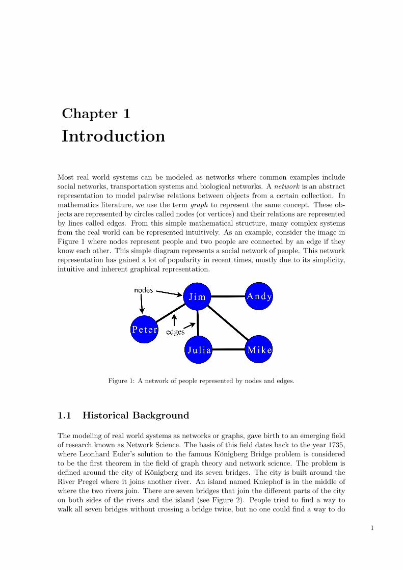
1 A network of people represented by nodes and edges. . . . . . . . . . . . . . . 1
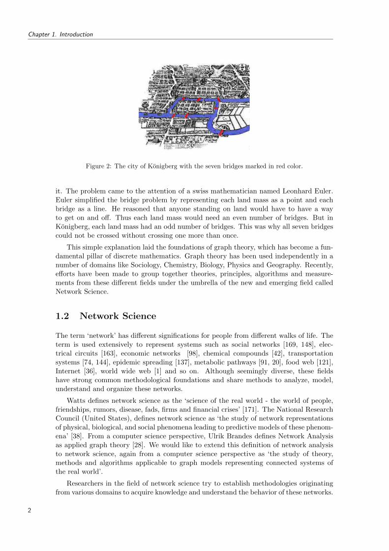
2 The city of Konigberg with the seven bridges marked in red color. . . . . . . 2
3 A typical scale free degree distribution showing highly skewed behavior andlong-tail like structure. The graph was generated using the model of Barabasiand Albert [13]. . . . . . . . . . . . . . . . . . . . . . . . . . . . . . . . . . . . 7
4 From a Regular network to a Random Network, where random rewiring of fewedges in a regular network produces a small world network with high clusteringcoefficient and low average path length. . . . . . . . . . . . . . . . . . . . . . 8
5 An example of Maxd−DIS before and after calculating Max4−DIS. . . . . . . 26
6 Visualization of Maxd-DIS graphs for the Geometry network. (a) Entire Net-work (b) Max5-DIS (c) Max10-DIS (d) Max15-DIS. . . . . . . . . . . . . . . . 28
7 (a)Histograms and (b) Log-Log scatter plot of the Degree Distribution of Ge-ometry Network. . . . . . . . . . . . . . . . . . . . . . . . . . . . . . . . . . . 29
8 (a)Four cliques representing different articles in an co-authorship network (b)The cliques are combined to form high average path length with certain nodeshaving higher degree (c) The cliques are combined to form low average pathlength with Node A standing out as a very high degree node. . . . . . . . . . 30
9 Visualization of Maxd-DIS graphs for the Dblp2008 network. (a) Part of Max5-DIS (b) Part of Max10-DIS. . . . . . . . . . . . . . . . . . . . . . . . . . . . . 32
10 Visualization of Maxd-DIS graphs for the Opte network. (a) Part of Max5-DIS(b) Part of Max15-DIS. . . . . . . . . . . . . . . . . . . . . . . . . . . . . . . 34
11 Visualization of Maxd-DIS graphs for the AirTransport network. (a) Max25-DIS (b) Part of Max50-DIS. . . . . . . . . . . . . . . . . . . . . . . . . . . . . 35
12 Visualization of Maxd-DIS graphs for the Protein network (a) Max7-DIS (b)Part of Max10-DIS. . . . . . . . . . . . . . . . . . . . . . . . . . . . . . . . . . 36
13 An example of Mind−DIS before and after calculating Min4−DIS. . . . . . . 36
14 Visualization of Mind-DIS graphs for the AirTransport network (a) Entire Net-work (b) Min250-DIS with the 10 highest degree nodes (c) Min185-DIS with the20 highest degree nodes (d) Min94-DIS with the top 5% highest degree nodes. 38
15 Min17-DIS of Geometry network with 5% highest degree nodes. . . . . . . . . 40
16 Min17-DIS of Dblp2008 network with 5% highest degree nodes. . . . . . . . . 40
17 Min7-DIS of Opte network with 5% highest degree nodes. . . . . . . . . . . . 41
ix
List of Figures
18 Mind-DIS of Protein network with 5% highest degree nodes. . . . . . . . . . . 41
19 k-core decomposition of the geometry network for different values of k (a)k =1 contains the entire network (b)k = 5 contains 610 nodes and 3594 edges(c)k = 10 contains 133 nodes and 1296 edges (d)k = 21 is the highest possiblevalue of k for the network and contains 22 nodes and 231 edges making it aclique. . . . . . . . . . . . . . . . . . . . . . . . . . . . . . . . . . . . . . . . . 43
20 (a)Max59-DIS of Geometry network containing top 22 nodes with highest de-gree (b) k-core of Geometry network containing top 22 nodes with k = 21.Only one node is common to the two subgraphs. . . . . . . . . . . . . . . . . 44
21 Consider two graphs with same number of nodes and edges and thus having thesame density in terms of number of nodes and number of edges. (a) Nodes wellconnected to each other forming quads, (b) Nodes sharing neighbors to formtriads. Clustering Coefficient for graph (a) is 0.0 and (b) is 0.69 representingthe absence of triads in graph (a). This example shows that nodes can bedensely connected even if the clustering coefficient is low. . . . . . . . . . . . 45
22 Two graphs with the same number of nodes and edges (a) Four Groups ofNodes well connected within and disconnected with other groups.(b) Nodessharing neighbors in the form of triads. Clustering Coefficient for graph (a) is0.70 and (b) is 0.69. High values for clustering coefficient does not necessarilyimply the presence of distinct community structures in a network as shown ingraph (b). . . . . . . . . . . . . . . . . . . . . . . . . . . . . . . . . . . . . . . 46
23 Component Density (CD) calculated for the Max5-DIS of Geometry network.(a) shows color encoding on the nodes from high (blue) to low (ref) values.Nodes in blue color can be easily identified as densely connected components.(b) shows the projection of CD values of Max5-DIS on the entire network withthe same color encoding. This gives an idea of how the densely connectedcomponents are spread out in the entire network. . . . . . . . . . . . . . . . . 48
24 Component Densities of Graphs for the 5 data sets.{(a)(c)(e)(g)(i)} representthe CDGMaxd
and {(b)(d)(f)(h)(j)} represents the CDGMindvalues. . . . . . 52
25 Six connected components from Max15-DIS of Geometry network. (a) and(b) are loosely connected, (c) and (d) are well connected and (e) and (f) aredensely connected. The variation in node-edge density suggests the presenceof community structures in the network. . . . . . . . . . . . . . . . . . . . . . 58
26 Max15-DIS of a network generated using Holme-Kim model with m0 = 5 andm = 1, which gives a network of size approximately equal to the NetSciencenetwork. Higher degree cliques are clearly missing. The subgraph contains 373nodes and 584 edges as compared to the entire network with 379 nodes and757 edges. . . . . . . . . . . . . . . . . . . . . . . . . . . . . . . . . . . . . . . 59
27 Network generated using Wang et al. model for random pseudofractal net-works. We see how the network evolves from t = 0 to t = 5. . . . . . . . . . . 59
28 Network generated using Klemm and Eguiluz model.(1) Network starts withm = 4 (2) A new node (red) is added connecting to all existing nodes (3) Anode is disactivated (black) based on probability proportional to its degree (4)Another node is added (red) (5) Another nodes is disactivated. . . . . . . . . 60
x
List of Figures
29 Network generated using Klemm and Eguiluz Model where size is approx. equalto the NetScience network. Figure (a) and (b) show the Max5-DIS and Max10-DIS respectively. The absence of cliques and the presence of giant componentare clearly observable. . . . . . . . . . . . . . . . . . . . . . . . . . . . . . . . 61
30 Network generated using Wang and Rong Model where size is approx. equalto the NetScience network. (a) Max5-DIS: shows the presence of cliques ofdifferent sizes (b) Max10-DIS: shows the uniform distribution of these cliques inthe network and cliques rarely overlap. Cliques are connected to each other byedges as compared to real social networks where these small social communitiesoverlap to form our society. . . . . . . . . . . . . . . . . . . . . . . . . . . . . 63
31 Step 1: Network after execution of step 1 with minSize=1, maxSize=5 andk=10. . . . . . . . . . . . . . . . . . . . . . . . . . . . . . . . . . . . . . . . . 67
32 Merging two nodes from two different cliques so that a node becomes part oftwo cliques. . . . . . . . . . . . . . . . . . . . . . . . . . . . . . . . . . . . . . 67
33 Network generated using proposed network model where the size is approx.equal to NetScience network. cliques=200 minSize=1, maxSize=7 (a) Entirenetwork (b) Max5-DIS. . . . . . . . . . . . . . . . . . . . . . . . . . . . . . . 69
34 Network generated using proposed network model where the size is approx.equal to Geometry network. cliques=3000 minSize=1, maxSize=9 (a) Max5-DIS (b) Max10-DIS. . . . . . . . . . . . . . . . . . . . . . . . . . . . . . . . . 71
35 Degree Distribution of equivalent size networks generated using the proposedModel. (a,c,e) Represent the bar charts and (b,d,f) represent the Log-Log plotof the Frequency-Degree distribution. . . . . . . . . . . . . . . . . . . . . . . 72
36 Geometry Network (a) Entire Network (b) Focus on a Small Portion (c) Partof Max5-DIS (d) Part of Max10-DIS . . . . . . . . . . . . . . . . . . . . . . . 79
37 K-Sink operation illustrated (a) 1-Sink (b) 2-Sink Type A (c) 2-Sink Type B. 80
38 Changing the order of K-Sink operation changes the hierarchy slightly but itremains consistent as the nodes find themselves grouped together in the samecluster (a) 1-Sink Operation first, sinking node 4 into node 3 followed by a2-Sink operation of Type A where nodes 1,2 and 5 are grouped together. (b)2-Sink operation of Type A first, where nodes 1 and 2 are grouped together asnode 7, followed by a 1-Sink operation where node 4 gets sinked into node 3. 81
39 Tightening Operation where Nodes 1 and 2 get disconnected leaving the othernodes densely connected. . . . . . . . . . . . . . . . . . . . . . . . . . . . . . 82
40 Graph showing linear behavior of running time in secondes of the TDHC al-gorithm with increasing graph size. . . . . . . . . . . . . . . . . . . . . . . . . 88
41 Screen shot of the top seven Search Results returned by Google for the searchedterm Jaguar. . . . . . . . . . . . . . . . . . . . . . . . . . . . . . . . . . . . . 92
42 Wikipedia web page for CAC 40 showing a number of links to web pages insections ‘See Also’, ‘References’ and ‘External Links’. . . . . . . . . . . . . . 93
43 Visualizing Clusters and Bridges of the entire jaguar network. Distinct clusters(yellow nodes) clearly separate according to the different meanings of thiskeyword across web pages. . . . . . . . . . . . . . . . . . . . . . . . . . . . . . 94
xi

List of Figures
44 Plot of the node degree distribution : degrees appears on the x-axis and thefrequencies associated on the y-axis. . . . . . . . . . . . . . . . . . . . . . . . 95
45 Co-occurrence Network of Words: Pages Browsed from CAC 40 Wikipediaweb page . . . . . . . . . . . . . . . . . . . . . . . . . . . . . . . . . . . . . . 95
46 Framework of the proposed system. There are three basic steps, simplificationof the network through node duplication, removal of bridges and identificationof clusters, visualization of clusters and bridges. . . . . . . . . . . . . . . . . . 98
47 (a) Word-Word Graph constructed from browsing CAC 40 and related webpages (b) Graph after node duplication (c) Graph after removing bridges (d)Graph with Clusters and Bridges using proposed visualization. . . . . . . . . 100
48 Histogram of degree distribution for the Cac40 data set. . . . . . . . . . . . . 100
49 A tool tip allows to easily browse keywords of a cluster and figure out itsintrinsic semantics. . . . . . . . . . . . . . . . . . . . . . . . . . . . . . . . . . 103
50 Right-clicking on a cluster reveals URL’s of all web pages associated withkeywords. In the example, URLs already indicate that the cluster gatherspages about Jaguar Cars. . . . . . . . . . . . . . . . . . . . . . . . . . . . . . 104
51 Visual Layout of Clusters and Bridges for the keyword Hepburn where a setof clusters are disconnected to other clusters. . . . . . . . . . . . . . . . . . . 104
52 Focus on a connected set of clusters for the search keyword Hepburn. . . . . . 105
53 (a) A small part isolated from Figure 47(d) showing Titles of Web pages clus-tered together and Bridges(b) Duplicated nodes highlighted after selection . . 105
54 (a) Represents a clique (b) presents a star-like structure and (c) is a set ofnodes connected to each other in a chain-like structure. . . . . . . . . . . . . 108
55 Represents three graphs with enclosed nodes being the clusters. All the clustershave the same cut size which is equal to 1. Based on the cut size alone thequality of the clustering cannot be judged. . . . . . . . . . . . . . . . . . . . . 109
56 AirTransport network drawn using Hong Kong at the center and some airportsdirectly connected to Hong Kong. We can see the worlds most importantcities having a direct flight to Hong Kong whereas there are lots of regionalairports connected to Hong Kong representing a star-like structure as discussedpreviously in Figure 54(b) and 55(b). . . . . . . . . . . . . . . . . . . . . . . 110
57 Internet Tomography Network representing routing paths from a test host toother networks. Two nodes clearly dominate the number of connections as theyplay the role of hubs to connect several clients. Another example of star-likestructures in the real world. . . . . . . . . . . . . . . . . . . . . . . . . . . . . 110
58 Artificial and Clustered Networks with predefined intra-cluster edges and ran-dom inter-cluster edges. (a)Clusters with cliques (b)Clusters with Star-likeStructures (c) Clusters with Chain-like Structures. . . . . . . . . . . . . . . . 115
xii

List of Tables
1 n=nodes, e=edges, ad=average degree, hd=highest node degree, cc=clusteringcoefficient, apl= average path length . . . . . . . . . . . . . . . . . . . . . . . 22
2 Comparing and Summarizing different Artificial Network Generation Modelsexisting in the literature. n=nodes, m=edges . . . . . . . . . . . . . . . . . . 64
3 Comparing different models with the Collaboration Network of Scientists fromthe NetScience data. APL=Average Path length, CC=Clustering Coefficient,HD=Highest Node Degree . . . . . . . . . . . . . . . . . . . . . . . . . . . . . 72
4 Comparing different models with the Collaboration Network of Scientists fromthe Computational Geometry data. APL=Average Path length, CC=ClusteringCoefficient, HD=Highest Node Degree . . . . . . . . . . . . . . . . . . . . . . 73
5 Comparing different models with the Imdb network from the IMDB dataset.APL=Average Path length, CC=Clustering Coefficient, HD=Highest NodeDegree . . . . . . . . . . . . . . . . . . . . . . . . . . . . . . . . . . . . . . . . 73
6 Comparing the results of Divisive Clustering based on Edge Distribution (Div.Clus.), Bisecting K-Means (Bis. K-Means) and Strength Clustering (Strength)algorithms with the TDHC algorithm. . . . . . . . . . . . . . . . . . . . . . . 86
7 Comparing the execution times of Divisive Clustering based on Edge Distribu-tion (Div. Clus.), Bisecting K-Means (Bis. K-Means) and Strength Clustering(Strength) algorithms with the TDHC algorithm. . . . . . . . . . . . . . . . . 87
8 Execution time of TDHC for graphs of increasing size. . . . . . . . . . . . . . 88
9 Evaluating the quality of clustering using three topologically different andartificially generated clustered data sets. . . . . . . . . . . . . . . . . . . . . . 115
10 Evaluating the quality of clustering real world data sets using the existing andthe proposed cluster evaluation technique. . . . . . . . . . . . . . . . . . . . . 116
xiii

xiv
Chapter 1
Introduction
Most real world systems can be modeled as networks where common examples includesocial networks, transportation systems and biological networks. A network is an abstractrepresentation to model pairwise relations between objects from a certain collection. Inmathematics literature, we use the term graph to represent the same concept. These ob-jects are represented by circles called nodes (or vertices) and their relations are representedby lines called edges. From this simple mathematical structure, many complex systemsfrom the real world can be represented intuitively. As an example, consider the image inFigure 1 where nodes represent people and two people are connected by an edge if theyknow each other. This simple diagram represents a social network of people. This networkrepresentation has gained a lot of popularity in recent times, mostly due to its simplicity,intuitive and inherent graphical representation.
Figure 1: A network of people represented by nodes and edges.
1.1 Historical Background
The modeling of real world systems as networks or graphs, gave birth to an emerging fieldof research known as Network Science. The basis of this field dates back to the year 1735,where Leonhard Euler’s solution to the famous Konigberg Bridge problem is consideredto be the first theorem in the field of graph theory and network science. The problem isdefined around the city of Konigberg and its seven bridges. The city is built around theRiver Pregel where it joins another river. An island named Kniephof is in the middle ofwhere the two rivers join. There are seven bridges that join the different parts of the cityon both sides of the rivers and the island (see Figure 2). People tried to find a way towalk all seven bridges without crossing a bridge twice, but no one could find a way to do
1
Chapter 1. Introduction
Figure 2: The city of Konigberg with the seven bridges marked in red color.
it. The problem came to the attention of a swiss mathematician named Leonhard Euler.Euler simplified the bridge problem by representing each land mass as a point and eachbridge as a line. He reasoned that anyone standing on land would have to have a wayto get on and off. Thus each land mass would need an even number of bridges. But inKonigberg, each land mass had an odd number of bridges. This was why all seven bridgescould not be crossed without crossing one more than once.
This simple explanation laid the foundations of graph theory, which has become a fun-damental pillar of discrete mathematics. Graph theory has been used independently in anumber of domains like Sociology, Chemistry, Biology, Physics and Geography. Recently,efforts have been made to group together theories, principles, algorithms and measure-ments from these different fields under the umbrella of the new and emerging field calledNetwork Science.
1.2 Network Science
The term ‘network’ has different significations for people from different walks of life. Theterm is used extensively to represent systems such as social networks [169, 148], elec-trical circuits [163], economic networks [98], chemical compounds [42], transportationsystems [74, 144], epidemic spreading [137], metabolic pathways [91, 20], food web [121],Internet [36], world wide web [1] and so on. Although seemingly diverse, these fieldshave strong common methodological foundations and share methods to analyze, model,understand and organize these networks.
Watts defines network science as the ‘science of the real world - the world of people,friendships, rumors, disease, fads, firms and financial crises’ [171]. The National ResearchCouncil (United States), defines network science as ‘the study of network representationsof physical, biological, and social phenomena leading to predictive models of these phenom-ena’ [38]. From a computer science perspective, Ulrik Brandes defines Network Analysisas applied graph theory [28]. We would like to extend this definition of network analysisto network science, again from a computer science perspective as ‘the study of theory,methods and algorithms applicable to graph models representing connected systems ofthe real world’.
Researchers in the field of network science try to establish methodologies originatingfrom various domains to acquire knowledge and understand the behavior of these networks.
2
1.3. Properties of Networks
The question is, how can this knowledge be applied and where? An early example comesfrom the field of sociology and the development of the sociogram in 1933, where JacobMoreno, a psychologist, used a network to represent how the interpersonal structure of agroup of people looks. He used the example of a group of elementary school students whereboys were friends of boys and girls were friends of girls except for one boy who said heliked a single girl. This representation of sociogram has been used in social networks eversince and has found many useful applications to understand and analyze social networks.
Moving on from social networks to a completely different domain of electric supplynetwork, we consider the example borrowed from the article of Wang and Chen [168].A famous cascading series of failures in power lines took place in August 1996, whichlead to blackouts in 11 US states and 2 Canadian provinces. This incident left about 7million customers without power for up to 16 hours, and cost billions of dollars in totaldamage. An analysis of this type of network can help identify break points and put inplace a protection strategy to avoid further instances of power failure of this magnitudeby proposing alternate routing paths.
In the examples briefly described above, it is important to understand that these realworld systems can easily be modeled as graphs. The simple mathematical model of agraph presents a robust and flexible platform to build models for complex systems with alarge number of attributes and varying relationships. Recent developments in computertechnology has prompted a huge scaling factor in networks. Nowadays, networks withhundreds of thousands of nodes and edges are easily constructed for various domains.This progress has played the role of a catalyst to attract researchers to study variousproperties, characteristics and measures for these networks, and hence has led towards thedevelopment of the research domain called network science.
Traditionally the study of networks has been considered as a sub-domain of graphtheory. Before 1950s, regular graphs were studied extensively [143, 129], but since then,most large scale networks with no apparent design principle were described as randomgraphs introduced by two Hungarian mathematicians Paul Erdos and Alfred Renyi [54, 55].According to the Erdos-Renyi model, we start with n nodes and connect every pair of nodeswith probability p, creating a graph with approximately p[n(n − 1)/2] edges distributedrandomly. This model has been the corner stone for many scientific discoveries and notableresults [14]. Although random graphs occur readily in the real world, most systems exhibitnon-random characteristics. As researchers tried to develop new concepts and measures forin-depth analysis and understanding of networks, three of these properties have attractedlots of attention. We discuss these properties in the following section.
1.3 Properties of Networks
Motivated by several observations, inherent by construction or evident due to underlyingtopology, three concepts have attracted lots of attention in the research of real worldnetworks and to some extent, revolutionized the study of networks as it stands today.These concepts are the Small World Effect, Clustering Coefficient and Degree Distribution.We discuss these concepts below:
Small World Effect or Average Path LengthIn the late 1960s, an American social psychologist, Stanley Milgram conducted a set of
3
Chapter 1. Introduction
experiments which are referred to as, the small world experiment [118, 159]. The idea wasto resolve the question of the number of degrees of separation in actual social networks.Milgram gave 300 letters to participants living in the cities of United States, Boston andOmaha, along with instructions to deliver them to one particular target person by mailingthe letter to an acquaintance they considered to be closer to the target. That person thengot the same set of instructions, which therefore, set up a chain. Milgram found thatthe average path length of these chains was about six. The research was groundbreakingin that it suggested that human society is a small world type network characterized byshort path lengths. The experiments are often associated with the phrase ‘six degrees ofseparation’, although Milgram did not use this term himself, instead it was John Gaurein 1990 who coined this term [72]. In literature, this concept is often referred to as theaverage path length of a network. It gives an idea of, on average, how far apart any twonodes lie in a network.
Formally, we can define the average path length as the mean geodesic (shortest) dis-tance between node pairs in a network. Consider this distance be represented by l for anetwork, mathematically we can define l by the following equation:
l =1
n ∗ (n− 1)
∑i,j
dij
where dij is the geodesic distance from node i to node j and n is the total number ofnodes in the network. We assume that the distance between two nodes is 0 if they cannotbe reached by one another and the distance of a node to itself is also 0.
For large size networks, the typical geodesic distance between any two nodes scalesas the logarithm of the number of nodes, suggesting that the average distance betweenany two nodes in the network is quite low. Erdos and Renyi have shown that the averagedistance in random graphs, also scales as the logarithm of the number of nodes, so tospeak, random graphs have also the small world effect [143].
This information can be quite useful in different networks. For example, studying howto control and take precautions against an epidemic spread in social networks [122, 180],designing marketing strategies and targeting customers for the launch and dissemination ofnew products and technologies [45], and to more technical applications such as estimatingthe number of hops required for an information packet to get from one computer to anotheron the Internet [185].
Clustering Coefficient or TransitivityAnother important characteristic of real world networks is the high average clustering
coefficient of nodes [170]. This concept is sometimes referred to as Transitivity [129], orthe fraction of transitive triples in a network [169]. This is done so to avoid confusionfrom the concept of Community Structures or Clusters [28, 68] which will be discussedextensively in the chapters to follow.
Coming back to transitivity, the concept is very well known in social networks andcan be described as the friend of your friend is likely to be your friend. The roots of thisidea come from the work of Georg Simmel [150] who introduced the concept of triads asa fundamental structure for social networks. In fact, the smallest and most elementarysocial unit, a dyad is a social group composed of two members while a triad is a socialgroup composed of three members. Groups of larger size are also possible but since a
4
1.3. Properties of Networks
variety of relationships can form in them, they are less stable [150] and often less studiedin sociology. Although high clustering coefficients were first observed in social networks,many other networks have shown this tendency such as the world wide web [1], transportnetworks [149] and metabolic networks [20, 165].
To quantify the clustering coefficient, two definitions exist in the literature. They canbe classified as global clustering coefficient and local clustering coefficient. The globalclustering coefficient measures the fraction of triples that have their third edge filled in,to complete the triangle [132] and is calculated by the following equation:
Cglobal =3 ∗ number of triangles in the networknumber of connected triples of vertices
The factor of three in the numerator accounts for the fact that each triangle contributesto three triples and ensures that the value lies in the range [0,1]. In simple terms, theglobal clustering coefficient is the mean probability that two vertices that are networkneighbors of the same other vertex will themselves be neighbors. This value gives anoverall picture about the presence of triads in a network.
The definition of local clustering coefficient was given by Watts and Strogatz [170] andis calculated for each vertex in a network. The local clustering coefficient for a node n,having kn edges which connects it to kn neighbors is given below:
Clocal(n) =2 ∗ en
kn ∗ (kn − 1)
If the nearest neighbors of the original node were part of a clique, there would bekn(kn−1)/2 edges between them. The ratio between the number of edges en that actuallyexist between kn nodes and the total number kn(kn−1)/2 gives the value of the clusteringcoefficient of node n. To calculate the clustering coefficient of the entire network, we takethe average for all nodes in the network.
The two definitions of clustering coefficient given above result in different values whencalculated for the same network. One tries to calculate the mean of ratio, and the other,the ratio of the means respectively [129]. But the important concept here is that both ofthem tries to capture the same notion, the presence of triads in a network. Throughoutthis document, we use the second definition without differentiating between global andlocal clustering coefficient as it is more widely accepted [73].
In a random graph, since the edges are distributed randomly, the presence of thesetransitive triples or triads is rare, as compared to real world networks where usually highclustering coefficients are observed. It is interesting to note that the presence of these triadsis a direct implication of how real world systems behave in the real world. The probabilitythat you are going to become friends with a person who has a common acquaintance isquite high. This can be quite helpful in predicting the evolution of networks and generationof new links between existing objects specially in social networks. An obvious examplecomes from the scientific collaboration network of researchers. If a researcher say a, co-authors two artifacts with researchers b and c separately, it is likely that their researchdomain is the same and researchers b and c might end up collaborating as well. There area number of articles citing these collaboration networks such as [125, 127].
5
Chapter 1. Introduction
Degree DistributionThe degree of a node refers to the number of connections a node has in the network.
Formally, we define pk to be the fraction of vertices in the network that have degree k.The term pk also represents the probability that a vertex chosen uniformly at random hasdegree k. A plot of pk for any given network can be formed by making a histogram of thedegrees of vertices. This histogram is the degree distribution for the network (see Figure 3as example).
Generally, it was believed that the degree distribution in most networks follows aPoisson distribution but in reality, real world networks have a highly skewed degree dis-tribution following power-laws. Power-laws are expressions of the form y ∝ xγ , where γis a constant, x and y are the measures of interest [152].
One of the early works in this direction was carried out in the year 1925 by GeorgeUdny Yule, a British statistician, who explained the power-law distribution of the numberof species per genus of flowering plants [182]. The process is sometimes called a Yuleprocess in his honor. Another notable work came years later on by Derek de Solla Pricein 1965 where he studied networks of citations between scientific papers [44]. The numberof citations they received had a heavy-tailed distribution following a Pareto distributionor power law. In a later paper in 1976, Price also proposed a mechanism to explain theoccurrence of power laws in citation networks, which he called cumulative advantage [138].Price was the first to apply the process to the growth of a network and explained hownetworks evolve.
Recent interest in networks with power-law degree distribution started in 1999 withthe work by Barabasi and colleagues at the University of Notre Dame who mapped thetopology of a portion of the Web [13], finding that some nodes, which they called hubs,had many more connections than others and that the network as a whole had a power-lawdistribution of the number of links connecting to a node. They coined the term scale-free network to refer to these networks with the degree distribution following power law.Barabasi and Albert also proposed a mechanism to explain the appearance of the power-law distribution, which they called preferential attachment [13], which is essentially thesame as that proposed by Price in 1976.
Another common term used to refer to this principle is ‘the rich get richer’, firstused by Robert H. Jackson, Counsel to the Internal Revenue Bureau, in a hearing of theSenate Finance Committee in 1935 [87]. He tried to explain the economic system and theinequalities in the distribution of wealth and the burden of taxation in the United States.In terms of network theory, all these concepts refer to the idea that if a node has a highdegree, it has a higher probability to attract more connections and thus its connectivitygrows at a faster rate than other nodes with low connectivity.
In sociology, the ‘Matthew effect’ is a term which refers to the principle of rich getricher. This term was coined by Robert K. Merton [115] to describe how, among otherthings, eminent scientists will often get more credit than a comparatively unknown re-searcher, even if their work is similar; it also means that credit will usually be given toresearchers who are already famous. For example, a prize will almost always be awardedto the most senior researcher involved in a project, even if all the work was done by agraduate student.
In a random graph, each edge is present or absent with equal probability, and hencethe degree distribution is, as mentioned earlier, Poisson in the limit of large graph size.Real world networks are mostly found to be very unlike the random graph in their degree
6

1.4. Small World and Scale Free Networks
distributions. Far from having a Poisson distribution, the degrees of the vertices in mostnetworks are highly right skewed, meaning that their distribution has a long right tail.Figure 3 shows the degree distribution of a network generated using the network generationmodel of [13] for scale free networks. The histogram of the degree distribution clearly showsthe right skewed behavior with a long tail like structure.
Figure 3: A typical scale free degree distribution showing highly skewed behavior andlong-tail like structure. The graph was generated using the model of Barabasi andAlbert [13].
In terms of a network, this scale free behavior suggests that few nodes have a veryhigh number of connections and lots of nodes are connected to a few nodes only. Thisinformation has quite practical implications in the design and study of networks. Forexample, in a social network, these hubs (nodes with high degree) play an important roleto diffuse information as they are people having many social links [23]. Many marketingand business strategies can be developed revolving around hubs, as these people havemany social contacts that can be used effectively to promote products and acquire businesscollaborations.
1.4 Small World and Scale Free Networks
From these three measures, two important classes of networks emerge, Small World Net-works and Scale Free Networks. A small world network as defined by Watts and Stro-gatz [170], is a network with high clustering coefficient and small average path length.A scale free network as defined by Barabasi and Albert [13], is a network where the de-gree distribution follows a power law. Models were proposed by respective researchers toexplain how networks with these properties appear in the real world.
Lets have a look at the small world model proposed by Watts and Strogatz. We startwith a ring of n vertices in which each vertex is connected to its k nearest neighbors, for agiven k. This forms a regular graph as shown in Figure 4(a). Then, each edge is rewiredwith a given probability p by choosing randomly a new vertex to connect. In a regulargraph, since neighbors are connected to each other, the overall clustering coefficient is
7

Chapter 1. Introduction
Figure 4: From a Regular network to a Random Network, where random rewiring offew edges in a regular network produces a small world network with high clusteringcoefficient and low average path length.
very high. On the other hand, the average path length is very low as vertices are onlyconnected to their neighbors. Randomly rewiring a few nodes introduces edges connectingnodes lying at long distances, which in turn, reduces the overall average path length. Sincemany vertices are connected to their neighbors, the overall clustering coefficient remainshigh whereas the average path length is reduced, giving us the properties of a small worldnetwork (see Figure 4(b)). If the process of random rewiring continues, we eventuallyend up rewiring every node which results in a random graph as vertices no longer sharecommon neighbors. It is important to note that networks produced using this model donot have scale free degree distribution. Since every vertex in the network initially has afix k degree, random rewiring of only a few vertices does not effect the overall behaviorof the degree distribution. More formal studies of this model have been conducted withinteresting results [50]. Other models have been proposed to produce networks with smallworld properties without using this basic model such as [112, 73].
Barabasi and Albert explained how scale free networks emerge in real world networksthrough another model. To begin, there are n vertices and no edges connecting them. Atevery time step t, a new vertex v with m edges is added to the network. These edges areconnected to existing vertices with the probability proportional to the degree of the nodesin the network. Obviously, at the beginning, when there are no edges, the probability ofconnection of all the vertices is the same. As the network grows, gradually few nodes beginto have higher node degree and thus higher probability of connecting to newly introducednodes in the network. This preferential bias in the connectivity is termed as preferentialattachment as new nodes prefer to attach to high degree nodes. Mathematical resultsfor scale free graphs have been studied by several researchers such as [22, 23]. Alternatemodels have been proposed to produce scale free degree distribution without using thepreferential attachment such as [34, 2].
Although these two classes have been introduced separately, most real world networksbelong to them at the same time. A more generic term, Complex Networks is used to referto networks belonging to both these classes, although, many researchers call networks ascomplex when they are either small world only or scale free only. There is no precisedefinition for a complex network but any network which is not regular, nor random andhas any characteristic behavior such as high clustering coefficient or right skewed degreedistribution can be termed as a complex network. In this thesis, we restrict ourselves tonetworks with small world or scale free behavior, or both at the same time and we refer
8

1.5. Complex Networks
to them as complex networks throughout this study.
1.5 Complex Networks
As described previously, the ideas of small world and scale free properties date back to18th and 19th century, they have been made popular recently with the works of Wattsand Strogatz in 1998 [170] and Barabasi and Albert in 1999 [13]. A number of books, sur-veys, reports and research articles have addressed issues revolving around these complexnetworks. Although the study of complex networks has sound foundations from mathe-matics and graph theory, the field itself is in its infancy, as more and more researcherstry to develop new theories and behaviors common to different kinds of networks, be itbiological, technological or social. Most of the early research work focuses on identifyingthe small world and/or scale free behavior of networks from different domains.
One such study to analyze Internet networks was performed by Faloutsos et al. [58]where they identify three power-laws for the topology of the Internet. They also introduceda graph metric to quantify the density of a graph and proposed a rough power-law approx-imation of that metric. They also showed the use of power laws and the proposed metricto estimate useful parameters of the Internet, such as the average number of neighborswithin h hops.
A more profound mathematical analysis of small world networks was performed byBarrat and Weigt [15] where they studied the geometrical properties of small world net-works which interpolate continuously between a one-dimensional ring and a certain randomgraph. The long ranged links contribute to the low average path length which stronglydepends on the amount of disorder in the global structure. The local structure contributesto links between two neighboring vertices and leads to a high clustering coefficient.
Mathias and Gopal [112] studied neural and transportation networks and tried toexplain how the small world property arises as a consequence of a trade off betweenmaximal connectivity and minimal wiring as proposed by Watts and Strogatz [170]. Theypresent an alternate approach to generate small world behavior through the formation ofhubs and small clusters where one vertex is connected to a large number of neighbors.
Amaral et al. [7] also studied the small world networks and presented a classificationof these networks based on the behavior of the degree distribution of several real worldnetworks. The three classes were identified as:
1. scale-free networks, characterized by a vertex connectivity distribution that decaysas a power law.
2. broad-scale networks, characterized by a connectivity distribution that has a powerlaw regime followed by a sharp cutoff.
3. single-scale networks, characterized by a connectivity distribution with a fast decay-ing tail.
To justify this classification, they present two concepts, Aging of the vertices and Costof adding links to the vertices or the limited capacity of a vertex. The idea of Aging is thatwith the passage of time, some vertices stop connecting to new links, an example is thatof social network of movie actors, when actors retire, the nodes representing these actors
9

Chapter 1. Introduction
in the network stop interacting with new nodes and thus need to be taken into accountfor a growing network. The Cost of Vertex refers to the concept of practical efficiency innetworks such as network of world airports where direct flights represent links betweentwo airports. Simply for commercial issues, it is practical to have hub airports wheremany routes connect, but with certain limitations such as the maximum flights an airportcan host.
Barabasi’s book titled Linked: The New Science of Networks [14] studies differentnetworks demonstrating that these networks have an underlying order. This knowledgecan be used effectively in a variety of domains, from designing optimal organization ofa firm to stopping a disease outbreak before it spreads catastrophically. A review fromAlbert and Barabasi titled Statistical mechanics of complex networks [143] shows empiricalresults on the topology of several real world networks and focuses on generation models toproduce artificial complex networks mimicking real world systems. Another survey in thesimilar direction is that from Dorogovtsev and Mendes titled Evolution of networks [48]where they discuss a number of issues like how networks organize into scale-free structuresand the role of the mechanism of preferential attachment, the topological and structuralproperties of evolving networks. An interesting study of applications of the general resultsto particular networks in nature are discussed and connections of the network growthprocesses with the general problems of non-equilibrium physics, econophysics, evolutionarybiology are established. Dorogovtsev and Mendes also wrote a book titled Evolution ofNetworks: From Biological Nets to the Internet and WWW [49] based on their previoussurvey.
A survey by Mark Newman, Structure and Function of Complex Networks [129] pro-vides another good review of developments in the field of network science. He presents aloose categorization of these networks, as Social, Information, Technological and Biolog-ical networks. Newman et al. also edited a collection of research works in this domaincalled The Structure and Dynamics of Networks [133].
Another property of complex networks was studied by Newman [128], which is themixing patterns of these complex networks. A network is said to show assortative mixingif the nodes in the network that have many connections tend to connect to other nodeswith many connections. Newman reports that in a variety of networks, social networksare mostly assortatively mixed, but that technological and biological networks tend to bedisassortative.
Duncan Watts, in his book Six Degrees: The Science of a Connected Age [171] tries touse plenty of examples from real life to explain the new and growing science of networks andtheir collective behavior. The book targets general public and presents network conceptsby examining everyday life examples such as disease epidemics and the stock market. MarkBuchanan’s book, Nexus: Small Worlds and the Groundbreaking Theory of Networks [32]demonstrates practical applications of network theories to diverse problems as well asan attempt to understand the dynamic interactions within our physical as well as socialworlds.
Bornholdt and Schuster compiled a number of articles related to this subject in a booktitled Handbook of Graphs and Networks: From the Genome to the Internet [25]. Thebook discusses the field of complex networks and presents the dynamics of networks andtheir structure as a key concept across disciplines such as Traffic Networks and EconomicNetworks.
10
1.5. Complex Networks
An interesting article written by Judith Kleinfeld [99] takes a look at the experimentsconducted by Milgram to show the ‘six degrees of separation’ principle. Many questionsare raised to challenge the validity of the experiments and the claims made by Milgram.Recall from the earlier section where we described the experiment, the idea was to delivera letter to a particular target person, a stockbroker living in Boston. The person chosen byMilgram was well known in the community, and does not represent the entire population.Also, the people selected to deliver the letter were not chosen randomly. The experimenttells that three hundred people living in Omaha, were selected to deliver the letter, butactually one hundred were in Boston. Out of the remaining two hundred people, only96 were randomly selected from a mailing list, the others were blue-chip stock investors.Starting from these 96 randomly selected people, only eighteen reached the eventual tar-get which is a very low percentage. Other researchers have failed to replicate the sameexperiment and leaves a big question mark on the results achieved. Even with these bi-ased experiments, the results were widely and easily accepted by the population at large,Kleinfeld suggests that this is largely due to the perception that with the advancement intechnology, the world is becoming smaller, and we want to believe that we live in a smallworld. She concludes that it is possible that we live in a small world separated by sixdegrees, but experimental evidence is lacking and should be reconsidered.
Another perspective to study complex networks is given by Bollobas [22] who classifiesthe work in this field into the following categories.
1. Direct studies of the real-world networks themselves, measuring various propertiessuch as degree-distribution, diameter, clustering, etc.
2. Suggestions for new random graph models motivated by this study.
3. Computer simulations of the new models, measuring their properties.
4. Heuristic analysis of the new models to predict their properties.
5. Rigorous mathematical study of the new models, to prove theorems about theirproperties.
He focuses on the mathematical study of these networks and models including sev-eral new results, mostly demonstrating that large-scale real world networks confirm thecomputer generated models reviewed. He concludes that there is still a lot of work thatneeds to be done in terms of mathematical study of these models and networks. This workappears in the book compiled by Bornholdt and Schuster, but due to its importance, wementioned it again.
One such mathematical study comes from Lun Li et al. [106], who performed an exten-sive study of scale free graphs in an attempt to formalize the mathematical foundationsand definitions pertaining to the topic. They introduce a structural metric called s-metricthat allows us to differentiate between all simple, connected graphs having an identicaldegree sequence, which is of particular interest when that sequence satisfies a power lawrelationship. The metric is used to falsify the claim that scale free networks are robust torandom loss of nodes but fragile to targeted worst-case attacks on hubs as shown by Albertet al. [4]. The examples considered are of router-level Internet [107, 5] and metabolic net-works [155] where the networks in question do not have hubs. The most highly connected
11
Chapter 1. Introduction
nodes do not necessarily represent nodes fragile to attack and that their robust, yet fragilefeatures actually come from aspects that are only indirectly related to graph connectivity.
Another interesting book compiled by editors Brandes and Erlebach titled NetworkAnalysis : Methodological Foundations [28] covers methods for specific levels of analysissuch as individual elements, groups of elements and the entire network. The book containsan extensive study of concepts, metrics and algorithms and rightly claims to be the firstbook to do so, from a methodological perspective independent of specific application areasto analyze networks.
Summarizing the existing literature on networks, most of the early work is relatedto bringing networks from different real world examples under the classification of eithersmall world networks, scale free networks or both at the same time. Several models havebeen proposed and studied in detail to replicate the behavior of these real world networksas a tool to understand the structure and evolution of complex systems. Researchershave realized that although the low average path length, high clustering coefficient andpower law degree distribution are common features for these networks from various do-mains, there is a strong need to develop mathematical foundations, models and measuresto understand how these systems differ from one domain to the other. An attempt todevelop common theories and algorithms for these complex networks can not only leadto enhanced scientific understanding of the physical systems around us but can also helpbuild a common ground for real world applications that can be useful to solve real worldproblems. All this knowledge acquired by the researchers contributes in the developmentof this new and emerging science called network science.
Another important yet less studied aspect that has changed our approach towards thestudy of these complex systems is the advent and availability of computer aids to visualizethese networks. Euler used a graph to represent the Konigberg Bridge problem and sodid Jacob Moreno for a sociogram, but with the explosion in the size of networks recently,drawing these graphs has prompted radical changes in how we visualize information. Spe-cially with new and innovative rendering technologies and interactive exploration possible,the study of networks has changed and evolved during the last decades. Although, notconsidered as an integral part of network science, we believe that Network Visualizationis an important aspect of this growing field. In our point of view, this drift certainlysuggests that network science has overlapping goals with fields such as Information Visu-alization [19, 96], Visual Data Mining [151, 96] and Visual Analytics [157]. One way todifferentiate these fields from network science is that, in all these fields, visualization isan essential concept and they cannot exist if visual aspect is taken away from these fieldswhereas network science does not depend solely on visualization. From this brief reviewof the literature, in the next section, we move towards categorizing the research in thefield of network science and specially complex networks.
1.6 Study of Complex Networks
Reviewing the literature, the study of these networks can be grouped under four categorieswhich are:
> Analysis
> Structure
12
1.6. Study of Complex Networks
> Processes and Organization
> Visualization
Analysis comprises of several metrics and measurements proposed to study the statis-tical properties of complex networks. These properties can be further categorized basedon the granularity of the measure used, such as element level, group level and entire net-work [28]. Metrics such as the clustering coefficient and degree distribution have played afundamental role in the origins of complex networks. Current research is heavily focusedon developing more metrics that can quantify new and interesting properties of thesenetworks.
Structure refers to the research carried out in modeling real world networks. There havebeen a number of principles identified as being the driving force to produce small worldnetworks, scale free networks or networks having both these properties. Researchers haveproposed a host of algorithms in an attempt to understand the structure and evolution ofcomplex systems.
Processes and Organization is the collection of numerous processes exploiting the smallworld or scale free behavior of these complex networks. Common problems like searchingspecific nodes or paths in networks, searching and identifying frequent motifs, groupingsimilar vertices to organize and understand the overall behavior of networks are all ex-amples of common processing tasks performed on complex networks. One of the mostwidely used methods to group similar vertices is called Clustering which has found practi-cal applications in numerous domains. Clustering is defined as a decomposition of verticesinto ‘Natural Groups’. More precisely, we can say that a cluster is a set of vertices withhigh interconnectivity among vertices of the same cluster and low connectivity of verticesof different clusters. In sociology, often clusters are termed as community structures orsimply communities.
Visualization groups the techniques existing in the domain of graph drawing, informa-tion visualization and visual analytics applied to these real world networks for interactiveexploration and extraction of hidden knowledge. Visualization of graphs is an inherentfeature of network science as its basis lies in graph theory. Researchers have used the grow-ing technological advancements in these fields to derive interesting results about complexnetworks.
Although each of these categories has clear and well defined objectives, they are notnecessarily independent of each other. For example, the metrics and measurements devel-oped for these networks are heavily used in developing models to understand the structureof these networks. Processes of grouping similar nodes are commonly used to reduce thevisual complexity and present a summarized graphical view such that domain experts caninterpolate and extrapolate knowledge about these complex systems. Thus, although wecan identify these categories of research for network science, the research itself is carriedout tightly integrating these categories such that it is difficult to separate one from theother.
13
Chapter 1. Introduction
1.7 Research Contributions
In this thesis, we address specific problems for each category and try to resolve somecommon issues pertaining to the study of complex networks, and contribute to the ad-vancement of this new and exciting field of study.
In terms of Analysis, we start by presenting a visual analytics way to explore thesecomplex networks. A method combining a new metric and visualization technique toanalyze and explore these graphs is proposed where the idea is to study how the edges aredistributed among nodes of varying degree. Several real world networks are analyzed usingthe proposed methods with interesting observations and results are presented in details inChapter 3.
Next, we study the structure of these complex networks and review a number of differ-ent network generation models specially focusing on models that produce small world andscale free networks. Although these models generate random networks with scale free andsmall world properties, there is no apparent community structure present at the macrolevel in the networks generated by these models. We present a new model which is usefulto generate small world and scale free networks with community structures. The modelcan be useful to help generate test data sets for experimentation of empirical studies ofcomplex systems with known and well defined structure. This topic is discussed in detailin Chapter 4.
To study the topic of processes and organization, our research efforts are directedtowards the problem of clustering as fundamental procedure to organizing complex net-works. With the increasing storage capacity for large size networks, fast algorithms arerequired that are able to cluster complex networks. We propose an algorithm which ishighly efficient in terms of time complexity and uses the analysis method proposed inChapter 3 to build a clustering algorithm. Comparative results show that the algorithmgives acceptable results in terms of cluster quality. The details are presented in Chapter 5.
In terms of visualization, a common problem with these networks is that drawingthese networks using existing methods produces highly entangled and cluttered drawingsas several networks were drawn using force directed algorithms in Chapter 3 for visualanalysis. We propose a method to address this issue, combined with another clusteringalgorithm specially designed to handle the visualization aspect of complex networks. Wehave applied the method on co-occurrence networks obtained from the web where severalcase studies show the efficiency of the proposed clustering and visualization system. Wediscuss the details of the proposed solution in Chapter 6.
Continuing with the topic of clustering, we study different metrics that are used toevaluate the quality of clusters in the absence of ground truth and bench mark cluster-ings for different data sets. Based on our findings from the analysis of several complexnetworks in Chapter 3, we identified that several networks do not have densely connectedsubgraphs and thus node-edge density should not be used as a primary ingredient to an-alyze the quality of a clustering algorithm in the absence of dense subgraphs. Furthermore, the presence of star-like structures was identified as an important pattern in somecomplex networks. We propose a new method based on average path lengths that is ableto overcome the drawbacks of density based evaluation metrics and correctly evaluate thequality of a cluster in the presence of star-like structures. The details are presented inChapter 7.
14

1.8. Organization of Thesis
1.8 Organization of Thesis
In the next chapter, we present necessary background knowledge and present a number ofreal world networks that are used for experimentation and empirical studies in this thesis.The chapter ends with a tabular listing of some statistical measures of these networks.
Chapters (3, 4, 5, 6, 7) all introduce common problems related to the study of com-plex networks. Chapter 3 is related to visual analysis and metrics for complex networks.Chapter 4 discusses the structure of networks having both small world and scale freeproperties. In Chapter 5, we focus on clustering of complex networks presenting a newalgorithm which is highly efficient in terms of time complexity. Chapter 6 focuses onclustering and visualization of these networks. Chapter 7 addresses the issue of evaluatingthe quality of clustering algorithms for networks without densely connected regions.
Chapter 8 lists the articles that we published during this period. We also listed otherresearch work that we carried out during the thesis and are related to the study of complexnetworks but are not part of the thesis. Brief introduction is given followed by variouspublications that resulted from the research.
Finally, in Chapter 9, we present our conclusions and future research prospects.
15

16

Chapter 2
Preliminaries
In this chapter, first we briefly describe the mathematical terminologies used throughoutthis document. Next, we introduce a number of real data sets that have been used forexperimentation in various chapters. We also provide a number of statistical measures forthese data sets at the end of this chapter.
2.1 Mathematical Foundations
This section reviews some basic definitions used extensively in network science and mostlyborrowed from graph theory. We use the terms network and graph interchangeablythroughout this document.
Graph: A graph is an abstract representation of a set of objects connected throughlinks. The objects are denoted by the set V of vertices (also called nodes) and theirconnections denoted by the set E of edges (also called links). These links join pairs ofvertices, where two vertices joined are adjacent to each other or are called neighbors ofeach other. An edge is usually represented by a pair of nodes (u, v) where u ∈ V andv ∈ V . A degree of a node n is the number of connections it has with other nodes and isrepresented by deg(n).
Undirected and Directed Graph: Graphs can be undirected or directed. In undi-rected graphs, the order of the vertices of an edge (u, v) is immaterial as there is noorientation associated to an edge. In a directed graph, each directed edge (arc) has anorigin (tail) and a destination (head). An edge with origin u ∈ V and destination v ∈ Vis represented by an ordered pair (u, v). The in-degree of a node n is the number of edgeswhere n is a head. Subsequently the out-degree of n is the number of edges where n is atail.
Simple and Multigraph: In both undirected and directed graphs, we may allow theedge set E to contain the same edge several times, i.e., E can be a multiset. The edgesoccurring several times in E are called parallel edges. An edge joining a vertex to itself,i.e., an edge whose end vertices are identical, is called a loop. A graph is called loop-freeif it has no loops. A graph is called a Multigraph if it has parallel edges and/or loops asopposed to a graph where there are no parallel edges and loops, such a graph is termedas Simple Graph.
Weighted and Unweighted Graphs: A graph is a weighted graph if a number(weight) is assigned to each edge. An unweighted graph can be considered as a specialcase of weighted graph. Any unweighted graph is equivalent to a weighted graph withunit edge weights.
17
Chapter 2. Preliminaries
Complete Graphs: A complete graph is a simple graph in which every pair of distinctvertices is connected by a unique edge. Thus for an undirected graph with n nodes, thetotal number of edges in a complete graphs can be calculated using the following equation:
TotalEdges(G) =n ∗ (n− 1)
2
Regular Graph: A regular graph is a graph without loops and multiple edges whereeach vertex has the same number of neighbors; i.e. every vertex has the same degree.A regular directed graph must also satisfy the stronger condition that the in-degree andout-degree of each vertex are equal to each other. A regular graph with vertices of degreek is called a k-regular graph or regular graph of degree k.
Bipartite Graph: A bipartite graph (or bigraph) is a graph whose vertices can bedivided into two disjoint sets U and V such that every edge connects a vertex in U to onein V . Nodes of the same set are not connected to each other.
Subgraph: A graph G′ is a subgraph of a graph G if the vertex set of G′ is a subsetof the vertex set of G and if the edge set of G′ is a subset of the edge set of G. That is, ifG′ = (V ′, E′) and G = (V,E), then G′ is a subgraph of G if V ′ ⊂ V and E ⊂ E′.
Induced Subgraph: An induced subgraph is a subgraph formed by specifying a setof vertices V ′ from V and then selecting all of the edges from the original graph G thatconnects any two vertices in V ′. So in this case E′ = {(u, v) ∈ E : u, v ∈ V ′}.
Path and Cycle: A path in a graph is a sequence of vertices such that from each ofits vertices there is an edge to the next vertex in the sequence. A path may be infinite,but a finite path always has a first vertex, called its start vertex, and a last vertex, calledits end vertex. The other vertices in the path are internal vertices. A Cycle is a path suchthat the start vertex and end vertex are the same.
Connected Component: A connected component of an undirected graph is a sub-graph in which any two vertices are connected to each other by paths. Subsequently, ifa pair of nodes in a subgraph does not have a path connecting them, the graph is calleddisconnected graph and the subgraphs forming that are connected in this big graph arecalled connected components.
Clique: A clique in an undirected graph is a subset of its vertices such that every twovertices in the subset are connected by an edge.
Tree: A tree is a graph in which any two vertices are connected by exactly one path.In other words, any connected graph without cycles is a tree. A tree is called a rootedtree if one vertex has been designated the root, in which case the edges have a naturalorientation, towards or away from the root. In a rooted tree, the parent of a vertex is thevertex connected to it on the path to the root; every vertex except the root has a uniqueparent. A child of a vertex v is a vertex of which v is the parent. A leaf is a vertexwithout children.
Cut: A cut is a partition of the vertices of a graph into two disjoint subsets. The cut-set of the cut is the set of edges whose end points are in different subsets of the partition.Edges are said to be crossing the cut if they are in its cut-set. In an unweighted undirectedgraph, the cut size or cut weight is the number of edges crossing the cut. In a weightedgraph, the same term is defined by the sum of the weights of the edges crossing the cut.
18

2.2. Real World Networks
2.2 Real World Networks
In this section, we present a number of real world networks studied by different researchersfrom various domains. We use the categorization introduced by Mark Newman [129] brieflydiscussed earlier in Chapter 1. Note that this categorization is not based on structuralsimilarity between the networks, rather it regroups networks of similar domain. The idea isto provide us with a global perspective and not a structural comparison of these networks,as Newman puts it, it is a loose categorization of these networks. Thus we recommendthe readers should not take these categories as the absolute and rigid classification ofnetworks.
These networks will be used for experimentation throughout this document. We havenamed (bold fonts) each of these networks and use these names to refer to them through-out. Note that some of these graphs were originally directed, weighted or multigraphsbut for our experiments we have transformed these graphs into simple, undirected andunweighted graphs. Moreover, we have only kept the biggest connected component for ex-perimentation and removed the nodes that were disconnected from the biggest connectedcomponent.
2.2.1 Social Networks
Social networks represent connectivity patterns among humans. Nodes represent peopleand two nodes are linked by an edge if there is a social interaction between the two people.These social interactions can take many different types such as a friendship network [183]or a business relationship [65] and depends on the network itself.
Two well studied networks in this category are the co-authorship network in aca-demics [125] and the IMDB network (http://www.imdb.com/) from the movie domain.In a co-authorship network, two people are linked to each other if they have written acommon artifact and in the IMDB network, two actors are linked together if they appearin a movie together. Other networks commonly found in the real world are the networkof telephone calls [3] where people call other people and email communication [51] wheresending an email establishes a link between two people.
NetScience Network is a co-authorship network of scientists working on networktheory and experiments, as compiled by M. Newman in May, 2006 [131]. The network wascompiled from the bibliographies of two review articles on networks, M. Newman, SIAMReview and S. Boccaletti et al., Physics Reports, with a few additional references added byhand. The biggest connected component is considered for experimentation which contains379 nodes and 914 edges.
Geometry Network is another collaboration network of authors in the field ofcomputational geometry. The network was produced from the BibTeX bibliography ob-tained from the Computational Geometry Database ‘geombib’, version February 2002(see http://www.math.utah.edu/~beebe/bibliographies.html). Problems with dif-ferent names referring to the same person are manually fixed and the data base is madeavailable by Vladimir Batagelj and Andrej Mrvar: Pajek datasets from the website http:
//vlado.fmf.uni-lj.si/pub/networks/data/. Only the biggest connected componentis considered containing 3621 nodes and 9461 edges.
Dblp2008 Network is another co-authorship network constructed from the DBLPdatabase. It contains of a network of authors who have co-authored a scientific article
19
Chapter 2. Preliminaries
in the year 2008. The snapshot was taken in January 2009. The complete data setcan be downloaded from the DBLP Computer Science Bibliography website http://www.
informatik.uni-trier.de/~ley/db/. Again only the biggest connected component wasconsidered which contains 93498 nodes and 260152 edges.
Imdb Network is an actor network where nodes represent actors and two actors areconnected to each other if they have acted in a movie together. The data set we use hereis a subset taken from the IMDB database ( http://www.imdb.com/) of movies. Thisnetwork contains 7640 nodes and 277029 edges.
2.2.2 Information Networks
This category represents networks that embed knowledge about the structure of the net-work in the real world. A common example is the co-occurrence network of words. Theco-occurrence of words in sentences or pages reflects language organization in a subtlemanner that can be described in terms of a graph of word interactions where words arerepresented by nodes and an edge represents that these words appear together in a sentenceof some text, or possibly on the same page of a book [101, 59].
One of the largest networks studied to date is the World Wide Web which belongs tothis category. Web pages are objects and are linked to each other if they are connectedthrough a hyper link [84]. Another network that falls in this category is the citationnetworks, which is a network of ‘articles’ as nodes and two nodes are linked to each otherif one article cites the other [52].
Jaguar Network is a co-occurrence network of key words collected from web pages.The Exalead search engine (http://www.exalead.com/) was used to search the key wordjaguar. A number of web pages were returned as search results from the wikipedia repos-itory. An edge connects two keywords if they appear on the same web page. The wordjaguar is a good example of words with semantic ambiguity as it represents completelydifferent subjects like the Jaguar Cars, the animal etc. We have used this data set to testour clustering algorithm where the idea is to show that the clustering algorithm success-fully groups web pages of similar semantic meanings. The top 50 web pages returned assearch results were used to extract 466 keywords connected through 5154 edges. These keywords were extracted automatically by the Exalead Search API by parsing the collectionof web pages.
Hepburn Network is also a co-occurrence network of key words collected from webpages. The key word Hepburn was used as a search query to gather web pages using theExalead search engine on the Wikipedia encyclopedia. We searched the word Hepburnbecause it is a famous family name in Scotland. It is also quite frequent in some otherareas of Europe. Many famous people have emerged from this family such as writers,actors, businessmen and we expected to construct a social network of people belonging tothis family. Again, the top 50 web pages were used to extract 524 keywords connectedthrough 5120 edges. These key words were extracted automatically by the Exalead SearchAPI by parsing the collection of web pages.
Cac40 Network is another co-occurrence network collected as as an example ofbrowsing web pages. These web pages were collected starting from the page CAC 40 onWikipedia (http://en.wikipedia.org/wiki/CAC_40). All the pages in the ‘See Also’,‘References’ and ‘External Links’ sections were further explored and the process was re-peated for links up to depth 3. A total of 50 web pages were collected this way. Key words
20

2.2. Real World Networks
were extracted from the Meta tag of the web pages. The total number of words collectedafter the removal of stop words (like ‘for’, ‘the’ etc.) was 412 with 4125 edges. Cac 40 isan index associated with the top 40 companies listed in the Paris Stock Exchange. Thesecompanies vary in their business activities from dealing in commodities to manufactur-ing products. The idea was to study the relationships between companies as we use thisexample to show the effectiveness of our proposed visualization of complex systems.
2.2.3 Technological Networks
The third category of networks is the collection of networks mostly man-made related todistribution of resources or related to infrastructure. One of the earliest networks studiedin this category is the topology of Western States Power Grid in the United States [170].Transmission lines for electrical energy, when interconnected with each other, become highvoltage transmission networks and are referred to as power grids. They are are used forbulk transfer of electrical energy, from generating power plants to substations located nearto population centers.
One network which has attracted lots of attention in the field of network science isthe Internet, where the network of physical connections between computers has beenstudied extensively [58]. Another type of network placed in this category is the networkof software classes [161] where nodes represent software classes and two classes are linkedif they interact with each other.
Other networks such as railways [104, 149], airplane routes [8, 7], and roads [94] allfall into this category where train stations, airports and cities act as nodes and a directconnection represents an edge between them.
Opte Network is an Internet Tomography network which is a collection of routingpaths from a test host to other networks on the Internet. The database contains routingand reachability information, and is available to the public from the Opte Project website(http://opte.org/). The network has 35836 nodes and 42387 edges.
AirTransport Network is a network of air traffic between cities. The cities arerepresented by nodes and edges between two nodes represent that a direct flight existsfrom one city to the other, irrespective of the airports in the city. This network hasattracted lots of researchers from the field of geography and transportation. For moredetails, readers can refer these articles [8, 47, 144]. The network is a simple, undirectedgraph which contains flight information from the year 2000. The graph has 1540 nodesand 16523 edges.
2.2.4 Biological Networks
The final category groups networks appearing in the field of biology. The most studiedexample of these networks is the metabolic pathways found in living cells. In these net-works, substrates are treated as vertices, while chemical reactions connecting substratesand educts are treated as directed links [20, 91, 155]. Other notable networks in thiscategory are, the food web [175, 121]. These are networks of ‘species’ which are definedas functional groups of taxa that share the same predators and prey. Edges connect twospecies if one consumes the other. Another commonly found network is a Protein Inter-action network [66]. Neural networks have also been studied where the most widely usedexample is that of the neural network of the nematode C. elegans [174].
21

Chapter 2. Preliminaries
Network n e ad hd cc apl
NetScience 379 914 2.4 34 0.74 6.0
Geometry 3621 9461 2.6 102 0.53 5.31
Dblp2008 93498 260152 2.7 164 0.71 -
Imdb 7640 277029 36.26 1271 0.87 2.94
Jaguar 466 4816 10.3 293 0.90 2.42
Hepburn 524 5120 9.7 268 0.92 2.51
Cac40 412 4125 9.5 216 0.91 2.56
Opte 35836 42387 1.18 259 0.003 16.74
AirTransport 1540 16523 10.7 487 0.49 2.93
Protein 1246 3142 2.5 53 0.23 4.89
Table 1: n=nodes, e=edges, ad=average degree, hd=highest node degree,cc=clustering coefficient, apl= average path length
Protein Network is a Protein-Protein interactions network. The data represents aset of S. cerevisiae interactions identified by TAP purification of protein complexes followedby mass-spectrometric identification of individual components [66]. The data is availablefrom http://dip.doe-mbi.ucla.edu/dip and contains 1246 nodes and 3142 edges.
22

Chapter 3
Analysis using Topological De-composition
3.1 Introduction
From the days of Euler’s solution to the famous Konigberg bridge problem and Simmel’ssociogram, the development of computers has seen the ability to store, process and visu-alize large size networks. The world has also seen the exponential growth of several datasets of this technological age such as the Web [1] and Internet [36]. All these advancementsin technology bring new challenges to the field of network science. We require new androbust methods to analyze and understand these networks. In this chapter, we proposea new method to analyze networks which is based on decomposition and visualizationof networks. We present our analysis of several real world networks using the proposedmethod to help extract interesting knowledge.
Before we present our method, we look at a brief taxonomy of existing methods ofanalysis. There are a number of ways to analyze networks. One way is to develop statisticalmeasures that return quantitative knowledge about these networks. A good example of anelement level measure is the degree of a node, which refers to the number of connections anode has to other nodes in the network. An example of network level metric is the degreedistribution of the network. A good summary of these metrics can be found in [28].
Another way to analyze these networks is to layout a network into a graphical repre-sentation and let humans and/or more precisely domain experts visually analyze it. Visualanalysis is a useful method to discover hidden knowledge and extract interesting patternsin data [96] and has been effectively applied in a number of different fields. A number ofbooks and surveys are available addressing the graph drawing problem in general such as[158], and more precisely drawings for visualization and extraction of information [19, 81].
Most of the real world networks in question today have hundreds of thousands ofnodes and edges. An interesting approach is to decompose the entire network into sub-components and then apply either statistical measures or visualization methods on thesesub-components to analyze a network. The study of large scale networks has motivatedresearch in this direction as the size of these networks presents new challenges. Methodsand Measurements that require high time complexity are no longer of use for these largesize networks even with the increasing computational power, we still need faster meth-ods, heuristics and decomposition methods that can process these networks in reasonabletime frames. Moreover, with these large size networks, measures like centrality and struc-tural organization of networks are no longer dominated by elements but rather, groupsand subsets. The complex interactivity of these subsets play, an important role in the
23

Chapter 3. Analysis using Topological Decomposition
overall behavior and evolution of networks, thus presenting researchers with a challengingproblem.
Decomposition techniques have particularly important significance for visualizationmethods as it is practically impossible to visualize these large size networks on a computerscreen even with the new and advanced visualization tools and interactive techniques forvisualization [81]. A number of tools have been proposed that combine decompositionmethods with visualization to analyze these networks where we cite only a few of these[10, 53, 80].
Decomposition of a network can be performed in several ways. Note that the termdecomposition can refer to different concepts depending upon the application domain. Inthe current context, we refer to the idea where the nodes of the network can be dividedinto subsets based on some criteria such that the structural relations between nodes arepreserved. We do not impose any conditions on how this division is performed. Forexample, nodes can belong to multiple sets at the same time, the only requirement is thatwe obtain a subset of nodes from the given network and if there are edges connectingnodes in the subset, they essentially occur in the whole network as well.
In this chapter, we introduce a decomposition method for networks which is basedon their topology, therefore we call it, topological decomposition. This decomposition ismotivated by two important features of real world networks. The first is that these net-works have non-uniform degree distribution which is a fundamental property to identifythese networks in comparison to random and regular networks. The second, visualiza-tion of these networks produce highly entangled and hard to read drawings. Our idea isto decompose the network into small subgraphs and then visualize these small parts tounderstand, analyze and extract information from them.
The idea to decompose and study complex networks is not new. A decompositionbased on the connectivity of vertices was proposed by Batagelj and Zaversnik called the k-core decomposition [16]. The method consists of identifying subsets of the network calledk-cores. These subsets are obtained by recursively removing all the vertices of degreesmaller than k, until the degree of all remaining vertices is larger than or equal to k. Sofor example, to obtain a 2 − core of a network, we remove all the vertices with degreeless than 2 in the network, which is nodes of degree 1. After this removal, certain verticesthat previously had high degree might now have degree 1, the removal process is repeatedagain until there are no vertices of degree 1 left in the network. All the vertices left afterthis removal become part of 2− core and the process can be restarted for higher values ofk.
Cores with larger values of k correspond to sets of vertices with high degree andconnected to high degree vertices only. This gives cores with larger values of k, a morecentral position in the network’s structure [6]. This method has been used in severaldomains to analyze networks and the connectivity of vertices for example, in the analysis ofprotein interaction networks [178, 12] and networking to filter out peripheral AutonomousSystems [64]. Apart from its utilization in analysis, it has also been used to visualize largescale networks as it decomposes a network into subsets of vertices of increasing centrality.It can also help focus on certain regions of interest in a network [6, 17].
The method we propose is significantly different from k-cores, although both k-coreand the proposed topological decomposition are based on degree of vertices and creatingsubsets. Topological decomposition focuses on studying how edges are distributed in highand low degree nodes. k-cores focus on recursively identifying central nodes and has clearly
24

3.2. Topological Decomposition
different objectives. The differences will become more evident as we explain the details ofour method.
3.2 Topological Decomposition
We introduce the idea of Degree Induced Subgraphs abbreviated as DIS. We define a DIS asan induced subgraph created by imposing constraints on node degrees. These constraintscan be either having a certain degree for nodes, or lying between a certain interval. Wedefine two such graphs:
Definition 1: Maxd-DIS is an induced subgraph of G with vertex set V ′ such thatnodes in V ′ have maximum degree d in G. Mathematically for a graph G(V,E) where Vis a set of nodes and E is a set of edges, the Maxd-DIS is defined as an induced subgraphG′(V ′, E′) such that V ′ ⊆ V and ∀u ∈ V ′, degG(u) ≤ d where d can have values from 0 tothe maximum node degree possible for the network under consideration.
Definition 2: Mind-DIS is an induced subgraph of G with vertex set V ′ such thatnodes in V ′ have minimum degree d in G. Mathematically for a graph G(V,E) where Vis a set of nodes and E is a set of edges, the Mind-DIS is defined as an induced subgraphG′(V ′, E′) such that V ′ ⊆ V and ∀u ∈ V ′, degG(u) ≥ d where d can have values from 0 tothe maximum node degree possible for the network under consideration.
Throughout this document, we use the term DIS to refer to these degree inducedsubgraphs. In the following sections, we take a detailed look of the proposed decompositiontechnique and their usefulness to analyze real world networks.
3.2.1 Maxd-DIS: A closer look
Consider a graph shown in Figure 5 (left) and we calculate the Max4-DIS shown on theright in the figure. The nodes are labeled by their degree in the entire graph. Calculatingthe Max4-DIS, the nodes with degree 5 and 6 are removed and an induced subgraph fromthe remaining nodes is obtained as a result. In this example, it is quite clear that inMax4-DIS, the nodes break into disconnected components. Thus a simple deduction isthat the entire network was connected by high degree nodes, as soon as we removed them,the network broke into smaller connected components. Another interesting observation isthat we can study how edges are distributed in low degree nodes as by definition, the Maxd-DIS considers only low degree nodes for low values of parameter d. Recall the definition ofhubs from Chapter 1 given by [13], one way to look at this construction is that we want toavoid the hubs and look at how nodes connect to each other without the hubs. Comparingit with the k-cores, a hub might end up in a core with low k value depending upon thedegree of nodes that connect to a hub. On the other hand, in topological decompositionproposed here, hubs are by definition, nodes with high degree and thus they can neverend up in low d values of a Maxd-DIS graph.
Let us take another example from a real world graph, that of the Geometry co-authorship network by drawing several Maxd-DIS graphs. The graphs are drawn usingFast Multipole Multilevel Method (FM3) [76] which is a force directed algorithm. Thesealgorithms put nodes densely connected to each other closer in the layout and pushesnodes that are not connected away from each other. These algorithms are ideally suitedfor visual detection of community structures in networks. But in case of networks having
25

Chapter 3. Analysis using Topological Decomposition
Figure 5: An example of Maxd−DIS before and after calculating Max4−DIS.
scale free properties, where lots of nodes connect to only a few nodes, most of the time itbecomes difficult to visually identify the presence of these communities. This is becausenodes with very high connectivity are placed in the center of the layout and nodes of lowdegree are placed towards the outer periphery. As a result, these drawings are very hardto read specially in the center where all the high degree nodes are placed as shown inFigure 6(a), we can see the entire network drawn using FM3 algorithm. The networkcontains over 3500 nodes which makes it quite difficult to see anything interesting in thenetwork.
Figures 6(b),(c) and (d) are Maxd-DIS graphs constructed for values d = {5, 10, 15}respectively. We studied subgraphs for different values of d and choose these three valuesbased on our analysis as they seemed to have interesting observations. These values areby no means an indication of how d values should be selected for other data sets and varyfrom one data set to the other.
Figure 6(b) shows the Max5-DIS and is an interesting way to look at how nodes withlow degrees are connected to each other. The subgraph contains 2757 nodes which is morethan 76% of the total nodes in the entire graph. This suggests that most of the nodesin the network have low degree. Most of the time, our focus is towards the high degreenodes that stand out in the analysis of these complex networks. But the majority of thenodes have low node degree and we stress that analysis methods should also focus on thesenodes as they are in majority and influence the overall behavior of the network to a largeextent.
There are 1481 edges in the subgraph which makes the average node degree 0.53 ascompared to the overall average of 2.6 which is a huge difference in the context. Themaximum node degree for the entire network is 102. This means that most of these lowdegree nodes tend to connect with ‘higher’ degree nodes. Note that we emphasize therelative degree and use ‘higher’ instead of ‘highest’, this is to suggest that since we areanalyzing Max5-DIS with degree limit 5, these nodes might end up connecting to nodeswith degrees 6, 7, 8 and not necessarily with nodes of degree closer to the highest nodedegree which is 102. We will have a look at this when we analyze the Max10-DIS andMax15-DIS graphs.
Another interesting observation is the number of connected components, which inthis case is 1537 and there are lots of nodes with degree 0 in the Max5-DIS. Rememberthat the entire network is a single connected component, this high number of disconnectedcomponents suggest that as high degree nodes appear, these smaller connected componentsmerge to form one big single connected component in the network.
Finally, an important observation is about the structure formed by these low degreenodes when connecting to each other. Recall from Chapter 1, where we discussed Simmel’s
26
3.2. Topological Decomposition
sociology and the formation of triads. Figure 6(b) verifies the theory as we see a numberof triads in the figure. Triads are present not only in connected components of more thanthree nodes, but also in connected components of exactly three nodes. Moreover, we donot only observe triads forming cliques of three nodes, but also of bigger sizes, althoughrare, but they are clearly present. There are a few cliques of size 4 and even one of size 5.By construction of this co-authorship network, we expect cliques to be present. Since thedata set is about scientific articles in which it is common to have 3, 4 or more authors,it is quite obvious that we will find these cliques when visualizing the network. To avoidany false implications, we would like to refer to Figure 5 once again, notice the clique of 5nodes, when a Maxd-DIS is constructed, it no longer remains a clique of same size. Thuswhen analyzing a subgraph such as Figure 6(b), we should not conclude that there areonly cliques of size 3 or 4 in the network, rather there are definitely cliques of larger sizesin the entire network.
Figure 6(c) shows the Max10-DIS of the same network. Looking at the graph, wecan immediately see that lots of small connected components from Figure 6(b) are nowbeginning to connect. Two such connected components are quite evident and there isanother one which is of considerable size. In mathematics, this phenomena is calledthe emergence of a giant component [90]. Physicists call it percolation and refer to thisphenomena as phase transition [56]. The network changes drastically as certain links areintroduced, and becomes a single connected component [14]. In this case these links areintroduced in the network by higher degree nodes that are responsible for connecting allthese smaller components. The number of connected components in Max10-DIS are 942as compared to 1537 in Max5-DIS, which is a considerable decrease as we do not havevery high degree nodes.
Note that we still do not have the presence of very high degree nodes. If we look atthe degree distribution of Geometry network shown in Figure 7, we see that it is arounddegree value 10 that the long tail starts to develop. In terms of clustering, this is quitesignificant. Consider if we want to group similar nodes, we can use this idea that in theabsence of high degree nodes, this network breaks into smaller connected components,and from the subgraph, we can say that there are two big and a smaller cluster of nodesin the entire network. As high degree nodes are introduced in this network, the networkbecomes one big connected component and it becomes difficult to identify clusters. Wewill discuss this idea in more detail in the following chapters, for the moment we continuewith the analysis of networks using Maxd-DIS decomposition.
One observation from the degree distribution is that the highest frequency of nodesis for degree value 2, which is 817, followed closely by degree 1 and degree 3 nodes withfrequencies 751 and 617 respectively which suggest that 60% of the total nodes have degreeless than 4.
And finally we move to Figure 6(d) which shows the Max15-DIS. A clear developmentin this graph is the formation of the big connected component which comprises of 2133nodes and 3523 edges. Notice that this graph only contains nodes with a maximum nodedegree of 15 in the entire network as compared to the highest node degree, which is 102.This shows that approx. 59% of the nodes are linked in a single connected componentwithout the presence of very high degree nodes.
An obvious question arises, how do we define ‘high’ or ‘very high’ degree nodes? Obvi-ously there is no concrete definition, but a rather vague estimation can be made by usinga number of heuristics. If we compare 15 with 102, the gap seems to be quite wide and it
27
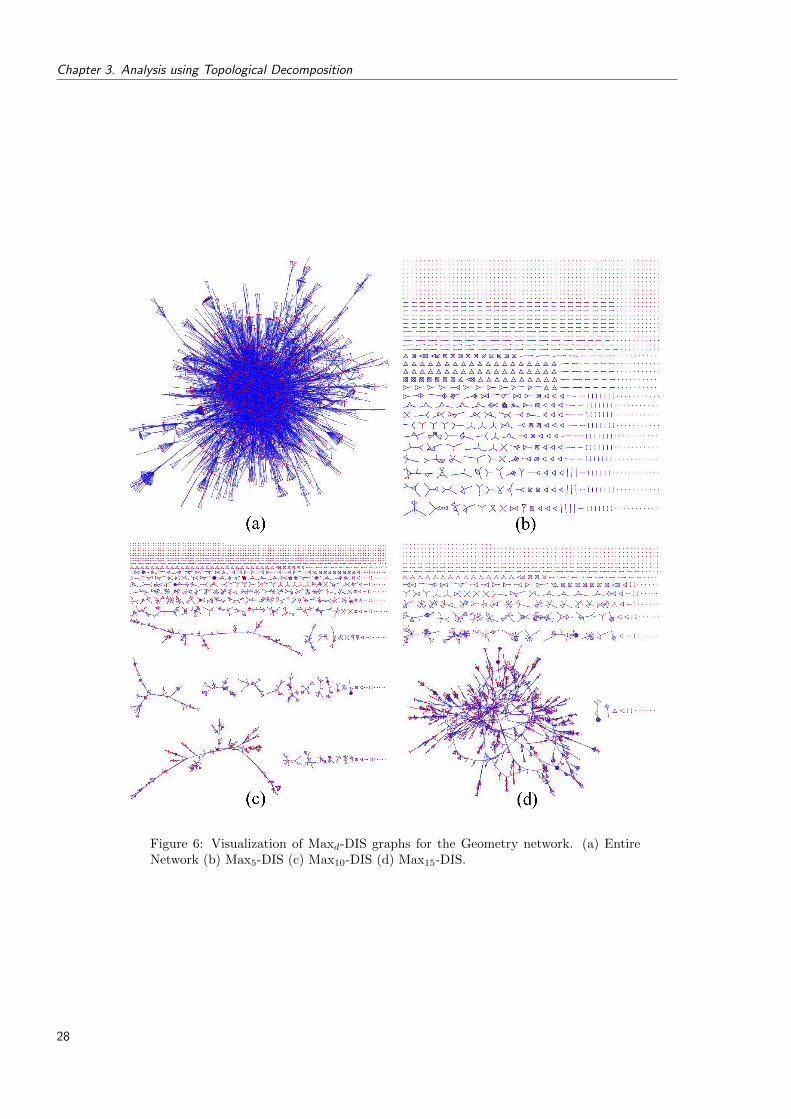
Chapter 3. Analysis using Topological Decomposition
Figure 6: Visualization of Maxd-DIS graphs for the Geometry network. (a) EntireNetwork (b) Max5-DIS (c) Max10-DIS (d) Max15-DIS.
28

3.2. Topological Decomposition
Figure 7: (a)Histograms and (b) Log-Log scatter plot of the Degree Distribution ofGeometry Network.
is easy to say that the value 15 does not really represent ‘high’ values of degree. On theother hand, if we compare 15 with the average node degree which is 2.6, the value seemsto be quite high and can be considered as a high value for node degree. If we look in termsof percentage, the Max15-DIS contains 3413 nodes which is 208 nodes less than the totalnumber of nodes in the network and makes a percentage of around 94%. If we considerthe top 5% nodes as the high degree nodes, Max15-DIS suggests that in the absence ofhigh degree nodes, 59% of the nodes in the network are still connected.
Thus we suggest that the Maxd-DIS can be used as a method to study an importantfeature of scale free networks studied by Albert et al. [4] i.e. scale free networks are robustto random loss of nodes but fragile to targeted worst-case attacks on hubs (introducedearlier in Chapter 1).
Looking at the average degree in this subgraph, for the 94% of the nodes in the entirenetwork is 1.33 as compared to overall value of 2.6 for the entire network. Thus the highdegree nodes heavily influence the total number of edges (or the average degree of nodes)in the entire network. Obviously this is a direct implication of the long tail in the degreedistribution. The longer the tail, the bigger would be the difference in the average nodedegree of low degree nodes and the overall network.
About the connectivity of the nodes and the three bigger connected components inFigure 6(c), there is an interesting observation about the average path lengths of thesebigger connected components. The three components have values of 12.9, 12.4 and 9.7which when compared to the overall value of 5.31 are quite high. Even the biggest con-nected component in Figure 6(d) has a very high average path length of 12.1. As the highdegree nodes appear in the network the average path length drops considerably in the finalnetwork. If we look closely at Figure 6(a,b,c), we understand an important connectivityprinciple of these networks. When nodes connect to each other through ‘higher’ degreenodes, the average path length is a bit higher as the connections form long paths, andwhen nodes connect through ‘very high’ degree nodes, the average path length is lower.
We further explain this using an example of co-authorship network. Consider the fourcliques in Figure 8(a) representing four different articles, where the number of authors forthe four cliques are 5,3,4,3 and each node is labeled with letters from A to O.
The four cliques can be connected to each other by two principles. The first one is
29

Chapter 3. Analysis using Topological Decomposition
Figure 8: (a)Four cliques representing different articles in an co-authorship network(b) The cliques are combined to form high average path length with certain nodeshaving higher degree (c) The cliques are combined to form low average path lengthwith Node A standing out as a very high degree node.
shown in Figure 8(b), which is in the absence of very high degree nodes. Consider a personauthoring two articles with two different sets of people, in that case, that person will sitin between two cliques. From the example in the figure we consider person A and G arethe same person and thus they connect the two cliques as shown in Figure 8(b). Anotherway to connect two cliques is to add edges between people writing different articles. Inthis example we add an edge between F and I, suggesting that earlier these people workedwith a different set of people, but now they have collaborated to write together. Similarly,person J is the same as O, and L is the same person as N. This connectivity patternintroduced is due to the absence of very high degree nodes as, in this connected network,no node has a very high degree. The result is that we get a long string of cliques connectedto each other just as we saw in Figure 6(c,d).
On the other hand, another way to connect these cliques is shown in Figure 8(c) wherea single person co-authors many articles with other people, in this case, that person isshown as node A, which collaborates with all other authors. This gives a certain node avery high node degree and reduces the overall average path length to a large extent. Boththese connectivity patterns are present in the Geometry network as we see long paths inFigure 6(c,d) and short paths in Figure 6(a).
30

3.2. Topological Decomposition
Let us summarize what we have explained in this section. We have tried to analyze theGeometry network using the Maxd-DIS decomposition. We identified several interestingobservations such as:
1. Studying how edges are distributed in low degree nodes.
2. Observe the structure of networks such as the formation of triads and cliques ofbigger sizes.
3. Analyze the connectivity of nodes in the absence of hubs and see if a network isfragile to targeted attacks.
4. Break up of nodes in several disconnected components in the absence of high degreenodes, which motivates the idea of possibly grouping the connected components asclusters.
5. For higher values of d, the smaller components begin to merge into a single connectedcomponent even if very high degree nodes are not present.
6. The average path length of biggest connected components in the DIS subgraphs isconsiderably higher in the absence of very high degree nodes indicating that veryhigh degree nodes are also responsible for reducing the overall average path length.
7. Two connectivity patterns are observed, one in the presence of higher degree nodes,and the other, when very high degree nodes appear. These patterns effect the averagepath length of a connected component.
From this detailed analysis of the Geometry network, we will have a look at some otherreal world networks and try to see if we observe similar findings in other networks.
Next, we consider another co-authorship network, the Dblp2008 network. In Fig-ure 9(a) and (b), we show the Max5-DIS and Max10-DIS of the network. In both thesefigures, we show only part of the entire subgraphs as Max5-DIS contains over 60000 nodesand Max10-DIS over 80000 nodes. The analysis is quite similar to that of the Geometrynetwork as in the Max5-DIS we see lots of smaller connected components forming cliquesof sizes between 1 and 5.
In Figure 9(b) we clearly see that the smaller components start to combine into onebig connected component just as the case of geometry network shown in Figure 6(c) andFigure 6(d). This suggests that even at degree value 10, smaller connected componentsbegin to merge into one single connected component.
Figure 10(a) and (b) show the Max5-DIS and Max15-DIS of the Opte network. Thereare 33418 nodes and 21067 edges in Max5-DIS which is 93% of the nodes have a degreeless than or equal to 5. If we look at the average degree of the entire network which is1.18, this information comes as no surprise as it is expected to have many nodes of lowdegree.
There is an absence of cliques when we observe the Max5-DIS of Opte network ascompared to the previous two examples. The absence of cliques can be deduced from thelow clustering coefficient of the network. The most important observation is the presencea motif which stands out as recurrent, is the presence of star-like structure where onenode is connected to many other nodes of degree exactly equal to 1. This structure has an
31
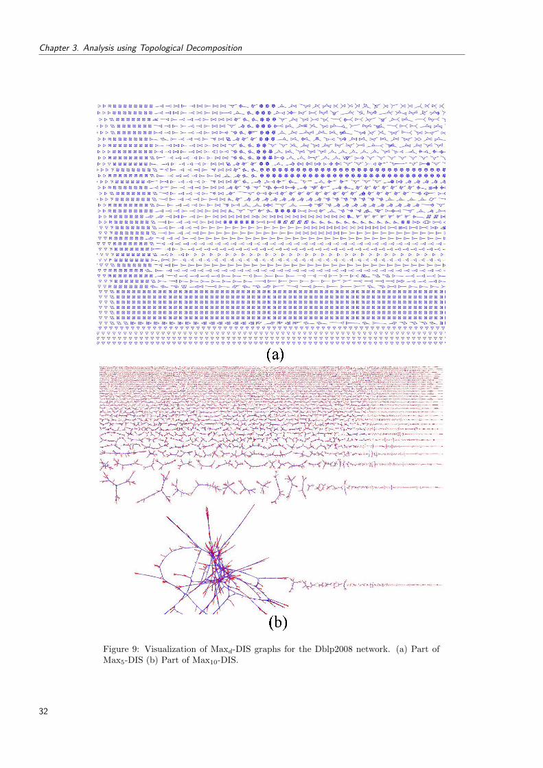
Chapter 3. Analysis using Topological Decomposition
Figure 9: Visualization of Maxd-DIS graphs for the Dblp2008 network. (a) Part ofMax5-DIS (b) Part of Max10-DIS.
32

3.2. Topological Decomposition
implicit justification, it is highly efficient in terms of cost of transmission channels. Cliquesare not required as data can be transmitted only if a single path exists from one computerto the other. Mostly the computers in such a network are organized in this star topologywhere the computer with all the connections serves as a communication channel for theother computers and the rest of the network. In network terminology, we can say thatthere are no densely connected components as compared to the previous two networks,but rather the star topology dominates this type of network.
Just as the previous networks, there are lots of disconnected components in this net-work. One common behavior with the two previous examples is that as we increase the dvalue, smaller connected components begin to merge into a single connected componentas shown in Figure 10(b). As compared to the highest node degree in this network, whichis 259, if we look at the Max15-DIS, the biggest connected components has 24414 nodes,which shows that 68% of the nodes make a single connected component with maximumnode degree of 15 only. Another interesting observation about this biggest connected com-ponent is the average path length of the nodes. In the absence of very high degree nodes,the average path length of these 68% nodes is 21.6 as compared to the overall value of16.7. This suggests that the high degree nodes are again the reason of reduced averagepath length in these real networks.
We move to another example of technological network, the AirTransport network.Figure 11(a) shows the Max25-DIS and Figure 11(b) shows part of the Part of Max50-DIS.We choose relatively higher values of d in this example because there were not sufficientnodes or edges to observe anything interesting for lower values of d. From Figure 11(a),we can see that there are many disconnected components in the network as the previousexamples. Recall, this signifies that these networks require higher degree nodes to connectto each other.
The structure of the network is quite an interesting one. We see that there are triadsas well as stars in Figure 11(a). If we look at the overall clustering coefficient, the presenceof triads is confirmed from the relatively high value of 0.49 as compared to that of theOpte network which is 0.003. If we look closely at the biggest connected component inFigure 11(b) with the Max50-DIS, we see that there are many star like structures, i.e. manynodes with degree 1 connect to a single node. This makes a very interesting example tostudy as we see that this network is a good mix of the two fundamental structures that wehave identified, the cliques and the stars. Moreover, the average node degree in Max50-DISis 1.49, which is very low as compared to the overall average degree of 10.7. Along withthe highest node degree of 487, these values suggest that the high degree nodes are verywell connected to other nodes in the network and thus push the average node degree to ahigh value of 10.7.
Note that as with the previous examples, the smaller connected components start tomerge as we move to higher values of d while constructing the Maxd-DIS graphs.
The biggest connected component in Figure 11(b) has 832 nodes and 1941 edges whichis 54% of the total nodes. The average path length of the nodes in this component is 5.9as compared to the overall value of 2.9 and the considerable difference again suggests thatvery high degree nodes are responsible for the decrease in the overall average path lengthof the entire network.
Finally, we consider an example from the Biological data. The Protein network againpresents a proof of the presence of star like connectivity among nodes. There are a fewtriads as well but no bigger size cliques as can be seen from Figure 12(a) and (b) showing
33

Chapter 3. Analysis using Topological Decomposition
Figure 10: Visualization of Maxd-DIS graphs for the Opte network. (a) Part of Max5-DIS (b) Part of Max15-DIS.
34

3.2. Topological Decomposition
Figure 11: Visualization of Maxd-DIS graphs for the AirTransport network. (a)Max25-DIS (b) Part of Max50-DIS.
35
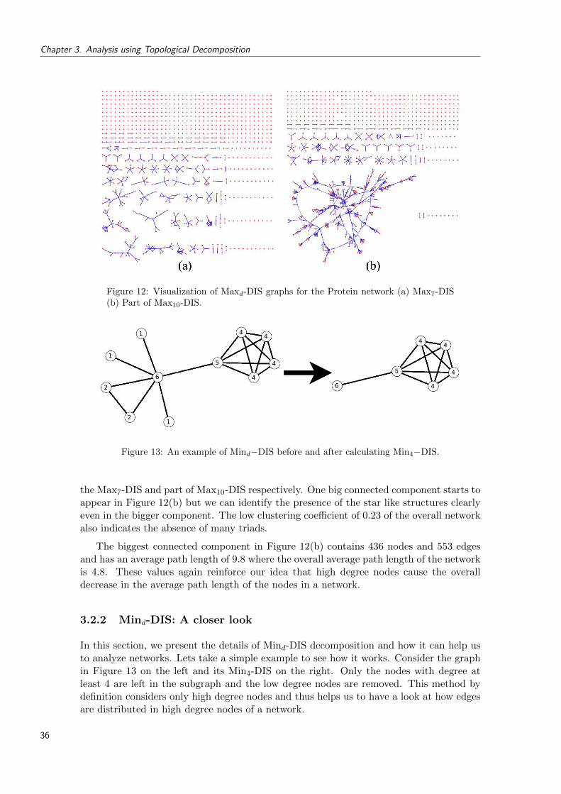
Chapter 3. Analysis using Topological Decomposition
Figure 12: Visualization of Maxd-DIS graphs for the Protein network (a) Max7-DIS(b) Part of Max10-DIS.
Figure 13: An example of Mind−DIS before and after calculating Min4−DIS.
the Max7-DIS and part of Max10-DIS respectively. One big connected component starts toappear in Figure 12(b) but we can identify the presence of the star like structures clearlyeven in the bigger component. The low clustering coefficient of 0.23 of the overall networkalso indicates the absence of many triads.
The biggest connected component in Figure 12(b) contains 436 nodes and 553 edgesand has an average path length of 9.8 where the overall average path length of the networkis 4.8. These values again reinforce our idea that high degree nodes cause the overalldecrease in the average path length of the nodes in a network.
3.2.2 Mind-DIS: A closer look
In this section, we present the details of Mind-DIS decomposition and how it can help usto analyze networks. Lets take a simple example to see how it works. Consider the graphin Figure 13 on the left and its Min4-DIS on the right. Only the nodes with degree atleast 4 are left in the subgraph and the low degree nodes are removed. This method bydefinition considers only high degree nodes and thus helps us to have a look at how edgesare distributed in high degree nodes of a network.
36

3.2. Topological Decomposition
In terms of analysis of real world networks, lets consider the AirTransport networkfor a detailed analysis using Mind−DIS. Figure 14(a) shows the entire network containing1540 nodes and 16523 edges.
Figure 14(b) shows the Min250−DIS of the network showing the top 10 highest degreenodes of the network connected through 44 edges, which is just one less to make it a clique.This suggests that the worlds most widely connected airports have all a direct flight toeach other with the exception of one case. Recall from the construction of this networkexplained in Chapter 2, two cities are connected to each other if there is a direct flightfrom one to the other. The high degree of a city refers to its many different connectionsto other cities and not heavy traffic nor does it refer to the world’s busiest airports.
Figure 14(c) shows the top 20 widely connected airports in the world drawn using acircular layout [158]. We have also labeled the nodes with the city names. The nodesare connected through 189 edges, missing the only edge for it to be a clique. This highconnectivity of high degree nodes essentially comes from the design strategy of airlines andconnectivity of any two cities of the world. Since the idea is to minimize the number ofhops required to go from one place to the other, all the hubs in the network are connecteddirectly to each other.
Figure 14(d) shows the top 5% high degree nodes of the network. There are 77 nodesconnected through 1822 edges which is an average degree of 23. In this subgraph, this highconnectivity can be measured in terms of average path length, which is 1.3 as compared tothe average path length value for the entire graph which is 2.93. This is a huge differencein the context. Note that there is not a single node disconnected in this network, thus highconnectivity of hubs has been used as a method to increase the efficiency of transportationwhere the criteria is obviously minimizing the hops as described earlier.
This example shows an application of how Mind-DIS can help analyze the connectivityof hubs in real world networks. From the above example, we learned that the hubs arevery tightly connected to each other. We used the average path length to quantify howclose the nodes are to each other. Using Mind-DIS, we can also study the phenomenaof assortative mixing [128] introduced in chapter 1 where nodes with many connectionshave a tendency to connect to other nodes with many connections. And finally we noticedthat all the nodes were connected in a single component and there were no disconnectedcomponents. We summarize the type of analysis that can be performed using Mind-DISbelow:
> Study how edges are distributed in high degree nodes or hubs.
> Observe the connectivity pattern of high degree nodes forming one big connectedcomponent. We use Average path length to quantify how closely the hubs are con-nected to each other.
> Analyze networks for assortative mixing.
Next, we consider the other four networks that were analyzed using Maxd-DIS, theGeometry, Dblp2008, Opte and Protein networks. For each of these networks, we took theMind-DIS with approximately 5% highest degree nodes. The results are shown in Figures{15,16,17,18} respectively for the above mentioned networks.
The Geometry network contains 179 nodes and 1384 edges. There are only two nodesthat are not connected to the biggest connected component as shown in Figure 15. The
37
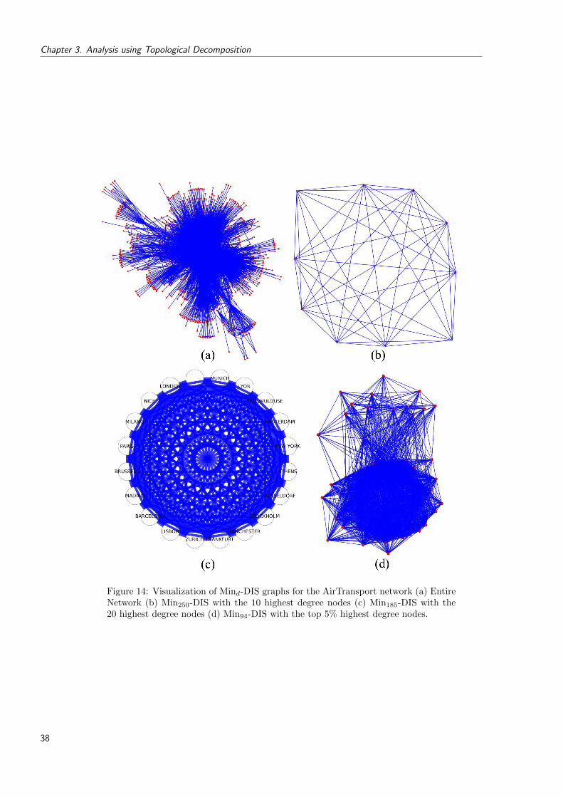
Chapter 3. Analysis using Topological Decomposition
Figure 14: Visualization of Mind-DIS graphs for the AirTransport network (a) EntireNetwork (b) Min250-DIS with the 10 highest degree nodes (c) Min185-DIS with the20 highest degree nodes (d) Min94-DIS with the top 5% highest degree nodes.
38
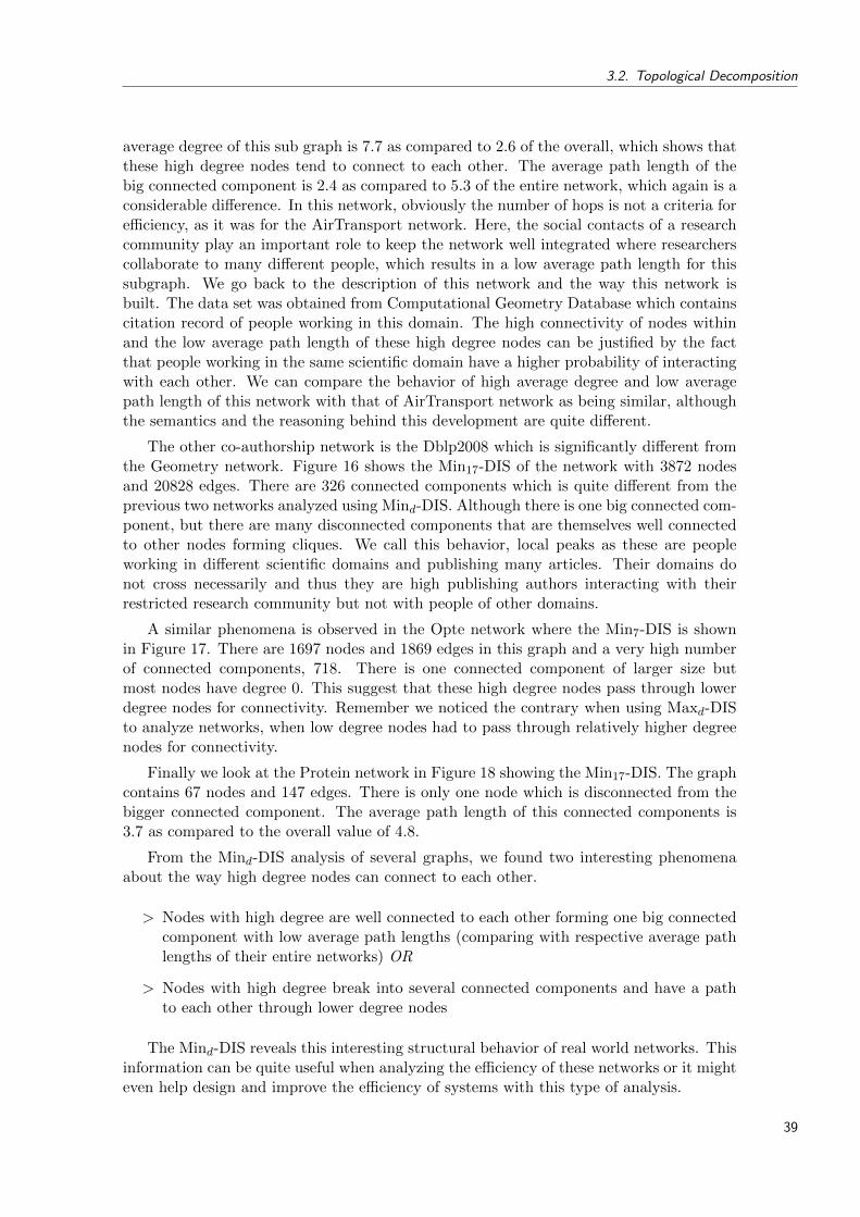
3.2. Topological Decomposition
average degree of this sub graph is 7.7 as compared to 2.6 of the overall, which shows thatthese high degree nodes tend to connect to each other. The average path length of thebig connected component is 2.4 as compared to 5.3 of the entire network, which again is aconsiderable difference. In this network, obviously the number of hops is not a criteria forefficiency, as it was for the AirTransport network. Here, the social contacts of a researchcommunity play an important role to keep the network well integrated where researcherscollaborate to many different people, which results in a low average path length for thissubgraph. We go back to the description of this network and the way this network isbuilt. The data set was obtained from Computational Geometry Database which containscitation record of people working in this domain. The high connectivity of nodes withinand the low average path length of these high degree nodes can be justified by the factthat people working in the same scientific domain have a higher probability of interactingwith each other. We can compare the behavior of high average degree and low averagepath length of this network with that of AirTransport network as being similar, althoughthe semantics and the reasoning behind this development are quite different.
The other co-authorship network is the Dblp2008 which is significantly different fromthe Geometry network. Figure 16 shows the Min17-DIS of the network with 3872 nodesand 20828 edges. There are 326 connected components which is quite different from theprevious two networks analyzed using Mind-DIS. Although there is one big connected com-ponent, but there are many disconnected components that are themselves well connectedto other nodes forming cliques. We call this behavior, local peaks as these are peopleworking in different scientific domains and publishing many articles. Their domains donot cross necessarily and thus they are high publishing authors interacting with theirrestricted research community but not with people of other domains.
A similar phenomena is observed in the Opte network where the Min7-DIS is shownin Figure 17. There are 1697 nodes and 1869 edges in this graph and a very high numberof connected components, 718. There is one connected component of larger size butmost nodes have degree 0. This suggest that these high degree nodes pass through lowerdegree nodes for connectivity. Remember we noticed the contrary when using Maxd-DISto analyze networks, when low degree nodes had to pass through relatively higher degreenodes for connectivity.
Finally we look at the Protein network in Figure 18 showing the Min17-DIS. The graphcontains 67 nodes and 147 edges. There is only one node which is disconnected from thebigger connected component. The average path length of this connected components is3.7 as compared to the overall value of 4.8.
From the Mind-DIS analysis of several graphs, we found two interesting phenomenaabout the way high degree nodes can connect to each other.
> Nodes with high degree are well connected to each other forming one big connectedcomponent with low average path lengths (comparing with respective average pathlengths of their entire networks) OR
> Nodes with high degree break into several connected components and have a pathto each other through lower degree nodes
The Mind-DIS reveals this interesting structural behavior of real world networks. Thisinformation can be quite useful when analyzing the efficiency of these networks or it mighteven help design and improve the efficiency of systems with this type of analysis.
39

Chapter 3. Analysis using Topological Decomposition
Figure 15: Min17-DIS of Geometry network with 5% highest degree nodes.
Figure 16: Min17-DIS of Dblp2008 network with 5% highest degree nodes.
40
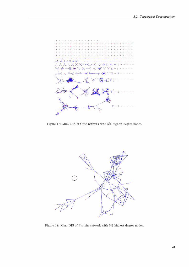
3.2. Topological Decomposition
Figure 17: Min7-DIS of Opte network with 5% highest degree nodes.
Figure 18: Mind-DIS of Protein network with 5% highest degree nodes.
41

Chapter 3. Analysis using Topological Decomposition
The proposed DIS method seems to be effective in a number of different ways whencombined with visual analysis. In the above section we analyzed some real world net-works and showed how this method can be useful. Apart from the visual analysis ofthe decomposed networks, the method can serve as the basis for the development of othermethods, metrics and algorithms for various applications. We present one such applicationin section 3.4 that can be useful in different domains.
3.3 Comparing DIS and K-cores
Comparing the k-core decomposition with the Topological decomposition based on DIS,first we consider the Maxd-DIS. Consider the example of Geometry network describedearlier and shown in Figure 6. The highest k value possible is 21 for the k-core decom-position whereas the highest node degree is 102 for the DIS decomposition. Thus, thesubgraphs constructed for the two methods are 21 and 102 respectively. Subgraphs withmore nodes are produced using k-core for different values of k as shown in Figure 19. Oneclear observation from the visualization of graphs in Figure 19(b) and (c) is that k-coredecomposition cannot be used to study how low degree nodes connect to each other ascompared to Maxd-DIS. By definition, as it progressively contains nodes with high con-nectivity, for low values of k, we have quite large graphs cluttered in one big connectedcomponent. This makes any visual analysis impossible. Thus Maxd-DIS has a clear ad-vantage over k-core decomposition as it provides a way to study the connectivity of lowdegree nodes as discussed earlier in the previous section.
Looking at the Min17-DIS of the geometry network, in Figure15, the network contains179 nodes with 1384 edges. Comparing it with Figure 19(c) showing 10 − core of thesame network with 133 nodes and 1296 edges, we can clearly see that Min17-DIS containsmany nodes with low connectivity in the subgraph. This is because the way the twosubgraphs are built by definition. k-core focuses on nodes that only connected to otherhigh connectivity nodes and thus in the subgraph, each node has at least degree 10. Onthe other hand, Min17-DIS contains nodes that are highly connected to other nodes andthus in the induced subgraph, it is quite possible to find nodes with low degree. Thenode edge density of the two subgraphs is a good indication of different set of nodes beingselected for the two graphs with some similarities.
Finally we compare the top 22 nodes obtained by the two methods shown here inFigure 20. The author names are displayed and except for an author ‘Pankaj K. Agarwal’,no other author is common to the two subgraphs. This clearly shows that by definition,the two decomposition methods target a different set of nodes.
Summarizing the above findings, the k-core decomposition is more closer to the Mind-DIS as both these methods try to focus on nodes of higher degree. To differentiate betweenthese two, assume that for some network, we are looking for ‘important’ nodes in somerespect. Using the definition of Mind-DIS, the ‘important’ nodes would be the ones thathave high degree, irrespective of who they are connected to. On the other hand, using thedefinition of k-cores, ‘important’ nodes would be the ones that have high degree and areconnected only to other ‘important’ nodes.
A word on the time complexity of these two methods. k-core can be calculated inO(n + e) [6] where n is the number of nodes and e is the number of edges. Mind-DIScan be calculated in O(n) time which is much faster than the k-core decomposition. The
42

3.3. Comparing DIS and K-cores
Figure 19: k-core decomposition of the geometry network for different values of k(a)k = 1 contains the entire network (b)k = 5 contains 610 nodes and 3594 edges(c)k = 10 contains 133 nodes and 1296 edges (d)k = 21 is the highest possible valueof k for the network and contains 22 nodes and 231 edges making it a clique.
43
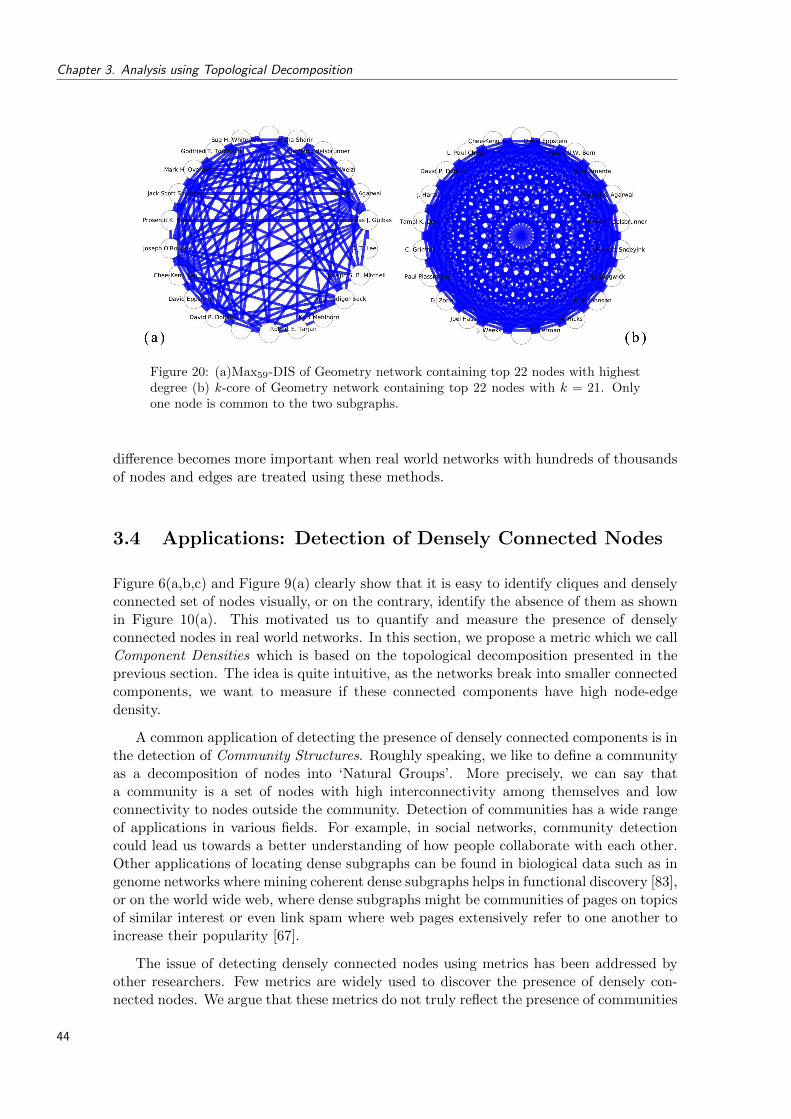
Chapter 3. Analysis using Topological Decomposition
Figure 20: (a)Max59-DIS of Geometry network containing top 22 nodes with highestdegree (b) k-core of Geometry network containing top 22 nodes with k = 21. Onlyone node is common to the two subgraphs.
difference becomes more important when real world networks with hundreds of thousandsof nodes and edges are treated using these methods.
3.4 Applications: Detection of Densely Connected Nodes
Figure 6(a,b,c) and Figure 9(a) clearly show that it is easy to identify cliques and denselyconnected set of nodes visually, or on the contrary, identify the absence of them as shownin Figure 10(a). This motivated us to quantify and measure the presence of denselyconnected nodes in real world networks. In this section, we propose a metric which we callComponent Densities which is based on the topological decomposition presented in theprevious section. The idea is quite intuitive, as the networks break into smaller connectedcomponents, we want to measure if these connected components have high node-edgedensity.
A common application of detecting the presence of densely connected components is inthe detection of Community Structures. Roughly speaking, we like to define a communityas a decomposition of nodes into ‘Natural Groups’. More precisely, we can say thata community is a set of nodes with high interconnectivity among themselves and lowconnectivity to nodes outside the community. Detection of communities has a wide rangeof applications in various fields. For example, in social networks, community detectioncould lead us towards a better understanding of how people collaborate with each other.Other applications of locating dense subgraphs can be found in biological data such as ingenome networks where mining coherent dense subgraphs helps in functional discovery [83],or on the world wide web, where dense subgraphs might be communities of pages on topicsof similar interest or even link spam where web pages extensively refer to one another toincrease their popularity [67].
The issue of detecting densely connected nodes using metrics has been addressed byother researchers. Few metrics are widely used to discover the presence of densely con-nected nodes. We argue that these metrics do not truly reflect the presence of communities
44

3.4. Applications: Detection of Densely Connected Nodes
Figure 21: Consider two graphs with same number of nodes and edges and thus havingthe same density in terms of number of nodes and number of edges. (a) Nodes wellconnected to each other forming quads, (b) Nodes sharing neighbors to form triads.Clustering Coefficient for graph (a) is 0.0 and (b) is 0.69 representing the absence oftriads in graph (a). This example shows that nodes can be densely connected even ifthe clustering coefficient is low.
by presenting counter examples. This is because these metrics concentrate on local co-hesiveness among nodes and the goal is to judge whether two nodes belong to the samecommunity or not. Thus loosing the overall perspective of the presence of communities inthe entire network.
One of the most widely used metric in network analysis is the clustering coefficientdescribed earlier. This metric can be often misleading due to its name as this metricdoes not guarantee the presence of clusters in a network. Consider the example shown inFigure 21 with two graphs. Both contain the same number of nodes and edges. Thus thedensity (ratio of number of edges to number of nodes) of the two graphs is exactly thesame. Graph (a) is constructed using Quads instead of triads where a quad is a set of fournodes connected through four edges in a ring. We then compare this graph with anothergraph constructed with triads. Both these graphs are shown in Figure 21(a) and (b). Theclustering coefficient of graph (a) is 0.0 representing the absence of triads as compared tograph (b) with a value of 0.69. This is no surprise as clustering coefficient, by definition,measures the quantity of triads in a graph. This simple example suggests that a graphcan be densely connected even in the absence of triads. The presence of triads has beenidentified in social networks, but not necessarily in networks from other domains, thus ametric is required that can identify the presence of densely connected nodes in the absenceof triads.
Let us consider another example, shown in Figure 22. Figure 22(a) clearly has fourdensely connected components highly connected within and disconnected to each other.Figure 22(b) has several nodes sharing common neighbors in the form of triads but visually,no distinct groups. Both these graphs have the same number of nodes and edges wherethe clustering coefficient for graph (a) is 0.70 and of (b) is 0.69. No information aboutthe presence of four densely connected components can be deduced from the clusteringcoefficient of graph (a).
Another popular metric is the Jaccard Index introduced by [86] also known as Jaccardsimilarity coefficient. This metric is used to measure the similarity of two elements basedon common neighborhood. More precisely the index looks at the number of commonneighbors of the two elements and compares it with the size of all the neighbors of the twoelements. An edge is assigned high similarity value if they share lots of neighbors. Coming
45
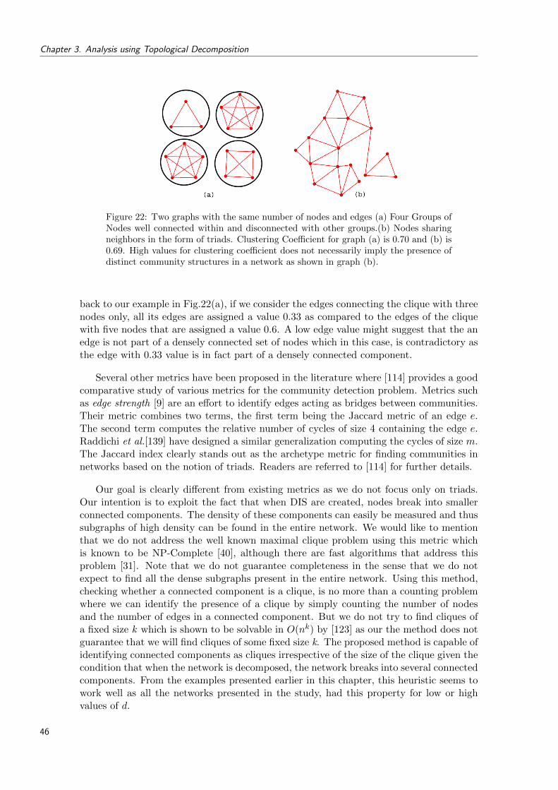
Chapter 3. Analysis using Topological Decomposition
Figure 22: Two graphs with the same number of nodes and edges (a) Four Groups ofNodes well connected within and disconnected with other groups.(b) Nodes sharingneighbors in the form of triads. Clustering Coefficient for graph (a) is 0.70 and (b) is0.69. High values for clustering coefficient does not necessarily imply the presence ofdistinct community structures in a network as shown in graph (b).
back to our example in Fig.22(a), if we consider the edges connecting the clique with threenodes only, all its edges are assigned a value 0.33 as compared to the edges of the cliquewith five nodes that are assigned a value 0.6. A low edge value might suggest that the anedge is not part of a densely connected set of nodes which in this case, is contradictory asthe edge with 0.33 value is in fact part of a densely connected component.
Several other metrics have been proposed in the literature where [114] provides a goodcomparative study of various metrics for the community detection problem. Metrics suchas edge strength [9] are an effort to identify edges acting as bridges between communities.Their metric combines two terms, the first term being the Jaccard metric of an edge e.The second term computes the relative number of cycles of size 4 containing the edge e.Raddichi et al.[139] have designed a similar generalization computing the cycles of size m.The Jaccard index clearly stands out as the archetype metric for finding communities innetworks based on the notion of triads. Readers are referred to [114] for further details.
Our goal is clearly different from existing metrics as we do not focus only on triads.Our intention is to exploit the fact that when DIS are created, nodes break into smallerconnected components. The density of these components can easily be measured and thussubgraphs of high density can be found in the entire network. We would like to mentionthat we do not address the well known maximal clique problem using this metric whichis known to be NP-Complete [40], although there are fast algorithms that address thisproblem [31]. Note that we do not guarantee completeness in the sense that we do notexpect to find all the dense subgraphs present in the entire network. Using this method,checking whether a connected component is a clique, is no more than a counting problemwhere we can identify the presence of a clique by simply counting the number of nodesand the number of edges in a connected component. But we do not try to find cliques ofa fixed size k which is shown to be solvable in O(nk) by [123] as our the method does notguarantee that we will find cliques of some fixed size k. The proposed method is capable ofidentifying connected components as cliques irrespective of the size of the clique given thecondition that when the network is decomposed, the network breaks into several connectedcomponents. From the examples presented earlier in this chapter, this heuristic seems towork well as all the networks presented in the study, had this property for low or highvalues of d.
46
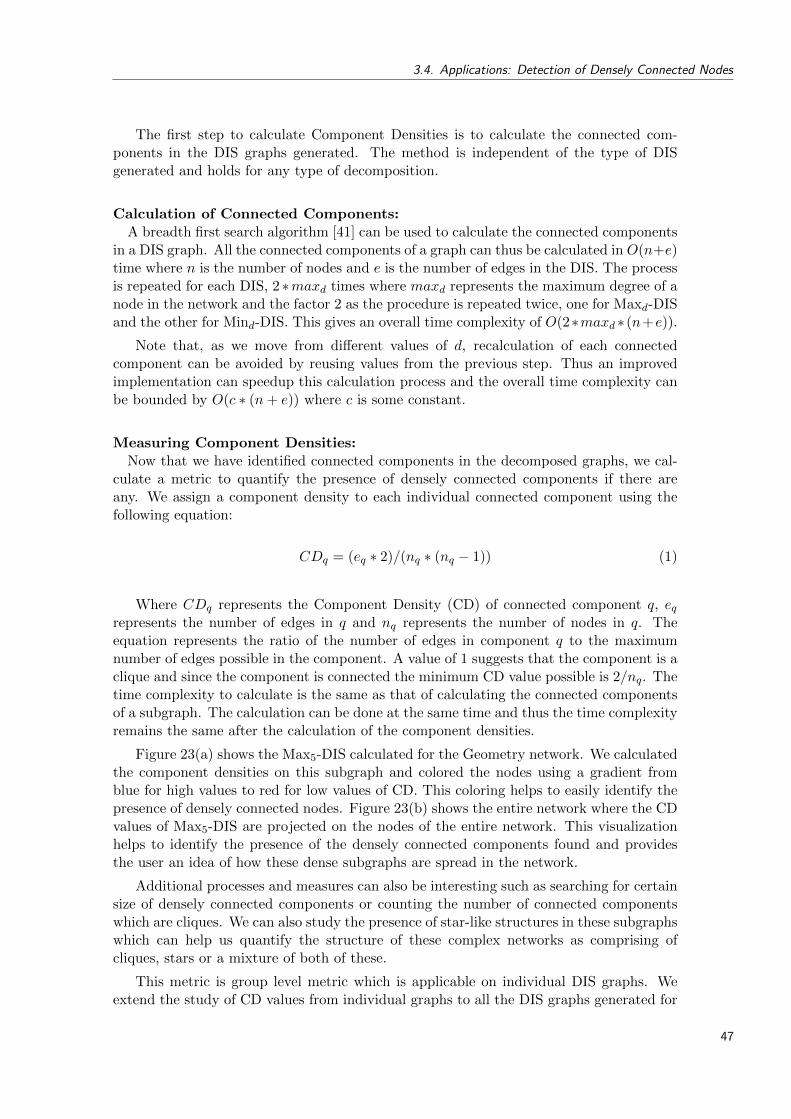
3.4. Applications: Detection of Densely Connected Nodes
The first step to calculate Component Densities is to calculate the connected com-ponents in the DIS graphs generated. The method is independent of the type of DISgenerated and holds for any type of decomposition.
Calculation of Connected Components:A breadth first search algorithm [41] can be used to calculate the connected components
in a DIS graph. All the connected components of a graph can thus be calculated in O(n+e)time where n is the number of nodes and e is the number of edges in the DIS. The processis repeated for each DIS, 2 ∗maxd times where maxd represents the maximum degree of anode in the network and the factor 2 as the procedure is repeated twice, one for Maxd-DISand the other for Mind-DIS. This gives an overall time complexity of O(2∗maxd ∗ (n+e)).
Note that, as we move from different values of d, recalculation of each connectedcomponent can be avoided by reusing values from the previous step. Thus an improvedimplementation can speedup this calculation process and the overall time complexity canbe bounded by O(c ∗ (n+ e)) where c is some constant.
Measuring Component Densities:Now that we have identified connected components in the decomposed graphs, we cal-
culate a metric to quantify the presence of densely connected components if there areany. We assign a component density to each individual connected component using thefollowing equation:
CDq = (eq ∗ 2)/(nq ∗ (nq − 1)) (1)
Where CDq represents the Component Density (CD) of connected component q, eqrepresents the number of edges in q and nq represents the number of nodes in q. Theequation represents the ratio of the number of edges in component q to the maximumnumber of edges possible in the component. A value of 1 suggests that the component is aclique and since the component is connected the minimum CD value possible is 2/nq. Thetime complexity to calculate is the same as that of calculating the connected componentsof a subgraph. The calculation can be done at the same time and thus the time complexityremains the same after the calculation of the component densities.
Figure 23(a) shows the Max5-DIS calculated for the Geometry network. We calculatedthe component densities on this subgraph and colored the nodes using a gradient fromblue for high values to red for low values of CD. This coloring helps to easily identify thepresence of densely connected nodes. Figure 23(b) shows the entire network where the CDvalues of Max5-DIS are projected on the nodes of the entire network. This visualizationhelps to identify the presence of the densely connected components found and providesthe user an idea of how these dense subgraphs are spread in the network.
Additional processes and measures can also be interesting such as searching for certainsize of densely connected components or counting the number of connected componentswhich are cliques. We can also study the presence of star-like structures in these subgraphswhich can help us quantify the structure of these complex networks as comprising ofcliques, stars or a mixture of both of these.
This metric is group level metric which is applicable on individual DIS graphs. Weextend the study of CD values from individual graphs to all the DIS graphs generated for
47

Chapter 3. Analysis using Topological Decomposition
Figure 23: Component Density (CD) calculated for the Max5-DIS of Geometry net-work. (a) shows color encoding on the nodes from high (blue) to low (ref) values.Nodes in blue color can be easily identified as densely connected components. (b)shows the projection of CD values of Max5-DIS on the entire network with the samecolor encoding. This gives an idea of how the densely connected components arespread out in the entire network.
different values of d. The idea is to study how CD values behave over different values ofd, we call these Component Densities for Graphs (CDG).
Component Densities for Graphs:We calculate the weighted component density for all the connected components in a
DIS to ensure that large and dense components are assigned high values as comparedsmall and less dense components. Remember that the number of nodes in each connectedcomponent changes as the d value changes and some connected components have manynodes specially as the giant component appears in a DIS. We represent this value by CDGd
for d degree induced subgraph and is calculated by the equation:
CDGd =
qmax∑q=0
nq ∗ CDq
nd(2)
Where CDGd represents the weighted Component Density of d-DIS. While calculatingthe CDGd, we exclude the weight of components having only 1 or 2 nodes as it biases theCDGd. We do count them in the total number of nodes (nd) present in the induced sub-graph though. This is because if a graph has lots of 0 degree nodes, its overall componentdensity will be lower than a graph with well connected higher degree nodes. The weight isassociated to ensure that components having more nodes are weighted more as comparedto components having fewer nodes. The CDGd can be calculated for different values of dwhere the d can take values from 0 to the maximum degree of a node in G. The calcula-tions in Eq. 1 and Eq. 2 are totally independent of how the subgraph was constructed andthus can be used to calculate the component densities of either Maxd-DIS or Mind-DIS.
48
3.4. Applications: Detection of Densely Connected Nodes
The CDG values of Maxd-DIS (given by CDGMaxd) and Mind-DIS (given by CDGMind
)represents the presence or absence of dense components in the subgraphs generated bythese decompositions. High values of CDG suggest that there are densely connected nodesin the induced subgraph which can eventually represent communities in the entire graphas well. Another supplementary information that can be extracted from CDG values isthat by identifying the peak value of CDGMaxd
and CDGMind, we can point out the
induced subgraphs in which these dense subgraphs are present, instead of analyzing eachand every subgraph as we explained earlier in section 3.2.1 and section 3.2.2. Looking atCDG values, we can not only identify the subgraph of interest, but quantify the presenceof dense subgraphs for comparative study over different data sets.
We plot graphs for the respective CDGMaxdand CDGMind
values for different datasets that have been studied in this chapter. The graphs are shown in Figure 24. The valueson the x-axis represent the maximum degree of each network, which in turn represents thenumber of subgraphs generated for each network. The values on the y-axis are the CDGvalues which are between 0 and 1 where 1 represents the presence of cliques. For eachreal world data set, we have also generated small world [170] and random networks [54] ofequivalent number of nodes and edges so that we can compare the behavior of the metricwith the corresponding artificially generated network. These networks are drawn usingDotted-Line for Small world networks and Dashed-Line for Random networks.
The evaluation of CDGMaxdand CDGMind
for Random networks and Small worldnetworks for graphs of different sizes can be generalized easily. For random networks, wedo not expect to find any community structure and thus these networks have low CDGvalues for all the test cases as shown in Figure 24. On the other hand, we have the smallworld networks which by definition contain communities and this is well reflected by thehigh CDG values for all the artificially generated networks. One exception is the casewhere the generated small world graph is equivalent to the size of the Opte network. Thisis due to the low overall density of the graph itself as the edges scale linearly with thenumber of nodes. Thus we do not expect to find densely connected set of nodes and thisis reflected by the metric and is clearly observable in the graph.
We first look at the CDG values of the two co-authorship networks, the Geometryand the Dblp2008 network shown in Figure 24(a,b,c,d). The high values of Maxd-DIS forboth these graphs are observed as compared to the respective small world and randomgraphs. Remember that the overall node-edge densities of these networks vary a lot, thusthey cannot be compared with each other. This is the reason why we generated artificialnetworks to have a sort of a benchmark value for these networks. The graphs followalmost the same behavior as high values are observed for d value of around 6 and 8 andthe values fall of consistently as d values increases. This result has logical semantics toit, as we are considering a collaboration network of researchers and they are connectedto each other if they publish an article. Mostly less than 8 people appear as authorsin an article forming cliques in the collaboration network of sizes smaller than 8. Thisinformation is well represented by the CDGMaxd
values.
The most interesting observation is the Mind-DIS graph where we observe high val-ues for the Geometry network and low values for the Dblp2008 network. This differencewas highlighted earlier in section 3.2.2 where we justified that since Geometry networkcomprises of people working in the same scientific domain, they are more likely to collab-orate with each other where as the Dblp2008 network is a mixture of people from variousdomains, not every one collaborates with the other and the phenomena of local peaks is
49

Chapter 3. Analysis using Topological Decomposition
evident as shown in Figure 16.
The CDG values for Opte network are shown in Figure 24(e) and (f). The network isnot classified as a small world as it is has very low clustering coefficient of 0.003. Using ourmetric, we do not find any presence of densely connected nodes neither in the CDGMaxd
nor in the CDGMindgraphs thus reflecting the correctness of the metric. As we analyzed
the structure of this network using Maxd-DIS, we realized that this network has star likestructures that are not at all dense, and thus the low values of CDG are observed for thisnetwork.
The AirTransport network is an interesting example(Figure 24(g) and (h)). Using ourmetric, we are able to find densely connected nodes as we get high values for Mind−DIS.The densely connected subgraphs found for high values of Mind−DIS are shown in Fig-ure 14(b) and (c) where all the worlds widely connected airports are linked to each otherthrough a direct flight. This makes sense as the worlds most important airports like NewYork, Paris, London all have a direct flights to each other. On the contrary, we did notfind any dense components in the Maxd−DIS as this is because regional airports that donot have many connections rarely have alternate paths to connect to each other, theyusually pass through a central hub to connect to other less widely connected airports. Soif you live in a small city, you probably have to go to a local hub, to take a connectingflight to far off cities.
Finally the Protein network where the CDG values are shown in Figure 24(i) and (j).The high values in CDGMind
suggest that the high degree nodes are well connected to eachother as compared to the low degree nodes. This reveals the networks similarity with theGeometry and AirTransport network where both these networks have densely connectednodes for high degree nodes.
Inferences and Observations:Apart from identifying the presence of densely connected nodes in different networks,
interesting properties of real world networks can be observed using the CDGMaxdand
CDGMindgraphs. We list these below:
> Networks are usually classified as either Random, Small World, Scale Free or bothSmall World-Scale free at the same time. Using the proposed metric, we can havefurther insight in these networks by understanding how the edges are distributed inlow or high degree nodes of these networks. Dense subgraphs can exist in nodes thathave a low degree in the graph (as is the case with the two Co-authorship networks),or they can exist only in high degree nodes (Geometry, AirTransport and Proteinnetwork).
> The absence of communities can have two consequences, either the network is Ran-dom or it consists of star like structures where many nodes connect to a single node.Typical example is the routing information of servers in case of the Opte network.From the proposed metric, we are able to find the same behavior in the low degreenodes of AirTransport network.
Although this preliminary analysis reveals some interesting facts about the differentdata sets, a more detailed study by the domain experts might reveal more information.A huge advantage of this metric is that it is highly efficient in terms of time complexity.
50
3.5. Findings and Future Research Prospects
As discussed previously, the overall time complexity for the calculation of CDGMaxdand
CDGMindtakes O(2 ∗maxd ∗ (n+ e)) time. The factor maxd representing the maximum
node degree in the network is quite low in reality and varies from one network to theother. Furthermore, for varying values of d, the subgraphs contain much less nodes andedges than n or e, which makes the algorithm run quite fast in reality and scales almostlinearly with the factor (n+ e).
3.5 Findings and Future Research Prospects
In this chapter we have introduced a method to analyze networks based on the topologicaldecomposition and visualization of networks. The most important contribution of thismethod is that it enables us to visualize networks and see how nodes and edges connectto each other in different networks. Combining metrics and visualization technique toanalyze complex large size networks proves to be quite useful as the method allows us tounderstand different connectivity behaviors as networks change from one domain to theother.
As one of the applications of the proposed method, we introduced a metric for grouplevel analysis called component density which can be extended to the decomposed sub-graphs. The metric helps us to identify the presence of densely connected components inreal world complex networks. Calculation of this metric takes almost linear time in termsof number of edges and proves to be very fast when applied to large size data sets. Wehave tested the metric with different data sets and show the effectiveness of the metricby comparing the results with small world and random network models. We found someinteresting behavior in the way the edges are distributed in high and low degree nodes.Based on this distribution, we can actually see that as a function of degree, dense sub-graphs can be present in high degree nodes, low degree nodes, both or no where in thenetwork. Some interesting results about the structure of networks were discovered, orre-discovered such as the presence of triads, cliques of higher degree, star-like structures,showing the effectiveness of the proposed method.
The topological decomposition proposed opens new dimensions in the field of visualdata mining as complex networks can be simplified using the proposed method. Con-nectivity of nodes can be studied as a function of varying node degree of a network andhelps us to discover how edges are distributed in a network. We see this method as astep forward towards the better understanding of complex networks and an importanttool to analyze networks for various applications such as searching in networks, findinginteresting patterns, studying the connectivity behavior of nodes in networks and developlocal as well as group level metrics.
Throughout this thesis, we use the DIS decomposition in a number of different ways.In Chapter 4, we analyze the structure of a number of models to generate artificial graphs.As another application of the presented DIS decomposition, in Chapter 5, we present ahierarchical clustering algorithm with a low asymptotic complexity.
51
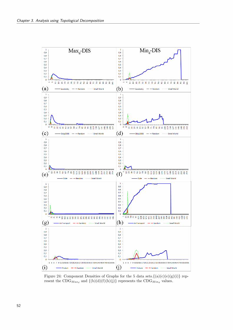
Chapter 3. Analysis using Topological Decomposition
Figure 24: Component Densities of Graphs for the 5 data sets.{(a)(c)(e)(g)(i)} rep-resent the CDGMaxd
and {(b)(d)(f)(h)(j)} represents the CDGMindvalues.
52
Chapter 4
Structure of Networks
4.1 Introduction
An important aspect in the study of complex networks is how they are structured in thereal world. Watts and Strogatz presented a model [170] to explain how the two prop-erties of small world networks, high clustering coefficient and low average path lengthappear in networks. Barabasi and Albert gave a model [13] to explain how networkswith power-law degree distribution arise in networks. From these two ground breakingresults, many researchers have introduced different models to explain the appearance ofnetworks with small world and scale free properties in the real world. In this chapter, westudy a number of these models in the light of several concepts borrowed from the fieldof sociology to understand the structure of real world social networks. We analyze theartificial networks produced by these network models using the Topological decompositionpresented in Chapter 3. The differences and similarities of these models are highlightedand their shortcomings are identified. Further more, we present a new model which pro-duces networks with both small world and scale free properties to overcome the identifiedshortcomings.
As a general classification, these different models can be grouped into two categories;Evolving models and Static models. Evolving models are the models that explain theevolution of complex networks as a function of time where the idea is to model the growthbehavior of these networks. A good example is the Barabasi and Albert model for scale freenetworks. Nodes are introduced continuously in the network and following the principleof preferential attachment, power-law degree distribution appears. Static models are themodels that are concerned with how networks are structured so that certain properties ofcomplex networks are present. Here, the term structure means the arrangement of nodesand edges, how they connect to each other. The Watts and Strogatz model is such anexample, as they start with a certain number of nodes and edges, that do not increasewith the passage of time but explain how high clustering coefficient and low average pathlengths appear in a network.
Both evolving and static models are of interest as they serve different purposes. Evolv-ing models try to identify the principles that govern the evolution of the physical systemsaround us. Static models propose methods to understand the structure and formation ofnetworks. Both these types of models can be used to construct artificial networks withproperties similar to real world networks to facilitate experimental and empirical studies.Since the introduction of small world and scale free properties, many researchers have de-veloped network models that generate artificial small-world and scale free networks. Wereview a number of these models in section 4.3.
53

Chapter 4. Structure of Networks
In this chapter we focus particularly on social networks. Described in Chapter 2, asocial network can be defined as a set of people, or groups of people interacting witheach other [148, 169]. Social network modeling and analysis allows us to understand thedifferent types of relationships that can either facilitate or impede knowledge creation andtransfer in a society on the whole, in an organization in particular, and in individuals,providing an insight on the underlying patterns and the social structures present in thesenetworks [173, 43].
An important aspect of social network study is their substructure in terms of clusters.Sociologists use the term community structures or communities [37] as compared to thestatistical and data mining domain where people use the term clusters [160] to referto the same concept. We earlier defined a community as a decomposition of verticesinto ‘Natural Groups’. There is no universally accepted definition of clusters [57], mostresearchers describe a cluster by considering the internal homogeneity and the externalseparation as the fundamental criteria for defining a cluster [69, 79, 88].
The properties of clusters in a network can tell us a lot about the likely behavior of thenetwork as a whole. How fast will some information propagate across the network? Howto identify representative nodes of a network? How do the clusters and social structurescommunicate and overlap one another? All of these aspects about structure of a networkcan be very relevant to predicting the behavior of the network as a whole [89, 173].
We explicitly target social networks and argue that using concepts from social networkstudy, we can generate artificial networks replicating real world social networks. Theseconcepts are discussed in section 4.2. For the sake of discussion and explanatory purposes,throughout this chapter, we are going to discuss four social networks, two of which are wellstudied and well structured and two of them although hypothetical, are yet common inour every day life and easy to comprehend. One of the two well structured social networksis the collaboration network of authors where nodes represent people and two people areconnected to each other if they have written an artifact together [125]. The other is theactor collaboration network from the movies where two actors are connected to each otherif they have appeared in a movie together [13] introduced earlier in Chapter2. We refer toit as the Actor or Imdb network. We also consider two cases from everyday life. Considera person joining a new organization as an employee and a person joining a sports clubas a leisure activity. We will refer them as Actor, Author, Employee and Club networksrespectively throughout this chapter.
In this chapter, we study a number of network generation models that produce smallworld-scale free networks. We show that there are considerable structural differences inthese artificial networks and real world networks. We propose a new static model togenerate artificial networks with small world-scale free properties.
The rest of the chapter is organized as follows: In section 4.2, we discuss a number ofdifferent social characteristics and argue that with a little modification to these concepts,we can understand how networks have community structures in the real world. Next, wecompare the existing network models in the light of these concepts and show their inabilityto produce networks which are close to the real networks studied in detail in Chapter 3. Wethen present a network generation model in section 4.4. In 4.5, we evaluate the proposedmodel as compared to other models. Next, in section 4.6, we present comparative resultswith real world networks to demonstrate the correctness of the proposed model. Finallywe conclude by giving possible future directions of our research in section 4.7.
54

4.2. Structure of Social Networks
4.2 Structure of Social Networks
In this section, we discuss a number of concepts from the domain of sociology in an attemptto better understand how social networks in the real world are structured.
Social TiesPeople in the real world are linked to each other through social ties. A wide range of
ties exist in the society and their study has attracted lots of research activity [169]. Asdiscussed in Chapter 1, the simplest form of a tie is Dyad [150] where two people arelinked to each other. This is considered as the unit of studying relationships in a socialnetwork. Triads are relationships between three people and have been the focus of manysocial network studies [169]. Groups of larger size are also possible but since a variety ofrelationships can form in them, they are less stable [150] and often less studied in sociology.They are often identified by their dense connectivity and clear bounds forming a cluster.Common questions studied in the analysis of these groups are how large they are in anetwork? How does their sizes vary in a society? how sparsely connected they are to oneanother? To what extent people belonging to multiple groups connect different groups?
Due to dense interconnectivity, these ties are termed as strong ties [102] where nodesthat are loosely connected to each other are said to have weak ties [70]. A significant workto highlight the importance of these weak ties is by Granovetter [70] where he concludesthat effective social coordination does not arise from dense interlocking but from thepresence of occasional weak ties. Each of us in the society has these weak ties along withstrong relationships. These weak ties or acquaintances are important for developing newrelationships and possibly joining new social communities. There is a fine mix of boththese weak and strong ties that exist in our society and both should be considered todevelop a model to generate artificial social networks.
HomophilyAn important human characteristic is homophily, tendency of actors or entities to asso-
ciate with other actors or entities of similar type [141, 142]. Homophily helps to explainwhy you know the people that you do, because you all have something in common, butone might also wonder how people you know at present determine the people you willknow in the future. This also introduces the idea of dynamics in triadic closures. Twopeople who have a mutual friend will tend to become acquainted in time [141]. A modelbased on these ideas was proposed by Rapoport who called it Random Biased Nets. Theidea was to modify the traditional random model of networks such that it incorporatessocial behaviors. Rapoport also concluded that we occasionally do things that are derivedentirely from our intrinsic preferences and characteristics, and these actions may lead us tomeet new people who have no connections to our previous friends at all. Although theseactions might appear to be random, but can be justified as having strong social back-ground with logical explanations. We limit our study to address this characteristic andrefer it as random connectivity pattern. In the light of homophily and social dynamics, wecan conclude that new connections between people are formed based on two properties,random connectivity and homophily.
Extraversion-IntroversionIt is interesting to note that in our society, we come across people that are well known
55

Chapter 4. Structure of Networks
and famous, and then there are people who have very few friends and contacts. These ideasare the direct implication of the human trait of extraversion-introversion [93]. Extroverts,who are open to meeting new people and developing new relationships are expected tohave high degree of connectivity in a social network as compared to Introverts, who tendto be more reserved, less outgoing, and less sociable.
An important use of this human characteristic is to explain the scale free degree be-havior of social networks. A famous person is likely to become more famous as comparedto a person who is not well known in the social community. Termed as the principle ofPreferential Attachment [13], it explains the growth behavior of networks with power lawdegree distribution. The idea is that in real world networks, nodes having high degree,have a high probability of attracting more connections as compared to nodes with lowconnectivity. Thus new social connections have to take this property into considerationas well.
In our society, we do not form individual relations with people, but with groups ofpeople. These relations are defined by particular circumstances, interests or some contextlike our school, work place, family [142, 70] and can be explained by homophily. Sincethese groups are densely connected to each other, often forming cliques, their social tiesare considered as strong ties. Since our society is built using these cliques, we call them‘Building Blocks’ of our society.
Each of these ‘building block’ or ‘group’ is like a small cluster joined to each otherby people belonging to more than one group [171]. When these small clusters have manyconnections to each other, they form bigger size clusters. The size of clusters in a network,vary to a large extent, and so does the number of clusters. Both these parameters dependlargely on how the individuals and their ties evolve in a society, how new connections areformed and older ones maintained or destroyed.
Let us consider the example of the actor network. When an actor acts in a movie, thesocial interactions will take place within the entire cast of the movie and form new tiesbetween actors if they do not exist previously. These interactions will be represented witha clique where all the nodes representing the actors will be connected to each other. Theauthorship network is no different as people co-authoring an artifact will form a clique.Similarly in the real world, usually groups of larger size are formed. Continuing withthe two examples, a new employee will most likely interact with different colleagues inthe same organization who work together on the same project or with whom a personshares an office for example. For a person joining a sports club, he will interact withpeople sharing similar activities instead of just one or two others. This is to highlight theidea that a person not necessarily interacts with only one or two other people, but morethan two people and this is the reason why we obtain cliques of larger sizes as shown inChapter 3.
Addressing the principle of Preferential Attachment, we argue that for every node in agroup (or Clique), few nodes have higher connectivity with other nodes. For example, in agroup representing the actors playing in the same movie, the famous actors will have manyconnections with others as they would have played a role in many movies, and the actorswho are starting their career, or are not so well known will have only a few connections.Similarly, in the authorship network, an experienced researcher would have published anartifact with many other researchers and thus would have a high number of connections.
Finally, we look at the society on the whole where we consider the average path lengthof the networks. We earlier discussed in Section 3.2.1 that the low average path lengths
56
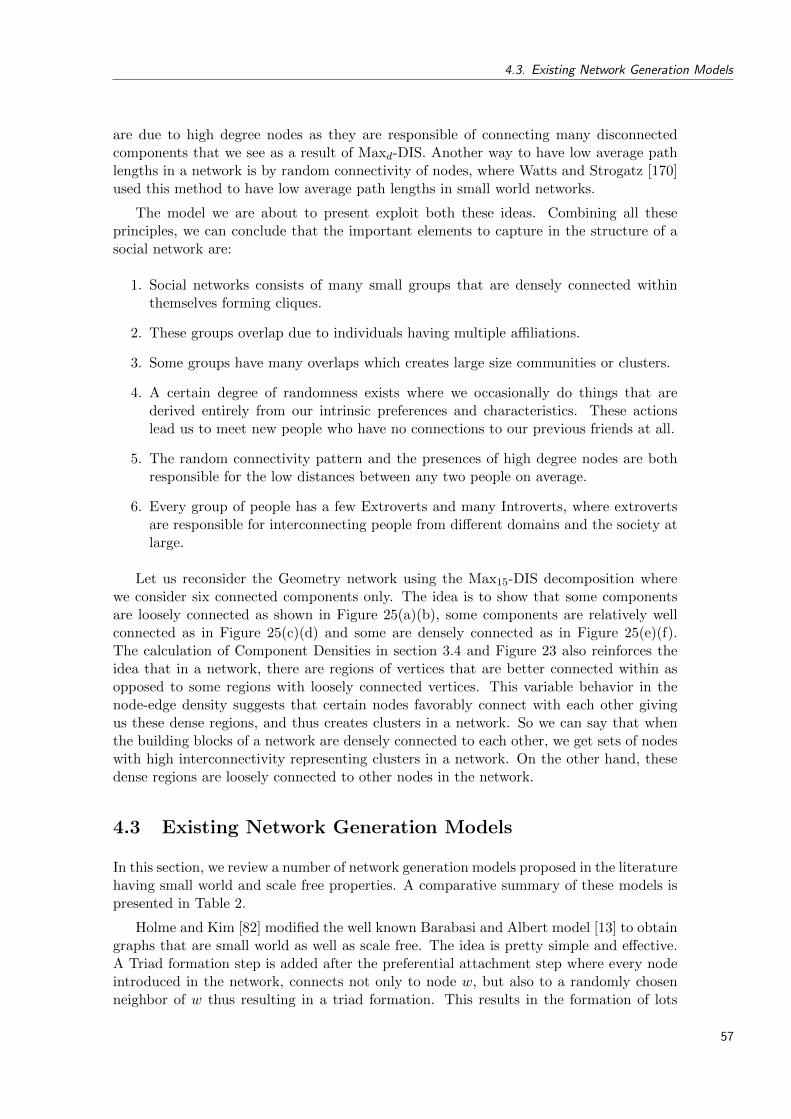
4.3. Existing Network Generation Models
are due to high degree nodes as they are responsible of connecting many disconnectedcomponents that we see as a result of Maxd-DIS. Another way to have low average pathlengths in a network is by random connectivity of nodes, where Watts and Strogatz [170]used this method to have low average path lengths in small world networks.
The model we are about to present exploit both these ideas. Combining all theseprinciples, we can conclude that the important elements to capture in the structure of asocial network are:
1. Social networks consists of many small groups that are densely connected withinthemselves forming cliques.
2. These groups overlap due to individuals having multiple affiliations.
3. Some groups have many overlaps which creates large size communities or clusters.
4. A certain degree of randomness exists where we occasionally do things that arederived entirely from our intrinsic preferences and characteristics. These actionslead us to meet new people who have no connections to our previous friends at all.
5. The random connectivity pattern and the presences of high degree nodes are bothresponsible for the low distances between any two people on average.
6. Every group of people has a few Extroverts and many Introverts, where extrovertsare responsible for interconnecting people from different domains and the society atlarge.
Let us reconsider the Geometry network using the Max15-DIS decomposition wherewe consider six connected components only. The idea is to show that some componentsare loosely connected as shown in Figure 25(a)(b), some components are relatively wellconnected as in Figure 25(c)(d) and some are densely connected as in Figure 25(e)(f).The calculation of Component Densities in section 3.4 and Figure 23 also reinforces theidea that in a network, there are regions of vertices that are better connected within asopposed to some regions with loosely connected vertices. This variable behavior in thenode-edge density suggests that certain nodes favorably connect with each other givingus these dense regions, and thus creates clusters in a network. So we can say that whenthe building blocks of a network are densely connected to each other, we get sets of nodeswith high interconnectivity representing clusters in a network. On the other hand, thesedense regions are loosely connected to other nodes in the network.
4.3 Existing Network Generation Models
In this section, we review a number of network generation models proposed in the literaturehaving small world and scale free properties. A comparative summary of these models ispresented in Table 2.
Holme and Kim [82] modified the well known Barabasi and Albert model [13] to obtaingraphs that are small world as well as scale free. The idea is pretty simple and effective.A Triad formation step is added after the preferential attachment step where every nodeintroduced in the network, connects not only to node w, but also to a randomly chosenneighbor of w thus resulting in a triad formation. This results in the formation of lots
57

Chapter 4. Structure of Networks
Figure 25: Six connected components from Max15-DIS of Geometry network. (a) and(b) are loosely connected, (c) and (d) are well connected and (e) and (f) are denselyconnected. The variation in node-edge density suggests the presence of communitystructures in the network.
of triads in the network increasing the overall clustering coefficient. A parameter m0 isused to decide the initial number of vertices with no edges. Another parameter m isused to decide the number of edges a newly added node will have in the network. Thisparameter can be used to control the node-edge density of the network. The newly addedvertex connects to m different nodes based on the probability which is proportional totheir degree. As a result, every new node introduced in the network will form a triad withthe highest degree node, which results in lots of triads around high degree nodes. Butsince the m vertices are chosen solely on the basis of their degree, no clear communitystructure appears. Another drawback of this model is that it does not generate cliquesof larger size as it only forces the presence of triads. We show Max15-DIS of the networkgenerated using this model in Figure 26. The parameters are set to generate a network ofapproximately the same size as that of NetScience network.
The idea of Holme and Kim is similar to another model separately proposed by Doro-govtsev et al. [48] in the same year where every new node added to the network is con-nected to both ends of a randomly chosen link where one of the nodes of this link isselected through preferential attachment. Similar behavior is obtained in terms of connec-tivity as lots of triads are created and the absence of large size cliques remains a drawback.Moreover no other criteria is used to enforce the presence of community structures in thenetwork.
These models inspired Jian-Guo et al. to introduce another similar model [109]. Thenetwork starts with a triangle and at each time step, a new node is added to the networkwith two edges. The first edge would choose a node to connect preferentially, and thesecond edge will choose a node connected to the first node, again based on preferentialattachment. This is different from the previous two models where the second node is
58

4.3. Existing Network Generation Models
Figure 26: Max15-DIS of a network generated using Holme-Kim model with m0 = 5and m = 1, which gives a network of size approximately equal to the NetSciencenetwork. Higher degree cliques are clearly missing. The subgraph contains 373 nodesand 584 edges as compared to the entire network with 379 nodes and 757 edges.
Figure 27: Network generated using Wang et al. model for random pseudofractalnetworks. We see how the network evolves from t = 0 to t = 5.
randomly chosen. No structural changes occur with this modification in terms of clusterformation, the clustering coefficient is increased by the presence of triads but bigger sizecliques are still missing and nodes do not attach to each other based on their domain orsurroundings but only on their degree.
Wang et al. [167] proposed a model to generate random pseudofractal networks withsmall world-scale free properties. The model starts with two nodes connected through anedge. At each time step, a new node is added with two edges. The new node is connectedto the two ends of an edge and the process is repeated for every existing edge in thenetwork. There is obviously no community structure present in the network. We showthe evolution of the network in Figure 27.
Fu and Liao [63] proposed another extension to the Barabasi and Albert model whichthey called the Relatively Preferential Attachment method. At each time step, the newly
59
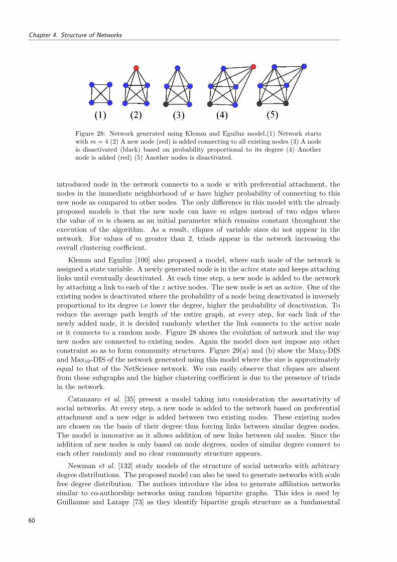
Chapter 4. Structure of Networks
Figure 28: Network generated using Klemm and Eguiluz model.(1) Network startswith m = 4 (2) A new node (red) is added connecting to all existing nodes (3) A nodeis disactivated (black) based on probability proportional to its degree (4) Anothernode is added (red) (5) Another nodes is disactivated.
introduced node in the network connects to a node w with preferential attachment, thenodes in the immediate neighborhood of w have higher probability of connecting to thisnew node as compared to other nodes. The only difference in this model with the alreadyproposed models is that the new node can have m edges instead of two edges wherethe value of m is chosen as an initial parameter which remains constant throughout theexecution of the algorithm. As a result, cliques of variable sizes do not appear in thenetwork. For values of m greater than 2, triads appear in the network increasing theoverall clustering coefficient.
Klemm and Eguiluz [100] also proposed a model, where each node of the network isassigned a state variable. A newly generated node is in the active state and keeps attachinglinks until eventually deactivated. At each time step, a new node is added to the networkby attaching a link to each of the z active nodes. The new node is set as active. One of theexisting nodes is deactivated where the probability of a node being deactivated is inverselyproportional to its degree i.e lower the degree, higher the probability of deactivation. Toreduce the average path length of the entire graph, at every step, for each link of thenewly added node, it is decided randomly whether the link connects to the active nodeor it connects to a random node. Figure 28 shows the evolution of network and the waynew nodes are connected to existing nodes. Again the model does not impose any otherconstraint so as to form community structures. Figure 29(a) and (b) show the Max5-DISand Max10-DIS of the network generated using this model where the size is approximatelyequal to that of the NetScience network. We can easily observe that cliques are absentfrom these subgraphs and the higher clustering coefficient is due to the presence of triadsin the network.
Catanzaro et al. [35] present a model taking into consideration the assortativity ofsocial networks. At every step, a new node is added to the network based on preferentialattachment and a new edge is added between two existing nodes. These existing nodesare chosen on the basis of their degree thus forcing links between similar degree nodes.The model is innovative as it allows addition of new links between old nodes. Since theaddition of new nodes is only based on node degrees, nodes of similar degree connect toeach other randomly and no clear community structure appears.
Newman et al. [132] study models of the structure of social networks with arbitrarydegree distributions. The proposed model can also be used to generate networks with scalefree degree distribution. The authors introduce the idea to generate affiliation networkssimilar to co-authorship networks using random bipartite graphs. This idea is used byGuillaume and Latapy [73] as they identify bipartite graph structure as a fundamental
60
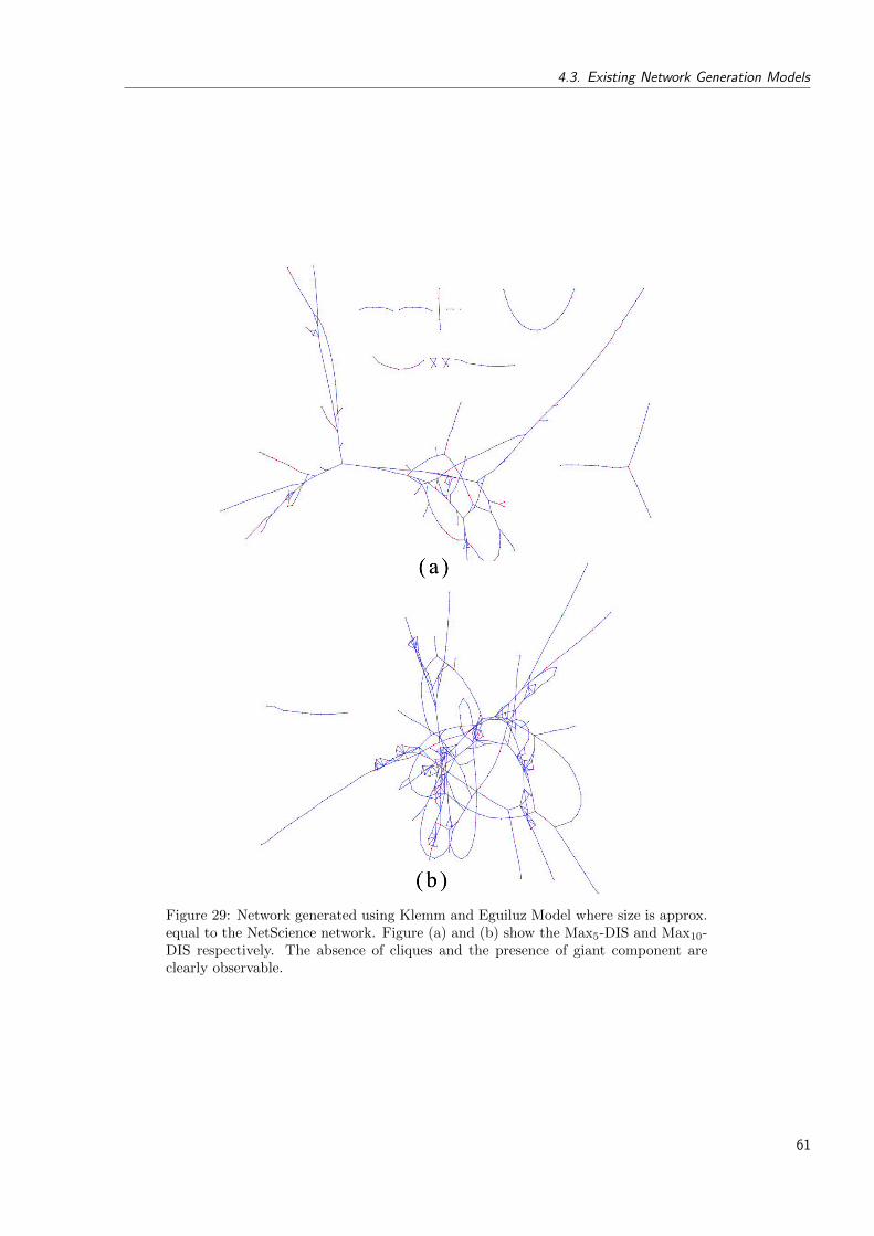
4.3. Existing Network Generation Models
Figure 29: Network generated using Klemm and Eguiluz Model where size is approx.equal to the NetScience network. Figure (a) and (b) show the Max5-DIS and Max10-DIS respectively. The absence of cliques and the presence of giant component areclearly observable.
61

Chapter 4. Structure of Networks
model of complex networks by giving real world examples. The two disjoint sets of abipartite graph are called bottom and top. At each step, a new top node is added and itsdegree d is sampled from a prescribed distribution. For each of the d edges of the newvertex, either a new bottom vertex is added or one is picked among the pre-existing onesusing preferential attachment.
A more generalized model based on similar principles was proposed by Bu et al. whereinstead of using the bipartite structure, a network can contain t disjoint sets (insteadof just two sets, as is the case of the bipartite graph). In the paper, they discuss theexample of sexual web [108] which is based on the bipartite structure. A sexual web isa network where nodes represent men and women having relationships to opposite sex,and similar nodes do not interact with each other. At each time step, a new node andm new edges are added to the network with the sum of the probabilities equal to 1. Thepreferential attachment rule is followed as the new node links with the existing nodes witha probability proportional to the degree of the nodes.
Wang and Rong [166] proposed a slightly different model, which is still a modifiedform of the preferential attachment model. Instead of adding one node at a time, themodel proposes to add n nodes at each time step which are connected in a ring formation.Any two nodes in the n new nodes are connected to the existing network where theseconnections are determined through preferential attachment. The network breaks intocliques of different sizes but since there is no biased connectivity among the nodes, thecliques are spread uniformly over the network and we cannot find any densely connectedset of nodes. Figure 30(a) and (b) show the the Max5-DIS and Max6-DIS respectively.Again the network is generated to be equivalent to the size of the NetScience network.Figure 30(a) shows the presence of cliques of different sizes and Figure 30(b) shows theuniform distribution of these cliques in the network without any clear community structureand cliques are connected to each other through edges. As compared to our society, wherepeople belonging to multiple groups connect these small groups forming our connectedsociety at large.
Guo and Kraines [75] proposed a model to study how the clustering coefficient affectsthe formation of a giant component. The model generates a random social network withfinely tunable clustering coefficient. The generator is composed of three steps: first, adegree sequence is generated following a power law. Next, the generator constructs arandom network using the algorithm of Molloy and Reed [120]. Finally, the networkconnections are modified to achieve the desired clustering coefficient. The model is astatic one, as it adds all the nodes initially to the network following a prescribed degreedistribution. Next, the network is modified to introduce triangles which increases theoverall clustering coefficient.
Generation models for clustered graphs exist in the literature such as the work ofCondon and Karp [39] and Virtanen[164] where the idea is to generate graphs that arealready clustered as opposed to random graph models of Rapoport [141] and Erdos andRenyi [55]. But these generation models do not produce graphs with small world and scalefree properties which are fundamental to most real world networks. Thus the study andcomparison of these other models remain out of the scope of the paper.
Comparing the different network generation models (See Table 2), the first five modelsare quite similar to each other, as they try to force the triad formation step, one wayor the other. Another common aspect in the first five models is that in every step, onlyone node and two edges are added to the network. The only other taxonomical grouping
62

4.4. Proposed Network Generation Model with Communities
Figure 30: Network generated using Wang and Rong Model where size is approx.equal to the NetScience network. (a) Max5-DIS: shows the presence of cliques ofdifferent sizes (b) Max10-DIS: shows the uniform distribution of these cliques in thenetwork and cliques rarely overlap. Cliques are connected to each other by edgesas compared to real social networks where these small social communities overlap toform our society.
possible is the three models where the bipartite and n-partite structures are used as thefundamental property of real world networks. The model of Wang and Rong is slightlydifferent as it allows the addition of m new nodes at every time step. The idea of Klemmand Eguiluz, Catanzaro et al. are quite original and provide another way to look at theevolution and structure of complex networks.
4.4 Proposed Network Generation Model withCommunities
As described earlier, the proposed model generates a static network. There are three basicsteps in the model which are discussed below.
In the first step, we introduce what we call building blocks in the network. As describedin the previous sections, our society is composed of many small groups. So, insteadof adding one node at a time, we add cliques of various sizes representing these smallgroups of the real world. This results in the network having high clustering coefficient. Incomparison to various models described earlier, where one node at a time is added to thenetwork. These cliques represent the building blocks of our society as described earlier inSection 4.1.
The next step is to join these cliques to form a connected society. These cliques areconnected to each other because people belong to multiple groups. From the propertyof Extraversion-Introversion, we know that there are people with many social contacts aswell as people with only a few contacts. These ideas lead us to define for every entity, thenumber of groups, it belongs to. For a node belonging to two different groups, we simply
63

Chapter 4. Structure of Networks
Comparative Summary of Existing Network Generation Models
Model, Year n m Innovation
Holme andKim, 2002
1 m Triad formation step, forcing a new node to connectto the neighbors of the first node it links to, in orderto have triangles and increase the clustering coefficient.
Dorogovtsev etal., 2002
1 2 Randomly chose an edge and attach both ends ofthis edge with the new node where the probability ofchoosing an edge is based on the degree of the nodesat its ends.
Jian-Guo etal., 2005
1 2 Each new node attaches to existing node with prefer-ential attachment and choses one of its neighbors againbased on preferential attachment (and not randomlyas compared to Holme and Kim).
Wang et al.,2006
1 2 For each edge, a new node with two edges is added,which is attached to both end nodes of the edge.Produces Fractals rather than a random graph.
Fu and Liao,2006
1 m Once a new node attaches to a node, its neighborhoodhas a higher probability of connecting to the new node.
Klemm andEguiluz, 2002
1 m Activate and deactivate nodes based on node degreewhere nodes having low degree have a high probabilityof getting deactivated.
Catanzaro etal., 2004
1 m Assortativity &Allows growth in old nodes by allowing new edges.
Newman et al.,2002
1 m Random network following a prescribed degree dis-tribution is generated. Bipartite graphs are used togenerate affiliation networks and obtain high clusteringcoefficient.
Guillaume andLatapy, 2004
1 m Bipartite Structure identified as a fundamental char-acteristic for real world graphs (similar to Newman etal., 2002).
Bu et al., 2007 1 m n-partite Structure, where nodes do not connect tosimilar node types.
Wang andRong, 2008
n m Add m new nodes and any two nodes in the mnew nodes link together from each other and theylink to existing nodes based on preferential attachment.
Guo andKraines, 2009
- - Static model that generates a random network withscale free degree distribution for n nodes. Next,the connections are modified to achieve the desiredclustering coefficient.
Table 2: Comparing and Summarizing different Artificial Network Generation Modelsexisting in the literature. n=nodes, m=edges64

4.4. Proposed Network Generation Model with Communities
merge two nodes from different groups, as a result, two cliques are combined with a singlenode being part of the two cliques as shown in Figure 32.
To achieve this, we associate a possible connectivity attribute drawn from a degreedistribution following power law. Few nodes when being part of many groups, will end uphaving many social contacts and represent the extroverts in the society.
For each node, this connectivity attribute, called Open connections (OC) determinesthe number of merges for each node. Note that the number of merges are directly propor-tional to the final node degree. If a few nodes are merged with many nodes, these nodeswill end up with many connections and thus the scale free degree distribution will appearin the network. This attribute is an integer between [1,P] where P is some constant valueand represents the maximum node degree a node can have in the network.
Finally, based on these number of merges which represent open connections of nodes(OC), we merge two nodes to build a connected network. We do this by randomly selectingtwo nodes from the network with open connections (OC). These nodes are merged together.In case, where two nodes of different building blocks are selected and that are alreadyconnected to each other by some other node, multiple overlaps appear. This results insmall groups connected by more that one node. This represents the phenomena of thereal world networks where two small groups are connected to each other by more thantwo people.
As the network is built from cliques and the connections are directed by scale free de-gree distribution, we get a network with high clustering coefficient and degree distributionfollowing power law. The average path length of the overall network remains low due totwo connectivity patterns, the random connections and the scale free degree distribution.The random connectivity of nodes has been shown to be one of the reasons for low averagepath lengths by [54, 55]. As for the scale free degree distribution, from the analysis ofAirTransport network in Chapter 3, we saw that airline companies use the hub strategyto minimize the number of hops (or in other words, the path lengths) to improve theefficiency of the network.
We explain the details of the proposed algorithm below. The following mathematicalnotations are used throughout the explanation: G(V,E) represents an undirected multi-graph where V is a set of n nodes and E is a set of e edges. The graph G is initiallyempty and the nodes and edges are added as the algorithm progresses. C represents a setof cliques such that C = {C1, C2, · · · , Ck} are different cliques each comprising of severalnodes.
Step 1: Building BlocksIn contrast to existing network generation models, instead of adding one node or triad
at a time, to generate the network, we start by adding cliques of variable sizes to G.Recall from Chapter 3, we identified cliques as one of the fundamental patterns present innetworks and the Author and Actor network considered as examples here have cliques byconstruction.
The algorithm takes as parameter, the number of cliques to be generated (k), theminimum (minSize) and the maximum size (maxSize) of the cliques to be generated.A random number is generated between these two limits and for each random number, aclique Ci is added to the graph G such that nodes and edges of the clique become membersof V and E respectively. As a result, G contains nodes that are well connected to each
65
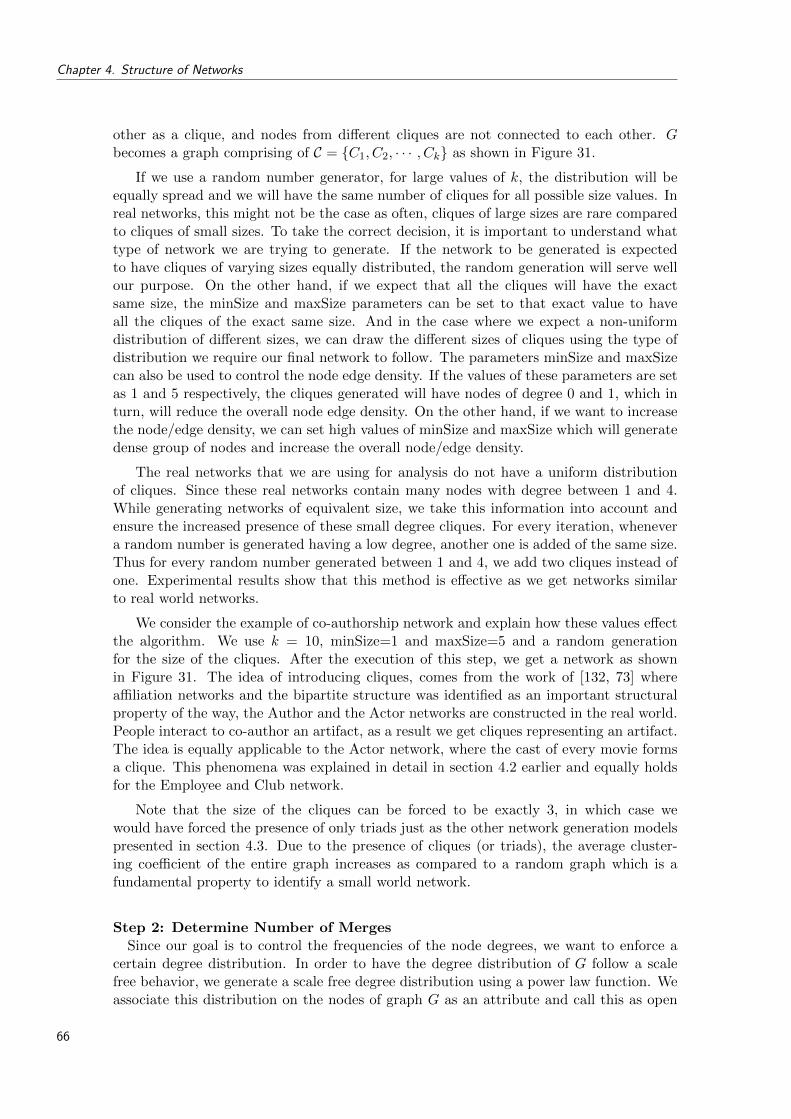
Chapter 4. Structure of Networks
other as a clique, and nodes from different cliques are not connected to each other. Gbecomes a graph comprising of C = {C1, C2, · · · , Ck} as shown in Figure 31.
If we use a random number generator, for large values of k, the distribution will beequally spread and we will have the same number of cliques for all possible size values. Inreal networks, this might not be the case as often, cliques of large sizes are rare comparedto cliques of small sizes. To take the correct decision, it is important to understand whattype of network we are trying to generate. If the network to be generated is expectedto have cliques of varying sizes equally distributed, the random generation will serve wellour purpose. On the other hand, if we expect that all the cliques will have the exactsame size, the minSize and maxSize parameters can be set to that exact value to haveall the cliques of the exact same size. And in the case where we expect a non-uniformdistribution of different sizes, we can draw the different sizes of cliques using the type ofdistribution we require our final network to follow. The parameters minSize and maxSizecan also be used to control the node edge density. If the values of these parameters are setas 1 and 5 respectively, the cliques generated will have nodes of degree 0 and 1, which inturn, will reduce the overall node edge density. On the other hand, if we want to increasethe node/edge density, we can set high values of minSize and maxSize which will generatedense group of nodes and increase the overall node/edge density.
The real networks that we are using for analysis do not have a uniform distributionof cliques. Since these real networks contain many nodes with degree between 1 and 4.While generating networks of equivalent size, we take this information into account andensure the increased presence of these small degree cliques. For every iteration, whenevera random number is generated having a low degree, another one is added of the same size.Thus for every random number generated between 1 and 4, we add two cliques instead ofone. Experimental results show that this method is effective as we get networks similarto real world networks.
We consider the example of co-authorship network and explain how these values effectthe algorithm. We use k = 10, minSize=1 and maxSize=5 and a random generationfor the size of the cliques. After the execution of this step, we get a network as shownin Figure 31. The idea of introducing cliques, comes from the work of [132, 73] whereaffiliation networks and the bipartite structure was identified as an important structuralproperty of the way, the Author and the Actor networks are constructed in the real world.People interact to co-author an artifact, as a result we get cliques representing an artifact.The idea is equally applicable to the Actor network, where the cast of every movie formsa clique. This phenomena was explained in detail in section 4.2 earlier and equally holdsfor the Employee and Club network.
Note that the size of the cliques can be forced to be exactly 3, in which case wewould have forced the presence of only triads just as the other network generation modelspresented in section 4.3. Due to the presence of cliques (or triads), the average cluster-ing coefficient of the entire graph increases as compared to a random graph which is afundamental property to identify a small world network.
Step 2: Determine Number of MergesSince our goal is to control the frequencies of the node degrees, we want to enforce a
certain degree distribution. In order to have the degree distribution of G follow a scalefree behavior, we generate a scale free degree distribution using a power law function. Weassociate this distribution on the nodes of graph G as an attribute and call this as open
66
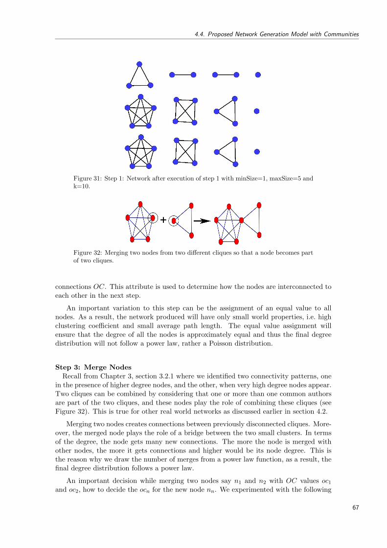
4.4. Proposed Network Generation Model with Communities
Figure 31: Step 1: Network after execution of step 1 with minSize=1, maxSize=5 andk=10.
Figure 32: Merging two nodes from two different cliques so that a node becomes partof two cliques.
connections OC. This attribute is used to determine how the nodes are interconnected toeach other in the next step.
An important variation to this step can be the assignment of an equal value to allnodes. As a result, the network produced will have only small world properties, i.e. highclustering coefficient and small average path length. The equal value assignment willensure that the degree of all the nodes is approximately equal and thus the final degreedistribution will not follow a power law, rather a Poisson distribution.
Step 3: Merge NodesRecall from Chapter 3, section 3.2.1 where we identified two connectivity patterns, one
in the presence of higher degree nodes, and the other, when very high degree nodes appear.Two cliques can be combined by considering that one or more than one common authorsare part of the two cliques, and these nodes play the role of combining these cliques (seeFigure 32). This is true for other real world networks as discussed earlier in section 4.2.
Merging two nodes creates connections between previously disconnected cliques. More-over, the merged node plays the role of a bridge between the two small clusters. In termsof the degree, the node gets many new connections. The more the node is merged withother nodes, the more it gets connections and higher would be its node degree. This isthe reason why we draw the number of merges from a power law function, as a result, thefinal degree distribution follows a power law.
An important decision while merging two nodes say n1 and n2 with OC values oc1and oc2, how to decide the ocn for the new node nn. We experimented with the following
67
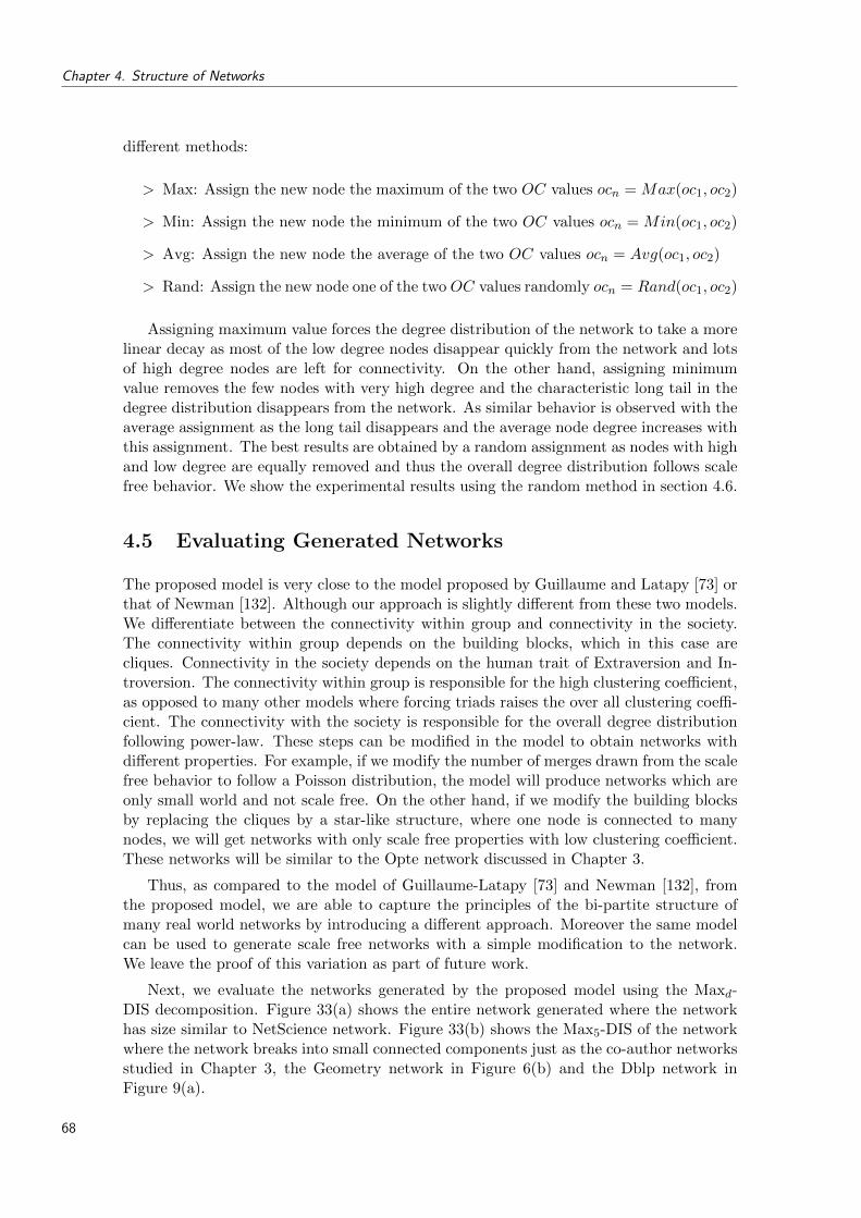
Chapter 4. Structure of Networks
different methods:
> Max: Assign the new node the maximum of the two OC values ocn = Max(oc1, oc2)
> Min: Assign the new node the minimum of the two OC values ocn = Min(oc1, oc2)
> Avg: Assign the new node the average of the two OC values ocn = Avg(oc1, oc2)
> Rand: Assign the new node one of the two OC values randomly ocn = Rand(oc1, oc2)
Assigning maximum value forces the degree distribution of the network to take a morelinear decay as most of the low degree nodes disappear quickly from the network and lotsof high degree nodes are left for connectivity. On the other hand, assigning minimumvalue removes the few nodes with very high degree and the characteristic long tail in thedegree distribution disappears from the network. As similar behavior is observed with theaverage assignment as the long tail disappears and the average node degree increases withthis assignment. The best results are obtained by a random assignment as nodes with highand low degree are equally removed and thus the overall degree distribution follows scalefree behavior. We show the experimental results using the random method in section 4.6.
4.5 Evaluating Generated Networks
The proposed model is very close to the model proposed by Guillaume and Latapy [73] orthat of Newman [132]. Although our approach is slightly different from these two models.We differentiate between the connectivity within group and connectivity in the society.The connectivity within group depends on the building blocks, which in this case arecliques. Connectivity in the society depends on the human trait of Extraversion and In-troversion. The connectivity within group is responsible for the high clustering coefficient,as opposed to many other models where forcing triads raises the over all clustering coeffi-cient. The connectivity with the society is responsible for the overall degree distributionfollowing power-law. These steps can be modified in the model to obtain networks withdifferent properties. For example, if we modify the number of merges drawn from the scalefree behavior to follow a Poisson distribution, the model will produce networks which areonly small world and not scale free. On the other hand, if we modify the building blocksby replacing the cliques by a star-like structure, where one node is connected to manynodes, we will get networks with only scale free properties with low clustering coefficient.These networks will be similar to the Opte network discussed in Chapter 3.
Thus, as compared to the model of Guillaume-Latapy [73] and Newman [132], fromthe proposed model, we are able to capture the principles of the bi-partite structure ofmany real world networks by introducing a different approach. Moreover the same modelcan be used to generate scale free networks with a simple modification to the network.We leave the proof of this variation as part of future work.
Next, we evaluate the networks generated by the proposed model using the Maxd-DIS decomposition. Figure 33(a) shows the entire network generated where the networkhas size similar to NetScience network. Figure 33(b) shows the Max5-DIS of the networkwhere the network breaks into small connected components just as the co-author networksstudied in Chapter 3, the Geometry network in Figure 6(b) and the Dblp network inFigure 9(a).
68
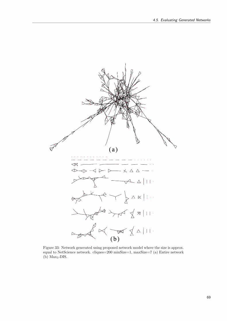
4.5. Evaluating Generated Networks
Figure 33: Network generated using proposed network model where the size is approx.equal to NetScience network. cliques=200 minSize=1, maxSize=7 (a) Entire network(b) Max5-DIS.
69

Chapter 4. Structure of Networks
Similar observations can be made about the network generated equivalent in size to theGeometry network. Figure 34(a) shows the Max5-DIS of the network where the networkbreaks into small connected components just as the co-author networks studied in Chap-ter 3. Figure 34(b) shows the Max10-DIS of the network with the appearance of the giantcomponent. Since the model is based on cliques as the building blocks to construct theentire network, it is obvious that using the topological decomposition, we find the presenceof these small densely connected group of nodes. As the node degree is increased, in thecase of Figure 34(b) where Max10-DIS contains nodes of at most degree equal to 10, wefind a similar behavior in the connectivity of nodes just as we analyzed in the previouschapter, a phase shift take place and a single giant connected component appears.
Figure 35 shows the degree distribution of the networks generated using the pro-posed model. We have generated networks of size equivalent to three social networks,the NetScience, Geometry and Imdb network. The degree distribution clearly shows thatthe networks generated follow the power law.
4.6 Results and Discussion
We have used the NetScience, Geometry and Imdb data sets for a comparative study.These are well studied examples of social networks and have been used by several re-searchers for empirical and experimental studies.
We calculate a number of statistics using various Network generation models andcompare them with the real world networks of equal sizes. The results are shown inTable 3, Table 4 and Table 5. We have included the statistics for a random networkfor the three data sets. In some cases, the models are not parameterized and thus thenode-edge density could not be controlled. We tried to generate models of similar size interms of number of nodes, and where possible, similar number of edges. An importantobservation about these networks is that since all of them use the preferential attachmentto produce the scale free property, the degree distribution for all the models follow apower law. To the best of our knowledge, there is no metric which tries to identify thepresence of communities in a network by analyzing the graph on the whole in a globalperspective, thus the presence of community structure in the proposed model is onlyjustified by construction.
Looking at some individual results for the various models in comparison to the realworld networks. For example, graphs generated using the model of Guillaume and Latapy,the node-edge density in every case is very high and could not be controlled. The model ofFu and Liao, in all the three examples, have a very low clustering coefficient as comparedto the respective real world network and thus could not really be classified as generatingsimilar networks to the real world networks used as examples in our study. Looking atthe clustering coefficient of the model by Wang and Rong in Table 4, it is quite clear thatthe model fails to generate a high clustering coefficient for a similar size network. Anobservation about the model of Holme and Kim, In Table 5, where the node-edge densityof the network is comparatively high to other two networks but the the network has a largesize, the clustering coefficient drops considerably. The model of Klemm and Eguiluz scaleswell in terms of clustering coefficient, and the average path length can controlled througha parameter (see Table 3) which gives a good approximate result. Also, from Table 5, theaverage path length in case of a number of models is 1.99, which is a direct implication
70

4.6. Results and Discussion
Figure 34: Network generated using proposed network model where the size is approx.equal to Geometry network. cliques=3000 minSize=1, maxSize=9 (a) Max5-DIS (b)Max10-DIS.
71

Chapter 4. Structure of Networks
Figure 35: Degree Distribution of equivalent size networks generated using the pro-posed Model. (a,c,e) Represent the bar charts and (b,d,f) represent the Log-Log plotof the Frequency-Degree distribution.
Comparison between NetScience and Other Network Models
Model Nodes Edges APL CC HD
NetScience 379 914 6.04 0.74 34
Random Graph 379 914 3.94 0.01 11
Zaidi et al. 364 935 4.7 0.65 22
Holme and Kim 379 757 4.86 0.77 42
Fu and Liao 379 744 4.03 0.75 31
Klemm and Eguiluz 379 755 6.40 0.5 24
Catanzaro et al. 379 898 2.42 0.58 197
Guillaume & Latapy 379 5315 2.30 0.54 109
Bu et al. 379 755 3.05 0.37 80
Wang and Rong 379 943 4.32 0.37 14
Table 3: Comparing different models with the Collaboration Network of Scientistsfrom the NetScience data. APL=Average Path length, CC=Clustering Coefficient,HD=Highest Node Degree
72
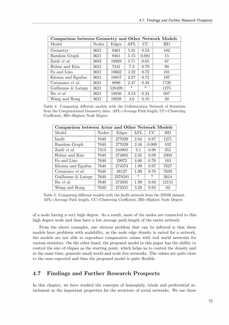
4.7. Findings and Further Research Prospects
Comparison between Geometry and Other Network Models
Model Nodes Edges APL CC HD
Geometry 3621 9461 5.31 0.53 102
Random Graph 3621 9461 5.15 0.001 15
Zaidi et al. 3682 10928 5.71 0.65 67
Holme and Kim 3621 7241 7.3 0.79 90
Fu and Liao 3621 10662 4.22 0.72 101
Klemm and Eguiluz 3621 10857 2.27 0.72 197
Catanzaro et al. 3621 8896 2.47 0.48 1720
Guillaume & Latapy 3621 528499 * * 1275
Bu et al. 3621 10856 3.13 0.24 607
Wang and Rong 3621 10828 4.6 0.10 30
Table 4: Comparing different models with the Collaboration Network of Scientistsfrom the Computational Geometry data. APL=Average Path length, CC=ClusteringCoefficient, HD=Highest Node Degree
Comparison between Actor and Other Network Models
Model Nodes Edges APL CC HD
Imdb 7640 277029 2.94 0.87 1271
Random Graph 7640 277029 2.48 0.009 102
Zaidi et al. 7413 244905 3.1 0.98 352
Holme and Kim 7640 274865 2.35 0.09 2303
Fu and Liao 7640 29972 4.00 0.76 163
Klemm and Eguiluz 7640 274374 1.99 0.97 7627
Catanzaro et al. 7640 28127 1.99 0.78 7639
Guillaume & Latapy 7640 2378281 * * 2614
Bu et al. 7640 274935 1.99 0.83 12151
Wang and Rong 7640 273355 3.28 0.94 83
Table 5: Comparing different models with the Imdb network from the IMDB dataset.APL=Average Path length, CC=Clustering Coefficient, HD=Highest Node Degree
of a node having a very high degree. As a result, most of the nodes are connected to thishigh degree node and thus have a low average path length of the entire network.
From the above examples, one obvious problem that can be inferred is that thesemodels have problems with scalability, as the node edge density is varied for a network,the models are not able to reproduce comparative values with real world networks forvarious statistics. On the other hand, the proposed model in this paper has the ability tocontrol the size of cliques as the starting point, which helps us to control the density andat the same time, generate small world and scale free networks. The values are quite closeto the ones expected and thus the proposed model is quite flexible.
4.7 Findings and Further Research Prospects
In this chapter, we have studied the concepts of homophily, triads and preferential at-tachment as the important properties for the structure of social networks. We use these
73
Chapter 4. Structure of Networks
concepts to present a model to generate artificial social networks. We evaluated a numberof network generation models that successfully generated small world and scale free net-works but fail to capture another important characteristic of real world network i.e. thepresence of Community Structures. We compared the existing and the proposed networkmodel with real world social networks using a number of statistics. Results show thatthe proposed model indeed generates networks that have community structures and aretopologically similar to real world networks as compared to the other existing models thatgenerate small world and scale free networks. Moreover, we identified another problemfor the existing models, the scalability in terms of node-edge density, where it is difficultto maintain the high clustering coefficient and low average path length as networks ofvarying sizes are produced.
We intend to extend our study to other types of networks such as biological andtechnology networks to propose network generation models for these types of networks aswell. Although experimentation is required, but we believe that by replacing the buildingblocks in this model, we can generate different types of networks as such as the InternetRouter networks and AirTransport network.
74

Chapter 5
Organization of Complex Net-works through Clustering
5.1 Introduction
Organization is an important process to arrange and group vertices in a network. Or-ganization of a network presents users and analysts a macro level view of the networki.e. instead of focusing on individual elements in a network, nodes are grouped togetherbased on some criteria and the behavior of the entire network is studied by analyzing thebehavior of these subgroups. There are a number of ways to group similar nodes wheremethods from the domain of Data Mining and more precisely, Graph Mining have beenused frequently to summarize networks. Three broad methods are Clustering, Classifica-tion and Association [111]. The most widely used method is Clustering which we definedearlier as a method to decompose vertices into ‘Natural Groups’.
We like the definition of a cluster given by Wasserman and Faust [169], a cluster canbe defined as a group of elements having the following properties:
> Density: Group members have many contacts to each other. In terms of graphtheory, it is considered to be the ratio of the number of edges present in a group ofnodes to the total number of edges possible in that group.
> Separation: Group members have more contacts inside the group than outside.
> Mutuality: Group members choose neighbors to be included in the group. In agraph-theoretical sense, this means that they are adjacent.
> Compactness: Group members are ‘well reachable’ from each other, though notnecessarily adjacent. Graph-theoretically, elements of the same cluster have shortdistances.
The topic of clustering has been studied extensively in pattern recognition and machinelearning [88, 179]. The goal of clustering is to divide a data set into subgroups such thatthe items in a group are similar in some predefined sense and, dissimilar to items of othergroups. Clustering is viewed as an unsupervised form of discovering patterns as no priorinformation is required about the group labels that are expected to be found. In networkor graph terminology, clustering is the task of grouping similar vertices together in acluster. Often this similarity is defined in terms of edges such that similar vertices arewell connected to each other by edges, not necessarily through direct edges but by a short
75

Chapter 5. Organization of Complex Networks through Clustering
path. For further details, Schaeffer [147] provides a good summary of the literature ongraph clustering.
Detection of clusters has a wide range of applications in various fields. For example, insocial networks, clustering could lead us towards a better comprehension of the interactionstaking place between people, or for biological networks, a useful application of clusteringis in the identification of biomarkers in a protein-protein interaction network. Otherapplications of clustering include a wide range of domains such as marketing to find groupsof customers with similar behavior, earthquake studies to cluster observed earthquakeepicenters to identify dangerous zones, libraries and electronic documents to group andorganize similar information resources together.
Different clustering techniques have been proposed to suit a variety of application do-mains and user requirements. Clusters produced by an algorithm can be organized in ahierarchy, or, on a single level called flat or partitional clustering. Hierarchical clusteringalgorithms can be further classified as agglomerative or divisive. An agglomerative algo-rithm starts with each vertex in a single cluster, these clusters are repeatedly merged intolarger groups until all clusters are merged into a single cluster or some stopping criteriais reached such as number of clusters or depth of the hierarchy. A divisive algorithmstarts with all the vertices in a single cluster which are repeatedly divided into subgroups.The process continues until clusters have only single nodes or some predefined criteriais reached. If the result of a clustering algorithm associates vertices to a single cluster,they are called Hard clustering algorithms, whereas, if vertices are allowed to belong tomultiple clustering algorithms, they are called Fuzzy or Soft clustering algorithms.
An important issue that needs to be addressed while developing clustering algorithmsfor real world networks is their Time Complexity. Due to large size real networks, itbecomes almost impractical to use slow clustering algorithms. Algorithms exist in theliterature addressing the clustering problem for large size complex networks but a tradeoff exists between Clustering Accuracy and the Time Complexity. We discuss a numberof these algorithms in section 5.2. Thus it is evident that faster algorithms are requiredto achieve high speed clustering as well as high accuracy to handle large size networks.
The motivation of this work comes from the fact that in the absence of high de-gree nodes, a network breaks into smaller connected components as discussed in detail inChapter 3 where we presented the DIS-topological decomposition. The process of detect-ing whether these components are densely connected using Component Densities provesto be very efficient and runs in O(maxd ∗ (n + e)). A simple intuition is to group thesedensely connected nodes as clusters, repeated application of this process for varying valuesof d can give us an algorithm which will be quite fast in terms of time complexity.
Along with this basic idea, we also noticed a high presence of low degree nodes asmost of the real world networks had nodes of degree below 5. From this observation, weintroduce some high speed heuristics that help to reduce the size of a network in lineartime in terms of the number of edges. This further helps in increasing the time efficiencyof the algorithm maintaining high cluster quality. Note that since the algorithm is basedon DIS, it works only for networks with non-uniform degree distribution. As most realworld networks exhibit this property, the algorithm is quite useful for real world networks.
The rest of the chapter is organized as follows: Section 5.2 discusses a number of clus-tering algorithms present in the literature where the idea is to focus on their asymptotictime complexity. Based on the topological decomposition presented in Chapter 3, we in-troduce our proposed algorithm in section 5.3. In section 5.4, we present the experimental
76

5.2. Review of Clustering Algorithms
setup, the data sets, other clustering algorithms and metrics to evaluate cluster quality.We compare the results of the proposed algorithm with existing algorithms in section 5.5,finally concluding in section 5.6.
5.2 Review of Clustering Algorithms
Many different approaches have been proposed to discover clusters in complex networks.For example, Girvan and Newman [68] used edge betweenness to produce a divisive hier-archical clustering algorithm. The basic idea is to identify intra cluster edges as comparedto inter cluster edges. Edges lying between clusters will have a higher betweenness central-ity as compared to edges within a cluster. The clustering algorithm removes edges withhigh betweenness centrality to identify clusters and recalculates the betweenness central-ity. The algorithm performs well in the detection of clusters but suffers from high timecomplexity. The worst case time complexity is given by O(e2n).
Wu et al.[176] introduce a multilevel mesh structure to cluster large networks. Theclustering algorithm uses Betweenness centrality and node degree to identify a set ofrepresentative nodes. All the other nodes are assigned the nearest representative nodes toobtain clusters. The agglomerative process is repeated to obtain a hierarchical clusteringwhich they call multilevel mesh. At each level, the user chooses a branching factor whichdetermines the number of clusters for that level. This number might not represent theactual number of clusters in the dataset as they are determined by the user without theuse of any heuristic or statistical measure. The overall complexity of the algorithm isgiven by O(e2n).
Boccaletti et al. propose a clustering method based on the cluster de-synchronizationproperties of phase oscillators [21]. Starting from a fully synchronized state of the network,a dynamical change in the weights of the interactions that retain information on theoriginal betweenness distribution, yields a progressive hierarchical clustering that fullydetects the dense communities. Since the initial calculation of betweenness takes O(n2),the algorithm scales quadratically as the number of nodes increase.
Newman [130] presents a faster agglomerative hierarchical clustering algorithm whichis based on a quality function called modularity Q. The algorithm repeatedly joins com-munities together in pairs, choosing at each step, the join that results in the greatestincrease in Q. The time complexity for the algorithm is given by O((e+n)n) which scalesquadratically in terms of number of nodes in the graph.
Boutin et al. [27] used a focus based filtering and clustering technique for complexnetworks. This technique extracts a tree-like graph so that the resulting structure can bedrawn using any force directed algorithm leaving the final drawing easily readable. One ofthe drawbacks of this system is that the user has to choose an initial entry point to filterthe graph. Moreover since edges are removed to simplify the structure of the network,important information can be lost.
Efficient algorithms to cluster networks with only small world properties have beenproposed like [9] [162]. These systems perform well if the topology of the network followssmall world properties but fail to perform in the presence of scale free properties. Thisis due to the fact that in a scale free network, a few nodes dominate the entire networksconnections and makes it difficult to identify the clusters. Similarly methods to cluster
77

Chapter 5. Organization of Complex Networks through Clustering
networks with only scale free properties have been proposed. For example [136] pro-posed a method based on Minimum Spanning tree(MST). While constructing the MST,they take into account the nodes having high degrees and increase the importance of theedges connected to these high degree nodes which are called hubs. This makes the edgesconnected to the hubs more important and thus are retained during the construction ofthe spanning tree. This approach works well if the underlying network structure has onlyscale free properties but in the presence of small world phenomena, it does not performwell. This is because the approach assumes that the high degree nodes are the probablecluster centers. While in reality, it is possible to have a clique in the network in whichtwo nodes connect to two different hubs, the MST method will force the clique structureto break and assign the nodes to two different clusters resulting in loss of information.
An important class of clustering algorithms called Spectral Clustering algorithms haveattracted considerable interest [153]. They are based on computing the eigenvectors ofthe adjacency matrix, or some other matrix representing the graph structure. The biggestadvantage of these algorithms is that they are able to detect clusters without a specific formas compared to classical algorithms such as k-means. They are well suited for large sizenetworks as well. But these algorithms are suited only for data sets where the similaritygraphs are sparse [110]. Furthermore, choosing a good similarity graph is not trivial, andspectral clustering can be quite unstable under different choices of the parameters for theneighborhood graphs.
In this section, we presented a number of clustering algorithms designed for complexnetworks. This review is not an extensive one as the clustering problem has been addressedin many different research domains and it is quite difficult to perform an extended studyof all these algorithms. For more details, readers can refer to surveys on the topic ofclustering such as [88, 179, 147].
5.3 Proposed Clustering Method: TDHC
Consider the example of the Geometry network which we analyzed in detail in Chapter 3and shown here in Figure 36. The entire network is shown in Figure 36(a), where asFigure 36(b) shows a small portion being focused where the encircled nodes representdensely connected nodes or more precisely cliques. Figure 36(c) and (d) show portions ofthe Max5-DIS and Max10-DIS. In these two figures, it is quite easy to visually detect thecliques or the densely connected nodes.
The inspiration of our clustering algorithm comes from this visualization. We explainedthat calculation of component densities can be performed in O(maxd ∗ (n + e)) time forall the Maxd-DIS graphs. The idea is to group the densely connected components forincreasing values of d as we iterate over Maxd-DIS. As a result, we end up agglomeratingvertices into clusters producing a hierarchical clustering algorithm. Thus we call thealgorithm, Topological Decomposition for Hierarchical Clustering abbreviated as TDHC.
As introduced in earlier chapters, from the topological decomposition, we can identifydensely connected sets of nodes that can be grouped to form clusters. The notion of howto define density is addressed in section 5.3.3. As the process is repeated for differentvalues of d, the number of iterations do not depend on nodes n or edges e of G but on thefactor d which is the maximum degree a node can have in G. Along with the detectionof densely connected nodes through Maxd-DIS, we also introduce several heuristics that
78

5.3. Proposed Clustering Method: TDHC
Figure 36: Geometry Network (a) Entire Network (b) Focus on a Small Portion (c)Part of Max5-DIS (d) Part of Max10-DIS
optimize the performance of the clustering algorithm. All these steps are highly efficientin terms of time complexity as we discuss the details in the following sections. First weintroduce all the major processing steps used in the algorithm before listing the algorithmitself.
Node Sink using K-Sink OperationWe define the K-Sink operation as follows: The nodes having degree 1 in a network are
connected to a single node. We merge the 1-degree nodes into their neighbors creatinga new node for each such merger. The 1-degree nodes merged into the neighbors arecalled the Sinkers. The nodes in which the 1-degree nodes get merged are called theSinkholes. This operation is justified because a 1-degree node cannot be clustered withany other node as it is simply connected to only one node. We call this operation, a 1-Sinkoperation and it is illustrated in Figure 37(a) where node 2 is the sinker and node 1 isthe sinkhole. If two nodes have degree 1 and are connected to each other, this means thatthey are disconnected from the rest of the network and in this case either of the node canbe chosen to be the sinker and the other as the sinkhole.
Similarly we define a 2-Sink operation, consider two nodes, say node 2 and node 3 both
79
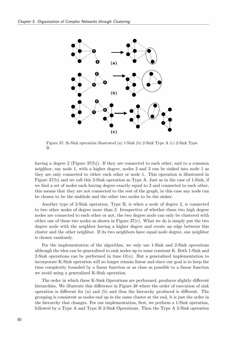
Chapter 5. Organization of Complex Networks through Clustering
Figure 37: K-Sink operation illustrated (a) 1-Sink (b) 2-Sink Type A (c) 2-Sink TypeB.
having a degree 2 (Figure 37(b)). If they are connected to each other, and to a commonneighbor, say node 1, with a higher degree, nodes 2 and 3 can be sinked into node 1 asthey are only connected to either each other or node 1. This operation is illustrated inFigure 37(b) and we call this 2-Sink operation as Type A. Just as in the case of 1-Sink, ifwe find a set of nodes each having degree exactly equal to 2 and connected to each other,this means that they are not connected to the rest of the graph, in this case any node canbe chosen to be the sinkhole and the other two nodes to be the sinker.
Another type of 2-Sink operation, Type B, is when a node of degree 2, is connectedto two other nodes of degree more than 2. Irrespective of whether these two high degreenodes are connected to each other or not, the two degree node can only be clustered witheither one of these two nodes as shown in Figure 37(c). What we do is simply put the twodegree node with the neighbor having a higher degree and create an edge between thiscluster and the other neighbor. If its two neighbors have equal node degree, one neighboris chosen randomly.
For the implementation of the algorithm, we only use 1-Sink and 2-Sink operationsalthough the idea can be generalized to sink nodes up to some constant K. Both 1-Sink and2-Sink operations can be performed in time O(n). But a generalized implementation toincorporate K-Sink operation will no longer remain linear and since our goal is to keep thetime complexity bounded by a linear function or as close as possible to a linear functionwe avoid using a generalized K-Sink operation.
The order in which these K-Sink Operations are performed, produces slightly differenthierarchies. We illustrate this difference in Figure 38 where the order of execution of sinkoperation is different for (a) and (b) and thus the hierarchy produced is different. Thegrouping is consistent as nodes end up in the same cluster at the end, it is just the order inthe hierarchy that changes. For our implementation, first, we perform a 1-Sink operation,followed by a Type A and Type B 2-Sink Operations. Then the Type A 2-Sink operation
80

5.3. Proposed Clustering Method: TDHC
Figure 38: Changing the order of K-Sink operation changes the hierarchy slightly butit remains consistent as the nodes find themselves grouped together in the same cluster(a) 1-Sink Operation first, sinking node 4 into node 3 followed by a 2-Sink operationof Type A where nodes 1,2 and 5 are grouped together. (b) 2-Sink operation of TypeA first, where nodes 1 and 2 are grouped together as node 7, followed by a 1-Sinkoperation where node 4 gets sinked into node 3.
is repeated finally followed by a 1-Sink Operation. The choice to perform the operationsin this order is based on experiments where the convergence is faster and higher accuracyis achieved for the clusters produced.
Another aspect is that both the 1-Sink and 2-Sink operations can be iterated severaltimes. Choosing a fixed number of iterations for these two operations will not effectthe overall time complexity but if they are executed until no more nodes can sink inother nodes, the overall time complexity will no longer remain linear, and thus we avoiditerating over these operations. Moreover our experimental evaluation suggests that wedo not increase the quality of clustering to a large extent by repeating these operationsmany times.
Maximum Degree Induced SubgraphThe next step in the algorithm is to create a Maxd-DIS with a small value of d. Due to
this small value, the network might break into several components disconnected to eachother as shown in Figure 36(c) and (d). In the clustering algorithm, the value iteratesfrom a start value of 2 and goes on till the maximum degree value possible.
Tightening: Disconnect Loosely Connected NodesAfter obtaining the Maxd-DIS, we perform an operation that we call Tightening. We
look at the nodes having degree 1 in this subgraph and we simply remove the edgesconnecting degree 1 nodes from the induced subgraph. This process helps us to make theconnected components found in the subgraph more dense as shown in Figure 39 wherenodes 1 and 2 are disconnected by removal of edges. This step delays the decision ofputting node 1 and 2 with the other nodes in a cluster. Recall that this operation isperformed on the induced subgraph, nodes 1 and 2 can thus be densely connected withother nodes in the entire graph. Due to this reason, the step delays aggregating degree 1nodes with densely connected nodes. The step can be performed in time O(n) where nhas small values as compared to the entire graph G.
81
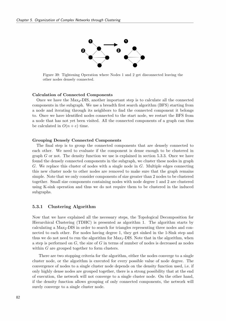
Chapter 5. Organization of Complex Networks through Clustering
Figure 39: Tightening Operation where Nodes 1 and 2 get disconnected leaving theother nodes densely connected.
Calculation of Connected ComponentsOnce we have the Maxd-DIS, another important step is to calculate all the connected
components in the subgraph. We use a breadth first search algorithm (BFS) starting froma node and iterating through its neighbors to find the connected component it belongsto. Once we have identified nodes connected to the start node, we restart the BFS froma node that has not yet been visited. All the connected components of a graph can thusbe calculated in O(n+ e) time.
Grouping Densely Connected ComponentsThe final step is to group the connected components that are densely connected to
each other. We need to evaluate if the component is dense enough to be clustered ingraph G or not. The density function we use is explained in section 5.3.3. Once we havefound the densely connected components in the subgraph, we cluster these nodes in graphG. We replace this cluster of nodes with a single node in G. Multiple edges connectingthis new cluster node to other nodes are removed to make sure that the graph remainssimple. Note that we only consider components of size greater than 2 nodes to be clusteredtogether. Small size components containing nodes with node degree 1 and 2 are clusteredusing K-sink operation and thus we do not require them to be clustered in the inducedsubgraphs.
5.3.1 Clustering Algorithm
Now that we have explained all the necessary steps, the Topological Decomposition forHierarchical Clustering (TDHC) is presented as algorithm 1. The algorithm starts bycalculating a Max2-DIS in order to search for triangles representing three nodes and con-nected to each other. For nodes having degree 1, they get sinked in the 1-Sink step andthus we do not need to run the algorithm for Max1-DIS. Note that in the algorithm, whena step is performed on G, the size of G in terms of number of nodes is decreased as nodeswithin G are grouped together to form clusters.
There are two stopping criteria for the algorithm, either the nodes converge to a singlecluster node, or the algorithm is executed for every possible value of node degree. Theconvergence of nodes to a single cluster node depends on the density function used, i.e. ifonly highly dense nodes are grouped together, there is a strong possibility that at the endof execution, the network will not converge to a single cluster node. On the other hand,if the density function allows grouping of only connected components, the network willsurely converge to a single cluster node.
82
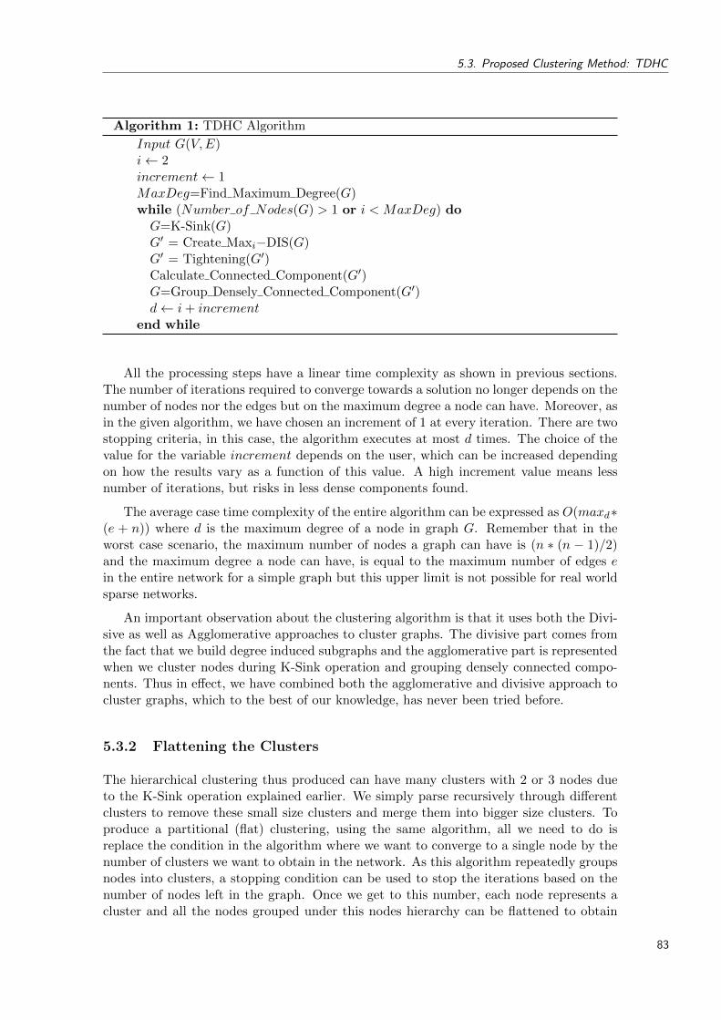
5.3. Proposed Clustering Method: TDHC
Algorithm 1: TDHC Algorithm
Input G(V,E)i← 2increment← 1MaxDeg=Find Maximum Degree(G)while (Number of Nodes(G) > 1 or i < MaxDeg) doG=K-Sink(G)G′ = Create Maxi−DIS(G)G′ = Tightening(G′)Calculate Connected Component(G′)G=Group Densely Connected Component(G′)d← i+ increment
end while
All the processing steps have a linear time complexity as shown in previous sections.The number of iterations required to converge towards a solution no longer depends on thenumber of nodes nor the edges but on the maximum degree a node can have. Moreover, asin the given algorithm, we have chosen an increment of 1 at every iteration. There are twostopping criteria, in this case, the algorithm executes at most d times. The choice of thevalue for the variable increment depends on the user, which can be increased dependingon how the results vary as a function of this value. A high increment value means lessnumber of iterations, but risks in less dense components found.
The average case time complexity of the entire algorithm can be expressed as O(maxd∗(e + n)) where d is the maximum degree of a node in graph G. Remember that in theworst case scenario, the maximum number of nodes a graph can have is (n ∗ (n − 1)/2)and the maximum degree a node can have, is equal to the maximum number of edges ein the entire network for a simple graph but this upper limit is not possible for real worldsparse networks.
An important observation about the clustering algorithm is that it uses both the Divi-sive as well as Agglomerative approaches to cluster graphs. The divisive part comes fromthe fact that we build degree induced subgraphs and the agglomerative part is representedwhen we cluster nodes during K-Sink operation and grouping densely connected compo-nents. Thus in effect, we have combined both the agglomerative and divisive approach tocluster graphs, which to the best of our knowledge, has never been tried before.
5.3.2 Flattening the Clusters
The hierarchical clustering thus produced can have many clusters with 2 or 3 nodes dueto the K-Sink operation explained earlier. We simply parse recursively through differentclusters to remove these small size clusters and merge them into bigger size clusters. Toproduce a partitional (flat) clustering, using the same algorithm, all we need to do isreplace the condition in the algorithm where we want to converge to a single node by thenumber of clusters we want to obtain in the network. As this algorithm repeatedly groupsnodes into clusters, a stopping condition can be used to stop the iterations based on thenumber of nodes left in the graph. Once we get to this number, each node represents acluster and all the nodes grouped under this nodes hierarchy can be flattened to obtain
83

Chapter 5. Organization of Complex Networks through Clustering
a partitional clustering. We have used this same approach to compare the results of theTDHC algorithm with the other clustering algorithms.
5.3.3 Density Function
There are several definitions of how to calculate the density of a graph, the readers arerecommended [113] for details. For simplicity we use the node to edge ratio (m/n) to referto the density of the graph. [113] argues that the density of a graph varies as a functionof application domain giving real world examples. For the proposed clustering algorithm,we use a density function to determine how well a set of nodes is connected to each other.Based on the arguments and examples provided in [113], we argue that we cannot havea generic density value set as a threshold to decide whether a set of nodes is connectedwell enough or not. Moreover, the question of whether a set of nodes are connected wellenough to be clustered, depends not only on the density of the entire graph but on theunderlying structure of the network. This issue was discussed previously in Chapter 3for networks such as Opte and AirTransport network where Maxd-DIS did not containdensely connected nodes.
To resolve this problem, we propose a floating density function i.e. we propose a set offunctions starting from high density values to progressively less dense functions. The ideais to try to find highly dense communities first, for all possible values of the Maxd-DIS,and then replace the density function with a less dense function. We start by looking forthe maximum number of edges possible for a set of nodes and eventually end up lookingfor the minimum number of edges possible for a set of nodes to be connected. We clustera set of nodes if the number of edges m is:
e = n(n− 1)/2
e ≥ n(n− 1) ∗ 0.8/2
e ≥ n(n− 1) ∗ 0.6/2
e ≥ n(n− 1) ∗ 0.4/2
e ≥ (2 ∗ n)
e ≥ n− 1
The set of equations represent a gradual decrease in the node-edge density requiredfor a group of nodes to be considered as dense enough to be clustered together. Thefirst equation represents the maximum number of edges possible for a set of nodes, thesecond, third and fourth equation represents 80%, 60%, 40% of the possible edges. Thefourth equation requires twice as many edges as nodes for a set of nodes to be consideredas dense and finally the last equation represents the minimum number of edges requiredby a set of nodes to remain connected. Note that this final case can occur in real datasets such as the Opte network or the AirTransport network discussed earlier in Chapter 3as these networks do not contain highly dense components.
Although using the floating equation idea can effect the number of iterations requiredto cluster the entire data set, it assures that the clusters found are as dense as possible.This is the only control parameter that is required by the proposed algorithm and variesfrom one dataset to the other depending upon the average density of a data set as discussedpreviously in Chapter 3. The overall complexity of the algorithm remains the same as thenumber of equations ranges from a constant value of 2 to 6. So in effect the final algorithm
84
5.4. Experimentation
is run once for each of these equations in the given order until all the nodes converge toa single node. As mentioned earlier, the choice of these equations depends upon the dataset being used and the inherent network structure but as our experiments show, this orderand set of equations seems to give good results for the different data sets that we have usedfor experimentation. Apart from the density function, the other control parameter for thealgorithm is the number of clusters required to generate, which by default, agglomeratesthe entire data into a single cluster.
An important exception in the algorithm is when it is executed for the last equation,Tightening step is not executed as we do not need to add an extra hierarchical level sincewe are no longer looking for dense components.
5.4 Experimentation
We use different data sets to compare the performance of the proposed TDHC algorithmwith other clustering algorithms using a number of evaluation metrics to judge the clusterquality.
Data SetsWe have used the NetScience, Opte and Protein network. Since the Divisive Clustering
algorithm has a high time complexity, we only consider a subset of the Opte data setconstructed by considering a hub and the nodes connected at distance 5 from it. Thesubset consists of 1049 nodes and 1319 edges.
The choice of these data sets is based on the criteria that all these networks belongto different classification of networks as described in the literature [129]. The authornetwork represents a social network of collaboration, the internet network represents atechnological network and the protein network represents a biological network. We haveused networks that contain a few thousand nodes and edges only, since we want to comparethe results of the proposed algorithm with slow but highly efficient algorithms in terms ofcluster quality.
Clustering AlgorithmsTo cluster these data sets, we use two known clustering algorithms, the Bisecting K-
Means algorithm [154] and the Divisive Clustering algorithm based on Edge Centrality [68].The choice of these algorithms is based on the criteria that these algorithms do not tryto optimize or influence the clustering algorithm based on the density or some othercluster quality metric as compared to other algorithms present in the literature suchas [130]. Moreover they are known to perform well for a number of real world data sets[181, 68]. We also use the Strength Clustering algorithm proposed by [9] which was initiallyintroduced to cluster social networks. The algorithm has been shown to perform well forthe identification of densely connected components as clusters.
The Bisecting K-Means algorithm and the Divisive Clustering algorithm based on EdgeCentrality are both divisive algorithms, i.e. they start by considering the entire graph asa single cluster and repeatedly divide the cluster into two clusters. Both these algorithmscan be used to create a hierarchy where the divisive process stops when each cluster hasexactly one node left. Instead of generating the entire hierarchy, we stop the process assoon as the number of clusters reaches around 20. Moreover since we do not propose
85

Chapter 5. Organization of Complex Networks through Clustering
Cluster Quality Metric
Data Set Algorithm MQ Q RD
NetScienceDiv. Clus. 0.53 0.77 0.63Bis. K-Means 0.42 0.77 0.63Strength 0.83 0.26 0.23TDHC 0.55 0.82 0.42
OpteDiv. Clus. 0.32 0.79 0.69Bis. K-Means 0.41 0.59 0.58Strength 0.50 0.35 0.55TDHC 0.42 0.85 0.49
ProteinDiv. Clus. 0.31 0.63 0.49Bis. K-Means 0.41 0.33 0.31Strength 0.52 0.16 0.29TDHC 0.38 0.44 0.23
Table 6: Comparing the results of Divisive Clustering based on Edge Distribution(Div. Clus.), Bisecting K-Means (Bis. K-Means) and Strength Clustering (Strength)algorithms with the TDHC algorithm.
a method to evaluate the quality of a hierarchical clustering algorithm, we consider theleaves as a single partitional clustering. Note that the clustering algorithm might createsingletons but we do not consider these smaller clusters while generating 20 clusters andthese clusters are also neglected while evaluating the quality of clusters.
Cluster Evaluation MetricsWe used three different metrics to evaluate the quality of clusters produced by the
algorithms. Modularity(Q) [126] (Q metric) is a metric that measures the fraction of theedges in the network that connect within-community edges minus the expected value of thesame quantity in a network with the same community divisions but random connectionsbetween the vertices. If the number of within-community edges is no better than random,we will get Q = 0. Values approaching Q = 1, which is the maximum, indicate strongcommunity structure. The second metric used by Auber et al. [9] is called the MQmetric. It comprises of two factors where the first term contributes to the positive weightrepresented by the mean value of edge density inside each cluster. The second termcontributes as a negative weight and represents the mean value of edge density betweenthe clusters. Finally the Relative Density (RD) [116] of a cluster calculates the ratio ofthe edge density inside a cluster to the sum of the edge densities inside and outside thatcluster. The final RD is the averaged sum of the these individual relative densities for allclusters. Note that all these metrics are normalized between [0,1] where 1 signifies perfectclustering. More details on evaluating the quality of clusters can be found in Chapter 7.
5.5 Results and Discussion
We discussed the algorithm’s average case time complexity is O(maxd∗(n+e)). In reality,the algorithm runs much faster than its average case. This is because as the algorithmprogresses, the nodes are aggregated into clusters and the size of the network becomessmaller.
86
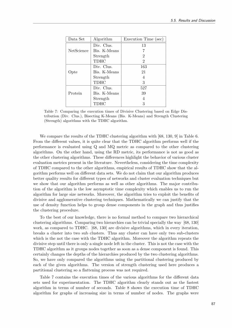
5.5. Results and Discussion
Data Set Algorithm Execution Time (sec)
NetScienceDiv. Clus. 13Bis. K-Means 7Strength 2TDHC 2
OpteDiv. Clus. 163Bis. K-Means 21Strength 4TDHC 3
ProteinDiv. Clus. 527Bis. K-Means 39Strength 4TDHC 3
Table 7: Comparing the execution times of Divisive Clustering based on Edge Dis-tribution (Div. Clus.), Bisecting K-Means (Bis. K-Means) and Strength Clustering(Strength) algorithms with the TDHC algorithm.
We compare the results of the TDHC clustering algorithm with [68, 130, 9] in Table 6.From the different values, it is quite clear that the TDHC algorithm performs well if theperformance is evaluated using Q and MQ metric as compared to the other clusteringalgorithms. On the other hand, using the RD metric, its performance is not as good asthe other clustering algorithms. These differences highlight the behavior of various clusterevaluation metrics present in the literature. Nevertheless, considering the time complexityof TDHC compared to the other algorithms, empirical results of TDHC show that the al-gorithm performs well on different data sets. We do not claim that our algorithm producesbetter quality results for different types of networks and cluster evaluation techniques butwe show that our algorithm performs as well as other algorithms. The major contribu-tion of the algorithm is the low asymptotic time complexity which enables us to run thealgorithm for large size networks. Moreover, the algorithm tries to exploit the benefits ofdivisive and agglomerative clustering techniques. Mathematically we can justify that theuse of density function helps to group dense components in the graph and thus justifiesthe clustering procedure.
To the best of our knowledge, there is no formal method to compare two hierarchicalclustering algorithms. Comparing two hierarchies can be trivial specially the way [68, 130]work, as compared to TDHC. [68, 130] are divisive algorithms, which in every iteration,breaks a cluster into two sub clusters. Thus any cluster can have only two sub-clusterswhich is the not the case with the TDHC algorithm. Moreover the algorithm repeats thedivisive step until there is only a single node left in the cluster. This is not the case with theTDHC algorithm as it groups nodes together as soon as a dense component is found. Thiscertainly changes the depths of the hierarchies produced by the two clustering algorithms.So, we have only compared the algorithms using the partitional clustering produced byeach of the given algorithms. The version of strength clustering used here produces apartitional clustering so a flattening process was not required.
Table 7 contains the execution times of the various algorithms for the different datasets used for experimentation. The TDHC algorithm clearly stands out as the fastestalgorithm in terms of number of seconds. Table 8 shows the execution time of TDHCalgorithm for graphs of increasing size in terms of number of nodes. The graphs were
87
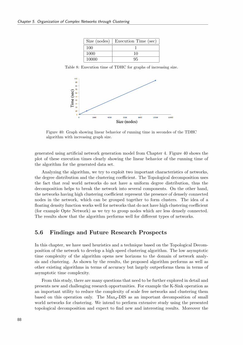
Chapter 5. Organization of Complex Networks through Clustering
Size (nodes) Execution Time (sec)
100 1
1000 10
10000 95
Table 8: Execution time of TDHC for graphs of increasing size.
Figure 40: Graph showing linear behavior of running time in secondes of the TDHCalgorithm with increasing graph size.
generated using artificial network generation model from Chapter 4. Figure 40 shows theplot of these execution times clearly showing the linear behavior of the running time ofthe algorithm for the generated data set.
Analyzing the algorithm, we try to exploit two important characteristics of networks,the degree distribution and the clustering coefficient. The Topological decomposition usesthe fact that real world networks do not have a uniform degree distribution, thus thedecomposition helps to break the network into several components. On the other hand,the networks having high clustering coefficient represent the presence of densely connectednodes in the network, which can be grouped together to form clusters. The idea of afloating density function works well for networks that do not have high clustering coefficient(for example Opte Network) as we try to group nodes which are less densely connected.The results show that the algorithm performs well for different types of networks.
5.6 Findings and Future Research Prospects
In this chapter, we have used heuristics and a technique based on the Topological Decom-position of the network to develop a high speed clustering algorithm. The low asymptotictime complexity of the algorithm opens new horizons to the domain of network analy-sis and clustering. As shown by the results, the proposed algorithm performs as well asother existing algorithms in terms of accuracy but largely outperforms them in terms ofasymptotic time complexity.
From this study, there are many questions that need to be further explored in detail andpresents new and challenging research opportunities. For example the K-Sink operation asan important utility to reduce the complexity of scale free networks and clustering thembased on this operation only. The Maxd-DIS as an important decomposition of smallworld networks for clustering. We intend to perform extensive study using the presentedtopological decomposition and expect to find new and interesting results. Moreover the
88

5.6. Findings and Future Research Prospects
choice of density function at the moment is trivial and can vary from one data set tothe other. Another approach to cluster networks which requires more exploration is thefact that the density function can be replaced by some other criteria, depending upon theinherent network topology, the motifs found in those networks. We also intend to performa user evaluation by domain experts to further validate the performance and quality ofthe proposed clustering algorithm.
89

90
Chapter 6
Co-Occurrence Networks fromthe Web: Clustering andVisualization
6.1 Introduction
Another domain where the presence of complex networks is commonly observed is theweb [1]. Web pages are a common resource of information containing textual information.Usually a set of key words can be extracted from these web pages to represent the contentsof the web page. Using these key words, a co-occurrence network can be built wherenodes represent key words and edges represent a link between two key words if theyappear together on the same page. Other examples of co-occurrence networks can bewhen one considers a novel and construct a co-occurrence network of characters if theyappear in the same paragraph or on the same page [59]. Looking at the properties of theseco-occurrence networks, they follow small world and scale free behavior and present aninteresting example of complex networks for study and experimentation as web pages arewidely used to collect information.
Recall from Chapter 1, visualization is an important method to analyze these networks.In Chapter 3 we used layout algorithms to show a number of real world complex networksbut the drawings produced were highly entangled and cluttered. One important result thatwe have extracted from the analysis using DIS is that in the absence of high degree nodes,these networks break into smaller connected components making it easier to visualize. Weused this motivation to simplify co-occurrence networks produced using key words fromweb pages to produce readable drawings so that we can easily understand and analyzeweb documents. The research domain concerned with the extraction of knowledge fromdocuments is called Information Analysis (IA) or more precisely Content Analysis (CA).This is an active area of research where the goal is to explore and analyze contents ofa set of documents in order to discover patterns and hidden knowledge [156]. Weareprovides a good overview of the challenges presented to the CA research community bythe World Wide Web [172]. Document Content Visualization Systems can be used asa tool for CA where the goal is to represent textual contents of a set of documents in avisual form so as to facilitate the process of mining and discovering patterns in a collectionof documents [124, 71]. We use the co-occurrence networks of key words extracted fromweb pages to perform CA. The exponential increase in the information available on theweb requires efficient organization and visualization systems to facilitate faster access to
91
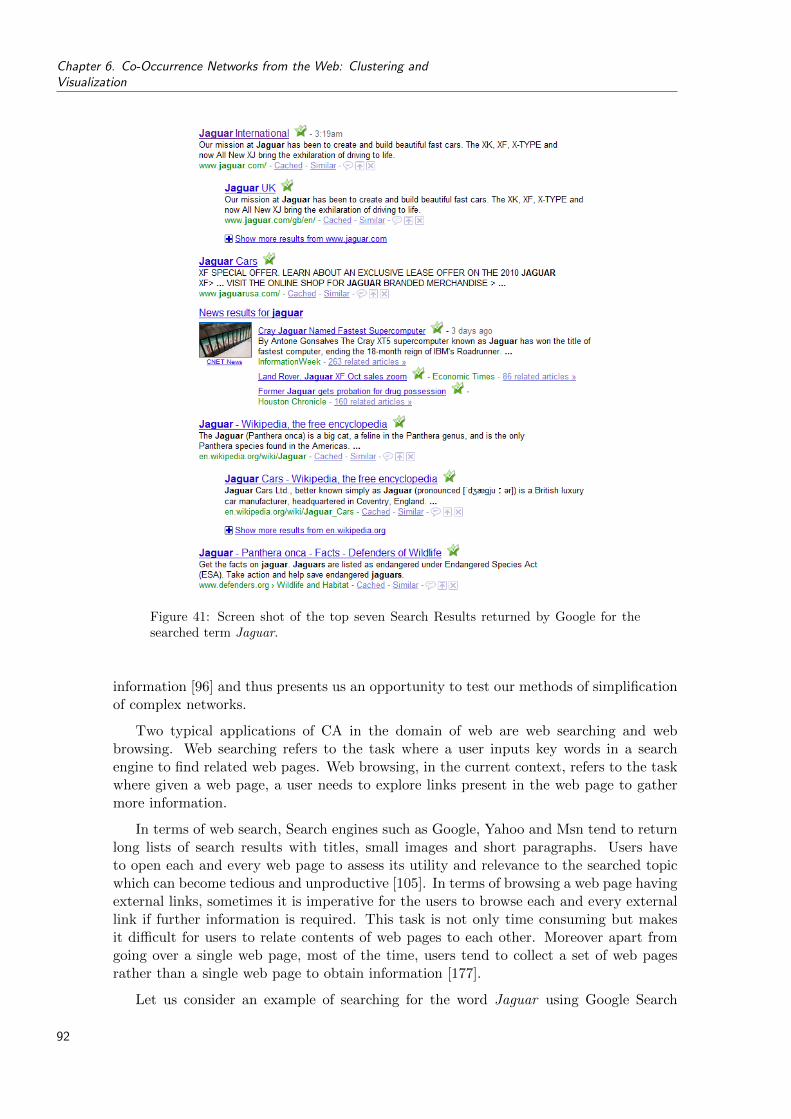
Chapter 6. Co-Occurrence Networks from the Web: Clustering andVisualization
Figure 41: Screen shot of the top seven Search Results returned by Google for thesearched term Jaguar.
information [96] and thus presents us an opportunity to test our methods of simplificationof complex networks.
Two typical applications of CA in the domain of web are web searching and webbrowsing. Web searching refers to the task where a user inputs key words in a searchengine to find related web pages. Web browsing, in the current context, refers to the taskwhere given a web page, a user needs to explore links present in the web page to gathermore information.
In terms of web search, Search engines such as Google, Yahoo and Msn tend to returnlong lists of search results with titles, small images and short paragraphs. Users haveto open each and every web page to assess its utility and relevance to the searched topicwhich can become tedious and unproductive [105]. In terms of browsing a web page havingexternal links, sometimes it is imperative for the users to browse each and every externallink if further information is required. This task is not only time consuming but makesit difficult for users to relate contents of web pages to each other. Moreover apart fromgoing over a single web page, most of the time, users tend to collect a set of web pagesrather than a single web page to obtain information [177].
Let us consider an example of searching for the word Jaguar using Google Search
92

6.1. Introduction
Figure 42: Wikipedia web page for CAC 40 showing a number of links to web pagesin sections ‘See Also’, ‘References’ and ‘External Links’.
Engine. Looking at the top seven results returned by Google (see Figure 41), these resultsare distributed heterogeneously in the list, i.e. pages 1, 2, 3 and 6 are about the carmanufacturing company called Jaguar, Pages 5 and 7 are about the animal also calledJaguar and Page 4 is about a super computer called Jaguar. If we look further in thelist, we will find pages related to a software solution provider, a musical group, a guitarmanufacturing company all having the name Jaguar.
As an example of browsing, let us consider browsing the web page ‘CAC 40’ on theWikipedia encyclopedia. CAC 40 is a benchmark for French stock market index whichrepresents a capitalization-weighted measure of the 40 most significant values among the100 highest market caps on Euronext Paris 1. There are many links on this page in sections‘See Also’, ‘References’ and ‘External Links’ as shown in Figure 42. Users searching formore details would use these links to jump to other web pages and look for furtherinformation. Usually they will go through these web pages one at a time to find moreinformation which is not only time consuming but makes it difficult to relate what theyhave already found as information and what else they require.
Ideally we would like to group the collection of pages together based on their contentso that users can immediately realize the multiple themes related to the searched topicas shown in Fig. 43. This would also give the user an idea about the sub-topics thatrevolve around the major topic. To represent the contents of these groups, displayingnoun phrases and keywords would allow users to glance contents of search results withoutreading or scanning individual web pages and thus reduce their effort in locating relevantinformation [177]. Once they have located the pages of interest, a more detailed analysiscan be conducted by visiting the relevant pages.
Moreover the users would like to see how these sub-topics are related to each other.Words appearing in more than one document can play a role of bridges between thesegroups thus creating a link between words from two different groups. Nodes organized intocircles in Figure 43 correspond to keywords extracted from a set of documents. Clearly,the figure shows that documents roughly organize into several sub topics such as JaguarCars and Jaguar Animal. In other words, Figure 43 shows the clusters of web pages[68, 9]. Additionally, a few nodes have been isolated and bridge these subgroups, furtherindicating topics that link the different subgroups. The bridging nodes thus sit out of the
1 http://en.wikipedia.org/wiki/CAC_40
93

Chapter 6. Co-Occurrence Networks from the Web: Clustering andVisualization
Figure 43: Visualizing Clusters and Bridges of the entire jaguar network. Distinctclusters (yellow nodes) clearly separate according to the different meanings of thiskeyword across web pages.
community structure (the structural hole as Burt names it [33]) and act as broker betweencommunities. This provides an additional benefit to understand the underlying topics andtheir relationships of the entire collection of web pages, either returned as search resultsor collected as a result of browsing links existing on a single web page.
The automated text processing systems that help in the process of analysis sufferfrom two major drawbacks. One, the textual data is highly redundant due to synonymy(different words having same meaning e.g. singer, vocalist) and two: the data is highlyambiguous due to homonymy (same word having different meaning e.g. bank can be afinancial institution or a river bank) [71]. Thus a visual representation of the contentscan quicken the process of focusing the search process, help in analysis and discovery ofknowledge and develop a better understanding of the set of documents.
Our starting point is thus the network of links between words extracted from webpages. As we shall see in the coming sections (see Figure 45), the co-occurrence network weobtain after the extraction process is actually quite complex and its structure forbids to useit as a graphical representation as such. The problem we address in this chapter is to revealhidden community structures in complex networks. We use the term ‘hidden’ because thevisual layout of the co-occurrence networks conceals the presence of these communitiesas shown in Figure 45. Our approach also allows us to identify the bridges within thesenetworks. The uncovered structure can then be used to build a graphical representationof the whole network to help visualize and interactively explore these relationships.
We know that due to the presence of high degree nodes in co-occurrence networks(see Figure 44 and Figure 45), it is difficult to visualize networks and the communitiespresent within the network structure [6]. As we saw from the analysis of various complexnetworks in Chapter 3, this is largely due to the fact that a few nodes have a very highdegree and they create links between the underlying community structure hiding thecommunities. Figure 45 shows the co-occurrence network obtained by browsing pages onthe Wikipedia encyclopedia starting from the CAC 40 page. Again, we have used a force
94
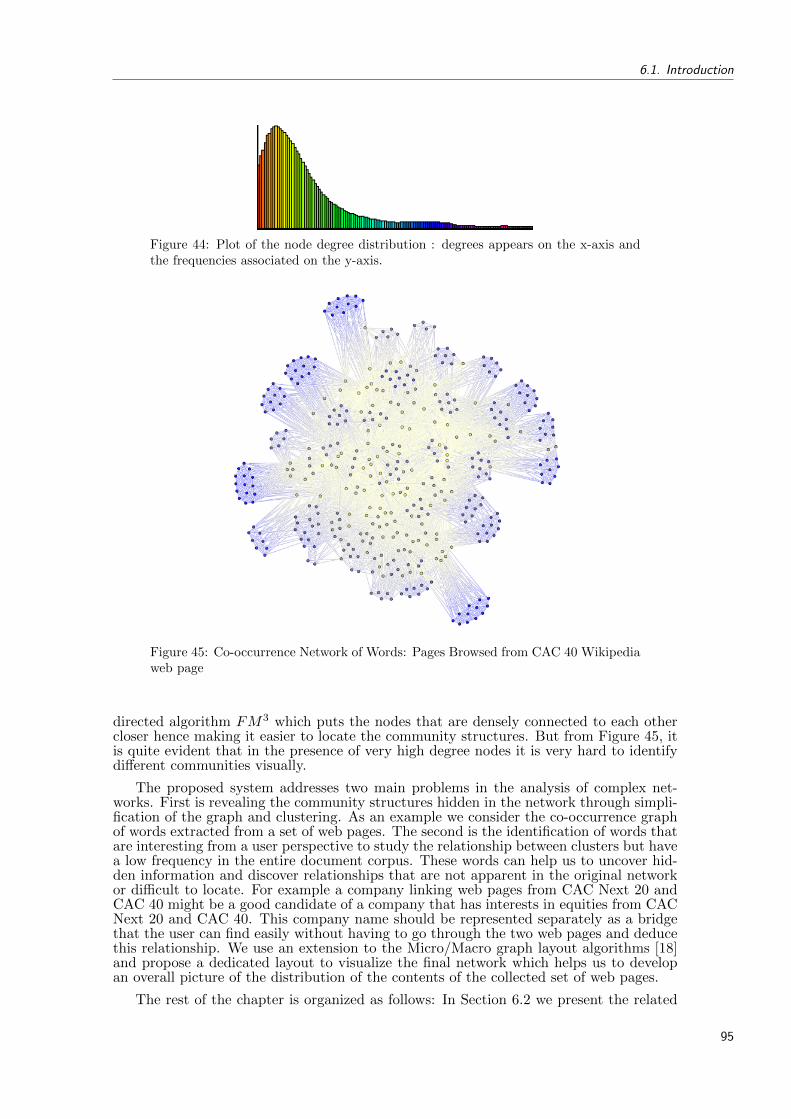
6.1. Introduction
Figure 44: Plot of the node degree distribution : degrees appears on the x-axis andthe frequencies associated on the y-axis.
Figure 45: Co-occurrence Network of Words: Pages Browsed from CAC 40 Wikipediaweb page
directed algorithm FM3 which puts the nodes that are densely connected to each othercloser hence making it easier to locate the community structures. But from Figure 45, itis quite evident that in the presence of very high degree nodes it is very hard to identifydifferent communities visually.
The proposed system addresses two main problems in the analysis of complex net-works. First is revealing the community structures hidden in the network through simpli-fication of the graph and clustering. As an example we consider the co-occurrence graphof words extracted from a set of web pages. The second is the identification of words thatare interesting from a user perspective to study the relationship between clusters but havea low frequency in the entire document corpus. These words can help us to uncover hid-den information and discover relationships that are not apparent in the original networkor difficult to locate. For example a company linking web pages from CAC Next 20 andCAC 40 might be a good candidate of a company that has interests in equities from CACNext 20 and CAC 40. This company name should be represented separately as a bridgethat the user can find easily without having to go through the two web pages and deducethis relationship. We use an extension to the Micro/Macro graph layout algorithms [18]and propose a dedicated layout to visualize the final network which helps us to developan overall picture of the distribution of the contents of the collected set of web pages.
The rest of the chapter is organized as follows: In Section 6.2 we present the related
95
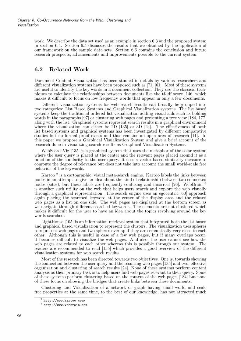
Chapter 6. Co-Occurrence Networks from the Web: Clustering andVisualization
work. We describe the data set used as an example in section 6.3 and the proposed systemin section 6.4. Section 6.5 discusses the results that we obtained by the application ofour framework on the sample data sets. Section 6.6 contains the conclusion and futureresearch prospects, advancements and improvements possible to the current system.
6.2 Related Work
Document Content Visualization has been studied in details by various researchers anddifferent visualization systems have been proposed such as [71] [61]. Most of these systemsare useful to identify the key words in a document collection. They use the classical tech-niques to calculate the relationships between documents like the tf-idf score [146] whichmakes it difficult to focus on low frequency words that appear in only a few documents.
Different visualization systems for web search results can broadly be grouped intotwo categories: List Based Systems and Graphical Visualization systems. The list basedsystems keep the traditional ordered list visualization adding visual aids such as boldingwords in the paragraphs [97] or clustering web pages and presenting a tree view [184, 177]along with the list. Graphical systems represent search results in a graphical environmentwhere the visualization can either be 2D [135] or 3D [24]. The effectiveness of bothlist based systems and graphical systems has been investigated by different comparativestudies but no formal proof exists and thus remains an open area of research [11]. Inthis paper we propose a Graphical Visualization System and give a brief account of theresearch done in visualizing search results as Graphical Visualization Systems.
WebSearchViz [135] is a graphical system that uses the metaphor of the solar systemwhere the user query is placed at the center and the relevant pages placed around it as afunction of the similarity to the user query. It uses a vector-based similarity measure tocompute the degree of relevance but does not take into account the small world-scale freebehavior of the keywords.
Kartoo 2 is a cartographic, visual meta-search engine. Kartoo labels the links betweennodes in an attempt to give an idea about the kind of relationship between two connectednodes (sites), but these labels are frequently confusing and incorrect [26]. WebBrain 3
is another such utility on the web that helps users search and explore the web visuallythrough a graphical representation. The search engine uses an egocentric [60] approachagain placing the searched keyword at the center of the display area and the relatedweb pages as a list on one side. The web pages are displayed at the bottom screen aswe navigate through different searched keywords. The elements are not clustered whichmakes it difficult for the user to have an idea about the topics revolving around the keywords searched.
LightHouse [105] is an information retrieval system that integrated both the list basedand graphical based visualization to represent the clusters. The visualization uses spheresto represent web pages and two spheres overlap if they are semantically very close to eachother. Although this is useful in case of a few web pages, but if many overlaps occur,it becomes difficult to visualize the web pages. And also, the user cannot see how theweb pages are related to each other whereas this is possible through our system. Thereaders are recommended to read [135] which provides a good overview of the differentvisualization systems for web search results.
Most of the research has been directed towards two objectives. One is, towards showingthe connection between the user query and the resulting web pages [135] and two, effectiveorganization and clustering of search results [24]. None of these systems perform contentanalysis as their primary task is to help users find web pages relevant to their query. Someof these systems perform clustering based on the content of the web pages [184] but noneof these focus on showing the bridges that create links between these documents.
Clustering and Visualization of a network or graph having small world and scalefree properties at the same time, to the best of our knowledge, has not attracted much
2 http://www.kartoo.com/3 http://www.webbrain.com
96
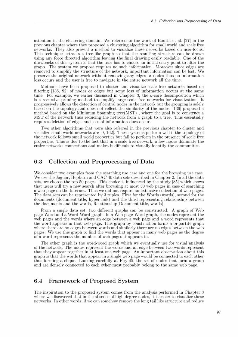
6.3. Collection and Preprocessing of Data
attention in the clustering domain. We referred to the work of Boutin et al. [27] in theprevious chapter where they proposed a clustering algorithm for small world and scale freenetworks. They also present a method to visualize these networks based on user-focus.This technique extracts a tree-like graph so that the resulting structure can be drawnusing any force directed algorithm leaving the final drawing easily readable. One of thedrawbacks of this system is that the user has to choose an initial entry point to filter thegraph. The system we propose requires no such information. Moreover since edges areremoved to simplify the structure of the network, important information can be lost. Wepreserve the original network without removing any edges or nodes thus no informationloss occurs and the user is free to navigate in the entire network all the time.
Methods have been proposed to cluster and visualize scale free networks based onfiltering [136, 92] of nodes or edges but some loss of information occurs at the sametime. For example, we earlier discussed in Chapter 3, the k-core decomposition whichis a recursive pruning method to simplify large scale free networks for visualization. Itprogressively allows the detection of central nodes in the network but the grouping is solelybased on the topology and does not reflect the similarity of the nodes. [136] proposed amethod based on the Minimum Spanning tree(MST) , where the goal is to construct aMST of the network thus reducing the network from a graph to a tree. This essentiallyrequires deletion of edges and loss of information does occur.
Two other algorithms that were also referred in the previous chapter to cluster andvisualize small world networks are [9, 162]. These systems perform well if the topology ofthe network follows small world properties but fail to perform in the presence of scale freeproperties. This is due to the fact that in a scale free network, a few nodes dominate theentire networks connections and makes it difficult to visually identify the communities.
6.3 Collection and Preprocessing of Data
We consider two examples from the searching use case and one for the browsing use case.We use the Jaguar, Hepburn and CAC 40 data sets described in Chapter 2. In all the datasets, we choose the top 50 pages. This choice is influenced by the study [85] which showsthat users will try a new search after browsing at most 30 web pages in case of searchinga web page on the Internet. Thus we did not require an extensive collection of web pages.The data sets can be represented by 3 tuples. First for the Words (words), second for thedocuments (document title, hyper link) and the third representing relationship betweenthe documents and the words, Relationship(Document title, words).
From a single data set, two different graphs can be constructed. A graph of Webpage-Word and a Word-Word graph. In a Web page-Word graph, the nodes represent theweb pages and the words where an edge between a web page and a word represents thatthe word appears in that web page. This graph by construction forms a bi-partite graphwhere there are no edges between words and similarly there are no edges between the webpages. We use this graph to find the words that appear in many web pages as the degreeof a word represents the number of web pages it appears in.
The other graph is the word-word graph which we eventually use for visual analysisof the network. The nodes represent the words and an edge between two words representthat they appear together in at least one web page. An important observation about thisgraph is that the words that appear in a single web page would be connected to each otherthus forming a clique. Looking carefully at Fig. 45, the set of nodes that form a groupand are densely connected to each other most probably belong to the same web page.
6.4 Framework of Proposed System
The inspiration to the proposed system comes from the analysis performed in Chapter 3where we discovered that in the absence of high degree nodes, it is easier to visualize thesenetworks. In other words, if we can somehow remove the long tail like structure and reduce
97
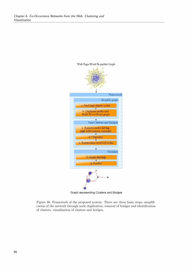
Chapter 6. Co-Occurrence Networks from the Web: Clustering andVisualization
Figure 46: Framework of the proposed system. There are three basic steps, simplifi-cation of the network through node duplication, removal of bridges and identificationof clusters, visualization of clusters and bridges.
98
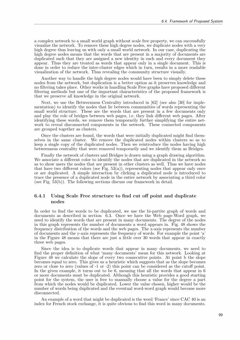
6.4. Framework of Proposed System
a complex network to a small world graph without scale free property, we can successfullyvisualize the network. To remove these high degree nodes, we duplicate nodes with a veryhigh degree thus leaving us with only a small world network. In our case, duplicating thehigh degree nodes means that the words that are present in a majority of documents areduplicated such that they are assigned a new identity in each and every document theyappear. Thus they are treated as words that appear only in a single document. This isdone in order to reduce the inter-cluster edges which in turn, results in a more readablevisualization of the network. Thus revealing the community structure visually.
Another way to handle the high degree nodes would have been to simply delete thesenodes from the network, but duplication is a better option as it preserves knowledge andno filtering takes place. Other works in handling Scale Free graphs have proposed differentfiltering methods but one of the important characteristics of the proposed framework isthat we preserve all knowledge in the original network.
Next, we use the Betweenness Centrality introduced in [62] (see also [30] for imple-mentation) to identify the nodes that lie between communities of words representing thesmall world structure. These are the words that are present in a few documents onlyand play the role of bridges between web pages, i.e. they link different web pages. Afteridentifying these words, we remove them temporarily further simplifying the entire net-work to reveal disconnected components in the network. These connected componentsare grouped together as clusters.
Once the clusters are found, the words that were initially duplicated might find them-selves in the same cluster. We remove the duplicated nodes within clusters so as tokeep a single copy of the duplicated nodes. Then we reintroduce the nodes having highbetweenness centrality that were removed temporarily and we identify them as Bridges.
Finally the network of clusters and Bridges is drawn using a graph drawing algorithm.We associate a different color to identify the nodes that are duplicated in the network soas to show users the nodes that are present in other clusters as well. Thus we have nodesthat have two different colors (see Fig. 53(a)), representing nodes that appear only onceor are duplicated. A simple interaction by clicking a duplicated node is introduced totrace the presence of a duplicated node in the entire network by associating a third color(see Fig. 53(b)). The following sections discuss our framework in detail.
6.4.1 Using Scale Free structure to find cut off point and duplicatenodes
In order to find the words to be duplicated, we use the bi-partite graph of words anddocuments as described in section 6.3. Once we have the Web page-Word graph, weneed to identify the words that are present in many documents. The degree of the nodesin this graph represents the number of documents a word appears in. Fig. 48 shows thefrequency distribution of the words and the web pages. The x-axis represents the numberof documents and the y-axis represents the frequency of words. For example the point ‘a’in the Figure 48 means that there are just a little over 30 words that appear in exactlythree web pages.
Since the idea is to duplicate words that appear in many documents, we need tofind the proper definition of what ‘many documents’ mean for this network. Looking atFigure 48 we calculate the slope of every two consecutive points. At point b the slopebecomes equal to zero. This gives us a heuristic which suggests that as the slope becomeszero or close to zero (values of -1 or -2) this point can be considered as the cutoff point.In the given example, it turns out to be 6, meaning that all the words that appear in 6or more documents must be duplicated. Although this heuristic provides a good startingpoint for the system, the user is free to manually choose a value for the degree a partfrom which the nodes would be duplicated. Lower the value chosen, higher would be thenumber of words being duplicated and the eventual word-word graph would become moredisconnected.
An example of a word that might be duplicated is the word ‘France’ since CAC 40 is anindex for French stock exchange, it is quite obvious to find this word in many documents.
99

Chapter 6. Co-Occurrence Networks from the Web: Clustering andVisualization
Figure 47: (a) Word-Word Graph constructed from browsing CAC 40 and related webpages (b) Graph after node duplication (c) Graph after removing bridges (d) Graphwith Clusters and Bridges using proposed visualization.
Figure 48: Histogram of degree distribution for the Cac40 data set.
100

6.4. Framework of Proposed System
This step introduces new nodes in the word-word graph but keeps the number of edgesexactly the same. Thus the graph gets simplified as shown in Figure 47(a) and 47(b).
Note that in graph drawing terminology, this duplication is called node splitting asseveral copies of a node are created, but these copies do not carry all the edges with them,instead, a small subset of edges is connected to each copy of the node.
6.4.2 Iterative removal of Nodes with high Betweenness Centrality
Once we have the word-word graph with duplicate nodes, we calculate the betweennesscentrality of the nodes which is a metric proposed by Freeman [62]. It calculates therelative importance of nodes within a network by calculating the shortest paths betweenpairs of nodes. Nodes that occur on many shortest paths between other nodes have higherbetweenness than those that do not. This metric is a good representation of the nodesthat play the role of connecting different communities and thus helps us in identifying thebridges.
Girvan et al. [68] have used a clustering algorithm which is based on a modified formof this metric. They calculate edge betweenness based on the same principal where theyfind edges that are central to a network. Then they iteratively remove the most centraledge in the network and recalculate the edge betweenness until no more edges are left.
Since our goal is to find the bridges we apply the same method on nodes to identifythe bridges. We calculate the betweenness centrality of the nodes, remove the node withthe highest betweenness centrality and repeat this process a certain number of times.Girvan repeated the process until there were no edges left as the goal was to produce ahierarchical clustering. We use a heuristic to determine the number of iterations which isbased on the total number of documents used for extraction of words and the number ofbridges we want to see between groups of documents. For the given example we choose15 as it would give us a bridge for nearly every three documents.
Number of Iterations = bNumber of Documents/3c (3)
Where de represents the ceiling function.
The user is free to choose any value depending on the requirements, higher the num-ber of iterations and higher would be the number of bridges and smaller would be thesize of clusters. Figure 47(c) represents the graph after the removal of nodes with highbetweenness centrality.
6.4.3 Finding Communities through Clustering
Removal of high betweenness nodes results in disconnected components in the graph asshown in Figure 47(c). We then group the connected components as clusters. Once theclusters are found, each and every cluster is scanned for nodes that were duplicated andfound themselves in the same cluster. We remove this node duplication within a clusterand keep a single instance of a duplicated node within a cluster.
6.4.4 Reintroducing Nodes with High Betweenness Centrality andIdentification of Bridges
The next step after clustering of the nodes is to re-introduce the nodes that were earlierremoved due to high betweenness centrality. These nodes are considered to be the Bridgesas they are responsible for connecting different clusters. Keeping in view that the wordsthat were present in many web pages were duplicated and thus their degree was reduced,the nodes having high centrality in this final network are words that appear in a few webpages only. These words are important from the user perspective as they link web pagesand might play an important role to understand the relationship between web pages.
101

Chapter 6. Co-Occurrence Networks from the Web: Clustering andVisualization
As a result of the proposed method, We obtain a bipartite graph G(B,C,E) where Bis a set of bridges, C is a set of clusters and E is a set of edges connecting nodes from setB and C. An edge exists between b ∈ B and c ∈ C if b appears on the same web page asat least one of the nodes (keywords) present in the cluster c.
6.4.5 Visualization of Clusters and Bridges
Now that we have a set of nodes representing clusters and bridges as separate entities,a visualization system is required such that it helps the user analyze, understand andnavigate through this graph. It is important to have a clear picture with clusters laidout such that bridges between clusters are well placed to give the user an idea of how theclusters are related to each other. Node and edge overlapping also needs to be taken intoaccount as it is one of the fundamental criteria to produce readable drawings.
Foremost, we try to position the nodes of graph G(B,C,E) in such a way that sim-ilar nodes are placed closely to each other, while dissimilar nodes are more separatedgeometrically. By using the lengths of shortest paths in the network, the proximity ina graph-theoretical sense serves as a proxy for topical similarity. In the graph drawingliterature, this approach is often called ‘organic’; positions are computed by a simulationof physical forces or numerically minimizing an objective function [29].
In some preliminary experiments with different types of layout approaches and li-braries, we found that existing implementations and traditional general-purpose layoutalgorithms are only of limited usefulness when particular aspects of the data are to beemphasized. Therefore, we adapt existing layout algorithms to produce a more dedicatedlayout method which explicitly takes into account the particular structure of our net-works. It is more specific to the analytic perspective in our context and thus facilitatesinterpretation of clusters and bridges. Recall that the size of clusters is much bigger thanthat of bridges which needs to be accounted for when existing layout algorithms are used.The details of the dedicated layout algorithm can be found in [145] and remains out ofscope of this document.
6.4.5.1 Navigation and Interaction
Visualization of clusters and bridges help users to build an overall picture of the searchresults. For a profound understanding and exploration of the returned results we proposedifferent interactions to the user. Mouse rollover effect over a cluster displays the list ofall the keywords present in the cluster as the tool tip (see Figure 49). This helps the userto instantly identify what the cluster is about and take a decision about further exploringit. Moreover, the labels of the bridges are displayed which are useful to understandthe relationships between clusters. Clicking on a cluster expands a cluster showing allthe keywords in the cluster as nodes and clicking on it again, collapses the cluster (seeFigure 53). A Right click on a cluster displays the links to the web pages that are groupedin the cluster where the user can open any particular web page as shown in Figure 50.
Apart from these interactions with the cluster, we can also interact with individualnodes within a cluster. Moving the mouse on a node, the label is displayed as the tool tip.We have used two colors to distinguish the split nodes (keywords) shown in Light GreenColor as compared to the other shown in Dark Green. Upon clicking a split concept,all the instances of this keyword change their color to pink (see Figure53) and increasethe size so as to locate the high degree nodes that were split in the node splitting stepdescribed earlier.
Two different colors are associated to the nodes within a cluster. (Light green anddark green as shown in Figure 53.) The light green color represents the nodes that areduplicated throughout the network. An important interaction is clicking on a duplicatednode, which highlights all of its instances in the entire network as shown in Figure 53(b)using a different color (Pink) and size. This is to help locate the duplicated instances ofa node in the network.
102

6.5. Case Studies
Figure 49: A tool tip allows to easily browse keywords of a cluster and figure out itsintrinsic semantics.
6.5 Case Studies
6.5.1 Searching Example: Jaguar
As a first example, we searched the word jaguar. As discussed in the section 6.1, thisword represents completely different subjects like the Jaguar Cars, the animal etc.
Typically, semantic ambiguity of a word leads a search engine to return pages that arenot semantically related, listing them in no particular order with respect to the possiblemeanings of the word jaguar. This is also present in the co-occurrence network, wherekeywords found in pages about Jaguar cars will be connected to keywords present inpages about the animal. The node splitting step identifies jaguar as a high degree nodeand disconnects keywords belonging to web pages related to cars or to the animal. Thisjustifies our approach as nodes that have a high degree of connections need not to begrouped together in a single cluster as they are usually generic terms appearing with highfrequency but not necessarily useful in terms of grouping related information together.
As a consequence, the visualization clearly positions different groups (cars, animals,video games, etc.) as distinct visual entities as shown in Figure 43. Distinct clustersare placed apart and already indicate that the search results organize into groups ofpages addressing different topics. Using the tool tip and browsing keywords contained ina cluster, users can quickly identify the underlying trends of the associated web pages.Figure 49 illustrates this, showing keywords associated with pages dealing with a Japanesegag Manga named Pyu to Fuku! Jaguar.
Right-clicking on a cluster shows the URL of web pages associated with keywords. AsFigure 50 shows, in some cases the URLs already provide information about the underlyingtopic of a cluster. In our example, all pages obviously relate to different models of Jaguarcars.
6.5.2 Searching Example: Hepburn
The second example represents a type of social network. We searched the word Hepburnwhich is a famous family name in Scotland. It is also quite frequent in some other areasof Europe, and we expect to find a social network of people belonging to that family.
Figure 51 show the entire network obtained after applying the proposed visualization.This example again shows the effectiveness of the proposed method as the node splittingand bridge removal does not disconnect the clusters that are semantically related to eachother. As shown in Figure 52, we focus on four clusters that are connected to each other.These clusters are pages related to two actresses Audrey Hepburn and Katherine Hepburn.They are not completely disconnected from the other clusters since they have the cinemaas a common field. Let’s take the example of the bridge Tiffany’s which is extractedfrom a web page about a film called Breakfast at Tiffany’s (1961) thus linking Audreyand Katherine with the cinema industry. Similarly, Audrey Hepburn appeared in a T.V
103

Chapter 6. Co-Occurrence Networks from the Web: Clustering andVisualization
Figure 50: Right-clicking on a cluster reveals URL’s of all web pages associated withkeywords. In the example, URLs already indicate that the cluster gathers pages aboutJaguar Cars.
Figure 51: Visual Layout of Clusters and Bridges for the keyword Hepburn where aset of clusters are disconnected to other clusters.
commercial for the KLM airlines and Katherine played the role of Ann Hamilton in afilm called Undercurrent. Thus the four clusters connected to each other are semanticallyrelated to each other. The clusters that appear apart from these clusters are pages relatedto politicians, writers belonging to the Hepburn family.
104
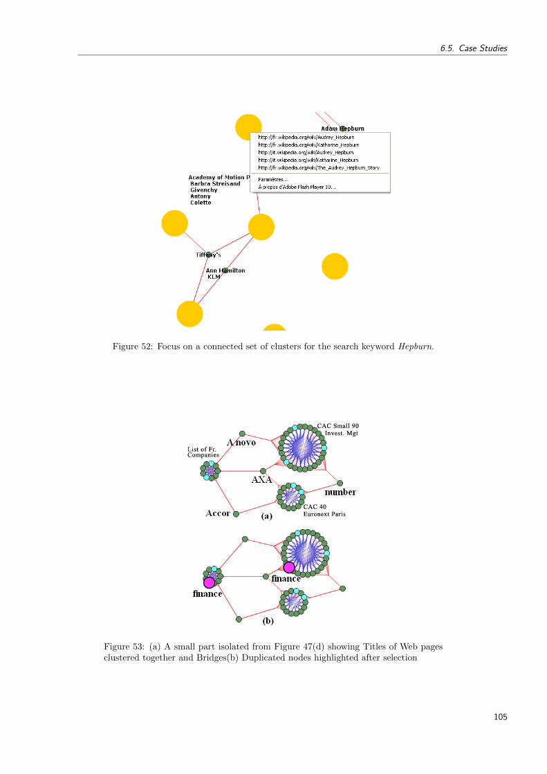
6.5. Case Studies
Figure 52: Focus on a connected set of clusters for the search keyword Hepburn.
Figure 53: (a) A small part isolated from Figure 47(d) showing Titles of Web pagesclustered together and Bridges(b) Duplicated nodes highlighted after selection
105
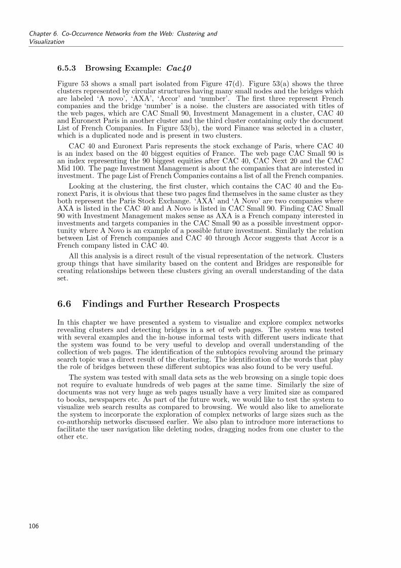
Chapter 6. Co-Occurrence Networks from the Web: Clustering andVisualization
6.5.3 Browsing Example: Cac40
Figure 53 shows a small part isolated from Figure 47(d). Figure 53(a) shows the threeclusters represented by circular structures having many small nodes and the bridges whichare labeled ‘A novo’, ‘AXA’, ‘Accor’ and ‘number’. The first three represent Frenchcompanies and the bridge ‘number’ is a noise. the clusters are associated with titles ofthe web pages, which are CAC Small 90, Investment Management in a cluster, CAC 40and Euronext Paris in another cluster and the third cluster containing only the documentList of French Companies. In Figure 53(b), the word Finance was selected in a cluster,which is a duplicated node and is present in two clusters.
CAC 40 and Euronext Paris represents the stock exchange of Paris, where CAC 40is an index based on the 40 biggest equities of France. The web page CAC Small 90 isan index representing the 90 biggest equities after CAC 40, CAC Next 20 and the CACMid 100. The page Investment Management is about the companies that are interested ininvestment. The page List of French Companies contains a list of all the French companies.
Looking at the clustering, the first cluster, which contains the CAC 40 and the Eu-ronext Paris, it is obvious that these two pages find themselves in the same cluster as theyboth represent the Paris Stock Exchange. ‘AXA’ and ‘A Novo’ are two companies whereAXA is listed in the CAC 40 and A Novo is listed in CAC Small 90. Finding CAC Small90 with Investment Management makes sense as AXA is a French company interested ininvestments and targets companies in the CAC Small 90 as a possible investment oppor-tunity where A Novo is an example of a possible future investment. Similarly the relationbetween List of French companies and CAC 40 through Accor suggests that Accor is aFrench company listed in CAC 40.
All this analysis is a direct result of the visual representation of the network. Clustersgroup things that have similarity based on the content and Bridges are responsible forcreating relationships between these clusters giving an overall understanding of the dataset.
6.6 Findings and Further Research Prospects
In this chapter we have presented a system to visualize and explore complex networksrevealing clusters and detecting bridges in a set of web pages. The system was testedwith several examples and the in-house informal tests with different users indicate thatthe system was found to be very useful to develop and overall understanding of thecollection of web pages. The identification of the subtopics revolving around the primarysearch topic was a direct result of the clustering. The identification of the words that playthe role of bridges between these different subtopics was also found to be very useful.
The system was tested with small data sets as the web browsing on a single topic doesnot require to evaluate hundreds of web pages at the same time. Similarly the size ofdocuments was not very huge as web pages usually have a very limited size as comparedto books, newspapers etc. As part of the future work, we would like to test the system tovisualize web search results as compared to browsing. We would also like to amelioratethe system to incorporate the exploration of complex networks of large sizes such as theco-authorship networks discussed earlier. We also plan to introduce more interactions tofacilitate the user navigation like deleting nodes, dragging nodes from one cluster to theother etc.
106

Chapter 7
Evaluating the Quality ofClustering Algorithms
7.1 Introduction
Clustering plays a pivotal role in the organization of complex networks. An importantaspect of clustering algorithms is to evaluate their performance, also known as clusterfitness measures. From the intuitive definition of clustering as, the best possible decom-position into Natural Groups, we would like to mathematically express the quality ofclustering algorithms by structural indices. We focus our attention to the numerous realworld networks discussed particularly in Chapter 3 where we studied the varying behaviorof connectivity of nodes in certain regions. The idea is to study how the quality of clustersproduced for these networks can be evaluated through concrete measures.
Generally, the quality indices give a quantitative evaluation of how good the clusteringis and serves the purpose of choosing between alternative cluster algorithms and comparetheir performances for various data sets [147]. Another useful contribution of these metricscan be eventual identification of clusters [130].
There are different approaches to evaluate cluster quality and can be classified as exter-nal, relative or internal. The term external validity criteria is used when the results of theclustering algorithm can be compared with some pre-specified clustering structures [77]or in the presence of ground truth [140]. Relative validity criteria measure the quality ofclustering results by comparing them with the results of other clustering algorithms [111].Internal validity criteria involve the development of functions that compute the cohesive-ness of a clustering by using density, cut size, distances of entities within each cluster,or the distance between the clusters themselves etc [119, 134, 78]. We will discuss thesemeasures in detail, shortly.
For most real world networks, an external validity criteria is simply not available. Inthe case of relative validity criteria, as Jain[88] argues, there is no clustering technique thatis universally applicable in uncovering the variety of structures present in multidimensionaldata sets. Thus we do not have an algorithm that can generate a bench mark clusteringfor data sets with varying properties. For these reasons we focus our attention only oninternal quality metrics. Further more, we restrict the discussion to quality metrics forpartitional or flat clustering algorithms that are non-overlapping.
We look again at the definition of a cluster given by Wasserman and Faust [169] earlierintroduced in Chapter 5. This time, our perspective is to associate measures to evaluatethe quality of clustering.
A cluster can be defined as a group of elements having the following properties:
> Density: Group members have many contacts to each other. In terms of graphtheory, it is considered to be the ratio of the number of edges present in a group ofnodes to the total number of edges possible in that group.
> Separation: Group members have more contacts inside the group than outside.
107
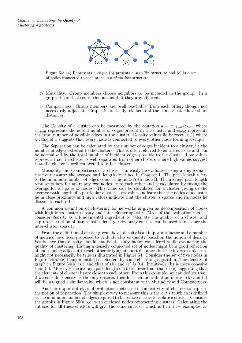
Chapter 7. Evaluating the Quality ofClustering Algorithms
Figure 54: (a) Represents a clique (b) presents a star-like structure and (c) is a setof nodes connected to each other in a chain-like structure.
> Mutuality: Group members choose neighbors to be included in the group. In agraph-theoretical sense, this means that they are adjacent.
> Compactness: Group members are ‘well reachable’ from each other, though notnecessarily adjacent. Graph-theoretically, elements of the same cluster have shortdistances.
The Density of a cluster can be measured by the equation d = eactual/etotal whereeactual represents the actual number of edges present in the cluster and etotal representsthe total number of possible edges in the cluster. Density values lie between [0,1] wherea value of 1 suggests that every node is connected to every other node forming a clique.
The Separation can be calculated by the number of edges incident to a cluster, i.e thenumber of edges external to the clusters. This is often referred to as the cut size and canbe normalized by the total number of incident edges possible to the cluster. Low valuesrepresent that the cluster is well separated from other clusters where high values suggestthat the cluster is well connected to other clusters.
Mutuality and Compactness of a cluster can easily be evaluated using a single quan-titative measure: the average path length described in Chapter 1. The path length refersto the minimum number of edges connecting node A to node B. The average path lengthrepresents how far apart any two nodes lie to each other and is calculated by taking theaverage for all pairs of nodes. This value can be calculated for a cluster giving us theaverage path length of a particular cluster. Low values indicate that the nodes of a clusterlie in close proximity and high values indicate that the cluster is sparse and its nodes liedistant to each other.
A common definition of clustering for networks is given as decomposition of nodeswith high intra-cluster density and inter-cluster sparsity. Most of the evaluation metricsconsider density as a fundamental ingredient to calculate the quality of a cluster andcapture the notion of intra-cluster density. Obviously cut size can be used to measure theinter-cluster sparsity.
From the definition of cluster given above, density is an important factor and a numberof metrics have been proposed to evaluate cluster quality based on the notion of density.We believe that density should not be the only factor considered while evaluating thequality of clustering. Having a densely connected set of nodes might be a good reflectionof nodes being adjacent to each other or lying at short distances but the inverse conjecturemight not necessarily be true as illustrated in Figure 54. Consider the set of five nodes inFigure 54(a,b,c) being identified as clusters by some clustering algorithm. The density ofgraph in Figure 54(a) is 1 and that of (b) and (c) is 0.4. Intuitively (b) is more cohesivethan (c). Moreover the average path length of (b) is lower than that of (c) suggesting thatthe elements of cluster (b) are closer to each other. From this example, we can deduce that,if we consider density as the only criteria, then for such an evaluation metric, (b) and (c)will be assigned a similar value which is not consistent with Mutuality and Compactness.
Another important class of evaluation metric uses connectivity of clusters to capturethe notion of Separation. The simplest way to measure this is the cut size which is definedas the minimum number of edges required to be removed so as to isolate a cluster. Considerthe graphs in Figure 55(a,b,c) with enclosed nodes representing clusters. Calculating thecut size for all these clusters will give the same cut size, which is 1 in these examples, as
108

7.1. Introduction
Figure 55: Represents three graphs with enclosed nodes being the clusters. All theclusters have the same cut size which is equal to 1. Based on the cut size alone thequality of the clustering cannot be judged.
each cluster is connected to the rest of the graph through exactly one edge. The examplesuggests that cut-size alone is not a good representation of the quality of clustering as allthe clusters in Figure 55 have the same cut-size.
More sophisticated measures combining density and cut size have been investigatedwith the most important example being relative density [116]. Even combining these twometrics, the clusters in Figure 55(b) and (c) will be assigned an equal score, failing toincorporate Mutuality and Compactness of a cluster. Calculating the density and the cutsize of these two clusters will result in the exact same value. We present other clusterevaluation techniques in Section 7.2.
If we consider Density, Mutuality and Compactness together to evaluate the qualityof clusters present in Figure 55, the highest measure should be associated to cluster (a)as it is the cluster with the highest Density, Mutuality and Compactness. Then cluster(b) where it has high Mutuality and Compactness but low density and finally cluster(c) which is the least Dense, Mutual and Compact cluster of the three clusters presentin Figure 55. We show that the existing cluster evaluation metrics do not evaluate thequality of clusters in this order. We discuss the details in Section 7.4.
Until now, we have argued that ignoring Mutuality and Compactness of a clusterto evaluate its quality can give inconsistent results. A simple question can be raisedabout the importance of these two criterion especially for real world data sets. To answerthis question, we turn our focus towards some real world data sets. Consider the Air-Transport Network which was discussed in detail using the DIS in Chapter 3. In thisparticular case, we took the city of Hong Kong as an example by taking some airportsdirectly connected to it as shown in Figure 56. On one side, we can see some of the world’sbiggest cities having direct flights to Hong Kong where on the other hand, we have lotsof regional airports also directly connected to Hong Kong. If we consider a cluster byputting Hong Kong with the regional airports, the resulting cluster will have very lowdensity and high cut size which are undesirable features for a cluster. In the other case,where we consider Hong Kong as part of the cluster with the biggest cities in the world,the cluster with Hong Kong will have a high cut size. Moreover, the regional airportscould not be clustered together as they will no longer remain connected to each other.We will end up with lots of singleton clusters which again will reduce the overall qualityof any clustering algorithm.
Another example of these star-like structures comes from Opte network. Consideringtwo hubs from this data set and taking all the nodes lying at distance five from thesehubs, we obtain a structure as shown in Figure 57. The two hubs dominate the numberof connections in these networks presenting the star-like behavior in real world data sets.
In Chapter 3, we identified these star-like structures as a common structure presentin most real world data sets along with triads and cliques. Social networks are good ex-amples of networks having cliques. Recall that we considered two co-authorship networks(Geometry and Dblp2008 networks) as examples where cliques are present.
Metrics based on density and cut size prove to be adequate for networks having denselyconnected nodes or cliques. Results have shown that different clustering algorithms per-form well for these networks [68, 126, 9]. On the other hand, in case where lots of star-likestructures exist (see Figure 56 and 57), an evaluation based on density and cut size fails toperform well as shown in the examples discussed previously. To resolve this problem, we
109

Chapter 7. Evaluating the Quality ofClustering Algorithms
Figure 56: AirTransport network drawn using Hong Kong at the center and someairports directly connected to Hong Kong. We can see the worlds most importantcities having a direct flight to Hong Kong whereas there are lots of regional airportsconnected to Hong Kong representing a star-like structure as discussed previously inFigure 54(b) and 55(b).
Figure 57: Internet Tomography Network representing routing paths from a test hostto other networks. Two nodes clearly dominate the number of connections as theyplay the role of hubs to connect several clients. Another example of star-like structuresin the real world.
propose a new cluster evaluation metric which takes into account the underlying networkstructure by considering the average path lengths to evaluate the cluster quality.
Apart from these cliques and star-like structures, other interesting topologies existin different data sets but are highly dependent on the application domain. Examplesinclude motifs in Chemical Compounds [42] or Metabolic Networks [103] where the goalis to search motifs in graphs and not to cluster them based on some similarity. We focusour attention only to generic data sets as opposed to evaluating clustering algorithms forspecific data sets and particular patterns.
The design principle for the proposed metric is very simple and intuitive. Instead ofconsidering density as the fundamental component to evaluate the quality of a clusteringalgorithm, we use the average path length to determine the closeness of the elements ofa cluster. It is obvious that in case of a clique, the path length between the nodes is 1which is the minimum possible value for two connected nodes. But the important aspecthere is that a star-like structure will have a higher average path length as compared to achain like structure thus providing a way to evaluate how close the nodes are of a cluster,
110

7.2. Cluster Quality Metrics
irrespective of the density of edges. We discuss the details of the proposed metric furtherin Section 7.3.
The rest of the chapter is organized as follows. In the following section, we providea brief overview of some widely used metrics to evaluate cluster quality. In Section 7.3we present the proposed metric and we discuss our findings by performing a comparativestudy of the different evaluation metrics in Section 7.4. Finally in Section 7.5 we presentour conclusions and future research directions in light of the newly proposed metric.
7.2 Cluster Quality Metrics
In this section, we review a number of cluster quality metrics designed for networks andused commonly by researchers.
Coverage [28] measures the weight of intra-cluster edges, compared to the weight ofall edges. With respect to the definition we are using, coverage measures only the densitywithin the clusters and therefore does not take into account if an individual cluster issparse or the number of inter-cluster edges is large.
Conductance [95] measures the degree of connectivity between two clusters as opposedto Coverage and focuses on inter-cluster density. Ideally, two clusters should not beconnected at all or have a minimum cut size. The standard minimum cut is not wellsuited as it neglects the size of each cluster, Conductance tries to overcome this problemby ensuring that clusters under consideration have roughly the same size and at thesame time, minimum number of edges are required to isolate them from each other. Thedrawback of this metric is quite obvious, it does not take into account how dense a clusteris, and thus fails to differentiate between dense and sparsely connected clusters.
Performance [28] is a metric that combines the two metrics, Coverage and Conduc-tance. The idea is to count the number of edges within all clusters to measure the intra-cluster density and count the number of non-existent edges between clusters to measurethe inter-cluster density.
Another metric based on similar principles is the MQ used by Auber et al. [9] toeffectively evaluate the quality of clustering for small world graphs. The metric wasinitially proposed by Mitchell et al. [117] as a partition cost function in the field of softwarereverse engineering. It comprises of two factors where the first term contributes to thepositive weight represented by the mean value of edge density inside each cluster. Thesecond term contributes as a negative weight and represents the mean value of edgedensity between the clusters. Mathematically, given a clustering C = {C1, C2, · · · , Cp},MQ is defined as:
MQ =1
p
p∑i=1
(Ci, Ci)−1
p(p− 1)/2
p∑i=1,j=1
(Ci, Cj) : (i 6= j) (4)
The main draw back of Performance and MQ metric is the handling of very sparsegraphs. Clusterings with good Performance and MQ evaluation tend to have many smallclusters. This is largely due to the fact that most real world networks have low node-edge density [113] and these metrics try to evaluate the quality as compared to cliques orhighly dense connected components. So if a clustering algorithm groups triads as clusters,the evaluation quality of such a clustering algorithm would be very high, irrespective ofthe size of clusters. If a set of 100 nodes is grouped together as a cluster, for real worldnetworks it is highly unlikely that this set will be a clique, as a result, these two metricswill assign a quality based on its density. If there are many triads in this set of nodes,separating them would result in better quality of the clustering algorithm and thus wouldresult in many small size clusters.
An alternative to these approaches is the metric Modularity(Q) [126]. The metric Qmeasures the fraction of the edges in the network that connect within-community edges
111
Chapter 7. Evaluating the Quality ofClustering Algorithms
minus the expected value of the same quantity in a network with the same community di-visions but random connections between the vertices. If the number of within-communityedges is no better than random, we will get Q = 0. Values approaching Q = 1, which isthe maximum, indicate strong community structure.
Mathematically, for a specific division of a network into C clusters, a symmetric matrixc can be defined as C ×C whose element cij is the fraction of all edges in the network thatlink nodes in community i to nodes in community j. For this clustering, the Modularity(Q)can be defined as:
Q = Tr c−∥∥c2∥∥ (5)
The term Tr c refers to the trace of the matrix c which gives the fraction of edges inthe network that connect vertices in the same community. The term
∥∥c2∥∥ is the squaredsum of the elments of matrix c.
The major drawback of Q metric is its inability to distinguish between the star-likestructures and chain-like structures as both clusters with these different structures areassigned the same evaluation.
Another metric that tries to evaluate cluster quality based on density of the networkis the Relative Density [116] (RD). It calculates the ratio of the edge density inside acluster to the sum of the edge densities inside and outside that cluster. The final RelativeDensity is the averaged sum of the these individual relative densities for all clusters.
Mathematically, the Relative Density (RD) can be calculated by:
RD =degint(Ci)
degint(Ci) + degext(Ci)(6)
The term degint(Ci) refers to the internal degree of cluster Ci defined as the number ofedges connecting nodes in cluster Ci and the term degext(Ci) refers to the external degreeof cluster Ci defined as the number of edges connecting nodes from cluster Ci to nodes ofother clusters.
For our experimentation and comparison, we use the MQ, Q and RD metrics only.The other metrics like coverage [28], conductance [95], performance [28] are based onsimilar principles to evaluate the quality of clusterings so we do not include them in thisstudy.
7.3 Proposed Metric For Cluster Evaluation: Cluster PathLengths
As we discussed earlier, the design principle which makes our metric novel, is the factthat we consider the path length of elements of a cluster. Our inspiration comes from theMQ metric [9] and thus is quite similar in the formulation. Just as the MQ metric, theproposed metric is composed of two components, the positive component(M+(G)) whichassigns a positive score to a cluster and a negative component(M−(G)) which attributes anegative score to edges between clusters. The positive score is assigned on the basis of thedensity, compactness and mutuality of the cluster whereas the negative score is assignedon the basis of the separation of the cluster from other clusters. The final quality of acluster is simply the sum of the two components given by the equation:
M(G) = M+(G)−M−(G) (7)
In the above equation, the two components are weighted equally. An option can beto assign different weights to the two components, for example a higher weight to the
112

7.3. Proposed Metric For Cluster Evaluation: Cluster Path Lengths
positive component, for the sake of simplicity, we have not experimented with differentweights. We discuss the details of how the positive and the negative components arecalculated below.
7.3.1 Positive Component:
The goal is to assign a quantitative value to a cluster based on its density, compactnessand mutuality. Looking at the different clusters in Figure 55, if we calculate the averagepath length of the nodes within the cluster, the least value would be assigned to cluster(a), then cluster (b) and finally (c). This is quite intuitive as we reduce the averagedistance between nodes of a cluster, the density tends to increase. Lets call the averagepath length of each cluster Cluster Path Length. The best possible average path lengthfor any cluster can be 1 in the case when every node is connected to every other nodeforming a clique.
The upper bound for the average path can be calculated with respect to number ofnodes in the cluster and grows linearly as the number of nodes grow in the cluster. Incase of disconnected set of nodes in the same cluster, there are two possibilities. If theapplication does not require the nodes within a cluster to be connected, in this case,the average path length of each connected component can be calculated separately andaverage afterwards. In case where disconnected nodes within clusters are undesirable, avery large value such as the maximum number of nodes in the network can be assignedas the average path length. This gives a very poor evaluation to this cluster as we expectnodes of a cluster to have at least a path to each other. Another option is to assign theCPLi of this cluster as 0 directly without calculating the average path length.
We calculate the average cluster path length and take its inverse given by the followingequation:
CPLi =1
AvgPathLeni(8)
Where CPLi represents the cluster path length of cluster i and AvgPathLeni repre-sents the average path length of the nodes in cluster i. Higher this value is for a cluster,better is the quality of the cluster where the values lie in the range of [0,1]. The overallcluster path lengths for the entire network are then averaged for all clusters where k isthe total number of clusters, giving us the value for the positive component to evaluatethe quality of the clustering:
M+(G) = CPL1···k =1
k
k∑i=1
CPLi (9)
7.3.2 Negative Component:
The next step is to assign a negative score to penalize the inter-cluster edges. The valueof M− evaluates the separation of the two clusters. This score is calculated for each pairof clusters and is based on the number of edges that link two clusters i and j comparedto the total number of edges possible between these two clusters. Let ni and nj be thenumber of nodes contained in clusters i and j respectively. Therefore, the edge penaltyfor the edges present between these two clusters would be given by the equation:
EdgePenalty(i,j) =eij
ni ∗ nj(10)
Where eij is the number of edges present between clusters i and j. The overall EdgePenalty (M−(G)) is the average calculated for all pair of clusters given by the equation:
113

Chapter 7. Evaluating the Quality ofClustering Algorithms
M−(G) =2
k ∗ (k − 1)
k∑i=1,j=1
EdgePenalty(i,j) where(i 6= j) (11)
The negative score sums all edge penalties over all pairs of clusters and then normalizesthe value by k(k − 1)/2 to produce an overall penalty in the range [0,1]. This value islinearly proportional to the number of edges present between clusters where low valuescorrespond to few broken edges and a better clustering quality. Note that the negativecomponent is exactly equal to the one introduced in the MQ metric.
To summarize the proposed metric, we use the cluster path lengths to assign a positivescore to evaluate the quality of clustering subtracted by a negative score which is based onthe inter-cluster density. The values lie in the range of [-1,1] and are normalized between[0,1]. Low values indicate poor clustering and high values indicate better clustering. Werefer to the metric as CPL for Cluster Path Lengths (although we subtract the Edgepenalties from the CPLs calculated).
The time complexity to calculate the metric is dominated by the calculation of pos-itive component. The calculation of average path length can be achieved by Dijkstra’salgorithm[46] which calculates the shortest path from a node to all other nodes in O(n2)for a graph with n nodes. The repeated application can be used to calculated the shortestpath between all pair of nodes giving an overall time complexity of O(n3). Since themetric is applied on clusters, the number of nodes in each cluster is a portion of the totalnodes. As a result, the calculation of the metric runs faster than its worst case timecomplexity. One drawback of using this metric is that it cannot be used as a criteria toobtain clusters for large size graphs due to its high time complexity.
of calculating the average path length o
7.4 Experimentation
For evaluating different cluster quality metrics, we use two different experiments. Thefirst, where we generate artificial data sets and the second where we use real world datasets.
7.4.1 Artificial and Clustered Data Set
For the artificial data set, we directly generate clusters to avoid biasing the experimentusing any particular clustering algorithm. We generate three clustered graphs of size n.We generate a random number k between 1 and Max to determine the size of a cluster.For the first graph, we add k nodes such that each node is connected to the other forminga clique as shown in Figure 58(a). For the second graph, k nodes are added such that astar-like structure is formed and finally k nodes are added to the third graph forming achain-like structure as shown in Figure 58(b) and Figure 58(c) respectively. The processis repeated until the maximum number of nodes in the graphs reach n. The clustersin each of these graphs are connected by randomly adding RandE edges. This numberdecides the number of inter-cluster edges that will be produced for each graph. The choiceof selecting the variables n, Max and RandE are independent of the experiment and donot change the final evaluation. For our experiment, we used n = 200, Max = 20 andRandE = 40.
Two important inferences can be drawn from the experiment described above. Thefirst, where we compare how the different evaluation metrics perform for evaluating thequality of clusters where each cluster is a clique with some inter-cluster edges. Lookingat the high values for the all the evaluation metrics, we can justify that all the metricsare consistent in evaluating the quality of clusters including the newly proposed metric.As discussed previously, density based metrics perform well when the clusters are denselyconnected, and so does the proposed metric.
114
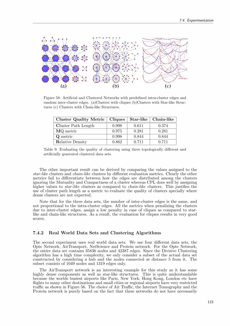
7.4. Experimentation
Figure 58: Artificial and Clustered Networks with predefined intra-cluster edges andrandom inter-cluster edges. (a)Clusters with cliques (b)Clusters with Star-like Struc-tures (c) Clusters with Chain-like Structures.
Cluster Quality Metric Cliques Star-like Chain-like
Cluster Path Length 0.998 0.611 0.374
MQ metric 0.975 0.281 0.281
Q metric 0.998 0.844 0.844
Relative Density 0.862 0.711 0.711
Table 9: Evaluating the quality of clustering using three topologically different andartificially generated clustered data sets.
The other important result can be derived by comparing the values assigned to thestar-like clusters and chain-like clusters by different evaluation metrics. Clearly the othermetrics fail to differentiate between how the edges are distributed among the clustersignoring the Mutuality and Compactness of a cluster whereas CPL does well by assigninghigher values to star-like clusters as compared to chain-like clusters. This justifies theuse of cluster path length as a metric to evaluate the quality of clusters specially wheredense clusters are not expected.
Note that for the three data sets, the number of inter-cluster edges is the same, andnot proportional to the intra-cluster edges. All the metrics when penalizing the clustersdue to inter-cluster edges, assign a low penalty in case of cliques as compared to star-like and chain-like structures. As a result, the evaluation for cliques results in very goodscores.
7.4.2 Real World Data Sets and Clustering Algorithms
The second experiment uses real world data sets. We use four different data sets, theOpte Network, AirTransport, NetScience and Protein network. For the Opte Network,the entire data set contains 35836 nodes and 42387 edges. Since the Divisive Clusteringalgorithm has a high time complexity, we only consider a subset of the actual data setconstructed by considering a hub and the nodes connected at distance 5 from it. Thesubset consists of 1049 nodes and 1319 edges only.
The AirTransport network is an interesting example for this study as it has somehighly dense components as well as star-like structures. This is quite understandablebecause the worlds busiest airports like Paris, New York, Hong Kong, London etc haveflights to many other destinations and small cities or regional airports have very restrictedtraffic as shown in Figure 56. The choice of Air Traffic, the Internet Tomography and theProtein network is purely based on the fact that these networks do not have necessarily
115
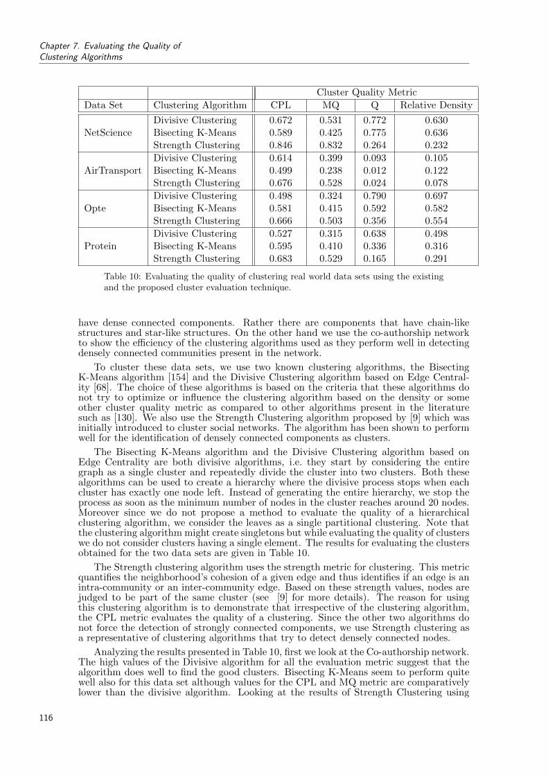
Chapter 7. Evaluating the Quality ofClustering Algorithms
Cluster Quality Metric
Data Set Clustering Algorithm CPL MQ Q Relative Density
NetScienceDivisive Clustering 0.672 0.531 0.772 0.630Bisecting K-Means 0.589 0.425 0.775 0.636Strength Clustering 0.846 0.832 0.264 0.232
AirTransportDivisive Clustering 0.614 0.399 0.093 0.105Bisecting K-Means 0.499 0.238 0.012 0.122Strength Clustering 0.676 0.528 0.024 0.078
OpteDivisive Clustering 0.498 0.324 0.790 0.697Bisecting K-Means 0.581 0.415 0.592 0.582Strength Clustering 0.666 0.503 0.356 0.554
ProteinDivisive Clustering 0.527 0.315 0.638 0.498Bisecting K-Means 0.595 0.410 0.336 0.316Strength Clustering 0.683 0.529 0.165 0.291
Table 10: Evaluating the quality of clustering real world data sets using the existingand the proposed cluster evaluation technique.
have dense connected components. Rather there are components that have chain-likestructures and star-like structures. On the other hand we use the co-authorship networkto show the efficiency of the clustering algorithms used as they perform well in detectingdensely connected communities present in the network.
To cluster these data sets, we use two known clustering algorithms, the BisectingK-Means algorithm [154] and the Divisive Clustering algorithm based on Edge Central-ity [68]. The choice of these algorithms is based on the criteria that these algorithms donot try to optimize or influence the clustering algorithm based on the density or someother cluster quality metric as compared to other algorithms present in the literaturesuch as [130]. We also use the Strength Clustering algorithm proposed by [9] which wasinitially introduced to cluster social networks. The algorithm has been shown to performwell for the identification of densely connected components as clusters.
The Bisecting K-Means algorithm and the Divisive Clustering algorithm based onEdge Centrality are both divisive algorithms, i.e. they start by considering the entiregraph as a single cluster and repeatedly divide the cluster into two clusters. Both thesealgorithms can be used to create a hierarchy where the divisive process stops when eachcluster has exactly one node left. Instead of generating the entire hierarchy, we stop theprocess as soon as the minimum number of nodes in the cluster reaches around 20 nodes.Moreover since we do not propose a method to evaluate the quality of a hierarchicalclustering algorithm, we consider the leaves as a single partitional clustering. Note thatthe clustering algorithm might create singletons but while evaluating the quality of clusterswe do not consider clusters having a single element. The results for evaluating the clustersobtained for the two data sets are given in Table 10.
The Strength clustering algorithm uses the strength metric for clustering. This metricquantifies the neighborhood’s cohesion of a given edge and thus identifies if an edge is anintra-community or an inter-community edge. Based on these strength values, nodes arejudged to be part of the same cluster (see [9] for more details). The reason for usingthis clustering algorithm is to demonstrate that irrespective of the clustering algorithm,the CPL metric evaluates the quality of a clustering. Since the other two algorithms donot force the detection of strongly connected components, we use Strength clustering asa representative of clustering algorithms that try to detect densely connected nodes.
Analyzing the results presented in Table 10, first we look at the Co-authorship network.The high values of the Divisive algorithm for all the evaluation metric suggest that thealgorithm does well to find the good clusters. Bisecting K-Means seem to perform quitewell also for this data set although values for the CPL and MQ metric are comparativelylower than the divisive algorithm. Looking at the results of Strength Clustering using
116

7.4. Experimentation
CPL and MQ, the values are quite high indicating that the algorithm found high qualityclusters but the low Q metric and Relative Density values create some doubt about theperformance of the algorithm. This variation is due to the large number of clustersgenerated by Strength clustering (122) as compared to Divisive (23) and Bisecting K-Means (38) algorithm. While evaluating the quality using Q metric and Relative Density,this high number of clusters reduces its quality as it results in high number of inter-clusteredges.
In case of the Air Traffic network, the clusterings generated by the Bisecting K-Meansand Divisive algorithms are relatively poorly judged as compared to the CPL and MQmetric. This is a clear indication that when considering the star-like structures as clusterswhich are present in abundance in the Air-Traffic network, the evaluation metrics judgethe performance of the clustering algorithms to be poor. This is because there are notmany densely connected airports in the network. High values of CPL indicate that eventhough, the clusters are not densely connected, they lie in close proximity and thus arejudged to be good clusters. The overall node-edge density plays an important role as wellsince the entire network has a high node-edge density, Q metric and Relative Densityexpect highly dense clusters to be found and their absence results in low values for thesemetrics. As mentioned in the introduction, there are a few nodes that have a very highnumber of connections, airports such as Paris, London and New York, which increasesthe overall density of the network, but most of the airports have a very low number ofconnections. Thus many clusters found are representatives of regional or with-in countryairports connecting all its cities, as shown in Fig 56. These results are a good justificationof why the CPL is a good cluster evaluation metric as it does not rate the quality of suchclusters poorly as compared to the other metrics.
Next, we look at the Internet Network. Almost all the evaluation metrics rate thequality of clustering highly for the three clustering algorithms except for the Strengthclustering-Q metric value. Again, we refer to the overall node-edge density of this graphwhich is quite low. Due to this, Q metric and Relative Density do not expect highly denseclusters and thus even though there are lots of star-like clusters found in this network,their quality is rated as good.
Finally the analysis of the Protein network is quite close to that of the Airport network.The overall density is not that high, but still the node-edge ratio is 1:3. The network is agood mix of some highly dense clusters and some star-like and/or chain-like clusters. Thestrength algorithm again generates a very high number of clusters (169) as compared toDivisive (91) and Bisecting K-Means (117). The divisive algorithm has the lowest numberof clusters and thus has relatively high Q metric and Relative Density values.
For all the different data sets and algorithms, the CPL metric assigns high valuesconsistently. This is an indication that by definition and from previous experimentalresults on a wide variety of data sets, these algorithms perform well in grouping similaritems together. The Q metric and the Relative density are heavily dependent on theoverall node-edge density for the evaluation of a clustering. In case of high node-edgedensity, these metrics expect highly dense clusters and in case of low node-edge density,less dense clusters can be rated as high quality irrespective of the underlying clustertopology, where we have argued that Mutuality and Compactness should be taken intoconsideration. The CPL metric is consistent with algorithms and dense data sets wheretightly connected clusters are expected as is the case with the co-authorship network andto some extent, the protein network.
From the above discussion, comparing different results of clustering algorithms withdifferent data sets, we can clearly see that CPL has a clear advantage over the othermetrics. As it does not rely on node-edge density, the quality is evaluated irrespectiveof density and based on the closeness of the elements of a cluster. CPL successfullyreproduces high values for clusters that have cliques, which is consistent with the othermetrics. It is also able to differentiate between star-like structures where nodes are closerto each other as compared to chain-like structures that are rated the worst using theCPL metric. This is not possible using the other metrics. It also performs well for datasets which have varying local density such as the AirTransport network, overcoming thedrawbacks of Q and RD metric.
117
Chapter 7. Evaluating the Quality ofClustering Algorithms
We would like to mention that the experimentation and the results described in thischapter compare different cluster evaluation techniques and should not be generalized tocompare the different clustering algorithms used. This is because the number of clustersand their sizes vary from one clustering algorithm to the other. Specially, Bisecting K-Means and Divisive Clustering based on Edge Centrality can not be compared with theStrength clustering algorithm in terms of performance and quality of clusters generatedas strength clustering generates many small size clusters as compared to the other twoclustering algorithms.
7.5 Findings and Future Research Prospects
In this chapter we introduced a new metric called the CPL metric to evaluate the qualityof clusters produced by clustering algorithms. We argued that Density and Cut Sizebased metrics play an important role in the evaluation of dense graphs but Mutualityand Compactness are also important for the evaluation of clusters in graphs that arenot densely connected. The proposed metric takes into account the underlying networkstructure and considers the average path length as an important factor in evaluating thequality of a cluster. We evaluated the performance of some existing cluster evaluationtechniques showing that the new metric actually performs better than the metrics usedlargely by the research community.
As part of future work, we intend to extend the metric to evaluate the quality ofhierarchical clustering algorithms based on the principles introduced in this paper. Amore extended study is needed to compare different clustering algorithms for data setshaving varying network topologies to comprehend the behavior of different clusteringalgorithms which in turn can lead us towards a better understanding of how to judgethese algorithms.
Another important result that can be derived from this study is about the importanceof quality metrics. The most common problem when trying to cluster a data set isconsidered the choice of a ‘good clustering algorithm’, but equally important is how todecide what ‘good’ is? The choice of selecting a good quality metrics goes hand in handwith the selection of a clustering algorithms and we suggest that both these problemsshould be addressed together when looking for a clustering solution to a problem.
118

Chapter 8
Publications and OtherResearch Activities
Here is a list of articles that we were able to publish during the course of this these.
1. Zaidi, F.; Sallaberry, A.; Melancon, G. Revealing Hidden Community Structures andIdentifying Bridges in Complex Networks: An Application to Analyzing Contents ofWeb Pages for Browsing WI-IAT ’09. Proceedings of the 2009 IEEE/WIC/ACM In-ternational Conference on Web Intelligence and Intelligent Agent Technology, 2009,198-205.
2. Sallaberry, A.; Zaidi, F.; Pich, C.; Melancon, G. Interactive Visualization and Nav-igation of Web Search Results Revealing Community Structures and Bridges. Pro-ceedings of Graphics Interface, 2010, 105-112.
3. Zaidi, F.; Melancon, G. Identifying the Presence of Communities in Complex Net-works Through Topological Decomposition and Component Densities EGC 2010,Extraction et Gestion de Connaissance, 163-174, 2010, E-19, RNTI.
4. Zaidi, F.; Archambault, D.; Melancon, G. Evaluating the Quality of ClusteringAlgorithms Using Cluster Path Lengths. Advances in Data Mining: Applicationsand Theoretical Aspects, 10th Industrial Conference, ICDM, 2010, 42-56.
Apart from the research presented in this thesis, I had the opportunity to work onsome other problems related to complex networks. I have not included them in this thesis,but I would like to mention them briefly with short abstracts.
Interactive Searching and Visualization of Patterns in Attributed Graphs:An important process on complex networks is searching for patterns and visualizing the
search results. This is an active area of research with numerous application, notably in bi-ological and technological networks. Traditionally, these networks are stored in relationaldatabases where querying these databases often results in multiple solutions. Text-basedsystems present search results as a list, and going over all solutions can be tedious. Thisresearch tries to present an interactive visualization system that helps users find patternsin graphs and visualize them. The interactive system allows the user to draw a source pat-tern and label it with attributes. Based on these attributes and connectivity constraints,simplified subgraphs are generated, containing all the possible solutions. The system isquite generic and capable of searching patterns and approximate solutions in a variety ofnetworks. For more details, readers can refer to the following publications:
1. Simonetto P.; Koenig, P.-Y.; Zaidi, F.; Archambault D.;, Gilbert F.; Quang T. T.P.; Mathiaut M.; Lambert A.; Dubois J.; Sicre R.; Brulin M.; Vieux R.; MelanconG. Solving the Traffic and Flitter Challenges with Tulip, in: IEEE Symposium onVisual Analytics Science and Technology (VAST 2009), 2009, 247-248.
2. Koenig, P.; Zaidi, F.; Archambault, D. Interactive Searching and Visualization ofPatterns in Attributed Graphs. Proceedings of Graphics Interface, 2010, 113-120.
119

Chapter 8. Publications and OtherResearch Activities
Communities and Hierarchical Structures in Dynamic Social Networks:Another interesting aspect of these complex networks is their dynamic behavior. Social
networks also exhibit dynamic nature and detection and visualization of communitieschanging over time is a challenging problem. Often these communities change as a functionof events taking place in the society and the role people play in it. We addressed allthese issues in this research and proposed a system to study the dynamic behavior ofcommunities in the networks. The system is based on dynamic graph discretization andclustering and allows the detection of major structural changes taking places in socialcommunities over time. It also reveals hierarchies by identifying influential people in asocial network. For more details, readers can refer to the following publications:
1. Bourqui, R.; Zaidi, F.; Gilbert, F.; Sharan, U.; Simonetto, P. VAST 2008 Challenge:Social network dynamics using cell phone call patterns, IEEE Symposium on VisualAnalytics Science and Technology (VAST 2008), 2008.
2. Bourqui, R.; Gilbert, F.; Simonetto, P.; Zaidi, F.; Sharan, U.; Jourdan, F. DetectingStructural Changes and Command Hierarchies in Dynamic Social Networks, Inter-national Conference on Advances in Social Network Analysis and Mining, IEEEComputer Society, 2009, 83-88.
3. Gilbert, F.; Simonetto, P.; Zaidi, F.; Jourdan, F.; Bourqui, R.; Communities andHierarchical Structures in Dynamic Social Networks: Analysis and Visualization.To appear in Journal of Social Network Analysis and Mining, 2010.
Analysis of Ports in Multi-level Maritime Networks:We also studied the network of ports and the shipping movements taking place in the
Atlantic ocean. Maritime transport handles about 90% of world trade volumes, but it hasnot attracted as much attention as other transport systems from a network perspective.As a result, the relative situation and the evolution of maritime within networks seaportsare not well understood. This research studies the hub-and-spoke strategies of ports andocean carriers which has modified the structure of a maritime networks over the pastdecade. We apply network metrics and methods of clustering on liner movements on datasets made available to us from the year 1996 and 2006. The methodology underlines theports which are increasing their carrier’s position by circulation patterns on various scales.More details can be found in the publication listed below:
1. Ducruet, C.; Rozenblat, C.; Zaidi, F. Ports in multi-level maritime networks: evi-dence from the Atlantic, Journal of Transport Geography, 2010, 18, 508-518.
Organization of Information using Hierarchical Fuzzy Clustering:Usually information on the web is organized using hierarchical and fuzzy clustering as
a single web page can belong to multiple categories. Common algorithms used for thispurpose require some parameters such as the number of clusters and initial centroids.Values are not easy to choose for these parameters as some insight or information isrequired to give an initial estimation, or different values need to be tried before finding thecorrect parameter values. Using the Mind-DIS decomposition on co-occurrence networksof keywords, we try to solve this problem by proposing an algorithm that identifies thetopics present in a document collection. We compare the results of the proposed algorithmwith existing algorithms in the literature requiring parameters and our results show thatthe algorithm performs as well in terms of cluster quality, without requiring any input toestimate the initial parameters. More details can be found in the following article:
1. Zaidi, F. and Melancon, G. Organization of Information for the Web using Hier-archical Fuzzy Clustering Algorithm based on Co-Occurrence Networks, WI-IAT’10: Proceedings of the 2010 IEEE/WIC/ACM International Conference on WebIntelligence and Intelligent Agent Technology, 2010, 421-424.
120
Chapter 9
Conclusions and Perspectives
We performed a detailed study of complex networks in this thesis. In our point of view,the research activities in this field can be grouped into four different categories, Anal-ysis, Structure, Processes-Organization and Visualization. We addressed several issuesthroughout the thesis in all these categories. We can summarize our contributions asfollows:
In Chapter 3, we introduced a visual analytics method to analyze complex networks.The method uses a decomposition of networks based on node degree. The decomposedgraph is then visualized to find interesting observations and results. We also extend themethod to develop a metric that can be used to measure the presence of densely connectedvertices in networks. The low time complexity to calculate the metric makes it practicalfor most real world large size networks.
As part of future work, we discussed the prospects of developing more local as well asgroup level metrics based on the proposed decomposition. Examples include quantifyingthe presence of star-like structures or the presence of cliques. The method can also beused to find interesting connectivity patterns in networks, search for paths between nodesand
In Chapter 4, we study several models proposed to generate small world and scale freenetworks. These models generate random networks without clear community structures.We present a new model which generates networks with these two properties along withthe presence of community structures. The model aims to provide artificial data sets thatare more closer to real world networks.
The model focuses on social networks, but it can easily be extended to produce othertypes of networks such as technological and biological networks. This remains an openarea of research and further testing and implementation is required to verify the abilityof the model to produce networks for other domains.
Chapter 5 presents a new algorithm for clustering complex networks motivated bythe ideas introduced in Chapter 3. The algorithm is highly efficient in terms of timecomplexity making it applicable on large size complex networks. Results show that thequality of clustering produced is comparable to other clustering algorithms with high timecomplexity. We have tested the quality of clustering using external quality metrics andthe results show that the algorithm performs as good as other clustering algorithms.
A more detailed and in-depth analysis is required by domain experts to verify theresults of the proposed clustering algorithm. We would also like to study the behavior ofthe algorithm for weighted and directed graphs and test its sustainability to this change.
In Chapter 6, we propose yet another clustering algorithm, this time our focus istowards the visualization of complex networks. Inspired by the visualizations producedin Chapter 3, we introduce a method to reduce the visual complexity of these networks.Further processing and clustering allows us to produce visual layouts that are much morereadable and easier to analyze these complex networks.
We verified the method by using co-occurrence networks from the web but we wouldlike to extend the study to networks from other domains. We would also like to testthe robustness of the method with larger size networks and see how the execution time
121

Chapter 9. Conclusions and Perspectives
varies as large size networks are processed and laid out using the proposed method. Animportant aspect of the algorithm is the use of betweenness centrality to identify bridges,which is asymptotically quite slow. We would like to test other centrality metrics thatare efficient in terms of time complexity to improve the overall time efficiency of thealgorithm.
Finally, in Chapter 7, we study the problem of evaluating the quality of clusteringalgorithms. We argue that the existing methods are heavily biased by the node-edgedensity to evaluate the quality of clusters. For networks having low density, these metricsare inappropriate and incorrect. We propose a new metric which overcomes the drawbacksof existing methods to evaluate the quality of clustering algorithms. We introduced theidea of closeness between the elements of a cluster and used it to evaluate the quality ofa cluster.
As part of future work, instead of using average path length to calculate the closeness ofvertices in a cluster which is slow in terms of time complexity, we would like to experimentwith other faster metrics that try to capture the same notion. We would also like to extendthe work to use the same idea and build an evaluation metric for hierarchical clusteringalgorithms. Another addition to the existing work is to incorporate the evaluation ofweighted networks and their clustering.
In our opinion, the methods and algorithms presented in these chapters are an attemptto contribute towards the growth of this fast emerging science of networks. Since physicalsystems from various domains can be modeled as networks, there is a huge opportunityto apply these results in a number of different fields. We hope to extend these studies andcollaborate with research colleagues from other domains to further ascertain the resultswe obtained.
122

Chapter 9
Bibliography
[1] Lada A. Adamic. The small world web. In Proceedings of the Third EuropeanConference on Research and Advanced Technology for Digital Libraries, volume 1696of Lecture Notes in Computer Science, pages 443–452. Springer-Verlag, 1999.
[2] William Aiello, Fan Chung, and Linyuan Lu. A random graph model for power lawgraphs. Experimental Math, 10:53–66, 2000.
[3] William Aiello, Fan R. K. Chung, and Linyuan Lu. Random evolution in massivegraphs. In FOCS, pages 510–519, 2001.
[4] Albert, Jeong, and Barabasi. Error and attack tolerance of complex networks.Nature, 406:378–382, 2000.
[5] David Alderson, Lun Li, Walter Willinger, and John C. Doyle. UnderstandingInternet topology: principles, models, and validation. IEEE/ACM Transactions onNetworking, 13(6):1205–1218, 2005.
[6] Jose Ignacio Alvarez-Hamelin, Luca Dall’Asta, Alain Barrat, and Alessandro Vespig-nani. k-core decomposition: a tool for the visualization of large scale networks.Advances in Neural Information Processing Systems, 18:41–50, 2006.
[7] L. A. N. Amaral, A. Scala, M. Barthelemy, and H. E. Stanley. Classes of small-worldnetworks. Proceedings of the National Academy of Sciences of the United States ofAmerica, 97(21):11149–11152, 2000.
[8] M. Amiel, G. Melancon, and C. Rozenblat. Reseaux Multi-Niveaux : L’Exempledes Echanges Aeriens Mondiaux de Passagers. Mappemonde, 79, 2005.
[9] D. Auber, Y. Chiricota, F. Jourdan, and G. Melancon. Multiscale visualization ofsmall world networks. In INFOVIS ’03: Proceedings of the IEEE Symposium onInformation Visualization, pages 75–81, 2003.
[10] David Auber. Tulip - a huge graph visualization framework. In Petra Mutzel andMickael Junger, editors, Graph Drawing Software, Mathematics and VisualizationSeries. Springer Verlag, 2003.
[11] A. Aula. Enhancing the readability of search result summaries. In Proceedings ofthe HCI 2004: Design for Life, Leeds, UK., volume 2, 2004.
[12] Gary Bader and Christopher Hogue. An automated method for finding molecularcomplexes in large protein interaction networks. BMC Bioinformatics, 4(1):2, 2003.
[13] A. L. Barabasi and R. Albert. Emergence of scaling in random networks. Science,286(5439):509–512, 1999.
[14] Albert-Laszlo Barabasi. Linked: The New Science of Networks. Basic Books, 1stedition, May 2002.
123

Bibliography
[15] A. Barrat and M. Weigt. On the properties of small-world network models. TheEuropean Physical Journal B - Condensed Matter and Complex Systems, 13(3):547–560, 2000.
[16] V. Batagelj and M. Zaversnik. Generalized cores. In CoRR, 2002.
[17] M. Baur, U. Brandes, M. Gaertler, and D. Wagner. Drawing the as graph in 2.5dimensions. In Proc. Graph Drawing 2004, pages 43–48, 2004.
[18] Michael Baur and Ulrik Brandes. Multi-circular layout of micro/macro graphs. InSeok-Hee Hong, Takao Nishizeki, and Wu Quan, editors, Graph Drawing, volume4875 of Lecture Notes in Computer Science, pages 255–267. Springer, 2007.
[19] Benjamin B. Bederson and Ben Shneiderman, editors. The Craft of InformationVisualization: Readings and Reflections (Interactive Technologies). Morgan Kauf-mann, 1 edition, April 2003.
[20] Sven Bilke and Carsten Peterson. Topological properties of citation and metabolicnetworks. Rev. E, 64:036106, 2001.
[21] S. Boccaletti, M. Ivanchenko, V. Latora, A. Pluchino, and A. Rapisarda. Detectionof complex networks modularity by dynamical clustering. Physical Review E, 75,2007.
[22] B. Bollobas. Mathematical results on scale-free random graphs. In In Handbook ofGraphs and Networks, pages 1–34. Wiley-VCH, 2003.
[23] Erik M. Bollt and Daniel ben Avraham. What is special about diffusion on scale-freenets? New J. Phys., 7:26, 2004.
[24] Nicolas Bonnel, Vincent Lemaire, Alexandre Cotarmanac’H, and Annie Morin. Ef-fective organization and visualization of web search results. In Proceedings of the24th IASTED International Multi-Conference Internet and Multimedia Systems andApplications, 2006.
[25] Stefan Bornholdt and Heinz Georg Schuster, editors. Handbook of Graphs andNetworks: From the Genome to the Internet. John Wiley & Sons, Inc., New York,NY, USA, 2003.
[26] Maged Boulos. The use of interactive graphical maps for browsing medical/healthinternet information resources. International Journal of Health Geographics, 2(1):1,2003.
[27] Francois Boutin, Jerome Thievre, and Mountaz Hascoet. Focus-based filtering +clustering technique for power-law networks with small world phenomenon. InVDA’06: Visual Data Analysis - SPIE-IS&T Electronic Imaging, volume 6060,pages 001–012. SPIE P., U.S., 2006.
[28] U. Brandes and T. Erlebach. Network Analysis : Methodological Foundations (Lec-ture Notes in Computer Science). Springer, March 2005.
[29] Ulrik Brandes. Drawing on physical analogies. In Michael Kaufmann and DorotheaWagner, editors, Drawing Graphs: Methods and Models, volume 2025 of LectureNotes in Computer Science, pages 71–86. Springer, 2001.
[30] Ulrik Brandes. A faster algorithm for betweenness centrality. Journal of Mathemat-ical Sociology, 25:163–177, 2001.
[31] Coen Bron and Joep Kerbosch. Algorithm 457: finding all cliques of an undirectedgraph. Commun. ACM, 16:575–577, September 1973.
[32] Mark Buchanan. Nexus: Small Worlds and the Groundbreaking Theory of Networks.W. W. Norton & Co. Inc., New York, USA, 2003.
124

[33] Ronald S. Burt. Brokerage and Closure. Oxford University Press, 2005.
[34] G. Caldarelli, A. Capocci, P. De Los Rios, and M. A. Munoz. Scale-free networksfrom varying vertex intrinsic fitness. Phys Rev Lett, 89(25), December 2002.
[35] Michele Catanzaro, Guido Caldarelli, and Luciano Pietronero. Assortative modelfor social networks. Physical Review E (Statistical, Nonlinear, and Soft MatterPhysics), 70(3), 2004.
[36] Bill Cheswick, Hal Burch, and Steve Branigan. Mapping and visualizing the internet.In ATEC ’00: Proceedings of the annual conference on USENIX Annual TechnicalConference, pages 1–1, Berkeley, CA, USA, 2000. USENIX Association.
[37] J. S. Coleman. An Introduction to Mathematical Sociology. Collier-Macmillan,London, UK, 1964.
[38] National Research Council Committee on Network Science for Future Army Appli-cations. Network Science. The National Academies Press, 2005.
[39] Anne Condon and Richard M. Karp. Algorithms for graph partitioning on theplanted partition model. Random Structures and Algorithms, 18(2):116–140, 1999.
[40] S. A. Cook. The complexity of theorem-proving procedures. In Proc. of the 3rdAnnual ACM Symp. on Theory of Computing, pages 151–158, 1971.
[41] Thomas H. Cormen, Charles E. Leiserson, Ronald L. Rivest, and Clifford Stein.Introduction to Algorithms. McGraw-Hill Science / Engineering / Math, 2nd edition,December 2003.
[42] D. G. Corneil and C. C. Gotlieb. An efficient algorithm for graph isomorphism.Journal of the ACM (JACM), 17:51–64, 1970.
[43] Rob Cross, Andrew Parker, and Stephen P. Borgatti. A bird’s-eye view: Using socialnetwork analysis to improve knowledge creation and sharing. Knowledge Directions,2(1):48–61, 2000.
[44] Derek de Solla Price. Networks of scientific papers. Science, 149:510–515, 1965.
[45] Sebastiano Delre, Wander Jager, and Marco Janssen. Diffusion dynamics in small-world networks with heterogeneous consumers. Computational & Mathematical Or-ganization Theory, 13(2):185–202, 2007.
[46] Edsger. W. Dijkstra. A note on two problems in connexion with graphs. NumerischeMathematik, 1:269–271, 1959.
[47] Carine Discazeaux, Celine Rozenblat, Pierre-Yves Koenig, and Guy Melancon. Ter-ritorial and topological levels in worlwide air transport network. In 15TH Euro-pean Colloquium on Theoretical and Quantitative Geography, Montreux, Switzer-land, 2007.
[48] S. N. Dorogovtsev and J. F. F. Mendes. Evolution of networks. Advances in Physics,51:1079–1187, June 2002.
[49] S. N. Dorogovtsev and J. F. F. Mendes. Evolution of Networks: From BiologicalNets to the Internet and WWW. Oxford University Press, March 2003.
[50] S.N. Dorogovtsev and J.F.F. Mendes. Exactly solvable small-world network. Euro-pean Physics Letters, 50(1):1–7, 2000.
[51] Holger Ebel, Lutz-Ingo Mielsch, and Stefan Bornholdt. Scale-free topology of e-mailnetworks. Phys. Rev. E, 66:035103, 2002.
[52] L. Egghe and R. Rousseau. Introduction to Informetrics. Elsevier, 1990.
125
Bibliography
[53] John Ellson, Emden Gansner, Eleftherios Koutsofios, and Stephen North. Graphviz.Avaiable on http://www.research.att.com/sw/tools/graphviz.
[54] P. Erdos and A. Renyi. On random graphs, i. Publicationes Mathematicae (Debre-cen), 6:290–297, 1959.
[55] P. Erdos and A. Renyi. On the evolution of random graphs. Publ. Math. Inst. Hung.Acad. Sci, 5:17–61, 1960.
[56] J W Essam. Percolation theory. Reports on Progress in Physics, 43(7):833, 1980.
[57] Brian S. Everitt, Sabine Landau, and Morven Leese. Cluster Analysis. Wiley, 4thedition, January 2009.
[58] Michalis Faloutsos, Petros Faloutsos, and Christos Faloutsos. On power-law rela-tionships of the internet topology. In SIGCOMM ’99: Proceedings of the conferenceon Applications, technologies, architectures, and protocols for computer communi-cation, pages 251–262, New York, NY, USA, 1999. ACM.
[59] R. Ferrer I Cancho and R. V. Sole. The small world of human language. Proc RSoc Lond B Biol Sci, 268(1482):2261–2265, November 2001.
[60] Danyel Fisher. Using egocentric networks to understand communication. IEEEInternet Computing, 9(5):20–28, 2005.
[61] B. Fortuna, D. Mladenic, and M. Grobelnik. Visualization of text document corpus.Informatica Journal, 29(4):497–502, 2005.
[62] L. C. Freeman. A set of measures of centrality based on betweenness. Sociometry,40:35–41, 1977.
[63] Peihua Fu and Kun Liao. An evolving scale-free network with large clusteringcoefficient. In ICARCV, pages 1–4. IEEE, 2006.
[64] M. Gaertler and M. Patrignani. Dynamic analysis of the autonomous system graph.In IPS 2004, International Workshop on Inter-domain Performance and Simulation,pages 13–24, 2004.
[65] J. Galaskiewicz and P. V. Marsden. Interorganizational resource networks: Formalpatterns of overlap. Social Science Research, 7:89–107, 1978.
[66] Anne-Claude Gavin, Markus Bosche, Roland Krause, Paola Grandi, MartinaMarzioch, Andreas Bauer, Jorg Schultz, Jens M. Rick, Anne-Marie Michon,Cristina-Maria Cruciat, Marita Remor, Christian Hofert, Malgorzata Schelder,Miro Brajenovic, Heinz Ruffner, Alejandro Merino, Karin Klein, Manuela Hudak,David Dickson, Tatjana Rudi, Volker Gnau, Angela Bauch, Sonja Bastuck, BettinaHuhse, Christina Leutwein, Marie-Anne Heurtier, Richard R. Copley, Angela Edel-mann, Erich Querfurth, Vladimir Rybin, Gerard Drewes, Manfred Raida, TewisBouwmeester, Peer Bork, Bertrand Seraphin, Bernhard Kuster, Gitte Neubauer,and Giulio Superti-Furga. Functional organization of the yeast proteome by sys-tematic analysis of protein complexes. Nature, 415(6868):141–147, January 2002.
[67] David Gibson, Ravi Kumar, and Andrew Tomkins. Discovering large dense sub-graphs in massive graphs. In VLDB ’05: Proceedings of the 31st internationalconference on Very large data bases, pages 721–732. VLDB Endowment, 2005.
[68] Michelle Girvan and M. E. J. Newman. Community structure in social and biologicalnetworks. Proc. Natl. Acad. Sci. USA, 99:8271–8276, 2002.
[69] A. D. Gordon. Classification: Methods for the Exploratory Analysis of MultivariateData. Chapman & Hall Ltd., London, 1981.
[70] M. Granovetter. The strength of weak ties. American Journal of Sociology,78(6):1360–1380, May 1973.
126
[71] M. Grobelnik and D. Mladenic. Visualization of news articles. Informatica Journal,28, 2004.
[72] John Guare. Six degrees of separation: A play. Vintage, New York, 1990.
[73] Jean-Loup Guillaume and Matthieu Latapy. Bipartite graphs as models of complexnetworks. In Workshop on Combinatorial and Algorithmic Aspects of Networking(CAAN), LNCS, volume 1, 2004.
[74] R. Guimera, S. Mossa, A. Turtschi, and L. A. N. Amaral. The worldwide airtransportation network: Anomalous centrality, community structure, and cities’global roles. Proceedings of the National Academy of Sciences of the United Statesof America, 102(22):7794–7799, 2005.
[75] Weisen Guo and Steven B. Kraines. A random network generator with finely tunableclustering coefficient for small-world social networks. In CASON ’09: Proceedingsof the 2009 International Conference on Computational Aspects of Social Networks,pages 10–17, Washington, DC, USA, 2009. IEEE Computer Society.
[76] Stefan Hachul and Michael Junger. Drawing large graphs with a potential-field-based multilevel algorithm. Graph Drawing, pages 285–295, 2005.
[77] Maria Halkidi, Yannis Batistakis, and Michalis Vazirgiannis. Cluster validity meth-ods: Part i. ACM SIGMOD Record, 31, 2002.
[78] Maria Halkidi and Michalis Vazirgiannis. Clustering validity assessment: Findingthe optimal partitioning of a data set, 2001.
[79] Pierre Hansen and Brigitte Jaumard. Cluster analysis and mathematical program-ming. Math. Program., 79(1-3):191–215, 1997.
[80] Jeffrey Heer and Danah Boyd. Vizster: Visualizing online social networks. InINFOVIS ’05: Proceedings of the Proceedings of the 2005 IEEE Symposium onInformation Visualization, page 5, 2005.
[81] Ivan Herman, Guy Melancon, and M. Scott Marshall. Graph visualization and nav-igation in information visualization: A survey. IEEE Transactions on Visualizationand Computer Graphics, 6(1):24–43, 2000.
[82] Petter Holme and Beom Jun Kim. Growing scale-free networks with tunable clus-tering. Physical Review E, 65:026107, 2002.
[83] Haiyan Hu, Xifeng Yan, Yu Huang, Jiawei Han, and Xianghong J. Zhou. Miningcoherent dense subgraphs across massive biological networks for functional discovery.Bioinformatics, 21(suppl 1):i213–221, June 2005.
[84] B. A. Huberman. The Laws of the Web. MIT Press, Cambridge, MA, 2001.
[85] iProspect. iprospect’s search engine user attitudes. survey results. white paper,2004.
[86] P. Jaccard. Bulletin del la societe vaudoisedes. Sciences Naturelles, 37:241–272,1901.
[87] Robert H. Jackson. The rich get richer. Article originally appeared at 84 NewRepublic 68, 1935.
[88] A. K. Jain, M. N. Murty, and P. J. Flynn. Data clustering: a review. ACM Comput.Surv., 31(3):264–323, 1999.
[89] Mohsen Jamali and Hassan Abolhassani. Different aspects of social network analysis.In WI ’06: Proceedings of the 2006 IEEE/WIC/ACM International Conferenceon Web Intelligence, pages 66–72, Washington, DC, USA, 2006. IEEE ComputerSociety.
127

Bibliography
[90] S. Janson, D. E. Knuth, T. Luczak, and B. Pittel. The birth of the giant component.ArXiv Mathematics e-prints, September 1993.
[91] H. Jeong, B. Tomber, R. Albert, Z. N. Oltvai, and A.-L. Barabasi. The large-scaleorganization of metabolic networks. Nature, 407:651–654, 2000.
[92] Yuntao Jia, Jared Hoberock, Michael Garland, and John Hart. On the visualizationof social and other scale-free networks. IEEE Transactions on Visualization andComputer Graphics, 14(6):1285–1292, 2008.
[93] Carl J. Jung. Psychologischen Typen, volume Translation H.G. Baynes, 1923.Rascher Verlag, Zurich, 1921.
[94] V. K. Kalapala, V. Sanwalani, and C. Moore. The structure of the united statesroad network, 2003.
[95] R. Kannan, S. Vempala, and A. Vetta. On clusterings - good, bad and spectral.Journal of the ACM, 51 (3):497–515, 2004.
[96] Daniel A. Keim. Information visualization and visual data mining. IEEETVCG:IEEE Transactions on Visualization and Computer Graphics, 8(1):1–8, 2002.
[97] M.D. Kickmeier and D. Albert. The effects of scanability on information search: Anonline experiment. Proc. Volume 2 of the HCI 2003: Designing for Society, 2:33–36,2003.
[98] Alan Kirman. The economy as an evolving network. Journal of Evolutionary Eco-nomics, Springer, 7(4):339–353, 1997.
[99] Judith S. Kleinfeld. Could it be a big world after all ? Society, 39(2):61–66, 2002.
[100] Konstantin Klemm and Victor M. Eguiluz. Growing scale-free networks with smallworld behavior. Physical Review E, 65:057102, 2002.
[101] Donald E. Knuth. The Stanford GraphBase: a platform for combinatorial comput-ing. ACM, New York, NY, USA, 1993.
[102] D. Krackhardt. The strength of strong ties: the importance of philos in networksand organization. In Nitin Nohria and Robert G. Eccles, editors, Networks andOrganizations. 1992.
[103] V. Lacroix, C.G. Fernandes, and M.-F. Sagot. Motif search in graphs: Applicationto metabolic networks. Computational Biology and Bioinformatics, IEEE/ACMTransactions on, 3(4):360–368, Oct.-Dec. 2006.
[104] V. Latora and M. Marchiori. Is the boston subway a small-world network? PhysicaA, 314:109–113, 2002.
[105] A. Leuski and J. Allan. Lighthouse: showing the way to relevant information. InInfoVis 2000. IEEE Symposium on Information Visualization, pages 125–129, 2000.
[106] Lun Li, David Alderson, John C. Doyle, and Walter Willinger. Towards a theory ofscale-free graphs: Definition, properties, and implications. Internet Mathematics,2:4, 2005.
[107] Lun Li, David Alderson, Walter Willinger, and John Doyle. A first-principles ap-proach to understanding the internet’s router-level topology. In Raj Yavatkar,Ellen W. Zegura, and Jennifer Rexford, editors, SIGCOMM, pages 3–14. ACM,2004.
[108] Fredrick Lilijeros, Cristofer Edling, Luıs Amaral, Eugene Stanley, and Yvonneaberg. The web of human sexual contacts. Nature, 411:907–908, 2001.
128
[109] Jian-Guo Liu, Yan-Zhong Dang, and Zhong tuo Wang. Multistage random grow-ing small-world networks with power-law degree distribution. Chinese Phys. Lett.,23(3):746, October 31 2005. Comment: 3 figures, 4 pages.
[110] Ulrike Luxburg. A tutorial on spectral clustering. Statistics and Computing,17(4):395–416, 2007.
[111] O. Maimon and L. Rokach. Data Mining and Knowledge Discovery Handbook.Springer, September 2005.
[112] Nisha Mathias and Venkatesh Gopal. Small worlds: How and why. Physical ReviewE, 2001.
[113] Guy Melancon. Just how dense are dense graphs in the real world?: a methodologicalnote. In BELIV ’06: Proceedings of the 2006 AVI workshop on BEyond time anderrors, pages 1–7, 2006.
[114] Guy Melancon and Arnaud Sallaberry. Edge metrics for visual graph analytics: Acomparative study. In IV, pages 610–615. IEEE Computer Society, 2008.
[115] Robert K. Merton. The matthew effect in science. Science, 159 (3810):56–63, 1968.
[116] M. Mihail, C. Gkantsidis, A. Saberi, and E. Zegura. On the semantics of internettopologies, tech. rep. gitcc0207. Technical report, College of Computing, GeorgiaInstitute of Technology, Atlanta, GA, USA, 2002.
[117] B.S. MIitchell, Mancoridis S., Yih-Farn C., and Gansner E. Bunch: A clustering toolfor the recovery and maintenance of software system structures. In InternationalConference on Software Maintenance, ICSM., 1999.
[118] Stanley Milgram. The small world problem. Psychology Today, 1:61–67, May 1967.
[119] Glen W. Milligan. A monte-carlo study of 30 internal criterion measures for cluster-analysis. Psychometrica, 46:187–195, 1981.
[120] M. Molloy and B. Reed. A critical point for random graphs with a given degreesequence. Random Structures and Algorithms, 6:161–180, 1995.
[121] J. M. Montoya and R. V. Sole. Small world patterns in food webs. Journal of Theor.Biol., 214:405–412, February 2002.
[122] Cristopher Moore and M. E. J. Newman. Epidemics and percolation in small-worldnetworks. Phys. Rev. E, 61:5678–5682, 1999.
[123] J. Nesetril and S. Poljak. On the complexity of the subgraph problem. Comment.Math. Univ. Carolinae, 26:415–419, 1985.
[124] Kimberly A. Neuendorf. The Content Analysis Guidebook. Sage Publications, Inc,December 2001.
[125] M. E. Newman. Scientific collaboration networks. i. network construction and fun-damental results. Phys Rev E Stat Nonlin Soft Matter Phys, 64(1 Pt 2), July 2001.
[126] M. E. Newman and M. Girvan. Finding and evaluating community structure innetworks. Phys Rev E Stat Nonlin Soft Matter Phys, 69(2 Pt 2), February 2004.
[127] M. E. J. Newman. Scientific collaboration networks. ii. shortest paths, weightednetworks, and centrality. Physical Review E, 64(1):016132, June 2001.
[128] M. E. J. Newman. Assortative mixing in networks. Phys. Rev. Lett, 89-20, May2002.
[129] M. E. J. Newman. The structure and function of complex networks. SIAM Review,45:167, 2003.
129
Bibliography
[130] M. E. J. Newman. Fast algorithm for detecting community structure in networks.Physical Review E, 69:066133, 2004.
[131] M. E. J. Newman. Finding community structure in networks using the eigenvectorsof matrices. Physical Review E (Statistical, Nonlinear, and Soft Matter Physics),74(3), 2006.
[132] M. E. J. Newman, D. J. Watts, and S. H. Strogatz. Random graph models of socialnetworks. Proceedings of the National Academy of Sciences of the United States ofAmerica, 99(Suppl 1):2566–2572, February 2002.
[133] Mark J. Newman, Albert-Laszlo Barabasi, and Duncan J. Watts. The Structure andDynamics of Networks: (Princeton Studies in Complexity). Princeton UniversityPress, Princeton, NJ, USA, 2006.
[134] Quynh H. Nguyen, Rayward, and V. J. Smith. Internal quality measures for cluster-ing in metric spaces. International Journal Business Intelligence and Data Mining,3(1):4–29, 2008.
[135] T.N. Nguyen and J. Zhang. A novel visualization model for web search results.Visualization and Computer Graphics, IEEE Transactions on, 12(5):981–988, 2006.
[136] Niina Paivinen. Clustering with a minimum spanning tree of scale-free-like struc-ture. Pattern Recogn. Lett., 26(7):921–930, 2005.
[137] R. Pastor-Satorras and A. Vespignani. Epidemic spreading in scalefree networks.Phys. Rev. Lett., 86(14):3200–3203, 2001.
[138] Derek De Solla Price. A general theory of bibliometric and other cumulative ad-vantage processes. Journal of the American Society for Information Science, pages292–306, 1976.
[139] F. Radicchi, C. Castellano, F. Cecconi, V. Loreto, and D. Parisi. Defining andidentifying communities in networks. In Proceedings of the National Acadademy ofScience USA, volume 101, pages 2658–2663, 2004.
[140] William M. Rand. Objective criteria for the evaluation of clustering methods. Jour-nal of the American Statistical Association, 66(336):846–850, 1971.
[141] A. Rapoport. Contribution to the theory of random and biased nets. Bulletin ofMathematical Biophysics, 19:257–277, 1957.
[142] Anatol Rapoport and William J. Horvath. A study of a large sociogram. BehavioralScience, 6(4):279–291, 1961.
[143] Albert Reka and Barabasi. Statistical mechanics of complex networks. Rev. Mod.Phys., 74:47–97, June 2002.
[144] Celine Rozenblat, Guy Melancon, and Pierre-Yves Koenig. Continental integrationin multilevel approach of world air transportation (2000-2004). Networks and SpatialEconomics, 2008.
[145] A. Sallaberry, F. Zaidi, C. Pich, and G. MelanA§on. Interactive visualization andnavigation of web search results revealing community structures and bridges. InProceedings of Graphics Interface, pages 105–112, 2010.
[146] Gerard Salton and Chris Buckley. Term-weighting approaches in automatic textretrieval. Information Processing and Management, 24(5):513–523, 1988.
[147] Satu E. Schaeffer. Graph clustering. Computer Science Review, 1(1):27–64, August2007.
[148] John P. Scott. Social Network Analysis: A Handbook. SAGE Publications, January2000.
130

[149] P. Sen, S. Dasgupta, A. Chatterjee, P. A. Sreeram, G. Mukherjee, and S. S. Manna.Small-world properties of the indian railway network, 2002.
[150] Georg Simmel and Kurt H. Wolff. The sociology of Georg Simmel / translated andedited with an introduction by Kurt H. Wolff. Free Press, Glencoe Ill, 1950.
[151] Simeon J. Simoff, Michael H. Bohlen, and Arturas Mazeika, editors. Visual DataMining - Theory, Techniques and Tools for Visual Analytics, volume 4404 of LectureNotes in Computer Science. Springer, 2008.
[152] Herbert A. Simon. On a class of skew distribution functions. Biometrika,42(3/4):425–440, 1955.
[153] Daniel A. Spielman and Shang-Hua Teng. Spectral partitioning works: Planargraphs and finite element meshes. In In IEEE Symposium on Foundations of Com-puter Science, pages 96–105, 1996.
[154] Michael Steinbach, George Karypis, and Vipin Kumar. A comparison of documentclustering techniques. Technical report, Departement of Computer Science andEngineering, University of Minnesota, 2000.
[155] R. Tanaka. Scale-rich metabolic networks. Physical Review Letters, 94:168101, 2005.
[156] VinhTuan Thai, Siegfried Handschuh, and Stefan Decker. Ivea: An information vi-sualization tool for personalized exploratory document collection analysis. In Man-fred Hauswirth, Manolis Koubarakis, and Sean Bechhofer, editors, Proceedings ofthe 5th European Semantic Web Conference, LNCS, Berlin, Heidelberg, June 2008.Springer Verlag.
[157] James J. Thomas and Kristin A. Cook. Illuminating the Path: The Research andDevelopment Agenda for Visual Analytics. National Visualization and AnalyticsCtr, 2005.
[158] Ioannis G. Tollis, Giuseppe Di Battista, Peter Eades, and Roberto Tamassia. GraphDrawing: Algorithms for the Visualization of Graphs. Prentice Hall, 1999.
[159] J. Travers and Stanley Milgram. An experimental study of the small world problem.Sociometry, 32:425–443, 1969.
[160] R. C. Tryon. Cluster analysis. Edwards Brothers, Ann Arbor, Michigan, 1939.
[161] S. Valverde, R. F. Cancho, and R. V. Sole. Scale-free networks from optimal design.Europhysics Letters, 60:512–517, 2002.
[162] F. van Ham and J.J. van Wijk. Interactive visualization of small world graphs.In INFOVIS 2004. IEEE Symposium on Information Visualization, pages 199–206,2004.
[163] W. M. Vancleemput and J. G. Linders. An improved graph-theoretic model for thecircuit layout problem. In DAC ’74: Proceedings of the 11th Design AutomationWorkshop, pages 82–90, Piscataway, NJ, USA, 1974. IEEE Press.
[164] Satu Virtanen. Properties of nonuniform random graph models. Research ReportA77, Helsinki University of Technology, Laboratory for Theoretical Computer Sci-ence, Espoo, Finland, May 2003.
[165] Andreas Wagner and David Fell. The small world inside large metabolic networks,August 21 2000.
[166] Jianwei Wang and Lili Rong. Evolving small-world networks based on the modifiedba model. Computer Science and Information Technology, International Conferenceon, 0:143–146, 2008.
131
Bibliography
[167] L. Wang, F. Du, H. P. Dai, and Y. X. Sun. Random pseudofractal scale-free networkswith small-world effect. The European Physical Journal B - Condensed Matter andComplex Systems, 53:361–366, 2006.
[168] Xiao F. Wang and Guanrong Chen. Complex networks: small-world, scale-free andbeyond. Circuits and Systems Magazine, IEEE, 3(1):6–20, 2003.
[169] S. Wasserman and K. Faust. Social Network Analysis: Methods and Applications.Cambridge University Press, Cambridge, 1994.
[170] D. J. Watts and S. H. Strogatz. Collective dynamics of ’small-world’ networks.Nature, 393:440–442, June 1998.
[171] Duncan J. Watts. Six Degrees: The Science of a Connected Age. W. W. Norton &Company, 1st edition, February 2003.
[172] Christopher Weare and Wan-Ying Lin. Content analysis of the world wide web: Op-portunities and challenges. Social Science Computer Review, 18(3):272–292, August2000.
[173] Barry Wellman. For a social network analysis of computer networks: a sociologicalperspective on collaborative work and virtual community. In SIGCPR ’96: Pro-ceedings of the 1996 ACM SIGCPR/SIGMIS conference on Computer personnelresearch, pages 1–11, New York, NY, USA, 1996. ACM Press.
[174] J. G. White, E. Southgate, J. N. Thompson, and S. Brenner. The structure of thenervous system of the nematode c. elegans. Phil. Trans. of the R. Soc. of London,Series B: Biological Sciences, 314:1–340, 1986.
[175] R. J. Williams and N. D. Martinez. Simple rules yield complex food webs. Nature,404:180–183, 2000.
[176] Andrew Y. Wu, Michael Garland, and Jiawei Han. Mining scale-free networksusing geodesic clustering. In KDD ’04: Proceedings of the tenth ACM SIGKDDinternational conference on Knowledge discovery and data mining, pages 719–724,2004.
[177] Yi-fang Brook Wu, Latha Shankar, and Xin Chen. Finding more useful informationfaster from web search results. In CIKM ’03: Proceedings of the twelfth internationalconference on Information and knowledge management, pages 568–571, 2003.
[178] S. Wuchty and E. Almaas. Peeling the yeast protein network. Proteomics, 5(2):444–449, February 2005.
[179] Rui Xu and D. Wunsch. Survey of clustering algorithms. Neural Networks, IEEETransactions on, 16(3):645–678, 2005.
[180] Eiko Yoneki, Pan Hui, and Jon Crowcroft. Wireless epidemic spread in dynamichuman networks. In Pietro Lio, Eiko Yoneki, Jon Crowcroft, and Dinesh C. Verma,editors, BIOWIRE, volume 5151 of Lecture Notes in Computer Science, pages 116–132. Springer, 2007.
[181] Illhoi Yoo and Xiaohua Hu. A comprehensive comparison study of document clus-tering for a biomedical digital library medline. In JCDL ’06: Proceedings of the 6thACM/IEEE-CS joint conference on Digital libraries, pages 220–229, 2006.
[182] George Udny Yule. A mathematical theory of evolution, based on the conclusionsof dr. j. c. willis, f.r.s. Philosophical Transactions of the Royal Society of London,Ser. B(213):21–87, 1925.
[183] W. W. Zachary. An information flow model for conflict and fission in small groups.Journal of Anthropological Research., 33:452–473, 1977.
132

[184] Hua-Jun Zeng, Qi-Cai He, Zheng Chen, Wei-Ying Ma, and Jinwen Ma. Learningto cluster web search results. In SIGIR ’04: Proceedings of the 27th annual in-ternational ACM SIGIR conference on Research and development in informationretrieval, pages 210–217, 2004.
[185] Hui Zhang, Ashish Goel, and Ramesh Govindan. Using the small-world modelto improve Freenet performance. Computer Networks (Amsterdam, Netherlands:1999), 46(4):555–574, November 2004.
133
Copyright © 2022 FDOKUMEN