
Behavioral and Emotional Problems Reported by Parents of Children Ages 6 to 16 in 31 Societies
Upload
khangminh22Category
view
3download
0
UNIVERSITA’ DELLA CALABRIA
Dipartimento di Ingegneria Informatica, Modellistica, Elettronica e Sistemistica
Dottorato di Ricerca in
Information and Communication Technologies
CICLO
XXXI
USER BEHAVIORAL PROBLEMS IN COMPLEX SOCIAL NETWORKS
Settore Scientifico Disciplinare ING-INF/05
Coordinatore: Prof. Felice Crupi
Firma _____________________________
Supervisore/Tutor: Prof. Andrea Tagarelli
Firma______________________
Dottorando: Dott. Diego Perna
Firma _____________________
i


iii
UNIVERSITÀ DELLA CALABRIA
AbstractDipartimento di Ingegneria Informatica, Modellistica, Elettronica e
Sistemistica (DIMES)
Doctor of Philosophy
User behavioral problemsin complex social networks
by Diego Perna
Over the past two decades, we witnessed the advent and the rapid growth ofnumerous social networking platforms. Their pervasive diffusion dramaticallychanged the way we communicate and socialize with each other. They intro-duce new paradigms and impose new constraints within their scope. On theother hand, online social networks (OSNs) provide scientists an unprecedentedopportunity to observe, in a controlled way, human behaviors. The goal of theresearch project described in this thesis is to design and develop tools in thecontext of network science and machine learning, to analyze, characterize andultimately describe user behaviors in OSNs.
After a brief review of network-science centrality measures and ranking al-gorithms, we examine the role of trust in OSNs, by proposing a new inferencemethod for controversial situations. Afterward, we delve into social boundaryspanning theory and define a ranking algorithm to rank and consequently iden-tify users characterized by alternate behavior across OSNs. The second part ofthis thesis deals with machine-learning-based approaches to solve problems oflearning a ranking function to identify lurkers and bots in OSNs. In the lastpart of this thesis, we discuss methods and techniques on how to learn a newrepresentational space of entities in a multilayer social network.

iv
“Behavior analysis is not merely the sum of its basic and applied research andconceptual programs. It is their interrelationship, wherein each branch drawsstrength and integrity from the others. With the unity of behavior analysisclarified, the whole of behavior analysis emerges as greater than the sum of itsparts.”
Edward K. Morris

v
Acknowledgments
First and foremost I wish to express my sincere gratitude to my advisor, Prof.Andrea Tagarelli, for his distinguished continuous support, guidance and mo-tivation through the rough road of the Ph.D. My sincere gratitude for eachmoment spent on this project, for believing in this amazing experience, for al-lowing me to grow as a person and as a research scientist during these years.Also, I would like to thank him for the brilliant comments and suggestions, butalso for the hard questions which encouraged me to widen my research fromvarious perspectives. Without him, it would not be the same. Thank you verymuch for believing in my research ambitions, thank you for all the inspiringconversations that raised in me the motivation to pursue working every time Iwas almost giving it up.
Last but not least, I am particularly thankful to my family and my partnerfor never stopping motivating me, to infuse great optimism and energy especiallyin the darkest days.
Finally, I am infinitely thankful for my determination, courage, and ambi-tion. For the endless effort, dedication, and love to learn and discover.

vii
Contents
Abstract iii
Acknowledgments v
1 Introduction 11.1 Behaviorism in the modern era . . . . . . . . . . . . . . . . . . 1
1.1.1 Behaviorism . . . . . . . . . . . . . . . . . . . . . . . . . 11.1.2 The rise of online social networks . . . . . . . . . . . . . 3
1.2 Objectives and organization of this thesis . . . . . . . . . . . . . 5
2 User behavior in network science 72.1 Ranking and centrality measures . . . . . . . . . . . . . . . . . 7
2.1.1 Basic measures . . . . . . . . . . . . . . . . . . . . . . . 82.1.2 Eigenvector centrality and prestige . . . . . . . . . . . . 112.1.3 PageRank . . . . . . . . . . . . . . . . . . . . . . . . . . 132.1.4 Hubs and authorities . . . . . . . . . . . . . . . . . . . . 162.1.5 SimRank . . . . . . . . . . . . . . . . . . . . . . . . . . . 192.1.6 Content as topic . . . . . . . . . . . . . . . . . . . . . . 212.1.7 Trust as topic . . . . . . . . . . . . . . . . . . . . . . . . 242.1.8 Heterogeneous networks . . . . . . . . . . . . . . . . . . 262.1.9 Ranking in heterogeneous information networks . . . . . 272.1.10 Ranking-based clustering . . . . . . . . . . . . . . . . . . 29
2.2 Trust inference in controversial conditions . . . . . . . . . . . . 322.2.1 Introduction . . . . . . . . . . . . . . . . . . . . . . . . . 322.2.2 The motivating scenario . . . . . . . . . . . . . . . . . . 332.2.3 Related work . . . . . . . . . . . . . . . . . . . . . . . . 35
Trust inference . . . . . . . . . . . . . . . . . . . . . . . 35Trust controversy . . . . . . . . . . . . . . . . . . . . . . 36Local vs. global methods . . . . . . . . . . . . . . . . . . 38
2.2.4 The TrustZic algorithm . . . . . . . . . . . . . . . . . . 38Handling controversial cases with TrustZic . . . . . . . . 41
2.3 Conclusion . . . . . . . . . . . . . . . . . . . . . . . . . . . . . . 44
3 Alternate behaviors in multilayer social networks 453.1 Introduction . . . . . . . . . . . . . . . . . . . . . . . . . . . . . 45
3.1.1 Motivations . . . . . . . . . . . . . . . . . . . . . . . . . 453.1.2 Contributions . . . . . . . . . . . . . . . . . . . . . . . . 48
3.2 Related Work . . . . . . . . . . . . . . . . . . . . . . . . . . . . 493.3 Lurker and contributor behaviors in multilayer networks . . . . 50
3.3.1 Multilayer network model . . . . . . . . . . . . . . . . . 50

viii
3.3.2 Identifying contributors in multilayer networks . . . . . . 513.3.3 LurkerRank and its extension to multilayer networks . . 52
3.4 Multilayer Alternate Lurker-Contributor Ranking . . . . . . . . 543.5 Evaluation . . . . . . . . . . . . . . . . . . . . . . . . . . . . . . 58
3.5.1 mlALCR settings and notations . . . . . . . . . . . . . . 583.5.2 Competing methods . . . . . . . . . . . . . . . . . . . . 593.5.3 Assessment criteria . . . . . . . . . . . . . . . . . . . . . 603.5.4 Datasets . . . . . . . . . . . . . . . . . . . . . . . . . . . 61
3.6 Results . . . . . . . . . . . . . . . . . . . . . . . . . . . . . . . . 623.6.1 Evaluation of mlALCR . . . . . . . . . . . . . . . . . . . 63
Distribution of cross-layer rank variability . . . . . . . . 63Attachment distributions . . . . . . . . . . . . . . . . . . 64Role correlation analysis . . . . . . . . . . . . . . . . . . 67Impact of settings of αs . . . . . . . . . . . . . . . . . . 69Impact of layer weighting scheme . . . . . . . . . . . . . 70Convergence aspects . . . . . . . . . . . . . . . . . . . . 71Qualitative evaluation . . . . . . . . . . . . . . . . . . . 71Summary of mlALCR evaluation . . . . . . . . . . . . . . 73
3.6.2 Comparative evaluations . . . . . . . . . . . . . . . . . . 74Comparison with LurkerRank . . . . . . . . . . . . . . . 74Comparison with LR-aggregation methods . . . . . . . . 74Comparison with Multilayer LurkerRank . . . . . . . . . 75Comparison with Multiplex PageRank . . . . . . . . . . 75Summary of comparative evaluation . . . . . . . . . . . . 76
3.7 Conclusions . . . . . . . . . . . . . . . . . . . . . . . . . . . . . 77
4 A supervised approach to user behavioral problems 794.1 Introduction . . . . . . . . . . . . . . . . . . . . . . . . . . . . . 794.2 Learning to rank methods . . . . . . . . . . . . . . . . . . . . . 804.3 Bot detection . . . . . . . . . . . . . . . . . . . . . . . . . . . . 81
4.3.1 Related work . . . . . . . . . . . . . . . . . . . . . . . . 83Bot detection methods . . . . . . . . . . . . . . . . . . . 84
4.3.2 Proposed Framework . . . . . . . . . . . . . . . . . . . . 85Overview . . . . . . . . . . . . . . . . . . . . . . . . . . 85Account DB . . . . . . . . . . . . . . . . . . . . . . . . . 86Training Data . . . . . . . . . . . . . . . . . . . . . . . . 86Quality criteria . . . . . . . . . . . . . . . . . . . . . . . 89Framework setting . . . . . . . . . . . . . . . . . . . . . 89Evaluation goals . . . . . . . . . . . . . . . . . . . . . . 90
4.3.3 Experimental Results . . . . . . . . . . . . . . . . . . . . 90Evaluation w.r.t. feature subsets . . . . . . . . . . . . . 90Evaluation w.r.t. all features . . . . . . . . . . . . . . . . 91Discussion . . . . . . . . . . . . . . . . . . . . . . . . . . 91
4.3.4 Conclusion . . . . . . . . . . . . . . . . . . . . . . . . . . 924.4 Learning to rank Lurkers . . . . . . . . . . . . . . . . . . . . . . 97
4.4.1 Lurker ranking . . . . . . . . . . . . . . . . . . . . . . . 984.4.2 Learning to lurker rank framework . . . . . . . . . . . . 102

ix
Datasets . . . . . . . . . . . . . . . . . . . . . . . . . . . 103Training data . . . . . . . . . . . . . . . . . . . . . . . . 104Feature engineering . . . . . . . . . . . . . . . . . . . . . 104Framework setting . . . . . . . . . . . . . . . . . . . . . 105Feature informativeness . . . . . . . . . . . . . . . . . . 107Evaluation goals . . . . . . . . . . . . . . . . . . . . . . 108
4.4.3 Experimental results . . . . . . . . . . . . . . . . . . . . 109Evaluation on followship network data with relational fea-
tures only . . . . . . . . . . . . . . . . . . . . . 109Evaluation on heterogeneous network data . . . . . . . . 109Relevance of non-relational features . . . . . . . . . . . . 112Evaluation on distinct networks . . . . . . . . . . . . . . 119
4.4.4 Discussion . . . . . . . . . . . . . . . . . . . . . . . . . . 1194.4.5 Conclusion . . . . . . . . . . . . . . . . . . . . . . . . . . 120
5 Enhancing the modeling of complex social networks via embed-ding 1275.1 Introduction . . . . . . . . . . . . . . . . . . . . . . . . . . . . . 127
5.1.1 Graph embedding for multilayer networks . . . . . . . . 1285.2 From Word2Vec to Node2Vec and beyond . . . . . . . . . . . . 130
5.2.1 Node2Vec . . . . . . . . . . . . . . . . . . . . . . . . . . 1345.2.2 Node2Vec for multilayer networks . . . . . . . . . . . . . 135
5.3 Evaluation . . . . . . . . . . . . . . . . . . . . . . . . . . . . . . 1365.3.1 Framework setting . . . . . . . . . . . . . . . . . . . . . 1375.3.2 Assessment criteria . . . . . . . . . . . . . . . . . . . . . 1385.3.3 Datasets . . . . . . . . . . . . . . . . . . . . . . . . . . . 139
5.4 Experimental Results . . . . . . . . . . . . . . . . . . . . . . . . 1395.4.1 Link prediction . . . . . . . . . . . . . . . . . . . . . . . 1395.4.2 Classification and Clustering . . . . . . . . . . . . . . . . 143
5.5 Conclusion . . . . . . . . . . . . . . . . . . . . . . . . . . . . . . 146
6 Conclusions and future work 1496.1 Conclusions . . . . . . . . . . . . . . . . . . . . . . . . . . . . . 1496.2 Future work . . . . . . . . . . . . . . . . . . . . . . . . . . . . . 150
Bibliography 151


xi
List of Figures
1.1 Illustration of the Skinner Box . . . . . . . . . . . . . . . . . . . 31.2 Relative search interest smoothed by a six-month average (Data
from Google Trends) . . . . . . . . . . . . . . . . . . . . . . . . 4
2.1 Comparison of ranking performance of different centrality meth-ods on the same example graph. Node size is proportional to thenode degree. Lighter gray-levels correspond to higher rank scores. 18
2.2 A typical trust controversy case: it is not possible to infer whetheror not Paul should trust Ken. . . . . . . . . . . . . . . . . . . . 34
2.3 A controversy case addressed in a global scenario, where the sizeof the user figures is proportional to their reputation. . . . . . . 35
2.4 Main steps of the TrustZic algorithm. . . . . . . . . . . . . . . . 402.5 An undecidable controversial case. . . . . . . . . . . . . . . . . . 422.6 The controversial case resolved by TrustZic due to the increased
reputation of node B. . . . . . . . . . . . . . . . . . . . . . . . . 422.7 The controversial case resolved by TrustZic due to the decreased
reputation of node C. . . . . . . . . . . . . . . . . . . . . . . . . 43
3.1 Example multilayer social network, which illustrates eighteenusers located over three layer networks. . . . . . . . . . . . . . . 55
3.2 Density distributions of mlALCR-VarL and mlALCR-VarC on thevarious network datasets. (Best viewed in color version, availablein electronic format) . . . . . . . . . . . . . . . . . . . . . . . . 63
3.3 Complementary cumulative distributions of lurker-contributor at-tachment, on GH-SO-TW : (a)-(b) within-layer attachment inTwitter and (c)-(d) cross-layer attachment in GitHub. (Bestviewed in color version, available in electronic format) . . . . . 65
3.4 Per-layer evaluation of (C,L)-solutions, for each setting of αs,with uniform weighting scheme: Fagin-100 intersection heatmapson the various layers of GH-SO-TW , FF-TW-YT, HiggsTW ,and Flickr (from top to bottom). (Best viewed in color version,available in electronic format) . . . . . . . . . . . . . . . . . . . 66
3.5 Per-αs-setting evaluation of (C,L)-solutions, for each layer, withuniform weighting scheme: Fagin-100 intersection heatmaps cor-responding to (left) α〈0.5〉 and (right) α〈0.85〉. (Best viewed incolor version, available in electronic format) . . . . . . . . . . . 67
4.1 Main modules and data flows of our proposed learning-to-rank-social-bot (LTRSB) framework . . . . . . . . . . . . . . . . . . . 84
xii
4.2 LTRSB performance on all data, with balanced binary relevance(BB), and using different feature subsets. . . . . . . . . . . . . . 93
4.3 LTRSB performance on all data, with unbalanced binary rele-vance (UB), and using different feature subsets. . . . . . . . . . 94
4.4 LTRSB performance on all data, with graded relevance setting(Grad), and using different feature subsets. . . . . . . . . . . . . 95
4.5 LTRSB performance on all data and whole feature space, usingdifferent relevance labeling settings. . . . . . . . . . . . . . . . . 96
4.6 Localization of lurkers and non-lurkers in Twitter professional-oriented followship graph. (Best viewed in color) . . . . . . . . . 99
4.7 Localization of lurkers and non-lurkers in Twitter-Higgs follow-ship graph. (Best viewed in color) . . . . . . . . . . . . . . . . . 99
4.8 Localization of lurkers and non-lurkers in Flickr like-based inter-action graph. (Best viewed in color) . . . . . . . . . . . . . . . . 100
4.9 Illustration of our proposed learning-to-lurker-rank (LTLR) frame-work . . . . . . . . . . . . . . . . . . . . . . . . . . . . . . . . . 102
4.10 LTLR performance on followship network data with relationalfeatures only . . . . . . . . . . . . . . . . . . . . . . . . . . . . . 110
4.11 LTLR performance on all network data, using either relationalfeatures only (leftmost 3-column group) or all features (rightmost3-column group) . . . . . . . . . . . . . . . . . . . . . . . . . . . 111
4.12 LTLR performance on subset D1 (Flickr networks) . . . . . . . . 1134.13 LTLR performance on subset D2 (Flickr and Instagram networks) 1144.14 LTLR performance on subset D3 (Flickr and FriendFeed networks)1154.15 LTLR performance on subset D4 (GitHub network) . . . . . . . 1164.16 LTLR performance on subset D5 (StackOverflow network) . . . . 1174.17 LTLR performance on subset D6 (Twitter networks) . . . . . . . 1184.18 AdaRank and RankNet performance increase due to the use of
all features compared to the use of non-relational features only . 1214.19 LTLR performance on subset D2, with training on Flickr and
testing on Instagram . . . . . . . . . . . . . . . . . . . . . . . . 1224.20 LTLR performance on subset D2, with training on Instagram and
testing on Flickr . . . . . . . . . . . . . . . . . . . . . . . . . . . 1234.21 LTLR performance on subset D3, with training on FriendFeed
and testing on Flickr . . . . . . . . . . . . . . . . . . . . . . . . 1244.22 LTLR performance on subset D3, with training on Flickr and
testing on FriendFeed . . . . . . . . . . . . . . . . . . . . . . . . 125
5.1 Architecture of PMNE: (a) Network Aggregation, (b) ResultsAggregation, (c) Layer Co-analysis [216]. . . . . . . . . . . . . . 129
5.2 Example application of Skip-gram model for the generation oftraining-data for a text corpus. . . . . . . . . . . . . . . . . . . 130
5.3 Example of Word2Vec neural network architecture. . . . . . . . 1315.4 Example of Word2Vec computing the probability that the word
dog will appear nearby the word fox. . . . . . . . . . . . . . . . 1325.5 Node2Vec sampling strategy (from [196]) . . . . . . . . . . . . . 135
xiii
5.6 Performance results on CS-Aarhus data with an increasing num-ber of epochs. (Best viewed in color version, available in elec-tronic format) . . . . . . . . . . . . . . . . . . . . . . . . . . . . 140
5.7 Performance results on C.Elegans Connectome data with an in-creasing number of epochs (i.e., 1, 10, 25, 50, 100, and 250).. . . . . . . . . . . . . . . . . . . . . . . . . . . . . . . . . . . . 141
5.8 Performance results on Pierre Auger Collaboration data with anincreasing number of epochs (i.e., 1, 10, 25, 50, 100, and 250). . 142
5.9 Classification performance results of the following classifiers withthe macro-F1 measure: a) decision tree classifier, b) linear sup-port vector classifier, c) gaussian naive Bayes classifier, d) k-nearest neighbors, e) multi-layer perceptron classifier, and f)random forest classifier. . . . . . . . . . . . . . . . . . . . . . . . 144
5.10 Classification performance results of the following classifiers withthe micro-F1 measure: a) decision tree classifier, b) linear sup-port vector classifier, c) gaussian naive Bayes classifier, d) k-nearest neighbors, e) multi-layer perceptron classifier, and f)random forest classifier. . . . . . . . . . . . . . . . . . . . . . . . 145
5.11 K-means performance results on CS-Aarhus datasets with AMIa) and NMI b) evaluation metric. . . . . . . . . . . . . . . . . . 146


xv
List of Tables
3.1 Main notations used in this paper . . . . . . . . . . . . . . . . . 523.2 Main characteristics of evaluation datasets . . . . . . . . . . . . 623.3 Kendall correlation and Fagin-100 intersection on whole mlALCR
ranking solutions obtained on GH-SO-TW (top) and HiggsTW(bottom). (Prefixes “u” and “lp” stand respectively for uniformweighting scheme and layer-proportional weighting scheme.) . . 68
3.4 Kendall correlation for comparison of the weighting schemes: uni-form vs. proportional to layer edge-set size. . . . . . . . . . . . 70
4.1 Composition of the Account DB . . . . . . . . . . . . . . . . . . 864.2 Extracted features and their description. (∗) Statistics about content-
based features refer to the recent activity of a user. . . . . . . . . . 884.3 User relational characteristics in our evaluation networks . . . . 1034.4 Extracted features and their description . . . . . . . . . . . . . 105
5.1 Optimal parameters for MELL, PMNE , and Node2Vec variants. 1385.2 Main characteristics of evaluation datasets . . . . . . . . . . . . 139


1
Chapter 1
Introduction
“In an information-rich world, the wealth of information means a dearth ofsomething else: a scarcity of whatever it is that information consumes. Whatinformation consumes is rather obvious: it consumes the attention of its recip-ients. Hence a wealth of information creates a poverty of attention and a needto allocate that attention efficiently among the overabundance of informationsources that might consume it.”
Herbert Alexander Simon
1.1 Behaviorism in the modern eraOver the past two decades, we witnessed the advent and the rapid growth of nu-merous social networking platforms. Their extensive diffusion across the globeand in our lives dramatically changed the way we communicate and socializewith each other. These platforms introduced new paradigms and imposed newconstraints within their boundaries. Conversely, online social networks (OSNs)provide to scientist an unprecedented opportunity to observe, in a controlledway, human behaviors.
1.1.1 Behaviorism
Behaviorism focuses on observable behavior as a means of studying the humanpsyche. The primary principle of behaviorism is that psychology should concernitself with the observable behavior of people and animals, rather than intan-gible events that take place in their minds. While the behaviorists criticizedthe mentalists for their inability to demonstrate empirical evidence to supporttheir claims, the behaviorist school of thought claims that behaviors can bedescribed scientifically without requiring either to internal physiological eventsor to hypothetical constructs such as thoughts and beliefs, making behavior amore productive area of focus for understanding human or animal psychology.
During the first half of the twentieth century, John B. Watson devisedmethodological behaviorism, which rejected introspective methods and soughtto understand behavior by only measuring observable behaviors and events.The main contributors to behaviorist psychology were Ivan Pavlov, who inves-tigated classical conditioning [1], Edward Lee Thorndike, who introduced theconcept of reinforcement [2], [3] and was the first to apply psychological prin-ciples to learning; John B. Watson, who rejected introspective methods and
2 Chapter 1. Introduction
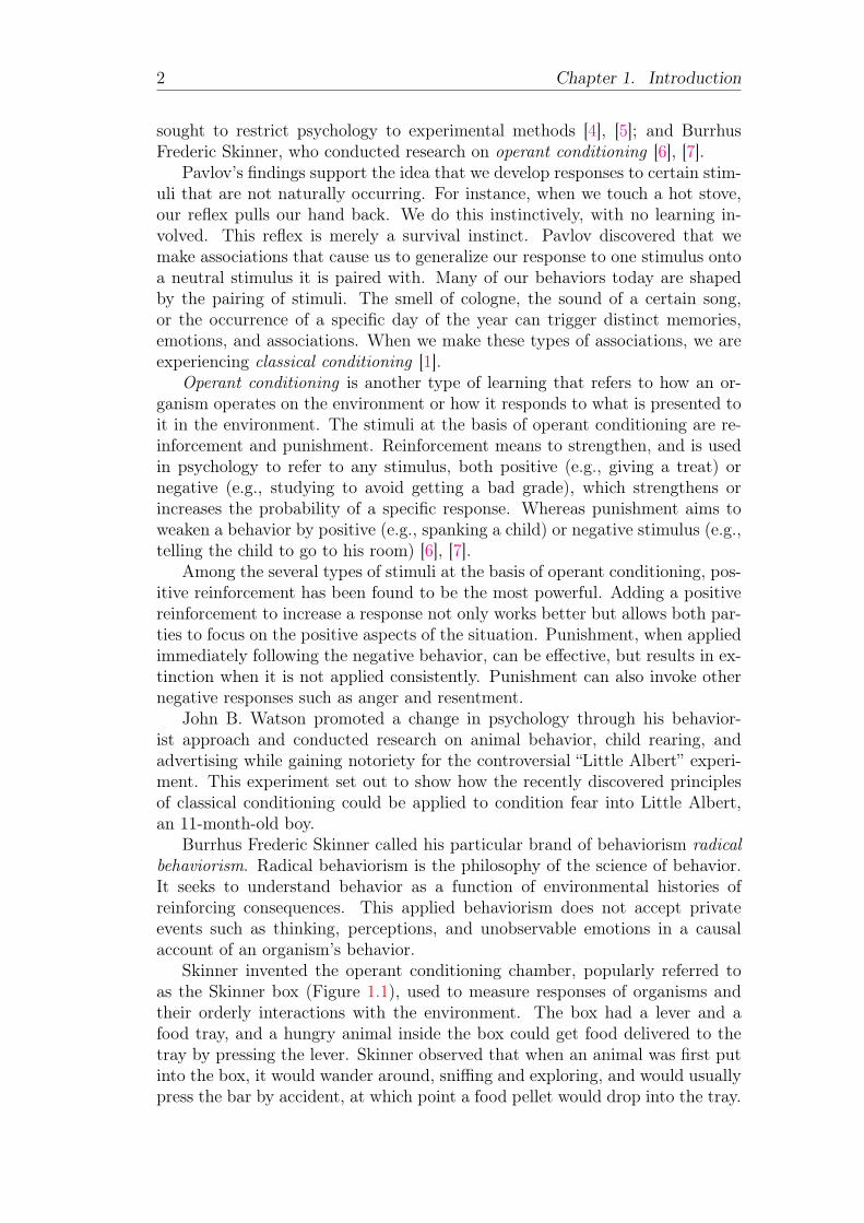
sought to restrict psychology to experimental methods [4], [5]; and BurrhusFrederic Skinner, who conducted research on operant conditioning [6], [7].
Pavlov’s findings support the idea that we develop responses to certain stim-uli that are not naturally occurring. For instance, when we touch a hot stove,our reflex pulls our hand back. We do this instinctively, with no learning in-volved. This reflex is merely a survival instinct. Pavlov discovered that wemake associations that cause us to generalize our response to one stimulus ontoa neutral stimulus it is paired with. Many of our behaviors today are shapedby the pairing of stimuli. The smell of cologne, the sound of a certain song,or the occurrence of a specific day of the year can trigger distinct memories,emotions, and associations. When we make these types of associations, we areexperiencing classical conditioning [1].
Operant conditioning is another type of learning that refers to how an or-ganism operates on the environment or how it responds to what is presented toit in the environment. The stimuli at the basis of operant conditioning are re-inforcement and punishment. Reinforcement means to strengthen, and is usedin psychology to refer to any stimulus, both positive (e.g., giving a treat) ornegative (e.g., studying to avoid getting a bad grade), which strengthens orincreases the probability of a specific response. Whereas punishment aims toweaken a behavior by positive (e.g., spanking a child) or negative stimulus (e.g.,telling the child to go to his room) [6], [7].
Among the several types of stimuli at the basis of operant conditioning, pos-itive reinforcement has been found to be the most powerful. Adding a positivereinforcement to increase a response not only works better but allows both par-ties to focus on the positive aspects of the situation. Punishment, when appliedimmediately following the negative behavior, can be effective, but results in ex-tinction when it is not applied consistently. Punishment can also invoke othernegative responses such as anger and resentment.
John B. Watson promoted a change in psychology through his behavior-ist approach and conducted research on animal behavior, child rearing, andadvertising while gaining notoriety for the controversial “Little Albert” experi-ment. This experiment set out to show how the recently discovered principlesof classical conditioning could be applied to condition fear into Little Albert,an 11-month-old boy.
Burrhus Frederic Skinner called his particular brand of behaviorism radicalbehaviorism. Radical behaviorism is the philosophy of the science of behavior.It seeks to understand behavior as a function of environmental histories ofreinforcing consequences. This applied behaviorism does not accept privateevents such as thinking, perceptions, and unobservable emotions in a causalaccount of an organism’s behavior.
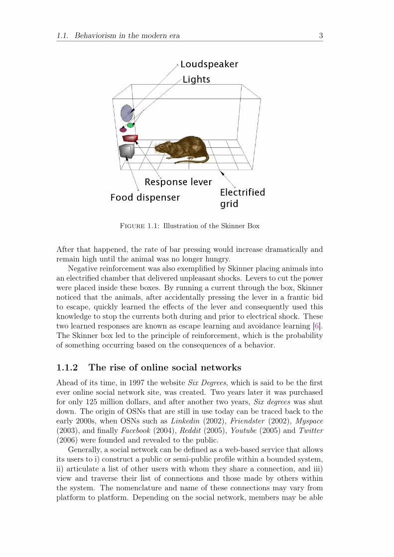
Skinner invented the operant conditioning chamber, popularly referred toas the Skinner box (Figure 1.1), used to measure responses of organisms andtheir orderly interactions with the environment. The box had a lever and afood tray, and a hungry animal inside the box could get food delivered to thetray by pressing the lever. Skinner observed that when an animal was first putinto the box, it would wander around, sniffing and exploring, and would usuallypress the bar by accident, at which point a food pellet would drop into the tray.
1.1. Behaviorism in the modern era 3
Figure 1.1: Illustration of the Skinner Box
After that happened, the rate of bar pressing would increase dramatically andremain high until the animal was no longer hungry.
Negative reinforcement was also exemplified by Skinner placing animals intoan electrified chamber that delivered unpleasant shocks. Levers to cut the powerwere placed inside these boxes. By running a current through the box, Skinnernoticed that the animals, after accidentally pressing the lever in a frantic bidto escape, quickly learned the effects of the lever and consequently used thisknowledge to stop the currents both during and prior to electrical shock. Thesetwo learned responses are known as escape learning and avoidance learning [6].The Skinner box led to the principle of reinforcement, which is the probabilityof something occurring based on the consequences of a behavior.
1.1.2 The rise of online social networks
Ahead of its time, in 1997 the website Six Degrees, which is said to be the firstever online social network site, was created. Two years later it was purchasedfor only 125 million dollars, and after another two years, Six degrees was shutdown. The origin of OSNs that are still in use today can be traced back to theearly 2000s, when OSNs such as Linkedin (2002), Friendster (2002), Myspace(2003), and finally Facebook (2004), Reddit (2005), Youtube (2005) and Twitter(2006) were founded and revealed to the public.
Generally, a social network can be defined as a web-based service that allowsits users to i) construct a public or semi-public profile within a bounded system,ii) articulate a list of other users with whom they share a connection, and iii)view and traverse their list of connections and those made by others withinthe system. The nomenclature and name of these connections may vary fromplatform to platform. Depending on the social network, members may be able

4 Chapter 1. Introduction
to contact any other member, or in other cases, members can contact anyonethey have a connection to. Some services require members to have a preexistingconnection to contact other members. While social networking has gone onalmost as long as societies themselves have existed, the unparalleled potentialof the World Wide Web to facilitate such connections has led to an exponentialand ongoing expansion of that phenomenon.
Other than personal, social networks can be also used by business purposes,such as increase brand recognition and loyalty by making the company moreaccessible to new customers and more recognizable for existing customers, orhelp promote a brand’s voice and content by spreading information about itsproducts or services. In the end, social networks have proved to be an essentialtool for businesses, particularly to help companies to find and retain their shareof the market and their customers.
The vast majority of OSNs cannot be considered to be generalist platformssince they are limited to a specific niche or purpose (e.g., photos, work-related,video, etc.). Even Facebook, which is now considered by most the ultimate toolfor social interactions, at its start was not more than a dating site, and later a“face book” (i.e., a student directory featuring photos and basic information).Therefore, with the exception of today’s Facebook platform, each social networktries to leverage the need for social interaction in a distinctive way. However,the reasons that push a user to join a social network seems to be driven bythe trend of the moment rather than a more significant added value, or publicutility (see Figure 1.2).
Figure 1.2: Relative search interest smoothed by a six-monthaverage (Data from Google Trends)
As often stated, the alleged final goal of a social network is to easily con-nect people and enable new fast ways to share information and experiences.However, from a less naive and more pragmatic perspective, user profiling and

1.2. Objectives and organization of this thesis 5
hence marketing remain the fundamentals of their business models. In the end,a social network platform is merely a tool that enables the tool-owner to extractinformation from the actual product, the user. Businesses that base their rev-enue on such models have been defined as attention merchants, platforms thatevaluate their success on measures like time spent on the platform, number ofaccess per day, and so on, are characterized by a single goal, that is profit.
Furthermore, the monopoly that Facebook created and its continuous effortto provide a complete suite of tools limits the needs and reasons for which itsusers could feel the need to leave the platform. This could result in limitingthe online experience to one single platform, which increases the chances to beconfined in an echo chamber. An echo chamber (also known as filter bubble),is commonly defined as a metaphorical description of a situation in which be-liefs are amplified or reinforced by communication and repetition inside a closedsystem, represented, in this case, by friends and relatives present on the plat-form. Other examples of echo chamber are those caused by the excessive use ofpersonalization algorithms, which generates personalized e-comfort zones (i.e.,feedback loops in which biases are reinforced rather than dismantled or simplyconfronted) for each one of us. Being confined in an echo chamber may increasepolitical and social polarization and extremism, and limit the opportunities ofchanging idea or even thinking about a personal belief.
Conversely, the massive pervasiveness of these platforms gives to scientiststhe unprecedented opportunity of analyzing human behavior in a controlledenvironment and in a quantitative way. Similarly to a Skinner box1.1, a socialnetwork platform can be considered a digital box, in which human behavior isconstantly monitored and rewards are in the form of instant gratification (e.g.,notifications).
1.2 Objectives and organization of this thesisIn the fast-growing research area of social network analysis, by leveraging rank-ing and machine-learned-based methods, we focus our attention to the identi-fication of users characterized by a specific type of behavior (i.e., automated,lurking, etc.), and also to users that show multiple, opposite behaviors in morethan one social media platforms, as well as learning new representation of graphdata in order to enable the application of a vast and variegated type of methods.
The aim of this research project is the development of method and algo-rithms that can have a high potential impact on the users of one or more socialnetworks. For instance, methods able to identify lurkers can be used to putin practice policies of user engagement. Conversely, detecting users who actas a bridge between multiple social networks can help to identify real contentcreators by unmasking plagiarism behaviors.
In the following chapters, we firstly describe well-studied measures used inthe context of network science to characterize user behavior. Then, we devotedthe third chapter to the social boundary spanning theory, with the goal ofidentifying users which share and transfer their knowledge across the bordersof a social network, we describe our approach to alternate behaviors rankingin multilayer social networks. The fourth chapter contains the description of

6 Chapter 1. Introduction
two applications of the supervised learning framework Learning-to-rank (LTR)in the context of OSNs. More in detail, through leveraging state-of-the-artLTR algorithms, we aim to learn a ranking function to identify and rank usersaccording to their bot or lurking status. In the last chapter of this dissertation,in the context of supervised learning, we try to advanced research on the networkembedding problem, by developing and testing several new methods designedto be able to deal with multilayer networks.
7
Chapter 2
User behavior in network science
In the first part of this chapter, we describe well-known centrality measures andranking algorithms in order to introduce, by a more technical point of view, thefollowing chapters. In the second part of the chapter, we focus our attention onthe problem of trust inference in controversial situations.
2.1 Ranking and centrality measuresHyperlinks provide a valuable source of information for web search. In fact, theanalysis of the hyperlink structure of the Web, commonly called link analysis ,has been successfully used for improving both the retrieving of web documents(i.e., which webpages to crawl) and the scoring of web documents according tosome notion of “quality” (i.e., how to rank webpages). The latter is in generalmeant either as the relevance of the documents with respect to a user queryor as some query-independent, intrinsic notion of centrality . In network theoryand analysis, the identification of the “most central” nodes in the network (e.g.,documents in the web network, actors in a social network, etc.) represents acore task.
The term centrality commonly resembles that of importance or prominenceof a vertex in a network, i.e., the status of being located in strategic locationswithin the network. However, there is no unique definition of centrality, as forinstance one may postulate that a vertex is important if it is involved in manydirect interactions, or if it connects two large components (i.e., if it acts as abridge), or if it allows for quick transfer of the information also by accountingfor indirect paths that involve intermediaries. Consequently, there are only veryfew desiderata for a centrality measure, which can be expressed as follows:
• A vertex centrality is a function that assigns a real-valued score to eachvertex in a network. The higher the score, the more important or promi-nent the vertex is for the network.
• If two graphs G1, G2 are isomorphic and m(v) denotes the mapping func-tion from a node v in G1 to some node v′ in G2, then the centrality of vin G1 needs to be the same as the centrality of m(v) = v′ in G2. In otherterms, the centrality of a vertex is only depending on the structure of thenetwork.
The term centrality is originally designed for undirected networks. In thecase of directional relations, which imply directed networks, the term centrality

8 Chapter 2. User behavior in network science
is still used and refers to the “choices made”, or out-degrees of vertices, whilethe term prestige is introduced to examine the “choices received”, or in-degreesof vertices [8]. Moreover, the vertex centrality scores can be aggregated overall vertices in order to obtain a single, network-level measure of centrality, oralternatively centralization, which aims to provide a clue on the variability ofthe individual vertex centrality scores with respect to a given centrality notion.In the following, we will overview the most prominent measures of centralityand prestige, and their definitions for undirected and directed networks. Partic-ularly, we will focus on two well-known methods, namely PageRank and Hubs& Authorities, which have been widely applied to web search contexts.
Through the rest of this section and in the subsequent sections of this chap-ter, we will denote with G = (V,E) a network graph, which consists of two setsV and E, such that V 6= ∅ and E is a set of pairs of elements of V . If thepairs in E are ordered the graph is said directed, otherwise is undirected. Theelements in V are the vertices (or nodes) of G, while the elements in E are theedges (or links) of G.
2.1.1 Basic measures
Vertex-level centrality. The most intuitive measure of centrality for anyvertex v ∈ V is the degree centrality, which is defined as the number of edgesincident with v, or degree of v:
cD(v) = deg(v). (2.1)
Being dependent only on adjacent neighbors of a vertex, this type of centralityfocuses on the most “visible” vertices in the network, as those that act as majorpoint of relational information; by contrast, vertices with low degrees are pe-ripheral in the network. Moreover, the degree centrality depends on the graphsize: indeed, since the highest degree for a network (without loops) is |V |−1,the relative degree centrality is:
cD(v) =cD(v)
|V |−1=deg(v)
|V |−1. (2.2)
The above measure is independent on the graph size, and hence it can be com-pared across networks of different sizes.
The definitions of both absolute and relative degree centrality and degreeprestige of a vertex in a directed network are straightforward. In that case,the degree and the set of neighbors have two components: we denote withBi = {vj|(vj, vi) ∈ E} the set of in-neighbors (or “backward” vertices) of vi,and with Ri = {vj|(vi, vj) ∈ E} the set of out-neighbors (or “reference” vertices)of vi. The sizes of sets Bi and Ri are the in-degree and the out-degree of vi,denoted as in(vi) and out(vi), respectively.
Note also that the degree centrality is also the starting point for variousother measures; for instance, the span of a vertex, which is defined as thefraction of links in the network that involves the vertex or its neighbors, and

2.1. Ranking and centrality measures 9
the ego density, which is the ratio of the degree of the vertex to the theoreticalmaximum number of links in the network.
Unlike degree centrality, closeness centrality takes also into account indirectlinks between vertices in the network, in order to score higher those verticesthat can quickly interact with all others because of their lower distance to theother vertices [9]:
cC(v) =1∑
u∈V d(v, u), (2.3)
where d(v, u) denotes the graph theoretic, or geodesic, distance (i.e., length ofshortest path) between vertices v, u. Since a vertex has the highest closenessif it has all the other vertices as neighbors, the relative closeness centrality isdefined as:
cC(v) = (|V |−1)cC(v) =|V |−1∑u∈V d(v, u)
. (2.4)
In the case of directed networks, closeness centrality and prestige can be com-puted according to outgoing links (i.e., how many hops are needed to reach allother vertices from the selected one) or incoming links (i.e., how many hops areneeded to reach the selected vertex from all other vertices), respectively. Notethat the closeness centrality is only meaningful for a connected network—infact, the geodesics to a vertex that is not reachable from any other vertex areinfinitely long. One remedy to this issue is to define closeness by focusing ondistances from the vertex v to only the vertices that are in the influence rangeof v (i.e., the set of vertices reachable from v) [8].
Besides (shortest) distance, another important property refers to the abilityof a vertex to have control over the flow of information in the network. Theidea behind betweenness centrality is to compute the centrality of a vertex v asthe fraction of the shortest paths between all pairs of vertices that pass throughv [10]:
cB(v) =∑
u,z∈V,u6=v,z 6=v
mu,z(v)
mu,z(V ), (2.5)
where mu,z(v) is the number of shortest paths between u and z and passingthrough v, and mu,z(V ) is the total number of shortest paths between u andz. This centrality is minimum (zero) when the vertex does not fall on anygeodesic, and maximum when the vertex falls on all geodesics, which is equalto (|V |−1)(|V |−2)/2. Analogously to the other centrality measures, it’s rec-ommended to standardize the betweenness to obtain a relative betweennesscentrality:
cB(v) =2cB(v)
(|V |−1)(|V |−2), (2.6)
which should be divided by 2 for directed networks. Note that, unlike closeness,betweenness can be computed even if the network is disconnected.
It should be noted that the computation of betweenness centrality is themost resource-intensive among the above-discussed measures: while standardalgorithms based on Dijkstra’s or breadth-first search methods require O(|V |3)time and O(|V |2) space, algorithms designed for large, sparse networks requireO(|V |+|E|) space andO(|V ||E|) andO(|V ||E|+|V |2log|V |) time on unweighted

10 Chapter 2. User behavior in network science
and weighted networks, respectively [11]. A number of variants of betweennesscentrality have also been investigated; for instance, in [12], an extension ofbetweenness to edges is obtained by replacing the termmu,z(v) in equation (2.5)by a term mu,z(e) calculating the number of shortest (u, z)-paths containingthe edge e. An application of this version of edge betweenness is the clusteringapproach by Newman and Girvan [13], where edges of maximum betweennessare removed iteratively to decompose a graph into relatively dense subgraphs.
Besides computational complexity issue, a criticism to betweenness central-ity is that it assumes that all geodesics are equally likely when calculating if avertex falls on a particular geodesic. However, a vertex with large in-degree ismore likely to be found on a geodesic. Moreover, in many contexts, there maybe equally likely that other paths than geodesics are chosen for the informationpropagation, therefore the paths between vertices should be weighted depend-ing on their length. The index defined by Stephenson and Zelen [14] buildsupon the above generalization, by accounting for all paths, including geodesics,and assigning them with weights, which are computed as the inverse of thepath lengths (geodesics are given unitary weights). The same researchers alsodeveloped an information centrality measure, which focuses on the informationcontained in all paths that originate and end at a specific vertex. The informa-tion of a vertex is a function of all the information for paths flowing out fromthe vertex, which in turn is inversely related to the variance in the transmissionof a signal from a vertex to another. Formally, given an undirected network,possibly with weighted edges, a |V |×|V | matrix X is computed as follows: thei-th diagonal entry is equal to 1 plus the sum of weights for all incoming linksto vertex vi, and the (i, j)-th off-diagonal entry is equal to 1, if vi and vj arenot adjacent, otherwise is equal to 1 minus the weight of the edge between viand vj. For any vertex vi, the information centrality is defined as:
cI(vi) =1
yii + 1|V |(∑
vj∈V yjj − 2∑
vj∈V yij), (2.7)
where {yij} are the entries of the matrix Y = X−1. Since function cI is onlylower bounded (the minimum is zero), the relative information centrality forany vertex vi is obtained by dividing cI(vi) by the sum of the cI values for allvertices.
Network-level centrality. A basic network-level measure of degree cen-trality is simply derived by taking into account the (standardized) average ofthe degrees: ∑
v∈V cD(v)
|V ||V − 1|=
∑v∈V cD(v)
|V |, (2.8)
which is exactly the density of the network.Focusing on a global notion of closeness, a simplification of this type of
centrality stems from the graph-theoretic center of a network. This is in turnbased on the notion of eccentricity of a vertex v, i.e., the distance to a vertexfarthest to v. Specifically, the Jordan center of a network is the subset of verticesthat have the lowest maximum distance to all other vertices, i.e., the subset ofvertices within the radius of a network.

2.1. Ranking and centrality measures 11
A unifying view of network-level centrality is based on the notion of networkcentralization, which expresses how the vertices in the network graph G differin centrality [15]:
C(G) =
∑v∈V maxC− C(v)
max∑
v∈V maxC− C(v), (2.9)
where C(·) is a function that expresses a selected measure of relative centrality,and maxC is the maximum value of relative centrality over all vertices in thenetwork graph. Therefore, centralization is lower when more vertices have sim-ilar centrality, and higher when one or few vertices dominate the other vertices;as extreme cases, a star network and a regular (e.g., cycle) network have cen-tralization equal to 1 and 0, respectively. According to the type of centralityconsidered, the network centralization assumes different form. More specifically,considering the degree, closeness, and betweenness centralities, the denominatorin equation (2.9) is equal to (n−1)(n−2), (n−1)(n−2)/(2n−3), and (n−1),respectively.
2.1.2 Eigenvector centrality and prestige
None of the previously discussed measures reflects the importance of the ver-tices that interact with the target vertex when looking at (in)degree or distanceaspects. Intuitively, if the influence range of a vertex involves many prestigiousvertices, then the prestige of that vertex should also be high; conversely, theprestige should be low if the involved vertices are peripheral. Generally speak-ing, a vertex’s prestige should depend on the prestige of the vertices that pointto it, and their prestige should also depend on the vertices that point to them,and so “ad infinitum” [16]. It should be noted that the literature usually refersto the above property as status , or rank .
The idea behind status or rank prestige by Seeley, denoted by function r(·),can be formalized as follows:
r(v) =∑u∈V
A(u, v)r(u), (2.10)
where A(u, v) is equal to 1 if u points to v (i.e., u is an in-neighbor of v), and0 otherwise. Equation (2.10) corresponds to a set of |V | linear equations (with|V | unknowns) which can be rewritten as:
r = ATr, (2.11)
where r is a vector of size |V | storing all rank scores, and A is the adjacencymatrix. Or, rearranging terms, we obtain (I−AT)r = 0, where I is the identitymatrix of size |V |.
Katz [17] first recommended to manipulate the matrix A by constrainingevery row in A to have sum equal to 1, thus enabling equation (2.11) to havefinite solution. In effect, equation (2.11) is a characteristic equation used to findthe eigensystem of a matrix, in which r is an eigenvector of AT corresponding toan eigenvalue of 1. In general, equation (2.11) has no non-zero solution unlessAT has an eigenvalue of 1.

12 Chapter 2. User behavior in network science
A generalization of equation (2.11) was suggested by Bonacich [18], wherethe assumption is that the status of each vertex is proportional (but not neces-sarily equal) to the weighted sum of the vertices to whom it is connected. Theresult, known as eigenvector centrality, is expressed as follows:
λr = ATr. (2.12)
Note that the above equation has |V | solutions corresponding to |V | values ofλ. Therefore, the general solution can be expressed as a matrix equation:
λR = ATR, (2.13)
where R is a |V |×|V | matrix whose columns are the eigenvectors of AT and λis a diagonal matrix of eigenvalues.
Katz [17] also proposed to introduce in equation (2.11) an “attenuation pa-rameter” α ∈ (0, 1) to adjust for the lower importance of longer paths be-tween vertices. The result, known as Katz centrality, measures the prestige asa weighted sum of all the powers of the adjacency matrix:
r =∞∑i=1
αiATir. (2.14)
When α is small, Katz centrality tends to probe only the local structure ofthe network; as α grows, more distant vertices contribute to the centrality of agiven vertex. Note also that the infinite sum in the above equation convergesto r = [(I− αAT)−1 − I]1 as long as |α|< 1/λ1, where λ1 is the first eigenvalueof AT.
All the above measures may fail in producing meaningful results for networksthat contain vertices with null in-degree: in fact, according to the assumptionthat a vertex has no status if it does not receive choices from other vertices,vertices with null in-degree do not contribute to the status of any other vertex. Asolution to this problem is to allow every vertex some status that is independentof its connections to other vertices. The Bonacich & Lloyd centrality [19],probably better known as alpha-centrality, is defined as:
r = αATr + e, (2.15)
where e is a |V |-dimensional vector reflecting exogenous source of information orstatus, which is assumed to a vector of ones. Moreover, parameter α here reflectsthe relative importance of endogenous versus exogenous factors in determiningthe vertex prestige. The solution of equation (2.15) is:
r = (I− αAT)−1e. (2.16)
It can easily be proved that equation (2.16) and equation (2.14) differ only bya constant (i.e., one) [19].
2.1. Ranking and centrality measures 13
2.1.3 PageRank
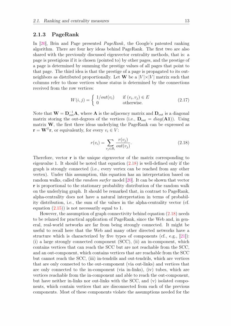
In [20], Brin and Page presented PageRank , the Google’s patented rankingalgorithm. There are four key ideas behind PageRank. The first two are alsoshared with the previously discussed eigenvector centrality methods, that is: apage is prestigious if it is chosen (pointed to) by other pages, and the prestige ofa page is determined by summing the prestige values of all pages that point tothat page. The third idea is that the prestige of a page is propagated to its out-neighbors as distributed proportionally. Let W be a |V |×|V | matrix such thatcolumns refer to those vertices whose status is determined by the connectionsreceived from the row vertices:
W (i, j) =
{1/out(vi) if (vi, vj) ∈ E0 otherwise. (2.17)
Note that W = D−1outA, where A is the adjacency matrix and Dout is a diagonal
matrix storing the out-degrees of the vertices (i.e., Dout = diag(A1)). Usingmatrix W, the first three ideas underlying the PageRank can be expressed asr = WTr, or equivalently, for every vi ∈ V :
r(vi) =∑vj∈Bi
r(vj)
out(vj). (2.18)
Therefore, vector r is the unique eigenvector of the matrix corresponding toeigenvalue 1. It should be noted that equation (2.18) is well-defined only if thegraph is strongly connected (i.e., every vertex can be reached from any othervertex). Under this assumption, this equation has an interpretation based onrandom walks, called the random surfer model [20]. It can be shown that vectorr is proportional to the stationary probability distribution of the random walkon the underlying graph. It should be remarked that, in contrast to PageRank,alpha-centrality does not have a natural interpretation in terms of probabil-ity distribution, i.e., the sum of the values in the alpha-centrality vector (cf.equation (2.15)) is not necessarily equal to 1.
However, the assumption of graph connectivity behind equation (2.18) needsto be relaxed for practical application of PageRank, since the Web and, in gen-eral, real-world networks are far from being strongly connected. It might beuseful to recall here that the Web and many other directed networks have astructure which is characterized by five types of components (cf., e.g., [21]):(i) a large strongly connected component (SCC), (ii) an in-component, whichcontains vertices that can reach the SCC but are not reachable from the SCC,and an out-component, which contains vertices that are reachable from the SCCbut cannot reach the SCC, (iii) in-tendrils and out-tendrils, which are verticesthat are only connected to the out-component (via out-links) and vertices thatare only connected to the in-component (via in-links), (iv) tubes, which arevertices reachable from the in-component and able to reach the out-component,but have neither in-links nor out-links with the SCC, and (v) isolated compo-nents, which contain vertices that are disconnected from each of the previouscomponents. Most of these components violate the assumptions needed for the

14 Chapter 2. User behavior in network science
convergence of a Markov process. In particular, when a random surfer entersthe out-component, she will eventually get stuck in it; as a result, vertices thatare not in the out-component will receive a zero rank, i.e., one cannot distin-guish the prestige of such vertices. More specifically, equation (2.18) needs tobe modified to prevent anomalies that are caused by two types of structures:rank sinks , or “spider traps”, and rank leaks , or “dead ends”. The former aresets of vertices that have no links outwards, the latter are individual verticeswith no out-links.
If leak vertices would be directly represented in matrix W, then they wouldcorrespond to rows of zero, thus making W substochastic: as a result, by re-iterating equation (2.18) for a certain number k of times (i.e., by computingWTkr), then some or all of the entries in r will go to 0. To solve this issue, twoapproaches can be suggested: (i) modification of the network structure, and (ii)modification of the random surfer behavior. In the first case, leak vertices couldbe removed from the network so that they will receive zero rank; alternatively,leak vertices could be “virtually” linked back to their in-neighbors, or even to allother vertices. The result will be a row-stochastic matrix, that is, a matrix thatis identical to W except that it will have the columns corresponding to leakvertices that sum to 1. If we denote with d a vector indexing the leak vertices(i.e., d(i) = 1 if vi has no outlinks, and d(i) = 0 otherwise), this row-stochasticmatrix S is defined as:
S = W + d1T/|V |. (2.19)
However, equation (2.19) will not solve the problem of sinks. Therefore, Pageand Brin [20] also proposed to modify the random surfer behavior by allowingfor teleportation, i.e., the random surfer who gets stuck in a sink, or simply gets“bored” occasionally, she can move by randomly jumping to any other vertex inthe network. This is the fourth idea behind the PageRank measure, which isimplemented by a damping factor α ∈ (0, 1) that enables to weigh the mixtureof random walk and random teleportation:
r = αSTr + (1− α)p. (2.20)
Above, vector p, usually called personalization vector , is by default set to 1/|V |,but it can be any probability vector. Equation (2.20) can be rewritten as:
G = αS + (1− α)E, (2.21)
where E = 1pT = 11T/|V |. The convex combination of S and E makes theresulting “Google matrix” G to be both stochastic and irreducible.1 This isimportant to ensure (i) the existence and uniqueness of the PageRank vector asstationary probability distribution π, and (ii) the convergence of the underlyingMarkov chain (at a certain iteration k, i.e., π(k+1) = Gπ(k)) independently ofthe initialization of the rank vector.2
1A matrix is said irreducible if every vertex in its graph is reachable from every othervertex.
2Recall that the property of irreducibility of a matrix is related to those of primitivity andaperiodicity. A nonnegative, irreducible matrix is said primitive if it has only one eigenvalueon its spectral circle; a simple test by Frobenius states that a matrix X is primitive if and only
2.1. Ranking and centrality measures 15
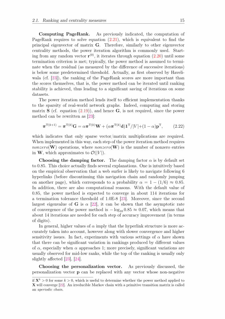
Computing PageRank. As previously indicated, the computation ofPageRank requires to solve equation (2.21), which is equivalent to find theprincipal eigenvector of matrix G. Therefore, similarly to other eigenvectorcentrality methods, the power iteration algorithm is commonly used. Start-ing from any random vector r(0), it iterates through equation (2.20) until sometermination criterion is met; typically, the power method is assumed to termi-nate when the residual (as measured by the difference of successive iterations)is below some predetermined threshold. Actually, as first observed by Haveli-wala (cf. [23]), the ranking of the PageRank scores are more important thanthe scores themselves, that is, the power method can be iterated until rankingstability is achieved, thus leading to a significant saving of iterations on somedatasets.
The power iteration method lends itself to efficient implementation thanksto the sparsity of real-world network graphs. Indeed, computing and storingmatrix S (cf. equation (2.19)), and hence G, is not required, since the powermethod can be rewritten as [23]:
πT(k+1) = πT(k)G = απT(k)W + (απT(k)d)1T/|V |+(1− α)pT, (2.22)
which indicates that only sparse vector/matrix multiplications are required.When implemented in this way, each step of the power iteration method requiresnonzero(W) operations, where nonzero(W) is the number of nonzero entriesin W, which approximates to O(|V |).
Choosing the damping factor. The damping factor α is by default setto 0.85. This choice actually finds several explanations. One is intuitively basedon the empirical observation that a web surfer is likely to navigate following 6hyperlinks (before discontinuing this navigation chain and randomly jumpingon another page), which corresponds to a probability α = 1 − (1/6) ≈ 0.85.In addition, there are also computational reasons. With the default value of0.85, the power method is expected to converge in about 114 iterations fora termination tolerance threshold of 1.0E-8 [23]. Moreover, since the secondlargest eigenvalue of G is α [22], it can be shown that the asymptotic rateof convergence of the power method is − log10 0.85 ≈ 0.07, which means thatabout 14 iterations are needed for each step of accuracy improvement (in termsof digits).
In general, higher values of α imply that the hyperlink structure is more ac-curately taken into account, however along with slower convergence and highersensitivity issues. In fact, experiments with various settings of α have shownthat there can be significant variation in rankings produced by different valuesof α, especially when α approaches 1; more precisely, significant variations areusually observed for mid-low ranks, while the top of the ranking is usually onlyslightly affected [23], [24].
Choosing the personalization vector. As previously discussed, thepersonalization vector p can be replaced with any vector whose non-negative
if Xk > 0 for some k > 0, which is useful to determine whether the power method applied toX will converge [22]. An irreducible Markov chain with a primitive transition matrix is calledan aperiodic chain.

16 Chapter 2. User behavior in network science
components sum up to 1. This hence includes the possibility that the verticesin V might be differently considered when the random surfer restarts her chainby selecting a vertex v with probability p(v), which is not necessarily uniformover all the vertices.
The teleportation probability p(v) can be determined to be proportionalto the score the vertex v obtains with respect to an external criterion of im-portance, or to the contribution that the vertex gives to a certain topologicalcharacteristic of the network. For instance, one may want to assign any ver-tex with a teleportation probability that is proportional to the in-degree of thevertex, i.e.,
p(v) =in(v)∑u∈V in(u)
.
The personalization vector can also be used to boost the PageRank scorefor a specific subset of vertices that are relevant to a certain topic, thus makingthe PageRank to be topic-sensitive.
2.1.4 Hubs and authorities
A different approach to the computation of vertex prestige is based on the no-tions of hubs and authorities . In a web search context, given a user query,authority pages are ones most likely to be relevant to the query, while hubpages act as indices of authority pages without being necessarily authoritiesthemselves. These two types of webpages are related to each other by a mutualreinforcement mechanism: in fact, if a page is relevant to a query, one would ex-pect that it will be pointed to by many other pages; moreover, pages pointing toa relevant page are likely to point as well to other relevant pages, thus inducinga kind of bipartite graph where pages that are relevant by content (authorities)are endorsed by special pages that are relevant because they contain hyperlinksto locate relevant contents (hubs)—although, it may be the case that a page isboth an authority and a hub.
The above intuition is implemented by the Kleinberg’s HITS (Hyperlink In-duced Topic Search) algorithm [25], [26]. Like PageRank and other eigenvectorcentrality methods, HITS still handles an iterative computation of a fix-pointinvolving eigenvector equations; however, it originally views the prestige of apage as a two-dimensional notion, thus resulting in two ranking scores for everyvertex in the network. Also in contrast to PageRank, HITS produces rankingscores that are query-dependent. In fact, HITS assumes that hubs and au-thorities are identified and ranked for vertices that belong to a query-focusedsub-network. This is usually formed by an initial set of randomly selected pagescontaining the query terms, which is expanded by also including the neighbor-hoods of those pages.
Let a and h be two vectors storing the authority and hub scores, respectively.The hub score of a vertex can be expressed as proportional to the sum of theauthority scores of its out-neighbors; analogously, the authority score of a vertexcan be expressed as proportional to the sum of the hub scores of its in-neighbors.

2.1. Ranking and centrality measures 17
Formally, HITS equations are defined as:
a = µATh (2.23)
h = λAa, (2.24)
where µ, λ are two (unknown) scaling constants that are needed to avoid thatthe authority and hub scores will grow beyond bounds; in practice, a and hare normalized so that the largest value in each of the vectors equals 1 (or,alternatively, all values in each of the vectors sum up to 1). Therefore, HITSworks as follows:
1. For every vertex in the expanded query-focused subnetwork, initialize huband authority score (e.g., to 1).
2. Compute the following steps until convergence (i.e., a termination toler-ance threshold is reached):
(a) authority vector a using equation (2.23);
(b) hub vector h using equation (2.24);
(c) normalize a and h.
Note that, at the first iteration, a and h are none other than the vertex in-degrees and the out-degrees, respectively.
By substituting equation (2.23) and equation (2.24) in each other, hub andauthority can in principle be computed independently of each other, through thecomputation of AAT (for the hub vector) and ATA (for the authority vector).Note that, the (i, j)-th entry in matrix AAT corresponds to the number ofpages jointly referred by pages i and j; analogously, the (i, j)-th entry in matrixATA corresponds to the number of pages that jointly point to pages i and j.However, both matrix products lead to matrices that are not as sparse, hencethe only convenient way to compute a and h is iteratively in a mutual fashionas described above. In this regard, just as in the case of PageRank, the rateof convergence of HITS depends on the eigenvalue gap, and the ordering ofhubs and authorities becomes stable with much fewer iterations than the actualscores.
It should be noted that the assumption of identifying authorities by meansof hubs might not hold in other information networks other than the Web; forinstance, in citation networks, important authors typically acknowledge otherimportant authors. This has somehow impacted on the probably less popularityof HITS with respect to PageRank—which, conversely, has been successfullyapplied to many other contexts, including citation and collaboration networks,lexical/semantic networks inferred from natural language texts, recommendersystems, and social networks.
The TKC effect. Beyond limited applicability, HITS seems to suffer fromtwo issues that are related to both the precision and coverage of the query searchresults. More precisely, while the coverage of search results directly affectsthe size of the subnetwork, the precision can significantly impact the tightlyknit communities (TKC) effect, which occurs when relatively many pages are

18 Chapter 2. User behavior in network science
●
●
●
●
●
●
●
●
●
●
●
●
(a) closeness (b) betweenness
●
●
●
●
●
●
●
●
●
●
●
●
(c) eigenvector centrality (d) PageRank
●
●
●
●
●
●
●
●
●
●
●
●
(e) Kleinberg’s hub score (f) Kleinberg’s authority score
Figure 2.1: Comparison of ranking performance of differentcentrality methods on the same example graph. Node size is
proportional to the node degree. Lighter gray-levels correspondto higher rank scores.
identified as authoritative via link analysis although they actually pertain toone aspect of the target topic; for instance, this is the case when hubs pointboth to actual relevant pages and to pages that are instead relevant to “related

2.1. Ranking and centrality measures 19
topics” [27]. The latter phenomenon is also called topic drift .While the TKC effect can be attenuated by accounting for the analysis of
contents and/or the anchor texts of the webpages (e.g., [28], [29]), other linkanalysis approaches have been developed to avoid overly favoring the authoritiesof tightly knit communities. Lempel and Morgan [27] propose the StochasticApproach for Link Structure Analysis, dubbed SALSA. This is a variation ofKleinberg’s algorithm: it constructs an expanded query-focused subnetwork inthe same way as HITS, and likewise, it computes an authority and a hub scorefor each vertex in the neighborhood graph (and these scores can be viewedas the principal eigenvectors of two matrices). However, instead of using thestraight adjacency matrix, SALSA weighs the entries according to their in andout-degrees. More precisely, the authority scores are determined by the sta-tionary distribution of a two-step Markov chain through random walking overin-neighbors of a page and then random walking over out-neighbors of a page,while the hub scores are determined similarly with inverted order of the twosteps in the Markov chain. Formally, the Markov chain for authority scores hastransition probabilities:
pa(i, j) =∑
vq∈Bi∩Bj
1
in(vi)
1
out(vk)(2.25)
and the Markov chain for hub scores has transition probabilities:
ph(i, j) =∑
vq∈Ri∩Rj
1
out(vi)
1
in(vk). (2.26)
Lempel and Morgan proved that the authority stationary distribution a issuch that a(vi) = in(vi)/
⋃v∈V in(v), and that the hub stationary distribution h
is such that h(vi) = out(vi)/⋃v∈V out(v). Therefore, SALSA does not follow the
mutual reinforcement principle used in HITS, since hub and authority scores ofa vertex depend only on the local links of the vertex. Also, in the special caseof a single-component network, SALSA can be seen as a one-step truncatedversion of HITS [30]. Nevertheless, the TKC effect is overcome in SALSAthrough random walks on the hub-authority bipartite network, which impliesthat authorities can be identified by looking at different communities.
Figure 2.1 shows an illustrative comparison of various centrality methodsdiscussed in this section, on the same example network graph. The nodes in thegraph are colored using a gray palette, such that lighter gray-levels correspondto higher rank scores that a particular centrality method has produced overthat graph.
2.1.5 SimRank
SimRank [31] is a general, iteratively mutual reinforced similarity measure ona link graph, which is applicable in any domain with object-to-object relation-ships. The main intuition behind SimRank is that “two objects are similar ifthey are related to similar objects”. For instance, on a hyperlinked documentdomain like the Web, two webpages can be regarded as similar if there exist

20 Chapter 2. User behavior in network science
hyperlinks between them, or in a recommender system, we might say that twousers are similar if they rate similar items (and, in a mutual reinforcement fash-ion, two items are similar if they are rated by similar users). The underlyingmodel of SimRank is the “random surfer-pairs model”, i.e., SimRank yields aranking of vertex pairs. The basic SimRank equation formalizes the intuitionthat two objects are similar if they are referenced by similar objects. Given anytwo vertices u and v, their similarity, denoted as S(u, v), is defined as 1 if u = v,otherwise an iterative process is performed, in which the similarity between uand v is recursively calculated in terms of in-neighbors of u and v, respectively.The generic step of random walk of this process is defined as:
S(u, v) = α1
|Bu||Bv|∑i∈Bu
∑j∈Bv
S(i, j), (2.27)
where α is a constant between 0 and 1. As a particular case, if either u or vhas no in-neighbors, then S(u, v) = 0. It should be noted that equation (2.27)expresses the average similarity between in-neighbors of u and in-neighbors ofv. Moreover, it is easy to see that SimRank scores are symmetric.
The basic SimRank equation lends itself to several variations, which accountfor different contingencies in a network graph. One of these variations allowsfor resembling the HITS algorithm (cf. Section 2.1.4), since it considers thatvertices in a graph may take on different roles, like hub and authority for im-portance. Within this view, equation (2.27) can be replaced by two mutuallyreinforcing functions that express the similarity of any two vertices in terms ofeither their in-neighbors or out-neighbors:
S1(u, v) = α11
|Ru||Rv|∑i∈Ru
∑j∈Rv
S2(i, j) (2.28)
andS2(u, v) = α2
1
|Bu||Bv|∑i∈Bu
∑j∈Bv
S1(i, j), (2.29)
where constants α1, α2 have the same semantics as α in equation (2.27). Anothervariation of SimRank is themin-max variation, which captures the commonalityunderlying two similarity notions that express the endorsement of one vertextowards the choices of another vertex, and vice versa. Given vertices u, v, twointermediate terms are defined as:
Su(u, v) = α1
|Ru|∑i∈Ru
maxj∈Rv
S(i, j) (2.30)
andSv(u, v) = α
1
|Rv|∑i∈Rv
maxj∈Ru
S(i, j), (2.31)
with final similarity score computed as S(u, v) = min{Su(u, v), Sv(u, v)}, whichensures that each vertex chooses the other’s choices.
SimRank is a computationally expensive method. The space required for
2.1. Ranking and centrality measures 21
each iteration is simply O(|V |2), whereas the time required is O(I|V |2d), whered denotes the average of |Bu||Bv| over all vertex-pairs u, v, and I is the numberof iterations. One way to reduce the computational burden is to prune thelink graph, which avoids to compute the similarity for every vertex-pair by con-sidering only vertex-pairs within a certain radius from each other [31]. Manyother methods to speed up the SimRank computation have been developed inthe literature. For instance, Fogaras and Racz [32] proposed a probabilisticapproximation based on the Monte Carlo method. Lizorkin et al. [33] proposeddifferent optimization techniques, including partial sums memoization that canreduce repeated calculations of the similarity among different pairs by cachingpart of similarity summations for later reuse. Antonellis et al. [34] extendedSimRank using evidence factor for incident nodes and link weights. More re-cently, Yu et al. [35] proposed a fine-grained memoization method to share thecommon parts among different partial sums; the same authors also studied ef-ficient incremental SimRank computation over evolving graphs. At the time ofwriting of this chapter, the most recent study is that by Du et al. [36], whichhave focused on SimRank problems in uncertain graphs.
In this section we discuss main approaches to make the process of rank-ing web documents, or similarly their corresponding users, topic-sensitive. Thegeneral goal is to drive the ranking mechanism in such a way that the obtainedordering and scoring reflects a target scenario in which the vertices in the net-work are to be evaluated based on their relevance to a topic of interest. Theterm topic is here intentionally used with two different meanings, which corre-spond to different perspectives of quality of web resources: the one normallyrefers to the content of web documents, whereas the other one refers to therelation of web documents with web spammers, and more specifically to theirtrustworthiness, or likelihood of not being a spammer’s target.
2.1.6 Content as topic
As previously mentioned, the PageRank personalization vector p can be re-placed with any probability vector defined to boost the PageRank score for aspecific subset of vertices that are relevant to a certain topic of interest.
A natural way to implement the above idea is to make the teleportationquery-dependent, in such a way that a vertex (page) is more likely to be chosenif it covers the query terms. More precisely, if we denote with B ⊆ V a subsetof vertices of interest, then p = 1/|V | is replaced with another vector biasedby B, pB whose entries are set to 1/|B| only for those vertices that belong toB, and zero otherwise. Because of the concentration of random walk restarts atvertices from B, these vertices will obtain a higher PageRank score than theyobtained using a conventional (non-topic-biased) PageRank.
Intuitively, this way of altering the behavior of random surfing reflects thedifferent preferences and interests that the random surfer may have and specifyas terms in a query. Moreover, for efficient indexing and computation, the subsetB usually corresponds to a relatively small selection of vertices that cover somesmall number of topics. For instance, one might want to constrain the restartof the random walk to select only pages that are classified under one or more

22 Chapter 2. User behavior in network science
categories (e.g., “politics”, “sports”, “technology”, and so on) of the Wikipediatopic classification system3 or any other publicly available web directory. Theconsequence of this topic-biased selection is that not only the random surferwill be at pages that are identified as relevant to the selected topics, but alsoany neighbor page and any page reachable along a short path (from one of theknown relevant pages) will be likely relevant as well.
Topic affinity and user ranking. Determining topic affinity in websources is central to identifying webpages that are related to a set of targetpages. Topic affinity can be measured by using one or combination of thefollowing three main approaches.
• Text-based methods. Besides cosine similarity in vector space models(e.g., [37]), text-based approaches can also involve resemblance measures(e.g., Jaccard or Dice coefficients) which are defined in terms of the overlapbetween two documents modeled as sets of text chunks [38].
• Link-based methods. The link-based topic affinity approach has tradi-tionally borrowed from citation analysis, since the hyperlinking systemof endorsement is in analogy with the citation mechanism in researchcollaboration networks. Particularly, co-citation analysis is effective indetecting cores of articles or authors given a particular subject matter.Early applications of co-citation analysis to topical affinity detection andweb document clustering include [39]–[41]. Essentially, a citation-basedmeasure of topic affinity can be formalized as co-citation strength or, alter-nately, as bibliographic-coupling (also called co-reference) strength; i.e.,two documents are related proportionally to the frequency with whichthey are cited together (resp., the frequency with which they have refer-ences in common). Furthermore, similarity between two documents canbe also evaluated in terms of number of direct paths between the twodocuments.
• Usage-based methods. Finally, the usage-based topic affinity approach isbased on the assumption that the interaction of users with web resources(stored via user access and activity logs) can aid to improve the qualityof content, thus increasing the performance of web search systems. Thisapproach is strictly related to techniques of web personalization and adap-tivity based on customization or optimization of the users’ navigationalexperiences, as originally studied by Perkowitz and Etzioni [42], [43].
Topic affinity detection is however not only essential to characterize sim-ilarity and relatedness of webpages by content but also helpful to drive thetopic-sensitive ranking of web sources and their users.
TwitterRank. Topic-sensitive ranking in combination with topic affinitymeasures is in fact widely used in online user communities, such as social medianetworks and collaboration networks. An exemplary method is representedby the TwitterRank algorithm [44], which was originally designed to compute
3http://en.wikipedia.org/wiki/Category:Main_topic_classifications.

2.1. Ranking and centrality measures 23
the prestige or influence of users in the Twitter environment; the algorithmcan however be applied to other platforms similar to Twitter, or in general toany social network providing microblogging services. A directed graph G =(V,E) is used to model followship relations among users in Twitter, i.e., thereis an edge from vertex vi to vertex vj if the i-th user follows the j-th user.Therefore, according to PageRank, the higher the number and influence of thefollowers, the higher the influence of a user in Twitter. Besides the PageRankprinciple, a key assumption in TwitterRank is that, since followship presumescontent consumption (i.e., reading, or replying to tweets), the influence a userhas on each follower is determined by the relative amount of content the followerreceived from her. This means that in TwitterRank a random surfer performsa topic-specific random walk. Moreover, since users generally have differentinterests in various topics, influence of Twitter users also vary with respect todifferent topics. Formally, the (stochastic) transition probability matrix Pt usedin TwitterRank is specified contextually to a topic t, and defined in such a waythat, for any users vi, vj:
Pt(i, j) =|Tj|∑
(vi,vk)∈E|Tk|simt(i, j), (2.32)
where Tj is the set of tweets published by user vj, and simt(i, j) is the similaritybetween vi and vj with respect to topic t.
To compute the similarity between two users conditionally to a given topic,TwitterRank evaluates the difference between the probability that the two usersare interested in the same topic t:
simt(i, j) = 1− |DT it − DT jt|, (2.33)
where DT is the row-normalized version of the document-topic matrix DT,whose (i, t)-th entry stores the number of times a word in the tweets by uservi has been assigned to topic t. The document-topic matrix represents a low-dimensional representation of a collection of documents, where a document herecorresponds to the set of tweets of a user. This document representation can inprinciple be obtained by using some linear projection technique, such as LSI,which is able to provide a low dimensional mapping from a high dimensionalvector space, using an orthogonal transformation based on singular value de-composition to convert a set of observations of possibly correlated variables intoa set of linearly uncorrelated variables (or components). A document-topic rep-resentation can also be obtained via statistical topic modeling , which assumesthat a document can be represented as a mixture of probability distributionsover its constituent terms, where each component of the mixture refers to a maintopic. While still using a “bag of words” assumption (a document is treated as avector of word counts), the document representation is obtained by a generativeprocess, i.e., a probabilistic process that expresses document features as beinggenerated by a number of latent variables. Compared to conventional vector-space modeling, statistical topic models are generally able to involve (latent)semantic aspects underlying correlations between words to leverage the struc-ture of topics within a document. TwitterRank utilizes the well-known Latent

24 Chapter 2. User behavior in network science
Dirichlet Allocation (LDA) method [45].As a variant of topic-biased PageRank, TwitterRank equation, for a given
topic t, is defined as:rt = αPtrt + (1− α)et, (2.34)
where et is the t-th (normalized) column vector of the DT matrix. By aggre-gating over all topics, the global TwitterRank vector is given as: r =
∑t ωtrt,
where ωt is the weight associated to topic t. The authors of TwitterRank suggesta number of ways to compute these topic weights. One of these ways is to setωt as the prior probabilities of the various topics, estimated proportionally tothe number of times unique words have been assigned to corresponding topics.Alternatively, rt can be set as the probabilities that a particular user vi is inter-ested in different topics, which are calculated according to the number of timeswords in vi’s tweets have been assigned to corresponding topics as captured inDT.
2.1.7 Trust as topic
PageRank is vulnerable to adversarial information retrieval. In fact, link spam-ming techniques can enable webpages to achieve higher score than what theyactually deserve. To do this, spammers normally create the so-called spamfarms, i.e., collections of pages whose role is to support the artificial increase ofthe PageRank score of target pages. In a typical scenario, a spam farm ownsa certain number n of supporting pages, each of which has a bidirectional con-nection only with the target page. Moreover, the target page has also incominglinks from outside the spam farm; this is made possible by applying one ormore link spamming strategies, such as inviting others to post comments on thespammer site (target page). It can easily be demonstrated that the PageRankscore r(s) of the spammer’s target page can be computed as:
r(s) =r(ns)
1− α2+
α
1 + α
n
N, (2.35)
assuming that a certain amount r(ns) of PageRank comes from outside the spamfarm (i.e., from the pages not owned by the spammer but linked to the targetpage), and that there are N pages on the Web. Therefore, the size and structureof the spam farm can be manipulated to amplify the PageRank score of thespammer’s target page.
Combating link spam has been a necessary task for developers of web searchsystems in the last years. One approach is to locate the spam farms, knowingthat, as we previously discussed, they may have a typical structure where onepage links to a very large number of pages, each of which links back to it.However, this approach is not scalable since spammers can always develop farmstructures that differ from the known ones.
TrustRank. A different approach is instead to make the PageRank awareof spam or, in general, untrustworthy pages, by inducing topic-sensitivity inorder to lower the score of those pages. Within this view, a well-known methodthat was introduced to combat web spam and finally detect trustworthy pages

2.1. Ranking and centrality measures 25
is TrustRank [46]. Basically, the algorithm first selects a small seed set of pageswhose “spam status” needs to be determined. A human expert then examinesthe seed pages, and tells the algorithm if they are spam (bad pages) or not(good pages). Finally, the algorithm identifies other pages that are likely to begood based on their connectivity with the good seed pages. The pages in theseed set are classified using a function called oracle, which is as:
O(p) =
{0 if p is bad1 if p is good. (2.36)
However, at a large scale, oracle invocations are expensive, and in fact it isused only over the seed set. Therefore, to evaluate pages without relying on theoracle function, the likelihood that a given page p is good will be estimated.A key assumption used in TrustRank to identify good pages is the so-calledapproximate isolation principle, that is, “high-quality pages are unlikely to pointto spam or low-quality pages”. Upon this principle, a trust function T is definedthat yields a range of values between 0 (bad) and 1 (good). Ideally, for any pagep, T (p) gives the probability that p is good: T (p) = Pr[O(p) = 1]. Desirableproperties for the trust function are:
• Ordered Trust Property:
T (p) < T (q)⇔ Pr[O(p) = 1] < Pr[O(q) = 1]
T (p) = T (q)⇔ Pr[O(p) = 1] = Pr[O(q) = 1]
• Threshold Trust Property:
T (p) > δ ⇔ O(p) = 1.
Given the network graph G = (V,E), TrustRank first computes the seed set,characterized by a vector s, via the following iterative equation:
s = βUs + (1− β)1
|V |1, (2.37)
where β is a decaying factor ranging between 0 and 1, and U is the “inverse”connectivity matrix of the graph:
U(i, j) =
{1/in(vj) if (vi, vj) ∈ E0 otherwise. (2.38)
Note that pages in the seed set should be well-connected to other pages in orderto propagate trust to many pages quickly. Therefore, they are chosen amongthose that have a large out-degree. For this purpose, PageRank is computed byreversing the in-links with out-links in the graph; here a high PageRank scorewill indicate that trust can flow with a small number of hops along out-links.
Once the s vector is computed, it is sorted in decreasing order according tothe probability that every vertex belongs to the seed set. Only the top-L verticesare retained in the seed set. The next step consists in the computation of the

26 Chapter 2. User behavior in network science
personalization vector p, such that p(vi) = 1 if the vertex vi belongs to the seedset and is a good page, and 0 otherwise. The TrustRank vector is finally com-puted using the basic PageRank equation (cf. Section 2.1.2, equation (2.20)),with personalization vector set to the normalized p.
2.1.8 Heterogeneous networks
So far we have discussed information networks under the common assumptionof representation as homogeneous networks, i.e., nodes are objects of the sameentity type (e.g., webpages, users) and links are relationships of the same type(e.g., hypertext linkage, friendship). However, nodes and node relations canbe of different types. For instance, in a research publication network context,nodes can represent authors, publications and venues, while relations can beof type “written by” (between publication nodes and author nodes), “cited by”(between publication nodes), co-authorship (between author nodes), and so on.As another example, an online social network consists not only of persons, butalso of different objects like photos, tags, texts, and so on; moreover, differentkinds of relations may occur among different objects (e.g., a photo may belabeled with a certain tag, a person can upload a photo, write a text or requestfriendship to another person). Similar scenarios can be found in a variety ofapplication domains, including online e-commerce systems, medical systems,and many others. Consequently, such real-world networks might be convenientlymodeled as heterogeneous or typed networks, in order to better capture the(possibly subtly) different semantics underlying the different types of entitiesand relationships.
Following [47], given a set of vertex types T and a set of edge types R, aheterogeneous information network (HIN) is defined as a directed graph G =(V,E) with a vertex type mapping function τ : V → T and an edge typemapping function φ : E → R, where each vertex v ∈ V belongs to oneparticular vertex type τ(v) ∈ T , each edge e ∈ E belongs to a particularrelation φ(e) ∈ R. If two edges belong to the same relation type, they share thesame starting vertex type as well as the ending vertex type. Moreover, it holdsthat either |T |> 1 or |R|> 1; otherwise, as a particular case, the informationnetwork is homogeneous.
The network schema, denoted as SG = (T ,R), is a meta template for aheterogeneous network G = (V,E) with set of vertex types T and set of edgetypes R.
In [47], Sun and Han provide a set of suggestions to guide systematic analysisof HINs, which are reported as follows.
1. Information propagation. A first challenge is how to propagate informa-tion across heterogeneous types of nodes and links; in particular, how tocompute ranking scores, similarity scores, and clusters, and how to makegood use of class labels, across heterogeneous nodes and links. Objectsin HINs are interdependent and knowledge can only be mined using theholistic information in a network.
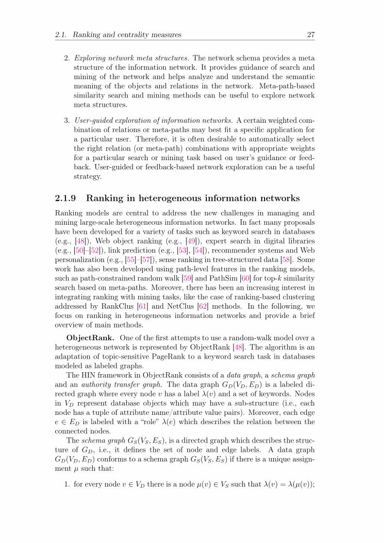
2.1. Ranking and centrality measures 27
2. Exploring network meta structures. The network schema provides a metastructure of the information network. It provides guidance of search andmining of the network and helps analyze and understand the semanticmeaning of the objects and relations in the network. Meta-path-basedsimilarity search and mining methods can be useful to explore networkmeta structures.
3. User-guided exploration of information networks. A certain weighted com-bination of relations or meta-paths may best fit a specific application fora particular user. Therefore, it is often desirable to automatically selectthe right relation (or meta-path) combinations with appropriate weightsfor a particular search or mining task based on user’s guidance or feed-back. User-guided or feedback-based network exploration can be a usefulstrategy.
2.1.9 Ranking in heterogeneous information networks
Ranking models are central to address the new challenges in managing andmining large-scale heterogeneous information networks. In fact many proposalshave been developed for a variety of tasks such as keyword search in databases(e.g., [48]), Web object ranking (e.g., [49]), expert search in digital libraries(e.g., [50]–[52]), link prediction (e.g., [53], [54]), recommender systems and Webpersonalization (e.g., [55]–[57]), sense ranking in tree-structured data [58]. Somework has also been developed using path-level features in the ranking models,such as path-constrained random walk [59] and PathSim [60] for top-k similaritysearch based on meta-paths. Moreover, there has been an increasing interest inintegrating ranking with mining tasks, like the case of ranking-based clusteringaddressed by RankClus [61] and NetClus [62] methods. In the following, wefocus on ranking in heterogeneous information networks and provide a briefoverview of main methods.
ObjectRank. One of the first attempts to use a random-walk model over aheterogeneous network is represented by ObjectRank [48]. The algorithm is anadaptation of topic-sensitive PageRank to a keyword search task in databasesmodeled as labeled graphs.
The HIN framework in ObjectRank consists of a data graph, a schema graphand an authority transfer graph. The data graph GD(VD, ED) is a labeled di-rected graph where every node v has a label λ(v) and a set of keywords. Nodesin VD represent database objects which may have a sub-structure (i.e., eachnode has a tuple of attribute name/attribute value pairs). Moreover, each edgee ∈ ED is labeled with a “role” λ(e) which describes the relation between theconnected nodes.
The schema graph GS(VS, ES), is a directed graph which describes the struc-ture of GD, i.e., it defines the set of node and edge labels. A data graphGD(VD, ED) conforms to a schema graph GS(VS, ES) if there is a unique assign-ment µ such that:
1. for every node v ∈ VD there is a node µ(v) ∈ VS such that λ(v) = λ(µ(v));

28 Chapter 2. User behavior in network science
2. for every edge e ∈ ED from node u to node v there is an edge µ(e) ∈ ESfrom µ(u) to µ(v) and λ(e) = λ(µ(e)).
The authority transfer graph can refer to both a schema graph or a data graph.The authority transfer schema graph GA(VS, EA) reflects the authority flowthrough the edges of the graph. In particular, for each edge in ES two authoritytransfer edges are created, which carry the label of the schema graph edgeforward and backward and are annotated with a (potentially different) authoritytransfer rate. The authority transfer schema graph can be based on a trial anderror process or on a domain expert task.
A data graph conforms to an authority transfer schema graph if it conformsto the corresponding schema graph. From a data graph GD(VD, ED) and aconforming authority transfer schema graph GA(VS, EA) an authority transferdata graph GAD(VD, EAD) can be derived. Edges of the authority transfer datagraph are annotated with authority transfer rates as well, controlled by a for-mula which propagates the authority from a node based on the number of itsoutgoing edges.
ObjectRank can be used to obtain a keyword-specific ranking as well as aglobal ranking. Given a keyword w, the keyword-specific ObjectRank is a biasedPageRank in which the base set is built upon the set of nodes containing thekeyword w:
rw = αArw +1− α|S(w)|
s, (2.39)
where S(w) denotes the base set specific to w, and si = 1 if vi ∈ S(w) andsi = 0 otherwise. The global ObjectRank is basically a standard PageRank.The final score of a node given a keyword w is then obtained by combining thekeyword-specific rank and the global rank.
In [48], Balmin et al. also discussed an optimization of the ranking taskin the case of directed acyclic graphs (DAGs). More specifically, the authorsshowed how to serialize the ObjectRank evaluation over single-pass ObjectRankcalculations for disjoint, non-empty subsets L1, . . . , Lq obtained by partitioningthe original set of vertices in a DAG. Upon a topological ordering of Lh (h = 1..q)that imposes no backlink from every vertex in Lj to any vertex in Li, with i < j,the ranking of nodes is first computed on L1 ignoring the rest of the graph, thenonly the ranking scores of vertices in L1 connected to vertices in L2 are reusedto calculate ObjectRank for L2, and so on.
PopRank. In [49], PopRank is proposed to rank heterogeneous web objectsof a specific domain by using both web links and object relationship links.The rank of an object is calculated based on the ranks of objects of differenttypes connected to it, and a parameter called popularity propagation factor isassociated to every type of relation between objects of different types.
The PopRank score vector rτ for objects of type τ0 is defined as a combina-tion of the individual popularity r and influence from objects of other types:
rτ = αr + (1− α)∑τt
γτtτ0MTτtτ0
rτt (2.40)

2.1. Ranking and centrality measures 29
where γτtτ0 is the popularity propagation factor of the relationship link froman object of type τt to an object of type τ0 and
∑τtγτtτ0 = 1, Mτtτ0 is the
row-normalized adjacency matrix between type τt and type τ0 , and rτt is thePopRank score vector for type τt. In order to learn the popularity propagationfactor γτtτ0 , a simulated annealing-based algorithm is proposed, according topartial ranking lists given by domain experts.
Bipartite SimRank. The SimRank algorithm discussed in Section 2.1.5can naturally be extended to bipartite networks such as, e.g., user-item ratingnetworks. Intuitively, the similarity of users and the similarity of items are mu-tually reinforcing notions that can be formalized by two equations analyticallysimilar to equation (2.28) and equation (2.29). More precisely, assuming thatedges are directed from vertices of type 1 (e.g., users) to vertices of type 2 (e.g.,items), and using superscripts (1) and (2) to denote the two types of vertices,respectively, we have the following equations:
S(u(1), v(1)) = α11
|Ru(1)||Rv(1)|∑
i∈Ru(1)
∑j∈R
v(1)
S(i, j), (2.41)
andS(u(2), v(2)) = α2
1
|Bu(2)||Bv(2)|∑
i∈Bu(2)
∑j∈B
v(2)
S(i, j), (2.42)
where constants α1, α2 have the same semantics as α in equation (2.27). Equa-tion (2.41) corresponds to the similarity between vertices of type-1 is the averagesimilarity between the vertices (of type-2) that they refer to (e.g., items that thetwo users rated), whereas equation (2.42) corresponds to the similarity betweenvertices of type-2 is the average similarity between the vertices (of type-1) thatthey are referred to (e.g., the users who rated the two items).
2.1.10 Ranking-based clustering
Given the diversity of node and link types that characterizes HINs, it is alsoimportant to understand how the various nodes of different types can be groupedtogether. An effective solution is to “integrate” ranking and clustering tasks.This is the basic idea behind methods such as RankClus and NetClus, whichwill be discussed next.
RankClus. In [61], the RankClus algorithm is introduced, which integratesclustering and ranking on a bi-typed information network G = (V,E), such thatV = V0 ∪ V1, with V0 ∩ V1 = ∅. Hence, the nodes in the network belong to oneof two predetermined types, hereinafter denoted as τ0, τ1. The authors use abibliographic network as running example, which contains venues and authorsas nodes. Two types of links are considered: author-venue publication links,with edge weights indicating the number of papers an author has published ina venue, and co-authorship links, with edge weights indicating the number oftimes two authors have collaborated. A formal definition of bi-typed informationnetwork is reported as follows.

30 Chapter 2. User behavior in network science
A key issue in clustering tasks over network objects is that, unlike in tra-ditional attribute based datasets, object features are not explicit. RankClusexplores rank distribution for each cluster to generate new measures for targetobjects, which are low-dimensional. The clusters are improved under the newmeasure space. More importantly, this measure can be further enhanced duringthe iterations of the algorithm, so that the quality of clustering and ranking canbe mutually enhanced in RankClus.
Two ranking functions over bi-typed bibliographic network are defined in [61]:Simple Ranking and Authority Ranking. Simple Ranking is based on the num-ber of publications, which is proportional to the number of papers acceptedby a venue or published by an author. Using this measure, authors publishingmore papers will have higher rank score, even if these papers are all in junkvenues. Authority Ranking is defined to give an object higher rank score if ithas more authority. Iterative rank score formulas for authors and venues aredefined based on two principles: (i) highly ranked authors publish many papersin highly ranked venues, and (ii) highly ranked venues attract many papers fromhighly ranked authors. When considering the co-author information, the rankof an author is enhanced if s/he co-authors with many highly ranked authors.
Differently from Simple Ranking (which takes into account only the neigh-borhood of a node), the score of an object with Authority Ranking is based onthe score propagation over the whole network. Assuming to have an initial (e.g.,random) partition of K clusters {Ck}Kk=1 of nodes of target type τ0 of a bi-typedinformation network, the conditional rank of τ1-type nodes should be very differ-ent for each of the K clusters of τ0-type nodes (e.g., in the bibliographic networkcase, the rank of authors should be different for each venue-cluster). The idea isthat, for each cluster Ck, conditional rank of V1, rV1|Ck
, can be viewed as a rankdistribution of V1 , which in fact is a measure for cluster Ck. Then, for eachnode v ∈ V0, the distribution of object u ∈ V1 can be viewed as a mixture modelover K conditional ranks of V1, and thus can be represented as a K dimensionalvector in the new space [61]. The authors use an expectation-maximizationalgorithm to estimate parameters of the mixture model for each target object,and then define a cosine similarity based distance measure between an objectand a cluster.
Given a bi-typed information networkG = (V0∪V1, E), the ranking functionsfor V0 and V1, and a number K of clusters, RankClus produces K clusters overV0 with conditional rank scores for each v ∈ V0, and conditional rank scores foreach u ∈ V1. The main steps of the RankClus algorithm are summarized asfollows [47].
• Step 0 - Initialization: Assign each target node with a cluster label from1 to K randomly.
• Step 1 - Ranking for each cluster: Calculate conditional ranks for nodesof type V1 and V0 and within-cluster ranks for nodes of type V0. If anycluster is empty, the algorithm needs to restart in order to produce Kclusters.

2.1. Ranking and centrality measures 31
• Step 2 - Estimation of the cluster membership vectors for the target ob-jects: Estimate the parameter of the mixture model, obtain new represen-tations for each target object and centers for each target cluster: sv andsCk
.
• Step 3 - Cluster adjustment: Calculate the distance from each object toeach cluster center and assign it to the closest cluster.
• Repeat Steps 1, 2 and 3 until clusters are stable or change by a very smallratio ε, or until a predefined maximum number of iterations.
NetClus. NetClus [62] extends RankClus from bi-type information net-works to multi-typed heterogeneous networks with a star network schema, wherethe objects of different types are connected via a unique “center” type. An in-formation network, G = (V,E,W ), with T + 1 types of objects such that V ={Vt}Tt=0, has a star network schema if ∀ e = (vi, vj) ∈ E, vi ∈ V0 ∧ vj ∈ Vt(t 6= 0)or vice versa. Type τ0 is called the center or target type, whereas τt(t 6= 0) areattribute types.
Examples of star networks are tagging networks, usually centered on a tag-ging event, and bibliographic networks, which are centered on papers. In gen-eral, a star network schema can be used to map any n-nary relation set (e.g.,records in a relational database, with each tuple in the relation as the centerobject and all attribute entities linking to the center object).
NetClus aims to discover a set of sub-network clusters, and within each clus-ter a generative model for target objects is built given the ranking distributionsof attribute objects in the network. This ranking distribution is calculated usingan authority ranking process based on a power iteration method that combinesthe weight matrices defined between the various types and the center type.The clusters generated are not groups of single typed objects but a set of sub-networks with the same topology as the input network, called net-clusters. Eachnet-cluster is a sub-layer representing a concept of community of the network,which is an induced network from the clustered target objects, and attachedwith statistic information for each object in the network.
NetClus maps each target object, i.e., that from the center type, into aK-dimensional vector measure, where K is the number of clusters specifiedby the user. The probabilistic generative model for the target objects in eachnet-cluster is ranking-based, which factorizes a net-cluster into T independentcomponents, where T is the number of attribute types. NetClus uses the sameranking functions defined for RankClus (Simple Ranking and Authority Rank-ing) adapted to the star network case. The core steps of the NetClus algorithm,given the desired number of clusters K, are summarized as follows [47].
• Step 0: Generate initial partitions for target objects and induce initialnet-clusters from the original network according to these partitions, i.e.,{C0
k}Kk=1.
• Step 1: For each net-cluster, build ranking-based probabilistic generativemodel, i.e., {P (v|Ct
k)}Kk=1.
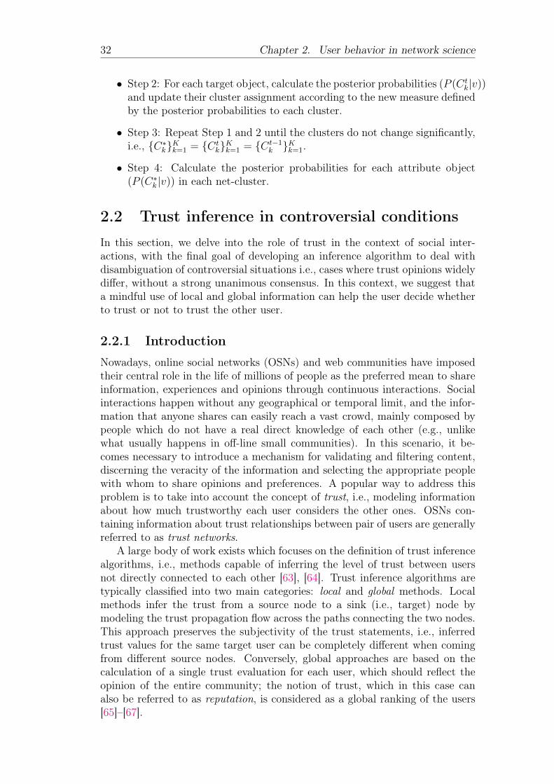
32 Chapter 2. User behavior in network science
• Step 2: For each target object, calculate the posterior probabilities (P (Ctk|v))
and update their cluster assignment according to the new measure definedby the posterior probabilities to each cluster.
• Step 3: Repeat Step 1 and 2 until the clusters do not change significantly,i.e., {C∗k}Kk=1 = {Ct
k}Kk=1 = {Ct−1k }Kk=1.
• Step 4: Calculate the posterior probabilities for each attribute object(P (C∗k |v)) in each net-cluster.
2.2 Trust inference in controversial conditionsIn this section, we delve into the role of trust in the context of social inter-actions, with the final goal of developing an inference algorithm to deal withdisambiguation of controversial situations i.e., cases where trust opinions widelydiffer, without a strong unanimous consensus. In this context, we suggest thata mindful use of local and global information can help the user decide whetherto trust or not to trust the other user.
2.2.1 Introduction
Nowadays, online social networks (OSNs) and web communities have imposedtheir central role in the life of millions of people as the preferred mean to shareinformation, experiences and opinions through continuous interactions. Socialinteractions happen without any geographical or temporal limit, and the infor-mation that anyone shares can easily reach a vast crowd, mainly composed bypeople which do not have a real direct knowledge of each other (e.g., unlikewhat usually happens in off-line small communities). In this scenario, it be-comes necessary to introduce a mechanism for validating and filtering content,discerning the veracity of the information and selecting the appropriate peoplewith whom to share opinions and preferences. A popular way to address thisproblem is to take into account the concept of trust, i.e., modeling informationabout how much trustworthy each user considers the other ones. OSNs con-taining information about trust relationships between pair of users are generallyreferred to as trust networks.
A large body of work exists which focuses on the definition of trust inferencealgorithms, i.e., methods capable of inferring the level of trust between usersnot directly connected to each other [63], [64]. Trust inference algorithms aretypically classified into two main categories: local and global methods. Localmethods infer the trust from a source node to a sink (i.e., target) node bymodeling the trust propagation flow across the paths connecting the two nodes.This approach preserves the subjectivity of the trust statements, i.e., inferredtrust values for the same target user can be completely different when comingfrom different source nodes. Conversely, global approaches are based on thecalculation of a single trust evaluation for each user, which should reflect theopinion of the entire community; the notion of trust, which in this case canalso be referred to as reputation, is considered as a global ranking of the users[65]–[67].
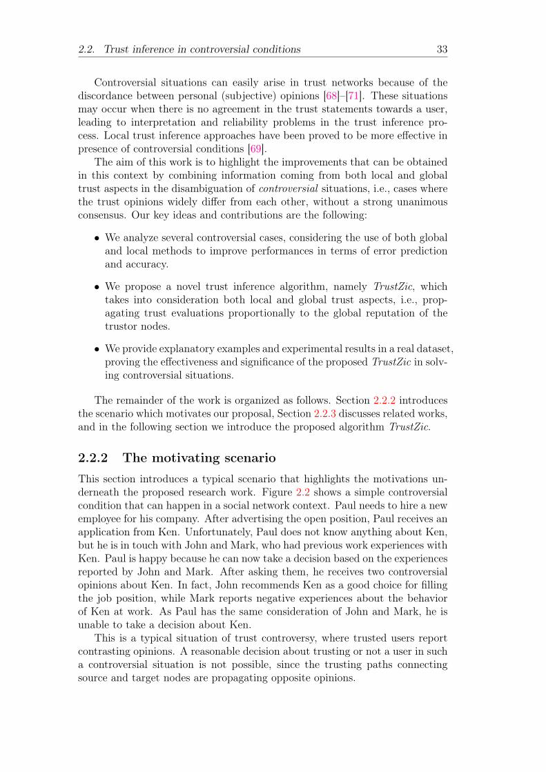
2.2. Trust inference in controversial conditions 33
Controversial situations can easily arise in trust networks because of thediscordance between personal (subjective) opinions [68]–[71]. These situationsmay occur when there is no agreement in the trust statements towards a user,leading to interpretation and reliability problems in the trust inference pro-cess. Local trust inference approaches have been proved to be more effective inpresence of controversial conditions [69].
The aim of this work is to highlight the improvements that can be obtainedin this context by combining information coming from both local and globaltrust aspects in the disambiguation of controversial situations, i.e., cases wherethe trust opinions widely differ from each other, without a strong unanimousconsensus. Our key ideas and contributions are the following:
• We analyze several controversial cases, considering the use of both globaland local methods to improve performances in terms of error predictionand accuracy.
• We propose a novel trust inference algorithm, namely TrustZic, whichtakes into consideration both local and global trust aspects, i.e., prop-agating trust evaluations proportionally to the global reputation of thetrustor nodes.
• We provide explanatory examples and experimental results in a real dataset,proving the effectiveness and significance of the proposed TrustZic in solv-ing controversial situations.
The remainder of the work is organized as follows. Section 2.2.2 introducesthe scenario which motivates our proposal, Section 2.2.3 discusses related works,and in the following section we introduce the proposed algorithm TrustZic.
2.2.2 The motivating scenario
This section introduces a typical scenario that highlights the motivations un-derneath the proposed research work. Figure 2.2 shows a simple controversialcondition that can happen in a social network context. Paul needs to hire a newemployee for his company. After advertising the open position, Paul receives anapplication from Ken. Unfortunately, Paul does not know anything about Ken,but he is in touch with John and Mark, who had previous work experiences withKen. Paul is happy because he can now take a decision based on the experiencesreported by John and Mark. After asking them, he receives two controversialopinions about Ken. In fact, John recommends Ken as a good choice for fillingthe job position, while Mark reports negative experiences about the behaviorof Ken at work. As Paul has the same consideration of John and Mark, he isunable to take a decision about Ken.
This is a typical situation of trust controversy, where trusted users reportcontrasting opinions. A reasonable decision about trusting or not a user in sucha controversial situation is not possible, since the trusting paths connectingsource and target nodes are propagating opposite opinions.

34 Chapter 2. User behavior in network science
Paul
John
Ken
Mark
Trusts
Trusts Does not trust
Trusts
Figure 2.2: A typical trust controversy case: it is not possibleto infer whether or not Paul should trust Ken.
The main idea of our proposed approach to solve this problem is to exploitinformation from the rest of the trust network in order to find a way for solv-ing the controversial situation. To this purpose, it is necessary to introduce acriterion of discernment. The most natural way to differentiate the reportedtrust opinions is to give a different weight depending on the reputation of thetrustors. In fact, each user has a different influence with respect to the rep-utation built in the specific context. The reputation influences the way theopinions, suggestions and recommendations are considered.
Figure 2.3 reports an extended version of the previous example, where thefocus is broadened to include more the network. In this case, the global rep-utation of the nodes can be used to take a reasonable decision about whetherPaul should or should not trust Ken. The extended scenario shows that Johnis trusted by all his in-neighbors, while Mark received both trust and no-truststatements: in this condition it is clear that John has a higher reputation thanMark. After considering the different reputations of John and Mark, Paul de-cides to take a final resolution about Ken. In fact, Paul finds that the reputationof John is much higher than that of Mark, so he decides to consider the opin-ion coming from John more reliable, and finally hires Ken. According to thereported considerations, in the proposed approach the reputation will be usedas a discerning weighting factor in controversial situations.
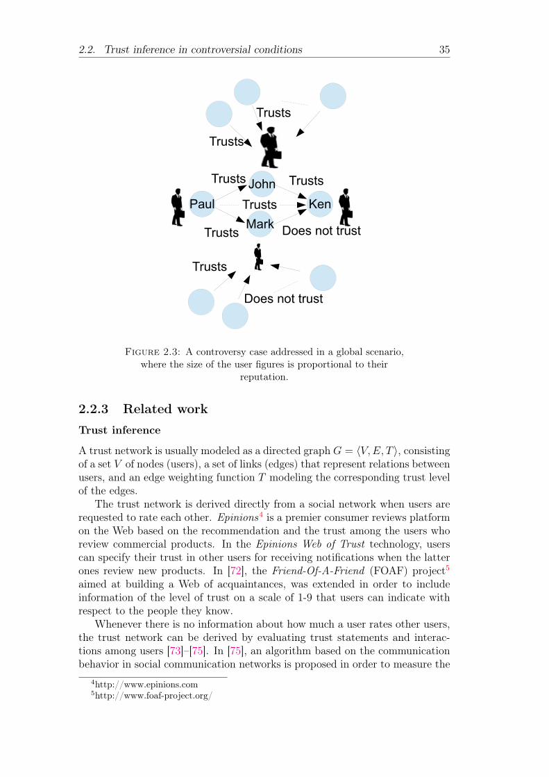
2.2. Trust inference in controversial conditions 35
Paul
John
Ken
Mark
Trusts
Trusts Does not trust
Trusts
Trusts
Trusts
Trusts
Does not trust
Trusts
Figure 2.3: A controversy case addressed in a global scenario,where the size of the user figures is proportional to their
reputation.
2.2.3 Related work
Trust inference
A trust network is usually modeled as a directed graph G = 〈V,E, T 〉, consistingof a set V of nodes (users), a set of links (edges) that represent relations betweenusers, and an edge weighting function T modeling the corresponding trust levelof the edges.
The trust network is derived directly from a social network when users arerequested to rate each other. Epinions4 is a premier consumer reviews platformon the Web based on the recommendation and the trust among the users whoreview commercial products. In the Epinions Web of Trust technology, userscan specify their trust in other users for receiving notifications when the latterones review new products. In [72], the Friend-Of-A-Friend (FOAF) project5aimed at building a Web of acquaintances, was extended in order to includeinformation of the level of trust on a scale of 1-9 that users can indicate withrespect to the people they know.
Whenever there is no information about how much a user rates other users,the trust network can be derived by evaluating trust statements and interac-tions among users [73]–[75]. In [75], an algorithm based on the communicationbehavior in social communication networks is proposed in order to measure the
4http://www.epinions.com5http://www.foaf-project.org/

36 Chapter 2. User behavior in network science
trust among users. The trust is measured by quantifying the behavior in termsof length and frequency of communications, and propagation of informationamong users. Experiments were conducted on Twitter, where the mechanism ofretweet was used for measuring the trust contribution coming from propagation.
The purpose of a generic trust inference algorithm IT is to compute a pre-diction of the trust from a source node u to a sink node v when there is nodirect link between the two nodes, i.e., (u, v) /∈ E. Obviously, there is noneed to calculate a prediction when an explicit trust statement was issued,i.e., IT (u, v) = T (u, v) if (u, v) ∈ E. Several trust inference algorithms havebeen proposed in literature for prediction purposes with different characteris-tics and performances. The trust inference algorithms can be classified intotwo main categories: global and local methods [76]. Global algorithms computean overall evaluation, here commonly named reputation, for each user of thetrust network; thus, the reputation can be considered as the synthesis of thetrust evaluations from the entire network with respect to a single user. Thewell-known PageRank [77] can be considered as a basis for the development ofglobal trust methods [65].
Nevertheless, global trust inference methods are not suited to preserve thecharacteristic of personalization in the subjective expression of an opinion,which can instead be achieved by using local trust inference algorithms. One ofthe most popular local trust inference algorithms is TidalTrust [76], which com-putes the trust between non-adjacent nodes by considering only shortest pathsthrough trusted neighbors. Another local method is proposed in [78], namelyTISoN (Trust Inference within online Social Networks). In this case a selectionof the trust paths from a source node to a sink node is performed with respectto two criteria: the maximum allowed depth of the path, and the minimumthreshold level allowed for the trust edges in the path. Then the inferred trustis computed selecting the most trustable path, based on the average of the trustedges in the path, the path variance of the trust edges w.r.t. the average, and apath weight based on its length. As regards other approaches, a detailed surveyof trust inference algorithms in literature is presented in [64].
Trust controversy
As trust statements reflect subjective opinions built on personal experiences, itis often the case that users report contrasting and different trust opinions aboutthe same target. When trust statements differ too much from each other, it be-comes challenging to derive affordable inferred trust information. The presenceof controversial conditions makes the trust inference problem more complex toaddress. Thus, the identification of controversial conditions requires to be ex-plicitly taken into account when dealing with trust networks. The concept ofcontroversy in trust networks has been widely studied in literature [68]–[71].
In [68], the controversy is referred to as single users that are trusted anddistrusted by many, i.e., without a global agreement as regards their trustwor-thiness. The level of controversy for a generic user u is defined by two metrics,controversiality level (cl) and controversiality percentage (cp) as follows:
cl(u) = min(#rt(u),#rd(u)) (2.43)

2.2. Trust inference in controversial conditions 37
cp(u) =#rt(u)−#rd(u)
#rt(u) + #rd(u)(2.44)
where the received trust (#rt) and the received distrust (#rd) represent thenumber of trust and distrust edges to the node u, respectively.
Controversy was studied by [70] and [79] in the context of recommendersystems, where controversial reviews are defined as those reviews that receivea variety of high and low scores, reflecting disagreement about reviews. Thosestudies introduced a measure of controversy in terms of standard deviation σof the reviews of an item i and the level of disagreement α defined as follows:
α(∆, i) = 1− maxα∈{1,...,m−∆+1}
(
∑a+∆−1s=a fi(s)∑ms=1 fi(s)
) (2.45)
where ∆ is the level of a discrete rating scale from 1 to m, and fi(s) is thenumber of times that the item i received a rating of score s.
In this work, we will use the metric proposed in [71] in order to evaluate thecontroversy of the trust inferred from a source node A to a generic sink node Z.The main idea is to consider the controversy as the variance among the trustopinions of the predecessors of the source nodes. To this purpose, the meantrust TM(A,Z) is calculated as follows:
TM(A,Z) =
∑Pi∈Pred(Z) IT (A,Pi)× T (Pi, Z)∑
Pi∈Pred(Z) IT (A,Pi)(2.46)
where Pred(Z) is the set of predecessors of the node Z, IT indicates the inferredtrust values and T the original trust weights.
According to Equation 2.46, the mean trust is the weighted average of thetrust values assigned by the predecessors Pi of node Z, where the weights arethe inferred trusts from the source node A to the predecessor nodes Pi. As thecontroversy measure is related to the level of discordance among the differenttrust opinions reported to the source node through the trust chains up to thesink node, the controversy measure TC(A,Z) is defined as the weighted varianceof the inferred trust paths, as reported in the following:
TC(A,Z) =
∑Pi∈Pred(Z)
IT (A,Pi)× (T (Pi, Z)− TM(A,Z))2
∑Pi∈Pred(Z)
IT (A,Pi)(2.47)
The normalized trust controversy measure (NTC), introduced to bring TCinto the range [0, 1], can be computed as follows:
NTC(A,Z) =TC(A,Z)
((Tmax− Tmin)/2)2(2.48)
where Tmin and Tmax are the extremes of the trust range.
38 Chapter 2. User behavior in network science
Local vs. global methods
How global and local methods should be used to solve different trust inferenceproblems was widely explored in [80]. An interesting comparison of local andglobal trust metrics is reported in [68], where the characteristics of the twoapproaches are argued in detail. Results on real datasets proved that globalmethods show intrinsic limit when controversial users (i.e. users judged in dif-ferent ways by other users) are analyzed, while local methods are more suitablein contexts where opinions are more subjective like in the controversial condi-tions. The study in [69] showed how local trust metrics outperform global oneswhen predicting the trustworthiness of users characterized by both trust anddistrust evaluations.
The idea of improving the performance of prediction systems by exploitingboth global and local trust metrics is not new in literature. A hybrid global-local method was introduced by [81] in the context of service recommendationsystems. The scenario depicted in [81] is different from the one discussed in thiswork, as it considers a recommendation system consisting of different servicesrated by users integrated with a trust network. The trust network is used tosupport the computation of the personalized rating prediction PT (u, s) of aservice s from a user u as the weighted average reported in Equation 2.49 of theglobal r(s) and local T (u, s) rating evaluation of the service s, where wl andwr are the weights used for properly tuning the local and global contributions,respectively:
PT (u, s) =r(s)× wr + T (u, s)× wl
wr + wl(2.49)
The promising results obtained by exploiting both global and local per-spectives in recommendation systems have encouraged us to investigate howcombining the two approaches can be beneficial for improving the performanceof trust inference algorithms in controversial conditions.
2.2.4 The TrustZic algorithm
The proposed trust inference method, namely TrustZic, aims at solving prob-lems arising when trying to infer trust values in controversial cases, by exploit-ing global and local trust information in a combined solution. In the proposedapproach, the level of trust inferred from the source to the sink will still bepersonalized because it depends on the propagation of trust along the pathsbetween the source and the sink across the trust graph. Nevertheless, the nodesin the traversed paths are not equally considered, but they exert a different biason the trust propagation, i.e., proportional to their reputation which is obtainedby applying a global trust method.
Figure 2.4 shows the main steps of the TrustZic approach: in the first stepa global ranking is calculated from the trust graph in order to get a reputationvalue r(i) for each node i. The trust-reputation network is obtained from thetrust network by adding the reputation information on the nodes. In the secondstep, the trust between nodes not directly connected in the trust network isinferred. The trust inference method propagates the trust from the source node

2.2. Trust inference in controversial conditions 39
to the sink through the trust paths weighted based upon the reputation ofeach node traversed across the path. The resulting trust inference network is acomplete graph in which nodes are connected by trust relations (solid edges) orinferred trust relations (dashed edges). In the following, we will give detailedinformation on how we perform these steps.
Step 1: computation of the global trust values. A PageRank -likealgorithm is here used to implement the first step of the proposed method (i.e.,obtaining the global ranking of all the nodes in the network). The stochasticmatrix M is obtained as the transpose and normalized version of the trustmatrix T , as shown in (2.50).
M [i, j] =T [j, i]∑
k∈adj(j)T [j, k]
(2.50)
The vector r of reputations for all the N nodes is calculated as in (2.51),where α is a smoothing factor (by default set to 0.85) and p is the column vectorwith the initial reputation value (by default p = 1, i.e., the column vector ofones).
r = αMr +1− αN
p (2.51)
We then adopt the final PageRank solution (i.e., vector of the stationarydistribution of PageRank scores at convergence) to assign reputation values tothe nodes in the network. However, this can be thought of as a general workflow,where different global ranking methods can be used in theory at this step.
Step 2: local trust inference propagation. The second step consistsin propagating the trust from a source node to a sink node by taking intoconsideration not only the trust T but also the reputation r. The inferred trustIT (i, j) from the source node i to the sink node j is computed as reported in(2.52), where d ∈ (0, 1] is the decay trust factor, introduced for modeling thefact that the trust generally decreases when increasing the distance from thesource node.
IT (i, j) =
T (i, j) if there is a direct trust∑k∈neighbor(i)
r(k)×d×T (i,k)×IT (k,j)∑k∈neighbour(i)
r(k)×T (i,k)otherwise (2.52)
In order to disambiguate controversy, trust is propagated from the sourcenode through all the different paths reaching the sink node, without excludingthe contribution of low trusted paths. Starting from the source node, the trustinference is calculated by averaging the trust (direct or inferred) for the sinknode reported by all the directly connected trusted nodes (neighbors). More indetail, the aggregation of the trust coming from the different paths is obtainedas a weighted average, where the reported trust is weighted by the reputation ofthe neighbors. The trust inference function is recursively computed along thepaths in order to propagate the trust up to the target node.

40 Chapter 2. User behavior in network science
A
T(A,C)
B
C
T(A,B)
D
E
T(B,D)
T(B,E)
T(C,E)
Reputation
A
T(A,C)
B
C
T(A,B)
D
E
T(B,D)
T(B,E)
T(C,E)
r(A)
r(B) r(E)
r(C)
r(D)
Trust network
Trust–Reputation network
Trust Inference
A
T(A,C)
B
C
T(A,B)
D
E
T(B,D)
T(B,E)
T(C,E)
r(B) r(E)
r(C)
r(D) Trust Inference network
IT(A,D)
IT(A,E) r(A)
Figure 2.4: Main steps of the TrustZic algorithm.

2.2. Trust inference in controversial conditions 41
Handling controversial cases with TrustZic
In this section we will give some preliminary numerical examples in order toshow how TrustZic is able to address controversial cases by exploiting the rep-utation of the intermediate nodes. We consider a trust range TR = [0, 1], sothat T (i, j) ∈ [0, 1] ∀(i, j) ∈ E. T (i, j) = 1 means that user i fully trusts userj, while T (i, j) = 0 means lack of trust.
For the sake of simplicity and to isolate the reputation effect, only in thisexplanatory example, all the trust opinions will be considered equal to 1, whilethe lack of trust is uniformly considered equal to 0, and the effect of the trustdecay with the path length is neglected (d = 1).
Figures 2.5, 2.6 and 2.7 show three different controversial cases. In the firstcase (Fig. 2.5), a node Z receives two opposite trust opinions from nodes B andC, propagated up to node A. In this case, the reputation of nodes B and C isthe same due to the symmetric configuration, thus the resulting inferred trustis exactly the mean of the two reported trust opinions (IT (A,Z) = 0.5).
This is a critical situation when trust inference is used to make decisions.In fact, trust inference can be used as a decision support system by setting atrust threshold value for delimiting the trusting by the no-trusting zones. Ageneric node X decides to trust another node Y only if the inferred trust fromthe network is above a fixed threshold. In this specific example, if the thresholdis reasonably set to the intermediate value (Thres = 0.5) of the [0, 1] trustrange, no decisions can be taken because the inferred trust is exactly equal tothe threshold (IT (A, Z ) = 0.5 = Thres).
The second and the third cases (Figures 2.6 and 2.7) consider the connectionsof the rest of the trust network with nodes B and C, and their effects on theirreputation. In the second case, the reputation of node B is higher (r(B) = 0.28)than that of C (r(C ) = 0.13) because of the two nodes (D and E ) trustingB. In the third case, the reputation of node C is further decreased (r(C ) =0.12) as a consequence of the 0-trust inner edge from (F ). The effects of thereputation changes become relevant for the resolution of the controversial casein the inferred trust between nodes A and Z. In fact, in the cases reported inFigures 2.6 and 2.7, the inferred trust allows to easily take decisions: node Awill trust node Z because the reputation of node B, reporting a positive opinion,is higher than that of node C, reporting a lack of trust opinion.

42 Chapter 2. User behavior in network science
A
T(A,C) = 1
B
C
Z
T(A,B) = 1 T(B,Z) = 1
T(C,Z) = 0
r(B) = 0.23
r(C) = 0.23
IT(A,Z) = 0.5 = Thres
Figure 2.5: An undecidable controversial case.
A
T(A,C) = 1
B
C
Z
T(A,B) = 1 T(B,Z) = 1
T(C,Z) = 0
r(B) = 0.28
r(C) = 0.13
IT(A,Z) = 0.69 > Thres
D E
T(D,B) = 1T(E,B) = 1
Figure 2.6: The controversial case resolved by TrustZic dueto the increased reputation of node B.
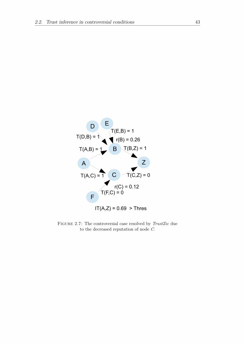
2.2. Trust inference in controversial conditions 43
A
T(A,C) = 1
B
C
Z
T(A,B) = 1 T(B,Z) = 1
T(C,Z) = 0
r(B) = 0.26
r(C) = 0.12
IT(A,Z) = 0.69 > Thres
D E
T(D,B) = 1T(E,B) = 1
FT(F,C) = 0
Figure 2.7: The controversial case resolved by TrustZic dueto the decreased reputation of node C.
44 Chapter 2. User behavior in network science
2.3 ConclusionTrust regulates relations among people, in offline relations as well as in onlinesocial networks and web communities, where the interaction among users inthe absence of any direct connection can easily happen. In this context, trustinference algorithms are a fundamental tool to estimate missing trust evalu-ations. Controversial situations caused by disagreement in the existing truststatements towards a user need to be specifically taken into account during theinference process. The trust inference algorithm TrustZic, in which global andlocal trust aspects are combined to infer reliable trust values also in presence ofcontroversial situations, has shown significance and effectiveness of its approachin solving critical trust inference scenarios (experimental results can be foundat [71]).

45
Chapter 3
Alternate behaviors in multilayersocial networks
3.1 IntroductionOnline user behaviors have been traditionally investigated in function of therole(s) that a user takes as a member of a single web-based social environment.This often corresponds to focusing on online social networks (OSNs) that arebuilt on a single type of user relation type (e.g., followship, liking/rating, com-menting) or platform context. However, nowadays it is naturally occurring thatan individual has multiple accounts across different OSNs. This makes it impor-tant to link distributed user profiles belonging to the same user from multipleplatforms, which can be beneficial for several applications; for instance, per-sonalized Web services such as recommendation systems can take advantage ofthe aggregation of user profiles to alleviate the cold-start problem. A furtherscenario comes out by considering that real-life relations (e.g., working relation-ship, having lunch, etc.) can be available for the same population of an OSN,and hence they should be profitably exploited to enhance our understanding ofthe individuals and their relations in an OSN [82].
The above scenarios and furthermore others correspond to complex real-world network systems, which are indeed pervasive in many fields of science.Such systems can effectively be studied using a multilayer network model, whichespecially in social computing, has been recognized as a powerful tool to better(i.e., more realistically) understand the characteristics and dynamics of different,interconnected types of user relations [82]–[84].
3.1.1 Motivations
The dichotomy between production and consumption of resources inOSNs. Regardless of the peculiarities of the scenarios above discussed, theintrinsic complexity of a multilayer network system, in which users and theirrelations are represented, inevitably impacts on the motivational factors thatultimately determine the users’ behavioral profiles. According to the unifiedmodel proposed in [85], there are essentially four categories of factors influenc-ing user behaviors: environmental factors — which affect the user’s feeling ofthe community and therefore influences the user’s willingness to spend time orto contribute to the community; commitment factors and quality requirement

46 Chapter 3. Alternate behaviors in multilayer social networks
factors — which are based on the relationship between the users and the com-munity; and, of course, individual factors — which refer to the personalities ofthe users and their purpose of joining the community, such as needs and ex-pectations, but also self-efficacy, extroversion/introversion, self-disclosure, etc.Through the combination of these factors, the resulting online behaviors can beanalyzed from three broad perspectives: the development and spread of com-munity norms, the contribution of valuable resources, and the consumption ofresources.
Let us focus on the dichotomy between contribution and consumption ofinformation resources. In this respect, depending on one or many of the influ-encing factors discussed above, the same user may take different roles in termsof contribution and consumption of resources. This is even more intuitive in amultilayer network context, where each layer corresponds to a distinct socialenvironment that might significantly differ from that of the other layers. Forinstance, consider a multilayer network representing users that are membersof many OSNs: it is not surprising that a user can frequently post contentsand/or actively interact with other users in one or more layer OSNs, and on thecontrary, s/he may be less involved in tangible participation and interactionswith other members, thus assuming a silent behavior on other OSNs. Generallyspeaking, in the first case the user is producing resources, while in the othercase s/he is rather consuming resources. Here we leave out of consideration theinactivity status, since users that are subscribers of an OSN without accessing itshould not be considered as real members of the underlying online community.
The value of lurkers. Unlike inactive users, silent users actually gainbenefit from the community, since they observe the user-generated communica-tions though rarely visibly participating in them and contributing informationthemselves. For this reason, they are also called as lurkers. Lurking behaviorshave been widely studied in social science, and the importance of analyzing itas a valuable form of online behavior has been definitively recognized [85], [86].Moreover, lurking is strictly related to legitimate peripheral participation tolearn the netiquette and social norms [87], individual information strategy ofmicrolearning [88] and knowledge sharing barriers [89], individual motivationfor interpersonal surveillance [90]. According to the model by [85] previouslymentioned, reasons for lurking include environmental influence (e.g., bad usabil-ity/interaction design, information overload, low response rate, low reciprocity),personal aspects (e.g., introversion, bashfulness, lack of self-efficacy, no need topost – only seeking for information), lack of commitment to the community (e.g.,low verbal and affective intimacy with others, unwillingness to spend too muchtime to maintain a commitment), or security concerns (e.g., worrying aboutthe violation of private information, perception of poor quality requirements ofsecurity). The latter aspect is particularly crucial as related to the challengingdesign of defense strategies in the cyberspace, especially of social network plat-forms whose common habit is rather to encourage their users to self-disclosetheir personal information. In fact, as studied in [91], lurking can be explainedas a conservative communication strategy adopted by users to protect their per-sonal information while, in the form of passive participation, still connected inonline communities; also, users having lack of computer self-efficacy may resort
3.1. Introduction 47
to lurking, thus keeping themselves as part of the online communications butwithout causing any harm to themselves or to members of their social network.
The coexistence of contributor and lurker behaviors. By gettinginformation from other members of an OSN, lurkers become aware of the ex-istence of different perspectives and may make use of these perspectives inorder to form their own ideas, opinions, and even competence. Therefore, lurk-ers have the potential of exploiting the acquired knowledge outside their ownOSN. On the other hand, when users decide to contribute to the communityby performing a social action, often they may have formed their decision fromexogenous sources of ubiquitous and/or specialist knowledge. In this regard,social boundary spanning theory [92], [93] explains how OSN users may natu-rally get knowledge from some of their social contacts and span it from one ormore components to others in the network. A key role is played by those usersthat lay on the boundary of a component and act as bridges over other com-ponents. Relations have been studied not only between bridges and influentialcontributor users (e.g., [94]–[96]), but also between lurkers and bridges. Forinstance, Morales et al. [95] highlight the importance of bridges in spreadingmessages throughout a Twitter network organized into an event-driven commu-nity structure, where information-producers are found to create communitiesof information-consumers around them. In our previous work [97], we explainthe relation between lurkers and community bridges identified through perco-lation analysis based on directed topological overlap. In another study [98],lurkers are found more likely to acquire information from outside their owncommunity than to spread information towards other communities; this findingis also complementary to an important result of the application of an influence-maximization method of lurker engagement developed in [98], whereby activeusers who might help in engaging lurkers could be identified among membersof communities external to those of lurkers. Major principles underlying thesocial boundary spanning theory can also be extended to a multilayer network,where the layers correspond to the boundaries in the complex system.
Following the above intuition, in this work we focus on the understandingof the knowledge flow across different layers of a complex network, from theperspective of both contributors and lurkers. Given the different contingenciesoccurring in the various layers and, consequently, the different behavioral pro-files the same user can have therein, we leverage the importance of studyingthe behavior of users which may alternately take the role of contributors andlurkers over different layer networks.
Applications. The analysis of such alternate behaviors is of crucial im-portance in order to deeply understand how information and knowledge areproduced, consumed, and shared through multiple OSNs. We believe that thedevelopment of effective methods for the problem under consideration can sup-port several classes of applications. One of these concerns information filteringand propagation for advertising, marketing campaigns and related applications.For instance, in tasks of influence maximization [99], we can reasonably assumethat contributors are candidates to be selected as initial influencers (i.e., seedusers), and lurkers as potential targets of the information to be propagated;in a multilayer context, in order to invest on a more socially diversified set of
48 Chapter 3. Alternate behaviors in multilayer social networks
promoters, it would be useful to learn the seeds not only among the (indirect)social contacts of a target in a layer network, but also among her/his contactsover other layers. Analogously, the identification of users that may consumeinformation from a specific network and subsequently spread it across differentplatforms would also be beneficial in campaigns of information containment.This is also important for security reasons, e.g., to control that specific (e.g.,sensitive) information be shielded from certain users, to cope with the diffusionof fake news through different web sources, etc.
Another class of applications concerns user engagement. OSNs encourageusers to self-disclose their own opinions and actively contribute to the com-munity life. This requires the development of so-called “delurking” strategies,such as providing rewards (i.e., grants to be offered to the users for their activecontributions to the community) [100], enhancing users’ commitment to thecommunity [101], making lurkers understand the necessity of their contribu-tion [102], learning or improving usability of the system [103]. Generalizing toa complex system, valuable indications might be provided from the platform(s)on which a user is an active contributor to tailor a suitable strategy for engagingher/him on other platforms.
From a broader perspective, identifying alternate behaviors in multiple OSNcontexts can be a key tool to enhance the development of effective communica-tion strategies through different online social environments, and ultimately toface challenges in today’s knowledge management systems that concern users’motivations for online participation in different forms (i.e., active vs. passiveparticipation).
3.1.2 Contributions
In this work, we address the novel problem of identifying and characterizingusers who alternately behave as contributors and as lurkers over multiple layernetworks in a complex system.
To the best of our knowledge, we are the first to study the dichotomy betweeninformation-producers (i.e., contributors) and information-consumers (i.e., lurk-ers) and their interplay over a multilayer network. To support this claim of nov-elty, note that while research on the identification and ranking of contributorsand users with related roles (i.e., influencers, leaders, experts, etc.) in multilayernetworks has recently gained momentum (e.g., [83], [84], [104]–[108]), none ofthese studies addresses problems of analysis of opposite and alternately occur-ring behaviors. Moreover, computational approaches to the analysis of lurkingbehaviors have been developed only for monoplex networks [97], [98], [109]–[112]. By contrast, in this work, we take into consideration both behavioral“opposites”, leveraging on their duality and possible, “alternate” manifestationsover many, interconnected layers of the same complex network system. This rep-resents a major novelty aspect of our approach, which introduces a previouslyunexplored notion of centrality or prominence in multilayer network that caneffectively be used to support emerging and challenging applications in complexnetwork systems, as previously discussed in Sect. 3.1.1.
3.2. Related Work 49
Our proposed approach is devised in terms of a twofold, mutually reinforcingranking model, which can capture the interplay of the two behavioral roles overa multilayer network. The meaning of “alternate” stands for the contingencythat the behavior of the same user can be regarded as lurking in one layer andas active participation in one or many of the other layers, or vice versa. Weformally define the alternate lurker-contributor behavior status of any node ina multilayer network, conditionally to a given layer, following interrelated prin-ciples of cross-layer lurker behavior and cross-layer contributor behavior. Uponthis, the proposed Alternate Lurker-Contributor Ranking method (mlALCR) ismathematically expressed as two mutually dependent equation systems, whereone system determines the layer-specific lurking score and the other system de-termines the layer-specific contributor score for all nodes in the interconnectedlayers of the complex network.
Our mlALCR has been extensively evaluated on four real-world multilayernetworks, specifically two cross-platform user multi-relational networks, a single-platform user multi-relational network, and a single-platform temporal multi-slice network. We assessed significance and meaningfulness of mlALCR bothquantitatively and qualitatively. Experimentation also includes comparison ofmlALCR with the basic (i.e., monoplex) lurker ranking method, its extension tomultilayer networks — originally proposed in this work — ranking aggregationmethods, and the Multiplex PageRank method. Results show the unique abil-ity of mlALCR to effectively determine the two behavioral opposites in termsof information-production and information-consumption that a user may takeover different layers of a complex network.
The remainder of this chapter is organized as follows. Section 3.2 brieflydiscusses related work, focusing on approaches to the measurement of nodecentrality in multilayer networks. Section 3.3 introduces to the identificationof contributors in multilayer networks and the analysis of lurking behaviors.Section 3.4 is devoted to our proposed mlALCR method. Sections 3.5 and 3.6present experimental methodology and results. Section 3.7 concludes the chap-ter.
3.2 Related WorkThe notion of centrality commonly resembles the importance or prominenceof a node in a network, i.e., the status of being located in strategic locationswithin the network. Concerning multilayer networks, we can distinguish twomain approaches in the literature, which mainly differ from each other in theway they handle the additional complexity introduced by inter-layer edges. Oneapproach is based on some strategy of aggregation, i.e., projection of the mul-tilayer network to a single aggregated layer or aggregation of layer-wise resultsindependently generated. The other approach comprises techniques which aredesigned to take into account both intra- and inter-layer connections.
Aggregation and projection-based approaches. Brodka et al. proposea definition of degree centrality for multilayer networks in [113]. The cross-layerdegree centrality of a node v is measured as proportional to the weighted sum ofedges connecting v with the members of its multilayered neighborhood, which is

50 Chapter 3. Alternate behaviors in multilayer social networks
the set of nodes directly connected with v on at least a certain number of layers.In [106], De Domenico et al. study main factors influencing the navigability ofmultilayer networks, using random walks over a layer-aggregated network. Theauthors find that navigability is influenced by both structural characteristicsand exploration strategies, and that a multilayer network is more resilient torandom failures than the single layers separately. In general, when dealingwith centrality scores produced at distinct layer networks, the use of differentaggregation and normalization techniques is shown to strongly bias the finalresults [114].
Cross-layer approaches. Sole et al. [105] define a multilayer extension ofthe betweenness centrality by taking into account shortest paths which includeinter-layer edges. This measure is shown to favor nodes which act as bridges be-tween layers, allowing to connect individuals which are disconnected inside thelayers. A cross-layer betweenness centrality is proposed in [115], also includ-ing applications of the proposed measure to multilayer community detectionand message spreading tasks. Two classes of multilayer degree-biased randomwalks are proposed in [116], in order to analyze to what extent this kind ofrandom walks can make the exploration of multilayer networks more efficient.The two classes refer to extensive walkers (i.e., biased w.r.t. node propertiesindependently considered for each layer) and intensive walkers (i.e., the bias isproportional to intrinsically multilayer features, as the overlapping degree andthe participation coefficient). Kuncheva and Montana [117] also employ multi-layer random walks for community detection purposes. Their method utilizesinter-layer transition probabilities that depend on local topological similaritybetween corresponding nodes, in order to facilitate the discovery of cross-layercommunities. A hierarchical clustering method is finally used to produce thecommunities based on the outcome of a random walk process. An importantmention here regards the multilayer extension of the well-known PageRank al-gorithm proposed in [104], which we shall discuss in detail in Sect. 3.3.2 and thatwill be used as one of the competing methods in our experimental evaluation.
It should be noted that all the aforementioned approaches are either exten-sion of classic centrality measures to a multilayer context [105], [113], [115], orapproaches which exploit random walk models on multilayer networks to extendeigenvector centrality [104], [116] or to use it for specific tasks (e.g., communitydetection [115], [117]). By contrast, we propose a new ranking method explic-itly designed to model opposite behaviors and their interplay over the multiplelayers of a complex network system, leveraging information coming from userinteractions through the different layers.
3.3 Lurker and contributor behaviors in multi-layer networks
3.3.1 Multilayer network model
Let L = {L1, . . . , L`} be a set of layers, with size equal to or greater than two.Each layer corresponds to a particular user relational context. Given a set V

3.3. Lurker and contributor behaviors in multilayer networks 51
of entities (i.e., users), for each choice of user in V and layer in L, we need toindicate whether the user is present in that layer. We denote with VL ⊆ V × Lthe set containing the user-layer combinations (i.e., tuples) in which a user ispresent in the corresponding layer. The set EL ⊆ VL× VL contains the directedlinks between user-layer tuples. Note that, when all layers refer to the sameaspect or dimension (e.g., same temporal dimension, same group of interactions,etc.) like in our setting, the elements in VL simply correspond to pairs 〈node,layer〉. We hence denote with GL = (VL, EL,V ,L) the multilayer network graphwith set of entities V and set of layers L.
For every layer Li ∈ L, let VLi=⋃v∈V(v, Li) be the set of pairs expressing
the occurrences of entities in the graph of Li, and ELi⊆ VLi
× VLibe the
set of edges in Li; to simplify notations, we will also refer to VLiand ELi
asVi and Ei, respectively. Moreover, we will use notation v ∈ Vi to indicatev ∈ V s.t. ∃(v, Li) ∈ Vi. For any node v ∈ Vi, we denote with N in
i (v) = {u ∈Vi|((u, Li), (v, Li)) ∈ Ei} the set of nodes that are in-neighbors of v within thesame layer of v, and with N in
¬i(v) =⋃j 6=i{u ∈ Vj|(u, Lj), (v, Lj) ∈ Ej} the set
of nodes that are in-neighbors of v within any of the other layers. Analogousdefinitions hold for the out-neighbor sets N out
i (v) and N out¬i (v).
Note that while entities (i.e., elements of V) are not required to participatein all layers, each entity has to appear in at least one layer. Moreover, the onlyinter-layer edges are regarded as “couplings” of nodes representing the sameentity between different layers, according to a multiplex network representation.Table 3.1 summarizes main notations used throughout this chapter.
3.3.2 Identifying contributors in multilayer networks
When modeling asymmetric relations in OSNs, centrality is more intuitivelyused to refer to the social endorsement received by a user, which represents astatement of the way other users (e.g., followers) support one’s activity in thenetwork. In this regard, the well-known PageRank has been widely recognizedas an effective method to rank users according to their influential activity (i.e.,contribution) status.
As mentioned in Sect. 3.2, Multiplex PageRank (mpxPR) is an extensionof PageRank to multilayer networks developed by Halu et al. in [104]. Thebasic idea underlying mpxPR is that, given two layers in a predetermined order,the PageRank score a node has in one layer affects the PageRank score of thenode in another layer. The authors introduce two main definitions of multilayerPageRank. The first definition corresponds to a personalized PageRank in whichthe bias to one layer lies in the random teleportation towards any node inanother layer. The method is dubbed “additive” as the effect of a layer Li onanother layer Lj is exerted by adding some value to the PageRank score thenodes have in Lj proportionally to the PageRank in Li. The second method,dubbed “multiplicative”, refers to the case in which the effect of layer Li on layerLj lies in multiplying the relevance a node receives from its in-neighbors in Ljby a factor proportional to the node’s PageRank in Li. The two types of biascan also be integrated to provide a “combined” variant of mpxPR.

52 Chapter 3. Alternate behaviors in multilayer social networks
notation descriptionV Set of entities (i.e., users)
L; L; ` Layer; set of layers; number of layersVL Set of user-layer tuples (i.e., pairs)EL Set of directed links between user-layer tuplesGL Multilayer network graph
VLi(or Vi) Set of users in layer Li
N ini (v) Set of users that are in-neighbors of v within Li
N in¬i(v) Set of users that are in-neighbors of v outside Li
N outi (v) Set of users that are out-neighbors of v within Li
N out¬i (v) Set of users that are out-neighbors of v outside Li
ωi (i = 1..`) Layer relevance coefficientsmlLR(v) Multilayer LurkerRank score of v ∈ V
mlALCR(v) Alternate Lurker-Contributor Ranking score of v ∈ VLRlurki (v) Cross-layer lurking score of v ∈ VL
(or L-mlALCR)Rcontribi (v) Cross-layer contributor score of v ∈ VL
(or C-mlALCR)αl, αc ∈ (0, 1) Damping factors in the mlALCR method
α〈x〉 Setting αl = αc = x, with x ∈ (0, 1)(C,L) Pair of C-mlALCR and L-mlALCR solutions
name(Li) Label of layer LiC_name(Li) Projection of C-mlALCR to name(Li)L_name(Li) Projection of L-mlALCR to name(Li)
mlALCR-VarL(v) Cross-layer variability of the deviations of L-mlALCRranks of v from the median ranks
mlALCR-VarC(v) Cross-layer variability of the deviations of C-mlALCRranks of v from the median ranks
mlALCRmax(v), mlALCR score of v corresponding to its highest (max),mlALCRmin(v), lowest (min), or median (med) ranking positionmlALCRmed(v)
Table 3.1: Main notations used in this paper
Although mpxPR was specifically designed for a duplex network, the authorsalso discuss an extension to the general case with more than two layers, byexploiting a cascade of single-layer PageRank instances (i.e., the PageRank ona layer contributes to the PageRank on the next layer in the ordering, in arecursive way).
3.3.3 LurkerRank and its extension to multilayer networks
In [97], [110], the authors have originally brought the concept of centrality in thecontext of lurking behavior analysis, with the goal of characterizing and rankingthe users according to their degree of lurking in an OSN. Following an unsuper-vised learning paradigm, the lurker ranking models utilize only the topology in-formation of an OSN (like PageRank and other classic ranking methods), whichis seen as a directed graph where any edge (u, v) means that v is “consuming”or “receiving” information from u. Upon the assumption that lurking behaviorsbuild on the amount of information a node consumes, the key intuition is that
3.3. Lurker and contributor behaviors in multilayer networks 53
the strength of a user’s lurking status can be determined based on three basicprinciples, which are here informally summarized as follows: overconsumption(i.e., the excess of information-consumption over information-production, esti-mated proportionally to the in/out-degree ratio of a node), the authoritativenessof the information received from the in-neighbors, and the non-authoritativenessof the information produced, i.e., sent to the out-neighbors. These principlesform the basis for three ranking models, whereby a complete specification wasprovided in terms of PageRank and alpha-centrality based formulations. Forthe sake of brevity here, and throughout this chapter, we will refer to only oneof the formulations described in [97], [110], which is that based on the in-out-neighbors-driven lurker ranking, hereinafter referred to as LurkerRank (LR).
Given a directed graphG = (V,E), and a node v ∈ V , letN in(v) andN out(v)denote the set of in-neighbors and the set of out-neighbors of v, respectively.For any node v, the LurkerRank score LR(v) is defined as follows [97]:
LR(v) = α[Rin(v) (1 +Rout(v))] + (1− α)p(v) (3.1)
where Rin(v) is the in-neighbors-driven lurking function:
Rin(v) =1
|N out(v)|∑
u∈N in(v)
|N out(u)||N in(u)|
LR(u) (3.2)
and Rout(v) is the out-neighbors-driven lurking function:
Rout(v) =|N in(v)|∑
u∈Nout(v)|N in(u)|∑
u∈Nout(v)
|N in(u)||N out(u)|
LR(u) (3.3)
Above, p(v) is the value for v in the personalization vector, which is by defaultset to 1/|V |, and α is a damping factor ranging within [0,1], usually set to 0.85.The ratio underlying the Rin(·) model is that the score of a node increaseswith the number of its in-neighbors and with their likelihood of being non-lurkers (i.e., having relatively high out/in-degree); also, this model incorporatesa factor that is inversely proportional to the node’s out-degree, thus finallyaccounting for both the contribution of the node’s in-neighbors and its ownin/out-degree property. Concerning the Rout(·) model, the lurking score of anode increases with the tendency of its out-neighbors of being lurkers; also thismodel incorporates a factor that penalizes the node’s scores if it receives lessthan what its out-neighbors receive. Note also that the combination of thetwo models is such that the strength of non-lurking behavior of in-neighbors isdominant, which ensures a better fit of the hypothetical likelihood function fora given node, as demonstrated in [97]. The interested reader is referred to [97]for further details.
We propose here an adaptation of the original (i.e., monoplex) LurkerRankformulation to deal with multiple layers. Following the lead of [118], the keyidea is to make the underlying random-walk model be expressed by as manytransition probability matrices as the different layers. These matrices are thenlinearly combined, using a proper weighting scheme (e.g., weights following a

54 Chapter 3. Alternate behaviors in multilayer social networks
probability distribution, or reflecting some user preference or knowledge on therelevance of the various layers).
Given a multilayer graph GL = (VL, EL,V ,L), we define the multilayerLurkerRank, hereinafter denoted as mlLR, by the following system of equations,for all v ∈ V :
mlLR(v) = α[Rin(v) (1 +Rout(v))] + (1− α)p(v) (3.4)
where Rin(v) is the multilayer in-neighbors-driven lurking function:
Rin(v) =∑Li∈L
wi|N out
i (v)|∑
u∈N ini (v)
|N outi (u)||N in
i (u)|mlLR(u), (3.5)
Rout(v) is the multilayer out-neighbors-driven lurking function:
Rout(v)=∑Li∈L
wi|N ini (v)|∑
u∈Nouti (v)|N in
i (u)|∑
u∈Nouti (v)
|N ini (u)|
|Nouti (u)|
mlLR(u) (3.6)
and the layer weighting scheme is specified by non-negative real-valued coef-ficients ω1, . . . , ω`, such that
∑Li∈L ωi = 1. Note that, with the exception of
(i) the specification of layer in the summation terms and (ii) the layer-specificweighting coefficient (for the linear combination), the analytical forms Eq. 5and Eq. 6 in mlLR are identical to those of the basic LurkerRank method, i.e.,Eq. 2 and Eq. 3, respectively.
3.4 Multilayer Alternate Lurker-Contributor Rank-ing
The previously discussed methods offer proper solutions to problems of char-acterization of the user prominence, in terms of either lurking or contributorbehaviors, that is somehow embedded in a multilayer network. These methodsprovide a useful opportunity for detecting properties related to the behavior ofusers that would otherwise remain unveiled if each of the layer networks wasanalyzed in isolation. However, they are not designed to identify and rank usersaccording to opposite (i.e., lurking and contributor) behaviors they can alter-nately show across interconnected layer networks, which is the main problemunder consideration in this work.
Motivating Example 1. Consider the example multilayer social network shownin Fig. 3.1. We might suppose that layers correspond to three distinct OSNs towhich users participate using their respective multiple accounts. We use symbolsL1, L2, L3 to denote the layers, from top to bottom. The meaning of edge (u, v)on any layer is that v endorses u, or consumes information produced by u (e.g.,v follows u, or v likes/comments contents posted by u, etc.).
At first, let us focus on simple topological characteristics, particularly on theratio between in-neighbors and out-neighbors (hereinafter in/out-degree ratio)the nodes have on each of the layers. In layer L1, users 2, 5 and, 6 appear to

3.4. Multilayer Alternate Lurker-Contributor Ranking 55
5 1
4 0
8
9 10
11
2
6
3
7
5 1
4 0
8
9 10
11
2
6
3
7
5 1
4
0 8
16
15
2
6
3
7 14
13
17
Figure 3.1: Example multilayer social network, whichillustrates eighteen users located over three layer networks.
behave as contributors, since their in/out-degree ratio is lower than one (i.e.,0.33); by contrast, users 3, 4, 7, 10, 11 and 8 are potential lurkers since theirin/out-degree is equal to 2. In layer L2, users 1, 2, 5, 6, 10, 11 have the highestin/out-degree ratio (i.e., 2), so they are candidate lurkers in this specific layer.While users 0, 3, 7, 4 have the lowest ratio, and hence should be regarded ascontributors. In layer L3, candidate contributors are 13, 2, 4, 6, 14, 8 within/out-degree ratio greater than one, while candidate lurkers are 0, 3, 7 within/out-degree ratio equal to 3, and 1, 5, 15 with in/out-degree ratio equal to 2.
As previously discussed, there is however much more to be considered thana trivial in/out-degree ratio to effectively analyze lurking behaviors (and dually,
56 Chapter 3. Alternate behaviors in multilayer social networks
contributor behaviors), which further complicates in a multilayer network. Forinstance, user 8 receives information from two main components while providinglimited information to a smaller component in L1 and L2, thus behaving as alurker. By contrast, it is evident that the same user in L3 acts as a majorcontributor by feeding various components; while not being the most active userin the layer (he is only the 6th if we consider the in/out degree ratio), user 8might have the most distinctive alternate behavior in the multilayer network.
Also, user 3 receives information from her/his membership component inlayer L1 (which includes a local top-contributor such as 2), while in layer L3 isfed by users 2, 7, and above all by the top-contributor user 8. By contrast, in L2,user 3 is top-contributor in her/his turn, as s/he receives information only fromuser 7 and feeds her/his component and user 8. Therefore, user 3 seems to showan important alternate behavior, which is strengthened by the effect of linkageto top-contributors/lurkers in all the three layers, and also nicely dovetails withthe alternate behavior of user 8.
As another example, user 0 plays a marginal role in layer L1, where she hasonly one outgoing link and one incoming link both limited to her/his component,and so s/he should not be identified either as a relevant lurker or contributor.Nevertheless, in the other layers s/he shows an alternate role: in layer L3,s/he receives information from her/his own component, from user 8 and frompreviously unseen user 14; in layer L2, s/he provides information to user 8 andtowards her/his component.
We translate and generalize the requirements and intuitions underlying theabove illustrated example to formulate a new ranking problem in multilayernetworks, named Alternate Lurker-Contributor Ranking. In doing so, we adoptan unsupervised learning approach, based solely on structural information of themultilayer network. The reason behind this choice is that we do not want ourmethod relies on any a-priori knowledge on influencing factors, topical expertise,or exogenous sources which, while contributing to some extent to forming theindividual’s behavior, they cannot easily be determined and measured.
Our basic assumption is that the lurker (resp. contributor) status of a userrelies on the contributor (resp. lurker) status of some of her/his neighbors.Upon this, the key idea underlying the proposed approach is to determine thelurker and contributor behaviors of users in terms of two functions, each of whichcharacterizes one role and is contextualized to a specific layer. The behavior tobe identified is expected to be “alternated” over the various layers, in the sensethat a user may act as a lurker (resp. contributor) in one layer while converselybehaving as a contributor (resp. lurker) in one or many of the other layers.Moreover, since the two behavioral properties are inter-related, we want thatthe scores determined by one of such functions depend on the scores by theother function.
Definition 1 (Alternate Lurker-Contributor Ranking). Let GL = (VL, EL,V ,L)be a multilayer OSN graph, and let us consider any user in V that appears in anon-empty, non-singleton subset of L. Let v ∈ VL denote the particular instanceof the user in a specific layer Li ∈ L. The alternate lurker-contributor behavior

3.4. Multilayer Alternate Lurker-Contributor Ranking 57
status of node v in GL conditionally to its membership layer Li follows twoprinciples, each expressed by two mutually reinforcing terms:
• Principle 1 – Cross-layer lurker behavior, whose strength is proportionalto the v’s status as lurker in Li, and to the v’s status as contributor in anon-empty subset L′ of layers other than Li;
• Principle 2 – Cross-layer contributor behavior, whose strength is propor-tional to the the v’s status as contributor in Li, and to the v’s status aslurker in a non-empty subset L′′ of layers other than Li;
More formally, by denoting with φL and φC two scoring functions respectivelyfor the lurker and contributor status of nodes conditionally to a given (set of)layers, we want to determine the ranking solutions rankL and rankC, such thatfor any v ∈ VL in Li ∈ L:
• rankL(v) is higher by simultaneously increasing φL(v;Li, φC) and φC(v;L′, φL),
• rankC(v) is higher by simultaneously increasing φC(v;Li, φL) and φL(v;L′′, φC),
where L′, L′′ ⊆ L \ {Li}.
Upon the above stated problem, we define the Alternate Lurker-ContributorRanking method (mlALCR), which solves two mutually dependent systems ofequations that are computed simultaneously (in the style of classic Kleinberg’sHITS algorithm for the ranking of hubs and authorities in web pages [26]):one system determines the layer-specific lurking score and the other systemdetermines the layer-specific contributor score for all nodes in the layers of thecomplex network. According to the principles stated in Def. 1, we devise eachof the role scoring functions (i.e., equation systems) as a linear combination oftwo terms: the one measuring the user’s behavior locally to his/her membershiplayer, and the other measuring the opposite behavior the same user might showexternally to his/her membership layer.
Given a multilayer graph GL = (VL, EL,V ,L), each layer is modeled as adirected graph according to the lurking-oriented direction of edges, i.e., (u, v)means that v endorses u by implicitly consuming/receiving information fromu. For any node v ∈ VL located in layer Li ∈ L, the cross-layer lurking scoreof v w.r.t. Li, denoted as Rlurk
i (v), is determined by two terms: the one is(i) proportional to the number of v’s in-neighbors and their status as cross-layer contributor in Li, and (ii) inversely proportional to the number of v’sout-neighbors in Li; the second term is (i) proportional to the number of v’sout-neighbors and their status as cross-layer lurker in each of the remaininglayers Lj (with j 6= i), and (ii) inversely proportional to the number of v’sin-neighbors in each Lj.

58 Chapter 3. Alternate behaviors in multilayer social networks
Rlurki (v) = αl
ωi|N out
i (v)|∑
u∈N ini (v)
Rcontribi (u)
|N out¬i (u)|︸ ︷︷ ︸
v as lurker in Li
+
(1− αl)∑Lj∈L
ωj|N in
j (v)|∑
u∈Noutj (v)
Rlurkj (u)
|N ini (u)|
︸ ︷︷ ︸
v as contributor in Lj , with j 6= i
(3.7)
Dually, the cross-layer contributor score of v w.r.t. Li, denoted asRcontribi (v),
is determined by two terms: the one is (i) proportional to the number of v’sout-neighbors and their status as cross-layer lurker in Li, and (ii) inverselyproportional to the number of v’s in-neighbors in Li; the second term is (i)proportional to the number of v’s in-neighbors and their status as cross-layercontributor in each of the remaining layers Lj (with j 6= i), and (ii) inverselyproportional to the number of v’s out-neighbors in each Lj.
Rcontribi (v) = αc
ωi|N in
i (v)|∑
u∈Nouti (v)
Rlurki (u)
|N in¬i(u)|︸ ︷︷ ︸
v as contributor in Li
+
(1− αc)∑Lj∈L
ωj|N out
j (v)|∑
u∈N inj (v)
Rcontribj (u)
|N outi (u)|
︸ ︷︷ ︸
v as lurker in Lj , with j 6= i
(3.8)
In both Eqs. 3.7–3.8, αl, αc ∈ (0, 1) are damping factors that control thecontribution of the “within-layer” behavior against the “outside-layer” oppositebehavior. Moreover, ωi (with Li ∈ L) are non-negative coefficients, such that∑
Li∈L ωi = 1, which embed some relevance scheme that might be assignedto the various layers in the network. Note that, in order to avoid divergenceof values and hence guarantee convergence of the algorithm, both Rlurk andRcontrib score vectors are normalized after each iteration.
3.5 Evaluation
3.5.1 mlALCR settings and notations
The damping factors αl and αc will be varied in the set of values {0.5, 0.85};specifically, we will present results that correspond to the following settings:

3.5. Evaluation 59
αl = αc = 0.5, balanced setting, used as default; αl = αc = 0.85, which weightsmore the user’s behavior locally to the layer graph in which s/he is located. Wewill use shortcut α〈x〉 to indicate the setting αl = αc = x; for example, α〈0.85〉corresponds to αl = αc = 0.85.
As concerns the layer weighting scheme in mlALCR, we consider two cases:uniform weighting, used as default, and proportional to the edge-set size of eachlayer, i.e., ωi = |Ei|/|EL| (with Li ∈ L), also referred to as layer-proportionalweighting.
We will use prefixes C- and L- to denote the mlALCR contributor ranking(Eq. 3.8) and the lurker ranking (Eq. 3.7) solution, respectively. To refer to apair of C-solutions and L-solutions, for any given setting of mlALCR, we willalso use short notation (C,L). Moreover, we will denote with C_name(Li)(resp. L_name(Li)) the projection of the contributor (resp. lurker) mlALCRranking solution to a particular layer Li labeled as name(Li), i.e., the selectionof a ranking solution corresponding to nodes that belong to Li.
Our proposed mlALCR is computed using a power iteration method, forwhich we set up the termination threshold for score convergence as 1.0e-5.
3.5.2 Competing methods
We compare our proposed mlALCR with five methods: the Multiplex Page-Rank (mpxPR), the basic (i.e., monoplex) LurkerRank (LR), its extension tomultilayer networks (mlLR) proposed in this work, and two ranking aggregationmethods, originally presented here as well. Methods mpxPR, LR, and mlLR havebeen discussed in Sect. 3.3; as concerns their experimental setting, the dampingfactors α will be set to the default value, i.e., 0.85. In the following we describethe proposed ranking aggregation methods.
LR-aggregation methods. We define two ranking aggregation methodsthat leverage on the ranking solutions provided by the basic LR on every layer.These methods are designed to manipulate the rank assigned by LR to everynode of each layer, in order to account for the heterogeneous distribution of theLR ranks of a node over the layers. We introduce notation ranki(v) to denotethe rank (not the ranking score) assigned by LR to node v in layer Li.
The first method, hereinafter denoted as LRa1i (with Li ∈ L), computes ascore for every node v ∈ VL in Li, by summing two terms: the first increasingfor higher rank (i.e., lower values of rank function) of the node in Li, and thesecond increasing for lower rank of the node in the other layers (Lj 6= Li) inwhich it appears:
LRa1i(v) =|Vi|−ranki(v) + 1
|Vi|+
1
|L|−1
∑Lj , j 6=i
rankj(v)
|Vj|(3.9)
The second method, hereinafter denoted as LRa2, computes a global scorefor every v ∈ V appearing in two or more layers. It expresses the variability
60 Chapter 3. Alternate behaviors in multilayer social networks
over the layers of the deviations of the LR rank of v from the median rank:
LRa2(v) = VarLi∈L
(ranki(v)− |Vi|/2
|Vi|
)(3.10)
where Var is the variance operator.
3.5.3 Assessment criteria
Significance of mlALCR. We exploit the analytical form of Eq. 3.10 to alsodetermine the variability of the L-mlALCR ranks and C-mlALCR ranks that anode has over the layers of a network. Specifically, for each v ∈ V appearing intwo or more layers, we compute the cross-layer variability of the deviations ofL-mlALCR ranks of v from the median ranks as:
mlALCR-VarL(v) = VarLi∈L
(rankLi (v)− |Vi|/2
|Vi|
)(3.11)
where rankLi (v) is the v’s rank in the projection to layer Li of the L-mlALCR so-lution; analogously, for the contributor role, we define function mlALCR-VarC(v).
We use the above measures to characterize the significance of the alter-nate lurker-contributor behavior of each user so that the higher the value ofmlALCR-VarL(v) (resp. mlALCR-VarC(v)), the stronger the cross-layer lurker(resp. contributor) behavior of the node.
Comparison with competing methods. To evaluate mlALCR againstcompeting methods, we used two well-known ranking assessment criteria, namelyKendall rank correlation coefficient [119] and Fagin’s intersection metric [120].
Kendall correlation evaluates the similarity between two rankings, expressedas sets of ordered pairs, based on the number of inversions of pairs which areneeded to transform one ranking into the other. Formally: τ(R′,R′′) = 1 −2∆(P(R′),P(R′′))
M(M−1), where R′ and R′′ are the two rankings to be compared, M =
|R′|= |R′′| and ∆(P(R′),P(R′′)) is the symmetric difference distance betweenthe two rankings, calculated as the number of unshared pairs between the twolists. The score returned by τ is in the interval [−1, 1], where a value of 1 meansthat the two rankings are identical and a value of −1 means that one rankingis the reverse of the other.
Fagin measure determines how well two ranking lists are in agreement witheach other, by accounting for the problem of comparing “partial rankings”, i.e.,assuming that elements in one list may not be present in the other list. More-over, it expresses top-weightedness, i.e., the top of the list gets higher weightthan the tail. Given two k-size lists R′,R′′, the Fagin score is defined as:F (R′,R′′, k) = (1/k)
∑kq=1(|R′:q ∩ R′′:q|)/q, where R:q denotes the sets of nodes
from the 1st to the qth position in the ranking. Therefore, F is the average overthe sum of the weighted overlaps based on the first k nodes in both rankings.F is within [0, 1], whereby values closer to 1 correspond to better scores. Forthe experiments discussed in the following, we setup k to 100, for short denotedas Fagin-100.
3.5. Evaluation 61
Note that all methods under consideration in this work compute a local (i.e.,layer-specific) score for any node in VL, whereas LRa2 and mlLR compute a globalscore for any element of V . To enable comparison of the latter methods withmlALCR, we will evaluate the status of any v ∈ V in the ranking of LRa2 or mlLRthrough three cases: the status of v corresponding to its highest (max), lowest(min), or median (med) ranking position occurring in a solution provided bymlALCR. We will use notations mlALCRmax, mlALCRmin, mlALCRmed to denotethe three different cases.
3.5.4 Datasets
We used four real-world multilayer OSNs, which correspond to three differentcategories, as described next.1
Cross-platform, user multi-relational networks. We used two datasetsin which the graphs of different OSNs are modeled as layers: FF-TW-YT(stands for FriendFeed, Twitter, and YouTube) [82] and GH-SO-TW (stands forGitHub, StackOverflow and Twitter) [121]. The former was built by exploitingthe feature of FriendFeed as social media aggregator to align registered userswho were also members of Twitter and YouTube. The latter is a dataset origi-nally built to characterize specialist expertise of users engaged in Web-mediatedprofessional activities. Inter-layer edges link the same user across the differentnetworks. Within-layer edges express followships (i.e., “who follows whom”),with the exception of StackOverflow in GH-SO-TW which is a help networkbuilt around questions and answers of the users, hence the meaning of edges is“who answers to whom”.
(Single-platform) User multi-relational network. HiggsTW is a Twit-ter dataset built through 2012 to collect user interactions about the event of theannouncement of the discovery of the Higgs boson [122]. The meaning of thefour layers is “who retweets/mentions/replies to/follows whom”, respectively.
(Single-platform) Temporal multi-slice network. Flickr refers to theFlickr dataset studied in [123], [124] which contains time information about thefavorite markings assigned to the uploaded photos. We used the correspond-ing timestamped interaction network whose links express “who puts a favorite-marking to a photo of whom”. We extracted the layers on a month-basis andaggregated every six (or more) months to achieve a quite balanced multilayernetwork.2
Table 3.2 reports for each dataset, the size of set V , the number of edges inall layers, the description of layers along with the percentage of nodes in eachparticular layer, the average coverage of node set (i.e., 1/|L|
∑Li∈L(|Vi|/|V|)),
and the average coverage of edge set (i.e., 1/|L|∑
Li∈L(|Ei|/∑
Li|Ei|)).
We also calculated basic, monoplex structural statistics, such as in-degree,average path length, and clustering coefficient, for the layer networks of each
1Our evaluation datasets can be retrieved from the web page supporting this manuscript,available at http://people.dimes.unical.it/andreatagarelli/mlalcr/.
2We point out that, though some interpretability issue may arise about mutual dependenceunderlying the time slices extracted from the same network, here we assume not to analyze thesystem as a time-evolving network, rather as comprised of time steps which are all observedas a whole at the last time available in the network.

62 Chapter 3. Alternate behaviors in multilayer social networks
dataset #nodes #edges layer notation and description node set edge set(w/ % nodes) coverage coverage
GH-SO-TW 55 140 1 551 842 gh: Github (68.6%) 0.68 0.36so: StackOverflow (40.8%)tw: Twitter (94.5%)
FF-TW-YT 6 407 106 299 ff: FriendFeed (86.5%) 0.62 0.40tw: Twitter (89%)yt: YouTube (10.4%)
HiggsTW 456 626 15 367 315 fw: followship (100%) 0.48 0.26mt: mention (25.5%)rp: reply (8.5%)rt: retweet (56.2%)
Flickr 789 019 17 071 325 t1: Aug 2004-Mar 2005 (4.6%) 0.33 0.22t2: Apr-Sep 2005 (14.1%)t3: Oct 2005-Mar 2006 (26.9%)t4: Apr-Sep 2006 (49.3%)t5: Oct 2006-Mar 2007 (69.2%)
Table 3.2: Main characteristics of evaluation datasets
dataset (results not shown). Notably, according to all statistics, we observedmuch higher structural similarity between the layers in Flickr (e.g., clusteringcoefficient and average path length consistently around 0.03–0.04 and 3.8–3.9,respectively) than between the layers in each of the other datasets.
Graph representation. As discussed in Sect. 3.4, in order to directlyinput a multilayer network graph to our mlALCR, the orientation of edges ismodeled according to the information that flows from the producer to the con-sumer. Therefore, we inverted the original orientation of the edges in each layerand dataset, so that an edge (u, v) means that v follows/likes/retweets u; oneexception is for HiggsTW where we left the original orientation in layers re-ply and mention, i.e., (u, v) means u replies to/mentions v: the rationale hereis that u is required to be actively involved in producing content for replyingto/mentioning v, which in turn due to causality is stimulated to consume thiscontent. We advocate that, in general, this may apply to any type of user in-teraction that is more likely to express both production and consumption ofinformation in a bidirectional way, than least-effort relations/interactions likefollowships, liking, and retweeting.
3.6 ResultsWe organize the presentation of experimental results according to the followingevaluation goals:
• Significance of mlALCR.We determine the strength of the alternate lurker-contributor behavior of users, and investigate how this is related to thedifferent per-layer positions that users have in the ranking provided bymlALCR for each role (Sect. 3.6.1). We also investigate attachment distri-butions of lurkers versus contributors, and vice versa (Sect. 3.6.1).
• Analysis of the performance of mlALCR. We study the dichotomy of thelurker and contributor ranking solutions provided by mlALCR, through anextensive analysis of correlation (Sect. 3.6.1). We also assess the effect of

3.6. Results 63
(a) GH-SO-TW (b) FF-TW-YT
(c) HiggsTW (d) Flickr
Figure 3.2: Density distributions of mlALCR-VarL andmlALCR-VarC on the various network datasets. (Best viewed in
color version, available in electronic format)
the various configurations of mlALCR on its performance and convergenceaspects (Sect. 3.6.1).
• Meaningfulness of the solutions provided by mlALCR. We investigate howthe actual behavior of mlALCR reflects the theoretically expected oneby manually inspecting the online profile of the top-ranked users withalternate lurker-contributor behavior (Sect. 3.6.1).
• Uniqueness of mlALCR. We present different stages of comparative eval-uation with other methods (i.e., LR, LR-aggregation methods, mlLR, andmpxPR), in order to demonstrate the unique ability of mlALCR to deter-mine alternate behaviors of lurking and active participation in multilayernetworks (Sect. 3.6.2).
3.6.1 Evaluation of mlALCR
Distribution of cross-layer rank variability
We analyzed the density distributions of mlALCR-VarL and mlALCR-VarC , whichare shown in Fig. 3.2. (Results correspond to the default setting of mlALCR, i.e.,

64 Chapter 3. Alternate behaviors in multilayer social networks
α〈0.5〉 and uniform weighting). As we expected, all distributions are positivelyskewed, meaning that highest density corresponds to users which show smallor negligible variability in their cross-layer lurker/contributor behavior. Whileno particular difference in shape occurs between per-dataset mlALCR-VarL andmlALCR-VarC distributions, the densities are quite different over the datasets,withGH-SO-TW and Flickr corresponding to the least and most skewness/peakedness,respectively. More interestingly, all distributions are also found to be heavy-tailed (leptokurtic), with range up to around 0.25, which confirms the presenceof users with significant variability in their cross-layer lurker/contributor be-havior.
Moreover, we gained an insight into the users corresponding to the head andtail of the distributions, by analyzing the quartile position that a user has ineach layer-specific projection of the L-mlALCR and C-mlALCR solutions. Therationale here is that the higher the distance between the layer-specific quartilesthe same user has in the L-mlALCR (resp. C-mlALCR) solution, the strongerthe cross-layer lurker (resp. contributor) behavior of the user. In particular,for each role and corresponding mlALCR-Var distribution, we expect that usersin the tail are likely to alternate their rank in distant positions (e.g., the 3rdand 1st quartiles) of the layer-specific projections of mlALCR; at the same time,we expect that users with low value of mlALCR-VarL (resp. mlALCR-VarC)tend to be ranked more uniformly, possibly over the same and lower quartile ofL-mlALCR (resp. C-mlALCR).
Results have fully confirmed our above hypothesis, since in all datasetsthe top-ranked users (located in the 3rd quartile) in both mlALCR-VarL andmlALCR-VarC have always an alternate behavior; in particular, considering thefraction of those users who are ranked alternately among the 3rd and 1st quar-tiles of the layer-specific projections of mlALCR, GH-SO-TW offers the highestpercentage of users with such strong alternate behavior (14.5%), followed byHiggsTW (8.2%), FF-TW-YT (6.1%), and Flickr (4.9%). Moreover, the lowerquartile of mlALCR-VarL (resp. mlALCR-VarC) only contains users who arelocated over either the 1st or 2nd quartile of L-mlALCR (resp. C-mlALCR).
Attachment distributions
We discuss here our evaluation of the attachment between lurkers and contrib-utors. We conducted two stages of analysis of the attachment distributions oflurkers and contributors based on the solutions provided by mlALCR. The twoanalyses mainly differ from each other in the way we selected the set of lurkersand the set of contributors under examination.
• In the first stage of analysis, we have kept one layer fixed at a time, thusconsidering within-layer attachment. To this purpose, we selected thesame portion (i.e., 25%) of the head from the layer-specific projectionsof L-mlALCR and C-mlALCR in order to choose the set of top-rankedlurkers and the set of top-ranked contributors, respectively. Then, wecalculated two distributions for every layer: (i) complementary cumulativedistribution of the number of contributors followed by lurkers, and (ii)
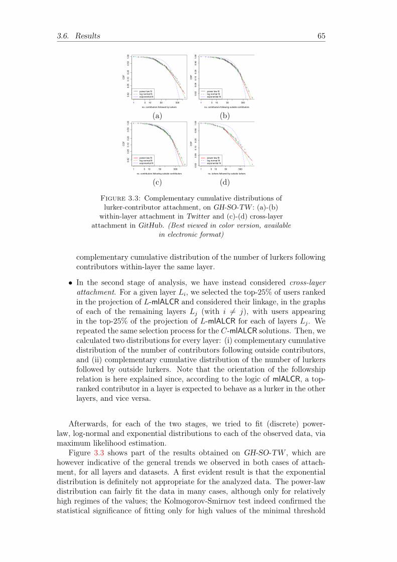
3.6. Results 65
1 5 10 50 500
0.02
0.05
0.10
0.20
0.50
1.00
no. contributors followed by lurkers
CDF
power law fitlog normal fitexponential fit
1 5 10 50 500
0.02
0.05
0.10
0.20
0.50
1.00
no. contributors following outside contributors
CDF
power law fitlog normal fitexponential fit
(a) (b)
1 5 10 50 500
0.02
0.05
0.10
0.20
0.50
1.00
no. contributors following outside contributors
CDF
power law fitlog normal fitexponential fit
1 5 10 50 500
0.02
0.05
0.10
0.20
0.50
1.00
no. lurkers followed by outside lurkers
CDF
power law fitlog normal fitexponential fit
(c) (d)
Figure 3.3: Complementary cumulative distributions oflurker-contributor attachment, on GH-SO-TW : (a)-(b)
within-layer attachment in Twitter and (c)-(d) cross-layerattachment in GitHub. (Best viewed in color version, available
in electronic format)
complementary cumulative distribution of the number of lurkers followingcontributors within-layer the same layer.
• In the second stage of analysis, we have instead considered cross-layerattachment. For a given layer Li, we selected the top-25% of users rankedin the projection of L-mlALCR and considered their linkage, in the graphsof each of the remaining layers Lj (with i 6= j), with users appearingin the top-25% of the projection of L-mlALCR for each of layers Lj. Werepeated the same selection process for the C-mlALCR solutions. Then, wecalculated two distributions for every layer: (i) complementary cumulativedistribution of the number of contributors following outside contributors,and (ii) complementary cumulative distribution of the number of lurkersfollowed by outside lurkers. Note that the orientation of the followshiprelation is here explained since, according to the logic of mlALCR, a top-ranked contributor in a layer is expected to behave as a lurker in the otherlayers, and vice versa.
Afterwards, for each of the two stages, we tried to fit (discrete) power-law, log-normal and exponential distributions to each of the observed data, viamaximum likelihood estimation.
Figure 3.3 shows part of the results obtained on GH-SO-TW , which arehowever indicative of the general trends we observed in both cases of attach-ment, for all layers and datasets. A first evident result is that the exponentialdistribution is definitely not appropriate for the analyzed data. The power-lawdistribution can fairly fit the data in many cases, although only for relativelyhigh regimes of the values; the Kolmogorov-Smirnov test indeed confirmed thestatistical significance of fitting only for high values of the minimal threshold

66 Chapter 3. Alternate behaviors in multilayer social networks
L, 0.85
L, 0.50
C, 0.85
C, 0.50
C, 0.50 C, 0.85 L, 0.50 L, 0.85
0.000.250.500.751.00
value
L, 0.85
L, 0.50
C, 0.85
C, 0.50
C, 0.50 C, 0.85 L, 0.50 L, 0.85
0.000.250.500.751.00
value
L, 0.85
L, 0.50
C, 0.85
C, 0.50
C, 0.50 C, 0.85 L, 0.50 L, 0.85
0.000.250.500.751.00
value
GitHub StackOverflow Twitter(a) GH-SO-TW
L, 0.85
L, 0.50
C, 0.85
C, 0.50
C, 0.50 C, 0.85 L, 0.50 L, 0.85
0.250.500.751.00
value
L, 0.85
L, 0.50
C, 0.85
C, 0.50
C, 0.50 C, 0.85 L, 0.50 L, 0.85
0.250.500.751.00
value
L, 0.85
L, 0.50
C, 0.85
C, 0.50
C, 0.50 C, 0.85 L, 0.50 L, 0.85
0.250.500.751.00
value
FriendFeed Twitter YouTube(b) FF-TW-YT
L, 0.85
L, 0.50
C, 0.85
C, 0.50
C, 0.50 C, 0.85 L, 0.50 L, 0.85
0.000.250.500.751.00
value
L, 0.85
L, 0.50
C, 0.85
C, 0.50
C, 0.50 C, 0.85 L, 0.50 L, 0.85
0.000.250.500.751.00
value
followship mention
L, 0.85
L, 0.50
C, 0.85
C, 0.50
C, 0.50 C, 0.85 L, 0.50 L, 0.85
0.000.250.500.751.00
value
L, 0.85
L, 0.50
C, 0.85
C, 0.50
C, 0.50 C, 0.85 L, 0.50 L, 0.85
0.000.250.500.751.00
value
reply retweet(c) HiggsTW
L, 0.85
L, 0.50
C, 0.85
C, 0.50
C, 0.50 C, 0.85 L, 0.50 L, 0.85
0.000.250.500.751.00
value
L, 0.85
L, 0.50
C, 0.85
C, 0.50
C, 0.50 C, 0.85 L, 0.50 L, 0.85
0.000.250.500.751.00
value
L, 0.85
L, 0.50
C, 0.85
C, 0.50
C, 0.50 C, 0.85 L, 0.50 L, 0.85
0.000.250.500.751.00
value
t1 t2 t3
L, 0.85
L, 0.50
C, 0.85
C, 0.50
C, 0.50 C, 0.85 L, 0.50 L, 0.85
0.000.250.500.751.00
value
L, 0.85
L, 0.50
C, 0.85
C, 0.50
C, 0.50 C, 0.85 L, 0.50 L, 0.85
0.000.250.500.751.00
value
t4 t5(d) Flickr
Figure 3.4: Per-layer evaluation of (C,L)-solutions, for eachsetting of αs, with uniform weighting scheme: Fagin-100
intersection heatmaps on the various layers of GH-SO-TW ,FF-TW-YT, HiggsTW , and Flickr (from top to bottom). (Best
viewed in color version, available in electronic format)
for fitting, xmin; for instance, considering the plots in Fig. 3.3, the followingpairs (xmin, γ) were computed, with γ here denoting the exponent of the fittedpower-law distribution: (a) (96, 2.04), (b) (74, 1.94), (c) (300, 2.73), and (d)

3.6. Results 67
L_gh
L_so
L_tw
C_gh
C_so
C_tw
C_tw C_so C_gh L_tw L_so L_gh
0.000.250.500.751.00
value
L_gh
L_so
L_tw
C_gh
C_so
C_tw
C_tw C_so C_gh L_tw L_so L_gh
0.000.250.500.751.00
value
(a) GH-SO-TW (b) GH-SO-TW
L_ff
L_tw
L_yt
C_ff
C_tw
C_yt
C_yt C_tw C_ff L_yt L_tw L_ff
0.250.500.751.00
value
L_ff
L_tw
L_yt
C_ff
C_tw
C_yt
C_yt C_tw C_ff L_yt L_tw L_ff
0.250.500.751.00
value
(c) FF-TW-YT (d) FF-TW-YT
L_mtL_rpL_rtL_fwC_mtC_rpC_rtC_fw
C_fw C_rt C_rp C_mt L_fw L_rt L_rp L_mt
0.000.250.500.751.00
value
L_mtL_rpL_rtL_fwC_mtC_rpC_rtC_fw
C_fw C_rt C_rp C_mt L_fw L_rt L_rp L_mt
0.000.250.500.751.00
value
(e) HiggsTW (f) HiggsTW
L_t1L_t2L_t3L_t4L_t5C_t1C_t2C_t3C_t4C_t5
C_t5C_t4C_t3C_t2C_t1L_t5 L_t4 L_t3 L_t2 L_t1
0.000.250.500.751.00
value
L_t1L_t2L_t3L_t4L_t5C_t1C_t2C_t3C_t4C_t5
C_t5C_t4C_t3C_t2C_t1L_t5 L_t4 L_t3 L_t2 L_t1
0.000.250.500.751.00
value
(g) Flickr (h) Flickr
Figure 3.5: Per-αs-setting evaluation of (C,L)-solutions, foreach layer, with uniform weighting scheme: Fagin-100
intersection heatmaps corresponding to (left) α〈0.5〉 and (right)α〈0.85〉. (Best viewed in color version, available in electronic
format)
(35, 1.65). By contrast, as we observe from the plots, a much more reasonablefit was provided by log-normal distributions, which is also confirmed by theShapiro-Wilk test of (log-)normality on our data.
Role correlation analysis
We analyzed how the 2-role mlALCR ranking solutions are correlated to eachother. While varying the setting of damping factors, we first measured corre-lation at a layer level, i.e., between the layer-specific projections of the lurkerand contributor mlALCR solutions obtained on each dataset; for this analysis,we present results corresponding to uniform weighting of layers. Then, we ex-tended our analysis to the whole C-mlALCR ranking and L-mlALCR rankingsolutions (i.e., ranking lists over all nodes and layers, ordered by decreasingscore).

68 Chapter 3. Alternate behaviors in multilayer social networks
KendallFagin-100
L, α〈0.5〉 C, α〈0.5〉 L, α〈0.85〉 C, α〈0.85〉 L, α〈0.5〉, C, α〈0.5〉, L, α〈0.85〉, C, α〈0.85〉,
u-weighted u-weighted u-weighted u-weighted lp-weighted lp-weighted lp-weighted lp-weightedL, α〈0.5〉, u-weighted 1.000 0.000 0.892 0.000 0.892 0.000 0.891 0.000C, α〈0.5〉, u-weighted -0.044 1.000 0.000 0.878 0.000 0.808 0.000 0.878L, α〈0.85〉, u-weighted 0.731 -0.129 1.000 0.000 1.000 0.000 1.000 0.000C, α〈0.85〉, u-weighted -0.051 0.873 -0.120 1.000 0.000 0.691 0.000 0.990L, α〈0.5〉, lp-weighted 0.535 -0.206 0.659 -0.172 1.000 0.000 1.000 0.000C, α〈0.5〉, lp-weighted -0.072 0.677 -0.210 0.638 -0.382 1.000 0.000 0.696L, α〈0.85〉, lp-weighted 0.637 -0.173 0.837 -0.159 0.671 -0.271 1.000 0.000C, α〈0.85〉, lp-weighted -0.053 0.749 -0.117 0.865 -0.161 0.647 -0.155 1.000
KendallFagin-100
L, α〈0.5〉 C, α〈0.5〉 L, α〈0.85〉 C, α〈0.85〉 L, α〈0.5〉, C, α〈0.5〉, L, α〈0.85〉, C, α〈0.85〉,
u-weighted u-weighted u-weighted u-weighted lp-weighted lp-weighted lp-weighted lp-weightedL, α〈0.5〉, u-weighted 1.000 0.000 0.653 0.000 0.672 0.000 0.665 0.000C, α〈0.5〉, u-weighted -0.361 1.000 0.000 0.413 0.000 0.934 0.000 0.434L, α〈0.85〉, u-weighted 0.732 -0.354 1.000 0.000 0.808 0.000 0.901 0.000C, α〈0.85〉, u-weighted -0.320 0.652 -0.321 1.000 0.000 0.413 0.000 0.977L, α〈0.5〉, lp-weighted 0.834 -0.466 0.745 -0.395 1.000 0.000 0.906 0.000C, α〈0.5〉, lp-weighted -0.372 0.942 -0.366 0.644 -0.480 1.000 0.000 0.434L, α〈0.85〉, lp-weighted 0.625 -0.419 0.858 -0.370 0.729 -0.434 1.000 0.000C, α〈0.85〉, lp-weighted -0.323 0.626 -0.334 0.942 -0.395 0.641 -0.383 1.000
Table 3.3: Kendall correlation and Fagin-100 intersection onwhole mlALCR ranking solutions obtained on GH-SO-TW (top)
and HiggsTW (bottom). (Prefixes “u” and “lp” standrespectively for uniform weighting scheme and
layer-proportional weighting scheme.)
Per-layer correlation. By varying the setting of αs and considering onelayer at a time, we first evaluated Kendall correlation between pairs of layer-projected (C,L)-solutions (results not shown). On all layers of GH-SO-TW ,layers mention and followship of HiggsTW , and layer t5 of Flickr, results areequal to or very close to zero, thus indicating total lack of correlation betweenthe rankings of the two roles. In the remaining cases, Kendall correlation tendsto be higher, up to values in the range 0.2–0.3 for FF-TW-YT and layers t1–t4 in Flickr. Note however that Kendall correlation does not discriminate thehead from the tail of the rankings being compared; furthermore, the abovecontingencies actually correspond to the presence of one or more layers that areclearly under-dimensioned and/or have topological similarity (e.g., YouTubein FF-TW-YT, early time slices in Flickr) with respect to the others in thenetwork (cf. Sect. 3.5.4).
To support the above intuition and verify that any degree of correlation doesnot regard the head of rankings, we analyzed the top-ranked users from eachof the layer-projected (C,L)-solutions in terms of Fagin intersection (Fig. 3.4).As we hypothesized, results show zero-correlation between any pair of (C,L)-solutions on GH-SO-TW , HiggsTW and Flickr for all layers and both settingsof αs, while on FF-TW-YT Fagin-100 values are positive (0.14) only for theunder-dimensioned layer YouTube.
Per-αs-setting correlation. In addition to the previous analysis, westudied the correlation between layer-projected (C,L)-solutions by varying thelayers and considering one setting of the αs at a time. To indicate the layers of

3.6. Results 69
a dataset network, we will refer to their short notation (reported in Table 3.1).We discuss here Fagin-100 values, shown in Fig. 3.5.
At a first glance, by comparing the plots corresponding to α〈0.5〉 with thosecorresponding to α〈0.85〉, we observe few differences from C-solutions vs. L-solutions. More in detail, on GH-SO-TW , some differences occur betweenC_tw and L_gh (0.44 for α〈0.5〉 and 0.28 for α〈0.85〉), and between C_twand L_so (0.36 for α〈0.5〉 and 0.13 for α〈0.85〉). Interestingly, the peak value(0.47) between C_gh and L_tw is yielded for both settings of αs. On theother cross-platform dataset, FF-TW-YT, high Fagin intersection correspondsto C_ff vs. L_tw (0.80 for α〈0.5〉 and 0.62 for α〈0.85〉) and to C_tw vs. L_ff(0.86 for α〈0.5〉 and 0.61 for α〈0.85〉). On Flickr, Fagin-100 values between(C,L)-pairs of different layers tend to be above zero mostly for temporally con-secutive pairs of layers, with peaks between C_t4 and L_t5 (0.49, for α〈0.5〉),and between L_t4 and C_t5 (0.47). Considering HiggsTW , for α〈0.5〉, signif-icant correlation occurs between L_fw and C_rt (0.31), and between C_fwand L_mt (0.16). These are further strengthened for α〈0.85〉: (i) 0.47 betweenL_fw and C_rt, whereas (ii) C_fw reveals to be highly correlated also withL_rt (0.97) and L_rp (0.82), besides with L_mt (0.74). The former correla-tion can reasonably be explained based on a least-effort economy principle ofuser interactional behavior: user tend to adopt the retweeting behavior morethan producing contents (on which mentioning other users), in line with theintuition that a greater effort (in terms of time and communication economy)must be done to drive the social interaction towards active participation. Thelatter correlations instead would hint for a strong characterization of users thatare mainly active as producers of social content (which explains their grantedendorsement) from those who transfer others’ information.
Whole ranking correlation. In a further stage of analysis, we studiedranking correlation by considering the whole solutions provided by mlALCRfor each role and configuration of parameters. Table 3.3 summarizes Kendalland Fagin-100 results obtained on GH-SO-TW and HiggsTW (here chosen asrepresentatives of a scenario that is substantially consistent over all datasets ingeneral).
Considering pairs of (C,L)-solutions, we observed lack of positive correla-tion, for any setting of αs and weighting scheme. More specifically, Fagin-100values are consistently equal to zero whereas Kendall values tend to be nega-tive, with range -0.38–0 on GH-SO-TW and -0.48–0 on HiggsTW . This clearlyindicates that, as expected, the lack or difference in correlation between thecontributor and lurker rankings obtained by mlALCR are exacerbated whenconsidering the entire solutions over all layers.
Impact of settings of αs
From the previous stage of evaluation of C-solutions vs. L-solutions, we ob-served no clear differences due to the setting of αs. In effect, looking at Table 3.3and considering each role at a time, we find both high Kendall correlation andFagin intersection between C-solutions as well as between L-solutions, for anyfixed weighting scheme and varying the setting of αs. Interestingly, in most

70 Chapter 3. Alternate behaviors in multilayer social networks
role, αs config. GH-SO-TW FF-TW-YT HiggsTW Flickrgh so tw ff tw yt fw mt rp rt t1 t2 t3 t4 t5
L α〈0.5〉 0.728 0.589 0.799 0.917 0.928 0.750 0.887 0.880 0.815 0.911 0.928 0.945 0.951 0.955 0.951C α〈0.5〉 0.713 0.864 0.807 0.905 0.907 0.938 0.923 0.868 0.839 0.945 0.882 0.916 0.936 0.947 0.974L α〈0.85〉 0.771 0.714 0.945 0.947 0.926 0.799 0.976 0.833 0.588 0.620 0.936 0.951 0.958 0.963 0.959C α〈0.85〉 0.794 0.911 0.883 0.914 0.928 0.919 0.927 0.932 0.887 0.933 0.864 0.911 0.939 0.954 0.987
Table 3.4: Kendall correlation for comparison of the weightingschemes: uniform vs. proportional to layer edge-set size.
cases values corresponding to the comparison of L-solutions are significantlyhigher than those corresponding to the comparison of C-solutions, for bothassessment criteria.
Considering layer-projected solutions, again it stands up the good correla-tion between any two C-solutions (resp. L-solutions) corresponding to α〈0.85〉and α〈0.5〉, over all datasets. Let us next provide details concerning Kendall cor-relation. On FF-TW-YT, correlation values for L-solutions are quite uniformand range from 0.84 on YouTube to 0.88 on Twitter and FriendFeed, whereasC-solutions for different αs have correlation of 0.91 on YouTube, 0.83 on Twit-ter, and 0.68 on FriendFeed. On GH-SO-TW , there is a tendency of highercorrelation between C-solutions than between L-solutions on GitHub (0.93 vs.0.8) and StackOverflow (0.95 vs. 0.76), while similar values are obtained onTwitter (around 0.87). An opposite tendency occurs in Flickr, where correla-tion between L-solutions ranges from 0.93 to 0.96 whereas correlation betweenC-solutions ranges from 0.88 to 0.94. On HiggsTW , there is an interesting ten-dency in the difference between comparisons of L-solutions and comparisons ofC-solutions, which relies on the followship layer. In fact, C-solutions for differ-ent αs are characterized by higher correlation values (0.91, 0.91, 0.86) on layersretweet, mention, and reply respectively, while layer followship corresponds tocorrelation of about 0.28; conversely, L-solutions have high correlation only forfollowship, while on mention, retweet, and reply the values are relatively lower(0.49, 0.48, 0.25, respectively).
Impact of layer weighting scheme
We also compared the solutions of mlALCR corresponding to the two layerweighting schemes, i.e., uniform and proportional to each layer edge-set size, inorder to understand their impact on the ranking performance.
Considering whole ranking solutions, we generally observed very high valuesof both assessment criteria, for any fixed role and setting of αs; for instance,from Table 3.3, Kendall correlation is above 0.53 on GH-SO-TW and 0.83 onHiggsTW , whereas Fagin-100 intersection is above 0.9 in most cases. Analo-gously, correlation is moderate or very high also in the case of layer-projectedsolutions, as reported in Table 3.4 for Kendall correlation.
Let us next consider, for each layer, the mean and standard deviation overthe two roles and setting of αs. On FF-TW-YT, Kendall (resp. Fagin-100) meanvalues are 0.92 (resp. 0.9) for FriendFeed, 0.85 (resp. 0.86) for YouTube, 0.92(resp. 0.93) for Twitter, with standard deviation below 0.09 in all cases. Similarsituation occurs for Flickr, whereas some exception is observed on HiggsTW :
3.6. Results 71
while Kendall mean is 0.93 for followship, and 0.88 for mention with standarddeviation always above 0.04, for layers reply and retweet we observe very highcorrelation (0.81 or above) for the C-mlALCR solutions and, with α〈0.5〉, also forthe L-mlALCR solutions (quite lower values, between 0.59 and 0.62, correspondto L-mlALCR solutions with α〈0.85〉).
It should be noted that using one scheme relies on the choice of the properweight to assign the size of any particular layer: the uniform weighting schemeconsiders the actual proportion of the layer to the complex system, while thelayer-proportional scheme should be used to normalize the above effect. InSect. 3.6.2, where we comparatively evaluate mlALCR with other methods, wewill refer to the use of uniform weights, unless using the layer-proportionalscheme would yield to significant difference in the relative performances of themethods.
Convergence aspects
mlALCR can achieve score convergence in few tens of iterations, in most of ourevaluation cases (results not shown). In particular, on FF-TW-YT, the al-gorithm converged in 90 or fewer iterations, down below 40 with α〈0.85〉 andlayer-proportional weighting scheme. While the weighting scheme, however,does not seem to impact on the convergence rate, we observed instead a signif-icant reduction in the execution of mlALCR for the setting of αs to 0.85. Thissuggests that accounting more for the user’s behavior locally to the membershiplayer would contribute to make mlALCR reach its equilibrium faster than in thebalanced setting (i.e., α〈0.5〉).
mlALCR also showed to be relatively robust when the presence of users withstrong alternate lurker-contributor behavior over the layers is less evident, likein the case of Flickr; on this dataset, mlALCR converged slowly, but withinabout 150 iterations with α〈0.85〉.
Qualitative evaluation
We investigated the meaningfulness of the ranking solutions produced by mlALCRin order to get evidence of that our proposed approach actually behaves as the-oretically expected. For this purpose, we retrieved the publicly available webpages of top-ranked users, for both lurker and contributor mlALCR solutions,and manually inspected their profiles.
For this analysis we focused on GH-SO-TW , mainly because of three rea-sons: freshness, richness, and significance. Among our evaluation datasets, it isthe most recently crawled one, which ensures better consistency with the userrelations exploited to build the multilayer network. It is also the richest datasetin terms of variety and number of user features that can intuitively be seenas indicators of the users’ online activities, both in terms of production andconsumption of information. Specifically, from each network and user page,we selected and extracted (via Rest API) quantitative as well as qualitativeinformation, which are reported next:
72 Chapter 3. Alternate behaviors in multilayer social networks
• from Twitter: number of tweets, number of lists the user belongs to,number of likes provided to posts of other users, membership date;
• from GitHub: number of commits during the last week, number of contri-butions during the last year, number of starred repositories, current andlast streak (days-in-a-row) if any, membership date, time of last contri-bution, duration of the longest streak (in days), and date of the longeststreak;
• from StackOverflow: number of the people reached, number of profileviews, number of badges or medals (gold, silver, and bronze), date of thelast access, top-overall percentage and reputation score, number of topposts, score relative to the top tags, and a description of the user profile.
Moreover, GH-SO-TW is particularly suitable for our analysis because itrepresents a prototype online social environment for sharing knowledge acrossdifferent levels of expertise of the users, through various and sophisticated waysof endorsement and interaction among them, which opens to different user be-havioral scenarios.
One of these scenarios concerns users who might want to exploit Twitter tocreate and spread information related to software development (e.g., for market-ing reasons) but, perhaps due to the higher cost of contribution when specialistexpertise is required, without contributing to the domain to which the expertisepertains. Indeed, we actually found several cases of users that are very active onTwitter, while behaving as lurkers on the other two platforms. Taking as casein point user S. K. which is a top-ranked user in the L-mlALCR solution overthe GitHub layer, he joined GitHub on November 2012, counts a high numberof followees (177) but a low number of followers (12), and has starred (in recenttimes) a good number (27) of repositories; the latter aspect indicates the will-ingness of the user of being recognized as member of the GitHub community,though as observer rather than as content producer (his last contribution is infact dated October 2015). The same user shows an even more consumption-oriented behavior on StackOverflow, whereas he appears to be very active andpopular on Twitter, with more than 10k tweets produced, only 185 followeesand almost 8k followers.
Among the top-ranked users, we also identified several cases of people whichare active on Twitter as well as they show a strong preference towards oneparticular developer community, i.e., they are active contributors on GitHubwhile showing lurking behaviors on StackOverflow, or vice versa. One exampleis given by user C. H., which is top-ranked in the C-mlALCR solution overTwitter. He joined the platform on April 2009 and he has only 64 followees,more than 10k followers and more than 4k tweets. He is definitely a contributoralso on GitHub, with unbalanced counts of followers (2.8k) and followees (54).He has starred more than 300 repositories and his last contribution is quiterecent (January 2016). It should be noted that his high score in the C-mlALCRranking is explained not only by his active contribution on Twitter, but alsofrom his lurking status on StackOverflow, where he shows low reputation (64),asked only 4 questions and answered none.

3.6. Results 73
Other users might seek to gain benefits for their profession by actively par-ticipating in the StackOverflow and/or GitHub developer communities, whilenot being much interested in posting tweets. This is the case, for example, ofuser R. B., which appears to be a master on StackOverflow and GitHub, butrelatively inactive on Twitter. He indeed shows an extremely active/influentbehavior on StackOverflow, where he has numerous badges and more than 10(resp., 100, 200) gold (resp. silver, bronze) medals. He shows extremely highreputation (above 40k), reaching about 2.7M people, answering almost 1k ques-tions and asking more than 200 questions. However, his status is different onGitHub, where he provided a few contributions over the last year, and on Twit-ter, showing in both platforms quite a low level of socialization.
Summary of mlALCR evaluation
We summarize here our main findings from the evaluation of mlALCR.
• We have pointed out the meaningfulness of the problem under studyon real-world multilayer networks, which indeed contain users that arecharacterized by evident variability in their cross-layer lurker/contributorbehavior. Our mlALCR has shown to be able to identify users showingalternate behavior over the different layer networks.
• Both within-layer and cross-layer attachment distributions of lurkers vs.contributors, and vice versa, are better fitted by log-normal distributionsthan power-law ones.
• Lurker and contributor mlALCR solutions are clearly uncorrelated overthe same network. When considering layer-specific projections of the so-lutions, there is a total disagreement in matching between the top-rankedusers of C-mlALCR and L-mlALCR over the same layer, while correlationgets high for any pair of layers characterized by the presence of users withalternate lurker-contributor behavior.
• Neither the setting of damping factors αl and αc nor the weighting schemehas heavy effect on the ranking solutions of mlALCR; however, the settingof αs impacts on the convergence of mlALCR, whereby accounting morefor the user’s behavior locally to the membership layer (i.e., α〈0.85〉) leadsmlALCR converge faster.
• Empirical evidence based on manual inspection of top-ranked users hasconfirmed the ability of mlALCR in detecting users that simultaneouslyexhibit lurking behavior on one layer (e.g., OSN platform) while theyspread the acquired knowledge acting as contributor on other layers, orvice versa.

74 Chapter 3. Alternate behaviors in multilayer social networks
3.6.2 Comparative evaluations
Comparison with LurkerRank
In order to understand how mlALCR differs from the basic monoplex LR method,we analyzed the LR solution obtained on each layer of a network and the cor-responding layer projections of mlALCR. Here we discuss Kendall correlationresults (not shown).
In two datasets, namely FF-TW-YT and Flickr, correlation is very close tozero and does not significantly vary with the choice of role and layer, and withthe setting of αs. Specifically, on FF-TW-YT, correlation values are mostly inthe range ±1.0e-3 for Twitter and FriendFeed, and tend to be slightly negativefor YouTube (around -3.0e-2). On Flickr, correlation with LR is in the samerange (0.07) for both L- and C-solutions on layers t1, t2, t3, while is lower onlayer t4. The most recent time slot (t5) presents a negative correlation withL-solutions and a positive correlation with C-solutions both in the range of0.01.
In the other two datasets, we mostly observed a few cases of significantnegative (resp. positive) correlation between LR and C-solutions (resp. L-solutions) of mlALCR. For instance, for Twitter on GH-SO-TW , correlationvalues range from -0.26 to -0.16 w.r.t. C-solutions, and from 0.44 to 0.56 w.r.t.L-solutions, which indicates a tendency of having lurkers in Twitter that arelikely to be active in the other platforms; further analysis in terms of Fagin-100,with values below 0.06, however shows that such correlation is not determinedby the top-ranked lurkers.
More interesting is the situation analyzed on HiggsTW . Here there is asignificant negative correlation between LR and C-solutions over each layer;specifically, up to -0.26 on followship, -0.23 on mention, and -0.20 on reply .This clearly characterizes a strong mismatching between lurkers determinedby LR according to a given user relation and the corresponding contributorsdetermined by mlALCR for the same relation, which might behave as lurkersfor other relations. Considering L-solutions, we observed relatively discordantresults depending on the setting of αs: positive, up to 0.32 (resp. negative, up to-0.21) for solutions with α〈0.5〉 on retweet (resp. reply), and conversely slightlynegative, up to -0.14 (resp. positive, up to 0.32) for solutions with α〈0.85〉. Bycontrast, on followship and mention, we observed good correlation (0.60 and0.33, respectively); this is also strengthened by significant matching in terms ofFagin-100 results: 0.22–0.27 for followship and 0.12–0.39 for mention, which isin line with our analysis of results on HiggsTW presented in Sect. 3.6.1.
Comparison with LR-aggregation methods
We compared the mlALCR solutions (by varying the role, configuration of (αc, αl)and weighting scheme) with each of the two proposed ranking aggregation meth-ods. For this evaluation, we discuss Fagin-100 results (not shown).
In general, we observe that the comparison with both ranking aggregationmethods is characterized by near-zero or zero Fagin-100 with L-mlALCR as wellas with C-mlALCR. More in detail, considering first LRa1, values are zero on
3.6. Results 75
Flickr and GH-SO-TW (in all cases). On FF-TW-YT, Fagin-100 is 0.021 on av-erage, with peak of 0.04, w.r.t. C-solutions, and 0.023 on average, with peak of0.02, w.r.t. L-solutions. While on HiggsTW , Fagin-100 values range from 0 to0.02 (the latter obtained w.r.t. C-solution with α〈0.85〉). Comparing mlALCR toLRa2, all of non-zero Fagin-100 values correspond to mlALCRmax, being around0.03 for C-solutions and around 0.07 for L-solutions on GH-SO-TW . On Hig-gsTW , Fagin-100 is always zero w.r.t. mlALCRmin for C-solutions, while non-zero values are equal to 0.02 (resp. 0.12) for mlALCRmed (resp. mlALCRmax);concerning L-solutions there is no matching w.r.t. mlALCRmin and mlALCRmed,while mlALCRmax values are close to 0.18. On FF-TW-YT, in regard to C-solutions all non-zero values are below 0.1 except for mlALCRmed w.r.t. α〈0.5〉and non-uniform weighting with values equal to 0.16 (resp. 0.23) for C-solution(resp. L-solution). No matching at all is observed between mlALCR and LRa2on Flickr.
Overall, we find out that the statistical manipulation of ranks over the layersprovided by both LRa1 and LRa2 leads to no significant matching with top-ranked users by mlALCR.
Comparison with Multilayer LurkerRank
Comparing mlALCR with mlLR (results not shown), we observed some casesof positive Kendall correlation over the datasets. On FF-TW-YT, maximumcorrelation is obtained between L-mlALCRmax (for any setting of αs) and mlLRranging from 0.57 to 0.61, which decreases down below 0.5 when compared withmlALCRmed. On the other datasets, the maximum correlation corresponds al-ways to comparison with L-mlALCRmax, but with lower values (on GH-SO-TW ,0.33 with α〈0.85〉, and 0.26 with α〈0.5〉; on HiggsTW , between 0.27 and 0.4 withα〈0.5〉). Minimum correlation is always obtained with mlALCRmin (between 0.12and 0.16 on GH-SO-TW , around 0.08 on FF-TW-YT, 0.04 on HiggsTW , whileit varies from -0.08 to 0.1 considering C-solutions and L-solutions, respectively,on Flickr).
The observation of Fagin-100 results sheds light on the evidence that, overall datasets and regardless of the role and setting of αs, matching is alwaysclose to zero (below 0.07 on HiggsTW , 0.05 on GH-SO-TW and FF-TW-YT,0.01 on Flickr). Coupled with the previously given observations about Kendallcorrelation, this indicates that mlALCR and mlLR might be relatively correlatedthough mainly along the tail.
Comparison with Multiplex PageRank
Our final stage of evaluation concerns a twofold comparison between mlALCRand the Multiplex PageRank method, in all of its three variants (Sect. 3.5.2).On the one hand, analogously to the previous analyses, we want to understandwhether mpxPR solutions can be, to a certain extent, correlated to L-mlALCR,i.e., whether mpxPR can be able to discover users that behave as lurkers inone layer and as contributors in other layers; on the other hand, we want tocapitalize on the actual nature of mpxPR (i.e., searching for high PageRank users

76 Chapter 3. Alternate behaviors in multilayer social networks
in a multilayer context), and hence we compared it with C-mlALCR solutions todetermine any affinity in the identification of contributors on individual layers.In the latter case, to properly set the input for mpxPR for this task, we reversedthe orientation of the layer graphs, in the classic influence-oriented centralitymodel (i.e., edge (u, v) expresses endorsement of u to v).
We used FF-TW-YT and GH-SO-TW as cases in point. This implies that,being the number of layers equal to three in both datasets, there are six differentlayer configurations (two per layer) for the application of any of the variants ofmpxPR. (Recall that mpxPR is dependent on the layer ordering.)
On FF-TW-YT, for both C- and L-solutions values are near-zero or zerofor all three variants of mpxPR, for both assessment criteria. More variegated isinstead the situation on GH-SO-TW . Considering L-solutions, Kendall correla-tion and Fagin-100 intersection range from -0.15 to 0.05 and from 0.16 to 0.18,respectively, with the exception of GitHub where Fagin-100 has a peak around0.5 when comparing with the combined variant of mpxPR. Considering the com-parison with C-solutions, all variants of mpxPR again tend to yield near-zerocorrelation with C-mlALCR by Kendall, and between 0.07 and 0.18 in terms ofFagin-100.
This can intuitively be explained since users that are highly central (i.e.,contributors in the case of comparison with C-mlALCR, lurkers in the othercase) on one layer L′, and less central on the others, are more likely to receive afinal ranking score from mpxPR which is substantially determined by the scoreon L′. Therefore, for all users determined by mlALCR as contributors (resp.lurkers) on L′ but who do not show a strong alternate behavior elsewhere, theremight be a relatively higher correlation with those users’ ranking obtained bympxPR.
It should also be noted that all variants of mpxPR are sensitive to the or-dering of the layers: as an example, for the comparison with L-mlALCR andfinal ranking on Twitter, we observed two controversial results yielded by theadditive variant: Kendall of 0.005 for the sequence tw←so←gh but -0.12 fortw←gh←so.
Summary of comparative evaluation
Comparing mlALCR with other methods allowed us to draw the following mainremarks:
• Within-layer lurkers identified by LR have generally no correlation (resp.strong mismatching) with cross-layer lurkers (resp. contributors) identi-fied by mlALCR in the same layer. However, some correlation might beobserved when lurkers in a given layer are likely to behave actively onother layers (for example, in single-platform contexts like HiggsTW thismight occur for followship vs. retweet, according to a least-effort economyprinciple of interactional behavior).
• No significant matching is found between mlALCR and any of the ag-gregation methods which statistically manipulate the layer-specific ranksobtained by LR.

3.7. Conclusions 77
• Top-ranked users in mlALCR and in the multilayer LR (mlLR) have nomatching, while any positive correlation that may occur by comparingthe entire ranking solutions depends on their respective tails.
• Upon testing in both lurking-oriented and contributor/influential-orienteduser relation models, mpxPR can reward a user only according to the samerole s/he consistently has over the layers of a network (though biased bythe ordering of examination of the layers), while in any case it cannotdetect cross-layer opposite roles.
Overall, the conducted comparative evaluation has shown the uniquenessof mlALCR in mining alternate lurker-contributor behaviors on a multilayernetwork.
3.7 ConclusionsIn this work we focused on the dichotomy between contribution and consump-tion of information over multilayer OSNs. In this respect, we addressed the novelproblem of identification and characterization of opposite behaviors that usersmay alternately exhibit over the multiple layers of a complex network. We pro-posed the first topology-driven ranking method for alternate lurker-contributorbehaviors on a multilayer OSN, named mlALCR, which is designed to identifyusers that behave as lurkers (resp. contributors) in one layer while converselyacting as contributors (resp. lurker) in one or many of the other layers. Signifi-cance and uniqueness of mlALCR have been empirically demonstrated over fourreal-world multilayer networks. We have also discussed a number of applicationsthat might benefit from the proposed approach, including user engagement, vi-ral marketing and information containment.
Natural extensions of our mlALCR include the embedding of the temporaldimension and content information into the mlALCR ranking model. It would beinteresting to study relations between the alternate lurker-contributor behaviorsand properties of assortativity at network level [125] or at node level [126] whichmight be defined based on suitable notions of cross-layer centrality. Optimal-convergence analysis for specific settings of the α parameters would also repre-sent an interesting theoretical investigation, which could be effectively addressedvia gradient-based optimization (e.g., [127]). In addition, we believe it wouldbe interesting to integrate mlALCR into a task of community detection in orderto analyze knowledge transfer flows between cross-layer communities.


79
Chapter 4
A supervised approach to userbehavioral problems
4.1 IntroductionLearning-to-rank (LTR), i.e., using machine learning to automatically build aranking model, has become one of the key technologies for modern web search,retrieval and personalization [128], [129]. As in traditional ranking functions, apartial ordering (i.e., ranking) is provided for a set of objects, according to theirdegree of relevance to a given query; in LTR, the ranking function is learnedfrom training data given in the form of 〈query, object, relevance label〉 tuples. Inthis chapter, we investigate whether learning-to-rank (LTR) can be successfullyapplied to ranking problems in OSNs. In particular we concentrate our effortto the detection of two specific types of online behavior: automated (i.e., bots)and lurking.
Automated behavior. Bots have often been regarded as harmless pro-grams confined within the cyberspace. However, recent events in our societyproved that they can have important effects on real life as well. Bots have in factbecome one of the key tools for disseminating information through online so-cial networks (OSNs), influencing their members and eventually changing theiropinions. With a focus on classification, social bot detection has lately emergedas a major topic in OSN analysis; nevertheless more research is needed to en-hance our understanding of such automated behaviors, particularly to unveilthe characteristics that better differentiate legitimate accounts from bots. Weargue that this demands for learning behavioral models that should be trainedusing a large and heterogeneous set of behavioral features, so to detect andcharacterize OSN accounts according to their status as bots. Within this view,in Sect. 4.3 we push forward research on bot analysis by proposing a machine-learning framework for identifying and ranking OSN accounts based on theirdegree of bot relevance.
Lurking behavior. While being long researched in social science and com-puter human interaction, lurking behaviors in online social networks (OSNs)have been computationally studied only in recent years. Remarkably, deter-mining lurking behaviors has been modeled as an unsupervised, eigenvector-centrality-based ranking problem, and it has been shown that lurkers can effec-tively be ranked according to the link structure of an OSN graph. Although thisapproach has enabled researchers to overcome the lack of ground-truth data at

80 Chapter 4. A supervised approach to user behavioral problems
a large scale, the complexity of the problem hints at the opportunity of learn-ing from past lurking experiences as well as of using a variety of behavioralfeatures, including any available, possibly platform-specific information on theactivity and interaction of lurkers in an OSN. In this work, we leverage thisopportunity in a principled way, by proposing a machine-learning frameworkwhich, once trained on lurking/non-lurking examples from multiple OSNs, al-lows us to predict the ranking of unseen lurking behaviors, ultimately enablingthe prioritization of user engagement tasks.
4.2 Learning to rank methodsLearning-to-rank (LTR) is a supervised learning approach to build a rankingmodel. LTR methods are commonly organized into three categories, namelypointwise, pairwise and listwise [128], which correspond to different modelingof the input data and types of loss function to be minimized. Pointwise meth-ods assume that every query-object pair is a learning instance, whose score hasto be predicted. Ordinal scales are mapped into numeric values, therefore theranking problem is seen as regression or ordinal classification. Object pairs arethe learning instances in pairwise methods, which hence aim to learn which ob-ject in a pair precedes the other in the ranking. Optimization here consists inminimizing the number of switched/misclassified object pairs. In listwise meth-ods, a learning instance is comprised of a query and its objects, and a qualitycriterion is optimized over all queries in the training data. Unlike the othertwo types of LTR, listwise methods take into consideration that the selection offeatures is not unbiased, since they depend on the queries, which in turn vary,so that some objects or object pairs might not be comparable with each other.
Several LTR methods have been developed since the last fifteen years [128],[130]. Here, for the purpose of this research, we focus on pairwise and list-wise methods, which have shown to perform generally better than the earlierpointwise ones, and we briefly recall some of the most representative methods.
RankNet [131] is a pairwise method, which has become popular in commer-cial search engines (e.g., Microsoft Bing R©). In RankNet, the training schemeis based on a neural network with two hidden layers and one output node, andback-propagation is used to minimize the following cost function, which rep-resents the pair-wise cross entropy between the target probability Pij and themodeled probability Pij, for each pair objects i, j:
Cij = −Pij log(Pij)− (1− Pij) log(1− Pij) (4.1)
Coordinate Ascent [132] is a listwise method, where the scores of the query-object pairs are computed as weighted combination of the features values. Theweights are tuned by using coordinate ascent optimization, a derivative-freeoptimization technique, in which the objective function can be any arbitraryIR evaluation criterion, and such that the optimization is performed in onedimension at a time while keeping the other dimensions fixed. If we denote
4.3. Bot detection 81
with λi the i-th parameter to learn, then the update rule is given by:
λ′i = arg maxλi
E(R∆, T ) (4.2)
where R∆ is the set of rankings induced over all of the queries, T is the trainingdata, and E(·, ·) denotes an evaluation function.
AdaRank [133] is a listwise boosting method inspired by the classificationalgorithm AdaBoost [134]. Through the use of a stepwise greedy optimizationtechnique, it maximizes a chosen IR evaluation criterion by repeatedly building“weak rankers” on the basis of re-weighted training data. These weak rankers arefinally linearly combined to produce the ranking predictions. One key aspect inAdaRank is that higher weights are assigned to queries whose relevant objectsare more difficult to rank, whereas already learned queries are associated withlower weights on the basis of the forward stage-wise additive modeling paradigm.The objective function to be minimized has the form:
minht∈Hαt∈R+
L(ht, αt) =m∑i=1
exp(−E(π(qi,di, ft−1 + αtht),yi)) (4.3)
where E is the quality criterion function, π represents the permutation for thei-th query qi, the list di of retrieved documents for qi, and the ranking model f .Moreover, yi corresponds to the relevance labels (i.e., desired ranks), H denotesthe set of possible weak rankers ht, and αt is a positive weight.
LambdaMART [135] is an ensemble method that combines LambdaRank [136]and MART [137]. The former performs optimization via the gradient of the lossfunction, while the latter is a boosted regression tree model in which the outputis a linear combination of the outputs of a set of regression trees. LambdaRankis based on a neural network, like RankNet, and it stands out for one mainaspect: instead of focusing on the definition of a less expensive cost function,it takes into account the gradient of the cost function directly, avoiding theadditional computational cost introduced by sorting operations [138]. For eachpair of objects i, j, the λ-gradient is defined as:
λij = Sij
∣∣∣∣∣ ∆Zij∂Cij
∂(si − sj)
∣∣∣∣∣ (4.4)
where si − sj is the difference of ranking scores of the two objects w.r.t. aquery, Cij = si− sj + log(1 + exp(si− sj)) is the cross-entropy cost, ∆Zij is theevaluation value gained by swapping the two objects, and Sij is equal to +1 ifobject i is more relevant than object j, −1 otherwise.
4.3 Bot detectionSoftware robots, or bots, are computer programs designed to carry out one ormore specific automated tasks. Social bots are a particular type of chat-botsemployed in social media platforms to automatically interact with members

82 Chapter 4. A supervised approach to user behavioral problems
and generate contents. Bots can be used to provide useful services such ascustomer support, meeting scheduling, tracking of product shippings, and soon. On the other hand, social bots often mimic a human being by controllinga social media account, and when acting as a group (i.e., botnet) they can alsopursue malevolent intents, such as fostering fame [139], [140], biasing publicopinion [141], [142], spamming or limiting free speech by submerging importantmessages with a deluge of automated bot messages [143].
In the last years, also thanks to minimal skill requirements, the use of auto-mated accounts has seen an unprecedented rise [144]–[146]. Remarkably, groupsof orchestrated bots are being used to steer public opinion and influence theelectoral audience through the spread of (mis)information and fake news [147];the most representative example is related to the latest US presidential elec-tion [141], [142], but several other cases can be listed [148]–[151].
Bot detection is a challenging problem, also due to the variety of strategiesimplemented by bots. For instance, they can mimic human behavior in orderto blend in among legitimate accounts (i.e., users) and earn their trust, makingbot detection more difficult [152], [153]. Bots can also achieve an amplifyingeffect by replicating contents related to a specific topic in order to distort theperception of its popularity, or create the appearance of grassroots support fora position (i.e., astroturfing) by over-promoting that point of view [154], [155].
The software behind social botnets is constantly evolving, introducing newexpedients that result in sophisticated simulations of human behavior in OSNs [145],[146], [156], making the identification of automated accounts ever more com-plicated. Therefore, there is an emergence for the development of effectivemethods able to better understanding the behavioral patterns that characterizeautomated OSN accounts.
Research questions. Despite several approaches have been developedto detect bots in OSNs, a single method often covers only one specific patternof automated behavior, leaving the identification challenge open. Taking in-spiration from ensemble learning theory, whereby multiple weak learners arecombined together in order to boost prediction performance, in this work weaim at developing a more general framework for the identification of bots thatcan exploit different sources of information and be capable of learning from mul-tiple type of bot detection methods. Within this view, we raise the followingquestions:
• How can we exploit previously identified automated accounts to tune amodel for detecting and ranking bots?
• How can we successfully combine several bot identification methods to cap-ture different behavioral patterns?
• How can we incorporate into a bot ranking model various “signals” thatcan be used as behavioral features, upon which the evaluation of any user-account w.r.t. a given context is performed?
Motivations. We believe that LTR is particularly suitable for address-ing the aforementioned problem, helping us to improve our understanding of

4.3. Bot detection 83
automated behaviors in online social environment. The inherent complexity ofthe bot detection problem hints at the exploitation of techniques capable of de-termining the status as bot of a (suspected) OSN account, rather than simplyindicating whether or not an account is a bot. In fact, LTR adopts a supervisedapproach to learn from past user experiences, which might be annotated accord-ing to the degree of bot relevance. LTR training is accomplished according to aset of features which, being of different types, can be useful predictors capturingdifferent aspects of automated behaviors. LTR also offers unprecedented oppor-tunities for incremental scenarios: once trained a learning-to-bot-rank model,this can be used to assign any previously unobserved account with a bot rele-vance score.
Contributions. In this work, we propose the first LTR framework todetect and characterize social bots in OSNs. We develop a learning-to-rank-social-bot methodology based on state-of-the-art LTR methods that exploits,in the process of feature extraction, information of different type (such as, userprofile, user’s activity rate, media content) and is supported by three state-of-the-art bot-detection methods, namely DeBot, BotWalk, and BotOrNot. Re-sults obtained on four state-of-art datasets have shown the significance of ourapproach, confirming our initial hypothesis that LTR can be effective for un-veiling automated behaviors.
The remainder of this chapter is organized as follows. Section 4.3.1 brieflydiscusses related work, whereas Section 4.2 describes LTR and bot-detectionmethods utilized in our framework. Section 4.3.2 is devoted to the proposedLTRSB framework. Section 4.3.3 presents experimental results and Section 4.3.4concludes the chapter.
4.3.1 Related work
Bot detection Currently adopted approaches for bot detection belong tothree main categories: graph-based, time-series-analysis-based, and hybrid meth-ods. The former group utilizes network information (e.g., contacts, interactions,(re)tweets) in order to discern between legitimate accounts and bots [157]–[159].The second group of methods focuses on identifying distinctive temporal behav-ioral patterns of bots (e.g., burst of interactions, non-stop activity, etc.) [160]–[164]. The third group includes software systems that are designed to use fea-tures of different type to train one classifier [165]–[167] or an ensemble of classi-fiers [168]. A different perspective is taken from BotWalk [169], which computesan aggregated anomaly score based on an ensemble of unsupervised anomalydetection methods.
Remarkably, most of existing methods aim to detect bots either focusingon a specific aspect of automated behavior, and for this reason they cannotbe considered general enough, or by exploiting features of different type while,however, focusing on binary classification problems.
Learning-to-rank in OSNs Originally developed to meet the rising needsof modern web retrieval systems, LTR techniques have also been exploited inOSN analysis contexts. In particular, LTR frameworks have been developed to
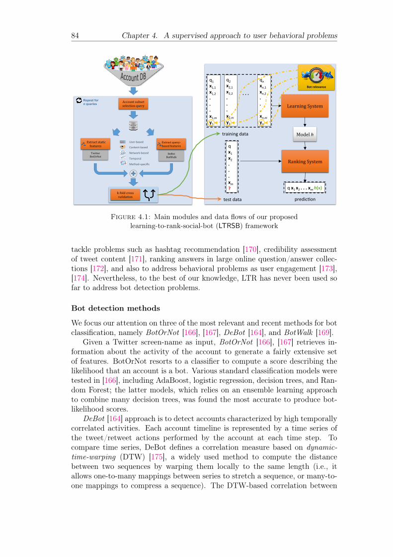
84 Chapter 4. A supervised approach to user behavioral problems
Botrelevance
q x1x2...xm?
trainingdata
testdata predic0on
qx1x2...xmh(x)
RankingSystem
Modelh
LearningSystem
q1x1,1x1,2...x1,my1
q2x2,1x2,2...x2,my2
qnxn,1xn,2...xn,myn
...
Accountsubsetselectionquery
k-foldcrossvalidation
User-based
Content-based
Network-based
Temporal
Method-specific
TwitterBotOrNot
Extractstaticfeatures
DeBotBotWalk
Extractquery-basedfeatures
Repeat for n queries
Figure 4.1: Main modules and data flows of our proposedlearning-to-rank-social-bot (LTRSB) framework
tackle problems such as hashtag recommendation [170], credibility assessmentof tweet content [171], ranking answers in large online question/answer collec-tions [172], and also to address behavioral problems as user engagement [173],[174]. Nevertheless, to the best of our knowledge, LTR has never been used sofar to address bot detection problems.
Bot detection methods
We focus our attention on three of the most relevant and recent methods for botclassification, namely BotOrNot [166], [167], DeBot [164], and BotWalk [169].
Given a Twitter screen-name as input, BotOrNot [166], [167] retrieves in-formation about the activity of the account to generate a fairly extensive setof features. BotOrNot resorts to a classifier to compute a score describing thelikelihood that an account is a bot. Various standard classification models weretested in [166], including AdaBoost, logistic regression, decision trees, and Ran-dom Forest; the latter models, which relies on an ensemble learning approachto combine many decision trees, was found the most accurate to produce bot-likelihood scores.
DeBot [164] approach is to detect accounts characterized by high temporallycorrelated activities. Each account timeline is represented by a time series ofthe tweet/retweet actions performed by the account at each time step. Tocompare time series, DeBot defines a correlation measure based on dynamic-time-warping (DTW) [175], a widely used method to compute the distancebetween two sequences by warping them locally to the same length (i.e., itallows one-to-many mappings between series to stretch a sequence, or many-to-one mappings to compress a sequence). The DTW-based correlation between

4.3. Bot detection 85
two (normalized) time series x and y is defined as:
wC(x, y) = 1− DTW 2(x, y)
2P(4.5)
where P is the number of squared errors that are added to obtain a distance(i.e., the path length) [164]. DeBot performs a 4-stage workflow: first, tweetsthat contain selected keywords are gathered for a period of T hours, then itassembles the time series for each user. These series are processed based ona hash index in order to identify correlated activity patterns between two ormultiple accounts. Third, the activity of suspected accounts is closely monitoredthrough the stream Twitter API. The last step computes a pairwise warpedcorrelation matrix, over the newly generated time series, and generates clustersof highly correlated users.
BotWalk [169] is a near real-time adaptive bot-identification method basedon an ensemble of anomaly detection methods. Like DeBot, BotWalk adopts anunsupervised approach and focuses on specific distinguish patterns of automatedbehavior. In addition, BotWalk utilizes 130 features extracted from network,content, temporal and metadata information. Starting from a seed-bot and aset of random accounts, BotWalk retrieves each account’s details, timeline, andone-hop follower neighborhood, with the goal of maximizing the likelihood ofreaching other bots across the OSN. The output of the method is representedby an aggregated score, obtained by combining four different anomaly detectionscores.
4.3.2 Proposed Framework
Overview
Figure 4.1 shows a schematic illustration of the proposed Learning-To-Rank-Social-Bots (LTRSB) framework.
We are given a database storing information about legitimate accounts andbots gathered from heterogeneous sources. This database feeds information toa component that is in charge of (i) repeatedly selecting a subset of accounts todefine queries for the LTR module, and (ii) extracting static as well as dynamicfeatures of different types, as we shall describe later.
In this work we use Twitter as case in point, although our framework is inprinciple designed to be versatile and applicable to other OSN platforms. Thefeature extraction step is performed through Twitter API as well as throughretrieving functionalities provided by BotOrNot, BotWalk and DeBot methods.In particular, Twitter API and BotOrNot are used to retrieve static and aggre-gate features, whereas BotWalk and DeBot are used to compute query-basedfeatures. More in detail, each DeBot run is characterized by a time-window offixed length, in which all the users belonging to the query are being listened inorder to compute clusters. Clusters are then examined to compute the warpedcorrelation matrix and, finally, the DeBot features.

86 Chapter 4. A supervised approach to user behavioral problems
bots non-bots source annotations
452 970 [166] human generated1254 1595 [177] human generated5937 2819 [143] human generated2371 2567 [176] honeypot-based1420 - DeBot runs DTW-based11434 7951 Total
Table 4.1: Composition of the Account DB
Account DB
Table 3.2 shows main characteristics of our evaluation data, for a total of about19K accounts, 11K of which correspond to bots and the remaining to non-bots.Most of the account instances are from datasets originally built and analyzed inrecent studies [143], [166], [176], [177], although from each of these datasets weremoved accounts that are suspended by Twitter or no longer active; moreover,we gathered additional bot instances from Twitter through several DeBot runs.
The account instances stored in the database were originally annotated witha binary ground-truth label (i.e., bot or non-bot) according to three differentapproaches. The majority of instances were labeled by human experts. Ac-counts from [176] were instead labeled depending on whether an account is afollower of a target honeypot account. (Since honeypots are designed in such away that a human can immediately tell if they are bots, any user in the networkthat connects to a honeypot will be considered as a bot). In addition to thedatasets available from other studies, we exploited DeBot, which has shown toprovide almost null false-positive rate, to further collect bot instances havingcorrelation score of 0.995 or above.
Training Data
LTR training data consists of triplets 〈query, object, relevance label〉. We aregiven n queries, each corresponding to a subset ofm. Each object is an account’sfeature vector, and the relevance label denotes one or several grades of bot status,so that higher grades correspond to more likely bots.
Relevance labeling We devised three approaches for bot relevance labeling,depending on the selection of relevant/non-relevant instances, and the type ofrelevance label:
• In the first configuration, dubbed BB, we considered binary relevance,i.e., bot and non-bot, and performed a balanced selection of relevant andnon-relevant accounts.
• In the second configuration, dubbed UB, we again considered binary rel-evance, and performed unbalanced selection of relevant (30%) and non-relevant (70%) accounts.
4.3. Bot detection 87
• In the third configuration, dubbed Grad, we considered balanced selectionof relevant and non-relevant accounts, but seven grades of bot status.
The first two configurations of relevance labeling correspond to the use theoriginal binary-annotation information in the datasets reported in Table 4.1.For the Grad configuration, we computed the relevance labels as follows. First,we uniformed the feature representation for all the accounts in our databaseto the BotOrNot model, by retrieving from Twitter missing information for allthe accounts not previously processed by BotOrNot. Second, we applied theBotOrNot-RandomForest classifier to produce the bot likelihood score for eachinstance, which varies within [0, 1]. Third, we discretized the bot scores in sevenintervals, with the interval [0, 0.3] corresponding to legitimate accounts, subse-quent intervals with increment of 0.1, and [0.8, 1] corresponding to definitely abot account.
Feature set We organize the set of features extracted from our evaluationdata into five categories: aggregate, user-based, network-based, content-based,and temporal.
Table 4.4 provides a concise description of the features. The first group iscomprised of nine aggregate indicators provided by BotOrNot (i.e., from A.1 toA.9) and a query-wise score produced by the BotWalk anomaly detection task.User-based features describe Twitter account settings and basic information,such as account lifetime, time-zone and language, and whether the accountwas verified or not. Network-based features describe node-wise properties of auser in the social network graph, and include indicators of the user’s centrality,popularity and role. Content-based features represent the largest group andinclude several indicators illustrating the diversity and alleged quality of thecontent created by a user. Considering normal human-limitations in terms oftime spent on social-media platforms, we defined several activity-rate featuresas indicators of overproduction. We also included basic statistics on the inter-arrival time of consecutive tweets, and on user activity distributions to gaininsights into content production patterns of social bots.
Note that, to ensure comparability across queries, all feature values werescaled between 0 and 1, through min-max normalization.
Feature informativeness We investigated about the usefulness or informa-tiveness of the features, with a twofold goal: to discover possible correlationbetween features (possibly w.r.t. the relevance class attribute), and to esti-mate their impact on the ranking prediction performance. For this purpose,we resorted to five standard methods used in feature selection tasks: principalcomponent analysis (PCA), information gain, Pearson’s correlation coefficient,correlation-based feature selection (CFS) [178], and learner-based feature selec-tion exploiting J48 decision tree model.
The outcome of the analysis confirmed the significance of most of the fea-ture categories, namely content-based, aggregate, network-based and temporalfeatures. However, it also highlighted the necessity of diversifying features insuch a context. As we shall declare in our evaluation goals (cf. Section 4.3.2),

id description id description
User-based
U.1 Short length of user description
Con
tent-based
(∗)
C.1 Number of favorites/likesU.2 Number of links appearing in the description C.2 Number of tweetsU.3 URL website (Boolean value) C.3 Number of tweets with at least one hashtagU.4 Verified account (Boolean value) C.4 Number of tweets with at least one URLU.5 Number of lists created by the user C.5 Number of retweets performedU.6 Number of posts (tweets) C.6 Number of URLsU.7 Account lifetime C.7 Number of domainsU.8 Geo enabled (Boolean value) C.8 Number of hashtagsU.9 Time zone (ID number) C.9 Number of retweets receivedU.10 Language (ID number) C.10 Number of duplicate URLsU.11 Default profile & background (Boolean value) C.11 Number of duplicate domainsU.12 Default profile image (Boolean value) C.12 Number of duplicate hashtags
Network-based
N.1 Number of followers C.13 Mean of the Jaccard similarity of inter-tweet bag-of-wordsN.2 Number of friends (followees) C.14 Minimum of the Jaccard similarity of inter-tweet bag-of-wordsN.3 Number of tweets with at least one mention C.15 Maximum of the Jaccard similarity of inter-tweet bag-of-wordsN.4 Number of mentions C.16 Standard deviation of the Jaccard similarity of inter-tweet bag-of-wordsN.5 Number of duplicate mentions C.17 Average number of special charactersN.6 Follower / followee ratio C.18 Minimum number of special charactersN.7 Mention / tweet ratio C.19 Maximum number of special characters
Tem
poral
T.1 Duration of the longest tweet session without breaks longer than 10 minutes C.20 Standard deviation of number of special charactersT.2 Mean (µ) of the inter-arrival time of consecutive tweets C.21 Average of tweet lengthsT.3 Minimum of the inter-arrival time of consecutive tweets C.22 Minimum of tweet lengthsT.4 Maximum of the inter-arrival time of consecutive tweets C.23 Maximum of tweet lengthsT.5 Standard deviation (σ) of the inter-arrival time of consecutive tweets C.24 Standard deviation of tweet lengthsT.6 Burstiness, i.e., (σ − µ)/(σ + µ) C.25 Retweets / tweets ratioT.7 χ2 second-of-minute, refers to tweet distributions across time C.26 Number of URLs on tweetsT.8 χ2 minute-of-hour, refers to tweet distributions across time C.27 Number of hashtags on tweetsT.9 χ2 hour-of-day, refers to tweet distributions across time C.28 Number of media files (photos or videos) on tweetsT.10 Average number of tweets per day C.29 Average number of retweets received per tweetT.11 Maximum number of tweets per day C.30 Average number of likes/favorites received per tweet
T.12 Minimum number of tweets per day
Aggregate
A.1 Content indicator (based on statistics about length andentropy of shared text, POS tagging, etc.) [BotOrNot]
T.13 Standard deviation of number of tweets per day A.2 Friend indicator (based on follower-friend relations,number of replies, etc.) [BotOrNot]
T.14 Entropy inter-arrival time A.3 Network indicator (based on mentions, retweets, andhashtags) [BotOrNot]
T.15 Average number of likes per day A.4 Sentiment indicator (based on several sentimentextraction techniques) [BotOrNot]
T.16 Average number of tweets per day A.5 Temporal indicator [BotOrNot]T.17 Query-wise average DTW-based Correlation [DeBot] A.6 User’s basic information [BotOrNot]T.18 Query-wise DTW-based Correlation offset [DeBot] A.7 Universal score (overall score for universal language) [BotOrNot]T.19 Query-wise activity rate [DeBot] A.8 English score (overall score for English language) [BotOrNot]
A.9 Overall score (average value between universal andEnglish score) [BotOrNot]
A.10 Query-wise aggregated anomaly score [BotWalk]
Table 4.2: Extracted features and their description.(∗) Statistics about content-based features refer to the recent activity of a user.

4.3. Bot detection 89
this prompted us to focus the evaluation of our framework on using either thefull space of features or different subsets of feature categories.
Quality criteria
Most LTR methods minimize a loss function, which is related to standard IRmeasures for ranking evaluation [128], [179]. These are used as quality criteriain the optimization and/or evaluation of an LTR model. We will consider themost widely used criteria, namely P@k, MAP and nDCG@k.
Given a rank threshold k, precision on the top-k objects (P@k) is definedas the fraction of objects in the first k positions that are relevant to the query.Unlike P@k, mean average precision (MAP ) considers also objects ranked afterthe k-th position: for each query q from a set Q of queries, it first computesP@k with k corresponding to the rank position of each relevant object, thenthese precision values are averaged, and average precision values are furtheraveraged over all queries:
MAP =
∑Qq=1AP (q)
Q(4.6)
with AP = 1m
∑nk=1 P@k ·rel(k), where n andm are the number of retrieved ob-
jects and relevant objects, respectively, and rel(k) denotes an indicator functionthat yields 1 if the object at rank k is relevant, zero otherwise.
Normalized discounted cumulative gain (nDCG) uses graded relevance labelsto measure the goodness of the ranking of each object. It is defined as the ratiobetween the discounted cumulative gain (DCG) [180] to its ideal ranking, takinginto account the top-k objects in the two rankings.
nDCG@k =DCG@k
DCGmax@k(4.7)
with DCG@k equal to:
DCG@k =k∑i=1
2rel(i) − 1
log2(i+ 1)(4.8)
DCG is based on the assumption that highly relevant objects appearing in lowerpositions should be more penalized as the graded relevance value is reducedlogarithmically proportional to the position in the ranking.
Framework setting
In our evaluation we included all the LTR methods discussed in Section 4.2.We used the Java implementations of RankLib under the Lemur Project, withdefault settings.1 We trained and tested through 5-cross-validation each of theLTR methods using MAP , P@k, and nDCG@k, with k ∈ {10, 100}, both foroptimization (except for RankNet) and evaluation. We defined n = 20 queries,
1http://www.lemurproject.org

90 Chapter 4. A supervised approach to user behavioral problems
each of which corresponding to m = 1000 instances. Also, we set to 15 minutesthe width of the listening time-window in DeBot executions.
Evaluation goals
We pursue two main evaluation goals.
• Performance on feature subsets: We are interested in evaluating the use-fulness and informative richness of aggregate, user-based, network-based,content-based, and temporal features sets w.r.t. the ability to characterizeautomated behavior in OSNs. We tested each group of features sepa-rately in order to evaluate the support provided in the characterization ofautomated behavior.
• Performance on the whole feature space: We want to assess the capabilityof our LTRSB framework to detect several automated behavioral patternsand its ability to leverage the whole feature space. Therefore, we evaluatedits performance on all available data, using all the methods described inSection 4.2.
4.3.3 Experimental Results
We organize the presentation of experimental results according to the previ-ously discussed evaluation goals. For each stage of evaluation, we will summa-rize results through heatmaps, with numerical detail on the performance scorescorresponding to the various assessment criteria, by varying LTR method andsetting. Note that, for the sake of readability, particularly to avoid clutteringof the figures, we have intentionally hidden entries in every heatmap that referto optimal performance values (i.e., equal to 1).
Evaluation w.r.t. feature subsets
At a first glance looking at Figures 4.2–4.4, we observe a variegate situation,whereby the status of bot can be successfully determined only for some partic-ular configurations.
Results corresponding to the balanced binary relevance setting (Fig. 4.2)show that Coordinate Ascent and LambdaMART can achieve good or near-optimal performance for most of the configurations of the assessment criteriaand feature subsets. This would suggest their ability in the BB scenario to learnenough information for the construction of the ranking model from every subsetof features. By contrast, there is an evident emergence for a more comprehensivefeature space for methods like RankNet and AdaRank.
In general, it is not straightforward to recognize the most informative subsetof features, already for the BB scenario which is expected to be the simplestamong the three we devised. The variability of performance across featuregroups seems to suggest that, due to the inherent difficulty of the detectiontask at hand, a single subset (i.e., type) of features is not sufficient to learn aproper ranking function capable of identifying different behavioral patterns.

4.3. Bot detection 91
Under the UB, we aimed to stress the LTRSB ability to learn from fewerexamples of bots, thus making the ranking task more difficult. Results shownin Fig. 4.3 confirm the above-mentioned difficulty. Overall, quite poor per-formance characterizes RankNet, especially when using aggregate features only,and AdaRank, with user-based and network-based features only. LambdaMARTand Coordinate Ascent show to be able to learn a ranking model that can suc-cessfully rank the top-10 instances, using any subset of features, though theirperformance in terms of all assessment criteria significantly decrease when con-sidering top-100 or all instances.
As previously stated, the third scenario (Grad) corresponds to a balancedselection of relevant and non-relevant instances, with graded relevance labelsderived from the bot probabilities computed by BotOrNot. We observe somedifficulty in discerning between different levels of bot status; in particular, interms of nDCG@10 and nDCG@100 criteria, almost all methods are affected bypoor performance when only one subset of features is used. The only significantexception is represented by LambdaMART and Coordinate Ascent which, whentrained on the subspace of aggregate features, are able to achieve optimal orvery good ranking prediction accuracy. This might be explained since aggregatefeatures includes highly descriptive features derived from BotOrNot as well asfrom BotWalk.
Evaluation w.r.t. all features
Figure 4.5 reports on LTRSB performance results on all datasets, exploitingthe whole space of features, with different selections of relevant/non-relevantinstances, and both graded and binary relevance labels.
One general remark is that, in most cases, LTRSB can achieve good per-formance, with any LTR method, especially in the case of balanced settingswith both binary and graded relevance labels. Under the balanced binary rel-evance setting, small variations in terms of performance are observed betweenthe methods. Performance results vary from 0.883 to 1, with two exceptions cor-responding to AdaRank (0.578) and LambdaMART (0.67) according to MAP .For Grad, Coordinate Ascent and LambdaMART show to be robust w.r.t. theassessment criteria, with scores above 0.88 and, in most case, close or equal to1. RankNet (resp. AdaRank) can also achieve optimal (resp. near-optimal)performance, according to P@10 and P@100, but perform poorly in terms ofnDCG@10.
The unbalanced setting is characterized by a high variance across all assess-ment criteria and methods, with evidence of some difficulty in ordering instancesbelonging to the tail of the ranking solution; in particular, according to MAPand P@100, AdaRank, LambdaMART, and RankNet perform quite poor (i.e.,< 0.5). Coordinate Ascent achieves best overall performance ranging from aminimum value of about 0.6 to the near optimal 0.957.
Discussion
Detecting and characterizing bot accounts in OSNs is a non-trivial learningproblem. On the one hand, OSN platforms like Twitter only recently took
92 Chapter 4. A supervised approach to user behavioral problems
more serious actions in order to ban, and better regulate bots within theirboundaries. On the other hand, bot-masters are developing more sophisticatedtools in order to better mimic human behaviors, thus increasing their potentialto influence people, bias public opinion, and even pursue malevolent intents. Forthose reasons, it is strongly recommended to develop software systems that canexploit all the information available, and leverage useful “signals” of differenttype, in order to unveil suspicious bot activities.
Answering the research questions stated in the Introduction:
• Our proposed LTRSB framework is designed to learn from examples of botsand non-bots in order to detect and rank previously unseen bot accounts;when equipped with Coordinate Ascent or LambdaMART, LTRSB canachieve optimal ranking performance.
• LTRSB demonstrates that different methods for bot detection, developedupon different criteria and models, can be incorporated into a unifyingmachine-learning framework for determining the status of OSN accountsat various levels of bot status.
• LTRSB evaluation has shown that leveraging a large and heterogeneousspace of features is beneficial and, in most cases, essential to effectivelydetect and rank bots, whose traits might in general refer to different be-havioral patterns.
4.3.4 Conclusion
In this work, we advanced research on bot behavior analysis by developing arobust, supervised ranking model, leveraging different behavioral signals of botactivity. Our learning-to-rank framework, named LTRSB, exploits the mostrelevant existing methods on bot detection for enhanced feature extraction,and state-of-the-art learning-to-rank methods for the optimization. LTRSB wasevaluated using ground-truth data, according to different assessment criteria.
As future work, it would be interesting to evaluate LTRSB using queries andground-truth data that correspond to multiple classes of bots, from harmless(e.g., advertisement bots, entertainment bots) to malicious bots (e.g., spambots,scraper bots).
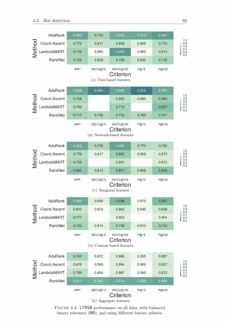
4.3. Bot detection 93
(a) User-based features
(b) Network-based features
(c) Temporal features
(d) Content-based features
(e) Aggregate features
Figure 4.2: LTRSB performance on all data, with balancedbinary relevance (BB), and using different feature subsets.

94 Chapter 4. A supervised approach to user behavioral problems
(a) User-based features
(b) Network-based features
(c) Temporal features
(d) Content-based features
(e) Aggregate features
Figure 4.3: LTRSB performance on all data, with unbalancedbinary relevance (UB), and using different feature subsets.

4.3. Bot detection 95
(a) User-based features
(b) Network-based features
(c) Temporal features
(d) Content-based features
(e) Aggregate features
Figure 4.4: LTRSB performance on all data, with gradedrelevance setting (Grad), and using different feature subsets.

96 Chapter 4. A supervised approach to user behavioral problems
(a) BB
(b) UB
(c) GradFigure 4.5: LTRSB performance on all data and whole feature
space, using different relevance labeling settings.

4.4. Learning to rank Lurkers 97
4.4 Learning to rank LurkersLurking in an online social network (OSN) characterizes those users in the crowdwho do not significantly take an active and tangible role in the interaction withother members [85], [86], [181], [182]. Such users are referred to as lurkers, sincethey gain benefit from information produced by others, though their presenceis legitimated [87], expected and even welcome [101], [183]. More importantly,lurkers might hold potential social capital, because they acquire knowledge fromthe OSN: by observing user-generated communications, they can form theirown opinions and even expertise, though they rarely will let other people knowtheir “value”. Therefore, it might be desirable to make lurkers’ social capitalavailable to other users [184]. This can be accomplished through mechanismsof engagement [102], [103], [185]–[187], ultimately encouraging lurkers to moreactively participate in the OSN life.
In [97], [110], the authors presented the first tool, namely LurkerRank, forautomatically bringing order into the crowd of users that may show lurkingbehaviors at varying degrees. LurkerRank adopts a query-independent, eigen-vector-centrality based approach that utilizes the link graph structure underly-ing user relationships (e.g., followships, like/comment interactions). Its rankingsolution can enable a way to prioritize the engagement of (top-ranked) lurk-ers. LurkerRank has also been adapted as query-dependent (e.g., trust-biased)ranking method [97], [112], extended to handle time-evolving networks [111], orexploited for targeting users in an influence maximization task [188].
Research questions. Nevertheless, several challenges remain open, sincethe complexity of lurking behaviors hints at the opportunity of using any avail-able, possibly platform-specific information on the activity and interaction oflurkers in an OSN. In particular, the following questions may arise:
• Can we incorporate into a lurker ranking model various “signals” that canbe used as behavioral features, upon which the evaluation of the degree oflurking of any user w.r.t. a given context (i.e., online environment) isperformed?
• Can we enable a lurker ranking model to accurately be tuned by exploitingpast lurking experiences?
• What if information on lurking behaviors is available from populations ofdifferent networks?
• Can we predict the lurking behavior of a previously unexamined user byavoiding to rank from scratch all users?
The LTR opportunity. In this work we aim at answering the above ques-tions by developing a principled, machine-learning-based ranking framework forthe analysis of lurking behaviors. Learning-to-rank (LTR), i.e., using machinelearning to automatically build a ranking model, has become one of the keytechnologies for modern web search, retrieval and personalization [128], [129].As in traditional ranking functions, a partial ordering (ranking) is provided fora set of objects, according to their degree of relevance to a given query; in LTR,

98 Chapter 4. A supervised approach to user behavioral problems
the ranking function is learned from training data given in the form of 〈query,object, relevance label〉 tuples.
Motivations. We believe that LTR is particularly suitable for addressingthe aforementioned research questions, thus helping us to improve our under-standing of a behavioral analysis problem that is inherently dynamic as well assensitive to many aspects. In fact, LTR adopts a supervised approach to learnfrom past user experiences, which might be annotated according to the degreeof lurking behavior. LTR training is accomplished according to a set of featureswhich, being possibly of different types, would capture different aspects thatcan be useful predictors of lurking behaviors.
Due to learning from different, properly engineered features, LTR is a robustapproach in cases where it would be difficult to gather sufficient and significantlurking information from the graph of user relationships: this would lead to aweak or sparse link structure, which negatively affects the effectiveness of anygraph-based lurker ranking method. In addition, by inheriting robustness tooutliers of some machine learning methods, LTR models can effectively handleinconsistent or false lurking behaviors (e.g., those shown by users that are to-tally inactive in the online platform). To a more general extent, by treatingmultiple OSN platforms as different queries and building an LTR model frominstances (users) that belong to the various platforms, lurker ranking results canbe compared through different OSNs, thus generalizing the concept of lurkingto multiple networks.
Last, but not least, LTR offers unprecedented opportunities for incrementallurking scenarios: once trained a learning-to-lurker-rank model, this can be usedto assign any previously unobserved user with a lurking score, thus avoiding thecalculation from scratch of a ranking scheme over the entire OSN graph.
Contributions. In this work, we propose the first LTR framework toanalyze lurkers in OSNs. Note that LTR has been previously used to addressbehavioral problems, in particular user engagement. For instance, the studyin [173] aims at ranking tweets by the amount of user participation in them;however, identifying and ranking lurkers is a more complex problem, whichrequires proper modeling of users and their behavioral features.
By exploiting state-of-the-art LTR methods, we develop a learning-to-lurker-rank methodology which exploits the unsupervised LurkerRank method to de-rive binary or graded relevance labels, and a feature engineering phase thataccounts for relational (i.e., topology-based), media-based, activity rate, andplatform-specific information on the commitment and interaction of users fromdifferent OSNs. Results obtained on 23 network datasets, which were built from7 OSNs, have shown the significance of our approach, confirming our initial hy-pothesis that LTR can be effective for ranking lurking behaviors.
4.4.1 Lurker ranking
In [97], [110], the authors have originally brought the concept of centrality in thecontext of lurking behavior analysis, with the goal of characterizing and ranking

4.4. Learning to rank Lurkers 99
top-lurkers mid users top-active users
top-lurkers mid users top-active users
Figure 4.6: Localization of lurkers and non-lurkers in Twitterprofessional-oriented followship graph. (Best viewed in color)
top-lurkers mid users top-active users
top-lurkers mid users top-active users
Figure 4.7: Localization of lurkers and non-lurkers inTwitter-Higgs followship graph. (Best viewed in color)

100 Chapter 4. A supervised approach to user behavioral problems
top-lurkers mid users top-active users
top-lurkers mid users top-active users
Figure 4.8: Localization of lurkers and non-lurkers in Flickrlike-based interaction graph. (Best viewed in color)
the users according to their degree of lurking in an OSN. Following an unsuper-vised learning paradigm, the lurker ranking models utilize only the topology in-formation of an OSN (like PageRank and other classic ranking methods), whichis seen as a directed graph where any edge (u, v) means that v is “consuming”or “receiving” information from u. Upon the assumption that lurking behaviorsbuild on the amount of information a node consumes, the key intuition is thatthe strength of a user’s lurking status can be determined based on three basicprinciples, which are here informally summarized as follows: overconsumption(i.e., the excess of information-consumption over information-production, esti-mated proportionally to the in/out-degree ratio of a node), the authoritativenessof the information received from the in-neighbors, and the non-authoritativenessof the information produced, i.e., sent to the out-neighbors. These principlesform the basis for three ranking models, whereby a complete specification wasprovided in terms of PageRank and alpha-centrality based formulations. Forthe sake of brevity here, and throughout this chapter, we will refer to only oneof the formulations described in [97], [110], which is that based on the in-out-neighbors-driven lurker ranking, hereinafter referred to as LurkerRank (LR).
Given a directed graphG = (V,E), and a node v ∈ V , letN in(v) andN out(v)denote the set of in-neighbors and the set of out-neighbors of v, respectively.For any node v, the LurkerRank score LR(v) is defined as follows [97]:
LR(v) = α[Rin(v) (1 +Rout(v))] + (1− α)p(v) (4.9)

4.4. Learning to rank Lurkers 101
where Rin(v) is the in-neighbors-driven lurking function:
Rin(v) =1
|N out(v)|∑
u∈N in(v)
|N out(u)||N in(u)|
LR(u) (4.10)
and Rout(v) is the out-neighbors-driven lurking function:
Rout(v) =|N in(v)|∑
u∈Nout(v)|N in(u)|∑
u∈Nout(v)
|N in(u)||N out(u)|
LR(u) (4.11)
Above, p(v) is the value for v in the personalization vector, which is by defaultset to 1/|V |, and α is a damping factor ranging within [0,1], usually set to 0.85.
It should be noted that, although the principles underlying LR are genericand applicable to any OSN, the particular type of social context managed bythe online platform, the semantics of user relations therein, and the structuralproperties of the corresponding graph(s) modeling the user relations in theplatform, can have different impact on the understanding of lurking behaviors,and consequently on how lurkers relate themselves to the other (i.e., active)users.
Figure 4.8 shows three examples of social network graphs, in which differ-ent colors are assigned to nodes in order to distinguish between lurkers andusers that can be regarded as moderately or highly active in the correspondingnetwork. For every network, we first computed the LurkerRank score for eachnode, then we determined the weight of each edge (u, v) proportionally to thefraction of the original lurking score of v given by its in-neighbor u, exploit-ing the notion of influence probability defined in [188]. Node colors are chosenaccording to the quartile of membership in the LurkerRank ranking solution:nodes belonging to the 3rd quartile, i.e., the top-25% lurkers, are colored inred, whereas nodes in the 1st quartile, i.e., the top-25% active users, are col-ored in green, and the remaining nodes (mid users) in black. We generated thegraph plots using the force-directed layout OpenOrd [189], which is well-suitedto display the formation of agglomerations around nodes that, in our setting,receive incoming connections with higher weights. Looking at the figure, lurkerscan be differently influenced by few or many groups of active users, presumablydepending on the popularity and appealingness of the topics discussed. Theleftmost graph plot represents a Twitter subnetwork of developers (which alsohave an account on GitHub and StackOverflow; cf. Sect. 4.4.2). Here, the local-ization of lurkers tends to be around a few groups of the developers, dependingon the attractiveness of the software development project the active users areworking on. The middle graph plot corresponds to a portion of Twitter focusedon a single main theme, i.e., the announcement of the Higgs boson. Comparedto the previous example graph, lurkers tend even more to agglomerate withonly some of the active users, the latter presumably being the most visible (i.e.,popular) users that are active in the spreading of information about Higgs bo-son. The rightmost graph plot corresponds to favorite/like-based interactions ofusers in Flickr. Here we observe many micro-agglomerations that imply a quitediversified configuration in terms of localization of lurkers and active users, due

102 Chapter 4. A supervised approach to user behavioral problems
Figure 4.9: Illustration of our proposedlearning-to-lurker-rank (LTLR) framework
to higher heterogeneity of the topics discussed in the network (i.e., photo-driventhemes); moreover, according to previous studies on lurking behaviors in sce-narios of least-effort types of interaction [111], the difference between lurkersand active users is much less evident than in two other graphs.
The above-presented example points out an emergence for enhancing ageneric, topology-based ranking model for lurking behaviors by leveraging thepeculiarities of user relations and media-based properties that are specific tothe OSN under examination. Within this view, in this work we take an oppor-tunity for the development of a new framework that is able to learn from userbehavioral features and past pieces of evidence of lurking states, over multipleOSNs, to predict and rank previously unseen lurking states.
4.4.2 Learning to lurker rank framework
In this section we describe our proposed learning-to-lurker-rank (LTLR) frame-work. Figure 4.9 provides a schematic illustration, which sheds light on the mainmodules and data flows involved in the framework. In this regard, we assumethat a number of social media sources are available (e.g., Twitter, Instagram,etc.), from which three types of information are extracted and organized intothree main components, namely user-relational (i.e., topological) network data,media data, and platform-specific meta-data. These are processed to build thefeature space for the representation of the training data. The learning-to-ranksystem is designed to work with training data instances, each of which is anno-tated with a relevance label expressing the degree of lurking of the correspondinguser (module LurkerRank-based labeling, on the top-right corner of the internalbox shown in the figure). In the following, we elaborate on each of the mainaspects of the proposed LTLR framework.
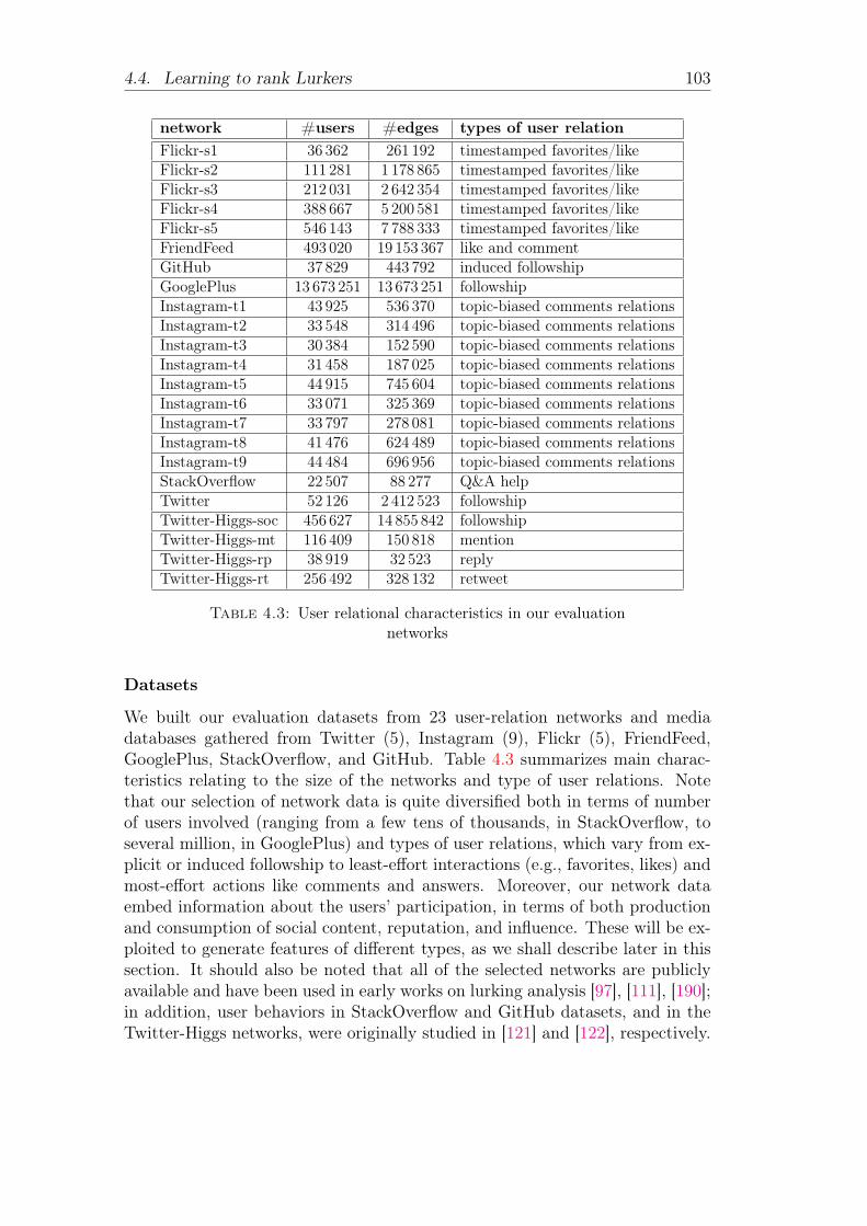
4.4. Learning to rank Lurkers 103
network #users #edges types of user relationFlickr-s1 36 362 261 192 timestamped favorites/likeFlickr-s2 111 281 1 178 865 timestamped favorites/likeFlickr-s3 212 031 2 642 354 timestamped favorites/likeFlickr-s4 388 667 5 200 581 timestamped favorites/likeFlickr-s5 546 143 7 788 333 timestamped favorites/likeFriendFeed 493 020 19 153 367 like and commentGitHub 37 829 443 792 induced followshipGooglePlus 13 673 251 13 673 251 followshipInstagram-t1 43 925 536 370 topic-biased comments relationsInstagram-t2 33 548 314 496 topic-biased comments relationsInstagram-t3 30 384 152 590 topic-biased comments relationsInstagram-t4 31 458 187 025 topic-biased comments relationsInstagram-t5 44 915 745 604 topic-biased comments relationsInstagram-t6 33 071 325 369 topic-biased comments relationsInstagram-t7 33 797 278 081 topic-biased comments relationsInstagram-t8 41 476 624 489 topic-biased comments relationsInstagram-t9 44 484 696 956 topic-biased comments relationsStackOverflow 22 507 88 277 Q&A helpTwitter 52 126 2 412 523 followshipTwitter-Higgs-soc 456 627 14 855 842 followshipTwitter-Higgs-mt 116 409 150 818 mentionTwitter-Higgs-rp 38 919 32 523 replyTwitter-Higgs-rt 256 492 328 132 retweet
Table 4.3: User relational characteristics in our evaluationnetworks
Datasets
We built our evaluation datasets from 23 user-relation networks and mediadatabases gathered from Twitter (5), Instagram (9), Flickr (5), FriendFeed,GooglePlus, StackOverflow, and GitHub. Table 4.3 summarizes main charac-teristics relating to the size of the networks and type of user relations. Notethat our selection of network data is quite diversified both in terms of numberof users involved (ranging from a few tens of thousands, in StackOverflow, toseveral million, in GooglePlus) and types of user relations, which vary from ex-plicit or induced followship to least-effort interactions (e.g., favorites, likes) andmost-effort actions like comments and answers. Moreover, our network dataembed information about the users’ participation, in terms of both productionand consumption of social content, reputation, and influence. These will be ex-ploited to generate features of different types, as we shall describe later in thissection. It should also be noted that all of the selected networks are publiclyavailable and have been used in early works on lurking analysis [97], [111], [190];in addition, user behaviors in StackOverflow and GitHub datasets, and in theTwitter-Higgs networks, were originally studied in [121] and [122], respectively.
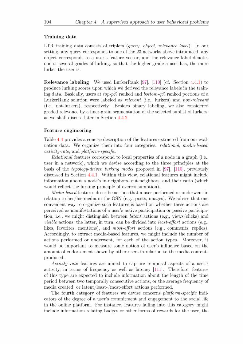
104 Chapter 4. A supervised approach to user behavioral problems
Training data
LTR training data consists of triplets 〈query, object, relevance label〉. In oursetting, any query corresponds to one of the 23 networks above introduced, anyobject corresponds to a user’s feature vector, and the relevance label denotesone or several grades of lurking, so that the higher grade a user has, the morelurker the user is.
Relevance labeling We used LurkerRank [97], [110] (cf. Section 4.4.1) toproduce lurking scores upon which we derived the relevance labels in the train-ing data. Basically, users at top-p% ranked and bottom-q% ranked portions of aLurkerRank solution were labeled as relevant (i.e., lurkers) and non-relevant(i.e., not-lurkers), respectively. Besides binary labeling, we also consideredgraded relevance by a finer-grain segmentation of the selected sublist of lurkers,as we shall discuss later in Section 4.4.2.
Feature engineering
Table 4.4 provides a concise description of the features extracted from our eval-uation data. We organize them into four categories: relational, media-based,activity-rate, and platform-specific.
Relational features correspond to local properties of a node in a graph (i.e.,user in a network), which we devise according to the three principles at thebasis of the topology-driven lurking model proposed in [97], [110], previouslydiscussed in Section 4.4.1. Within this view, relational features might includeinformation about a node’s in-neighbors, out-neighbors, and their ratio (whichwould reflect the lurking principle of overconsumption).
Media-based features describe actions that a user performed or underwent inrelation to her/his media in the OSN (e.g., posts, images). We advise that oneconvenient way to organize such features is based on whether these actions areperceived as manifestations of a user’s active participation or passive participa-tion, i.e., we might distinguish between latent actions (e.g., views/clicks) andvisible actions; the latter, in turn, can be divided into least-effort actions (e.g.,likes, favorites, mentions), and most-effort actions (e.g., comments, replies).Accordingly, to extract media-based features, we might include the number ofactions performed or underwent, for each of the action types. Moreover, itwould be important to measure some notion of user’s influence based on theamount of endorsement shown by other users in relation to the media contentsproduced.
Activity rate features are aimed to capture temporal aspects of a user’sactivity, in terms of frequency as well as latency [111]. Therefore, featuresof this type are expected to include information about the length of the timeperiod between two temporally consecutive actions, or the average frequency ofmedia created, or latent/least-/most-effort actions performed.
The fourth category of features we devise concerns platform-specific indi-cators of the degree of a user’s commitment and engagement to the social lifein the online platform. For instance, features falling into this category mightinclude information relating badges or other forms of rewards for the user, the

4.4. Learning to rank Lurkers 105
id descriptionrelation
alR.1 #in-neighborsR.2 (1 + #out-neighbors)−1
R.3 #in-neighbors / #out-neighborsR.4 (1 + #in-neighbors of a user’s in-neighbors)−1
R.5 #out-neighbors of a user’s in-neighborsR.6 #out-neighbors / #in-neighbors of a user’s in-neighborsR.7 #in-neighbors of a user’s out-neighborsR.8 (1 + #out-neighbors of a user’s out-neighbors)−1
R.9 #in-neighbors / #out-neighbors of a user’s out-neighbors
med
iabased
M.1 #latent actions performedM.2 (1 + #least-effort actions performed)−1
M.3 (1 + #most-effort actions performed)−1
M.4 (#latent actions performed )/(1 + #least-effort actions performed)M.5 (#latent actions performed )/(1 + #most-effort actions performed)M.6 Inv. exp. of EI defined on least-effort actions received for media createdM.7 Inv. exp. of EI defined on most-effort actions received for media created
activity-rate
A.1 Mean per-day #latent actions performedA.2 (1 + mean per-day #least-effort actions performed)−1
A.3 (1 + mean per-day #most-effort actions performed)−1
A.4 A.1 * A.2A.5 A.1 * A.3A.6 Mean #days between two consecutive actions of new content productionA.7 (1 + mean #days between two consecutive actions of content consumption))−1
platform-specific
P.1 (1 + #times the user was tagged)−1 [Instagram]P.2 (1 + #days in a row of current active contribution)−1 [GitHub]P.3 #days in a row of last active contribution [GitHub]P.4 (1 + #days of the longest active contribution)−1 [GitHub]P.5 (1 + reputation score earned)−1 [StackOverflow]P.6 (1 + top-overall percentage)−1 [StackOverflow]P.7 (1 + #people reached)−1 [StackOverflow]P.8 (1 + #profile views)−1 [StackOverflow]P.9 (1 + #gold badges received)−1 [StackOverflow]P.10 (1 + #silver badges received)−1 [StackOverflow]P.11 (1 + #bronze badges received)−1 [StackOverflow]P.12 (1 + #top answers given)−1 [StackOverflow]P.13 (1 + #lists the user belongs to)−1 [Twitter]P.14 (1 + #tweets)−1 [Twitter]
Table 4.4: Extracted features and their description
number of lists a user belongs to, or the length of time period for intensivelyactive contribution.
)
Framework setting
In our evaluation we included all the LTR methods discussed in Sect. 4.2. Weused the Java implementations of RankLib under the The Lemur Project, with

106 Chapter 4. A supervised approach to user behavioral problems
default settings.2 We trained and tested through 5-cross-validation each of theLTR methods usingMAP , P@k, and nDCG@k, with k ∈ {10, 100, 1000}, bothfor optimization (except for RankNet) and evaluation.
From our built evaluation datasets (cf. Table 4.3), we devised three casesdepending on the selection of relevant/non-relevant instances:
• In the first case, dubbed BB, we considered binary relevance, i.e., lurkingand not-lurking, and performed a balanced selection of relevant and not-relevant users.
• In the second case, dubbed UB, we performed unbalanced selection ofrelevant/not-relevant.
• In the third case, dubbed Grad, we considered m grades of relevance oflurking users. We will present results based on the setting of BB cor-responding to top-5% and bottom-5% users by LurkerRank as relevantand not-relevant, resp., the setting of UB corresponding to top-5% andbottom-25% users by LR as relevant and not-relevant, resp., and the set-ting of Grad with m = 3 corresponding to top-5% (relevance 3), second5% (relevance 2), third 5% (relevance 1) as relevant and bottom-25% asnot-relevant.
Table 4.4 provides a concise description of the features extracted from ourevaluation datasets. The first group of features (i.e., from R.1 to R.9) describesnetwork-topology-based indicators of user relations, whose strength would pro-portionally increase with the lurking status of a user. Features from M.1 toM.7 capture the user’s behavior from the perspective of the production andconsumption of media. Note that, except for M.6 and M.7, we chose inverselinear function (for those features requiring inverse proportionality to a certainstatistic count) for smoother numerical decrease. Symbol EI in features M.5–M.7 stands for empirical influence, a measure used to estimate a user’s influencebased on the amount of information s/he produced and that her/his followershave stated to endorse (e.g., liked, replied, etc.) [97], [191]. The third group offeatures contains measurements of the production and consumption activities ofa user, including aggregate indicators such as the mean per-day ratio betweenlatent and least-effort (resp. most-effort) actions. The last group of featuresrefers to a number of aspects, including user’s reputation, popularity, and ac-tivity, that are specific to a single-platform. Finally, it should be noted thatto ensure comparability across queries, all feature values were scaled between 0and 1, through min-max normalization.
Mapping the selected datasets (Table 4.3) with the features in Table 4.4, wederived the following subsets of data:
1. D1: Flickr networks are associated with relational features (i.e., from R.1to R.9) plus M.2, M.6, A.2, and A.7.
2. D2: Flickr and Instagram networks are associated with relational featuresplus A.2 and A.7.
2http://www.lemurproject.org

4.4. Learning to rank Lurkers 107
3. D3: Flickr and FriendFeed networks are associated with relational fea-tures plus M.2 and M.6.
4. D4: GitHub network is associated with relational features plus P.2, P.3,and P.4.
5. D5: StackOverflow network is associated with relational features plus P.2,and from P.5 to P.12.
6. D6: Twitter networks are associated with relational features plus P.13.
Feature informativeness
We investigated about the usefulness or informativeness of the selected features,with a twofold goal: to discover possible correlations between features (possiblyw.r.t. the lurking-relevance class attribute), and to estimate their impact on theranking prediction performance. For this purpose, we resorted to five standardmethods used in feature selection tasks: principal component analysis (PCA),information gain, Pearson’s correlation coefficient, correlation-based feature se-lection (CFS) [178], and learner-based feature selection exploiting J48 decisiontree model.
Using PCA, we found that in most cases the first principal component isa linear combination of relational features (among which, R.2, R.5, and R.8are often characterized by the highest variance), however several exceptions arepresent. For instance, on StackOverflow data, the built-in reputation system(i.e., features P.5, P.9, P10, and P.11) corresponds to the first principal compo-nent, while the subsequent components consist of various linear combinationsof mostly relational features. On Flickr data, the first principal component is acombination of non-relational (M.2 and M.6) and relational features (R.1–R.9).
By employing the information gain method, unlike in PCA, we could takeinto account the class of relevance, both for the binary and graded relevancesettings. As expected, since that the constituent parts of the defining principlesof LR are topology-driven, the most informative features w.r.t. to the lurkingrelevance labels are relational as well (in particular, from R.1 to R.8), for allthe analyzed networks. Nevertheless, non-relational features such as M.6, A.6,and P.14 (which are of media-based, activity-rate, and platform-specific type,respectively) are the subsequent most informative features.
Similarly, an analysis based on Pearson’s correlation recognizes relationalfeatures as the most relevant, followed by the number of tweets posted and thenumber of lists a user belongs to (P.13 and P.14) in Twitter, the reputationsystem and medals present in StackOverflow (P.5, P.9, P.10, P.11), the numberof days in a row of active contribution and the number of least-effort actionsperformed (P.3, M.2) in GitHub. As concerns the CFS method, while being con-sistent with the other methods regarding the relational features, its selection ofmost informative non-relational features includes A.6, for the setting of gradedrelevance label, and P.5, M.3 for the binary settings. Finally, J48 confirmsthe overall scenario described by the other methods, where relational features(in particular, R.3, R.5, and R.6) strongly correlate with the lurking-relevanceclass, followed by M.6 and P.9.

108 Chapter 4. A supervised approach to user behavioral problems
Pearson’s correlation coefficient also deals with both the class of relevanceand the feature under examination, it treats them like random variables whilemeasuring the linear correlation between them.
To sum up, relational (i.e., topological) features revealed to take an essentialrole in predicting the lurking status of users, although different subsets of non-relational were found as equally informative. This prompted us to focus ourempirical evaluation of LTLR on two main settings: the one with relationalfeatures only, or non-relational features only, and the other one correspondingto the full space of features.
Evaluation goals
We organize the presentation of experimental results according to the followingevaluation goals.
• Performance on followship network data, with relational features:
With the intent of setting an initial benchmark we tested our LTLR frame-work on followship network data represented over the space of relationalfeatures only (Section 4.4.3), which are the primary features as they cor-respond to the constituent factors of the topology-driven lurking notionupon which the LurkerRank method is built.
• Performance on heterogeneous data:
In order to assess the capability of the LTLR framework to generalize thelurking behavior across different domains and its ability to leverage thewhole features space we evaluate its performance on all available data,corresponding to the various evaluation networks and represented in thefull space of features (Section 4.4.3).
• Relevance of non-relational features:
We were interested in evaluating the usefulness and informative richnessof media-based, activity-rate and platform-specific features sets w.r.t. theability to predict lurking behavior in OSNs. We focused on a compari-son between the use of non-relational features only (which may vary fromplatform to platform) and all features together for the training data (Sec-tion 4.4.3).
• Performance on distinct networks:
We also investigated whether the ranking model learned from a specificplatform, could be successfully applied to another network sharing thesame feature space. To verify and evaluate this ability, we selected thedata subsets composed of at least two networks, and for each subset, wetrained all the LTR algorithms on one network and tested on the other,and vice-versa (Section 4.4.3).

4.4. Learning to rank Lurkers 109
4.4.3 Experimental results
We organize the presentation of experimental results according to the previ-ously discussed evaluation goals. For each stage of evaluation, we will summa-rize results through heatmaps with numerical detail on the performance scorescorresponding to the various assessment criteria, by varying LTLR method andsetting. Note that, for the sake of readability, particularly to avoid clutteringof the figures, we have intentionally hidden entries in every heatmap that referto optimal performance values (i.e., equal or very close to 1).
Evaluation on followship network data with relational features only
In the first stage of analysis, we tested our framework on followship networksonly, i.e., GitHub, GooglePlus, and Twitter networks, focusing on relationalfeatures. Results are shown in Fig. 4.10. One general remark is that in manycases LTLR can achieve optimal or near-optimal performance. More specifically,in line with the current literature, LambdaMART and Coordinate Ascent revealto be highly effective in learning to rank lurkers, regardless of the assessmentcriterion (except for P@1000) and setting. RankNet shows good performanceas well, except for P@1000 and for nDCG with Grad setting. By contrast,AdaRank achieves quality results around 0.5 for the BB setting (with a peak of0.875 for nDCG@1000), but much lower scores for UB (all criteria) and Grad(nDCG).
In general, LTLR methods tend to achieve the highest scores according tonDCG@1000 and the worst ones with P@1000. This would suggest that theheads of the ranking solutions are effectively detected in most cases, while themethods exhibit some difficulty in ranking most of the relevant users in thetop-k positions, especially in the UB case.
Evaluation on heterogeneous network data
Figure 4.11 reports on LTLR performance results on all network data, whichare divided into two representation settings: the one corresponding to rela-tional features only (first three columns in the heatmap) and the other onecorresponding to all features. At a first glance, we observe a variegate situa-tion, whereby the lurking status of users can be successfully determined onlyfor some of the methods and settings. Among the LTLR methods, the high-est scores are again achieved by LambdaMART and Coordinate Ascent, whichare equally able to perform nearly optimally with all settings of distribution ofrelevant/non-relevant instances, when only relational features are used. Also,these methods seem not to gain any particular benefit from the use of all thefeatures, with few positive exceptions (e.g., Coordinate Ascent with nDCG) andnegative exceptions (e.g., LambdaMART with MAP and P@1000). Competi-tive behavior is also shown by the representative pairwise approach, RankNet,which appears to benefit from the use of all networks and features, especiallyfor the binary relevance cases (BB and UB) and withMAP and nDCG criteria;for the graded relevance case, however, despite the improvement w.r.t. the pre-vious evaluation scenario with followship networks and relational features, the

110 Chapter 4. A supervised approach to user behavioral problems
Figure 4.10: LTLR performance on followship network datawith relational features only
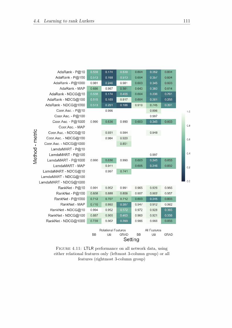
4.4. Learning to rank Lurkers 111
Figure 4.11: LTLR performance on all network data, usingeither relational features only (leftmost 3-column group) or all
features (rightmost 3-column group)
112 Chapter 4. A supervised approach to user behavioral problems
RankNet scores remain far lower than LambdaMART and Coordinate Ascent.The other listwise method, AdaRank, again is found to perform quite poorly inmost cases (below 0.7), with a minimum score of 0.168 (UB, P@100). We tendto ascribe this to an inability of the method of selecting good enough subspacesof features for the building of weak learners and their subsequent combination.
Overall, comparing the performances of LTLR methods on heterogeneousdata against those obtained on followship networks and relational features only,we conclude that training and testing from heterogeneous data, by exploit-ing various types of features, does not undermine the significance of the LTLRframework. Moreover, since the general performance trends by the methodsare similar to the restricted case of followship networks with relational features,the basic topology-driven principles underlying LurkerRank (and hence the def-inition of the relevance labels in the training data) are applicable in differentplatform contexts.
Relevance of non-relational features
Figures 4.12–4.17 show the prediction capabilities obtained with the use ofmedia-based, activity-rate, and platform-specific features, with and withoutthe addition of relational features, on specific subsets of network data (D1–D6,cf. Section 4.4.2). As a general remark, LambdaMART and, to some extent,Coordinate Ascent do not gain any benefit from the extension of the featurespace, while AdaRank and RankNet show significant improvement in most cases.More specifically, concerning subsets D1–D3 (Figs. 4.12–4.14), all the LTLRmethods show none or negligible variation in performances when including ornot the relational features, in most cases. This would suggest that, for relativelyhomogeneous sets of network data, non-relational features can induce most orall of the lurker-ranking prediction ability exhibited by LTLR, i.e., topologicalinformation could become redundant. On the other hand, it also indicatesthat the topology-driven formulation of LurkerRank is able to capture user’sbehavioral patterns that are consistent with the production and consumptionof contents, and relating activity-rate.
On D4–D6 (Figs. 4.15–4.17), we observe a more diversified situation. WhileLambdaMART and Coordinate Ascent are still able to extract all the needed in-formation from few non-relational features and induce a well-performing rankingmodel (with the usual exception regarding P@1000), AdaRank and RankNetoffer poor performance.
Figures 4.18-a)–4.18-d) provide further insights into the behavior of AdaRankand RankNet, showing the percentage increase in performance when using allfeatures compared to a representation of network data based on non-relationalfeatures only.
As anticipated before, most of the percentage values are actually nearly zeroor negative. For instance, in Fig. 4.18-a), RankNet shows a relatively smalldecrease in performance for all settings, while AdaRank takes little advantagein using all features for the UB setting;
in Fig. 4.18-c), with the exception of RankNet nDCG@10 in the Gradsetting, whereby using all the features is extremely advantageous (200% of in-crease), the variations turn out to be positive but negligible for AdaRank, while
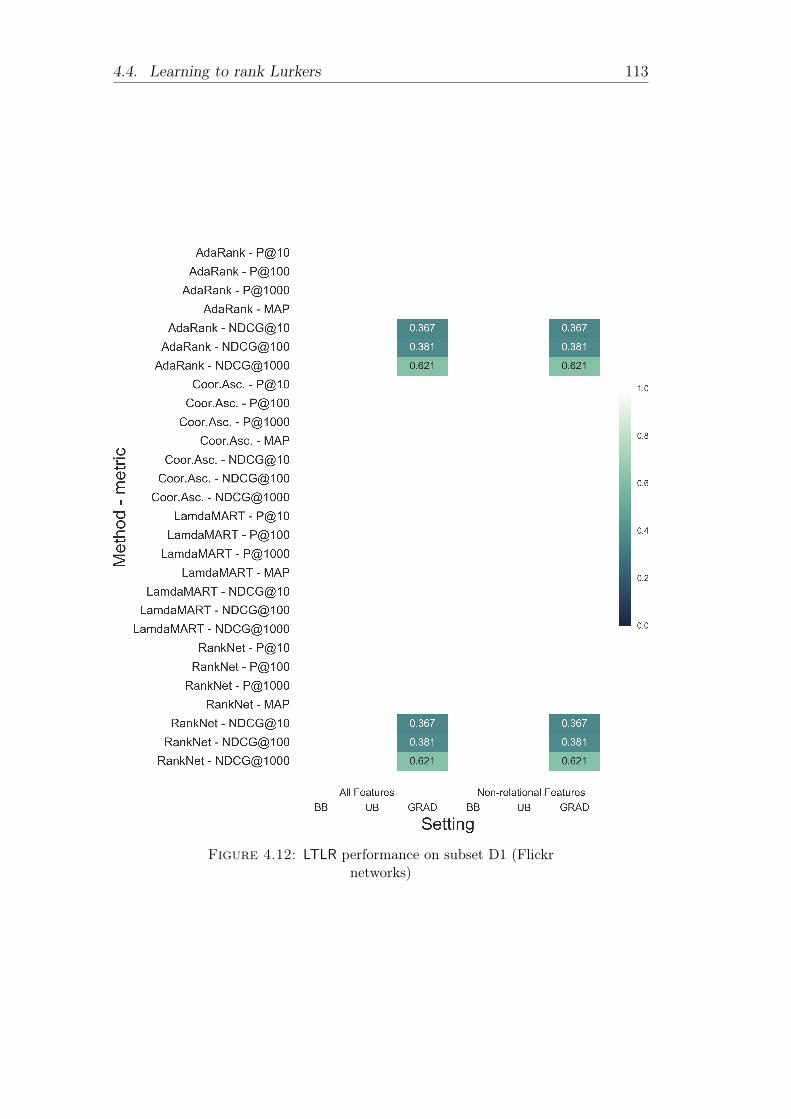
4.4. Learning to rank Lurkers 113
Figure 4.12: LTLR performance on subset D1 (Flickrnetworks)

114 Chapter 4. A supervised approach to user behavioral problems
Figure 4.13: LTLR performance on subset D2 (Flickr andInstagram networks)

4.4. Learning to rank Lurkers 115
Figure 4.14: LTLR performance on subset D3 (Flickr andFriendFeed networks)

116 Chapter 4. A supervised approach to user behavioral problems
Figure 4.15: LTLR performance on subset D4 (GitHubnetwork)
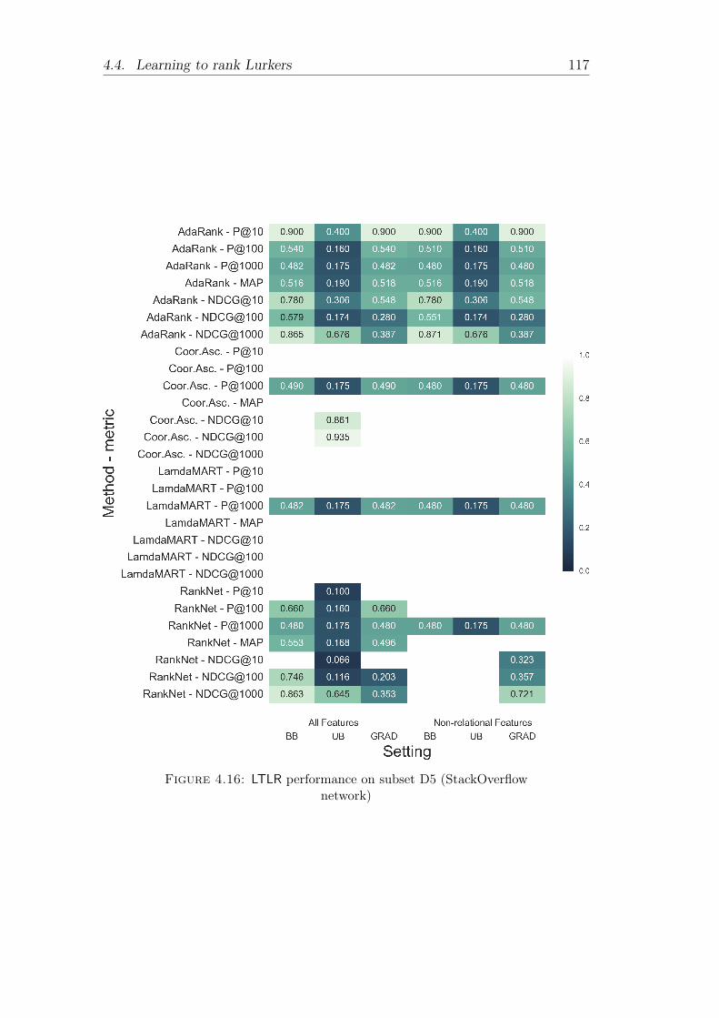
4.4. Learning to rank Lurkers 117
Figure 4.16: LTLR performance on subset D5 (StackOverflownetwork)

118 Chapter 4. A supervised approach to user behavioral problems
Figure 4.17: LTLR performance on subset D6 (Twitternetworks)

4.4. Learning to rank Lurkers 119
being significant and disadvantageous for RankNet for all the settings. Similar,but extended to AdaRank as well, is the situation corresponding to Fig. 4.18-d)relating to Twitter data. Overall, in the majority of the cases, the BB settingseems to be the least affected by the extension of the feature set, while mostand higher variations are observed for UB and Grad. Note however that theabove outcomes should be taken with a grain of salt, since the two weakestLTR methods among those selected particularly suffer from a limited amountof training data, which affects their inability to generalize from the availableexamples.
Evaluation on distinct networks
Figures 4.21-4.20 report on the performance of LTLR methods on test data,after training on network data belonging to different platforms/contexts. Onegeneral remark that stands out is the ability of LambdaMART and CoordinateAscent to effectively learn a ranking function from a specific network, even fromrelatively few instances, and use it to successfully rank lurkers that belong toanother network. As expected, the other two methods may have mid-to-lowperformance especially when there is unbalancing towards the size of test data(i.e., Fig. 4.21 and Fig. 4.20), in which case the use of all features could bebeneficial. More interestingly, in the opposite case (i.e., when Flickr networkdata is used as training), AdaRank and RankNet yield as optimal performanceas LambdaMART and Coordinate Ascent, with the exception of Grad settingand nDCG criterion (which might be explained since the grain of relevancelabels corresponding to the training instances could be coarse in some cases);note also that the performance of each method does not vary depending onwhether all features or only non-relational-features are used.
4.4.4 Discussion
Results have shown that LTLR can be effective in learning to rank lurkers. Moreprecisely, some LTLR methods are able to predict the ranking of lurkers oncetrained according to the (graded or not) relevance labels originally providedby LurkerRank. While best-performing LambdaMART and Coordinate Ascentcan optimally predict the correct rank on test data even with few media-based,activity-rate or platform-specific features, a general trend is that a combina-tion between relational and additional features should be used to improve ac-curacy and ranking performance, especially for worst-performing methods likeAdaRank and RankNet.
Our preliminary evaluation on the feature informativeness (cf. Section 4.4.2)indicated that relational features are the most important to estimate the pre-diction capability of the LTLR framework: while this is not actually surpris-ing, since the training annotations in our network data were originally definedupon topological information, it is partially contradicted by our comprehen-sive evaluation of the performance of the learning-to-rank methods used in ourframework. In fact, the most effective methods can equally perform by usingnon-relational features only or all features, whereas less effective LTR methods

120 Chapter 4. A supervised approach to user behavioral problems
might take advantage from the use of all features compared to either relationalor non-relational features only.
As a final remark, it should be noted that, though LambdaMART offersthe best overall performance in our LTLR framework, it also turns out to needthe highest memory requirements as well as to be the slowest method alongwith RankNet, being several order of magnitude slower than AdaRank andCoordinate Ascent. While the former, despite its efficiency, has not shown togenerate a robust ranking model in most cases, Coordinate Ascent offers thebest trade-off between accuracy and execution time.
4.4.5 Conclusion
In this work, we advanced research on the topic of lurking behavior analysis,by pursuing the goal of developing a robust, multi-platform, supervised lurker-ranking model upon the unsupervised, eigenvector-centrality-based models ex-isting in the literature. To this end, we proposed a learning-to-rank frame-work, named LTLR, whose key aspect is the capability of exploiting differenttypes of information available from multiple OSNs in order to build trainingdata tuples over different subspaces of features. These features include media-based, activity-rate and platform specific characteristics, besides topologicalinformation underlying lurking principles in OSNs. The proposed frameworkis versatile w.r.t. the learning-to-rank method. Experiments conducted on 23network datasets and involving four state-of-the-art learning-to-rank methodshave shown the meaningfulness of LTLR, which often corresponded to highlyeffective ranking.
It should be noted that our proposed framework is also versatile w.r.t. themethodology for labeling the training data: while LurkerRank methods wereused in this work to compensate for the lack of human-generated relevancelabels, we nonetheless advocate for the use of ground-truth scores to assign withobserved lurking behaviors. Moreover, it would be interesting to enhance LTLRto learn from cross-platform features, in order to improve our understandingof behavioral profiles of users who may act as lurkers in one network and,conversely, as contributors in one or more other networks [190].
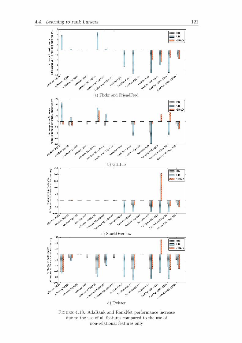
4.4. Learning to rank Lurkers 121
a) Flickr and FriendFeed
b) GitHub
c) StackOverflow
d) Twitter
Figure 4.18: AdaRank and RankNet performance increasedue to the use of all features compared to the use of
non-relational features only
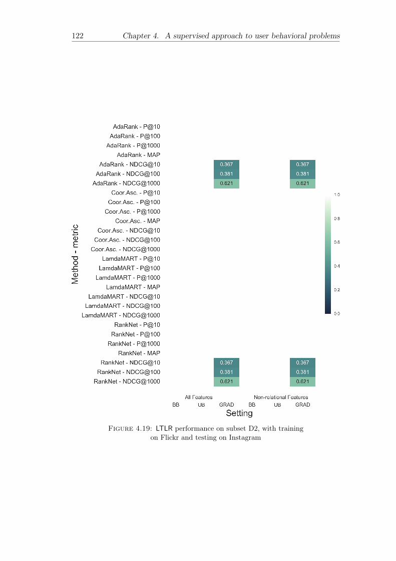
122 Chapter 4. A supervised approach to user behavioral problems
Figure 4.19: LTLR performance on subset D2, with trainingon Flickr and testing on Instagram

4.4. Learning to rank Lurkers 123
Figure 4.20: LTLR performance on subset D2, with trainingon Instagram and testing on Flickr

124 Chapter 4. A supervised approach to user behavioral problems
Figure 4.21: LTLR performance on subset D3, with trainingon FriendFeed and testing on Flickr

4.4. Learning to rank Lurkers 125
Figure 4.22: LTLR performance on subset D3, with trainingon Flickr and testing on FriendFeed


127
Chapter 5
Enhancing the modeling ofcomplex social networks viaembedding
5.1 IntroductionGraph embedding techniques aim to transform a graph in a low-dimensionalrepresentation, enabling the use of a rich set of tools mostly based on state-of-the-art machine-learning methods [192]. A clear advantage in obtaining alow-dimensional representation is to reduce the memory-footprint requirementswhile retaining relevant information for the task at hand [193]. Example tasksinclude node classification, node clustering, node recommendation, retrieval andranking, link (i.e., edge) prediction, and graph classification [194]. Moreover,since the embedding corresponds to a vectorial representation, vector operationson the learned model might in principle be computationally more convenientthan graph operations.
The general goal of a graph embedding process is to learn a function f thatmaps one or many features of the network (i.e., nodes, edges, or the wholegraph) to a new d-dimensional space Rd. For instance, in the case of nodeembedding for a multilayer network, the function to learn can be of the formf : A → Rd or f : V → Rd where A and V denote respectively the set ofactors and the set of nodes. In effect, graph embedding approaches can beclassified based on the constituent(s) of a graph they are designed for. Severalworks have been recently developed for nodes [195], [196], edges [197], subgraphs(e.g., communities [198], [199]), and whole-graph embedding[200]–[202].
Matrix factorization based algorithms [203]–[205] are the pioneering meth-ods in graph embedding, since they apply a decomposition technique to a ma-trix representation of an input graph. There are mainly two types of matrix-factorization-based graph embedding: factorization of graph Laplacian eigen-maps, and direct factorization of the node proximity matrix [192]. One of theearliest methods designed for multilayer networks, specifically for communitydetection purposes, is Principled Modularity Maximization (PMM) [206]. PMMinfers a latent community structure for the nodes in a multilayer network byperforming a two-step methodology. Firstly, PMM extracts low dimensionalvectors from each layer through modularity maximization and aggregates the

128 Chapter 5. Enhancing the modeling of complex OSNs via embedding
extracted information through cross-dimension integration. Finally, a simple k-means is carried out on the learned representation to find out the communitiesof the network.
From a different perspective, in the LINE method [207], two functions aredefined for both first- and second-order proximities, where first-order proximityrefers to edge weights and second-order proximity refers to neighborhood sim-ilarity. LINE defines two joint probability distributions for each pair of nodesand minimizes the Kullback–Leibler divergence of these two distributions.
More recently, there has been momentum for the development of deep-learning-oriented techniques. DeepWalk [195] and Node2Vec [196] are two ex-emplary random-walk-based methods. According to the Skip-gram [208] model,these methods treat nodes as words and paths as sentences, then apply deeplearning to the sampled random-walk paths. As the skip-gram model aims tomaximize the co-occurrence probability among the words that appear within awindow in the same sentence, the resulting graph embedding by DeepWalk andNode2Vec preserves first- and second-order proximity of nodes.
Deep-learning-oriented methods include the use of autoencoders and theirvariants (i.e., denoising, variational, etc.), which aim to maximize the recon-struction accuracy of the input graph, by applying a decoder block to the latentrepresentation learned by an encoder [209]–[211]. Another deep-learning com-mon approach is to directly apply a convolutional neural network (CNN) toEuclidean data generated from a graph [212], or to adapt CNN to graphs [213],[214]. In addition to this group of methods, GraphSAGE [215] aims to learn afunction that generates embeddings by sampling and aggregating features froma node’s local neighborhood. GraphSAGE, which can be seen as an extensionof the GCN [213] framework to the inductive setting, can deal with evolvinggraphs and can easily generate embedding vectors for previously unseen nodes.
5.1.1 Graph embedding for multilayer networks
At the time of writing of this thesis, there is a relatively small corpus of deep-learning-oriented methods of graph embedding specifically conceived for multi-layer networks, namely: PMNE [216], MNE [217], and MELL [218].
The first two methods adapt and extend the Word2Vec [219], [220] modelto multilayer and multiplex networks, respectively. The input sentences (i.e.,paths) are generated by a second-order random walk process, which is con-strained to explore one layer at the time, with the exception of PMNE Layerco-analysis method in which the random walker gains the ability to jump froma layer to another. As depicted in Fig.5.1, PMNE includes three different ap-proaches: two naive baselines, and one natively multilayer. In the NetworkAggregation approach, the multilayer network is merged into a single weightednetwork (where multiple edges between two nodes are not allowed) and the em-beddings for actors are computed on the aggregated network, i.e., f : A → Rd.In the Results Aggregation approach, the embeddings are computed separatelyon each layer and then successively concatenated together, i.e., fl : V → Rdl
and f = f1||f2|| · · · ||f|L| with f : V → Rd′|L|. Unlike the previous two ap-proaches, in the Layer Co-analysis approach the second-order random walker

5.1. Introduction 129
(a)
(b)
(c)
Figure 5.1: Architecture of PMNE: (a) Network Aggregation,(b) Results Aggregation, (c) Layer Co-analysis [216].
acquires the ability to jump across layers, allowing the generation of walks thatare not limited to a single layer of the network, i.e., f : V → Rd. In all of thethree approaches, the Node2Vec model is chosen to be applied to the generatedpaths.
MNE generates a layer-wise embedding vin, for every node n and layer i,which consists of an embedding bn shared across all the layers and that describesthe node n globally, and a local (i.e., layer-wise) embedding uin:
vin = bn + wi ·XiTuin.
In the above equation, wi denotes the importance of layer i, and XiT is atransformation matrix that aligns the global and local embedding vectors.
MELL is based on a regression framework, and unlike the previously de-scribed methods, it also takes into account the directionality of the edges (i.e.,(u, v) 6= (v, u)) by using two vectors for each node vH and vT . Node embed-dings belonging to the same node are enforced to be close to each other througha regularization term. In addition to node embedding, MELL also learns a setof layer vectors representing layers’ connectivity, in order to differentiate edgeprobabilities in each layer. The probability between two nodes vli and vlj, bothbelonging to the layer l, is equal to:
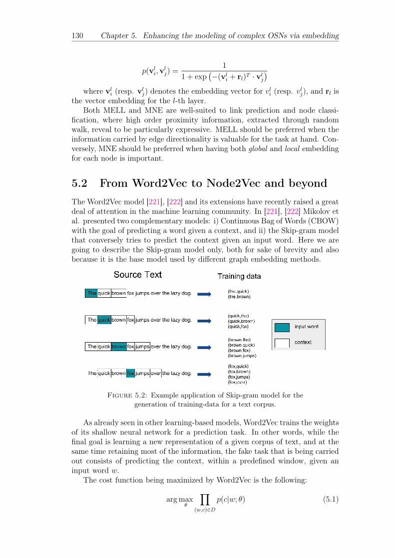
130 Chapter 5. Enhancing the modeling of complex OSNs via embedding
p(vli,vlj) =
1
1 + exp(−(vli + rl)T · vlj
)where vli (resp. vlj) denotes the embedding vector for vli (resp. vlj), and rl is
the vector embedding for the l-th layer.Both MELL and MNE are well-suited to link prediction and node classi-
fication, where high order proximity information, extracted through randomwalk, reveal to be particularly expressive. MELL should be preferred when theinformation carried by edge directionality is valuable for the task at hand. Con-versely, MNE should be preferred when having both global and local embeddingfor each node is important.
5.2 From Word2Vec to Node2Vec and beyondThe Word2Vec model [221], [222] and its extensions have recently raised a greatdeal of attention in the machine learning community. In [221], [222] Mikolov etal. presented two complementary models: i) Continuous Bag of Words (CBOW)with the goal of predicting a word given a context, and ii) the Skip-gram modelthat conversely tries to predict the context given an input word. Here we aregoing to describe the Skip-gram model only, both for sake of brevity and alsobecause it is the base model used by different graph embedding methods.
Figure 5.2: Example application of Skip-gram model for thegeneration of training-data for a text corpus.
As already seen in other learning-based models, Word2Vec trains the weightsof its shallow neural network for a prediction task. In other words, while thefinal goal is learning a new representation of a given corpus of text, and at thesame time retaining most of the information, the fake task that is being carriedout consists of predicting the context, within a predefined window, given aninput word w.
The cost function being maximized by Word2Vec is the following:
arg maxθ
∏(w,c)∈D
p(c|w; θ) (5.1)
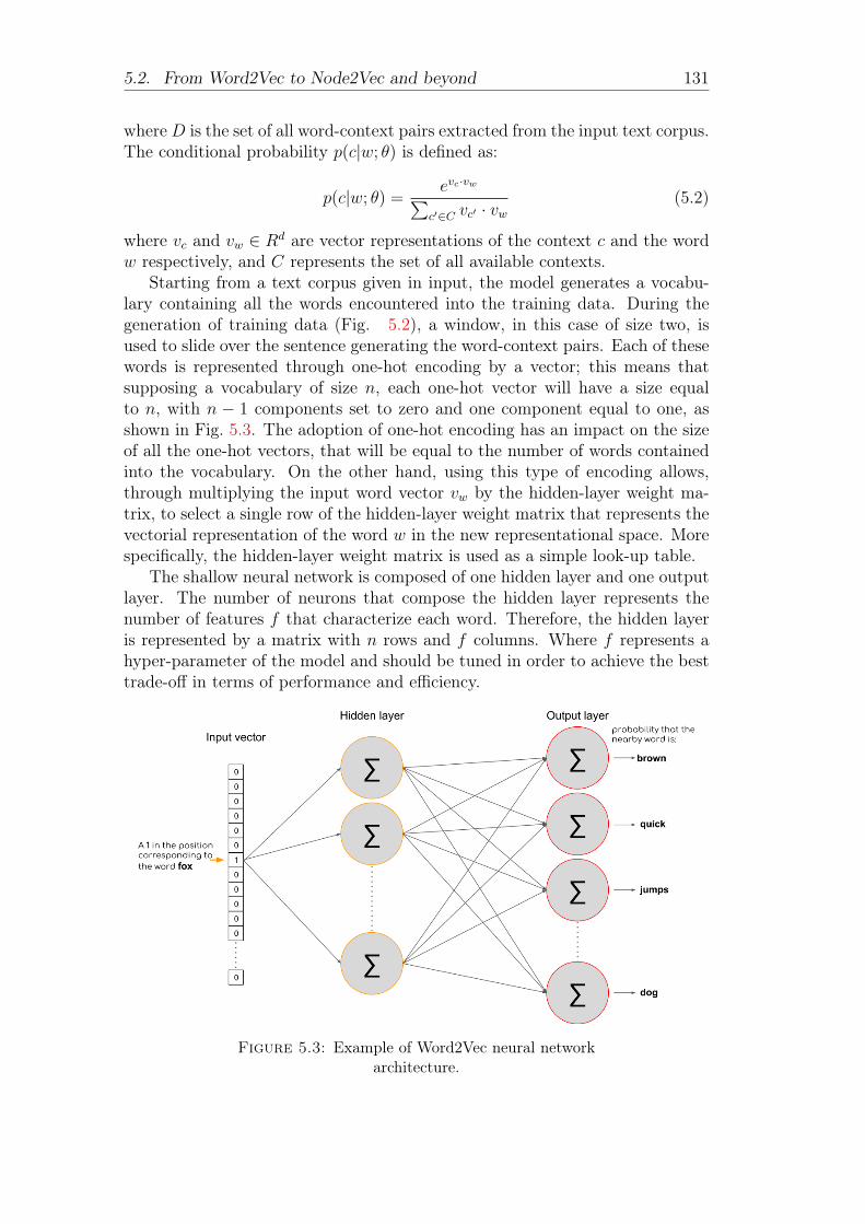
5.2. From Word2Vec to Node2Vec and beyond 131
whereD is the set of all word-context pairs extracted from the input text corpus.The conditional probability p(c|w; θ) is defined as:
p(c|w; θ) =evc·vw∑
c′∈C vc′ · vw(5.2)
where vc and vw ∈ Rd are vector representations of the context c and the wordw respectively, and C represents the set of all available contexts.
Starting from a text corpus given in input, the model generates a vocabu-lary containing all the words encountered into the training data. During thegeneration of training data (Fig. 5.2), a window, in this case of size two, isused to slide over the sentence generating the word-context pairs. Each of thesewords is represented through one-hot encoding by a vector; this means thatsupposing a vocabulary of size n, each one-hot vector will have a size equalto n, with n − 1 components set to zero and one component equal to one, asshown in Fig. 5.3. The adoption of one-hot encoding has an impact on the sizeof all the one-hot vectors, that will be equal to the number of words containedinto the vocabulary. On the other hand, using this type of encoding allows,through multiplying the input word vector vw by the hidden-layer weight ma-trix, to select a single row of the hidden-layer weight matrix that represents thevectorial representation of the word w in the new representational space. Morespecifically, the hidden-layer weight matrix is used as a simple look-up table.
The shallow neural network is composed of one hidden layer and one outputlayer. The number of neurons that compose the hidden layer represents thenumber of features f that characterize each word. Therefore, the hidden layeris represented by a matrix with n rows and f columns. Where f represents ahyper-parameter of the model and should be tuned in order to achieve the besttrade-off in terms of performance and efficiency.
Figure 5.3: Example of Word2Vec neural networkarchitecture.

132 Chapter 5. Enhancing the modeling of complex OSNs via embedding
The output vector consists of n components, but differently from the input,does not use one-hot encoding: more than one component can be greater thanzero, and their value ∈ [0, 1] represents the probability that the word corre-sponding to that position will be part of the context of the input word withina predefined window. The output layer, thanks to the use of softmax function,achieves two desirable characteristics of the output of the neural network: allthe values are in the range [0, 1], and all the values sum up to one.
It is important to notice that the model does not learn a different set ofweights whether the words belonging to the context are usually found before orafter the word w.
In Fig. 5.4 we show, through an example, how Word2Vec computes theprobability that the word dog will be selected randomly to be nearby the wordfox. As reported before, the one-hot encoding vector of the word fox selects theword vector vfox, which is then multiplied by the context vector vcontext, in thiscase of the word dog (i.e., vdog), and finally, the softmax function is in chargeof normalizing the output of the model. It is important to remember that theweights learned are going to reflect the frequency of occurrence for each pair ofwords-context present in the training data.
Figure 5.4: Example of Word2Vec computing the probabilitythat the word dog will appear nearby the word fox.
Depending on the number of features f and the number of unique words ncontained in the input data, the number of weights that compose the shallowneural network can be relatively high. For instance, if we use f = 100 and acorpus with 10, 000 unique words, the number of weights will be equal to twomillion, i.e., one million for the hidden layer and another million for the outputlayer.
In order to improve efficiency, scalability and the performance of theWord2Vecmodel, Mikolov et al. introduce three main modifications: i) to treat commonword pairs or phrases as single “words” (i.e., New_York instead of New andYork), ii) to sub-sample frequent words in order to decrease the number oftraining examples, iii) “negative sampling” is applied mainly in order to limitthe number of weights that are being updated while processing new trainingdata.
5.2. From Word2Vec to Node2Vec and beyond 133
Treat common word pairs as single words reflect the differences in termsof meaning between the two words the compose the pair, if taken separately,and the pair itself. For example, the word pair “Boston Globe” (a newspaper)has a different meaning than the individual words “Boston” and “Globe”. Thisapproach should not be limited to bi-grams, and can be extended to n-grams(e.g., New_York_Times instead of New York Times).
As shown in Fig. 5.2, very common words such as the stop-word the in theexample, will be present in several training instances without adding meaning oruseful information to the word pair. Also, given the frequency of words such asthe in a generic corpus, we will have a higher number of training instances con-taining the word the than needed. In [221], to address this problem Word2Vecimplements a “sub-sampling” scheme, where for each word encountered in thetraining text, there is a chance that the word will be effectively deleted fromthe text, and the probability of cutting the word is related to its frequency. Theprobability that defines whether Word2Vec will keep the word wi is:
Pkeep(wi) =
(√z(wi)
0.001+ 1
)· 0.001
z(wi)(5.3)
where z(wi) represents the ratio between the number of occurrences of the wordwi over the total number of words.
Training a neural network generally means to take several training examples,and for each one of them, slightly adjust all the weights using stochastic gradientdescent (or other optimization techniques), in order to improve the accuracy ofthe model by learning from the processed data. As discussed above, the size ofthe vocabulary, and consequentially the number of weights, could range from oneto several million, all of which would need to be updated while processing everytraining sample. Mikolov et al. overcome this scalability issue by updating onlya small portion of the weights for each training example. For instance, whentraining the neural network on the word pair fox-quick we aim to modify theweights of the network in order to have in output a one in correspondence ofthe word quick when the input word is fox, and zero for all the other words.
Based on Noise Contrastive Estimation [223], [224], negative sampling aimsto update a small portion of the weights of the neural network. In addition to the“positive” weight, we randomly select just a small number k of “negative” wordsfor which the weights are updated. With the term negative is intended a wordfor which the desired output is zero with the current input word. The selectionof the negative samples relies on a unigram distribution, and the probability forselecting a word as a negative sample is related to its frequency. In particular,more frequent words are more likely to be selected as negative samples, asdescribed by the following equation:
Pnegative(wi) =freq(wi)
3/4∑nj=0(freq(wi)3/4)
(5.4)
where freq(wi) indicates the frequency of the word wi.Probably one of the most significant properties of the vectors learned by
Word2Vec is that the vector representing a specific word carries also its semantic

134 Chapter 5. Enhancing the modeling of complex OSNs via embedding
meaning, and more surprisingly the representation tends to obey to the law ofanalogy, as shown by the well-known example “Woman is to queen as man is toking”, corresponding to:
vqueen − vwoman + vman ≈ vking (5.5)
where vqueen, vwoman, vman ,and vking are the vector representation of the wordsqueen, woman, man, and king respectively.
5.2.1 Node2Vec
The first work in which the Skip-gram model has been applied to a graph is byPerozzi et al. in [195], followed by Grover and Leskovec with Node2Vec in [196].Since Node2Vec can be considered a generalization of the DeepWalk algorithm,therefore we will concentrate our focus on Node2Vec only.
The main challenge in applying Word2Vec to a graph is represented by thetransformation of a graph in a corpus. In particular, the structure of a groupof nodes does not resemble the one of a sentence, a paragraph, or a document:while, in a generic corpus, each word is linked to t previous (resp. consecutive)words, in the case of a graph, the structure is usually more complex, allowingconnections potentially between every two nodes.
Node2Vec adds to the Skip-gram model a pre-processing step in charge ofgenerating a set of sentences from a graph by applying a specific samplingstrategy. More in detail, Grover and Leskovec resorted to a second-order randomwalk with two parameters p and q, which guide the walk through the graph.Depending on the values assigned to p and q, the exploration can be carried outin a breadth-first sampling or depth-first sampling fashion.
The return parameter p controls the likelihood of immediately revisiting anode in the walk. Setting it to a high value (> max(q, 1)) ensures that we areless likely to sample an already-visited node in the following two steps (unlessthe next node in the walk had no other neighbor). This strategy encouragesmoderate exploration and avoids 2-hop redundancy in sampling. On the otherhand, if p is low (< min(q, 1)), it would lead the walk to backtrack a step(Figure 5.5) and this would keep the walk “local” close to the starting nodeu [196].
The In-out parameter q allows the search to differentiate between “inward”and “outward” nodes. Going back to Figure 5.5, if q > 1, the random walk isbiased towards nodes close to node t. Such walks obtain a local view of theunderlying graph with respect to the start node in the walk and approximateBreadth-first Sampling behavior in the sense that our samples comprise of nodeswithin a small locality. In contrast, if q < 1, the walk is more inclined to visitnodes which are further away from the node t. Such behavior is reflective ofDepth-first Sampling which encourages outward exploration [196].
For every node u in the graph, n walks, of fixed length l are being simulated.With the starting node c0 = u, the nodes ci are sampled by the followingdistribution:

5.2. From Word2Vec to Node2Vec and beyond 135
P (ci = x|Ci−1 = v) =
{πvxZ
if(v, x) ∈ E0 otherwise
(5.6)
where πvx represents the unnormalized transition probability between nodes vand x, and Z is the normalizing constant. The unnormalized transition proba-bility is set to πvx = αp,q(t, x) · wvx, where:
αp,q(t, x) =
{ 1pifdtx = 0
1ifdtx = 11qifdtx = 2
(5.7)
and wvx represents the weight of the edge that links x and v, dtx denotes theshortest path distance between nodes t and x.
Figure 5.5: Node2Vec sampling strategy (from [196])
The use of random walks, to sample neighbors from a graph, brings efficiencyadvantages both in terms of space and time. The complexity to store the im-mediate neighbors of every node is O(|E|), whereas for a second-order randomwalks, which stores the interconnections between the neighbors of every node,the space complexity is O(a2|V |), where a represents the average degree of thegraph. Concerning time complexity, the main advantage of random-walks-basedmethods is the ability to reuse samples across different starting nodes.
5.2.2 Node2Vec for multilayer networks
With the goal of conceiving a method able to deal with multilayer networks, westarted by devising four variations of Node2Vec, that can be organized into twogroups, i) method based on a multilayer random walk, and ii) methods basedon local (i.e., single-layer) random walk.
Neighborhood-similarity-based methods. In the first group, with thenames Sim-ngh (i.e., similar neighborhood) and Dissim-ngh (i.e., dissimilarneighborhood) we identify two Node2Vec implementations inspired by the com-munity detection method dubbed LART (Locally Adaptive Random Transi-tions) [225]. The similarity between these two methods and the communitydetection one is limited to how the inter-layers weights are computed. These

136 Chapter 5. Enhancing the modeling of complex OSNs via embedding
weights are needed because, differently from Node2Vec algorithm, the second-order random walker present in Sim-ngh (resp. Dissim-ngh) has gained theability to jump across layers, and in this case, the probability of changing layeris defined to be proportional to the similarity (resp. dissimilarity) of the neigh-borhood of the current node in the two layers under consideration (i.e. thestarting layer and the supposed destination layer). This probability is associ-ated to the inter-layer weight that reflects the similarity (resp. dissimilarity) inlocal topology between vki and vli and it is defined as the number of edges thatthe two nodes have in common between the two layers:
wi;kl = |Ni,k ∩Ni,l|
In order to express dissimilarity among the numerous tested inversion func-tions we selected:
winvertedi;kl =1
1 + |Ni,k ∩Ni,l|Furthermore, it is important to notice that the weights are in the range ∈ [0, 1]due to a normalization step.
Context-mixing-based methods. To introduce the other two methods,dubbed Lcm and Ncm, we need to briefly restate the basics of Word2Vec frame-work, on which Node2Vec and all these variations are based. In Word2Vec theconditional probabilities at the core of the optimization problem are:
p(c|w; θ) =evc·vw∑
c′∈C evc′ ·vw
(5.8)
where vc and vw ∈ Rd are vector representations for the context c and the wordw, and C is the set of all available contexts.
We define Lcm (Layer-based context-mixing) and Ncm (Neighborhood-basedcontext-mixing) upon the notion of context mixing, i.e., integrating node-contextwith information from other layers, depending on a layer-wise (resp. neighborhood-wise) similarity measure. More in detail, Lcm mixes the node’s context withinformation coming from other layers, proportionally to layer similarity. Con-versely, by evaluating neighborhood similarity Ncm decides to mix the contextby a finer grain w.t.r. to Lcm.
In summary, we propose four variations of Node2Vec, based on the notion ofneighborhood similarity (resp. context-mixing), namely Sim-ngh and Dissim-ngh (resp. Lcm and Ncm).
5.3 EvaluationIn order to assess the effectiveness of the proposed methods, we compared theirperformance with that of two graph embedding methods available designed todeal with multilayer networks, namely Effective Embedding Method for Mul-tiplex Networks (MELL) [218] and Principled Multilayer Network Embedding(PMNE) [216], presented in Sec. 5.1.1.

5.3. Evaluation 137
Our evaluation consists of a twofold comparison that concerns the ability ofeach method to predict the missing edges from every dataset in Table 5.2 andthe alleged quality of the embeddings in terms of information retained.
Concerning the link prediction task, for each dataset we split the set ofexisting edges into train and testing sets: the former is used to train eachmodel and the latter to test its link prediction performance. Moreover, all theedges belonging to the test set involve nodes that already exist on the specificlayer. We tested all the methods on four train-test split percentages, 60%-40%,70%-30%, 80%-20%, and 90%-10%.
To assess the presumed existence of an edge, from the point of view of thenewly learned representation, we compute the distance for each node pairs inthe test edge set, ordered the list of distance values in ascending order (i.e.,lower values at the top), and selected the top-10% as predicted edges.
For the second task of the evaluation process, we resort to the CS-Aarhus [226]dataset. The reason behind the use of this dataset relies upon the existence ofground-truth values for all the actors present in the network; ground-truth val-ues represent the membership to a specific research group or department.
We learned a new vectorial representation with all the methods discussedabove on increasing training rate in the classification testbed and on all edgeavailable i.e., with a training rate equal to 100% in the clustering testbed.Starting from the newly learned representations, we tested several classificationand clustering algorithms and compared their results with the available ground-truth.
5.3.1 Framework setting
To perform a fair comparison, given the high number of parameters that char-acterize Node2Vec and thus its variants, we tuned each method’s parameter inorder to obtain the best performance.
For both competing methods and Node2Vec variants, we assumed the em-bedding dimension to be constant and equal to 128, whereas in the case ofMELL, since the embedding vector consists of three components, a head anda tail vector, and a layer vector; considering the size of the layer vector to benegligible, we set the size of both head and tail vectors to be d/2 (i.e., 64).Concerning the rest of the parameters of the MELL method, we optimized thenumber of negative samples k, the regularization coefficient of embedding vec-tor λ, the regularization coefficient of the variance β, and the regularizationcoefficient for the layer vector γ. For the rest of the methods (i.e., PMNE andthe Node2Vec variants) we tuned the following parameters: the length of eachwalk l, the number of walks per node n, the size of the context window cw,and the parameters that control the exploration of the multilayer graph (i.e., p,q, and r). Please note that the parameter r in PMNE and Node2Vec variantsrepresents the probability to change layer. The best set of parameters for eachpair of dataset-method is reported in Table 5.1.

138 Chapter 5. Enhancing the modeling of complex OSNs via embedding
Dataset Method Set of best parametersCS-Aarhus
MELLk = 1, λ = 10, β = 1, γ = 4
Pierre Auger Collaboration k = 8, λ = 10, β = 1, γ = 4C.Elegans Connectome k = 4, λ = 10, β = 100, γ = 1
CS-AarhusPMNE
l = 100, n = 20, cw = 14, p = 0.15, q = 0.15, r = 0.15Pierre Auger Collaboration l = 50, n = 16, cw = 14, p = 0.15, q = 0.95, r = 0.6C.Elegans Connectome l = 50, n = 18, cw = 10, p = 0.95, q = 0.15, r = 0.95
CS-AarhusSim-ngh
l = 100, n = 20, cw = 14, p = 0.25, q = 0.25, r = 0.15Pierre Auger Collaboration l = 50, n = 16, cw = 14, p = 0.15, q = 0.95, r = 0.8C.Elegans Connectome l = 50, n = 18, cw = 10, p = 0.95, q = 0.15, r = 0.95
CS-AarhusDissim-ngh
l = 100, n = 20, cw = 14, p = 0.15, q = 0.25, r = 0.15Pierre Auger Collaboration l = 50, n = 16, cw = 10, p = 0.15, q = 0.95, r = 0.6C.Elegans Connectome l = 50, n = 16, cw = 10, p = 0.6, q = 0.15, r = 0.95
CS-AarhusNode2Vec
l = 100, n = 20, cw = 14, p = 0.8, q = 0.15Pierre Auger Collaboration l = 100, n = 16, cw = 12, p = 0.15, q = 0.95C.Elegans Connectome l = 100, n = 16, cw = 10, p = 0.8, q = 0.15
CS-AarhusLcm
l = 100, n = 20, cw = 14, p = 0.6, q = 0.15, r = 0.15Pierre Auger Collaboration l = 50, n = 16, cw = 12, p = 0.15, q = 0.95, r = 0.8C.Elegans Connectome l = 50, n = 16, cw = 10, p = 0.8, q = 0.15, r = 0.95
CS-AarhusNcm
l = 100, n = 20, cw = 14, p = 0.95, q = 0.25, r = 0.15Pierre Auger Collaboration l = 50, n = 16, cw = 12, p = 0.15, q = 0.95, r = 0.8C.Elegans Connectome l = 50, n = 16, cw = 10, p = 0.8, q = 0.15, r = 0.95
Table 5.1: Optimal parameters for MELL, PMNE , andNode2Vec variants.
5.3.2 Assessment criteria
We resort to well-known evaluation measures for both tasks. Given the classimbalance nature of the test, in the link prediction testbed, we compared per-formance results in terms of the area under the precision-recall curve (AUPR),summarized by the trapezoidal rule. Despite being well-known, for the sake ofself-sufficiency, we briefly describe their definitions.
The Precision-Recall curve is defined as the plot of the precision versus therecall values, and the area under this curve well summarizes the performance ofthe classifier under evaluation. The comparison in the classification test relieson two common measures, macro- and micro-average of the F1-score, dubbedmicro-F1 and micro-F1. The F1 score is defined as:
F1 =2 ∗ (precision ∗ recall)
(precision + recall)(5.9)
Conversely, the assessment of the performance on the K-means algorithmsrelies on Normalized Mutual Information (NMI) and Adjusted Mutual Informa-tion (AMI) measures. NMI is a normalization of the Mutual Information (MI)score to scale the results between 0 and 1.
NMI(Y,C) =2 · I(Y ;C)
[H(Y ) +H(C)](5.10)
AMI is an adjustment of the mutual information score to account for chance.It accounts for the fact that the mutual information is generally higher fortwo clusterings with a larger number of clusters, regardless of whether there isactually more information shared. For two clusterings U and V , the AMI isgiven as:

5.4. Experimental Results 139
dataset #nodes #edges #layer directionalityCS-Aarhus [226] 61 620 5 undirectedPierre Auger Collaboration [229] 514 7153 16 undirectedC.Elegans Connectome [227], [228] 279 5863 3 directed
Table 5.2: Main characteristics of evaluation datasets
AMI(U, V ) =[MI(U, V )− E(MI(U, V ))]
[avg(H(U), H(V ))− E(MI(U, V ))](5.11)
where H represents the entropy associated with the partitioning U , and E isthe expected mutual information.
5.3.3 Datasets
Table 5.2 reports the size of set V , the number of edges in all layers, the num-ber of layers, and the directionality of network (i.e., directed or undirected).We used three real-world multilayer networks of different type, namely social,co-authorship, and neural. The first dataset, dubbed AUCS [226], is a socialnetwork that includes both online and offline connections for a total of 5 layers.The 61 nodes in the multilayer network represent professors, postdoctoral re-searchers, Ph.D. students and administrative staff of a university department.The second dataset is a co-authorship network, where the layers represent themain topic/keyword of the publication. The network is composed by 16 layers,relating to topics ranging from neutrinos to astrophysical-scenarios. The thirddataset, dubbed Caenorhabditis elegans connectome [227], [228] is a neural net-work where layers correspond to different synaptic junctions: electric, chemicalmonadic, and chemical polyadic.
5.4 Experimental ResultsIn this section we show preliminary results of ongoing experiments concerningthe extension of Node2Vec framework and the competing methods presented inSect. 5.2.2. According to what previously stated in Sect. 5.3, we organize thepresentation of the results into two parts: i) link prediction performance and ii)performance comparison of all the methods described in the previous sections,in terms of embedding quality, corresponding to information retained.
5.4.1 Link prediction
As previously described in Sect. 5.3, we compared the performance of Sim-ngh, Dissim-ngh, Lcm, and Ncm to the competing methods Node2Vec, PMNE,and MELL. We used four training rates, namely 60%, 70%, 80%, and 90%, andincremented the number of epochs from 1 to 250. To improve readability AUPRscores for varying training-rate and different methods, are reported in heatmapformat.
One general remark is that MELL achieves the best overall performance atthe cost of efficiency, i.e., in order to achieve best results MELL needs a number
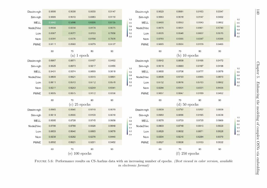
140Chapter
5.Enhancing
themodeling
ofcomplex
OSN
svia
embedding
(a) 1 epoch (b) 10 epochs
(c) 25 epochs (d) 50 epochs
(e) 100 epochs (f) 250 epochs
Figure 5.6: Performance results on CS-Aarhus data with an increasing number of epochs. (Best viewed in color version, availablein electronic format)
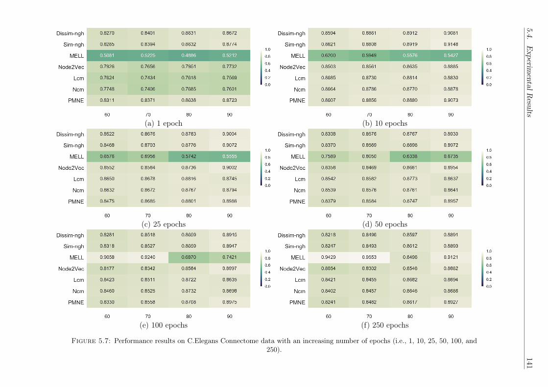
5.4.Experim
entalResults
141
(a) 1 epoch (b) 10 epochs
(c) 25 epochs (d) 50 epochs
(e) 100 epochs (f) 250 epochs
Figure 5.7: Performance results on C.Elegans Connectome data with an increasing number of epochs (i.e., 1, 10, 25, 50, 100, and250).

142Chapter
5.Enhancing
themodeling
ofcomplex
OSN
svia
embedding
(a) 1 epoch (b) 10 epochs
(c) 25 epochs (d) 50 epochs
(e) 100 epochs (f) 250 epochs
Figure 5.8: Performance results on Pierre Auger Collaboration data with an increasing number of epochs (i.e., 1, 10, 25, 50, 100,and 250).
5.4. Experimental Results 143
of epochs equal to or higher than 100, and in general the higher the better.Conversely, Node2Vec-based methods generally achieve the best performancewith just 1 epoch, and increasing the number of iterations rarely leads to anincrease in performance.
In all three datasets, CS-Aarhus, C.Elegans Connectome, and Pierre AugerCollaboration network, we see two recurrent patterns. While the MELL algo-rithm increases its performance with a growing number of epochs, at the sametime Node2Vec-based algorithms slightly decrease their performance with anincreasing number of epochs and usually, the best result is achieved with 1, 10or at most 25 epochs.
Figure 5.6 reports performance results on CS-Aarhus data. Among all meth-ods, the best performance result with only 1 epoch is achieved by Dissim-nghin correspondence of a 90% training rate with a 0.915 of AUPR, closely fol-lowed by PMNE and Sim-ngh. The other algorithms are separated by 0.1,with the exception of MELL, that sets the bar between 0.61 and 0.56. Amongthe Node2Vec-based methods, we see a distinctive pattern, where Sim-ngh andDissim-ngh, albeit defined on opposite intuitions, have similar results and leadthe rank, whereas Lcm and Ncm are relegated to the bottom of the rank. No-tice that in this case, 25 epochs are enough for MELL algorithm to find agood arrangement of its embedding structure and become the best performingmethod.
The inherent complexity of the C.Elegans Connectome data requires a highernumber of epochs needed for all the methods (see Figure 5.7). In particular,MELL needs 100 epochs to achieve the best result for 60% and 70% trainingrate, and 250 epochs in the case of 90% training rate. However, for the remainingcase, i.e., a training rate equal to 80%, 250 iterations are not enough to exceedthe other methods. Conversely, Sim-ngh and Dissim-ngh start, with 1 epoch,among the best with the PMNE algorithm, but are then reached by Lcm andNcm at 10 iterations and then outperformed by Lcm and Ncm.
The Pierre Auger Collaboration data seems to be easy to learn and makeprediction on by Node2Vec-based algorithms. With only 1 iteration they achievenear-optimal performance with a minimum AUPR value of 0.954 (Lcm methodand 60% training rate) and a maximum value of 0.981 in correspondence of atraining rate of 80% and the Dissim-ngh method (results shown in Figure 5.8).On the other hand, with the maximum number of iterations, all methods, in-cluding MELL, achieve near-optimal performance in all cases, ranging fromaround 0.96 to 0.998.
5.4.2 Classification and Clustering
In this subsection, we describe the performance results obtained in the classi-fication and clustering task described in Section 5.3. In the former task, afterlearning a new representation, we tested six well-known classification algorithmscomparing their prediction to the ground-truth values. In particular, we resortto macro-F1 and micro-F1 measures and to the following classification meth-ods: k-nearest neighbors [230], linear support vector classifier [231], decision

144Chapter
5.Enhancing
themodeling
ofcomplex
OSN
svia
embedding
(a) (b)
(c) (d)
(e) (f)
Figure 5.9: Classification performance results of the following classifiers with the macro-F1 measure: a) decision tree classifier, b)linear support vector classifier, c) gaussian naive Bayes classifier, d) k-nearest neighbors, e) multi-layer perceptron classifier, and f)
random forest classifier.

5.4.Experim
entalResults
145
(a) (b)
(c) (d)
(e) (f)
Figure 5.10: Classification performance results of the following classifiers with the micro-F1 measure: a) decision tree classifier, b)linear support vector classifier, c) gaussian naive Bayes classifier, d) k-nearest neighbors, e) multi-layer perceptron classifier, and f)
random forest classifier.

146 Chapter 5. Enhancing the modeling of complex OSNs via embedding
(a)
(b)
Figure 5.11: K-means performance results on CS-Aarhusdatasets with AMI a) and NMI b) evaluation metric.
tree classifier [232], random forest classifier [233], multi-layer perceptron clas-sifier [234], [235], and gaussian naive Bayes classifier [236].
Analyzing the results in Figure 5.9 and Figure 5.10, and putting aside thecomparison between the different classifiers, we concentrate our effort to esti-mate how easily and with which results, a generic classifier can correctly predictthe class of membership with only the information contained into the learnedrepresentation at its disposable.
One general remark is that, for both evaluation metrics, all the methodsbased on random walks and the Word2Vec model are characterized by inferiorperformance than MELL algorithm. However, it is important to point outthat in most cases all methods, including MELL, show worse performance withan increasing training rate, highlighting the limitations of this approach forcomplex data. Among Node2Vec-based algorithms, Sim-ngh, Dissim-ngh, andPMNE show consistently better performance than Node2Vec, Ncm, and Lcm.
5.5 ConclusionIn this chapter, we described some preliminary results in pursuing the devel-opment of a new network-embedding method for multilayer networks. To thisend, we proposed several extensions of the Node2Vec algorithm. While per-formance results, in the link prediction task, are similar among the proposed

5.5. Conclusion 147
methods and their competitors, the classification and clustering testbeds shedlight about the inability of random-walk-based algorithms to extrapolate usefulinformation about every single actor of the network to build a new representa-tion able to predict the class of membership.
In most cases, better results are obtained by MELL algorithm, especiallyin the classification and clustering task. Albeit MELL is based on a regressionframework, and is less efficient than Node2Vec and its variants (PMNE in-cluded), in terms of number of epochs needed to achieve the best performance,MELL algorithm resulted to be a better choice for both the link prediction taskand especially the quality of its embeddings.

149
Chapter 6
Conclusions and future work
6.1 ConclusionsThe research presented in this thesis focused on the development of methodsin the context of complex network systems to investigate and characterize, ina quantitative manner, user behaviors in OSNs. One of the main contributionsof this work is represented by the mlALCR ranking algorithm, which tackles thenovel problem of identifying and characterizing opposite behaviors that usersmay alternately exhibit over the multiple layers of a complex network. In thisrespect, we proposed the first topology-driven ranking method for alternatelurker-contributor behaviors on a multilayer OSN, which is designed to identifyusers that behave as lurkers (resp. contributors) in one layer while converselyacting as contributors (resp. lurker) in one or many of the other layers. Weempirically demonstrated, over four real-world multilayer networks, the signifi-cance and uniqueness of mlALCR solutions.
The second part of this research project has been devoted to leveragingmachine-learning techniques to learn models from data in the context of behav-ioral analysis. In this context, we faced the tasks of identifying and rankingboth lurking and automated (i.e., bot) behaviors in OSNs. Tackling the for-mer problem, we developed a robust, multi-platform, supervised lurker-rankingmodel upon the unsupervised, eigenvector-centrality-based models existing inthe literature. To this end, we proposed a learning-to-rank framework, namedLTLR, whose key aspect is the capability of exploiting different types of infor-mation available from multiple OSNs in order to build training data tuples overdifferent subspaces of features. Regarding the latter problem, we developed asupervised ranking model, that leverages different behavioral signals of bot ac-tivity. The proposed learning-to-rank framework, dubbed LTRSB, exploits themost relevant existing methods on bot detection for enhanced feature extrac-tion, and state-of-the-art learning-to-rank methods for the optimization. Weproved the meaningfulness and effectiveness of both framework on real-worlddata, according to different assessment criteria.
Finally, we described preliminary results in pursuing the development of anew network-embedding method for multilayer networks. While performanceresults, in the link prediction task, are similar for the proposed methods andtheir competitors, the classification and clustering testbeds shed light aboutthe inability of random-walk-based algorithms to extrapolate enough usefulinformation about every single actor of the network in order to build a newrepresentation able to predict the class of membership.

150 Chapter 6. Conclusions and future work
6.2 Future workOver the past decades, we have witnessed the introduction of new technologies,and while the ongoing digital transformation is improving our daily life, is alsocreating new unprecedented challenges. The development of new tools andplatforms, their high diffusion and immediate accessibility, shape and transformthe world we know.
With the information era and the consequentially over-production of infor-mation, it has become essential to properly select and assess the quality of theinformation we consume each day. The risk of consuming untrue informationthat aims to polarize our opinion is high and increasing. In this context, onemain challenge concerns the development of tools that can protect the end userfrom the deluge of information, by helping her/him in the assessment of thetruthfulness and the allegedly quality of contents. The challenge includes theconception of new business models that can promote the creation of high-qualitycontent and prevent the diffusion of click-baits and fake pieces of information byleveraging new technologies. In this context, it is important also to evaluate therole of automated behavior as an enabling factor in the process of informationdissemination.
In the last decade, thanks to the rapid diffusion of mobile technology, sep-arating offline from the online experience has become more and more difficult.Such problems as bullying, from being limited in the context of school or work,recently it has expanded to digital space potentially losing its temporal andspatial limitation. In this context, a socially relevant challenge is to tackle theproblem of cyber-bullying, with the goal of limiting or preventing stressful ex-periences, especially to young adults and teenagers. Moreover, leveraging theknowledge and the tools developed for the analysis of lurking behaviors couldbe interesting to analyze and understand bystanders and devise methods toincrease their participation and thus preventing bullying acts.
In the past few years, the growing computational power of modern GPUsand the availability of large datasets have allowed the successful application ofneural networks, characterized by a high number of layers, to Euclidean data.While deep learning models have proven to be an effective and powerful toolwhen dealing with data such as speech, images, or video, recently there has beena growing interest in trying to apply deep learning on non-Euclidean data. Inthis context, the development of emerging techniques attempting to generalizedeep neural models to domains such as graphs and manifolds, with the goal ofextending the application of deep learning models, represents a challenging lineof research.

151
Bibliography
[1] I Pavlov, “Conditioned reflexes.”, 1927.
[2] E. L. Thorndike, Animal intelligence. MacMillan, Princeton, NJ, 1898.
[3] E. Thorndike, The fundamentals of learning new york: Teachers college,columbia university, 1932.
[4] J. B. Watson, “Psychology as the behaviorist views it.”, Psychologicalreview, vol. 20, no. 2, p. 158, 1913.
[5] J. B. Watson and R. Rayner, “Conditioned emotional reactions.”, Journalof experimental psychology, vol. 3, no. 1, p. 1, 1920.
[6] B. Skinner, “The behavior of organisms: An experimental analysis.”, NewYork, 1938.
[7] B. F. Skinner, About behaviorism. Random House, New York, 1974.
[8] S. Wasserman and K. Faust, Social Networks Analysis: Methods andApplications. Cambridge University Press, 1994.
[9] G. Sabidussi, “The centrality index of a graph”, Psychometrika, vol. 31,pp. 581–603, 1966.
[10] L. C. Freeman, “A set of measures of centrality based on betweenness”,Sociometry, vol. 40, pp. 35–41, 1977.
[11] U. Brandes, “A faster algorithm for betweenness centrality”, Journal ofMathematical Sociology, vol. 25, no. 2, pp. 163–177, 2001.
[12] U. Brandes, “On variants of shortest-path betweenness centrality andtheir generic computation”, Social Networks, vol. 30, no. 2, pp. 136–145,2008.
[13] M. E. J. Newman and M. Girvan, “Finding and evaluating communitystructure in networks”, Physical Review E, vol. 69, 026113, 2004.
[14] K. Stephenson and M. Zelen, “Rethinking centrality: Methods and ap-plications”, Social Networks, vol. 11, pp. 1–37, 1989.
[15] L. C. Freeman, “Centrality in social networks conceptual clarification”,Social Networks, vol. 1, no. 3, pp. 215–239, 1979.
[16] J. R. Seeley, “The net of reciprocal influence: a problem in treating so-ciometric data”, Canadian Journal of Psychology, vol. 3, pp. 234–240,1949.
[17] L. Katz, “A new status index derived from sociometric analysis”, Psy-chometrika, vol. 18, no. 1, pp. 39–43, 1953.

152 Bibliography
[18] P. Bonacich, “Factoring and weighing approaches to status scores andclique identification”, Journal of Mathematical Sociology, vol. 2, pp. 113–120, 1972.
[19] P. Bonacich and P. Lloyd, “Eigenvector-like measures of centrality forasymmetric relations”, Social Networks, vol. 23, pp. 191–201, 2001.
[20] S. Brin and L. Page, “The anatomy of a large-scale hypertextual Websearch engine”, Computer Networks and ISDN Systems, vol. 30, no. 1-7,pp. 107–117, 1998.
[21] A. Rajaraman and J. D. Ullman,Mining of Massive Datasets. CambridgeUniversity Press, 2011.
[22] C. D. Meyer, Matrix Analysis and Applied Linear Algebra. SIAM, 2000.
[23] A. N. Langville and C. D. Meyer, “Deeper inside PageRank”, InternetMathematics, vol. 1, no. 3, pp. 335–400, 2005.
[24] L. Pretto, “A theoretical analysis of PageRank”, in Proc. of the Int. Sym-posium on String Processing and Information Retrieval, 2002, pp. 131–144.
[25] J. M. Kleinberg, “Authoritative sources in a hyperlinked environment”,in Proc. of the ACM-SIAM Symposium on Discrete Algorithms (SODA),1998, pp. 668–677.
[26] J. M. Kleinberg, “Authoritative sources in a hyperlinked environment”,Journal of ACM, vol. 46, no. 5, pp. 604–632, 1999.
[27] R. Lempel and S. Moran, “The stochastic approach for link-structureanalysis (SALSA) and the TKC effect”, Computer Networks, vol. 33,no. 1-6, pp. 387–401, 2000.
[28] K. Bharat and M. R. Henzinger, “Improved algorithms for topic distil-lation in hyperlinked environments”, in Proc. of the ACM Conf. on Re-search and Development in Information Retrieval (SIGIR), 1998, pp. 104–111.
[29] S. Chakrabarti, B. Dom, P. Raghavan, S. Rajagopalan, D. Gibson, andJ. M. Kleinberg, “Automatic resource compilation by analyzing hyperlinkstructure and associated text”, in Proc. of the ACM Conf. on World WideWeb (WWW), 1998, pp. 65–74.
[30] A. Borodin, G. O. Roberts, J. S. Rosenthal, and P. Tsaparas, “Findingauthorities and hubs from link structures on the World Wide Web”, inProc. of the ACM Conf. on World Wide Web (WWW), 2001, pp. 415–429.
[31] G. Jeh and J. Widom, “SimRank: a measure of structural-context sim-ilarity”, in Proc. ACM Int. Conf. on Knowledge Discovery and DataMining (KDD), 2002, pp. 538–543.
[32] D. Fogaras and B. Racz, “Scaling link-based similarity search”, in Proc.ACM Conf. on World Wide Web (WWW), 2005, pp. 641–650.

Bibliography 153
[33] D. Lizorkin, P. Velikhov, M. N. Grinev, and D. Turdakov, “Accuracyestimate and optimization techniques for SimRank computation”, Proc.of the VLDB Endowment (PVLDB), vol. 1, no. 1, pp. 422–433, 2008.
[34] I. Antonellis, H. Garcia-Molina, and C. Chang, “SimRank++: queryrewriting through link analysis of the click graph”, Proc. of the VLDBEndowment (PVLDB), vol. 1, no. 1, pp. 408–421, 2008.
[35] W. Yu, X. Lin, and W. Zhang, “Towards efficient SimRank computationon large networks”, in Proc. Int. Conf. on Data Engineering (ICDE),2013, pp. 601–612.
[36] L. Du, C. Li, H. Chen, L. Tan, and Y. Zhang, “Probabilistic SimRankcomputation over uncertain graphs”, Information Sciences, vol. 295, pp. 521–535, 2015.
[37] R. Weiss, B. Vélez, and M. A. Sheldon, “Hypursuit: A hierarchical net-work search engine that exploits content-link hypertext clustering”, inProc. ACM Conf. on Hypertext, 1996, pp. 180–193.
[38] A. Broder, S. Glassman, M. Manasse, and G. Zweig, “Syntactic clusteringof the web”, in Proc. ACM Conf. on World Wide Web (WWW), 1997.
[39] L. Egghe and R. Rousseau, Introduction to Informetrics. Elsevier SciencePublishers. Amsterdam, The Netherlands, 1990.
[40] R. R. Larson, “Bibliometrics of the world wide web: An exploratory anal-ysis of the intellectual structure of cyberspace”, in Proc. Annual MeetingAmerican Society for Information Science, vol. 33, 1996, pp. 71–78.
[41] J. Pitkow and P. Pirolli, “Life, death and lawfulness on the electronicfrontier”, in Proc. ACM SIGCHI Conf. on Human Factors in ComputingSystems (CHI), 1997.
[42] M. Perkowitz and O. Etzioni, “Adaptive web sites: an AI challenge”, inProc. Int. Joint Conf. on Artificial Intelligence (IJCAI), 1997.
[43] M. Perkowitz and O. Etzioni, “Towards adaptive web sites: Concep-tual framework and case study”, Computer Networks, vol. 31, no. 11-16,pp. 1245–1258, 1999.
[44] J. Weng, E. P. Lim, J. Jiang, and Q. He, “TwitterRank: Finding Topic-Sensitive Influential Twitterers”, in Proc. ACM Conf. on Web Search andWeb Data Mining (WSDM), 2010, pp. 261–270.
[45] D. M. Blei, A. Y. Ng, and M. I. Jordan, “Latent Dirichlet Allocation”,Journal of Machine Learning Research, vol. 3, no. 4–5, pp. 993–1022,2003.
[46] Z. Gyöngyi, H. Garcia-Molina, and J. O. Pedersen, “Combating WebSpam with TrustRank”, in Proc. Int. Conf. on Very Large Data Bases(VLDB), 2004, pp. 576–587.
[47] Y. Sun and J. Han, Mining Heterogeneous Information Networks: Prin-ciples and Methodologies, ser. Synthesis Lectures on Data Mining andKnowledge Discovery. Morgan & Claypool Publishers, 2012.

154 Bibliography
[48] A. Balmin, V. Hristidis, and Y. Papakonstantinou, “ObjectRank: Authority-Based Keyword Search in Databases”, in Proc. Int. Conf. on Very LargeData Bases (VLDB), 2004, pp. 564–575.
[49] Z. Nie, Y. Zhang, J.-R. Wen, andW.-Y. Ma, “Object-level ranking: bring-ing order to Web objects”, in Proc. ACM Conf. on World Wide Web(WWW), 2005, pp. 567–574.
[50] S. D. Gollapalli, P. Mitra, and C. L. Giles, “Ranking authors in digitallibraries”, in Proc. Int. Joint Conf. on Digital Libraries (JCDL), 2011,pp. 251–254.
[51] M. Zhang, S. Feng, J. Tang, B. A. Ojokoh, and G. Liu, “Co-Ranking Mul-tiple Entities in a Heterogeneous Network: Integrating Temporal Factorand Users’ Bookmarks”, in Proc. Int. Conf. on Asian Digital Libraries(ICADL), 2011, pp. 202–211.
[52] H. Deng, J. Han, M. R. Lyu, and I. King, “Modeling and exploitingheterogeneous bibliographic networks for expertise ranking”, in Proc. Int.Joint Conf. on Digital Libraries (JCDL), 2012, pp. 71–80.
[53] D. Liben-Nowell and J. M. Kleinberg, “The link-prediction problem forsocial networks”, Journal of the American Society for Information Sci-ence and Technology, vol. 58, no. 7, pp. 1019–1031, 2007.
[54] D. A. Davis, R. Lichtenwalter, and N. V. Chawla, “Multi-relational linkprediction in heterogeneous information networks”, in Proc. Int. Conf.on Advances in Social Networks Analysis and Mining (ASONAM), 2011,pp. 281–288.
[55] S. E. Helou, C. Salzmann, and D. Gillet, “The 3A Personalized, Contex-tual and Relation-based Recommender System”, J. UCS, vol. 16, no. 16,pp. 2179–2195, 2010.
[56] S. Lee, S. Song, M. Kahng, D. Lee, and S. Lee, “Random walk basedentity ranking on graph for multidimensional recommendation”, in Proc.ACM Conf. on Recommender Systems (RecSys), 2011, pp. 93–100.
[57] V. Vasuki, N. Natarajan, Z. Lu, B. Savas, and I. S. Dhillon, “ScalableAffiliation Recommendation using Auxiliary Networks”, ACM Trans. In-telligent Systems and Technology, vol. 3, no. 1, p. 3, 2011.
[58] R. Interdonato and A. Tagarelli, “Multi-relational PageRank for TreeStructure Sense Ranking”, World Wide Web Journal, 2014.
[59] N. Lao and W. W. Cohen, “Relational retrieval using a combinationof path-constrained random walks”, Machine Learning, vol. 81, no. 1,pp. 53–67, 2010.
[60] Y. Sun, J. Han, X. Yan, P. S. Yu, and T. Wu, “PathSim: Meta Path-Based Top-K Similarity Search in Heterogeneous Information Networks”,Procs. of the VLDB Endowment (PVLDB), vol. 4, no. 11, pp. 992–1003,2011.

Bibliography 155
[61] Y. Sun, J. Han, P. Zhao, Z. Yin, H. Cheng, and T. Wu, “RankClus:integrating clustering with ranking for heterogeneous information net-work analysis”, in Proc. Int. Conf. on Extending Database Technology(EDBT), 2009, pp. 565–576.
[62] Y. Sun, Y. Yu, and J. Han, “Ranking-based clustering of heterogeneousinformation networks with star network schema”, in Proc. ACM Int.Conf. on Knowledge Discovery and Data Mining (KDD), 2009, pp. 797–806.
[63] W. Jiang, G. Wang, M. Z. A. Bhuiyan, and J. Wu, “Understandinggraph-based trust evaluation in online social networks: Methodologiesand challenges”, ACM Comput. Surv., vol. 49, no. 1, 10:1–10:35, 2016.
[64] W. Sherchan, S. Nepal, and C. Paris, “A survey of trust in social net-works”, ACM Comput. Surv., vol. 45, no. 4, 47:1–47:33, 2013.
[65] Z. Gyöngyi, H. Garcia-Molina, and J. Pedersen, “Combating web spamwith trustrank”, in Proc. of Conf. on Very Large Data Bases (VLDB),2004, pp. 576–587.
[66] S. D. Kamvar, M. T. Schlosser, and H. Garcia-Molina, “The eigentrustalgorithm for reputation management in P2P networks”, in Proc. of Conf.on World Wide Web (WWW), 2003, pp. 640–651.
[67] R. Aringhieri, E. Damiani, S. D. C. Di Vimercati, S. Paraboschi, andP. Samarati, “Fuzzy techniques for trust and reputation management inanonymous peer-to-peer systems”, J. Am. Soc. Inf. Sci. Technol., vol. 57,no. 4, pp. 528–537, 2006.
[68] P. Massa and P. Avesani, “Trust metrics on controversial users: Balancingbetween tyranny of the majority”, Int. J. Semantic Web Inf. Syst., vol. 3,no. 1, pp. 39–64, 2007.
[69] P. Massa and P. Avesani, “Controversial users demand local trust metrics:An experimental study on epinions.com community”, in Proc. of NationalConf. on Artificial Intelligence and Conf. on Innovative Applications ofArtificial Intelligence, 2005, pp. 121–126.
[70] P. Victor, C. Cornelis, M. D. Cock, and A. Teredesai, “A compara-tive analysis of trust-enhanced recommenders for controversial items”,in Proc. AAAI Conf. on Weblogs and Social Media (ICWSM), 2009.
[71] P. Zicari, R. Interdonato, D. Perna, A. Tagarelli, and S. Greco, “Contro-versy in trust networks”, in Proc. of Int. Conf. on Trust and TrustworthyComputing (TRUST), 2016, pp. 82–100.
[72] J. Golbeck, B. Parsia, and J. A. Hendler, “Trust networks on the seman-tic web”, in Workshop on Cooperative Information Agents (CIA), 2003,pp. 238–249.
[73] W. Jiang, G. Wang, and J. Wu, “Generating trusted graphs for trustevaluation in online social networks.”, Future Generation Comp. Syst.,pp. 48–58, 2014.

156 Bibliography
[74] S. Nepal, W. Sherchan, and C. Paris, “Strust: A trust model for socialnetworks”, in Proc. of IEEE Conf. on Trust, Security and Privacy inComputing and Communications (TrustCom), 2011, pp. 841–846.
[75] S. Adali, R. Escriva, M. K. Goldberg, M. Hayvanovych, M. Magdon-Ismail, B. K. Szymanski, W. A. Wallace, and G. T. Williams, “Mea-suring behavioral trust in social networks”, in Proc. of IEEE Conf. onIntelligence and Security Informatics (ISI), 2010, pp. 150–152.
[76] J. A. Golbeck, “Computing and applying trust in web-based social net-works”, PhD thesis, College Park, MD, USA, 2005.
[77] L. Page, S. Brin, R. Motwani, and T. Winograd, “The pagerank citationranking: Bringing order to the web”, Stanford, USA, Tech. Rep., 1999.
[78] S. Hamdi, A. Bouzeghoub, A. L. Gançarski, and S. B. Yahia, “Trust infer-ence computation for online social networks.”, in Proc. of IEEE Conf. onTrust, Security and Privacy in Computing and Communications (Trust-Com) / IEEE Symposium on Parallel and Distributed Processing withApplications (ISPA) / IEEE Conf. on Ubiquitous Computing and Com-munications (IUCC), 2013, pp. 210–217.
[79] P. Victor, C. Cornelis, M. D. Cock, and A. Teredesai, “Trust- and distrust-based recommendations for controversial reviews”, IEEE Intelligent Sys-tems, vol. 26, no. 1, pp. 48–55, 2011.
[80] C. Haydar, A. Roussanaly, and A. Boyer, “Local trust versus global trustnetworks in subjective logic”, in Proc. IEEE/WIC/ACM InternationalJoint Conferences on Web Intelligence (WI) and Intelligent Agent Tech-nologies (IAT), 2013, pp. 29–36.
[81] M. Tang, Y. Xu, J. Liu, Z. Zheng, and X. F. Liu, “Combining global andlocal trust for service recommendation”, in Proc. of IEEE Conf. on WebServices (ICWS), 2014, pp. 305–312.
[82] M. E. Dickison, M. Magnani, and L. Rossi, Multilayer social networks.Cambridge University Press, 2016.
[83] S. Boccaletti, G. Bianconi, R. Criado, C. I. del Genio, J. Gómez-Gardeñes,M. Romance, I. Sendiña-Nadal, Z. Wang, and M. Zanin, “The structureand dynamics of multilayer networks”, Physics Reports, vol. 544, pp. 1–122, 2014.
[84] M. Kivela, A. Arenas, M. Barthelemy, J. P. Gleeson, Y. Moreno, andM. A. Porter, “Mutilayer networks”, Journal of Complex Networks, vol. 2,no. 3, pp. 203–271, 2014.
[85] N. Sun, P. P.-L. Rau, and L. Ma, “Understanding lurkers in online com-munities: A literature review”, Computers in Human Behavior, vol. 38,pp. 110–117, 2014.
[86] N. Edelmann, “Reviewing the definitions of “lurkers” and some impli-cations for online research”, Cyberpsychology, Behavior, and Social Net-working, vol. 16, no. 9, pp. 645–649, 2013.
Bibliography 157
[87] J. Lave and E. Wenger, Situated Learning: Legitimate Peripheral Partic-ipation. Cambridge University Press, 1991.
[88] N. Kahnwald and T. Köhler, “Microlearning in virtual communities ofpractice? an explorative analysis of changing information behaviour”, inProc. Microlearning Conf., 2006, pp. 157–172.
[89] A. Ardichvili, “Learning and knowledge sharing in virtual communitiesof practice: motivators, barriers, and enablers”, Advances in DevelopingHuman Resources, vol. 10, pp. 541–554, 2008.
[90] J. T. Child and S. C. Starcher, “Fuzzy Facebook privacy boundaries:Exploring mediated lurking, vague-booking, and Facebook privacy man-agement”, Computers in Human Behavior, vol. 54, pp. 483–490, 2016.
[91] B. Osatuyi, “Is lurking an anxiety-masking strategy on social media sites?the effects of lurking and computer anxiety on explaining information pri-vacy concern on social media platforms”, Computers in Human Behavior,vol. 49, pp. 324–332, 2015.
[92] J. Cranefield, P. Yoong, and S. L. Huff, “Beyond Lurking: The InvisibleFollower-Feeder In An Online Community Ecosystem”, in Proc. PacificAsia Conf. on Information Systems (PACIS), 2011, p. 50.
[93] “Boundary spanning”, in Encyclopedia of Social Network Analysis andMining, R. Alhajj and J. Rokne, Eds., 2014, p. 82.
[94] H. Tong, S. Papadimitriou, C. Faloutsos, P. S. Yu, and T. Eliassi-Rad,“Gateway finder in large graphs: Problem definitions and fast solutions”,Inf. Retr., vol. 15, no. 3-4, pp. 391–411, 2012.
[95] A. J. Morales, J. C Losada, and R. M. Benito, “Users structure andbehavior on an online social network during a political protest”, PhysicaA, vol. 391, no. 21, pp. 5244–5253, 2012.
[96] E. Zhong, W. Fan, and Q. Yang, “User Behavior Learning and Transferin Composite Social Networks”, ACM Trans. Knowl. Discov. D., vol. 8,no. 1, art. 6, 2014.
[97] A. Tagarelli and R. Interdonato, “Lurking in social networks: Topology-based analysis and ranking methods”, Social Netw. Analys. Mining, vol. 4,no. 230, p. 27, 2014.
[98] R. Interdonato, C. Pulice, and A. Tagarelli., “Community-based delurk-ing in social networks”, in Proc. Int. Conf. on Advances in Social Net-works Analysis and Mining (ASONAM), 2016.
[99] W. Chen, L. V. S. Lakshmanan, and C. Castillo, Information and In-fluence Propagation in Social Networks, ser. Synthesis Lectures on DataManagement. Morgan & Claypool Publishers, 2013.
[100] A. Anderson, D. Huttenlocher, J. Kleinberg, and J. Leskovec, “Steeringuser behavior with badges”, in Proc. ACM Conf. on World Wide Web(WWW), 2013.

158 Bibliography
[101] Z. Pan, Y. Lu, and S. Gupta, “How heterogeneous community engagenewcomers? The effect of community diversity on newcomers’ perceptionof inclusion: An empirical study in social media service”, Computers inHuman Behavior, vol. 39, pp. 100–111, 2014.
[102] J. Imlawi and D. G. Gregg, “Engagement in online social networks: Theimpact of self-disclosure and humor”, Int. J. Hum. Comput. Interaction,vol. 30, no. 2, pp. 106–125, 2014.
[103] R. Farzan and P. Brusilovsky, “Encouraging user participation in a courserecommender system: An impact on user behavior”, Computers in Hu-man Behavior, vol. 27, no. 1, pp. 276–284, 2011.
[104] A. Halu, R. J. Mondragon, P. Panzarasa, and G. Bianconi, “Multiplexpagerank”, PLOS One, vol. 8, no. 10, e78293, 2013.
[105] A. Sole, M. D. Domenico, S. Gomez, and A. Arenas, “Centrality rankingsin multiplex networks”, pp. 149–155, 2014.
[106] M. D. Domenico, A. Sole, S. Gomez, and A. Arenas, “Navigability ofinterconnected networks under random failures”, PNAS, vol. 111, no. 23,pp. 8351–8356, 2014.
[107] J. Kim and J. Lee, “Community detection in multi-layer graphs: A sur-vey”, SIGMOD Record, vol. 44, no. 3, pp. 37–48, 2015.
[108] C. W. Loe and H. J. Jensen, “Comparison of communities detectionalgorithms for multiplex”, Physica A, vol. 431, pp. 29–45, 2015.
[109] M. Fazeen, R. Dantu, and P. Guturu, “Identification of leaders, lurkers,associates and spammers in a social network: Context-dependent andcontext-independent approaches”, Social Netw. Analys. Mining, vol. 1,no. 3, pp. 241–254, 2011.
[110] A. Tagarelli and R. Interdonato, ““Who’s out there?”: Identifying andRanking Lurkers in Social Networks”, in Proc. Int. Conf. on Advances inSocial Networks Analysis and Mining (ASONAM), 2013, pp. 215–222.
[111] R. Interdonato and A. Tagarelli, “Time-aware analysis and ranking oflurkers in social networks”, Social Netw. Analys. Mining, vol. 5, no. 1,46:1–46:23, 2015.
[112] R. Interdonato and A. Tagarelli, “To trust or not to trust lurkers?: Eval-uation of lurking and trustworthiness in ranking problems”, in Proc. Int.School and Conf. on Network Science (NetSciX), 2016.
[113] P. Bródka, K. Skibicki, P. Kazienko, and K. Musial, “A degree central-ity in multi-layered social network”, in Proc. Conf. on ComputationalAspects of Social Networks (CASoN), 2011, pp. 237–242.
[114] S. Tavassoli and K. A. Zweig, “Most central or least central? how muchmodeling decisions influence a node’s centrality ranking in multiplex net-works”, CoRR, vol. abs/1606.05468, 2016.
[115] T. Chakraborty and R. Narayanam, “Cross-layer betweenness centralityin multiplex networks with applications”, in Proc. Int. Conf. on DataEngineering (ICDE), 2016, pp. 397–408.

Bibliography 159
[116] F. Battiston, V. Nicosia, and V. Latora, “Efficient exploration of multi-plex networks”, New Journal of Physics, vol. 18, no. 4, p. 043 035, 2016.
[117] Z. Kuncheva and G. Montana, “Community detection in multiplex net-works using locally adaptive random walks”, in Proc. Int. Conf. on Ad-vances in Social Networks Analysis and Mining (ASONAM), 2015, pp. 1308–1315.
[118] R. Interdonato and A. Tagarelli, “Multi-relational PageRank for treestructure sense ranking”, World Wide Web, vol. 18, no. 5, pp. 1301–1329,2015.
[119] H. Abdi, “The Kendall Rank Correlation Coefficient”, in Encyclopedia ofMeasurement and Statistics, 2007.
[120] R. Fagin, R. Kumar, and D. Sivakumar, “Comparing Top k Lists”, SIAMJournal on Discrete Mathematics, vol. 17, no. 1, pp. 134–160, 2003.
[121] G. Silvestri, J. Yang, A. Bozzon, and A. Tagarelli, “Linking accountsacross social networks: The case of stackoverflow, github and twitter”, inProcs. Int. Workshop on Knowledge Discovery on the Web, 2015, pp. 41–52.
[122] M. D. Domenico, A. Lima, P. Mougel, and M. Musolesi, “The anatomyof a scientific rumor”, Scientific Reports, vol. 3, no. 2980, 2013.
[123] A. Mislove, H. S. Koppula, P. K. Gummadi, P. Druschel, and B. Bhat-tacharjee, “Growth of the Flickr Social Network”, in Proc. of the FirstWorkshop on Online Social Networks (WOSN), 2008, pp. 25–30.
[124] M. Cha, A. Mislove, and K. P. Gummadi, “A Measurement-driven Anal-ysis of Information Propagation in the Flickr Social Network”, in Proc.ACM Conf. on World Wide Web (WWW), 2009, pp. 721–730.
[125] M. E. J. Newman, “Assortative mixing in networks”, Phys. Rev. Lett.,vol. 89, no. 208701, 2002.
[126] M. Piraveenan, M. Prokopenko, and A. Y. Zomaya, “Local assortative-ness in scale-free networks”, EPL, vol. 84, no. 28002, 2008.
[127] L. Bogolubsky, P. Dvurechensky, A. Gasnikov, G. Gusev, Y. Nesterov,A. M. Raigorodskii, A. Tikhonov, and M. Zhukovskii, “Learning Super-vised PageRank with Gradient-Based and Gradient-Free OptimizationMethods”, in Proc. Annual Conf. on Neural Information Processing Sys-tems (NIPS), 2016, pp. 4907–4915.
[128] T. Liu, Learning to Rank for Information Retrieval. Springer, 2011.
[129] S. Chakrabarti, “Learning to Rank in Vector Spaces and Social Net-works”, Internet Mathematics, vol. 4, no. 1–3, pp. 267–298, 2007.
[130] R. Busa-Fekete, G. Szarvas, T. Elteto, and B. Kégl, “An apple-to-applecomparison of learning-to-rank algorithms in terms of normalized dis-counted cumulative gain”, in Proc. ECAI Work. on Preference Learning:Problems and Applications in AI, vol. 242, 2012.

160 Bibliography
[131] C. J. C. Burges, T. Shaked, E. Renshaw, A. Lazier, M. Deeds, N. Hamil-ton, and G. N. Hullender, “Learning to rank using gradient descent”, inProc. Int. Conf. on Machine Learning (ICML), 2005, pp. 89–96.
[132] D. Metzler and W. B. Croft, “Linear feature-based models for informa-tion retrieval”, Inf. Retr., vol. 10, no. 3, pp. 257–274, 2007.
[133] J. Xu and H. Li, “Adarank: A boosting algorithm for information re-trieval”, in Proc. ACM SIGIR Conf. on Research and Development inInformation Retrieval (SIGIR), 2007, pp. 391–398.
[134] Y. Freund and R. E. Schapire, “A decision-theoretic generalization of on-line learning and an application to boosting”, in Proc. European Conf.on Computational Learning Theory (EuroCOLT), 1995, pp. 23–37.
[135] Q. Wu, C. J. C. Burges, K. M. Svore, and J. Gao, “Adapting boosting forinformation retrieval measures”, Inf. Retr., vol. 13, no. 3, pp. 254–270,2010.
[136] C. J. C. Burges, R. Ragno, and Q. V. Le, “Learning to rank with nons-mooth cost functions”, in Proc. Conf. on Neural Information ProcessingSystems (NIPS), 2006, pp. 193–200.
[137] J. H. Friedman, “Greedy function approximation: A gradient boostingmachine”, Annals of Statistics, vol. 29, pp. 1189–1232, 2000.
[138] C. J. Burges, “From ranknet to lambdarank to lambdamart: An overview”,Tech. Rep. MSR-TR-2010-82, 2010, p. 81.
[139] M. Cha, H. Haddadi, F. Benevenuto, and P. K. Gummadi, “Measuringuser influence in twitter: The million follower fallacy”, in Proc. Int. Conf.on Weblogs and Social Media (ICWSM), 2010.
[140] G. Stringhini, M. Egele, C. Kruegel, and G. Vigna, “Poultry markets:On the underground economy of twitter followers”, in Proc. of ACMWorkshop on Online Social Networks (WOSN), 2012, pp. 1–6.
[141] J. Ratkiewicz, M. Conover, M. R. Meiss, B. Gonçalves, S. Patil, A. Flam-mini, and F. Menczer, “Truthy: Mapping the spread of astroturf in mi-croblog streams”, in Proc. ACM Conf. on World Wide Web (WWW),2011, pp. 249–252.
[142] A. Bessi and E. Ferrara, “Social bots distort the 2016 U.S. presidentialelection online discussion”, First Monday, vol. 21, no. 11, 2016.
[143] S. Cresci, R. D. Pietro, M. Petrocchi, A. Spognardi, and M. Tesconi,“The paradigm-shift of social spambots: Evidence, theories, and toolsfor the arms race”, in Proc. ACM Conf. on World Wide Web (WWW),2017, pp. 963–972.
[144] E. Ferrara, O. Varol, C. A. Davis, F. Menczer, and A. Flammini, “Therise of social bots”, Commun. ACM, vol. 59, no. 7, pp. 96–104, 2016.
[145] K. Lee, B. D. Eoff, and J. Caverlee, “Seven months with the devils: Along-term study of content polluters on twitter”, in Proc. Int. Conf. onWeblogs and Social Media, 2011.

Bibliography 161
[146] Y. Boshmaf, I. Muslukhov, K. Beznosov, and M. Ripeanu, “Design andanalysis of a social botnet”, Computer Networks, vol. 57, no. 2, pp. 556–578, 2013.
[147] S. Hegelich and D. Janetzko, “Are social bots on twitter political actors?empirical evidence from a ukrainian social botnet”, in Proc. Int. Conf.on Weblogs and Social Media (ICWSM), 2016, pp. 579–582.
[148] P. N. Howard and B. Kollanyi, “Bots, #strongerin, and #brexit: Com-putational propaganda during the UK-EU referendum”, Social ScienceResearch Network (SSRN) Electronic Journal, 2016.
[149] M. Forelle, P. Howard, A. Monroy-Hernández, and S. Savage, “Politicalbots and the manipulation of public opinion in venezuela”, Social ScienceResearch Network (SSRN) Electronic Journal, 2015.
[150] J. Ratkiewicz, M. Conover, M. R. Meiss, B. Gonçalves, A. Flammini, andF. Menczer, “Detecting and tracking political abuse in social media”, inProc. Int. Conf. on Weblogs and Social Media (ICWSM), 2011.
[151] P. T. Metaxas and E. Mustafaraj, “Social media and the elections”, Sci-ence, vol. 338, no. 6106, pp. 472–473, 2012.
[152] L. M. Aiello, M. Deplano, R. Schifanella, and G. Ruffo, “People arestrange when you’re a stranger: Impact and influence of bots on socialnetworks”, in Proc. Int. Conf. on Weblogs and Social Media (ICWSM),2012.
[153] G. Wang, M. Mohanlal, C. Wilson, X. Wang, M. J. Metzger, H. Zheng,and B. Y. Zhao, “Social turing tests: Crowdsourcing sybil detection”,in Proc. of Symp. on Network and Distributed System Security, NDSS,2013.
[154] J. Zhang, D. Carpenter, and M. Ko, “Online astroturfing: A theoreticalperspective”, in Proc. Americas Conf. on Information Systems (AMCIS),2013.
[155] F. B. Keller, D. Schoch, S. Stier, and J. Yang, “How to manipulate socialmedia: Analyzing political astroturfing using ground truth data fromsouth korea”, in Proc. Int. Conf. on Weblogs and Social Media (ICWSM),2017, pp. 564–567.
[156] C. Wagner, S. Mitter, C. Körner, and M. Strohmaier, “When social botsattack: Modeling susceptibility of users in online social networks”, inProc. ACM Conf. on World Wide Web (WWW), 2012, pp. 41–48.
[157] Q. Cao, M. Sirivianos, X. Yang, and T. Pregueiro, “Aiding the detectionof fake accounts in large scale social online services”, in Proc. of Symp. onNetworked Systems Design and Implementation, NSDI, 2012, pp. 197–210.
[158] Y. Xie, F. Yu, Q. Ke, M. Abadi, E. Gillum, K. Vitaldevaria, J. Walter,J. Huang, and Z. M. Mao, “Innocent by association: Early recognitionof legitimate users”, in Proc. of ACM Conf. on Computer and Commu-nications Security, (CCS), 2012, pp. 353–364.

162 Bibliography
[159] A. Paradise, R. Puzis, and A. Shabtai, “Anti-reconnaissance tools: De-tecting targeted socialbots”, IEEE Internet Computing, vol. 18, no. 5,pp. 11–19, 2014.
[160] A. Beutel, W. Xu, V. Guruswami, C. Palow, and C. Faloutsos, “Copy-catch: Stopping group attacks by spotting lockstep behavior in socialnetworks”, in Proc. ACM Conf. on World Wide Web (WWW), 2013,pp. 119–130.
[161] Q. Cao, X. Yang, J. Yu, and C. Palow, “Uncovering large groups ofactive malicious accounts in online social networks”, in Proc. of 2014ACM SIGSAC Conference on Computer and Communications Security,2014, pp. 477–488.
[162] G. Wang, T. Konolige, C. Wilson, X. Wang, H. Zheng, and B. Y. Zhao,“You are how you click: Clickstream analysis for sybil detection”, in Proc.of Symp. on Security USENIX, 2013, pp. 241–256.
[163] Z. Yang, C. Wilson, X. Wang, T. Gao, B. Y. Zhao, and Y. Dai, “Uncov-ering social network sybils in the wild”, TKDD, vol. 8, no. 1, 2:1–2:29,2014.
[164] N. Chavoshi, H. Hamooni, and A. Mueen, “Debot: Twitter bot detec-tion via warped correlation”, in Proc. IEEE Int. Conf. on Data Mining(ICDM), 2016, pp. 817–822.
[165] Z. Chu, S. Gianvecchio, H. Wang, and S. Jajodia, “Detecting automationof twitter accounts: Are you a human, bot, or cyborg?”, IEEE Trans.Dependable Sec. Comput., vol. 9, no. 6, pp. 811–824, 2012.
[166] O. Varol, E. Ferrara, C. A. Davis, F. Menczer, and A. Flammini, “Onlinehuman-bot interactions: Detection, estimation, and characterization”, inProc. Int. Conf. on Weblogs and Social Media (ICWSM), 2017, pp. 280–289.
[167] C. A. Davis, O. Varol, E. Ferrara, A. Flammini, and F. Menczer, “Botornot:A system to evaluate social bots”, in Proc. ACM Conf. on World WideWeb (WWW), 2016, pp. 273–274.
[168] J. P. Dickerson, V. Kagan, and V. S. Subrahmanian, “Using sentimentto detect bots on twitter: Are humans more opinionated than bots?”, inProc. Int. Conf. on Advances in Social Networks Analysis and Mining(ASONAM), 2014, pp. 620–627.
[169] A. J. Minnich, N. Chavoshi, D. Koutra, and A. Mueen, “Botwalk: Effi-cient adaptive exploration of twitter bot networks”, in Proc. Int. Conf.on Advances in Social Networks Analysis and Mining (ASONAM), 2017,pp. 467–474.
[170] S. Sedhai and A. Sun, “Hashtag recommendation for hyperlinked tweets”,in Proc. ACM SIGIR Conf. on Research and Development in InformationRetrieval (SIGIR), 2014, pp. 831–834.
[171] A. Gupta, P. Kumaraguru, C. Castillo, and P. Meier, “Tweetcred: Real-time credibility assessment of content on twitter”, pp. 228–243, 2014.

Bibliography 163
[172] M. Surdeanu, M. Ciaramita, and H. Zaragoza, “Learning to rank answerson large online QA collections”, in Proc. of the 46th Annual Meeting ofthe Association for Computational Linguistics, vol. 8, 2008, pp. 719–727.
[173] H. Zamani, A. Shakery, and P. Moradi, “Regression and learning torank aggregation for user engagement evaluation”, in Proc. ACM Rec-ommender Systems Challenge (RecSysChallenge), 2014.
[174] D. Perna and A. Tagarelli, “An evaluation of learning-to-rank methodsfor lurking behavior analysis”, in Proc. Int. Conf. on User Modeling,Adaptation and Personalization, UMAP, 2017, pp. 381–382.
[175] X. Wang, A. Mueen, H. Ding, G. Trajcevski, P. Scheuermann, and E. J.Keogh, “Experimental comparison of representation methods and dis-tance measures for time series data”, Data Min. Knowl. Discov., vol. 26,no. 2, pp. 275–309, 2013.
[176] F. Morstatter, L. Wu, T. H Nazer, K. M Carley, and H. Liu, “A newapproach to bot detection: Striking the balance between precision andrecall”, in Proc. Int. Conf. on Advances in Social Networks Analysis andMining (ASONAM), 2016, pp. 533–540.
[177] Z. Gilani, E. Kochmar, and J. Crowcroft, “Classification of twitter ac-counts into automated agents and human users”, in Proc. Int. Conf. onAdvances in Social Networks Analysis and Mining (ASONAM), ACM,2017, pp. 489–496.
[178] M. A. Hall, “Correlation-based feature selection for machine learning”,1999.
[179] W. Chen, T. Y. Liu, Y. Lan, Z. Ma, and H. Li, “Ranking measures andloss functions in learning to rank”, in Proc. Conf. on Neural InformationProcessing Systems (NIPS), 2009, pp. 315–323.
[180] K. Järvelin and J. Kekäläinen, “Ir evaluation methods for retrievinghighly relevant documents”, in Proc. ACM SIGIR Conf. on Researchand Development in Information Retrieval (SIGIR), 2000, pp. 41–48.
[181] B. Nonnecke and J. J. Preece, “Lurker demographics: Counting the silent”,in Proc. ACM Conf. on Human Factors in Computing Systems (CHI),2000, pp. 73–80.
[182] J. J. Preece, B. Nonnecke, and D. Andrews, “The top five reasons forlurking: Improving community experiences for everyone”, Computers inHuman Behavior, vol. 20, no. 2, pp. 201–223, 2004.
[183] H. Tsai and P. Pai, “Why do newcomers participate in virtual communi-ties? An integration of self-determination and relationship managementtheories”, Decision Support Systems, vol. 57, pp. 178–187, 2014.
[184] R. Farzan, J. M. DiMicco, and B. Brownholtz, “Mobilizing lurkers with atargeted task”, in Proc. Int. Conf. on Weblogs and Social Media (ICWSM),2010.
[185] D. Easley and J. Kleinberg, Networks, Crowds, and Markets: Reasoningabout a highly connected world. Cambridge University Press, 2010.
164 Bibliography
[186] F. D. Malliaros and M. Vazirgiannis, “To stay or not to stay: Modelingengagement dynamics in social graphs”, in Proc. ACM Conf. on Infor-mation and Knowledge Management (CIKM), 2013, pp. 469–478.
[187] M. Rowe, “Mining user lifecycles from online community platforms andtheir application to churn prediction”, in Proc. IEEE Int. Conf. on DataMining (ICDM), 2013, pp. 637–646.
[188] R. Interdonato, C. Pulice, and A. Tagarelli, ““Got to have faith!”: TheDEvOTION algorithm for delurking in social networks”, in Proc. Int.Conf. on Advances in Social Networks Analysis and Mining (ASONAM),2015, pp. 314–319.
[189] S. Martin, W. M. Brown, R. Klavans, and K. W. Boyack, “Openord: Anopen-source toolbox for large graph layout”, in Visualization and DataAnalysis, 2011.
[190] D. Perna, R. Interdonato, and A. Tagarelli, “Identifying users with al-ternate behaviors of lurking and active participation in multilayer socialnetworks”, IEEE Transactions on Computational Social Systems, 2017.
[191] E. Bakshy, J. M. Hofman, W. A. Mason, and D. J. Watts, “Everyone’san influencer: quantifying influence on Twitter”, in Proc. ACM Conf. onWeb Search and Web Data Mining (WSDM), 2011, pp. 65–74.
[192] H. Cai, V. W. Zheng, and K. Chang, “A comprehensive survey of graphembedding: Problems, techniques and applications”, IEEE Transactionson Knowledge and Data Engineering, 2018.
[193] Y. Bengio, A. Courville, and P. Vincent, “Representation learning: Areview and new perspectives”, IEEE transactions on pattern analysisand machine intelligence, vol. 35, no. 8, pp. 1798–1828, 2013.
[194] P. Goyal and E. Ferrara, “Graph embedding techniques, applications,and performance: A survey”, Knowl.-Based Syst., vol. 151, pp. 78–94,2018.
[195] B. Perozzi, R. Al-Rfou, and S. Skiena, “Deepwalk: Online learning ofsocial representations”, in Proc. ACM SIGKDD Int. Conf. on KnowledgeDiscovery and Data Mining (KDD)", ACM, 2014, pp. 701–710.
[196] A. Grover and J. Leskovec, “Node2vec: Scalable feature learning for net-works”, in Proc. ACM SIGKDD Int. Conf. on Knowledge Discovery andData Mining (KDD)", ACM, 2016, pp. 855–864.
[197] N. Zhao, H. Zhang, M. Wang, R. Hong, and T. Chua, “Learning content-social influential features for influence analysis”, IJMIR, vol. 5, no. 3,pp. 137–149, 2016.
[198] X. Wang, P. Cui, J. Wang, J. Pei, W. Zhu, and S. Yang, “Communitypreserving network embedding”, 2017, pp. 203–209.
[199] S. Cavallari, V. W. Zheng, H. Cai, K. C. Chang, and E. Cambria, “Learn-ing community embedding with community detection and node embed-ding on graphs”, in Proc. ACM Conf. on Information and KnowledgeManagement (CIKM), 2017, pp. 377–386.
Bibliography 165
[200] C. Morris, K. Kersting, and P. Mutzel, “Glocalized weisfeiler-lehmangraph kernels: Global-local feature maps of graphs”, in 2017 IEEE In-ternational Conference on Data Mining, ICDM, 2017, pp. 327–336.
[201] M. Niepert, M. Ahmed, and K. Kutzkov, “Learning convolutional neuralnetworks for graphs”, in Proc. Int. Conf. on Machine Learning (ICML),2016, pp. 2014–2023.
[202] S. F. Mousavi, M. Safayani, A. Mirzaei, and H. Bahonar, “Hierarchicalgraph embedding in vector space by graph pyramid”, Pattern Recogni-tion, vol. 61, pp. 245–254, 2017.
[203] T. Hofmann and J. M. Buhmann, “Multidimensional scaling and dataclustering”, in Advances in Neural Information Processing Systems 7,[NIPS Conference, 1994, pp. 459–466.
[204] Y. Han and Y. Shen, “Partially supervised graph embedding for posi-tive unlabelled feature selection”, in Proc. Int. Joint Conf. on ArtificialIntelligence (IJCAI), 2016, pp. 1548–1554.
[205] M. Yin, J. Gao, and Z. Lin, “Laplacian regularized low-rank represen-tation and its applications”, IEEE Trans. Pattern Anal. Mach. Intell.,vol. 38, no. 3, pp. 504–517, 2016.
[206] L. Tang, X. Wang, and H. Liu, “Uncoverning groups via heterogeneousinteraction analysis”, in Proc. ICDM, IEEE, 2009, pp. 503–512.
[207] J. Tang, M. Qu, M. Wang, M. Zhang, J. Yan, and Q. Mei, “LINE: large-scale information network embedding”, in Proc. ACM Conf. on WorldWide Web (WWW), 2015, pp. 1067–1077.
[208] T. Mikolov, K. Chen, G. Corrado, and J. Dean, “Efficient estimation ofword representations in vector space”, arXiv preprint arXiv:1301.3781,2013.
[209] F. Tian, B. Gao, Q. Cui, E. Chen, and T.-Y. Liu, “Learning deep repre-sentations for graph clustering.”, in AAAI, 2014, pp. 1293–1299.
[210] S. Cao, W. Lu, and Q. Xu, “Deep neural networks for learning graphrepresentations.”, in AAAI, 2016, pp. 1145–1152.
[211] D. Wang, P. Cui, and W. Zhu, “Structural deep network embedding”,in Proc. ACM SIGKDD Int. Conf. on Knowledge Discovery and DataMining (KDD)", ACM, 2016, pp. 1225–1234.
[212] M. Niepert, M. Ahmed, and K. Kutzkov, “Learning convolutional neuralnetworks for graphs”, in International conference on machine learning,2016, pp. 2014–2023.
[213] T. N. Kipf and M. Welling, “Semi-supervised classification with graphconvolutional networks”, arXiv preprint arXiv:1609.02907, 2016.
[214] F. Scarselli, M. Gori, A. C. Tsoi, M. Hagenbuchner, and G. Monfar-dini, “The graph neural network model”, IEEE Transactions on NeuralNetworks, vol. 20, no. 1, pp. 61–80, 2009.

166 Bibliography
[215] W. L. Hamilton, Z. Ying, and J. Leskovec, “Inductive representationlearning on large graphs”, in Advances in Neural Information Process-ing Systems 30: Annual Conference on Neural Information ProcessingSystems, 2017, pp. 1025–1035.
[216] W. Liu, P. Chen, S. Yeung, T. Suzumura, and L. Chen, “Principledmultilayer network embedding”, in IEEE International Conference onData Mining Workshops, ICDM.
[217] H. Zhang, L. Qiu, L. Yi, and Y. Song, “Scalable multiplex network em-bedding”, in Proc. Int. Joint Conf. on Artificial Intelligence (IJCAI),2018, pp. 3082–3088.
[218] R. Matsuno and T. Murata, “MELL: effective embedding method formultiplex networks”, in Companion of the The Web Conference 2018 onThe Web Conference 2018, WWW 2018, Lyon , France, April 23-27,2018, 2018, pp. 1261–1268.
[219] T. Mikolov, I. Sutskever, K. Chen, G. S. Corrado, and J. Dean, “Dis-tributed representations of words and phrases and their compositional-ity”, in Advances in Neural Information Processing Systems 26: 27thAnnual Conference on Neural Information Processing Systems, 2013,pp. 3111–3119.
[220] T. Mikolov, W. Yih, and G. Zweig, “Linguistic regularities in continuousspace word representations”, in Human Language Technologies: Confer-ence of the North American Chapter of the Association of ComputationalLinguistics, 2013, pp. 746–751.
[221] T. Mikolov, I. Sutskever, K. Chen, G. S. Corrado, and J. Dean, “Dis-tributed representations of words and phrases and their compositional-ity”, in Advances in Neural Information Processing Systems 26: 27th An-nual Conference on Neural Information Processing Systems 2013., 2013,pp. 3111–3119.
[222] T. Mikolov, K. Chen, G. Corrado, and J. Dean, “Efficient estimation ofword representations in vector space”, in Int. Conf. on Learning Repre-sentations, ICLR, 2013.
[223] M. Gutmann and A. Hyvärinen, “Noise-contrastive estimation of unnor-malized statistical models, with applications to natural image statistics”,Journal of Machine Learning Research, vol. 13, pp. 307–361, 2012.
[224] A. Mnih and Y. W. Teh, “A fast and simple algorithm for training neuralprobabilistic language models”, in Proc. Int. Conf. on Machine Learning(ICML), 2012.
[225] Z. Kuncheva and G. Montana, “Community detection in multiplex net-works using locally adaptive random walks”, in Proc. Int. Conf. on Ad-vances in Social Networks Analysis and Mining (ASONAM), ACM, 2015,pp. 1308–1315.
[226] L. Rossi and M. Magnani, “Towards effective visual analytics on mul-tiplex and multilayer networks”, Chaos, Solitons and Fractals, vol. 72,pp. 68–76, 2015.

Bibliography 167
[227] B. L. Chen, D. H. Hall, and D. B. Chklovskii, “Wiring optimization canrelate neuronal structure and function”, Proc. of the National Academyof Sciences, vol. 103, no. 12, pp. 4723–4728, 2006.
[228] M. De Domenico, M. A. Porter, and A. Arenas, “Muxviz: A tool formultilayer analysis and visualization of networks”, Journal of ComplexNetworks, vol. 3, no. 2, pp. 159–176, 2015.
[229] M. De Domenico, A. Lancichinetti, A. Arenas, and M. Rosvall, “Iden-tifying modular flows on multilayer networks reveals highly overlappingorganization in interconnected systems”, Physical Review X, vol. 5, no. 1,p. 011 027, 2015.
[230] N. S. Altman, “An introduction to kernel and nearest-neighbor nonpara-metric regression”, The American Statistician, vol. 46, no. 3, pp. 175–185, 1992.
[231] A. J. Smola and B. Schölkopf, “A tutorial on support vector regression”,Statistics and computing, vol. 14, no. 3, pp. 199–222, 2004.
[232] L. Breiman, Classification and regression trees. Routledge, 2017.
[233] L. Breiman, “Random forests”, Machine Learning, vol. 45, no. 1, pp. 5–32, 2001.
[234] F. Rosenblatt, “Principles of neurodynamics. perceptrons and the theoryof brain mechanisms”, CORNELL AERONAUTICAL LAB INC BUF-FALO NY, Tech. Rep., 1961.
[235] D. E. Rumelhart, G. E. Hinton, and R. J. Williams, “Learning internalrepresentations by error propagation”, California Univ San Diego La JollaInst for Cognitive Science, Tech. Rep., 1985.
[236] S. Russell, P. Norvig, and A. Intelligence, “A modern approach”, ArtificialIntelligence. Prentice-Hall, Egnlewood Cliffs, vol. 25, no. 27, pp. 79–80,1995.
Copyright © 2022 FDOKUMEN