Optimization-based analysis and control of complex networkswith nonlinear dynamics

Komplex, nemlineáris dinamikájú hálózatok analíziseés irányítása optimalizálási módszerekkel

János RudanA thesis submitted for the degree of Doctor of Philosophy

Pázmány Péter Catholic UniversityFaculty of Information Technology and Bionics

Supervisors:Prof. Gábor Szederkényi (PPCU FIT)

Prof. Katalin M. Hangos (HAS SZTAKI)

Budapest, 2014.

DOI:10.15774/PPKE.ITK.2014.002

Non est volentis, neque currentis, sed miserentis Dei

DOI:10.15774/PPKE.ITK.2014.002

Acknowledgements

First of all, I would like to thank Prof. Katalin M. Hangos and Prof. Gábor Szederkényifor their continuous support, guidance and encouragement during my studies.

I would also like to thank Zoltán Tuza for all the work we have done together throughour student years.

I wish to express my gratitude to all my colleagues for their advice, and for discussingabout my ideas: Dóra Bihary, Bence Borbély, Dr. Csercsik Dávid, Balázs Jákli, Csaba Józsa,György Lipták, István Reguly, Norbert Sárkány, Dr. András Horváth, Miklós Koller, MihályRadványi, Gábor Tornai and Dr. Kristóf Iván. It was a pleasure for me to work with you. Ialso would like to thank Bart Kersbergen, Ton van den Boom and Prof. Bart De Schutterfor the opportunity of joint research. I am grateful to the Delft University of Technology forhosting me as guest researcher.

I owe sincere thankfulness to Dr. Judit Nyékyné Gaizler, Dr. Péter Szolgay and Dr.Tamás Roska, and I could not have completed this work without the support of the Facultyof Information Technology and Bionics of Pázmány Péter Catholic University.

I am especially grateful to Csenge for all her patience and support.Last but not least, I am very grateful to my mother and father and to my whole family

who always supported me in all possible ways.

Part of the work has been supported by the grants K83440 and NF104706 of the HungarianResearch Fund.

1

DOI:10.15774/PPKE.ITK.2014.002

Abstract

There are several types of dynamical systems that can be described as networks. It isalso known, that graph-based system description is a powerful tool to represent networkedsystem structures on different levels of abstraction.

As the focus of the research of networked systems shifted towards the large-scale networksconstructed from real-life data, the importance of highly effective computational methodsapplicable for the analysis and control of these systems increased. Due to the rapid devel-opment of computer technology and the underlying computational and analytical methods,optimization methods became an important tool in system theory, applied also for the optimalcontrol of complex, networked systems.

The work summarized in this thesis focuses on the application of centralized, but par-allelizable optimization-based methods in the analysis and control of networked systemshaving nonlinear dynamics. Two classes of networked systems are investigated because theycome from basically different approaches of networked system description, while they can behandled with similar mathematical tools.

Firstly, new methods for the structural and dynamical analysis of kinetic reaction networksare proposed. With the help of the introduced algorithms, the search for different alternativerealizations of dynamically equivalent or linearly conjugate reaction networks can be completedwhile considering dynamical and/or structural constraints. Moreover, most of the algorithmshave polynomial time complexity enabling us to handle large scale, biologically relevantnetworks, too. Extensive simulations are completed to evaluate the performance and thecorrectness of the proposed methods.

Secondly, optimal rescheduling method for the control of railway networks in case ofdelayed operation is proposed. The presented controller is capable to generate new timetablesfor the network in order to minimize the sum of the train delays along the prediction horizon.Moreover, with the help of the proposed framework the sensitivity of the railway network canbe measured in case of single delays. Additionally, a new model formulation is introducedhaving an advantageous constraint structure, which gives the opportunity of the deeperanalysis of the dependencies between events and control actions in the network. The proposedmethods are tested on the model of the Dutch railway network.

2

DOI:10.15774/PPKE.ITK.2014.002

Összefoglalás

A hálózatos formában történő reprezentáció gyakran hasznos eszköz bizonyos dinamikusrendszerek működésének megértésében és leírásában. Ismert tény, hogy a gráf alapú leíráshatékony eszköz a hálózatos struktúrájú rendszerek különböző absztrakciós szinten történőleírására.

Ahogy a hálózatos struktúrájú rendszerek kutatásának fókusza az adat-alapú, nagy méretűhálózatok vizsgálata felé tolódik, úgy nyernek egyre nagyobb teret az ilyen típusú rendszerekanalízisére és irányítására alkalmazható, hatékony számítási módszerek. A számítógépes tech-nológiák és a segítségükkel alkalmazott számítási és analitikai megoldások gyors fejlődésénekköszönhetően az optimalizációs módszerek igen fontos eszközzé váltak a rendszerelméletben,melyeket gyakran alkalmaznak a komplex, hálózatos rendszerek optimális irányítására is.

A jelen dolgozatban összefoglalt munka fókuszában a nagyméretű, nemlineáris dinamikávalrendelkező hálózatos struktúrájú rendszerek centralizált, de párhuzamosítható optimalizálásimódszereken alapuló analízise és irányítása áll. Két hálózatokon alapú modellosztályt vizs-gáltam, amelyek leírásai alapvetően más megfontolásokból származnak, ám mégis hasonlómatematikai módszerekkel kezelhetők.

Egyrészről új módszereket adtam kinetikus reakcióhálózatok strukturális és dinamikustulajdonságainak analízisére. A bemutatott módszerek segítségével dinamikusan ekvivalens ill.lineárisan konjugált alternatív reakcióhálózatok határozhatók meg dinamikus és/vagy struk-turális korlátozások figyelembe vétele mellett. A javasolt algoritmusok legtöbbje polinomiálisidőbeli komplexitással rendelkezik, ami lehetővé teszi azt, hogy nagy méretű, biológiailagreleváns hálózatokat kezeljünk segítségükkel. A bemutatott módszerek helyességét és teljesít-ményét kiterjedt szimulációkkal vizsgáltam.

Másrészről optimális újraütemezésen alapuló irányítási módszert javasoltam késésesesetek kezelésére vasúti hálózatokban. A bemutatott szabályzó új menetrendeket állít előolyan módon, hogy a predikciós horizont mentén minimális legyen a vonatok késésénekösszege. Emellett a módszer lehetőséget ad a vasúti hálózat érzékenységének vizsgálatáravonatok egyedi késése esetén. Új, előnyös korlátozás-struktúrát mutató problémaalakotjavasoltam, melynek segítségével a hálózatban történő események és a kontrollváltozókközötti kapcsolatok könnyen vizsgálhatók. A bemutatott módszereket a holland vasútihálózat modelljén szimuláltam.

3

DOI:10.15774/PPKE.ITK.2014.002

Contents

1 Introduction 61.1 Networks in system modeling . . . . . . . . . . . . . . . . . . . . . . . . . . . 71.2 Aim and structure of this thesis . . . . . . . . . . . . . . . . . . . . . . . . . . 81.3 Optimization in system analysis and control . . . . . . . . . . . . . . . . . . . 91.4 Networks and dynamics . . . . . . . . . . . . . . . . . . . . . . . . . . . . . . 101.5 Kinetic reaction networks as unified models of smooth nonlinear systems . . . 131.6 Transportation networks . . . . . . . . . . . . . . . . . . . . . . . . . . . . . . 15

2 Basic tools and notations 162.1 Convex optimization . . . . . . . . . . . . . . . . . . . . . . . . . . . . . . . . 162.2 Linear Programming . . . . . . . . . . . . . . . . . . . . . . . . . . . . . . . . 17

2.2.1 Problem formulation . . . . . . . . . . . . . . . . . . . . . . . . . . . . 182.2.2 Solution methods . . . . . . . . . . . . . . . . . . . . . . . . . . . . . . 192.2.3 Comparison of solution methods . . . . . . . . . . . . . . . . . . . . . 21

2.3 Mixed Integer Linear Programming . . . . . . . . . . . . . . . . . . . . . . . 212.3.1 Problem formulation . . . . . . . . . . . . . . . . . . . . . . . . . . . . 222.3.2 Solution methods . . . . . . . . . . . . . . . . . . . . . . . . . . . . . 22

3 Applying optimization methods to find kinetic reaction networks withpreferred structural and dynamical properties 263.1 Kinetic Reaction Networks . . . . . . . . . . . . . . . . . . . . . . . . . . . . . 27

3.1.1 Describing a kinetic system as a KRN . . . . . . . . . . . . . . . . . . 273.1.2 Dynamical equivalence and linear conjugacy of KRNs . . . . . . . . . 303.1.3 Known methods to compute dynamically equivalent KRNs . . . . . . 343.1.4 Weak reversibility . . . . . . . . . . . . . . . . . . . . . . . . . . . . . 383.1.5 Known methods to compute dynamically equivalent, weakly reversible

KRNs . . . . . . . . . . . . . . . . . . . . . . . . . . . . . . . . . . . . 423.1.6 Mass conservation in KRNs . . . . . . . . . . . . . . . . . . . . . . . . 43

3.2 Finding dynamically equivalent realizations with LP . . . . . . . . . . . . . . 443.2.1 Finding sparse realizations . . . . . . . . . . . . . . . . . . . . . . . . 443.2.2 Finding dense realizations . . . . . . . . . . . . . . . . . . . . . . . . . 45

4

DOI:10.15774/PPKE.ITK.2014.002

3.2.3 Comparative study of the presented algorithms . . . . . . . . . . . . . 473.2.4 Possible parallelization of the proposed algorithms . . . . . . . . . . . 483.2.5 Finding sparse/dense realizations in case of large kinetic reaction networks 49

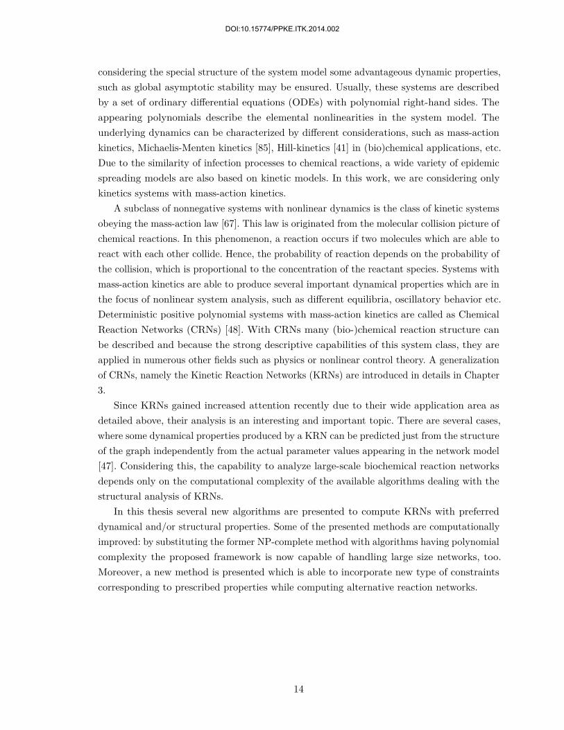
3.3 Finding dynamically equivalent weakly reversible realizations with LP . . . . 493.3.1 Introduction of new algorithms to compute weakly reversible realizations 503.3.2 Performance analysis of the different methods . . . . . . . . . . . . . . 55

3.4 Finding dynamically equivalent realizations with mass conservation . . . . . . 573.5 Summary . . . . . . . . . . . . . . . . . . . . . . . . . . . . . . . . . . . . . . 60

4 Efficient scheduling of railway networks using optimization 624.1 Optimization-based control of railway networks to minimize total delays . . . 63

4.1.1 Basics of the model formulation . . . . . . . . . . . . . . . . . . . . . . 634.1.2 Constraint set formulation . . . . . . . . . . . . . . . . . . . . . . . . 654.1.3 MILP problem formulation . . . . . . . . . . . . . . . . . . . . . . . . 684.1.4 Introducing delays into the model . . . . . . . . . . . . . . . . . . . . 70

4.2 New solution methods of the railway scheduling problem to increase solutionefficiency . . . . . . . . . . . . . . . . . . . . . . . . . . . . . . . . . . . . . . 714.2.1 Track-based transformation of the problem matrix . . . . . . . . . . . 724.2.2 Transformation of individual constraints . . . . . . . . . . . . . . . . . 73

4.3 A case study . . . . . . . . . . . . . . . . . . . . . . . . . . . . . . . . . . . . 794.3.1 Performance analysis of the proposed control technique . . . . . . . . 824.3.2 Comparison of time consumption of solutions in case of different model

formulations . . . . . . . . . . . . . . . . . . . . . . . . . . . . . . . . 824.3.3 Sensitivity analysis based on single delays . . . . . . . . . . . . . . . . 85

4.4 Summary . . . . . . . . . . . . . . . . . . . . . . . . . . . . . . . . . . . . . . 87

5 Conclusions 895.1 New scientific contributions of the work (thesis points) . . . . . . . . . . . . . 895.2 Utilization of the presented results, further work . . . . . . . . . . . . . . . . 91

The Author’s Publications 93

References 94

Appendix 104A. List of abbreviations . . . . . . . . . . . . . . . . . . . . . . . . . . . . . . . . 104B. List of notations . . . . . . . . . . . . . . . . . . . . . . . . . . . . . . . . . . 105C. Procedural description of the transformation method presented in Sec. 4.2.2 106

5

DOI:10.15774/PPKE.ITK.2014.002

Chapter 1

Introduction

Dynamical models have central role in several fields of science and technology. Withthem we can describe the operation of production processes, power generation systems,transportation networks and individual vehicles, agent-based systems etc. Besides modelsapplied in traditional engineering fields, numerous biological processes and phenomena canalso be understood and explained by creating their dynamical model. Dynamical modelingbecomes necessary if the state of the investigated system, namely the quantities describingthe properties of the system, evolves in time and/or space [96].

As a complex system we mean large-scale dynamical systems with complex structurecontaining nonlinearities. An important requirement in the modeling of complex systemsis simplification: the model should most importantly describe only those phenomena andprocesses which have significant effect on the dynamics of the system. Using a dynamicalmodel, the future behavior of the system can be predicted with respect to a given initialstate, thus the analysis and simulation of the system is possible. These are crucial stepstowards the controlling of the given system which is essential to achieve desired operation.The understanding and targeted manipulation of these kind of models are the main topics ofsystem and control theory.

In order to describe a large scale, complex system having many components properstructuring of the model should be applied [15]. A modular and clean model formulationhelps to capture and understand the most important properties of the investigated system.To accomplish this, a widely used and straightforward way is to separate the dynamics ofthe individual parts/elements and the connections between them leading to a descriptionwith networked structure. A deeply investigated and well known example of this phenomenais the theory of linear networks [42]. A more detailed review of the networked systems canbe found in Sec. 1.1.

Nonlinearities in a system can be incorporated into the system model through severalways. Using continuous models, the simplest case is to introduce smooth nonlinearitiesoptionally extended with discrete variables to describe switching-type events. In case ofapplying discrete models, the theory of discrete event systems [102, 7] is able to handle many

6

DOI:10.15774/PPKE.ITK.2014.002

important phenomena.From these theories, it is known, that we can classify dynamical models based on different

points of view [91]. By determining the model class corresponding to the investigated system,we are able to determine the set of applicable methods and techniques for the analysis andcontrol of the given system.

Because of the complex nature of many practically relevant control problems, the methodsapplicable for nonlinear systems with a networked structure are especially important, butthey present challenges at the same time. This thesis focuses on the optimization-basedsolutions of the control problems related to complex systems having networked structure.

1.1 Networks in system modeling

There are several types of dynamical systems that can be described as networks. Supplychains, transportation and public transport networks, in-cell reaction systems, genetic reg-ulatory networks are some of the widely investigated systems having networked structure.Basically, networks consist of two main elements: a set of nodes and a set of links connectingthe nodes to each other. Both the nodes and the links can be static or dynamic elements,depending on the properties of the system described by the network [15].

Usually, to describe the structure of networks in a mathematical framework, graph theoryis used where nodes and links in the network are corresponding to vertices and edges in thegraph, respectively. The way, how graphs can describe dynamical systems can have multipleinterpretation: e.g. in case of transportation networks a topographical layout of verticesand edges can be handful, representing junctions and sections of the network. Meanwhile, amore abstract, graph-based description of a system is also possible, e.g. in case of discreteevent systems, where vertices are standing for the different states of the system while edgesrepresent possible state transitions. As it can be seen from these examples the graph-basedsystem description is a powerful tool to represent several system structures on different levelsof abstraction.

If we investigate a static system a graph-based representation of the system can describestructural dependencies between the components of the system where both the vertices andedges are static or passive. If the dynamics is also incorporated into the system description, thefollowing setup is usual. The vertices represent the individual components of the system, whilethe edges between them set constraints on the behavior of the dynamics. The quantitativeproperties of the constraints usually appear as edge weights in a weighted, directed graph.

The topic of combining several, individual dynamical systems into a complex, networkedsystem is elaborated in the theory of interconnected subsystems in systems and control theory.In [36] mathematical tools are provided to analyze the connectability of composite systems,which property ensures the controllability and observability of the complex system. The fact,that the controllability and observability of a networked system depends on the properties of

7

DOI:10.15774/PPKE.ITK.2014.002

the linkages between the components leads to the concept of structural controllability andobservability [78]. These ideas are further developed in [79] showing the crucial propertiesof a relatively small number of driver nodes while controlling the dynamics of a complexnetworked system.

The importance of the quality and quantity of the connections in the graph is emphasizedby the research of the dynamics appearing in extreme large networks, such as social networks[14]. The statistical analysis of the behavior patterns in these kind of networks enables us tounderstand the significance of weak connections in social communities, the reordering patternsin such systems etc. As several databases became available containing data about large-scalenetworks, the techniques to analyze the data moved towards fractal-based description [113],graph-focused data mining techniques [66] and other improved techniques, which instead ofanalyzing the individual elements of the network, focus on the graph-theory based descriptionof the representing structures.

The work summarized in this thesis focuses on the application of optimization-basedmethods in the analysis and control of networked systems. Two classes of networked systemsare investigated because they come from basically different approaches of networked systemdescription, while they can be handled with similar mathematical tools. In case of a reactionnetwork, the model is translated into a network by describing the relations between theterms of the underlying differential equations as links between the nodes of a network thatrepresent the elementary nonlinearities. In contrast with this, in transportation networks(in this particular case, in railway networks) both the nodes and the links are passive, theyare only a topological mapping of the routes, junctions and/or stations. Nonlinearities areintroduced into this model by the absolute values appearing in the basic system model. Bothsystem classes are nonnegative [60], and can be handled as smooth nonlinear systems (byincorporating vehicle dynamics into the microscopic modeling of the system).

1.2 Aim and structure of this thesis

The aim of the present thesis is to develop optimization based methods applied to theanalysis and control of specific, practically important dynamical systems having complexnetworked structure. By analyzing the structure of the original, networked system and thestructure of the emerging optimization problem, problem-specific improvements are proposedto decrease the complexity of the computational tasks, thus they become applicable on largescale networks, too. Generally, these tasks are formulated as MILP problems, but in severalcases, they can be simplified to Linear Programming (LP) tasks.

In this thesis, two different system classes are examined having networked structure:kinetic reaction networks and railway networks. In both cases, we will use optimization-based techniques to solve problems in the field of system analysis and control. In case ofreaction networks, structural (parameter-independent) system analysis and the computation

8

DOI:10.15774/PPKE.ITK.2014.002

of alternative reaction networks will be completed using optimization based methods.In case of the railway networks control actions are going to be computed for optimal

rescheduling in order to minimize the sum of the delays of the trains. By applying optimizationbased control methods, our aim is to decrease the sensitivity of the railway network againstsmall appearing delays and by reducing the delay propagation effect. To accomplish this, amodel formulation is needed which enables us to simplify the analysis of the effect of thedispatching actions with respect to the individual delays of the trains. It is also desired,that formulated optimization problems should be solvable in a reasonable time, thus thepossibility to handle large-scale networks with algorithms using them is present.

The structure of the thesis is the following. In Chapter 2 the basic notions and themathematical tools are introduced, which serve as a basis of the methods presented in thefurther parts of this work. Chapter 3 introduces the Kinetic Reaction Networks in details,summarizes the results known from the literature and the corresponding results of the author.In Chapter 4 the topic of railway networks are investigated, presenting the different modelformulations, the proposed new methods and the simulation results. In Chapter 5 the mainscientific contributions of the presented work are briefly summarized and the possible furtherdevelopments are enumerated.

1.3 Optimization in system analysis and control

As it is detailed in [24], optimization problems play an important role in several fields ofsystem theory. In particular, any controller design problem is in fact a constrained optimizationproblem with the control aim as loss function and the system model as a constraint.

Due to the rapid development of computer technology and the available computational andanalytical methods, several new application area of optimization methods appeared in systemtheory. Two application domains have become particularly important: the computationalmethods themselves and those conceptual developments which make it possible to implementthe developed methods in real-life applications (e.g. Model Predictive Control framework[53]). Considering the underlying computational methods, it can be said, that most of theformulated optimization problems can be traced back to mathematical programming problemswhich are able to handle cost functions and constraints on the variables.

With the help of the tools emerging from optimization several different tasks in systemanalysis and control can be solved: identification problems, parameter estimation tasksand control problems can also be formulated in such a framework [80]. Identification andparameter estimation form a closely inter-related set of problems where the application ofoptimization methods focuses on the computation of system parameters using the presented,usually noisy and limited measurement data [126]. Several methods applied in the control ofdynamic systems can also be traced back to optimization: e.g. the method of Linear MatrixInequalities [23] to design robust controllers, decentralized control [54] to deal with systems

9

DOI:10.15774/PPKE.ITK.2014.002

incorporating multiple decision maker units, Linear-Quadratic (LQ) control problems [83] inclassical control theory or state estimation [112].

Techniques applied in optimal control were further developed to the control of networkedsystems, where the entities of the system are connected to each other via links, altogetherconsidered as a graph structure as it is detailed before. Optimization tasks are formulated fromthe coordinated control task of the entities in case of different connectivity properties [68],synthesis of complex process plants with a networked structure [50] satisfying different typeof constraints and having objective functions with multiple components etc. Also, methodsare developed to compute different properties and representations of a given system havingnetworked structure, such as minimal representation, identifying key connections etc. One ofthe developed methods is capable of computing a maximal superstructure corresponding toa given process network in polynomial time [49] in a centralized way. From the computedsuperstructure, with the help of additionally applied constraints all possible solutions ofthe original problem can be extracted enabling us to analyze the properties of the solutionswith high computational efficiency. As the focus of the research of networked systems shiftedtowards the large-scale networks constructed from real-life data, the importance of thehighly effective computational methods applicable for the solution of optimization problemsincreased.

Problem formulation in an optimization framework has a great conceptual importance:in case of a properly formulated problem its feasibility can be checked, meaning that theexistence of at least one solution can be shown even if the underlying problem is hard tosolve. The fact, that infeasibility (non-existence of a solution) can be explicitly detected hasgreat importance both in theory and in application.

The aim of the present thesis is to investigate the analysis and control of complex nonlineardynamical systems having networked structure using optimization-based techniques. Thistopic is examined through two problems, namely the structural and dynamical analysis ofkinetic reaction networks and the dynamical rescheduling problem of railway networks. Incase of both problems, we formulate the dynamical model of the corresponding networkedsystem and the solutions of the examined tasks are derived to a mathematical optimizationproblem. In case of reaction networks a structural analysis has been completed and alternativerealizations are computed, while in case of railway networks, the effect of delay propagationis reduced by applying optimal control actions in the schedule of the trains.

1.4 Networks and dynamics

The research of systems composed by a large number of interconnected dynamical unitsgained increased attention recently. The analysis and modeling of large scale coupled systemsfrom the field of biology, chemistry, transportation, logistics, social sciences etc. became animportant topic in science as the computational performance of the computer systems grows

10

DOI:10.15774/PPKE.ITK.2014.002

and the detailed processing of huge amount of data is possible. This gives us the opportunityto shift our attention from the investigation of individual properties of small-scale networkstowards the analysis of large scale systems with complex interconnection patterns, sometimesby focusing only on the statistical properties of the modeled system. Some important resultsabout these topics are summarized in [89].

The two main issues while investigating a complex coupled system are the following:firstly, to identify the structure of the connections between the actors of the system in orderto describe the system with the help of phenomena known from classical network theory. Herethe central task is to properly define the nodes in the network and the links in between them,which usually considered as vertices and edges in the graph corresponded to the network,respectively. Secondly, the type and behavior of the interactions should be identified withrespect to the formulated structure. These can be described as the properties of the edges inthe graph of the network. The obtained network models can be applied to analyze and if it isneeded, to control the underlying dynamics. A detailed review of the possible model classesand their applications can be found in [19].

Among many others, complex networked systems can be classified based on the role ofthe nodes in the network. In one hand, there are model types where the nodes have activerole in the dynamics of the network (they have some generalized computing task), and thenetwork can be considered as a set of agents connected to each other as it is defined bythe structure of the network. On the other hand there are models where nodes are onlyinterconnecting elements in the network connecting different edges, but they do not havespecific ”computational” tasks. These kind of models are similar to pipeline networks, wherenodes are created at the junctions of pipe sections.

Let us shortly review some system classes that can be modeled with the previouslyintroduced, agent-based network formulation.

Artificial neural networks are motivated by biological neural networks, and their aim wasto create a computational method that has as strong learning capabilities as the biologicalneural networks have. The proposed perceptron model [106] is based on strong simplificationsof the biological neurons but still tried to capture their main properties. The artificialneural network is defined as a set of processing nodes which have similar role than the cellbody of neurons while weighted edges connect the processing nodes as the axons connectneurons. The connectivity pattern strongly influences the behavior of the network and someclassical configuration of artificial networks emerged such as feed-forward networks andHopfield-networks [64].

The phenomena of individual processing nodes connected by weighted edges furtherdeveloped leading to the appearance of Cellular Neural Networks (CNN) [31]. CNNs area general framework to build parallel processing units with nonlinear dynamics arrangedtopographically in a grid. The connections between the nodes are local: only neighboringprocessing units can communicate with each other, thus the behavior of the whole network

11

DOI:10.15774/PPKE.ITK.2014.002

is characterized by the local connections. The obtained architecture called CNN UniversalMachine is capable to combine analog array operations with local logic. The application areasof these kind of spatio-temporal universal machines are very wide and they have interestingconnections with the state-of-the-art supercomputers and many-core computational devices[107].

Another interesting example of this field is the (bio-)chemical reaction networks. In [63] ithas been expressed that modern biology should not only describe the function of individualcellular components but their interconnections and interactions should also be explained, asa complex network of biochemical elements. Thus, computer-aided investigation of geneticregulator networks, intracellular signaling pathways and in-vivo reaction cascades is oneof the main topics of computational biology. The nonlinear dynamics appear in these kindof networks can be captured with several mathematical model classes. In this work, wefocus on the application of Chemical Reaction Network Theory (CRNT) to describe andanalyze (bio-)chemical reaction networks. In these models, the nodes of the network are thechemical complexes (consisting of different chemical substances) and they are interacting witheach other in chemical reactions described by the edges. CRNT can be further generalizedleading us to a set of mathematical problems which can produce several complex dynamicalphenomena as it is detailed in Chapter 3.

Behavioral patterns in systems consisting of living entities such as animals or humans canalso be described with the help of networks. A.-L. Barabási and T. Vicsek investigate thesetopics in details, while uncovering several manifestation of complex network-based dynamicsin living systems. As it is detailed in [14], several very complex phenomena appearing in thehuman society (e.g. scale-free properties of social networks, importance of weak links betweenpeople in the society) can be explained with the help of mathematical tools known fromnetwork and graph theory. The fundamental importance of network theory-based analysis ofbehaviors in living communities is also emphasized in [132, 131], where both the events in thegroups and the evolution of the group are explained with the help of relatively small changesin a scale-free networked structure. The phenomena learned from living communities oftenapplied in robotic systems consisting of several robots, networked sensors or cooperativecomponents [94, 129]. In [90] a wide variety of graph-theory based mathematical constructionsmodeling epidemiological processes are summarized. It has also been shown that the spreadingof several diseases can be efficiently simulated with network theory based models.

As it was mentioned, besides of networks having so-called agents in the nodes, thereare several types of networks, where the nodes are just meeting points of edges. Let usnow examine a subclass of these pipeline-like networks, namely the class of transportationnetworks. In transportation networks, the nodes are usually considered as junctions, crossingsor stations and the edges are routes or tracks. Vehicles are moving along the edges towards apre-defined target node or along a pre-defined route while following some type of schedulingand considering safety constraints. It can be seen that transportation networks usually can

12

DOI:10.15774/PPKE.ITK.2014.002

be depicted as topographically ordered graphs. Analysis of transportation networks (e.g.traffic flow analysis on highways, train traffic analysis in railway networks) can have severaldifferent aims: to find the most sensible parts of the network (e.g. with respect to accidents,delays, traffic jams etc.), find parts of the network which are suboptimally used etc. It isknown that vehicles in the network can have complex dynamics (see e.g. [70]) emerging fromthe properties of the network and the presented constraints. To control these behaviors, thetracking and control of individual vehicles is needed [130]. Controlling traffic has extremeimportance in case of railway networks, because of the increased load on the tracks and thefact that delays can be quickly propagated all over the network due to the limited reroutingcapability and the lack of overtaking. To overcome these issues several railway control methodwere developed [133] to increase throughput of railway networks, to limit delay propagation,to minimize passenger delays etc. A control method to minimize delays in a railway networkis proposed in Chapter 4.

Considering these, it can be said that the network-based analysis and control of largesize, interconnected systems is a widely investigated but still current topic in science. Thecomplex dynamics that can be modeled within this framework can describe a large variety ofreal-life phenomena, and the understanding and control these kind of systems can have hugeimpact on several problems both in science and everyday life, too.

1.5 Kinetic reaction networks as unified models of smoothnonlinear systems

Nonnegative systems are dynamical systems having the property that all state variablesstay nonnegative if the system is started from the nonnegative orthant. If none of the statesof a nonnegative system can reach zero, than we speak about a positive system. Nonnegativesystems appear in several fields of science, usually in cases where there are physical constraintson the nonnegativitiy of the states, such as population dynamics or (bio-)chemistry. It shouldbe noted that with the help of proper coordinate transformation, many systems can betransformed to be nonnegative. These transformations usually consist of two parts: the first isthe shifting of the coordinates into the nonnegative orthant, then the second is a time-scaling[120] ensuring that the trajectories of the system remain in the desired operation domain.

An interesting nonnegative system class is the class of kinetic systems, which are closedthermodynamic systems under isobaric and isothermal conditions. Kinetic systems can beinterpreted as an extension of chemical reaction systems, where the system contains chemicalspecies reacting with each other influencing the evolution of the system over time. Theextension involves the relaxation of some of the assumptions, such as mass conservation,naturally present in chemical reaction systems thus enabling complex nonlinear behavior ofthe kinetic system class.

The state vector of kinetic systems is formulated from the concentration of the species,which are nonnegative by nature. Kinetic systems can have smooth nonlinearities, and by

13

DOI:10.15774/PPKE.ITK.2014.002

considering the special structure of the system model some advantageous dynamic properties,such as global asymptotic stability may be ensured. Usually, these systems are describedby a set of ordinary differential equations (ODEs) with polynomial right-hand sides. Theappearing polynomials describe the elemental nonlinearities in the system model. Theunderlying dynamics can be characterized by different considerations, such as mass-actionkinetics, Michaelis-Menten kinetics [85], Hill-kinetics [41] in (bio)chemical applications, etc.Due to the similarity of infection processes to chemical reactions, a wide variety of epidemicspreading models are also based on kinetic models. In this work, we are considering onlykinetics systems with mass-action kinetics.

A subclass of nonnegative systems with nonlinear dynamics is the class of kinetic systemsobeying the mass-action law [67]. This law is originated from the molecular collision picture ofchemical reactions. In this phenomenon, a reaction occurs if two molecules which are able toreact with each other collide. Hence, the probability of reaction depends on the probability ofthe collision, which is proportional to the concentration of the reactant species. Systems withmass-action kinetics are able to produce several important dynamical properties which are inthe focus of nonlinear system analysis, such as different equilibria, oscillatory behavior etc.Deterministic positive polynomial systems with mass-action kinetics are called as ChemicalReaction Networks (CRNs) [48]. With CRNs many (bio-)chemical reaction structure canbe described and because the strong descriptive capabilities of this system class, they areapplied in numerous other fields such as physics or nonlinear control theory. A generalizationof CRNs, namely the Kinetic Reaction Networks (KRNs) are introduced in details in Chapter3.

Since KRNs gained increased attention recently due to their wide application area asdetailed above, their analysis is an interesting and important topic. There are several cases,where some dynamical properties produced by a KRN can be predicted just from the structureof the graph independently from the actual parameter values appearing in the network model[47]. Considering this, the capability to analyze large-scale biochemical reaction networksdepends only on the computational complexity of the available algorithms dealing with thestructural analysis of KRNs.

In this thesis several new algorithms are presented to compute KRNs with preferreddynamical and/or structural properties. Some of the presented methods are computationallyimproved: by substituting the former NP-complete method with algorithms having polynomialcomplexity the proposed framework is now capable of handling large size networks, too.Moreover, a new method is presented which is able to incorporate new type of constraintscorresponding to prescribed properties while computing alternative reaction networks.

14

DOI:10.15774/PPKE.ITK.2014.002

1.6 Transportation networks

Transportation networks are interesting and widely investigated examples of networkswith complex dynamics. The main components of these networks are the topological networkof routes (air corridors, railway tracks, highways, streets) and the vehicles moving alongthem. If any disturbance (accident, route blocking etc.) appear in the traffic, the capacityof the network can be reduced dramatically leading to unsatisfied passengers, increasedtransportation costs or other inconveniences. To avoid these problems traffic control methodsare applied to reschedule or reroute vehicles if it is needed. While controlling a transportationnetwork in such a way, a control aim is targeted (minimizing delays w.r.t. a predefinedschedule, maximizing throughput of the network etc.) while important safety measures shouldalso be considered.

The ever increasing load on the railway networks in recent years poses serious challengesfor network managers. To ensure the smooth operation of the network especially in caseof delayed operation, a lot of research effort has been put in the topic of timetable design.Delays can be caused by technical failures, accidents, weather conditions or other unexpectedsituations. Because in most cases a delayed train obstructs a whole track and through thisthe following and connecting trains will also be affected, delays can quickly propagate all overthe network [33]. To avoid such a large scale interruption in the network stable and robusttimetables [58] are designed. But in case of large delays modification of the schedule, such asrerouting or reshuffling trains or breaking connections can be necessary to minimize the effectof the disturbance. Proper rescheduling of the trains give us the opportunity to limit thepropagation of the delay and recover the nominal operation of the network as soon as possible[69]. However, breaking connections can lead to high passenger delays while keeping traindelays low [125]. From a computational point of view, the solution of scheduling problemsboils down to mathematical programming problems. A comprehensive survey of schedulingmethods used in railway management can be found in [136].

A delay-management problem handled as mixed-integer programming first appeared in[110] and more recently in [124]. In [20, 21] a permutation-based methodology was proposedwhich uses max-plus algebra to derive a Mixed Integer Linear Programming (MILP) to findoptimal rescheduling patterns [65]. These control methods have the advantage against greedyalgorithms (e.g. [127]) that they can guarantee an optimal control action with respect to theperformance index, but on the other hand they could have issues regarding the computationaltime.

In this thesis, we propose new model formulations for model predictive controllers appliedto the control of railway networks. The rescheduling problem is traced back to the solutionof a MILP problem, but in case of large and dense networks the increase of solution speed isneeded. With the help of the proper restructuring of the MILP problem, significant speedupis achieved. Also, a new model formulation is proposed which can lead to the development ofproblem-specific analytic tools and solution methods.

15

DOI:10.15774/PPKE.ITK.2014.002

Chapter 2

Basic tools and notations

In this Chapter, we will introduce the main concepts and tools used in this work. We willshortly review the theory of optimization and some classes of optimization problems used inthe methods presented in Chapters 3-4. Also, the main ideas behind the applied solutionmethods of these type of optimization problems are introduced. Moreover, we will summarizesome results corresponding to the topic of dynamical systems represented by networks.

2.1 Convex optimization

A mathematical optimization problem has the following form [24]:

min f0(x)

w.r.t. fi(x) ≤ bi i = 1, ..., ω.

where the vector x = (x1, ..., xk) contains the so-called optimization variables, the functionf0 : Rk → R is the objective function and functions fi : Rk → R, i = 1, ..., ω define theconstraints. Constants bi, i = 1, ..., ω are the limits for the constraints. A vector x∗ is calledoptimal solution if it has the smallest objective value from the set of vectors satisfying all theconstraints. An optimization problem is a convex optimization problem if both the objectivefunction and the constraint functions are convex, meaning that they satisfy the followinginequality:

fi(αx+ βy) ≤ αfi(x) + βfi(y)

for i = 0, ..., ω and for all x, y ∈ Rk, α, β ∈ R+0 where α+ β = 1.

Among many other subclasses of convex optimization, we will shortly introduce two widelyused special subclasses: linear optimization and least-squares. An optimization problem islinear, if the following holds:

fi(αx+ βy) = αfi(x) + βfi(y)

16

DOI:10.15774/PPKE.ITK.2014.002

for i = 0, ..., ω and for all x, y ∈ Rk, α, β ∈ R. It can be seen that if an optimization problemis linear, than it is convex, too. An optimization problem is called as a least-square problemif it contains no constraints but the objective function has a special form aTi x− bi:

min f0(x) = ‖Ax− b‖22 =k∑i=1

(aTi x− bi)2

where A ∈ Rω×k, ω ≥ k, the rows of A denoted as aTi and again, x stands for the vector ofthe optimization variables.

Both can be solved numerically very efficiently while they have a fairly complete theoryand they are used in a wide variety of applications, too. However, recently several relatedimportant developments have appeared. The interior-point methods [77] developed in the1980s are able to solve linear programming problems and in general, convex optimizationproblems as well. Besides of these, convex optimization became a central topic in the area ofautomatic control systems, estimation and signal processing, communications and networks,data analysis and modeling etc. as the techniques based on Linear Matrix Inequalities (LMIs)[23] earned more and more attention in the recent years. Convex optimization is also widelyapplied in combinatorial optimization and global optimization problems to find optimalsolutions, approximate them or find bounds on them.

Considering these, it can be advantageous to formulate a given problem in the convexoptimization framework, because it is proven that convex optimization problems can besolved (meaning that a solution can be found or it can be proven that no solution exists),moreover, reliable and efficient methods are present to compute the solution. Also it shouldbe noted, that in general the formulation of a convex optimization problem has serious effecton the complexity and computational difficulty of the solution. Hence, the investigation ofthe problem structure and the methods applied during the solution are important in orderto achieve advantageous problem formulation to avoid unnecessary computational issues.With the help of the theoretical results on convex optimization, a model form applicablefor distributed solution can be obtained, or sometimes a formulation with advantageousproperties is achievable.

There are several available software packages [139, 59, 140] that implement differentsolution methods and processing techniques for convex optimization problems and specially,linear optimization problems. The methods applied by the solvers are different, thereforesolver selection can have serious effect on the computational complexity of the solution incase of a given optimization problem.

2.2 Linear Programming

Linear Programming (LP) is perhaps the most successful discipline of the field of operationsresearch [104]. A linear program is a constrained convex optimization problem, where a linearfunction of the real-valued optimization variables is minimized (or maximized) with respect

17

DOI:10.15774/PPKE.ITK.2014.002

to linear equality and inequality constraints.Application fields of linear programming are very wide. From mathematical economics

to linear algebra there are several topics in which linear programming plays a central role.Linear programs can be formulated to incorporate problems like portfolio optimization tasks,manufacturing and transportation problems, routing and network design methods in the fieldof telecommunication, traveling salesman-type of problems used for vehicle routing or VLSIchip board design etc.

In the following we will define the LP problem itself and then the main ideas of thesolution methods are summarized.2.2.1 Problem formulation

A standard LP problem is formulated as follows:

minxcTx

Ax ≤ bxi ∈ R, i = 1, ..., k

(2.1)

where x is the k-dimensional vector of decision variables consisting of real valued elements.The collection of ω linear inequality constraints are defined by matrix A ∈ Rω×k called asconstraint matrix and vector b ∈ Rk. With the above formulation, equality constraints canalso be treated by rewriting the problem to contain purely inequality constraints [30]. Thelinear function cTx with c ∈ Rk is the objective function to be minimized. This formulationdescribes a simplex in Rk where the given constrains define the bordering hyperplanes. It isknown that the optimal solution of the LP has to be in one of the corners of the simplex,although there may be multiple alternative optimal solutions.

Let us note that this formulation defines the so-called primal LP. For each primal LPthere exists a dual LP, which can be obtained from the primal problem directly by properalgebraic transformations. The dual problem of the LP defined in eq. (2.1) can be expressedas:

minybT y

AT y ≥ cyi ∈ R, i = 1, ..., k

(2.2)

As it can be seen, the problem formulations of the primal and dual LPs are connected to eachother, moreover, it can be said that if a linear program has an optimal solution x∗, then sodoes its dual (let us denote it as y∗) and their objective values are equal: cTx∗ = bT y∗ [24].These problem formulations have different properties exploited in the solution methods, too.

The solution of linear programs is a widely investigated topic because of it’s crucialimportance in several application areas. Both the theoretical and implementational part ofthe methods have a wide literature: we suggest to review for example [88, 95].

18

DOI:10.15774/PPKE.ITK.2014.002

2.2.2 Solution methods

The main tool for solving LP problems in practice is the class of simplex algorithmsproposed by Dantzig [34]. While considering the issue of computational complexity, thepractical performance of the simplex algorithm is satisfying, because in case of a wide classof LPs the number of iterations during the solution seemed polynomial or even linear in thedimensions of problems being solved. Although, examples having exponential complexitywere constructed few decades later then the original publications about the simplex methodappeared. However, methods derived from nonlinear programming techniques, based onKarmarkar’s work [77] can also handle certain classes of linear programming problems withoutstanding efficiency while ensuring polynomial computational complexity in general [88].

In the following, we will shortly review these methods in order to introduce the mainelements of the algorithms. A comprehensive survey of the LP solution methods can be foundin [72].2.2.2.1 Simplex method

The simplex method is the most widely used method to solve LPs, originally proposedin [34]. Recall that any LP problem having a solution must have an optimal solution thatcorresponds to a corner of the simplex corresponding to the LP. Hence, the method iteratesover these corners while trying to move towards the optimal solution. The simplex method isbased on a tableau formulation which allows us to evaluate various combinations of decisionvariables to determine how to improve the solution. A specific simplex tableau describes agiven corner of the simplex corresponding to the problem.

Let us summarize the main points of this method based on [105].

1. Formulate the LP and construct a simplex tableau. Add slack variables, if it is needed(e.g. because of the reformulation of inequalities into equalities). Select the initial set ofthe basic variables and set the other variables to 0.

2. Find the sacrifice and improvement rows. These rows indicate what will be lost andgained in the cost function by making a change in the decision variables.

3. Select an entering variable, which is a currently non-basic variable that will mostimprove the objective if its value is increased from 0.

4. By applying a selection method (e.g. random selection, selecting the most limitingdecision variable etc.), pick a basic variable (different from the currently enteringvariable) that will be excluded from the basic set. Mark it as the exiting variable.

5. Construct a new simplex tableau. Replace the exiting variable in the basic variableset with the new entering variable and change the corresponding rows in the tableauproperly.

6. Repeat steps 2 through 5 until you no longer can improve the solution.

19

DOI:10.15774/PPKE.ITK.2014.002

Step No. 5. (namely the change of the basic variable set) is called as pivot operation. Asit can be seen, the simplex method is basically a sequence of pivot operations. Note thatthe selection method applied to pick the entry and exit variables determines the numberof iterations needed to find the solution. Hence, this basically determines the (worst-case)behavior of the solution method in terms of computational complexity [84].

2.2.2.2 Interior Point Methods

There are at least three major types of interior point methods (IPMs): the potentialreduction algorithm which most closely embodies the constructs of Karmarkar (see [77] fordetails), the affine scaling algorithm which is perhaps the simplest to implement, and pathfollowing algorithms which combine the excellent behavior of the above two in theory andpractice. Because of its advantageous properties, the third method-family (namely the pathfollowing methods) is implemented in the state-of-the art solvers.

Let us summarize the main points of the IPM method based on [72]. For a detailedexplanation of the appeared concepts see [88], too.

The primal-dual path following algorithm is an example of an IPM that operates simul-taneously on the primal and dual linear programming problems. The use of path followingalgorithms to solve linear programs is based on three ideas [72]:

• the application of the Lagrange multiplier method of classical calculus to transform anequality constrained optimization problem into an unconstrained one;

• the transformation of an inequality constrained optimization problem into a sequenceof unconstrained problems by incorporating the constraints in a logarithmic barrierfunction that imposes a growing penalty as the boundary defined by the constraints inthe model is approached;

• the solution of a set of nonlinear equations using Newton’s method, thereby arriving ata solution to the unconstrained optimization problem.

As it is detailed in [72], the steps of the IPM can be summarized as follows:

1. Look for feasible initial solutions for the primal and dual problem.

2. Test optimality by computing the optimality gap. If the gap is under the prescribedthreshold, the solution is found, return with it.

3. Compute the direction of the next step for Newton’s method.

4. Compute the step size for Newton’s method.

5. Take a step in the Newton direction as the update of the solution.

6. Repeat steps 2-5.

20

DOI:10.15774/PPKE.ITK.2014.002

Note that during solution process, it is assumed that the constraint matrix A from eq. (2.1)has full rank. This is usually achieved by some preprocessing of the presented constraint set.From an implementational point of view, the main issue is performing the matrix inversionsneeded to compute the Newton directions, which is usually handled by implementing a properfactorization instead of direct inversion.

2.2.3 Comparison of solution methods

In the following, we will shortly compare the two main solution methods of the LinearProgramming problem, namely the Simplex Method and the Interior Point Method.

Simplex Method Interior Point Method

Theoretical

(worst-case)

complexity

NP P

Practical complexity P P

Interpretationclear geometrical: visiting the

vertices

complex exploration of the feasible

region

Best applicable for small problems large, sparse problems

Generalizable to

non-linear problemsno yes

2.3 Mixed Integer Linear Programming

Mixed Integer Linear Programming (MILP) is a special case of linear programming,where some of the decision variables are integer valued. A MILP can be treated as a classof combinatorial constrained optimization problems with continuous and integer decisionvariables, where the objective function and the constraining linear inequalities are linear.Some optimization problems having nonlinear constraints and/or nonlinear cost functionscan be transformed to MILP problems: some nonlinear constraints can be handled as a setof linear constraints (where the introduction of auxiliary variables can be necessary), andsome nonlinear cost functions can be approximated by piecewise linear functions [28, 111].

A wide variety of real life problems boil down to an MILP problem. In problems, wheresome of the resources (represented by the decision variables) are quantized and solutionscontaining non-integer values for these are meaningless, the application of integer valueddecision variables is inevitable. MILP problems arise in the field of logistics, economics andsocial science. Moreover, the combinatorial problems, like the knapsack problem, warehouselocation problem, machinery selection problem, set covering problems and many schedulingproblems can also be solved as MILPs.

In this Section the problem formulation of the MILP problem and its main solutiontechniques are reviewed.

21

DOI:10.15774/PPKE.ITK.2014.002

2.3.1 Problem formulation

An MILP problem can be stated as follows [25]:minxcTx

Ax ≤ bxi ∈ R, i = 1, ..., kxj ∈ Z, j = k + 1, ..., l

(2.3)

where, similarly to the LP problem (see eq. (2.1)), x is the l-dimensional vector of decisionvariables consisting of k real and l−k integer elements. Note that those constraints that definethat some of the decision variables should be integer valued, called integrality constraints.Matrix A ∈ Rω×l and vector b ∈ Rl define the set of linear inequality constraints containingω constraints. Equality constraints can also be treated by rewriting the problem to containpurely inequality constraints [30]. The linear function cTx with c ∈ Rl is the objectivefunction to be minimized. As it can be seen, if all decision variables are real (i.e. k = l), theneq. (2.3) defines a standard LP problem. If all the decision variables are integer valued (i.e.k = 0), than the obtained problem is called as an Integer Program (IP).2.3.2 Solution methods

The solution methods of MILPs have some similarities with the ones used to solve pureLPs. Again, the linear constraints define a simplex in an l-dimensional space, but in thiscase, the optimal solution is searched on a lattice of feasible integer points instead of thecorners of the simplex. The integer programming problems can have multiple local optimaand finding a global optimum is ensured if and only if it is shown that the given solutionhas better objective value than all the other feasible points. In other words, it means thatMILP problems do not scale very well w.r.t. the size of the original problem. It has beenshown that MILP problems are generally NP-hard [93], hence they are usually solved bycomputationally very intensive heuristics-driven techniques which are sometimes unreliablein case of a large-scale problem.

The three main classes of MILP solution methods are shortly reviewed in the following.As an LP relaxation of a MILP problem we mean the LP problem obtained from the MILPby excluding the integrality constraints. For further details about the presented methods, seee.g. [81, 115, 51].2.3.2.1 Cutting plane method

Cutting plane method are based on polyhedral combinatorics. These methods can beshortly summarized as follows. The algorithm is looking for parts of the simplex defined bythe LP relaxation of the MILP problem, which can be excluded from the search space byintroducing extra constraints while the remaining space still includes the integer solution.New constraints are introduced until the obtained LP-solution (restricted by the originaland the added constraints) fulfills the integrality constraints, too. It is shown in [55] that

22

DOI:10.15774/PPKE.ITK.2014.002

the cutting plane method presented by Gomory [56] is finitely convergent. Several differentmethods are known to compute proper cuts [92].

Due to the great variety of the possible techniques of cut generation this method canhave increased impact on the solution process. A bunch of different cut generation techniquesare included in the available solvers (e.g. using the CGL library [137]).

2.3.2.2 Tree-search-based methods

By solving the LP relaxation of the original MILP problem, a solution can be obtainedwhich contains at least one variable which takes real value but its domain is restricted tointeger values by the integrality constraints, and rounding it to an integer results in theviolation of at least one constraint. In this case, auxiliary constraints can be added to therelaxed LP guiding the solution away from the current non-integer value, towards the fulfillingof the integrality constraints required by the original MILP.

Considering these, searching for the optimal solution ends up in a tree-search betweenpossible (MI)LP problems (called partial solutions) that fulfill some of the integrality con-straints, but not necessarily all of them. Heuristics-driven tree search exploration techniquesare used to build up, handle and explore the search tree emerging during the solution of aMILP [101]. The efficient exploration of the emerging large size search tree is necessary forthe solution of the MILP problem.

As the solution process progresses, the new nodes are introduced into the search treerepresenting new problems generated from the original LP by adding extra constraintsto it. This process called branching. Some of the nodes will be thrown away, because theproblem represented by them can not have better solution than other, already examinednode. This step is called as bounding. By the combination of these two steps, the so-calledbranch-and-bound method is created.

The main steps of the branch-and-bound technique applied for MILP solution are thefollowings:

1. Relax the integrality constraints from the original problem. Solve the resulting LP toobtain a global upper bound on the MILP objective function value. If the LP solutionhas integer values for those variables that were defined as integers in the original MILP,the optimal solution is present.

2. Branching: (Otherwise,) there should be a variable defined as discrete but having realvalue. Choose a non-discrete variable and branch on it: create new nodes, one for eachrounded value of the variable (e.g. two node for the down- and up-rounded values).Insert the nodes into the search tree.

3. Select a node from the tree which will be expanded later on. It should be noted thatseveral sophisticated algorithms and heuristics are available for node selection, e.g.

23

DOI:10.15774/PPKE.ITK.2014.002

depth-first logic (select a partial solution with most fixed variables), best-first (select apartial solution having with best parent bounds and heuristic values) etc.

4. Bounding: Create an LP relaxation of the problem represented by the selected nodeand solve it. If the LP is infeasible or the obtained objective value exceeds the currentupper bound, prune the node. If the solution is lower than the current lower bound andfeasible to the MILP mark it as the new incumbent solution. The incumbent solution isthe currently best (w.r.t. the objective value) feasible solution known up to this point.

5. If there is no remaining node, mark the current incumbent solution as final solution. Ifthere is at least one unvisited node, jump to Step 2.

Naturally, there are several modification and extension of this general technique, which mainlyaddress the issue of the computational effort needed to explore the tree (see e.g. [18, 17, 101]).In general, one should note that heuristics applied during the branch-and-bound processhave enormous impact on the solution speed and the quality of the solution. Each solver hasits own implementation which makes them suitable for different type of problems. A deeperanalysis of the solvers’ performance can be found in [143].

2.3.2.3 Decomposition algorithms

Decomposition algorithms are trying to isolate sets of constraints from the original problemto generate multiple separated, smaller size (thus easy to solve) optimization problems.Auxiliary variables are introduced to link the otherwise independent subproblems. Thenthe results of the subproblems are combined properly to obtain the solution of the originalproblem. The main decomposition techniques are summarized in [99, 100], and reviewed indetails in [51]. All of these methods can be interpreted as polyhedral approximations of theoptimal solution and they can be handled in a common framework, as it has been done in[51].

In general, there are two main decomposition techniques: the Dantzig-Wolfe method [35](denoted as DWD) and the Lagrangian method [108] (denoted as LD).

The LD method works as follows. Some constraints are selected to be omitted fromthe constraint set and introduced into the cost function together with the multiplicatorsintroduced in a Lagrangian fashion. Also, auxiliary constraints generated from the dual ofthe LP relaxation of the original problem are introduced into the model, and the model issplit into two separate parts one for the original constraints and one for the dual constraints.The solution of the dual problem helps to improve the bounds on the original problem whichcan eliminate possible solutions from the search space.

The key idea of DWD is to reformulate the original problem by substituting its variableswith a convex combination of the extreme points of the polyhedron corresponding to asubstructure of the formulation. The problems generated for the substitutions are solved as

24

DOI:10.15774/PPKE.ITK.2014.002

independent subproblems (similarly to the column-generation methods [9]) and a coordinatingprogram generates the result of the original problem based on the sub-results.

A common property of the decomposition methods is that their computational effectivenessstrongly depends on the structure of the original problem, namely the the structure of theconstraint matrix. The most advantageous formulation is when matrix A from eq. (2.3) hasa block-angular form, meaning that the nonzero elements are ordered into non-overlappingblocks while the constraints connecting these blocks are also grouped together. There areautomatic processes (some of them are included into state-of-the-art solvers as preprocessors)which try to reorder the constraint matrix to obtain this form [16], but in general, a well-formulated constraint set based on problem-specific knowledge outperforms these methods.

25

DOI:10.15774/PPKE.ITK.2014.002

Chapter 3

Applying optimization methods tofind kinetic reaction networks withpreferred structural and dynamicalproperties

The analysis of the structural properties and dynamical behavior of biologically motivatedkinetic systems is a quickly developing field. The rigorous structural and dynamical analysisof biologically motivated kinetic systems such as intracellular signaling pathways and generegulation networks has gained an increased attention. Meanwhile, the amount and qualityof experimental data are continuously improving due to the fast development of sensors andcomputer systems. Determining the structure and the exact parameters in such a networkcan be difficult due to the complexity of the described system or imperfect data. It is knownthat there are several important properties that only depend on the structure of the model,while the reaction graph structure corresponding to a given kinetic dynamics is generallynon-unique.

These facts motivate us to construct algorithms that can compute kinetic systems withpreferred structures (e.g. weakly reversible, minimal or maximal number of reactions, etc.)that may provide useful information about the dynamical behavior of the system. Themotivation behind the parallel improvement of modeling and computational methods is clear,to be able to handle the growing amount of data and to analyse more complex, possiblybiologically relevant processes and networks. By using optimization based methods, a clearframework can be built to handle the emerging computational tasks. The advanced methodsimplemented in the state-of-the-art solvers enable us to solve large optimization problems inparallel which results in relatively moderated solution times.

By Kinetic Reaction Networks (KRNs) we mean deterministic kinetic systems obeyingthe mass action law. Some of the assumptions, however, that are natural for chemical reaction

26

DOI:10.15774/PPKE.ITK.2014.002

systems, such as mass conservation, are relaxed when considering the mathematical structureof KRNs that enables us to use them as an important general descriptor class in dynamicsystem theory. It is known that such systems form a wide class of smooth nonlinear systemsthat are able to produce all important qualitative phenomena in nonlinear dynamics suchas oscillations, multiplicities and even chaos [43]. Thus, the kinetic system form can beuseful for the description of nonnegative models outside of (bio)chemistry, e.g. for epidemic,transportation or economic models as well [60, 109].

The general applicability of kinetic models is definitely extended by the strong results ofChemical Reaction Network Theory (CRNT). CRNT was initiated in the 1970’s and 80’s withthe first publications about the relations between the structure and qualitative dynamics ofCRNs treated as a general nonlinear system class [67, 47, 46]. Since then, numerous deep anduseful results have been published in this continuously developing field (see, e.g. [43, 12, 114]).

In this Chapter, the description of dynamical systems with the help of Chemical ReactionNetwork Theory and the corresponding concepts are described. In Section 3.2 two newLP-based algorithms are presented to compute dynamically equivalent realizations containingminimal and maximal number of reactions. In Section 3.3 a new LP-based method isproposed to find dynamically equivalent, weakly reversible realizations while in Section 3.4 aMILP-based method is introduced to compute dynamically equivalent realizations with massconservation.

3.1 Kinetic Reaction Networks

In this Section, the structural and dynamical description of KRNs are introduced basedon [118, 121, 122]. Besides the notations, some important properties are also recalled relatedto the scope of the current work.3.1.1 Describing a kinetic system as a KRN

The set S = {Xi, . . . , Xn} represents the n (chemical) species contained in a given KRN.The concentrations of the species denoted by xi = [Xi], i = 1, . . . , n form the state vectorx ∈ Rn of the system. The whole system obeys the mass action law and, therefore, all thevalues of the states are nonnegative [60]. Complexes are formally represented as nonnegativelinear combinations of the species:

Cj =n∑i=1

αi,jXi for j = 1, . . . ,m, (3.1)

where m is the number of the complexes in the network, and αi,j for i = 1, . . . , n, are thenonnegative integer stoichiometric coefficients of the jth complex. An elementary reactionstep, where the source complex Cj =

∑ni=1 αi,jXi is transformed into the product complex

Cl =∑ni=1 βi,lXi is denoted by

Cj → Cl (3.2)

27

DOI:10.15774/PPKE.ITK.2014.002

The reaction rate corresponding to reaction (3.2) can be written according to the massaction law as:

ρj,l(x) = kj,l

n∏i=1

xαi,j

i , (3.3)

where kj,l > 0 is the reaction rate coefficient.If for any i 6= l both reactions Ci → Cl and Cl → Ci are present in the network (i.e.

we have a reversible reaction), they are handled as separate elementary reactions. It is alsorequired from the above model class that Ci 6= Cj for i 6= j, i, j = 1, . . . ,m, and self-reactions(i.e. loop edges) of the form Ci → Ci are not allowed for i = 1, . . . ,m.3.1.1.1 Dynamical description with ODEs

In the literature dynamical systems representing chemical reaction networks are usuallydescribed by the state vector x containing the concentrations of the species (or chemicalcomponents), the stoichiometric matrix S and the vector-valued function R(x) representingthe reaction rates as follows [71]:

x = SR(x). (3.4)

The stoichiometric matrix S is a constant matrix containing structural information aboutthe network. The matrix is composed as follows: each row of the matrix corresponds to aspecie, each column of the matrix corresponds to a reaction in the network, positive valuesappear for products and negative values for reactants. Thus, the rank of the stoichiometricmatrix equals to the number of independent reactions in the network [13]. This formulationserves as a base of many methods formulated to compute reaction networks with specialproperties, such as minimal networks, identifying key reactions etc. [76].

This framework can be further generalized by the introduction of kinetic reaction networkswhich have dynamics obeying the mass action law can be described by a set of polynomialdifferential equations. In this case, chemical reaction networks can be considered as a subclassof kinetic reaction networks.

From the several different possibilities, we will use the following computationally advan-tageous factorization of the right hand side of the kinetic ODEs describing the dynamics ofthe concentrations (see, e.g. [48, 118]):

x = Y ·Ak · ψ(x) (3.5)

where x ∈ Rn is the vector of specie concentrations. Y ∈ Rn×m is the complex compositionmatrix in which the jth column contains the stoichiometric coefficients of complex Cj , i.e.Yi,j = αi,j . The vector mapping ψ = [ψ1 . . . ψm]T ∈ Rn → Rm is defined as:

ψj(x) =n∏i=1

xYi,j

i , j = 1, . . . ,m (3.6)

28

DOI:10.15774/PPKE.ITK.2014.002

Matrix Ak describes the reaction graph as follows:

[Ak]i,j ={kj,i, if i 6= j and reaction Cj → Ci is present in the CRN0, if i 6= j and Cj → Ci is not present in the CRN

(3.7)

Moreover, the non-positive diagonal elements of Ak are given by

[Ak]i,i = −m∑

l = 1l 6= i

[Ak]l,i. (3.8)

Hence, Ak is a Metzler-type column conservation matrix (that is actually the negativetranspose of the Laplacian matrix of the reaction graph), often called the Kirchhoff matrixof the KRN [86, 87].

A set of polynomial ODEs is called kinetic, if it can be written in the form eq. (3.5),where Y contains pairwise different columns of nonnegative integers, eq. (3.6) holds, andAk is a Kirchhoff matrix. Necessary and sufficient conditions of the kinetic property forpolynomial systems with a constructive proof were first given in [62] (see also [27]). Let usintroduce the matrix M for the monomial coefficients of the model eq. 3.5, i.e.

M = Y ·Ak. (3.9)

Using the above notation, eq. (3.5) can be written as

x = M · ψ(x). (3.10)

3.1.1.2 Graph representation

A KRN can be represented as a weighted, directed graph D = (Vd, Ed) called reactionnetwork or simply reaction graph, consisting of a finite nonempty set Vd of vertices and afinite set Ed containing ordered pairs of distinct vertices called directed edges. The complexesare represented by the vertices, i.e. Vd = {C1, . . . Cm}, and the edges stand for the reactions:(Cj , Cl) ∈ Ed if complex Cj is transformed to Cl in one of the reactions in the network. Theweight of the edge (Cj , Cl) is the reaction rate coefficient kj,l. A reaction network is calledreversible, if whenever the reaction Cj → Cl exists, then the reverse reaction Cl → Cj is alsopresent in the network. By the structure of a KRN we mean the unweighted directed graphof the reaction network.

29

DOI:10.15774/PPKE.ITK.2014.002

3.1.2 Dynamical equivalence and linear conjugacy of KRNs

It is known that the polynomial differential equations of a given kinetic system can havemultiple different reaction graph structures. Considering that in this thesis we use the formeq. (3.9), still several (Y, Ak) pairs can be found which can describe the same dynamicalbehavior. In this present work, we limit the set of complexes to a fixed set (generated usingthe method described in [62]), hence matrix Y is fixed.

The matrix pair (Y, Ak) is called a realization of a KRN described by M if eq. (3.9) holds,all the elements of Y are nonnegative integers, and Ak is a Kirchhoff matrix. It follows fromthe structural non-uniqueness that many important structural properties are not encodeduniquely in the polynomial differential equations of a kinetic system i.e. they are realizationproperties. In the following two Subsections, two phenomena are introduced correspondingto the explained non-uniqueness of the realizations.

3.1.2.1 Dynamical equivalence

Since the factorization eq. (3.9) is generally not unique (even if Y is fixed), the KRNsdefined by the pairs (Y (1), A

(1)k ) and (Y (2), A

(2)k ) are called dynamically equivalent realizations

of the kinetic system in eq. (3.10) (or that of each other) if Y (i) are valid complex compositionmatrices (a complex composition matrix is called valid if it contains nonnegative integerelements and there are no identical columns in it), A(i)

k are Kirchhoff for i = 1, . . . , 2, and

Y (1) ·A(1)k = Y (2) ·A(2)

k = M. (3.11)

In general the alternative realizations may contain complexes that do not appear in theoriginal network. In this work we restrict the focus of our search to alternative KRNs wherethe set of complexes are the subset of the set of complexes of the original network.

Considering the above facts, it is possible to determine different realizations for the samedynamics for which the reaction graph has prescribed structural properties. Let us introducethe following notations: we call a realization sparse if the number of the non-zero elementsin matrix Ask is minimal. A realization is called dense if it contains the maximal number ofnon-zero elements in matrix Adk. It was shown in [118] that the dense realization is a uniquesuperstructure containing all mathematically possible reactions, i.e for a given complex set,it contains all possible other realization structures as sub-graphs of the dense one. It shouldbe noted that while the dense realization is necessarily unique the sparse realization may notbe unique: possibly several different sparse structures and/or parameter set can representthe same dynamical behavior.

Example. To illustrate the notion of dynamical equivalence on a small-scale example, wewill use a classical 3-dimensional kinetic Lorenz system that was introduced in [128]. Theclassical Lorenz system can be transformed to kinetic form through coordinates-shifting and an

30

DOI:10.15774/PPKE.ITK.2014.002

appropriate time-scaling (see [128] for the computation details). After these transformations,the kinetic ODEs of the system are

x1 = σx1x22x3 − σx2

1x2x3 + σ(w1 − w2)x1x2x3

x2 = (ρ+ c3)x21x2x3 + (w2 − w1ρ− w1w3)x1x2x3 − x1x

22x3 − x2

1x2x23 + w1x1x2x

23(3.12)

x3 = x21x

22x3 − w2x

21x2x3 − w1x1x

22x3 + (w1w2 + βw3)x1x2x3 − βx1x2x

23

where σ = 10, ρ = 28, β = 8/3, and W = [w1 w2 w3] = [24 25 26]. It is shown in [128] thatusing these parameters, eq. (3.12) shows chaotic behavior with an attractor that is verysimilar to the attractor of the classical non-kinetic Lorenz system.The complex composition matrix of the system is given by:

Y l =

1 0 2 1 2 1 1 1 2 2 2 1 21 1 1 2 2 0 1 2 1 0 1 2 21 1 1 1 1 1 2 2 2 2 0 0 2

,where the ith column contains the composition of complex Ci (i.e. C1 = X1 + X2 + X3,C2 = X2 +X3 etc.). The non-zero off-diagonal elements of the network’s Kirchhoff matrixAlk are the following:

[Alk]2,1 = 679.3324, [Alk]6,1 = 1940.3342, [Alk]13,1 = 669.3342, [Alk]11,3 = 59, [Alk]12,3 = 10,

[Alk]13,3 = 44, [Alk]10,4 = 0.5, [Alk]12,4 = 34, [Alk]13,4 = 9.5, [Alk]13,5 = 1, [Alk]8,7 = 22.6666,

[Alk]12,7 = 1.3334, [Alk]10,9 = 1.

Then the monomial coefficient matrix can be written as

M = Y l ·Alk =

−10 0 −10 10 0 0 1 0 0 0 0 0 0−1271 0 54 −1 0 0 24 0 −1 0 0 0 0

669.3342 0 −25 −24 1 0 −2.6667 0 0 0 0 0 0

. (3.13)The graph representation of this network can be seen in Fig. 3.1a. Alternative realizationscontaining minimal and maximal number of edges can be seen in Figs 3.1a and 3.1b,respectively. The reaction rates of the sparse realizations are depicted as edge weights in Figs3.1a and 3.1b. In Fig. 3.1c, the structure of the reaction graph can be seen, while the non-zerooff-diagonal elements of the corresponding Kirchhoff matrix Adk (containing 51 reactions) are

31

DOI:10.15774/PPKE.ITK.2014.002

the following:

[Adk]2,1 = 679.6342, [Adk]3,1 = 0.1, [Adk]4,1 = 0.1, [Adk]5,1 = 0.1, [Adk]6,1 = 602.3658, [Adk]7,1 = 0.1,

[Adk]8,1 = 0.1, [Adk]9,1 = 0.1, [Adk]10,1 = 669.1342, [Adk]11,1 = 0.1, [Adk]12,1 = 0.1, [Adk]13,1 = 0.1,

[Adk]1,3 = 0.1, [Adk]2,3 = 0.1, [Adk]4,3 = 0.1, [Adk]5,3 = 44.6, [Adk]6,3 = 0.1, [Adk]7,3 = 0.1,

[Adk]8,3 = 0.1, [Adk]9,3 = 0.1, [Adk]10,3 = 0.1, [Adk]11,3 = 16.2, [Adk]12,3 = 9.3, [Adk]13,3 = 0.1,

[Adk]1,4 = 0.1, [Adk]2,4 = 0.1, [Adk]3,4 = 0.1, [Adk]5,4 = 9.6, [Adk]6,4 = 0.1, [Adk]7,4 = 0.1,

[Adk]8,4 = 0.1, [Adk]9,4 = 0.1, [Adk]10,4 = 0.1, [Adk]11,4 = 0.1, [Adk]12,4 = 24.4, [Adk]13,4 = 0.1,

[Adk]13,5 = 1, [Adk]1,7 = 0.1, [Adk]2,7 = 0.6, [Adk]3,7 = 0.1, [Adk]4,7 = 0.1, [Adk]5,7 = 0.1,

[Adk]6,7 = 0.1, [Adk]7,7 = −25.4, [Adk]8,7 = 23.2166, [Adk]9,7 = 0.1, [Adk]10,7 = 0.1, [Adk]11,7 = 0.1,

[Adk]12,7 = 0.68335, [Adk]13,7 = 0.1, [Adk]10,9 = 1.1, [Adk]13,9 = 0.1.

3.1.2.2 Linear conjugacy

It is known from the literature that the kinetic property of a system of ODEs is generallypreserved up to the re-ordering and positive scaling of the state variables [45]. Therefore,in [73] the notion of linear conjugacy was introduced, where two KRNs are called linearlyconjugate if (in the case of appropriate initial conditions) there is a positive linear diagonalmapping between the solutions of the corresponding kinetic ODEs. In order to explain this,let us consider the kinetic systems defined by (Y,Ak) and (Y,A′k):

Σ1 : x = Y ·Ak · ψ(x)

Σ2 : ˙x = Y ·A′k · ψ(x),

where x, x ∈ Rn+, Y ∈ Rn×m and Ak, A′k ∈ Rm×m are Kirchhoff matrices and ψ(x) =

[ψ1(x) ψ2(x) . . . ψm(x)]T as it is defined in eq. (3.6). Now Σ1 and Σ2 are called as linearlyconjugate kinetic systems if there is a vector d ∈ Rn+ for which T = diag(d) and in case ofx(0) = T x(0) the following holds:

x(t) = T x(t) ∀t > 0.

Let’s assume that Σ1 and Σ2 are linearly conjugate. Than the following can be derived:

˙x = T−1x = T−1Y Akψ(x) = T−1Y Akψ(T x) = T−1Y Ak · diag(ψ(d)) · ψ(x).

Considering this and the definition of Σ2 we can conclude that

T−1Y Ak · diag(ψ(d)) = Y A′k,

32

DOI:10.15774/PPKE.ITK.2014.002

(a) A possible KRN structure realizing eq. 3.12.The corresponding matrices are (Y l, Al

k). Reac-tion rates appear as edge weights.

(b) Another possible KRN structure containing mini-mal number of edges realizing eq. 3.12. Reaction ratesappear as edge weights.

(c) A KRN structure containing maximal numberof edges, realizing eq. 3.12. Edge weights are listedin Ad

k.

Figure 3.1: Alternative realizations of a KRN. Ci refers to the complex defined in the ithcolumn of Y . Example appears in Subsection 3.1.2.1.

which leads us to the following result:

Y Ak = TY A′k · (diag(ψ(d)))−1 = TY Ab, (3.14)

where Ab = A′k · (diag(ψ(d)))−1, so A′k = Ab ·diag(ψ(d)). It can be seen that Ab is a Kirchhoffmatrix which is structurally equivalent with A′k (meaning that the indices of the zero andnon-zero elements are the same in these matrices), because Ab is computed from A′k bymultiplying its columns with positive scalar values.

From the above detailed results the following can be concluded. Let us consider a kineticsystem denoted by Σ1. Also, let’s assume that there is a Kirchhoff matrix Ab and a vectord ∈ Rn+ that Y Ak = TY Ab, where T = diag(d). Than, there exists a kinetic system Σ

33

DOI:10.15774/PPKE.ITK.2014.002

described by (Y, Ak) such as Σ1 and Σ are linearly conjugate and

Ak = Ab · diag(ψ(d)). (3.15)

Also, considering eq. (3.14), eq. (3.5) can be formulated as follows:

M = TY Ak (3.16)

As it can be seen, linear conjugacy can be considered as an extension of dynamicalequivalence. The two phenomena meet by taking the transformation to be the identity. It isalso clear that the qualitative properties of the solutions (number and stability of equilibriumpoints, persistence/extinction of species, dimensions of invariant spaces etc.) of two linearlyconjugate KRNs are always the same.

Example. In the following example originally appeared in [75] two linearly conjugatereaction networks are shown. The network is characterized by

Y =

1 2 2 2 1 2 1 2 1 12 2 1 0 0 0 0 0 1 00 0 0 0 0 1 2 2 2 1

and the Kirchhoff matrix A

(1)k containing the following non-zero off-diagonal elements:

[A(1)k ]2,1 = 1, [A(1)

k ]4,2 = 0.5, [A(1)k ]5,4 = 1.5, [A(1)

k ]7,4 = 0.5, [A(1)k ]1,7 = 0.5, [A(1)

k ]4,7 = 1. Thecorresponding reaction graph can be seen in Fig. 3.2a.

A linearly conjugate realization can be described with the following non-zero off-diagonalelements in the matrix A(2)

k : [A(2)k ]2,1 = 0.001, [A(2)

k ]4,2 = 0.005, [A(2)k ]7,4 = 0.002, [A(2)

k ]1,7 =0.005, [A(2)

k ]4,7 = 0.001 and linear conjugacy matrix T = diag([ 10.001 ,

10.001 ,

10.004 ]). The

corresponding reaction graph can be seen in Fig. 3.2b. For these values, the equation forlinear conjugacy Y ·A(1)

k = T · Y ·A(2)k holds (see eq. (3.16)).

3.1.3 Known methods to compute dynamically equivalent KRNs

The original method of computing alternative realizations is based on the natural formu-lation of the problem as a MILP problem [25]. However, some alternative LP-based methods(see e.g. [119] or [135]) have also been published in the literature recently. We will shortlyreview these known solutions to be able to compare them with our new methods detailed inSection 3.2.

34

DOI:10.15774/PPKE.ITK.2014.002

(a) Reaction graph of the KRN described by(Y, A

(1)k ).

(b) Reaction graph of the KRN describedby (Y, A

(2)k ).

Figure 3.2: Linearly conjugate realizations of a KRN. Ci refers to the complex defined in theith column of Y . Isolated complexes are omitted from the figure. Reaction rates appear asedge weights. Example appears in Subsection 3.1.2.2.

3.1.3.1 Computing dynamically equivalent realizations with MILP

Let us formulate the KRN alternative realization problem as an MILP. This formulationhas also a crucial role in one of the new LP-based methods presented later on. We willrepresent the Kirchhoff matrix defined in Subsection 3.1.1 as:

Ak =

−a11 a12 . . . a1m

a21 −a22 a2m...

...am1 am2 . . . −amm

. (3.17)

The Kirchhoff property of Ak can be expressed by the following linear constraints:

m∑i=1

[Ak]i,j = 0, j = 1, . . . ,m (3.18)

[Ak]i,j ≥ 0, i, j = 1, . . . ,m, i 6= j (3.19)

Let us call eq. (3.9) and eqs. (3.18)-(3.19) altogether as kinetic constraints because theyclearly characterize the kinetic system structure of the model, and they can be considered asa constraint set in an optimization problem.

To formulate a MILP structure, where the real-valued decision variables correspond tothe off-diagonal elements of Ak, the following additional bounds for these elements are given:

[Ak]i,j ≤ li,j , i, j = 1, . . . ,m, i 6= j (3.20)

li,i ≤ [Ak]i,i, i = 1, . . . ,m. (3.21)

35

DOI:10.15774/PPKE.ITK.2014.002

where li,j for i, j = 1, . . . ,m are appropriately chosen bounds (with sufficiently large absolutevalues). Then the nonzero property of the individual reaction rate coefficients can now bewritten as

δi,j = 1↔ [Ak]i,j > ε, i, j = 1, . . . ,m, i 6= j. (3.22)

where δi,j are binary decision variables, ↔ denotes the ’if and only if ’ relation, and ε is asmall positive number used for distinguishing between practically zero and non-zero values.

The linear constraints in eq. (3.22) can be translated to the following linear inequalities[25]

0 ≤ [Ak]i,j − εδi,j , i, j = 1, . . . ,m, i 6= j (3.23)

0 ≤ −[Ak]i,j + li,jδi,j , i, j = 1, . . . ,m, i 6= j. (3.24)

From now, the constraint matrix can be formulated (see eq. (2.3)), while the minimization ormaximization of the objective function

c(δ) =m∑

i, j = 1i 6= j

δi,j (3.25)

leads to the computation of sparse or dense realizations, respectively.

3.1.3.2 Computing sparse realizations with an iterative LP-based technique

In [135] an LP-based algorithm is presented to search for sparse linear models of generegulation networks. The algorithm uses an iterative method to approximate the elementsof the Ak matrix. The approach is quite efficient: as it is mentioned in [135], the methodusually doesn’t need more than a few (less than 10) iterations to converge.

We briefly describe how to apply this method for the computation of sparse KRNrealizations. Let Apk denote the Ak in the pth step. Firstly set all off-diagonal elements ofA0k to 1. Let us define a weight wpi,j for each off-diagonal element of Apk and initialize them

as w0i,j = 1 for each i, j = 1, . . . ,m, i 6= j. In the pth iteration step, let us recalculate the

weights wpi,j as follows:

wpi,j = β

β + |[Ak]p−1i,j |

for i, j = 1, . . .m, i 6= j (3.26)

for an appropriate β > 0 value. The off-diagonal elements of Apk are obtained by solving alinear programming problem constrained by eq. (3.9) and eqs. (3.18)-(3.70) with the following

36

DOI:10.15774/PPKE.ITK.2014.002

objective function:

J = minm∑

i, j = 1i 6= j

wpi,j [Ak]pi,j (3.27)

The incorporated kinetic constraints (see eqs. (3.18)-(3.19)) ensure that in each iteration theobtained matrix Apk represents a dynamically equivalent realization and it has the Kirchoffproperty. The algorithm repeats eq. (3.27)-(3.26) until the objective value J will not changesignificantly between two successive steps. At the end of the iteration process the algorithmreturns with Apk obtained in the last iteration step as a sparse realization of the network. Inthe following, we will refer to this algorithm as Iterative LP.

3.1.3.3 Computing dense realizations using multiple LP steps

This method was published in [119] and it can find dense realizations in polynomial time.The method uses m · (m− 1) LP computation steps to generate the result. We will use themethod for comparison with our new approach, therefore we summarize it for convenience(more details can be found in [119]).

For each p, q = 1, . . .m, p 6= q, solve the optimization problem:

max cpq = [Ak]p,q (3.28)

with respect to the eq. (3.9) and eqs. (3.18)-(3.19) together with appropriate bounds eq.(3.20)-(3.21).

The reaction Cq → Cp is present in the dense realization only if max cpq > 0. Let usdenote the solution corresponding to (p, q), p 6= q by Apqk . Now we will use these solutionsto compute the final optimization step to generate the dense realization using the followingquantities:

εij =

1

m(m− 1)

m∑p, q = 1p 6= q

Apqk

i,j

, i 6= j (3.29)

As we can see, εi,j ≥ 0 ∀i 6= j and εi,j > 0 iff the reaction Cj → Ci is in the dense realization.By solving the following LP feasibility problem for Ak with arbitrary linear cost function,the dense realization can be obtained:

37

DOI:10.15774/PPKE.ITK.2014.002

Y ·Ak = M∑mi=1[Ak]i,j = 0 j = 1, . . .m

εi,j ≤ [Ak]i,j ≤ UBi,j i, j = 1, . . .m, i 6= j

[Ak]i,i ≤ 0 i = 1, . . .m

(3.30)

where UBi,j are proper upper bounds with sufficiently large positive value. In the following,we will refer to this algorithm as Element-wise LP.

3.1.4 Weak reversibility

The existence of a dynamically equivalent or linearly conjugate weakly reversible KRNrealization can be useful in the analysis of the qualitative dynamical properties of the system[74]. This property has a crucial role in the theory of KRNs, since it connects structuralproperties of the reaction graph to qualitative features of the dynamical behavior of thereaction network which is especially useful in the deficiency zero and deficiency one cases.The deficiency of a reaction network can be defined as follows [47, 48]: for each reactionCi → Cj in the network we can define the reaction vector ek = [Y ]·,j − [Y ]·,i, k = 1, ..., rwhere [Y ]·,i stands for the ith column of matrix Y . From the set of the reaction vectors thestoichiometric subspace can be defined as S = span{e1, ..., er}. The positive stoichiometriccompatibility class containing a concentration x0 is the following set: (x0 +S)∩Rn+ where Rn+denotes the positive orthant in Rn. The deficiency δ of a reaction network is calculated as:δ = m− l − rank({e1, ..., er}), where m is the number of the complexes, l is the number oflinkage classes in the reaction graph. As it is formulated in the Deficiency Zero Theorem [46]for a KRN having zero deficiency and a weakly reversible structure, there exists precisely oneasymptotically stable equilibrium point in each stoichiometric compatibility class. Accordingto the Boundedness conjecture for which no counterexamples have been found, the solutionsof any weakly reversible KRN are bounded. The conjecture was proved in [11] for the singlelinkage class case. Moreover, there exist important general results about the existence ofequilibrium points in weakly reversible reaction networks [37, 22].

From a graph-theoretic point of view, weak reversibility holds if and only if all components(i.e. linkage classes) of the reaction graph are strongly connected components (i.e. if thereexists a directed path between nodes Ci and Cj then there exists a directed path from Cj toCi).

As an example, let us consider a KRN having the following complex set:

Y =[

1 2 1 2 10 0 1 1 2

](3.31)

and a reaction graph depicted in Fig. 3.3a. The dynamics of this reaction network can beseen in Fig. 3.3b. Later on, the reaction graph has been extended to contain addition edges

38

DOI:10.15774/PPKE.ITK.2014.002

(a) Reaction graph. (b) Dynamics of the system.

Figure 3.3: Structure and dynamics of a reaction network. Complexes are from eq. (3.31).

(a) Reaction graph. (b) Dynamics of the system.

Figure 3.4: Structure and dynamics of a weakly reversible reaction network obtained byextending a non-reversible network (see Fig. 3.3a.). Complexes are from eq. (3.31).

as it can be seen in Fig. 3.4a. The obtained network is weakly reversible. The corresponding(stable) dynamics can be seen in Fig. 3.4b.

Additionally, it is known that a KRN with a Kirchhoff matrix Ak is weakly reversible ifand only if there exists a strictly positive vector in the kernel of Ak [74], i.e.

Ak · h = 0 (3.32)

hj > 0, j = 1, . . . ,m (3.33)

where h = [h1 . . . hm]T .For simplicity, we introduce the following notions. A Kirchhoff matrix is called weakly

reversible if the corresponding reaction graph is weakly reversible. A vector p ∈ Rn is called

39

DOI:10.15774/PPKE.ITK.2014.002

strictly positive if it is element-wise strictly positive, i.e. pi > 0 for i = 1, . . . , n. Two n× nmatrices V and W are called structurally equal if the following is fulfilled: Vi,j 6= 0 if and onlyif Wi,j 6= 0 for i, j = 1, . . . , n. (Therefore, two structurally equal Kirchhoff matrices encodethe same unweighted reaction graph structure.)

It can be seen that eq. (3.32) itself is a nonlinear constraint if both Ak and h are unknowns.In order to formulate it as set of linear constraints, we can introduce a scaled Kirchhoffmatrix Ak as follows:

[Ak]i,j = [Ak]i,j · bj , i, j,= 1, . . . ,m (3.34)

Now, Ak corresponds to a weakly reversible KRN if and only if 1(m) = [1 1 . . . 1]T ∈ Rm isan element of ker(Ak). Moreover, it is trivial that Ak is weakly reversible if and only if theoriginal Kirchhoff matrix Ak is also a weakly reversible one. Based on these facts, the linearconstraint set for weak reversibility can be formulated as follows:

m∑i=1

[Ak]i,j = 0, j = 1, . . . ,mm∑i=1

[Ak]j,i = 0, j = 1, . . . ,m

[Ak]i,j ≥ 0, i, j = 1, . . . ,m, i 6= j,

(3.35)

where Ak and Ak are structurally equal.3.1.4.1 The dense weakly reversible realization forms a super-structure for a

fixed complex set

It was shown in [118] that the dense realization is a unique superstructure containing allmathematically possible reactions. In the following, we will prove that a dense and weaklyreversible realization contains all possible weakly reversible realizations if the complex set isfixed.

Theorem 1. Consider a kinetic system Σ : x = M · ψ(x). Suppose that (Y,Ak) is a weaklyreversible dynamically equivalent realization of Σ that contains the maximal number of nonzeroelements in Ak. Then, for any weakly reversible Kirchhoff matrix A′k for which Y ·Ak = Y ·A′kthe following holds: [A′k]i,j > 0 implies [Ak]i,j > 0 for any i 6= j.

Proof. (by contradiction) Consider a weakly reversible Kirchhoff matrix A′k for which Y ·Ak =Y · A′k. Suppose that there exists 1 ≤ i, j ≤ m, i 6= j for which [A′k]i,j > 0, but [Ak]i,j = 0.Let us define the matrix Ak as

Ak = Ak +A′k2 (3.36)

Clearly, Y · Ak = Y · Ak, and [Ak]i,j > 0. It follows from the weak reversibility of Ak thatthere exists a strictly positive vector p ∈ Rm such that Ak · p = 0. Similarly, there exists astrictly positive vector p′ in the kernel of A′k, too. Let us define the following scaled Kirchhoff

40

DOI:10.15774/PPKE.ITK.2014.002

matrices: Ak = Ak · diag(p), A′k = A′k · diag(p′). Then Ak and A′k are Kirchhoff, and they arestructurally equal to Ak and A′k, respectively. Moreover, Ak ·1(m) = A′k ·1(m) = 0, where 1(m)

denotes the m dimensional column vector composed of ones. Let Ak = Ak + A′k. Then Ak isa weakly reversible Kirchhoff matrix, since Ak · 1(m) = (Ak + A′k) · 1(m) = 0. It is also clearthat Ak is structurally equal to Ak. This implies that Ak is a weakly reversible Kirchhoffmatrix containing more non-zero off-diagonal elements than Ak, which is a contradiction.

To briefly illustrate the above theorem, consider a kinetic system Σ : x = M · ψ(x)characterized by the following matrices:

Y =[

1 2 1 12 1 3 1

], M =

[0 −2 0 2−3 2 −2 0

](3.37)

This kinetic system was studied before in [73] and in [123]. A possible dense weakly reversiblerealization (Y,A(1)

k ) of Σ is given by the Kirchhoff matrix:

A(1)k =

−3.2 1.8 0.1 0

0 −2 0 20.1 0.1 −1.05 03.1 0.1 0.95 −2

. (3.38)

On the other hand, the following Kirchhoff matrix encodes a complex balanced and thusweakly reversible realization (Y,A(2)

k ) of Σ (see [123]):

A(2)k =

−3 1.5 0 0

0 −2 0 20 0.25 −1 03 0.25 1 −2

. (3.39)

Finally, a sparse weakly reversible realization containing only 5 reactions (Y,A(3)k ) is defined

by:

A(3)k =

−3.2 2 2 0

0 −2 0 20.1 0 −2 03.1 0 0 −2

. (3.40)

It can be easily checked that all (Y,A(1)k ), (Y,A(2)

k ) and (Y,A(3)k ) are dynamically equivalent

weakly reversible realizations of Σ. The reaction graph structures of the three realizations aredepicted in Fig. 3.5. It is clearly visible from the figure that the unweighted reaction graphsof (Y,A(2)

k ) and (Y,A(3)k ) are indeed proper subgraphs of the unweighted reaction graph of

(Y,A(1)k ).

41

DOI:10.15774/PPKE.ITK.2014.002

(a) Dense weakly reversible struc-ture defined by A

(1)k .

(b) Weakly reversible structure of acomplex balanced realization givenby A

(2)k .

(c) Sparse weakly reversiblestructure with 5 reactions de-fined by A

(3)k .

Figure 3.5: Possible dynamically equivalent weakly reversible reaction graph structures ofthe kinetic system eq. (3.37).

3.1.5 Known methods to compute dynamically equivalent, weakly reversibleKRNs

In this Subsection a short review of several different existing algorithms to find dynamicallyequivalent weakly reversible realizations of a KRN can be found. Besides of two MILP-basedmethods, an LP-based method has been described, too. Later on, these methods will becompared in terms of computational time to the proposed LP-based methods (see Sec. 3.3.2).

3.1.5.1 One-step MILP procedure to compute weakly reversible realizationswith additional preferred structural properties

First, we briefly recall the part ensuring the structural equality of Ak and Ak of thealgorithm presented in [75]. In that paper, a set of boolean decision variables are introducedand used as follows:

[Ak]i,j > ε↔ [A]i,j > ε, i, j = 1, . . . ,m, i 6= j, (3.41)

where again, ↔ means the ’if and only if ’ relation from classical binary logic and ε is asmall fixed positive threshold value to distinguish between practically zero and nonzeroedge weights in the reaction network. This logical condition can be expressed in the form ofequivalent linear constraints (for the general framework, see e.g. [103]):

0 ≤ [Ak]i,j − εδi,j , i, j = 1, . . . ,m, i 6= j,

0 ≤ −[Ak]i,j + pu · δi,j , i, j = 1, . . . ,m, i 6= j. (3.42)

0 ≤ [Ak]i,j − εδi,j , i, j = 1, . . . ,m, i 6= j

0 ≤ −[Ak]i,j + pu · δi,j , i, j = 1, . . . ,m, i 6= j,

42

DOI:10.15774/PPKE.ITK.2014.002

where δi,j , i, j = 1, . . . ,m, i 6= j are boolean decision variables and pu is the upper boundfor the elements of Ak and Ak.

Due to the introduction of the δ variables, the resulting problem could be solved in theframework of MILP, making the handling of larger networks difficult. On the other hand,these boolean variables can be used to keep track of the presence of individual reactions, andby minimizing or maximizing the sum

∑mi,j=1 δi,j in the objective function of the optimization

problem, a sparse or dense realization (containing the maximal or minimal number of reactions,respectively) can be obtained [118]. It should be noted that this method do not scale up verywell with the size of the network due to the integer variables in the optimization.

3.1.5.2 Graph-theory inspired, iterative procedure to find dense weakly re-versible realizations

In [123] a completely different, graph-theory motivated method is presented (only forthe case of dynamical equivalence) which leads to an iterative MILP-based algorithm. Thealgorithm requires Y and M as inputs, and computes an initial dense realization for them.Afterwards, it determines all the edges in the network that connect different strong components.In the next step, by solving an MILP problem a valid dense realization is determined withoutthese edges (if it exists). These steps are repeated until the reaction graph of the resultingKRN is found to be weakly reversible. The algorithm ends with failure if there does notexist any dynamically equivalent realization that does not contain the directed edges to beexcluded.

In the original publication, an MILP problem is solved in each iteration step. Fortunately,as it is described in [1], the MILP problem for the computation of dense reaction structurescan be safely replaced with a purely LP-based algorithm. This enables us to significantly speedup the solution process of the original method published in [123]. Therefore, we implementedand used the LP-based modified version of this graph-theory inspired algorithm for thepresent work to compare its performance to our new methods. This algorithm will be shortlycalled the graph-based-LP method in this work.

3.1.6 Mass conservation in KRNs

During the mathematical generalization of mass-action KRN systems the mass conserva-tion assumptions which are present in classical chemical theory were usually omitted, becausethis property is not essential for the kinetic representation of general nonlinear systems.However, mass conservation is an important constraint when modeling physically plausiblereaction sets [61].

In [61] (stoichiometric) mass conservation is formulated as follows. Let us define gv as thescaled molecular weight of the species Xv with strictly positive value. If reaction Ci → Cj is

43

DOI:10.15774/PPKE.ITK.2014.002

present in the network, the following can be written:

n∑v=1

αvigv =n∑v=1

αvjgv = cs. (3.43)

where cs is a strictly positive scalar value. Let us define vector g ∈ Rn+ as a row vectorformulated from the scaled molecular weights. Now eq. (3.43) can be rewritten as g ·Y (·, i) =g · Y (·, j) = cs where Y (·, i) refers to the ith column of matrix Y . Finally, it can be said thata reaction is mass conservative if the following holds:

g · ρ(i,j) = 0 (3.44)

where ρ(i,j) = Y (·, i)−Y (·, j) is the reaction vector and g is strictly positive. In [61] the massconservative reaction set is defined as a set of the reactions having the above property. Itshould be noted that a given KRN is called mass conservative if all of its reactions are in themass conservative reaction set and a common strictly positive g can be determined for them.

In Section 3.4, an algorithm will be defined to compute dynamically equivalent realizationswhich are mass conservative in the above defined sense.

3.2 Finding dynamically equivalent realizations with LP

In Subsection 3.1.2 it has been mentioned that in case of a specific KRN with givendynamics and fixed complex set, different (Y,Ak) pairs can fulfill eq. (3.9). Based on these,one can define structural properties such as minimal or maximal number of nonzero elementsin matrix Ak and search for alternative representations of the given network which fulfillthese criteria. In this particular case, we want to determine the sparse and dense realizationsdenoted by (Y s, Ask) and (Y d, Adk), respectively.

Using the 3-dimensional Lorenz system introduced in Subsection 3.1.2, the validationof the proposed methods on a small-scale KRN has been completed. The comparativeperformance analysis of the presented methods on large random networks is detailed inSubsection 3.2.3. Let us note that it is known from [128] that this system can be representedby KRNs having 3 species and 13 complexes with sparse realizations containing 13 off-diagonalnon-zero elements, and its dense realization contains 51 off-diagonal non-zero elements.

In this Section, the results corresponding to Thesis I. (see 4.3.3) are detailed.3.2.1 Finding sparse realizations

The results in [38] show that in the case of large size, under-determined system of linearequations (even in the case of non-negative decision variables) formulated as Ax = b, thel1-norm based minimization can produce a sparse solution out of the infinitely many possiblesolutions of the problem. Furthermore, in [39] it has been shown that similar technique can beused to find sparse nonnegative solutions for these kind of problems. In this context, sparse

44

DOI:10.15774/PPKE.ITK.2014.002

solution means that the given x vector contains the minimal number of non-zero elements. Inother words, under specific conditions, the combinatorial optimization problem of finding thesparse realization can be efficiently approached as a convex optimization problem. This ispossible if the solution vector x with length n is sparse enough: it should not have more thanρ · n nonzero elements. In [38] an empirical limit ρ = 0.3 is suggested, we also used this value.

The l1 minimization method is applied in our case as follows. Recall that in a given KRNthere are n species and m complexes. The equality constraints of the optimization problemare the kinetic constraints (see eq. (3.9) and eqs. (3.18)-(3.70)). For a single column of Akcontaining m elements, the number of kinetic constrains will be n + 1. Hence, in case ofn+ 1 < m the emerging equality-type constraints as a system of linear equations remainsunder-determined. Therefore, a column-wise l1-norm based minimization is completed andthe resulting vectors are considered as the column vectors of the sparse realization of theKRN:

minm∑i=1

abs([Ak]i,j) for ∀j = 1, . . .m, i 6= j (3.45)

Let us denote the ratio of non-zero and zero elements in [Ak]·,j as τ . If τ < ρ ·m, then theminimization successfully finds the sparse solution. In the following, we will refer to thisalgorithm as the l1-norm based algorithm.

Computing the sparse realization of the 3-dimensional Lorentz system took 17.172 secondsin case of the MILP based method. Iterative LP were able to find a valid sparse realizationin 0.0144 seconds while the proposed l1-norm based sparse search can complete this task in0.0166 seconds.

The above presented results are summarized in Thesis I.a. Detailed computational resultscan be found in Subsection 3.2.3. These results were originally published in [1].3.2.2 Finding dense realizations

The proposed method is based on the construction of the MILP problem formulationgiven in Subsection 3.1.3. The main idea was to formulate the problem by relaxing theintegrality constraints and then solve the remaining LP problem. By maximizing the sum ofthe relaxed auxiliary variables, the number of directed edges (i.e. the number of non-zerooff-diagonal elements of Ak) is maximized, too, in the reaction graph of the KRN.

The constraint matrices were built up again using the kinetic constraints (eqs. (3.18)-(3.19)). Similarly to the MILP case, a set of auxiliary variables were defined: a σi variable foreach decision variable ai (recall that each decision variable represents an off-diagonal elementof the Ak matrix). All these auxiliary variables are real valued. The constraints keeping trackof nonzero reaction rate coefficients are given by

σi = 1←→ ai > εe (3.46)

where εe is a minimal (naturally positive) edge weight under which the edge is excluded from

45

DOI:10.15774/PPKE.ITK.2014.002

the network (i.e. the corresponding reaction rate coefficient is considered zero). After therelaxation of the integrality constrains the relation in eq. (3.46) becomes:

ε · σi ≤ ai (3.47)

where σi ∈ [0; 1] and ε > 0 is a sufficiently small number, but ε > εe. By considering ε as ascaling factor, after short reformulation we obtain:

−ai + σi ≤ 0 (3.48)

σi ∈ [0; ε] (3.49)

where ineq. (3.48) is formulated as a constraint and eq. (3.49) is formulated as lower andupper bounds in the LP problem.

Now the optimization problem is defined as follows:

maxm∑i=1

σi (3.50)

Y ·Ak = M∑mi=1[Ak]i,j = 0 j = 1, . . .m

0 ≤ σi ≤ ε i = 1, . . .m

−ai + σi ≤ 0 i = 1, . . .m

(3.51)

Let us show that the solution of the above optimization problem indeed determines thedense network: suppose that a given edge (corresponding to the decision variable ai) can bepresent in the network which means that there is no such kinetic constraint which forbidsthat ai could be larger than zero. In this case, according to the constraint formulated in ineq.(3.48), σi > 0 will occur which yields ai ≥ ε. Because of ε > εe, the edge will be present inthe network. In the opposite case, when the edge represented by ai should be excluded fromthe network according to the kinetic constraints, ai = 0 leading to σi = 0 according to ineq.(3.48). As a result of the maximization, a dense realization with edge weights larger than εeis obtained. In the following, we will refer to this algorithm as the LP-MAX algorithm.

Computing the dense realization of the 3-dimensional Lorentz system was also successfullycomputed by all three algorithms. The original MILP based algorithm completed it in 5.3477seconds, Element-wise LP consumed 0.2524 seconds, and the LP-MAX algorithm needs0.0446 seconds to compute the solution.

The above presented results are summarized in Thesis I.b. Detailed computational resultscan be found in Subsection 3.2.3. These results were originally published in [1].

46

DOI:10.15774/PPKE.ITK.2014.002

3.2.3 Comparative study of the presented algorithms

Both the l1-norm based search and the LP-MAX methods were involved in a comparativestudy in which extensive simulations were completed to evaluate the performance of theproposed methods. Large scale problems were investigated to present the capability of dealingwith biologically relevant problems, too. The MILP-based methods and the LP-based methodspresented in Subsection 3.1.3 were used as a basis of comparison. These results were originallypublished in [1].

To solve the LP problems, we used the CLP solver [138] from the COIN-OR community.The formulated MILP problems were solved by the DIP solver [52] from the COIN-ORcommunity [139] because it can solve these type of problems very efficiently. All the simulationswere done on a 8-core 3.0GHz computer. The computational problems were handled inMATLAB environment with the help of the CRNReals Toolbox [117] and YALMIP Toolbox[82].

All the methods were tested on several large, randomly generated KRNs to be able totest their performance and time consumption of the solution. The methodology of generatingthe random kinetic systems was the following. n as the number of species and m as thenumber of complexes were defined as parameters. First, a polynomial representation of thesystem with the given parameters was generated. Then a kinetic polynomial system of theform eq. (3.10) was generated where the elements of M were uniformly distributed randomreal numbers from the interval [10, 110]. The exponents of the monomials of ψ were chosenas uniformly distributed random integers from the interval [0, 5]. This kinetic polynomialsystem was converted to a so-called canonical KRN representation (Y,Ak) as it is describedin [62].

Altogether more than 100 different scenarios were used to examine the performance ofthe proposed algorithms. The networks used during these tests were different both in theirstructure and in their size. In the following, the numerical results of some scenarios arepresented. More results can be found in an electronic supplement athttp://daedalus.scl.sztaki.hu/PCRG/works/CRN_Alter_Struct.zip.

In all cases the following numerical values were used: reactions having reaction ratesmaller than 10−6 were handled as zero in the networks. Let us consider two differentrealizations of the same KRN, namely (Y,A1

k) and (Y,A2k) and define the R matrix as follows:

R = abs(Y ·A1k − Y ·A2

k). These two realizations were considered as dynamically equivalentrepresentations if R < 10−3.

In Table 3.1, the summary of the search for the sparse realization can be found. Each rowrepresents a different problem size: the number of species was fixed to 10 but the numberof complexes was increased to enlarge the computational task. In the first row block thenumber of off-diagonal non-zero elements can be found in the resulting Ak matrices. Onecan see the match in the values which implies that all the algorithms successfully found therealization containing the minimal number of reactions. In the second row block, the running

47

DOI:10.15774/PPKE.ITK.2014.002

Number of complexes Number of reactions in the sparse realizationl1-norm based MILP-based Iterative LP

220 200 200 200330 300 300 300440 400 400 400550 500 500 500

Computational time (s)220 0.49 603.32 29.16330 1.55 1597.21 134.17440 3.35 2784.53 447.85550 4.22 4330.62 1028.59

Table 3.1: Comparing the LP- and MILP-based methods while searching for the sparserealization. The size of the computational problem grows as the number of complexesincreases.

Number of complexes Number of reactions in the dense realizationLP-MAX MILP-based Element-wise LP

220 4380 4380 4380330 10528 10528 10528440 18438 18438 18438550 30936 30936 30936

Computational time (s)220 6.25 1413.16 156.41330 35.53 2251.98 703.77440 66.71 3828.73 1736.76550 304.75 5422.87 4093.58

Table 3.2: Comparing the LP- and MILP-based methods while searching for the denserealization. The size of the computational problem grows as the number of complexesincreases.

time of the algorithms can be seen while evaluating the previously presented scenarios. InTable 3.2, the result of the search for the dense superstructure is summarized. The structureof the table is similar to Table 3.1. To summarize the above presented results we can saythat the presented new, LP-based algorithms successfully compute both the dense and sparserealizations while outperform all the previously presented methods. With the help of thesemethods the computation of the alternative realizations of biologically relevant, large sizenetworks can be done efficiently.

3.2.4 Possible parallelization of the proposed algorithms

As the size of the emerging computational problem grows during the search for thealternative realizations, the need for possible parallelization is increasing. Fortunately, as

48

DOI:10.15774/PPKE.ITK.2014.002

the reader can notice, all the proposed algorithms can be parallelized easily because all theoptimization problems are built up by taking the Ak matrix column-wise. Moreover all theresults of the optimizations are incorporated into the final result independently of each other.

This means that in case of having an Ak matrix with size m × m the search for thealternative realizations (both in case of sparse and dense realizations) can be split up intom independent, parallelly solvable problems. This gives the opportunity to gain even morespeedup in the solution process.

3.2.5 Finding sparse/dense realizations in case of large kinetic reactionnetworks

As it was mentioned before, we would like to use our methods to study the possiblestructures of large scale, biologically relevant networks. As a case study the ErbB networkdescribed in [29] was investigated and the obtained results were originally published in [1].The ErbB signaling pathways regulate several physiological responses such as cell survival,proliferation and motility. The malfunction or hyperfunction of these pathways are involvedin the explanation of various types of human cancers. These types of pathways are underactive examination as possible drug targets.

In our representation the ErbB signaling pathway model consists of 504 species, 1082complexes and 1654 reactions. The model description was originally a sparse representation.With the help of the LP-MAX algorithm the dense realization is computed. The algorithmusing the MILP approach was unable to complete the optimization within reasonable time.The resulting dense realization contains 1683 reactions: 29 mathematically possible extrareactions originating from 15 different complexes compared to the published model. Theoverall computational time was 4993 seconds. The extra reactions introduced into the networkcan be seen in Fig. 3.6. The list of the extra reactions can be found in Table 3.3. The notationsof the complexes in Table 3.3 are the same as in the original model description published at[141].

The sparse realization was also extracted from the dense realization with the help of thel1-norm based sparse search. The resulting network had the same structure as the originalsparse representation. The computational time was around 430 seconds.

3.3 Finding dynamically equivalent weakly reversible realiza-tions with LP

In the following, new, LP-based methods will be introduced to compute weakly reversiblerealizations of KRNs. The presented methods are compared to the previously enumeratedmethods known from the literature (see Subsection 3.1.5 for details) in terms of computationaltime while trying to find weakly reversible realizations of large-size KRNs.

49

DOI:10.15774/PPKE.ITK.2014.002

Figure 3.6: Structure of the Ak matrix representing the dense realization of the ErbB network.The differences between the sparse and dense realizations are colored and marked by thearrows.

3.3.1 Introduction of new algorithms to compute weakly reversible real-izations

The algorithms to compute weakly reversible realizations of KRNs presented in theliterature are based on MILP, which makes them computationally hard. Thus, the analysisof large scale networks is practically impossible. Besides of that, these algorithms are unableto handle the phenomena of linear conjugacy.

In the following, two LP-based methods are introduced. The first can compute dynamicallyequivalent, weakly reversible realizations of KRNs while the other is able to extend the searchto linearly conjugate networks.3.3.1.1 New, LP-based method to compute dynamically equivalent weakly re-

versible realizations

In [2] a new, LP-based method appeared to compute dynamically equivalent, weaklyreversible realizations of KRNs. In the following this algorithm, shortly referred to as WR-LP1in the rest of the thesis, is briefly introduced.

Let us denote the ith column of Ak and M with zi and mi, respectively. Then eq. (3.9)can be written as

Y zi = mi, i = 1, . . . ,m (3.52)

It is well-known from linear algebra that all solutions for eq. (3.52) can be characterized as thesum of particular solutions and the linear combinations of the solutions of the homogeneous

50

DOI:10.15774/PPKE.ITK.2014.002

Starting complex → ending complex1. (ErbB3:ErbB2)_P:GAP:Grb2:Gab1_P:PI3K + PIP3

→ PIP3 + (ErbB3:ErbB2)_P:GAP:Grb2:Gab1_P:PI3K:PIP22. (ErbB3:ErbB2)_P:GAP:Grb2:Gab1_P:PI3K:PIP2

→ (ErbB3:ErbB2)_P:GAP:Grb2:Gab1_P:PI3K→ PIP3 + (ErbB3:ErbB2)_P:GAP:Grb2:Gab1_P:PI3K:PIP2

3. PIP3 + (ErbB3:ErbB2)_P:GAP:Grb2:Gab1_P:PI3K:PIP2→ (ErbB3:ErbB2)_P:GAP:Grb2:Gab1_P:PI3K:PIP2→ PIP3 + (ErbB3:ErbB2)_P:GAP:Grb2:Gab1_P:PI3K:(PIP2)2

4. (ErbB3:ErbB2)_P:GAP:Grb2:Gab1_P:PI3K:(PIP2)2→ (ErbB3:ErbB2)_P:GAP:Grb2:Gab1_P:PI3K:PIP2→ PIP3 + (ErbB3:ErbB2)_P:GAP:Grb2:Gab1_P:PI3K:(PIP2)2

5. PIP3 + (ErbB3:ErbB2)_P:GAP:Grb2:Gab1_P:PI3K:(PIP2)2→ (ErbB3:ErbB2)_P:GAP:Grb2:Gab1_P:PI3K:(PIP2)2→ PIP3 + (ErbB3:ErbB2)_P:GAP:Grb2:Gab1_P:PI3K:(PIP2)3

6. (ErbB3:ErbB2)_P:GAP:Grb2:Gab1_P:PI3K:(PIP2)3→ (ErbB3:ErbB2)_P:GAP:Grb2:Gab1_P:PI3K:(PIP2)2→ PIP3 + (ErbB3:ErbB2)_P:GAP:Grb2:Gab1_P:PI3K:(PIP2)3

7. PIP3 + (ErbB3:ErbB2)_P:GAP:Grb2:Gab1_P:PI3K:(PIP2)3→ (ErbB3:ErbB2)_P:GAP:Grb2:Gab1_P:PI3K:(PIP2)3→ PIP3 + (ErbB3:ErbB2)_P:GAP:Grb2:Gab1_P:PI3K:(PIP2)4

8. (ErbB3:ErbB2)_P:GAP:Grb2:Gab1_P:PI3K:(PIP2)4→ (ErbB3:ErbB2)_P:GAP:Grb2:Gab1_P:PI3K:(PIP2)3→ PIP3 + (ErbB3:ErbB2)_P:GAP:Grb2:Gab1_P:PI3K:(PIP2)4

9. PIP3 + (ErbB3:ErbB2)_P:GAP:Grb2:Gab1_P:PI3K:(PIP2)4→ (ErbB3:ErbB2)_P:GAP:Grb2:Gab1_P:PI3K:(PIP2)4→ PIP3 + (ErbB3:ErbB2)_P:GAP:Grb2:Gab1_P:PI3K:(PIP2)5

10. (ErbB3:ErbB2)_P:GAP:Grb2:Gab1_P:PI3K:(PIP2)5→ (ErbB3:ErbB2)_P:GAP:Grb2:Gab1_P:PI3K:(PIP2)4→ PIP3 + (ErbB3:ErbB2)_P:GAP:Grb2:Gab1_P:PI3K:(PIP2)5

11. (ErbB3:ErbB2)_P:GAP:Grb2:Gab1_P:PI3K + PIP2→ (ErbB3:ErbB2)_P:GAP:Grb2:Gab1_P:PI3K→ (ErbB3:ErbB2)_P:GAP:Grb2:Gab1_P:PI3K:PIP2 + PIP2

12. (ErbB3:ErbB2)_P:GAP:Grb2:Gab1_P:PI3K:PIP2 + PIP2→ (ErbB3:ErbB2)_P:GAP:Grb2:Gab1_P:PI3K:PIP2→ (ErbB3:ErbB2)_P:GAP:Grb2:Gab1_P:PI3K:(PIP2)2 + PIP2

13. (ErbB3:ErbB2)_P:GAP:Grb2:Gab1_P:PI3K:(PIP2)2 + PIP2→ (ErbB3:ErbB2)_P:GAP:Grb2:Gab1_P:PI3K:(PIP2)2→ (ErbB3:ErbB2)_P:GAP:Grb2:Gab1_P:PI3K:(PIP2)3 + PIP2

14. (ErbB3:ErbB2)_P:GAP:Grb2:Gab1_P:PI3K:(PIP2)3 + PIP2→ (ErbB3:ErbB2)_P:GAP:Grb2:Gab1_P:PI3K:(PIP2)3→ (ErbB3:ErbB2)_P:GAP:Grb2:Gab1_P:PI3K:(PIP2)4 + PIP2

15. (ErbB3:ErbB2)_P:GAP:Grb2:Gab1_P:PI3K:(PIP2)4 + PIP2→ (ErbB3:ErbB2)_P:GAP:Grb2:Gab1_P:PI3K:(PIP2)4→ (ErbB3:ErbB2)_P:GAP:Grb2:Gab1_P:PI3K:(PIP2)5 + PIP2

Table 3.3: List of all the extra reactions in the dense realization of the ErbB signaling pathwaynetwork. 29 mathematically possible extra reactions originating from 15 different complexeswere found.

51

DOI:10.15774/PPKE.ITK.2014.002

system that can be written as

zi = z(p)i +

r∑j=1

κi,jz(f)j , i = 1, . . . ,m (3.53)

where κi,j ∈ R, r is the nullity (i.e. kernel dimension) of Y , z(p)i is a particular solution for

(3.52), and z(f)j is the jth kernel base vector of Y . Since Y and M are given, z(p)

i and z(f)j

are known for i = 1, . . . ,m and j = 1, . . . , r. Thus, the unknowns in the problem will be thecoefficients κi,j .

Recall eq. (3.32), namely that a KRN is weakly reversible if and only if there is a strictlypositive vector h = [h1 . . . hm]T in the kernel of the matrix Ak. Then the condition eq.(3.32) is given by

m∑i=1

zihi = 0. (3.54)

Substituting eq. (3.53) into eq. (3.54) gives

m∑i=1

z(p)i hi +

m∑i=1

r∑j=1

hiκi,jz(f)j = 0 (3.55)

Let us introduce the following new variables

vi,j = hiκi,j , i = 1, . . . ,m, j = 1, . . . , r (3.56)

Using this notation, eq. (3.55) reads

m∑i=1

z(p)i hi +

m∑i=1

r∑j=1

vi,jz(f)j = 0 (3.57)

that is now linear in the variables hi and vi,j .We are in a lucky situation considering the sign constraints of the elements of the original

matrix Ak, since h is element-wise strictly positive (i.e. multiplying with h does not alterthe signs of the elements in Ak). Let us denote by z(p)

i,j and z(f)i,j the jth scalar elements of

the vectors z(p)i and z(f)

i , respectively. Then we can set the following constraints:

z(p)i,k hi +

r∑j=1

vi,jz(f)j,k ≥ 0, i, k = 1, . . . ,m, i 6= k (3.58)

z(p)i,i hi +

r∑j=1

vi,jz(f)j,i ≤ 0, i = 1, . . . ,m. (3.59)

For convenience and easy implementation, the steps of the WR-LP1 algorithm aresummarized in Table 3.4, where the input data are Y and M , and the output is the Kirchhoff

52

DOI:10.15774/PPKE.ITK.2014.002

Ak=WR-LP1(Y ,M)1 Ak:=0 ∈ Rm×m

2 Determine the particular and homogeneous solutions z(p)i

for i = 1, . . .m, and z(f)j for j = 1, . . . , r from eq. (3.52).

3 Check the feasibility of eq. (3.55) and eqs. (3.58)-(3.59) with variables h and vas a linear programming problem with arbitrary linear objective function.

4 If there exists a feasible solution:5 Determine κi,j from eq. (3.56).6 Compute the values of the original variable Ak according to eq. (3.53).7 return Ak;8 Else9 return 0;

Table 3.4: Steps of the method WR-LP1 for finding weakly reversible, dynamically equivalentrealization.

matrix of the computed weakly reversible dynamically equivalent realization if such exists, or0 if the problem is infeasible.

3.3.1.2 New, LP-based method to compute linearly conjugate weakly reversiblerealizations

In this Subsection, we are going to present a new algorithm which is related to the MILP-based method briefly summarized in Subsection 3.1.5. The presented results correspond toThesis II. (see 4.3.3). The mentioned method is now extended to be able to deal with linearconjugacy and is also modified to eliminate the boolean decision variables from the model toobtain an LP-based algorithm. This algorithm originally appeared in [2].

Let us assume that the matrix M defined in eq. (3.9) containing the monomial coefficientsof a kinetic system is given. It is known from [74] that linear conjugacy between two KRNmodels can be expressed by the following constraints:

M = T · Y ·Ak (3.60)m∑i=1

[Ak]i,j = 0, j = 1, . . . ,m (3.61)

[Ak]i,j ≥ 0, i, j = 1, . . . ,m, i 6= j, (3.62)

di > 0, i = 1, . . . , n, (3.63)

where the unknowns are the parameters of the positive diagonal transformation T = diag(d),and the off-diagonal elements of the Kirchhoff matrix Ak. The actual Kirchhoff matrix A′k ofthe KRN realization that is linearly conjugate to the original kinetic system eq. 3.10 defined

53

DOI:10.15774/PPKE.ITK.2014.002

by M and Y , can be computed from Ak and d using the following scaling (see for [74] thedetails):

A′k = Ak · diag(ψ(d)). (3.64)

Additionally, we use the auxiliary variable Ak defined in eq. (3.34) and constraints (3.35) toensure weak reversibility, where again, Ak and Ak are structurally equal.

Using the fact that the off-diagonal elements of Kirchhoff matrices are non-negative,we can enforce the structural equality of Ak and Ak in our improved method using linearconstraints without integer variables. Similarly to the solution in [74] (the constraints of whichwere summarized in eqs. (3.41)-(3.42)), we consider an off-diagonal element of a Kirchhoffmatrix practically nonzero if it is greater than an appropriately chosen small positive valuepl such that 0 < pl � 1. (This means that off-diagonal elements less than pl are truncated tozero in Ak and Ak.) Moreover, the following upper bounds are assumed for the off-diagonalelements of Ak and Ak with pu = 1

pl.

[Ak]i,j < pu and [Ak]i,j < pu for i, j = 1, . . . ,m, i 6= j. (3.65)

Now we set the following constraints for ensuring the structural equality of Ak and A′k.

[Ak]i,j − p2u · [Ak]i,j ≤ 0, i, j = 1, . . . ,m, i 6= j (3.66)

−[Ak]i,j + p2l · [Ak]i,j ≤ 0, i, j = 1, . . . ,m, i 6= j (3.67)

Let us examine the correctness of the constraints (3.66)-(3.67). For this, we have to take intoaccount the upper bounds in eq. (3.65), too.

• If [Ak]i,j > pl and [Ak]i,j > pl then one can see that [Ak]i,j < p2u · [Ak]i,j so ineq. (3.66)

is fulfilled. Moreover, because [Ak]i,j > p2l · [Ak]i,j , ineq. (3.67) holds, too.

• If [Ak]i,j = 0 and [Ak]i,j = 0 then ineqs. (3.66) and (3.67) are trivially fulfilled.

• If [Ak]i,j > pl and [Ak]i,j = 0 then ineq. (3.66) is violated.

• Similarly, if [Ak]i,j = 0 and [Ak]i,j > pl then ineq. (3.67) is violated.

In summary, the linear constraint set containing only continuous variables to find weaklyreversible linearly conjugate KRN realizations is the following: eq. (3.60) stands for the linearconjugacy, (3.61)-(3.62) encode the Kirchhoff property of Ak, and ineq. (3.63) ensures thepositivity of the linear conjugacy transformation T . Constraints (3.35) introduce a scaledauxiliary Kirchhoff matrix Ak that is weakly reversible, and finally, (3.66)-(3.67) ensurethe structural equality of Ak and Ak. The input data of the method are Y and M and thedecision variables are the matrix elements [Ak]i,j , [Ak]i,j for i, j = 1, . . . ,m, i 6= j, and thescaling factors dk for k = 1 . . . , n for the transformation T . Clearly, the feasibility of the

54

DOI:10.15774/PPKE.ITK.2014.002

constraints can be checked within the framework of linear programming. In this case, theobjective function can be utilized to prescribe certain additional properties of the solution (ifit exists). For example, to obtain a sparse weakly reversible realization of the studied kineticsystem, the l1-norm of the elements of Ak can be minimized, provided that the number ofcomplexes in the KRN is large enough [40, 1].

Later on, we will refer to this method as the WR-LP2 algorithm.

3.3.2 Performance analysis of the different methods

The capabilities of the above presented algorithms are illustrated through three examples.The presented results originally appeared in [2]. In the first example a dynamically equivalentweakly reversible realization does not exist but interestingly, a linearly conjugate, weaklyreversible one does exist, and both cases are handled correctly by the applied computationalmethod. The second example highlight a case where the algorithms are able to show thenon-existence of a dynamically equivalent weakly reversible realization of a given KRN, as itis previously expected. Finally, the algorithms are compared in terms of computational time.All the computations were performed in the same environment described in Subsection 3.2.3.The CLP solver [138] was used to solve the LP problems, while the GLPK solver [142] wasused to compare the results with the previously published MILP-based method [74]. Thethreshold to discriminate between zero and nonzero rate coefficients was set to 10−3.Example 1. In this example which originally appeared in [75], a reaction network isshown which doesn’t have a dynamically equivalent weakly reversible realization, but it hasa linearly conjugate weakly reversible one. The network is characterized by

Y =

1 2 2 2 1 2 1 2 1 12 2 1 0 0 0 0 0 1 00 0 0 0 0 1 2 2 2 1

and the Kirchhoff matrix Ak containing the following non-zero off-diagonal elements: [Ak]2,1 =1, [Ak]4,2 = 0.5, [Ak]5,4 = 1.5, [Ak]7,4 = 0.5, [Ak]1,7 = 0.5, [Ak]4,7 = 1. One can see that this(Y,Ak) realization is non-reversible.

Firstly, while applying the presented WR-LP2 algorithm on the above described system,we have fixed the T matrix as an identity. This means that instead of looking for linearlyconjugate realizations during the search, only the dynamically equivalent realizations wereconsidered. The algorithm found the constraint set infeasible as expected.

Then, by relaxing the fixed value of the matrix T we enabled the search for linearlyconjugate realizations, too. Now the algorithm succeeded, determining a linearly conjugateweakly reversible realization with the following non-zero off-diagonal elements in the matrixA

(2)k : [A(2)

k ]2,1 = 0.001, [A(2)k ]4,2 = 0.005, [A(2)

k ]7,4 = 0.002, [A(2)k ]1,7 = 0.005, [A(2)

k ]4,7 = 0.001and linear conjugacy matrix T = diag([ 1

0.001 ,1

0.001 ,1

0.004 ]). For these values, the equation forlinear conjugacy Y ·Ak = T · Y ·A(2)

k holds (see eq. (3.60)).

55

DOI:10.15774/PPKE.ITK.2014.002

Example 2. Let us consider the KRN representation of the classical 3-dimensional kineticLorenz system as it is described in Subsection 3.1.2.1. The system is characterized by thematrices (Y l, Alk) from eq. 3.13.

The WR-LP2 algorithm found the problem infeasible during the search for dynamicallyequivalent and linearly conjugate weakly reversible realization. This coincides with the resultsof [128], where several thousand dynamically equivalent sparse realizations were computedwith an efficient method, but none of them was weakly reversible.

Example 3. In this example containing several randomly generated KRNs, the resultsof the performance comparison of the presented algorithms are summarized while dealingwith large scale networks. As it was shown, all three algorithms, namely the graph-basedmethod and the WR-LP1 method presented in Subsection 3.1.5, and the WR-LP2 methodfrom Subsection 3.3.1.2 are purely LP-based algorithms. To be able to compare the threemethods, only dynamically equivalent realizations were searched for.

All the algorithms were tested on a set of randomly generated KRNs. All the networkswere built up from 10 species but contained different number of complexes: scenarios with 9,30, 56, 90 complexes were set up, respectively. The methodology of generating the randomkinetic systems was the same as in Subsection 3.2.3. The obtained random KRN was extendedwith additional directed edges (if needed) to ensure that the resulting reaction graph isweakly reversible. This step was solved as an unweighted graph augmentation task [44, 98].The Kirchhoff matrix of the augmented weakly reversible network is denoted by A′k. Theinputs for the realization computation algorithms were the matrices Y and M ′ = Y ·A′k.

The evaluation of the effectiveness of the algorithms - i.e. how the solution time is changingas the size of the computational task is growing - can be found in Table 3.5. The columnsof the table show the size of the matrix Ak (i.e. the number of complexes in the network)which basically determines the number of variables and constraints (depending also on theindividual method). For each problem size, 10 different random KRNs were tested. In somecases the solver was unable to solve the problem in the given time limit (300s), these wereconsidered as unsuccessful solution attempts. For any method, no incorrect solutions wereobtained. Only the successful solutions were taken into account during the calculation of theaverage solution times. One can find the number of successful solutions (out of the original10 problems for each problem size) in the corresponding rows of Table 3.5. In the remainingrows, the averaged solution times and the sizes of the generated LPs can be found for eachalgorithm.

One can note, that despite of the fact that both the WR-LP1 and the WR-LP2 algorithmssolve a single LP problem, there is a significant difference between the solution times. This iscaused by the different structure of the problem generated by the two algorithms. Althoughthe number of variables and constraints is higher, the algorithm WR-LP2 generates a clearand sparse structure both for the equality and inequality constraints as it can be seen inFig. 3.8, while WR-LP1 generates a nearly full coefficient matrix to describe the equality

56

DOI:10.15774/PPKE.ITK.2014.002

Network size (m) 9 30 56 90Graph-based-LP

time (s) 0.04 0.77 4.26 18.98success 10/10 10/10 10/10 10/10

# of optim. vars * 14 37 65 101# of eq. constr. * 4 6 8 10# of ineq. constr. * 14 37 65 101

WR-LP1time (s) 0.001 2.04 5.98 -success 10/10 10/10 4/10 0/10

# of optim. vars 63 780 2800 7380# of eq. constr. 9 30 56 90# of ineq. constr. 81 900 3136 8100

WR-LP2time (s) 0.003 0.23 1.62 11.28success 10/10 10/10 10/10 10/10

# of optim. vars 162 1800 6272 16200# of eq. constr. 45 210 504 990# of ineq. constr. 324 3600 12544 32400

Table 3.5: Comparison of the presented algorithms in terms of computational time whiledealing with KRNs having different sizes. WR-LP2 algorithm outperforms all the othermethods. All the compared methods are based on LPs as the constrained dense search isalso implemented with LP for the graph-based method. The size of the generated LPs alsoappear in the table. *: the graph-based method calculates m2 LPs with the given size.

constraints (see Fig. 3.7). This fact has a serious effect on the computational time of thesolution of the corresponding LP problems causing that WR-LP1 can not complete thecomputation within the predefined time limit in the case of larger networks.

3.4 Finding dynamically equivalent realizations with massconservation

In this Section, we introduce additional constraints into the optimization problem originallydefined in [118] to ensure that the resulting realizations, besides other requirements, alsofulfill the mass-conservation property. The resulting computation method of the realizationsleads to an MILP problem. The presented results correspond to Thesis II. (see 4.3.3) andoriginally presented in [4].

Recall that the linear constraints corresponding to the mass action dynamics and theKirchhoff property can be originated from eq. (3.9) and (3.8) leading to the form defined ineqs. (3.18)-(3.19).

Considering eq. (3.44) in order to ensure the mass-conservation property, a reaction

57

DOI:10.15774/PPKE.ITK.2014.002

(a) Structure of the matrix describing the equalityconstraints in the LP problem. The size of the matrixis 9 × 63.

(b) Structure of the matrix describing the inequalityconstraints in the LP problem. The size of the matrixis 81 × 63.

Figure 3.7: Structure of the constraint set in case of the WR-LP1 algorithm. Rows andcolumns represent constraints and variables, respectively. The original KRN contains 2 speciesand 9 complexes. Non-zero elements of the matrices are marked. It can be seen that that theequality constraints formulate a nearly full matrix.

(a) Structure of the matrix describing the equalityconstraints in the LP problem. The size of the matrixis 45 × 162.

(b) Structure of the matrix describing the inequalityconstraints in the LP problem. The size of the matrixis 324 × 162.

Figure 3.8: Structure of the constraint set in case of the WR-LP2 algorithm. Rows andcolumns represent constraints and variables, respectively. The original KRN contains 2species and 9 complexes. Non-zero elements of the matrices are marked. As one can note,the algorithm generates sparse constraint matrices with clear structure.

between complex i and j can be present if and only if g · ρ(i,j) = 0 where g is the vector ofscaled molecular weights and ρ(i,j) = [Y ]·,i − [Y ]·,j is the reaction vector [10]. This constraintis formulated for each (i, j) pair i, j = 1, . . . ,m, i 6= j in the following way:

g · ρ(i,j) = 0 ⇒ [Ak]i,j + [Ak]j,i ≥ 0 (3.68)

where ⇒ stands for the logical implication operation. To keep track of which complexes are

58

DOI:10.15774/PPKE.ITK.2014.002

able to react with each other (while preserving the mass-conservation) we introduced anauxiliary binary valued decision variable δl, l = 1, . . . ,m · (m− 1)/2 for each constraint inthe following way:

g · ρ(i,j) = 0 ⇒ δl = 0g · ρ(i,j) 6= 0 ⇒ δl = 1

(3.69)

δl = 0 ⇒ [Ak]i,j + [Ak]j,i ≥ 0 (3.70)

δl = 1 ⇒ [Ak]i,j + [Ak]j,i = 0 (3.71)

where eq. (3.70)-(3.71) control the reaction graph structure: if reaction Ci → Cj is forbiddenthen [Ak]i,j is forced to be 0, otherwise it has a non-negative value. After proper reformulation,these constraints can be incorporated into the MILP problem.

The proper bounds for the elements of g is introduced to ensure that g is a strictlypositive vector. Also, if the problem in question dictates it, it is possible to exclude isomers(i.e. species with the same scaled molecular weights) by adding the following constraint:g(i) 6= g(j), i, j = 1, . . . , n, i 6= j.

Finally, a KRN which fulfills all the constraints is obtained by evaluating arbitraryobjective function with respect to the above listed constraints, where the optimizationvector consists of the elements of matrix Ak and vector g as real-valued variables, andm · (m− 1)/2 binary valued variables obtained from eqs. (3.68)-(3.71). It should be notedthat specific objective functions can lead to realizations having further special properties, e.g.minimal/maximal number of reactions etc.

The size of the emerging MILP problem is mainly determined by the number of appearingauxiliary binary variables which has the magnitude O(m2).Example. Let us consider the following kinetic ODEs:

x1 = −2x21x2 + 4x2

2 − 2x41

x2 = x21x2 − 2x2

2 + x41 (3.72)

The so-called “canonical” reaction graph of eq. (3.72) can be formulated with the help of thealgorithm described in [62]. The resulting reaction network is depicted in Fig. 3.9a where thecomplex composition matrix is the following:

Y =[

2 1 0 1 4 3 2 0 41 1 2 2 0 0 2 1 1

](3.73)

The non-zero off-diagonal elements of the matrix Ak describing the reaction graph are thefollowing: Ak(2, 1) = 2, Ak(7, 1) = 1, Ak(4, 3) = 4, Ak(8, 3) = 2, Ak(6, 5) = 2, Ak(9, 5) = 1.Based on eq. (3.5) the algebraic structure of the system can be characterized by the following

59

DOI:10.15774/PPKE.ITK.2014.002

(a) Canonical realization of eq. (3.72). (b) A mass conservative realization ofeq. (3.72).

Figure 3.9: The canonical and an alternative, dynamically equivalent mass conservativerealization of the dynamical system described in (3.72) In both subfigures, node numbersrefer to the columns of Y from eq. (3.73). Elements of Ak and Amck appear as edge weightson the proper subfigures.

matrix:

Y ·Ak =[−2 0 4 0 −2 0 0 0 01 0 −2 0 1 0 0 0 0

]

It can be seen that this realization is not mass conservative because in each linkage class atleast one semi-positive reaction vector can be found.

By applying the proposed algorithm with the maximization of the cost function, adynamically equivalent reaction network was found, which fulfills the mass-conservationproperty. The resulting reaction graph is presented in Fig. 3.9b. Isolated complexes (i.e. thosecomplexes which do not react with any other) were omitted. By looking at the reactionvectors in the reaction graph and the obtained vector of scaled molecular weights g = [1 2],the presence of the mass-conservation property can be seen. The resulting reaction graphis described by matrix Amck in which the non-zero off-diagonal elements are the following:Amck (3, 1) = 1, Amck (1, 3) = 2, Amck (1, 5) = 1. For this system the complex composition matrixY is still the one from eq. (3.73). It can be seen that Y · Ak = Y · Amck . Therefore the twosystems are dynamically equivalent based on eq. (3.11).

3.5 Summary

In this Chapter a set of new algorithms were proposed to compute alternative realizationsof KRNs with prescribed structural/dynamical properties. By analyzing the properties of thesystem model and the classical MILP-based description, simplified algorithms were developedwhich have polynomial complexity. Also, it has been shown that new, physically meaningfulphenomena (such as mass conservation) can be incorporated into an optimization-basedframework applied to the computation of alternative realizations.

Two new algorithms were introduced to compute dynamically equivalent realizations ofreaction networks having minimal and maximal number of reactions in Sections 3.2 and3.3, respectively. The algorithms formulate the problems in an LP-framework, thus they are

60

DOI:10.15774/PPKE.ITK.2014.002

capable to deal with large-scale, biologically meaningful reaction networks. The algorithmsreplace the previously published MILP-based methods which have complexity issues if thesize of the network is increased. The correctness of the new algorithms has been shown. Theywere compared to the classical, combinatorial optimization based techniques with respect tothe solution time in case of several reaction networks having different sizes. The algorithmscan be easily applied in a parallel framework, too.

Also, linear programming based methods were have developed and analyzed to computedynamically equivalent weakly reversible realizations of kinetic systems. Similarly to a resultpublished in [122], it was shown that the dense dynamically equivalent weakly reversiblerealization structure of a kinetic system contains all other possible dynamically equivalentweakly reversible structures as proper subgraphs if the complex set is fixed. Based on theauthor’s results on the LP-based computation of dense realizations, a previously publishedgraph-theory-based method was re-implemented without integer variables. In addition, twonew computation methods were also proposed, having polynomial time complexity, too. Theimplemented methods were tested on examples taken from the literature, and then theywere compared from the point of view of computational performance on reaction networks ofincreasing size. The numerical tests showed that the LP-based methods solve the problemscorrectly, while avoiding the complexity issue which emerges during the solution of the formerMILP-based problems. It was also shown that the structure of the constraint set in the LPproblems has serious impact on the solution time of the problem.

During the development of the above mentioned method, it has been concluded that aninteresting research direction would be the inclusion of certain conservation laws into theLP-structure. These requirements can be any structural or parametrical properties whichcan be formulated as linear constraints. Such developments would support the elimination ofphysically infeasible reaction networks from the set of mathematically possible solutions.

This leads us to the formulation of the third method introduced in this Chapter. ThisMILP-based method is able to compute dynamically equivalent realizations of KRNs withmass conservation property. The correctness of the proposed method has been shown withthe help of examples taken from the literature. By extending the proposed method a largeset of network properties could be investigated, too, e.g. linear conjugate KRNs with massconservation, structural/parametrical uniqueness of mass conservative networks etc. Also,by improving the proposed methods, controller design methods can be implemented to findstabilizing controllers for dynamical systems represented with KRNs [116].

The results described in this Chapter are summarized in Thesis I. and II. (see Subsection4.3.3 and 4.3.3, respectively). The corresponding publications are [1, 2, 4].

61

DOI:10.15774/PPKE.ITK.2014.002

Chapter 4

Efficient scheduling of railwaynetworks using optimization

The increasing load on transportation networks, especially on railway networks motivateus to develop new network controlling methods. With the help of them, the throughput ofthe railway network can be kept on the maximal level in case of disturbances, too. In thiswork, we focus on the case when the disturbances are delays, no track blocking or loss oftrains are considered. As it is known, delays can quickly propagate all over a railway networkdue to the nearly impossible overtake of the delayed train [33]. Hence, to recover a networkfrom a delay as soon as possible, the rescheduling of the trains is inevitable.

In this Chapter, we address the problem of the rescheduling of a railway network incase of delayed operation. This problem is also known from the literature as the dispatchingproblem of railway networks (see e.g. [26, 32]), where a train dispatcher tries to react todelays during operations.

The scheduling problem in railway networks is investigated in a model predictive controlframework, formulated as an MILP problem. Using dynamic traffic management we developand study techniques that minimize the total delay over the prediction horizon by changingthe order of the trains in an optimal way. The formulation of the optimization problem isdescribed in Section 4.1.

By exploiting the structure of the problem we show that a problem-specific reordering ofthe constraints in the model results in a significant speedup in the solution time comparedto the built-in methods of the MILP solvers. Moreover, with proper reformulation of theconstraints the dependence between the events in the network and the control variablesbecomes easy to analyse. The proposed formulation enables the future development ofa problem-specific solution method to replace the general purpose MILP solvers in thesolution process. The advantages of the resulting model formulations are detailed and thecomputational efforts needed to find the optimal solution are compared using each forms ofthe model. The simulation results confirm the effectiveness of the proposed control technique

62

DOI:10.15774/PPKE.ITK.2014.002

in case of complex delay scenarios, too. Furthermore, we show that the formulated model isapplicable to find the most delay-sensitive parts of the network. The algorithm is applied onthe model of the Dutch railway network.

The results presented in the current Chapter are summarized in Thesis III., see Subsection4.3.3 and originally appeared in [5, 3].

4.1 Optimization-based control of railway networks to mini-mize total delays

Delay management is a topic having crucial importance in case of railway networks. Dueto the fact that overtaking is nearly impossible in railway networks, the delay propagation isvery fast and a small disturbance in the prescribed schedule can cause large delays all overthe network.

Recently, several methods were proposed to help the recovering of the network from adelay scenario. Robust timetables were designed [58], rescheduling methods and connectionbreaking rules were introduced to minimize the effect of the disturbance on the network [69].The model-based control of the railway networks give us the opportunity to apply properrescheduling actions and improve the robustness of the network against delays.

A railway network can be modeled using the so-called microscopic approach, where alot of infrastructural elements are contained in the model [97]. These elements include alltracks, points, signals, stop boards, speed indicators, platforms, and other elements requiredfor mapping a rail network in deep details. However, due to the extremely large size ofthese models, long computation times can appear for large and highly utilized networks.The macroscopic approach used in this thesis gives us the opportunity to handle large size(country-wide) networks by omitting some details from the network description [57]. In thisthesis, only stations and tracks are modeled together with the trains running on them.

In this Section we show how to design a feedback controller that is able to predict thefuture behavior of the railway network with a cyclic timetable and reorder the trains using thesame track in an optimal way to minimize the total secondary delay in the network [21]. Thecontrol problem is formulated as a MILP problem [25] in a model predictive framework usingthe switching control methodology. In this approach each operation mode of the network ismodeled and can be selected by choosing the appropriate combination of control variables.In this particular setup control variables are binary valued. During the optimization this setof binary control variables is determined while minimizing the given cost function, namelythe total secondary delay over the prediction horizon. The solution of the emerging MILPproblems can lead to computational difficulties since integer programming is known to beNP-hard (see Subsection 2.3.2 and [93]).4.1.1 Basics of the model formulation

The general structure of the control architecture can be seen in Fig. 4.1. The railwaynetwork is affected by delays shifting the departure and arrival times away from their nominal

63

DOI:10.15774/PPKE.ITK.2014.002

Figure 4.1: Structure of the railway traffic management system. In this work, the algorithmused in the Model Predictive Controller is detailed.

values. The controller reads the departure and arrival times of each train from the monitoringsystem and - by considering the nominal timetable and the network model - an actualtimetable is generated, which can be used to generate optimal trajectories and routes forthe trains. The calculation of a new actual timetable can be completed every time when anevent (departure or arrival) is captured by the monitoring system.

Let us consider a railway network scheduled by a periodic timetable having cycle time Tc.The timetable is repeated every Tc minutes. In one cycle all trains departing in one period ofthe nominal timetable are modeled. Periodic timetables ensure the stability of the schedulein such a way that if a delay of a given train exceeds the cycle time, then that specific trainis omitted from the schedule and the train from the next cycle will run instead of it. Thismeans that the delays are upper bounded with the value of Tc.

Generally, the network has three main operation mode. During nominal operation trainsdepart and arrive according to the original timetable following a pre-determined route. Inthis mode of operation, the order of the trains on the tracks is defined by the timetable itself.In perturbed operation the timetable is corrupted by an emerging delay, causing the deviationof the network from the nominal operation. Every change from the nominal schedule canbe associated with a perturbed mode. In order to recover the network from delays, controlactions are taken to formulate a schedule which can decrease the effect of the delays on thenetwork. This mode of operation is called controlled operation. In this work, control actionsare narrowed down to the reordering of the trains on a track and breaking up connections.The aim of the controlled operation is to find a schedule which has minimal deviation fromthe nominal timetable. The measure of the deviation from the nominal timetable is the sum

64

DOI:10.15774/PPKE.ITK.2014.002

of the secondary delays. Note, that early arrivals are not considered in the delay calculation.The model presented in [20, 21] is further extended in this work to handle double tracks witha controlled track selection, and joint trains with controlled breakup if needed.

The operation of the railway network is described as a set of train runs. Train runsalways start and end in a (virtual) station meaning that departures and arrivals denote thebeginning and the end of the runs. Virtual stations are formulated where a track ends but nostation is present, e.g. at crossings and junctions. Note, that virtual stations also have infinitecapacity because there is no dwelling time at these type of stations, meaning that trains donot stop at virtual stations, they serve only as place for possible track change operation. Aset of train runs can formulate a line if the same physical train moves along them. In theremainder of this thesis we will simply refer to a ’train run’ as a ’train’.

In this work we consider a model which can handle two parallel tracks between stations,where each track has a dedicated direction. If between two stations only a single track ispresent, overtaking is only possible at stations. It should also be noted that we consider thecapacity of the stations as infinite meaning that each station can host an unlimited numberof trains at the same time. Also, we assumed that the order of departures from stations canbe arbitrarily chosen. Although it should be noted, that limiting the capacity of the stationsto a finite value and the exclusion of certain order of train departures can be formulated aslinear constraints. Hence, the inclusion of these constraints can be easily completed using theproposed framework.

4.1.2 Constraint set formulation

In the following, we will define the constraint set describing the dependency between theevents in the railway network. All the constraints are linear inequality constraints containingcontinuous and integer-valued variables.

The departure and arrival times of the trains are defined by the following constraints. Atrain is allowed to depart as soon as all of the corresponding constraints are satisfied.• Timetable constraint: the timetable constraint should be satisfied which means that a

departure di(k) may not occur before its scheduled departure time

di(k) ≥ rdi (k) (4.1)

where rdi (k) is the scheduled departure time for the ith train in the kth cycle. A similarconstraint is formulated for the arrival time ai(k):

ai(k) ≥ rai (k). (4.2)

This constraint formulation enforces the trains to accomplish the given run with anominal running time which is usually greater than the minimal running time. Notethat the arrival constraints can be omitted by setting rai (k) to −∞.

65

DOI:10.15774/PPKE.ITK.2014.002

• Running time constraint: let ti(k) be defined as the minimum running time of the ithtrain. Then the running time constraint is formulated as follows:

ai(k) ≥ di(k − δii) + ti(k) (4.3)

where δii = 0 if the departure time and the arrival time are in the same cycle andδii = 1 if there is a cycle difference between departure and arrival.

• Dwell time constraint (or continuity constraint): in the model formulation, a physicaltrain moving across the network through several stations is divided into several trainruns, one between each two successing (virtual) stations. Dwell time constraints areformulated to order these train runs after each other enabling the model to simulatethe move of the physical train. Let us denote a train run and its preceding train runby i and pi, respectively. Let spi(k) be the minimum dwell time between arrival of thetrain run pi and the departure of train run i, then the dwell time constraint which hasto be satisfied is the follows:

di(k) ≥ api(k − δipi) + spi(k) (4.4)

where δipi = 0 if in cycle (k) train pi arrives and proceeds as train i in the same cycle,and δipi = 1 otherwise.

• Headway constraints: let us collect those trains which are moving over the same track inthe same direction as train i and are scheduled before train i in the nominal operationmode into the set Hi(k). Let us define hdij and haij as the minimum headway times fordeparture and arrival, respectively, between train j and train i where j ∈ Hi(k). Foreach train j the headway constraints are defined for both departure and arrival:

di(k) ≥ dj(k−δij) + hdij + uij(k)β, ∀j ∈ Hi(k)dj(k−δij) ≥ di(k) + hdji + (1−uij(k))β, ∀j ∈ Hi(k)

(4.5)

ai(k) ≥ aj(k−δij) + haij + uij(k)β, ∀j ∈ Hi(k)aj(k−δij) ≥ ai(k) + haij + (1−uij(k))β, ∀j ∈ Hi(k)

(4.6)

where β is a large negative number (β � 0) and uij(k) is a binary control variable usedto determine the order of the trains through manipulating the values in the constraints.Note that for uij(k) = 0, the first constraints of ineq. (4.5) and ineq. (4.6) will beactive, and for uij(k) = 1, the second constraints of ineq. (4.5) and ineq. (4.6) willbe active. Note, that the constant β is incorporated into the right hand side of theconstraints as a lower bound in order to implement the capability to select the properconstraints corresponding to the value of the given control variable. If β is active ina constraint (meaning it is multiplied with a non-zero valued control variable), that

66

DOI:10.15774/PPKE.ITK.2014.002

specific constraint will become meaningless because a stricter constraint will be presentin the system.

• Meeting constraints: similarly to the headway constraints, let us collect those trainswhich are moving over the same track in the opposite direction as train i, and arescheduled before train i in the nominal operation mode into the set Mi(k). Let usdefine wij as the minimum separation time between arrival of train j and departure oftrain i where j ∈Mi(k). For each train j the separation constraint is defined as

di(k) ≥ aj(k−δij) + wij + uij(k)β, ∀j ∈Mi(k)dj(k−δij) ≥ ai(k) + wji + (1−uij(k))β, ∀j ∈Mi(k)

(4.7)

where the roles of β and uij(k) are similar to the roles they have for the headwayconstraints.

• Double tracks: there are parts of the railway network where two parallel tracks arepresent in the same direction. In this case not only the order of the trains can bechanged by the controller but they can be reallocated to an another track. The headwayconstraints introduced between trains running on different tracks should be deactivatedbut they should be active if the trains are allocated onto the same track. Let us denotethe set of trains that move over a double track in the same direction as train i, andscheduled before i in the nominal operation as Di(k). Now the headway constraints aremodified in the following way to handle double tracks:

di(k) ≥ dj(k − δij) + hdij + uij(k)β + utij(k)β, ∀j ∈ Di(k)dj(k − δij) ≥ di(k) + hdji + (1− uij(k))β + utij(k)β, ∀j ∈ Di(k)

(4.8)

ai(k) ≥ aj(k − δij) + haij + uij(k) + utij(k)β, ∀j ∈ Di(k)aj(k − δij) ≥ ai(k) + haij + (1− uij(k))β + utij(k)β, ∀j ∈ Di(k)

(4.9)

where uti and utj are binary control variables denoting which track is selected for train iand j, respectively, and utij = uti ⊕ utj where ⊕ stands for the classical xor operation(logical exclusive OR operation). All other notations are the same as in the case of theheadway constraints.

• Joint trains: in a railway schedule it can occur that two trains are coupled, whichmeans that they are running together through some part of the network. These trainsare called joint trains. If one of the trains is heavily delayed then the controller shouldbe able to break up the coupling connection and run the two train parts separately. Wecan assume that if train i and j are coupled, they are in the same cycle which meansthat δij = 0 in all cases.

In case of a joint train the headway constraints in between the two train parts shouldbe deactivated while in case of splitting up the coupling they should be reactivated.

67

DOI:10.15774/PPKE.ITK.2014.002

Let us denote the set of trains that move on the same track in the same direction astrain i, and are scheduled before it in the nominal operation as Ji(k). To handle jointtrains, the headway constrains are formulated as follows:

di(k) ≥ dj(k) + ucij(k)β, ∀j ∈ Ji(k)di(k) ≥ dj(k) + (1− ucij(k))β + hdij + uij(k)β, ∀j ∈ Ji(k)

dj(k) ≥ di(k) + ucij(k)β, ∀j ∈ Ji(k)dj(k) ≥ di(k) + (1− ucij(k))β + hdij + (1− uij(k))β, ∀j ∈ Ji(k)

(4.10)

ai(k) ≥ aj(k) + ucij(k)β, ∀j ∈ Ji(k)ai(k) ≥ aj(k) + (1− ucij(k))β + haij + uij(k)β, ∀j ∈ Ji(k)

aj(k) ≥ ai(k) + ucij(k)β, ∀j ∈ Ji(k)aj(k) ≥ ai(k) + (1− ucij(k))β + haij + (1− uij(k))β, ∀j ∈ Ji(k)

(4.11)

where ucij is a binary control variable which equals to 0 if train i and j are coupled and1 otherwise. All the other notations are the same as in case of the headway constraints.

It should be noted that for the logical variables uti, utj , uti, ucij the following statementshould hold: ¬(utiutj ucij∨utiutj ucij) for all joint train i for all the trains in the correspondingJi(k). This can be turned to linear constraints as follows:

(1− uti) + utj + ucij > 0uti + (1− utj) + ucij > 0

(4.12)

These constraints ensure that no infeasible control input combination can appear,namely that the two parts of a joint train would be allocated to different parallel tracks.

In order to simplify the understanding of the above described constraints, we collected thenotations of the introduced control variables into the following table:

Notation Meaning

uij(k) controls the order of the ith and jth train in the kth cycleucij(k) connects the ith and jth trains if they are coupled trainsuti(k) controls the track-selection of the ith train in case of double tracks

The above defined constraints defines the time-evolution of the system during operation,thus eqs. (4.1)-(4.12) can be considered as a dynamical model of the system.

Note that in case of nominal operation all δij values are equal to zero or one. In caseof perturbed operation other values are also possible. For sake of simplicity, we will onlyconsider the case when δij = {0, 1}.

4.1.3 MILP problem formulation

In order to reformulate the above presented model as an MILP problem which weredetailed in Section 2.3, the following steps should be taken.

68

DOI:10.15774/PPKE.ITK.2014.002

Let us consider a network having n train runs (or shortly trains) as it has been definedbefore, and define the following vectors for the kth cycle:

x(k) =

di(k)...

dn(k)a1(k)

...an(k)

∈ R2n; r(k) =

rd1(k)...

rdn(k)ra1(k)...

ran(k)

∈ R2n. (4.13)

Besides of these, the elements of uij(k) and ucij(k) with j ∈ {Hi(k),Mi(k),Di(k),Ji(k)}, i =1...n and variables uti(k), utj(k) for i, j = 1...n are collected in one column vector u(k) ∈ Rm

where m is the total number of control variables in the model for one cycle. Due to thefact that only two events (departure and arrival) is connected to a given train run, but it iscontrolled by several control variables (e.g. to control the order of the trains running on thesame track in the same direction in the given cycle), in case of real-life network models thefollowing relation holds: m� 2n.

The exact state equation of the model can be defined in a description form using thetools from max-plus algebra, as it is detailed in [21]. In our model the time index k runs forthe cycles, and the state variable x(k) contains the occurrence times of the lower level eventswithin one cycle. Therefore, there are two time evolutions described in two time scales, theoptimization is concerned with the time evolution of the upper (cycle) time scale. The lowerlevel dynamics itself is a discrete event system with pure time delays.

The goal of the model predictive controller is to minimize the sum of the delays overthe prediction horizon, which can be calculated as the sum of the deviation of the currentmodel from the reference model. Hence, the objective function (or performance index) canbe formulated as

J(k) =Np∑j=0

( n∑i=1

σi(xi(k + j)− ri(k + j)

)+

m∑l=1

ρlul(k + j))

(4.14)

where Np is the prediction horizon, and vectors σ ∈ Rn and ρ ∈ Rn are containing non-negative weighting scalars. The objective function eq. (4.14) can be interpreted as follows:the first term penalizes the predicted departure and arrival delays while the second termis related to the changes in the order of the trains during cycle k + j. Note that due toconstraints (4.1)-(4.2) there holds xi(k + j)− ri(k + j) ≥ 0, ∀j and so J(k) ≥ 0. During thiswork, vectors σ and ρ are considered as uniform valued constants. Although they give thepossibility to classify the trains and penalize the delays or schedule modifications of giventrain types on different levels.

69

DOI:10.15774/PPKE.ITK.2014.002

By defining the extended vectors

x(k) =

x(k)

x(k + 1)...

x(k +Np)

∈ R2nNp

u(k) =

u(k)

u(k + 1)...

u(k +Np)

∈ RmNp

(4.15)

the objective function is expressed as:

J(k) =[cx cu

]T [ x(k)u(k)

](4.16)

where cx contains σ and cu contains ρ. Also the constraints (4.1)-(4.7) defining the events inthe network can be formulated as a constraint matrix, by using the vectors x and u:

[Ax Au

] [ x(k)u(k)

]≤ b(k) (4.17)

where k = 1, . . . , Np and the following holds: [Ax]ij ∈ {−1, 0, 1} and [Au]ij ∈ {−β, 0, β}, ∀i, j.The matrix A = [ Ax Au ] is called the constraint matrix. Vector b(k) is determined asfollows:

b(k) = b0 + b1 x(k − 1) + θ(k) (4.18)

where [b0]i ∈ {0, β}, [b1]i ∈ {0, 1}, x(k − 1) is the past value, and θ(k) is a vector containingthe schedule times rd(k), ra(k), the minimum running time t(k), the minimum dwell timess(k), the minimum heading times h(k) and the minimum separation times w(k).

Considering the definition of an MILP problem from Section 2.3, we have now all theingredients to recast the model predictive control problem into a MILP structure, where eq.(4.16) defines the objective function and ineq. (4.17) defines the constraints.

Note that for every delay scenario a feasible solution can be found. But, not every possiblecontrol combination results in a feasible timetable.4.1.4 Introducing delays into the model

Let us consider a delay scenario defined by the parameter vector θ containing containingall the deviations from values in the original schedule described by θ0 (see eq. (4.18)). Withother words, a delay scenario is a specific realization of delays in the network. The parameterset of the delayed model is obtained as the element-wise sum of the two vectors: θ + θ0.Numerical details about the θ0 vectors used during simulations can be found in Section 4.3.

70

DOI:10.15774/PPKE.ITK.2014.002

To be able to simulate the perturbed operation, delays should be introduced into themodel. Practically this is done by increasing the values corresponding to the dwell time orrunning time in case of departure or arrival delay, respectively. Let us detail an example incase of an arrival delay. Consider train j scheduled as a train run in the kth cycle by variablesdj and aj referring to the departure and arrival time, respectively. The correspondencebetween the two values are given by ineq. (4.3) as follows: aj ≥ dj + t where t stands for therunning time defined for the given train run. Considering ineq. (4.17) this will be reformulatedas

aj − dj ≥ t (4.19)

where variables dj and aj are the elements of vector x, their coefficients (signs) are incorporatedinto Ax and t is the element of b corresponding to the specific constraint. Let us assume thatt′ delay is detected during train run j causing an increased running time. In this case ineq.(4.19) is modified as follows:

aj − dj ≥ t+ t′ (4.20)

by introducing t′ into θ and through it into the new b vector. Obtaining a new b vectortriggers the re-computation of the MILP task resulting a new, feasible schedule which nowincorporates the increased running time of train j and proper control actions if they areneeded.

In case of dependent model formulation, the model corresponding to the given delayscenario can be computed by building up the whole constraint set from scratch. In case ofthe independent model the constraints depend only the on the structure of the network:once the constraint set is generated for a given railway network, the delay scenarios can beincorporated into the right-hand side of the constraints, namely into vector b. This meansthat in case of the independent model the regeneration of the whole model is unnecessaryuntil the structure of the network is unchanged, only the parameter vector describing thedelay scenario should be plugged into the model.

4.2 New solution methods of the railway scheduling problemto increase solution efficiency

In Subsection 4.1.2 a detailed description of the constraint set is presented which describesthe correlations between the departure and arrival events in the network, considering thegiven references and the control inputs. In the following, two different transformation methodsare proposed which lead to simplified constraint structures in the MILP model. The newconstraint structures form the basis of the new efficient solution methods for the underlyingMILP problem. The first method reorders the constraints so the the solution speed ofthe emerging MILP problem significantly improves. The second method reformulates the

71

DOI:10.15774/PPKE.ITK.2014.002

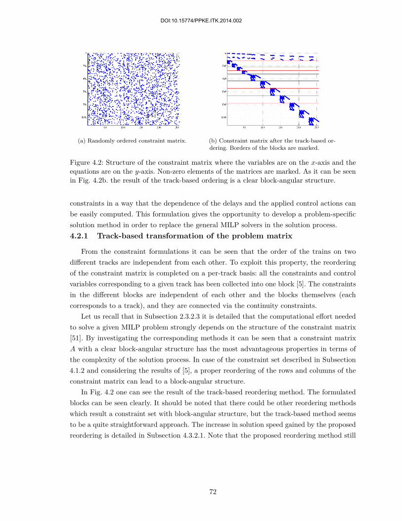
(a) Randomly ordered constraint matrix. (b) Constraint matrix after the track-based or-dering. Borders of the blocks are marked.

Figure 4.2: Structure of the constraint matrix where the variables are on the x-axis and theequations are on the y-axis. Non-zero elements of the matrices are marked. As it can be seenin Fig. 4.2b. the result of the track-based ordering is a clear block-angular structure.

constraints in a way that the dependence of the delays and the applied control actions canbe easily computed. This formulation gives the opportunity to develop a problem-specificsolution method in order to replace the general MILP solvers in the solution process.4.2.1 Track-based transformation of the problem matrix

From the constraint formulations it can be seen that the order of the trains on twodifferent tracks are independent from each other. To exploit this property, the reorderingof the constraint matrix is completed on a per-track basis: all the constraints and controlvariables corresponding to a given track has been collected into one block [5]. The constraintsin the different blocks are independent of each other and the blocks themselves (eachcorresponds to a track), and they are connected via the continuity constraints.

Let us recall that in Subsection 2.3.2.3 it is detailed that the computational effort neededto solve a given MILP problem strongly depends on the structure of the constraint matrix[51]. By investigating the corresponding methods it can be seen that a constraint matrixA with a clear block-angular structure has the most advantageous properties in terms ofthe complexity of the solution process. In case of the constraint set described in Subsection4.1.2 and considering the results of [5], a proper reordering of the rows and columns of theconstraint matrix can lead to a block-angular structure.

In Fig. 4.2 one can see the result of the track-based reordering method. The formulatedblocks can be seen clearly. It should be noted that there could be other reordering methodswhich result a constraint set with block-angular structure, but the track-based method seemsto be a quite straightforward approach. The increase in solution speed gained by the proposedreordering is detailed in Subsection 4.3.2.1. Note that the proposed reordering method still

72

DOI:10.15774/PPKE.ITK.2014.002

decreases the solution time while the preprocessor of the solver is also used.4.2.2 Transformation of individual constraints

Let us refer to the constraints which depend on two different continuous variables asdependent constraints while those which depend only on one continuous variable as independentconstraints. Note that both the dependent and the independent constraints can depend onmultiple control variables.

The proposed algorithm transforms the dependent constraints into independent onesleading to a quite clear problem structure. The main advantages of the new structure are thefollowing: firstly, the constraint matrix of a model containing purely independent constraintsis independent of the given delay scenario. Hence, the formulation of the MILP problemcorresponds to a given delay scenario requires only the computation of the vector b(k), whilethe constraint matrix A remains the same, instead of computing new A matrix for everydelay scenario as it is needed in case of dependent constraints are present. Note that thisholds until the structure of the railway network remains unchanged (no blocked track etc.).Secondly, in case of independent constraints one specific event in the system - out of thebinary control variables - has a direct dependence on only one other event. This fact givesthe opportunity to investigate deeper the model structure which was not possible in case ofthe presence of dependent constraints.

We will exploit the special properties of the constraint set described in Subsection 4.1.2.Namely, the coefficients corresponding to the continuous variables can have only {−1, 0, 1}values, and for each constraint only one 1 and one −1 value can be present. Furthermore, itis known that if a 1 appears, a −1 value is also present in that given constraint.

As it is mentioned before, the proposed algorithm transforms the dependent constraintsinto independent ones. This means that the Ax matrix from ineq. (4.17) is transformed toa matrix that will only contain {0,−1} values and only one non-zero coefficient for eachconstraint.

The proposed model transformation method - which will be introduced next - is basedon an iterative substitution of the constraints into each other resulting in new constraints.The procedure continues until the expected constraint structure is achieved. A proceduraldescription of the proposed method is presented in Sec. Appendix C. To ease the understandingof the procedure, an illustrative example is also presented.4.2.2.1 Reformulation of the model for the substitution

The model described in ineq. (4.17) is reshaped into an other form in order to ease theunderstanding the proposed procedure. Let us use the following notations: xi refers to anevent in the network represented by a continuous variable. The sign of xi is related to thecorresponding elements of Ax. rj is a reference time of the jth event. Elements of τ arereferring to numerical values calculated from the running times, dwell times, headway timesand separation times and related to the elements of b(k). ul is a binary control variable andβ is a large negative value appearing in Au. 1m refers to a full-one vector having m rows,

73

DOI:10.15774/PPKE.ITK.2014.002

matrices denoted by letter E have a block structure while matrices denoted by letter A containnon-zero elements without specific pattern. Operation ⊗ refers to the Kroenecker-product.

The constraint set of the given model is ordered in two different ways resulting differentmodel formulations. These formulations can be used implement the substitution of theconstraints to formulate the iterative method. In the following, we define the two modelformulations and the substitution procedure.

Model formulation 1 Let us order the constraints in the model based on the variableson their left-hand side. Now the following structure can be obtained:

E1...En

x ≥A1...An

x+

B1...Bn

u+

c1...cn

(4.21)

which can be read asE x ≥ Ax+B u+ c (4.22)

where mi is the number of constraints in the model having xi in their left-hand side,Ei ∈ {0, 1}mi×n, Ai ∈ {0, 1}mi×n, Bi ∈ {−β, 0, β}mi×n, ci ∈ Rmi and i = 1...n.

It should be noted that this model formulation is related to the original model, it willnot change during the substitution process.

Model formulation 2 During the iteration, constraints emerged from the model areordered based on the right-side of the inequality constraints. Let us describe the modelformulation in the ` = 0 case where ` is the iteration counter. Now, the sub-matrices aredenoted as follows:

A`0A`1...A`n

x ≥E`0E`1...E`n

x+

B`

0B`

1...B`n

u+

c`0c`1...c`n

(4.23)

which can be rewritten asA`x ≥ E`x+ B`u+ c` (4.24)

where A`i ∈ {0, 1}m`i×n, E`i ∈ {0, 1}m

`i×n, B`

i ∈ {−β, 0, β}m`i×n, c`i ∈ Rm`

i , i = 0...n. Note thatin the `th iteration step m`

0 and m`i equals to the number of the independent and dependent

constraints corresponding to xi, respectively.Let us note that this kind of model formulation groups the independent constraints

together leading to the appearance of the sub-matrices indexed by 0 (namely A`0, E`0, B`0

and c`0). In Model formulation 1, these constraints are incorporated into the Ei, Ai, Bi, ci(i = 1...n) matrices, too. Also, it can be seen that a permutation matrix P exists for which

74

DOI:10.15774/PPKE.ITK.2014.002

the following holds: P · E = A`, P ·A = E`, P ·B = B` and P · C = C`.

4.2.2.2 Substitution procedure

Now using the two forms of the model presented previously, an iterative substitutionprocess is proposed to achieve a model structure containing only independent constraints.

It is known that for i > 0:1mi ⊗ E`i = 1m`

i⊗ Ei

Use Model formulation 2 :A`0

1m1 ⊗ A`11m2 ⊗ A`21m3 ⊗ A`3

x ≥

E`01m1 ⊗ E`11m2 ⊗ E`21m3 ⊗ E`3

x+

B`

01m1 ⊗ B`

11m2 ⊗ B`

21m3 ⊗ B`

3

u+

c`0

1m1 ⊗ c`11m2 ⊗ c`21m3 ⊗ c`3

By using ineq. (4.22) we find

E`01m1 ⊗ E`11m2 ⊗ E`21m3 ⊗ E`3

x+

B`

01m1 ⊗ B`

11m2 ⊗ B`

21m3 ⊗ B`

3

u+

c`0

1m1 ⊗ c`11m2 ⊗ c`21m3 ⊗ c`3

=

E`0

1m`1⊗ E1

1m`2⊗ E2

1m`3⊗ E3

x+

B`

01m`

1⊗ B`

1

1m2 ⊗ B`2

1m3 ⊗ B`3

u+

c`0

1m`1⊗ c`1

1m2 ⊗ c`21m3 ⊗ c`3

=

E0 x

1m`1⊗ E1 x

1m`2⊗ E2 x

1m`3⊗ E3 x

+

B`

01m1 ⊗ B`

11m2 ⊗ B`

21m3 ⊗ B`

3

u+

c`0

1m1 ⊗ c`11m2 ⊗ c`21m3 ⊗ c`3

≥

E`0 x

(1m`1⊗A1)x+ (1m`

1⊗B1)u+ (1m`

1⊗ c1)

(1m`2⊗A2)x+ (1m`

2⊗B2)u+ (1m`

2⊗ c2)

(1m`3⊗A3)x+ (1m`

3⊗B3)u+ (1m`

3⊗ c3)

+

1m0 ⊗ B`

01m1 ⊗ B`

11m2 ⊗ B`

21m3 ⊗ B`

3

u+

1m0 ⊗ c`01m1 ⊗ c`11m2 ⊗ c`21m3 ⊗ c`3

=

E`0

(1m`1⊗A1)

(1m`1⊗A2)

(1m`1⊗A3)

x+

B`

0(1m1 ⊗ B`

1) + (1m`1⊗B1)

(1m2 ⊗ B`2) + (1m`

2⊗B2)

(1m3 ⊗ B`3) + (1m`

3⊗B3)

u+

c`0

(1m1 ⊗ c`1) + (1m`1⊗ c1)

(1m2 ⊗ c`2) + (1m`2⊗ c2)

(1m3 ⊗ c`3) + (1m`3⊗ c3)

75

DOI:10.15774/PPKE.ITK.2014.002

which results in the new inequality:

A` x ≥ E` x+ B` u+ c` (4.25)

where

A` = P

A`0

1m1 ⊗ A`11m2 ⊗ A2

1m3 ⊗ A`3

E` = P

E`0

(1m`1⊗A1)

(1m`1⊗A2)

(1m`1⊗A3)

B` = P

B`

0(1m1 ⊗ B`

1) + (1m`1⊗B1)

(1m2 ⊗ B`2) + (1m`

2⊗B2)

(1m3 ⊗ B`3) + (1m`

3⊗B3)

c` = P

c`0

(1m1 ⊗ c`1) + (1m`1⊗ c1)

(1m2 ⊗ c`2) + (1m`2⊗ c2)

(1m3 ⊗ c`3) + (1m`3⊗ c3)

where P is again a proper permutation matrix such that E` has the correct structure.

After computing ineq. (4.25), those inequalities, which contain terms uiβ and (1− ui)βfor the same i should be removed from the constraint set. Furthermore, the constraints withthe following form

xi ≥ xi +Bi u+ ci

can be replaced with the following inequalities:

Bi u+ ci ≤ 0.

Some of these inequalities can be removed immediately, because they lead to a controlcombination corresponding to an infeasible series of events. This is caused by the fact thatin case of n control variables the number of possible combinations (2n) is larger than thepossible valid control input combinations. A simple example is the following: consider threetrains running on the same track, ordered by three control variables. The number of possiblecontrol combinations is 23 = 8 but there are only 6 feasible train orderings. For example,an infeasible train order appears if the first train is scheduled before the second, the secondis scheduled before the third and the third is scheduled before the first. To overcome onthis problem, the proposed algorithm filters out those constraints which contain infeasiblecontrol combinations. Note, that the reachability set of the system is not changed becauseonly infeasible control combinations are removed.

Now an iteration step can be formulated as follows. In the `th step we consider ineq.(4.24) and ineq. (4.22) and obtain ineq. (4.25). Initialize the next step by letting A`+1 = A`,B`+1 = B` and c`+1 = c`. It can be seen that for each iteration step the following inequalityholds: row(A`0) ≤ row(A`+1

0 ), where row stands for the number of rows in the given matrix.For each event there exists at least one independent constraint in the starting model (e.g.

76

DOI:10.15774/PPKE.ITK.2014.002

the timetable constraint), hence the process will finish with the elimination of the dependentconstraints in finite steps: ∃` : m`

i = 0 where i > 0 and ` ≤ n.As it is shown, the main purpose of this algorithm is to transform the originally dependent

constraints into independent ones. It differs from other matrix decomposition or factoringmethods because of its capability to handle the strongly over-determined constraint set withthe restricted set of allowed operations on the constraints.

4.2.2.3 Example

Let us consider a small model containing three events. xi denotes the time of a specificevent while ri denotes the reference time of the given event. τij is a headway time definedbetween events xi and xj . Control variables are denoted by uk and β is a large negativenumber.

x1 ≥ r1

x2 ≥ r2

x3 ≥ r3

x2 ≥ x1 + τ21 + (1− u1)β

x3 ≥ x1 + τ31 + (1− u3)β

x1 ≥ x2 + τ12 + u1β

x3 ≥ x2 + τ32 + (1− u2)β

x1 ≥ x3 + τ13 + u3β

x2 ≥ x3 + τ23 + u2β

(4.26)

This constraint set will be reformulated with the proposed transformation and the resultingnew constraint set is presented, too.

Model formulation 1 :

1 0 01 0 01 0 00 1 00 1 00 1 00 0 10 0 10 0 1

x ≥

0 0 00 1 00 0 10 0 01 0 00 0 10 0 01 0 00 1 0

x+ β

0 0 01 0 00 0 10 0 0−1 0 00 1 00 0 00 0 −10 −1 0

u+

r1

τ12

τ13

r2

τ21 + β

τ23

r3

τ31 + β

τ32 + β

77

DOI:10.15774/PPKE.ITK.2014.002

Model formulation 2:

1 0 00 1 00 0 10 1 00 0 11 0 00 0 11 0 00 1 0

x ≥

0 0 00 0 00 0 01 0 01 0 00 1 00 1 00 0 10 0 1

x+ β

0 0 00 0 00 0 0−1 0 00 0 −11 0 00 −1 00 0 10 1 0

u+

r1

r2

r3

τ21 + β

τ31 + β

τ12

τ32

τ13

τ13

Using the above introduced transformation procedure, the constraint set defined in ineq.(4.26) turned into the following set:

x1 ≥ r1

x2 ≥ r1 + τ21 + (1− u1)β

x2 ≥ r1 + τ23 + τ31 + u2β + (1− u3)β

x3 ≥ r1 + τ31 + (1− u3)β

x3 ≥ r1 + τ32 + τ21 + (1− u1)β + (1− u2)β

x2 ≥ r2

x1 ≥ r2 + τ12 + u1β

x1 ≥ r2 + τ13 + τ32 + u3β + (1− u2)β

x3 ≥ r2 + τ32 + (1− u2)β

x3 ≥ r2 + τ31 + τ12 + u1β + (1− u3)β

x3 ≥ r3

x1 ≥ r3 + τ13 + u3β

x1 ≥ r3 + τ12 + τ23 + u1β + u2β

x2 ≥ r3 + τ23 + u2β

x2 ≥ r3 + τ13 + τ21 + (1− u1)β + u3β

0 > u1β + u2β + (1− u3)β

0 > (1− u1)β + (1− u2)β + u3β

(4.27)

As it can be seen, ineq. (4.27) contains only independent constraints: on the right-handside only control variables, reference times and headway times can be found (denoted by ui,ri and τij , respectively).

78

DOI:10.15774/PPKE.ITK.2014.002

4.2.2.4 Partial transformation of the model

The advantageous property of the model achieved by the procedure described in Subsection4.2.2 - namely that all constraints are independent constraints - has the drawback that thenumber of the constraints in the model is increased dramatically. This has also effect on therunning time of the transformation.

To overcome this, the algorithm is modified to process the constraint set on an iterativeway. In one iteration a subset of events are selected and only those constraints are processedwhich correspond to these events in the network. By limiting the size of this subset, thecomputational requirements of an iteration and the resulting model size can be limited, too.

This kind of modification also means that the final model will contain some dependentconstraints. These could not be translated into independent ones because some of theconstraints needed for the substitution were out of the processed constraint set having limitedsize. Hence, the resulting model can be regarded as a partially independent model.

The partial transformation can preserve the advantageous properties of the model havingonly independent constraints (e.g. the dependencies between the events can keep a clearstructure) while it overcomes the problems emerging if the constraint set is enlarged. Itshould be noted that the ratio of the remaining dependent constraints can be controlled bychanging the size of the subset containing the events processed in one iteration step.

Computational results and comparisons between the original and transformed modelscan be found in Subsection 4.3.2.

4.2.2.5 Structure of the transformed constraint set

The constraint set composed in Subsection 4.1.2 can be transformed into a new constraintmatrix by using the previously detailed algorithm. The resulting problem containing indepen-dent constraints shows a clear connection between the events in the network through solelythe control variables.

As an example, a constraint set containing 23278 dependent constraints and 4769 variables(from which 1930 are continuous variables, the others are binary control variables) is convertedto contain independent constraints. The number of the constraints increased to 520194. Thestructure of the constraint set can be seen in Fig. 4.3. The running time of the transformationalgorithm was around 4300 seconds. Note, that this is an off-line transformation meaningthat it should be completed once for each model until the model structure (the structure ofthe railway network and the routes and number of trains in it) is unchanged. An estimationfor the number of the constraints in the independent model is possible but would take seriouscomputational efforts, hence it strongly depends on the structure of the dependent model.

4.3 A case study

Simulations were done using the model of the Dutch railway system (see Fig. 4.4), with a

79

DOI:10.15774/PPKE.ITK.2014.002

Figure 4.3: Structure of the constraint matrix containing independent constraints. Blue andgreen marks are for positive and negative values in the matrix, respectively. Red marks arefor values corresponding to control variables. In this particular case the track-based orderinghas not been used. The total size of the matrix is 520194 rows and 4769 columns.

80

DOI:10.15774/PPKE.ITK.2014.002

Figure 4.4: The Dutch railway network.

timetable having cycle time Tc = 60 min. The network model consists of 66 stations and191 tracks. In the timetable the international, interregional and most of the local trainsare included, but freight trains and some smaller lines that are not connected to the mainnetwork are excluded. For the simulations Np = 2 is selected, so the prediction is done for2 hours in the future. A new schedule is generated if any of the trains have more than 2minutes of delay. The generated problem originally has 54090 constraints and 13136 variablesfrom which 3860 are continuous variables (departure and arrival times) and the remaining9276 are binary control variables. The time constants in the model are set as follows: headwaytimes haij = hdij = 3min, dwell time spi(k) = 2min and separation time wij = 3min.

The computations were completed on a personal computer equipped with a PentiumIV CPU having 4 cores, running on 3.4GHz. Model generation and transformations weredone in MATLAB. To solve the generated MILP problem, the Gurobi 5.50 [59] solver wasused with enabled multi-threaded solution capability. It should be mentioned that duringthe computations the default parameter settings of the solver were used in order to ensurethe comparability of the results.

The delay scenarios were introduced into the model as it is described in Subsection 4.1.4.Each delay scenario contains several, individual initial delays, representing the time-shiftingof an event (departure or arrival) from its reference time. The sum of the introduced initialdelays by a given scenario is referred as the total initial delay. It is shown in [134] that thedistribution of delays appearing in a train network follows a Weibull distribution. In ourcase the delays were generated randomly, according to a Weibull-distribution having shapeparameter 0.8 and scale parameter 5. The maximum amount of an individual delay event wasset to 10 min and the average introduced delay to 3 min. During the scenario generation apredefined percentage of the trains were selected to be delayed: the delay values were addedto their departure and arrival data. In general, using the previously parametrized Weibulldistribution, delaying 7% of the events ends up in a realistic delay scenario considering theabsolute values and distribution of the delays. This means that 260 events were delayed overthe prediction horizon, leading to 130 delayed event in an hour. Note that according to the

81

DOI:10.15774/PPKE.ITK.2014.002

infrastructure manager company of the Dutch Railways, in the first nine months of 2012,10.5% of the trains in the Netherlands had 3 minutes or more delay.

The aim of the controller is to minimize the sum of the secondary delays over the predictionhorizon. This is calculated as the sum of the deviations from the predefined timetable andreferred as total secondary delay in case of a given delay scenario.4.3.1 Performance analysis of the proposed control technique

The performance of the proposed control technique is showed by comparing the open loopand closed loop (uncontrolled and controlled, respectively) behavior of the railway network.The simulations were completed on 45 scenarios. In case of these scenarios, the average of thetotal initial delay was 3448.2 min with s = 146.1 min, where s stands for standard deviation.

The open-loop simulation is done by setting all control inputs to zero. This means thatneither the order of the trains, nor the selected tracks or the coupled runs were changed.By simulating the operation of the network over the prediction horizon, the total secondarydelay appeared during the uncontrolled behavior can be computed. The obtained values arethe following: 4264.2 min total secondary delay in average, with s = 549.7 min.

In controlled mode the previously introduced control method was applied on the railwaynetwork. Again, at the end of the prediction horizon the difference between the actualtimetable and the reference schedule is calculated as the total secondary delay. It is turnedout that by applying the proposed control method the average total secondary delay hasbeen reduced to 2164.2 min with s = 238.6 min.

The simulations showed the effectiveness of the proposed control technique as it can beseen in Fig. 4.5. The controller can decrease the the total secondary delay with approximately48.9% in average compared to the uncontrolled case. In average, 48 control actions wereapplied.

Note, that considering a given delay scenario, selecting longer prediction horizons willincrease the difference between the sum of the total secondary delays of the network in uncon-trolled and controlled modes. Although, the computational time needed for the optimizationprocess will increase, too. It should be also noted, that from a practical point of view andconsidering the frequency of unexpected events in the network, it does not worth to dealwith prediction horizons longer than 3 hours.4.3.2 Comparison of time consumption of solutions in case of different

model formulations

Due to the large size of the emerging MILP problems in case of a busy railway networkand long prediction horizon, time consumption of the rescheduling become a crucial problem.In the following, the model formulations detailed in Subsection 4.2.1 and 4.2.2 are comparedin terms of the solution time.

82

DOI:10.15774/PPKE.ITK.2014.002

Figure 4.5: Effect of the proposed control technique while minimizing the total secondarydelays. The optimal reordering of the trains can significantly reduce the total delay over thecontrol horizon.

4.3.2.1 Effect of constraint reordering on the solution time

It is known that proper restructuring of an MILP problem can have serious impact onthe solution time [51]. In the present work a track-based ordering is proposed (see Sec. 4.2.1)which results in a clear block-angular structure in the constraint matrices. The followingresults verify that even in the presence of the solver’s preprocessor serious gains can beachieved using this specific ordering of the constraints.

During the generation of the constraint matrices, two different methods were compared.First the columns and rows of the formulated matrices were generated in a random orderresulting an unordered matrix structure. In the other case we built up the matrices of thesame problem with track-based ordering.

The solution times in both cases for several different scenario can be seen in Fig. 4.6. for30 different scenarios. The average solution time was 53.763 sec (s = 43.194 sec) withoutand 29.674 sec (s = 27.703 sec) with reordering which means an average speedup ratio1.813. It should be noted that according to the simulations larger problem sizes lead tolarger speedup ratio. This emphasizes the importance of the structured problem formulationbased on problem-specific knowledge. Note, that this reordering method outperforms all thepreprocessing methods implemented in the applied solver meaning that the built-in methodswere not as effective in the formulation of the block-diagonal structure as the proposedmethod was.

4.3.2.2 Effect of constraint reformulation on the solution time

In Subsection 4.2.2 a model transformation method is proposed. Now the effect of thistransformation on the solution time is detailed. As it was mentioned before, the reformulationof the constraints from dependent to independent ones enlarges the problem matrix byincreasing the number of constraints. This naturally causes some overhead during the

83

DOI:10.15774/PPKE.ITK.2014.002

Figure 4.6: Solution times in case of a random constraint matrix structure and in case ofthe track-based reordering. The simulation results show that even in the presence of thepreprocessor of the solver proper reordering can yield to significant speedup. Scenarios areplotted in an increasing order w.r.t. the solution time in case of track-based ordering.

optimization process. Hence, we expected that in case of a (partially) transformed model thesolution will be slower than the original model.

In order to test the proposed methods in scenarios which can be considered as realisticones, the following computations were completed. The dependent and independent modelsof 50 different, randomly generated scenarios were solved. In each scenario 7% of the trainswere delayed which means that the average introduced total initial delay was 2790 min

(s = 108.8 min). The average solution time in case of the dependent model was 853.91 sec(s = 975.91 sec) while in case of the independent model 1676.06 sec (s = 2292.92 sec) wasachieved. The resulting solution times can be seen in Fig. 4.7. Due to the larger size of theindependent model, in several cases it is slower to solve it than the dependent one. On theother hand, in case of some delay scenarios the dependent model can be solved slowly andthe solution of the independent model (even its larger size) can gain on it. It should be alsonoted, that the solution speed of the independent model strongly depends on the number ofredundant or unnecessary constraints which can be eliminated from the model by the solver’spreprocessor, which is influenced by the values effected by the given delay scenario.

Further analysis were completed to investigate the changes in the solution time if the delayscenarios become more complex. 45 different, randomly generated scenarios were createdwhile the percentage of the delayed trains was enabled to grow up to 15% (affecting 260events per hour). This means that in average 3394 min (s = 1702 min) total initial delay wasadded to the models. From the 45 scenarios, 36 and 39 were solved successfully in case of thedependent and independent model formulation, respectively. In case of the remaining onesthe solution process was run out of memory. The dependence between the introduced totalinitial delay and the solution times can be seen in Fig. 4.8. To ease the understanding of theresults, trend lines were inserted into the diagram using power regression. The comparisonof the solution times in case of the dependent and independent model formulation can be

84

DOI:10.15774/PPKE.ITK.2014.002

Figure 4.7: Solution times in case of models containing dependent and independent constraints.Scenarios are plotted in an increasing order w.r.t. the solution time in case of dependentmodels.

seen in Fig. 4.9. Note, that as the complexity of the delay scenarios are increasing (denotedby the increasing amount of primary delays) the effectiveness of the solver’s preprocessordecreases. This means that less size reduction can be achieved in case of the independentmodel, resulting larger problem sizes and increased solution times.

It can be said that despite the fact that the independent model contains a lot moreconstraints than the dependent one, the solution times are in the same range in case ofcomplex scenarios, too.

The main advantage of the formulated model is that it expresses the dependence of theevents and the control variables in a very clear and simple way (see ineq. (4.27)): everycontinuous variable depends only on precomputable scalars and binary control variables.This also means that the dependence between the delays and the control variables can bedirectly formulated, by substracting the reference times from the time of the events, thus theeffect of a given control variable on the evolution of the delays can be directly computed.By considering these, a problem-specific solution method can be developed to replace thegeneral methods of the MILP solvers, which could have serious impact on the performanceof the solution process. The development of this solver is out of the scope of this work butseems to be a very promising future work.

4.3.3 Sensitivity analysis based on single delays

It is known that in a railway network the change of the departure or arrival time of onetrain can a have small effect, but the change of the parameters of other trains can lead to animmense effect on the whole system. In the following it is shown that the proposed modelstructure is capable of showing the most delay-sensitive parts of the network.

To investigate the effect of a given train’s delay on the network, the following setup wasused. Two different cases were examined introducing 5 and 10 minutes of individual initialdelay to a given train, respectively. Note that in case of this special setup the introduced total

85

DOI:10.15774/PPKE.ITK.2014.002

Figure 4.8: Dependence between the introduced total initial delays and the solution times incase of dependent and independent model formulation. The power regression lines has thefollowing parameters and correlation coefficients. In case of the dependent model: 5 ·10−9x3.18,R2 = 0.831, in case of the independent model: 4.155 · 10−6x2.43, R2 = 0.809.

Figure 4.9: Comparison of the solution times of the dependent and independent modelformulation in case of several different delay scenarios. Scenarios are plotted in an increasingorder w.r.t. the solution time in case of dependent models. As it is shown in Fig. 4.8, thishas a strong correlation with the total initial delay introduced into the given scenario.

86

DOI:10.15774/PPKE.ITK.2014.002

Figure 4.10: Result of delay-sensitivity tests in case of uncontrolled mode. Both the scenarioshaving 5 and 10 minutes initial delay are presented.

initial delay is equal to the individual delay of the given train. The whole network model withNp = 2 was generated and simulated over the prediction horizon. Both uncontrolled case andcontrolled case were evaluated. This procedure was iterated over all trains in the network.

This setup enables us to analyze the effect of delay on a given train. If the selected trainis a bottle-neck node in the network, then the introduced initial delays will end up in highsecondary delay values, showing that many other trains are effected by the delay of thisspecific train.

The generated results can be seen in Fig. 4.10 and in Fig. 4.11. In case of the 5 min initialdelay, the average of secondary delay in uncontrolled mode is 778.37 min (s = 11.95 min)while in controlled mode 413.96 min (s = 10.37 min) is achieved. In case of 10 min initialdelay, the average of the secondary delays is 800.99 min (s = 39.65 min) and 430.49 min(s = 27.08 min) in uncontrolled and controlled case, respectively. The results are concurringwith the expectations, namely that the effect of a relatively small delay (5 min) can behandled more effectively than the effect of a larger delay (10 min) because of the larger scaleof delay propagation. These results also confirm that the proposed control technique caneffectively reduce the amount of the delay in the network.

It should be noted that this algorithm works with the train runs in the model. As itis introduced in Subsection 4.1.1 a train run is a representation of a specific train over agiven track. Handling train runs brings the advantage that besides being able to analyze thedelay-sensitivity of a train we can also determine the most delay-sensitive track in the train’sroute.

4.4 Summary

In this Chapter a railway scheduling problem is formulated as an MILP and solved in anMPC architecture. The model is based on the one presented in [21]. The aim of the controlmethod is to minimize the total delay of the trains over the prediction horizon. Due to the

87

DOI:10.15774/PPKE.ITK.2014.002

Figure 4.11: Result of delay-sensitivity tests in case of controlled mode. Both the scenarioshaving 5 and 10 minutes initial delay are represented. Delay values are clearly smaller thanin Fig. 4.10.

computational complexity of the emerging MILP problem and the need of an algorithmwhich can solve the rescheduling in a reasonable time limit, it was necessary to speed up thesolution with proper handling of the original problem. Hence, the obtained constraint sethas been reformulated on two different ways, resulting in different model structures. Thetime consumption of the solutions have been compared to each other in case of both modelforms, having different delay scenarios. The performance of the proposed control techniqueto minimize total secondary delays has been analyzed.

The main contributions presented in this Chapter and summarized in Thesis II. arethe following: using a track-based ordering a significant speedup can be achieved duringthe solution process. By replacing the dependent constraints with independent ones, amuch simpler constraint structure has been obtained which gives the opportunity of thedeeper analysis of the dependencies between events and control actions in the network. Theeffectiveness of the proposed control technique is shown by extensive simulations: an averageof 48.9% reduction can be achieved in the sum of delays. The proposed method is capable tosimulate the effect of individual initial delays which enables us to determine the most criticalparts of the railway network in terms of delays.

The general approach - namely the formulation of a scheduling problem as a MILPproblem in an MPC framework - could be utilized in other control problems, e.g. the optimalcontrol of complex nonlinear systems by using the piecewise affine approximation of thenonlinear system model.

88

DOI:10.15774/PPKE.ITK.2014.002

Chapter 5

Conclusions

In this thesis, optimization based methods were used to analyze and control networkedsystems in large scale, with complex nonlinear dynamics. New methods were presented bothin the topic of the structural analysis of the Kinetic Reaction Networks and the solution ofthe scheduling problems of traffic networks.

The main effort has been focused on the analysis of the structure of the investigatedproblems. It has been shown that a proper problem representation can be obtained byexploiting the special structure of problem itself, which leads to the simplification of theemerging optimization problems (e.g. see Figs. 3.7-3.8 and Fig. 4.2 and their interpretation).In some cases LP problems can be formulated to substitute the original MILP problems andin other cases the MILP structure is transformed resulting in computational tasks that canbe solved in reasonable time. Also, it has been shown that the methods can be applied on aparallel architecture.

5.1 New scientific contributions of the work (thesis points)

The new scientific results presented in this work are summarized in this Section. Theyare arranged in three thesis points as follows.

Thesis I. Numerically efficient algorithms to find sparse and dense realiza-tions of kinetic reaction networks.

I have proposed two algorithms both based on linear programming (LP) having polynomialtime complexity to compute dynamically equivalent alternative realizations of a kinetic reac-tion network (KRN). I have showed that with the help of the proposed methods alternativerealizations of large scale, biologically motivated KRNs can be computed, too. The algorithmsare compared with the mixed-integer linear programming (MILP) based algorithm available inthe literature and the correctness of the solutions is shown. I have also concluded that theintroduced new methods outperform the MILP-based solution in terms of the time consumptionof the solution. (Section 3.2)

Corresponding publications: [1, 6]

89

DOI:10.15774/PPKE.ITK.2014.002

Thesis I.a

I have proposed an LP-based algorithm to compute dynamically equivalent realizationsof a KRN containing minimal number of reactions. The so-called sparse realization of thereaction network is computed via the column-wise L1-norm minimization of the off-diagonalelements of the Kirchhoff-matrix. (Section 3.2.1)

Thesis I.b

I have proposed an LP-based algorithm to compute a dynamically equivalent realizationof a KRN containing maximal number of reactions which is proven to contain all possiblerealizations of the reaction graph as a subgraph. The method to compute the so-called denserealization of the reaction network is based on the relaxation of the MILP-based method knownfrom the literature: the column-wise sum of the introduced real-valued auxiliary variablescorresponding to the off-diagonal elements of the Kirchhoff-matrix has been maximized.(Section 3.2.2)

Thesis II. New methods to compute weakly reversible and mass conservingrealizations of kinetic reaction networks.

I have proposed new methods to compute dynamically equivalent and linearly conjugatealternative realizations of a kinetic reaction network while constraints in terms of the structuralproperties of the reaction graph and/or dynamical properties of the described system arepresent, too.

Corresponding publications: [2, 4]

Thesis II.a.

A new, linear programming-based method with polynomial time complexity is proposedto compute linearly conjugate, weakly reversible realizations of a kinetic reaction network(KRN). I have compared the method to other linear programming- and mixed-integer linearprogramming-based algorithms from the literature and it is shown that it outperforms all theothers in terms of computational time, hence the algorithm is capable to handle large scaleKRNs, too. (Section 3.3)

Thesis II.b.

I have proposed a mixed-integer linear programming-based algorithm to compute dynami-cally equivalent realizations of a kinetic reaction network with mass-conservation property.

90

DOI:10.15774/PPKE.ITK.2014.002

The correctness of the results was shown through examples taken from the literature. (Section3.4)

Thesis III. New solution methods of scheduling problems in traffic networks.

I have proposed a model formulation method for model-predictive controllers which aimto deal with the scheduling problem of railway networks in case of delayed operation. Thecontroller reorders the trains in order to minimize the total delay in the network over theprediction horizon. The model is described with the help of linear constraints. Thus, thecontrolling problem is formulated as a mixed-integer linear programming (MILP) problem. Ihave showed the effectiveness of the proposed control technique and a method is proposed forthe sensitivity analysis of the model in case of single delays. (Chapter 4)

Corresponding publications: [5, 3]

Thesis III.a.

I have proposed a reordering method of the constraint matrix that can speed up the solutionof the MILP problem in the presence of the solver’s preprocessor, too. The method is basedon the track-based reordering of the constraint matrix. The track-based reordering means thatthe constraints corresponding to a given track are collected into one block resulting that theconstraint matrix of the emerging MILP problem has a clear block-angular structure. (Section4.2.1)

Thesis III.b.

I have proposed an algorithm to reformulate the constraints in order to achieve a moresimple model formulation. The resulting model shows a clear and simple correspondencebetween the continuous variables describing the schedule of the events in the network and thebinary control variables. Considering these, further analysis of the internal relations of thenetwork model can be done, while problem-specific solution methods can be developed insteadof the application of the general-purpose MILP solvers. (Section 4.2.2)

5.2 Utilization of the presented results, further work

In this thesis the topic of the analysis and control of complex, nonlinear dynamicalsystems with networked structure has been investigated through two open problems. Namely,in Chapter 3 a set of new or improved methods were presented to compute dynamicallyequivalent or linearly conjugate KRNs with additional structural or dynamical constraints.

91

DOI:10.15774/PPKE.ITK.2014.002

The introduced algorithms give us the opportunity to analyze large scale, biologically relevantnetworks, too. In Chapter 4 new model formulations were proposed for the dynamical railwayscheduling problem in case of delayed operation. Moreover, a model predictive controller-based framework was formulated to generate timetables corresponding to delay scenarios inorder to minimize the total secondary delay in the network. New timetables are obtainedfrom the nominal one by swapping trains, splitting joint trains or move them onto alternativeparallel tracks. It has been shown, that by applying the presented model formulations, inone hand, the solution speed of the emerging optimization problems can be increased. Onthe other hand, with proper reformulation, a very clean model structure can be obtainedwhich can serve as a basis of the development of problem-specific solvers.

There are several fields where the results of the presented work can be further developed.The implementation of the applied methods on many-core computing devices can lead tomassive improvement in solution time which further extends the applicability of the introducedmethods. It should be noted, that each presented algorithm can be embedded into a parallelframework: during the problem formulation parallelly solvable problems can be generated orthe solution process of the underlying optimization problem (e.g. the tree-exploration phaseof the MILP solution) can be parallelized.

A possible further work can be the application of problem-specific decomposition methodson the given optimization problems. As an example, a topographical decomposition methodcan be mentioned in case of the railway networks: if the original, large scale railway networkwould be split into several, weakly connected parts, the MILP problem having huge sizewould also be split into smaller problems connected to each other via boundary conditions.The emerged set of smaller size MILPs can be solved parallelly, leading to decreased solutiontime.

From a modeling point of view, both topics offer several possible directions of development:in case of KRNs the search for realizations with further structural and dynamical constraintscan be implemented, such as realizations with minimal/zero deficiency, computing all possibledynamically equivalent realizations etc. Also a controller design method with static ordynamic extension of the network could be possible using the presented framework.

In the railway scheduling topic further extensions of the model describing the events inthe railway network would be useful, introducing capacity limits of the stations, priorizingtrains based on their types, handling track blocking etc. Moreover, it would be interesting tomodify the framework to control passenger delays instead of train delays leading to a morepassenger-friendly rescheduling method.

In general, it could be said that the optimization based control of analysis and control ofcomplex dynamical systems having networked structures can be an interesting research topicin the future, too, leading to the deeper understanding of the behavior of large-scale systemsincorporating many interconnected units.

92

DOI:10.15774/PPKE.ITK.2014.002

The Author’s Publications

[1] J. Rudan, G. Szederkényi, and K. M. Hangos, “Efficiently computing alternativestructures of large biochemical reaction networks using linear programming,” MATCHCommun. Math. Comput. Chem., vol. 71, pp. 71–92, 2014.

[2] J. Rudan, G. Szederkényi, K. M. Hangos, and T. Péni, “Polynomial time algorithmsto determine weakly reversible realizations of chemical reaction networks,” Journal ofMathematical Chemistry, pp. 1–19, 2014.

[3] B. Kersbergen, J. Rudan, T. van den Boom, and B. D. Schutter, “Railway traffic man-agement using switching max-plus-linear systems,” Discrete Event Dynamic Systems,submitted.

[4] J. Rudan, G. Szederkényi, and K. M. Hangos, “Computing dynamically equivalentrealizations of biochemical reaction networks with mass conservation,” in 11th interna-tional Conference of Numerical Analysis and Applied Mathematics 2013: ICNAAM 2013,vol. 1558, pp. 2356–2359, AIP Conference Proceedings, 2013. ISBN: 978-0-7354-1184-5.

[5] J. Rudan, B. Kersbergen, T. van den Boom, and K. M. Hangos, “Performance analysisof MILP based model predictive control algorithms for dynamic railway scheduling,”in European Control Conference (ECC2013), July 17-19 2013, Zurich, pp. 4562–4567,2013.

[6] J. Rudan, G. Szederkényi, and K. M. Hangos, “Effectively computing dynamicallyequivalent structures of large biochemical reaction networks,” in International Con-ference on Bioinformatics and Computational Biology – BIOCOMP 2012, Bulgaria,Varna, p. 80, 2012.

[7] J. Rudan, K. M. Hangos, and G. Szederkényi, “Analysis and supervisory control of apressurizer using coloured Petri nets,” in 9th European Workshop on Advanced Controland Diagnosis - ACD 2011, pp. 1–6, 2011.

[8] G. Szederkényi, G. Lipták, J. Rudan, and K. M. Hangos, “Optimization-based designof kinetic feedbacks for nonnegative polynomial systems,” in IEEE 9th InternationalConference of Computational Cybernetics, July 8-10, Tihany, Hungary, pp. 67–72, 2013.ISBN: 978-1-4799-0063-3.

93

DOI:10.15774/PPKE.ITK.2014.002

References

[9] I. F. S. G. A. Capone, G. Carello and F. Malucelli, “Solving a resource allocationproblem in wireless mesh networks: A comparison between a CP-based and a classicalcolumn generation,” Networks, vol. 55, pp. 221–233, 2010.

[10] S. Akle, O. Dalal, R. M. Fleming, M. Saunders, N. Taheri, and Y. Ye, “Existence ofpositive steady states for mass conserving and mass-action chemical reaction networkswith a single terminal-linkage class,” arXiv preprint arXiv:1105.2359, 2011.

[11] D. F. Anderson, “Boundedness of trajectories for weakly reversible, single linkage classreaction systems,” Journal of Mathematical Chemistry, vol. 49, pp. 1–16, 2011. DOI:10.1007/s10910-011-9886-4.

[12] D. Angeli, “A tutorial on chemical network dynamics,” European Journal of Control,vol. 15, pp. 398–406, 2009.

[13] R. Aris and R. Mah, “Independence of chemical reactions,” Industrial & EngineeringChemistry Fundamentals, vol. 2, no. 2, pp. 90–94, 1963.

[14] A.-L. Barabási and J. Frangos, Linked: The New Science Of Networks Science OfNetworks. Basic Books, 2002.

[15] A. Barrat, M. Barthelemy, and A. Vespignani, Dynamical processes on complex networks,vol. 574. Cambridge University Press Cambridge, 2008.

[16] M. Bergner, A. Caprara, A. Ceselli, F. Furini, M. E. Lübbecke, E. Malaguti, andE. Traversi, “Automatic dantzig-wolfe reformulation of mixed integer programs.”

[17] L. Bertacco, M. Fischetti, and A. Lodi, “A feasibility pump heuristic for general mixed-integer problems,” Tech. Rep. Technical Report OR-05-5, University of Padova, Italy,2005.

[18] T. Berthold, “Primal heuristics for mixed integer programs,” Master’s thesis, Technis-chen Universitat Berlin, 2006.

[19] S. Boccaletti, V. Latora, Y. Moreno, M. Chavez, and D.-U. Hwang, “Complex networks:Structure and dynamics,” Physics reports, vol. 424, no. 4, pp. 175–308, 2006.

94

DOI:10.15774/PPKE.ITK.2014.002

[20] T. van den Boom and B. D. Schutter, “On a model predictive control algorithm fordynamic railway network management,” in 2nd International Seminar on RailwayOperations Modelling and Analysis (Rail-Hannover2007), 2007.

[21] T. J. van den Boom, N. Weiss, W. Leune, R. M. Goverde, and B. D. Schutter, “Apermutation-based algorithm to optimally reschedule trains in a railway traffic network,”in IFAC World Congress, 2011.

[22] B. Boros, “On the existence of the positive steady states of weakly reversible deficiency-one mass action systems,” Mathematical Biosciences, vol. 245, pp. 157–170, 2013.

[23] S. Boyd, L. El-Ghaoui, E. Feron, and V. Balakrishnan, Linear Matrix Inequalities inSystems and Control Theory. SIAM Books, Philadelphia, PA, 1994.

[24] S. Boyd and L. Vandenberghe, Convex Optimization. Cambridge University Press,2004.

[25] S. P. Bradley, A. C. Hax, and T. L. Magnanti, Applied Mathematical Programming.Addison-Wesley, 1977.

[26] A. Caprara, M. Fischetti, and P. Toth, “Modeling and solving the train timetablingproblem,” Operations Research, vol. 50, no. 5, pp. 851–861, 2002.

[27] V. Chellaboina, S. P. Bhat, W. M. Haddad, and D. S. Bernstein, “Modeling and analysisof mass-action kinetics – nonnegativity, realizability, reducibility, and semistability,”IEEE Control Systems Magazine, vol. 29, pp. 60–78, 2009.

[28] D.-S. Chen, R. G. Batson, and Y. Dang, Applied integer programming: modeling andsolution. John Wiley & Sons, 2011.

[29] W. W. Chen, B. Schoeberl, P. J. Jasper, M. Niepel, U. B. Nielsen, D. A. Lauffenburger,and P. K. Sorger, “Input-output behavior of erbb signaling pathways as revealed by amass action model trained against dynamic data,” Molecular Systems Biology, vol. 5,Jan. 2009.

[30] J. W. Chinneck, Practical Optimization: A Gentle Introduction. Carleton University,2009.

[31] L. O. Chua and T. Roska, “The cnn paradigm,” IEEE Transactions on Circuits andSystems I: Fundamental Theory and Applications, vol. 40, no. 3, pp. 147–156, 1993.

[32] F. Corman, “Real-time railway traffic management: Dispatching in complex, large andbusy railway networks,” tech. rep., TRAIL Research School, 2010.

[33] A. D’Ariano and M. Pranzo, “An advanced real-time train dispatching system forminimizing the propagation of delays in a dispatching area under severe disturbances,”Networks and Spatial Economics, vol. 9, no. 1, pp. 63–84, 2009.

95

DOI:10.15774/PPKE.ITK.2014.002

[34] G. B. Dantzig, Linear Programming and Extensions. Princeton University Press, 1963.

[35] G. B. Dantzig and P. Wolfe, “Decomposition principle for linear programs,” Operationsresearch, vol. 8, no. 1, pp. 101–111, 1960.

[36] E. Davison, “Connectability and structural controllability of composite systems,” Au-tomatica, vol. 13, no. 2, pp. 109 – 123, 1977.

[37] J. Deng, C. Jones, M. Feinberg, and A. Nachman, “On the steady states of weaklyreversible chemical reaction networks.” http://arxiv.org/abs/1111.2386, Nov. 2011.

[38] D. L. Donoho, “For most large underdetermined systems of linear equations theminimal l1-norm solution is also the sparsest solution,” Comm. Pure Appl. Math,vol. 59, pp. 797–829, 2004.

[39] D. L. Donoho and J. Tanner, “Sparse nonnegative solutions of underdetermined linearequations by linear programming,” in Proceedings of the National Academy of Sciences,pp. 9446–9451, 2005.

[40] D. L. Donoho and J. Tanner, “Sparse nonnegative solution of underdetermined linearequations by linear programming,” Proc. of the National Academy of Sciences of theUSA (PNAS), vol. 102, no. 27, pp. 9446–9451, 2005.

[41] H. Ehrmantraut and E. Rabinowitch, “Kinetics of hill reaction,” Archives of biochemistryand biophysics, vol. 38, no. 1, pp. 67–84, 1952.

[42] B. Elspas, “The theory of autonomous linear sequential networks,” Circuit Theory,IRE Transactions on, vol. 6, no. 1, pp. 45–60, 1959.

[43] P. Érdi and J. Tóth, Mathematical Models of Chemical Reactions. Theory and Appli-cations of Deterministic and Stochastic Models. Manchester, Princeton: ManchesterUniversity Press, Princeton University Press, 1989.

[44] K. P. Eswaran and R. E. Tarjan, “Augmentation problems.,” SIAM J. Comput., vol. 5,pp. 653–665, 1976.

[45] G. Farkas, “Kinetic lumping schemes,” Chemical Engineering Science, vol. 54, pp. 3909–3915, 1999.

[46] M. Feinberg, “Chemical reaction network structure and the stability of complex isother-mal reactors - II. Multiple steady states for networks of deficiency one,” ChemicalEngineering Science, vol. 43, pp. 1–25, 1988.

[47] M. Feinberg, “Chemical reaction network structure and the stability of complex isother-mal reactors - I. The deficiency zero and deficiency one theorems,” Chemical EngineeringScience, vol. 42 (10), pp. 2229–2268, 1987.

96

DOI:10.15774/PPKE.ITK.2014.002

[48] M. Feinberg, Lectures on chemical reaction networks. Notes of lectures given at theMathematics Research Center, University of Wisconsin, 1979.

[49] F. Friedler, K. Tarján, Y. W. Huang, and L. T. Fan, “Graph-theoretic approach toprocess synthesis: polynomial algorithm for maximal structure generation,” Computerand Chemical Engineering, vol. 17, pp. 929–942, 1993.

[50] F. Friedler, K. Tarján, Y. W. Huang, and L. T. Fan, “Graph-theoretic approachto process synthesis: axioms and theorems,” Chemical Engineering Science, vol. 47,pp. 1973–1988, 1992.

[51] M. Galati, Decomposition Methods for Integer Linear Programming. PhD thesis, LehighUniversity, 2010.

[52] M. V. Galati and T. K. Ralphs, “DIP: A framework for decomposition in integerprogramming,” tech. rep., COR@L Laboratory, Lehigh University, 2012.

[53] C. E. Garcia, D. M. Prett, and M. Morari, “Model predictive control: theory andpractice - a survey,” Automatica, vol. 25, no. 3, pp. 335–348, 1989.

[54] J. C. Geromel, J. Bernussou, and P. Peres, “Decentralized control through parameterspace optimization,” Automatica, vol. 30, no. 10, pp. 1565–1578, 1994.

[55] R. E. Gomory, “An algorithm for integer solutions to linear programs,” Recent advancesin mathematical programming, vol. 64, pp. 260–302, 1963.

[56] R. E. Gomory et al., “Outline of an algorithm for integer solutions to linear programs,”Bulletin of the American Mathematical Society, vol. 64, no. 5, pp. 275–278, 1958.

[57] R. M. Goverde, “A delay propagation algorithm for large-scale railway traffic networks,”Transportation Research Part C: Emerging Technologies, vol. 18, no. 3, pp. 269 – 287,2010. 11th {IFAC} Symposium: The Role of Control.

[58] R. M. Goverde, “Railway timetable stability analysis using max-plus system theory,”Transportation Research Part B: Methodological, vol. 41, no. 2, pp. 179–201, 2007.

[59] I. Gurobi Optimization, “Gurobi optimizer reference manual,” 2013.

[60] W. M. Haddad, V. Chellaboina, and Q. Hui, Nonnegative and Compartmental Dynam-ical Systems. Princeton University Press, 2010.

[61] K. M. Hangos and G. Szederkényi, “The effect of conservation on the dynamics ofchemical reaction networks,” in IFAC Workshop on Thermodynamic Foundations ofMathematical Systems Theory, TFMST’13, 2013.

97

DOI:10.15774/PPKE.ITK.2014.002

[62] V. Hárs and J. Tóth, “On the inverse problem of reaction kinetics,” in QualitativeTheory of Differential Equations (M. Farkas and L. Hatvani, eds.), vol. 30 of Coll. Math.Soc. J. Bolyai, pp. 363–379, North-Holland, Amsterdam, 1981.

[63] L. H. Hartwell, J. J. Hopfield, S. Leibler, and A. W. Murray, “From molecular tomodular cell biology,” Nature, vol. 402, pp. C47–C52, 1999.

[64] S. Haykin, Neural networks: a comprehensive foundation. Prentice Hall PTR, 1994.

[65] B. Heidergott and R. d. Vries, “Towards a (max,+) control theory for public trans-portation networks,” Discrete Event Dynamic Systems, vol. 11, pp. 371–398, Oct.2001.

[66] L. B. Holder and D. J. Cook, “Graph-based data mining.,” Encyclopedia of datawarehousing and mining, vol. 2, pp. 943–949, 2009.

[67] F. Horn and R. Jackson, “General mass action kinetics,” Archive for Rational Mechanicsand Analysis, vol. 47, pp. 81–116, 1972.

[68] O. C. Imer, S. Yüksel, and T. Başar, “Optimal control of lti systems over unreliablecommunication links,” Automatica, vol. 42, no. 9, pp. 1429–1439, 2006.

[69] S. M. Z. Iqbal, H. Grahn, and J. T. Krasemann, “A comparative evaluation of re-scheduling strategies for train dispatching during disturbances,” Proc. of the 13th Int’lConf. on Design and Operation in Railway Engineering (Computers in Railways XIII),pp. 567–579, 2012.

[70] S. Iwnicki, Handbook of railway vehicle dynamics. CRC Press, 2006.

[71] N. Jamshidi and B. O. Palsson, “Mass action stoichiometric simulation models: In-corporating kinetics and regulation into stoichiometric models,” Biophysical Journal,vol. 98, no. 2, pp. 175 – 185, 2010.

[72] P. A. Jensen and J. F. Bard, Operations Research Models and Methods. Wiley, 2003.

[73] M. D. Johnston and D. Siegel, “Linear conjugacy of chemical reaction networks,”Journal of Mathematical Chemistry, vol. 49, pp. 1263–1282, 2011.

[74] M. D. Johnston, D. Siegel, and G. Szederkényi, “A linear programming approach toweak reversibility and linear conjugacy of chemical reaction networks,” Journal ofMathematical Chemistry, vol. 50, pp. 274–288, 2012.

[75] M. D. Johnston, D. Siegel, and G. Szederkényi, “Dynamical equivalence and linearconjugacy of chemical reaction networks: new results and methods,” MATCH Commun.Math. Comput. Chem., vol. 68, pp. 443–468, 2012.

98

DOI:10.15774/PPKE.ITK.2014.002

[76] S. Jonnalagadda, B. Balagurunathan, and R. Srinivasan, “Graph theory augmentedmath programming approach to identify minimal reaction sets in metabolic networks,”Computers & Chemical Engineering, vol. 35, no. 11, pp. 2366 – 2377, 2011.

[77] N. Karmarkar, “A new polynomial-time algorithm for linear programming,” Proceedingsof the 16th Annual ACM Symposium on Theory of Computing, pp. 302–11, 1984.

[78] C.-T. Lin, “Structural controllability,” Automatic Control, IEEE Transactions on,vol. 19, no. 3, pp. 201–208, 1974.

[79] Y.-Y. Liu, J.-J. Slotine, and A.-L. Barabási, “Controllability of complex networks,”Nature, vol. 473, no. 7346, pp. 167–173, 2011.

[80] L. Ljung, System identification. Springer, 1998.

[81] A. Lodi and J. T. Linderoth, Encyclopedia for Operations Research and ManagementScience, ch. MILP Software. Wiley, 2011.

[82] J. Löfberg, “YALMIP : A toolbox for modeling and optimization in MATLAB,” inProceedings of the CACSD Conference, (Taipei, Taiwan), 2004.

[83] P. Makila and H. Toivonen, “Computational methods for parametric lq problems–asurvey,” Automatic Control, IEEE Transactions on, vol. 32, no. 8, pp. 658–671, 1987.

[84] N. Megiddo, “On the complexity of linear programming,” Advances in economic theory,pp. 225–268, 1987.

[85] L. Michaelis and M. L. Menten, “Die kinetik der invertinwirkung,” Biochem. z, vol. 49,no. 333-369, p. 352, 1913.

[86] H. Minc, Nonnegative Matrices. J. Wiley, 1988.

[87] W. Mitkowski, “Dynamical properties of metzler systems,” Technical Sciences, vol. 56,no. 4, 2008.

[88] Y. E. Nesterov and A. S. Nemirovski, Interior-Point Polynomial Algorithms in ConvexProgramming (Studies in Applied and Numerical Mathematics). Society for IndustrialMathematics, 1994.

[89] M. Newman, A.-L. Barabasi, and D. J. Watts, The structure and dynamics of networks.Princeton University Press, 2006.

[90] M. E. Newman, “The structure and function of complex networks,” SIAM review,vol. 45, no. 2, pp. 167–256, 2003.

[91] B. A. Ogunnaike and W. H. Ray, Process dynamics, modeling, and control, vol. 9.Oxford University Press New York, 1994.

99

DOI:10.15774/PPKE.ITK.2014.002

[92] M. Padberg and G. Rinaldi, “A branch-and-cut algorithm for the resolution of large-scale symmetric traveling salesman problems,” SIAM Review, vol. 33, pp. pp. 60–100,1991.

[93] C. H. Papadimitriou, “On the complexity of integer programming,” J. ACM, vol. 28,pp. 765–768, Oct. 1981.

[94] L. C. Pimenta, V. Kumar, R. C. Mesquita, and G. A. Pereira, “Sensing and coveragefor a network of heterogeneous robots,” in Decision and Control, 2008. CDC 2008.47th IEEE Conference on, pp. 3947–3952, IEEE, 2008.

[95] F. A. Potra and S. J. Wright, Primal-dual interior-point methods. Citeseer, 1997.

[96] C. J. Puccia and R. Levins, Qualitative modeling of complex systems. Harvard UniversityPress Cambridge, 1985.

[97] E. Quaglietta, “A microscopic simulation model for supporting the design of railwaysystems: development and applications,” 2011.

[98] S. Raghavan, The Next Wave in Computing, Optimization, and Decision Technolo-gies, ch. ‘A Note on Eswaran and Tarjan’s Algorithm for the Strong ConnectivityAugmentation Problem’, pp. 19–26. Kluwer Academic Press, 2005.

[99] T. Ralphs and M. Galati, “Decomposition methods,” in Encyclopedia of OperationsResearch and Management Science (J. Cochran, ed.), Wiley, 2010.

[100] T. Ralphs and M. Galati, “Decomposition and dynamic cut generation in integerprogramming,” tech. rep., Lehigh University, 2003.

[101] T. K. Ralphs, Parallel Combinatorial Optimization, ch. Parallel Branch and Cut,pp. 53–101. Wiley, 2006.

[102] P. J. Ramadge and W. M. Wonham, “The control of discrete event systems,” Proceedingsof the IEEE, vol. 77, no. 1, pp. 81–98, 1989.

[103] R. Raman and I. Grossmann, “Modelling and computational techniques for logic basedinteger programming,” Computers and Chemical Engineering, vol. 18, pp. 563–578,1994.

[104] R. L. Rardin, Optimization in operations research, vol. 166. Prentice Hall New Jersey,1998.

[105] J. Reeb, S. Leavengood, and O. S. U. E. Service, Using the Simplex Method to SolveLinear Programming Maximization Problems. EM (Oregon State University. ExtensionService), Oregon State University Extension Service, 1998.

100

DOI:10.15774/PPKE.ITK.2014.002

[106] F. Rosenblatt, “The perceptron: a probabilistic model for information storage andorganization in the brain.,” Psychological review, vol. 65, no. 6, p. 386, 1958.

[107] T. Roska, “Cellular wave computers for nano-tera-scale technology - beyond boolean,spatial-temporal logic in million processor devices,” Electronics letters, vol. 43, no. 8,pp. 427–429, 2007.

[108] A. Ruszczyński, “An augmented lagrangian decomposition method for block diagonallinear programming problems,” Operations Research Letters, vol. 8, no. 5, pp. 287–294,1989.

[109] N. Samardzija, L. D. Greller, and E. Wassermann, “Nonlinear chemical kinetic schemesderived from mechanical and electrical dynamical systems,” Journal of ChemicalPhysics, vol. 90 (4), pp. 2296–2304, 1989.

[110] A. Schöbel, “A model for the delay management problem based on mixed-integer-programming,” Electr. Notes Theor. Comput. Sci., vol. 50, no. 1, pp. 1–10, 2001.

[111] A. Schrijver, Theory of linear and integer programming. John Wiley & Sons, 1998.

[112] D. Simon, Optimal state estimation: Kalman, H infinity, and nonlinear approaches.John Wiley & Sons, 2006.

[113] C. Song, S. Havlin, and H. A. Makse, “Self-similarity of complex networks,” Nature,vol. 433, no. 7024, pp. 392–395, 2005.

[114] E. Sontag, “Structure and stability of certain chemical networks and applications to thekinetic proofreading model of T-cell receptor signal transduction,” IEEE Transactionson Automatic Control, vol. 46, pp. 1028–1047, 2001.

[115] T. L. M. Stephen P. Bradley, Arnoldo C. Hax, Applied Mathematical Programming.Addison-Wesley, 1977.

[116] G. Szederk’enyi, G. Lipt’ak, J. Rudan, and K. Hangos, “Optimization-based designof kinetic feedbacks for nonnegative polynomial systems,” in IEEE 9th InternationalConference of Computational Cybernetics, July 8-10, Tihany, Hungary, pp. 67–72, 2013.ISBN: 978-1-4799-0063-3.

[117] G. Szederkényi, J. R. Banga, and A. A. Alonso, “CRNreals: a toolbox for distinguisha-bility and identifiability analysis of biochemical reaction networks,” Bioinformatics,vol. 28, pp. 1549–1550, June 2012.

[118] G. Szederkényi, “Computing sparse and dense realizations of reaction kinetic systems,”Journal of Mathematical Chemistry, vol. 47, pp. 551–568, 2010.

101

DOI:10.15774/PPKE.ITK.2014.002

[119] G. Szederkényi, J. R. Banga, and A. A. Alonso, “Inference of complex biologicalnetworks: distinguishability issues and optimization-based solutions,” BMC SystemsBiology, vol. 5, p. 177, 2011.

[120] G. Szederkényi, K. Hangos, and A. Magyar, “On the time-reparametrization of quasi-polynomial systems,” Physics Letters A, vol. 334, pp. 288–294, 2005.

[121] G. Szederkényi and K. M. Hangos, “Finding complex balanced and detailed balancedrealizations of chemical reaction networks,” Journal of Mathematical Chemistry, vol. 49,pp. 1163–1179, 2011.

[122] G. Szederkényi, K. M. Hangos, and T. Péni, “Maximal and minimal realizationsof reaction kinetic systems: computation and properties,” MATCH Commun. Math.Comput. Chem., vol. 65, pp. 309–332, 2011.

[123] G. Szederkényi, K. M. Hangos, and Z. Tuza, “Finding weakly reversible realizations ofchemical reaction networks using optimization,” MATCH Commun. Math. Comput.Chem., vol. 67, pp. 193–212, 2012.

[124] J. Törnquist and J. A. Persson, “N-tracked railway traffic re-scheduling during distur-bances,” Transportation Research Part B: Methodological, vol. 41, pp. 342–362, March2007.

[125] K. Tamura, N. Tomii, and K. Sato, “An optimal rescheduling algorithm from passengers’viewpoint based on mixed integer programming formulation,” in 5th InternationalSeminar on Railway Operations Modelling and Analysis (IAROR), May 13-15 2013,Copenhagen, 2013.

[126] A. Tarantola, Inverse problem theory and methods for model parameter estimation.siam, 2005.

[127] J. Tornquist Krasemann, “Design of an effective algorithm for fast response to there-scheduling of railway traffic during disturbances,” Transportation Research Part C:Emerging Technologies, 2011.

[128] Z. A. Tuza, G. Szederkényi, K. M. Hangos, and J. R. B. A. A. Alonso, “Computing allsparse kinetic structures for a Lorenz system using optimization methods,” InternationalJournal of Bifurcation and Chaos, vol. accepted, p. to appear, 2013.

[129] Z. Tuza, J. Rudan, and G. Szederkényi, “Developing an integrated software environmentfor mobile robot navigation and control,” in 2010 International Conference on IndoorPositioning and Indoor Navigation, IPIN 2010; Zurich; 15 September 2010 through 17September 2010, p. no. 5647506 (on CD), 2010. ISBN: 978-142445864-6.

102

DOI:10.15774/PPKE.ITK.2014.002

[130] P. Varaiya, “Smart cars on smart roads: problems of control,” Automatic Control, IEEETransactions on, vol. 38, no. 2, pp. 195–207, 1993.

[131] T. Vicsek, Fluctuations and scaling in biology. Oxford University Press New York,2001.

[132] T. Vicsek, M. F. Shlesinger, and M. Matsushita, Fractals in Natural Sciences. WorldScientific, 1994.

[133] R. Watson, Railway Scheduling. In: Handbook of Transport Systems and Traffic Control.2001.

[134] J. Yuan, “Capturing stochastic variations of train event times and process times withgoodness-of-fit tests,” tech. rep., Delft University of Technology, 2007.

[135] M. M. Zavlanos, A. A. Julius, S. P. Boyd, and G. J. Pappas, “Inferring stable geneticnetworks from steady-state data,” Automatica, vol. 47, no. 6, pp. 1113–1122, 2011.

[136] N. A. H. Zuraida Alwadood, Adibah Shuib, “A review on quantitative models in railwayrescheduling,” in International Journal of Scientific and Engineering Research, vol. 3,2012.

[137] Cut Generation Library.https://projects.coin-or.org/Cgl.

[138] CLP - Coin-or linear programming.https://projects.coin-or.org/Clp.

[139] COmputational INfrastructure for Operations Research.http://coin-or.org.

[140] “IBM ILOG CPLEX Optimizer.”http://www-01.ibm.com/software/integration/optimization/cplex-optimizer/.

[141] BioModels Database - ErbB signalling pathway.http://www.ebi.ac.uk/compneur-srv/biomodels-main/publ-model.do?mid=BIOMD0000000255.

[142] GLPK - GNU Linear Programming Toolkit.https://www.glpk.org.

[143] Benchmarks for Optimization Software.http://plato.asu.edu/bench.html.

103

DOI:10.15774/PPKE.ITK.2014.002

Appendix

A. List of abbreviations

The abbreviations used in this thesis are listed below.

Notation MeaningKRN Kinetic Reaction NetworkCRN Chemical Reaction NetworkLP Linear Programming

MILP Mixed Integer Linear ProgrammingMPC Model Predictive ControlWR Weak ReversibilityLC Linear Conjugacy

104

DOI:10.15774/PPKE.ITK.2014.002

B. List of notations

The most important notations used through the thesis are listed below.

Notation MeaningA constraint matrix of an optimization problemb right-hand side of an optimization problemc cost function in an optimization problemε small positive value (ε� 1)n number of species in a given KRNm number of complexes in a given KRNxi concentration of the ith speciex state vector of a KRN containing all xi, i = 1, . . . , nCj jth complex, j = 1, ...,mαi,j stoichiometric coefficient of the jth complex, i = 1, . . . , nkj,l reaction rate coefficientY complex composition matrix Y ∈ Rn×m

Ak Kirchhoff matrix of a KRN, Ak ∈ Rm×m

D weighted, directed graph representing a KRNVd set of vertices in the weighted, directed graph of a KRNEd set of edges in the weighted, directed graph of a KRNAk scaled Kirchhoff matrix of a KRNd scaling vector for linear conjugacy, d ∈ Rn

T diagonal transformation for linear conjugacy, T = diag(d)h a strictly positive vector from ker(Ak)pu an upper boundpl a lower boundg vector of scaled molecular weightsTc cycle time of a timetable of a railway networkNp prediction horizon in a model predictive frameworkβ large negative number, e.g. β = −200

di(k), ai(k) departure and arrival times of the ith train in the kth cyclerdi (k), rai (k) reference times for the departure and arrival of the given train

u a binary valued control variableJ(x) value of the objective function (performance index)

105

DOI:10.15774/PPKE.ITK.2014.002

C. Procedural description of the transformation method pre-sented in Sec. 4.2.2

The substitution method presented in Subsec. 4.2.2.2 can be described in a proceduralway as follows. Note, that Ax(i, j) refers to the element of Ax in the ith row and jth column.

Procedure 1 for generating independent constraints

1. Pick the lth row from Ax so that Ax(l, j) = 1.

2. Let i is the position of a −1 in the lth row.

3. Search for all dependent constraint which has −1 in the jth column and collectthem in set S.

4. If set S is non-empty, than

4.1. Let us iterate over the rows in S with index m.

4.2. Select mth row from the set S having a 1 element at the position k

and substitute it into the constraint in the lth row of [AxAu]. Set thecorresponding element of b to the proper value calculated from b(m) andb(l).

4.3. If the new constraint emerged from the substitution contains infeasiblecontrol combination, remove it.

5. Else

5.1. Select an independent constraint having a −1 in the jth column andsubstitute it into the lth constraint. Adjust the coefficients of Au andvalue of b properly. Put the resulting constraint back to the constraint set.

6. Remove the lth row from Ax and Au.

7. If there is at least one 1 element in Ax then

7.1. If a 1 can be found in the jth column than jump to (1).

7.2. If there is no 1 in the jth column than let us pick a new j value and jumpto (1).

8. If there is no any 1 element left in Ax then let A = [AxAu] and b = b andterminate.

106

DOI:10.15774/PPKE.ITK.2014.002