Arti�cial Neural Networks Optimization by means ofEvolutionary AlgorithmsI. De Falco1, A. Della Cioppa1, P. Natale2 and E. Tarantino11 Research Institute on Parallel Information SystemsNational Research Council of Italy (CNR)Via P. Castellino 111, Naples, ITALY.2 Department of Mathemathics and Applications, University of Naples \Federico II"Monte S. Angelo via Cintia, Naples, ITALY.Keywords: Evolutionary Algorithms, Breeder Genetic Algorithms, Arti�cial Neural Networks.AbstractIn this paper Evolutionary Algorithms are investigated in the �eld of Arti�cial Neural Networks.In particular, the Breeder Genetic Algorithms are compared against Genetic Algorithms in facingcontemporaneously the optimization of (i) the design of a neural network architecture and (ii) the choiceof the best learning method for nonlinear system identi�cation. The performance of the Breeder GeneticAlgorithms is further improved by a fuzzy recombination operator. The experimental results for the twomentioned evolutionary optimization methods are presented and discussed.1. IntroductionEVOLUTIONARY Algorithms have been applied successfully to a wide variety of optimizationproblems. Recently a novel technique, the Breeder Genetic Algorithms (BGAs) [1, 2, 3] which canbe seen as a combination of Evolution Strategies (ESs) [4] and Genetic Algorithms (GAs) [5, 6], has beenintroduced. BGAs use truncation selection which is very similar to the (�; �){strategy in ESs and thesearch process is mainly driven by recombination making BGAs similar to GAs.In this paper the ability of BGAs in the �eld of Arti�cial Neural Networks (ANNs) [7] has beeninvestigated. Di�erently from GAs, which have been widely applied to design these networks [8], BGAshave not been examined in this task. The most popular neural network, the Multi{Layer Perceptron(MLP) [9], for which the best known and successful training method is the Back Propagation (BP) [10],has been considered.A response must be given on how to construct the network and reduce the learning time. The BPmethod is a gradient descent method making use of derivative information to descend along the steepestslope and reach a minimum. This technique has two drawbacks: it may get stuck in local minima andrequires the speci�cation of a number of parameters so that the training phase can take a very long time.In fact, learning neural network weights can be considered a hard optimization problem for which thelearning time scales exponentially becoming prohibitive as the problem size grows [10]. Besides in anynew problem a lot of time can be wasted to �nd an appropriate network architecture. It seems naturalto devote attention to heuristic methods capable of facing satisfactorily both problems.Several heuristic optimization techniques have been proposed. In most cases the heuristic techniqueshave been used for the training process [11, 12, 13]. Whitley has faced the above tasks separately [14].A di�erent approach in which GAs have been utilized both for the architecture optimization and tochoose the best variant of the BP method among four proposed in literature is followed in [15]. In [16]the GAs and the Simulated Annealing have been employed with the aim to optimize the neural networkarchitecture and train the network with a particular model of BP.Our approach is to use BGAs to yield the network architecture optimization and contemporaneouslychoose the best technique to update the weights in the BP optimizing the related parameters. In this way,an automatic procedure to train the neural network and to handle the network topology optimizationat the same time is provided. Nonlinear system identi�cation has been chosen as test problem to verifythe e�ciency of the approach proposed. This test is representative of a very intriguing class of problemsfor control systems in engineering and allows to e�ect signi�cant experiments in combining evolutionarymethods and neural networks.

The paper is organized as follows. In section 2 BGAs are brie y described. Section 3 is dedicated tothe MLP and the BP methods, while in section 4 an explanation of the aforementioned identi�cationproblem is reported. In section 5 some implementation details are outlined. In section 6 the experimentalresults are presented and discussed. Section 7 contains �nal remarks and prospects of future work.2. Breeder Genetic AlgorithmsBGAs are a class of probabilistic search strategies particularly suitable to deal with continuous parameteroptimization. They, di�erently from GAs which model natural evolution, are based on a rational scheme`driven' by the breeding selection mechanism. This consists in the selection, at each generation, of the� best elements within the current population of � elements (� is called truncation rate and its typicalvalues are within the range 10% to 50% of �).The selected elements are let free to mate (self{mating is prohibited) so that they generate a newpopulation of ��1 individuals. The former best element is then inserted in this new population (elitism)and the cycle of life continues. In such a way the best elements are mated together hoping that this canlead to a �tter population. These concepts are taken from other sciences and mimic animal breeding.A wide set of appropriate genetic recombination and mutation operators has been de�ned to takeinto account all these topics. Typical recombination operators are the Discrete Recombination (DR),the Extended Intermediate Recombination (EIR) and the Extended Line Recombination (ELR) [2].As concerns mutation operators, the continuous and discrete mutation schemes (CM) are considered.However, a comprehensive explanation of these operators can be found in [2].Moreover, in our approach the fuzzy recombination operator described below has also been considered[17]. Let us consider the following genotypes x = fx1; : : : ; xng and y = fy1; : : : ; yng, where the generic xiand yi are real variables. The probability to obtain the i{th value of the o�spring z is given by a bimodaldistribution p(zi) = f (xi); (yi)g where (r) is a triangular probability distribution with modal valuesxi and yi withxi � d j yi � xi j� r � xi + d j yi � xi j and yi � d j yi � xi j� r � yi + d j yi � xi jfor xi � yi and d is usually chosen in the range [0:5; 1:0]. For our aims the following triangular probabilitydistribution is introduced: bs(r) = 1� 2 j s� r jbwhere s is the centre and b is the basis of the distribution.A BGA can be formally described by:BGA = (P0; �; �;R;M;F ; T )where P0 is the initial random population, � the population size, � the truncation threshold, R therecombination operator,M the mutation operator, F the �tness function and T the termination criterion.A general scheme of a BGA is outlined in the following:Procedure Breeder Genetic Algorithmbeginrandomly initialize a population of � individuals;while (termination criterion not ful�lled) doevaluate goodness of each individual;save the best individual in the new population;select the best � individuals;for i = 1 to �� 1 dorandomly select two elements among the �;recombine them so as to obtain one o�spring;perform mutation on the o�spring;odupdate variables for termination;odend

3. Arti�cial Neural NetworksANNs represent an important area of research which opens a variety of new possibilities in di�erent �eldsincluding control systems in engineering.The MLP are ANNs consisting of a number of elementary units arranged in a hierarchical layeredstructure, with each internal unit receiving inputs from all the units in the previous layer and sendingoutputs to all the units in the following layer. In the reception phase of the unit the sum of the inputs ofthe unit is evaluated. Except than in the input layer, each incoming signal is the synaptic weighted outputof another unit in the network. Let us consider that the MLP is composed of L layers with each layerl containing N l neurons. Moreover, let us suppose that the neurons in the �rst layer contain N 0 = minputs each, every such neuron receiving the same number of inputs and the output layer containsNL = nneurons. The total activation of the i{th neuron in the hidden layer l, denoted by hli, is calculated asfollows: hli(wli; yl�1) = N l�1Xj=1 wlijyl�1j +�i i = 1; : : : ;N l l = 1; : : : ;L (1)where wlij represents the connection weight between the j{th neuron in layer l � 1 and the i{th neuronin layer l, yl�1j is the input arriving from the layer l� 1 to the i{th neuron, and �i is the threshold of theneuron. In the transmission phase, the output of the neuron is an activation value yli = f(hli) computedas a function of its total activation. In the experiments performed three forms have been used for thisfunction; in particular the `sigmoid':yli = f(hli) = 11 + e�khli k > 0 (2)the related form symmetric about the h{axis:yli = f(hli) = tanh �hli� (3)and a further semi{linear function here introduced:yli =8<:1 if hli > 1hli if � 1 � hli � 1�1 if hli < �1 (4)The learning phase consists in �nding an appropriate set of weights from the presentation of theinputs and the corresponding outputs. The most popular method for this phase is the BP. The system istrained by using a set containing p example patterns. Therefore, when the single pattern is presented tothe network, the output of the �rst layer is evaluated. Then the neurons in the hidden layers will computetheir outputs propagating them until the last layer is reached. The output of the network will be givenby the neurons at this level, i.e. yLi for i = 1; : : : ;NL. In the supervised learning, the goal is to minimize,with respect to the weight vector, the sum E of the squares of the errors observed at the output unitsafter the presentation of the chosen pattern:E = pXs=1Es = 12 pXs=1 nXi=1(ys;Li � dsi )2 (5)where dsi represents the desired output at the i{th output unit in response to the s{th training case.The weight changes are chosen so as to reduce the output error by an approximation to gradient descentuntil an acceptable value is attained. The last step is to \change" the weights by a small amount in thedirection which causes the error, i.e. the direction opposed to the partial derivative of the (5) with respectto the weights in the hidden layers. Hence the following update procedure is introduced:

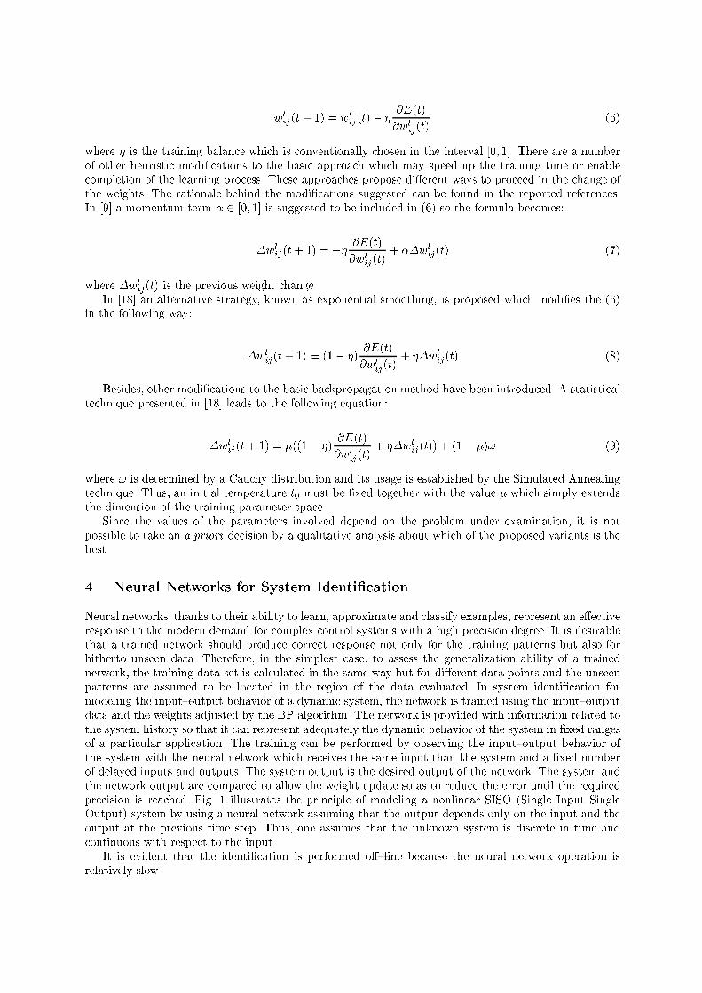
wlij(t+ 1) = wlij(t)� � @E(t)@wlij(t) (6)where � is the training balance which is conventionally chosen in the interval [0; 1]. There are a numberof other heuristic modi�cations to the basic approach which may speed up the training time or enablecompletion of the learning process. These approaches propose di�erent ways to proceed in the change ofthe weights. The rationale behind the modi�cations suggested can be found in the reported references.In [9] a momentum term � 2 [0; 1] is suggested to be included in (6) so the formula becomes:�wlij(t+ 1) = �� @E(t)@wlij(t) + ��wlij(t) (7)where �wlij(t) is the previous weight change.In [18] an alternative strategy, known as exponential smoothing, is proposed which modi�es the (6)in the following way: �wlij(t+ 1) = (1� �) @E(t)@wlij(t) + ��wlij(t) (8)Besides, other modi�cations to the basic backpropagation method have been introduced. A statisticaltechnique presented in [18] leads to the following equation:�wlij(t+ 1) = �((1� �) @E(t)@wlij(t) + ��wlij(t)) + (1� �)! (9)where ! is determined by a Cauchy distribution and its usage is established by the Simulated Annealingtechnique. Thus, an initial temperature t0 must be �xed together with the value � which simply extendsthe dimension of the training parameter space.Since the values of the parameters involved depend on the problem under examination, it is notpossible to take an a priori decision by a qualitative analysis about which of the proposed variants is thebest.4. Neural Networks for System Identi�cationNeural networks, thanks to their ability to learn, approximate and classify examples, represent an e�ectiveresponse to the modern demand for complex control systems with a high precision degree. It is desirablethat a trained network should produce correct response not only for the training patterns but also forhitherto unseen data. Therefore, in the simplest case, to assess the generalization ability of a trainednetwork, the training data set is calculated in the same way but for di�erent data points and the unseenpatterns are assumed to be located in the region of the data evaluated. In system identi�cation formodeling the input{output behavior of a dynamic system, the network is trained using the input{outputdata and the weights adjusted by the BP algorithm. The network is provided with information related tothe system history so that it can represent adequately the dynamic behavior of the system in �xed rangesof a particular application. The training can be performed by observing the input{output behavior ofthe system with the neural network which receives the same input than the system and a �xed numberof delayed inputs and outputs. The system output is the desired output of the network. The system andthe network output are compared to allow the weight update so as to reduce the error until the requiredprecision is reached. Fig. 1 illustrates the principle of modeling a nonlinear SISO (Single Input SingleOutput) system by using a neural network assuming that the output depends only on the input and theoutput at the previous time step. Thus, one assumes that the unknown system is discrete in time andcontinuous with respect to the input.It is evident that the identi�cation is performed o�{line because the neural network operation isrelatively slow.

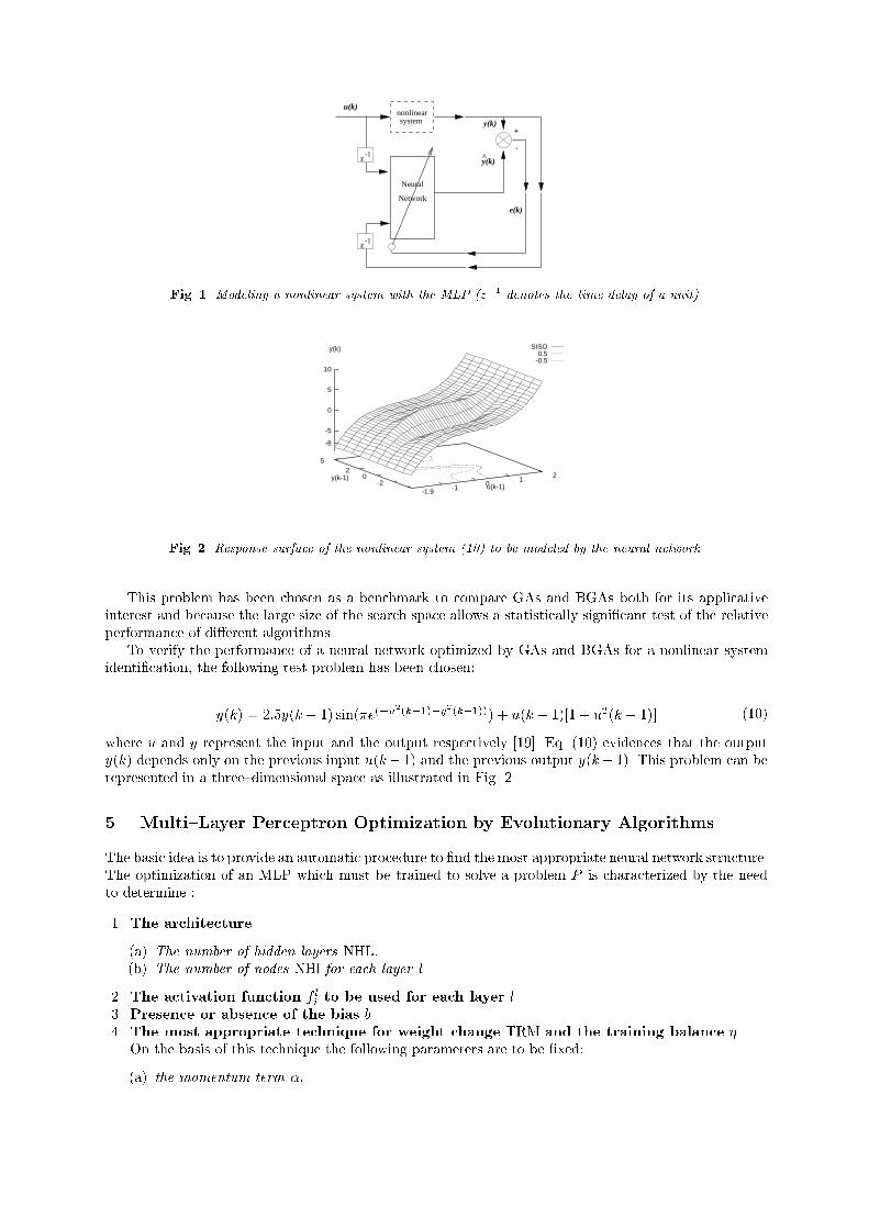
z-1

z-1

u(k)

y(k)+

-

y(k)

e(k)

^

system

Neural

Network

nonlinear

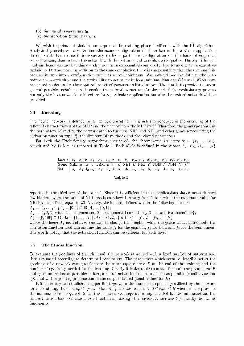
Fig. 1. Modeling a nonlinear system with the MLP (z�1 denotes the time delay of a unit).SISO

0.5 -0.5

-1.9 -10

12

-20

25

-8

-5

0

5

10

u(k-1)y(k-1)

y(k)

Fig. 2. Response surface of the nonlinear system (10) to be modeled by the neural network.This problem has been chosen as a benchmark to compare GAs and BGAs both for its applicativeinterest and because the large size of the search space allows a statistically signi�cant test of the relativeperformance of di�erent algorithms.To verify the performance of a neural network optimized by GAs and BGAs for a nonlinear systemidenti�cation, the following test problem has been chosen:y(k) = 2:5y(k � 1) sin(�e(�u2(k�1)�y2(k�1))) + u(k � 1)[1 + u2(k � 1)] (10)where u and y represent the input and the output respectively [19]. Eq. (10) evidences that the outputy(k) depends only on the previous input u(k� 1) and the previous output y(k� 1). This problem can berepresented in a three{dimensional space as illustrated in Fig. 2.5. Multi{Layer Perceptron Optimization by Evolutionary AlgorithmsThe basic idea is to provide an automatic procedure to �nd the most appropriate neural network structure.The optimization of an MLP which must be trained to solve a problem P is characterized by the needto determine :1. The architecture(a) The number of hidden layers NHL,(b) The number of nodes NHl for each layer l.2. The activation function f li to be used for each layer l.3. Presence or absence of the bias b.4. The most appropriate technique for weight change TRM and the training balance �.On the basis of this technique the following parameters are to be �xed:(a) the momentum term �,

(b) the initial temperature t0,(c) the statistical training term �.We wish to point out that in our approach the training phase is e�ected with the BP algorithm.Analytical procedures to determine the exact con�guration of these factors for a given applicationdo not exist. Each time it is necessary to �x a particular con�guration on the basis of empiricalconsiderations, then to train the network with the patterns and to evaluate its quality. The algorithmicalanalysis demonstrates that this search presents an exponential complexity if performed with an exaustivetechnique. Furthermore, in addition to the time complexity, there is the possibility that the training failsbecause it runs into a con�guration which is a local minimum. We have utilized heuristic methods toreduce the search time and the probability to get stuck in local minima. Namely, GAs and BGAs havebeen used to determine the appropriate set of parameters listed above. The aim is to provide the mostgeneral possible technique to determine the network structure. At the end of the evolutionary processnot only the best network architecture for a particular application but also the trained network will beprovided.5.1. EncodingThe neural network is de�ned by a \genetic encoding" in which the genotype is the encoding of thedi�erent characteristics of the MLP and the phenotype is the MLP itself. Therefore, the genotype containsthe parameters related to the network architecture, i.e. NHL and NHl, and other genes representing theactivation function type f li , the di�erent BP methods and the related parameters.For both the Evolutionary Algorithms considered, the chromosome structure x = (x1; : : : ; xn),constituted by 17 loci, is reported in Table 1. Each allele is de�ned in the subset Ai; i 2 f1; : : : ; 7gLocus x1 x2 x3 x4 x5 x6 x7 x8 x9 x10 x11 x12 x13 x14 x15 x16 x17Gene NHL � � b TRM � t0 f0i NH1 f1i NH2 f2i NH3 f3i NH4 f4i f5iSet A1 A2 A2 A3 A4 A2 A5 A7 A6 A7 A6 A7 A6 A7 A6 A7 A7Table 1.reported in the third row of the Table 1. Since it is su�cient in most applications that a network havefew hidden layers, the value of NHL has been allowed to vary from 1 to 4 while the maximum value forNHl has been �xed equal to 20. Namely, the loci are de�ned within the following subsets:A1 = f1; : : : ; 4g;A2 = [0; 1] � IR;A3 = f0; 1g;A4 = f1; 2; 3g with f1 � momentum; 2 � exponential smoothing; 3 � statistical techniqueg;A5 = [0; 100] � IR;A6 = f1; : : : ; 20g;A7 = f1; 2; 3g with f1 � f1; 2 � f2; 3 � f3gwhere the locus A4 individuates the way to change the weights, while the genes which individuate theactivation function used can assume the value f1 for the sigmoid, f2 for tanh and f3 for the semi{linear;it is worth noting that the activation function can be di�erent for each layer.5.2. The �tness functionTo evaluate the goodness of an individual, the network is trained with a �xed number of patterns andthen evaluated according to determined parameters. The parameters which seem to describe better thegoodness of a network con�guration are the mean square error E at the end of the training and thenumber of epochs ep needed for the learning. Clearly it is desirable to attain for both the parameters Eand ep values as low as possible: in fact, a neural network must learn as fast as possible (small values forep), and with a good approximation of the output desired (small values for E).It is necessary to establish an upper limit epmax to the number of epochs ep utilized by the networkfor the training, thus 0 < ep � epmax. Moreover, it is desirable that 0 � emin � E where emin representsthe minimum error required. Since the heuristic techniques are implemented for the minimization, the�tness function has been chosen as a function increasing when ep and E increase. Speci�cally the �tnessfunction is:

F(x) = epepmax +E (11)The choice of this �tness function is justi�ed as it takes into account both E and the learning speed ep,weighting these contributions in a dynamic manner. Note that emin is generally chosen equal to 10�awith a > 2.5.3. The optimization algorithm for the neural network structureLet MLP(xi) be the algorithm for training the MLP related to the individual xi representing a neuralnetwork con�guration. The general schema for the BGA is the following1:Given a pattern set P for the network training ;Procedure Breeder Genetic Algorithmbeginrandomly initialize a population of � neural network structures;while (termination criterion not ful�lled) dotrain xi by means of MLP(xi) on P ;evaluate the trained network xi;save the best trained network in the new population;select the best � neural network con�gurations;for i = 1 to �� 1 dorandomly select two structures among the �;recombine them so as to obtain one o�spring;perform mutation on the o�springodupdate variables for termination;odendThe procedure is constituted by an evolutionary algorithm, a BGA, and by a procedure for trainingthe MLP encapsulated in the main program. This procedure returns the values for the �tness evaluation.Its action is completely transparent to the main program which can only evaluate the goodness of theresult.6. Experimental resultsDue to the fact that the choice of the best selection method and genetic operators would require veryhigh execution times if preliminary tests were e�ected directly for the non linear system identi�cation,we have decided to use as benchmark a subset of the classical test functions known as F6, F7 and F8 [20].For the GA these experiments have been performed to establish the best selection method. Inparticular, the truncation selection has resulted to have better performance than that achieved by theproportional, the tournament and the exponential selections.For the BGA the objective of the tests has been to determine the best combination among mutationand recombination operators. The experimental results have proved that the discrete mutation incombination with the fuzzy recombination operator has led to the best performance. It has to be pointedout that the fuzzy recombination allows to obtain a reduction of about 40% in terms of the convergencetime with respect to the extended intermediate and the extended line recombination operators. Otherpreliminary tests for the MLP have been conducted by using as application the well{known \exclusiveOR" (XOR) function. This task is commonly considered an initial test to evaluate the network ability toclassify data.The GA has a population of 30 individuals and it utilizes the truncation selection with a 1{elitiststrategy. The percentage of the truncation is set equal to 30%. The algorithm has been executed 10times �xing as termination criteria epmax = 500 and emin = 10�8. A one-point crossover operator withprobability pc = 0:6 and a mutation operator with probability pm = 0:06 have been employed. The1 For the GA there are two o�spring so the cycle for is to be repeated ��12 times.

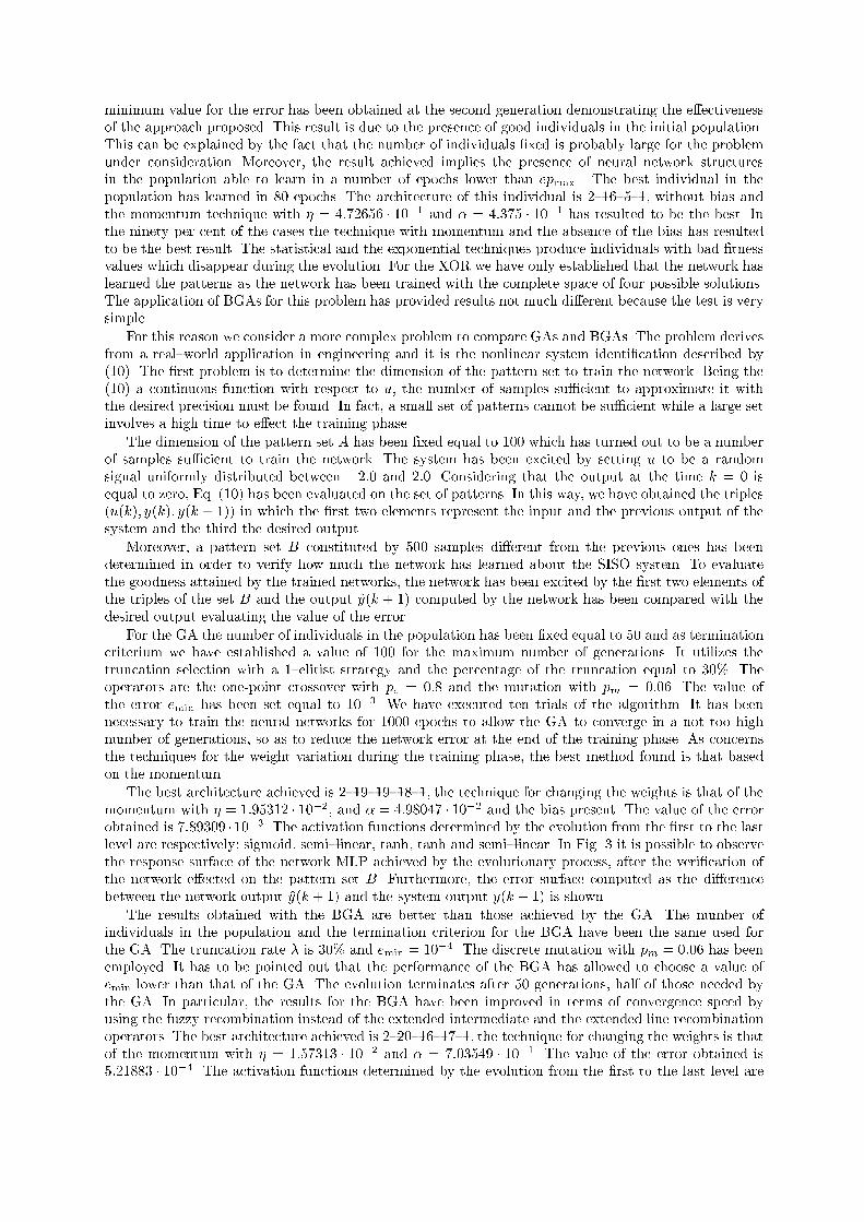
minimum value for the error has been obtained at the second generation demonstrating the e�ectivenessof the approach proposed. This result is due to the presence of good individuals in the initial population.This can be explained by the fact that the number of individuals �xed is probably large for the problemunder consideration. Moreover, the result achieved implies the presence of neural network structuresin the population able to learn in a number of epochs lower than epmax . The best individual in thepopulation has learned in 80 epochs. The architecture of this individual is 2{16{5{1, without bias andthe momentum technique with � = 4:72656 � 10�1 and � = 4:375 � 10�1 has resulted to be the best. Inthe ninety per cent of the cases the technique with momentum and the absence of the bias has resultedto be the best result. The statistical and the exponential techniques produce individuals with bad �tnessvalues which disappear during the evolution. For the XOR we have only established that the network haslearned the patterns as the network has been trained with the complete space of four possible solutions.The application of BGAs for this problem has provided results not much di�erent because the test is verysimple.For this reason we consider a more complex problem to compare GAs and BGAs. The problem derivesfrom a real{world application in engineering and it is the nonlinear system identi�cation described by(10). The �rst problem is to determine the dimension of the pattern set to train the network. Being the(10) a continuous function with respect to u, the number of samples su�cient to approximate it withthe desired precision must be found. In fact, a small set of patterns cannot be su�cient while a large setinvolves a high time to e�ect the training phase.The dimension of the pattern set A has been �xed equal to 100 which has turned out to be a numberof samples su�cient to train the network. The system has been excited by setting u to be a randomsignal uniformly distributed between �2:0 and 2:0. Considering that the output at the time k = 0 isequal to zero, Eq. (10) has been evaluated on the set of patterns. In this way, we have obtained the triples(u(k); y(k); y(k + 1)) in which the �rst two elements represent the input and the previous output of thesystem and the third the desired output.Moreover, a pattern set B constituted by 500 samples di�erent from the previous ones has beendetermined in order to verify how much the network has learned about the SISO system. To evaluatethe goodness attained by the trained networks, the network has been excited by the �rst two elements ofthe triples of the set B and the output y(k + 1) computed by the network has been compared with thedesired output evaluating the value of the error.For the GA the number of individuals in the population has been �xed equal to 50 and as terminationcriterium we have established a value of 100 for the maximum number of generations. It utilizes thetruncation selection with a 1{elitist strategy and the percentage of the truncation equal to 30%. Theoperators are the one-point crossover with pc = 0:8 and the mutation with pm = 0:06. The value ofthe error emin has been set equal to 10�3. We have executed ten trials of the algorithm. It has beennecessary to train the neural networks for 1000 epochs to allow the GA to converge in a not too highnumber of generations, so as to reduce the network error at the end of the training phase. As concernsthe techniques for the weight variation during the training phase, the best method found is that basedon the momentum.The best architecture achieved is 2{19{19{18{1, the technique for changing the weights is that of themomentum with � = 1:95312 � 10�2, and � = 4:98047 � 10�2 and the bias present. The value of the errorobtained is 7:89309 � 10�3. The activation functions determined by the evolution from the �rst to the lastlevel are respectively: sigmoid, semi{linear, tanh, tanh and semi{linear. In Fig. 3 it is possible to observethe response surface of the network MLP achieved by the evolutionary process, after the veri�cation ofthe network e�ected on the pattern set B. Furthermore, the error surface computed as the di�erencebetween the network output y(k + 1) and the system output y(k + 1) is shown.The results obtained with the BGA are better than those achieved by the GA. The number ofindividuals in the population and the termination criterion for the BGA have been the same used forthe GA. The truncation rate � is 30% and emin = 10�4. The discrete mutation with pm = 0:06 has beenemployed. It has to be pointed out that the performance of the BGA has allowed to choose a value ofemin lower than that of the GA. The evolution terminates after 50 generations, half of those needed bythe GA. In particular, the results for the BGA have been improved in terms of convergence speed byusing the fuzzy recombination instead of the extended intermediate and the extended line recombinationoperators. The best architecture achieved is 2{20{16{17{1, the technique for changing the weights is thatof the momentum with � = 1:57313 � 10�2 and � = 7:03549 � 10�1. The value of the error obtained is5:21883 � 10�4. The activation functions determined by the evolution from the �rst to the last level are

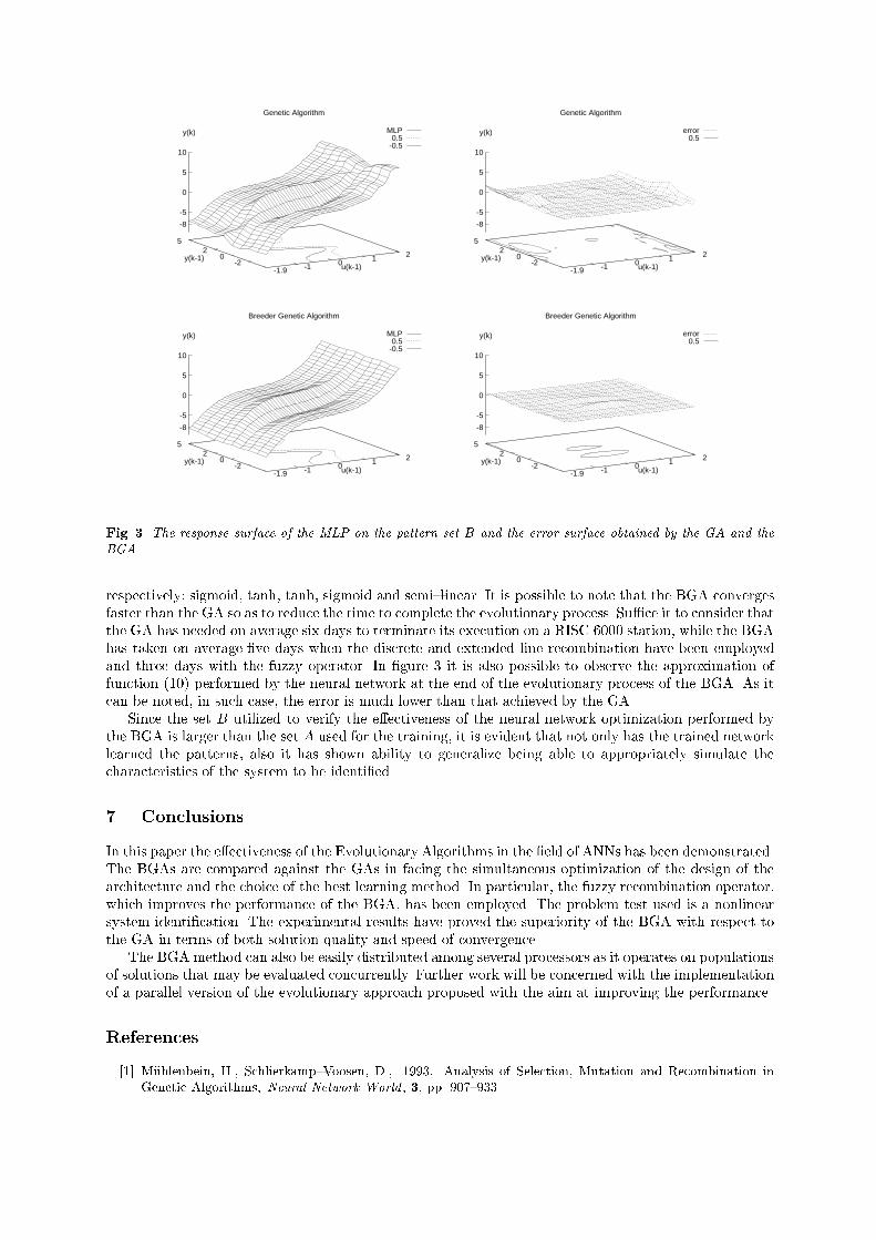
Genetic Algorithm

MLP 0.5 -0.5

-1.9 -1 0 1 2-2

02

5

-8

-5

0

5

10

u(k-1)y(k-1)

y(k)

Genetic Algorithm

error 0.5

-1.9 -1 0 1 2-2

02

5

-8

-5

0

5

10

u(k-1)y(k-1)

y(k)

Breeder Genetic Algorithm

MLP 0.5 -0.5

-1.9 -1 0 1 2-2

02

5

-8

-5

0

5

10

u(k-1)y(k-1)

y(k)

Breeder Genetic Algorithm

error 0.5

-1.9 -1 0 1 2-2

02

5

-8

-5

0

5

10

u(k-1)y(k-1)

y(k)

Fig. 3. The response surface of the MLP on the pattern set B and the error surface obtained by the GA and theBGA.respectively: sigmoid, tanh, tanh, sigmoid and semi{linear. It is possible to note that the BGA convergesfaster than the GA so as to reduce the time to complete the evolutionary process. Su�ce it to consider thatthe GA has needed on average six days to terminate its execution on a RISC 6000 station, while the BGAhas taken on average �ve days when the discrete and extended line recombination have been employedand three days with the fuzzy operator. In �gure 3 it is also possible to observe the approximation offunction (10) performed by the neural network at the end of the evolutionary process of the BGA. As itcan be noted, in such case, the error is much lower than that achieved by the GA.Since the set B utilized to verify the e�ectiveness of the neural network optimization performed bythe BGA is larger than the set A used for the training, it is evident that not only has the trained networklearned the patterns, also it has shown ability to generalize being able to appropriately simulate thecharacteristics of the system to be identi�ed.7. ConclusionsIn this paper the e�ectiveness of the Evolutionary Algorithms in the �eld of ANNs has been demonstrated.The BGAs are compared against the GAs in facing the simultaneous optimization of the design of thearchitecture and the choice of the best learning method. In particular, the fuzzy recombination operator,which improves the performance of the BGA, has been employed. The problem test used is a nonlinearsystem identi�cation. The experimental results have proved the superiority of the BGA with respect tothe GA in terms of both solution quality and speed of convergence.The BGA method can also be easily distributed among several processors as it operates on populationsof solutions that may be evaluated concurrently. Further work will be concerned with the implementationof a parallel version of the evolutionary approach proposed with the aim at improving the performance.References[1] M�uhlenbein, H., Schlierkamp{Voosen, D., 1993, Analysis of Selection, Mutation and Recombination inGenetic Algorithms, Neural Network World , 3, pp. 907{933.

[2] M�uhlenbein, H., Schlierkamp{Voosen, D., 1993, Predictive Models for the Breeder Genetic Algorithm I.Continuous parameter optimization, Evolutionary Computation, 1(1), pp. 25{49.[3] M�uhlenbein, H., Schlierkamp{Voosen, D., 1994, The Science of Breeding and its Application to the BreederGenetic Algorithm, Evolutionary Computation, 1, pp. 335{360.[4] B�ack, T., Ho�meister, F., Schwefel H.P., 1991, A survey of evolution strategies. Proceedings of the FourthInternational Conference on Genetic Algorithms, San Mateo CA, USA, Morgan Kau�mann, pp. 2{9.[5] Holland, J.H., 1975, Adaptation in Natural and Arti�cial Systems, University of Michigan Press, AnnArbor.[6] Goldberg, D. E., 1989, Genetic Algorithms in Search, Optimization and Machine Learning , Addison-Wesley, Reading, Massachussets.[7] Hertz, J., Krogh, A., Palmer, R.G., 1991, Introduction to the Theory of Neural Computation, Addison{Wesley Publishing.[8] Kuscu, I., Thornton, C., 1994, Designing Neural Networks using Genetic Algorithms: Review and Prospect,Cognitive and Computing Sciences, University of Sussex.[9] Rumelhart, D. E., Hinton, G. E., Williams, R. J, 1986, Learning Internal Representations by ErrorPropagation, Parallel Distributed Processing: Explorations in the Microstructure of Cognition, VIII, MITPress.[10] Rumelhart, D. E., McLelland, J. L., 1986, Parallel Distributed Processing, I-II, MIT Press.[11] Montana, D. J., Davis, L., 1989, Training Feedforward Neural Networks using Genetic Algorithms,Proceedings of the Eleventh International Joint Conference on Arti�cial Intelligence, pp. 762{767.[12] Hiestermann, J., 1990, Learning in Neural Nets by Genetic Algorithms, Parallel Processing in NeuralSystems and Computers, North{Holland, pp. 165{168.[13] Battiti, R., Tecchiolli, G., 1995, Training Neural Nets with Reactive Tabu Search, IEEE Trans. on NeuralNetworks, 6(5), pp. 1185{1200.[14] Whitley, D., Starkweather, T., Bogart, C., 1990, Genetic Algorithms and Neural Networks: OptimizingConnections and Connectivity, Parallel Computing , 14, pp. 347{361.[15] Reeves, C. R., Steele, N. C., 1992, Problem{solving by Simulated Genetic Processes: a Review andApplication to Neural Networks, Proceedings of the Tenth IASTED Symposium on Applied Informatics,pp. 269{272.[16] Stepniewski, S., Keane, A. J., Pruning back propagation Neural Networks using Modern StochasticOptimization Techniques, to appear in Neural Computing & Applications.[17] Voigt, H.M., M�uhlenbein, H., Cvetkovi�c, D., 1995, Fuzzy Recombination for the Continuous BreederGenetic Algorithm, Proceedings of the Sixth International Conference on Genetic Algorithms, MorganKau�mann.[18] Wassermann, P. D., 1989, Neural Computer Theory and Practice, Van Nostrand Reihnold, New York.[19] Yaw{Terng Su, Yuh-Tay Sheen, 1992, Neural Networks for System Identi�cation, Int. J. of Systems Sci.,23(12), pp. 2171{2186.[20] M�uhlenbein, H., Schomish, M., Born, J., 1991, The Parallel Genetic Algorithm as Function Optimizer,Parallel Computing , 17, pp. 619{632.