Range-limited Centrality Measures in Complex Networks

Maria Ercsey-Ravasz,1, 2, ∗ Ryan Lichtenwalter,2, 3 Nitesh V. Chawla,2, 3 and Zoltan Toroczkai2, 3, 4, †

1Faculty of Physics, Babes-Bolyai University, Str. Kogalniceanu Nr. 1, RO-400084 Cluj-Napoca, Romania2Interdisciplinary Center for Network Science and Applications (iCeNSA),

University of Notre Dame, Notre Dame, IN, 46556 USA3Department of Computer Science and Engineering,

University of Notre Dame, Notre Dame, IN, 46556 USA4Department of Physics, University of Notre Dame, Notre Dame, IN, 46556 USA

(Dated: November 24, 2011)

Here we present a range-limited approach to centrality measures in both non-weighted andweighted directed complex networks. We introduce an efficient method that generates for ev-ery node and every edge its betweenness centrality based on shortest paths of lengths not longerthan ` = 1, . . . , L in case of non-weighted networks, and for weighted networks the correspond-ing quantities based on minimum weight paths with path weights not larger than w` = `∆,` = 1, 2 . . . , L = R/∆. These measures provide a systematic description on the positioning im-portance of a node (edge) with respect to its network neighborhoods 1-step out, 2-steps out, etc. upto including the whole network. They are more informative than traditional centrality measures, asnetwork transport typically happens on all length-scales, from transport to nearest neighbors to thefarthest reaches of the network. We show that range-limited centralities obey universal scaling lawsfor large non-weighted networks. As the computation of traditional centrality measures is costly,this scaling behavior can be exploited to efficiently estimate centralities of nodes and edges for allranges, including the traditional ones. The scaling behavior can also be exploited to show that theranking top-list of nodes (edges) based on their range-limited centralities quickly freezes as functionof the range, and hence the diameter-range top-list can be efficiently predicted. We also show howto estimate the typical largest node-to-node distance for a network of N nodes, exploiting the afore-mentioned scaling behavior. These observations are illustrated on model networks and on a largesocial network inferred from cell-phone trace logs (∼ 5.5 × 106 nodes and ∼ 2.7 × 107 edges). Fi-nally, we apply these concepts to efficiently detect the vulnerability backbone of a network (definedas the smallest percolating cluster of the highest betweenness nodes and edges) and illustrate theimportance of weight-based centrality measures in weighted networks in detecting such backbones.

PACS numbers: 89.75.Hc, 89.65.-s, 02.10.Ox

I. INTRODUCTION

Network research [1–5] has experienced an explosivegrowth in the last two decades, as it has proven itselfto be an informative and useful methodology to studycomplex systems, ranging from social sciences throughbiology to communication infrastructures. Both the nat-ural and man made world is abundant with networkedstructures that transport various entities, such as infor-mation, forces, energy, material goods, etc. As many ofthese networks are the result of evolutionary processes,it is important to understand how the graph structure ofthese systems determines their transport performance,structural stability and behavior as a whole. A ratheruseful concept in addressing such questions is the no-tion of centrality, which describes the positioning “im-portance” of a structure of interest such as a node, edgeor subgraph with respect to the whole network. Althoughthe notion of centrality in graph theory dates back to themathematician Camille Jordan (1869), centrality mea-

∗Electronic address: mercseyr@nd.edu†Electronic address: toro@nd.edu

sures were expanded, refined and applied to a great ex-tent for the first time in social sciences [6–10], and todaythey play a fundamental role in studies involving a largevariety of complex networks across many fields. Probablythe most frequently used centrality measure is between-ness centrality (BC) [10–16], introduced by Anthonisse[11] and Freeman [12] defined as the fraction of all net-work geodesics (shortest paths) passing through a node(edge or subgraph). Since transport tends to minimizethe cost/time of the route from source to destination, itexpectedly happens along geodesics, and therefore cen-trality measures are typically defined as a function ofthese, however generalizations to arbitrary distributionsof transport paths have also been introduced and studied[17, 18]. Geodesics are important for structural connec-tivity as well: removing nodes (edges) with high BC, oneobtains a rapid increase in diameter, and eventually thestructural breakup of the graph.

In general, centrality measures are defined in the con-text of the assumptions (sometimes made implicitly) re-garding the type of network flow [16]. These are as-sumptions regarding the nature of the paths such as be-ing shortest, or arbitrary length paths, weighted/valuedpaths, walks (repeated nodes and edges) [19] etc.; andthe nature of the flow, such as transport of indivisible

arX

iv:1

111.

5382

v1 [

phys

ics.

soc-

ph]

23

Nov

201

1

2

units (packets), or spreading/broadcasting processes (in-fection, information). Besides betweenness centrality,many other centrality measures have been introduced[10], depending on the context in which network flowsare considered; for a partial compilation see the paperby Brandes [14], here we only review a limited list. Inparticular, stress centrality [20–22], simply counts thenumber of all-pair shortest paths passing through a node(edge) without taking into account the degeneracy of thegeodesics (there can be several geodesics running betweenthe same pair of nodes). Closeness centrality [8, 13, 23]and its variants are simple functions of the mean geodesicdistance (hop-count) of a node from all other nodes. Loadcentrality [14, 24, 25] is generated by the total amount ofload passing through a node when unit commodities arepassed between all source-destination pairs using an algo-rithm in which the commodity packet is equally dividedamongst the neighbors of a node that are at the samegeodesic distance from the destination. Group betwee-ness centrality [26, 27] computes the betweenness associ-ated with a set of nodes restricted to all-pair geodesicsthat traverse at least one of the nodes in the group. Egonetwork betweenness [28] is a local betweenness measurecomputed only from the immediate neighborhood of anode (ego). Eigenvector centrality [29, 30] represents apositive score associated to a node, proportional to thesum of the scores of the node’s neighbors, solved consis-tently across the graph. The corresponding score vectoris the eigenvector associated with the largest eigenvalueof the adjacency matrix. Random walk centrality [31, 32]is a measure of the accessibility of a node via randomwalks in the network. Other centrality measures includeinformation centrality of Stephenson and Zelen [33]; andinduced endogenous and exogenous centrality by Everettand Borgatti [34].

Bounded-distance betweenness was introduced by Bor-gatti and Everett [10] as betweenness centrality result-ing from all-pair shortest paths not longer than a givenlength (hop-count). It is this measure that we expandand investigate in detail in the present paper. A con-densed version for unweighted networks has been pre-sented in Ref. [35]. Since we are also generalizing themeasure and the corresponding algorithm to weighted(valued) networks, we are referring to it as range-limitedcentrality. Note that range-limitation can be imposed onall centrality measures that depend on paths, and there-fore the analysis and algorithm presented here can beextended to all these centrality measures.

Centrality measures have received numerous applica-tions in several areas. In social sciences they have beenextensively used to quantify the position of individualswith respect to the rest of the network in various so-cial network data sets [6, 16]. In physics and computerscience they have seen widespread applications relatedto routing algorithms in packet switched communicationnetworks and transport problems in general [17, 24, 36–41]. The connection of generalized betweenness central-ity based on arbitrary path distributions (not just short-

est) to routing that minimizes congestion has been in-vestigated by Sreenivasan et al [17] using minimum spar-sity vertex separators. This makes a direct connectionto max-flow min-cut theorems of multicommodity flows,extensively studied in the computer science literature[42, 43]. Other works that use essentially edge between-ness type quantities to quantify congestion in Internet-like graphs include Refs [44, 45]. Dall’Asta et.al. connectnode and edge detection probabilities in traceroute-basedsampling of networks to their betweenness centrality val-ues [46, 47]. Other applications include detection of net-work vulnerabilities in face of attacks [48], cascading fail-ures [49–51] or epidemics [52], all involving betweenness-related calculations.

An important extension of centrality is to weighted,or valued networks [25, 53–57]. In this case the edges(and also the nodes) carry an associated weight, whichmay represent a measure of social relationship in socialnetworks [58], channel capacity in the case of communi-cation networks, transport capacity (e.g., nr of lanes) inroadway networks or seats on flights [59].

From a theory point of view, there have been fewerresults, as producing analytic expressions for centralitiesin networks is difficult in general. However, for scale-freetrees, Szabo et.al. [60] developed a mean-field approachfor computing node betweenness, which later was maderigorous by Bollobas and Riordan [61]. Fekete et.al. pro-vide a calculation of the distribution of edge betweenesson scale-free trees conditional on node in-degrees [62],and Kitsak et.al. [63] have derived scaling results on be-tweenness centrality for fractal and non-fractal scale-freenetworks.

Unfortunately, computation of betweenness can becostly (O(NM), where N is the number of nodes andM is the number of edges, thus O(N3) worst case)[14, 25, 54, 64–66], especially for large networks with mil-lions of nodes, hence approximation methods are needed.Existing approximations [32, 67, 68], however, are sam-pling based, and not well controlled. Additionally, trans-port in real networks does not occur with uniform prob-ability between arbitrary pairs of nodes, as transport in-curs a cost, and therefore shorter-range transport is ex-pectedly more frequent than long-range. Accordingly,the usage of network paths is non-uniform, which shouldbe taken into account if we want to connect centralityproperties with real transport. In order to address someof the limitations of existing centrality measures, we re-cently focused on range-limited centrality [35]. We haveshown that when geodesics are restricted to a maximumlength L, the corresponding range-limited L-betweennessfor large graphs assumes a characteristic scaling form asfunction of L. This scaling can then be used to pre-dict the betweenness distribution in the (difficult to at-tain) diameter limit, and with good approximation, topredict the ranking of nodes/edges by betweenness, sav-ing considerable computational costs. Additionally, therange-limited method generates l-betweenness values forall nodes and edges and for all 1 ≤ l ≤ L, providing

3

(1,1,37/30)!

(0,1,8/15)!

!

G1

!

G3

!

G2

!

G0

i !"

!"

!"

!"

#"

#"

!" $"

%"

#"

(3,3,3)!

[1,1,37/30]!

(1,3/2,16/15)!

[0,1/2,16/30]!(0,1,16/15)! (0,0,1)!

[0,0,2/5]!

(0,0,1)!

(0,0,1)!

j k

p m n

(1,1/2,7/10)!

(0,1,7/5)!

(a) (b)

i j

k n p m

FIG. 1: a) Consecutive shells of the C3 subgraph of node i (black) are colored red, blue, green. Grey elements are not part ofthe subgraph. b) The (x, y, z) near a node j are the b`(i|j) values for ` = 1, ` = 2 and ` = 3. The [x, y, z] on an edge (j, k)give the b`(i|j, k) values for ` = 1, ` = 2 and ` = 3 . Given a node j, the number inside its circle is the total number of shortestpaths σij to j from i. Colors indicate quantities based on ` = 1 (red), ` = 2 (blue), and ` = 3 (green).

systematic information on geodesics on all length-scales.

In this paper we give a detailed derivation of the al-gorithm and the analytical approximations presented in[35] and we demonstrate the efficiency of the method ona social network (SocNet) inferred from mobile phonetrace-logs [69]. This network has a giant cluster withN = 5, 568, 785 nodes and M = 26, 822, 764 directededges. The diameter of the underlying undirected net-work is approximately D ' 26 and the calculation ofthe traditional (diameter-range based) BC values (usingBrandes’ algorithm) on this network took 5 days on 562computers.

In addition, we present the derivations for an algo-rithm that efficiently computes range-limited centralitieson weighted networks. We then apply these concepts andalgorithms to the network vulnerability backbone detec-tion problem, and show the differences between the back-bones obtained with both hop-count based centralitiesand weighted centralities.

The paper is organized as follows. Section II intro-duces the notations and provides the algorithm for un-weighted graphs; section III gives an analytical treatmentthat derives the existence of a scaling behavior for cen-trality measures in large graphs; it gives a method on howto estimate the largest typical node-to-node distance (alower-bound to the diameter); discusses the complexityof the algorithm and the fast freezing phenomenon ofranking by betweenness of nodes and edges. Section IVillustrates the power of the range-limited approach (byshowing how well can one predict betwenness centrali-ties and ranking of individual nodes and edges) using thesocial-network data described above. Section V describesthe algorithm for weighted graphs and section VI uses the

range-limited betwenness measure to define a vulnerabil-ity backbone for networks and illustrates the differencesin identification of the backbone obtained with and with-out weights on the links.

II. RANGE-LIMITED CENTRALITY FORNON-WEIGHTED GRAPHS

A. Definitions and notations

Let us consider a directed simple graph G(V,E), whichconsists of a set V of vertices (or nodes) and a setE ⊆ V ×V of directed edges (or links). We will denote by(vi, vj) ∈ E an edge directed from node vi ∈ V to nodevj ∈ V . The graph has N nodes and M ≤ N(N − 1)edges. The algorithm below can easily be modified forundirected graphs, we will not treat that case separately.A directed path ωmn from some node m to a node nis defined as an ordered sequence of nodes and linksωmn = {m, (m, v1), v1, (v1, v2), v2, ....vl, (vl, n), n} with-out repeated nodes. The “distance” d(m,n) is the lengthof the shortest directed path going from node m to noden. We give a definition of distance (path weight) forweighted networks in Section V. In non-weighted net-works the directed path length is simply the number ofedges (“hop-count”) along the directed path from m ton. There can be multiple shortest paths (same length),and we will denote by σmn the total number of shortestdirected paths from node m to n. σmn(i) will representthe number of shortest paths from node m to node ngoing through node i. As convention we set

σmn(m) = σmn(n) = σmn, σmm(i) = δi,m . (1)

4

The total number of all-pair shortest paths runningthrough a node i is called the stress centrality (SC) ofnode i, S(i) =

∑m,n∈V σmn(i). Betweenness central-

ity (BC) [10–12, 14, 54] normalizes the number of pathsthrough a node by the total number of paths (σmn) fora given source-destination pair (m,n):

B(i) =∑

m,n∈V

σmn(i)

σmn. (2)

Similar quantities can be defined for an edge (j, k) ∈ E:

B(j, k) =∑

m,n∈V

σmn(j, k)

σmn. (3)

In order to define range-limited betweenness centrali-ties, let bl(j) denote the BC of a node j for all-pair short-est directed paths of fixed, exact length l. Then

BL(j) =

L∑l=1

bl(j) (4)

represents the betweenness centrality obtained frompaths not longer than L. For edges, we introduce bl(j, k)and BL(j, k) using the same definitions. For simplicity,here we include the start- and end-points of the pathsin the centrality measures, however, our algorithm caneasily be changed to exclude them, as described later.

Similar to other algorithms, our method first calculatesthese BCs for a node j (or edge (j, k)) from shortest di-rected paths all emanating from a “root” node i, then itsums the obtained values for all i ∈ V to get the finalcentralities for node j (or edge (j, k)). This can be donebecause the set of all shortest paths can be uniquely de-composed into subsets of shortest paths distinguished bytheir starting node. Thus it makes sense to perform ashell decomposition of the graph around a root node i.Let us denote by CL(i) the L-range subgraph of node icontaining all nodes which can be reached in at most Lsteps from i (Fig. 1a). Only links which are part of theshortest paths starting from the root i to these nodes areincluded in CL. We decompose CL into shells Gl(i) con-taining all the nodes at shortest path distance l from theroot, and all incoming edges from shell l − 1, Fig. 1b).The root i itself is considered to be shell 0 (G0(i) = {i}).Let

brl (i|k) =∑

n∈Gl(i)

σin(k)

σin, brl (i|j, k) =

∑n∈Gl(i)

σin(j, k)

σin(5)

denote the fixed-l betweenness centrality of node k, andedge (j, k), respectively, based only on shortest pathsall starting from the root i. Here r is not an indepen-dent variable: given i and k (or (j, k)), r is the radius ofshell Gr(i) containing k (or (j, k)), that is k ∈ Gr(i) and(j, k) ∈ Gr(i). Note that σin(k) = 0 (or σin(j, k) = 0) ifk (or (j, k)) do not belong to at least one shortest pathfrom i to n, and thus there is no contribution from those

points n from the l-th shell. The condition for k (or (j, k))to belong to at least one shortest path from i to n can al-ternatively be written in the case of (5) as d(k, n) = l− ra notation, which we will use later.

For simplicity of writing, we refer to the fixed-l be-tweenness centralities (the bl-s) as “l-BCs” and to thecumulative betweenness centralities (the BL-s obtainedfrom summing the l-BCs, see (4)) as [L]-BCs.

B. The range-limited betweenness centralityalgorithm

While the basics of our algorithm are similar to Bran-des’ [14, 54], we derive recursions that simultaneouslycompute the [l]-BCs for all nodes and all edges and forall values l = 1, . . . , L. The algorithm thus generates de-tailed and systematic information (an L-component vec-tor for every node and every edge) about shortest pathson all length-scales and thus, providing a tool for multi-scale network analysis.

First we give the algorithm, then we derive the specificrecursions used in it. For the root node i we set theinitial condition: σii = 1. For other nodes, k 6= i, weset σik = 0. The following steps are repeated for everyl = 1, . . . , L:

1. Build Gl(i), using breadth-first search.

2. Calculate σik for all nodes k ∈ Gl(i), using:

σik =∑

j∈Gl−1(i)

(j,k)∈Gl(i)

σij , (6)

and set

bll(i|k) = 1. (7)

3. Proceeding backwards, through r = l − 1, . . . , 1, 0:

a) Calculate the l-BCs of links (j, k) ∈ Gr+1(i)(thus j ∈ Gr(i), k ∈ Gr+1(i)) recursively:

br+1l (i|j, k) = br+1

l (i|k)σijσik

, (8)

b) and of nodes j ∈ Gr(i) using (8) and:

brl (i|j) =∑

k∈Gr+1(i)

(j,k)∈Gr+1(i)

br+1l (i|j, k) . (9)

4. Finally, return to step 1) until the last shell GL(i)is reached.

In the end, the cumulative [l]-BCs, that is the Bl-s canbe calculated using (4). Fig. 1 shows a concrete exam-ple. The subgraph of node i has three layers. Each layerGl(i) and the corresponding l-BCs are marked with dif-ferent colors: l = 1 (red), l = 2 (blue), and l = 3 (green).

5

As described above, the first step creates the next layerGl(i), then in step 2., for every node k ∈ Gl(i) we cal-culate the total number of shortest paths σik from theroot to node k. These are indicated by numbers withinthe circles representing the nodes in Fig. 1 (e.g., σij = 1,σik = 2, σin = 5). As given by (6), σik is calculated bysumming the number of shortest paths that end in thepredecessors of node k located in Gl−1(i). For examplenode p ∈ G3(i) in Fig. 1 is connected to nodes k and min shell G2(i), and thus: σip = σik + σim = 2 + 1 = 3.

Eq. (7) states that the l-BC of nodes located in Gl(i)is always 1. This follows from Eq. (5) for r = l and usingthe convention σik(k) = σik. Knowing these values, weproceed backwards (step 3.) and calculate the l-BCs ofall edges and nodes in all the previous layers. Recursion(8) is obtained from a well known recursion for shortestpaths. If k (or (j, k)) belongs to at least one shortest pathgoing from i to n, then σin(k) = σikσkn and σin(j, k) =σijσkn. Inserting these in Eq. (5) for r 7→ r+1 we obtain:

br+1l (i|k) = σik

∑n∈Gl(i)

d(k,n)=l−r−1

σknσin

(10)

br+1l (i|j, k) = σij

∑n∈Gl(i)

d(k,n)=l−r−1

σknσin

(11)

where d(k, n) = l − r − 1 expresses the condition thatthe sum is restricted to those n from Gl(i), which haveat least one shortest path (from i), going through k or(j, k). Dividing these equations we obtain (8). For e.g.,in Fig 1: b33(i|k, n) = b33(i|n)σik/σin = 1× (2/5) = 2/5.

Having determined the l-BCs of all edges in layerGr+1(i), we can now compute the l-BC of a given node inGr(i) by summing the l-BCs of its outgoing links, that isusing (9) (e.g., on Fig 1: b23(i|k) = b33(i|k, p)+b33(i|k, n) =(2/3) + (2/5) = 16/15).

This algorithm can be easily modified to compute othercentrality measures. For example, to compute all therange-limited stress centralities, we have to replace Eq.(7) with: sll(i|j) = σij . All other recursions will haveexactly the same form, we just need to replace the l-BCs(brl (i|j), brl (i|j, k)) with the l-SCs (srl (i|j), srl (i|j, k)).

If we want to exclude start- and end-points when com-puting BCs or SCs, we first let the above algorithm finish,then we do the following steps: a) set the l-BC of the rootnode i to 0, b0l (i|i) = 0 for all l = 1, . . . , L, and b) for ev-ery node k ∈ Gl(i) reset bll(i|k) = 0, for all l = 1, . . . , L,(for e.g., on Fig 1 k is in the second shell, G2(i), so its 2-BC will become 0 instead of 1). Then via (4), the [l]-BCsand the corresponding [l]-SCs are easily obtained.

III. CENTRALITY SCALING - ANALYTICALAPPROXIMATIONS

In [35] we have shown that the [l]-BC obeys a scal-ing behavior as function of l. This was found to hold

for all sufficiently large random networks that we stud-ied (Erdos-Renyi (ER), Barabasi-Albert (BA) scale-free,Random Geometric Graphs (RGG), etc.) including thesocial network inferred from mobile phone trace-log data(SocNet) [70]. Here we detail the analytical argumentsthat indeed show that the existence of this scaling be-havior for large networks is a general property, by ex-ploiting the scaling of shell sizes. The scaling of shellsizes was already studied previously, for e.g., in randomgraphs with arbitrary degree distributions [71, 72]. Forsimplicity of the notations, we only show the derivationsfor undirected graphs.

A. Betweenness of individual nodes

Let us define 〈·〉 as an average over all root nodes i inthe graph, and denote by zl(i) the number of nodes onshell Gl(i). We define the branching factor as:

αl = 〈zl+1〉/〈zl〉 , (12)

and model the growth of shell sizes as a branching process

zl+1(i) = zl(i)αl[1 + εl(i)

]. (13)

Here εl(i) is a per-node, shell occupancy noise term, en-coding the relative deviations, or fluctuations from the (i-independent) functional form of αl. Typically, |εl| � 1,it obeys 〈εl(i)〉 = 0 and 〈εl(i)εm(j)〉 = 2Alδl,mδi,j , withAl decreasing with l. In undirected graphs if i ∈ Gm(j)then it implies that j ∈ Gm(i), and vice-versa. Hence, inthis case:

bl+1(j) =1

2

∑i∈V

bl+1(i|j) =1

2

l+1∑m=0

∑i∈Gm(j)

bml+1(i|j) (14)

The 1/2 factor comes from the fact that any given pathwill be included twice in the sum (once in both direc-tions). In case of m = 0 the only node in G0(j) is jitself, and the inner sum is equal with b0l+1(j|j). Dueto convention (1) σjn(j) = σjn and hence from (5) weobtain b0l+1(j|j) =

∑n∈Gl+1(j)

σjn(j)/σjn = zl+1(j). For

m = l + 1, bl+1l+1(i|j) = 1 (see Eq. (7)) and the inner sum

is again zl+1(j). Thus we can write:

bl+1(j) = zl+1(j) +1

2

l∑m=1

∑i∈Gm(j)

bml+1(i|j) ≡

≡ zl+1(j) +1

2ul+1(j), (15)

Note that the number of terms in the inner sum∑i∈Gm(j) b

ml+1(i|j) is zm(j), which is rapidly increasing

with m, and thus is expected to have a weak dependenceon j. Accordingly, we make the approximation:

ul+1(j) 'l∑

m=1

∑i∈Gm(j)

vml+1(i), (16)

6

where we replaced bml+1(i|j) by vml+1(i), which is an av-erage (l + 1)-BC computed over the shell of radius m,centered on node i :

vml+1(i) =

∑k∈Gm(i) b

ml+1(i|k)

zm(i). (17)

However, the sum of (l + 1)-BCs in any m ≤ l + 1layer is equal with the number of nodes in shell Gl+1:∑k∈Gm(i) b

ml+1(i|k) = zl+1(i). We can convince ourselves

about this last statement by using (5) and observingthat

∑k∈Gm(i) σin(k) = σin as all paths from i to n

(n ∈ Gl+1(i)) must “pierce” every shell m ≤ l + 1 inbetween. Fig. 1 shows an example: there are 3 nodes inG3 and the sum of 3-betweenness values (green) in layerG2 is (7/5) + (16/15) + (8/15) = 3. Therefore, we maywrite:

vml+1(i) ' zl+1(i)

zm(i)=zl(i)αl

[1 + εl(i)

]zm(i)

, (18)

where we used the recursion defined above for zl+1(i) as abranching process (13). Inserting this in (16) we obtain:

ul+1(j) ' αll∑

m=1

∑i∈Gm(j)

zl(i)[1 + εl(i)

]zm(i)

'

' αl

l∑m=1

∑i∈Gm(j)

zl(i)

zm(i)'

' αl

zl(j) +

l−1∑m=1

∑i∈Gm(j)

zl(i)

zm(i)

(19)

where we neglected the small noise term due to the largenumber of terms in the inner sum, and we used the factthat for m = l the leading term of the inner sum is justzl(j). From Eqs. (16) and (18), however, the double sumin (19) equals ul(j) and we obtain the following recursion:

ul+1(j) ' αl[zl(j) + ul(j)

]. (20)

Eqs (13), (15) and (20) lead to a recursion for bl+1(j):

bl+1(j) ' αl[bl(j) + zl(j)/2 + zl(j)εl(j)], (21)

which can be iterated down to l = 1, where b1(j) =z1(j) = kj is the degree of j:

bl(j) ' βl kj eξl(j) , (22)

with

βl =l + 1

2

l−1∏m=1

αm =l + 1

2

〈zl〉〈k〉

, (23)

ξl(j) =

l−1∑n=1

l + 1− nl + 1

εn(j) . (24)

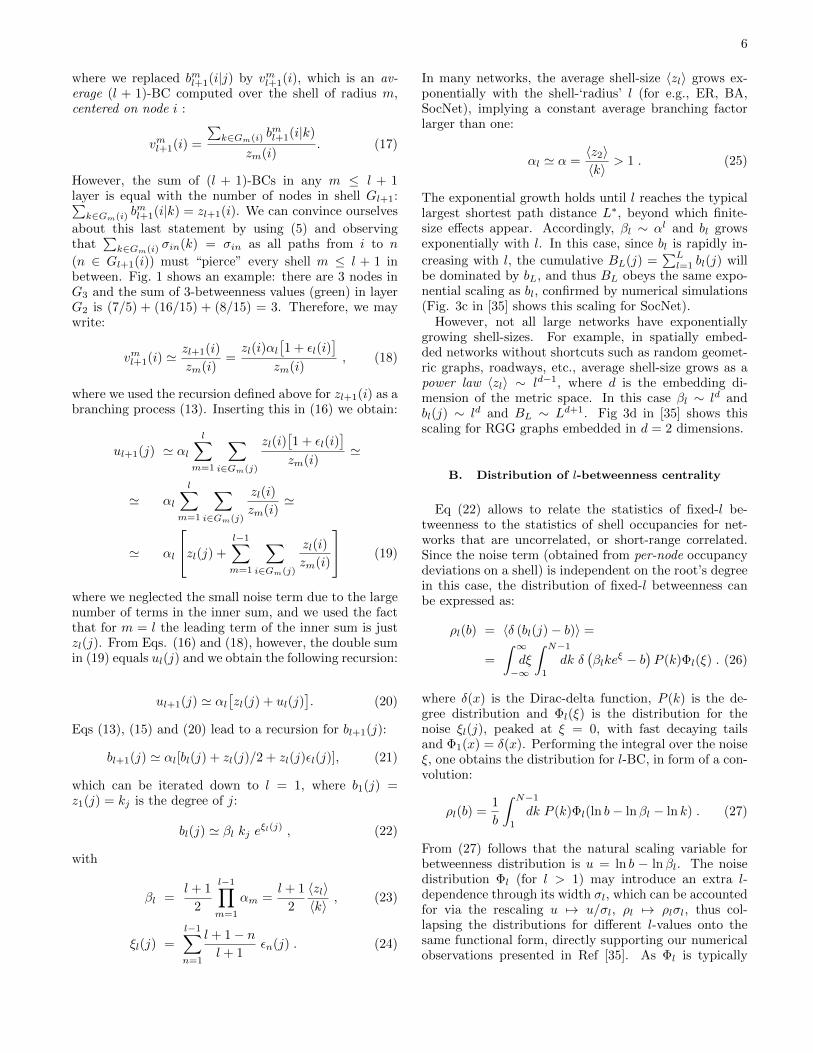
In many networks, the average shell-size 〈zl〉 grows ex-ponentially with the shell-‘radius’ l (for e.g., ER, BA,SocNet), implying a constant average branching factorlarger than one:

αl ' α =〈z2〉〈k〉

> 1 . (25)

The exponential growth holds until l reaches the typicallargest shortest path distance L∗, beyond which finite-size effects appear. Accordingly, βl ∼ αl and bl growsexponentially with l. In this case, since bl is rapidly in-

creasing with l, the cumulative BL(j) =∑Ll=1 bl(j) will

be dominated by bL, and thus BL obeys the same expo-nential scaling as bl, confirmed by numerical simulations(Fig. 3c in [35] shows this scaling for SocNet).

However, not all large networks have exponentiallygrowing shell-sizes. For example, in spatially embed-ded networks without shortcuts such as random geomet-ric graphs, roadways, etc., average shell-size grows as apower law 〈zl〉 ∼ ld−1, where d is the embedding di-mension of the metric space. In this case βl ∼ ld andbl(j) ∼ ld and BL ∼ Ld+1. Fig 3d in [35] shows thisscaling for RGG graphs embedded in d = 2 dimensions.

B. Distribution of l-betweenness centrality

Eq (22) allows to relate the statistics of fixed-l be-tweenness to the statistics of shell occupancies for net-works that are uncorrelated, or short-range correlated.Since the noise term (obtained from per-node occupancydeviations on a shell) is independent on the root’s degreein this case, the distribution of fixed-l betweenness canbe expressed as:

ρl(b) = 〈δ (bl(j)− b)〉 =

=

∫ ∞−∞dξ

∫ N−1

1

dk δ(βlke

ξ − b)P (k)Φl(ξ) . (26)

where δ(x) is the Dirac-delta function, P (k) is the de-gree distribution and Φl(ξ) is the distribution for thenoise ξl(j), peaked at ξ = 0, with fast decaying tailsand Φ1(x) = δ(x). Performing the integral over the noiseξ, one obtains the distribution for l-BC, in form of a con-volution:

ρl(b) =1

b

∫ N−1

1

dk P (k)Φl(ln b− lnβl − ln k) . (27)

From (27) follows that the natural scaling variable forbetweenness distribution is u = ln b − lnβl. The noisedistribution Φl (for l > 1) may introduce an extra l-dependence through its width σl, which can be accountedfor via the rescaling u 7→ u/σl, ρl 7→ ρlσl, thus col-lapsing the distributions for different l-values onto thesame functional form, directly supporting our numericalobservations presented in Ref [35]. As Φl is typically

7

sharply peaked around 0, the most significant contribu-tion to the integral (27) for a given b comes from degreesk ' b/βl. Since k ≥ 1, we have a rapid decay of ρl(b) inthe range b < βl, a maximum at b = βlk where k is thedegree at which P (k) is maximum, and a sharp decay forb > (N − 1)βl.

C. Estimating the average node-to-node distancein large networks.

The scaling law on its own does not provide infor-mation about the typical largest node-to-node distance,which is always a manifestation of the finiteness of thegraph. However, knowing the size of the network in termsof the number of nodes N , one can exploit our formulasto find the average largest node-to-node distance as theradius L∗ of the typical largest shell beyond which finite-size effects become strong, that is where network edgeeffects appear. This can be estimated as the point wherethe sum of the average shell sizes reaches N . Hence:

ZL∗ =

L∗∑l=1

〈zl〉 =

L∗∑l=1

2

l + 1〈k〉βl = N , (28)

providing an implicit equation for L∗. The βl-s are de-termined numerically for l = 1, 2, 3, . . . and a correspond-ing functional form fitting its scaling with l can be ex-trapolated for larger l values up to L∗, when the sumin (28) hits N . For our social network data one obtainsL∗ ' 9.35 (Fig. 2). Here L∗ is not necessarily an inte-ger, because it is obtained from the scaling behavior ofthe average shell sizes, and represents the typical radiusof the largest shell. Expression (28) can be easily spe-

0 1 2 3 4 5 6 7 8 9 10l

1

1e+2

1e+4

1e+6

Zl

N=5,568,785

L*~9.35

FIG. 2: In the SocNet the sum, Zl, of the average shell sizesgrows exponentially as function of l. Extrapolating, we canpredict that it reaches the N = 5, 568, 785 mark at L∗ ' 9.35.

cialized for the two classes of networks discussed abovenamely, for those having exponential average shell-sizegrowth 〈zl〉 ∼ 〈k〉αl−1 and for those having a power-lawaverage shell-size growth as 〈zl〉 ∼ 〈k〉ld−1. For the ex-

ponential growth case we obtain:

L∗ =1

lnαln

(1 +

α− 1

〈k〉N

), (29)

resulting in the L∗ ∼ lnN behavior for large N .For the power-law growth case there is no easily invert-

ible expression for the sum, however, if we replace thesummation with an integral, we find the approximate

L∗ '(

1 +d

〈k〉N

)1/d

(30)

expression, with the expected asymptotic behavior L∗ ∼N1/d as N →∞.

D. Algorithm complexity

We are now in position to estimate the average-casecomplexity of the range-limited centrality algorithm. Forevery root i, we sequentially build its l = 1, 2, ..., L shells.When going from shell Gl−1(i) to building shell Gl(i), weconsider all the zl−1 nodes on Gl−1(i). For every suchnode j we add all its links that do not connect to alreadytagged nodes (a tag labels a node that belongs to Gl−1(i)or Gl−2(i)) to Gl(i), and add the corresponding nodes aswell. This requires on the order of 〈k〉 operations forevery node j, hence on the order of 〈k〉〈zl−1〉 operationsfor creating shell Gl(i). Next is Eq (6), which involves〈el〉 steps, where el is the number of edges connectingnodes in shell Gl−1(i) to nodes in shell Gl(i). Eq (7)involves 〈zl〉 steps. Eqs (8) and (9) generate a total of

2∑lm=1〈em〉 operations. Hence, for a given l there are a

total of 〈k〉〈zl−1〉+〈el〉+〈zl〉+2∑lm=1〈em〉 operations on

average. Thus the average complexity of the algorithm Ccan be estimated as:

C ∼ NL∑l=1

(〈k〉〈zl−1〉+ 〈el〉+ 〈zl〉+ 2

l∑m=1

〈em〉

)(31)

Note that the set of edges in the shells Gm−1(i) andGm(i) are all fanning out from nodes in Gm−1(i), andthus we can approximate 〈em−1〉+ 〈em〉 with 〈k〉〈zm−1〉.Thus, the estimate becomes:

C ∼ N〈k〉L∑l=1

l∑m=1

〈zm〉 = N〈k〉L∑l=1

(L− l + 1)〈zl〉 (32)

From (32) it follows that

N〈k〉L∑l=1

〈zl〉 < C < LN〈k〉L∑l=1

〈zl〉 . (33)

For fixed L, the complexity grows linearly with N as N →∞. For L = L∗ we can use (28) to conclude that

O(NM) < C < O(L∗NM) (34)

8

where M = N〈k〉/2 denotes the total number of edgesin the network. Recall that the Brandes or Newman al-gorithm has a complexity of O(NM) for obtaining thetraditional betweenness centralities. Specializing the ex-pression (32) to networks with exponentially growingshells one finds the same O(NM) complexity (that is theupper bound O(NM lnM) in (34) is not realized); fornetworks with power-law growth shells, however, we findO(N1+1/dM), as in the upper bound of (34). The extracomputational cost is due to the fact that instead of a sin-gle value, our algorithm produces a set of L numbers (thel-BCs), providing multiscale information on betweennesscentrality for all nodes and all edges in the network.

E. Freezing of ranking by range-limitedbetweenness

In Ref [35] we have provided numerical evidence thatthe ranking of the nodes (same holds for edges) by their[L]-BC values freezes at relatively small values of L. Herewe show how this freezing phenomenon emerges. Con-sider two arbitrary nodes i and j, with degrees ki and kj .Using Eq (22) we can write

lnbl(j)

bl(i)= ln

kjki

+ ξl(j)− ξl(i) = lnkjki

+ ∆l . (35)

Based on (24):

∆l = ξl(j)− ξl(i) =

l−1∑n=1

l + 1− nl + 1

Xn (36)

where Xn = εn(j) − εn(i). By definition, εn(j) isthe per node variation of shell-occupancy from its root-independent value, for the n-th shell centered on rootnode j. Expectedly, for larger shells (larger n), the sizeof the shells becomes less dependent on the local graphstructure surrounding the root node, and for this reasonthis noise term has a decaying magnitude |εn(j)| withn. Thus, the Xn can be considered as random variablescentered around zero, with a magnitude that is decay-ing with increasing n. The contributions of the noiseterms coming from larger radius shells in the sum (36)is decreasing not only because the corresponding Xn-sare decreasing in absolute value, but also because theirweight in the sum is decreasing (as 1/(l+ 1)), and there-fore when moving from l to l+ 1 in (36) the change (thefluctuation) in ∆l decreases for larger l. This effectivelymeans that the rhs of (35) saturates, and thus, accord-ingly, the lhs saturates as well, freezing the ordering ofbetweenness values. If the two nodes have largely differ-ent degrees (ln kj/ki is relatively large), the noise term∆l will not be able to change the sign on the rhs of (35),even for small l values, and thus, the ordering betweennodes with very different degrees will freeze the fastest,followed by nodes with degrees that are close to eachother. Clearly, the freezing of ordering between nodes

with identical degrees (kj = ki) will happen last. Theprobability for the ordering to flip when increasing therange from l to l+1 can be calculated for specific networkmodels, however, it will not be discussed here.

IV. RANGE-LIMITED CENTRALITIES IN ALARGE-SCALE SOCIAL NETWORK

In this section we illustrate the power of the range-limited approach on a real-world social network inferredfrom cell-phone call-logs (SocNet). We show that com-puting the [L]-BCs up to a relatively small limit lengthcan already be used to predict the full, diameter-basedbetweenness centralities of individual nodes (and edges),their distribution and the top list of nodes with highestcentralities.

This social network was constructed from 708 millionanonymized phone-calls between 7.2 million callers gen-erated in a period of 65 days. Restricting ourselves topairs of individuals between which phone-calls have beenobserved in both directions in this period as a definitionof an edge, we found that the giant component of this net-work has about 5.5 million nodes and 27 million edges.The 65 days is long enough to guarantee that individualswith strong social bonds have called each other at leastonce during this interval, and therefore will be linked byan edge in our graph.

To test and validate our predictions using the range-limited method, we actually performed the computationof the full, diameter-based betweenness centralities of allthe nodes in SocNet. To deploy the computation, weused a distributed computing utility called Work Queue,developed in the Cooperative Computing Lab at NotreDame. The utility consists of a single management serverthat sends tasks out to a collection of heterogeneousworkers/processors. Specifically, our workers consistedof 250 Sun Grid Engine cores, 300 Condor cores, and 12local workstation cores, for a total of 562 cores. This al-lowed us to finish thousands of days of computation inthe course of 5 days. Each worker received a request tocompute the contribution of shortest paths starting from50 vertices to the betweenness centrality of every vertexin the network, summed the 50 results, and sent themback to the management server. Each time the man-agement server received a contribution, it summed thecontribution with all the others and provided another 50vertices for the worker.

We also determined the network diameter from thedata using a similar distributed computing method, ob-taining D = 26. At first sight this value seems to beat odds with the famous six-degrees of separation phe-nomenon, which implies a much smaller diameter. How-ever, there are two observations that one can make here.1) The social network has a dense core with protrudingbranches (“tentacles”), which mathematically speaking,can generate a large diameter. However, the experimen-tally determined six degrees of separation does not probe

9

all the branches, it actually relies on the denser core forinformation flow. Hence it should be rather similar tothe average node-to-node distance, rather than the rig-orously defined network diameter. Indeed, the value ofL∗ = 9.35 that we obtained is rather close to the six-degrees observation. 2) The social network constructedbased on cell-phone communications gives only a sam-ple subgraph of the true social network, where commu-nications happen also face-to-face and through land-linephone calls. Hence, one would likely measure an evensmaller L∗ would such data be available.

A. Predicting betweenness centralities ofindividual nodes

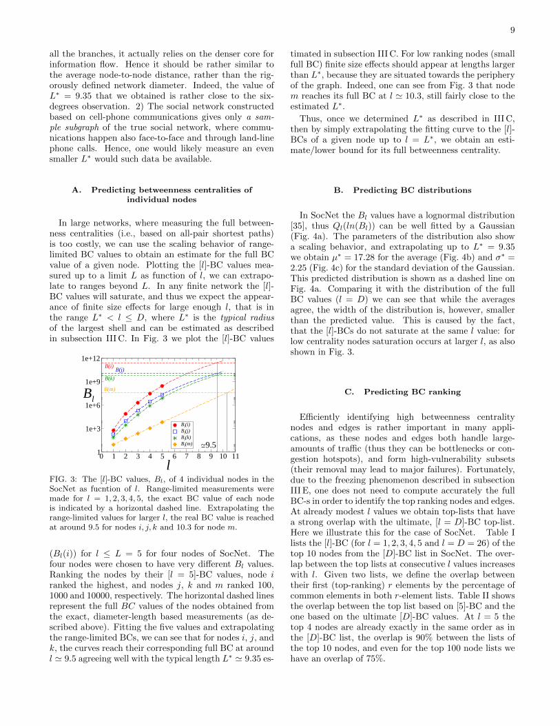
In large networks, where measuring the full between-ness centralities (i.e., based on all-pair shortest paths)is too costly, we can use the scaling behavior of range-limited BC values to obtain an estimate for the full BCvalue of a given node. Plotting the [l]-BC values mea-sured up to a limit L as function of l, we can extrapo-late to ranges beyond L. In any finite network the [l]-BC values will saturate, and thus we expect the appear-ance of finite size effects for large enough l, that is inthe range L∗ < l ≤ D, where L∗ is the typical radiusof the largest shell and can be estimated as describedin subsection III C. In Fig. 3 we plot the [l]-BC values

0 1 2 3 4 5 6 7 8 9 10 11l

1

1e+3

1e+6

1e+9

1e+12

Bl

Bl(i)Bl(j)Bl(k)Bl(m) ~9.5

B(i) B(j)B(k)

B(m)

FIG. 3: The [l]-BC values, Bl, of 4 individual nodes in theSocNet as fucntion of l. Range-limited measurements weremade for l = 1, 2, 3, 4, 5, the exact BC value of each nodeis indicated by a horizontal dashed line. Extrapolating therange-limited values for larger l, the real BC value is reachedat around 9.5 for nodes i, j, k and 10.3 for node m.

(Bl(i)) for l ≤ L = 5 for four nodes of SocNet. Thefour nodes were chosen to have very different Bl values.Ranking the nodes by their [l = 5]-BC values, node iranked the highest, and nodes j, k and m ranked 100,1000 and 10000, respectively. The horizontal dashed linesrepresent the full BC values of the nodes obtained fromthe exact, diameter-length based measurements (as de-scribed above). Fitting the five values and extrapolatingthe range-limited BCs, we can see that for nodes i, j, andk, the curves reach their corresponding full BC at aroundl ' 9.5 agreeing well with the typical length L∗ ' 9.35 es-

timated in subsection III C. For low ranking nodes (smallfull BC) finite size effects should appear at lengths largerthan L∗, because they are situated towards the peripheryof the graph. Indeed, one can see from Fig. 3 that nodem reaches its full BC at l ' 10.3, still fairly close to theestimated L∗.

Thus, once we determined L∗ as described in III C,then by simply extrapolating the fitting curve to the [l]-BCs of a given node up to l = L∗, we obtain an esti-mate/lower bound for its full betweenness centrality.

B. Predicting BC distributions

In SocNet the Bl values have a lognormal distribution[35], thus Ql(ln(Bl)) can be well fitted by a Gaussian(Fig. 4a). The parameters of the distribution also showa scaling behavior, and extrapolating up to L∗ = 9.35we obtain µ∗ = 17.28 for the average (Fig. 4b) and σ∗ =2.25 (Fig. 4c) for the standard deviation of the Gaussian.This predicted distribution is shown as a dashed line onFig. 4a. Comparing it with the distribution of the fullBC values (l = D) we can see that while the averagesagree, the width of the distribution is, however, smallerthan the predicted value. This is caused by the fact,that the [l]-BCs do not saturate at the same l value: forlow centrality nodes saturation occurs at larger l, as alsoshown in Fig. 3.

C. Predicting BC ranking

Efficiently identifying high betweenness centralitynodes and edges is rather important in many appli-cations, as these nodes and edges both handle large-amounts of traffic (thus they can be bottlenecks or con-gestion hotspots), and form high-vulnerability subsets(their removal may lead to major failures). Fortunately,due to the freezing phenomenon described in subsectionIII E, one does not need to compute accurately the fullBC-s in order to identify the top ranking nodes and edges.At already modest l values we obtain top-lists that havea strong overlap with the ultimate, [l = D]-BC top-list.Here we illustrate this for the case of SocNet. Table Ilists the [l]-BC (for l = 1, 2, 3, 4, 5 and l = D = 26) of thetop 10 nodes from the [D]-BC list in SocNet. The over-lap between the top lists at consecutive l values increaseswith l. Given two lists, we define the overlap betweentheir first (top-ranking) r elements by the percentage ofcommon elements in both r-element lists. Table II showsthe overlap between the top list based on [5]-BC and theone based on the ultimate [D]-BC values. At l = 5 thetop 4 nodes are already exactly in the same order as inthe [D]-BC list, the overlap is 90% between the lists ofthe top 10 nodes, and even for the top 100 node lists wehave an overlap of 75%.

10

Vertex B1 B2 B3 B4 B5 BD

1 600 7.76× 104 2.06× 106 3.01× 107 2.87× 108 1.26× 1011

2 715 9.71× 104 2.22× 106 3.05× 107 2.85× 108 1.25× 1011

3 458 5.04× 104 1.26× 106 1.87× 107 1.86× 108 9.82× 1010

4 377 3.11× 104 8.56× 105 1.31× 107 1.29× 108 5.82× 1010

5 337 2.29× 104 5.04× 105 7.23× 106 7.55× 107 5.34× 1010

6 285 1.93× 104 5.03× 105 7.56× 106 7.85× 107 5.07× 1010

7 488 2.82× 104 5.84× 105 7.94× 106 7.96× 107 4.89× 1010

8 299 2.56× 104 6.91× 105 1.09× 107 1.10× 108 4.88× 1010

9 244 1.47× 104 3.44× 105 4.87× 106 4.83× 107 4.87× 1010

10 239 1.64× 104 4.57× 105 7.48× 106 8.06× 107 4.81× 1010

TABLE I: Bl values of the top 10 nodes in the [D]-BC top-list for SocNet, for l = 1, 2, 3, 4, 5, D, where D = 26 is the diameter.

0 5 10 15 20 25ln(Bl)

0

0.1

0.2

0.3

0.4

0.5

Ql

l=1l=2l=3l=4l=5l=L*l=D

1 2 3 4 5 6 7 8 9 10l

0

5

10

15

20

µ

L*

µ!=17.28

1 2 3 4 5 6 7 8 9 10l

1

1.5

2

2.5

!

L*

!"=2.25

(a)

(b)

(c)

FIG. 4: a) Distribution Ql of the ln(Bl) values in the SocNetfor l = 1, 2, 3, 4, 5, D, where D = 26 is the diameter, and thepredicted distribution for L∗. The distributions can be fittedwith a Gaussian. b)The average µ and c) standard deviationσ as function of l. Extrapolating to L∗ = 9.35 we obtainµ∗ = 17.28 and σ∗ = 2.25.

Top x nodes Overlap (%)1 1002 1003 1004 10010 9050 72100 75500 70.21000 67.1

TABLE II: Overlap between the lists of the top r nodes withhighest [5]-BC and with the highest [D]-BC values.

V. RANGE-LIMITED CENTRALITY INWEIGHTED GRAPHS

In unweighted graphs the length of the shortest pathbetween two nodes is defined as the number of edges in-cluded in the shortest path. In weighted networks eachedge has a weight or “length”: wij . Depending on the na-ture of the network this length can be an actual physicaldistance (e.g., in road networks), or a cost or a resistancevalue. We define the “shortest” (or lowest-weight) pathbetween nodes i and j as the network path along whichthe sum of the weights of the edges included is mini-mal. We will call this sum as the “shortest distance”d(i, j) from node i to node j (note that we allow for di-rected links, which implies that d(i, j) is not necessarilythe same as d(j, i)).

In order to define a range-limited quantity, let bl(j)denote the (fixed) l-BC of node j from all-pair short-est directed paths of length Wl−1 < d ≤ Wl, whereW1 < W2 < · · · < WL are a series of predefined weightvalues or “distances”. The simplest way to define theseWl distances is to take them uniformly Wl = l∆w, how-ever depending on the application these may be redefinedin any suitable way. BL will again denote the cumulativeL-betweenness, which represents centralities from pathsnot longer than WL. Note that we are still countingpaths when computing centralities, that is σmn(i) stillmeans the number of shortest paths from m to n passingthrough i, except for the meaning of “shortest”, which is

11

now generalized to lowest-cost.The algorithm is similar to the one presented above for

unweighted networks. We again build the subgraph of anode i, but now a shell Gl(i) will contain all the nodesk at shortest path distance Wl−1 < d(i, k) ≤ Wl fromthe root node i. An edge j → k is considered to be partof the layer in which node k is included. In unweightedgraphs a connection j → k can be part of the subgraphonly if the two nodes are in two consecutive layers: ifj ∈ Gr(i) then k ∈ Gr+1(i). In weighted networks thesituation is different (Fig. 5a)). In principle we may haveedges connecting nodes which are not in two consecutivelayers, but possibly further away from each other ( thelinks i→ n, j → o in Fig. 5a)), or even in the same layer(the link m→ n in the same figure).

When building the subgraph using breadth-first search,we need to save the exact order in which the nodesand edges are discovered and included in the subgraph(Fig. 5b,c). Let us denote with v(p) the index of thenode which is included at position p in this node’s list(Fig. 5b). This means that the following conditions hold:d(i, v(1)) ≤ d(i, v(2)) ≤ d(i, v(3)) ≤ . . . . Similarly wehave a list of edges, where qx(p) → qy(p) is the edge inposition p of the list, and qx, qy denote the indexes of thetwo nodes connected by the edge (Fig. 5c). This impliesthe conditions: d(i, qy(1)) ≤ d(i, qy(2)) ≤ d(i, qy(3)) ≤. . . (note that every edge qx(p) → qy(p) is included inthe edge-list when node qy(p) is discovered). Again, wecalculate brl (i|k) for a node k, and brl (i|j, k) for an edgej → k. As defined above, these values take into ac-count only the shortest paths starting from node i, andr denotes the shell containing the corresponding node oredge. One uses the same initial conditions σii = 1, andσik = 0 for all k 6= i, as before.

The algorithm has the following main steps. For everyl = 1, . . . , L:

1) We build the next layer Gl(i) using breadth firstsearch. During this search we build the list of indexesv, qx, qy as defined above. We denote the total numberof nodes included in the list (from all shells G1(i) up toGl(i)) as Nl and the number of edges included as Ml.During this breadth-first search we also calculate the σikof the discovered nodes. Every time a new edge j → k isadded to the list we update σik by adding to it σij (usingalgorithmic notation, σik := σik + σij). Recall that σikdenotes the total number of shortest paths from i to k. Ifthe edge j → k is included in the subgraph (meaning thatit is part of a shortest path) the number of shortest pathsending in j has to be added to the number of shortestpaths ending in k.

2) The l-betweenness of all nodes included in the newlayer is set to bll(i|k) = 1, similarly to Eq. (7).

3) Going backwards through the list of edges we cal-culate the fixed-l BC of all nodes and edges. For p =Ml, . . . , 1, we perform the following recursions:

a) for the edge qx(p)→ qy(p):

brl (i|qx(p), qy(p)) = brl (i|qy(p))σiqx(p)

σiqy(p)(37)

!

G1

!

G3

!

G2

!

G0

i !"

!"

!"

#"

!"

$"

j

k

m

n

%&'"

%&$"!"

!"%&("

)"%&*"

)&!"

+#,#"+),)"+!,!"

o

(a)

(b) p v(p) b1 b2 b3

1 i 2 2 1 2 j 1 4/3 1/2 3 k 1 1/3 1/4 4 m 0 4/3 1/4 5 n 0 1 3/4 6 o 0 0 1

p qx(p)!qy(p) � b1 b2 b3

1 i ! j 1 4/3 1/2 2 i ! k 1 1/3 1/4 3 j ! m 0 4/3 1/4 4 i ! n 0 1/3 1/4 5 k ! n 0 1/3 1/4 6 m ! n 0 1/3 1/4 7 j ! o 0 0 1/4 8 n ! o 0 0 3/4

(c)

W1=1 W2=2 W3=3

FIG. 5: a) Shells of the C3 subgraph of node i (black) arecolored red, blue, green. Distances defining the shells are:W1 = 1, W2 = 2, W3 = 3. The weight or length is shownnext to each edge. Given a node j, the number inside itscircle is the total number of shortest paths coming from theroot i: σij . b) The list of nodes v(p) and c) list of edgesqx(p) → qy(p) are shown together with their 1-, 2-, and 3-betweenness values.

b) immediately after the BC of an edge is calculated, thebetweenness of node qx(p) must also be updated. Wehave to add to its previous value the l-BC of the edgeqx(p)→ qy(p):

brl (i|qx(p)) = brl (i|qx(p)) + brl (i|qx(p), qy(p)) (38)

4) We return to step 1) until the last shell GL(i) isreached.

As we have seen, the algorithm and the recursions arevery similar to the one presented for unweighted graphs.The crucial difference is that the exact order of the dis-covered nodes and edges has to be saved, because the BCvalues of edges and nodes in a shell cannot be updated inan arbitrary order. As an example, Fig. 5 shows a smallsubgraph and the list of nodes and edges together withtheir 1-, 2- and 3-betweenness values.

VI. VULNERABILITY BACKBONE

An important problem in network research is identify-ing the most vulnerable parts of a network. Here wedefine the vulnerability backbone (VB) of a graph asthe smallest fraction of the highest betweenness nodes

12

!"#$ %&'(

$

'&)(

$

)&*(

$

*&+,($

+,&+-(

$

+.&,+(

$

+-&+.(

$

,/&,0(

$

,+&,/(

$

,0&'%(

$

'%&+%%($

l=1

l=5

l=45

l=2

l=15

l=

D=

195

FIG. 6: The vulnerability backbone VB of a random geo-metric graph in the unit square with N = 5000, 〈k〉 = 5and D = 195. The top 30% of nodes are colored from redto yellow according to their [l]-BC ranking (see color bar).The VB based on the [l]-BC is shown for different values:l = 1, 2, 5, 15, 45, 195.

forming a percolating cluster through the network. Re-moving simultaneously all elements of this backbone willefficiently shatter the network into many disconnectedpieces. Although the shattering performance can be im-proved by sequentially removing and recomputing thetop-ranking nodes [48], here we focus only on the simulta-neous removal of the one-time computed VB of a graph,the generalization being straightforward.

Next we illustrate that range-limited BCs can be usedto efficiently detect this backbone by performing calcu-lations up to a length much smaller than the diameter.This is of course expected in networks that have a smalldiameter (D = O(lnN) or smaller), however, it is lessobvious for networks with large diameter (D = O(Nα),α > 0). For this reason, in the following we consider ran-dom geometric (RG) graphs [73, 74] in the plane. The

graphs are obtained by sprinkling at random N pointsinto the unit square and connecting all pairs of pointsthat are found within a given distance R of each other.We will use the average degree 〈k〉 = NπR2 [74] in-stead of R to parametrize the graphs. In Fig. 6 wepresent measurements on a random geometric graph withN = 5000 nodes, average degree 〈k〉 = 5. The hop-count diameter of this graph is D = 195. The weightsof connections are considered to be the physical (Eu-clidean) distances. Clearly, since the links of the graphare built based on a rule involving the Euclidean dis-tances, the weight structure and the topology of thegraph should be tightly correlated. Thus, we do expectstrong correlations between the [l]-BC values measuredboth from the unweighted and the weighted graph. Theweight ranges Wl defining the layers during the algorithmwere chosen as Wl = 0.00725l, l = 1, . . . , D, so thatWD = 0.00725D = 1.413 is close to the diagonal lengthof the unit square

√2. The nodes and connections are

colored according to their [l] − BC ranking for differentl values (see the color bar in Fig 6). The backbone is al-ready clearly formed at l = 45. Fig. 7 compares the VBs

weighted unweighted <k

>=5

<k>=

10

FIG. 7: Vulnerability backbones based on full BC rankingsin two random geometric graphs with N = 5000 nodes, andaverage degrees 〈k〉 = 5 and 〈k〉 = 10, respectively. Therankings were calculated both on the unweighted graph (leftcolumn) and weighted one (right column).

of the graphs obtained with and without considering theconnection weights (distances). Two RGs with densities〈k〉 = 5 and 〈k〉 = 10 are presented. In the case of thedenser graph the backbone is concentrated towards thecenter of unit square, as periphery effects in this case arestronger (we do not use periodic boundary conditions).Although qualitatively the two VBs are similar, the VBis sharper and clearer in the weighted case. There can

13

!"#$%&'"$()

*+,-!"#$)

.-+/)

01$2+"3)

4#25#'&6$)

72$$/)

892&/:72$$/)

72$$/;$""'<)

;$""'<)

=+/3$"&'/)

>2+/:$)

?$3>2+/:$)

?$3)

!2&@A?$3)

B)

CBB)

DBBBB)

E$(<

$$//$66)

-­‐1.5  

1.5  

0  

(a) (b) k = 5 k =10

FIG. 8: Comparison between the rankings obtained with andwithout considering the weights of connections for the twoRG graphs in Fig. 7. Colors indicate the ln(rnw/rw) val-ues, where rnw is the rank of a node obtained using thenon-weighted algorithm and rw is obtained with the weightedgraph (see the color bar). In denser graphs the differencesbecome more significant.

be actually significant differences between the two back-bones, in spite the fact that one would expect a strongoverlap. In Fig. 8 we show these differences by color-ing the nodes of the two graphs from Fig 7 according tothe ln(rnw/rw) values, where rnw is the rank of a nodeobtained using the non-weighted algorithm and rw is ob-tained using the weighted graph. The nodes are coloredfrom blue to red, blue corresponding to the case whenthe unweighted algorithm strongly underestimates theweighted ranking of a node and red is used when it over-estimates it. Although it is of no surprise that weightedand unweighted backbones differ in networks where thegraph topology and the weights are weakly correlated,the fact that there are considerable differences also forthe strongly correlated case of random geometric graphs(the blue and red colored parts in the right panel of Fig8) is rather unexpected, underlining the importance ofusing weigh-based centrality measures in weighted net-works.

VII. CONCLUSIONS

In this paper we have introduced a systematic ap-proach to network centrality measures decomposed bygraph distances for both unweighted and weighted di-rected networks. There are several advantages to suchrange-based decompositions. First, they provide muchfiner grained information on the positioning importanceof a node (or edge) with respect to the network, than thetraditional (diameter-based) centrality measures. Tradi-tional centrality values are dominated by the large num-

ber of long-distance network paths, even though most ofthese paths might not actually be used frequently by thetransport processes occurring on the network. Due tothe fast growth of the number of paths with distance inlarge complex networks, one expects that the distribu-tion of the centrality measures (which incorporate thesepaths) to obey scaling laws as the range is increased.We have shown both numerically and via analytic ar-guments (identifying the scaling form) that this is in-deed the case, for unweighted networks; for the samereasons, however, we expect the existence of scaling lawsfor weighted networks as well. We have shown that thesescaling laws can be used to predict or estimate efficientlyseveral quantities of interest, that are otherwise costlyto compute on large networks. In particular, the largesttypical node-to-node distance L∗, the traditional indi-vidual node and edge centralities (diameter range) andthe ranking of nodes and edges by their centrality val-ues. The latter is made possible by the existence of thephenomenon of fast freezing of the rank ordering by dis-tance, which we demonstrated both numerically and viaanalytic arguments. We have also introduced efficient al-gorithms for range-limited centrality measures for bothunweighted and weighted networks. Although they havebeen presented for betweenness centrality, they can bemodified to obtain all the other centrality measure vari-ants. Finally, we presented an application of these con-cepts in identifying the vulnerability backbone of a net-work, and have shown that it can be identified efficientlyusing range-limited betweenness centralities. We havealso illustrated the importance of taking into accountlink-weights [75] when computing centralities, even innetworks where graph topology and weights are stronglycorrelated.

Acknowledgments

This work was supported in part by NSF BCS-0826958,HDTRA 1-09-1-0039 and by the Army Research Labora-tory under Cooperative Agreement Number W911NF-09-2-0053 and MER in part by PN-II-RU-TE-2011-3-0121.The views and conclusions contained in this documentare those of the authors and should not be interpretedas representing the official policies, either expressed orimplied, of the Army Research Laboratory or the U.S.Government. The U.S. Government is authorized to re-produce and distribute reprints for Government purposesnotwithstanding any copyright notation here on.

[1] R. Cohen and S. Havlin, Complex Networks: Structure,Robustness and Function (Cambridge Univ. Press, 2010).

[2] M. Newman, Networks: An Introduction (Oxford Uni-versity Press, USA, 2010).

[3] A. Barrat and A. Vespignani, Dynamical Processes on

Complex Networks (Cambridge Univ. Press, 2008).[4] S. Boccaletti, V. Latora, Y. Moreno, M. Chavez, and D.-

U. Hwang, Phys. Rep. 424, 175 (2006).[5] E. Ben-Naim, F. Frauenfelder, and Z. Toroczkai, eds.,

Complex Networks, Lecture Notes in Physics (Springer-

14

Verlag, Berlin, 2004).[6] S. Wasserman and K. Faust, Social Network Analysis:

methods and applications (Cambridge Univ. Press, 1994).[7] J. Scott, Social Network Analysis: A Handbook (Sage

Publications, 1991).[8] G. Sabidussi, Psychometrika 31, 581 (1966).[9] N. E. Friedkin, Amer. J. of Soc. 96, 1478 (1991).

[10] S. P. Borgatti and M. G. Everett, Social Networks 28,466 (2006).

[11] J. M. Anthonisse, Tech. Rep. BN 9/71, Stichting Math.Centr., Amsterdam (1971).

[12] L. C. Freeman, Sociometry 40, 35 (1977).[13] L. C. Freeman, Soc. Netw. 1, 215 (1979).[14] U. Brandes, Soc. Netw. 30, 136 (2008).[15] D. White and S. Borgatti, Soc. Netw. 16, 335 (1994).[16] S. Borgatti, Soc. Networks 27, 55 (2005).[17] S. Sreenivasan, R. Cohen, E. Lopez, Z. Toroczkai, and

H. E. Stanley, Phys.Rev.E 75, 036105 (2007).[18] S. Dolev, Y. Elovici, and R. Puzis, J. ACM 57 (2010).[19] B. Bollobas, Modern Graph Theory, Graduate Texts in

Mathematics (Springer-Verlag, New York, Berlin Heidel-berg, 1991).

[20] A. Shimbel, Bulletin of Math. Biophys. 15, 501 (1953).[21] A. Perer and B. Shneiderman, IEEE Trans. on Visual-

ization and Computer Graphics 12, 693 (2006).[22] S. Lammer, B. Gehlsen, and D. Helbing, Phys. A - Stat.

Mech. and Appl. 363, 89 (2006).[23] D. Eppstein and J. Wang, J. Graph Alg. Appl. 8, 39

(2004).[24] K. I. Goh, B. Kahng, and D. Kim, Phys. Rev. Lett. 87,

278701 (2001).[25] M. E. J. Newman, Phys. Rev. E 64, 016132 (2001).[26] M. Everett and S. Borgatti, J. of Math. Soc. 23, 181

(1999).[27] R. Puzis, Y. Elovici, and S. Dolev, Phys. Rev. E 76,

056709 (2007).[28] M. Everett and S. Borgatti, Soc. Networks 27, 31 (2005).[29] P. Bonacich, J. Math. Soc. 2, 113 (1972).[30] P. Bonacich, Social Networks 29, 555 (2007).[31] J. D. Noh and H. Rieger, Phys. Rev. Lett. 92, 118701

(2004).[32] M. Newman, Soc. Netw. 27, 39 (2005).[33] K. Stephenson and M. Zelen, Soc. Networks 11, 1 (1989).[34] M. G. Everett and S. P. Borgatti, Soc. Networks 32, 339

(2010).[35] M. Ercsey-Ravasz and Z. Toroczkai, Phys. Rev. Lett.

105, 038701 (2010).[36] A. Arenas, A. Diaz-Guilera, and R. Guimera, Phys. Rev.

Lett. 86, 3196 (2001).[37] R. Guimera, A. Diaz-Guilera, F. Vega-Redondo,

A. Cabrales, and A. Arenas, Phys. Rev. Lett. 89, 248701(2002).

[38] G. Yan, T. Zhou, B. Hu, Z.-Q. Fu, and B.-H. Wang, Phys.Rev. E 73, 046108 (2006).

[39] B. Danila, Y. Yu, S. Earl, J. A. Marsh, Z. Toroczkai, andK. E. Bassler, Phys. Rev. E 74, 046114 (2006).

[40] B. Danila, Y. Yu, J. A. Marsh, and K. E. Bassler, Phys.Rev. E 74, 046106 (2006).

[41] B. Danila, Y. Yu, J. A. Marsh, and K. E. Bassler, Chaos17, 026102 (2007).

[42] F. T. Leighton and S. Rao, J. ACM 46, 787 (1999).[43] V. V. Vazirani, Approximation Algorithms (Springer,

2003), 2nd ed.[44] C. Gkantsidis, M. Mihail, and A. Saberi, in Proceedings

of the 2003 ACM SIGMETRICS international confer-ence on Measurement and modeling of computer systems(ACM, 2003).

[45] A. Akella, S. Chawla, A. Kannan, and S. Sheshan, inProceedings of the ACM Principles of Distributed Com-puting (PODC) Conference (Boston, MA, 2003).

[46] L. Dall’Asta, I. Alvarez-Hamelin, A. Barrat, A. Vazquez,and A. Vespignani, Theor. Comp. Sci. 355, 6 (2006).

[47] L. Dall’Asta, I. Alvarez-Hamelin, A. Barrat, A. Vazquez,and A. Vespignani, Phys. Rev. E 71, 036135 (2005).

[48] P. Holme, B. J. Kim, C. N. Yoon, and S. K. Han, Phys.Rev. E 65, 056109 (2002).

[49] A. E. Motter and Y. C. Lai, Physical Review E 66,065102 (2002).

[50] A. E. Motter, Phys. Rev. Lett. 93, 098701 (2004).[51] A. Vespignani, Science 325, 425 (2009).[52] L. Dall’Asta, A. Barrat, M. Barthelemy, and A. Vespig-

nani, J. Stat. Mech. - Theory and Experiment (2006).[53] L. C. Freeman, S. P. Borgatti, and D. R. White, Soc.

Networks 13, 141 (1991).[54] U. Brandes, J. Math. Sociology 25, 163 (2001).[55] A. Barrat, M. Barthelemy, R. Pastor-Satorras, and

A. Vespignani, Proc.Natl.Acad.Sci. USA 101, 3747(2004).

[56] H. Wang, J. M. Hernandez, and P. V. Mieghem, Phys.Rev. E 77, 046105 (2008).

[57] T. Opsahl, F. Agneessens, and J. Skvoretz, Soc. Networks32, 245 (2010).

[58] M. Granovetter, American Journal of Sociology 78, 1360(1973).

[59] V. Colizza, R. Pastor-Satorras, and A. Vespignani, Na-ture Phys. 3, 276 (2007).

[60] G. Szabo, M. Alava, and J. Kertesz, Phys. Rev. E 66,026101 (2002).

[61] B. Bollobas and O. Riordan, Phys. Rev. E 69, 036114(2004).

[62] A. Fekete, G. Vattay, and L. Kocarev, Phys. Rev. E 73,046102 (2006).

[63] M. Kitsak, S. Havlin, G. Paul, M. Riccaboni, F. Pam-molli, and H. E. Stanley, Phys. Rev. E 75, 056115 (2007).

[64] D. B. Johnson, J. ACM 24, 1 (1977), ISSN 0004-5411.[65] R. W. Floyd, Commun. ACM 5, 345 (1962).[66] S. Warshall, J. ACM 9, 11 (1962), ISSN 0004-5411.[67] U. Brandes and C. Pich, I. J. Bif. and Chaos 17, 2303

(2007).[68] R. Geisberger, P. Sanders, and D. Schultes, in ALENEX

(2008), pp. 90–100.[69] M. C. Gonzalez, C. A. Hidalgo, and A.-L. Barabasi, Na-

ture 453, 779 (2008).[70] J. Onnela, J. Saramaki, J. Hyvonen, G. Szabo,

D. Lazer, K. Kaski, J. Kertesz, and A. Barabasi,Proc.Natl.Acad.Sci. USA 104, 7332 (2007).

[71] M. E. J. Newman, S. H. Strogatz, and D. J. Watts, Phys.Rev. E 64, 026118 (2001).

[72] J. Shao, S. V. Buldyrev, L. A. Braunstein, S. Havlin, andH. E. Stanley, Phys. Rev. E 80, 036105 (2009).

[73] M. Penrose, Random Geometric Graphs (Oxford Stud-ies in Probability) (Oxford University Press, USA, 2003),ISBN 0198506260.

[74] J. Dall and M. Christensen, Phys. Rev. E 66, 016121(2002).

[75] M. A. Serrano, M. Boguna, and A. Vespignani, PNAS106, 6483 (2009).