Voronoi-based range and continuous range query processing in mobile databases
15
Journal of Computer and System Sciences 77 (2011) 637–651 Contents lists available at ScienceDirect Journal of Computer and System Sciences www.elsevier.com/locate/jcss Voronoi-based range and continuous range query processing in mobile databases Kefeng Xuan a , Geng Zhao a , David Taniar a,∗ , Wenny Rahayu b , Maytham Safar c , Bala Srinivasan a a Clayton School of Information Technology, Monash University, Australia b Department of Computer Science and Computer Engineering, La Trobe University, Australia c Computer Engineering Department, Kuwait University, Kuwait article info abstract Article history: Received 15 September 2009 Received in revised form 11 January 2010 Available online 1 March 2010 Keywords: Mobile databases Range search Mobile query processing Voronoi diagram With the wide availability of mobile devices (smart phones, iPhones, etc.), mobile location- based queries are increasingly in demand. One of the most frequent queries is range search which returns objects of interest within a pre-defined area. Most of the existing methods are based on the road network expansion method – expanding all nodes (intersections and objects) and computing the distance of each node to the query point. Since road networks are extremely complex, node expansion approaches are inefficient. In this paper, we propose a method, Voronoi Range Search (VRS) based on the Voronoi diagram, to process range search queries efficiently and accurately by partitioning the road networks to some special polygons. Then we further propose Voronoi Continuous Range (VCR) to satisfy the requirement for continuous range search queries (moving queries) based on VRS. Our empirical experiments show that VRS and VCR surpass all their rivals for both static and moving queries. © 2010 Elsevier Inc. All rights reserved. 1. Introduction Mobile databases [31] have benefited through the rapid advancement of global positioning systems (GPS) [3] and ge- ographic information system (GIS) [35,18], as well as the mobile device itself [12]. As a result, there has been a growing demand for mobile location-based service applications [13,9,4] and ubiquitous applications [34]. One of the most common queries in mobile, as well as in spatial, databases is range search [33] that finds all objects of interest within the given region or radius. It can be defined formally as: given a query point q, a user specified range e and a set of objects of interest ℘, find all objects of interest from ℘ within range e from q. Range search on road networks has been applied to mobile navigation. The two most well-known methods are Range Eu- clidean Restriction (RER) and Range Network Expansion (RNE) [15], which calculate the shortest network distance between two objects located on the road networks. All objects of interest returned to users are evaluated according to their network distances to the query point, which can be calculated easily using the Dijkstra algorithm [2]. Therefore RER and RNE [15] provide more accurate results than the Euclidean range search approaches [8]. The disadvantages of these approaches [15] are also obvious, since RER and RNE are based on expansion methods and consequently, many false hits are retrieved dur- ing the expansion, which makes these methods time consuming. Moreover, if the density of the objects is very low, the performance of expansion-based approaches will decrease dramatically. * Corresponding author. E-mail addresses: [email protected] (K. Xuan), [email protected] (G. Zhao), [email protected] (D. Taniar), [email protected] (W. Rahayu), [email protected] (M. Safar), [email protected] (B. Srinivasan). 0022-0000/$ – see front matter © 2010 Elsevier Inc. All rights reserved. doi:10.1016/j.jcss.2010.02.005
-
Upload
independent -
Category
Documents
-
view
2 -
download
0
Transcript of Voronoi-based range and continuous range query processing in mobile databases

Journal of Computer and System Sciences 77 (2011) 637–651
Contents lists available at ScienceDirect
Journal of Computer and System Sciences
www.elsevier.com/locate/jcss
Voronoi-based range and continuous range query processing in mobiledatabases
Kefeng Xuan a, Geng Zhao a, David Taniar a,∗, Wenny Rahayu b, Maytham Safar c,Bala Srinivasan a
a Clayton School of Information Technology, Monash University, Australiab Department of Computer Science and Computer Engineering, La Trobe University, Australiac Computer Engineering Department, Kuwait University, Kuwait
a r t i c l e i n f o a b s t r a c t
Article history:Received 15 September 2009Received in revised form 11 January 2010Available online 1 March 2010
Keywords:Mobile databasesRange searchMobile query processingVoronoi diagram
With the wide availability of mobile devices (smart phones, iPhones, etc.), mobile location-based queries are increasingly in demand. One of the most frequent queries is range searchwhich returns objects of interest within a pre-defined area. Most of the existing methodsare based on the road network expansion method – expanding all nodes (intersectionsand objects) and computing the distance of each node to the query point. Since roadnetworks are extremely complex, node expansion approaches are inefficient. In this paper,we propose a method, Voronoi Range Search (VRS) based on the Voronoi diagram, to processrange search queries efficiently and accurately by partitioning the road networks to somespecial polygons. Then we further propose Voronoi Continuous Range (VCR) to satisfy therequirement for continuous range search queries (moving queries) based on VRS. Ourempirical experiments show that VRS and VCR surpass all their rivals for both static andmoving queries.
© 2010 Elsevier Inc. All rights reserved.
1. Introduction
Mobile databases [31] have benefited through the rapid advancement of global positioning systems (GPS) [3] and ge-ographic information system (GIS) [35,18], as well as the mobile device itself [12]. As a result, there has been a growingdemand for mobile location-based service applications [13,9,4] and ubiquitous applications [34]. One of the most commonqueries in mobile, as well as in spatial, databases is range search [33] that finds all objects of interest within the given regionor radius. It can be defined formally as: given a query point q, a user specified range e and a set of objects of interest ℘ ,find all objects of interest from ℘ within range e from q.
Range search on road networks has been applied to mobile navigation. The two most well-known methods are Range Eu-clidean Restriction (RER) and Range Network Expansion (RNE) [15], which calculate the shortest network distance betweentwo objects located on the road networks. All objects of interest returned to users are evaluated according to their networkdistances to the query point, which can be calculated easily using the Dijkstra algorithm [2]. Therefore RER and RNE [15]provide more accurate results than the Euclidean range search approaches [8]. The disadvantages of these approaches [15]are also obvious, since RER and RNE are based on expansion methods and consequently, many false hits are retrieved dur-ing the expansion, which makes these methods time consuming. Moreover, if the density of the objects is very low, theperformance of expansion-based approaches will decrease dramatically.
* Corresponding author.E-mail addresses: [email protected] (K. Xuan), [email protected] (G. Zhao), [email protected]
(D. Taniar), [email protected] (W. Rahayu), [email protected] (M. Safar), [email protected] (B. Srinivasan).
0022-0000/$ – see front matter © 2010 Elsevier Inc. All rights reserved.doi:10.1016/j.jcss.2010.02.005
638 K. Xuan et al. / Journal of Computer and System Sciences 77 (2011) 637–651
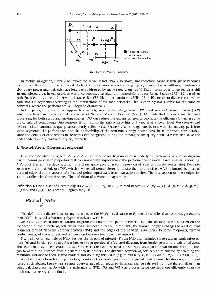
Fig. 1. Network Voronoi Diagram.
In mobile navigation, users who invoke the range search may also move, and therefore, range search query becomescontinuous; therefore, the server needs to let the users know when the range query results change. Although continuouskNN query processing methods have long been addressed by many researchers [28,11,19,35], continuous range search is stillan unexplored area. In our previous work, we proposed an algorithm named Continuous Range Search (CRS) [32] based onboth Euclidean distance and network distance. But CRS, like other continuous kNN [28,11,19], needs to divide the travelingpath into sub-segments according to the intersections of the road networks. This is certainly not suitable for the complexnetworks, where the performance will degrade dramatically.
In this paper, we propose two approaches, namely, Voronoi-based Range Search (VRS) and Voronoi Continuous Range (VCR)which are based on some natural properties of Network Voronoi Diagram (NVD) [14], dedicated to range search queryprocessing for both static and moving queries. VRS can reduce the expansion area to promote the efficiency by using somepre-calculated components. Furthermore, it can reduce the rate of false hits and keep it at a lower level. We then extendVRS to include continuous query, subsequently called V C R . Because VCR no longer needs to divide the moving path intosome segments, the performance and the applicability of the continuous range search have been improved considerably.Since the details of connections in networks can be ignored during the moving of the query point, VCR can also solve theundefined-trajectory continuous query properly.
2. Network Voronoi Diagram: a background
Our proposed algorithms, both VRS and VCR use the Voronoi diagram as their underlying framework. A Voronoi diagramhas numerous geometric properties that can immensely improvement the performance of range search queries processing.A Voronoi diagram is a decomposition of a plane space according to the position of a set of discrete points (site). Each sitegenerates a Voronoi Polygon (VP), which involves all points closer to its site than to any other. A VP is formed by a set ofVoronoi edges that are subsets of a locus of points equidistant from two adjacent sites. The intersection of these edges fora site is called the Voronoi vertex. The definition of a Voronoi diagram is:
Definition 1. Given a set of discrete objects ℘ = (P1, . . . , Pn) (n > 1) in road networks, VP(Pi) = {∀p | dn(p, Pi) � dn(p, P j)}(i, j ∈ In and i �= j). The Voronoi Diagram for ℘ is:
VD(℘) =n⋃
i=1
VP(Pi)
This definition indicates that for any point inside the VP(Pi), its distance to Pi must be smaller than to others generators,then VP(Pi) is called a Voronoi polygon associated with Pi .
An NVD is a special kind of Voronoi diagram constructed on spatial networks [14]. The decomposition is based on theconnection of the discrete objects rather than Euclidean distance. In the NVD, the Voronoi polygon changes to a set of roadsegments termed Network Voronoi polygon (NVP) and the edges of the polygons also shrink to some midpoints, termedborder points, of the road network connection between two objects of interest.
Fig. 1 shows an example of NVD. Besides the objects of interest (P ), an NVD also includes some road network intersec-tions (n) and border points (b). According to the properties of a Voronoi diagram, from border points to a pair of adjacentobjects is equidistant (e.g. dis(b7, P1) = dis(b7, P3)), then we just need to use Dijkstra’s algorithm within one Voronoi poly-gon to obtain the distance from a generator to its borders. The distance between objects can be calculated by selecting theminimum distance to their shared borders and doubling this value (e.g. MIN(dis(P3, P1)) = 2 ∗ dis(b7, P3) = 2 ∗ dis(b7, P1)).
As all distances from border points to generators/other border points can be precalculated using Dijkstra’s algorithm andstored in databases, then when a range query is issued, all required distances can be retrieved from databases rather thanbeing calculated online. So with the assistance of NVD, VRS and VCR can process range queries more efficiently than thetraditional range search methods.

K. Xuan et al. / Journal of Computer and System Sciences 77 (2011) 637–651 639
3. Related work
This section will briefly introduce some existing approaches that focus on network range search, Voronoi-based methodson kNN and CkNN, and a continuous range search approach. We conclude with a summary of their limitations.
3.1. Network range search methods
Range search on network distance is very different from the previous methods. The most efficient algorithms for rangesearch on network distance are known as RER and RNE [15].
RER applies a range search on Euclidean distance e from query point q to retrieve all possible candidates, as the Euclideandistance can be seen as the lower boundary for network distances de(q, p) � dnet(q, p), which ensures that all objects ofinterest within the searching range will not be missed. But a large number of false hits, which have de(q, p) < e, anddnet(q, p) > e, are involved in this procedure. These false hits have to be filtered from the candidates list by performingnetwork expansion in the next step until all the candidates tested or all the segments in the range have been exhausted.
According to the algorithm of RER, if only a few objects are located in complex networks, the processing time willincrease sharply, because most of the operation will be wasted on the network expansion to retrieve only a small numberof objects. In another scenario where the network distances are quite different from the corresponding Euclidean distance,the candidates sets will include numerous false hits which need to be crossed out one by one in the filter step.
RNE outperforms RER by using an expansion method whereby a set of segments within the network range e filters thefalse hits first. Then RNE uses R-tree indexing to find the objects of interest falling on the valid segments, which intersectwith minimum boundary rectangles (MBRs) [8]. Finally, when R-tree indexing is finished, the results are sorted to removethe duplicates.
However, RNE still cannot solve the problem of some unnecessary expansions being performed. If the range area isenormous, RNE will need to scan every segment even if there are just a few objects needing to be retrieved in the searchingrange. So we try to seek a new approach which can avoid false hits or keep it at a reasonable level, whilst at the same time,minimizing the expansion.
3.2. Continuous range search method
Our previous work on continuous range search, which we call CRS [32], processes continuous range query by dividingthe predefined trajectory into sub-segments according to the intersections of the networks. For each sub-segment, CRS usesthe network expansion range search technique, such as RER/RNE [15] at two ends to retrieve all objects of interest withinthe predefined range. Then with the movement of the query point, objects that become accessible or inaccessible will beadded or deleted respectively from the candidate list at the split point.
The disadvantages of CRS are also obvious. Firstly, the trajectory needs to be segmented according to the intersections. Ifthe number of intersections is massive, the number of the sub-segments will be extremely large, which will occupy not onlyhuge storage space, but also unnecessary repeats processes. Secondly, since CRS uses network expansion, all nodes on roadnetworks need to be accessed and compared with the searching range. Thirdly, CRS can process only pre-defined trajectorycontinuous queries. If the moving path is changed on the way to the destination, CRS cannot be applied.
3.3. Voronoi-based methods for kNN and CkNN
Numerous algorithms for kNN [10,18] and continuous kNN [28,11,19] based on the Voronoi diagram have been proposedin recent years. All of them utilize the geometry properties of the Voronoi diagram to provide a better performance thanother traditional network expansion methods.
The Voronoi diagram was first adopted in kNN by Kolahdouzan and Shahabi [10] in whose performance results showedthat their approach VN3 outperformed its main competitor INE [15] by up to one order of magnitude. One year later, theyproposed two new approaches for CkNN query, named IE and UBA [11]. They used these approaches to find the differentvariation trends of the network distance to the query point between adjacent objects in the candidates set when the querypoint is moving. The only difference between IE and UBA is that the former compares kNN results of the two ends of theroad segment, while UBA just extends the kNN results at one end to enhance the execution performance.
At the same time, another group proposed an improved algorithm of VN3, called PINE [18]. After that, DAR and eDAR[19] were proposed for continuous kNN queries. Voronoi diagram has also been utilized in other newer query types, suchas multiple type objects kNN [36] and Reverse Nearest Neighbour (RNN) [20].
The limitations of the above approaches are summarized in Table 1.
4. Voronoi-based Range Search (VRS)
In this section, we present our static range search based on NVD, which we name Voronoi-based Range Search (VRS).

640 K. Xuan et al. / Journal of Computer and System Sciences 77 (2011) 637–651
Table 1Existing methods.
Query classification Methods Limitations
Continuous Range Search CRS Inefficient performance
Network range search RER/RNE High number of false hits and large expansion areaVN3/PINE
Voronoi based kNN/CkNN IE/UBA Work on kNN/CkNN, not on range searchDAR/eDAR
Fig. 2. Data structure of object of interest.
4.1. Data structure and storage schema
To demonstrate our approach, the data structure of the key objects, the NVD generators and Q pre used to store candidatesshould be clearly defined as well as the network distance calculation techniques (see Fig. 2).
• Adjacent Components: Store the generators of adjacent NVPs for Pi .• Border points: Store all border points that belong to NVP(Pi), each border point bx that stores the pre-calculated com-
ponents relevant to itself, disnet(bx, P j) and disnet(bx,by), j �= i, x �= y, bx,by ∈ BoP(NVP(Pi)).• NVP(Pi): A network Voronoi polygon associates with Pi . If NVP(Pi) = NVP(Pq), then NVP(Pi) contains the query
point q.• disnet(q, Pi): It involves two kinds of network distance calculation mechanisms: (a) Incremental Network Expansion
(INE) [15], (b) Off-line Precalculation [18]. Within the first polygon NVP(Pq) including the query point, INE will be usedto get the distances (disnet(q,bx)) from query point to the border points of NVP(Pq). After that, pre-calculated distances(e.g. border to generators and border to border) will be invoked to incorporate with disnet(q,bx) to obtain the entiredistance disnet(q, Pi), see Eq. (1).
disnet(q, Pi) = disnet(q,bx) + disnet(bx, Pi) (1)
• Inside/outside: A Boolean variable indicates the relative position of Pi within the given searching range. When Pi isadded into Q pre , the default value is true.
• Q pre: A sorted queue storing a set of objects whose validity needs to be checked. Q pre does not involve only all validobjects within the searching range, but also includes a few false hits just out of the searching range.
4.2. Terminologies
We also need to formally define a number of basic terms to be used in VRS, namely Expected Searching Range, CurrentSearching Range and Range Borderline.
Definition 2. Given a static query point q in the networks, the Expected Searching Range is a set of road segments, on whichany point p to q is smaller than/equal to e.
p ∈ Expected Searching Range ⇔ disnet(p,q) � e
The thick lines in Fig. 3 represent an example of Expected Searching Range.
Definition 3. Range Borderline is the boundary of the expected searching range and it is represented as an irregular polygonby connecting the adjacent ends of expected searching range.

K. Xuan et al. / Journal of Computer and System Sciences 77 (2011) 637–651 641
Fig. 3. Expected Searching Range. Fig. 4. Range Borderline.
Fig. 5. Current Searching Range. Fig. 6. Inside/outside NVP.
Range Borderline gives us a visualized boundary of the searching range, which provides a mappable way to observe therelative position of the objects of interest within the searching range. Fig. 4 shows a Range Borderline of the expectedsearching range shown in Fig. 3.
Definition 4. Current Searching Range is composed by a set of road segments ending at some generators of NVPs, whosenetwork distances to q need to be compared with e. Current Searching Range is represented by the largest network distancefrom query point q to the furthest retrieved objects.
Current Searching Range = dismax = MAX(disnet(q, Pi)
)
In Fig. 5, current searching range ends at P2, P3, P4, P5, P6, P7 and it is represented by dismax = MAX(disnet(q, Pi)) =disnet(q, P6).
Definition 5. Inside/outside NVP (inNVP/outNVP) is a set of adjacent NVPs of current NVP(Pi), whose network distance fromquery point to its generator is smaller/larger than the distance from query point to Pi , denote as inNVPPi ()/outNVPPi (). Itsgenerator is called the inside/outside adjacent generator of Pi , denote as inAGPi ()/outAGPi ().
∃NVP(P j) ∈ inNVPPi ⇒ disnet(P j,q) < disnet(Pi,q)
∃NVP(P j) ∈ outNVPPi ⇒ disnet(P j,q) > disnet(Pi,q)
The inside and outside is relevant to the relative position of the query point and the generator of NVP (see Fig. 6). For P1,its adjacent NVPs are NVP(P2), NVP(P3), NVP(P4), NVP(P5), NVP(P6), NVP(P7) in which NVP(P5) is P1’s inside NVP, whilerest are its outside NVPs.

642 K. Xuan et al. / Journal of Computer and System Sciences 77 (2011) 637–651
4.3. Main process
The main process of VRS can be summarized as performing network-segment expansion in the first polygon, and thenbulk loading a set of NVPs recursively, until all objects of interest within the expected searching range are retrieved. Duringthis procedure, there are three main steps: (i) Locating the Query Point, (ii) Expanding Current Searching Range, and (iii) LocatingRange Borderline.
Step 1 Locating Query Point: invoke function contain(q) which can invoke a common spatial index structure (e.g. R-Tree)to find the NVP, called NVP(q), where the query point located, and add its generator Pq into Q pre . In the processof locating the query point, no distance needs to be calculated to obtain the location of the query point in NVD.The efficiency of locating the query point will be manifested when the expected searching range is small (such as,expected searching range is inside of the NVP(q)), in this case, Pq is the only object within the searching range.
Step 2 Current Searching Range Expansion: use network Voronoi polygon expansion instead of the traditional network expan-sion used by other range search approaches. The network expansion method, e.g. INE, needs to go through everynode (intersection, object) in the road network. In the worst environment, if the intersections of the networks areenormous, the efficiency of the network expansion will decrease dramatically. The NVP expansion bulk-loads a set ofNVPs, with a consequence that it avoids going through the details in the polygons, until all objects within the rangeare retrieved. Meanwhile, all objects that need to be tested will be inserted into Q pre and the range borderline willbe located. The advantage of NVP expansion is that it is not restricted by the pattern of the networks. In each step,the expansion area is much larger than the network expansion methods.
We introduce the following properties to illustrate when the current searching range expansion needs to be implementedand to constrain the expansion area to only outNVPs of current retrieved NVPs.
Property 1. Q pre = (P1, P2, . . . , Pn) ∈ ℘ , i ∈ n, Pi ∈ ℘ , outAGPi () = (Pm, Pm+1, . . . , Pm′ ) ∈ ℘ , m′ < 6n, if dismax = disnet(q, Pi).According to the definition of the outside adjacent generator, then ∀P j ∈ outAGPi (), disnet(q, P j) > dismax .
Property 2. Q pre = (P1, P2, . . . , Pn) ∈ ℘ , i ∈ n, Pi ∈ ℘ , dismax = disnet(q, Pi) > Constant. According to the definition of theoutside adjacent generator, then P j ∈ outAGPi () ⇒ disnet(q, P j) > Constant.
The initial current searching range is the first polygon determined in the locating query point step, whereby dismax =disnet(q, Pq). According to Property 1, the outside adjacent generators of Pq must be further to q. If Pq is already outside ofrange dismax > e, follow Property 2: dismax > e ⇒ disnet(q, P j) > e, then there is no need to do the expansion. Otherwise, alloutside adjacent generators of Pq will be inserted into Q pre to expand the current searching range. After that, the third stepwill be called to verify the objects in Q pre and check whether to keep expanding or to carry out Gradual Shrinking (refer toStep 3). Fig. 7 illustrates the procedure of current searching range expansion.
Referring to Fig. 7, the current search range can be slightly larger than the expected range, which causes Q pre to producesome false hits that need to be filtered. For the final searching range which overflows only slightly, the number of the falsehits can be controlled to a low-level. Compared with the efficiency of the expansion, the negative effects of this overflowand retrieval of false hits can be disregarded.
Example 1. Fig. 7 illustrates an example of current searching range expansion.
– The initial current searching range is NVP(q). Q pre = {P1}.– The first expansion is represented by 1. Q pre = {P1, P2, P3, P4, P5, P7, P8}.– The second expansion is represented by 2. Q pre = {P1, P2, P3, P4, P5, P7, P8, P6, P9, P10, P11, P12, P13, P14, P15}.
Step 3 Validating Objects and Gradual Shrinking: Essentially, Validating Objects is the distance comparison between range eand dismax in Q pre . It is normally iterative with current searching range expansion or Gradual Shrinking. If e � dismax ,the current searching range overflows the expected searching range. According to Property 2, we do not need to doan expansion at this moment. Although dismax overflows the searching range, the algorithm could not be terminatedaccording to Property 4, which indicates there could be the outside adjacent generators of other objects in Q pre
within the searching range. Then the current searching range needs to be shrunk naturally by discarding the currentdismax and go to next one in Q pre . On the other hand, if e > dismax , this means that the current searching range isinside the expected searching range. According to Property 3, the rest of the candidates in Q pre do not need to betested, then the current searching range expansion will be invoked again. When the algorithm is terminated, Q pre
must have the following structure:
Q pre(. . . , P x(. . . , False), P y(. . . ,True), . . .
)

K. Xuan et al. / Journal of Computer and System Sciences 77 (2011) 637–651 643
Fig. 7. Current Searching Range Expansion.
Fig. 8. Result of Q pre .
Property 3. Q pre = (P1, P2, . . . , Pn) ∈ ℘ , i ∈ n, Pi ∈ ℘ , if dismax = disnet(q, Pi) < Constant, then ∀P j(True) ∈ ℘ , j ∈ n,disnet(q, P j) Constant.
Property 4. Q pre = (P1, P2, . . . , Pn) ∈ ℘ , i, j ∈ n, Pi ∈ ℘ , then dismax = disnet(q, Pi) > disnet(q, P j) � disnet(q, Pi′ ) >
disnet(q, P j′ ), Pi′ ∈ outAGPi (), P j′ ∈ outAGP j ().
The positions of Px and P y define the domain of the expected search range (refer to Fig. 8). Because Q pre is an orderedqueue, Px is the nearest object out of the expected searching range to the query point, while P y , is the furthest objectswithin the expected searching range.
4.4. VRS algorithm
The processing of VRS can be summarized as the extraction of candidate samples and the filtering of candidate samples.The former adds some sample objects of interest needed to be checked into Q pre , while the latter finalizes the resultprecisely with a set of comparisons and filters the false hits. The pseudo of VRS algorithm is shown in Algorithm 1.
To clarify working principle of VRS, we explain the following example (refer to Fig. 9). The query point is symbolized asa triangle, and ℘ are a set of objects of interest which are expressed as dots in road networks. The range search query canbe described as getting all objects of interest within 12 kms which is recognized as the expected searching range. InitiallyQ pre is initialized without any candidate.
Example 2. Network range search using VRS:Firstly, according to Locating Query Point, the contain(q) function is implemented to define the query position in NVD, thenP1 is retrieved into Q pre with NULL value disnet(q, P1). After that, INE is invoked to get this network distance, which isassigned to dismax().
Q pre = {P1}, dismax = disnet(P1,q)
Secondly, Validating Objects and Gradual Shrinking suggests that if e � dismax(), then the inside/outside property of P1will be set to false meaning that no object of interest is within the expected searching range, the algorithm of VRS willterminate. Otherwise, if e > dismax(), then Current Searching Range Expansion will be invoked, which means the searchingrange needs to be expanded.
dismax < e ⇒ Current Searching Range Expansion

644 K. Xuan et al. / Journal of Computer and System Sciences 77 (2011) 637–651
Fig. 9. An example of VRS.
Algorithm 1 VRSInput: query point: q, searching range: eOutput: Q pre
1: Pi ← Containe(q) /*Locating the query point*/2: Q pre ← Q pre ∪ Pq /*Add Pq into Q pre*/3: dismax ← disnet(Pi ,q) /*NVD(q) = NVD(Pi)*/4: if e < disnet(q, Pi) then5: Set the property of current Pi to false6: Return Q pre ← ∅7: else8: repeat9: Add all the neighbors of object into Q pre with true property
10: if P already exists in Q pre then11: Discard it12: end if13: Sort Q pre in descending order according to disnet(q, P )
14: if Exist Px whose property is false after P y in Q pre /*P y is the new object inserted into Q pre*/ then15: Set Inside/outside property of P y to false16: dismax ← disnet(P j ,q) /*P j has the largest disnet to q with true property*/17: end if18: while e < dismax do19: Set the property of current P to false20: Test next P in Q pre21: end while22: until no P added to Q pre23: Return P s whose inside/outside property is true in Q pre24: end if
Thirdly, after implementing the Current Searching Range Expansion, the current searching range expanded from pointNVP(P1) to the neighbor NVPs of P1, namely, P2, P3, P4, P5, P7, P8, which refers to 1st Current Searching Range Expan-sion in Fig. 9. These objects are inserted into Q pre as well as the network distances to q that can be calculated by usingdisnet(q, P1) and some pre-calculated distances. Then Q pre is sorted in a descending order to filter some candidates furtherthan the current object. Then the largest disnet in Q pre will be assigned to dismax .
Q pre = (P4(. . . ,True), P3, P5, P2, P8, P7, P1,
), dismax = disnet(P4,q)
Fourthly, Validating Objects will be invoked again. For dismax = disnet(q, P4) < e, then the current searching range shouldshrink a little. So the inside/outside property of P4 is set to false and test the next Pi in Q pre until e � dismax , then we callCurrent Searching Range Expansion/Gradually Shrinking and Validating Objects iteratively until no objects of interest are addedinto Q pre .
dismax > e ⇒ Gradual Shrinking
Q pre = (P4(. . . , False), P3(. . . ,True), P5, P2, P8, P7, P1,
), dismax = disnet(P3,q)
Current Searching Range Expansion only adds the neighbors of objects whose inside/outside property is true into Q pre ,which narrows the searching range in the next step. To avoid adding the same object of interest into Q pre , we inspect theinside/outside property and check whether the object already exists in the Q pre . The object with false property will beskipped over and the duplicated objects will be discarded. The termination condition of VRS is that no object of interest isadded to the Q pre any more, then all objects of interest with true inside/outside property in Q pre are returned to the user.
K. Xuan et al. / Journal of Computer and System Sciences 77 (2011) 637–651 645
5. Voronoi Continuous Range (VCR)
Range query should not be confined to static range search, but also needs to be feasible for continuous range queries.Our previous work, Continuous Range Search (CRS) as the only existing algorithm cannot avoid employing network segmentdivision used by most continuous k nearest neighbors query processing methods (e.g. IE, UBA and eDAR), which performancedepends on the number of intersections in the networks. Since the actual pattern of the road networks is normally extremelycomplex (numerous intersections), road segmentation creates a significant problem in performance.
In this section, we propose a novel approach, Voronoi Continuous Range (VCR), a search method based on VRS, which doesnot do road segmentation.
5.1. Problem definition
Firstly, we need to define continuous range search query.Predefined trajectory continuous range search query is defined as retrieving all objects of interest on any point of a given
trajectory in the networks. It is similar to continuous kNN query. The predefined path is a necessary element of this kind ofquery. Our previous work illustrates how CRS can solve the traditional continuous range search query properly.
S–D continuous range search query is defined as retrieving all objects of interest on any point during the moving of thequery point from the start point (S) to the destination (D) in the networks. In this case, the moving trajectory of the querypoint is not predefined, which requires the method to have a better flexibility in the road network environment.
VCR is designed for both of the aforementioned queries.
5.2. Operational principle of VCR
For Q pre generated in VRS, this does not involve only the valid objects in the expected searching range, but also includesa few outside objects close to the searching range. The domain of the expected searching range can be located by P x , P y .Px is the nearest object to the query point outside of the searching range, while P y is the furthest one to the query pointin the expected searching range.
Property 5. Given the Q pre return by VRS, then P of min(|e − disnet(Px,q)|, |e − disnet(P y,q)|) is the priority whose in-side/outside property can be changed, when the query point is moving.
In the continuous environment, when the query point is moving, it will cause a series of variations on the pattern ofexpected searching range in respect to the moving distance of the query point during the movement of the query point.Some objects could be moved out, others could be moved in. To decrease the frequency of updating, we need to knowwhere the result can be changed and that is the position where the detection should be executed. According to Property 5,if the inside/outside property of Px/P y is unchanged, no object of interest can move in/out of the expected searching range,which provides us with a method to monitor the changes during the movement of the query point.
Definition 6. Detection point (dp) is a point used to predict the position where the range search result needs to be updatedon the trajectory of the moving query in the networks. It can be expressed by a network distance to the current position ofquery point, min(|e − disnet(Px,q)|, |e − disnet(P y,q)|), Px has minimum disnet to q with false value, P y has maximum disnet
to q with true value.
At every dp, VRS will be invoked to detect whether there is an object of interest that can be added/removed from Q pre .Because the velocity, the moving direction of the query point and the pattern of the road networks are ignored, the
changes at the detection point cannot be guaranteed, and the number of dp will be larger than the split point used by othercontinuous approaches. But VCR focuses on the moving distance of the query point that can be calculated and monitoredeasily, meaning that the continuous query processing is put in a more simple environment by removing most of the in-fluencing factors, which provides VCR with the capability to process both predefined trajectory and S–D continuous rangesearch queries.
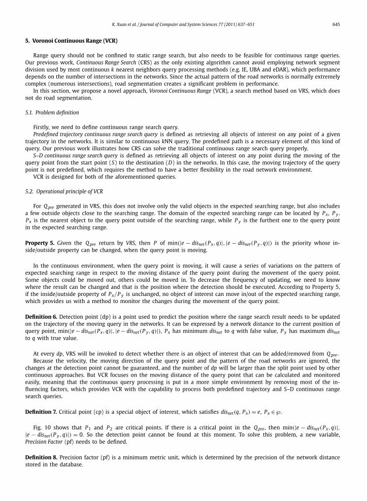
Definition 7. Critical point (cp) is a special object of interest, which satisfies disnet(q, Px) = e, Px ∈ ℘ .
Fig. 10 shows that P1 and P2 are critical points. If there is a critical point in the Q pre , then min(|e − disnet(Px,q)|,|e − disnet(P y,q)|) = 0. So the detection point cannot be found at this moment. To solve this problem, a new variable,Precision Factor (pf) needs to be defined.
Definition 8. Precision factor (pf) is a minimum metric unit, which is determined by the precision of the network distancestored in the database.

646 K. Xuan et al. / Journal of Computer and System Sciences 77 (2011) 637–651
Fig. 10. Critical points.
For example, if the network distance stored in the database is 12.47 km, then pf = 0.01 km. If ∃cp ∈ Q pre , then dp is nolonger calculated by min(|e − disnet(Px,q)|, |e − disnet(P y,q)|). In this case, dp = pf , after updating Q pre at the dp, cp will becleared. To summarize, pf is used to detect the moving trend of a cp.
Using pf appears to be a time consuming method, but actually, when we examine the processing which involve, pf , wefind its performance quite acceptable. Assuming min(|e − disnet(Px,q)|, |e − disnet(P y,q)|) = a and max(|e − disnet(Px,q)|,|e − disnet(P y,q)|) = A. In the worst case, the times of calculation to find the next object is n = 1 + log2(A − a)/2pf , andduring this processing, the only data that can be slightly changed is the network distance and the inside/outside propertyof the critical point. In other words, there is no other object of interest moving in/out of the range, except this critical point.Moreover, the critical point is rare in real cases.
5.3. VCR algorithm
The pseudo code of VCR is shown below and the main step of our proposed Voronoi-based continuous range will beillustrated as follows (see Algorithm 2):
Algorithm 2 VCRInput: start point: S , destination point: D , (pre-defined path: S D), searching range: eOutput: a set of Q pre
1: VRS (S, e)2: Totaldis ← disnet(S, D)
3: repeat4: Find Px and P y from Q pre /*Px is the nearest object to q out e; P y is the furthest object to q in e*/5: dp ← min(|e − disnet(Px,q)|, |e − disnet(P y ,q)|)6: if dp �= 0 /*no object is a critical point*/ then7: VRS (dp, e)8: Update Totaldis ← disnet(dp, D)
9: else10: dp = dp + pf11: Update the information of critical point at dp12: Update Totaldis ← disnet(dp, D)
13: end if14: until Totaldis = 0
Step 1 For a given start point S and end point D or a path S D , we define the value of Totaldis = disnet(S, D), which will beused to evaluate the position of query point to the destination.
Step 2 Find an object of interest, Px , with the maximum network distance in the range, while finding one, P y , with theminimum network distance out of the range from Q pre will be used to calculate the detection point where the resultof the range search can be changed. If there is no P within the range or outside the range, then the correspondingnetwork distance is recorded as disnet = 0.
Step 3 Find a detection point using dp = min(|e − disnet(Px,q)|, |e − disnet(P y,q)|).Step 4 At the detection point, test any object of interest as a critical point to determine whether or not to employ pf for
the next detection point. Update the corresponding information at the detection point.Step 5 Repeat steps 3 and 4 until the query point reaches to the end point, Totaldis = 0.
Example 3. The initial search range is 12 km and Totaldis = disnet(S, D) = 18.8, then at point S , the data in the Q pre isshown in Table 2. Learning through observation and comparison, we get the first detection point dp1 = min(|12 − 11.64|,
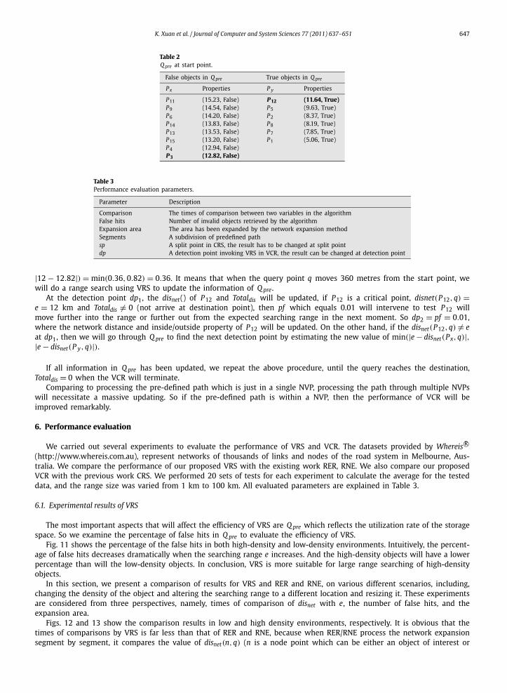
K. Xuan et al. / Journal of Computer and System Sciences 77 (2011) 637–651 647
Table 2Q pre at start point.
False objects in Q pre True objects in Q pre
Px Properties P y Properties
P11 (15.23, False) P12 (11.64, True)P9 (14.54, False) P5 (9.63, True)P6 (14.20, False) P2 (8.37, True)P14 (13.83, False) P8 (8.19, True)P13 (13.53, False) P7 (7.85, True)P15 (13.20, False) P1 (5.06, True)P4 (12.94, False)P3 (12.82, False)
Table 3Performance evaluation parameters.
Parameter Description
Comparison The times of comparison between two variables in the algorithmFalse hits Number of invalid objects retrieved by the algorithmExpansion area The area has been expanded by the network expansion methodSegments A subdivision of predefined pathsp A split point in CRS, the result has to be changed at split pointdp A detection point invoking VRS in VCR, the result can be changed at detection point
|12 − 12.82|) = min(0.36,0.82) = 0.36. It means that when the query point q moves 360 metres from the start point, wewill do a range search using VRS to update the information of Q pre .
At the detection point dp1, the disnet() of P12 and Totaldis will be updated, if P12 is a critical point, disnet(P12,q) =e = 12 km and Totaldis �= 0 (not arrive at destination point), then pf which equals 0.01 will intervene to test P12 willmove further into the range or further out from the expected searching range in the next moment. So dp2 = pf = 0.01,where the network distance and inside/outside property of P12 will be updated. On the other hand, if the disnet(P12,q) �= eat dp1, then we will go through Q pre to find the next detection point by estimating the new value of min(|e − disnet(Px,q)|,|e − disnet(P y,q)|).
If all information in Q pre has been updated, we repeat the above procedure, until the query reaches the destination,Totaldis = 0 when the VCR will terminate.
Comparing to processing the pre-defined path which is just in a single NVP, processing the path through multiple NVPswill necessitate a massive updating. So if the pre-defined path is within a NVP, then the performance of VCR will beimproved remarkably.
6. Performance evaluation
We carried out several experiments to evaluate the performance of VRS and VCR. The datasets provided by Whereis R©(http://www.whereis.com.au), represent networks of thousands of links and nodes of the road system in Melbourne, Aus-tralia. We compare the performance of our proposed VRS with the existing work RER, RNE. We also compare our proposedVCR with the previous work CRS. We performed 20 sets of tests for each experiment to calculate the average for the testeddata, and the range size was varied from 1 km to 100 km. All evaluated parameters are explained in Table 3.
6.1. Experimental results of VRS
The most important aspects that will affect the efficiency of VRS are Q pre which reflects the utilization rate of the storagespace. So we examine the percentage of false hits in Q pre to evaluate the efficiency of VRS.
Fig. 11 shows the percentage of the false hits in both high-density and low-density environments. Intuitively, the percent-age of false hits decreases dramatically when the searching range e increases. And the high-density objects will have a lowerpercentage than will the low-density objects. In conclusion, VRS is more suitable for large range searching of high-densityobjects.
In this section, we present a comparison of results for VRS and RER and RNE, on various different scenarios, including,changing the density of the object and altering the searching range to a different location and resizing it. These experimentsare considered from three perspectives, namely, times of comparison of disnet with e, the number of false hits, and theexpansion area.
Figs. 12 and 13 show the comparison results in low and high density environments, respectively. It is obvious that thetimes of comparisons by VRS is far less than that of RER and RNE, because when RER/RNE process the network expansionsegment by segment, it compares the value of disnet(n,q) (n is a node point which can be either an object of interest or
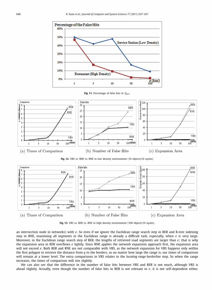
648 K. Xuan et al. / Journal of Computer and System Sciences 77 (2011) 637–651
Fig. 11. Percentage of false hits in Q pre .
Fig. 12. VRS vs. RER vs. RNE in low density environment (10 objects/10 sq.km).
Fig. 13. VRS vs. RER vs. RNE in high density environment (100 objects/10 sq.km).
an intersection node in networks) with e. So even if we ignore the Euclidean range search step in RER and R-tree indexingstep in RNE, examining all segments in the Euclidean range is already a difficult task, especially, when e is very large.Moreover, in the Euclidean range search step of RER, the lengths of retrieved road segments are larger than e; that is whythe expansion area in RER overflows e lightly. Since RNE applies the network expansion approach first, the expansion areawill not exceed e. Both RER and RNE are not comparable with VRS, as the network expansion for VRS happens only withinthe first polygon to retrieve the distance from q to the borders, so no matter how large the range is, our times of comparisonwill remain at a lower level. The extra comparisons in VRS relates to the locating range borderline step. So when the rangeincreases, the times of comparison will rise slightly.
We can also see that the difference in the number of false hits between VRS and RER is not much, although VRS isahead slightly. Actually, even though the number of false hits in RER is not relevant to e, it is not self-dependent either.

K. Xuan et al. / Journal of Computer and System Sciences 77 (2011) 637–651 649
Fig. 14. Accuracy of dp.
Table 4VCR vs. CRS.
VCR vs. CRS
Low Density environment 10 objects/10 sq.km
e = 1 km e = 10 km e = 100 km
VCR CRS VCR CRS VCR CRS VCR CRS VCR CRS VCR CRS
Segments 1 532 1 4028 1 532 1 4028 1 532 1 4028sp(CRS) – 33 – 390 – 465 – 4379 – 4308 – 38745dp(VCR) 67 – 382 – 826 – 3659 – 7948 – 78976 –
High Density environment 100 objects/10 sq.km
e = 1 km e = 10 km e = 100 km
VCR CRS VCR CRS VCR CRS VCR CRS VCR CRS VCR CRS
Segments 1 532 1 4028 1 532 1 4028 1 532 1 4028sp(CRS) – 325 – 3885 – 4530 – 448764 – 46971 – 400653dp(VCR) 638 – 4007 – 8487 – 3779 – 78754 – 764399 –
The only influencing fact of the number of false hits is the degree of similarity of disnet and dise . So, in good conditions, thenumber of false hits in RER can be very small, and vice versa. For the utilization of the sorting algorithm and inside/outsideproperty, the number of false hits is dominated in a reasonable range and the external factors, have no effect; only the sizeof the Voronoi polygon which is determined by the density of the objects of interest.
As mentioned previously, RNE reduces the number of false hits, and is better than VRS, especially in a high densityenvironment. But when we examine the algorithm of VRS carefully, we can find that false hits in VRS are quite differentfrom those in RER. In fact, false hits in VRS are only for locating the range borderline and do not affect the performance ofVRS at all. In summary, VRS performs very well in these three aspects, and in particular VRS outperforms RER and RNE.
6.2. Experimental results of VCR
The most frequent concept in VCR is dp that tries to detect the changes during the movement of the query point. Butsometimes the changes do not happen at dp, so the accuracy of dp is an important parameter for estimating the performanceof VCR.
Fig. 14 shows the rate of the accuracy of dp in both high-density and low-density environments. Intuitively, the rate ofthe accuracy of dp always remains at a good level when the searching range e increases. And the high-density objects willhave a lower percentage than the low-density objects. So the density is the main factor that will affect the accuracy of dp.
Because of very limited existing works on continuous range using NVD, we compare only VCR and CRS, by offeringthe results of several experiments using different scenarios, including: changing the density of the object and altering thesearching range to different location and resize it. These experiments focus on: number of comparison of disnet with e,number of false hits and the proportion of the expansion area.
Table 4 shows the comparison results between VCR and CRS. It is obvious that VCR does not divide the path intosegments, while CRS has to implement the path segmentation to avoid changes when moving on the segment. If thereis an intersection in the middle of the segment, we cannot guarantee that the changes of disnet are unidirectional. Nosegmentation gives VCR a better performance and applicability.

650 K. Xuan et al. / Journal of Computer and System Sciences 77 (2011) 637–651
On the other hand, the number of dp in VCR is larger than the split node in CRS most of the time. Unlike the splitnode, detection points do not ensure that there will be a change in that point. If the accuracy of split node is 100%, thendp maintains the accuracy at a lower level. But the number of dp is very similar with the corresponding value of split node,for VCR does not focus on the details of the network.
According to the result in Table 4, VCR is not suitable for a wide range and high density environment and when thevalue of range e approximate to the path length, CRS is strongly competitive.
7. Conclusions and future work
After analyzing the existing range and continuous range search methods, and evaluating their disadvantages, we findthat the main problem lies in the expansion technique. If we can shrink the expansion area, much computation time willbe saved. In order to offer a better solution, we use a Network Voronoi Diagram as the basis for our methods, namedVoronoi-based Range Search (VRS) and Voronoi Continuous Range (VCR). We utilize some new properties of NVD and developthree main steps for VRS, namely, Current Searching Range Expansion, Query Position Definition and Locating Range Borderline,to remove unnecessary expansion and decrease the number of false hits. Moreover, Q pre , which stores the candidates, wasalso introduced as the basic data structure for VCR, which efficiently retrieves the objects of interest within the searchingrange for the moving user. Unlike other continuous algorithms, VCR focuses only on the moving distance of the query pointinstead of the details of networks. When the result of Q pre is likely to change, we employ VRS at detection point to updatethe searching results. Our experiments show that both VRS and VCR outperform their competitors in most scenarios.
To sum up, VRS and VCR retrieve the expected results for network range search queries and provide better performancesthan do the existing approaches and it is also a solution for the new type of continuous range search. VRS stores a largeset of pre-computed components in the database, which increases the storage space and indexing time. It is thereforeimperative to address the storage requirements of these components [7]. We plan to apply an object-relational technique[16,17], and global indexing [24,21] for an efficient storage.
Although the performance of VRS and VCR outstrips their competitors, due to the use of the property of Voronoi diagram,performance can be expected to further increase by employing parallel techniques. We also plan to investigate the use ofparallelism [27,22,23,25] to process spatial and mobile queries more efficiently. Performance of mobile queries is expectedto be enhanced through data broadcast [30,29], instead of server processing [9]. Another aspect that may be incorporatedinto mobile continuous query processing is through mining mobile users’ movements [5,6,26,1].
Acknowledgment
This research has been partially funded by the Australian Research Council (ARC) Discovery Project (ProjectNo. DP0987687).
References
[1] O. Daly, D. Taniar, Exception rules mining based on negative association rules, in: Proceedings of the International Conference on ComputationalScience and Its Applications (ICCSA), part IV, in: Lecture Notes in Comput. Sci., vol. 3046, Springer, 2004, pp. 543–552.
[2] E.W. Dijkstra, A note on two problems in connection with graphs, Numer. Math. 1 (22) (1959) 269–271.[3] P. Fülöp, K. Lendvai, T. Szálka, S. Imre, S. Szabó, Accurate mobility modeling and location prediction based on pattern analysis of handover series in
mobile networks, Mobile Inf. Syst. 5 (3) (2009) 255–289.[4] J. Goh, D. Taniar, Mobile data mining by location dependencies, in: Proceedings of the 5th International Conference on Intelligent Data Engineering
and Automated Learning – IDEAL, in: Lecture Notes in Comput. Sci., vol. 3177, Springer, 2004, pp. 225–231.[5] J. Goh, D. Taniar, Mining frequency pattern from mobile users, in: Proceedings of the 8th International Conference on Knowledge-Based Intelligent
Information and Engineering Systems (KES), part III, in: Lecture Notes in Comput. Sci., vol. 3215, Springer, 2004, pp. 795–801.[6] J. Goh, D. Taniar, Mining parallel patterns from mobile users, Internat. J. Business Data Commun. Netw. 1 (1) (2005) 50–76.[7] L. Gómez, B. Kuijpers, B. Moelans, A. Vaisman, A survey of spatio-temporal data warehousing, Internat. J. Data Warehousing Min. 5 (3) (2009) 28–55.[8] A. Guttman, R-trees: A dynamic index structure for spatial searching, in: Proceedings of ACM SIGMOD, ACM Press, June 1984, pp. 47–57.[9] J. Jayaputera, D. Taniar, Data retrieval for location-dependent queries in a multi-cell wireless environment, Mobile Inf. Syst. 1 (2) (2005) 91–108.
[10] M.R. Kolahdouzan, C. Shahabi, Voronoi-based k nearest neighbor search for spatial network databases, in: Proceedings of the 30th VLDB, MorganKaufmann Publishers Inc., Toronto, Canada, August 2004, pp. 840–851.
[11] M.R. Kolahdouzan, C. Shahabi, Alternative solutions for continuous k nearest neighbor queries in spatial network databases, GeoInformatica 9 (4) (2005)321–341.
[12] D. Komaki, K. Ohnishi, Y. Arase, T. Hara, G. Hattori, S. Nishio, Design and implementation of a Click–Search interface for web browsing using cellularphones, Internat. J. Web Grid Serv. 5 (1) (2009) 66–84.
[13] Z. Mammeri, F. Morvan, A. Hameurlain, N. Marsit, Location-dependent query processing under soft real-time constraints, Mobile Inf. Syst. 5 (3) (2009)205–232.
[14] A. Okabe, B. Boots, K. Sugihara, S.N. Chiu, Spatial Tessellations: Concepts and Applications of Voronoi Diagrams, second edition, John Wiley and SonsLtd., West Sussex, England, 2000.
[15] D. Papadias, J. Zhang, N. Mamoulis, Y. Tao, Query processing in spatial network databases, in: Proceedings of the 29th VLDB, Morgan KaufmannPublishers Inc., Berlin, Germany, September 2003, pp. 802–813.
[16] J.W. Rahayu, E. Chang, T. Dillon, D. Taniar, A methodology for transforming inheritance relationships in an object-oriented conceptual model to rela-tional tables, Inf. Software Tech. 42 (8) (2000) 571–592.
[17] J.W. Rahayu, E. Chang, T. Dillon, D. Taniar, Performance evaluation of the object-relational transformation methodology, Data Knowledge Engrg. 38 (3)(2001) 265–300.
K. Xuan et al. / Journal of Computer and System Sciences 77 (2011) 637–651 651
[18] M. Safar, K nearest neighbor search in navigation systems, Mobile Inf. Syst. 1 (3) (2005) 207–224.[19] M. Safar, D. Ebrahimi, eDAR algorithm for continuous KNN queries based on PINE, Internat. J. Inf. Tech. Web Engrg. 1 (4) (2006) 1–21.[20] M. Safar, D. Ebrahimi, D. Taniar, Voronoi-based reverse nearest neighbor query processing on spatial networks, Multimedia Syst. 15 (5) (2009) 295–308.[21] D. Taniar, J.W. Rahayu, A taxonomy of indexing schemes for parallel database systems, Distrib. Parallel Databases 12 (1) (2002) 73–106.[22] D. Taniar, J.W. Rahayu, Parallel database sorting, Inform. Sci. 146 (1–4) (2002) 171–219.[23] D. Taniar, J.W. Rahayu, Parallel sort-merge object-oriented collection join algorithms, Internat. J. Comput. Syst. Sci. Engrg. 17 (3) (2002) 145–158.[24] D. Taniar, J.W. Rahayu, Global parallel index for multi-processors database systems, Inform. Sci. 165 (1–2) (2004) 103–127.[25] D. Taniar, R. Tan, C. Leung, K. Liu, Performance analysis of “Groupby-After-Join” query processing in parallel database systems, Inform. Sci. 168 (1–4)
(2004) 25–50.[26] D. Taniar, J. Goh, On mining movement pattern from mobile users, Int. J. Distrib. Sensor Netw. 3 (1) (2007) 69–86.[27] D. Taniar, C.H.C. Leung, J.W. Rahayu, S. Goel, High Performance Parallel Database Processing and Grid Databases, John Wiley and Sons Ltd., ISBN 978-
0-470-10762-1, October 2008, 576 pp.[28] Y. Tao, D. Papadias, Q. Shen, Continuous nearest neighbor search, in: Proceedings of the 28th VLDB, Morgan Kaufmann Publishers Inc., Hong Kong,
China, August 2002, pp. 287–298.[29] A. Waluyo, B. Srinivasan, D. Taniar, Optimal broadcast channel for data dissemination in mobile database environment, in: Proceedings of the 5th
International Workshop on Advanced Parallel Programming Technologies, APPT, in: Lecture Notes in Comput. Sci., vol. 2834, Springer, 2003, pp. 655–664.
[30] A. Waluyo, B. Srinivasan, D. Taniar, A taxonomy of broadcast indexing schemes for multi channel data dissemination in mobile database, in: Proceedingsof the 18th International Conference on Advanced Information Networking and Applications (AINA), vol. 1, IEEE Computer Society, 2004, pp. 213–218.
[31] A. Waluyo, B. Srinivasan, D. Taniar, Research in mobile database query optimization and processing, Mobile Inf. Syst. 1 (4) (2005) 225–252.[32] K. Xuan, G. Zhao, D. Taniar, B. Srinivasan, Continuous range search query processing in mobile navigation, in: Proceedings of the 14th ICPADS 2008,
IEEE, Melbourne, Victoria, Australia, December 2008, pp. 361–368.[33] K. Xuan, G. Zhao, D. Taniar, B. Srinivasan, M. Safar, M.L. Gavrilova, Network Voronoi Diagram based range search, in: Proceedings of the IEEE 23rd
International Conference on Advanced Information Networking and Applications (AINA), 2009, pp. 741–748.[34] A. Yamazaki, A. Koyama, J. Arai, L. Barolli, Design and implementation of a ubiquitous health monitoring system, Internat. J. Web Grid Serv. 5 (4) (2009)
339–355.[35] G. Zhao, K. Xuan, J.W. Rahayu, D. Taniar, M. Safar, M. Gavrilova, B. Srinivasan, Voronoi-based continuous k nearest neighbor search in mobile navigation,
IEEE Trans. Ind. Electronics 56 (2009) (online since June 2009).[36] G. Zhao, K. Xuan, D. Taniar, M. Safar, M. Gavrilova, B. Srinivasan, Multiple object types KNN search using network Voronoi diagram, in: Proceedings
of the International Conference on Computational Science and Its Applications (ICCSA), part II, in: Lecture Notes in Comput. Sci., vol. 5593, Springer,2009, pp. 819–834.