Topological Stability and Dynamic Resilience in Complex Networks

UNIVERSITY OF CALGARY

Topological Stability and Dynamic Resilience in Complex Networks

by

Satindranath Mishtu Banerjee

A THESIS

SUBMITTED TO THE FACULTY OF GRADUATE STUDIES

IN PARTIAL FULFILLMENT OF THE REQUIREMENTS FOR THE

DEGREE OF DOCTOR OF PHILOSOPHY

DEPARTMENT OF COMPUTER SCIENCE

CALGARY, ALBERTA

SEPTEMBER, 2012

c© Satindranath Mishtu Banerjee 2012

UNIVERSITY OF CALGARY

FACULTY OF GRADUATE STUDIES

The undersigned certify that they have read, and recommend to the Faculty of Graduate

Studies for acceptance, a thesis entitled “Topological Stability and Dynamic Resilience in

Complex Networks” submitted by Satindranath Mishtu Banerjee in partial fulfillment of the

requirements for the degree of DOCTOR OF PHILOSOPHY.

Supervisor, Dr. Ken BarkerDepartment of Computer Science

Dr. Peter HøyerDepartment of Computer Science

Dr. Carey WilliamsonDepartment of Computer Science

Internal, Dr. Sui HuangDepartment of Biological Sciences

Institute for Systems Biology

External, Dr. Robert E. UlanowiczArthur R. Marshall Laboratory,

University of Florida

Date

Abstract

Stability is a concern in complex networks as disparate as power grids, ecosystems, financial

networks, the Internet, and metabolisms. I introduce two forms of topological stability that

are relevant to network architectures: cut and connection stability. Cut-stability concerns a

network’s ability to resist being broken into pieces. Connection-stability concerns a network’s

ability to resist the spread of viral processes.

These two forms of stability are antagonistic. Therefore, no network can ever be com-

pletely architecturally stable. Changes to network topology that increase one form of sta-

bility, compromise the other. This may seem disappointing, but there is good news. Dy-

namic processes can stabilize a network and compensate for architectural limitations. Let

us call such stabilizing processes, ‘resilient mechanisms’. Such resilient mechanisms can be

abstracted from stabilizing processes in biology, or designed de novo.

Resilient processes have evolved to dynamically stabilize biological networks in the face

of architectural limitations. They have been studied by biologists in several areas from

homeostasis to evolutionary robustness. These processes exist today because they have been

effective over evolutionary time scales. This provides an opportunity for computer scientists

to learn from biology about processes that can stabilize the complex networks characteristic

of distributed systems.

I introduce a multi-agent framework, Probabilistic Network Models (PNMs), within

which we can test different candidate resilient processes under varying network architec-

tures. I focus on a PNM for a viral instability where the resilient process is the simple

immune response of sending a warning message. Counter-intuitively, network architectures

that favour the virus, also favour the warning message running ahead. Dynamic resilience,

thus allows for an architectural weakness in connection-stability to be circumvented by pro-

cesses as simple as sending a warning message.

ii

Permutations

unfold and arise

from within and fracture what was simply simple

into many.

Repeat is scattered by rhythm and

released in

multitudes that stand in the plain void.

– from ’Flux’, by S.N. Salthe

iii

Acknowledgements

The ideas presented here have percolated for over twenty years. Enduring questions about

stability in biology, ultimately led me to computer science, whose formal methods allowed

me to articulate my intuitions and build the conceptual tools I needed.

The ideas that led to this thesis originated in discussions with a diverse collection of sci-

entists seeking to understand the interplay of physical and informational constraints involved

in originating and elaborating biological systems. They include Jack Maze, Daniel Brooks,

John Collier, Robert Ulanowicz, Stanley Salthe and Koichiro Matsuno. Over the nearly 20

years I worked in industry and outside of academia, they always found the time to answer my

questions. While the resulting theory of topological stability most obviously descends from

Robert Ulanowicz’s ecological theory of ascendency, it owes equally to all these individuals

and the inspiration their work provided me.

A few of my mentors at the University of Calgary (U of C) deserve special mention.

Ken Barker, my thesis supervisor, has been a constant source of encouragement, and gently

led me out of many intellectual dead ends as I developed the hypotheses that ground this

thesis. Peter Høyer, both understood my mathematical limitations, and guided me to rectify

them. In doing so, he introduced me to the lovely rigour of thinking through proofs. I am

indebted to his patient teaching and his high standards; board sessions with Peter have

been the highlight of my academic career here. Jorg Denzinger was a generous source of

ideas, critique, and insight connecting the multi-agent simulation approach to the biological

problems that drove me. There was no good idea he was not willing to discuss and no bad

idea that he was reticent about pointing out. Sui Huang introduced me to systems biology

over numerous discussions and his work and vision integrating empirical and theoretical

aspects of systems biology motivated much of Chapters 5 and 6. Ken Barker, Jalal Kawash,

Lisa Higham, Philipp Woelfel, and John Aycock, collectively as the ‘virus group’, gamely

iv

took my biologically inspired question about the simplest possible immune reaction and

guided it into the arena of networked systems in the form of a probabilistic network model,

the prototypical PNM.

My time at the U of C was smoothed by our excellent administrative staff, particularly

Susan Lucas, Stacey Chow, and Mary Lim.

Four people enriched my daily life on campus immensely, became close collaborators and

dear friends. They are Craig Schock, Jalal Kawash, Leanne Wu, and Rosa Karimi Adl.

My immediate and extended family both supported me, and lost me during the years of

this thesis. I am sorry I can never return that time lost to us. First and foremost, my wife

Julie Rao encouraged and supported me in all ways possible. She was my best critic and

translator from jargon to plain english. My family – Satyen, Maya and Mita Banerjee – and

my dear friend, Audrey Eastham, were constant sources of encouragement. Lois Garton and

Mavis Wahl kept me physically intact.

I thank my supervisory committee (Ken Barker, Peter Høyer, and Carey Williamson)

and externals (Robert Ulaniwicz and Sui Huang) for undertaking to evaluate a complex

multidisciplinary thesis.

This thesis is dedicated to the memory of my father, who would have enjoyed reading it,

and encouraged me to go a little further still.

v

Table of Contents

Abstract . . . . . . . . . . . . . . . . . . . . . . . . . . . . . . . . . . . . . . . . . iiAcknowledgements . . . . . . . . . . . . . . . . . . . . . . . . . . . . . . . . . . . ivTable of Contents . . . . . . . . . . . . . . . . . . . . . . . . . . . . . . . . . . . . viList of Tables . . . . . . . . . . . . . . . . . . . . . . . . . . . . . . . . . . . . . . ixList of Figures . . . . . . . . . . . . . . . . . . . . . . . . . . . . . . . . . . . . . . xList of Symbols . . . . . . . . . . . . . . . . . . . . . . . . . . . . . . . . . . . . . xi1 Roadmap and Introduction . . . . . . . . . . . . . . . . . . . . . . . . . . . . 11.1 Roadmap . . . . . . . . . . . . . . . . . . . . . . . . . . . . . . . . . . . . . 11.2 Introduction and Motivation . . . . . . . . . . . . . . . . . . . . . . . . . . . 3

1.2.1 Guiding Questions . . . . . . . . . . . . . . . . . . . . . . . . . . . . 31.2.2 Preliminary Concepts . . . . . . . . . . . . . . . . . . . . . . . . . . . 6

1.3 Literature Review . . . . . . . . . . . . . . . . . . . . . . . . . . . . . . . . . 111.3.1 Some Basic Terminology . . . . . . . . . . . . . . . . . . . . . . . . . 111.3.2 Current Network Models . . . . . . . . . . . . . . . . . . . . . . . . . 121.3.3 Cut Stability . . . . . . . . . . . . . . . . . . . . . . . . . . . . . . . 131.3.4 Connection Stability . . . . . . . . . . . . . . . . . . . . . . . . . . . 141.3.5 Development . . . . . . . . . . . . . . . . . . . . . . . . . . . . . . . 14

1.4 Contributions . . . . . . . . . . . . . . . . . . . . . . . . . . . . . . . . . . . 162 A Brief Survey of Stability . . . . . . . . . . . . . . . . . . . . . . . . . . . . 182.1 Abstract . . . . . . . . . . . . . . . . . . . . . . . . . . . . . . . . . . . . . . 182.2 Introduction: Stability Through the Looking Glass . . . . . . . . . . . . . . 182.3 Philosophy: Stability, Cohesion, Individuality . . . . . . . . . . . . . . . . . 192.4 Dynamical Systems: Poincaire Stability . . . . . . . . . . . . . . . . . . . . . 212.5 Thermodynamics: Instability and Self-Organization . . . . . . . . . . . . . . 232.6 Biology: Homeostasis and Developmental Canalization . . . . . . . . . . . . 262.7 Computer Science: Byzantine Dilemmas . . . . . . . . . . . . . . . . . . . . 312.8 Stable Inferences . . . . . . . . . . . . . . . . . . . . . . . . . . . . . . . . . 342.9 Commonalities . . . . . . . . . . . . . . . . . . . . . . . . . . . . . . . . . . 383 Mathematical Preliminaries . . . . . . . . . . . . . . . . . . . . . . . . . . . 413.1 Abstract . . . . . . . . . . . . . . . . . . . . . . . . . . . . . . . . . . . . . . 413.2 Introduction . . . . . . . . . . . . . . . . . . . . . . . . . . . . . . . . . . . . 413.3 Networks . . . . . . . . . . . . . . . . . . . . . . . . . . . . . . . . . . . . . . 423.4 Probability . . . . . . . . . . . . . . . . . . . . . . . . . . . . . . . . . . . . 433.5 Information (Classical) . . . . . . . . . . . . . . . . . . . . . . . . . . . . . . 443.6 Information (Algorithmic) . . . . . . . . . . . . . . . . . . . . . . . . . . . . 473.7 Derivation of Ascendency . . . . . . . . . . . . . . . . . . . . . . . . . . . . . 484 Topological Network Stability . . . . . . . . . . . . . . . . . . . . . . . . . . 544.1 Abstract . . . . . . . . . . . . . . . . . . . . . . . . . . . . . . . . . . . . . . 544.2 Introduction and Motivation I: A Network Architect’s Perspective . . . . . . 554.3 Cut-stability and Connection-stability Definitions . . . . . . . . . . . . . . . 57

4.3.1 Cut-stability . . . . . . . . . . . . . . . . . . . . . . . . . . . . . . . . 584.3.2 Connection-stability . . . . . . . . . . . . . . . . . . . . . . . . . . . 58

vi

4.3.3 Extension of Cut and Connection Stability to Disconnected Graphs . 594.3.4 Extension of Cut-Stability and Connection-Stability to Directed Graphs 604.3.5 Antagonism . . . . . . . . . . . . . . . . . . . . . . . . . . . . . . . . 61

4.4 Cut-Stability and Connection-stability are Antagonistic . . . . . . . . . . . . 624.5 Introduction and Motivation II: An Ecologist’s Perspective . . . . . . . . . . 644.6 Directed Graphs and Mutual Information . . . . . . . . . . . . . . . . . . . . 714.7 Mutual Information and Topological Stability . . . . . . . . . . . . . . . . . 79

4.7.1 Roadmap to Our Argument . . . . . . . . . . . . . . . . . . . . . . . 794.7.2 Cut-Stability and Connection-Stability in Strongly Connected Graphs 814.7.3 Monotonicity Conditions . . . . . . . . . . . . . . . . . . . . . . . . . 844.7.4 A Construction for Monotonic Decrease . . . . . . . . . . . . . . . . . 87

4.8 Balanced Stability . . . . . . . . . . . . . . . . . . . . . . . . . . . . . . . . 904.8.1 Visualizing Balanced Stability . . . . . . . . . . . . . . . . . . . . . . 904.8.2 Balanced Stability and Information Hiding . . . . . . . . . . . . . . . 94

4.9 Connections to Other Perspectives . . . . . . . . . . . . . . . . . . . . . . . 1004.9.1 Error and Attack Tolerance for Complex Networks . . . . . . . . . . 1014.9.2 Keystone Species, Indirect Effects and Cycling in Ecological Networks 1044.9.3 Social Networks . . . . . . . . . . . . . . . . . . . . . . . . . . . . . . 1074.9.4 Graph Spectra . . . . . . . . . . . . . . . . . . . . . . . . . . . . . . 109

4.10 The Story So Far, The Road Ahead . . . . . . . . . . . . . . . . . . . . . . . 1105 Probabilistic Network Models . . . . . . . . . . . . . . . . . . . . . . . . . . 1145.1 Abstract . . . . . . . . . . . . . . . . . . . . . . . . . . . . . . . . . . . . . . 1145.2 Introduction and Motivation . . . . . . . . . . . . . . . . . . . . . . . . . . . 1145.3 The PNM Model . . . . . . . . . . . . . . . . . . . . . . . . . . . . . . . . . 1175.4 Computational and Biological Contexts . . . . . . . . . . . . . . . . . . . . . 1226 Modelling with PNMs . . . . . . . . . . . . . . . . . . . . . . . . . . . . . . 1266.1 Abstract . . . . . . . . . . . . . . . . . . . . . . . . . . . . . . . . . . . . . . 1266.2 Introduction and Motivation . . . . . . . . . . . . . . . . . . . . . . . . . . . 1276.3 Model 1 – Virus and Immune Response . . . . . . . . . . . . . . . . . . . . . 1326.4 Model 2 – Mutualism and Autocatalysis . . . . . . . . . . . . . . . . . . . . 1366.5 Model 3 – Gene Regulation . . . . . . . . . . . . . . . . . . . . . . . . . . . 1396.6 Model 4 – Differentiation . . . . . . . . . . . . . . . . . . . . . . . . . . . . . 1476.7 Model 5 – Semiochemicals . . . . . . . . . . . . . . . . . . . . . . . . . . . . 1496.8 Model 6 – Ecosystem Flow Networks . . . . . . . . . . . . . . . . . . . . . . 1546.9 Future Directions . . . . . . . . . . . . . . . . . . . . . . . . . . . . . . . . . 1617 Dynamic Resilience . . . . . . . . . . . . . . . . . . . . . . . . . . . . . . . . 1667.1 Abstract . . . . . . . . . . . . . . . . . . . . . . . . . . . . . . . . . . . . . . 1667.2 Introduction and Motivation: Viruses in Computer Science and Biology . . . 1687.3 Dynamic Resilience . . . . . . . . . . . . . . . . . . . . . . . . . . . . . . . . 169

7.3.1 Dynamical Resilience in terms of Topological Network Stability andPNMs . . . . . . . . . . . . . . . . . . . . . . . . . . . . . . . . . . . 169

7.3.2 Resilience Concepts In Other Areas of Computer Science . . . . . . . 1717.4 Resilience Examples . . . . . . . . . . . . . . . . . . . . . . . . . . . . . . . 173

7.4.1 Resilience Example 1: Agent Hardening . . . . . . . . . . . . . . . . 1737.4.2 Resilience Example 2: Viral Propagation . . . . . . . . . . . . . . . . 175

vii

7.4.3 Resilience Example 3: Virus Immune Response Under Different Net-work Connectivities . . . . . . . . . . . . . . . . . . . . . . . . . . . . 177

7.4.4 Insights from the Examples: A Little Resilience Can Go A Long Way. 1807.5 Refining Resilient Mechanisms . . . . . . . . . . . . . . . . . . . . . . . . . . 181

7.5.1 Combining Resilient Mechanisms: Agent Resistance and Immune Re-sponse . . . . . . . . . . . . . . . . . . . . . . . . . . . . . . . . . . . 181

7.5.2 Further Refinements to the Virus and Immune Response PNM . . . . 1857.6 The Epidemiological and Immune Metaphors in Computer Science . . . . . . 1877.7 An Evolutionary Perspective . . . . . . . . . . . . . . . . . . . . . . . . . . . 1918 The Nascent Moment . . . . . . . . . . . . . . . . . . . . . . . . . . . . . . . 1958.1 Abstract . . . . . . . . . . . . . . . . . . . . . . . . . . . . . . . . . . . . . . 1958.2 Recap of Contributions . . . . . . . . . . . . . . . . . . . . . . . . . . . . . . 1958.3 Future Directions . . . . . . . . . . . . . . . . . . . . . . . . . . . . . . . . . 197

8.3.1 Theoretical Next Steps . . . . . . . . . . . . . . . . . . . . . . . . . . 1978.3.2 Methodological Next Steps . . . . . . . . . . . . . . . . . . . . . . . . 1988.3.3 Empirical Applications . . . . . . . . . . . . . . . . . . . . . . . . . . 199

8.4 On the Origin of Interactions . . . . . . . . . . . . . . . . . . . . . . . . . . 200Bibliography . . . . . . . . . . . . . . . . . . . . . . . . . . . . . . . . . . . . . . 202

viii

List of Tables

4.1 Adjacency Matrix for MacArthur’s Food Web . . . . . . . . . . . . . . . . . 744.2 Mutual Information Calculation for MacArthur’s Food Web . . . . . . . . . 754.3 Adjacency Matrix for MacArthur’s Modified Food Web . . . . . . . . . . . . 764.4 Mutual Information Calculation for MacArthur’s Modified Food Web . . . . 76

ix

List of Figures and Illustrations

1.1 Unconstrained Network . . . . . . . . . . . . . . . . . . . . . . . . . . . . . . 71.2 Constrained Network . . . . . . . . . . . . . . . . . . . . . . . . . . . . . . . 7

4.1 MacArthur’s Food Web . . . . . . . . . . . . . . . . . . . . . . . . . . . . . . 744.2 MacArthur’s Modified Food Web . . . . . . . . . . . . . . . . . . . . . . . . 774.3 Stability Measures in Terms of Cumulative Probability of Summation Terms 93

6.1 MacArthur’s Modified Food Web . . . . . . . . . . . . . . . . . . . . . . . . 158

7.1 Simulation Plot Matrix. From left to right, viral level increases. From top tobottom network connectivity increases. Red diamonds: viral vertices. Bluesquares: neutral vertices. Green triangles: immune vertices. For each com-bination of Virus Level and Network Connectivity the average of 30 trials issummarized by iteration . . . . . . . . . . . . . . . . . . . . . . . . . . . . . 179

x

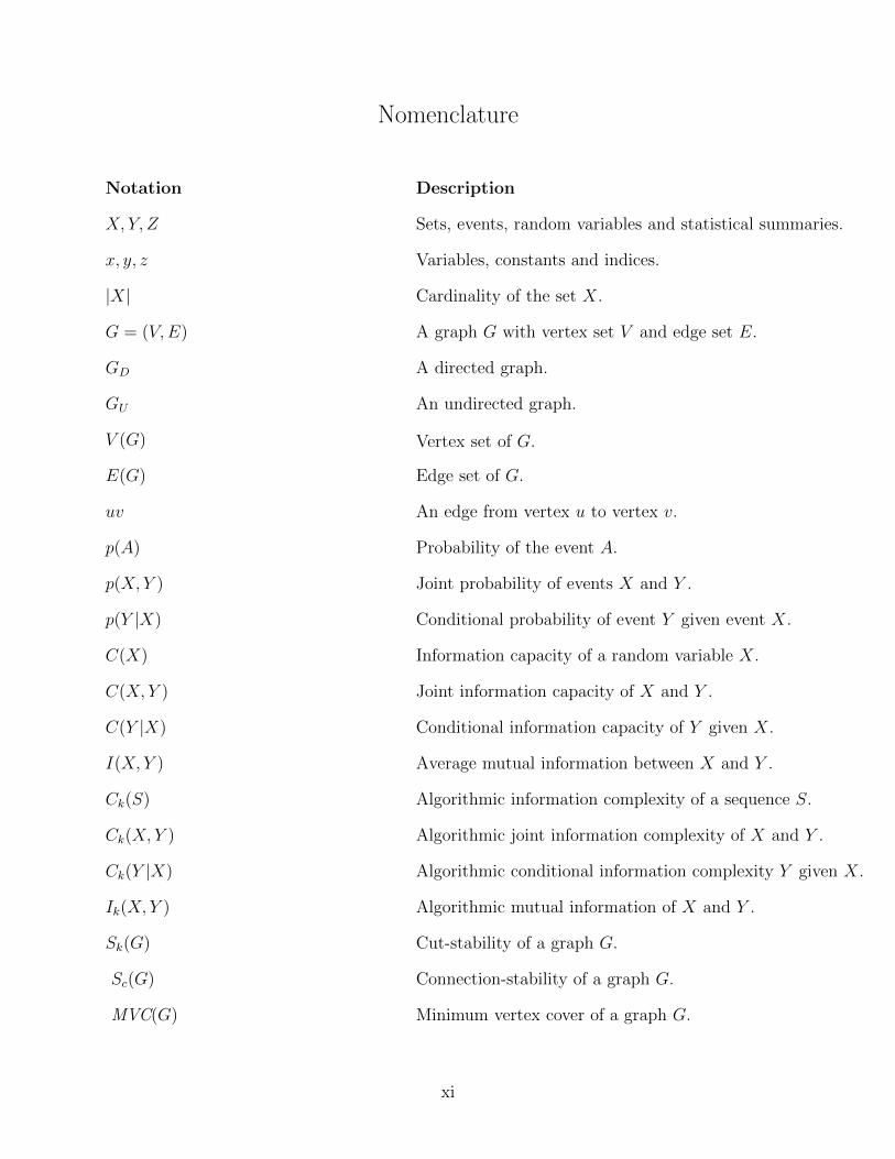
Nomenclature

Notation Description

X, Y, Z Sets, events, random variables and statistical summaries.

x, y, z Variables, constants and indices.

|X| Cardinality of the set X.

G = (V,E) A graph G with vertex set V and edge set E.

GD A directed graph.

GU An undirected graph.

V (G) Vertex set of G.

E(G) Edge set of G.

uv An edge from vertex u to vertex v.

p(A) Probability of the event A.

p(X, Y ) Joint probability of events X and Y .

p(Y |X) Conditional probability of event Y given event X.

C(X) Information capacity of a random variable X.

C(X, Y ) Joint information capacity of X and Y .

C(Y |X) Conditional information capacity of Y given X.

I(X, Y ) Average mutual information between X and Y .

Ck(S) Algorithmic information complexity of a sequence S.

Ck(X, Y ) Algorithmic joint information complexity of X and Y .

Ck(Y |X) Algorithmic conditional information complexity Y given X.

Ik(X, Y ) Algorithmic mutual information of X and Y .

Sk(G) Cut-stability of a graph G.

Sc(G) Connection-stability of a graph G.

MVC(G) Minimum vertex cover of a graph G.

xi

MFS(v∗, G) The set of vertices in G flood-able from v∗, including v∗.

IE(G) Average mutual information calculated on the edges of a graph.

ecuv Edge constraint; value an edge from uv contributes to IE(G).

X tj A random variable X of the jth agent at time t.

Γ(j) Neighbourhood of an agent j.

xii

Chapter 1

Roadmap and Introduction

What is stable?

1.1 Roadmap

This chapter is a conceptual introduction to the major themes of this thesis and a roadmap

through subsequent chapters. I introduce two forms of stability that are relevant to network

architectures: cut-stability and connection-stability. Cut-stability concerns a network’s abil-

ity to resist being broken into pieces. Connection-stability concerns a network’s ability to

resist the spread of mal-information. I examine the literature on complex networks in several

fields to see how these two forms of stability have appeared in various forms. I introduce the

notion that these two forms of stability are antagonistic.

Chapter 2 provides a brief history of stability concepts from various fields. Its goal is

to sharpen our intuition about what stability in a system implies. We all have some basic

intuitive notions of stability, but these basic intuitions take specific forms in each field.

There are different implications to stability as it has been represented in the literature in

philosophy, physics, biology and computer science.

Chapter 3 provides mathematical preliminaries for the rest of the thesis. It introduces

some basic concepts in probability theory, information theory, and graph theory, as well as an

ecological application of these concepts known as ascendency [Ulanowicz 97, Ulanowicz 04,

?]1.

The concepts of cut-stability and connection-stability introduced in Chapter 1 are more

1 Put simply, ascendency is a measure of how information is constrained to certain paths in a network,such that ascendency is zero when there is no constraint on information, and maximal when information isconstrained to a single path.

1

formally developed in Chapter 4, as is the contention that cut-stability and connection-

stability are antagonistic. This leads to the insight that no network is architecturally stable.

The concept of balanced stability is introduced and developed to explore the idea that net-

works able to resist diverse attacks require a modicum of both cut-stability and connection-

stability. Following Chapter 4 we switch to a more process oriented viewpoint.

Chapter 5 introduces a new multi-agent modelling framework, Probabilistic Network Mod-

els (PNMs), that can be used to explore message passing processes on a network.

Chapter 6 is a survey of PNMs abstracted from processes associated with stability in

biological systems. Our goal is to illustrate the utility and breadth of this multi-agent

modelling approach when applied to different levels in the biological hierarchy from cellular

to ecosystem level phenomena. The PNM approach, when applied to biological processes,

stresses the network structure of biological interactions, and the logical form of biological

information transfers. It allows biological processes and their interactions to be captured in

a compact form amenable to computer simulation.

Chapter 7 brings together tools developed in Chapters 4–6 to introduce the idea that

dynamic processes may stabilize a network, and compensate for architectural limitations.

Such processes are referred to as resilient processes. Resilient processes allow a network

to be dynamically stabilized, even when the network would be otherwise architecturally

unstable. We explore this concept of resilient processes via a virus and immune response

PNM.

A theory of topological stability and dynamic resilience in complex networks is built

across Chapters 1–7. Finally, Chapter 8 looks back on the landscape we have just covered.

We restate the contributions made in this thesis. We briefly examine the scope for future

work via extending ideas developed in the thesis, and new questions arising from those ideas.

We end with some speculations on the origin of interactions that lead to complex networks

in nature, and which may provide further insight to the design, growth and development of

2

complex networks in technology.

The argument developed across Chapters 1–7 relies heavily on concepts and techniques

originally developed outside of computer science. While our focus throughout remains on the

stability of complex networks, we provide motivation, illustrations, and introduce specific

concepts from a range of biological fields. In Chapter 4 concepts are introduced from ecology

to relate our formal development of cut-stability and connection-stability to an ongoing

debate on the stability of ecological networks. In Chapters 5–6 concepts are introduced

from systems biology to illustrate how stabilizing processes from biological systems can

be abstracted into multi-agent models such as PNMs. Chapter 7 introduces ideas from

epidemiology and immunology concerning viruses and immune responses to explore how

resilient processes may dynamically stabilize a network. Chapter 7 also introduces some ideas

on evolutionary arms races which may apply to computer virus and anti-virus development.

Computer science thus provides a unifying methodological approach to stability concepts

that have been developed in different fields of biology. Biology thus provides a source of

new metaphors and concepts that can be introduced into computer science to guide its

development of increasingly complex systems.

1.2 Introduction and Motivation

1.2.1 Guiding Questions

The Internet is the basis of our email, our daily check of various news sites on Google, a

way to keep up with friends and acquaintances on Facebook, our portable online office, and

a host of other things. These functionalities are ultimately determined by the ability of the

Internet to efficiently move information as bits over space, point to point, router to router.

We are becoming so dependent on the presence of the Internet that, like air, it becomes

invisible. We cease to question the conditions for its continued existence. The Internet

is a network. It is currently the worlds most famous network. However, there are many

3

other kinds of networks in the world: gene interaction networks, social networks, metabolic

networks, electrical grids, and ecological networks to name a few. Since everyone is familiar

with the Internet, it is a good starting point for us to ask some specific questions about

stability in networks. These questions would apply equally to any other network.

Some questions are so simple, they nearly pass us by:

• Is the Internet stable? How do we characterize stability in a networked system such

as the Internet? The Internet is subject to errors in its components, attacks on its physical

structure, and malware propagating viruses. Is it possible to design an Internet architecture

that will be stable in the face of any of these perturbations?

• How is the Internet like an ecosystem? The Internet is a system of information flows.

Ecosystems are systems of material flows. Is it possible that methods to assess material flows

in ecosystems could also be used to assess information flows in the Internet? How would such

a translation of concepts, analysis, and metrics across disciplines as disparate as ecosystems

and the Internet be realized?

• Can the stability of the Internet be solely secured by architecture, or is specific

software necessary? What capabilities should such software possess?

• How easy will it be to determine the stability of the Internet (or any networked

system)?

These are the questions that drive this work. My thesis seeks to develop a conceptual

framework in which answers as well as further questions can be pursued.

Is the Internet stable? My conjecture is ‘No’. My argument begins by asserting that

two forms of stability occur in any networked system such as the Internet: cut-stability

and connection-stability. These two forms of stability can be defined without assuming

any particular model of network connectivity. Finally, I contend, that these two forms of

stability are antagonistic. It is impossible to design an Internet architecture that would be

4

simultaneously fully attack and error tolerant (cut-stable) and also maximally resistant to

viruses (connection-stable)2.

Is it possible that methods to assess material flows in ecosystems could be used to assess

information flows in the Internet? I believe, ‘Yes’ and introduce ascendency’ [Ulanowicz 97,

Ulanowicz 04, ?], a well-known methodology to assess ecosystem stability that can be ap-

plied to any complex message passing network, including the Internet3. Seeking methods

for Internet studies from ecosystem studies is part of a growing trend to seek commonali-

ties across systems. Deep similarities have been found across diverse systems such as the

Internet, ecosystems, gene-interaction networks, metabolic pathways and social networks

[Dorogovtsev 03, Kleinberg 08, Junker 09, Newman 03, Newman 06, Sole 01]. This raises

the possibility that insights and methods can be translated across disciplines that differ in

their details, but correspond to a common abstraction. Each of the systems I mentioned

above are for analytical purposes abstracted as networks.

Can the stability of the Internet be solely secured by architecture, or is specific software

necessary? Following from my ‘No’ to stability via architecture, the only route left open is

stability via software. Here, my answer is a tentative ‘Yes’. I introduce the notion of ‘resilient

mechanisms’, shared software that may provide additional stability to a system so it may

circumvent the limitations of its architecture. In this context, ‘resilience’ is the additional

stability in a network due to active mechanisms4, rather than passive architecture. While

the stability due to resilience is dynamically maintained, the stability due to architecture is

2 I suspect the stability of a network may be pre-requisite to it being additionally secure and private –but the proof of that intuition is beyond the scope of my thesis.

3 Ascendency is based on two concepts, mutual information and throughput. Mutual information, whenmeasured on a network of material or information flows, reflects the constraints in the network. The moreconstrained the paths through which matter/information can flow, the greater the mutual information.Throughput is a measure of the total amount of matter or information flowing through the system. Ascen-dency is mutual information (the system constraints) multiplied by throughput (total flows, an estimate ofsystem size).

4 These active mechanisms may be due to algorithms in technical systems, or due to processes in biologicalsystems.

5

static (given a particular architecture). Though it is impossible to design an architecture

that can overcome the antagonism between cut-stability and connection-stability, it is in

principle possible, with appropriate software, to circumvent architectural limitations. I will

provide an example inspired by work in immunology [Cohen 00a] and epidemiology [Daley 99]

of a situation with minimal connection-stability whose resilience can be enhanced by the

presence of software to send warning messages. I demonstrate that if the warning message

can get ahead of the viral payload, a network that is architecturally cut-stable will also be

dynamically connection-stable, via the shared software (which could be considered a simple

immune response). The specific capabilities required by such shared software to recognize

a virus and organize a counter-response are left as post-thesis challenges. I limit myself to

demonstrating the required conditions for successful resilience.

How easy will it be to determine the stability of the Internet (or any networked system of

moderate size)? The short answer is, ‘Not easy’. As Chapter 4 demonstrates, cut-stability

can be related to a known NP-complete problem, the minimum vertex cover problem5.

However, under special conditions, cut-stability can be estimated by a much simpler to

calculate measure, the mutual information. This argument will also be developed in Chapter

4.

1.2.2 Preliminary Concepts

This thesis is grounded in two concepts: cut-stability and connection-stability in networks.

From these two concepts, we derive a third concept, balanced stability. Since these are

new concepts, I want to briefly articulate them through simple examples. The task of the

thesis will be to formalize these three stability concepts. An additional task in the thesis

will be to relate these new concepts to existing stability concepts such as, for example,

Poincaire stability in dynamical systems [Gowers 08, Peterson 03] or homeostasis in biology

5 ‘NP’ represents a class of problems in computer science for which it is currently believed there are noefficient (polynomial time) general algorithms that will handle all cases, but for which a candidate solutionis efficiently verifiable [Arora 09, Garey 79].

6

Figure 1.1: Unconstrained Network

Figure 1.2: Constrained Network

([Ricklefs 79a]:pg.146, [Lehninger 65]:pg. 236, [Salisbury 85]:pg. 456).

Let us begin with a simple network image. Think of a fully connected network, where each

vertex is connected to all other vertices. This is the interconnection structure required for

tier-1 Internet Service Providers (ISPs) – each tier-1 ISP must be directly connected to every

other tier-1 ISP. These ISPs are collectively called the ‘Internet backbone’ ([Kurose 08]:31).

This structure reflects an emphasis in the early days of the Internet on robustness and

survivability, including a network being able to function even if a large portion was lost to

failure ([Leiner 03]:note 5). Figure 1.1 is an example of this kind of connection pattern for

four vertices. Consider each of the vertices as able to either generate messages, or forward

messages received from another vertex, and consider the edges to be channels along which

the messages can be passed. Each of the vertices is connected to the other three. The

7

‘arrowhead’ on each arrow indicates the direction messages can travel. Thus, the twelve

arrows in Figure 1.1 allow messages to travel back and forth between any two vertices. Since

a message on any vertex can go to any other vertex in a single step, we consider this pattern

‘unconstrained’. If we had a measure of constraint on this network, we would expect it to

have a minimal value. Since messages could take many paths (they do not necessarily have

to take the shortest 1-hop route between two vertices), having received a message, at some

vertex Y from some vertex X, we might be surprised by the actual path it took. In this

sense, constraint and surprise are inversely related.

Now, what happens if one of the vertices are cut? The other three vertices still remain

connected to each other. Cut a second vertex and the other two vertices remain connected.

Finally, on the cut of a third vertex, the fourth remaining vertex is isolated, and has no

other vertices to send messages to. This particular pattern, where each vertex is connected

to all other vertices with edges in both directions could be said to be cut-stable, in that it

takes as many cuts to vertices as possible to break the network down to isolated vertices

(that have nowhere to communicate). In general, for a network connected in this way, it will

take V − 1 cuts to break the network to pieces, so all that is left is a single island. Figure

1.1 represents a network that is maximally cut-stable. Two other associated properties are

the multiple paths available to a message between any two vertices, and the corresponding

surprise associated with finding a message to have taken a particular path. Our tier-1 ISPs

and their interconnections would be an example of such cut-stability.

Figure 1.2, by contrast, is a much simpler pattern. Indeed all the edges in this figure were

already in Figure 1. Now in Figure 1.2, there is a single path in which messages can move. In

this sense, the network is as constrained as it can be. Conversely, if you received a message

at some vertex Y from some vertex X, you would have absolutely no sense of surprise at

the path it took. If you cut a single vertex, there will be at least one vertex that no longer

receives messages. It is very easy to find two vertices that, if cut, will split this network into

8

two islands that cannot communicate. No matter how many vertices you arranged in this

pattern, only two well placed cuts are needed to split this network into islands. Subsequent

cuts of vertices in each island will split this network into even more pieces that cannot

communicate. So, from the perspective of cut-stability, this network design does not appear

particularly stable.

Now, let us take another point of view. Imagine instead of cuts to a vertex, there are

certain ‘bad’ messages that can pass through the network causing harm. While badness (or

goodness) is in the eye of the beholder, let us call these bad messages ‘viruses’. We assume

the bad messages have some kind of harmful effect: they slow down transmission, cause faults

to occur, corrupt other messages, et cetera. Our real concern is how such messages may pass

through a system. In Figure 1.1, every vertex is a single hop away from every other vertex;

if a bad message is generated at a particular vertex, in one step it could be transmitted to

all other vertices. Figure 1.1, while being very cut-stable is not very connection-stable, that

is, able to resist an attack that takes advantage of the pattern of connection in the network.

Figure 1.2, by contrast is about as connection stable as you can be. Any message starting at

some vertex will take V-1 steps to pass through the whole system. At the time the Internet

was originally designed, viruses were not a major problem. If prevention of viral spread was

the design focus, the tier-1 backbone may have ended up looking much more like Figure 1.2

than Figure 1.1.

In summary, the pattern in Figure 1.1 is highly cut-stable, but is not connection-stable.

By contrast, the pattern in Figure 1.2 is highly connection-stable but not cut-stable. One

pattern resists subsets of the network becoming isolated via cuts to vertices. The other

pattern resists viral spread of bad information. Two corollaries follow: we can improve

the cut-stability of a network via the selective addition of edges, and we can improve the

connection-stability of a network by selective removal of edges.

From our simple examples, cut-stability and connection-stability appear to be antagonis-

9

tic principles. A pattern that maximizes one; sacrifices the other. This leads to the notion

of balanced-stability : the ability to resist, to some degree, both kinds of perturbations. Let

us think about balanced stability in a different way, utilizing some of our insights from

cut-stability and connection-stability. The pattern that is maximally cut-stable has V − 1

incoming and outgoing edges for every vertex. The pattern that is maximally connection-

stable has exactly one incoming and one outgoing edge per vertex. If we had a rough idea of

the number of vertices in a large network, and observed that every vertex we encountered had

edges going in and edges coming out close to the number of vertices in the network, we would

go ‘Aha, cut-stable, therefore connection-unstable’, and if we were malevolent, we might be-

gin to design a connection-attack. Alternately, if every vertex we encountered had close to

one incoming or outgoing edge, we might go ‘Aha connection-stable, therefore cut-unstable’,

and again, if we were malevolent, begin designing a cut attack. If we were beneficent, we

would attempt to develop a way to guard the system from structural perturbations of any

kind. We could reason, if a potential adversary by traversing part of the network were to

gain sufficient local information (say, the degree of each vertex) to construct either a cut or

connection attack, they would do so. We can then turn that reasoning on its head and say

that if there existed a network from which no structured local information can be gained

by traversing a part of it, then the potential adversary can gain no information that allows

them to decide upon an attack strategy. Such a network would be an example of balanced

stability6. Since, we have previously seen that cut-stability is associated with minimal con-

straints and connection stability is associated with maximal constraints, we can infer that

this idealized network with balanced stability will have intermediate levels of constraint.

6 Such a network would not be maximally resistant to a cut attack. Nor would it be maximally resistantto a connection attack. It would, however, have some degree of stability with respect to both kinds ofattacks. Let us assume the information obtained at each point in the network the adversary is traversing isthe incoming and outgoing edges at each vertex. For the adversary to be unable to decide between a cut orconnection attack, the data obtained by the adversary must appear essentially random, with no underlyingpattern to leverage. In this case, the distribution of incoming and outgoing edges would have to appearrandom as the adversary traversed the network.

10

1.3 Literature Review

Ecosystems develop over time, and their constituent species are products of an evolution-

ary process. Technological systems such as the Internet, begin with design, but then often

develop in directions that could not be anticipated in the original design. Metaphorical rela-

tionships between the development of the Internet and ecological and evolutionary processes

appear fairly frequently in the literature. Huberman [Huberman 01] looks at the technical

and social interactions facilitated by the Internet as an ‘ecology of information’. Two re-

cent texts on Internet studies take an evolutionary perspective on the Internet and network

structural change in general [Dorogovtsev 03, Pastor-Satorras 04]. In this section we will

briefly examine how studies of ecological networks and the Internet mutually illuminate and

cross-validate each other.

I would like to briefly summarize some of the results across both the ecological and

Internet literature to identify common ground with respect to models, cut-stability and

connection-stability, as well as the development and evolution of networks. Later in the

thesis (Chapters 4, 5, 6, and 7), additional literature from other biological disciplines that

are relevant to complex networks is introduced.

1.3.1 Some Basic Terminology

Complex networks such as the Internet are vulnerable to various kinds of perturbations.

Error tolerance is the ability of a network to resist random faults (such as a router breaking

down). Attack tolerance is the ability of a network to resist directed attacks (on servers,

websites, routers). Finally, epidemic spread concerns the vulnerability of networks to mal-

ware such as viruses and worms that takes advantage of the connection structure of the

network. There are numerous papers on each of these three subjects (see below). The

papers are usually in the context of one of three models: random networks, small-world

networks and scale-free networks. For our purposes, error and attack tolerance are examples

11

of cut-stability; epidemic spread concerns connection-stability.

1.3.2 Current Network Models

The concept of stability we are developing depends on general properties of networks and in

its development we do not need to reference specific models of network connectivity such as

random graphs, small-worlds, or scale-free. However, we need to cover these models briefly

since much of the initial discussion of stability in the literature has been in terms of these

models.

Over the last decade the relevant models in studies of Internet structure have rapidly iter-

ated from Erdos–Renyi random graphs, to small-worlds, to scale-free [Newman 06]. Current

critiques [Keller 05] as well as empirical evidence that moves beyond power law character-

izations [Dunne 02a, Li 05, Seshadri 08]7 are leading both to refinements of the scale-free

model [Li 05] that popularized Internet structure in the late 1990s, and to the development

of newer models that have more complex mathematical structure [Leskovec 08]. The various

models and their refinements have reignited interest in graph theory as it pertains to complex

networks [Chung 09, Chung 06].

Each model focusses on a particular process for creating a network. While networks

tend to be interpreted in terms of one model or another, there is no reason why a network

corresponds to a particular model, nor why subsets of a network could not correspond to

different models. Uniformity is a simplifying assumption of the modeller rather than a

necessary property of real networks. The three most relevant models – random graphs,

small-world, and scale-free – are summarized in several reviews [Albert 02, Newman 03,

Newman 06].

The random graphs model assumes a process where one randomly and independently

selects undirected edges for a graph. The only parameters in the model are (a) n, the

7 The limitations of power law models in explaining empirical data has been noted in systems as diverseas ecosystems [Dunne 02a] and mobile-phone call based social networks [Seshadri 08].

12

number of vertices and (b) p, the probability of edge selection, denoted as G(n, p). As p

approaches 1/n, a giant connected component appears that includes the majority of vertices.

The small-world model assumes a process where a regular lattice8 is randomly re-wired.

You can essentially consider it the random graphs model applied to a pre-existing regular

lattice. As the graph is rewired, the average diameter (average shortest path) between any

two random points drops. A small–world network is defined in contrast with a random

graph. If a graph’s clustering coefficient is higher than that expected for a random graph

and has an average shortest path distance similar to that in the random graphs model, the

graph is considered to be small-world.

The scale-free model assumes a growth process called ‘preferential attachment’ where the

likelihood of a new vertex being attached to an existing vertex is proportional to the degree

of the existing vertex. It is characterized by a power-law (exponential) degree distribution:

p(k) ∼ k−b

where there is a finite probability of very high degree nodes; p(k) is the probability of a node

of degree k. The exponent b usually varies from 2-3 in empirical studies.

1.3.3 Cut Stability

Studies on ecological systems [Sole 01] and the Internet [Albert 00, Calloway 00, Cohen 00b,

Cohen 01, Crucitti 04] indicate networks in both domains are stable against random errors,

but susceptible to directed attacks. The Internet studies were primarily model driven (con-

trasting the Erdos–Renyi random graph model and the scale-free model) while the ecological

results used topologies of measured ecosystems. In both cases, the results can be explained in

a very common-sense way. In ecosystems, keystone species9 take the role of hubs connecting

various parts of an ecosystem. In the Internet, certain sites or certain parts of the Internet

backbone play the same hub-like role. Attacks (or random errors) that miss the hubs have

8 Imagine a network where that is either a grid, or a ring.9A keystone species is one that has a large number of links to other species [Sole 06] so that any pertur-

bation in the keystone species strongly affects the dynamics of the ecosystem as a whole.

13

limited effect. Perturbations affecting hubs (whether random or targeted) have a large effect.

As topological analysis has indicated, ecosystems and the Internet both fall into the range

of intermediate constraints.

1.3.4 Connection Stability

The empirical evidence from Internet studies of virus persistence [Pastor-Satorras 01] indi-

cate surviving viruses have a low level of persistence and affect only a tiny proportion of

all computers. Scale-free models that were developed to explain this data concluded that

there is no necessary minimum viral threshold below which an epidemic cannot occur (such a

threshold is the logic behind inoculation programs). The likelihood of an epidemic is largely

dependent on the transmission probability of a virus, under the assumption of a scale-free

network [Newman 02a], and is dependent on the presence of a giant component10 in the

network [Newman 02b]. Finally, there has been an interesting cross-disciplinary trend in

this literature for models first developed for human epidemiology to be transferred to a net-

work context, and the revised network models to be applied back to human epidemiology

[Meyers 05].

1.3.5 Development

To a biologist, development and evolution are processes of irreversible change; the former

occurring within individual organisms and the latter occurring across ancestor-descendant

lineages. Development has a characteristic pattern of moving from immaturity, to maturity,

to senescence11. This movement from immaturity to senescence is often associated with

increasing levels of constraint which, as a system matures, allow for efficient functioning, but

as a system becomes senescent, lead to brittleness [Salthe 93, Ulanowicz 97]. A technological

system like the Internet may begin with a particular designed structure. An early local

10See [Chung 06] for a compact description of the origin of the giant component in random graphs.11 Senescence refers to the biological process of deterioration with age.

14

area network structure was a token ring, whose graph structure is a cycle. The Arpanet

that preceded the Internet was initially designed to be a somewhat more complex connected

network. Unlike biological systems that tend to be initially loosely constrained, technological

systems can begin anywhere along the constraint spectrum according to their original design.

The question is, once things grow past the original design, what happens next? From its

origins in the Arpanet, the Internet developed a structure that is much larger but also much

sparser, and which is dominated by a small number of well connected hubs, whether they be

very popular sites, or the routers in the core. The Internet’s explosive growth phase began

soon after the emergence of the World Wide Web in the mid 1990s. It was the structure

resulting from that growth that was captured in studies of Internet topology in the late 1990s.

Change has continued apace over the last few years as peer-to-peer traffic flows became the

dominant source of bytes flowing through the Internet [Crovella 06], residential broadband

matured as a point of Internet connectivity [Maier 09] and organizations with sufficient

resources began to route around the Internet core routers, bypassing Tier-1 ISP’s [Gill 08].

This latter finding is particularly intriguing, as it indicates that the Internet as a whole is less

the product of design by any individual, organization, or committee, and is instead part of

an organic human response to the capabilities of the Internet to date. Internet development

parallels human cultural development, in the opportunistic use of existing tools, invention of

new tools, and combinatorial exploration of inter-connected tools. We study the Internet the

way we study any developing system – by seeking to map it at a broad scale and understand

its mechanisms at a fine scale. The low level mechanisms, the protocols on which the Internet

runs, are ultimately products of design. However, the uses of those protocols in a distributed

setting are less a case of a priori design and more reflective of a posteriori exploration. Gill

et al. [Gill 08] question whether these new developments should be considered the natural

evolution of the Internet or unsightly architectural barnacles that weaken the structure of the

system as a whole. They note that the final result is a flattening of Internet topology. From

15

our constraints oriented viewpoint, the development of these additional wide area networks

that can bypass Tier 1 ISP’s is an indicator of alternate pathways being developed via a

combination of technical, market and social/political forces. Do these barnicular alternate

pathways level the playing field in terms of flow heterogeneity? Do they provide a form of

additional cut-stability, in that if the core routers were ever to go down, there are alternate

paths through the system? Is it possible that just as Tier 2 is currently routing around

Tier 1, in the future Tier 3 may route around Tier 2, and possibly ‘Tier 4’ (the end users)

may route around Tier 3? Finally, the notion of technical barnacles, and local tinkering

invoked by Gill et al. is quite familiar to those who view evolution itself as a process of

tinkering over and around architectural constraints. This view was famously invoked by

the evolutionary biologists Gould and Lewontin [Gould 79] as a reply to selectionist purists

who saw evolution as a relentless progress towards optimization. Indeed, a new theory of

technology [Arthur 09] takes the explicit view that technologies are evolutionary phenomena,

where new technologies emerge from existing technologies and known natural effects (such as

heat, light, sound and magnetism) and then diversify through combining with other extant

technologies. We see this in the perpetual transformation of the Internet; new capabilities

are realized, as the opportunistic progress of the Internet constantly works around its original

design. Like living systems, the Internet appears to evolve.

1.4 Contributions

In the course of the thesis I make the following contributions towards developing a theory

of topological stability and dynamic resilience in complex networks:

1. Definitions of cut-stability, connection-stability and balanced-stability are pro-

vided. The ways in which these concepts may be related to information theory

is also developed. (Chapters 1,4).

16

2. The antagonism between cut-stability and connection-stability is demonstrated

(Chapter 4).

3. A formal model for PNMs is developed, and PNMs are designed that reflect a

range of biological processes associated with stability (Chapters 5,6).

4. Resilient processes and resilient mechanisms are defined (Chapter 7).

5. A PNM representing a virus and immune response is explored to identify

conditions under which a resilient mechanism is effective (Chapter 7).

6. Interdisciplinary contributions are made at various points. Topological sta-

bility concepts are applied to error and attack tolerance in technological net-

works, to stability in ecosystems, and is connected to some current concepts

in social networks (Chapter 4). Concepts from computational systems biol-

ogy inspire the development of the PNM approach, and the design of specific

PNMs (Chapters 5, 6). Concepts from epidemiology, immunology, and evo-

lutionary biology are incorporated into our development of resilient processes

and resilient mechanisms (Chapter 7).

17

Chapter 2

A Brief Survey of Stability

Seek

the common echo

binding disciplines.

2.1 Abstract

We survey the concept of stability in different fields of study. Looking back we want to connect

the notions of network stability introduced in the last chapter to stability in terms of other

kinds of systems and contexts. Looking forward, we want to abstract what is common to the

notion of stability across very different domains.

2.2 Introduction: Stability Through the Looking Glass

Chapter 1 introduced the notion that a network may be stable in one of two ways. It may

be cut-stable, able to resist perturbations that destroy vertices. It may be connection-stable,

able to resist perturbations that move virally along edges. A series of thought experiments

were used to explore these two forms of stability and we argue they are antagonistic: opti-

mizing cut-stability requires sacrificing connection-stability, and vice-versa. Both forms of

stability appear in the Internet literature, with cut-stability abstracting the notion of attack

or error tolerance [Albert 00, Crucitti 04] and connection-stability abstracting the notion

of resistance to viral epidemics [Pastor-Satorras 01]. Balanced stability would be dual re-

sistance to both attack/error tolerance and viral epidemics. We will revisit these topics in

Chapter 4. But how do these twinned notions of network stability compare to the con-

18

cept of stability in other fields of scholarship? Consider the egg-shaped logician, Humpty

Dumpty for whom a word means ‘just what I choose it to mean – neither more nor less’.

We could define cut-stability and connection-stability, mathematize the definition (Chap-

ter 4) and be done with it. I will argue contrariwise that the notions of cut-stability and

connection-stability are consistent with the notion of stability as it appears in a number of

fields of study. The details of each field differ considerably, but stability in each field has

some common characteristics, and a common form.

Our technique is comparative: to examine examples from several fields, strip away from

the examples the details specific to the field, and ask what remains. What remains will pro-

vide us with a general conception of stability that supplies the context for the network centric

concepts of cut-stability and connection-stability developed in the chapters that follow.

As a starting point, here is a standard dictionary definition [Sykes 82]:

‘stable. a. firmly fixed or established, not easily to be moved or changed or unbalanced

or destroyed or altered in value...; firm, resolute, not wavering or fickle.’

2.3 Philosophy: Stability, Cohesion, Individuality

Stability has a long history in philosophy. Aristotle’s ‘De Anima’ (‘On the Soul’) [Bambrough 63,

McKeon 92] considers the stability of such putative properties of organisms as soul and

mind. Its third book develops an argument about the relationship of the stability of

sense organs in terms of the intensity of the sensory stimulus that perturbs such an organ,

and given certain stimuli, may destroy the animal itself. We will examine a contempo-

rary example based on philosopher John Collier’s development of the notion of ‘cohesion’

[Collier 03, Collier 04, Collier 07, Collier 08, Collier 99].

Collier is interested in the philosophical notion of the identity or essence of a thing. He

contrasts previous notions where identity is associated with ‘essential properties’ of things

19

(which could be considered to exist a-priori) with an account of how properties that identify

something, and individuate it from similar things, may emerge. An example from biology

where such ideas play a role is the nature of biological species. Some scholars argue a species

can be defined via positing a class of essential properties for a given species. Other scholars

believe species to be similar to individuals who can change through time, yet maintain a

core identity1. Ideas on the nature of species, while touching on ancient philosophical issues,

have practical implications in terms of how we may make logical inferences in constructing

a taxonomy. The inferences we would make under the assumption that species are classes

are not those we might make under the assumption that species are individuals.

Collier provides an account of how identity may emerge in a system. He begins by

developing a philosophical account of the nature of cohesion. Cohesion, Collier argues, is

a necessary pre-requisite for a system to have a specific identity, and individuality that is

maintained temporally and spatially. Why am I Mishtu now, and 10 minutes from now?

Why am I not simply the collection of my parts: hand, eye, foot? Cohesion is required to

stabilize a system so it may continue to exist. A consequence of the stabilizing behaviour

of such cohesion is the emergence of new properties of the whole, that cannot be assigned

to properties of the parts. Collier’s standard example is a framed cloth kite in the wind.

It reacts as a whole to the lift in the wind to rise. The cloth integrates the actions of the

individual collisions with air molecules and transfers it to the frame to lift the kite. Parts

of its cloth do not react individually to the wind to scatter in different directions. Contrast

the behavior of a kite whose surface is cohesive with that of say a soap bubble in a kite

shaped frame [Collier 99]. How does a soap bubble react to molecular motions of the air?

It dissipates. It does not maintain its initial form, it eventually becomes indistinguishable

from the air. Though the frame and the soap bubble are shaped like a kite, there is no lift,

because there is no surface cohesion. Cohesion is called ‘the dividing glue’ [Collier 04] in that

the cohesion that holds a system together distinguishes that system from other systems, and

1 See for example [Sober 84] Chapters 28-35 for a range of contemporary views on this issue.

20

from its surrounding environment. When I die, my dust will not be distinguishable from your

dust, or from the dust in the corner of your room. Cohesion first makes a system insensitive

to local variations in its parts (the framed kite as oppossed to the framed soap-bubble) and

secondly affords for the emergence of properties of the whole that are not properties of the

parts.

Collier’s account of cohesion is part of a general programme (with philosopher Cliff

Hooker) of viewing all systems whether natural or man-made as dynamical [Collier 99].

This leads us to the next example – how the concept of stability appears within dynamical

systems theory.

2.4 Dynamical Systems: Poincaire Stability

In 1887, the physicist-mathematician, Henry Poincaire introduced a precise mathematical

description of stability in the context of dynamical systems in a prize winning paper on

what is called the ‘three-body-problem’2. In essence you have three bodies in gravitational

rotation around each other. What is their long term behavior? To make the situation more

concrete, imagine the three bodies to be parts of a miniature solar system. You have a star,

you have a planet orbitting the star, and finally you have a moon orbitting the planet. Will

the planet fall into the sun? Will the moon fly away from the planet? Is each complete

orbit of the planet around the sun, or the moon around the planet, going to resemble the

previous complete cycle? Or, will the cycles themselves change? To ask these questions

about a general three-body system is to ask them about our particular planet and the solar

system we are embedded in.

Poincaire’s essential idea ([Gowers 08]:pg. 495) was to introduce a notion of asymptotic

stability. An orbit is asymptotically stable if all sufficiently close orbits approach it as

time tends towards infinity. You could call this asymptotically stable orbit the ‘attractor’

2 See [Peterson 03] for a popular account and [Gowers 08] for a brief but very clear technical account.

21

([Arnold 92]:pg. 26) to which slightly perturbed nearby orbits tend. We will call this notion

of asymptotic stability in the orbits of a dynamical system, ‘Poincaire stability’ to distinguish

it from some of the other stability concepts introduced later in this chapter.

While the term ‘dynamical system’ was not coined until the mid-twentieth century, one of

its core concepts is this notion of ‘Poincaire stability’. The notion was extended in the mid-

twentieth century to incorporate ideas of ‘robust’ or ‘structurally stable’ systems in which

the perspective telescoped outward from consideration of the orbits of individual bodies to

the notion of systems. A dynamical system is structurally stable if all systems close to it

have the same qualitative behavior (topologically equivalent).

Finally, Poincaire stability leads to a pair of late twentieth century developments: chaos

and complexity. These twin research fields could be considered examples of descent with

modification for concepts originating in dynamics.

Consider chaos the inversion of Poincaire stability: slight perturbations in an orbit lead to

exponential divergence so that two dynamical objects with slight perturbations in their initial

conditions have very different final conditions. Poincaire first observed such a phenonmenon

in terms of the three-body problem and it later became the signature of chaotic systems:

sensitive dependance on initial conditions. In this sense chaos and stability are mirror images

of the same concept.

While chaos can be neatly defined in a single image of nearby trajectories rapidly diverg-

ing, complexity theory resists such characterization. Complexity can be seen as representing

a change in focus on the kinds of systems to be investigated with tools originally developed

in the study of dynamical and chaotic systems. Complexity theory3 appears to have bifur-

cated from chaos theory in the early 1990s, and entered public perception due to a pair of

popular books published in 1992 that centered on the activities of the Santa Fe institute

[Lewin 92, Waldrop 92]. The computer scientist Melanie Mitchell provides an excellent re-

3 This form of complexity is distinct from the computer science subfield with a similar name, ‘computa-tional complexity’.

22

cent overview on the scope of complexity theory that identifies a triplet of commonalities for

any system called complex ([Mitchell 09]:pp.12-13): complex collective behavior, signaling

and information processing, and adaption. Additionally, the components of complex systems

are often embedded in a network. Interestingly, these commonalities in complexity theory

(and the network perspective) are also common to much work in the computer science disci-

plines of multiagent systems [Shoham 09] and evolutionary computation [De Jong 06]. The

progression from dynamical systems and chaos to complexity appears to parallel a shift in

emphasis from systems whose behavior is modeled by equations to those whose behavior

is modeled via algorithms. To the extent that dynamics and chaos are components of any

theory of complexity, their stability concepts rest on a commonality: Poincaire stability. A

contrary view of complexity is offered by the physicist-chemist Philip Ball ([Ball 04]:pp. 5,

126), in which its conceptual core is simply the physics of collective behavior, which leads

us naturally to consider stability in thermodynamics.

2.5 Thermodynamics: Instability and Self-Organization

The physicist Ilya Prigogine makes an interesting distinction between dynamics and thermo-

dynamics, the former referring to situations in which the direction of time does not matter,

and the latter is concerned with situations in which the direction of time does matter. Heat

and temporal irreversibility are intricately linked in the science of thermodynamics. Pri-

gogine notes([Prigogine 80]:pg. 5):

‘If we heat part of a macroscopic body and then isolate this body thermally, we observe

that the temperature gradually becomes uniform. In such processes, then, time displays

an obvious “one-sidedness” ’.

Where dynamics offers a characterization of stability in terms of the motions of one to

several bodies, thermodynamics explores the properties of collectives that may be stable.

23

We make a distinction between the macrostate of the system, in terms of the microstates of

its parts. For example the macrostate of a system might be represented by some quantity

such as temperature or pressure. The microstates via a particular distribution in terms of

position and momentum for each particle in the system. Certain microstates (a distribution

of positions and momentums across all particles) will correspond to a particular macrostate

(or overall temperature and pressure) for the system. Thus, there is a preliminary notion of

hierarchy in thermodynamics where system-level properties (temperature, pressure) become

stable because the behaviour of the underlying collective of particles tends towards a uniform

distribution for velocity and position. We have moved from systems that are deterministic

in their characterization, to ones which are indeterministic in their characterization.

Thermodynamics offers us further insight into mechanisms by which systems may become

stable. One obvious form of stability is the equilibrium concept. If a system of particles is iso-

lated from its environment, different initial distributions of particles tend towards a uniform

final distribution, which represents maximum disorder. Imagine a box with a particulate gas

where the gas particles are spread out evenly throughout the box. In thermodynamics the

measure of molecular disorder is called entropy. Since there are statistically many more ways

to arrange for a uniform distribution of particles than a non-uniform distribution an isolated

system tends towards maximum disorder. Simply put, there are many more configurations

of particles where they are spread out over the box, than those where all particles end up in

the top left hand corner of the box.

The focus of Prigogine’s research was on nonequilibrium systems – systems which are not

isolated from their environment, and on dissipative structures – patterns that can emerge

and stabilize in such systems. Dynamics via Poincaire stability gave us a useful definition

of stability in terms of one to several dynamical bodies. Within thermodynamics those con-

cepts are extended to collectives of bodies. Furthermore thermodynamics offers particular

mechanisms towards creating stability. The equilibrium concept above is one. More inter-

24

esting from our perspective are stability conditions near equilbirium (a small perturbation

away) and farther from equilbrium – since it is in these realms that most real as opposed to

theoretical systems exist. Near equilbirium Prigogine ([Prigogine 80]:pp. 90-91) cites a trio

of relations that must be met for thermodynamic stability: thermal stability, mechanical

stability, and stability with respect to diffusion. Perturbations that violate these conditions

will lead to instability near equilibrium.

Up till now we have discussed the stability of a particular state in a thermodynamic

system with respect to perturbations. Dissipative structures originate via perturbations,

in such a way that fluctuations lead the system to a new stable state that is maintained

away from equilibrium ([Nicolis 89]:pp.65-71). Two such examples of stability away from

equilibrium via the formation of dissipative structures are Benard cell formation and the

Belousov-Zhabotinsky (BZ) reaction4. Benard cells are formed when heating a viscous fluid

from below between two plates, such that there is a temperature gradient between the bottom

and top plate. Benard cells form when the fluctuations in the density of the fluid overcome

the fluid viscosity faster than they can be dissipated, leading to coherent convection cells that

rotate. As long as the heat differential is maintained, the Benard cells form a stable pattern.

In the BZ reaction, the oxidation of an organic acid in the presence of appropriate catalysts

creates either a stable spatial pattern, or the formation of waves of chemical activity such

that the solution oscillates through a range of colours [Prigogine 80, Prigogine 84].

In both these examples, which Prigogine calls ‘dissipative structures’, internal fluctua-

tions (essentially due to an imposed gradient) result in the emergence of relatively complex

patterns that are stable as long as the gradient is maintained. The self-organization in these

systems is likened to the kind of self-organization that might have occurred early in biological

systems. Prigogine notes, that in chemical systems the initial instability that allows for the

emergence of a dissipative structure may originate in autocatalytic cycles ([Prigogine 84]pg.

4 See [Prigogine 84] for non-technical accounts of these two phenomena, and [Prigogine 80] for a moretechnical account.

25

145) ‘where the product of a chemical reaction is involved in its own synthesis’.

From our stability perspective, the key insight is that while stability was initially defined

in terms of resistance to perturbations; perturbations of particular types may themselves

initiate other forms of stability as long as other factors (such as the temperature gradient in

the Benard cell case, and the availability of appropriate reactants and catalysts in the BZ

reaction case) are held constant. This stability manifests itself in what looks like coordinated

activity in a system that would otherwise be considered random. Once formed, these patterns

are stable to small perturbations below a threshold, and this form of conditional stability is

called metastable.

Prigogine saw deep biological significance in these examples of stability in dissipative

structures, likening their self-organization to that required in biology. The jump from heated

plates and organic chemistry to biological metabolism, development, and evolution while

intuitively plausible, is very difficult to demonstrate conclusively. There is however the

truism that biology is far from equilibrium, and to the extent that individuals in biology

retain their identity in the face of small perturbations, we are all metastable.

2.6 Biology: Homeostasis and Developmental Canalization

In biology, our problem is not to define a particular stability concept, but rather to deal

with the abundance of stability concepts existing historically in the field, and currently in

the literature. In bridging empirical results and theory in biology there can be tension

between pre-existing biological notions and intuitions of stability, and the attempt to fit

them to modern concepts (and associated mathematical techniques) from dynamics and

thermodynamics. Additionally, hierarchical thinking is prevalent in biology. Biologists think

of an organ in terms of the whole individual, think of a whole individual in terms of a

population, think of populations in terms of a species, and so on. The stability of any

particular ‘focal’ system is seen as dependent from below on the stability of the components of

26

that system, and from above on the stability of the larger system that the focal system is itself

part of ([Salthe 85]: Chapter 4). To give a concrete example, consider a bog ecosystem. We

might consider the ecosystem’s stability to be dependent from below on flows of energy and

matter through the particular assemblage of species that it is composed of, and particularly

sensitive to the stability of the sphagnum moss that creates the conditions for the bog. We

might consider the bog’s stability to be dependant from above on the larger system it is part

of, or what is happening at its boundaries. For example, the stability of a bog ecosystem is

highly dependent on the forest around it. Cut down the forest, and the bog will disappear.

This tendency towards hierarchical thinking will show up repeatedly in the examples below

concerning stability concepts drawn from physiology and development.

We will begin with a quick look at the notion of homeostasis, which might be consid-

ered a quintessentially biological notion of stability. We then contrast the kind of stability

associated with homeostasis with notions of stability in organismal development.

Let us begin with standard dictionary definition for homeostasis [Sykes 82]:

‘homeostasis tendency towards relatively stable equilibrium between interdependent

elements, esp. as maintained by physiological processes’

In biological texts, such a capsule definition is easily expanded into whole chapters. We

will look at an example from a standard ecology text ([Ricklefs 79a]:pg.146):

‘Homeostasis refers to the ability of an organism to maintain consistent internal

conditions in the face of a different and usually varying external environment. All

organisms exhibit homeostasis to some degree, although the occurrence and effectiveness

of homeostatic mechanisms varies.’

The text goes on to cite a number of specific mechanisms that maintain homestasis

including: temperature regulation, salt-content regulation, and water balance. A single

form of homeostasis, such as temperature regulations, can be further subdivided into specific

27

mechanisms applicable to mammals, reptiles, and plants.

Some features should be noted about this biological definition of homeostasis. First of all,

note that equilibrium is used here in a somewhat different context than in thermodynamics.

In thermodynamics it refers to the most likely macrostate state of an isolated system given a

range of possible microstates. In biology it refers to a form of balance between inter-related

parts. Furthermore, there is an explicit hierarchical notion of stability of internal conditions,

with respect to external perturbations. This is almost the converse of stability as viewed in

classical thermodynamics, where the fluctuations are internal. Finally, mechanisms towards

homeostasis, rather than being few and general, are myriad and organism specific.

In general, homeostasis applies to stability at the level of an individual organism or below,

so we may speak of the homeostasis of a tissue, or a cell, or even an organelle. However, above

the level of individuals, one usually speaks of ‘sustainability’ (of a population, a species, an

ecosystem). The levels in the biological hierarchy to which homeostasis applies have greater

cohesion than the levels towards which sustainability applies.

While homeostasis in biology has a wider field of intention than stability in thermody-

namics, the biochemist Albert Lehninger provides an eloquent characterization of homeosta-

sis as it occurs at the lowest of hierarchical levels in biology (where energetics dominate),

which harken back to the notions introduced in the previous section on thermodynamics

([Lehninger 65]:pg. 236):

‘The exquisitely developed self-adjusting mechanisms which are intrinsically present in

many enzyme molecules, programmed into them by their amino-acid sequence, make

possible the continuous self-adjustment of the steady state of the cell to accommodate

changes in the environment. In this way they can keep entropy production always at a

minimum. The dynamic turnover of cell components is thus a thermodynamic necessity

to sustain the low entropy state of living organisms in the most efficient manner.’

To some degree, the notion of stability in thermodynamics intersects with the notion of

28

homeostasis, but each of the concepts also have non-overlapping implications.

Finally, in its original sense, the stability that homeostasis refers to is one that is actively

maintained by the organism. The physician-writer S.B. Nuland looks at the various ways the

human body maintains homeostasis, and quotes the physiologist W.B. Canon who coined

the term in the 1920s ([Nuland 97]:pg. 30):

‘As a rule, whenever conditions are such as to affect the organism harmfully, factors

appear within the organism itself that protect it or restore its disturbed balance.’

There is a second notion of stability prevalent within the biological literature in terms

of development, that is very different from homeostasis. In the development of particular

tissues, the end state (say the mature tissue and associated cell types) can be achieved in

spite of perturbations in earlier stages of development. The developmental biologist C.H.

Waddington put these ideas into their modern form via a pair of related concepts, ‘canal-

ization’ and ‘chreods’. Waddington’s final work, ‘Tools for Thought’ [Waddington 77] is a

unique synthesis of ideas from development and ideas from dynamical systems, cybernetics

and information theory that places developmental notions of stability in dynamical form.

In a chapter on ‘Stabilization in Complex Systems’ Waddington begins by distinguishing

the two forms of stability in biological systems ([Waddington 77] pg. 105):

‘While the process of keeping something at a stable, or stationary, value is called

homeostasis, ensuring the continuity of a given type of change is called homeorhesis, a

word which means preserving a flow.

Waddington continues by introducing two closely related concepts, ‘canalization’ and

‘chreods’. Developmental canalization can be considered those constraints that restrict the

pathways of change in a particular cell lineage. For example, in plants there is a tissue called

the vascular cambium that runs throughout stems and branches – and cells on the inside of

this tissue have very different developmental fates than cells on the outside of this tissue.

29

The particular pathways of change, Waddington calls chreods, which means ‘necessary path’.

He notes, that over the course of development, different types of cells move along different

paths towards a final morphology, which he likened to a landscape of peaks and valleys he

called the ‘epigenetic landscape’. Waddington likened the depth of a valley as corresponding

to the stability of a particular cell fate. Deep valleys in this epigenetic landscape would

require greater perturbations to push a cell lineage to an alternate fate than shallow basins.

He rapidly recalibrates his developmental language to equate the basins in an epigenetic

landscapes as attractors, and uses the term ‘attractor’ as it is applied to dynamical systems.

If a particular immature cell (or cell lineage) moving towards its mature state is viewed in

an abstract space consisting of those attributes that may characterize its shape, then in that

space each cell (or lineage) can be seen as circumscribing an orbit or trajectory. In this sense,

within biology we have recovered something very much like Poincaire stability. However, this

is not quite true in that Poincaire stability concerns two nearby trajectories regressing to a

common attractor. In development it is often possible to have cells with very different initial

morphologies moving towards the same final state.

We find stability concepts in biology that overlap those in both dynamics and thermo-

dynamics, but which also differ from their complementary concepts in those fields in terms

of mechanisms, scope, and implication. The particular stability concepts used then depend

on those appropriate to the level in the biological hierarchy under investigation. Indeed,

particular investigations usually involve two or more hierarchical levels. A developmental

biologist is likely to study cells in terms of their maturation and incorporation into particular

tissues or organs. A geneticist is likely to study genetic differences between individuals, and

their stability with respect to fitness in multiple environments in the context of populations

or species. An ecologist is likely to examine the sustainability of a particular ecosystem in

terms of the particular species it is composed of and their relationships and external sources

of disturbance to the ecosystem (for example, acid rain, deforestation, immigration of new

30

species from another ecosystem). A developmental biologist is likely to look at stability in a

very different way than a geneticist, who again is likely to look at stability differently than

an ecologist. Since they are all biologists, and may be using similar jargon terms, but with

different implications in their sub-fields, it is very easy in biology to talk past each other.

Finally, in biology the stability of the whole, is often actively maintained by the parts.

2.7 Computer Science: Byzantine Dilemmas

In computer science – the stability of a computer system depends on its ability to recover

from errors. You would not consider a computer stable if it failed every 15 minutes and you

had to constantly restart it. A particularly difficult case is that of a distributed system, where

there are multiple processors with no central control. Imagine each processor as a vertex,

and the communication paths as edges. The processors must work together to complete a

computation. There are numerous schemes to prevent error states, to detect errors, and to

recover from errors in a distributed computer system [Ozsu 99], many of which are based on

heuristics.

A special case of such problem is known as the ‘Byzantine General’s Problem’ [Pease 80,

Lamport 82]. It abstracts the notion of a distributed system reaching agreement in the pres-

ence of errors (‘faults’) so the system as a whole can come to a consensus even when a portion

of the system’s processors convey unreliable information, or do not pass on information at

all. Lamport et al. ([Lamport 82]:pg. 382) introduce this highly abstract problem in terms

of a story:

‘Reliable computer systems must handle malfunctioning components that give conflicting

information to different parts of the system. This situation can be expressed abstractly

in terms of a group of generals of the Byzantine army camped with their troups around

an enemy city. Communicating only by messenger, the generals must agree upon a

common battle plan. However, one or more of them may be traitors who will try to

31

confuse the others. The problem is to find an algorithm to ensure that the loyal generals

will reach agreement.’

The Byzantine Generals problem is: how do the generals reach consensus when a traitor

exists? By analogy, Byzantine fault tolerance in distributed computer systems, concerns

how the system achieves consensus when some parts are not following the same protocol,

and may fail in arbitrary ways. These failing parts, which might be sending erroneous or

corrupted messages, are analogous to the traitors in the original Byzantine Generals problem.

Byzantine failures stand in for the large range of ways parts in a distributed system may

arbitrarily fail from hardware errors, network traffic issues, to take-over by malicious code.

The original papers demonstrated that agreement is possible only if less than one-third

of the generals (parts) default, so that greater than two thirds remain loyal. A distributed

system can reach consensus only when less than a third of the processors are faulty. Within

that bound, the game is to define an algorithm for consensus with several key features

[Abraham 08]. First, the consensus scheme should be ‘optimally reslient’, that is it should

allow defaults up to the limit of one-third. Secondly the algorithm should ‘terminate’, so

that all non-faulty processors correctly complete the algorithm. Finally, for the algorithm

to be practically implementable it should be ‘polynomially efficient’. While, there is a large

literature in computer science trying to meet these three goals either singly or in combination

– our concern is the structure of this problem from a stability perspective.

The Byzantine agreement problem is interesting because it potentially applies to any case

where coordination is required amongst a series of autonomous agents, some of which might

not be following a protocol. When described in such a way, it could apply to any problem of

distributed coordination, and such problems occur in many fields outside computer science.

As a biological example of failures in coordination, consider cancer as certain cells defaulting

from the ‘protocol’ for growth and spread for their cell type. To reflect this generality, let us

now refer to ‘agents’ instead of processors. The agents have the capability to follow rules (an

32

algorithm) and communicate with each other. They also have the potential capability of not

following the algorithm. This could be due to an internal error, or it could be a choice. The

nature of the problem does not distinguish between reasons why an agent in a distributed

system may default.

The stability in concern, is the consensus decision, where all non-faulty agents (those

who follow the protocol) must arrive at exactly the same decision with unanimity. Consider

each defaulting agent as perturbing the system when it does not follow the protocol. The

system can tolerate perturbations due to default of up to one third of the agents, and still

reach consensus. After that point, consensus is not possible – the system can not reach

a stable result. Similar to the biological notion of homeostasis, the system actively seeks

its stability. Unlike homeostasis, perturbations are from sub-components of the system,

rather than external to the system. However, the Byzantine generals problem is neutral on

the causes by which a faulty agents may default, and those influences could be internal or

external to the system.

Recently there have been attempts to introduce ideas from the Byzantine generals for-

mulation in computer science to another area that has a distinct notion of stability, namely

game theory [Abraham 06, Halpern 08]. In game theory, every agent has a strategy and

is assigned a utility value which is its payoff for following the strategy. Nash equilibrium

is a set of strategies such that no player has incentive to unilaterally change their action.

([Shoham 09]:pg. 62):

‘Intuitively, a Nash equilibrium is a stable strategy profile: no agent would want to change

his strategy if he knew what strategies the other agents were following.’

If any player were to change their strategy, their utility would be less. The key concepts

being brought in from the Byzantine generals problem to game theory are first to move from

equilibrium with respect to the default of a single player, to equilibrium with respect to the

default of a coalition of players, and secondly to move from the assumption of rational agents

33

(who will only act to increase their utility) which is standard in game theory to consider

irrational agents that may be willing to sacrifice their utility or whose utilities are arbitrary.

In computer science, particularly distributed systems, we have the situation where sta-

bility is with respect to a particular protocol (say for reaching consensus), and perturbations

are in terms of the number of local defaults from that protocol that still allows the protocol

to correctly complete at a system level, and for all non-defaulting agents.

2.8 Stable Inferences

Thus far we have looked at the notion of stability in various fields, searching for common-

alities. We will conclude with a brief look at the way we make data based inferences. The

ideas here apply in a narrow sense to statistical inference, and in a broader frame to scientific

inference.

With respect to stability and statistical inferences, we have three issues that concern us:

error, sensitivity, and independence.

A short story from the history of science illustrates these three issues. Only in the mid

1800’s was it discovered that the hygiene of physicians is directly related to the health of

their patients ([Hempel 66]:pp.3–8). The physician Ignaz Semmelweis was distressed at the

number of his patients who were dying in childbirth. He noticed that the number of women

dying differed between two maternity wards in the same hospital, and wished to determine

the cause. One ward had three times the death rate of the other. He quickly worked through

several hypotheses. He had multiple lines of evidence at hand. First, women were dying at

a higher rate in the hospital than those who were overcome by labour in transit and gave

birth on the street. Secondly, he wondered if rough medical exams by medical students

could be the cause. Semmelweis rejected this hypothesis, noting that the injuries due to

birth are greater than those that might be caused by partially trained medical students.

He also noted that in the ward with fewer deaths, the midwives were using much the same

34

examination procedures as the medical students were using in the ward with the higher

death rate. Semmelweis wondered if a priest ringing a bell for the last sacraments could

have terrorized the women to death. He convinced the priest to change his route and the

deaths did not appear to decrease regardless of changes made to the priest’s route. Starting

to get desperate to solve this mystery he noted that in one ward women were delivered on

their backs and in another ward women were delivered on their sides. He examined switching

delivery positions, with no effect. Finally he had a critical insight. A colleague of his received

a puncture wound while performing an autopsy, and soon died of an illness that appeared

identical to that of his female childbirth patients. Semmelweis wondered if the contact of

‘cadaverous’ matter and an open wound might be implicated. It then occurred to him (in

a moment of horror we might imagine) that he and his medical students often attended to

one of the maternity wards immediately after conducting dissections in the autopsy room,

and did not thoroughly wash their hands. He immediately ordered all medical students to

wash their hands in a chlorinated lime solution before examining women. Very soon after,

the number of patients in the ward with the higher death rate fell to match the other ward.

At that point, several bits of evidence he had fell into place. The ward with the lower death

rate was attended by mid-wives who do not do autopsies. Secondly, women who give birth

on the street, are usually not examined on arrival, and hence avoided getting infected.

Semmelweis was constantly making inferences from data. His data and experimental

methods might not satisfy a modern day researcher, but there is no faulting his process of

inference. With respect to stability, there are three aspects of his (or anyone’s) inference

process that concern us: error, independence, and sensitivity. First Semmelweis developed

hypotheses, and based on these, developed predictions. He noted the error between his

predictions, and the actual results obtained. Based on this error, he refined hypotheses

to make new predictions. For example, he later found that not only cadaverous material,

but also putrid material from living patients could cause the fever. Secondly, he altered

35

conditions. If he found that the results were independant of all possible conditions for a

single factor he could alter (such as position of delivery), he ruled out that factor. Finally,

he looked at the sensitivity of his results to additional data. In addition to the women who

died at childbirth of fever, he considered their children. Only the children of mothers who

contracted the disease during labour also fell sick.

The philosopher, Deborah Mayo contends that error is the basis of experimental knowl-

edge [Mayo 96]. Error in this sense, is the difference between a prediction from a hypothesis

and the actual results obtained. Often our predictions are in terms of particular statistics,

such as the mean or variance. In that case, we also need to take into account the range

of variability in the statistics – the confidence limits. In the case where we have multiple

alternate hypotheses, we have strong grounds to choose in favour of a particular hypotheses

if the error for it is much less than the others and falls within the confidence limits for the

data obtained. These concepts lead to the idea of ‘severe tests’, where an experiment is

set up such that a hypothesis either clearly passes or fails. In essence there is a very high

probability the test procedure would not yield a passing result if the hypothesis were false.

The stability of our inferences, then depends on the ability to provide severe tests amongst

alternate hypotheses.

We have noted repeatedly that stability is often defined in reference to perturbations. To

the degree that a system property (say thermal equilibrium) is constant, given some pertur-

bation, it is considered stable. A pithy informal definition of the notion of independence is

given by philosopher Ian Hacking ([Hacking 01]:pg. 40): ‘Two events are independent when

the occurrence of one does not influence the probability of the occurrence of the other’.

Twisting that definition slightly, one could say, an event is stable with respect to another

event to the degree that it is independent of it.

Finally, we make inferences based on statistics we calculate from data. The degree to

which our inferences are stable derives in part from the stability of the statistics we are

36

basing our inferences on, given perturbations in data. Put another way, we are interested

in the sensitivity of particular statistics given such factors as outliers in the data, or even

assumptions required about the data. This leads to the search for robust statistics, which

make minimal distributional assumptions, and are insensitive to outliers. Examples of such

statistics can be found in the literature [Hoaglin 83, Hoaglin 85]. One particularly simple

and elegant example of the relationship between stability and perturbation is encompassed

in a statistical procedure known as ‘the jacknife’ ([Mooney 93]:pp. 22-27). As its name

suggests, the jacknife is an all purpose tool. A data set is systematically perturbed by

dropping one sample out. The required statistic is calculated for this perturbed data set.

The calculation is repeated for all perturbed datasets, each of which have another sample

left out. The variation in the statistic calculated this way represents a confidence interval

around the statistic. The stability of the statistic, is inversely proportional to its variation in

the jacknife. If the statistic’s value is very similar for each jackknifed data set – the statistic

is stable given the data. If the statistics value is extremely variable across jacknifed data

sets, the statistic is not stable given the data.

Ultimately, inferences are chains of ‘if-then’ reasoning from some premise to a conclusion.

If from a single premise, there are multiple chains of plausible reasoning to the conclusion,

one could say that the conclusion is stabilized’ via the alternative pathways available to

reach it. Halpern provides a visual example of chains of reasoning represented as a network

([Halpern 03]:pp. 132-133). In this case, the premise is that ‘one parent smokes’ and the

conclusion is ‘has cancer’. One line of reasoning runs from premise to conclusion via the

inference chain: parent smokes, therefore exposed to second hand smoke, therefore individ-

ual has cancer. A second line of reasoning runs via the inference chain: parent smokes,

therefore individual smokes, therefore individual has cancer. In this case, a cut in one chain

of inference, does not rule out the inference from premise to conclusion via another chain. In

that sense, conclusions supported by multiple chains of reasoning from premise to conclusion

37

could be said to be cut-stable.

2.9 Commonalities

Each of the fields briefly examined above has a perspective unique to the history and specific

problems encountered in that area. Each of these perspectives refracts, providing partial

illumination. From the various angles, what is common to the notion of stability?

In each case, stability seems to be a concept composed of several parts. Every case begins

by demarcating a system: a dynamical system, an ecosystem, a bridge, ..., a network. In

each system there is some property, let us call it ‘S’. This property is related to another

property of the system we will call ‘P ’. Property P is variable. It can be perturbed in some

way. Let us denote a perturbation of P as M P . A system is stable to the degree that as P

is perturbed, S is invariant. At one extreme, a small change in P can lead to a large change

in S. At another extreme, no change in P affects S, and so S is stable with respect to P .

These ideas could be stated symbolically as follows5:

A system is stable if the probability of a system having stability property, S, is invariant

given perturbations on some other systemic property P . Let p(S) be the probability of

observing the property S in the system. Let p(S| M P ) be the probability of observing the

property S in the system given perturbation M P . So, a system S is stable with respect

to P when:

p(S| M P ) = p(S).

The property S is independent of perturbation on property P , and therefore stable to

any perturbations M P to property P .

While the stability concept is usually focussed on relationships between properties in a

system, it could be extended to describe properties between systems. In this case, let us

5 This symbolic summary represents stability as a kind of conditional probability, the notation for whichis covered in Chapter 3.

38

call the problem ‘measurement’. Now let us consider one system to measure another to the

extent that a change in the first system for some property P causes a change in the second

for some property S. For example, while reading this essay, changes in the text should (I

hope!) be causing changes in the state of your mind. If you could not read, simply scanning

the text is unlikely to be causing changes in your mind – the text would appear meaningless.

On the other end, we can not measure neutrinos, because they pass through us; but we can

measure X-rays because our bodies can stop them. At low dosage levels X-rays perturbing

our bodies allow another device, X-ray machines to take measurements. At higher dosage

levels, our measure of X-ray dosage is that our cells respond by becoming cancerous.

As an extreme example where such stability does not hold, consider the famous EPR

paradox in quantum mechanics [Bell 87] where a measurement (a perturbation) on one part

of a quantum system has a non-local effect on another part of the quantum system. Thus,

the state of the latter part is not independent of the state of the former measured part even

when they are far apart.

In the context of a network, we could say three forms of stability apply. The dynamical

systems notion of Poincaire stability applies in terms of values that may be assigned to

vertices. When stability is discussed in model network systems such as Boolean automata

[Kauffman 93], it is this form of stability that is usually in mind. It presumes a network of

a particular structure, and the stability referred to is with respect to the values the vertices

take. If the values are constant, the system is stable. If the values never settle down, the

system is chaotic. When we are concerned with alternate network architectures or network

architectures that are dynamically changing structure, cut-stability and connection-stability

apply. Cut-stability and connection-stability require knowledge only of the structure of a

network. Poincaire stability requires knowledge of both the structure of a network, and

of the specific functions that are assigned to vertices. Additionally, Poincaire stability is

usually evaluated in the context of a fixed architecture. For these reasons, we designate

39

cut-stability and connection-stability as forms of topological stability, to distinguish them

from the dynamical systems notion of Poincaire stability6.

We return to the topic of topological stability in networks, and a more formal character-

ization of cut-stability and connection-stability in Chapter 4. Chapter 3 provides us with

some mathematical preliminaries.

6 The ultimate elucidation of the relationship between topological and Poincaire stability is beyond thescope of this thesis, though my intuition is that the concepts are orthogonal. Two networks of identicalstructure (and therefore identical topological stability) could have very different levels of Poincaire stability.Similarly, two networks of identical Poincaire stability could have very different levels of topological stability.For now, we note that topological stability has more modest input information requirements than requiredfor Poincaire stability, requiring only the network structure.

40

Chapter 3

Mathematical Preliminaries

The apparition of a network.

Commingled events

scattered and gathered

like petals.

3.1 Abstract

We introduce basic mathematical concepts and definitions that we will build upon as we

develop our argument for topological stability and dynamic resilience in complex networks.

We begin with a trio of mathematical concepts: networks, probability, and information. These

three concepts come together in an ecological application, ascendency, which we briefly derive.

3.2 Introduction

To develop the notion of network stability in the next chapter we must bring together ideas

from several distinct mathematical fields and combine them as we formalize our concep-

tualization of topological stability. Networks form the basic architecture with which we

are concerned. Probability theory provides an avenue into the concept of information from

classical information theory [Shannon 63]. We take a second route into information via algo-

rithmic information theory. Finally, we briefly derive ascendency, an application of classical

information theory applied to ecological networks

Sources consulted in these areas are: networks [Bondy 08, Chartrand 77, Chung 06,

Easley 10, Newman 03, Newman 10, Newman 06, Trudeau 76], probability [Feller 66, Grinstead 97,

Hacking 01, King 09, von Mises 57], classical information theory [Luenberger 06, MacKay 03,

41

Renyi 87], algorithmic information theory [Chaitin 99, Li 97, Li 04] and ascendency [Ulanowicz 97,

Ulanowicz 99a, Ulanowicz 04].

In subsequent chapters we build on the mathematical preliminaries introduced in this

chapter. We introduce new notation, concepts, and definitions as required to develop our

arguments for topological stability and dynamic resilience in complex networks.

3.3 Networks

A network is a directed graph with real valued edges.

A network, N , is an ordered pair (V,E) where V is a set of vertices1, and E is a set of

directed edges (ordered pairs of vertices, where the first member of the pair can be seen as

the tail of the edge and the second member can be seen as the head of the edge). The edge

vi − − > vj is distinct from the edge vj − − > vi. |V | is the cardinality of the vertex set.

|E| is the cardinality of the directed edge set.

Each edge is associated with a real number value: f(E) ∈ <.

An empty network is a network with no edges: N = (V, ∅).

A null network is a network with neither nodes nor edges: N = (∅, ∅)

The out-degree of a vertex vi are the number of edges with vi as the tail. The in-degree

of a vertex vi are the number of edges with vi as the head.

The neighbourhood of a vertex is the induced subgraph for the vertex consisting of all

other vertices adjacent to it. In terms of a directed graph the neighbours can be assigned to

two sets: in-neighbours and out-neighbours.

A subnetwork, A is a subset of of the nodes and edges of a particular network, N: A ⊆ N .

Paths in a network are sequences of distinct vertices, such that each vertex is the tail of

the edge to its immediate successor vertex.

A component for a network is a set of vertices such that in the corresponding undirected

1Vertices are also commonly referred to as nodes.

42

graph, there is (a) a path between any two vertices and (b) it is the largest such set (i.e. there

are no more vertices or edges to add from the network). You could consider components

‘distinct pieces’ of a graph [Trudeau 76].

We could consider other kinds of graphs as being restrictions on networks. For example,

a directed graph GD is a network, where edge values are uniform2. An undirected graph,

GU is further restricted from GDin that the edge vi −− > vj is no longer distinct from the

edge vj−− > vi. In the literature, ‘network’ has been used to refer to networks as we define

them, as well as to directed and undirected graphs.

The complement of a directed graph, GD is the corresponding directed graph GD defined

on the same vertices, where a vertex in GD is an in-degree or out-degree neighbour just when

it is not in GD.

Finally, two graphs are isomorphic if there is a mapping such that every vertex u and v

that are adjacent in the first graph correspond to vertices φ(u) and φ(v) in the second graph

where φ is a one-to-one mapping from one graph to the other [Chartrand 77].

3.4 Probability

We will take the frequentist approach to probability [von Mises 57], as opposed to the belief

approach. A reasoned and non-partisan discussion of the dual approaches to probability can

be found in [Hacking 01].

Assume a sample space E that is the set of all possible distinguishable outcomes, ei, of

an experiment. A subset of this sample space is called an event, A. The probability of A

occurring given the sample space E is the ratio of the cardinality of these two sets:

p(A) = |A||E| .

The probability of an event A and it’s complement A sum to 1: p(A) + p(A) = 1.

Let us assume there are two events, X and Y .

2Typically the edge values in a directed graph are set to 1.

43

If X and Y are mutually exclusive so that either X occurs or Y occurs:

p(X ∪ Y ) = p(X) + p(Y ).

If X and Y are independent events, then when both X and Y occurs:

p(X ∩ Y ) = p(X)× p(Y ).

The joint occurrence of X and Y , p(X ∩ Y ) is more simply denoted as: p(X, Y ).

Conditional probability, is the probability of some event Y happening, given some prior

event, X has happened. It is denoted as p(Y |X) and expressed as,

p(Y |X) = p(X,Y )p(X)

.

In the case where X and Y are independent:

p(Y |X) = p(X)×p(Y )p(X)

= p(Y ).

The formulae: p(Y |X) = p(X,Y )p(Y )

is often re-expressed in terms of the joint probability:

p(X, Y ) = p(X)P (Y |X).

This equation can be generalized to account for more events. For example, in the case of

three events, X, Y and Z:

p(X, Y, Z) = p(X|(Y, Z))× p(Y |Z)× p(Z).

Finally, we can represent the outcome of an experiment that depends on chance as a

random variable. Let X now be a random variable that represents flipping a fair coin.

X = 1 if the coin lands heads. X = 0 if the coin lands tails. Then, p(X = 1) = 0.5.

3.5 Information (Classical)

We will approach information theory in two ways – via classical information theory [Shannon 63],

which is defined on probabilities of events, and via algorithmic information theory which is

defined on strings.

Information is about the uncertainty associated with a particular event. It assumes from

44

probability theory a sample space, and all the other rules of probability. Multiplicative rules

in probability theory become additive rules in information theory.

The uncertainty around a particular event is proportional to the probability of that event.

Let us call this uncertainty c(x), and express it as,

c(x) = 1p(x)

.

The information capacity C(X) (also called the entropy) is the average uncertainty as-

sociated with an outcome:

C(X) = Σip(xi)log1

p(xi).

For a given number of distinguishable outcomes xi in X, C(X) reaches its maximum

value when all outcomes are equiprobable.

When p(x1) = p(x2) = ... = p(xN), Cmax(X) = logN .

If we are interested in the co-occurrence of two types of events X and Y, the information

capacity equation is modified to reflect the joint probabilities:

C(X, Y ) = ΣiΣjp(xi, yj)log1

p(xi,yj).

Information capacities are additive for independent random variables:

C(X, Y ) = C(X) + C(Y ) ⇐⇒ p(x, y) = p(x)p(y).

Otherwise they are sub-additive:

C(X, Y ) ≤ C(X) + C(Y ).

Finally, the conditional information capacity reflects the uncertainty associated with some

variable Y, knowing X has already occurred:

C(Y |X) = ΣiΣjp(xi, yj)log1

p(yj |xi) .

These three forms of information capacity can be related together by the chain rule for

information capacities (Mackay, pg 139):

C(X, Y ) = C(X) + C(Y |X) = C(Y ) + C(X|Y ).

45

The mutual information is the difference between the information capacity and the con-

ditional information capacity:

I(X, Y ) = C(Y )− C(Y |X) (and by symmetry, I(Y,X) = C(X)− C(X|Y )).

Invoking the chain rule for information capacities, we can re-express C(Y |X) as:

C(Y |X) = C(X, Y )− C(X).

Substituting this into the formula for I(X, Y ) we get:

I(X, Y ) = C(Y )− (C(X, Y )− C(X)) = C(Y ) + C(X)− C(X, Y ).

Thus we can interpret the mutual information as the sum of the information capacities

for X and Y , minus their joint information capacity3. We know that in the case where X

and Y are independent,

C(X, Y ) = C(X) + C(Y ).

Thus, the mutual information increases to the degree X and Y are not independent.

Given that:

C(X) = Σip(xi)log1

p(xi).

C(Y ) = Σip(yi)log1

p(yi).

C(X, Y ) = ΣiΣjp(xi, yj)log1(p(xi, yj).

Then:

I(X, Y ) = Σip(xi)log1

p(xi)+ Σip(yi)log

1p(yi)− ΣiΣjp(xi, yj)log

1(p(xi,yj)

.

I(X, Y ) = ΣiΣjp(xi, yj)log1

(p(xi)×p(yj)− ΣiΣjp(xi, yj)log

1p(xi,yj)

.

I(X, Y ) = ΣiΣjp(xi, yj)log(p(xi,yj)

(p(xi)×p(yj).

There are certain general properties of mutual information, I, we will want to emphasize

([Renyi 87]:24).

1. I is positive: I(X, Y ) ≥ 0. If X and Y are independant, I(X, Y ) = 0.

3 One other way to express the mutual information is as the joint information from which the conditionalinformation has been subtracted: I(X,Y ) = C(X,Y )− C(X|Y )− C(Y |X).

46

2. I is symmetric: I(X, Y ) = I(Y,X).

3. I is bounded: I(X, Y ) ≤ min(C(X), C(Y )).

3.6 Information (Algorithmic)

While classic information theory begins with a set of events and the probabilities associated

with an event as its basic ingredients, algorithmic information theory begins with a sequence,

S. It defines the information in that sequence with the length (in bits) of the smallest pro-

gram, d(S) that could generate the sequence [Chaitin 99, Li 04]. In this context, a random

sequence is defined as one where the length d(S) approximately equals S. In this context,

algorithmic information theory derives a measure that is analogous to the information ca-

pacity, C, in classical information theory. Rather than a capacity, they name this measure a

complexity. We will call this algorithmically defined information measure, Ck, to distinguish

it from our previous classical information theory measures:

Ck(S) = |d(S)|.

Similarly there is an analogue for mutual information, which we will again distinguish by

the subscript, k:

Ik(X, Y ) = Ck(X)− Ck(X|Y ). which can again be looked at as the sum of complexities

X and Y minus their joint complexity:

Ik(X, Y ) = Ck(X) + Ck(Y )− Ck(X, Y ).

For Komogorov complexity, the bug in the information theory ointment is the small

problem of the existence, and haltingness, of the minimal program d(S), which renders

the actual complexities uncomputable. They can however be estimated, for example by

compression programs [Li 04].

The ultimate relationship between these two complementary theories of information is

still to be determined. Refer to [Muller 07] for an attempt to reconcile the several information

47

theories currently in existance.

3.7 Derivation of Ascendency

Networks and classical information theory come together is ascendency, an ecological appli-

cation of these concepts4. Ascendency is a quantitative approach to measuring the degree

of constraint (order) and growth in ecological networks. Ascendency is essentially a com-

bination of mutual information, applied to an ecological network, scaled by a measure of

system size, throughput. Throughput represents the amount of material flowing through an

ecosystem. In ascendency, we can consider different species as our vertices, and predator-

prey relationships (who eats whom) as our directed edges. The value assigned to an edge is

proportional to the amount of matter passing through a predator-prey relationship over an

interval of time. Thus ascendency compactly brings together the pattern of material flows in

an ecosystem (via the mutual information) and the size of the ecosystem (via the through-

put). When mutual information and throughput are tracked over extended periods of time,

ascendency characterizes the material growth, and changing constraints as the ecosystem

develops.

Our derivation of ascendency differs slightly from the standard derivation [Ulanowicz 91,

Ulanowicz 99a, Ulanowicz 04, Ulanowicz 09c] in that we first introduce ascendency in terms

of a directed graph (where directed edges all have a uniform value of 1), and then in terms of

a flow network (where directed edges have a flow value proportional to the material transfers

between two species). In many technological networks, it is the structure of the network

that is recorded initially, and only upon more detailed studies, are the finer grained data

4 While we emphasize ascendency as a methodology that brings networks and information theory togetherin such a way that it gives us an approach to topological stability, in Ulanowicz’s hands ascendency formsthe basis of a general theory of ecology. Ulanowicz builds on ascendency to integrate a wide range ofecological phenomena and unify several earlier lines of theory. Adding in other theoretical constructs suchas autocatalytic cycles and indirect mutualism, he develops a general explanatory framework for ecosystemorigins, growth and development. The scientific and philosophical implications of these ideas are exploredby Ulanowicz in two book length treatments [Ulanowicz 97, ?].

48

as to actual flows of information recorded. Ascendency can apply to both situations. We

emphasize that the network structure, and information calculations now apply specifically

to material transfer (predator-prey) relationships between species in an ecosystem.

We first define some information theoretic measures for the case where we have data on

the topology of flows, but no finer grained data. We then expand our measures to the case

where we can measure both topology and the values for specific flows.

Let us first consider the case where all we know about a flow is that it exists. In that

case, every directed edge has a value 1 (flow exists between an ordered pair of species) or 0

(flows do not exist between an ordered pair of species).

Maximum information capacity, Cmax, for a network of |V | vertices is:

Cmax = log |V |2, which represents a complete graph with self-loops (in which every pos-

sible directed edge is realized) where |V |2 = |E|. Cmax represents the situation where given

a source i (a prey species), it is possible to move to any destination j (a predator species)

in a single step, i.e. no constraints.

For a network of |V | vertices and |E| edges, the information capacity, C, will be less than

Cmax: C = log |E|.

We can define a few other simple probabilistic measures. There are i sources (prey

species) and j destinations (predator species). Let si, dj be the flow value for a directed edge

from prey i to predator j. Let si refer to an edge for which prey i is the source. Let dj refer

to an edge for which predator j is the destination.

The marginal probability of a source i being part of a flow is:

p(si) =Σjsi|E| .

Similarly the marginal probability of a destination j being part of a flow is:

p(dj) =Σidj|E| .

The joint probability that there is a flow with row i as its source and column j as its

destination, :

49

p(si, dj) =sidj|E| = 1

|E| .

These marginal and joint probabilities allow us to define the mutual information, I, for

a set of flows from sources i to destinations j.

I(si, dj) = ΣiΣjp(si, dj)logp(si,dj)

(p(si)×p(dj).

Mutual information measures the degree to which flows are constrained to certain paths.

I has a few properties worth noting. First, if a flow starting at i has equal likelihood

of going to any destination, j, then I = 0. Second, if a flow starting at i can only go to j,

then I = C. Thus, I is bounded by the information capacity of the system. The first case

represents maximum disorder (the flow i could go to any j) and the second case represents

maximum order (the flow from i can go to only a single j). I is a measure of constraint. Its

mirror image is a measure of disorder, which we will call D:

D = C − I or equivalently C = I +D.

Essentially, the information capacity C of a network can be decomposed into an ordered

component, I and a disordered component, D. Recall, that we have defined these measures

on a network topology. Let us denote this by adding a subscript, t to indicate these metrics

are based on network topology. Then,

C = It +Dt.

We can organize the information measures developed so far:

Cmax ≥ C = It +Dt.

Since the information capacity scales with the number of edges, it is often useful to

rescale these measures by dividing by C. This allows us to compare the relative constraints

of systems that could have very different numbers of vertices and edges. We will add the

subscript r to denote these rescaled measurements, which are relative to the information

capacity of the network.

50

Cmax

C≥ 1 = Itr +Dtr.

If we can go beyond determining the topology of a set of flows, and measure flow values

for each directed edge, then we can define the same measures, but now based on flows.

To proceed, we note that all edges previously had a value of 1, and that the sum of all

the edge values was |E|, the number of edges. This is no longer the case if flows have positive

real number values. Let us call the sum of the flows the throughput, T .

T = ΣiΣjsidj.

The divisors in the joint and marginal probabilities are now T , rather than |E|, and the

edge values are now based on flow measurements.

p(si) =ΣjsiT

.

p(dj) =ΣidjT

.

p(si, dj) =sidjT

.

The formulae for all other calculations stay the same, but are now based on a measured

flow values. To distinguish these measures from those based on network topology only, let

us denote these new measures by the subscript f , for flows.

Cmax ≥ C = If +Df .

These measures can also be rescaled so they are relative to the information capacity; the

rescaled measures are again denoted by the subscript, r.

Cmax

C≥ 1 = Ifr +Dfr.

The move from mutual information to ascendency requires one more, seemingly miniscule

shift in perspective, which has proven to have greater than anticipated returns in practical

utility. Ulanowicz [?] realized that If , as a measure of constraint in a system, did not allow

one to distinguish between two systems with similar constraint, but very different amounts of

material throughput, T . That is, we are interested in both constraint on a system measured

51

by If , and also on the size of a system measured by T .

Ascendency, A, is the mutual information scaled by the throughput, T :

A = T × If .

The units of A are based on the units of measurement for the data used to calculate flows.

In ecosystems development, there is a tendency over time for A to continue to increase, which

led Ulanowicz [Ulanowicz 97] (pg 75) to state:

‘In the absence of overwhelming external disturbances, living systems exhibit a natural

propensity to increase in ascendency’.

This rise in ascendency is an empirical fact of ecosystems; as ecosystems mature, they

become both more highly constrained in terms of the structure of flows (greater mutual in-

formation), and those flows lead to increases in ecosystem performance (greater throughput).

Similar to ascendency, we may scale the disordered component of our flow metrics by

throughput, T, to create a measure of overhead, O.

O = T ×Df .

How are ascendency and overhead, as structural measures, related to system perfor-

mance? In the case of a completely ordered system (If = C), all the material flowing

through the system might be organized into a single path, say a cycle. In this case, ascen-

dency is maximal. There are no alternative paths. There is no overhead. However, such a

system is brittle in that the disruption of any single flow, will disrupt the system as a whole

(i.e., it is cut-unstable). The existence of alternate paths will add to the disorder of a system,

and lower its ‘efficiency’ in getting materials from point A to point B (and often require, in

technical systems, additional support infrastructure), but increase its cut-stability, in that if

one path is disrupted, other paths exist. Overhead is the measure of those alternate paths.

It is in this sense that the structure of a system is related to its performance.

In summary:

52

T × C = A+O,

which can be rescaled as,

T = Ar +Or.

This allows us to partition the total flow of materials through a system into an ordered

(ascendency) and disordered (overhead) component. If we consider disorder to be a form

of chaos, we could say these metrics allow us to estimate the mix of order and chaos in

a particular ecological network, or by extension, any technological network upon which

information flow values can be calculated.

53

Chapter 4

Topological Network Stability

When stabilities oppose

the middle road is balance.

4.1 Abstract

We now formalize the notions of connection-stability and cut-stability from the previous

chapters to build a theory of topological network stability. Graph theoretic definitions of

network stability are used to demonstrate that the cut-stability and connection-stability of

a graph are antagonistic in an undirected connected graph. Cut-stability is related to the

Minimum Vertex Cover problem in graphs. Connection-stability is related to the time to

flood a graph. Changes to a graph that increase one stability property, tend to decrease the

other stability property. Cut-stability and connection-stability are shown to be related to the

average mutual information of a directed graph. From this relationship between topological

stability and mutual information, the concept of balanced stability is developed. Balanced

stability is then extended to develop the notion of perfect information hiding on a graph. The

application of topological stability theory to technological, ecological and social networks is

briefly considered.

In this chapter, we build up a theory of topological network stability by alternating

between two very different perspectives: that of a network architect and that of an ecologist1.

The network architect is concerned with the stability of the systems he constructs to various

kinds of attacks, which are difficult to anticipate. The ecologist is concerned with the stability

1 The main text will contain the through-line of the argument, while footnotes are used to make ancillarypoints supporting the main argument, to fill in ecological details a computer scientist is not likely to know,and to add mathematical background that that may be outside the standard training of ecologists.

54

of the ecosystems she studies to various kinds of natural and man-made perturbations.

Consider our network architect and ecologist as playing a kind of game of intellectual leap-

frog with each other, where each applies their particular training and perspective to build

on the others’ results. Hopefully, seeing across disciplines in this fashion allows for the

construction of a richer theory, and a wider set of applications, as each has insights and

access to techniques that would be foreign to the other’s perspective.

In this fashion, we will first formalize our definitions of cut-stability and connection-

stability, and examine how they are antagonistic in the context of undirected graphs. We will

then extend our concepts to directed graphs, and show how they can be linked to information

theoretic concepts with a long history in ecology. We also show how our stability concepts

can provide insight into a foundational debate in ecology known as the ‘diversity-stability’

debate. Next, we develop a notion of balanced stability in a network, and show how it can

be related to classic work in information theory on the limits of inference. Finally we will

briefly survey areas of applicability of the theory of topological stability developed here to

other fields such as attack and error tolerance in technological networks, cohesion in social

networks, and critical concepts that have been hypothesized to stabilize ecosystems: keystone

species, indirect effects, cycling.

We begin with our network architect.

4.2 Introduction and Motivation I: A Network Architect’s Perspective

Imagine you are the architect of a large, critical, networked system. You want to evaluate

the stability of your architecture under different kinds of perturbations. Intuitively, you

know a few things. At one extreme a network where every vertex is connected to every

other vertex, is stable to loss of vertices, whether the loss is due to direct attacks or random

breakdowns. As vertices are lost, the system can still function since you can re-route the

system around failures. The system can lose a large proportion of its vertices and still be

55

able to pass a message between any two vertices. Let us call this idea ‘cut-stability’. At

another extreme, you know that if you construct a network that is very sparsely connected,

a virus beginning at a single vertex will be limited in its rate of spread, and provide human

operators or automated systems with more time to react. Let us call this idea ‘connection-

stability’. Finally you know that a system which can lose a large portion of its vertices and

still be functional, is very susceptible to viral attacks. The very connectivity that makes it

resistant to loss of vertices also makes it susceptible to viral attacks. The converse is also

true, that a sparsely connected system that limits the rate of viral spread is susceptible to

being easily cut into pieces by the removal of a few critical vertices. You sense that there is an

antagonism between these two aspects of network stability. You decide that the system you

will construct will have an architecture somewhere between these two extremes, providing a

modicum of stability in both senses – cut and connection.

Making these decisions is the ‘craft’ part of your job. Your decisions reflect previous

cases, rules of thumb, and your personal experience. Now comes the science: how do you go

about valuing the exact stability your system has, and the trade-offs you have made between

these intuitive notions of cut-stability and connection-stability. You have to justify your

decisions to your team, who will build on your architecture, to your managers, and to the

users of your network, who will assume it is functional and stable day in and day out. You

need to offer something more than ‘in my expert opinion ...’.

You need in fact, at minimum, two things. First, tight definitions of cut-stability and

connection-stability that move intuition to empirical verifiability. Second, a demonstration

that these definitions are indeed antagonistic. You need to think about the trade-offs you

are making in a way that can be transparent to others. You want to begin the journey

towards providing minimal guarantees about your network such as ‘it will function as long

as less than N vertices are cut’ or ‘it will take T transfers for a virus to propagate through the

system, and so we will design response mechanisms that can detect and block a viral system

56

in less than T’.

We begin the first steps of that journey by offering initial graph theoretical definitions of

cut-stability and connection-stability, and a demonstration of their antagonism.

4.3 Cut-stability and Connection-stability Definitions

Notation follows [Chartrand 77, Chung 06].

Let G = (V,E) be a graph with a vertex set, V , and an edge set, E.

Denote V (G) as the vertex set of G.

Denote E(G) as the edge set of G.

A pair of vertices u, v are adjacent if uv ∈ E(G).

Let GU designate an undirected graph, where each edge in E(G) is an unordered pair of

vertices.

Let GD designate a directed graph, where each edge in E(G0 is an ordered pair of vertices.

Unless otherwise stated assume an undirected graph so that if uv ∈ G then vu ∈ G.

A graph H is a subgraph of G if V (H) ⊆ V (G) and E(H) ⊆ E(G).

A graph G is connected if there is a path between all vertex pairs u and v, where a path

is an alternating sequence of vertices and edges beginning with u and ending with v.

C(G) are the set of components of G, i.e. maximal connected subgraphs of G.

If E(G) = ∅, G is an empty graph (also referred to as an ‘edgeless’ or ‘null’ graph).

If E(G) = (V, V ) = (v1, v2) : v1, v2 ∈ V , G is a complete graph with self loops2.

The complement of a graph, G is G′; two distinct vertices are adjacent in G

′only if they

are not adjacent in G. The complement of the complete graph is the empty graph. The

union of a graph and its complement is a complete graph.

2 While the standard definition for a complete graph is E(G) = (V, V ) = (v1, v2) : v1, v2 ∈ V, v1 6= v2,and excludes self loops, we will later be considering graphs with self loops, as they are used in ecologicalnetwork analysis.

57

4.3.1 Cut-stability

Let G be an undirected, connected graph.

Let MVC(G) be a ‘least cut set’ for G. MVC(G) is a smallest set of vertices which if

removed from G (along with their associated edges) results in a graph G∗ that is an empty

graph. MVC(G) is also a ‘minimum vertex cover’ for the graph, which is usually defined

as a smallest set vertices such that each edge in the graph is incident to at least one vertex

in this set ([Garey 79]. pg. 190). The two ideas, of a least cut set and a minimum vertex

cover are equivalent in that it is exactly smallest set of vertices that cover every edge, whose

removal along with their associated edges, results in an empty graph.

V (G∗) = V (G)−MVC(G) such that E(G∗) = ∅.

Let |MVC(G)| be the cardinality of MVC(G).

Definition 1. Let Sk(G) be the cut-stability of G.

For an empty graph G we define Sk(G) = 0.

Sk(G) = |MVC(G)|

For a complete graph, Sk(G) ≤ |V | − 1.

Sk(G)|V | ≤ 1 provides a normalized measure of cut-stability.

4.3.2 Connection-stability

Let v∗ be a vertex in G, from which G can be maximally flooded in the fewest iterations. A

‘flood’ begins at a vertex vi and in its first iteration includes all nodes adjacent to vi, and

continues to add adjacent nodes in each iteration.

Since G is connected, all vertices are reachable by a flooding process.

Let MFS(v∗, G) be the set of vertices flood-able from v∗ and include v∗.

Let |MFS(v∗, G)| be the cardinality of MFS(v∗, G).

Let T (G) be the number of iterations of flooding required to create MFS(v∗, G) from v∗.

Definition 2. Let Sc(G) be the connection-stability of G.

58

Sc(G) = T (G)× |V (G)||MFS(v∗,G)| .

Since G is undirected and connected, all vertices are reachable.

|MFS(v∗, G)| = |V (G)| so |V (G)||MFS(v∗,G)| = 1.

Therefore Sc(G) = T (G) in an undirected connected graph.

For an empty graph, there is no vertex adjacent to any vi, so |MFS(v∗, G)| = 1, and by

definition T =∞. For a complete graph T = 1.

With these definitions, our intuitive notions of cut-stability and connection stability

developed over the previous chapters has now been formalized3.

4.3.3 Extension of Cut and Connection Stability to Disconnected Graphs

Assume now a disconnected undirected graph. If the graph is not the empty graph, it is

composed of connected components. We transfer our previous definitions to apply to the

connected components.

For cut-stability, since the cut set for each component must be part of the cut set for the

graph as a whole, or else the conditions G∗ = G −MVC(G) and E(G∗) = ∅ are violated,

the definition for cut stability does not change. However we can refine the definition so it is

in terms of C(G), the components of G. We assume Sk(G) as the cut-stability of a graph,

and Sk(ci) as the cut-stability of the ith component in G, then,

Sk(G) = ΣiSk(ci).

For connection-stability, we can assume the stability of the graph as the weighted sum of

the connection-stability of individual components, weighted by the size (in vertices) of the

component.

Sc(G) = Σiwi ∗ Sc(ci) where wi = (|V (ci)| / |V (G)|) is the weight for each component.

3 Interestingly, the definition of cut-stability depends on Minimum Vertex Cover, a known NP-completeproblem [Garey 79, Dinur 05] while connection-stability depends on a flooding process akin to a breadth firstsearch [Kleinberg 06]pp. 79-82, 97-98 whose time complexity is O(|E|+ |V |).

59

4.3.4 Extension of Cut-Stability and Connection-Stability to Directed Graphs

Our first challenge is to deal with notions of connectivity and components in directed graphs.

Let GD be a directed graph. Let GU be the corresponding undirected graph resulting from

replacing each directed edge with an undirected edge.

Definition 3. A strongly connected directed graph, GD is one in which there is a directed

path between every pair of distinct vertices. A directed graph, GD is ‘weakly connected’ if

there is a directed path between any pair of distinct vertices in its corresponding undirected

graph, GU . [van Steen 10]pg. 61. A minimal strongly connected directed graph, GD, is one

in which the removal of a single edge will result in GD no longer being strongly connected.

Weakly connected components in a directed graph are the components of the corre-

sponding undirected graph. Strongly connected components in a directed graph are the

more restrictive case that for all vertices u and v in the strongly connected component, there

is both a directed path from u to v and from v to u, so all pairs of nodes are mutually

reachable ( [Kleinberg 06]pp. 98-99).

The notion of strongly connected components is too restrictive, in that we would consider

a directed graph fully flooded if every vertex vi is reachable from v∗ even if v∗ is not reachable

from all vi.

We use the notion of weak connectivity for our definitions at this stage. The formulae

for disconnected graphs above are unchanged other than that summation is now over the

weakly connected components. Later in this chapter we will consider our stability concepts

with respect to strongly connected directed graphs.

Since MVC(GD) depends only on the structure of adjacency in a graph, and not on edge

directions:

Therefore Sk(GD) = Sk(GU).

However, with respect to connection-stability and the notion of a flood, directionality of

edges does matter. This has two consequences. First, in a weakly connected component, all

vertices are no longer necessarily reachable due to the directionality of arrows:

60

|MFS(v∗i , Ci)| 6= |V (v∗i , Ci)| so 1 ≤ |V (v∗i , Ci)| / |MFS(v∗i , Ci)| ≤ |V (v∗i , Ci)|.

Therefore Sc(GD) ≥ Sc(GU).

Intuitively, cut-stability is related to the amount of effort required to cut a network to

pieces. The greater the cut stability of the network, the more effort required to cut it to

pieces. Intuitively, connection-stability is related to the time it would take for a viral process

to run through a network. The longer the process would take, the greater the network’s

connection stability4.

Our next task is to demonstrate these two stability concepts are antagonistic.

4.3.5 Antagonism

Definition 4. Two properties, A and B of an object, are considered antagonistic (or ‘antag-

onistically related’), if for a repeated operation o (excluding the identity operation) conducted

i times on the object, (a) there exists at least one instance where the value of each property

changes, and (b) one property monotonically increases in value, while the other property

monotonically decreases in value such that:

If: A(o0) ≥ A(o1) ≥ A(o2) ≥ A(o3) ≥ · · · ≥ A(oi)

Then: B(o0) ≤ B(o1) ≤ B(o2) ≤ B(o3) ≤ · · · ≤ B(oi)

or vice-versa5.

A special case is where two properties are inversely related; in this case the properties are

strictly antagonistic:

If: A(o0) > A(o1) > A(o2) > A(3) > · · · > A(oi)

4 For undirected graphs, T in connection-stability is bounded by the diameter of a component D(Ci)where D(Ci) is the maximal shortest path between a pair of vertices in the component. D(Ci) ≤ 2T (Ci).Since, every reachable vertex in a component (or weakly connected component for a directed graph) isreachable from vi in T steps, and assuming at worst that the paths have no vertices in common other thanv∗, the maximum possible diameter between two vertices vx and vy which only share v∗ would be the pathwhere they are joined in v∗ which will be at most 2T . For an undirected component: ∴ Sc(Ci) ≤ D(Ci)/2.So in an undirected network, calculating the diameter of the network will provide a quick estimate of thelevel of connection stability possible, though your actual connection stability may be much less. In the caseof directed network, which does not only depend on T , but also on the ratio of |V (GD)| / |MFS(v∗, GD)|,the relationship between connection-stability and diameter does not hold.

5 An example of such an antagonistic relationship is database transactions, where speed and security areantagonistic. Optimizing for transaction speed sub-optimizes for transaction security. Features that add totransaction speed do not necessarily add to security, and may reduce security. Features that add to transactionsecurity do not necessarily add to speed, and may reduce transaction speeds.

61

Then: B(o0) < B(o1) < B(o2) < B(o3) > · · · < B(oi)

or vice-versa6.

4.4 Cut-Stability and Connection-stability are Antagonistic

Theorem 1. In a connected undirected graph, G, Sk(G) and Sc(G) are antagonistic under

the operations of adding or deleting edges.

Proof. We assume our initial object is an undirected connected graph, G.

Let G→ G+ denote the addition of an edge to G.

Let G→ G− denote the removal of an edge from G.

Several cases need to be proved for each stability definition. Each definition is tied to a

critical set: MVC(G) for cut-stability, and MFS(v∗, G) for connection-stability. We need

to consider the case where an edge is added or removed from vertices within the respective

critical set, the case where an edge is added or removed from vertices without the respective

critical set, and the case where an edge crosses from a vertex within the respective critical

set to outside the critical set.

CASES 1 to 2: Addition of Edges Within or Outside the Critical Set.

The critical set is in MVC(G) for cut-stability; in MFS(v∗, G) for connection-stability.

Sk increases or stays the same on addition of an edge. If the edge is added within

MVC(G) then Sk(G) = Sk(G+). If the edge is added outside MVC(G) then, we need to

add one vertex of the edge to MVC(G+), so

Sk(G) + 1 = Sk(G+)

Sc decreases or stays the same on addition of an edge. Since all vertices are inMFS(V ∗, G)

and are already reachable in T iterations for G 7, the addition of an edge can only provide

a shortening in the number of iterations, or no change at all8, so

Sc(G) ≥ Sc(G+).

6 An example of such an inverse relation from quantitative genetics is the heritability of a trait andvariation in the same trait. As variation increases, heritability necessarily decreases.

7There is a path less than or equal to T from v∗.8The addition of an edge could lead a new vertex to becoming a candiate for v∗, only if it leads to a

smaller T than already exists.

62

CASE 3: Addition of Edges that Cross the Critical Set

For a graph G an edge crosses MVC(G) (or MFS(V ∗, G) respectively) if one vertex of

the edge is within the set, and one vertex of the edge is outside the set.

Sk does not change on the addition of an edge crossing MVC(G), as one vertex is in

MVC(G), and so that edge is lost when the least cut set is removed.

Sk(G) = Sk(G+).

For Sc in a connected undirected graph, it is impossible for there to be a crossing edge

by definition.

Summarizing Cases

Combining the sub-cases above,

Sk(G) ≤ Sk(G+).

Sc(G) ≥ Sc(G+).

The converse of these arguments hold in the opposite direction, as G→ G− so that

Sk(G) ≥ Sk(G−).

Sc(G) ≤ Sc(G−).

Antagonism

By transitivity, a series of i edge addition operations G → G+, where G0 is the original

graph, G1 is the graph after the first edge addition, G2 is the graph after the second edge

addition and Gi is the graph after the ith edge addition results in the antagonistic partial

orders:

Sk(Go) ≤ Sk(G1) ≤ Sk(G2) ≤ Sk(G3) ≤ ... ≤ Sk(Gi).

Sc(G0) ≥ Sc(G1) ≥ Sc(G2) ≥ Sc(G3) ≥ ... ≥ Sc(Gi).

Hence Sk and Sc, are antagonistic under either repeated edge additions or repeated edge

deletions on a graph, G, that is connected and undirected.

At this point, our network architect has arrived at some basic definitions of cut-stability

and connection-stability, and a demonstration of their antagonism. These are the core build-

ing blocks for a theory of topological stability, which we will begin to expand upon in the

63

sections that follow.

4.5 Introduction and Motivation II: An Ecologist’s Perspective

In the previous sections we took on the perspective of a network architect to motivate the

concepts of cut-stability, connection-stability, and their antagonistic relationship. We now

switch to the perspective of an ecologist. How would she view the results of the last section?

An ecologist is likely to relate the antagonism between cut-stability and connection-

stability to the kinds of networks she is most likely to work with, food webs, and ecological

flow networks9. A food web represents an ecosystem as a directed graph [Dunne 06], in which

the directed edges define who is eating whom. The vertices are species. If species v eats

species u, there is a directed edge, uv between those two species, where u is the edge source,

and v is the edge destination. An ecological flow network is like a food web with additional

detail added. Now, each directed edge has a value that reflects the amount of material flowing

along that edge over some time interval. These values usually represent the flow of matter

(via being eaten) from u to v over some observational period. The summation of all edge

values represents the total flow of matter through the system, called ‘throughput’. While the

edge values in ecological flow networks are usually quantified in terms of carbon transfers,

they could also be in terms of particular limiting nutrients, or even the flow of a toxin through

an ecosystem [Fath 99, Ulanowicz 97, Ulanowicz 04, Ulanowicz 99b]. Suppressing the edge

values in an ecological flow network results in the corresponding food web10.

Within the context of food webs and ecosystem flow networks our ecologist can view the

antagonism between cut-stability and connection-stability in terms of a foundational debate

9 Conversely, a network architect might interpret an ecologist’s directed graphs to their own field asmessages passing through a network. While reading what follows, it is useful to maintain both perspectives,that of the ecologist studying evolved ecosystems and that of the network architect designing informationecosystems de novo.

10 From the network designers perspective the directed graph of a food web is analogous to the pattern ofmessage flows in a network, while an ecological flow network is analgous to quantifying the actual messageflows over time.

64

in ecology commonly known as the ‘diversity-stability’ debate [McCann 00, Tilman 99]. The

diversity-stability debate, which links theoretical concepts to empirically testable results, has

been a point of contention for over fifty years in ecological studies, with vocal advocates for

different resolutions to the debate. The essence of this debate concerns whether ecosystems

with more species and densely connected food webs are more stable than ecosystems with

a few species and sparsely connected food webs. These issues have been approached both

theoretically and empirically.

In the 1950s observations by Elton [Elton 58] and Odum [Odum 53] suggested that species

rich communities were more stable than simpler communities with few species, and thus

diversity was positively associated with stability in ecosystems. MacArthur [MacArthur 55]

realized such observations could be used to make precise statements about the structure of

food webs, and used information theory to measure the stability of an ecosystem as reflected

in its food web. MacArthur summarized the idea behind his information theoretic conception

of stability in a food web as follows [MacArthur 55]:pg. 534:

‘The amount of choice which the energy has in following the paths up through the food

web is a measure of the stability of the community.’

MacArthur’s conception of stability (a) focussed on using information metrics to capture

aspects of the topology of a food web, (b) was intimately tied to energetic considerations, and

(c) considered two food webs with different topologies equivalently stable if their structure

incorporated the same amount of choice in energetic paths [MacArthur 55]:pg. 535, Figs. 3

and 4. He explicitly considered changes to stability as the topology of a food web is altered,

for example by adding species and links. His conception of ecosystem stability appears

analogous to cut-stability.

MacArthur’s theoretical conception of the relationship between stability and diversity in

ecosystems, influenced the field for close to twenty years. In the 1970s, theoretical work sum-

marized in May’s landmark book, Stability and Complexity in Model Ecosystems introduced

65

a different conception of stability in the context of dynamical systems models of ecosystem

interactions11. May found such models to become unstable to perturbations as the number of

species and interactions increases (where species are vertices and interactions are edges), so

that species are lost [May 00, Pimm 79]. These theoretical studies in the 1970s appeared to

contradict the earlier observational and theoretical work from the 1950s. May’s conception

of stability followed from the concept of ‘neighbourhood stability’ in dynamical systems the-

ory which concerns perturbations close to an equilibrium state. Each species rate of change

in population size is a function of the population sizes of all of the species with which it

interacts. In the equilibrium state, all species in the model ecosystem maintain stable pop-

ulations that do not change in size. A model ecosystem is stable, if when perturbed away

from an equilibrium point, it returns to it12.

May suggested that MacArthur’s earlier information theory based stability conclusions

that diversity and stability increase together in ecosystems had been mistakenly given the

status of a mathematical theorem ([May 00]:pp. 37-38, [May 09]:pg. 1643). While praising

MacArthur’s insight, May suggested MacArthur’s conclusions, while intuitive, were not for-

mally proven. This led to May’s own investigation of stability in terms of dynamical systems

models of ecological communities13. May’s views altered the conception of stability ecologists

11 Additionally, May’s follow up work on discrete time models [Gleick 87, May 74, May 76b, May 76a]introduced the concept of chaos into ecology as well as to other scientific disciplines.

12 May’s conceptualization of stability above is often contrasted with a closely related ecological concept,‘resilience’ developed by Holling [Holling 73]pg. 17, ‘Resilience determines the persistence of relationshipswithin a system and is a measure of the ability of these systems to absorb changes of state variables, drivingvariables,and parameters and still persist.’ He goes on to note that systems can be very resilient, whilefluctuating greatly, and thus having low stability. This suggests an antagonism between stability (relativeto equilbrium) and resilience similar to the antagonism between cut-stability and connection-stability. Hisparticular example was spruce budworm forest communities, and he noted that the large fluctuations inpopulation size between budworms and their predators, which could be seen as instability, were essentialto the persistence of the ecological community consisting of budworms, their predators, and their host treespecies. The example is particularly apropos in that one of the mitigating factors of the current bark beetleepidemic sweeping across B.C. and Alberta was a long term policy of fire suppression to control fluctuationsin the beetles host species, lodgepole pine, which resulted in a corridor of trees all in an age class susceptibleto beetle infestation [Halter 11b].

13 May ([May 00]:pg. 38) while appearing to cite Hutchinson’s influential 1959 essay, ‘Homage ToSanta Rosalia or Why are There So Many Kinds of Animals’, actually disputes Hutchinson’s belief[Hutchinson 59]:pg.149 that ‘Recently MacArthur (1955) using an ingenious but simple application of in-formation theory has generalized the points of view of earlier workers by providing a formal proof of the

66

were using from one centered around choice of energy flows in alternate topologies to one

around perturbations from an equilibrium point. However, there have been ongoing prob-

lems in resolving stability conclusions from dynamical systems models of ecosystems against

stability findings from empirical studies of ecosystems14. Furthermore, May’s dynamical

systems based conceptions of ecological stability have been critiqued for making unrealistic

assumptions about the nature of ecosystems, particularly the assumption that stability is

tied to equilibria in real ecosystems. McCann notes [McCann 00]:pg 229:

‘... ecological theory has tended traditionally to rely on assumptions that a system is

stable if, and only if, it is governed by stable equilibrium dynamics (that is, equilibrium

stability and equilibrium resilience). As discussed in the previous section, these are strong

assumptions with no a priori justification.’

Through the 1990s to present, studies that have manipulated actual ecosystems [Fagan 97,

Naeem 97, Romanuk 06a, Romanuk 06b, Romanuk 09a, Romanuk 10, Tilman 96, Tilman 94]

or compared food webs from different ecosystems [Aoki 01], have found a positive relation-

ship between diversity and stability, while studies simulating species losses based on real

food webs [Dunne 02b, Dunne 04, Dunne 09] find greater species connectance (more edges)

associated with robustness to species deletions. These empirical results echo MacArthur’s

earlier theoretical work. However the disparity between diversity-stability conclusions of the

growing weight of empirical results versus theoretical predictions from dynamical systems

models has been a source of creative tension in the field which is succinctly stated in Dell et

increase in stability of a community as the number of links in its food web increases.’14 May’s original conclusions were based on randomly connected food webs, and subsequent work on ecolog-

ical models that more closely matched to connection structure of real food webs [De Angelis 75, Hastings 84,Yodzis 81] had greater stability to perturbations around the equilibrium point. Hastings in particular, con-trasts two different stability concepts from the dynamical systems perspective ‘Lyapunov stability’ (stabilityto perturbations in the neighbourhood of an equilibrium point, the stability concept May used) against‘structural stability’ (stability against perturbations in the system parameters) [Hastings 84]:pg. 172, whichmay be antagonistic so that highly connected systems that are Lyapunov stable are structurally unstable, andnotes anecdotally that the conflicting requirements between these two forms of stability may be implicatedin power blackouts and immune response [Hastings 84]:pg. 176.

67

al. [Dell 05]:pp.425-42615.

‘This disparity between real patterns and those predicted by theory has been one of the

most pressing issues facing ecologists for the past few decades. If the mechanisms driving

trophic dynamics of natural communities are to be understood, this paradox needs to be

resolved and a robust theoretical framework needs to be developed that adequately explains

the persistence of complex food webs in a way that is consistent with high quality empirical

data.’

Information theory applied to ecological flow networks spans the complete history of

this debate. In the 1950s MacArthur [MacArthur 55] associated stability with informa-

tion capacities and the amount of choice in pathways via which energy16 flows through in

an ecosystem as represented by its food web. In the 1970s Rutledge et al. [Rutledge 76]

extended MacArthur’s stability measures to ecological flow networks, and incorporated

throughput, the total amount of energy travelling through the system. This paper also

introduced average mutual information as a measure of ecosystem organization. From

the 1980s onwards Ulanowicz extended these earlier ideas to focus on mutual informa-

tion scaled by throughput in ecological flow networks, identifying ecosystem stability as

a balance between constraints on energy pathways, and the existence of alternate pathways

[Ulanowicz 97, Ulanowicz 04, Ulanowicz 09a]17. Constraint of much of the energy throughput

to particular pathways allowed energy to flow efficiently through a system, while alternative

pathways allowed for resilience if the main pathways were somehow blocked. Ulanowicz’s

conception extended MacArthur’s original insights by emphasizing a balance between both

choice in alternative paths (akin to cut-stability), and constraints when long paths or cy-

cles develop in ecosystems (akin to connection-stability)18. Throughout the history of the

15 While Dell et al. [Dell 05] emphasize the empirical evidence, Dunne et al. [Dunne 05] provide acomplementary perspective on refining dynamical models to better match data.

16 In ecosystems energy flows are approximated by carbon flows.17 Ulanowicz’s information theoretic metrics are derived in Chapter 3.18 MacArthur’s information based stability measures [MacArthur 55] in turn extended and mathematized

68

diversity-stability debate, the information theory approach has emphasized the topology of

a network of ecological relationships, as a reflection of ecosystem energetics. This is clear

in MacArthur’s original paper that both originates the information theory approach, and

historically grounds the diversity-stability debate [MacArthur 55]:534.

‘This stability can arise in two ways. First it can be due to patterns of interaction

between the species forming the community; second it can be intrinsic to the

individual species. While the second is a problem requiring knowledge of the physiology

of the particular species, the first can at least be partially understood in the general case.’

Cut-stability and connection-stability trim the extreme edges of the diversity-stability

debate by showing that there are two antagonistic forms of topological stability that need

to be considered. An ecosystem with very few interactions, say a food chain, can be bro-

ken due to any disruption of the chain (it is not cut-stable). An ecosystem with a large

number of species as alternative food sources, can be disrupted by the rapid dissemination

of a toxin or disease that can be transferred across species (it is not connection-stable).

Any real ecosystem is subject to a wide range of perturbations, which implies that it must

balance between cut-stability and connection-stability, having intermediate levels of both19.

Similarly, the information theoretic perspective on ecosystem stability balances between two

tendencies, for ecosystems to be organized along certain major paths for energy flow (similar

to connection-stability) while retaining sufficient alternate paths to to deal with disruptions

Lindeman’s diagrammatic discussion of energy pathways in an ecosystem [Lindeman 42]. Worster, in ‘Na-tures Economy’, a history of ecology, emphasizes Lindeman’s focus on energetics of ecosystems as pivotal inthe birth of the New Ecology (essentially modern ecology) [Worster 77]:pg. 306, leading directly to a moremathematical and abstract theoretical framework for ecology as well as enduring analogies between ecologicalenergetics and economics [Worster 77]pg. 311. Ulanowicz [Ulanowicz 09b]pp. 4-7 and 80-89, provides a briefhistory of the lineage of ideas forward from Lindeman to his own focus on mutual information as an indi-cator of the organization of ecosystems. Ulanowicz’s ideas, in turn, have been extended outside ecosystemsto apply to the analysis of municipal water networks [Bodini 02], supply chain networks [Battini 07], andeconomic sustainability [Goerner 09].

19 How would our network designer view the diversity-stability debate from the perspective of his field? Itis essentially a debate about what constitutes a robust network design, given some reasonable assumptionsabout the agents that will be passing messages through the system and their dynamics.

69

to ecosystem structure (similar to cut-stability). Recently, Allesina and Tang [Allesina 12]

bring together dynamical and topological perspectives to show from within the dynamical

systems perspective pioneered by May that stability criteria are possible such that diver-

sity does not beget instability. These criteria are tied to applying more realistic network

topologies. These results echo an earlier line of investigation by Yodzis, that sought to tie

the results elucidated in May’s exercise on model ecosystems to the actual topology of real

ecosystems [Yodzis 80, Yodzis 81, Yodzis 82].

Can we relate our topological measures of stability to information theoretic metrics that

have been associated with stability in ecosystems? There are several benefits if we can

do so. First, we place stability concepts developed in ecology in the broader context of

topological stability in networks. Secondly, if a relationship is found, it allows us to use

information metrics as indicators of topological stability. Finally, it broadens the diversity-

stability debate so it can be applied to networks outside of ecology. Can we mathematically

relate mutual information directly to our measures of topological stability20?

In the sections that follow, we develop the mathematical relationships between mutual

information applied to a network and our measures of topological stability. We begin by

first reviewing some terminology we will be using. We then note that information theoretic

measures have been applied to graphs in several fields and that there is a relationship be-

tween the adjacency matrix representation of a graph, and the data required for a mutual

information calculation, so that every adjacency matrix for a graph can be used to calculate

its mutual information, and every calculation of mutual information for discrete probability

distributions can be represented as a graph. We then proceed to clarify the relationship be-

tween the properties of an adjacency matrix and the associated data table used to calculate

mutual information on a graph, and the properties of our topological stability measures: cut-

stability and connection-stability. Finally, we leverage the properties of mutual information

20 If we are successful in mathematically relating mutual information to our topological stability concepts,we create an additional metric for network stability that can be utilized by our network architect to test theperformance of his system under message loads.

70

to develop a concept of ‘balanced stability’.

4.6 Directed Graphs and Mutual Information

To recap from Chapter 3, I(X, Y ) is the average mutual information between two types of

events, X and Y . It measures the dependency between two kinds of events. If X and Y are

independent, I(X, Y ) = 0. If X and Y are dependent, the average mutual information is

bounded by the information capacities associated with the two event types,

I(X, Y ) ≤ min((C(X), C(Y )) where C(X) and C(Y ) are the information capacities

associated with the two event types.

In terms of information capacities the mutual information can be expressed as:

I(X, Y ) = C(Y ) + C(X) − C(X, Y ) where C(X, Y ) is the joint information capacity of

X and Y .

In terms of the associated event probabilities, where xi ∈ X and yj ∈ Y , the mutual

information can be expressed as:

I(X, Y ) = ΣiΣjp(xi, yj) logp(xi,yj)

(p(xi)×p(yj).

In terms of either an adjacency or a flow matrix, p(xi, yj) are calculated from the ma-

trix cell values, while p(xi) and p(yj) are calculated from matrix row and column sums,

respectively.

Let V (G) be the vertex set of a graph, G. Let E(G) be the edge set of a graph, G.

Unless, otherwise indicated, we are now referring to directed graphs rather than undirected

graphs and will now refer to directed graphs simply as G, rather than subscripted as GD.

Let X be those events where in a directed graph, G, a vertex xi ∈ X is the source of an

edge. Let Y be those events where in a directed graph G, a vertex yj ∈ Y is the destination

of an edge. Since both types of event are defined upon the edges of G, and there are at most

71

|V (G)| edge sources (X) and edge destinations (Y ),

X, Y ⊂ V (G) and |X|, |Y | ≤ |V (G)|.

Following Dehmer and Mowshowitz [Dehmer 11] (Section 2.2) we distinguish between

information measures calculated on edges versus those calculated on vertices of a graph21.

Let IE(G) be the average mutual information calculated on the edges of a graph.

IE(G) = I(X, Y ).

The average mutual information calculated on the edges of a graph is bounded by the

information capacities associated with the two event types X, Y . These information ca-

pacities are maximum when any vertex is equally probable as an edge source or as an edge

destination. In this case the information capacity is the logarithm of the number of equally

probable events, i.e. the vertices that can be edge sources or destinations.

IE(G) ≤ min((C(X), C(Y )) and Cmax(X) = Cmax(Y ) = log |V (G)|,

IE(G) ≤ log |V (G)|.

IE(G) is (a) upper bounded by log|V (G)|, is (b) always a positive value, and is (c) 0 if X

and Y are independent [Renyi 87]:pg. 24, leading to clear bounds on the mutual information

associated with any directed graph of |V (G)| vertices,

0 ≤ IE(G) ≤ log |V (G)|.

To an ecologist studying food webs, the event types X and Y have specific biological

meanings. X represents those species that are being eaten by other species. Y represents

those species who are eating other species. Imagine a repeated experiment where we ran-

domly select an individual organism, note its species and further note what species it is eaten

21An example of an information measure calculated on the vertices of the graph would be the informationcapacity calculated on the degree distribution of a graph. For an undirected graph, let there be k classes ofvertices of different degree. Let CV (G) be the information capacity of the vertices. Let pk be the probability

of the kth vertex class. Then, CV (G) = Σkpklog1pk

.

72

by (or the species it eats). If, selecting an individual of prey species, xi ∈ X (or of predator

species, yj ∈ Y ) fully determines the predator species who eats it (or the prey species who is

eaten), IE(G) = log |V (G)|. If, selecting an individual of prey species, xi ∈ X (or of predator

species, yj ∈ Y ) does not reduce our uncertainty as to the predator species who eats it (or

the prey species who is eaten), IE(G) = 0.

The essential idea is that every directed graph (representing food webs) and every di-

rected graph with positive real valued edges (representing flow networks) can be the basis for

a calculation of mutual information. These graphs are represented respectively by adjacency

matrices and flow matrices, and the probabilities required to determine the average mutual

information are calculated from the cell values; each cell value and its associated row and

column sums defines a term in the corresponding mutual information calculation. It is this

ability to go back and forth between the adjacency or flow matrix representations and the

mutual information calculation that leads to every directed graph having an associated mu-

tual information, and every mutual information calculation on discrete data being associated

with a corresponding directed graph.22.

An adjacency matrix representation of a directed graph can be seen as a row by column

data table where rows represent the source vertices for edges and where columns represent

the destination vertices for edges [van Steen 10]:pp. 31. In the case of an adjacency matrix

a cell with a 1 indicates a directed edge, from a source vertex (row) to a destination vertex

(column). In the case of a flow matrix, the edges, rather than being represented by 1s, are

represented by positive real values. An example of a flow matrix in tabular form is in Chapter

3. Introductions to information theory often display a joint distribution table as the basis

for a mutual information calculation where the rows represent data about the probabilities

22 This relationship between graphs and mutual information is leveraged in studies of flow networks[Zorach 03], food webs and other directed graphs occurring in technology [Bersier 02, Sole 04], and hasbeen surveyed across a range of fields from biology, chemistry and sociology [Dehmer 11]. Recent workby Bianconi has taken a statistical mechanics approach to calculate the information capacity of networkensembles satisfying particular structural constraints (usually constraints on the degree sequence of vertices)[Anand 09, Bianconi 07, Bianconi 09a, Bianconi 09b].

73

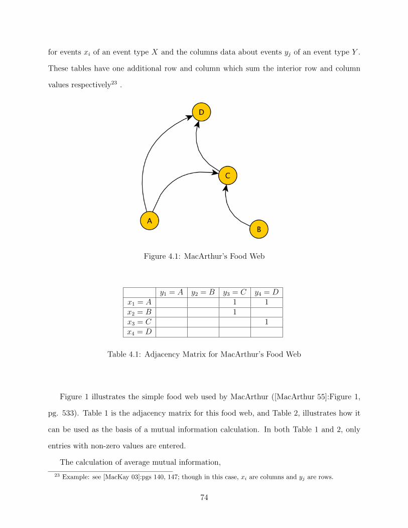
for events xi of an event type X and the columns data about events yj of an event type Y .

These tables have one additional row and column which sum the interior row and column

values respectively23 .

Figure 4.1: MacArthur’s Food Web

y1 = A y2 = B y3 = C y4 = Dx1 = A 1 1x2 = B 1x3 = C 1x4 = D

Table 4.1: Adjacency Matrix for MacArthur’s Food Web

Figure 1 illustrates the simple food web used by MacArthur ([MacArthur 55]:Figure 1,

pg. 533). Table 1 is the adjacency matrix for this food web, and Table 2, illustrates how it

can be used as the basis of a mutual information calculation. In both Table 1 and 2, only

entries with non-zero values are entered.

The calculation of average mutual information,

23 Example: see [MacKay 03]:pgs 140, 147; though in this case, xi are columns and yj are rows.

74

y1 y2 y3 y4 p(xi)x1 p(x1, y3) = 1

4p(x1, y4) = 1

4p(x1) = 2

4

x2 p(x2, y3) = 14

p(x2) = 14

x3 p(x3, y4) = 14

p(x3) = 14

x4

p(yj) p(y3) = 24

p(y3) = 24

Table 4.2: Mutual Information Calculation for MacArthur’s Food Web

IE(G) = ΣiΣjp(xi, yj) logp(xi,yj)

p(xi)×p(yj),

can be related to the terms in Table 2 . The joint probability p(xi, yj) is the cell value

from the adjacency matrix (Table 1) divided by the number of edges. Where the adjacency

matrix cell value is 1, p(xi, yj) = 1|E(G)| , otherwise 0. Let the row total be Ti. = Σjxi and

p(xi) = Ti.|E(G)| is then the marginal probability for xi. Similarly, let the column total be

T.j = Σiyj and p(yj) =T.j|E(G)| is then the marginal probability for yj.

Thus,p(xi,yj)

p(xi)×p(yj)=

1|E(G)|

Ti.|E(G)|×

T.j|E(G)|

= |E(G)|Ti.×T.j ,

so summing over cells in the adjacency matrix with 1 entries,

IE(G) = ΣiΣj1

|E(G)| log |E(G)|Ti.×T.j .

For MacArthur’s food web in Figure 1,

IE(G) = 14

log 42×2

+ 14

log 42×2

+ 14

log 41×2

+ 14

log 41×2

= 0+0 = 14

log 2+ 14log2 = 1

2log 2 = 1

2.

Since, the maximum value for the average mutual information is log|V (G)|, we can express

the relative constraint asIE(G)

log|V (G)| =12

log 4= 1

4.

Figure 2 illustrates the modified food web MacArthur derived while Table 3 provides its

adjacency matrix and Table 4 illustrates the mutual information calculation. MacArthur’s

modified food web is based on the biologically reasonable assumption that the energy leaving

the ecosystem equals that coming into it. This idea is captured by vertex E and the six grey

75

y1 = A y2 = B y3 = C y4 = D y5 = Ex1 = A 1 1 1x2 = B 1 1x3 = C 1 1x4 = D 1x5 = E 1 1

Table 4.3: Adjacency Matrix for MacArthur’s Modified Food Web

y1 y2 y3 y4 y5 p(xi)x1 p(x1, y3) = 1

10p(x1, y4) = 1

10p(x1, y5) = 1

10p(x1) = 3

10

x2 p(x2, y3) = 110

p(x2, y5) = 110

p(x2) = 210

x3 p(x3, y4) = 110

p(x3, y5) = 110

p(x3) = 210

x4 p(x4, y5) = 110

p(x4) = 110

x5 p(x5, y1) = 110

p(x5, y2) = 110

p(x5) = 210

p(yj) p(y1) = 110

p(y2) = 110

p(y3) = 210

p(y4) = 210

p(y5) = 410

Table 4.4: Mutual Information Calculation for MacArthur’s Modified Food Web

76

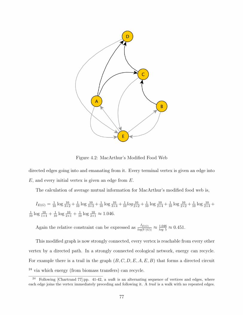
Figure 4.2: MacArthur’s Modified Food Web

directed edges going into and emanating from it. Every terminal vertex is given an edge into

E, and every initial vertex is given an edge from E.

The calculation of average mutual information for MacArthur’s modified food web is,

IE(G) = 110

log 103×2

+ 110

log 103×2

+ 110

log 103×4

+ 110log 10

2×2+ 1

10log 10

2×4+ 1

10log 10

2×2+ 1

10log 10

2×4+

110

log 101×4

+ 110

log 102×1

+ 110

log 102×1≈ 1.046.

Again the relative constraint can be expressed asIE(G)

log|V (G)| ≈1.046log 5≈ 0.451.

This modified graph is now strongly connected, every vertex is reachable from every other

vertex by a directed path. In a strongly connected ecological network, energy can recycle.

For example there is a trail in the graph (B,C,D,E,A,E,B) that forms a directed circuit

24 via which energy (from biomass transfers) can recycle.

24 Following [Chartrand 77]:pp. 41-42, a walk is an alternating sequence of vertices and edges, whereeach edge joins the vertex immediately preceding and following it. A trail is a walk with no repeated edges.

77

Note that in a strongly connected graph, there is at least one entry for every row and

column in the adjacency matrix or flow matrix. If this property did not exist, there would

be some vertex that either connects to no other vertices, or is not connected to any other

vertex.

Fact 1. In a strongly connected graph, there is at least one entry for every row and column

in the corresponding adjacency matrix.

Proof. Since every vertex is reachable from every other vertex by a direct path, each vertex

must have at least one incoming edge (a column entry in the adjacency matrix), and have

at least one outgoing edge (a row entry in the adjacency matrix).

This property is necessary in the adjacency matrix of any strongly connected graph, but

is not sufficient to prove connectivity. For example, if all edges were self-loops, this property

would hold, though the underlying graph is disconnected. If every row and column of the

adjacency matrix has exactly one entry, the corresponding graph is composed of one or more

components, each of which is a directed cycle. If there is only a single component, then the

whole graph is a directed cycle, and therefore also strongly connected. At the other extreme,

if the number of components equals the number of vertices, each component is a self-loop.

These properties can be captured in the notion of a cycle cover.

Definition 5. For a directed graph, G, a cycle cover is a set of vertex disjoint cycles, where

each vertex belongs to exactly one cycle [Kleinberg 06]:pg. 528.

If we consider a self-loop a kind of trivial cycle, then there are three kinds of cycle covers

we could expect, (a) a single directed cycle, (b) a set of components each of which is a

directed cycle, and (c) a set of self-loops. In the first case, the whole graph is minimally

strongly connected; in the second case, each component is minimally strongly connected; in

the third case, each self loop could be considered minimally strongly connected, again in a

A path is a trail with no repeated vertices. A circuit is a trail that begins and ends at the same vertex. Acycle is a circuit that does not repeat any vertices except the first and last. The trail (B,C,D,E,A,E,B)repeats the vertex E, so it is not a directed cycle.

78

trivial sense, since it is the same vertex on the incoming and outgoing edge, rather than

distinct vertices.

Lemma 1. A directed graph, G, is composed solely of a cycle cover (with no additional

vertices or edges), if and only if, it has exactly one entry for each row and column of its

corresponding adjacency matrix.

Proof. In a directed graph, G composed solely of a cycle cover, every vertex belongs to

one cycle only. Therefore every vertex has exactly one incoming and outgoing edge, and

correspondingly is associated with only a single column and row entry. In a directed graph,

G, where there is only a single entry for each row and column of the adjacency matrix, the

underlying graph must be a cycle cover. If any vertex were the member of more than one

cycle, it would have more than one incoming or outgoing edge (and thus more than one

column or row entry). If a vertex was a root, it would have no incoming edge (and thus one

column would have no entry). If any vertex was terminal, it would have no outgoing edge

(and thus one row would have no entry.)

While the property of exactly one entry in every row and column of the adjacency matrix

is not sufficient to prove a graph is strongly connected, it demonstrates that the components

of the graph are strongly connected, even in the trivial case of a graph consisting only of

self-loops.

4.7 Mutual Information and Topological Stability

4.7.1 Roadmap to Our Argument

We now proceed to examining the relationship between mutual information and topological

stability. We first introduce the idea of a mutualistic property, which complements the

concept of antagonistic properties25 developed earlier in this chapter. We then proceed to

25 Our use of the terms mutualistic and antagonistic are inspired by the ecological concepts of mutualismand antagonism, the first being the case where two entities mutually benefit each other and the latter beingthe case where benefit to one entity is a detriment to the other.

79

demonstrate the conditions under which the average mutual information of a graph IE(G)

can be related to our measures of cut-stability, Sk(G), and connection-stability, Sc(G).

Definition 6. Two properties, A and B of an object, are considered mutualistic (or ‘mutually

related’), if for a repeated operation o (excluding the identity operation) conducted i times on

the object, (a) there exists at least one instance where the value of each property changes, and

(b) one property monotonically increases/decreases in value, the other property monotonically

increases/decreases, respectively in value such that:

If: A(o0) ≥ A(o1) ≥ A(o2) ≥ A(o3) ≥ · · · ≥ A(oi),

Then: B(o0) ≥ B(o1) ≥ B(o2) ≥ B(o3) ≥ · · · ≥ B(oi).

If: A(o0) ≤ A(o1) ≤ A(o2) ≤ A(o3) ≤ · · · ≤ A(oi),

Then: B(o0) ≤ B(o1) ≤ B(o2) ≤ B(o3) ≤ · · · ≤ B(oi).

Our essential idea is that in a strongly connected directed graph, the average mutual

information of the graph will generally be antagonistic with cut-stability and mutualistic

with connection stability. We will build up to this result in small steps, by establishing:

1. Our original proof of antagonism for cut-stability and connection-stability

based on undirected graphs can be extended to directed graphs. Once that

is established, we will then relate our topological stability definitions to the

average mutual information via the following steps.

2. Strongly connected directed graphs have at least one entry for every row and

column in their adjacency matrix (demonstrated above).

3. Directed graphs with exactly one entry for every row and column in their

adjacency matrix consist solely of a cycle cover (demonstrated above).

4. Directed graphs consisting solely of a cycle cover are at their maximum bound

for the average mutual information.

80

5. For directed graphs consisting solely of a cycle cover, the first additional edge

must reduce the value of the average mutual information, and thus be antago-

nistic with cut-stability, and conversely mutualistic with connection stability.

6. It is possible to identify conditions under which a strongly connected directed

graph would monotonically decline in average mutual information upon edge

addition.

7. A construction exists, based on layering cycle covers, that represents an upper

bound on the decline of average mutual information as edges are added to a

strongly connected graph.

To build up some intuition around these ideas, we will also go through a graph con-

struction exercise that results in a directed graph with exactly one entry for every row and

column, and analyze the contribution individual terms make.

4.7.2 Cut-Stability and Connection-Stability in Strongly Connected Graphs

First off, let us extend our proof of antagonism from connected undirected graphs, to strongly

connected directed graphs.

Theorem 2. In a strongly connected directed graph, G, Sk(G) and Sc(G) are antagonistic

under the operations of adding or deleting edges

Proof. Cut-stability, Sk(G) is a property of the size of minimum vertex cover, |MVC(G)|.

Since cutting a vertex removes all its associated edges, the directionality of edges does not

affect |MVC(G)|. In the case of connection-stability, Sc(G), edge directionality does matter.

However, if an edge is added that increases Sk(G), it will either decrease Sc(G) or have no

effect, since the graph is already strongly connected. All the addition of an edge can achieve

with respect to Sc(G), is to lower the value of T , time to flood.

This establishes the extension of antagonism from connected undirected graphs to strongly

connected directed graphs. Next, we must establish that a directed graph, consisting solely

81

of a cycle cover is at its maximum bound for average mutual information.

Lemma 2. A directed graph, G, consisting solely of a cycle cover is at its maximum bound

for mutual information, such that IE(G) = log|V (G)|.

Proof. A directed graph, consisting solely of a cycle cover, has the same number of edges as

vertices, as each vertex is in one cycle only, and thus has only one incoming and one outgoing

edge. Therefore, the degree for each vertex is 2. Since for any graph the sum of the degrees,

is twice the number of edges (2|E|) ([Chartrand 77]pg.28), the number of vertices equals the

number of edges.

|V (G)| = |E(G)|.

The adjacency matrix value for each edge, as well as the row and column sums associated

with each edge are all 1. Each edge contributes,

1|E(G)| log

1|E(G)|

1|E(G)|×

1|E(G)|

to the average mutual information.

There are |E(G)| edges and the average mutual information summation is,

|E(G)|( 1|E(G)| log

1|E(G)|

1|E(G)|×

1|E(G)|

) = log|E(G)| = log|V (G)|

To understand the conditions required for cut-stability and the average mutual infor-

mation to be antagonistic, let us first examine a constructive example where they are not

initially antagonistic. We will examine a construction that results in a directed cycle through

all vertices of a graph (which is both a cycle cover and a minimal strongly connected graph).

Via this construction we can examine the relationship between topological stability and mu-

tual information past that point. Our construction proceeds on the adjacency matrix, as

follows.

1. Begin with an empty graph (no edges).

2. Randomly add a directed edge.

82

3. Keep adding random directed edges with the following constraints: (a) the

new edge results in a subgraph that is minimal strongly connected, (b) the

new edge uses a column and row that have no previous entries.

4. Stop, when (b) is no longer possible. The result is a directed cycle through all

vertices of the graph

To simplify our notation a little, we will designate the number of edges in a graph, |E(G)|

by m. So, as we add an edge to a graph, it is designated by m + 1. As each edge is added

in the construction of this directed cycle, the m previous edges contribution to a mutual

information summation are modified. Since all edges have the same cell value, and row and

column sums due to our construction rules, we can determine their contributions to the

mutual information summation by a formula.

There are m edges whose contribution is modified. The original contribution of each of

these edges , prior to addition of the m+1th edge is 1mlog(m). The modified contribution for

each of these edges after the addition of the m+1th edge is, 1m+1

log(m+1).The contribution

of the new edge is 1m+1

log(m + 1). Adding new edges up to a directed cycle on the graph,

increases mutual information because the contribution of the new edge is greater than the

accumulated reductions in contribution from the existing edges. This relationship is captured

in the following inequality,

m( 1mlog(m)− 1

m+1log(m+ 1)) < 1

m+1log(m+ 1).

The left hand side of the inequality are the reductions in contribution for existing edges.

The right hand side is the contribution of the new edge. With some algebraic manipulation

the inequality reduces to,

log(m) < log(m+ 1),

so the additional contribution of each new edge to the mutual information summation is,

83

log(m+1m

).

What if we added one new edge past the creation of the directed cycle through all vertices?

The addition of a new edge would increase cut stability. Would it continue to increase the

mutual information?

It is impossible for this single additional edge (whichever edge we choose to add) to

increase the average mutual information of the graph, because of the relationship,

I(X, Y ) ≤ min((C(X), C(Y )),

places a clear upper bound on the average mutual information. In this case, the maximum

possible value for mutual information is,

C(X) = C(Y ) = log|V (G)|.

Therefore, the addition of any additional edge can only decrease the mutual informa-

tion.26.

Lemma 3. For directed graphs consisting solely of a cycle cover, the addition of a single

edge must reduce the value of the average mutual information, or leave it unchanged.

Proof. By lemma 3, the average mutual information is already at its upper bound in a

directed graph composed solely of a cycle cover. Any additional edge subsequent to the

formation of the cycle cover, must therefore result in a total contribution (the contribution

of the new edge, plus reductions in the contribution of existing edges) that is negative, and

thus reduces the average mutual information below its upper bound.

4.7.3 Monotonicity Conditions

For the average mutual information to be antagonistic with cut-stability and conversely

mutualistic with connection stability, we need to understand the conditions under which a

26 While our construction was specific to the creation of a directed cycle through all the vertices, thedecrease in mutual information past a cycle cover applies without loss of generality, since any graph consistingsolely of a cycle cover will be at its upper bound for average mutual information.

84

sequence of edge additions following a cycle cover will lead to monotonic decrease in the

average mutual information. We first need a formulation that allows us to reason about

changes in the mutual information summation upon addition of edges past a cycle cover27.

We then need to identify conditions in the formulation that are a ‘worst case’, that is,

they contribute as much to the mutual information summation as possible. If, under this

worst case, the mutual information summation still decreases as edges are added, then a

construction exists that will monotonically decrease, and which will decrease slower (upper

bound) than other other possible edge addition sequences which may not monotonically

decrease.

These considerations lead us to construct a formula that tracks changes in the mutual

information summation. Upon addition of an edge there is an addition to: (a) the total

number of edges, (b) the row sum for the row in which the new edge is placed and (c) the

column sum for the column in which the new edge is placed.

As before, we will delineate the number of edges in a graph |E(G)| by m. We note

that the row sum Ti. is just the out-degree of a vertex vi, and the column sum T.j is just

the in-degree of a vertex vj. We will simplify our notation further to emphasize how our

calculations relate to graphs. Let ri be the outdegree of vertex vi and sj the indegree of

vertex vj.

Upon edge addition the number of edges increase by one, the out-degree of a vertex vi

increases by one, and the in-degree of a vertex vj increases by one:

1. m→ m+ 1. Let δ = mm+1

.

2. ri → ri + 1. Let δi = riri+1

.

3. sj → sj + 1. Let δj =sjsj+1

.

27 The development of this formulation and identification of monotonicity conditions for decrease inaverage mutual information upon edge addition is joint work with Peter Hoyer.

85

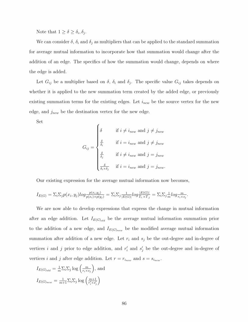
Note that 1 ≥ δ ≥ δi, δj.

We can consider δ, δi and δj as multipliers that can be applied to the standard summation

for average mutual information to incorporate how that summation would change after the

addition of an edge. The specifics of how the summation would change, depends on where

the edge is added.

Let Gij be a multiplier based on δ, δi and δj. The specific value Gij takes depends on

whether it is applied to the new summation term created by the added edge, or previously

existing summation terms for the existing edges. Let inew be the source vertex for the new

edge, and jnew be the destination vertex for the new edge.

Set

Gij =

δ if i 6= inew and j 6= jnew

δδi

if i = inew and j 6= jnew

δδj

if i 6= inew and j = jnew

δδi×δj if i = inew and j = jnew.

Our existing expression for the average mutual information now becomes,

IE(G) = ΣiΣjp(xi, yj)logp(xi,yj)

p(xi)×p(yj)= ΣiΣj

1|E(G)| log

|E(G)|Ti.×T.j = ΣiΣj

1mlog m

ri×sj .

We are now able to develop expressions that express the change in mutual information

after an edge addition. Let IE(G)old be the average mutual information summation prior

to the addition of a new edge, and IE(G)new be the modified average mutual information

summation after addition of a new edge. Let ri and sj be the out-degree and in-degree of

vertices i and j prior to edge addition, and r′i and s′j be the out-degree and in-degree of

vertices i and j after edge addition. Let r = rinew and s = sinew .

IE(G)old = 1m

ΣiΣj log(

mri×sj

), and

IE(G)new = 1m+1

ΣiΣj log(m+1r′i×s′j

)

86

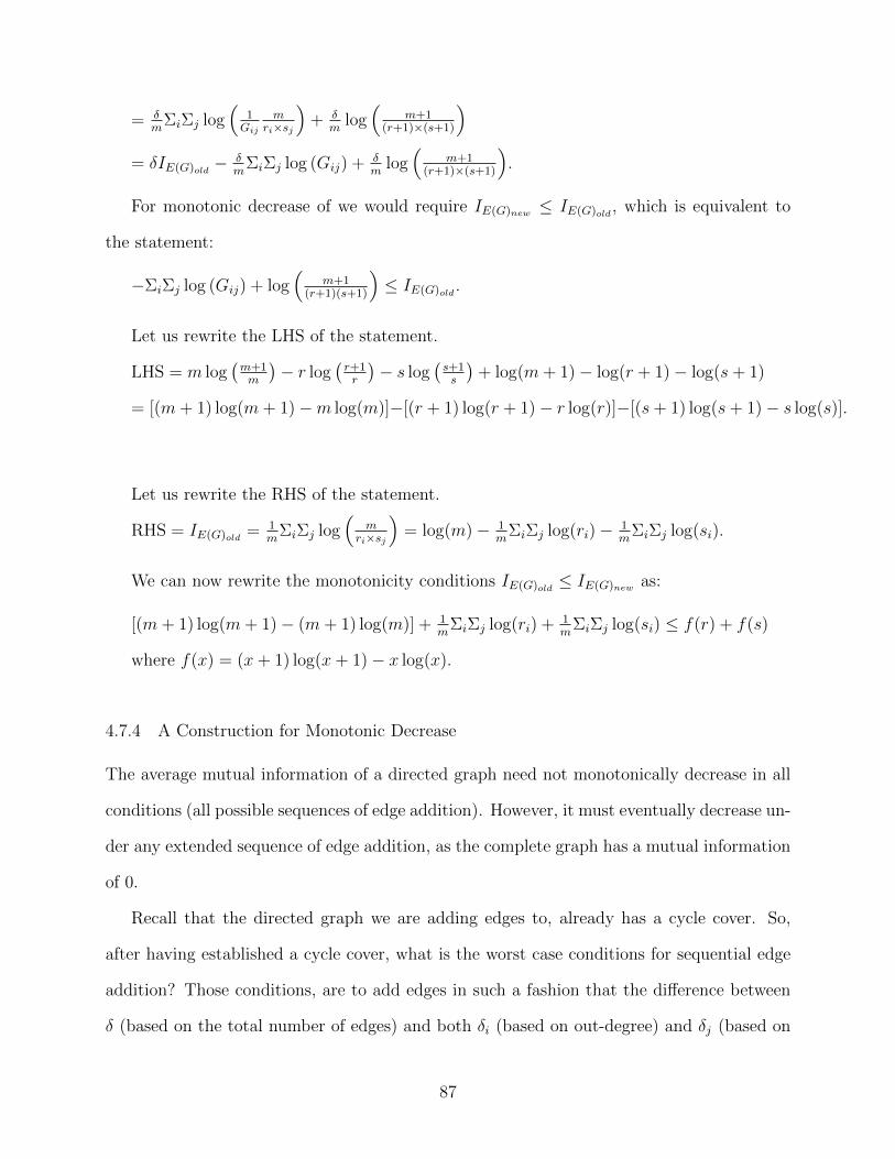
= δm

ΣiΣj log(

1Gij

mri×sj

)+ δ

mlog(

m+1(r+1)×(s+1)

)= δIE(G)old − δ

mΣiΣj log (Gij) + δ

mlog(

m+1(r+1)×(s+1)

).

For monotonic decrease of we would require IE(G)new ≤ IE(G)old , which is equivalent to

the statement:

−ΣiΣj log (Gij) + log(

m+1(r+1)(s+1)

)≤ IE(G)old .

Let us rewrite the LHS of the statement.

LHS = m log(m+1m

)− r log

(r+1r

)− s log

(s+1s

)+ log(m+ 1)− log(r + 1)− log(s+ 1)

= [(m+ 1) log(m+ 1)−m log(m)]−[(r + 1) log(r + 1)− r log(r)]−[(s+ 1) log(s+ 1)− s log(s)].

Let us rewrite the RHS of the statement.

RHS = IE(G)old = 1m

ΣiΣj log(

mri×sj

)= log(m)− 1

mΣiΣj log(ri)− 1

mΣiΣj log(si).

We can now rewrite the monotonicity conditions IE(G)old ≤ IE(G)new as:

[(m+ 1) log(m+ 1)− (m+ 1) log(m)] + 1m

ΣiΣj log(ri) + 1m

ΣiΣj log(si) ≤ f(r) + f(s)

where f(x) = (x+ 1) log(x+ 1)− x log(x).

4.7.4 A Construction for Monotonic Decrease

The average mutual information of a directed graph need not monotonically decrease in all

conditions (all possible sequences of edge addition). However, it must eventually decrease un-

der any extended sequence of edge addition, as the complete graph has a mutual information

of 0.

Recall that the directed graph we are adding edges to, already has a cycle cover. So,

after having established a cycle cover, what is the worst case conditions for sequential edge

addition? Those conditions, are to add edges in such a fashion that the difference between

δ (based on the total number of edges) and both δi (based on out-degree) and δj (based on

87

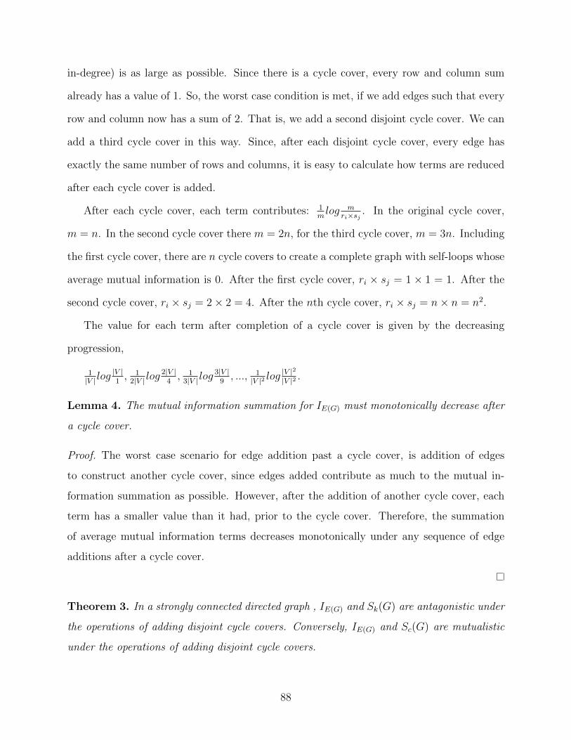
in-degree) is as large as possible. Since there is a cycle cover, every row and column sum

already has a value of 1. So, the worst case condition is met, if we add edges such that every

row and column now has a sum of 2. That is, we add a second disjoint cycle cover. We can

add a third cycle cover in this way. Since, after each disjoint cycle cover, every edge has

exactly the same number of rows and columns, it is easy to calculate how terms are reduced

after each cycle cover is added.

After each cycle cover, each term contributes: 1mlog m

ri×sj . In the original cycle cover,

m = n. In the second cycle cover there m = 2n, for the third cycle cover, m = 3n. Including

the first cycle cover, there are n cycle covers to create a complete graph with self-loops whose

average mutual information is 0. After the first cycle cover, ri × sj = 1 × 1 = 1. After the

second cycle cover, ri × sj = 2× 2 = 4. After the nth cycle cover, ri × sj = n× n = n2.

The value for each term after completion of a cycle cover is given by the decreasing

progression,

1|V | log

|V |1, 1

2|V | log2|V |

4, 1

3|V | log3|V |

9, ..., 1

|V |2 log|V |2|V |2 .

Lemma 4. The mutual information summation for IE(G) must monotonically decrease after

a cycle cover.

Proof. The worst case scenario for edge addition past a cycle cover, is addition of edges

to construct another cycle cover, since edges added contribute as much to the mutual in-

formation summation as possible. However, after the addition of another cycle cover, each

term has a smaller value than it had, prior to the cycle cover. Therefore, the summation

of average mutual information terms decreases monotonically under any sequence of edge

additions after a cycle cover.

Theorem 3. In a strongly connected directed graph , IE(G) and Sk(G) are antagonistic under

the operations of adding disjoint cycle covers. Conversely, IE(G) and Sc(G) are mutualistic

under the operations of adding disjoint cycle covers.

88

Proof. By Lemma 1, a directed graph composed solely of a cycle cover has exactly one entry

in every row and column of its adjacency matrix and a directed graph with exactly one entry

for every row and column in its adjacency matrix is a cycle cover.

By Lemma 3, the addition of a single edge in a graph beyond the creation of a cover

cycle will result in a decrease (or no change) in mutual information.

By Lemma 4, the average mutual information must monotonically decrease after each

addition of a cycle cover.

Since, by Theorem 2, additional edges will add to the cut-stability, Sk(G), of a strongly

connected directed graph, cut-stability and the average mutual information must be antag-

onistic in strongly connected directed graphs under the addition of cycle covers.

Since by Theorem 2, additional edges will decrease the connection stability, Sc(G), in a

strongly connected directed graph, connection-stability and the average mutual information

must be mutualistic under the additon of cycle covers28.

The addition of cycle covers could be seen as providing an upper bound for monotonic

decrease of the IE(G) such that any other edge addition sequence, whether it monotonically

declines, or occasionally increase and then declines, will always be below this upper bound.

We conjecture that the majority of edge addition sequences do monotonically decline, so that

with high probability, IE(G) and Sk(G) are antagonistic while IE(G) and Sc(G) are mutualistic

under edge addition or deletion.

The intuition behind the conjecture of the antagonism between the average mutual

information and cut-stability in strongly connected graphs (and the mutualism between

connection-stability and average mutual information) is quite simple. In a strongly connected

graph, there exists a path between every vertex. Adding an edge will increase cut-stability

28 In this chapter we have stressed the relationship of cut and connection stability to mutual information,a measure of constraints in a network. The fact that the mutual information is bounded by the informationcapacity of the network, allows us to also express a complementary relationship tied to a measure of theuncertainty that remains in the network, given the constraints. Let UE(G) = log|V (G)| − IE(G) and be ameasure of uncertainty. It then follows, that for a fixed |V (G)|, as IE(G) increases, UE(G) must necessarilydecrease. Thus, UE(G) will have the opposite relationship to cut and connection stability as IE(G). UE(G)

will be mutualistic with cut-stability, Sk(G), and antagonistic with connection-stability, Sc(G). IE(G) andUE(G), are similar to Ulanwicz’s ascendency and overhead measures respectively which were reviewed inChapter 3.

89

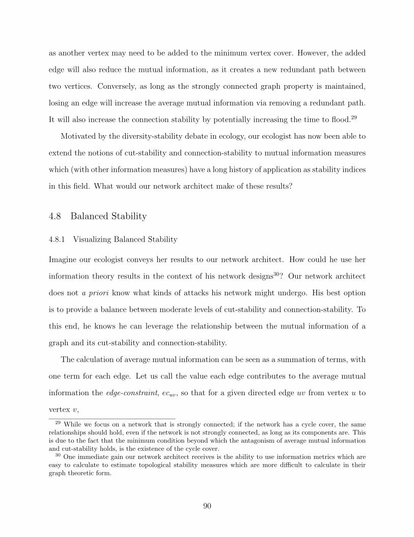
as another vertex may need to be added to the minimum vertex cover. However, the added

edge will also reduce the mutual information, as it creates a new redundant path between

two vertices. Conversely, as long as the strongly connected graph property is maintained,

losing an edge will increase the average mutual information via removing a redundant path.

It will also increase the connection stability by potentially increasing the time to flood.29

Motivated by the diversity-stability debate in ecology, our ecologist has now been able to

extend the notions of cut-stability and connection-stability to mutual information measures

which (with other information measures) have a long history of application as stability indices

in this field. What would our network architect make of these results?

4.8 Balanced Stability

4.8.1 Visualizing Balanced Stability

Imagine our ecologist conveys her results to our network architect. How could he use her

information theory results in the context of his network designs30? Our network architect

does not a priori know what kinds of attacks his network might undergo. His best option

is to provide a balance between moderate levels of cut-stability and connection-stability. To

this end, he knows he can leverage the relationship between the mutual information of a

graph and its cut-stability and connection-stability.

The calculation of average mutual information can be seen as a summation of terms, with

one term for each edge. Let us call the value each edge contributes to the average mutual

information the edge-constraint, ecuv, so that for a given directed edge uv from vertex u to

vertex v,

29 While we focus on a network that is strongly connected; if the network has a cycle cover, the samerelationships should hold, even if the network is not strongly connected, as long as its components are. Thisis due to the fact that the minimum condition beyond which the antagonism of average mutual informationand cut-stability holds, is the existence of the cycle cover.

30 One immediate gain our network architect receives is the ability to use information metrics which areeasy to calculate to estimate topological stability measures which are more difficult to calculate in theirgraph theoretic form.

90

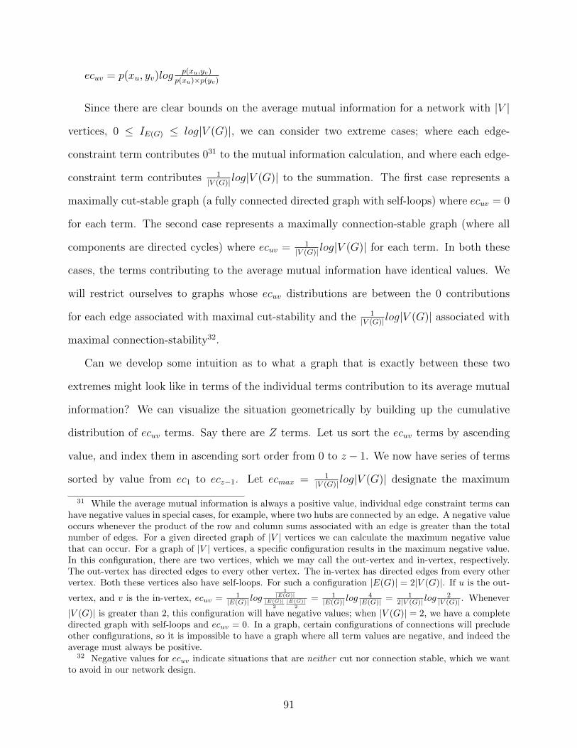
ecuv = p(xu, yv)logp(xu,yv)

p(xu)×p(yv)

Since there are clear bounds on the average mutual information for a network with |V |

vertices, 0 ≤ IE(G) ≤ log|V (G)|, we can consider two extreme cases; where each edge-

constraint term contributes 031 to the mutual information calculation, and where each edge-

constraint term contributes 1|V (G)| log|V (G)| to the summation. The first case represents a

maximally cut-stable graph (a fully connected directed graph with self-loops) where ecuv = 0

for each term. The second case represents a maximally connection-stable graph (where all

components are directed cycles) where ecuv = 1|V (G)| log|V (G)| for each term. In both these

cases, the terms contributing to the average mutual information have identical values. We

will restrict ourselves to graphs whose ecuv distributions are between the 0 contributions

for each edge associated with maximal cut-stability and the 1|V (G)| log|V (G)| associated with

maximal connection-stability32.

Can we develop some intuition as to what a graph that is exactly between these two

extremes might look like in terms of the individual terms contribution to its average mutual

information? We can visualize the situation geometrically by building up the cumulative

distribution of ecuv terms. Say there are Z terms. Let us sort the ecuv terms by ascending

value, and index them in ascending sort order from 0 to z − 1. We now have series of terms

sorted by value from ec1 to ecz−1. Let ecmax = 1|V (G)| log|V (G)| designate the maximum

31 While the average mutual information is always a positive value, individual edge constraint terms canhave negative values in special cases, for example, where two hubs are connected by an edge. A negative valueoccurs whenever the product of the row and column sums associated with an edge is greater than the totalnumber of edges. For a given directed graph of |V | vertices we can calculate the maximum negative valuethat can occur. For a graph of |V | vertices, a specific configuration results in the maximum negative value.In this configuration, there are two vertices, which we may call the out-vertex and in-vertex, respectively.The out-vertex has directed edges to every other vertex. The in-vertex has directed edges from every othervertex. Both these vertices also have self-loops. For such a configuration |E(G)| = 2|V (G)|. If u is the out-

vertex, and v is the in-vertex, ecuv = 1|E(G)| log

1|E(G)|

|E(G)|2

|E(G)|2

= 1|E(G)| log

4|E(G)| = 1

2|V (G)| log2

|V (G)| . Whenever

|V (G)| is greater than 2, this configuration will have negative values; when |V (G)| = 2, we have a completedirected graph with self-loops and ecuv = 0. In a graph, certain configurations of connections will precludeother configurations, so it is impossible to have a graph where all term values are negative, and indeed theaverage must always be positive.

32 Negative values for ecuv indicate situations that are neither cut nor connection stable, which we wantto avoid in our network design.

91

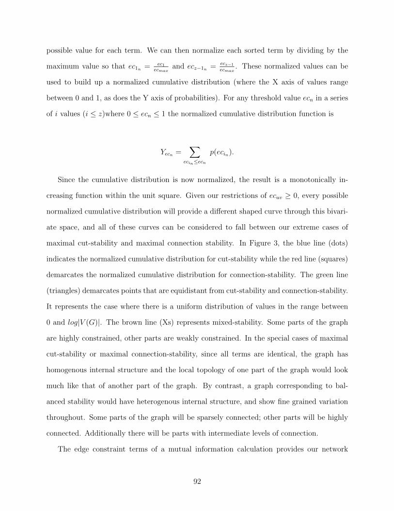
possible value for each term. We can then normalize each sorted term by dividing by the

maximum value so that ec1n = ec1ecmax

and ecz−1n = ecz−1

ecmax. These normalized values can be

used to build up a normalized cumulative distribution (where the X axis of values range

between 0 and 1, as does the Y axis of probabilities). For any threshold value ecn in a series

of i values (i ≤ z)where 0 ≤ ecn ≤ 1 the normalized cumulative distribution function is

Yecn =∑

ecin≤ecn

p(ecin).

Since the cumulative distribution is now normalized, the result is a monotonically in-

creasing function within the unit square. Given our restrictions of ecuv ≥ 0, every possible

normalized cumulative distribution will provide a different shaped curve through this bivari-

ate space, and all of these curves can be considered to fall between our extreme cases of

maximal cut-stability and maximal connection stability. In Figure 3, the blue line (dots)

indicates the normalized cumulative distribution for cut-stability while the red line (squares)

demarcates the normalized cumulative distribution for connection-stability. The green line

(triangles) demarcates points that are equidistant from cut-stability and connection-stability.

It represents the case where there is a uniform distribution of values in the range between

0 and log|V (G)|. The brown line (Xs) represents mixed-stability. Some parts of the graph

are highly constrained, other parts are weakly constrained. In the special cases of maximal

cut-stability or maximal connection-stability, since all terms are identical, the graph has

homogenous internal structure and the local topology of one part of the graph would look

much like that of another part of the graph. By contrast, a graph corresponding to bal-

anced stability would have heterogenous internal structure, and show fine grained variation

throughout. Some parts of the graph will be sparsely connected; other parts will be highly

connected. Additionally there will be parts with intermediate levels of connection.

The edge constraint terms of a mutual information calculation provides our network

92

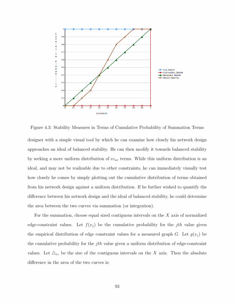
Figure 4.3: Stability Measures in Terms of Cumulative Probability of Summation Terms

designer with a simple visual tool by which he can examine how closely his network design

approaches an ideal of balanced stability. He can then modify it towards balanced stability

by seeking a more uniform distribution of ecuv terms. While this uniform distribution is an

ideal, and may not be realizable due to other constraints, he can immediately visually test

how closely he comes by simply plotting out the cumulative distribution of terms obtained

from his network design against a uniform distribution. If he further wished to quantify the

difference between his network design and the ideal of balanced stability, he could determine

the area between the two curves via summation (or integration).

For the summation, choose equal sized contiguous intervals on the X axis of normalized

edge-constraint values. Let f(xj) be the cumulative probability for the jth value given

the empirical distribution of edge constraint values for a measured graph G. Let g(xj) be

the cumulative probability for the jth value given a uniform distribution of edge-constraint

values. Let 4x, be the size of the contiguous intervals on the X axis. Then the absolute

difference in the area of the two curves is:

93

AbsDiffAreas = Σj |f(xj) − g(xj)| 4x, where |f(xj) − g(xj)| is the absolute value of

the difference.

For differentiation, let the interval sizes become infinitesimals.

Now the absolute difference in the area of the two curves is:

AbsDiffAreas =∫ 1

0|f(xj)− g(xj)| dx

AbsDiffAreas may be interpreted as a measure of distance from balanced stability of a

measured graph G. Since we are keeping the summation (or integration) bounded between

0 (the network matches the uniform distribution of balanced stability) and the area of a

triangle (representing either maximum cut stability or maximum connection stability) in the

unit square, the maximum value is 12, which in the case of maximal cut-stability is the area

above the balanced stability line, and in the case of maximal connection stability is the area

below the balanced stability line.

This gives our network designer a first cut approximation of balanced stability. But

he could go further. He could reason that the cumulative distribution gives him an idea

of the overall contribution of terms, but no idea of how they are locally organized within

the network. For example, say all the vertices with smaller values are closer to each other

than vertices with larger value. Over the whole network, the cumulative distribution might

approximate a uniform distribution – but there might be local regularities that might be

leveraged by an attacker.

4.8.2 Balanced Stability and Information Hiding

Networks are subject to various kinds of attacks. Can we extend our concept of balanced

stability order to develop the notion of a network architecture for which an adversary would

have a difficult time determining which type of attack to launch?

Our network designer now considers – what might a network look like with no local

regularities that would allow an attacker to decide between a cut-attack and a connection-

94

attack? He imagines an attacker taking a walk on his network, moving from vertex to

vertex via directed edges (and he imagines the attacker does not hit any vertex or edge

more than once). This attacker can count the edges into and out from each vertex he has

sampled, and thus locally calculate ecuv for each edge along the vertices he has traversed.

Balanced stability would be the case where if he walked t steps, and calculated the value of

some property on each vertex (in our case ecuv), he would have no information by which to

predict the value of that property as he proceeded over the next edge, prior to reaching it,

and actually measuring it. He would simply have to guess the next value randomly from a

uniform distribution.

Let m1...t be the sequence of values measured (or calculated from measurements) for

some local graph property in t steps33 (the local properties could be measured on either the

vertices or the edges). Let mt+1 be the value of the property measured or calculated in the

next step. Let kt be the number of distinct values observed in the sequence m1...t34.

If, knowing the values on our walk m1...t provides no information by which to predict the

value encountered on our next vertex, mt+1, all we can do is guess at the value by assuming

a uniform distribution bounded between the lowest and highest values we have encountered

so far. Without additional prior information, it is impossible to do more. In this case we

have the probability of at most 1kt

of guessing the correct value35. There is no information

gained in the walk that helps us to predict the value of the next step in the sequence.

Definition 7. Perfect Information Hiding (PIH) exists on a graph, G, if and only if for

every t-step walk on the vertices (or edges) of a graph via traversing edges (or vertices) in

which no previously encountered edge (or vertex) is crossed, information obtained on the

33 Consider m1...t to denote the series of values from t sequential measurements, m1,m2,m3...mt.34 Depending on the nature of the measurement taken, the maximum possible value for kt, which we

will denote kmax, might be pre-determined. For example, if we know we are in an undirected graph of |V |vertices without self-loops, and our measured value is the degree of each vertex, then kmax = |V | − 1 whichis the largest possible degree for a vertex. In general, as we extend the walk beyond t, it may be possible tomeasure new distinct values.

35 If our walk so far has not encountered the true upper or lower bounds for our measured values, ourprobability is less than 1

kt.

95

previous vertices (or edges) for some property m provides no information on m for the next

vertex encountered.

If m has k distinct values observed in t steps,

p(mt+1|m1...t) ≤ 1kt

.

Since,

p(mt+1|m1...t) = p(m1...t,mt+1)p(m1...t)

.

If m1...t provides no information on mt+1, then m1...t and mt+1 are independent. In

the case of independence, the joint probability of a pair of events is equal to product of

the probabilities for each event [Hacking 01]:pp.25, 41-42, 60-62. Thus, p(m1...t,mt+1) =

p(m1...t)p(mt+1). Therefore,

p(mt+1|m1...t) = p(m1...t)p(mt+1)p(m1...t)

p(mt+1|m1...t) = p(mt+1)

Given we (a) only have information from previous measurements, and (b) no criteria on

which to bias our guesses over k distinct values encountered in t steps, and (c) there is the

possibility that a new distinct value may be encountered in the next step,

p(mt+1|m1...t) = p(mt+1) ≤ 1kt

.

PIH can be seen as an ideal, which may not be fully realized, for both graph theoretic

and practical reasons in the context of designing a network. PIH indicates very fine but

unpredictable sub-structuring of the graph in terms of the local property to be measured.

Two examples of properties we could apply PIH to are the ecuv values for each term

in a mutual information calculation for a sequence of edges, or the degree distribution for

a sequence of vertices. If applied to the values for each term in a mutual information

calculation, PIH extends our concept of balanced stability above. However, PIH can be

applied to any measurable property of a sequence of vertices edges.

96

Perfect Balanced Stability (PBS) is a special case of PIH. Perfect Balanced Stability

(PBS) exists on a graph, G, if PIH exists on G for the property, m measured on each edge,

where m is ecuv.

For PBS the cumulative distribution of observations of ecuv on every walk will be that

for a uniform distribution.

The idea of perfect information hiding on a graph from which we draw our concept of per-

fect balanced stability is quite similar to von Mises definition of randomness [von Mises 81],

as well as two other information theoretic concepts: Shannon’s information theoretic defi-

nition of perfect secrecy [Shannon 49] and the notion of the algorithmic complexity of a se-

quence which was independently developed by Kolmogorov [Kolmogorov 68b, Kolmogorov 68a],

Solomnoff [Solomonoff 64a, Solomonoff 64b], and Chaitin [Chaitin 66].

In von Mises classic text on probability, ‘Probability statistics and Truth’ randomness is

conceptualized in terms of a sequence of observations he calls a ‘collective’ [von Mises 81].

While his examples of collectives are sequences of observations made by casting dice, or

observing small and large stones during a walk, the idea applies equally to the observations

made during the walk of a graph [von Mises 81]:pp. 24-25.

‘A collective appropriate for the application of the theory of probability must fullfill two

conditions. First the relative frequencies of the attributes must possess limiting values.

Second, these limiting values must remain the same in all partial sequences which may

be selected from the original one in an arbitrary way.’

PIH occurs when the sequence of local property values obtained from any walk on a

graph are effectively random. If PIH holds not only at a walk of length t but between every

subsequence of that walk, and the next vertex encountered, the values obtained in the walk

must be random.

Shannon’s notion of perfect security [Shannon 49] is based on leveraging the relationship

between conditional probability and statistical independence. Shannon states the essential

97

idea simply in terms of cryptograms, E and the plaintext message PE(M) they correspond

to : [Shannon 49]: pg. 680.

‘The cryptanalyst intercepts a particular E and can then calculate, in principle at least,

the a posteriori probabilities for the various messages, PE(M). It is natural to define

perfect secrecy by the condition that, for all E the a posteriori probabilities are equal to

the a priori probabilities independently of the values of these. In this case, intercepting

the message has given the cryptanalyst no information.’

Luenberger [Luenberger 06]:pp. 186-189 summarizes Shannon’s key idea that perfect

security requires statistical independence between messages and ciphertext. Let M be a

plaintext message (Shannon’s PE(M)) and C the ciphertext of the encrypted message (Shan-

non’s E). A system is perfectly secure, if for all possible messages M , the probability of the

message given the ciphertext, p(M |C) is equal to the probability of the message, p(M).

p(M |C) = p(M).

So, the probability of a particular message, M is unchanged by information about the

ciphertext.

In such a case, the average mutual information across all messages and ciphertexts, is 0,

I(M,C) = 0.

By Bayes’ Rule [Tijms 07]:pp. 251-256:

p(M |C) = p(C|M)p(M)p(C)

.

p(M |C) = p(M) only if p(C|M) = p(C), which happens only if M and C are independent

so that,

p(M |C) = p(C)p(M)p(C)

= p(M).

In the case of PIH, the observations made during a walk of length t correspond to the

ciphertext, and the value of the next step in the walk, constitutes the message.

PIH relates also to the problem of inductive inferences, which leads directly to algorith-

98

mic information theory. Solomonoff [Solomonoff 64a, Solomonoff 64b] viewed all inductive

inference problems as essentially concerning whether given a sequence of symbols (say the

data from an experiment, or a walk upon a graph), the possibility of extrapolating the next

values in the sequence. [Solomonoff 64a]: pp. 2:

The problem will be the extrapolation of a long sequence of symbols – those symbols being

drawn from some finite alphabet. More specifically given a long sequence, represented by T ,

what is the probability that it will be followed by the subsequence represented by a? .... we

want c(a, T ), the degree of the confirmation of the hypothesis that a will follow, given the

evidence that T has just occurred.

In the context of PIH, the sequence are those observations already obtained by walking

a graph, and we want to infer a subsequence which is the next observation to be made in

the walk. Can observations in our walk so far help us to predict the next observation?

Solomonoff [Solomonoff 64a, Solomonoff 64b], and independently Kolmogorov [Kolmogorov 68b,

Kolmogorov 68a] and Chaitin [Chaitin 66], all arrived at the same solution creating the field

of algorithmic information theory, and its associated measure Kolmogorov complexity36. The

essential idea is that the Kolmogorov complexity, Ck(S) of a sequence is the minimal length

program d(S) that can generate the sequence. From Chapter 3,

Ck(S) = |d(S)|.

This measure can be related to the degree of randomness of the sequence S in that for a

random string, the Kolmogorov complexity is approximately the length of the string. That

is, if a sequence is random, the minimal program to generate the sequence is approximately

the size of the sequence itself. In that sense, random sequences are incompressible [Li 97]:pp.

36 A capsule summary of the different approaches by which algorithmic information theories three co-founders arrived at their results is given in [Muller 07]. A detailed consideration of Solomonoff’s ideas oninductive reasoning is in [Li 97]: Chapter 5. The idea that all approaches towards defining randomnesseventually arrive at algorithmic information theory is explored by [Volchan 02] who notes (pg. 48) ‘Inter-estingly, all these proposals ended up involving two notions apparently foreign to the subject of randomness:algorithms and computability. With hindsight, this is not totally surprising. In a sense to be clarified as weproceed, randomness will be closely associated with “noncomputability.”’

99

379.

It follows that if PIH holds at t steps and for all smaller walks with less that t steps, then

the best we can do to infer the next observation in a walk on a graph given the previous

observations is to simply guess. As we build up the sequence of observations, step by step,

PIH requires the sequence of observed values to be incompressible.

It may be that PIH may not hold for some graph topologies, due to other graph properties

providing the basis for an informed guess37. In that case, PIH represents the theoretical ideal

of perfect information hiding, and any demonstration the ideal can not be met because it

violates some other graph property, guarantees information leakage.

PBS simply follows by applying PIH to a particular locally observed graph property, ecuv.

Both PIH and PBS are intimately tied to the idea of random sequences via the connection

to algorithmic information theory. Furthermore, the existence of PBS depends now, not only

on the average value of the mutual information, but also on the distribution of the terms

contributing to the mutual information as encountered in a walk on the graph.

For PIH to exist in a graph, every sequence of t local values obtained from a walk on the

graph must be independent of the t+ 1th value obtained in the next step, and the sequences

of values are themselves incompressible or random. Conversely, if it can be demonstrated

for a particular graph that independence does not hold between m1...t and mt+1 or if it can

be demonstrated that the sequences t are compressible, then that graph can be said to leak

information about itself.

4.9 Connections to Other Perspectives

Our perspectives in this chapter have been drawn from both ecology and a network archi-

tect’s focus on designing a robust network that resists cut-attacks and connection-attacks.

37 As an example consider in particular invariant properties of graphs, where the same relationship holdsfor every graph. One example is the relationship between the sum of the degree distribution on verticesand the total number of edges, where the sum of the vertex degrees equals twice the number of edges[Chartrand 77]:pp. 28.

100

The concepts developed in this chapter can be applied to other perspectives such as error

and attack tolerance in technological networks, specific stabilizing mechanisms theorized to

operate in ecological networks, and to mechanisms believed to stabilize social networks. Ad-

ditionally, the stability concepts developed here may have relations to other mathematical

approaches such as graph spectra. Application of the topological stability concepts developed

here complements stability concepts from other existing perspectives on complex networks

and provides additional insight into both the mechanisms associated with stability, as well

as the stability ramifications of the underlying network models. Connections to these other

perspectives are briefly discussed below. These connections identify specific lines of appli-

cation along which the theory of topological network stability may be extended in future

work.

4.9.1 Error and Attack Tolerance for Complex Networks

Together our network architect and our ecologist have conceptualized topological network

stability by formalizing intuitive concepts from their respective fields. In this section we

briefly examine how our network architect could apply those concepts to gain insights into

the existing literature of network resistance to errors and attacks.

Our approach has been to develop our topological stability concepts in the general

context of undirected and directed graphs, and general attack strategies, cut-attacks and

connection-attacks, rather than in terms of specific graph generation models or detailed at-

tack protocols38. We want to understand how a network’s topology may be resistant to

attacks that cannot be anticipated. Much of the model specific literature deals with vari-

ants of our cut-stability and connection-stability concepts in the context of specific attack

protocols. In Chapter 1, we noted a number of literature examples of cut-stability in In-

ternet [Albert 00, Calloway 00, Cohen 00b, Cohen 01, Crucitti 04, Gallos 05] and ecological

38 For example, the scale-free, small-worlds, or the Erdos-Renyi random graphs models which were brieflysummarized in Chapter 3. Attack protocols could include random attacks, or directed attacks proceeding indescending vertex degree order.

101

[Sole 01] studies tied to the scale-free model, all of which indicate these networks can resist

random attacks, but are susceptible to directed attacks (that usually begin with the highest

degree vertices). From our perspective, these results follow naturally from scale-free graphs

having a relatively small vertex cover relative to the total number of vertices in a graph, such

that the ratio |MVC(G)||V (G)| is small. Therefore, the probability of hitting an element of MVC(G)

in a random attack is small, but a directed attack on elements of MVC(G) will be highly

effective in disrupting the graph structure, since only a relatively small portion of the total

network needs to be attacked. This is particularly true in Barabasi and Alberts preferential

attachment model for scale free graphs [Barabasi 99] where the bias of new vertices to attach

to existing vertices with high degree essentially guarantees that the minimum vertex cover

will increase at a slower rate than the rate of increase for vertices so that as the network

grows, the ratio |MVC(G)||V (G)| gets smaller and smaller39.

A recent study [Buldyrev 10, Vespignani 10] notes that when two networks are coupled

together and therefore interdependent, such as increasingly occurs between power networks

and Internet networks, they are more vulnerable to cascading failures than any single network

prior to coupling. Their results were obtained using percolation theory applied to pairs

of Erdos–Renyi random networks and scale-free networks respectively. Within a pair of

networks (generated via the same model), every vertex in one network is assumed to be

39 Using reasoning similar to that applied to the preferential attachment model, we can easily see the topo-logical stability consequences for other popular network generation models. Watts and Strogatz [Watts 98]and Kleinberg [Kleinberg 00] have both produced models which generate small worlds graphs. Key toboth models is the addition of extra edges to a regular graph (random rewiring) that connect directlynodes that would otherwise be distant (have a long path between them). The consequence of such ad-ditions is to increase cut-stability (the extra edges can add to the size of |MVC(G)|), but at the costof decreasing connection stability (the extra edges create shortcuts that can reduce the time to floodG). In particular, Kleinberg’s ideas have been extended to examine the searchability of arbitrary graphs[Duchon 06a, Duchon 06b, Fraigniaud 09, Fraigniaud 10]. These methods depend on making a graph moresearchable via augmenting a ‘base graph’ with additional random edges. The probability of an augmentededge from u to v is proportional to the distance(path length) between u and v. Again, any increase in search-ability due to creation of edges comes at a cost of connection-stability. Finally, the Erdos-Renyi randomgraph generation model [Chung 06]:pp. 91-92, depends on two parameters, n, the number of vertices, andp, the probability of selecting an edge. For a fixed number of vertices (constant n) as p approaches one,the graphs generated are increasingly cut-stable as they approach the complete graph at p = 1. Via theantagonism of cut-stability and connection-stability, as p approaches 1 the generated graphs are decreasinglyconnection-stable.

102

linked to a single vertex in the other member of the pair, and is functionally dependant

on it. Failure of a vertex in one network causes a coupled failure in a vertex of the paired

network. We can understand this phenomena of coupled networks being more vulnerable

to cascading failures via connection-stability, without reference to a specific network model.

For a pair of networks, there is now a set of additional edges linking the two networks which

provide pathways so that an instability that begins in one network can move virally to the

other network. Let us consider two undirected networks G1 and G2 with the same number

of vertices, so |V (G1)| = |V (G2)|. G1 and G2 are each connected networks. Let Sc(G1) = T1

be the connection-stability of G1 on its own. Let Sc(G2) = T2 be the connection-stability

of G2 on its own. These are the connection-stabilities if the networks were independent of

each other. Now, consider each vertex in G1 to have an edge connecting it to some vertex

in G2. This allows the possibility of some pair of vertices in G1 (or G2) to have a shorter

path connecting them via vertices in G2 (or G1) than exists in G1 (or G2) on its own. Let

T (G1|G2) represent the number of iterations required to flood G1 given a coupled network G2

exists. Let T (G2|G1) represent the number of iterations required to flood G2 given a coupled

network G1 exists. Then T (G1|G2) ≤ T1 and T (G2|G1) ≤ T2. The connection-stability of

the networks thus becomes sub-additive so that Sc(G1 + G2) ≤ Sc(G1) + Sc(G2). Coupling

the networks results in equal or less connection-stability for each of the networks, due to the

creation of alternate routes for flooding. The cascade due to coupling can be particularly

rapid if vertices that are distant in one network are connected via vertices that are close in

the second coupled network, so that a cascade beginning in the first network, can utilize the

second network to rapidly flood nodes that would otherwise be distant.

The brief examples above illustrate the utility of our topological stability approach to

provide a general route to insights originally obtained through, and tied to specific net-

work generation models. Recent studies of networks from a defence/security perspective

increasingly focus on (a) graph properties that are not tied to specific graph generation

103

models [Dekker 04], (b) the actual topologies networks under attack or surveillance evolve to

[Lindelauf 09], or (c) on strategies by which networks may actively re-structure themselves to

resist attack [Nagaraja 06, Nagaraja 08]. The three defense strategies to topological attacks

investigated by Nagaraja and Ross [Nagaraja 06] can be interpreted in terms of topological

stability40. The ‘random replenishment’ strategy consists of replacing vertices lost due to

attack with new vertices that are randomly attached to existing vertices, leading to a more

amorphous network. This corresponds to replenishing the minimum vertex cover for the

network, and thus its cut-stability. The ‘dining steganographers’ strategy consists of replac-

ing high degree vertices with rings of vertices, so that external connections of the original

vertex are distributed uniformly across the ring. Essentially this defence strategy increases

the connection-stability of a network by slowing down the rate at which the network can be

flooded. The ‘revolutionary cells’ strategy is similar except that now high degree vertices

are replaced with a clique41. It increases the cut-stability of the network by replacing sin-

gle vertices with cliques. In a study where networks are attacked in alternating waves of

targeted and random attacks [Tanizawa 05] the network structure that was the slowest to

degrade had a bimodal distribution with a proportion of the vertices forming a single clique

(small contributions to mutual information) and the remainder having a single edge (larger

contributions to mutual information) connecting it to the clique, a very simple form of mixed

stability.

4.9.2 Keystone Species, Indirect Effects and Cycling in Ecological Networks

What applications might our ecologist find for the topological stability concepts to integrate

theory in her field. Three concepts associated with stability of ecosystems are ‘keystone

species’, ‘indirect effects’ and ‘cycling’. Below we briefly examine each of these concepts and

40 The antagonism between cut-stability and connection-stability is defined in terms of alternate edgeconfigurations for a graph with a fixed set of vertices. The defense strategies below all consist of addingvertices to a network, so their cut-stability and connection-stability implications must be interpreted withrespect to alternate graphs with the same number of vertices.

41 A clique is a subset of the vertices of a graph, where every pair of vertices is adjacent.

104

how they can be related to topological stability.

Keystone species are members of an ecological community that have a disproportionately

large influence on community structure. In the context of ecological networks characterized

by trophic interactions, keystone species may be considered those species which, if removed,

lead to a major restructuring of the food web [Jain 02, Jordan 09, Jordan 05, Jordan 99,

Quince 05]. An intuitive concept, keystone species have been defined in various operational

ways by different authors42. Jordan notes [Jordan 09]:pp.1735 that perhaps the simplest

identifier of a keystone species in a food web is the degree of the vertex associated with

that species (combining both incoming and outgoing edges)43. Thus the ‘keystoneness’ is

associated with vertex degree. Another relatively straight-forward approach is to define

keystoneness via a simulation where certain species are knocked out, and species dependant

on them are eliminated. Keystoneness is now tied to whether such a simulated knock-out

signifcantly changes the structure of the graph beyond the initial vertex removed [Quince 05].

Indirect effects can be defined in contrast to direct effects. If direct effects refers to

any two species that share an edge in a trophic network, indirect effects refer to species

between which a path exists [Fath 99]:pg. 173, [Jordan 01]:pg. 1844. Some researchers also

include as indirect effects the ability of one species to modify the direct effects (i.e. the

value of the edge) between a pair of directly linked species [Wootton 94]:pg. 445. Several

researchers have demonstrated that indirect effects may have greater influence than direct

effects such that two species connected by a path have a stronger relationship than the

direct connections of either species [Fath 98, Fath 99, Jordan 01, Higashi 86, Higashi 89]45.

42 Indeed keystone species are defined in different not only across research groups, but also in several ofthe papers above with a common author, F. Jordan.

43 Jordan et al. [Jordan 05] provides a nice illustration of keystone species in marine ecosystems wherea few species such anchovies and sardines act like hubs connecting lower trophic levels (species anchoviesand sardines can eat) to higher trophic levels (species that eat anchovies and sardines), where the lower andhigher trophic levels have many more species than the hubs. Such ecosystems are then very sensitive to lossof these hub species, which act as keystones.

44 Indirect effects are also similar to Yodzis [Yodzis 00] conception of ‘diffuse effects’, which refers to themediating action of nonlocalized effects of other species on the interaction between a pair of species.

45 Bondavalli and Ulanowicz [Bondavalli 99] provide a nice illustration of indirect effects in cyprus swamps.They find the direct negative effects of alligators on certain prey (frogs, mice and rats), to be more than

105

A recent series of empirical papers on ecological flow networks demonstrates that indirect

effects come to rapidly dominate direct flows [Borrett 07, Borrett 10, Salas 11]. Keystone

species and indirect effects are not mutually exclusive concepts, in that a keystone species

influence might very well be via its indirect effects.

The concepts of indirect effects and keystone species can be viewed in light of topological

stability by asking of them seemingly naive questions. If keystone species are important for

stabilizing ecosystems, why are not all species keystone species? On the simplest definition of

a keystone species, vertex degree, this would imply a trophic network that can be represented

as a complete graph. It would also represent maximum cut stability. However, in that case,

the very meaning of keystone species would disappear, since loss of a single species would be

compensated for by connections through other species. However, from a connection-stability

perspective, in such a complete graph, any fluctuation in one species may rapidly transfer

to, and potentially disrupt, all other species. If indirect effects are important for stabilizing

ecosystems, why are they not maximal? If the trophic network were a large directed cycle,

most effects between species pairs would be indirect. It would also represent maximum

connection stability. However in such a case, there are no alternate trophic pathways, and

the ecosystem would be extremely vulnerable to loss of species. Actual ecosystems are

arranged between these two extremes in some semblance of balanced stability.

Cycling is another concept long associated with stability in ecosystems. It concerns

whether a resource (either energetic or nutrient) will be used again by the same species, i.e.

recycled. Lindeman’s original diagramattic view of energy cycling in ecosystems [Lindeman 42]

has been formalized into various cycling indices [Fath 07a, Finn 76, Patten 85, Patten 84,

Patten 90, Ulanowicz 83, Ulanowicz 04] and is associated with the existence of strongly con-

nected components which create subsystems in the ecological network [Allesina 05, Borrett 07].

compensated by the indirect positive effects on those prey, by alligators also feeding on their predators (turtlesand snakes). Notably, alligators also play a keystone species role in cyprus swamps. Indirect effects are alsoa complicating factor in attempts to ‘manage’ ecosystems. The classic cautionary tale is the use of DDT oncrop pests having unanticipated effects further up the food chain on predatory birds [Ulanowicz 09b]:pg. 7.

106

Intuitively, cycling concerns the movement of both energy (locked in the biomass of the dif-

ferent species) and nutrient flows through an ecosystem in such a way the energy or nutrients

cycle through the system, rather than being lost to the system. The usual picture of ecosys-

tem cycling begins with energy and nutrients captured initially in plants then flowing through

various levels of herbivores and predators, and then as individuals die, decomposers make

the energy and nutrients stored in biomass once again available to the system in simpler

form. Fath and Halnes [Fath 07a]:pg.18, provide a succinct structural definition that can be

applied to ecological networks:

‘A structural cycle is the presence of a pathway in the ecological network in which

matter-energy passes through biotic or abiotic stores returning for availability to the

same or lower trophic levels. Structural cycling is present ion food webs due to intraguild

predation, cannibalism, or other predation events that connect laterally or backwards in

the hierarchy.’

The conditions under which mutual information can be interpreted as a topological sta-

bility measure require exactly such structural cycling, via the existence of strongly connected

components.

The ecological concepts detailed in this chapter all hinge on material transfers from

species to species. They may have analogues in the field of economics, if we move from

trophic networks to networks of goods and services. Recent papers have begun to apply

lessons from stability in ecological networks, to economic networks taking both information-

theoretic [Goerner 09] and dynamical systems [May 08] perspectives into account.

4.9.3 Social Networks

The theory of topological network stability can provide insights into fields outside of the

perspectives of our network architect and ecologist. In this section, we take a brief look

at how topological stability can connect to theory developed in, or inspired by, the field of

social networks.

107

White and Harary [White 01] define social cohesion upon the k − connectivity of a

network (also known as the vertex-connectivity), where k is the minimum number of ver-

tices that would have to be cut in a connected network to create a disconnected network

[Harary 69]:pg.43, i.e. groups with no means of communicating with each other. For exam-

ple, a tree is 1 − connected because a single vertex cut can split it into two components,

while a cycle is 2 − connected because it requires at least two vertex cuts to split it into

two components. A group’s social cohesion then is equivalent to the value k for the social

network of that group. By contrast, |MVC(G)| is a more extreme notion, which represents

the number of vertices that must be cut, so that all that remains are components that consist

of a single vertex46. While k − connectivity reflects the amount of effort required to reduce

a cohesive network into two or more groups, |MVC(G)| is the amount of effort required to

reduce the group into single-person islands, cut off from communication with anyone else47.

We can similarly view connection-stability in the context of social networks. For a con-

nected graph, the connection stability, Sc(G) = T . T is proportional to the minimum time

it takes for a piece of information known by one member, to be known by all members via

gossip. As T decreases, gossip can spread more easily. Gossip, or rumour spreading has been

the subject of a number of recent papers [Censor-Hillel 11, Chierichetti 09, Chierichetti 10,

Giakkoupis 11] which relate it to a graph theoretic measure, the conductance [Bollobas 98]:

pg. 321, and seek to find efficient algorithms to spread rumours. The performance of these

algorithms is tied to the conductance of a graph. The conductance of a graph is based on

cutting a graph into two sets of vertices. Across all such cuts, the graph conductance is

the minimum value for the ratio of the number of edges that cross the two sets of vertices

divided by the size of the smaller group of vertices. A complete graph would have the highest

46 The resulting graph is now not merely disconnected, but totally disconnected.47 Given that the minimum vertex cover is a known NP-complete problem, whereas polynomial time

algorithms exist for the k−connectivity of a graph [Henzinger 00], recursive application of a k−connectivityalgorithm to a graph until it is reduced to disconnected vertices would result in an estimate of a vertexcover, though its membership will be larger than the membership of the minimum vertex cover and thusover-estimate the topological stability.

108

value for conductance, which might suggest conductance as another measure of cut-stability.

However the lowest value for conductance would be a graph composed of two equal sized

complete subgraphs that are joined by a single edge, which would also have a large degree

of cut-stability (but very low connection stability).

A recent study by Kossinets et al. [Kossinets 08] examining the structure of informa-

tion pathways in an email network identified a network backbone, the subgraph over which

information flows quickest. The network backbone was found to balance two antagonistic

tendencies, ‘flows that arrive at long range over weaker ties; and flows that travel quickly

through densely clustered regions in the network’ [Kossinets 08]:pg 7. Such a description,

while arrived at via very different techniques than applied here, sounds much like a system

balancing between connection-stability (via long range weaker ties) and cut-stabillity (via

densely connected regions that rapidly disseminate information.); and indeed bears some

resemblance to the dual roles of keystone species and indirect links in ecosystems.

4.9.4 Graph Spectra

Another fruitful area for future research that crosses disciplines, is the link between topolog-

ical stability as developed here, and graph spectra in complex networks, an area of rapidly

increasing interest [Chung 06, Van Miegham 11]. Graph spectra consist of geometric trans-

formations on an adjacency matrix using linear algebra. Graph spectra are ultimately based

on the properties of an adjacency matrix, as is the mutual information approach we have

developed in this chapter. Graph spectra have found applications in both ecology, and the

study of viral processes.

In ecology, Fath and Halnes [Fath 07a] have argued that the strength of structural cycling

in an ecological network is given by the size of the largest eigenvalue (also called the spectral

radius) of the corresponding adjacency matrix. Borret et al. [Borrett 07] have argued that

such cycling plays a strong role in functionally integrating subgroups of species via cyclic

indirect effects. Together with [Allesina 05] these studies imply that strongly connected

109

components in an ecological network act as functional modules, and spectral analysis can is

a useful indicator of the strength of cycling relationships within such modules.

In studying virus spread in networks, Wang et al. proposed [Wang 03] and Van Mieghem

et al. demonstrated [Van Mieghem 09] that the epidemic threshold is tied to the size of the

largest eigenvalue, while Draief et al. [Draief 08] concluded that the ratio of cure to infection

rates must be greater than the largest eigenvalue for a virus to be contained and not result

in an epidemic.

In both the ecological and viral applications of graph spectra, the size of the first eigen-

value is related to the ability of a process (energy cycling, viral spread) to move rapidly

through the network, a feature we have associated with high cut-stability (and correspond-

ingly low connection stability). This raises the interesting question: could changes in the

spectral radius of a network be related to cut-stability and connection-stability via being

correlated to changes in the mutual information of a network?

4.10 The Story So Far, The Road Ahead

We are now at the half-way point of our journey. The story so far has focussed on con-

ceptualizing topological stability in complex networks. We began with intuitive concepts of

cut-stability and connection-stability (Chapter 1), surveyed stability concepts across several

scientific disciplines (Chapter 2), then introduced basic ideas from graph, probability, and

information theory required to formalize our stability concepts (Chapter 3). In this chapter

(Chapter 4) we have formalized our concepts of cut-stability and connection-stability, then

extended them to mutual information, and finally used this extension to derive a concept of

balanced stability where network architectures can resist both cut and connection attacks.

We have provided a simple visual technique to test for balanced stability. We have shown

that these topological stability concepts apply to such disparate problems as the diversity-

stability debate in ecology, and to conceptualizing a network’s susceptibility to cut and

110

connection attacks, which we might call, ‘topological network security’.

Up to this point, our view has been focussed on the structure of a network. We have

alternated in this chapter between the perspectives of a network architect, and an ecologist,

as each learns from, and extends upon the other’s perspective. From these perspectives

we have been able to develop theory about the structural limitations of networks to resist

perturbations. However, networks are not merely static structures, they are structures within

which processes operate.

We now turn in the next two chapters to developing a dynamic framework in which we

can talk about processes on a network that lead to flows of messages, and examine how

dynamic processes can circumvent structural limitations. Again, we will alternate between

a computational and a biological perspective, but now in the context of a computational

systems biologist who must bridge both skill sets.48. Her goal is to develop a flexible modelling

framework capable of representing the wide range of signalling processes in biology, that

can be used to integrate experiment and theory in systems biology. The perspective of

our computational systems biologist could again be applied to that of a network architect.

Now his concern focusses on what kinds of processes might he incorporate into a network

to stabilize it. Having learned from our ecologist the benefits of looking to biology for

inspiration and evolutionarily tested design examples, he may consider processes that have

been known to stabilize biological systems

Chapter 5 introduces a probabilistic multi-agent model for message passing in networks,

the Probabilistic Network Model (PNM). Chapter 6 demonstrates the model can be used

to capture a broad range of process interactions relevant to biologists, which allows for (a)

from our network architect’s perspective, abstracting biological processes into computational

models that can be implemented on networks, and (b) from our computational systems

48 Systems biology is an interdisciplinary field focussed on interactions in biological systems, usually atthe molecular level. Computational systems biology focusses on computational techniques to analyze datareflecting patterns of biological interaction, and to develop computational simulation techniques that can beused to study how such interaction systems develop over time. Ideally computational systems biology canprovide a way of linking experimental data to theory in systems biology.

111

biologist’s perspective, develops a conceptual tool set that allows one to develop probabilistic

simulations of biological processes that can incorporate experimental data into the network

structures used as well as initialization of probabilities.

Chapter 7 brings together our conceptualization of topological stability and PNMs. The

cut-stability and connection-stability definitions in this chapter are extended to define a

new concept, resilience, the ability of a specific dynamic process to circumvent topological

limitations in cut-stability and connection-stability. Specifically, we explore a virus-immune

PNM introduced in Chapter 6 to examine the resilience provided by the very simple immune

response of sending a warning message, to limit the effects of a viral connection attack. Since

viruses occur in both biological and computational systems, we take both the perspectives

of our network architect, stress-testing a prospective topology, and also that of an epidemi-

ologist/immunologist seeking to understand situations in which a potential epidemic can be

damped by an early warning system. From both these perspectives, PNM simulations now

provide a framework to explore the relationship between topological stability and dynamic

resilience.

Finally, a few brief comments about lessons from the diversity-stability debate in ecology

that provide further avenues for future research. In our discussion of the diversity-stability

debate we saw the historical progress of both topological and dynamical notions of stability.

The topological and dynamic systems approaches stress different aspects of stability, and

their associated mathematical concepts have been developed independently. The original

information theoretic arguments about ecosystem stability arose from considering choices in

alternate pathways if a network’s structure is perturbed. The original dynamical systems

views on ecosystem stability focussed on perturbations from an equilibrium state for a given

network topology. If one takes a message passing viewpoint, common in computer science,

topological stability can be considered to focus on the paths via which messages flow, while

dynamical stability focuses on the values associated with messages; and whether the system

112

arrives at a single value, cycles among values, or moves chaotically through the complete

range of values. In principle, it is possible for messages to flow in an orderly manner, but

the values associated with the messages to be chaotic. Equally, in principle, it is possible

for messages flows to be disorderly, but the values associated with messages to be uniform.

In that sense, topological stability and dynamical stability may be considered orthogonal; in

principle they can be combined in all possible levels of topological and dynamical stability.

However, in specific systems in nature and technology, both topological and dynamic factors

may come into play. Ways to integrate these approaches provide avenues for future research.

Our development of the PNM models in Chapters 5-8, while grounded in the multi-agent

literature of computer science rather than dynamical systems theory per se, consider both

the paths via which messages may flow, and the actions triggered by messages having a

particular value. They begin to combine both topological and dynamic aspects of stability.

113

Chapter 5

Probabilistic Network Models

Behaviours

are the signals

that made a difference.

5.1 Abstract

In this chapter we develop Probabilistic Network Models (PNMs), a network centric multi-

agent system. PNMs are loosely inspired by cellular signalling in biology [Dray 90, Bray 09].

In a PNM, agents are represented as vertices, directed edges represent the communication

network amongst agents, and each agent is assigned a set of probabilistic behaviours that

determines how it responds to messages from other agents in the network. This chapter

establishes the PNM model, while Chapter 6 demonstrates how it can be used to capture the

structure of various biologically inspired information processes.


In the preceding chapters we have introduced the concepts of cut-stability and connection-

stability (Chapter 1), reviewed stability concepts in various sciences (Chapter 2), and finally

developed a theory of topological stability by formalizing our concepts of cut-stability and

connection-stability (Chapter 4). Our view so far has focussed on the architecture of a

network, vis-a-vis its ability to resist different forms of perturbation. We now move from

an architectural perspective to one that is more dynamic, and begin to consider processes

operating on networks. Our ultimate goal is to bring together our earlier architectural con-

siderations on the limits of topological stability in networks, with a framework for examining

114

how dynamic processes built into a network may overcome such limitations. To move from

architecture to dynamics, we begin to consider networks as multi-agent systems. Specifically

we are inspired by cellular signalling in biology [Dray 90, Bray 09] which plays a role in co-

ordinating development, and construct a model that can capture aspects of such systems. In

this chapter, we introduce Probabilistic Network Models (PNMs), and in the next we survey

how PNMs can be used to abstract various biological processes associated with stability.

PNMs allows us to do two things. First, going from biology to computer science, they

allow us to abstract from biological processes and mechanisms to computational models

that can be applied to distributed message passing systems. Secondly, going from computer

science to biology, they provide us with a computational modelling framework in which to

develop theoretical models of biological processes. Ideally, such models are constructed so

they can be tied to experimental data on the structure and likelihood of different kinds of

signalling based interactions in biology 1. Our ability to move in both directions is based on

the idea that systems as disparate as computer networks and cells in a tissue can both be

viewed in the abstract as distributed message passing systems, where the dynamics of the

system are tied to the types, initial distribution, and responses to messages received; be the

messages bits passed through a wire or chemicals bound at a cell surface.

A PNM is a form of multi-agent system (MAS). The agents are represented as vertices

on a network. The edges of the network represent communication channels between agents.

The agents are very limited – they cannot move, they can merely send messages. Agents

send messages or change state based on a combination of their current state, and messages

received from their local neighbourhood (incoming edges). Conditional probabilities are

used to represent transition functions of an agent sending a particular message, or entering

into a particular state. These conditional probability transition equations and the network

1 The PNM approach is well suited to incorporating experimental data from biological networks; such datacan be used to initialize the transition probabilities and network structure. In cases where no experimentaldata may be available, it allows the development of in-silico experiments, looking at the dynamics of a modelunder a range of transition probabilities and various network structures.

115

topology govern the dynamics of a particular model.

By focussing on such simple agents, whose main capabilities are to send and receive mes-

sages, and to change their state in response to messages, these models stress the information

dynamic capabilities of a messaging or signalling system. Message passing is a common

technique in framing distributed systems in computer science [Attiya 04]. We show similar

techniques can be used to model the information dynamics of several biological processes.

PNMS consist of the following elements:

1. A set of agents, which are represented as vertices in a directed graph.

2. A set of random variables that hold state. Each agent has its own set of

random variables.

3. A set of behaviours which are defined by conditional probability transition

functions describing state transitions in the random variables. Each agent has

one or more behaviours associated with it. Different agents can have different

behaviours.

4. A communication network, which is represented as directed edges amongst the

vertices.

PNMs allow biological processes to be translated into a computational framework in a

very compact form. Biological details are abstracted to the specific transition equations, how

they may be assigned in the network, and the architecture of the network. For the specific

PNM based biological models introduced in Chapter 6, we emphasize the stability question

underlying the modelled biological process. The stability in question in these models, may be

broader than the formally defined notions of cut-stability and connection-stability in Chapter

4, reflecting the various nuances of stability considerations as covered in Chapter 2.

116

The PNM approach, by focussing on agents interacting via messages, meets Mitchell’s

challenge to move beyond static analysis of network structures, and focus on information

processing in networks ([Mitchell 06]:pg. 1202):

‘To understand and model information propagation, one has to take into account not

only network structure, but also the details of how individual nodes and links propagate,

receive, and process information, and of how the nodes, links, and overall network

structure change over time in response to those activities. This is a much more complex

problem than characterizing static network structure’

5.3 The PNM Model

A probabilistic network model (PNM) consists of a directed graph and a set of behaviours.

Vertices of the graph represent agents, and directed edges represent communication channels

between agents. Consider two agents, A and B. If A communicates with B, there is a directed

edge from A to B. If A and B communicate with each other, there is a directed edge from A to

B and a second directed edge from B to A. Behaviours are represented in stimulus-response

fashion as functions, where the inputs are signals or messages received from neighbouring

agents, and the outputs are the signal/message sent by a target agent in response. The

models are stochastic, in that messages/signals are received (or sent) with some probability.

A given PNM is initialized by setting the initial conditions for each agent (its internal state),

and initializing message receipt probabilities to specific values between 0 and 1.

Let S be a PNM model, consisting of a directed graph and a set of associated behaviours.

S = (G,B) where G is the directed graph and B are the associated behaviours.

Vertices in G represent agents while directed edges in G represent communication chan-

117

nels amongst pairs of agents2.

Directed edges are defined by an ordered pair (u, v) ∈ G denoting a directed edge from

u into v. The first member of the ordered pair, u, is called the tail and the second member

of the ordered pair, v, is called the head. Self loops, where u = v, are allowed, and provide

a channel for an agent to send a message to itself3. Undirected graphs are emulated by

symmetric directed graphs for which every directed edge (uv) ∈ G has a matching inverted

edge (vu) ∈ G.

The indegree of a vertex, v, is the number of directed edges into v. The outdegree of a

vertex, v, is the number of directed edges out from v.

The neighbourhood of a vertex, v, is represented symbolically as Γv and for our purposes

consists of those vertices with a directed edge into v.4

There are N agents represented by vertices.

V = {v1, v2, ...vN}, |V | = N .

There are O behaviors represented by functions.

B = {f1, f2, ...fO}, |B| = O.

Each agent j, is associated with a specific group of behaviours.

∀Vj ∈ V ∃Bj ⊆ B , |Bj| ≥ 1.

If two agents i and j have identical sets of behaviour, Bi = Bj, then they are considered

of the same class. Otherwise they are of different classes. The biological analogy is that two

2 Directed graphs are described as per chapter 4. Our graph notation is briefly recapped here, and follows[Chartrand 77, Chung 06]. A graph is a pair, G = (V,E) where V are the vertices, and E are the directededges. Denote V (G) as the vertex set of G. Denote E(G) as the edge set of G.

3 The model may be extended to multigraphs, allowing for several edges between two vertices, whichcould represent different message channels. In that case, each directed edge from u to v is uniquely labelledwith a subscript, so that (uv)l 6= (uv)m, and l, m represent different message passing channels between thetwo vertices

4 In an undirected graph the neighbourhood would be all vertices adjacent to v.

118

agents with the same set of behaviours are analogous to members of the same species. The

computational analogy is that two agents with the same behaviours are similar to instances

of the same class with the same methods. The biological analogy breaks down if taken too

far, as biological species membership also assumes two agents share an ancestor-descendent

lineage.

For our purposes, we will represent behaviours via conditional probability transition

functions. These functions consist of random variables and probabilities in the general form:

p(X tj = a | X t∗<t

j = b ∧ fi∈Γ(j)(Y t∗<t

i = c)) = z .

X tj is a random variable of the jth agent, at the current time t, which holds state, and

X t∗<tj is the same random variable of the jth agent at an earlier time; a and b are specific

states of the random variable Xj. Y t∗<ti is another random variable in state c for agents

i that are in the neighbourhood of j. In summary, the transition probability of a change

of state in X depends on its previous state in the agent, and also depends on the previous

state of j’s neighbourhood5. Finally, z is the probability of a message being received given

all conditions are met. So, if a message is received with probability z, X will change state

from b to a. If z = 1, the transition becomes deterministic rather than stochastic.

The message probabilities are either directly given in the model, or inferred from the

neighbourhood of agents that can send messages to a given agent. If inferred from the

neighbourhood around an agent, j,

z : f(Γ(j)).

Given the PNM formalism, we tend to interpret it in terms of a system of incoming

and outgoing messages/signals. We interpret state changes in a PNM to be associated with

5 The expression fi∈Γ(j)(Y t∗<t

i = c) reflects that for the required state transition to occur, a calculationmust be made on the neighbourhood; the calculation usually involves logical conditions and mathematicaloperations such as summation or products on the state values. Alon [Alon 06]:16 notes that genes emulatinglogical and gates, logical or gates, and summation functions occur rather frequently. Some gene systemssuch as the lac system in E. coli may exhibit even more complex functions.

119

the sending of a message/signal. So, an agent receives a message with some probability, z,

which causes a state change that triggers an outgoing message. We can interpret the specific

conditions associated with receiving a message to refer to different kinds of messages; the

biological corollary is that the different conditions required for a state change are analogous

to different binding sites for chemical signals in a cell. Let us use a virus model as a simple

illustration of the application of the conditional probability function above6. Consider an

agent j. In the previous time step, j was uninfected (X t∗<tj = b) and one agent, i, in j’s

neighbourhood was infected (Y t∗<ti = c). The probability that j will be infected in the current

time step (X tj = a) is z. While our PNM models can capture fairly complex situations, this

example illustrates in simple form the common pattern of message transmission.7

Since the message output by one function can serve as the message input by another

function, these functions can be composed. If the message output by a function f is the

input to a function g then,

(g ◦ f)(x) = g(f(x)) where x is a message received.

An agent’s state is thus held collectively by the states of its associated random variables,

which in turn are associated with the specific behaviours of that agent.

A PNM model needs to be initialized for a simulation run. The additional informa-

tion required are the initial states of the random variables associated with each conditional

probability transition function for an agent. Additionally, the probability values that are

explicitly given at run-time for the conditional probability transition functions need to be

set to a value between 0 and 1.

6 In Chapter 6 we introduce a more elaborate version of the virus model, considering both the virus andan immune response.

7 From the point of view of the infected agent i in the virus model, we could say it roles a dice alongeach of its directed edges outwards, and transmits the virus with probability z. This is distinct from twoother possible cases of message transmission. The first is where i broadcasts the infection on all edgesdirected outwards; the second is where i produces a single unit of a message, which is randomly assigned toone outwardly directed edge – in which case the probability of message transmission would depend on thenumber of outgoing edges.

120

Let Ij be the initialized version of Bj where the initial states of all variables are assigned,

and probability values are assigned.

Then I∗ is the set of all initialized conditional probability functions assigned to the N

agents.

I∗ = {I1, I2, I3, ..., IN}, |I| = N .

If two agents i and j of the same class (i.e. having identical sets of behaviour) have addi-

tionally identical initializations, Ii = Ij, then they are considered to have identical potential

behaviours. Otherwise they do not have identical potential behaviours. If i and j had their

locations swapped in the network, they would behave exactly like their counterpart in that

location. Identical potential behaviour, however, is not the same as identical expressed be-

haviour. Given i and j have different positions in the network and different neighbourhoods,

their expressed behaviour over a simulation run could be quite different. The biological anal-

ogy is that two agents that are behaviourally identical are like genetically identical twins,

or like clones. While PNM models can apply to many levels of biology, at the organismal

level, where each agent represents an individual organism, we can apply a particular inter-

pretation. All agents in the same class are like members of the same species. All agents with

identical potential behaviour can be considered genetically identical individuals.

A simulation run requires the PNM model, S, and the initialization of all individual agent

behaviours, I∗:

Run(S, I∗) : f(S, I∗).

Two runs of a PNM with the same initializations are guaranteed to be identical in their

dynamics only if all probability values in the transition functions are set to 1.

121

5.4 Computational and Biological Contexts

While the next chapter considers specific biologically inspired PNMs, as well as connections

between PNMs and other modelling approaches, we would like to briefly consider PNMs in

computational and biological contexts.

Denzinger and colleagues have created a general classification of multi-agent systems

[Denzinger 04], which provides insight into the PNM as a particular kind of MAS. They

view an agent, Ag as a triplet, Ag = (Sit, Act,Dat). Sit represents the situations an Ag

experiences. In PNMs these correspond to the patterns of messages that can be received by

an agent from its neighbourhood. Act represents the actions an agent can take. In PNMs

these correspond to the messages an agent can output. Dat are the internal states an agent

can possibly be in. These internal states could be seen as akin to memory. In PNMs these

correspond to the state of the random variables assigned to PNM behaviours in an agent. The

actions an agent can choose are defined by a function, fAg, where fAg : Sit×Dat→ Act.

In PNMs these correspond to the conditional probability transition functions that represent

behaviours. Within this classification of MAS a distinction is made between reactive and

proactive agents. An Ag is reactive if the influence of Dat on actions is relatively small. An

Ag is proactive (or knowledge based) if the influence of Dat on actions is relatively large. In

the current incarnation of PNMs, where Dat corresponds to the states of random variables

assigned to an agent, an agent’s memory of its history consists largely of counters developed

via sequential transitions of an agent’s internal state. PNMs are thus reactive MAS. For them

to be proactive MAS would require addition of mechanisms that allow an agent’s internal

state to become increasingly complex over time as it encodes its history. Development of

such mechanisms are a natural future direction for modification of the probabilistic network

model.

While we have examined the PNM framework in the context of multi-agent systems, it

could be compared to other modelling frameworks developed in computer science and statis-

122

tics. For instance, there are similarities with Petri-nets which are used to model concurrency,

as well as with Bayesian networks which are used to model causality. We have previously

related PNMs to Boolean networks which are a special class of dynamical systems. The

unique motivation, and scope of PNMs, is to describe, as simply as possible, the signal pass-

ing amongst agents, particularly as it occurs in biology, where there is a mix of determinism

and stochasticity. In the next section we briefly consider the biological application of PNMs

to bring theory and experiment together.

The probabilistic network model (PNM) is inspired by signalling systems in biology.

Complex signalling systems are found at almost every level in biology from cells to ecosys-

tems. Let us consider the cellular level. At any point in time in a cell, numerous processes

are occurring simultaneously, each dependant on different chemical signals. Much of the

technical development in molecular biology has depended on the creation of more sophisti-

cated tools that can detect such chemical signalling. Since PNMs depend upon the types,

initial distribution, and responses to messages received, they provide a flexible framework

to translate information on chemical signalling in specific cells and tissues to agent based

models. As part of that translation, the details of biological systems are abstracted to a

form that emphasizes their structure as distributed systems. In doing so, conceptual tools

from distributed systems become available to think about biological systems. Since we have

populations of agents (with potentially different behaviours), this approach leads naturally

to think about signalling in populations of cells. For example, consider heterogeneity in the

states of a population of cells that are otherwise genetically identical. Such heterogeneity

has been implicated in lineage choice in cells [Chang 08, Huang 11]8

Let us think about heterogeneity and lineage choice in cells from the perspective of po-

tential and expressed behaviours in PNMs. For example, if we consider the set of behaviours

associated with an agent as the potential behaviour of that agent; the actual expressed be-

8 Lineage choice in cells concerns whether a cell differentiates into a particular cell types. Heterogeneityin cell populations can thus lead to differentiation into different kinds of cells.

123

haviour will depend on both the behaviours of an agent j, and the incoming signals from

its neighbourhood. Some behaviours may never be expressed given the neighbourhood of an

agent j. These represent states a particular agent (cell) will never realize. Since behaviours

may be composed, we can define a sequence of signalling behaviours that works its way

across multiple agents (cells)9. In the case where every agent has only a single behaviour,

such a sequence of k behaviours is only possible if there is a directed path through agents

containing behaviours 1 through k. Consider a PNM model in which two agents, i and

j have identical potential behaviours and whose conditional probability functions all have

probability 1, i.e. the system is deterministic. Under what conditions will the dynamics

of the two agents in terms of the messages they send be identical? If the agents have no

dependance on their neighbourhoods, then their output messages will be identical. However,

if their state changes depend on the incoming signals form their neighbourhood the situation

becomes more complex. For a single time iteration, if the two agents have neighbourhoods

in the same state their message sending dynamics will be identical. Over two time iterations,

dependance will be on both the neighbourhoods of the two agents, and the neighbourhood

of all agents in the neighbourhood of agents i and j. With three time iterations, depen-

dance is on the neighbourhood twice removed from the immediate neighbourhoods of i and

j. Working through this thought experiment a bit further, it becomes clear that even a

little heterogeneity with respect to incoming signals from agents neighbourhoods can lead

two agents who are otherwise identical in their initializations and behaviours (i.e. geneti-

cally identical, with identical potential behaviours) to behave differently, and can possibly

move into very different states (realizing very different expressed behaviours). Indeed, the

situation where the neighbourhoods would be guaranteed to be identical for a deterministic

9 Such a signalling sequence may be considered a list of distinct messages between agents at subsequenttime steps. Thus a series of agents passing on the same message in each time step might have a sequence[m1,m1,m1, ...,m1], while a series of agents passing on a pair of alternating messages might lead to a sequenceof the form [m1,m2,m1,m2, ....,m1,m2]. Such sequences are common in gene regulation networks [Alon 06]where transcription factor a may bind to gene A leading to the generation of transcription factor b, bindingto gene B and so on; where the final gene product is not transcribed unless the complete sequence can beactualized.

124

PNM (where all transition function probabilities are 1) is just the case where all agents have

identical potential behaviour, and the network is regular (each vertex has the same number

of neighbours). For a PNM that is not deterministic (the usual case where transition func-

tion probabilities are less than 1) incoming signals from the neighbourhoods of identically

initialized agents will not be uniform. Such reasoning may provide insight into non-genetic

heterogeneity in clonal cell populations [Chang 08, Huang 11] in that it immediately identi-

fies two general mechanisms that can lead to clonal variability: The length and order of a

sequence of signalling behaviours leading to a final message output (and final state), and the

heterogeneity of neighbourhoods in terms of incoming signals. From the PNM perspective,

if cells are modelled as agents, heterogeneity in expressed behaviour arises quite naturally

even if all cells (agents) have the same potential behaviour. PNMs thus provide a context

for translating biological detail about specific types of messages and the actions (and in-

teractions) they trigger into distributed systems models that can be used to examine the

dynamics arising from biological signalling.

In the next chapter we focus on abstracting PNMs from biological processes that have

been associated with the stability of biological systems.

125

Chapter 6

Modelling with PNMs

Life began

when cyclic reactions

began to signal

then intermingle.

6.1 Abstract

In this chapter we survey Probabilistic Network Models (PNMs) that are broadly inspired by

processes that have been associated with stability in biology. This chapter establishes how

such processes may be modelled. Our goal is breadth, to show that a wide range of mecha-

nisms associated with stability in biology can be modelled via the PNM framework. In doing

so, we can bring these mechanisms into computer science, where they can be investigated

as approaches to stabilizing distributed systems. We look at how the PNM framework can

be used to construct models of viral processes, mutualism and autocatalysis, gene regula-

tion, differentiation, chemical signalling amongst organism, and ecological networks. The

model of viral processes introduced here, is further explored in Chapter 7, where it is used

to demonstrate that the antagonism between cut-stability and connection-stability introduced

in Chapter 4 may be circumvented via resilient processes. In computer science we might

implement such processes by software mechanisms; in biology they are often tied to chemical

and configurational changes involving biomolecules.

126


Philosophers have a predilection towards compressing deep philosophical issues into apho-

risms they then proceed to unfold. What if I were a brain in a vat [Putnam 82] is philosoph-

ical shorthand as to whether you can determine if there truly is an external world. Biologists

have begun to ask a similarly deep question which could be stated aphoristically as, What

if I were a computer in soup? Well, not soup exactly, but colloidal materials such as exist

in cells [Pollack 01]. Exactly this idea inspires Dennis Bray’s Wetware. A Computer in

Every Living Cell. Wetware examines how molecular diffusion, molecular interactions, and

conformational changes in molecules within the cells can orchestrate a complex of biological

circuits where proteins act as both switches and message carriers, and where diffusion gra-

dients act as the wires1. This allows us to abstract a logical picture of cellular processes as

a network of interactions, a set of composed circuits. Such an abstraction has both power,

and peril; as Bray notes[Bray 09]:p.87:

‘So there are no wires. In fact, the term biochemical circuits is flawed in several respects,

a product, no doubt, of our propensity to attach spatial metaphors to processes of all kinds.

In reality, a signal traveling through a cell is a change in the numbers of specific molecules at

particular locations. Signals move from one place to another by diffusion and the influence

of enzyme catalysis. It sounds like a clumsy and haphazard process to us. But in the world

of atoms and molecules it can be astonishingly rapid and efficient. Let us hope it is anyway,

since our thoughts and actions depend on this very mechanism!’

Wetware like many recent works in computational systems biology2 has a small set of

1 Living cells are likened not only to computers, but also to distributed systems. Indeed, signallingproteins have been likened to ‘smart’ agents that play the coordinating role in the distributed system thatis the network of protein signalling interactions in a cell [Fisher 99].

2 Systems biology is an emerging biological field that focusses on complex interactions in biology (pri-marily at the molecular level). A good review of systems biology principles is available in [Huang 04].Computational systems biology focusses on developing computational models that can integrate data fromsystems biology into simulation models that can both be compared to, and suggest future, experiments.High level summaries of computational systems biology are available in [Kahlem 06, Kitano 02].

127

paradigmatic analogies: complex molecular interactions can be viewed as circuits; cells and

cellular machinery can be viewed as performing computations; system level understanding

arises from comprehending how individual biological circuits and computations are coordi-

nated and feed back into each other.3 These computational analogies can be run in the

opposite direction, to ask, how can a computer be more like a cell? In a cell, there is no de-

signer of hardware or algorithm; rather the line between hardware and software is blurred as

molecular interactions work in synchrony to maintain the functions of a cell. This synchrony

has come about over evolutionary time scales – the innovations we see today are those that

have resulted in systems sufficiently stable to persist and evolve.

In this chapter, we will develop several abstract models of biological processes. In ab-

stracting biological processes into message passing systems, we are designing distributed

systems models based on biological systems that have withstood rather harsh tests of time

and environmental change. Some of our abstractions will be from intra-cellular systems,

where the ‘agents’ are molecules of various types. Other abstractions will be at higher level,

where the respective agents may be cells, organisms, or species.

Imagine a computational systems biologist wishes to explore the similarities and differ-

ences of various biological processes that have been associated with stability. Is it possible

3 Cellular components and processes, viewed as the means by which cells produce computations, havebeen an effective analogy spurring biological investigations from the mid-twentieth century onwards. Bray’sWetware is a current example and popularization of a long line of work benefitting from the cell as computeranalogy. Some landmarks are the elucidation of specific regulatory components such as the lac operon byJacob and Monod as a kind of regulatory circuit [Jacob 66], Kauffman’s investigation of generic propertiesof gene regulation networks using Boolean networks [Glass 73, Kauffman 69b, Kauffman 69a, Kauffman 74,Kauffman 93, Kauffman 04], Conrad’s investigation of information processing capabilities of biomolecules[Conrad 72, Conrad 79, Conrad 85, Conrad 90, Conrad 81], Alon’s recent investigations of specific types ofcircuit patterns unique to living systems [Alon 06, Alon 07, Milo 02, Shen-Orr 02], and Davidson’s extendedseries of elegant experimental studies deciphering specific gene regulatory elements and circuits, primarily insea urchins [Davidson 08, de Leon 07, Erwin 09, Istrail 05, Istrail 07, Levine 05, Nam 10, Oliveri 08, Yuh 98,Yuh 01]. The work of Davidson’s group, in particular, gives detailed empirical flesh to the bones of theanalogy that regulation in development can be viewed as if it were a network of computations. The analogybetween cellular processes and computations also figures in efforts to design specific types of computers andalgorithms using biological materials [Abelson 00, Adleman 98, Conrad 85, Knight 98] . Evelyn Fox Kellerhas provided a historical analysis of the enduring power of computational metaphors in biology, particularlydevelopment [Keller 02], while from the opposite direction, Nancy Forbes has documented the wide range ofbiologically inspired computing [Forbes 04].

128

to use a single framework to model a wide range of processes? On the biology side she

would want the flexibility to incorporate biological details of individual processes. Ideally,

she would like to be able to incorporate into the models details from current experiments.

On the computational side, she would want a framework that allows the different models to

be subject to similar types of analyses, allowing for theoretical comparisons of the processes

underlying the models. Modelling thus becomes the means by which our computational

systems biologist can integrate theory and experiment.

Our goal in this chapter is to build on the PNM model introduced in the previous chapter

and develop specific PNM models of different biological processes. In doing so, we are in

essence taking a short tour through several areas of computational biology. As we do so, we

will use each model to first establish the flexibility and utility of the PNM approach, and

secondly we will use the abstract model to further investigate biological notions of stability.

It is no understatement to say that stability concerns pervade biology; and that the nuances

of such concerns are never fully captured in formal definitions – either the stability definitions

in dynamical systems theory or the topological stability definitions developed in Chapter 4.

In both the evolutionary time scale of a species and the developmental time scale of an

individual, subsystems must persist as conditions change, but also be flexible enough to

alter as new conditions emerge.

Our models strip away the biological details – the specifics of molecular components,

chemical interactions, conformation changes, diffusion rates – to develop a cartoon picture

of the structure of the interactions as a PNM. We are then able, within our simplified

picture or abstraction, to examine the different kinds of stability concerns that might be

associated with different kinds of biological processes. Our cartoon models are simple multi-

agent systems that provide a way of bridging biology and computer science. This allows

conceptual flow in both directions.

The PNM framework, when applied to developing specific biologically inspired models,

129

is a means to unfolding the pattern of interactions characteristic of biology at various scales

from the cell to the ecosystem. The resulting models, if they capture aspects of the biological

systems they are abstracted from, can build up our theoretical understanding of biological

processes, so we see more clearly the similarities between processes that operate at different

scales and upon different components. Alternatively, we can unmoor the models from their

original biological context, and examine their suitability as elements of a distributed system.

By abstracting from biological systems for which there is no designer, we arrive at design

principles we can use for technological or even modified biological systems we may design.

To recap from the last chapter: a probabilistic network model (PNM) is a form of multi-

agent system. The agents are represented as vertices on a network. Edges represent commu-

nication channels between agents. Depending on the network we wish to represent, the edges

may be considered either directed or undirected. The agents are very limited – they can not

move, they can merely send messages. Agents send messages or change state based on a

combination of their current state, and the messages received from their local neighbour-

hood (incoming edges). Conditional probabilities are used to represent transition functions

of an agent sending a particular message, or entering into a particular state. These condi-

tional probability transition functions and the network topology govern the dynamics of a

particular model.

We will first introduce a model of viral processes, the virus and immune response model.

This model is further investigated in Chapter 7. This PNM incorporates in simple form

ideas from both epidemiology and immunology about how a virus may spread and how it

may be limited in a system. Since the idea of a virus has implications to stability in both

biology and computer science, it seems like a good starting point for our investigation of

PNMs. We then proceed with a trio of models of specific biological processes which have

been considered critical to discussions of the origin and maintenance of stability in biological

systems: mutualism and autocatalytic networks, gene regulation, and differentiation. Next

130

we introduce a model of message passing amongst organisms (semiochemicals) that is based

on recent literature in multi agent systems. Finally, we introduce a simple ecological flow

network model inspired by the ecological networks that motivated much of the theoretical

development in Chapter 4. With these half dozen models we illustrate the diverse range of

biological processes that can be modeled within the PNM framework.

The PNM approach meets Mitchell’s challenge [Mitchell 06] to move beyond static analy-

sis of network structures, and focus on information processing in networks ([Mitchell 06]:pg. 1202):

‘To understand and model information propagation, one has to take into account not

only network structure, but also the details of how individual nodes and links propagate,

receive, and process information, and of how the nodes, links and overall network

structure change over time in response to those activities. This is a much more complex

problem than characterizing static network structure’

The PNM approach is well suited to incorporating experimental data, where the transi-

tion probabilities and network structure can be based on empirical results. In cases where

no experimental data may be available, they allow the development of in-silico experiments,

looking at the dynamics of a model under a range of transition probabilities.

In the sections below, we focus on the conditional probability transition functions asso-

ciated with a given model. A specific model includes these functions, but further requires

(a) the assignment of particular functions to each agent to define agent behaviours, (b) the

specific network architecture representing the communication channels amongst agents and

(c) initialization of random variables and probabilities. The same set of functions can lead

to diverse models, depending on how they are assigned to and initialized within agents, and

the network architecture they are applied to.

For each biologically inspired model, we emphasize the underlying stability question that

the modelled biological process applies to. The stability in question in these models, may

be broader than the formally defined notions of cut-stability and connection-stability in

131

Chapter 4, reflecting the various nuances of stability considerations as covered in Chapter

2. In general, we are seeking some property S of a system, that can be maintained as some

other property of a system P is perturbed, such that S is invariant given perturbations in

P . Then S is stable with respect to P .

6.3 Model 1 – Virus and Immune Response

A natural starting point for our computational systems biologist is viral phenomena, which

are implicated in the stability of both biological and technical networks. In the form of

rumour spreading and gossip, viral processes also affect social networks. The virus and

immune response model is our choice for detailed investigation since viruses exist in both

the technological and biological realms. The dynamics of the virus model4 under various

network topologies is the main subject of Chapter 7, ‘Dynamic Resilience’.

We consider a virus infection and an immune response moving through a network of

agents. The immune response is the simplest possible in that it is the sending of a warning

message. This proto immune response is found in systems as diverse as the human immune

system and the root communities of plants (‘allelochemicals’). Immune responses stabilize

biological systems in the face of externally originating perturbations such as pathogens,

wounding, and foreign substances.

Our model attempts to capture as simply as possible the interplay between a viral process

subverting the function of agents and an immune response that can lead to an agent response.

We focus only on the spread of the warning message, not the specifics of the orchestrated

response, since we assume the warning message must first travel through a system before a

response can be orchestrated. Future models can explore various forms of response.

Consider a viral process operating on a network, where an agent (a processor, an organ-

ism) is able to send a warning message with some probability q before transmitting a viral

4 Model 1 co-developed with the Virus Group at University of Calgary Computer Science that alsoincluded: John Aycock, Ken Barker, Lisa Higham, Jalal Kawash and Philipp Woelfel.

132

package with some probability r. Given a particular network, under what combinations of

q and r will the immune response run ahead of the viral contagion, and vice versa. We are

considering the notion of a ‘viral process’ broadly to be any case where information can be

communicated through a network via the connectivity of that network. Usually we asso-

ciate the notion of a ‘virus’ with mal-information that negatively affects the functioning of

a system. However, a viral process may also be beneficial – for example the spread of an

innovation or a new idea through a social network. In the model we develop, both our ‘virus’

and our ‘immune response’ could be considered viral processes.

In computer science viral processes could include models for Internet viruses and worms.

In biology this could include models for viruses, bacteria, pesticides or other poisons moving

through an ecosystem, as well as allelopathic5 responses in plants (‘chemical warfare’). On

the beneficial end of the spectrum, viral processes could represent marketing efforts, the

spread of innovation, dissemination of ideas and other social phenomena that spread via

word-of-mouth.

In the virus model we make some assumptions that allow us to simplify our model. We

begin by assuming the following round structure, including phases within rounds:

• Round 0 – initial infection (of a single node in the network).

• Round 1, Phase 1 – an immune message is sent.

• Round 1, Phase 2 – the viral payload is sent.

We assume that immunity is conferred by the reception of a warning message from a

node i to a node j.

Within a network, if a neighbour of j is immune in a previous time step it conveys its

immunity with probability 1 to j. In the case of infected neighbour(s) to j in the previous

time step, there is the probability q that immunity is conferred to j. In the case of infected

neighbour(s) in the previous time step, and no neighbour that has conferred immunity, the

5 In allelopathy chemicals are produced by roots that have usually detrimental (though sometimespositive) effects on neighbouring plants of differing species.

133

probability that j gets infected is r.

The random variable X tj is 1, if node j is infected at time t, otherwise 0.

The random variable Y tj is 1, if node j is immune at time t, otherwise 0.

In our model, there are three different possible states for an agent: V(iral), I(mmune)

and N(eutral)6.

The infection model equations are:

The previously infected case:

p(X tj = 1 | X t−2

j = 1) = 1.

The previously uninfected case:

p(X tj = 1 | X t−2

j = 0 ∧ Y t−1j = 0 ∧ ∀i∈Γ(j)

Y t−1i = 0) = 1−

∏i∈Γ(j)

(1−X t−2i ∗ r).

Put into words, if an agent j is previously infected, it remains infected (non-functional).

A previously uninfected agent, j has a probability of being infected at step t (given that j

is not previously immune) if any of its neighbours are infected. The probability of infection

for j is dependant on the number of its neighbours who are infected.

The immune model equations are:

The previously immune case:

p(Y tj = 1 | Y t−2

j = 1) = 1.

The previously immune neighbours case:

p(Y tj = 1 | Σi∈Γ(j)

Y t−2i > 0 ∧ Y t−2

j = 0) = 1.

The previously infected neighbours case:

p(Y tj = 1 | X t−1

j = 0 ∧ Y t−2j = 0 ∧ ∀i∈Γ(j)

Y t−2i = 0) = 1−

∏i∈Γ(j)

(1−X t−1i ∗ q).

Put into words, if an agent, j is previously immune, it remains immune. An agent, j,

6 The neutral state can switch to either viral or immune given receipt of the appropriate messages. Inconventional epidemiological models this state is often called ‘susceptible’.

134

that was not previously immune, is immune at step t if any of its neighbours are previously

immune OR it is immune with some probability if any of its neighbours are infected (and no

neighbour was immune in the previous time step).

The virus model can be easily extended to include other kinds of behaviours, such as

resistance to a virus, or spontaneous recovery from a virus. In the latter case, the model

may never terminate. Our stability question, which is addressed in the next chapter is

simply, under what network topology, and choice of q and r may the warning message run

ahead of the virus, and essentially block or limit a viral attack, thus dynamically providing

connection-stability.

This model can be seen as a variant of the compartmental models prevalent in the epi-

demiological modelling literature (see models and references in [Daley 99]) with a few key

distinctions. First, we state the models in terms of transition probabilities of an individual

agent moving from one compartment to another, rather than in terms of differential equa-

tions characterizing the populations movement through various compartments. Secondly, we

incorporate both the spread of the virus and the immune message into our model. Third,

our model can be interpreted as focussed on the cellular rather than organism level. While

organisms may recover from a virus, cells are often destroyed via lysis at the point of viral

transmission to other cells.

The model can also be considered to reflect a simple scenario in a distributed computing

setting. Say a computer virus deploys it’s payload to a specific logical port. The warning

message, if received by a server, blocks it from listening on that logical port.

In the next chapter we will consider this model under several different network archi-

tectures, and determine the conditions under which the virus races ahead (leading to an

epidemic) or the warning message races ahead (thus blocking the virus from creating an

epidemic), dynamically stabilizing the network.

In the next three sections our computational systems biologist considers a trio of models

135

that could be said to represent stability concerns at different qualitative levels of complex-

ity in a biological hierarchy from molecules, to cells, to tissues. The first model(s) concern

mutualism and autocatalysis, which are often associated with origin of life scenarios. Gene

regulation models then raise the question of how, within a cell, gene products can be main-

tained at a level required for the cell to be viable, via genes regulating other genes through

both negative and positive feedback. Finally, differentiation concerns how the development

of cell types within a tissue can be coordinated in a stable way as an organism develops

from a single-cell stage to multicellularity. While the first three models are all focussed on

processes within and between cells, the final two models look at interactions amongst organ-

isms and integrate the ideas from both systems biology and ecology. We examine a model

of the interactions of bees and their pollen sources inspired by the multi-agent literature in

computer science and recent ecologicalliterature on pollinator networks in biology. Finally,

we integrate the perspective of our computational systems biologist and our ecologist from

Chapter 4 to look at predator-prey relationships in a simplified ecosystem.

6.4 Model 2 – Mutualism and Autocatalysis

One of the most fascinating questions in biology is: how do stable sub-systems originate that

can maintain themselves separately from their environment? The origin scenario is often a

primordial ‘soup’ of chemical reagents. Biologists wonder how likely is a series of reactions

that can self-stabilize in the sense that the reactions maintain themselves. It is assumed that

such a series of reactions was necessary in creating the first proto-metabolism. In terms of

chemical reactions this phenomena is called ‘autocatalysis’. In ecology the term ‘mutualism’

is used for a set of positive interactions that mutually sustain each other.

Strictly speaking, autocatalysis requires both a set of processes that causally promote

each other, and a set of catalysts. Models of autocatalysis figure prominently in ori-

gin of life scenarios [Deacon 06, Kauffman 86, Hordijk 04, Hordijk 10, Konnyu 08, Kun 08,

136

Maynard Smith 99, Szathmary 06, Szathmary 07]. We will begin with the simpler case of

mutualism and then add in the features for autocatalysis. Rather than considering specific

chemical or ecological interactions, we will take an approach that could represent phenomena

in a distributed computational system, a series of processes that can turn each other on (or

off).

Consider three processes whose states are represented by the Boolean random variables,

X, Y , Z. Each process is either on (state =1) or off (state=0). Let o, q, r represent

transitional probabilities.

o: probability X is switched on for an agent i if Z is already on in a neighbouring agent.

q: probability Y is switched on for an agent i if X is already on in a neighbouring agent.

r: probability Z is switched on for an agent i if Y is already on in a neighbouring agent.

The mutualism model equations are:

Process 1: p(X tj = 1 | X t−1

j = 0) = 1−∏

i∈Γ(j)(1− Zt−1

i ∗ o).

Process 2: p(Y tj = 1 | Y t−1

j = 0) = 1−∏

i∈Γ(j)(1−X t−1

i ∗ q).

Process 3: p(Ztj = 1 | Zt−1

j = 0) = 1−∏

i∈Γ(j)(1− Y t−1

i ∗ r).

If we limit each agent to being assigned only a single process, then a self-perpetuating

cycle of positive interactions would require its precursor process to be in its neighbourhood of

vertices which have edges incoming to that agent. A biological example of such a mutualistic

set of processes is given by Ulanowicz [Ulanowicz 97] (pp: 42-45). Bladderworts are aquatic

plants. They absorb nutrients via filamentous stems and leaves. These leaves provide the

substrate for a film called ‘periphyton’ (itself a mix of bacteria, diatoms and blue-green algae).

Zooplankton feed on the periphyton film. These zooplankton are absorbed into the bladders

of the bladderwort where they decompose. The nutrients from their decomposition promote

137

the growth of new stems and leaves of the bladderwort, thus closing the cycle of mutualistic

interactions. So bladderworts (analogous to process 1) are promoted by zooplankton. The

periphyton film (analogous to process 2) are promoted by the growth of the bladderwort

leaves. The zooplankton (analogous to process 3) are promoted by the periphyton film.

To mutualism, let us now add the idea that in addition to a set of processes that mutually

support each other, there are some other processes that act as catalysts. For the purposes

of our model, if there exists some process X which if running can promote some process Y

with probability o, then the action of a catalyst is to increase the probability from o to o′

(o′ > o).

Let us imagine the mutualistic cycle previously but now with three catalysts, A, B and

C. For our purposes, a catalyst must at least double the probability of a reaction.

In the presence of catalyst A = 1, s = o+ l where o+ l ≤ 1 and l ≥ o.

In the presence of catalyst B = 1, t = q +m where q +m ≤ 1 and m ≥ q.

In the presence of catalyst C = 1, u = r + n where r + n ≤ 1 and n ≥ r.

In chemical reaction systems, the likelihood of a reaction in the absence of a catalyst

(o, q, r) is negligible relative to the likelihood of a reaction in the presence of a catalyst

(s, t, u).

The original equations from the mutualism model still apply, but we must now add the

following three equations to also account for the presence of catalysts, A, B and C.

The autocatalysis model equations are:

p((X tj = 1 | X t−1

j = 0) ∧ (Σi∈ΓjAt−1i ≥ 1 ∨ At−1

j )) = 1−∏

i∈Γ(j)(1− Zt−1

i ∗ s).

p((Y tj = 1 | Y t−1

j = 0) ∧ (Σi∈ΓjBt−1i ≥ 1 ∨Bt−1

j )) = 1−∏

i∈Γ(j)(1−X t−1

i ∗ t).

p((Ztj = 1 | Zt−1

j = 0) ∧ (Σi∈ΓjCt−1i ≥ 1 ∨ Ct−1

j )) = 1−∏

i∈Γ(j)(1− Y t−1

i ∗ u).

In both the mutualism and autocatalysis models, the stability question concerns the

138

distribution of agents and the initial agent states that allows for mutualistic or autocatalytic

cycles such that the whole system is continually in the ‘on’ state for all random variables in

all agents7.

6.5 Model 3 – Gene Regulation

Random Boolean Networks (RBN) were an early model of regulation (specifically, gene

regulation) developed in the late sixties by Stuart Kauffman [Kauffman 69b, Kauffman 69a,

Kauffman 93]. In this model, the agents represent genes. Each ‘gene’ holds one Boolean

logical function. The logical functions are randomly assigned to the genes. Each gene is

connected to k other genes. The model is deterministic in that the output of each gene

depends only on the inputs. Randomness only exists in (a) the initial assignment of logical

functions to genes and (b) the initial state of each gene (1, 0), but not in the course of

a simulation run given those initial conditions. The model was originally developed to

examine homeostasis and differentiation [Kauffman 69a], which we previously encountered

in Chapter 2. To recap from that chapter, homeostasis is the ability of interdependent

elements in a biological system to be relatively stable in their relationships to each other

even as external conditions change, whereas differentiation is a constrained change in the

relationships amongst parts in the course of development, usually from less specific to more

specific cell types.

In the RBNs Kauffman initially investigated, he noted two patterns that he proposed

may explain some general features of homeostasis and differentiation. First he noted that

while there are 2N possible states (where N is the number of genes), only a small proportion

of those states are realized in the simulations. Consider a disordered system one where

each state has equal probability of appearing during the course of a simulation. Relative

7 In biology, stability considerations are often in the context of maintaining functional processes. Home-ostasis, covered in Chapter 2, is with respect to an maintaining an internal environment where processeskeeping an organism alive can function. Death could be considered an extremely stable state, but notfunctional.

139

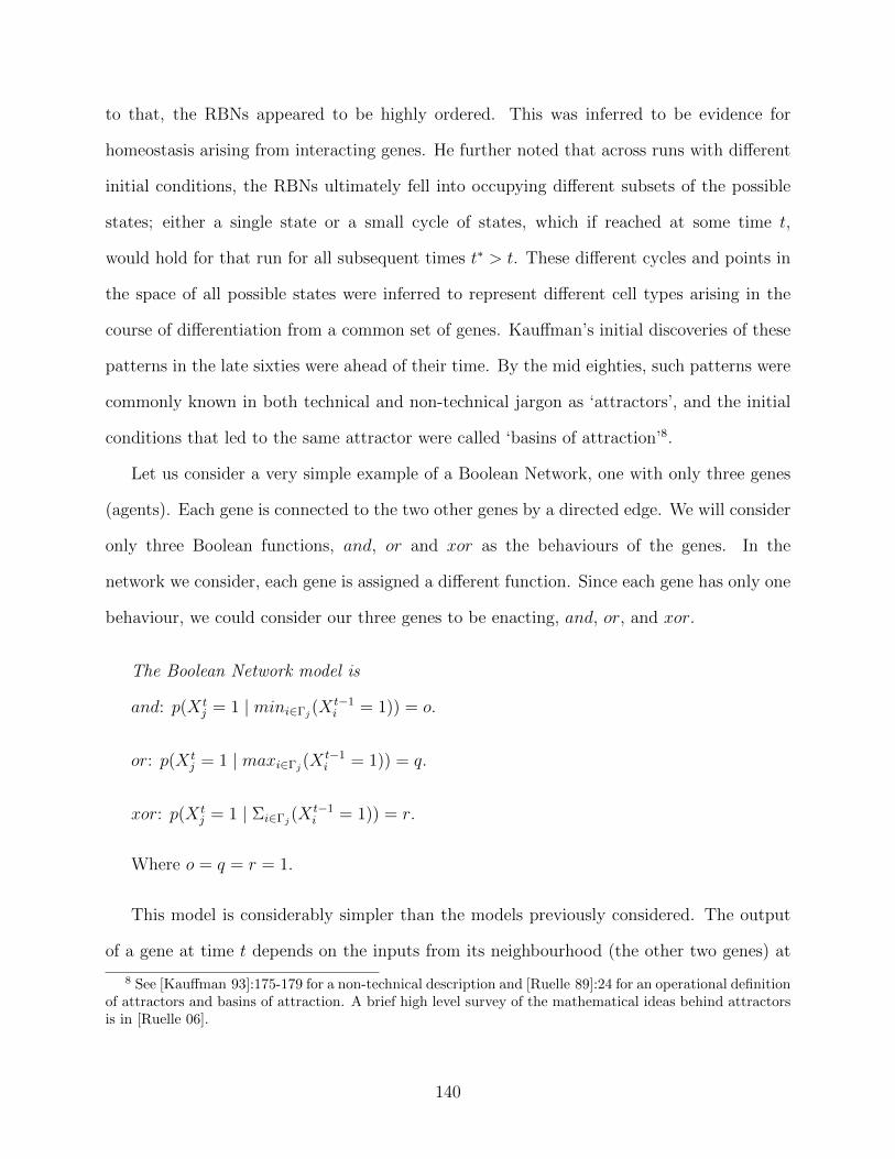
to that, the RBNs appeared to be highly ordered. This was inferred to be evidence for

homeostasis arising from interacting genes. He further noted that across runs with different

initial conditions, the RBNs ultimately fell into occupying different subsets of the possible

states; either a single state or a small cycle of states, which if reached at some time t,

would hold for that run for all subsequent times t∗ > t. These different cycles and points in

the space of all possible states were inferred to represent different cell types arising in the

course of differentiation from a common set of genes. Kauffman’s initial discoveries of these

patterns in the late sixties were ahead of their time. By the mid eighties, such patterns were

commonly known in both technical and non-technical jargon as ‘attractors’, and the initial

conditions that led to the same attractor were called ‘basins of attraction’8.

Let us consider a very simple example of a Boolean Network, one with only three genes

(agents). Each gene is connected to the two other genes by a directed edge. We will consider

only three Boolean functions, and, or and xor as the behaviours of the genes. In the

network we consider, each gene is assigned a different function. Since each gene has only one

behaviour, we could consider our three genes to be enacting, and, or, and xor.

The Boolean Network model is

and: p(X tj = 1 | mini∈Γj

(X t−1i = 1)) = o.

or: p(X tj = 1 | maxi∈Γj

(X t−1i = 1)) = q.

xor: p(X tj = 1 | Σi∈Γj

(X t−1i = 1)) = r.

Where o = q = r = 1.

This model is considerably simpler than the models previously considered. The output

of a gene at time t depends on the inputs from its neighbourhood (the other two genes) at

8 See [Kauffman 93]:175-179 for a non-technical description and [Ruelle 89]:24 for an operational definitionof attractors and basins of attraction. A brief high level survey of the mathematical ideas behind attractorsis in [Ruelle 06].

140

time t− 1.

We can give a message passing interpretation to the model. If a gene is in state 1 a

chemical message is sent to the genes it is connected to, whereas if it is in state 0, no message

is sent. Working through simple Boolean networks like this by hand is a good way to gain

intuition. Let us consider the above network beginning in the state: and = 1, or = 1, xor = 1.

Note that if the case and = 0, or = 0, xor = 0 occurs, no messages are sent, and we could

consider this system to halt at that point. The state of the system at a particular point in

time, is just the triplet of the states of the individual genes. Thus, (1, 1, 1) and (0, 0, 0) are

system states that reflect the state of all three genes at a particular point in time.

Say our initial state is (1, 1, 1). This is shorthand to indicate:and = 1, or = 1, xor = 1.

The initial and following states are listed below, one system state per line (time step).

Our associated probabilities for o, q, r are all set at 1, so the system essentially behaves

deterministically.

Run 0: Deterministic

and, or, xor

(1, 1, 1)

(1, 1, 0)

(0, 1, 0)

(0, 0, 1)

(0, 1, 0)

(0, 0, 1)

(0, 1, 0)

....

Even in this extremely simple example, we can see that the system runs through only 4 of

8 possible states for the given initial conditions, and after a few iterations, cycles only between

141

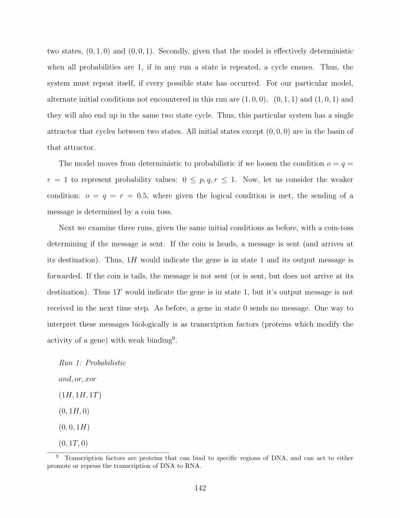
two states, (0, 1, 0) and (0, 0, 1). Secondly, given that the model is effectively deterministic

when all probabilities are 1, if in any run a state is repeated, a cycle ensues. Thus, the

system must repeat itself, if every possible state has occurred. For our particular model,

alternate initial conditions not encountered in this run are (1, 0, 0), (0, 1, 1) and (1, 0, 1) and

they will also end up in the same two state cycle. Thus, this particular system has a single

attractor that cycles between two states. All initial states except (0, 0, 0) are in the basin of

that attractor.

The model moves from deterministic to probabilistic if we loosen the condition o = q =

r = 1 to represent probability values: 0 ≤ p, q, r ≤ 1. Now, let us consider the weaker

condition: o = q = r = 0.5, where given the logical condition is met, the sending of a

message is determined by a coin toss.

Next we examine three runs, given the same initial conditions as before, with a coin-toss

determining if the message is sent. If the coin is heads, a message is sent (and arrives at

its destination). Thus, 1H would indicate the gene is in state 1 and its output message is

forwarded. If the coin is tails, the message is not sent (or is sent, but does not arrive at its

destination). Thus 1T would indicate the gene is in state 1, but it’s output message is not

received in the next time step. As before, a gene in state 0 sends no message. One way to

interpret these messages biologically is as transcription factors (proteins which modify the

activity of a gene) with weak binding9.

Run 1: Probabilistic

and, or, xor

(1H, 1H, 1T )

(0, 1H, 0)

(0, 0, 1H)

(0, 1T, 0)

9 Transcription factors are proteins that can bind to specific regions of DNA, and can act to eitherpromote or repress the transcription of DNA to RNA.

142

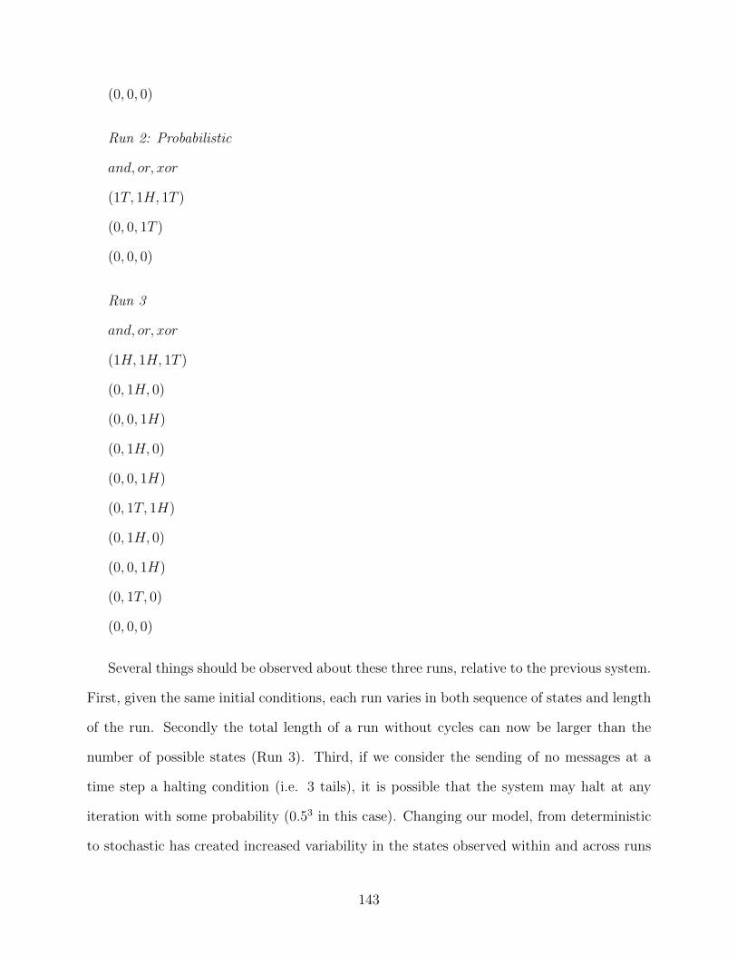
(0, 0, 0)

Run 2: Probabilistic

and, or, xor

(1T, 1H, 1T )

(0, 0, 1T )

(0, 0, 0)

Run 3

and, or, xor

(1H, 1H, 1T )

(0, 1H, 0)

(0, 0, 1H)

(0, 1H, 0)

(0, 0, 1H)

(0, 1T, 1H)

(0, 1H, 0)

(0, 0, 1H)

(0, 1T, 0)

(0, 0, 0)

Several things should be observed about these three runs, relative to the previous system.

First, given the same initial conditions, each run varies in both sequence of states and length

of the run. Secondly the total length of a run without cycles can now be larger than the

number of possible states (Run 3). Third, if we consider the sending of no messages at a

time step a halting condition (i.e. 3 tails), it is possible that the system may halt at any

iteration with some probability (0.53 in this case). Changing our model, from deterministic

to stochastic has created increased variability in the states observed within and across runs

143

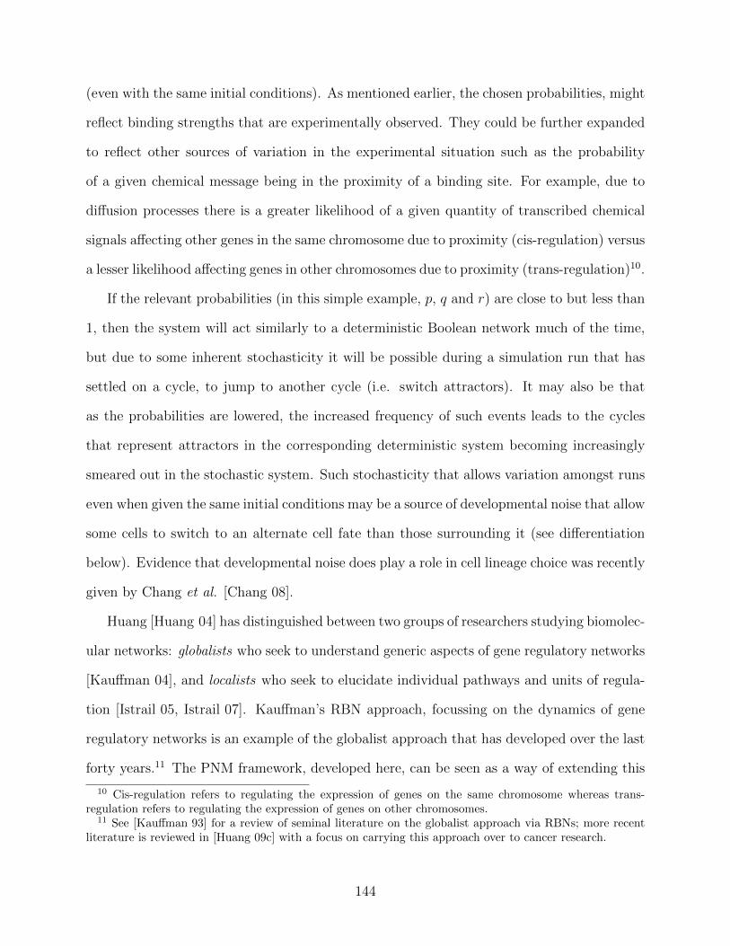
(even with the same initial conditions). As mentioned earlier, the chosen probabilities, might

reflect binding strengths that are experimentally observed. They could be further expanded

to reflect other sources of variation in the experimental situation such as the probability

of a given chemical message being in the proximity of a binding site. For example, due to

diffusion processes there is a greater likelihood of a given quantity of transcribed chemical

signals affecting other genes in the same chromosome due to proximity (cis-regulation) versus

a lesser likelihood affecting genes in other chromosomes due to proximity (trans-regulation)10.

If the relevant probabilities (in this simple example, p, q and r) are close to but less than

1, then the system will act similarly to a deterministic Boolean network much of the time,

but due to some inherent stochasticity it will be possible during a simulation run that has

settled on a cycle, to jump to another cycle (i.e. switch attractors). It may also be that

as the probabilities are lowered, the increased frequency of such events leads to the cycles

that represent attractors in the corresponding deterministic system becoming increasingly

smeared out in the stochastic system. Such stochasticity that allows variation amongst runs

even when given the same initial conditions may be a source of developmental noise that allow

some cells to switch to an alternate cell fate than those surrounding it (see differentiation

below). Evidence that developmental noise does play a role in cell lineage choice was recently

given by Chang et al. [Chang 08].

Huang [Huang 04] has distinguished between two groups of researchers studying biomolec-

ular networks: globalists who seek to understand generic aspects of gene regulatory networks

[Kauffman 04], and localists who seek to elucidate individual pathways and units of regula-

tion [Istrail 05, Istrail 07]. Kauffman’s RBN approach, focussing on the dynamics of gene

regulatory networks is an example of the globalist approach that has developed over the last

forty years.11 The PNM framework, developed here, can be seen as a way of extending this

10 Cis-regulation refers to regulating the expression of genes on the same chromosome whereas trans-regulation refers to regulating the expression of genes on other chromosomes.

11 See [Kauffman 93] for a review of seminal literature on the globalist approach via RBNs; more recentliterature is reviewed in [Huang 09c] with a focus on carrying this approach over to cancer research.

144

approach from deterministic to stochastic systems, in a natural way that allows for incorpo-

ration of specific signalling behaviours drawn from different areas of biology.12 Over the last

decade or so, a localist view has developed that has been very influential in the development

of systems biology, namely network motifs [Alon 07]. Network motifs are individual ‘circuits’

of interactions, that appear in gene regulatory networks much more frequently than expected

in random networks. They too, can be described, and extended via the PNM framework.

Network motifs are typically one-to-several genes and their associated transcription factors.

Their extreme specificity, allows them to be models for specific genes, or small sets of genes

that interact. Two common network motifs are negative autoregulation, where a transcrip-

tion factor represses the transcription of its own gene, and positive autoregulation, where a

transcription factor promotes the transcription of its own gene.

A very simple PNM model of autoregulation consists of a single agent, that sends messages

to itself. The simplest example would be to associate a gene (agent) with two probabilities,

o and q, that are respectively the probability of a gene transcribing itself in the case where

it has not previously received a transcription factor message, and the probability of a gene

transcribing itself in the case where it has previously received a transcription factor message.

p(X tj = 1 | X t−1

j = 0) = o.

p(X tj = 1 | X t−1

j = 1) = q.

In this model, o > q represents negative autoregulation, while q > o represents positive

autoregulation. The absolute value of the difference p − q represents the intensity of the

regulatory response.

A more graduated example of autoregulation would be where the probability of sending

a message to itself decreases with the number of messages received, i.e. creates a weak form

12 Within the RBN framework, Ilya Shmulevich has developed a probabilistic extension [Shmulevich 02a,Shmulevich 02b] where each agent rather than being assigned a single Boolean function, is assigned a set offunctions, and at each time step chooses amongst those functions with some probability.

145

of memory, essentially the building of a counter13.

Consider a series of probabilities s1, s2, s3...sN for a gene transcribing itself. Let these

probabilities be associated with an indexed series of random variables where the nth stage

towards complete suppression or complete promotion at some time t for some vertex j is

represented by X t(n)j:

p(X t(n)j = 1 | X t−1

(n−1)j = 1) = sn.

If the probabilities are related such that s1 > s2 > s3 > ... > sN , we have a graduated

negative autoregulation. If the probabilities are related such that s1 < s2 < s3 < ... < sN ,

we have a graduated positive autoregulation.

As a slightly more complex example, consider a feedforward loop, a network motif found

in many gene systems across a range of organisms. There are three genes (represented by

random variables), X, Y , Z. X regulates both Y and Z. Y also regulates Z. Therefore, Z is

regulated by both X and Y . Let us represent a feedforward loop, where Z transcribes only

if transcription factor messages are received from both X and Y , and where Y transcribes,

only if it has received a transcription factor message from X. Let o be the probability that

X sends a message to Y . Let q be the probability that X sends a message to Z. Let r be

the probability that Y sends a message to Z.

p(Y t = 1 | X t−1 = 1) = o.

p(Zt = 1 | X t−1 = 1 ∧ Y t−1 = 1) = q × r.

Again, under a message passing interpretation, we could consider the probabilities o, q,

and r to represent values determined from experiment that may represent either binding

strengths for the chemical messages or the likelihood of the messages being in proximity.

Such empirical facts, once determined, could either be put into single values for p, q and

r, or result in these probabilities being determined by the other probabilities, such as those

13 In the current incarnation of the PNM model, the amount of memory in a system is tied to the numberof random variables that hold state, which act as simple registers that can hold a single value.

146

that may reflect the interaction of binding strength and proximity.

The enduring stability question in gene regulation is quite simply this: how does an

assemblage of interacting genes maintain production of chemical messages so as to allow the

cell to maintain function in the face of both external and internal perturbations. In this

context, not only does every single identified ‘gene circuit’ have to stay within tight bounds,

but the system as a whole, across interacting circuits, must stay within tight bounds that

allow for cell functionality, i.e. maintain homeostasis.

Maintaining homeostasis is a necessary condition at the higher level of cells, affording the

possibility of differentiation: regular directed changes in cells that lead from a single generic

cell type to multiple more specialized cell types that allow for complex organisms.

6.6 Model 4 – Differentiation

In this section, we will briefly consider differentiation in the context of cell-cell signalling.

How does one cell become many in the course of differentiation? To even begin to consider

this question, we have to develop several tools. First we have to identify the simplest models

under which a single primary cell type can differentiate into a secondary cell type. Secondly

we have to examine the conditions under which a distribution of different cell types can be

stably maintained. Third, to link theory to experiment, we must develop models that can

be tuned with experimental data on specific chemical signals (cytokines14) to develop virtual

experimental systems.

Below is a very high level model of the problem of differentiation, which serves as a

first step to develop more specific models of differentiation tied to particular tissues and cell

types15.

In the model cells are organized into tissues. Within a tissue each cell type has a specific

distribution. The switch from one cell type to another depends both on signals generated

14 Cytokines are small proteins used in communication amongst cells.15 Model 4 co-developed with Sui Huang.

147

internally and by neighbouring cells. The result is a family of PNMs of the general form:

p(Ctj = Stj | Ct−1

j = St−1j ) = f(Ct−1

i∈Γ(j), St−1

i ).

In words, the probability of a new cell type Ctj and its internal states Stj given the

immediate preceding cell type Ct−1j and its internal states St−1

j depends on the cells it can

receive signals from Ct−1i∈Γ(j)

and their internal states St−1i . For each cell at a particular point

in time the vector of internal cell states S takes the form [s1, s2, s3...sN ] and defines which

signals the cell is capable of receiving or sending at that point of time.

In the context of such a model, network structure becomes vital, and is determined by

the pattern of signals passed both between and within cells. Since the network topology

reflects interactions via signalling, it can be more complex than the topology of cells that

are immediate physical neighbours.

In differentiation, change is directed so as to result in a viable organism with functional

parts. Any botanist who has looked at a leaf incongruously appearing where a flower petal

should be, recognizes the effect of mis-signalling – to move a cell towards a different fate.

Thus, differentiation is a process where change is strongly constrained, so as to lead to stable

forms. One of the classic tools of developmental morphology in botanical studies was to study

teratologies – just those situations in which developmental change has gone awry, and by

doing so, to elucidate what signals or processes must have been altered from the course of

‘normal’ development to cause such a change. For example, the observation of leaves where

petals should be led to the idea that petals are actually modified leaves.

To the extent that we can develop models of the signalling processes resulting in dif-

ferentiation, we have a virtual toolkit to allow the examination of how cell fates come into

being, and how they can possibly be stabilized, or in the case of creating stem cells, be re-

programmed so that differentiated cells can give rise to more general cell types [Huang 09b].

We have shown how several specific areas of biological phenomena at the cellular level

and below are amenable modelling via the PNM framework. We now turn to a biologically

148

inspired multi-agent model of signalling amongst organisms via semiochemicals. Finally, we

build up in several stages a PNM model of ecological flow networks.

6.7 Model 5 – Semiochemicals

Our computational systems biologist can seek inspiration equally from biological phenomena,

as well as computational systems inspired by biology. We now turn to looking at signalling

amongst organisms, and amongst different species which has inspired several types of multi-

agent systems in computer science.

Semiochemicals, chemicals that carry a message, are means of signalling amongst organ-

isms. A well known case is the phenomenon of stigmergy16, or indirect coordination in ant

and termite colonies via laying down pheromone trails. Stigmergy is the inspiration behind

heuristic optimization techniques such as ant colony optimization [Bonabeau 99, Dorigo 04],

in which a multi-agent system collectively solves a problem. In these systems, local actions

by individual agents (self-)organize global coherent behaviour in the system as a whole.

Stigmergy is just one example of the use of semiochemicals. Semiochemical signalling mech-

anisms amongst organisms occurs widely in both plants and animals, between sexes, between

species, and within species. They can be mutualistic, symbiotic, and antagonistic. Suffice it

to say that in biology one finds a long history and numerous examples of distributed message

passing systems leading to coordinated behaviour.

Our next PNM model is loosely inspired by the work of Kasinger, Bauer, and Denzinger on

multi-agent models based on semiochemicals. They use digital semiochemical coordination as

a framework for building self-organizing multi-agent systems to solve specific computational

problems [Hudson 10, Kasinger 06, Kasinger 08b, Kasinger 08a, Kasinger 09b, Kasinger 09a,

Kasinger 10, Steghofer 10] , particularly the pickup and delivery problem [Savelsbergh 95].

16 Stigmergy is a form of indirect communication observed in insect populations which allows for decen-tralized coordinated behaviour. An organism leaves a trace in the environment that other organisms cansense and act upon. The standard example is an ant leaving a pheremone trail on returning from a foodsource. Other ants can follow these pheromone trails to find the same food sources.

149

Digital semiochemical coordination is one example of organic computing, the attempt to

incorporate self-organization, self-repair, and adaptive features inspired by biology into the

design of distributed computing systems [Branke 06]. Their work is inspired by pollination

biology, particularly the mutualistic relationship between insects (pollinators) and plants

(pollen sources and pollen destinations), where insects receive food from plants in the course

of pollination, and plants depend on the activity of the insects for pollination. These ac-

tivities are coordinated by a number of chemical and visual signals produced by plants, to

attract pollinators. The activity of pollinators can be related to pickup and delivery prob-

lems, where plants play the role of pickup and delivery sites, while pollinators play the role

of transport vehicles. As Kasinger, Bauer and Denzinger note [Kasinger 08b] biological solu-

tions may not be efficient in use of resources, in that pollinators can, and do, land on flowers

that either have no pollen to pickup or require no pollen delivered. They go on to examine

how the use of various kinds of digital semiochemicals for coordination can lead to efficient

solutions of pickup and delivery problems.

We eschew efficiency concerns for now, and capture the basic structure of the problem in

a PNM. Our PNM model assumes three agent types: PollenSources (male flowers, analogous

to pickup areas), PollenDestinations (female flowers, analogous to delivery sites) and Polli-

nators (analogous to vehicles picking up and delivering packages). Each agent’s behaviour

is encapsulated in conditional probability functions that define the messages it can respond

to, and the messages it sends out in response.

As with the virus model, we will assume a round structure, where each round has the

following phases:

• Phase 1 – Messages from PollenSources received by Pollinators.

• Phase 2 – Messages from PollenDestinations received by Pollinators

• Phase 3 – A Pollinator forwards PollenSource messages to other Pollinators.

• Phase 4 – A Pollinator forwards PollenDestination messages to other Pollinators.

150

• Phase 5 – A Pollinator picks pollen from a PollenSource and then delivers it to a

PollenDestination. It then re-initializes itself to await the next pollen delivery.

Pollinators have the following behaviours:

A Pollinator waits until it has received a message (PollenP ickup = 1) either directly from

a PollenSource, or forwarded from another pollinator. A PollenSource sends messages with

probability o if it requires a PollenPickup. A Pollinator forwards a PollenPickup message

with probability q.

p(PickPollentj = 1 | PickPollent−5j = 0) =

1− (∏

i∈Γ(j)(1− PollenP ickupt−5

i ∗ o)×∏

i∈Γ(j)(1− PollinatorP ickupt−3

i ∗ q)).

A Pollinator waits until it has received a message (PollenDelivery = 1) either directly

from a PollenSource, or forwarded from another pollinator. A PollenDestination sends mes-

sages with probability r if it requires a PollenPickup. A Pollinator forwards a PollenDelivery

message with probability s.

p(DeliverPollentj = 1 | DeliverPollent−5j = 0) =

1− (∏

i∈Γ(j)(1− PollenDeliveryt−5

i ∗ r)×∏

i∈Γ(j)(1− PollinatorDeliveryt−3

i ∗ s)).

Once both messages are received (PickPollen = 1, DeliverPollen = 1), the Pollinator

makes a pickup and delivery, then re-initializes itself (PickPollen = 0, DeliverPollen = 0)

to prepare for receipt of pickup and delivery messages in the next round. While the mechanics

of pickup and delivery are an implementation detail, one approach is have each agent have

a unique identifier, and incorporate additional state variables that can hold the value of the

identifiers for a pickup and a delivery.

p(PickPollentj = 0 ∧DeliverPollentj = 0 |

PickPollent−1j = 1 ∧DeliverPollent−1

j = 1) = 1.

PollenSources have the following behaviours:

151

A PollenSource requires a PollenPickup with some probability u, and does not require a

PollenPickup with some other probability v. If u = 1 and v = 0, that PollenSource always

requires a PollenPickup. Conversely, if u = 0 and v = 1, that PollenSource never requires a

PollenPickup.

p(PollenP ickuptj = 1 | PollenP ickupt−5j = 0) = u.

p(PollenP ickuptj = 0 | PollenP ickupt−5j = 1) = v.

PollenDestinations have the following behaviours:

A PollenDestination requires a PollenDelivery with some probability w, and does not

require a PollenDelivery with some other probability x. If w = 1 and x = 0, that Pol-

lenDestination always requires a PollenDelivery. Conversely, if w = 0 and x = 1, that

PollenDestination never requires a PollenPickup.

p(PollenDeliverytj = 1 | PollenDeliveryt−5j = 0) = w.

p(PollenDeliverytj = 0 | PollenDeliveryt−5j = 1) = x.

In a PNM model,increasing the efficiency of solutions with respect to resource use would

primarily involve tuning the probabilities associated with the behaviour of the agents, given

a particular network structure, that defines both the distribution of, and communication

channels for agents.17 In the semiochemical models developed by Kasinger, Bauer and Den-

zinger, much of the modelling effort was towards developing rules and data structures that

allow for efficient pickup and delivery [Hudson 10, Kasinger 09b, Kasinger 09a, Kasinger 10,

Steghofer 10], so that pickup and delivery sources are neither under nor over served, and all

vehicles are taking the shortest routes possible to ensure all required pickups and deliveries.

17 For example, given a network where each agent can receive messages from all other agents (which couldrepresent the Pollinators in a central depot, and PollenSources and PollenDestinations that are roughlyequidistant from that central depot), and in which there are more PollenSource and PollenDestinations thanPollinators, an efficient solution would be one where probabilities are tuned upwards from 0 such that inevery round every available pollinator makes a delivery. If there were more Pollinators than sources anddestinations, probabilities would be tuned downwards from 1 so that in each round each PollenSource andPollenDestination is served by only a single Pollinator on average.

152

Our PNM model is much simpler, by eschewing many of the implementation details of more

efficient solutions. Adding such details back in, would lead to the PNM model becoming

increasingly elaborate.

In natural systems the solutions that have evolved tend towards redundancy rather than

resource utilization efficiency, in that much more pollen is generated than is required, insects

visit both flowers without pollen and flowers that do not require pollen, and more nectar is

produced than strictly required to attract pollinators. Why does life tend towards abundance

(and redundancy) rather than optimal resource utilization? One reason might be that in nat-

ural systems, the populations of plants and insect pollinators are changing both within and

between seasons. Redundancy allows more flexibility towards changing conditions, whereas

an optimal solution for one set of conditions might be very suboptimal if the conditions

change. In that sense, redundancy and efficiency seem to be antagonistic in many natural

systems. Flexibility to changing conditions is gained at the price of reduced efficiency for a

particular set of conditions.

The actual structure of insect-plant relationships with respect to pollination is much more

complex than we have indicated so far. Insects do not pollinate all plants. Some insect species

are generalists, and may pollinate a wide range of plants. Other insects species are specialists,

pollinating only a few (or a single) species of plant(s). Within a single species of insect, dif-

ferent populations may preferentially pollinate different species of plants. Plant species may

be generalists, specialists, or not depend on insect species at all (wind pollinated). This more

complex set of relationships between insect-pollinators and the plants they pollinate results

in what are known as pollination networks. A current concern with such pollination net-

works is their stability, particularly with respect to extinction of pollinators [Bascompte 09,

Kaiser-Bunbury 10, Memmott 04, Oleson 07, Petanidou 08, Williams 11] due to factors such

as climate change [Halter 07, Visser 08], and ongoing crashes of bee populations covered in

both the popular press [McCarthy 11] and books [Halter 11a]. While pollination networks

153

can be seen as analogous to the predator-prey networks covered in Chapter 4, their struc-

ture is necessarily bipartite18, all edges in the network cross two groups of species, pollinators

and plants. Loss of generalist pollinators is implicated in decline in plant species diversity

[Memmott 04], and have been hypothesized to lead to complete collapse of a pollination

network [Kaiser-Bunbury 10].19 Pollination networks are but one example of insect-plant re-

lationships that result in bipartite networks; another example is host-parasite relationships

such as those between tree species and bark beetles [Halter 11c]. Semiochemical models,

while drawing inspiration from the signalling phenomena behind various plant-insect rela-

tionships, may also contribute to developing models which help us to understand the stability

of such networks under perturbations such as climate change, or loss of pollinators.

6.8 Model 6 – Ecosystem Flow Networks

We now move up another few levels in the biological hierarchy from interactions amongst

individuals to interactions amongst populations and species in an ecosystem.

With the advent of systems biology in the last decade, networks of interaction in molec-

ular and cell biology have been a growth area of scholarship. However, in ecology, in-

teractions have always been the raison d’etre. The modelling of ecological interactions

has a long history with diverse mathematical approaches reflecting different conceptual

perspectives including: population dynamics [Allesina 12, Caswell 01, Fox 02, Lotka 20,

May 00, McCauley 99, McCann 12, McCauley 08, Sole 06, Vasseur 08, Wang 09], network

architecture [Allesina 08, Allesina 09, Williams 10, Williams 11, Williams 00], bioenerget-

ics20 [Otto 07, Williams 08, Williams 07, Yodzis 92], network flow relationships [Fath 04,

18 A bipartite graph is one where there are two disjoint sets from which vertices can be drawn, and everyedge in the graph crosses these sets. So, for example, in pollinator networks, there are two disjoint sets,Plants and Pollinators, and all edges cross these two sets.

19 Topological stability theory, developed in Chapter 4 provides a nice context to think about stabilitylimits in pollinator networks. In such networks, the size of the minimum vertex cover (cut-stability) willbe less or equal to the size of the smaller of the two sets from which vertices are drawn, Pollinators andPlants. Viral processes (connection-stability) are forced to weave their way across the two sets.

20 Bioenergetic models combine aspects of population dynamic models with energetic considerations,

154

Fath 06, Fath 07b, Pahl-Wostl 94, Salas 11], stoichiometry21 [Li 11, Loladze 00, Marleu 11,

Wang 10a], various spatial, temporal and geographic scales [Brown 89, Levin 92, Massol 11,

Maurer 99, Pahl-Wostl 92], environmental heterogeneity [Eveleigh 07, Levins 68] and com-

binations of the above models [Romanuk 09b]. Levins, in an essay [Levins 66] taken to heart

by several generations of ecologists, notes that ecological models must strategically trade off

between generality, precision and realism, depending on the goals of a particular study. This

leads to a multiplicity of models reflecting different conceptual and methodical approaches.

PNMs provide yet another conceptual perspective within which to explore ecological inter-

actions. In a PNM for an ecological network, nutrient or carbon transfers are seen as akin

to passing messages.

We expand on our mutualism model to first build a flow network model, and then to build

an ecosystem model with a simple trophic structure22. The PNM model for mutualism is built

up to incorporate additional constraints abstracted from ecosystems. While our example is

specific to ecosystems, this approach illustrates how a simple model can be elaborated by

adding in the constraints particular to specific systems.

Every model we have considered so far could be considered a flow network, in that there

is a flow of messages passing through the system. However, ecological flow networks tracking

nutrient or biomass passage through species include several additional constraints that reflect

the energetic constraints ecosystems must operate within.

With respect to an ecosystem flow network these constraints are:

1. There is a limited amount of matter in the system.

2. Matter is conserved.

primarily related to body mass and size ratios (‘allometry’) between species.21 Ecological stoichiometry models are essentially population dynamics models that consider both energy

flow and nutrient cycling by incorporating constraints about the ratios of different nutrients relative to carbonin the interaction between a primary producer and a grazer.

22 Trophic structure refers to the roles species play as food consumers and food producers, and is intimatelyrelated with energy flow through an ecosystem [Ricklefs 79b]:pp 780-781. Examples of roles are green plantswhich are primary producers, herbivores which are primary consumers, carnivores which are secondary andhigher consumers.

155

3. Some matter is lost from the system, or is in a form no longer available to the

system (dissipated).

These constraints relate to the thermodynamic limitations on energy transfers in ecosys-

tems23. In a PNM they are translated into constraints on messages. The first constraint

restricts the number of messages that can be generated. The second constraint indicates

that all messages must be accounted for. In a PNM of ecosystem flows, the messages rep-

resent matter. Matter can move from one part of the system to another, it can exit the

system boundary, or it can enter the system from outside its boundary. The third constraint

indicates that some messages will become unavailable for use by other agents in the PNM

of ecosystem flows. Our tracking of energy changes through an ecosystem assumes mass

conservation between a designated ecosystem and its environment.

To introduce these constraints into a PNM requires an accounting system that tracks

messages (material transfers)24. Such accounting systems form the basis for ecological flow

analysis, and define the flow values assigned to edges in an ecosystem flow network.

To extend the mutualism model to a flow network, we must add now an accounting

framework. We do so, by first modifying the round structure, so that in each round there

are two phases.

1. Accounting phase

2. Message passing phase.

23 The second constraint follows from the first law of thermodynamics, though strictly speaking, it isenergy that is conserved. The third constraint follows from the second law of thermodynamics, though it,strictly speaking, refers to energy becoming unavailable to do work. Since energetic transfers in an ecosystem,above the level of plants, are via biomass transfers from feeding, the ecological constraints are in terms ofmatter. A more detailed overview of ecosystems viewed from a thermodynamic perspective is in Patten’sclassic paper on the cybernetics of ecosystems which links thermodynamic concerns to information theory[Patten 59].

24 Such an accounting system is used by Feynman to illustrate conservation of energy via the conceit ofa small child playing with blocks. His mother accounts for where the blocks have gone. Some of the blocksare in his bedroom, i.e. in the system. Some of the blocks have exited the bedroom via an open window, i.e.passed beyond the system boundary ([Feynman 95]:pp. 69-72). See also ([Ness 69]:pp. 3-8), for a slightlymore complex elaboration of Feynmans conceit, now involving sugar cubes which, unlike blocks, can dissolve.

156

The message passing phase operates as previously described. The accounting phase must

first account for the number of messages currently in Processes 1–3. Secondly, it must prevent

conflicts that would violate the three constraints on material flows we have described above.

In the model below, we will emphasize the message passing phase, while providing some

basic details of the items the accounting phase must take care of. To simplify the model, we

will assume the accounting phase occurs immediately following message passing, and does

not require its own time step.

First we must introduce a message counting function. Let P be a process random variable.

Pk is the random variable assigned to the kth process (in the mutualism model, k = 3).

Count(P t−1jk

) returns the number of messages M associated with a process random vari-

able Pk for agent j at time step t−1. For example, Count(Zt−1j ) would count all the messages

associated with Process 1, whose associated random variable is Z.

Count(P t−1jk

) = M t−1jk

.

Secondly we must introduce another Boolean state variable Qt−1jk

that depends on the

returned value of Count(P t−1jk

).

p(Qt−1jk

= 1 | Count(P t−1jk

) ≥ 1)) = 1.

Qt−1jk

determines if agent j has any messages that could be sent in the next round.

The constraint, of having to check if there are any messages available to send, now is

incorporated into the mutualism model via a multiplier, Qt−1jk

. Since, in the mutualism

model, we are assuming each agent has only a single process, we can drop the k subscript.

The mutualism model equations incorporating message flow constraints are25:

Process 1: p(X tj = 1 | X t−1

j = 0) = 1−∏

i∈Γ(j)(1−Qt−1

j ∗ Zt−1i ∗ o).

25 An implementation would require some additional functions to decrement M tj upon a message being

passed, and increment it upon a message being recieved. As well, the number of messages associated witheach process within an agent would have to be initialized.

157

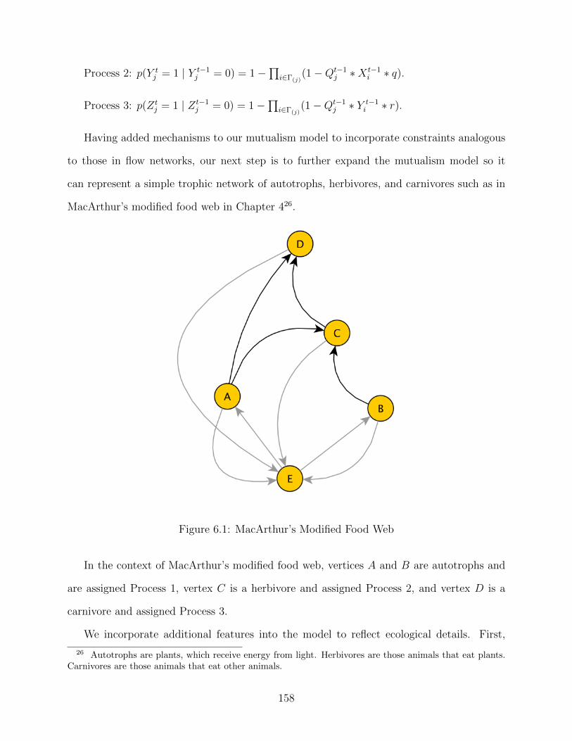
Process 2: p(Y tj = 1 | Y t−1

j = 0) = 1−∏

i∈Γ(j)(1−Qt−1

j ∗X t−1i ∗ q).

Process 3: p(Ztj = 1 | Zt−1

j = 0) = 1−∏

i∈Γ(j)(1−Qt−1

j ∗ Y t−1i ∗ r).

Having added mechanisms to our mutualism model to incorporate constraints analogous

to those in flow networks, our next step is to further expand the mutualism model so it

can represent a simple trophic network of autotrophs, herbivores, and carnivores such as in

MacArthur’s modified food web in Chapter 426.

Figure 6.1: MacArthur’s Modified Food Web

In the context of MacArthur’s modified food web, vertices A and B are autotrophs and

are assigned Process 1, vertex C is a herbivore and assigned Process 2, and vertex D is a

carnivore and assigned Process 3.

We incorporate additional features into the model to reflect ecological details. First,

26 Autotrophs are plants, which receive energy from light. Herbivores are those animals that eat plants.Carnivores are those animals that eat other animals.

158

autotrophs will have an intrinsic growth rate, which is reflected in the model via a message

generation mechanism. Second, all organisms dissipate some energy, which is reflected in

the model as lost messages.

For each autotroph, we will model the intrinsic growth rate via the logistic growth equa-

tion27. This equation in its differential and difference forms is often used as a beginning

point for ecological models of both bounded growth within species and competition between

species( [Begon 81]:pp. 77-80, [May 76b], [McCann 12]:pp. 53-56). To model logistic growth,

we add another behaviour for autotrophs, that reflects growth. Let M tj be the messages

associated with the jth autotroph. Let c be the the total number of messages that can

be assigned to that autotroph. In ecological modelling, c is interpreted as the maximum

population a site can support, called the carrying capacity. The growth rate is denoted by

g.

The logistic growth equation used for autotrophs is:

M tj = g ∗M t−1

j (c−Mt−1

j

c).

Every agent j has a probability dj of losing messages to the environment. Whether an

agent will lose a message in the current round is held by a random variable, D.

p(Dtj = 1) = dj.

The number of messages M held by the dissipation agent is:

M tj = M t−1

j + Σi∈Γ(j)Dt−1i .

MacArthur’s assumption in constructing the modified food web is that energy lost from

the ecosystem equals that arriving at the ecosystem. Therefore, our final agent, E, receives

the dissipated messages. E, in turn, can pass messages onto the autotrophs.

27The logistic difference equation, while exceedingly simple, has a special place in the hearts of bothecologists and chaos theorists, due to Robert May’s elucidation of the chaotic properties 28 at the heart ofsome of the simplest models ecologists use.

159

We now have four trophic compartments: autotrophs, herbivores, carnivores, and dissi-

pation. The mutualism model is now further extended to reflect the relationships between

these trophic compartments.

Our trophic model is:

Autotroph Trophic Process 1: p(W tj = 1 | W t−1

j = 0) = 1−∏

i∈Γ(j)(1−Qt−1

j ∗ Zt−1i ∗ o).

Herbivore Trophic Process 2: p(X tj = 1 | X t−1

j = 0) = 1−∏

i∈Γ(j)(1−Qt−1

j ∗W t−1i ∗ q).

Carnivore Process 3: p(Y tj = 1 | Y t−1

j = 0) = 1−∏

i∈Γ(j)(1−Qt−1

j ∗X t−1i ∗ r).

Dissipation Process 4: p(Ztj = 1 | Zt−1

j = 0) = 1−∏

i∈Γ(j)(1−Qt−1

j ∗Dt−1i ∗ s).

If we used MacArthur’s modified food web as the network structure for this simple ecolog-

ical model, it would represent a strongly connected graph. Strongly connected components

in ecological networks have recently been found to act as integrating modules in ecosystems

[Borrett 07]. Their internal structure deviates from that expected from random graphs with

identical numbers of edges and vertices. Such evidence suggests strongly connected compo-

nents may be an ecological network motif29 [Bascompte 09, Milo 02, Rip 10]. In this context,

each agent could be considered to represent a species, and the network represents the flows

of matter between species. The message transfers represent individuals of one species being

eaten by another. So, M tj actually represents the population of the jth species at a par-

ticular point in time30. As emphasized in Chapter 4, our stability concerns with respect to

ecosystems are both topological and dynamic. From a topological perspective we could ask

a pair of questions. First, if the network structure is modified, and certain agents are lost

(extinction), is there still a path amongst the remaining agents via which messages can flow

29 In the case of a strongly connected component, the motif would be a specific class of directed graphs,rather than a specific directed graph. This might more properly be called a motif class.

30 We leave as an exercise the extension of this model where species are agents, to one where individuals of aspecies are agents, and the network structure represents proximity information. Population, now rather thanbeing represented by the number of messages in the system, are represented by the number of vertices, andthe proximity of individuals is reflected by the network structure. Extra credit for incorporating preferentialfood choice into carnivore and herbivore agents.

160

between any two species and cycle (cut-stability)? Second, if a toxin were to pass through

the ecosystem in the form of a tainted message, how long would it take to pass through

all agents (connection-stability). Finally, from the perspective of dynamics, what are the

initial number of messages assigned to each agent, and the probabilities for message transfer

associated each agent j and the specific process behaviour it is assigned? These intial values

and probabilities will govern whether the system reaches a steady state of message flows,

and second, how it would recover from disruptions to the steady state of message flows.

Within the context of PNMs, a common abstraction of message passing emphasizes the

unity of processes occurring in cells and tissues, to signalling amongst organisms, to processes

occurring at the level of ecosystems.

6.9 Future Directions

In his last book, Tools for Thought [Waddington 77], the great developmental biologist, C.H.

Waddington, drew into biology conceptual tools first developed in other fields – dynamical

systems, information theory, and game theory, amongst others. He introduced each of these

tools via biological analogies, often from organismal development. In doing so, he created

bridges between biological phenomena and techniques in other fields, that allowed the widen-

ing of his biological intuition outward towards those fields. Our goal in this chapter has been

to work in the opposite direction, to draw concepts developed within biology into other

fields, particularly computer science when it is concerned with complex interacting systems

that communicate via, and change state due to, the passing of messages. In doing so, we

also draw on the biological intuition that has been developed around phenomena such as

viral spread and immune response, mutualism and autocatalysis, gene regulatory networks,

differentiation, semiochemical signalling and ecological flow networks. Developing models of

these biological phenomena as multi-agent systems sets the stage to explore how they can

be expanded out to technological message passing systems such as the Internet.

161

The PNM framework allows us to compactly represent a wide array of biological phe-

nomena as distributed message passing systems, where each agent receives and generates

messages according to a set of behaviours. In doing so we emphasize the role of various

forms of message passing in biology in shaping interactions at the molecular, cellular, or-

ganismic, and ecological scales. The primary role of interactions at all levels in biological

systems provides a unifying perspective for diverse biological phenomena. In representing

these phenomena in terms of a multi-agent system, we also develop a toolkit of biologically

inspired processes that we can apply to stabilizing computational systems.

One important question to ask in identifying future directions for the PNM model is,

what is the expressive range for these models? While many of the examples in this chapter

have focussed primarily on Boolean conditions being met – conditional probability func-

tions can easily be extended to deal with conditions from predicate logic, as in the virus

and immune response PNM which uses the universal quantifier. The PNM approach, in

representing physical situations (either biological or technological) depends, first on there

existing a detector of logical conditions based on incoming signals, secondly on a network

that represents the paths signals may travel along, and finally on a response mechanism, so

that if a logical condition is met for incoming signals, an outgoing signal is generated with

some probability.

As noted in the previous chapter, the current version of the PNM model corresponds to

a reactive multi-agent system. What additions would be needed to allow for more expressive

behaviours? Currently, memory is simply contained in the state of the random variables

assigned to an agent. Histories can be built via addition of counters. However in biological

systems, memory appears to be held in conformations, and itself appears to be a network

property involving connections between different cell types31, rather than a value held in

31 Computer architect and neurobiologist Jeff Hawkins makes the point that human memory is fundamen-tally different than computer memory [Hawkins 04], and concerns storage and recall of sequences of patternsin invariant form; human memory is not about storage of specific values in a register, but a dynamic pro-cess. Recent work in neurobiology is finding that astrocytes, non-electrical conducting cells, that are denselyconnected to neurons (which would otherwise be more sparsely connected) play a role in the formation of

162

a register. In biology, persistent memory is considered due to a configuration of neural

architecture; as the architecture changes, so does memory. As long as the configuration does

not change, the memory is persistent. Every time a new synaptic connection gets built, there

is the possibility of modifying existing or creating new memories. This is inherently different

than computer memory, where memory is instantiated into a fixed state. The architecture

here, is not changing, as persistent memories change. Finally, behaviour in biological systems

is often anticipatory, and this would seem to imply the underlying logic must be extended to

at least modal logic. Incorporation of more elaborate memory structures, and anticipatory

behaviours are two obvious directions in which to extend the model.

With our emphasis on the behaviours assigned to each agent, another natural extension

is towards social agents. A large literature has grown up in the social sciences based on

relatively simple agents with no more memory or anticipatory power than currently incor-

porated into PNMs [Batty 05, Epstein 06, Epstein 96, Gilbert 08, Miller 07]. Such agents

often have goals that must be satisfied, but that is often manifested as changes in behaviour

triggered by internal state variables, which can be expressed in the PNM framework.

One area in biology that the PNM approach may be applied is in the study of robustness.

Models of gene regulation and cell-fates as we have sketched in this chapter also provide

insight into the biological study of robustness. Robustness in biological systems is a concept

that has appeared repeatedly in the history of biology in various forms, and has most recently

been developed in modern form by Wagner [Wagner 05]. A capsule definition of robustness is:

‘Robustness is the persistence of an organismal trait under perturbations’ ([Felix 08]:pg 132).

As used by Wagner’s group, it applies to all levels of biology from molecular to organismal.

The definition is quite close to the multi-disciplinary definition of stability we developed

in Chapter 2, so robustness as applied to biological systems can be considered yet another

stability concept. In robustness, the perturbations are seen as occurring from three different

sources: stochastic noise, environmental change, and genetic variation. Sources of robustness

long term memory [Bezzi 11, Santello 10, Henneberger 10].

163

are found in redundancy (the same part exists in multiple copies; whether it be copies of a

gene, an organ, or a cell type) and in alternative pathways (to the same functional result).

PNMs may provide a way to explore robustness, by explicitly examining alternate paths

in the network that lead to the sending of a particular message type, and by comprising a

network of redundant agents with the same behaviours.

The focus on redundancy and alternate pathways in the biological conception of robust-

ness should trigger in a computer scientist analogous thoughts on the roles of redundancy

and alternate pathways in the design of fault tolerant systems, where no single failure should

be allowed to disrupt a system. Robustness is often considered to have evolved in biolog-

ical systems, which introduces the idea of combining the PNM model with evolutionary

computation methods that modify network architecture and tune probabilities.

Another area of biology where PNMs may contribute, is the current renessaissance

of epigenetics, originally introduced in the middle of the last century by C.H. Wadding-

ton [Huang 12, Jamniczky 10, Slack 02, Speybroeck 02, Waddington 42]. Epigenetics is the

study of heritable changes above the level of the genome, which can include gene expres-

sion noise, and the complex activity of gene regulation networks [Chang 08, Huang 09a,

Huang 12, Wang 10b]. Experimental knowledge of the specific signalling behind gene regu-

lation can be the basis of PNM behaviours, whereas the stochastic nature of PNMs can be

used to explore the specific combination of behaviours and network conditions under which

gene expression noise can switch cell fates [Huang 09b, Huang 10, Huang 11].

Finally, as computational systems begin to reach a level of complexity usually associated

with the biological, the PNM approach provides a framework in which we can model stabi-

lizing mechanisms for systems of such complexity we can not anticipate all forms of attack.

In the next chapter, we begin a very preliminary approach to that goal. We develop the no-

tion of a proto-immune system on a network via implementing the virus model developed in

this chapter. Combining the PNM framework from the last two chapters, with theory from

164

Chapter 4, we also introduce one final theoretical concept, resilient processes, and examine

the virus and immune response PNM to see how a simple warning message may act as a

resilient process enhancing connection-stability.

165

Chapter 7

Dynamic Resilience

Homeostasis

is like a ballerina

on point.

Resilient processes

bend, block, redirect, sashay

perturbations through structure.

7.1 Abstract

We want to distinguish the stability (cut-stability or connection-stability) passively afforded

by a given network architecture from the stability that could be dynamically afforded by one

or several processes acting from within that architecture. We will call this latter form of

dynamic stability, resilience. The concept of dynamic resilience is developed in the context

of topological stability theory (Chapter 4) and PNMs (Chapters 5–6). Resilience is the ad-

ditional stability provided by active processes above and beyond that provided passively by

network structure. A resilient process is one that dynamically maintains cut-stability or

connection-stability. In biology, resilient processes can be seen in various organic responses

that provide for immunity and homeostasis in living systems. Similarly, resilient processes in

a networked technological system would be those actions the system itself may be programmed

to take that can confer greater stability to it. We explore resilience via first looking at several

simple cases of cut-resilience and connection-resilience, to demonstrate that resilient pro-

cesses can compensate for architectural limitations. We further explore connection-resilience

via the virus–immune PNM under various network architectures from sparsely connected to

166

highly connected, and at several levels of viral propagation. Counter-intuitively, network ar-

chitectures that favour the virus, also favour the warning message running ahead. Dynamic

resilience, thus allows for an architectural weakness in connection-stability to be circum-

vented by processes as simple as sending a warning message. These results suggest that there

is benefit in building such immune capabilities into distributed technological systems.

In this chapter we unite the topological perspective of Chapter 4 with the dynamical per-

spective of PNMs developed through Chapters 5–6. We first define resilient processes and

resilient mechanisms in terms of their effect on cut-stability and connection-stability. We

then explore the consequences of resilience through several simple examples. Next we use the

virus–immune PNM (called the ‘virus model’ in Chapter 6) to examine via simulation the

interplay of network structure, and dynamic processes that can act to stabilize a network. Fi-

nally we explore ways in which we can elaborate upon the virus–immune PNM to incorporate

further resilience. A virus model is particularly apt, as there is a large amount of conceptual

transfer between the biological and computational epidemiology literature focussed on net-

works [Cohen 03, Danon 11, Draief 08, Goel 04, Li 07, Lloyd 01, May 06, May 01, Meyers 05,

Mishra 07, Newman 02a, Newman 02b, Pastor-Satorras 01, Van Mieghem 09, Vogt 07, Yuan 08].

Two take-home messages emerge out of our examples and simulations. First, dynamic pro-

cesses can be used to circumvent structural weakness. Secondly, topology modifies dynamics,

and hence resilience. Dynamically stable systems depend on the interaction of structure and

process. The most stable architecture, in the absence of resilient processes, may not be the

architecture that best supports stability via a resilient process.

We will again begin with a contrast in perspectives, that of our network architect, and

that of an immunologist.

167

7.2 Introduction and Motivation: Viruses in Computer Science and Biology

Our network architect has a problem. He recognizes that based on cut-stability, any highly

connected network that is cut-stable is also connection-unstable. Designing a scale free

network does not get around this problem, since it is also susceptible to viral attacks. A

network with balanced stability will have some resistance to viral attacks while also being

resistant to other forms of attack. Initially he thought that was the best he could do, but now

he wonders, is there a way to do more? Even a connected network with balanced stability

merely slows viral progress, rather than stopping it. He can, of course, harden the system

by locking down resources, removing unnecessary software, and having tightly restricted

access protocols. However, it is usually only a matter of time before some ingenious though

unscrupulous malware designer finds a way around his hardened system. While he fervently

hopes all the network administrators are regularly updating their anti-viral software, he

knows this to be not in fact the case. He also has the queasy feeling that despite all the

antivirus solutions available, he does not in fact feel the system is more secure, because virus

designers seem to be able to develop new viruses faster than anti-virus designers can decipher

them. He also worries about the fact that his network must interface with other networks,

and he has seen how the connection in-stability of linked networks is greater than each

network on its own. Having previously gotten useful ideas from an ecologist, he now decides

to consult with an immunologist on their common problem: viruses, be they computational

or biological.

Our immunologist listens closely to the network architect’s dilemma, then smiles, and

says, ‘I think I can help you.’ He explains to our network architect that human inoculation

programs work largely because humans already have an immune system, and inoculation

programs are simply augmenting the existing capabilities of the human immune system. He

also introduces some new concepts unfamiliar to our network architect, specific gene-for-

gene resistance versus broad multi-gene resistance. He says that anti-virus programs appear

168

to be analogous to vertical (gene-for-gene) resistance, in that they depend on deciphering a

specific virus signature, and building an antiviral solution that will detect and eliminate that

specific virus. He then explains the idea of horizontal (multi-gene) resistance, which results

in a systemic capability to resist viruses, that is not tied to any specific viral signature.

Finally, he introduces a truly enigmatic concept to our network architect, the Red Queen

Hypothesis from evolutionary theory. The Red Queen Hypothesis, concerns the fact that

co-evolving systems, such as hosts (computers) and parasites (viruses) continually respond

to each other, leading to an escalating arms race simply to maintain themselves relative

to each other. While neither vertical nor horizontal resistance can circumvent such arms

races, gene-for-gene resistance (vertical) systems require only a single break through on the

part of the parasite (virus) to regain advantage, though they offer complete protection prior

to such a breakthrough. By contrast, multi-gene (horizontal ) resistance usually provides

less than complete protection, but also is more difficult to circumvent. In short, vertical

resistance leads to more accelerated evolutionary arms races than horizontal resistance. An

arms race seems to our network architect as apropos to the current state of affairs vis-a-vis

antivirus solutions and malicious viruses that can enter the network. Our network architect

asks, ‘What is the simplest thing I can do?’ Our immunologist answers, ‘Have the system

recognize when something is wrong, and send a warning message; this is one of the simplest

forms of horizontal resistance possible. Here’s a simple model you can play with, developed

by a computational systems biologist I work with’. With the virus– immune PNM in hand,

our network architect gets to work to try and understand what kinds of processes may

augment his network’s stability.

7.3 Dynamic Resilience

7.3.1 Dynamical Resilience in terms of Topological Network Stability and PNMs

A standard dictionary definition of resilience is [Sykes 82]:

169

‘resilient. a. recoiling, springing back; resuming original form after stretching, bending,

etc. (of person) readily recovering from depression, etc., buoyant.’

In short, we are looking for processes by which a system can ‘spring back’ from a pertur-

bation that may affect either its cut-stability or connection-stability. By ‘process’, we simply

mean a series of steps or actions taken to achieve a particular end, in this case, system sta-

bilization. While resilient processes can refer to any series of actions a system (biological or

technical) might take, in the more restricted case of computers, computational models and

specific algorithms, we might speak of resilient mechanisms. This leads us to a few initial

definitions of resilient processes and mechanisms below. We will define the resilient processes

generally for a system, while we define the resilient mechanisms more specifically in terms of

networks containing agents with behaviours, that is, in terms of our PNMs. If we see such

behaviours as shared algorithms, we can extend these ideas to other kinds of multi-agent

systems, and to distributed computing models. Recall from Chapter 5 that in a PNM:

There are N agents represented by vertices.

V = {v1, v2, ...vN}, |V | = N .

There are O behaviors represented by functions.

B = {f1, f2, ...fO}, |B| = O.

Each agent j, is associated with a specific group of behaviors.

∀Vj ∈ V ∃Bj ⊆ B , |Bj| ≥ 1.

Our intuition is that resilient process is a sequence of actions taken by a system to

stabilize itself against perturbations. A resilient process provides a system with enhanced

stability above and beyond its structure.

Definition 8. A resilient mechanism is a behaviour(s) fi associated with one (minimally)

to all (maximally) agents vj in a network that conveys to the network greater stability (cut-

stability or connection-stability) than that due purely to network topology.

170

A system may have multiple resilient processes (mechanisms) for different kinds of per-

turbations, or several resilient processes (mechanisms) may work in tandem to stabilize a

system against a particular perturbation. Following from the definitions above, we can speak

of cut-resilient mechanisms (processes) and connection-resilient mechanisms (processes). It

is possible that some mechanisms (processes) may be both cut-resilient and connection-

resilient. It is also possible that different resilient mechanisms (processes) can augment or

interfere with each others effects on system resilience.

Recall from Chapter 4, that cut-stability and connection-stability both depend on certain

sets of vertices in a network. The cut-stability of a network G depends on the minimum

vertex cover MVC(G) of that network. The connection-stability of a network G depends

on the maximum flood set that is possible in the network MFS(v∗, G), and T , the time or

number of iterations required to create MFS(v∗, G), where v∗ is a vertex in G from which G

can be flooded in the fewest iterations. We can define cut-resilient and connection-resilient

mechanisms based on these sets.

Definition 9. A cut-resilient mechanism is a behaviour(s) fi associated with one (minimally)

to all (maximally) agents vj in a network that conveys to the network greater cut-stability by

protecting members of MVC(G) from being cut.

Definition 10. A connection-resilient mechanism is a behaviour(s) fi associated with one

(minimally) to all (maximally) agents vj in a network that conveys to the network greater

connection-stability by preventing a malicious viral process from reaching members of MFS(v∗, G),

or by increasing the number of iterations T required to flood MFS(v∗, G).

7.3.2 Resilience Concepts In Other Areas of Computer Science

In the above formulations of resilient mechanisms, we have left open the exact nature of the

problem(s) a multi-agent network might be engaged in. Our rationale for this is that we

do not want to make much in the way of assumptions as to a specific problem domain. We

simply assume networked systems, and that any particular problem solving capability for

171

the multi-agent network benefits from the resilience (cut or connection) of the network.

The notion of resilience also appears in work of J. Halpern and colleagues that attempts to

unite ideas in computational game theory [Abraham 06, Halpern 08] where a ‘secret sharing

game’ is played in a distributed computing environment to ideas in the context of Byzantine

agreement or consensus problems [Abraham 08]. In these works resilience is related to the

number of agents that can default from protocol, while allowing the problem to be solved.

In the game theory work, the notion of k-resilient Nash equilbria are introduced – which

is essentially an extension of the notion of Nash equilbrium from a single default (k = 1)

to the default of a coalition (of size k). In the Byzantine agreement work, the focus is on

optimal resilience which is the notion of allowing a coalition up to the bound allowed for the

Byzantine agreement problem, where an impossibility proof exists that consensus can not

be reached for n processes if at least 13rd of the processes default. The game theory paper,

by first defining an extension of Nash equilibrium where coalitions default, and secondly

by introducing a notion of non-rational defaults (‘t-immunity’) develops bridge concepts

between game theory and the Byzantine problem. From our network-centric perspective we

should note that both works assume a fully connected network. This is achieved in the game

theory work via the notion of cheap talk, and in the Byzantine agreement work by the notion

of public broadcast. While the resilience in these works is technically defined with respect to

a particular problem and a particular assumed network architecture, the commonality with

resilience as I have defined it above is that resilience is due to dynamic actions of agents,

some of whom may default. Since solution to the consensus or secret sharing problem both

depend on the messages getting through to all agents, they could be seen as potentially

compromised by perturbations leading to connection-instability and cut-instability.

In a recent review of the role of ‘network thinking’ as it may contribute to artificial

intelligence, M. Mitchell [Mitchell 06] notes that the network literature has emphasized static

structural properties of networks (as opposed to their dynamic properties). To make the case

172

for dynamic properties, she first reviews dynamics in the context of cellular automata (which

could be considered extremely simple 1 or 2-D grid networks) [Wolfram 84, Wolfram 94] to

develop a notion of information processing on a network, followed by an examination of

information processing as it appears to occur in immune systems, from which she derives

several general principles for information processing in decentralized systems. ‘Information

processing’ in the sense Mitchell uses it, is to account both for network structure and how

vertices and edges deal with messages they may receive and/or propagate, including how the

network structure itself may alter over time. The notion of a resilience mechanism we have

introduced is in a similar spirit.

As different as the fields of game theory, distributed systems (and the Byzantine consensus

problem) and biologically inspired artificial life may be, they have as commonality the notion

of multi-agent systems and that the communication on such systems1 can be represented by

a network. Thus, the stability of multi-agent systems with communication, depends on the

development of (a) suitable architectures that passively provide stability and (b) resilience

methods that dynamically provide stability when architecture fails.

7.4 Resilience Examples

Our definition of resilience in terms of resilient mechanisms operating in networks allows

us to examine the gains to topological stability by adding particular resilient mechanisms.

We briefly run through several numerical examples, to see how resilient mechanisms can

augement the topological stability of a system.

7.4.1 Resilience Example 1: Agent Hardening

Hardening a computer network can take various forms, from securing the operating systems

of individual computers via mechanisms such as passwords, restricting access to critical files

the operating system needs to run, removing unnecessary services and keeping patches up to

1 Not all game theory formulations assume communication between agents.

173

date. Hardening a network, usually includes hardening the individual operating systems, and

additionally reducing network access, using secure communication protocols, and limiting

protocols and services allowed to operate on the network. From the context of PNMs, a

simple way to think about various hardening mechanisms is in terms of the resistance of

an agent to an attack. Thus any set of actions that allows an agent to resist failure under

attack can be considered a cut-resilient mechanism. What do we gain from such resilient

mechanisms?

Consider a simple resistance model where an agent can be in one of two states, F = 1, and

F = 0, representing failure, and functionality respectively. Let A = 1 represent an attack,

and A = 0 represent no attack. Let t represent discrete time. Finally let fail represent the

probability of failure if attacked.

p(F tj = 1 | At−1

j = 1) = fail.

The value for fail could be obtained from empirical data of the failure rate of computers

in a network under particular types of attack. If fail = 1, agents always fail if attacked. If

fail = 0, agents never fail if attacked. Given such a resistance model, what degree of cut-

resilience is afforded a system under attack? Let us consider a directed attack on MVC(G)

which can be considered the minimal effort an attacker can make for the maximum effect of

cutting the network to pieces. If the agents have no resistance, obviously the network is cut

to pieces in the first wave of attack. Let w be the attack wave, where in each attack wave all

remaining agents in MVC(G) are targeted for attack. We will call these remaining agents

RMV Cw(G). Then we can approximate the remaining agents after each attack wave as:

|RMV Cw(G)| ∼ |MVC(G)| × (1− fail)w.

We can consider fail = 1 the situation where there is no resilient mechanism, and hence

the whole network is cut to pieces in the first wave of the directed attack. All other situations,

where there is some resilient mechanism such that 0 ≤ fail < 1, some component of the

174

network will survive the first wave of attack, and as F → 0, subsequent waves of attack.

7.4.2 Resilience Example 2: Viral Propagation

Let us first informally recap the main features of the virus and immune PNM from Chapter

6. Agents can be in one of three states: (V)iral, (I)mmune, and (N)eutral. The viral state

refers to agents infected with the virus. All three states are mutually exclusive, an agent can

only be in one of these states at each time step. The immune state refers to agents immune

to the virus. The neutral state refers to agents prior to having changed state due to receiving

either a viral or immune message. Initially all but one agent are in the neutral state, and a

single agent is infected with the virus. When an agent is infected with the virus, it can send a

warning message to its neighbours with some probability q that immunizes recipients, before

transmitting a viral payload with some probability r that infects recipients. An agent that is

immune, transfers its immunity to all neighbours with probability 1; i.e. a functional agent

can act effectively to warn all its immediate neighbours. Within each round, the immune

messages are sent (either from infected agents, or immune agents) before viral messages are

sent.

Let us consider two cases of the virus and immune PNM under very different network

structures, a directed cycle and a directed complete graph. We will assume both networks

have the same number of vertices. The absence of a resilient mechanism corresponds to

q = 0, no immune messages get sent.

In the case of a directed cycle, or maximum connection-stability, each infected agent can

only infect one other neighbour. Let us set r = 1, for maximum virality. In the absence

of a resilient mechanism, the virus will run through the rest of the network in n − 1 steps,

where n is the number of vertices in the cycle. So, in the absence of a resilient mechanism,

the probability the whole network will eventually be infected is 1. We will express this as

p(allinfected) = 1. However, if we now add some degree of resilience via 0 < q ≤ 1, the

expression for p(allinfected) for a directed cycle is:

175

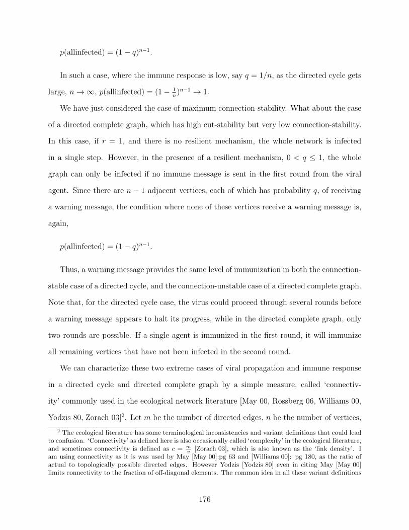
p(allinfected) = (1− q)n−1.

In such a case, where the immune response is low, say q = 1/n, as the directed cycle gets

large, n→∞, p(allinfected) = (1− 1n)n−1 → 1.

We have just considered the case of maximum connection-stability. What about the case

of a directed complete graph, which has high cut-stability but very low connection-stability.

In this case, if r = 1, and there is no resilient mechanism, the whole network is infected

in a single step. However, in the presence of a resilient mechanism, 0 < q ≤ 1, the whole

graph can only be infected if no immune message is sent in the first round from the viral

agent. Since there are n− 1 adjacent vertices, each of which has probability q, of receiving

a warning message, the condition where none of these vertices receive a warning message is,

again,

p(allinfected) = (1− q)n−1.

Thus, a warning message provides the same level of immunization in both the connection-

stable case of a directed cycle, and the connection-unstable case of a directed complete graph.

Note that, for the directed cycle case, the virus could proceed through several rounds before

a warning message appears to halt its progress, while in the directed complete graph, only

two rounds are possible. If a single agent is immunized in the first round, it will immunize

all remaining vertices that have not been infected in the second round.

We can characterize these two extreme cases of viral propagation and immune response

in a directed cycle and directed complete graph by a simple measure, called ‘connectiv-

ity’ commonly used in the ecological network literature [May 00, Rossberg 06, Williams 00,

Yodzis 80, Zorach 03]2. Let m be the number of directed edges, n be the number of vertices,

2 The ecological literature has some terminological inconsistencies and variant definitions that could leadto confusion. ‘Connectivity’ as defined here is also occasionally called ‘complexity’ in the ecological literature,and sometimes connectivity is defined as c = m

v [Zorach 03], which is also known as the ‘link density’. Iam using connectivity as it is was used by May [May 00]:pg 63 and [Williams 00]: pg 180, as the ratio ofactual to topologically possible directed edges. However Yodzis [Yodzis 80] even in citing May [May 00]limits connectivity to the fraction of off-diagonal elements. The common idea in all these variant definitions

176

and c be the connectivity defined on directed edges and vertices. Then c = mv2

, and is in-

terpreted as the ratio of actual to possible directed edges. For a directed cycle, m = n, so

c = mn2 = n

n2 = 1n. For a complete directed graph with self loops, m = n2, so c = m

n2 = n2

n2 = 1.

Thus, for directed graphs that are strongly connected, 1n≤ c ≤ 1.

Our simple calculations suggest the warning message may have greater opportunity to

race ahead at higher connectivities. In the next section we take a closer look at how network

connectivity may affect resilience.

7.4.3 Resilience Example 3: Virus Immune Response Under Different Network Connectiv-

ities

Essentially the two cases from the previous section could be seen as a ‘game’, somewhat like

Go, between the viral and immune response played out on a board that is the network’s

topology. We want to understand what the board needs to look like to give the immune

response its best chance of running ahead. We will do so by imagining how this game gets

played out in networks with different connectivities.

Let us consider a small simulation based experiment where we examine networks of

various connectivities, from low to high, and various levels of virulence and immune response,

from low virulence and high immune response to high virulence and low immune response.

We simulate the virus and immune PNM on small networks with 25 agents. We have

four levels of connectivity: (S)parse = 25 edges (c = 25625

= 0.04), (‘C)ritical’ = 50 edges

(c = 50625

= 0.08)3, (M)oderate = 100 edges (c = 100625

= 0.16) and (H)igh = 300 edges

(c = 300625

= 0.48). Let GD(n,m) be a directed graph drawn randomly from the family of

is to measure how many directed edges there are relative to directed edges possible.3 The ‘(C)ritical’ network size of 50, is so-called because it represents a connectivity level greater than the

point in the corresponding undirected random graph at which the giant component appears in Erdos-Renyirandom graph models [7]. In an undirected graph, the giant (connected) component appears at a phasetransition where the probability of an edge being selected for a graph with n vertices is 1

n . The averagedegree for a vertex at that point is n× 1

n = 1. Chung and Lu [7] note that when the average degree is lessthan 1, all connected components are small and there is no giant component. When the average degree isgreater than 1 the giant component is present. By implication when the probability of edge selection is 1/n,the giant component is in the process of emerging.

177

all graphs with n vertices and m directed edges [Luczak 90], which is the directed graph

extension of the G(n,m) model [Erdos 60, Luczak 94]. In these simulations, n = 25, and m

varies from 25 to 300. For each connectivity level, three different virus and immune response

levels are considered. Low virulence high immune response is r = 0.1 and q = 0.9. Moderate

virulence moderate immune response is r = q = 0.5. High virulence low immune response

is r = 0.9 and q = 0.1. For each connectivity level, three different random networks are

generated from the GD(n,m) model. For each network ten simulations are run at each of

the three virus and immune response levels. The initial infected vertex is randomly selected

in each simulation. There were 360 simulations run on twelve different networks, with

30 simulations run for each of the twelve network connectivity level by virus and immune

response level combinations.

In the spirit of exploratory data analysis [Chambers 83, Cleveland 85, Diaconis 85, Wainer 05,

Tukey 66] we focus on a simple graphical summary of average trends in our experiment as

we vary connectivity and the relative strength of viral and immune responses. Simulation

results are summarized in Figure 7.1, a simulation plot matrix which illustrates the average

progress of simulations across connectivity levels and virus and immune response levels. For

each plot in the matrix, blue squares represent neutral vertices that have not changed their

state, green triangles represent vertices that are immune, and red diamonds represent vertices

that are infected with the virus. Looking at the matrix from left to right (low virus/high

immune to high virus/low immune), the immune response acts as a resilient mechanism that

protects some portion of the network, even when virus response is high relative to immune

response. Looking at the matrix from top to bottom (low connectivity to high connectivity),

the immune response increases in effectiveness (number of vertices immunized) as connec-

tivity increases, and regardless of the specific combination of viral and immune response.

In all cases, the immune response acts as a resilient mechanism, protecting some agents.

In the top column, representing low connectivity, the lack of connected components limits

178

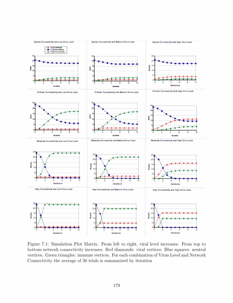
Figure 7.1: Simulation Plot Matrix. From left to right, viral level increases. From top tobottom network connectivity increases. Red diamonds: viral vertices. Blue squares: neutralvertices. Green triangles: immune vertices. For each combination of Virus Level and NetworkConnectivity the average of 30 trials is summarized by iteration

179

the progress of both the virus and the immune response. Finally, if we focus on the middle

column where the viral and immune response approximate the flipping of a fair coin, the

immune response exceeds the viral response in all four instances. For the bottom two rows,

representing moderate and high connectivity, all agents that begin neutral switch to viral or

immune by the end of the simulation, indicating they are part of the same strongly connected

component.

This small simulation experiment confirms the idea suggested by our earlier calculations

that the immune response, as a connection-resilient mechanism, is most effective as connec-

tivity increases. It provides increasing resilience as the structural connection-stability of the

network decreases. The reason the immune response of sending a warning message can run

ahead of the virus, even when both are at the same level is simply due to the fact that if a

‘healthy’ agent receives the warning message, it can warn all it’s neighbours, a reasonable

assumption in biological systems. If applied to a computational setting, this is equivalent

to assuming that healthy processors can propagate the warning message to neighbours with

probability 1.

7.4.4 Insights from the Examples: A Little Resilience Can Go A Long Way.

In all three examples, the resilient mechanisms provide a degree of protection, but not nec-

essarily absolute protection. In the case of resistant agents (agent hardening), the idea of

absolute resistance (no failure under attack), is unrealistic at the level of individual agents4.

However, even moderate resistance (say failure under attack is equivalent to flipping a fair

coin), preserves parts of the network for several rounds of attack, where the network would

have otherwise been cut to pieces in the first round. In the examples concerning a viral and

immune response, if the immune response and viral response have the same initial proba-

bility of propagation, the immune response has an advantage that increases as the system

4 It might however be more realistic as a goal at the level of networks or systems that absolutely mustnot fail, where guarantees of lack of failure might be achieved via multiple redundant systems.

180

connectivity increases. If we can assume that healthy agents (cells, processors) having re-

ceived a warning message can communicate efficiently with all their neighbours, the immune

response can race ahead. In a sense, the immune response could be looked at as a ‘good

virus’5 that has a home court advantage over the ‘bad virus’. The implication is that re-

silient mechanisms need not provide absolute guarantees of protection under various kinds

of attack, but a higher propensity for parts of the system to remain functional under various

kinds of attack, whether they be cut-attacks or connection-attacks.

Our examples have been exceedingly simple, focussed on extremely basic resilient mech-

anisms acting singly. In many biological systems homeostasis is maintained by multiple

redundant systems and processes, which suggests that the goal should not to be to design

‘the’ resilient mechanism that can handle all situations, but to design an array of resilient

mechanisms that may act together to handle different situations. Furthermore, while for

simplicity, we have the same resilient mechanism operating in each agent, diversity of re-

silient mechanisms across agents will make life harder for a malware designer, by putting

them essentially in the same position the anti-virus designer is in today.

7.5 Refining Resilient Mechanisms

We now briefly consider a few possible refinements for the virus–immune PNM which, while

they add complexity to the model, move it towards greater realism, and illustrate the idea

that different resilient mechanisms may work together.

7.5.1 Combining Resilient Mechanisms: Agent Resistance and Immune Response

One resilient mechanism that can contribute to the stability of a network is to make agents

‘resistant’ to failure. We have examined the consequences of such a resilient mechanism

earlier in the context of directed attacks. Now let us consider adding such a form of resilience

5 The idea of viewing the immune response as a beneficial virus was suggested by John Aycock.

181

to the existing virus–immune PNM. We will start off with a basic PNM for viral resistance,

and then combine it with our existing virus–immune PNM.

As before, we would like to black-box the low-level mechanisms – either due to hardware,

software, or cellular processes – by which a network component can be resistant to viruses,

and focus instead on the effects of a degree of resistance on the network; we are interested

in the consequences of a particular level of resistance. This approach is common in bio-

logical studies of epidemiology [Daley 99], where the immunological specifics of low level

host-intrusion and defence mechanisms at the level of individual agents (vertices in our case)

are black-boxed, to concentrate on how a contagion spreads through a population (networks

in our case) given particular assumptions about contact (adjacent agents in our case).

An agent is considered ‘exposed’ if it receive a viral message. Let us assume that having

been exposed, an agent transits to the viral state with some probability s that reflects how

susceptible the agent is to being infected upon exposure. Resistance, then is the comple-

mentary probability 1 − s of not transiting to the viral state when exposed. Let r be the

probability that an infected neighbour i transmits a viral message to j. The neighbourhood

around some agent j is symbolized by Γ(j).

We first need to model exposure in a network, and then resistance given exposure.

The random variable Ztj is 1 if vertex j is exposed at time t otherwise it is 0.

The random variable X tj is 1 if vertex j is infected at time t otherwise it is 0.

The basic exposure model is:

p(Ztj = 1 | Zt−1

j = 0) = 1−∏

i∈Γ(j)(1−X t−1

i ∗ r).

The basic resistance model is6:

6 This is the same resistance model we have seen earlier, p(F tj = 1 | At−1

j = 1) = fail. We havemerely changed notation to be consistent with the virus–immune PNM. Thus we now speak of ‘exposure’and ‘susceptibility’, rather than ‘attack’ and ‘failure’. We use the probability s for susceptibility, ratherthan its complement, so we may make statements in terms of probability of a change of state (rather thanprobability of remaining in the same state).

182

p(X tj = 1 | Zt−1

j = 1) = s.

To incorporate this simple viral resistance PNM into our viral–immune PNM, we first

have to modify our round structure from Chapter 6.

• Round 0 – initial infection (of a single agent in the network).

• Round 1, Phase 1 – an immune message is sent.

• Round 1, Phase 2 – the viral payload is sent (exposure).

• Round 1, Phase 3 – the viral payload is either accepted (infection) or rejected (resis-

tance) by the agent.

The phase structure within rounds serves to linearize the order of various message types,

thus preventing race conditions where two types of messages (say immune and viral) simul-

taneously arrive. Practically speaking they represent the situation where as a virus infects

an agent, it has some probability of sending out a warning message before it becomes conta-

gious, and that upon exposure to a virus, there is a delay before the vertex is either infected

or able to resist the virus.

Our modified model(s) incorporating both resistance and immune response is (are):

Resistance Model:

The previously infected case:

p(X tj = 1 | X t−3

j = 1) = 1.

The previously uninfected case:

p(X tj = 1 | X t−3

j = 0 ∧ Zt−1j = 1) = s.

Exposure Model:

p(Ztj = 1 | Zt−3

j = 0 ∧ Y t−1j = 0 ∧ ∀i∈Γ(j)

Y t−1i = 0) = 1−

∏i∈Γ(j)

(1−X t−2i ∗ r).

Immune Model:

The previously immune case:

183

p(Y tj = 1 | Y t−3

j = 1) = 1.

The previously immune neighbours case:


Y t−3i > 0 ∧ Y t−3

j = 0) = 1.

The previously infected neighbours case:

p(Y tj = 1 | X t−1

j = 0 ∧ Y t−3j = 0 ∧ ∀i∈Γ(j)

Y t−3i = 0) = 1−

∏i∈Γ(j)

(1−X t−1i ∗ q).

The key effort in creating a joint model incorporating both resistance and immunity is to

first modify the phase structure within rounds, and second to modify the conditions associ-

ated with the probability of an event such as exposure. In this combined model, resistance

and immunity via the warning message work in a complementary fashion to promote the

resilience of the network to a viral attack. Immunity via the warning message blocks the

paths along which the virus may propagate (so not all of MFS(v∗, G) can be reached) while

resistance slows down the rate of viral propagation (increasing the time, T , required for the

virus to propagate through the network). Jointly, these two effects promote the likelihood

of the warning message racing ahead and the virus being contained to a portion of the net-

work, and are together more effective than either mechanism would be singly. The warning

message can race ahead even faster now relative to the viral message. This illustrates, in a

simple way, the benefits of multiple resilient mechanisms working together, which is the true

basis of immune responses in biology.

Hardening agents, so they are resistant to attacks can provide resilience in the face of

both cut-attacks such as targeted denial of service attacks, and against connection-attacks

such as viruses. In transferring these insights from models to real systems, we must of

course dig into the black box of the specific mechanisms used to harden a real world agent

(be it a cell, and individual organism, a processor). The resilient mechanism for hardening

against a denial of service attack is unlikely to be the same as that required for providing

viral resistance. While it is useful to first understand the effects of different kinds of resilient

184

mechanisms in general, a natural progression in the development of PNMs is to next consider

the detailed mechanics of specific resilient mechanisms7. For now, we will continue with our

investigation of how the current virus–immune PNM might be further elaborated without

getting into the specifics of how resistance and immunity will be orchestrated in detail. As

those details are added in, one begins to move from model to virtual implementation.

7.5.2 Further Refinements to the Virus and Immune Response PNM

In creating our combined model, we have made a number of simplifying assumptions, to keep

the model reasonably tractable. The simplifying assumptions include:

• Resistance is constant under repeated exposure.

• An immune response where receipt of a warning message is sufficient to convey

immunity, and where immune nodes immunize their neighbours with probability 1.

We briefly sketch how such assumptions may be made more realistic, at the price of

increased model complexity. As we elaborated the mutualism PNM into an ecosystem PNM

in Chapter 6, we can continue to refine the virus–immune PNM by refining and combining

existing resilient mechanisms, and developing new ones.

First of all, let us assume resistance is not constant, but a function of repeated exposure,

such that on each subsequent exposure of an agent, resistance decreases (or conversely sus-

ceptibility increases). Let us assume a series of probabilities s1, s2, s3...sN with relationship

s1 < s2 < s3 < ... < sN . Let us assume an indexed series of random variables where the nth

stage towards infection at some time t for some vertex j is represented by X t(n)j. Then,

7 The Virus Group at University of Calgary Computer Science in developing the initial version of thevirus–immune PNM has considered several more detailed mechanisms that could be elaborations of thatPNM. A partial list includes: (a) adding virulence period to the PNM, (b) adding terms to the PNM thatreflect the work it might take to send an immune message to all adjacent agents, (c) adding delay parametersto reflect cases where a virus is not immediately detected, (d) having an initial distribution of infected agents,rather than a single infected agent, and (e) having identifiers of infected agents travel with the immune agent,so only messages from those agents are selectively blocked (which essentially also dynamically alters networkstructure in terms of open and blocked channels). All of these elaborations consist of expanding on the basecase that immunity is conferred via first receiving a warning message.

185

p(X t(n)j = 1 | Zt−1

j = 1 ∧X t−3(n−1)j = 1) = sn.

In making such an adjustment, we have done two things. First we have made agents

increasingly susceptible upon repeat exposures, which is often a realistic assumption. Sec-

ondly, we have added a very weak form of memory. In some sense, by introducing an indexed

series of states, each agent now ‘knows’ how many times it has been exposed.

We could further make immunity realistic, by assuming that an immune neighbour does

not immunize with probability 1, but with some probability l between 0 and 1. The equation

for the case of immune neighbours would then have to be suitably adjusted along the lines

of,


Y t−3i > 0 ∧ Y t−3

j = 0) = 1−∏

i∈Γ(j)(1− Y t−3

i ∗ l).

Other possibilities are easily imaginable, such as having immunity conferred only on

agents some distance away from the original warning message. This corresponds to the

notion that as the warning message races ahead, only those vertices at a distance from the

infection centre have the time to develop an effective immune response8.

Each of these modifications towards greater realism adds complexity to the model, so

there is a necessary balance between the effort required to make a useful model, and the

additional complexity added along the way. With reasonable effort, future versions of the

combined model may be made much more ‘realistic’ with respect to the nature of the resis-

tance and immune responses.

Even our simplifying assumption of a phase structure to linearize the order in which

different types of messages may be removed, though at the additional complexity of having

to add precedence rules for different kinds of messages that may be seen to be arriving (near)

simultaneously, moving us into the realm of asynchronous models [Attiya 04].

8 This idea was suggested by J. Denzinger.

186

7.6 The Epidemiological and Immune Metaphors in Computer Science

Some metaphors run deep, and the concept of a virus resonates in both the literature of

biology and computer science. Responses to viruses can be looked at from two different

biological perspectives, epidemiological and immunological. The epidemiological perspec-

tive concerns how viruses progress through a population of individuals, population patterns

(contact structure) that can promote or delay viral propagation, as well as techniques that

can slow or prevent such viral progress, such as an inoculation program. The immunological

perspective concerns how cellular mechanisms within an individual (the immune system) can

first recognize, and secondly block the spread of a virus, or any other foreign agent (antigen).

Immunological processes incorporate the functioning of several tissues and organs as well as

their interactions and chemical products (antibodies) to allow individuals to maintain home-

ostasis in the face of both external invaders, and internal processes9. Depending on how

we choose to interpret the virus–immmune PNM under a particular network structure, as a

population of cells within an individual, or as a population of individuals, we could either

perspective. Both perspectives have been applied to computer networks, but in different

ways. Each perspective has different implications. For example, immunization programs

are focussed on mass inoculation and not on the propagation of an immune response. The

inoculation approach has been adopted in the development of software anti-virus packages.

However, immune system responses have been adopted in biologically inspired network secu-

rity. We will briefly examine each perspective, the way it has entered into computer science,

and its relationship to resilient mechanisms.

The literature on mathematical epidemiology is broad and has a long history [Hethcote 00,

Nowak 06] in the biological literature. However, the starting point for a mathematical epi-

demiology model is usually to begin with a set of equations that represent reasonable as-

sumptions about the dynamics of a virus (either based on intuition, or the study of exist-

9 Cohen [Cohen 00a]:pp. 103–105 presents an agent based view of the immune system in terms of theagents required, their arrangement in space, and their interactions in time.

187

ing empirical data). The basic epidemiological model of which most other models can be

considered elaborations is the: (S)usceptible, (I)nfected, (R)ecovered model (SIR model 2)

[Hethcote 00]:pg. 604. This model consists of three differential equations, tracking Suscep-

tible, Infected, and Recovered population members over time.

dSdt

= −BIS.

dIdt

= BIS − vI.

dRdt

= vI.

S, I, and R represent the states susceptible, infected and recovered, respectively. B is

the contact rate, or likelihood of obtaining a disease via contact with an infected subject,

and v is the rate of recovery from an infection (the time it takes an individual to get over a

viral infection).

Essentially the progress of a virus through a population is modeled as transfers between

sequential compartments. Susceptible individuals are transferred to the Infectious compart-

ment and finally to Recovered compartment. Several studies on network epidemiology have

focussed on transferring classic models of population epidemiology from their original bi-

ological context [Daley 99] to a network context that can apply to Internet epidemiology

[Calloway 00, Newman 02a, Pastor-Satorras 01, Yuan 08]. This interaction has also worked

in the reverse direction, where network based models are applied back to biology [Meyers 05].

A recent work that considers immunity [Mishra 07] in a network context, models it as part

of the recovery state in a SIR type model, so does not consider its propagation.

The virus–immune PNM is even simpler than these epidemiological models in one sense,

and more complex in another. It is simpler in that the model has no recovery component.

This is akin to considering the infection deadly and without recovery. It is more complex

in that a new compartment is added, immune. While our virus–immune PNM is based on a

probabilistic rule set, the simulation results of the model (see Figure 7.1) can be recast as

188

rate equations similar to those in the SIR model10.

The obvious insight from Figure 7.1 is that the nature of the resulting rate equations

would be dependant on network connectivity. At each level of connectivity, there is a different

pattern of propagation for the virus and the immune response. To make a direct comparison

between our virus–immune PNM, and the simplest classic epidemiological model, SIR, we

would have to both add a component to and remove a component from our model. We would

have to add a state transition for recovery and an associated lag time. We would have to

remove the immune response, which is not a feature of classic epidemiological models.

Our current virus–immune PNM freezes or halts eventually in that over iterations every

agent that changes state, enters either a viral or immune state, and once in that state,

does not change. If the PNM were extended so that there is a recovered state (essentially

a transition from the viral state back to the neutral state such as in SIS models), there

is the possibility of cycles and chaotic behaviour developing within the model. Modified

models where the recovered state is again susceptible to viral infection, and where immunity

is temporary, may result in waves of viral and immune responses running through the system

without ever settling down.

While epidemiological models in biology focus on populations of organisms [Hethcote 00,

Nowak 06], immune responses are properties of individuals, arising from interactions between

cells and tissues. We could consider immunity an intrinsic property we can attempt to

build into a distributed system so that it autonomously deals with infection. Just such

an approach is beginning to appear in the literature on Internet worms [Cheetancheeri 06,

Costa 05]. Immune system inspired resilient mechanisms do come into play in the network

security literature [Forrest 97a, Somayaji 04], however at the low level of the mechanics of

a particular immunological mechanism, focussing on anomaly detection and distinguishing

‘self’ from ‘non-self’ (i.e. autonomous detection of potential viruses or other malware). This

10 A closely related variant is the SIS model (Susceptible, Infected, Susceptible) whose major difference isthat the infected vertices recovery state is one in which they are again susceptible to infection

189

has led to the concept of developing agent based artificial immune systems for computational

networks whose behaviour is analogous to that of natural immune systems [Forrest 07]. The

effectiveness of such low level resilient mechanisms, whether immunologically inspired or

not, can be used to empirically assign the resistance and immune response probabilities in

PNMs. Simultaneously, the biological immunology literature is beginning to incorporate

network structure into models of specific immunological processes [Callard 05]. Unlike the

epidemiological literature, where existing models are being transferred directly from biology

to computer science, it is the concept of an immune system orchestrating specific immune

mechanisms to recognize self from non-self, to isolate non-self, and to engage in self-repair

that are being transferred from the biological literature into computer science. The virus–

immune PNM, if it is interpreted as a virus propagating through cells, fits well within this

immunological perspective.

From a distributed systems perspective [Attiya 04, Ozsu 99] the propagation of an im-

mune response arises naturally from a design perspective that focuses on message passing

and communication overhead. In such contexts, the network represents processors (agents)

and communication channels (directed edges). Distributed processors can send varying mes-

sages along channels. Viruses and immune responses are essentially just differing message

types, whose receipt either compromises functionality (viruses) or helps maintain function-

ality (immune responses) relative to the goals the system is intended to fullfill.

Topological network stability, and the derived concepts of resilient processes and mecha-

nisms provides a theoretical framework within which we can investigate specific epidemiolog-

ical models and immune system inspired processes and mechanisms. The PNM framework

provides a general modelling approach to explore the interplay of these different models and

mechanisms.

190

7.7 An Evolutionary Perspective

The perspective that unifies sub-disciplines in modern biology is evolution. Resilient pro-

cesses in biology are not designed, but are products of evolution. Increasingly we are seeing

evolutionary themes, originally developed in a biological context, entering into computer

science. We began this chapter with our network architect learning a little about resilient

processes in biology from an immunologist with an evolutionary bent. The Red Queen Hy-

pothesis developed by Leigh van Valen [Ridley 93, van Valen L. 73], focuses our attention on

the fact that host-parasite arms races have a strong tendency to develop in complex systems.

They are to some extent unavoidable. The notions of vertical and horizontal resistance are

well established in crop science [Robinson 95], and lead to alternate breeding strategies11.

Antivirus inoculation systems may be an effective resilient mechanism, but one with a high

overhead in terms of keeping up in the resulting arms race (by staying current with viral sig-

natures), and with both the strengths (total resistance for a period of time) and weaknesses

(when resistance is overcome susceptibility is complete) of vertical resistance. As computer

security expert Bruce Schneier notes [Schneier 04]:pg. 154, ‘Viruses have no cure. It’s been

mathematically proven that it is always possible to write a virus that any existing antivirus

program can’t stop. ... if the virus writer knows what the antivirus program is looking for,

he can always design his virus not to be noticed. Of course, the antivirus programmers can

always create an update to their software to detect the new virus after the fact.’ In the

evolutionary arms race in technology between viruses and antivirus programs, the antivirus

programs are always one step behind, playing catchup. In a similar vein, Balthrop et al.

conclude that vaccination strategies whether targeted or random are unlikely to be effective

across all network structures, and suggest instead a dynamic mechanism such as ‘throttling’

(limiting the number of connections a computer can make to other machines ), essentially a

connection-resilient mechanism that increases T .

11 Specifically, breeding programs for vertical resistance have emphasized inbred lines, while horizontalresistance have emphasized heterogenous populations [Robinson 95].

191

In this chapter we have illustrated the ways in which a few resilient mechanisms analogous

to horizontal resistance may be useful in providing resilience to a network. Such mechanisms

do not provide absolute protection of all agents (cells, processors), but they do provide

general mechanisms by which simple aspects of immune systems drawn from biology can be

built into technological networks.

Diversity, homeostasis, and immune system inspired defence mechanisms are suggested

as sources of design principles that can be transferred from evolutionary biology to computer

science to develop more robust systems [Forrest 97a, Forrest 97b, Forrest 05, Somayaji 07a].

Indeed some computer scientists have begun scouring the evolutionary literature for addi-

tional evolutionary metaphors [Somayaji 04] that can be used as design principles.

In describing the many ‘bad things that can happen to a network’ our language for

networked systems can borrow from biology [Somayaji 07b]. Thus, in this chapter we have

used terms such as ‘exposure’, ‘virus’, ‘resistance’ and ‘immune response’, all of which are

common in the immunological [Cohen 00a] and epidemiological [Daley 99] literature. We

have chosen to focus on a high-level view of resilient mechanisms, concentrating on the effects

of such mechanisms as resistance, or the propagation of a warning message, but black-boxing

lower level details as to the construction of such resistance or warning systems. This allows

us to concentrate on the effects if such mechanisms existed, to quickly examine different

mechanisms, and to determine those that might be most effective given a particular network

architecture. A natural follow-up is then to begin working on the constructive details of

those resilient mechanisms that prove particularly effective under a particular architecture.

Studies of how technological systems change over time are increasingly leading to analo-

gies between the behaviour of complex technical systems and development and evolution

in ecosystems and organisms. Forbes in ‘Imitation of Life’ [Forbes 04] details the range of

concepts and techniques from biology that are being brought into computer science. Biology

provides vocabulary, concepts and analytical methodology to track changing organization

192

in systems which are increasingly applied outside of biology. Examples of other disciplines

borrowing from biology are Arthur’s theory of the evolution of technology [Arthur 09], Hu-

berman’s interpretation of the Internet as an ecology of information [Huberman 01] and

Dovrolis view of the Internet as an evolving ecosystem that has many parallels with biologi-

cal evolution [Dhamdere 08, Dhamdere 10, Dovrolis 08a, Dovrolis 08b, Rexford 10]. Dovrolis

focuses on the concept of evolvability, those features of the Internet that allow it to adapt as

its environment changes. This is an example where technological systems are borrowing evo-

lutionary concepts even while they are in active debate in biology [Kitano 04, Wagner 05]. At

the fundamental level of computation itself, there is the recognition that computations occur

within biological structures such as cells and DNA, and that the molecular interaction and

diffusion based methods of computation in these biological structures provides a ‘biotechnol-

ogy’ for computation [Adleman 98, Bray 09, Calude 01, Conrad 85, Shapiro 06, Winfree 98]

that is very different from our traditional computer architectures and their underlying com-

putational models.

Given the analogies between biological patterns and the development of technological sys-

tems, it is natural to adapt into computer science concepts first developed in biology. In the

opposite direction, biology borrows concepts from computer science such as the application

of distributed system concepts in the study of immune systems [Segel 01], the analogy that

biological processes are like distributed system protocols [Doyle 05, Doyle 07] or the explicit

use of message-passing as a framework for biological signalling that is applied in this chapter.

In new interdisciplinary fields such as systems biology, where theory construction includes

computational models encompassing complex biological phenomena, the opportunities for

conceptual transfer are particularly rich. In particular, studies of system structure and pro-

cess designs that have resulted from evolution in biological systems may be apt starting point

for testable designs for complex technological systems [Doyle 05, Doyle 07].

Computer science is perhaps unique among the sciences for its ability to borrow concepts

193

widely from other disciplines and fashion them into tools for its own use. Past examples have

been the incorporation of biological ideas into the development of neural networks (which by

a long chain of development lead to graphical models), genetic algorithms and evolutionary

computing, reinforcement learning, swarm computing, and semiochemical models. As such

computer scientists have unique opportunities to develop cross disciplinary insight as they

draw methods and concepts into their discipline by abstracting from other disciplines.

While biology may be a source for guiding concepts for resilient mechanisms that can

dynamically stabilize complex networks, there is no reason to assume that effective resilient

mechanisms are limited to the biological. It may even be possible to take a genetic algorithms

approach and search through the space of possible resilient mechanisms for those whose

effects prove most stabilizing under a particular network architecture (which we could call

‘narrow-sense resilience’) and those which are stabilizing under a wide range of network

architectures (which we could call ‘broad-sense resilience’).

Topological network stability, dynamic resilience, and the PNM approach provide a the-

oretical and modelling framework which allows computer scientists to borrow concepts from

a wide range of biological systems focussed on interactions, strip away much of the biological

detail, until the interactions are laid bare, and then examine the structure of interactions, and

mechanisms for interactions. In doing so, there are conceptual benefits to computer science

in terms of inspiration for new algorithms and stabilizing mechanisms, and benefits back to

those sciences which are conceptually drawn upon by computer science in the development

of new computational models and analyses – new tools for thought useful in epidemiology,

immunology, ecology, systems biology and evolutionary biology. Along the way, we move

from loose analogies, to suggestive metaphors, to the transfer of logical structure from one

discipline to another, seeking unification. The goal of the previous seven chapters has been

to take a small step on this path, to elucidate a single concept – topological stability in

complex networks – and its consequences, dynamic resilient processes and mechanisms.

194

Chapter 8

The Nascent Moment

This is the moment

of stillness

when before

and after

truncate

at the birth

of a distinction:

what is now,

was not then.

8.1 Abstract

We briefly review the major contributions of this thesis and identify several future research

directions. Finally, we speculate on the origin of interactions that are the basis of com-

plex networks in biology, and that may begin to drive the evolution of complex networks in

technology.

8.2 Recap of Contributions

Chapter 1 listed the contributions this thesis makes towards a theory of topological stability

and dynamic resilience in complex networks:

1. Definitions of cut-stability, connection-stability and balanced-stability are pro-

vided. The ways in which these concepts may be related to information theory

195

is also developed. (Chapters 1, 4).

2. The antagonism between cut-stability and connection-stability is demonstrated

(Chapter 4).

3. A formal model for PNMs is developed, and PNMs are designed that reflect a

range of biological processes associated with stability (Chapters 5, 6).

4. Resilient processes and resilient mechanisms are defined (Chapter 7).

5. A PNM representing a virus and immune response is explored to identify

conditions under which a resilient mechanism is effective (Chapter 7).

6. Interdisciplinary contributions are made at various points. Topological sta-

bility concepts are applied to error and attack tolerance in technological net-

works, to stability in ecosystems, and is connected to some current concepts

in social networks (Chapter 4). Concepts from computational systems biol-

ogy inspire the development of the PNM approach, and the design of specific

PNMs (Chapters 5, 6). Concepts from epidemiology, immunology, and evo-

lutionary biology are incorporated into our development of resilient processes

and resilient mechanisms (Chapter 7).

The essential contribution of this thesis is simply to argue over seven chapters for a theory

of topological stability and dynamic resilience in complex networks. To develop this thesis re-

quired us to develop arguments that cut across, and thereby connect, several sub-disciplines

in computer science and biology. We have emphasized interactions as the common basis of

complex networks in different fields. The stability of a complex network originates in the

stability properties of the interactions that underlie it. In biological systems, such interac-

tions originate as processes become coupled. In technological systems, we design some of the

interactions into the system, but others emerge due to the coupling of processes that may not

196

have been anticipated by the system designer, such as social processes, economic processes,

and as recent international events have shown, political processes. In the construction of

large technological networks, such processes, outside of our explicit design considerations,

may ultimately have strong influence on the stability of the systems we develop. In consid-

ering the effects of such interactions, it is useful to have a theory about the stability of a

network of process based interactions. Our goal in this thesis has been to provide a start to

such a theory.

8.3 Future Directions

Our theory is a starting point, from which implications, like directed edges, may connect in

various directions: theoretical, methodological, and empirical applications. In each of these

areas, I will briefly state some questions that interest me. The list is not exhaustive, but

reflects my mix of computational and biological interests. A social scientist, an engineer, or

an economist might come up with a very different list of next steps. A physicist might ask

similar questions, but pursue very different applications.

8.3.1 Theoretical Next Steps

Having developed a conception of perfect information hiding (Chapter 4), in the context of

balanced stability, one question that immediately interests me is whether perfect information

hiding is possible, or whether it may violate some other invariant topological properties of a

graph. If the latter is true, it could be said that every network leaks information from which

an attacker can learn.

In Chapter 4, we demonstrated that the antagonism of cut-stability and connection-

stability could be related to mutual information under a specific construction of layering

cycle covers. I wonder if this phenomena might be much more general, and whether a

probabilistic argument may be developed for cut-stability and connection-stability, by which

197

the vast majority of edge addition sequences (increasing cut stability) will result in monotonic

declines in the average mutual information.

Towards the end of Chapter 4, it was mentioned that spectral analysis of networks has

been related to estimates of a network’s susceptibility to viral attacks. These results, and

those in Chapter 7, suggest that we may be able to formalize the relationship between the

average mutual information and spectral analysis on a complex network.

Finally, concepts developed in this thesis originated in my slow recognition over a period

of twenty years that there are multiple conceptualizations of stability. In Chapter 4 we illus-

trated the different perspectives between topological and dynamical approaches to stability

in the ecological literature. The relationship between topological stability and what I have

called Poincaire stability in this thesis needs further exploration. One possible road inwards

is the recognition that the community matrix [McCann 12] that is the basis of dynamical

approaches to the diversity-stability debate in ecology may be interpreted topologically in

terms of cut-stability and connection-stability properties of the graph it corresponds to.

8.3.2 Methodological Next Steps

The majority of this thesis has been concerned with developing a single theory. However,

theory can be a guide to, and inspire new techniques for, data analysis. Chapter 4 introduced

a simple visual technique that can be used to explore how a particular network deviates from

balanced stability. Chapter 7 briefly illustrated how the analysis of simulations can provide

insight into resilient mechanisms. One area I am interested in developing methodologically

is an analysis framework specific to PNMs, both at the level of model, and specific simu-

lation. Here, I am inspired by the lovely techniques that come out of dynamical systems

theory [Glass 88, Guastello 95, McCann 12, Sprott 03], and would aspire to similarly develop

the theory of topological stability and dynamic resilience as the basis of a data analytical

framework that can be used to bridge theory and experimental data.

In Chapter 6 I identified several directions for the elaboration of PNMs, including explor-

198

ing modal logic to create anticipatory systems within PNMs, and introducing more complex

memory mechanisms inspired by biology, particularly recent work in neurobiology. Other

obvious approaches are to combine PNMs with methods from evolutionary computation to

create evolvable PNMs.

Finally, I am interested in the ways in which a combination of topological stability theory

and PNMs can be used to develop design principles for complex networks, and a framework

in which network and process designs can be tested in silico before being released into the

wild.

8.3.3 Empirical Applications

Complex networks concepts have provided a framework to integrate empirical data in several

fields including: computer science, systems biology, ecology, epidemiology, finance and the

social and political sciences.

The empirical applications I list reflect my specific interests, and colleagues whose work

has inspired me to apply my techniques to their problems.

In computer science, I am interested in using topological stability as a way to elucidate

design principles for complex technological systems, be they the network of code relationships

in a complex piece of software, or the network of infrastructure and process in our most

complex technological network, the Internet.

Again, in computer science, I am fascinated with the ways in which multi-agent systems

(including PNMs) can generalize the notion of dynamical systems, and be used to explore,

via simulation, basic concepts in coordination, problem solving and self-organization via

heterogenous agents.

In systems biology, I am particularly interested in the application of topological stability

theory, PNMs, and other concepts from distributed systems theory to multicellularity, in

particular to understand the conditions under which cells can switch fates under the influence

of cell–cell signalling.

199

Epidemiology and immunology have already contributed to computer science, as ref-

erenced in Chapter 7. The exploration of artificial immune systems, and epidemiological

dynamics within the context of PNMs is a natural extension of the latter stages of my thesis.

The majority of my working life has been focussed on understanding ecosystems at small,

intermediate, and large scales. This thesis began in my efforts to understand the stability I

saw in ecosystems relative to the numerous perturbations they were exposed to1. No doubt,

the conceptual tools from this thesis will be focussed on further understanding stabilizing

processes in ecosystems under stress, whether it be due to climate change, loss of pollinators,

or human actions that change the structure and functioning of ecosystems.

8.4 On the Origin of Interactions

‘The Architecture of Complexity’ is the title of two essays separated by forty-five years. Tech-

nology pioneer, Herbert Simon’s, essay of 1962 [Simon 62] was concerned with elucidating

design principles for complex technological systems such as modularity, near decomposabil-

ity, and hierarchy (amongst others) that allowed complex systems to be assembled out of

simpler constructions. Albert-Laslo Barbasi’s essay of 2007 [Barbasi 07] does not cite its

predecessor, but covers much of the same ground, now from the perspective of complex net-

works. If such an essay were to be again written, a few decades hence, it might very well

again cover similar ground, but now from the perspective of the origin of interactions.

Biologists have several views on the origin of interactions. The evolutionary theorist

and systematist D.R. Brooks has pointed out that the explanation of many current ecologi-

cal interactions originates in the interactions amongst the ancestors of contemporary species

1 In particular, I can still visualize the small sphagnum patches that were on the study site for myM.Sc. in the Sooke Mountains. These patches created miniature sphagnum bogs in a larger subalpine forestecosystem. Such miniature ecosystems were dependant both on the conditions of the larger ecosystem theywere contained in, and dependant on vagaries within that larger ecosystem, such as a fallen stump creatinga pool in which some sphagnum moss was initially established, which then created the conditions for otherbog plants. It impressed me then and now, that while perturbations can disrupt ecosystems, they can alsobe the basis for the existence of, and scale of ecosystems

200

[Brooks 02]. The biophysicist Koichiro Matsuno has noted that synchronized behaviour in bi-

ology, such as the motion of a muscle fiber, originates in asynchronous stochastic phenomena

that suddenly becomes coordinated. He looks to the mechanisms of such initial coordina-

tion [Matsuno 97, Matsuno 98], originating in the interplay of quantum and thermodynamic

constraints [Matsuno 99, Matsuno 01]. Several leading theoretical biologists have implicated

autocatalytic cycles in the origin of biological interactions. It is emphasized in the work of

Stuart Kauffman [Kauffman 93], R.E. Ulanowicz [Ulanowicz 97, Ulanowicz 09b], as well as in

the evolutionary synthesis of John Maynard-Smith and Eors Szathmary [Maynard Smith 99].

All these perspectives centre on the origin of biological processes.

Ulanowicz defines a process operationally as ([Ulanowicz 09b]:pg. 29):

‘A process is the interaction of random events upon a configuration of constraints that

results in a nonrandom but indeterminate outcome.’

All these approaches to the origin of interactions speak to that nascent moment, when

random collisions become meaningful interactions; become increasingly constrained and syn-

chronized into a process. Processes, once sufficiently coherent, could interact with each other,

leading to a combinatorial hierarchy of interactions. A theory of the origin of such interac-

tions is necessary to understand the origin of biological processes. The logical switches in

gene regulatory systems were only so at the end of such a history of constraint and synchro-

nization. Put simply, how out of many possible interactions, did a smaller set of regular, and

relatively cut-stable and connection-stable interaction networks emerge and evolve to create

the processes that structure ecosystems, gene regulatory networks and immune systems?

Hopefully, the conceptual tools developed in this thesis can be further developed to address

this question of the origins of the interactions, the nascent moment.

201

Bibliography

[Abelson 00] H. Abelson & N. Forbes. Amorphous Computing. Complexity, vol. 5, no. 3,pages 22–25, 2000.

[Abraham 06] I. Abraham, D. Dolev, R. Gonen & J. Halpern. Distributed Computing MeetsGame Theory: Robust Mechanisms for Rational Secret Sharing and MultipartyComputation. In PODC’06, 2006.

[Abraham 08] I. Abraham, D. Dolev & J. Y. Halpern. An almost-surely terminating poly-nomial protocol for asynchronous Byzantine agreement with optimal resilience.PODC’08, vol. 8, pages 405–414, 2008.

[Adleman 98] L. M. Adleman. Computing with DNA. Scientific American (August, pages54–61, 1998.

[Albert 00] R. Albert, H. Jeong & A.-L. Barbasi. Attack and Error Tolerance of ComplexNetworks. Nature, vol. 406, pages 378–382, 2000.

[Albert 02] R. Albert & A-L. Barabasi. Statistical Mechanics of Complex Networks. Re-views of Modern Physics, vol. 74, pages 47–97, 2002.

[Allesina 05] S. Allesina, A. Bodini & C. Bondavalli. Ecological Subsystems Via Graph The-ory: The Role of Strong Components. Oikos, vol. 110, pages 164–176, 2005.

[Allesina 08] S. Allesina, D. Alonso & M. Pascual. A General Model for Food Web Structure.Science, vol. 320, pages 658–661, 2008.

[Allesina 09] S. Allesina & M. Pascual. Food Web Models: A Plea for Groups. EcologyLetters, vol. 12, pages 652–662, 2009.

[Allesina 12] S. Allesina & S. Tang. Stability Criteria for Complex Systems. Nature, vol. 483,pages 205–208, 2012.

[Alon 06] U. Alon. An introduction to systems biology. design principles of biologicalcircuits. Chapman and Hall/CRC, 2006.

[Alon 07] U. Alon. Network Motifs: Theory and Experimental Approaches. Nat. Rev.Genet., vol. 8, pages 450–461, 2007.

[Anand 09] K. Anand & G. Bianconi. Entropy Measures for Networks: Towards an In-formation Theory of Complex Topologies. Physical Review E, vol. 80, page045102(R), 2009.

[Aoki 01] I. Aoki. Biomass diversity and stability of food webs in aquatic systems. Eco-logical Research, vol. 16, pages 65–71, 2001.

[Arnold 92] V. I. Arnold. Catastrophe theory. third edition. Springer-Verlag, 1992.

202

[Arora 09] S. Arora & B. Barak. Computational complexity. a modern approach. Cam-bridge University Press, 2009.

[Arthur 09] B. Arthur. The nature of technology. what it is and how it evolves. Free Press,2009.

[Attiya 04] H. Attiya & J. Welch. Distributed computing. fundamentals, simulations, andadvanced topics. second edition. Wiley, Interscience, 2004.

[Ball 04] P. Ball. Critical mass. how one thing leads to another. Farrar, Straus andGiraux, 2004.

[Bambrough 63] R. Bambrough. The philosophy of aristotle. New American Library, 1963.

[Barabasi 99] A-L Barabasi & R. Alberts. Emergence of Scaling In Random Networks. Sci-ence, vol. 286, pages 509–512, 1999.

[Barbasi 07] A-L. Barbasi. The Architecture of Complexity. From Network Structure toHuman Dynamics. IEEE Control Systems Magazine., August 2007.

[Bascompte 09] J. Bascompte & D. B. Stouffer. The Assembly and Disassembly of EcologicalNetworks. Phil. Trans. R. Soc. B, vol. 364, pages 1781–1787, 2009.

[Battini 07] D. Battini, A. Persona & S. Allesina. Towards a Use of Network Analysis:Quantifying the Complexity of Supply Chain Networks. Int. J. Electronic Cus-tomer Relationship Management, vol. 1, no. 1, pages 75–90, 2007.

[Batty 05] M. Batty. Cities and complexity. The MIT Press, 2005.

[Begon 81] M. Begon & M. Mortimer. Population ecology. a unified study of animals andplants. Blackwell Scientific Publications Ltd, 1981.

[Bell 87] J. S. Bell. Speakable and unspeakable in quantum mechanics. CambridgeUniversity Press, 1987.

[Bersier 02] L-F. Bersier, C. Banasek-Richter & M-F. Cattin. Quantitative Descriptors ofFood-Web Matrices. Ecology, vol. 83, no. 9, pages 2394–2407, 2002.

[Bezzi 11] P. Bezzi & A. Volterra. Astrocytes: Powering Memory. Cell, vol. 144, pages644–645, 2011.

[Bianconi 07] G. Bianconi. A Statistical Mechanics Approach for Scale-Free Networks andFinite-Scale Networks. Chaos, vol. 17, page 026114, 2007.

[Bianconi 09a] G. Bianconi. Entropy of Network Ensembles. Physical Review E, vol. 79,page 036114, 2009.

[Bianconi 09b] G. Bianconi, P. Pin & M. Marsili. Assessing the Relevance of Node Featuresfor Network Structure. PNAS, vol. 106, no. 28, pages 11433–11438, 2009.

203

[Bodini 02] A. Bodini & C. Bondavalli. Towards a Sustainable Use of Water Resources: AWhole-ecosystem Approach Using Network Analysis. Int. J. Environment andPollution, vol. 18, no. 5, pages 463–485, 2002.

[Bollobas 98] B. Bollobas. Modern graph theory. Springer, 1998.

[Bonabeau 99] E. Bonabeau, M. Dorigo & G. Theraulaz. Swarm intelligence. from naturalto artificial systems. Oxford University Press, 1999.

[Bondavalli 99] C. Bondavalli & R. E. Ulanowicz. Unexpected Effects of Predators UponTheir Prey: The Case of the American Alligator. Ecosystems, vol. 2, pages49–63, 1999.

[Bondy 08] J. A. Bondy & U. S. R. Murty. Graph theory. Springer, 2008.

[Borrett 07] S. R. Borrett, B. D. Fath & B. C. Patten. Functional Integration of EcologicalNetworks Through Pathway Proliferation. J. Theor. Biol., vol. 245, pages 98–111, 2007.

[Borrett 10] S. R. Borrett, J. Whipple & B. C. Patten. Rapid Development of IndirectEffects In Ecological Networks. Oikos, vol. 119, pages 1136–1148, 2010.

[Branke 06] J. Branke, M. Mnif, C. Miller-Schloer, H. Prothmann, U. Richter, F. Rochner& H. Schmeck. Organic Computing – Addressing Complexity by Controlled SelfOrganization. In Proceedings of ISoLA 2006, pages 200–206, 2006.

[Bray 09] D. Bray. Wetware. a computer in every living cell. Yale University Press, 2009.

[Brooks 02] D. R. Brooks & D. A. McLennan. The nature of diversity. an evolutionaryvoyage of discovery. The University of Chicago Press, 2002.

[Brown 89] J. H. Brown & B. A. Maurer. Macroecology: The Division of Food and SpaceAmong Species on Continents. Science, vol. 243, pages 1145–1150, 1989.

[Buldyrev 10] S. V. Buldyrev, R. Parshani, H.E. Pau G. Stanley & S. Havlin. CatastrophicCascade of Failures in Interdependent Networks. Nature, vol. 464, pages 1025–1028, 2010.

[Callard 05] R. E. Callard & A. J. Yates. Immunology and Mathematics: Crossing theDivide. Immunology, vol. 115, pages 21–33, 2005.

[Calloway 00] D. E. Calloway, M. E. J. Newman, S. H. Strogatz & D. J. Watts. NetworkRobustness and Fragility: Percolation on Random Graphs. Phys. Rev. Lett.,vol. 85, pages 5468–5471, 2000.

[Calude 01] C. S. Calude, & G. Paun. Computing with cells and atoms. an introduction toquantum, dna and membrane computing. Taylor and Francis Inc., 2001.

[Caswell 01] H. Caswell. Matrix population models. construction, analysis, and interepre-tation. second edn. Sinauer Associates Inc Publishers, 2001.

204

[Censor-Hillel 11] K. Censor-Hillel & H. Shachnai. Fast Information Spreading in Graphswith Large Weak Conductance. In SODA 2011, pages 440–448, 2011.

[Chaitin 66] G. J. Chaitin. On the Length of Programs for Computing Finite Binary Se-quences. Journal of the ACM, vol. 13, pages 547–569, 1966.

[Chaitin 99] G. J. Chaitin. The unknowable. Springer, 1999.

[Chambers 83] J. M. Chambers, W. S. Cleveland, B. Kleiner & P. A. Tukey. Graphical meth-ods for data analysis. Wadsworth International Group and Duxbury Press,1983.

[Chang 08] H. Chang, M. Hemberg, M. Barahona, D Ingber & S. Huang. Transcriptome-wide noise controls lineage choice in mammalian progenitor cells. Nature,vol. 453, pages 544–547, 2008.

[Chartrand 77] G. Chartrand. Introductory graph theory. Dover Publications Inc., 1977.

[Cheetancheeri 06] S. G. Cheetancheeri, J. M. Agosta, D. H. Dash, K. N. Levitt, J. Rowe &E. M. Schooler. A distributed host-based worm detection system. SIGCOMM06 Workshops. Sept 11-15. Pisa, Italy, 2006.

[Chierichetti 09] F. Chierichetti, S. Lattanzi & A. Panconesi. Rumour Spreading and GraphConductance. In SODA 2010, pages 773–781, 2009.

[Chierichetti 10] F. Chierichetti, S. Lattanzi & A. Panconesi. Almost Tight Bounds forRumour Spreading with Conductance. In STOC 2010, pages 399–408, 2010.

[Chung 06] F. Chung & L. Lu. Complex graphs and networks. American MathematicalSociety, 2006.

[Chung 09] F. Chung. Graph theory in the information age. Noether Lecture at the AMS-MAA-SIAM Annual meeting, Jan. 2009, 2009.

[Cleveland 85] W. S. Cleveland. The elements of graphing data. Wadsworth AdvancedBooks and Software, 1985.

[Cohen 00a] I. R. Cohen. Tending adam’s garden. evolving the cognitive immune self. Aca-demic Press, 2000.

[Cohen 00b] R. Cohen, K. Erez, D. Ben-Avraham & S. Havlin. Resilience of the Internet toRandom Breakdowns. Phys. Rev. Lett., vol. 85, pages 4626–4628, 2000.

[Cohen 01] R. Cohen, K. Erez, D. ben Avraham & S. Havlin. Breakdown of the Internetunder Intentional Attack. Phys. Rev. Lett., vol. 85, pages 4626–4628, 2001.

[Cohen 03] R. Cohen, S. Havlin, & D. ben Avraham. Efficient Immunization Strategies forComputer Networks and Populations. Phys. Rev. Lett., vol. 91, no. 24, page247901, 2003.

205

[Collier 99] J. D. Collier & C. A. Hooker. Complexly Organised Dynamical Systems. OpenSystems and Information Dynamics, vol. 6, pages 241–302, 1999.

[Collier 03] J. Collier. Hierarchical Dynamical Information Systems with a Focus on Biol-ogy. Entropy, vol. 5, pages 100–124, 2003.

[Collier 04] J. Collier. Self-Organization, Individuation and Identity. Revue Internationalede Philosophie, vol. 59, pages 151–172, 2004.

[Collier 07] J. Collier. A Dynamical Approach to Identity and Diversity. In P. Cil-liers & K. Richardson, editeurs, Explorations in Complexity Thinking. Pre-Proceedings of the 3rd International Workshop on Complexity and Philosophy.Isce Publishing, 2007.

[Collier 08] J. Collier. A Dynamical Account of Emergence. Cybernetics and Human Know-ing, vol. 15, no. 3-4, pages 75–100, 2008.

[Conrad 72] M. Conrad. Information Processing in Molecular Systems. Currents in ModernBiology, vol. 5, pages 1–14, 1972.

[Conrad 79] M. Conrad. Mutation-Absorption Model of the Enzyme. Bulletin of Mathemat-ical Biology, vol. 41, pages 387–405, 1979.

[Conrad 81] M. Conrad & A. Rosenthal. Limits on the Computing Power of BiologicalSystems. Bulletin of Mathematical Biology, vol. 43, pages 59–67, 1981.

[Conrad 85] M. Conrad. On Design Principles for a Molecular Computer. Communicationsof the ACM, vol. 28, no. 5, pages 464–480, 1985.

[Conrad 90] M. Conrad. The Geometry of Evolution. Biosystems, vol. 24, pages 61–81,1990.

[Costa 05] M. Costa, J. Cowcroft, M. Castro, A. Rowstron, L. Zhou, L. Zhang &P. Barham. Vigilante: End-to-End Containment of Internet Worms. SOSP05, pages 23–26, October 2005.

[Crovella 06] M. Crovella & B. Krishamurthy. Internet measurement. infrastructure, trafficand applications. Wiley, John and Sons, 2006.

[Crucitti 04] P. Crucitti, V. Latora, M. Marchiori & A. Rapisarda. Error and Attack Toler-ance of Complex Networks. Physica A, vol. 340, pages 388–394, 2004.

[Daley 99] D. J. Daley & J. Gani. Epidemic modelling. an introduction. CambridgeUniversity Press, 1999.

[Danon 11] L. Danon, A. P. Ford, T. House, C. P. Keeling Jewell, Roberts M. J., J.V.G. O. Ross & M.C. Vernon. Networks and the Epidemiology of InfectiousDisease. Interdisciplinary Perspectives on Infectious Diseases, vol. 2011, page284909, 2011.

206

[Davidson 08] E. H. Davidson & M. S. Levine. Properties of Developmental Gene RegulatoryNetworks. PNAS, vol. 105, no. 51, pages 20063–20066, 2008.

[De Angelis 75] D. De Angelis. Stability and Connectance in Food Web Models. Ecology,vol. 56, pages 238–243, 1975.

[De Jong 06] K.A. De Jong. Evolutonary computation. a unified approach. The MIT Press,2006.

[de Leon 07] S.B-T. de Leon & E.H. Davidson. Gene Regulation: Gene Control Network inDevelopment. Annu. Rev. Biophys. Biomol. Struct., vol. 2007, pages 191–212,2007.

[Deacon 06] T. W. Deacon. Reciprocal Linkage between Self-organizing Processes is Suffi-cient for Self-reproduction and Evolvability. Biological Theory, vol. 1, no. 2,pages 136–149, 2006.

[Dehmer 11] M. Dehmer & A. Mowshowitz. A History ofGraph Entropy Measures. Infor-mation Sciences, vol. 181, pages 57–78, 2011.

[Dekker 04] A. H. Dekker & B. D. Colbert. Network Robustness and Graph Topology. InASC2004, pages 359–368. 2004.

[Dell 05] A. I. Dell, G. D. Kokkoris, C. Banasek-Richter, L-F. Bersier, J. A. Dunne,M. Kondoh, T. N. Romanuk & N.D. Martinez. How Do Complex Food WebsPersist In Nature? In P.C. de Ruiter, V. Wolters & J.C Moore, editeurs,Dynamic Food Webs Multispecies Assemblages, Ecosystem Development andEnvironmental Change, pages 425–436. Academic Press, 2005.

[Denzinger 04] J. Denzinger & J. Hamdan. Improving Modeling of Other Agents Using Ten-tative Stereotypes and Compactification of Observations. In Proc. IAT 2004IAT2004, pages 106–112, 2004.

[Dhamdere 08] A. Dhamdere & C. Dovrolis. Ten Years in the Evolution of the InternetEcosystem. IMC’08, 2008.

[Dhamdere 10] A. Dhamdere & C. Dovrolis. The Internet is Flat: Modeling the Transitionfrom a Transit Hierarchy to a Peering Mesh. ACM CoNEXT, vol. 2010, 2010.

[Diaconis 85] P. Diaconis. Theories of Data Analysis: From Magical Thinking ThroughClassical Statistics. In D.C. Tukey J.W. Hoaglin & F. Mosteller, editeurs,Exploring Data Tables, Trends and Shapes. Wiley-Interscience, 1985.

[Dinur 05] I. Dinur & S. Safra. On the Hardness of Approximating Minimum Vertex Cover.Annals of Mathematics, vol. 162, pages 439–485, 2005.

[Dorigo 04] T. Dorigo M. andStutzle. Ant colony optimization. The MIT Press, 2004.

[Dorogovtsev 03] S. N. Dorogovtsev & J. F. F. Mendes. Evolution of networks. from biolog-ical nets to the internet and www. Oxford University Press, 2003.

207

[Dovrolis 08a] C. Dovrolis. What Would Darwin Think About Clean-slate Architectures.In Computer Communication Review 38(1):, pages 29–34. ACM SIGCOMM,2008.

[Dovrolis 08b] C. Dovrolis & J. T. Streelman. Evolvable Network Architectures: What CanWe Learn From Biology. ACM SIGCOMM Computer Communication Review,vol. 40, no. 2, pages 72–77, 2008.

[Doyle 05] J. C. Doyle, D. L. Alderson, L. Li, M. Roughan, S. Shalunov, R. Tanaka &W. Willinger. The ‘Robust Yet Fragile’ Nature of the Internet. PNAS, vol. 102,no. 41, pages 14497–14502, 2005.

[Doyle 07] J. Doyle & M. Csete. Rules of Engagement. Nature, vol. 446, no. 860, 2007.

[Draief 08] M. Draief, A. Ganesh & L. Massoulie. Thresholds for Virus Spread On Net-works. The Annals of Applied Probability, vol. 18, no. 2, pages 359–378, 2008.

[Dray 90] D. Dray. Intracellular Signalling as a Parallel Distributed Process. J. Theor.Biol., vol. 143, pages 215–231, 1990.

[Duchon 06a] P Duchon, N. Hanusse, E. Lebhar & N. Schabanel. Could Any Graph BeTurned Into a Small-World. Theoretical Computer Science, vol. 355, pages96–103, 2006.

[Duchon 06b] P Duchon, N. Hanusse, E. Lebhar & N. Schabanel. Towards Small WorldEmergence. In SPAA ’06, pages 225–232, 2006.

[Dunne 02a] J. A. Dunne, R. J. Williams & N. D. Martinez. Food-web Structure and NetworkTheory: The Role of Connectance and Size. PNAS, vol. 99, no. 20, pages12917–12922, 2002.

[Dunne 02b] J. A. Dunne, R. J. Williams & N. D. Martinez. Network Structure and Bio-diversity Loss in Food Webs: Robustness Increases with Connectence. EcologyLetters, vol. 5, pages 558–567, 2002.

[Dunne 04] J. A. Dunne, R. J. Williams & N. D. Martinez. Network Structure and Robust-ness of Marine Food Webs. Marine Ecology Progress Series, vol. 273, pages291–302, 2004.

[Dunne 05] J. A. Dunne, U. Brose, R. J. Williams & N. D. Martinez. Modelling Food-Web Dynamics: Complexity-Stability Implications. In A. Belgrano, U. Scharler,J.A. Dunne & R.E. Ulanowicz, editeurs, Aquatic Food Webs: An EcosystemApproach, pages 117–129. Oxford University Press, 2005.

[Dunne 06] J. A. Dunne. The Network Structure of Food Webs. In Ecological Networks.Linking Structure to Dynamics in Food Webs, pages 27–86. Oxford UniversityPress, Pascual, M. and Dunne, J.A, 2006.

[Dunne 09] J. A. Dunne & R. J. Williams. Cascading Extinctions and Community Collapsein Model Food Webs. Phil. Trans. R. Soc. B, vol. 364, pages 1711–1723, 2009.

208

[Easley 10] D. Easley & J. Kleinberg. Networks, crowds and markets. reasoning about ahighly connected world. Cambridge University Press, 2010.

[Elton 58] C. S. Elton. Ecology of invasions by animals and plants. Chapman and Hall,1958.

[Epstein 96] J. M. Epstein & R. Axtell. Growing artificial societies. social science from thebottom up. The MIT Press, 1996.

[Epstein 06] J. M. Epstein. Generative social science. studies in agent-based computationalmodeling. Princeton University Press, 2006.

[Erdos 60] P. Erdos & A. Renyi. The Evolution of Random Graphs. Publications of theMathematical Institute of the Hungarian Academy of Sciences, vol. 5, pages17–61, 1960.

[Erwin 09] D. H. Erwin & E. H. Davidson. The Evolution of Hierarchical Gene RegulatoryNetworks. Nat. Rev. Genet., vol. 10, pages 141–148, 2009.

[Eveleigh 07] E. S. Eveleigh, K. S. McCann, P. C. McCarthy, S. J. Pollock, C. J. Lucarotti,B. Morin, G. A. McDougall, D. B. Strongman, J. T. Huber, J. Umbanhowar &L. D. B. Faria. Fluctuations In Density of an Outbreak Species Drive DiversityCascades in Food Webs. PNAS, vol. 104, no. 43, pages 16976–16981, 2007.

[Fagan 97] W. F. Fagan. Omnivory as a Stabilizing Feature of Natural Communities.American Naturalist, vol. 150, pages 554–567, 1997.

[Fath 98] B. D. Fath & B. C. Patten. Network Synergism: Emergence Of Positive Re-lations In Ecological Systems. Ecological Modelling, vol. 107, pages 127–143,1998.

[Fath 99] B. D. Fath & B. C. Patten. Review of the Foundations of Network EnvironAnalysis. Ecosystems, vol. 2, pages 167–179, 1999.

[Fath 04] B. D. Fath. Ecological Network Analysis Applied to Large-scale Cyber-ecosystems. Ecological Modelling, vol. 171, pages 329–337, 2004.

[Fath 06] B. D. Fath & W. E. Grant. Ecosystems as Evolutionary Complex Systems:Network Analysis of Fitness Models. Environmental Modelling and Software,vol. 22, no. 5, pages 693–700, 2006.

[Fath 07a] B. D. Fath & G. Halnes. Cyclic Energy Pathways in Ecological Food Webs.Ecological Modelling, vol. 208, pages 17–24, 2007.

[Fath 07b] B. D. Fath, U. M. Scharler, R. E. Ulanowicz & B. Hannon. Ecological NetworkAnalysis: Network Construction. Ecological Modelling, vol. 208, pages 49–55,2007.

209

[Felix 08] M-A. Felix & A. Wagner. Robustness and Evolution: Concepts, Insights andChallenges from a Developmental Model System. Heredity, vol. 100, pages 132–140, 2008.

[Feller 66] W. Feller. An introduction to probability theory and its applications. volume1. second edition. Wiley, John and Sons Inc, 1966.

[Feynman 95] R. P. Feynman. Six easy pieces. essentials of physics explained by its mostbrilliant teacher. Addison Wesley, 1995.

[Finn 76] J. T. Finn. Measures of Ecosystem Structure and Function Derived From Anal-ysis of Flows. J. Theor. Biol., vol. 56, pages 363–380, 1976.

[Fisher 99] M. J. Fisher, R. C. Paton & K. Matsuno. Intracellular Signalling Proteins as‘Smart’ Agents in Parallel Distributed Processes. Biosystems, vol. 50, pages159–171, 1999.

[Forbes 04] N. Forbes. Imitation of life. how biology is inspiring computing. The MITPress, 2004.

[Forrest 97a] S. Forrest, S. A. Hofmeyr & A. Somayaji. Computer Immunology. Communi-cations of the ACM, vol. 40, no. 10, pages 88–96, 1997.

[Forrest 97b] S. Forrest, A. Somayaji & D. Ackley. Building Diverse Computer Systems.In Proceedings of the Fourth Workshop on Hot Topics in Operating Systems,pages 67–72. 1997.

[Forrest 05] S. Forrest, J. Balthrop, M. Glickman & D. Ackley. Computation in the Wild.In K. Park & W Willinger, editeurs, The Internet as a Large Scale ComplexSystem. Oxford University Press, 2005.

[Forrest 07] S. Forrest & C. Beauchemin. Computer Immunology. Immunological Reviews,vol. 216, pages 176–197, 2007.

[Fox 02] J. W. Fox. Testing a Simple Rule for Dominance in Resource Competition.The American Naturalist, vol. 159, no. 3, pages 305–319, 2002.

[Fraigniaud 09] P. Fraigniaud & G. Giakkoupis. The Effect of Power-Law Degrees on theNavigability of Small Worlds. In PODC’09, pages 240–249, 2009.

[Fraigniaud 10] P. Fraigniaud & G. Giakkoupis. On the Searchability of Small-World Net-works with Arbitrary Underlying Structure. In STOC 2010, 2010.

[Gallos 05] L. K. Gallos, R. Cohen, P. Argyrakis, A. Bunde & S. Havlin. Stability andTopology of Scale-Free Networks under Attack and Defense Strategies. Phys.Rev. Lett., vol. 94, page 188701, 2005.

[Garey 79] M. R. Garey & D. S. Johnson. Computers and intractability. a guide to thetheory of np-completeness. W.H. Freeman and Company, 1979.

210

[Giakkoupis 11] G. Giakkoupis. Tight Bounds for Rumor Spreading in Graphs of a GivenConductance. In STACS 2011, pages 57–68, 2011.

[Gilbert 08] N. Gilbert. Agent-based models. SAGE Publications, 2008.

[Gill 08] P. Gill, M. Arlitt, Z. Li & A. Mahanti. The flattening internet topology:Natural evolution, unsightly barnacles or contrived collapse, volume PAM08.Cleveland, 2008.

[Glass 73] L. Glass & S. A. Kauffman. The Logical Analysis of Continuous, Nonlinear,Biochemical Control Networks. J. Theor. Biol., pages 103–129, 1973.

[Glass 88] L. Glass & M. C. Mackey. From clocks to chaos. the rhythms of life. PrincetonUniversity Press, 1988.

[Gleick 87] J. Gleick. Chaos: Making a new science. Viking, 1987.

[Goel 04] S. Goel & S. F. Bush. Biological Models of Security for Virus Propagation inComputer Networks. ;Login, vol. 29, no. 6, pages 49–56, 2004.

[Goerner 09] S. J. Goerner, B. Lietar & R. E. Ulanowicz. Quantifying Economic Sustain-ability: Implications for Free-Enterprise Theory. Ecol. Econ., vol. 69, pages76–81, 2009.

[Gould 79] S. J. Gould & R. C. Lewontin. The Spandrels of San Marco and the PanglossianParadigm: A Critique of the Adaptionist Programme. Proc. R. Soc. Lond. B,vol. 205, pages 581–598, 1979.

[Gowers 08] T. (ed) Gowers. The princeton companion to mathematics. Princeton Univer-sity Press, 2008.

[Grinstead 97] C. M. Grinstead & J. L. Snell. Introduction to probability. second revisededition. American Mathematical Society, 1997.

[Guastello 95] S. J. Guastello. Chaos, catastrophe and human affairs. applications of nonlin-ear dynamics in work, organizations and social evolution. Lawrence ErlbaumAssociates Inc., Publishers, 1995.

[Hacking 01] I. Hacking. An introduction to probability and inductive logic. CambridgeUniversity Press, 2001.

[Halpern 03] J. Y. Halpern. Reasoning about uncertainty. The MIT Press, 2003.

[Halpern 08] J. Y. Halpern. Beyond Nash Equilibrium: Solution Concepts for the 21st Cen-tury. In PODC’08, pages 1–10. 2008.

[Halter 07] R. Halter. Wild weather: The truth behind global warming. second edition.Altitude Publishing, 2007.

211

[Halter 11a] R. Halter. The incomparable honeybee and the economics of pollination. re-vised and updated. Rocky Mountain Books, 2011.

[Halter 11b] R. Halter. The insatiable bark beetle. RMB Books, 2011.

[Halter 11c] R. Halter. The insatiable bark beetle. Rocky Mountain Books, 2011.

[Harary 69] F. Harary. Graph theory. Perseus Books Publishing L.L.C, 1969.

[Hastings 84] H. M. Hastings. Stability of Large Systems. Biosystems, vol. 17, pages 171–177, 1984.

[Hawkins 04] J. Hawkins & S. Blakeslee. On intelligence. Henry Holt and Company, 2004.

[Hempel 66] C. G. Hempel. Philosophy of natural science. Prentice-Hall, 1966.

[Henneberger 10] C. Henneberger, T. Papouin, S. H. R. Oliet & D. Rusakov. Long-termPotentiation Depends on Release of D-serine from Astrocytes. Nature, vol. 463,pages 232–237, 2010.

[Henzinger 00] M. Henzinger, S. Rao & H. N. Gabow. Computing Vertex Connectivity: NewBounds from Old Techniques. Journal of Algorithms, vol. 34, pages 222–250,2000.

[Hethcote 00] H. W. Hethcote. The Mathematics of Infectious Diseases. SIAM Review,vol. 42, no. 4, pages 599–653, 2000.

[Higashi 86] M Higashi & B. C. Patten. Further Aspects of theAanalysis of Indirect EffectsIn Ecosystems. Ecol. Modell., vol. 31, pages 69–77, 1986.

[Higashi 89] M Higashi & B. C. Patten. Dominance and Indirect Causality in Ecosystems.Am. Nat, vol. 133, pages 288–302, 1989.

[Hoaglin 83] D. C. Hoaglin, F. Mosteller & J. W. Tukey, editeurs. Understanding robustand exploratory data analysis. John Wiley and Sons, 1983.

[Hoaglin 85] D. C. Hoaglin, F. Mosteller & J. W. Tukey, editeurs. Exploring data tables,trens, and shapes. John Wiley and Sons, 1985.

[Holling 73] C. S. Holling. Resilience and Stability of Ecological Systems. Annu. Rev. Rev.Ecol. Syst., vol. 4, pages 1–23, 1973.

[Hordijk 04] W. Hordijk & M. Steel. Detecting Autocatalytic, Self-sustaining Sets In Chem-ical Reaction Systems. J. Theor. Biol., vol. 227, pages 451–461, 2004.

[Hordijk 10] W. Hordijk, J. Hein & M. Steel. Autocatalytic Sets and the Origin of Life.Entropy, vol. 12, pages 1733–1742, 2010.

[Huang 04] S. Huang. Back to the Biology in Systems Biology: What Can We Learn fromBiomolecular Networks? Briefings in Functional Genomics and Proteonomics,vol. 2, no. 4, pages 279–297, 2004.

212

[Huang 09a] S. Huang. Non-genetic Heterogeneity of Cells in Development: More ThanJust Noise. Development, vol. 136, no. 23, pages 3853–3862, 2009.

[Huang 09b] S. Huang. Reprogramming Cell Fates: Reconciling Rarity with Robustness.Bioessays, vol. 31, pages 546–560, 2009.

[Huang 09c] S. Huang, I. Ernberg & S. Kauffman. Cancer Attractors: A Systems Viewof Tumors from a Gene Network Dynamics and Developmental Perspective.Semin. Cell Dev. Biol., vol. 20, pages 869–876, 2009.

[Huang 10] S. Huang. Cell Lineage Determination in State Space: A Systems View BringsFlexibility to Dogmatic Canonical Rules. PLoS, vol. 8, no. 5, 2010.

[Huang 11] S. Huang. Systems Biology of Stem Cells: Three Useful Perspectives To HelpOvercome the Paradigm of Linear Pathways. Phil. Trans. R. Soc. B., vol. 366,pages 2246–2259, 2011.

[Huang 12] S. Huang. The Molecular and Mathematical Basis of Waddington’s EpigeneticLandscape: A Framework for Post-Darwinian Biology? Bioessays, vol. 34,no. 2, pages 149–157, 2012.

[Huberman 01] B. A. Huberman. The laws of the web. patterns in the ecology of information.The MIT Press, 2001.

[Hudson 10] J. Hudson, J. Denzinger, H. Kasinger & B. Bauer. Efficiency Testing of Self-adaption Systems by Learning Event Sequences. In Proc. Adaptive-10, pages200–205, 2010.

[Hutchinson 59] G. E. Hutchinson. Homage to Santa Rosalia or Why Are There So ManyKinds of Animals? Am. Nat., vol. 93, pages 145–159, 1959.

[Istrail 05] S. Istrail & E. H. Davidson. Logic Functions of the Genomic Cis-regulatoryCode. PNAS, vol. 102, no. 14, pages 4944–4959, 2005.

[Istrail 07] S. Istrail, S. B-T. de Leon & E. H. Davidson. The Regulatory Genome and theComputer. Developmental Biology, vol. 310, pages 187–195, 2007.

[Jacob 66] F. Jacob. Genetics of the Bacterial Cell. Science, vol. 152, no. 3278, pages1470–1478, 1966.

[Jain 02] S. Jain & S. Krishna. Large Extinctions in an Evolutionary Model: The role ofinnovation in keystone species. PNAS, vol. 99, no. 4, pages 2055–2060, 2002.

[Jamniczky 10] H. A. Jamniczky, J. Boughner, C. Rolian, P. N. Gonzalez, C. D. Powell, E. J.Schmidt, T. E. Parsons, F. L. Bookstein & B. Hallgrımsson. RediscoveringWaddington in the Post-genomic Age. Bioessays, vol. 32, pages 1–6, 2010.

[Jordan 99] F. Jordan, A. Takacs-Santa & I. Molnar. A Reliability Theoretical Quest forKeystones. Oikos, vol. 86, no. 3, pages 453–462, 1999.

213

[Jordan 01] F. Jordan. Strong Threads and Weak Chains? - A Graph Theoretical Estima-tion of the Power of Indirect Effects. Community Ecology, vol. 2, no. 1, pages17–20, 2001.

[Jordan 05] F. Jordan, W-C Liu & T. Wyatt. Topological Constraints on the Dynamics ofWasp-Waist Ecosystems. Journal of Marine Systems, vol. 57, pages 250–263,2005.

[Jordan 09] F. Jordan. Keystone Species and Food Webs. Phil. Trans. R. Soc. B, vol. 364,pages 1733–1741, 2009.

[Junker 09] B. H. Junker & F. Schreiber, editeurs. Analysis of biological networks. JohnWiley and Sons, 2009.

[Kahlem 06] P. Kahlem & E. Birney. Dry Work in a Wet World: Computation in SystemsBiology. Molecular Systems Biology, vol. 2, page 40, 2006.

[Kaiser-Bunbury 10] C. N. Kaiser-Bunbury, S. Muff., J. Memmott & M˙ The Robustness ofPollination Networks to the Loss of Species and Interactions: A QuantitativeApproach Incorporation Pollinator Behaviour. Ecology Letters, vol. 13, no. 4,pages 442–452, 2010.

[Kasinger 06] H. Kasinger & B. Bauer. Pollination - A Biologically Inspired Paradigm forSelf-Managing Systems. Journal of Systems Science and Applications, vol. 3,no. 2, pages 147–156, 2006.

[Kasinger 08a] H. Kasinger, B. Bauer & J Denzinger. The Meaning of Semiochemicals to theDesign of Self-Organizing Systems. In Proceedings of SASO, pages 139–148,2008.

[Kasinger 08b] H. Kasinger, J. Denzinger & B. Bauer. Digital Semiochemical Coordination.Communications of SIWN, vol. 4, pages 133–139, 2008.

[Kasinger 09a] H. Kasinger & J. Denzinger. Design Pattern for Self-Organizing EmergentSystems Based on Digital Infochemicals. In Proc. EASe 2009, pages 45–55,2009.

[Kasinger 09b] H. Kasinger, J. Denzinger & B. Bauer. Decentralized Coordination of Ho-mogenous and Heterogenous Agents by Digital Infochemicals. In SAC’09, pages1223–1224, 2009.

[Kasinger 10] H. Kasinger, B. Bauer, J. Denzinger & T. Holvoet. Adapting Environment-Mediated Self-Organizing Emergent Systems by Exception Rules. In Proc.SOAR 2010. SOAR, 2010.

[Kauffman 69a] S. Kauffman. Homeostasis and Differentiation in Random Genetic ControlNetworks. Nature, vol. 224, pages 177–178, 1969.

[Kauffman 69b] S. A. Kauffman. Metabolic Stability and Epigenesis in Randomly Con-structed Genetic Nets. J. Theor. Biol. ., vol. 22, pages 437–467, 1969.

214

[Kauffman 74] S. Kauffman. The Large Scale Structure and Dynamics of Gene ControlCircuits: An Ensemble Approach. J. Theor. Biol., vol. 44, pages 167–190,1974.

[Kauffman 86] S. Kauffman. Autocatalytic Sets of Proteins. J. Theor. Biol., vol. 119, pages1–24, 1986.

[Kauffman 93] S. A. Kauffman. The origins of order. self organization and selection inevolution. Oxford University Press, 1993.

[Kauffman 04] S. Kauffman. A Proposal for Using the Ensemble Approach to UnderstandGenetic Regulatory Networks. J. Theor. Biol., vol. 230, pages 581–590, 2004.

[Keller 02] E. F. Keller. Making sense of life. explaining biological development with mod-els, metaphors, and machines. Harvard University Press, 2002.

[Keller 05] E. F. Keller. Revisiting ’Scale Free’ Networks. BioEssays, vol. 27, pages 1060–1068, 2005.

[King 09] J. P. King. Mathematics in 10 lessons. the grand tour. Prometheus Books,2009.

[Kitano 02] H. Kitano. Computational Systems Biology. Nature, vol. 420, pages 206–210,2002.

[Kitano 04] H. Kitano. Biological Robustness. Nature Reviews Genetics, vol. 5, pages 826–837, 2004.

[Kleinberg 00] J. Kleinberg. Navigation In A Small World. Nature, vol. 406, no. 845, 2000.

[Kleinberg 06] J. Kleinberg & E. Tardos. Algorithm design. Addison Wesley, 2006.

[Kleinberg 08] J. Kleinberg. The Convergence of Social and Technological Networks. Com-munications of the ACM, vol. 51, no. 11, pages 66–72, 2008.

[Knight 98] T. F. Knight & G. J. Sussman. Cellular Gate Technology. In C.S. Claude &M.J. Dinneen, editeurs, Unconventional Models of Computation, pages 257–272. Springer-Verlag, 1998.

[Kolmogorov 68a] A. N. Kolmogorov. Logical Basis for Information Theory and ProbabilityTheory. IEEE Transactions on Information Theory, vol. 14, no. 5, pages 662–664, 1968.

[Kolmogorov 68b] A. N. Kolmogorov. Three Approaches to the Quantitative Definition ofInformation. International Journal of Computer Mathematics, vol. 2, pages157–168, 1968.

[Konnyu 08] B. Konnyu, T. Czaran & E. Szathmary. Prebiotic Replicase Evolution In ASurface-bound Metabolic System: Parasites As a Source of Adaptive Evolution.BMC Evolutionary Biology, vol. 8, page 267, 2008.

215

[Kossinets 08] G. Kossinets, J. Kleinberg & D. Watts. The Structure of Information Path-ways in a Social Communication Network. In KDD’08, 2008.

[Kun 08] A. Kun, B. Papp & E. Szathmary. Computational Identification of ObligatorilyAutocatalytic Replicators Embedded in Metabolic Networks. Genome Biology,vol. 9, 2008.

[Kurose 08] J. F. Kurose & K. W. Ross. Computer networking. a top-down approach. 4thedition. Addison Wesley, 2008.

[Lamport 82] L. Lamport, R. Shostak & M. Pease. The Byzantine Generals Problem. ACMTransactions on Programming Languages and Systems, vol. 4, no. 3, pages382–401, 1982.

[Lehninger 65] A. L. Lehninger. Bioenergetics. the molecular basis of biological energy trans-formations. W.A. Benjamin Inc, 1965.

[Leiner 03] B. M. Leiner, V. G. Cerf, D. D. Clark, R. E. Kahn, L. Kleinrock, D. C. Lynch,J. Postel, L. G. Roberts & S. Wolff. A brief history of the internet version 3.32.Internet Society, http//www.isoc.org/internet/hisotry/brief.shtml, 2003.

[Leskovec 08] J. Leskovec. Dynamics of large networks. Phd. Dissertation. Cornell Univer-sity, 2008.

[Levin 92] S. A. Levin. The Problem of Pattern and Scale in Ecology. Ecology, vol. 73,no. 6, pages 1943–1967, 1992.

[Levine 05] M. Levine & E. H. Davidson. Gene Regulatory Networks for Development.PNAS, vol. 102, no. 14, pages 4936–4942, 2005.

[Levins 66] R. Levins. The Strategy of Model Building in Population Biology. AmericanScientist, vol. 54, no. 4, pages 421–431, 1966.

[Levins 68] R. Levins. Evolution in changing environments. some theortetical explorations.Princeton University Press, 1968.

[Lewin 92] R. Lewin. Complexity. life at the edge of chaos. Macmillan Publishing Com-pany, 1992.

[Li 97] M. Li & P. Vitanyi. An introduction to komogorov complexity and its appli-cations. second edition. Springer, 1997.

[Li 04] M. Li, X. Chen, X. Li, B. Ma & P. M. B. Vitanyi. The Similarity Metric. IEEETransactions on Information Theory, vol. 50, no. 12, pages 3250–3264, 2004.

[Li 05] L. Li, D. Alderson, J. C. Doyle & W. Willinger. Towards a Theory of Scale-Free Graphs: Definition, Properties, and Implications. Internet Mathematics,vol. 2, no. 4, pages 431–523, 2005.

216

[Li 07] J. Li & P. Knickerbocker. Functional similarities between computer worms andbiological pathogens. 338-347, Computers and Security 26, 2007.

[Li 11] X. Li, H. Wang & Y. Kuang. Global Analysis of a Stoichiometric Producer-grazer Model with Holling Type Functional Response. Mathematical Biology,pages DOI 10.1007/s00285–010–0392–2, 2011.

[Lindelauf 09] R. Lindelauf, P. Borm & H. Hamers. Understnading Terrorist NetworkTopologies and their Resilience Against Disruption. CentER Discussion Pa-per No, vol. 2009, no. 85, 2009.

[Lindeman 42] R. L. Lindeman. The Trophic Dynamic Aspect of Ecology. Ecology, vol. 23,pages 399–418, 1942.

[Lloyd 01] A. L. Lloyd & R. M. May. How Viruses Spread Among Computers and People.Science, vol. 292, pages 1316–1317, 2001.

[Loladze 00] I. Loladze, Y. Kuang & J. J. Elser. Stoichiometry in Producer-Grazer Systems:Linking Energy Flow with Element Cycling. Bulletin of Mathematical Biology,vol. 62, pages 1137–1162., 2000.

[Lotka 20] A. J. Lotka. Analytical Note on Certain Rhythmic Relations in Organic Sys-tems. PNAS, vol. 6, pages 410–415, 1920.

[Luczak 90] T. Luczak. The Phase Transition in the Evolution of Random Digraphs. Jour-nal of Graph Theory, vol. 14, no. 2, pages 217–223, 1990.

[Luczak 94] T. Luczak. Phase Transition Phenomena In Random Discrete Structures. Dis-crete Math, vol. 1994, pages 225–242, 1994.

[Luenberger 06] D. G. Luenberger. Information science. Princeton University Press, 2006.

[MacArthur 55] R. MacArthur. Fluctuations of Animal Populations and a Measure of Com-munity Stability. Ecology, vol. 36, pages 533–536, 1955.

[MacKay 03] D. J. C. MacKay. Information theory, inference, and learning algorithms.Cambridge University Press, 2003.

[Maier 09] G. Maier, A. Feldmann, V. Paxson & M. Allman. On dominant characteristicsof residential broadband internet traffic. Proc. ACM IMC, November 2009,2009.

[Marleu 11] J. Marleu, Y. Jin, J. G. Bishop, W. F. Fagan & M. A. Lewis. A StoichiometricModel of Early Plant Primary Succession. American Naturalist, vol. 177, no. 2,pages 233–245, 2011.

[Massol 11] F. Massol, D. Mouquet Gravel, Cadotte N., Fukami M. W., T. & M.A. Leibold.Linking Community and Ecosystem Dynamics Through Spatial Ecology. Ecol.Lett., vol. 14, pages 313–323, 2011.

217

[Matsuno 97] K. Matsuno. Biodynamics for the Emergence of Energy Consumers. Biosys-tems, vol. 42, pages 119–127, 1997.

[Matsuno 98] K. Matsuno. Dynamics in Time and Information in Dynamic Time. Biosys-tems, vol. 46, pages 57–71, 1998.

[Matsuno 99] K. Matsuno. Cell Motility As An Entangled Quantum Coherence. Biosystems,vol. 51, pages 15–19, 1999.

[Matsuno 01] K. Matsuno. Cell Motility and Thermodynamic Fluctuations Tailoring Quan-tum Mechanics for Biology. Biosystems, vol. 62, no. 1–3, pages 67–85, 2001.

[Maurer 99] B. A. Maurer. Untangling ecological complexity. the macroscopic perspective.University of Chicago Press, 1999.

[May 74] R. M. May. Biological Populations with Nonoverlapping Generations: StablePoints, Stable Cycles and Chaos. Science, vol. 186, pages 645–647, 1974.

[May 76a] R. M. May & G. F. Oster. Bifurcations and Dynamical Complexity in SimpleEcological Models. Am. Nat., vol. 110, pages 573–599, 1976.

[May 76b] R.M. May. Simple Mathematical Models with Very Complicated Dynamics.Nature, vol. 261, pages 459–467, 1976.

[May 00] R. M. May. Stability and complexity in model ecosystems. princeton landmarksin biology edn. Princeton University Press, 2000.

[May 01] R. M. May & A. L. Lloyd. Infection Dynamics on Scale-free Networks. PhysRev. E, vol. 64, page 066112, 2001.

[May 06] R. M. May. Network Structure and the Biology of Populations. Trends EcolEvol, vol. 21, no. 7, pages 394–399, 2006.

[May 08] R. M. May, S. A. Levin & G. Sugihara. Complex Systems: Ecology for Bankers.Nature, vol. 451, pages 893–895, 2008.

[May 09] R. M. May. Food-web Aseembly and Collapse: Mathematical Models and Im-plications for Conservation. Phil. Trans. R. Soc. B, vol. 364, pages 1643–1646,2009.

[Maynard Smith 99] J. Maynard Smith & E. Szathmary. The origins of life: From the birthof life to the origins of language. Oxford University Press, 1999.

[Mayo 96] D. G. Mayo. Error and the growth of experimental knowledge. The Universityof Chicago Press, 1996.

[McCann 00] K. S. McCann. The Diversity–Stability Debate. Nature, vol. 405, pages 228–233, 2000.

[McCann 12] K. McCann. Food webs. Princeton University Press, 2012.

218

[McCarthy 11] M. McCarthy. Decline of Honey Bees Now a Global Phe-nomenon, Says United Nations. The Independent, pageshttp://www.independent.co.uk/environment/nature/decline–of–honey–bees–now–a–global–phenomenon–says–united–nations–2237541.html?printService=print, March 2011.

[McCauley 99] E. McCauley, R. M. Nisbet, R. M. Murdoch, A.M. de Roos & W.S.C. Gur-ney. Large-amplitude Cycles of Daphnia and its Algal Prey in Enriched Envi-ronments. Nature, vol. 402, pages 653–656, 1999.

[McCauley 08] E. McCauley, W. A. Nelson & R. M. Nisbet. Small-amplitude Cycles Emergefrom Stage-structured Interactions in Daphnia-algal Systems. Nature, vol. 455,pages 1240–1243, 2008.

[McKeon 92] R. McKeon, editeur. Introduction to aristotle. The Modern Library, 1992.

[Memmott 04] J. Memmott, N. M. Waser & M. V. Price. Tolerance of Pollination Networksto Species Extinctions. Proc. R. Soc. Lond. B, vol. 271, pages 2605–2611, 2004.

[Meyers 05] L. A. Meyers, B. Pourbohloul, M. E. J. Newman, D. M. Skowronski & R. C.Brunham. Network Theory and SARS: Predicting Outbreak Diversity. J.Theor. Biol., vol. 232, pages 71–81, 2005.

[Miller 07] J. H. Miller & S. E. Page. Complex adaptive systems. an introduction tocomputational models of social life. Princeton University Press, 2007.

[Milo 02] R. Milo, S. Shen-Orr, S. Itzkovitz, N. Kashan, D. Chklovskii & U. Alon. Net-work Motifs: Simple Building Blocks of Complex Networks. Science, vol. 298,pages 824–827, 2002.

[Mishra 07] B. K. Mishra & D. K. Saini. SEIRS Epidemic Model with Delay for Trans-mission of Malicious Objects in Computer Network. Appl. Math. Comput.,vol. 188, pages 1476–1482, 2007.

[Mitchell 06] M. Mitchell. Complex Systems: Network Thinking. Artificial Intelligence,vol. 170, no. 18, pages 1194–1212, 2006.

[Mitchell 09] M. Mitchell. Complexity a guided tour. Oxford University Press, 2009.

[Mooney 93] C. Z. Mooney & R. D. Duval. Bootstrapping. a nonparametric approach tostatistical inference. Sage Publications, 1993.

[Muller 07] S. J. Muller. Assymetry: The foundation of information. Springer, 2007.

[Naeem 97] S. Naeem & Li S. Biodiversity Enhances Ecosystem Reliability. Nature,vol. 390, pages 507–509, 1997.

[Nagaraja 06] S. Nagaraja & R. Anderson. The Topology of Covert Conflict. In T. Moore,editeur, Pre-Proceedings of the Fifth Workshop on the Economics of Informa-tion Security, 2006.

219

[Nagaraja 08] S. Nagaraja. Robust Covert Network Topologies. PhD thesis, University ofCambridge, 2008.

[Nam 10] J. Nam, P. Dong, R. Tarpine, S. Istrail & E. H. Davidson. Functional Cis-regulatory Genomics for Systems Biology. PNAS, vol. 107, no. 8, pages 3930–3935, 2010.

[Ness 69] Van Ness & H. C. Understanding thermodynamics. Dover Publications Inc.,1969.

[Newman 02a] M. E. J. Newman. Spread of Epidemic Disease On Networks. Phys. Rev. E.,vol. 66, page 016128, 2002.

[Newman 02b] M. E. J. Newman, S. Forrest & J. Balthrop. Email Networks and the Spreadof Computer Viruses. Phys. Rev. E., vol. 66, page 035101, 2002.

[Newman 03] M. E. J. Newman. The Structure and Function of Complex Networks. SIAMReview, vol. 45, pages 167–256, 2003.

[Newman 06] M. Newman, A. Barbasi & D. J. Watts, editeurs. The structure and dynamicsof networks. Princeton University Press, 2006.

[Newman 10] M. E. J. Newman. Networks. an introduction. Oxford University Press, 2010.

[Nicolis 89] G. Nicolis & I. Prigogine. Exploring complexity. an introduction. W.H. Free-man and Company, 1989.

[Nowak 06] M. A. Nowak. Evolutionary dynamics. exploring the equations of life. Belk-nap/Harvard, 2006.

[Nuland 97] S. B. Nuland. The wisdom of the body. Alfred A. Knopf, 1997.

[Odum 53] E. P. Odum. Fundamentals of ecology. Saunders, 1953.

[Oleson 07] J. Oleson, J. Bascompte, Y. Dupont & P. Jordano. The Modularity of Polli-nation Networks. PNAS, vol. 104, no. 19, pages 891–896, 2007.

[Oliveri 08] P. Oliveri, Q. Tu & E. H. Davidson. Global Regulatory Logic for Specificationof an Embryonic Cell Lineage. PNAS, vol. 105, no. 16, pages 5955–5962, 2008.

[Otto 07] S. B. Otto, B. C. Rali & U. Brose. Allometric Degree Distributions FacilitateFood Web Stability. Nature, vol. 450, pages 1226–1230, 2007.

[Ozsu 99] M.T. Ozsu & P. Valduriez. Principles of distributed database systems. secondedition. Prentice Hall, 1999.

[Pahl-Wostl 92] C. Pahl-Wostl. Information Theoretical Analysis of Functional Temporaland Spatial Organization in Flow Networks. Mathl. Comput. Modelling, vol. 16,no. 3, pages 35–52, 1992.

220

[Pahl-Wostl 94] C. Pahl-Wostl. Sensitivity Analysis of Ecosystem Dynamics Based OnMacroscopic Community Descriptors: A Simulation Study. Ecological Mod-elling, vol. 75/76, pages 51–62, 1994.

[Pastor-Satorras 01] R. Pastor-Satorras & A. Vespignani. Epidemic Spreading in Scale-freeNetworks. Phys. Rev. Lett., vol. 86, no. 14, pages 3200–3203, 2001.

[Pastor-Satorras 04] R. Pastor-Satorras & A. Vespignani. Evolution and structure of theinternet. a statistical physics approach. Cambridge University Press, 2004.

[Patten 59] B. C. Patten. An Introduction to the Cybernetics of the Ecosystem: TheTrophic-Dynamic Aspect. Ecology, vol. 40, no. 2, pages 221–231, 1959.

[Patten 84] B. C. Patten & M. Higashi. Modified cycling index for ecological applications.Ecol. Modell., vol. 25, no. 1-3, pages 69–83, 1984.

[Patten 85] B. C. Patten. Energy cycling in the ecosystem. Ecol. Modell., vol. 28, pages1–71, 1985.

[Patten 90] B. C. Patten, M. Higashi & T. P. Burns. Trophic Dynamics in EcosystemNetworks: Significance of Cycles and Storage. Ecol. Modell., vol. 51, pages1–28, 1990.

[Pease 80] M. Pease, R. Shostak & L. Lamport. Reaching Agreement in the Presence ofFaults. Journal of the Association for Computing Machinery, vol. 27, no. 2,pages 228–234, 1980.

[Petanidou 08] T. Petanidou, A. Kallimanis, J. Tzanopoulos, S. Sgardelis & J. D. Pantis.Long Term Observation of a Pollination Network: Fluctuations in Species andInteractions, Relative Invariance of Network Structure, and Implications forEstimates of Specialization. Ecol. Lett., vol. 11, pages 564–575, 2008.

[Peterson 03] I. Peterson. Newton’s clock. chaos in the solar system. W.H. Freeman andCompany, 2003.

[Pimm 79] S. L. Pimm. The Structure of Food Webs. Theoretical Population Biology,vol. 16, pages 144–158, 1979.

[Pollack 01] G. H. Pollack. Cells, gels and the engines of life. a new, unifying approach tocell function. Ebner and Sons, 2001.

[Prigogine 80] I. Prigogine. From being to becoming. time and complexity in the physicalsciences. W.H. Freeman and Company, 1980.

[Prigogine 84] I. Prigogine & I. Stengers. Order out of chaos. man’s new dialogue withnature. Bantom Books, 1984.

[Putnam 82] H. Putnam. Reason, truth, and history. Cambridge University Press, 1982.

221

[Quince 05] C. Quince, P. G. Higgs & A. J. McKane. Deleting Species from Model FoodWebs. Oikos, vol. 110, pages 283–296, 2005.

[Renyi 87] A. Renyi. A diary on information theory. John Wiley and Sons, 1987.

[Rexford 10] J. Rexford & C. Dovrolis. Future Internet Architecture: Clean-Slate VersusEvolutionary Research. CACM, vol. 53, no. 9, pages 36–40, 2010.

[Ricklefs 79a] R. E. Ricklefs. Ecology. second edition. Chiron Press, 1979.

[Ricklefs 79b] R. E. Ricklefs. Ecology. second edn. Chiron Press, 1979.

[Ridley 93] M. Ridley. The red queen: Sex and the evolution of human nature. HarperPerennial, 1993.

[Rip 10] J. M. K. Rip, K. S. McCann, D. H. Lynn & S. Fawcett. An ExperimentalTest of a Fundamental Food Web Motif. Proc. R. Soc. B: Biological Sciences,vol. 277, pages 1743–1749, 2010.

[Robinson 95] R. A. Robinson. Return to resistance: Breeding crops to reduce pesticidedependence. IDRC, 1995.

[Romanuk 06a] T. N. Romanuk, B. E. Beisner, N. D. Martinez & J. Kolasa. Non-omnivorousGenerality Promotes Population Stability. Biol. Lett., vol. 2, pages 374–377,2006.

[Romanuk 06b] T. N. Romanuk, R. J. Vogt & J. Kolasa. Nutrient Enrichment Weakens theStabilizing Effect of Species Richness. Oikos, vol. 114, pages 291–302, 2006.

[Romanuk 09a] T. N. Romanuk, R. J. Vogt & J. Kolasa. Ecological Realism And MechanismsBy Which Diversity Begets Stability. Oikos, vol. 118, pages 819–828, 2009.

[Romanuk 09b] T. N. Romanuk, Y. Zhou, U. Brose, E. L. Berlow, R. J. Williams & N. D.Martinez. Predicting Invasion Success In Complex Ecological Networks. Philo-sophical Transactions of the Royal Society B, vol. 364, pages 1743–1754, 2009.

[Romanuk 10] T. N. Romanuk, R. J. Vogt, A. Young, C. Tuck & M. W Carscallen. Main-tenance of Positive Diversity-Stability Relations Along A Gradient of Environ-mental Stress. PLoS ONE, vol. 5, no. 4, 2010.

[Rossberg 06] A. G. Rossberg, K. Yanagi, T. Amemiya & K. Itoh. Estimating Trophic LinkDensity form Quantitative but Incomplete Diet Data. J. Theor. Biol., vol. 243,pages 261–272, 2006.

[Ruelle 89] D. Ruelle. Chaotic evolution and strange attractors. Cambridge UniversityPress, 1989.

[Ruelle 06] D. Ruelle. What is a Strange Attractor. Notices of the AMS, vol. 53, no. 7,pages 764–765, 2006.

222

[Rutledge 76] R. W. Rutledge, B. L. Basore & R. J. Mulholland. Ecological Stability: AnInformation Theory Viewpoint. J. Theor. Biol., vol. 57, pages 355–371, 1976.

[Salas 11] A. K. Salas & S. R. Borrett. Evidence for the Dominance of Indirect Effects in50 Trophic Ecosystem Networks. Ecological Modelling, vol. 222, pages 1192–1204, 2011.

[Salisbury 85] F. B. Salisbury & C. W. Ross. Plant physiology, third edition. WadsworthPublishing Company, 1985.

[Salthe 85] S. N. Salthe. Evolving hierarchical systems. Columbia University Press, 1985.

[Salthe 93] S. N. Salthe. Development and evolution: Complexity and change in biology.MIT Press, The, 1993.

[Santello 10] M. Santello & A. Volterra. Astrocytes as Aide-memoires. Nature, vol. 463,pages 169–170, 2010.

[Savelsbergh 95] M. W. P. Savelsbergh & M. Sol. The General Pickup and Delivery Problem.Transportation Science, vol. 29, pages 17–29, 1995.

[Schneier 04] B. Schneier. Secrets and lies. digital security in a networked world. with newinformation about post-9/11 security. Wiley Publishing Inc., 2004.

[Segel 01] L. A. Segel & I. R. Cohen, editeurs. Design principles for the immune systemand other distributed autonomous systems. Oxford University Press, 2001.

[Seshadri 08] M. Seshadri, S. Machiraju, A. Sridharan, J. Bolot, C. Faloutsos & J. Leskovec.Mobile call graphs: Beyond power-law and lognormal distributions. KDD’08,2008.

[Shannon 49] C. Shannon. Communication Theory of Secrecy Systems. Bell System Tech-nical Journal, vol. 28, no. 4, pages 656–715, 1949.

[Shannon 63] C. E. Shannon & W. Weaver. The mathematical theory of commmunication.University of Illinois Press, 1963.

[Shapiro 06] E. Shapiro & Y. Benenson. Bringing DNA Computers To Life. ScientificAmerican (May, pages 45–51, 2006.

[Shen-Orr 02] S. S. Shen-Orr, R. Milo, S. Mangan & U. Alon. Network Motifs in the Tran-scriptional Regulation Network of Escherichia coli. Nature Genetics, vol. 31,pages 64–68, 2002.

[Shmulevich 02a] I. Shmulevich, E. R. Dougherty, S. Kim & W. Zhang. Probabilistic BooleanNetworks: A Rule-based Uncertainty Model for Gene Regulatory Networks.Bioinformatics, vol. 18, no. 2, pages 261–274, 2002.

223

[Shmulevich 02b] I. Shmulevich, E. R. Dougherty & W. Zhang. From Boolean to Probabilis-tic Boolean Networks as Models of Genetic Regulatory Networks. Proceedingsof the IEEE, vol. 90, no. 11, pages 1778–1792, 2002.

[Shoham 09] Y. Shoham & K. Leyton-Brown. Multiagent systems. algorithmic, game-theoretic, and logical foundations. Cambridge University Press, 2009.

[Simon 62] H. A. Simon. The Architecture of Complexity. Proc. Am. Philos. Soc., vol. 106,no. 6, pages 467–482, 1962.

[Slack 02] J. M. W. Slack. Conrad Hal Waddington: the Last Rennaissance Biologist?Nat. Rev. Genet., vol. 3, pages 889–895, 2002.

[Sober 84] E. Sober, editeur. Conceptual issues in evolutionary biology. The MIT Press,1984.

[Sole 01] R. V. Sole & J. M. Montoya. Complexity and Fragility in Ecological Networks.Proc. R. Soc. Lond. B., vol. 268, pages 2039–2045, 2001.

[Sole 04] R. V. Sole & S. Valverde. Information Theory of Complex Networks: OnEvolution and Architectural Constraints. Lect. Note. Phys., vol. 650, pages189–207, 2004.

[Sole 06] R. V. Sole & J. Bascompte. Self-organization in complex ecosystems. PrincetonUniversity Press, 2006.

[Solomonoff 64a] R. J. Solomonoff. A Formal Theory of Inductive Inference Part I. Infor-mation and Control, vol. 7, no. 1, pages 1–22, 1964.

[Solomonoff 64b] R. J. Solomonoff. A Formal Theory of Inductive Inference Part II. Infor-mation and Control, vol. 7, no. 2, pages 224–254, 1964.

[Somayaji 04] A. Somayaji. How To Win an Evolutionary Arms Race. IEEE Security andPrivacy, vol. 2, no. 6, pages 70–72, 2004.

[Somayaji 07a] A. Somayaji. Immunology, Diversity, and Homeostasis: The Past and Futureof Biologically-Inspired Computer Defenses. Inf. Secur. Tech. Rep., vol. 12,no. 4, pages 228–234, 2007.

[Somayaji 07b] A. Somayaji, M. Locasto & J. Feyereist. Panel: The Future of Biologically-Inspired Security: Is There Anything Left To Learn? New Security ParadigmsWorkshop, vol. 2007, 2007.

[Speybroeck 02] Van Speybroeck. From Epigenesis to Epigenetics. The Case of C.H.Waddington. Ann. N.Y. Acad. Sci., vol. 981, pages 61–81, 2002.

[Sprott 03] J. Sprott. Chaos and time-series analysis. Oxford University Press, 2003.

224

[Steghofer 10] J.P. Steghofer, H. Denzinger, H. Kasinger & B. Bauer. Improving the Ef-ficiency of Self-Organizing Emergent Systems by an Advisor. In Proc. EASe2010, pages 63–72, 2010.

[Sykes 82] J. B. (ed) Sykes. The concise oxford dictionary of current english. OxfordUniversity Press, 1982.

[Szathmary 06] E. Szathmary. The Origin of Replicators and Reproducers. Phil. Trans. R.Soc. B, vol. 361, pages 1761–1776, 2006.

[Szathmary 07] E. Szathmary. Coevolution of Metabolic Networks and Membranes: the Sce-nario of Progressive Sequestration. Phil. Trans. R. Soc. B, vol. 362, pages1781–1787, 2007.

[Tanizawa 05] T. Tanizawa, G. Paul, R. Cohen & H. E. Stanley. Optimization of NetworkRobustness to Waves of Targeted and Random Attacks. Physical Review E,vol. 71, 2005.

[Tijms 07] H. Tijms. Understanding probability. chance rules in everyday life. secondedition. Cambridge University Press, 2007.

[Tilman 94] D. Tilman & J. A. Downing. Biodiversity and Stability in Grasslands. Nature,vol. 367, pages 363–365, 1994.

[Tilman 96] D. Tilman. Biodiversity: Population Versus Ecosystem Stability. Ecology,vol. 77, no. 2, pages 350–363, 1996.

[Tilman 99] D. Tilman. The Ecological Consequences of Changes in Biodiversity: A SearchFor General Principles. Ecology, vol. 80, pages 231–251, 1999.

[Trudeau 76] R. J. Trudeau. Introduction to graph theory. Dover Press, 1976.

[Tukey 66] J. W. Tukey & M. B. Wilk. Data Analysis and Statistics: An ExpositoryOverview. AFIPS Conf Proc., Fall Joint Comput. Conf., vol. 29, pages 695–709, 1966.

[Ulanowicz 83] R. E. Ulanowicz. Identifying the Structure of Cycling In Ecosystems. Bio-science, vol. 65, pages 219–237, 1983.

[Ulanowicz 91] R. E. Ulanowicz & W. F. Wolff. Ecosystem Flow Networks: Loaded Dice?Mathematical Biosciences, vol. 103, pages 45–68, 1991.

[Ulanowicz 97] R. E. Ulanowicz. Ecology, the ascendent perspective. Columbia UniversityPress, 1997.

[Ulanowicz 99a] R. E. Ulanowicz. Life After Newton: An Ecological Metaphysic. Biosys-tems, vol. 50, pages 127–142, 1999.

225

[Ulanowicz 99b] R. E. Ulanowicz & D. Baird. Nutrient Controls on Ecosystem Dynamics:the Chesapeake Mesohaline Community. Journal of Marine Systems, vol. 19,pages 159–172, 1999.

[Ulanowicz 04] R. E. Ulanowicz. Quantitative Methods for Ecological Network Analysis.Computational Biology and Chemistry, vol. 28, pages 321–339, 2004.

[Ulanowicz 09a] R. E. Ulanowicz. The Dual Nature of Ecosystem Dynamics. EcologicalModelling, vol. 220, pages 1886–1892, 2009.

[Ulanowicz 09b] R. E. Ulanowicz. A third window. natural life beyond newton and darwin.Templeton Foundation Press, 2009.

[Ulanowicz 09c] R. E. Ulanowicz, S. Goerner, B. Lietaer & R. Gomez. Quantifying Sus-tainability: Resilience, Efficiency and the Return of Information Theory. Ecol.Complex., vol. 6, pages 27–36, 2009.

[Van Miegham 11] P. Van Miegham. Graph spectra for complex networks. Cambridge Uni-versity Press, 2011.

[Van Mieghem 09] P. Van Mieghem, Omic J. & R. Kooij. Virus Spread In Networks.IEEE/ACM Transactions on Networking, vol. 17, no. 1, pages 1–14, 2009.

[van Steen 10] M. van Steen. Graph theory and complex networks. an introduction. Maartenvan Steen, 2010.

[van Valen L. 73] van Valen L. A New Evolutionary Law. Evolutionary Theory, vol. 1, pages1–30, 1973.

[Vasseur 08] D. A. Vasseur & J. W. Fox. Phase-locking and Environmental FluctuationsGenerate Synchrony in a Predator-prey Community. Nature, vol. 460, pages1007–1011, 2008.

[Vespignani 10] A. Vespignani. The Fragility of Interdependency. Nature, vol. 464, pages984–985, 2010.

[Visser 08] M. E. Visser. Keeping up with a Warming World; Assessing the Rate of Adap-tation to Climate Change. Proc. R. Soc. B, vol. 275, pages 649–659, 2008.

[Vogt 07] R. Vogt, J. Aycock & M. J. Jacobson. Quorom Sensing and Self-StoppingWorms. WORM’07, pages 16–22, 2007.

[Volchan 02] S. B. Volchan. What is a Random Sequence? The Mathematical Associationof America Monthly, vol. 109, pages 46–63, 2002.

[von Mises 57] R. von Mises. Probablity, statistics and truth. Dover Publications, Inc, 1957.

[von Mises 81] R. von Mises. Probability, statistics and truth. Dover Publications, Inc.,1981.

226

[Waddington 42] C. H. Waddington. Canalization of Development and the Inheritance ofAcquired Characters. Nature, vol. 150, pages 563–565, 1942.

[Waddington 77] C. H. Waddington. Tools for thought. how to understand and apply thelatest scientific techniques of problem solving. Basic Books, 1977.

[Wagner 05] A. Wagner. Robustness and evolvability in living systems. Princeton UniversityPress, 2005.

[Wainer 05] H. Wainer. Graphic discovery. a trout in the milk and other visual adventures.Princeton University Press, 2005.

[Waldrop 92] M. M. Waldrop. Complexity. the emerging science at the edge of order andchaos. Simon and Schuster, 1992.

[Wang 03] Y. Wang, D. Chakrabarti, C. Wang & C. Faloutsos. Epidemic Spreading inReal Networks: An Eigenvalue Viewpoint. In Proc. 22nd Int. Symp. ReliableDistributed Systems (SRDS’03)22nd Int. Symp. Reliable Distributed Systems(SRDS’03, pages 25–34, 2003.

[Wang 09] H. Wang, J. D. Nagy, O. Gilg & Y. Kuang. The Roles of Predator MaturationDelay and Functional Response in Determining the Periodicity of Predator-Prey Cycles. Mathematical Biosciences, vol. 221, pages 1–10, 2009.

[Wang 10a] H. Wang. Revisit Brown Lemming Population Cycles in Alaska: An Exam-ination of Stoichiometry. International Journal of Numerical Analysis andModeling, Series B, vol. 1, no. 1, pages 93–108, 2010.

[Wang 10b] J. Wang, L. Xu, E. Wang & S. Huang. The Potential Landscape of GeneticCircuits Imposes The Arrow of Time In Stem Cell Differentiation. BiophysicalJournal, vol. 99, pages 29–39, 2010.

[Watts 98] D. J. Watts & S. H. Strogatz. Collective Dynamics of ‘Small-World’ Networks.Nature, vol. 393, pages 440–442, 1998.

[White 01] D. R. White & F. Harary. The Cohesiveness of Blocks in Social Networks: NodeConnectivity and Conditional Density. Sociological Methodology, vol. 31, no. 1,pages 305–359, 2001.

[Williams 00] R. J. Williams & N. D. Martinez. Simple Rules Yield Complex Food Webs.Nature, vol. 404, pages 180–183, 2000.

[Williams 07] R. J. Williams, U. Brose & N. D. Martinez. Homage to Yodzis and Innes1992: Scaling Up Feeding-Based Population Dynamics To Complex EcologicalNetworks. In From Energetics to Ecosystems: Dynamics and Structures ofEcological Systems, pages 37–51. Springer, 2007.

[Williams 08] R. J. Williams. Effects of Network and Dynamical Model Structure On SpeciesPersistence in Large Model Food Webs. Theoretical Ecology, pages 141–151,2008.

227

[Williams 10] R. J. Williams. Simple MaxEnt Models Explain Food Web Degree Distribu-tions. Theor. Ecol., vol. 3, pages 45–52, 2010.

[Williams 11] R. J. Williams. Biology, Methodology or Chance? The Degree Distributionsof Bipartite Ecological Networks. PLoS ONE, vol. 6, no. 3, 2011.

[Winfree 98] E. Winfree. Algorithmic Self-Assembly of DNA. PhD thesis, California Insti-tute of Technology, 1998.

[Wolfram 84] S. Wolfram. Cellular Automata as Models of Complexity. Nature, vol. 311,pages 419–424, 1984.

[Wolfram 94] S. Wolfram. Cellular automata and complexity. collected papers. AddisonWesley, 1994.

[Wootton 94] J. T. Wootton. The Nature and Consequences of Indirect Effects in EcologicalCommunities. Annu. Rev. Rev. Ecol. Syst., vol. 25, pages 443–466, 1994.

[Worster 77] D. Worster. Nature’s economy. a history of ecological ideas. Cambridge Uni-versity Press, 1977.

[Yodzis 80] P. Yodzis. The Connectance of Real Ecosystems. Nature, vol. 284, pages 544–545, 1980.

[Yodzis 81] P. Yodzis. The Stability of Real Ecosystems. Nature, vol. 289, pages 674–676,1981.

[Yodzis 82] P. Yodzis. The Compartmentation of Real and Assembled Ecosystems. Am.Nat, vol. 120, no. 5, pages 551–570, 1982.

[Yodzis 92] P. Yodzis & S. Innes. Body Size and Consumer-Resource Dynamics. Am. Nat,vol. 139, pages 1151–1175, 1992.

[Yodzis 00] P. Yodzis. Diffuse Effects in Food Webs. Ecology, vol. 81, no. 1, pages 261–266,2000.

[Yuan 08] H. Yuan & G. Chen. Network Virus-epidemic Model With the Point-To-GroupInformation Propagation. Appl. Math. Comput., vol. 206, pages 357–367, 2008.

[Yuh 98] C-H Yuh, H. Bolouri & E. H. Davidson. Genomic Cis-Regulatory Logic: Exper-imental and Computational Analysis of a Sea Urchin Gene. Science, vol. 279,pages 1896–1902, 1998.

[Yuh 01] C-H Yuh, H. Bolouri & E. H. Davidson. Cis-regulatory Logic in the Endo16Gene: Switching from a Specification to a Differentiation Mode of Control.Development, vol. 128, pages 617–629, 2001.

[Zorach 03] A. C. Zorach & R. E. Ulanowicz. Quantifying the Complexity of Flow Networks:How Many Roles are There? Complexity, vol. 8, no. 3, pages 68–76, 2003.

228

Topological Stability and Dynamic Resilience in Complex Networks

Documents

Transcript of Topological Stability and Dynamic Resilience in Complex Networks