On Link Predictions in Complex Networkswith an Application to Ontologies and Semantics

Inaugural-Dissertationzur

Erlangung des Doktorgradesder Philosophie des Fachbereiches

Sprache, Literatur, Kultur (05)der Justus-Liebig-Universitat Gießen

vorgelegt vonBastian Entrup

aus Hardegsen

2016

Dekan: Prof. Dr. Magnus Huber1.Berichterstatter: Prof. Dr. Henning Lobin2.Berichterstatter: Prof. Dr. Thomas GloningTag der Disputation: 21.06.2017

2

For my wife.

3

Contents

List of Figures 7

List of Tables 9

1 Introduction 11

2 Graph Theory and Complex, Natural Networks 19

2.1 Properties of Graphs and Networks . . . . . . . . . . . . . . . . . . . . . . 19

2.1.1 Vertices, Edges, In- and Out-Degree . . . . . . . . . . . . . . . . . . 19

2.1.2 Components, Cliques, Clusters, and Communities . . . . . . . . . . 22

2.1.3 Multigraphs, Trees, and Bipartite Graphs . . . . . . . . . . . . . . 23

2.1.4 Measure of Centrality and Importance of Vertices . . . . . . . . . . 24

2.1.5 Small-World Networks and Scale-Free Distribution . . . . . . . . . 28

2.1.6 Terminology . . . . . . . . . . . . . . . . . . . . . . . . . . . . . . . 31

2.2 Language Networks and Computational Models of Language . . . . . . . . 31

2.3 Graphs of Language . . . . . . . . . . . . . . . . . . . . . . . . . . . . . . 34

2.3.1 Hierarchical Structures of the Mind . . . . . . . . . . . . . . . . . . 34

2.3.2 Complex Network Growth and Models of Language Network Evo-

lution . . . . . . . . . . . . . . . . . . . . . . . . . . . . . . . . . . 36

2.4 Conclusion . . . . . . . . . . . . . . . . . . . . . . . . . . . . . . . . . . . . 42

3 Lexical Semantics and Ontologies 45

3.1 Frame Semantics and Encyclopedic Knowledge . . . . . . . . . . . . . . . . 47

3.2 Field Theories . . . . . . . . . . . . . . . . . . . . . . . . . . . . . . . . . . 49

3.3 Distributional Semantics . . . . . . . . . . . . . . . . . . . . . . . . . . . . 51

3.4 Semantic Relations . . . . . . . . . . . . . . . . . . . . . . . . . . . . . . . 56

3.4.1 Synonymy . . . . . . . . . . . . . . . . . . . . . . . . . . . . . . . . 56

3.4.2 Hyponymy . . . . . . . . . . . . . . . . . . . . . . . . . . . . . . . . 56

3.4.3 Meronymy . . . . . . . . . . . . . . . . . . . . . . . . . . . . . . . . 57

3.4.4 Antonymy and Opposition . . . . . . . . . . . . . . . . . . . . . . . 57

3.5 Ontologies . . . . . . . . . . . . . . . . . . . . . . . . . . . . . . . . . . . . 59

3.5.1 Conception . . . . . . . . . . . . . . . . . . . . . . . . . . . . . . . 59

3.5.2 Ontology Formalizations . . . . . . . . . . . . . . . . . . . . . . . . 60

3.6 Conclusion . . . . . . . . . . . . . . . . . . . . . . . . . . . . . . . . . . . . 65

4

4 Relation Extraction and Prediction 68

4.1 Extending Ontologies: Relation Extraction from Text . . . . . . . . . . . . 68

4.2 Predicting Missing Links . . . . . . . . . . . . . . . . . . . . . . . . . . . . 73

4.3 Possible Machine Learning Algorithms . . . . . . . . . . . . . . . . . . . . 80

4.3.1 Machine Learning . . . . . . . . . . . . . . . . . . . . . . . . . . . . 80

4.3.2 Machine Learning Algorithms . . . . . . . . . . . . . . . . . . . . . 83

4.4 Conclusion . . . . . . . . . . . . . . . . . . . . . . . . . . . . . . . . . . . . 92

5 WordNet: Analyses and Predictions 95

5.1 Ambiguity: Polysemy and Homonymy . . . . . . . . . . . . . . . . . . . . 96

5.1.1 Homonymy . . . . . . . . . . . . . . . . . . . . . . . . . . . . . . . 96

5.1.2 Polysemy . . . . . . . . . . . . . . . . . . . . . . . . . . . . . . . . 97

5.2 Architecture of WordNet . . . . . . . . . . . . . . . . . . . . . . . . . . . . 106

5.2.1 Nouns . . . . . . . . . . . . . . . . . . . . . . . . . . . . . . . . . . 108

5.2.2 Adjectives . . . . . . . . . . . . . . . . . . . . . . . . . . . . . . . . 111

5.2.3 Adverbs . . . . . . . . . . . . . . . . . . . . . . . . . . . . . . . . . 114

5.2.4 Verbs . . . . . . . . . . . . . . . . . . . . . . . . . . . . . . . . . . . 114

5.2.5 Overview and Shortcomings . . . . . . . . . . . . . . . . . . . . . . 117

5.3 Network Analysis . . . . . . . . . . . . . . . . . . . . . . . . . . . . . . . . 120

5.3.1 WordNet as a Graph . . . . . . . . . . . . . . . . . . . . . . . . . . 120

5.3.2 Graphs of Single POS . . . . . . . . . . . . . . . . . . . . . . . . . 127

5.3.3 Network Analysis: Overview . . . . . . . . . . . . . . . . . . . . . . 131

5.4 Link Prediction: Polysemy . . . . . . . . . . . . . . . . . . . . . . . . . . . 134

5.4.1 State of the Art: Finding Polysemy in WordNet . . . . . . . . . . . 134

5.4.2 Feature Selection: the Network Approach . . . . . . . . . . . . . . . 138

5.4.3 Data Preparation . . . . . . . . . . . . . . . . . . . . . . . . . . . . 143

5.5 Evaluation and Results . . . . . . . . . . . . . . . . . . . . . . . . . . . . . 144

5.5.1 Homograph Nouns . . . . . . . . . . . . . . . . . . . . . . . . . . . 144

5.5.2 Homograph Adjectives . . . . . . . . . . . . . . . . . . . . . . . . . 152

5.5.3 Homograph Adverbs . . . . . . . . . . . . . . . . . . . . . . . . . . 156

5.5.4 Homograph Verbs . . . . . . . . . . . . . . . . . . . . . . . . . . . . 160

5.6 Results . . . . . . . . . . . . . . . . . . . . . . . . . . . . . . . . . . . . . . 162

6 DBpedia: Analyses and Predictions 166

6.1 DBpedia: an Ontology Extracted from Wikipedia . . . . . . . . . . . . . . 166

6.1.1 Knowledge Bases . . . . . . . . . . . . . . . . . . . . . . . . . . . . 166

6.1.2 What Is DBpedia? . . . . . . . . . . . . . . . . . . . . . . . . . . . 166

5

6.1.3 Extraction of Data from Wikipedia . . . . . . . . . . . . . . . . . . 167

6.1.4 DBpedia Ontology . . . . . . . . . . . . . . . . . . . . . . . . . . . 168

6.1.5 Similar Approaches . . . . . . . . . . . . . . . . . . . . . . . . . . . 169

6.1.6 Shortcomings of DBpedia . . . . . . . . . . . . . . . . . . . . . . . 171

6.2 Network Analysis . . . . . . . . . . . . . . . . . . . . . . . . . . . . . . . . 173

6.3 Approach to Link Identification in DBpedia . . . . . . . . . . . . . . . . . 176

6.3.1 Related Work . . . . . . . . . . . . . . . . . . . . . . . . . . . . . . 176

6.3.2 Identifying Missing Links and the Network Structure of DBpedia . 178

6.4 The Data Sets . . . . . . . . . . . . . . . . . . . . . . . . . . . . . . . . . . 181

6.5 Identification of Missing Links: Evaluation and Results . . . . . . . . . . . 185

6.5.1 Setup: Apriori . . . . . . . . . . . . . . . . . . . . . . . . . . . . . . 185

6.5.2 Quantitative Evaluation: Apriori . . . . . . . . . . . . . . . . . . . 186

6.5.3 Setup: Clustering . . . . . . . . . . . . . . . . . . . . . . . . . . . . 188

6.5.4 Quantitative Evaluation: Clustering . . . . . . . . . . . . . . . . . . 189

6.6 Unsupervised Classification of Missing Links . . . . . . . . . . . . . . . . . 190

6.6.1 Setup: Link Classification Using Apriori Algorithm . . . . . . . . . 190

6.6.2 Evaluation . . . . . . . . . . . . . . . . . . . . . . . . . . . . . . . . 191

6.7 Conclusion . . . . . . . . . . . . . . . . . . . . . . . . . . . . . . . . . . . . 198

7 Discussion, Conclusion, and Future Work 202

8 References 212

A Appendix 232

6

List of Figures

1 Simple example graphs. . . . . . . . . . . . . . . . . . . . . . . . . . . . . . 21

2 Closed triangle assumption. . . . . . . . . . . . . . . . . . . . . . . . . . . 22

3 A small, simple tree. . . . . . . . . . . . . . . . . . . . . . . . . . . . . . . 24

4 A simple bipartite graph with two different kinds of vertices: {a,c,e} and

{b,d}. . . . . . . . . . . . . . . . . . . . . . . . . . . . . . . . . . . . . . . 25

5 Weighted graphs: (a) weighted by degree, (b) weighted by betweenness

centrality, and (c) weighted by closeness centrality. . . . . . . . . . . . . . 27

6 Plot of frequency and rank of words based on the Brown Corpus: (a) the

data following a power law and (b) the same data plotted on logarithmic

scale. . . . . . . . . . . . . . . . . . . . . . . . . . . . . . . . . . . . . . . . 29

7 The same data as in Fig. 6(b) but scaled by a factor of 2. . . . . . . . . . . 30

8 An Erdos and Renyi random graph with 100 vertices and a connectivity

probability of 0.2. . . . . . . . . . . . . . . . . . . . . . . . . . . . . . . . . 37

9 Watts and Strogatz graphs with n = 20 and k = 4. . . . . . . . . . . . . . 38

10 A Barabasi and Reka graph with 100 vertices. . . . . . . . . . . . . . . . . 39

11 Degree distributions of Erdos and Renyi, Watts and Strogatz, and Barabasi

and Reka models. . . . . . . . . . . . . . . . . . . . . . . . . . . . . . . . 40

12 An exemplary RDF graph. . . . . . . . . . . . . . . . . . . . . . . . . . . . 63

13 Sample of hierarchically structured text. . . . . . . . . . . . . . . . . . . . 71

14 Sample of hierarchically structured text with marked terms. . . . . . . . . 71

15 HRG: hierarchical random graph model. . . . . . . . . . . . . . . . . . . . 79

16 Word senses, synsets, and word forms in WordNet. . . . . . . . . . . . . . 107

17 Exemplary organization of nouns in WordNet. . . . . . . . . . . . . . . . . 111

18 Exemplary organization of adjectives in WordNet. . . . . . . . . . . . . . . 114

19 Exemplary organization of adverbs in WordNet. . . . . . . . . . . . . . . . 115

20 Exemplary organization of verbs in WordNet. . . . . . . . . . . . . . . . . 116

21 WordNet degree distribution (directed network). . . . . . . . . . . . . . . . 122

22 WordNet degree distribution (ignoring direction) with fitted power law. . . 123

23 Schematic plot of synset {law, jurisprudence} and its first- and second-

degree neighbors. . . . . . . . . . . . . . . . . . . . . . . . . . . . . . . . . 124

24 NCC plot of WordNet. . . . . . . . . . . . . . . . . . . . . . . . . . . . . . 126

25 Degree distribution, in- and out-degree combined, of the four WordNet

subsets with the appropriate power law fitting. Note the different scaling

of the plots. . . . . . . . . . . . . . . . . . . . . . . . . . . . . . . . . . . . 129

26 NCP plots of the WordNet POS subsets. . . . . . . . . . . . . . . . . . . . 132

7

27 Classes of instances yes/blue and no/red plotted according to the geodesic

path. . . . . . . . . . . . . . . . . . . . . . . . . . . . . . . . . . . . . . . . 146

28 Instances containing word senses from an adverb and the other given POS

and their membership of class yes (blue) or no (red). . . . . . . . . . . . . 155

29 Correlation of geodesic path and class (yes/blue and no/red) in the adjec-

tive test and training set. . . . . . . . . . . . . . . . . . . . . . . . . . . . . 155

30 Classes in adverb set relative to geodesic path. . . . . . . . . . . . . . . . . 158

31 Correlation of degree (word form 1) and class in the adverb test and training

set. . . . . . . . . . . . . . . . . . . . . . . . . . . . . . . . . . . . . . . . . 158

32 Closeness of the two word sense vertices involved in the instances. . . . . . 159

33 Changes in the WordNet graph: connected and unconnected word forms

of bank. . . . . . . . . . . . . . . . . . . . . . . . . . . . . . . . . . . . . . 165

34 Exemplary graph: DBpedia classes and instances and their interrelations. . 169

35 Connectivity between the four Beatles in DBpedia. . . . . . . . . . . . . . 171

36 The Beatles and their neighbors in DBpedia. . . . . . . . . . . . . . . . . . 172

37 DBpedia degree distribution. . . . . . . . . . . . . . . . . . . . . . . . . . . 174

38 Unconnected triad with assumed connection (dotted edge) between two

vertices A and C. . . . . . . . . . . . . . . . . . . . . . . . . . . . . . . . . 180

39 Precision and recall in relation to the similarity. . . . . . . . . . . . . . . . 187

40 Classification results with all selected classes: predicted relations in %.

Green: correct classifications, red: incorrect classifications. . . . . . . . . . 192

41 Screenshot of Wikipedia page: Barenaked Ladies. . . . . . . . . . . . . . . 194

42 Classification results with only well-performing classes: predicted relations

in %. Green: correct classifications, red: incorrect classifications. . . . . . . 196

43 Existing relations (grey, dotted) and newly added relations (black) between

the four Beatles in DBpedia. . . . . . . . . . . . . . . . . . . . . . . . . . . 201

8

List of Tables

1 Lexical field wısheit. Left: ca. 1200; right: ca. 1300. . . . . . . . . . . . . . 49

2 Componential analysis of seats (Pottier, 1978, p. 404). . . . . . . . . . . . . 50

3 Exemplary co-occurrence matrix. . . . . . . . . . . . . . . . . . . . . . . . 53

4 Exemplary word vector: food. . . . . . . . . . . . . . . . . . . . . . . . . . 54

5 Binary semantic property of siblings. . . . . . . . . . . . . . . . . . . . . . 58

6 Logical operators, restrictions, and set theoretic expressions used in de-

scription logics. . . . . . . . . . . . . . . . . . . . . . . . . . . . . . . . . . 62

7 Evaluation in IR: true positives, false positives, true negatives, and false

negatives. . . . . . . . . . . . . . . . . . . . . . . . . . . . . . . . . . . . . 82

8 List of 25 unique beginners in the noun set of WordNet. . . . . . . . . . . . 109

9 Relations in WordNet. . . . . . . . . . . . . . . . . . . . . . . . . . . . . . 118

10 Overview: relations per word class. . . . . . . . . . . . . . . . . . . . . . . 119

11 Proposed feature set for the machine learning task. . . . . . . . . . . . . . 141

12 Instances of the kind noun ↔ POS. . . . . . . . . . . . . . . . . . . . . . . 145

13 Ablation study: accuracy difference obtained by removal of single feature

in the noun set. Features in italics are used for evaluation later on. . . . . 147

14 Precision and recall or the random-forest algorithm on the noun set using

only basic network measures. . . . . . . . . . . . . . . . . . . . . . . . . . . 148

15 Correctly and incorrectly classified instances in the noun set using only

basic network-based measures. . . . . . . . . . . . . . . . . . . . . . . . . . 148

16 Comparison of feature sets. . . . . . . . . . . . . . . . . . . . . . . . . . . . 149

17 Comparison: support vector machines. . . . . . . . . . . . . . . . . . . . . 150

18 Comparison: Naive Bayes classifier. . . . . . . . . . . . . . . . . . . . . . . 150

19 Comparison: J48 decision tree. . . . . . . . . . . . . . . . . . . . . . . . . . 151

20 Comparison: multilayer perceptron neural network using back-propagation. 151

21 Comparison: logistic regression. . . . . . . . . . . . . . . . . . . . . . . . . 152

22 Homograph pairs of the kind adjective ↔ POS. . . . . . . . . . . . . . . . 152

23 Correctly and incorrectly classified instances in adjective test set. . . . . . 153

24 Ablation study: accuracy difference obtained by removal of single feature

in adjective set. . . . . . . . . . . . . . . . . . . . . . . . . . . . . . . . . . 153

25 Precision and recall of the random-forest algorithm on the adjective test set.156

26 Instances of the kind adverb ↔ POS. . . . . . . . . . . . . . . . . . . . . . 157

27 Correctly and incorrectly classified instances in adverb test set. . . . . . . . 157

28 Precision difference obtained by removal of the single feature in adverb set. 158

29 Precision and recall of the random-forest algorithm on the adverb test set. 159

9

30 Instances of the kind verb ↔ POS. . . . . . . . . . . . . . . . . . . . . . . 160

31 Correctly and incorrectly classified instances in verb set. . . . . . . . . . . 161

32 Precision difference obtained by removal of the single feature in the verb set.161

33 Precision and recall of the random-forest algorithm on the verb set. . . . . 162

34 Confusion matrix: verb classification. . . . . . . . . . . . . . . . . . . . . . 162

35 Overview: the different models’ performances. . . . . . . . . . . . . . . . . 163

36 The average path length l, the power-law exponent γ, and the clustering

coefficient C for Wikipedia and DBpedia. Wikipedia values for l and γ are

taken from Zlatic et al. (2006), C is given in Mehler (2006). . . . . . . . . 175

37 Graph-based features of DBpedia data set (dbp2). . . . . . . . . . . . . . . 183

38 Most frequent classes in dbp2. . . . . . . . . . . . . . . . . . . . . . . . . . 184

39 Correctly and incorrectly classified missing connections in DBpedia using

the a priori approach. . . . . . . . . . . . . . . . . . . . . . . . . . . . . . . 187

40 True positives and other values for the classification of missing connections

in DBpedia using the a priori approach. . . . . . . . . . . . . . . . . . . . . 188

41 Confusion matrix: clustering DBpedia instances. . . . . . . . . . . . . . . . 189

42 Confusion matrix: clustering DBpedia instances using only network-based

measures. . . . . . . . . . . . . . . . . . . . . . . . . . . . . . . . . . . . . 190

43 Classes and the percentage of correct and incorrect classifications compared

to the whole test set. . . . . . . . . . . . . . . . . . . . . . . . . . . . . . . 192

44 Apriori rules to predict relation in DBpedia (excerpt I). . . . . . . . . . . . 193

45 Apriori rules to predict relation in DBpedia (excerpt II). . . . . . . . . . . 195

46 Complete list of Apriori rules to predict relations in DBpedia. . . . . . . . 232

10

1 Introduction

When Alan Turing started to occupy himself seriously with artificial intelligence (AI),

it was still something most had never heard of. In the 1940s, Isaac Asimov wrote his

first stories about intelligent robots; his most prominent books were not published before

the 1950s. Most earlier literature did not think of man creating intelligent machines.

Before science fiction, human creations were mostly unintelligent beings: from the Jewish

Golem myth, to Frankenstein’s monster, or Hoffmann’s Clara in Der Sandmann, all these

artificial humans did not come close to human intelligence. It must have seemed way off

that humans might actually engineer something intelligent.

Before Turing occupied himself with AI, he lay the foundation of modern computers

and computer science with his work On computable numbers with an application to the

Entscheidungsproblem and the definition of what was later called the Turing machine

(Turing, 1937).

Turing proposed computing machines1 to solve the so-called Entscheidungsproblem

formulated by Hilbert at the beginning of the 20th century:

Das Entscheidungsproblem ist gelost, wenn man ein Verfahren kennt, das

bei einem vorgelegten logischen Ausdruck durch endlich viele Operationen

die Entscheidung uber die Allgemeingultigkeit bzw. Erfullbarkeit erlaubt.2

(Hilbert and Ackermann, 1928, p. 73)

Alonzo Church was the first to show that there is no such formula using the lambda

calculus (Church, 1936a,b). Turing found a different solution. He defined the later on

so-called Turing machine, a hypothetical machine that consists of a set of rules and an

input. Today’s computers still do not do anything more than a Turing machine does. If

a programming language can be used to simulate a Turing machine, given the theoretical

fact that it has unlimited computational capacity, it is called Turing complete. The uni-

versal Turing machine (UTM) is a Turing machine that can read and execute programs: It

can simulate or execute other Turing machines. With regards to the Entscheidungsprob-

lem, Turing defined the so-called halting problem: Can there be a Turing machine that

can, given the rules and input of another Turing machine, determine whether the Turing

machine will come to a halt (i.e., whether the program will finish or run on infinitely).

Turing found and proved that no such Turing machine exists.3 Since the halting problem

1In the time before modern computers based on Turing machines, the word computer referred to aperson doing calculations. The computing machines of Turing are essentially computing instructions thatcan be executed by human computers.

2Translation: The Entscheidungsproblem is solved if there is a procedure that can decide in a numberof finite steps whether a given logical expression is universal or satisfiable.

3All one can do is follow (i.e., execute) the set of instructions, the program code. But since an infinite

11

is equivalent to the Entscheidungsproblem, Turing could show that there was no way to

solve the Entscheidungsproblem (Turing, 1937). He thereby came to the same answer to

Hilbert’s question as Church a few months earlier and what came to be known as the

Church–Turing thesis. Before the first computer was ever build or used, Turing had al-

ready defined the foundations of every modern computer and also outlined its limitations.

Turing shows that the UTM can carry out any work any Turing machine can compute.

Despite other claims, he does not show that a UTM can compute what any machine could

compute.4 It is “common in modern writing on computability and the brain . . . to hold

that Turing’s results somehow entail that the brain, and indeed any biological or physical

system whatever, can be simulated by a Turing machine” (Copeland, 2008). If this was

true, our own mind should be explainable in terms of a Turing machine, what Copeland

(2002) calls the narrow mechanism. Hence our mind would underlie the same restrictions

that apply to UTM. But as Copeland (2008) put it: “Yet it is certainly possible that

psychology will find the need to employ models of human cognition that transcend Turing

machines”. Copeland (2002) calls the assumption that the brain is a machine, but possibly

one that cannot be mimicked by a Turing machine, the wide mechanism. Although it still

remains unclear what the philosophical implications of the Church–Turing thesis, the

negation of the Entscheidungsproblem, are for our own minds (cf. Jack Copeland, 2008,

p. 15), Turing seems to have had no doubts that, regardless of the limitation of computers,

AI was a solvable problem:

The original question, “Can machines think?” I believe to be too meaningless

to deserve discussion. Nevertheless I believe that at the end of the century use

of words and general educated opinion will have altered so much that one will

be able to speak of machines thinking without expecting to be contradicted.

(Turing, 1950, p. 442)

In 1950, he invented the imitation game, today referred to as the Turing test, a game in

which a human person asking questions has to decide whether his or her opponent, the

one answering the questions, is human or not. Turing (1950, p. 442) says the following:

I believe that in about fifty years’ time it will be possible, to programme

computers . . . to make them play the imitation game so well that an average

interrogator will not have more than 70 per cent chance of making the right

identification after five minutes of questioning.

running program never comes to a halt, one cannot determine if any infinite running program ever comesto a stop in an endless number of steps.

4There might still be non-Turing machines.

12

Even though his belief in the progress to be made during the 20th century turned out to

be exaggerated, his ideas started what we call AI. The imitation game is actually played

on a regular basis, and, despite other claims made in 2014,5 the systems have not yet

accomplished the final goal of making the computer behave, act, and think like a human

being. One important point towards this goal is work being done on natural language

semantics and the computational processing of it. An intelligent machine has to master a

couple of obstacles, among them are basic necessities that are still not solved, like natural

language processing (NLP) and understanding (i.e., the treatment and understanding of

semantics or even pragmatics), as well as image processing and interpretation, before one

can come to more advanced technologies such as knowledge retrieval or logical inferences,

not to mention creativity and self-awareness.

Besides a computational treatment of syntactic structures, the main goal is the under-

standing of human language and hence semantics. The branch of formal semantics takes

insights from logics, and philosophy to treat language in a formal, hence computable, way.

Montague (1974) realized not only that the semantics of a sentence come from the compo-

sition of its parts, and is therefore parallel to the syntax, as well as that first-order logics

could be used to describe a subset of English. Frege, often seen as one of the founding

fathers of modern logic, is often credited with the principle of compositionality :

The principle of compositionality: The meaning of a complex expression

is a function of the meanings of its parts and of the way they are syntactically

combined. (Partee, 2011, p. 16)

Following the principle of compositionality, the combination of words make up the

meaning of a sentence. But what is the meaning of a word? This is the second big

question in the computational treatment of natural language semantics. Theories such as

those of the lexical field, or Harris’ distributional structure (Harris, 1954), have been ap-

plied to construct word semantics. Work on lexical fields and semantic domains, including

semantic relations like synonymy or hyponymy, can be formalized in terms of logics and

hence in the form of ontologies. We will see how ontologies can be used to describe the

meaning of lexical units or objects and how such ontologies are put to use. Ontologies in

the computer science context do not describe the essence of all that is, as in the philosoph-

ical use of the word, but rather small parts of the world or domains. Such ontologies are

either manually compiled, a time- and money-consuming task, or they are automatically

derived from texts, databases, and other knowledge resources. A combination of both is

also very common.

5The University of Reading claimed that the Turing test was passed at its Turing Test 2014 (http://www.reading.ac.uk/news-and-events/releases/PR583836.aspx), while this interpretation is verymuch doubtable (http://www.wired.com/2014/06/turing-test-not-so-fast/).

13

Ontologies are a building block of question answering (QA) systems. Examples for

such ontologies can be found in modern Internet technologies. Apple’s Siri is a question

answering system that uses an ontology, Wolfram Alpha, at the core. Google is working on

an apparently automatically derived ontology to support its search, making it a semantic

search engine apart from its statistical knowledge employed today.

The IBM Watson Jeopardy! challenge is a good example of the capabilities of AI, and

it is built on techniques from NLP and on information or knowledge bases in the form

of ontologies. IBM Watson is a QA system. It was built to take part in the Jeopardy!

TV show where three contestants are presented with an answer, like This US president

was the only president to be elected three times, to which the correct question has to

be formulated (e.g., Who was Franklin D. Roosevelt? ). The Watson system first has to

analyze the given input, the answer, to identified clues, such as US president and elected

three times, transform these into a logical form that can be used to query a database (e.g.,

a list of US presidents), and infer information such as the fact that Franklin D. Roosevelt

(FDR) won three elections.

To perform such inferences on data, one needs an ontology that formalizes possible

relations and connections between entities, and thereby allows not having to store every

single bit of information, but just enough so that the information is given at least implic-

itly, like the fact that FDR was elected three times through three relations of the form

FDR won us presidential election 1932 and so on.

The IBM team uses a range of different ontologies, among them Freebase,6 part of the

Google Knowledge Graph, and DBpedia, an ontology extracted from Wikipedia. Further-

more they applied WordNet to do fine-grained distinctions between words.

In NLP, and in the IBM Watson Jeopardy! task as such, different ontologies serve

two different purposes: On the one hand, there are those ontologies that contain world

knowledge on different entities, such as the US presidents, and that are mainly used to

infer and find knowledge about entities of the real world. On the other hand, ontologies

like WordNet are used to find the meaning of a single word of, in the case of WordNet,

English, which does not necessarily refer to a physical entity of the extra-linguistic world.

Concepts such as love or democracy, as well as actions in the form of verbs or modifiers in

the form of adverbs and adjectives, are described in relation and contrast to each other.

As will be shown, both domains, word and world knowledge, make up the human

lexicon and both are essential to process natural language and to find answers to questions

or to perform orders given in natural language.

One property of ontologies that offers the possibility to extend the information over

6Google announced in December of 2014 that it is not going to develop Freebase any further. Thedata will be loaded into Wikidata, a collaboratively edited database of facts.

14

what is directly observable in an ontology is the so-called inference and reasoning. But

reasoning only works in small defined areas, where such relations have been defined. One

can for example define a relation sibling as a relation between any two entities that share

common parents without the necessity for the human collecting the data to know this

relation and manually assign this relation to the entities in question.

A set of entities connected by relations, such as in ontologies, necessarily makes up a

network. The nodes or vertices of the network are the entities, connected by the relations,

the edges in the network jargon. While it is commonly known that ontologies are based

on semantic networks, and that they form (directed) graphs (cf. Hesse, 2002, p. 478), I

have found almost no work actually treating ontologies as networks. There have been

graph analyses of WordNet and other ontologies, but the findings have not yet been used

to improve the quantity or quality of the ontology in question.

Network or graph theory is, nonetheless, often applied in NLP and especially in se-

mantics, especially to word networks based on co-occurrences or collocations. These

networks are built from words and their co-occurrence with other words in large corpora.

The co-occurrence can either be estimated by direct neighbors, by word windows around

focus words, or by the dependency or syntactic structure, which might not necessarily

correspond to the word order. A network built from occurrences connects words in syn-

tagmatic relations to other words. When looking at words that share neighbors in such

a graph, these words are paradigmatically related and occur in similar contexts. Words

that share many common neighbors can be thought of as being semantically similar. The

meaning of a word can then be represented as the connections it has in the network, or

as a word vector, where the occurrence of every word in the defined neighborhood of a

word is counted.

Although these networks do not reach the fine-grained sense distinctions a manually

composed ontology contains and do not offer the possibility to perform logical inference,

they have the major advantage of being knowledge free and being built without the

necessity of human interference. Still, distributional semantics can make some interesting,

though for a linguist maybe not surprising, distinctions based on the distribution of words.

For example, Biemann (2009) was able to distinguish female and male first names based on

their distribution. Mikolov et al. (2013) have shown that word vectors are compositional

to a certain degree. The word vector for London minus the word vector for England is

pretty similar to the word vector of Paris minus the word vector of France.

Since ontologies add human knowledge and analysis of the usage of words to pure

distribution, they achieve better results but do not have the broad coverage of the dis-

tributional approach. The time and work that is put into ontologies is on the one hand

the reason for its accuracy, but on the other hand a mayor downside when it comes to

15

coverage. This leads to the two main problems that occur when working with ontologies:

First, they are very work intensive to build and second, they might still be missing needed

information; that is, they are incomplete.

Some automatic or semi-automatic approaches to extending ontology data without

the need to employ human knowledge and human labor have been proposed. These will

be reviewed later. Many of these approaches use text structures (i.e., syntactical or hier-

archical text structures such as headings or paragraphs) to identify useful and meaningful

relations that can be added to the data set. But what if the necessary information is

already given, even if it is hidden, in the ontology data?

It is assumed that ontologies can be represented and treated as networks and that these

networks show properties of so-called complex networks. Just like ontologies “our current

pictures of many networks are substantially incomplete” (Clauset et al., 2008, p. 3ff.).

For this reason, networks have been analyzed and methods for identifying missing edges

have been proposed. The goal of this thesis is to show how treating and understanding

an ontology as a network can be used to extend and improve existing ontologies, and

how measures from graph theory and techniques developed in social network analysis and

other complex networks in recent years can be applied to semantic networks in the form

of ontologies. Given a large enough amount of data, here data organized according to

an ontology, and the relations defined in the ontology, the goal is to find patterns that

help reveal implicitly given information in an ontology. The approach does not, unlike

reasoning and methods of inference, rely on predefined patterns of relations, but it is

meant to identify patterns of relations or of other structural information taken from the

ontology graph, to calculate probabilities of yet unknown relations between entities.

The methods adopted from network theory and social sciences presented in this thesis

are expected to reduce the work and time necessary to build an ontology considerably by

automating it. They are believed to be applicable to any ontology and can be used in

either supervised or unsupervised fashion to automatically identify missing relations, add

new information, and thereby enlarge the data set and increase the information explicitly

available in an ontology. As seen in the IBM Watson example, different knowledge bases

are applied in NLP tasks. An ontology like WordNet contains lexical and semantic knowl-

edge on lexemes while general knowledge ontologies like Freebase and DBpedia contain

information on entities of the non-linguistic world. In this thesis, examples from both

kinds of ontologies are used: WordNet and DBpedia.

WordNet is a manually crafted resource that establishes a network of representations

of word senses, connected to the word forms used to express these, and connect these

senses and forms with lexical and semantic relations in a machine-readable form. As will

be shown, although a lot of work has been put into WordNet, it can still be improved.

16

While it already contains many lexical and semantical relations, it is not possible to

distinguish between polysemous and homonymous words. As will be explained later, this

can be useful for NLP problems regarding word sense disambiguation and hence QA.

Using graph- and network-based centrality and path measures, the goal is to train a

machine learning model that is able to identify new, missing relations in the ontology and

assign this new relation to the whole data set (i.e., WordNet). The approach presented

here will be based on a deep analysis of the ontology and the network structure it exposes.

Using different measures from graph theory as features and a set of manually created ex-

amples, a so-called training set, a supervised machine learning approach will be presented

and evaluated that will show what the benefit of interpreting an ontology as a network is

compared to other approaches that do not take the network structure into account.

DBpedia is an ontology derived from Wikipedia. The structured information given

in Wikipedia infoboxes is parsed and relations according to an underlying ontology are

extracted. Unlike Wikipedia, it only contains the small amount of structured information

(e.g., the infoboxes of each page) and not the large amount of unstructured information

(i.e., the free text) of Wikipedia pages. Hence DBpedia is missing a large number of

possible relations that are described in Wikipedia. Also compared to Freebase, an ontology

used and maintained by Google, DBpedia is quite incomplete. This, and the fact that

Wikipedia is expected to be usable to compare possible results to, makes DBpedia a good

subject of investigation.

The approach used to extend DBpedia presented in this thesis will be based on a

thorough analysis of the network structure and the assumed evolution of the network,

which will point to the locations of the network where information is most likely to be

missing. Since the structure of the ontology and the resulting network is assumed to reveal

patterns that are connected to certain relations defined in the ontology, these patterns can

be used to identify what kind of relation is missing between two entities of the ontology.

This will be done using unsupervised methods from the field of data mining and machine

learning.

The thesis is structured as follows: In Chp. 2, the most important concepts of

graph/network theory, regarding the scope of this thesis, are introduced. It will also

be shown what distinguishes complex networks from simple networks. In Chp. 2.2, it is

shown how especially graphs, and mathematical concepts in general, can be helpful for

the understanding of the functioning of the human mind. It will be shown how early

approaches have taken similar (graph-based) notions to understanding lexical process-

ing in the human mind and to what extent graph theory is more than just a helpful

computational model and could indeed explain the function of the mind itself.

In Chp. 3, an overview of important theories in semantics is given, to a degree that

17

is helpful to follow the argumentation and experiments given in this thesis. Especially

lexical semantics, including frame semantics (Chp. 3.1), field theories (Chp. 3.2), dis-

tributional approaches (Chap. 3.3), and semantic relations (Chp. 3.4), are introduced.

Semantic fields, domains, and relations are important to understand the architecture of

WordNet. Domains are important when it comes to computational treatment of poly-

semy and the nature of DBpedia and similar ontologies. Furthermore, the fundamental

notions of ontologies, their conception and formalization, are treated briefly in Chp. 3.5.

These will not only be helpful for working with WordNet, but also for working with the

DBpedia.

In Chp. 4.1, non-graph-based approaches to automatically extending ontologies are in-

troduced and explained. In Chp. 4.2, approaches from extending and completing networks

are discussed with regards to their applicability in the context of this thesis. Chapter 4.3

shortly presents possible machine learning algorithms that are evaluated later on.

In Chp. 5, both the architecture (Chp. 5.2) and the network structure (Chp. 5.3)

of WordNet are analyzed to be able to deduce useful features for a machine learning

algorithm. Afterwards the state of the art regarding polysemy identification in WordNet

is presented and discussed; then useful features of WordNet for this task are presented in

Chp. 5.4, before the data preparation and the machine learning algorithms to be applied

are discussed. Afterwards these algorithms and the obtained results are evaluated and

presented in Chp. 5.5.

In Chp. 6, DBpedia, its creation (Chp. 6.1), and the ontology and network structure

(Chp. 6.1.4 and Chp. 6.2) are presented. In Chp. 6.3, already existing approaches to

automatically extending DBpedia are presented and it is shown how these can be extended

using the findings of social network analysis. Afterwards the proposed features are used

in a machine learning task and the results are evaluated.

The results will be presented and discussed. The findings will be analyzed in their

context. Further open questions will be shortly discussed, and possible future work will

be laid out.

18

2 Graph Theory and Complex, Natural Networks

Networks are a universal, natural way of organization. In the world around us, one can

find things that are treated or represented as a network, as well as many structures that

are in fact organized in the form of networks. In biology there are the blood circuit, the

nervous system, the brain, and even genes; in human interaction one finds social networks;

in engineering there are networks of transportation and communication (e.g., the Internet

or the world wide web). Especially social networks will be of great interest for this thesis

and will often be referred to.

Newman (2010, p. 1) defines a network in its simplest form as a “collection of points

joined together in pairs by lines. In the jargon of the field the points are referred to as

vertices or nodes and the lines are referred to as edges”.

The mathematical field of graph theory forms the basis of network analysis. A graph

G is a set G = (V,E), where V is a set of vertices and E is a set of edges. Vertices are

connected by edges. An edge between v1 ∈ V and v2 ∈ V is usually written as {v1, v2}.In the same way a network is defined.

In the following, the basic terminology of graph theory will be introduced, measures

commonly used in network analyses will be presented,7 and theories about network and

language evolutions will be discussed to a degree that is helpful in understanding the

argumentation of the following chapters.

2.1 Properties of Graphs and Networks

2.1.1 Vertices, Edges, In- and Out-Degree

Vertices or nodes are connected to each other by edges. The number of edges a vertex is

connected by is called its degree. The degree k of vertex i can be calculated as

ki =n∑j=1

Aij, (1)

where n is the number of vertices and A is the adjacency matrix. In matrix A, we can

see whether or not an edge between some vertex i and another vertex j exists. If Aij is

1, the two vertices are connected by an edge.

7The overview, including the formulas, shown in the following follow, if not stated differently Newman(2010). The examples, matrices and graphs, are my own.

19

A =

0 1 1 1

1 0 1 0

1 1 0 1

1 0 1 0

In a graph, edges can be undirected (see Fig. 1(a) or the corresponding matrix A8)

or directed (see Fig. 1(b) or matrix A′). Directed graphs are called digraphs. When the

edges are directed (i.e., pointing in one direction from one vertex to another) they are

often referred to as arcs. An edge {a, c} hence is an edge whose source vertex is a and

whose target vertex is c.

A′ =

0 1 1 0

0 0 1 0

0 0 0 1

1 0 0 0

In a digraph, the in- and out-degree can be distinguished. In-degree is the number of

edges pointing to the vertex, while the out-degree is the number of edges pointing from

the vertex to others. In the undirected case in Fig. 1(a), vertex a has a degree of three.

In the digraph in Fig. 1(b), vertex a has an out-degree of two (sum of the first row of A′)

and an in-degree of one (sum of the first column of A′). The total degree is hence three.

The average degree of a network is the sum of the degrees of all vertices, divided by the

number of vertices.

A sequence of neighboring edges forms a path. The length of a path connecting

two vertices is called their distance. The geodesic path is the shortest path between two

vertices. The longest geodesic path between two vertices of a network is called the network

diameter. A path connecting two vertices over three edges has the length three. If there

is no possible shorter path, this is also the shortest distance. Distance measures will be

of special importance throughout this thesis. Especially networks with an overall high

centrality have a low geodesic distance.

Looking at Fig. 1, one can see the difference between a digraph and an undirected

graph regarding the distance: In the undirected graph in Fig. 1(a), one can see that the

shortest distance from a to d is through edge 4. Other paths do exist (e.g., through edges

8The matrix is orthogonal, which means that its inverse is also its transpose.

20

a b1

c

5

d

4 2

3

(a) Undirected graph

a b1

c

5

d

4 2

3

(b) Directed graph

Figure 1: Simple example graphs.

5, 3 or 1, 2, 3) but these are longer (length of two and three). In the digraph in Fig. 1(b),

the shortest path between a and d is the path through edges 5, 3. The other possible path

through 1, 2, 3 is longer. Furthermore there is no path from a to d through edge 4, since

the edge’s direction is from d to a.

For example, in social networks, two friends would have a distance of one, because

there is one edge connecting them directly (i.e., the path is of the length one). The

friend of a friend has the distance two; There is a shortest path of two edges connecting

one vertex to the friend of a friend. Given three vertices in a social network where two

vertices are connected, there is often assumed to be a missing connection between the two

yet unconnected vertices, especially if many such constellations indicate this connection.

In this case, these three vertices make up an unconnected triad. In social networks, it

is usually assumed that given many common neighbors, two vertices are expected to be

connected as well. This is commonly known as homophily, same-love. Homophily is

the principle that we tend to be similar to our friends. Typically, your friends

don’t look like a random sample of the underlying population: Viewed collec-

tively, your friends are generally similar to you (Easley and Kleinberg, 2010,

p. 86).

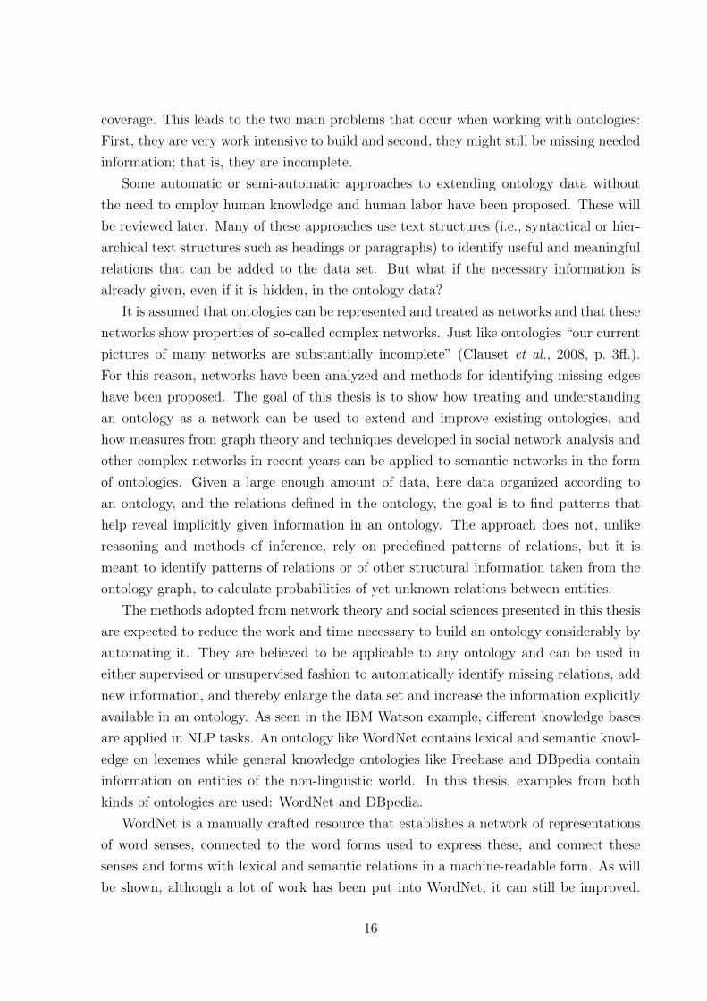
In Fig. 2(a) an example of a connection between two persons is given. Following the

homophily assumption that a friend of a friend is likely to be a friend as well, one can

assume the connection given in the dotted line in Fig. 2(b). This is called the closed

triangle assumption or triadic closure.

21

a

b c

(a) Open triangle: threenodes connected by twoedges.

a

b c

(b) Closed triangle: as-sumed connection.

Figure 2: Closed triangle assumption.

The degree to which vertices are connected to their possible neighbors in a network is

called the clustering coefficient or its transitivity. It can be calculated as

C =number of closed triads

number of geodesic paths of length two. (2)

2.1.2 Components, Cliques, Clusters, and Communities

The terms components, cliques, clusters, and communities all refer to subsets of vertices

of a graph that are, in one way or another, connected to each other.

A component is a subset of vertices of a graph such that there exists a path from any

vertex to any other vertex of the component. In directed graphs, theses paths have to be

directed. In many cases, and it will be shown for WordNet as well, a network consists of

more than one component: Not every vertex can be reached by a path from any other

vertex.

A network that consists of only one large component is called connected. A fully

connected graph is one where each vertex is connected to any other vertex of the network

directly by an edge.

Cliques are sets of vertices such that there exists an edge (i.e., a path of length one)

from any member of the clique to every other vertex of the clique and such that no other

vertex could be added that fulfills the first requirement.

Clustering is “the division of network nodes into groups within which the network

connections are dense, but between which they are sparser” (Newman and Girvan, 2004,

p. 1). Not every vertex of a cluster, or community, is connected to every other vertex,

but the vertices of a cluster are, overall, more interconnected within their cluster than

22

they are to vertices of other clusters. Still, there can be paths from one cluster to another

cluster. A connected component can, and in social networks this is almost surely the case,

contain many clusters.

Looking for example at the members of a parliament and treating the members as

vertices and their interactions as edges, one would surely find that there is more interaction

between the members of the same fraction, the same committee, and things like these than

between members of different fractions or committees. The fractions and committees are

the natural clusters of such a network.

Clusters are harder to identify than the straightforwardly defined components and

cliques. There might be cases where vertices lie on the intersection of different clusters

and might belong to not just one of them. Clustering algorithms in general aim to identify

groups or similar elements. In networks this means to identify the sets that are strongly

interconnected. In Chp. 4.3.2, clustering algorithms with an application to machine

learning and network analysis will be discussed.

2.1.3 Multigraphs, Trees, and Bipartite Graphs

Vertices of a graph can be connected by more than one edge, called multiedges. Such

graphs are called multigraphs. A matrix of a multigraph would not only contain Boolean

values of 0 and 1, but can also contain any number R≥0 as can be seen in matrix B.

In other cases, graphs can contain self-loops (i.e., vertices that are connected through

an edge to themselves). Matrix B is a matrix of a multigraph containing self-loops (see

second row, second column).

B =

0 1 2

2 3 1

1 4 0

The ontologies we are going to examine are multigraphs. Entities of an ontology can be

connected to one another by more than one relation.

A special form of a connected graph that contains no loops is a tree. An interesting

property of a tree is “that a tree of n vertices always has exactly n− 1 edges.” (Newman,

2010, p. 128). Even though the tree does not have to be directed, a tree always implies

a hierarchical structure since multiple inheritance is not permitted (i.e., a vertex cannot

have more than one direct parent vertex as can be seen in Fig. 3). This leads to the

conditio sine qua non that a tree of n vertices always has exactly n− 1 edges.

23

a

b c

d e f g

Figure 3: A small, simple tree.

Another special graph that will be of interest later on is the so-called bipartite graph.

A bipartite graph consists also of vertices and edges, but the vertices are of two different

kinds (see Fig. 4). An example of such a graph can be a network of co-working in the

movie business. Three actors {a, c, e} are linked to the movies {b, d} they appear in. The

vertices are of the kind movie and actor. Such affiliation networks are widely used in

social network analyses. There are no direct connections between the actors, they are

only connected through the movies both appear in. One can also reduce these graphs

to monopartite graphs (i.e., actors are seen as connected if they worked together on a

movie). The latter graph of course is not as meaningful as the original bipartite graph.

2.1.4 Measure of Centrality and Importance of Vertices

An important measure for vertices in a network is the centrality. The degree centrality is

the degree of a vertExample A vertex with a relatively high degree in a network can be

described as central.

The overall centrality of a network can be measured using Freeman’s (1978) general

formula of centrality:

CD =

∑ni=1[CD(a∗)− CD(ai)]

n2 − 3n+ 2, (3)

where n is the number of vertices, ai the particular node, and a∗ the maximum degree of

24

a

b

c

d

e

Figure 4: A simple bipartite graph with two different kinds of vertices: {a,c,e} and {b,d}.

a vertex in the network. The centrality CD of a network is thus defined as the sum from

i = 1, . . . , n of the centrality of the vertex where the degree is at the maximum minus

the centrality of a vertex ai divided by the number of vertices n2 minus 3 times n plus 2

(Freeman, 1978, p. 226ff.).

Beside the very basic degree centrality measure, other measures like the eigenvector

centrality, betweenness, closeness, and PageRank are commonly applied in network analy-

sis. All the measures that are to be presented here will be used later on in link prediction

tasks.

Eigenvector Centrality

Newman (2010, p. 169) says that

[i]n many circumstances a vertex’s importance in a network is increased by

having connections to other vertices that are themselves important. This is

the concept behind eigenvector centrality. Instead of awarding vertices just

one point for each neighbor, as in degree centrality, eigenvector centrality gives

each vertex a score proportional to the sum of the scores of its neighbors.

Bonacich (1987, p. 1173) defines the eigenvector centrality as shown in Eq. 4 and Eq. 5.

The centrality of vertex i is calculated as the sum over edges between i and any connected

25

vertex j multiplied by the centrality of j (Cj) times β plus a:

ci(αβ) =∑j

(α + βcj)Aij, (4)

or

c(αβ) = α(I − βA)−1A1, (5)

where A is the adjacency matrix of the graph and I is the identity matrix:9

I =

1 0 0

0 1 0

0 0 1

.Vector ‘1’ is a column vector of all ones.10 The constants α and β determine the impor-

tance or influence of the degree of a vertex.

Quite similar to the Eigenvector centrality is the so-called Katz centrality (Katz, 1953).

The two constant values α and β in Eq. 6 result in the fact that even if the centrality of

a vertex is 0, it will still be awarded β:

λxi = αn∑j=1

aijxj + β, i = 1, . . . , n. (6)

Given any vertex that is pointed to by many vertices that themselves have no other

vertices pointing to them, the Eigenvector centrality would be low or 0, while the Katz

measure still rewards these links. The constant α is used to control the weight of the

eigenvector in relation to β (Newman, 2010, p. 172).

Betweenness Centrality

Another important measure in (social) networks is the so-called betweenness. It is “based

on the assumption that information is passed from one person to another only along the

9The identity matrix, being its own inverse, is the matrix multiplication equivalent to 1: A n × mmatrix R multiplied by In,m is R.

10Multiplying an adjacency matrix by a vector of all ones sums up the values of each column of amatrix which corresponds to the degree of a vertex.

26

(a) (b) (c)

Figure 5: Weighted graphs: (a) weighted by degree, (b) weighted by betweenness central-ity, and (c) weighted by closeness centrality.

shortest paths linking them” (Freeman et al., 1991, p. 142). This means, if one is looking

at the spread of information in a social network, those vertices are best informed that lie

on a high number of shortest paths between any two vertices. A vertex can have a very

high degree but still a very small betweenness, and vice versa. If the number of geodesic

paths between the vertices j and k is gjk, and the number of these paths between j and

k going through vertex i is gjk(i), the betweenness centrality of i is the quotient

bjk(i) =gjk(i)

gjk. (7)

Now, one has to sum up this value for all pairs of vertices where i 6= j 6= k to get the

overall betweenness centrality of i.

Closeness Centrality

Closeness, as defined by Freeman (1978, cf. p. 221), indicates the length of the average

geodesic distance between a vertex i and any other vertex of a network.

Cc(i) =

[∑i=1n d(i, j)

n− 1

]−1(8)

Dividing the average distance between i and j by the number of total vertices minus

1 (n − 1) normalizes the value of Cc(i). This equation is problematic in networks with

unconnected components (Freeman, 1978, cf. p. 226): When there are vertices to which

no path exists, the sum is infinite. Inverting an infinite number leads to a value of 0 as

the outcome of the equation. Opsahl et al. (2010, p. 245) suggest to “sum the inversed

distance instead of the inverse sum of distances”.

27

PageRank

The last measure to introduce at this point is PageRank. Page et al. (1998) developed

this ranking system at Stanford before founding Google on the basis of PageRank. On

the World Wide Web, it assigns each web page a rank not based on its in-degree alone

but on the in-degree of the vertices pointing to the page.11 Again we take a vertex i to be

ranked. The sum over all vertices j in Bi pointing to i is normalized by a factor c. The

rank of j is divided by Ni (i.e., the number of links i is pointing to).

R(i) = c∑j∈Bi

R(j)

Ni

(9)

This function is different from the ones shown above because it only takes into account

the in-degree of the vertex itself and its nearest neighbors. One does not need information

on the whole network to calculate the importance of a node. In case of a huge network

like the World Wide Web, this is an advantage.

The measures of degree, betweenness, and closeness are compared in Fig. 5(a)–(c).

The size of the vertices indicates the corresponding value of the measure in question.

2.1.5 Small-World Networks and Scale-Free Distribution

Social networks have been of special interest in the social sciences for decades. It has been

found that social networks show a property that is called the small-world phenomenon.

Small-world networks and social networks as such expose two distinguishing features.

First, they have a short average geodesic path and, second, a high clustering coefficient

(compared to random graphs). Both features result in the common observation that a

friend of a friend tends to be a friend as well.

One of the first pieces of systematic research in the field of social networks that be-

came extraordinarily popular, so popular indeed that its findings are now part of general

knowledge, was the work of Milgram (1967). Milgram sent out letters to randomly cho-

sen people in the US and asked them to hand the letter to a first-name acquaintance of

theirs in order for the letter to reach a specific person located in Boston. The letters that

actually made it to their destination got there through about six stations (on average 5.8

steps). This is commonly known as the six degrees of separation and it can be seen as the

11The WWW is a directed multigraph (see Chp. 2.1.3).

28

(a) (b)

Figure 6: Plot of frequency and rank of words based on the Brown Corpus: (a) the datafollowing a power law and (b) the same data plotted on logarithmic scale.

short average geodesic path of the social network of US citizens.

Not only was the average path from a randomly chosen starting point to the destination

relatively short, but most of the letters came to their destination through the hands of only

a few people connected to the destination person. Travers and Milgram (1969) call these

people authorities, since they seem to be very well connected not only to the destination

person as well as to others they were getting the letters from. These authorities are also

called hubs, and they have ever since been found in many networks with a small geodesic

distance. Those networks of course also tend to be clustered: groups of vertices (strongly

connected) build clusters, and their degree distributions follow a power law: Very few

vertices have a very high degree, while most vertices have a very low degree.

A good example of a power-law distribution is given by the so-called Zipf’s law.12 Zipf

(1965) found that the distribution of the frequency of words is inversely proportional to

their rank. A distribution of this kind can be plotted to a graph as can be seen in Fig.

6(a). This distribution follows a power law of the form p(x) = Cx−α.

An interesting observation on the plotting of this kind can be seen in Fig. 6(b): When

plotted on a logarithmic scale, the graph pretty much follows a straight line.13

12Adamic (2002) shows that Zipf’s law and the Pareto distribution are equivalent. The differenceconsists in the usage of the two axes that are inverted.

13According to Newman (2004), this observation was first made by Auerbach (1913) in his work on the

29

Power-law distributions are scale free. This means they show the same distribution no

matter what the scale is. To understand what scale free means, one can have a look at

Fig. 6(a) and Fig. 7, which show the same data scaled by a factor of 2. The distribution

“is the same whatever scale we look at it on” (Newman, 2004, p. 334).

Figure 7: The same data as in Fig. 6(b) but scaled by a factor of 2.

The degree distribution of many real-world networks follows such power laws with

the limitation that the number of vertices is not infinite. But power laws have not only

been found in word frequencies or degree distributions of networks. In sociology, it has

been shown that the distribution of the size of cities and distribution of wealth among

people follows a power law: Compared to the number of cities in the world, only very few

have a very high number of inhabitants, while a very large number have only very few

inhabitants (though probably not only one). In other words, large cities attract ever more

inhabitants. Similarly it has been found that people with a large fortune, which are only

very few people, tend to increase their wealth further, while the great number of people

have much less wealth. This has been called the rich-get-richer principle. We will come

back to how such structures (i.e., that words with many connections tend to attract ever

more connections) arise in (language) networks later on (see Chp. 2.2).

density of population (Bevolkerungsdichte).

30

2.1.6 Terminology

A number of terms that can be used synonymously have been introduced already, and

there are still more terms in use that have not been mentioned yet: graph and network,

vertex and node, edges, arcs, and links, vertex and site, edge and bonds, or in the social

sciences vertex and actor, and edge and tie. In Chp. 3.5, the terms entities and relations in

the context of ontologies will be introduced. These terms correspond, when the ontology

is referred to as a network, to vertex and edge in graph theory. Throughout this thesis,

I will use either vertex or entity and edge or relation, depending on the context and

the connotation, either meaning the element of the graph or the entity of the ontology.

Sometimes the relations of an entity will be called its attributes or properties.

2.2 Language Networks and Computational Models of Language

Graph and network theory have been used in different ways in linguistics, especially in the

study of semantics, language evolution, language acquisition, as well as in neurosciences.

Some questions that are of interest for the evaluation of the results of this thesis are based

on the following models. Questions such as How do networks in natural language arise?

How can network or (hierarchical) graph models explain the processes of the human mind

and how accurate are they? have to be kept in mind when using network methods to

model natural language.

The idea of computation in language processing in the human mind is not new. Chom-

sky (1988) suggests that language understanding, learning, and evolution depends on the

human mind’s capability to carry out computations. Hauser, Chomsky, and Fitch call this

the faculty of language in a narrow sense, which they define as “the core computational

mechanisms of recursion” (Hauser et al., 2002, p. 1573). And in his computational theory

of mind (CTM), Pinker (2005, p. 22) defines the mind as a “naturally selected system of

organs of computation”. In the early 1990s, Steven Pinker proposed a dual mechanism:

The brain contains on the one hand a lexicon where words are stored and on the other

hand a grammar apparatus to infer, among other things, regular forms of words (Pinker,

1991; Pinker and Prince, 1991). Pinker denies the idea of either a “homogeneous associa-

tive memory structure or alternatively, of a set of genetically determined computational

modules in which rules manipulate symbolic representations” (Pinker, 1991, p. 253), and

he thereby contradicts Chomsky. Pinker’s distinction implies that there must be a differ-

31

ence between the retrieval of an irregular past-tense verb stored in the human memory

and a regular verb generated by a rule-based mechanism. The lexicon must contain not

only word–meaning pairs for the word stems but also irregular word forms that cannot be

mentally computed using grammatical rules. Other research that will be shortly reviewed

now has been undertaken that back this idea.

When it comes to the actual storage of words in the brain, several different approaches

to investigate the structure can be distinguished. One indication of the internal network

structure of the brain are findings that semantically related words take less retrieval time

than a mere phonological relationship. In these studies, subjects were shown a prime–

target sequence (e.g., ‘swan/goose’ and ‘gravy/grave’). The semantical relation in the

brain in the first case was stronger, resulting in less reaction time than the phonological

relation between the semantically unrelated words gravy and grave (Marslen-Wilson and

Tyler, 1997, p. 592).

Furthermore, Marslen-Wilson and Tyler (1997) took a prime/target approach compar-

ing the relation between a stem and its past-tense form, whether regular or irregular, in

comparison between different neurological damage. Two aphasic patients with ungram-

matical speech were compared to one patient with right and left hemisphere damage and

a group of healthy subjects. The results suggest that the two aphasic patients are not

able to use regular past-tense forms but are able to retrieve irregular forms. This suggests

damage to the part of the brain where the grammatical mental computation is done. The

other patient neither shows semantic priming nor is he able to retrieve irregular verb

forms, suggesting that his mental lexicon is damaged. His grammatical apparatus for

mental computation is not affected; he is able to use regular verb forms.

Other studies undertaken by Indefrey et al. (1997) and Jaeger et al. (1996) using

positron emission tomography (PET) show that different regions of the brain are used

to form regular verb forms and to retrieve irregular ones. According to Indefrey et al.

(1997, p. 548), both “regular and irregular morphological production induced significant

rCBF [regional cerebral blood flow] increases in midbrain and cerebellum, but showed no

overlap in cortical areas”.

A study on German irregular plural forms using event-related brain potentials (ERPs)

provides, according to the authors, “a clear electrophysiological distinction between reg-

ular and irregular inflections” (Weyerts et al., 1997, p. 961), supporting the hypothesis of

32

a dual mechanism.14

Ullman et al. (1997) analyze the capacities of patients with Alzheimer’s disease (AD),

which leads to impairments of the lexical memory, on the one hand, and Parkinson’s

disease (PD), which leads to impairments of the grammatical rules, on the other hand.

Their findings also suggest that the distinction between the lexicon and the grammatical

apparatus is correct. They find that patients with impairments of the lexical memory

(AD patients) have more trouble finding irregular verbs than converting even unknown

verbs to the regular past tense. PD patients showed the opposite pattern.

Manning et al. (2012) study how the retrieval of words in the human mind is influ-

enced by their semantic similarity. Electrocorticographic recordings of 46 “neurosurgical

patients who were implanted with subdural electrode arrays and depth electrodes during

presurgical evaluation of a treatment for drug-resistant epilepsy” (Manning et al., 2012,

p. 8872), memorizing and remembering words on a list, show how individuals store re-

lated words. Manning et al. (2012) chose a latent semantic analysis (LSA) to describe the

semantics of a given word. They say:

If a participant shows a strong correspondence between neural and semantic

similarity . . . , then we consider them to exhibit neural clustering in the sense

that neural patterns associated with words that are similar in meaning (ac-

cording to LSA) will be clustered nearby in their neural space (where each

point in neural space is a pattern of neural activity) (Manning et al., 2012,

p. 8873f.).

They calculate the cosine similarity between the semantic vectors as well as the simi-

larity between the patterns of brain activity during memorizing and recall of semantically

related words. Using an underlying LSA to explain the meaning of their findings, these

results indicate that the words are, in a network sense, similarly connected. This experi-

ment shows that there is a relation between a network of words and the neural network

in the human mind, or as they put it: “This indicates that temporal and frontal networks

organize conceptual information by representing relationships among stored concepts”

(Manning et al., 2012, p. 8876), as in a network or even more as in an ontology.

14A differing view from Indefrey et al. (1997) on the localization of the human linguistic capacities isheld by Grodzinsky (2000). The exact region or regions responsible for human linguistic abilities remainunclear. This is mostly because of the unsatisfactory accuracy of the applied neuroimaging methods(PET and ERP).

33

The presented studies suggest (1) that a mental lexicon exists in the human brain

that connects semantically related words more closely than other words, i.e., a network

structure,15 and that (2) a part of the brain fulfills mental computations using grammatical

rules to convert regular nouns and verbs.

2.3 Graphs of Language

From these and similar considerations and findings in medicine, psychology, and biology,

different theories about how language networks evolve have been proposed. In the follow-

ing, some approaches will be presented. Starting with an older computational model of

a hierarchically ordered tree-like structure of lexico-semantic information, models of how

networks evolve and develop will be presented that finally lead to a model of language

network growth that can explain some statistical features of complex networks represent-

ing human language. Afterwards, the properties that can be expected from a language

network and complex network compared to simple or ordered networks can be defined.

2.3.1 Hierarchical Structures of the Mind

Quillian (1967) uses a tree-like, hierarchically structured taxonomy model for the “simula-

tion of some basic semantic capabilities” (Quillian, 1967, p. 459) in the form of a computer

program. His model of “memory as a ‘semantic network’ [is] representing factual asser-

tions about the world” (Quillian, 1969, p. 459) in a hierarchical class model. Quillian

stores each word with “a configuration of pointers to other words in the memory; this

configuration represents the word’s meaning” (Collins and Quillian, 1969, p. 240), and in

his opinion it is a reverse-engineered model of the human semantic capacity. 16

Collins and Quillian’s (1969) model allows one to make predictions about the time it

should take to retrieve information. They argue that if the information is hierarchically

organized in the form of a tree, where children vertices inherit the information of their

parent vertices, the retrieval time for information inherited from the parent should be

longer than that for information belonging to the vertex itself.

As an example they use the concept of a canary bird. Like all birds, canaries have

15This lexicon also contains irregular forms of words that cannot be formed using grammatical rules.16These considerations are very early examples of semantic networks that finally lead to the development

of ontologies. The words are the vertices; the pointers are edges of the network.

34

feathers and can fly.17 Like all animals, birds have skin. Since a canary is a bird, and a

bird is an animal, it has skin as well. Moreover, a canary is yellow and can sing. Collins

and Quillian predict that there should be a higher retrieval time for information that is

inherited. To show this, subjects have to decide whether a sentence is true or false and

while their reaction time is measured.

The subjects are shown sentences like: “A canary can sing.”, “A canary can fly.”, or

“A canary has skin.” (all taken from Collins and Quillian (1969, p. 241)). These sentences

are all true, but the authors assume that there should be difference in the time necessary

to retrieve the needed information. They suspect that singing is a property of the canary

itself, while flying is a property of birds and hence one level higher in the hierarchy, and

that having skin is a property of animals and hence one further step higher in the tree.

They measure the reaction time and find that it takes about 75 ms “to move from a

vertex to its superset” (Collins and Quillian, 1969, p. 244). They conclude that “there

was substantial agreement between the predictions and the data” (Collins and Quillian,

1969, p. 246).

However, later studies could not verify these findings (McCloskey and Glucksberg,

1979; Murphy and Brownell, 1985). Furthermore, McClelland and Rogers (2003) argue

that the hierarchical model has some issues. They are asking

just which superordinate should be included, and which properties should be

stored with them? At what point in development are they introduced? What

are the criteria for creating such categories? And how does one deal with the

fact that properties that are shared by many items, which could be treated

as members of the same category, are not necessarily shared by all members?

(McClelland and Rogers, 2003, p. 311)

From their study of language acquisition and forms of dementia, McClelland and Rogers

suggest a network model: Information is “latent in the connections among the neurons

in the brain that processes semantic information” (McClelland and Rogers, 2003, p. 310).

The generalized properties (e.g., that all birds fly) are derived from clusters of the network,

or from the distance between word vectors in a vector space.

Interestingly enough, McClelland and Rogers (2003) deny a hierarchical organization

17Exceptions like an ostrich or a penguin would have to be marked as a bird that cannot fly. It is “moreeconomical to store generalized information with superset vertices rather than with all the individuals towhich such a generalization might apply” (Collins and Quillian, 1969, p. 246).

35

and instead propose – without further looking into this – that neighborhood and the

connectivity of a concept implicitly provide this information.

2.3.2 Complex Network Growth and Models of Language Network Evolution

After seeing how language can be treated as a graph or network, the question has to be

asked how such networks evolve. There have been different proposals for different kinds

of networks. The most important ones are to be presented and compared here.

Random Networks (Erdos and Renyi)

In 1959, Erdos and Renyi proposed a model of random graphs. They start with n vertices

and connect those with N edges with a probability P (Erdos and Renyi, 1959, p. 290).

Such a network’s degree distribution follows a Poisson distribution. The Poisson distri-

bution indicates the probability that a certain state occurs. If we know that a graph has

n vertices and N edges, the average number of edges a vertex has, its degree, should be

A = nN

. The Poisson distribution shows the probability of the state A ± x to occur. An

example of an Erdos and Renyi graph is given in Fig. 8.

With a lack of data on real-world networks, this model could not be tested extensively.

The model constructs a random network that is not like real-world, complex networks, as

we have seen them already and will analyze later on in this thesis. The model is missing

the most basic features of complex networks: Neither the power law distribution, and thus

the scale-free feature, nor the small-world property of natural networks can be explained

using this model (Barabasi and Reka, 1999, p. 510).

Small-World Networks (Watts and Strogatz)

One feature of complex networks that the above shown model does not predict is the

small-world phenomenon. Watts and Strogatz (1998) propose a model that explains how

small-world networks emerge.

Having a network of n vertices and k edges per node, Watts and Strogatz “rewire

each edge at random with probability p” (Watts and Strogatz, 1998, p. 440), where p = 0

results in an ordered network (see Fig. 9(a)), and p = 1 results in an unordered network

(see Fig. 9(c)). While an ordered network has a long average path length L (a large-

world network), and a high clustering coefficient C, a network of 0 < p > 1 (see Fig.

36

Figure 8: An Erdos and Renyi random graph with 100 vertices and a connectivity prob-ability of 0.2.

9(b)) leads to a less clustered network with a short average path length or small-world

network. Even for “small p, each short cut has a highly nonlinear effect on L, contracting

the distance not just between the pair of vertices that it connects, but between their

immediate neighbourhoods” (Watts and Strogatz, 1998, p. 440). But this model stills

misses the power-law distribution that is typically found in complex networks, and it is

no explanation of how such networks evolve since it does not incorporate growth of any

kind.

Preferential Attachment (Barabasi and Reka)

Network models of language allow one to analyze the supposed structure of the mind and

to predict and analyze the evolution of language. Barabasi and Reka (1999) describe a

model of network growth using preferential attachment:18 Having a network, this mod-

els predicts that “new vertices in the growing network are preferentially attached to an

existing vertex with a probability proportional to the degree of such a node” (Ferrer and

Sole, 2001, p. 2263). This is equivalent to the rich-get-richer principle introduced before.

The model leads to a power law distribution, which is generally seen as a natural result

18Preferential attachment applies Bayesian models which are also used (e.g., to predict the growing ofthe mind (cf. Tenenbaum et al., 2011)). Bayesian models complement network approaches and are usedwidely in language models in psychology, linguistics, and medicine.

37

(a) Probability p = 0. (b) Probability p = 0.5. (c) Probability p = 1.

Figure 9: Watts and Strogatz graphs with n = 20 and k = 4.

of the way a system, like a network, grows over time. Barabasi and Reka state that this

indicates that “the development of large networks is governed by robust self-organizing

phenomena that go beyond the particulars of the individual systems” (Barabasi and Reka,

1999, p. 509).19

In formal terms, the probability P (ki) that a new vertex in a network starting with

m0 vertices and adding a new vertex at every time step t with m ≤ m0 edges will connect

to an existing vertex i depends on the degree ki of that node:

P (ki) =ki∑jkj

.

This leads to a random network with t + m0 vertices and mt edges that is “following a

power law with the an exponent ymodel = 2.9± 0.1” (Barabasi and Reka, 1999, p. 5).

An example is given in Fig. 10. Comparing this graph to an Erdos and Renyi random

graph, one can see that the distribution of edges per vertex is not distributed in Poisson

fashion, but that some vertices have a reasonably higher degree than others. This also

leads to clustering as Fig. 10 shows.

This model predicts degree distributions that follow a power law, more or less like it

can be observed in networks of natural language or, in general, in scale-free, small-world

networks.

In Fig. 11, the degree distributions of the models presented above are given. In

19In protein networks, for example, scale-free distribution follows from preferential attachment in thegrowing process, which seems to be a result of gene duplication (cf. Barabasi and Oltvai, 2004, p. 106).

38

Figure 10: A Barabasi and Reka graph with 100 vertices.

accordance with what has been stated above and as one can see, neither the degree

distribution shown in Fig. 11(a) nor the one in Fig. 11(b) follows a power law. Only the

model of Barabasi and Reka (1999), Fig. 11(c), shows a degree distribution that is found

in most natural networks, such as social networks, and, as will be shown in later chapters,

in ontologies.

Language Network Models (Steyvers and Tenenbaum)

Steyvers and Tenenbaum compare the Barabasi and Reka model to findings in natural

language networks20 and find that preferential attachment as proposed by Barabasi and

Reka (1999) does not explain the structure of semantic networks.

From a language evolution21 point of view, Steyvers and Tenenbaum argue that

“[w]ords that enter the network early are expected to show higher connectivity” (Steyvers

and Tenenbaum, 2005, p. 44). Also existing complex concepts (i.e., those with a high

20Unfortunately, they restrict themselves to an analysis of networks and ignore the large amount oflinguistic research in the areas of language evolution and language change.

21Steyvers and Tenenbaum’s model could just as well be applicable to individual language acquisition,even though it cannot account for all the diverse processes that happen during the acquisition or evolutionof natural languages.

39

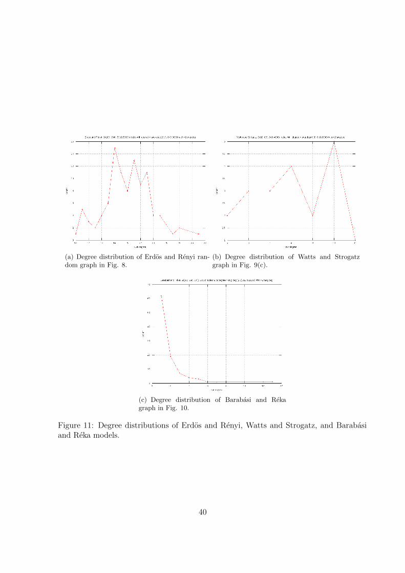
(a) Degree distribution of Erdos and Renyi ran-dom graph in Fig. 8.

(b) Degree distribution of Watts and Strogatzgraph in Fig. 9(c).

(c) Degree distribution of Barabasi and Rekagraph in Fig. 10.

Figure 11: Degree distributions of Erdos and Renyi, Watts and Strogatz, and Barabasiand Reka models.

40

connectivity or degree) in a language are more likely differentiated over time. This means

complex and very wide terms tend to be differentiated into narrower terms. There are of

course a lot of other processes that can be discussed concerning the evolution of a natural

language, but this process is leading to concepts with a high connectivity (i.e., hubs or

authorities) and thereby to a small-world network.

Two models for the growth of language networks are proposed by the authors: The

first explains the growing of an undirected network, while the second one explains the

growth of a directed network (e.g., a semantic relationship network of words such as

WordNet or other language ontologies).

The first growth model can be formulated as follows: Given is a fully connected

network of size n that grows over time, at each time point t with t(n) vertices, a randomly

chosen vertex i is differentiated by adding a new vertex with M connections (M < n) to

randomly chosen vertices in the neighborhood of i. This leads to the effect that a “new

vertex can be thought of as differentiating the existing node, by acquiring a similar but

slightly more specific pattern of connectivity” (Steyvers and Tenenbaum, 2005, p. 57).

Now the probability that vertex i is chosen has to be defined. The probability Pi(t) is

corresponding to the connectivity of the vertex i (i.e., its degree):

Pi(t) =ki(t)∑i−1n(t) ki(t)

.

The degree of i at t, ki(t), is divided by the sum of degrees from i − 1 to n(t) (i.e., all

vertices at time t)

To choose a vertex j in the neighborhood Hi of i that the vertex to be added will

be connected to, the probability Pij(t) is calculated in proportion to the utility of the

corresponding node:

Pij(t) =1

ki(t).

This is repeatedly done until M vertices from Hi have been chosen. Then the new vertex

is connected to them. These steps are repeated until the desired network size is reached.

The network produced by the model can then be compared to a real-world network of the

same size.

The second model of network growth results in a directed network. The process is

very similar to the first model. The only difference is the connection of the new node:

41

Still, the vertices it will be connected to are chosen with the probability Pij(t), but the

direction of the connecting edges is chosen randomly.

While this model fits the examined features of language graphs, it should be mentioned

that a model of the growth or evolution of a language network should also account for the

loss of words (i.e., at randomly chosen time steps the network should to be pruned and

poorly connected concepts should be erased). A diachronic analysis of language shows not

only a differentiation of words and hence a semantic shift, as well as that concepts that

are poorly connected and therefore less frequently used, cease to exist in the vocabulary

of a single person or even a language community (cf. Pagel et al., 2013). This property

is, in my opinion, missing in the model. Also, Dorogovtsev and Mendes (2001) point out,

because of a semantic shift, existing concepts should at time be rewired to other concepts.

2.4 Conclusion

The use of network models of language and the application of methods of graph theory

were explained and legitimized taking findings from linguistics and from other relevant

fields of research.

Basic concepts of graph theory as well as sophisticated measures of network structure

and vertex centrality have been introduced and will be utilized to analyze the structure of

networks extracted from ontologies and as features for machine learning tasks to extend

the ontologies. As will be shown in Chp. 4, many interesting ideas from social networks

analyses might also be applicable to ontologies. The network structure, nonetheless, will

be the main basis for the application of machine learning to identify and classify missing

edges in the network structure. Furthermore, properties of complex, natural networks,

the degree distribution, and the small-world phenomenon (i.e., the short average geodesic

path and high clustering coefficient) have been introduced. These features distinguish

complex network from (e.g., random networks as proposed by Erdos and Renyi (1959)).

Looking at the neurological network in the human brain, a definition of the seman-

tics of a word or concept was found that is not only true for semantic networks as are

the ontologies used in this thesis. Manning et al. (2012, p. 8873f.) find “that neural

patterns associated with words that are similar in meaning . . . will be clustered nearby

in their neural space” of the human brain. Hence, the meaning of a word is defined as

its connections or relations to other words or, more general, as a pattern of connectivity

(cf. Steyvers and Tenenbaum, 2005). As will be shown in the following chapter, similar

42

definitions of meaning have been made in semantics. Based on these definitions, applying

machine learning algorithms to predict patterns can be employed to build or complete

word networks.

Trees, as a special network structure, and hierarchies can also be found in represen-

tations of human grammar (e.g., phrase structure grammars (PSGs)). Hierarchical struc-

tures like these are considered to be a unique feature of human communication. Other

animals are capable of learning finite-state grammars (FSGs) but fail to learn the recur-

sive rules of a PSG. Fitch and Hauser explain that other species than humans “suffer from

a specific and fundamental computational limitation on their ability to spontaneously rec-

ognize or remember hierarchically organized acoustic structures” (Fitch and Hauser, 2004,

p. 380) and conclude with the thesis that the “acquisition of hierarchical processing ability

may have represented a critical juncture in the evolution of the human language faculty”

(Fitch and Hauser, 2004, p. 380). This is again a further indication of the existence of

data structured in hierarchical form and for an organ of computation which supports the

use of computational methods to model language. It is no explanation for why this form

of organization, a network, is employed, though.

Phrases can be embedded in other phrases; sentences form a syntax tree. Analogous

to a syntax tree, semantic relations between entities in human language are also organized

in the form of a tree. We find structures, especially trees, that can be interpreted as a

network on all levels of the human language.

Seeing that the evolution of language and of vocabulary, at least when looked at

as a network, is generally similar to the growth of a neural network is not surprising

since it is the neural network of the human brain that stores, retrieves, and manipulates

language. Network structures are a very robust way of organization. The structure of the

data system (the human brains neural network) seems naturally reflected in the internal

structure of language processed by this system. In this way, the structure of the language

capacity is adapted to the medium. Of course the human neural network does not function

as the much simpler network model applied in the following. One does not find vertices

representing words in the neural network of the brain, but still patterns of network activity

seem to correspond to distinct words, concepts, and their understanding and processing.

Therefore, using this resemblance and the term network to indicate a similarity between

technical processes and mental processes can be very problematic.

The notion of artificial neural networks (ANNs) in so-called deep learning has become

very popular in recent years. ANNs were developed having in mind the (simplified)

43

understanding of how the human neural network behaves.

While the practical advantages of such techniques are indisputable, the notion that

such systems are inspired or even work like the human brain has to be rejected. Many

people in machine learning have contradicted this understanding of neural networks. For

example Michael Jordan has pointed out in an interview that to “infer that something

involving neuroscience is behind it . . . is just patently false” (Gomes, 2014).

When networks and ideas from psychology, and especially neurology, were first used

to explain semantics, Fillmore (1975, p. 124) found that the analogies to the human mind

and brain might “sound like extremely naive psychology”. In an interview with The New

York Times, Andrew Ng, one of the heads behind the Google Brain project, admits that

it is a “loose and frankly awful analogy . . . that our numerical parameters correspond to

synapses”. 22

22Source: http://www.nytimes.com/2012/06/26/technology/in-a-big-network-of-computers-

evidence-of-machine-learning.html.

44

3 Lexical Semantics and Ontologies

Most of what’s called “semantics” is, in my opinion, syntax. It is the part of syntax

that is presumably close to the interface system that involves the use of language.

So there is that part of syntax and there certainly is pragmatics in some general

sense of what you do with words and so on. But whether there is semantics in the

more technical sense is an open question. I don’t think there’s any reason to believe

that there is. (Chomsky, 2001, p. 73)

This quote of Chomsky will be referred to a few times in the following. In my opinion

its main message is not there is no semantics, but rather that semantics cannot be any-

thing coming from outside the language, but can only be understood from the language

structure. In this sense, it is a very structuralist statement, although Chomsky denies the

fruitfulness of empirical linguistics and, as such, many structuralist attempts.

In the following, different theories of semantics that are vital to understanding com-

putational semantics are going to be introduced shortly to an extent necessary and useful

for the understanding and the argumentation in the following chapters of this thesis.

This is not an introduction to semantics. In this sense, this section does neither aim

at an as-broad-as-possible overview, nor is the chronological order of the development of

these theories very important. Hence the subsections are arranged in a logical order.

Starting from the quote above, the first theory to be introduced very shortly here is

formal or Montague semantics. It is the attempt to translate natural language into a

logical form. A phrase like

(1) fierce black cat

corresponds to a logical form like

(2) λx[fierce(x) ∧ black(x) ∧ cat(x)]

which means that the entity x is fierce, black, and a cat (cf. Copestake et al., 2005,

p. 284). Predicate logics can be used to formalize all kinds of relations, not only rela-

tions expressed in natural language. For example, if the cat had a name, this could be

represented using a relation hasName as shown in Example 3.

(3) ∃x[cat(x) ∧ hasName(x,Anton)]

45

While complete semantic parsing, based on predicate logics, is for many reason not

possible, among them the incompleteness of Montague Semantics (i.e., its inability to

account for more than a snippet or natural English), the more simplistic approach of

semantic role labeling is often applied to parse sentences and to derive logical relations

from the syntactic structure of natural language.23 These relations are of special interest in

NLP, both in parsing texts as well as in ontologies. When parsing natural language texts,

often a more simplistic representation is chosen. A possible logical form for Example 424 is

given in Example 5, which also corresponds to the dependency structure of the sentence.

(4) Julius gave Anne a rose.

(5) give(Julius, Anne, a rose)

Example 5 shows a give relation (predicate) with three arguments for the agent (sub-

ject), recipient (indirect object), and the theme (direct object). The semantic role has to

be distinguished from the grammatical or syntactical role. This very basic, compared to

a full logical analysis, assumption of semantic roles is in fact being applied in NLP quite

regularly (cf. Jaworski and Przepiorkowski, 2014; Lally et al., 2012)

The logic-based approach to derive meaning from syntax, and thereby showing the

strong relationship between both, is a very effective tool to describe the semantics of a

complex phrase. But it stops at a very basic point: the words or lexical units. Formal

semantics can show how different parts of phrases are combined and how the composi-

tionality constructs meaning, but it does not describe the meaning of any lexical unit.

What or who are Julius and Anne, what is to give and what is a rose? And of course a

word like love does not receive its meaning from the syntactical structure but rather from

its paradigmatic relations.

While the main contributions to formal semantics were made in the Anglo-American

research community, the structuralism of Europe developed a different concept of describ-

ing meaning during the last century. These theories, among others, are to be presented

in the following since there is a direct link between how natural language semantics is

treated and how ontologies work.

23Lohnstein (2011) shows and explains what he calls the isomorphism between syntactic and seman-tic structures (“. . . Isomorphie zwischen syntaktischen und semantischen Strukturen”) (Lohnstein, 2011,p. 153).

24This example is taken from Wittenberg et al. (2014).

46

3.1 Frame Semantics and Encyclopedic Knowledge

“[E]verything you know about the concept is part of its meaning . . . . From

this it follows that there is no essential difference between (linguistic) seman-

tic representation and (general) knowledge representation” (Croft and Cruse,

1993, p. 336f).

Frame semantics takes a very broad concept of meaning. Unlike other approaches

that are to be discussed later on in this chapter, frame semantics explicitly includes

non-linguistic knowledge, world knowledge or general knowledge, of concepts into the

representation of the concept’s meaning. This is for one meant to be close to the mean-

ing representation humans have of concepts, words, or facts, as well as to be a base for

AI, where the understanding of human utterances makes knowledge about concepts im-

portant. Therefore, researchers from cognitive linguists, like Fillmore (1975), as well as

computer scientists, such as Minsky (1974), contributed to this theory of semantics.

Fillmore distinguishes between a scene and a frame, where the scene is the situation

itself, and the frame makes up for the linguistic material available or connected to that

scene (cf. Fillmore, 1975, 1977). The frame or domain is nothing that necessarily exists in

the language itself. It is derived from experience and can be seen as the (non-linguistic)

context of a word. Fillmore states that

frames and scenes, in the mind of a person who has learned the associations

between them, activate each other; and that furthermore frames are associated

in memory with other frames by virtue of their shared linguistic material,

and that scenes are associated with other scenes by virtue of sameness or

similarity of the entities or relations or substances in them, or their contexts

of occurrence. (Fillmore, 1975, p. 124)

For example, when in a garage, both speaker and listener have frames of cars and tools

associated with the scene (garage) that can be used; for example, cars have engines, they

drive fast, and much more.

Fillmore proposes his frame theory as an “integrated view of language structure, lan-

guage behavior, language comprehension, language change, and language acquisition”

(Fillmore, 1977, p. 55); in fact he gives detailed examples from those fields, as well as

from issues of language translation that cannot be repeated here.

47

The frame, the base, itself gives meaning to the unit. If one understands the scene,

the event, or activity in question, “then, given that knowledge, we can know exactly what

the vocabulary pertaining to that semantic domain means” (Fillmore, 1977, p. 60). The

scene itself is independent of the frame and the lexical material. When a child learns a

new word within a frame, the scene does not alter, only the associated frame is changed

(cf. Fillmore, 1977, p. 66).

Langacker (1987) refines Fillmore’s notion of the frame, such that the “semantic value

of a symbolic expression is given only by the base and profile together” (Langacker, 1987,

p. 187). The profile is “a substructure of designation” (Langacker, 1987, p. 183); it is

what distinguishes a word from others connected to the same base/domain/frame.

One often finds network-related terms in cognitive linguistics and especially in the

field of frame semantics: “[a]lthough in theory all knowledge about an entity is accessible

– that is, the whole knowledge network is accessible – some knowledge is more central

. . . , and the pattern of centrality and peripherality is a major part of what distinguishes

the meaning of one word from that of another” (Croft and Cruse, 1993, p. 337). Frame

theory is based on a supposed understanding of the neural network of the human brain,

although this might “sound like extremely naive psychology” (Fillmore, 1975, p. 124).

Minsky’s early work is highly influenced by the metaphor of network. Therefore it seems

unsurprising that there is a straight line from the notion of frames to that of networks

and ontologies representing general knowledge used in NLP today.

As mentioned above, the knowledge represented by a frame is not entirely linguistic,

as well as contains general knowledge or knowledge derived from experience. It is no

coincidence that Minsky was involved in establishing this theory. From his background in

AI he realized that a lexical resource to be used in AI needs to be more than a dictionary.

If a machine is to understand language (i.e., complex sentences, texts, and discourses)

it needs knowledge beyond linguistic knowledge of the single words. Text and language

understanding is more then parsing syntactic structures; it is more than understanding

grammatical relations or dependencies. It is even more than the understanding of basic

lexical units, the words of a language. In today’s state-of-the-art NLP systems, a number

of different resources are used. Besides linguistic ontologies like WordNet, different general

knowledge ontologies are used to understand statements, or to find answers to questions.

There is a straight line from the notion of the frame to these ontologies. In Chp. 6,

DBpedia, an ontology often used in NLP tasks, covering different real-world concepts,

persons, and places, will be introduced, analyzed, and extended.

48

3.2 Field Theories

Jost Trier first famously described a concept he called Wortfeld. Wortfeld is often trans-

lated as semantic field. Geckeler (1982, p. 89) argues that the English term semantic field

and the French term champ semantique, are not very good translations. Since the term

semantic does not solely refer to the lexical dimension of meaning. Therefore, he prefers

the terms lexical field and champ lexical (Geckeler, 1982, p. 85). Although this distinction

does not seem to be universally accepted and the term semantic field is still used to refer

to the German Wortfeld, I will use lexical field in this context.

A lexical field contains semantically related lexical units. Words in a lexical field can

replace each other in a paradigm, but differ from each other semantically in one way or

another. They have distinguishing semantic features, later called semes. Trier (1931) gave

his prominent example of a lexical field study using the Middle High German wısheit. His

diachronic study compares the field at a first state around 1200 and a second state around

1300. While wısheit is the superordinate of kunst and list around 1200, the field changes

over time and in the 1300s, wısheit, kunst, and wissen make up the field, but wısheit no

longer includes the other members of the field (see Table 1).

In the first state wısheit (knowledge) is the hypernym of kunst (courtly knowledge) and

list (other knowledge). In the work of Meister Eckhart around 1300, the field has changed:

wısheit (closer to the modern German Weisheit (wisdom); especially in a mystical and

religious sense), kunst (art), and wizzen (knowledge) are now members of the field. The

word list shifted closer to its modern meaning (cunning).

Table 1: Lexical field wısheit. Left: ca. 1200; right: ca. 1300.

wısheitkunst list

wısheitkunstwizzen

Trier states that the meaning of a word depends on its neighbors in the field (Trier,

1931, p. 3); the position of the word in a field determines its meaning. The user’s knowl-

edge of the composition of the field affects his or her understanding of the word. In Trier’s

understanding, the members of a field are like a mosaic: only by seeing all members of a

field can one grasp the whole meaning.

Geckeler (1982, p. 199) names the most important properties of a lexical field:

49

• Lexical fields are not taxonomies.

• The distinguishing traits of the members of a field do not have to be evident in

the things themselves. This is especially true for adjectives such as young/old,

beautiful/ugly, and so on.

• Lexical fields do not consist of associations.

• The fields do not depend on the usage of a word.

Lexical fields consist not only of similar or nearly synonymous words but also of

antonymous pairs of words. What the members of fields do have in common is a mutual

semantic trait. Young/old denote the age of a person, beautiful/ugly appearance. In

the structural analysis of a lexical field, three terms are of special relevance: lexeme,

archilexeme, and seme. Lexeme corresponds to the (simple) words as the units of a

language. The archilexeme is the head of a lexical field. Lexemes in a lexical field are

distinguished by semantic features, the semes. The seme is a distinguishing trait of a

lexeme.

Examining the semes of the lexemes of a field is called a componential analysis. Pottier

(1978, p. 404) defines the difference between a chair and a stool as the existence or non-

existence of a back.

Table 2: Componential analysis of seats (Pottier, 1978, p. 404).

Seme Used for Sitting On legs With a BackLexeme

Chair + + +Stool + + −

The archilexeme of the lexical field is seats, the members of the field are the lex-

emes. The seme used for sitting can be called an archiseme. Both words in the example

above share the semes used for sitting and on legs. Existence of a back can be seen as a

differentiating seme in the lexical field of seating.

One problem with the seme analysis is the question of where these distinctions arise

from. The idea was taken from phonology, where a phoneme is the smallest, possibly

50

meaning-changing unit of the language. In phonology this distinction arises from the

language itself.

What do chair and stool have in common that allows them to be members of the same

field? The componential analysis assumes that there is some common semantic trait, here

that the object is made for sitting, and that there are fine-grained differences between the

words that distinguishes them from each other: they stand in opposition to each other in a

paradigm. This analysis, of course, seems to be mainly extra-linguistic: There is nothing

having-a-back-like about the word chair that distinguishes it from stool. The distinction

is rather found on the signifieds than on the signifiers. This of course does not do right to

the structuralist claim of how linguistics should be done. Or as Lyons (1977, p. 267) put

it: “What is lacking . . . , as most field-theorists would probably admit, is a more explicit

formulation of the criteria which define a lexical field than has yet been provided”.

Despite of the justifiable criticism against lexical fields and the fact that it never found

its way into the curriculum of North American linguistics, it contributed some interesting

points that are still of importance today as will be shown in this and the following chapters.

Not only semantic relations as well as modern ontologies are based on the ideas of Trier

and others.

The dilemma of how the lexical fields are constructed, if not by opposition of semes,

and by facts we know about objects, can be solved using another structuralist approach.

Based on Trier’s ideas and on Wittgenstein’s and Harris’ assumption that the usage, or

the distribution, of words in the language make up the meaning, Gliozzo and Strapparava

(2009) describe in great detail how to computationally construct lexical fields, which they

call semantic domains, by looking at the distribution of words in large text corpora. To

answer the question asked above, what chair and stool have in common – they are similar

in the sense that they share very similar contexts in speech, or that they are, in certain

contexts, interchangeable.

3.3 Distributional Semantics

Die Bedeutung eines Wortes ist sein Gebrauch in der Sprache. (PU §43 [Lud-

wig Wittgenstein: Philosophische Untersuchungen,. 1953])25

These words of Wittgenstein are supposedly the most often cited reference when intro-

25The meaning of a word is its use in the language (translated by the author).

51

ducing the notion of distributional semantics. The sentence itself remains a little vague.

But Wittgenstein continues to ask:

Aber besteht der gleiche Sinn der Satze nicht in ihrer gleichen Verwendung?

(PU §20b [Ludwig Wittgenstein: Philosophische Untersuchungen, 1953])26

or as Firth famously put it:

You shall know a word by the company it keeps. (Firth, 1957, p. 11)

Wittgenstein’s rhetorical question indicates that two expressions share the same mean-

ing if they are interchangeable. Firth shows that it is the context of an expression that

indicates its meaning. Hence, one can conclude that two words that share a similar en-

vironment are likely to share a similar meaning as well. Most researchers account the

notion of distribution in the sense used here to Harris (1968). Harris analyzes language

on a purely distributional basis, and in a way his conclusions remind one in a strange

way of Chomsky when Harris states that “it frequently happens that when we do not rest

with the explanation that something is due to meaning, we discover that it has a formal

regularity of ‘explanation’.” (Harris, 1968, p. 785). This is close to Chomsky’s opinion

on semantics that the main transmission of meaning does not lie in an inexplicable and

obscure meaning, but in structural findings; here the distribution of words.27

Miller and Charles (1991) define semantic similarity as follows: “the more often two

words can be substituted into the same contexts the more similar in meaning they are”

(Miller and Charles, 1991, p. 1).

This does not mean, however, that two words that are being substituted on a regular

basis are synonymous. Far from that, phrases such as the following do not indicate that

good, tasty, spicy, and bad are synonyms.

(6) good food

(7) tasty food

(8) spicy food

26But does not the equality of meaning of the sentences exist in their equal use? (translated by theauthor).

27Still, Chomsky explicitly neglects corpus-based, empirical, and hence distributional approaches tolinguistics. Chomsky writes: “I think that we are forced to conclude that grammar is autonomous andindependent of meaning, and that probabilistic models give no particular insight into some of the basicproblems of syntactic structure” (Chomsky, 1957, p. 17) and in an interview he even says: “Corpuslinguistics doesn’t mean anything” (Andor, 2004, p. 97).

52

(9) bad food

They show a range of different relations from partly synonymous (Example 6 and Example

7) to antonymous (Example 6 and Example 9, or Example 7 and Example 9).

Of the theories presented here, distributional semantics is closest to what is called

structuralism. Looking at the syntagmatic relations of a word, presuming the text cor-

pus is large enough, gives hints about its paradigmatic relations. The adjectives {good,

tasty, spicy, bad} are paradigmatically related and can, depending on the context, sub-

stitute each other. All these adjectives stand in syntagmatic relations with food and in

paradigmatic opposition with each other.

Looking at a word in a large corpus, its occurrences, or more exactly its co-occurrences,

with other words are counted. Assuming the examples above to be our corpus, a possible

word co-occurrence matrix is shown in Table 3.

Table 3: Exemplary co-occurrence matrix.

good tasty spicy bad food

good 0 0 0 0 1tasty 0 0 0 0 1spicy 0 0 0 0 1bad 0 0 0 0 1food 1 1 1 1 0

This simplistic approach, Boolean values to indicate if words co-occur, is seldom uti-

lized. One can also count the absolute number of co-occurrence to weight the connection

between two words. The window of words taken into account (i.e., the number of neigh-

bors to the right or to the left) can be set higher than 1. Other approaches do not look at

the direct co-occurrence, but at syntactic relations between words by parsing the sentences

(Pado, 2002; Pado, 2007).

The distance between two words can be used to weight the co-occurrence. Also, more

elaborated statistical measures (e.g., the log likelihood (G2) (Dunning, 1993) to find only

significant co-occurrences) have been proposed and employed to identify significant word

pairs (cf. Biemann and Quasthoff, 2009).

The co-occurrence matrix in Table 3 can be read and interpreted in the same way

the network matrices have been treated before. Each row or column corresponds to one

53

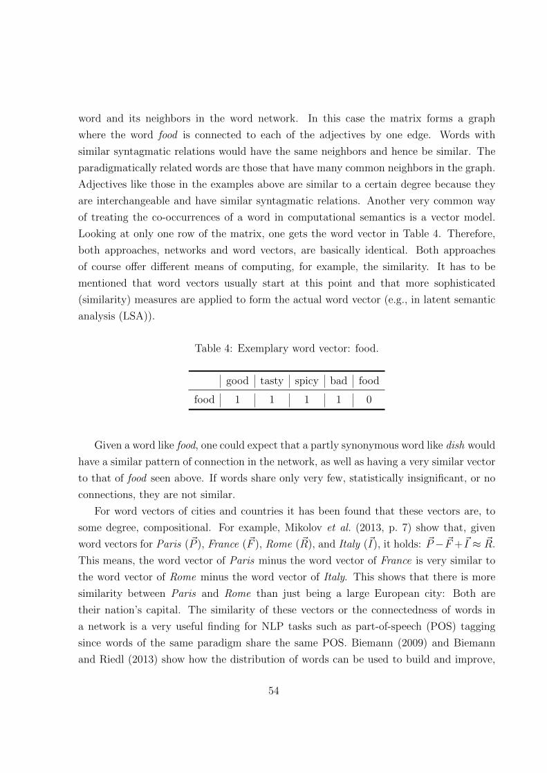
word and its neighbors in the word network. In this case the matrix forms a graph

where the word food is connected to each of the adjectives by one edge. Words with

similar syntagmatic relations would have the same neighbors and hence be similar. The

paradigmatically related words are those that have many common neighbors in the graph.

Adjectives like those in the examples above are similar to a certain degree because they

are interchangeable and have similar syntagmatic relations. Another very common way

of treating the co-occurrences of a word in computational semantics is a vector model.

Looking at only one row of the matrix, one gets the word vector in Table 4. Therefore,

both approaches, networks and word vectors, are basically identical. Both approaches

of course offer different means of computing, for example, the similarity. It has to be

mentioned that word vectors usually start at this point and that more sophisticated

(similarity) measures are applied to form the actual word vector (e.g., in latent semantic

analysis (LSA)).

Table 4: Exemplary word vector: food.

good tasty spicy bad food

food 1 1 1 1 0

Given a word like food, one could expect that a partly synonymous word like dish would

have a similar pattern of connection in the network, as well as having a very similar vector

to that of food seen above. If words share only very few, statistically insignificant, or no

connections, they are not similar.

For word vectors of cities and countries it has been found that these vectors are, to

some degree, compositional. For example, Mikolov et al. (2013, p. 7) show that, given

word vectors for Paris (~P ), France (~F ), Rome (~R), and Italy (~I), it holds: ~P − ~F +~I ≈ ~R.

This means, the word vector of Paris minus the word vector of France is very similar to

the word vector of Rome minus the word vector of Italy. This shows that there is more

similarity between Paris and Rome than just being a large European city: Both are

their nation’s capital. The similarity of these vectors or the connectedness of words in

a network is a very useful finding for NLP tasks such as part-of-speech (POS) tagging

since words of the same paradigm share the same POS. Biemann (2009) and Biemann

and Riedl (2013) show how the distribution of words can be used to build and improve,

54

respectively, POS taggers. Knowing that a word that is not in the vocabulary of a POS

tagger is distributionally similar to a known word allows one to assign the same POS

to the out-of-vocabulary word (Biemann and Riedl, 2013). The approach presented in

Biemann (2009) is solely based on distribution and shows that the distribution allows

for very fine distinctions of POS. The adjectives in examples 6 to 9 can be expected to

be the neighbors of both food and dish, and in fact both words are of the same POS.

Furthermore, Biemann (2009) shows that it is possible to distinguish between female and

male first names. Also the author is able to form clusters of similar words (e.g., the city

names used in the example above). The finding that names form clusters, allows to be

used for named entity recognition and tagging. A great part of the work done on semantic

networks in recent years was undertaken on distributional data. Many findings that were

made in different kinds of networks, among them the lexical networks presented here, will

be used and be ported to applications in ontologies.

Only quite recently has distributed computing (i.e., the usage of a cluster of personal

computers) made distributional analysis of huge text corpora possible without the need

of having a super computer. Huge text corpus here means at least a few million sen-

tences that are processed and analyzed. Only such large numbers of sentences make the

assumptions taken from them meaningful.

Unlike ontologies and other hand-crafted resources, distributional semantics is what

is called knowledge free: It does not reside on a priori information. While it is much

more computationally intensive, it requires less human work to analyze huge amounts of

texts statistically. Still, the results are not yet as accurate as man-made resources, as

will be shown later on. Despite its accordance with the requirements of structuralism,

distributional semantics differs from even the structuralist approaches presented earlier.

Unlike semantic fields, it is heavily based on empiricism and includes paradigmatic as well

syntagmatic relations. The distinction between the kinds of relations that exist between

the words (i.e., the semantic relations) is still an open problem; also some experiments

show that a distinction between different relations should be possible (Erk and Pado,

2008; Mikolov et al., 2013; Socher et al., 2013). The negation of words (e.g., bad versus

not bad versus not not bad) and their representation in a vector model are problematic.

Or in general the question “how textual logic would best be represented in a continuous

vector space model remains an open problem” (Hermann et al., 2013, p. 74f.).

In comparison to frame semantics, distributional semantics does not at all include

extra-linguistic knowledge. As Harris formulates it, the co-occurrences of a word “may

55

still be ‘due to meaning’ in one sense, but it accords with a distributional regularity”

(Harris, 1968, p. 785). All the vagueness of semantic fields and frames is avoided; only

empirical distributional regularities remain.

3.4 Semantic Relations

The distributional approach connects words both in a syntagmatic way, the neighbors in

the network, as well as in a paradigmatic way, words with a similar pattern of connec-

tivity. It does not specify how the relation between two words is exactly, only in terms

of similarity. The following chapter will shortly recap the basic semantic relations, espe-

cially those that are going to be of interest when examining ontologies, i.e., those relations

realized in WordNet and other ontologies. Because they will be discussed in more detail,

especially with regards to the specific implementation within WordNet in Chp. 5, only a

very short overview will be given here.

3.4.1 Synonymy

Synonymy as the total semantic identity of two words is a very rare feature. Different

words hardly ever mean exactly the same in all contexts of a natural language.28 Cruse

(1986, p. 88) defines cognitive synonymy of X and Y if both are syntactically identical

and any sentence S containing X has equivalent truth conditions to an identical sentence

S1 where X is replaced by Y .

Even though big and large can substitute each other in some contexts, they cannot

substitute each other in every context. While a big boy is a boy that is behaving like an

adult, a large boy is an overweight boy. Big/large are therefore only partly synonymous.

3.4.2 Hyponymy

The relations of hypernymy (token > type relation) and its inverse hyponymy (type <

token relation) are hierarchical relations, or, in terms of set theory, relations of inclusion.

A hypernym includes all its hyponyms. A is the hypernym of B (A ⊃ B) if B is a

hyponym of A (B ⊂ A). For example, tree is a hypernym of oak and oak is a hyponym of

tree. The set of all trees also includes cherry, linden, and other kinds of trees. All these

28Technical vocabulary and scientific language as special forms of a language are exceptions.

56

trees are co-hyponyms; they share the same hypernym. Most hypernym–hyponym pairs

make up a taxonomy.

The hyponymy relation is sometimes called a kind-of relation. As Lobner (2003,

p. 133) states in his introduction to semantics, a car is a type of (motor) vehicle, but

a boy is not a type of child. Cruse (2000, p. 152) illustrates some problems arising

when hyponymy is defined as X is a kind/type/sort of Y. When saying a kitten is a

sort/type/kind of cat, Cruse argues, this sounds rather odd. He therefore tries to find

definitions of hyponymy aside the inclusion definitions given above.

In computational approaches, hyponymy is often called a IS−A relation. If we apply

the IS −A relation to kitten/cat, this problem does not arise at all. It is perfectly fine to

say that a kitten is a cat or a boy is a child. A quite regular case of hyponym–hypernym

pairs is that of the endocentric compounds, where the compound is a hyponym of the

head of the compound (e.g., a lifeboat is a kind of boat)29.

3.4.3 Meronymy

A related concept is the meronymy relation, or part–whole relation. A meronym A of B

is not a hierarchical subconcept of B, but a part of B itself. A hand has fingers and a

palm. The inverse relation is called a holonym. Concept B does not logically include A;

it is more of the physical constitution or definition of B to include A. Computationally,

especially with respect to ontologies, this relation is often included in the HAS − A or

a PART − OF relation. We speak of meronymy only if both relations apply. As Cruse

(1986, p. 161) shows, a wife has a husband and changing diapers is part of being a mother

do not indicate a meronymy relation. Only if both conditions are satisfied do we speak

of meronymy: A hand has a finger, and a finger is part of a hand.

3.4.4 Antonymy and Opposition

Antonymous words are mutually exclusive and mark points of a scale, like large and small.

We call this opposition antonymy. Two expressions are contradictory if “the truth of one

implies the falsity of the other and [. . . ] contrary if only one proposition can be true but

both can be false” (Fellbaum et al., 1990, p. 29). Logically incompatible, antonymous

word pairs are not necessarily complementary, meaning that the negation of one does not

29Of course there are many exceptions, where a compound’s meaning is not directly derived from itsparts. A skinhead is not special form of a head

57

equal its antonym. Not large is not the same as small but can also lie in between these

two on a scale (cf. Lobner, 2003, p. 124); the words are bi-polar. The negated form does

not inevitably “express the opposite value of an attribute but something like ‘everything

else’ ” (Fellbaum et al., 1990, p. 35).

Lyons (1977, p. 286) states that the opposition of two words arises from “some dimen-

sion of similarity”, meaning that only two words that are similar up to a certain point,

and are different from each other in one property, can be antonymous. Murphy (2003,

p. 170) says that in antonymy “only one relevant property of the words is contrasted”.

Both brother and sister denote a sibling. The only difference is the gender of the sibling

referred to30. This can be called a binary semantic property (see Table 5). Both words are

semantically complementary. They are not the opposite of each other, but complementary

and exclusive.

Table 5: Binary semantic property of siblings.

Expression Sibling Female

brother + −sister + +

As Murphy (2003, p. 167) puts it: “The boundary between synonymy and antonymy

is not always so clear”. She states that antonyms are co-hyponyms with exclusive senses,

while (near-)synonymous words are co-hyponyms with similar or “overlapping senses”

(Murphy, 2003, p. 167).

Fellbaum (1995) shows that semantically related words across part of speech (POS)

also co-occur at very a high rate. A word pair like dead (noun) and live (verb) co-occur

more often than the antonym pair live/die. This shows that there is of course a semantic

relation between both concepts and that lexical entities from different POS are being used

contrastively. From a semantic point of view, leaving out the paradigmatic or grammatical

level, the relation between words across different POS is just as strong as those of the

same POS. Still, this effect should not be confused with antonymy.

In a NLP context, one would still be interested in the information that the pair

dead/live describes a kind of opposition.

30This kind of antonymy is called a relational antonymy.

58

3.5 Ontologies

3.5.1 Conception

Unlike in metaphysics in philosophy, the term ontology in the context of information and

computer sciences does not refer to a system that tries to explain or categorize everything-

that-is in one coherent scheme. Instead the term refers to a system describing special

relations or meaning in a concrete domain, based on ideas taken from early semantic

networks as they have been introduced in Chp. 2.2. Furthermore, ontologies are closely

related to lexical fields and frame semantics.

An often cited definition of an ontology states that an ontology is an “explicit spec-

ification of a conceptualization” (Gruber, 1993). This definition has been criticized for

being overly broad (e.g., by Smith and Welty (2001)), and, at the same time, for excluding

especially some linguistic ontologies (i.e., WordNet (Stuckenschmidt, 2009)). To under-

stand the definition one has to also define what explicit specification and conceptualization

are.

Taking these critiques into account, Gruber later defines ontologies in the context of

information sciences as

a set of representational primitives with which to model a domain of knowledge

or discourse. The representational primitives are typically classes (or sets), at-

tributes (or properties), and relationships (or relations among class members).

The definitions of the representational primitives include information about

their meaning and constraints on their logically consistent application (Gru-

ber, 2009).

This second definition gives some clues about the way an ontology formalizes knowledge.

Classes, attributes, and properties are used to build a consistent system of knowledge

that is logically connected. If such a system is treated as an open world, it is said to be

incomplete: Not every existing entity, relation, or class has to be modeled in the ontology.

Non-existence in the ontology is no proof of falsehood. Entities of an ontology may as

well have other neither explicitly, nor implicitly, mentioned properties.

The closed-world assumption means that what is not existent in the model is treated

as false (Stuckenschmidt, 2009, p. 35). The ontologies that are going to be examined in

this thesis are open-world ontologies. They are incomplete but can be extended by new

elements.

59

The objects an ontology describes are called instances or entities. Instances are mem-

bers of a class. Classes are defined as having special attributes or properties. They are

ordered hierarchically. Child classes inherit properties of their parent class. A class can

have different attributes which might be used to describe the instances of a class. If we

imagine a class mammal, all child classes and all their instances share some common at-

tributes: Their offspring is born alive, they have skin, and fur or hair. But child classes

might have special properties. Felines have four feet, fur and so on, while the members

of the class Homo sapiens walk upright on two feet and have a mostly hairless or at least

furless skin. One instance of Homo sapiens might have the name Peter. It has a birthday,

hair color, address, sex, and more properties that distinguish this instance from others of

the same class.

Instances can be members of different classes or, in terms of set theory, members of

different sets. Set theoretical concepts (e.g., the inclusion, union, intersection, and so on)

form the basis of ontology formalization.

3.5.2 Ontology Formalizations

Ontologies can be formalized in different ways. The membership of an instance to a

class, or of a class to a parent class, might be expressed using sets. Relationships between

classes or instances, properties, and attributes, as well as inheritance and hierarchy can be

described using description logics. Standard notations such as the Resource Description

Framework (RDF) or the Web Ontology Language (OWL) can be used to write description

logic equivalent statements in the form of an XML notation. The following chapters give

a short overview of those formalisms.

3.5.2.1 Description Logics

The fundamental concepts of ontology formalization lie within the so-called description

logics (DL). DL are a defined subset of predicate logic expressions. They can be defined

to be more or less expressive, depending on the application (cf. Nardi and Brachman,

2003, p. 7). DL are a family of knowledge representation formalisms

that represent the knowledge of an application domain (the ‘world’) by first

defining the relevant concepts of the domain (its terminology), and then using

60

these concepts to specify properties of objects and individuals occurring in the

domain (the world description) (Baader and Nutt, 2003, p. 47).

The formalization of a domain (e.g., classes, relations or hierarchies) is called the DL

TBox (terminological box ) while the data is called ABox (assertional box ) (cf. Nardi and

Brachman, 2003, p. 17). The TBox is intensional. This information does not change.

The ABox describes objects, i.e., their concrete relations or attributes. New information

might be added to an ABox.

The most basic relations in a DL are those of set theory (e.g., the inclusion (A ⊆ B)

or equivalence (A ≡ B)). A can be defined as atomic concept B as happened here, or

the right side of the equation could be a complex logical expression. In this fashion,

definitions of the TBox are specified.

An ABox consists of expressions on entities or individuals. For example, an entity (e)

can be assigned to a class (C) e : C. Given that a relation bandMember was defined in the

TBox, the expression in Ex. 10 and Example 11 can be made. The examples are taken

from the data set of DBpedia and have been translated to a possible DL expression.

(10) bandMember(The Beatles, Paul McCartney)

(11) bandMember(The Beatles, John Lennon)

The information that both musicians played in the same band should be automatically

available through reasoning. Later we will come back to the complex of inference when

it comes to link predictions in large networks built from ontology data, the ABox.

Table 6 gives a brief overview of possible DL notations. Some of these notations have

direct equivalents in the semantic relations that were shown before. The subset/superset

(⊆ / ⊇) correspond to hyponymy and hypernymy. The equivalence (≡) is similar to

synonymy.31 It has already been explained that the antonym of an expression is not

necessarily its negation (¬). But antonyms are mutually exclusive. An entity is either a

member of the set uncle (U) or of the set aunt (A): U ∨ A.

The universal restriction (∀) can be used to assign some property to every member

of a class (e.g., every person has a name), while the existential restriction (∃) is used to

allow an entity to have a value (e.g., an academic title) without saying that every instance

has to have one. Using this set of notions, other, more sophisticated relations between

entities or classes, such as meronymy, can be defined and used in an ontology.

31In Chp. 5, I will claim that the synonymy relation in WordNet actually defines an equivalence.

61

Table 6: Logical operators, restrictions, and set theoretic expressions used in descriptionlogics.

∀ universal restriction: ∀x, for all x∃ existential restriction: ∃x, there is at least one x¬ negation (non)∧ conjunction (et)∨ disjunction (vel)∩ intersection∪ union

⊆ / ⊇ subset/superset≡ equivalence: assertion

The more expressive a DL is, the more complex, or even impossible is the reasoning.

DL are based on the open-world assumption (i.e., concepts that cannot be found in an

ontology), or information missing in a data set is not necessarily false. Other information

might exist that just has not been formalized. Reasoning on data makes some implicit

information accessible.

3.5.2.2 RDF

The Resource Description Framework (RDF) is a World Wide Web Consortium (W3C)

specification for the description of any kind of resource. A resource can be a website,

a web service, as well as other resources like physical objects of the real world. It is a

description framework (i.e., a set of terms used to describe objects) “for describing just

about anything” (McBride, 2004, p. 51).

The description principle of RDF is a directed graph. Directed graphs have been

examined in Chp. 2. To reference the objects that are being described, universal resource

identifiers (URIs) are used. The most widely known examples are web addresses. URIs

consist of a schema (e.g., http), an authority (e.g., w3c.org), a path, the simplest being /,

and optional query or fragment. In the case of a web address, the URI references exactly

one website (cf. Berners-Lee, 1994). Full URIs can be seen in Listing 1.

In the ontologies that are examined in this thesis, URIs are used to reference objects,

62

such as persons, institutions, and concepts, as well as their descriptions. Objects are

linked using attributes. But attributes can also take literal or numerical values.

Figure 12: An exemplary RDF graph.

This can be seen in Fig. 12. The elliptic nodes, labeled by URIs, represent resources.

The edges stand for attributes or relations labeled as well by a URI. The rectangular

nodes stand for literal values. Empty nodes are equivalent to the ∃-quantor in predicate

logic: There is at least one, not further defined, value or object in this relation. The

different types of nodes are going to be of importance to distinguish when it comes to

predicting relations in an ontology. Literal values and empty nodes might not be of great

interest or use in the predictions of new attributes of a given object. As seen in Fig. 12,

literal values such as the population of a city or country or the age or birthday of a person

are likely to contain special values that are not common to, or shared by, a cluster of

elements. The graphical representation in the form of a graph (see Fig. 12) is not the

only possible formalization of RDF data.

The description framework consists of terms to describe relations between objects.

RDF has several possible formal description languages. The two most important notations

in the context of this thesis are N-triples and the RDF/XML notation.32 N-triples consist

of three elements, in this case URIs (see Listing 1).

Listing 1: N-Triple taken from DBpedia<http:// dbpedia.org/resource/Sammy_Davis ,_Jr.>

<http: // dbpedia.org/property/deathDate >"1990 -05 -16"

The first refers to the object that is being described. The second refers to the relation

that exists between the first object and the third element in the triple. In this case the

third element is not a URI-referenced object like the first or the second, but a literal

value. N-triples are widely used to exchange resource descriptions or the ABox of a DL.

Lists of such triples make up the data of DBpedia (see Chp. 6).

32Many other ways to formalize RDF exist that cannot be presented here.

63

The RDF/XML notation describes the same relation between two objects but makes

use of the Extensible Markup Language (XML). The syntax is more sophisticated and

can be processed by widely used XML processors. XML is often used to exchange data

between different systems. Not the whole expressibility of RDF/XML can be discussed

here. For further information see (e.g., Carroll and Klyne (2004)).

RDF is capable of describing concrete objects or abstract ideas, but it cannot be

used to describe a domain or knowledge in the way ontologies do. RDF is therefore

not an adequate instrument to model ontologies, but rather to describe relations. An

extension of RDF called RDFS solves some problems that occur when using RDF. It adds

the possibility to declare subsets of classes and the use of negation (cf. McBride, 2004,

p. 63). Still, more expressiveness is needed to formalize description logics. Some of these

shortcomings were resolved with the development of OWL.

3.5.2.3 OWL – Web Ontology Language

To make full use of the expressiveness of descriptions logics, the Web Ontology Language

(OWL) was developed. Usually, OWL is written in an XML notation.

Among OWL’s distinct expressions are the possibility to declare properties that may

exist only between objects of some defined classes (Antoniou and Harmelen, 2003, p. 92).

Given the relations seen in examples 10 and 11, the restriction to a relation bandMember(x, y)

is that x is in fact a member of the class Band (x : Band), and that y is a person

(y : Person). The first is called a relation’s domain, the latter is called the range.

Classes can be disjoint, meaning that there cannot exist objects that are members of

both classes A and B, or, in other words, the intersection A ∩ B is empty. For example,

the set of male and female members of a group have no intersection and are disjoint.

Disjointness implies that the intersection is an empty set, but an empty intersection does

not imply the disjointness of two sets.

Similarly, OWL allows one to define subsets (A ⊂ B) and unions (A ∪B). Properties

can also be defined to have a special data type.

OWL is defined in three versions, each with its own level of expressiveness: OWL Full

is a superset of OWL DL, which is itself a superset of OWL Lite. OWL Full is hence the

most expressive variant of OWL, and it is undecidable. The subset OWL DL is a version

that is based on description logics. It is decidable and there are reasoning algorithms that

work with OWL DL. OWL Lite was intended as a much simpler version of OWL. Still, it

64

has been shown that it is in fact just as expressive as OWL DL (Grau et al., 2008).

In the context of this thesis, it is relevant to know that there are differences between

RDF and OWL, especially those described above, and that OWL can be used as an

ontology language to define the terminology of an ontology (TBox), while RDF is in this

context mostly used to define relations between entities or classes that are defined in an

ontology (ABox).

As one can easily see from the descriptions above, the relations used in RDF that are

defined in an ontology using OWL make up not only a graph as well as a network of

entities and their properties and relations.

The ABox of an ontology is made up by directed triples, describing relations between

one entity and another entity or describing a property of an entity. Looking at Listing 1

above, one could also think of a triple as describing a graph. In the graph notation, the

first and the third element each refer to a vertex of the graph. As mentioned before, a

graph can be written as an edge list. For example, given two vertices v1 and v2 that are

connected by an edge, the corresponding notation is {v1, v2}.In case of ontology data, the triple has to be interpreted as directed. The first element

points to the third element, not vice versa.

3.6 Conclusion

In Chp. 2, definitions of semantics based on a network were given that are, in many

aspects, very close to what has been shown in this chapter. The idea that the meaning of

a word is based on its relation to other words33, or the word’s neighbors, can be found in

the distributional approaches, in frame semantics, and in lexical field theories. Trier states

that “Worte im Feld stehen in gegenseitiger Abhangigkeit voneinander. Vom Gefuge des

Ganzen her empfangt das Einzelwort seine inhaltliche begriffliche Bestimmtheit”34 (Trier,

1973, p. 41). He compares the meaning of a word to a mosaic, where only the knowledge

of all neighboring words gives the meaning of the word. Instead of mosaic one could also

speak of a network. In a network, and in an ontology as well, the meaning of a concept

or word is given by its neighbors, by the entities or vertices it is related to.

Semantic relations define how words are connected. Where the picture of the mosaic

33These relations, ultimately, result from the usage of the words.34Translation: Words of a field stand in mutual dependency with each other. From the structure of

the field the single word receives its conceptual determination.

65

and network only gives the fact that a relation exists, semantic relations define, similar to

ontologies, how words are dependent on each other. Frame semantics furthermore states

that the extra-linguistic knowledge of entities is important and tries to formalize them in

a coherent way. Like formal semantics, ontologies are grounded in logics, in description

logics to be precise. This reliable philosophical–mathematical framework makes ontologies

very adaptive to different domains and needs, and allows one to apply logical reasoning

and inference.

Ontologies are not restricted to purely intra-linguistic information, but can be open to

world knowledge as has been proposed in frame semantics. Relations between entities can

take different forms and further define the meaning of an entity. Synonymy, antonymy,

hyponymy, meronymy are all basic relations not only in the human language as well as in

the relationships between things. They are therefore commonly used in ontologies. Based

on relations between entities, the data naturally forms a graph or a network.

Distributional semantics, an approach that looks at words in context (i.e., at the

realization in syntagmatic and paradigmatic relations) aims to find these regularities in

large amounts of data. Distributional semantics has only been recognized within the last

20 years as being very useful and is today probably the most often used approach to

semantics in NLP. This is of course due to the possibilities modern computers and the

Internet offer. Today it is widely used not only in state-of-the-art search engines (e.g.,

in the form of latent semantic analysis (LSA) (Deerwester et al., 1990) as well as in a

variety of other NLP tasks such as POS tagging (Biemann and Riedl, 2013), word-sense

disambiguation (Biemann and Giesbrecht, 2011), and others).

Distributional semantics does not need human interaction and knowledge; it is usually

referred to as knowledge free and is hence much easier to apply. Still, the results are not as

semantically exact as hand-made resources. Ontologies have very exact relations and can

have very fine-grained sense distinctions. But this advantage comes at a price: Creating

ontologies, both the formalization and the data, is very time intensive. Therefore, the

goal of this thesis is to improve existing ontologies without the need of human interaction

or with only very limited interaction. For both ontologies that are to be analyzed and

extended here (i.e., WordNet and DBpedia), the proposed methods are based on findings

and techniques developed in social sciences, biology, and physics in recent years. These

methods and ideas are to be reviewed in the following before adapting the ideas to ontolo-

gies, taking into account what has been said about graphs and networks in the chapter

before. Afterwards, the two ontologies in question are analyzed first to identify possibly

66

missing information and, secondly, to find features that might help in identifying missing

relations between two entities automatically.

67

4 Relation Extraction and Prediction

The structure and properties of networks, as seen in Chp. 2.1, show a special feature of

networks: The information given in a network is present not only in the vertices and their

edges as well as in the overall structure. A good example is the centrality measures intro-

duced before: They are calculated by looking at least at the direct neighbors, but most

of them take the whole network into account. The information given in the complexity

of a network is more than the pure sum of its vertices.

The structure of networks has been used to make assumptions about the probability of

the existence of non-defined edges between vertices. The information given in the graph

is used to predict possible relations between two vertices that the graph, or an ontology

that will be treated as a graph in the context of this thesis, does not actually represent,

but that the network structure makes plausible.

This has lately been used especially in online social networks or in the context of

marketing and advertisement, as will be shown in Chp. 4.2. In Chp. 4.3, I will present

existing machine learning techniques to compute such probabilities, before discussing the

conceptual difference between a social network and a semantic network and the implica-

tions these differences have on the methods that are to be applied to predicting links or

identifying missing edges in semantic networks.

Before turning to techniques based on networks, classical text-based approaches to

extending ontologies shall be discussed.

4.1 Extending Ontologies: Relation Extraction from Text

Ontology creation and development is a time-consuming, often manually undertaken, task.

Enrichment and automatic extension of ontologies have therefore been a field of intense

study in the last decades.

This thesis is going to focus on methods adopted from graph and network analysis

and ontologies will be looked at as graphs. Still, there have been different approaches to

enrich ontologies, especially semantic ontologies like WordNet.

In the following, I will evaluate existing methods of ontology enrichment through rela-

tion extraction from natural language texts. These approaches do not take the ontology

(e.g., WordNet or DBpedia and its network structure) into account, but rather work with

freely available texts from different domains. The methods are based on the idea that

68

natural language texts contain and convey knowledge in the form of (syntactic) structures

and that language can be parsed, processed, and information extracted. Three related,

yet quite different, approaches shall be examined here.

Hearst (1992) proposes a method to extract hyponymy–hypernymy relations from texts

only taking into account the surface structure of sentences (i.e., only a shallow analysis

based on POS tagging). This method is evaluated in Hearst (1998).

Lungen and Lobin (2010) introduce a method to transform information given in table

of contents to a Multilayered Semantic Network (MultiNet). Unlike the first approach, a

deep syntactic analysis of the dependency structure is undertaken to identify entities and

relations. Furthermore, the text structure and organization are taken into account.

Others, such as McCord et al. (2012), take parsing trees and the deep structure of

sentences into account when looking for recognizable patterns to match information given

in texts to semantic relations such as those of DBpedia.

Hearst (1998) presents a method she calls lexico-syntactic pattern extraction to find

relations between words. The method is meant to support a lexicographer in his work

(e.g., the developers of WordNet). The goal is to find constructions “that frequently and

reliably indicate the relation of interest” (Hearst, 1992, p. 540). Hearst (1998, p. 134)

gives some examples of such constructions in texts:

(12) . . . works by such authors as Herrick, Goldsmith, and Shakespeare.

(13) Bruises, . . . , broken bones, or other injuries

Example 12 shows a typical itemization of names that are subsumed by the preceding

noun phrase (NP) authors. The pattern that matches such constructions is

(14) such NP as {NP, }* {, and/or} NP.

The first NP is a hypernym of the following NPs:

• hyponym(Herrick, author),

• hyponym(Goldsmith, author), and

• hyponym(Shakespeare, author).

The pattern of interest in example 13 is of the form

(15) NP {, NP}* {,} or other NP.

69

The NP in the first slot are all hyponyms of the NP in the last position.35 In

total, Hearst identifies eight such patterns that unambiguously and reliably indicate a

hypernymy/hyponymy relation.

One way of finding such patterns is to derive a list of words that are already connected

by the relation in question in WordNet and to extract sentences from large text corpora

that contain the two words. Looking at the derived sentences should give a good overview

of possible constructions and hence patterns.

However, adding newly found relations to WordNet comes with some problems. Since

the structure of WordNet is not word based, but rather word sense based (see Chp. 5.2

for a deeper analysis of the WordNet structure), one has to decide which one is the word

sense present in the relation. The word sense has to be disambiguated to the WordNet

senses. This is, as will be explained later, not an easy task. More over, if one word form

does not exist, the lexicographer has to decide to what word sense (called synonymous

set of short synset) to add this word form or to create a new synset.

Another problem arises when text genres other than encyclopedic texts are used to

find new relations. Especially in newspapers, a genre for which a great amount of corpus

data is available, authors often present subjective interpretations.

Hearst (1998, p. 17) found that this leads to some noise when extracting relations from

newspaper articles.

The weakness of this approach lies in its inability to find patterns for relations other

than hyponymy/hypernymy. Nonetheless, the method was used in the creation of Word-

Net and helped identify hyponymous words.

While Hearst (1998) only mentions the possibility to apply a deeper analysis, Lungen

and Lobin (2010) transfer the idea of finding patterns in language structures that indicate

a certain semantic relation, not necessarily a lexical relation, to table of contents (TOC)

of academic text books. They find that the hierarchical order of text structures, such as

sections, paragraphs, and others, in combination with morpho-syntactic information can

be used to identify semantic relations between terms in headings.

The number of possible relations identified by different patterns is quite large. The

35Although this notion a widely accepted in the field of natural language processing, it is probablyrejected by many scientists in other fields (cf. Kripke, 1980). Hyponymy is not used in a strictly linguisticsense here. It is used to refer to a logical categorization of objects in nature. Important in the field onNLP is that a pattern like this one allows to categorize entities, here represented by proper names. Itgives meaning to a proper name that otherwise to a computer is only a string of characters without anymeaning.

70

structure of headings, especially in academic textbooks, indicates per se a hierarchical

relation that also exists between the single elements of the TOC. In a first step, a number

of syntactic and grammatical analyses are undertaken (e.g., lemmatization and syntactic

parsing). Statistical methods can be applied to find technical terms that are specific to

a domain (see bold-faced terms in Fig. 13). Between these terms, depending on the

hierarchical and syntactical order, the relations are established.

Hebborn (2013, p. 204) gives the example shown in Fig. 13, where an exemplary

excerpt from a TOC can be seen.

2.3.5 Weitere Kern Merkmale politischer Systeme

2.3.5.1 Die Stellung des Parlaments

2.3.5.2 Die vertikale Gewaltenteilung

2.3.5.3 Verfassungsgerichte

Figure 13: Sample of hierarchically structured text.

A human reader easily understands that the subordinated sections and paragraphs

extend or explain the superordinate section. The terms that are related are in bold.36

2.3.5 [Weitere Kern[merkmale]keyword [politischerSysteme]A]NPGen

2.3.5.1 Die [Stellung des Parlaments]B

2.3.5.2 Die [vertikale Gewaltenteilung]C

2.3.5.3 [Verfassungsgerichte]D

Figure 14: Sample of hierarchically structured text with marked terms.

In Fig. 14, the important elements are labeled:37 The keyword Merkmal (English:

property), in plural, here in the form of a compound, in the superordinate heading (Fur-

ther main properties of political systems) is the head of a NPGen (of political systems)

along with the term A, politischer Systeme (political systems) that indicates the focus of

36The accentuation does not exist in the original TOC but were added by Hebborn.37Based on Hebborn (2013, p. 204); extended by appropriate tags.

71

the following headings. The subordinate headings contain the terms B −D. This struc-

ture implicitly comprises relations of the kind has(termA, termX) (e.g., has(politisches

System, Verfassungsgericht)). The focus term in the superordinate heading is explained

or extended in the subordinate headings.

This approach is very fruitful when working with general knowledge ontologies, or when

creating such an ontology. The approach seems unfitting for WordNet, where a relatively

small set of semantic relations exists, and where the focus is not on general knowledge

terms. It could, nonetheless, be applied to DBpedia and other similar ontologies to fill

existing gaps. Still, because of its relatively free use of relations, one might have to create

further rules to match these relations to those defined in the ontology. An example of how

to match relations given in texts to relations in an ontology will be given in the following

approach.

Based on the syntactic structure of utterances, the isomorphism or parallelism between

syntactic and semantic structures can be exploited to assign semantic roles to phrases.

For example, in question answering (QA) systems such as the already mentioned IBM

Watson, finding information on different entities is needed to understand a question and

to find the appropriate answer. In IBM Watson, relation extraction is used at different

points in the workflow. Watson uses, besides other knowledge sources, DBpedia.

In contrast to the approach of Hearst, deep dependency parsing in used in Watson.

A parser returns a parsing tree indicating syntactic and semantic dependencies between

constituents. While a solely surface analysis depends on situations where the structure of

a sentence corresponds to a predefined pattern, the parsing allows one to identify entities

in nested structures or complex phrases. Also multi-word tokens are easily identified as

single vertices in such a dependency tree.

The parser used by IBM is a so-called slot grammar (SG) (McCord, 1980). In SG,

verbs are assigned basic semantic types indicating their sense. This information is stored

within the system’s lexicon module (McCord, 1993, p. 127).

During the work on the Watson Jeopardy! challenge, the semantic type system was

extended to include WordNet synset information and to match nouns to related verb

frames. This can be used to define semantic relations by choosing a class of verbs or verb

senses to be responsible to express the relation (McCord et al., 2012, p. 5). Having a

verb frame writeVerb, each verb belonging to this frame is expected to express a writing

relation. The semantic typing system and the WordNet synsets are used to match different

verbs, such as write, compose, and others, as well as constructions such as the composer

72

of to this frame that establishes an authorOf relation.

The dependency structure of a sentence38 like

(16) In 1936, he wrote his last play, “The Boy David”; an actress played the title role

(McCord et al., 2012, p. 10).

can easily be displayed in a predicate–argument structure such as

writeVerb(“he”,“his last play, ‘The Boy David”’)39

while still keeping in memory the internal structure of the object phrase. The relation

can be reduced to

(17) writeVerb(he, The Boy David).

Dissolving the pronoun to the correct entity is then the actual problem in this question-

answering problem. The underlying question to answer is “Who wrote The Boy David?”.

From different ontologies as well as a large number of natural language texts that are

processed in the same way as the example question above, the system tries to find the

answer. It has to look for a relation like the one in Example 17, where the first slot of the

relation, the he, is filled with the actual author name: J. M. Barrie.

These and other approaches to extending sparse information of ontologies or to ana-

lyzing relations in natural language texts are based on text corpora, i.e., external sources

of information. In the following, approaches to extending networks will be presented that

make no use of external knowledge but focus on the network structure itself.

4.2 Predicting Missing Links

Alternatively to the approaches mentioned so far, some recent work from the field of

social network analyses (SNAs), especially link prediction and inferring missing links,

will be presented and discussed. These will later on be ported and applied to extending

ontologies.

Social networks are formed by (human) interaction, and they are “structures whose

vertices represent people or other entities embedded in a social context, and whose edges

38The example might appear a little odd. This is due to the fact that IBM Watson was used to takepart in the US TV show Jeopardy!, where the contestants have to find a fitting question to a given answer.

39Only the two important slots, subj and obj (i.e., direct object), are shown here; other argumentshave already been removed.

73

represent interaction, collaboration, or influence between entities” (Liben-Nowell and

Kleinberg, 2007, p. 1).

Liben-Nowell and Kleinberg (2007, p. 1) define the link-prediction problem in social

networks as follows:

Given a snapshot of a social network at time t, we seek to accurately predict

the edges that will be added to the network during the interval from time t to

a given future time t′.

This definition sets link prediction close to the “problem of inferring missing links from

an observed network” (Liben-Nowell and Kleinberg, 2007, p. 2), and as we will see, most

studies in the field do not take different time points into account but work on static

networks as will be the case for the problems given in this thesis.

Link prediction in SNA has been an active field of research40 in the last decade. Most

of the link prediction studies undertaken on either Facebook, co-authorship graphs, or

other social networks are pretty similar in their approach to predict unseen links and

with regards to the kinds of links they predict (e.g., suggesting new friends, predicting

future interactions between users, or other behaviors).

The first three approaches presented in the following are all based on the Facebook

graph. They do not try to identify possible edges between existing users (i.e., vertices in

the network) but predict personal information from what one likes, friends outside of the

social network, or the home residence by looking at their friends’ activities.41 Afterwards,

other approaches are presented that try to find missing links from networks using some

heuristics based on human/social behavior or using machine learning techniques.

On Facebook the users are connected to other users, their friends, as well as to sites

representing entities like companies, places, and so on that the users like. Furthermore,

Facebook users are connected with properties like their age, sex, and many more.

Kosinski et al. (2013) examine a relatively large sample of vertices (here users and

their personal information) and edges (page likes) from Facebook. From these, they

remove, one after another, attributes such as the age, gender, political or religious views,

40A good review of methods used can be found in Sarkar et al. (2011).41In case of the first two studies presented here one should mention that the possible threat to user’s, or

even non-user’s, privacy was a main concern of the researchers. Others have warned about the possibilityto predict the user’s personality (Golbeck et al., 2011) or to identify people in anonymized data (Butler,2007). The third paper presented in this section is less critical and was published by Facebook employees.It shows what Facebook actually does with the user data.

74

relationship status, and sexual orientation of the users. The pages a user likes are used as

features to predict the user’s personal information. They further take the user’s network

size and density as well as information they derive from questionnaires filled out by the

users into account (e.g., they estimate the user’s intelligence).

The authors try to predict two different kinds of properties of a user: numerical

values (density, size, intelligence, or age) and sets of dichotomous attributes, including the

political view (i.e., liberal or conservative), sexuality (i.e., heterosexual or homosexual).

Despite some odd findings (e.g., that liking curly fries is, according to the machine learning

model they trained, a good indicator of intelligence42), Kosinski et al. (2013) are able

to classify users quite well. The highest accuracy was obtained when predicting the

ethnicity (95%) followed by the gender (93%) and political views (85%) as well as the

sexual orientation (homosexuality of males 88%, females 75%).

To classify the numeral values, Kosinski et al. (2013) employ a regular regression

model. To predict the other values they use a logistic regression model. Regression is,

alongside other machine learning techniques, going to be explained in Chp. 4.3.

In a narrow sense, these predictions are not link predictions since they do not add or

predict links between vertices (users or sites in Facebook) but predict attributes connected

to the user or even attributes defined outside of Facebook (e.g., the intelligence is inferred

from questionnaires the participants filled out). Information like gender, age, sexual

orientation, or political views contains attributes that are present in the Facebook graph

and could therefore be treated as vertices themselves. Still, this is not what this thesis is

about.

Horvat et al. (2012) aim at a different goal. Taking a part of the Facebook graph,

containing users and their friendships, plus the user’s address book outside of Facebook,

Horvat et al. predict the probability of two non-members being friends if they have

common friends on Facebook. Although the accuracy is not very high, it is still higher

than a baseline of randomly assigned edges (Horvat et al., 2012, p. 5ff.).

The findings are, from a user’s or better non-user’s point of view, maybe even more

alarming than the ones seen before. In this case, one can speak of a good example of the

prediction of edges in a network, thereby extending it. The approach does not aim at

finding links between existing vertices but at extending the network by new vertices.

As features for their prediction, Horvat et al. (2012) take the degree, the shortest path

42There is of course no significant correlation or even causality.

75

and few other measures into account. These measure are then used to train a random-

forest classifier, and to build decision trees. This machine learning approach will also be

discussed in Chp. 4.3.

A third study that is to be presented here was undertaken by three Facebook employ-

ees. Backstrom et al. (2010) propose an algorithm to predict “the location of an individual

from a sparse set of located users with performance that exceeds IP-based geolocation”

(Backstrom et al., 2010, p. 61).43 They state that about 6% of the ca. 100 million users

in the US entered a home address. From these, they were able to parse about 60%. This

gives about 3.5 million addresses that can be geolocated. They observed that with an

increasing distance the probability of friendship decreased. This observation allows one to

predict the location of users without an address on Facebook by taking into account the

locations of their friends. The likelihood of one user living close to its next friends, the

ones he has the most contact with, is very high and makes these predictions possible. But

since this assumption only holds true for social networks, this approach is not adequate to

be used to predict other relations. After looking at these possibilities to predict different

features of vertices in a social network, link prediction or the identification of possibly

missing edges within a social network is the main purpose of the following approaches.

Often used, or extended, is the approach of Adamic and Adar (2003) (cf. Davis et al.,

2011; Liben-Nowell and Kleinberg, 2007; Sarkar et al., 2012; Scellato et al., 2011). Adamic

and Adar (2003) look at faculty home pages (i.e., personal websites of faculty members

of a university), which are thought of as representing the user’s social environment and

can therefore be used to “learn a great deal about both virtual and real-world communi-

ties of people” (Adamic and Adar, 2003, p. 212). To build a network out of these home

pages, four sources are used: the text of a home page, the out- and in-links, and mailing

lists of the different departments involved. Combining these, a network structure arises

that is believed to show the same clusters as the actual involvement of the persons. The

network should therefore exhibit structures that arise from university department struc-

tures or from projects in different departments. The analysis was undertaken for different

universities (e.g., Stanford University and Massachusetts Institute of Technology).

Looking at the in- and out-links, the mailing list membership, and the home page

text, Adamic and Adar (2003) “predict whether one person is associated with another

[. . . ]. [The] matchmaking algorithm is based on the well-established result in sociology

43IP-based geolocation works by looking up a user’s IP in a special database that returns a closeapproximation of the location of the user.

76

that friends tend to be similar . . . . Hence the more things two people have in common,

the more likely they are to be friends, and the more likely they are to link to each other

on their homepages” (Adamic and Adar, 2003, p. 222). This has been called homophily

before, and it is what is meant when Adamic and Adar (2003) speak of similarity: the

similarity of connections.

Liben-Nowell and Kleinberg (2007, p. 4) treat link prediction as “computing a measure

of proximity or ‘similarity’ between vertices x and y, relative to the network topology”.

To calculate this similarity, they apply a number of measures, some of them very similar.

The most basic approach is the length of the shortest path between the two vertices. Also,

the measure presented in Katz (1953) is applied: It defines the sum over all path, up to

a certain length, between the two vertices, where, because of a parameter β, the longer

path contributes only very little to the sum.

Since two different time points of the same social network are being examined, evolu-

tion models such as preferential attachment can be used as well. Furthermore, PageRank

and random walk models, as well as clustering algorithms are used. Liben-Nowell and

Kleinberg (2007, p. 8) state that many of the measures they applied overlap each other.

Based on the closed triangle assumption or the homophily that Adamic and Adar

(2003) use to predict connections, they apply a measure based on the common neighbor-

hood. It is a score for common neighbors (i.e., the intersection of the set of neighbors of

x (Γ(x)) and the set of neighbors of y (Γ(y))).

Widely used in information retrieval and similarity calculations tasks is the Jaccard

coefficient (Jaccard, 1912), which divides the intersection of two sets by the union of the

two sets and thereby calculates the similarity of the two sets:

|Γ(x) ∩ Γ(y)||Γ(x) ∪ Γ(y)|

.

Taskar et al. (2003) take a different step in predicting links in social networks. They

are not only asking “Is there a link between two vertices” as well as , what type of link

it is. Just as Adamic and Adar (2003), Taskar et al. look at faculty website and their

interaction in the form of hyperlinks and similarity (i.e., topics mentioned on the sites

themselves), which gives them a broad network. They use a method called relational

Markov network (RMN) to make predictions. RMNs find cliques in the data which are

77

then used to make predictions.44 What makes this approach interesting is the fact that

it takes into account what kind of link may exist between the vertices. For every two

vertices an attribute exists is defined, which gives information on whether a link between

the two vertices can exist or not. This can be applied to ontologies with respect to possible

domain/range restrictions.

Another example of using supervised machine learning in link prediction is given in

Hasan et al. (2006). Hasan et al. use different features given in co-authorship networks,

though not all of them are topological features of the network. The shortest path is

one of the network measures utilized but also the common neighbors, as seen above, and

the clusters. Among the tested classification algorithms (e.g., support vector machines,

decision trees, multilayer perceptron, and Naive Bayes) they find that all of them work

comparably well with an accuracy between 80% and 90%. These classifiers will also be

evaluated in this thesis.

Looking at the research done in SNA, one can find some clues to link prediction that

might be applied to ontologies as well. First, one can see that a profound analysis and

understanding of the data helps in finding ways to predict unseen structures. Considering

link prediction as a classification task is a second one. The consideration that two people

are likely to interact if they share a lot of common acquaintances is not true for language

networks such as WordNet,45 but might be applied to DBpedia data set. A problem

arising when working with ontologies is that of domain or range restrictions, which are

not formalized in graphs. Taskar et al. (2003) have shown how these restrictions might be

handled to avoid false predictions that contradict the ontology. In the following chapters

I will explain how these range restrictions can be handled in WordNet and DBpedia.

The next step in evaluating existing methods is to look at other mathematical models

that have been proposed to make predictions in complex, non-social networks. Predicting

links in social networks is based on some basic assumptions made on the structure of

human interaction. Two vertices that share many common neighbors are more likely to

be related (at some point) because humans tend to meet their friend’s friends and people

with similar interests and hobbies. But this is not true for other networks, for example

gene networks or semantic networks. Techniques that can be employed to successfully

44As we will see in the analysis of the WordNet graph, cliques are no help in predicting links in semanticword nets like WordNet.

45In WordNet, many neighbors are unconnected because of the structure of the WordNet ontology.Synonyms, for example, are child nodes of a common synset but are not connected themselves.

78

(a) Hierarchical organizationD with vertices {a,. . . ,f} of G.

(b) Original graph G withvertices {a,. . . ,f}.

Figure 15: HRG: hierarchical random graph model.

predict links in social networks can therefore not directly be ported to other types of

networks. A more general approach that is not limited to social networks since it is not

based on properties of social interaction, will be reviewed in the following.

Clauset et al. (2008, p. 99.) state that “our current pictures of many networks are

substantially incomplete”. This is due to the incompleteness of most networks available.46

To predict the missing links they introduce their approach of hierarchical random

graphs (HRGs). HRGs are arbitrary hierarchical structures that correspond in their topol-

ogy (i.e., in terms of statistical properties such as degree distribution, or path length etc.)

to the original graph. Clauset et al. (2008) claim that the hierarchical structure itself

can explain these features of a graph. The algorithm produces a set of different random

graphs representing the original graph’s features (i.e., “hierarchical random graphs with

probability proportional to the likelihood that they generate the observed network . . . each

of which is a reasonably likely model of the data” (Clauset et al., 2008, p. 98)). These

hierarchical random graphs are then combined.

Figure 15(a) shows the dendrogram D of graph G that can be seen in Fig. 15(b). The

vertices {a,. . . ,f} are the vertices taken from G. The non-leaf vertices of the tree indicate

the probability of potential edges between the vertices on the left and the right subtree.

Reading from left to right, the vertices e and f are less likely to be connected to a or b

than for example d.

Looking at the hierarchical graph in Fig. 15, one can see that closely related vertices

(e.g., a and b) are very likely to be connected, while, moving up the tree, this probability

decreases. This also corresponds to one’s intuition when looking at the original graph.

46Hence the need to extend networks, just as ontologies, by predicting missing edges.

79

This kind of clusters can be called assortative.

But the HRG model is also capable of representing what the authors call disassortative

structures, which indicate that the vertices are unlikely to be related directly, even though

they are connected by a short geodesic path.

The algorithm comes with some problems with regard to the problem of this thesis.

First, it ignores different kinds of edges as they exist in ontologies. The different kinds of

relations are expected to yield important information. It also ignores the directedness of

the graph. Both are features that might be of great interest in the context of ontologies.

Another problem that is not solely related to this algorithm but to most clustering

algorithms is the treatment of clusters as disjoint sets: No intersection between these sets

exists; that is, no vertex can be a member of more than one cluster.

Even though the authors state that their approach, calculating HRGs for the network,

should be more efficient than doing calculations for every possible pair of vertices of a

graph to check the possibility of them being connected,47 the approach of calculating

random graphs that fit the network and combining these graphs is, when done on large

networks such as semantic networks, highly computationally intense.

Both WordNet and DBpedia seem unfitting for this approach. WordNet’s structure,

as will be shown in the following chapter, is different from many other networks and

looks incompatible to the ideas underlying HRGs. Also, both ontologies are very large,

too large for these computations to be finished in a reasonable time. In the appendix to

Clauset et al. (2008), Clauset et al. state that the algorithm works well with networks of

a few thousand vertices. WordNet and DBpedia have a few hundred thousand vertices.

The authors admit that “equilibration could take exponential time in the worst case”

(Appendix to Clauset et al. (2008)).

4.3 Possible Machine Learning Algorithms

4.3.1 Machine Learning

From the great amount of available machine learning algorithms, three main directions

can be identified: classification, clustering, and association. All three shall be shortly

introduced here. Afterwards, those algorithms that have either been used in similar tasks

47The goal is to avoid checking every possible combination of vertices, by restricting the possible pairsbefore doing such calculations. How this can be achieved will be shown in the following chapters.

80

(see Chp 4.2, Chp. 5.4.2, and Chp. 6.3.1) or seem to fit the requirements for the task of

this thesis will be explained in more detail.

Machine learning algorithms, be they clustering, classification, or association algo-

rithms, work on instances. These instances represent events or entities that are thought

of as manifesting some underlying patterns. An instance consists of a number of (mean-

ingful) features, a so called feature vector, that can be used to distinguish, relate, or

compare instances.

Machine learning algorithms can be either supervised or unsupervised. Supervised

approaches are based on a labeled data set that has been (manually) classified or measured

in some way. The set of instances is split into two subsets, one used to train the algorithm

and one for testing, used to evaluate the formula on previously unseen data. A special

case of validation is the x-fold cross validation, where the whole set is split up in x subsets

of the same size and in each iteration x−1x

sets are used for training and the remaining 1x

of the whole set for testing/evaluating.

Unsupervised approaches are not based on a training set, but are meant to find mean-

ingful distinctions or similarities between the instances of the data themselves, without a

manual annotation.

Classification tasks are supervised and work on a predefined set of already classified

instances. Often the class is binary (e.g., classifying emails as either spam or not-spam)

but it can also have multiple classes, e.g., in number recognition the elements have to be

assigned one of the digits from 0 to 9. The instances have one class attribute. The goal

of classification is to learn or identify non-obvious rules of attribute combinations that

predict the class of each instance. The necessary rules can be obtained using different

algorithms: from decision trees to support vector machines. New instances, data not

previously learned in the training set can then be classified using these rules.

Clustering algorithms are unsupervised and used to form (meaningful) subsets of in-

stances of a data set. These clusters can be previously unknown. The task is to find

patterns that make it very likely that different instances are somehow connected. Two

different kinds of clustering algorithms are of relevance here: The first group is used to

cluster networks; that is, it is used to identify densely connected communities within a

graph. The second kind works on feature sets and can be thought of as clustering similar

vectors. If one thinks of instances as vectors in a vector space, one can also calculate

the distance between two vectors, using the Euclidean distance or other calculations like

the cosine similarity. Those vectors with a small distance form a cluster. In the end it

81

is a question of data representation, either as a network or as a set of vectors, which

algorithms can be used. Most data can be represented in both fashions.

Association techniques are unsupervised and most often used in marketing and sales

contexts. To my knowledge association rules were first described by Agrawal et al. (1993)

and applied to sales data to show “an association between departments in the customer

purchasing behavior” (Agrawal et al., 1993, p. 215). Association rules do not classify

instances; they are, in a way, similar to clustering approaches though: They do not look

at the properties of single instances themselves, but they look for patterns of their co-

occurrence. Looking at marketing contexts, the idea is to find any kind of association rule

between items that are, for example, often purchased together or by the same customer.

This information can be used to build a recommendation system, for example.

The most important measures of quality in evaluating machine learning models are

the precision, the recall, and the accuracy. These measures are taken from information

retrieval (IR) and can be applied most successfully to classification tasks. They are

computed using the fractions of correctly identified, or classified, instances versus those

that were not found.

Table 7: Evaluation in IR: true positives, false positives, true negatives, and false nega-tives.

Assigned classfalse true

Actual classfalse fn tntrue fp tp

The documents the system regards as relevant are called hits. In IR, the precision

is the fraction of relevant hits divided by the number of total hits. As can be seen in

Table 7, the relevant hits are called true positives (tp); the number of irrelevant hits are

called false positives (fp). The documents the system correctly identifies as irrelevant

are called true negatives (tn). Those documents that the system incorrectly regards as

irrelevant are called false negatives (fn).

Transferring this idea to a classification task, precision is the fraction of correctly

82

classified instances divided by sum of correctly and incorrectly classified instances:

precision =tp

tp+ fp. (10)

Recall in IR refers to the coverage of the correctly identified hits divided by number

of relevant documents (i.e., those that are correctly classified (tp) and those that are

incorrectly regarded as irrelevant (fn)).

recall =tp

tp+ fn(11)

Most systems tend to have either a high precision but a low coverage (recall) or tend

to have a high coverage with a low precision. To estimate how well the system is balanced,

the so-called F measure is used:

F = 2 ∗ precision ∗ recallprecision+ recall

. (12)

The accuracy is the number of documents that are correctly classified (tp and tn)

divided by the total number documents (i.e., the sum of tp, tn, fp, and fn):

accuracy =tp+ tn

tp+ tn+ tp+ fn. (13)

In IR as well as in classification tasks, the goal is to find a system or model that

provides both high precision and high recall. For a multiclass classification task, the

calculation of precision, recall, F -measure, and accuracy has to be done for each class

separately. The results can then be averaged.

4.3.2 Machine Learning Algorithms

In the following, possible algorithms will be introduced before being tested on actual

network data in the following chapters. The set of algorithms to test is based on two

considerations: The first is if they have been applied to similar tasks or in similar contexts

in the past. The second is based on the idea of treating link prediction as a classification

task (i.e., to decide whether or not two vertices are connected).

First, supervised classification algorithms will be presented. Afterwards clustering

algorithms, sometimes also called unsupervised classification, will be presented for both

83

vector and network data before looking at association rule mining.

4.3.2.1 Classification

Logistic Regression

Logistic regression is a supervised classification algorithm. Besides the misleading name,

“it should be emphasized that this is a model for classification rather than regression”

(Bishop, 2006, p. 205). The name is derived from the sigmoid function, also known as the

logistic function. The logistic function is given by le Cessie and van Houwelingen (1992,

p. 192) as follows:

p(Xi) =eXiβ

1 + eXiβ. (14)

p(Xi) is the so-called hypothesis (i.e., the probability that instance Xi is of class

Yi = 1), where X is a matrix containing all instances and the corresponding features, and

β a vector containing the parameters that are to be used in the logistic regression.

To calculate how well the parameters in β fit the data (i.e., the classes given by Y ),

the cost is calculated. The overall cost is basically the sum of the difference between the

class and the hypotheses. It can be calculated as follows:

m∑i=1

[Yilog(p(Xi))− (1− Yi)log(1− p(Xi)]. (15)

The logistic regression further needs some algorithm to find the optimal values of β

(i.e., those values of β that minimize the cost function given above). There are different

algorithms that can be used to iterate over possible values of β (e.g., gradient descent).

Its result is a sum over the products of the parameters and the features and takes the

form of a polynomial: β1Xi1 + β2Xi2 + β3Xi12 + β4Xi2

2. Each feature of the data set

corresponds to one parameter of the polynomial expression. To predict a new instance,

the instance’s features and the parameters are used in the sigmoid function. The results

lie between 0 and 1. This can be interpreted as either false for a value < 0.5 or true for

a value ≥ 0.5.

84

Bayes Classifier

The Naive Bayes algorithm is a supervised algorithm and hence uses a set of instances

that are already classified to a specific class. To use the Naive Bayes classifier, we need

the vectors containing the features ~d1. . . ~dn for the instances d1. . . dn, and the possible

classes be c1. . . cn. Given the data set (i.e., the instances and their feature vectors), one

can calculate the probability that a certain value for a feature predicts the assigned class.

John and Langley (1995, p. 340)48 give a simple example: Given a data set with a

class attribute {true, false} and a nominal feature that is either {a, b} containing the

instances {(true, a), (true, b), (true, a), (false, b), (false, b)}, the probability of class true

is P (true) = 3/5. The probability of true given a is 2/3, i.e., P (true|a) = 2/3. The prob-

ability of class true for the value b is correspondingly P (true|b) = 1/3. These probabilities

are absolutely independent of any other existing features, which is why this algorithm is

called naıve. The algorithm calculates the probability of an instance belonging to any of

the possible classes given the feature vector ~d. Each feature value has its own probabil-

ity of predicting any of the possible classes. These predictions are, based on the naıve

assumptions of being independent, combined and the instance is assigned the class with

the highest probability.

In a more general way, considering this information, Bayes’ theorem is given as (Aas

and Eikvil, 1999, p. 13f.) the probability of class cj given ~d:

P (cj|~d) =P (cj)P (~d|cj)

P (~d). (16)

Since the probability P (~d) is independent of the class, the formula can be reduced to the

following:

P (cj|~d) = P (cj)P (~d|cj). (17)

The naıve idea “that all attributes of the examples are independent of each other

given the context of the class . . . is clearly false in most real-world tasks” (McCallum and

Nigam, 1998, p. 1). Nevertheless, accepting this naıve assumption, we can calculate the

48The original data set was slightly altered to fit the other examples used in this section.

85

probability of class cj given vector ~d as

P (cj|~d) = P (cj)M∏i=1

P (di|cj) (18)

such that its overall probability of the class P (cj) is multiplied by the product of the

probabilities of each feature di given class cj.

Support Vector Machines

Support vector machines (SVMs) are very widely applied in all different kinds of super-

vised classification tasks. They are claimed to be “the most robust and accurate methods

among all well-known algorithms” (Wu et al., 2007, p. 10), and it “requires only a dozen

examples for training, and is insensitive to the number of dimensions” (Wu et al., 2007,

p. 10).

Looking at a two-class classification problem such as the question of whether or not

two vertices of a network are likely to be connected, the algorithm treats the instances

and their n features as vectors in an n+x-dimensional space.49 From the infinite number

of possible hyperplanes that divide the space into two sets, the algorithm identifies the

hyperplane with the highest margin to the two sets. The margin is defined as the shortest

distance of any data point of each class to the hyperplane.

To train an SVM, the SVM optimization problem has to be solved. Two parameters

are used in the implementation of Chang and Lin (2011) that will be used later on: a

margin parameter C and a (Gaussian) radial basis function kernel (RBF kernel) parameter

γ. The implementation uses a grid search to determine the best combination of values for

C and γ.

Decision Trees

Without going into too great detail about the mathematical foundations of decision trees

such as ID3 (Quinlan, 1986) or C4.5 (Quinlan, 1993), the basis of these supervised classi-

fication algorithms shall be described here. Starting from a root node, decision trees split

up in different branches; at the end of these, the leaves indicate the classes.

49SVM use mapping techniques to increase the number of dimensions.

86

At each split the algorithm takes into account the available attributes in the data set

and chooses the attribute with the highest information gain (i.e., the feature that best

distinguishes between the classes). For each value, or range of values, of the attribute,

a new branch is built. This is repeated recursively until each remaining instance that

reaches or satisfies the conditions defined on the way there is of the same class.

To classify an instance, the algorithm follows the tree top-down. The tree can be

thought of as a series of if/else conditions: Attribute xy of instance y satisfies some

condition c, and the next condition is checked recursively until the class can be assigned.

At each split it checks the defined feature and its value. Then it follows the path according

to the value of the feature. The number of steps depends on the depth of the tree as well

as on the instance. Some features might unambiguously split the data set in the classes if

they reach certain values, but sometimes a number of different features have to be checked

against the values defined in the model. This way the algorithms end up at leaves that

indicate the class.

Random Forests

Following the definition of Breiman (2001, p. 6) a “random forest is a classifier consisting

of a collection of tree-structured classifies where . . . each tree casts a unit vote for the

most popular class”.

A random forest is a collection of random trees (hence forest). The number is not

fixed and can be changed according to the needs. The trees are random in the way that

at every node in the tree, n random features from the training set are chosen to split

the tree on. The decision what feature to choose is not based on the information gain

or entropy of the feature but purely random, which distinguishes this approach from the

decision trees seen above.

The depth of the tree can be set and an accordingly large or small random tree is

built. The random trees are then combined and used to vote on the class of any given

input instance x.

Due to the randomness, the number of trees and the number of random features

selected at every split have a great influence on the performance, while a single feature

might not have the strong influence it has on decision trees. A higher number of random

features does not necessarily result in better classifications. In fact, Breiman (2001, p. 14)

found that “using a single randomly chosen input variable to split on at each node could

87

produce good accuracy”.

Unlike decision trees that can be read and give strict instructions on how to select the

appropriate class, random-forest models are shrouded by (random) trees. There can be a

few hundred underlying trees. In the end, each instance is assigned the class that most of

these trees voted on. Accordingly, the random-forest model outputs a likelihood for each

class.

Deep Learning and Neural Networks

Deep learning has become a buzz word just as big data in recent years. Deep learning

comprises the idea that, given enough computational resources and enough data, a system

can learn in an unsupervised fashion. Often cited in this context is the joint venture of

Google and members of Stanford University presented in Le et al. (2012) that has become

widely popular due to the fact that the neural network employed was able to not only

categorize pictures of faces into clusters as well as to identify cat faces. All this was

undertaken in an unsupervised fashion, using 16,000 cores in 1,000 machines during a

period of three days.

Underlying the idea of deep learning are artificial neural networks (ANNs). ANNs

consist of artificial neurons (i.e., vertices in an artificial neural network). Given some

input vertices (e.g., the features of the instances to be classified), a number of hidden

layers perform calculations and transformations on the input and subsequently produce

the output (i.g., the corresponding class of an instance).

In each layer, a sigmoid activation function is used. It takes the output of the layer

before as an input and using different parameters at each layer, in the ANN terminology

called weights, performs relatively simple calculations. Combining these simple functions

can result in complex functions by adding extra layers.50

Given is the input, instances, their features, and classes, as well as the output, the

class. Now one has to decide on the number of hidden layers and one has to assign the

weights or parameters in such a way that the output corresponds to the class. Again,

there is a cost or error function that computes the difference between the classification

made by the algorithm, called forward-propagation, and the classes given in the data

set. To minimize the cost, back-propagation can be used. Back-propagation was first

50For example, given a hidden layer that computes the logical function OR and AND with a third layerthat computes the OR function, one gets an XNOR function.

88

described in Rumelhart et al. (1986). First the error value for the last layer, the output

layer, is calculated. Using this value, the error of the previous layer is calculated and so

forth until the input layer is reached. In each layer, the weights are changed according to

the error that is back-propagated.

It is often stated (e.g., in Le et al. (2012)) that the architecture of artificial neural

networks is similar to that of a human neural network, although “with around 10 million

parameters . . . our network is still tiny compared to the human visual cortex, which is 106

times larger in terms of the number of neurons and synapses (Le et al., 2012, p. 3). It has

already been mentioned that such statements have to be interpreted with care.

4.3.2.2 Clustering

In the following, vector-based and network-based approaches of clustering are presented.

While the first kind treats instances as vectors and searches for clusters containing only

instances with a small distance between each other, network approaches are looking for

sets of densely connected vertices.51

Clustering is an unsupervised machine learning approach: Vectors, representing the

instances, are compared and those that are most similar are clustered together.

k-Means

Given the number of clusters k and a data set with n data points, the algorithm has to find

the centers for the k clusters in a way “to minimize . . . the sum of the squared distances

between each point and its closest center” (Arthur and Vassilvitskii, 2007, p. 1027). Doing

this exactly is an NP-hard52 problem (Drineas et al., 2004).

Lloyd (1982) presents what today usually is referred to as the k-means algorithm.

The k-means algorithm is a straightforward vector-space-based clustering algorithm. It

clusters the set of vectors into k clusters. In a first step, k centroids are chosen randomly

(i.e., k points in the vector space representing the k clusters). Then the algorithm iterates

over two phases: First, all instances are assigned to their nearest cluster centroid. Then

the center of the cluster is moved to the mean (i.e., the centroid is reassigned). These

51Of course one could transform each network to a vector and many vectors to networks. Working withnumbers though, distance measures on vectors work better than a network representation of the samedata.

52Non-deterministic polynomial-time hard problems are believed to be unsolvable in polynomial time.

89

steps are repeated until it converges (i.e., until the clusters no longer change during the

iterations).

As Arthur and Vassilvitskii (2007, p. 1027) state, “the empirical speed and simplicity

of the k-means algorithm come at the price of accuracy.” In fact, the choice of the initial

centroids is a weak point of the algorithm, since choosing the wrong initial centroids leads

to less than optimal clusters.

Usually the Euclidean distance is used to find the nearest cluster centroid. Other

measures are possible. The cost function is then the minimum distance to the centroids,

which means that assigning a vector to a cluster other than the nearest cluster increases

the cost. To avoid problems arising from poorly chosen centroids in the first step, the

process is often repeated several times using different initial centroids.

Arthur and Vassilvitskii (2007) propose a modified version of the algorithm called k-

means++. Instead of choosing k centroids purely at random in the first step, they only

choose the first centroid at random from the whole set of data points. The remaining

k − 1 clusters are subsequently chosen taking into account “the shortest distance from

a data point x to the closest center we have already chosen” (Arthur and Vassilvitskii,

2007, p. 1029), such that the centroids are not near each other.

Network Clustering: Based on Edge Betweenness

There is very wide range of different algorithms to identify communities in networks (e.g.,

based on the edge betweenness (Newman and Girvan, 2004), using greedy optimization

of modularity (Clauset et al., 2004), based on propagating labels (Raghavan et al., 2007),

using eigenvectors (Newman, 2006), using multi-level optimization (Blondel et al., 2008),

the maximal modularity score (Brandes et al., 2008), short random walks (Pons and Lat-

apy, 2005), or the similarity of the neighborhood (Biemann, 2006)). Some have complexity

that is linear to the number of edges or vertices; some are not that efficient. Here, only

one commonly used approach shall be presented.

Using the edge betweenness to identify communities in networks was proposed in

Newman and Girvan (2004). The betweenness measures, a “measure that favors edges

that lie between communities and disfavors those that lie inside communities” (Newman

and Girvan, 2004, p. 3), has been discussed before (see Chp. 2.1.4). Here the edge

betweenness is calculated (i.e., those edges are identified that lie on the most shortest

paths between the vertices of the network).

90

The assumption underlying this approach is that clusters are densely connected among

its members but not to members of other clusters. Given different clusters that are con-

nected by only a few edges, these edges can be expected to have a very high betweenness

since they connect all the vertices from one cluster to those of the other clusters. This is

because “all paths through the network from vertices in one community to vertices in the

other must pass along one of those few edges” (Newman and Girvan, 2004, p. 3).

The algorithm works by first calculating the betweenness for each edge. Then the edge

with the highest betweenness is removed. Afterwards the betweenness is recalculated

to again find those remaining edges with the highest betweenness. These values can

change between the steps. These steps are repeated and can be stopped at any given

moment. The components of the network resulting from removing the edges can be

considered the originals networks communities or clusters. Because of the recalculation

of the betweenness values in every iteration, the run time of this algorithm is quite long

for larger networks.

4.3.2.3 Association Rules

Apriori Algorithm

The Apriori algorithm is unsupervised and was developed for marketing tasks. Hence

the instances are called item sets. The goal is to mine rules from a large set of shopping

baskets containing different items to find items that are regularly combined and purchased

together. Although these techniques were developed 20 years ago, only online shopping

sites with millions of data sets made these techniques widely popular and known to the

general public.

The algorithm itself is quite simple and easy to implement. It first counts the oc-

currences of each set of co-occurring items of size n = 1 and compares the counts to

a predefined value called minimum support (i.e., the minimum occurrence of the item).

Afterwards the algorithm increases n by one and iterates over the set until no new sets

that satisfy the minimum support value can be found.

The second important value is the confidence value of a rule. Having found all large

item sets (i.e., all sets with at least minimum support), the system can formulate rules

that predict what items are usually bought together. Agrawal et al. (1993, p. 487) give

the example that people who “purchase tires and auto accessories also get automotive

91

services done”. Such a rule has to meet a predefined confidence rule which is the fraction

of cases in the data set in which this rules makes a correct prediction. If given a data

set containing tire purchase and auto accessories in four item sets, but only two of these

contain automotive services as well, the confidence of this rule is only 0.5.

While the minimum support defines the item sets that are used to conclude rules from,

the confidence defines how accurate these rules have to be in the data set. If the minimum

support is very low, many rules have to be considered. These rules might even reach the

necessary confidence. For example, if an item was only purchased once, the confidence

that this item predicts the purchase of the other items in the item set would be 1. This

is why it is important to set both values to a reasonably high, but not too high, value.

The fact that the algorithm only works with nominal data is a restriction. Each feature

is identified by a name and counted. Numerical values are not recognized or treated as

such.

4.4 Conclusion

One common problem that arises when working with both networks and ontologies is the

sparsity of data. In both cases, the creation of new data is very time-consuming. There-

fore, since the rise of electronic ontologies such as WordNet, a number of researchers have

tried to extract structured information, entities, and their relations, from unstructured

sources, especially free texts.

Exploiting the syntactic relations in human language, given by either syntax or hi-

erarchical text structures, it was shown how ontologies can be extended by identifying

patterns of texts (or syntactic structures) that describe a certain relation between two

entities. Having identified a new relation between two entities of an ontology, this relation

can be added to the ontology’s ABox, or the data set.

Problems arise from mainly two points: For one, when using WordNet or other seman-

tic networks with a high degree of homonymy, the problem of word sense disambiguation

to identify the right word sense in the dictionary has to be solved. The second problem is

related to the relation itself: For WordNet it was found that only hypernymy/hyponymy

relations could be identified with a high accuracy based on natural language texts. For

other ontologies the problem of mapping the relation given by the texts to the set of terms

defined by the ontology arises: One has to find different patterns for every relation given

in the ontology to reasonably extend an existing ontology. The pattern-based approach

92

therefore has its limitations, especially when working with ontologies and even more so

when working with WordNet.

While all these approaches rely on external sources to extend ontologies and the net-

works they expose, findings in the work with social networks indicate that the structure

of the network itself (e.g., the neighborhood of the vertices in question) can give approx-

imations to what vertices are likely to be connected or not.

Some of the approaches introduced in this chapter are based on human observations

while a great number of approaches apply different machine learning algorithms. These

algorithms, plus some others that have not yet been used but that seem to be promising

or are heavily used in other neighboring fields, have been introduced here and will be

tested on the WordNet or DBpedia ontologies in the following.

From the comparison of social-network-based and non-social-network-based approaches

in this chapter, we can conclude that the best method of solving the problem of identifying

missing relations can only be chosen after the structure of the network, of the ontology,

has been analyzed. For example, while in social networks some behaviors of human beings

can be employed to predict connections between them (e.g., the homophily, the fact that

friends tend to be similar in their connectedness within the network), these are no fit

for other complex networks, such as gene networks, or, as will be shown shortly in more

detail, ontologies like WordNet. A deep understanding of the source the data was taken

from or arises from is just as important as an understanding of the structure of the data

itself to choose correct features to identify missing relations.

The structure is thought of as not only providing the missing information as well as

indicating how this information might be contained. What this means in detail will be

clarified in the following chapters in regards to WordNet and DBpedia.

As has been pointed out by Clauset et al. (2008), checking every vertex of a large

network against any other vertex might be very uneconomical. Looking at the problems

that are to be solved regarding WordNet and DBpedia, and at the ontologies themselves,

ways have to be described to circumvent this problem. Helpful with this problem might be

a special property of ontologies: Relations are restricted as to what classes of vertices they

can connect in the first place. This is called a relation’s range or domain restriction. The

restrictions can forbid some vertices to be connected by certain relations or might even

forbid two vertices to be connected at all. Furthermore it is expected that the structure

of the networks will show densely connected areas, called clusters, where new relations

might be probable, but it might also show where connections might be missing. Based on

93

a deep analysis of the networks exposed by the ontologies, one should be able to determine

what kind of machine learning is the most promising approach to solving the problem,

as well as what kinds of features of the ontology and networks should be the most useful

ones.

94

5 WordNet: Analyses and Predictions

In the following, the structure of the WordNet ontology, and of the corresponding graph,

will be examined. This will show what kind of relations exist in WordNet, how these

relations can be used in the subsets of WordNet, corresponding to the POS nouns, verbs,

adjectives, and adverbs. This will also disclose some shortcomings of the WordNet data.

WordNet is widely used in many NLP tasks. Since it contains accurate and detailed

information on English nouns, verbs, adjectives, and adverbs, it can be used to calculate

similarity between words, find related words, and group words among others. But Word-

Net is based on word sense rather then words or lemmas. The relation between most

word senses sharing a common lemma remains unclear in WordNet. A further difficulty

is the very fine sense distinction that is not reachable with today’s NLP methods.

Stokoe (2005) undertakes a study on the impact of word sense disambiguation, espe-

cially in cases of homonymy and polysemy, for information retrieval (IR) methods. The

author concludes that “making fine-grained sense distinctions can offer increased retrieval

effectiveness” (Stokoe, 2005, p. 409). Lacking other resources, WordNet is used as a basis

of distinguishing homonymy from polysemy. As Biemann (2012) shows, the fine-grained

sense distinction of WordNet is a hinderance in word sense disambiguation (i.e., the task

of assigning a word in context a given sense in WordNet). Many closely related senses are

not distinguishable, and therefore the accuracy is limited to an upper bound of 80%.

While others have tried to group closely related word senses to reduce the number

of senses generally (e.g. Snow et al., 2007), only word senses sharing a common lemma

are to be considered in this thesis. Hence, the approach tries to distinguish between

word senses that share a common lemma by chance (homonymy) and those that share

a common lemma because of an underlying semantic relation (polysemy) based on some

kind of cognitive process that is to be discussed further in the following.

The general idea that it should be possible to exploit the network structure to either

identify missing links or to add new relations to the ontology, and the relation between all

semantically related or polysemous word senses is such a missing relation. In Chp. 5.1,

polysemy and homonymy will be examined more closely.

Chapter 5.2 will show the WordNet architecture in more detail. In Chp. 5.3, a network

analysis will be undertaken on the WordNet data, treating the word forms and word senses

and their interrelations as a graph. Analyzing the ontology structure and the network will

give hints as to what measures or features are promising to be used in a machine learning

95

task.

In Chp. 5.4, the state of the art in identifying polysemy in WordNet will be presented,

before a new approach is presented that makes use of the network structure and machine

learning.

In Chp. 5.5, these features are used to classify data and the results are evaluated and

compared to other possible approaches.

5.1 Ambiguity: Polysemy and Homonymy

While all lexical units are possibly vague or ambiguous, polysemy is a special case of

semantic ambiguity and it is common in natural languages. It is often found in jokes,

punch lines, metaphorical, and metonymical uses of language. In polysemy, one lexeme

has several related meanings (Lyons, 1995, p. 58). Croft and Cruse (2004, p. 111) define

polysemic units as “derived from the same lexical source, being the result of processes of

extension such as metaphor and metonymy”.

Homonymy, from Greek meaning having the same name, describes the fact that dif-

ferent objects are referred to by the same word form. We speak of a true homonym when

the same string of characters (homograph) and the same sound (homophone) refer to

different, unrelated things. In cases of polysemy, the different senses of homograph/ho-

mophone words are related. Polysemy is an interesting aspect in human language, because

it shows human creativity and also allows a glimpse at how the evolution of languages

works. Furthermore, as will be explained later on, knowing what words are related in-

stead of just arbitrarily being homographs might improve word sense disambiguation and

question-answering tasks.

In the following, only the written forms (i.e., homographs) is considered, since Word-

Net does not offer information on pronunciations.

5.1.1 Homonymy

On first sight, homonymy seems like a very straightforward matter. Homonymy in a

broad sense refers to two or more words that have the same graphical representation and

the same pronunciation. Since we are only looking at written words, homophony is not

relevant, since no information on the pronunciation is available. The cases that are of

interested here are, actually, homographs (i.e., words that share the same spelling). Words

96

like lead (/li:d/), meaning a position of leadership, and lead (/lEd/), Latin plumbum, a

heavy metal, are homographs but not homophones. Still, in the computational processing

based on texts, not spoken language, these have to be treated as homonyms as well.

Working only with the written form of language here, we can call two words homony-

mous if they are written identically, but have no semantical or etymological relation. The

biggest problem of this definition is the last part, the etymology. There are cases where

the semantical relation between two words that once might have existed is not known

or not obvious to the users of today’s form of a language anymore. Due to semantic

shift, the meaning of a word may have changed and the common meaning that two once

polysemous words shared, might be lost.

A very common example is that of bank1, meaning a financial institution, and that of

bank2 meaning the slope of a river or water. The first is derived from the Italian banco,

while the etymology of the second can be traced back to a Germanic origin. The same

example shows how problematic this distinction can be. The Romance word Italian/S-

panish banco, French banque and thereby bank2 originally derive from the same Germanic

word meaning bench, counter, hillock.53 Still, the two lexemes bank1 and bank2 should be

considered homonymous. They are, as Lyons (1995, p. 28) puts it, “semantically unre-

lated: there is assumed to be no connexion – more precisely, no synchronically discernible

connexion”.

The easiest way to define homonymy, and also a very fruitful one in a computational

approach,54 is to ignore the etymological roots of two homonymous words. The etymology

is not relevant for the understanding of a word’s sense and mapping this sense to other,

related meanings.

5.1.2 Polysemy

Polysemy is regarded as either regular polysemy55 or irregular polysemy. First, regular

polysemy will be defined, before taking a closer look at those cases that do not match

this definition and are hence to be treated as irregular polysemy.

53Bank meaning bench still exists in German in this form. Other Germanic languages have similarforms. The English word bench shows signs of the regular phonological change of English.

54When looking at homonymous words, the important question for an NLP task is whether two wordsare semantically related. Polysemous words are, but homonymous words, even if they might share somecommon ancestor or a sense lost over time, are not. In natural language understanding, this distinctionis important.

55The terms systematic or productive polysemy can also be used synonymously.

97

Apresjan (1974, p. 16) defines regular polysemy as follows:

Polysemy of the word A with the meanings ai and aj is called regular if, in

the given language, there exists at least one other word B with the meanings

bi and bj, which are semantically distinguished from each other in exactly the

same way as ai and aj and if ai and bi, aj and bj are nonsynonymous.

What Apresjan calls regular polysemy is a very common phenomenon, and the process

of transferring the meaning or a sense of one word to another follows some rules.

The word olive for example has the following senses:56

1. olive – small ovoid fruit of the European olive tree; important food and source of oil

2. olive, European olive tree, Olea europaea – evergreen tree cultivated in the Mediter-

ranean region since antiquity and now elsewhere; has edible shiny black fruits

3. olive – hard yellow often variegated wood of an olive tree; used in cabinetwork

4. olive – one-seeded fruit of the European olive tree usually pickled and used as a

relish

5. olive – a yellow-green color of low brightness and saturation

One can easily see that the senses all bear a common feature: their relation to the olive

tree (sense 2).57 The wood taken from this tree is also called olive (sense 3) and so are the

fruits (sense 4), the food made from the fruits (sense 1) and the color of the fruit (sense

5). One could say an olive (tree) has olive (wood) and olives (fruit) (cf. meronymy). The

relation between the senses seems to be of metonymic nature: Either a part stands for

the whole (pars pro toto), or the name of the whole is used to refer to its parts.

If we now look at other trees with fruits (e.g., a cherry) we find a very similar pattern.

Cherry can refer to a tree, wood,58 fruit, food, and color. The same is true for other trees

as well.

A more general process is that of the relation between fruit and food. The food is

often called the same as the fruit. The same is true in many cases of the naming of food

56Taken from WordNet.57One could just as well argue that all of them are related to the fruit. Still, using the tree as a common

reference point makes this approach consistent with non-fruit-bearing trees.58WordNet 3.1 is missing this sense of cherry.

98

gained from animals. For example, chicken can refer to the bird and the meat.59 This

case of regularity (i.e., the metonymic usage of the animal name for products gained from

the animal) is called grinding.

According to frame semantics, the interpretation of a polysemous word has to be done

by taking into account both profile and base of the word. Katz and Fodor (1963) give the

following prominent example of a polysemous word bachelor :

1. a young knight serving under the standard of another knight

2. one who possesses the first and lowest academic degree

3. a man who has never married

4. a young fur seal when without a mate during the breeding time.

Fillmore argues that the word was borrowed from one frame, the one expressed in sense

no. 3, based on analogy and then transferred to a new domain, the one expressed in

sense no. 4, instead of claiming that the sense of bachelor was extended from the range

of humans to animals (cf. Fillmore, 1977, p. 68). Pustejovsky formalizes the vague notion

analogy found in polysemous words: He states that “every lexical item exhibits some

degree of ambiguity, what I call logical polysemy” (Pustejovsky, 1993, p. 73). This view

leads to the conclusion that the meaning of a word cannot at all be named but can only

be concluded from the context.

While the classical lexicographic approach to semantics, the sense enumeration as

Pustejovsky calls it, is suitable for (hypothetic, non-natural) monomorphic languages

(i.e., “[a] language where lexical items and complex phrases are provided a single type

and denotation” (Pustejovsky, 1998, p. 56))60, Pustejovsky finds speaking of background

knowledge suitable for meaning shifts in unrestricted polymorphic languages, where “there

is nothing inherent in the language that constrains the meaning of the words in context”

(Pustejovsky, 1998, ibid.). The weakly polymorphic languages lie in between the two

extremes, and hence where “semantic operations of lexically determined type changing

(e.g., type coercions) operate under well-defined constraints” (Pustejovsky, 1998, p. 57).

59In English, many words used to refer to food gained from animals, such as beef, pork, or venison, areAnglo-Norman loanwords and hence of Romance origin. Still, the process of deriving the term for meatfrom the animal is still working as examples such as chicken, pheasant, or lamb show. Furthermore, theAnglo-Norman words themselves are derived using grinding in old northern French dialects.

60Such as programming languages or logic-based languages.

99

Pustejovsky’s (1998) generative lexicon overcomes some flaws of traditional sense enu-

meration lexicons, where every entry stands for a sense. Sense enumerations not only

have to provide an entry for every possible or thinkable use of a word, but the entries

are also not flexible and not open to creative usage of the word: The “numbers of, and

distinctions between, senses within an entry are ‘frozen’ ” (Pustejovsky, 1993, p. 73).

Furthermore, these entries do no account for the connection and relatedness of the mean-

ings. Polysemous words (i.e., their meanings) share one entry in the lexicon. But this

does not offer insight into the processes that lie behind the meaning shift that is under-

taken to use a word in a different context (Pustejovsky, 1998, p. 47). The core element

of the generative lexicon is the qualia structure. It “tells us . . . [that] a concept is the

set of semantic constraints by which we understand a word when embedded within the

language” (Pustejovsky, 1998, p. 86) and hence supplies “the structural template over

which semantic transformations may apply to alter the denotation of a lexical item or

phrase” (Pustejovsky, 1998, p. 86). Pustejovsky (1998, p. 45) gives the following example

of different senses of the word want :

(18) Mary wants another cigarette.

(19) Bill wants a beer.

(20) Mary wants a job.

Want has to be interpreted differently in all three examples. Words like want and others

are not strictly polysemous or ambiguous, Pustejovsky (1998, p. 87) calls them “simply

underspecified, with respect to the particular activity being performed”.

Example 18 can be paraphrased as Mary wants to smoke another cigarette, while

Example 19 would be Bill wants to drink a beer, and the Example 20 can be something like

Mary wants to find a job or something similar.61 The actual type found in the exemplary

sentences is that of an NP or in the form of semantic types that of << e, t >, t >. Now

it is assumed that want expects an argument of type t, i.e, a phrase like to drink a beer.

This can be seen in the interpretations given above. This is a case of type coercion, where

a verb coerces its expected type to its argument. The argument places have to be filled to

avoid a type error. To fill the argument place, the qualia of the noun is used. The qualia

consists of four different roles: constitutive, formal, telic, and agentive. The formal level

indicates what an object is (e.g., its orientation, shape, dimensionality, or color). The

61The interpretation as wants to have a job would not help much, since have can be used as a light orunderspecified verb as well.

100

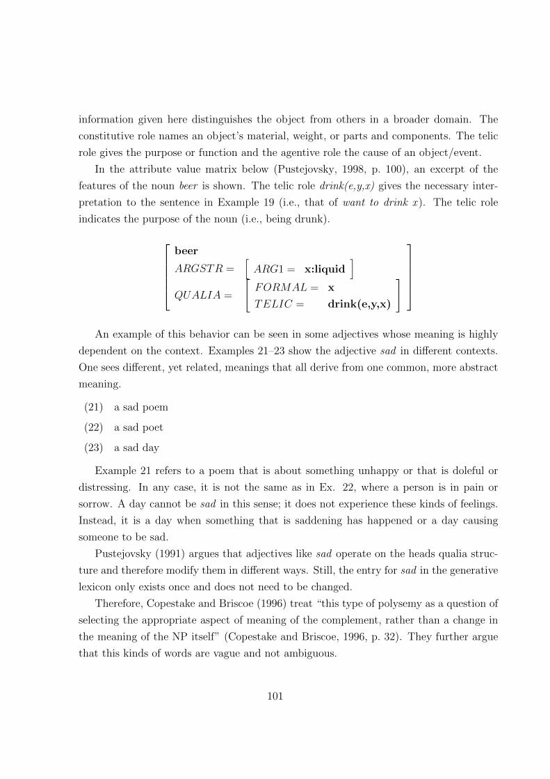
information given here distinguishes the object from others in a broader domain. The

constitutive role names an object’s material, weight, or parts and components. The telic

role gives the purpose or function and the agentive role the cause of an object/event.

In the attribute value matrix below (Pustejovsky, 1998, p. 100), an excerpt of the

features of the noun beer is shown. The telic role drink(e,y,x) gives the necessary inter-

pretation to the sentence in Example 19 (i.e., that of want to drink x ). The telic role

indicates the purpose of the noun (i.e., being drunk).

beer

ARGSTR =[ARG1 = x:liquid

]QUALIA =

[FORMAL = x

TELIC = drink(e,y,x)

]

An example of this behavior can be seen in some adjectives whose meaning is highly

dependent on the context. Examples 21–23 show the adjective sad in different contexts.

One sees different, yet related, meanings that all derive from one common, more abstract

meaning.

(21) a sad poem

(22) a sad poet

(23) a sad day

Example 21 refers to a poem that is about something unhappy or that is doleful or

distressing. In any case, it is not the same as in Ex. 22, where a person is in pain or

sorrow. A day cannot be sad in this sense; it does not experience these kinds of feelings.

Instead, it is a day when something that is saddening has happened or a day causing

someone to be sad.

Pustejovsky (1991) argues that adjectives like sad operate on the heads qualia struc-

ture and therefore modify them in different ways. Still, the entry for sad in the generative

lexicon only exists once and does not need to be changed.

Therefore, Copestake and Briscoe (1996) treat “this type of polysemy as a question of

selecting the appropriate aspect of meaning of the complement, rather than a change in

the meaning of the NP itself” (Copestake and Briscoe, 1996, p. 32). They further argue

that this kinds of words are vague and not ambiguous.

101

Copestake and Briscoe (1996) subdivide the field of regular polysemy further into con-

structional polysemy and sense extension. Constructional polysemy is used to describe

cases in which a “lexical item is assigned one (often more abstract) sense and processes

of syntagmatic combination or ‘composition’ . . . are utilized to specialize this sense ap-

propriately”. An example can be the lexical unit reel, which is assigned the meaning

of container and is then disambiguated according to context or syntagmatic relations to

refer to a reel of film or fishing reel62 (cf. Copestake and Briscoe, 1996, p. 31).

The second group of regular polysemous words, following Copestake and Briscoe

(1996), is characterized by sense extension. This second group also includes the cases

of grinding where the animal’s name can be used for a product made from it (e.g., meat

or fur/skin). For grinding they propose a rule that transforms one feature structure to

another, from animal to meat as shown in Lexical Rule 1 (cf. Copestake and Briscoe,

1996, p. 41), where c subst. stands for comestible substance.

Lexical Rule 1. 〈〉〈 grinding 〉〈〉

〈0 QUALIA〉 = animal

〈1 QUALIA〉 = c subst.

While these are metonymic (i.e., pars pro toto) sense extensions, there also exists a

metaphorical sense extension. These include calling people by the name of an animal

and therefore transfer some, not predictable, connotation of that animal to the person in

question. For example, the epithet Lion, which was, for centuries, attributed to many

kings, can refer to many positive attributes of lions: their strength, their courage, or the

notion of the lion as the ruler of animal kingdom63. These examples are a metaphorical

word usage (i.e., they are comparisons without the use of a word of comparison). Calling

someone a lion means that the person is as strong as a lion or has courage like a lion. Such

“associations . . . would not be encoded in the qualia structure” (Copestake and Briscoe,

1996, p. 37). We will shortly come back to similar cases of irregular polysemy.

Nunberg describes “productive linguistic processes that enable us to use the same

expression to refer to what are intuitively distinct sorts of categories of things” (Nunberg,

1996, p. 109), which he calls predicate transfer and defines in more detail as “[t]he principal

62Furthermore, container nouns can be used to refer to their content.63The Frankish historian Fredegar referred to Clovis I as a lion and interpreted this in terms of his

courage (Jaeger et al., 1996, p. 22).

102

. . . that the name of a property that applies to something in one domain can sometimes

be used as the name of a property that applies to things in another domain, provided the

two properties correspond in a certain way” (Nunberg, 1996, p. 111). In a more formal

way, he defines the condition on predicate transfer as

Definition 1. “Let P and P ′ be sets of properties that are related by a salient transfer

function gt: P → P ′. Then if F is a predicate that denotes a property P ∈ P, there is also

a predicate F ′, spelt like F , which denotes the property P ′, where P ′ = gt(P ).” (Nunberg,

1996, p. 112)

In the example to be shown below (24), the correspondence P and P ′ can be described

using a salient function h from a set A, where F denotes a property P ∈ A, to a disjoint

set B so that F ′

λP.λy(∀xdomh.h(x) = y → P (x)), (19)

or

λP.λy(∃xdomh.h(x) = y ∧ P (x)), (20)

representing the universal and the existential interpretation of the utterance.

Nunberg (1996, p. 115) gives a straightforward example of a metonymic relation that

can be explained using the functions above:

(24) Who is the ham sandwich?

This is from the context of a restaurant. Here, at least from the point of view of the

service personal, “customers acquire their most usefully distinctive properties in virtue

of their relations to the dishes they order” (Nunberg, 1996, p. 115). Without going too

deep into detail, one can say that the predicate F is taken from the set P , which roughly

compasses the menu of the establishment, and that F ′ refers to an object of P ′, being the

customers, and where the common property or relation is given by the order.

The example given by Nunberg is interesting, yet for the direction taken in this thesis

not of too much importance, since only lexicalized words, and then only those cases of

polysemy that can be found in WordNet, are of interest. Still, the formalism given in

Definition 1 gives an interesting explanation of processes that take place in the creation

of polysemy. In my eyes it is not only true in regular cases, as those similar to Example

24, but also for the irregular ones looked at in the following.

103

Before looking at examples of irregular cases of polysemy, one should recall what has

been said about the application of animal names to humans: that the characteristics

“cannot be predicted from knowledge of the animal sense” and that “properties ascribed

to a person . . . are stereotypical associations with the animal, which would not be encoded

in the qualia structure” (Copestake and Briscoe, 1996, p. 37). Two things are noteworthy

in this statement: For one, the non-predictability64 of the property transferred from one

usage of a word to the other seems to be evidence that we are not dealing with regular

polysemy here.

The case of grinding is not concerned by this ascertainment. Grinding is a regular

process, even though it might be used to refer to different products derived from an animal.

But these products, even if not necessarily predictable, are not open to all properties of

the given animal. Other than irregular polysemy: When someone is called a pig for

example, this is likely to refer to cleanliness or tidiness of that person, or more precisely

the lack of it, or the body size of a person. Still, such metaphorical usage of words can

also be constructed ad hoc depending on context. Copestake and Briscoe simply call this

“stereotypical associations with the animal”, which is also the reason why it would not

be found in the qualia-structure. Even though the characteristics that are transferred

“cannot be predicted from knowledge of the animal sense”, they are taken, nonetheless,

from the world knowledge about that animal.65 Taking into account what has been said in

Definition 1, the properties of one thing in one domain can be used to refer to something

else by the same name in a different domain. Given the relations shown in equations 19

and 20, we can see that this definition can indeed be used to also describe processes of

irregular polysemy.

The case of irregular polysemy is one that seems much harder to process automatically

by a computer than regular cases, where explicit rules can be stated. Often a single nuance

of the connotation or world knowledge about an entity is transferred to a new situation.

A look at the word senses of chicken, quoted from WordNet, shows the problem:

1. chicken, poulet, volaille – the flesh of a chicken used for food

64From a computational point of view, there are no clear rules, so the program can make no a prioriassumptions about the meaning transfer.

65Of course there is also distributional evidence of these associations: Looking at a large corpus ofEnglish text, such as the one given in the Wortschatz Leipzig project (http://corpora.informatik.uni-leipzig.de/), a very frequent co-occurrence of pig is indeed fat. In other words, there is more than juststereotypes: There is structural evidence in the usage of the words, which could be taken into account.

104

2. chicken, Gallus gallus – a domestic fowl bred for flesh or eggs; believed

to have been developed from the red jungle fowl

3. wimp, chicken, crybaby – a person who lacks confidence, is irresolute and

wishy-washy

4. chicken – a foolhardy competition; a dangerous activity that is continued

until one competitor becomes afraid and stops.

Sense 1 and 2 follow the pattern of grinding. But sense 3 and 4 are different. A

chicken, as in sense 2, is attributed as easily scared. From this attribute, not a lexical

property of chicken (sense 2), but an attribute taken from the world knowledge, sense 3,

is derived. When calling someone a chicken this does not mean he or she has feathers,

lays eggs, or anything like that; only the attribute easily scared is transferred to the new

context: The person is easily scared like a chicken. Sense 4 is derived from sense 3: Two

competitors play against each other until one becomes the chicken (sense 3).

The processes, which take place in the above-described cases of polysemy, require a

certain amount of world knowledge.66 A person living on an isolated island who has never

seen a chicken, and therefore is not accustomed to its characteristics, could not understand

why a wimp may be called a chicken.

Copestake and Briscoe (1996, p. 28f.) propose rules, like the one in lexical rule 1,

for this kind of meaning transfer as well. Their rules allow names of animals being used

for referents other than animals, e.g., humans, but it does not however formalize an

abstraction of meaning such that the underlying meaning transfer from the animal to the

denoted human would be made explicit.

This is of course a problem for a computer automatically processing language. The

connection that exists between the senses 3 and 4 of chicken on the one hand and sense

2 of chicken on the other hand is not directly evident in the lexical material or in the

network of WordNet. The computer, so to say, lacks the necessary general knowledge.

Also, the metaphorical usage of words bears connotations. While lion is usually a positive

byname, chicken and pig are not. This is not evident to a computer and the underlying

meaning transfer is not directly observable or deduce-able from a resource like WordNet.

66Admittedly to a degree that is not available in WordNet directly.

105

5.2 Architecture of WordNet

In WordNet, a word is defined as “a conventional association between a lexicalized concept

and an utterance that plays a syntactic role” (Miller et al., 1990a, p. 3). The term word

normally refers to both the meaning and the realization. Therefore, word form will be

used to refer to the physical realization of the word and word meaning or word sense will

be used to refer to the concept. This division of words into form and meaning raises the

question of how these two concepts are represented and connected.

Synonymy is the most basic lexical relation between word forms in WordNet. Syn-

onymy is described by a set of words forms that constitute the word sense, so-called

synonymy sets (synsets). Synsets contain word forms that are synonymous.67 While real

synonymy is usually defined as two words that can be substituted in every linguistic sit-

uation and where this substitution never changes the truth value (true or false) of an

expression, WordNet defines synonymy as follows:

two expressions are synonymous in a linguistic context C if the substitution

of one for the other in C does not alter the truth value (Miller et al., 1990a,

p. 6).

Synsets are formed by a set of word forms that in a defined context C can be substi-

tuted for each other. These word forms are therefore in terms of C synonymous. A synset

does not however describe the meaning of the set of word forms. The meaning is formed

by the synset’s members and the relations the synset has, the synset’s neighbors.

In Fig. 16(a), a prototypical synset is shown: The synset is made up of word forms

that together constitute the meaning. Figure 16(b) gives an example from WordNet: the

synset bank as in a container for keeping money at home. As one can see, the word form

bank is used to refer to this word sense and only in combination with other word forms

like money box can one understand the meaning of bank in this example compared to

other synsets that contain bank word forms but have a different meaning.68

67English is quite rich in synonyms. A possible explanation is the large number of loanwords from theNordic languages (e.g., meat, derived from the Nordic word for food, replaces the Anglo-Saxon flesh), aswell as loanwords that were used by different social classes after the Normans conquered England (again,many Norman words replaced the Old English animals names in the context of food), and of coursethe expansion of English over huge parts of the world resulting in the development of synonyms (e.g.,autumn/fall ; although this pair can be treated as synonymous, there are still diatopic differences).

68This dependence on the neighbors or a word to define the meaning has already been shown in thechapters before for lexical fields in what Trier called the mosaic, but also for other approaches like frametheory and also a basic assumption in medical studies.

106

(a) Structure of Synset, formed by wordforms.

(b) Structure of synset bank, a container for keeping moneyat home.

Figure 16: Word senses, synsets, and word forms in WordNet.

Synonymy (S) is a symmetric relation,69 meaning that it is equal to its inverse function

(S ≡ S−1). If a and b are synonymous (S) (i.e., aSb), the inverse S−1 is also synonymous

(i.e., bSa). This implies that aSb =⇒ bSa.

Furthermore, and this is true for at least true or full synonymy as well as the actual

formalization of synonymy in WordNet, but may not always be true for all uses of syn-

onymy in linguistics, it is transitive: aSb ∧ bSc =⇒ aSc. Also, one could say that

synonymy is reflexive: aSa.70 If a relation is symmetric, transitive, and reflexive, it is an

equivalence relation: a ∼ b or simply a = b.71

These conditions are actually the mathematical explanation for the clustering of the

WordNet graph. Every synset contains equivalent elements. There are no elements that

belong to more than one synset. In other words, the intersection between every two

synsets s1 and s2 of a graph G is empty or they are disjoint: ∀s1, s2 ∈ G : s1 ∩ s2 = ∅.Following the definition of synonymy given above, WordNet distinguishes different

parts of speech (e.g., nouns, verbs, adjectives, and adverbs). Since an adjective cannot re-

place a noun without changing the truth value of the expression, the relation of synonymy

is always restricted to elements of the same POS.

The synonymy relation clusters, or partitions, all vertices of the network into synsets.

69This is also shortly mentioned in Miller et al. (1990a, p. 7). The two following types of relations,transitive and reflexive, are not mentioned. Nor are the implications on the network these propertieshave.

70By definition two expressions are synonymous if the replacement of one for the other does not changethe truth value of the expression in a context C. This is not the case if one replaces one word with itself.

71This is at least true for fully synonymous words in natural language, but also for synsets in WordNetwith the restriction that word forms making up a synset are not necessarily equivalent to each other interms of lexical relations, such as antonymy.

107

These synsets represent the meaning. Their parts make up the synset and define the

meaning, while at the same time the synset is the entity that contains the meaning and

defines the meaning of its parts. This reminiscent of Trier’s statement that from the parts

the whole receives its meaning.

WordNet is not one fully connected component. It actually consists of four compo-

nents, or subnetworks – one for nouns, adjectives, adverbs, and verbs – which are only

loosely connected by morphosemantic relations between related word forms. In the follow-

ing the different POS contained in WordNet will be discussed and their interconnection

will be shown. WordNet distinguishes between lexical relations (i.e., relations between the

lexical units or word forms) and semantic relations (i.e., relations between word meanings

or synsets).

5.2.1 Nouns

Synonymy, as defined above, is one of the main structuring features of nouns in WordNet.

The lexemes in WordNet are not organized in a hierarchical tree, but Synsets are orga-

nized hierarchically. Hyponymy and hypernymy are semantic relations between synsets

in WordNet.72 These relations are the inverse of each other. Furthermore, they are tran-

sitive and asymmetrical (Lyons, 1977, p. 292) as well as irreflexive. Transitive relations

have already been defined above. In turn, an asymmetric relation R between two synsets

a and b (aRb) is defined in a way that the inverse (bRa) is always false. Furthermore, as

an asymmetric relation it is defined as irreflexive, meaning no relation of the kind aRa

is defined.73 From this it also follows that a 6= b. In mathematics a relation having the

features of being transitive, asymmetrical, and irreflexive is called a partial order and

orders a set of elements.

The set of all nouns is therefore ordered hierarchically. A hyponym inherits all features

of its hypernym and “adds at least one feature that distinguishes it from its superordinate

and from any other hyponyms of that superordinate” (Miller et al., 1990b, p. 8). Multiple

inheritance is possible. If A is a superordinate or hypernym and B is its hyponym, then

the logical expression ∀x[B(x)→ A(x)] applies. In terms of set theory one can say B ⊂ A.

72This is also a feature in the WordNet structure that is very similar to that in lexical field theory:Not the lexeme themselves are ordered hierarchically, but the fields (i.e., synsets) are.

73Lyons (1977, p. 308) claims that dog can be its own hypernym when asking whether a dog (1) is a dog(2) or a bitch. But dog (2) must be distinguished fromdog (1). Usage (1) refers to the set of all animalsof the species Canis lupus familiaris. Usage (2) only refers to the male members of this set, excludingthe female members that are called bitch.

108

For example, the set of all trees is a subset of plants. If an object belongs to the class or

set of trees it can also be said to be a plant and share the common features of plants such

as using photosynthesis.

The main distinctive feature in the organization of nouns in WordNet, is their hi-

erarchical structure. Originally, this did not mean a fully connected graph: 25 unique

beginners were identified that subdivide the nouns into multiple hierarchies which “corre-

spond to relatively distinct semantic fields, each with its own vocabulary” (Miller et al.,

1990b, p. 16). They can be seen in Table 8.

Miller (1998, p. 28) says that a unique beginner “corresponds roughly to a primitive

semantic component in a compositional theory of lexical semantics”. Like lexical fields,

they are not built on lexical differences but on differences found in the nature of things,

be they physical, biological, or philosophical, and are therefore of an ontological, in a

philosophical sense, nature.74 The unique beginners are mainly used in the organization

of the lexicographer’s work. Each one represents one file that the lexicographers work on.

Table 8: List of 25 unique beginners in the noun set of WordNet.

{act, activity} {food} {possession}{animal, fauna} {group, grouping} {process}{artifact} {location} {quantity, amount}{attribute} {motivation, motive} {relation}{body} {natural object} {shape}{cognition, knowledge} {natural phenomenon} {state}{communication} {person, human being} {substance}{event, happening} {plant, flora} {time}{feeling, emotion}

During the compilation of WordNet however, some of these unique beginners have

been grouped together, leading to only 11 unique beginners that are assigned the attribute

nouns.tops in the WordNet database. Although it is often75 stated that the unique be-

74While this association between nature and language has be disputed in linguistics for many decadesnow, the more pragmatic approach in NLP still constantly relates utterances to objects in the real word.The knowledge NLP is interested in, is to understand what objects or things in the real world a personis referring to. From a linguistic point of view and for the speaker of a language, this is of course quiteobvious.

75In Miller (1998, p. 28), the possibility of one top most synset or root vertex of the noun tree was

109

ginners do not have a superordinate synset, this is, at least in the most recent version of

WordNet 3.1, not true. The synsets marked as nouns.tops are in fact hyponyms of entity.

Hence, all nouns are organized in one single tree. A distinguishing feature of those top

vertices or unique beginners is that they, due to their usage as an auxiliary construction,

do not contain word forms.

Meronymy is the part–whole relation (has-a). Given a synset X = {x1, x2, . . . , xn} and

a synset Y = {y1, y2, . . . , yn}, the meronymy between X and Y is defined if ∀x[X(x) →hasA(y, x)] is true: If x is an element of X, then y has a x applies for every x.

Meronymy, and its inverse holonymy, is also said to be transitive and asymmetrical

(Cruse, 1986, p. 165). But it is, just as the hypernymy relation, also irreflexive. There

is no synset that can be its own meronym. Meronymy and holonymy are only available

in the noun set. As a relation that is transitive and asymmetrical, meronymy therefore

forms a partial order, just like hypernymy/hyponymy.

Besides these semantic relations that exist between synsets, WordNet also contains a

set of lexical relations. One lexical relation is antonymy. Antonymy is not a very rich

feature of nouns. Still some nouns do have antonyms (e.g., war is an antonym of peace).

Antonymy is very common within the field of descriptive adjectives.

Nouns (i.e., noun word forms) can also be related to word forms of other POS by

morphological relations indicating derivational processes. An adjective can refer to a

similar concept or situation as a noun from which it is derived. This will be discussed

later.

The derivationally related relation exists between word forms of different POS. It

indicates, besides the morphological processes underlying the word formation, a relation

in meaning since it transfers the meaning from one POS to another (e.g., music (noun)

and musical (adjective)). This information can be of great use for the purposes of this

thesis, since it may connect word forms belonging to a polysemous word, but it should

not exist between word forms of a homonymous word.

Figure 17 shows an exemplary graph of a possible organization of nouns in WordNet.

One can see that some relations are restricted to synsets (i.e., in terms of an ontology, the

relation’s range and domain are restricted to entities of the type synset). Other relations

are lexical and therefore only exist between the lexical units or word forms. The relation

of synonym in the graph is dotted since this relation is not explicitly stated by a relation

rejected, saying that there exists no linguistic justification for it and that this vertex would only be a“generic concept” (Miller, 1998, p. 28). Still, WordNet 3.1 does exhibit exactly this behavior.

110

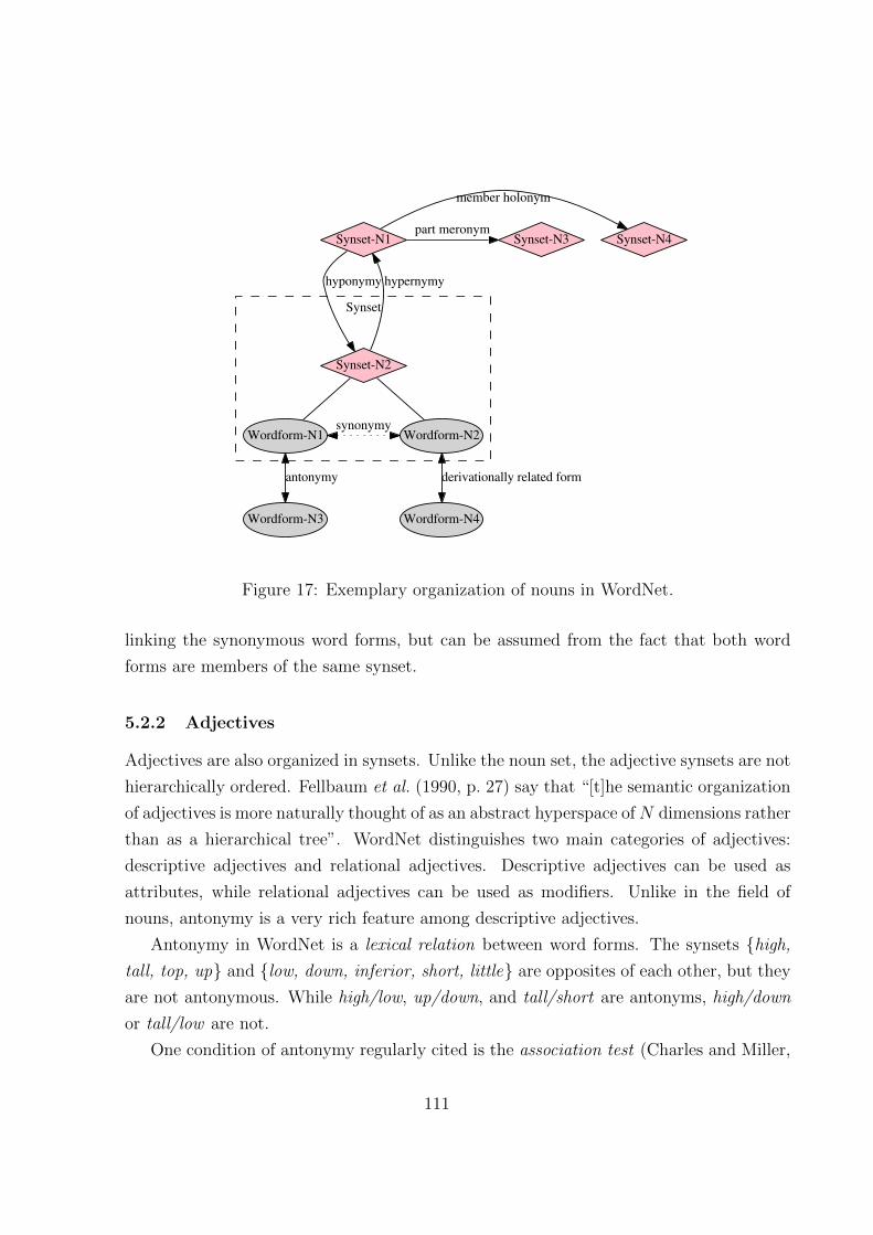
Synset

Synset-N1 Synset-N3part meronym

Synset-N4

member holonym

Synset-N2

hyponymy

Wordform-N3 Wordform-N4

hypernymy

Wordform-N1 Wordform-N2

antonymy

synonymy

derivationally related form

Figure 17: Exemplary organization of nouns in WordNet.

linking the synonymous word forms, but can be assumed from the fact that both word

forms are members of the same synset.

5.2.2 Adjectives

Adjectives are also organized in synsets. Unlike the noun set, the adjective synsets are not

hierarchically ordered. Fellbaum et al. (1990, p. 27) say that “[t]he semantic organization

of adjectives is more naturally thought of as an abstract hyperspace ofN dimensions rather

than as a hierarchical tree”. WordNet distinguishes two main categories of adjectives:

descriptive adjectives and relational adjectives. Descriptive adjectives can be used as

attributes, while relational adjectives can be used as modifiers. Unlike in the field of

nouns, antonymy is a very rich feature among descriptive adjectives.

Antonymy in WordNet is a lexical relation between word forms. The synsets {high,

tall, top, up} and {low, down, inferior, short, little} are opposites of each other, but they

are not antonymous. While high/low, up/down, and tall/short are antonyms, high/down

or tall/low are not.

One condition of antonymy regularly cited is the association test (Charles and Miller,

111

1989; Fellbaum et al., 1990; Justeson and Katz, 1991, 1992). In case of antonymy, the use

of a lexical item automatically invokes its antonym. Given a descriptive adjective, people

are asked to name associated words. The answers turn out to be mostly their antonyms:

Good invokes bad, and high invokes low. Also, the antonym of a word x is not always

¬x. Saying that someone is not rich does not say that he or she is poor (cf. Miller et al.,

1990a, p. 7). Still, poor and rich are antonyms, or as said in Chp. 3.4.4, they lie on

opposite ends of a scale of wealthiness. High and low are antonymous adjectives. They

are said to be possible values of an attribute HEIGHT (cf. Fellbaum et al., 1990, p. 27).

Most attributes are bipolar: The values of HEIGHT can lie between low and high.

This explains why the opposed pair of high/down is not treated as antonyms in Word-

Net. For one, they are not values of the same attribute HEIGHT, and secondly they

“are not familiar antonym pairs” (Fellbaum et al., 1990, p. 28). Of course, the second

condition, the association test with English speakers, is connected to the first one.

Antonymy is “not the same as the conceptual opposition between word meanings”

(Fellbaum et al., 1990, p. 28). Except some descriptive adjectives of Germanic origin

(e.g., good/bad), most antonymous pairs of descriptive adjectives in English are derived

through morphological rules by adding a negation suffix like un-, in-, and others. This

is the reason why Fellbaum et al. (1990) call antonymy a relation between word forms:

“Morphological rules apply to word forms, not word meaning” (Fellbaum et al., 1990,

p. 28). Following this statement, it is argued that antonymy is not a semantic relation,

but a lexical relation: “Antonymy is a lexical relation between word forms, not a semantic

relation between word meanings” (Miller et al., 1990b, p. 7).

Opposing pairs, such as high/down, do not have a special relation in WordNet. Look-

ing for an opposing adjective when no direct antonyms are available means looking for

synonyms that have an explicit antonym. All descriptive adjectives in WordNet have at

least indirect antonyms.

The second main class of adjectives in WordNet is that of relational adjectives. These

adjectives can be compared to a modifying noun. Relational adjectives are used to indi-

cate some form of association to a noun. Fellbaum et al. (1990, p. 34) give the examples

of dental having to do with teeth, or fraternal, associated with brother. But not only

adjectives of Latin origin can be used as relational adjectives. Using derivation, some

nouns, such as music, “give rise to two homonymous adjectives; one relational adjective

112

restricted to predicative use, the other descriptive” (Fellbaum et al., 1990, p. 34).76 This

results in polysemous adjectives, here musical, which have two senses as in musical in-

strument (an instrument used to play music) and musical child, a child with a musical

ability. In contrast to descriptive adjectives, relational adjectives are not related to a

scalable attribute of a noun. Instead, these adjectives are semantically closely related to

the corresponding noun (i.e., they “refer to the same concept, but they differ formally

(morphologically)” (Fellbaum et al., 1990, p. 35)). Also, they mostly have no direct or

indirect antonyms.

Other adjectives include what Fellbaum et al. (1990) call reference-modifying adjec-

tives and the color adjectives. The latter ones naturally have no antonyms but can have

synonyms.77

Color adjectives are widely used in metaphors and metonymy and are a rich source of

polysemous words. Polysemous usage of color adjectives is not always regular, as was the

example of olive above. In most cases there will be some semantic connection and not

only coincidental accordance of word forms, but these connections might not be obvious.78

Examples of metonymic usage of color adjectives include the reds, referring, according to

WordNet, to Marxists, or the name greys for the soldiers of the Confederate army wearing

grey uniforms, similar to the term redcoat for the red-wearing soldiers of the British army

during the revolutionary war. These metonymical usages stand pars pro toto for the

soldiers wearing the color. Furthermore, adjectives can be used as verbs to mean that

something turns its color, e.g., to blue, or to yellow.

Figure 18 shows a possible graph of an adjective synset in WordNet. The relations of

synonymy and antonymy have already been discussed. Apart from these lexical relations

among word forms, adjective synsets are not ordered hierarchically by relations such as

hyponymy or hypernymy. Instead they can be linked by also see or similar to. If we are

looking at an adjective synset such as {good}, this will be linked to the corresponding

comparison {better} by also see. Similar to indicates an almost synonymous relation but

not between word forms, but between synsets. Again the synset {good} might be related

76Fellbaum et al. (1990) state the relation between the two lexemes of the adjective musical as homony-mous. Polysemous would be more appropriate here to make a distinction to homonymy as defined inChp. 5.1.

77In WordNet, purple and violet are subsumed in one synset, though such adjectives are highly dis-cussable, culture dependent, and often up to subjective estimation.

78For example, Ammer (1993, p. 192) traces back the meaning of the expression that is not very oftenused anymore you’re yellow meaning someone is a coward to the connection of yellow with betrayal.Judas Iscariot has often been portrayed wearing yellow clothes.

113

Synset

Synset-ADJ2

Wordform-ADJ4

Synset-ADJ3

Wordform-ADJ5

Synset-N1

Wordform-N1

Wordform-ADJ3

Synset-ADJ1

Also SeeSimilar To

Attribute

Wordform-ADJ1 Wordform-ADJ2

antonymy

synonymy

Figure 18: Exemplary organization of adjectives in WordNet.

to that of {fresh}. Saying an apple is good or an apple is fresh is not the same, but they

are closely related. A fresh apple is expected to be good and vice versa, though this is no

categorical causal nexus.

An adjective synset {good} might be used as an attribute in a special context. It is

then linked to a noun synset it can be used to describe (e.g., the {quality}). As can be

seen in Fig. 19, adjectives can also be related to word forms from other POS through a

derivationallyRelated connection, which indicates a relation through derivation.

5.2.3 Adverbs

The modeling of adverbs in WordNet is similar to that of adjectives, though more simplis-

tic. The adverb graph mostly only consists of a collection of unrelated synsets. Sometimes

word forms have antonyms or some adverbs are derived from adjectives and therefore

derivationally related to an adjective synset (cf. Miller, 1998, p. 64ff.). This can be seen

in Fig. 19. As one can see, the structure of adverbs is not very elaborate. The complexity

of the graph is low; there are no larger clusters or even connected components. The level

of information given in an adverb graph is therefore expected to be very low.

5.2.4 Verbs

Not only in grammars or syntactic theories, as well as in most semantic theories such

as frame semantics (Fillmore, 1976), semantics in construction grammars (Pollard and

114

Synset

Synset-ADJ1

Wordform-Adj1

Wordform-Adv3

Synset-Adv1Derivationally related

Wordform-Adv1 Wordform-Adv2synonymy

Figure 19: Exemplary organization of adverbs in WordNet.

Sag, 1988), or formal semantics, the verb is the linchpin of the theory. Since WordNet

treats verbs just as other POS, they are not assigned any kind of further grammatical

information. For example they contain no information on combinatory restrictions (e.g.,

they are not restricted to what nouns they can be combined with or the number or kind

of grammatical object they bind). The meaning of a verb can change with the arguments

it takes. The most common verbs in English (e.g., have, be, run, make, set, go, take) do

not have one meaning but a multitude of possible senses.79

Fellbaum (1990, p. 40) says that verbs in Collins English Dictionary have on average

2.11 senses while nouns only have 1.74. This finding can also be made in WordNet: Verbs

are much more polysemous than nouns. Homograph word forms make up 30.38% of the

nouns, while 74.94% of the verbs are homographs.

WordNet currently contains 13,767 verb synsets. These are organized in different files

corresponding to semantic domains such as “verbs of bodily care and functions, change,

cognition, communication, competition, consumption, contact, creation, emotion, motion,

perception, possession, social interaction, and whether verbs” (Fellbaum, 1990, p. 41) and

79Fellbaum (1990, p. 40) cites Gentner and France (1988), who conducted an experiment where verbswere used in violation to their selectional restriction for nouns. When subjects where asked to paraphrasethe sentences, they reinterpreted the verbs in relation to the nouns and assigned a new semantic meaning,differing from the verb’s known senses. They conclude that “noun representations may be typically moreinternally cohesive than verb representations and therefore less easily altered. . . . Change of meaning doesoccur to accommodate contextual constraints, but that change involves computations over the internalstructure of the word meanings, particularly that of the verb” (Gentner and France, 1988, p. 379).

115

one file containing verbs of states that are not semantically connected otherwise.

Synset

Synset-V1

Synset-V4

Hyponymy

Synset-V2Synset-V3Verb Group

Synset-N1

Domain of synset - TOPIC

Wordform-V1

Entailment

Wordform-N1

Derivationally related form

Hypernymy

Wordform-V1

Figure 20: Exemplary organization of verbs in WordNet.

Figure 20 shows an exemplary verb structure in WordNet. One can see the hierarchical

structure that is established through hyponymy and hypernymy relations. Even though

there are very few synonymous verbs, verbs are also organized in synsets. These mostly

contain only one word form. The relation verbgroup is used to group verb synsets that

are closely related though not synonymous and can be thought of as similar to frames in

frame semantics, as well as to the notion of fields mentioned earlier. This relation is of

special interest since it is expected to relate polysemous verb synsets. It is for example

used to relate the following two senses of have: have or possess, either in a concrete or

an abstract sense and have as a feature. This relation is not applied in a coherent way in

WordNet (i.e., it is often missing where it could have been applied).

Not yet mentioned was the entailment relation. Entailment includes various relations.

Fellbaum (1998, p. 77) defines entailment as a “relation between two verbs V1 and V2

that holds when the sentence Someone V1 logically entails the sentence Someone V2 ”.

The relation in WordNet exists between two synsets as can be seen in Fig. 20. For

example, Someone snores entails Someone sleeps. One of the relations subsumed under

entailment is troponymy, “which relates synset pairs such that one expresses a particular

manner of the other (e.g., {whisper}-{talk} and {punch}-{strike})” (Fellbaum, 2006,

p. 667). Further entailment relations in WordNet according to Fellbaum (1998, p. 77ff.)

are backward entailment {divorce–marry}, presupposition {buy–pay}, and cause {show–

see} (Fellbaum, 1998, p. 83).

116

An interesting feature of verb synsets is the possible relation domain. A domain can

designate a topic (i.e., a noun synset). Verb synsets like {run}, {jump}, and {play} can

be associated with the domain {sports}.

5.2.5 Overview and Shortcomings

Table 9 gives an overview over the existing relations in WordNet with respect to the type

(i.e., a lexical or semantic relation) the POS in question, and a short example.

In order to understand how a network-based link prediction in WordNet might be

done, one should also look at these relations in more detail. Table 10 shows the relations

with regard to the word classes and the number of their occurrences in absolute numbers.

Especially the small relations will be of great interest. Derivationally related word

forms are a good indicator of closely related meanings that might indicate polysemy if the

two word forms are homographs. The same is true for the attribute, pertainym, similar

to, see also, verb group, entailment, and cause relation. These are often referred to as the

cousin relations in WordNet.

These relations, even though small in number and apparently unequally distributed,

are, if they connect homograph word forms, a first indicator of polysemy but will only

apply to a small percentage of the possibly polysemous cases. In the WordNet graph,

these relations will lead to short distances; in the case of a lexical relation this geodesic

path will be 1, in case of semantic relations 3.80 Furthermore, these relations also tightly

relate otherwise further separated meanings, which are not directly connected otherwise.

This should lead to a small-world structure.

Some etymologically related word forms will tend to have small shortest geodesic path

due to relations that connect (derivationally) related forms. Unfortunately, this is only

true for very few polysemic cases in WordNet. In general one can expect forms that are

closely related, maybe with a geodesic path of <3 or a little over that, to be polysemous

or have at least a very high probability of being related. This does not mean that word

forms that are separated by a geodesic path with a much longer or indefinite path length

can be related.

This analysis of the structure of WordNet that was undertaken in this chapter reveals

80Semantic relations connect the synsets. Therefore the distance between the word forms within thesynsets is 3.

117

Table 9: Relations in WordNet.

Relation Type Part ofSpeech

Examples

synonymy lexical N,V,Adj, Adv {buy, purchase}antonymy lexical N,V,Adj, Adv good, badhyponymy semantic N,V {oak,. . . },

{tree,. . . }hypernymy semantic N,V {tree,. . . },

{oak,. . . }meronymy semantic N {leg,. . . },

{chair,. . . }holonymy semantic N {chair,. . . },

{leg,. . . }entailment semantic V {jump,. . . },

{fall,. . . }cause semantic V {burn,. . . },

{combust,. . . }also see lexical V,Adj jump, jump onverb group semantic V {burn,fire,. . . },

{incinerate}domain ofsynset

semantic V,N {run,. . . },{sport,. . . }

similar to semantic Adj {good,. . . },{fresh,. . . }

attribute semantic Adj, N {good,. . . },{quality,. . . }

derivationallyrelated

lexical N,V,Adj, Adv good, goodness

118

Table 10: Overview: relations per word class.

Relation Noun Adjective Verb Adverb

synonymy 146312 30070 25061 5592antonymy 1560 3547 690 540hyponymy 84427 0 13256 0hypernymy 84427 0 13256 0meronymy 22196 0 0 0holonymy 22196 0 0 0entailment 0 0 408 0cause 0 0 221 0see also 0 2690 349 0verb group 0 0 1744 0domain of synset 6352 1427 1284 110member of domain 9242 0 0 0similar to 0 21434 0 0attribute 639 639 0 0derivationally related 22100 8994 13274 7pertainym 0 3751 0 0participle 0 59 0 0

119

some shortcomings and possible problems that might arise when using WordNet in the

context of NLP.

In the scope of NLP, WordNet is sometimes found to be too fine-grained. In word sense

disambiguation (WSD), some homonymous words are found in too many, sometimes very

closely related synset, which makes WSD in correspondence to WordNet a very hard or

maybe even impossible task (cf. Mccarthy, 2006; Navigli, 2009). Biemann (2012) mentions

an upper bound of 80%, which WSD algorithms do not exceed due to the “fine-grained

sense structure of WordNet” (Biemann, 2012, p. 4038).

Biemann and Riedl (2013) also found that WordNet’s coverage in some domains is

very low. Depending on the texts that are to be processed, one might find homonyms

whose senses are not fully represented by WordNet. Biemann and Riedl use Wikipedia

and find that anime was contained in two synsets but none was of the sense Japanese

animation movie. Such findings might further hinder WSD tasks based on WordNet.

A further problem that might arise when using WordNet is its limitation to semantic

relations.81 Verbs have no information on the numbers of objects or kinds of objects they

bind or possible selection restrictions. Sometimes verbs that share a common word form

can be distinguished using such features.

The so-called cousin relations have been found to be a good indication of polysemy

between word forms. It has also been stated that these relations, unfortunately, are only

used very seldom and are missing in most cases.

5.3 Network Analysis

In this chapter, the network topology of WordNet will be analyzed. This analysis gives

insight into the structure and characteristics of the network. Together with the in-depth

analysis of the ontology structure, this information will be used to choose features for the

link-prediction task.

5.3.1 WordNet as a Graph

The network has a total of 324, 602 nodes. These vertices include all word forms and

synsets contained in WordNet, and they are connected by 584, 528 edges. The graph is

not connected; it consists of 5, 051 weakly connected components.

81Even though there exists some morphological relations as well.

120

The degree distribution shows how many vertices have a certain degree. As has been

mentioned before, small-world networks expose a degree distribution that can be fitted to

a power law. If such a distribution is fitted to a log–log scale, one can see the scale-free

distribution as a more or less straight line. Furthermore, a small-world network is defined

as having relatively short geodesic paths (due to vertices with a very high degree, so-called

hubs or authorities) and as having a high clustering coefficient.

The small-world phenomenon is important because the paths between every two ver-

tices in the network are relatively short. This behavior has especially been noticed for

social networks, as well as other complex networks, and as such for semantic networks.

In Figure 21, the degree distribution of the WordNet network is when the directed-

ness of the edges is respected. Figure 21(a) shows the in-degree distribution and the

corresponding power law p(x) = xα, where α = −2.708156.82 Figure 21(b) shows the

out-degree distribution and the power law p(x) = x−3.498834 fitted to it.

Figure 22 shows the degree distribution when the direction of the edges is ignored,

and the fitted power law p(x) = x−2.820797. The overall findings in these three degree

distributions show the typical behavior one would expect of a small-world, scale-free

network. Still, the clustering coefficient is much smaller than would be expected from a

small-world network: 0.004.

As suspected from these findings, the geodesic path in the graph, (i.e., the average

shortest path or degree of separation) is found to be ∼ 9.7 edges. This is within the range

of geodesic distances normally found in social networks. The network diameter (i.e., the

farthest geodesic path between two vertices) is 27.

Small world networks contain few vertices with a very high degree, while most vertices

have a degree close to the average or lower. These vertices result in the degree distribution

seen above and in the short geodesic paths. In WordNet, the synset containing the word

forms {metropolis, city, urban-center} has the highest out- and in-degree: 674 and 671,

respectively, which results in a total degree of 1, 345.

In this case, most relations are instance relation. Instead of using the hypernym

relation, the WordNet architecture offers the instance relation. Instance is a subtype

82The power-law distribution is limited by the lowest possible value, which is 0, and the highest, whichis, as we will see, 1, 345. The lowest value being 0 is due to the fact that every word form belongs to asynset. Since all vertices are either a word form or a synset, the lowest possible degree is 1. Looking ata directed graph, some word forms might have a 0 out-degree and synsets a 0 in-degree. So the lowestpossible value, when treating the graph as directed, is 0 and 1 when treating the graph as directed.

121

100

101

102

103

104

105

106

100

101

102

103

Co

un

t

In-degree

graph. G(324602, 582036). 22256 (0.0686) nodes with in-deg > avg deg (3.6), 5196 (0.0160) with >2*avg.deg

2e+05 * x-2.645

R2:0.97

(a) In-degree distribution with fitted power law.

100

101

102

103

104

105

106

100

101

102

103

Co

un

t

Out-degree

graph. G(324602, 582036). 48964 (0.1508) nodes with out-deg > avg deg (3.6), 9382 (0.0289) with >2*avg.deg

4e+05 * x-2.764

R2:0.96

(b) Out-degree distribution with fitted power law.

Figure 21: WordNet degree distribution (directed network).

122

100

101

102

103

104

105

106

100

101

102

103

Count

In-degree

graph. G(324602, 398135). 97270 (0.2997) nodes with in-deg > avg deg (2.5), 32521 (0.1002) with >2*avg.deg

6e+05 * x-2.824

R2:0.97

Figure 22: WordNet degree distribution (ignoring direction) with fitted power law.

of hypernym or hyponym.83 Hubs or authorities are interesting since they connect one

synset to another synset with a relatively short path. A synset such as Dakar can be an

instance of city as well as another geographical entities such as port. This offers a rich

source of possibly polysemous use of words (e.g., city names can refer to the city, and the

port, airport, and so on).

But not only synsets containing a lot of instances, such as cities, can have many

relations and thus a high degree. The {law, jurisprudence} synset’s (see Fig. 23) in-degree

is 613, its out-degree 615, and the total degree sums up to 1, 228. This synset is connected

to others by the topic of relation, which is the inverse of the domain relation. This relation

connects nouns, adjectives, verbs, and adverbs. Synsets like {law, jurisprudence} connect

the different subsets (e.g., nouns, adjectives, verbs, and adverbs) of WordNet and are

therefore of special interest. A hub like this builds shortcuts between related vertices in

the graph.

The degree distribution, and the low average geodesic path length it is caused by, fits

the definition of a small world. Still, the clustering coefficient is very low in WordNet.

The clustering coefficient indicates how well connected the vertices and its neighbors are.

83An instance in an ontology is a vertex that is not an abstract category, but an entity. In this casethe instances are city names.

123

Figure 23: Schematic plot of synset {law, jurisprudence} and its first- and second-degreeneighbors.

124

The synset structure, a synset is connected to the word forms, but the word forms are not

connected to themselves (see Fig. 16), causing the very low clustering coefficient of 0.004.

Also, given the hierarchical structure of the synsets, not all child synsets of a superconcept

are connect (e.g., most co-hyponyms subsumed under the synset {metropolis, city, urban

center} are not connected in any way). This is a behavior that is not expected of social

networks for example.

In other words, WordNet exposes an unusual network topology that is caused by de-

sign choices made in the ontology (e.g., that synonyms and co-hyponyms are not directly

connected). While many complex networks and their topology can be explained relying

on the preferential attachment model by Barabasi and Reka (1999), WordNet’s struc-

ture does not match the features for social networks. It has been claimed by Steyvers and

Tenenbaum (2005) that WordNet and other semantic networks evolve similarly to the pref-

erential attachment model, but with a certain probability of new vertices to be connected

not only to an existing node with a probability that depends on the vertex degree, as well

as to other neighbors of this vertExample Steyvers and Tenenbaum (2005) claim that this

process can be thought of as refining an existing representation of a word’s meaning by

adding a new vertex with a similar, still different, pattern of connectivity. An example

for such a behavior might be the already mentioned synset of {law, jurisprudence} that

is defined by many connections in very different domains.

The short average geodesic path and the degree distribution indicate a network growth

model that can be explained suspecting new vertices being added following preferential at-

tachment. New vertices are, at first sight, more likely to connect to already well-connected

vertices in the graph. This would also be expected by the Steyvers and Tenenbaum (2005)

growth model. Still, this latter model would predict a much higher clustering coefficient,

even higher than that of preferential attachment.

To further investigate the supposed evolution of a static network, the large-scale struc-

ture of a network can be examined by looking at the communities of the network. Espe-

cially in large networks, such as the WordNet network, plotting the community structure

can give a good impression of the topology of the network. The so-called network com-

munity profile (NCP) (Leskovec et al., 2008a,b, 2010) can give such an overview.

In Leskovec et al. (2010), different social and information networks are compared and

their NCPs analyzed. Leskovec et al. (2010, p. 4) define a good community as a set

of vertices that “have many internal edges and few edges pointing to the rest of the

network”. This phenomenon is known as conductance. The lower the conductance, the

125

more community-like is the set of nodes. The NCP is a function over the size of possible

communities in a network. The NCP plot for the WordNet network can be seen in Fig.

24.

10-3

10-2

10-1

100

100

101

102

103

104

105

106

Φ (

conducta

nce)

k (number of nodes in the cluster)

Graph: ../wnAll.txt -> wnAll wnAll. A=0.001, K=10-1.5-100M, Cvr=10, SzFrc=0.001 G(362941, 425352)

ORIGINAL MIN (362941, 425352)

Figure 24: NCC plot of WordNet.

The local minima of the plot indicate the size k of the communities and the corre-

sponding low conductance. As one can see, the best community sizes for the WordNet

networks (i.e., those with the lowest conductance) lie between 102 and 103 vertices per

community.

This plot shares some typical properties with other complex networks such as large

social or information networks. Leskovec et al. (2010) found that the best community

sizes for most of the large networks they examined lie between 102 and 105, more likely

to be near 102.

NCP plots of small social networks are normally sloping downward. This means, with

increasing size, the conductance also increases, which means that smaller communities can

be added up to larger, still meaningful communities. Complex networks do not normally

show this behavior. Most large networks expose an upward sloping plot, meaning that

the communities get less community-like when growing in size.

126

The graph in Fig 24 first slopes down and after reaching the local minima slopes

slightly up again. Following the analysis of Leskovec et al. (2010, p. 41) on the typical

NCP for different network evolution models, a network created using pure preferential

attachment is expected to slope up more before reaching an almost flat line.

When comparing the WordNet plot to the plots generated by different evolution mod-

els, none perfectly fits the given plot. While preferential attachment can explain the

degree distribution and the short geodesic paths, it does not account for the community

structure of WordNet. The model proposed by Steyvers and Tenenbaum (2005) also ac-

counts for the degree distribution, but not for the low clustering coefficient that is caused

by the design choices in WordNet. Both models fail to predict or explain the existence

of the components WordNet is made of. The existence of such components seems to be

responsible for the slope of the NCP plot. Therefore, they can not be readily used to

give insight into how missing relations should be connected. We will see later on that,

for other networks such as DBpedia, the evolution models give a very good indication of

where relations might be missing.

5.3.2 Graphs of Single POS

When looking at the graphs built of only those vertices of the same POS, one can expect

to see some structural properties that can also be concluded from the analysis of the

WordNet architecture. For one, one might expect to find non-connected graphs with

relatively long geodesic paths in comparison to the graph that is built of all word forms

and synsets. This is due to the fact that a lot of WordNet’s structure is found in inter-POS

relations (e.g., derivational relations that are missing within these subsets).

In a first attempt to extract subsets from WordNet, I defined the subsets as all vertices

belonging to one POS plus its immediate neighbors (including those of other POS). This

definition leads to unexpected and unusable results (e.g., that all subsets, including the

adverb subset, exposed a power law degree distribution which cannot be expected from

the WordNet analysis). This was due to the fact that the subsets are interconnected

through a relatively small number of hubs (e.g., a noun synset acting as the domain of

many adjective or adverb synsets). Especially adjectives and nouns are related through

derivation and domain relations. The latter is also true for adverbs that are related to

nouns via the domain relation and not to verbs as one might expect for their use in

127

language.84 Nouns are furthermore strongly connected to verbs. This shows the central

role of the noun subset of vertices in WordNet. Such highly connected vertices are expected

to have a high betweenness value, since many shortest paths between vertices of different

POS-based subsets are expected to run through them.

The definition was redefined to only those relations between two vertices of which both

are members of the same POS. Doing so, all information on interconnection is lost. Also

the vertices do not show their full degree, only that existent within the subset. The whole

graph is more than the sum of these subsets since those connections from one POS to any

other POS are missing.

The Noun Graph

The noun graph is a weakly (but fully) connected graph (i.e., there is a path from every

vertex to every other vertex of the graph). The graph is weakly connected because the

direction of the edges has to be ignored to find a path from every vertex to any other

vertex of the graph.85

The connectedness of the noun subset is caused by the fact that all nouns are organized

in a taxonomy, sharing one common root node, while the adjectives and adverbs are not.

The noun graph consists of 251.396 vertices and 412.772 edges. The longest geodesic

path between two vertices is 22, and the average geodesic path length is ∼ 9.55 and hence

slightly shorter than that of the whole graph.

The vertices with the highest degree (i.e., the hubs) are those already mentioned

before.

Since the noun subset makes up more than half of WordNet, it is not surprising that

it shows very similar properties as the whole WordNet graph. The degree distribution of

the noun graph, as shown in Fig. 25(a), is similar to that of the whole graph. It fits a

power law with α = −2.67. With regard to the small-world phenomenon, the clustering

coefficient of the subset is 0.004 as well.

The NCC plot in Fig. 26(a) is also very similar but indicates a stronger clustering at

the size of around 103.

84One has to keep in mind that this grammatical or syntactical information is not present in WordNet.85Every synset points to its members, but the members do not point back.

128

100

101

102

103

104

105

106

100

101

102

103

Count

In-degree

graph. G(251396, 296729). 69413 (0.2761) nodes with in-deg > avg deg (2.4), 24904 (0.0991) with >2*avg.deg

4e+05 * x-2.777

R2:0.97

(a) Degree distribution of the noun subset andfitted power law with α = −2.67.

100

101

102

103

104

105

106

100

101

102

103

104

Count

In-degree

graph. G(56153, 77798). 21134 (0.3764) nodes with in-deg > avg deg (2.8), 3457 (0.0616) with >2*avg.deg

2e+05 * x-3.001

R2:0.97

(b) Degree distribution of the verb subset andfitted power law with α = −2.91.

100

101

102

103

104

105

106

100

101

102

103

Count

total-degree

graph. G(61212, 61187). 32111 (0.5246) nodes with total-deg > avg deg (2.0), 5572 (0.0910) with >2*avg.deg

1e+05 * x-3.205

R2:0.97

(c) Degree distribution of the adjective subsetand fitted power law with α = −3.36.

101

102

103

104

105

100

101

Count

In-degree

graph. G(12335, 9203). 4738 (0.3841) nodes with in-deg > avg deg (1.5), 1026 (0.0832) with >2*avg.deg

2e+04 * x-4.064

R2:0.95

(d) Degree distribution of the adverb subset andfitted power law with α = −5.52.

Figure 25: Degree distribution, in- and out-degree combined, of the four WordNet subsetswith the appropriate power law fitting. Note the different scaling of the plots.

129

The Verb Graph

The verb subset contains 56, 138 vertices and 78.741 edges. It is thus significantly smaller

than the noun graph. The clustering coefficient is 0.004 and thus the same as in the noun

graph. The average geodesic path length is ∼ 11 and hence longer than that of the whole

WordNet graph. The length of the furthest geodesic path between two vertices (i.e., the

diameter of the graph) is 33. Although verbs do not share one common root node, the

verb graph consists of only one weakly connected component. This is mainly due to the

fact that verbs are organized in verb groups, similar to frames in frame semantics.

The degree distribution that the verb graph exposes (see Fig. 25(b)) resembles that

of the total graph and that of the noun subset, but the power law shows a steeper slope

and more noise around the count of 104 as well as around 10. The power laws α value

lies around −2.91. The NCP plot (see Fig. 26(b)) is more constant without clear cuts or

local minima with a slight downward slope. This means there is no clear tendency as to

the size of optimal clusters. The higher the number of vertices in the cluster, the better

are these clusters. This general downward slope is not surprising: The whole connected

component apparently makes up the best cluster of the graph.

The Adjective Graph

The nouns and the verbs are organized in a hierarchical order. The adjectives do not

form such hierarchies. This results in 3, 774 small unconnected components. The graph

consists of 61, 212 vertices and 77, 456 edges. The average geodesic path, which converges

to infinity due to the unconnectedness, can nonetheless be calculated using methods such

as random walks.

Still, this results in very long paths, on average 17.77, and diameter of the adjective

graph is even 44 edges long. The degree distribution of the adjective graph seen in

Figure 25(d) follows in general a very similar power law with α = −3.36 as the noun or

verb graph, even with similar limits and similar noise around the end of the distribution.

The clustering coefficient is, again, 0.004.

Since the graph is not wholly connected, the NCP plot shows several local minima

of cluster sizes k between 102 and 103. Not surprisingly the NCP plot in Figure 26(d)

shows an upward slope indicating that the bigger k gets, the less likely are those clusters

optimal clusters. This conforms with the architecture of WordNet and the existence of

components, i.e., the non-connectedness of the adjective subset.

130

The Adverb Graph

Like adjectives, adverbs are not organized in a connected structure, but in many smaller

components, 3, 198 in number. It consists of 12, 335 vertices but only 9, 566 edges. This

is due to the fact that most of the graph is made of synsets only consisting of the synset

and one word form. The clustering coefficient is 0.

Since the 3, 301 components mostly only consist of one synset the average path length

between the connected vertices is only 1.39. The longest geodesic path is only 4. This

shows how small those connected components are.

The degree distribution does not fit the power law with α = −5.52 well (see Fig.

25(d)). The plot is less noisy as well as not as steep as the ones seen for the whole graph

and the other subsets.

The overall skewed NCP plot shown in Fig. 26(d) indicates this strange behavior of the

graph. The mixture of small average degree, small connectedness, and the large number

of unconnected components as well as the relatively small number of vertices leads to this

finding. The optimal cluster size k lies slightly above 10, indicating the relatively small

components described above.

5.3.3 Network Analysis: Overview

Mehler (2008) hypothesizes that “agents build communities in the form of small worlds in

order to generate knowledge networks which themselves are small worlds” and that “word

networks tend to evolve as small worlds though very differently” (Mehler, 2008, p. 622).

The analysis of the WordNet network structure supports this assumption, although it

comes with the constraint that the clustering coefficient is quite low. The network analysis

of WordNet has shown that WordNet is a small-world network with respect to the degree

distribution, and hence the existence of hubs and a small average geodesic path, but that

the clustering coefficient is much lower than in other complex networks such as neural or

social networks.

Small-world networks expose a degree distribution that follows a power law and a high

clustering coefficient. Social networks show just these features. Some vertices have a great

number of connections (i.e., a high degree) while others have close to zero connections.

In social networks, vertices are very likely to be connected to the same vertices as their

neighbors, hence the high clustering coefficient. The synset structure of WordNet causes

this low clustering coefficient (0.0004). From the analysis of the WordNet ontology, one

131

10-3

10-2

10-1

100

100

101

102

103

104

105

106

Φ (

conducta

nce)

k (number of nodes in the cluster)

Graph: /Users/bastianentrup/Dropbox/Promotion/Experimente/wn/wnnounexlno.pairs -> wnnounexlno wnnounexlno. A=0.001, K=10-1.5-100M, Cvr=10, SzFrc=0.001 G(251396, 296729)

ORIGINAL MIN (251396, 296729)

(a) NCC plot of the noun subset.

10-2

10-1

100

100

101

102

103

104

105

Φ (

conducta

nce)

k (number of nodes in the cluster)

Graph: /Users/bastianentrup/Dropbox/Promotion/Experimente/wn/wnverbexlwF.pairs -> wnverbexlwF wnverbexlwF. A=0.001, K=10-1.5-100M, Cvr=10, SzFrc=0.001 G(56153, 77798)

ORIGINAL MIN (56153, 77798)

(b) NCC plot of the verb subset.

10-3

10-2

10-1

100

100

101

102

103

104

105

Φ (

conducta

nce)

k (number of nodes in the cluster)

Graph: /Users/bastianentrup/Dropbox/Promotion/Experimente/wn/wnadjexlno.pairs -> wnadjexlno wnadjexlno. A=0.001, K=10-1.5-100M, Cvr=10, SzFrc=0.001 G(38626, 41241)

ORIGINAL MIN (38626, 41241)

(c) NCC plot of the adjective subset.

10-2

10-1

100

100

101

102

Φ (

conducta

nce)

k (number of nodes in the cluster)

Graph: /Users/bastianentrup/Dropbox/Promotion/Experimente/wn/wnadvexlno.pairs -> wnadvexlno wnadvexlno. A=0.001, K=10-1.5-100M, Cvr=10, SzFrc=0.001 G(32, 31)

ORIGINAL MIN (32, 31)

(d) NCC plot of the adverb subset.

Figure 26: NCP plots of the WordNet POS subsets.

132

can suspect that this very low value is caused by the structure of the synsets and how

large synsets are connected to their members; theses synonymous word forms are not

connected to each other. Also, co-hyponyms are not necessarily connected. The semantic

relations that were found in WordNet order the network hierarchically, while only the

lexical relations interconnect vertices in different parts of the hypernym/hyponym tree.

All this leads to a relative sparseness of edges in the network.

These assumptions based on the ontology structure are confirmed by the network

analysis. Especially looking at the subsets built by the different POS shows how sparsely

connected the parts of WordNet can be: Adjectives and adverbs form many unconnected

components. Also, the community structure caused by the components leads to the

low clustering coefficient. The verb subset shows an NCP plot that indicates that the

whole component is the most community-like set within the verbs, while especially the

unconnected sets of adverbs and adjectives show that the components found in the data

are actually very small: between 100 vertices for the adjectives, and only 10 for the

adverbs.

Steyvers and Tenenbaum (2005) describe a model that should be able to explain the

WordNet structure. After looking at the degree distribution of the WordNet graph and

the subsets separately, as well as the NCP plots, their model seems unlikely to explain

WordNet’s structure. While the NCP plot of the noun subset in Fig. 26(a) resembles

that of a network generated using preferential attachment found by Leskovec et al. (2008a,

p. 42), the other subsets as well as the total graph do not.

The assumption that vertices that exist for a longer time in the graph, are, over

time, more likely to be well connected, is not generally true. Other factors might be the

frequency of usage as well as the POS. The Steyvers and Tenenbaum (2005) assumption

that the meaning of a word becomes more differentiated the longer the word is used cannot

be proved using WordNet. The analysis undergone here cannot confirm the findings and

interpretations of Steyvers and Tenenbaum (2005). The model does not account for the

existence and evolution over the large number of components, and it was shown what

a strong influence this division has on the network analysis. Actually, to confirm their

finding, Steyvers and Tenenbaum (2005) only look at WordNet’s biggest components,

ignoring the strong division of the network into components.

WordNet’s structure is hence different from other complex networks. One can conclude

that measures or features that take the neighbor of a vertex into account, as seen in

the social networks approaches to link prediction, as well as purely geodesic-path-based

133

approaches, will not be good fits for this network structure. A new set of features has

to be found that differs from previous attempts on other networks to meet WordNet’s

special properties.

It has been assumed that the so-called cousin relations might be very precise indicators

of polysemy as defined in the context of this thesis. Still, looking at the frequency of usage

of these relations, the coverage is expected to be very low. From the existence of different

components in the subsets, as well as the range and domain restrictions that de facto

exist for some relations, one can conclude that the relations that interconnect different

POS might be of special interest. Also, it can be assumed that some POS are more likely

to take part in the polysemy relation that is to predicted in the following. The geodesic

path has been claimed to be very precise, but it is not sufficient to classify an instance as

being polysemous of homonymous.

Having in mind these properties and the topology of WordNet and its subsets, appro-

priate properties of vertices and the graphs can be taken into account when attributes for

the machine learning algorithms are being chosen. WordNet’s structure is very different

to that of social networks. Second degree neighbors that a vertex shares many connec-

tions with are not good candidates to connected the vertex to. This is due to the synset

structure as well as the hierarchical structure formed by hyponymy and hypernymy.

It has been stated before that checking every possible combination of any two vertices

of a graph for similarity or probability of connectedness is not very economical (cf. Clauset

et al., 2008). Since only forms with the same lemma can be polysemous or homonymous,

the number of possible candidates to check (i.e., the number of pairs of word forms

in WordNet with a shared lemma) is reduced significantly compared to checking every

vertex against any other vertex of the network. While this solution here is caused by the

definition of the relation in question, we will further see when looking at the DBpedia

later on how the network topology can also be used to solve the problem.

5.4 Link Prediction: Polysemy

5.4.1 State of the Art: Finding Polysemy in WordNet

The CoreLex resource (Buitelaar, 1998) defines a set of 39 basic types. These basic types

are assigned to noun synsets in WordNet and are meant to indicate a property of all

subordinate synsets. For example, the basic types animal or food are assigned to different

WordNet vertices and thus define the type of these vertices and their hyponyms. All

134

synsets that are a child element of animal are animals and all child elements food are

foods.

As mentioned before, nouns are hierarchically ordered and the topmost (empty) synsets

are called unique beginners. The basic types are an extension to the existing hyper-

nymy/hyponymy tree of the WordNet noun subnet and aim to be more exact and espe-

cially useful for the identification of regular polysemy.

Many of the approaches presented here are based on, or are related to, CoreLex and

thus restricted to nouns. The general idea is to provide a taxonomy of basic types that

can be used to identify regular polysemy based on the definition by Apresjan (1974) seen

before. Taking for example the grinding rule, it is expected to find regular patterns of

co-occurrence of homograph words both in the set of vertices subsumed under animal and

food.

Based on the CoreLex resource, Boleda et al. (2012) and Utt and Pado (2011) present

an approach to identify regular polysemy (i.e., common patterns used by speakers that

form polysemous words such as in grinding). The authors identify common pairs of basic

types, like the one shown above, that indicate a productive (i.e., regular) polysemy pattern

(cf. Utt and Pado, 2011). If given a word like lamb with many word forms in WordNet,

the system looks up the sense’s basic types. If it finds one sense corresponding to the

type animal and another of the type food, this pattern can also be found for chicken and

others.

Utt and Pado (2011) state that “[i]n polysemy . . . sense variation is systematic, i.e., ap-

pears for whole sets of words” (Utt and Pado, 2011, p. 265) and go on to define polysemy,

with respect to the mentioned 39 basic types, as “high-frequency (systematic) basic ambi-

guities . . . , and low-frequency (idiosyncratic) basic ambiguities as homonymous” (ibid.).

The basic types a lemma is connected to are expected to show patterns of reoccurring

combinations of basic types indicating regular polysemy. The more of these patterns a

lemma is related to, the more polysemous it is.

Even though in the context of the paper this definition is an understandable reduction,

it is, in my opinion, problematic in many aspects. Polysemy is not only regular polysemy

which is what is in fact defined here. In many cases more subtle or deep relations between

two senses play a role that cannot be explained by these regular patterns.

Taking the lamb example, lamb can also mean “a sweet innocent mild-mannered person

(especially a child)” (WordNet), which refers not to the fact that lamb is an animal or

food but to the (subjective) characterization of a lamb as innocent. Utt and Pado see

135

polysemy as a property of words, not of word forms. If among the word forms they find at

least two that fit one of the defined patterns, this word is treated as polysemous. This is

in my opinion an oversimplification and should be avoided. There are cases in which some

word forms belonging to one lemma are indeed related while others belonging to the same

lemma are obviously not (e.g., bank may refer to a financial institution and the building

that institution resides in (polysemy) as well as to a slope of land (homonymous)). To

avoid this pitfall, or to at least reduce the negative effect, Utt and Pado (2011) calculate

a ratio whose values lie between 0 and 1.

Afterwards they define a cutoff value of the ratio >0 to distinguish between polysemous

words and homonymous words. Utt and Pado (2011, p. 268) state that they “consider

polysemy and homonymy the two points on a gradient, where the words in the middle

show elements of both”. Although this is a nice thought, it of course leads to nothing since

they still define a border (i.e., cutoff value) between both. Also the necessity to define

such a ratio in the first place is only necessary because polysemy is defined on the word

level and not on the sense level. The question remains how to treat the different senses

and related word forms of bank : In WordNet, most of the senses of bank are connected to

the financial institution, only four to mound or river bank. Is bank thus polysemous since

most senses are related, or is it homonymous since there are two quite different clusters

of meaning? Many people would surely agree that bank is homonymous. Regarding the

problem of identifying word forms that are related in WordNet, and WordNet is based on

senses, not on words or lemmas, neither of the two possibilities solves the problem. The

only possibility is to adapt the problem and the definition of homonymy and polysemy to

WordNet and look at the relations on the level of word forms. Also, when thinking of the

possible use-case in word WSD, working with sense instead of words is necessary since

the task is to distinguish between the different senses based on the usage of a word.

Peters and Peters (2000) examine how the-top level vertices (nouns.TOPS ) of the

WordNet hierarchies could be used to identify regular polysemy. The top-level vertices

each enfold a tree of hypernym/hyponym relations beneath it. The idea is similar to that

of CoreLex but uses the structure of the WordNet data set and uses the different files.

Each file corresponds to one top-level vertex used to store parts of the noun tree.

Every noun in WordNet is a child of at least one of these unique beginners, i.e.,

categories that structure the whole noun subgraph (e.g., artifact: a man-made object

or group: any number of entities (members) considered as a unit). Peters and Peters

(2000) identify cases where polysemous lemmas are members of both artifact or group.

136

For example, the name of an institution can refer to an organization (group) and the

corresponding building (artifact). This also shows the metonymic character of regular

polysemy since it can be argued that the building – belonging to, owned, or rented by the

institution – is part of that institution.

To identify more cases, they also added other hypernyms within a given geodesic path

(≤ 4) to find pairs of other (super) concepts that show a similar regularity. So taking a

word form w1 and word form w2 that share the same lemma, not only their corresponding

unique beginner is taken into account, as well as their hypernyms up to the geodesic path

of 4.

The polysemy concept used by Peters and Peters (2000) is similar to the one used here

as it only looks at pair-wise combinations of word forms and at words, i.e., sets of word

forms that correspond in appearance but necessarily in meaning, to identify polysemy.

It is the internal WordNet structure, the non-existence of the word concept, and the

organization in synsets formed by word forms that makes this treatment of polysemy a

property of word forms, and not of words, plausible in this context.

The goal of the Peters and Peters is to extend WordNet by looking for missing pairs

(i.e., cases where one sense is missing). One pair is that of container/quantity (e.g., cup

is the container as well as the amount of substance in it). The same pattern of regular

polysemy could be applied to every container (e.g., an amphora) to build the sense of

the quantity, as in He drank the whole amphora of wine. According to this goal, their

evaluation only looks at those cases that were identified to see if they are found in WordNet

and thereby right (true positives), or wrong (true negatives) (i.e., those pairs that did not

shown the pattern) without taking into account those cases that were not covered by their

approach (false positives) (i.e., patterns that might not be identified in the first place).86

Another interesting, diverging, method is introduced by Veale (2004). Instead of

looking at structural similarities, he proposes a system that compares the glossaries of

synsets containing potentially polysemous word forms to identify those that are in fact

related. Since this method is not applicable in the context of this thesis (i.e., using

the network structure to identify missing relations) because it ignores the structure of

WordNet altogether, I will not elaborate on the details of how this similarity is computed.

My approach differs from the ones cited above. First, after looking at the different

approaches and at the structure of WordNet, I consider polysemy a relation on the level

86Another approach that is based on the systems mentioned so far is presented by Barque and Chau-martin (2009), but it does not offer much new information, insight, or ideas.

137

of word forms (i.e., the elements that make up a word sense) and not on the level of

words, a concept that does not exist in WordNet in this form. Some word forms can be

seen as polysemous: their sense is related and they share a lemma, while other forms

only share a lemma but the senses are not related. There is no binary opposition on

the word level between polysemous and homonymous words but only between related (or

polysemous) and unrelated (or homonymous) pairs of word forms. A word can therefore

exhibit polysemous senses (cf. to bank (money) and bank as financial institution) and

homonymous senses (cf. the before mentioned senses of bank and one meaning shore or

sandbank) at the same time. Some senses of bank form a set of polysemous semantically

related meanings while at the same time they share a common form (homograph) with

others only by chance. Secondly, I do not restrict my approach to only nouns. Restricting

the research to only nouns seems to be a result of two factors. One is the hierarchical

structure of the noun graph that supports disambiguation. CoreLex is based on nouns

and often used. Furthermore, the hierarchical structure makes computing the similarity

easier than in other subnets that do not offer hierarchies. The other reason is the fact

that many researchers in the field have information retrieval tasks in mind and nouns

are by far the most searched for word class. But the distinction between polysemous and

homonymous might also play a role in word sense disambiguation and machine translation

tasks where there is no restriction to only nouns.

Also, the approach presented here does not ignore irregular cases of polysemy. The

goal is to identify both those cases that are formed by regular rules, as well as those

formed using some other kind of similarity between object, be this relation metaphorical

or metonymic.

5.4.2 Feature Selection: the Network Approach

As Davis et al. (2011) put it: “Choosing features that sufficiently represent the infor-

mation inherent in the network topology is a serious challenge”. In Chp. 2, a number

of measurements were introduced that can be utilized to support machine learning algo-

rithm on semantic networks; also some approaches to link prediction in social networks

were introduced in Chp 4.

If we try to predict polysemy in WordNet, we will find that polysemous concepts

are often, though not always, related in WordNet. Especially the cousin relations and

morpho-syntactic relations like derivation seem promising. As seen from the network

138

analysis, WordNet consists of different components. Also, the network is relatively sparse

and has a low clustering coefficient. This results in the fact that homograph word forms do

not always have common neighbors and do not necessarily denote closely related concepts,

even though they share a common semantic trait.

Calculating semantic similarity might be a possible step towards the classification since

it is assumed that polysemous word forms belong to word senses that share some common

semantic trait. Some similarity measures are based on the networks topology and will be

applied to the task presented in this thesis. Some are not and will only be mentioned for

the sake of completeness.

In the following, the set of graph-based measures and similarity measures will be

introduced. Some notion on the reasons for choosing these measures will be given. All

selected features can be found in Table 11.

5.4.2.1 Features Based on Similarity

In Snow et al. (2007), an approach to word sense merging in WordNet is presented.

Because of the observation that WordNet senses are too fine-grained, they propose an

alternate version of WordNet where synsets are merged. Even though this is not directly

related to the distinction between polysemy and homonymy, their methods are of great

interest to the problem concerned in this work.

Snow et al. (2007) use a supervised support vector machine classifier, the two classes

being whether to merge two synsets or not. If two synsets are found to be closely enough

related, they are merged (i.e., a new synset is formed containing the word forms of both

original synsets).87 Snow et al. (2007) use three measures that are based on path calcula-

tions, three based on information content, and two gloss-based and therefore not strictly

graph-based measure. The similarity measures include the following that are of inter-

est for this thesis: Resnik and Yarowsky (1999), Lin (1998), Jiang and Conrath (1997),

Banerjee and Pedersen (2003), Hirst and St-Onge (1998), Leacock et al. (1998), and Wu

and Palmer (1994).88

The original Lesk measure (Lesk, 1986) was proposed for use in WSD. The neighbor-

hood of a word to be disambiguated was compared to the glosses of possible word forms

available in WordNet. Starting from this assumption, Banerjee and Pedersen (2003) pro-

87To evaluate the approach they use hand-labeled data sets of groupings of WordNet senses. The firstone is presented in Kilgarriff (2001); the second one can be found in Philpot et al. (2005).

88Snow et al. (2007) use the WordNet::Similarity package described in Pedersen et al. (2004).

139

pose their extended gloss overlap measure, which assumes that the more words two glosses

share, the more closely related are the corresponding synsets. This is also true for synsets

that are not directly related in WordNet (e.g., the glosses for car and tire do share a

certain amount of lexical material). They also include the glosses of related synsets (e.g.,

hypernyms as well as other relations). In contrast to Lesk (1986), they do not simply

count overlapping words. They add a higher score to overlapping phrases, since “phrasal

n-word overlap is a much rarer occurrence than a single word overlap” (Banerjee and

Pedersen, 2003, p. 806).

The Hirst and St-Onge (1998) measure is based on the path between two synsets and

takes into account the direction of these relations. A change in the direction is used as

an indicator of a weaker similarity. If a path consists of only hypernymy or hyponymy

relations, both concepts are more similar or related than in cases where both hypernymy

and hyponym relations exist in the path between two concepts. Similarly based on the

path between two vertices are the measures described in Leacock et al. (1998) and Wu

and Palmer (1994).

Lin (1998) proposes a different measure of similarity that can be applied to WordNet,

as well as to other word representations (e.g., vectors). Two synsets to be evaluated

are compared in relation to their mutually shared hypernyms taking into account the

probability of a synset being the hyponym of the found hypernyms. This is called infor-

mation content (Cover and Thomas, 1991). The measures of Jiang and Conrath (1997)

and Resnik and Yarowsky (1999) are also based and the information content of the closest

common hypernym and are computed on a corpus of raw texts.

Analyzing what other approaches seem promising (e.g., including some features from

Snow et al. (2007)), especially the measures of semantic similarity, the features in Table 11

will be included in the machine learning approach proposed in this thesis.

Other approaches to polysemy/homonymy distinction (cf. Boleda et al., 2012; Buite-

laar, 1998; Peters and Peters, 2000; Utt and Pado, 2011) have to be examined and com-

pared with those features chosen here. However, the CoreLex basic types will not be

used as a feature, since it is an external source of knowledge and the idea of this thesis

is to show how information contained in an ontology, especially in form of graph-based

measures, can be used to predict not yet existing connections.

140

Table 11: Proposed feature set for the machine learning task.

Abbreviation Source or Description POS

Resnik and Yarowsky Resnik and Yarowsky (1999) N, VLin Lin (1998) N, VJiang and Conrath Jiang and Conrath (1997) N, VHirst and St. Onge Hirst and St-Onge (1998) NLeacock, Miller, andChodorow

Leacock et al. (1998) N, V

Wu and Palmer Wu and Palmer (1994) N, VminDist2SharedHypernym Snow et al. (2007) N,VisA-Rel is-A relation between word forms N,VareDerivationalRelated is one word form derived from all

the other? Snow et al. (2007)closeness the closeness value of the node allbetweenness the betweenness value of a node allPOS the part of speech of word form allshortestPath geodesic path between the two nodes allword sense degree degree of the word sense nodes allsynset degree degree of the synset nodes alleigenvector centrality the eigenvector centrality values of the nodes allpage rank the page rank values of the vertices Page

et al. (1998)all

POS the part of speech of word form allsharedLemmas number of lemmas shared by the synsets allisSameVerbFrame geodesic path between the two nodes V

141

5.4.2.2 Network-Based Features

Apart from measures of semantic similarity, some basic features deduced from the Word-

Net ontology structure, and from the network topology and the position or centrality of

the vertices of the networks, are to be considered.

The minimum geodesic path of two presumingly polysemous word senses to their

closed common hypernym is a feature derived from a quite similar feature mentioned in

Snow et al. (2007). All hypernyms of both word forms are compared; the shared ones are

stored. Then the geodesic path between the two word forms and the shared hypernym

are calculated and the nearest one is selected.

The authors look at the possibility, of whether word senses contained in the synsets

in question are derivationally related or whether they share a common antonym or per-

tainym. They found that especially the binary feature of two word senses being deriva-

tionally related (or not) when used as an explicit feature increased the F -score up to 9.8%.

Indicating whether two word forms share an antonym only improved the prediction in the

verb subset, while indicating common pertainyms did not improve the performance. On

the contrary, it impaired the results. Both features are not to be expected from polyse-

mous word forms.

Indicating a shared verb group improved the results of Snow et al.. Interesting might be

their measure of closest shared hypernym and accordingly the maximal shared hypernym.

Again, theses feature are only available for verbs and nouns. Other features they included

are not of interest in the approach undertaken in this thesis, because they are not based

on the network itself.

Apart from the features used in Snow et al., the WordNet ontology structure indicates

that other relations might be of special interest as well. The isA-Rel feature calculates

whether the two synsets the word forms belong to are either a hypernym or hyponym of

the other. The assumption is that a word sense that subsumes another word sense using

the same lemma is polysemous (e.g., the synset {human, man} subsumes {man} (male

human being)).

The shortestPath indicates the length of the geodesic path connecting both word

forms. It can be assumed that those word forms closely connected in WordNet are more

likely to be polysemous than those connected through a long path. Furthermore the

areDerivationalRelated feature will be used, indicating whether or not one word form

was derived from the other; this in itself indicates polysemy. Such derivationally relations

142

also lead to a short geodesic path. But Snow et al. (2007) suggest that using this relation

explicitly as a features improves the results in their experiments. This will be evaluated

here as well. The same is true isSameVerbFrame, which can only be used for verbs.

Besides these relations that are based on the WordNet structure, network-based mea-

sures (i.e., the degree, closeness, betweenness, eigenvector centrality, and page rank of the

vertex, are used as features). Vertices with high closeness are likely to be connected to

more vertices than others. Vertices with a high betweenness are likely to be connected to

many vertices via relatively short paths, and a high degree itself indicates a higher con-

nectedness than vertices with a very low degree. The degree will not only be calculated

for the word form itself, but also for its synset. Vertices with these features might show

relatively short paths to other vertices, but this might not always be a sign of semantic

relatedness. Also, the POS of the word form in question is added as a feature.

Another feature that seems promising is calculating the number of lemmas shared by

the two synsets the word forms in question are taken from. Though not a graph feature,

it is information that is available in the graph without using any external knowledge.

All these features will be evaluated individually to see their impact on the performance

of the machine learning algorithm used and to finally arrive at an optimal feature set for

the task.

5.4.3 Data Preparation

In order to use the network data given in WordNet, I extract the graph from WordNet

using the MIT Java Wordnet Interface.89 Most calculations are done in R using an R–

Java interface90 and igraph91 for R. Instead of using the WordNet::Similarity package

(Pedersen et al., 2004) for Perl directly, I use David Hope’s of the University of Sussex

Java implementation92, which also uses the MIT Java Wordnet Interface. I changed

the implementation to my needs, i.e., I added methods to compare MIT Java Wordnet

Interface objects to each other instead of comparing just strings, representing words, with

each other. To evaluate different machine learning algorithms the WEKA software is used

(Hall et al., 2009).

The process starts by obtaining a list of all word forms. Then these word forms are

89http://projects.csail.mit.edu/jwi/.90http://www.rforge.net/Rserve/.91http://igraph.org/.92http://www.sussex.ac.uk/Users/drh21/.

143

compared to each other to find those forms that are homographs. The retrieved sets of

homograph word forms are then processed in pairs of two, each word form to every other

word form in the set, and the above-mentioned calculations are made using either the Java

implementation of WordNet or the igraph R package. Since performance in question of

run-time is of no high priority in this case because this data extraction is only performed

once and the stored data can then be reused for evaluation and training purposes, using

the R-Java interface, which in fact is quite slow and would not be sufficient for any real

time purposes, can be justified. Any application that needed to do calculations on the fly

would need to implement other approaches.

The data set consists of instances. Each instance contains two homograph word forms,

the features that are to be chosen, and the class. It can be thought of as a table containing

information on the two individual word forms and on the relations between these according

to the feature set that is to be explained in Chp. 5.5. Each instance in the training and

test set was manually assigned a class: either yes or no, indicating whether the two word

forms are related or not (polysemous vs. homonymy).

5.5 Evaluation and Results

5.5.1 Homograph Nouns

5.5.1.1 Data Set and Baseline

44,449 noun word forms in WordNet are homographs of at least one other word form.

This makes up 30.38% of the all noun word forms.

Table 12 shows the number of instances containing a noun and a member of the other

subnets. Almost half of the instances contain two nouns (49.09%). Many noun and verb

word forms share a lemma: 40.35% of instances contain, besides a noun, a verb, while

9.62% of the instances connect a noun word form to an adjective word form, and only

0.93% of the instances in the noun set contain an adverb as second word form. In total,

124,034 instance, pairs of homograph word form and the features to be extracted, exist

in WordNet.

From these, a subset of 2,511 was manually classified as either sharing a similar/com-

mon meaning or as being just arbitrarily a homograph. 1,237 pairs have been classified

as related, while 1,274 have been classified as being unrelated. Using a simple prediction

of the most common class (i.e., no) as a baseline, an algorithm has to top at least 50.74%

144

Table 12: Instances of the kind noun ↔ POS.

Part of Speech Total No. of Occurrences PercentageTotal No. of Instances 124,034

nouns 60,893 49.09%adjectives 11,938 9.62%verbs 50,053 40.35%adverbs 1,150 0.93%

of correctly classified instances.

In the following, some algorithms that have been found to exceed the base line will

be evaluated. First, the model with the highest accuracy, precision, and recall will be

presented. The model was obtained training a random forest. This algorithm was also

used by Horvat et al. (2012), as has been shown before. Parts of this evaluation have

already been presented in Entrup (2014).

5.5.1.2 Evaluation: Random Forest

A good feature divides the data unambiguously, if possible, into the given classes. None

of the features proposed here can account for this behavior on its own. The best measure

to determine if two word forms share a common meaning seems to be, at first glance, the

geodesic path. This is at the same time the easiest and best known measure of similarity

in WordNet. Figure 27 shows the data plotted according to the geodesic path on both

axes and the two classes. While the geodesic path is a very good indicator for the class yes

(i.e., a good indicator of semantic relatedness) it is, unfortunately, not a secure indicator

of two word forms being unrelated: Instances below a certain geodesic path, around 6,

are definitely of class yes. Yet, being high or even infinite does not indicate the other

class. Still, the probability of an instance being classified as no rises with the length of

the geodesic path.

The random forest is black-box when it comes to evaluating the impact of the attributes

used. Since this is a known problem of many algorithms, I chose a way of evaluating the

feature set inspired by Snow et al. (2007): One feature at a time is removed from the set

and a new model trained leaving all other properties the same. This is called an ablation

study. The gain and loss resulting from this new evaluation give an indication of how

145

Figure 27: Classes of instances yes/blue and no/red plotted according to the geodesicpath.

important the features are in the context of the model.

Since the random-forest model randomly chooses features for every vertex it builds,

the impact of one feature might be relatively small. As Breiman (2001) shows, even

features with a small information content can, when combined in the right way, result in

a very good model.

In the following, the different features that have been proposed will be evaluated and

compared. First, the features in Table 13 will be examined and the impact of the features

will be evaluated. Afterwards, a subset of high-quality features will be extracted. These

will be compared to machine learning models based on other feature sets that have been

used in polysemy detection in WordNet before: the CoreLex basic types of Buitelaar

(1998) and unique beginners used in Peters and Peters (2000).

Using only the features shown in Table 13, a random-forest model has been trained

that is based on 100 random trees, each constructed while considering 17 random features

and 10 seeds. The model reaches a precision of 0.87 out of 1. The algorithm achieves

87.02% of correctly classified instances and thus outperforms the baseline by 36.28 points.

The gain or loss when one feature is left out and the model trained again using the

exact same properties is shown in Table 13; a negative number indicates a gain in accuracy

if the feature is left out.

The graph measures of closeness and betweenness result in a good gain of precision.

Even the simple measure of degree, the page rank, and the eigenvector centrality have a

146

Table 13: Ablation study: accuracy difference obtained by removal of single feature inthe noun set. Features in italics are used for evaluation later on.

Attribute Loss Attribute Loss

word 1 degree 0.52 word 2 pos 0.48word 1 closeness 5.98 word 2 degree −0.24word 1 betweenness 1.19 word 2 closeness 0.16word 1 eigenvector centrality 0.68 word 2 betweenness 0.24word 1 page rank 1.23 word 2 eigenvector centrality 0.32word 1 synset degree 3.46 word 2 page rank 0.36is-A rel. 0.78 word 2 synset degree 0.52areDerivationalRelated 0.52 minDis2SharedHypernym 0.20sharedLemmas 0.92 Lin 0.36Hirst and St. Onge 0.36 Resnik and Yarowsky 0.36Leacock and Chodorow 0.48 Jiang and Conrath 0.84Wu and Palmer 0.28 geodesic path −1.95

high impact. The graph-based measures that were proposed in this thesis (see features in

italics in Table 13) perform mostly well or even very well.

Surprisingly enough, the shortest path, as mentioned above a good indicator of class

yes, is better left out: It has a negative impact on the performance. The other semantic

similarity measures (see non-italic features in Table 13), which are all based on paths

between two vertices, add little to the precision.

After this evaluation step, the path-based, semantic similarity measures were com-

pletely left out and only the graph-based measures were used. This new feature set, now

only containing basic network measures such as degree, closeness, betweenness, eigenvec-

tor centrality, page rank, plus the number of shared lemmas in the synsets, the distance

to the next common hypernym, if applicable, and the information if both word forms

are derivationally related, results in a precision of 90.12% of correctly classified instances.

Recall, precision, and F -measure are all around 0.9, as can be seen in Table 14.

The semantic similarity measures that were thought to indicate semantic relatedness

and could thus be used to find polysemous word forms in WordNet do not have a positive

impact after all. Using only graph-based measures (see italic features in Table 13) yields

a higher precision and outperforms classic similarity measures on WordNet. An overview

147

Table 14: Precision and recall or the random-forest algorithm on the noun set using onlybasic network measures.

Precision Recall F Measure Class

0.904 0.894 0.899 yes0.898 0.908 0.903 no

weighted average 0.901 0.901 0.901 both

Table 15: Correctly and incorrectly classified instances in the noun set using only basicnetwork-based measures.

Correctly Classified Instances 2,263 90.12%Incorrectly Classified Instances 248 9.88%Total No. of Instances 2,511

of the model’s performance is given in Table 15.

To compare the graph-based features to the CoreLex basic types, every noun was an-

notated by the appropriate basic type assigned by the CoreLex resource. The assumption

is that those basic types show regular patterns of polysemy that the algorithm used for

classification should be able to identify. The actual rules proposed by Buitelaar (1998),

Utt and Pado (2011), and Boleda et al. (2012) were not used. Also, this is of course

no direct comparison to those results. But it should give insight into the quality of the

features used.

The CoreLex approach can only be used to identify regular polysemy. The ratio of

correctly classified instances can therefore be expected to drop compared to the graph-

based approach. In addition, only nouns can be assigned basic types. All instances of

nouns sharing a lemma with other POS will not show any significant patterns.93 This

again can be expected to result in a drop of accuracy.

Using only the basic types to train a model and evaluating it as before results in

64.99% correctly classified instances.94 This is 25.13 points less accurate than the method

93Even though it was stated by Buitelaar (1998) that a similar resource could be made available forother POS as well, this seems questionable since only nouns employ a deep hierarchical tree. Verbs onlyform shallow trees, and adverb and adjectives have no hierarchical order at all.

94The numbers given in the following are always the highest possible rates of accuracy of a random-

148

proposed in this thesis.95

As has already been mentioned, the CoreLex basic types cannot be used to classify

instances containing other POS than nouns. Using only just-noun instances and no other

POSs, and only the basic types as features, results in 66.77% accuracy. Using the graph-

based measures instead results in 82.9%. Thus, they are still 16.13 points more accurate.

Instead of using the basic types, Peters and Peters (2000) used patterns of WordNet

unique beginners to identify polysemous word forms. On the set of instances containing

different POS, a model trained using only the unique beginners results in 62.01% of

correctly classified instances and is thus outperformed by the CoreLex basic types and

the measures of network topology. On only noun instances, it reaches an accuracy of

63.52%. Buitelaar (1998) states that the basic types are more fine-grained and therefore

more meaningful than using the unique beginners that were later used by Peters and

Peters (2000). Here, using the random-forest model, this statement seems to be valid. As

will be shown when looking at other algorithms, this is not necessarily true, at least when

using this data set.

A combination of the graph-based measures presented in this thesis, the CoreLex

basic types, and the unique beginners yields the best results: 93.31% correctly classified

instances on the set containing instances of nouns and other POS and 87.9% when only

pairs comparing nouns to nouns are used. An overview of all results is given in Table 16.

Table 16: Comparison of feature sets.

Data Set Attributes Accuracy (%) Precision Recall F Measure

All network measures 90.12 0.9 0.9 0.9Instances basic types 61.61 0.62 0.62 0.62

unique beginners 62.01 0.64 0.62 0.60all 93.39 0.93 0.93 0.93

Only network measures 82.9Noun basic types 66.23 0.67 0.66 0.66Pairs unique beginners 63.46 0.63 0.64 0.63

all 87.9 0.88 0.88 0.88

forest model of 100 trees. The number of randomly selected features varies.95Different models were trained using different algorithms. Still the random-forest model was the most

accurate one.

149

5.5.1.3 Evaluation: Other Algorithms

In Chp. 4.2, a number of other machine learning algorithms have been proposed. At this

point, the introduced algorithms (i.e., support vector machines, naive Bayes classifier, the

J48 decision tree, multilayer perceptron (neural network), and logistic regression) are to

be evaluated on the different feature sets.

Table 17: Comparison: support vector machines.

Data Set Attributes Cost Value gamma value Accuracy in %

All Instances network measures 128 8.0 73.64basic types 2.0 0.125 62.37unique beginners 8192 8.0 62.49all 2048 0.5 81.00

Overall, the results are quite similar to those of the random-forest algorithms with

regards to what feature sets work best. Nonetheless, no algorithm comes close to the

results obtained using the random-forest algorithm.

Support vector machines and appropriate values of γ (gamma) and c (cost), using

the implementation presented in Chang and Lin (2011), the proposed feature set of only

graph-based measures still outperforms the other features sets by far (73.64% compared

to 62.36% for basic types and 62.49% for unique beginners, respectively). Combining all

feature sets results in 82% correctly classified instances (see Fig. 17).

Table 18: Comparison: Naive Bayes classifier.

Data Set Attributes Accuracy in %

All Instances network measures 68.42basic types 56.67unique beginners 60.10all 72.48

Using the Naive Bayes classifier (see Fig. 18), the graph-based features still perform

best. In this case, even the unique beginners perform better than the CoreLex basic types.

150

The precision is, overall, much lower than that of the random-forest model and even that

of the SVM.

Table 19: Comparison: J48 decision tree.

Data Set Attributes Accuracy in %

All Instances only network measures 77.82basic types 60.14unique beginners 62.01all 81.08

A similar picture gives the evaluation of the results obtained from the J48 decision

tree (see Fig. 19), although the accuracy is a little higher: graph-based measures perform

best, followed by the unique beginners and the CoreLex basic types.

Table 20: Comparison: multilayer perceptron neural network using back-propagation.

Data Set Attributes Accuracy in %

All Instances only network measures 70.37basic types 61.45unique beginners 57.11all 78.1

Using a neural network, a multilayer perceptron, with back-propagation, the network-

based feature set proposed in this thesis reaches a value of 70.37% accuracy (see Table 20)

compared to the basic types with 61.45%, and the unique beginners with only 57.11%.

All three feature sets combined reach 78.1% accuracy.

The logistic regression could be expected to perform less accurately than the other,

more sophisticated, algorithms. Indeed, it yields the lowest results. The picture remains

similar: The graph-based measures out-perform the other proposed feature sets (see Table

21).

These short evaluations confirm the results stated above and found using the random-

forest algorithm. There is no bias between the feature sets and a special algorithm, but the

results are quite comparable over a number of different algorithms. The statement that

151

Table 21: Comparison: logistic regression.

Data Set Attributes Accuracy in %

All Instances only network measures 62.80basic types 60.57unique beginners 57.15all 72.48

the CoreLex basic types are better suited to identify regular polysemy than the unique

beginners in WordNet can, at least when using a data set containing not only nouns and

not only regular polysemic cases, not be confirmed.

In the following steps, the algorithms presented here will not be evaluated any further.

Only the random-forest algorithm will be used for the remaining POS sets.

5.5.2 Homograph Adjectives

5.5.2.1 Data Set and Baseline

Out of the total 38,917 instances containing adjectives, ≈ 40% contain an adjective as

second word form as well; 30.67% of the instances contain a noun, 15.25% contain adjec-

tives and verbs, and 7% adjectives and adverbs. Table 22 gives an overview over both the

percentages and the total number of instances. The numbers show that adjectives tend

to be more polysemous than nouns.

Table 22: Homograph pairs of the kind adjective ↔ POS.

Part of Speech Total No. of Occurrences PercentageTotal No. of Instances 38,917

nouns 11,938 30.67%adjectives 18,319 40.07%verbs 5,934 15.25%adverbs 2,726 7%

For the test and training set, 1,291 instances have been classified manually. Of these,

152

1,122 instances were classified as yes, and 169 instances as no. A basic baseline, assigning

each instance the most common class (yes) reaches 86.91% of correctly classified instances.

A model for machine learning has to top this relatively high value.

5.5.2.2 Evaluation of the Feature Set

The random-forest model was trained using 100 trees and 5 random features at each

vertex of these trees. Interestingly enough, very simple and few pieces of information ex-

tracted from the WordNet graph are enough to reach a total of 91.17% correctly classified

instances, as can be seen in Table 23. This is a gain of accuracy of 4.26 points compared

to the baseline.

Table 23: Correctly and incorrectly classified instances in adjective test set.

Correctly Classified Instances 1,177 91.17%Incorrectly Classified Instances 114 8.83%Total No. of Instances 1,291

The features, similar to those used in the noun set, and their impact (i.e., the loss or

gain to the model if left out) can be seen in Table 24.

Table 24: Ablation study: accuracy difference obtained by removal of single feature inadjective set.

Attribute Loss Attribute Loss

word 1 degree 0.31 word 2 degree 0.72word 1 closeness 0.85 word 2 closeness 1.01word 1 betweenness 0.54 word 2 betweenness 0.00word 1 eigenvector centrality 0.39 word 2 eigenvector centrality 0.08word 1 page rank 0.70 word 2 page rank 0.47word 1 synset degree 0.16 word 2 synset degree 0.62geodesic path 0.77 word 2 pos 0.93sharedLemmas 1.16 areDerivationalRelated 0.39

Again, the combination of useful attributes is more important than the information

153

gain of one single attribute. Attributes need to divide the data set in a useful way. Since

there exists no single features that divides the whole data set in the desired way, the

goal is best achieved using more attributes that in turn interlock and therefore, in their

combination, result in a good model for the data.

The difference between the loss values of the features is, compared to the noun set,

relatively small. Good performance is shown by the graph measures (i.e., closeness, be-

tweenness, eigenvector centrality, and page rank) of the two vertices involved. Remember

that the second word form may be, or is likely to be, of another POS. Especially the

closeness of both vertices has a high impact, 0.85 and 1.01. The betweenness of the first

word form has a relatively high gain value, while the betweenness of the second vertex

involved has no relevance for the model. The impact of the first vertex graph measures

is overall higher than that of the second vertex: The eigenvector centrality and the quite

similar page rank both have a considerable gain compared to the same measures of the

second word form. Only the degree of the second word form seems to add more infor-

mation than the counterpart of the first word form. This is also true for the degree of

the related synset. While the vertices degree indicate lexical relations, the synset’s degree

indicates the number of semantic relations a word sense has.

The number of shared lemmas of the two synsets involved results in a gain in accuracy.

The information if two word forms are derivationally related yields a relatively small

amount of information. Although it can be thought of being a very good indicator of

class yes, it is a very rare relation in WordNet. Therefore it only exists in few instances

in the test and training set.

The degree values of the synsets have a lower impact than the same measures of the

word forms. This could indicate that the lexical relations that result in the degree of the

word forms add more to the model than the semantic relations connected to the synsets.

There is a considerable correlation between the POS of the second word sense and the

likelihood of it being related to an adjective in the first place. This can be seen in Fig. 28:

Instances containing nouns are much more likely to be of class no (red) than instances

where both word sense belong to the adjective subnet.

Unlike the model used in the noun set, the model evaluated here actually gains from

using the geodesic path (see Fig 29 for details) between the two word forms in question. A

major difference is that the noun is connected (i.e., there exists a path from every vertex

of the set to any other) while the adjective set is unconnected.

Table 25 gives more detailed information on the precision in regard to the different

154

Figure 28: Instances containing word senses from an adverb and the other given POS andtheir membership of class yes (blue) or no (red).

Figure 29: Correlation of geodesic path and class (yes/blue and no/red) in the adjectivetest and training set.

155

classes. In the adjective set the classification task is even harder than in the noun set, since

the no-class is strongly underrepresented in the test and training sets, and supposedly in

the whole of all instances.

Table 25: Precision and recall of the random-forest algorithm on the adjective test set.

Precision Recall F Measure Class

0.923 0.98 0.951 yes0.778 0.456 0.575 no

Weighted Average 0.904 0.912 0.901

Admittedly, the results also show the weakness of the model. While it is relatively

easy to reach the 88.61% of the baseline, this is shown by the high precision and recall

for the yes class96. it is much harder to find and identify those relatively few cases of

no, which is reflected by the, in comparison the other class, pretty low precision, recall,

and F measure. While 78% of the instances that were classified as belonging to no were

classified correctly, only 46% of all cases of no were identified in the first place.

5.5.3 Homograph Adverbs

5.5.3.1 Data Set and Baseline

Out of 6,403 instances containing at least one adverb, 17.69% contain an adverb and a

noun word form, 42.57% an adverb and an adjective, and 10.15% between an adverb and

a verb, and 29.73% instances describe homography between two adverbs.

Out of these possible instances, 925 instances have been classified manually: 688 as yes

and 237 as no. This results in a baseline, if every instance is assigned the most common

class, of 74.38%.

5.5.3.2 Evaluation of the Feature Set

As can be seen in Table 27, the random-forest model trained using 100 trees and 5 random

features yields a total of 87.35% correctly classified instances and 12.65% incorrectly

96Remember that the baseline assigns each instance the class yes and therefore reaches a recall of 100%,while the precision is lower due to the fact that all no instances were also classified as yes.

156

Table 26: Instances of the kind adverb ↔ POS.

Part of Speech Total No. of Occurrences PercentageTotal No. of Instances 6,403

nouns 1,150 17.96%adjectives 2,726 42.57%verbs 650 10.15%adverbs 1,904 29.73%

Table 27: Correctly and incorrectly classified instances in adverb test set.

Correctly Classified Instances 808 87.35%Incorrectly Classified Instances 117 12.65%Total No. of Instances 925

classified instances. This outperforms the baseline of 74.38% by 12.97 points. To train

the model, the features in Table 28 were used.

The geodesic path feature has a relatively high impact on the adverb model taking into

account how sparse the adverb subnet is (i.e., how few of the adverb vertices actually are

connected to vertices outside of the subnet). Many vertices are only connected with their

synset but not with any other vertex in the network. Therefore, most adverbs have an

infinite geodesic path to any other vertex of WordNet. Figure 30(a) shows those instances

that actually are connected. The blue crosses are those pertaining to yes ; the red ones

belong to the no class. As one can see, there is correlation between yes and a geodesic

path lower than around 10. Figure 30(b) shows all instances in the set. But also an

infinitely long geodesic path between two vertices indicates neither yes nor no.

A higher degree of a word form (e.g., it is connected to an adjectives it is derived from)

indicates that the adverb word form is more likely to be sharing meaning with other word

forms. This can be seen in Fig. 31: The higher the degree, the more dominant are the

blue (class yes) dots compared to the red ones (those instances classified as no). The

same holds for the synset’s degree.

Again, we find that a word form’s or node’s closeness is a very good feature. Fig-

ure 32(a) shows the closeness values of the first word form and the corresponding classes.

157

Table 28: Precision difference obtained by removal of the single feature in adverb set.

Attribute Loss Attribute Loss

word 1 degree 0.43 word 2 degree 0.86word 1 closeness 3.35 word 2 closeness 3.57word 1 betweenness 0.21 word 2 betweenness 0.54word 1 eigenvector centrality 0.43 word 2 eigenvector centrality −0.33word 1 page rank 1.51 word 2 page rank 0.21word 1 synset degree 1.84 word 2 synset degree −0.33sharedLemmas 0.21 word 2 pos −0.11geodesic path 0.86 areDerivationalRelated 0.54

(a) geodesic path of instances plotted against theclasses: yes/blue, no/red.

(b) geodesic path of instances on x axis, numberof instances on y axis. The colors indicate theclasses: yes/blue, no/red.

Figure 30: Classes in adverb set relative to geodesic path.

Figure 31: Correlation of degree (word form 1) and class in the adverb test and trainingset.

158

Figure 32(b) shows the same for the second word form. These are only simplified illus-

trations, one bar for values lower than 0.5 and one for higher values. Still, one can see

that especially in the second word form, a low value indicates a higher probability of the

class yes.

(a) Simplified plot of closeness values and classesin relation to word sense 1.

(b) Simplified plot of closeness values and classesin relation to word sense 2.

Figure 32: Closeness of the two word sense vertices involved in the instances.

The page rank and eigenvector value of the first word sense have a high impact on the

model trained and evaluated here. Besides the POS feature that was already mentioned,

also the synset’s degree of the second word form involved and the eigenvector centrality

of the second word form have a negative influence on the model’s performance.

Table 29: Precision and recall of the random-forest algorithm on the adverb test set.

Precision Recall F Measure Class0.9 0.933 0.916 yes

0.783 0.7 0.739 noWeighted Average 0.874 0.874 0.871

Like the adjective model, this model works better on the yes class than on the instances

159

classified as no. Details can be found in Table 29. Still, it is an improvement compared

to the baseline that, of course, only reaches 0.0 points in precision and recall on the no

class, since it does not classify any instance as no. The model presented here reaches a

precision of 78% on those instances. The instances classified as no are in 78% of the cases

actually of the class no. The recall of 70% indicates that 7 our of 10 of all no cases were

actually found. In total, the precision reaches 0.9 and recall reaches 0.93.

5.5.4 Homograph Verbs

5.5.4.1 Data Set and Baseline

As can be seen in Table 30, 47.42% of the instances contain two verbs, 46.47% a noun,

5.5% an adjective, and only 0.6% an adverb. Again, most instances exist between forms of

the same POS, while those sharing a lemma with a noun, because of the general dominance

of nouns in WordNet, make up the second largest group.

Table 30: Instances of the kind verb ↔ POS.

Part of Speech Total No. of Occurrences PercentageTotal No. of Instances 107,715

nouns 50,053 46.47%adjectives 5,934 5.5%verbs 51,078 47.42%adverbs 650 0.6%

Out of the 107,715 possible instances, 1,019 have been classified manually, resulting

in 926 instances classified as yes and only 93 classified as no. Again, using the most

common class (yes) and assigning it to every instance as the most basic approach results

in a baseline of 90.87%. This pretty high baseline has to be topped by a model trained

using the proposed feature set.

5.5.4.2 Evaluation of the Feature Set

Using the random-forest algorithm, 100 trees with 14 random features per vertex of the

tree, results in 94.11% correctly classified instances and only 5.89% incorrectly classified

instances (see Table 31). It thus outperforms the baseline by 3.24 points.

160

Table 31: Correctly and incorrectly classified instances in verb set.

Correctly Classified Instances 959 94.11%Incorrectly Classified Instances 60 5.89%Total No. of Instances 1,019

Table 32 shows the features that have been used to train the model. Most features

have, if removed, only very small impact. If removed from the set, some even result in

a gain of correctly classified instances. Working well on both vertices involved in the

instances is the page rank measure resulting in a drop of 1.19 for the first vertex and 1.08

points for the second vertex respectively. A similar influence has, again, the closeness of

the second word sense node. Little impact is seen in the synset degree (i.e., the semantic

relations the connected synset has). The number of shared lemmas and the distance to

the closest common hypernym are also of little impact. All other features have no or even

a negative influence of the model and could be left out to train a model to be used in a

real-life scenario. Almost no influence can be found in the geodesic path.

Table 32: Precision difference obtained by removal of the single feature in the verb set.

Attribute Loss Attribute Loss

word 1 degree 0.00 word 2 degree −0.10word 1 closeness −0.20 word 2 closeness 0.88word 1 betweenness −0.10 word 2 betweenness 0.00word 1 eigenvector centrality 0.10 word 2 eigenvector centrality −0.10word 1 page rank 1.19 word 2 page rank 1.08word 1 synset degree 0.19 word 2 synset degree 0.29geodesic path 0.11 word 2 pos −0.10sharedLemmas 0.10 areDerivationalRelated 0.00is-a relation 0.00 minDis2SharedHypernym 0.10same verbframe −0.10

The semantic similarity measures have been left out in this evaluation since they were

shown to have a negative impact on the model in the noun set. Also the low impact of

the geodesic path in the feature set is an indicator that theses measures are (almost) no

161

improvement to the model. Still, a model was trained including the appropriate semantic

similarity measures. This second model did not result in a significant gain in precision and

only one more instance was classified correctly. Again, the semantic similarity measures

can be left out; the network measures turn out to be the a good feature set for this

classification task. Table 33 shows that 80% of the cases the algorithm identified an

instance as belonging to class no were correctly classified by the model. The recall (i.e.,

the number of instances of the class that were actually identified and correctly classified)

is much lower, around 0.48 out of 1.

Table 33: Precision and recall of the random-forest algorithm on the verb set.

Precision Recall F Measure Class

0.95 0.987 0.968 yes0.789 0.484 0.6 no

Weighted Average 0.935 0.941 0.935

This can also be seen in the confusion matrix in Table 34: Only 45 out of 93 instances

of class no were correctly classified, while most cases of the class yes were classified

correctly.

Table 34: Confusion matrix: verb classification.

Assigned Classfalse true

Actual Classfalse 12 914true 45 48

5.6 Results

The structure of WordNet is not arbitrary but formed in a systematic manner that helps

identifying new, not yet formalized relations that can then be added in a coherent way.

The sparseness of the network as well as what we know about other semantic networks

makes the assumption that there are missing connections plausible. The network measures

162

are therefore a good feature set to classify instances, sets of two nodes and their features

and class, as either showing these new relations or not.

A new set of features derived from the network structure was proposed that can be

used to identify both regular and irregular polysemy and that can also be used on all four

POS present in WordNet.

After training, testing, and evaluating the proposed feature set consisting of basic

network centrality measures and features derived from WordNet’s ontology structure,

these have been found to be a very good fit for the task of identifying related and unrelated

homograph word forms (i.e., polysemous from homonymous word forms). Indeed the

features perform even better than similarity measures and other features that have been

proposed to identify polysemy in WordNet.

Table 35: Overview: the different models’ performances.

random forest:Part of Speech trees features Baseline Model Performance Gain

nouns 100 17 50.74% 90.12% 39.38adjectives 100 5 86.91% 91.17% 4.26adverbs 100 5 74.38% 87.35% 12.97verbs 100 14 90.87% 94.11% 3.24

After evaluating different classification algorithms on the noun set, only the random-

forest model was used for training and testing of the other models. Furthermore, the noun

set was used to compare the network-based features that have been proposed to identify

polysemy in WordNet (i.e., the WordNet unique beginners (cf. Peters and Peters, 2000)

and the CoreLex basic types (Buitelaar, 1998)). These features come with some down

sides: They can only be applied to the hierarchical structure of the noun set and not to

adverbs, adjectives, and also not readily to verbs. Furthermore, they are only thought of

as indicating regular polysemy, thereby treating irregular polysemy as mere homonymy.

Regarding the evaluation of the proposed feature set, an overview of the results, the

baseline that had to be topped, the actual percentage of correctly classified instances, and

the resulting gain compared to the baseline, is given in Table 35. The gain values seem to

vary considerably. This is related to the very different baselines: While only every second

homograph instance containing a noun is regarded as being related (i.e., can be called

163

polysemous), over 90% of the instances containing a verb are of the class yes and hence

polysemous. Therefore the range of possible out-performance of the baseline varies.

In the end, all models reach an accuracy of around 90%, regardless of the baseline.

The verb set reaches over 94.11%, the adverbs reach 87.35%, while nouns, 90.12%, and

adjectives, 91.17%, lie between these values.

When looking at the undertaken evaluation of the single features, one can find some

features that work consistently well. The degree of either the vertex itself (i.e., the

number of lexical relations a word form has) or of the related synset (i.e., the number of

semantic relations a word sense has) often has a positive influence on the performance.

The number of shared lemmas, if > 1, of the two involved synsets often exhibits a close

relation between the two synsets and therefore indicates polysemy. The page rank was

found to be helpful in the adverb set as well as in the verb set, while the geodesic path

between the two vertices involved had almost no impact on verbs, a negative impact on

nouns, and a positive impact on adjectives and adverbs.

Before evaluating the data sets, the geodesic path and related measures of semantic

similarity that have been proposed and used for similar task, e.g., in Snow et al. (2007),

were thought of as indicating the relatedness and therefore showing non-arbitrary ho-

mography of two word forms in WordNet. After the evaluation of the different sets, this

cannot be confirmed: Both the verb and especially the noun set do not profit from us-

ing the geodesic path as a feature. Furthermore, the noun set model’s performance even

worsens when the semantic similarity measures are used.

The highest impact have the closeness values of one or both nodes. The closeness

indicates the close neighborhood of a vertex to any other vertex. A high closeness value

therefore indicates a good connectedness (i.e., relatively short geodesic paths to any other

vertex in the network). This does not, however, indicate that a high closeness is neces-

sarily an indication of either polysemy or homonymy. Since the random-forest model is

a black box consisting of many independent decision trees that are combined to classify

an instance, it was tried to estimate both the impact a single features has as well as how

this feature might be used to classify an instance. Different features can be combined

to get results the single features cannot offer. In this sense, it cannot be said whether a

high or low closeness is generally a good indicator for either of both classes, only that the

closeness is an important feature in identifying the correct class.

Basically, using the proposed graph and ontology based features, non-arbitrary ho-

mography between different word sense could be identified in WordNet Using the same

164

(a) Nodes with the lemma bank and their inter-connections before applying the machine learningmodel presented here.

(b) Nodes with the lemma bank and their inter-connections after applying the machine learningmodel presented here.

Figure 33: Changes in the WordNet graph: connected and unconnected word forms ofbank.

or similar network-based features, it should also be possible to predict other relations be-

tween word forms or word senses in WordNet, as well as in other ontologies. For example,

the so-called cousin relations are not consequently used in every possible case. The ap-

proach presented here, using network-based features, might also be used to identify cases

where these relations are missing in WordNet.

Finally, looking at Fig. 33, which shows a very small subset of WordNet nodes, one

can see the impact the new found edges have on WordNet. In Fig. 33(a), the intercon-

nections of the word forms with the lemma bank in WordNet are shown. Four vertices are

unconnected to the others. In contrast, Fig. 33(b) shows the same subset with the newly

identified relations of semantic relatedness. Now all forms of bank that are semantically

related are directly connected. Furthermore, one can see that two components emerge:

one (red) with those forms of bank related to the financial system, the other one (grey)

related to a slope (of land). There are no interconnections between the components, and

the four nodes, before not connected to the rest of the graph, are now connected to the

correct component.

165

6 DBpedia: Analyses and Predictions

6.1 DBpedia: an Ontology Extracted from Wikipedia

6.1.1 Knowledge Bases

The meaning of a word is not solely defined by its semantic or lexical relations such as

those used in WordNet. Looking at WordNet, we know that a bird is a vertebrate and

hence an animal. We do not know that birds are animals that fly, have feathers, lay eggs,

sing, and are related to dinosaurs. This is not all part of the meaning of a word, but it is

the knowledge (almost) every speaker of English has about a bird.

A computer does not have this information. Early on (e.g., in Minsky (1974)) it was

stated that an intelligent machine must have this kind information at hand, and it is

similar to what Fillmore (1975) proposed to be called the frame of a lexical unit.

To have access to this and similar information, a computer needs a special database

called a knowledge base (KB). A KB contains some kind of information in an organized or

structured way. A triple store for examples contains triples of the kind subject–predicate–

object. Often these triples follow an underlying ontology that describes implications of

relations or what kind of objects can be connected with certain relations. KBs contain

either specific domain knowledge or general knowledge. Depending on the purpose of a

NLP or AI system one is planning to build, one might need different kinds of KBs for

different purposes.

In the WordNet use case, it was shown that using different similarity and distance

measures taken from graph and network theory can be used to train a machine learning

model to predict new relations from a set of manually made classifications. The task

presented in this chapter differs not only in the usage of a different ontology, DBpedia,

but also in its scope. Since DBpedia is expected to be very sparse and missing connections,

the assumption is that by looking at the network and ontology structure of DBpedia it

should be possible to fill the existing gaps in the KB.

6.1.2 What Is DBpedia?

DBpedia, DB stands for database, is extracting structured information from Wikipedia

to make this source of knowledge accessible, inter-linkable, and especially machine read-

able. Assigning one identifier and a stable URI to each entity, nets of linked open data

are being established that can be used to enrich existing information by freely adding

166

new relations. Exploiting the availability of Wikipedia in different languages, it is mul-

tilingual and connects different information from different languages under one common

identifier. Furthermore, it links to entities outside Wikipedia/DBpedia and offers links

to other knowledge bases (WordNet, YAGO, Freebase, the Gemeinsame Normdatei97

(GND), GeoNames, and others).

Unlike many other sources of knowledge, DBpedia is domain independent and covers

all the areas that are covered by Wikipedia. Offering Wikipedia data in a structured form

can be used as a knowledge base in different kinds of tasks, such as semantic search (cf.

Perez-aguera et al., 2010), named entity disambiguation (cf. Mendes et al., 2011), or the

disambiguation of geographical identifiers (cf. Volz et al., 2007).

6.1.3 Extraction of Data from Wikipedia

Most information in DBpedia is taken from Wikipedia. Wikipedia consists in great part

of unstructured data in the form of free text, but almost every page of Wikipedia contains

structured data in the form of so-called infoboxes as well. These are often displayed in the

right upper corner of a Wikipedia page (but can also be in other places). The infoboxes

use underlying templates that transform data given in the form of a table, similar to key

value pairs, to what it later displayed to the user.

These key values pairs can take a form such as

(25) birth date ={{Birth date—1940—10—9—df=yes}},

which is taken from the page John Lennon. During the process of creating DBpedia, all

wikipages are parsed and such structured information is transformed into triples of the

kind John Lennon birthdate 1940-10-9.98

Unfortunately there is no single infobox template that is coherent over all pages or

languages in Wikipedia. Instead there are different templates that can be used to describe

entities. For example, describing a person, the birth date can be expressed as birthdate

or as dateofbirth.

The name of a wikipage is unique and can hence be used as an identifier. Each wikipage

contains an abstract that is also available as free text in DBpedia. Links to versions in

different languages are created according to Wikipedia’s linking.

97English: Integrated Authority File.98This is only a simplified presentation. In the real data set these objects consist of full URIs.

167

Wikipedia furthermore contains redirect pages (i.e., a page that points to a page with

a different name). This is how Wikipedia handles synonyms, and this can of course also

be exploited in DBpedia. Correspondingly, Wikipedia contains disambiguation sites that

point from one name to different pages that represent different entities with the same

name. This way homonyms are handled, identified, and disambiguated.

Geodata (i.e., coordinates of places from Geonames99) is available and stored in DB-

pedia. Wikipedia also contains a rich set of hierarchical categories and links to resources

such as YAGO that contain their own categories. All these categories are available in

DBpedia as classes or types. Furthermore, DBpedia is based on an ontology that defines

its own category system.

The DBpedia data set contains several subsets of different size. When the term DB-

pedia data set is used henceforth, it refers to the so-called mapping-based version. While

the generic infobox extraction creates triples as seen above, the mapping-based approach

maps all information found in an infobox to the corresponding DBpedia relation if pos-

sible. The different templates using birthdate or dateofbirth are both mapped to one

DBpedia relation. Since not all information can be mapped, this data set is a little smaller

than the generic data set. Still, it is connected to the underlying ontology and does not

contain ambiguous relations.

6.1.4 DBpedia Ontology

The mapping-based data set describes 843, 169 entities from 170 classes in over 7 million

triples using 720 properties described in DBpedia ontology (Bizer et al., 2009).

The classes are organized in a shallow hierarchy: The class Person for example sub-

sumes the class Artist, which is the superclass of Actor and MusicalArtist among

others. Subclasses inherit properties of their superclasses. An entity of the class Actor is

a Person as well. Other upper-level classes are Place, Organisation, and Work.

A member of the class Person can have, among others, the properties name, birthdate,

birthplace, or spouse. Artists have activeyears, awards, genre, and many more

properties. Some of these classes and their relations can be seen in Fig. 34. An Artist

inherits the relations from its superclass, and every instance can have the properties of a

Person. But not every Person can have the properties of Artist. The relations can have

exact range and domain restrictions. For example, the birthplace relation is defined as

99http://www.geonames.org.

168

Person (Class)

Actor (Class)

subclass superclass

Person (Instance)

is_a

Place (Class)

Place (Instance)

is_abirthplace

YYYY-MM-DD

birthdate

Figure 34: Exemplary graph: DBpedia classes and instances and their interrelations.

can be seen in Listing 2:

Listing 2: XML/OWL declaration of the birthplace relation<owl:ObjectProperty rdf:about="http: // dbpedia.org/ontology/birthPlace">

<rdfs:domain rdf:resource="http: // dbpedia.org/ontology/Person"/><rdfs:range rdf:resource="http:// dbpedia.org/ontology/Place"/>

</owl:ObjectProperty >

This OWL definition can be read as follows: The relation http://dbpedia.org/

ontology/birthPlace (which is a URI) can only point from a member of the class

http://dbpedia.org/ontology/Person to an instance of the class http://dbpedia.

org/ontology/Place. In other words, only a person can have a birthplace, and only

a place can be a birthplace. Fictional characters and animals do not have this relation

(according to the DBpedia ontology).

The domain and range restrictions as well as the whole ontology were manually created

from Wikipedia infobox templates.

6.1.5 Similar Approaches

The DBpedia project is not the only effort undertaken to make the knowledge and in-

formation contained in Wikipedia machine-accessible and machine-readable. Freebase

169

(Bollacker et al., 2007) and YAGO (Mahdisoltani et al., 2015) are two other knowledge

bases that exploit Wikipedia to offer structured information.

YAGO is quite similar to DBpedia in its design and coverage. Just as DBpedia it parses

Wikipedia to extract semi-structured data from links, redirection pages, and infoboxes.

Just as DBpedia it works with an underlying ontology that defines classes, relations, and

so on. DBpedia is available in different languages. YAGO takes the idea of a multilingual

knowledge base a step further and does not offer different versions of its data in different

languages but parses the multilingual versions of Wikipedia to extract information from

them and to combine the information found across different languages in one data set.

In other words, if certain information only exists in one version of Wikipedia (e.g., only

in German for a certain German actor or city), this information is not available in the

English version of DBpedia. YAGO aims at combining the different information from

different Wikipedia sites and adds new entities as well as new facts (Mahdisoltani et al.,

2015).

Freebase is a “collaboratively built, graph-shaped database of structured general hu-

man knowledge” (Bollacker et al., 2007, p. 1962). As such it contains tuples and supports

querying the database using the Metaweb Query Language (MQL) just as DBpedia does

using SPARQL. Furthermore, Freebase offers an API to not only read as well as write data

to Freebase. Unlike DBpedia or YAGO, Freebase does not directly exploit information

given in Wikipedia. The information is collaboratively assembled and can come, and does

come, from many different sources. Freebase is not based on one underlying ontology as

DBpedia or YAGO are. In contrast it offers the possibility to “design . . . simple types

and properties” (Bollacker et al., 2007, p. 1963). Hence different types and properties

exist that reflect different views on objects and facts at the same time. The downside of

this approach is the inability to conduct logical reasoning on the data. Still, categorizing

all possible knowledge in one coherent ontology would have been a very ambitious task,

especially when working collaboratively. Freebase is open source. In 2010 it was acquired

by Google and serves as a basis for Google’s Knowledge Graph.100

100As of December 2014, Freebase was announced to be closed. Existing data are meant to be transferredto the similar Wikidata project.

170

6.1.6 Shortcomings of DBpedia

DBpedia is an automatically extracted, non-domain-specific ontology and its data set, the

ABox, is incomplete. This is a problem that exists is many ontologies.

Paul_McCartney

The_Beatles

John_Lennon

Ringo_StarrGeorge_Harrison

Figure 35: Connectivity between the four Beatles in DBpedia.

In Fig. 35, a small and simplified example taken from DBpedia can be seen. It shows

the small social network of The Beatles, i.e., only the members of The Beatles and their

direct relations to each other.

It can be seen that the shortest distance between John Lennon and Paul McCartney

on the one side, and George Harrison and Ringo Starr on the other side, is 2, while

Paul McCartney and John Lennon are directly connected (shortest path of length 1).

They are all connected through The Beatles. One would expect these nodes to be more

interconnected. We know from our experience and external knowledge that they are

connected, not just through their membership in The Beatles. In Wikipedia, the corre-

sponding pages are more interlinked. This information is apparently missing in DBpedia.

Furthermore, their connection to The Beatles tells us, nonetheless, that they have

to be connected in other ways as well. Possible properties for these connections within

DBpedia ontology are associatedAct or associatedMusicalArtist.

As has been shown for the Facebook data, people that are closely connected share

common attributes (e.g., all the Beatles are from Liverpool, they are likely to know Yoko

171

Figure 36: The Beatles and their neighbors in DBpedia.

172

Ono, they are English singers, and they all worked with Apple records). This information

is also not complete in DBpedia. All this seems to be obvious to a human reader, but it

is not for a computer, the user of the DBpedia ontology. Figure 36 provides a picture of

the characteristics the four Beatles actually share according to DBpedia.

6.2 Network Analysis

The data set will be examined to find the typical properties of a non-random, or com-

plex, network. These properties can be used to calculate new, not yet available relations

between the entities.

As mentioned before, there are several characteristics of natural networks that arise

in different domains and distinguish these from random networks. The distinguishing

marks form a formal basis not only for the analysis of networks but also for predic-

tions, classifications, and other computational tasks performed on network data. Steyvers

and Tenenbaum (2005) mention five characteristics: sparsity, connectedness, short path

lengths, neighborhood clustering, and power-law degree distribution.

If the relatedness of the network of entities of the entire ontology is similar to that

usually found in natural social network, techniques used to compute attributes in a social

network might also be employed to calculate attributes of other entities in the ontology.

The degree distribution of many natural, complex networks follows a power law of the

form

P (k) ∼ k−γ.

The in-degree distribution, plotted on a log–log scale in Fig. 37(a), fits the power law

with γ = 1.91 pretty well. The out-degree plot (see Fig. 37(b)) is more skewed and does

not fit the power law with γ = 3.79 too well. Ignoring the directedness, as seen in Fig.

37(c), the degree distribution is quite close to the power law with γ = 2.11.

This distribution is caused by hubs or authorities, vertices with a very high degree.

These hubs also cause a small geodesic path l. Caused by the evolution of growth of

complex networks, small-world networks expose a clustering coefficient C (i.e., the sum

over the number of links between any vertex and the vertices its direct neighbors are

connected to), which is, on average, relatively high.101

These measures, l, γ, and C, have been analyzed in Zlatic et al. (2006) for a number

101This means it is expected to be higher than in a random network.

173

(a) In-degree distribution with fittedpower law (green line), γ = 1.91.

(b) Out-degree distribution with fittedpower law (green line), γ = 3.79.

(c) DBpedia degree distribution (ignoring direction) withfitted power law (green line), γ = 2.11.

Figure 37: DBpedia degree distribution.

174

Network l γ C

Wikipedia 3.28 2.37 0.0098DBpedia 5.5 2.11 0.0003

Table 36: The average path length l, the power-law exponent γ, and the clustering coef-ficient C for Wikipedia and DBpedia. Wikipedia values for l and γ are taken from Zlaticet al. (2006), C is given in Mehler (2006).

of Wikipedia sites of different languages and, overall, the study shows that the reported

features are quite similar for Wikipedia sites of different languages. They also report the

tendency that with a larger number of vertices, the clustering coefficient drops.

The in- and out-degree distribution of Wikipedia, as well as the undirected degree

distribution, is overall very similar to the findings for DBpedia above. In Table 36, an

overview over the different measures, the γ values, the average path length l, and the

clustering coefficient C, for the English Wikipedia, which is also the basis for DBpedia

version used in this paper, is shown. Only the numbers for an undirected network, ignoring

the direction of the edges between the vertices, are shown. The numbers for the clustering

coefficient C are taken from Mehler (2006).

Comparing these values of Wikipedia to those of DBpedia shows that the numbers

do not match each other. The average shortest path, for Wikipedia only 3.28 edges, is

longer in DBpedia but not unlikely for an SWN: l = 5.5. 102 The clustering coefficient is

calculated to be 0.0003 in DBpedia (see Table 36), and hence very low. The C value of

Wikipedia is around 30 times higher.

Although smaller differences can be expected from the different structures of Wikipedia

and DBpedia (e.g., DBpedia introduces types that are not represented in Wikipedia struc-

ture and some other links to other ontologies, such as the friend-of-a-friend ontology), the

differences, especially for l and C, are quite large and all of them point to one underlying

problem: missing links.

102This is also shown when one looks at the diameter (i.e., the longest shortest path between any twovertices in the network), which equals 41 edges of length.

175

6.3 Approach to Link Identification in DBpedia

6.3.1 Related Work

Much of the information that is contained in Wikipedia is lost during the process of

extracting it from Wikipedia to DBpedia. Different approaches are perceivable to enrich

DBpedia. For example, extracting relations from free text in Wikipedia using pattern

recognition techniques (e.g., Blessing and Kuhn, 2014) might be used to add new triples

to DBpedia data set.

Approaches to enriching ontologies automatically, based solely on the ontologies them-

selves, have been proposed. This field of research is called ontology mining and aims

at discovering underspecified knowledge in ontological knowledge bases (d’Amato et al.,

2010). Due to the great workload that is necessary to build high-quality ontologies,

methods have to be found to make knowledge more accessible even from data that do not

explicitly contain this information. Recent progress in this field includes the automatic

induction of a schema by statistically analyzing relational data sets and thereby inducing

the ontology and its rules based on observed interactions of entities (Volker and Niepert,

2011). Patterns of links between instances are extracted that can be used to heuristi-

cally find information on the type of an instance and possible relations a type might have

(Paulheim, 2012). And Paulheim and Bizer (2013) show that the classical inference sys-

tem does not work well on DBpedia, and they therefore propose an inference system that

takes probabilities into account.

Paulheim and Bizer (2013) find that inferring the types of entities using reasoning

on the RDF data of DBpedia leads to false conclusions. The existence of only one false

statement results in nonsensical types of entities. For example, “there are more than

38,000 statements about dbpedia:Germany, i.e., an error rate of only 0.0005 is enough

to end up with . . . a complete nonsensical reasoning result” (Paulheim and Bizer, 2013,

p. 2). This means that, even if the RDF data are over 99.9% correct, this could still result

in wrong results. Also, reaching 99.9% is almost impossible in the first place. Paulheim

and Bizer (2013, p. 2) state:

These problems exist because traditional reasoning is only useful if (a) both

the knowledge base and the schema do not contain any errors and (b) the

schema is only used in ways foreseen by its creator. . . . Both assumptions are

not realistic for large and open knowledge bases.

176

Since certain relations only occur with defined types (e.g., due to range/domain re-

strictions), the types should be inferable from the relations an entity has. Therefore, the

probability of an entity belonging to a certain class based on the observations of relations

is calculated. If only very few relations (e.g., one of the above mentioned 38,000) predict

a certain type, the confidence or probability will be very low. Since many relations might

be overrepresented in the data set, the probability is weighted based on the deviation of

the property in the whole data set. The approach is hence a probability-based kind of

inference and reaches a precision of up to 0.99.

The idea presented in Volker and Niepert (2011) is to use the ontology’s ABox, i.e.,

the relational data, to conclude how these relations must be defined. In other words, the

assumption is “that the semantics of any RDF resource, such as a predicate for example,

is revealed by patterns we can observe when considering the usage of this resource in

the repository” (Volker and Niepert, 2011, p. 129). To identify these patterns or rules,

association rule mining, the Apriori algorithm, is used. This assumption is tested mining

DBpedia’s ABox and evaluating the resulting rules against DBpedia’s TBox. Since the

“expressivity of the DBpedia ontology is relatively low (it equals the complexity of the

ALF (D) description logic)” (Volker and Niepert, 2011, p. 134), and the rules are tested

against DBpedia itself, it can assumed that not all false classifications would actually be

false but could just be missing in the ontology itself. This approach reaches a precision

of up to 0.854, while having a low recall of only 0.258.

In Paulheim (2012), missing types of instances are calculated by looking at the co-

occurrence of types. While a large and very expressible ontology could be used to infer

types using the axioms of the ontology, “most of the ontologies used in Linked Open Data

do not provide that rich level of axiomatization” (Paulheim, 2012). Hence, the types

cannot be inferred from the ontology. To overcome this problem and to add missing types

in the data set of DBpedia, the author employs the Apriori algorithm. Given the fact

that an entity is assigned the class Singer and the class AmericanMusicians, one might

like to infer the fact that the entity is also of the type AmericanSinger.

Using association rule mining, a pattern or rule can be identified that states the

following: if an entity e1 is a member of the classes c1 and c2, it is also a member of

class c3. To make sure the rules conform to the ontology, rules are checked for their

plausibility (e.g., if any class that is to be assigned is disjoint from any already explicitly

assigned class of the entity, this class cannot be assigned). Also, classes are only inferred

in a combination observable for the data. As the author states, there are no entities

177

that are both an Athlete and an AmericanMusician, and therefore no rule predicting

this combination would be accepted. The system reaches an accuracy between 82.9% and

85.6% (Paulheim, 2012, p. 5). The author concludes a similar system could be defined that

predicts “missing statements other than types” (Paulheim, 2012). This is exactly what

will be done in the following, based on both the structure of the ontology and network,

taking into account the assumed evolution of the network.

Given the small-world-like structure of Wikipedia and the differing structure of DB-

pedia, one can assume that DBpedia could be, in its structure, much more like a social

network. Hence applying some of the methods taken from SNA mentioned above might be

applicable to DBpedia as well. The approaches to type inference proposed in Volker and

Niepert (2011), Paulheim (2012), and Paulheim and Bizer (2013) are based on DBpedia

as well. The usage of association rules and especially the Apriori algorithm as proposed

in Volker and Niepert (2011) and Paulheim (2012) seems promising. Still, having in

mind that general prediction of missing statement is a broader field than the prediction of

missing types, the accuracy to be expected from a similar approach based on the Apriori

algorithm can be assumed to be considerably lower. In the following, a method to predict

potential relations between entities of DBpedia based on the ontology structure and some

general assumptions about prediction in complex networks is proposed and the underlying

assumptions explained.

6.3.2 Identifying Missing Links and the Network Structure of DBpedia

Most of DBpedia is constructed using structured information given in Wikipedia in-

foboxes. This leaves out all the unstructured information, including the links between

Wikipedia pages, since these links cannot easily be matched to the relations given in the

DBpedia ontology.

To identify these missing links, some of the assumption about networks and DBpedia

presented above are combined to formulate an approach that finds missing connections

between vertices of the DBpedia graph with a very high precision. In a first step, a

method for identifying vertices that are likely to be connected is presented; afterwards

the same approach is used to predict the kind of relation existing between these vertices.

Here, a network-based approach trying to predict the most likely connected vertices

is used. Afterwards, network-based methods will be used to predict the kind of relation

missing between the two vertices.

178

Looking at the research done in SNA, one can find some clues to link prediction that

might be applied to ontologies as well. First, one can see that a profound analysis and

understanding of the data helps in finding ways to predict not seen structures. Different

notions of similarity (e.g., short geodesic path between two vertices and common neigh-

bors) are applied to find those vertices most likely to be missing a connection or to be

connected in the future.

As has been shown, link prediction has been an active field of research in the last

decade. The dawn of online social networks, such as Facebook or Twitter, and co-

authorship graphs, enable researchers to conduct SNA on a new scale. Still, as stated

in Clauset et al. (2008, p. 99), “our current pictures of many networks are substantially

incomplete”. When looking at the comparison of Wikipedia graph and DBpedia graph

above, one can extend this statement to our current pictures of many ontologies are sub-

stantially incomplete.

As said before, the difference between the clustering coefficient in Wikipedia and

DBpedia leaves room for improvements to DBpedia. While the low clustering coefficient

of the WordNet graph was, in combination with the analysis of the ontology structure,

an indication that the neighbors of a vertex do not play a vital role in WordNet when it

comes to link prediction, the conclusion drawn from the numbers here has to be different.

The structure of DBpedia is sparser than that of Wikipedia, and the difference between

both is expected to be missing. As the Beatles example above shows, there are missing

connections.

The network structure is of course a result of how the ontology is expected to develop

over time (i.e., its evolution): The power-law distribution, the average geodesic path, and

the clustering coefficient indicate an evolution model based on preferential attachment

with some kind of variance that causes neighbors to be interconnected like the model

given by Steyvers and Tenenbaum (2005). Hence, new vertices are connected not only to

those vertices with a high degree but also to the vertex’ neighbors. These second degree

neighbors that are not yet connected to the vertex in question are possible candidates for

the classification of a missing connection.

A basic assumption that will define what vertices are to be checked for missing relations

in DBpedia can be formulated: Given a vertex A, plus it’s neighbors (e.g., B) and second-

degree neighbors (e.g., C), the higher value for l and relatively small value of C, indicate

that the probability of A being connected to C is higher than the probability of it being

connected to a random vertex of the graph.

179

B

CA

Figure 38: Unconnected triad with assumed connection (dotted edge) between two verticesA and C.

Often the vertices A and C will not only have one common neighbor, here B, as the

simplified Fig. 38 might suggest, but they can have many common neighbors. Following

this assumption, unconnected triads from DBpedia will be classified as either missing a

connection between A and C, or not. What appears to be a quite straightforward task is

hindered by the fact that DBpedia is incomplete. The unconnected triads are containing

false negatives (i.e., cases where there should be a connection but where there is none).

This complicates the application of machine learning techniques, since noisy data has to

be cleaned to get a data set to draw conclusions from. To achieve this goal, all connected

triads where A and C are in fact connected are extracted from DBpedia, ignoring the

unconnected and therefore possibly erroneous instances. Using the relations between the

three vertices (i.e., the relation from A to B (rel(A,B)), from B to C (rel(B,C)) as well

as the connection rel(A,C) from A to C), association rules are mined using the Apriori

algorithm. These rules are of the kind if rel(A,B) equals to x and rel(B,C) equals y, then

rel(A,C) equals z. Furthermore, each rule is assigned a confidence value, which indicates

the probability with which the rule predicts the assigned class (i.e., the relation between

A and C).

The rules obtained are applied to the unclosed triads, where A and C are unconnected.

In the first step it will be evaluated if a rule can be applied and, if so, if A and C should

be connected. The problem here is that while there is a good set of connected cases

in DBpedia, there is no such set for unconnected cases, since the yet unconnected cases

are believed to be erroneous. Afterwards, in a second step, the cases that are missing a

connection are assigned a fitting relation and the results are evaluated.

In the following, the different data sets to be used in the different tasks and evaluations

are introduced. The different data sets are necessary to predict both where connections

180

are missing and what kind of connection or relation is missing. Furthermore, different

machine learning algorithms use different kinds of features.

Afterwards these data sets will be used in different setups. Two unsupervised methods

to predicting missing connection are to be tested: the Apriori algorithm that is often

used in ontology mining and that has already been applied to DBpedia, and the k-means

clustering algorithm. For the link classification task, the Apriori algorithm will be used.103

6.4 The Data Sets

DBpedia’s ABox can be downloaded in the form of triples of the kind <node> <relation>

<node>.104 These triples follow the underlying DBpedia ontology and make up a network

of relations between the entities in DBpedia.

Data Set dbp0

To build a data set as a basis of further investigation and evaluation, the mapping-based

DBpedia set has been cleaned (i.e., all relations not belonging to DBpedia ontology have

been removed and all instances that have no correspondence in Wikipedia105 will be

ignored in the evaluation process).

Data Set dbp1

This data set will be used to train a machine learning algorithm to identify whether two

second degree neighbors in the network should be connected. Two vertices A and C that

share at least one common neighbor,e.g., B, are extracted. The relations from A to any

member of the set of common neighbors of A and C (i.e., the intersection of the set of

neighbors of A Γ(A) and C Γ), and from any member of this set to C are stored and will

be used to find patterns that predict the connectedness of the triad.

One item hence consists of the set of relations rel(A,B), and the relations rel(B,C).

103Supervised methods are less feasible. Although there are many relations in the DBpedia data set,these are not fit for training a supervised algorithm. The reason is that the data set contains a lot ofnoise in the form of missing information (i.e., false negatives).104Here, Version 31 was used. It can be downloaded from http://wiki.dbpedia.org/Downloads31.105In many cases, an entity given in DBpedia cannot be mapped to a Wikipedia page. DBpedia contains

special entities that represent, for example, career steps or life phases of athletes. These support entitiesdo not exist in Wikipedia and can hence not be evaluated. Therefore, these entities, or rather items ortriads containing such entities, were left out of the process.

181

These sets contain at least one relation but may very well contain many more relations

from and to different common neighbors of A and C. To process these data, the sets of

relations are transformed to a vector model: If relation x exists between A and any B,

then it is counted as 1; otherwise the value is 0 or a missing value. The same is done for

all relations rel(B,C). In other words, for any pair of A and C, the data set contains

two vectors indicating the existence of a certain relation between A and any common

neighbor, and one vector containing the relation from any common neighbor to vertex C.

Since no rules based on the absence of relations are desired (these would be thousands)

the vector model is altered in the way that only the connected values remain and the

unrelated are missing. Thus the algorithm does not try to find rules containing non-

existing, 0 or missing values. In total, the data set contains 917 attributes (i.e., different

possible relations rel(A,B), and rel(B,C)).

For evaluation purposes, a local installation of Wikipedia database was used to de-

termine what page of Wikipedia, which corresponds to the DBpedia entities, links other

sites.106 This data is not used for training, but only to estimate the quality of the results.

The dbp1 data set was extracted as both a training set with 272,566 items and as a

test set with 721,299 items.

Data Set dbp2

The dbp2 data set will be used for clustering. Besides the relations as in dbp1, it contains

the closeness, betweenness, degree, and the page rank value of vertices A and C. Fur-

thermore, the Jaccard similarity coefficient of the number of common neighbors of node

A and C are available in the data set. For the set of neighbors of A (an) and the set of

neighbors of C (cn), the Jaccard coefficient J is computed as the size of the intersection

of both sets, divided by the size of the union of both sets:

J(A,C) =|an ∩ cn||an ∪ cn|

.

Also, the number of paths of length 2 is given as a feature. An overview showing all

features in more detail is given in Table 37. The greater number of relations is less

frequent and not shown in the table.

The dbp2 data set consists of 949,193 items. Of these, 470,942 are connected and

106DBpedia offers a data set with all links between all wikipages as well.

182

Table 37: Graph-based features of DBpedia data set (dbp2).

Feature Name Feature Name

J(A,C) no. of shortest pathsdegree A degree C

closeness A closeness Cbetweenness A betweenness Cpage rank A page rank C

contain rel(A,C) as a class attribute. An overview over the most frequent classes is given

in Table 38.

Data Set dbp3

The data set dbp3 is different from dbp1 and dbp2. First, it contains full, connected

triads: the relation from A to B, from B to C, and from A to C. This last relation

will be used to find rules to classify missing relations in unconnected triads. Again these

relations are given in the form of a vector, where a relation between two vertices is either

indicated as being presented or absent.

Since the total number of possible relations in the data set is very high, it seems most

promising to restrict oneself to the most common classes in the data set. In Table 38,

an overview over the most common classes is given. Some relations (e.g., those related

the biological taxonomies, like kingdom, class, family) are by definition hierarchical

and transitive and are hence ignored in the following for the sake of clarity. For each of

the remaining classes, 4,000 items were extracted, i.e., triads where the existing relation

between A and C is a member of the set of classes. Furthermore, 10,000 unconnected

triads, according to Wikipedia, were added to the data set. A test set with 10,000 items

yet unconnected in DBpedia, but according to Wikipedia connected, was extracted as

well.

The choice to use a fixed number of occurrences per class regardless of the actual

distribution of classes in the data set was due to the fact that the distribution of classes is

very skewed. While some classes make up for over 10% of the total data set, most classes

only exist in less than 1% of the items (see Table 38). Therefore, a good restriction on the

183

Table 38: Most frequent classes in dbp2.

Class No. of Instances in %

team 50,417 10.71country 47,895 10.17isPartOf 38,949 8.27genre 30,649 6.51order 23,193 4.92class 22,041 4.68kingdom 21,932 4.66family 21,579 4.58phylum 17,251 3.66birthPlace 16,608 3.53recordLabel 15,358 3.26location 11,817 2.51timeZone 9,957 2.11producer 8,814 1.87artist 7,218 1.53deathPlace 6,731 1.43hometown 5,361 1.14division 5,349 1.15writer 4,219 0.9region 4,202 0.89associatedMusicalArtist 4,169 0.89

184

minimum support is very hard to find: For the very common classes there are hundreds

of rules, while no rules for the less common classes could be identified. Such a setup

would be very unpractical in supervised approaches, where the class distribution itself

can indicate the overall probability of a class. The Apriori algorithm is insusceptible for

this effect.

An overview of the selected classes is given in Table 43.

6.5 Identification of Missing Links: Evaluation and Results

Two methods of unsupervised learning seem promising to solve the task of identifying

missing relations using the data set dbp1 described above: clustering and association rule

mining, using k-means and the Apriori algorithm.

Starting with an approach based on the Apriori algorithm, a quantitative analysis and

evaluation of the method presented here will be given.

6.5.1 Setup: Apriori

The Apriori algorithm, which was described in Chp. 4.3.2, is used to extract rules from

the data set dbp1 described above. The vector model of relations is used to find rules of

the form if the set of relations from A to any B contains the relation x, and the set of

relations from any B to C contains the relation y, the two vertices A and C are connected.

For several reasons only the in fact connected items were used in the Apriori algorithm.

For one, the proportion between the connected and unconnected triads is strongly biased

towards those cases that are unconnected. Furthermore, we are not interested in rules

predicting when a triad is not connected in the data set. Also, the data are expected to

contain noise: The yet unconnected items are believed to be missing connections (false

negatives in the learning set) and are hence not well suited for learning.

The minimum support was set to 0.01, which equates to a minimum number of 2,726

items exposing one rule.107 The confidence was set to 0.9. The confidence is the a measure

of certainty of a discovered rule (i.e., the probability with which the rule predicts the class,

being connected, or having a relation)). In other words, only if an identified rule predicts

the class connected in at least 90% of the times, and exists in at least 2,729 items, the

rule is accepted.

107This is a quite conservative choice which, as will be seen later on, guarantees only high-quality rulesto be generated.

185

The evaluation of this first step is undertaken as follows: For each triad or item taken

from DBpedia graph in the database, the Wikipedia database is queried to find if a

connection between A and C exists. This information is only used for evaluation and not

during training of the machine learning algorithm.

6.5.2 Quantitative Evaluation: Apriori

If only the connections between A and B, and B and C are taken as features, the algorithm

identifies 62 rules. The rules generated as described above are then applied to the items

of the dbp1 test set, which contains the yet unconnected triads. The rules generated by

the algorithm find only very few true positives, and both precision and recall are very

low. Different combinations of features and sets of training items were tested.

If the right pattern of features is found and the rule matches the item, this prediction

is compared to Wikipedia. If both the prediction and Wikipedia indicate a connection,

this event is counted as a true positive. If the rule predicts a connection that does not

exist in Wikipedia, this event is counted as a false positive (see Table 39). From these two

values the precision can be calculated. Taking the number of items that are unconnected

in DBpedia but that are connected in Wikipedia, the recall can be calculated as well.

Here the unsupervised approach reaches its limits. The similarity feature is hard to

consider in Apriori rules since the algorithm does not handle numerical values. Nonethe-

less, it is suspected that the similarity (i.e., the ratio of shared neighbors of yet uncon-

nected vertices) can play a role in identifying these cases.

To test this assumption, the evaluation was undertaken again. This time, the similarity

J for the two vertices in question was calculated and a cut-off value for J specified: The

similarity, or the cut-off value, lying between 0 and 1, was raised in every step until it

reached 1. Only those cases that top the cut-off value for J were considered in each step.

As can be seen in Fig 39, the precision rises with a higher similarity and reaches its

highest point of 0.74 for a similarity of 0.8. The recall, which is very low to begin with,

drops further and approximates 0. It reaches a low at 0.004 for a similarity of 0.9.

The best results are hence reached using the 62 a priori rules and accepting a classifi-

cation only if the similarity of the two vertices in question tops a predefined threshold of

0.8.

The numbers in Table 39 seem quite promising: Almost 74% of all instances are

classified correctly; the error rate is close to 26%. These numbers are not very good,

186

Figure 39: Precision and recall in relation to the similarity.

Table 39: Correctly and incorrectly classified missing connections in DBpedia using thea priori approach.

Correctly Classified Instances 678,420 73.98%Incorrectly Classified Instances 42,879 26.02%Total No. of Instances 721,299

187

but in fact they are even worse than they look at first glance. One has to look at the

true positive and false positive values (see Table 40) to find the real problem behind this

approach. While most classified items are correctly classified as being unconnected, only

236 missing connections out of 721, 299 triads could be identified. The recall is very low

and the approach is missing many connections (i.e., the false negatives: 678, 184).

After looking at the results of this first evaluation step, it seems very likely that the

relations between three vertices A, B, and C, where A and B and B and C are known to

be connected, do not necessarily predict the existence of a connection between vertices A

and C.

In the following, clustering will be applied trying to solve the same problem, before

drawing a final conclusion on the step of link prediction in DBpedia.

Table 40: True positives and other values for the classification of missing connections inDBpedia using the a priori approach.

in Wikipediaconnected unconnected

the algorithmconnected 236 (tp) 83 (fp)unconnected 678,184 (fn) 62,796 (tn)

6.5.3 Setup: Clustering

To evaluate how well-connected and unconnected triads can be distinguished using a

clustering approach, the data set dbp2 was used. Since clustering works well with numer-

ical features, this data set contains the relations, the similarity J , plus the measures of

centrality (see Table 37).

The k-means algorithm described in Chp. 4.3.2 was used. It takes the data set as

a vector in an n-dimensional space and tries to find two centroids, where each vector is

assigned the class of its closest centroid. The actual classes derived from Wikipedia are

not used by the algorithm. It tries to find a natural distinction between the two sets.

While supervised learning can weigh certain features according to the class, unsupervised

learning, especially clustering, has to find distinctions in the data set that make a split

into two classes most plausible. Therefore the precision is expected to be lower than the

results found in the WordNet data set using supervised learning.

188

6.5.4 Quantitative Evaluation: Clustering

In a first step, the clustering is performed using the above-mentioned subset with all

relations and all numerical features.

The k-means algorithm divides the set into two clusters, one for each class; 871,491

instances are identified as being unconnected, class false, and 77,702 as being connected,

class true.

Table 41: Confusion matrix: clustering DBpedia instances.

assigned classfalse true

actual classfalse 702,887 47,113true 168,604 30,589

The cases that are classified as true and that are of the class true are the true positives

(30,585). The false negatives are those that are connected in Wikipedia, but not accord-

ing to the clustering (168,604). The cases that have been correctly classified as being

unconnected are the true negatives (702,887), while those instances that were classified as

being connected but that are not connected according to Wikipedia are the false positives

(47,113). All values are given in Table 41.

The precision is calculated as the fraction of the true positives over the sum of true

positives and false positives and equates to 0.4. The recall is the fraction of the true

positives over the sum of the true positives and the false negatives and equates to 0.39.

These numbers do not change considerably if the numerical features are ignored and

only the relations are used. As seen above, this seems to indicate that the relations make

no good feature to predict the existence of a connection between two vertices A and C in

an unconnected triad.

Since the numbers are very unsatisfactory, the relations will be ignored and only the

numerical features, the network-based measures that were already used for the WordNet

problem, are considered.

In this data set, 5% of the instances (i.e., 48,052 instances) are assigned the class true.

Table 42 shows the confusion matrix.

As one can see, 727,187 instances of the class false are correctly classified as false (true

189

Table 42: Confusion matrix: clustering DBpedia instances using only network-based mea-sures.

assigned classfalse true

actual classfalse 727,287 22,713true 173,854 25,339

negatives); 173,854 instances that actually are of the class true have been classified as

belong to class false (false negatives); 25,229 instances have been correctly identified as

being connected (true positives), while 22,713 instances that are of the class false were

wrongfully assigned the class true (false positives).

Even though the overall error rate is only 20.71%, or 196,567 instances out of 949,193,

which means that almost 80% of the data set was clustered correctly, over 17 thousand

instances were not correctly identified, and even worse, over 22 thousand instances were

incorrectly classified as being related. The precision value is only 0.53 and hence 0.14

points higher than when the relations are included in the form of a vector, and the recall

is only 0.13 for the true class. Hence, ignoring the relations, and only using numerical

features calculated on the network structure works a little better than considering the

relations. Using only the network-based measures yields results in 0.14 points higher

than when the relations are included. Still, the results are very unsatisfactory. The

problem of automatically identifying where edges are missing DBpedia network could,

at least using Wikipedia as a gold standard and using the setup presented here, not be

solved.

6.6 Unsupervised Classification of Missing Links

6.6.1 Setup: Link Classification Using Apriori Algorithm

The step before consisted of predicting whether two second degree neighbors are missing

a relation or not. Since this information is given in Wikipedia, the task of classifying the

missing relation can still be fulfilled even though the results above are far from optimal.

The data set dbp3 is used to predict not whether two yet unconnected vertices are

missing a direct connection or edge but to predict what kind of edge is missing. The task

190

is to assign a fitting relation defined in DBpedia ontology to triads that are connected in

Wikipedia but not in DBpedia using the Apriori algorithm.

The confidence was set to 0.9 (i.e., only if a pattern corresponds to the class, the kind

of relation between two vertices, in at least 90% of the times, the rule is accepted). The

minimum support was set to 0.001. To test the identified rules, the dbp3 test set is used

and the classification is manually evaluated using Wikipedia.

The data set is made up by unconnected second degree neighbors that share a set

of common neighbors and their relation to these neighbors as set or a vector indicating

the existence or non-existence of a certain relation between entity A and any common

neighbor B, and any of these neighbors and C. Other setups would have been conceivable

(e.g., using each path from A through any B to C as a feature and mining rules on this

data set). Still, the chosen setup, and the vector representing the relations, is thought of

as exhibiting more information since it shows all relations that exist on any path of length

2 from A to C. As shall be explained later, this setup does in fact have some advantages

over other possible data sets.

6.6.2 Evaluation

The Apriori algorithm identifies 42 (see Table 46 in Appendix A) rules of the following

form: If one rel(A,B) is of kind x, and one rel(B,C) is of kind y, then the relation A−−Cis expected to be of kind z. The predictions are then checked against the information

found in Wikipedia.

Table 43 gives an overview of the classes to be predicted and the corresponding number

of correct and incorrect classifications related to the class. In total, considering all classes

shown in Table 43, the rules result in a total of 78.49% correctly classified instances and

20.51% error rate. The recall can only be estimated. Out of 100 unconnected entities, the

rules shown here predict a relation in 12.5 cases. Given that there could be more than

one relation missing between two entities, this coverage is expected to be even a little

smaller. The most commonly assigned class is region, which is assigned to almost 17%

of all instances in the test set. The cases correctly classified as region make up 16.73%

of the data set; the incorrectly classified cases only make up 0.4%.

Looking at the ratio between correctly and incorrectly classified instances, one can see

that not every class is predicted equally well (see Table 43). The large red portions of

the bars in Fig. 40 show this: The isPartOf relation for example is more often wrongly

191

Table 43: Classes and the percentage of correct and incorrect classifications compared tothe whole test set.

Predicted Relation Percent Incorrect Percent Correct

associatedMusicalArtist 15.14 1.20author 1.99 3.98country 15.54 0.00isPartOf 6.77 10.36location 0.00 0.00region 16.73 0.40team 7.97 0.00writer 8.37 1.99hometown 5.98 3.59

78.49 20.51

Frequency and Accuracy of Predicted Relations

Fre

quen

cy in

%

0

5

10

15

20

asso

ciat

edM

usic

alA

rtis

t

auth

or

coun

try

isP

artO

f

loca

tion

regi

on

team

writ

er

hom

etow

n

Figure 40: Classification results with all selected classes: predicted relations in %. Green:correct classifications, red: incorrect classifications.

192

assigned (10.36%) than used in correct classifications (6.77%). Also the error rate of the

author and hometown relation is higher than the correct classifications, and the location

relation is not assigned one single time in the test set. This is due to the fact that no rule

satisfying the minimum support and confidence values was identified in the data set.

Table 44: Apriori rules to predict relation in DBpedia (excerpt I).

Rel. A–B Rel. B–C Prediction Counter

isPartOf isPartOf/part isPartOf 4, 960isPartOf isPartOf isPartOf 1, 510associatedBand associatedBand associatedMusicalArtist 2, 689associatedMusical

Artist

formerBandMember associatedMusicalArtist 2, 557

producer bandMember/writer writer 1, 874careerStation team team 496city/state country country 668region/department country country 266department region/isPartOf region 438

Two different rules predicting a isPartOf relation are given in Table 44. The first

applies if A is part of any common neighbor B and any B is part of C and there also exists

a relation part between B and C108. The semantics behind part is similar to isPartOf

but has a range restriction on dbpedia-owl:Place. The second rule applies if A is part of

any B and any B is part of C. While the first rule results in 92% incorrect classifications,

the second rule, contrarily, makes correct classifications in 87% of the cases.

The error rate of the hometown relation classifications is also very high. In the test

set, eight different rules predict this relation; in some cases, numerous rules predict the

same relation in the case of two concrete entities. In the following, an example will be

shown that is related to the Canadian band Barenaked Ladies. In total, five of the eight

rules in the rule set apply to the entity and all five rules classify Toronto as the band’s

hometown.

First, one should have a look at Wikipedia to see if this assumed relation is indeed

correct. The information to be identified is not given in the infobox of a Wikipage, but in

108One has to remember that due to the setup of the data set, B can represent any shared neighbor ofboth vertices, but not strictly and necessarily the same neighbor in both conditions!

193

the free text of the page as can be seen in the screenshot of the corresponding wikipage

in Fig. 41.

Figure 41: Screenshot of Wikipedia page: Barenaked Ladies.

The applied rules predict the relation in different ways. A quite simplistic rule states

that if Barenaked Ladies has the hometown Scarborough, Ontario, and both entities

share a common neighbor that is part of Toronto, then the Barenaked Ladies are from

Toronto. Another rule indicates that if at least one band member of the band is from

Toronto, then the band is from Toronto. Despite its simplicity and that there obviously

must be many exceptions, this rule is often correct and can even predict cases where there

is no clear evidence even in the free text of the corresponding wikipage and where parsing-

based approaches, as those discussed before (cf. Blessing and Kuhn, 2014; McCord et al.,

2012), would not be able to identify the desired relation. Within the test set, there is

the example of a Norwegian heavy metal band called I (band), which, according to the

presented rule here, originates from the city of Bergen. The free text mentions Bergen

only as a place were the band had their first, and apparently only, public performance. To

answer the question of whether the band itself is from Bergen, one can look at the band

members and can find that they are in fact from Bergen. This is what the rule states. Of

course, there might, and there in fact are, exceptions from this and other similar rules.

Especially these geography-related rules have been found to be used in a rather unex-

pected way in the original data set. While evaluating the predictions made by the rules,

some seem rather odd at first glance. For example, the Harwich Town railway station

was said to be related to Essex by a country relation. Since Essex is not a country, and

the range restriction of the relation states that it has to be a country, this seems wrong.

194

Still, Essex is a country according to DBpedia. Other types (e.g., a region) would have

been more appropriate. Also, US states are de facto of the type country, according to

the relation they take part in. Also, the hometown relation has a range restriction on the

type Settlement. Still, settlement is apparently a very broad term in DBpedia and can

also refer to countries. The hometown and country relations are actually quite often used

in DBpedia, and hence the rules presented here also predict that some country would be

the hometown of some person. This is not wrong according to the ontology and is also

frequently done in the original data set, but it still shows that some relations of DBpedia

seem clearly underspecified with regards to their range or domain restriction.

Overall, the error rate of the proposed rule set is quite high. To minimize the error

rate, one could leave out not only the rules that predict classes that are often wrongly

classified, but just as well rules that seem not very convincing to the human implementing

the rules in (e.g., SPARQL (a recursive abbreviation for SPARQL Protocol And RDF

Query Language), a graph-based query language for RDF data).

To reach a higher accuracy in the classifications, the four classes with either no clas-

sifications or a high error rate, author, isPartOf, hometown and location, and the

corresponding rules will be ignored. Applying the remaining rules to the test set results

in the values shown in Table 45. Summing up the percentages of correctly classified

instances results in an accuracy of 94.67% and hence an error rate of 5.33%.

Table 45: Apriori rules to predict relation in DBpedia (excerpt II).

Predicted Relation Percent Incorrect Percent Correct

associatedMusicalArtist 1.78 22.49country 0.00 23.08region 0.59 24.85team 0.00 11.83writer 2.96 12.43

5.33 94.67

These numbers are visualized in Fig. 42: The large green portions of the bars indicate

the correct classifications. The team and country relations are always assigned correctly;

the rules predict these relations with a very high accuracy.

In Table 44, two rules predicting the relation associatedMusicalArtist are shown.

195

Frequency and Accuracy of Predicted Relations

Fre

quen

cy in

%

0

5

10

15

20

25

30

asso

ciat

edM

usic

alA

rtis

t

coun

try

regi

on

team

writ

erFigure 42: Classification results with only well-performing classes: predicted relations in%. Green: correct classifications, red: incorrect classifications.

Each of these two rules is applied over 2.5 thousand times in the data set. The first says

that if A is connected to a common neighbor with C by the relation associatedBand, and

a common neighbor of both C and A is connected to C by associatedBand as well, A

and C are related through associatedMusicalArtist. In other words, if A,B and C are

all bands, and A and B as well as B and C are associated, A and C are also associated.

The second rules states that if the set of shared neighbors of A and C contains an

associatedMusicalArtist of A, and a formerBandMember or C, A and C are missing a

relation associatedMusicalArtist. There might of course be exceptions to this special

rule.

Listing 3: The band members of the Ramones and the newly identified relations between

them.Johnny_Ramone associatedMusicalArtist Dee_Dee_RamoneJohnny_Ramone associatedMusicalArtist Joey_RamoneJohnny_Ramone associatedMusicalArtist Tommy_RamoneJohnny_Ramone associatedMusicalArtist Marky_RamoneJohnny_Ramone associatedMusicalArtist Richie_RamoneJohnny_Ramone associatedMusicalArtist Clem_BurkeJohnny_Ramone associatedMusicalArtist C._J._Ramone

196

The examples in Listing 3 show cases where one of the most common classes is assigned

to otherwise unconnected entities, the members of the punk-rock band Ramones. Unlike

one might think, the members of the Ramones are not familiarly related and the names

of band members are pseudonyms. In the list shown here, the only exception seems

to be Clem Burke. In fact, Clem Burke was the drummer of the band Blondie and

worked with the Ramones during a limited period of time during which he went by the

pseudonym Elvis Ramone. Each of these relations is predicted by two different, yet similar,

rules. If there exists a relation associatedBand between A and a member of the set of

shared neighbors of A and C, as well as between one of the shared neighbors and C,

and if there further is a relation formerBandMember to C, the rule predicts the relation

associatedMusicalArtist. The second rule only differs in the fact that it checks if A

and any B are connected by an associatedMusicalArtist relation.

This also shows, in part, what the difficulty in identifying such rules manually might

be. In total, a number of 10 different rules are identified that predict the relation

associatedMusicalArtist. While one can easily think of a number of possible rela-

tions in a triad that could be expected to result in this class for rel(A,C), one would need

to study the ontology intensively and might still not think of every possible rule. Given

the fact that there are almost 500 possible relations in DBpedia and at least 3 relations

involved in a rule, this results in 5003 (i.e., 125 million) possible combinations. Given the

fact that there is no reason why only one relation could exist between two entities, this

number has to be increased further.

As mentioned before, single triads containing exactly one relation from A to B and

from exactly this B to C, hence forming a possible path of length 2 between the two

entities in question, would have been a possible alternative to the vector model used here.

Mining rules on a data set built in this fashion was found to result in a large number of

nonsensical relations. For example, the often used team relation that is never incorrectly

assigned in this data set led to rules that would predict this relation to exist between two

teams themselves. This is not strictly forbidden by the ontology and hence the predictions

are made, but they contradict the common meaning. The underlying problem is that some

relations expose a fuzzy semantic, as shown above, and are hence used in wide variety of

ways. Furthermore, relations like the team are lacking a defined domain restriction (e.g.,

person) since only a person can be a member of a team.

197

6.7 Conclusion

DBpedia is an automatically derived ontology based on structured information given

in Wikipedia pages. It is already widely used in NLP tasks although the knowledge

base is quite incomplete. Just how incomplete can be seen when comparing the network

analysis of DBpedia to that of Wikipedia. DBpedia is a complex network (i.e., it shows

a degree distribution that follows a power law). It is hence a small-world network with a

short average geodesic path length between any two vertices of the network, and it has a

clustering coefficient higher than a random network with a similar average degree.

Since the structure of DBpedia is based on the Wikipedia structure, entities that are

connected in Wikipedia and unconnected in DBpedia are assumed to be missing a relation.

Therefore, the second step (i.e., classifying the missing relations between any two entities)

can be accomplished by comparing both resources. First, an analysis of Wikipedia’s and

DBpedia’s network structure shows that Wikipedia has a shorter average geodesic path

length than DBpedia. As has been shown in the small-world network model (Watts and

Strogatz, 1998), adding very few wide-spanning relations between entities otherwise only

connected by a large geodesic path can cause a very small average path length in the whole

network. In other words, the fact that the average geodesic path length of DBpedia is

shorter than that of Wikipedia might only indicate very few missing relations. Comparing

the clustering coefficients of both networks shows that Wikipedia’s clustering coefficient

was over 30 times higher than that of DBpedia. Since the clustering coefficient is the

ratio of second degree neighbors the vertex is also connected to, or, in other words, the

degree to which a vertex is connected in its neighborhood, the much smaller value in

DBpedia indicates that a great number of missing relations is missing within the vertex’

neighborhood, the neighbors of its neighbors.

This assumption is further confirmed when analyzing the network’s structure and look-

ing at how this structure would evolve. Taking into account that the degree distribution

follows a power law, one can assume that an evolution model using preferential attach-

ment can explain this finding. Furthermore, the clustering coefficient is higher than a

pure preferential attachment model (Barabasi and Reka, 1999) would predict. As has

been proposed by Steyvers and Tenenbaum (2005), a model that fits the structure of se-

mantic networks has to be extended in a way that newly added vertices are connected not

only to other already well-connected vertices as well as to vertices in the neighborhood.

The probability by which this is done influences the clustering coefficient.

198

From these findings in the network, and from the consideration made in social network

analysis that neighbors tend to be similar in their connectedness to their neighborhood,

the assumption was emerged that looking in the neighborhood of a vertex for missing

connections would be a good starting point for a link prediction task. Hence the connected

and unconnected triads, pairs of second degree neighbors that are not connected yet, were

extracted. The Wikipedia graph gives indications at what pairs should be connected, and

this information can be used to check the quality of any prediction made.

Two tasks have been identified in order to extends the ontology based on the network it

exposes: First, those second degree neighbors that shall be connected have to be identified;

second, the relation between those two entities has to be classified.

Examining the state-of-the-art methods in ontology mining, techniques that have al-

ready been applied to derive missing type relations in DBpedia, the Apriori algorithm

was identified as a possibly suitable algorithm. Another possible unsupervised approach

that was tested was the k-means clustering algorithm.

Testing different setups, it was found that the results of the task of identifying possibly

related entities using the Apriori algorithm were very unsatisfactory. The relations and

paths between the entities in question seem unfitting to fulfill this task. Furthermore,

including network-based centrality measures, clustering was employed to solve the task of

identifying possibly connected vertices. Here the centrality measures caused an increase in

accuracy of 0.14 points. In the end, this problem could not be solved using unsupervised

approaches relying on the ontology and network structure using the features proposed

here. The reason for this is believed to be found in the creation and the structure of

Wikipedia itself. Many wikipages make reference to other sites of Wikipedia in a way

that DBpedia, in its current form, does not account for: Many people are connected

based on common professions; places are connected by geographic closeness. Most of

these relations are missing in DBpedia, and the interlinked pages are otherwise poorly

connected since their degree of relatedness is expected to be very low. It is assumed here

that this property of Wikipedia structure might be hindering a successful identification,

at least when Wikipedia is used as a gold standard to define what entities should be

connected and what entities should not be connected.

The task of classifying missing relations was solved using the known difference between

DBpedia and its defined gold standard, Wikipedia. By comparing both resources, one

can know exactly where there are missing relations.

It was stated before that approaches of parsing the free text of Wikipedia can be used

199

to extract relations that are given in natural language. Here, however, the network and

the ontology structure are considered as features to identify rules that can classify what

relation is missing. For a defined, and admittedly relatively small set of possible relations,

the method evaluated here was found to reach an accuracy of 94.67%. In order to build an

industrial level system, one could remove relations that are predicted with a low accuracy,

as it was done here, one could also have a look at single rules and only use those rules

that work with a high accuracy, as it was suggested above.

The rules proposed here can easily be translated to SPARQL, the language used to

query DBpedia. The example given in Listing 4 corresponds to the rule that for any n

that has a hometown of x and is part of z, n has also the hometown z.109.

Listing 4: SPARQL queryPREFIX p: <http:// dbpedia.org/property/>PREFIX o: <http:// dbpedia.org/ontology/>PREFIX dbpedia: <http:// dbpedia.org/resource/>

SELECT DISTINCT ?n ’<http: // dbpedia.org/ontology/hometown >’ ?z ’.’WHERE {?n p:hometown ?x.?x o:isPartOf ?z.}

Limit 100

During the manual evaluation, some relations were found to exhibit a rather strange

distribution (i.e., they were used to relate entities that did not seem to be matching an

intuitive semantics of the relations). Especially the geography-related connections were

found to be underspecified with regards to their range or domain restrictions. A relation

like hometown can essentially be used in the same way as country or region. Furthermore,

the country relation, although restricted to countries, can also refer to regions like Essex

that are clearly not an independent country and have not been an independent country

or kingdom for many centuries.

These missing restrictions, as well as the de facto pretty vague typing system, might

be problematic for ontology mining tasks as the one presented here. If there is no clear

distinction between certain relations, they are redundant. Furthermore, the expressiveness

is clearly reduced if a certain number of the possible almost 500 relations cannot be clearly

109DBpedia offers an online tool to run such queries. at http://dbpedia.org/snorql/. The numberof results is limited though.

200

distinguished from each other. This reduced expressiveness, of course, might result itself

in less precise results in ontology mining.

Paul_McCartney

The_Beatles

John_Lennon

Ringo_StarrGeorge_Harrison

Figure 43: Existing relations (grey, dotted) and newly added relations (black) betweenthe four Beatles in DBpedia.

Nonetheless, it was found while evaluation and checking the predicted relations against

Wikipedia that some predicted relations could not be easily identified in Wikipedia, since

even the free text in the wikipage did not contain this information. The example of the

Norwegian metal band I was given above, where only a closer look at the band members

revealed the information that the band must be from the city of Bergen. Hence, the

network of entities not only encompasses much of the information given in the form of

natural language in Wikipedia, but even indicates information that cannot be found or

observed directly in Wikipedia but that can only be concluded from information given by

its neighbors.

At the beginning of the chapter, the four Beatles and their interconnections were men-

tioned. It was stated that although they share a number of neighbors in the network,

they are not connected to each other, as would be expected from both our world knowl-

edge and the existing linkings from the corresponding wikipages. Following the approach

presented here, the four Beatles can now be identified as associatedMusicalArtist by

a number of rules given in Table 46 in Appendix A. Figure 43 shows the newly added

relations between the band members.

201

7 Discussion, Conclusion, and Future Work

Networks naturally evolve all around us. They are often found in nature. For example, the

neurons of the brain form networks, the blood circuit is a network, genes can be treated

as a network, and so on. But not only natural organisms and structures take the form of

a network. Human interaction takes the form of networks too, such as social networks,

communication networks, transportation networks.

Networks are suited to be used in these different tasks because of their robustness.

Thinking of the network of streets in a city, there is a way from every point to any other

point even if certain streets are closed. Thinking of the Internet, even if one undersea

cable were malfunctioning, there would always be a route using another cable. In this

sense, even the non-existence or a damage to one of the edges of a network does not

jeopardize the whole network.

Therefore, this form of organizing objects of any kind is often chosen in nature and

in human action. Humans choose the organization in the form of networks either con-

sciously, as in the organization of train tracks across a country, or unconsciously, as the

networks arising from human language show. Underlying the idea of treating language

as a network is the assumption that language networks, just as many other kinds of hu-

man interaction and especially social networks or communication networks, evolve as a

result of the working of the human mind that is network like. It has been claimed in this

thesis that the similarities between the organization of the human brain and the human

language are not a coincidence, but an isomorphism, where the organization of the first

is reflected in the second110.

The neural network of the human brain is thought of as exposing patterns of connec-

tivity, it shows patterns of interactions of different clusters of neurons in the network that

correspond to the semantics of words or concepts. Even though the analogy between the

neural network of a brain and that of word networks is very skewed since word networks

never reach the fine-grained, detailed, and large structure the simplest neural networks in

biology reach, the idea of treating the interaction of words as a network offers new ways

to understand language, and, as was the goal of this thesis, can be used to extend existing

systems in NLP.

Furthermore, networks not only make good models of interactions because they are

110Similarly, it has been claimed in Mehler (2008) that wikis are formed as a result of the small-worldstructure of their users.

202

fitting, but they also offer a concise mathematical approach to problems. As has been

shown, graph theory offers the possibilities to undertake calculations on networks that help

understand its structure, its evolution, and might finally be used to extend networks.

Especially the evolutions of different networks was looked at in greater detail. The

idea is, by looking at the status quo of a network, to understand what processes drove

the objects or vertices in the network to be organized in the way they are now. By

understanding which processes can explain the structure we see, we can conclude how

future growth should function and how a networks structure is supposed to behave when

it grows (i.e., if new vertices or edges are added).

Looking at the semantic theories that were proposed and employed during the last

century, the idea of networks arises in most of the more common theories. Starting

with the lexical fields, where words are thought of as entities whose meaning is defined

in relation to its neighbors, and frame semantics, where the extra-linguistic situation,

the extra-linguistic knowledge, and the lexical units themselves are related and interact

with each other, to semantic relations that define the word meaning in hierarchical or

vertical lexical and semantic relations, to the above already mentioned paradigmatic and

syntagmatic relations words expose in distributional approaches to semantics based on

large text corpora. Co-occurrence graphs are built from large amounts of texts and the

co-occurrence of two words establishes a relation between them. The more often two

words co-occur, the stronger the tie. Such syntagmatic co-occurrence graphs also exhibit

paradigmatic relations (i.e., a certain degree of similarity as these words can substitute

each other, of course not without changing the meaning or truth value of an utterance).

Modern ontologies combine many properties of the above-mentioned semantic theories

in a coherent, mathematical framework. A straight line of evolution has been made out

in this thesis that connects the ideas of lexical fields, frame semantics, and lexical rela-

tions to ontologies used in information sciences and NLP. Furthermore, the distributional

approaches are closely related to ontologies in the way they form networks and hence

in the ways they can be treated mathematically. Starting with Frege and Leibniz, over

Montague semantics, mathematical logics was introduced into the treatment of linguis-

tics. Logic is also used to define ontologies and to infer meaning from ontologies. It seems

therefore only plausible that since ontologies form networks and are based on logics, they

should be treated in mathematical ways, using reasoning and graph theory.

Ontologies have been found to be of very great use to many problems in NLP. But

they have almost just as often been found to have major shortcomings: either their

203

incompleteness due to the limitation given by their manual creation of their incompleteness

or erroneousness due to an automatically extraction.

Different ways have been proposed to extend or refine ontologies by (e.g., including

data from other data or knowledge bases, or by parsing natural language and thereby

exploiting the fact that syntax gives indications to relations expressed in natural languages

and hence to the semantics of words or concepts). Most approaches are based on external

unstructured data (i.e., texts). The term unstructured refers to the fact that the structure

is not machine readable without further preprocessing. Texts and language of course follow

a defined structure. This structure is so complex that automatic approaches, unlike the

human mind, have problems to understand, identify, and use these structures. Lacking a

thinking machine that understands language the way humans do, researchers have build

sets of rules that have been found to express certain relations.

Although these techniques are used regularly, problems arise especially when working

with ontologies and trying to add new information to an existing ontology. For one,

an ontology defines a closed set of vocabulary that can be used to describe relations.

If a relation is identified in a text, it has to be mapped to the ontology. The other

problem arises from the entities in questions. Especially in WordNet, a word, a certain

string of characters, is not unambiguously existent in the ontology. Some kind of sense

disambiguation has to be performed to map what is found in a data set or in an human

utterance to what exists in the ontology.

Because of the difficulties arising from these approaches, this thesis looks at the net-

work the data (i.e., the ontology) exposes. Ontologies and other knowledge bases can be

treated as networks too. It has often been stated that RDF triples form a graph and

that a large amount of such triples makes up a network. Still, most approaches treating

ontologies as networks so far have only been concerned with structural properties of such

graphs in relation to other complex networks such as collaboration networks (cf. Mehler,

2007).

Both networks and ontologies suffer from the fact they many of them are incomplete

and missing information (cf. Clauset et al., 2008). Therefore, the methods presented

in this thesis are based on the mathematical foundation of graph theory as well as on

findings made in different research fields such as computational social sciences that, when

looking at social networks, some vertices are much more likely to be connected than

others. An extensive review of different techniques, approaches, and studies undertaken

in this and neighboring fields has been presented here. In social networks, especially the

204

neighborhood of two vertices indicates a relation. In other words, two vertices in a social

network that are connected tend to have similar neighborhoods. This is called homophily.

Based on assumptions made in the social science, research from physics and other

areas of research, and based on basic concepts of graph and network theory, this thesis

presented two very different approaches to find, predict, and classify missing relations

in two different kinds of ontologies that are regularly used in NLP tasks: WordNet and

DBpedia.

WordNet is a manually crafted resource that interlinks word senses and word forms

with each other. It contains information on nouns, adjectives, adverbs, and verbs, and

organizes these in the form of a network by establishing different lexical and semantical

relations between them. It is one of the most often used resources in English NLP.

Although undoubtedly a very helpful resource, it has often been criticized for either being

to fine grained in its distinction of meaning, or for missing certain information.

As has been shown in this thesis, a lot of work has been put into the distinction of

polysemous and homonymous words in WordNet. Looking at the linguistic literature

regarding polysemy, a polysemous word can be defined as being underspecified or very

broad in meaning, and therefore it can be used in very different contexts and thus refer to

different concepts. The most basic example is the so-called grinding rule, where animal

names are regularly used to refer to products gained from the animal, be it fur, skin, or

meat. Animal names also offer the possibility to be used to refer to people, and in this

case there is no a priori rule of what property connected to the animal is transferred to

the new referent. If someone is called a lion or tiger it might be due to their strength,

but it might also refer to their power, or even cruelness. These connotations are available

to humans, but they are not part of WordNet.111

Homonymy, in a narrow sense, refers to the fact that the same sound (homophony)

and the same form (homography) refer to distinct, unrelated things in the extra-linguistic

world. In the setting of this thesis, only homograph cases can be considered since WordNet

does not offer any information on the pronunciation of words. Homonyms are hence

arbitrarily similar forms of words that have no semantic connection. Resulting from this,

the thesis arose that polysemous word forms should be semantically more closely related.

Since WordNet is based on word forms and word senses, the term word is of no use in

this context. In the context of WordNet, and especially when looking at what the use of

111Other resources such as FrameNet contain more circumstantial knowledge of lexical units, since theyare thought of as belonging to the meaning of a word as well.

205

the knowledge of a word being polysemous or homonymous is, i.e., knowing if a certain

sense of it is semantically related to the other senses, the problem has to be redefined:

The task is to identify if two (homograph) word forms, and hence the meaning connected

to them, are related or unrelated. Using different similarity measures for social networks

and WordNet, was originally assumed to be a fruitful approach to identifying polysemy

in WordNet.

Furthermore, the different centrality measures, closeness, betweenness, degree, and

page rank, plus some measures based on considerations made from the analysis of the

ontology structure of WordNet, among them the number of shared lemmas of two synsets

or the existence of certain relations (e.g., indicating derivationally relatedness) were ex-

tracted for any pair of homograph word forms in WordNet.

A large set of these instances was then manually tagged as either being related (i.e.,

sharing a common meaning or being underspecified) or as being unrelated and hence

homonymous. This is of course not the usual definition of polysemy and homonymy, but

it is the one applicable to WordNet and it also fulfills the task to know if two word senses

share a common semantic trait or if these senses are just purely at random expressed

using homograph word forms.

The task of finding homograph word forms restricts the possible candidates in the

network to a relatively small set of instances. It has been claimed before that checking

every vertex of a complex network against any other vertex would not be a good strategy

(Clauset et al., 2008). In this task, the set of instances is naturally restricted. The

instances, containing the word forms and synsets in question, plus the set of features

defined in this thesis, and the class attribute, were used in different machine learning

algorithms, to train a model that could be applied to yet unseen instances to classify the

two word forms in question as polysemous or homonymous.

The best results were obtained using a random-forest algorithm (i.e., a set of decision

trees based on random feature selection, where each tree casts a vote and where the finally

assigned class is the most often voted for class). Other algorithms have been tested as

well. None of them came close to the results of the random-forest model though.

Interestingly enough, the features of semantic similarity, including the geodesic path

between the two word forms, were found to have a negative influence on the model’s

performance of the noun and verb sets. The shortest path does have a positive influence

on the results for adjectives and adverbs.

Other features that have previously been proposed to identify polysemy in WordNet

206

were compared to the feature set presented in this thesis, namely the CoreLex basic types

(Buitelaar, 1998) that have been used by Utt and Pado (2011) and Boleda et al. (2012)

among others, and the WordNet unique beginners that were used in Peters and Peters

(2000).

Both approaches rely on the identification of patterns of co-occurrence of either basic

types or unique beginners that would predict regular polysemy. Three main problems

arise here: The approaches are only applicable to nouns, they are only able to identify

regular cases of polysemy, and they, especially the basic types, do not work well on the

word form level, but rather treat all homograph word forms as one word and assign either

the label polysemy or homonymy to it, even though many words show both related and

unrelated senses112. The goal in this thesis was instead to work on the word form level

and hence identify those word senses that are in fact similar. Furthermore, the approach

presented here is not restricted to nouns or to regular cases of polysemy.

As could be expected from these restrictions, the beforehand proposed methods did

not perform well on the new task (i.e., identifying polysemy over different POS, including

irregular cases, and looking at the word forms and not at sets of word forms).

Using the proposed set of graph-based features (i.e., the centrality measures, plus

the measures based on the WordNet structure) yielded an accuracy between 87.35% for

adverbs,and 94.11% for verbs, where as the results for adjectives (91.17%) and nouns

(90.12%) lie between these values.

Using the same features, it is expected to also be possible to identify other missing

relations in WordNet. The so-called cousin relations for example are only used very seldom

in WordNet. Since they offer very rich information on the connectedness of otherwise

unconnected word senses or forms, it might be useful to add these relations in as many

cases as possible, without the need to do this work manually.

The second ontology is not a purely linguistic ontology, but it contains general knowl-

edge and it is in its structure much more similar to social and other complex networks

than WordNet. DBpedia is an ontology that is automatically derived from the structured

data of Wikipedia (e.g., the infoboxes, redirect pages and others). While this information

is quite precise and accurate, it is missing many links that exist in Wikipedia that are

not identified during the extraction of DBpedia and that cannot be mapped to relations

defined in the ontology.

112Related and unrelated with regards to their semantics in todays language and not with regards toother historical stages of the language.

207

A comparison between Wikipedia and DBpedia on network level shows these differ-

ences. The average geodesic path in DBpedia is longer than that of Wikipedia. This

indicates that some, but maybe only very few, connections between vertices are missing

that are otherwise separate by far in the network. As has been shown in the small-world

model (Watts and Strogatz, 1998), adding only very few of these connections can reduce

the length of the average geodesic path greatly. Looking at the clustering coefficient C,

one can see that Wikipedia’s C value is much higher than that of DBpedia. This indicates

that there are missing connections in the direct neighborhood of the vertices in DBpedia

network. Therefore, unconnected triads are examined in this thesis. The second-degree

neighbors of any vertex are looked at, and if the vertices are unconnected the idea is to

estimate if a connection is missing or not. Furthermore, this approach reduces the com-

plexity of the task, since not every vertex has to be checked against any other vertex of the

network. The resulting classifications, either missing a relation or not, can be compared

to the Wikipedia graph.

In a second step, it was tried to classify the missing relation (i.e., in the case that

a connection is missing) a machine learning algorithm tries to identify the most plausi-

ble relation defined in DBpedia ontology. Looking at the field of ontology mining, the

Apriori algorithm was identified as a promising technique to solve the given task. It was

used before to automatically derive ontologies based on DBpedia (Volker and Niepert,

2011) and to infer missing types in DBpedia (Paulheim and Bizer, 2013). Especially the

identification of missing types is to some degree similar to the tasks in this thesis.

Since the Apriori algorithm only counts occurrences of events, it does not distinguish

between numerical values and nominal values. The algorithm can be applied straight-

forwardly but only to nominal features. The occurrence of different relations between

the unconnected vertices is taken into account. It is assumed that certain patterns arise

(i.e., the occurrence of two relations between two vertices should indicate whether they

are connected or not). One main problem is the noise in the data set (i.e., errors that

exist and therefore hinder machine learning). This noise is caused by the fact that many

unconnected vertices in DBpedia should in fact be connected.

Trying to solve the first problem, the Apriori algorithm identifies 62 rules that seem

to indicate a connection, but there are many exceptions from these rules. Applying

the identified rules to unconnected vertices in DBpedia set and checking the predictions

against the Wikipedia graph showed that the rules are not very accurate. The results

are unsatisfactory, and the task of identifying missing relations using DBpedia relations

208

and the Apriori and the k-means algorithms remains unsolved. Other approaches might

be conceivable, for example using supervised learning and bootstrapping for example to

overcome the problem of noise.

The second task was to classify the kind of relation missing between two entities. Since

DBpedia is extracted from Wikipedia, it is expected to show a similar interlinking. From

the Wikipedia graph, it is known what entities are connected and are possibly missing a

link in DBpedia. An Apriori rule mining approach was undertaken to identify patterns

of connections between two (unconnected) entities sharing a common neighborhood that

could be used to classify the missing relation. Using only a small subset of the possible

almost 500 different relations in DBpedia, 42 rules were mined that can be used to identify

what relation is missing between two second-degree neighbors that should be connected.

After analyzing the accuracy of the rules, it was decided to exclude further relations that

were shown to perform inaccurately. Other possible ideas to reduce the error rate might be

excluding only certain rules from the rule set that can be shown to perform inaccurately.

Applying the proposed rule set results in an accuracy of 94.67%. Since the data set

only contains a very small subset of possible relations, the recall or coverage of these

rules is assumed to be rather low. Examining how the proposed rules work and what the

reasons for bad performance might be, some issues that might be causing the problems

with some of the classes or rules could be identified.

For one, it was found that many relations are rather redundant in both their applica-

tion in DBpedia and with regards to their semantics. This can be seen in many already

existing triples in DBpedia data set but just as well in some of the predictions made here.

The hometown relation for example is often used where one would expect a country or

region relation. In other words, some relations are just too similar and therefore hard

to distinguish. This might be causing problems when trying to predict these relations as

it was found in this thesis. Related to this problem, many relations are underspecified

with regards to their domain and range restrictions. The hometown relation is similar

to the other mentioned relations because it has no restriction to towns or cities, but to

settlements. But in DBpedia settlements can be anything, from a country to a village.

Hence, the relations are very similar since they do not differ in their range and domain

restrictions in a way that would be expected. Others such as the team relation might be

expected to only exist between a person and a sports team. Instead, anything could be

connected to a team by this relation without contradicting the ontology.

Another reason for the non-optimal performance of many of the above-mentioned

209

geographic relations might be found in the linking structure of Wikipedia and is hence

related to the chosen gold standard. Wikipedia offers rich interlinking between (e.g.,

villages or cities pertaining to a common region or district). While this information is

actually given in a more or less structured way, it is not given in a way readily readable

for DBpedia extraction mechanism. Wikipedia automatically inserts special navigation

boxes at the bottom of a page based on the information given in the Wikipage. The line

{{List of European capitals by region}} in a wikipage causes Wikipedia to insert a

list of other European capitals for the user. Since this is done on runtime and based on the

category system of Wikipedia, this information is not extracted for DBpedia. In DBpedia

this results in many missing connections that exist according to the Wikipedia linking

table. Furthermore, since these relations are missing for every Wikipage in DBpedia, there

are not many examples for these missing relations in the data set to mine corresponding

rules from. Most of these relations cannot usefully be mapped to the existing DBpedia

relations. They were not taken into account when the DBpedia ontology was designed.

This last point is the main reason why the link predictions task, identifying whether

a link is missing or not, based on triads does not work with an acceptable accuracy.

Wikipedia graph is just not a perfect gold standard for the kind of relations that are

missing and that are of interest in DBpedia. The low coverage of the link classification

task can also partly be traced back to this systematic mismatch between both data sets,

Wikipedia and DBpedia.

Other attempts to extract relations from Wikipedia include text-parsing approaches.

Interestingly enough the evaluation undertaken in this thesis shows that a graph- or

network-based approach is, in some cases, even more accurate than a parsing approach. It

was shown that some of the predictions or classifications that the approach presented here

make were also not given in the text of the related Wikipage. In the example presented

in Chp. 6.6.2, a hometown relation between a band and a city was established. This

information was taken from the interconnection of the wikipages and was not contained

in the single page. Only by reading other related pages (i.e., those regarding the band

members) could the information that the band was indeed from the city be confirmed by

a human reader. A parsing-based approach would not be able to identify this information

given by the network structure.

Both approaches to identifying different relations, in different contexts, using different

machine learning or data mining techniques, indicate that interpreting language as a

network can be of great use in many NLP tasks, as shown here for ontologies. Ontologies

210

build complex networks, and as other networks they are often incomplete. But just as

it has been shown for social networks and other complex networks in recent years, the

network structure contains in itself a lot of information that can be exploited to extend the

network and hence the ontology in question. Given two solid candidates, two entities of the

ontologies or two vertices in the network, one is likely able to predict certain properties

of these vertices (e.g., what kind of relation should be connecting them). While the

network structure of both language and ontologies has often been stressed before, this

thesis presents the first approach to extend knowledge given in an ontology by exploiting

its network structure.

211

8 References

References

Aas, K. and Eikvil, L. (1999). Text categorisation: A survey.

Adamic, L. (2002). Zipf, power-laws, and pareto – a ranking tutorial.

http://www.hpl.hp.com/research/idl/papers/ranking/ranking.html.

Adamic, L. A. and Adar, E. (2003). Friends and neighbors on the web. Social Networks ,

25(3), 211 – 230.

Agrawal, R., Imielinski, T., and Swami, A. (1993). Mining association rules between sets

of items in large databases. SIGMOD Rec., 22(2), 207–216.

Ammer, C. (1993). Seeing Red Or Tickled Pink: Color Terms in Everyday Language.

Plume Books for Wordwatchers. Plume.

Andor, J. (2004). The master and his performance: An interview with noam chomsky.

Intercultural Pragmatics , 1, 93 – 111.

Antoniou, G. and Harmelen, F. V. (2003). Web ontology language: Owl. In Handbook on

Ontologies in Information Systems , pages 67–92. Springer-Verlag.

Apresjan, J. U. D. (1974). Regular Polysemy. Linguistics , 12, 5–32.

Arthur, D. and Vassilvitskii, S. (2007). K-means++: The advantages of careful seeding. In

Proceedings of the Eighteenth Annual ACM-SIAM Symposium on Discrete Algorithms ,

SODA ’07, pages 1027–1035, Philadelphia, PA, USA. Society for Industrial and Applied

Mathematics.

Auerbach, F. (1913). Das Gesetz der Bevolkerungskonzentration. Petermanns Geographis-

che Mitteilungen, LIX, 73–76.

Baader, F. and Nutt, W. (2003). Basic description logics. In Baader et al. (2003), pages

43–95.

Baader, F., Calvanese, D., McGuinness, D. L., Nardi, D., and Patel-Schneider, P. F.,

editors (2003). The Description Logic Handbook: Theory, Implementation, and Appli-

cations . Cambridge University Press.

212

Backstrom, L., Sun, E., and Marlow, C. (2010). Find Me If You Can : Improving

Geographical Prediction with Social and Spatial Proximity. Proceeding WWW ’10

Proceedings of the 19th international conference on World wide web, pages 61–70.

Banerjee, S. and Pedersen, T. (2003). Extended gloss overlaps as a measure of semantic re-

latedness. In Proceedings of the Eighteenth International Joint Conference on Artificial

Intelligence, pages 805–810.

Barabasi, A.-L. and Oltvai, Z. N. (2004). Network biology: understanding the cell’s

functional organization. Nature Reviews Genetics , 5(2), 101–113.

Barabasi, A.-L. and Reka, A. (1999). Emergence of Scaling in Random Networks. October ,

286(October), 509–512.

Barque, L. and Chaumartin, F.-R. (2009). Regular polysemy in wordnet. JLCL, 24(2),

5–18.

Berners-Lee, T. (1994). Universal resource identifiers in www. Technical report,

http://www. ietf.org/rfc/rfc1630.txt.

Biemann, C. (2006). Chinese Whispers – an Efficient Graph Clustering Algorithm and its

Application to Natural Language Processing Problems. In Proceedings of TextGraphs:

the Second Workshop on Graph Based Methods for Natural Language Processing , pages

73–80, New York City. Association for Computational Linguistics.

Biemann, C. (2009). Unsupervised part-of-speech tagging in the large. Res. Lang. Com-

put., 7(2-4), 101–135.

Biemann, C. (2012). Turk bootstrap word sense inventory 2.0: A large-scale resource for

lexical substitution. In N. Calzolari, K. Choukri, T. Declerck, M. U. Dogan, B. Mae-

gaard, J. Mariani, J. Odijk, and S. Piperidis, editors, LREC , pages 4038–4042. Euro-

pean Language Resources Association (ELRA).

Biemann, C. and Giesbrecht, E. (2011). Distributional semantics and compositional-

ity 2011: Shared task description and results. In Proceedings of the Workshop on

Distributional Semantics and Compositionality , pages 21–28, Portland, Oregon, USA.

Association for Computational Linguistics.

213

Biemann, C. and Quasthoff, U. (2009). Networks generated from natural language text.

In N. Ganguly, A. Deutsch, and A. Mukherjee, editors, Dynamics On and Of Complex

Networks , Modeling and Simulation in Science, Engineering and Technology, pages

167–185. Birkhauser Boston.

Biemann, C. and Riedl, M. (2013). Text: Now in 2d! a framework for lexical expansion

with contextual similarity. Journal of Language Modelling , 1(1).

Bishop, C. M. (2006). Pattern Recognition and Machine Learning (Information Science

and Statistics). Springer-Verlag New York, Inc., Secaucus, NJ, USA.

Bizer, C., Lehmann, J., Kobilarov, G., Auer, S., Becker, C., Cyganiak, R., and Hellmann,

S. (2009). {DBpedia} – a crystallization point for the web of data. Web Semantics:

Science, Services and Agents on the World Wide Web, 7(3), 154 – 165.

Blessing, A. and Kuhn, J. (2014). Textual emigration analysis (tea). In N. C. C. Chair),

K. Choukri, T. Declerck, H. Loftsson, B. Maegaard, J. Mariani, A. Moreno, J. Odijk,

and S. Piperidis, editors, Proceedings of the Ninth International Conference on Lan-

guage Resources and Evaluation (LREC’14), Reykjavik, Iceland. European Language

Resources Association (ELRA).

Blondel, V. D., Guillaume, J.-L., Lambiotte, R., and Lefebvre, E. (2008). Fast unfold-

ing of communities in large networks. Journal of Statistical Mechanics: Theory and

Experiment , 2008(10), P10008 (12pp).

Boleda, G., Pado, S., and Utt, J. (2012). Regular polysemy: A distributional model. In

Proceedings of the First Joint Conference on Lexical and Computational Semantics –

Volume 1: Proceedings of the Main Conference and the Shared Task, and Volume 2:

Proceedings of the Sixth International Workshop on Semantic Evaluation, SemEval ’12,

pages 151–160, Stroudsburg, PA, USA. Association for Computational Linguistics.

Bollacker, K. D., Cook, R. P., and Tufts, P. (2007). Freebase: A shared database of struc-

tured general human knowledge. In Proceedings of the Twenty-Second AAAI Confer-

ence on Artificial Intelligence, July 22-26, 2007, Vancouver, British Columbia, Canada,

pages 1962–1963. AAAI Press.

Bonacich, P. (1987). Power and Centrality: A family of Measures. The American Journal

of Sociology , 92(5), 1170–1182.

214

Brandes, U., Delling, D., Gaertler, M., Grke, R., Hoefer, M., Nikoloski, Z., and Wagner,

D. (2008). On modularity clustering. IEEE Trans. Knowl. Data Eng., 20(2), 172–188.

Breiman, L. (2001). Random forests. Machine Learning , (45), 5–32.

Buitelaar, P. (1998). Corelex: An ontology of systematic polysemous classes. In Proceed-

ings of the 1st International Conference on Formal Ontology in Information Systems

(FOIS’98), June 6–8 , volume 46 of Frontiers in Artificial Intelligence and Applications ,

pages 221–235, Trento, Italy. IOS Press.

Butler, D. (2007). Data sharing threatens privacy. Nature, 449(7163), 644–645.

Carroll, J. J. and Klyne, G. (2004). Resource description framework (RDF): Concepts

and abstract syntax. W3C recommendation, W3C.

Chang, C.-C. and Lin, C.-J. (2011). Libsvm: A library for support vector machines. ACM

Trans. Intell. Syst. Technol., 2(3), 27:1–27:27.

Charles, W. G. and Miller, G. A. (1989). Contexts of antonymous adjectives. Applied

Psycholinguistics , 10, 357–375.

Chomsky, N. (1957). Syntactic structures . Janua linguarum ; 4. Mouton, ’s-Gravenhage.

Chomsky, N. (1988). Language and Problems of Knowledge: The Managua Lectures .

Current studies in linguistics series. MIT Press.

Chomsky, N. (2001). The architecture of language. Oxford Univ. Press, Oxford, 2. impr.

edition.

Church, A. (1936a). A note on the entscheidungsproblem. J. Symbolic Logic, 1(1), 40–41.

Church, A. (1936b). An unsolvable problem of elementary number theory. American

Journal of Mathematics , 58(2), pp. 345–363.

Clauset, A., Newman, M. E. J., , and Moore, C. (2004). Finding community structure in

very large networks. Physical Review E , pages 1– 6.

Clauset, A., Moore, C., and Newman, M. E. J. (2008). Hierarchical structure and the

prediction of missing links in networks. Nature, 453, 98–101.

215

Collins, A. M. and Quillian, M. R. (1969). Retrieval time from semantic memory. Journal

Of Verbal Learning And Verbal Behavior , 8(2), 240–247.

Copeland, B. J. (2008). The church-turing thesis. In E. N. Zalta, editor, The Stanford

Encyclopedia of Philosophy . Fall 2008 edition.

Copeland, J. (2002). Narrow versus wide mechanism. In M. Scheutz, editor, Computa-

tionalism: New Directions , volume 97, pages 5–32. MIT Press.

Copestake, A. and Briscoe, T. (1996). Semi-productive polysemy and sense extension. In

Pustejovsky and Boguraev (1996), pages 15–68.

Copestake, A., Flickinger, D., Pollard, C., and Sag, I. (2005). Minimal Recursion Seman-

tics: An Introduction. Research on Language &amp; Computation, 3(2-3), 281–332.

Cover, T. M. and Thomas, J. A. (1991). Elements of information theory . Wiley-

Interscience, New York, NY, USA.

Croft, W. and Cruse, D. (1993). Cognitive Linguistics . Cambridge Textbooks in Linguis-

tics. Cambridge University Press.

Croft, W. and Cruse, D. A. (2004). Cognitive linguistics . Cambridge textbooks in lin-

guistics. Cambridge Univ. Press, Cambridge.

Cruse, D. A. (1986). Lexical semantics . Cambridge textbooks in linguistics. Cambridge

Univ. Press, Cambridge.

Cruse, D. A. (2000). Meaning in language : an introduction to semantics and pragmatics .

Oxford linguistics. Oxford Univ. Press, Oxford [u.a.].

d’Amato, C., Fanizzi, N., and Esposito, F. (2010). Inductive learning for the Semantic

Web: What does it buy? Semantic Web, 1(1-2), 53–59.

Davis, D. A., Lichtenwalter, R., and Chawla, N. V. (2011). Multi-relational link prediction

in heterogeneous information networks. In IEEE/ACM International Conference on

Advances in Social Networks Analysis and Mining , pages 281–288. IEEE Computer

Society.

216

Deerwester, S., Dumais, S. T., Furnas, G. W., Landauer, T. K., and Harshman, R. (1990).

Indexing by latent semantic analysis. Journal Of The American Society For Information

Science, 41(6), 391–407.

Dorogovtsev, S. N. and Mendes, J. F. F. (2001). Language as an evolving word web.

Proceedings of the Royal Society of London B: Biological Sciences , 268(1485), 2603–

2606.

Drineas, P., Frieze, A., Kannan, R., Vempala, S., and Vinay, V. (2004). Clustering large

graphs via the singular value decomposition. Machine Learning , 56(1), 9–33.

Dunning, T. (1993). Accurate methods for the statistics of surprise and coincidence.

Comput. Linguist., 19(1), 61–74.

Easley, D. A. and Kleinberg, J. M. (2010). Networks, Crowds, and Markets – Reasoning

About a Highly Connected World . Cambridge University Press.

Entrup, B. (2014). Graph-Based, Supervised Machine Learning Approach to (Irregular)

Polysemy in WordNet , pages 84–91. Springer International Publishing, Cham.

Erdos, P. and Renyi, A. (1959). On random graphs. Publications Mathematicae, 6,

290–297.

Erk, K. and Pado, S. (2008). A structured vector space model for word meaning in

context. In Proceedings of EMNLP , pages 97–906, Honolulu, HI.

Fellbaum, C. (1990). English verbs as a Semantic Net. In Five Papers on WordNet ,

Princeton University, Cognitive Sciece Laboratory, pages 40–61. (Tech. Rep. No. CSL-

43), Princeton, NY.

Fellbaum, C. (1995). Co-Occurrence and Antonymy. International Journal of Lexicogra-

phy , 8(4), 281–303.

Fellbaum, C. (1998). A semantic network of English verbs. In C. Fellbaum, editor,

WordNet: an Electronic Lexical Database, pages 69–104. MIT.

Fellbaum, C. (2006). WordNet(s). Encyclopedia of Language & Linguistics , 13(Second

edition), 665–670.

217

Fellbaum, C., Gross, D., and Miller, K. (1990). Adjectives in WordNet. In Five Papers

on WordNet , Princeton University, Cognitive Sciece Laboratory, pages 26–39. (Tech.

Rep. No CSL-43), Princeton, NY.

Ferrer, R. and Sole, R. V. (2001). The small-world of human language. Proc R Soc Lond

B , 268, 2261–2266.

Fillmore, C. J. (1975). An alternative to checklist theories of meaning. Proceedings of the

First Annual Meeting of the Berkeley Linguistics Society , 1, 123–131.

Fillmore, C. J. (1976). Frame semantics and the nature of language. Annals of the New

York Academy of Sciences: Conference on the Origin and Development of Language

and Speech, 280(1), 20–32.

Fillmore, C. J. (1977). Scenes-and-frames semantics . Number 59 in Fundamental Studies

in Computer Science. North Holland Publishing.

Firth, J. R. (1957). A synopsis of linguistic theory, 1930-55. Studies in Linguistic Analysis

(special volume of the Philological Society), 1952-59, 1–32.

Fitch, W. T. and Hauser, M. D. (2004). Computational constraints on syntactic processing

in a nonhuman primate. Science New York NY , 303(5656), 377–80.

Freeman, L. C. (1978). Centrality in Social Networks Conceptual Clarification. Social

Networks , 1(1978), 215–239.

Freeman, L. C., Borgatti, S. P., and White, D. R. (1991). Centrality in valued graphs: A

measure of betweenness based on network flow. Social Networks , 13(2), 141–154.

Geckeler, H. (1982). Strukturelle Semantik und Wortfeldtheorie. Fink, Munchen, 3. edi-

tion.

Gentner, D. and France, I. M. (1988). The verb mutability effect: Studies of the combi-

natorial semantics of nouns and verbs. In Lexical Ambiguity Resolution, pages 343–382.

Morgan Kaufman, San Mateo, CA.

Gliozzo, A. M. and Strapparava, C. (2009). Semantic Domains in Computational Lin-

guistics . Springer.

218

Golbeck, J., Robles, C., and Turner, K. (2011). Predicting personality with social media.

In CHI ’11 Extended Abstracts on Human Factors in Computing Systems , CHI EA ’11,

pages 253–262, New York, NY, USA. ACM.

Gomes, L. (2014). Machine-Learning Maestro Michael Jordan on the Delusions of Big

Data and Other Huge Engineering Efforts.

Grau, B. C., Horrocks, I., Motik, B., Parsia, B., Patel-Schneider, P., and Sattler, U.

(2008). {OWL} 2: The next step for {OWL}. Web Semantics: Science, Services and

Agents on the World Wide Web, 6(4), 309 – 322.

Grodzinsky, Y. (2000). The neurology of syntax: Language use without Broca’s area.

Behavioral and Brain Sciences , 23(1), 1–21.

Gruber, T. (1993). A translation approach to portable ontologies. Knowledge Acquisition,

5(2), 199–220.

Gruber, T. (2009). Ontology. Encyclopedia of Database Systems .

Hall, M., Frank, E., Holmes, G., Pfahringer, B., Reutemann, P., and Witten, I. H. (2009).

The weka data mining software: an update. SIGKDD Explor. Newsl., 11(1), 10–18.

Harris, Z. (1954). Distributional structure. Word , 10(23), 146–162.

Harris, Z. (1968). Mathematical Structures of Language. John Wiley and Son, New York.

Hasan, M. A., Chaoji, V., Salem, S., and Zaki, M. (2006). Link prediction using supervised

learning. In In Proc. of SDM 06 workshop on Link Analysis, Counterterrorism and

Security .

Hauser, M. D., Chomsky, N., and Fitch, W. T. (2002). The faculty of language: What is

it, who has it, and how did it evolve? Science, 298, 1569–1579.

Hearst, M. A. (1992). Automatic acquisition of hyponyms from large text corpora. In In

Proceedings of the 14th International Conference on Computational Linguistics , pages

539–545.

Hearst, M. A. (1998). Automated discovery of WordNet relations. In C. Fellbaum, Word-

Net: An Electronic Lexical Database, pages 131–153. MIT Press.

219

Hebborn, M. (2013). Automatische Extraktion semantischer Relationen fr die Ontolo-

gieerstellung aus Textgliederungsstrukturen : ein SBCG-Ansatz . Kassel Univ. Press,

Kassel.

Hermann, K. M., Grefenstette, E., and Blunsom, P. (2013). ”not not bad” is not ”bad”:

A distributional account of negation. CoRR, abs/1306.2158.

Hesse, W. (2002). Ontologie(n) – aktuelles schlagwort. Informatik Spektrum, 25(6),

477–480.

Hilbert, D. and Ackermann, W. (1928). Grundzuge der theoretischen Logik . Die

Grundlehren der mathematischen Wissenschaft. Bd27. J. Springer.

Hirst, G. and St-Onge, D. (1998). Lexical chains as representations of context for the

detection and correction of malapropisms. In C. Fellbaum, editor, WordNet: An Elec-

tronic Lexical Database, pages 305–332. MIT Press.

Horvat, E.-A., Hanselmann, M., Zweig, K., and Hamprecht, F. (2012). One Plus One

Makes Three (for Social Networks). PloS one, 7(4), 1–8.

Indefrey, P., Brown, C. M., Hagoort, P., Herzog, H., Sach, M., and Seitz, R. J. (1997). A

PET Study of Cerebral Activation Patterns Induced by Verb Inflection. Neuroimage,

5, 548.

Jaccard, P. (1912). The distribution of the flora in the alpine zone. New Phytologist ,

11(2), 37–50.

Jack Copeland, B. (2008). Computation, pages 1–17. Blackwell Publishing Ltd.

Jaeger, J. J., Lockwood, A. H., Kemmerer, D. L., Valin, R. D. V., Murphy, B. W.,

Khalak, H. G., Language, S., Sep, N., Jaeger, J. J., Lockwood, A. H., and Kemmerer,

D. L. (1996). A Positron Emission Tomographic Study of Regular and Irregular Verb

Morphology in English. Language, 72(3), 451–497.

Jaworski, W. and Przepiorkowski, A. (2014). Syntactic approximation of semantic roles.

In A. Przepiorkowski and M. Ogrodniczuk, editors, Advances in Natural Language Pro-

cessing , volume 8686 of Lecture Notes in Computer Science, pages 193–201. Springer

International Publishing.

220

Jiang, J. J. and Conrath, D. W. (1997). Semantic similarity based on corpus statistics

and lexical taxonomy. Computing Research Repository .

John, G. H. and Langley, P. (1995). Estimating continuous distributions in bayesian classi-

fiers. In Proceedings of the Eleventh Conference on Uncertainty in Artificial Intelligence,

UAI’95, pages 338–345, San Francisco, CA, USA. Morgan Kaufmann Publishers Inc.

Justeson, J. S. and Katz, S. M. (1991). Co-occurrences of antonymous adjectives and

their contexts. Comput. Linguist., 17(1), 1–19.

Justeson, J. S. and Katz, S. M. (1992). Redefining antonymy the textual structure of a

semantic relation. Literary and Linguistic Computing , 7(3), 176–184.

Katz, J. J. and Fodor, J. A. (1963). The structure of a semantic theory. Language, 39(2),

pp. 170–210.

Katz, L. (1953). A new status index derived from sociometric analysis. Psychometrika,

18(1), 39–43.

Kilgarriff, A. (2001). English lexical sample task description. In The Proceedings of the

Second International Workshop on Evaluating Word Sense Disambiguation Systems ,

SENSEVAL ’01, pages 17–20, Stroudsburg, PA, USA. Association for Computational

Linguistics.

Kosinski, M., Stillwell, D., and Graepel, T. (2013). Private traits and attributes are pre-

dictable from digital records of human behavior. Proceedings of the National Academy

of Sciences .

Kripke, S. A. (1980). Naming and necessity . Cambridge, Mass. : Harvard University

Press.

Lally, A., Prager, J. M., McCord, M. C., Boguraev, B. K., Patwardhan, S., Fan, J., Fodor,

P., and Chu-Carroll, J. (2012). Question analysis: How watson reads a clue. IBM J.

Res. Dev., 56(3), 250–263.

Langacker, R. (1987). Foundations of Cognitive Grammar: Theoretical prerequisites .

Number Bd. 1 in Foundations of Cognitive Grammar. Stanford University Press.

221

Le, Q., Ranzato, M., Monga, R., Devin, M., Chen, K., Corrado, G., Dean, J., and Ng,

A. (2012). Building high-level features using large scale unsupervised learning. In

International Conference in Machine Learning .

le Cessie, S. and van Houwelingen, J. (1992). Ridge estimators in logistic regression.

Applied Statistics , 41(1), 191–201.

Leacock, C., Miller, G. A., and Chodorow, M. (1998). Using corpus statistics and wordnet

relations for sense identification. Comput. Linguist., 24(1), 147–165.

Lesk, M. (1986). Automatic sense disambiguation using machine readable dictionaries:

how to tell a pine cone from an ice cream cone. In Proceedings of the 5th annual

international conference on Systems documentation, SIGDOC ’86, pages 24–26, New

York, NY, USA. ACM.

Leskovec, J., Lang, K. J., Dasgupta, A., and Mahoney, M. W. (2008a). Community

Structure in Large Networks: Natural Cluster Sizes and the Absence of Large Well-

Defined Clusters.

Leskovec, J., Lang, K. J., Dasgupta, A., and Mahoney, M. W. (2008b). Statistical prop-

erties of community structure in large social and information networks. In Proceedings

of the 17th international conference on World Wide Web, WWW ’08, pages 695–704,

New York, NY, USA. ACM.

Leskovec, J., Lang, K. J., and Mahoney, M. W. (2010). Empirical Comparison of Algo-

rithms for Network Community Detection.

Liben-Nowell, D. and Kleinberg, J. M. (2007). The link-prediction problem for social

networks. JASIST , 58(7), 1019–1031.

Lin, D. (1998). An information-theoretic definition of similarity. In J. W. Shavlik, editor,

Proceedings of the 15th International Conference on Machine Learning (ICML 1998),

July 24–27, 1998, Madison, WI, USA, pages 296–304. Morgan-Kaufman Publishers,

San Francisco, CA, USA.

Lloyd, S. P. (1982). Least squares quantization in PCM. IEEE Transactions on Informa-

tion Theory , 28, 129–136.

222

Lobner, S. (2003). Semantik : eine Einfuhrung . De Gruyter Studienbuch. de Gruyter,

Berlin.

Lohnstein, H. (2011). Formale Semantik und naturliche Sprache. Mouton de Gruyter,

Berlin, New York.

Lungen, H. and Lobin, H. (2010). Extracting domain knowledge from tables of contents.

In Proceedings of Digital Humanities , pages 331–334, London.

Lyons, J. (1977). Semantics . Cambridge University Press, Cambridge, vol. 1-2 edition.

Lyons, J. (1995). Linguistic Semantics: An Introduction. Cambridge University Press,

Cambridge.

Mahdisoltani, F., Biega, J., and Suchanek, F. M. (2015). Yago3: A knowledge base

from multilingual wikipedias. In 7th Biennial Conference on Innovative Data Systems

Research (CIDR 2015).

Manning, J. R., Sperling, M. R., Sharan, A., Rosenberg, E. A., and Kahana, M. J. (2012).

Spontaneously Reactivated Patterns in Frontal and Temporal Lobe Predict Semantic

Clustering during Memory Search. The Journal of Neuroscience, 32(26), 8871–8878.

Marslen-Wilson, W. D. and Tyler, L. K. (1997). Dissociating types of mental computation.

Nature, 387(June), 592–594.

McBride, B. (2004). The resource description framework (RDF) and its vocabulary de-

scription language RDFS. In S. Staab and R. Studer, editors, Handbook on Ontologies ,

pages 51–66. Springer, 2 edition.

McCallum, A. and Nigam, K. (1998). A comparison of event models for naive bayes text

classification. In AAAI-98 Workshop on ’Learning for Text Categorization’ .

Mccarthy, D. (2006). Relating wordnet senses for word sense disambiguation. In In

Proceedings of the ACL Workshop on Making Sense of Sense, pages 17–24.

McClelland, J. L. and Rogers, T. T. (2003). The parallel distributed processing approach

to semantic cognition. Nat Rev Neurosci , 4(4), 310–322.

223

McCloskey, M. and Glucksberg, S. (1979). Decision processes in verifying category mem-

bership statements: Implications for models of semantic memory. Cognitive Psychology ,

11(1), 1 – 37.

McCord, M. C. (1980). Slot grammars. Comput. Linguist., 6(1), 31–43.

McCord, M. C. (1993). Heuristics for broad-coverage natural language parsing. In Pro-

ceedings of the workshop on Human Language Technology , HLT ’93, pages 127–132,

Stroudsburg, PA, USA. Association for Computational Linguistics.

McCord, M. C., Murdock, J. W., and Boguraev, B. (2012). Deep parsing in watson. IBM

Journal of Research and Development , 56(3), 3.

Mehler, A. (2006). Text linkage in the wiki medium: A comparative study. In In Proceed-

ings of the EACL 2006 Workshop on New Text: Wikis and Blogs and Other Dynamic

Text Sources , pages 1–8.

Mehler, A. (2007). Evolving Lexical Networks. A Simulation Model of Terminological

Alignment. In A. Benz, C. Ebert, and R. Van Rooij, editors, Proceedings of the Work-

shop on Language Games and Evolution at the 9th European Summer School in Logic

Language and Information ESSLLI 2007 Trinity College Dublin 6–17 August , pages

57–67.

Mehler, A. (2008). Structural Similarities of Complex Networks: a Computational Model

By Example of Wiki Graphs. Applied Artificial Intelligence, 22(7-8), 619–683.

Mendes, P. N., Jakob, M., Garcıa-silva, A., and Bizer, C. (2011). DBpedia Spotlight :

Shedding Light on the Web of Documents. pages 1–8.

Mikolov, T., Chen, K., Corrado, G., and Dean, J. (2013). Efficient Estimation of Word

Representations in Vector Space. ArXiv e-prints .

Milgram, S. (1967). The small world problem. Psychology Today , 1, 61.

Miller, G. A. and Charles, W. G. (1991). Contextual correlates of semantic similarity.

Language and Cognitive Processes , 6(1), 1–28.

Miller, G. A., Beckwith, R., Fellbaum, C., Gross, D., and Miller, K. J. (1990a). Introduc-

tion to WordNet: an on-line lexical database. International Journal of Lexicography ,

3(4), 235–244.

224

Miller, G. A., Beckwith, R., Fellbaum, C., Gross, D., and Miller, K. (1990b). Introduction

to WordNet: An On-line Lexical Database. In Five Papers on WordNet , Princeton Uni-

versity, Cognitive Sciece Laboratory, pages 1–25. (Tech. Rep. No CSL-43), Princeton,

NY.

Miller, K. J. (1998). Modifiers in WordNet. In C. Fellbaum, editor, WordNet: an Elec-

tronic Lexical Database, pages 47–67. MIT, London.

Minsky, M. (1974). A framework for representing knowledge. Technical report, Cambridge,

MA, USA.

Montague, R. (1974). Formal Philosophy; Selected Papers of Richard Montague. New

Haven,Yale University Press.

Murphy, G. and Brownell, H. (1985). Category differentiation in object recognition: Typi-

cality constraints on the basic category advantage. Experimental Psychology: Learning,

Memory, and Cognition, 11(1), 70–84.

Murphy, M. L. (2003). Semantic relations and the lexicon : antonymy, synonymy and

other paradigms . Cambridge Univ. Press, Cambridge.

Nardi, D. and Brachman, R. J. (2003). An introduction to description logics. In Baader

et al. (2003), pages 1–40.

Navigli, R. (2009). Word sense disambiguation: a survey. ACM Computing Surveys ,

41(2), 1–69.

Newman, M. (2010). Networks: An Introduction. Oxford University Press, Inc., New

York, NY, USA.

Newman, M. E. J. (2004). Power laws, Pareto distributions and Zipf’s law. October ,

46(x), 28.

Newman, M. E. J. (2006). Finding community structure in networks using the eigenvectors

of matrices. Physical Review E , 74(3), 036104+.

Newman, M. E. J. and Girvan, M. (2004). Finding and evaluating community structure

in networks. Phys. Rev. E , 69(2), 026113.

225

Nunberg, G. (1996). Transfers of meaning. In Pustejovsky and Boguraev (1996), pages

109–132.

Opsahl, T., Agneessens, F., and Skvoretz, J. (2010). Node centrality in weighted networks:

Generalizing degree and shortest paths. Social Networks , 32(3), 245 – 251.

Pado, S. (2002). Extracting semantic information from corpora using dependency rela-

tions.

Pado, S. (2007). Cross-Lingual Annotation Projection Models for Role-Semantic Infor-

mation. Saarland University.

Page, L., Brin, S., Motwani, R., and Winograd, T. (1998). The pagerank citation ranking:

Bringing order to the web. In Proceedings of the 7th International World Wide Web

Conference, pages 161–172, Brisbane, Australia.

Pagel, M., Atkinson, Q. D., S. Calude, A., and Meade, A. (2013). Ultraconserved words

point to deep language ancestry across eurasia. Proceedings of the National Academy

of Sciences , 110(21), 8471–8476.

Partee, B. H. (2011). Formal Semantics: Origins, Issues, Early Impact. The Baltic

International Yearbook of Cognition, Logic and Communication, 6, 1–52.

Paulheim, H. (2012). Browsing linked open data with auto complete. In Semantic Web

Challenge.

Paulheim, H. and Bizer, C. (2013). Type inference on noisy rdf data. In H. Alani, L. Kagal,

A. Fokoue, P. T. Groth, C. Biemann, J. X. Parreira, L. Aroyo, N. F. Noy, C. Welty,

and K. Janowicz, editors, International Semantic Web Conference (1), volume 8218 of

Lecture Notes in Computer Science, pages 510–525. Springer.

Pedersen, T., Patwardhan, S., and Michelizzi, J. (2004). Wordnet: : Similarity – measur-

ing the relatedness of concepts. In D. L. McGuinness and G. Ferguson, editors, AAAI ,

pages 1024–1025. AAAI Press / The MIT Press.

Perez-aguera, J. R., Greenberg, J., and Perez-iglesias, J. (2010). INEX + DBPEDIA : A

Corpus for Semantic Search Evaluation. pages 1161–1162.

226

Peters, W. and Peters, I. (2000). Lexicalised systematic polysemy in wordnet. In Proceed-

ings of the Second International Conference on Language Resources and Evaluation,

LREC 2000 . European Language Resources Association.

Philpot, A., Hovy, E., and Pantel, P. (2005). The omega ontology. In Proceedings of the

ONTOLEX Workshop at IJCNLP 2005 , pages 59–66.

Pinker, S. (1991). Rules of Language. Science, 253, 530–535.

Pinker, S. (2005). So how does the mind work? Mind and Language, 20, 1–24.

Pinker, S. and Prince, A. (1991). Regular and Irregular Morphology and the Psychological

Status of Rules of Grammar. Proceedings of the Seventeenth Annual Meeting of the

Berkeley Linguistics Society: General Session and Parasession on The Grammar of

Event Structure, pages 230–251.

Pollard, C. and Sag, I. A. (1988). Information-based syntax and semantics: Vol. 1: fun-

damentals . Center for the Study of Language and Information, Stanford, CA, USA.

Pons, P. and Latapy, M. (2005). Computing communities in large networks using random

walks. In Proceedings of the 20th International Conference on Computer and Informa-

tion Sciences , ISCIS’05, pages 284–293, Berlin, Heidelberg. Springer-Verlag.

Pottier, B. (1978). Die semantische Definition in den Worterbuchern. In H. Geckeler, ed-

itor, Strukturelle Bedeutungslehre, pages 402–411. Wissenschaftliche Buchgesellschaft,

Darmstadt.

Pustejovsky, J. (1991). The generative lexicon. Computational Linguistics , 17.

Pustejovsky, J. (1993). Type coercion and lexical selection. In J. Pustejovsky, editor,

Semantics and the Lexicon, pages 73–94. Kluwer, London.

Pustejovsky, J. (1998). The Generative Lexicon. MIT Press, 2nd edition.

Pustejovsky, J. and Boguraev, B. (1996). Lexical Semantics: The Problem of Polysemy .

Clarendon paperbacks. Clarendon Press.

Quillian, M. R. (1967). Word concepts: a theory and simulation of some basic semantic

capabilities. Behavioral Science, 12(5), 410–430.

227

Quillian, M. R. (1969). The teachable language comprehender: A simulation program

and theory of language. Commun. ACM , 12(8), 459–476.

Quinlan, J. R. (1986). Induction of decision trees. Mach. Learn., 1(1), 81–106.

Quinlan, J. R. (1993). C4.5: Programs for Machine Learning . Morgan Kaufmann Pub-

lishers Inc., San Francisco, CA, USA.

Raghavan, U. N., Albert, R., and Kumara, S. (2007). Near linear time algorithm to detect

community structures in large-scale networks.

Resnik, P. and Yarowsky, D. (1999). Distinguishing systems and distinguishing senses:

new evaluation methods for word sense disambiguation. Natural Language Engineering ,

5(2), 113–133.

Rumelhart, D., Hintont, G., and Williams, R. (1986). Learning representations by back-

propagating errors. Nature, 323(6088), 533–536.

Sarkar, P., Chakrabarti, D., and Moore, A. W. (2011). Theoretical justification of popu-

lar link prediction heuristics. In Proceedings of the Twenty-Second international joint

conference on Artificial Intelligence, IJCAI’11, pages 2722–2727. AAAI Press.

Sarkar, P., Chakrabarti, D., and Jordan, M. I. (2012). Nonparametric link prediction in

dynamic networks. In ICML. icml.cc / Omnipress.

Scellato, S., Noulas, A., and Mascolo, C. (2011). Exploiting place features in link pre-

diction on location-based social networks. In Proceedings of the 17th ACM SIGKDD

international conference on Knowledge discovery and data mining , KDD ’11, pages

1046–1054, New York, NY, USA. ACM.

Smith, B. and Welty, C. A. (2001). Ontology – towards a new synthesis. Proceedings of

the International Conference on Formal Ontology in Information Systems .

Snow, R., Prakash, S., Jurafsky, D., and Ng, A. Y. (2007). Learning to merge word senses.

In Proceedings of the 2007 Joint Conference on Empirical Methods in Natural Language

Processing and Computational Natural Language Learning, June 28–30, 2007 , pages

1005–1014. ACL.

228

Socher, R., Bauer, J., Manning, C. D., and Ng, A. Y. (2013). Parsing With Compositional

Vector Grammars. In ACL.

Steyvers, M. and Tenenbaum, J. B. (2005). The large-scale structure of semantic networks:

statistical analyses and a model of semantic growth. Cognitive Science, 29(1), 41–78.

Stokoe, C. (2005). Differentiating homonymy and polysemy in information retrieval. In

Proceedings of the conference on Human Language Technology and Empirical Methods

in Natural Language Processing , pages 403–410, Stroudsburg, PA, USA. Association

for Computational Linguistics.

Stuckenschmidt, H. (2009). Ontologien: Konzepte, Technologien und Anwendungen (In-

formatik Im Fokus). Springer, Berlin, 1 edition.

Taskar, B., fai Wong, M., Abbeel, P., and Koller, D. (2003). Link prediction in relational

data. In in Neural Information Processing Systems .

Tenenbaum, J. B., Kemp, C., Griffiths, T. L., and Goodman, N. D. (2011). How to grow

a mind: statistics, structure, and abstraction. Science, 331(6022), 1279–1285.

Travers, J. and Milgram, S. (1969). An Experimental Study of the Small World Problem.

Sociometry , 32(4), 425–443.

Trier, J. (1931). Der deutsche Wortschatz im Sinnbezirk des Verstandes : von den

Anfangen bis zum Beginn des 13. Jahrhunderts . Germanische Bibliothek. Winter, Hei-

delberg.

Trier, J. (1973). Aufsatze und Vortrage zur Wortfeldtheorie. Janua linguarum ; 174.

Mouton, The Hague [u.a.].

Turing, A. M. (1937). On computable numbers, with an application to the entschei-

dungsproblem. Proceedings of the London Mathematical Society , s2-42(1), 230–265.

Turing, A. M. (1950). Computing machinery and intelligence. Mind , 49(1950), 433–460.

Ullman, M. T., Corkin, S., Hickok, G., Growdon, J. H., Koroshetz, W. J., and Pinker, S.

(1997). A Neural Dissociation within Language : Evidence that the Mental Dictionary

Is Part of Declarative Memory, and that Grammatical Rules Are Processed by the

Procedural System. Journal of Cognitive Neuroscience, 9(2), 266–276.

229

Utt, J. and Pado, S. (2011). Ontology-based distinction between polysemy and homonymy.

In Proceedings of the Ninth International Conference on Computational Semantics ,

IWCS ’11, pages 265–274, Stroudsburg, PA, USA. Association for Computational Lin-

guistics.

Veale, T. (2004). Polysemy and category structure in wordnet: An evidential approach. In

Proceedings of the Fourth International Conference on Language Resources and Evalu-

ation, LREC 2004 . European Language Resources Association.

Volker, J. and Niepert, M. (2011). Statistical schema induction. In G. Antoniou, M. Gro-

belnik, E. Simperl, B. Parsia, D. Plexousakis, P. De Leenheer, and J. Pan, editors, The

Semantic Web: Research and Applications , volume 6643 of Lecture Notes in Computer

Science, pages 124–138. Springer Berlin Heidelberg.

Volz, R., Kleb, J., and Mueller, W. (2007). Towards ontology-based disambiguation of

geographical identifiers.

Watts, D. J. and Strogatz, S. H. (1998). Collective dynamics of ‘small-world’ networks.

Nature, 393(June), 440–442.

Weyerts, H., Penke, M., Dohrn, U., Clahsen, H., and Munte, T. F. (1997). Brain po-

tentials indicate differences between regular and irregular German plurals. Cognitive

Neuroscience and Neuropsychology , 8(4), 957–962.

Wittenberg, E., Paczynski, M., Wiese, H., Jackendoff, R., and Kuperberg, G. (2014). The

difference between giving a rose and giving a kiss: Sustained neural activity to the light

verb construction. Journal of Memory and Language, 73(0), 31 – 42.

Wu, X., Kumar, V., Ross Quinlan, J., Ghosh, J., Yang, Q., Motoda, H., McLachlan, G. J.,

Ng, A., Liu, B., Yu, P. S., Zhou, Z.-H., Steinbach, M., Hand, D. J., and Steinberg, D.

(2007). Top 10 algorithms in data mining. Knowl. Inf. Syst., 14(1), 1–37.

Wu, Z. and Palmer, M. (1994). Verbs semantics and lexical selection. In Proceedings of

the 32nd annual meeting on Association for Computational Linguistics , ACL ’94, pages

133–138, Stroudsburg, PA, USA. Association for Computational Linguistics.

Zipf, G. K. (1965). Human Behaviour and the Principle of Least Effort . Hafner Publishing,

reprint of edition.

230

Zlatic, V., Bozicevic, M., Stefancic, H., and Domazet, M. (2006). Wikipedias: Collabo-

rative web-based encyclopedias as complex networks. Physical Review E , 74(1).

231

A Appendix

Table 46: Complete list of Apriori rules to predict relations

in DBpedia.

Relation A–B Relation B–C Prediction Counter

careerStation team team 496

recordLabel/

associatedBand

associatedMusicalArtist associatedMusicalArtist 174

isPartOf part isPartOf/ part 4960

bandMember hometown hometown 75

associatedBand bandMember/

associatedBand

associatedMusicalArtist 2689

city/ state country country 668

hometown location hometown 55

associatedMusicalArtist formerBandMember associatedMusicalArtist 2557

hometown hometown hometown 120

department region region 6

formerBandMember/

bandMember

associatedBand associatedMusicalArtist 468

department country country 0

bandMember country hometown 19

arrondissement isPartOf region 16

province isPartOf region 17

region/ department country country 266

department region/ isPartOf region 438

subsequentWork/

producer

bandMember writer 337

bandMember birthPlace hometown 68

state country country 395

producer writer/ bandMember writer 1874

associatedBand associatedBand/

formerBandMember

associatedMusicalArtist 2557

232

formerBandMember hometown hometown 49

bandMember associatedMusicalArtist associatedMusicalArtist 338

formerBandMember birthPlace hometown 69

recordLabel/

associatedBand

associatedBand associatedMusicalArtist 174

previousWork author author 18

isPartOf isPartOf isPartOf 1510

hometown birthPlace hometown 61

currentMember team team 61

formerBandMember associatedMusicalArtist associatedMusicalArtist 468

arrondissement region region 6

hometown/associatedBand country hometown 232

district country country 232

series/ subsequentWork writer writer 75

isPartOf state isPartOf 4

associatedMusicalArtist bandMember

/associatedBand

associatedMusicalArtist 2689

formerBandMember country hometown 19

hometown/

associatedBand

isPartOf hometown 216

successor region region 113

bandMember associatedBand associatedMusicalArtist 338

subsequentWork author author 20

233