The Physical and Chemical Evolution of Star Forming Regions
147
The Physical and Chemical Evolution of Star Forming Regions A Thesis submitted for the Degree of Doctor of Philosophy of the University of London by Deborah Patricia Ruffle UCL Department of Physics & Astronomy University College London University of London September 1998
-
Upload
khangminh22 -
Category
Documents
-
view
1 -
download
0
Transcript of The Physical and Chemical Evolution of Star Forming Regions
The Physical and Chemical
Evolution of
Star Forming Regions
A Thesis subm itted for the Degree
of
Doctor of Philosophy of the University of London
by
Deborah Patricia Ruffle
UCL
D epartm ent of Physics & Astronomy
University College London
University of London
September 1998
ProQuest Number: U641922
All rights reserved
INFORMATION TO ALL USERS The quality of this reproduction is dependent upon the quality of the copy submitted.
In the unlikely event that the author did not send a complete manuscript and there are missing pages, these will be noted. Also, if material had to be removed,
a note will indicate the deletion.
uest.
ProQuest U641922
Published by ProQuest LLC(2015). Copyright of the Dissertation is held by the Author.
All rights reserved.This work is protected against unauthorized copying under Title 17, United States Code.
Microform Edition © ProQuest LLC.
ProQuest LLC 789 East Eisenhower Parkway
P.O. Box 1346 Ann Arbor, Ml 48106-1346
A bstract
A wide variety of molecular species are observed in regions of star formation. The
chemistry is measured to change between different sources; analysis of these observed
chemical changes provides a probe of the physical and chemical mechanisms occur
ring within different regions. Of particular importance is the gas-dust interaction,
which affects the physical and chemical properties of interstellar gas.
In this thesis, theoretical models of the physics and chemistry in star forming
regions are applied to existing observational data, in attem pts to deduce the evolu
tionary history and physical conditions of such regions. In some cases, the models
are used to suggest other species tha t could be observed to further explore the
dominant mechanisms occurring in different regions.
An investigation into the initial support and collapse of diffuse clumps to form
dense cores suggests tha t a clump may require a minimum column density for star
formation to occur. For the first tim e the chemical evolution of a cloud tha t is
initially magnetically supported against collapse perpendicular to the field lines,
but is collapsing along the field lines, up to an unknown but critical density is
explored. It is shown tha t observations may reveal the value of the critical density.
Study is made of the gas-dust interaction. Some molecular species which have
been used as signposts of cloud evolution are demonstrated to be indicative of both
early and late times; implications of this are discussed. The sulphur depletion
problem is explored; a simple model is suggested where S'*” is accreted rapidly onto
dust grains. In addition, the elemental depletions in star-forming cores are examined
with reference to the use of species to search for signatures of infall.
Finally, it is established tha t low tem perature homonuclear diatomic molecules,
which are thought to be unobservable, should be detectable in cold interstellar
clouds.
Contents
1 In trodu ction 10
1 . 1 Overview .............................................................................................................. 11
1 . 2 Clumpy Giant Molecular Cloud c o m p le x es ................................................ 18
1.3 Low-mass star formation in a cluster of dense c o r e s ..................................... 21
1.4 TM C - 1 ....................................................................................................................... 23
1.5 Collapse of dense cores in regions of low-mass star fo rm a tio n .....................25
1.6 Theoretical studies of the chemistry of dense core collapse in regions
of low-mass star fo rm a tio n ................................................................................. 31
1.7 S u m m a r y ................................................................................................................ 33
2 C h em istry and physics o f collapsing in terstellar clouds 35
2 . 1 Chemical r e a c t io n s ................................................................................................35
2 .1 . 1 Gas phase c h e m is try ...............................................................................36
2 .1 . 2 Grain surface p ro d u c tio n ........................................................................ 37
2.2 Elemental a b u n d a n c e s ......................................................................................... 38
2.3 Ghemical n e tw o rk s ................................................................................................40
2.3.1 Hydrogen and deuterium c h e m is try ....................................................40
2.3.2 Garb on ch em istry ..................................................................................... 41
2.3.3 Oxygen chem istry ..................................................................................... 42
2.3.4 Nitrogen c h e m is try ..................................................................................43
2.3.5 Sulphur chem istry ..................................................................................... 44
2.4 The ionization s t r u c tu r e ......................................................................................44
2.5 Physics of collapsing clouds ............................................................................... 46
2.5.1 Freeze-out and d e s o rp t io n .....................................................................46
2.5.2 C o lla p se .......................................................................................................48
2.6 The m o d e l................................................................................................................ 48
3 Ion ization structure and a critical v isual ex tin ctio n for tu rb u len t
su p p orted clum ps 52
3.1 In tro d u c tio n ............................................................................................................. 52
3.2 Fractional ionization as a function of A y , uh, ^s, ^s\ and ...................57
3.3 Collapse from A y = 3 ......................................................................................... 63
3.4 C o n c lu sio n s ............................................................................................................. 69
4 C yan op olyyn es as indicators of la te -tim e ch em istry and dep letion
in star form ing regions 70
4.1 In tro d u c tio n ......................................................................................................... 70
4.2 Model a ssu m p tio n s ................................................................................................75
4.3 R e su lts ....................................................................................................................... 76
4.4 D iscussion ................................................................................................................ 80
4.5 New observations of TMC - 1 ...............................................................................84
4.6 New measurement of the rate coefficient for the reaction of N with Hs"*" 8 6
5 On th e d etec tio n o f in terstellar hom onuclear d ia tom ic m olecu les 88
5.1 In tro d u c tio n .............................................................................................................89
5.2 Vibrational emission from N2 ............................................................................92
5.2.1 Calculating Einstein T - v a lu e s ................................................................ 95
5.2.2 C a s c a d e .......................................................................................................97
5.3 An estim ate of the detectability of the e m is s io n ........................................ 102
5.4 C o n c lu sio n s ........................................................................................................... 103
6 T he sulphur dep letion problem 105
6.1 In tro d u c tio n ........................................................................................................... 105
6.2 The model of sulphur c h e m is try .......................................................................108
6.3 R e su lts ..................................................................................................................... 109
6.4 D iscu ssio n .............................................................................................................. 113
6.5 C o n c lu s io n s ........................................................................................................... 117
7 S e lective dep letion s and th e abundances o f m olecu les used to stu d y
star form ation 118
7.1 In tro d u c tio n .........................................................................................................118
7.2 The model and the r e s u l t s .............................................................................. 120
7.3 D iscussion ............................................................................................................ 121
7.4 C o n c lu sio n s ......................................................................................................... 126
8 C onclusions and future work 129
A Further tab les o f results for C hapter 7 133
A cknow ledgm ents 139
B ib liograph y 141
List of Tables
1 . 1 Observed interstellar molecules .................................................................... 1 2
1 . 2 Observed interstellar ic e s ................................................................................. 13
1.3 Im portant tim e sca le s ........................................................................................ 17
1.4 Table of infall c an d id a te s ..................................................................................... 28
2.1 Solar elemental a b u n d a n c e s ............................................................................... 39
2.2 Some model parameters ..................................................................................... 50
3.1 Examples of gas grain r e a c t io n s ........................................................................ 57
3.2 Fractional elemental abundances used in the ionization structure models 58
3.3 Fractional abundances as functions of ny for two collapse models . . . 67
4.1 Param eters for late-time chemistry m o d e ls .....................................................79
4.2 Times of and fractional abundances at HC3 N m a x im a ................................ 80
4.3 Observed fractional abundances in TMC-1 core D ....................................... 84
5.1 Fractional abundance of O2 and N2 in interstellar c l o u d s ..........................89
5.2 Vibrational excitation cross-sections for N2 .................................................... 93
5.3 Vibrational m atrix elements for N2 ..................................................................94
5.4 Spectroscopic data for N2 .................................................................................. 96
5.5 Transition wavelengths, A-value and number photons em itted in each
transition of N2 ..................................................................................................... 98
6.1 Elemental abundances used in sulphur m o d e ls ............................................108
6 . 2 Observations of sulphur-bearing molecules in dense clouds .................... 1 1 2
6.3 Observations of sulphur-bearing molecules in ices and Hot Molecular
C o res ....................................................................................................................... 114
6
7.1 Standard elemental abundances used in depletion m o d e ls ........................120
7.2 Depletion model comparisons ..........................................................................122
7.3 Rotational constants for species used to detect in fa ll..................................127
A .l Fractional abundances of observable species for the depletion models . 134
List of Figures
1.1 Map of the Rosette Molecular C l o u d .......................................................... 18
1.2 Map of the Taurus-Auriga c o m p le x ................................................................. 20
1.3 map of Barnard 5 ........................................................................................21
1.4 The evolution of uy for a cyclic model ...........................................................22
1.5 Contour map of the CCS emission from TM C - 1 .......................................... 23
1.6 Contour map of the NHg emission from TMC-1 .......................................... 24
1.7 Contour map of the HC3 N emission from TMC-1 .......................................25
1 . 8 Collapse s ig n a tu re s ............................................................................................... 26
1.9 The NH3 line profile of L1498 ....................................................................... 30
2 . 1 Carbon chemistry n e tw o rk ..................................................................................41
2.2 Oxygen chemistry n e tw o rk ..................................................................................43
2.3 Chemistry controlling the ionization structure in a dark cloud . . . . 44
2.4 Diagram of HD fo r m a t io n ..................................................................................46
2.5 Diagram of DCO'*’ and HCO^ c h e m is try ........................................................46
3.1 Relation of peak ^^CO column density to clump mass, for clumps in
the RMC ............................................................................................................... 53
3.2 Fractional ionization as a function of A y , Tg, Tg; and .....................56
3.3 Fractional abundances of species as functions of A y for t7h = 1 0 cm“ 59
3.4 Fractional abundances of species as functions of A y for nH=5xlO^
cm“^ ......................................................................................................................... 60
3.5 Fractional abundances during collapse from rzHc=2xlO'^ cm“^ ...................65
3.6 Fractional abundances during collapse from nHc=6 xlT* cm“^ ...................6 6
4.1 Routes to HC3 N and C2 H formation .......................................................... 72
4.2 Fractional abundances in model 1 ..................................................................... 77
4.3 Fractional abundances in model 5 ..................................................................... 78
4.4 Fractional abundances for potential observational pointers ..................... 83
6.1 Metallic depletion indices as a function of condensation tem perature . 106
6 . 2 Fractional abundances for D*=0.1 and D { S ' ^ ) = l ........................................ 110
6.3 Fractional abundances for D*=0.1 and D { S ' ^ ) = 2 ........................................ I l l
Chapter 1
Introduction
Over the last quarter of a century observations of interstellar molecular emissions
have perm itted the determination of the physical and chemical properties of star
forming regions within the Galaxy, and a basic picture of how stars form has been
developed. Giant Molecular Clouds, containing up to about 10® M© are sites of
stellar birth and contain translucent clumps with masses ranging from of the order
of 1 0 M@ to 10® M© (Williams, Blitz & Stark 1995). The translucent clumps possess
supertherm al turbulence tha t probably consists of a superposition of Alfvén waves
(Arons & Max 1975). The clumps are supported against gravitationally driven
collapse by the turbulence and by the large-scale magnetic field. As described in
section 2.4, the decay rate of the turbulence due to ion-neutral friction and the
evolution of the large-scale magnetic field depend on the ionization structure, which
is governed by the chemistry. The eventual collapse of a translucent clump leads to
the formation of dense objects called dense cores. The therm al structure of m aterial
in translucent clumps and in the dense cores is determined by molecular processes.
Thus, the evolution of translucent clumps and dense cores leading to star formation
'is controlled by, as well as traced through, chemical processes.
In this thesis we describe original work aimed at the exploitation of molecular
diagnostics of star forming regions, to elucidate the roles of chemistry in controlling
star formation. Particular emphasis is placed on the role of the gas-dust interaction
in affecting the chemical and physical properties of interstellar gas. We begin below
by presenting an overview of a scenario for star formation and the physical and
10
chemical mechanisms of importance in it.
1.1 O verview
Gas and dust are the main constituents of interstellar clouds. (Dust contains roughly
1 % of the mass.) In Table 1 . 1 we provide a list of all the interstellar molecular species
detected in the gas phase (van Dishoeck 1998; NRAO list 1998). These species
have been observed in absorption lines against background stars and through their
emission lines at millimetre wavelengths (van Dishoeck & Blake 1998; van Dishoeck
1998). The presence of interstellar dust grains is inferred from several observational
results, including the reddening of starlight (see the review by Williams & Taylor
1996). From the observations of dust we can gain information on its properties, such
as grain size and composition, which we discuss further in section 2.5.1.
The gas is greatly modified through interactions with the dust grains. The grain
surfaces provide sites for the formation of molecules. Indeed, molecular hydrogen
must be produced on grain surfaces in order for its observed high abundance to
obtain (Williams & Taylor 1996). Gas phase species can accrete onto grain surfaces;
these molecules are adsorbed to the surface, which leads to their depletion from the
gas phase as they are now frozen-out onto the grain. We can measure the extent to
which species are depleted from the gas phase, as described in section 2 .2 .
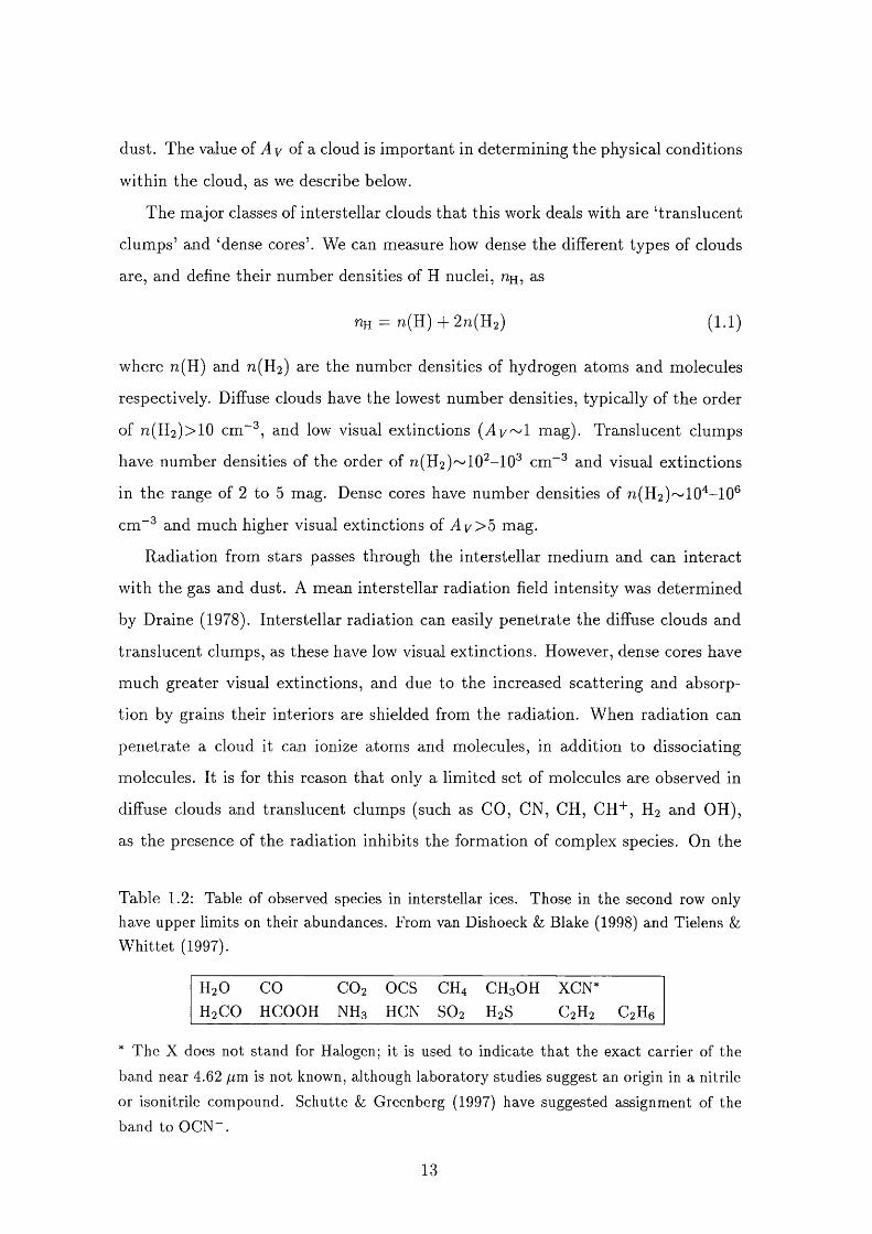
Species tha t have frozen-out onto a dust grain form an icy m antle around the
grain core. We can observe molecules tha t are trapped in icy mantles and in Table
1.2 we give a list of these species (van Dishoeck & Blake 1998; Tielens & W hittet
1997). The molecules in ices are observed through the absorption of radiation from
background stars. Once a species is frozen-out onto a grain’s surface it can be
ejected back into the gas phase via desorption processes. Several possible desorption
mechanisms exist and these include chemical, radiative and high energy cosmic ray
processes (Williams & Taylor 1996; see section 2.5.1).
A measure of the quantity of dust along a line of sight or in a cloud is the visual
extinction. A y , measured in magnitudes. The visual extinction equals 1.086 times
the optical depth at the wavelength 5550 Â, due to both scattering and absorption by
11
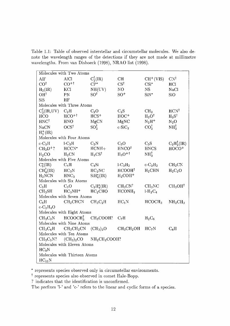
Table 1.1: Table of observed interstellar and circumstellar molecules. We also denote the wavelength ranges of the detections if they are not made at millimetre wavelengths. From van Dishoeck (1998), NRAO list (1998).
Molecules with Two AtomsAIF AlCl Cj(IR) CH CH+(VIS) CNfCQf CQ+t CP* CSf CSP HClH2 (IR) KCl NH(UV) NO NS NaClGRt PN SQt S0+ SiN* SiOSiS HFMolecules with Three Atomsd(IR ,U V ) C2 H C2O C2S CH2 HCNtHCO HCO+t HCS+ HOC+ H2 0 t H2StH N d HNO MgCN MgNC N2 H+ N2ONaCN ocs^ s o | c-SiCz c o | NH|Hj-(IR)Molecules with Four AtomsC-C3 H I-C3 H C3 N C3 O C3 S C2 H|(IR)CH2D+? HCCN* HCNH+ HNCOf HNCS HOCO+H2 CO H2CN HjCSt H30+t NRtMolecules with Five AtomsQ (IR ) C4 H C4 Si I-C3 H2 C-C3 H2 CH2CNc h J(ir ) HC3 N HC2 NC HCOOH+ H2CHN H2C2OH2NCN HNC3 SiH*(IR) H2COH+Molecules with Six AtomsCsH C5O C2 H;(IR) CH3CNt CH3 NC CHsOHtCH3 SH HC3 NH+ HC2CHO HCONH2 I-H2 C4
Molecules with Seven AtomsCeH CH2 CHCN CH3 C2H HC5N HCOCH3 NH2CH3C-C2 H4 OMolecules with Eight AtomsCH3 C3 N HCOOCH+ CH3COOH? C7H H2 C6
Molecules with Nine AtomsCH3 C4 H CH3 CH2CN (CH3)20 CH3 CH2 OH HC7 N CsHMolecules with Ten AtomsCH3 C5 N? (CH3 )2C0 NH2 CH2 COOH?Molecules with Eleven AtomsHCgNMolecules with Thirteen AtomsHCiiN
* represents species observed only in circumstellar environments. represents species also observed in comet Hale-Bopp.? indicates tha t the identification is unconfirmed.The prefixes ’1-’ and ’c-’ refers to the linear and cyclic forms of a species.
12
dust. The value of Ay of a cloud is im portant in determining the physical conditions
within the cloud, as we describe below.
The major classes of interstellar clouds that this work deals with are ‘translucent
clum ps’ and ‘dense cores’. We can measure how dense the different types of clouds
are, and define their number densities of H nuclei, uh, as
hh = n(H) + 2n(H2) (1.1)
where n(H) and n(H 2 ) are the number densities of hydrogen atoms and molecules
respectively. Diffuse clouds have the lowest number densities, typically of the order
of n(H 2 ) > 1 0 cm~^, and low visual extinctions ( T y ~ l mag). Translucent clumps
have number densities of the order of n(H 2 ) ~ 1 0 ^ -1 0 cm“ and visual extinctions
in the range of 2 to 5 mag. Dense cores have number densities of n(H 2 ) ~ 1 0 ^ -1 0 ®
cm “ and much higher visual extinctions of i4y>5 mag.
Radiation from stars passes through the interstellar medium and can interact
with the gas and dust. A mean interstellar radiation field intensity was determined
by Draine (1978). Interstellar radiation can easily penetrate the diffuse clouds and
translucent clumps, as these have low visual extinctions. However, dense cores have
much greater visual extinctions, and due to the increased scattering and absorp
tion by grains their interiors are shielded from the radiation. W hen radiation can
penetrate a cloud it can ionize atoms and molecules, in addition to dissociating
molecules. It is for this reason tha t only a limited set of molecules are observed in
diffuse clouds and translucent clumps (such as CO, CN, CH, CH+, H2 and OH),
as the presence of the radiation inhibits the formation of complex species. On the
Table 1.2: Table of observed species in interstellar ices. Those in the second row only have upper limits on their abundances. From van Dishoeck & Blake (1998) and Tielens & W hittet (1997).
H2 0 CO CO2 o c s CH4 CH3 OH XCN*H2 C0 HCOOH NH3 HCN SO2 H2S C2H2 C2 H6
* The X does not stand for Halogen; it is used to indicate that the exact carrier of the band near 4.62 fim is not known, although laboratory studies suggest an origin in a nitrile or isonitrile compound. Schutte & Greenberg (1997) have suggested assignment of the band to OCN~.
13
other hand, in dense cores we observe many different complex species. In addition
to the interstellar radiation field, cosmic rays (energetic protons) are another source
of ionization which contribute to the ionization in diffuse clouds and are the m ajor
source in dense cores. In dense cores the cosmic rays can directly interact with
species to ionize and dissociate, in addition to inducing photons which can then
destroy species. The cosmic ray ionization of H2 results in an energetic electron
which then collides with and excites H2 . When the excited hydrogen molecule re
laxes it produces ultraviolet photons (Prasad & Tarafdar 1983; Gredel et al. 1989).
The direct cosmic ray ionization rate is lower than tha t of the interstellar radiation
field, although its exact value is not clear as we discuss in section 2.4. The exact
ionization level or ‘structure’ in a cloud is determined by the chemistry, as we also
describe in section 2.4.
The tem peratures of diffuse clouds, translucent clumps and dense cores also
differ. Typically, the tem perature in a diffuse cloud is approximately 100 K and in
a translucent clump or a dense core it is around 10-30 K. The tem perature that
obtains is the result of a balance between the heating and cooling mechanisms that
operate in a cloud. UV radiation and cosmic rays can heat a cloud by the ionization
of species. The ionizing source imparts energy to the gas as the ejected electron
carries away excess energy. Photons, including those produced as a consequence of
cosmic-ray induced ionization, provide an additional heating source.
The gas is cooled when radiation is em itted by the atoms and molecules tha t
comprise the gas. Recombination of an atomic or molecular ion with an electron
results in the emission of a photon, which can then escape from the gas; energy is
lost from the system and the gas is cooled. The collisional excitement of an atom
or a molecule also results in the emission of a photon, as the excited species decays
back to the ground state. Both of these cooling mechanisms depend on the number
density to the power of two, which results in dense regions tending to be cooler than
more diffuse environments. An additional loss mechanism is provided by the grains,
which are heated when they absorb radiation. The grains then radiate this energy in
the infrared, which can then escape from the cloud. The dominant coolant in both
translucent clumps and dense cores is CO. It can be excited at gas tem peratures of
14
only a few Kelvins. However, its effectiveness is reduced as its abundance rises in
denser clouds since the radiation em itted by one CO molecule can be absorbed by
another. This is a process called radiation trapping.
An im portant point to note is that in dense cores the cosmic rays cannot m aintain
the tem peratures that are measured, when the cooling mechanisms are accounted
for. Another heating process is needed. A potential source is some form of dynamical
heating where movements within the gas produce frictional heating.
Once we have determined the tem perature and number density of a cloud we
can consider its therm al pressure. Diffuse clouds and translucent clumps have low
therm al pressures unlike dense cores which have therm al pressures around a hun
dred times greater. The material between clumps and dense cores is referred to as
the interclump medium. The properties of the interclump medium are poorly un
derstood but its total pressure must be comparable to tha t of a translucent clump.
(Contributions to the total pressure include the therm al, turbulent and magnetic
pressures.) Pressure equilibrium between a translucent clump and the interclump
medium should be established on roughly the timescale for a fast-mode magnetic
wave to cross the clump; for an assumed fast-mode speed of 3 km s " \ this is 10®
years for a clump that is 3 pc across.
We now discuss how the gas is supported against collapse. We regard translu
cent clumps and dense cores as representing two different stages of star formation:
the translucent clumps collapse to form dense cores. Dense cores are identified as
the direct progenitors of stars. Investigation into the star formation process is con
ventionally divided into considerations of low-mass and high-mass star formation
separately. Stars of low-mass (with masses less than 4 M©) are thought to form as a
result of a gradual weakening of the magnetic fields. However, higher mass stars are
believed to form because the ratio of the magnetic flux to the clumps mass is too
small for the magnetic field to prevent collapse when the pressure external to the
clump is increased above a critical value (e.g. Mouschovias 1987). High-mass star
formation can therefore be triggered by increases in the pressure of the interclump
medium. Potential catalysts include winds and the supernovae of other high-mass
stars (e.g. Elmegreen & Lada 1977; Mouschovias 1987). In this work we are con
15
cerned with the formation of low-mass stars. Hence, all further descriptions, unless
stated otherwise, refer to low-mass star formation only.
The gas in translucent clumps is confined by the pressure exerted by the warm,
tenuous interclump medium as these objects are not gravitationally bound. They
are believed to be supported against collapse by magnetic fields and magnetohydro-
dynamic (MED) waves which comprise the turbulence (e.g. Mouschovias 1987; Shu,
Adams & Lizano 1987). We describe the evidence for turbulence in section 1.2. The
MED waves can be dissipated, and the damping rate depends inversely on the ion
num ber density. The ionization structure of a cloud is determined by the chemistry
(see section 2.4). Eence, as the fractional ionization drops, the rate of wave damping
increases and the clump will begin to collapse along the magnetic field lines. (In
Chapter 3 we investigate the nature of decreases in the fractional ionization.) The
collapse of a translucent clump by this process leads to the formation of a dense
core.
By contrast, dense cores are supported by therm al pressure and magnetic pres
sure. Waves are not im portant for their support (see Chapter 3). Their further
collapse is governed by ambipolar diffusion, the drift of the neutral component of
the gas relative to the charged component. The charged component of the gas con
sists of ions and electrons, and the grains which carry one negative charge (Draine
& Sutin 1987). The magnetic field acts on the charged components and tends to
push particles out of the cloud. The magnetic force does not act directly on the
neutral component. Gravity acts to pull the neutral component inward. The rela
tive motions produce friction between the neutral and charged components which
acts to reduce their relative velocities. The friction therefore leads to the ‘magnetic
re tardation’ of collapse (and may provide the additional heating source tha t is re
quired in order for dense cores to have their observed tem peratures, as mentioned
above, and as described by Scalo 1987). The time for which the collapse of a cloud
remains magnetically retarded is the time required for the neutrals to drift through
the charged particles due to gravity. This is the ambipolar diffusion timescale. In
Table 1.3 we give approximate expressions for this and some of the other im portant
timescales in star forming regions.
16
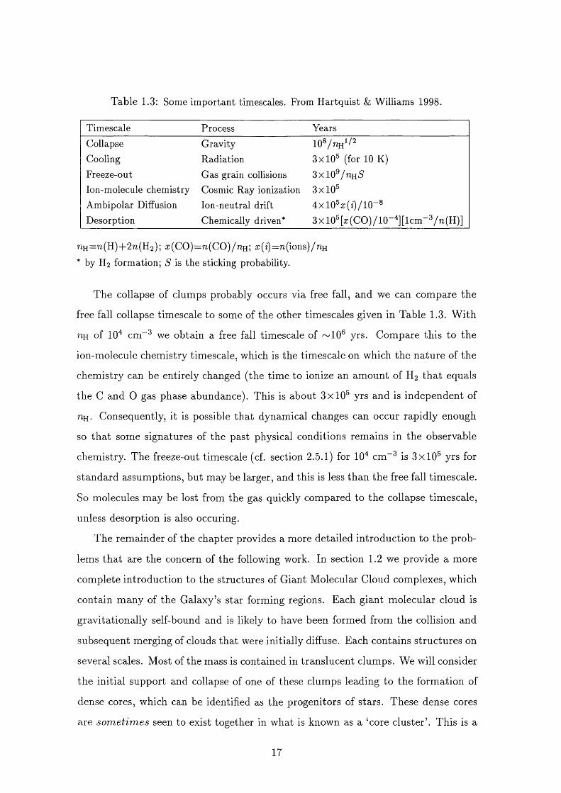
Table 1.3: Some important timescales. From Hartquist k Williams 1998.
Timescale Process YearsCollapse GravityCooling Radiation 3x10^ (for 10 K)Freeze-out Gas grain collisions 3xlO^/MH^Ion-molecule chemistry Cosmic Ray ionization 3x10^Ambipolar Diffusion Ion-neutral drift 4xl0^æ(z)/10-^Desorption Chemically driven* 3xlO^[a:(CO)/10“ '^][lcm~^/n(H)]
nH=n(H)+2 n(H2 ); a:(CO)=n(CO)/nH; x(i)=n(ions)/ nu * by H2 formation; S is the sticking probability.
The collapse of clumps probably occurs via free fall, and we can compare the
free fall collapse timescale to some of the other timescales given in Table 1.3. W ith
hh of 1 0 cm~^ we obtain a free fall timescale of ~ 1 0 ® yrs. Compare this to the
ion-molecule chemistry timescale, which is the timescale on which the nature of the
chemistry can be entirely changed (the time to ionize an amount of H2 th a t equals
the C and 0 gas phase abundance). This is about 3x10^ yrs and is independent of
hh. Consequently, it is possible that dynamical changes can occur rapidly enough
so tha t some signatures of the past physical conditions remains in the observable
chemistry. The freeze-out timescale (cf. section 2.5.1) for lO' cm“ is 3x10^ yrs for
standard assumptions, but may be larger, and this is less than the free fall timescale.
So molecules may be lost from the gas quickly compared to the collapse timescale,
unless desorption is also occuring.
The remainder of the chapter provides a more detailed introduction to the prob
lems tha t are the concern of the following work. In section 1.2 we provide a more
complete introduction to the structures of Giant Molecular Cloud complexes, which
contain many of the Galaxy’s star forming regions. Each giant molecular cloud is
gravitationally self-bound and is likely to have been formed from the collision and
subsequent merging of clouds that were initially diffuse. Each contains structures on
several scales. Most of the mass is contained in translucent clumps. We will consider
the initial support and collapse of one of these clumps leading to the formation of
dense cores, which can be identified as the progenitors of stars. These dense cores
are som e t im es seen to exist together in what is known as a ‘core cluster’. This is a
17
collection of several cores, which are close enough to one another that the birth of
even a low-mass star in one of the cores may then regulate the further evolution of
tlie other cores within the cluster. In section 1.3 we discuss the possible scenarios
for the development of core clusters, in which low-mass stars form. Another core
cluster, TM C-1 , which is one of the closest and most thoroughly observed, is the
topic of section 1.4. TMC-1 consists of several dense cores which lie in a ridge in
the vicinity of a recently formed low-mass star. A chemical gradient is observed
along the ridge and is used to infer information on the dynamical properties of the
source. In section 1.5 we examine the observational studies of dense core collapse
which leads to the formation of stars. Finally in section 1.6 we treat the theoretical
studies of the collapse of dense cores. Section 1.7 is a summary, and also sets out
the content of the thesis.
1.2 Clum py Giant M olecular Cloud com plexes
^ - 1.5
- 2
- 2.5
208.5 208 207.5 207 206.5 206 205.5
G alac t ic Long i tude (° )
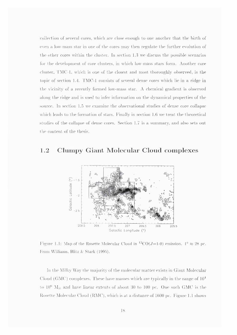
Figure 1.1: Map of the Rosette Molecular Cloud in ^^CO(J=1-0) emission. 1° % 28 pc.
lAom Williams, Blitz & Stark (1995).
In tlie Milky Way the majority of the molecular m atter exists in Giant Molecular
('loud (CMC) complexes. These liave masses which are typically in the range of 1 0 "
to 1 (F M q and have linear extents of a loon t 30 to 1 0 0 pc. One such GMC is the
Rosette Molecular Cloud (RMC), which is at a distance of 1600 pc. Figure 1 . 1 shows
18
the integrated ( J = l - 0 ) emission line map of the RMC. The ^^00 ( J = l - 0 ) and
^^00 ( J = l - 0 ) emission maps of the RMC have been analyzed in detail by Williams,
Blitz & Stark (1995). Their work has provided information on the structure of this
particular GMC complex. The projected cross section of the RMC is about 2200
pc^, it has a mass of about 1-2x10^ M©, a mean H2 column density of 4x10^^ cm “
and a mean H2 number density of 30 cm“ . Much of the molecular m aterial in the
RMC exists in approximately 70 clumps which have masses between about 30 and
2500 M©; the number of clumps with masses between M and M +dM scales as
dM. Less massive clumps may also exist within the complex, but only a few were
detected at the limit of the sensitivity of the observations.
The clumps which have been identified occupy only approximately eight percent
of the volume of the RMC. In most clumps n(H 2 ) ~ 2 0 0 cm “ ; a variation of about
a factor of 4 in this value is found, but the measured variation may be more limited
than the real variation in density because CO is a poor tracer of denser gas. This is
due to the small dipole moment of CO resulting in the CO rotational level population
distribution becoming thermalized at values of n(H 2 ) of several hundred cm “ . The
peak ^^CO column density through a clump scales roughly as and is about
10 ® cm “ for M=10^ M©; the H2 column density is assumed to be a factor of 5x10^
larger. There are seven embedded stars which exist in the three most massive and
the fifth, seventh, eleventh, and eighteenth most massive clumps. The clumps tha t
contain stars are all amongst the 16 clumps having the highest ^^CO column densities
of about 1 0 ® cm “ and more.
For a feature formed in an individual clump the line of sight full width at half
maxim um lies in the range of about 0.9 to 3.3 km s“ L For comparison, the value
for ^^CO tha t is thermally broadened only and is at 30 K (which is roughly the
maxim um tem perature obtaining in the clumps) is only 0.22 km s~^. It has been
inferred tha t about half of the clumps are not bound by their own gravitational fields,
from the comparison of the velocity dispersion with the escape velocity estim ated
from the mass and radius of each clump. This is a result tha t appears to also apply
to clumps in other GMCs (Bertoldi & McKee 1992). A clump tha t is not bound
by its own gravity must be bound by the pressure of an interclump medium, which
19
may consist primarily of gas at about 10 K.
The clumps have magnetic fields which are im portant for their support (e.g.
Mouschovias 1987). Turbulent pressure, which is associated with the broad lines
th a t are observed, is im portant for clump support and acts along the magnetic field
lines. The form of the turbulence is a superposition of Alfvén waves (Arons & Max
1975; Mouschovias & Psaltis 1995).
In Chapter 3 we examine the collapse of a clump to form a dense core. We argue
th a t collapse may begin if a critical column density is exceeded, and tha t this is
directly related to the extent of turbulent support in a clump.
30*1- LI5I7
28*,
26*
MCI
TMC2
— CO EMISSION• DENSE CORE+ OBSCURED STAR• T TAURI S T A R /^
L I5 3 6
20*,
18"
16' __
4*’5 5 ' 45 4 " 0 535"' 25"'RIGHT ASCENSION ( 1 9 5 0 )
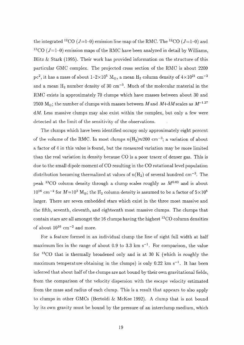
Figure 1.2: The distribution of dark cores and low-mass stars in the Taurus — Auriga
complex. From Myers (1986).
20
1.3 Low-m ass star form ation in a cluster o f dense
cores
30
20
IRS410
2.0
UJ
IRS210w
0 .25- 2 0
-3 030 20 010 -10 -20 - 3 0
RA OFFSET (o re min )
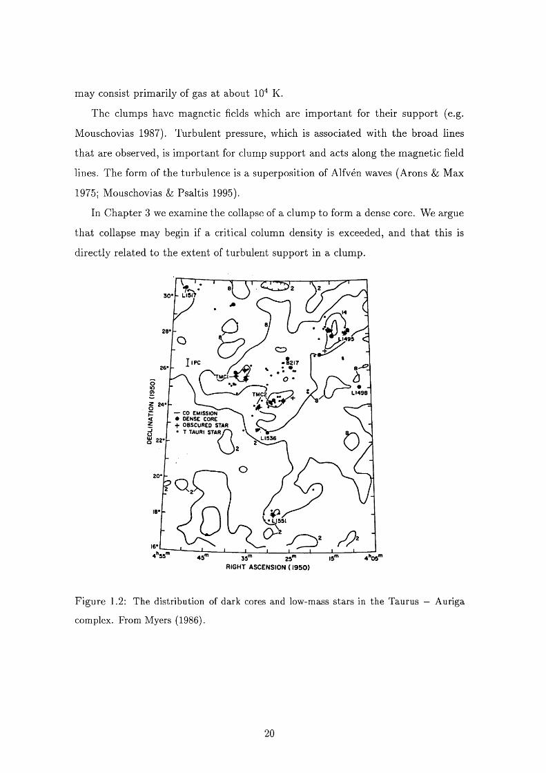
Figure 1.3: contour map of B5. The positions of four infrared sources (IRSl-4)
associated with young stars are shown. From Goldsmith, Langer & Wilson (1986).
W hen a clump like one of those observed in the RMC collapses, it fragments and
objects known as dense cores form (e.g. Myers 1990). Ammonia emission has been
used to map many of the dense cores (e.g. Benson & Myers 1989). Dense cores
typically have masses of one to several tens of solar masses each, number densities
n(H 2 ) ~ 1 0 —10 cm~^ and temperatures of ~ 10—30 K. However, some dense cores
are observed to have number densities of up to roughly 1 0 cm “ and masses of
more than one hundred solar masses, particularly in regions where massive stars
form. In Fig. 1.2 the dense core distribution in the Taurus — Auriga complex is
shown. Approximately half of all dense cores are associated with young low-mass
stars. Dense cores are considered to be the direct progenitors of protostars.
Figure 1.2 shows that many (but not all) of the dense cores are near other dense
cores. Barnard 5 (B5) contains a cluster of five dense cores and four young low-
21
CLUMP COLLAPSE ABLATION AND SHOCK•HBUBBLE
TBAVEBSAL
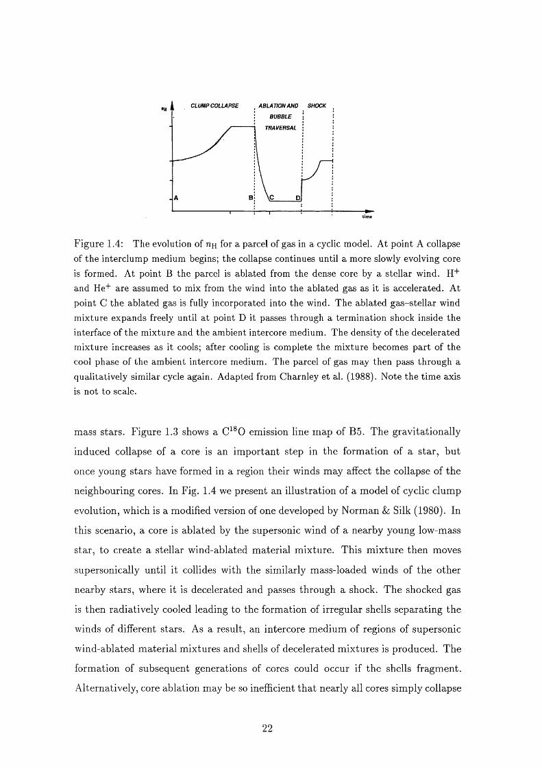
Figure 1.4: The evolution of nu for a parcel of gas in a cyclic model. At point A collapseof the interclump medium begins; the collapse continues until a more slowly evolving core is formed. At point B the parcel is ablated from the dense core by a stellar wind. H'*' and He"*" are assumed to mix from the wind into the ablated gas as it is accelerated. At point C the ablated gas is fully incorporated into the wind. The ablated gas-stellar wind mixture expands freely until at point D it passes through a termination shock inside the interface of the mixture and the ambient intercore medium. The density of the decelerated mixture increases as it cools; after cooling is complete the mixture becomes part of the cool phase of the ambient intercore medium. The parcel of gas may then pass through a qualitatively similar cycle again. Adapted from Charnley et al. (1988). Note the time axis is not to scale.
mass stars. Figure 1.3 shows a emission line map of B5. The gravitationally
induced collapse of a core is an im portant step in the formation of a star, but
once young stars have formed in a region their winds may affect the collapse of the
neighbouring cores. In Fig. 1.4 we present an illustration of a model of cyclic clump
evolution, which is a modified version of one developed by Norman & Silk (1980). In
this scenario, a core is ablated by the supersonic wind of a nearby young low-mass
star, to create a stellar wind-ablated m aterial m ixture. This m ixture then moves
supersonically until it collides with the similarly mass-loaded winds of the other
nearby stars, where it is decelerated and passes through a shock. The shocked gas
is then radiatively cooled leading to the formation of irregular shells separating the
winds of different stars. As a result, an intercore medium of regions of supersonic
wind-ablated m aterial mixtures and shells of decelerated mixtures is produced. The
formation of subsequent generations of cores could occur if the shells fragment.
Alternatively, core ablation may be so inefficient tha t nearly all cores simply collapse
22
to form stars, before they can be significantly eroded. The material that was in a
core l)iit does not go into a star may then be blown to a large enough distance from
the cluster of cores, by the stellar winds, such that it cannot be considered to be
associated with the cluster.
1.4 TM C-1
.y*)CCS {t>)CCS J{ =2 i -1Q
Beam Slz#(HPÏWV)
5 0 - 5*r,(arcmin)
Beam S iteiVIPSW)
-10 5 0 -5io(arcmin)
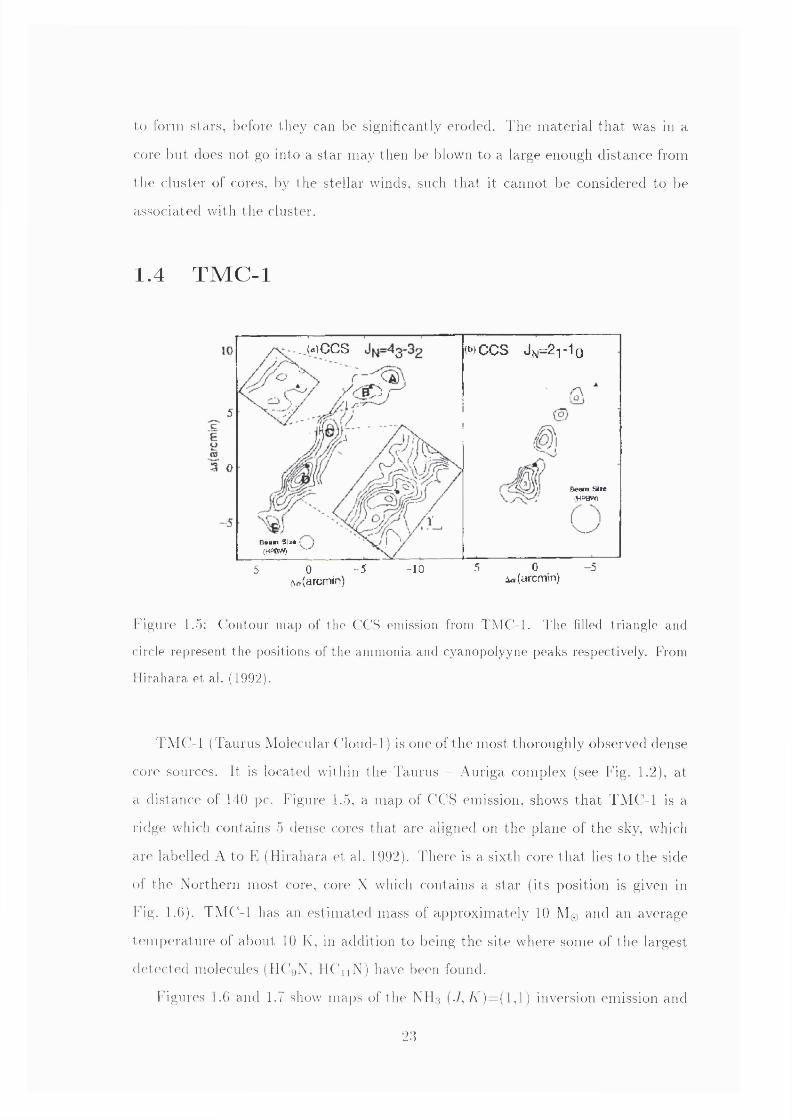
higure 1.5: Contour map of the CCS emission from TMC-1 . The filled triangle and
circle represent the positions of the ammonia and cyanopolyyne peaks respectively. From
I lirahara et al. (1992).
TMC - 1 (Taurus Molecular Cloud-1 ) is one of the most thoroughly observed dense
core sources. It is located within the Taurus - Auriga complex (see Fig. 1 .2 ), at
a distance of 140 pc. Figure 1.5, a map of CCS emission, shows that TAlC- 1 is a
ridge which contains 5 dense cores that are aligned on the plane of the sky, which
are labelled A to E (Hirahara et ah 1992). There is a sixth core that lies to the side
of the Northern most core, core X which contains a star (its position is given in
f ig. 1.6). TMC-1 has an estimated mass of approximately 1 0 M@ and an average
tem perature of about 1 0 K, in addition to being the site where some of the largest
detected molecules (lICgN, IICuN) have been found.
Figures 1.6 and 1.7 show maps of the NII3 (.7, A') = ( l , l ) inversion emission and
23
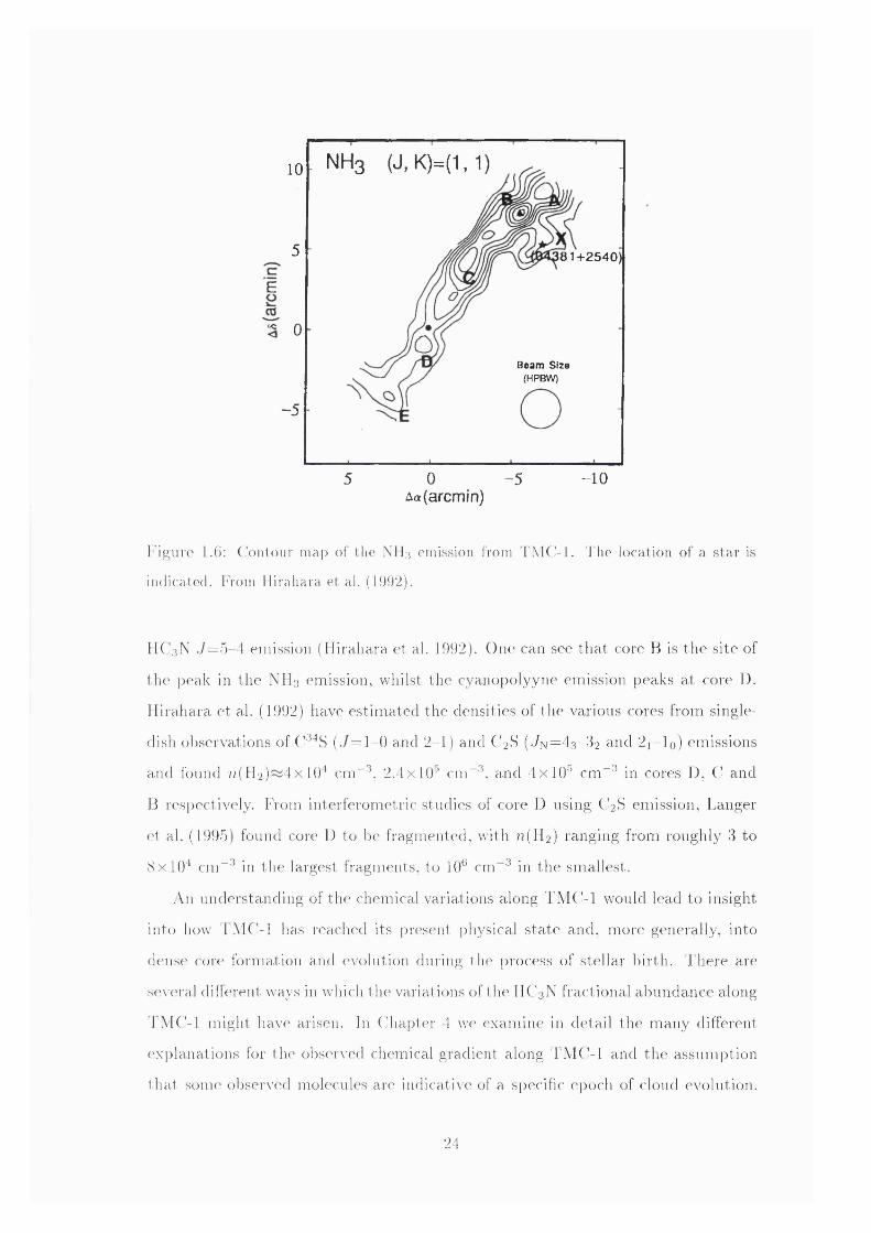
. NH3 (J,KH1,1)10
5 81 + 2 540 )
<c 0
B ea m S iz e(HPBW)
-5
05 -105Aa{arcmin)
I'^igure 1.6: Contour map of the NII3 emission from TMC-1. The location of a star is
indicated. From Hirahara et al. (1992).
IIC3 N .7=5-4 emission (Hirahara et al. 1992). One can see that core B is the site of
t he peak in the NII3 emission, whilst the cyanopolyyne emission peaks at core D.
Hirahara et al. (1992) have estimated the densities of the various cores from single
dish observations of C '^S (.7=1-0 and 2 - 1 ) and C2 S (.7 ^ = 4 3 - 8 2 and 2 i - 1 q) emissions
and found ?7.(H2 )~ 4 x 1 0 '* cm"^, 2.4x10^ cm“ , and 4x10^ cm“ in cores D, C and
B respectively. From interferornetric studies of core D using C2 S emission, Langer
et al. (1995) found core D to be fragmented, with 77(H2 ) ranging from roughly 3 to
8 x 1 0 '* cm“ in the largest fragments, to 1 0 * cm~^ in the smallest.
An understanding of the chemical variations along TMC - 1 would lead to insight
into how TMC-1 has reached its present physical state and, more generally, into
dense core formation and evolution during the process of stellar birth. There are
several different ways in which the variations of the HC3 N fractional abundance along
FMC-1 might have arisen. In Chapter 4 we examine in detail the many different
explanations for the observed chemical gradient along TMC - 1 and the assumption
that some observed molecules are indicative of a specihc epoch of cloud evolution.
24
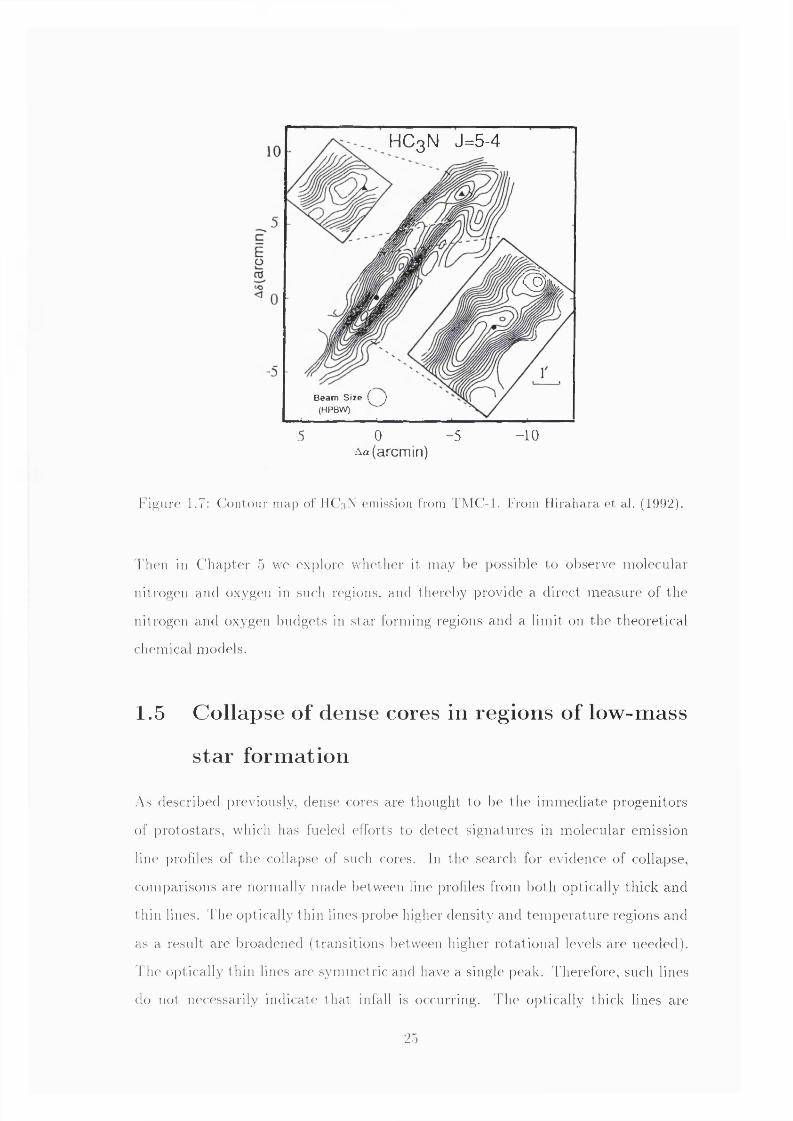
HC3N J=5-4
( g
B e a m S iz e T J (HPBW)
5 0Aa(arcmin)
-5 -10
I’ igurc 1.7: C'oiitour map of IK^gN emission from TMCl-l. From llirahara et al. (1992).
'riien in (llia])tcr 5 we explore wliether it may be possible to observe molecular
nitrogen and oxygen in such regions, and thereby provide a direct measure of the
nitrogen and oxygen budgets in star forming regions and a limit on the theoretical
chemical models.
1.5 Collapse of dense cores in regions o f low-m ass
star form ation
As described previously, dense cores are thought to be the immediate progenitors
of protostars, which has fueled efforts to detect signatures in molecular emission
line profiles of the collapse of such cores. In the search for evidence of collapse,
comparisons are normally made between line ])rohles from both optically thick and
1 hin lines. The o])tically thin lines probe higher density and tem perature regions and
as a residt are broadened (transitions between higher rotational levels are needed).
The o]M ically thin lines are symmetric and have a single peak. Therefore, such lines
do not necessarily indicate that in fall is occurring. Tlie optically thick lines are
25
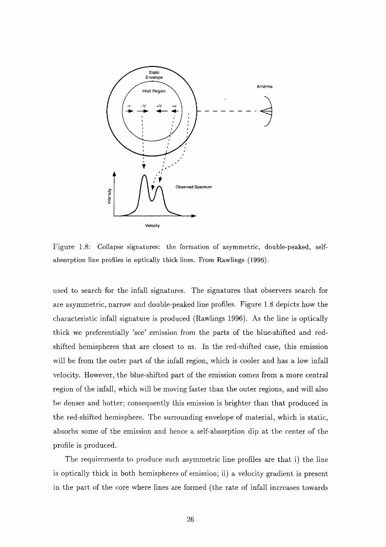
StaticEnvelope
Infall Region
+V
O bserved Spectrum
Velocity
A ntenna
Figure 1.8: Collapse signatures: the formation of asymmetric, double-peaked, self
absorption line profiles in optically thick lines. From Rawlings (1996).
used to search for the infall signatures. The signatures tha t observers search for
are asymmetric, narrow and double-peaked line profiles. Figure 1.8 depicts how the
characteristic infall signature is produced (Rawlings 1996). As the line is optically
thick we preferentially ’see’ emission from the parts of the blue-shifted and red-
shifted hemispheres tha t are closest to us. In the red-shifted case, this emission
will be from the outer part of the infall region, which is cooler and has a low infall
velocity. However, the blue-shifted part of the emission comes from a more central
region of the infall, which will be moving faster than the outer regions, and will also
be denser and hotter; consequently this emission is brighter than tha t produced in
the red-shifted hemisphere. The surrounding envelope of m aterial, which is static,
absorbs some of the emission and hence a self-absorption dip at the center of the
profile is produced.
The requirements to produce such asymmetric line profiles are tha t i) the line
is optically thick in both hemispheres of emission; ii) a velocity gradient is present
in the part of the core where lines are formed (the rate of infall increases towards
26
the core centre); iii) the observed species is also present in the static outer envelope;
and iv) a positive tem perature gradient towards the cloud centre exists.
Observational detections of this sort of blue-red asymmetric self-absorption were
made for a number of clouds in CO emission line profiles by Snell & Loren (1976), but
these results were challenged by Leung & Brown (1977) who argued tha t the infall
explanation for the origin of the asymmetric features was not unique. (Turbulence,
rotation and outflows also produce double-peaked profiles. However, as described
by Zhou (1997), these motions should produce equal amounts of blue-shifted and
red-shifted emission.) Walker et al. (1986) reported the detection of infall in IRAS
16293-2422 using a CS emission line study. However, Menten et al. (1987) showed
th a t the observed line profiles could be explained using a model in which the emission
from a rapidly rotating core undergoes foreground absorption.
In an a ttem pt to establish more thoroughly what the characteristics of spectral
line profiles formed in collapse models are, Zhou (1992) performed radiative transfer
calculations based on simplifying approximations. One particular collapse model
th a t Zhou (1992) used is one studied analytically by Shu (1977). Shu (1977) showed
th a t an initially static, singular isothermal sphere (with n ~ r “ ^) will undergo self
similar collapse with the collapse wave propagating out from the centre where the
collapse velocity and the density are infinite. Collapse in which the infall speed
decreases with radius and the outer radius of the collapsing region, Tout, increases
with tim e has come to be known as “inside-out” collapse. Computations like those
of Zhou (1992) and the more accurate Monte-Carlo calculations of Choi et al. (1995)
give results tha t imply tha t for cores undergoing inside-out collapse and in which
the tem perature decreases with radius:
1 . optically thick lines show the blue-red self-absorption asymmetry,
2 . for fixed angular resolution and equal optical depths the width of a line of a
transition for which the critical density is large is greater than the width of a
line of a transition for which the critical density is small,
3. the self-absorption and linewidth of a line appear to increase with increasing
angular resolution of the central parts of a core.
27
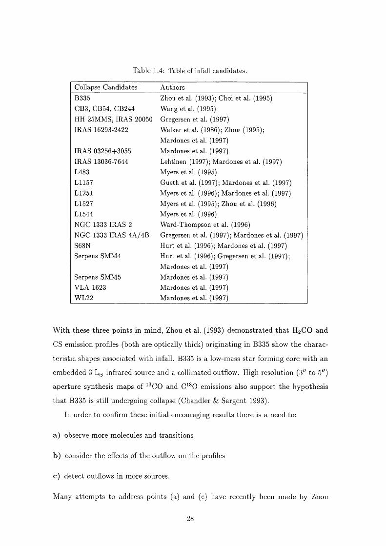
Table 1.4: Table of infall candidates.
Collapse Candidates AuthorsB335 Zhou et al. (1993); Choi et al. (1995)CB3, CB54, CB244 Wang et al. (1995)HR 25MMS, IRAS 20050 Gregersen et al. (1997)IRAS 16293-2422 Walker et al. (1986); Zhou (1995);
Mardones et al. (1997)IRAS 03256+3055 Mardones et al. (1997)IRAS 13036-7644 Lehtinen (1997); Mardones et al. (1997)L483 Myers et al. (1995)L1157 Gueth et al. (1997); Mardones et al. (1997)L1251 Myers et al. (1996); Mardones et al. (1997)L1527 Myers et al. (1995); Zhou et al. (1996)L1544 Myers et al. (1996)NGC 1333 IRAS 2 Ward-Thompson et al. (1996)NGC 1333 IRAS 4A/4B Gregersen et al. (1997); Mardones et al. (1997)S6 8 N Hurt et al. (1996); Mardones et al. (1997)Serpens SMM4 Hurt et al. (1996); Gregersen et al. (1997);
Mardones et al. (1997)Serpens SMM5 Mardones et al. (1997)VLA 1623 Mardones et al. (1997)WL22 Mardones et al. (1997)
W ith these three points in mind, Zhou et al. (1993) dem onstrated th a t H 2 CO and
CS emission profiles (both are optically thick) originating in B335 show the charac
teristic shapes associated with infall. B335 is a low-mass star forming core w ith an
embedded 3 L@ infrared source and a collimated outflow. High resolution (3" to 5")
aperture synthesis maps of and emissions also support the hypothesis
tha t B335 is still undergoing collapse (Chandler & Sargent 1993).
In order to confirm these initial encouraging results there is a need to:
a) observe more molecules and transitions
b) consider the effects of the outflow on the profiles
c) detect outflows in more sources.
Many attem pts to address points (a) and (c) have recently been made by Zhou
28
et al. (1994), Mardones et al. (1994), Myers et al. (1995), Velusamy et al. (1995),
Wang et al. (1995), Zhou et al. (1996), Myers et al. (1996), Gregersen et al. (1997)
and Mardones et al. (1997). Many new infall candidates have been discovered and
are listed in Table 1.4. The characteristic infall signatures have been observed in a
variety of molecular lines: (2 - 1 ), C3 H2 (2 i,2-lo ,i), C2 S (2 i-lo ), HCO+, ^^00
and HCN, besides H2 CO and CS. However, point (b) is a difficult one to address be
cause it further complicates already sophisticated models. Myers et al. (1996) have
developed a simple analytic model of radiative transfer in which the contribution
of outflowing gas to spectral line profiles from contracting clouds is also considered.
This model provides a simple way to quantify characteristic infall speeds, and its
use to interpret data strongly suggests that the inward motions derived from the
line profiles are gravitational in origin.
One way to avoid complications due to the presence of stellar outflows is to
observe starless cores which, presumably, do not have outflows. Some of these
objects may be collapsing, yet are starless due to insufficient development time. To
date, only one starless core L1544 has shown evidence of infall asymm etry profiles
which strongly suggest infall motions (Myers et al. 1996; Tafalla et al. 1998). The
measured linewidths in L1544 are extremely small (~0.3 km s“ ) and imply tha t
therm al pressure is playing an im portant role in the dynamics. In addition, it is one
of the most opaque cores in the Taurus Molecular Cloud, suggesting the presence of
high column densities. Myers and collaborators have therefore defined L I544 as the
most evolved starless core. L1498 is another interesting starless core which shows
an intriguing double-peaked CS feature with the blue peak stronger than the red
peak (Lem m eet al. 1995). However, L1498 has a complicated physical and chemical
structure which hinders an easy interpretation of observational data (see Kuiper,
Langer & Velusamy 1996). Figure 1.9 shows the shape of an NH3 emission line
feature arising in the dense core L1498 (Myers & Benson 1983). As the source was
observed in two separate lines a tem perature could be derived. The NH3 emission
profile shows very little deviation from that expected from a static core with very
subsonic turbulence. There are no broad wings like those tha t might be expected to
arise, during some stages of the gravitationally induced collapse of a core in which
29
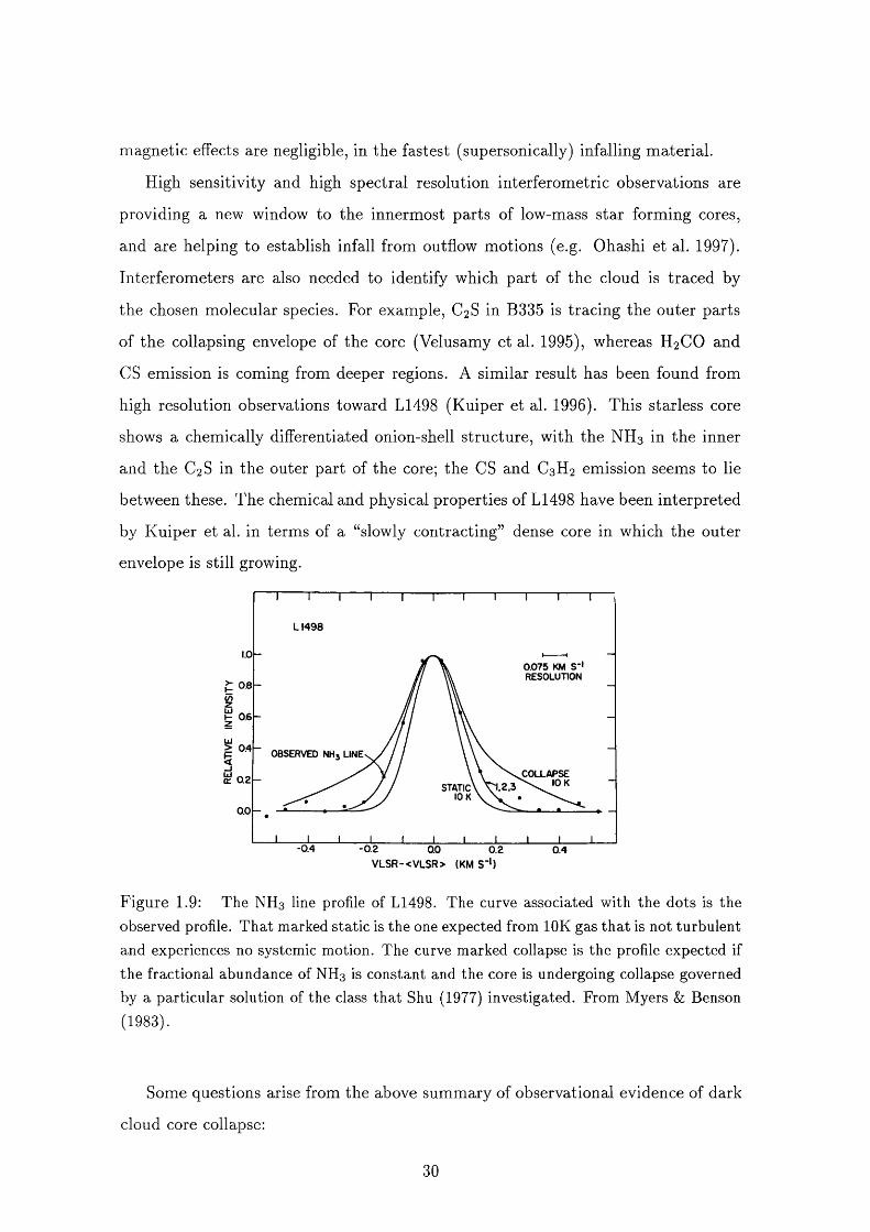
magnetic effects are negligible, in the fastest (supersonically) infalling material.
High sensitivity and high spectral resolution interferometric observations are
providing a new window to the innermost parts of low-mass star forming cores,
and are helping to establish infall from outflow motions (e.g. Ohashi et al. 1997).
Interferometers are also needed to identify which part of the cloud is traced by
the chosen molecular species. For example, C2 S in B335 is tracing the outer parts
of the collapsing envelope of the core (Velusamy et al. 1995), whereas H 2 CO and
CS emission is coming from deeper regions. A similar result has been found from
high resolution observations toward L1498 (Kuiper et al. 1996). This starless core
shows a chemically differentiated onion-shell structure, with the NH3 in the inner
and the C2 S in the outer part of the core; the CS and C3 H2 emission seems to lie
between these. The chemical and physical properties of L1498 have been interpreted
by Kuiper et al. in terms of a “slowly contracting” dense core in which the outer
envelope is still growing.
LI498
0.075 KM S -' RESOLUTION 0.8
H 0.6
> 0 .4 OBSERVED NH3 LINE
COLLAPSE 10 K0.2
1.2.3STATIC 10 K
0.0
-0.4 - 0.2 0.0 0.2 0.4V L SR -< V L S R > (K M S*')
Figure 1.9: The NH3 line profile of L1498. The curve associated with the dots is theobserved profile. That marked static is the one expected from lOK gas that is not turbulent and experiences no systemic motion. The curve marked collapse is the profile expected if the fractional abundance of NH3 is constant and the core is undergoing collapse governed by a particular solution of the class that Shu (1977) investigated. From Myers & Benson (1983).
Some questions arise
cloud core collapse:
from the above summary of observational evidence of dark
30
1 . How deeply in the core are infalling motions traced by H2CO and CS obser
vations? These are the species used most for this kind of study.
2. How strongly do stellar outflows affect the abundance and the excitation of
the above molecular species?
3. Why does NH3 not reveal infall signatures?
4. Why do CS and C2 S seem to trace “envelope” m aterial, even though they are
both high density tracers? They should trace densities higher than NH3 but
their emission seems to be external to ammonia emission.
5. W hat is happening to molecular material in a region immediately surrounding
the accreting young star, and can depletion onto grains occur in spite of the
proximity of a central source?
More high sensitivity and high resolution observations are required to answer
these questions, to better understand the physics of gravitational collapse in cloud
cores, and the chemical processes in star forming regions.
1.6 T heoretical studies of the chem istry o f dense
core collapse in regions o f low -m ass star for
m ation
Analysis of dense cores have revealed variations in their chemical composition and
these have effects on the profiles of lines observed to study core collapse. In order
to obtain the maximum information from the profiles about the dynamics of core
collapse, the observed variations in chemical composition must be understood theo
retically so tha t their effects on the profiles can be reliably deconvolved from those
of the dynamics.
As mentioned in the previous section, a key problem associated with dense
core observations is the absence of infall signatures in NH3 line profiles. Menten
et al. (1984) suggested that depletion in the infalling gas may be so high tha t NH3
31
is not observable in it. This suggestion was taken by Rawlings et al. (1992) to be
the starting point for a theoretical examination of chemistry in dense core collapse.
H artquist & Williams (1989) argued that for some ranges of depletion, some species
should have gas phase fractional abundances tha t increase as depletion occurs (see
Chapter 4). Following these findings of Hartquist & Williams (1989), Rawlings
et al. (1992) attem pted to identify gas phase species tha t have non-diminishing or
at most slowly diminishing fractional abundances during some stages of depletion.
The proposal by Rawlings et al. (1992) was tha t the lines of such species would be
the most suitable ones to observe when attem pting to discover unambiguous spec
tra l signatures of ongoing collapse, such efforts having been unsuccessful up to tha t
time.
The model of collapse adopted was tha t of the inside-out collapse of a singular
isothermal sphere due to Shu (1977), as described in 1.5. Rawlings et al. (1992) cal
culated time-varying profiles for optically thin lines of a number of species. The line
profiles were calculated for angular resolutions obtainable with existing single dish
telescopes and for an object at the distance of L1498. Species found to have notice
ably broader line profiles than NH3 included HCO, HNO, N2 H" , HCO"^, HS, CH and
H 2 S. For a number of these species the primary cause for their greater widths was
th a t as depletion occurs the reduction of the high gas phase H2 O fractional abun
dance (which was an artifact of the initial conditions used in the model) decreases
the rate of the primary removal mechanism of the species itself or a species tha t is
a progenitor of it. It was concluded that the suggestion of Menten et al. (1984) is
plausible, and th a t the proposal may be further tested by study of the line profiles
of the additional species listed above.
Unfortunately, Rawlings et al. (1992) did not follow the behaviour of CS. The
behaviour of the sulphur depletion is a key unanswered question in star formation.
Sulphur is observed to be practically undepleted in diffuse clouds, yet it is heavily
depleted in dense cores even when carbon, nitrogen and oxygen are not (Taylor
et al. 1996). It is not known whether the depletion of S increases where C and 0
depletions are more substantial, but it is apparent tha t S depletes in a very different
way to C, N and 0 . In Chapter 6 we investigate the sulphur depletion problem in
32
detail and propose a potential mechanism to explain the unusual behaviour of S.
Various models of the ways in which magnetic fields and ambipolar diffusion
affect dense core collapse exist (e.g. Ciolek & Mouschovias 1995). It is sometimes
valuable to adopt a simple description of the dynamics or even assume a fixed den
sity to explore the effects of depletions in models with varying initial conditions,
rather than performing complex calculations for detailed dynamical models. Nejad,
H artquist & Williams (1994) studied the chemical evolution in a single parcel of gas
undergoing cycling in one cyclic model. Species found to have fractional abundances
increasing with tim e or at least remaining fairly level with tim e included CH, OH,
C2 H, H2 CO, HCN, HNC and CN, for model times when some im portant TMC-1
fractional abundances were reasonably well matched by the model fractional abun
dances. These species might be good candidates to observe in studies of infall, as
H2 CO has, in fact, proven to be (Zhou et al. 1993). We investigate the dependences
of the fractional abundances of a number of species on the selective depletions of
elemental carbon, nitrogen, oxygen and sulphur, as well as metals in Chapter 7.
1.7 Sum m ary
In the previous sections we have outlined some fundamental questions th a t inhibit
our understanding of the star formation process. In the following chapters we ex
amine these problems in detail.
In Chapter 2 we discuss further the chemistry and physics of star forming re
gions, and provide an introduction to the model which is employed in the remaining
chapters. We investigate the initial support and collapse of translucent clumps to
form dense cores in Chapter 3. In Chapter 4 we study the effects th a t the gas
grain interaction has on observable molecular species and the assumption th a t cer
tain types of molecules are indicative of a specific evolutionary epoch in a clouds
lifetime.
In an attem pt to test the accuracy of the models tha t we use, we examine the
feasibility of a novel proposal to observe molecular nitrogen in a dark, dense core
in Chapter 5. We study in Chapter 6 the long standing sulphur depletion problem:
33
why is S observed to be much more depleted in dense cores than carbon, nitrogen
and oxygen are? In Chapter 7 we investigate the suitability of different molecular
species for use in attem pts to observe regions of infall.
Finally in Chapter 8 we summarise the results presented in the preceeding chap
ters and explore the future avenues of research tha t the work presented here indi
cates.
34
Chapter 2
Chem istry and physics of
collapsing interstellar clouds
In this chapter we provide an introduction to the chemical and dynamical modelling
employed in this work. In section 2.1 we describe the basic chemical reactions that
occur in both the gas phase and grain surface production schemes. Section 2 . 2
concerns the relative abundances of the elements, values of which need to specified
in a model. In section 2.3 we examine the chemical networks for a few selected
elements and in section 2.4 we discuss how the ionization structure is determined by
the chemistry. We summarise the physics tha t is involved in the model in section
2.5. Finally in section 2.6 we describe in detail the m ethod of using the model and
producing values for the evolution with tim e of the abundances of species in the
model.
2.1 C hem ical reactions
Many different models have been used in attem pts to explain the observed inter
stellar molecular species and their abundances. There are two basic schemes for the
formation of molecules tha t have been established. The first scheme involves reac
tions taking place in the gas phase (Bates & Spitzer 1951; Herbst & Klemperer 1973;
Black & Dalgarno 1973), and the second involves reactions on interstellar grain sur
faces (Hollenbach & Salpeter 1971; Tielens & Hagen 1971). It has become apparent
35
from recent observations of an increasing number of molecular species tha t both gas
phase and grain surface production of molecules must be included into models (e.g.
Williams & Taylor 1996; Crawford & Williams 1997). We examine these different
schemes in turn.
2 .1 .1 G as phase chem istry
Molecules can be formed via ion-molecule or neutral-neutral reactions. The rates of
these reactions are given by k n (X )n { Y ) in cm~^ s“ , where k is the reaction rate
coefficient (in cm^ s“ ) and n is the number density of the species (in cm“^). The
reactants X and Y could be any of the following: atoms, molecules, atomic ions or
molecular ions.
Ion-molecule reactions are particularly effective in forming increasingly complex
species, and the reactions are rapid even at the low tem perature conditions of inter
stellar clouds. If the reaction is exothermic then from Langevin theory the reaction
ra te coefficient will be independent of tem perature, and will depend only on the
reduced mass of the system and the polarizability of the molecule. Rate coefficients
for ion-molecule reactions are typically of the order of cm“ s“ . However,
if the molecule has a permanent dipole (e.g. H2 O), then the enhanced long range
attraction leads to rate coefficients of between ten to a hundred times larger.
Both an ion and a molecule are required to initiate this chemistry. The starting
molecule is H2 , and when H2 is present the effectiveness of ion-molecule chemistry is
directly related to the ion formation rate. Ionization can be induced by ultraviolet
radiation or cosmic rays (cf. section 1 .1 ).
Various loss mechanisms exist to hinder the build up of complex species. These
include dissociative recombination of molecular ions and radiative recombination of
atomic ions. Both of these processes also control the ionization level within a cloud.
Photodissociation of molecules is another destructive mechanism. This last process
can be caused by photons from the background interstellar radiation field or by
photons which are generated as a result of cosmic ray ionization (see section 1 .1 ).
N eutral-neutral reactions can also occur. Neutral exchanges are the most im
portant form of these reactions (e.g. CH-fO—>^CO-fH). If the two reactants are
36
atoms then they are more likely to bounce off one another than form a molecule
and reach stability by the emission of a photon. This is known as radiative associa
tion. However, if at least one of the reactants is a molecule a nonradiative reaction
may be possible. Many of these reactions have activation energy barriers. On the
other hand, there are some reactions that are measured to be very rapid, even at
the low tem perature conditions of the interstellar medium. Some are only a factor
of ~5 slower than ion-molecule reactions (Sims & Smith 1995; Smith 1997). The
types of neutral-neutral reactions that are found to be rapid involve two radicals
(e.g. CN-t-0 2 ), a radical and an unsaturated molecule (e.g. CN-I-C2 H 2 ) and even a
radical and a saturated molecule (e.g. CN4 -C2H6 ). Also reactions of some radicals
with atoms having non zero angular momentum (e.g. 0 HH-0 (^P2 )) are rapid.
2 .1 .2 G rain surface production
Dust grain surfaces provide sites for the formation of molecules. Two atoms A and
B may rarely combine in the gas as the time of the collision is so short and radiative
association is slow. However, on a surface there are sites to which A and B are drawn
and held long enough for a reaction to occur. In such cases some of the excess energy
produced by the reaction goes into the grain. The observed abundance of molecular
hydrogen in the interstellar medium cannot be explained by gas phase production
routes. The formation of H2 on dust grain surfaces has therefore been invoked (e.g.
Williams & Taylor 1996). The first H atom collides with the grain surface and is
weakly bound. The second H atom arrives at the grain and finds the first H atom
and combines with it to form the molecule. The recent observations of NH in diffuse
clouds apparently requires that it too is formed on grains (Meyer & Roth 1991;
Crawford & Williams 1997).
The dust tem perature is low, at around 10 K (e.g. Williams & Taylor 1996), so
molecules tend to stick to the surface when they collide with the grains. By this
process icy mantles covering the grain surface are produced. Atoms including 0 ,
C and N can also stick to the grains. These are probably converted via hydrogen
addition into water, methane and ammonia. Such icy mantles have been detected
(as indicated in section 1.1, Table 1.2).
37
Many different molecular species may be created in the icy mantles (Williams
& Taylor 1996). These molecular species can then be returned to the gas phase via
one or more of the various desorption processes, which may occur sporadically or
constantly with tim e (sections 1 .1 , 2.5.1).
2.2 E lem ental abundances
The relative abundances of the elements are key to the chemistry in a model as these
will greatly influence the relative importance of reactions in the chemical network.
Table 2.1 gives the solar elemental abundances relative to hydrogen. These are
derived from photospheric and meteoritic studies (Grevesse & Noels 1993). However
these values for the relative elemental abundances are not representative of those
in the interstellar medium. It is observed tha t the abundances of the elements are
depleted relative to the solar values. Table 2.1 provides a comparison of the measured
solar values to those obtained towards ( Ophiuchi. ( Oph is a bright star which is
about 130 pc distant from the Sun. Absorption of visible and ultraviolet light from
the spectrum is due to the presence of a low density cloud which contains a variety
of different atomic and molecular species. The table also gives the calculated values
of the logarithmic depletions, Dx, where
Dx -- logAT(X)N ( E ) \
- log# (X )
(2 .1)
where A^(X) and # (H ) are the column densities of elements X and H respectively.
Typically, oxygen and carbon are reduced by ~30% (Meyer 1997) and large fractions
of the heavier elements, which have high condensation tem peratures (e.g. Si, Mg
and Fe), are incorporated into dust grains (Jenkins 1987; also see Fig. 6.1 in Chapter
6 ). It should be noted that Snow & W itt (1995) suggested th a t the solar abundances
may not be representative of the interstellar medium, as they appear to be richer in
heavy elements. However, we shall still use the solar abundances as the baseline for
comparison. In the models of chemistry that we utilize, we incorporate the following
elements; H, He, C, N, 0 , S, Na, Mg and Si.
38
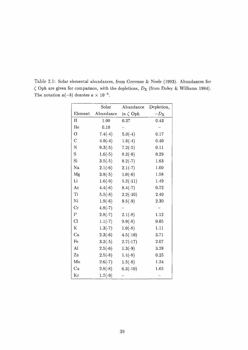
Table 2.1: Solar elemental abundances, from Grevesse & Noels (1993). Abundances for C Oph are given for comparison, with the depletions, Dx (from Du ley h Williams 1984). The notation &(—6 ) denotes a x 10“ .
ElementSolar
AbundanceAbundance in C Oph
Depletion,- D x
H 1 . 0 0 0.37 0.43He 0 . 1 0 - -
0 7.4(-4) 5.0(-4) 0.17C 4.0(-4) 1.6(-4) 0.40N 9.3(-5) 7.2(-5) 0 . 1 1
S 1.6(-5) 8 .2 (-6 ) 0.29Si 3.5(-5) 8.2(-7) 1.63Na 2 .1 (-6 ) 2.1(-7) 1 . 0 0
Mg 3.8(-5) 1 .0 (-6 ) 1.58Li 1.6(-9) 5.2(-ll) 1.49Ar 4.4(-6) 8.4(-7) 0.72Ti 5.5(-8) 2 .2 (-1 0 ) 2.40Ni 1.9(-6) 9.5(-9) 2.30Cr 4.8(-7) - -
P 2.8(-7) 2 .1 (-8 ) 1 . 1 2
Cl l.l(-7) 9.9(-8) 0.05K 1.3(-7) 1 .0 (-8 ) 1 . 1 1
Ca 2.3(-6) 4.5(-10) 3.71Fe 3.2(-5) 2.7(-17) 2.07Al 2.5(-6) 1.3 (-9) 3 j#Zn 2.5(-8) 1.4(-8) 0.25Mn 2.6(-7) 1.5(-8) 1.24Cu 2 .8 (-8 ) 6.3(-10) 1.65Kr 1.7(-9) - -
39
2.3 C hem ical networks
In the following sections we describe the im portant reactions in the hydrogen, car
bon, oxygen, nitrogen and sulphur networks.
2.3 .1 H ydrogen and d euterium ch em istry
Hydrogen is the most abundant element in the Universe and plays a very im portant
role in the chemistry of star forming regions. Molecular hydrogen is formed on the
surfaces of grains as described in section 2 .1 .2 , and is mainly destroyed by photodis
sociation with radiation of wavelengths near 1000 Â. The destructive mechanism
is a two step process. Firstly radiation is absorbed and the molecule is excited to
electronic states B and C from the ground electronic state X. The molecule will
then emit radiation and in about 1 0 % of these transitions the molecule falls into
the vibrational continuum of state X; i.e. the two atoms fly apart. The excitation
occurs within very narrow wavelength bands and the radiation at wavelengths out
side these bands do not destroy the molecule. W hen hydrogen molecules at the edge
of a cloud are destroyed this reduces the intensity of the radiation in the narrow
bands. Eventually the intensity is reduced to such an extent tha t the formation
of H2 is more rapid than the destruction. In this situation molecular hydrogen is
self-shielding against destructive radiation and further into the cloud it becomes the
main hydrogen carrier. H2 can also be destroyed via chemical reactions which is of
particular importance in dark clouds.
The cosmic ray ionization of H2 produces H2 ‘ in 97 % of the encounters (H"^
is created the remaining 3 % of the time). This then leads to the creation of the
im portant molecular ion H3 +,
H+ -f H2 -> H+ -f H. (2.2)
At the low tem peratures of dark, dense interstellar clouds, carbon and oxygen do
not react with H2 . Instead, reactions with initiate these chemistries. Hs" has
only recently been detected in the interstellar medium (McCall et al. 1998; Geballe
& Oka 1996).
40
Although H2 cannot readily be produced by gas phase reactions, HD arises from
gas phase reactions once H2 has formed (see Fig. 2.4). However, HD is destroyed
more rapidly by photodissociation than H2 as due to its lower abundance it does
not become self-shielding against the photodissociating radiation. We discuss the D
chemistry further in section 2.4.
2 .3 .2 C arbon chem istry
DenseCloud
DiffuseCloud
CH* CH
v.C*
CH,
CH»* C,H
C*.C Com plexH ydrocarbonsCBU* C.H,
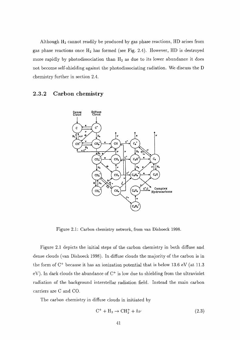
Figure 2.1: Carbon chemistry network, from van Dishoeck 1998.
Figure 2.1 depicts the initial steps of the carbon chemistry in both diffuse and
dense clouds (van Dishoeck 1998). In diffuse clouds the m ajority of the carbon is in
the form of C’*' because it has an ionization potential tha t is below 13.6 eV (at 11.3
eV). In dark clouds the abundance of C" is low due to shielding from the ultraviolet
radiation of the background interstellar radiation field. Instead the main carbon
carriers are C and CO.
The carbon chemistry in diffuse clouds in initiated by
C+ + H 2 CH+ + hu (2.3)
41
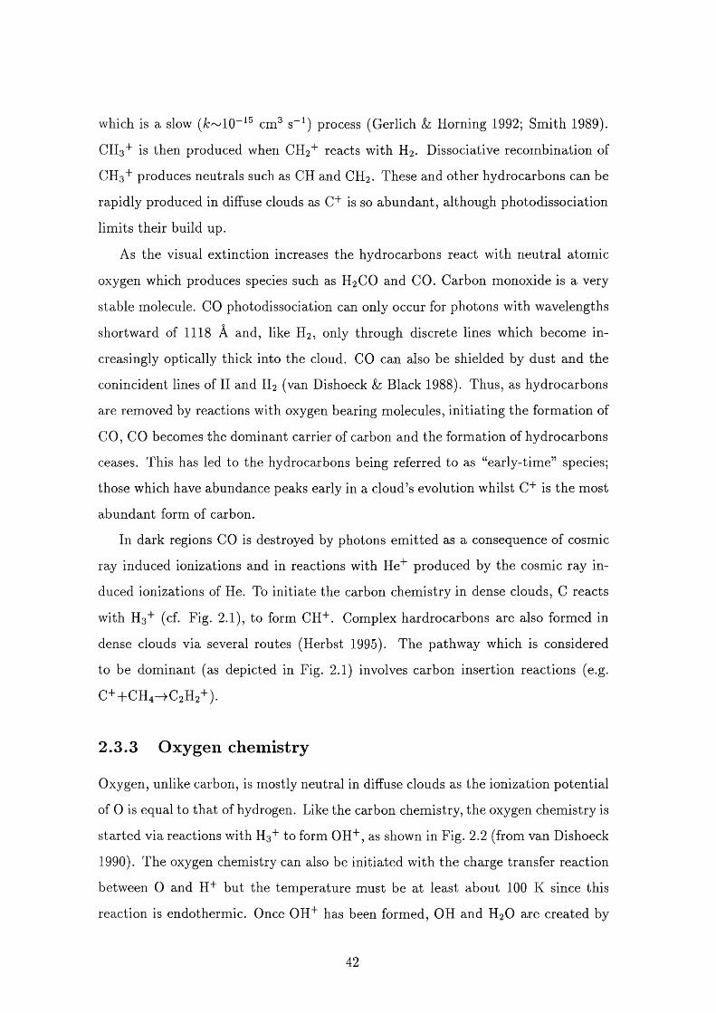
which is a slow cm^ s“ ) process (Gerlich & Horning 1992; Smith 1989).
CH3 + is then produced when CH2 ''' reacts with H2 . Dissociative recombination of
C E 3 + produces neutrals such as CH and CH2 . These and other hydrocarbons can be
rapidly produced in diffuse clouds as is so abundant, although photodissociation
limits their build up.
As the visual extinction increases the hydrocarbons react with neutral atomic
oxygen which produces species such as H2 CO and CO. Carbon monoxide is a very
stable molecule. CO photodissociation can only occur for photons with wavelengths
short ward of 1118 Â and, like H2 , only through discrete lines which become in
creasingly optically thick into the cloud. CO can also be shielded by dust and the
conincident lines of H and H2 (van Dishoeck k, Black 1988). Thus, as hydrocarbons
are removed by reactions with oxygen bearing molecules, initiating the formation of
CO, CO becomes the dominant carrier of carbon and the formation of hydrocarbons
ceases. This has led to the hydrocarbons being referred to as “early-tim e” species;
those which have abundance peaks early in a cloud’s evolution whilst C+ is the most
abundant form of carbon.
In dark regions CO is destroyed by photons em itted as a consequence of cosmic
ray induced ionizations and in reactions with He" produced by the cosmic ray in
duced ionizations of He. To initiate the carbon chemistry in dense clouds, C reacts
with H3 "'" (cf. Fig. 2.1), to form CH"^. Complex hardrocarbons are also formed in
dense clouds via several routes (Herbst 1995). The pathway which is considered
to be dominant (as depicted in Fig. 2.1) involves carbon insertion reactions (e.g.
C+d-CH4-^C2H2+).
2 .3 .3 O xygen chem istry
Oxygen, unlike carbon, is mostly neutral in diffuse clouds as the ionization potential
of 0 is equal to tha t of hydrogen. Like the carbon chemistry, the oxygen chemistry is
started via reactions with H3 " to form OH^, as shown in Fig. 2.2 (from van Dishoeck
1990). The oxygen chemistry can also be initiated with the charge transfer reaction
between 0 and H" but the tem perature must be at least about 100 K since this
reaction is endothermie. Once OH^ has been formed, OH and H2 O are created by
42
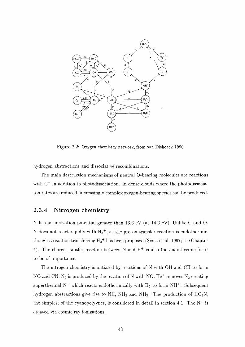
H.Hj
! HCO*l
Figure 2.2: Oxygen chemistry network, from van Dishoeck 1990.
hydrogen abstractions and dissociative recombinations.
The main destruction mechanisms of neutral 0-bearing molecules are reactions
with O'*" in addition to photodissociation. In dense clouds where the photodissocia-
ton rates are reduced, increasingly complex oxygen-bearing species can be produced.
2 .3 .4 N itro g en chem istry
N has an ionization potential greater than 13.6 eV (at 14.6 eV). Unlike C and O,
N does not react rapidly with H3 +, as the proton transfer reaction is endothermie,
though a reaction transferring H2 ^ has been proposed (Scott et al. 1997; see Chapter
4). The charge transfer reaction between N and H"'" is also too endothermie for it
to be of importance.
The nitrogen chemistry is initiated by reactions of N with OH and CH to form
NO and CN. N2 is produced by the reaction of N with NO. He’*’ removes N2 creating
supertherm al N+ which reacts endothermically with H2 to form NH"*". Subsequent
hydrogen abstractions give rise to NH, NH2 and NH3 . The production of HC3 N,
the simplest of the cyanopolyynes, is considered in detail in section 4.1. The N+ is
created via cosmic ray ionizations.
43
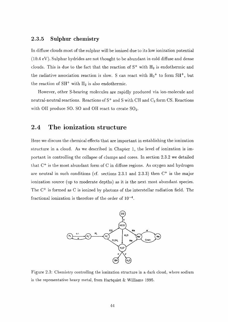
2 .3 .5 Sulphur chem istry
In diffuse clouds most of the sulphur will be ionized due to its low ionization potential
(10.4 eV). Sulphur hydrides are not thought to be abundant in cold diffuse and dense
clouds. This is due to the fact that the reaction of S'*" with H2 is endothermie and
the radiative association reaction is slow. S can react with to form SH"*", but
the reaction of SH* with Hg is also endothermie.
However, other S-bearing molecules are rapidly produced via ion-molecule and
neutral-neutral reactions. Reactions of S" and S with CH and C2 form CS. Reactions
with OH produce SO. SO and OH react to create SO2 .
2.4 T he ionization structure
Here we discuss the chemical effects tha t are im portant in establishing the ionization
structure in a cloud. As we described in Chapter 1 , the level of ionization is im
portant in controlling the collapse of clumps and cores. In section 2.3.2 we detailed
th a t C" is the most abundant form of C in diffuse regions. As oxygen and hydrogen
are neutral in such conditions (cf. sections 2.3.1 and 2.3.3) then C"*" is the major
ionization source (up to moderate depths) as it is the next most abundant species.
The C" is formed as C is ionized by photons of the interstellar radiation field. The
fractional ionization is therefore of the order of 1 0 “ ' .
CO
HOC*
CO Na
Na' NaG rainNa
OH H,0
Figure 2.3: Chemistry controlling the ionization structure in a dark cloud, where sodium
is the representative heavy metal, from Hartquist & Williams 1995.
44
At increasing visual extinctions more of the carbon will be neutral (see section
2.3.2). W hen A y>5 mag, the major source of ionization is provided by cosmic rays
(cf. section 1.1). In section 2.3.1 we saw how the cosmic ray ionization of Hg leads
to the formation of In dense cores the most abundant molecular ion is often
HCO"^, formed when reacts with CO. The removal rates of HCO'*' are impor
tan t in establishing the ionization level in dense cores. HCO'*' can dissociatively
recombine with an electron to form CO or react with water to form H3 O"*". Alter
natively, it can undergo charge transfer reactions with neutral metallic ions, such as
Na or Mg (as HgO" does too). This last pathway is extremely im portant as Na"*"
and Mg'*" recombine slowly with electrons, at a rate tha t is ~10^ times slower than
th a t for HCO"^; these species are also relatively unreactive at low tem peratures.
Hence, these species are long lived and help to m aintain high ionization levels in the
cloud. The dominant removal mechanism of metallic ions are grain collisions, where
the charge is transferred to the grain. The fractional ionization in dense cores is
around 1 0 “®; it increases as v T (the cosmic ray ionization rate) and decreases with
the number density as In dense cores the most abundant ions are the metallic
atomic ions, with HCO"*" being the next most im portant, with an abundance tha t
is 10-100 times lower. Figure 2.3 depicts the chemistry tha t controls the ionization
level in a dark cloud (Hartquist & Williams 1995).
The fractional ionization is im portant in controlling the evolution of clumps
and cores, and depends on the cosmic ray ionization rate. The rate of cosmic
ray ionization is an im portant yet unknown param eter for interstellar chemistry.
In Fig. 2.4 we depict the formation and removal mechanisms for HD (Hartquist
& Williams 1995). The cosmic ray ionization rate can be inferred for a diffuse
cloud using the measured HD abundance once the cloud density and tem perature
structure, the cosmic deuterium abundance and the photodissociation rate of HD
are known. Typically, the derived value is around 10“ ^ s“ (Hartquist & Williams
1995).
In dark clouds the D chemistry can again be used in attem pts to establish the
ionization level. In Fig. 2.5 we display the chemistry th a t determines the DCO"*"
to HCO'*' abundance (Hartquist & Williams 1995). Observations of the DCO"*" to
45
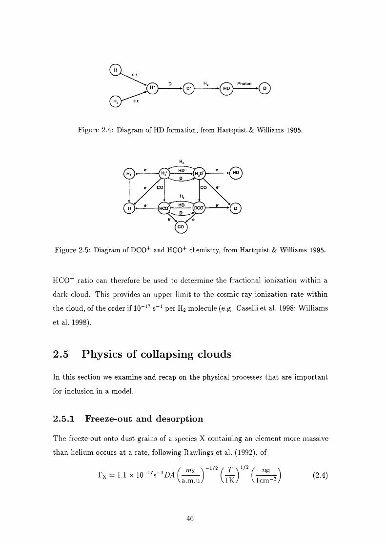
c.r.
c.r.
Photon
Figure 2.4: Diagram of HD formation, from Hartquist & Williams 1995.
HD HD
CO 00
HD000“HOC"
CO
Figure 2.5: Diagram of DCO"*" and HCO"*" chemistry, from Hartquist & Williams 1995.
HCO"*" ratio can therefore be used to determine the fractional ionization within a
dark cloud. This provides an upper limit to the cosmic ray ionization rate within
the cloud, of the order if 10“ ^ s"^ per H2 molecule (e.g. Caselli et al. 1998; Williams
et al. 1998).
2.5 P hysics o f collapsing clouds
In this section we examine and recap on the physical processes tha t are im portant
for inclusion in a model.
2 .5 .1 Freeze-out and d esorption
The freeze-out onto dust grains of a species X containing an element more massive
than helium occurs at a rate, following Rawlings et al. (1992), of
a.m.u VlK. lcm~^(2.4)
46
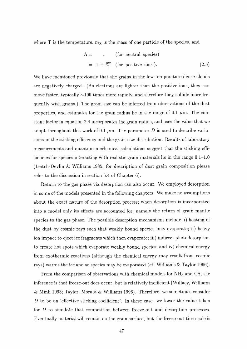
where T is the tem perature, mx is the mass of one particle of the species, and
A = 1 (for neutral species)
= 1 + ^ (for positive ions.). (2.5)
We have mentioned previously that the grains in the low tem perature dense clouds
are negatively charged. (As electrons are lighter than the positive ions, they can
move faster, typically ~ 1 0 0 times more rapidly, and therefore they collide more fre
quently with grains.) The grain size can be inferred from observations of the dust
properties, and estimates for the grain radius lie in the range of 0.1 fim. The con
stant factor in equation 2.4 incorporates the grain radius, and uses the value tha t we
adopt throughout this work of 0.1 //m. The param eter D is used to describe varia
tions in the sticking efficiency and the grain size distribution. Results of laboratory
measurements and quantum mechanical calculations suggest tha t the sticking effi
ciencies for species interacting with realistic grain materials lie in the range 0 .1 - 1 . 0
(Leitch-Devlin & Williams 1985; for description of dust grain composition please
refer to the discussion in section 6.4 of Chapter 6 ).
R eturn to the gas phase via desorption can also occur. We employed desorption
in some of the models presented in the following chapters. We make no assumptions
about the exact nature of the desorption process; when desorption is incorporated
into a model only its effects are accounted for; namely the return of grain m antle
species to the gas phase. The possible desorption mechanisms include, i) heating of
the dust by cosmic rays such that weakly bound species may evaporate; ii) heavy
ion impact to eject ice fragments which then evaporate; iii) indirect photodesorption
to create hot spots which evaporate weakly bound species; and iv) chemical energy
from exothermic reactions (although the chemical energy may result from cosmic
rays) warms the ice and so species may be evaporated (cf. Williams &: Taylor 1996).
From the comparison of observations with chemical models for NHg and CS, the
inference is tha t freeze-out does occur, but is relatively inefficient (Willacy, Williams
& Minh 1993; Taylor, M orata & Williams 1996). Therefore, we sometimes consider
D to be an ‘effective sticking coefficient’. In these cases we lower the value taken
for D to simulate tha t competition between freeze-out and desorption processes.
Eventually material will remain on the grain surface, but the freeze-out timescale is
47

enhanced. By this approach we can explore the competing effects of accretion and
desorption on the chemistry.
2 .5 .2 C ollapse
In some models ng was taken to be fixed as was A y - In other models hh was
assumed to increase from an initial level, hho, to account for collapse via free fall. In
these cases, uh was taken to vary, following Rawlings et al. (1992) (and references
therein), as
1 / 31 / 4 \ 1 / 3 r r / \ 1 / 3 n 1 / 2
1 2 4 . Gm^nn n r , _ i
"Ho(2 .6)
dt \ n n o J [
where t is time, G is the gravitational constant, m H =l a.m .u., and B is a constant
(for gravitational free fall B = I). We can consider B to be a retardation factor. If
magnetic effects and rotational support were to be accounted for then B would have
a value <1.0 tha t is density dependent. After uh reached some chosen value,
it was kept constant. In models with varying hh the value oi A y was also taken to
vary with time.
2.6 T he m odel
In this section we provide a recipe for constructing a model by which the time-
dependent abundances of a chosen set of species can be followed. For all of the
chemical and dynamical models tha t are presented in the following Chapters (3,
4, 6 and 7) we used the UMIST rate file (Millar, Farquhar & Willacy 1997) as
the source of reaction rate coefficients and rates. The UMIST database contains
ra te coefficients and rates for 3864 reactions between 395 species composed of 12
elements. The im portant reactions for both interstellar and circumstellar chemistries
are included. The types of reactions tha t are incorporated are neutral-neutral, ion-
neutral, radiative electron attachm ent, dissociative recombination, ionizations due
to cosmic rays, photoreactions driven by the interstellar ultraviolet radiation field
and cosmic ray induced photoreactions. The file gives values for the variables a .
48
(3 and 7 for each reaction. These are then used to calculate k, the reaction rate
coefficient.
For two-body reactions,
^ “ ( s m ) (2.7)
where T is the gas kinetic tem perature. For interstellar photoreactions
A; = (2.8)
where a represents the rate in the unshielded UV radiation field and 7 is used to
account for the extinction of the UV radiation by dust particles. The Draine (1978)
UV radiation field was used to determine a.
For direct cosmic ray ionizations
k = a s “ (2.9)
and for cosmic ray induced photoreactions
k = t F V - s - ' (2.10)( 1 - to)
where w is the grain albedo in the far UV (typically 0.6 at 150 nm) and 7 is the
probability per cosmic ray ionization that the appropriate photoreaction occurs (we
use w=0.5 and 7 = 1 in all models). For both these types of reactions the rates
are given for a ‘standard’ value for the interstellar cosmic ray ionization rate of
1.3x10“ ^ s~T Any of the above parameters can be rescaled appropriately in the
model.
As the physical characteristics of a star forming region evolve and change, so too
do the relevant chemical processes (as we described in section 2.3). Different atomic
and molecular species are im portant in different regions and at different epochs. In
order to allow for this complexity in the models, we must specify a species set tha t is
sufficiently comprehensive. This set does not contain all those that are available in
the UMIST database. There are several reasons why the use of a lim ited species set
is preferred. Firstly the computational overheads are reduced. The second reason
is th a t we still do not understand the chemistries of many of the species contained
in the UMIST database, and their addition to a model increases the uncertainties
49
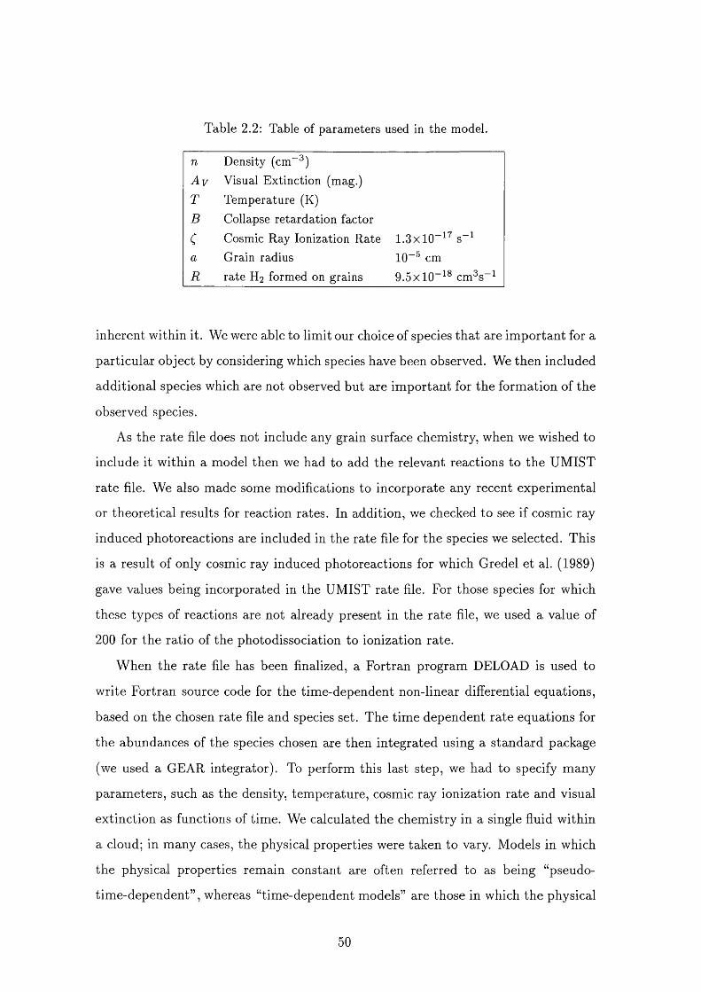
Table 2.2: Table of parameters used in the model.
n Density (cm“ )A y Visual Extinction (mag.)T Temperature (K)B Collapse retardation factor
c Cosmic Ray Ionization Rate 1.3x10“ ^ s"ia Grain radius 1 0 “ cmR rate H2 formed on grains 9.5x10“ ® cm^s“ ^
inherent within it. We were able to limit our choice of species tha t are im portant for a
particular object by considering which species have been observed. We then included
additional species which are not observed but are im portant for the formation of the
observed species.
As the rate file does not include any grain surface chemistry, when we wished to
include it within a model then we had to add the relevant reactions to the UMIST
rate file. We also made some modifications to incorporate any recent experimental
or theoretical results for reaction rates. In addition, we checked to see if cosmic ray
induced photoreactions are included in the rate file for the species we selected. This
is a result of only cosmic ray induced photoreactions for which Gredel et al. (1989)
gave values being incorporated in the UMIST rate file. For those species for which
these types of reactions are not already present in the rate file, we used a value of
2 0 0 for the ratio of the photodissociation to ionization rate.
W hen the rate file has been finalized, a Fortran program DELOAD is used to
write Fortran source code for the time-dependent non-linear differential equations,
based on the chosen rate file and species set. The time dependent rate equations for
the abundances of the species chosen are then integrated using a standard package
(we used a GEAR integrator). To perform this last step, we had to specify many
param eters, such as the density, tem perature, cosmic ray ionization rate and visual
extinction as functions of time. We calculated the chemistry in a single fluid within
a cloud; in many cases, the physical properties were taken to vary. Models in which
the physical properties remain constant are often referred to as being “pseudo-
tim e-dependent” , whereas “time-dependent models” are those in which the physical
50
properties vary. There are many parameters other than those listed above tha t
m ust be specified (e.g. the grain size for calculation of freeze-out rates), and in
Table 2.2 we present a compendium of these with their adopted values. For the
models th a t we present in the following chapters these are the adopted values unless
stated otherwise.
51
Chapter 3
Ionization structure and a critical
visual extinction for turbulent
supported clumps
In Chapter 1 we described the types of objects arising in different evolutionary
stages in star forming regions. In section 1.2 we considered the structures of CMC
complexes, and focused on one object, the Rosette Molecular Cloud. We described
how translucent clumps in GMCs are initially supported by magnetic fields and
turbulence. In this chapter we examine the initial support and the collapse of
translucent clumps. Such collapse results in the formation of dense cores.
3.1 Introduction
In their work on the clumpy structure of the Rosette Molecular Cloud (RMC),
W illiams, Blitz & Stark (1995) identified seven star forming clumps, none of which
has an estim ated ^^CO column density, TV(^^CO), of less than 10 ® cm “ . From
Pig. 3.1 (Fig. 2 1 from Williams, Blitz & Stark 1995) it appears tha t eight or nine
other clumps have 7V(^^CO)>10^^ cm “ but contain no stars. The estim ated values
of A^(^^CO) for the star forming clumps, with one exception, vary by only a factor
of about 2, and the estim ated masses vary by a factor of about 7 (cf. section 1.2).
W hile one could argue that the Williams et al. (1995) data point to the existence
52
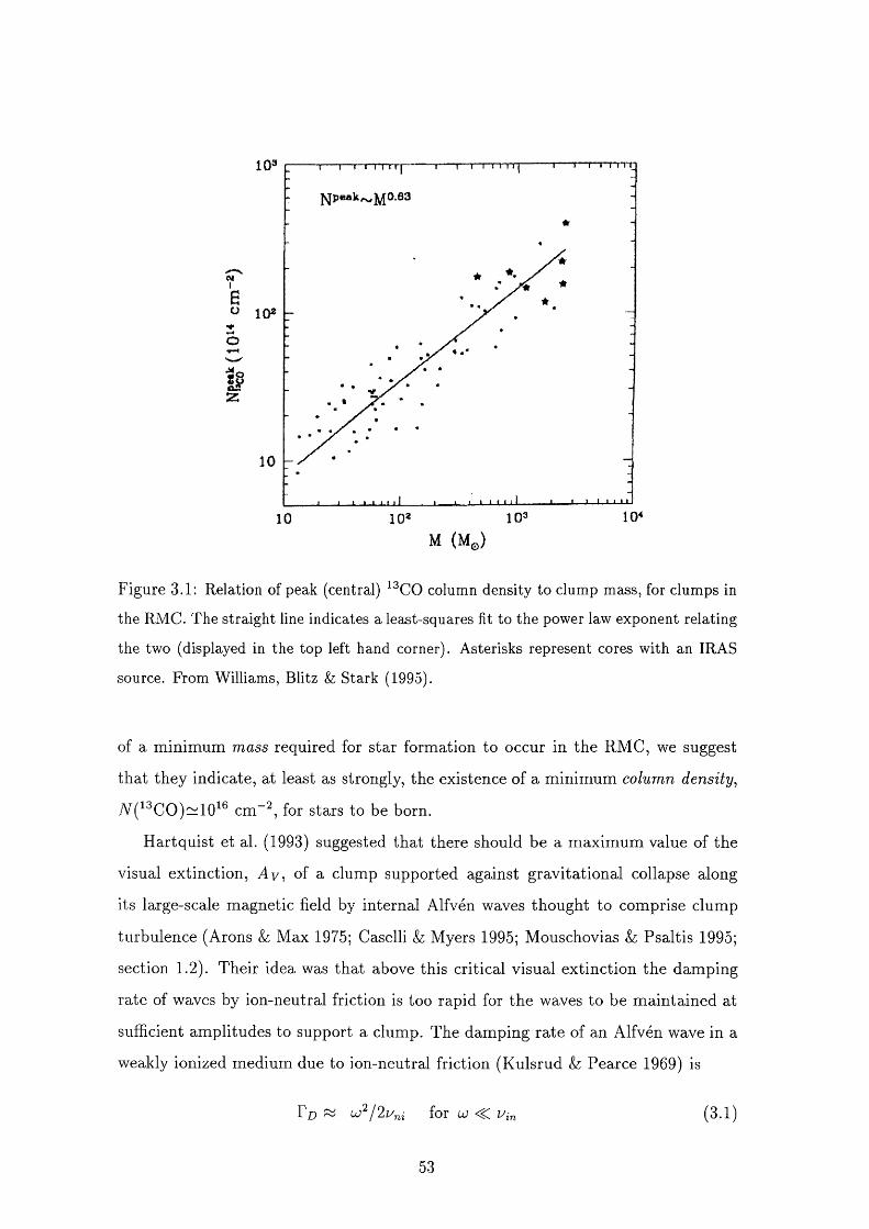
<4I
o
10M (Me)
Figure 3.1: Relation of peak (central) column density to clump mass, for clumps in
the RMC. The straight line indicates a least-squares fit to the power law exponent relating
the two (displayed in the top left hand corner). Asterisks represent cores with an IRAS
source. From Williams, Blitz & Stark (1995).
of a minimum mass required for star formation to occur in the RMC, we suggest
that they indicate, at least as strongly, the existence of a minimum column density,
A^(^^CO)~1 0 ® cm“ , for stars to be born.
H artquist et al. (1993) suggested tha t there should be a maximum value of the
visual extinction, Ay, of a clump supported against gravitational collapse along
its large-scale magnetic field by internal Alfven waves thought to comprise clump
turbulence (Arons & Max 1975; Caselli & Myers 1995; Mouschovias & Psaltis 1995;
section 1.2). Their idea was that above this critical visual extinction the damping
rate of waves by ion-neutral friction is too rapid for the waves to be m aintained at
sufficient amplitudes to support a clump. The damping rate of an Alfven wave in a
weakly ionized medium due to ion-neutral friction (Kulsrud & Pearce 1969) is
Ff) py up'1 for LÜ i i (3.1)
53
Fd > W for Vni < W < Uin (3.2)
Fd ~ Kn/2 for w > z/m, (3.3)
where uj is the angular frequency of the wave, Uin is the inverse stopping tim e of an
ion by the neutrals, and Uni is the inverse stopping tim e of a neutral by the ions.
For ions of mass m* colliding with H2 (Osterbrock 1961)
1.8 X 10-^ s - ' ( ----- 1 (3.4)\ m i + mHs) Vcm
and
( ^ ) (“^ ) (3 5)where is the mass of an H2 molecule and rii is the number density of ions.
The value of rii decreases with visual extinction. As discussed in section 2.4, the
fractional ionization in the outer regions of a molecular cloud is generally at least
10"4 because the gas phase carbon remains primarily in C"*" due to the efficiency of
photodissociation and photoionization processes, whereas the fractional ionization is
several orders of magnitude lower than this in dark regions, in which the ionization
is due almost entirely to cosmic rays. From equations 3.1 and 3.4 one sees clearly
tha t the damping rate of waves in which the ion-neutral motions are well-coupled
declines with extinction because it increases as the inverse of the number density
of ions. Hi, (and proportionally to the square of the frequency). Recent numerical
simulations of wave behaviour in self-gravitating clumps show tha t nonlinear magne-
tohydrodynamic waves can, in fact, support such clumps against collapse (Gammie
& Ostriker 1996). In view of its relevance to wave damping in clumps, it is now par
ticularly timely to return to the issue of the behaviour of the fractional ionization,
Xi {x i= n i lnu i where ny is the number density of hydrogen nuclei), as a function of
the visual extinction. Ay-
The view taken by Hartquist et al. (1993) and by us in this work, is, thus, tha t
much of the molecular material in giant molecular clouds is translucent to radiation
and tha t photoionization affects its fractional ionization, which in turn plays a role
in determining the rate at which m aterial collapses. This view is one th a t has much
in common with that adopted by McKee (1989) who argued tha t star formation
regulates itself because the births of stars lead to the production of radiation which
54
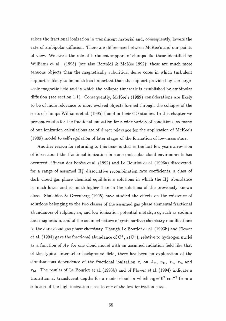
raises the fractional ionization in translucent m aterial and, consequently, lowers the
rate of ambipolar diffusion. There are differences between McKee’s and our points
of view. We stress the role of turbulent support of clumps like those identified by
Williams et al. (1995) (see also Bertoldi & McKee 1992); these are much more
tenuous objects than the magnetically subcritical dense cores in which turbulent
support is likely to be much less im portant than the support provided by the large-
scale magnetic held and in which the collapse timescale is established by ambipolar
diffusion (see section 1 .1 ). Consequently, McKee’s (1989) considerations are likely
to be of more relevance to more evolved objects formed through the collapse of the
sorts of clumps Williams et al. (1995) found in their CO studies. In this chapter we
present results for the fractional ionization for a wide variety of conditions; so many
of our ionization calculations are of direct relevance for the application of McKee’s
(1989) model to self-regulation of later stages of the formation of low-mass stars.
Another reason for returning to this issue is tha t in the last few years a revision
of ideas about the fractional ionization in some molecular cloud environments has
occurred. Pineau des Forêts et al. (1992) and Le Bourlot et al. (1993a) discovered,
for a range of assumed dissociative recombination rate coefficients, a class of
dark cloud gas phase chemical equilibrium solutions in which the abundance
is much lower and Xi much higher than in the solutions of the previously known
class. Shalabiea & Greenberg (1995) have studied the effects on the existence of
solutions belonging to the two classes of the assumed gas phase elemental fractional
abundances of sulphur, a g, and low ionization potential metals, ojm, such as sodium
and magnesium, and of the assumed nature of grain surface chemistry modifications
to the dark cloud gas phase chemistry. Though Le Bourlot et al. (1993b) and Flower
et al. (1994) gave the fractional abundance of C" , a;(C"^), relative to hydrogen nuclei
as a function of Ay for one cloud model with an assumed radiation field like tha t
of the typical interstellar background field, there has been no exploration of the
simultaneous dependence of the fractional ionization X{ on A y, tth, Tg, xs\ and
ZM- The results of Le Bourlot et al. (1993b) and of Flower et al. (1994) indicate a
transition at translucent depths for a model cloud in which nH = 1 0 cm“ from a
solution of the high ionization class to one of the low ionization class.
55
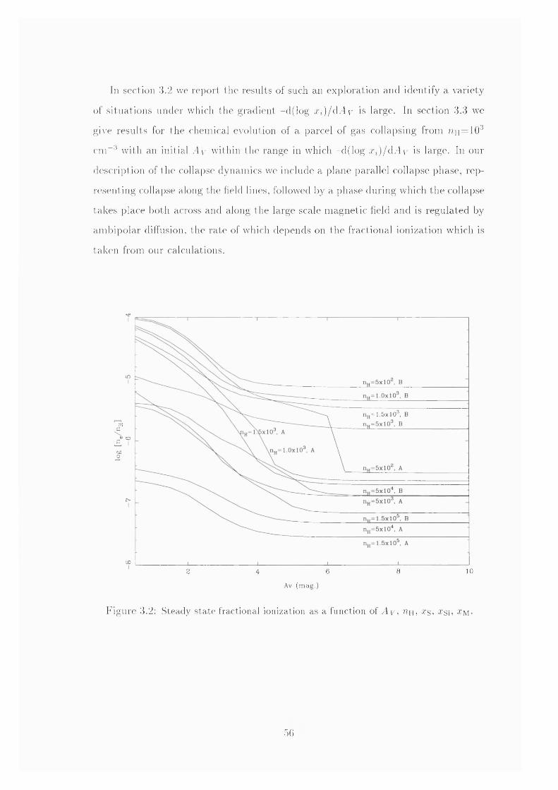
In section 3.2 we report the results of such an exploration and identify a variety
of situations under which the gradient -d(log a\)/d.4 y is large. In section 3.3 we
give results for the chemical evolution of a parcel of gas collapsing from 77h = 1 0
cm“ with an initial A y within the range in which -d(log Xi ) /dA\ / is large. In our
description of the collapse dynamics we include a plane parallel collapse phase, rep
resenting collapse along the held lines, followed by a phase during which the collapse
takes place both across and along the large scale magnetic held and is regulated by
ambipolar diffusion, the rate of which depends on the fractional ionization which is
taken from our calculations.
= 1 5 x 1 0 ^ ,
Xc
COcoflo
COI 8 102 64
Av (mag.)
Figure 3.2: Steady state fractional ionization as a function of 4 y , nji, xs, .x’si, x m -
56
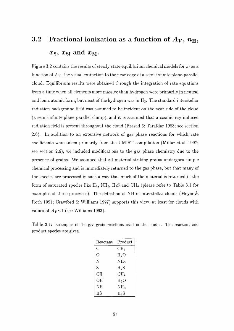
3.2 Fractional ionization as a function o f Ay, uh?
æs, æsi and ^ m -
Figure 3.2 contains the results of steady state equilibrium chemical models for Xi as a
function of Ay, the visual extinction to the near edge of a semi-infinite plane-parallel
cloud. Equilibrium results were obtained through the integration of rate equations
from a tim e when all elements more massive than hydrogen were prim arily in neutral
and ionic atomic form, but most of the hydrogen was in H2 . The standard interstellar
radiation background field was assumed to be incident on the near side of the cloud
(a semi-infinite plane parallel clump), and it is assumed that a cosmic ray induced
radiation field is present throughout the cloud (Prasad &: Tarafdar 1983; see section
2.6). In addition to an extensive network of gas phase reactions for which rate
coefficients were taken primarily from the UMIST compilation (Millar et al. 1997;
see section 2 .6 ), we included modifications to the gas phase chemistry due to the
presence of grains. We assumed that all material striking grains undergoes simple
chemical processing and is immediately returned to the gas phase, but tha t many of
the species are processed in such a way that much of the m aterial is returned in the
form of saturated species like H2 , NH3 , H2 S and CH4 (please refer to Table 3.1 for
examples of these processes). The detection of NH in interstellar clouds (Meyer &
Roth 1991; Crawford & Williams 1997) supports this view, at least for clouds with
values of A y ~ l (see Williams 1993).
Table 3.1; Examples of the gas grain reactions used in the model. The reactant and product species are given.
Reactant ProductC CH40 H2ON NH3
S H2S
CH CH4OH H2ONH NH3
HS H2S
57
Table 3.2: Fractional elemental abundances relative to nn-
A‘dark”
B“diffuse”
He 7 X 1 0 - 2 7 X 1 0 - 2
C 1 X lQ-4 1 X 10⁻⁴N 2 X 10⁻⁵ 2 X 10-50 2 X 10⁻⁴ 2 X 10⁻⁴s 2 X 1 0 - 8 3 X 1 0 - 8
Si 7 X 10⁻⁹ 1 X 1 0 - 8
M 2 X 10⁻⁷ 1 X 1 0 - 8
The rate at which particles of neutral species X were assumed to strike grain
surfaces is
3.5 X 10“ ^®s~^(mx/amu)~^/^(nH/cm^), (3.6)
where we used equation 2.4 and took the tem perature to be 10 K. The charged
particles were assumed to strike grains (mostly negatively charged) at a rate th a t is
18 times larger (following Rawlings et al. 1992; see section 2.5.1). All ions striking
grains were assumed to return to the gas phase as neutral atoms and molecules. The
cosmic ray ionization rate was taken to be 1.3x10“ ^ s"^ (cf. section 2.6). Molecular
hydrogen is self-shielding, and CO was assumed to be sufficiently self-shielded and
shielded by Hg that only photons produced as a consequence of cosmic ray induced
ionization are im portant for its photodissociation.
The results in Fig. 3.2 are for the two sets of assumed gas phase elemental
abundances given in Table 3.2 (see Shalabiea & Greenberg 1995). Set A is similar
to th a t required in many cases to reproduce chemical abundances measured for
dark cores while Set B, which has higher fractional abundances of low ionization
potential elements, is selected because diffuse clouds have much higher gas phase
fractional abundances of those species than dark cores. The issue of the mechanisms
th a t control the depletion of the elements with low ionization potentials is unclear
at present (hence the parametrised approach adopted here), but is one of major
im portance for the chemistry of star formation, as the results in this chapter indicate.
Inspection of Fig. 3.2 shows that for nH=5xlO^ cm “ (typical of the RMC
58
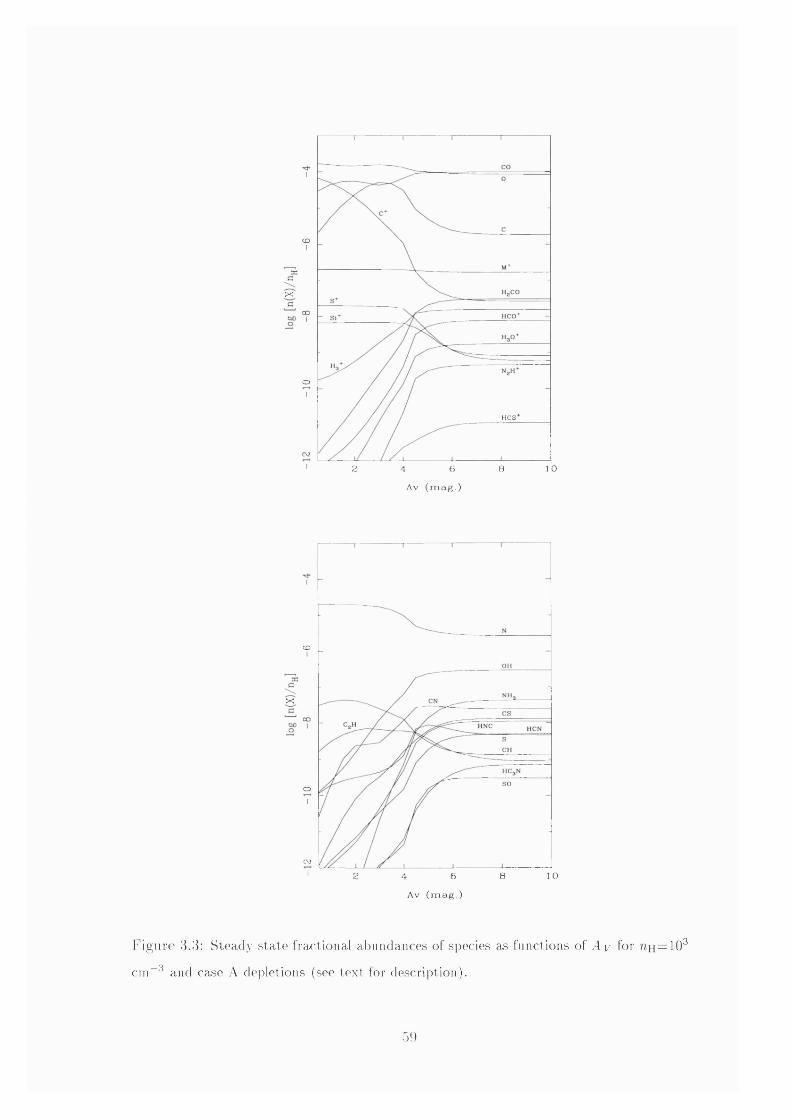
I
CDI
X
oI
HCS*
I 2 6 B 104
Av ( m a g . )
I
CO
X
oI
cvI 8 102 4 6
Av ( m a g . )
I 'ig iire 3.3: S teady s ta te fractional abundances of species as functions of A y for = 1 0
cni“ and case A depletions (see text for description).
59
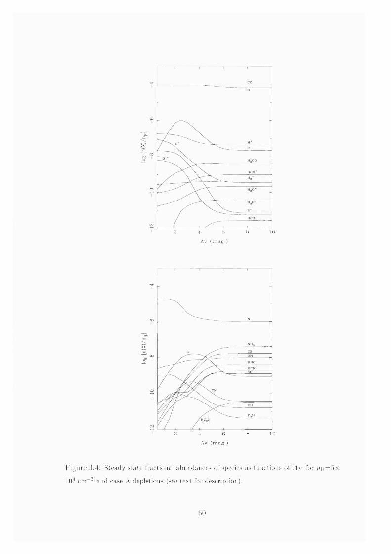
I
CDI
X
o
8 1 02 64
Av ( m a g . )
COI
X
30:
I
CgHH C ,N
I 2 8 104 6
Av ( m a g . )
I ' ig m e 3.4: Steady s ta te fractional abundances of species as functions of .4 v for 7? n = 5 x
1 0 * cin“ and case A depletions (see text for description).
60
clumps) the gradient -d(Iog X i ) ld A v reaches a maximum in the range A y ^ 2 - 3
for Set B depletions and a local maximum for the same range of A y for Set A
depletions. For Set A depletions and nH=500 cm“ a much higher value of -d(log
X i ) / d A y exists for a very small range of high values of A y where a chemical phase
transition occurs, but the high value of -d(log X i ) / à A y in the range of Ay%2-3
for Set A as well as Set B depletions, is no doubt im portant for the ion-neutral
damping of turbulence supporting RMC-like clumps. We can calculate the visual
extinction tha t corresponds to the critical measured value of the column den
sity for RMC clumps (which is 1x10^® cm“^). Taking (1x10^® cm “ ^ /2 ) to be half
the critical measured value of the column density from the edge of an RMC
clump to its centre, n(^^CO)/nH=l x 10“® (Williams et al. 1995), and the standard
conversion of the hydrogen nuclei column density to Ay (Savage & Mathis 1979),
where
A y = 5 X 10” ^ mag (H nuclei cm“^)“ ,
we find tha t the critical visual extinction from the centre of an RMC clump to its
edge is 2.5, in agreement with the regime of maximum -d(log X i ) / d A y for ne =500
cm “ identified in our calculations.
This agreement between the minimum A y for the existence of stars and the A y
range of extreme logarithmic derivative of the fractional ionization is in harmony
with the suggestion (Hartquist et al. 1993) that the minimum A y for the existence
of stars is associated with a maximum Ay at which turbulent support of clumps is
effective in preventing collapse along magnetic field lines.
Results for X{ are also given in Fig. 3.2 for a range of values of nn- As stated
above, the ion-neutral damping rate of a wave of sufficiently low frequency is propor
tional to the square of the wave frequency divided by A comparison of the Set
A graphs for riH=5xlO^ cm“® and nH=5xlO'^ cm~^ shows tha t at A y =3, the values
of Hi for the two model clumps are roughly equal. Therefore the ion-neutral wave
damping rate for a given frequency has roughly the same functional dependence on
A y, implying tha t even for dense cores the Ay dependence of X{ must be taken into
account in any consideration of wave propagation.
Unfortunately, the depletions in nH~10® cm“ clumps like those in the RMC are
61
unknown; while the set B depletions are closer to those measured in absorption line
studies of diffuse interstellar clouds, the set A depletions are typical of those required
for dense core chemical models to reproduce measured fractional abundances of
species. A key outstanding set of questions in the chemistry and dynamics of star
formation is tha t which concerns the nature of depletion and desorption processes
of elemental S, Si, Fe, Na and Mg in translucent and dark clouds; it is remarkable
th a t those elements are so much more depleted in many regions than O, C and N
but still have high enough gas phase abundances in those regions for their presence
in the gas phase to have significant chemical consequences (see Chapters 6 and 7).
We therefore present further results from the chemical calculation yielding a: , as
information about the depth dependence of many other chemical abundances is also
provided. Figures 3.3 and 3.4 give results for the fractional abundances of a number
of species for a nH =lxlO ^ cm“ . Set A clump and a nH=5xlO^ cm“ . Set A dense
core. The model results indicate that other than CO emissions only CH and OH
emissions are likely to be detectable towards RMC clumps with nn^lOOO cm “ , and
also tha t the CH, OH and CO fractional abundances are not sensitive to xs, xsi
and Xm, making the inference of the values of those depletions in such objects a
very difficult goal. Unfortunately, values of CH and OH abundances are difficult to
infer observationally. A comparison of Fig. 3.4 with Fig. 3.3 shows tha t M’*' is the
dominant ion throughout a dense core, while C" is the dominant ion over a large
range of Ay in t2h = 1 0 0 0 cm“ gas. Unlike RMC-type clumps with A y =3, a dense
core with A y =3 and nn^SxlO'^ cm“ is likely to produce observable emissions in a
num ber of molecular species other than CH, OH and CO, including HCO'*', N2H'*',
H2CO, ON, NH3, CS and possibly H NC and H C N.
Though our results are more extensive than those of previous authors, they are in
harmony with those of Le Bourlot et al. (1993b), Flower et al. (1994), and Shalabiea
& Greenberg (1995) in regions where comparisons can be made.
62
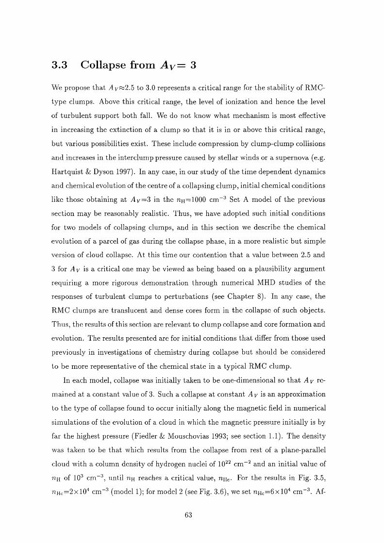
3.3 C ollapse from A y = 3
We propose that to 3.0 represents a critical range for the stability of RMC-
type clumps. Above this critical range, the level of ionization and hence the level
of turbulent support both fall. We do not know what mechanism is most effective
in increasing the extinction of a clump so tha t it is in or above this critical range,
but various possibilities exist. These include compression by clump-clump collisions
and increases in the interclump pressure caused by stellar winds or a supernova (e.g.
H artquist & Dyson 1997). In any case, in our study of the tim e dependent dynamics
and chemical evolution of the centre of a collapsing clump, initial chemical conditions
like those obtaining at A y = S in the nn^lOOO cm “ Set A model of the previous
section may be reasonably realistic. Thus, we have adopted such initial conditions
for two models of collapsing clumps, and in this section we describe the chemical
evolution of a parcel of gas during the collapse phase, in a more realistic but simple
version of cloud collapse. At this time our contention tha t a value between 2.5 and
3 for Ay is a critical one may be viewed as being based on a plausibility argument
requiring a more rigorous demonstration through numerical MHD studies of the
responses of turbulent clumps to perturbations (see Chapter 8 ). In any case, the
RMC clumps are translucent and dense cores form in the collapse of such objects.
Thus, the results of this section are relevant to clump collapse and core formation and
evolution. The results presented are for initial conditions th a t differ from those used
previously in investigations of chemistry during collapse but should be considered
to be more representative of the chemical state in a typical RMC clump.
In each model, collapse was initially taken to be one-dimensional so th a t A y re
mained at a constant value of 3. Such a collapse at constant A y is an approximation
to the type of collapse found to occur initially along the magnetic field in numerical
simulations of the evolution of a cloud in which the magnetic pressure initially is by
far the highest pressure (Fiedler & Mouschovias 1993; see section 1 .1). The density
was taken to be that which results from the collapse from rest of a plane-parallel
cloud with a column density of hydrogen nuclei of 1 0 ^ cm “ and an initial value of
72H of 10 cm“ , until nn reaches a critical value, uhc- For the results in Fig. 3.5,
?2hc= 2 x I 0 ' cm“ (model I); for model 2 (see Fig. 3.6), we set t2 hc= 6 x I 0 cm “ . Af-
63
ter nH = 7 Hc5 collapse was taken to occur at a rate slower than the spherical free-fall
timescale, given by equation 2 .6 , by a factor of
in harmony with the object being magnetically subcritical (i.e., supported by the
magnetic field) and subsequent collapse taking place at a rate controlled by ambipo
lar diffusion (Mouschovias 1987). For nn>nHc we set
Ay = 0.5 + 2.5 1—y (3.8)\ m c /
in the models, where an interclump medium was assumed to be responsible for the
constant contribution to the Ay- For the purposes of our calculation we assumed
th a t the collapse halts at a density of 3x 1 0 ® cm”®, after which the cloud was treated
as static. The models incorporate the grain-modified gas phase chemistry described
in the previous section. Note that this implies tha t freeze-out is off-set by desorption.
Results are given for both models in Table 3.3, where ti and t 2 are the times since
collapse began in the cases nHc=2 xlT^ cm ”® (model 1 ) and the y%Hc=6 x 1 0 cm ”®
(model 2), respectively. Here, Ti(X) and X2 (X) denote the fractional abundance of
species X relative to nn in the two models (z i(X )= n i(X )/ nn), where i represents
ions. These exploratory calculations of chemical evolution are the first in which
the initial collapse is plane parallel along the held lines, setting up conditions for
multidimensional collapse moderated realistically by ambipolar diffusion.
Note tha t the desorption of unsaturated species is here assumed to eject all
molecules arriving at grain surfaces (see Williams & Taylor 1996), so tha t the abun
dances in Figs. 3.5 and 3.6 are not constrained by freeze-out. Consequently, the
late-tim e peaks in hydrocarbons and related species (see Chapter 4) are not evi
dent. In fact, the results in Figs. 3.5 and 3.6 are similar in character to those of
Howe et al. (1996) who showed that reasonable hts to the chemistry in cores A-D
of TMC-1 could be obtained if a low effective freeze-out rate is assumed.
In Table 3.3, when the collapse has attained a density of nH=2xlO^ cm ”®, the
calculated fractional abundances for all species are the same in both models. At this
point the two models have yet to diverge. After this point, the fractional ionization in
model 1 , in which the plane-parallel collapse at constant A y occurs until nHc=2 xlO^
64
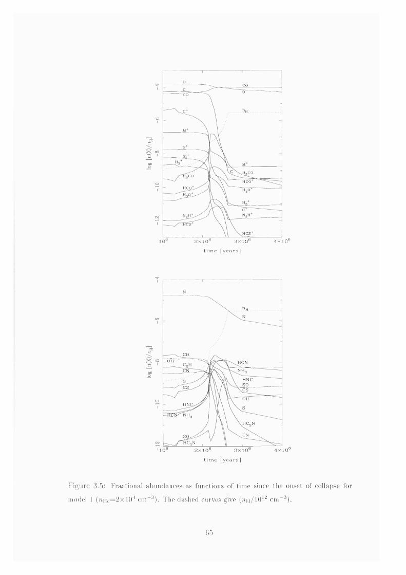
c
CO
CO
COI
I
H„ CO,coH COO
H COI
ICS
H C S
1 3 x 1 o' 4 x 1 02x10't i m e [ y e a r s ]
c CH
I _ 0 H HCN
CN NH,
HNCSOCS CS
OHoHNC
NH.
HC-N
CNSO^HC„N
4 x 1 0
t i m e [ y e a r s ]
1'igure 3.5: Fractional abundances as functions of time since the onset of collapse for
model 1 10^ cm"^). The dashed curves give (nn/lO^^ cm “ ^).
65
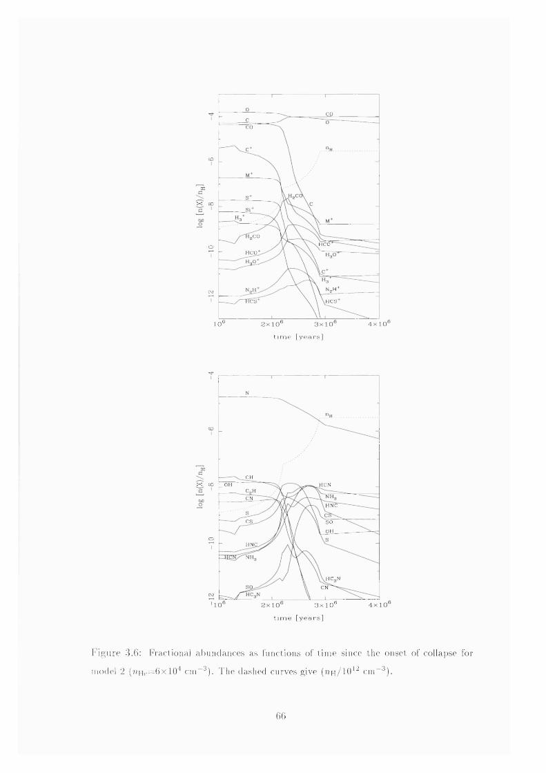
COI
CO
COI
X COI
;COHC Oo
HCO
NgHcvICS H C S
10®t i m e [ y e a r s
t i m e [ y e a r s ]
COI
CHX CO H C NOH
INH.CNH N C
CS S O
O Ho
HN<I
NH.
H C _ N
CN
3 x 1 0 ®
I' igure 3.6: iTactional abundances as functions of time since the onset of collapse for
model 2 ( 7?Hc=6 x c m ~ ^ ) . The dashed curves give (t?h/10*^ cm “ ^).
66
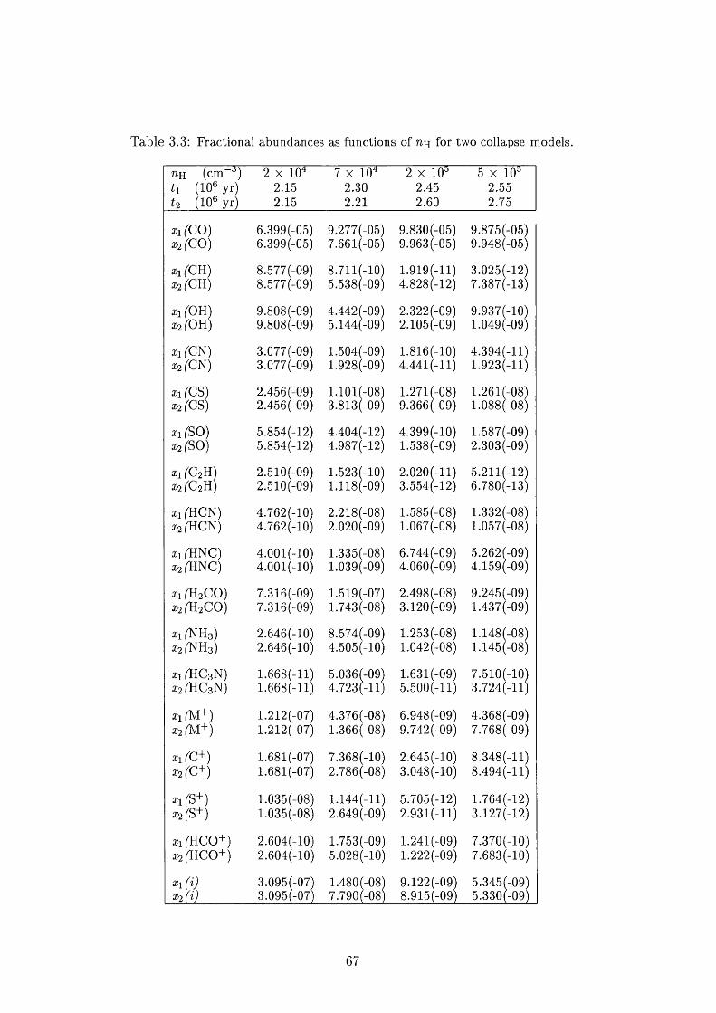
Table 3.3: Fractional abundances as functions of tih for two collapse models.
( c m “ '^)
t i (1 0 ® yr) t 2 (1 0 ® yr)
2 X 10^2.152.15
7 X lO'" 2 .3 0 2 . 2 1
2 x 1 0 ®2 ^ ^2.60
5 X 10® 2 ^ ^ 2 J 5
z i r c o )Z2 (C 0 )
6.399(-05)6 .3 9 9 (-0 5 )
9.277(-05)7.661(-05)
9.830(-05)9 .9 6 3 (-0 5 )
9 .8 7 5 (-0 5 )9 .9 4 8 (-0 5 )
xi (CH) 8.577(-09)8 .5 7 7 (-0 9 )
8.711(-10)5 .5 3 8 (-0 9 )
1.919(-11)4 .8 2 8 (-1 2 )
3 .0 2 5 (-1 2 )7 .3 8 7 (-1 3 )
z i^ O H )Z2 ("0 H )
9 .8 0 8 (-0 9 )9 .8 0 8 (-0 9 )
4.442(-09)5.144(-09)
2 .3 2 2 (-0 9 )2.105(-09)
9.937(-10)1.049(-09)
z i^ C N ) 3.077(-09)3.077(-09)
1 .5 0 4 (-0 9 )1.928(-09)
1.816(-10)4.441(-11)
4.394(-ll)1.923(-11)
z i fC S )%2 fC S )
2 .4 5 6 (-0 9 )2 .4 5 6 (-0 9 )
1.101(-08)3 .8 1 3 (-0 9 )
1.271(-08)9 .3 6 6 (-0 9 )
1.261(-08)1 .0 8 8 (-0 8 )
2 1 ^ 0 )% (S 0 )
5 .8 5 4 (-1 2 )5 .8 5 4 (-1 2 )
4.404(-12)4 .9 8 7 (-1 2 )
4 .3 9 9 (-1 0 )1 .5 3 8 (-0 9 )
1 .5 8 7 (-0 9 )2 .3 0 3 (-0 9 )
z i r C 2 H )2:2 rC 2 H )
2.510(-09)2.510(-09)
1.523(-10)1.118(-09)
2 .0 2 0 (-ll)3 .5 5 4 (-1 2 )
5.211(-12)6.780(-13)
2 1 (H C N )2 2 (H C N )
4.762(-10)4.762(-10)
2 .2 1 8 (-0 8 )2.020(-09)
1 .5 8 5 (-0 8 )1.067(-08)
1 .3 3 2 (-0 8 )1.057(-08)
2 i ( H N C ) 2 2 (H N C )
4.001(-10)4.001(-10)
1 .3 3 5 (-0 8 )1.039(-09)
6.744(-09)4.060(-09)
5 .2 6 2 (-0 9 )4.159(-09)
2 i (H 2 C 0 )2 2 (H 2 C 0 )
7.316(-09)7.316(-09)
1.519(-07) 1.743 (-08)
2 .4 9 8 (-0 8 )3.120(-09)
9 .2 4 5 (-0 9 ) 1 .4 3 7 (-0 9 )
2 1 (N H g)2 2 (N H 3 )
2.646(-10)2.646(-10)
8 .5 7 4 (-0 9 )4.505(-10)
1 .2 5 3 (-0 8 )1 .0 4 2 (-0 8 )
1 .1 4 8 (-08) 1 .1 4 5 (-08)
2 i ( H C 3 N )2 2 (H C 3 N )
1 .6 6 8 (-1 1 )1 .6 6 8 (-1 1 )
5.036(-09)4.723(-ll)
1.631(-09)5.500(-ll)
7.510(-10)3.724(-ll)
2 1 (M + )2 2 (M + )
1.212(-07)1.212(-07)
4 .3 7 6 (-0 8 )1 .3 6 6 (-0 8 )
6 .9 4 8 (-0 9 )9 .7 4 2 (-0 9 )
4 .3 6 8 (-0 9 )7 .7 6 8 (-0 9 )
2 1 CC+)% r c + )
1.681(-07)1.681(-07)
7.368(-10)2 .7 8 6 (-0 8 )
2.645(-10)3.048(-10)
8 .3 4 8 ( - l l )8 .4 9 4 ( - l l )
Zi ("S+) Z2 (S + )
1.035(-08)1.035(-08)
1.144(-11)2 .6 4 9 (-0 9 )
5 .7 0 5 (-1 2 )2.931(-11)
1.764(-12)3.127(-12)
2 i ( H C 0 + )2 2 ( H C 0 + )
2.604(-10)2.604(-10)
1.753(-09)5 .0 2 8 (-1 0 )
1 .2 4 1 (-0 9 )1 .2 2 2 (-0 9 )
7 .3 7 0 (-1 0 )7 .6 8 3 (-1 0 )
ziTV 3.095(-07)& 0 9 5 6 4 7 )
1 .480 (-08) 7 .7 9 0 (-0 8 )
9.122(-09)8 .9 1 5 (-0 9 )
5 .3 4 5 (-0 9 )5 .3 3 0 (-0 9 )
67
cm “ , is lower than in model 2 where nHc=6 xlO'^ cm“ . This is a consequence of
the visual extinction being lower in model 2 , leading to the background interstellar
photons continuing to be im portant for longer than in model 1 . This leads to a
suppression by photodissociation of the peaks at early times of some species in model
2 , which do exhibit early-time peaks in model 1 . In addition, greater amounts of C,
C"*" and 0 ^ occur in model 2 than in model 1 at nH=7xlO^ cm“ . However, one
may account for the timescale difference between the two models; model 2 reaches
the density of t2h = 7 x 1 0 cm~^ earlier than model 1 and then reaches the following
displayed density of nH=2 xlO^ cm“ at a later time than model 1 .
The late-tim e abundances of early-time species is reduced in model 2 as a result
of the lower visual extinction at nH=2 xlO^ cm~^ and the longer tim e th a t model
2 takes to reach that density. However, N H 3 , SO and CS are seen to be increasing
further in abundance in model 2 , whilst in model 1 their abundances have already
peaked.
In Chapter 4 we argue that the abundances of H C 3 N and C 2 H will rise at late
times in dense cores as depletion occurs; Caselli et al. (1998) have even used the
measured fractional abundances of H C 3 N in numerous cores to infer the depletions,
relative to solar abundances, of C, N and 0 on the assumption tha t they did not vary
from element to element. Ultimately, to establish reliably tha t depletion is usually
the cause of high abundances of such putative early-time molecules, considerable
data about the behaviour of species with abundances tha t are sensitive to the relative
depletions of trace elements must be gathered (see Chapters 6 and 7). Our current
results show tha t for cores in which high fractional abundances of H C 3 N and C 2 H
exist but are not due to high depletions, the ratio of the abundances of those two
species will be significant for the inference of how A y varied with uh during collapse.
In some regions, the emission from young low-mass stars may have a significant
effect on the ionization structures of dense cores (McKee 1989), even though those
stars are not strong sources of far ultraviolet (FUV) radiation. For some gas phase
abundances of elements such as magnesium and sodium, photons from nearby low-
mass stars may maintain a much higher fraction of those metals in ionized states than
would be expected on the basis of the sorts of calculations tha t we have performed.
Non-FUV radiation may be responsible for the fractional ionizations tha t have been
inferred for some dense core material from observational data to be sufhciently large
tha t the ambipolar diffusion timescales are at least 10 yr (Myers & Khersonsky
1995). It should be remembered that the results in Fig. 3.4 are for gas tha t is
collapsing directly from an initially much lower density object in a relatively starless
region; the results are of most relevance to the chemistry in the cores in which the
first stars to form locally are born.
3.4 C onclusions
The sharp decline in fractional ionization at A y~ 2-3 is here associated with the
distinction between starless and star-containing cores in the RMC, through changes
in turbulent support. This concept has led us to perform a preliminary study of the
chemical evolution of a collapsing cloud, in which the cloud can first collapse only
along the magnetic field lines. As the collapse proceeds, the fractional ionization
declines until a multidimensional collapse moderated by ambipolar diffusion ensues.
The nature of the collapse dynamics - in particular the density at which multidimen
sional collapse becomes significant - affects the chemical abundances. We predict
th a t observations can distinguish between the models used and may be used to infer
the details of collapse.
69
Chapter 4
Cyanopolyynes as indicators of
late-tim e chemistry and depletion
in star forming regions
In section 1.4 we described a cluster of dense cores in the Taurus - Auriga complex
(Fig. 1 .2 ) called TM C-1 . A chemical gradient is observed along this object and
in this chapter we discuss a variety of different explanations for this gradient. We
examine in detail the assumption that some observed molecules can be used to
differentiate between different evolutionary stages of star formation and consider
the implications of the results to the interpretation of the observed chemistry in
TM C-1 .
4.1 Introduction
An assumption frequently (but not always) made in the construction of models of the
chemistry in dense molecular regions is that all elements more massive than hydrogen
(which is normally assumed to be primarily in Hg) are initially in atomic form.
The fractional abundances of some molecular species reach pronounced m axim a in
many such models at times tha t are a few tenths as long as those required for
chemical equilibrium to be reached (e.g. Millar 1990). Species with such m axim a
are often referred to as “early-time” molecules, while those tha t have fractional
70
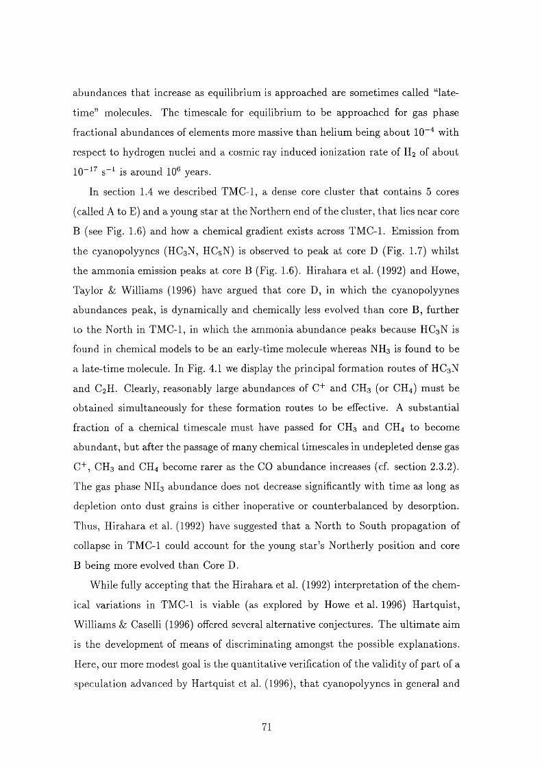
abundances tha t increase as equilibrium is approached are sometimes called “late
tim e” molecules. The timescale for equilibrium to be approached for gas phase
fractional abundances of elements more massive than helium being about 1 0 "^ with
respect to hydrogen nuclei and a cosmic ray induced ionization rate of H2 of about
1 0 “ ^ s~^ is around 1 0 ® years.
In section 1.4 we described TM C-1 , a dense core cluster tha t contains 5 cores
(called A to E) and a young star at the Northern end of the cluster, tha t lies near core
B (see Fig. 1 .6 ) and how a chemical gradient exists across TM C-1 . Emission from
the cyanopolyynes (HC3 N, HC5 N) is observed to peak at core D (Eig. 1.7) whilst
the ammonia emission peaks at core B (Fig. 1.6). H irahara et al. (1992) and Howe,
Taylor & Williams (1996) have argued that core D, in which the cyanopolyynes
abundances peak, is dynamically and chemically less evolved than core B, further
to the North in TMC-1, in which the ammonia abundance peaks because HC3 N is
found in chemical models to be an early-time molecule whereas NH3 is found to be
a late-tim e molecule. In Fig. 4.1 we display the principal formation routes of HC3 N
and C 2 H. Clearly, reasonably large abundances of C" and CH3 (or CH4 ) must be
obtained simultaneously for these formation routes to be effective. A substantial
fraction of a chemical timescale must have passed for CH3 and CH4 to become
abundant, but after the passage of many chemical timescales in undepleted dense gas
C" , CH3 and CH4 become rarer as the CO abundance increases (cf. section 2.3.2).
The gas phase N E 3 abundance does not decrease significantly with tim e as long as
depletion onto dust grains is either inoperative or counterbalanced by desorption.
Thus, Hirahara et al. (1992) have suggested that a North to South propagation of
collapse in TMC-1 could account for the young s ta r’s Northerly position and core
B being more evolved than Core D.
While fully accepting tha t the Hirahara et al. (1992) interpretation of the chem
ical variations in TMC-1 is viable (as explored by Howe et al. 1996) H artquist,
W illiams & Caselli (1996) offered several alternative conjectures. The ultim ate aim
is the development of means of discriminating amongst the possible explanations.
Here, our more modest goal is the quantitative verification of the validity of part of a
speculation advanced by Hartquist et al. (1996), tha t cyanopolyynes in general and
71
c+y
C o H
c +
C H +
C H +
C H +
r "e
\
C H 4J i
\ C H +
C 2 H +
C 2 H 2
CH3 4 C2H5H +
/C2H+ a C2HJ C2H+ ^ C2H,
/ i ' " r - 7
c+ c+/ y
C3H+ ^ C3H+
C 2 H 3
'3X12
Nr" \HC3N+ C3H+
r ' y
C2H+ ™ H2C3N+r"
H C 3 N
Figure 4.1: Routes to HC3 N and CgH formation.
72
HCsN in particular have later secondary m axim a in their fractional abundances, for
a variety of conditions, after depletion has become significant. No reliable models
for the production of cyanopolyynes more complicated than HC3 N currently exist,
and we restrict ourselves to the consideration of HC3 N rather than all of the de
tected cyanopolyynes. To date, the largest cyanopolyyne to be detected in TMC-1
is H CiiN (Bell & Matthews 1985).
However, before we embark on this investigation, we briefly summarise the other
proposed explanations by Hartquist et al. (1996) for the observed chemical gradient
along TMC-1. In one picture, the higher depletion in core D is attributed to des
orption from grain surfaces being more efficient in core B than in core D, a possible
consequence of the proximity of core B to the protostar. This proposed explanation
is based on the assumption tha t the chemistry has reached an equilibrium in each
core and also relies on the result that the H C 3 N abundance increases with increasing
depletion. There is a large cloud-to-cloud variation of the minimum visual extinction
at which H2 0 -ice features (due to vibrational transitions) at a wavelength of 3.1 /im
are observable in absorption against embedded young stars. Williams, H artquist
& W hitte t (1992) have argued tha t this implies tha t desorption must be driven by
radiation tha t is attenuated significantly in m aterial through which the m agnitude
of the visual extinction is a few to ten. Infrared radiation at a wavelength of 3.1 j im
experiences such attenuation. Hartquist et al. (1996) pointed out tha t the infrared
radiation field arising from the nearby star’s interaction with diffuse m aterial around
it may limit depletion in core B but have little effect on depletion in core D.
Alternatively, the origin of the higher HC3 N abundance in core D is due to for
m ation in the boundary layer between the dense core and the stellar wind. Williams
h H artquist (1991) and Hartquist et al. (1996) have suggested tha t mixing of stellar
wind ions into dense core material in the interface between the stellar wind m ate
rial and the dense core material in TMC-1 creates conditions favourable for HC3 N
production. Though they explored mixing within a somewhat different physical con
tex t, the model results of Chieze, Pineau des Forets h Herbst (1991) are consistent
with this suggestion. The peak in the HC3 N is at core D rather than core B because
the thickness of a boundary layer and, hence, the degree of mixing (if mixing occurs
73
at all) increases along the boundary layer.
A noticeable characteristic of the HC3 N emission from TMC-1 is its sharp gradi
ent downwind from the cores (Fig. 1.7). This sharp boundary may be at the location
of a wind term ination shock positioned just upstream of a contact discontinuity be
tween the stellar wind (mass-loaded with the m aterial tha t it has ablated and with
which it has mixed from the cores) and an ambient intercore or circumcore medium
into which the wind-blown bubble is propagating.
We close this section with some comments on the possible dynamics tha t es
tablished the current physical state of TM C-1 . These comments are of particular
relevance to the “early-time” and boundary-layer models of the production of H C 3 N
in core D but they bear on other chemical models as well.
The decrease of core density with distance from the star, as found by Hirahara
et al. (1992), is compatible with the pressure in each core being equal to the local
ram pressure of the stellar wind. Cores in a variety of stages of structural and
chemical evolution may have been present before the stellar wind turned on and
then been compressed by shocks driven into them by the stellar wind. A shock
speed of only 1 km s~ gives rise to a density increase of a factor of about 1 0 , if
it propagates into gas at 10 K in which the magnetic pressure is negligible, and
it takes approximately 10 yr to implode a core having a radius of 0.1 pc. This
implosion timescale is shorter than the gas phase chemical timescale, which implies
th a t the chemical composition of a pre-implosion state would survive as depletion
becomes significant. For standard assumptions, depletion takes place on a timescale
comparable to 10 yr at densities around those given by Hirahara et al. (1992) for
core D (see Table 1.3). Thus, a less dense pre-implosion core with a chemical age (in
the early-time chemical picture) of several times 1 0 yr could have been the site of
the production of the H C 3 N to be observable in core D for the next 10 yr (Hartquist
et al. 1996).
Another possibility is tha t the entire TMC-1 ridge was formed by the stellar wind
interacting with an initially more extended clump that fragmented into separate
cores due to instabilities arising during the interaction. In this dynamical picture
the birth of a star within a single core near a more extended clump triggers the
74
formation of other cores (e.g Hanawa, Yamamoto & Hirahara 1994).
In the next section we describe the model assumptions. Section 4.3 contains
results, while section 4.4 is a discussion of the results and their relevance to studies
of TM C - 1 and other regions of star formation. In section 4.5 we discuss some
new observations of TMC-1 and some initial attem pts to reproduce the observed
abundances.
4.2 M odel assum ptions
The tim e dependent rate equations for the abundances of 196 gas phase species were
integrated in each model calculation. The rate coefficients for gas phase reactions
were taken from the UMIST rate file (Millar et al. 1997; section 2.6), and we included
dissociation by photons produced as a consequence of cosmic ray ionization (as
described in section 2 .6 ) and due to photons of the interstellar background radiation
field. The cosmic ray induced ionization rate, ( , was taken to be 1.3x10“ ^ s“ . (We
explored the effect of the altering the value taken for ( on the calculated fractional
abundances, by halving and doubling the value of ( quoted above in turn; very little
effect was found on the values obtained for the fractional abundances.) The visual
extinction to the nearest point on the edge of a semi-infinite plane-parallel cloud. A y ,
was specified (and in some models varied with tim e as described in the next section)
so tha t the contributions of photons of external origin to the dissociation rates could
be evaluated. The contributions of photons of external origin to the dissociation rate
of CO was calculated with software developed by Wagenblast (1992). This m ethod
accounts for the line self-shielding of CO, as described in section 2.3.2.
We used equation 2.4 for the freeze-out rate of each species X containing an
element more massive than helium onto dust. We took the tem perature to be equal
to 10 K for all runs and we varied the param eter D in equation 2.4, which is used
to account for variations in the sticking efficiency and the grain size distribution.
Return to the gas phase via desorption processes was assumed not to occur unless
we state otherwise.
In some models uh was taken to be fixed as was Ay - In other models uy was
75
assumed to vary as described by equation 2.6, for spherical free-fall. The param eter
B in equation 2.6 was set equal to a value of 1 or less. After uh reached 4x10^ cm“
it was kept constant. In models with varying uh the value of Ay was also taken to
vary with tim e as described below.
Hydrogen was assumed to initially be almost entirely in H2 . All other elements
were taken to be in atomic form initially, except for carbon which was ionized. The
initial gas phase elemental fractional abundances relative to hydrogen by number
were set to 1.7x10“ ' , 7.3x10“ , 2.1x10“ , 2x10“® for 0 , C, N, and S respectively.
The fractional elemental abundance of sulphur is often taken to be so small so tha t
model results for the CS fractional abundance are not unrealistically high. The
sulphur depletion problem is the topic of investigation in Chapter 6 .
4.3 R esu lts
Figure 4.2 shows the time evolution of the fractional abundances of a number of
species for a core at a constant density with nn= 2x l0^ cm“® and Ay = 10; D=0.1.
In this model, which we designate as model 1, a late-tim e maximum as well as an
early-tim e maximum, occurs in the HC3 N fractional abundance. A pronounced late
tim e C2 H maximum and noticeable late-time rise in the CH fractional abundance
are also evident.
Figure 4.3 shows analogous results for model 5 which is for dense m aterial tha t
increases in density from uh^IxIG® to 2 x 1 0 cm “® according to equation 2 . 6 and
for which/ \ 2 / 3
A r = 0.7 + 1 .5 — , (4.1)V ^Ho /
where uhq is the initial number density. An intercore medium is assumed to con
tribu te 0.7 magnitudes to the visual extinction while the increase of the visual ex
tinction arising in the core itself is assumed to scale as it would for spherically
sym m etric collapse. For model 5, B=1 and D=0.1. Late-time rises are evident
here, for the same species as in Fig. 4.2.
Table 4.1 gives the parameters characterizing the various models for which we
obtained results, is the final value of uy. If uh is constant for a model then the
76
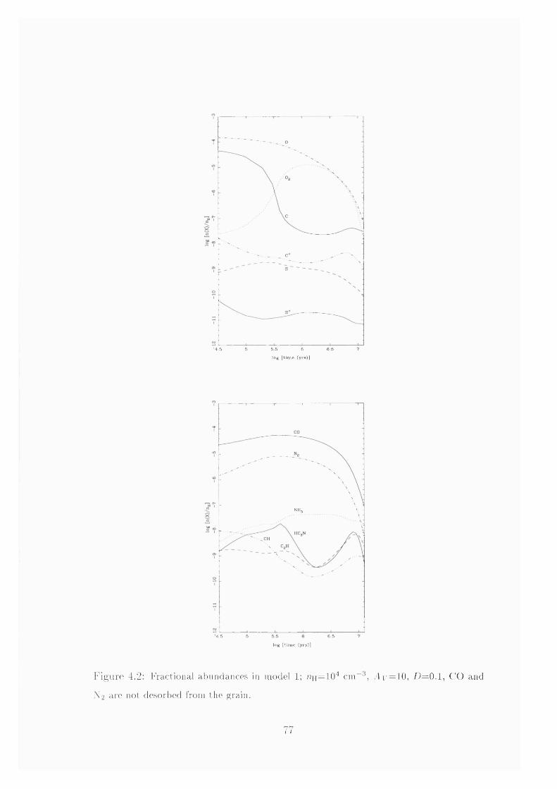
' 4 .5 5 5.5 6 6.6log [ t im e (y r s ) I
log [ t im e (y rs ) ]
NH3
' 4 .5 6.5
1'igure 4.2: Fractional abundances in model 1 ; n n = 1 0 '' cm .4v = i 0 , 74=0.1, CO and
i\ ' 2 are not desorbed from the grain.
I I
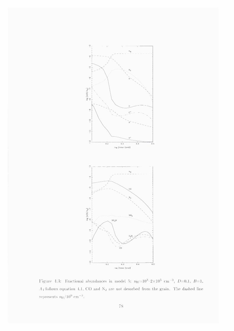
6.56 2 6.3 6 4
log [ l im e ( y r s ) )
6.56.2 6.3
lo g [ t im e (y r s ) ]
I ' ig u re 4.3: Fractional abundances in model 5; ?7 h = 1 0 '^-2 x 1 0 cm “ ^, 79=0.i, 77=1,
■ Ivfollows equation 4.1, C'O and N -2 are not desorbed from the grain. The dashed line
represents ??h/1 0 ' cni“ ' .
78
constant value of Av is given; if nu is not constant then (4.1) is used to indicate
th a t equation 4.1 was assumed to govern the evolution of A y and (4.2) is used to
indicate tha t A y was assumed to evolve as
2 / 3
A y = 0.5Uh
MHo(4.2)
The values of D and B for each model are given. CO and N2 ices are gener
ally more readily desorbed than many other ices including those of H2O, NH3 and
CH4 (cf. Hasegawa, Herbst & Leung 1992). Hence, in some models CO and N2
molecules tha t strike grains were assumed to be immediately returned unaltered to
the gas phase. A column is included in Table 4.1 to indicate for which models this
assumption was made.
Due to the screening of CO, by itself and by H2 , from photons of external origin
th a t induce CO dissociation, CO is often the only very abundant molecule in clouds
th a t are not dark. Dense cores may in some cases form in such clouds on a timescale
shorter than the chemical timescale. Thus, for two models almost all carbon was
assumed to be initially in CO. In both of these models all nuclei more massive than
the hydrogen nucleus and not contained in CO were assumed to be initially in atoms
and not molecules. A column in Table 4.1 gives [a;(CO)/zc]i, the initial value of the
fraction of carbon tha t is contained in CO.
Table 4.1: Parameters for late-time chemistry models.
Model HHo hh, A y D B (C0 &N2 )freeze-out (X (C O )/X c)i1 2.0 X 10^ 2.0 X 10“ 10. 0.1 — yes 0.00
2 2.0 X 10^ 2.0 X 10“ 10. 0.1 — no 0.00
3 2.0 X 10“ 2.0 X 10“ 5. 0.1 — yes 0.00
4 2.0 X 10“ 2.0 X 10“ 10. 0.01 yes 0.00
5 1.0 X 10^ 2.0 X 10® (4.1) 0.1 1 yes 0.00
6 1.0 X 10^ 2.0 X 10® (4.1) 0.1 1 no 0.007 1.0 X 10^ 2.0 X 10® (4.1) 0.1 1 yes 0.998 1.0 X 10® 2.0 X 10® (4.1) 0.1 1 no 0.999 1.0 X 10® 2.0 X 10® (4.2) 0.1 1 yes 0.00
10 1.0 X 10® 2.0 X 10® (4.2) 0.1 1 no 0.00
79
T a b l e 4 .2 : T im e s o f a n d f ra c t io n a l a b u n d a n c e s a t H C 3N m a x im a . t i a n d (2 re fe r to th e
t im e s o f th e e a r ly a n d la te - t im e H C 3N m a x im a , re sp e c tiv e ly . T h e n o ta t io n a { —b) re fe rs
to
Model t u h (yr) (CO) (N2 ) (NH3 ) (HC3 N) (C 2 H)
1 4.0(5)8 .0 (6 )
5.557(-5)1.715(-6)
8.307(-6)1.514(-7)
2.439(-8)2.371(-8)
1.858(-8)8.647(-9)
1.540(-9)6 .559(-9)
2 4.0(5)2.4(7)
6.265(-5)4.565(-6)
9.249(-6)4.510(-6)
2.275(-8)4.317(-8)
1.891(-8)4 .026(-8)
1.526(-9)8 .180(-9)
3 4.0(5)8 .0 (6 )
5.760(-5)1.876(-6)
8.306(-6)1.915(-7)
1.809(-8)1.593(-8)
6.232(-9)4.462(-9)
2 .584(-9)2 .732(-8)
4 4.0(5)8.0(7)
6.591(-5)1.564(-6)
9.790(-6)1.300(-7)
2.204(-8)2.542(-8)
1.827(-8)8.142(-9)
1.208(-9)2 .891(-9)
5 1 .6 (6 )2 .8 (6 )
4 .593(-5)3.693(-7)
8.560(-6)4.136(-8)
2.284(-8)6.110(-9)
7.933(-9)8.223(-10)
8.578(-10)4.172(-10)
6 1 .6 (6 )8 .0 (6 )
5.729(-5)6.348(-6)
9.427(-6)5.042(-6)
1.787(-8)1.693(-8)
1.095(-8)1.387(-8)
1.204(-9)9.395(-10)
7 1.5(6)2.9(6)
6.530(-5)3.153(-7)
8.516(-6)2.338(-8)
3.000(-8)4.845(-9)
1.986(-9)5.205(-10)
2.636(-10)3.591(-10)
8 1.5(6)9.0(6)
6.992(-5)5.350(-6)
8.795(-6)4.472(-6)
2.777(-8)1.695(-8)
2.111(-9)1.389(-8)
2.757(-10)9.728(-10)
9 1.7(6)2.9(6)
1.955(-5)1.092(-7)
6.850(-6)2.150(-8)
4.847(-8)6.411(-9)
1.674(-10)8 .2 6 4 (- ll)
9.453(-12)8 .9 9 4 (- ll)
1 0 1.7(6)5.0(6)
2.328(-5)5.297(-6)
7.711(-6)5.735(-6)
4.633(-8)2.103(-8)
1.816(-10)1.311(-8)
l .O l l ( - l l )9.519(-10)
Table 4.2 gives results for the times at which HC3 N fractional abundance m axim a
occur in each model and the fractional abundances of several species at each tim e
for each model. An early-time maximum and a late-tim e maximum was found in
each model.
4.4 D iscussion
The model results show that a late-time HC3 N fractional abundance maximum
occurs in a dense, dark core in which depletion has taken place. This behaviour
80
was forecast by Hartquist et al. (1996) from earlier considerations of H artquist &
Williams (1989) tha t led them to realize that the CH fractional abundance rises as
depletion occurs as long as
He+ -f CO C+ + 0 + He (4.3)
is the dominant mechanism for removing He’*'. He”*" is produced at a constant rate by
cosmic ray induced ionization; hence, as long as reaction 4.3 is its prim ary removal
mechanism the production rate of C""" remains unaffected by depletion. However
as depletion occurs, C" is more likely to react with H2 than with oxygen bearing
species leading to an increase in the rates of production of CH and other carbon
bearing species tha t contain no oxygen. In addition the rates of removal of carbon-
bearing species containing no oxygen decrease as depletion reduces the fractional
abundances of oxygen-bearing species that remove them (see Fig. 2.1).
Comparison of the results for models 1 and 5 shows tha t the initial H C 3 N max
imum is slightly less pronounced and later in model 5. This is due in part to the
im portance of photodissociation in model 5 until A y reaches a sufficiently high
value. That photodissociation induced by photons of external origin is im portant
at low A y is confirmed by the contrast between H C 3 N results for models 1 and 3.
Comparison between results for models 1 and 5 also show th a t the late-tim e H C 3 N
maxim um is less pronounced in higher density regions.
Results for the pairs of models 1 and 2, 5 and 6 , 7 and 8 , and 9 and 10 indicate
th a t if CO and N2 are returned immediately to the gas phase after striking grains,
rather than retained as ices on the grains, the late-tim e HC3 N maximum is much
greater. We constructed some models in which N2 remained on grains but CO did
not; in each the late-time HC3 N maximum was not significantly enhanced relative to
th a t in an analogous model in which all species more massive than helium remained
on grains.
T h e c o n t r a s t s b e t w e e n m o d e l s 5 a n d 7 a n d b e t w e e n m o d e l s 6 a n d 8 s h o w t h a t
i f c a r b o n is i n i t i a l l y p r i m a r i l y in CO t h e e a r l y - t i m e H C 3 N p e a k is s u b s t a n t i a l l y
r e d u c e d . T h e b e h a v io u r o f C 2 H is s im i la r t o t h a t o f H C 3 N , a s is t h a t o f C 2 S a n d
C 3S ( s e e F ig . 4 .4).
High late-time H C 3 N maxima are achieved only when the freeze-out timescale
81
is long compared to the chemical timescale. In a model of a collapsing core it must
also be long compared to the collapse timescale.
The point made by Hartquist et al. (1996) th a t the presence of HC3 N in a dense
core does not necessarily indicate chemical or dynamical youth is supported by
the work reported here. This point is of importance for the study of low-mass
star forming cores in general (e.g. Williams, Hartquist & Caselli 1996; references
therein) and possibly for TMC-1 in particular (Hartquist et al. 1996). However, Cl
emission is observed to rise towards the cyanopolyyne emission peak in TMC-1,
(Schilke et al. 1995), and the inferred value of the C° and CO column density ratios
is larger than tha t of roughly 0.03 tha t we have found to obtain in the models during
the duration of the late-tim e HC3 N maximum. Schilke et al. (1995) suggested tha t
the Cl emission arises in gas at least an order of magnitude less dense than tha t
in which the cyanopolyyne emission originates, in which case the presence of the
Cl emission probably gives information about an intercore medium rather than the
core. Alternatively, the Cl emission may be associated with the denser core gas
and may have been formed as a consequence of mixing in boundary layers of stellar
wind ions and gas in a previous generation of cores and survived until now because
tha t m ixture of material collapsed on a timescale short compared to the chemical
timescale (Williams et al. 1996; references therein). Considerably more mapping of
the Cl emission needs to be performed in the direction of the TM C - 1 cyanopolyyne
peak in order to establish where it forms and its relationship to the cyanopolyynes
there.
Another argument in favour of this model may be tha t the to tal column density
of gas increases with time. Although we have assumed tha t uh is constant when
it reaches the value if times later than this are associated with the phase in
which magnetic support is lost from the core, then hydrodynamic models suggest the
density will continue to slowly increase. Hence, although the fractional abundance
may not change, the actual column of each species may increase significantly at late
times.
We conclude this section by suggesting tha t HC3 N is an excellent species to
observe in attem pts to detect core collapse if the absence of evidence of such collapse
82
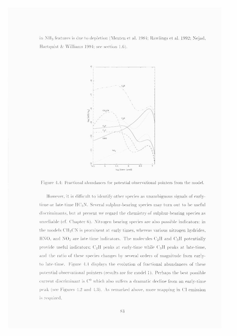
in N II 3 fea tu res is due to dep le tion (M en ten e t al. 1984; R aw lings e t al. 1992; N ejad ,
I lar tcp iis t & W illiam s 1994; see section 1.6).
C3S
N03
' 4 .5 5 5,5
log [ l im e ( y r s ) l
f i g u r e 4.4: Fractional abundances for potential observational pointers from the model.
However, it is difficult to identify o th er species as u n a m b ig u o u s signals of ea rly -
t im e or I a te - t im e IIC 3 N. Several su lp h u r-b e a r in g species m a y tu r n o u t to be useful
d is c r im in a n ts , b u t a t ])resent we regard th e c h e m is t ry of s u lp h u r-b e a r in g species as
u n re l iab le (cf. C h a p te r 6 ). N itrogen bearing species are also possib le in d ica to rs : in
I he m o d e ls C I I 3 CN is p ro m in en t a t early t im es , w hereas various n i t ro g en h y d r id es ,
U N O , a n d N O 2 a re l a te - t im e ind ica to rs . T h e m olecules C 2 IÏ a n d C 3 H p o te n t ia l ly
])rovide useful ind icato rs ; C 2 H peaks a t e a r ly - t im e w hile C 3 II peaks a t l a te - t im e ,
an d th e ra t io of these species changes by several o rders of m a g n i tu d e from early -
to la te - t im e . F igure 4.4 d isplays th e evo lu tion of frac t iona l a b u n d a n c e s of th ese
p o te n t ia l observa tiona l po in te rs ( resu lts are for m o d e l 1 ). P e rh a p s th e bes t possib le
c u r re n t d isc r im in an t is CT which also suffers a d ra m a t ic dec line from an e a r ly - t im e
peak (see F igures 4.2 and 4.3). As rem ark ed above, m ore m a p p in g in C l em ission
is recpiired.
83
The existence of a plethora of explanations for chemical variations in TMC-1
requires tha t more species be mapped because their abundance variations will no
doubt differ between models. Also, considerably more theoretical exploration of the
models must be undertaken.
4.5 N ew observations o f TM C -1
In Table 4.3 we present some of the very recent values for molecular abundances
in core D of TMC-1, determined by Ohishi & Kaifu (1998) through a multi-line
study. For comparison we also give abundances determined in previous studies
(where available). One can clearly see that the abundance of the hydrocarbons and
sulphur-bearing species are enhanced relative to the previously inferred values. In
this section we briefly present the results of our initial a ttem pts to improve the
correlation between the theoretically calculated abundances for these species and
the new observed values.
Table 4.3: Observed fractional abundances in core D of TMC-1. Those in the first column (Abun 1) are from Ohishi & Kaifu (1998), values in the second column (Abun 2) are from Hirahara et al. (1992). The notation a[-b) denotes &xlO"\
Species Abun 1 Abun 2C4 H 6(-7) 2(-7)HC3 N 8 (-8 ) 8.5(-9)H2 CO 7.5 (-8 ) -
NH3 3(-8) 2 (-8 )C3 H 2 (-8 ) -
CCS 9(-9) 5(-9)CS 8(-9) l(-8 )
As we have described in the previous sections, late-tim e chemistry and depletion
can be used to explain the high abundances of cyanopolyynes and hydrocarbons
in core D of TM C-1 . Some of the models which we discussed in section 4.4 u ti
lized the limited desorption of species from grain surfaces. Our contention is tha t
a more detailed model of both accretion onto and desorption from grain surfaces
should be explored to achieve better agreement between the observed and calcu
84
lated abundances (e.g Hasegawa & Herbst 1993). However, in this work, due to
tim e lim itations, we used a simple approximation of desorption. We chose only one
species, which can be considered to be representative, to be desorbed from the icy
grain mantle. Our hope is that this limited first a ttem pt will dem onstrate whether
this is a viable path to pursue.
Hall & Williams (1995) studied the effects of the injection of small hydrocarbon
molecules into the gas phase chemistry of diffuse clouds. The species were assumed
to be injected by the erosion of carbonaceous grains at the cloud boundaries. Here,
we investigate the effect of the injection of small hydrocarbons on the chemistry in
dark cores. In our model we assume that the hydrocarbons are ejected from the
grain surface as a result of desorption from the grain mantle, by one of the many
possible desorption processes (cf. sections 1.1, 2.5.1).
As argued by Hall & Williams (1995), C4 H2 is a good candidate species to be
injected as its chemistry is relatively well understood. We assumed tha t the injec
tion was continuous; any C4 H2 that is accreted onto a grain surface is immediately
removed, by some desorption process, and injected back into the gas phase. We
did not incorporate the production of C4 H2 by grain surface chemistry. We em
ployed the same model as described in section 4.2, with modifications to account
for the injection. We found that the effect on the calculated abundances was minor,
and tha t only slight increases in the abundances were found. This lim ited effect
was deduced to be partly due to the fact tha t the chosen injected species, C4 H 2 ,
is never very abundant in the models. We therefore changed the injected species
to be C4 H, which also has a reasonably well known chemistry, yet is found (in the
models presented in the previous sections) to be more abundant in molecular clouds
than C4 H2 (for model 1 at 1 0 ® years a:(C4 H )= 6 x 1 0 “® whereas o:(C4 H2 ) = 9 x 1 0 “ ^^).
However, the effects on the chemistry were again not very significant. We are forced
to conclude tha t the high abundances, especially for HC3 N determined by Ohishi &
Kaifu (1998) in TMC - 1 are not presently understood.
Although this initial study has not proven to be very successful in enhancing the
abundances of hydrocarbons further at late-times, we believe tha t there are several
alternative approaches tha t are worth exploring. Firstly, we suggest th a t if an in
85
stantaneous injection were to be utilized, then the effects on the gas phase chemistry
may be more significant, and may further boost the production of hydrocarbons in
late-tim e chemistry. The use of a different species to be injected may also prove
to be beneficial. The selection should be treated carefully, with preference given
to species tha t have chemistries tha t we understand well and tha t have significant
abundances. Another approach may be to consider the effects of ions on the late
tim e chemistry. This idea follows from the discussion in section 4.1 tha t the mixing
of dense core material with stellar wind ions in a boundary layer may favour the
production of H C 3 N . We plan to explore these proposals through further modelling.
4.6 N ew rate for th e reaction o f N w ith
We now briefly describe a study of the effects on the model chemistry of the inclusion
of a new reaction. As we mentioned in section 2.3.4, on the nitrogen chemsitry of
interstellar clouds, a new reaction has been proposed to transfer H 2'^ to N . The
reaction in question is
N + H+ ^ NH+ -h H. (4.4)
The earlier theoretical study of Herbst, DeFrees & McLean (1987) suggested tha t
this reaction would proceed at a negligible rate; hence it was not included into the
UMIST rate file (Millar et al. 1997). However, Scott et al. (1997) have measured this
reaction to be rapid at room tem perature, with a rate coefficient of /c—4.5x10“ ° cm^
s“ U Consequently, we performed some calculations to test the effect of the inclusion
of this reaction onto the chemistry used in the models presented in the previous
sections (also see similar studies by Scott, Freeman & McEwan 1997; Terzieva &
Herbst 1998). We included the reaction in our models with a value for the rate
coefficient as quoted above. The production of ammonia should be affected by the
inclusion of this reaction; the product species NH]"*" will react with H2 to form NH4 "'",
which then dissociatively recombines with an electron to form N H 3 .
We found tha t the calculated abundances were affected by the inclusion of this
reaction. The calculated fractional abundances of NH2 '^, N H 3 and N 2 were all seen
to rise by up to two orders of magnitude. However, this occurred at early times
and only for low densities conditions (in models identical to model 9 presented in
section 4.2, the increase occurred during the initial collapse). These species are not
observed in translucent environments, but are detected in higher density regions
(refer to Chapter 5). However, the new, increased abundances achieved are still not
detectable. When this reaction is incorporated into a model identical to the dense
core model 1 presented in 4.2, the increase is not significant; for NH2""", NH3 and N2
the rise in the fractional abundance is of the order of 10% or less. The effect is more
prominent at early-times and for low density regions as these conditions lead to N
being the main nitrogen-bearing species; at higher densities most of the nitrogen
is locked into N2 , as we describe in the next chapter. N2 is formed through rapid
neutral-neutral reactions in dense cores, as described in section 2.3.4.
87
Chapter 5
On the detection of interstellar
homonuclear diatomic m olecules
In the m ajority of the work presented in this thesis we have employed theoretical
models of the physics and chemistry in star forming regions in attem pts to explain ex
isting observational data and to infer the physical parameters and evolutionary state
of those regions. In some cases, we have been able to suggest from the model results
th a t the observation of other species would be particularly useful to explore the dif
ferent types of clouds. In this chapter we diverge from this approach; here we explore
whether homonuclear diatomic molecules may be detectable in interstellar clouds.
The models that we have used (Chapters 3 ,4 ,6 and 7) predict th a t homonuclear
diatomic molecules may be abundant in dense, low tem perature interstellar clouds
(see the description below). However, a homonuclear diatomic molecule does not
possess a permanent dipole moment and therefore does not have a pure rotational
spectrum. Consequently, low tem perature homonuclear diatomics are considered
undetectable (though, of course, at high tem perature they emit vibrational spectra;
H 2 1 - 0 is the prime example of this). It is possible to infer abundances for these
species via related species (see below). However, in this chapter we consider a novel
approach tha t may provide a direct measure of the abundance of these species at low
tem perature; we explore whether homonuclear diatomic molecules may in fact be
observable. Such observations would provide an accurate measure of the abundances
of these species in cool interstellar clouds, in addition to providing direct limits on
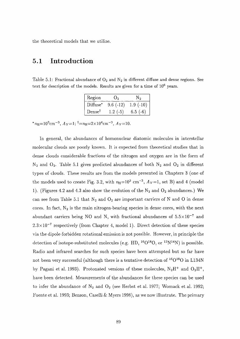
the theoretical models tha t we utilize.
5.1 Introduction
Table 5.1: Fractional abundance of O2 and N2 in different diffuse and dense regions. See text for description of the models. Results are given for a time of 10® years.
Region O2 N 2
Diffuse* 9.6 (-12) 1.9 (-10)Dense^ 1 . 2 (-5) 6.5 (-6 )
* n H = 1 0 ® c m A v = l ' i ^ = n H = 2 x l 0 ^ c m T y = 1 0 .
In general, the abundances of homonuclear diatomic molecules in interstellar
molecular clouds are poorly known. It is expected from theoretical studies th a t in
dense clouds considerable fractions of the nitrogen and oxygen are in the form of
N2 and O 2 . Table 5.1 gives predicted abundances of both N2 and O2 in different
types of clouds. These results are from the models presented in Chapters 3 (one of
the models used to create Fig. 3.2, with uh = 10® cm~®, Ty = l , set B) and 4 (model
1). (Figures 4.2 and 4.3 also show the evolution of the N2 and O2 abundances.) We
can see from Table 5.1 tha t N2 and O2 are im portant carriers of N and 0 in dense
cores. In fact, N2 is the main nitrogen-bearing species in dense cores, with the next
abundant carriers being NO and N, with fractional abundances of 5.5x10“ and
2 .3x10“ respectively (from Chapter 4, model 1 ). Direct detection of these species
via the dipole-forbidden rotational emission is not possible. However, in principle the
detection of isotope-substituted molecules (e.g. HD, or is possible.
Radio and infrared searches for such species have been attem pted but so far have
not been very successful (although there is a tentative detection of in L134N
by Pagani et al. 1993). Protonated versions of these molecules, N 2H"'" and O2 H+,
have been detected. Measurements of the abundances for these species can be used
to infer the abundance of N2 and O2 (see Herbst et al. 1977; Womack et al. 1992;
Fuente et al. 1993; Benson, Caselli & Myers 1998), as we now illustrate. The prim ary
formation route of N2H+ is
N2 + H+ ^ N 2H+ + H2 . (5.1)
The main destruction routes are
N2 H+ + CO ^ HCO+ T N2 (5.2)
N2 H+ + e -> N2 + H. (5.3)
Hence, an expression for the abundances of N2 can be derived, which depends on the
rates of the above three reactions, and the fractional abundance of CO, H3 "'", N2 H"'"
and electrons (refer to Benson, Caselli & Myers 1998 for a detailed discussion).
A similar relation can be found for O2 and 0 2 H""". Observations of N2 H"'" and
0 2 H" support the view tha t N2 and O 2 are abundant in dense clouds (e.g. Benson,
Caselli & Myers 1998). This method, though, is limited by the accuracy of the
measurements made for several different species and the reliability of the rates for
several reactions. Consequently, there is uncertainty in the inferred abundances of
N2 and O2 . Therefore, it would be of great benefit to obtain a direct measure of
the N 2 and O2 fraction in dense cores. We now describe how these species may be
observable.
Molecular hydrogen is widely detected in regions of high excitation through its
vibrational emission. In principle, other homonuclear diatomics should also em it in a
similar fashion, though such emission has not, to date, been detected. However, these
excited regions may not be characteristic of the denser regions in molecular clouds,
and it would therefore be useful to measure directly the abundances of homonuclear
molecules in quiescent dense clouds, and to improve our knowledge of the nitrogen
and oxygen budgets in these environments. In this chapter we propose tha t dense
quiescent clouds may be sources of vibrational emissions normally associated with
regions of high excitation such as post-shock or photon-dom inated regions. The
energy for this process is proposed to arise from non-thermal energy sources available
even in dark clouds.
In quiescent dense, dark clouds sources of non-thermal energy are rather few.
Chemical reactions constitute one possible source (Duley & Williams 1992); in the
90
case of Ng such a process might work as follows
N2 + H+ -4 N2 H+ + H2 (5.4)
N2 H+ + e -4 N; + H (5.5)
N; -4 Nj + hi/. (5.6)
Here, NJ represents a rovibrationally excited N2 molecule; internal excitation nor
mally arises in reactions tha t are sufficiently exothermic. The emission of the photon,
hi/ (equation 5.6), occurs via a quadrupole transition, if the gas density is low enough
(as it is in the interstellar medium) for collisional de-excitation to be negligible.
Estim ates for similar processes involving CO and for emission from H2 newly
formed on dust have been made by Duley & Williams (1992, 1993). Another possible
energy source is the cosmic ray induced radiation field (Prasad & Tarafdar 1984):
H2 T c.r. -> H + + e* (5.7)
H2 -fe* H; + e" (5.8)
h ; -> H 2 + hz/. (5.9)
where H2 represents a rovibrationally excited H2 , e* denotes a fast electron and
E(e*')<E(e*). The radiation field arising from equation (5.9) is present even when
the ambient interstellar radiation field is totally excluded. This induced radiation
field may excite other molecules present. However, it seems likely tha t direct exci
tation of homonuclear diatomics by superthermal electrons will be more effective:
e " - k X 2 X ; 4 - e * ' ( 5 .1 0 )
X ; X g + h z / ' ( 5 .1 1 )
where hi/' is a photon em itted by the internally excited molecule Xg.
To explore the effectiveness of this process, in this chapter we estim ate the inten
sity of emission from N2 molecules in a dense interstellar cloud, ignoring all chemical
and radiative excitation. The excitation of rotational and vibrational levels within
N 2 is assumed to be caused by the superthermal electrons generated within the
cloud by the flux of cosmic rays (cf. equation 5.11). In section 5.2 we estim ate the
supertherm al electron flux, and describe the cascade process following excitation.
91
In section 5.3 we calculate the intensity of emission in several of the strongest lines
and discuss the detectability of this emission.
5.2 V ibrational em ission from N 2
The mean energies of electrons generated by the cosmic ray ionization of H 2 in
interstellar clouds are around 32-36 eV, (Dalgarno & McCray 1972), but much of
the energy is radiated away quickly through excitation of resonance transitions in
H and H 2 . Electron energies therefore fall rapidly to below 10.2 eV, the excitation
energy of H(2p). Energy loss below this value continues mainly through elastic
collisions with H2 and He. The non-thermal electron energy spectrum for energies
less than 1 0 . 2 eV is therefore assumed in this paper to be determined by these
processes. Inelastic or elastic collisions with N2 leading to energy loss are very
minor channels, and do not significantly affect the supertherm al electron spectrum.
The rotational emission from cold (~10 K) interstellar N 2 in its ground vibra
tional and J = 0 , 1 rotational levels following excitation through collision with a non-
therm al electron are:
e*-f N2 (0 ; 0,1) —>■ e*^-f-N2 (n, <7) (5.12)
N2 (n ,J ) ^ N2 ( n ' \ r ) + hz/, (5.13)
and the subsequent cascade from state (n ,J) will produce a large number of in
frared lines. We need to determine which of the many possible transitions will be
the strongest and hence the most likely to be observable. We have therefore cal
culated the cascade table of rovibrational transitions for N2 . In relaxing from an
excited rovibrational level, the N2 molecule may cascade through many different
levels governed by the selection rules for transitions. The selection rules governing
rovibrational transitions are as follows:
A v = V — v ” > 0 (5.14)
A J = / — J " = —2 , 0 , 2 ( 0 0 forbidden). (5.15)
Therefore, pure rotational transitions and pure vibrational transitions are allowed,
92
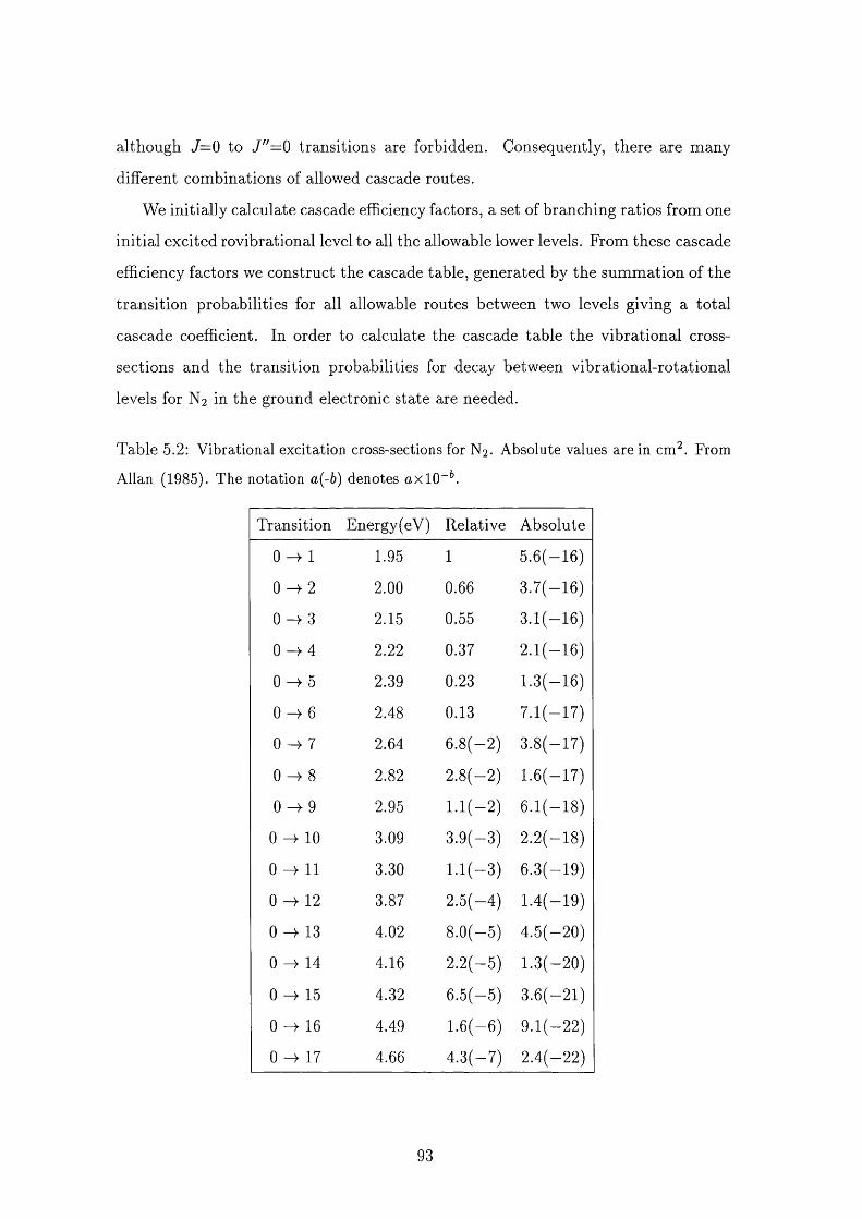
although J = 0 to J"= 0 transitions are forbidden. Consequently, there are many
different combinations of allowed cascade routes.
We initially calculate cascade efficiency factors, a set of branching ratios from one
initial excited rovibrational level to all the allowable lower levels. From these cascade
efficiency factors we construct the cascade table, generated by the sum m ation of the
transition probabilities for all allowable routes between two levels giving a total
cascade coefficient. In order to calculate the cascade table the vibrational cross-
sections and the transition probabilities for decay between vibrational-rotational
levels for N2 in the ground electronic state are needed.
Table 5.2: Vibrational excitation cross-sections for N2 . Absolute values are in cm^. From
Allan (1985). The notation a(-b) denotes ax 10“ .
Transition Energy(eV) Relative Absolute
0 1 1.95 1 5 .6(-16)
0 ^ 2 2 . 0 0 0 . 6 6 3 .7(-16)
0 -> 3 2.15 0.55 3.1(-16)
0 -> 4 2 . 2 2 0.37 2 .1(-16)
0 - ^ 5 2.39 R23 1.3(—16)
0 - > 6 2.48 0.13 7.1(-17)
0 ^ 7 2.64 6 .8 ( - 2 ) 3 .8(-17)
0 - ^ 8 2.82 2 .8 ( - 2 ) 1 .6(-17)
0 ^ 9 2.95 l . l ( - 2 ) 6 .1(-18)
0 ^ 1 0 3.09 3 .9 (-3 ) 2 .2(-18)
0 ^ 1 1 3.30 l . l ( - 3 ) 6 .3(-19)
0 ^ 1 2 3.87 2 .5 (-4 ) 1 .4(-19)
0 13 4.02 8 .0 (-5 ) 4 .5(-20)
0 ^ 14 4.16 2 .2 (-5 ) 1 .3(-20)
0 15 4.32 6 .5 (-5 ) 3 .6(-21)
0 16 4.49 1 .6 ( - 6 ) 9 .1(-22)
0 - 4 17 4.66 4 .3 (-7 ) 2 .4(-22)
93
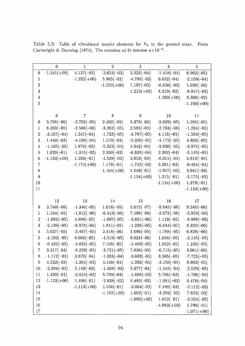
Table 5.3: Table of vibrational matrix elements for N2 in the ground state. Cartwright & Dunning (1974). The notation a{-b) denotes ax 10“ .
From
0 1 2 3 4 50 -1.241(4-00) 4 .1 3 7 (-0 2 ) -2 .6 5 3 ( -0 3 ) 3 .2 3 2 (-0 4 ) -1 .4 1 8 ( -0 4 ) 6 .9 0 2 ( - 0 5 )
1 -1.232(+00) 5 .8 6 5 (-0 2 ) -4 .7 8 0 ( -0 3 ) 6 .6 5 2 ( -0 4 ) -2.159(-04)2 -1 .2 2 2 (+ 0 0 ) 7 .1 9 7 (-0 2 ) -6 .8 5 6 ( -0 3 ) 1 .0 2 6 ( -0 3 )
3 -1.213(-h00) 8.319(-02) -8 .9 4 7 ( -0 3 )
4 -1.203(+00) 9 .3 0 8 ( -0 2 )
5 -1.193(-h00)
6 7 8 9 1 0 1 1
0 3 .7 8 8 ( -0 6 ) -3.703(-05) 2 .4 0 2 (-0 5 ) 5 .3 7 8 (-0 6 ) -2 .0 2 9 ( -0 5 ) 1 .2 9 5 ( -0 5 )
1 8 .4 9 3 ( -0 5 ) -2 .5 6 6 ( -0 6 ) -3 .2 6 2 ( -0 5 ) 2 .5 8 5 (-0 5 ) -2 .7 9 3 ( -0 6 ) -1.234(-05)2 -3.107(-04) 1.247 (-04) -1 .7 2 3 ( -0 5 ) -3.787(-05) 4.118(-05) -1.503(-05)3 1 .440 ( -0 3 ) -4.199(-04) 1 .5 7 0 (-0 4 ) - 2 .3 2 6 ( -0 5 ) -4 .1 7 2 ( -0 5 ) 4.803(-05)4 -1.105(-02) 1 .8 7 8 (-0 3 ) -5 .3 2 2 ( -0 4 ) 1 .942 ( -0 4 ) -3 .8 2 0 ( -0 5 ) -3.975(-05)5 1 .0 2 0 (-0 1 ) -1.315(-02) 2 .3 5 0 (-0 3 ) -6.628(-04) 2 .3 8 2 ( -0 4 ) -5.145(-05)6 -1 .1 8 3 (4 -0 0 ) 1 .1 0 2 (-0 1 ) -1.528(-02) 2 .8 5 3 (-0 3 ) -8.011(-04) 2.812(-04)7 -1.174(4-00) 1 .1 7 8 (-0 1 ) -1 .7 4 2 ( -0 2 ) 3 .3 8 1 ( -0 3 ) - 9 .4 9 4 ( -0 4 )
8 -1.164(4-00) 1.249(-01) -1 .9 5 7 ( -0 2 ) 3 .9 4 1 ( -0 3 )
9 -1.154(4-00) 1 .3 1 5 (-0 1 ) - 2 .1 7 5 ( -0 2 )
1 0 -1.144(4-00) 1 .3 7 9 ( -0 1 )
1 1 -1.133(4-00)
1 2 13 14 15 16 170 3.740(-06) -1.346(-05) 1.016(-05) 5.012(-07) - 8 .8 4 5 ( -0 6 ) 9.245(-06)1 1.164(-05) -1.812(-06) - 6 .4 4 3 ( -0 6 ) 7.469(-06) -2.672(-06) -2.923(-06)2 -1.082(-05) 1 .888 ( -0 5 ) -1.007(-05) -3 .6 9 1 ( -0 6 ) 1 .1 1 9 ( -0 5 ) - 8 .9 8 8 ( -0 6 )
3 -2.139(-05) -6.978(-06) 1.841(-05) -1.230(-05) -6 .6 4 4 ( -0 7 ) 9 .3 2 2 ( -0 6 )
4 5.637(-05) -3.407(-05) 2 .4 1 8 (-0 6 ) 1 .696 ( -0 5 ) -1 .7 8 8 ( -0 5 ) 6 .8 2 8 ( -0 6 )
5 -4.192(-05) 6.660(-05) -4.519(-05) 9.024(-06) 1 .6 3 4 (-0 5 ) -2 .1 4 5 ( -0 5 )
6 - 6 .4 3 2 ( -0 5 ) -4.035(-05) 7 .1 9 8 (-0 5 ) -5 .4 8 9 ( -0 5 ) 1 .8 5 2 (-0 5 ) 1.100(-05)7 3.317(-04) -8 .2 2 9 ( -0 5 ) - 3 .7 2 1 ( -0 5 ) 7 .8 3 6 (-0 5 ) -6.715(-05) 3.061(-05)8 -1.112(-03) 3.870(-04) -1 .0 0 3 ( -0 4 ) -3.602(-05) 8.505(-05) - 7 .7 2 5 ( -0 5 )
9 4.532(-03) -1.284(-03) 4 .4 4 0 (-0 4 ) -1 .2 0 3 ( -0 4 ) -3 .1 5 6 ( -0 5 ) 8.902(-05)1 0 -2.394(-02) 5.149(-03) - 1 .4 6 8 ( -0 3 ) 5.077(-04) -1.445 (-04) -2.529(-05)1 1 1.439(-01) -2.615(-02) 5.799(-03) -1 .6 6 8 ( -0 3 ) 5.766(-03) -1.706(-04)1 2 -1.123(-h00) 1 .4 9 6 (-0 1 ) - 2 .8 3 8 ( -0 2 ) 6 .4 8 0 (-0 3 ) -1 .8 8 1 ( -0 3 ) 6 .4 7 6 ( -0 4 )
13 -1 .1 1 3 (4 -0 0 ) 1.550(-01) -3.064(-02) 7 .1 8 8 ( -0 3 ) - 2 .1 1 2 ( -0 3 )14 - 1 . 1 0 2 (4 - 0 0 ) 1 .6 0 2 (-0 1 ) -3 .2 9 2 ( -0 2 ) 7 .9 2 3 ( -0 3 )
15 -1.092(+00) 1 .6 5 2 (-0 1 ) -3 .5 2 4 ( -0 2 )
16 -1.082(4-00) 1.700(-01)17 -1.071(4-00)
94
The cross sections for reaction (5.12) are required as functions of energy. In
fact, these cross sections appear only to have been measured at a single energy, 2
eV (Allan 1985). We have, therefore, assumed that the molecule has a distribution
of internal excited states as determined by Allan for the excitation of N2 by 2 eV
electrons, and follow the cascade from those states. The values for the vibrational
excitation cross-sections are given in Table 5.2.
Explicit measurements of the Einstein A-values for rovibrational transitions of N2
in the ground electronic state are not available as discussed by Itiwaka et al. (1994).
This is due to the longevity of the rovibrational levels of N 2 making accurate ex
perim ental measurements of them impractical. Molecular nitrogen is a homonu
clear diatomic molecule and therefore has no electric dipole moment; however, its
quadrupole moment is non zero. The transition probabilities for quadrupole transi
tions are smaller than those for dipole transitions by a factor of typically 1 0 “®, which
has led to quadrupole transitions being labelled as forbidden. Calculations of the
quadrupole m atrix elements for N2 (Cartwright & Dunning 1974) are available for
transitions between the vibrational levels u=0,17 and for the rotational levels J = 2
to J"= 0 , which are given in Table 5.3. Through the use of standard equations (e.g.
James & Coolidge 1938), the matrix elements are used to determine the Einstein
A-values.
5 .2 .1 C alcu lating E instein A -values
The m atrix elements of the quadrupole moment are denoted by R v , j , v " , J ” (in a.u.),
where u, J refer to the upper rovibrational level and u", J ” the lower. The equation
to convert these into A-values is:
( 5 .1 6 )
where represents the frequency of the transition and / ( J , J ”) are the
branching ratios, where
^ 2 J ( J + 1)(2J + 1) .
3 ( 2 J - l ) ( 2 J - f 3 )
95
{2J - 1)A J = —2.
Equation 5.16 can be simplified to the form:
,J" ^v ,J , v " ,J " f J ” )
where 6=1,6796127x10“ ^^, and the branching ratios / ( J , J") are now
{J + 1)( J + 2)=
(2J + l)2(2J + 3) 2 J ( J + 1)
3(2t/ — l)(2 t/ + 3)(2t/ + 1)
- 1 ) ( 2 J - 1 ) ( 2 J + 1)2
A J = 2
A J = 0
A J = —2 .
(5.17)
A computer program was written to convert the quadrupole m atrix elements of
Cartwright & Dunning (1974) into Einstein A-values using equation 5.17. Cartwright
& Dunning (1974) found that the m atrix elements were largely independent of J
and as a result only presented values for the J = 2 to J "= 0 case. We therefore take
the values of the m atrix elements for J = 2 to J"= 0 cases for all the J dependent
cases, for J = 0 ,1 0 .
Table 5.4: Spectroscopic data for N2 (in cm ), from Herzberg (1950)
LOpX ^eVe a.
2359.61 14.456 +0.00751 2.010 0.0187
The frequencies of the transitions, ■> are also needed for the calculation
of the A-coeflhcients. The frequencies of the transitions were obtained from spectro
scopic data taken from Herzberg (1950), given in Table 5.4, and the equation,
Etot — Evib + Erot
= h c W e “ h c W e Z e + h c W g
+ h c B J (J + 1 ) - h c D J \ j + I f (5.18)
96
where
D = - f (5.19)"e
and
B = Be — ae(n + 1 / 2 ). (5.20)
From the data described above a complete list of Einstein >1-values was produced
for rovibrational transitions in the ground electronic state of N2 , for f= 0 ,17 and
J=0,10.
In order to test the accuracy of the program, attem pts were made to reproduce
the v4-values found for H2 by Black & Dalgarno (1976). The transition frequencies
were calculated using the same technique developed for N2 and the spectroscopic
data for H2 was taken from Herzberg (1950). Black & Dalgarno (1976) did not
give the exact values of the quadrupole m atrix elements which were used in their
calculations. In fact, their form of the equation for converting m atrix elements into
T-values is different to the one that we use, because they performed the integra
tion over quadrupole moments implicitly to find the m atrix elements. They used
quadrupole moments for H2 from Dalgarno et al. (1969), in which m atrix elements
are available. Unfortunately, only for transitions to u"=0. Hence, a rigorous testing
was not feasible. Given the restrictions involved in this comparison, the results were
acceptable.
5 .2 .2 C ascade
The calculated Einstein T-values are required to construct the cascade table which
we then used to determine which transitions may be observable in dark clouds. We
assumed that initially all the N2 is in the ground vibrational level u" = 0 and the
ground rotational levels J " = 0 ,1. An excited electron that has been produced by
cosmic ray ionization of H2 was then assumed to collide and excite the N 2 molecule.
The excitation could be into any of the rovibrational levels. Once excited, the
molecule eventually relaxes to the ground state. We assumed a rate of one excitation
per second, and normalised the excitation using the experimental cross-sections for
rovibrational excitation of N2 at 2 eV (Allan 1985; Table 5.2).
97
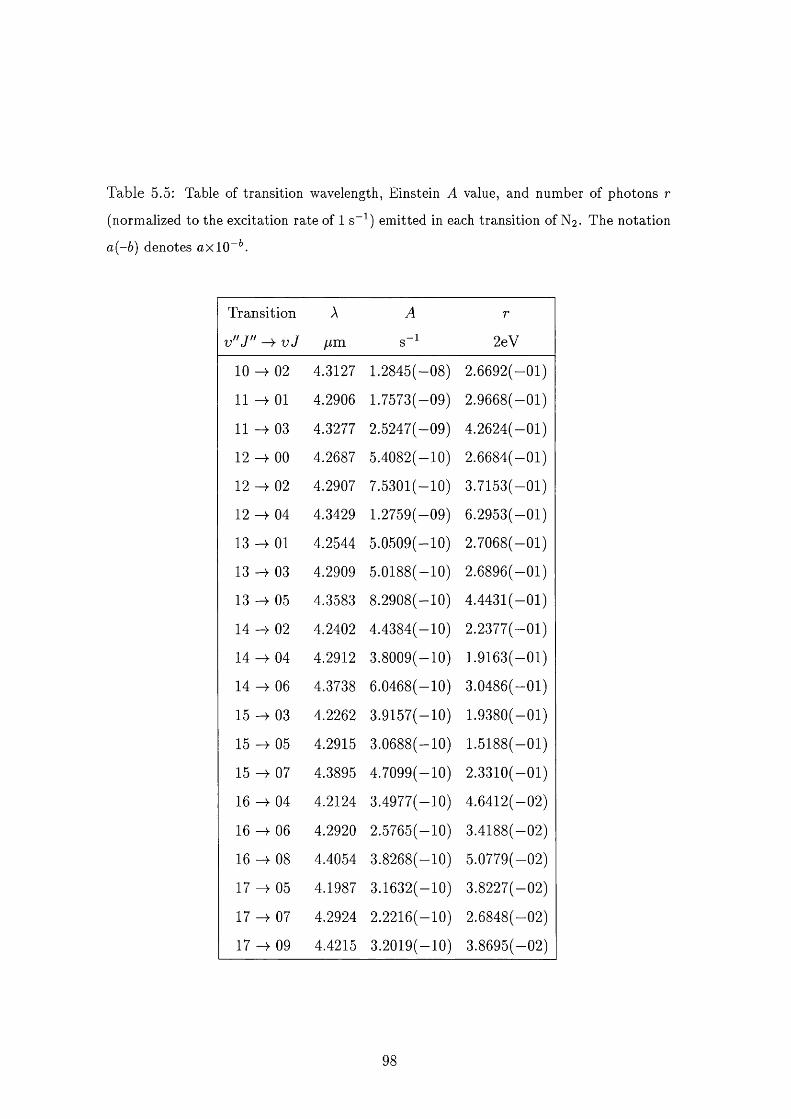
Table 5.5: Table of transition wavelength, Einstein A value, and number of photons r
(normalized to the excitation rate of 1 s“ ) emitted in each transition of N2 . The notation
a(-b) denotes ax 1 0 “ .
Transition A A r
jLim s- 2eV
1 0 0 2 4.3127 1.2845 -0 8 ) 2.6692 - 0 1 )
1 1 0 1 4.2906 1.7573 -0 9 ) 2.9668 - 0 1 )
1 1 -> 03 4.3277 2.5247 -0 9 ) 4.2624 - 0 1 )
1 2 -)• 0 0 4.2687 5.4082 - 1 0 ) 2.6684 - 0 1 )
1 2 -)■ 0 2 4.2907 7.5301 - 1 0 ) 3.7153 - 0 1 )
1 2 -4- 04 4.3429 1.2759 -0 9 ) 6.2953 - 0 1 )
13 0 1 4.2544 5.0509 - 1 0 ) 2.7068 - 0 1 )
13 03 4.2909 5.0188 - 1 0 ) 2.6896 - 0 1 )
13 05 4.3583 8.2908 - 1 0 ) 4.4431 - 0 1 )
14 0 2 4.2402 4.4384 - 1 0 ) 2.2377 - 0 1 )
14 04 4.2912 3.8009 - 1 0 ) 1.9163 - 0 1 )
14 06 4.3738 6.0468 - 1 0 ) 3.0486 - 0 1 )
15 03 4.2262 3.9157 - 1 0 ) 1.9380 - 0 1 )
15 -)• 05 4.2915 3.0688 - 1 0 ) 1.5188 - 0 1 )
15 07 4.3895 4.7099 - 1 0 ) 2.3310 - 0 1 )
16 04 4.2124 3.4977 - 1 0 ) 4.6412 - 0 2 )
16 -> 06 4.2920 2.5765 - 1 0 ) 3.4188 - 0 2 )
16 08 4.4054 3.8268 - 1 0 ) 5.0779 - 0 2 )
17 05 4.1987 3.1632 - 1 0 ) 3.8227 - 0 2 )
17 07 4.2924 2.2216 - 1 0 ) 2.6848 - 0 2 )
17 -> 09 4.4215 3.2019 - 1 0 ) 3.8695 - 0 2 )
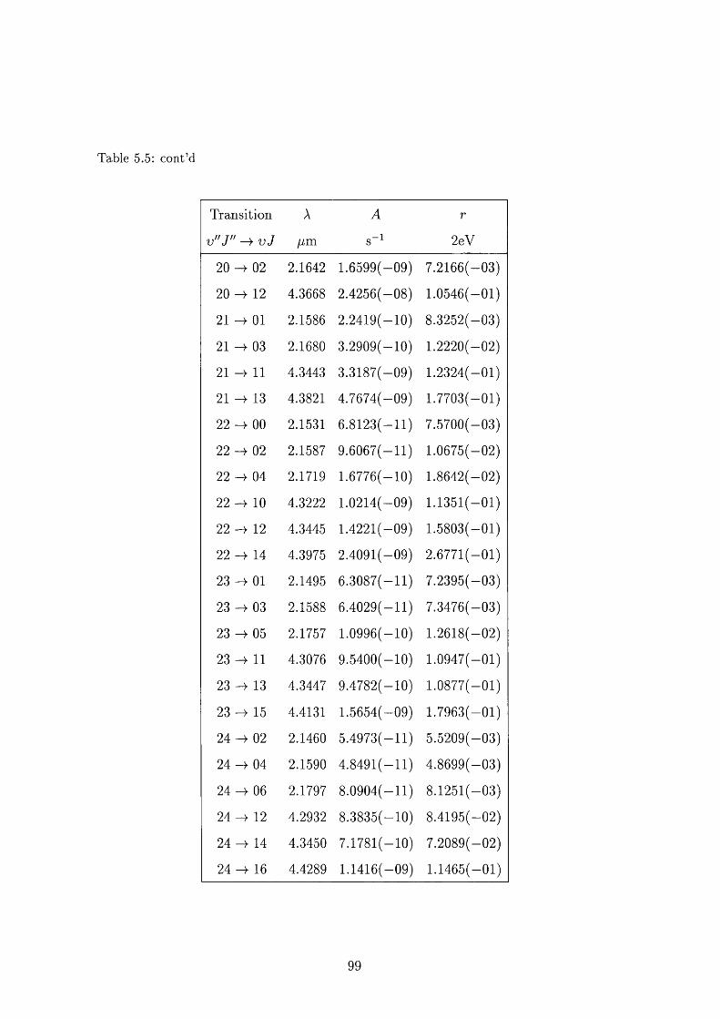
Table 5.5: cont’d
Transition A A r
fim s~ 2eV
2 0 0 2 2.1642 1.6599 -0 9 ) 7.2166 -0 3 )
2 0 1 2 4.3668 2.4256 -0 8 ) 1.0546 - 0 1 )
2 1 -4 0 1 2.1586 2.2419 - 1 0 ) 8.3252 -0 3 )
2 1 -4 03 2.1680 3.2909 - 1 0 ) 1 . 2 2 2 0 - 0 2 )
2 1 -> 1 1 4.3443 3.3187 -0 9 ) 1.2324 - 0 1 )
2 1 13 4.3821 4.7674 -0 9 ) 1.7703 - 0 1 )
2 2 -4- 0 0 2.1531 6.8123 - 1 1 ) 7.5700 -0 3 )
2 2 -4 0 2 2.1587 9.6067 - 1 1 ) 1.0675 - 0 2 )
2 2 -4 04 2.1719 1.6776 - 1 0 ) 1.8642 - 0 2 )
2 2 -4 1 0 4.3222 1.0214 -0 9 ) 1.1351 - 0 1 )
2 2 -4 1 2 4.3445 1.4221 -0 9 ) 1.5803 - 0 1 )
2 2 -4 14 4.3975 2.4091 -0 9 ) 2.6771 - 0 1 )
23 -4 0 1 2.1495 6.3087 - 1 1 ) 7.2395 -0 3 )
23 -4 03 2.1588 6.4029 - 1 1 ) 7.3476 -0 3 )
23 -4 05 2.1757 1.0996 - 1 0 ) 1.2618 - 0 2 )
23 1 1 4.3076 9.5400 - 1 0 ) 1.0947 - 0 1 )
23 -4 13 4.3447 9.4782 - 1 0 ) 1.0877 - 0 1 )
23 -4 15 4.4131 1.5654 -0 9 ) 1.7963 - 0 1 )
24 -)■ 0 2 2.1460 5.4973 - 1 1 ) 5.5209 -0 3 )
24 -> 04 2.1590 4.8491 - 1 1 ) 4.8699 -0 3 )
24 06 2.1797 8.0904 - 1 1 ) 8.1251 -0 3 )
24 -)■ 1 2 4.2932 8.3835 - 1 0 ) 8.4195 - 0 2 )
24 14 4.3450 7.1781 - 1 0 ) 7.2089 - 0 2 )
24 -)■ 16 4.4289 1.1416 -0 9 ) 1.1465 - 0 1 )
99
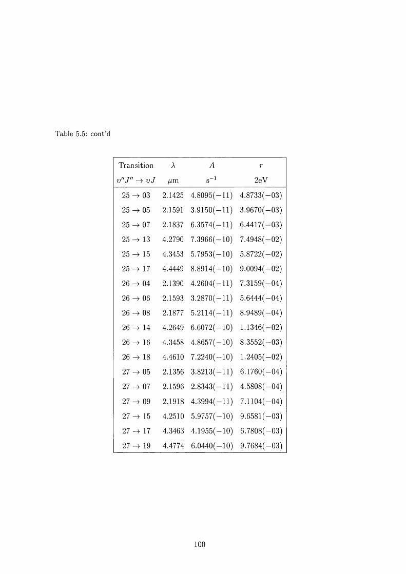
Table 5.5: cont’d
Transition A A r
U 'V ' -4 % J /im 8 - 1 2eV
2 5 -4 03 2.1425 4 .8 0 9 5 (-ll) 4.8733(-03)
25 ^ 05 2.1591 3.9150(-11) 3.9670(-03)
25 ^ 07 2.1837 6 .3 5 7 4 (-ll) 6.4417(-03)
2 5 -4 13 4.2790 7.3966(-10) 7.4948(-02)
25 15 4.3453 5.7953(-10) 5.8722(-02)
25 -4 17 4.4449 8.8914(-10) 9.0094(-02)
26 -4 04 2.1390 4 .2 6 0 4 (-ll) 7.3159(-04)
26 —y 06 2.1593 :T2870(-11) 5.6444(-04)
26 -4 08 2.1877 5.2114(-11) 8.9489(-04)
26 -4 14 4.2649 6.6072(-10) 1.1346(-02)
26 -4 16 4.3458 4.8657(-10) 8.3552(-03)
2 6 -4 18 4.4610 7.2240(-10) 1.2405(-02)
27 -4 05 2.1356 3.8213(-11) 6.1760(-04)
27 -4 07 2.1596 2 .8 3 4 3 (- ll) 4.5808(-04)
27 -4 09 2.1918 4 .3 9 9 4 (- ll) 7.1104(-04)
27 -4 15 4.2510 5.9757(-10) 9.6581(-03)
27 -4 17 4TW63 4.1955(-10) 6.7808(-03)
27 -4 19 4.4774 6.0440(-10) 9.7684(-03)
100
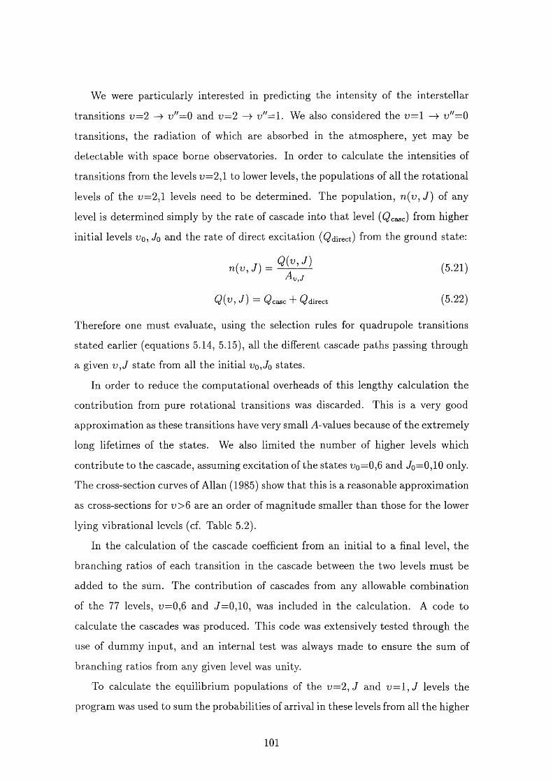
We were particularly interested in predicting the intensity of the interstellar
transitions v=2 -4 n"=0 and v=2 v"= \ . We also considered the v = l — v"=0
transitions, the radiation of which are absorbed in the atmosphere, yet may be
detectable with space borne observatories. In order to calculate the intensities of
transitions from the levels v = 2 , l to lower levels, the populations of all the rotational
levels of the v= 2 , l levels need to be determined. The population, J ) of any
level is determined simply by the rate of cascade into tha t level (Qcasc) from higher
initial levels Uq, Jq and the rate of direct excitation (Qdirect) from the ground state:
n { v , J ) = (5.21)
Q{v, J) = Qcasc + Qdirect (5.22)
Therefore one must evaluate, using the selection rules for quadrupole transitions
stated earlier (equations 5.14, 5.15), all the different cascade paths passing through
a given state from all the initial Uo,Jo states.
In order to reduce the computational overheads of this lengthy calculation the
contribution from pure rotational transitions was discarded. This is a very good
approximation as these transitions have very small A-values because of the extremely
long lifetimes of the states. We also limited the number of higher levels which
contribute to the cascade, assuming excitation of the states i;o=0 , 6 and Jo= 0 , 1 0 only.
The cross-section curves of Allan (1985) show that this is a reasonable approximation
as cross-sections for n > 6 are an order of magnitude smaller than those for the lower
lying vibrational levels (cf. Table 5.2).
In the calculation of the cascade coefficient from an initial to a final level, the
branching ratios of each transition in the cascade between the two levels must be
added to the siim. The contribution of cascades from any allowable combination
of the 77 levels, u=0,6 and J=0,10, was included in the calculation. A code to
calculate the cascades was produced. This code was extensively tested through the
use of dummy input, and an internal test was always made to ensure the sum of
branching ratios from any given level was unity.
To calculate the equilibrium populations of the v = 2 ^ J and t>=l, J levels the
program was used to sum the probabilities of arrival in these levels from all the higher
101
levels, (uo=3,6 Jq=0, 10) for v=2 and (no=2,6 Jo = 0 ,10) for v = l . The Table 5.5
indicates r, the numbers of photons per second emerging in the strongest transitions
out of the levels u "= 2 ,l (for an assumed excitation rate of 1 per second), and a
distribution into initial internal excited states before cascade as determined by Allan
(1985). In this calculation we have ignored the collisional quenching of the excited
levels, th a t may occur at the highest densities of n(H 2 ) = 1 0 cm“ .
5.3 A n estim ate of the d etectab ility o f th e em is
sion
We now calculate whether such quadrupole transition lines may be observable. The
photon generation rate per unit volume (cm~^ s“ ) from N 2 , n "= 2 ,l in specific lines
is
= Z / M ( e \ ^ ; ) u ( e \ E ) (;(?;'% . e ) n ( N 2 ) d E (5.23)
where n(e*, E ) d E is the number density of excited electrons with energy in the range
E^ E-\-dE, and u(e*, E) is the corresponding speed; a ( v ^ E ) is the cross section for
vibrational excitation at energy E, and n(N 2 ) is the number density of N 2 . We
assumed tha t n(e*) is determined by the cosmic ray ionization rate, as
n(e*) ~ ( n r
where n is the number density and r is the mean lifetime of e*, given by
~ ncTeiu(e*). (5.24)
Estim ating i?p, using the cross sections of Allan (1985) at 2 eV and equation (5.24),
we find, approximately, tha t
Rp ~ (n (N 2 ) r (5.25)
which, for example, with (= 3 x 1 0 “ ^ s“ , n(N 2 ) = l cm“ and r= 0 .01-0.1 (cf. Table
5.5), gives Rp in the range 10“ * - 10“ ^ photons cm"^ s“ E
For a cloud of dimension L at a distance d with the cloud just filling the telescope
beam, we find that the intensity is given by
102
»-16 aX7_-2..™-1 / ( ] ( ^ ( ^ 2)V 3 X lQ-17 g-1 / I 1 cm “3
f L y / 3 X iQ i^ m yVlO ® m / \ d y \ AA )
where AA is the wavelength resolution. In the case of Core D of TMC-1 at a distance
of 140 pc and with a radius of about 0.1 pc, then with n(N 2 ) = 1 0 cm“ the predicted
intensity is about 1.4x10“ ^ If the current detection lim it is about
1 0 ~ ® then slightly more favourable param eter choices could make this
object detectable in these lines. Other objects may be more favourably placed. In
any case, with the likely improvements in sensitivity there is a real hope of detecting
this emission from N2 . For other diatomics, the situation may be more favourable;
e.g. O2 is expected to be significantly more abundant than N2 in interstellar clouds
(cf. Table 5.1). Recently, Maréchal, Vi al a & Benayoun (1997) have performed
detailed calculations of the chemistry of O2 in interstellar clouds, and concluded
th a t several transitions may be detectable by future satellite and balloon borne
submillimetre receivers (ODIN, SWAS, PRONAOS-SMH and PIROG 8 ). Indeed, our
work strengthens the predictions of Maréchal et al. , as our process provides more
emission than the therm al excitation processes they incorporated into their model.
5.4 C onclusions
The non-thermal tail of the electron distribution in dark clouds generated by cosmic
ray ionization will excite rovibrational levels of molecules, in particular, homonu-
clear diatomics. Emission from these levels is normally regarded as characteristic of
regions of high excitation, but should also occur at the levels indicated in section
5.3 in cold quiescent regions. We have made a crude estim ate of the intensities of
some of the stronger lines from N2 excited by supertherm al electrons, and found
these lines to be below the current limit of detectability for a canonical source, core
D of TMC-1. Improvements in sensitivity in the near future should bring these lines
into the detectable regime. Other excitation mechanisms will, however, also con
tribu te to the emission. Of these, direct formation of N2 on dust or other diatomics
103
may be im portant in denser regions (n ~ 1 0 cm“^) where hydrogenation reactions
are suppressed in favour of the formation of heavier diatomics (Pickles & Williams
1977). In addition, excitation of the N2 triplet system by supertherm al electrons
with energies in the range 6.5-10.2 eV will also decay into the ground vibrational
system. The triplet state also overlaps with the Lyman band fluorescence of H 2 and
so may couple with the cosmic ray induced radiation field. The predicted intensity
of lines is, therefore, likely to be an underestimate.
We therefore believe that a search for 2-1 lines of N2 and O 2 in nearby cold,
dark, dense molecular clouds is recommended. This novel observational approach, if
successful, would provide the first direct measure of the N 2 and O2 fraction in dense
clouds. An immediate benefit would be a more accurate limit on the N 2 and O2
abundances in theoretical models. Furthermore, such measurements could be used
to constrain the N, C and 0 abundances in dense clouds, if other param eters (e.g.
uh, T, interstellar radiation field) are well defined (Maréchal, Viala & Benayoun
1997). We have an observing proposal in preparation to search for the 2-1 lines of
N 2 and O 2 in the well studied object TMC-1, in which N 2H+ has been detected.
104
Chapter 6
The sulphur depletion problem
In several of the preceding chapters we have referred to and described the “sulphur
depletion problem” . In this chapter we investigate this problem and propose a
mechanism to explain the unusual behaviour of sulphur.
6.1 Introduction
At visual extinctions of less than two to three magnitudes the dominant ion in a
dense core may be C'*', or a metallic ion, such as Mg" or Na+, depending on the
depletions of elemental carbon, sulphur and metals (see Fig. 3.4). The fractional
ionization is an im portant param eter in a dense core, for it determines the rate of
ambipolar diffusion and controls the rate at which m aterial from the envelope of a
dense core accretes onto a star that forms within it (e.g. Ciolek & Mouschovias 1995;
also see sections 1.1, 2.4 and 3.1). Hence, the ways in which carbon, sulphur and
metals freeze-out of the gas phase onto grains have consequences for the dynamics of
star formation. The depletion of sulphur is also im portant for observational studies
of star formation, as CS is one of the species frequently observed in attem pts to find
spectral signatures of dense core collapse (e.g. Zhou et al. 1993; cf. sections 1.5 and
1.6).
In diffuse regions, the abundance of sulphur is near its cosmic abundance as
shown in Fig. 6.1, from Federman et al. (1993). However, if models of dark cloud
chemistry are reliable, sulphur must be depleted by two to three orders of magnitude
105
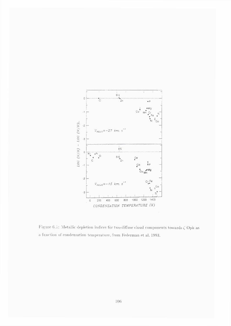
r
= î .i ' °Zn • p
-
!Ou*
♦ Mg
Mn Cr —
Ni 'Co
'h£LIO~~^T k m s
. . . k .......Kr *N
C4 .
ZnG e
I p —- G a
- -
^HCUC-~ I 5 km S ’Cr Fe
1 C! . i . i . ! 1 , 1 i 1 , ,0 200 400 600 800 1000 1200 1400
CONDENSATION TEMPERATURE (K)
l ' ig u re 6.1: Metallic depletion indices for two diffuse cloud components towards ( Oph as
a function of condensation tem perature, from Federman et al. 199.3.
106
in dark regions - even where elemental carbon, oxygen and nitrogen are depleted by
factors of only a few or less, for computed abundances of CS and other simple gas
phase sulphur-bearing species to agree with the measured fractional abundances.
This is the sulphur depletion problem: why is sulphur so much more depleted than
carbon, oxygen and nitrogen in dense cores?
In this chapter, we propose that sulphur is much more highly depleted in dense
interstellar regions than some of the other common elements because in a collapsing
translucent clump a large fraction of the gas phase sulphur is in the form of S'*" (see
Fig. 3.4 in Chapter 3). In such regions grains typically carry one negative charge
(Gail & Sedlmayr 1975; Bel et al. 1989; also see section 2.5.1) and therefore
may collide with grains on a timescale tha t is an order of magnitude smaller than
those associated with the neutral species containing most of the carbon, oxygen
and nitrogen in translucent regions. Collisions of ions with grains may well be
characterised by higher sticking coefficients (i.e. the probabilities th a t collisions will
result in depletion) than collisions of neutrals with grains, although some controversy
exists about this point (e.g. Watson & Salpeter 1972). As collapse continues,
the visual extinction increases and the fraction of gas phase sulphur incorporated
in neutral species will increase. Thus, any enhancement in the elemental sulphur
depletion rate due to S’*" containing a large fraction of the gas phase sulphur will
decline as the collapse continues, resulting in enough residual gas phase sulphur for
species containing it to be observable for long periods.
We present here the results of model calculations for the chemistry in a collapsing
cloud in which S’*" is assumed to be removed from the gas phase at a rate much larger
than the rates associated with the removal of neutral species and other ions. We
identify removal rates for and other species which lead to computed abundances
compatible with those measured for some simple sulphur-bearing species and other
simple species. The m aterial is assumed to have undergone a spherical collapse at
the free-fall rate.
107
Table 6.1: Initial fractional elemental abundances used in the model. The notation a{-b)denotes ax 10“ .
He C N 0 Na S Si0.07 1 (-4) 2 (-5) 2 (-4) 1 (-6 ) 3 (-6 ) 1 (-6 )
6.2 T he m odel o f sulphur chem istry
Initially, hh, the number density of hydrogen nuclei and the visual extinction to the
edge of the cloud, Ay-, were taken to be 1x10^ cm“ and 3, characteristic of many
clumps in giant molecular clouds (Williams, Blitz & Stark 1995; also see Chapters
1 and 3). Collapse was taken to occur at a the free fall rate, the evolution of
was governed by equation 2.6, with the param eter B set equal to 1. Collapse
was halted at u h = 2 x 1 0 cm“ , typical of dense cores. Our assumption is th a t the
cloud is supported at this density by the large-scale magnetic field; a magnetically
subcritical dense core is assumed to have formed. The visual extinction obeyed
/ \ 2 /3
= 0.5 + 2.5 I — I , (6 .1 )\"H o /
appropriate for spherical collapse of a clump embedded in an interclump medium
th a t contributes 0.5 magnitudes to the visual extinction.
During the collapse, freeze-out of gas phase species j onto dust grains was as
sumed to occur at a rate given by equation 2.4, tha t is
r o ) = 1.1 X ( i ) ' " ( j ^ )
where equation 2.5 specifies the value of A for neutral species and positive ions, and
D(j) describes variations in the sticking efficiency and grain size distribution; m(j)
is the mass of a single particle of species j and T is the clump tem perature taken
to be 20 K. In fact we set D(])=D* for all species except S'^. We specify models by
giving values of D* and D(S'^). As during most of the evolution almost all carbon,
oxygen and nitrogen are in neutral species the values adopted for quantities such
as D(C"""), D(0"^) and D(N+) have little effect on results, and we have taken only
D(S+) to differ from D*.
108
All hydrogen was assumed to be initially in the form of H2 , and all other elements
except carbon, sulphur and sodium (which were assumed to be contained entirely in
S’*" and Na'*') were assumed to be initially completely in neutral atomic form.
The fractional elemental abundances used initially are given in Table 6.1 (note these
are the same as Set B abundances for diffuse clouds specified in Chapter 3). The
value for S is consistent with its depletion behaving with density like tha t of Zn
(which has about the same condensation tem perature as S) in diffuse clouds (see
Fig. 6.1; also see Jenkins 1987).
The model included 217 gas phase species which are connected through 2773
reactions. We took the reactions from the UMIST rate file, which incorporates the
sulphur chemistry of Millar & Herbst (1990) (Millar et al. 1997; see section 2.6).
We also included dissociation of molecules by photons tha t arise from the cosmic
ray ionization of H and H2 . We adopted a cosmic ray ionization rate of 1.3x10“ ^
s“ T In addition we incorporated dissociation induced by photons of the interstellar
background radiation field.
6.3 R esu lts
Table 6.2 is a compilation of measured fractional abundances of sulphur-bearing
species in a number of clouds. Comparisons between entries in it and numerical
model results presented in the figures in this chapter allow us to identify values of
D* and D{S'^) which are compatible with observations. Figure 6 . 2 presents results
for a model with D*=0.1 and D(S""")=1 and Fig. 6.3 for a model with D*=0.1 and
D{S'^)=2. Each of these models displays a rapid decrease followed by significant
plateau in the gas phase CS fractional abundance. The sensitivity of the CS plateau
abundance value to D(S'^) is obvious from inspection of the two figures. However, it
is clear th a t the model results for CS are compatible with observations for a choice
of D(S"^) which in no way seems unrealistic. For D*=0.1, significant abundances of
species, including sulphur-bearing species, remain in the gas phase for times th a t are
likely to exceed the dense core lifetimes, which are limited by ambipolar diffusion.
The param eters D* and D(S'^) depend on the sticking efficiency of species onto
109
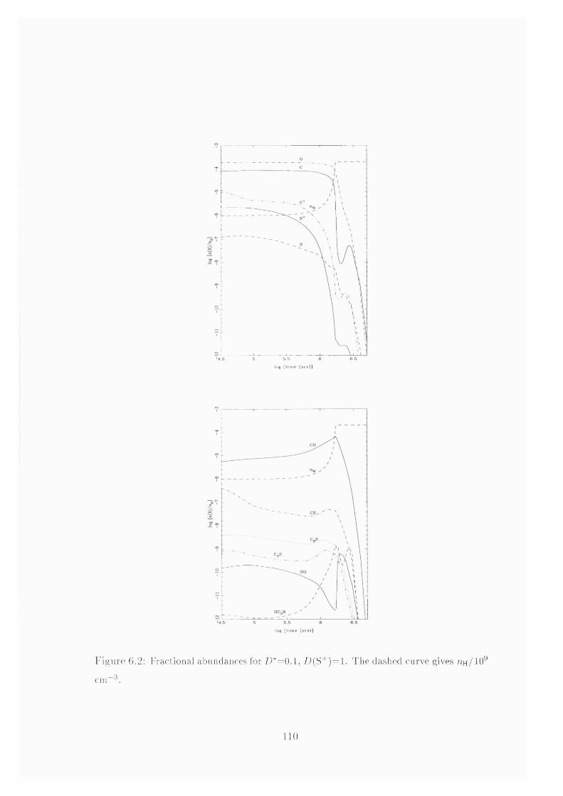
5,5
log [ l im e ( y r s ) l
log [ t im e (y r s ) )
iMgiire 6.2: Fractional abundances for D *= 0 . i , D(S+) = i. The dashed curve gives nn/lO"
cm
1 10
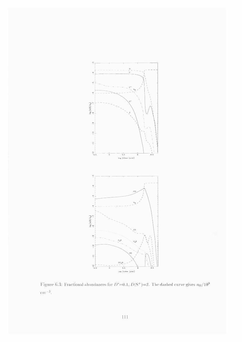
log [ l im e ( y r s ) l
log [ l im e ( y r s ) l
I ' lgu re 6.3: Fractional abundances for D *= 0 .i , D(S"*")=2. The dashed curve gives n n / lO '
cni~3.
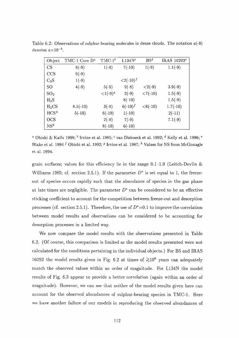
Table 6.2: Observations of sulphur-bearing molecules in dense clouds. The notation a{-b)denotes ax 10“ .
Object TMC- 1 Core D“ TMC-l* L134N** BS** IRAS 16293*CS 8(-9) l(-8 ) 7(-10) l(-9) l.l(-9)CCS 9(-9)CsS l(-9) < 2 (-1 0 )/so 4(-9) 5(-9) 2 (-8 ) <2(-9) 3.9(-9)S0 2 <l(-9)« 2(-9) <7(-10) 1.5 (-9)H2 S 8 (-1 0 ) 1.5(-9)H2 CS 8.5(-10) 3(-9) 6 (-1 0 )-' < 6 (-1 0 ) 1.7(-10)HCS+ 5(-10) 6 (-1 0 ) I(-IO) 2 (-ll)OCS 2(-9) 7(-9) 7.1(-9)NS'* 8 (-1 0 ) 6 (-1 0 )
“ Ohishi & Kaifu 1998; Irvine et al. 1985; van Dishoeck et al. 1992; Kelly et al. 1996; Blake et al. 1994 Ohishi et al. 1992; Irvine et al. 1987; Values for NS from McGonagle et al. 1994.
grain surfaces; values for this efficiency lie in the range 0.1-1.0 (Leitch-Devlin &
Williams 1985; cf. section 2.5.1). If the param eter D* is set equal to 1 , the freeze-
out of species occurs rapidly such that the abundance of species in the gas phase
at late times are negligible. The param eter D* can be considered to be an effective
sticking coefficient to account for the competition between freeze-out and desorption
processes (cf. section 2.5.1). Therefore, the use of D*=0.1 to improve the correlation
between model results and observations can be considered to be accounting for
desorption processes in a limited way.
We now compare the model results with the observations presented in Table
6 .2 . (Of course, this comparison is limited as the model results presented were not
calculated for the conditions pertaining in the individual objects.) For B5 and IRAS
16293 the model results given in Fig. 6.2 at times of ^10® years can adequately
m atch the observed values within an order of magnitude. For L134N the model
results of Fig. 6.3 appear to provide a better correlation (again within an order of
magnitude). However, we can see tha t neither of the model results given here can
account for the observed abundances of sulphur-bearing species in TM C-1 . Here
we have another failure of our models in reproducing the observed abundances of
112
species in TMC-1 (cf. section 4.5). Perhaps in TMC-1 the sulphur-bearing species
tha t have been lost from the gas phase by freeze-out are being returned efficiently
by desorption processes, resulting in the high observed abundances. In section 4.5
we began an investigation into whether a model that incorporated the injection of
mantled species into the gas phase may better produce the unusually high observed
abundances of hydrocarbons and cyanopolyynes in TMC-1. From the comparisons
made here, it is clear tha t we should include the desorption of S-bearing species in
any such study. We are forced to again conclude tha t the observed high abundances
of hydrocarbons, cyanopolyynes and S-bearing species in TMC-1 is not understood.
The fractional abundances of C 2 S and C 3 S are more sensitive to T)(S'^) than that
of C S is. The SO to C S abundance ratio is a particularly sensitive function of tim e
and can be used as a chemical clock.
6.4 D iscussion
In section 2.3.5 we described the sulphur chemistry in translucent clumps and dense
cores; the sulphur hydrides are not thought to be abundant as the reactions to
form them are endothermie. However, the organo-sulphides and sulphur oxides can
be formed rapidly by ion-molecule and neutral-neutral reactions. In Chapter 5 we
described how homonuclear diatomic molecules are difficult to observe, although we
have predicted tha t it may be possible to detect non-thermal vibrational emission
from N2 and O2 in cold, dense cores. The cosmic abundance of sulphur is an order
of magnitude less than tha t of nitrogen. Hence, as the intensity of non-therm al
vibrational emission from a species is proportional to its fractional abundance (cf.
equation 5.26), if the m ajority of sulphur were to be stored as S2 in dark cores
it would be difficult, but potentially feasible to detect by the process proposed in
Chapter 5. However, the main formation routes of S2 are slow; two involve reactions
with S2 H''" which has a low abundance (cf. section 2.3.5) and a th ird involves the
neutral-neutral reaction of S with SO, which has a low reaction rate coefficient. As
a result, the S2 fractional abundance produced in models of translucent clumps and
dense cores is very low, typically of the order of 10“ ' . If the ‘missing’ S in dark
113
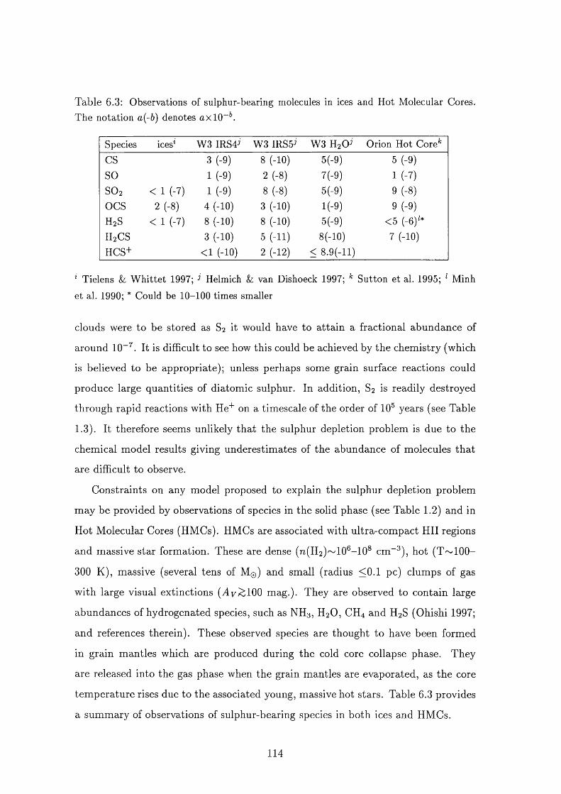
Table 6.3: Observations of sulphur-bearing molecules in ices and Hot Molecular Cores. The notation a{-b) denotes ax 10“ .
Species ices* W3 IRS4J W3 m s s ' W3 HsCy Orion Hot Core^CS 3 (-9) 8 (-1 0 ) 5(-9) 5 (-9)SO 1 (-9) 2 (-8 ) 7(-9) 1 (-7)S0 2 < 1 (-7) 1 (-9) 8 (-8 ) 5(-9) 9 (-8 )OCS 2 (-8 ) 4 (-10) 3 (-10) l(-9) 9 (-9)H2 S < 1 (-7) 8 (-1 0 ) 8 (-1 0 ) 5(-9) <5 (-6 )'*H2 CS 3 (-10) 5 (-11) 8 (-1 0 ) 7 (-10)HCS+ < 1 (-1 0 ) 2 (-1 2 ) < 8.9(-ll)
Tielens & Whittet 1997; Helmich & van Dishoeck 1997; Sutton et al. 1995; Minh et al. 1990; * Could be 10-100 times smaller
clouds were to be stored as S2 it would have to attain a fractional abundance of
around 10“ . It is difficult to see how this could be achieved by the chemistry (which
is believed to be appropriate); unless perhaps some grain surface reactions could
produce large quantities of diatomic sulphur. In addition, S2 is readily destroyed
through rapid reactions with He" on a timescale of the order of 10 years (see Table
1.3). It therefore seems unlikely that the sulphur depletion problem is due to the
chemical model results giving underestimates of the abundance of molecules tha t
are difficult to observe.
Constraints on any model proposed to explain the sulphur depletion problem
may be provided by observations of species in the solid phase (see Table 1.2) and in
Hot Molecular Cores (HMCs). HMCs are associated with ultra-com pact HII regions
and massive star formation. These are dense (n(H 2 ) ~ 1 0 ®-1 0 ® cm“^), hot (T ~100-
300 K), massive (several tens of M@) and small (radius <0.1 pc) clumps of gas
w ith large visual extinctions (Ty,^100 mag.). They are observed to contain large
abundances of hydrogenated species, such as N H 3 , H2 O, CH4 and E 2 S (Ohishi 1997;
and references therein). These observed species are thought to have been formed
in grain mantles which are produced during the cold core collapse phase. They
are released into the gas phase when the grain mantles are evaporated, as the core
tem perature rises due to the associated young, massive hot stars. Table 6.3 provides
a summary of observations of sulphur-bearing species in both ices and HMCs.
114
Hatchell et al. (1998) and Charniey (1997) have attem pted to model the observed
HMC sulphur chemistry. Initially, an injection of H2 S into the gas phase is specified
(which is assumed to have been formed in the grain mantle), and the subsequent
chemical evolution is followed. Hatchell et al. (1998) and Charniey (1997) found
th a t an assumed H2 S injection of 10“® (from the Minh et al. 1990 measurements
of H2 S in Orion) overproduces most of the observed sulphur-bearing species, by at
least an order of magnitude. However, the value of 10“® for H 2 S in Orion of Minh
et al. (1990) is uncertain, because the H2 column density is not well known. In
addition, Minh et al. assumed that the H2 S transitions are collisionally thermalised,
which may not be true. Hence, the measured value may be lower by a factor of 10-
100 (Charniey 1997). Therefore, the results of Hatchell et al. (1998) and Charniey
(1997) indicate a problem with the S chemistry in HMCs too; in particular with the
initial abundance of S that is available for injection into the gas phase. We propose
th a t this problem is related and linked to the S depletion problem in dense cores.
We believe tha t the nature of the S depletion during the cold core collapse phase
may be used to explain the S chemistry problem in HMCs.
In the model tha t is proposed in this chapter for the sulphur depletion problem
in dense cores, sulphur is accreting onto grain surfaces rapidly, faster than neutral
species are. Therefore the sulphur goes ‘down’ onto the grain surface before oxygen
does; accreted oxygen will undergo H abstractions to form water ice (Williams &
Taylor 1996). Consequently, it is conceivable tha t the S is somehow trapped on
the grain surface as a layer below tha t of the icy mantle, and does not mix with
the mantle. This picture could explain the detection of S-bearing species in ices
and HMCs with abundances that are very similar to the observations of S-bearing
species in dense cores (cf. Tables 6.3 and Table 6.2), as we now describe. The
sulphur accreted during the early stages of collapse, before the water ice is formed,
is locked beneath the icy mantle. Some S is still available in the m antle to form
the observed solid phase species (Table 6.3), as our model predicts the accretion of
sulphur bearing species at late times. (Bergin & Langer 1995 found th a t sulphur-
bearing species exhibit large depletions at the later stages of evolution, independent
of the grain m antle properties.) It is this sulphur that is observed in ices th a t can
115
be released into the gas phase, in some form, in HMCs. We therefore suggest tha t
the model presented here supports the reduction of the initial abundance of sulphur-
bearing species tha t is utilized in the treatm ent of the chemistry of HMCs; rather
than using abundances near the ‘cosmic’ values, depleted values for S (as measured
in dark cores) should be employed.
Caselli, Hasegawa & Herbst (1994) considered the production of condensed phase
CO in dense cores, which has a fractional abundance in such regions of the order of
>10“ (W hittet & Duley 1991); their model incorporated both gas phase and grain
surface chemistry. Caselli, Hasegawa & Herbst invoked large depletions of sulphur
in order for their model results to reproduce the observed abundances of condensed
phase CO. The sulphur on the grain converts H into H2 through reactions tha t
involve HS and H 2 S; thus reducing the amount of H available to hydrogenate CO
and the models were therefore able to reproduce the observed values.
An interesting point noted by Hatchell et al. (1998) is the detection of high frac
tional abundance of S-bearing species (of the order >10“^) towards shocked regions,
such as the molecular outflow of L1157 (Bachiller et al. 1997). Hartquist, Oppen-
heimer & Dalgarno (1980) predicted tha t shock chemistry may produce large quanti
ties of sulphur-bearing species. In the scheme that we propose, the trapped sulphur
can be returned to the gas phase only when grain cores are destroyed by sputtering
and /o r grains collisions. Perhaps this is occuring in such shocked regions as the
molecular outflow of LI 157; the freed sulphur can then be involved in the shock
chemistry.
An interesting question is the form of the sulphur in the dust, which will naturally
depend on the nature of the grain surface, which is not well known (e.g. Williams &
Taylor 1996). However, it is believed tha t the dust contains both silicates (which are
amorphous) and carbons (crystalline and amorphous, which is partly hydrogenated);
it is not clear if the grains are either silicate or carbonaceous, or whether some sort
of core/m antle structure exists (see Williams & Taylor 1996; Dorschner & Henning
1995). Perhaps the S’*" is inserted into the HAC (Hydrogenated Amorphous Carbon)
layer, to then be released as C^S when the grains are eroded. (This picture could
be helpful in attem pting to model the observed high abundances in TM C-1 .) An
116
alternative route is tha t the S'*" is inserted into silicons or oxides. However, Klem
perer favours tha t the S is trapped on the grain as sulphuric acid, H2 SO4 (private
com m unication).
6.5 C onclusions
The freeze-out rate of S ions onto negatively charged grains in molecular clouds
is expected to be enhanced over the rate for neutrals. We have computed the
abundances of sulphur-bearing species in a single-point model of chemistry, using
the two param eters, D(S'^) and D*, to explore the consequences of relative freeze-
out rates of and other species. The results of these computations support the
proposal tha t the differences between depletions in diffuse clouds and dense clouds
are compatible with S'*" being incorporated into dust grains more efficiently than the
neutral species.
117
Chapter 7
Selective depletions and the
abundances of molecules used to
study star formation
In section 1,5 we gave a detailed account of the observations tha t have been made
of regions of infall and in section 1 . 6 we discussed theoretical studies of dense core
collapse. In Chapter 6 we have explored the behaviour of the sulphur depletion,
and seen tha t it does not follow tha t of carbon, nitrogen and oxygen. Indeed, there
is no reason to expect tha t all the species will freeze-out at the same rate. Hence,
it is worthwhile to investigate the dependences of the fractional abundances of a
num ber of species on the selective depletions of elemental carbon, nitrogen, oxygen
and sulphur, as well as metals.
7.1 Introduction
In the last several years numerous detections of line profiles showing putative signa
tures of the collapse of dense cores to give birth to low mass stars have been reported
(e.g. Zhou et al. 1993; Zhou et al. 1994; Mardones et al. 1994; Myers et al. 1995;
Velusamy, Kuiper & Langer 1995; Wang et al. 1995; Zhou, Evans & Wang 1996;
Gregersen et al. 1997; Mardones et al. 1997), as described in detail in section 1.6. In
order to gain insight into the dynamics of collapse, models of the radiative trans-
118
fer must be constructed to interpret the line profiles (e.g. Choi et al. 1995; Myers
et al. 1996). Though in most cases the use of radiative transfer models to interpret
the infall signatures has been based on the assumption tha t the fractional abun
dances of gas phase species are invariant in the collapsing gas, knowledge of the
ways in which the gas phase chemistry varies in the infalling m aterial is also vital.
Pickles & Williams (1981) examined the effects of various combinations of car
bon and oxygen depletions on gas phase abundances of a lim ited number of very
simple species. Ment en et al. (1984) suggested tha t the freeze-out onto dust grains
of elements more massive than helium has a considerable effect on the gas phase
abundances of some species with emissions observed in attem pts to detect spectral
signatures of infall. Hartquist & Williams (1989) gave arguments th a t for some
ranges of depletion, some species should actually have gas phase fractional abun
dances tha t increase with depletion. Rawlings et al. (1992) made a first a ttem pt to
identify species tha t are more likely to show signatures of infall in line profiles if
depletion is responsible for the absence of such signatures in many observed NH3
line profiles (see sections 1.5 and 1.6). In tha t calculation, the tim e-dependent and
spatially dependent chemical evolution in the collapse of a singular isothermal sphere
was followed in each of a large number of fluid elements. The complexity of the dy
namical description prevented the investigation of the effects of selective depletion
and it was assumed tha t the sticking coefficients for many species were equal.
In fact, we know that some elements become highly depleted from the gas phase
well before others do. For instance, as we have discussed in Chapter 6 , sulphur must
be a couple of orders of magnitude more depleted in many dense core regions than
it is in diffuse clouds in order for the gas phase abundance of CS to be as low as is
observed, even though in those same regions the abundances of other species show
th a t the elements carbon, nitrogen and oxygen are each not depleted by more than a
factor of a few than in diffuse clouds. As described in Chapter 6 , we suggest th a t this
is a consequence of a much higher fraction of sulphur than of those other elements
being ionized at m oderate densities, in addition to the collision rates and sticking
coefficients of ions with grains being higher than those of neutrals. Nevertheless, we
do not know for certain why the sulphur depletion differs so much from those of some
119
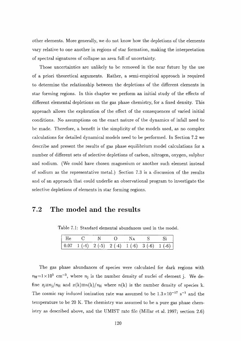
other elements. More generally, we do not know how the depletions of the elements
vary relative to one another in regions of star formation, making the interpretation
of spectral signatures of collapse an area full of uncertainty.
Those uncertainties are unlikely to be removed in the near future by the use
of a priori theoretical arguments. Rather, a semi-empirical approach is required
to determ ine the relationship between the depletions of the different elements in
star forming regions. In this chapter we perform an initial study of the effects of
different elemental depletions on the gas phase chemistry, for a fixed density. This
approach allows the exploration of the effect of the consequences of varied initial
conditions. No assumptions on the exact nature of the dynamics of infall need to
be made. Therefore, a benefit is the simplicity of the models used, as no complex
calculations for detailed dynamical models need to be performed. In Section 7.2 we
describe and present the results of gas phase equilibrium model calculations for a
num ber of different sets of selective depletions of carbon, nitrogen, oxygen, sulphur
and sodium. (We could have chosen magnesium or another such element instead
of sodium as the representative metal.) Section 7.3 is a discussion of the results
and of an approach tha t could underlie an observational program to investigate the
selective depletions of elements in star forming regions.
7.2 T he m odel and th e results
Table 7.1: Standard elemental abundances used in the model.
He C N 0 N a S Si0.07 1 (-4) 2 (-5) 2 (-4) 1 (-6 ) 3 (-6 ) 1 (-6 )
The gas phase abundances of species were calculated for dark regions with
nH = lx lO ^ cm“^, where uj is the number density of nuclei of element j. We de
fine a:j=nj/nH and x(k)=n(k)/nH where n(k) is the number density of species k.
The cosmic ray induced ionization rate was assumed to be 1.3x10“ ^ s“ and the
tem perature to be 20 K. The chemistry was assumed to be a pure gas phase chem
istry as described above, and the UMIST rate file (Millar et al. 1997; section 2.6)
120

was taken as the source of most data. The model included 238 gas phase species
which are connected through 2732 reactions. In these models we do not incorporate
the freeze-out of species onto the dust grain; instead the depletions are determined
at the start of the calculation. As ’standard’ elemental abundances with respect
to hydrogen we took the values displayed in Table 7.1 (note these are the same
values as used in Chapters 3 and 6 ). The value for xhc was the same in all models.
To designate a particular model we give each elem ent’s symbol in upper case if the
corresponding Xj is taken to be the ’standard’ value, and to be in lower case if the cor
responding Xj is 1/3 the ’standard’ value. For three models we used a value of xq tha t
is 1/9 times the ’standard’ value, which is indicated by og. For instance, CNONaS
is the one for which all elements are assumed to have their ’standard’ abundances,
while the model designated cNONaS is the one for which all elements except carbon
are assumed to have ’standard’ abundances, but carbon has an abundance 1/3 its
standard value. cnogUas signifies tha t the abundances of each of carbon, nitrogen,
sodium and sulphur is 1/3 its ’standard’ value and the abundance of oxygen is 1/9
its ’standard’ value.
Table 7.2 gives the ratio of the value of %(k) in one model to its value in another
model for a number of im portant species and for a number of pairs of models. (Table
A . l in Appendix A gives the values of %(k) for some im portant species once steady
state has been reached in all 35 of the calculated models.)
7.3 D iscussion
In Table 7.2, column 7 for CNoNaS/CNON aS shows the well known differences
between chemistries in oxygen-rich and carbon-rich environments. As the oxygen
abundance is reduced, less carbon is locked into CO and fewer oxygen-bearing species
are available to destroy the build up of carbon-bearing species (cf. sections 2.3.2
and 2.3.3). Consequently, large increases are seen in the abundance of C-bearing
species (see W att 1985; Terzieva & Herbst 1998).
The columns to the left of column 7 are for carbon-rich environments and those
to the right are for oxygen-rich environments. We shall focus first on the oxygen-rich
121
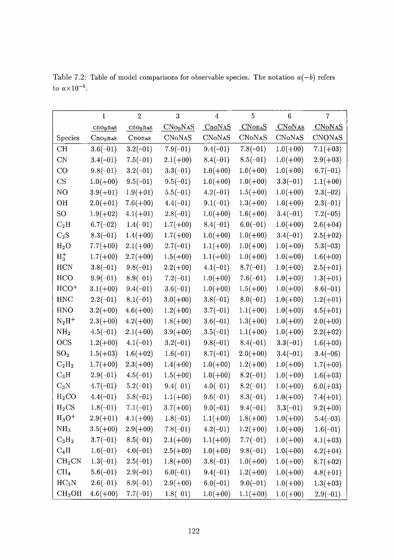
Table 7.2: Table of model comparisons for observable species. The notation n(—6) refersto axlO - b
2cn o g n a s cn o g n as CN O qN a S
S p e c ie s C nognaS C n o n a s C N oN a S
4C noN A S
C N oNaS
5C N o n a S
6 7C N oN as C N oN aS
C N oNaS C N oN aS CNONAS
C H
C N
COCS
N O
O H
SOCgHC2 SH2 OHj-H C N
H C O
H C O +
H N C
H N O
N2 H+NH2
OCSS0 2
C2H2C 3 H
C 3 N
H2 C0
H2 CSH3 0 +N H 3
C3H2C 4 H
C H 2 CN
C H 4
H C 3 N
C H 3 0 H
3.6
3.49 .8
1.03.9 2.01.96.7 8 .3
7.71.73 .8
9 .9
3.12.23.22 .3
4.5 1.2
1.51.72 .9
4.74.41.82 .9
3 .5
3.71.6
1.35.62.6 4.6
-01
-0 1
-01
+ 0 0
+ 0 1
+ 0 1
+ 0 2
- 0 2
( - 0 1
( + 0 0
( + 0 0
( - 0 1
( - 0 1
(+00(-01
(+00(+00( - 0 1
( + 0 0
(+03( + 0 0
( - 0 1
- 0 1
- 0 1
( - 0 1
(+01
( + 0 0
( - 0 1
- 0 1
- 0 1
-0 1
- 0 1
+ 0 0
3 .2
7.53 .2
9.5 1.97.64.11.41.42.1
2.79 .8
8 .9
9.4 8.14.64.2 2.1
4.11.6
2 .3
4.55.25 .8
7.14.12.9
8 .5
4.02.52.9
8 .9
7.7
- 01 )
- 01 )
- 01 )
-01)+ 01)+ 00)+ 01)- 01 )
+ 00)+ 0 0 )+ 0 0 )- 0 1 )- 0 1 )- 0 1 )
(-0 1 )(+ 0 0 )(+ 0 0 )(+ 0 0 )(-0 1 )(+ 0 2 )(+ 0 0 )(-0 1 )- 0 1 )- 0 1 )- 0 1 )+ 0 0 )+ 0 0 )- 0 1 )- 0 1 )- 0 1 )- 0 1 )- 0 1 )- 0 1 )
7.9(-01)2 .1 (4-00)
3.3(-01)9.5(-01)5.5(-01)4.4(-01)2.8(-01)1.7(+00)1.7(+00)2 .7 ( - 0 1 )
1.5(4-00)2.2 (+ 00)7.2(-01)3.6(-01)3.0(+00)1.2 ( + 00)1.8 ( + 00)3.9(+00)3.2(-01)1.6(-01)1.4(+00)1.5(+00)9.4(-01)1.1(4-00)3.7(+00)1.8 (-01)7.8(-01)2 .1(4-00)2.5(+00)1.8 ( + 00)
e .o ( - o i )2.9(+00)1.8 ( -01)
9.48.4 1.0
1.0
4 .2
9.1 1 . 0
8.4
1 . 0
1 . 1
1 . 1
4.1 1 . 0
1 . 0
3.8
3.73.6
3.59.8
8.7 1.0
1.0
4.09.6
9.01 . 1
4.2 1 . 1
1 . 0
3.8
9.4 6 . 0
1 . 0
- 0 1 )(-0 1 )(+ 0 0 )(+ 0 0 )(-0 1 )(-0 1 )(+ 0 0 )(-0 1 )(+ 0 0 )(+ 0 0 )(+ 0 0 )(-0 1 )(+ 0 0 )(+ 0 0 )(-0 1 )- 0 1 )- 0 1 )- 0 1 )- 0 1 )
(-0 1 )(+ 0 0 )(+ 0 0 )(-0 1 )- 0 1 )
(-0 1 )(+ 0 0 )(-0 1 )(+ 0 0 )(+ 0 0 )(-0 1 )- 0 1 )
(-0 1 )(+ 0 0 )
7.8(-01)8.5(-01)1.0 (+ 00)1.0 ( + 00)1.5(+00)1.3(+00)1.6 ( + 00)6 .0(-01)1.0 ( + 00)
1.0 ( + 00)
1.0 ( + 00 )
8.7(-01)7.6(-01)1.5(+00)8 .0 (-01)1 .1 (4- 00 )
1.3(+00)1 .1(4-00)
8.4(-01)2 .0 ( + 00)
1.2 ( + 00)8.2 ( - 01)8 .2(-01)8 .3 ( - 0 1 )
9.4(-01)1.8 ( + 00)1.2 ( + 00)7.7(-01)9.8(-01)1.0 (+ 00)1.2 ( + 00)9.0(-01)1.1(4-00)
1.0 ( + 00)1.0 ( + 00)1.0 ( + 00)3.3(-01)1.0 ( + 00)1.0 ( + 00)3.4(-01)1.0 ( + 00)3.4(-01)1.0 ( + 00)
1.0 (+ 00)1.0 ( + 00)1.0 (+ 00)1.0 (+ 00)1.0 ( + 00)1.0 ( + 00)
1.0 ( + 00)1 .0 (+ 0 0 )3.3(-01)3.4(-01)1 .0 (+ 0 0 )1 .0 (+ 0 0 )1 .0 (+ 0 0 )1 .0 (+ 0 0 )3 .3 ( - 0 1 )
1 .0 (+ 0 0 )1 .0 (+ 0 0 )1.0 (+ 00)1 .0 (+ 0 0 )1.0 ( + 00)1.0 ( + 00)
1.0 ( + 00)1.0 ( + 00)
7.1(+03)2.9(+03)6.7(-01)1 .1 (4- 00)
2.3(-02)2.3(-01)7.2(-05)2.6(+04)2.5(+02)5.3(-03)1.6 ( + 00)2.5(+01)1.3(+01)8 .6 (-01)1.2 ( + 01)4.5(4-01)2 .0 ( + 00)2 .2 ( + 02)
1.6 ( + 00)3.4(-06)1.7(+00)1.6(+03)6.0(+03)7.4(+01)9.2(+00)5.4(-03)1.6( -01)4.1(+03)4.2(+04)8.7(+02)4.8(+01)1.3(+03)2.9(-01)
122
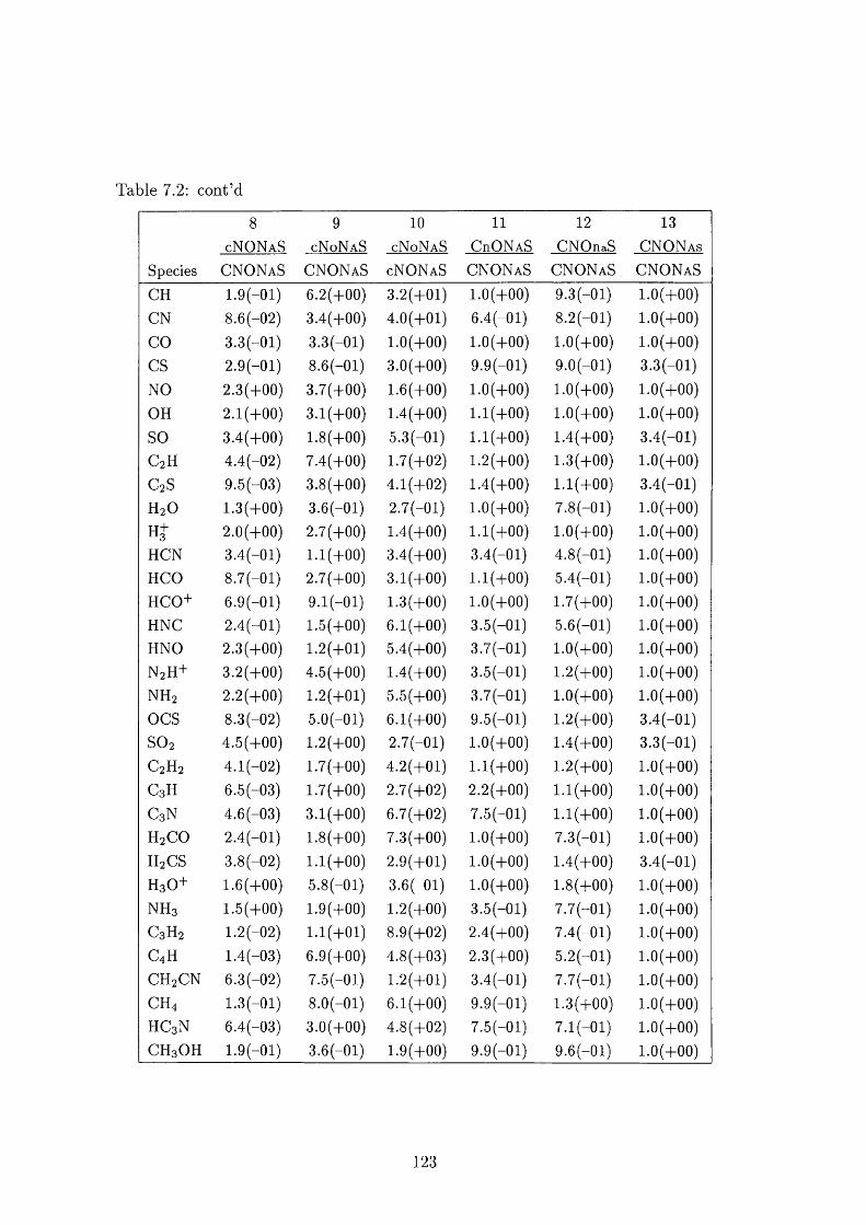
Table 7.2: cont’d
SpeciescN O N a S
C N O N A S
9cN oN a S
10
cN oN a S
11 12 13C r O N a S C N O n a S C N O N as
C N O N A S cN O N a S C N O N A S C N O N a S C N O N a S
C H
C N
C O
C S
N O
O H
S O
CgH
CgSH2 0
H C N
H C O
H C O +
H N C
H N O
N2H+
NH2
O C S
S0 2
C2H2C 3 H
C3 NH 2 CO
H 2 CS
H 3 0 +
N H 3
C3H2C 4 H
C H 2 CN
CH4H C 3 N
C H 3 0 H
1.9 8.63 .3
2.9
2 .3
2.1
3.44.49.51.3 2.03.48 .7
6.92.4 2 .3
3.22.2
8 .3
4.54.1
6.5
4.62.4
3 .8
1.6
1.51.2
1.4
6 .3
1.36.41.9
- 01 )
-02)- 01)
-01)+ 00)+00)+00)- 02 )
( -0 3 )
( + 00) ( + 00)(-01)- 01 )
- 01 )
( - 0 1 )
( + 00)
(+ 0 0 )(+ 0 0 )( - 0 2 )
(+ 0 0 )(-0 2 )-03)-03)- 0 1 )
( - 0 2 )
( + 00)(+ 0 0 )(-0 2 )- 0 3 )
-02)- 01 )
-03)- 0 1 )
6 .2 (+ 00)3.4(+00)
3.3(-01)8.6(-01)3.7(+00)3.1(4-00)1.8 (4-00)
7.4(+00)3.8(+00)3.6(-01)2.7(+00)1 .1 (4-00 )
2.7(4-00)9.1(-01)1.5(4400)1.2(4401)4.5(4400)1.2(4401)5 .0 ( - 0 1 )
1 .2 (4400)
1.7(+00)1.7(+00)3.1(4-00)1.8(4400)
1.1(4400)5.8(-01)1.9(4400)1.1(4401)
6.9(4400)7.5(-01)S.O(-Ol)3.0(4-00)3.6(-01)
3.2(4401)4.0(+01)1.0 (4400)
3.0(4400)
1.6 (+ 00)1.4(+00)
5.3(-01)1.7(+02)4.1(4-02)2.7(-01)1.4(+00)3.4(+00)3.1(4400)1.3(4400)6 .1 (4400)
5.4(+00)1.4(+00)5.5(+00)6 .1(4400)
2 .7 ( - 0 1 )
4.2(+01)2.7(+02)6.7(+02)7.3(+00)
2.9(4401)3.6(-01)1.2 (+ 00)8 .9 (+ 0 2 )
4 .8 (+ 0 3 )
1 .2 (4401)
6 .1 (4400)
4 .8 (+ 0 2 )
1.9(+00)
1 .0 (4- 00)
6 .4 ( - 0 1 )
1 .0 (4- 00)
9.9(-01)
1 .0 ( + 00)
1.1(4-00)
1. 1 (4- 00 )
1.2 ( + 00)
1.4(+00)1.0 ( + 00)
1.1 (4- 00)
3.4(-01)1 .1(4-00)
1.0 ( + 00)3.5(-01)3.7(-01)3.5(-01)3.7(-01)9.5(-01)1.0 ( + 00)
1.1(4400)2 .2 ( + 00)
7.5(-01)1.0 ( + 00)
1.0 ( + 00)
1.0 ( + 00)
3.5(-01)2.4(+00)2.3(+00)3.4(-01)
9 .9 ( - 0 1 )
7.5(-01)9.9(-01)
9.3(-01)8 .2(-01)1.0 ( + 00)9.0(-01)1.0 ( + 00)
1.0 ( + 00)
1.4(+00)1.3(+00)1.1(4400)7.8(-01)1.0 ( + 00)4.8(-01)5 .4 ( - 0 1 )
1.7(+00)5.6(-01)1 .0 ( + 00)
1.2 ( + 00) 1.0 ( + 00) 1.2 ( + 00)1.4(+00)1.2 ( + 00)
1 .1 (4- 00 )
1.1 (4- 0 0 )
7.3(-01)
1.4(+00)1.8 ( + 00)
7.7(-01)7 .4 ( - 0 1 )
5.2(-01)7.7(-01)1.3(+00)7.1(-01)9.6(-01)
1.0(+ 00) 1.0 ( + 00)
1.0 ( + 00)
3.3(-01)1.0 ( + 00)
1.0 ( + 00)
3.4(-01)1 .0 ( + 00)
3.4(-01)1.0 (+ 00) 1.0 ( + 00)
1.0 ( + 00)
1.0 ( + 00) 1.0 ( + 00) 1.0 ( + 00) 1.0 ( + 00) 1.0 ( + 00)1 .0 (+ 0 0 )3.4(-01)3.3(-01)1 .0 (+ 0 0 )1 .0 (+ 0 0 )1 .0 (+ 0 0 )1 .0 (+ 0 0 )3 .4 ( - 0 1 )
1 .0 (+ 0 0 )1 .0 (+ 0 0 )1.0 ( + 00)1 .0 (+ 0 0 )1.0 ( + 00) 1.0 ( + 00) 1.0 ( + 00) 1.0 ( + 00)
123
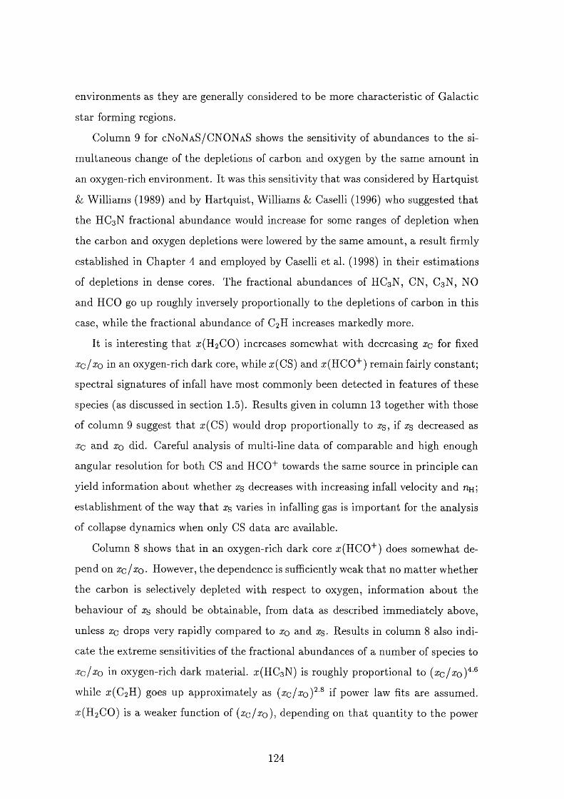
environments as they are generally considered to be more characteristic of Galactic
star forming regions.
Column 9 for cNoNaS/CNONaS shows the sensitivity of abundances to the si
multaneous change of the depletions of carbon and oxygen by the same amount in
an oxygen-rich environment. It was this sensitivity tha t was considered by H artquist
& Williams (1989) and by Hartquist, Williams & Caselli (1996) who suggested tha t
the HC3 N fractional abundance would increase for some ranges of depletion when
the carbon and oxygen depletions were lowered by the same amount, a result firmly
established in Chapter 4 and employed by Caselli et al. (1998) in their estimations
of depletions in dense cores. The fractional abundances of HC3 N, CN, C3 N, NO
and HCO go up roughly inversely proportionally to the depletions of carbon in this
case, while the fractional abundance of C2 H increases markedly more.
It is interesting tha t z(H 2 C 0 ) increases somewhat with decreasing xc for fixed
x c / Xq in an oxygen-rich dark core, while a;(CS) and z(HCO"^) remain fairly constant;
spectral signatures of infall have most commonly been detected in features of these
species (as discussed in section 1.5). Results given in column 13 together with those
of column 9 suggest that x(CS) would drop proportionally to %, if xs decreased as
Xc and xq did. Careful analysis of multi-line data of comparable and high enough
angular resolution for both CS and HCO^ towards the same source in principle can
yield information about whether zg decreases with increasing infall velocity and ny;
establishment of the way tha t zg varies in infalling gas is im portant for the analysis
of collapse dynamics when only CS data are available.
Column 8 shows that in an oxygen-rich dark core z (H C 0 ‘*') does somewhat de
pend on zc/zQ. However, the dependence is sufficiently weak tha t no m atter whether
the carbon is selectively depleted with respect to oxygen, information about the
behaviour of zg should be obtainable, from data as described immediately above,
unless zc drops very rapidly compared to zq and zg. Results in column 8 also indi
cate the extreme sensitivities of the fractional abundances of a number of species to
zc/zo in oxygen-rich dark material. z(H C 3 N) is roughly proportional to (zc/zo)^'^
while z(C 2 H) goes up approximately as (zc/zq)^'^ if power law fits are assumed.
z (H 2 C 0 ) is a weaker function of ( z c / z q ), depending on tha t quantity to the power
124
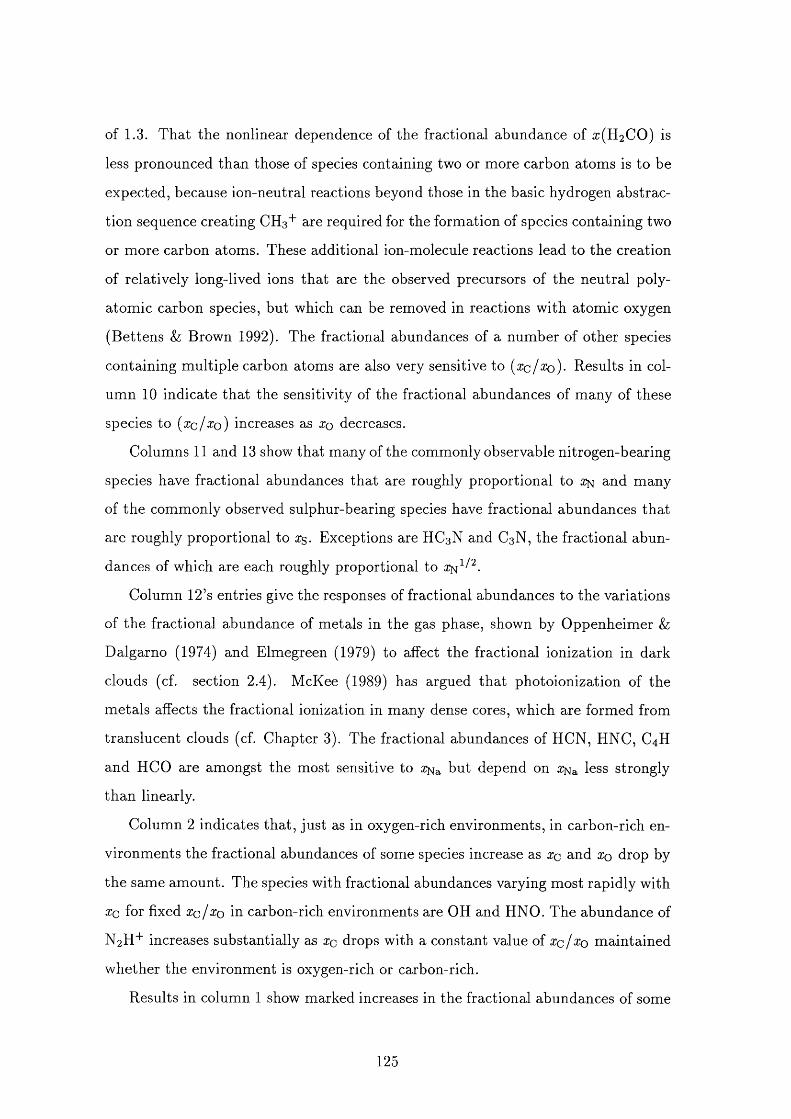
of 1,3. That the nonlinear dependence of the fractional abundance of z(H 2 C 0 ) is
less pronounced than those of species containing two or more carbon atoms is to be
expected, because ion-neutral reactions beyond those in the basic hydrogen abstrac
tion sequence creating CHa'*' are required for the formation of species containing two
or more carbon atoms. These additional ion-molecule reactions lead to the creation
of relatively long-lived ions tha t are the observed precursors of the neutral poly
atomic carbon species, but which can be removed in reactions with atomic oxygen
(Bettens & Brown 1992). The fractional abundances of a number of other species
containing multiple carbon atoms are also very sensitive to (%/%>). Results in col
um n 1 0 indicate tha t the sensitivity of the fractional abundances of many of these
species to (% /% ) increases as xq decreases.
Columns 1 1 and 13 show that many of the commonly observable nitrogen-bearing
species have fractional abundances tha t are roughly proportional to &nd many
of the commonly observed sulphur-bearing species have fractional abundances tha t
are roughly proportional to %. Exceptions are HC3 N and C3 N, the fractional abun
dances of which are each roughly proportional to
Column 12’s entries give the responses of fractional abundances to the variations
of the fractional abundance of metals in the gas phase, shown by Oppenheimer &
Dalgarno (1974) and Elmegreen (1979) to affect the fractional ionization in dark
clouds (cf. section 2.4). McKee (1989) has argued tha t photoionization of the
m etals affects the fractional ionization in many dense cores, which are formed from
translucent clouds (cf. Chapter 3). The fractional abundances of HCN, HNC, C4 H
and HCO are amongst the most sensitive to a Na but depend on a^a less strongly
than linearly.
Column 2 indicates tha t, just as in oxygen-rich environments, in carbon-rich en
vironments the fractional abundances of some species increase as xc and xq drop by
the same amount. The species with fractional abundances varying most rapidly with
Xc for fixed xq/ xq in carbon-rich environments are OH and HNO. The abundance of
N 2 H+ increases substantially as xq drops with a constant value of xq/ xq m aintained
whether the environment is oxygen-rich or carbon-rich.
Results in column 1 show marked increases in the fractional abundances of some
125
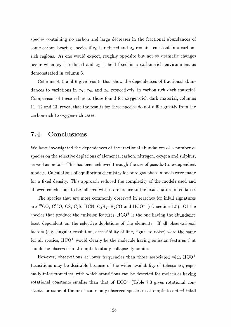
species containing no carbon and large decreases in the fractional abundances of
some carbon-bearing species if xq is reduced and x q remains constant in a carbon-
rich regions. As one would expect, roughly opposite but not so dram atic changes
occur when xq is reduced and xq is held fixed in a carbon-rich environment as
dem onstrated in column 3.
Columns 4, 5 and 6 give results tha t show the dependences of fractional abun
dances to variations in x^^ and respectively, in carbon-rich dark material.
Comparison of these values to those found for oxygen-rich dark m aterial, columns
11, 12 and 13, reveal tha t the results for these species do not differ greatly from the
carbon-rich to oxygen-rich cases.
7.4 C onclusions
We have investigated the dependences of the fractional abundances of a number of
species on the selective depletions of elemental carbon, nitrogen, oxygen and sulphur,
as well as metals. This has been achieved through the use of pseudo-time-dependent
models. Calculations of equilibrium chemistry for pure gas phase models were made
for a fixed density. This approach reduced the complexity of the models used and
allowed conclusions to be inferred with no reference to the exact nature of collapse.
The species tha t are most commonly observed in searches for infall signatures
are ^^CO, C'®0, CS, CgS, HCN, C3 H2 , HgCO and HCO+ (cf. section 1.5). Of the
species tha t produce the emission features, HCO""" is the one having the abundance
least dependent on the selective depletions of the elements. If all observational
factors (e.g. angular resolution, accessibility of line, signal-to-noise) were the same
for all species, HCO"^ would clearly be the molecule having emission features tha t
should be observed in attem pts to study collapse dynamics.
However, observations at lower frequencies than those associated with HCO'*'
transitions may be desirable because of the wider availability of telescopes, espe
cially interferometers, with which transitions can be detected for molecules having
rotational constants smaller than tha t of HCO"^ (Table 7.3 gives rotational con
stants for some of the most commonly observed species in attem pts to detect infall
126
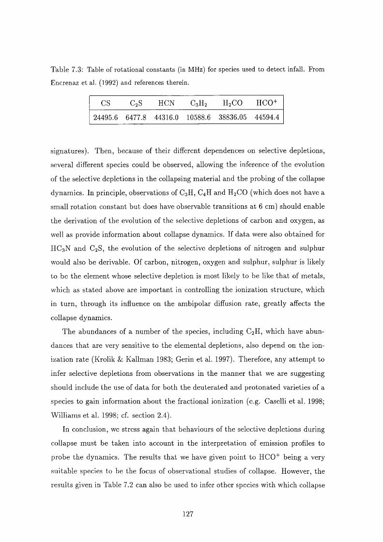
Table 7.3: Table of rotational constants (in MHz) for species used to detect infall. From
Encrenaz et al. (1992) and references therein.
CS C2S HCN C3H2 H2 CO HCO+
24495.6 6477.8 44316.0 10588.6 38836.05 44594.4
signatures). Then, because of their different dependences on selective depletions,
several different species could be observed, allowing the inference of the evolution
of the selective depletions in the collapsing m aterial and the probing of the collapse
dynamics. In principle, observations of C3 H, C4 H and H2 CO (which does not have a
small rotation constant but does have observable transitions at 6 cm) should enable
the derivation of the evolution of the selective depletions of carbon and oxygen, as
well as provide information about collapse dynamics. If data were also obtained for
HC3 N and C2 S, the evolution of the selective depletions of nitrogen and sulphur
would also be derivable. Of carbon, nitrogen, oxygen and sulphur, sulphur is likely
to be the element whose selective depletion is most likely to be like tha t of metals,
which as stated above are im portant in controlling the ionization structure, which
in turn , through its influence on the ambipolar diffusion rate, greatly affects the
collapse dynamics.
The abundances of a number of the species, including C2 H, which have abun
dances tha t are very sensitive to the elemental depletions, also depend on the ion
ization rate (Krolik & Kallman 1983; Gerin et al. 1997). Therefore, any a ttem pt to
infer selective depletions from observations in the manner th a t we are suggesting
should include the use of data for both the deuterated and protonated varieties of a
species to gain information about the fractional ionization (e.g. Caselli et al. 1998;
Williams et al. 1998; cf. section 2.4).
In conclusion, we stress again tha t behaviours of the selective depletions during
collapse must be taken into account in the interpretation of emission profiles to
probe the dynamics. The results that we have given point to HCO^ being a very
suitable species to be the focus of observational studies of collapse. However, the
results given in Table 7.2 can also be used to infer other species with which collapse
127
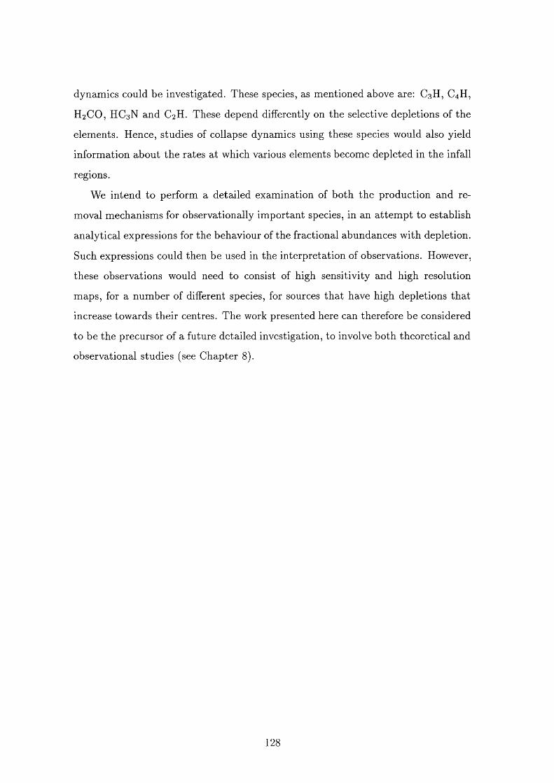
dynamics could be investigated. These species, as mentioned above are: C3H, C4H,
H2CO, HC3N and C2H. These depend differently on the selective depletions of the
elements. Hence, studies of collapse dynamics using these species would also yield
information about the rates at which various elements become depleted in the infall
regions.
We intend to perform a detailed examination of both the production and re
moval mechanisms for observationally im portant species, in an a ttem pt to establish
analytical expressions for the behaviour of the fractional abundances with depletion.
Such expressions could then be used in the interpretation of observations. However,
these observations would need to consist of high sensitivity and high resolution
maps, for a num ber of different species, for sources tha t have high depletions tha t
increase towards their centres. The work presented here can therefore be considered
to be the precursor of a future detailed investigation, to involve both theoretical and
observational studies (see Chapter 8 ).
128
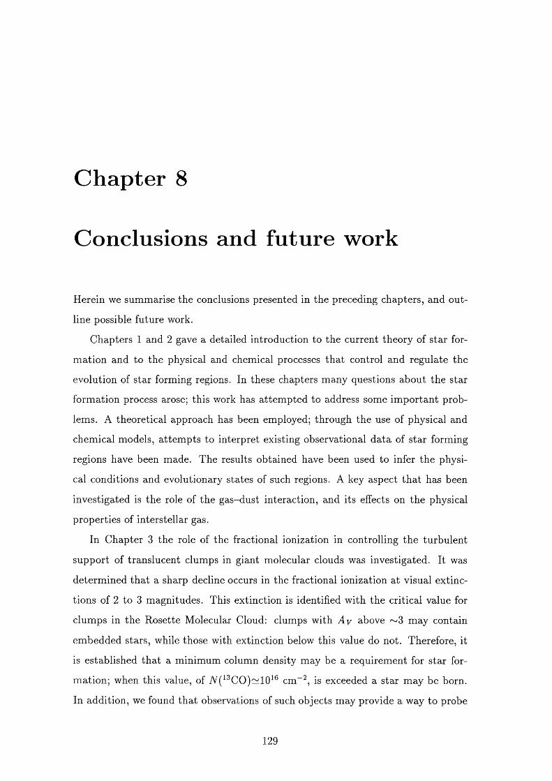
Chapter 8
Conclusions and future work
Herein we summarise the conclusions presented in the preceding chapters, and out
line possible future work.
Chapters 1 and 2 gave a detailed introduction to the current theory of star for
m ation and to the physical and chemical processes tha t control and regulate the
evolution of star forming regions. In these chapters many questions about the star
formation process arose; this work has attem pted to address some im portant prob
lems. A theoretical approach has been employed; through the use of physical and
chemical models, a ttem pts to interpret existing observational data of star forming
regions have been made. The results obtained have been used to infer the physi
cal conditions and evolutionary states of such regions. A key aspect tha t has been
investigated is the role of the gas-dust interaction, and its effects on the physical
properties of interstellar gas.
In Chapter 3 the role of the fractional ionization in controlling the turbulent
support of translucent clumps in giant molecular clouds was investigated. It was
determ ined tha t a sharp decline occurs in the fractional ionization at visual extinc
tions of 2 to 3 magnitudes. This extinction is identified with the critical value for
clumps in the Rosette Molecular Cloud: clumps with A y above ~ 3 may contain
embedded stars, while those with extinction below this value do not. Therefore, it
is established tha t a minimum column density may be a requirement for star for
mation; when this value, of A^(^^CO)~1 0 ® cm“ , is exceeded a star may be born.
In addition, we found tha t observations of such objects may provide a way to probe
129
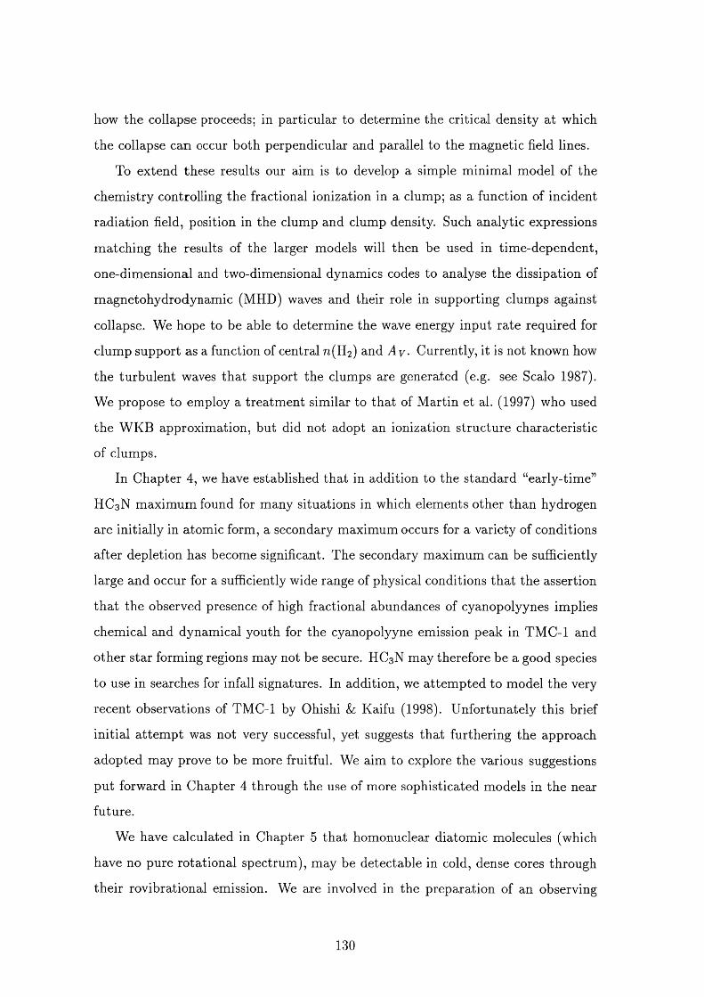
how the collapse proceeds; in particular to determine the critical density at which
the collapse can occur both perpendicular and parallel to the magnetic field lines.
To extend these results our aim is to develop a simple minimal model of the
chemistry controlling the fractional ionization in a clump; as a function of incident
radiation field, position in the clump and clump density. Such analytic expressions
m atching the results of the larger models will then be used in tim e-dependent,
one-dimensional and two-dimensional dynamics codes to analyse the dissipation of
magnetohydrodynamic (MHD) waves and their role in supporting clumps against
collapse. We hope to be able to determine the wave energy input rate required for
clump support as a function of central n(H 2 ) and T y . Currently, it is not known how
the turbulent waves tha t support the clumps are generated (e.g. see Scalo 1987).
We propose to employ a treatm ent similar to tha t of M artin et al. (1997) who used
the WKB approximation, but did not adopt an ionization structure characteristic
of clumps.
In Chapter 4, we have established tha t in addition to the standard “early-tim e”
HCgN maximum found for many situations in which elements other than hydrogen
are initially in atomic form, a secondary maximum occurs for a variety of conditions
after depletion has become significant. The secondary maximum can be sufficiently
large and occur for a sufficiently wide range of physical conditions tha t the assertion
th a t the observed presence of high fractional abundances of cyanopolyynes implies
chemical and dynamical youth for the cyanopolyyne emission peak in TM C - 1 and
other star forming regions may not be secure. HC3 N may therefore be a good species
to use in searches for infall signatures. In addition, we attem pted to model the very
recent observations of TMC-1 by Ohishi & Kaifu (1998). Unfortunately this brief
initial a ttem pt was not very successful, yet suggests tha t furthering the approach
adopted may prove to be more fruitful. We aim to explore the various suggestions
put forward in Chapter 4 through the use of more sophisticated models in the near
future.
We have calculated in Chapter 5 tha t homonuclear diatomic molecules (which
have no pure rotational spectrum), may be detectable in cold, dense cores through
their rovibrational emission. We are involved in the preparation of an observing
130
proposal to search for the 2 - 1 lines of N] and O2 in cold, dense interstellar clouds.
We hope tha t the various other attem pts to detect interstellar O2 (e.g. by SWAS)
will prove successful in the near future. Once accurate measurements of the O 2 and
N 2 abundances in dense clouds are available we will review the chemistry of these
molecules tha t the models currently utilize.
In Chapter 6 we considered the sulphur depletion problem and proposed tha t
the fact th a t much of the sulphur is in in translucent clumps (nH<1 0 cm“^)
plays a significant role in why it is so depleted in denser sources. Ions collide more
rapidly with grains and may stick more efficiently to them than neutrals. As a
clump collapses, sulphur may therefore become depleted in it more rapidly than
elements which are not primarily ionized in translucent material. Eventually in the
collapse, gas phase sulphur will become contained mostly in neutral species, which
in our picture leads to a large decrease in its depletion rate and a rem nant gas
phase elemental fractional abundance high enough for sulphur bearing species in
dense cores to be detectable. The nature of the sulphur in the dust will be the
subject of future research (see also Klemperer & Scappini 1998). Once the more
accurate multifluid MHD collapse models are established (the development of which
we described above) we will re-address this problem.
Chapter 7 investigated the dependences of the fractional abundances of a num
ber of species on the selective depletions of elemental carbon, nitrogen, oxygen and
sulphur, as well as metals. We determined that HCC^ has a fractional abundance
tha t is least sensitive to the selective elemental depletions; for this reason it is a
particularly appropriate species to study in efforts to diagnose collapse dynamics in
star formation from the analysis of infall signatures in spectral line profiles. We also
suggested a combination of molecules tha t could be the focus of observations aimed
at the investigation of collapse dynamics; comparisons of the profiles of spectral
features of these species would also give insight into the behaviours of the selective
depletions of the different elements in the infalling gas. We intend to embark on a
joint theoretical and observational study to further these results (see Chapter 7 ),
through an extensive collaboration with both theoreticians and observers. We intend
to establish analytical expressions for the behaviours of the fractional abundances
131
with depletion for the observationally im portant species tha t this work has deter
mined. These expressions would then be used to interpret the observations tha t
we propose to also perform; to determine the correlations between the depletions
of different elements. An im portant long-term application is to utilize the results
obtained to study the core collapse dynamics from spectral signatures of infall to
form stars.
132
A ppendix A
In this section we present further results from Chapter 7. Overleaf are tables which
give the values of æ(k) for some im portant species once steady state has been reached,
for all 35 of the calculated models. To briefly recap on the notation used (which is
described in detail in section 7.2). An elem ent’s symbol is given in upper case if the
initial fractional abundance used was taken to be the ’standard’ value (see Table
7.1). If the elem ent’s symbol is given in the lower case, this signifies tha t the initial
fractional abundance used was 1/3 the standard value. In three models we adopted
a value for the oxygen abundance tha t is 1/9 times the ’standard’ value. These
models are indicated through the use of og. To illustrate this, consider the model
label CNONaS; this model uses standard values for all the elemental abundances.
However, cnonas indicates tha t all the elemental abundances used are 1/3 of the
standard value.
133
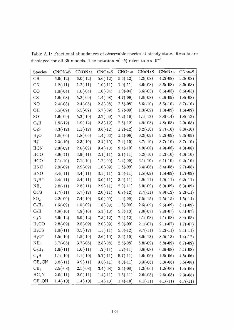
Table A .l: Fractional abundances of observable species at steady-state. Results are displayed for all 35 models. The notation a(—b) refers to a x 10“ .
S p e c ie s C N O N A S C N O N A S C N O n a S C N O n a s C N oN a S C N oN as C N o n a S
C H 6.0(-12) 6.0(-12) 5.6(-12) 5.6(-12) 4 .2 (-0 8 ) 4 .2 (-0 8 ) 3 .3 (-0 8 )
C N 1.2(-11) 1.2(-11) l.O(-ll) l.O(-ll) 3 .6 (-0 8 ) 3.6(-08) 3.0(-08)C O 1.0 (-04 ) 1.0(-04) 1.0 (-04) 1.0(-04) 6.6(-05) 6.6(-05) 6.6(-05)C S 1.6(-08) 5.2(-09) 1.4 (-08) 4.7(-09) 1 .8 (-0 8 ) 6 .0 (-0 9 ) 1 .8 (-0 8 )
N O 2 .4 (-0 8 ) 2 .4 (-0 8 ) 2 .5 (-0 8 ) 2 .5 (-0 8 ) 5.6(-10) 5.6(-10) 8 .7 (-1 0 )
O H 5.5(-09) 5.5(-09) 5.7(-09) 5.7(-09) 1.3 (-09) 1.3(-09) 1 .6 (-0 9 )
S O 1.6(-09) 5.3(-10) 2 .2 (-0 9 ) 7 .2 (-1 0 ) 1.1(-13) 3 .8 (-1 4 ) 1.8(-13)C z H 1.9(-12) 1.9(-12) 2.5(-12) 2 .5 (-1 2 ) 4 .9 (-0 8 ) 4 .8 (-0 8 ) 2 .9 (-0 8 )
C gS 3.3(-12) 1.1(-12) 3.6(-12) 1 .2 ( - 1 2 ) 8 .2 ( - 1 0 ) 2 .7 (-1 0 ) 8 .3 (-1 0 )
H 2 0 1.8(-06) 1.8(-06) 1.4(-06) 1 .4 (-0 6 ) 9 .2 (-0 9 ) 9 .2 (-0 9 ) 9 .3 (-0 9 )
Hj 2.3(-10) 2.3(-10) 2 .4 (-1 0 ) 2 .4 (-1 0 ) 3.7(-10) 3 .7 (-1 0 ) 3 .7 (-1 0 )
H C N 2.0(-09) 2.0(-09) 9.4(-10) 9 .4 (-1 0 ) 4 .9 (-0 8 ) 4 .9 (-0 8 ) 4.3(-08)H C O 3.9(-ll) 3.9(-ll) 2 . 1 ( - 1 1 ) 2.1(-11) 5.2(-10) 5.2(-10) 4.0(-10)H C O + 7.1(-10) 7.1(-10) 1.2(-09) 1 .2 (-0 9 ) 6 . 1 ( - 1 0 ) 6 . 1 ( - 1 0 ) 9 .2 (-1 0 )
H N C 2.9(-09) 2.9(-09) 1.6 (-09) 1.6 (-09) 3 .4 (-0 8 ) 3 .4 (-0 8 ) 2 .7 (-0 8 )
H N O 3.4(-ll) 3.4(-ll) 3.5(-ll) 3.5(-ll) 1.5(-09) 1.5(-09) 1 .7 (-0 9 )
N 2 H + 2.4(-ll) 2.4(-ll) 3.0(-ll) 3.0(-ll) 4.9(-ll) 4 . 9 ( - l l ) 6 .2 ( - l l )
N H 2 2.8(-ll) 2.8(-ll) 2 . 9 ( - l l ) 2.9(-ll) 6 .0 (-0 9 ) 6 .0 (-0 9 ) 6.3(-09)ocs 1.7(-11) 5.7(-12) 2 .0 ( - l l ) 6 .7 (-1 2 ) 2 . 7 ( - l l ) 8 .9 (-1 2 ) 2 .2 ( - l l )
S 0 2 2 .2 (-0 9 ) 7.4(-10) 3.0(-09) 1 .0 (-0 9 ) 7.5(-15) 2 .5 (-1 5 ) 1.5(-14)C 2 H 2 1.5(-09) 1.5(-09) 1 .8 (-0 9 ) 1.8(-09) 2 .5 (-0 9 ) 2 .5 (-0 9 ) 3 .1 (-0 9 )
C 3 H 4.8(-10) 4.9(-10) 5.3(-10) 5.3(-10) 7 .8 (-0 7 ) 7 .8 (-0 7 ) 6 .4 (-0 7 )
C 3 N 6.9(-12) 6.9(-12) 7.3(-12) 7.4(-12) 4 .1 (-0 8 ) 4.1(-08) 3 .4 (-0 8 )
H 2 C 0 2 .8 (-0 9 ) 2 .8 (-0 9 ) 2 .0 (-0 9 ) 2.0(-09) 2 .1 (-0 7 ) 2 .1 (-07) 1.7(-07)H 2 C S l.O(-ll) 3.5(-12) 1.5(-11) 5 .0 (-1 2 ) 9 . 7 ( - l l ) 3.2(-ll) 9.1(-11)H 3 0 + 1.5(-10) 1.5(-10) 2.6(-10) 2 .6 ( - 1 0 ) 8.0(-13) 8.0(-13) 1.4(-12)N H 3 3.7(-08) 3.7(-08) 2 .8 (-0 8 ) 2 .8 (-0 8 ) 5 .8 (-0 9 ) 5 .8 (-0 9 ) 6 .7 (-0 9 )
C 3 H 2 1.6(-11) 1.6(-11) 1.2(-11) 1.2(-11) 6 .6 (-0 8 ) 6 .6 (-0 8 ) 5.1(-08)C 4 H l.l(-lO) l.l(-lO) 5.7(-ll) 5.7(-ll) 4.6(-06) 4 .6 (-0 6 ) 4.5(-06)C H 2 C N 3.8(-ll) 3.9(-ll) 3.0(-ll) 3.0(-ll) 3 .3 (-0 8 ) 3 .3 (-0 8 ) 3.5(-08)C H 4 2 .5 (-0 8 ) 2 .5 (-0 8 ) 3.4(-08) 3.4(-08) 1 .2 (-0 6 ) 1 .2 (-0 6 ) 1 .4 (-0 6 )
H C 3 N 2.0(-ll) 2.0(-ll) 1.4(-11) 1.5(-11) 2 .6 (-0 8 ) 2 .6 (-0 8 ) 2 .3 (-0 8 )
C H 3 0 H 1.4(-10) 1.4(-10) 1.4(-10) 1.4(-10) 4.1(-11) 4.1(-11) 4.7(-ll)
134
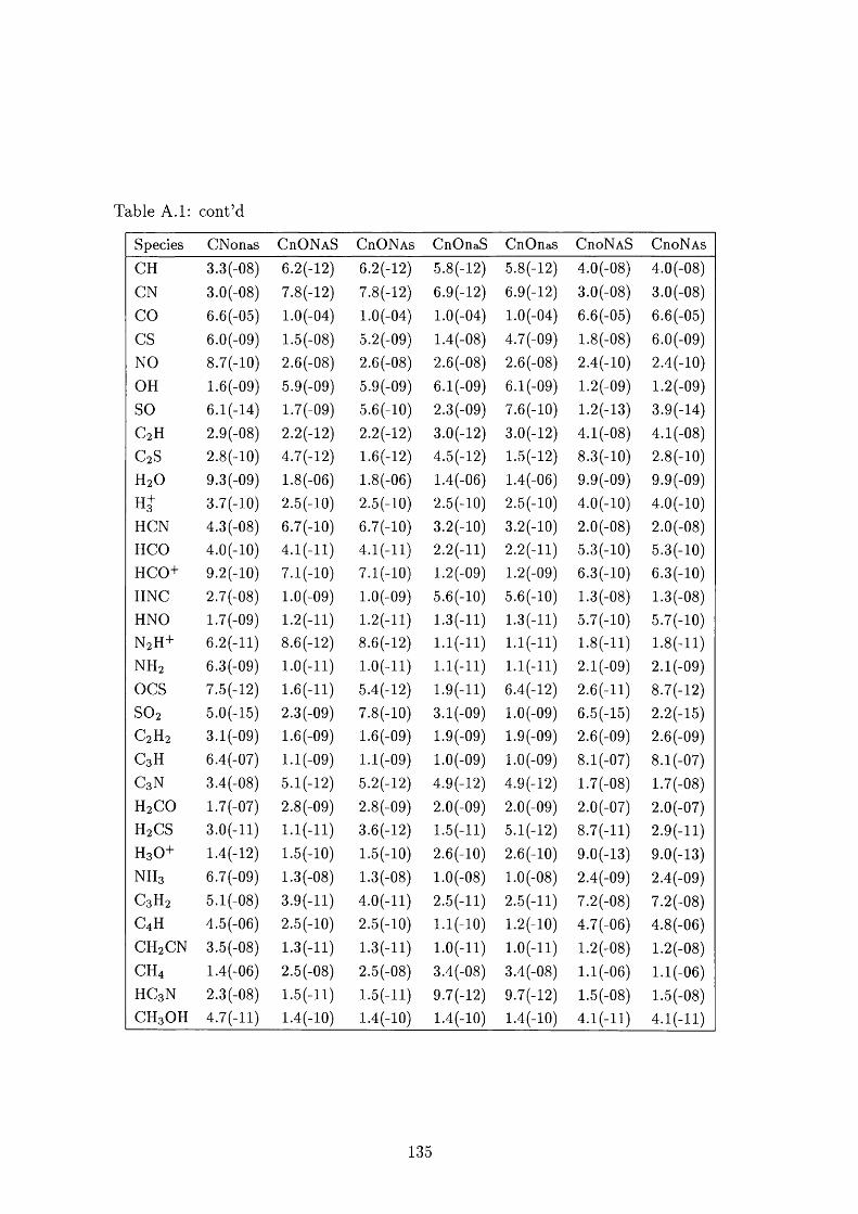
Table A.l: cont’d
Species C Nonas C hO N a S C hO N as CnOnaS CnOnas C h oN a S C h oN asCH 3.3(-08) 6.2(-12) 6.2(-12) 5 .8 (-1 2 ) 5 .8 (-1 2 ) 4 .0 (-0 8 ) 4 .0 (-0 8 )
C N 3.0(-08) 7.8(-12) 7 .8 (-1 2 ) 6 .9 (-1 2 ) 6.9(-12) 3.0(-08) 3.0(-08)c o 6.6(-05) 1.0 (-04) 1.0(-04) 1.0(-04) 1.0(-04) 6.6(-05) 6.6(-05)CS 6.0(-09) 1.5 (-08) 5.2(-09) 1 .4 (-0 8 ) 4.7(-09) 1 .8 (-0 8 ) 6.0(-09)NO 8.7(-10) 2 .6 (-0 8 ) 2 .6 (-0 8 ) 2 .6 (-0 8 ) 2 .6 (-0 8 ) 2 .4 (-1 0 ) 2 .4 (-1 0 )
OH 1.6(-09) 5.9(-09) 5.9(-09) 6 .1 (-0 9 ) 6 .1 (-0 9 ) 1 .2 (-0 9 ) 1 .2 (-0 9 )
S O 6.1(-14) 1.7(-09) 5.6(-10) 2 .3 (-0 9 ) 7.6(-10) 1 .2 (-1 3 ) 3 .9 (-1 4 )
C2H 2 .9 (-0 8 ) 2.2(-12) 2 .2 ( - 1 2 ) 3 .0 (-1 2 ) 3.0(-12) 4 .1 (-0 8 ) 4 .1 (-0 8 )
C 2 S 2.8(-10) 4.7(-12) 1 .6 ( - 1 2 ) 4.5(-12) 1.5(-12) 8 .3 (-1 0 ) 2 .8 ( - 1 0 )
H20 9.3(-09) 1.8(-06) 1 . 8 (-06 ) 1.4(-06) 1 .4 (-0 6 ) 9 .9 (-0 9 ) 9 .9 (-0 9 )
3.7(-10) 2.5(-10) 2.5(-10) 2.5(-10) 2.5(-10) 4 .0 (-1 0 ) 4 .0 (-1 0 )
HCN 4 .3 (-0 8 ) 6.7(-10) 6.7(-10) 3.2(-10) 3 .2 (-1 0 ) 2 .0 (-0 8 ) 2 .0 (-0 8 )
HCO 4.0(-10) 4.1(-11) 4.1(-11) 2 .2 ( - l l ) 2 .2 ( - l l ) 5.3(-10) 5.3(-10)HCO+ 9.2(-10) 7.1(-10) 7.1(-10) 1 .2 (-0 9 ) 1 .2 (-0 9 ) 6 .3 (-1 0 ) 6 .3 (-1 0 )
HNC 2.7(-08) 1.0(-09) 1 .0 (-0 9 ) 5.6(-10) 5.6(-10) 1 .3 (-0 8 ) 1 .3 (-0 8 )
HNO 1.7(-09) 1.2(-11) 1.2(-11) 1.3(-11) 1.3(-11) 5.7(-10) 5.7(-10)N2H+ 6.2(-ll) 8 .6 ( - 1 2 ) 8 .6 ( - 1 2 ) l.l(-ll) l.l(-ll) 1 .8 ( - 1 1 ) 1 .8 ( - 1 1 )
NH2 6.3(-09) l.O(-ll) l.O(-ll) l.l(-ll) l.l(-ll) 2.1 (-09) 2 .1 (-09 )
O C S 7.5(-12) 1.6(-11) 5 .4 (-1 2 ) 1.9(-11) 6 .4 (-1 2 ) 2 .6 ( - l l ) 8 .7 (-1 2 )
S 0 2 5.0(-15) 2.3(-09) 7 .8 (-1 0 ) 3 .1 (-0 9 ) 1 .0 (-0 9 ) 6.5(-15) 2.2(-15)C2H2 3.1(-09) 1.6 (-09) 1.6(-09) 1 .9 (-0 9 ) 1 .9 (-0 9 ) 2.6(-09) 2.6(-09)C3H 6.4(-07) 1.1 (-09) 1.1 (-09) 1 .0 (-0 9 ) 1 .0 (-0 9 ) 8 .1 (-0 7 ) 8 .1 (-0 7 )
C 3 N 3.4(-08) 5.1(-12) 5.2(-12) 4.9(-12) 4 .9 (-1 2 ) 1 .7 (-0 8 ) 1 .7 (-0 8 )
H2C0 1.7(-07) 2 .8 (-0 9 ) 2 .8 (-0 9 ) 2.0(-09) 2.0(-09) 2.0(-07) 2 .0 (-0 7 )
H2CS 3.0(-ll) l.l(-ll) 3 .6 (-1 2 ) 1.5(-11) 5.1(-12) 8 . 7 ( - l l ) 2.9(-ll)H30+ 1.4(-12) 1.5(-10) 1.5(-10) 2.6(-10) 2 .6 ( - 1 0 ) 9 .0 (-1 3 ) 9 .0 (-1 3 )
NH3 6.7(-09) 1 .3 (-0 8 ) 1 .3 (-0 8 ) 1 .0 (-0 8 ) 1 .0 (-0 8 ) 2 .4 (-0 9 ) 2 .4 (-0 9 )
C3H2 5.1(-08) 3 . 9 ( - l l ) 4.0(-ll) 2.5(-ll) 2.5(-ll) 7 .2 (-0 8 ) 7 .2 (-0 8 )
C4H 4.5(-06) 2.5(-10) 2.5(-10) l.l(-lO) 1.2(-10) 4.7(-06) 4 .8 (-0 6 )
CH2CN 3 .5 (-0 8 ) 1.3(-11) 1.3(-11) l.O(-ll) l.O(-ll) 1 .2 (-0 8 ) 1 . 2 (-08 )
CH4 1.4(-06) 2 .5 (-0 8 ) 2 .5 (-0 8 ) 3 .4 (-0 8 ) 3 .4 (-0 8 ) l.l(-06) 1.1 (-06)HC3N 2 .3 (-0 8 ) 1.5(-11) 1.5(-11) 9 .7 (-1 2 ) 9 .7 (-1 2 ) 1.5(-08) 1.5(-08)CH30H 4.7(-ll) 1.4(-10) 1.4(-10) 1.4(-10) 1.4(-10) 4.1(-11) 4.1(-11)
135
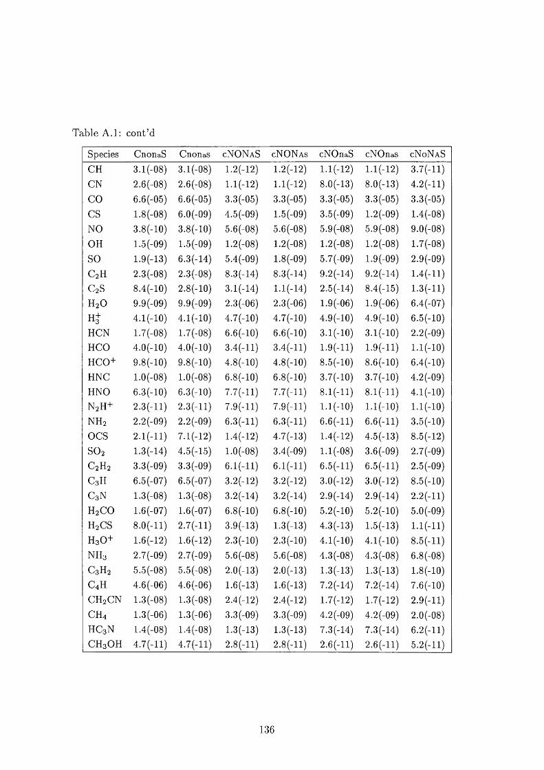
Table A.l: cont’d
Species CnonaS CnonaS cNONAS cN O N as cNOnaS cNOnas cN oN a S
CH 3.1(-08) 3.1(-08) 1 .2 (-1 2 ) 1 .2 (-1 2 ) 1 .1 (-1 2 ) 1 .1 (-1 2 ) 3.7(-ll)CN 2.6(-08) 2.6(-08) 1 .1 (-1 2 ) 1 .1 (-1 2 ) 8.0(-13) 8.0(-13) 4.2(-ll)CO 6.6(-05) 6.6(-05) 3.3(-05) 3.3(-05) 3.3(-05) 3.3(-05) 3.3(-05)CS 1.8(-08) 6.0(-09) 4.5(-09) 1.5(-09) 3.5(-09) 1.2(-09) 1.4(-08)NO 3.8(-10) 3.8(-10) 5.6(-08) 5.6(-08) 5.9(-08) 5.9(-08) 9.0(-08)OH 1.5(-09) 1.5(-09) 1.2(-08) 1.2(-08) 1 . 2 (-08) 1.2(-08) 1.7(-08)SO 1.9(-13) 6.3(-14) 5.4(-09) 1.8(-09) 5.7(-09) 1.9(-09) 2.9(-09)C2 H 2.3(-08) 2.3(-08) 8.3(-14) 8.3(-14) 9.2(-14) 9.2(-14) 1.4(-11)C2 S 8.4(-10) 2 .8 (-1 0 ) 3.1(-14) 1.1(-14) 2.5(-14) 8.4(-15) 1.3(-11)H2 O 9.9(-09) 9.9(-09) 2.3(-06) 2.3(-06) 1.9(-06) 1.9(-06) 6.4(-07)
H j 4.1(-10) 4.1(-10) 4.7(-10) 4.7(-10) 4.9(-10) 4.9(-10) 6.5(-10)HCN 1.7(-08) 1.7(-08) 6 .6 (-1 0 ) 6 .6 (-1 0 ) 3.1(-10) 3.1(-10) 2.2(-09)HCO 4.0(-10) 4.0(-10) 3.4(-ll) 3.4(-ll) 1.9(-11) 1.9(-11) l.l(-lO)HCO+ 9.8(-10) 9.8(-10) 4.8(-10) 4.8(-10) 8.5(-10) 8 .6 (-1 0 ) 6.4(-10)HNC 1.0(-08) 1.0(-08) 6 .8 (-1 0 ) 6 .8 (-1 0 ) 3.7(-10) 3.7(-10) 4.2(-09)HNO 6.3(-10) 6.3(-10) 7.7(-ll) 7.7(-ll) 8 .1 (-1 1 ) 8 .1 (-1 1 ) 4.1(-10)N2 H+ 2.3(-ll) 2.3(-ll) 7.9(-ll) 7.9(-ll) l.l(-lO) l.l(-lO) l.l(-lO)NH2 2.2(-09) 2.2(-09) 6.3(-ll) 6.3(-ll) 6 .6 (-ll) 6 .6 (-ll) 3.5(-10)OCS 2 .1 (-1 1 ) 7.1(-12) 1.4(-12) 4.7(-13) 1.4(-12) 4.5(-13) 8.5(-12)S0 2 1.3(-14) 4.5(-15) 1 . 0 (-08) 3.4(-09) 1 . 1 (-08) 3.6(-09) 2.7(-09)C2 H2 3.3(-09) 3.3(-09) e . i ( - i i ) e . i ( - i i ) 6.5(-ll) 6.5(-ll) 2.5(-09)C3 H 6.5(-07) 6.5(-07) 3.2(-12) 3.2(-12) 3.0(-12) 3.0(-12) 8.5(-10)C3 N 1.3 (-08) 1.3(-08) 3.2(-14) 3.2(-14) 2.9(-14) 2.9(-14) 2 .2 (-ll)H2 C0 1.6(-07) 1.6(-07) 6 .8 (-1 0 ) 6 .8 (-1 0 ) 5.2(-10) 5.2(-10) 5.0(-09)H2 CS 8 .0 (-ll) 2.7(-ll) 3.9(-13) 1.3(-13) 4.3(-13) 1.5(-13) l . l ( - l l )H3 0 + 1 .6 (-1 2 ) 1 .6 (-1 2 ) 2.3(-10) 2.3(-10) 4.1(-10) 4.1(-10) 8.5(-ll)NH3 2.7(-09) 2.7(-09) 5.6(-08) 5.6(-08) 4.3(-08) 4.3(-08) 6.8(-08)C3 H2 5.5(-08) 5.5(-08) 2.0(-13) 2.0(-13) 1.3(-13) 1.3(-13) 1 .8 (-1 0 )C4 H 4.6(-06) 4.6(-06) 1.6(-13) 1.6(-13) 7.2(-14) 7.2(-14) 7.6(-10)CH2 CN 1.3(-08) 1.3(-08) 2.4(-12) 2.4(-12) 1.7(-12) 1.7(-12) 2.9(-ll)CH4 1.3(-06) 1.3(-06) 3.3(-09) 3.3(-09) 4.2(-09) 4.2(-09) 2.0(-08)HC3 N 1.4 (-08) 1.4(-08) 1.3(-13) 1.3(-13) 7.3(-14) 7.3(-14) 6 .2 (-ll)CH3 0 H 4.7(-ll) 4.7(-ll) 2 .8 (-ll) 2 .8 (-ll) 2 .6 (-ll) 2 .6 (-ll) 5.2(-ll)
136
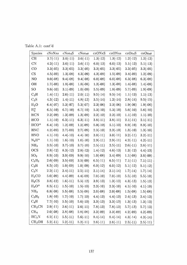
Table A.l; cont’d
S p ec ie s cN oN as cN o n aS cN o n as crO N a S cüO N as cn O n a S c n O n a s
C H 3 . 7 ( - l l ) 3 . 6 ( - l l ) 3 . 6 ( - l l ) 1 .3 (-1 2 ) 1 .3 (-1 2 ) 1 .2 ( - 1 2 ) 1 .2 ( - 1 2 )
C N 4 . 2 ( - l l ) 3 . 6 ( - l l ) 3 . 6 ( - l l ) 6 .0 (-1 3 ) 6 .0 (-1 3 ) 5 .1 (-1 3 ) 5 .1 (-1 3 )
C O 3 .3 (-0 5 ) 3 .3 (-0 5 ) 3 .3 (-0 5 ) 3 .3 (-0 5 ) 3 .3 (-0 5 ) 3 .3 (-0 5 ) 3 .3 (-0 5 )
C S 4 .5 (-0 9 ) 1 .3 (-0 8 ) 4 .3 (-0 9 ) 4 .3 (-0 9 ) 1 .5 (-09) 3 .4 (-0 9 ) 1 .2 (-0 9 )
N O 9 .0 (-0 8 ) 9 .4 (-0 8 ) 9 .4 (-0 8 ) 6 .0 (-0 8 ) 6 .0 (-0 8 ) 6 .3 (-0 8 ) 6 .3 (-0 8 )
O H 1 .7 (-0 8 ) 1 .8 (-0 8 ) 1 .8 (-0 8 ) 1.3 (-08) 1 .3 (-08) 1 .4 (-08) 1 .4 (-0 8 )
S O 9 .6 (-1 0 ) 3 .1 (-09) 1 .0 (-0 9 ) 5 .5 (-0 9 ) 1 .8 (-0 9 ) 5 .7 (-0 9 ) 1 .9 (-0 9 )
C gH 1 .4 (-1 1 ) 2 .0 ( - l l ) 2 .0 ( - l l ) 9 .5 (-1 4 ) 9 .5 (-1 4 ) 1 .1 (-1 3 ) 1 .1 (-1 3 )
C 2 S 4 .3 (-1 2 ) 1 .4 (-1 1 ) 4 .8 (-1 2 ) 3 .5 (-1 4 ) 1 .2 (-1 4 ) 2 .8 (-1 4 ) 9 .5 (-1 5 )
H 2 O 6 .4 (-0 7 ) 5 .3 (-0 7 ) 5 .3 (-0 7 ) 2 .3 (-0 6 ) 2 .3 (-0 6 ) 1 .9 (-0 6 ) 1 .9 (-0 6 )
6 .5 (-1 0 ) 6 .7 (-1 0 ) 6 .7 (-1 0 ) 5 .3 (-1 0 ) 5 .3 (-1 0 ) 5 .6 (-1 0 ) 5 .6 (-1 0 )
H C N 2 .2 (-0 9 ) 1 .3 (-0 9 ) 1 .3 (-0 9 ) 2 .2 ( - 1 0 ) 2 .2 ( - 1 0 ) l . l ( - l O ) l . l ( - lO )
H C O l . l ( - l O ) 6 . 3 ( - l l ) 6 . 3 ( - l l ) 3 . 8 ( - l l ) 3 . 8 ( - l l ) 2 . 1 ( - 1 1 ) 2 . 1 ( - 1 1 )
H C O + 6 .4 (-1 0 ) 1 .2 (-0 9 ) 1 .2 (-0 9 ) 5 .0 (-1 0 ) 5 .1 (-1 0 ) 8 .9 (-1 0 ) 8 .9 (-1 0 )
H N C 4 .2 (-0 9 ) 2 .7 (-0 9 ) 2 .7 (-0 9 ) 2 .3 (-1 0 ) 2 .3 (-1 0 ) 1 .3 (-1 0 ) 1 .3 (-1 0 )
H N O 4 .1 (-1 0 ) 4 .4 (-1 0 ) 4 .4 (-1 0 ) 3 . 0 ( - l l ) 3 . 0 ( - l l ) 3 . 2 ( - l l ) 3 . 2 ( - l l )
N 2 H + l . l ( - l O ) 1 .6 ( - 1 0 ) 1 .6 ( - 1 0 ) 2 . 9 ( - l l ) 2 . 9 ( - l l ) 4 . 2 ( - l l ) 4 . 2 ( - l l )
N H 2 3 .5 (-1 0 ) 3 .7 (-1 0 ) 3 .7 (-1 0 ) 2 . 5 ( - l l ) 2 . 5 ( - l l ) 2 .6 ( - l l ) 2 .6 ( - l l )
O C S 2 .8 ( - 1 2 ) 8 .3 (-1 2 ) 2 .8 ( - 1 2 ) 1 .4 (-1 2 ) 4 .6 (-1 3 ) 1 .3 (-1 2 ) 4 .4 (-1 3 )
S 0 2 8 .9 (-1 0 ) 3 .0 ( 0 9 ) 9 .9 (-1 0 ) 1 . 0 (-08) 3 .4 (-0 9 ) 1 . 1 (-08 ) 3 .6 (-0 9 )
C 2 H 2 2 .6 (-0 9 ) 3 .5 (-0 9 ) 3 .5 (-0 9 ) 6 . 5 ( - l l ) 6 . 5 ( - l l ) 7 .1 (-1 1 ) 7 .1 (-1 1 )
C 3 H 8 .5 (-1 0 ) 1 .0 (-0 9 ) 1 .0 (-0 9 ) 6 .0 (- 1 2 ) 6 .0 ( - 1 2 ) 5 .1 (-1 2 ) 5 .1 (-1 2 )
C 3 N 2 .2 ( - l l ) 2 . 4 ( - l l ) 2 . 5 ( - l l ) 2 .1 (-1 4 ) 2 .1 (-1 4 ) 1 .7 (-1 4 ) 1 .7 (-1 4 )
H 2 C O 5 .0 (-0 9 ) 4 .4 (-0 9 ) 4 .4 (-0 9 ) 7 .0 (-1 0 ) 7 .0 (-1 0 ) 5 .5 (-1 0 ) 5 .5 (-1 0 )
H 2 C S 3 .8 (-1 2 ) 1 .6 ( - 1 1 ) 5 .5 (-1 2 ) 3 .9 (-1 3 ) 1 .3 (-1 3 ) 4 .3 (-1 3 ) 1 .5 (-1 3 )
H 3 0 + 8 . 5 ( - l l ) 1 .5 (-1 0 ) 1 .5 (-1 0 ) 2 .3 (-1 0 ) 2 .3 (-1 0 ) 4 .1 (-1 0 ) 4 .1 (-1 0 )
N H 3 6 .8 (-0 8 ) 5 .5 (-0 8 ) 5 .5 (-0 8 ) 2 .0 (-0 8 ) 2 .0 (-0 8 ) 1 .5 (-0 8 ) 1 .5 (-0 8 )
C 3 H 2 1 .8 ( - 1 0 ) 1 .7 (-1 0 ) 1 .7 (-1 0 ) 4 .4 (-1 3 ) 4 .4 (-1 3 ) 2 .4 (-1 3 ) 2 .4 (-1 3 )
C 4 H 7 .7 (-1 0 ) 5 .5 (-1 0 ) 5 .6 (-1 0 ) 3 .3 (-1 3 ) 3 .3 (-1 3 ) 1 .3 (-1 3 ) 1 .3 (-1 3 )
C H 2 C N 2 . 9 ( - l l ) 2 .6 ( - l l ) 2 .6 ( - l l ) 7 .8 (-1 3 ) 7 .8 (-1 3 ) 5 .7 (-1 3 ) 5 .7 (-1 3 )
C H 4 2 .0 (-0 8 ) 2 .8 (-0 8 ) 2 .8 (-0 8 ) 3 .3 (-09) 3 .3 (-0 9 ) 4 .2 (-0 9 ) 4 .2 (-0 9 )
H C 3 N 6 .2 ( - l l ) 5 . 5 ( - l l ) 5 . 6 ( - l l ) 8 .4 (-1 4 ) 8 .4 (-1 4 ) 4 .3 (-1 4 ) 4 .3 (-1 4 )
C H 3 0 H 5 . 2 ( - l l ) 5 . 2 ( - l l ) 5 . 2 ( - l l ) 2 .6 ( - l l ) 2 .6 ( - l l ) 2 . 5 ( - l l ) 2 . 5 ( - l l )
137
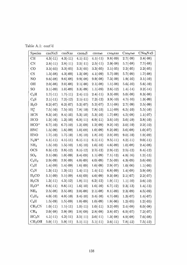
Table A.l: cont’d
Species choN a S cnoNAs cnonaS cnonaS cnognas CnOgHaS CNogNAS
C H 4 . 3 ( - l l ) 4 . 3 ( - l l ) 4 .1 (-1 1 ) 4 .1 (-1 1 ) 9 .8 (-0 9 ) 2 .7 (-0 8 ) 3 .4 (-0 8 )
C N 2 .8 ( - l l ) 2 .8 ( - l l ) 2 . 5 ( - l l ) 2 . 5 ( - l l ) 2 .0 (-0 8 ) 5 .7 (-0 8 ) 7 .7 (-0 8 )
C O 3 .3 (-0 5 ) 3 .3 (-0 5 ) 3 .3 (-0 5 ) 3 .3 (-0 5 ) 2 .1 (-0 5 ) 2 .2 (-0 5 ) 2 .2 (-0 5 )
C S 1.3 (-08) 4 .3 (-0 9 ) 1 .2 (-0 8 ) 4 .1 (-09) 5 .7 (-0 9 ) 5 .7 (-0 9 ) 1 .7 (-0 8 )
N O 9 .6 (-0 8 ) 9 .6 (-0 8 ) 9 .9 (-0 8 ) 9 .9 (-0 8 ) 7 .3 (-0 9 ) 1 .9 (-1 0 ) 3 .1 (-1 0 )
O H 2 .0 (-0 8 ) 2 .0 (-0 8 ) 2 . 1 (-08) 2 .1 (-0 8 ) l . l ( - 0 8 ) 5 .6 (-1 0 ) 5 .6 (-1 0 )
S O 3 .1 (-0 9 ) 1 .0 (-0 9 ) 3 .3 (-0 9 ) 1.1 (-09) 2 .6 ( - 1 2 ) 1 .4 (-1 4 ) 3 .2 (-1 4 )
C g H 1 .7 (-1 1 ) 1 .7 (-1 1 ) 2 . 4 ( - l l ) 2 . 4 ( - l l ) 3 .3 (-0 9 ) 5 .0 (-0 8 ) 8 .3 (-0 8 )
C gS 2 . 1 ( - 1 1 ) 7 .2 (-1 2 ) 2 . 1 ( - 1 1 ) 7 .2 (-1 2 ) 3 .9 (-1 0 ) 4 .7 (-1 0 ) 1 .3 (-0 9 )
H 2 0 6 .2 (-0 7 ) 6 .2 (-0 7 ) 5 .2 (-0 7 ) 5 .2 (-0 7 ) 2 .1 (-0 8 ) 2 .7 (-0 9 ) 2 .5 (-0 9 )
Hj 7 .5 (-1 0 ) 7 .5 (-1 0 ) 7 .8 (-1 0 ) 7 .8 (-1 0 ) l . l ( - 0 9 ) 6 .5 (-1 0 ) 5 .5 (-1 0 )
H C N 8 .3 (-1 0 ) 8 .4 (-1 0 ) 5 .3 (-1 0 ) 5 .3 (-1 0 ) 1 .7 (-0 8 ) 4 .5 (-0 8 ) 1.1 (-07)
H C O 1 .2 ( - 1 0 ) 1 .2 ( - 1 0 ) 6 . 9 ( - l l ) 6 . 9 ( - l l ) 3 .6 (-1 0 ) 3 .6 (-1 0 ) 3 .8 (-1 0 )
H C O + 6 .7 (-1 0 ) 6 .7 (-1 0 ) 1.2 (-09) 1 .2 (-0 9 ) 9 .2 (-1 0 ) 3 .0 (-1 0 ) 2 .2 ( - 1 0 )
H N C 1 .5 (-0 9 ) 1 .6 (-0 9 ) 1 .0 (-0 9 ) 1 .0 (-0 9 ) 8 .2 (-0 9 ) 3 .6 (-0 8 ) 1 .0 (-0 7 )
H N O 1 .7 (-1 0 ) 1 .7 (-1 0 ) 1 .8 ( - 1 0 ) 1 .8 ( - 1 0 ) 2 .9 (-0 9 ) 9 .0 (-1 0 ) 1 .9 (-09)
N 2 H + 4 .1 (-1 1 ) 4 .1 (-1 1 ) e . i ( - i i ) e . i ( - i i ) 9 . 5 ( - l l ) 4 . 2 ( - l l ) 9 . 0 ( - l l )
N H 2 1 .5 (-1 0 ) 1 .5 (-1 0 ) i . e ( - i o ) 1 .6 ( - 1 0 ) 4 .6 (-0 9 ) 1 . 0 (-08) 2 .4 (-0 8 )
O C S 8 .3 (-1 2 ) 2 .8 ( - 1 2 ) 8 . 1 ( - 1 2 ) 2 .7 (-1 2 ) 2 .9 (-1 2 ) 2 .5 (-1 2 ) 8 .4 (-1 2 )
S 0 2 3 .1 (-0 9 ) 1 .0 (-0 9 ) 3 .4 (-0 9 ) 1.1 (-09) 7 .1 (-1 3 ) 4 .8 (-1 6 ) 1 .2 (-1 5 )
C 2 H 2 2 .9 (-0 9 ) 2 .9 (-0 9 ) 4 .0 (-0 9 ) 4 .0 (-0 9 ) 7 .5 (-0 9 ) 4 .3 (-0 9 ) 3 .6 (-0 9 )
C 3 H 1 .4 (-0 9 ) 1 .4 (-0 9 ) 1 .6 (-0 9 ) 1 .6 (-0 9 ) 2 .9 (-0 7 ) 1 .0 (-0 6 ) l . l ( - 0 6 )
C 3 N 1 .3 (-1 1 ) 1 .3 (-1 1 ) 1 .4 (-1 1 ) 1 .4 (-1 1 ) 6 .8 (-0 9 ) 1 .4 (-0 8 ) 3 .9 (-0 8 )
H 2 C 0 5 .1 (-0 9 ) 5 .1 (-0 9 ) 4 .6 (-0 9 ) 4 .6 (-0 9 ) 9 .3 (-0 8 ) 2 .1 (-0 7 ) 2 .2 (-0 7 )
H 2 C S 1 .3 (-1 1 ) 4 .3 (-1 2 ) 1 .8 ( - 1 1 ) 6 .2 ( - 1 2 ) 1 .9 (-1 1 ) l . l ( - l O ) 3 .6 (-1 0 )
H 3 0 + 8 .6 ( - l l ) 8 .6 ( - l l ) 1 .6 ( - 1 0 ) 1 .6 ( - 1 0 ) 6 .7 (-1 2 ) 2 .3 (-1 3 ) 1 .4 (-1 3 )
N H 3 2 .5 (-0 8 ) 2 .5 (-0 8 ) 2 .0 (-0 8 ) 2 .1 (-0 8 ) 8 .1 (-0 9 ) 2 .3 (-0 9 ) 4 .5 (-0 9 )
C 3 H 2 4 .0 (-1 0 ) 4 .0 (-1 0 ) 3 .4 (-1 0 ) 3 .4 (-1 0 ) 4 .7 (-0 8 ) 1 .3 (-0 7 ) 1 .4 (-0 7 )
C 4 H 1 .5 (-0 9 ) 1 .5 (-0 9 ) 1 .0 (-0 9 ) 1 .0 (-0 9 ) 1 .9 (-0 6 ) 1 .2 (-0 5 ) 1 .2 (-0 5 )
C H 2 C N l .O ( - l l ) l . l ( - l l ) l .O ( - l l ) l .O ( - l l ) 3 .2 (-0 9 ) 2 .4 (-0 8 ) 6 .0 (-0 8 )
C H 4 2 .0 (-0 8 ) 2 .0 (-0 8 ) 2 .8 (-0 8 ) 2 .8 (-0 8 ) 3 .8 (-0 7 ) 6 .9 (-0 7 ) 7 .2 (-0 7 )
H C 3 N 4 .1 (-1 1 ) 4 . 2 ( - l l ) 3 . 5 ( - l l ) 3 . 6 ( - l l ) 1 .3 (-0 8 ) 4 .9 (-0 8 ) 7 .6 (-0 8 )
C H 3 0 H 5 . 0 ( - l l ) 5 . 0 ( - l l ) 5 .1 (-1 1 ) 5 .1 (-1 1 ) 3 . 6 ( - l l ) 7 .8 (-1 2 ) 7 .5 (-1 2 )
138
Acknowledgm ents
Welcome to the section of tru ths, where I acknowledge the many people who are
responsible for making this thesis possible, and for making the tim e whilst doing
it fun! This is one of the hardest sections to write; both to express my gratitude
fully and to adm it that my time here at UCL is coming to an end. However, on the
bright side, it is the part where I can waffle on to my heart’s content!
Are you sitting comfortably? I hope so....
Firstly, I must express my profuse thanks to my supervisor David Williams. It
has been a pleasure to work with you, and to know that no question (no m atter how
daft), at any tim e, would be answered! Thank you for the critical reading of this
m anuscript, and for getting me to stop running my models and to start writing!
I also owe a huge debt to Tom H artquist, who has kept me on my toes (slave
driver!) and taught me so much about molecular astrophysics. I must also say
thanks again for the hospitality in Baltimore and Leeds, and the groovy ‘night of
shrimp and vodka’ !
To my family: Mum, Dad, Peter and William; thank you for all your encourage
m ent and support. Also, huge and profuse thanks for my trips home with the visits
to my sanctuaries (Cadbury’s World & Alton Towers - even if you did get the ride
stopped Peter (oh the shame) and you can’t handle the pace William!), the endless
supplies of Bacon and Eggs, the rides on motorbikes, and the Baileys ’n ’ coffee. Ta
to my lovely Nan too for the never ending supply of Jam m y Dodgers!
Aideen, thank you for so many things; the introduction to Garth, trips to Ireland,
H eather movies (and ours to be of course), the long letters (hoho), the future fun in
the States and for being a wonderful friend. Rachel, thank you too for being a great
friend, for listening to me panic and then giving me great advice, the shopping trips.
139
drinking binges and tarting it up! To Paul, you are a star; thank you for putting
me up in D.C. and for helping me to program with the evil Fortran!. To Neil in TO
- huge thanks for showing Canada to me, introducing me to ‘Subs’ and for being
only on the other side of Lake Erie!
More thanks too to Paola Caselli for very useful discussions, answering all my
questions and, of course, the fun chats! Also, thanks to Steve Taylor for the pro
grams.
I m ust also offer ‘thanks’ to the gang here, for being so much fun to hang out with
(lets not forget the great parties (Chris and Kate I owe you one!), trips to Bread &
B utter, the groovy tim e in Edinburgh and the many visits to Gordons, the Houseman
Room, the Union and other watering holes) and for helping me out along the way.
So a big kiss to: Chris Jomaron (gadget boy and source of general debauchery:
ta for help with computers, chocolates and my video); Serena Viti (for remaining
sane around this lot and for helping me with my programs and this thesis!); Kaj
Siebert (for rides to Mill Hill and lots of programming help); M atthew Pontefract
(our ‘water-baby’; thanks for the discussions and even more program help); Chris
Evans (for his unnerving impression of the Chewitt Monster, chats, coffee, drinks
and his never ending attem pts to sort his life out!); Nic ’CTQ ’ Achilleos and Kevin
’CTQ 2 ’ (for knowing more celeb trash than me!); Tammay (for fun and gossip - we
must do the girlie night out soon!); Phil O’Neill and Tom Stallard (for coffee times
and expanding my music collections respectively).
Even more thanks are needed, so ‘ta chucks’ to: Nish (for lunches, drinks and
advice); Rex (for movies, munchies and the endless stream of jokes!); John Deacon
(for systems management); Vanessa (for Paris and vegemite); and last, but in no
way least, to train-boy for making tha t trip so much fun!
Thanks again to David, Tom, Serena, Chris E., Chris J., M atthew, Phil and Tom
S. for critical readings of the big T - you are all sweeties!
140
Bibliography
Allan M., 1985, J. Phys. B., 18, 4511
Arons J., Max C.E., 1975, ApJ, 196, L77
Bachiller R., Perez Gutierrez M., 1997, ApJ, 487, L93
Bates D.R., Spitzer L., 1951, ApJ, 113, 441
Bel N., Lafen J.-P .J., Vial a Y.P., Loirelux E., 1989, A&A, 208, 331
Bell M.B., Matthews H.E., 1985, ApJ, 291, L63
Benson P .J., Caselli P., Myers P.O., 1998, ApJ, in press
Benson P.J., Myers P.O., 1989, ApJS, 71, 89
Bergin E.A., Langer W.D., 1997, ApJ, 486, 316
Bertoldi F., McKee G.E., 1992, ApJ, 395, 140
Bettens R.P.A., Brown R.D., 1992, MNRAS, 258, 347
Black J.H ., Dalgarno A., 1973, Astrophys Letts, 15, 79
Black J.H ., Dalgarno A., 1976, ApJ, 203, 132
Blake G.A., van Dishoeck E.F., Jansen D.J., Groesbeck T., Mundy L.G., 1994, ApJ,
428,680
Cartwright D.C., Dunning T.H., 1974, J. Phys. B., 7, 1776
Caselli P., Hasegawa T.L, Herbst E., 1994, ApJ, 408, 548
Caselli P., Myers P.C., 1995, ApJ, 446, 665
Caselli P., Walmsley C.M., Terzieva R., Herbst E., 1998, ApJ, 499, 234
Chandler C .J., Sargent A.L, 1993, ApJ, 414, L29
Charnley S.B., 1997, ApJ, 481, 396
Charnley S.B., Dyson J.E ., Hartquist T.W ., Williams D.A., 1988, MNRAS, 235,
1257
Chieze J.P., Pineau des Forêts C., Herbst E., 1991, ApJ, 373, 110
141
Choi M., Evans II N .J., Gregersen E.M., Wang Y., 1995, ApJ, 448, 742
Ciolek G.E., Mouschovias T.Ch., 1995, ApJ, 454, 194
Crawford I.A., Williams D.A., 1997, MNRAS, 291, L53
Dalgarno A., Allison A.C., Browne J.C ., 1969, J. Atmos. Sci, 26, 946
Dalgarno A., McCray R.A., 1972, ARA&A, 10, 375
Dorschner J., Henning T., 1995, in Cutri R.M., Latter W .B., eds. Asp Conf Ser
Vol 58 - The first symposium on the infrared cirrus and diffuse interstellar clouds.
Astron. Soc. Pac., San Fransisco, p. 227
Draine B.T., 1978, ApJ, 36, 595
Draine B.T., Sutin B., 1987, ApJ, 320, 803.
Duley W .W ., Williams D.A., 1984, in Interstellar Chemistry. Academic Press, Lon
don.
Duley W .W ., Williams D.A., 1992, MNRAS, 257, 13
Duley W .W ., Williams D.A., 1993, MNRAS, 260, 37
Elmegreen B.C., 1979, ApJ, 232, 739
Elmegreen B.C., Lada C .J., 1977, ApJ, 214, 725
Encrenaz T., Crovisier J., D ’Hendecourt L., Lamy P., Tully J.A ., in Encrenaz T.,
Kessler M .F., 1992, eds. Infrared Astronomy with ISO. Nova Science Publishers,
Commack, p. 141
Federman S.R., Sheffer Y., Lambert D., Gilliland R.L., 1993, ApJ, 413, L51
Fiedler R., Mouschovias T.Ch., 1993, ApJ, 415, 680
Flower D.R., Le Bourlot J., Pineau des Forêts G., Roueff F., 1994, A&A, 282, 225
Fuente A., Cernicharo J., Garcia-Burillo S., Tejero J., 1993, A&A, 275, 558
G ail H.-P., Sedylmayr F., 1975, A&A, 41, 359
Gammie T .F ., Ostriker F.C ., 1996, ApJ, 466, 814
Geballe T.R ., Oka T., 1996, Nat, 384, 334
Gerin M., Phillips T.G., Benford D .J., Young K.H., Menten K.M., Frye B., 1997,
A&A, 318, 579
Gerlich D., Horning S., 1992, Chem. Rev., 92, 1509
Goldsmith P.P., Langer W.D., Wilson R. 1986, ApJ, 303, LU
Gredel R., Lepp S., Dalgarno A., Herbst F., 1989, ApJ, 347, 289
142
Gregersen E.M., Evans II N .J., Zhou S., Choi M., 1997, ApJ, 484, 256
Grevesse N., Noels A., 1993, in Pratzos N., et al. , eds. Origins and Evolution of the
Elements. CUP, p. 15
Gueth P., Guilloteau S., Dutrey A., Bachiller R., 1997, A&A, 323, 943
Hall P., Williams D.A., 1995, Ap&SS, 229, 49
Hanawa T., Yamamoto S., Hirahara Y., 1994, ApJ, 420, 318
H artquist T .W ., Dyson J.E ., 1997. in Reipurth B., Bertout C., eds, lAU Symp. 182
- Herbig-Haro Flows and the Birth of Low-Mass Stars. Kluwer, Dordrecht, p. 537
H artquist T.W ., Oppenheimer M., Dalgarno A., 1980, ApJ, 236, 182
H artquist T .W ., Rawlings J.M .C., Williams D.A., Dalgarno A., 1993, QJRAS, 34,
213
H artquist T.W ., Williams D.A., 1989, MNRAS, 241, 417
H artquist T.W ., Williams D.A., 1995, in The Chemically Controlled Cosmos. CUP.
H artquist T .W ., Williams D.A., 1998, in preparation
H artquist T.W ., Williams D.A., Caselli P., 1996, Ap&SS, 238, 303
Hasegawa T.L, Herbst E., 1993, MNRAS, 263, 589
Hasegawa T.L, Herbst E., Leung C.M., 1992, ApJS, 82, 167
Hatchell J., Thompson M.A., Millar T .J., Macdonald C.H., 1998, A&A, in press
Herbst E., DeFrees D.J., McLean A.D., 1987, ApJ, 321, 898
Herbst E., Green S., Thaddeus P., Klemperer W., 1977, ApJ, 215, 503
Herbst E., Klemperer W., 1973, ApJ, 185, 505
Herzberg C., 1950, Molecular Spectra and Molecular Structure, 1 Spectra of Di
atomic Molecules, van Nostrand, Princeton.
H irahara Y., Suzuki H., Yamamoto S., Kawaguchi K., Kaifu N., Ohishi M., Takano
S., Ishikawa S., Masuda A., 1992, ApJ, 394, 539
Hollenbach D.J., Salpeter E.E., 1971, ApJ, 163, 155
Howe D.A., Taylor S.D., Williams D.A., 1996, MNRAS, 279, 143
H urt R.L., Bar Sony M., Wootten A., 1996, ApJ, 456, 6 8 6
Irvine W .M., Schloerb P.P., Hjalmarson Â., Herbst E., 1985, in Black D.C., Matthews
M.S., eds. Protostars & Planets II. Univ. Arizona, Tucson, p. 579
Irvine W .M., Goldsmith P.P., Hjalmarson Â., 1987, in Hollenbach D .J., Thronsen
143
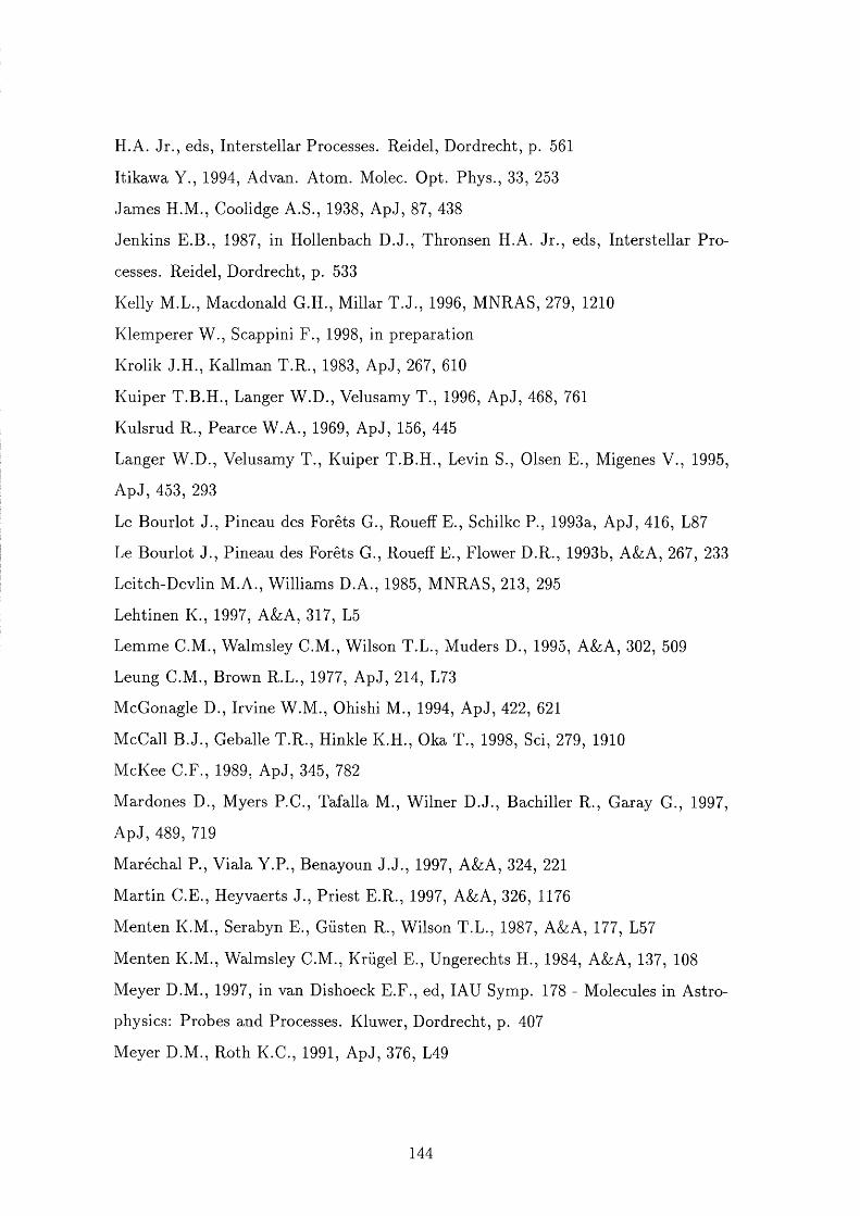
H.A. Jr., eds, Interstellar Processes. Reidel, Dordrecht, p. 561
Itikawa Y., 1994, Ad van. Atom. Molec. Opt. Phys., 33, 253
James H.M., Coolidge A.S., 1938, ApJ, 87, 438
Jenkins E.B., 1987, in Hollenbach D.J., Thronsen H.A. Jr., eds. Interstellar Pro
cesses. Reidel, Dordrecht, p. 533
Kelly M.L., Macdonald G .E., Millar T .J., 1996, MNRAS, 279, 1210
Klemperer W ., Scappini P., 1998, in preparation
Krolik J.H ., Kallman T.R., 1983, ApJ, 267, 610
Kuiper T.B.H., Langer W.D., Velusamy T., 1996, ApJ, 468, 761
Kulsrud R., Pearce W.A., 1969, ApJ, 156, 445
Langer W .D., Velusamy T., Kuiper T.B.H., Levin S., Olsen P., Migenes V., 1995,
ApJ, 453, 293
Le Bourlot J., Pineau des Forêts G., Roueff P., S chi Ike P., 1993a, ApJ, 416, L87
Le Bourlot J., Pineau des Forêts G., Roueff P., Flower D.R., 1993b, A&A, 267, 233
Leitch-Devlin M.A., Williams D.A., 1985, MNRAS, 213, 295
Lehtinen K., 1997, A&A, 317, L5
Lemme C.M., Walmsley C.M., Wilson T.L., Muders D., 1995, A&A, 302, 509
Leung C.M., Brown R.L., 1977, ApJ, 214, L73
McGonagle D., Irvine W.M., Ohishi M., 1994, ApJ, 422, 621
McCall B .J., Geballe T.R., Hinkle K.H., Oka T., 1998, Sci, 279, 1910
McKee C.F., 1989, ApJ, 345, 782
Mardones D., Myers P.C., Tafalla M., Wilner D.J., Bachiller R., Garay G., 1997,
ApJ, 489, 719
Maréchal P., Viala Y.P., Benayoun J .J ., 1997, A&A, 324, 221
M artin O.P., Heyvaerts J., Priest P.R., 1997, A&A, 326, 1176
Menten K.M., Serabyn P., Güsten R., Wilson T.L., 1987, A&A, 177, L57
M enten K.M., Walmsley C.M., Krügel P., Ungerechts H., 1984, A&A, 137, 108
Meyer D.M., 1997, in van Dishoeck P.P ., ed, lAU Symp. 178 - Molecules in Astro
physics: Probes and Processes. Kluwer, Dordrecht, p. 407
Meyer D.M., Roth K.C., 1991, ApJ, 376, L49
144
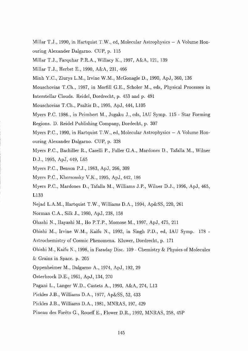
Millar T .J., 1990, in Hartquist T.W ., ed, Molecular Astrophysics — A Volume Hon
ouring Alexander Dalgarno. CUP, p. 115
Millar T .J., Farquhar P.R.A., Willacy K., 1997, A&A, 121, 139
Millar T .J., Herbst E., 1990, A&A, 231, 466
Minh Y.C., Ziurys L.M., Irvine W.M., McGonagle D., 1990, ApJ, 360, 136
Mouschovias T .Ch., 1987, in Morfill G.E., Scholer M., eds. Physical Processes in
Interstellar Clouds. Reidel, Dordrecht, p. 453 and p. 491
Mouschovias T.Ch., Psaltis D., 1995, ApJ, 444, L105
Myers P.C. 1986., in Peim bert M., Jugaku J., eds, lAU Symp. 115 - Star Forming
Regions. D. Reidel Publishing Company, Dordecht, p. 307
Myers P.C., 1990, in Hartquist T.W ., ed. Molecular Astrophysics — A Volume Hon
ouring Alexander Dalgarno. CUP, p. 328
Myers P.C., Bachiller R., Caselli P., Fuller G.A., Mardones D., Tafalla M., Wilner
D .J., 1995, ApJ, 449, L65
Myers P.C., Benson P.J., 1983, ApJ, 266, 309
Myers P.C., Khersonsky V.K., 1995, ApJ, 442, 186
Myers P.C., Mardones D., Tafalla M., Williams J.P ., Wilner D .J., 1996, ApJ, 465,
L133
Nejad L.A.M., Hartquist T.W ., Williams D.A., 1994, Ap&SS, 220, 261
Norman C.A., Silk J., 1980, ApJ, 238, 158
Ohashi N., Hay as hi M., Ho P.T.P., Momose M., 1997, ApJ, 475, 211
Ohishi M., Irvine W.M., Kaifu N., 1992, in Singh P.D., ed, lAU Symp. 178 -
Astrochemistry of Cosmic Phenomena. Kluwer, Dordrecht, p. 171
Ohishi M., Kaifu N., 1998, in Faraday Disc. 109 - Chemistry & Physics of Molecules
& Grains in Space, p. 205
Oppenheimer M., Dalgarno A., 1974, ApJ, 192, 29
Osterbrock D.E., 1961, ApJ, 134, 270
Pagani L., Langer W.D., Castets A., 1993, A&A, 274, L13
Pickles J.B ., Williams D.A., 1977, Ap&SS, 52, 433
Pickles J.B ., Williams D.A., 1981, MNRAS, 197, 429
Pineau des Forets G., Roueff E., Flower D.R., 1992, MNRAS, 258, 45P
145
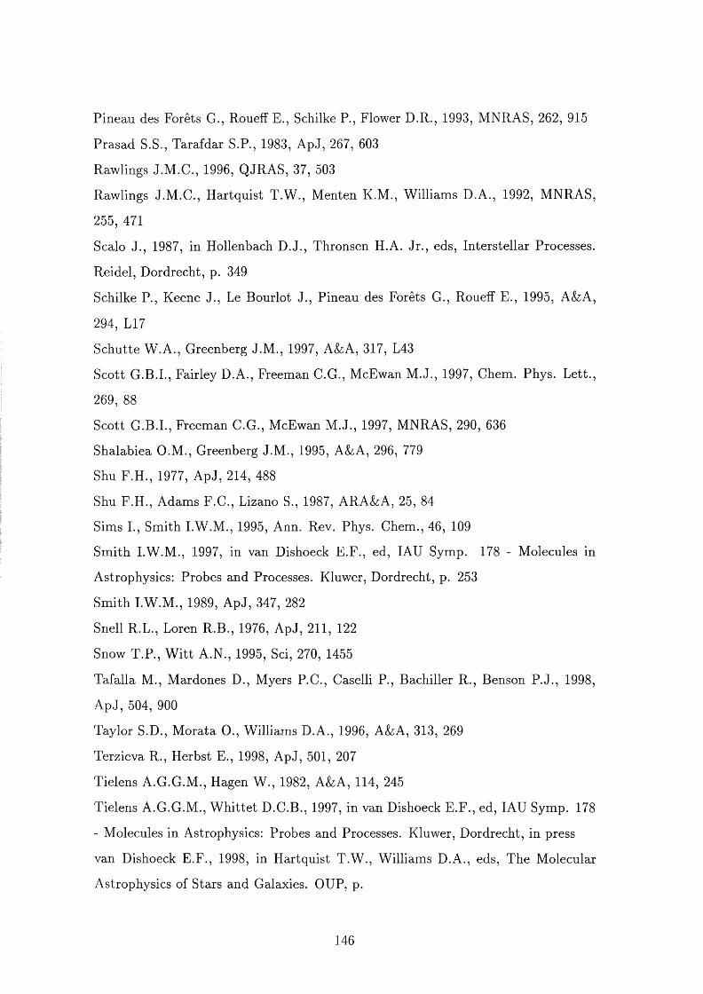
Pineau des Forêts G., RouefF E., Schilke P., Flower D.R., 1993, MNRAS, 262, 915
Prasad S.S., Tarafdar S.P., 1983, ApJ, 267, 603
Rawlings J.M .C., 1996, QJRAS, 37, 503
Rawlings J.M .C., Hartquist T.W ., Menten K.M., Williams D.A., 1992, MNRAS,
255,471
Scalo J., 1987, in Hollenbach D.J., Thronsen H.A. Jr., eds. Interstellar Processes.
Reidel, Dordrecht, p. 349
Schilke P., Keene J., Le Bourlot J., Pineau des Forêts G., Roueff E., 1995, A&A,
294, L17
Schutte W.A., Greenberg J.M., 1997, A&A, 317, L43
Scott G.B.I., Fairley D.A., Freeman C.G., McEwan M .J., 1997, Chem. Phys. Lett.,
269,88
Scott G.B.I., Freeman C.G., McEwan M .J., 1997, MNRAS, 290, 636
Shalabiea O.M., Greenberg J.M., 1995, A&A, 296, 779
Shu F.H., 1977, ApJ, 214, 488
Shu F.H., Adams F.G., Lizano S., 1987, ARA&A, 25, 84
Sims L, Smith I.W.M., 1995, Ann. Rev. Phys. Chem., 46, 109
Sm ith I.W .M., 1997, in van Dishoeck E.F., ed, lAU Symp. 178 - Molecules in
Astrophysics: Probes and Processes. Kluwer, Dordrecht, p. 253
Sm ith I.W .M., 1989, ApJ, 347, 282
Snell R.L., Loren R.B., 1976, ApJ, 211, 122
Snow T.P., W itt A.N., 1995, Sci, 270, 1455
Tafalla M., Mardones D., Myers P.O., Caselli P., Bachiller R., Benson P .J., 1998,
ApJ, 504, 900
Taylor S.D., M orata 0 ., Williams D.A., 1996, A&A, 313, 269
Terzieva R., Herbst E., 1998, ApJ, 501, 207
Tielens A.G.G.M., Hagen W., 1982, A&A, 114, 245
Tielens A.G.G.M., W hittet D.C.B., 1997, in van Dishoeck E.F., ed, lAU Symp. 178
- Molecules in Astrophysics: Probes and Processes. Kluwer, Dordrecht, in press
van Dishoeck E.F., 1998, in Hartquist T.W ., Williams D.A., eds. The Molecular
Astrophysics of Stars and Galaxies. GUP, p.
146