Molecular Hydrogen in Star-forming regions: implementation of its

micro-physics in Cloudy

G. Shaw,1 G. J. Ferland, 1 N. P. Abel,1 P. C. Stancil,2 and P. A. M.

van Hoof3

Abstract Much of the baryonic matter in the Universe is in the form of H2 which

includes most of the gas in galactic and extragalactic interstellar clouds.

Molecular hydrogen plays a significant role in establishing the thermal balance in

many astrophysical environments and can be important as a spectral diagnostic

of the gas. Modeling and interpretation of observations of such environments

requires a quantitatively complete and accurate treatment of H2. Using this

micro-physical model of H2, illustrative calculations of prototypical astrophysical

environments are presented. This work forms the foundation for future

investigations of these and other environments where H2 is an important

constituent.

Subject headings: ISM : molecules --- PDR

1 University of Kentucky, Department of Physics and Astronomy, Lexington, KY 40506;

gshaw@pa.uky.edu, gary@pa.uky.edu, npabel2@uky.edu

2 University of Georgia, Department of Physics and Astronomy and Center for Simulational

Physics, Athens, GA 30602; stancil@physast.uga.edu

3 APS Division, Department of Physics and Astronomy , Queen's University Belfast, BT7 1NN,

Northern Ireland; p.van-hoof@qub.ac.uk

1

1 Introduction Most of the hydrogen in the interstellar medium is in the form of H2 (Field et

al. 1966; Shull & Beckwith 1982; Black & van Dishoeck 1987; Draine & Bertoldi

1996). However, H2 is not an efficient emitter due to the lack of a permanent

electric dipole moment and its small moment of inertia, resulting in large energy

level spacings. H2 helps to define the chemical state of the gas, it plays a major

role in exciting important gas coolants, and it comprises the majority of the mass.

Therefore complete numerical simulations of a non-equilibrium gas must include

a detailed treatment of the physics of H2.

This paper describes the implementation of an extensive model of the H2

molecule into the spectral simulation code Cloudy. The code was last described

by Ferland et al. (1998). Cloudy determines the ionization and excitation state of

all constituents self-consistently by balancing all ionization and excitation

processes, the electron density from the ionization structure, and the gas kinetic

temperature from the balance between heating and cooling processes (e.g.

Osterbrock & Ferland 2005). This approach, as discussed in detail by Ferland

(2003), has energy conservation as its foundation. The goal of the current

implementation is to have all interactions of H2 with its environment, both

collisional and radiative, determined self-consistently with a limited number of

free parameters. Only the gas composition, density, column density, dynamical

state, and incident radiation field must be specified to uniquely determine the

physical conditions and emitted spectrum.

2 Physical model of the H2 molecule

2.1 Spectroscopic notation and energy levels

Figures 1, 2, and 3 show the energy levels included in our model. The figures

show, respectively, all energy levels, the levels within the ground electronic state,

2

and the lower levels within this state. There are 1893 levels in the model which

together produce a total of 524,387 lines.

Energies for the 301 rovibrational levels within the 11 gs Σ (denoted as X)

ground electronic state4 were adopted from the experimental compilation of

Dabrowski (1984). Errors in the energies of eight of the levels have been corrected

and energies of 17 missing levels have also been included (Roueff 2004, private

communication).

We also include the rovibrational levels within the lowest 6 electronic excited

states that are coupled to the ground electronic state by permitted electronic

transitions. The transition energies of Abgrall et al. (2000) were used to obtain

the upper electronic state rovibrational energies. These configurations and

shorthand notation are (B), 12 up +Σ 12 up Π (C+ and C-), 13 up +Σ (B’), and 13 up Π

(D+ and D-). These electronic excited states are relevant because they participate

in the Solomon process, the dominant H2 destruction mechanism when radiation

is present in the wavelength region between the Lyman continuum and Lyα.

Roughly 10% of the excitations following continuum radiation through the

electronic lines are followed by decays into the X continuum (Abgrall et al. 1992).

The majority of these photoexcitations are an indirect source for populating

highly excited X rovibrational levels which decay to lower levels producing

infrared emission lines. Finally, the UV absorption lines produced by these

transitions are an important probe of the temperature and density along the line

of sight through molecular gas.

The set of rovibrational levels within excited electronic states, however, is not

complete since they only include levels that are coupled to X through dipole-

allowed transitions. These excited rovibrational levels within the excited

4 The other 1s electron is suppressed here and throughout for convenience. Doubly-excited

states are not considered.

3

electronic states contain little of the H2 population. They are important only as an

intermediate step in photoexcitation of H2 into excited states or the continuum of

X. Dissociation energies from excited electronic states into the H(1s) + H(nl)

systems are taken from Sharp (1971).

The H2 molecule has ortho and para states defined by the alignment of the two

nuclear spins. Within the X ground electronic state, ortho (triplet nuclear spin)

states have odd rotational quantum number J, while para (singlet nuclear spin)

have even J. The same rule applies for the C- and D- electronic states, while for

the remainder of the electronic excited states the logic is reversed; ortho is even

and para is odd. Note that there are no rotational J = 0 states in the C and D

electronic states, because Λ = 1, and J ≥ Λ, where Λ is the projection of the total

electronic orbital angular momentum on to the internuclear axis.

Line wavelengths are derived by differencing these level energies and

correcting for the index of refraction of air for λ > 2000Å. Comparison of these

theoretical wavelengths with the observed wavelengths given in Timmermann et

al. (1996) and Rosenthal et al. (2000) show that our wavelengths derived from

electronic transition energies agree with the observed values to typically within

. 5/ 2 10δλ λ −×∼

Spectroscopic notations, such as “2-1 S(1)”, are commonly used to identify the

transitions. The first numbers indicate the change in vibrational levels. The

capital letter indicates the branch, which specifies the change in J, as shown in

table 1. The number in parenthesis is the lower J level of the transition. Radiative

decays between ortho and para are not possible because of the different nuclear

spin. Within the ground electronic state, lines have the selection rule

. For electronic transitions between Σ and Π, the selection rule is

, whereas the corresponding rule for Σ to Σ is

0, 2J∆ = ±

0, 1J∆ = ± 1J∆ = ± . For C+, the

4

selection rule is ∆ J = ± 1 whereas the corresponding rule for C- is ∆ J = 0. There is

no such selection rule for vibrational quantum numbers.

2.2 Bound-bound transitions

2.2.1 Transitions within the ground electronic state

Quadrupole radiative transition probabilities for rovibrational levels within

the ground electronic state are taken from Wolniewicz et al. (1998). This data set

is complete, i.e., transition probabilities are given for all allowed transitions

between the 301 rovibrational levels.

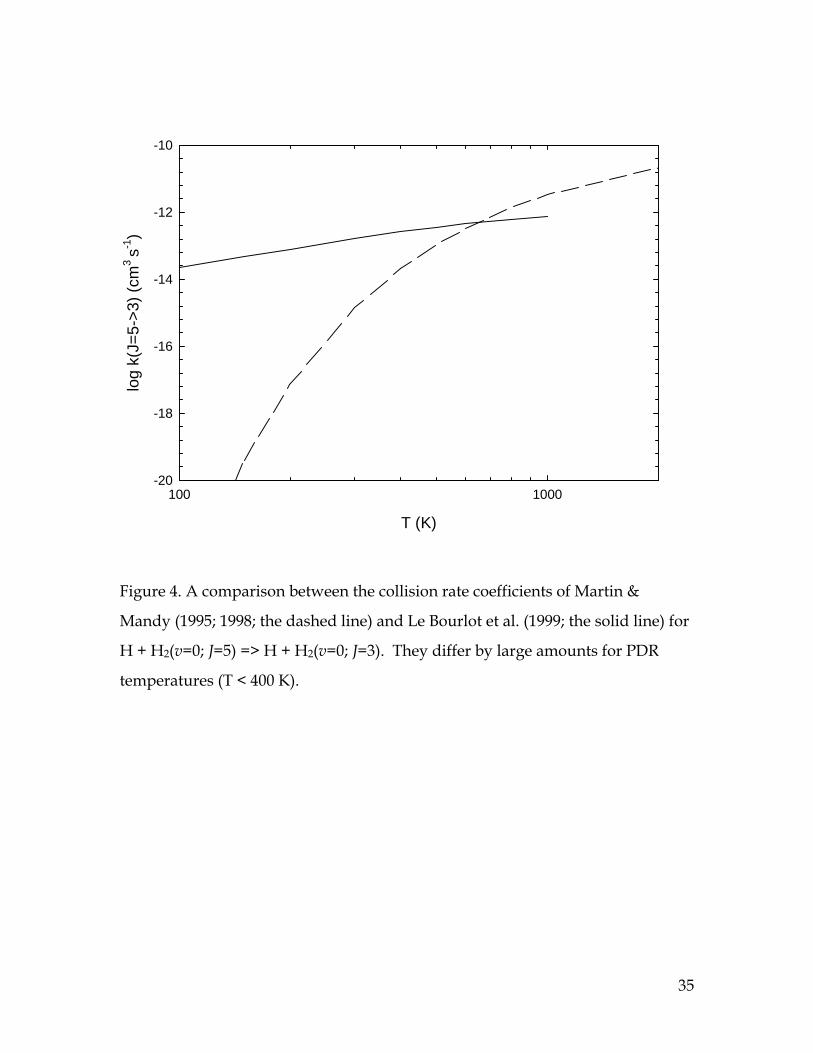
Rate coefficient fits for collisional excitation processes within the X state are

given by Le Bourlot et al. (1999; http://ccp7.dur.ac.uk/cooling_by_h2/ ) and

adopted here. These include rovibrational excitation of H2 by collisions with H,

He, and H2, but only for non-reactive transitions, i.e., those that do not involve

changes in nuclear spin.

The Le Bourlot et al. (1999) compilation, obtained with quantum mechanical

methods, should be appropriate to temperatures as low as ~10 K. However, this

compilation contains only rate coefficients of ~500 transitions, roughly 4% of the

12,535 possible transitions within X. The data set presented by Martin & Mandy

(1995; 1998) includes far more transitions but were not intended to be applied to

the low temperatures needed for the PDR models as they were obtained with

classical trajectory methods. Figure 4 compares their rate with the Le Bourlot et

al. (1999) values for rate coefficients for collisions between H2 and H for a typical

transition within X. They diverge by large factors below ~400 K.

The biggest effect of the missing collision data would be to introduce errors in

the populations and the heating or cooling effects of highly excited levels within

X. It seems more correct to use some physically motivated rate coefficients for the

missing levels rather than assume a rate coefficient of zero. We applied a version

of the “g-bar” approximation (van Regemorter 1962). Figure 5 shows collision

5

rates for all transitions within the Le Bourlot et al. (1999) data set at a given

temperature, plotted as a function of the transition energy. We took the simplest

possible approach, fitting these rates with the following function of energy

( ) 0log max( ,100)bk y a σ= + (1)

where σ is the transition energy in wavenumbers and k is in cm3s-1. The max

function prevents unphysically large rate coefficients from occurring when the

energy difference is very small. This fit is also shown in Figure 5, and Table 2

gives the fitting coefficients. These fits were within 1 dex of the majority

(typically 60% to 70%) of the rates. Tests presented below will show the impact

of these very approximate rates on the predicted spectrum.

We note that collisions of electronically excited states are neglected due to the

negligible population in these levels as noted in Section 2.1. This is appropriate

for densities well below 1015 cm-3.

2.2.2 Ortho – para conversion

The ortho and para H2 states can be mixed by exchange collisions with H, H+,

and H3+. H0 and H+ are the dominant forms of H at shallow depths into a PDR,

while deep within the PDR, all three species have only trace abundances. Rate

coefficients for H0 – H2 exchange collisions are from Sun & Dalgarno (1994; for

v=0 and J=0-1, 0-3, and 1-2 collisions). The rate coefficients for all other H0 – H2

exchange collisions are taken to be zero. The approximations to the rates given in

this paper diverge for temperatures below 100 K. Below this temperature a rate

of zero is assumed.

Rate coefficients for H+ - H2 exchange collisions were taken from Gerlich

(1990). The Gerlich data include both upward and downward transitions, but

they do not satisfy detailed balance. We adopted the rate coefficients for the

downward transitions and obtain the upward from detailed balance. These are

by far the fastest collisional rate coefficients, being ~1012 times larger than the H0

rate coefficient. This is by far the dominant process for ortho-para conversion.

6

However, Gerlich (1990) only computed rate coefficients for v = 0 and J < 10. We

therefore adopted the same procedure as discussed above to obtain the “g-bar”

approximation. The Gerlich rate coefficients were fitted as a function of transition

energy and used to estimate rate coefficients for all other transitions. Tests show

that the estimated rate coefficients have a small effect on the final level

populations and the ortho-para ratio. Le Bourlot (1991) notes that H3+ ortho-para

conversion collision rates are roughly equal to the H+ rates. We have used the H+

rates to include collisions with H3+. H3+ generally has a small abundance and so

does not strongly affect the results.

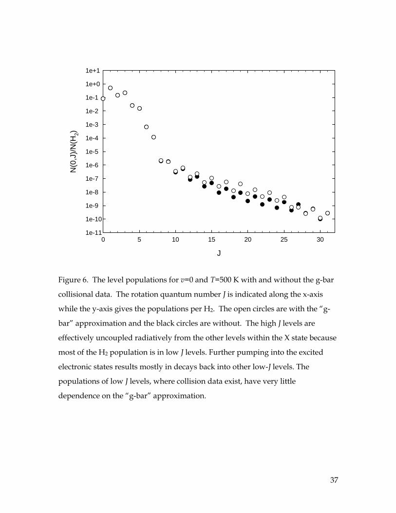
Figure 6 shows the effect of the “g-bar” approximation on v =0 level

populations at 500K. The lower rotational level populations where collisional

data exist have very little dependence on the approximation. In addition, ortho

H2 can be converted into para on grain surfaces (Le Bourlot 2000). This is

described in the section on grain physics below.

2.3 Coupling to the continuum

2.3.1 Electronic transitions and dissociation

Transition probabilities between excited electronic states and X were taken

from Abgrall et al. (2000). Excited electronic states can decay back into the

bound levels within X or dissociate into the continuum of the ground state.

Dissociation probabilities and the associated kinetic energy of the unbound

particles were also taken from Abgrall et al. (2000).

Allison & Dalgarno (1969) give photodissociation cross sections for transitions

from X into the continuum of the excited electronic states. These data are for the

energy range near the threshold and do not resolve the molecule into rotation

levels. The threshold for this process lies in the Lyman continuum of hydrogen

for lower v, J levels, and this continuum will be strongly absorbed by atomic

hydrogen in a PDR. The threshold does lie within the Balmer continuum for

higher v, J levels, however.

7

This process cannot be treated with great precision because of the lack of J-

resolved cross sections. We approximated the Allison & Dalgarno (1969) data as

a single cross section, 2.5 × 10-19 cm2, and evaluated the threshold energy for

each level.

2.3.2 Collisional dissociation from very high J

For temperatures within a PDR, T ≈ 500 K, collisional dissociation can only

occur from the very highest levels within X. Lepp & Shull (1983) give a general

expression for collisions between H and H2 that are valid for any J, but are

intended for much higher shock temperatures. Hassouni et al. (2001) give rate

coefficients for all v but only J = 0 for both H2 + H2 and H2 + H. For other

impactors Martin & Mandy (1995; 1998) give collisional dissociation rate

coefficients, but at higher temperatures.

We have taken a broad mean of the above references to obtain the rough

expression, used for collisional dissociation of H2 by impact with all colliders;

( ) (142 2 10 exp ( , ) /dissr H H v J kTχ−⇒ ≈ − ) [cm3 s-1] (2)

where χdiss(v,J) is the dissociation energy . Tests show that this process has little

effect on the predicted column densities and on the overall spectrum.

Electron collisions must be included as well. We know of no J-resolved

calculations of the electron collisional dissociation rates or cross sections.

Celiberto et al. (2001) give cross sections for excitation from X into B or C,

followed by dissociation. This process is only fast at temperatures much higher

(~50,000 K) than we expect in a PDR (~500 K). We do not include this process.

Stibbe & Tennyson (1999) give rates for dissociation by electron excitation from X

to the triplet state b. This is energetically far more favorable, and can occur at

500K. Unfortunately no J-resolved calculations exist, and dissociation from the

very highest J states should be the fastest.

8

The Stibbe & Tennyson (1999) data suggest an electron rate, in the small

limit, that is similar to the hydrogen rate given above. We assume

this rate in including electrons.

( , ) /diss v J kTχ

2.4 Grain processes

Our grain model can treat arbitrary grain types and size distributions. The

built-in Mie code can resolve the grain size distribution into as many size bins as

desired. The model can resolve the grain charge in multiple discrete charge

states, and can also treat the stochastic heating effect. Our treatment incorporates

the formalism described by Weingartner & Draine (2001). van Hoof et al. (2004)

provide further details and show that our representation reproduces the

Weingartner & Draine (2001) results in several test cases. In this approach the

temperature and charge for each grain type and size are determined by balancing

heating – cooling and ionization – recombination processes. Grain surface

recombinations of electrons and ions are included in the grain charge as well as

the ionization balance of the gas and the electron density. This gives a better

representation of the interactions between the gas and grains since the rates are

temperature dependent, and the grain temperature is set by the environment.

This unified treatment is applied to PAH’s (Polycyclic Aromatic Hydrocarbons)

as well as larger grains.

2.4.1 H2 formation on grains

H2 is predominantly formed on grains in the ISM although formation through

the H- route is not negligible. We use the rate given by Cazaux & Tielens (2002,

equation 18)

( ) ( ) ( ) ( )020.5 /

g

g g g Hn

n ur H n n H Hσ ε× ⎡ ⎤= ⎢ ⎥⎣ ⎦∑ HS T [s-1] . (3)

Here the sum is over all grain types and sizes and the factor of 0.5 accounts for

the fact that two hydrogen atoms become a single H2 molecule (see equation 3a

of Biham et al. 1998). The total hydrogen density n(H) is given by

9

0( ) ( ) ( ) ( )other

n H n H n H n HX+= + + ∑ , where HX represents all other H-bearing

molecules, and is basically used as a surrogate for the total grain density within

the term in the square brackets. This entire term is the projected grain area per

unit hydrogen nuclei. The atomic density n(H0) multiplies this term rather than

n(H) so that the rate becomes small in the limit where the gas is fully molecular

and little H0 is present (see equation 1 of Hirashita et al. 2003). The remaining

variables are uH, the average speed of a hydrogen atom, ε(H2), the H → H2

conversion efficiency, and SH(T), the H atom sticking probability. We take the

dimensionless sticking probability from Hollenbach & McKee (1979);

( )( )0.5 2

2 2 2

1

1 0.4 0.2 0.08H

g

S TT T T T

=+ + + + 2

, (4)

where T2 is the gas kinetic temperature in units of 100 K and Tg2 is the grain

temperature in these units. We assume the H2 conversion efficiency given by

Cazaux & Tielens (2002; equation 16), assuming 10-10 monolayers s-1. Tests show

that this results in a H2 formation rate within 10% of the Jura (1974) rate for grain

temperatures near 100 K.

Newly created H2 populates various rovibrational levels within the ground

electronic state. Population distribution functions have been considered by

Black & van Dishoeck (1987), Le Bourlot et al. (1995), Draine & Bertoldi (1996)

and more recently by Takahashi (2001) and Takahashi & Uehara (2001). We

follow the last two references. The other two distributions are also included in

the code as additional options to allow tests for their impact on results. We use

the Takahashi & Uehara (2001) vibrational distribution, and take the average of

the two forms of the rotational distribution, equations 6 and 7 in Takahashi

(2001). We assume that no population occurs when the Erot function of Takahashi

& Uehara (2001), their equation (3), becomes negative, as happens for large v.

This distribution function depends on the grain composition. For reference, the

10

carbonaceous, silicate, and ice compositions tend to deposit newly created H2 in

the v=2, 6, and 7 levels, respectively. We also used their product energy

distribution of newly formed H2 on various dust grains as given in Takahashi &

Uehara (2001).

2.4.2 Ortho – para conversion on grain surfaces

Conversion from ortho to para H2 can occur on grain surfaces at low

temperatures. We follow Le Bourlot (2000) in treating this process. The rate is

given by

( ) ( ) (2 2

2 ( )( ) / ( ) ,( )g

g g g H adn

n H un Hr n n H Tn H σ η⎛ ⎞⎟⎜= ⎟⎜ ⎟⎝ ⎠∑ )d HT S T

)

[s-1] . (5)

We assume that the sticking probability for molecular hydrogen is equal to

that for atomic hydrogen, and use the Hollenbach & McKee (1979) probability.

In implementing this we took a binding energy of T

2HS

ad = 800 K. A temperature

Tcrit is defined from Tad. This critical temperature is of the order of 20 K for these

materials.

The ortho to para conversion efficiency is then given by . We use

the form given in Le Bourlot (2000). In this process H

( ,c ad dT Tη

2 in any v, J, level strikes the

grain and is deexcited during its time on the surface. When Tgrain > Tcrit the H2 is

deexcited to either J=0 or 1, preserving the initial nuclear spin, before leaving the

grain surface. When Tgrain < Tcrit all H2 go to J=0. Since Tad is so low, the ortho-

para conversion will only be efficient in deep, well shielded, parts of a PDR.

2.5 The chemistry network

The chemistry network in the code has been described by Ferland et al. (1994;

2002). We have reviewed and updated all aspects of the chemistry to the data

sets given by Abel et al. (1997), Galli & Palla (1998), Hollenbach et al. (1991),

Maloney et al. (1998), Le Teuff et al. (2000), and Stancil et al. (1998). Only details

that affect the abundance and level populations of H2 are described here.

11

The chemistry network includes ~1000 reactions including 66 species

involving hydrogen, helium, carbon, nitrogen, oxygen, silicon, and sulphur.

Tests made during the Leiden PDR workshop (http://hera.ph1.uni-

koeln.de/~roellig/) show good agreement between our calculations and other

PDR models. Time-dependent advective terms are included when dynamical

models are considered (Ferland et al. 2002), and H2 may not be in a time-steady

state in some PDRs (Bertoldi & Draine 1996). The simulations presented here are

all stationary and represent gas that has had time to reach statistical equilibrium.

The micro-physical model of H2, described in Sections 2.1-2.4, is not explicitly

part of this network. Rather total formation and destruction rates are used to

determine a total H2 density. Following Tielens & Hollenbach (1985; hereafter

TH85), the molecule is divided into ground state H2g and excited state, H2*, and

these two are part of the H2 and CO chemistry networks. The density of H2* is

the sum of all populations in states with an excitation potential greater than 2.6

eV, and H2g as the population in lower levels. This was chosen to follow the

partitioning given by TH85, which then allows us to use their chemical rate

coefficients for reactions that involve H2*. The CO photodissociation rate is

calculated as in Hollenbach et al. (1991). The detail calculations concerning our

chemistry network will be in future publication.

The equilibrium deduced from the network is then used to set the state

specific H2 formation and destruction rates that affect the population with X. In

turn the micro-physical model of the hydrogen molecule defines state specific

destruction rates, which are sums over the state-specific rates. Destruction rates

predicted by the micro-physical H2 model are used in the chemical reaction

network, and state specific creation rates from the network are then included as

population mechanisms within the large molecule. The net effect is that each

level has a population that is determined by these creation and destruction

processes, along with internal excitations and deexcitations within the molecule.

The solutions obtained by the micro-physical model of the hydrogen molecule

12

(see Section 2.7 for a discussion of how the level populations are calculated) and

the full chemistry network are converged by multiple solution of both; so that the

H2 density from the chemistry network and the sum of populations within X

agree to a specified amount.

2.5.1 Creation from H-

Although H2 is mainly formed on grain surfaces in the ISM, it can also form by

the associative detachment reaction

− −+ → +2H H H e . (6)

Our detailed treatment of this process is described in Ferland & Persson (1989).

This is usually the fastest in moderately ionized regions (Ferland et al. 1994).

Abel et al. (1997) note that H2 is mostly formed in the para configuration (v=0,

J=0 and v=0, J=2) by this process.

We use the state-specific distribution functions for H2 formation from H- given

by Launay et al. (1991), and populate the newly formed H2 molecule using these

rates and the H- density determined by the molecular network. The population

distribution function tends to peak around v ~ 5 to 7 and mostly odd J, typically

between 3 and 7, although very large J can occur.

The Launay et al. distribution function does not, at face value, agree with the

Abel et al. (1997) distribution functions. Abel et al. (1997) assume that after

formation the molecule will reside only in low J levels (J = 0-2). According to

Abel et al. (1997), the rate coefficient for the process H + e- → H- + γ is smaller

than the rate coefficient for the process H2 (J=2) + H+ → H2 (J=1) + H+ + 170.5 K

(given by Flower and Watt 1984 and used by Abel et al. 1997), so the molecule

decays to lower levels more quickly than it is formed. So, newly formed H2 will

eventually be converted to the para state (v=0, J=0 and v=0, J=2). Abel et al.

(1997) give the final state after the system has had time to relax, which is

different from the state-specific rates given by Launay et al. 1991 (Ortho-para

conversion is treated separately.)

13

The chemistry network uses an integrated rate for the formation of H2. We

summed over all of the state specific rates in Launay et al. (1991) and fitted the

total rate with the following:

8

1( )5.4597 10 71239

k HT

− =× +

[cm3 s-1] . (7)

This expression is well-behaved for all temperatures, but was fitted to the

Launay et al. (1991) data over the temperature range they give, 10 K – 104 K.

Similarly, the process H2+ + H → H2 + H+ produces H2 in v=4 states. This

process can be important in deeper, molecular regions of a PDR. We use rates

from Krstić (2002). These are not J-resolved so we place all in J = 0.

2.6 High-energy effects

Cosmic rays can be included in a calculation as described by Ferland &

Mushotzky (1984) and Wolfire et al. (1995). X-rays have very nearly the same

effect. Although X-rays have little effect upon a gas at shallow depths, since

relatively few high-energy photons are present, deep within a cloud the

attenuated radiation field can be dominated by hard photons. These

predominantly interact with inner shells of the heavy elements producing hard

photoelectrons and inner shell vacancies which relax, producing high-energy

Auger electrons. Our treatment of this physics is described in Ferland et al.

(1998). All of these processes create electrons with a great deal of energy, and

within neutral or molecular regions, these energetic electrons create secondary

ionizations and excitations, while depositing only part of their initial energy as

heat.

The effects of non-thermal electrons in molecular gas are described by

Dalgarno et al. (1999), and in the papers on the chemistry of the ISM given above.

In particular, Tiné et al. (1997) give cosmic ray excitation rates for v=0 to 14 and

J=0-11 within X which we adopt. We adopt their values at a fractional ionization

14

10-3 as being typical. Rates for electronic excitation are from Dalgarno et al

(1999).

2.7 Determining level populations

The molecule is represented by the 1893 levels shown in Figure 1. Level

populations are determined by solving a system of simultaneous linear

equations. The level populations are evaluated several dozens of times per radial

step as the pressure, temperature, and ionization are simultaneously determined.

Conventional matrix inversion methods have a speed that goes as a power of the

number of levels, and would result in prohibitive execution times. Additionally,

many matrix inversion methods have stability problems with very large matrices

when the level populations range over several decades of orders of magnitude.

Rather, a linearized method was developed which takes into account the physical

properties of the molecule.

2.7.1 Excited electronic levels

Collisional excitation to electronic states is completely negligible due to the

low temperature in a PDR. Excitation is by photoexcitation in discrete lines, the

Solomon process, which can be followed by relaxation back into rovibrational

levels of the ground electronic state or by transitions into its continuum. The

electronic excited states have short lifetimes because of their large transition

probabilities. We neglect collisional processes within excited electronic states

since the critical densities, the density where the collisional deexcitation and

spontaneous radiative decay rates are equal, is ~1014 cm-3, far greater than the

densities encountered in a PDR.

The line photoexcitation rate is given by , /u l u lA g gνη [s-1], where

( )3 2/ 2 /J h cν νη ν= is the photon occupation number of the attenuated incident

continuum at the line frequency (Ferland & Rees 1988) and self absorption of a

single line is treated as in Ferland (1992). Line overlap is discussed below. The

15

excited level decays by allowed radiative transitions. The population of an

electronic excited state nu is then given by the balance equation

(ul ul u c ul

l ll

gn A n A Agνη

⎡ ⎤⎢= + +⎢⎣ ⎦

∑ ∑ )β δ ⎥⎥ (8)

where Ac indicates the transition probability from the excited state into the X

continuum, Aul is the transition probability between X and the excited states, β is

the escape probability and δ is the destruction probability. We follow the

treatment described in Ferland & Rees (1988). The total rate for H2 to decay into

the X continuum is then given by

( )2

1c

u

rn H

= ∑ u cn A [s-1] , (9)

which is the total destruction rate due to the Solomon process.

2.7.2 Populations within ground electronic state

Highly excited states within X are mainly populated by indirect processes.

The most important include decays into X from excited electronic states and

formation in excited states by the grain or H- route. Direct collisional excitation

is relatively inefficient, at least for higher J, due to the large excitation energies

and low gas kinetic temperatures.

We use a linearized numerical scheme that updates populations by

“sweeping” through the levels within X, from highest to lowest energies. Rates

into and out of a level are computed and an updated level population derived

from these rates. At the end of the sweep the updated and old populations are

compared, and revisions continue until the largest change in population is below

a threshold. The method achieves a solution in a time that is proportional to an2,

where n is the number of levels and a~5 is the number of iterations needed to

determine the H2 populations. By comparison to standard linear algebra, solving

16

the system with LU decomposition would require a time 313 n≈ , or 103 – 104 times

slower.

This process converges quickly because of the complete linearization that is

inherent to the entire code. During solution of the ionization, chemical, and

thermal equilibria within a particular zone, the H2 molecule populations will be

determined several dozens of times, and each new solution will be for conditions

that are not too far from previous solutions.

Two convergence criteria were used. The first is that the level populations

have stabilized to within a certain tolerance, usually 1%. This affects the

observed emission-line spectrum. Collisional deexcitation of excited levels within

X can be the dominant gas heating mechanism in parts of a PDR (TH85), and a

second criterion was that the net heating (or cooling) have stabilized to better

than a small fraction of the heating-cooling error tolerance. These criteria were

chosen so that the molecular data remained the main uncertainty in the solution.

2.7.3 Line overlap

For an isolated line we use equations A8 and A9 of Federman et al. (1979) to

treat coarse line overlap of the Doppler core and damping wings. For the case of

the electronic lines of H2, many thousands of lines and the heavy element

ionizing continua overlap. Neufeld (1990), Draine & Bertoldi (1996), and Draine

& Hao (2002) discuss ways of treating overlapping lines. Cloudy has always

included the effects of line overlap for important cases, which were added on an

individual basis (one case is discussed by Netzer et al. 1985). A general solution

to the overlap problem, with overlap treated in an automated manner is

necessary. We developed a method that looks to the long term evolution of the

code, since the overlap problem will only become worse as the simulations

become more complete and more lines are added.

17

The simplest approach is to make the continuum energy mesh fine enough to

resolve all lines; then lay the line opacities and source functions onto this mesh.

This approach is taken, for instance, by the Phoenix stellar atmosphere code for

atomic lines (Hauschildt & Baron 1999). It is not feasible to do this in Cloudy

since the code’s execution time is linearly dependent on the number of

continuum points. This is because of the repeated evaluation of photo-interaction

rates and continuous opacities – the far higher spectral resolution needed to

resolve lines would result in prohibitive execution times.

We use a multi-grid approach to treat line and continuum overlap. In this

scheme certain aspects of a problem are solved on a fine mesh, with far higher

spectral resolution, which is then propagated out onto a courser energy scale.

The coarse continuum cells are many hundreds of line-widths across, so it is not

possible to tell, on that scale, whether lines actually interact and to what extent.

The fine mesh has several fine-resolution continuum elements per linewidth; the

total line opacities and source functions are placed onto this fine mesh, and the

effects of line overlap is handled trivially. Lines are individually transferred

within the fine mesh and then referenced back onto the course grid to include

interactions between line and the continuum. An example of the coarse and fine

continua is presented in Section 3.3 below.

2.8 Heating – cooling

Processes that add kinetic energy to the free particles are counted as heating

agents, while cooling processes remove kinetic energy from the gas. H2 affects

the thermal state of its surroundings in several ways.

The dissociation from electronic states following photoexcitation is an

important heating process, which is given by a modified form of equation 9,

c u cu

G n A ε=∑ c [erg cm-3 s-1] (10)

18

where the sum is over all electronic excited states, Ac is the dissociation

probability, and εc is the kinetic energy per dissociation, as tabulated by Abgrall

et al. (2000).

Collisional processes are included for all levels within X, as described above.

The energy exchange associated with these collisions, expressed as a net cooling,

is given by

( )X l lu uu l u

L n C n C ε<

= −∑∑ ul lu [erg cm-3 s-1] (11)

where the sum is over all levels within X, and the C’s represent the sum of all

collisional rates that couple levels u and l. εlu is the difference in energies

between the levels. For conditions close to the illuminated face of a PDR, higher

levels are overpopulated relative to a Boltzmann distribution at the gas kinetic

temperature and collisions within X is a net heating process. Deep within the

cloud the process acts as a coolant.

3 Comparison calculations This section describes several comparison calculations that illustrate aspects of

the H2 simulations. We begin with the simplest case, a model in which the

molecule is dominated by thermal collisions. Next the case of cosmic ray

excitation is considered, then a situation similar to the illuminated face of a PDR,

in which populations are determined mainly by the Solomon process. Finally a

complete calculation of a standard PDR is presented, with the resulting H2

emission spectrum and column densities. These cases have been well established

by previous studies, for instance Abgrall et al. (1992), Black & van Dishoeck

(1987) and Sternberg & Neufeld (1999), but our main purpose is to document the

current implementation of the relevant physics. If no special values are

mentioned then all the model parameters have the values listed in Table 3.

19

3.1 Collision dominated regions

Collisions play an important role in determining H2 spectra in shocks, or gas

that is otherwise heated to warm temperatures. As a test case we have computed

the collisionally excited spectrum of a predominantly molecular gas.

In the low density limit, where every collisional excitation is followed by

emission of a photon, the collisional rate is given by ( )2 cu n H nσ , where the first

term is the excitation rate coefficient and nc is the density of colliders. The

emissivity is then given by ( )224 j u n Hπ σ= [erg cm-3 s-1]. In this limit the ratio

should depend mainly on the collision physics. ( )224 /j n Hπ

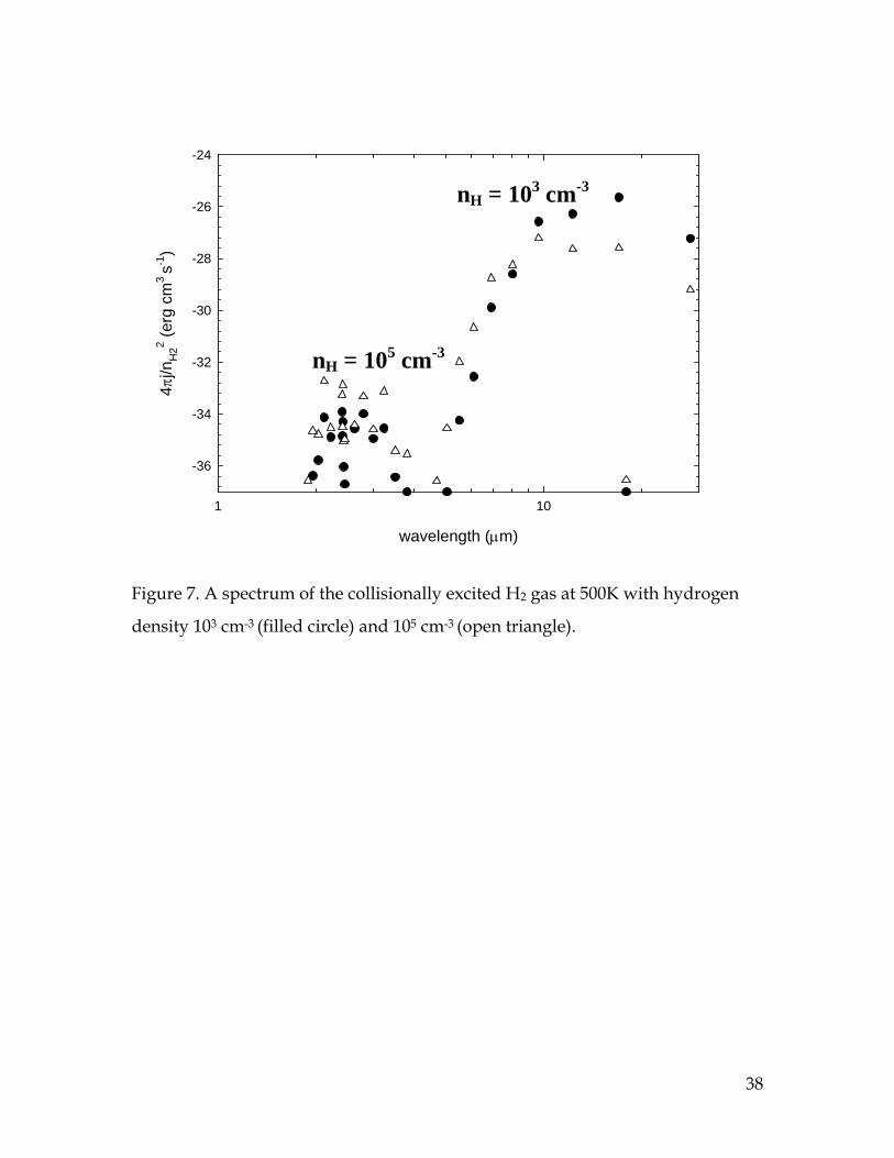
Figure 7 shows the spectra of collisionally dominated gas at 500K, a typical

PDR temperature. Two hydrogen densities, 103 cm-3 and 105 cm-3, are shown.

Figure 8 shows collisionally dominated spectra at 2000K, a typical shock

temperature, with the same densities. The Solomon process and cosmic ray

excitation were disabled to make the excitation due entirely to collisions with

thermal particles. The gas was almost entirely molecular (n(H2)/n(H) = 0.5).

Line emissivities are greater for higher temperature as expected. For both models

the long wavelength transitions, which form from smaller J in v = 0, have a

higher emissivity for the lower density. These lines are collisionally deexcited at

the high density. As the density increases, the higher ro-vibrational levels

become more populated by collisions from intermediate J resulting in more

intense lines originating from those high levels.

3.2 Cosmic ray dominated regions

Both very hard photons and cosmic rays may penetrate into regions where

hydrogen is predominantly molecular. In such environments the primary effect

of collisions between thermal matter and energetic particles or light is to produce

non-thermal electrons which then excite or ionize the gas. This can result in both

destruction and excitation of H2. We assume the galactic background ionization

20

rate quoted in Williams et al. (1998), ζ/nH = 2.5×10-17 cm3 s-1, where ζ is the

primary cosmic ray H0 ionization rate (s-1), and the excitation distribution

function of Tiné et al. (1997), as described above. This cosmic ray background

will be included in many of the models described below since this background

ionization process should be pervasive.

Non-thermal electrons can also excite rovibrational levels of H2, as described

above. As a test, we recomputed a 50 K model. The low temperature was chosen

so that cosmic ray excitation dominates. The electronic lines were forced to be

optically thick to make the Solomon excitation process unimportant, and as a

result the gas is almost entirely molecular. The predicted spectrum is shown in

Figure 9. Inspired by Tine et al. (1997), we also predicted a spectrum at 50K. The

differences are because of the full chemistry of this model, likely to be different,

which affects the thermal excitation rates. Given this uncertainty the agreement

with their calculation is quite satisfactory.

The cosmic ray dominated spectra is much richer in character than the

collision dominated spectra described above. The energy levels of H2 are widely

separated so most molecules reside in the ground vibrational level for fully

molecular environments. Thermal collisions cannot excite high rovibrational

levels. Cosmic rays are highly energetic and can pump H2 in higher rovibrational

levels resulting in numerous intense lines.

3.3 The Orion PDR

We consider the TH85 standard model since this has parameters chosen to be

similar to inner regions of the Orion complex and the model has become a

standard within the PDR community. Table 3 summarizes the parameters of the

TH85 Orion PDR. We assume the constant gas density, chemical composition,

and incident radiation field given in TH85. Ferland et al. (1994) discuss a

previous comparison of our results with this paper.

21

As outlined in section 2.4 above, our treatment of the grain physics has

improved, and this is a major source of differences with our earlier calculation.

We use a grain size distribution that is chosen to reproduce the overall extinction

properties of the extinction along the line of sight to the Orion environment.

Most of this extinction occurs within the Veil, a predominantly atomic layer of

gas that lies several parsecs towards the observer from the central star cluster.

The column density per unit extinction is taken from Shuping & Snow (1997) and

Abel et al. (2004). We have also included PAHs in our calculation. Grain charge,

temperature, and drift velocity are self-consistently determined for each type and

size of grain.

As a starting point we consider a point near the illuminated face of the PDR.

Figure 10 shows the populations per molecule for an unshielded atomic gas with

a constant temperature of 500 K. Collisions are relatively unimportant and the H2

level populations are determined by the Solomon process. As expected, the

populations are highly non-thermal, with large populations in high J and v levels

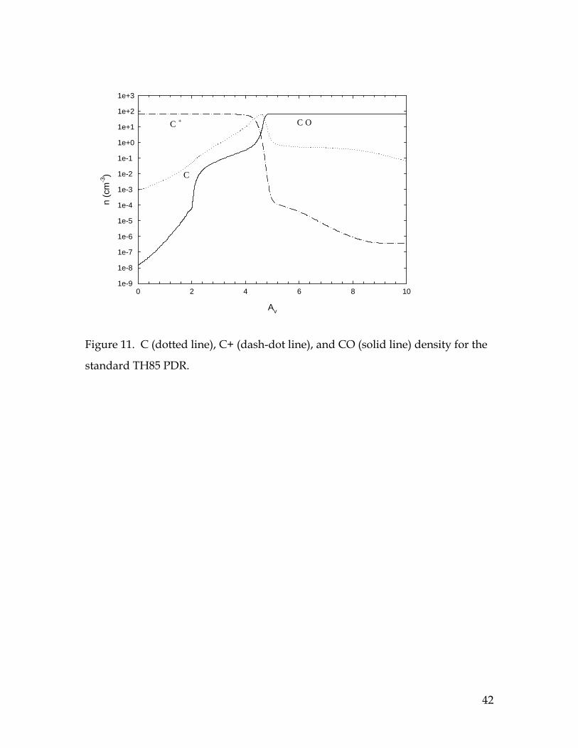
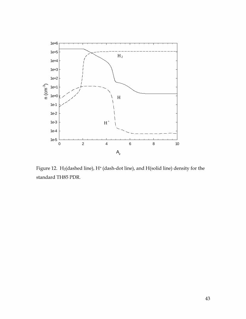
Next we compute the full ionization, chemical, and thermal structure of the

PDR. Figures 11 and 12 show the computed abundances of C+, C, CO, H+, H,

and H2. For AV > 2.4, H2 is the dominant species while all C is in the form of CO

for AV > 4.4. Figure 13 shows the computed temperature structure and the

electron density. At the illuminated face of the cloud the electron temperature is

> 200 K and T drops to 30K deep inside the cloud. At the edge of the cloud the

electron abundance is determined by the ionization of C and is equal to the C+

abundance. These results are in qualitative agreement with the original TH85

calculation.

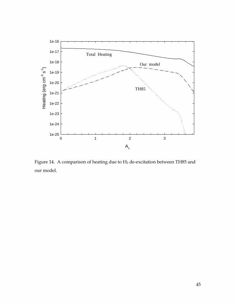
Collisional de-excitation of H2 is a significant gas heating mechanism. TH85

present a widely used theory for the process that involves a simple

representation of the H2 molecule. They use two levels, H2 and H2*, and their

heating rate (equation A13) is linearly dependent on H2*. Conversely, we

22

consider all 301 bound levels in the ground electronic state. Figure 14 compares

the heating due to the H2 de-excitation between TH85 and our model. Deep

inside the cloud, the H2* population is very small, since it is predominantly

produced by the Solomon process, which is inefficient due to line self-shielding.

This small population makes the TH85 de-excitation heating rate very small. In

our calculation heating at depth is mainly due to collisions with low J levels,

which are not included in the H2 and H2* representation. As a result, deep inside

the cloud these two are considerably different.

Photoelectric emission from grains is a major source of heating. As discussed

by Ferland et al. (1994), our model of grain photoelectric heating results in

generally lower temperatures than the original TH85 calculation. As discussed

above, our current treatment follows Weingartner & Draine (2001), and results in

slightly less heating. Figure 15 shows the variation of temperature for the

graphite and silicate grains and PAH. The PAHs are hotter than the other two

due to their smaller sizes, while the graphitic component is generally hotter than

the silicate. Within each type of grain, smaller grains are hotter than larger due

their reduced radiation efficiency. The dependence on grain size and

composition is in the expected sense. The H2 grain formation rate depends on

grain temperature, which shows the importance of using a realistic

representation of the grain physics in this simulation.

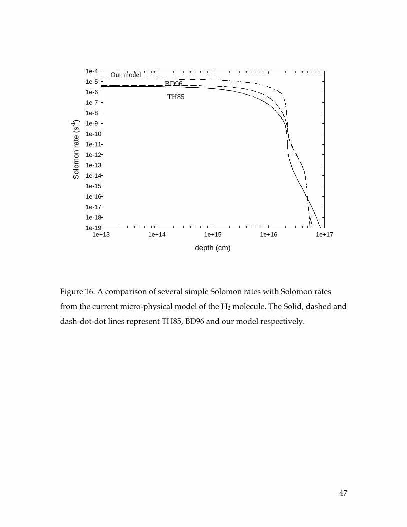
The Solomon process is the most important destructive mechanism for H2.

Figure 16 compares the Solomon process dissociation rates given by equation 9

with that computed using the approximation given by equation A8 of Tielens &

Hollenbach (1985) and by equation 23 given by Bertoldi & Draine (1996).

At the illuminated face of the cloud our model predicts greater Solomon rates

than the other two. This higher value of the Solomon rate has been observed by

the other groups present at the Leiden PDR workshop (2004). The effect is due to

the inclusion of 301 levels in X, which will produce more pumping from the

23

excited rovibrational levels to the higher electronic states resulting in a larger

Solomon rate. Deep inside the cloud self-shielding plays a crucial role and our

model matches better with the Draine & Bertoldi model (1996).

The integrated column densities for various J levels in the v = 0 level are

shown in Figure 17(a) by filled circles, whereas the LTE column densities are

given by open circles. It is clear from the plot that the J = 0-3 levels are in LTE.

The populations of these low levels are mostly affected by collisions and

henceforth have come into equilibrium. The populations of higher levels are

mainly populated by nonthermal pumping processes and are overpopulated

relative to their LTE value. The gas temperature can be derived safely for these

conditions from the ratio of column densities of J = 1 to J = 0 since these levels are

in LTE. We find a mean gas temperature of 49.4K from the ratios of column

densities shown in Figure 17(a). Ratios of higher rotational levels (J > 3) can be

used as diagnostic indicators of nonthermal pumping. The integrated column

densities for various J levels for the v = 1-8 vibration levels are shown in Figures

17(b) and 17(c). This type of diagnostic diagram is commonly used to determine

conditions within translucent molecular regions (Draine & Bertoldi, 1996). Most

of the H2 is in the ground vibrational level and its column density is much larger

than the excited vibrational levels. The column density decreases with increasing

v. The populations, and their variation with J, of the excited vibrational states are

different than the ground vibrational state and the distinction between ortho and

para states are more prominent for v >0.

The full H2 spectrum is shown in Figure 18. H2 can offer additional PDR

diagnostic indicators of the density and flux of the ionizing photons. Note that

optical lines should be detectable, although at very faint levels.

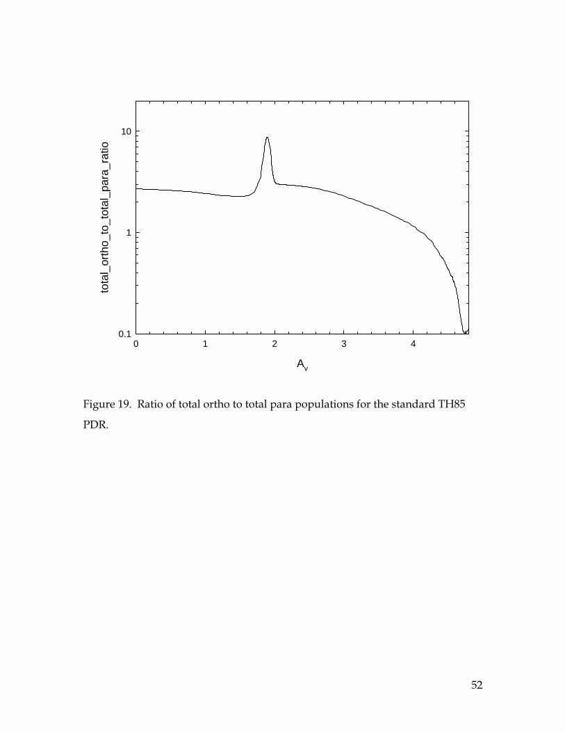
We also calculated the total ortho to total para ratio as a function of AV as

given by Abgrall et al. (1992) and Sternberg & Neufeld (1999). This is shown in

Figure 19. This has a similar characteristic as the previous calculations.

24

Earlier we discussed the treatment of line overlap. Figures 20(a) and 20(b)

show the coarse and fine continua for the point at the half-molecular location in

the PDR, where 2n(H2)/n(H) = 0.5. Figure 20(a) shows the coarse continuum,

used in the evaluation of the continuous opacities and photodissociation rates.

Thermal emission by dust dominated the infrared emission, with fine structure

atomic emission superimposed. PAH features are present in the near IR, and a

set of weak H2 lines are present in the 1-10 µm region. Figure 20(b) shows the fine

continuum transmission factors. This is similar in appearance to, for instance,

Figure 2 of Abgrall et al. (1992). We can see finer details as we zoom out the

wavelength scale.

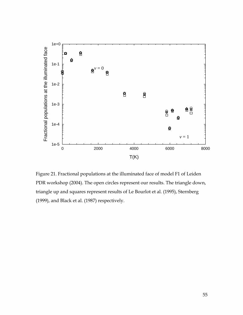
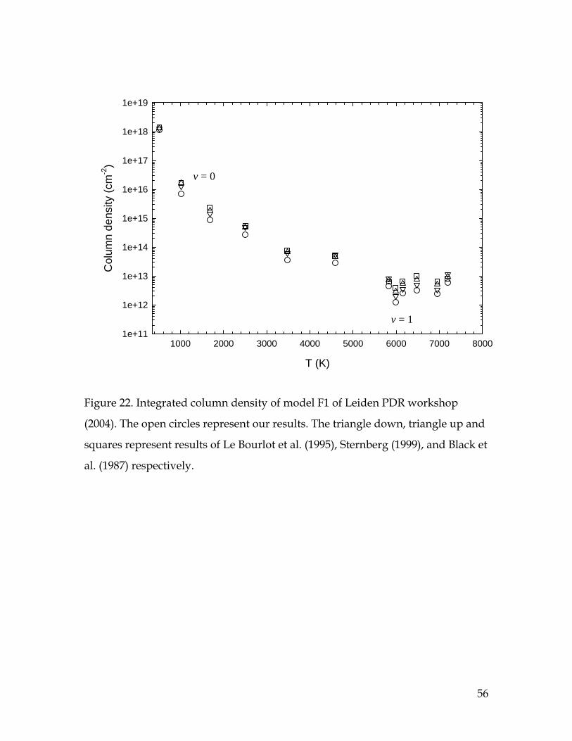
3.4 The Leiden (2004) PDR

We, along with eight other groups, participated in a PDR workshop held in

Leiden in the Spring of 2004. The purpose was to compare predictions of various

PDR codes. Three other codes included complete models of the H2 molecule, and

as test case was devised to check their predictions. The other codes were those

described by Sternberg & Neufeld (1999), Black et al. (1987), and Le Bourlot et al.

(1995). Here we compare the predictions of one of the constant temperature

models (F1). The parameters are given in Table 4. For simplicity an

equipartition distribution function, in which 1/3 of the energy of formation of H2

goes into the grains, internal excitation, and kinetic energy, was assumed in all

cases. Figure 21 compares the fractional populations at the illuminated face of

the cloud as a function of excitation energy. Figure 22 shows the integrated

column density for the same model as a function of excitation energy. Our results

agree well with the other groups with the differences due to implementation

details.

25

4 Conclusions The aim of the current manuscript was to document the physical, chemical,

and thermal processes relevant to H2 and the implementation of these processes

into the spectra simulation code Cloudy. Great effort has been made to treat all of

these processes self-consistently in a synergistic approach. By specifying the gas

composition, density, column density, dynamical state, and the incident

radiation field of a particular astrophysical environment, one can uniquely

determine its physical conditions and emitted spectrum. This work lays the

foundation for future investigations of the role of H2 in various astrophysical

environments. This version of Cloudy is available at http://www.nublado.org.

5 Acknowledgements We wish to thank M. Mihalache-Leca, H. Abgrall and E. Roueff, Jacques Le

Bourlot, Junko Takahashi and Lutoslaw Wolniewicz for their help. Ewine van

Dishoeck, Amiel Sternberg, Jacques Le Bourlot, and Evelyne Roueff graciously

allowed us to present their results in our Figures 21 and 22. We would like to

thank the anonymous referee for thoughtful suggestions which helped us to

improve our paper. GS would like to thank CCS, University of Kentucky for their

two years of support. NASA (NAG5-12020) and NSF (Ast 03-07720) also

supported this work. PCS acknowledges support from NSF grant AST 00-87172.

P.v.H is being supported by the engineering and Physical Sciences Research

Council of the United Kingdom.

6 Appendix – effects of uncertain collision rate coefficients

The uncertainties in the collisional rate coefficients are substantial. If the errors

are random and not correlated then we can simulate the uncertainty with

26

Gaussian random numbers. We assume the following form for the error

distribution

log ' log randr r= +

where rand is a Gaussian random number with a mean of 0 and a dispersion of

0.5.

This random noise in collisional rate coefficient changes the final spectra

(Figure 23) by less than 5% for very low rotational quantum numbers such as 0-0

S(0), 0-0 S(1) and 0-0 S(2), but by as much as 25% for higher rotational quantum

numbers such as 0-0 S(3), 0-0 S(4). Figure 24 plots the level populations for v=0

with and without the random Gaussian noise in collision data at 500K.

7 References Abel, N. P. Brogan, C. L., Ferland, G. J., O'Dell, C. R., Shaw, G., & Troland, T. H. 2004, ApJ, 609,

247

Abel, T., Anninos, P., Zhang, Y., & Norman, M. 1997, New Astronomy, 2, 181

Abgrall, H., Roueff, E., & Drira, I. 2000, A&AS, 141, 297

Abgrall, H., Le Bourlot, J., Pineau Des Forets, G., Roueff, E, Flower, D. R., & Heck, L. 1992, A&A,

253 525

Allison, A.C. & Dalgarno, A. 1969, Atomic Data, 1, 91

Bertoldi, F., & Draine, B. 1996, ApJ, 458, 222

Biham, O., Furman, I., Katz, N., Pirronello, V., & Vidali, G. 1998, MNRAS, 296, 869

Black, J.H., & van Dishoeck, E.F. 1987, ApJ, 322, 412

Cazaux, S., & Tielens, A.G.G.M. 2002, ApJ, 575, L29

Celiberto, R., Janev, R.K., Laricchiuta, A., Capitelli, M., Wadehra, J.M., & Atems, D.E. 2001,

ADNDT, 77, 161

Dabrowski, I. 1984, Can. J. Phys., 62, 1639

Dalgarno, A., Yan, Min, & Liu, Weihong 1999, ApJS, 125, 237

Draine, B.T., & Bertoldi, F. 1996, ApJ, 468, 269

Draine, B.T., & Hao, Lei 2002, ApJ, 569, 780

Federman, S. R.; Glassgold, A. E.; Kwan, J. 1979, ApJ, 227, 466

27

Ferland, G. J. 1992, ApJ 389, L63

Ferland, G. J. 2003, ARA&A, 41, 517

Ferland, G. J., Fabian, A. C., & Johnstone, R. 1994, MNRAS, 266, 399

Ferland, G. J., Fabian, A. C., & Johnstone, R. 2002, MNRAS, 333, 876

Ferland, G. J., Henney, W. J., Williams, R. J. R., Arthur, S. J. 2002, Revista Mexicana de

Astronomía y Astrofísica (Serie de Conferencias) Vol. 12, pp. 43

Ferland, G. J.; Korista, K. T.; Verner, D. A.; Ferguson, J. W.; Kingdon, J. B.; & Verner, E. M. 1998,

PASP, 110, 761

Ferland, G.J., & Mushotzky, R.F. 1984, ApJ, 286, 42

Ferland, G.J., & Persson, S. E. 1989, ApJ, 347, 656

Ferland, G. J., & Rees, M. J. 1988, ApJ, 332, 141

Field, G.B., Somerville, W.B., & Dressler, K. 1966, ARA&A, 4, 207

Flower, D.R., & Watt, G.D. 1984, MNRAS, 209, 25

Galli, D., & Palla, F. 1998, A&A, 335, 403

Gerlich, D. 1990, J. Chem Phys 92, 2377

Hassouni, K., Capitelli, M., Esposito, F., Gicquel, A. 2001, Chem Phys Letters, 340, 322

Hauschildt, P.H., & Baron, E. 1999, J. Comp. Appl. Math, 109, 41

Hollenbach, D., & McKee, C.F. 1979, ApJS, 41, 555

Hollenbach, D.J., Takahashi, T., & Tielens, A.G.G.M. 1991, ApJ, 377, 192

Hirashita, H., Ferrara, A., Wada, K., & Richter, P. 2003, MNRAS, 341, L18

Jura, M. 1974, ApJ, 191, 375

Krstić, Predrag S. 2002, Phys. Rev. A, 66, 042717

Launay, J.R., Le Dourneuf, M., & Zeippen, C.J. 1991, A&A, 252, 842

Le Bourlot, J.Z. 1991, A&A, 242, 235

Le Bourlot, J.Z. 2000, A&A, 360, 656

Le Bourlot, J.Z, Pineau des Forêts, G., & Flower, D. R. 1999, MNRAS, 305, 802 (see also

http://ccp7.dur.ac.uk/cooling_by_h2/ )

Le Bourlot, J ., Pineau des Forêts, G., Roueff, E., Dalgarno, A. & Gredel, R. 1995, ApJ, 449, 178

Le Teuff, Y. H., Millar, T. J., & Markwick, A. J. 2000, A&AS, 146,157

Lepp, S., & Shull, J.M. 1983, ApJ, 270, 578

Maloney, P.R., Hollenbach, D., & Tielens, A. G. G. M. 1998, ApJ, 466, 561

Martin, P.G., & Mandy, M.E. 1995, ApJ, 455, L8

Martin, P.G., & Mandy, M.E. 1998, ApJ, 499, 793

Netzer, H., Elitzur, M., & Ferland, G.J. 1985, ApJ, 299, 752

28

Osterbrock, D.E., Ferland, G.J. 2005, Astrophysics of Gaseous Nebulae and Active Galactic Nuclei

(2nd ed.; Sausalito, CA: University Science Books)

Neufeld, D.A. 1990, ApJ, 350, 216

Rosenthal, D., Bertoldi, F., Drapaz, S. 2000, A&A, 356, 705

Sharp, T.E. 1971, Atomic Data, 2, 119

Shull, J.M., & Beckwith, S. 1982, ARA&A, 20, 163

Shuping, R. Y., & Snow, T.P. 1997, ApJ, 480, 272

Stancil, P.C., Lepp, S., & Dalgarno, A. 1998, ApJ, 509, 1

Sternberg, A., & Neufeld, D.A. 1999, ApJ, 516, 371

Stibbe, D.T., & Tennyson, J. 1999, ApJ, 513, L147

Sun, Y., & Dalgarno, A. 1994, ApJ, 427, 1053

Takahashi, J. 2001, ApJ, 561, 254-263

Takahashi, J., & Uehara, H. 2001, ApJ, 561, 843

Tielens, A. G. G. M., & Hollenbach, D. 1985, ApJ, 291, 722

Timmermann, R., Bertoldi, F., Wright, C.M., Drapaz, S., Draine, B.T., Haser, L., & Sternberg, A.

1996, ApJ, 315, L281

Tiné, S., Lepp, S., Gredel, R., & Dalgarno, A. 1997, ApJ, 481, 282

van Hoof, P.A.M., Weingartner, J.C., Martin, P.G., Volk, K., & Ferland, G.J. 2004, MNRAS, 350,

1330

van Regemorter, H. 1962, ApJ, 136, 906

Weingartner, J.C., & Draine, B.T. 2001, ApJS, 134, 263

Williams, J.P., Bergin, E.A., Caselli, P., Myers, P.C., & Plume, R. 1998, ApJ, 503, 689

Wolfire, M. G., Hollenbach, D., McKee, C. F., Tielens, A. G. G. M., Bakes, E. L. O. 1995, ApJ, 443,

152

Wolniewicz, L., Simbotin, I., and Dalgarno, A. 1998, ApJS, 115, 293-313

29

Table 1. Branch notation

Branch Jup –Jlo

O -2

P -1

Q 0

R +1

S +2

Table 2. g-bar fitting coefficients

collider y_0 a b

H -9.9265 -0.1048 0.456

He -8.281 -0.1303 0.4931

H2(ortho) -10.0357 -0.0243 0.67

H2(para) -8.6213 -0.1004 0.5291

H+ -9.2719 -0.0001 1.0391

30

Table 3. Model parameters for Orion PDR

nH(cm-3) 2.3×105

G0 105

δvd(km s-1) 2.7

grains Orion, PAH

ζH (s-1) 2.5×10-17

Composition See text

Continuum See text

Av/N(H) 4×10-22

Table 4. Model parameters for F1 model of Leiden PDR workshop (2004)

nH(cm-3) 103

G0

(Draine field)

10

δvd(km s-1) 1

grains ISM 1.16

ζH (s-1) 2.5×10-17

grain temperature 20 K

constant gas

temperature

50 K

31

Figure 1. The full set of energy levels for all electronic states included in our

calculation. The configuration (with the other 1s electron suppressed for

convenience) is given above each group of levels, and the shorthand notation for

the level is below.

32

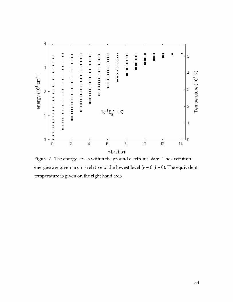
Figure 2. The energy levels within the ground electronic state. The excitation

energies are given in cm-1 relative to the lowest level (v = 0, J = 0). The equivalent

temperature is given on the right hand axis.

33

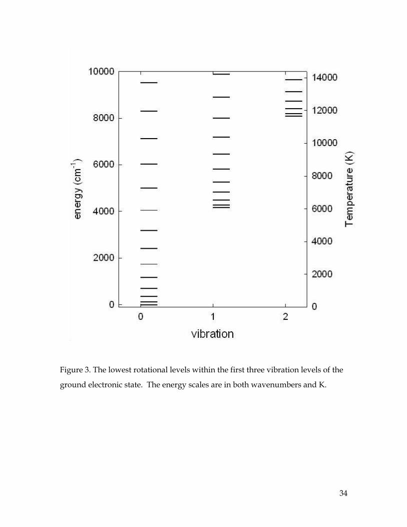
Figure 3. The lowest rotational levels within the first three vibration levels of the

ground electronic state. The energy scales are in both wavenumbers and K.

34

T (K)

100 1000

log

k(J=

5->3

) (cm

3 s-1

)

-20

-18

-16

-14

-12

-10

Figure 4. A comparison between the collision rate coefficients of Martin &

Mandy (1995; 1998; the dashed line) and Le Bourlot et al. (1999; the solid line) for

H + H2(v=0; J=5) => H + H2(v=0; J=3). They differ by large amounts for PDR

temperatures (T < 400 K).

35

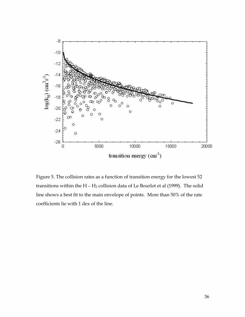
Figure 5. The collision rates as a function of transition energy for the lowest 52

transitions within the H – H2 collision data of Le Bourlot et al (1999). The solid

line shows a best fit to the main envelope of points. More than 50% of the rate

coefficients lie with 1 dex of the line.

36

J

0 5 10 15 20 25 30

N(0

,J)/N

(H2)

1e-11

1e-10

1e-9

1e-8

1e-7

1e-6

1e-5

1e-4

1e-3

1e-2

1e-1

1e+0

1e+1

Figure 6. The level populations for v=0 and T=500 K with and without the g-bar

collisional data. The rotation quantum number J is indicated along the x-axis

while the y-axis gives the populations per H2. The open circles are with the “g-

bar” approximation and the black circles are without. The high J levels are

effectively uncoupled radiatively from the other levels within the X state because

most of the H2 population is in low J levels. Further pumping into the excited

electronic states results mostly in decays back into other low-J levels. The

populations of low J levels, where collision data exist, have very little

dependence on the “g-bar” approximation.

37

wavelength (µm)

1 10

4πj/n

H22 (e

rg c

m3

s-1)

-36

-34

-32

-30

-28

-26

-24

nH = 103 cm-3

nH = 105 cm-3

Figure 7. A spectrum of the collisionally excited H2 gas at 500K with hydrogen

density 103 cm-3 (filled circle) and 105 cm-3 (open triangle).

38

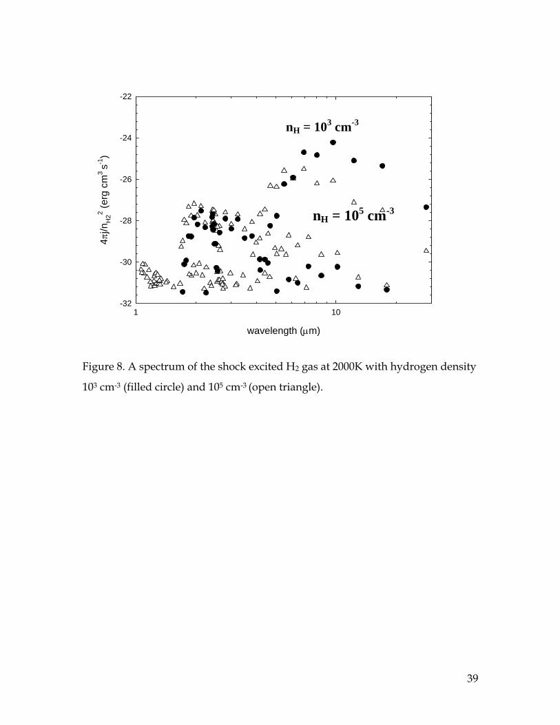
wavelength (µm)

1 10

4πj/n

H22 (e

rg c

m3

s-1)

-32

-30

-28

-26

-24

-22

nH = 105 cm-3

nH = 103 cm-3

Figure 8. A spectrum of the shock excited H2 gas at 2000K with hydrogen density

103 cm-3 (filled circle) and 105 cm-3 (open triangle).

39

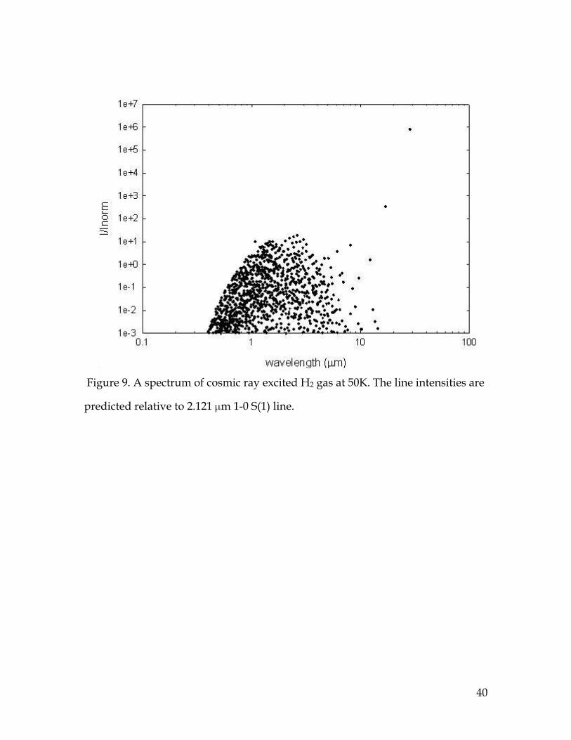
Figure 9. A spectrum of cosmic ray excited H2 gas at 50K. The line intensities are

predicted relative to 2.121 µm 1-0 S(1) line.

40

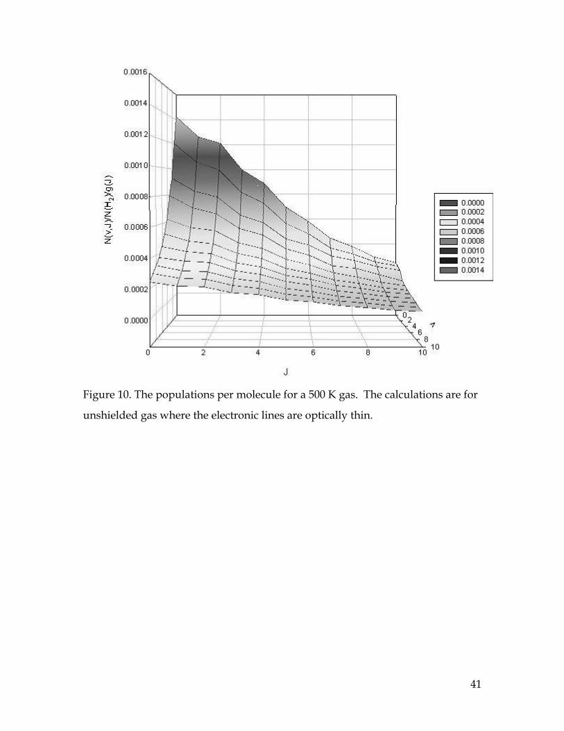
Figure 10. The populations per molecule for a 500 K gas. The calculations are for

unshielded gas where the electronic lines are optically thin.

41

Av

0 2 4 6 8 10

n (c

m-3

)

1e-9

1e-8

1e-7

1e-6

1e-5

1e-4

1e-3

1e-2

1e-1

1e+0

1e+1

1e+2

1e+3

C O C +

C

Figure 11. C (dotted line), C+ (dash-dot line), and CO (solid line) density for the

standard TH85 PDR.

42

Av

0 2 4 6 8 10

n (c

m-3

)

1e-5

1e-4

1e-3

1e-2

1e-1

1e+0

1e+1

1e+2

1e+3

1e+4

1e+5

1e+6

H +

H 2

H

Figure 12. H2(dashed line), H+ (dash-dot line), and H(solid line) density for the

standard TH85 PDR.

43

Av

0 2 4 6 8 10

n (c

m-3

)

0.001

0.01

0.1

1

10

100

1000

Te (K

)

0

50

100

150

200

250

300

350

Te

ne

Figure 13. The electron temperature (solid line) and electron density (dashed

line) from the standard TH85 PDR.

44

Av

0 1 2 3

Hea

ting

(erg

cm

-3 s

-1)

1e-25

1e-24

1e-23

1e-22

1e-21

1e-20

1e-19

1e-18

1e-17

1e-16

Total Heating

Our model

TH85

Figure 14. A comparison of heating due to H2 de-excitation between TH85 and

our model.

45

Figure 15. The grain (distributed in 10 bin sizes) temperature as a function of Av.

46

depth (cm)

1e+13 1e+14 1e+15 1e+16 1e+17

Solo

mon

rate

(s-1

)

1e-19

1e-18

1e-17

1e-16

1e-15

1e-14

1e-13

1e-12

1e-11

1e-10

1e-9

1e-8

1e-7

1e-6

1e-5

1e-4

TH85

BD96 Our model

Figure 16. A comparison of several simple Solomon rates with Solomon rates

from the current micro-physical model of the H2 molecule. The Solid, dashed and

dash-dot-dot lines represent TH85, BD96 and our model respectively.

47

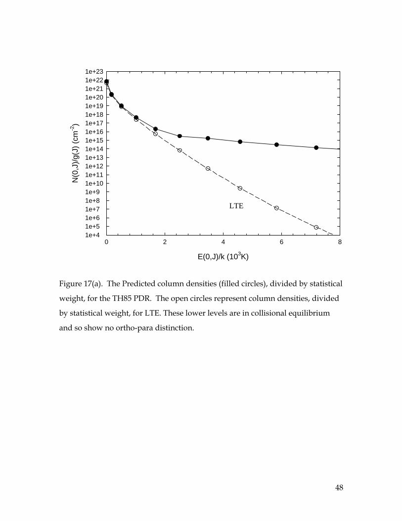
E(0,J)/k (103K)

0 2 4 6 8

N(0

,J)/g

(J) (

cm-2

)

1e+41e+51e+61e+71e+81e+91e+101e+111e+121e+131e+141e+151e+161e+171e+181e+191e+201e+211e+221e+23

LTE

Figure 17(a). The Predicted column densities (filled circles), divided by statistical

weight, for the TH85 PDR. The open circles represent column densities, divided

by statistical weight, for LTE. These lower levels are in collisional equilibrium

and so show no ortho-para distinction.

48

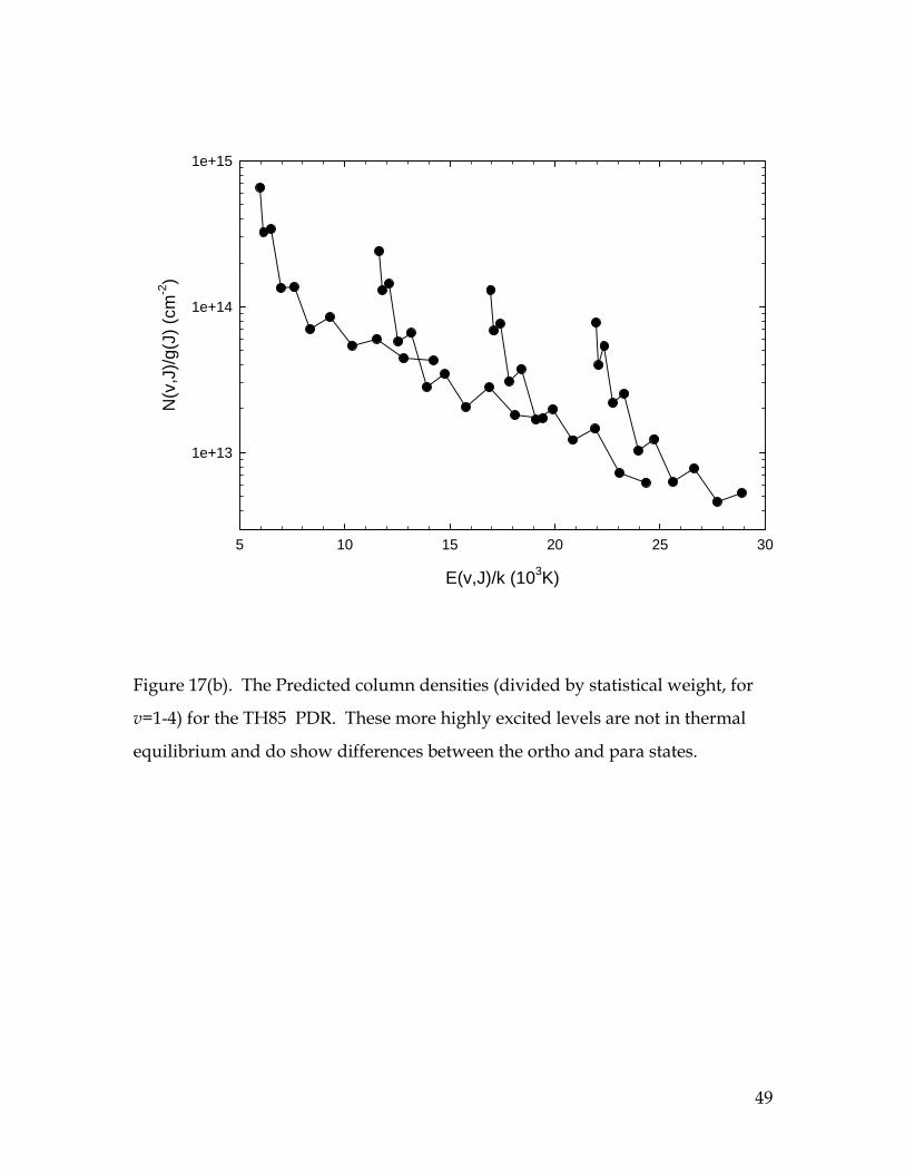
E(v,J)/k (103K)

5 10 15 20 25 30

N(v

,J)/g

(J) (

cm-2

)

1e+13

1e+14

1e+15

Figure 17(b). The Predicted column densities (divided by statistical weight, for

v=1-4) for the TH85 PDR. These more highly excited levels are not in thermal

equilibrium and do show differences between the ortho and para states.

49

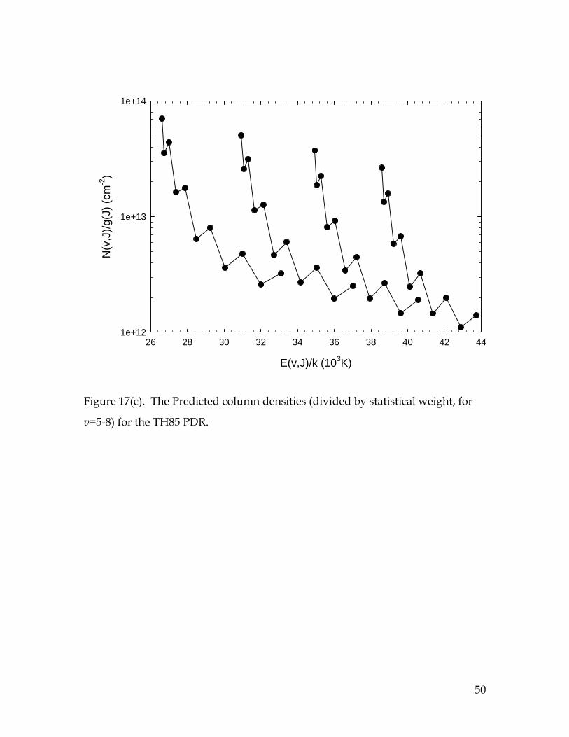
E(v,J)/k (103K)

26 28 30 32 34 36 38 40 42 44

N(v

,J)/g

(J) (

cm-2

)

1e+12

1e+13

1e+14

Figure 17(c). The Predicted column densities (divided by statistical weight, for

v=5-8) for the TH85 PDR.

50

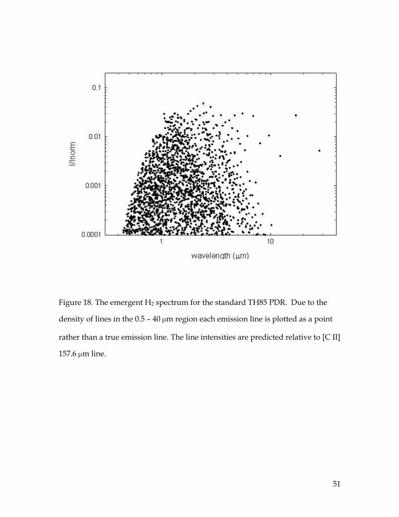
Figure 18. The emergent H2 spectrum for the standard TH85 PDR. Due to the

density of lines in the 0.5 – 40 µm region each emission line is plotted as a point

rather than a true emission line. The line intensities are predicted relative to [C II]

157.6 µm line.

51

Av

0 1 2 3 4

tota

l_or

tho_

to_t

otal

_par

a_ra

tio

0.1

1

10

Figure 19. Ratio of total ortho to total para populations for the standard TH85

PDR.

52

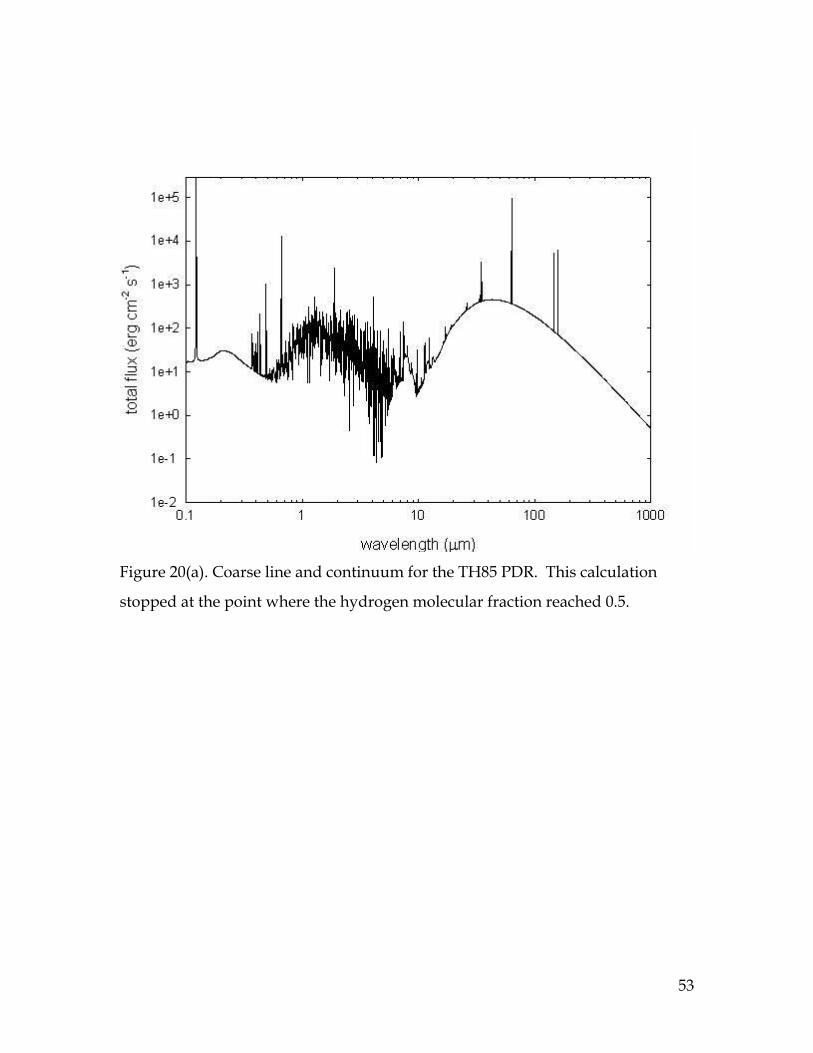
Figure 20(a). Coarse line and continuum for the TH85 PDR. This calculation

stopped at the point where the hydrogen molecular fraction reached 0.5.

53

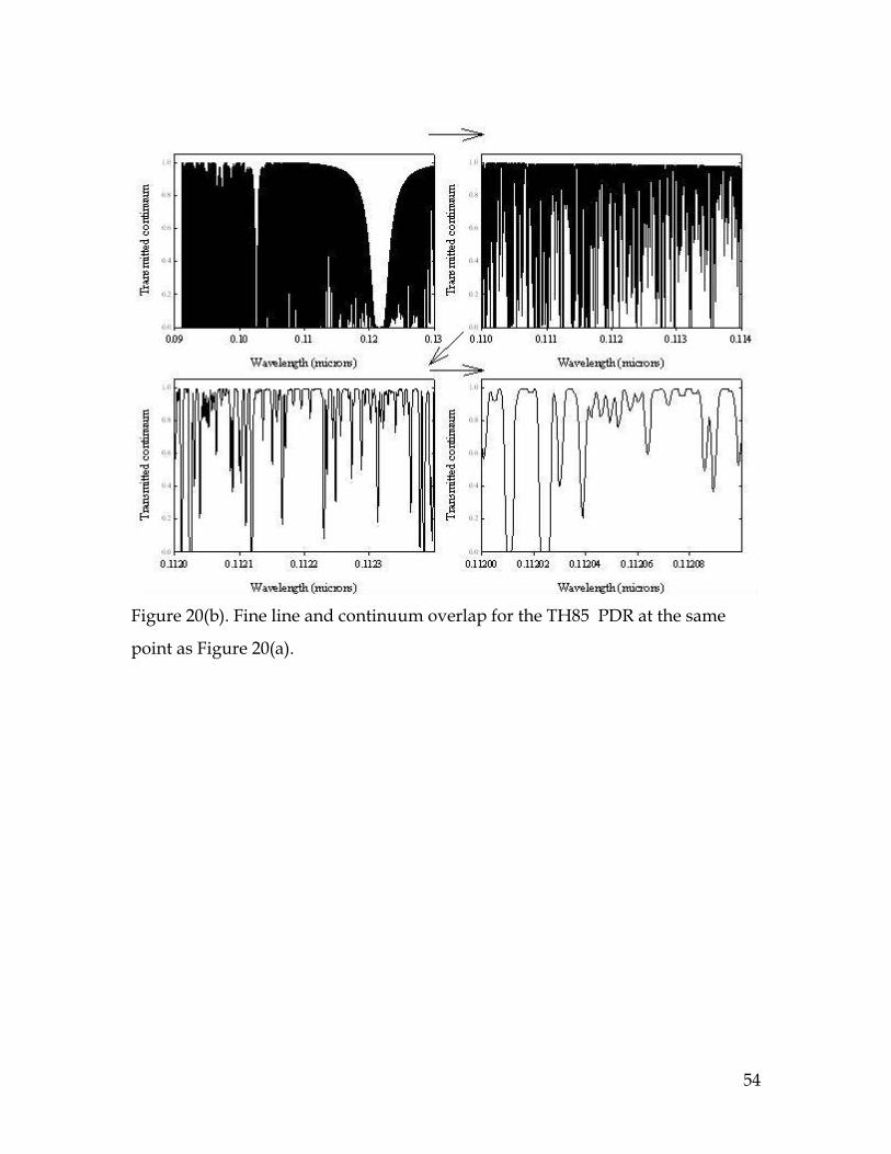
Figure 20(b). Fine line and continuum overlap for the TH85 PDR at the same

point as Figure 20(a).

54

T(K)

0 2000 4000 6000 8000

Frac

tiona

l pop

ulat

ions

at t

he il

lum

inat

ed fa

ce

1e-5

1e-4

1e-3

1e-2

1e-1

1e+0

v = 0

v = 1

Figure 21. Fractional populations at the illuminated face of model F1 of Leiden

PDR workshop (2004). The open circles represent our results. The triangle down,

triangle up and squares represent results of Le Bourlot et al. (1995), Sternberg

(1999), and Black et al. (1987) respectively.

55

T (K)

1000 2000 3000 4000 5000 6000 7000 8000

Col

umn

dens

ity (c

m-2

)

1e+11

1e+12

1e+13

1e+14

1e+15

1e+16

1e+17

1e+18

1e+19

v = 0

v = 1

Figure 22. Integrated column density of model F1 of Leiden PDR workshop

(2004). The open circles represent our results. The triangle down, triangle up and

squares represent results of Le Bourlot et al. (1995), Sternberg (1999), and Black et

al. (1987) respectively.

56

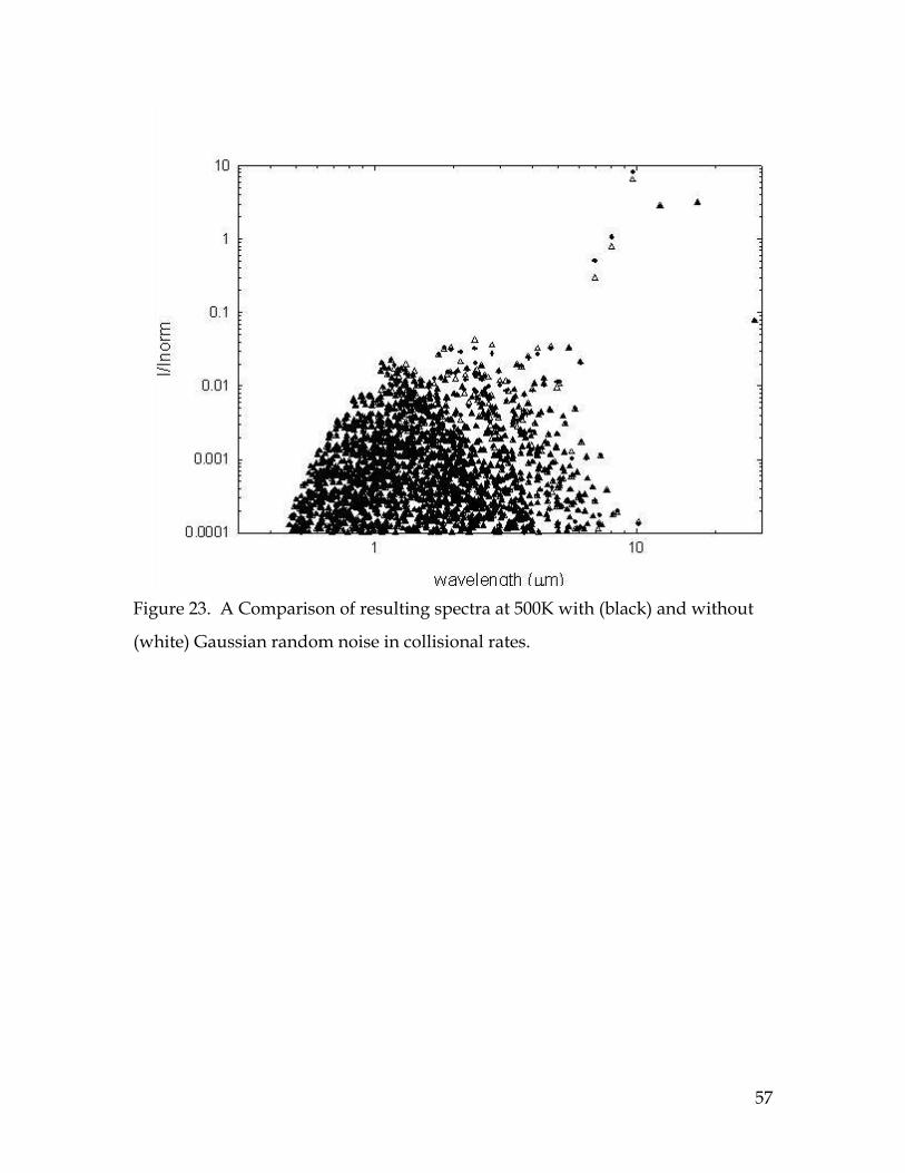
Figure 23. A Comparison of resulting spectra at 500K with (black) and without

(white) Gaussian random noise in collisional rates.

57

J

0 5 10 15 20 25 30

N(0

,J)/N

(H2)

1e-10

1e-9

1e-8

1e-7

1e-6

1e-5

1e-4

1e-3

1e-2

1e-1

1e+0

Figure 24. The level populations for v=0 and T=500 K with and without the

random Gaussian noise in collisional data. The rotation quantum number J is

indicated along the x-axis while the y-axis gives the populations per H2. The

black squares and open circles represent populations with and without noise.

58