Hindawi Publishing CorporationAdvances in MeteorologyVolume 2010, Article ID 707253, 10 pagesdoi:10.1155/2010/707253

Research Article

Evaluation of the WRF Double-Moment 6-Class MicrophysicsScheme for Precipitating Convection

Song-You Hong,1 Kyo-Sun Sunny Lim,1 Yong-Hee Lee,2 Jong-Chul Ha,2 Hyung-Woo Kim,3

Sook-Jeong Ham,3 and Jimy Dudhia4

1 Department of Atmospheric Sciences and Global Environment Laboratory, Yonsei University, Seoul 120-749, Republic of Korea2 Forecast Research Laboratory, National Institute of Meteorological Research, Korea Meteorological Administration,Seoul 156-010, Republic of Korea

3 73rd Weather Group, Korea Air Force, Chungnam 321-923, Republic of Korea4 Mesoscale and Microscale Meteorology Division, National Center for Atmospheric Research, Boulder, CO 80305, USA

Correspondence should be addressed to Song-You Hong, shong@yonsei.ac.kr

Received 24 December 2009; Revised 23 February 2010; Accepted 8 April 2010

Academic Editor: Zhaoxia Pu

Copyright © 2010 Song-You Hong et al. This is an open access article distributed under the Creative Commons AttributionLicense, which permits unrestricted use, distribution, and reproduction in any medium, provided the original work is properlycited.

This study demonstrates the characteristics of the Weather Research and Forecasting (WRF) Double-Moment 6-Class (WDM6)Microphysics scheme for representing precipitating moist convection in 3D platforms, relative to the WSM6 scheme that has beenwidely used in the WRF community. For a case study of convective system over the Great Plains, the WDM6 scheme improvesthe evolutionary features such as the bow-type echo in the leading edge of the squall line. We also found that the WRF withWDM6 scheme removes spurious oceanic rainfall that is a systematic defect resulting from the use of the WSM6 scheme alone.The simulated summer monsoon rainfall in East Asia is improved by weakening (strengthening) light (heavy) precipitation activity.These changes can be explained by the fact that the WDM6 scheme has a wider range in cloud and rain number concentrationsthan does the WSM6 scheme.

1. Introduction

The Weather Research and Forecasting (WRF) model [1] isa community numerical weather prediction (NWP) modelthat is applicable to various scales of weather phenomena.Application of the WRF model has recently been extendedto resolving regional details embedded within climate sig-nals from the general circulation model [2]. As computerresources become available, the use of high-resolution WRFwith a horizontal grid spacing of less than 5 km willimprove forecasts for convective-scale phenomena, includingexplicit information about the timing, intensity, and modeof convection (e.g., [3, 4]). These previous reports demon-strate a 4-km resolution in WRF forecasts, which explicitlyresolves convection yields for better guidance in precipitationforecasts, in comparison to 12-km resolution. Microphysicalschemes are explicit, whereas convective parameterizationsare implicit. As grid spacings decrease, convective param-eterizations become more inappropriate (and scientifically

questionable given the underlying assumptions), whereasthe explicit representation of microphysical processes canbe computed for increasingly small clouds, cloud particles,water droplets, and so forth.

In the WRF model, there are multiple choices for eachphysical component; for example, there are ten algorithmsfor the cloud microphysics scheme, as of August 2009.Among the microphysics packages for clouds and precipita-tion, the series of the WRF single-moment (WSM) schemes(WSM3, WSM5, and WSM6 [5, 6]) has been widely used.As of June 2009, there are about 50 institutions across theglobe running the WRF model on a real-time basis, andmany of these institutions chose the WSM scheme for themicrophysics option. As an example, the WRF model withthe WSM6 microphysics has provided useful information onhigh-resolution weather phenomena over the Great Plains inthe US [7, 8]. The Korean Meteorological Administration(KMA) and Korean Air Force (KAF) have also chosen theWSM6 scheme for real-time forecasts over East Asia, as noted

2 Advances in Meteorology

by Ha et al. [9] and Byun et al. [10]. There are numerousreports evaluating the performance of the WRF with WSMmicrophysics on various weather phenomena, including overthe US [11], for a hurricane over the Atlantic [12], heavyrainfall over East Asia [13] and polar weather [14]. Huang etal. [15] used the WSM5 scheme to develop an advanced dataassimilation system. Otkin and Greenwald [16] evaluated theWSM6 scheme using the MODIS-derived cloud data.

These studies demonstrated that the WSM schemes arecompetitive options in WRF by reproducing precipitatingconvection and associated meteorological phenomena. How-ever, some systematic deficiencies have been reported, suchas too much light precipitation activity [17] and an excessiveamount of graupel, as compared to snow [18]. Spurious lightprecipitation was a systematic problem in the KMA forecastsystems, as noted by Jo et al. [19]. A further revision tothe WSM6 scheme employing a combined sedimentationvelocity for graupel and snow [20] helped to alleviate theproblem of excessive graupel, but weak radar reflectivityremained a systematic problem (personal communicationwith J. Kain).

The WRF Double-Moment 6-class (WDM6) scheme[21] was announced to the WRF community in April2009. The WDM6 scheme enables the investigation of theaerosol effects on cloud properties and precipitation pro-cesses with the prognostic variables of cloud condensationnuclei (CCN), cloud water and rain number concentrations.The WDM6 scheme has been evaluated on an idealizedtwo-dimensional thunderstorm testbed [21], but its overallcharacteristics relative to the WSM6 scheme for 3D realcases has not been provided. For these reasons, it is crucialto provide physical reasons for the differences in simulatedprecipitation and clouds between the WDM6 and WSM6schemes.

A squall-line case over the Great Plains in the US willbe simulated with both WSM6 and WDM6 microphysicsschemes. In Lim and Hong [21], the fundaments in theWDM6 were described in detail, but the differences inthe simulated convection were demonstrated only for anidealized 2D storm. The purpose of a specific squall-linesimulation is to evaluate the basic differences in convectiveactivities between the WSM6 and WDM6 schemes in areal 3D model framework, prior to a robust evaluation ofthe hydrometeors and investigation studies on associateddynamics. Experimental evaluations of the WDM6 schemeover the WSM6 scheme at a real-time forecast platform atKMA have not shown distinct discrepancy in the predictedprecipitation, but at times there have been cases thatthe WDM6 scheme is superior to the WSM6 scheme. Areduction of spurious precipitation in the case of the WSM6scheme was systematically alleviated by the WDM6 scheme.We will demonstrate a mid-latitude cyclogenesis in East Asiaas an example. As another evaluation tool, a regional climatemodeling approach is adapted to examine the characteristicsof a summer monsoon precipitation in East Asia. Wefocus on differences in the simulated precipitation with apossible physical reasoning on the fundamental differencesin microphysics between the WSM6 and WDM6 schemes.The causes for the different model performances in the

underlying assumptions of WSM6 and WDM6 schemes willbe investigated. In addition, a statistical measure of skill inprecipitation forecasts over South Korea in summer 2008 willbe shown in the final section.

2. Model Setup

2.1. Overview of the WDM6 Scheme. Prognostic watersubstance variables include water vapor, clouds, rain, ice,snow, and graupel for both the WDM6 [21] and WSM6[5] schemes. Additionally, the prognostic number con-centrations of cloud and rain waters, together with theCCN, are considered in the WDM6 scheme. The numberconcentrations of ice species such as graupel, snow, andice are diagnosed following the ice-phase microphysics ofHong et al. [6]. This simplicity is theoretically based onthe fact that the prediction of ice-phase number concentra-tions has significantly less impact on the results than theprediction of warm-phase concentrations in deep convectivecases [22]. The activated CCN number concentration ispredicted and formulated using the drop activation processbased on Twomey’s relationship between the number ofactivated CCN and supersaturation [23, 24], which enablesa level of complexity to be added to the traditional bulkmicrophysics schemes through the explicit CCN-cloud dropconcentration feedback. The complete evaporation of clouddrops is assumed to return corresponding CCN particles tothe total CCN count. The CCN number concentration canbe regulated under the forced large-scale environment, evenfor the seasonal climate cases. Any other CCN sink/sourceterms, except for CCN activation and droplet evaporation,are ignored in the WDM6 scheme. Further details on theCCN activation process are described in appendix A ofLim and Hong [21]. Accurate 3D CCN information is animportant aspect of model simulations. However, obtainingreal-time CCN information in both the horizontal andvertical directions is difficult. Thus, we chose an initial valueof 100 cm−3for the CCN number concentration in this study,as in Lim and Hong [21].

The formulation of warm-rain processes such as auto-conversion and accretion in the WDM6 scheme is basedon the studies of Cohard and Pinty [25]. For other sourceand sink terms in warm-rain processes, the formulas in theWSM6 scheme were adopted. However, the microphysicsprocesses in the WDM6 scheme, even if the same formulais applied, work differently from those in the WSM6scheme due to the predicted number concentrations of cloudwater and rain, which in turn indirectly influence the iceprocesses. Lim and Hong [21] demonstrated that, comparedto the simulation of an idealized 2D thunderstorm withthe WSM6 scheme, the higher drop concentrations in theconvective core versus lower drop concentrations in thestratiform region are distinct in the WDM6. A markedradar bright band near the freezing level was produced withthe WDM6 microphysics scheme. Meanwhile, the WSM6scheme extended strong reflectivity to the ground level overthe stratiform region. The aerosol effects on the cloud/rainproperties and surface precipitation were also investigated by

Advances in Meteorology 3

varying the initial CCN number concentration. Varying theCCN number concentration had a nonmonotonic impact onrainfall amount.

2.2. Experimental Setup. The model used in this study isthe Advanced Research WRF version 3.1 [1]. The physicspackages, other than the microphysics, included the Kain-Fritsch cumulus parameterization scheme [26], the unifiedNoah land-surface model [27], a simple cloud-interactiveshortwave radiation scheme [28], the Rapid Radiative Trans-fer Model (RRTM) longwave radiation scheme [29], and theYonsei University planetary boundary layer (PBL) scheme,for vertical diffusion [30]. The PBL scheme was replacedwith the Mellor-Yamada-Janjic (MYJ) scheme [31, 32] for thesquall line case over US. The MYJ scheme has been widelyevaluated for convective systems over the Great Plains in theUS (e.g., [3, 4]).

The model configuration consisted of a nested domaindefined on a Lambert conformal projection for all theselected cases. For a squall-line case over the US Great Plains,we followed the same model configuration of Shi et al. [17].They investigated the impact of microphysical schemes onthe IHOP 2002 case. From the comparison between theresults from this study and those from Shi et al. [17], wecan easily examine the advantage of the WDM6 scheme. A1-km model covering Oklahoma (Domain 3, 540 × 465)was surrounded by a 3-km grid model (Domain 2, 480× 351), which in turn was nested by a 9-km grid model(Domain 1, 300 × 201) using a two-way interaction. Modelintegration was conducted during a 36-hour period, from0000 UTC June 12 to 1200 UTC June 13, 2002. The cumulusparameterization was applied, except for the 1-km and 3-km grid models for this case. A 30-km model covered theEast Asia region (199 × 189) for a mid-latitude cyclogenesiscase. This model configuration is identical to the model setupfor operational forecasts at KMA, as of summer 2008. Theexperiments were performed for 36 hours, from 0000 UTCFebruary 23 to 1200 UTC February 24, 2008. For a summermonsoon case in East Asia, a 50-km WRF was nested usinganalyzed data from the month of July 2006. The domaincovers the East Asian monsoon regions (109 × 86) centeredover the Korean peninsula. This configuration is identical tothe model setup for several regional climate studies over EastAsia (e.g., [33]). Koo and Hong [33] demonstrated that theWRF model is capable of reproducing the climatology andprecipitation embedded within the summer monsoon overEast Asia with the same model configuration of this study.The whole grid systems had 27 vertical layers, and the modeltop was located at 10 hPa for all the simulated cases. Initialand boundary conditions were generated by the NationalCenters for Environmental Prediction (NCEP)-Final Analy-sis (FNL) data on 1◦×1◦ global grids, every six hours.

The Tropical Rainfall Measuring Mission (TRMM)TRMM Multisatellite Precipitation Analysis (TMPA; [34])data on a 0.25◦ × 0.25◦ were used for an evaluation of thesimulated precipitation. In addition, simulated reflectivitieswere verified against observed ones, which were obtainedfrom the WSI IHOP Sector Mosaic Reflectivity Imagery

(2-km) provided by the NCAR/EOL across the United States[35, 36] for the squall-line case.

3. Results and Discussion

3.1. Squall Line Case over the US Great Plains. Thompson etal. [37] and Weisman et al. [38] recognized that the WSM6scheme tends to produce isolated intense convective corescompared to other schemes, such as that of Thompson [39].This defect in the WSM6 scheme often failed to produceradar reflectivity and the associated mesoscale features ofsquall lines. The International H2O project (IHOP 2002) wasconducted over southern Kansas, Oklahoma, and northernTexas for six weeks during May and June of 2002 (13 May to25 June 2002). A detailed summary of the physical processes(i.e., mesoscale convergence lines and gust fronts) associatedwith convective storm initiation and evolution for IHOPcases can be found in Wilson and Roberts [40].

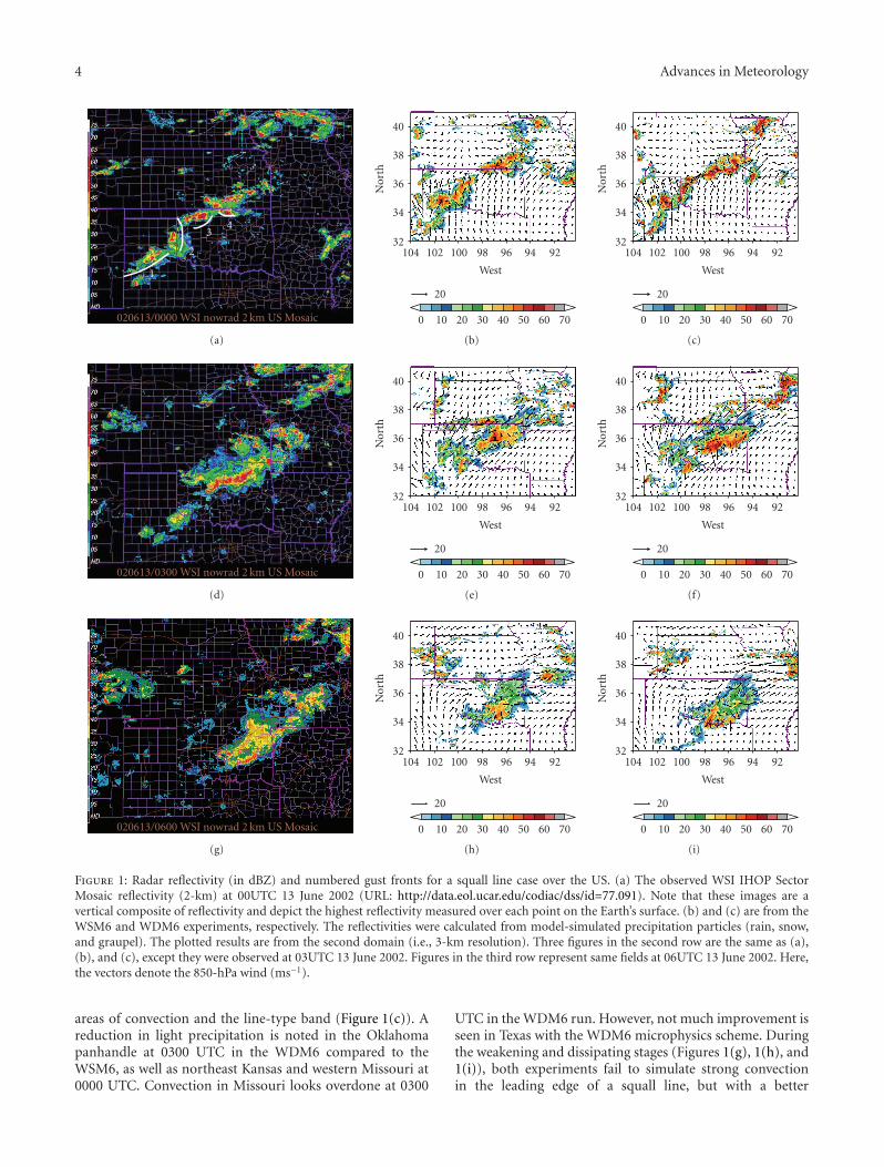
Figure 1 compares the radar reflectivity and numberedgust fronts associated with a squall line that developed on12 June in Kansas and moved southeastward. The WRF wasinitialized at 00 UTC 12 June 2002, and the simulation resultsat the 24-hr, 27-hr, and 30-hr forecast times are shown. Here,we focus on the evolutionary feature of the squall line passedOklahoma between 0000 UTC 13 June and 0600 UTC 13June, which can be evaluated though the comparisons withthe available observations.

The observed data at 00 UTC 13 (Figure 1(a)) exhibitsa line type convection core stretching from the Texaspanhandle northeastward to the border between Kansas andOklahoma. Wilson and Roberts [40] demonstrated that gustfronts 3 and 4 initiate many more storms than gust fronts 1or 2. With time gust fronts 3 and 4 merge and a continuoussquall line results in Figure 1(d). The storms associated withgust front 2 soon die, as does the gust front. The stormsassociated with gust front 1 live longer but never organizeinto a significant squall line. They also discovered that themost important factor for storm initiation and longevity isthe gust front differential wind velocity. Generally, upwardmotion beginning in the boundary layer near the gust frontextends up through the convective region, and slops moregently into the base of the trailing stratiform cloud. Thisdescending current passes through the melting level, andfinally enters the back of the convective region at low levelswhere it reinforces convergence at the leading gust front.Thus, the near-surface wind, normal to gust fronts, canenhance the convergence and organize a strong squall line.

The WSM6 run shows ambiguous separation of the twostorms associated with gust fronts 3 and 4, showing largerconvective areas than the observed areas data at 00 UTC 13(Figure 1(b)). These storms do not develop into a continuoussquall line after 3 hours. The storms associated with gustfronts 3 and 4 are well organized in the WDM6 run. After3 hours, these storms are combined and the squall linetraveled southeastward in central Oklahoma. However, thestrength of reflectivity from the WDM6 run is systematicallyhigher in a broad region compared to the WSM6 run andobservations. In addition, the WDM6 run shows narrowed

4 Advances in Meteorology

020613/0000 WSI nowrad 2 km US Mosaic

1

2

34

(a)

0 10 20 30 40 50 60 70

20

104 102 100 98 96 94 92

West

32

34

36

38

40

Nor

th

(b)

0 10 20 30 40 50 60 70

20

104 102 100 98 96 94 92

West

32

34

36

38

40

Nor

th

(c)

020613/0300 WSI nowrad 2 km US Mosaic

(d)

0 10 20 30 40 50 60 70

20

104 102 100 98 96 94 92

West

32

34

36

38

40N

orth

(e)

0 10 20 30 40 50 60 70

20

104 102 100 98 96 94 92

West

32

34

36

38

40

Nor

th(f)

020613/0600 WSI nowrad 2 km US Mosaic

(g)

0 10 20 30 40 50 60 70

20

104 102 100 98 96 94 92

West

32

34

36

38

40

Nor

th

(h)

0 10 20 30 40 50 60 70

20

104 102 100 98 96 94 92

West

32

34

36

38

40

Nor

th

(i)

Figure 1: Radar reflectivity (in dBZ) and numbered gust fronts for a squall line case over the US. (a) The observed WSI IHOP SectorMosaic reflectivity (2-km) at 00UTC 13 June 2002 (URL: http://data.eol.ucar.edu/codiac/dss/id=77.091). Note that these images are avertical composite of reflectivity and depict the highest reflectivity measured over each point on the Earth’s surface. (b) and (c) are from theWSM6 and WDM6 experiments, respectively. The reflectivities were calculated from model-simulated precipitation particles (rain, snow,and graupel). The plotted results are from the second domain (i.e., 3-km resolution). Three figures in the second row are the same as (a),(b), and (c), except they were observed at 03UTC 13 June 2002. Figures in the third row represent same fields at 06UTC 13 June 2002. Here,the vectors denote the 850-hPa wind (ms−1).

areas of convection and the line-type band (Figure 1(c)). Areduction in light precipitation is noted in the Oklahomapanhandle at 0300 UTC in the WDM6 compared to theWSM6, as well as northeast Kansas and western Missouri at0000 UTC. Convection in Missouri looks overdone at 0300

UTC in the WDM6 run. However, not much improvement isseen in Texas with the WDM6 microphysics scheme. Duringthe weakening and dissipating stages (Figures 1(g), 1(h), and1(i)), both experiments fail to simulate strong convectionin the leading edge of a squall line, but with a better

Advances in Meteorology 5

10121020

1016

1008

1012

1024

1020

1016

1028

1032

10121032

1028 1032

1028

1032

1036

1040

10161020

1024

1008

1012

1004

1000996

992

980

98

99298

0.15 1 5 10 20

B

A

(a)

10

1012

12

1024

10041000

996

1024

1012

1012

1016

1020

1024

1016

1012

1028

1016

1012

1032

1028

1024

1028

1024

10161020

1024

1032

1036

1032

1028

1032

1024

1028

10281024

1020

1020

1020

1016

1012

992988984

984980

9921036

1028

1032

0.15 1 5 10 20

(b)

1020

1012

1032

1024

10041000996

1024

1016

10121016

1012

1016

1020

1024

1016

1012

102810161012

1032

10281024

10281024

10161020

1024

1032

1036

1032

10281032

1024

1028

1028 10241020

1020

1020

10161012

992988

984

984980

9921036

1028

2

1028

0.15 1 5 10 20

(c)

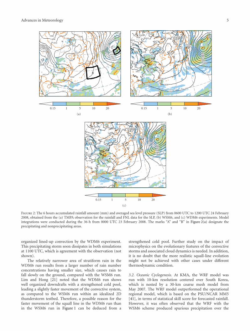
Figure 2: The 6 hours accumulated rainfall amount (mm) and averaged sea level pressure (SLP) from 0600 UTC to 1200 UTC 24 February2008, obtained from the (a) TMPA observation for the rainfall and FNL data for the SLP, (b) WSM6, and (c) WDM6 experiments. Modelintegrations were conducted during the 36-h from 0000 UTC 23 February 2008. The marks “A” and “B” in Figure 2(a) designate theprecipitating and nonprecipitating areas.

organized lined-up convection by the WDM6 experiment.This precipitating storm soon dissipates in both simulationsat 1100 UTC, which is agreement with the observation (notshown).

The relatively narrower area of stratiform rain in theWDM6 run results from a larger number of rain numberconcentrations having smaller size, which causes rain tofall slowly on the ground, compared with the WSM6 run.Lim and Hong [21] noted that the WDM6 run showswell organized downdrafts with a strengthened cold pool,leading a slightly faster movement of the convective system,as compared to the WSM6 run within an idealized 2Dthunderstorm testbed. Therefore, a possible reason for thefaster movement of the squall line in the WDM6 run thanin the WSM6 run in Figure 1 can be deduced from a

strengthened cold pool. Further study on the impact ofmicrophysics on the evolutionary features of the convectivestorms and associated cloud dynamics is needed. In addition,it is no doubt that the more realistic squall-line evolutionmight not be achieved with other cases under differentthermodynamic condition.

3.2. Oceanic Cyclogenesis. At KMA, the WRF model wasrun with 10-km resolution centered over South Korea,which is nested by a 30-km coarse mesh model fromMay 2007. The WRF model outperformed the operationalregional model, which is based on the PSU/NCAR MM5[41], in terms of statistical skill score for forecasted rainfall.However, it was often observed that the WRF with theWSM6 scheme produced spurious precipitation over the

6 Advances in Meteorology

1000

900

800

700

600

Pre

ssu

re(m

b)

0 5 10 15 20 25

NC (cm−3)

(a)

1000

900

800

700

600

Pre

ssu

re(m

b)

0 2e+4 4e+4 6e+4 8e+4 1e+5

NR (m−3)

(b)

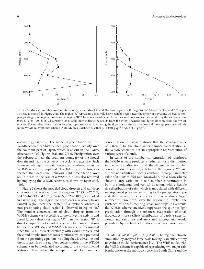
Figure 3: Modeled number concentrations of (a) cloud droplets and (b) raindrops over the regions “A” (closed circles) and “B” (opencircles), as marked in Figure 2(a). The region “A” represents a relatively heavy rainfall region near the center of a cyclone, whereas a non-precipitating cloud region is observed in region “B.” The values are obtained from the cloud area averaged values during the six hours from0600 UTC to 1200 UTC 24 February 2008. Solid lines indicate the results from the WDM6 scheme and dotted lines are from the WSM6scheme. The number concentration for raindrops can be calculated using the slope of rain size distribution and intercept parameter of rainin the WSM6 microphysics scheme. A cloudy area is defined as either qC > 0.01 g kg−1 or qR > 0.01 g kg−1.

oceans (e.g., Figure 2). The modeled precipitation with theWSM6 scheme exhibits banded precipitation activity overthe southern part of Japan, which is absent in the TMPAobservation (cf. Figures 2(a) and 2(b)). Precipitation overthe subtropics near the southern boundary of the modeldomain and near the center of the cyclone is excessive. Suchan excessively light precipitation is greatly reduced when theWDM6 scheme is employed. The KAF real-time forecastsverified that occasional spurious light precipitation overSouth Korea in the case of a WSM6 run was also removedby employing the WDM6 scheme, as shown by Byun et al.[10].

Figure 3 shows the modeled cloud droplets and raindropconcentrations averaged over the regions “A” (34◦–37.5◦N,154.5◦–160◦E) and “B” (26◦–32◦N, 132◦–140◦E), as markedin Figure 2(a). The region “A” represents a relatively heavyrainfall region near the center of a cyclone, whereas anon-precipitating cloud region is observed in region “B.”The number concentrations of cloud droplets from theWDM6 scheme vary according to the convective activity andreveal larger values over region “A” than over region “B”. Adirect comparison of cloud droplet number concentrationsbetween the WDM6 and WSM6 schemes is less meaningfulsince the CCN interacts explicitly with cloud droplets, andthe cloud droplet number concentrations, which is predictedfrom the governing equation including the 3D advection andthe source/sink of the number concentration in the WDM6scheme, can be modulated according to the environmentalfeatures. Nevertheless, the comparison of cloud number

concentration in Figure 3 shows that the constant valueof 300 cm−3 for the cloud water number concentration inthe WSM6 scheme is not an appropriate representation ofvarious types of clouds.

In terms of the number concentration of raindrops,the WSM6 scheme produces a rather uniform distributionin the vertical direction, and the differences in numberconcentration of raindrops between the regions “A” and“B” are not significant, with a constant intercept parametervalue of 8× 106 m−4for rain. Meanwhile, the WDM6 schemeshows a large variation in rain number concentration inboth the horizontal and vertical directions with a flexiblesize distribution of rain, which is modulated with differentmicrophysical processes according to the precipitation typeand the characteristics of convection. A relatively largernumber of rain drops over the region “B” implies theexistence of nonsedimenting small raindrops. As a result,the WDM6 scheme effectively suppresses the spurious lightprecipitation through the enhanced evaporation of smalldroplets. A more realistic distribution of particle sizes forclouds and raindrops and associated microphysics wouldprovide a physical feedback to the convective environment.

3.3. Monsoonal Rainfall in July 2006. The regional climatesimulation by analyzed large-scale forcing is an efficient wayto evaluate model performance [42]. The WRF model withthe WSM6 scheme is capable of reproducing two major rainbands, one over the subtropics covering South China and the

Advances in Meteorology 7

50 150 250 350 450 550 650 750

(a)

50 150 250 350 450 550 650 750

(b)

50 150 250 350 450 550 650 750

(c)

−800

−400

−200

−100 −5

0 50 100

200

400

800

(d)

−800

−400

−200

−100 −5

0 50 100

200

400

800

(e)

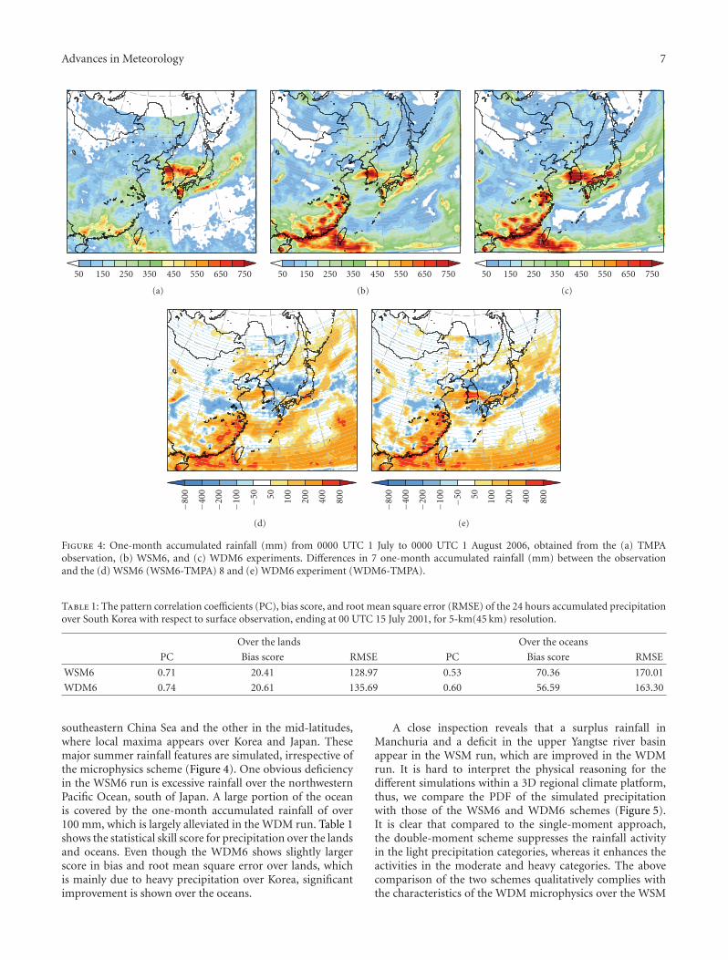
Figure 4: One-month accumulated rainfall (mm) from 0000 UTC 1 July to 0000 UTC 1 August 2006, obtained from the (a) TMPAobservation, (b) WSM6, and (c) WDM6 experiments. Differences in 7 one-month accumulated rainfall (mm) between the observationand the (d) WSM6 (WSM6-TMPA) 8 and (e) WDM6 experiment (WDM6-TMPA).

Table 1: The pattern correlation coefficients (PC), bias score, and root mean square error (RMSE) of the 24 hours accumulated precipitationover South Korea with respect to surface observation, ending at 00 UTC 15 July 2001, for 5-km(45 km) resolution.

Over the lands Over the oceans

PC Bias score RMSE PC Bias score RMSE

WSM6 0.71 20.41 128.97 0.53 70.36 170.01

WDM6 0.74 20.61 135.69 0.60 56.59 163.30

southeastern China Sea and the other in the mid-latitudes,where local maxima appears over Korea and Japan. Thesemajor summer rainfall features are simulated, irrespective ofthe microphysics scheme (Figure 4). One obvious deficiencyin the WSM6 run is excessive rainfall over the northwesternPacific Ocean, south of Japan. A large portion of the oceanis covered by the one-month accumulated rainfall of over100 mm, which is largely alleviated in the WDM run. Table 1shows the statistical skill score for precipitation over the landsand oceans. Even though the WDM6 shows slightly largerscore in bias and root mean square error over lands, whichis mainly due to heavy precipitation over Korea, significantimprovement is shown over the oceans.

A close inspection reveals that a surplus rainfall inManchuria and a deficit in the upper Yangtse river basinappear in the WSM run, which are improved in the WDMrun. It is hard to interpret the physical reasoning for thedifferent simulations within a 3D regional climate platform,thus, we compare the PDF of the simulated precipitationwith those of the WSM6 and WDM6 schemes (Figure 5).It is clear that compared to the single-moment approach,the double-moment scheme suppresses the rainfall activityin the light precipitation categories, whereas it enhances theactivities in the moderate and heavy categories. The abovecomparison of the two schemes qualitatively complies withthe characteristics of the WDM microphysics over the WSM

8 Advances in Meteorology

0.01

0.1

1

10

70

80

PD

F(%

)

0.1 4 8 16 24 32 40 48∼ 4 ∼ 8 ∼ 16 ∼ 24 ∼ 32 ∼ 40 ∼ 48 ∼

Intensity (mm/1hour)TMPAWDMWSM

Figure 5: Probability Distribution Function (PDF) of three-houraccumulated rainfall intensity from the TMPA observations, andthe corresponding results from the WDM6 and WSM6 experimentsover the whole domain during the one month from 0000 UTC 1July to 0000 UTC 1 August 2006.

algorithm in the 2D squall line case study of Lim and Hong[21], in that the WDM6 was responsible for the light (heavy)precipitation suppression (enhancement).

4. Concluding Remarks

The WRF model sensitivity to microphysical parameteriza-tion was analyzed from the WSM6 to the WDM6 schemefor the selected 3D test platforms. The case study for a squallline over the US Great Plains showed that the traveling speedof the simulated squall line is faster with the higher radarreflectivity when the double-moment scheme is used. It alsoappears that the double-moment approach of the WDM6scheme tends to resolve known systematic deficiencies inthe corresponding single-moment approach of the WSM6scheme. The WDM6 run suppressed spurious light precip-itation over the oceans. The simulated monsoonal summerrainfall climate over East Asia was improved by suppressingthe light precipitation and enhancing the heavy precipitation.

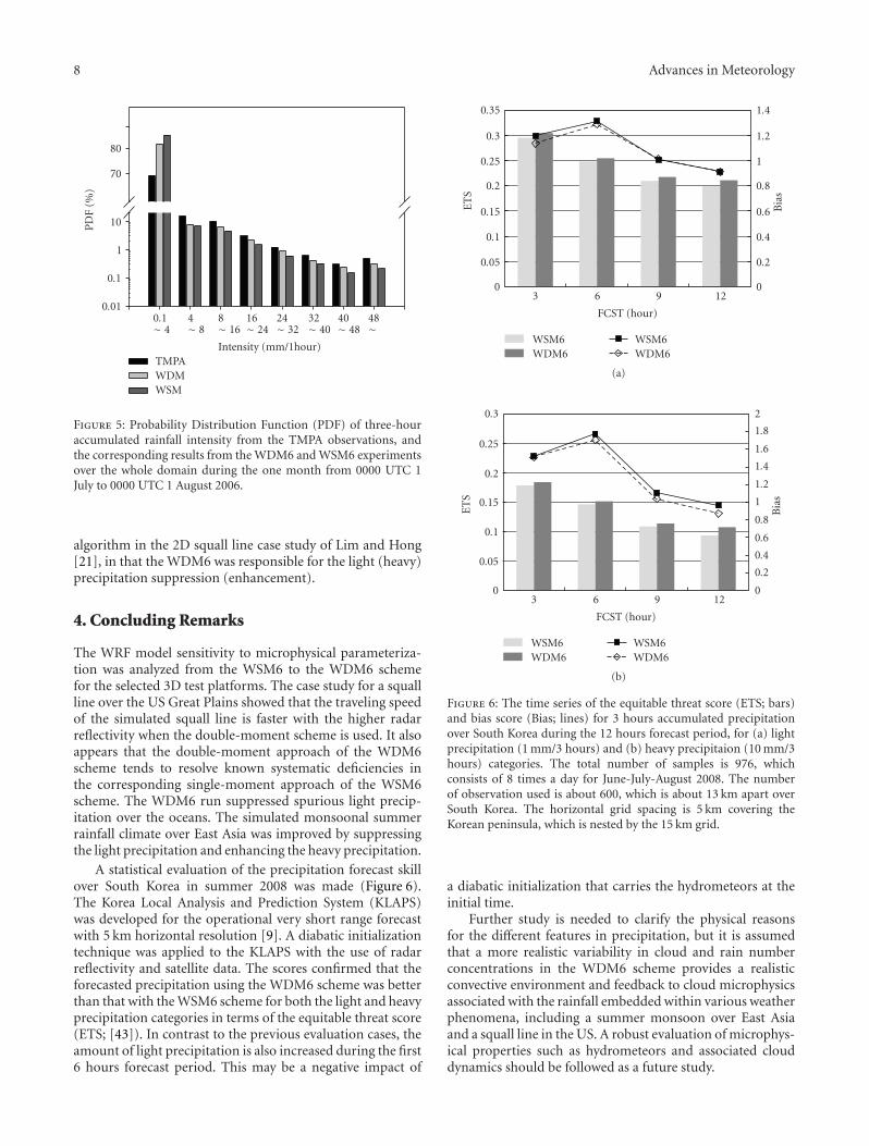
A statistical evaluation of the precipitation forecast skillover South Korea in summer 2008 was made (Figure 6).The Korea Local Analysis and Prediction System (KLAPS)was developed for the operational very short range forecastwith 5 km horizontal resolution [9]. A diabatic initializationtechnique was applied to the KLAPS with the use of radarreflectivity and satellite data. The scores confirmed that theforecasted precipitation using the WDM6 scheme was betterthan that with the WSM6 scheme for both the light and heavyprecipitation categories in terms of the equitable threat score(ETS; [43]). In contrast to the previous evaluation cases, theamount of light precipitation is also increased during the first6 hours forecast period. This may be a negative impact of

0

0.05

0.1

0.15

0.2

0.25

0.3

0.35

ET

S

0

0.2

0.4

0.6

0.8

1

1.2

1.4

Bia

s

3 6 9 12

FCST (hour)

WSM6WDM6

WSM6WDM6

(a)

0

0.05

0.1

0.15

0.2

0.25

0.3

ET

S

0

0.2

0.4

0.6

0.8

1

1.2

1.4

1.6

1.8

2

Bia

s

3 6 9 12

FCST (hour)

WSM6WDM6

WSM6WDM6

(b)

Figure 6: The time series of the equitable threat score (ETS; bars)and bias score (Bias; lines) for 3 hours accumulated precipitationover South Korea during the 12 hours forecast period, for (a) lightprecipitation (1 mm/3 hours) and (b) heavy precipitaion (10 mm/3hours) categories. The total number of samples is 976, whichconsists of 8 times a day for June-July-August 2008. The numberof observation used is about 600, which is about 13 km apart overSouth Korea. The horizontal grid spacing is 5 km covering theKorean peninsula, which is nested by the 15 km grid.

a diabatic initialization that carries the hydrometeors at theinitial time.

Further study is needed to clarify the physical reasonsfor the different features in precipitation, but it is assumedthat a more realistic variability in cloud and rain numberconcentrations in the WDM6 scheme provides a realisticconvective environment and feedback to cloud microphysicsassociated with the rainfall embedded within various weatherphenomena, including a summer monsoon over East Asiaand a squall line in the US. A robust evaluation of microphys-ical properties such as hydrometeors and associated clouddynamics should be followed as a future study.

Advances in Meteorology 9

Acknowledgments

This research was supported by the Basic Science ResearchProgram through the National Research Foundation of Korea(NRF) funded by the Ministry of Education, Science andTechnology (2010-0000840), by the Korean Foundation forInternational Cooperation Science & Technology (KICOS)through a grant provided by the Korean Ministry ofScience & Technology (MOST) in 2009, by the project,“Development of the numerical prediction technique forthe improved military weather support,” through a grantprovided by the Republic of Korea Air Force (ROKAF)in 2010, and by the National Institute of MeteorologicalResearch of the Korea Meteorological Administration undera major project “NIMR-2009-C-1.” The comments fromthe anonymous reviewers were helpful. WSI IHOP SectorMosaic Reflectivity Imagery (2-km) [NCAR/EOL] providedby NCAR/EOL under sponsorship of the National ScienceFoundation.

References

[1] W. C. Skamarock, J. B. Klemp, J. Dudhia, et al., “A descriptionof the advanced research WRF version 3,” Technical Note TN-475+STR, NCAR, 2008.

[2] L. R. Leung, Y.-H. Kuo, and J. Tribbia, “Research needsand directions of regional climate modeling using WRF andCCSM,” Bulletin of the American Meteorological Society, vol.87, no. 12, pp. 1747–1751, 2006.

[3] J. S. Kain, S. J. Weiss, J. J. Levit, M. E. Baldwin, and D. R.Bright, “Examination of convection-allowing configurationsof the WRF model for the prediction of severe convectiveweather: the SPC/NSSL Spring Program 2004,” Weather andForecasting, vol. 21, no. 2, pp. 167–181, 2006.

[4] M. L. Weisman, C. Davis, W. Wang, K. W. Manning, and J. B.Klemp, “Experiences with 0-36-h explicit convective forecastswith the WRF-ARW model,” Weather and Forecasting, vol. 23,no. 3, pp. 407–437, 2008.

[5] S.-Y. Hong and J.-O. J. Lim, “The WRF single-moment 6-class microphysics scheme (WSM6),” Journal of the KoreanMeteorological Society, vol. 42, no. 2, pp. 129–151, 2006.

[6] S.-Y. Hong, J. Dudhia, and S.-H. Chen, “A revised approach toice microphysical processes for the bulk parameterization ofclouds and precipitation,” Monthly Weather Review, vol. 132,no. 1, pp. 103–120, 2004.

[7] C. M. Shafer, A. E. Mercer, C. A. Doswell III, M. B. Richman,and L. M. Leslie, “Evaluation of WRF forecasts of tornadic andnontornadic outbreaks when initialized with synoptic-scaleinput,” Monthly Weather Review, vol. 137, no. 4, pp. 1250–1271, 2009.

[8] C. S. Schwartz, J. S. Kain, S. J. Weiss, et al., “Next-dayconvection-allowing WRF model guidance: a second look at2-km versus 4-km grid spacing,” Monthly Weather Review, vol.137, no. 10, pp. 3351–3372, 2009.

[9] J.-C. Ha, Y.-H. Lee, J.-S. Lee, H.-C. Lee, and H.-S. Lee,“Development of short range analysis and prediction sys-tem,” in Proceedings of the 9th Weather Research and Fore-casting Model Workshop, pp. 1–4, NCAR Mesoscale andMicroscale Meteorology Division, Boulder, Colo, USA, 2008,http://www.mmm.ucar.edu/wrf/users/workshops/.

[10] U.-Y. Byun, H.-W. Kim, Y.-K. Son, and Y.-K. Yum, “Evalu-ation of the KAF-WRF model during a summer season,” in

Autumn Meeting, Korean Meteorological Society, pp. 324–325,Kyungpook National University, Daegu, South Korea, 2009,http://www.komes.or.kr/journal search/ISS GotoSearch.php.

[11] K. A. James, D. J. Stensrud, and N. Yussouf, “Value of real-timevegetation fraction to forecasts of severe convection in high-resolution models,” Weather and Forecasting, vol. 24, no. 1, pp.187–210, 2009.

[12] X. Li and Z. Pu, “Sensitivity of numerical simulation ofearly rapid intensification of Hurricane Emily (2005) to cloudmicrophysical and planetary boundary layer parameteriza-tions,” Monthly Weather Review, vol. 136, no. 12, pp. 4819–4838, 2008.

[13] H. Shin and S.-Y. Hong, “Quantitative precipitation forecastexperiments of heavy rainfall over Jeju Island on 14–16September 2007 using the WRF model,” Asia-Pacific Journalof Atmospheric Sciences, vol. 45, no. 1, pp. 71–89, 2009.

[14] J. G. Powers, “Numerical prediction of an Antarctic severewind event with the Weather Research and Forecasting (WRF)model,” Monthly Weather Review, vol. 135, no. 9, pp. 3134–3157, 2007.

[15] X.-Y. Huang, Q. Xiao, D. M. Barker, et al., “Four-dimensionalvariational data assimilation for WRF: formulation andpreliminary results,” Monthly Weather Review, vol. 137, no. 1,pp. 299–314, 2009.

[16] J. A. Otkin and T. J. Greenwald, “Comparison of WRF model-simulated and MODIS-derived cloud data,” Monthly WeatherReview, vol. 136, no. 6, pp. 1957–1970, 2008.

[17] J. J. Shi, W.-K. Tao, S. Lang, S. S. Chen, S.-Y. Hong, andC. Peters-Lidard, “An improved bulk microphysical schemefor studying precipitation processes: comparisons with otherschemes,” in AGU Joint Assembly, Acapulco, Mexico, May2007, American AU11 Geophysical Union, ID A41D-02,http://www.agu.org/.

[18] Y. Lin and B. A. Colle, “The 4-5 December 2001 IMPROVE-2 event: observed microphysics and comparisons with theweather research and forecasting model,” Monthly WeatherReview, vol. 137, no. 4, pp. 1372–1392, 2009.

[19] I.-H. Jo, K.-D. An, E.-H. Lim, and D.-U. Chang,“Improvement of the precipitation forecasting of a light-precipitation category in the WRF microphysics schemeduring a winter season,” in Autumn Meeting, KoreanMeteorological Society, pp. 248–249, Kongju NationalUniversity, Daejeon, South Korea, 2008, http://www.komes.or.kr/journal search/ISS GotoSearch.php.

[20] J. Dudhia, S.-Y. Hong, and K.-S. Lim, “A new methodfor representing mixed-phase particle fall speeds in bulkmicrophysics parameterizations,” Journal of the MeteorologicalSociety of Japan, vol. 86A, pp. 33–44, 2008.

[21] K.-S. S. Lim and S.-Y. Hong, “Development of an effectivedouble-moment cloud microphysics scheme with prognosticCloud Condensation Nuclei (CCN) for weather and climatemodels,” Monthly Weather Review, vol. 138, pp. 1587–1612,2010.

[22] H. Morrison, G. Thompson, and V. Tatarskii, “Impact ofcloud microphysics on the development of trailing stratiformprecipitation in a simulated squall line: comparison of one-and two-moment schemes,” Monthly Weather Review, vol. 137,no. 3, pp. 991–1007, 2009.

[23] S. Twomey, “The nuclei of natural cloud formation part II: thesupersaturation in natural clouds and the variation of clouddroplet concentration,” Pure and Applied Geophysics, vol. 43,no. 1, pp. 243–249, 1959.

[24] M. Khairoutdinov and Y. Kogan, “A new cloud physicsparameterization in a large-eddy simulation model of marine

10 Advances in Meteorology

stratocumulus,” Monthly Weather Review, vol. 128, no. 1, pp.229–243, 2000.

[25] J.-M. Cohard and J.-P. Pinty, “A comprehensive two-momentwarm microphysical bulk scheme. I: description and tests,”Quarterly Journal of the Royal Meteorological Society, vol. 126,no. 566, pp. 1815–1842, 2000.

[26] J. S. Kain and J. Kain, “The Kain-Fritsch convective parame-terization: an update,” Journal of Applied Meteorology, vol. 43,no. 1, pp. 170–181, 2004.

[27] F. Chen and J. Dudhia, “Coupling and advanced land surface-hydrology model with the Penn State-NCAR MM5 model-ing system. Part I: model implementation and sensitivity,”Monthly Weather Review, vol. 129, no. 4, pp. 569–585, 2001.

[28] J. Dudhia, “Numerical study of convection observed duringthe winter monsoon experiment using a mesoscale two-dimensional model,” Journal of the Atmospheric Sciences, vol.46, no. 20, pp. 3077–3107, 1989.

[29] E. J. Mlawer, S. J. Taubman, P. D. Brown, M. J. Iacono, and S. A.Clough, “Radiative transfer for inhomogeneous atmospheres:RRTM, a validated correlated-k model for the longwave,”Journal of Geophysical Research D, vol. 102, no. 14, pp. 16663–16682, 1997.

[30] S.-Y. Hong, Y. Noh, and J. Dudhia, “A new vertical diffusionpackage with an explicit treatment of entrainment processes,”Monthly Weather Review, vol. 134, no. 9, pp. 2318–2341, 2006.

[31] Z. Janjic, “Nonsigular implementation of the Mellor-Yamadalevel 2.5 scheme in the NCEP global model,” NCEP OfficeNote, no. 437, 2002.

[32] G. L. Mellor and T. Yamada, “Development of a turbulenceclosure model for geophysical fluid problems,” Reviews ofGeophysics & Space Physics, vol. 20, no. 4, pp. 851–875, 1982.

[33] M.-S. Koo and S.-Y. Hong, “Diurnal variations of simulatedprecipitation over East Asia in two regional climate models,”Journal of Geophysical Research D, vol. 115, no. 5, Article IDD05105, 17 pages, 2010.

[34] G. J. Huffman, R. F. Adler, D. T. Bolvin, et al., “The TRMMmultisatellite precipitation analysis (TMPA): quasi-global,multiyear, combined-sensor precipitation estimates at finescales,” Journal of Hydrometeorology, vol. 8, no. 1, pp. 38–55,2007.

[35] T. D. Crum and R. L. Alberty, “The WSR-88D and the WSR-88D operational support facility,” Bulletin of the AmericanMeteorological Society, vol. 74, no. 9, pp. 1669–1687, 1993.

[36] W. Heiss, D. McGrew, and D. Sirmans, “NEXRAD: nextgeneration weather radar (WSR-88D),” Microwave Journal,vol. 33, pp. 79–98, 1990.

[37] G. Thompson, P. R. Field, W. D. Hall, and R. M. Rasmussen,“A new bulk microphysical parameterization for WRF andMM6,” in Proceedings of the 7th Weather Research andForecasting Model Workshop, pp. 1–11, NCAR Mesoscale andMicroscale Meteorology Division, Boulder, Colo, USA, 2006,http://www.mmm.ucar.edu/wrf/users/workshops/.

[38] M. L. Weisman, W. Wang, and K. Manning, “The useof the RUC DFI initialization for the 2009 WRF-ARW 3km explicit convective forecasts,” in Proceedings of the 10thWeather Research and Forecasting Model Workshop, pp. 1–18, NCAR Mesoscale and Microscale Meteorology Divi-sion, Boulder, Colo, USA, 2009, http://www.mmm.ucar.edu/wrf/users/workshops/.

[39] G. Thompson, P. R. Field, R. M. Rasmussen, and W. D. Hall,“Explicit forecasts of winter precipitation using an improvedbulk microphysics scheme. Part II: implementation of a newsnow parameterization,” Monthly Weather Review, vol. 136,no. 12, pp. 5095–5115, 2008.

[40] J. W. Wilson and R. D. Roberts, “Summary of convectivestorm initiaiton and evolution during IHOP: observationaland modeling perspective,” Monthly Weather Review, vol. 134,no. 1, pp. 23–47, 2006.

[41] G. A. Grell, J. Dudhia, and D. R. Stauffer, “A descriptionof the Fifth-Generation Penn State/NCAR mesoscale model(MM5),” Technical Note TN-398+STR, NCAR, 1994.

[42] S. J. Ghan, L. R. Leung, and J. McCaa, “A comparison ofthree different modeling strategies for evaluating cloud andradiation parameterizations,” Monthly Weather Review, vol.127, no. 9, pp. 1967–1984, 1999.

[43] F. Su, Y. Hong, and D. P. Lettenmaier, “Evaluation of TRMMmultisatellite precipitation analysis (TMPA) and its utilityin hydrologic prediction in the La Plata Basin,” Journal ofHydrometeorology, vol. 9, no. 4, pp. 622–640, 2008.

Submit your manuscripts athttp://www.hindawi.com

Hindawi Publishing Corporationhttp://www.hindawi.com

Volume 2013

Geological ResearchJournal of

Hindawi Publishing Corporation http://www.hindawi.com Volume 2013Hindawi Publishing Corporation http://www.hindawi.com Volume 2013

The Scientific World Journal

OceanographyHindawi Publishing Corporationhttp://www.hindawi.com Volume 2013

International Journal of

ISRN Oceanography

Hindawi Publishing Corporationhttp://www.hindawi.com Volume 2013

Hindawi Publishing Corporationhttp://www.hindawi.com Volume 2013

MineralogyInternational Journal of

Hindawi Publishing Corporationhttp://www.hindawi.com Volume 2013

Paleontology Journal

Geochemistry

Hindawi Publishing Corporationhttp://www.hindawi.com Volume 2013

Journal of

ISRN Geology

Hindawi Publishing Corporationhttp://www.hindawi.com Volume 2013

Hindawi Publishing Corporationhttp://www.hindawi.com Volume 2013

Petroleum EngineeringJournal of

ISRN Atmospheric Sciences

Hindawi Publishing Corporationhttp://www.hindawi.com Volume 2013

ISRN Geophysics

Hindawi Publishing Corporationhttp://www.hindawi.com Volume 2013

EarthquakesJournal of

Hindawi Publishing Corporationhttp://www.hindawi.com Volume 2013

Volume 2013

ISRN Paleontology

Hindawi Publishing Corporationhttp://www.hindawi.com

Meteorology

Hindawi Publishing Corporationhttp://www.hindawi.com Volume 2013

Advances in

Hindawi Publishing Corporation http://www.hindawi.com Volume 2013

International Journal of

Geophysics

Hindawi Publishing Corporationhttp://www.hindawi.com Volume 2013

Atmospheric SciencesInternational Journal of

ScientificaHindawi Publishing Corporationhttp://www.hindawi.com Volume 2013

ISRN Meteorology

Hindawi Publishing Corporationhttp://www.hindawi.com Volume 2013

Mining

Hindawi Publishing Corporationhttp://www.hindawi.com Volume 2013

Journal of