A New Double-Moment Microphysics Parameterization for Application in Cloud and Climate Models. Part...

A New Double-Moment Microphysics Parameterization for Application in Cloud andClimate Models. Part II: Single-Column Modeling of Arctic Clouds

H. MORRISON

Department of Aerospace Engineering, University of Colorado, Boulder, Colorado

J. A. CURRY

School of Earth and Atmospheric Science, Georgia Institute of Technology, Atlanta, Georgia

M. D. SHUPE AND P. ZUIDEMA

Cooperative Institute for Research in Environmental Sciences/NOAA ETL, Boulder, Colorado

(Manuscript received 18 December 2003, in final form 24 September 2004)

ABSTRACT

The new double-moment microphysics scheme described in Part I of this paper is implemented into asingle-column model to simulate clouds and radiation observed during the period 1 April–15 May 1998 ofthe Surface Heat Budget of the Arctic (SHEBA) and First International Satellite Cloud ClimatologyProject (ISCCP) Regional Experiment–Arctic Clouds Experiment (FIRE–ACE) field projects. Mean pre-dicted cloud boundaries and total cloud fraction compare reasonably well with observations. Cloud phasepartitioning, which is crucial in determining the surface radiative fluxes, is fairly similar to ground-basedretrievals. However, the fraction of time that liquid is present in the column is somewhat underpredicted,leading to small biases in the downwelling shortwave and longwave radiative fluxes at the surface. Resultsusing the new scheme are compared to parallel simulations using other microphysics parameterizations ofvarying complexity. The predicted liquid water path and cloud phase is significantly improved using the newscheme relative to a single-moment parameterization predicting only the mixing ratio of the water species.Results indicate that a realistic treatment of cloud ice number concentration (prognosing rather thandiagnosing) is needed to simulate arctic clouds. Sensitivity tests are also performed by varying the aerosolsize, solubility, and number concentration to explore potential cloud–aerosol–radiation interactions in arcticstratus.

1. Introduction

The importance of arctic clouds on the regional andglobal climate has been well documented (e.g., Curry1995; Curry et al. 1996). Cloud parameterizations usedin climate models have typically been developed forlower latitude regions. Thus, simulations of arcticcloudiness have generally fared poorly (e.g., Curry et al.1996; Tao et al. 1996; Walsh et al. 2002). Problems inmodeling these clouds have been hypothesized to arisefrom the complex vertical structure of the arctic bound-ary layer, the presence of leads (cracks) in the sea icesurface, the persistence of mixed-phase clouds, and thesusceptibility to modification by aerosol (Curry et al.1996). Difficulty in modeling and remotely sensing arc-tic clouds motivated the First International Satellite

Cloud Climatology Project (ISCCP) Regional Experi-ment–Arctic Clouds Experiment (FIRE–ACE), whichused research aircraft to provide in situ cloud micro-physical observations during April–July 1998 (Curry etal. 2000). FIRE–ACE was conducted in conjunctionwith the 1997–98 Surface Heat Budget of the ArcticOcean (SHEBA) field project (Uttal et al. 2002).

Deficiencies have been indicated in simulations ofcloudiness observed during SHEBA/FIRE–ACE.Single-column model (SCM) simulations of May 1998show a substantial underprediction of the liquid waterpath (LWP; Curry et al. 2000). Morrison et al. (2003)conducted a detailed comparison of simulated columncloud properties with observations for the period 1April to 16 May 1998. They found the model reason-ably predicted the mean cloud boundaries and fraction,but had difficulty correctly partitioning the cloud phase,resulting in a substantial underprediction in mean LWPand the fraction of time liquid water was present. Thesebiases were attributed to unrealistic modes of glaciation

Corresponding author address: Hugh Morrison, Dept. of Aero-space Engineering, University of Colorado, Boulder, CO 80309.E-mail: [email protected]

1678 J O U R N A L O F T H E A T M O S P H E R I C S C I E N C E S VOLUME 62

© 2005 American Meteorological Society

JAS3447

in the model. Girard and Curry (2001) found that simu-lation of LWP in supercooled arctic stratus was im-proved with the addition of crystal and droplet numberconcentrations as prognostic variables.

Correctly predicting the LWP and cloud phase is cru-cial in climate simulations since liquid water dominatesthe arctic surface radiative fluxes (Shupe and Intrieri2004; Zuidema et al. 2005), which in turn impact the seaice mass balance (Curry and Ebert 1990). Observationssuggest there is no simple temperature–phase relation-ship in supercooled arctic clouds. Lidar depolarizationratios indicated that liquid water was frequently presentin clouds during SHEBA (Intrieri et al. 2002; Shupeand Intrieri 2004). Liquid water was observed duringFIRE–ACE by in situ aircraft measurements at tem-peratures as low as �23°C, while ice was found at tem-peratures as warm as �4°C (Curry et al. 2000). Curry etal. (1996) cite observations of arctic clouds that werecompletely glaciated at �14°C. Intrieri et al. (2002) in-fer the presence of liquid water at temperatures as lowas �34°C using lidar depolarization ratios measuredduring SHEBA.

Previous studies have indicated the importance ofdroplet and crystal sizes and number concentrations indetermining the LWP and phase of cold clouds. Hobbsand Rangno (1998) and Rangno and Hobbs (2001) hy-pothesized that the occurrence of ice in slightly andmoderately supercooled arctic clouds is related to thedroplet size and number concentration. For example,clouds with a temperature in the range �4° to �10°Cand a maximum droplet effective radius �12 �m (typi-cally associated with a droplet number concentrationless than 100 cm�3) generally contained ice, whileclouds with a smaller maximum effective radius (asso-ciated with a higher droplet number concentration)were typically ice free (Rangno and Hobbs 2001). Ob-servations of polar maritime clouds suggested that gla-ciation was initiated by freezing of the largest drops(Hobbs and Rangno 1985; Rangno and Hobbs 1991).The formation of large drops may also lead to locallyhigh water supersaturations and accelerated ice nucle-ation rates (Hobbs and Rangno 1990). The crystal con-centration is important in supercooled clouds since itdetermines in part the phase relaxation time associatedwith ice. For example, when the ice concentration ishigh, phase relaxation is often short and the uptake ofwater vapor by the crystals occurs quickly. This en-hanced Bergeron–Findeisen process (i.e., transfer ofwater vapor from droplets to crystals due to lower icesaturation compared to water saturation) can rapidlyglaciate clouds (Hobbs and Rangno 1990). Crystal sizealso plays a role in the phase relaxation and is thereforean important parameter. Rauber and Tokay (1991) hy-pothesized that liquid water is maintained at the top ofmidlatitude, orographic mixed-phase clouds due to thepresence of small crystals and thus slow phase relax-ation.

Crystal and droplet concentrations and sizes are re-

lated to the number of ice nuclei (IN) and cloud con-densation nuclei (CCN) available. Since aerosol–cloudinteractions in the Arctic are complex and have notbeen extensively studied, the physical processes con-trolling IN and CCN concentrations are not well under-stood (Curry 1995; Curry et al. 1996; Lohmann et al.2001). The large sulfate component in arctic pollutionaerosol (arctic haze) may deactivate ice-forming nucleisince sulfate particles act as poor IN (Borys 1989).However, solution drops containing an insoluble sub-strate may serve as IN after deliquescence (Ohtake1993). CCN and IN may be depleted through nucle-ation and particle scavenging, which is particularly im-portant in the stable arctic boundary layer with few insitu sources of aerosol at the ice-covered surface (Curryet al. 2000). Pinto (1998) hypothesized that liquid waterwas maintained in mixed-phase clouds observed duringthe Beaufort and Arctic Storms Experiment (BASE)due to the depletion of IN. Evidence of low IN concen-trations in some mixed-phase stratus was suggested bysmall crystal concentrations (�1L�1) observed duringFIRE–ACE (Rogers et al. 2001). Several modelingstudies have demonstrated the importance of IN con-centration in determining the LWP and cloud phase(Harrington et al. 1999; Jiang et al. 2000; Girard andCurry 2001; Morrison et al. 2003). Lohmann et al.(2001) also found that the morphology and microphysi-cal characteristics of arctic cirrus were highly sensitiveto the number of IN and suggested that changes in thechemical and physical properties of aerosol can alsoinfluence ice clouds.

The new double-moment scheme described in Part Iof this paper (Morrison et al. 2005, hereafter Part I)predicts the mixing ratios and number concentrationsof droplets, cloud ice, snow, and rain and incorporatesclose coupling between the aerosol and cloud micro-physics for both liquid and ice. Therefore, it is wellsuited for modeling arctic clouds that are frequently ofmixed phase (Shupe and Intrieri 2004) and particularlysusceptible to modification by aerosol (Curry 1995;Curry et al. 1996). In this study, the microphysicsscheme is utilized in the Arctic Single Column Model(ARCSCM; Morrison et al. 2003) to simulate the 1April to 15 May 1998 period of SHEBA/FIRE–ACE.We assume that the supersaturation and droplet acti-vation are not resolved by the ARCSCM due to itscoarse resolution and hence use the nonresolved ver-sion of the scheme (see Part I), which is appropriate forlarger-scale models. We adopt the single-column mod-eling strategy described by Randall et al. (1996) andRandall and Cripe (1999). Single-column models, rep-resenting a single grid cell of a 3D climate model, allowfor a first-order evaluation of physical parameteriza-tions without added complications due to feedbackswith the large-scale dynamics. Since SCMs are compu-tationally inexpensive, a parameterization may betested over a wide range of conditions and parameterspace. After the scheme is judged to have performed

JUNE 2005 M O R R I S O N E T A L . 1679

reasonably in the SCM, it may then be implementedand tested in the 3D climate model.

The goal of this study is to determine the effective-ness of the ARCSCM in simulating arctic clouds andradiation using the new microphysics scheme. Modeloutput is compared to detailed observations andground-based retrievals obtained during SHEBA/FIRE–ACE. Results are also compared with parallelsimulations using a number of other microphysicsschemes of varying complexity to reveal improvementsusing the new scheme. Finally, sensitivity tests are de-scribed that assess how the model responds to changesin the specified aerosol properties. Since cloud phaseand LWP are particularly important climatologicallydue to their impact on the surface radiative fluxes andenergy balance, our analysis primarily focuses on theseparameters.

2. Observations

SHEBA is described in detail by Uttal et al. (2002).A heavily instrumented icebreaker was frozen into themultiyear sea ice on 1 October 1997 at 75.27°N,142.68°W and allowed to drift for one year across theBeaufort and Chukchi Seas. SHEBA was coordinatedwith the Atmospheric Radiation Measurement (ARM)program (Stokes and Schwartz 1994).

Temperature and relative humidity profiles atSHEBA were measured by rawinsondes launched twoto four times per day. A Nipher shielded snow gaugesystem measured total precipitation accumulations on adaily basis (or as new precipitation warranted). Theprecipitation data were corrected by the SHEBA Proj-ect Office to account for various factors of the high-latitude environment (e.g., blowing snow). Surface andnear-surface meteorological conditions were obtainedfrom measurements taken on or near the AtmosphericSurface Flux Group tower (Persson et al. 2002).

Cloud properties were retrieved from a collection ofground-based instruments deployed at the SHEBA icecamp. A vertically pointing, 35-GHz, millimeter cloudradar (MMCR) made continuous measurements of re-flectivity and mean Doppler velocity up to a height of13 km. Collocated with the MMCR were a dual-channel microwave radiometer (MWR) used for simul-taneous retrievals of LWP and precipitable water vapor(Westwater et al. 2001) and a depolarization lidar usedto remotely determine cloud boundaries and phase (In-trieri et al. 2002). Retrieval techniques for estimatingthe liquid and ice water contents are described in Shupeet al. (2001). Relative uncertainty for the retrieved icewater content (IWC) is 60%–70% (Shupe et al. 2001).Instrument noise and retrieval uncertainty contributeto an instantaneous uncertainty of 25 g m�2 for theMWR-derived LWP (Westwater et al. 2001). Uncer-tainties associated with the time-averaged quantitiesdescribed in this paper are expected to be somewhat

reduced due to the statistical nature of the retrievals(Morrison et al. 2003).

Radar retrievals of liquid water content (LWC) anddroplet size were not performed for mixed-phaseclouds (which occurred frequently during the period)since ice tends to dominate the radar signal. Estimatesof LWC have been made by assuming adiabatic ascentof a parcel from the lidar-determined cloud base andconstraining the column-integrated values to MWR re-trievals (Zuidema et al. 2005). Droplet effective radiusis determined from the constrained adiabatic LWC pro-files and an assumed size distribution dispersion andnumber concentration based on aircraft measurementsobtained on 4 and 7 May during FIRE–ACE (Zuidemaet al. 2005). Uncertainty in the LWC profiles is esti-mated to be about 0.05 g m�3. Comparisons with in situaircraft data validate this multisensor/adiabatic ap-proach for determining the liquid microphysical param-eters (Zuidema et al. 2005).

Cloud boundaries are based on combined MMCRand lidar data (Intrieri et al. 2002). In general, the lidarwas used to determine the cloud base since the radaralso responds to precipitation. The cloud top was de-termined by radar since the lidar was often attenuatedwithin the cloud. Various cloud fractions (separated bytype and altitude) are based on radar measurementsand cloud type classifications that include lidar data.

In situ cloud and aerosol microphysical propertieswere obtained from an array of instruments flown onthe NCAR C-130Q aircraft as part of FIRE–ACE.These instruments are detailed in Curry et al. (2000),Lawson et al. (2001), Zuidema et al. (2005), and Yumand Hudson (2001). The droplet number concentrationwas determined from a Forward Scattering Spectrom-eter Probe (FSSP). Total aerosol concentration is de-termined from condensation nuclei (CN) measure-ments (Yum and Hudson 2001). Aerosol properties areinferred from observed CCN activity spectra (i.e., num-ber of CCN as a function of the supersaturation; Yumand Hudson 2001) as described in section 4.

All of the water paths, contents, sizes, and numberconcentrations presented here are combinations ofcloud water and precipitation. Hereafter, LWP will re-fer to the combined rain and cloud water paths, LWC tothe combined cloud and rainwater contents, IWP to thecombined cloud ice and snow water paths, and IWC tothe combined cloud ice and snow water contents, forboth modeled and retrieved values.

3. SCM description

Simulations of the atmospheric column duringSHEBA were conducted using the new microphysicsscheme (see Part I) implemented into ARCSCM.ARCSCM was developed by Morrison et al. (2003) forthe purpose of evaluating physical parameterizationsand studying 1D thermodynamic interactions that occur


over the multiyear sea ice of the Arctic Ocean. Prog-nostic variables include temperature, T, and water va-por mixing ratio, q�, in addition to the quantities pre-dicted by the microphysics scheme (mixing ratios andnumber concentrations of droplets, cloud ice, rain, andsnow). Shortwave radiative transfer is treated usingthe two-stream delta–Eddington method of Briegleb(1992). Longwave radiative transfer is given by theRapid Radiative Transfer Model (RRTM; Mlawer et al.1997). The boundary layer and turbulence parameter-ization is a first-order nonlocal scheme described byHoltslag and Boville (1993). Sensible and latent heatfluxes over the ice-covered surface are calculated fol-lowing Schramm et al. (1997).

As in other single-column models, horizontal advec-tion and 3D winds must be specified in the ARCSCM.Vertical advection of scalar quantities (droplet andcloud ice mixing ratios and number concentrations) iscalculated using a first-order forward scheme followingthe Arctic Regional Climate System Model (ARCSyM;Lynch et al. 1995). Vertical advection of precipitation(rain and snow) is neglected since the fall speeds asso-ciated with these particles are much greater than thespecified vertical velocity. Horizontal advection ofcloud water and precipitation is neglected due to lack ofobservations.

The cloud microphysics and radiation parameteriza-tions are fully coupled using particle sizes diagnosedfrom the predicted number concentrations and mixingratios. Liquid and ice hydrometeor optical propertiesare calculated following Slingo (1989) and Ebert andCurry (1992), respectively. Single-scattering albedo andasymmetry parameter are appropriately weighted bythe optical depth associated with droplets and cloud icepredicted by the model. Precipitation (snow and rain) isneglected in solar radiative transfer but included inlongwave calculations. Turbulent diffusion of scalars iscalculated using an implicit solver (Grell et al. 1995).Turbulent mixing of precipitation (rain and snow) isneglected. Fractional cloudiness within the column isnot considered; instantaneous cloud fraction is 1, if anymodel level has a condensed water content greater than10�5 g m�3, and 0 otherwise, following the ARCSyM.The parameterization of shallow and deep cumulus isnot included since convection over arctic sea ice islimited with the exception of convective plumes ema-nating from leads (e.g., Pinto and Curry 1995). SinceARCSCM does not have a parameterization for sub-grid-scale cloudiness, it is assumed that the model isable to resolve stratiform clouds using grid-scale valuesof relative humidity. Fractional and subgrid-scalecloudiness may be less important in the Arctic com-pared to lower latitudes since cloud systems in the re-gion tend to be horizontally extensive (e.g., Curry andHerman 1985). However, vertical resolution is rela-tively important since arctic clouds often occur in hori-zontally extensive but vertically thin layers with sharpgradients in humidity above cloud top (Curry and Her-

man 1985; Morrison et al. 2003). These issues should bekept in mind when assessing the performance of themodel.

4. Model configuration and forcing

The ARCSCM simulations described here are runwith a vertical domain from the surface to 50 mb, with27 levels and increasing vertical resolution toward thesurface (�200 m in the lowest 1 km). The time step is 5min. The ARCSCM is run in forecast mode using 72-hsimulations. This approach helps to minimize modeldrift that might occur if the model was run with a singleforecast over the entire 1 April to 15 May period ofinterest. Simulations are initialized using profiles of Tand q� constructed from rawinsonde and tower data.Owing to uncertainties in the vertical distribution ofcloud water, the initial variables are set to zero, result-ing in a finite spinup time for the model to produceclouds. The sonde relative humidity (RH) measuredwith the Vaisala RS80-H humicap sensor may be proneto a dry bias (e.g., Wang et al. 2002; Turner et al. 2003).These RH errors include both systematic and tempera-ture-dependent (mostly at temperatures ��30°C) bi-ases (Wang et al. 2002). Systematic dry biases are ap-parent in the SHEBA sondes since RH generallyreached a maximum of only 90%–95% even when liq-uid water was indicated by retrievals. To account forthese systematic biases, the tropospheric relative hu-midity profile measured by each sonde is adjusted sothat it reaches a maximum of 100% if liquid water wasindicated by the retrievals (the mean RH adjustment is8.2%). When liquid water was not indicated, the meanadjustment value is applied to the sonde RH profile. Toaccount for temperature-dependent errors, we use thetemperature-dependent correction factor described byWang et al. (2002) applied to levels where the tempera-ture was below �30°C. Incorporating this temperature-dependent correction means that the sonde RH is ad-justed more in the mid and upper troposphere than inthe lower troposphere. Owing to uncertainties in theinitial RH and the finite spinup time to produce cloudwater, only hours 24–71 of the 72-h forecasts are ar-chived, with the first 24 h omitted. Three-day forecastsare thus run for every two days so that hours 24–71 ofthe forecasts are concatenated to produce a continuoustime series over the period 1 April to 15 May.

Hourly profiles of horizontal advection and wind andvertical velocity for the column overlying the SHEBAsite were obtained from hours 12–35 of 36-h fore-casts using the European Centre for Medium-RangeWeather Forecasts (ECMWF) model version 13R4with a nominal grid spacing of 60 km (Beesley et al.2000). The ECMWF forcing is used since advection andvertical velocity could not be derived from SHEBAobservations (sondes were launched from a single siteonly). The analysis of Morrison and Pinto (2004)showed substantial biases in the ECMWF advective


forcing for the SHEBA column, which is not surprisinggiven the lack of observational data for over the ArcticOcean. To account for these biases, the ECMWF ad-vective tendencies are constrained to SHEBA observa-tions following the method described by Morrison andPinto (2004). Even though biases in the constrainedadvection still occur over periods of a few days, they areconsistent with observations over periods of 1 month ormore. Since a statistical evaluation of the ARCSCMover a 1.5-month period is given here, we assume thatbiases in the constrained ECMWF forcing do not play asignificant role in the analysis. A detailed evaluation ofthe constrained forcing is given by Morrison and Pinto(2004).

Surface temperature, albedo, and pressure are speci-fied from SHEBA observations. Surface water vapormixing ratio is calculated by assuming ice-saturatedconditions. The effects of leads and open water areneglected. We note that open water contributes signifi-cantly to the local turbulent fluxes of heat and moisturein the Arctic (Pinto and Curry 1995) and can thereforeinfluence the cloud microphysics on a subgrid scale.

Aerosol properties are based on CN and CCN air-craft measurements taken during clear-sky periods inMay 1998 as part of FIRE–ACE (Yum and Hudson2001). We choose aerosol properties measured duringclear-sky conditions to avoid low concentrations asso-ciated with nucleation and particle scavenging in thecloud layer and below. The aerosol number concentra-tion, Na, is given by observed CN concentrations, whichranged from �350 to 700 cm�3 with the larger valuesoccurring at higher altitudes. These aerosol concentra-tions are similar to those obtained by Radke et al.(1984) during an arctic haze event. Since detailed mea-surements of aerosol size and composition were lack-ing, we must infer values for the aerosol parametersneeded by the model (i.e., size and composition) fromthe observed CCN activity spectra and reports in theliterature. A soluble volume fraction of 75% (with thesoluble portion consisting of ammonium sulfate) isspecified based upon the occurrence of high sulfateaerosols in the Arctic during springtime haze events(Borys 1989). The aerosol size parameters (mode andslope of the size distribution) were found by matchingcalculated CCN activity spectra [using the observednumber concentration and assumed composition in Eq.(14) of Part I] with observed CCN spectra obtainedduring the three sampling missions flown during clear-sky conditions. These values are 3.5 for the slope and0.05 �m for the mode. Note that these aerosol charac-teristics were observed near the end of May; it is likelythat the actual aerosol properties varied during 1 April–15 May as indicated by sun photometer measurementsof aerosol optical depth (R. Stone 2004, personal com-munication). The impact of aerosol size, number con-centration, and solubility on the cloud microphysics andradiation is examined in section 6b.

5. Baseline simulation

The SHEBA column was fairly cloudy during thetime period of interest, with lidar depolarization mea-surements indicating that supercooled liquid water wasfrequently present. Mixed-phase boundary layer stratusoccurred every few days in April and were presentmore or less continuously from 30 April to 15 Mayassociated with a surface-based mixed layer. Mid- andupper-level cloudiness occurred when synoptic condi-tions favored a moist southerly flow (Wylie 2001).Higher-level clouds often occurred over the boundarylayer stratus. Lower-tropospheric temperatures during1 April to 15 May were generally between �25° and�5°C. Surface air temperatures during much of Aprilwere unseasonably warm, although the troposphere re-mained below freezing during the entire period.

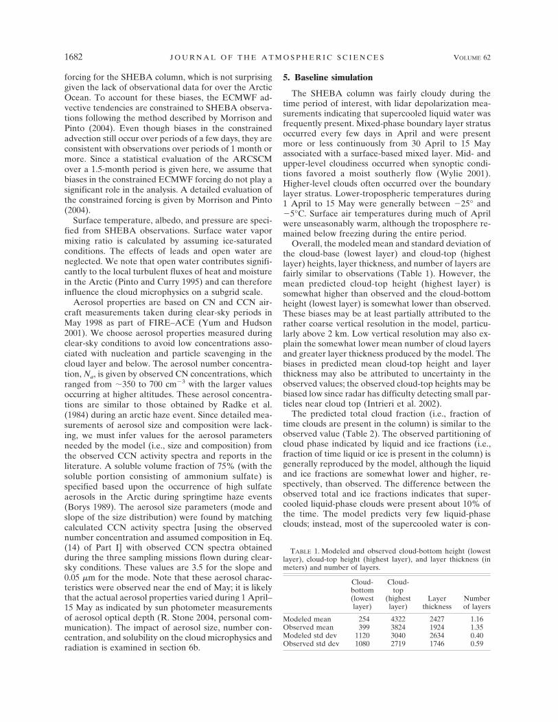
Overall, the modeled mean and standard deviation ofthe cloud-base (lowest layer) and cloud-top (highestlayer) heights, layer thickness, and number of layers arefairly similar to observations (Table 1). However, themean predicted cloud-top height (highest layer) issomewhat higher than observed and the cloud-bottomheight (lowest layer) is somewhat lower than observed.These biases may be at least partially attributed to therather coarse vertical resolution in the model, particu-larly above 2 km. Low vertical resolution may also ex-plain the somewhat lower mean number of cloud layersand greater layer thickness produced by the model. Thebiases in predicted mean cloud-top height and layerthickness may also be attributed to uncertainty in theobserved values; the observed cloud-top heights may bebiased low since radar has difficulty detecting small par-ticles near cloud top (Intrieri et al. 2002).

The predicted total cloud fraction (i.e., fraction oftime clouds are present in the column) is similar to theobserved value (Table 2). The observed partitioning ofcloud phase indicated by liquid and ice fractions (i.e.,fraction of time liquid or ice is present in the column) isgenerally reproduced by the model, although the liquidand ice fractions are somewhat lower and higher, re-spectively, than observed. The difference between theobserved total and ice fractions indicates that super-cooled liquid-phase clouds were present about 10% ofthe time. The model predicts very few liquid-phaseclouds; instead, most of the supercooled water is con-

TABLE 1. Modeled and observed cloud-bottom height (lowestlayer), cloud-top height (highest layer), and layer thickness (inmeters) and number of layers.

Cloud-bottom(lowestlayer)

Cloud-top

(highestlayer)

Layerthickness

Numberof layers

Modeled mean 254 4322 2427 1.16Observed mean 399 3824 1924 1.35Modeled std dev 1120 3040 2634 0.40Observed std dev 1080 2719 1746 0.59


tained in mixed-phase clouds. We note that it is possiblethat some of the clouds that were retrieved as liquidphase may have contained small amounts of ice. Themodeled cloud fractions are fairly insensitive to thethreshold water content (10�5 g m�3) indicating thepresence of cloud water. Even though the modeled liq-uid fraction is somewhat lower than observed, the pre-dicted ratio of mean LWP and IWP of 1.22 is largerthan the ratio of 0.74 for the retrievals, consistent withaccurate prediction of mean LWP but underpredictionof mean IWP (Table 3). These results indicate thatwhen the model predicts supercooled liquid water, theLWP is relatively large, even though liquid occurssomewhat less frequently in the simulation than wasindicated by retrievals. The modeled standard devia-tion of LWP is similar to the retrieved value, althoughthe standard deviation of IWP is much smaller. Largestandard deviation in the retrieved IWP may corre-spond with significant spatial variability in the ice hy-drometeor field in mixed-phase clouds observed duringFIRE–ACE (Lawson et al. 2001; Zuidema et al. 2005)that is difficult for the model to resolve.

Cloud phase partitioning is also indicated by the ratioLWP/TWP (TWP � LWP � IWP) as a function of thecloud-top temperature, Tct (Fig. 1). Values of LWP/TWP � 0.4 (indicating relatively large IWP) occur atTct less than about 262 K in both the simulation andretrievals. In addition, both the modeled and retrievedratios tend to cluster at either zero or �0.6. However,the retrievals show a number of values near unity evenat temperatures colder than 250 K, while the modelproduces values of LWP/TWP generally between 0.6and 0.95 at temperatures �254 K and very little liquidbelow 250 K. This bias may be due to an overestimationof the number of IN due to contact freezing at tem-peratures �254 K. The results exhibit moderate sensi-tivity to the number of contact IN, which is specifiedfollowing Cooper (1986; see Part I): Sensitivity testsusing the Fletcher (1962) or Meyers et al. (1992) for-mulations for the number of contact IN produce a meanLWP 27% larger and 34% smaller, respectively, com-pared to baseline. Low IN concentrations in the actualcloud layer may have occurred as a result of nucleation

and particle scavenging, with the production of ice con-trolled by intermittent entrainment of IN into the layer(Carrio et al. 2005) if sufficient IN were available in thefree atmosphere.

Time series of modeled and retrieved LWP duringthe period show that the predicted values of instanta-neous LWP often differ substantially from retrievedvalues (Fig. 2). However, this is not surprising given thedifficulty of correctly predicting the cloud and thermo-dynamic properties at given times due to errors in theinitialization and forcing profiles in addition to uncer-tainties in the model physics. Nonetheless, qualitativefeatures seen in the retrieved LWP time series are cap-tured by the model, including the periodic occurrenceof liquid water during 1–10 April, the presence of sig-

TABLE 2. Modeled and observed cloud fractions (%).

Total fraction Liquid fraction Ice fraction

Modeled 82.5 49.9 82.4Observed 85.4 64.4 74.8

TABLE 3. Modeled and retrieved LWP and IWP (g m�2).

LWP IWP

Modeled mean 28.0 22.9Retrieved mean 25.6 34.6Modeled std dev 50.7 60.8Retrieved std dev 45.4 92.1

FIG. 1. Modeled and retrieved LWP/TWP (TWP � LWP �IWP) as a function of cloud-top temperature for clouds with a topheight �3 km.

FIG. 2. Time series of modeled (solid) and MWR-retrieved(dotted) LWP (data are 6-h averages).


nificant liquid between 15–20 April, and nearly con-tinuous liquid water from 26 April to 15 May with theexception of 9 May. The largest values of LWP in thesimulation occur during mid May with LWPs exceeding300 g m�2.

The model biases are primarily associated with low(�3 km) rather than high (�3 km) clouds as shown inTable 4. The mean IWP for high clouds is somewhatlarger than retrieved, while the high-cloud ice fractionis quite close to observations. Note that the predictedhigh clouds are quite sensitive to the initial RH. A sen-sitivity simulation in which the temperature-dependentmodification to the initial RH (see section 4) is ne-glected produces a high-cloud ice fraction of only 31%.The mean IWP in low clouds is about one-half of theretrieved value. Since low-level clouds in the Arcticprimarily form as a result of air mass modificationrather than large-scale forcing (Curry 1983), this biasmay indicate a deficiency in the model physics. Themean modeled values of IWC in mixed-phase and lowclouds (Table 5) are smaller than retrieved (particularlyfor mixed-phase clouds) while the predicted mean highcloud IWC is somewhat larger (the modeled and re-trieved values are screened to include only ice watercontents �0.5 mg m�3). The mean total IWC (for IWCs� 0.5 mg m�3) is close to the retrieved value.

Mean surface downwelling shortwave (SW) andlongwave (LW) radiative fluxes predicted by the modelare somewhat higher and lower, respectively, than ob-served (Table 6). The mean total downwelling flux (SWplus LW) is close to observed, differing by only 1.6 Wm�2. The underprediction of LW flux and overpredic-tion of SW flux are consistent with the lower simulatedliquid fraction compared to retrievals. Biases in the ra-diative fluxes may also result from neglect of aerosol inthe calculations of radiative transfer.

The predicted total precipitation accumulated at thesurface during the time period (consisting almost en-tirely of snow) is close to observed (see Table 6). Theaccurate prediction of precipitation is not surprisinggiven that it is mostly determined by the large-scalemoisture convergence (Morrison and Pinto 2004),which was constrained to SHEBA observations (seesection 4).

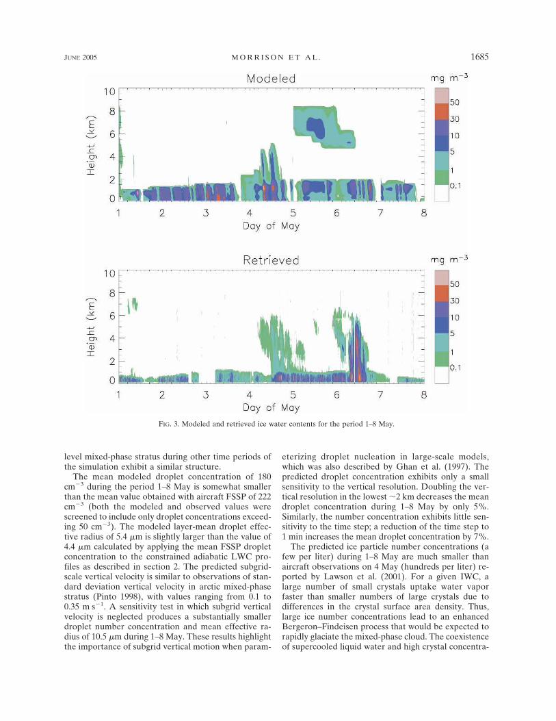
A detailed analysis of the simulation for the period1–8 May further illustrates the model’s performance.This period was characterized by a persistent low-levelmixed-phase stratus that has been a focus of severalobservational and modeling studies (e.g., Curry et al.

2000; Lawson et al. 2001; Girard and Curry 2001; Donget al. 2001; Carrio et al. 2005; Zuidema et al. 2005).Time–height plots of the modeled and retrieved IWC(Fig. 3) show that the model produces a persistent low-level stratus qualitatively similar to retrievals, althoughthe predicted cloud top is often 500 m or more higherthan retrieved. This bias may be attributed to potentialdeficiencies in the boundary layer parameterization,model forcing, and/or vertical resolution. The upper-level clouds indicated by retrievals on 4 and 6 Mayseeded the boundary layer cloud from above, leading torapid depletion of the supercooled liquid (Curry et al.2000; Zuidema et al. 2005). Similarly, the predicted low-level cloud is seeded by upper-level clouds on 4 May,although the cirrus predicted on 5 and 6 May does notprecipitate down to the boundary layer cloud.

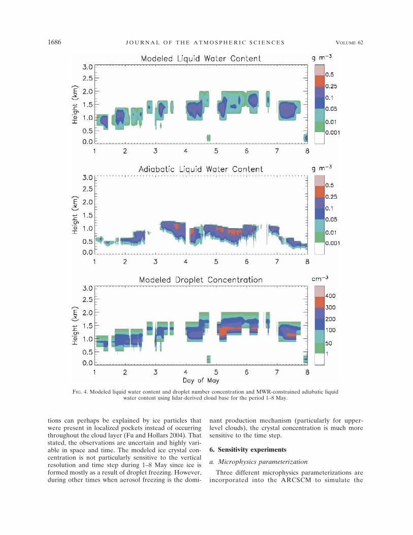
Time–height plots of the predicted LWC and dropletconcentration and the constrained adiabatic LWC inFig. 4 show that the predicted low-level cloud has aliquid-topped layer similar to observations. However,the predicted cloud-top height is generally 500 to 1000m too high as was discussed above. The modeled liquidwater contents also tend to be smaller than the con-strained adiabatic values, although this is compensatedby the greater vertical extent of the predicted liquidlayer. These differences may result in part from coarsevertical resolution in the model. The simulated dropletconcentration is high (�100 cm�3) through most of thecloud layer, with peak values near cloud base occasion-ally exceeding 300 cm�3. The droplet concentra-tions from aircraft FSSP measurements on 4 and 7 Mayare similar in magnitude but exhibited somewhat lessvariation with height (not shown). The modeled liquidlayer is maintained through radiative cooling and large-scale moisture convergence, with ice generated mostlythrough contact freezing and subsequently precipitatingbelow the liquid base. This canonical structure of a liq-uid-topped, weakly precipitating, mixed-phase stratusin both Arctic and midlatitude regimes has been de-scribed by many researchers (e.g., Rauber and Tokay1991; Hobbs and Rangno 1998; Rangno and Hobbs2001; Fleishauer et al. 2002; Korolev et al. 2003). Low-

TABLE 4. Modeled and observed high (�3 km) and low (�3km) cloud fractions (%) and mean IWP (g m�2).

Lowliquid

fraction

Lowice

fractionLowIWP

Highliquid

fraction

Highice

fractionHighIWP

Modeled 47.6 79.4 16.7 6.2 46.0 6.1Observed 63.7 68.9 30.4 8.5 44.1 4.3

TABLE 5. Modeled and retrieved mean IWC (mg m�3).

IWC(total)

IWC(mixed phase)

IWC(�3 km)

IWC(�3 km)

Modeled 12.3 10.9 13.0 8.2Retrieved 12.4 17.3 17.0 6.4

TABLE 6. Modeled and observed downwelling shortwave (SW),longwave (LW), and total (TOT) radiative flux (W m�2) andaccumulated precipitation (PREC) (cm) at the surface.

SW LW TOT PREC

Modeled 175.1 216.9 392.0 2.24Observed 165.1 225.3 390.4 2.16


level mixed-phase stratus during other time periods ofthe simulation exhibit a similar structure.

The mean modeled droplet concentration of 180cm�3 during the period 1–8 May is somewhat smallerthan the mean value obtained with aircraft FSSP of 222cm�3 (both the modeled and observed values werescreened to include only droplet concentrations exceed-ing 50 cm�3). The modeled layer-mean droplet effec-tive radius of 5.4 �m is slightly larger than the value of4.4 �m calculated by applying the mean FSSP dropletconcentration to the constrained adiabatic LWC pro-files as described in section 2. The predicted subgrid-scale vertical velocity is similar to observations of stan-dard deviation vertical velocity in arctic mixed-phasestratus (Pinto 1998), with values ranging from 0.1 to0.35 m s�1. A sensitivity test in which subgrid verticalvelocity is neglected produces a substantially smallerdroplet number concentration and mean effective ra-dius of 10.5 �m during 1–8 May. These results highlightthe importance of subgrid vertical motion when param-

eterizing droplet nucleation in large-scale models,which was also described by Ghan et al. (1997). Thepredicted droplet concentration exhibits only a smallsensitivity to the vertical resolution. Doubling the ver-tical resolution in the lowest �2 km decreases the meandroplet concentration during 1–8 May by only 5%.Similarly, the number concentration exhibits little sen-sitivity to the time step; a reduction of the time step to1 min increases the mean droplet concentration by 7%.

The predicted ice particle number concentrations (afew per liter) during 1–8 May are much smaller thanaircraft observations on 4 May (hundreds per liter) re-ported by Lawson et al. (2001). For a given IWC, alarge number of small crystals uptake water vaporfaster than smaller numbers of large crystals due todifferences in the crystal surface area density. Thus,large ice number concentrations lead to an enhancedBergeron–Findeisen process that would be expected torapidly glaciate the mixed-phase cloud. The coexistenceof supercooled liquid water and high crystal concentra-

FIG. 3. Modeled and retrieved ice water contents for the period 1–8 May.


Fig 3 live 4/C

tions can perhaps be explained by ice particles thatwere present in localized pockets instead of occurringthroughout the cloud layer (Fu and Hollars 2004). Thatstated, the observations are uncertain and highly vari-able in space and time. The modeled ice crystal con-centration is not particularly sensitive to the verticalresolution and time step during 1–8 May since ice isformed mostly as a result of droplet freezing. However,during other times when aerosol freezing is the domi-

nant production mechanism (particularly for upper-level clouds), the crystal concentration is much moresensitive to the time step.

6. Sensitivity experiments

a. Microphysics parameterization

Three different microphysics parameterizations areincorporated into the ARCSCM to simulate the

FIG. 4. Modeled liquid water content and droplet number concentration and MWR-constrained adiabatic liquidwater content using lidar-derived cloud base for the period 1–8 May.


Fig 4 live 4/C

1 April–15 May period of SHEBA. These results arecompared with the baseline simulation (hereafter re-ferred to as BASE) to further interpret its perfor-mance. The three parameterizations are briefly de-scribed below in order of increasing complexity. Valuesof relevant microphysical parameters (e.g., fall speeds,particle densities) are specified to be the same for thevarious schemes.

The first parameterization is a version of the Reisneret al. (1998) single-moment bulk scheme that predictsthe mixing ratios of droplets, cloud ice, rain, and snow(hereafter SM) and is capable of simulating mixed-phase clouds. The mixing ratio of each species is prog-nosed at a given level allowing for more realistic phasepartitioning than provided by simple temperature–phase relationships. This scheme has been used exten-sively for simulations of Arctic climate (Pinto et al.1999; Curry et al. 2000; Girard and Curry 2001; Morri-son et al. 2003). The cloud ice number concentration isspecified following Cooper (1986) as a function of thetemperature. Droplet and cloud ice populations are as-sumed to be monodisperse. Cloud–aerosol interactionsare neglected; droplet effective radius is assumed to be5 �m.

The second scheme combines the detailed ice-phaseparameterization of the BASE parameterization withthe simple liquid-phase microphysics of SM (hereafterDI). Thus, the DI scheme prognoses the number con-centrations of cloud ice and snow in addition to themixing ratios of the four hydrometeor species (droplets,cloud ice, rain, snow). The production of ice from freez-ing of aerosol is included, while droplet activation ofaerosol is neglected.

The third parameterization includes the ice-phaseand liquid-phase parameterizations of the BASEscheme but also predicts the mixing ratio and numberconcentration of graupel (hereafter GR). The graupelparameterization follows that described by Reisner etal. (1998), Murakami (1990), and Ikawa and Saito(1991).

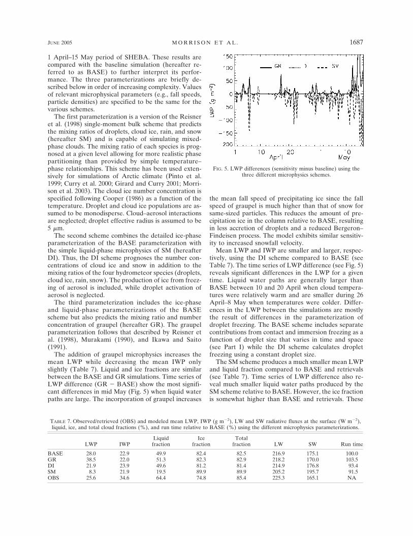
The addition of graupel microphysics increases themean LWP while decreasing the mean IWP onlyslightly (Table 7). Liquid and ice fractions are similarbetween the BASE and GR simulations. Time series ofLWP difference (GR � BASE) show the most signifi-cant differences in mid May (Fig. 5) when liquid waterpaths are large. The incorporation of graupel increases

the mean fall speed of precipitating ice since the fallspeed of graupel is much higher than that of snow forsame-sized particles. This reduces the amount of pre-cipitation ice in the column relative to BASE, resultingin less accretion of droplets and a reduced Bergeron–Findeisen process. The model exhibits similar sensitiv-ity to increased snowfall velocity.

Mean LWP and IWP are smaller and larger, respec-tively, using the DI scheme compared to BASE (seeTable 7). The time series of LWP difference (see Fig. 5)reveals significant differences in the LWP for a giventime. Liquid water paths are generally larger thanBASE between 10 and 20 April when cloud tempera-tures were relatively warm and are smaller during 26April–8 May when temperatures were colder. Differ-ences in the LWP between the simulations are mostlythe result of differences in the parameterization ofdroplet freezing. The BASE scheme includes separatecontributions from contact and immersion freezing as afunction of droplet size that varies in time and space(see Part I) while the DI scheme calculates dropletfreezing using a constant droplet size.

The SM scheme produces a much smaller mean LWPand liquid fraction compared to BASE and retrievals(see Table 7). Time series of LWP difference also re-veal much smaller liquid water paths produced by theSM scheme relative to BASE. However, the ice fractionis somewhat higher than BASE and retrievals. These

TABLE 7. Observed/retrieved (OBS) and modeled mean LWP, IWP (g m�2), LW and SW radiative fluxes at the surface (W m�2),liquid, ice, and total cloud fractions (%), and run time relative to BASE (%) using the different microphysics parameterizations.

LWP IWPLiquidfraction

Icefraction

Totalfraction LW SW Run time

BASE 28.0 22.9 49.9 82.4 82.5 216.9 175.1 100.0GR 38.5 22.0 51.3 82.3 82.9 218.2 170.0 103.5DI 21.9 23.9 49.6 81.2 81.4 214.9 176.8 93.4SM 8.3 21.9 19.5 89.9 89.9 205.2 195.7 91.5OBS 25.6 34.6 64.4 74.8 85.4 225.3 165.1 NA

FIG. 5. LWP differences (sensitivity minus baseline) using thethree different microphysics schemes.


results suggest incorrect phase partitioning in the SMscheme, that is, mixed-phase clouds are often predictedas entirely crystalline. The large differences in cloudphase and mean LWP result in differences in the meandownwelling LW and SW fluxes at the surface of �11.7and 20.2 W m�2, respectively, compared to BASE andeven larger biases relative to observations. These biasesare consistent with previous results using the scheme tosimulate mixed-phase stratus (Curry et al. 2000; Girardand Curry 2001; Morrison et al. 2003). As described byMorrison et al. (2003), the SM scheme is highly sensi-tive to the specified crystal concentration since it deter-mines in part the uptake of water vapor by crystals.Incorporating the Fletcher (1962) or Meyers et al.(1992) formulations produces a mean LWP of 16.6 and1.1 g m�2, respectively. This sensitivity highlights theimportance of realistically treating the ice number con-centration.

A limitation of using the Meyers et al., Fletcher, Coo-per, and similar formulations to parameterize the icenumber concentration is that these expressions aregenerally functions of either temperature or super-saturation. Extensions of classical nucleation theory(Khvorostyanov and Sassen 1998; Khvorostyanov andCurry 2000) suggest both a temperature and supersatu-ration dependence for the number of IN occurringthrough homogeneous or heterogeneous freezing. Em-pirical formulations can also produce unrealistic valueswhen extrapolated to cold temperatures (��30°C)and therefore must be arbitrarily modified (e.g., Reis-ner et al. 1998). In addition, sedimentation of ice intodrier layers or a rapid decrease in supersaturation afternucleation can result in high crystal concentrations atlow supersaturations that cannot be predicted if thecrystal concentration is diagnosed rather than prog-nosed. For example, initially large values of supersatu-ration can produce an impulse of nucleation and highcrystal concentration, but the supersaturation decreasesrapidly owing to vapor deposition onto the crystals. Di-agnosing the ice number concentration from supersatu-ration in this instance will result in an underpredictionof concentration after the supersaturation decreases.

An important consideration for any model param-

eterization is its computational cost. The cost associ-ated with each microphysics scheme is estimated bycomparing run times for the various simulations (seeTable 7). While this estimate cannot provide an exactcost for each scheme since other parameterizations inthe model also contribute to run time, it is useful forcomparing relative differences in efficiency betweenthe schemes. As expected, run times increase with in-creasing complexity of the microphysics parameteriza-tion, varying by �15% using the four different schemes.Incorporating the detailed ice-phase microphysics intothe SM scheme increases the run time by only a fewpercent for the DI scheme; using BASE increases thecost �10% relative to SM, while adding graupel micro-physics to BASE increases the run time by a few per-cent for the GR scheme. Another issue that must beconsidered in certain applications is memory allocationas the number of prognostic variables is increased. Thenumber of prognostic variables ranges from 4 in SM to10 in GR.

b. Aerosol characteristics

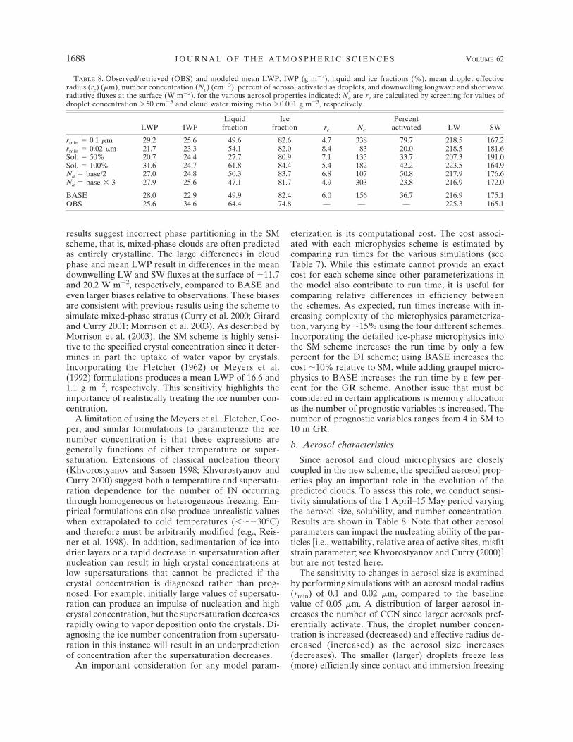
Since aerosol and cloud microphysics are closelycoupled in the new scheme, the specified aerosol prop-erties play an important role in the evolution of thepredicted clouds. To assess this role, we conduct sensi-tivity simulations of the 1 April–15 May period varyingthe aerosol size, solubility, and number concentration.Results are shown in Table 8. Note that other aerosolparameters can impact the nucleating ability of the par-ticles [i.e., wettability, relative area of active sites, misfitstrain parameter; see Khvorostyanov and Curry (2000)]but are not tested here.

The sensitivity to changes in aerosol size is examinedby performing simulations with an aerosol modal radius(rmin) of 0.1 and 0.02 �m, compared to the baselinevalue of 0.05 �m. A distribution of larger aerosol in-creases the number of CCN since larger aerosols pref-erentially activate. Thus, the droplet number concen-tration is increased (decreased) and effective radius de-creased (increased) as the aerosol size increases(decreases). The smaller (larger) droplets freeze less(more) efficiently since contact and immersion freezing

TABLE 8. Observed/retrieved (OBS) and modeled mean LWP, IWP (g m�2), liquid and ice fractions (%), mean droplet effectiveradius (re) (�m), number concentration (Nc) (cm�3), percent of aerosol activated as droplets, and downwelling longwave and shortwaveradiative fluxes at the surface (W m�2), for the various aerosol properties indicated; Nc are re are calculated by screening for values ofdroplet concentration �50 cm�3 and cloud water mixing ratio �0.001 g m�3, respectively.

LWP IWPLiquidfraction

Icefraction re Nc

Percentactivated LW SW

rmin � 0.1 �m 29.2 25.6 49.6 82.6 4.7 338 79.7 218.5 167.2rmin � 0.02 �m 21.7 23.3 54.1 82.0 8.4 83 20.0 218.5 181.6Sol. � 50% 20.7 24.4 27.7 80.9 7.1 135 33.7 207.3 191.0Sol. � 100% 31.6 24.7 61.8 84.4 5.4 182 42.2 223.5 164.9Na � base/2 27.0 24.8 50.3 83.7 6.8 107 50.8 217.9 176.6Na � base 3 27.9 25.6 47.1 81.7 4.9 303 23.8 216.9 172.0

BASE 28.0 22.9 49.9 82.4 6.0 156 36.7 216.9 175.1OBS 25.6 34.6 64.4 74.8 — — — 225.3 165.1


are functions of droplet size, producing larger (smaller)LWPs. Interestingly, when the droplet size is increaseddue to smaller specified aerosol (implying faster con-tact/immersion freezing rates and increased precipita-tion efficiency), the average mixed-phase cloud lifetime(indicated by the liquid fraction) actually increases.This occurs because the number of IN is reduced due todecreasing ice nucleability associated with the smalleraerosol (i.e., less surface area is available to form asubstrate for the ice crystal). With fewer crystals avail-able, the Bergeron–Findeisen mechanism is less effec-tive, leading to the persistence of liquid water in thesimulation. The mean LW and SW surface radiativefluxes reflect these results. The increase (decrease) indownwelling surface SW flux is consistent with a de-crease (increase) in the cloud albedo associated withlarger (smaller) droplet effective radius and smaller(larger) mean LWP. This indirect aerosol effect hasbeen described in numerous studies (e.g., Twomey1977; Ghan et al. 2001; Penner and Rotstayn 2001;Feingold et al. 2003). The LW flux responds more tochanges in the mixed-phase cloud lifetime. Relative tobaseline, the mean surface downwelling LW flux in-creases with decreasing aerosol size due to the in-creased mixed-phase cloud lifetime even though meanLWP is decreased 23%. This occurs because the pre-dicted clouds tend to emit as blackbodies in both thebaseline and sensitivity simulations.

The sensitivity of the model to changes in aerosolsolubility is examined by performing simulations with asoluble fraction of 100% and 50% compared to 75% forthe baseline value. Specifying a soluble fraction of100% implies no condensation freezing of aerosol inthe model (contact and immersion freezing of dropletsare still allowed). The solubility of an aerosol popula-tion depends on its source and may change over time.For example, solubility increases if sulfate loading ofthe aerosol occurs in a polluted air mass (Pruppacherand Klett 1997). Seasonal changes in solubility may co-incide with the presence of arctic pollution haze in thespring and early summer (e.g., Borys 1989; Curry 1995;Curry et al. 1996). The mean droplet number concen-tration and effective radius exhibit moderate sensitivityto soluble fraction while the average mixed-phase cloudlifetime exhibits large sensitivity. Decreasing solubilityleads to increased ice nucleability and shorter mixed-phase lifetimes. Even though solubility also influencesthe droplet effective radius, this effect is relatively mi-nor; the response of the SW and LW radiative fluxes isdominated by changes in the mixed-phase cloud life-time. Decreased (increased) mixed-phase cloud life-time due to decreased (increased) aerosol solubilityleads to increased (decreased) SW and decreased (in-creased) LW downwelling fluxes at the surface. Thus, amixed-phase cloud lifetime SW and LW radiative indi-rect aerosol effect due to modification of aerosol solu-bility is identified. Note that specifying a soluble frac-

tion of 100% produces results that are quite similar toobservations for a number of quantities.

Changes in the aerosol number concentration are ex-pected to impact the number of IN and CCN. Aerosolnumber concentration varies widely between air massesoriginating in different source regions (e.g., continentalversus marine). Anthropogenic aerosol can signifi-cantly modify the total aerosol concentration; in urbanenvironments, the aerosol concentration is often sev-eral orders of magnitude larger than in pristine condi-tions (Pruppacher and Klett 1997). The sensitivity ofthe model to aerosol number concentration is assessedby performing simulations with concentrations of aero-sol specified at three times and one-half times the base-line values described in section 4. Increasing (decreas-ing) the aerosol number concentration increases (de-creases) the mean droplet number and decreases(increases) the effective radius as expected. The down-welling SW flux at the surface is influenced by changesin droplet effective radius as the aerosol number con-centration is modified. The LW flux exhibits little sen-sitivity since the mixed-phase cloud lifetimes vary onlyslightly in response to changes in the aerosol numberconcentration.

These results suggest that the SW indirect aerosolradiative effect operates through distinct mechanisms(droplet size, LWP, and cloud lifetime effects), which isconsistent with previous studies. However, the cloudlifetime effect appears to differ in arctic mixed-phasestratus compared to liquid-phase clouds, which havebeen studied much more extensively. As opposed toliquid-phase clouds, the lifetime of arctic mixed-phasestratus appears to be strongly linked to the ice nucle-ability of the aerosol rather than the droplet size ornumber concentration. For example, modification ofaerosol resulting in more numerous and smaller drop-lets, which tends to increase the lifetime of liquid-phaseclouds (e.g., Albrecht 1989), may actually decrease thelifetime of mixed-phase clouds if the IN concentrationalso increases. This mixed-phase cloud lifetime effecton the downwelling SW flux is particularly evident forchanges in the aerosol solubility. These results also sug-gest a LW indirect aerosol radiative effect (cloud green-house effect), which is mostly determined by changes inthe mixed-phase cloud lifetime. Indirect aerosol effectson the LW flux have not been extensively studied, butmay be particularly important in the Arctic where theLW flux dominates the solar flux during most of theyear.

This study provides a link between the chemical andphysical properties of the aerosol and previous studiessuggesting that the maintenance of mixed-phase stratusis dependent upon the IN concentration (Pinto 1998;Harrington et al. 1999; Jiang et al. 2000; Morrison et al.2003). A similar IN cloud lifetime–radiative effect as-sociated with contact freezing of droplets was describedby Lohmann (2002) but did not explicitly relate cloudlifetime to aerosol properties in terms of condensation


freezing on aerosol. Inclusion of aerosol–IN interac-tions associated with contact and immersion freezing ofdroplets in the model (an area of future development)would likely enhance the IN cloud lifetime effect de-scribed here.

7. Summary and conclusions

A single-column model incorporating the new micro-physics scheme described in Part I was used to simulatethe 1 April–15 May period of SHEBA. Results werecompared to observations and ground-based retrievals.The model was initialized with SHEBA observationsand forced with constrained ECMWF model output.Aerosol properties needed by the microphysics schemewere based on aircraft measurements taken duringFIRE–ACE. Simulations were reinitialized every threedays to limit model drift in the temperature and watervapor profiles.

The model was able to reasonably predict the meancloud properties observed during the period. Cloudboundaries and total fraction were similar to observa-tions. Phase partitioning in the simulation, crucial forpredicting the surface radiative fluxes, was fairly similarto retrievals as indicated by liquid and ice fractions andratios of LWP and total water path as a function ofcloud-top temperature. However, the predicted liquidfraction was somewhat lower than retrieved and themodel produced relatively less liquid water than indi-cated by retrievals in strongly supercooled clouds witha cloud-top temperature �254 K. Mean LWP was closeto the retrieved value while mean IWP was somewhatsmaller than retrieved. Biases in the predicted down-welling surface solar and longwave radiative fluxeswere consistent with the small underprediction of liquidcloud fraction. Neglect of aerosol in the radiative trans-fer calculations may have also contributed to biases inthe radiative fluxes.

A detailed evaluation of the simulation for the period1–8 May showed that the model was able to qualita-tively reproduce many features of a persistent mixed-phase boundary layer stratus. However, the predictedcloud top was generally too high by about 500–1000 m,indicating potential deficiencies associated with theboundary layer parameterization, large-scale forcing,and/or coarse vertical resolution. Improvements inthese areas may be needed to fully benefit from im-provements in the new microphysics scheme. In addi-tion, the modeled ice phase microphysics differedwidely from in situ observations. However, the in situand retrieved ice microphysical properties are uncer-tain; a better characterization is needed, particularlyregarding the ice particle number concentration.

Parallel simulations using three different microphys-ics parameterizations were compared to further assessthe new scheme. The simple liquid/detailed ice andgraupel microphysics schemes produced mean LWPs

that were smaller and larger than baseline, respectively.Mean IWP and liquid and ice fractions did not varysignificantly from baseline using either scheme. Thesingle-moment scheme produced only a small amountof liquid water resulting in significant differences in thedownwelling surface radiative fluxes compared with ob-servations, consistent with previous studies (Curry et al.2000; Girard and Curry 2001; Morrison et al. 2003).This bias was mostly attributed to uncertainties in thediagnosed ice number concentration. These results sug-gest the importance of realistically treating the crystalconcentration. We argue that prognosing, rather thandiagnosing, the crystal concentration is needed for arealistic treatment of the ice microphysics. Computa-tional time increased somewhat (�10%–13%) usingthe more complex schemes, although the number ofprognostic variables (ranging from 4 in SM to 10 in GR)may be important if memory allocation is an issue in themodel. Of course, a drawback in using the simplerschemes (DI and SM) is that cloud–aerosol interactionsare not explicitly treated for both liquid and ice, limit-ing their ability to model indirect aerosol effects onclimate.

The sensitivity of the model to modification of thespecified aerosol was assessed. The response was deter-mined by two effects: 1) changes in the ice nucleabilityand thus IN concentration and 2) changes in CCN con-centration. Changes in IN concentration had a largeinfluence on the lifetime of mixed-phase clouds whilemodification of CCN affected droplet number concen-tration and effective radius. The response of the surfaceradiative fluxes was determined by the interplay be-tween these two effects. The downwelling shortwaveflux responded to changes in the cloud albedo as a func-tion of the droplet effective radius. The longwave fluxwas mostly influenced by changes in the lifetime ofmixed-phase clouds. The surface radiative fluxes (bothshortwave and longwave) exhibited particular sensitiv-ity to changes in the aerosol solubility mostly due to themixed-phase cloud lifetime effect. We note, of course,that the simulated response of clouds and radiation tomodification of aerosol is uncertain owing to an incom-plete treatment of the aerosol and cloud microphysicsand other physical processes, deficiencies in the initial-ization and forcing, and coarse resolution (exhibited bybiases in the clouds and radiation in the baseline simu-lation); nonetheless, these results suggest qualitativelythat aerosol indirect effects in arctic mixed-phaseclouds are complex and merit further study.

This work represents a first step in evaluating themicrophysics scheme. We note that there were uncer-tainties in the advective forcing, initialization profiles,specified aerosol properties, neglect of horizontal cloudwater advection, etc. In addition, other model param-eterizations (e.g., radiation, boundary layer schemes)can contribute to biases in the predicted cloud proper-ties. Hence, this study cannot provide an unambiguousevaluation of the microphysics parameterization. More


rigorous testing is needed including incorporation into3D models and application to regions outside of theArctic. Model results were particularly sensitive to theaerosol size, concentration, and composition, which arenot well known in the Arctic owing to limited observa-tions. This paper underlines the need for better char-acterization of aerosols in the region, including the de-velopment of a detailed aerosol climatology for the cen-tral Arctic.

We did not discuss at length how the model resolu-tion can affect results. Since the microphysics schemepredicts clouds based on grid-scale values of relativehumidity (i.e., there is no subgrid-scale cloud param-eterization), we implicitly assumed that clouds atSHEBA could be captured using the given resolution.While clouds that occurred at SHEBA were predomi-nately stratiform and horizontally extensive, they oftenoccurred in vertically thin layers. Thus, it is likely thatsome of these clouds were subgrid in the vertical, whichmay have contributed to model bias. We note, however,that it is difficult to test the model’s overall sensitivityto the vertical resolution since the vertical resolution ofthe specified advective forcing, which is important indriving the initial formation of cloud water, cannot beincreased. Incorporating the scheme into a 3D modelcan help to rectify this issue. Another issue that arises isthe difference in horizontal scale between the model(�60 km based on the scale of the advective forcing andvertical velocity) and observations (measured at asingle location). This difference likely accounted for thelarger variability in the retrieved cloud properties (e.g.,IWP), but was probably less important in comparisonsof the time-averaged cloud properties. Nonetheless, thespatial scale of the model is important in determiningappropriate values of resolution-dependent parametersin the microphysics scheme, which can influence thetime-averaged cloud properties (Fowler et al. 1996).Further study is needed to better understand the role ofspatial scale and subgrid cloudiness in predicting arcticclouds using a large-scale model.

Specified microphysical parameters in the newscheme play an important role in simulating arcticclouds. In particular, the ice parameters (e.g., bulk den-sity, fall speed, habit, spectral dispersion, collection ef-ficiency) are important in calculating several micro-physical processes; yet appropriate values for these pa-rameters remain uncertain, particularly for arcticclouds. A detailed assessment of the role of the speci-fied microphysics parameters was beyond the scope ofthis paper, but should be addressed in future work.

Acknowledgments. This research was supported byDOE ARM Grant DE-FG03-94ER61771 and NSFSHEBA Grant OPP-0084225. Microwave radiometerdata were obtained from the DOE ARM program. Pre-cipitation and rawinsonde measurements were ob-tained from the SHEBA Project Office at the Univer-sity of Washington Applied Physics Laboratory. Sur-

face forcing data were obtained from the SHEBAAtmospheric Surface Flux Group. We are grateful to C.Jakob and his colleagues at the ECMWF for providingthe dynamic and advective forcing.

REFERENCES.

Albrecht, B. A., 1989: Aerosols, cloud microphysics and fractionalcloudiness. Science, 237, 1020–1022.

Beesley, J. A., C. S. Bretherton, C. Jakob, E. L Andreas, J. M.Intrieri, and T. A. Uttal, 2000: A comparison of cloud andboundary layer variables in the ECMWF forecast model withobservations at the Surface Heat Budget of the Arctic Ocean(SHEBA) ice camp. J. Geophys. Res., 105, 12 337–12 349.

Borys, R. D., 1989: Studies of ice nucleation by arctic aerosol onAGASP-II. J. Atmos. Chem., 9, 169–185.

Briegleb, B. P., 1992: Delta-Eddington approximation for solarradiation in the NCAR Community Climate Model. J. Geo-phys. Res., 97, 7603–7612.

Carrio, G. G., H. Jiang, and W. R. Cotton, 2005: Impact of aerosolintrusions on the Arctic boundary layer clouds. Part I: 4 May1998 case. J. Atmos. Sci., in press.

Cooper, W. A., 1986: Ice initiation in natural clouds. PrecipitationEnhancement—A Scientific Challenge, Meteor. Monogr., No.43, Amer. Meteor. Soc., 29–32.

Curry, J. A., 1983: On the formation of polar continental air. J.Atmos. Sci., 40, 2279–2292.

——, 1995: Interactions among aerosols, clouds, and climate ofthe Arctic Ocean. Sci. Total Environ., 160, 777–791.

——, and G. F. Herman, 1985: Relationships between large-scaleheat and moisture budgets and the occurrence of Arctic stra-tus clouds. Mon. Wea. Rev., 113, 1441–1457.

——, and E. E. Ebert, 1990: Sensitivity of the thickness of arcticsea ice to the optical properties of clouds. Ann. Glaciol., 14,43–46.

——, W. B. Rossow, and J. L. Schramm, 1996: Overview of Arcticcloud and radiation properties. J. Climate, 9, 1731–1764.

——, and Coauthors, 2000: FIRE Arctic Clouds Experiment. Bull.Amer. Meteor. Soc., 81, 5–29.

Dong, X., G. G. Mace, P. Minnis, and D. F. Young, 2001: Arcticstratus cloud properties and their effect on the surface radia-tion budget: Selected cases from FIRE ACE. J. Geophys.Res., 106, 15 297–15 312.

Ebert, E. E., and J. A. Curry, 1992: A parameterization of ice-cloud optical properties for climate models. J. Geophys. Res.,97, 3831–3836.

Feingold, G., W. L. Eberhard, D. E. Veron, and M. Prevedi, 2003:First measurements of the Twomey indirect effect usingground-based remote sensors. Geophys. Res. Lett., 30, 1287,doi:10.1029/2002GL016633.

Fleishauer, R. P., V. E. Larson, and T. H. Vonder Haar, 2002:Observed microphysical structure of midlevel, mixed-phaseclouds. J. Atmos. Sci., 59, 1779–1804.

Fletcher, N. H., 1962: The Physics of Rainclouds. Cambridge Uni-versity Press, 386 pp.

Fowler, L. D., D. A. Randall, and S. A. Rutledge, 1996: Liquidand ice microphysics in the CSU General Circulation Model.Part 1: Model description and simulated microphysical pro-cesses. J. Climate, 9, 489–529.

Fu, Q., and S. Hollars, 2004: Testing mixed-phase cloud watervapor parameterizations with SHEBA/FIRE ACE observa-tions. J. Atmos. Sci., 61, 2083–2091.

Ghan, S. J., L. R. Leung, and R. C. Easter, 1997: Prediction ofcloud droplet number in a general circulation model. J. Geo-phys. Res., 102, 21 777–21 794.

——, and Coauthors, 2001: A physically-based estimate of radia-tive forcing by anthropogenic sulfate aerosol. J. Geophys.Res., 106, 5279–5293.


Girard, E., and J. A. Curry, 2001: Simulation of Arctic low-levelclouds observed during the FIRE Arctic Clouds Experimentusing a new bulk microphysics scheme. J. Geophys. Res., 106,15 139–15 154.

Grell, G. A., J. Dudhia, and D. R. Stauffer, 1995: A description ofthe Fifth-Generation Penn State/NCAR Mesoscale Model(MM5). NCAR Tech. Note NCAR/TN-398�STR, 138 pp.

Harrington, J. Y., T. Reisen, W. R. Cotton, and S. M. Kreiden-weis, 1999: Cloud resolving simulations of Arctic stratus: PartII: Transition-season clouds. Atmos. Res., 51, 45–75.

Hobbs, P. V., and A. L. Rangno, 1985: Ice particle concentrationsin clouds. J. Atmos. Sci., 42, 2523–2549.

——, and ——, 1990: Rapid development of ice particle concen-trations in small polar maritime clouds. J. Atmos. Sci., 47,2710–2722.

——, and ——, 1998: Microstructures of low and middle-levelclouds over the Beaufort Sea. Quart. J. Roy. Meteor. Soc.,124, 2035–2071.

Holtslag, A. M., and B. A. Boville, 1993: Local versus non-localboundary-layer diffusion in a global climate model. J. Cli-mate, 6, 1825–1842.

Ikawa, M., and K. Saito, 1991: Description of the nonhydrostaticmodel developed at the forecast research department of theMRI. Meteorological Institute Tech. Rep. 28, 238 pp.

Intrieri, J. M., M. D. Shupe, T. Uttal, and B. J. McCarty, 2002: Anannual cycle of Arctic cloud characteristics observed by radarand lidar at SHEBA. J. Geophys. Res., 107, 8030, doi:10.1029/2000JC000423.

Jiang, H., W. R. Cotton, J. O. Pinto, J. A. Curry, and M. J. Weis-bluth, 2000: Cloud resolving simulations of mixed-phase arc-tic stratus observed during BASE: Sensitivity to concentra-tion of ice crystals and large-scale heat and moisture advec-tion. J. Atmos. Sci., 57, 2105–2117.

Khvorostyanov, V. I., and K. Sassen, 1998: Cirrus cloud simula-tion using explicit micropohysics and radiation. Part 1: Modeldescription. J. Atmos. Sci., 55, 1808–1821.

——, and J. A. Curry, 2000: A new theory of heterogeneous icenucleation for application in cloud and climate models. Geo-phys. Res. Lett., 27, 4081–4084.

Korolev, A. V., G. A. Isaac, S. G. Cober, J. W. Strapp, and J.Hallett, 2003: Microphysical characterization of mixed-phaseclouds. Quart. J. Roy. Meteor. Soc., 129, 39–65.

Lawson, R. P., B. A. Baker, C. G. Schmitt, and T. L. Jensen, 2001:An overview of microphysical properties of Arctic cloudsobserved in May and July during FIRE ACE. J. Geophys.Res., 106, 14 989–15 014.

Lohmann, U., 2002: A glaciation indirect effect caused by sootaerosols. Geophys. Res. Lett., 29, 1052, doi:10.1029/2001GL014357.

——, J. Humble, W. R. Leaitch, G. A. Isaac, and I. Gultepe, 2001:Simulation of ice clouds during FIRE ACE using theCCCMA single-column model. J. Geophys. Res., 106, 15 123–15 138.

Lynch, A. H., W. L. Chapman, J. E. Walsh, and G. Weller, 1995:Development of a regional climate model of the western Arc-tic. J. Climate, 8, 1555–1570.

Meyers, M. P., P. J. DeMott, and W. R. Cotton, 1992: New pri-mary ice nucleation parameterization in an explicit model. J.Appl. Meteor., 31, 708–721.

Mlawer, E. J., S. J. Taubman, P. D. Brown, M. J. Iacono, and S. A.Clough, 1997: Radiative transfer for inhomogeneous atmo-spheres: RRTM a validated correlated-k model for the long-wave. J. Geophys. Res., 102, 16 663–16 682.

Morrison, H., and J. O. Pinto, 2004: A new approach for obtainingadvection profiles: Application to the SHEBA column. Mon.Wea. Rev., 132, 687–702.

——, M. D. Shupe, and J. A. Curry, 2003: Modeling clouds ob-served at SHEBA using a bulk parameterization imple-mented into a single-column model. J. Geophys. Res., 108,4255, doi:10.1029/2002JD002229.

——, J. A. Curry, and V. I. Khvorostyanov, 2005: A new double-moment microphysics scheme for application in cloud andclimate models. Part 1: Description. J. Atmos. Sci., 62, 1665–1677.

Murakami, M., 1990: Numerical modeling of the dynamical andmicrophysical evolution of an isolated convective cloud—The19 July 1981 CCOPE cloud. J. Meteor. Soc. Japan, 68, 107–128.

Ohtake, T., 1993: Freezing points of H2SO4 aqueous solutionsand formation of stratospheric ice clouds. Tellus, 45B, 138–144.

Penner, J. E., and L. D. Rotstayn, 2001: Indirect aerosol forcing,quasi forcing, and climate response. J. Climate, 14, 2960–2975.

Persson, P. O. G., C. W. Fairall, E. L Andreas, P. S. Guest, and D.K. Perovich, 2002: Measurements near the Atmospheric Sur-face Flux Group tower at SHEBA: Near-surface conditionsand surface energy budget. J. Geophys. Res., 107, 8045,doi:10.1029/2000JC000705.

Pinto, J. O., 1998: Autumnal mixed-phase cloudy boundary layersin the Arctic. J. Atmos. Sci., 55, 2016–2038.

——, and J. A. Curry, 1995: Atmospheric convective plumes ema-nating from leads. 2, Microphysical and radiative processes. J.Geophys. Res., 100, 4633–4642.

——, ——, and A. H. Lynch, 1999: Modeling cloud and radiationfor the November 1997 period of SHEBA using a columnclimate model. J. Geophys. Res., 104, 6661–6678.

Pruppacher, H. R., and J. D. Klett, 1997: Microphysics of Cloudsand Precipitation. Kluwer Academic, 954 pp.

Radke, L. F., J. F. Lyons, D. A. Hegg, and P. V. Hobbs, 1984:Airborne observations of arctic aerosols. Characterizationsof arctic haze. Geophys. Res. Lett., 11, 393–396.

Randall, D. A., and D. G. Cripe, 1999: Alternative methods forspecification of observed forcing in single-column models. J.Geophys. Res., 104, 24 527–24 546.

——, K.-M. Xu, R. J. C. Somerville, and S. Iacobellis, 1996: Single-column models and cloud ensemble models as links betweenobservations and climate models. J. Climate, 9, 1683–1697.

Rangno, A. L., and P. V. Hobbs, 1991: Ice particle concentrationsand precipitation development in small polar maritimeclouds. Quart. J. Roy. Meteor. Soc., 117, 207–241.

——, and ——, 2001: Ice particles in stratiform clouds in theArctic and possible mechanisms for the production of highice particle concentrations. J. Geophys. Res., 106, 15 065–15 075.

Rauber, R. M., and A. Tokay, 1991: An explanation for the exis-tence of supercooled water at the top of cold clouds. J. At-mos. Sci., 48, 1005–1023.

Reisner, J., R. M. Rasmussen, and R. T. Bruintjes, 1998: Explicitforecasting of supercooled liquid water in winter storms usingthe MM5 forecast model. Quart. J. Roy. Meteor. Soc., 124,1071–1107.

Rogers, D. C., P. J. DeMott, and S. M. Kreidenweis, 2001: Air-borne measurements of tropospheric ice-nucleating aerosolparticles in the Arctic spring. J. Geophys. Res., 106, 15 053–15 063.

Schramm, J. L., M. M. Holland, J. A. Curry, and E. E. Ebert, 1997:Modeling the thermodynamics of a sea ice distribution, 1:Sensitivity to ice thickness resolution. J. Geophys. Res., 102,23 079–23 091.

Shupe, M. D., and J. M. Intrieri, 2004: Cloud radiative forcing ofthe Arctic surface: The influence of cloud properties, surfacealbedo, and solar zenith angle. J. Climate, 17, 616–628.

——, T. Uttal, S. Y. Matrasov, and A. S. Frisch, 2001: Cloud watercontents and hydrometeor sizes during the FIRE ArcticClouds Experiment. J. Geophys. Res., 106, 15 015–15 028.

Slingo, A., 1989: A GCM parameterization for the shortwave op-tical properties of water clouds. J. Atmos. Sci., 46, 1419–1427.

Stokes, G. M., and S. E. Schwartz, 1994: The Atmospheric Ra-diation Measurement (ARM) Program: Programmatic back-


ground and design of the cloud and radiation test bed. Bull.Amer. Meteor. Soc., 75, 1201–1221.

Tao, X., J. E. Walsh, and W. L. Chapman, 1996: An assessment ofglobal climate model simulations of Arctic air temperatures.J. Climate, 9, 1060–1076.

Turner, D. D., B. M. Lesht, S. A. Clough, J. C. Liljegren, H. E.Revercomb, and D. C. Tobin, 2003: Dry bias and variabilityin Vaisala RS80-H radiosondes: The ARM experience. J. At-mos. Oceanic Technol., 20, 117–132.

Twomey, S., 1977: The influence of pollution on the shortwavealbedo of clouds. J. Atmos. Sci., 34, 1149–1152.

Uttal, T., and Coauthors, 2002: The surface heat budget of theArctic Ocean. Bull. Amer. Meteor. Soc., 83, 255–275.

Walsh, J. E., V. M. Kattsov, W. L. Chapman, V. Govorkova, andT. Pavlova, 2002: Comparison of Arctic climate simulationsby uncoupled and coupled global models. J. Climate, 15,1429–1446.

Wang, J., H. Cole, D. J. Carlson, E. R. Miller, K. Beierle, A.Paukkunen, and T. K. Lane, 2002: Corrections of humiditymeasurement errors from the Vaisala RS80 radiosonde—Application to TOGA COARE data. J. Atmos. OceanicTechnol., 19, 981–1002.

Westwater, E. R., Y. Han, M. D. Shupe, and S. Y. Matrasov, 2001:Analysis of integrated cloud liquid water and precipitablewater vapor retrievals from microwave radiometer duringSHEBA. J. Geophys. Res., 106, 32 019–32 030.

Wylie, D., 2001: Arctic weather during FIRE ACE. J. Geophys.Res., 106, 15 363–15 375.

Yum, S. S., and J. G. Hudson, 2001: Vertical distributions of cloudcondensation nuclei spectra over the springtime ArcticOcean. J. Geophys. Res., 106, 15 045–15 052.

Zuidema, P., and Coauthors, 2005: An arctic springtime mixed-phase cloud boundary layer observed during SHEBA. J. At-mos. Sci., 62, 160–176.


A New Double-Moment Microphysics Parameterization for Application in Cloud and Climate Models. Part...

Documents

Transcript of A New Double-Moment Microphysics Parameterization for Application in Cloud and Climate Models. Part...