Turbulent Flux Transfer over Bare-Soil Surfaces: Characteristics and Parameterization

Turbulent Flux Transfer over Bare-Soil Surfaces: Characteristics and Parameterization

KUN YANG,*,�� TOSHIO KOIKE,* HIROHIKO ISHIKAWA,� JOON KIM,# XIN LI,@ HUIZHI LIU,&

SHAOMIN LIU,** YAOMING MA,�� AND JIEMING WANG@

*Department of Civil Engineering, University of Tokyo, Tokyo, Japan�Disaster Prevention Research Institute, Kyoto University, Kyoto, Japan

#Department of Atmospheric Sciences, Yonsei University, Seoul, South Korea@Cold and Arid Regions Environmental and Engineering Research Institute, Chinese Academy of Sciences, Lanzhou, China

&Institute of Atmospheric Physics, Chinese Academy of Sciences, Beijing, China**State Key Laboratory of Remote Sensing Science, School of Geography, Beijing Normal University, Beijing, China

�� Institute of Tibetan Plateau Research, Chinese Academy of Sciences, Beijing, China

(Manuscript received 2 August 2006, in final form 15 April 2007)

ABSTRACT

Parameterization of turbulent flux from bare-soil and undercanopy surfaces is imperative for modelingland–atmosphere interactions in arid and semiarid regions, where flux from the ground is dominant orcomparable to canopy-sourced flux. This paper presents the major characteristics of turbulent flux transfersover seven bare-soil surfaces. These sites are located in arid, semiarid, and semihumid regions in Asia andrepresent a variety of conditions for aerodynamic roughness length (z0m; from �1 to 10 mm) and sensibleheat flux (from �50 to 400 W m�2). For each site, parameter kB�1 [�ln(z0m /z0h), where z0h is the thermalroughness length] exhibits clear diurnal variations with higher values during the day and lower values atnight. Mean values of z0h for the individual sites do not change significantly with z0m, resulting in kB�1

increasing with z0m, and thus the momentum transfer coefficient increases faster than the heat transfercoefficient with z0m. The term kB�1 often becomes negative at night for relatively smooth surfaces (z0m �1 mm), indicating that the widely accepted excess resistance for heat transfer can be negative, which cannotbe explained by current theories for aerodynamically rough surfaces. Last, several kB�1 schemes areevaluated using the same datasets. The results indicate that a scheme that can reproduce the diurnalvariation of kB�1 generally performs better than schemes that cannot.

1. Introduction

Turbulent flux near the earth’s surface is the keyquantity for hydrometeorological modeling of land–atmosphere interactions and remote sensing of waterresources. Aerodynamic and thermal roughness lengthsare the two crucial parameters for bulk transfer equa-tions to calculate turbulent flux. They are defined sothat a surface nonslip condition and surface skin tem-perature can be applied within the framework of Monin–Obukhov similarity theory. The aerodynamic rough-ness length z0m is a height at which the extrapolatedwind speed following the similarity theory vanishes,whereas the thermal roughness length z0h is a height at

which the extrapolated air temperature is identical tothe surface skin temperature. Both parameters are notphysically based and thus cannot be measured directly.Their values usually are inversely derived from obser-vations in field experiments or empirically estimatedfor practical applications. Aerodynamic roughnesslength z0m can be estimated according to the geometryof surface roughness elements (e.g., Wieringa 1993),whereas z0h is usually derived from parameter kB�1

[�ln(z0m /z0h)], which in turn needs parameterization.In past decades, the parameterization of kB�1 has

attracted a number of theoretical and experimentalstudies. It is generally accepted that z0m is differentfrom z0h (e.g., Beljaars and Holtslag 1991). Brutsaert(1982, hereinafter B82) summarized previous worksand concluded that kB�1 may depend on the roughnessReynolds number Re* for aerodynamically smooth andbluff-rough surfaces, and also on the leaf area indexand canopy structure for permeable roughness. Garratt

Corresponding author address: Dr. Kun Yang, P.O. 2871, Insti-tute of Tibetan Plateau Research, Chinese Academy of Sciences,Shuangqing Road 18, Haidian District, Beijing 100085, China.E-mail: [email protected]

276 J O U R N A L O F A P P L I E D M E T E O R O L O G Y A N D C L I M A T O L O G Y VOLUME 47

DOI: 10.1175/2007JAMC1547.1

© 2008 American Meteorological Society

JAM2600

and Francey (1978) recommended kB�1 � 2 for manynatural surfaces. There have been numerous experi-mental studies on kB�1 for vegetation canopies. Manystudies (e.g., Beljaars and Holtslag 1991; Stewart et al.1994; Verhoef et al. 1997) reported large kB�1 valuesfor partly vegetated surfaces. Diurnal variations ofkB�1 were also found for homogeneously vegetatedsurfaces (Kustas et al. 1989; Sun 1999) and sparse cano-pies (Verhoef et al. 1997). Thus, some methods to for-mulate this parameter have been developed for variousvegetation canopies (e.g., Sugita and Kubota 1994;Blümel 1999; Mahrt and Vickers 2004).

Over bare-soil surfaces, on the other hand, field ex-perimental studies are still limited (Kohsiek et al. 1993;Verhoef et al. 1997; Ma et al. 2002; Yang et al. 2003).Flux parameterization for bare-soil surfaces is impor-tant not only for modeling heat transfer from nonveg-etated surfaces but also for developing robust dual-source (canopy and undercanopy) models for vegetatedsurfaces (Su et al. 2001; Zeng et al. 2005). Such param-eterization is particularly important for studies of aridand semiarid regions, where ground-sourced turbulentflux is the dominant term of the total flux or com-parable to canopy-sourced flux. Current operationalgeneral circulation models tend to systematically un-derestimate the diurnal range of surface–air tempera-ture differences in arid and semiarid regions (Yang etal. 2007a), which might be related to inappropriateschemes for bare-soil and undercanopy heat transfer.Several studies show that the widely used formula ofB82 for bluff-rough surfaces may have overestimatedmean values of kB�1 (Kohsiek et al. 1993; Voogt andGrimmond 2000; Kanda et al. 2007, hereinafter K07).Furthermore, diurnal variations of kB�1 for bare-soilsurfaces have been reported, but there was no physicalexplanation (Verhoef et al. 1997; Ma et al. 2002; Yanget al. 2003).

In this study, we collected long-term datasets fromseven sites with bare-soil surfaces (section 2). Thesesites represent a variety of surface conditions with sur-face roughness lengths varying from �1 to 10 mm andsensible heat fluxes from �50 to 400 W m�2. We then

introduced the surface flux parameterization theory(section 3a) and data filtering (section 3b) before esti-mating aerodynamic roughness length and surfaceemissivity (section 4). The surface emissivity is requiredto determine surface temperature from longwave radia-tion. Turbulent heat transfer over these surfaces wasinvestigated in section 5. Major findings were 1) thediurnal variation of kB�1, which means diurnal varia-tion of excessive heat transfer resistance, and 2) nega-tive values of kB�1 at night, which indicated that heattransfer can be more efficient than momentum transfer.Then, we used these datasets to evaluate several kB�1

schemes for bare-soil surfaces and attempted to identifyan appropriate scheme to use with land surface models.

2. Data

Data were collected from seven sites in arid, semi-arid, and semihumid regions of China through severalinternational projects and a national project. Site infor-mation is summarized in Table 1, and the measure-ments associated with this study are given in Table 2.The datasets encompass a wide geographic distribution:two in Tibet, two in northwestern China, and three innortheastern China.

For the Tibetan Plateau, the Global Energy and Wa-ter Cycle Experiment (GEWEX) Asian Monsoon Ex-periment–Tibet (GAME-Tibet) research group pro-vided data from two plateau sites that was collectedduring an intensive observing period (May–September1998). The project was implemented through coopera-tion among scientists from Japan, China, and Korea(Koike et al. 1999). The two sites represented two typi-cal surfaces: the NPAM (also called MS3478) site’s sur-face was a rough earth hummock whereas the Amdo(also called Anduo) site had a relatively smooth sur-face. The surfaces were covered with bare soils untillate June after which they were partially covered withshort grasses that were evenly grazed for the rest of theseason. Hence, in our study, we only used the data forthe May–June period. Detailed descriptions for the twosites can be found in Tanaka et al. (2001) and Ma et al.

TABLE 1. Project, location, observing period, and vegetation information at the seven sites.

Project Station Lat (°N) Lon (°E) Alt (m) Period Vegetation

GAME Amdo 32.241 91.635 4700 May–Sep 1998 None before JulyNPAM 32.926 91.716 5063

CEOP TY-crop 44.416 122.867 184 Oct 2002–Sep 2003 None in winterTY-grass 44.416 122.867 184

BNU XTS 40.178 116.448 35 May–Jun 2005 NoneHEIFE Gobi �39 �100 1680 Aug 1990 None

Desert 39.383 100.167 1391 Jun 1991–Jul 1992 None

JANUARY 2008 Y A N G E T A L . 277

(2002) for Amdo, and Ma et al. (2002) and Yang et al.(2002, hereinafter Y02) for NPAM. All of the dataare accessible on the GAME-Tibet Web site (http://monsoon.t.u-tokyo.ac.jp/tibet/).

The Heihe River Basin Field Experiment (HEIFE)was a cooperative project between China and Japanthat was implemented in an arid river basin in north-western China from 1990 to 1992. In this very dry area,two flux sites (Gobi and Desert) were selected for thisstudy. The Gobi site was essentially flat, but the Desertsite was characterized with sand dunes. Details for thetwo sites can be found in Wang and Mitsuta (1991) andTamagawa (1996). The data were available from theHEIFE Internet site (http://ssrs.dpri.kyoto-u.ac.jp/�heife/).

In northeastern China, the Coordinated EnhancedObserving Period (CEOP; Koike 2004) Tongyu (TY)experiment was implemented in Jilin Province by Chi-nese scientists and is ongoing. This experiment pro-vided data at two nearby sites, the so-called Tongyu-cropland (TY-crop) and Tongyu-grassland (TY-grass),from October 2002 to September 2003. TY-crop was aflat cropland and TY-grass was a flat and degradedgrassland in the summer season, but they turned to baresoils in the winter season. We used the data for thebare-soil period (October 2002 to March 2003). Detailsabout the experiments can be found in Liu et al. (2006).The data are available from the CEOP Web site (http://www.ceop.net/). Another experiment in northeasternChina was implemented at Xiaotangshan (XTS) nearBeijing by Beijing Normal University (BNU) in thesummer of 2005, when the surface was covered withbare soil. Later the surface was turned into cropland(Liu et al. 2007).

At all seven sites, wind speed and direction, tempera-ture, humidity, turbulent momentum and heat flux, andradiation were measured. Turbulent fluxes were mea-sured by eddy-covariance technique with 30-min aver-aging time at all sites, except at the XTS site where aninterval of 10 min was used. The downward and upwardradiation components were measured at all sites. Sur-

face skin temperature was converted from the upwardand downward longwave radiation data. The surfaceemissivity used for this conversion was determined asdescribed in section 4b. An exception was the Gobi site,where we used surface temperature measured by fourthermometers because there was a big discrepancy be-tween the measured surface temperature and the tem-perature converted from the measured longwave radia-tion.

3. Theoretical consideration and data filtering

a. Surface flux parameterization

Flux–gradient relationships in a surface layer can bedescribed with the Monin–Obukhov similarity theory.Given wind speed U (m s�1) at level zm (m), air tem-perature Ta (K) at level zh (m), ground skin tempera-ture Tg (K), and roughness lengths z0m (m) and z0h (m),surface fluxes can be parameterized as

� � ��U�rm�, �1a�

H � �cp

�g � �a

rh, �1b�

rm � �lnzm

z0m� �m�z0m

L,zm

L ��2��k2U�, and �2a�

rh � Pr�lnzm

z0m� �m�z0m

L,zm

L �� ln

zh

z0h� �h�z0h

L,zh

L ��k2U�, �2b�

where (kg m�1 s�2) is the surface stress, H (W m�2)is the sensible heat flux, rm (s m�1) is the momentumtransfer resistance, rh (s m�1) is the heat transfer resis-tance, (kg m�3) is the air density, �a (�Ta � zhg/cp)and �g (�Tg) are local potential temperatures, cp

(�1004 J kg�1 K�1) is the specific heat of air at con-stant pressure, g (�9.81 m s�2) is the gravitational con-stant, k (�0.4) is the von Kármán constant; Pr is thePrandtl number (�1 if z/L � 0 and 0.95 if z/L � 0), L

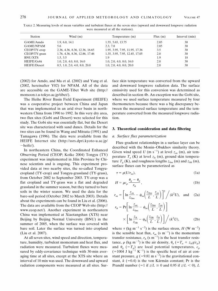
TABLE 2. Measuring levels of mean variables and turbulent fluxes at the seven sites (upward and downward longwave radiationwere measured at all the stations).

Station Wind (m) Temperature (m) Flux (m) Interval (min)

GAME/Amdo 1.9, 6.0, 14.1 1.55, 5.65, 13.75 2.85 30GAME/NPAM 5.6 2.3, 7.8 2.85 30CEOP/TY-crop 2.36, 4.36, 8.36, 12.36, 16.65 1.95, 3.95, 7.95, 11.95, 17.36 3.5 30CEOP/TY-grass 1.76, 4.36, 8.36, 12.86, 17.46 1.35, 3.95, 7.95, 12.45, 17.05 2.0 30BNU/XTS 1.5, 3.5 1.9 1.9 10HEIFE/Gobi 1.0, 2.0, 4.0, 8.0, 16.0 1.0, 2.0, 4.0, 8.0, 16.0 2.0 30HEIFE/Desert 0.5, 1.0, 2.0, 4.0, 8.0, 20.0 1.0, 2.0, 4.0, 8.0, 20.0 2.0 30


[�Tau2

*/(kgT*)] is the Obukhov length (m), u* [�(/)1/2] is the frictional velocity (m s�1), T* [��H/(cpu*)] is the frictional temperature (K), and m and h are the integrated stability correction terms for windand temperature profiles, respectively.

Following the universal functions in Högström (1996)and the mathematical form of the correction terms inPaulson (1970), for stable surface layers

�m�z0m

L,zm

L � � �5.3�zm � z0m� �L and �3a�

�h�z0h

L,zh

L � � �8.0�zh � z0h��L; �3b�

for unstable surface layers,

�m�z0m

L,zm

L � � 2 ln� 1 � x

1 � x0� � ln� 1 � x2

1 � x02�

� 2 tan�1x � 2 tan�1x0 and �4a�

�h�z0h

L,zh

L � � 2 ln� 1 � y

1 � y0�, �4b�

where x � (1 � 19zm /L)1/4, x0 � (1 � 19z0m /L)1/4, y �(1 � 11.6zh /L)1/2, and y0 � (1 � 11.6z0h /L)1/2.

The above bulk flux parameterization requiresroughness lengths z0m and z0h. In general, z0m and z0h

can be derived from turbulent flux data; however, wenormally want turbulent flux and hence need a param-eterization of z0m and z0h (or kB�1). Table 3 showsseveral parameterization schemes available in the lit-erature. Verhoef et al. (1997) introduced details ofSheppard (1958, hereinafter S58), Owen and Thomp-son (1963, hereinafter OT63), and B82. Zilitinkevich(1995, hereinafter Z95) has been widely used inweather forecasting models since Chen et al. (1997).Zeng and Dickinson (1998, hereinafter Z98) has beenused in a land surface model to unify undercanopy heattransfer processes between dense and sparse canopies(Zeng et al. 2005). K07 was derived from urban canopyexperiments. Yang et al. (2007b, hereinafter Y07b) hasbeen incorporated in a land data assimilation system forarid and semiarid regions. Y07b is a revised version ofYang et al. (2002) and a note is given in Table 3 for thisrevision. All the schemes in Table 3 will be evaluated insection 6.

b. Data filtering

To identify the major characteristics of turbulentheat transfer and to evaluate flux parameterizationschemes, parameters of z0m and �g (or Tg) are estimatedfrom the observed data. In this analysis, we excluded

the data under the following conditions, which deviatefar from the similarity theory:

min�Hprf, Hobs� � 0.5 max�Hprf, Hobs�, �5a�

��u*obs

U �2

� k2��lnzm

z0m� �m� z0m

Lobs,

zm

Lobs��2�

� �k2��lnzm

z0m�2�� 1, �5b�

Hobs � 0.8 min�HsfcS58, Hsfc

OT63, HsfcB82, Hsfc

Z95, HsfcZ98,

HsfcK07, Hsfc

Y07b�, �5c�

Hobs � 1.2 max�HsfcS58, Hsfc

OT63, HsfcB82, Hsfc

Z95, HsfcZ98,

HsfcK07, Hsfc

Y07b�, �5d�

z0h � 0.1zh, and �5e�

|H| � 10 W m�2, �5f�

where Hobs is the observed heat flux, Hprf is the fluxthat best fits observed wind and temperature profiles,and Hsfc is the flux derived from Eqs. (1)–(4) with ascheme in Table 3.

Equations (5a) and (5b) are the minimum require-ments to be applied for data filtering. Equations (5c)and (5d) are based on the assumption that the true heatflux should be within the range of heat flux values pre-dicted by the schemes in Table 3. This assumption is

TABLE 3. Flux parameterization schemes selected for this inter-comparison study; Re* � z0mu*/�, Pr � 0.71, k � 0.4, � is the fluidkinematical viscosity, � � 0.52 in OT63 and Z98, and � � 7.2 inY07b.

Formula Reference Abbreviation

kB�1 � ln(Pr � Re*

) Sheppard (1958) S58kB�1 � k�(8Re

*)0.45Pr0.8 Owen and Thomson

(1963)OT63

kB�1 � 2.46Re0.25* � 2 Brutsaert (1982) B82

kB�1 � 0.1Re0.5* Zilitinkevich (1995) Z95

kB�1 � k�Re0.45* Zeng and Dickinson

(1998)Z98

kB�1 � 1.29Re0.25* � 2 Kanda et al. (2007) K07

z0h � (70� /u*

)� exp(��u0.5

* |T*

| 0.25)Yang et al. (2007b) Y07b*

* Y07b is a revised scheme of Y02. The major difference isthat Y07b uses locally defined potential temperature [� �T (ps /p)Rd/cp, where ps is the surface pressure] while Y02 used aglobally defined one [� � T(p0 /p)Rd/cp, where p0 � 105 Pa].Because Y02 was based on data collected at highland sites, theuse of the globally defined �, which is nearly 20% larger than thelocally defined �, can be considered a miss in the analyses ofY02. Accordingly, the coefficient � in this table was changedfrom 10 in Y02 to 7.2 in Y07b. For the same reason, a statementin Y02 that B82 overestimates heat fluxes is questionable, andB82 is reevaluated in section 6.


generally true because some schemes in Table 3 over-estimate heat flux while others underestimate (see de-tails in section 6). This range is relaxed by 20% in Eqs.(5c) and (5d) because we cannot exclude the possibilitythat some data may lie beyond such a range. Equations(5e) and (5f) are applied to satisfy the similarity theoryand to consider the high sensitivity of kB�1 to measure-ment errors of small heat fluxes, respectively. In sum-mary, Eq. (5a) is applied to estimate z0m, Eqs. (5a) and(5b) are applied to estimate surface emissivity �s, Eqs.(5a)–(5d) are applied to evaluate schemes, and all areapplied to derive kB�1.

4. Determination of surface roughness length andemissivity

a. Aerodynamic roughness length

The aerodynamic roughness length, z0m, is physicallyrelated to the geometric roughness of underlying ele-ments for aerodynamically rough surfaces. It is not sen-sitive to diurnal variations of atmospheric stability (Sun1999). Kohsiek et al. (1993) estimated z0m from ob-served U/u* under near-neutral conditions. To derivestable and reliable z0m, Yang et al. (2003) suggestedfully using observed data under both neutral and non-neutral conditions. Following the idea, we estimated

z0m using a statistical method. The logarithmic windprofile is rewritten as

lnz0m � lnzm � �m�z0m

L,zm

L � � kU�u*. �6�

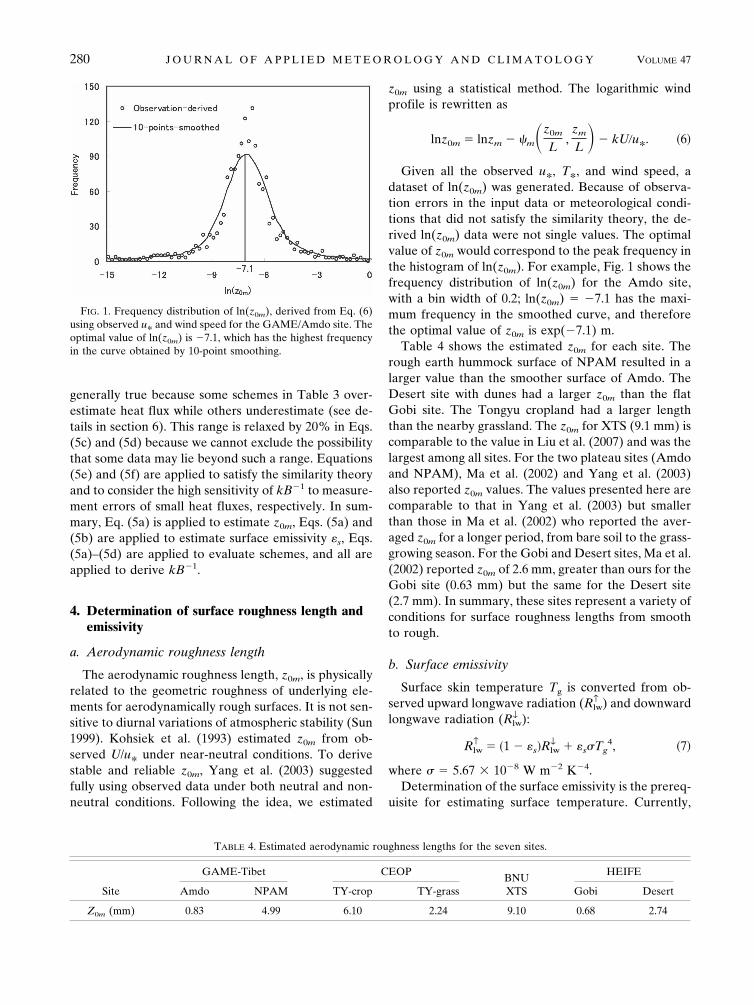
Given all the observed u*, T*, and wind speed, adataset of ln(z0m) was generated. Because of observa-tion errors in the input data or meteorological condi-tions that did not satisfy the similarity theory, the de-rived ln(z0m) data were not single values. The optimalvalue of z0m would correspond to the peak frequency inthe histogram of ln(z0m). For example, Fig. 1 shows thefrequency distribution of ln(z0m) for the Amdo site,with a bin width of 0.2; ln(z0m) � �7.1 has the maxi-mum frequency in the smoothed curve, and thereforethe optimal value of z0m is exp(�7.1) m.

Table 4 shows the estimated z0m for each site. Therough earth hummock surface of NPAM resulted in alarger value than the smoother surface of Amdo. TheDesert site with dunes had a larger z0m than the flatGobi site. The Tongyu cropland had a larger lengththan the nearby grassland. The z0m for XTS (9.1 mm) iscomparable to the value in Liu et al. (2007) and was thelargest among all sites. For the two plateau sites (Amdoand NPAM), Ma et al. (2002) and Yang et al. (2003)also reported z0m values. The values presented here arecomparable to that in Yang et al. (2003) but smallerthan those in Ma et al. (2002) who reported the aver-aged z0m for a longer period, from bare soil to the grass-growing season. For the Gobi and Desert sites, Ma et al.(2002) reported z0m of 2.6 mm, greater than ours for theGobi site (0.63 mm) but the same for the Desert site(2.7 mm). In summary, these sites represent a variety ofconditions for surface roughness lengths from smoothto rough.

b. Surface emissivity

Surface skin temperature Tg is converted from ob-served upward longwave radiation (R↑

lw) and downwardlongwave radiation (R↓

lw):

Rlw↑ � �1 � s�Rlw

↓ � sTg4, �7�

where � � 5.67 � 10�8 W m�2 K�4.Determination of the surface emissivity is the prereq-

uisite for estimating surface temperature. Currently,

FIG. 1. Frequency distribution of ln(z0m), derived from Eq. (6)using observed u* and wind speed for the GAME/Amdo site. Theoptimal value of ln(z0m) is �7.1, which has the highest frequencyin the curve obtained by 10-point smoothing.

TABLE 4. Estimated aerodynamic roughness lengths for the seven sites.

Site

GAME-Tibet CEOPBNUXTS

HEIFE

Amdo NPAM TY-crop TY-grass Gobi Desert

Z0m (mm) 0.83 4.99 6.10 2.24 9.10 0.68 2.74


there is no reliable method for its estimation. For ex-ample, Stewart et al. (1994) simply assumed �s � 1while Verhoef et al. (1997) assumed �s varying from0.91 to 0.94. There was no direct evidence to justify suchselection for different study sites. In this study, we useda physically based, semiempirical method to estimate�s. According to heat transfer theory, heat flux (positiveif upward) must have the same sign as that of �g(�s) ��a; that is,

Hsfc � �cp��g�s� � �a��rh. �8�

Under near-neutral conditions, if �s is either overes-timated or underestimated slightly, then the estimatedHsfc may have the sign opposite to the observed Hobs;therefore, the difference between Hsfc and Hobs is sen-sitive to the value of �s. Considering this sensitivity, weestimated �s using near-neutral heat fluxes by minimiz-ing the root-mean-square difference (RMS) betweenHobs and Hsfc.

The emissivity is assumed to be a constant through-out the observing period for each site, though it maychange with soil moisture. The algorithm is as follows:1) Given �s, estimate surface temperature Tg(�s) by Eq.(7). 2) If �10 W m�2 � Hobs � 30 W m�2 then calculateHsfc from Eqs. (2)–(4) and Eq. (8), with z0m in Table 4and z0h given by a kB�1 scheme. Note that small heatflux may occur in very stable cases and these casesshould be rejected. 3) Calculate the RMS between Hobs

and Hsfc. 4) Go back to step 1 until RMS(�s) is mini-mized.

Figure 2 shows the variation of RMS with �s for theAmdo site. It is clear that the �s value corresponding tothe minimum RMS is not very sensitive to the choice ofkB�1 schemes. Similar conclusions for other sites canbe drawn from Table 5. However, the estimated valuesseemed too low for XTS (0.855) and too high forNPAM (1.055); thus the values were adjusted to be 0.9for XTS and 1.0 for NPAM in the following analyses.These unrealistic values can be attributed to errors inmeasured R ↑

lw in Eq. (7) or the mismatch of footprintsbetween the radiation measurements and turbulent fluxmeasurements.

5. Characteristics of turbulent flux transfer

a. Diurnal variation of kB�1

Given z0m, �g, U, and �a, kB�1 can be inversely de-rived from Hobs through the following iterations: 1) as-sume z0h � z0m, 2) calculate Hsfc from Eqs. (1)–(4) withan analytical solution of Yang et al. (2001); 3) if Hsfc �Hobs then adjust kB�1 according to the difference inheat transfer resistance; 4) go back to step 2 until Hsfc �Hobs. If there were multiple combinations of wind speedand air temperature, then kB�1 was calculated for eachcombination and their average was used in the analysis.

Figure 3 shows that kB�1 exhibited a large variabilityat each site and diurnal variations were particularly ob-vious at Amdo and NPAM sites, with higher valuesduring the day and lower values at night. Figure 4ashows mean values and standard deviations of kB�1 forthe individual sites in ascending order of z0m. Becauseof the diurnal variations, data have been grouped intotwo classes: an H � 0 (or daytime) case and an H � 0(or nighttime) case; kB�1 generally increased with re-spect to z0m, but this tendency was contaminated by itslarge variance (1.6–3.2) at night when the derived kB�1

was more sensitive to measurement errors of heat flux.

FIG. 2. Emissivity dependence of RMS between observed near-neutral heat fluxes and parameterized heat fluxes for the GAME/Amdo site. The optimal value of surface emissivity (�0.97) cor-responds to the minimum RMS.

TABLE 5. Estimated surface emissivity for the seven sites exceptthe Gobi, using different kB�1. The estimated values seem toolow for XTS and too high for NPAM, and thus the optimal valuewas adjusted to be 0.9 for XTS and 1.0 for NPAM in this study.

kB�1

scheme

GAME-Tibet CEOPBNUXTS

HEIFEDesertAmdo NPAM TY-crop TY-grass

S58 0.968 1.053 0.948 0.958 0.848 0.924OT63 0.972 1.055 0.956 0.966 0.855 0.928B82 0.966 1.051 0.936 0.952 0.835 0.922Z95 0.968 1.054 0.946 0.958 0.850 0.926Z98 0.976 1.064 0.976 0.976 0.869 0.934K07 0.976 1.058 0.966 0.972 0.862 0.932Y07b 0.976 1.053 0.964 0.970 0.865 0.930Mean 0.972 1.055 0.956 0.964 0.855 0.928


Also, it is clear that the diurnal variability of kB�1 atindividual sites (Fig. 3) was larger than or comparableto its cross-site variability (Fig. 4a).

Figure 4b shows the mean values of z0h for each site.It indicates the mean z0h does not significantly changewith z0m. Therefore, the concept of kB�1, which scalesz0h by z0m, is questionable. Accordingly, the heat trans-fer coefficient CH increases with respect to z0m, but itsincrease is not as fast as for the momentum transfercoefficient CD, as shown in Figs. 4c,d. (Note CH and CD

are the transfer coefficient values that have been nor-malized to a height of 10 m so that they are comparableat the individual sites.) Mahrt (1996) speculated thatindividual roughness elements may enhance momen-tum transfer through form drag but contribute little to

area-averaged heat transfer. According to our results,this speculation is partially true and it may be moreappropriate to say that the increase of surface rough-ness lengths contributes more to momentum transferthan to heat transfer.

b. Negative values of kB�1

Verhoef et al. (1997) reported negative kB�1 valuesfor a nearly aerodynamically smooth bare-soil surface(Re* � 1), which is consistent with those predicted bytheory (Kondo 1975; B82). In this study, all the siteswere aerodynamically rough. Momentum transfer foraerodynamically bluff and rough flows is traditionallyconsidered to be more efficient than heat transfer (orkB�1 � 0) because momentum transfer can be en-

FIG. 3. The kB�1 values derived from observed heat fluxes, temperature, and wind speed for the individual sites; (a)–(g) shown inthe ascending order of z0m.


hanced through form drag. However, a number ofnegative values of kB�1 occurred during the night forthese surfaces. This finding indicates that heat transferefficiency can exceed momentum transfer, which wasalso reported by Su et al. (2001) for forced convection.

However, there is a lack of theory to explain such amechanism. Possibly, our findings can result from thebreakdown of the Monin–Obukhov similarity theorydue to interactions between active and inactive turbu-lence in the atmospheric surface layer (ASL). Choi etal. (2004) reported a lower efficiency of momentumexchange over a Tibetan site than over terrains at lowaltitudes. Unlike the similar magnitudes of transfer ef-ficiency of heat and water vapor, momentum exchangewas less efficient than the Monin–Obukhov similarityprediction. Recent experimental results show that inac-tive motions play an important role in the ASL andtransport processes are sensitive to outer-layer scalingparameters such as boundary layer depth (e.g., Mc-Naughton 2004; Hong et al. 2004). In fact, the above-mentioned diurnal variations of kB�1 could be attrib-uted to those of boundary layer depth and the associ-ated roles of inactive (nonlocal) eddies in the outerlayer. Interestingly, for two Tibetan sites, Hong et al.

(2004) reported that such inactive eddies in low fre-quencies did not affect momentum flux but caused heatflux to deviate from the Monin–Obukhov similaritytheory.

c. Excess resistance

Heat transfer resistance rh is linked with z0h or kB�1

through Eq. (2b), and a small z0h would result in a largeresistance. Table 6 shows mean values of observedrh and heat flux Hobs, together with mean values ofaerodynamic resistance rah derived with kB�1 � 0 andthe associated heat flux Hest. The excess resistance �r(�rh � rah) usually increases with z0m and is largerduring the day than at night. For some surfaces, theexcess resistance even becomes negative at night. Theexcess heat flux �H (�Hest � Hobs) during the day ismuch larger than at night. So the daytime excess resis-tance affects heat transfer far more than that of night-time, because of smaller total resistance during the day.Heat flux parameterized with kB�1 � 0 is nearly doublethe observed for the daytime period and rough sur-faces, strongly suggesting the necessity to account forthe excess resistance in bulk flux parameterizations.

FIG. 4. Mean values and variances of (a) kB�1, (b) ln(z0h), (c) bulk transfer coefficient for momentum CD, and (d) bulk transfercoefficient for heat CH for the individual sites. Data have been grouped into classes for H � 0 and H � 0; CH and CD are the transfercoefficients from surface to 10-m height.


d. Comparisons with previous experiments andtheories

Figure 5 shows mean kB�1 for each site of this study(for both H � 0 and H � 0 cases) and other bare-soilexperimental data in the literature (Kohsiek et al. 1993;Stewart et al. 1994; Verhoef et al. 1997), formula B82for bluff-rough surfaces, formula K07 for urban cano-pies, and the value �1.1 of Kondo (1975) for aerody-namically smooth surfaces. Our mean kB�1 values werelarger than that of Verhoef et al. (1997) while smallerthan or close to that of Kohsiek et al. (1993) and Stew-art et al. (1994), because kB�1 increased with z0m andour surfaces were rougher (z0m � 0.7–9 mm) than theformer study (z0m � 0.1 mm) while smoother than orcomparable to the latter two studies (z0m � 13 mm).Therefore, all of the experimental results in previousstudies are essentially consistent with our findings. Forthe two plateau sites (Amdo and NPAM), the diurnalvariations of kB�1 have been reported by Ma et al.(2002) and Yang et al. (2003). However, the reportedmean values were different from our study becausethey either included a vegetated period or used a dif-ferent criterion for data filtering.

6. Evaluation of kB�1 schemes

a. Intercomparisons of kB�1

Schemes for kB�1 are developed to derive u* and T*,which in turn are variables of the schemes in Table 3.Therefore, the following numerical iteration algorithmwas applied to derive kB�1: 1) assume kB�1 � 0; 2)

derive the value of z0h by z0h � z0m exp(�kB�1); 3)given z0m and z0h, calculate u*, T*, and Hsfc from Eqs.(1)–(4) with an analytical solution of Yang et al. (2001);4) given u* and T*, calculate kB�1 according to one ofthe schemes in Table 3; 5) go to step 2 until the differ-ence in T* between two successive iterations is less than0.0001 K, a threshold value used in this study. Table 7shows the correlation coefficient squared R2 betweenobserved kB�1 (in Fig. 3) and that parameterized withschemes in Table 1. Except for the sites with a smallnumber of data samples (Gobi and Desert), Y07b givesa higher R2 than other schemes. Figure 6 shows com-

FIG. 5. Variations of mean kB�1 with roughness Reynolds num-ber Re* (�z0mu*/�). Experimental data: present study (cases forH � 0 and H � 0), Verhoef et al. (1997), Kohsiek et al. (1993), andStewart et al. (1994). Theoretical or empirical formulas: B82, K07,and Kondo’s (1975) (kB�1 � �1.1).

TABLE 6. Mean values of aerodynamic parameters, resistance (rh: total resistance for heat transfer, derived from observed fluxes; rah:resistance calculated with kB�1 � 0; �r : excess resistance (�rh � rah), and heat fluxes (Hobs: observed fluxes; Hest: fluxes calculated withkB�1 � 0; �H: excess heat fluxes (�Hest � Hobs). Sites are listed in the ascending order of z0m.

Class Station Samplez0m

(mm)

kB�1 Resistance (s m�1) Flux (W m�2)

Avg Std rh rah �r Hobs Hest �H

H � 0 Gobi 92 0.68 0.70 1.00 93.1 85.0 8.2 149.7 170.3 20.6Amdo 306 0.83 2.36 1.36 76.0 57.7 18.2 183.6 259.3 75.7TY-grass 1186 2.24 3.64 1.82 104.3 65.8 38.6 74.5 126.4 51.9Desert 60 2.74 2.74 1.73 86.5 57.8 28.7 138.7 215.6 76.9NPAM 489 4.99 3.40 1.45 64.2 38.4 25.9 135.6 228.8 93.2TY-crop 758 6.10 4.49 2.22 93.2 50.5 42.8 91.6 181.0 89.4XTS 660 9.10 2.84 1.96 91.5 53.5 38.1 108.2 198.9 90.7

H � 0 Gobi 45 0.68 0.87 2.24 191.5 188.6 2.9 �13.6 �15.0 �1.4Amdo 153 0.83 0.15 2.20 209.6 220.5 �10.9 �13.6 �14.1 �0.6TY-grass 1068 2.24 2.06 2.23 174.1 160.8 13.3 �20.0 �24.1 �4.1Desert 15 2.74 2.10 2.17 149.3 132.2 17.1 �18.1 �22.4 �4.3NPAM 195 4.99 1.74 2.00 87.4 74.4 12.9 �21.9 �25.6 �3.7TY-crop 81 6.10 1.46 3.16 216.4 218.5 �2.1 �14.6 �18.0 �3.4XTS 63 9.10 1.70 1.64 191.2 169.8 21.4 �14.4 �17.0 �2.6


parisons of composite diurnal variations of kB�1 be-tween observation and schemes for the individual sites.The composite values for a time slot were calculatedonly when there was enough data (i.e., sample num-ber �5). All of the schemes parameterized with Re*produced a general increase in kB�1 with respect to

z0m. Overall, S58 and OT63 produced kB�1 more orless comparable to the observed values, but otherschemes either overestimated or underestimated sig-nificantly. No scheme produced clear diurnal variationsand negative values of kB�1 (as observed in section 5)except Y07b, which gave better agreements.

FIG. 6. Comparisons between composite diurnal variations of observed kB�1 and the scheme-predicted one for the seven bare-soil sites.

TABLE 7. Correlation coefficient squared between observed kB�1 (in Fig. 3) and that parameterized with schemes in Table 3. Thetwo columns Gobi and Desert have small numbers of samples (see Table 6 sample column).

Scheme Gobi Amdo TY-grass Desert NPAM TY-crop XTS

S58 0.33 0.60 0.50 0.38 0.26 0.60 0.51OT63 0.31 0.60 0.48 0.36 0.26 0.59 0.53B82 0.32 0.60 0.49 0.37 0.26 0.60 0.52Z95 0.31 0.60 0.48 0.36 0.26 0.59 0.53Z98 0.31 0.60 0.48 0.36 0.26 0.59 0.53K07 0.32 0.60 0.49 0.37 0.26 0.60 0.52Y07b 0.25 0.68 0.59 0.39 0.45 0.66 0.56


In fact, the different performance between Y07b andother schemes is not surprising. The former usesu0.5

* |T*|0.25 to parameterize kB�1, and therefore the di-urnal variation of kB�1 can be accounted for with T*.Other schemes use u* or Re* for the parameterization[ln(Re*) in S58; Re0.25

* in B82 and K07; Re0.45

* in OT63and Z98; and Re0.5

* in Z95]. This suggests a parametercombining both u* and T* can be a potential index formore realistic parameterizations of kB�1.

b. Intercomparisons of turbulent fluxes

At our sites wind speed and air temperature weremeasured at multiple levels, so there were many com-binations of wind speed and air temperature. Bulk pa-rameterization with these different combinations andsurface conditions (surface skin temperature androughness lengths) may result in different flux. The fol-lowing evaluation is based on the combination thatgives the minimum root-mean-square error (RMSE) inheat flux.

All of the schemes produced similar mean biases(MBE) and RMSE in momentum flux for all the sites(data not shown). However, the errors in heat flux weredistinct. Tables 8 and 9 show MBE in predicted heatflux and the standard deviation of the difference be-tween the observed and the predicted, respectively. Theboldface numbers represent the three best schemes.The two indices show that Y07b is among the three bestschemes for all sites and it has the smallest errors onaverage. OT63 and S58 also have small errors except at

XTS for S58 and at Amdo for OT63. B82 producesgood results for Amdo and TY-grass but tends to un-derestimate heat flux for other sites. Three otherschemes (Z95; Z98; K07) clearly overestimate flux forall sites. K07 has small errors for the roughest site(XTS) because K07 was fitted with urban canopy data.Recalling Fig. 6, it is clear that a scheme that gives high(low) kB�1 values has produced low (high) heat flux.

c. Sensitivity analyses

First, the sensitivity to the surface emissivity was in-vestigated. We calculated heat flux with surface emis-sivity varying from 0.85 to 1.0 for all sites except forGobi, where the ground temperature was directly mea-sured by four thermometers. Figures 7 and 8 show thevariations of RMSE and R2 with emissivity, respec-tively. The vertical dashed line in each panel corre-sponds to the optimal emissivity value in Table 5. De-spite some uncertainties in determining the emissivity,Y07b obviously gives small RMSE and the highest R2

values over a range near the optimal emissivity, show-ing better prediction than other schemes.

Second, the sensitivity to universal functions for sta-bility correction was tested. We applied Dyer’s (1974)universal functions to the analyses, in comparison toHögström’s (1996) universal functions used above.Only minor changes in errors and the similar overallperformance (data not shown) suggest our results arenot sensitive to universal functions of the similaritytheory.

TABLE 9. Similar to Table 8, but for std dev (W m�2) of the difference between observed and predicted heat fluxes.

Scheme Gobi Amdo TY-grass Desert NPAM TY-crop XTS Avg

S58 13.8 19.2 10.1 25.0 18.6 16.6 28.3 18.8OT63 12.7 31.6 14.6 28.2 18.9 18.3 25.7 21.4B82 16.8 16.5 9.1 26.6 23.3 15.7 32.1 20.0Z95 18.1 53.9 32.9 51.8 50.8 51.7 66.2 46.5Z98 15.6 47.7 27.4 43.5 39.4 39.7 47.3 37.2K07 16.9 45.9 21.2 34.7 26.7 26.4 30.1 28.8Y07b 14.1 14.0 12.8 23.6 18.7 16.7 24.6 17.8

TABLE 8. MBE (W m�2) in heat fluxes produced by the seven schemes for the seven sites. Boldface numbers are the best threeamong these schemes.

Scheme Gobi Amdo TY-grass Desert NPAM TY-crop XTS Avg (MBE) Avg (|MBE|)

S58 �8.7 5.6 1.6 �8.5 �4.5 �2.6 �17.3 �4.9 8.1OT63 �2.0 19.3 7.1 3.0 5.9 5.8 �8.3 4.4 8.6B82 �13.5 �0.6 �0.4 �11.2 �15.2 �7.9 �30.4 �11.3 13.2Z95 8.1 41.5 21.0 40.8 49.6 56.6 54.7 38.9 45.4Z98 4.5 35.5 17.0 29.9 36.2 40.3 32.6 28.0 32.7K07 7.5 36.4 12.6 18.5 20.1 20.5 7.9 17.6 20.6Y07b �0.8 2.9 6.8 �1.3 �3.6 6.6 �6.3 0.6 4.7


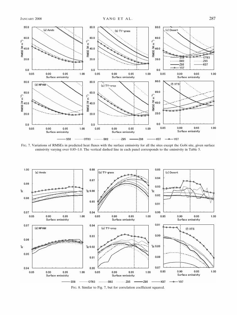
FIG. 8. Similar to Fig. 7, but for correlation coefficient squared.

FIG. 7. Variations of RMSEs in predicted heat fluxes with the surface emissivity for all the sites except the Gobi site, given surfaceemissivity varying over 0.85–1.0. The vertical dashed line in each panel corresponds to the emissivity in Table 5.


d. The role of diurnal variation of kB�1

Understanding the diurnal variation of kB�1 is im-portant in estimating heat flux. Figure 9 shows the av-eraged diurnal variations of relative mean biases in heatflux prediction for the seven sites. OT63, Z95, Z98, andK07 produce clear diurnal variation of errors in heatflux, positive biases during the day, and negative biasesat night. S58 and B82 underestimate flux for almost alltime slots. Y07b shows no more than 10% mean bias forall time slots, indicating its capability to reflect the di-urnal variation of kB�1. In summary, it is important fora scheme to give not only the mean value but also thediurnal variation of kB�1.

7. Conclusions and comments

Understanding the characteristics of turbulent trans-fer over bare-soil surfaces is crucial for parameterizingturbulent flux over nonvegetated surfaces. We pre-sented a comprehensive analysis on characteristics ofheat transfer over bare-soil surfaces in arid and semi-arid regions and also an extensive evaluation of severalschemes in the literature. The major findings from ourstudy are as follows:

1) Mean z0h does not change significantly with z0m, andtherefore there was no robust basis to parameterizez0h through kB�1 or z0m, although it is widely used.Observations also indicated that the heat transfercoefficient increases with z0m but not as much as themomentum transfer coefficient does.

2) Diurnal variations of z0h are common for all thebare-soil surfaces. The diurnal variability of kB�1 atindividual sites can be larger than or comparable to

cross-site variability. This indicates that z0h andkB�1 are flow dependent and the consideration ofboth u* and T* is important for improving flux pa-rameterization.

3) Diurnal variations of kB�1 cause much larger exces-sive heat transfer resistances during the day than atnight. Using a mean value of kB�1 may lead to sig-nificant overestimation (underestimation) in thedaytime (nighttime). A complete neglect of this re-sistance may give rise to more than 50% overesti-mation of heat flux in the daytime for rough sur-faces.

4) Negative values of kB�1 are often observed foraerodynamically rough surfaces, requiring theoreti-cal explanations. Such occurrence indicates heattransfer efficiency may exceed that of momentumtransfer, or the excess resistance for heat transfercan become negative if the aerodynamic transfer re-sistance becomes too large. This is in contrast to thetraditional opinion that momentum transfer is moreefficient than heat transfer because of the enhancedmomentum transfer through form drag around indi-vidual roughness elements (Thom 1972; Roth 1993).This “abnormal” phenomenon may be attributed toheat transport by inactive (nonlocal) eddies in theouter layer.

5) All of the parameterization schemes consideredhere perform equally well for momentum flux pre-diction, but they show different skills for heat fluxprediction. In general, the schemes parameterizedwith u* cannot produce the diurnal variations ofkB�1 whereas a scheme (Y07b) parameterized withu* and T* does. For the sites with z0m ranging from�1 to 10 mm, most schemes either significantly un-derestimate or overestimate heat flux. Y07b gener-ally performs better for these land sites and may bea better choice to be incorporated into current landsurface models.

Last, we have not considered in this study the poten-tial problem in surface energy budget closure that hasbeen widely observed (e.g., Twine et al. 2000; Wilson etal. 2002; Baker and Griffis 2005). If future work con-firms that the reported sensible heat flux was underes-timated by the current eddy-covariance technique,kB�1 and excessive resistance should have smaller val-ues than reported here. In accord with this, the Y07bscheme and/or other schemes would require recalibra-tions, but most of the above conclusions should be stillvalid.

Acknowledgments. The GAME-Tibet project wassupported by the MEXT, JST, FRSGC, and NASDA of

FIG. 9. The diurnal variation of the seven sites’ composite rela-tive mean biases in heat flux. Diurnal variation of relative meanbiases for each site was made first, and then averaged over theseven sites to obtain the composite one.


Japan, the Chinese Academy of Sciences, and the AsianPacific Network, and Dr. Kenji Tanaka from Kuma-moto University provided turbulent flux data for theAmdo site. The CEOP/Tongyu project was supportedby Institute of Atmospheric Physics, CAS. The Xiao-tangshan experiment was supported by an NSFCProject (40671128) and the GEF Project (TF053183) ofChina. HEIFE was a cooperative project betweenChina and Japan and implemented by DPRI, KyotoUniversity, Japan, and Lanzhou Institute of Plateau At-mospheric Science of CAS. Joon Kim acknowledgesthe support from the Eco-Technopia 21 Project of theMinistry of Environment and the BK21 program of theMinistry of Education and Human Resource of Korea.We are grateful to the reviewers whose suggestions anddiscussions have helped the authors to improve thequality of the paper.

REFERENCES

Baker, J. M., and T. J. Griffis, 2005: Examining strategies to im-prove the carbon balance of corn/soybean agriculture usingeddy covariance and mass balance techniques. Agric. For.Meteor., 128, 163–177.

Beljaars, A. C. M., and A. A. M. Holtslag, 1991: Flux parameter-ization over land surfaces for atmospheric models. J. Appl.Meteor., 30, 327–341.

Blümel, K., 1999: A simple formula for estimation of the rough-ness length for heat transfer over partly vegetated surfaces. J.Appl. Meteor., 38, 814–829.

Brutsaert, W. H., 1982: Evaporation Into the Atmosphere: Theory,History, and Applications. D. Reidel, 299 pp.

Chen, F., Z. Janjic, and K. Mitchell, 1997: Impact of atmosphericsurface-layer parameterizations in the new land-surfacescheme of the NCEP Mesoscale Eta Model. Bound.-LayerMeteor., 85, 391–421.

Choi, T., and Coauthors, 2004: Turbulent exchange of heat, watervapor, and momentum over a Tibetan prairie by eddy cova-riance and flux variance measurements. J. Geophys. Res., 109,D21106, doi:10.1029/2004JD004767.

Dyer, A. J., 1974: A review of flux-profile relationships. Bound.-Layer Meteor., 7, 363–372.

Garratt, J. R., and R. J. Francey, 1978: Bulk characteristics of heattransfer in the unstable, baroclinic atmospheric boundarylayer. Bound.-Layer Meteor., 15, 399–421.

Högström, U., 1996: Review of some basic characteristics of theatmospheric surface layer. Bound.-Layer Meteor., 78, 215–246.

Hong, J., T. Choi, H. Ishikawa, and J. Kim, 2004: Turbulencestructures in the near-neutral surface layer on the TibetanPlateau. Geophys. Res. Lett., 31, L15106, doi:10.1029/2004GL019935.

Kanda, M., M. Kanega, T. Kawai, R. Moriwaki, and H. Sugawara,2007: Roughness lengths for momentum and heat derivedfrom outdoor urban scale models. J. Appl. Meteor. Climatol.,46, 1067–1079.

Kohsiek, W., H. A. R. de Bruin, H. The, and B. van den Hurk,1993: Estimation of the sensible heat flux of a semi-arid areausing surface radiative temperature measurements. Bound.-Layer Meteor., 63, 213–230.

Koike, T., 2004: The Coordinated Enhanced Observing Period—An initial step for integrated global water cycle observation.WMO Bull., 53, 1–8.

——, T. Yasunari, J. Wang, and T. Yao, 1999: GAME–Tibet IOPsummary report. Proc. First Int. Workshop on GAME–Tibet,Xi’an, China, Chinese Academy of Sciences and JapaneseNational Committee for GAME, 1–2.

Kondo, J., 1975: Air-sea bulk transfer coefficients in diabatic con-ditions. Bound.-Layer Meteor., 9, 91–112.

Kustas, W. P., B. J. Choudhury, M. S. Moran, R. J. Reginato,R. D. Jackson, L. W. Gay, and H. L. Weaver, 1989: Determi-nation of sensible heat flux over sparse canopy using thermalinfrared data. Agric. For. Meteor., 44, 197–216.

Liu, H.-Z., G. Tu, W.-J. Dong, C.-B. Fu, and L.-Q. Shi, 2006:Seasonal and diurnal variations of the exchange of water va-por and CO2 between the land surface and atmosphere in thesemi-arid area (in Chinese). Chin. J. Atmos. Sci., 30, 108–118.

Liu, S., L. Lu, D. Mao, and L. Jia, 2007: Evaluating parameter-izations of aerodynamic resistance to heat transfer using fieldmeasurements. Hydrol. Earth Syst. Sci., 11, 769–783.

Ma, Y., O. Tsukamoto, J. Wang, H. Ishikawa, and I. Tamagawa,2002: Analysis of aerodynamic and thermodynamic param-eters on the grassy marshland surface of Tibetan Plateau.Prog. Nat. Sci., 12, 36–40.

Mahrt, L., 1996: The bulk aerodynamic formulation over hetero-geneous surfaces. Bound.-Layer Meteor., 78, 87–119.

——, and D. Vickers, 2004: Bulk formulation of the surface heatflux. Bound.-Layer Meteor., 110, 357–379.

McNaughton, K. G., 2004: Turbulence structure of the unstableatmospheric surface layer and transition to the outer layer.Bound.-Layer Meteor., 112, 199–221.

Owen, P. R., and W. R. Thomson, 1963: Heat transfer acrossrough surfaces. J. Fluid Mech., 15, 321–334.

Paulson, C. A., 1970: The mathematical representation of windspeed and temperature profiles in the unstable atmosphericsurface layer. J. Appl. Meteor., 9, 857–861.

Roth, M., 1993: Turbulent transfer relationships over an urbansurface. II: Integral statistics. Quart. J. Roy. Meteor. Soc., 119,1105–1120.

Sheppard, P. A., 1958: Transfer across the earth’s surface andthrough the air above. Quart. J. Roy. Meteor. Soc., 84, 205–224.

Stewart, J. B., W. P. Kustas, K. S. Humes, W. D. Nichols, M. S.Moran, and H. A. R. de Bruin, 1994: Sensible heat flux-radiometric surface temperature relationship for eight semi-arid areas. J. Appl. Meteor., 33, 1110–1117.

Su, Z., T. Schmugge, W. P. Kustas, and W. J. Massman, 2001: Anevaluation of two models for estimation of the roughnessheight for heat transfer between the land surface and theatmosphere. J. Appl. Meteor., 40, 1933–1951.

Sugita, M., and A. Kubota, 1994: Radiometrically determined skintemperature and scalar roughness to estimate surface heatflux. Part II: Performance of parameterized scalar roughnessfor the determination of sensible heat. Bound.-Layer Meteor.,70, 1–12.

Sun, J., 1999: Diurnal variations of thermal roughness height overa grassland. Bound.-Layer Meteor., 92, 407–427.

Tamagawa, I., 1996: Turbulent characteristics and bulk transfercoefficients over the desert in the HEIFE area. Bound.-LayerMeteor., 77, 1–20.

Tanaka, K., H. Ishikawa, T. Hayashi, I. Tamagawa, and Y. Ma,2001: Surface energy budget at Amdo on the Tibetan Plateau


using GAME/Tibet IOP98 data. J. Meteor. Soc. Japan, 79,505–517.

Thom, A. S., 1972: Momentum, mass and heat exchange of veg-etation. Quart. J. Roy. Meteor. Soc., 98, 124–134.

Twine, T. E., and Coauthors, 2000: Correcting eddy-covarianceflux underestimates over a grassland. Agric. For. Meteor.,103, 279–300.

Verhoef, A., H. A. R. de Bruin, and B. J. J. M. van den Hurk,1997: Some practical notes on the parameter kB-1 for sparsevegetation. J. Appl. Meteor., 36, 560–572.

Voogt, J. A., and C. S. B. Grimmond, 2000: Modeling surfacesensible heat flux using surface radiative temperatures in asimple urban area. J. Appl. Meteor., 39, 1679–1699.

Wang, J., and Y. Mitsuta, 1991: Turbulence structure and transfercharacteristics in the surface layer of the HEIFE Gobi area.J. Meteor. Soc. Japan, 69, 587–593.

Wieringa, J., 1993: Representative roughness parameters for ho-mogeneous terrain. Bound.-Layer Meteor., 63, 323–363.

Wilson, K. A., and Coauthors, 2002: Energy balance closure atFLUXNET sites. Agric. For. Meteor., 113, 223–243.

Yang, K., N. Tamai, and T. Koike, 2001: Analytical solution ofsurface layer similarity equations. J. Appl. Meteor., 40, 1647–1653.

——, T. Koike, H. Fujii, K. Tamagawa, and N. Hirose, 2002: Im-

provement of surface flux parameterizations with a turbu-lence-related length. Quart. J. Roy. Meteor. Soc., 128, 2073–2087.

——, ——, and D. Yang, 2003: Surface flux parameterization inthe Tibetan Plateau. Bound.-Layer Meteor., 106, 245–262.

——, and Coauthors, 2007a: Initial CEOP-based review of theprediction skill of operational general circulation models andland surface models. J. Meteor. Soc. Japan, 85, 99–116.

——, T. Watanabe, T. Koike, X. Li, H. Fujii, K. Tamagawa, Y.Ma, and H. Ishikawa, 2007b: Auto-calibration system devel-oped to assimilate AMSR-E data into a land surface modelfor estimating soil moisture and the surface energy budget. J.Meteor. Soc. Japan, 85, 229–242.

Zeng, X., and R. E. Dickinson, 1998: Effect of surface sublayer onsurface skin temperature and fluxes. J. Climate, 11, 537–550.

——, ——, M. Barlage, Y. Dai, G. Wang, and K. Oleson, 2005:Treatment of undercanopy turbulence in land models. J. Cli-mate, 18, 5086–5094.

Zilitinkevich, S. S., 1995: Non-local turbulent transport: Pollutiondispersion aspects of coherent structure of convective flows.Air Pollution Theory and Simulation, H. Power, N. Mous-siopoulos, and C. A. Brebbia, Eds., Vol. I, Air Pollution III,Computational Mechanics Publications, 53–60.


Turbulent Flux Transfer over Bare-Soil Surfaces: Characteristics and Parameterization

Documents

Transcript of Turbulent Flux Transfer over Bare-Soil Surfaces: Characteristics and Parameterization