materials

Article

An Efficient Computational Model for Magnetic Pulse Formingof Thin Structures

Mohamed Mahmoud *,† , François Bay † and Daniel Pino Muñoz †

Citation: Mahmoud, M.; Bay, F.;

Pino Muñoz, D. An Efficient

Computational Model for Magnetic

Pulse Forming of Thin Structures.

Materials 2021, 14, 7645. https://

doi.org/10.3390/ma14247645

Academic Editors: Mateusz Kopec

and Denis Politis

Received: 10 November 2021

Accepted: 8 December 2021

Published: 12 December 2021

Publisher’s Note: MDPI stays neutral

with regard to jurisdictional claims in

published maps and institutional affil-

iations.

Copyright: © 2021 by the authors.

Licensee MDPI, Basel, Switzerland.

This article is an open access article

distributed under the terms and

conditions of the Creative Commons

Attribution (CC BY) license (https://

creativecommons.org/licenses/by/

4.0/).

MINES Paris-Tech, PSL-Research University, CEMEF—Center for Material Forming, CNRS UMR 7635, BP 207,1 Rue ClaudeDaunesse, CEDEX, 06904 Sophia Antipolis, France; francois.bay@mines-paristech.fr (F.B.);daniel.pino_munoz@mines-paristech.fr (D.P.M.)* Correspondence: mohamed.mahmoud@mines-paristech.fr† These authors contributed equally to this work.

Abstract: Electromagnetic forming (EMF) is one of the most popular high-speed forming processesfor sheet metals. However, modeling this process in 3D often requires huge computational timesince it deals with a strongly coupled multi-physics problem. The numerical tools that are capable ofmodeling this process rely either on shell elements-based approaches or on full 3D elements-basedapproaches. The former leads to reduced computational time at the expense of the accuracy, whilethe latter favors accuracy over computation time. Herein, a novel approach was developed to reduceCPU time while maintaining reasonable accuracy through building upon a 3D finite element analysistoolbox which was developed in CEMEF. This toolbox was used to solve magnetic pulse forming(MPF) of thin sheets. The problem was simulated under different conditions and the results wereanalyzed in-depth. Innovative techniques, such as developing a termination criterion and usingadaptive re-meshing, were devised to overcome the encountered problems. Moreover, a solid shellelement was implemented and tested for thin structure problems and its applicability was verified.The results of this element type were comparable to the results of the standard tetrahedral MINIelement but with reduced simulation time.

Keywords: high-speed forming; magnetic pulse forming; computational mechanics; solid-shell finiteelement

1. Introduction

Lightweight structures have many applications, especially in aerospace and auto-motive industries. The huge demand on lightweight structures requires improvementsin the forming processes that would lead to cost reduction while maintaining struc-tural resistance. High-speed forming processes, such as explosive forming discussedby Mynors and Zhang [1], electro-hydraulic forming (EHF) by Rohatgi et al. [2] and elec-tromagnetic forming (EMF) by Zittel [3], have been proposed in the literature to overcomethe disadvantages of the conventional forming methods. The study of these problemshas been cumbersome for a long period of time. However, studying such problems hasbecome more feasible with the advancements in the computing power and the progress incomputational simulations.

Multi-physics simulation is a wide domain that contains various problems, includingfluid-structure [4], thermal-structural and electromagnetic-structure interactions [5]. Thiswork is mainly concerned with electromagnetic-structure simulations. Nevertheless, thereare two types of this simulation. First, the simulation related to using materials havingunique electric-magnetic properties, such as functionally graded piezoelectric material(FGPM) and piezomagnetic (PM) materials [6]. Second, the problems that include externalmagnetic sources that induce magnetic forces causing the metallic structure to deform,known as electromagnetic forming (EMF) [7].

Materials 2021, 14, 7645. https://doi.org/10.3390/ma14247645 https://www.mdpi.com/journal/materials

Materials 2021, 14, 7645 2 of 23

The electromagnetic forming (EMF) process applies an intense electromagnetic pulseon a metallic component, inducing plastic deformations. It is a high-speed forming processthat has strain rates ranging from 103 s−1 to 104 s−1. Psyk et al. [8] discussed, in detail,the advantages of high-speed forming processes over the conventional forming processes.First, there is a lack of contact between the tool and the workpiece, and thus no lubricationis needed. Second, there is improved formability with respect to the conventional formingprocesses. In this process, an intense magnetic field generated by a coil is applied on anadjacent electrical conductive workpiece. The induced current along with the applied mag-netic field produce Lorentz body forces on the workpiece. These forces supply additionalmomentum and energy to the workpiece, causing deformations [9]. Unger et al. [10] statedthat the electromagnetic part of the system is highly dependent on the spatio-temporalevolution of the deformation of the workpiece. Therefore, designing this process remainscumbersome as it deals with strongly coupled multi-physics phenomena.

Recently, many endeavors have been made to simulate this problem. Most of theseapproaches were mainly restricted to axisymmetric geometries or small deformation prob-lems. Fenton and Daehn [11] tackled the simulation problem of magnetic pulse weld-ing and Imbert et al. [12] worked on the simulation of a corner fill operation process,though both of them worked on axisymmetric geometries. Moreover, Schinnerl et al. [13]tackled the simulation of 3D magnetic pulse forming but in small deformations. How-ever, three-dimensional modeling along with plastic deformations are necessary to sim-ulate a real world metal forming process using electromagnetic forming. The numericalsimulation of this problem requires high standards of finite element formulation sincethe workpieces exhibit large bending and plasticity. Therefore, low order elements arenot favorable in such applications as they exhibit a locking effect in bending problemswhich deteriorates the accuracy of the results. There are many solutions to overcome thelocking effect. One possibility is to work with higher order elements [14]. Nonetheless,these formulations require complicated meshing procedures and complicated handlingof the contact algorithms. Another solution is to use the method of compatible modesor enhanced assumed strains [15,16]. However, these approaches require more internalelement variables to be determined, which leads to a higher computational cost. Re-cently, Belytschko and Bindeman [17], Liu et al. [18] and Reese et al. [19] have proposed amethodology to combine the assumed enhanced strain method with the reduced integra-tion technique and hourglass stabilization. This approach showed robust deformationbehavior along with low numerical cost. A new category of elements are based on the sameconcept, called solid shell elements [20,21]. Unger et al. [10] developed a model for 3Dsimulation of electromagnetic forming using a solid shell element [22] for the mechanicalsolution to reduce the computational cost. However, Unger et al. [10] addressed onlythe simple problem of a rectangular shape workpiece, which did not represent a real lifeapplication problem.

Additionally, many multi-physics commercial software already exist in the market,such as LS-DYNA [23]. The electromagnetic computations in LS-DYNA are based on thecoupling between finite elements for solid bodies and boundary elements [24] for thesurrounding air [25]; therefore, the air domain is not meshed. This can be more adaptedfor moving bodies but can significantly increase the computational time due to the factthat the boundary element system leads to solving a small linear system but with a fullmatrix. On the other hand, this work is complementary to the work of Alves Z and Bay [7],in which the authors use a tetrahedral solid element, called the Nedelec element [26], inwhich all fields are defined on the solid element’s edges instead of its nodes. Thus, allbodies in the system are different, solely by the material parameter, and have the samefinite element. This approach can be quite fast since it deals with a single element type inthe system. Moreover, since the approach produces a single linear system for the resolutionof the magnetic potential, the parallelism is also simplified [27]. Finally, remeshing ismore adapted to this approach since tetrahedra are the most suited elements for enablingautomatic and adaptive remeshing. It is one of the main advantages of our tool and the

Materials 2021, 14, 7645 3 of 23

work carried out here is aimed at developing an original strategy in order to preserve theefficiency of this strategy.

The main novelty of this work is the study of an application of the EMF processes,which is the magnetic pulse forming (MPF) of thin sheets. This process can be used ineither direct forming, used with highly conductive materials, or indirect forming, usedwith less conductive materials. Although the magnetic pulse forming problem can besimulated using axisymmetric model [28], we have chosen to use a 3D approach to modelthe problem for some reasons. First, the approaches developed in this paper are genericand are used to solve general 3D problems in the future. Second, the ultimate goal is toinclude the effect of plastic anisotropy in the future simulations and implementing 3Dconstitutive equations that are more convenient with most of the anisotropic yield criteria.Herein, the simulations are carried out using different element types: MINI element [29]and solid shell element [20]. This solid shell element was developed and modified to fitmagnetic pulse forming applications [30]. Using the solid shell element instead of the MINIelement reduces the computational cost of the simulation dramatically.

The paper is divided as follows: Section 2 discusses the modeling of the electro-magnetic problem and the mechanical problem, in brief, along with a glimpse of theimplementation strategy adopted for these simulations. Section 3 tackles the description ofthe magnetic pulse forming application, its finite element description, the results and theirphysical interpretation. Section 4 is an extensive study of the difficulties that have beenencountered in the problem and some proposed solutions to overcome these difficulties.Finally, Section 5 states the concluding remarks.

2. Modeling of the Magnetic Pulse Forming Process

Multi-physics simulations, including electromagnetic simulations, can be very com-putationally expensive. Additionally, design processes that include multiple simulationiterations and optimization processes require high computational power to be carriedout. Thus, it is important to select the most appropriate numerical method to solve theseproblems in a reasonable time while maintaining good accuracy.

A numerical toolbox based on finite elements methods for the electromagnetic formingapplications has been developed to solve electromagnetic forming problems [31,32]. Thistoolbox is a coupling between FORGE—for the mechanical modeling of large deformation—and MATELEC—which solves the electromagnetic wave propagation problem—basedon the Maxwell’s equations. The following subsections explain the electromagnetic andmechanical models used in the simulation of the magnetic pulse forming process.

2.1. Electromagnetic Model2.1.1. Maxwell’S Equations and the Potential Formulation

The electromagnetic solver is based on the well-known Maxwell’s electromagneticfield equations:

~∇× ~E = −∂~B∂t

(1)

~∇× ~H = ~J (2)

~∇ · ~D = 0 (3)

~∇ · ~B = 0 (4)

where

~E : Electric field intensity ~D : Electric flux intensity~H : Magnetic field intensity ~B : Magnetic flux intensityρe : Electric charge density ~J : Electric current density

• Equation (1): (Maxwell Faraday) represents the electric induction due to a varyingmagnetic field.

Materials 2021, 14, 7645 4 of 23

• Equation (2): (Maxwell Ampere) represents the creation of a magnetic field due to apassing electric current.

• Equation (3): (Maxwell gauss) represents the conservation of electric charge inthe material.

• Equation (4): Represents the conservation of the induced magnetic field in the material.

Although, a reduced form of Maxwell-gauss Equation (3) is used in which ρe = 0,since there is no fixed electric charge to be considered in this problem. Moreover, a reducedform of Maxwell-Ampere Equation (2) is used in the current applications of metal forming,since electromagnetic wave propagation may be neglected [33]; thus, ( ∂~D

∂t = 0).Then, the model is completed with the constitutive relations:

~B = µH ~H;~J =1

ρE~E (5)

where µH is magnetic permeability and ρE the electrical resistivity. These material param-eters depend on the temperature and µH depends also on the intensity of the magneticfield ||~H||.

In many cases, it is more convenient to express this system of equations in potentialformulation (~A,φ) [34] where ~A is the vector potential function and φ is the scalar potentialfunction that can be represented by the following equations:

~∇ · ~B = 0⇒ ~B = ~∇× ~A (6)

Combining Equation (1) with Equation (6):

~∇× ~E = −∂~B∂t⇒ ~∇× ~E = − ∂

∂t(~∇× ~A)

⇒ ~∇×(~E +

∂~A∂t

)= 0

(7)

Since for any scalar function φ, ~∇× (−~∇φ) = 0 holds, then

⇒ ~E +∂~A∂t

= −~∇φ

⇒ ~E = −~∇φ− ∂~A∂t

(8)

Finally, after substitution of (~A, φ) in Maxwell’s equation and considering law of thecharge conservation, the final equations can be written as follows:

1ρE

∂~A∂t

+ ~∇×(

1µH

~∇× (~A)

)= − 1

ρE~∇(φ)

~∇ · ( 1ρE

~∇φ) + ~∇ ·(

1ρE

∂t ~A)= 0

(9)

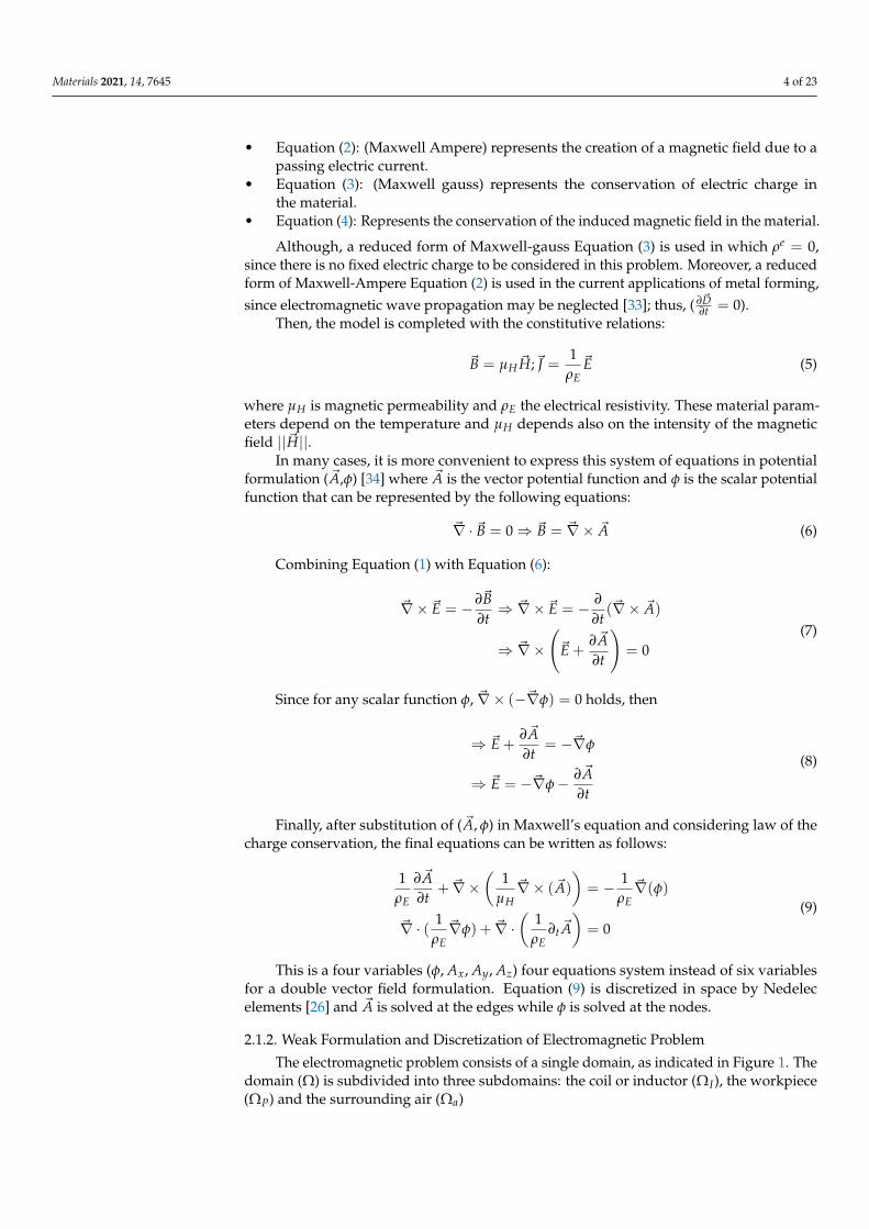
This is a four variables (φ, Ax, Ay, Az) four equations system instead of six variablesfor a double vector field formulation. Equation (9) is discretized in space by Nedelecelements [26] and ~A is solved at the edges while φ is solved at the nodes.

2.1.2. Weak Formulation and Discretization of Electromagnetic Problem

The electromagnetic problem consists of a single domain, as indicated in Figure 1. Thedomain (Ω) is subdivided into three subdomains: the coil or inductor (ΩI), the workpiece(ΩP) and the surrounding air (Ωa)

Materials 2021, 14, 7645 5 of 23

Figure 1. Boundaries of an EMF process. Ω represents the global domain solids + surroundings. ΩP

is the workpiece. ΩI represents the inductor domain. The electrical input and output connections ofthe inductor are given by ΓI

inp and ΓIout [35].

Reese et al. [28] utilized Coloumb gauge condition in order to guarantee uniquenessof solution. This condition indicates that:

~∇ · ~A = 0 (10)

Hence, the second equation of Equation (9) is reduced to:

~∇ · ( 1ρE

~∇φ) = 0 (11)

Therefore, the weak form of the electromagnetic differential equations in Equation (9)will take the following form:⟨

~Ψ, 1ρE

∂t ~A + ~∇× 1µH

~∇× ~A + 1ρE~∇φ⟩= 0

〈ϕ, ~∇ · ( 1ρE~∇φ)〉 = 0

(12)

for all ~Ψ ∈ Hcurl and ϕ ∈ H10. Where,

• Space of functions vanishing at the boundaryH10(Ω) ⊂ H1(Ω).

H10(Ω) =

ϕ ∈ H1(Ω)/ϕ = 0 ∈ ∂Ω

(13)

• Space of vector functions with square-integrable curl.

Hcurl (Ω) =

~Ψ ∈

(L2(Ω)

)3/~∇× ~Ψ ∈

(L2(Ω)

)3

(14)

• Inner products: The following notation for the inner product of the spaces will allowsimplifying the notation for the weak forms.∫

Ωf · gdΩ = 〈 f , g〉 (15)

Alves Zapata [27] developed the detailed mathematical model and considered naturalconditions to reach the final weak form:⟨

~Ψ, σ∂t ~A⟩+⟨~∇× ~Ψ, 1

µ~∇× ~A

⟩+ 〈~Ψ, 1

ρE~∇φ〉 = 0

〈~∇ϕ, 1ρE~∇φ〉 = 0

(16)

Materials 2021, 14, 7645 6 of 23

Afterwards, the approximate fields solutions representing the finite elements dis-cretization is defined as:

φ(t,~x) ≈ φh(t,~x) = ∑n

φn(t)ϕn(~x)

~A(t,~x) ≈ ~Ah(t,~x) = ∑d

ad(t)~Ψd(~x)(17)

where ϕn(~x) are the nodal shape functions and ~Ψd(~x) are the edge shape functions (Nedelecelements). Alves Zapata [27] addresses in more details the interpolation functions andfinite element formulation of this problem.

Finally, Lorentz forces can be computed from the potential formulation as follows:

~Florentz = ~J × ~B

~Florentz =1

ρE

[−∂~A

∂t× (~∇× ~A)

](18)

Lorentz force is only function in ~A, which can be computed directly after solving for ~A.

2.2. Solid Mechanics Model

The second part of the simulation is related to solid mechanics simulation in which theelectromagnetic forces are transferred to the metal part, causing deformation. In this paper,two different formulations are considered in the simulation results: a mixed pressure-velocity element formulation (MINI) element [29] and an enhanced assumed strain elementformulation [20]. In the following part, we will present a glimpse of both formulations.

2.2.1. Mini Element Formulation

For the MINI element, the strong form of the mechanical problem is defined byconservation equation along with the boundary conditions. Considering the decompo-sition of the stress tensor into spherical and deviatoric parts, the mechanical problem isrepresented on the domain Ω and the external boundary Γ = ∂Ω, shown in Figure 2.The boundary is decomposed to several parts depending on the type of loading applied:Γ = Γ f r ∪ Γt ∪ Γv ∪ Γc where:

• Γ f r : Free surface boundary.• Γt : Imposed external traction boundary.• Γv : Imposed external velocity boundary.• Γc : Contact condition on the boundary with other tools (rigid or deformable).

Figure 2. Representation of the domain Ω and the boundary conditions [27].

The system of equations representing the mechanical problem can be summarizedas follows:

Materials 2021, 14, 7645 7 of 23

~∇ · s− ~∇p = ~f ext

~∇ ·~v = −(

pκ

)~v = ~v0 on ∂Ωv

~t =~t0 on ∂Ωt

(19)

The first two equations represent the conservation of momentum in the system. Al-though, the representation used here is divided to deviatoric stress and pressure that willhelp later in developing the mixed formulation element approach.

Third equation represents Dirichlet boundary condition and fourth equation repre-sents Neumann boundary condition.

The weak form is based on a mixed velocity-pressure formulation. The formulation iswritten for test functions (v∗,p∗) as follows:

∫Ω s(~v) : ε(~v∗)dΩ−

∫Ω p~∇ ·~v∗dΩ−

∫Ω~Florentz ·~v∗dΩ−

∫∂Ωt

~t0 ·~v∗dΓ = 0∫Ω p∗

(−~∇ ·~v− p

κ

)dΩ = 0

∀(~v∗, p∗) ∈ V0 ×P

(20)

where s(~v) is the deviatoric stress, p is the pressure, ~v is the velocity vector, ε the strain rateand κ is the bulk modulus.

V0 =~v∗ ∈

(H1(Ω)

)3, ~v∗|∂Ωv=−→0 sur Ω

P = L2(Ω)

(21)

H1 is the Sobolov space and L2 is the Lp space of square functions summed on Ω .This problem has a unique solution. Although, from a numerical point of view,

numerical instabilities can arise depending on the choice of the discretization space for vand P. In order to ensure the stability of this approach, the numerical formulation shouldpass the Brezzi condition [36]. The P1+/P1 discretization allows to pass Brezzi conditionleading to a well posed discrete problem.

The element used for this formulation is tetrahedral linear 3D element in which boththe pressure and velocity are linearly interpolated. However, the velocity interpolation isenhanced by a dot at the center of the element, called “bubble”, as shown in Figure 3.

Figure 3. Degrees of freedom for the velocity and pressure for the tetrahedral element P1+/P1.

Materials 2021, 14, 7645 8 of 23

The following equation presents the interpolation function for both the velocity andpressure. The velocity field is divided into two parts: linear and bubble interpolation functions.

~vh(~x) = ∑Nbnodek=1 Nl

k(~x)~Vlk + ∑Nbelt

j=1 Nbj (~x)~V

bj

ph(~x) = ∑Nbnodek=1 Nl

k(~x)Pk

(22)

where Nlk , k = 1 . . . Nbnode are the shape function of the linear interpolation for the

velocity and pressure, while Nbj , j = 1 . . . Nbelt is the bubble function [37].

2.2.2. Shb Element Formulation

On the other hand, the general variational principle of SHB element is considered forthe mechanical problem from Hu–Washizu variational principle:

δπ(~v, ˙ε, σ) =∫

ΩeδεT · σdΩ + δ

∫Ωe

σT · (∇s(~v)− ˙ε)dΩ− δvT · ~f ext = 0 (23)

where δ denotes a variation,~v the velocity field, ˙ε the assumed strain rate, σ the interpolatedstress, σ the stress field evaluated by constitutive model, ~v the nodal velocities, ~f ext theexternal nodal forces (includes Lorentz forces and other external forces in the problem) and∇s(~v) the symmetric part of the velocity gradient.

Then a simplified form of this principle is achieved by considering the interpolatedstress orthogonal to the difference between the symmetric part of the velocity gradient andthe assumed strain rate, which gives:

δπ( ˙ε) =∫

ΩeδεT · σdΩ− δvT · ~f ext = 0 (24)

In order to avoid a locking problem, a finite element is constructed based on theenhanced assumed strain method and using reduced integration [20].

The element type is different from the one used for the MINI element. It is a linearprism element that interpolates the velocities as the only degrees of freedom. Figure 4shows the element used for this formulation and the alignment of the integration pointalong the thickness direction ζ. Trinh et al. [20] discuss, in detail, the element interpolationalong with the position of the integration points.

Figure 4. SHB element shape and integration points locations.

The interpolation of the coordinates xi and the displacements ui are as follows:

xi = xiI NI(ξ, η, ζ) =n

∑I=1

xiI NI(ξ, η, ζ) (25)

vi = viI NI(ξ, η, ζ) =n

∑I=1

viI NI(ξ, η, ζ) (26)

Materials 2021, 14, 7645 9 of 23

where NI , viI and xiI are the shape functions, the nodal velocities and the nodal coordinates,respectively. Moreover, the lowercase subscript i varies from 1 to 3, representing the spatialcoordinates, and the uppercase subscript I varies from 1 to n, representing the number ofnodes per element [20].

The implementation of the electromagnetic and mechanical solvers is not easy, es-pecially the coupling between them. The following subsection gives a glimpse of thenumerical implementation adopted in this work.

2.3. Numerical Implementation2.3.1. Coupling Algorithm

Figure 5 shows a schematic view of the coupling strategy between the electromagneticsolver and mechanical solver used to solve the MPF problem. A weak coupling is usedfor the electromagnetic and mechanical problems. Therefore, each solver (MATELEC,FORGE) solves its own physical problem separately, independently of the other solver.Although, after every time increment, the two solvers communicate the correspondingdata and variables between each other. This is known as a loosely-coupled scheme [7].Moreover, this approach allows adapting the mesh separately for each solver which iscrucial, especially in the electromagnetic solver in which the air surrounding the movingparts should be remeshed.

Figure 5. Schematic view of the coupling strategy between mechanical and electromagnetic solvers [7].

2.3.2. Shb Element Implementation Algorithm

The SHB element formulation uses prism elements that have been implemented ina tetrahedral element finite element software. Mahmoud et al. [30] developed a prismdivision algorithm that ensures that all prism elements are resembled as a set of tetrahedralelements in the software, with minimal changes in the code structure. The main idea wasto divide one prism element into six overlapping tetrahedral elements. The overlapping ofelements is crucial so that all the components of the original SHB stiffness matrix could bepresented in at least one of the generated tetrahedral elements.

Figure 6 shows the corresponding tetrahedral elements generated from the dividedprism element. Considering the number of tetra elements sharing each component (node)

Materials 2021, 14, 7645 10 of 23

of the prism stiffness matrix, the new stiffness matrices for the tetra elements can beconstructed as follows:

element1 :

K11

4K12

3K13

3K14

2K22

4K23

3K24

2K33

4K34

2K44

4

element2 :

K11

4K12

3K13

3K15

2K22

4K23

3K25

2K33

4K35

2K55

4

(27)

element3 :

K11

4K12

3K13

3K16

2K22

4K23

3K26

2K33

4K36

2K66

4

element4 :

K11

4K14

2K15

2K16

2K44

4K45

3K46

3K55

4K56

3K66

4

(28)

element5 :

K22

4K24

2K25

2K26

2K44

4K45

3K46

3K55

4K56

3K66

4

element6 :

K33

4K34

2K35

2K36

2K44

4K45

3K46

3K55

4K56

3K66

4

(29)

Figure 6. Prism division to six overlapping tetrahedral elements [30].

In this way, the prism element was presented implicitly through the usage of tetrahe-dral elements and there was no need to profoundly change the code structure used for thesimulation.

3. Magnetic Pulse Forming Case Study

Figure 7 shows the schematic view of the free bulging process. A round flat coil isused along with a ring-shaped matrix that blocks the displacement at the circumference ofthe workpiece. This problem is very convenient for clarifying the coupling between theelectromagnetic and mechanical solvers discussed earlier. The following subsections willtackle the details of the simulation setup with respect to the electromagnetic simulationand the mechanical simulation.

Materials 2021, 14, 7645 11 of 23

Figure 7. Illustration of magnetic pulse forming setup [38].

3.1. Electromagnetic Simulation Setup

Geometry: Figure 8a shows the geometry of the electromagnetic simulation with thedimensions. The aluminum workpiece has a 0.5 mm thickness and it is located 0.5 mmabove the coil.

Mesh: Figure 8b shows the mesh used in the electromagnetic simulation. Three-dimensional global mesh is composed of 43,000 nodes with 260,000 tetrahedral elements.The element size is selected so that the mesh is fine in regions where strong gradients areexpected and in the proximity of the metallic sheet.

(a) (b)Figure 8. Electromagnetic simulation setup. (a) Geometry and dimensions of the electromagnetic simulation; (b) meshconfiguration of the electromagnetic simulation.

Simulation properties: Table 1 shows the parameters that define the magnetic proper-ties of the materials according to Equation (5). Additionally, it shows the parameters of themachine that produces the electromagnetic field used for the MPF process.

3.2. Mechanical Simulation Setup

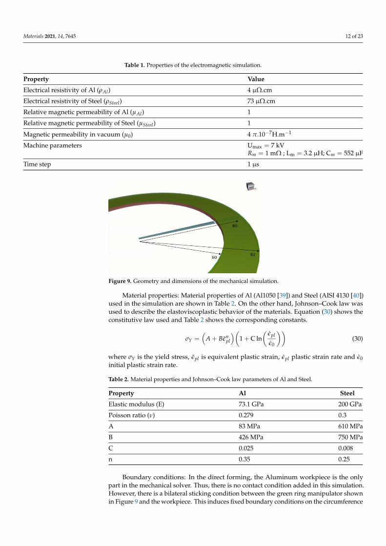
Geometry: Figure 9 shows the geometry of the 2 section of the workpiece. The work-piece is fixed in the region of the green ring shown in the figure. The fixed boundaryconditions come from the fact that the perimeter of the workpiece is held by a cylindricalclamp that prevent it from moving.

Mesh: Different mesh sizes and element types have been used to simulate the mechan-ical problem and the results were compared. In the results section, each curve will presentthe element type and the number of elements used for these results. Mesh study has beencarried out to investigate the difference in results using different mesh sizes in Section 4.3and the most appropriate mesh sizes are used in the results sections.

Materials 2021, 14, 7645 12 of 23

Table 1. Properties of the electromagnetic simulation.

Property Value

Electrical resistivity of Al (ρAl) 4 µΩ.cm

Electrical resistivity of Steel (ρSteel) 73 µΩ.cm

Relative magnetic permeability of Al (µAl) 1

Relative magnetic permeability of Steel (µSteel) 1

Magnetic permeability in vacuum (µ0) 4 π.10−7H.m−1

Machine parameters Umax = 7 kVRm = 1 mΩ ; Lm = 3.2 µH; Cm = 552 µF

Time step 1 µs

Figure 9. Geometry and dimensions of the mechanical simulation.

Material properties: Material properties of Al (Al1050 [39]) and Steel (AISI 4130 [40])used in the simulation are shown in Table 2. On the other hand, Johnson–Cook law wasused to describe the elastoviscoplastic behavior of the materials. Equation (30) shows theconstitutive law used and Table 2 shows the corresponding constants.

σY =(

A + Bεnpl

)(1 + C ln

(εpl

ε0

))(30)

where σY is the yield stress, εpl is equivalent plastic strain, εpl plastic strain rate and ε0initial plastic strain rate.

Table 2. Material properties and Johnson–Cook law parameters of Al and Steel.

Property Al Steel

Elastic modulus (E) 73.1 GPa 200 GPa

Poisson ratio (ν) 0.279 0.3

A 83 MPa 610 MPa

B 426 MPa 750 MPa

C 0.025 0.008

n 0.35 0.25

Boundary conditions: In the direct forming, the Aluminum workpiece is the onlypart in the mechanical solver. Thus, there is no contact condition added in this simulation.However, there is a bilateral sticking condition between the green ring manipulator shownin Figure 9 and the workpiece. This induces fixed boundary conditions on the circumference

Materials 2021, 14, 7645 13 of 23

of the part. On the other hand, the indirect forming contains two metal parts: Aluminumand Steel. There is a sliding contact condition between Aluminum and Steel so that thefriction does not affect the final deformation results. Table 3 summarizes all the boundaryconditions adopted in this simulation.

Table 3. Boundary conditions for the indirect forming simulation.

Al Steel

Steel Sliding

3D manipulator (matrix) Bilateral sticking Bilateral sticking

3.3. Results Overview

This section is fully dedicated to discussing the results of the MPF problem in theutmost details possible. The following subsections will tackle two basic types of the MPFprocess: direct forming and indirect forming. The former, a 160 mm diameter disc-shapedworkpiece, is formed by MPF directly, whereas the latter, an Aluminum disc, is placedbetween the coil and the Steel workpiece since Al has a much higher electrical conductivitythan Steel and will help better form the Steel material [7]. Many tests have been carried outeither by direct forming or indirect forming.

3.3.1. Direct Forming

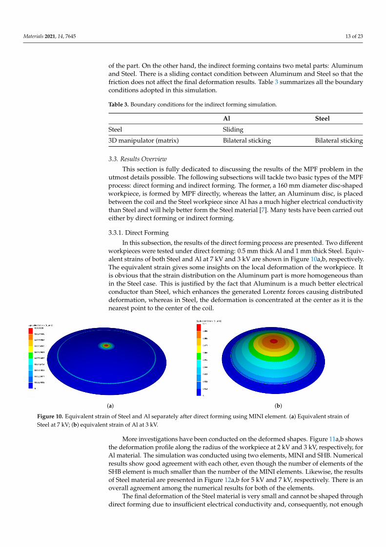
In this subsection, the results of the direct forming process are presented. Two differentworkpieces were tested under direct forming: 0.5 mm thick Al and 1 mm thick Steel. Equiv-alent strains of both Steel and Al at 7 kV and 3 kV are shown in Figure 10a,b, respectively.The equivalent strain gives some insights on the local deformation of the workpiece. Itis obvious that the strain distribution on the Aluminum part is more homogeneous thanin the Steel case. This is justified by the fact that Aluminum is a much better electricalconductor than Steel, which enhances the generated Lorentz forces causing distributeddeformation, whereas in Steel, the deformation is concentrated at the center as it is thenearest point to the center of the coil.

(a) (b)

Figure 10. Equivalent strain of Steel and Al separately after direct forming using MINI element. (a) Equivalent strain ofSteel at 7 kV; (b) equivalent strain of Al at 3 kV.

More investigations have been conducted on the deformed shapes. Figure 11a,b showsthe deformation profile along the radius of the workpiece at 2 kV and 3 kV, respectively, forAl material. The simulation was conducted using two elements, MINI and SHB. Numericalresults show good agreement with each other, even though the number of elements of theSHB element is much smaller than the number of the MINI elements. Likewise, the resultsof Steel material are presented in Figure 12a,b for 5 kV and 7 kV, respectively. There is anoverall agreement among the numerical results for both of the elements.

The final deformation of the Steel material is very small and cannot be shaped throughdirect forming due to insufficient electrical conductivity and, consequently, not enough

Materials 2021, 14, 7645 14 of 23

deformation range. Therefore, the rest of the work is focused on indirect forming in orderto obtain more deformation with the help of an aluminum hammer, which is the sameworkpiece used in direct forming (0.5 mm thick).

0 20 40 60 80

0

2

4

6

8

10

length[mm]

disp

lace

men

t[m

m]

SHB-1300MINI-52,000

(a)

0 20 40 60 80

0

5

10

15

length[mm]

disp

lace

men

t[m

m]

SHB-1300MINI-52,000

(b)

Figure 11. Displacement profile of direct forming process of Al. (a) 2 kV; (b) 3 kV.

0 20 40 60 80

0

1

2

3

length[mm]

disp

lace

men

t[m

m]

SHB-1300MINI-52,000

(a)

0 20 40 60 80

0

2

4

length[mm]

disp

lace

men

t[m

m]

SHB-1300MINI-52,000

(b)

Figure 12. Displacement profile of direct forming process of Steel. (a) 5 kV; (b) 7 kV.

3.3.2. Indirect Forming

The indirect forming process results will be the main focus of this section. Morein-depth investigation will be tackled in this subsection. Figure 13 shows the equivalentstrain of the workpiece in the indirect forming case, either for 5 kV or 7 kV. The equivalentstrain in the indirect forming is more homogeneous than that shown in the direct formingcase due to using the Aluminum workpiece underneath the Steel workpiece to enhance theforming process.

Likewise, numerical simulations are carried out for the indirect case using two ele-ments: MINI and SHB. More deformation has been noticed for the Steel when used with Alsince it makes use of the electrical conductivity of Al to gain more force to shape the Steel.

Figures 14 and 15 show the displacement profiles for SHB and MINI elements.The overall conclusion of these results is that the numerical results for both elementsare very close even though the mesh sizes are different.

Overall, the results of the recently implemented element SHB showed very goodagreement with its counterpart MINI element. These results are very encouraging to

Materials 2021, 14, 7645 15 of 23

use this element in such complicated simulations as it proved its precision and efficiency.Although, more investigation is required to better compare the two elements, which willbe introduced in the following section.

(a) (b)

Figure 13. Equivalent strain of Steel and Al after indirect forming using MINI element. (a) 5kV; (b) 7kV.

0 10 20 30 40 50 60 70 80 90

0

2

4

6

8

length[mm]

disp

lace

men

t[m

m]

SHB-2600MINI-104,000

Figure 14. Displacement profile of indirect forming process at 5 kV using different elements.

3.4. Simulation Time

The aim of implementing the new element SHB is to use a special element for bending-dominated problems and obtain accurate results with a low number of elements. The usageof this element was very remarkable as the simulation time was greatly affected. Figure 16shows a bar chart for the CPU time needed for both of the electromagnetic and mechanicalsimulations, separately, for indirect forming cases at two different voltages, 5 kV and 7 kV.In contrast to electromagnetic simulation times that were almost identical, the mechanicalsimulations times were greatly decreased using the SHB element. The simulation time isreduced by almost 10× in the SHB case.

Similarly, the CPU time of the direct forming process represents the same trend.Figure 17 shows the bar chart of the direct forming of Al at two different voltages, 2 kVand 3 kV. Electromagnetic simulation times are almost identical, whereas the mechanicalsimulation time is much lower, 3× for the SHB element than the MINI element. The MINI

Materials 2021, 14, 7645 16 of 23

element is used with a mesh of 52,000 tetra elements and SHB elements with 1300 elements.This difference in the number of elements causes the simulation time difference highlightedin these figures.

0 10 20 30 40 50 60 70 80 90

0

2

4

6

8

10

12

length[mm]

disp

lace

men

t[m

m]

SHB-2600MINI-104,000

Figure 15. Displacement profile of indirect forming process at 7 kV using different elements.

Meca 5 kV Emag 5 kV Meca 7 kV Emag 7 kV

0

500

1000

1500

1600

239

1560

232122

203103

198

Min

ute

MINISHB

Figure 16. Simulation time of indirect forming process.

Finding a way to reduce the simulation time of the magnetic pulse forming is tremen-dously important, especially in the optimization processes. Optimization iterations have tobe run to optimize the shape of the workpiece, study the effect of the workpiece’s thicknessand carry out the material parameter identification process. This is considered a crucialmilestone in the simulation of MPF processes and similar problems.

Materials 2021, 14, 7645 17 of 23

Meca 2 kV Emag 2 kV Meca 3 kV Emag 3 kV

40

60

80

100

120

90

117 116

93

30

106

46

92

Min

ute

MINISHB

Figure 17. Simulation time of direct forming process of Al.

4. Discussion

This section is dedicated to giving a better insight of the results, along with discussingother results that explain the physical intuition of the process. Nevertheless, some chal-lenges have been encountered while simulating the problem. Therefore, some of theseproblems are mentioned in the following subsections along with the proposed solutions.These problems include determining the final forming time, remeshing of the electromag-netic domain mesh and the effect of the mechanical mesh on the results. In the followingsubsections, the energy notion will be used to explain some of the difficulties that havebeen encountered while solving the problem. Therefore, it is important to explain theenergy components that exist in this problem.

The initial energy input in the electromagnetic system is as follows:

Ein =12· Cele ·V2 (31)

where Ein is the input energy, Cele is the electric capacitance of the coil and V is the voltageapplied to the coil.

This energy is equal to the total energy that exists in the system:

Etotal = Eelec + Etherm + EMeca

Eelec = 0

Etherm = 0

(32)

In our case, we are not considering the Eelec that is the dissipated energy due to electricresistance of the coil. Moreover, Etherm is neglected, which is the dissipated thermal energyin the coil and in the mechanical system. This leaves only EMeca that is represented by :

EMeca = Eel + Epl + Ekin

Eel =∫

σ : εeldt

Epl =∫

σ : εpldt

Ekin =12

ρ · v(x, t) : v(x, t)

(33)

Materials 2021, 14, 7645 18 of 23

where Eel , Epl , Ekin are the elastic strain energy, plastic strain energy and kineticenergy, respectively.

4.1. Final Forming Time

One of the main issues with all these models is determining the final forming time.At the beginning, the simulation time was set to 150 µs. However, the exact terminationtime of the process could not be determined and, by setting a too small value, we obtainedan intermediate displacement profile, not the final one. Figure 18 shows a set of transientdisplacement profiles at different time steps. Therefore, a second stop condition has beenadded. It is induced from the calculation of a variation of the total energy of the systembetween the two last time steps. From this point of view, it is possible to set a thresholdvalue at which calculation stops once reached. Otherwise, the recorded deformation willbe a transient state and will not represent the real solution.

0 20 40 60 80

0

5

10

15

length[mm]

disp

lace

men

t[m

m]

t = 100 µst = 200 µst = 300 µst = 400 µst = 500 µs

Figure 18. Displacement profile of direct forming process of Al at 3 kV.

To better understand this, Figure 19 shows the evolution of the mechanical energy(strain energy and kinetic energy) of the system in the indirect forming problem. The totalenergy increases at the beginning of the process in which the electromagnetic energy ismaximum (electromagnetic energy represents the total energy in the system, it is thentransformed to mechanical energy due to Lorentz force and thermal energy in the systemand some loss as electrical energy in the coil). After some time, the system stops acquiringenergy from the electromagnetic system and mechanical energy stays steady for the restof the simulation time (highlighted in red dashed rectangle). The final simulation time istaken once the steady state value has been reached.

0 100 200 300 400 500

0

2

4

6

·10−4

time[µs]

Ener

gy[k

J]

Mechanical Energy

Figure 19. Total mechanical energy evolution with forming time.

Materials 2021, 14, 7645 19 of 23

4.2. Remeshing of Electromagnetic Domain Mesh

At the beginning, the numerical simulations were carried out using a fixed but finemesh in the electromagnetic domain, as shown in Figure 20, since it is more convenientand more computationally efficient as remeshing takes more computation time. Althoughthe results were not very satisfactory, by checking the energy transferred between theelectromagnetic mesh and the mechanical mesh shown in Figure 21a, it is obvious that atthe end, there is energy loss.

Figure 20. Electromagnetic mesh without remeshing.

0 100 200 300 400 500

0

0.5

1

1.5

2

2.5·10−3

Energy loss

time[µs]

Ener

gy[k

J]

Emag EnergyTotal Meca Energy Energy

(a)

0 100 200 300 400 500

0

2

4

6

·10−4

time[µs]

Ener

gy[k

J]

Emag EnergyTotal Meca Energy

(b)

Figure 21. Electromagnetic energy vs. total mechanical energy of Al direct forming at 3 kV. (a) No Remeshing. (b) Remeshing.

On the other hand, Figure 21b shows the energy transferred with activating remeshingand the energy loss is negligible. The remeshing algorithm checks the deformation of theworkpiece in the mechanical simulation and remeshes the surrounding of the workpiecein the electromagnetic simulation. Once the elements around the workpiece are highlydeformed, the remesher refines these elements to maintain good mesh quality. Thistechnique ensures that the mesh around the workpiece is always fine and clean, and thusguarantees correct calculations of the electromagnetic field and Lorentz forces, preventingthe loss of energy. Figure 22 shows the electromagnetic mesh with activating remeshingbefore and after remeshing process.

Therefore, all the results in the previous subsections are obtained with remeshingactivated. Although this increased the total simulation time, the obtained results can betrusted and a negligible amount of energy is lost.

Materials 2021, 14, 7645 20 of 23

Figure 22. Electromagnetic mesh with remeshing.

4.3. Effect of Mechanical Mesh Refinement

One of the questions that was intriguing while studying this process was the effectof mechanical mesh on the accuracy of the results. Thus, the indirect forming process hasbeen simulated again with coarser mesh of the MINI element and its results have beencompared to both the MINI fine mesh and SHB element. Figure 23 shows the displacementprofile of the final deformed profiles for the previously mentioned elements and meshsizes. The overall observation of the results is that displacement profiles are too close tobe distinguishable. These results are not very comprehensible, since the MINI elementshould be stiffer than the SHB element and using a less number of elements shouldalter the displacement results. Moreover, in order to make sure that we have convergedto mesh independent results, the simulation was repeated using more SHB elements,≈3600 elements, as shown in the black curve. The difference between the red and the blackcurves are really small, meaning that the results obtained with the lower mesh size canbe trusted.

0 10 20 30 40 50 60 70 80 90

0

5

10

length[mm]

disp

lace

men

t[m

m]

MINI-10,4000MINI-7600SHB-2600SHB-3600

Figure 23. Displacement profile of indirect forming process at 7 kV using different elements andmesh sizes.

However, more insight has been given to the mechanical energy of the three cases.Figure 24 shows the total mechanical energy for the three mesh cases. It is fairly noticeablethat the energy of the SHB coarse mesh is the lowest and the MINI element with fine meshenergy is approaching it with minute difference. However, the energy of the MINI coarsemesh has a quite higher value. This means that given almost the same final deformationprofile, the energy required is smallest in the case of the SHB element, even with coarsemesh, while it takes higher energy to achieve the same displacement in the case of usingthe MINI element with coarse mesh, and the energy decreases approaching the energy ofthe SHB element by refining the mesh. This clearly indicates that the MINI element is stifferthan the SHB element and would need much finer mesh to achieve comparable results tothe SHB element.

Materials 2021, 14, 7645 21 of 23

0 50 100 150 200 250 300 350 400 450

0

0.5

1

1.5

2

2.5·10−3

time[µs]

Ener

gy[k

J]

MINI-7600MINI-104,000

SHB-2600

Figure 24. Total mechanical energy comparisons for different elements and mesh sizes for indirectforming at 7 kV.

5. Conclusions

An efficient approach for the simulation of the magnetic pulse forming process of thinsheet metals was developed by combining an electromagnetic solver, relying on Maxwell’sequations, with a mechanical solver, based on the conservation of momentum equations.In-depth analysis of the types of the magnetic pulse forming processes was carried out,namely on direct forming and indirect forming. Tetrahedral element (MINI) and solid-shell prism element were employed to solve the mechanical problem and quantitativecomparisons were carried out to assess their performance in such applications. The overallresults showed that the accuracy obtained with a low resolution SHB approach (lownumber of elements) was comparable to that of a high resolution MINI element basedtechnique (high number of elements). The SHB element was shown to be less stiff than theMINI element. Finally, a computational cost study was carried out and demonstrated ahigher computational efficiency for the SHB element since a smaller number of elementscould be used while maintaining comparable accuracy to that of the MINI element. Theseresults are very promising to study the performance of the SHB element, not only in MPFapplication but also in other applications. Many challenges were encountered duringthe simulation of this multi-physics problem and some solutions to overcome them weredevised. First, the final forming time. It was very challenging to determine the exactfinal simulation time since the deformation takes place in the order of magnitude ofmilliseconds. Consequently, criteria based on measuring the change in the mechanicalenergy variation were adopted to find the termination time at which the energy variationis minimum. Second, the electromagnetic mesh had to be adjusted to consider the newmechanical deformation since the electromagnetic solution is highly dependent on thespatio-temporal evolution of the deformation of the workpiece in the mechanical problem.Hence, a remeshing strategy was utilized for the electromagnetic mesh and the resultswere compared to those conducted without the remeshing step.

Author Contributions: Conceptualization, M.M. and D.P.M.; formal analysis, M.M. and F.B.; projectadministration, D.P.M.; software, M.M.; supervision, F.B. and D.P.M.; validation, M.M. and D.P.M.;visualization, M.M.; writing—original draft, M.M.; writing—review and editing, F.B. All authorshave read and agreed to the published version of the manuscript.

Funding: The APC was funded by Armines, France.

Institutional Review Board Statement: Not applicable.

Informed Consent Statement: Not applicable.

Conflicts of Interest: The authors declare no conflict of interest.

Materials 2021, 14, 7645 22 of 23

References1. Mynors, D.J.; Zhang, B. Applications and capabilities of explosive forming. J. Mater. Process. Technol. 2002, 125, 1–25. [CrossRef]2. Rohatgi, A.; Stephens, E.V.; Davies, R.W.; Smith, M.T.; Soulami, A.; Ahzi, S. Electro-hydraulic forming of sheet metals: Free-

forming vs. conical-die forming. J. Mater. Process. Technol. 2012, 212, 1070–1079. [CrossRef]3. Zittel, G. A Historical Review of High Speed Metal Forming; Institute für Forming Technology-Technical Universityät: Dortmund,

Germany, 2010.4. Dowell, E.H.; Hall, K.C. Modeling of fluid-structure interaction. Annu. Rev. Fluid Mech. 2001, 33, 445–490. [CrossRef]5. Keyes, D.E.; McInnes, L.C.; Woodward, C.; Gropp, W.; Myra, E.; Pernice, M.; Bell, J.; Brown, J.; Clo, A.; Connors, J.; et al.

Multiphysics simulations: Challenges and opportunities. Int. J. High Perform. Comput. Appl. 2013, 27, 4–83. [CrossRef]6. Singhal, A.; Sahu, S.A.; Chaudhary, S. Liouville-Green approximation: An analytical approach to study the elastic waves

vibrations in composite structure of piezo material. Compos. Struct. 2018, 184, 714–727. [CrossRef]7. Alves Z, J.R.; Bay, F. Magnetic pulse forming: Simulation and experiments for high-speed forming processes. Adv. Mater. Process.

Technol. 2015, 1, 560–576. [CrossRef]8. Psyk, V.; Risch, D.; Kinsey, B.L.; Tekkaya, A.E.; Kleiner, M. Electromagnetic forming—A review. J. Mater. Process. Technol. 2011,

211, 787–829. [CrossRef]9. Psyk, V.; Beerwald, C.; Henselek, A.; Homberg, W.; Brosius, A.; Kleiner, M. Integration of electromagnetic calibration into the

deep drawing process of an industrial demonstrator part. In Key Engineering Materials; Trans Tech Publications Ltd.: Bäch SZ,Switzerland, 2007; Volume 344, pp. 435–442.

10. Unger, J.; Stiemer, M.; Schwarze, M.; Svendsen, B.; Blum, H.; Reese, S. Strategies for 3D simulation of electromagnetic formingprocesses. J. Mater. Process. Technol. 2008, 199, 341–362. [CrossRef]

11. Fenton, G.K.; Daehn, G.S. Modeling of electromagnetically formed sheet metal. J. Mater. Process. Technol. 1998, 75, 6–16.[CrossRef]

12. Imbert, J.; Winkler, S.; Worswick, M.; Oliveira, D.; Golovashchenko, S. Numerical modeling of an electromagnetic corner filloperation. In Proceedings of the NUMIFORM, Columbus, OH, USA, 13–17 June 2004; pp. 1833–1839.

13. Schinnerl, M.; Schoberl, J.; Kaltenbacher, M.; Lerch, R. Multigrid methods for the three-dimensional simulation of nonlinearmagnetomechanical systems. IEEE Trans. Magn. 2002, 38, 1497–1511. [CrossRef]

14. Heyliger, P.; Reddy, J. A higher order beam finite element for bending and vibration problems. J. Sound Vib. 1988, 126, 309–326.[CrossRef]

15. Simo, J.C.; Armero, F. Geometrically non-linear enhanced strain mixed methods and the method of incompatible modes. Int. J.Numer. Methods Eng. 1992, 33, 1413–1449. [CrossRef]

16. Simo, J.; Armero, F.; Taylor, R. Improved versions of assumed enhanced strain tri-linear elements for 3D finite deformationproblems. Comput. Methods Appl. Mech. Eng. 1993, 110, 359–386. [CrossRef]

17. Belytschko, T.; Bindeman, L.P. Assumed strain stabilization of the eight node hexahedral element. Comput. Methods Appl. Mech.Eng. 1993, 105, 225–260. [CrossRef]

18. Liu, W.K.; Guo, Y.; Tang, S.; Belytschko, T. A multiple-quadrature eight-node hexahedral finite element for large deformationelastoplastic analysis. Comput. Methods Appl. Mech. Eng. 1998, 154, 69–132. [CrossRef]

19. Reese, S.; Wriggers, P.; Reddy, B. A new locking-free brick element technique for large deformation problems in elasticity. Comput.Struct. 2000, 75, 291–304. [CrossRef]

20. Trinh, V.D.; Abed-Meraim, F.; Combescure, A. A new assumed strain solid-shell formulation “SHB6” for the six-node prismaticfinite element. J. Mech. Sci. Technol. 2011, 25, 2345. [CrossRef]

21. Abed-Meraim, F.; Combescure, A. An improved assumed strain solid–shell element formulation with physical stabilization forgeometric non-linear applications and elastic–plastic stability analysis. Int. J. Numer. Methods Eng. 2009, 80, 1640–1686. [CrossRef]

22. Reese, S. A large deformation solid-shell concept based on reduced integration with hourglass stabilization. Int. J. Numer.Methods Eng. 2007, 69, 1671–1716. [CrossRef]

23. L’Eplattenier, P.; Çaldichoury, I. Update on the electromagnetism module in LS-DYNA. In Proceedings of the 12th LS-DYNAUsers Conference, Detroit, MI, USA, 3–5 June 2012.

24. Brebbia, C.A.; Dominguez, J. Boundary Elements: An Introductory Course; WIT Press: The New Forest, UK, 1994.25. Bahmani, M.A.; Niayesh, K.; Karimi, A. 3D Simulation of magnetic field distribution in electromagnetic forming systems with

field-shaper. J. Mater. Process. Technol. 2009, 209, 2295–2301. [CrossRef]26. Nédélec, J.C. A new family of mixed finite elements in R3. Numer. Math. 1986, 50, 57–81. [CrossRef]27. Alves Zapata, J. Magnetic Pulse Forming Processes: Computational Modelling and Experimental Validation. Ph.D. Thesis, Ecole

Nationale Supérieure des Mines de Paris, Paris, France, 2016.28. Reese, S.; Svendsen, B.; Stiemer, M.; Unger, J.; Schwarze, M.; Blum, H. On a new finite element technology for electromagnetic

metal forming processes. Arch. Appl. Mech. 2005, 74, 834–845. [CrossRef]29. Arnold, D.N.; Brezzi, F.; Fortin, M. A stable finite element for the stokes equations. Calcolo 1984, 21, 337–344. [CrossRef]30. Mahmoud, M.; Bay, F.; Munoz, D.P. An efficient multiphysics solid shell based finite element approach for modeling thin sheet

metal forming processes. Finite Elem. Anal. Des. 2021, 198, 103645. [CrossRef]

Materials 2021, 14, 7645 23 of 23

31. Bay, F.; Zapata, J.R.A. Computational modelling for electromagnetic forming processes. In Proceedings of the Interna-tional Scientific Colloquium Modelling for Electromagnetic Processing-MEP 2014, Hannover, Germany, 16–19 September2014; pp. 259–264.

32. Bay, F.; Jeanson, A.C.; Zapata, J.A. Electromagnetic forming processes: Material behaviour and computational modelling. ProcediaEng. 2014, 81, 793–800. [CrossRef]

33. Svendsen, B.; Chanda, T. Continuum thermodynamic formulation of models for electromagnetic thermoinelastic solids withapplication in electromagnetic metal forming. Contin. Mech. Thermodyn. 2005, 17, 1–16. [CrossRef]

34. Chari, M.; Konrad, A.; Palmo, M.; D’angelo, J. Three-dimensional vector potential analysis for machine field problems. IEEETrans. Magn. 1982, 18, 436–446. [CrossRef]

35. Biro, O.; Preis, K. On the use of the magnetic vector potential in the finite-element analysis of three-dimensional eddy currents.IEEE Trans. Magn. 1989, 25, 3145–3159. [CrossRef]

36. Brezzi, F.; Fortin, M. Mixed and Hybrid Finite Element Methods; Springer Science & Business Media: Berlin, Germany, 2012;Volume 15.

37. Fayolle, S. Etude de la Modélisation de la Pose et de la Tenue Mécanique des Assemblages par Déformation Plastique.Ph.D. Thesis, Ecole Nationale Supérieure des Mines de Paris, Paris, France, 2009.

38. Risch, D.; Beerwald, C.; Brosius, A.; Kleiner, M. On the significance of the die design for electromagnetic sheet metal form-ing. In Proceedings of the 1st International Conference on High Speed Forming, Dortmund, Germany, 31 March–1 April2004; pp. 191–200.

39. Jeanson, A.C.; Avrillaud, G.; Mazars, G.; Bay, F.; Massoni, E.; Jacques, N.; Arrigoni, M. Identification du comportement mécaniquedynamique de tubes d’aluminium par un essai d’expansion électromagnétique. In CSMA 2013-11ème Colloque National en Calculdes Structures; HAL: Giens, France, May 2013.

40. Johnson, J.R.; Taber, G.A.; Daehn, G.S. Constitutive relation development through the FIRE test. In Proceedings of the 4thInternational Conference on High Speed Forming, Columbus, OH, USA, 9–10 March 2010; pp. 295–306.