PSYCHOMETRIKA2014DOI: 10.1007/S11336-013-9396-3

THE LOGNORMAL RACE: A COGNITIVE-PROCESS MODEL OF CHOICEAND LATENCY WITH DESIRABLE PSYCHOMETRIC PROPERTIES

JEFFREY N. ROUDER AND JORDAN M. PROVINCE

UNIVERSITY OF MISSOURI

RICHARD D. MOREY

UNIVERSITY OF GRONINGEN

PABLO GOMEZ

DEPAUL UNIVERSITY

ANDREW HEATHCOTE

UNIVERSITY OF NEWCASTLE

We present a cognitive process model of response choice and response time performance data thathas excellent psychometric properties and may be used in a wide variety of contexts. In the model thereis an accumulator associated with each response option. These accumulators have bounds, and the firstaccumulator to reach its bound determines the response time and response choice. The times at whichaccumulator reaches its bound is assumed to be lognormally distributed, hence the model is race or minimaprocess among lognormal variables. A key property of the model is that it is relatively straightforward toplace a wide variety of models on the logarithm of these finishing times including linear models, structuralequation models, autoregressive models, growth-curve models, etc. Consequently, the model has excellentstatistical and psychometric properties and can be used in a wide range of contexts, from laboratoryexperiments to high-stakes testing, to assess performance. We provide a Bayesian hierarchical analysis ofthe model, and illustrate its flexibility with an application in testing and one in lexical decision making,a reading skill.

Key words: cognitive psychometrics, response-times models, race models.

Cognitive modelers and psychometricians analyze human performance data to measure in-dividual abilities, to measure the effects of covariates, and to assess latent structure in data. Yet,there is relatively little overlap between psychometric models and cognitive-process models. Thislack of overlap is in many ways understandable. Cognitive process modelers and psychometri-cians not only have different goals, they come from different traditions.

For cognitive modelers, the emphasis is on using structure in data to draw inferences aboutthe processes and mental representations underlying perception, memory, attention, decision-making, and information-processing. These researchers specify complex, detailed nonlinearmodels that incorporate theoretical insights on the acquisition, storage, and processing of men-tal information. Consider, for example, McClelland and Rumelhart’ interactive activation model(McClelland & Rumelhart, 1981; Rumelhart & McClelland, 1982), which describes how peo-ple recognize letters and words by making specific representation and processing assumptions.The goal of cognitive modelers is to uncover the true structures underlying mental life, and con-sequently, models are benchmarked by their ability to fit fine-grained features in the data. The

Requests for reprints should be sent to Jeffrey N. Rouder, University of Missouri, Columbia, MO, USA. E-mail:rouderj@missouri.edu

© 2014 The Psychometric Society

PSYCHOMETRIKA

disadvantages of this approach are as follows: (1) It may be difficult to analyze complicated non-linear cognitive process models, and in many cases parameter estimation proceeds with the helpof heuristics or trial-and-error. (2) It is almost always difficult to assess a constellation of issuesrelated to model fit including adequately characterizing the complexity of the models, charac-terizing the data patterns that could not be fit (Roberts & Pashler, 2000), and understanding therobustness to misspecification. (3) It is often not clear how process models may be extendedto account for covariates or used in a psychometric setting to understand variation across peo-ple.

Psychometricians, on the other hand, place an emphasis on the usefulness of models. Goodmodels may not fit the data in the finest detail, but they are statistically tractable, convenientto analyze, incorporate covariates of interest, and may be used to understand variation in la-tent traits and abilities across people. Psychometricians retain these desirable properties by us-ing models that cognitive modelers may consider too simple. Consider, for example, the RaschIRT model in which the key structural specification is that performance reflects the differ-ence between participant ability and item difficulty (Rasch, 1960). Because this specificationis simple, the model retains desirable statistical properties including ease of analysis and theability to understand misspecification. Moreover, because the base IRT model is so simple, itis straightforward to integrate sophisticated models on item and participant effects includingfactor models and structural equation models (Skrondal & Rabe-Hesketh, 2004; Embretson,1991).

In our view, cognitive modelers and psychometricians make different tradeoffs: Psychome-tricians gain the ability to more easily measure latent abilities by stipulating simple psycholog-ical processes and representations; cognitive modelers gain the ability to understand the detailsof these processes and representations by stipulating detailed and complex models, but at theexpense of statistical tractability. There is, however, a fertile middle ground of models, some-times called cognitive psychometrics (Riefer, Knapp, Batchelder, Bamber, & Manifold, 2002),where the goal is to develop psychological process models with good psychometric and statisticalproperties.

In this paper, we develop a model for the joint distribution of response choice and responsetime (RT) that we believe occupies this middle ground. The model captures a processing com-mitment: evidence for a response grows gradually in time in separate, independent, racing ac-cumulators. The response is made when one of these accumulators first wins the race, that is,it first attains sufficient evidence. We adopt perhaps the simplest version of this race-between-accumulators theme, and show how it retains desirable properties of useful psychometric models.Not only is the model statistically tractable, it is straightforward to place sophisticated modelcomponents, such as autoregressive components, on model parameters.

In the next section, we provide a brief and selective overview of the literature on accountingfor response time and response choice to provide context for our approach. We then present abase model that accounts for response choice and response time for a single participant observ-ing a number of replicate trials. Following that, the analysis of the base model with Bayesianmethods is discussed. The base model is easily extended for real-world applications, and weprovide two examples. The first is a Rasch-inspired testing application where for each item theparticipant may choose among n options. The second is an application in lexical decision whereparticipants decide if a presented letter string is a word or a nonword. The model describes howlatent accumulation for word and nonword information varies across experimental conditionsand people.

JEFFREY N. ROUDER ET AL.

1. Modeling Response Time and Response Choice Jointly

Making choices always produces two dependent measures, the choice selected and the timeit takes to make the selection (response time or RT). Given that experimenting and testing is oftencarried out via computer, RT is often readily available. The most popular approach in experimen-tal psychology and psychometrics is to model one dependent measure, either RT or choice, andto ignore the other. Although ignoring one of the measures may seem naive, it is often naturalin real-world settings. Analyzing one measure seems appropriate when there is variation in onlyone, or where the joint variation is so thoroughly correlated that all the information is effectivelycontained in one measure. Modeling both RT and accuracy jointly entails additional compli-cations over modeling one of these measure, and in some contexts the gain may be marginal.Whether jointly modeling RT and accuracy is worthwhile will vary from situation to situation,and may depend to some large extent on the researchers’ goals and desired interpretations ofparameters.

One conventional psychometric approach to modeling RT and choice jointly is to first placeseparate regression models on choice and RT (e.g., Thissen, 1983; van Breukelen, 2005; vander Linden, Scrams, & Schnipke, 1999; van der Linden, 2007, 2009). It is common to placea two-parameter lognormal model on RT although other specifications, including the Weibulland a more general proportional hazard model are precedented. Conventional 1PL, 2PL, or 3PLIRT models may be placed on choice, where choice is coded as either a correct response oran incorrect response. Choice and RT may then be linked by allowing RT to be a covariatein the IRT model on choice or by allowing choice to be a covariate in the lognormal modelon RT, or both (e.g., van Breukelen, 2005). Similarly, choice and RT may be linked throughshared latent parameters. For example, the person parameters in the IRT model and the lognormalmodel may be modeled as coming from a bivariate structure with a shared variance component.These approaches provides for tractability and flexibility in understanding how people and itemcovariates affect choice and RT. Moreover, because the modeling is within conventional IRT andmixed linear model frameworks, analysis follows a familiar path. Nonetheless, the models arestatistical and are neither informed by nor inform theories of cognitive process.

Perhaps the most popular cognitive-process alternative is based on Ratcliff and colleagues’diffusion model (Ratcliff, 1978; Ratcliff & McKoon, 2008; Ratcliff & Rouder, 1998). In Ratclff’sdiffusion model, latent evidence evolves gradually in time and is modeled as a diffusion processwhich terminates on one of two latent bounds. The model is applied to tasks where participantsmake dichotomous decisions in response to stimuli. Each of the two responses is associated withone of the two bounds. The decision occurs when the process is absorbed, and the response is theone associated with the absorbing bound. The key advantage of this approach is the separationof the latent bound from the rate of information accumulation. This separation provides for anatural account of speed-vs.-accuracy tradeoffs in decision making.

Recently, there has been a trend toward adapting the diffusion model so that it may be usedin psychometric settings: Wagenmakers, van der Maas, and Grasman (2007) provide a simpli-fied version that has somewhat increased statistical tractability over Ratlciff’s (1978) originalversion. Tuerlickx and De Boek (2005) show that the 2PL IRT model on choice data may be in-terpreted as a diffusion model with a simple relationship between item parameters and diffusionmodel parameters. van der Maas, Molenaar, Maris, Kievit, and Borsboom (2001), Vandekerck-hove, Verheyen, and Tuerlinckx (2010), and Vandekerckhove, Tuerlinckx, and Lee (2011) showhow latent-variable submodels may be added to diffusion model parameters to account for varia-tion among people, items, and conditions. This process-based approach is laudable and excitingbecause it is both substantively and psychometrically attractive.

Though the diffusion model approach has a number of benefits, it also has a few distinctdisadvantages. First, it is not straightforward to extend the diffusion model to an arbitrary number

PSYCHOMETRIKA

of choices. The analysis of absorption of a multidimensional diffusion process is complex thoughsome results are possible under certain conditions (see Diederich & Busemeyer, 2003). Second,the approach is not altogether convenient because the likelihood function is comprised of infinitesums of products of sinusoids and exponentials. The current approaches to analysis, such as thosein Vanderckhove et al. (2010, 2011), are based on default Metropolis Hastings (MH) sampling inJAGS and Winbugs. Because the likelihood is not easily analyzed and because analysis relies onseveral MH steps, it is not clear whether more complex models, such as autoregressive models,may be placed on parameters.

In this paper, we propose a simpler and more tractable cognitive process: a race betweenaccumulators (Audley & Pike, 1965; Smith, 2000). The version we develop and extend comesfrom Heathcote and Love (2012), who modeled the finishing times of each accumulator as alognormal. The lognormal race is not as feature rich as the diffusion process approach or morecomprehensive accumulator models (e.g., Brown & Heathcote, 2008) that, for example, provideparameters selectively accounting for speed-vs.-accuracy tradeoffs. The main advantages of theapproach are two-fold: First, the approach generalizes seamlessly to any number of responsechoices including large numbers of choices or even just one choice. Second, the analysis of theprocess is far more tractable than the diffusion model and more comprehensive accumulator mod-els.. This increase in tractability translates into pragmatic advantages. Here, we show not onlyhow IRT and cell-means models may be placed on accumulation rates, but how autoregressivecomponents may be placed on them as well.

2. Specification of the Base Lognormal Race Model

Consider a single participant who responds on J identical experimental trials. On each trial,the participant is shown a stimulus or is given an item. In responses, the participant endorses oneof n possible responses choices. Let xj and tj denote the response choice and response time forthe j th trial, respectively, with xj = 1, . . . , n; tj > 0; and j = 1, . . . , J . In race models, evidenceaccumulates linearly in competing accumulators, with each accumulator associated to one of then response. At some point, the evidence in the accumulator crosses the accumulator’s bound, andthat point of time is referred to as the finishing time. Let yij denote this finishing time for the ithaccumulator on the j th trial. The first accumulator that finishes determines the choice and theresponse time:

xj = m ⇐⇒ ymj = mini

(yij ), (1)

and response time tj is

tj = ψ + mini

(yij ), (2)

where ψ denotes an irreducible minimum shift that reflects the contribution of nondecision pro-cesses such as encoding the stimulus and executing the response (see Dzhafarov, 1992; Luce,1986; Ratcliff, 1978). The presence of shift parameter ψ complicates analysis to some degree,and its inclusion is necessitated by the fact that empirical RT distributions are often substantiallyshifted away from zero (Rouder, 2005). Indeed, we show here in our subsequent empirical ap-plication that these shifts are not only present, but substantial in size in a word-identificationtask.

We model each finishing time yij as log normally distributed:

yijind∼ Lognormal

(μi,σ

2i

).

JEFFREY N. ROUDER ET AL.

This parametric choice is suitable for response times because the lognormal has support on posi-tive reals, is unimodal, exhibits a characteristic positive skew, and has a soft left-tail rise. Parame-ters μ and σ 2 serve as scale and shape parameters, respectively. In this version of the race model,finishing times are assumed to be stochastically independent. A generalization of this assumptionseems possible (see Heathcote & Love, 2012), but the full ramifications of which have not beensystematically explored.

The joint density function of choice m at time t is

f (m, t) = g(t − ψ;μm,σ 2

m

) ∏

i �=m

(1 − G

(t − ψ;μi,σ

2i

)), (3)

where g and G are the density and cumulative distribution functions, respectively, of the two-parameter lognormal distribution. It is straightforward to expand this joint density to provide thelikelihood function across many independent observations.

We have specified different shape parameters σ 2i for each accumulator. Although this spec-

ification of different shapes is certainly general, it may affect the interpretability of results inpractice. In most applications, researchers will construct a contrast between these finishing timedistributions. If the homogeneity assumption σ 2

i = σ 2 is made, then contrasts between finishingtime distributions is captured completely by contrasts of μi . We describe the analysis of the basemodel without this homogeneity assumption for generality. In the subsequent applications, wemake the homogeneity assumption to increase the interpretability of μi . In some cases, espe-cially where researchers wish to account for the data in finer detail, the heterogeneity of shapesmay be warranted (see Heathcote & Love, 2012).

3. Bayesian Analysis of the Base Model

3.1. Prior Specification

The base lognormal race model is straightforward to analyze in the Bayesian framework.The parameters are ψ , μi , σ 2

i . Weakly informative semiconjugate priors may be specified asfollows:

π(ψ) ∝ 1, (4)

σ 2i

ind∼ Inverse-Gamma(ai, bi), (5)

μiind∼ Normal(ci, di), (6)

where the inverse gamma distribution has pdf

f(σ 2;a, b

) = ba

�(a)(σ 2)a+1exp

(− b

σ 2

), a, b, σ 2 > 0.

Perhaps the most important specification is that of conditionally independent priors on μi . Inapplications, we place substantively meaningful models as priors on μi .

3.2. Analysis

Analysis proceeds by MCMC integration of the joint posterior distribution by means of theGibbs sampler (Gelfand & Smith, 1990). The Gibbs sampler works by alternately sampling fromfull conditional posterior distributions. These conditional posteriors are conveniently expressed

PSYCHOMETRIKA

when conditioned on latent finishing times yij . Let zij = logyij , and let zi = J−1 ∑j zij . Con-

ditional posterior distribution for μi is

μi | · · · ∼ Normal(vi

[J zi/σ

2i + ci/di

], vi

)(7)

where

vi = (J/σ 2

i + 1/di

)−1.

The conditional posterior distribution of σ 2i is

σ 2i

∣∣ · · · ∼ Inverse-Gamma

(ai + J/2, bi +

∑

j

(zij − μi)2/2

).

The conditional posterior density of ψ is

f (ψ | · · · ) ∝{∏

ij g(yij − ψ;μi,σ2i ), ψ < minij (yij ),

0, otherwise,

where g is the density of the two-parameter lognormal distribution. The conditional posteriordistribution of the finishing times zij depends on whether the ith accumulator finished first onthe j th trial. If it did, then zij is a direct transform of the observed response time:

(zij | xj = i, . . .) = log(tj − ψ).

If the ith accumulator did not win the race, then the relevant information is that zij > log(tj −ψ).The posterior of zij is simply the prior conditional on zij > log(tj − ψ), e.g.,

(zij | xj �= i, . . .) ∼ Truncated Normal(μi,σ

2i , log(tj − ψ)

),

where the arguments in order are the mean, variance of the corresponding untruncated normal,and the lower bound of support.

To implement the Gibbs sampler, it is necessary to be able to sample from each of theseconditional posterior distributions. Such sampling is straightforward for μi , σ 2

i and zij as thecorresponding posterior distributions are well known. The conditional posterior for ψ , however,does not correspond to a known distribution. Because ψ is bounded above, care must be exercisedthat mass near the bound is sampled. We have found in previous work that adaptive rejectionsampling (Wild & Gilks, 1993) works well for sampling from bounded distributions (see Rouder,Sun, Speckman, Lu, & Zhou, 2003), but the approach requires log-concave distributions, i.e.,∂2

∂ψ2 logf (ψ | · · · ) < 0. Unfortunately, the full conditional posterior distribution for ψ is notgenerally log-concave. Consequently, we use a Metropolis step with a symmetric normal randomwalk to sample ψ . This approach seemingly worked well in the presented applications: mixingwas acceptable and it was easy to tune the proposal for a desired rejection rate. More details areprovided in the subsequent applications.

3.3. DIC Model Comparison

It is natural to perform model comparison with deviance-information-criteria (DIC, Spiegel-halter, Best, Carlin, & van der Linde, 2002) when analysis proceeds through MCMC. DIC isa Bayesian analog to AIC in that goodness of fit statistics are penalized by model complexity.It shares a philosophical commitment with AIC, namely the penalty captures predictive out-of-sample accuracy. Models with covariates that do not increase out-of-sample predictive accuracy

JEFFREY N. ROUDER ET AL.

are penalized more heavily. Although there are important and compelling critiques of DIC (see,for example, Dawid’s and Sahu’s discussion in response to Spiegelhalter et al. article in the sameissue), we recommend it here over other methods such as model comparison by Bayes factors(Kass & Raftery, 1995) because of tractability. DIC is relatively easy to calculate in MCMCchains for the lognormal race; the marginalization that comprises Bayes factors appears difficult.For some comparisons, however, Laplace approximation (Kass, 1993) or Savage-Dickey densityratio (Gelfand & Smith, 1990; Morey, Rouder, Pratte, & Speckman 2011) computations of Bayesfactors may be feasible. DIC for a model is computed as follows:

DIC = D + pD,

where D is the expected value of deviance with respect to the posterior distribution of the pa-rameters and pD is known as the effective number of parameters and serves as a penalty term.The computation of D is natural in the MCMC chain, and the deviance may be computed withthe straightforward extension of (3), provided that the observations are independent. The effec-tive number of parameters takes into account the role of priors in constraining parameters, andmodels with more constrained priors will be less penalized than models with diffuse priors. Theeffective number of parameters is

pD = D − D(θ),

where D(θ) is the deviance evaluated at the posterior means of the parameters. DIC across mod-els may be directly compared conditional on the same data, and the model with the lowest DICvalue is most preferred. Additional discussion of computing DIC is provided by Gelman, Carlin,Stern, and Rubin (2004), and the foundational assumptions underlying the above expressions isprovided by Spiegelhalter et al. (2002). We use DIC here to test the necessity of the parameter ψ ,but it could also be used, for instance, to test the assumption of the homogeneity of shapes acrossaccumulators.

4. The Lognormal Race Model Affords Enhanced Statistical Convenience

To extend the base model for real-world applications, more complex models are placed onthe log finishing times, zij . Examples of these more complex models include linear models toaccount for people, item, and condition effects, autoregressive models to account for trial-by-trial variation, or factor models to capture dimension-reducing structure. We refer to models onzij as backend models. Successful Bayesian analysis comprises the following two computationaltasks: (I) the sampling of posterior log finishing times conditional on all parameters including thebackend model parameters, and (II) the sampling the posterior backend parameters conditionalon log finishing times. The first task, sampling posterior log finishing times conditional on thebackend model is straightforward as these quantities are known for the winning accumulator andmay be sampled from a truncated normal for the remaining ones. The second task, samplingthe parameters of the backend model conditional on log finishing times, is the target of recentdevelopments in Bayesian analysis. These recent developments in analyzing linear models, au-toregressive models, and latent-variable models for normally distributed data may be leveraged,and model builders will find standard texts, say Gelman et al. (2004), Jackman (2009), and Lee(2007), to be informative. Included in these texts are efficient sampling algorithms applicable tolarge dimensional models.

We highlight the statistical convenience of the lognormal race with two applications. Thefirst is for testing, and we develop a simple Rasch-like IRT model that accounts for responsetime and response choice in a multiple-choice testing setting. The second is for experimental

PSYCHOMETRIKA

psychology, and we develop an AR(1) model with covariates to account for condition and partic-ipant effects while allowing trial-to-trial sequential dependencies. These applications highlightthe core attraction of the lognormal race—the ability to construct flexible and diverse modelswith a psychologically-motivated theoretical orientation.

5. Application I: A Rasch-Like IRT Model for Testing

In this section, we provide a lognormal-race model that is similar in spirit to a Rasch model(1PL) for an n-choice context. For concreteness, we assume that each subject responds to eachitem; the generalization to other designs is straightforward.

5.1. Model Specification

Let i = 1, . . . , n, j = 1, . . . , J , and k = 1, . . . ,K index choices, items, and participants,respectively. Let xjk , and tjk denote the response (xjk = 1, . . . , n) and response time for the kthsubject’s answer to the j th item. We model these variables as a lognormal race. Let zijk be thelog of finishing times. The race model for this application is

xjk = m ⇐⇒ zmjk = mini

(zijk),

tjk = ψk + exp(

mini

(zijk)),

where ψk is a participant-specific shift that models nondecisional latencies such as the time toread the question and execute the motor response.

The key structural part of the model is the decomposition of log finishing times into partic-ipant and item effects. We place an additive decomposition that is motivated by the Rasch 1PLIRT model. Let δij be an indicator variable that is 1 if i is the correct response for item j and 0otherwise. The structural component is

zijk = αij − δijβk + εijk, (8)

where α·j are a set of difficulties for the j th item, βk is the kth participant’s ability, and εijk

are independent and identically normally distributed zero-centered noise terms with variance σ 2.In (8), increases in β decrease the scale of the finishing time for the correct-item accumulator,resulting in better accuracy and quicker overall finishing times.

The model may be conveniently expressed in matrix notation. Let zk be the vector of log fin-ishing times for the kth participant, zk = (z11k, . . . , zn1k, z12k, . . . , znJk)

′. Let z be the vector oflog finishing times across all participants, z = (z′

1, . . . ,z′K)′. Parameters are likewise expressed

as vectors: α = (α11, . . . , αn1, α1J , . . . , αnJ )′ and β = (β1, . . . , βK)′. Let Xα , Xβ be design ma-trices that map the respective parameters into z such that

z = Xαα − Xββ + ε, (9)

where ε is the collection of zero-centered noise terms.In most IRT treatments, participants are modeled as random effects and items are modeled

as fixed effects. The random effect specification is achieved with a hierarchical prior on β:

β | σ 2β ∼ Normal

(0, σ 2

βI),

σ 2β ∼ Inverse-Gamma(a, b).

Note that participant parameters are zero-centered, and this specification is all that is needed foridentifiability.

JEFFREY N. ROUDER ET AL.

FIGURE 1.Simulation of a three-choice lognormal race model. (A) True item effects. The points labeled “1,” “2,” and “3” are the trueeffect for the correct option, the second most likely option, and the third most likely option, respectively. (B) Marginalresponse time distribution for simulated data. (C) Accuracy and mean RT for the 80 items from the simulated data.(D) Posterior-mean parameter estimates as a function of true value for effects (θ ) and shift (ψ ).

5.2. Simulation and Model Development

Simulated Data Set To assess whether the model can be analyzed efficiently, we performeda small simulation in which 80 people observed 80 items, where each item had three responseoptions. True item effect values for the 80 items are shown in Figure 1A. The points labeled“1” are for the correct response option; those labeled “2” and “3” are for the alternatives, withoption “2” being more likely than option “3.” These true values were chosen such that easieritems had correct options with smaller scales than did the incorrect options. True shift values

were ψkiid∼ Unif(1,2), where the parameters are the endpoints of the distribution. Figure 1B

show the marginal response time distribution for the simulated data. As can be seen, the loca-tion, scale and shape is characteristic of RT data. Figure 1C shows how simulated performancevaries by item. Plotted are distributions of item mean accuracy (J−1 ∑

j xij ) and item mean RT

(J−1 ∑j tij ), and these plots show that variability in item parameters lead to a reasonable range

of performance.

PSYCHOMETRIKA

Priors and Posteriors Priors are needed for parameters α, σ 2, and ψ . Independent normalpriors were placed on αij with a mean of c and a variance of d . To avoid autocorrelation inMCMC sampling, it is useful to treat α and β as a single vector, θ = (α′,β ′)′ (see Roberts &Sahu, 1997). With this specification, z = Xθ + ε, where X = (Xα,Xβ), and the prior on θ isa conditionally independent, multivariate normal. The conditional posterior on θ is derived inGelman et al. (2004):

θ | · · · ∼ Normal(φq,φ),

where

φ = (X′X/σ 2 + B

)−1,

q = X′z/σ 2 + Bμ0.

Vector μ0 is the prior mean, μ0 = (c1nJ ,0K)′ and matrix B is the prior precision, B =diag(1nJ /d,1K/σ 2

β ). In application, we set c = 0 and d = 5, which is a diffuse prior on itemeffects as these effects describe the log of the scales of finishing times.

We retain the inverse-gamma prior on σ 2. The conditional posteriors for both variance pa-rameters are:

σ 2∣∣ · · · ∼ Inverse-Gamma

(a1 + nJK/2, b1 + (z − Xθ)′(z − Xθ)/2

),

σ 2β

∣∣ · · · ∼ Inverse-Gamma(a + K/2, b + β ′β/2

).

Prior settings were a = a1 = 1 and b = b1 = 0.1, which are weakly informative. For σ 2, theycapture the a priori information that RTs have a noticeably long but not excessive right tail.Reasonable values of σ 2 range from 0.01 to 1.0. With these settings, the prior on σ 2 has massthrough this range. The prior settings also struck us as appropriate for σ 2

β , though this was morea matter of coincidence. The β parameter is the log of a scaling parameter, and variances of 1.0imply an almost three-fold increase in scale across people.

We retain the previous flat prior for ψ , and the conditional posterior is

f (ψk | · · · ) ∝{∏

ij g(exp(zijk) − ψk;μijk, σ2), ψk < minij (exp(zijk)),

0, otherwise,

where μijk = αij − δijβk is the expected value of zijk .

5.3. Results

MCMC analysis proceeds with Gibbs steps on all parameters except for ψ . Each ψk issampled with a separate Metropolis step with normally distributed candidates. We tuned the can-didate distribution for each participant with a single standard-deviation parameter, which was setto 0.08 sec for all 80 people. The resulting rejection rates varied from 0.32 to 0.64. We performed5 runs of 5,000 MCMC iterations with starting values varying randomly in a priori determinedreasonable ranges, with the exception of individuals’ shift parameters. These parameters need tobe less than the minimum RT for the individual, and we simply started chains with shifts thatwere 0.2 sec below this minimum. MCMC chains for selected parameters are shown Figure 2.Log-rate parameters, θ , show the best mixing, and there is little autocorrelation. There is someautocorrelation in σ 2 and in ψ . This autocorrelation reflects the structural properties of the log-normal where shift and shape are only weakly constrained. Detectable autocorrelation, whileundesirable, lasted for less 100 iterations in the example, and is thus manageable. Its presence,however, serves as a caveat that analysts must be aware of the potential for poorly mixing chains

JEFFREY N. ROUDER ET AL.

FIGURE 2.MCMC for selected parameters. Chains are plotted for 5000 iterations from a single run, and the degree of autocorrela-tion is manageable. Shown are the difficulty for a selected item difficulty, the variance σ 2, and the shift for a selectedparticipants. Chains for other items and participants look similar.

with this model. We set a burn-in period of 500 iterations, and convergence of the chains withburn-in excluded were assessed with Gelman et al.’s (2004) R and effective number-of-samples(Neff) statistics. The maximum R across all parameters was 1.007, which is well below 1.1, a rec-ommended benchmark for acceptable convergence. The median Neff across all five chains was6403, which means that targeted posterior quantities are estimated to reasonable high precision.Figure 1D shows parameter estimates (posterior means across all five runs) as a function a truevalues for log-scale and shift parameters. Here, parameter recovery is excellent for such a richlyparameterized model even in such a relatively small set of data.

In this model, the interpretation of person ability, βk , is the same as in the Rasch model withthe exception that ability in the lognormal race model does not have a fixed standard deviation of1.0. We also estimated the Rasch-model abilities from the dichotomous accuracy data (responseswere scored as correct or incorrect) with the ltm package in R with the constraint that all itemdiscriminabilities were set to 1.0. The upper triangle of Table 1 shows the Pearson correlationsbetween lognormal-race true abilities, lognormal race estimated abilities, IRT estimated abilities,and overall participant accuracy. As can be seen, all four vectors are highly correlated. For thisdesign and model, overall participant accuracy is highly diagnostic and drives ability estimates.The interpretation of item effects is more detailed in the lognormal race than the dichotomousIRT model because there are separate item effects per response. Figure 1A shows how these item-by-response effects may be organized. Importantly, there is no unique correlate to item difficultyas there are several parameters per item. One ad-hoc approach to constructing item difficultyis to contrast the item effect for the correct response with the minimum across all others. Weconstructed such a measure, and the lower triangle of Table 1 shows the correlations betweentrue lognormal-race item difficulty, estimated lognormal-race item difficulty, IRT estimated diffi-culty, and overall item accuracy. As before, overall item accuracy is highly diagnostic and drivesdifficulty estimates.

Given these high correlations, one could question the need for the lognormal race or evenIRT in this case because consideration of overall accuracies provides almost the same informa-tion. The appeal of the models is the interpretation of the parameters, as well as other nicetiessuch as the ability to generalize to complex cases where designs are not balanced, and the inter-

PSYCHOMETRIKA

TABLE 1.Correlations between ground truth and estimates of participant and item effects.

LNR truth LNR estimate IRT estimate Observed accuracy

LNR truth – 0.96 0.94 0.94LNR estimate 0.88 – 0.98 0.98IRT estimate 0.86 0.96 – 0.996Observed accuracy 0.86 0.96 0.996 –

Upper and lower triangle are correlations for participant and item effects, respectively.

pretation of their parameters. Moreover, IRT models are typically extended to account for itemdiscriminability and possible factor structures among abilities, and we see no reason that the log-normal race model could not be extended similarly. This particular lognormal race IRT modelpredicts strict constraints among RT and accuracy, and if these constraints do indeed hold in test-ing data, then IRT researchers may gain confidence that IRT models are not ignoring importantvariation in RT when modeling accuracy alone. Consequently, it is useful to establish whetherthe race model is a good description is of extant testing data, though it remains outside the scopeof this article.

6. Application II. Assessing Word and Nonword Effects on Finishing Times in LexicalDecision

One of the main advantages of the lognormal race is that it may be applied broadly acrossdomains. Here, we illustrate how it may be used in an experimental setting to understandingthe processes underlying reading ability. We analyze a previously unpublished data set from theWord-Nerds-And-Perception Laboratory of DePaul University. Participants performed a lexical-decision task in which they decided if five-letter strings formed valid English-language words.Some strings were valid words, such as TREE, while others were not, such as PREE. Theseinvalid strings are called nonwords. Participants simply classified strings as either words or non-words by pressing corresponding response buttons.

The data were collected to test predictions of competing process accounts of letter encodingin reading (Davis, 2010; Gomez, Ratcliff, & Perea, 2008; Whitney, Bertrand, & Grainger, 2011).Our goal here is more limited: we seek to characterize structure in the data using the lognormalrace. In the data set, some nonwords were formed by replacing a letter in a word. For example,PREE is formed by substituting a “P” for the “T” in TREE. There are 5 different substitutionconditions: either the first, second, third, fourth, or fifth letter in a valid word may be substitutedto form a nonword. Other nonwords were formed by transposing letters in valid words. Forexample, the nonword JUGDE is formed by transposing the “D” and “G” in JUDGE. Thereare 7 different transposition conditions depending on which two letters were transposed. (Theconditions were transpositions of positions 1 & 2, 1 & 3, 2 & 3, 2 & 4, 3 & 4, 3 & 5, and 4& 5.) Words were also coded by their frequency of occurrence.1 There were three categories:words were either considered low, medium, or high in frequency. The 5 nonword substitutionconditions, the 7 nonword transposition conditions, and the three word conditions comprise a

1Word frequency is the how often a word occurs in natural written discourse. It is simply the frequency of occurrencein a large corpora such as a large collection newspaper and magazine articles (Kucera & Francis, 1967). For instance,AJAR occurs less than once per million words of text, ECHO occurs 34 times per million words of text, and CITY occursover 200 times per million words of text.

JEFFREY N. ROUDER ET AL.

total of 15 conditions on the strings in the data set. One goal of the modeling is to understandthese condition effects.

One underappreciated concern in modeling is the correlation of responses times across trials.In most conventional analyses, trial order is not modeled, and there is an implicit assumption thatperformance on a trial is independent of performance on previous trials. Although it is readilyacknowledged that such sequential effects do indeed occur (Bertelson, 1961; Luce, 1986), theyare rarely modeled (for notable exceptions, see Falmagne, Cohen, & Dwivedi, 1975; Link, 1992;Craigmile, Peruggia, & Van Zandt, 2010; Peruggia, Van Zandt, & Chen, 2002). One potentialproblem with this lack of consideration is that the uncertainty in parameters is understated, whichcan lead to inflated error rates in statistical decision making. We model these correlations as anAR(1) process, which we believe is appropriate in this context—at least to first approximation—because sequential effects are often short lived (Luce, 1986; Peruggia et al., 2002; cf., Craigmileet al., 2010). It is important to emphasize, however, that our main point here is to show how abackend model such as the AR(1) model can be added to the lognormal race model, and not toargue that the AR(1) model is the best possible model for this purpose.

The data set consists of 93 participants each performing 720 trials. On half the trials, a non-word was presented, and this nonword was chosen from each of the 12 nonword conditions withequal frequency. On the remaining half, a word was presented, and this word was chosen fromeach of the 3 word conditions with equal probability. The pool of word and nonword stringswas exceedingly large, encompassing over 3000 strings. Each string was presented just a fewtimes throughout the experiment, and consequently, it is not possible to accurately model indi-vidual string effects. In the following development, we model condition and participant effectswithin a lognormal race. About 1 % of trials were discarded because the responses were outsidea prescribed window that was set before data collection.

6.1. Model Specification

The model for the lexical decision data set is quite similar to the IRT model, with condi-tion playing the role that item played previously. Let xjk = 1,2 and tjk > 0 be response choiceand response time for the kth participant on the j th trial (k = 1, . . . ,K , j = 1, . . . , Jk), wherex = 1 and x = 2 denote word and nonword responses, respectively. Response choice and RTare modeled as a lognormal race between a word-response accumulator and a nonword-responseaccumulator with log finishing times zijk , where i = 1,2 denotes the accumulator.

It may seem odd to think that nonword information can accumulate in the same manner asword information, because nonwords may be conceptualized as the absence of a word. Our ap-proach to treating the absence of an entity as analogous to an entity itself is not only common, butcompatible with extant findings. For example, some word-like nonword strings, such as neb, areresponded to more quickly than low-frequency words, such as ajar. This indicates that nonwordsare not simply the absence of words. Moreover, this approach is used in other domains, and agood example is novelty detection, where the observer can quickly orient to novel stimuli. Thenearly immediate salience of items or stimuli never experienced seems to indicate that novelty ispsychologically represented as more than the absence of familiarity. We realize notions of wordand nonword accumulations may be controversial (Dufau, Grainger, & Ziegler, 2012). Nonethe-less, they are theoretically interpretable and frequently used (e.g., Ratcliff, Gomez, & McKoon,2004), and thus we adopt them here.

In this application, we implement a first order autoregressive component, AR(1), on thelog finishing times for both accumulators. We specify the AR(1) components in univariate andmultivariate notation as both are convenient in deriving conditional posteriors. Let z1k and z2k

denote the vector of Jk latent log finishing times for the kth participant in the word and nonwordaccumulators, respectively. Let Xk be a design matrix that maps trials into the 15 experimentalconditions, and let μ1k and μ2k be vectors of 15 participant-specific condition means for the

PSYCHOMETRIKA

word and nonword accumulators, respectively. Finally, let uik = zik − Xkμik denote a vector ofJk residuals. The following AR(1) process is placed on residuals:

uijk = ρui,j−1,k + εijk (10)

where εijkiid∼ Normal(0, σ 2), |ρ| < 1, and ui,0,k = 0.

Needed is the joint expression of all uijk . To derive this expression, we note that the vectorof noise terms εik may be expressed as εik = Akuik , where

Ak =

⎡

⎢⎢⎢⎢⎢⎢⎢⎢⎢⎢⎣

1 0 0 · · · 0 0

−ρ 1. . .

. . . 0

0. . .

. . .. . .

. . ....

.... . .

. . .. . .

. . . 0

0. . .

. . . 1 00 0 · · · 0 −ρ 1

⎤

⎥⎥⎥⎥⎥⎥⎥⎥⎥⎥⎦

.

The joint expression is derived by inverting Ak . The inverse of Ak , denoted Lk is

Lk =

⎡

⎢⎢⎢⎢⎢⎢⎢⎢⎢⎢⎣

1 0 0 · · · 0 0

ρ 1. . .

. . . 0

ρ2 . . .. . .

. . .. . .

......

. . .. . .

. . .. . . 0

ρJk−2 . . .. . . 1 0

ρJk−1 ρJk−2 · · · ρ2 ρ 1

⎤

⎥⎥⎥⎥⎥⎥⎥⎥⎥⎥⎦

.

As uik = Lkεik , it follows that the joint distribution of uik is

uik ∼ Normal(0,�k),

where

�k = σ 2LkLk′.

With these expressions, the model on log finishing times can be expressed in multivariate notationas

z1k ∼ Normal(Xkμk,�k), (11)

z2k ∼ Normal(Xkμk,�k). (12)

The difference between the previous models and the AR(1) is reflected in the nonzero, off-diagonal elements of the covariance matrix �k . The main computational step is inverting thismatrix, but inversion is no more burdensome than the previous models because the inverse of�k = A′A/σ 2, and its determinant is σ 2Jk .

For this model, the estimation of parameters in μ1k and in μ2k tend to be unstable becauseof small sample sizes. For over 10 % of the parameters, there is not one observation; for over80 % , there are less than 20 observations. To stabilize estimates, we used the following additive

JEFFREY N. ROUDER ET AL.

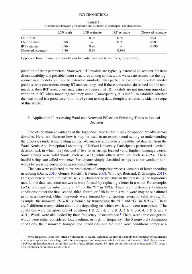
models as priors. Let = 1, . . . ,15 index the condition. Then

μ1k |α ,βk, δ1 ∼ Normal(α + βk, δ1), (13)

μ2k |γ , τk, δ2 ∼ Normal(γ + τk, δ2), (14)

where α and γ are the main effects of the th condition on word and nonword finishing times,respectively; βk and τk are the main effects of the kth participant on word and nonword finishingtimes, respectively; and δ1 and δ2 are the variance of the residual interaction terms.

Priors are needed for α, γ , β , and τ . As in the testing application, we place zero-centeredpriors on participant effect vectors β and τ . Priors on α and γ are slightly more complex. Theyare motivated by the fact that people are relatively accurate in the their lexical decisions. Con-sequently, finishing times for correct responses, that is word responses to words and nonwordresponses to non words, must be faster than finishing times for incorrect responses. In the currentdesign, there are 12 nonword conditions and 3 word conditions that are crossed with the nonwordand word accumulators. We used 4 hyperpriors to describe the crossing. Let μα = (μαw ,μαw

)

be a 2-item vector of condition means for word and nonword conditions, respectively, let μγ

be defined analogously, and let X0 be the 15 × 2 design matrix that maps each condition intowhether it is a word or nonword condition. Then the priors on condition means are

α | μα, σ 2α ∼ Normal

(X0μα, σ 2

αI),

γ | μγ , σ 2γ ∼ Normal

(X0μγ , σ 2

γ I).

The effect of this additional level in the hierarchical prior is to change the direction of shrinkage.In this model, the crossings of word and nonword conditions with word and nonword accu-mulators serve as unique points of shrinkage, and model different shrinkage points for correctword responses, incorrect word responses, correct nonword responses, and incorrect nonwordresponses. We place a flat prior on ψ , Inverse-Gamma priors on all variance parameters, anddiffuse normally-distributed priors on the μα and μγ parameters. The prior on ρ was uniformlydistributed from −1 to 1.

6.2. Analysis

The inclusion of the AR(1) component helps illustrate the two tasks needed to integrate com-plex backend models into the lognormal race framework. The first task is sampling the posteriorvalues of log finishing times conditional on all parameters. Let i and i denote the winning andlosing accumulator. For the winning accumulator, this value is known, and zijk = log(tjk − ψk).For the losing accumulator,

zijk| · · · ∼ Truncated-Normal(E[zijk] + ρui,j−1,k, σ

2, zijk

),

where ui,j−1,k is defined in (10), and E is the expected value of the parameter with respect toits prior. The vector of expectation values is simply the product of the relevant design matricesand parameter vectors. Sampling truncated normals is not computationally demanding, thoughsampling all latent finishing times is time consuming when there are a large number of trials andresponse alternatives. The second task is sampling the vectors of parameters and hyperparametersgiven the log finishing times. For all parameters except ψ , the conditional posterior distributionsremain conjugate; that is, they are multivariate normal and inverse-gamma, and for the dimen-sions of this application the sampling is convenient. The conditional posterior distribution of ρ

is

ρ | · · · ∼ Truncated-Normal(−1,1)

(m′/v′, σ 2/v′),

PSYCHOMETRIKA

FIGURE 3.The chain of values for parameter σ 2, the slowest converging parameter. The plots show outputs after thinning by a factorof 20. (A) MCMC outputs. (B) Autocorrelation function of outputs.

where

m′ =2∑

i=1

K∑

k=1

Jk−1∑

j=1

uijkui,j+1,k,

v′ =2∑

i=1

K∑

k=1

Jk−1∑

j=1

u2ijk.

Parameters ψ are sampled with Metropolis–Hastings steps, and we have found it quite easy totune these steps in practice to obtain reasonable rejection rates.

6.3. Results

Mixing We performed 5 independent runs of 10,000 MCMC iterations with a burn-in pe-riod of 500 iterations. Convergence of the chains with burn-in excluded were assessed in the samemanner as in the above IRT application using Gelman et al.’s (2004) R and effective number-of-samples (Neff) statistics. The maximum R across all parameters was 1.004 indicating acceptableconvergence to target posterior distributions. The median Neff across all five chains was 10400indicating that posterior quantities are estimated to reasonable high precision. Figure 3 shows theresulting MCMC outputs and autocorrelation function for σ 2, the slowest converging parameter,across the 5 runs after thinning by a factor of 20. All other parameters showed equally well orbetter mixing.

Model Fit The current model was built to be psychometrically useful rather than fit thedata precisely. Nonetheless, the model should fit at least coarsely if the parameters are to be in-terpreted. Figure 4A is a plot of observed mean response time for correct responses as a functionof the predicted value. Each point is from a particular participant in a particular condition. Thereis some misfit for slow RTs, but the overall pattern is reasonable for a measurement model. Fig-ure 4B is the same for the probability of a word response, and each point is from a particularparticipant-by-condition combination. There is some degree of misfit for nonword conditions.This slight mistfit is not surprising as these conditions have smaller numbers of observations (al-though there were 360 words and nonwords, the nonwords were divided into 12 conditions while

JEFFREY N. ROUDER ET AL.

FIGURE 4.Plots of observed data as a function of predicted values. Points denote values from the 1395 condition-by-participantcombinations. (A) Mean response time for correct responses. (B) Probability of a “word” response.

the words were divided into only 3 conditions). With such small numbers at the participant-by-condition level, there is a noticeable effect of the prior pulling very small probabilities away fromzero. This type of shrinkage is expected in hierarchical models, and strikes us as reasonable.

Parameter Estimates Figure 5 shows the condition effects on accumulators. The basic pat-tern is one of mirror symmetry where conditions that result in faster finishing times on one accu-mulator also result in slower finishing times on the other. The nonword accumulator seeminglyreacts to the conditions in an orderly and structured manner, indicating that the notion of non-word accumulation passes a minimal test. Finishing times for nonword errors in word conditionsand for word errors in nonword conditions are similar. There are, however, two subtle differencesbetween word and nonword finishing times: (1) The series labeled “a” shows word-accumulatorfinishing times for word items, and these are faster than the corresponding nonword finishingtimes for nonword items (series labeled “e” and “f”). (2) The effect of condition is greater forword accumulators than for nonword accumulators (as measured on the log scale): series “a” ismore varied than series “d;” series “b” is more varied than series “e;” series “c” is more variedthan series “f.” Note that this effect of greater variation holds for both word and nonwords. Insummary, although nonword accumulation is similar to word accumulation, the later seems moresensitive to manipulations than the former.

Figure 6 shows the parameter estimates of shift (ψ ) and autocorrelation (ρ). The thick seg-ments in Figure 6A are the posterior interquartile range for each shift estimate, and the thinsegments are the corresponding 95 % posterior credible intervals. As can be seen, these shiftparameters are well away from zero and vary substantially from one another. Therefore, theuse of individual shift parameters seems judicious as a general rule even though it does comewith some computational cost. Figure 6B shows the posterior distribution of ρ, and the degreeof trial-to-trial correlation is small, about 0.07. Nonetheless, it is reliably positive. Given thesmall size, models without sequential dependencies will provide for reasonable estimation ofcondition-effect parameters, the parameters of main interest.

We assessed whether shifts were necessary using DIC as discussed previously. Two models,one with unshifted lognormal distributions, and the above model were compared, though in nei-ther did we include sequential dependencies. The likelihood function is easily found from (3),and may be evaluated on each iteration of the chain. The DIC for the model without shifts is

PSYCHOMETRIKA

FIGURE 5.Finishing times for word and nonword accumulators as a function of condition.

FIGURE 6.(A) Posterior interquartile range (thick segment) and 95 % credible intervals (thin segment) for each participant’s shiftparameter ψ . (B) Posterior distribution of ρ.

−68,897 and that for the model with shifts is −77,374; hence, the model with shifts is preferred,and the difference of about 8,500 is overwhelming.

7. General Discussion

In this paper, we have provided a simple process model for response time and choice thathas desirable statistical properties. In this model, decisions are viewed as arising from a racebetween competing evidence-accumulation processes. Finishing times of accumulators are log-normal random variables; due to this assumption, the model is tractable when analyzed in theBayesian framework. It is straightforward to place sophisticated model components, such as au-toregressive models, on the finishing times, and it seems equally straightforward to place othersophisticated components such as factor and structural equation models. We view the model asretaining the core strengths of both the psychometric and cognitive-process model traditions: It is

JEFFREY N. ROUDER ET AL.

plausible from a process perspective, while being useful from a psychometric perspective. More-over, the model is applicable in a wide range of human performance settings, providing both atheoretical and practical means of uniting analysis in experimental psychology and high-stakestesting.

7.1. Relationship to Other Race Models

The lognormal race is a member of a larger class of racing-accumulator models. In thesemodels, each response has an associated accumulator, and information slowly accumulates. Ingeneral, this information is considered stochastic, that is, it has moment-to-moment variationand may be modeled as white noise (McGill, 1963). A decision occurs the first time this noisyinformation in the accumulators exceeds its bound (Audley & Pike, 1965; Smith, 2000). In ap-plication, the rate of information growth and the bound are free parameters estimated from thedata. One of the main advantages of the racing accumulator framework is neural plausibility,and the notion of neurons as accumulators has been supported by single-cell neurophysiologi-cal recordings. Firing rates in targeted neurons slowly increase with a rate that reflects stimulusstrength variables (Hanes & Schall, 1996; Huk & Shadlen, 2005; Roitman & Shadlen, 2002;Ratcliff, Thapar, & McKoon, 2003). This relationship between stimulus strength and firing ratescan be seen in several brain regions across a variety of stimuli and tasks (see Gold & Shadlen,2007; Schall, 2003, for reviews). Not surprisingly, racing accumulator models form the decision-making process in popular neural network approaches (Anderson & Lebiere, 1998; McClelland,1993; Usher & McClelland, 2001).

The lognormal race follows from Grice (1968), who provided an alternative specification forthe racing-accumulator class of models. He assumed there was no moment-to-moment variationin the information in the accumulators. The information accumulated deterministically and lin-early until it reached a bound. Let ν be the rate of information gain and η be the bound. Thenthe finishing time, y, is simply η/ν. Grice specified that the bound varied normally from trial-to-trial, and the resulting distribution of y, though incomplete, has been termed the reciprobitdistribution (Reddi & Carpenter, 2003). Brown and Heathcote (2008) assumed that both the rateof information accumulation and the bound varied from trial-to-trial. Heathcote and Love (2012)assumed that both ν and η were distributed as lognormals, with η ∼ Lognormal(μη,σ

2η ) and

ν ∼ Lognormal(μν, σ2ν ). The distribution of finishing time is y ∼ Lognormal(μη −μν,σ

2η +σ 2

ν ).From this expression, it is clear that with the lognormal distributional assumptions, bounds andaccumulation rates cannot be disentangled. Without loss of generality, the bounds may be set to1.0. This specification results in the base model presented here: y ∼ Lognormal(μ,σ 2) whereμ = −μν and σ 2 = σ 2

ν .The lognormal race model lacks identifiable decision bounds. The nonidentifiability follows

from the lognormal parametric assumption, and with it only the ratio of bounds-to-accumulation-rate is identifiable. This inability to identify bounds separate from accumulation rate is a theo-retical disadvantage, at least from a conventional view. We think, however, that it represents anappropriately cautious and humble position. Other race models that distinguish between accumu-lation rates from decision bounds do so with recourse to specific parametric assumptions, and theestimates of these quantities directly reflects the parametric assumptions. Even the separate esti-mation of bounds and drift rates in the diffusion model rests on a latent assumption that cannotbe tested directly, namely the stationarity of the diffusion process. We would prefer that measure-ment of these quantities not be conditional on such arbitrary assumptions. As a consequence, wegive up the ability to separate bounds from rates. The lognormal parametric specification maybe profitably viewed as an elegant way of avoiding fine conceptual distinctions that may not beinformed by data.

PSYCHOMETRIKA

7.2. Highly Accurate Responses

In many areas of experimental psychology, responses are highly accurate and the focus issolely on speed. An example is subliminal priming where the aim is to understand how a weakstimulus affects subsequent processing, and the main paradigm is to see how the presentationof a weak prime speeds the subsequent responses to related materials (e.g., Greenwald, Draine,& Abrams, 1996). In these cases, however, trials still admit multiple responses, even though thecorrect one is chosen almost always. One advantage of the lognormal race is that it is well suitedfor these paradigms. In the limit of perfect performance, the response times are lognormallydistributed, and this distributional model has been advocated both on practical and theoreticalgrounds (Ulrich & Miller, 1993). For highly accurate conditions, the analyst must be aware thatthe latent finishing times on the incorrect accumulators will largely reflect prior assumptionsbecause there are few error responses to inform estimation of these parameters. Nonetheless, theability to account for highly accurate data is a strong advantage, especially when compared tomodels that have separate parameters for bounds and accumulation rates. In these models, suchas the diffusion model, it is imperative to have some conditions that are far from ceiling to locatethe bounds. For the lognormal race, in contrast, such conditions are not necessary, and the modelworks well even for experiments where there is high accuracy in all conditions.

7.3. The Need for a Shift Parameter

We have explicitly included an individual specific shift parameter ψk . The inclusion of ashift parameter needs some justification because it is relatively novel in the psychometric litera-ture. Traditionally, psychometric researchers have implemented two-parameter unshifted skeweddistributions for RT that do not have a shift parameter (e.g., Thissen, 1983; van Breukelen, 2005;van der Linden et al., 1999). This choice is in contrast to cognitive process modelers who rou-tinely include shift parameters (Luce, 1986). Perhaps the reason psychometricians exclude theshift is convenience—the two-parameter (unshifted) lognormal is easily analyzed with the GLMfamily while the three-parameter (shifted) model is not. Hence, analysis of mixed two-parametermodels may be carried out through familiar means while analysis of the three-parameter modelrequires additional development. In our Bayesian development, the inclusion of the shift parame-ter necessitates the inclusion of a Metropolis step, and affects mixing under certain circumstancesthat are discussed subsequently. Nonetheless, we believe that the empirical data patterns neces-sitate the inclusion of shift, and models that do not contain a shift parameter will be needlesslymisspecified in many domains. Rouder (2005), in response to van Breukelen’s two-parameterlognormal model (van Breukelen, 2005) noted that minimum response times were often shiftedwell away from zero and that this shift varied across people. Indeed, this trend holds here inthe lexical-decision data set examined here. Not accounting for shifts will lead to a dramaticoverestimation of scale and an equally dramatic underestimation of shape.

7.4. Caveats

There are two practical difficulties that arise when analyzing lognormal race models: thepotential for poor mixing and the potential for undue influence of the priors.

Poor mixing may occur in the MCMC chain for the shape (σ 2) and shift (ψ ) parameters.This poor mixing results from the three-parameter lognormal parametric specification. In this dis-tribution, the left-tail becomes increasingly soft or shallow as the shape becomes more symmetric(that is, as σ 2 decreases). For small true values of σ 2, shift and shape are weakly identified, andthis weak identifiability leads to poor mixing. Hence, while the three parameter lognormal is agood choice overall, it becomes more suspect as RT distributions become less skewed. If theobserved data does not have noticeable skew then researchers may consider fixing the ψ to zero

JEFFREY N. ROUDER ET AL.

or abandoning the lognormal parametric specification entirely. Fortunately, RT distributions aretypically skewed (Luce, 1986).

A second issue is the potential for undue influence of the priors. This issue is germane forlow-probability responses. Consider a lexical decision experiment where all the words are com-mon and easy-to-read (e.g. dog, run, bread) and all the nonwords are clearly not words (e.g.,xqre, zvbt). In this case, we expect almost all words and nonwords to be identified as such, andvery few errors to occur. In analysis, however, we estimate finishing times for error responseseven though they are rare. In this case, the correct accumulator estimates will largely reflectthe data rather than the prior as correct responses are numerous. The difficulty is with the er-ror accumulator estimates, which may largely reflect prior assumptions when there are few ifany responses. Hence, researchers need to be aware of the sample size per response option inassessing the influence of the prior and interpreting parameter estimates for error accumulators.In the lexical decision application, we used a hierarchical prior that allows sharing of informa-tion across people-by-condition combinations. This approach is suitable even for small effectivesample sizes at the people-by-condition level, though researchers should keep in mind that theseestimates reflect the structure of the hierarchical prior.

Acknowledgements

This research is supported by National Science Foundation Grants SES-1024080 and BCS-1240359 (JNR) and Australian Research Council Professorial Fellowship (AH).

References

Anderson, J.R., & Lebiere, C. (1998). The atomic component of thought. Mahwah: Lawrence Erlbaum Associates.Audley, R.J., & Pike, A.R. (1965). Some alternative stochastic models of choice. British Journal of Mathematical and

Statistical Psychology, 18, 207–225.Bertelson, P. (1961). Sequential redundancy and speed in a serial two choice responding task. Quarterly Journal of

Experimental Psychology, 13, 290–292.Brown, S.D., & Heathcote, A. (2008). The simplest complete model of choice reaction time: linear ballistic accumulation.

Cognitive Psychology, 57, 153–178.Craigmile, P.F., Peruggia, M., & Van Zandt, T. (2010). Hierarchical Bayes models for response time. Psychometrika, 75,

613–632.Davis, C. (2010). The spatial coding model of visual word identification. Psychological Review, 117(3), 713.Diederich, A., & Busemeyer, J.R. (2003). Simple matrix methods for analyzing diffusion models of choice probability,

choice response time and simple response time. Journal of Mathematical Psychology, 47, 304–322.Dufau, S., Grainger, J., & Ziegler, J.C. (2012). How to say “no” to a nonword: a leaky competing accumulator model of

lexical decision. Journal of Experimental Psychology: Learning, Memory, and Cognition, 38, 1117–1128.Dzhafarov, E.N. (1992). The structure of simple reaction time to step-function signals. Journal of Mathematical Psychol-

ogy, 36, 235–268.Embretson, S.E. (1991). A multidimensional latent trait model for measuring learning and change. Psychometrika, 56,

495–516.Falmagne, J.C., Cohen, S.P., & Dwivedi, A. (1975). Two choice reactions as an ordered memory scanning process. In

P.M.A. Rabbit & S. Dornic (Eds.), Attention and performance V (pp. 296–344). New York: Academic Press.Gelfand, A., & Smith, A.F.M. (1990). Sampling based approaches to calculating marginal densities. Journal of the

American Statistical Association, 85, 398–409.Gelman, A., Carlin, J.B., Stern, H.S., & Rubin, D.B. (2004). Bayesian data analysis (2nd ed.). London: Chapman and

HallGold, J.I., & Shadlen, M.N. (2007). The neural basis of decision making. Annual Review of Neuroscience, 30, 535–574.Gomez, P., Ratcliff, R., & Perea, M. (2008). The overlap model: a model of letter position coding. Psychological Review,

115(3), 577.Greenwald, A.G., Draine, S.C., & Abrams, R.L. (1996). Three cognitive markers of unconscious semantic activation.

Science, 273(5282), 1699–1702.Grice, G.R. (1968). Stimulus intensity and response evocation. Psychological Review, 75, 359–373.Hanes, D.P., & Schall, J.D. (1996). Neural control of voluntary movement initiation. Science, 274(5286), 427–430.Heathcote, A., & Love, J. (2012). Linear deterministic accumulator models of simple choice. Frontiers in Cognitive

Science, 3, 292. http://www.frontiersin.org/Cognitive_Science/10.3389/fpsyg.2012.0029.

PSYCHOMETRIKA

Huk, A., & Shadlen, M.N. (2005). Neural activity in macaque parietal cortex reflects temporal integration of visualmotion signals during perceptual decision making. Journal of Neuroscience, 25, 10420–10436.

Jackman, S. (2009). Bayesian analysis for the social sciences. Chichester: Wiley.Kass, R.E. (1993). Bayes factors in practice. The Statistician, 42, 551–560.Kass, R.E., & Raftery, A.E. (1995). Bayes factors. Journal of the American Statistical Association, 90, 773–795.Kucera, H., & Francis, W.N. (1967). Computational analysis of present-day American English. Providence: Brown Uni-

versity Press.Lee, S.-Y. (2007). Structural equation modelling: a Bayesian approach. New York: Wiley.Link, S.W. (1992). Wave theory of difference and similarity. Hillsdale: Erlbaum.Luce, R.D. (1986). Response times. New York: Oxford University Press.McClelland, J.L. (1993). Toward a theory of information processing in graded, random, and interactive networks. In

D.E. Meyer & S. Kornblum (Eds.), Attention & performance XIV: synergies in experimental psychology, artificialintelligence and cognitive neuroscience. Cambridge: MIT Press.

McClelland, J.L., & Rumelhart, D.E. (1981). An interactive activation model of context effects in letter perception: I. Anaccount of basic findings. Psychological Review, 88, 375–407.

McGill, W. (1963). Stochastic latency mechanism. In R.D. Luce & E. Galanter (Eds.), Handbook of mathematical psy-chology (Vol. 1, pp. 309–360). New York: Wiley.

Morey, R.D., Rouder, J.N., Pratte, M.S., & Speckman, P.L. (2011). Using MCMC chain outputs to efficiently estimateBayes factors. Journal of Mathematical Psychology, 55, 368–378. http://dx.doi.org/10.1016/j.jmp.2011.06.004.

Peruggia, M., Van Zandt, T., & Chen, M. (2002). Was it a car or a cat I saw? An analysis of response times for wordrecognition. Case Studies in Bayesian Statistics, 6, 319–334.

Rasch, G. (1960). Probabilistic models for some intelligence and attainment tests. Copenhagen: Danish Institute forEducational Research.

Ratcliff, R. (1978). A theory of memory retrieval. Psychological Review, 85, 59–108.Ratcliff, R., & McKoon, G.M. (2008). The diffusion decision model: theory and data for two-choice decision tasks.

Neural Computation, 20, 873–922.Ratcliff, R., & Rouder, J.N. (1998). Modeling response times for decisions between two choices. Psychological Science,

9, 347–356.Ratcliff, R., Thapar, A., & McKoon, G. (2003). A diffusion model analysis of the effects of aging on brightness discrim-

ination. Perception and Psychophysics, 65, 523–535.Ratcliff, R., Gomez, P., & McKoon, G.M. (2004). A diffusion model account of the lexical decision task. Psychological

Review, 111, 159–182.Reddi, B., & Carpenter, R. (2003). Accuracy, information and response time in a saccadic decision task. Journal of

Neurophysiology, 90, 3538–3546.Riefer, D.M., Knapp, B.R., Batchelder, W.H., Bamber, D., & Manifold, V. (2002). Cognitive psychometrics: assessing

storage and retrieval deficits in special populations with multinomial processing tree models. Psychological Assess-ment, 14, 184–201.

Roberts, G.O., & Sahu, S.K. (1997). Updating schemes, correlation structure, blocking and parameterization for theGibbs sampler. Journal of the Royal Statistical Society, Series B, Methodological, 59, 291–317.

Roberts, S., & Pashler, H. (2000). How persuasive is a good fit? A comment on theory testing. Psychological Review,107, 358–367.

Roitman, J.D., & Shadlen, M.N. (2002). Response of neurons in the lateral intraparietal area during a combined visualdiscrimination reaction time task. Journal of Neuroscience, 22, 9475–9489.

Rouder, J.N. (2005). Are unshifted distributional models appropriate for response time? Psychometrika, 70, 377–381.Rouder, J.N., Sun, D., Speckman, P.L., Lu, J., & Zhou, D. (2003). A hierarchical Bayesian statistical framework for

response time distributions. Psychometrika, 68, 587–604.Rumelhart, D.E., & McClelland, J.L. (1982). An interactive activation model of context effects in letter perception: II.

The contextual enhancement effect and some tests and extensions of the model. Psychological Review, 89, 60–94.Schall, J.D. (2003). Neural correlates of decision processes: neural and mental chronometry. Current Opinion in Neuro-

biology, 13, 182–186.Skrondal, A., & Rabe-Hesketh, S. (2004). Generalized latent variable modeling: multilevel, longitudinal, and structural

equation models. Boca Raton: CRC Press.Smith, P.L. (2000). Stochastic dynamic models of response time and accuracy: a foundational primer. Journal of Mathe-

matical Psychology, 44, 408–463.Spiegelhalter, D.J., Best, N.G., Carlin, B.P., & van der Linde, A. (2002). Bayesian measures of model complexity and fit

(with discussion). Journal of the Royal Statistical Society, Series B, Statistical Methodology, 64, 583–639.Thissen, D. (1983). Timed testing: an approach using item response theory. In D.J. Weiss (Ed.), New horizons in testing:

latent trait test theory and computerized adaptive testing (pp. 179–203). New York: Academic Press.Tuerlickx, F., & De Boek, P. (2005). Two interpretations of the discrimination parameter. Psychometrika, 70, 629–650.Ulrich, R., & Miller, J.O. (1993). Information processing models generating lognormally distributed reaction times.

Journal of Mathematical Psychology, 37, 513–525.Usher, M., & McClelland, J.L. (2001). On the time course of perceptual choice: the leaky competing accumulator model.

Psychological Review, 108, 550–592.van Breukelen, G.J.P. (2005). Psychometric modeling of response time and accuracy with mixed and conditional regres-

sion. Psychometrika.Vandekerckhove, J., Tuerlinckx, F., & Lee, M.D. (2011). Hierarchical diffusion models for two-choice response time.

Psychological Methods, 16, 44–62.

JEFFREY N. ROUDER ET AL.

Vandekerckhove, J., Verheyen, S., & Tuerlinckx, F. (2010). A cross random effects diffusion model for speeded semanticcategorization decisions. Acta Psychologica, 133, 269–282.

van der Linden, W.J. (2007). A hierarchical framework for modeling speed and accuracy on test items. Psychometrika,72, 287–308.

van der Linden, W.J. (2009). Conceptual issues in response-time modeling. Journal of Educational Measurement, 14,247–272.

van der Linden, W.J., Scrams, D.J., & Schnipke, D.L. (1999). Using response-time constraints to control for differentialspeededness in computerized adaptive testing. Applied Psychological Measurement, 23, 195–210.

van der Maas, H.L.J., Molenaar, D., Maris, G., Kievit, R.A., & Borsboom, D. (2001). Cognitive psychology meetspsychometric theory: on the relation between process models for decision making and latent variable models forindividual differences. Psychological Review, 118, 339–356.

Wagenmakers, E.-J., van der Maas, H.L.J., & Grasman, R.P.P.P. (2007). An EZ-diffusion model for response time andaccuracy. Psychonomic Bulletin & Review, 14, 3–22.

Whitney, C., Bertrand, D., & Grainger, J. (2011). On coding the position of letters in words . Experimental Psychology(formerly Zeitschrift für Experimentelle Psychologie), 1–6.

Wild, P., & Gilks, W.R. (1993). Adaptive rejection sampling from log-concave density functions. Applied Statistics, 42,701–708.

Manuscript Received: 22 AUG 2012