Latency verification in execution traces of HW/SW partitioning ...
217
HAL Id: tel-03576841 https://tel.archives-ouvertes.fr/tel-03576841 Submitted on 16 Feb 2022 HAL is a multi-disciplinary open access archive for the deposit and dissemination of sci- entific research documents, whether they are pub- lished or not. The documents may come from teaching and research institutions in France or abroad, or from public or private research centers. L’archive ouverte pluridisciplinaire HAL, est destinée au dépôt et à la diffusion de documents scientifiques de niveau recherche, publiés ou non, émanant des établissements d’enseignement et de recherche français ou étrangers, des laboratoires publics ou privés. Latency verification in execution traces of HW/SW partitioning model Maysam Zoor To cite this version: Maysam Zoor. Latency verification in execution traces of HW/SW partitioning model. Embedded Systems. Institut Polytechnique de Paris, 2021. English. NNT: 2021IPPAT037. tel-03576841
-
Upload
khangminh22 -
Category
Documents
-
view
5 -
download
0
Transcript of Latency verification in execution traces of HW/SW partitioning ...
HAL Id: tel-03576841https://tel.archives-ouvertes.fr/tel-03576841
Submitted on 16 Feb 2022
HAL is a multi-disciplinary open accessarchive for the deposit and dissemination of sci-entific research documents, whether they are pub-lished or not. The documents may come fromteaching and research institutions in France orabroad, or from public or private research centers.
L’archive ouverte pluridisciplinaire HAL, estdestinée au dépôt et à la diffusion de documentsscientifiques de niveau recherche, publiés ou non,émanant des établissements d’enseignement et derecherche français ou étrangers, des laboratoirespublics ou privés.
Latency verification in execution traces of HW/SWpartitioning model
Maysam Zoor
To cite this version:Maysam Zoor. Latency verification in execution traces of HW/SW partitioning model. EmbeddedSystems. Institut Polytechnique de Paris, 2021. English. �NNT : 2021IPPAT037�. �tel-03576841�

626626
NNT
:2021IPPA
T037
Latency Verification in ExecutionTraces of HW/SW Partitioning Model
Thèse de doctorat de l’Institut Polytechnique de Parispréparée à Télécom Paris
École doctorale n◦626 l’Institut Polytechnique de Paris (ED IP Paris)Spécialité de doctorat: Informatique
Thèse présentée et soutenue à Sophia Antipolis, le 8-12-2021, par
Maysam Zoor
Composition du Jury :
Camille SalinesiProfesseur des universités, Université Paris 1 PanthéonSorbonne Président
Jean-Philippe BabauProfesseur, Université de Bretagne Occidentale RapporteurIulian OberEnseignant-chercheur,Université de Toulouse RapporteurEmmanuelle EncrenazAssociate Professor, Université Pierre et Marie Curie ExaminateurLudovic ApvrilleProfesseur,Télécom Paris Directeur de thèseRenaud PacaletDirecteur d’étude, Télécom Paris Co-directeur de thèse

To my parents who chose to give me the best education they could.


Acknowledgements
The research presented in this thesis was sponsored by AQUAS project. The AQUAS project is funded
by ECSEL JU under grant agreement No 737475.
This thesis would not have been possible without the support of many people. First of all, I would
like to thank my supervisors Ludovic Apvrille and Renaud Pacalet for welcoming me in the lab and
for their guidance throughout this work. Next, I would like to thank my committee members, Camille
Salinesi, Jean-Philippe Babau, Emmanuelle Encrenaz and Iulian Ober for their time to read my thesis
and participate in my defense. Their feedback and suggestions toward my thesis have been important to
enhence my manuscript.
I would also like to thank all members of LabSoc. I gratefully recognize the help of Rabéa Ameur-
Boulifa and Sophie Coudert to formally define my contributions. I’m proud of, and grateful for, my time
working with Emna, Matteo, Benjamin, Minh and Le Van. Our breaks together were always enjoyable
and refreshing. You have made this journey so much better.
And because no distance can lessen true friendships, I want to thank Lama, Rola, Ghada and Mira
for standing by me through thick and thin. And to my friends who were beside me, immense gratitude
for your support all through the years. My life is richer because of your presence in it. I especially want
to thank Gaetan, Mohammad, Ahmad and Rima for their endless support and listening to me talk things
out.
Lastly, my family deserves endless gratitude. I could not have done this without them. My mom,
Najwa, inspired me to do my best and showed me that a person can achieve anything they put in mind.
My dad, Refaat, supported me in every decision I have made and my brother, Majed, who I can always
count on him when life gets hard. Thank you for always offering support and love.
1
Contents
Acronyms 11
Glossary of Mathematical Notations 13
1 Introduction 17
1.1 Embedded Systems . . . . . . . . . . . . . . . . . . . . . . . . . . . . . . . . . . . . 19
1.2 Problem Statement . . . . . . . . . . . . . . . . . . . . . . . . . . . . . . . . . . . . 20
1.3 Contributions . . . . . . . . . . . . . . . . . . . . . . . . . . . . . . . . . . . . . . . . 23
1.3.1 Precise Latency Analysis Approach . . . . . . . . . . . . . . . . . . . . . . . . 26
1.3.2 Integration into a Model-Driven Engineering Framework . . . . . . . . . . . . . 27
1.4 Organization of This Thesis . . . . . . . . . . . . . . . . . . . . . . . . . . . . . . . . 27
2 Context 29
2.1 Structure of Embedded Systems . . . . . . . . . . . . . . . . . . . . . . . . . . . . . . 30
2.2 Model-Driven Engineering . . . . . . . . . . . . . . . . . . . . . . . . . . . . . . . . . 31
2.3 Timing Constraints . . . . . . . . . . . . . . . . . . . . . . . . . . . . . . . . . . . . . 34
2.4 SysML-Sec . . . . . . . . . . . . . . . . . . . . . . . . . . . . . . . . . . . . . . . . . 35
2.4.1 HW/SW partitioning . . . . . . . . . . . . . . . . . . . . . . . . . . . . . . . . 37
2.4.2 Simulation . . . . . . . . . . . . . . . . . . . . . . . . . . . . . . . . . . . . . 38
3 Related Work 41
3.1 Software Development Methodologies . . . . . . . . . . . . . . . . . . . . . . . . . . . 42
3.1.1 Functional and Nonfunctional Requirements . . . . . . . . . . . . . . . . . . . 43
2
3.1.2 Using UML design tools and techniques . . . . . . . . . . . . . . . . . . . . . . 46
3.2 Verification Techniques . . . . . . . . . . . . . . . . . . . . . . . . . . . . . . . . . . 47
3.2.1 Formal Verification Approaches . . . . . . . . . . . . . . . . . . . . . . . . . . 47
3.2.2 Runtime Verification Approaches . . . . . . . . . . . . . . . . . . . . . . . . . 51
3.2.3 Performance Evaluation . . . . . . . . . . . . . . . . . . . . . . . . . . . . . . 52
3.2.3.1 Simulation-Based Approaches . . . . . . . . . . . . . . . . . . . . . . 54
3.3 Information Flow Analysis . . . . . . . . . . . . . . . . . . . . . . . . . . . . . . . . . 58
3.3.1 Taint Analysis . . . . . . . . . . . . . . . . . . . . . . . . . . . . . . . . . . . 59
3.4 Conclusion . . . . . . . . . . . . . . . . . . . . . . . . . . . . . . . . . . . . . . . . . 61
4 Precise Latency Analysis Approach: Overview and Problem Formalization 64
4.1 Motivation . . . . . . . . . . . . . . . . . . . . . . . . . . . . . . . . . . . . . . . . . 64
4.2 Precise Latency Analysis Approach . . . . . . . . . . . . . . . . . . . . . . . . . . . . 66
4.3 System Model Formal Definition . . . . . . . . . . . . . . . . . . . . . . . . . . . . . . 67
4.3.1 Application . . . . . . . . . . . . . . . . . . . . . . . . . . . . . . . . . . . . . 67
4.3.2 Platform . . . . . . . . . . . . . . . . . . . . . . . . . . . . . . . . . . . . . . 80
4.3.3 Allocation . . . . . . . . . . . . . . . . . . . . . . . . . . . . . . . . . . . . . 82
4.3.4 Example 1 . . . . . . . . . . . . . . . . . . . . . . . . . . . . . . . . . . . . . 82
4.4 Model Executional Semantics . . . . . . . . . . . . . . . . . . . . . . . . . . . . . . . 84
4.5 Requirement on Model Execution . . . . . . . . . . . . . . . . . . . . . . . . . . . . . 88
4.6 Conclusion . . . . . . . . . . . . . . . . . . . . . . . . . . . . . . . . . . . . . . . . . 89
5 Primitive Precise Latency Analysis Approach 90
5.1 Execution Trace Analysis . . . . . . . . . . . . . . . . . . . . . . . . . . . . . . . . . . 91
5.1.1 Causality between operators: an Example . . . . . . . . . . . . . . . . . . . . . 91
5.1.2 Valid Execution Trace . . . . . . . . . . . . . . . . . . . . . . . . . . . . . . . 93
5.1.3 Read Write Dependencies Accuracy . . . . . . . . . . . . . . . . . . . . . . . . 101
5.1.4 Classification of Execution Transactions . . . . . . . . . . . . . . . . . . . . . . 106
5.1.4.1 Impact Sets . . . . . . . . . . . . . . . . . . . . . . . . . . . . . . . 106
3
5.1.4.1.1 On Path Sets . . . . . . . . . . . . . . . . . . . . . . . . . 106
5.1.4.1.2 In Functions Sets . . . . . . . . . . . . . . . . . . . . . . . 109
5.1.4.1.3 Contention Set . . . . . . . . . . . . . . . . . . . . . . . . . 112
5.1.4.1.4 No Contention Set . . . . . . . . . . . . . . . . . . . . . . . 119
5.1.4.1.5 Other Hardware Set (OH) . . . . . . . . . . . . . . . . . . . 121
5.1.4.1.6 Indirect Impact Set . . . . . . . . . . . . . . . . . . . . . . 121
5.1.4.1.7 No Impact Set . . . . . . . . . . . . . . . . . . . . . . . . . 123
5.2 Conclusion . . . . . . . . . . . . . . . . . . . . . . . . . . . . . . . . . . . . . . . . . 123
6 Advanced Precise Latency Analysis Approach Using Graph Tainting (PLAN-GT) 124
6.1 Motivation . . . . . . . . . . . . . . . . . . . . . . . . . . . . . . . . . . . . . . . . . 124
6.2 Example 2 . . . . . . . . . . . . . . . . . . . . . . . . . . . . . . . . . . . . . . . . . 125
6.3 Tainting . . . . . . . . . . . . . . . . . . . . . . . . . . . . . . . . . . . . . . . . . . 128
6.3.1 Static attributes . . . . . . . . . . . . . . . . . . . . . . . . . . . . . . . . . . 130
6.3.2 Dynamic attributes . . . . . . . . . . . . . . . . . . . . . . . . . . . . . . . . . 133
6.3.3 Tainting Algorithm . . . . . . . . . . . . . . . . . . . . . . . . . . . . . . . . . 136
6.3.4 Operator Transactions Granularity . . . . . . . . . . . . . . . . . . . . . . . . . 136
6.3.5 Calculating latency based on tainting . . . . . . . . . . . . . . . . . . . . . . . 139
6.3.5.1 Tainting Choice operators inside loops . . . . . . . . . . . . . . . . . 146
6.4 Collect transactions and compute latencies . . . . . . . . . . . . . . . . . . . . . . . . 149
6.5 Conclusion . . . . . . . . . . . . . . . . . . . . . . . . . . . . . . . . . . . . . . . . . 150
7 Integration into Model-Driven Engineering Framework 151
7.1 Application to UML/SysML . . . . . . . . . . . . . . . . . . . . . . . . . . . . . . . . 152
7.1.1 Model simulation . . . . . . . . . . . . . . . . . . . . . . . . . . . . . . . . . . 156
7.2 PLAN integration into TTool . . . . . . . . . . . . . . . . . . . . . . . . . . . . . . . 157
7.3 Industrial Drive System Use Case . . . . . . . . . . . . . . . . . . . . . . . . . . . . . 162
7.3.1 Description of the use case . . . . . . . . . . . . . . . . . . . . . . . . . . . . 164
7.3.2 Model simulation and trace analysis . . . . . . . . . . . . . . . . . . . . . . . . 165
4
7.4 Rail Carriage Mechanisms Use Case . . . . . . . . . . . . . . . . . . . . . . . . . . . . 167
7.4.1 Description of the use case . . . . . . . . . . . . . . . . . . . . . . . . . . . . 167
7.4.1.1 HW/SW partitioning models . . . . . . . . . . . . . . . . . . . . . . 168
7.4.2 Model simulation and trace analysis . . . . . . . . . . . . . . . . . . . . . . . . 170
7.5 Conclusion . . . . . . . . . . . . . . . . . . . . . . . . . . . . . . . . . . . . . . . . . 172
8 Conclusion 174
8.1 Resume of Contributions . . . . . . . . . . . . . . . . . . . . . . . . . . . . . . . . . . 175
8.2 Perspectives . . . . . . . . . . . . . . . . . . . . . . . . . . . . . . . . . . . . . . . . 177
8.2.1 Model enhancements at current abstraction level . . . . . . . . . . . . . . . . . 178
8.2.2 Model enhancement to support different abstraction levels . . . . . . . . . . . . 179
8.2.3 Verification aspects . . . . . . . . . . . . . . . . . . . . . . . . . . . . . . . . 179
8.2.4 Tooling aspects . . . . . . . . . . . . . . . . . . . . . . . . . . . . . . . . . . 180
9 Résumé 184
A List of System Model Formal Definitions 189
B Execution Trace in XML format 193
5
List of Figures
1.1 Motor drive system . . . . . . . . . . . . . . . . . . . . . . . . . . . . . . . . . . . . . 21
1.2 Motor controller behavior . . . . . . . . . . . . . . . . . . . . . . . . . . . . . . . . . 24
1.3 Motor controller behavior allocated to a candidate architecture . . . . . . . . . . . . . 25
1.4 Examples of simulation traces for: (a) Figure 1.3 (b) Figure 1.5 . . . . . . . . . . . . . 25
1.5 Motor controller behavior allocated to another candidate architecture . . . . . . . . . . 26
2.1 Mars 2020 Rover . . . . . . . . . . . . . . . . . . . . . . . . . . . . . . . . . . . . . . 31
2.2 Y-Chart approach . . . . . . . . . . . . . . . . . . . . . . . . . . . . . . . . . . . . . 33
2.3 SysML-Sec modeling profile used in TTool . . . . . . . . . . . . . . . . . . . . . . . . 36
2.4 SysML-Sec methodology diagram in TTool . . . . . . . . . . . . . . . . . . . . . . . . 37
2.5 The design area for an application model . . . . . . . . . . . . . . . . . . . . . . . . . 38
2.6 The design area for an activity diagram . . . . . . . . . . . . . . . . . . . . . . . . . 38
2.7 The design area for an architecture model . . . . . . . . . . . . . . . . . . . . . . . . . 39
2.8 The mapping of a task on a computational node . . . . . . . . . . . . . . . . . . . . . 39
2.9 The interactive simulation window . . . . . . . . . . . . . . . . . . . . . . . . . . . . . 40
4.1 Modeling stages required to apply the precise latency analysis approach . . . . . . . . . 68
4.2 Graphical representation of a loop . . . . . . . . . . . . . . . . . . . . . . . . . . . . . 76
4.3 Graphical representation of a loop that iterates 2 times . . . . . . . . . . . . . . . . . . 77
4.4 Application model where classification of dependencies is not a partitioning of Dm . . . 79
4.5 Graphical representation of the Application model of Example 1 . . . . . . . . . . . . . 83
4.6 Graphical representation of a possible allocation for the application model given in Figure 4.5 84
6
5.1 Graphical representation of a function behavior to illustrate causality between operator . 92
5.2 An Application model where oB execution does not necessary depend on oA execution . 95
5.3 A possible allocation of the application model given in Figure 5.2 . . . . . . . . . . . . 95
5.4 An Application model to illustrate interleaving between transactions of operators . . . . 99
5.5 A possible allocation of the application model given in Figure 5.4 . . . . . . . . . . . . 99
5.6 An Application model containing a ReadData and a WriteData operator with different
size attributes . . . . . . . . . . . . . . . . . . . . . . . . . . . . . . . . . . . . . . . 103
5.7 The remodeling of the Application model of Figure 5.6 . . . . . . . . . . . . . . . . . . 104
5.8 An Application model containing several operators with different size attributes . . . . . 104
5.9 The first round of remodeling the Application model of Figure 5.8 . . . . . . . . . . . . 105
5.10 The second round of remodeling the Application model of Figure 5.8 . . . . . . . . . . 105
5.11 Cross Function . . . . . . . . . . . . . . . . . . . . . . . . . . . . . . . . . . . . . . . 108
5.12 An Application model used to explain the in Functions Sets . . . . . . . . . . . . . . . 110
5.13 Dependency Paths to o31 in the Application model shown in Figure 4.5 . . . . . . . . . 114
5.14 First case where a transaction t′ is delayed due to contention . . . . . . . . . . . . . . 118
5.15 Second case where a transaction t′ is delayed due to contention . . . . . . . . . . . . . 118
5.16 A graphical representation showing no contention . . . . . . . . . . . . . . . . . . . . . 120
6.1 Graphical representation of an Application model with loops . . . . . . . . . . . . . . . 126
6.2 Graphical representation for the Allocation model of Figure 6.1 . . . . . . . . . . . . . 127
6.3 Dependency Graph of Figure 6.1 . . . . . . . . . . . . . . . . . . . . . . . . . . . . . 128
6.4 Graphical representation of state change . . . . . . . . . . . . . . . . . . . . . . . . . 130
6.5 Dependency Graph Showing fixedNumber of Figure 6.1 . . . . . . . . . . . . . . . . . . 131
6.6 Dependency graph showing taintMaxNumber of Figure 6.1 . . . . . . . . . . . . . . . . 132
6.7 Graphical representation of a function with two nested loops . . . . . . . . . . . . . . . 132
6.8 Dependency graph showing taintMaxNumber of Figure 6.7 . . . . . . . . . . . . . . . . 133
6.9 Flow chart of latency calculation based on Tainting . . . . . . . . . . . . . . . . . . . . 137
6.10 A transaction corresponding to oA is encountered (o = oA) . . . . . . . . . . . . . . . 140
6.11 Transaction corresponding to o8 is encountered . . . . . . . . . . . . . . . . . . . . . . 144
7

6.12 Transaction corresponding to o9 is encountered . . . . . . . . . . . . . . . . . . . . . . 144
6.13 Transactions corresponding to o10 then o11 are encountered . . . . . . . . . . . . . . . 145
6.14 Transactions corresponding to o12 then o13 are encountered . . . . . . . . . . . . . . . 145
6.15 Transactions corresponding to o10 then o11 are encountered . . . . . . . . . . . . . . . 145
6.16 Graphical representation of a function in an Application model where getTMN(o3) = 3 . 146
6.17 Changes occurring to the dynamic attribute taintConsideredNumber of Figure 6.16 oper-
ators while browsing the execution trace . . . . . . . . . . . . . . . . . . . . . . . . . 147
6.18 Changes occurring to the dynamic attribute taintChoiceExecNumber of Figure 6.16 op-
erators while browsing the execution trace . . . . . . . . . . . . . . . . . . . . . . . . 148
7.1 Functions of the example in Figure 4.5 . . . . . . . . . . . . . . . . . . . . . . . . . . 152
7.2 Behaviors of the functions of Figure 4.5 . . . . . . . . . . . . . . . . . . . . . . . . . . 153
7.3 Behaviors of the functions of Figure 4.5 in TTool . . . . . . . . . . . . . . . . . . . . . 154
7.4 A possible allocation of the application model given in the example in Figure 4.6 . . . . 155
7.5 Save simulation trace in XML format . . . . . . . . . . . . . . . . . . . . . . . . . . . 157
7.6 Precise Latency ANalysis approach (PLAN) window . . . . . . . . . . . . . . . . . . . 158
7.7 Tagging an operator as latency checkpoint . . . . . . . . . . . . . . . . . . . . . . . . 159
7.8 PLAN-Save Graph . . . . . . . . . . . . . . . . . . . . . . . . . . . . . . . . . . . . . 159
7.9 PLAN-Show All Operators . . . . . . . . . . . . . . . . . . . . . . . . . . . . . . . . . 160
7.10 PLAN-Compute Latency . . . . . . . . . . . . . . . . . . . . . . . . . . . . . . . . . . 160
7.11 PLAN classification output for a latency value . . . . . . . . . . . . . . . . . . . . . . 161
7.12 Specification of industrial drive . . . . . . . . . . . . . . . . . . . . . . . . . . . . . . 164
7.13 An excerpt of the application model of the industrial drive . . . . . . . . . . . . . . . . 165
7.14 An excerpt of the allocation model of the industrial drive . . . . . . . . . . . . . . . . . 165
7.15 PLAN output showing contention . . . . . . . . . . . . . . . . . . . . . . . . . . . . . 166
7.16 PLAN output showing no contention . . . . . . . . . . . . . . . . . . . . . . . . . . . 166
7.17 Functional view of Rail Carriage Mechanisms Use Case . . . . . . . . . . . . . . . . . . 169
8.1 Compute Latency in Two Simulation Traces . . . . . . . . . . . . . . . . . . . . . . . . 181
8
8.2 Compare PLAN Output Window for Two Rows . . . . . . . . . . . . . . . . . . . . . . 182
9
List of Tables
3.1 Simulation Trace Analysis Methods and Tools . . . . . . . . . . . . . . . . . . . . . . 62
4.1 Execution trace in tabular format . . . . . . . . . . . . . . . . . . . . . . . . . . . . . 87
6.1 A possible execution trace shown in tabular format of a HW/SW partitioning model whose
allocation model is shown in Figure 6.2 . . . . . . . . . . . . . . . . . . . . . . . . . . 127
6.2 Another possible execution trace shown in tabular format of a HW/SW partitioning model
whose allocation model is shown in Figure 6.2 . . . . . . . . . . . . . . . . . . . . . . 127
6.3 Part of an execution trace in tabular format . . . . . . . . . . . . . . . . . . . . . . . . 135
7.1 Operators in TTool . . . . . . . . . . . . . . . . . . . . . . . . . . . . . . . . . . . . 153
7.2 OrderedSequence and StaticForLoop operators in TTool . . . . . . . . . . . . . . . . . 155
7.3 Requirement Satisfaction Summary Table . . . . . . . . . . . . . . . . . . . . . . . . 172
10

Acronyms
AEBS Advanced Emergency Braking System 17
BCET Best-Case Execution Time 34, 35, 63
BEED Best End Execution Date 114, 115, 116, 121, 180
BSED Best Start Execution Date 114, 115, 116, 121, 180
CABA cycle-accurate, bit accurate 157
CPS Cyber-Physical System 19
ETA Execution Trace Analysis 65, 66, 89, 90, 91, 160, 161
EU European Union 17
MDE Model-Driven Engineering 27, 31, 32, 33
OMG Object Management Group 46
PC Personal Computer 19
PLAN Precise Latency ANalysis approach 8, 26, 27, 28, 65, 66, 85, 124, 150, 151, 157, 158, 159, 160,
161, 162, 166, 167, 170, 171, 172, 175, 176, 177, 178, 179, 180, 181, 184, 185, 186, 187
PWM Pulse Width Modulation 20, 21, 22, 23
RTL Register Transfer Level 33, 50
11

Acronyms Acronyms
SoC System-on-Chip 19, 58
SoS System of Systems 19
SysML Systems Modeling Language 46, 47, 151, 152, 157, 177
TEPE TEmporal Property Expression language 35
TLM Transaction Level Modeling 33
UML Unified Modeling Language 46, 47
VCD Value Change Dump 40, 56, 157
WCET Worst-Case Execution Time 34, 63
XML Extensible Markup Language 54, 85, 115, 120, 127, 157, 159, 162, 170, 193
12
Glossary of Mathematical Notations
s a system model sort 67
m HW/SW partitioning model sort 67, 82, 84, 92, 93, 124
F set of functions 67
P platform model 67, 80
A allocation model 67
F application model 67
CC set of communication channels 67
ccf,f ′ communication channel between two functions f and f ′ 69
DC set of all data channels of a model 69
SC set of all synchronization channels of a model 69
DCf,f ′ set of data channels between two functions f and f ′ 69
SCf,f ′ set of synchronization channels between two functions f and f ′ 69
scf,f ′ synchronization channel between two functions f and f ′ 69
SCType synchronization channel semantic 70
dcf,f ′ data channel between two functions f and f ′ 70
13
Glossary of Mathematical Notations Glossary of Mathematical Notations
DCType data channel semantic 71
f function in F 71
Bf behavior of function f 71
Of set of operators of function f 71, 73
Lf set of loops of function f 71
Cf set of control flow connections of function f 71
o an operator 73
Of,n set of all operators in Of whose category is n 73
ef an execution flow of a function f 78
H a set of hardware components 80
L a set of links 80
cP a communication path in a platform model P 81
πw a write path 81
πr a read path 81
CP a set of communication paths 81
τ execution time 84
M the set of all system models 84
EM the set of all possible execution traces of models in M 84
x execution trace 85
t an execution transaction 85
14

Glossary of Mathematical Notations Glossary of Mathematical Notations
to,i the transaction of the ith occurrence of operator o in an execution trace 87
r a maximum latency requirement 88
15

Chapter 1
Introduction
“There was a language in the world that everyone understood, a language the boy had used
throughout the time that he was trying to improve things at the shop. It was the language
of enthusiasm, of things accomplished with love and purpose, and as part of a search for
something believed in and desired.”
-Paulo Coelho, The Alchemist
Engineered systems that integrate hardware and software components and not intended to be a general
purpose computer have been referred to as Embedded systems [120, 236]. To have a safe and efficient
embedded system, its timing constraints should be respected. Delaying a critical event like an emergency
brake in a vehicle or motion stop command in a motion control system may result in safety problems. By
2050, the European Union (EU) goal is to reach zero traffic fatalities and serious injuries [19], an aim set by
the “Vision Zero” road traffic safety approach [8]. To achieve this long-term goal, European Parliament,
Council and Commission agreed that new safety technologies, including Advanced Emergency Braking
Systems (AEBSs), will become mandatory in European vehicles to protect passengers, pedestrians and
cyclists as of 2022 [18]. These measures are expecting to save over 25,000 lives and avoid at least 140,000
serious injuries by 2038 [18]. Safety systems such as AEBS should satisfy non-functional requirements like
deadlines, latencies or throughput to avoid human risks and damages leading to catastrophic results [27].
For example, automated braking of vehicles should react within a deadline after detecting an object in
17
CHAPTER 1. INTRODUCTION
which it might collide [15]. So, safety requirements must hold. However, by implementing these measures,
vehicles will be more automated and connected as these measures use a combination of hardware,
software and digital connections to help vehicles identify risks [47]. Since connected systems have more
interfaces, their attack surface is greater. Security requirements or safety requirements that might be
violated because of attacks can be handled with safety and security countermeasures. However, adding a
safety or security mechanism may have a direct impact on performance. Indeed, these mechanisms might
increase the delay between a stimulus and a corresponding response. In some cases, this increase may
be directly linked to extra computation power needs e.g., for encryption or decryption functions. Longer
exchanged messages may induce contentions on communication hardware and/or memory overflow. The
performance requirements should hold even after safety and security mechanism are added. In particular,
these performance requirements may concern the latency between two events. In that case, each time
the system model is updated, e.g., by adding or removing safety and security measures, proposing a
way to understand consequences on performance is expected to speed up the design process. System
engineering is there to design, develop and build a system that respects all its requirements.
Systems engineering is a multidisciplinary approach to develop a balanced system solution in response
to stakeholder needs. To achieve a system solution that meets those needs, in addition to planning
and controlling the management processes like system development cost, several steps must be followed
from specifying the system requirements to exploring different system designs and evaluating each one
compared to others, to verify that the system requirements are satisfied [92]. System Engineering can be
performed by using either a document-based or model-based approach. The difference between the two
approaches is in the primary artifact each one produces [80]. While document-based system engineering
produces a disjoint set of documents, spreadsheets, diagrams and presentations which is time-consuming
and prone to errors, model-based system engineering produces an integrated, coherent and consistent
system model resulting in a greater return on investment and more user-friendly output especially if a
graphical modeling language was used [80].
18
1.1. EMBEDDED SYSTEMS CHAPTER 1. INTRODUCTION
1.1 Embedded Systems
An embedded system is any system, other than an identified computer (Personal Computer (PC), laptop,
etc.) [227] [11], composed of hardware and software components that has a computer/microprocessor
encapsulated into it. Embedded systems are special-purpose systems designed to perform one allocated
function [152] [200]. Systems-on-Chip (SoCs) is used to describe a single chip that integrates complex
embedded systems [135]. As technology advances, hardware and sensors cost drop while their quality
improves, energy depends on alternative resources and communication becomes wireless thus enabling
computing and networking capabilities to be integrated into all types of physical world objects, creating
large-scale wide-area Systems of Systems (SoSs) [190]. This integration enabled the monitor and control
of the physical processes of these objects [150] thus bridging the gap between the cyber world and the
physical world, leading to an emerging technology called Cyber-Physical System (CPS) [124] [151]. A
CPS consists of three major components: communication, control and computation [124].
CPS are the core of the new industrial revolution [56]. These systems are deployed in a vast range
of applications including automotive and aerospace, transportation vehicles, robotic systems, factory au-
tomation, chemical processes, smart energy and water grids, health care, smart spaces. . . [55] [190] [150].
When consequences of the failure of these systems may result in loss of life, significant property damage,
financial loss or damage to the environment, they are considered as safety-critical systems [134] [142].
Systems that must react within a time constraint for an external event are known as real-time systems [54].
There exist many different methodologies to design an embedded system [192] [48] [89] [195]. These
methodologies start by taking at the very beginning the system specifications in order to produce the
software code and the electronic of the system, i.e., the platform.
Methods using model-based approaches first define abstract models of the system. These first models
are called high level models. Systems can be studied at a high level of abstraction as irrelevant aspects
of a system can be abstracted [79]. Then, a model can be iteratively refined until it includes all the
important details. It is most costly to find errors late in the methodology path. System engineers can
minimize the costly rework after production by analyzing and verifying that the system satisfies the
needed requirements through all phases of the system life-cycle and by detecting design flows in the early
design phase [152].
19
CHAPTER 1. INTRODUCTION 1.2. PROBLEM STATEMENT
Verification and evaluation techniques have been already proposed to be able to investigate whether
high level models conform to the requirements extracted from the system specifications. Among these
techniques, simulation have been widely explored but yet there are not so many contributions when a
requirement is not satisfied to help the designer to identify the cause of this non satisfaction. My Ph.D.
is focused on the determination of the causes of non satisfaction of time related requirement.
1.2 Problem Statement
Real-time and safety-critical embedded systems have to satisfy timing requirements [161] [74], e.g., a
maximum end-to-end delay between an input and its corresponding output [222] [139]. Other typical
temporal constraints concern periodic tasks that have to terminate their periodic execution before a
deadline [216] [226] [231]. To better handle the critical aspects of embedded systems, several methods
and approaches suggest using high-level system models, e.g., the Y-Chart approach [132]. Yet, even
when working at a high-level of abstraction, it may be difficult for a designer to understand the impact of
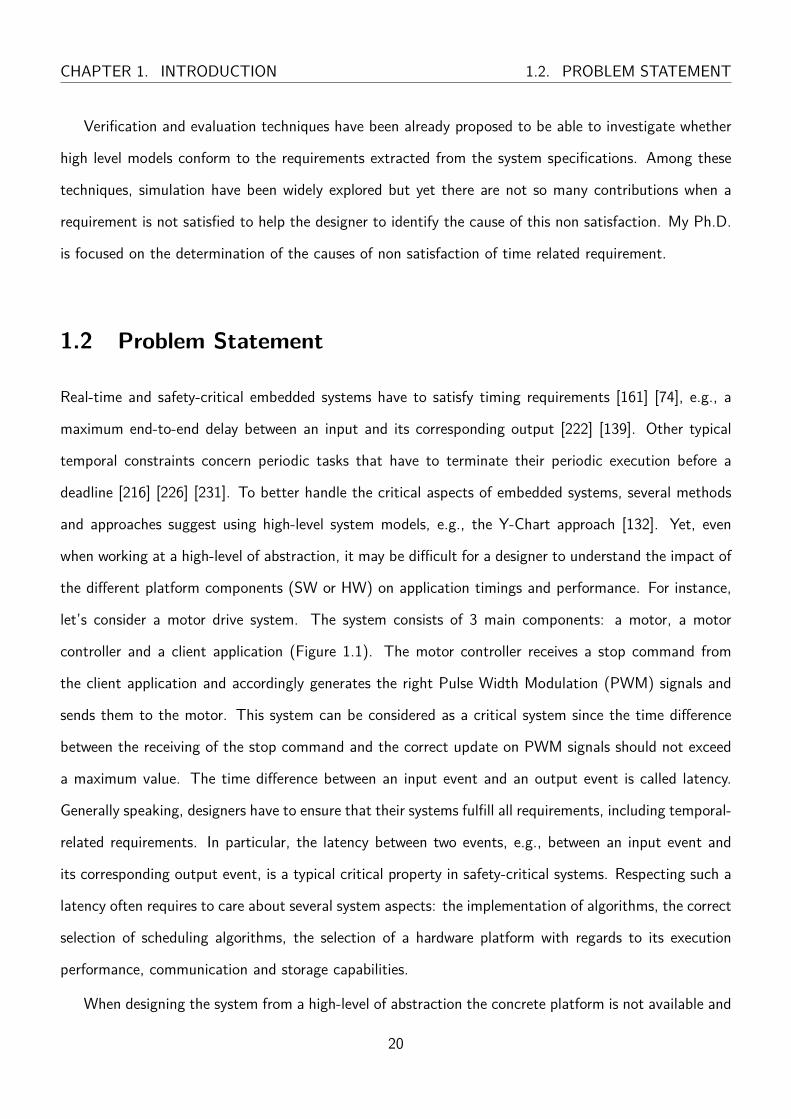
the different platform components (SW or HW) on application timings and performance. For instance,
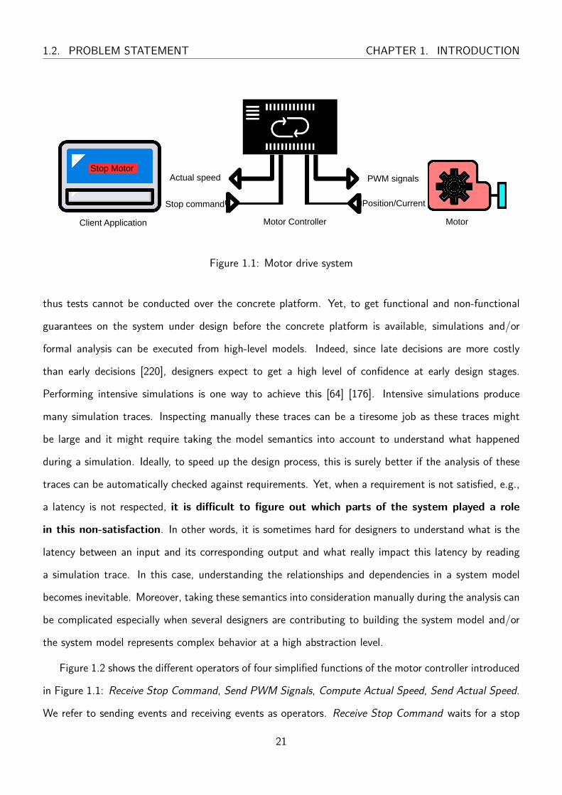
let’s consider a motor drive system. The system consists of 3 main components: a motor, a motor
controller and a client application (Figure 1.1). The motor controller receives a stop command from
the client application and accordingly generates the right Pulse Width Modulation (PWM) signals and
sends them to the motor. This system can be considered as a critical system since the time difference
between the receiving of the stop command and the correct update on PWM signals should not exceed
a maximum value. The time difference between an input event and an output event is called latency.
Generally speaking, designers have to ensure that their systems fulfill all requirements, including temporal-
related requirements. In particular, the latency between two events, e.g., between an input event and
its corresponding output event, is a typical critical property in safety-critical systems. Respecting such a
latency often requires to care about several system aspects: the implementation of algorithms, the correct
selection of scheduling algorithms, the selection of a hardware platform with regards to its execution
performance, communication and storage capabilities.
When designing the system from a high-level of abstraction the concrete platform is not available and
20
1.2. PROBLEM STATEMENT CHAPTER 1. INTRODUCTION
Client Application MotorMotor Controller
Stop command
Actual speed PWM signals
Position/Current
Stop Motor
Figure 1.1: Motor drive system
thus tests cannot be conducted over the concrete platform. Yet, to get functional and non-functional
guarantees on the system under design before the concrete platform is available, simulations and/or
formal analysis can be executed from high-level models. Indeed, since late decisions are more costly
than early decisions [220], designers expect to get a high level of confidence at early design stages.
Performing intensive simulations is one way to achieve this [64] [176]. Intensive simulations produce
many simulation traces. Inspecting manually these traces can be a tiresome job as these traces might
be large and it might require taking the model semantics into account to understand what happened
during a simulation. Ideally, to speed up the design process, this is surely better if the analysis of these
traces can be automatically checked against requirements. Yet, when a requirement is not satisfied, e.g.,
a latency is not respected, it is difficult to figure out which parts of the system played a role
in this non-satisfaction. In other words, it is sometimes hard for designers to understand what is the
latency between an input and its corresponding output and what really impact this latency by reading
a simulation trace. In this case, understanding the relationships and dependencies in a system model
becomes inevitable. Moreover, taking these semantics into consideration manually during the analysis can
be complicated especially when several designers are contributing to building the system model and/or
the system model represents complex behavior at a high abstraction level.
Figure 1.2 shows the different operators of four simplified functions of the motor controller introduced
in Figure 1.1: Receive Stop Command, Send PWM Signals, Compute Actual Speed, Send Actual Speed.
We refer to sending events and receiving events as operators. Receive Stop Command waits for a stop
21

CHAPTER 1. INTRODUCTION 1.2. PROBLEM STATEMENT
command sent by the client application. Once a stop command is received it sets the required speed
to zero. Send PWM Signals reads the required speed and accordingly computes the PWM values and
sends them to the motor. The actual speed of the motor is computed in Compute Actual Speed function
after reading the current and position of the motor. The actual speed is read in the Send Actual Speed
function and forwarded to the client application so the client can keep track of the motor speed. The
Compute actual speed function could directly send the actual speed to the client, however, we kept
Send Actual Speed function to separate functions that communicate with the client application from
those that communicate with the motor. The decision be keep this separation along with the chosen
architecture discussed next serve the illustrative purpose behind this system.
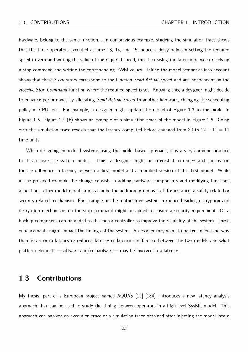
Figure 1.3 shows a candidate architecture of the Motor Controller with 2 CPUs, a bus and a memory.
The functions Receive Stop Command and Send Actual Speed are allocated to CPU 1 while Send PWM
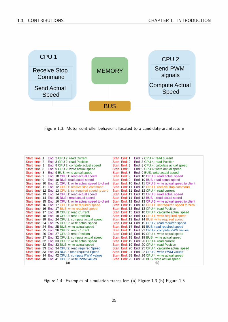
Signals and Compute Actual Speed are allocated to CPU 2. A possible simulation trace of this system is
shown in Figure 1.4 (a). The start time represents when the corresponding operator started executing, the
end is the time when the corresponding operator ended execution, followed by the hardware on which the
operator was executed and the operator’s name. In the simulation trace, the names of the operators are
colored: green for the Compute Actual Speed function, purple for Send Actual Speed, orange for Receive
Stop Command and blue for Send PWM Signals. To compute the latency between receiving a stop
command and writing the corresponding PWM values, these two operators along their simulation data
should be identified in the simulation trace. In Figure 1.4 (a), the operator corresponding to receiving a
stop command starts at time 11 and writing the corresponding PWM values starts at time 40 and ends
at time 41. So, the latency between these two operators is 41− 11 = 30 time units. While knowing only
the latency value might be satisfactory in some cases especially when the time constraint identified in
the timing requirement is met, a designer needs to know more details on the latency in case the timing
constraint is not met or to enhance the performance of the model. These details may include which
hardware or software component might delay a critical operator or what is really impacting the latency
between operators or what is the cause of a real-time constraint non-satisfaction. A way to investigate a
latency from a simulation trace is to consider both the information present in the simulation trace and the
dependencies between operators in the system model e.g., whether operators are executed on the same
22
1.3. CONTRIBUTIONS CHAPTER 1. INTRODUCTION
hardware, belong to the same function. . . In our previous example, studying the simulation trace shows
that the three operators executed at time 13, 14, and 15 induce a delay between setting the required
speed to zero and writing the value of the required speed, thus increasing the latency between receiving
a stop command and writing the corresponding PWM values. Taking the model semantics into account
shows that these 3 operators correspond to the function Send Actual Speed and are independent on the
Receive Stop Command function where the required speed is set. Knowing this, a designer might decide
to enhance performance by allocating Send Actual Speed to another hardware, changing the scheduling
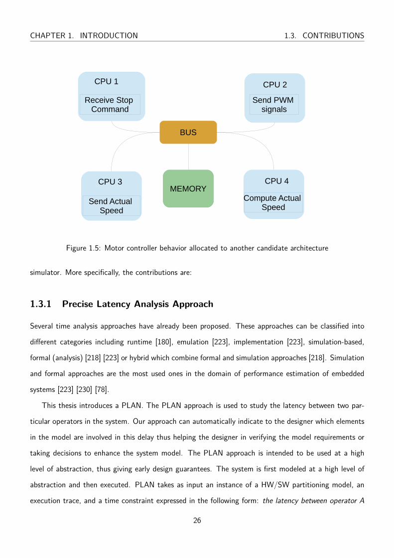
policy of CPU, etc. For example, a designer might update the model of Figure 1.3 to the model in
Figure 1.5. Figure 1.4 (b) shows an example of a simulation trace of the model in Figure 1.5. Going
over the simulation trace reveals that the latency computed before changed from 30 to 22 − 11 = 11
time units.
When designing embedded systems using the model-based approach, it is a very common practice
to iterate over the system models. Thus, a designer might be interested to understand the reason
for the difference in latency between a first model and a modified version of this first model. While
in the provided example the change consists in adding hardware components and modifying functions
allocations, other model modifications can be the addition or removal of, for instance, a safety-related or
security-related mechanism. For example, in the motor drive system introduced earlier, encryption and
decryption mechanisms on the stop command might be added to ensure a security requirement. Or a
backup component can be added to the motor controller to improve the reliability of the system. These
enhancements might impact the timings of the system. A designer may want to better understand why
there is an extra latency or reduced latency or latency indifference between the two models and what
platform elements —software and/or hardware— may be involved in a latency.
1.3 Contributions
My thesis, part of a European project named AQUAS [12] [184], introduces a new latency analysis
approach that can be used to study the timing between operators in a high-level SysML model. This
approach can analyze an execution trace or a simulation trace obtained after injecting the model into a
23

CHAPTER 1. INTRODUCTION 1.3. CONTRIBUTIONS
Start
End
Read actual Speed
Write actual Speed to client
Start
End
Compute PWM values
Start
End
Compute actual Speed
Start
Required Speed = 0Stop
command received?
End
Receive Stop CommandSend PWM Signals
Compute Actual SpeedSend Actual Speed
Yes
No
write PWM values
Read required Speed
Read Position
Write required speed
Write actual speed
Read Current
Start
End
Read
Write
Initial operator
Final operator
Legend
Receive operator
Send operator
Action operator
Control Flow
Function
Figure 1.2: Motor controller behavior
24
1.3. CONTRIBUTIONS CHAPTER 1. INTRODUCTION
BUS
MEMORY
CPU 2CPU 1
Receive Stop Command
Send PWM signals
Send Actual Speed
Compute Actual Speed
Figure 1.3: Motor controller behavior allocated to a candidate architecture
Start time: 1 End: 2 CPU 2: read CurrentStart time: 2 End: 3 CPU 2: read Position Start time: 3 End: 8 CPU 2: compute actual speed Start time: 8 End: 9 CPU 2: write actual speedStart time: 8 End: 9 BUS: write actual speed Start time: 9 End: 10 CPU 1: read actual speed Start time: 9 End: 10 BUS: read actual speedStart time: 10 End: 11 CPU 1: write actual speed to clientStart time: 11 End: 12 CPU 1: receive stop command Start time: 12 End: 13 CPU 1: set required speed to zero Start time: 13 End: 14 CPU 1: read actual speedStart time: 14 End: 15 BUS : read actual speed Start time: 15 End: 16 CPU 1: write actual speed to clientStart time: 16 End: 17 CPU 1: write required speed Start time: 16 End: 17 BUS: write required speed Start time: 17 End: 18 CPU 2: read Current Start time: 18 End: 19 CPU 2: read Position Start time: 19 End: 24 CPU 2: compute actual speed Start time: 24 End: 25 CPU 2: write actual speed Start time: 24 End: 25 BUS: write actual speed Start time: 25 End: 26 CPU 2: read Current Start time: 26 End: 27 CPU 2: read Position Start time: 27 End: 32 CPU 2: compute actual speedStart time: 32 End: 33 CPU 2: write actual speedStart time: 32 End: 33 BUS: write actual speedStart time: 33 End: 34 CPU 2: read required Speed Start time: 33 End: 34 BUS : read required SpeedStart time: 34 End: 42 CPU 2: compute PWM values Start time: 40 End: 41 CPU 2: write PWM values
(a)
Start End: 1 End: 2 CPU 4: read current Start End: 2 End: 3 CPU 4: read Position Start End: 3 End: 8 CPU 4: calculate actual speed Start End: 8 End: 9 CPU 4: write actual speedStart End: 8 End: 9 BUS: write actual speedStart End: 9 End: 10 CPU 3: read actual speed Start End: 9 End: 10 BUS: read actual speed Start End: 10 End: 11 CPU 3: write actual speed to clientStart End: 11 End: 12 CPU 1: receive stop command Start End: 11 End: 12 CPU 4: read currentStart End: 11 End: 12 CPU 3: read actual speed Start End: 11 End: 12 BUS : read actual speed Start End: 12 End: 13 CPU 3: write actual speed to clientStart End: 12 End: 13 CPU 1: set required speed to zero Start End: 12 End: 13 CPU 4: read Position Start End: 13 End: 18 CPU 4: calculate actual speed Start End: 13 End: 14 CPU 1: write required speed Start End: 13 End: 14 BUS: write required speed Start End: 14 End: 15 CPU 2: read required speed Start End: 14 End: 15 BUS: read required speed Start End: 15 End: 21 CPU 2: compute PWM values Start End: 18 End: 19 CPU 4: write actual speed Start End: 18 End: 19 BUS : write actual speed Start End: 19 End: 20 CPU 4: read current Start End: 19 End: 20 CPU 4: read Position Start End: 20 End: 25 CPU 4: calculate actual speed Start End: 21 End: 22 CPU 2: write PWM values Start End: 25 End: 26 CPU 4: write actual speed Start End: 25 End: 26 BUS: write actual speed
(b)
Figure 1.4: Examples of simulation traces for: (a) Figure 1.3 (b) Figure 1.5
25
CHAPTER 1. INTRODUCTION 1.3. CONTRIBUTIONS
BUS
MEMORYCPU 4CPU 3
CPU 2CPU 1
Receive Stop Command
Send PWM signals
Compute Actual Speed
Send Actual Speed
Figure 1.5: Motor controller behavior allocated to another candidate architecture
simulator. More specifically, the contributions are:
1.3.1 Precise Latency Analysis Approach
Several time analysis approaches have already been proposed. These approaches can be classified into
different categories including runtime [180], emulation [223], implementation [223], simulation-based,
formal (analysis) [218] [223] or hybrid which combine formal and simulation approaches [218]. Simulation
and formal approaches are the most used ones in the domain of performance estimation of embedded
systems [223] [230] [78].
This thesis introduces a PLAN. The PLAN approach is used to study the latency between two par-
ticular operators in the system. Our approach can automatically indicate to the designer which elements
in the model are involved in this delay thus helping the designer in verifying the model requirements or
taking decisions to enhance the system model. The PLAN approach is intended to be used at a high
level of abstraction, thus giving early design guarantees. The system is first modeled at a high level of
abstraction and then executed. PLAN takes as input an instance of a HW/SW partitioning model, an
execution trace, and a time constraint expressed in the following form: the latency between operator A
26
1.4. ORGANIZATION OF THIS THESIS CHAPTER 1. INTRODUCTION
and operator B should be less than L, where L is a maximum latency value. First PLAN checks if the
latency requirement is satisfied. If not, the main interest of PLAN is to provide the root cause of the
non satisfaction by classifying execution transactions according to their impact on latency: obligatory
transaction, transaction inducing a contention, transaction having no impact, etc. To do so, we extract a
dependency graph from the system model that preserves the causality between operators in the HW/SW
partitioning model. A first version of PLAN assumes an execution for which there is a unique execution
of operator A and a unique execution of operator B. A second version of PLAN can compute, for each
executed operator A, the corresponding operator B. For this, our approach relies on tainting techniques.
The thesis formalizes the two versions of PLAN and illustrates them with toy examples.
1.3.2 Integration into a Model-Driven Engineering Framework
In the scope of this thesis, PLAN was integrated into a Model-Driven Engineering Framework capable
of supporting the design and verification —by simulation— of embedded systems at a high level of
abstraction. We chose the free and open-source TTool toolkit [14] for this integration. PLAN was
integrated in SysML-Sec, one of the design and development environments supported by TTool. The
SysML-Sec method includes a HW/SW partitioning stage. Moreover, simulation is one of the verification
techniques available in TTool. TTool can indeed generate a transaction-based simulation trace using its
simulator [135]. Thus, PLAN can be directly applied to the simulation trace output. The two versions
of PLAN are illustrated with two case studies taken from the H2020 AQUAS project. In particular, we
show how tainting can efficiently handle the multiple and concurrent occurrences of the same operator.
1.4 Organization of This Thesis
The rest of this manuscript proceeds as follows. Chapter 2 gives an overview of embedded systems,
Model-Driven Engineering (MDE) and timing constraints. Moreover, in Chapter 2, we explain the
SysML-Sec profile within which our contribution is integrated. Chapter 3 presents the related work,
where performance verification approaches and simulation trace analysis methods are studied. Chapter 4
formally defines a HW/SW partitioning model, an execution trace and a maximum latency requirement.
27

CHAPTER 1. INTRODUCTION 1.4. ORGANIZATION OF THIS THESIS
Chapter 5 presents the formal definition of the first version of PLAN. The second version of PLAN that
relies on tainting techniques is presented in Chapter 6. The implementation of the contributions along
with two use cases are presented in Chapter 7. Finally, Chapter 8 concludes this thesis and discusses
potential future work.
28
Chapter 2
Context
“A text without a context is a pretext for a proof text.”
-Tom Carson
Embedded systems are becoming increasingly present all around us and impact our daily lives. They
are present in many domains like transportation, communication, health, home applications. In our
everyday life, we use devices with several embedded systems. Embedded systems complexity is increasing
as technology advances. Moreover, embedded systems are more and more integrated into safety-critical
equipment where their failure results in a catastrophic impact. Thus, it becomes inevitable to design and
verify that an embedded system meets its requirements before implementation.
Common embedded systems design flows enable designers to iteratively refine their design till the
requirements are met. Updating a design to meet the requirements can cost less than detecting these
errors after the embedded system is implemented [220]. For example, verifying that requirements are met
in the design of an embedded system can avoid dangerous software/hardware situations, decrease the
probability of system failure while in use and/or avoid the recall of the product from the market [10] [20].
29

CHAPTER 2. CONTEXT 2.1. STRUCTURE OF EMBEDDED SYSTEMS
2.1 Structure of Embedded Systems
Several definitions can be found in the literature for embedded systems [236, 170, 121, 108, 120, 235]. An
embedded system is built from software and hardware components. The software is a set of instructions
that determine part of the system functionalities. The hardware components form the platform on which
the software runs. An embedded system typical task is to process input from the system environment
and produce an output corresponding to this input. For example, a carbon monoxide detector regularly
monitors its environment with the help of a sensor for the presence of this colorless, odorless and
tasteless toxic gas. In case detected, an alarm goes on. The Apollo Guidance System built in 1960 by
MIT Instrumentation Laboratory is considered one of the first embedded systems [120]. From this time
till the 70’s embedded systems were non-commercial, heavy, expensive and used for a specific application
[120]. The development of Intel 4004 microprocessor in 1971 was a change point in the history of
embedded systems. Having this integrated, small, light and cheap chip paved the way for embedded
systems to develop. Since that date, embedded systems are more and more integrated into our daily
lives.
These systems, although deployed in diverse domains and having different functions, share several
common characteristics [162]. For instance, they must comply with a lot of tight constraints such as
performance measures, low power consumptions, short time-to-market, etc.
An embedded system underlies the Sampling and Caching Subsystem functionality of the Mars 2020
Rover Mission (Figure 2.1) [81]. The objective of this subsystem is to collect and store rocks and soil
samples that could be returned to earth [3].
The Mars 2020 Rover “brain” is made of a processor and a memory [2]. The processor executes
commands send by the flight team e.g., taking pictures. It is responsible for the control and computation
operations in the system. Also, it monitors the status of the rover e.g., rover temperature and stores
the values in reports in the memory. Power sources, cameras, robotic hands, wheels, sensors, antennas,
microphones, etc. are connected to the rover to ensure that it fulfill its functionalities by moving, using
its science instruments and communicating with Earth.
In an embedded system some of the main categories of hardware components include: micro-
controller/microprocessor, memory, memory management units, communication port, bus, bridge, power
30

2.2. MODEL-DRIVEN ENGINEERING CHAPTER 2. CONTEXT
Legend
brains: processors + memories
Figure 2.1: Mars 2020 Rover
supply, actuator, multiplexer/de-multiplexer, analog-to-digital/digital-to-analog converter, oscillator, sys-
tem timer clock, real-time clock, watchdog timer, interrupt controllers, etc.
2.2 Model-Driven Engineering
Designing embedded systems with complex functionalities requires the collaboration of several teams
from various domains and the integration of their work. These teams are working sometimes on differ-
ent tools, approaches and processes. Traditionally, these teams used files and documents to exchange
information about the system through the design process [80]. MDE techniques involve creating mod-
els [203]. In a top-down approach, a model is an abstraction blueprint of the system derived from system
requirements. Abstracting a system means ignoring some of its details. Ignoring only inessential details
is referred to as good abstraction [203]. A model can be generated for software [174] [169] [91] [203] or
hardware [228] [168].
To construct a model a designer uses modeling languages, methods and tools. A modeling language
31

CHAPTER 2. CONTEXT 2.2. MODEL-DRIVEN ENGINEERING
is used to define the elements in the model and the relationship between them. The modeling language
can be textual or graphical. The modeling method is a guide that defines a set of documented steps a
designer needs to follow to develop a model. A modeling tool supports one or more modeling languages
to enable a designer to create a model based on the components and relations defined in those languages
[80].
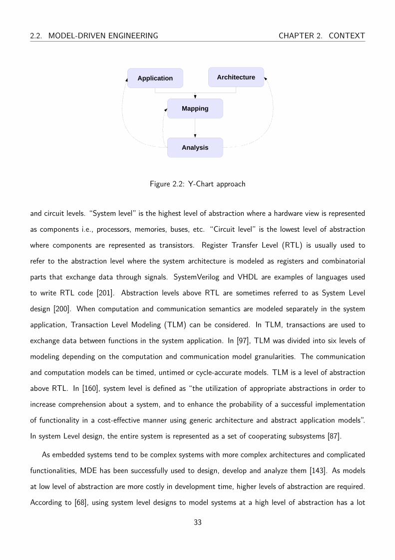
The Y-chart approach [132] is a MDE approach. It is a principal methodology to design a model-based
embedded system [147]. In the first step of the Y-chart approach, the application and the architecture of
the system are modeled separately as two independent views. The application represents the functionality
of the system while the architecture represents the platform of the system. The application and architec-
ture views are then linked in the mapping stage of the Y-chart approach where different functions along
their connections in the applications are allocated to components in the architecture creating a mapped
model of the system. The mapped model can be analyzed to see if it satisfies the system requirements.
In case the requirements are not satisfied and the design needs further modifications, the designer can
change the allocation of different functions in the mapped model, update the platform components in
the architecture view or apply changes to the functions in the application view. As changes are applied to
the application, architecture or mapped models, the analysis stage of the model can be performed again.
This iteration process of the Y-chart is of great importance as it allows designers to loop on different
views of the model until a mapping model satisfies all system requirements. This iteration process of the
Y-chart approach along with the clear identification of different steps along the approach enabled it to
be integrated into several design methodologies [147] [83].
The Y-chart approach and design methodologies can be applied to different levels of abstractions of
an embedded system [97]. In other words, a model can abstract a system on different levels. These levels
range from high abstraction levels to low abstraction levels depending on the amount of details present
in the model. The highest level of abstraction contains the least amount of detailed information about
the system. Standard languages such as C, C++, SystemC, UML, etc. can be used to model a system.
In literature, different modeling approaches consider different abstraction levels depending on the criteria
they abstract [35]. In [97], Gajski et al. defined four levels of abstraction depending on the abstraction
level of the components in the hardware view of the system. These levels are system, processor, logic
32
2.2. MODEL-DRIVEN ENGINEERING CHAPTER 2. CONTEXT
Application Architecture
Mapping
Analysis
Figure 2.2: Y-Chart approach
and circuit levels. “System level” is the highest level of abstraction where a hardware view is represented
as components i.e., processors, memories, buses, etc. “Circuit level” is the lowest level of abstraction
where components are represented as transistors. Register Transfer Level (RTL) is usually used to
refer to the abstraction level where the system architecture is modeled as registers and combinatorial
parts that exchange data through signals. SystemVerilog and VHDL are examples of languages used
to write RTL code [201]. Abstraction levels above RTL are sometimes referred to as System Level
design [200]. When computation and communication semantics are modeled separately in the system
application, Transaction Level Modeling (TLM) can be considered. In TLM, transactions are used to
exchange data between functions in the system application. In [97], TLM was divided into six levels of
modeling depending on the computation and communication model granularities. The communication
and computation models can be timed, untimed or cycle-accurate models. TLM is a level of abstraction
above RTL. In [160], system level is defined as “the utilization of appropriate abstractions in order to
increase comprehension about a system, and to enhance the probability of a successful implementation
of functionality in a cost-effective manner using generic architecture and abstract application models”.
In system Level design, the entire system is represented as a set of cooperating subsystems [87].
As embedded systems tend to be complex systems with more complex architectures and complicated
functionalities, MDE has been successfully used to design, develop and analyze them [143]. As models
at low level of abstraction are more costly in development time, higher levels of abstraction are required.
According to [68], using system level designs to model systems at a high level of abstraction has a lot
33
CHAPTER 2. CONTEXT 2.3. TIMING CONSTRAINTS
of advantages including simplifying the specification, verification and implementation of the systems,
enabling more efficient design space exploration, reducing time to market, improving problems discovery
and allowing verification of the model at early design stages.
2.3 Timing Constraints
Embedded systems are designed to perform specific functions. Timing constraints are used to define some
safety and performance measures in embedded systems. In [222], the timing behavior of an embedded
system is defined as the time interval between a pair of events: the starting event and the finishing event.
These events can be the start and end of task execution or receiving sensor data and executing the system
response. The maximum and minimum time intervals between these two events are referred to as the
worst and the best execution time respectively. An embedded system can run in different environments
thus facing different conditions resulting in different values for the Worst-Case Execution Time (WCET)
and a Best-Case Execution Time (BCET). This non-determinism can be due to input non-determinism
from the embedded system environment, communication semantics, hardware components like cache
memories, etc.
In some embedded systems, when the time constraint is not met, it may result in high financial costs
on the party or the business using this system. For example, the manufacture or selling company may
have to recall the products resulting in revenue loss or loss of interest of the customer to continue using
the product [140] [111]. These systems are business-critical systems.
A Real-Time embedded system is an embedded system in which the correctness of the outputs depends
also on the time at which these results are produced [215]. In other words, in real-time embedded systems
meeting time constraints is critical. The time constraints in real-time embedded systems are strictly
specified. Computation and response to input events must be executed before their deadline. Timing
constraints in real-time systems are classified into 3 types of restrictions [74]: maximum, minimum and
durational. Maximum restrictions specify that the latency between two events should be no more than
time t. This time constraint can be seen as the bound of the WCET or the worst-case response time. An
example of this time constrain can state that the response time between input from the sensor and output
34

2.4. SYSML-SEC CHAPTER 2. CONTEXT
of the system shall not exceeds 15 ms. When an embedded system exceeds the specified maximum limit,
which means that it does not meet the deadline, then the system is considered as failed. The minimum
restriction specifies the minimum acceptable latency between two events. This time constraint can be
seen as the lower bound of the BCET. An example of the minimum time constrain can state that no less
than 10 ms may elapse between no input signal and the output of the system like an alarm signal. In
duration time constraints, the amount of time during which a condition holds is specified. An example
of a durational time constraint in the carbon monoxide detector can state that an alarm will sound
after three and a half hours of continuous exposure of carbon monoxide at a level of 50 PPM [9]. It is
important to point here that although real-time systems have to comply with strict time constraints, the
time specified in these constraints is not always a short time. In our last example, the time duration was
three and a half hours.
2.4 SysML-Sec
TTool [14] is a free and open-source framework for the design and verification of embedded systems.
SysML-Sec is one of the modeling profiles supported by TTool. SysML-Sec is used to design safe
and secure embedded systems while taking performance into account. In the first stage of SysML-
Sec (Figure 2.3), requirements are identified and explicitly tagged as safety, security or performance.
Requirements are textual specifications regarding important properties of the system, defined informally
with an identifier and a text. The formal semantics of time-related and safety properties is defined
within TEmporal Property Expression language (TEPE) Parametric Diagrams [137]. Formally defining
properties with TEPE is usually possible only when part of the system has been designed. For instance,
TEPE properties can be used to relate block attributes together; such a property can be expressed
only once blocks have been expressed. Also, in this step, attacks that could target the system and
faults that could occur in the system are modeled in attack and fault trees respectively. SysML-Sec
contains the Y-Chart approach [131] so next, in the HW/SW partitioning step, the architecture and the
application (high-level tasks/functional behavior) are modeled before being linked in the mapping phase.
This step helps to decide how tasks should be split between hardware and software mechanisms, and how
35

CHAPTER 2. CONTEXT 2.4. SYSML-SEC
LegendModelingVerificationMethod Flow
Analysis
Attack Trees
Fault Trees
HW/SW Partitioning
Application Architecture
Mapping
Requirements
Safety Security Performance
(Formal) Verification
Performance
ProVerifUPPAAL
Safety Security
SimulatorSimulator
Safety
Software Design
Code Generation
(Formal) Verification
Figure 2.3: SysML-Sec modeling profile used in TTool
communications between tasks are realized using physical elements. Second, the design of the software
elements can be performed in the software design stage: tasks mapped to processors are expected to
be refined as software components. Verification can be performed with a press-button approach from
most views so as to check that all requirements are satisfied. TTool can perform verifications using
formal techniques (e.g., model-checking) and simulations. Safety verification relies on the TTool model
checker or on UPPAAL. Security verification relies on the ProVerif [45] external toolkit. Performance
verification relies on a System-C like simulator provided by TTool. Once a model has been verified, C
code generation can be performed from partitioning models or from software design.
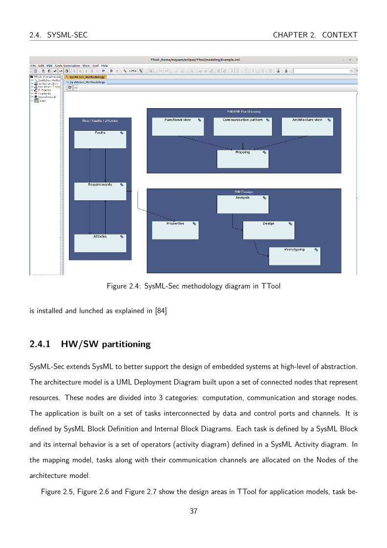
[84] is a tutorial for TTool that guides the reader through the complete design from modeling to
automatic code generation. Figure 2.4 shows the SysML-Sec methodology diagram in TTool after TTool
36
2.4. SYSML-SEC CHAPTER 2. CONTEXT
Figure 2.4: SysML-Sec methodology diagram in TTool
is installed and lunched as explained in [84]
2.4.1 HW/SW partitioning
SysML-Sec extends SysML to better support the design of embedded systems at high-level of abstraction.
The architecture model is a UML Deployment Diagram built upon a set of connected nodes that represent
resources. These nodes are divided into 3 categories: computation, communication and storage nodes.
The application is built on a set of tasks interconnected by data and control ports and channels. It is
defined by SysML Block Definition and Internal Block Diagrams. Each task is defined by a SysML Block
and its internal behavior is a set of operators (activity diagram) defined in a SysML Activity diagram. In
the mapping model, tasks along with their communication channels are allocated on the Nodes of the
architecture model.
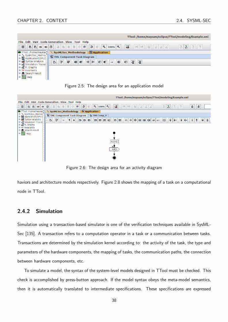
Figure 2.5, Figure 2.6 and Figure 2.7 show the design areas in TTool for application models, task be-
37
CHAPTER 2. CONTEXT 2.4. SYSML-SEC
Figure 2.5: The design area for an application model
Figure 2.6: The design area for an activity diagram
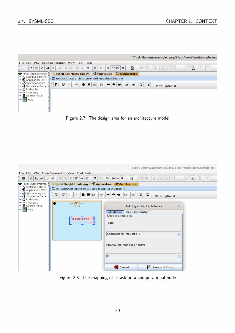
haviors and architecture models respectively. Figure 2.8 shows the mapping of a task on a computational
node in TTool.
2.4.2 Simulation
Simulation using a transaction-based simulator is one of the verification techniques available in SysML-
Sec [135]. A transaction refers to a computation operator in a task or a communication between tasks.
Transactions are determined by the simulation kernel according to: the activity of the task, the type and
parameters of the hardware components, the mapping of tasks, the communication paths, the connection
between hardware components, etc.
To simulate a model, the syntax of the system-level models designed in TTool must be checked. This
check is accomplished by press-button approach. If the model syntax obeys the meta-model semantics,
then it is automatically translated to intermediate specifications. These specifications are expressed
38
2.4. SYSML-SEC CHAPTER 2. CONTEXT
Figure 2.7: The design area for an architecture model
Figure 2.8: The mapping of a task on a computational node
39

CHAPTER 2. CONTEXT 2.4. SYSML-SEC
Figure 2.9: The interactive simulation window
in formal language and form a starting point to derive simulation code [136]. For TTool users, after
performing syntax checking of the model, the simulation code is generated. An interactive simulation
window (Figure 2.9) pops-up in TTool once the simulation source code is compiled. In addition to having
an interactive simulation through a graphical interface in TTool, the simulation progress is also animated
on the model views. The interactive simulation window provides information about the simulation and a
lot of functionalities for the designer. Among these functionalities: advancing the simulation in different
modes, resetting the simulation, saving and storing the simulation state, save simulation traces in Value
Change Dump (VCD), text or HTML format, visualize the simulation result in the form of a reachability
graph, etc.
40
Chapter 3
Related Work
“Those who don’t know history are doomed to repeat it.”
-Edmund Burke
To develop embedded systems, several development methodologies exist. Each has its phases and
way to navigate between these phases. Embedded systems must satisfy functional and nonfunctional
requirements. The requirements must be satisfied along all phases. As mentioned previously, it is more
costly to discover requirements non satisfaction later in the design life-cycle, i.e, in late phases. In this
chapter, we start in Section 3.1 by reviewing different development methodologies and the functional
and nonfunctional requirements that the system must satisfy.
Verification approaches can detect requirement satisfaction or violation (section 3.2). Numerous
works proposed different approaches for the verification and evaluation of model requirements. The
proposed approaches can be classified into different categories.
In this thesis, formal and runtime verification approaches are discussed in Section 3.2.1 and Sec-
tion 3.2.2 respectively. Evaluation is used when quantitative information regarding a system design is
required [163]. Performance evaluation gives information regarding delay or response time [49]. As in this
thesis we are interested in latency violation, Section 3.2.3 gives an overview on performance evaluation
techniques. Information flow analysis is also used for property analysis.
Since we use tainting in the second version of PLAN and since tainting is considered in information
41
CHAPTER 3. RELATED WORK 3.1. SOFTWARE DEVELOPMENT METHODOLOGIES
flow analysis, Section 3.3 gives a general overview information flow analysis and how it is used in terms
of performance evaluation. Then, Section 3.3.1 discuss taint analysis approaches and their main usage.
3.1 Software Development Methodologies
A product life cycle (PLC) is a sequence of stages through which a product goes starting from the
stage when the product was an idea until the product is recycled or destroyed [184] [198]. Broadly
speaking these stages are: (1) Imagine (2) Develop (3) Realize (4) Use/Support (5) Retire/Dispose. In
the imagine stage the product is an idea in someone’s head. In the develop stage the idea is described in
details, requirements are identified for example in technical specifications, and/or prototypes developed.
In the realise stage, the product is ready to be used by a customer. In the use stage the product is in
use by the customer and in the final stage the product is disposed when it is not useful anymore [198].
For software products the development stage is further broken down into phases. These phases start
with development analysis to testing and evaluation [149]. Navigation between these phases depends
on the methodology used by the development team. The software development methodologies can
be generally classified as traditional (e.g, Waterfall method and V-Model) or Agile. The Waterfall,
incremental, spiral, agile, etc, are examples of software development life cycle models. Each model has
its own strengths, weaknesses, features, and usages [22].
In the Waterfall method [192], the designer follows a sequence of non overlapping steps. First the
requirements are identified, then the system is designed, developed and tested [165]. In this method, the
set of all system requirements must be known in the first step.
In the Incremental Model multiple development cycles take place. Each development cycle— also
known as an increment— addresses a standalone feature of the product. Each incremental version is
usually developed using a waterfall model of development [23]. Thus, the incremental model is also
referred to as iterative waterfall model [195]. The first development cycle releases a core product in
which only basic requirements are tackled [187]. Once the core product is approved by the customer,
successive iterations are implemented until the product is released.
The spiral model [48] is a risk driven approach that combines the waterfall model with the iterative
42

3.1. SOFTWARE DEVELOPMENT METHODOLOGIES CHAPTER 3. RELATED WORK
model [187]. It starts with a planing phase in which costs, resources and time are estimated, then risk
analysis, development and evaluation phases [23]. With each spiral new requirements/functionalities can
be added until the product is ready. The spiral model aims to minimize the project risk [23].
The V-model [89] is a variation of the Waterfall method [195]. The stages of a V-model are rep-
resented in a V shape with a focus on the development stages and their respective verification and
validation stages [117]. On the left side of the V, the phases start from requirement analysis to system
design to development. On the right side of the V, validation phases are present [187].
In the Agile model [40], the software is developed in small patches and delivered to customers at
regular short intervals. Thus, the software product is done in an incremental and iterative process where
parts of the software are designed, developed and tested until the software product is complete [165]. This
iterative process makes the ability to respond to the changing requirements easier. According to [152],
Waterfall/V-model methodology is more popular for embedded system design.
3.1.1 Functional and Nonfunctional Requirements
Embedded systems must comply with functional and nonfunctional requirements. These requirements
can be verified using different approaches throughout a product life cycle from design time to runtime.
Functional requirements describe the behavior of the system while nonfunctional requirements spec-
ify constraints and quality attributes (properties) like system safety, security, performance, reliability,
etc. [22] [157].
In [100], a detailed overview, discussion and comparison between functional and nonfunctional require-
ments is provided.
Regardless of the development method used, at the end of each iteration, the product must be
validated against its requirements. In the product design stage, nonfunctional requirements drive the
process of decision-making and implementing the functionality of the product [208]. In other words,
without nonfunctional requirements, the design choices are arbitrary [157]. In general, requirements are
expressed in natural language or in appropriate formalism [157].
Timing constraints must be verified all along the design process to ensure that they are satisfied after
each design stage
43

CHAPTER 3. RELATED WORK 3.1. SOFTWARE DEVELOPMENT METHODOLOGIES
Nonfunctional Requirements
Nonfunctional requirements include, but are not limited to safety, security, performance, reliability, us-
ability, integrity, scalability, traceability, maintainability, energy efficiency, certification, fault-tolerance,
timing predictability, etc.
Safety Safety can be generally defined as making the system accident-free. It is the probability that
the system functions as required over a specified time interval without accidents. Safety requirements
should specify the reaction of the system in case an accident occurs thus avoiding reaching an unsafe
hazardous state [142] [172]. In other words, safety deals with protecting the systems environment from
the systems operation [217], it deals with avoiding losses due to either flaws in software or hardware
leading to malfunctions, or due to (abnormal) environmental conditions [152].
System safety has been taken into account since long time [105]. Since the 1990s, it has been dealt
with it in a systematic manner [229]. In 1998 the first edition of the generic Functional Safety standard
IEC 61508 was issued [229] [105]. IEC 61508 is an international standard for the functional safety of
systems comprised of electrical, electronic, and software components applied in industry [199] [141]. The
standard assure that the system will reach the required safety level by reducing risk [199]. To achieve
this, the standard applies hazard and risk analysis to derive the safety requirements, then the system
is designed such that theses safety requirements are fulfilled [141]. The standard follows a life cycle
model that goes along with the product life-cycle and assists the developer through several phases from
pre-design to the design, installation and operation phase of the system [141].
Based on IEC 61508, different industry-specific standards were derived [141] [229] such as IEC 61513
for the nuclear industry [141], IEC 61511 for industrial processes [141], ISO 26262 for the safety-related
aspects of electrical/electronic systems in automobiles [141] [199] and EN 50128 for railway (CEN-
ELEC) [229].
Security Security is concerned with protecting the systems operation from the environment usually
manifested as intentional attacks [217]. Security can be considered from different perspectives [22].
Historically, CIA triad was used to ensure security in information technology [69]. CIA triad consists of
44

3.1. SOFTWARE DEVELOPMENT METHODOLOGIES CHAPTER 3. RELATED WORK
confidentiality, integrity, and availability. In addition to these three properties, authenticity [138], non-
repudiation [217], secure storage of the code [138], content security [138] and data freshness [199] should
also be considered in some applications. These properties should be maintained along the device lifetime
even if it falls in the hands of a malicious parties, this is referred to as tamper resistance requirement [138].
While data confidentiality ensures that data are accessed and disclosed only by authorized enti-
ties, integrity guarantees that information was not modified or destroyed [69]. Availability ensures that
the system can be accessed and used in a timely and reliable manner without having performance is-
sues [138] [69]. Integrity also assures information non-repudiation and authenticity [69]. Kocher et
al [138] define authenticity as user identification if an authorized users accessed an embedded system or
as secure network access if an authorized device accessed a network or service. Non-repudiation verify
that the users cannot later deny that he performed an action [217]. In addition to these requirements,
embedded systems security requirements shall include secure storage of the code or data in the system
storage devices and content security or Digital Rights Management (DRM) for digital content used in
the system [138]. In some cases, it is also required to ensure the freshness of the data which means it is
not replayed [199].
IT security standards appeared after the safety ones and were the first forms of security standards.
Some IT standards are Common Criteria/IEC 15408 and ISO/IEC 27001 [105] [141].
Common Criteria/IEC 15408 is an international standard that specified the general evaluation model
for information technology including the general concept and principles for this evaluation. It defines the
process for guaranteeing the security of security-critical systems by identifying threats, assessing risks,
implementing countermeasures, and evaluating the effectiveness of countermeasures [152] [141].
ISO/IEC 27001 is the best-known standard in the ISO/IEC 27000 family for Information security
management systems (ISMS) [1]. Its main goal is to keep sensitive information of company secure.
In the field of security standards, in addition to IT related ones, some are concerned with Industrial
Automation and Control Systems such as IEC 62443 [105]. IEC 62443 is a series of standards, norms
and technical reports which define procedures for the implementation in IACS (Industrial Automation
and Control Systems [94] [105]. Specifically, it considers security of safety systems [141] and aim at
enhancing safety, availability, integrity, and confidentiality of IACS [105].
45

CHAPTER 3. RELATED WORK 3.1. SOFTWARE DEVELOPMENT METHODOLOGIES
Performance Embedded systems are involved in some applications where timing is critical thus real-
time constraints are essentials for these systems [223] [55]. Platforms timing requirements are often
application-related end-to-end maximum requirements [158]. In other words, the software controlling the
hardware must operate within timing constraints to guarantee correct functionality of the system [152].
According to [152], the percentage of usage of systems components and the timings characterize the
system performance. In a safety-critical system, failure to meet a timing requirement can have catas-
trophic consequences [171]. Thus, performance evaluation is necessary in order to guarantee timing
requirements [162].
3.1.2 Using UML design tools and techniques
Model-Driven Engineering is a powerful technology to analyze, design, simulate and document embedded
systems [232] [26]. As a reminder, a model is a description of (part of) a system in which functional and
non-functional requirements must be satisfied [93]. A model written in a well-defined language makes
communication between systems engineers working across the development life cycle easier [80].
System modeling is an important aspect of any system engineering methodology [232]. Unified
Modeling Language (UML) is probably the most widely accepted and used of the modeling languages
defined by Object Management Group (OMG) [93]. It is a graphical modeling language for specifying
and capturing system models that can applied to all application domains. Thus, it is referred to as
general purpose modeling language. Designers find UML user friendly and easy to understand [152].
However, for some particular domains, having domain-specific languages may be more efficient. Ac-
cording to OMG, there exist two ways to define a domain-Specific language. Either a language alternative
to UML is defined or UML extension mechanisms are used. In the latter case, UML extension mechanisms
enables it to adapt to a specific domains application by extending its syntax and semantics [93]. For
instance, [224] compared three alternatives to help roboticists apply MDE to robotics application: (1) by
using UML, (2) by using a UML profile for robot operating system and (3) by defining a Domain-Specific
Language (DSL) specifically designed for for robot operating system.
A UML profile is a collection of UML extensions. For instance, Systems Modeling Language (SysML) [80]
is an extension of UML more adapted for Model-Based Systems Engineering. It is one of several graphical
46

3.2. VERIFICATION TECHNIQUES CHAPTER 3. RELATED WORK
modeling languages that are UML profiles. However, SysML does not take into account the partition-
ing of embedded systems [26]. SysML-Sec is an extension of the UML Profile UML that supports
partitioning [26]. UML/MARTE [11] is an OMG UML profile to develop real-time and embedded sys-
tems. However, MARTE does not define how to use modeling elements [232] or address requirements
modeling [26].
3.2 Verification Techniques
Functional and nonfunctional requirements can be verified using different approaches throughout a prod-
uct life cycle (PLC) from design time to runtime. Formal verification approaches use mathematical logic
to prove that a property is satisfied [162] [180] [164]. Runtime verification approaches detect property
violations by monitoring the system during execution [180]. Runtime verification can be applied on traces
collected as the system runs (on-line) or afterwards. In the design stage of a product life cycle, simulation
is meant to represent system execution. A comparison between simulation and runtime verification is
presented in [193]. According to [193], simulation takes as input a model and outputs a set of executions
on which statics can be computed or requirements verified while runtime verification takes an execution
trace and a requirement as inputs and outputs a verdict (true or false) based on the evaluation of the
requirement over the trace. Thus, the purpose of simulation is seen as different from that of runtime
verification [193]. While simulation is used to enhance the system in the design stage before deployment,
runtime verification is used to detect faults in the system during operation and take required actions.
Schedulability analysis is the process of verifying that the execution of a series of functions in a system
respect the timing constraints of this system [225]. It uses information from the application and the
architecture of a system in the analysis making it useful to determine if an application can be deployed
on an architecture given a timing constrain on the system [90].
3.2.1 Formal Verification Approaches
To prove that a property is satisfied using mathematical logic, as a first step, a formal model is required
on which system properties can then be proven [162].
47

CHAPTER 3. RELATED WORK 3.2. VERIFICATION TECHNIQUES
Model Checking Model checking is a formal method that takes as input a finite-state model and a
formal property written in a suitable logic such as temporal logic to verify whether the model of the
system satisfies the property or not [37] [210] [210] [44]. To do so, reachable states of the design
are traversed. If the property is disproved for the model, a counter example is provided. The counter
example is in the form of a sequence of states [44]. According to [44], model checkers are considered
as complimentary not alternative to other verification methods as its time consuming to verify all the
desired properties of a system due to the huge state-spaces of such systems. Such exhaustive exploration
of state space can be computationally intensive and time consuming [28] [85]. To compact the state
explosion problem of model checking in which the size of the model grows exponentially, Symbolic Model
checking [53], Bounded Model Checking [41] and abstraction techniques [65] [178] were proposed.
In symbolic model checking, sets of states are represented using boolean functions. This represen-
tation reduces the list of states. In Bounded Model Checking (BMC), the basic idea is to search for a
counterexample in a certain number of transitions. BMC will only prove that the design is correct for
the first N transitions but that does not proof the absence of errors in the system. In abstraction tech-
niques, the concrete design is first simplified and then the analysis run on this smaller and more abstract
model. Counter example-guided abstraction refinement [65] is an example of automatically constructed
abstraction.
Symbolic model checking proposed using SAT solvers and presented the idea of SAT-based bounded
model checking [166] [43][42]. SAT solvers language is Boolean logic [31]. A SAT solver is a procedure
which decides whether an input boolean formula can always be replaced by the values TRUE or FALSE
in such a way that the formula evaluates to TRUE. If this is the case, we say an input Boolean formula
is satisfiable [206].
In [234], model checking is used to improve failure analysis and verification approach for integrated
modular avionics (IMA) systems. Software model checking can be used to automatically detect if
unreachable code is present in safety-critical embedded systems [202]. The absence of unreachable code
is one criteria of high quality software in safety-critical embedded systems specified by ISO 26262 [118]
standard for the automotive domain
UPPAAL [148] is a very popular tool for model checking. UPPAAL is used to develop abstract
48
3.2. VERIFICATION TECHNIQUES CHAPTER 3. RELATED WORK
models of a real-time system. UPPAAL consists of three main parts: a description language to describe
system behavior as networks of timed automata, a simulator to execute the model and verify safety and
bounded liveness properties on possible dynamic executions of a system, and a model-checker to verify
for invariant and reachability properties on exhaustive dynamic behavior of the system [148].
Formal Tropos [96] is a language that enables the automatic verification of requirements using model-
checking. Secure Tropos [179], an extension of the Tropos methodology, is for the analysis of security
requirements and functional ones.
Theorem Proving Theorem proving is a verification method that provides mathematical reasoning on
the verification results of the system properties [28]. It consists of two steps [104] (1) the description
of the system along its specification and (1) the proof. In the first step, a system and its specification
can be described in a single logical form [242]. In the second step, the logical form is used as a
verification condition [242]. Some theorem provers are based on variations of Hoare logic [175]. Hoare’s
approach [113] depends on pre and post conditions to reason about program correctness. A formula
known as “Hoare triple”.
According to [175], this formula can be read as “if property φpre holds before program P starts, φpostholds after the execution of P”. In embedded systems, φpre could for instance describe valid actions of
a system and φpost could define an undesired state for a formally defined system for a formally defined
system P .
Unlike model checking, theorem proving is not based on state space exploration. However, theorem
proving have some drawbacks as it requires a high degree of knowledge of the system and high special-
ization in higher order logic to reasons about the state space using system constraints only [85] [104].
Moreover, as automated generated proofs can be long and complicated to understand, fully automated
techniques are less popular for theorem proving [28].
In [242] a theorem-proving approach to schedulability analysis of Clock Constraint Specification
Language (CCSL) specifications is presented. CCSL is a clock-based formalism for the specification and
analysis of real-time embedded systems. The objective of schedulability analysis of CCSL specifications
is find whether there exists a clock behavior that satisfy a given CCSL specification.
49
CHAPTER 3. RELATED WORK 3.2. VERIFICATION TECHNIQUES
Satisfiability Modulo Theories (SMT) Satisfiability Modulo Theories is “the problem of deciding
the satisfiability of a first-order formula with respect to some decidable first-order theory” [206]. The
first-order formula is a boolean combinations of atomic propositions and atomic expressions. To benefit
from the advantage of fast and automated SAT solvers on higher level than the Boolean level, a SMT
solver is based on first-order logic and it combines a SAT solver with theory solvers [31]. Thus, SMT
solvers are verification engines at higher level of abstractions [31]. SMT has been applied in different
domains including formal verification. In [206] an extensive survey on SMT is presented. Unfortunately,
it is not simple to build an efficient SMT solver [206]
Equivalence Checking Combinational equivalence checking is a verification method that requires
as input two versions of a system design and output a result indicating whether the two inputs are
functionally equivalent [59]. While this method was usually applied on RTL [135] it was recently used
on higher level of abstraction where for instance, the two inputs may represent a design on a high level
of abstraction and its refined form [104]
Symbolic Execution Symbolic execution executes a system using symbols as inputs instead of concrete
inputs (e.g., numbers, integers or strings) and symbolic expressions instead of program variables [133] [67].
Symbolic execution can be used to formally verify system software and hardware [71]. For example,
for a real number input x to a function in a behavior, three symbolic executions for x > 0, x < 0
and x = 0 are conducted instead of executing the system for each value in the range of R [135] or
variables are inserted at the inputs of logic circuits [71]. The output of the system symbolic execution
is expressed in terms of the input symbols [67]. For each symbolic execution (i.e., for each execution
path), the execution engine builds a first-order boolean formula that describes the conditions satisfied
by the branches taken along that execution path. A model checker can be used to verify whether the
first-order Boolean formula satisfy the system property when symbols are replaced by concert values [29].
There are a wide range of usages of symbolic execution including verifying safety-critical systems [67],
test case generation, program optimization, program analysis and finding security vulnerabilities [24].
An advantage of symbolic execution is that one symbolic execution may replace a large number of normal
system executions [133]. However, a disadvantage of symbolic simulation is in exponential blow-up for
50
3.2. VERIFICATION TECHNIQUES CHAPTER 3. RELATED WORK
the symbolic expressions [71]. Moreover, when loops with dynamic bounds are present in a system,
special measures have to be taken for symbolic execution to be used [135].
3.2.2 Runtime Verification Approaches
Runtime verification approaches detect property violations by monitoring the system during execu-
tion [180]. In runtime verification system, a decision procedure for the property under study is referred
to as a monitor. Creating a monitor is the first step in the runtime verification process [85]. The monitor
takes as input events from the system under analysis. To generate these events the system is instru-
mented. Thus, the second step in the runtime verification process is system instrumentation. Then, the
system is executed and the monitor perform execution analysis on the generated events to generate a
verdict [85]. An overview of a taxonomy of work in runtime verification is described in [86]. It presents
seven major high-level concepts used to classify runtime verification approaches and classifies 20 runtime
verification tools according to this taxonomy. For instance, a property may be implicit or explicit. Im-
plicit properties describe correct concurrent behavior and aim at avoiding runtime errors e.g., absence of
deadlocks while explicit properties express functional or nonfunctional requirements. An extensive survey
of runtime verification approaches applied to hard real-time distributed avionics is presented in [101].
There is lot of existing work on specification languages for runtime verification [46] [76]. Temporal
Stream-Based Specification Language (TeSSLa) [70] is an example of runtime verification where the
language allows to express timing properties and events along execution traces. Unlike traditional Stream-
Based runtime verification approaches that process events in execution traces without considering timing
information, a timestamp is associated for every event (i.e., elements) of an execution trace [70]. Thus,
enabling access to the global order of events and performing calculations with the timestamps e.g.,
computing the time lapse between two events. Copilot language [180] is a runtime verification framework
for real-time embedded systems used in combination with NASA Core Flight System applications. Copilot
language supports a variety of Temporal Logics that can be used to express re-occurring patterns.
LOLA [73] is a specification language of synchronous systems that allows not only the monitoring of
boolean temporal specifications but also of quantitative/statistical properties of the system. It has been
successfully used to monitor synchronous, discrete time properties of autonomous aircraft [32].
51

CHAPTER 3. RELATED WORK 3.2. VERIFICATION TECHNIQUES
However, detecting the violation of some critical safety properties when the embedded system is in
operation is not acceptable [88]. Thus, runtime analysis must be used firstly for unexpected events while
requirements are expected to be verified in an earlier stage of the product life cycle.
At design-time, simulation-based verification is a commonly used [64]. It is considered a highly-
developed, time-honored verification technique [193]. It is used at design time thus it is applied on
system models before the system is completely built. These models have to be executable and the
simulation verification approach able to trace the execution of these models [114].
Simulation trace analysis is a technique to discover what happens during simulation [102]. It is
a powerful approach not only for verification but also to understand and optimize the behaviors of a
system [176], debug the application [176] [127], perform model checking [114], reverse engineering,
timing analysis, detecting of data races [109], etc. For instance, [21] describes a trace analysis approach
that allows the designer to reason at SysML/UML model level on the model execution. The aim of this
approach is to help the designer to explore and understand the model based analysis results.
Tools using simulation trace analysis technique to analyze and verify time related requirements are
discussed in Section 3.2.3.1.
3.2.3 Performance Evaluation
In [163], evaluation is defined as “the process of computing quantitative information of some key char-
acteristics (or “objectives”) of a certain (possibly partial) design”. Throughput, resource utilization and
response time are among the quantitative information of interest in performance measures [49]. Accord-
ing to [110], performance evaluation includes the analysis and optimization of time-dependent behavior
of systems. Performance evaluation may lead to the refactoring of hardware or software designs to meet
timing requirements. Thus, it has to be considered since the beginning of a design process [110].
Instrumentation [188] [204], emulation [188], symbolic execution, process algebras [238],etc. . . are
examples of techniques that can be used for performance evaluation.
Timing analysis approaches are commonly classified as simulation-based approaches, formal ap-
proaches and hybrid approaches [218]. Simulation tools and industrial frameworks e.g., Koski [123]
can only consider a limited set of execution traces and corner cases are usually unknown [223] however
52
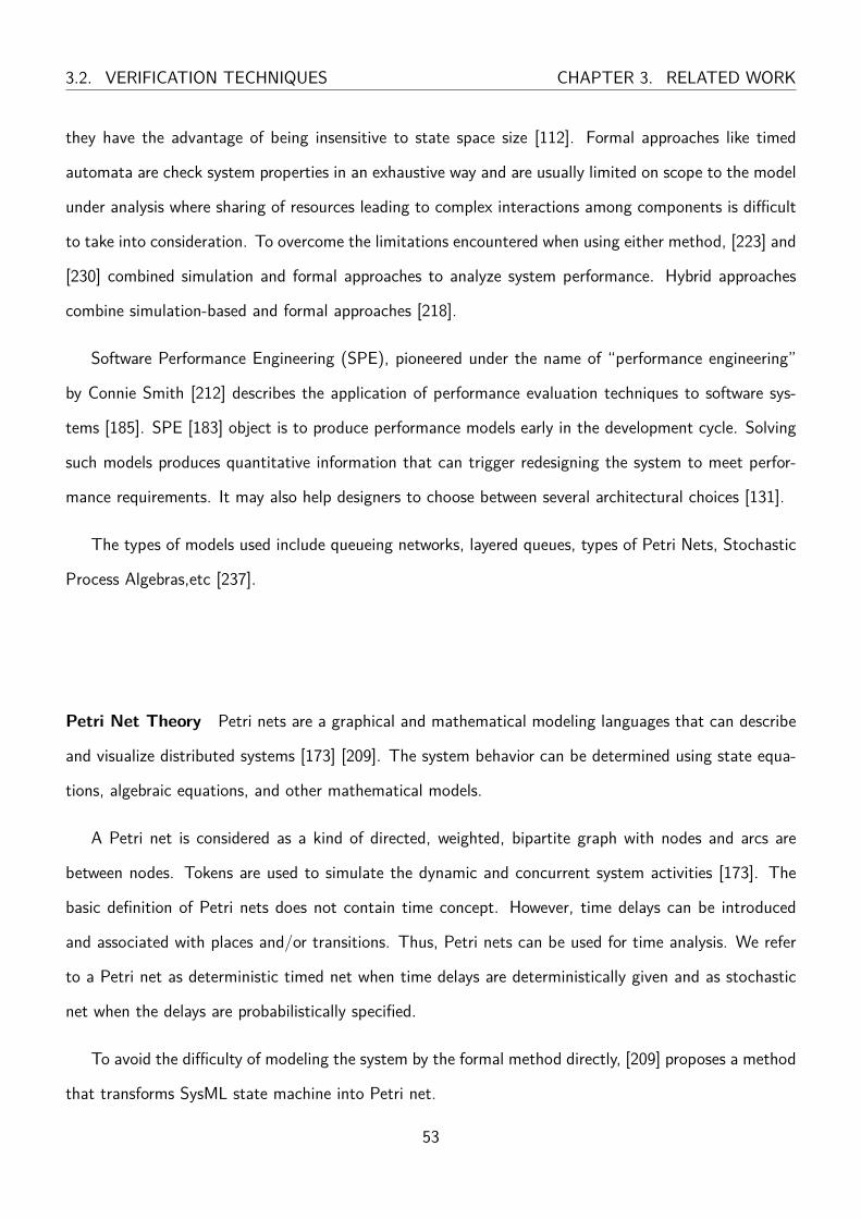
3.2. VERIFICATION TECHNIQUES CHAPTER 3. RELATED WORK
they have the advantage of being insensitive to state space size [112]. Formal approaches like timed
automata are check system properties in an exhaustive way and are usually limited on scope to the model
under analysis where sharing of resources leading to complex interactions among components is difficult
to take into consideration. To overcome the limitations encountered when using either method, [223] and
[230] combined simulation and formal approaches to analyze system performance. Hybrid approaches
combine simulation-based and formal approaches [218].
Software Performance Engineering (SPE), pioneered under the name of “performance engineering”
by Connie Smith [212] describes the application of performance evaluation techniques to software sys-
tems [185]. SPE [183] object is to produce performance models early in the development cycle. Solving
such models produces quantitative information that can trigger redesigning the system to meet perfor-
mance requirements. It may also help designers to choose between several architectural choices [131].
The types of models used include queueing networks, layered queues, types of Petri Nets, Stochastic
Process Algebras,etc [237].
Petri Net Theory Petri nets are a graphical and mathematical modeling languages that can describe
and visualize distributed systems [173] [209]. The system behavior can be determined using state equa-
tions, algebraic equations, and other mathematical models.
A Petri net is considered as a kind of directed, weighted, bipartite graph with nodes and arcs are
between nodes. Tokens are used to simulate the dynamic and concurrent system activities [173]. The
basic definition of Petri nets does not contain time concept. However, time delays can be introduced
and associated with places and/or transitions. Thus, Petri nets can be used for time analysis. We refer
to a Petri net as deterministic timed net when time delays are deterministically given and as stochastic
net when the delays are probabilistically specified.
To avoid the difficulty of modeling the system by the formal method directly, [209] proposes a method
that transforms SysML state machine into Petri net.
53
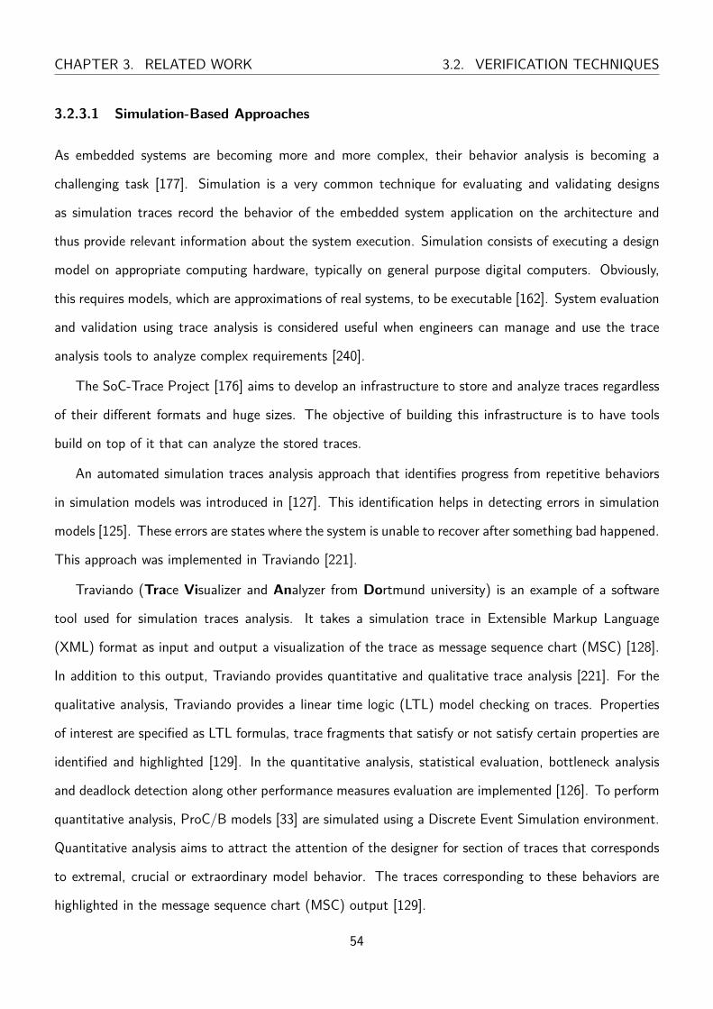
CHAPTER 3. RELATED WORK 3.2. VERIFICATION TECHNIQUES
3.2.3.1 Simulation-Based Approaches
As embedded systems are becoming more and more complex, their behavior analysis is becoming a
challenging task [177]. Simulation is a very common technique for evaluating and validating designs
as simulation traces record the behavior of the embedded system application on the architecture and
thus provide relevant information about the system execution. Simulation consists of executing a design
model on appropriate computing hardware, typically on general purpose digital computers. Obviously,
this requires models, which are approximations of real systems, to be executable [162]. System evaluation
and validation using trace analysis is considered useful when engineers can manage and use the trace
analysis tools to analyze complex requirements [240].
The SoC-Trace Project [176] aims to develop an infrastructure to store and analyze traces regardless
of their different formats and huge sizes. The objective of building this infrastructure is to have tools
build on top of it that can analyze the stored traces.
An automated simulation traces analysis approach that identifies progress from repetitive behaviors
in simulation models was introduced in [127]. This identification helps in detecting errors in simulation
models [125]. These errors are states where the system is unable to recover after something bad happened.
This approach was implemented in Traviando [221].
Traviando (Trace Visualizer and Analyzer from Dortmund university) is an example of a software
tool used for simulation traces analysis. It takes a simulation trace in Extensible Markup Language
(XML) format as input and output a visualization of the trace as message sequence chart (MSC) [128].
In addition to this output, Traviando provides quantitative and qualitative trace analysis [221]. For the
qualitative analysis, Traviando provides a linear time logic (LTL) model checking on traces. Properties
of interest are specified as LTL formulas, trace fragments that satisfy or not satisfy certain properties are
identified and highlighted [129]. In the quantitative analysis, statistical evaluation, bottleneck analysis
and deadlock detection along other performance measures evaluation are implemented [126]. To perform
quantitative analysis, ProC/B models [33] are simulated using a Discrete Event Simulation environment.
Quantitative analysis aims to attract the attention of the designer for section of traces that corresponds
to extremal, crucial or extraordinary model behavior. The traces corresponding to these behaviors are
highlighted in the message sequence chart (MSC) output [129].
54
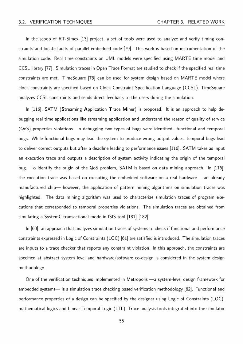
3.2. VERIFICATION TECHNIQUES CHAPTER 3. RELATED WORK
In the scoop of RT-Simex [13] project, a set of tools were used to analyze and verify timing con-
straints and locate faults of parallel embedded code [79]. This work is based on instrumentation of the
simulation code. Real time constraints on UML models were specified using MARTE time model and
CCSL library [77]. Simulation traces in Open Trace Format are studied to check if the specified real time
constraints are met. TimeSquare [78] can be used for system design based on MARTE model where
clock constraints are specified based on Clock Constraint Specification Language (CCSL). TimeSquare
analyzes CCSL constraints and sends direct feedback to the users during the simulation.
In [116], SATM (Streaming Application Trace Miner) is proposed. It is an approach to help de-
bugging real time applications like streaming application and understand the reason of quality of service
(QoS) properties violations. In debugging two types of bugs were identified: functional and temporal
bugs. While functional bugs may lead the system to produce wrong output values, temporal bugs lead
to deliver correct outputs but after a deadline leading to performance issues [116]. SATM takes as input
an execution trace and outputs a description of system activity indicating the origin of the temporal
bug. To identify the origin of the QoS problem, SATM is based on data mining approach. In [116],
the execution trace was based on executing the embedded software on a real hardware —an already
manufactured chip— however, the application of pattern mining algorithms on simulation traces was
highlighted. The data mining algorithm was used to characterize simulation traces of program exe-
cutions that corresponded to temporal properties violations. The simulation traces are obtained from
simulating a SystemC transactional mode in ISIS tool [181] [182].
In [60], an approach that analyzes simulation traces of systems to check if functional and performance
constraints expressed in Logic of Constraints (LOC) [61] are satisfied is introduced. The simulation traces
are inputs to a trace checker that reports any constraint violation. In this approach, the constraints are
specified at abstract system level and hardware/software co-design is considered in the system design
methodology.
One of the verification techniques implemented in Metropolis —a system-level design framework for
embedded systems— is a simulation trace checking based verification methodology [62]. Functional and
performance properties of a design can be specified by the designer using Logic of Constraints (LOC),
mathematical logics and Linear Temporal Logic (LTL). Trace analysis tools integrated into the simulator
55

CHAPTER 3. RELATED WORK 3.2. VERIFICATION TECHNIQUES
of Metropolis automatically check for the specified properties. This verification can be performed off-line
or during the simulation [62].
Co_Simulation Trace Analysis tool (COSITA) analyzes simulation traces in VCD format resulting
from SystemC-Simulink co-simulation and compare them to emulation traces. SystemC is used to model
hardware architecture and Simulink used as functional modeling language [130]. This technique is used
to verify properties of the modeled system. Automotive applications are modeled and properties that
allow the system to take a decision after a fault is encountered falls within the authors interest.
Trace Runtime Analysis Platform (TRAP) tool [240] is a model-based framework that analyzes
simulation traces to verify causal and temporal properties of embedded systems. Simulation traces are
generated by virtual prototype (VP) simulators. An error is raised in case a property is violated [240]. A
trace file generated by a VP simulator often contains a lot of detailed information about the system. To
minimizing the trace size, a Domain Specific Language, STML (Simulation Trace Mapping Language) is
used to abstract trace data into symbolic information (logical clocks) and remove irrelevant information.
This is where the originality of this tool lies. The objective of this framework is to predicts the reliability
and availability of an embedded system before it is integrated with the target hardware [211] .
Hedde and Pétrot [109] used virtual prototypes to produce non intrusive traces. These traces are
used for fine-grain analysis of software running on Multiprocessor Systems-on-Chip (MPSoCs). Complex
analysis such as verification of cache coherency protocol, memory consistency and data races detection
can be performed on traces [109]. The SoCLib framework along its System C Component library are used
for MPSoCs simulation. Moreover, the presented trace system method in [109] uses instrumentation of
component models to trace hardware events.
The traces collected in [109] are reconsidered in [144]. In [144], a framework based on data mining
approach is implemented to detect concurrent accesses to memory. The main aim of the data mining
approach is to automatically identify access patterns whose latency deviate significantly from the average
behavior of the traces and report them in a readable output to the software developers.
In [51], a non-intrusive instrumentation methodology for SystemC platform simulation models was
detailed. Using this methodology several types of analysis can be performed including runtime design
analysis and data analysis. Data analysis is part of an analysis framework that implements different
56
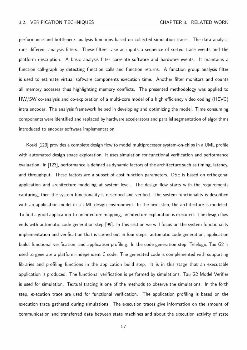
3.2. VERIFICATION TECHNIQUES CHAPTER 3. RELATED WORK
performance and bottleneck analysis functions based on collected simulation traces. The data analysis
runs different analysis filters. These filters take as inputs a sequence of sorted trace events and the
platform description. A basic analysis filter correlate software and hardware events. It maintains a
function call-graph by detecting function calls and function returns. A function group analysis filter
is used to estimate virtual software components execution time. Another filter monitors and counts
all memory accesses thus highlighting memory conflicts. The presented methodology was applied to
HW/SW co-analysis and co-exploration of a multi-core model of a high efficiency video coding (HEVC)
intra encoder. The analysis framework helped in developing and optimizing the model. Time consuming
components were identified and replaced by hardware accelerators and parallel segmentation of algorithms
introduced to encoder software implementation.
Koski [123] provides a complete design flow to model multiprocessor system-on-chips in a UML profile
with automated design space exploration. It uses simulation for functional verification and performance
evaluation. In [123], performance is defined as dynamic factors of the architecture such as timing, latency,
and throughput. These factors are a subset of cost function parameters. DSE is based on orthogonal
application and architecture modeling at system level. The design flow starts with the requirements
capturing, then the system functionality is described and verified. The system functionality is described
with an application model in a UML design environment. In the next step, the architecture is modeled.
To find a good application-to-architecture mapping, architecture exploration is executed. The design flow
ends with automatic code generation step [99]. In this section we will focus on the system functionality
implementation and verification that is carried out in four steps: automatic code generation, application
build, functional verification, and application profiling. In the code generation step, Telelogic Tau G2 is
used to generate a platform-independent C code. The generated code is complemented with supporting
libraries and profiling functions in the application build step. It is in this stage that an executable
application is produced. The functional verification is performed by simulations. Tau G2 Model Verifier
is used for simulation. Textual tracing is one of the methods to observe the simulations. In the forth
step, execution trace are used for functional verification. The application profiling is based on the
execution trace gathered during simulations. The execution traces give information on the amount of
communication and transferred data between state machines and about the execution activity of state
57
CHAPTER 3. RELATED WORK 3.3. INFORMATION FLOW ANALYSIS
machines [123]. The performance is determined by the simulation statistics of process execution timing
and communication latencies.
3.3 Information Flow Analysis
Dataflow graph is a model of computation that can be used to analyze properties of a system [36].
Examples of these properties include absence of deadlock, throughput bounds, performance requirements,
security requirements, etc [34] [36] [106] [153].
A dataflow graph is a directed graph consisting of nodes connected by edges. Nodes are called
actors [34]. Edges are arcs representing dependencies. Actors produce and consume tokens. A token
stores a fixed amount of data. An actor is enabled to fire a token when tokens are available on all
its input edges [115]. Synchronous data flow graph, cyclo-static dataflow graph, and dynamic dataflow
graph are examples of dataflow graphs.
In [219], synchronous time-constrained multimedia applications are modeled using dataflow graphs.
These graphs are then allocated to an embedded multiprocessor system using the proposed resource
allocation strategy that guarantees that the throughput bounds are respected.
The actors of synchronous dataflow models defined in [34], have a well-defined input/output behavior
and a worst-case response time. These models were used to derive the worst-case end-to-end temporal
behavior of real-time applications
[106] proposes to use cyclostatic dataflow graph to capture the behavior, allocate resources and
compute buffer sizes in larger SoC applications whose performance needs to be guaranteed.
The approach in [186] uses data flow analysis from UML/MARTE models and trace analysis to
improve design flexibility and evaluation capabilities of the models. To understand and analyze the
required timing behavior of the model, the user must define, in the UML model, the most important
paths followed by the data internally through the system. These internal data paths are monitored and
form the bases for timing analysis. The analysis output information about the correct path iterations,
and their timing characteristics (maximum, mean and minimum time), number of correct data paths
accomplishing the constraints sets, etc.
58

3.3. INFORMATION FLOW ANALYSIS CHAPTER 3. RELATED WORK
Taint analysis is a form of information flow analysis [153]. It includes tainting an object/data in a
system then tracking it using a data-flow analysis technique [103] [38]. To taint an object/data means
to mark it with a tag or label. The data flow analysis tracks the tainted object from the taint source,
where the taint object comes from, to the taint sink where the taint object leaves the system.
Taint analysis is mainly used in compiler optimization and security analysis [50] [156]. In [156], an
automated analysis and repair approach for existing software for autonomous robot systems was proposed.
The latter approach used a taint analysis method.
3.3.1 Taint Analysis
Taint analysis can run in two modes static and dynamic. In dynamic taint analysis the system is executed
to be analyzed while in static taint analysis the source code is parsed without execution [38] [153].
Dynamic taint analysis is used by several security algorithms to track information flow in soft-
ware [103]. It is mainly used to detect vulnerabilities and protect sensitive data [103]. Information
disclosure attacks [39] and confidentiality violations [107] can be detected using dynamic taint tracking.
In [145], a dynamic taint tracking technique was used to prevent buffer overflow. The main advantage
of dynamic analysis is that it is possible to detect attacks that need certain prerequisites like system
configuration while the main disadvantage of dynamic analysis is that only part of the program that was
executed is analyzed [38].
Techniques based on dynamic tainting have been successfully used in the context of application
security, and now their use is also being explored in different areas, such as program understanding,
software testing, and debugging [66].
Static taint analysis approaches can be used for different tasks including security and privacy issues
detection [153] [103]. At the time of development of C programs, static taint analysis can be used
to detect bugs [103]. For android apps, in addition to assessing their security, detecting app clones,
automating test cases generation and discovering performance or energy related issues can be achieved
through static analysis approaches [153]. However, static taint analysis approaches cannot analyze
encrypted or obfuscated code [38] and some of the code paths identified in static analysis could never
execute in real systems [239].
59
CHAPTER 3. RELATED WORK 3.3. INFORMATION FLOW ANALYSIS
While both static and dynamic techniques can be used for information disclosure attacks detection,
dynamic analysis according to [38] appears to be more promising. Moreover, hybrid approaches which
combines static and dynamic analysis improve the quality of security analysis.
DTaint [63] is a static analysis approach used to detect taint-style vulnerabilities in the firmware. The
firmware is a software embedded in devices to determine their functionality. The taint-style vulnerability
can be defined as a flaw where the input data reaches a sensitive sink through an unsafe path. DTaint
was applied to six firmware images from four manufacturers and 21 vulnerabilities were discovered among
them 13 previously-unknown and zero-day vulnerabilities.
Celik et al. [57] propose Saint, a tool used to detect privacy violations in IoT apps using static taint
analysis. Saint identifies potential flows of sensitive data by automatically tracking information flow from
taint sources (e.g., device state and user info) to taint sinks (e.g., Internet connections). SAINT operates
in three phases. First the taint sources and sinks are identified. Then the IoT source code is translated
into an intermediate representation (IR). After that static analysis is performed.
ContexIoT [119] is a context-based permission system for IoT apps. It gathers context information
(e.g., data source, and runtime data of a device) before a sensitive action is executed, and then asks for
user approval to execute this action through run-time prompts. ContexIoT provides contextual integrity
to permission granting and aims to detect the misuse of IoT devices by comparing the context information
of a normal behavior to a behavior set up by an attacker. ContexIoT defines context as execution paths of
an app functionality (inter-procedure control and data flow) including for example how the functionality
is triggered and what data is flowing along the execution path. To help users make informed decisions,
tainting is used in ContexIoT to labels the data source and track data on the execution path of an app
code. Thus, when presenting the context information to the user, taint analysis will allow the user to
distinguish for example if the data to be sent out is the user password or just the battery level and a user
can make a more informed decision on permission granting.
Tainting analysis is mainly used in mobile-phone platform [57]. Taintdroid [82], “the best known
taint-tracking system for Android” [38], uses dynamic taint analysis to allow users to track the flow of
information through third-party applications in real-time. In particular it monitors privacy-sensitive data
and address challenges specific to mobile phones [103]. Several Android security systems are based on
60

3.4. CONCLUSION CHAPTER 3. RELATED WORK
Taintdroid including MOSES [197], TreeDroid [72], VetDroid [241], YAASE [196], AppsPlayground [191],
DroidBox [146], ANDRUBIS [154], QuantDroid [159] and NDroid [189]. Mobile-Sandbox [214] is also
based on Taintdroid however, it is hybrid security analysis approach which combines and benefits of static
and dynamic analyses. In this approach, the dynamic taint analysis is guided by a static analysis phase.
Two successors of Taintdroid are TaintART and TaintMan [38].
The Blare project and the Blare tools aim to provide a set of tools to monitor information flows at
different level of granularity [98]. At the level of operating system, Blare [98] is used to monitor the
information flow. It tags files as files are information container at the OS level. The tag of the file is
propagated to the program when a program accesses a file. Conversely, each time the program writes to
a file, the tag of program is propagated to the file. Security policy are used to verify if the information
flow is authorized or not [233]. The tag propagation and security policy checks are performed by the
Linux kernel [233]. AndroBlare [25] modifies Blare to trace information flows on an Android operating
system.
DTA++ [122] enhance standard dynamic taint analysis approaches by propagating taint along control
dependencies. It targets the under-tainting problem of standard approaches where sensitive information
should be marked as tainted are not. This problem occurs when tainted data values affect control flow
in a program and then the control flow affects other data but the latter remain untainted. DTA++ is
implemented using the BitBlaze platform for binary analysis [213]. It is applied on off-the-shelf benign
Windows/x86 applications
3.4 Conclusion
Table 3.1 shows a summary of the methods and tools presented in Section 3.2.3.1 showing the type of
models they design, the purpose of their trace analysis approach and the technique they use in their
analysis.
Nevertheless, to the best of our knowledge, the aforementioned works do not address an approach
in which the execution trace of a high-level allocation model can be used to advice a designer on how
to enhance a model to satisfy a latency requirement by indicating which software/hardware component
61
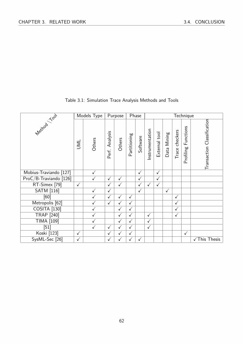
CHAPTER 3. RELATED WORK 3.4. CONCLUSION
Table 3.1: Simulation Trace Analysis Methods and Tools
Method \Tool Models Type Purpose Phase Technique
UML
Others
Perf.
Analy
sis
Others
Partitio
ning
Softw
are
Instr
umentatio
n
External
tool
Data
Mining
Tracecheckers
Profi
lingFu
nctio
ns
Transaction
Classifi
catio
n
Mobius-Traviando [127] X X XProC/B-Traviando [126] X X X X X
RT-Simex [79] X X X X X XSATM [116] X X X X
[60] X X X X XMetropolis [62] X X X X XCOSITA [130] X X X XTRAP [240] X X X X XTIMA [109] X X X X
[51] X X X X XKoski [123] X X X X X
SysML-Sec [26] X X X X X XThis Thesis
62

3.4. CONCLUSION CHAPTER 3. RELATED WORK
contributed to a latency between events. In other words, to our knowledge, other performance evaluation
methods do not identify which component leads to extra processing time or hardware contention. Most
of the analysis tools calculate the WCET or BCET or latency and throughput values. While in some
simple cases having the minimum and maximum latency can be beneficial for the designer, in other
complex cases, especially when new safety and security measures are added to the model, having these
values does not help much the designer on the precise cause of the latencies. Not understanding the
cause of the latency and what elements are contributing to its value will limit the designer’s knowledge
on how to enhance the model to further improve performance.
The introduced approach in the scope of this thesis does not require the use of instrumentation, data
mining or any external tool. It is based on the extraction from the model semantics a causality graph
and studying the execution trace along the generated graph as detailed in the next chapters.
Moreover, tainting which is mostly used to detect security flows as shown in section 3.3.1 is used in
the second version of our approach to calculate latency.
63

Chapter 4
Precise Latency Analysis Approach:
Overview and Problem Formalization
“Around here, however, we don’t look backwards for very long. We keep moving forward,
opening up new doors and doing new things, because we’re curious...and curiosity keeps
leading us down new paths.”
-Walt Disney Company
4.1 Motivation
Handling time is often a critical aspect for safety critical systems [223] [55]. These systems are known as
real-time systems. Real-time systems are characterized by their ability to accomplish a specific task and
respond to events within a specified time [58] [152]. In order for real-time systems to behave correctly,
they must not only execute the correct computations but also do so within predefined time constraints.
These time constraints are typically expressed in terms of end-to-end deadlines on the elapsed time
between a stimulus and the corresponding response [75] [223], the percentage of usage of system’s
components [152] and throughput [223] where throughput is defined as the number of events that can
be processed per time unit.
Real-time systems can be classified as hard real-time or soft real-time systems. In hard real-time
64
4.1. MOTIVATION CHAPTER 4. PROBLEM FORMALIZATION
systems failure to meet a deadline leads to a failure of the application resulting in catastrophic situations.
In soft real-time systems missing a deadline leads only to degraded quality of service of the application.
Designers must ensure that hard real-time systems respect their deadlines before systems are put in
operation [75]. In general, estimating the timing properties for a system as early as possible in the
design process is considered a valuable approach as it results in updating the model in a cost-efficient
manner [207] [230].
Real-time constraints expressed with respect to end-to-end deadlines can specify the maximum time
delay that the system can tolerate between two events. This maximum acceptable time delay is referred
to as deadline or maximum latency. Latency is the time delay between the execution of two events.
Latency is important when there is an expected feedback from the system corresponding to an input
event [205]. For example, a motor controller is expected to stop within 500 ms after it receives a stop
command from the user. Section 4.5 defines precisely and formally what a maximum latency requirement
is in the scope of our work.
In this chapter, a new latency analysis approach PLAN based on Execution Trace Analysis (ETA)
is introduced. This approach is meant to precisely indicate the cause of latency between two events in
a system. For this, PLAN can analyze the execution trace between the two events of interest. PLAN
answers whether the latency requirement is satisfied. If not, then the analysis produces a classification
of the transactions of the execution trace. To perform this analysis, PLAN has to use system semantics,
including the logical and physical dependencies between software and hardware components. In the
scope of this thesis, dependencies are specific to high level languages. For example, as shown later in
the chapter, the dependencies between writing and reading data are approximations that do not take
into account the value but the amount of data. So, dependencies are heuristic defined at high level of
abstraction. Applying PLAN to system models defined at lower level of abstraction i.e., assembly level
is discussed in Chapter 8 for future work.
65
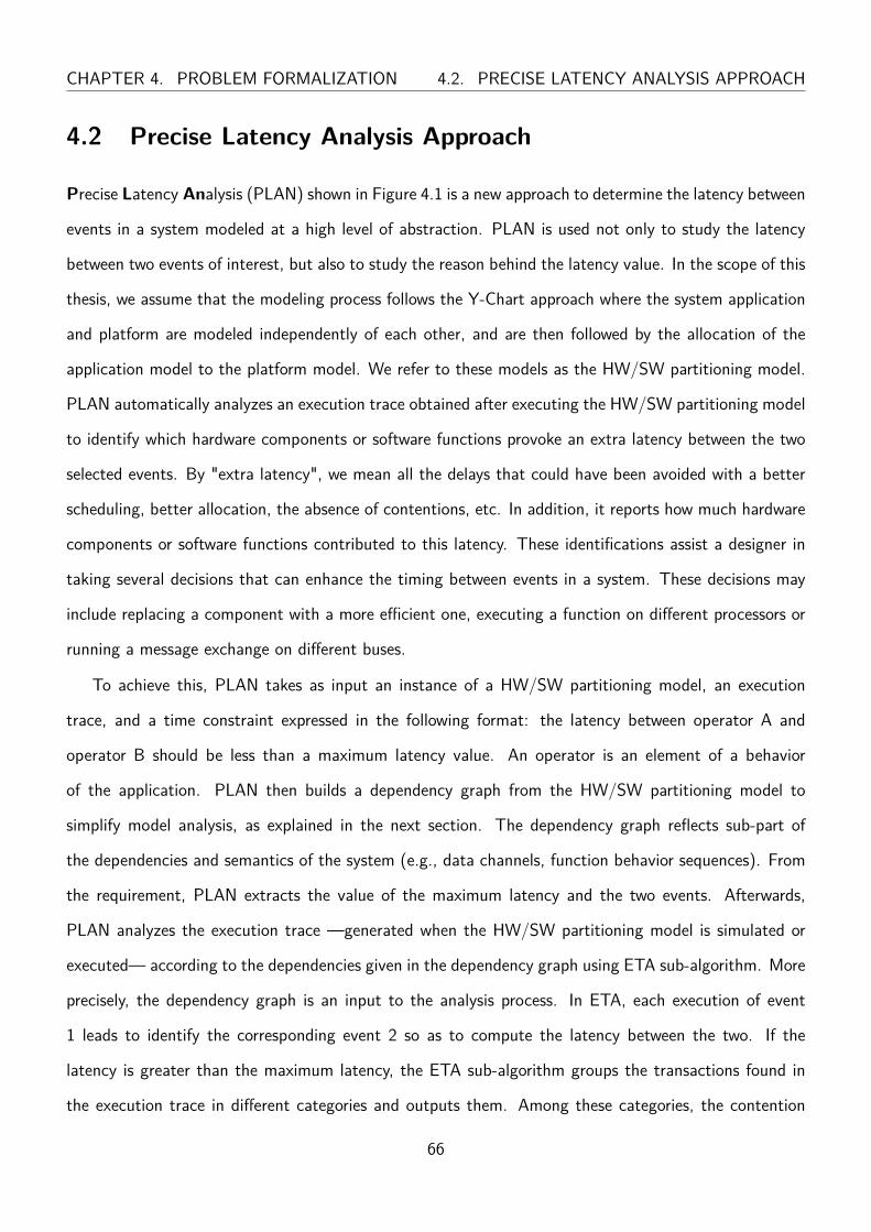
CHAPTER 4. PROBLEM FORMALIZATION 4.2. PRECISE LATENCY ANALYSIS APPROACH
4.2 Precise Latency Analysis Approach
Precise Latency Analysis (PLAN) shown in Figure 4.1 is a new approach to determine the latency between
events in a system modeled at a high level of abstraction. PLAN is used not only to study the latency
between two events of interest, but also to study the reason behind the latency value. In the scope of this
thesis, we assume that the modeling process follows the Y-Chart approach where the system application
and platform are modeled independently of each other, and are then followed by the allocation of the
application model to the platform model. We refer to these models as the HW/SW partitioning model.
PLAN automatically analyzes an execution trace obtained after executing the HW/SW partitioning model
to identify which hardware components or software functions provoke an extra latency between the two
selected events. By "extra latency", we mean all the delays that could have been avoided with a better
scheduling, better allocation, the absence of contentions, etc. In addition, it reports how much hardware
components or software functions contributed to this latency. These identifications assist a designer in
taking several decisions that can enhance the timing between events in a system. These decisions may
include replacing a component with a more efficient one, executing a function on different processors or
running a message exchange on different buses.
To achieve this, PLAN takes as input an instance of a HW/SW partitioning model, an execution
trace, and a time constraint expressed in the following format: the latency between operator A and
operator B should be less than a maximum latency value. An operator is an element of a behavior
of the application. PLAN then builds a dependency graph from the HW/SW partitioning model to
simplify model analysis, as explained in the next section. The dependency graph reflects sub-part of
the dependencies and semantics of the system (e.g., data channels, function behavior sequences). From
the requirement, PLAN extracts the value of the maximum latency and the two events. Afterwards,
PLAN analyzes the execution trace —generated when the HW/SW partitioning model is simulated or
executed— according to the dependencies given in the dependency graph using ETA sub-algorithm. More
precisely, the dependency graph is an input to the analysis process. In ETA, each execution of event
1 leads to identify the corresponding event 2 so as to compute the latency between the two. If the
latency is greater than the maximum latency, the ETA sub-algorithm groups the transactions found in
the execution trace in different categories and outputs them. Among these categories, the contention
66
4.3. SYSTEM MODEL FORMAL DEFINITION CHAPTER 4. PROBLEM FORMALIZATION
category is the most interesting one for the designer as it contains refers to the functions and hardware
components that have played a role in the latency: removing these contentions would lead to reduce the
latency under study. Otherwise, if all the latencies between events 1 and its corresponding events 2 are
below the maximum latency, the designer is notified that the system model respects the requirement.
In the following sections, the different stages shown in Figure 4.1 are presented. First, the HW/SW
partitioning model is formally defined in section 4.3. Section 4.4 gives an overview of the model execution
Semantics. Section 4.5 defines a maximum latency requirement.
4.3 System Model Formal Definition
The formal definition proposed in this subsection assumes that the Y-Chart scheme [132] is used to
capture the application, the platform and the allocation of the considered system.
Definition 1. System model
A system model s is a 2-uple denoted as s = 〈m,R〉 where m is a HW/SW partitioning model and
R a set of requirements.
Definition 2. HW/SW partitioning model
A HW/SW partitioning model m is a 3-uple denoted as m = 〈F ,P ,A〉 where F is an application
model, P a platform model and A an allocation model.
The elements within the HW/SW partitioning model are grouped into families called categories. We
use function cat(c) to return the category to which a component c belongs to. Elements of the model
have identifiers. In this thesis, they are conventionally denoted as ei where i is the identifier. Moreover,
when a tuple t is defined, the notation t[i] is used to retrieve the ith item of this tuple and |t| is used to
return the size of t.
4.3.1 Application
Definition 3. Application Model
An application model F consists of a set of functions F and a set of communication channels CC.
67
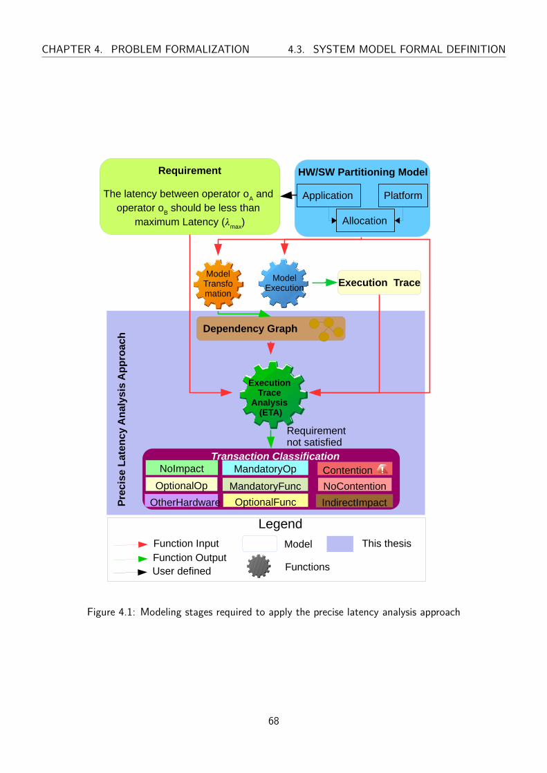
CHAPTER 4. PROBLEM FORMALIZATION 4.3. SYSTEM MODEL FORMAL DEFINITION
Execution Trace
HW/SW Partitioning Model
Application Platform
Allocation
Requirement
The latency between operator oA and
operator oB should be less than
maximum Latency (𝜆max
)
OptionalFunc
NoContentionMandatoryFunc
Contention MandatoryOpNoImpact
OptionalOp
OtherHardware
Requirement not satisfied
Dependency Graph
Pre
cis
e L
aten
cy A
nal
ysis
Ap
pro
ach
ModelExecution
ModelTransfomation
Execution Trace
Analysis (ETA)
Function Input
Legend
Function OutputThis thesis
User defined Functions
IndirectImpact
Model
Figure 4.1: Modeling stages required to apply the precise latency analysis approach
68

4.3. SYSTEM MODEL FORMAL DEFINITION CHAPTER 4. PROBLEM FORMALIZATION
We denote the application model as
F = 〈F, CC〉
Definition 4. Communication Channel
A communication channel connects together two functions with one function that can write in this
channel and one function that can read from this channel. A communication channel between two
functions f and f ′ where f can write and f ′ can read, is denoted as ccf,f ′∈ CC.
Our model supports two kinds of communication channels: data channels and synchronization chan-
nels. The set of all data channels of an application model is denoted as DC and the set of all synchro-
nization channels of a system is denoted as SC.
The set of data channels for writer f and reader f ′ is denoted as DCf,f ′ and for synchronization
channels SCf,f ′ . Finally, the set CCf,f ′ is a 2-uple defined as follows:
CCf,f ′ = 〈DCf,f ′ ,SCf,f ′〉
And DC, SC and CC are defined as:
DC =⋃{DCf,f ′ | (f, f
′) ∈ F2}SC =
⋃{SCf,f ′ | (f, f
′) ∈ F2}CC = DC ∪ SC
Definition 5. Synchronization Channel
A synchronization channel scf,f ′ ∈ SCf,f ′ is given one semantic among the three following ones:
Non-Blocking Notify - Blocking Wait Infinite FIFO (NBN-BW-INF), Non-Blocking Notify - Blocking
Wait Finite FIFO (NBN-BW-F) or Blocking Notify - Blocking Wait Finite FIFO (BN-BW-F).
SCType = {NBN-BW-INF,NBN-BW-F,BN-BW-F}
Synchronization messages sent from function f to function f ′ are managed using a FIFO buffer, which
69

CHAPTER 4. PROBLEM FORMALIZATION 4.3. SYSTEM MODEL FORMAL DEFINITION
can be finite or infinite. So, the receiver function is always blocked when the buffer is empty while the
sender function can be non blocking or blocking when the buffer is full. When the synchronization channel
has finite buffer semantics, of course, a buffer size attribute is specified and in case the buffer is full, no
synchronization messages can be added to it, so a sender function is blocked until the buffer is not full. So,
for a synchronization channel having Non-Blocking Notify - Blocking Wait Infinite FIFO type the sender
function f can always send synchronization messages without any constraint and the receiver function
f ′ is blocked when the buffer is empty. In case the synchronization channel has Non-Blocking Notify -
Blocking Wait Finite FIFO type, the sender function f can send synchronization messages without any
constraint and the receiver function f ′ is blocked when the buffer is empty. However, in the later type,
when the buffer is full, the oldest message in the buffer is removed to leave space for the new one that
is added. In case the synchronization channel has Blocking Notify - Blocking Wait Finite FIFO type,
the sender function f can send synchronization messages only until the buffer is full while the receiver
function f ′ can read synchronization messages if the buffer is not empty. The functions getSCType and
getSyncBufferSize take as argument a synchronization channel and return the synchronization channel
semantic (SCType) and the FIFO buffer size respectively.
getSCType : SCf,f ′ → SCType
getSyncBufferSize(scf,f ′)
=∞ if getSCType(scf,f ′) = NBN-BW-INF
∈ Z+ if getSCType(scf,f ′) ∈ {NBN-BW-F,BN-BW-F}
Definition 6. Data Channel
Data channels can have different semantics. A data channel dcf,f ′ ∈ DCf,f ′ has either a Non-
Blocking Write - Non-Blocking Read (NBW-NBR), Non-Blocking Write - Blocking Read (NBW-BR), or
Blocking Write - Blocking Read (BW-BR) type and a buffer size (which can be infinite).
DCType = {NBW-NBR,NBW-BR,BW-BR}
70
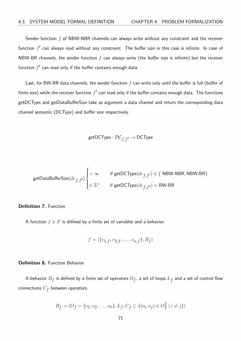
4.3. SYSTEM MODEL FORMAL DEFINITION CHAPTER 4. PROBLEM FORMALIZATION
Sender function f of NBW-NBR channels can always write without any constraint and the receiver
function f ′ can always read without any constraint. The buffer size in this case is infinite. In case of
NBW-BR channels, the sender function f can always write (the buffer size is infinite) but the receiver
function f ′ can read only if the buffer contains enough data.
Last, for BW-BR data channels, the sender function f can write only until the buffer is full (buffer of
finite size) while the receiver function f ′ can read only if the buffer contains enough data. The functions
getDCType and getDataBufferSize take as argument a data channel and return the corresponding data
channel semantic (DCType) and buffer size respectively.
getDCType : DCf,f ′ → DCType
getDataBufferSize(dcf,f ′)
=∞ if getDCType(dcf,f ′) ∈ { NBW-NBR,NBW-BR}
∈ Z+ if getDCType(dcf,f ′) = BW-BR
Definition 7. Function
A function f ∈ F is defined by a finite set of variables and a behavior.
f = 〈{v1,f , v2,f , . . . , vn,f}, Bf 〉
Definition 8. Function Behavior
A behavior Bf is defined by a finite set of operators Of , a set of loops Lf and a set of control flow
connections Cf between operators.
Bf = 〈Of = {o1, o2, . . . , on}, Lf , Cf ⊂ {(oi, oj) ∈ O2f | i 6= j}〉
71
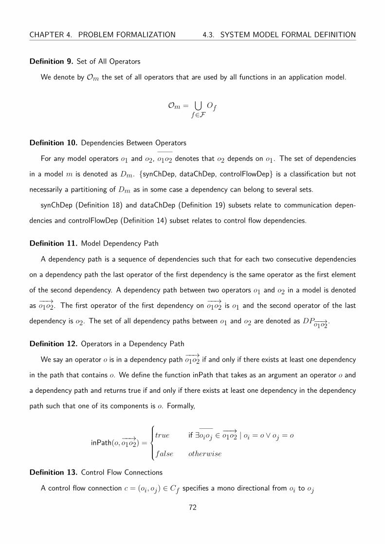
CHAPTER 4. PROBLEM FORMALIZATION 4.3. SYSTEM MODEL FORMAL DEFINITION
Definition 9. Set of All Operators
We denote by Om the set of all operators that are used by all functions in an application model.
Om =⋃f∈F
Of
Definition 10. Dependencies Between Operators
For any model operators o1 and o2, o1o2 denotes that o2 depends on o1. The set of dependencies
in a model m is denoted as Dm. {synChDep, dataChDep, controlFlowDep} is a classification but not
necessarily a partitioning of Dm as in some case a dependency can belong to several sets.
synChDep (Definition 18) and dataChDep (Definition 19) subsets relate to communication depen-
dencies and controlFlowDep (Definition 14) subset relates to control flow dependencies.
Definition 11. Model Dependency Path
A dependency path is a sequence of dependencies such that for each two consecutive dependencies
on a dependency path the last operator of the first dependency is the same operator as the first element
of the second dependency. A dependency path between two operators o1 and o2 in a model is denoted
as −−→o1o2. The first operator of the first dependency on −−→o1o2 is o1 and the second operator of the last
dependency is o2. The set of all dependency paths between o1 and o2 are denoted as DP−−→o1o2 .
Definition 12. Operators in a Dependency Path
We say an operator o is in a dependency path −−→o1o2 if and only if there exists at least one dependency
in the path that contains o. We define the function inPath that takes as an argument an operator o and
a dependency path and returns true if and only if there exists at least one dependency in the dependency
path such that one of its components is o. Formally,
inPath(o,−−→o1o2) =
true if ∃oioj ∈
−−→o1o2 | oi = o ∨ oj = o
false otherwise
Definition 13. Control Flow Connections
A control flow connection c = (oi, oj) ∈ Cf specifies a mono directional from oi to oj
72
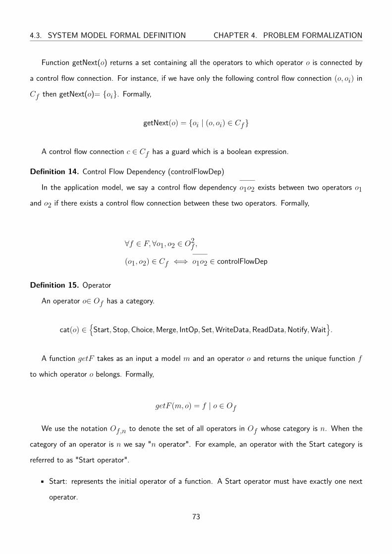
4.3. SYSTEM MODEL FORMAL DEFINITION CHAPTER 4. PROBLEM FORMALIZATION
Function getNext(o) returns a set containing all the operators to which operator o is connected by
a control flow connection. For instance, if we have only the following control flow connection (o, oi) in
Cf then getNext(o)= {oi}. Formally,
getNext(o) = {oi | (o, oi) ∈ Cf}
A control flow connection c ∈ Cf has a guard which is a boolean expression.
Definition 14. Control Flow Dependency (controlFlowDep)
In the application model, we say a control flow dependency o1o2 exists between two operators o1and o2 if there exists a control flow connection between these two operators. Formally,
∀f ∈ F, ∀o1, o2 ∈ O2f ,
(o1, o2) ∈ Cf ⇐⇒ o1o2 ∈ controlFlowDep
Definition 15. Operator
An operator o∈ Of has a category.
cat(o) ∈{Start, Stop,Choice,Merge, IntOp, Set,WriteData,ReadData,Notify,Wait
}.
A function getF takes as an input a model m and an operator o and returns the unique function f
to which operator o belongs. Formally,
getF (m, o) = f | o ∈ Of
We use the notation Of,n to denote the set of all operators in Of whose category is n. When the
category of an operator is n we say "n operator". For example, an operator with the Start category is
referred to as "Start operator".
• Start: represents the initial operator of a function. A Start operator must have exactly one next
operator.
73

CHAPTER 4. PROBLEM FORMALIZATION 4.3. SYSTEM MODEL FORMAL DEFINITION
• Stop: represents the end of the execution of a function. A Stop operator has no next operator.
• Choice: has at least one next operator. Only one control flow among the ones with a guard equal
to true can be selected by an execution engine. If no guard of the output control flow connections
evaluate to true, then the choice operator blocks. The choice operator is the only category that
can have more than one next operator.
• Merge: the merge operator makes it possible for several operators o1 to on to have the same next.
So the merge operator is the only one that can have several previous operators. It has exactly one
next.
• IntOp: specifies the complexity of an algorithm. An IntOp operator has exactly one next. An
important attribute of an IntOp operator is its complexity. A complexity attribute specifies the
number of low level operations, e.g., operations on integers, of an algorithm. If an algorithm has
several execution branches, the IntOp operator can be combined with a Choice operator to model
the duration of the different branches. The function getComplexity takes as an argument an IntOp
operator and returns the complexity attribute. So,
getComplexity : Of,IntOp → Z+
• Set: sets a new value to a variable. A Set operator has exactly one next.
• WriteData: specifies an amount of data to be written into a data channel. A WriteData operator
has exactly one next. The quantity of data to write is specified in a size attribute. Functions
getDataCh and getDataSize take as an argument a WriteData operator and return the data channel
and size attributes respectively.
• ReadData: specifies an amount of data to be read from a data channel. A ReadData operator has
exactly one next. Functions getDataCh and getDataSize defined for WriteData operators are also
defined in the same way for ReadData operators. Formally,
getDataCh : Of,WriteData ∪Of,ReadData → DC
74

4.3. SYSTEM MODEL FORMAL DEFINITION CHAPTER 4. PROBLEM FORMALIZATION
getDataSize : Of,WriteData ∪Of,ReadData → Z+
• Notify: specifies the sending of a synchronization message through a synchronization channel. A
Notify operator has exactly one next. The function getSyncCh takes as and argument a Notify
operator and returns the synchronization channel.
• Wait: specifies the receiving of a synchronization message through a synchronization channel. A
Wait operator has exactly one next. The function getSyncCh defined before can be applied to
Wait operators to retrieve the synchronization channel.
getSyncCh : Of,Notify ∪Of,Wait → SC
Definition 16. Fixed size Loop
We call a loop a 5-tuple 〈om, oc, os, v, nbr〉 where om, oc and os are a Merge operator, a Choice
operator and a Set operator respectively all belonging to the same function, v is the variable used in the
loop and nbr is the number of loop iterations (Figure 4.2).
Properties on a loop 〈om, oc, os, v, nbr〉 :
• The function getNext(om)={oc} i.e., there is a control flow connection between the Merge operator
and the Choice operator.
• The Choice operator has at least one dependency path to the Merge operator.
• The function getNext(os)={om} i.e., there is a control flow connection between the Set operator
and the Merge operator.
• The Choice operator must have at least 1 next which is the body of the loop and at most 2 next:
one the body of the loop and one the loop exit.
• All operators of the body of the loop must have dependency paths to the Merge operator
• All the dependency paths starting from operators in the body of the loop must lead to os
• All paths from the Choice operator to the Merge operator represent the inner body of a loop.
75
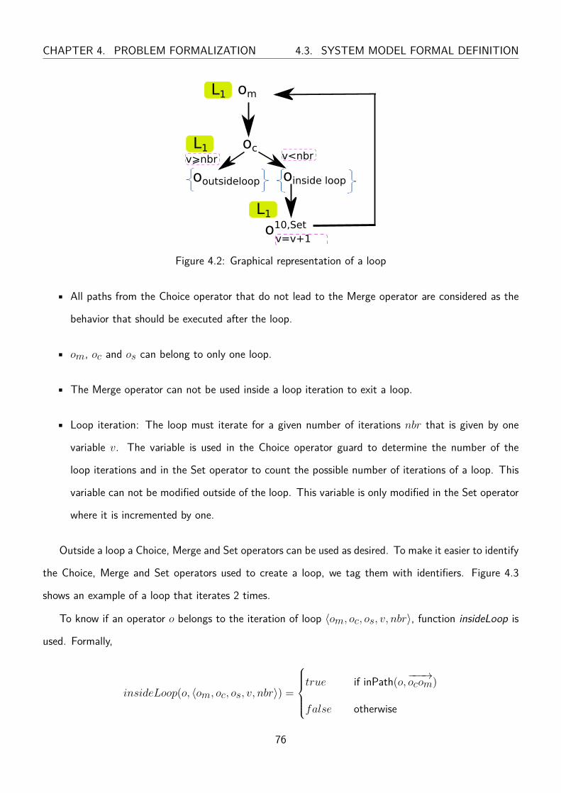
CHAPTER 4. PROBLEM FORMALIZATION 4.3. SYSTEM MODEL FORMAL DEFINITION
oc
om
ooutsideloop
v<nbrv⩾nbr
v=v+1o10,Set
L1
L1
L1
oinside loop
Figure 4.2: Graphical representation of a loop
• All paths from the Choice operator that do not lead to the Merge operator are considered as the
behavior that should be executed after the loop.
• om, oc and os can belong to only one loop.
• The Merge operator can not be used inside a loop iteration to exit a loop.
• Loop iteration: The loop must iterate for a given number of iterations nbr that is given by one
variable v. The variable is used in the Choice operator guard to determine the number of the
loop iterations and in the Set operator to count the possible number of iterations of a loop. This
variable can not be modified outside of the loop. This variable is only modified in the Set operator
where it is incremented by one.
Outside a loop a Choice, Merge and Set operators can be used as desired. To make it easier to identify
the Choice, Merge and Set operators used to create a loop, we tag them with identifiers. Figure 4.3
shows an example of a loop that iterates 2 times.
To know if an operator o belongs to the iteration of loop 〈om, oc, os, v, nbr〉, function insideLoop is
used. Formally,
insideLoop(o, 〈om, oc, os, v, nbr〉) =
true if inPath(o,−−−→ocom)
false otherwise
76
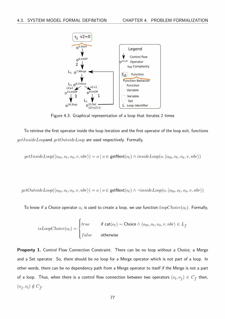
4.3. SYSTEM MODEL FORMAL DEFINITION CHAPTER 4. PROBLEM FORMALIZATION
f1
o6,IntOP
o16,Stop
o8,Choice
o7,Merge
o15,IntOP o9,IntOP
3
v2<2v2⩾2
Legend
oid,cat
fidFunction Behavior
Control flow
Operator
Function
oid Complexity
Variable
Set
Function
Variable
2
1
v2=0
v2=v2+1
o5,Start
o10,Set
L1
L1
L1
L Loop Identifier
Figure 4.3: Graphical representation of a loop that iterates 2 times
To retrieve the first operator inside the loop iteration and the first operator of the loop exit, functions
getInsideLoopand getOutsideLoop are used respectively. Formally,
getInsideLoop(〈om, oc, os, v, nbr〉) = o | o ∈ getNext(oc) ∧ insideLoop(o, 〈om, oc, os, v, nbr〉)
getOutsideLoop(〈om, oc, os, v, nbr〉) = o | o ∈ getNext(oc) ∧ ¬insideLoop(o, 〈om, oc, os, v, nbr〉)
To know if a Choice operator oc is used to create a loop, we use function loopChoice(oc). Formally,
isLoopChoice(oc) =
true if cat(oc) = Choice ∧ 〈om, oc, os, v, nbr〉 ∈ Lf
false otherwise
Property 1. Control Flow Connection Constraint. There can be no loop without a Choice, a Merge
and a Set operator. So, there should be no loop for a Merge operator which is not part of a loop. In
other words, there can be no dependency path from a Merge operator to itself if the Merge is not a part
of a loop. Thus, when there is a control flow connection between two operators (oi, oj) ∈ Cf then,
(oj , oi) /∈ Cf .
77
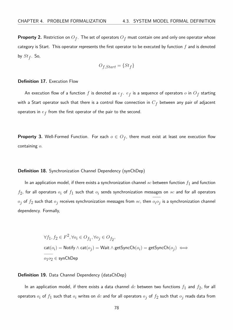
CHAPTER 4. PROBLEM FORMALIZATION 4.3. SYSTEM MODEL FORMAL DEFINITION
Property 2. Restriction on Of . The set of operators Of must contain one and only one operator whose
category is Start. This operator represents the first operator to be executed by function f and is denoted
by Stf . So,
Of,Start = {Stf}
Definition 17. Execution Flow
An execution flow of a function f is denoted as ef . ef is a sequence of operators o in Of starting
with a Start operator such that there is a control flow connection in Cf between any pair of adjacent
operators in ef from the first operator of the pair to the second.
Property 3. Well-Formed Function. For each o ∈ Of , there must exist at least one execution flow
containing o.
Definition 18. Synchronization Channel Dependency (synChDep)
In an application model, if there exists a synchronization channel sc between function f1 and function
f2, for all operators oi of f1 such that oi sends synchronization messages on sc and for all operators
oj of f2 such that oj receives synchronization messages from sc, then oioj is a synchronization channel
dependency. Formally,
∀f1, f2 ∈ F 2,∀oi ∈ Of1 ,∀oj ∈ Of2 ,
cat(oi) = Notify ∧ cat(oj) = Wait ∧ getSyncCh(oi) = getSyncCh(oj) ⇐⇒
o1o2 ∈ synChDep
Definition 19. Data Channel Dependency (dataChDep)
In an application model, if there exists a data channel dc between two functions f1 and f2, for all
operators oi of f1 such that oi writes on dc and for all operators oj of f2 such that oj reads data from
78

4.3. SYSTEM MODEL FORMAL DEFINITION CHAPTER 4. PROBLEM FORMALIZATION
f2
o11,Wait
f1
o8,WriteData
o7,Notify
sc5
o6,Start o10,Start
o13,WriteData
o9,Stop
dc4
o15,Stop
Legend
oid,cat
fid
Function Behavior
Control flow
Operator
Function
Synchronization channel
Data channel
oid correspondingdata ch.
oid correspondingSynchronization ch.
oid Complexity
oid Data Amount
dc41
dc31
sc5sc5
dc3
o12,ReadData
dc41
o14,ReadData
dc31
Figure 4.4: Application model where classification of dependencies is not a partitioning of Dm
dc, then oioj is a data channel dependency.
∀f1, f2 ∈ F 2,∀oi ∈ Of1 ,∀oj ∈ Of2 ,
cat(oi) = WriteData ∧ cat(oj) = ReadData ∧ getDataCh(oi) = getDataCh(oj) ⇐⇒
o1o2 ∈ dataChDep
Figure 4.4 shows a graphical representation of an Application model. Figure 4.4 represents two
functions f1 and f2 along with two data channels dc3 and dc4 and a synchronization channel sc5.
In addition, Figure 4.4 shows the behavior of each function beneath its name where an operator is
represented together with its id and category, and a control flow connection is represented by a directed
arrow between two operators.
In Figure 4.4, operator o7 sends synchronization messages on sc5 and operator o11 receives synchro-
nization messages from sc. Thus, o7o11 is a synchronization channel dependency.
In the same application model, operator o8 writes data on dc4 and operator o12 reads data from dc4.
Thus, o8o12 is a data channel dependency.
Moreover in this application model, there exists several control flow dependencies between operators.
For example, o6o7, o7o8 and o8o9 are control flow dependencies in f1.
79

CHAPTER 4. PROBLEM FORMALIZATION 4.3. SYSTEM MODEL FORMAL DEFINITION
As mentioned previously, a dependency can belong to several sets as the case for the dependency
o13o14 in Figure 4.4. As a control flow connection exists between these two operators, o13o14 belongs
to control flow dependencies subset. However, operator o13 writes data on dc3 and operator o14 reads
data from dc3. Thus, o13o14 also belongs to the data channel dependencies subset.
4.3.2 Platform
Definition 20. Platform Model
A platform model P is defined with a set of hardware components H and a set of links L.
P = 〈H,L〉
Definition 21. Hardware Component
A hardware component represents the physical electronic component plus its support software, e.g.,
an operating system for a processor. We consider three categories of hardware components: execution,
communication and storage. A hardware component having execution, communication or storage cate-
gory belongs to HE , HC or HS sub sets respectively. More Formally, {HE ,HC ,HS} is a partitioning
of H. For a hardware component in HE , a function getIntCyc takes as argument an execution category
hardware component and returns the number of clock cycles corresponding to one integer operation.
getIntCyc : HE → Z+
For a hardware component h, a function getByteNbr takes as argument a hardware component and
returns the size of data (in bytes) that can be handled in one clock cycle.
getByteNbr : H → Z
Definition 22. Links
A Link can be seen as an interface between two hardware components, with at least one of them
80
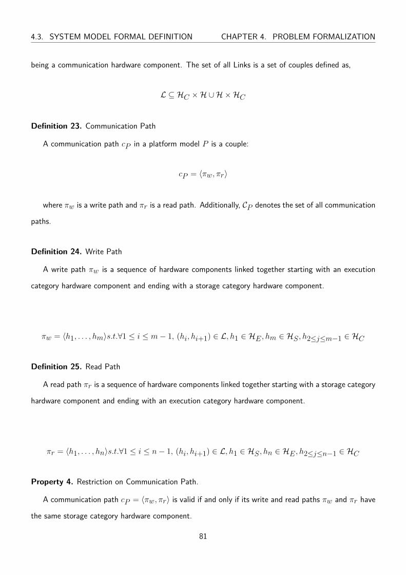
4.3. SYSTEM MODEL FORMAL DEFINITION CHAPTER 4. PROBLEM FORMALIZATION
being a communication hardware component. The set of all Links is a set of couples defined as,
L ⊆ HC ×H ∪H×HC
Definition 23. Communication Path
A communication path cP in a platform model P is a couple:
cP = 〈πw, πr〉
where πw is a write path and πr is a read path. Additionally, CP denotes the set of all communication
paths.
Definition 24. Write Path
A write path πw is a sequence of hardware components linked together starting with an execution
category hardware component and ending with a storage category hardware component.
πw = 〈h1, . . . , hm〉s.t.∀1 ≤ i ≤ m− 1, (hi, hi+1) ∈ L, h1 ∈ HE , hm ∈ HS , h2≤j≤m−1 ∈ HC
Definition 25. Read Path
A read path πr is a sequence of hardware components linked together starting with a storage category
hardware component and ending with an execution category hardware component.
πr = 〈h1, . . . , hn〉s.t.∀1 ≤ i ≤ n− 1, (hi, hi+1) ∈ L, h1 ∈ HS , hn ∈ HE , h2≤j≤n−1 ∈ HC
Property 4. Restriction on Communication Path.
A communication path cP = 〈πw, πr〉 is valid if and only if its write and read paths πw and πr have
the same storage category hardware component.
81

CHAPTER 4. PROBLEM FORMALIZATION 4.3. SYSTEM MODEL FORMAL DEFINITION
4.3.3 Allocation
Definition 26. Allocation
Functions are meant to be allocated to hardware components to be executed and to communicate.
We call "allocation" the function that maps functions and data channels in F to hardware resources in
P . Functions are allocated to hardware components in HE while each data channel dc must be allocated
to a cP ∈ CP . Synchronization channels are not allocated since we assume that their traffic on buses
and memories can be neglected with regards to the one of data channels.
Formally, allocation A is a 2-uple with two functions −→Af and −−→Adc.
A = 〈−→Af ,−−→Adc〉
The first function −→Af associates to each function f ∈ F a hardware component h ∈ HE .
−→Af : F → HE
The second function −→Adc associates to each data channel dc ∈ DC a communication path cP ∈ CP .
−−→Adc : DC → CP
Property 5. Allocation Restriction.
Let us consider two functions f1 and f2 belonging to F . Let us assume that −→Af (f1) = h1 and−→Af (f2) = h2. Let us also assume a data channel dcf1,f2 ∈ DC between f1 and f2. dcf1,f2 can be
allocated to a communication path cP = 〈πw, πr〉 if and only if the execution hardware component of
πw is h1 and the execution hardware component of πr is h2.
4.3.4 Example 1
Let us consider a HW/SW Partitioning Model m. Figure 4.5 shows a graphical representation of the
application model. Figure 4.5 represents five functions f1, f2, f3, f4 and f5 along with two data
channels dc6 and dc7 and a synchronization channel sc8. In addition, Figure 4.5 shows the behavior of
82
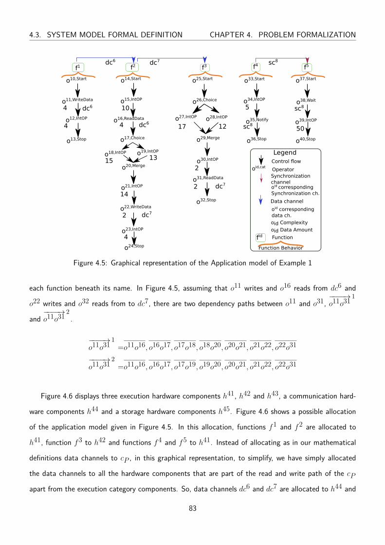
4.3. SYSTEM MODEL FORMAL DEFINITION CHAPTER 4. PROBLEM FORMALIZATION
f1
o10,Start
o12,IntOP
o11,WriteData
o13,Stop
o39,IntOP
o22,WriteData
f4
o35,Notify
o17,Choice
f3
o31,ReadData
o26,Choice
o28,IntOP
o29,Merge
o30,IntOP
o27,IntOP
f5
o38,Wait
o40,Stop
dc6 dc7 sc8
f2
o14,Start o25,Start o33,Start o37,Start
o36,Stop
o32,Stop
o24,Stop
o16,ReadData
o15,IntOP
o18,IntOP o19,IntOP
o20,Merge
o21,IntOP
o23,IntOP
o34,IntOP
Legend
oid,cat
fid
Function Behavior
Control flow
Operator
Function
Synchronization channel
Data channel
4 dc6
4
10
4 dc6
15 13
14
4
17 12
2
2
5
50
2 dc7
dc7
sc8
sc8
oid correspondingdata ch.
oid corresponding
Synchronization ch.
oid Complexity
oid Data Amount
Figure 4.5: Graphical representation of the Application model of Example 1
each function beneath its name. In Figure 4.5, assuming that o11 writes and o16 reads from dc6 and
o22 writes and o32 reads from to dc7, there are two dependency paths between o11 and o31,−−−−→o11o31
1
and−−−−→o11o31
2.
−−−−→o11o31
1=o11o16, o16o17, o17o18, o18o20, o20o21, o21o22, o22o31
−−−−→o11o31
2=o11o16, o16o17, o17o19, o19o20, o20o21, o21o22, o22o31
Figure 4.6 displays three execution hardware components h41, h42 and h43, a communication hard-
ware components h44 and a storage hardware components h45. Figure 4.6 shows a possible allocation
of the application model given in Figure 4.5. In this allocation, functions f1 and f2 are allocated to
h41, function f3 to h42 and functions f4 and f5 to h41. Instead of allocating as in our mathematical
definitions data channels to cP , in this graphical representation, to simplify, we have simply allocated
the data channels to all the hardware components that are part of the read and write path of the cPapart from the execution category components. So, data channels dc6 and dc7 are allocated to h44 and
83

CHAPTER 4. PROBLEM FORMALIZATION 4.4. MODEL EXECUTIONAL SEMANTICS
h41 h42 h43
h44 h45
f1 f3f2 f4 f5
dc6 dc7 dc6 dc7
Legend
hid Hardware componentAllocation
l46
l47 l48
l49
SlaveLinkidMaster
Figure 4.6: Graphical representation of a possible allocation for the application model given in Figure 4.5
h45 of a cP .
4.4 Model Executional Semantics
An execution engine can provide HW/SW partitioning models with an operational semantics so as to
make them executable either directly from the model or by generating an intermediate code from the
model.
Definition 27. System Execution
System executions are characterized by a function EXEC that takes as an input a HW/SW parti-
tioning model m and a time τ and returns a set of execution traces. Let M be the set of all system
models and EM be the set of all possible execution traces of models in M , formally,
EXEC : M × Z+ →P(EM )
Property 6. System execution Constraints.
Function EXEC must fulfill with the following constraints so we can analyze the execution trace:
• it must respect the operators dependencies including synChDep, dataChDep, and controlFlowDep.
• it must respect the number of iterations in loops
• it must comply with the communication channel semantics. In the scope of this thesis, we can
analyze execution traces that have used Non-Blocking Notify - Blocking Wait Infinite FIFO (NBN-
BW-INF) and Blocking Notify - Blocking Wait Finite FIFO (BN-BW-F) synchronization channels.
84
4.4. MODEL EXECUTIONAL SEMANTICS CHAPTER 4. PROBLEM FORMALIZATION
Data channel semantics are handled. Supporting other synchronization channels semantics is part
of the future work.
• it must respect that only one operator at a time can be executed on one given hardware component.
So, only one operator can be executed at a time on any execution category hardware component
and only one transfer of a function can be done at a time on any communication or storage category
hardware component.
• if a read or write path of a communication path has hardware components with different data sizes,
the throughput is constrained by the hardware component having the minimum of the data size
along the path.
As soon as the execution trace conforms with these constraints it can be analyzed in the PLAN
approach.
Definition 28. Execution Trace
An execution of a HW/SW partitioning model for a time interval [0, τ ] returns an execution trace
x = {t1, . . . , tk} where each ti is an execution transaction. Transactions in an execution trace are
ordered. The ordering is based on a unique sequence number assigned to each transaction. Listing 4.1
gives the XML description of one possible execution trace for the model of Figure 4.6 and for the time
interval [0, 50]. The id field corresponds to the operator identifier in the model of Figure 4.5.
In our examples, in addition to the system execution constraints, we assume that the execution time
of Start, Stop, Choice, Merge and Set operators is negligible with respect to ReadData, WriteData and
IntOp operators. Thus,they take no time to execute.
Definition 29. Execution Transaction
An execution transaction t represents the execution of an operator ot on a hardware component ht.
A transaction has a sequence number seqt, a start time τ ts and an end time τ te ≥ τ ts. Formally,
t = 〈seqt, τ ts, τ te, ht, ot〉
All transactions in an execution trace are assumed to be ordered according to their sequence number.
85
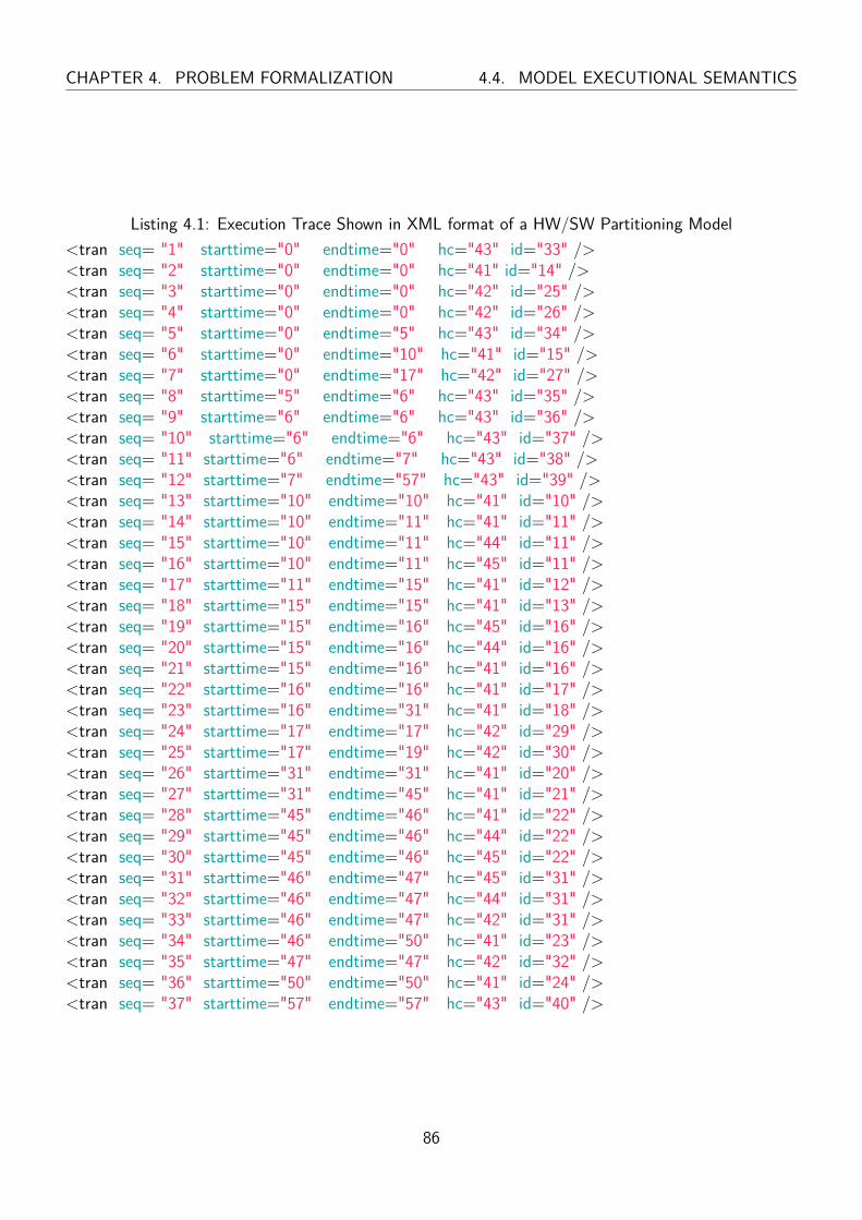
CHAPTER 4. PROBLEM FORMALIZATION 4.4. MODEL EXECUTIONAL SEMANTICS
Listing 4.1: Execution Trace Shown in XML format of a HW/SW Partitioning Model<tran seq= "1" starttime="0" endtime="0" hc="43" id="33" /><tran seq= "2" starttime="0" endtime="0" hc="41" id="14" /><tran seq= "3" starttime="0" endtime="0" hc="42" id="25" /><tran seq= "4" starttime="0" endtime="0" hc="42" id="26" /><tran seq= "5" starttime="0" endtime="5" hc="43" id="34" /><tran seq= "6" starttime="0" endtime="10" hc="41" id="15" /><tran seq= "7" starttime="0" endtime="17" hc="42" id="27" /><tran seq= "8" starttime="5" endtime="6" hc="43" id="35" /><tran seq= "9" starttime="6" endtime="6" hc="43" id="36" /><tran seq= "10" starttime="6" endtime="6" hc="43" id="37" /><tran seq= "11" starttime="6" endtime="7" hc="43" id="38" /><tran seq= "12" starttime="7" endtime="57" hc="43" id="39" /><tran seq= "13" starttime="10" endtime="10" hc="41" id="10" /><tran seq= "14" starttime="10" endtime="11" hc="41" id="11" /><tran seq= "15" starttime="10" endtime="11" hc="44" id="11" /><tran seq= "16" starttime="10" endtime="11" hc="45" id="11" /><tran seq= "17" starttime="11" endtime="15" hc="41" id="12" /><tran seq= "18" starttime="15" endtime="15" hc="41" id="13" /><tran seq= "19" starttime="15" endtime="16" hc="45" id="16" /><tran seq= "20" starttime="15" endtime="16" hc="44" id="16" /><tran seq= "21" starttime="15" endtime="16" hc="41" id="16" /><tran seq= "22" starttime="16" endtime="16" hc="41" id="17" /><tran seq= "23" starttime="16" endtime="31" hc="41" id="18" /><tran seq= "24" starttime="17" endtime="17" hc="42" id="29" /><tran seq= "25" starttime="17" endtime="19" hc="42" id="30" /><tran seq= "26" starttime="31" endtime="31" hc="41" id="20" /><tran seq= "27" starttime="31" endtime="45" hc="41" id="21" /><tran seq= "28" starttime="45" endtime="46" hc="41" id="22" /><tran seq= "29" starttime="45" endtime="46" hc="44" id="22" /><tran seq= "30" starttime="45" endtime="46" hc="45" id="22" /><tran seq= "31" starttime="46" endtime="47" hc="45" id="31" /><tran seq= "32" starttime="46" endtime="47" hc="44" id="31" /><tran seq= "33" starttime="46" endtime="47" hc="42" id="31" /><tran seq= "34" starttime="46" endtime="50" hc="41" id="23" /><tran seq= "35" starttime="47" endtime="47" hc="42" id="32" /><tran seq= "36" starttime="50" endtime="50" hc="41" id="24" /><tran seq= "37" starttime="57" endtime="57" hc="43" id="40" />
86
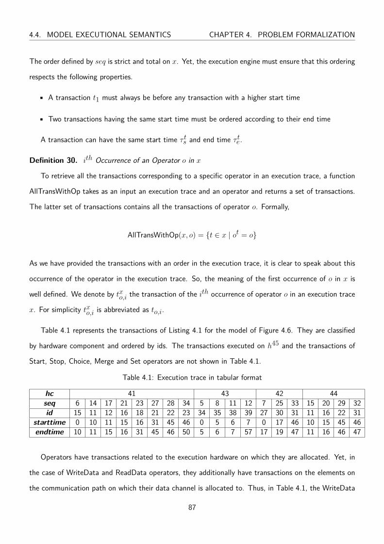
4.4. MODEL EXECUTIONAL SEMANTICS CHAPTER 4. PROBLEM FORMALIZATION
The order defined by seq is strict and total on x. Yet, the execution engine must ensure that this ordering
respects the following properties.
• A transaction t1 must always be before any transaction with a higher start time
• Two transactions having the same start time must be ordered according to their end time
A transaction can have the same start time τ ts and end time τ te.
Definition 30. ith Occurrence of an Operator o in x
To retrieve all the transactions corresponding to a specific operator in an execution trace, a function
AllTransWithOp takes as an input an execution trace and an operator and returns a set of transactions.
The latter set of transactions contains all the transactions of operator o. Formally,
AllTransWithOp(x, o) = {t ∈ x | ot = o}
As we have provided the transactions with an order in the execution trace, it is clear to speak about this
occurrence of the operator in the execution trace. So, the meaning of the first occurrence of o in x is
well defined. We denote by txo,i the transaction of the ith occurrence of operator o in an execution trace
x. For simplicity txo,i is abbreviated as to,i.
Table 4.1 represents the transactions of Listing 4.1 for the model of Figure 4.6. They are classified
by hardware component and ordered by ids. The transactions executed on h45 and the transactions of
Start, Stop, Choice, Merge and Set operators are not shown in Table 4.1.
Table 4.1: Execution trace in tabular format
hc 41 43 42 44seq 6 14 17 21 23 27 28 34 5 8 11 12 7 25 33 15 20 29 32id 15 11 12 16 18 21 22 23 34 35 38 39 27 30 31 11 16 22 31
starttime 0 10 11 15 16 31 45 46 0 5 6 7 0 17 46 10 15 45 46endtime 10 11 15 16 31 45 46 50 5 6 7 57 17 19 47 11 16 46 47
Operators have transactions related to the execution hardware on which they are allocated. Yet, in
the case of WriteData and ReadData operators, they additionally have transactions on the elements on
the communication path on which their data channel is allocated to. Thus, in Table 4.1, the WriteData
87

CHAPTER 4. PROBLEM FORMALIZATION 4.5. REQUIREMENT ON MODEL EXECUTION
operator o11 has two transactions. One transaction on the execution hardware component h41 and one
transaction on the communication hardware component h44. The latter transaction on h44 corresponds
to writing data on data channel dc6.
Moreover, since the data size of the elements of the communication path might not be equal to the
size to be written/read by the operator, a write/read operation may result in different transactions. For
example, let us assume a WriteData operator ow having size attribute equal to 10 writing data to a
data channel dc that is allocated to a communication path cP . Let hc be a communication hardware
component on the write path of cP . Let hc be the component with the lowest data size along cP
where the function getByteNbr(hc) returns 7. So, instead of one transaction for this operator e.g.,
〈0, 10, hc, ow〉 on the communication hardware component, several transactions are represented in an
execution trace e.g., 〈0, 7, hc, ow〉 and 〈7, 10, hc, ow〉.
4.5 Requirement on Model Execution
Generally, a requirement expresses a property on the system. Usually, it is a goal or an anti-goal that the
system must satisfy. Requirements are expected to be true for all possible execution traces.
Definition 31. Maximum Latency Requirement
Latency requirements specify timing constraints on the execution of a system. A maximum latency
requirement r specifies a maximum delay between elements of execution traces. Often, a maximum
latency requirement is expressed as "The maximum latency between oA and oB should be less than
maximum Latency λmax". Formally, a maximum latency requirement is denoted as:
r = 〈oA, oB , λmax〉
Obviously, since r refers to model elements, operators oA and oB must belong to the behaviors of
functions in the application model. In other word, there must exist functions in the application model in
which oA and oB are defined.
The set of all requirements of a HW/SW partitioning model (Definition 2) is denoted as R.
88

4.6. CONCLUSION CHAPTER 4. PROBLEM FORMALIZATION
4.6 Conclusion
This chapter described a HW/SW partitioning model, an execution trace and a maximum latency re-
quirement.
The next chapter defines a more precise requirement and presents the relevant ETA technique that
is used to classify transactions in case the requirement is not valid. The categories we use to classify
transactions in an execution trace are defined in Chapter 5
89
Chapter 5
Primitive Precise Latency Analysis Approach
“If we want to solve problems effectively...we must keep in mind not only many features but
also the influences among them.”
- Dietrich Dorner, The Logic of Failure: Recognizing and Avoiding Error in Complex Situa-
tions
PLAN approach runs the ETA algorithm when a maximum latency requirement (Definition 31) is not
satisfied. The ETA algorithm classifies all transactions of an execution trace based on the impact they
have on the latency between the two operators of a requirement as to be discussed in Section 5.1.4.
Definition 31 gives the requirement definition as it is usually defined by designers for periodic or
pseudo periodic applications.
More precisely, we assume in this chapter that in the execution trace we have a unique execution of
oA and a unique execution of oB such that the occurrence of oB corresponds to the occurrence of oA.
So, in this chapter, a maximum latency requirement can be explicitly defined as "The latency between
the first occurrence of operator oA and the first occurrence of operator oB should be less than maximum
Latency λmax".
Definition 32. Maximum Latency Requirement Validation
To check if a requirement is satisfied or not in a given trace, function RV takes as inputs a system
model, an execution trace and a maximum latency requirement and returns true or false. A maximum
90
5.1. EXECUTION TRACE ANALYSIS CHAPTER 5. PRIMITIVE PLAN
latency requirement is validated if and only if the difference between τtoB,1e and τ
toA,1s is less than
λmax.1 Formally,
RV(m,x, 〈oA, oB , λmax〉
)=
true if τ
toB,1e − τ
toA,1s ≤ λmax
false otherwise
Let us assume a maximum latency requirement r = 〈o11, o31, 35〉 on the execution trace of Listing 4.1.
According to Listing 4.1,
τto31,1e − τ
to11,1s = 47− 10 = 37
As 37 > 35 then RV (m,x, 〈o11, o31, 35〉)
= false.
The ETA technique that follows intends to determine the reasons of a maximum latency requirement
violation. The maximum latency requirement is an implicit parameter for the next definitions in this
chapter.
5.1 Execution Trace Analysis
In this section we assume that it has been established whether or not a requirement is satisfied for a
given execution trace. When a requirement is not satisfied, ETA classifies transactions in order to help
understanding the root causes of the nonsatisfaction.
In this section, m = 〈F ,P ,A〉 denotes a model, r = 〈oA, oB , λmax〉 denotes a requirement on m
and x is an execution trace of m computed by an execution engine.
5.1.1 Causality between operators: an Example
Section 4.3.1 has defined dependencies between operators. These dependencies enforce the causality
that the execution engine must satisfy. In an execution trace, the hardware is already referenced in
a transaction but not the dependencies between operators. The execution engine cares with hardware
aspects as it executes operators where they have been allocated. To understand the extra delays that could1It could have been different. If it was to be changed we have to reconsider further definitions.
91

CHAPTER 5. PRIMITIVE PLAN 5.1. EXECUTION TRACE ANALYSIS
o3,Choice
o1,Start
o2,Merge
Legend
oid,cat
Control flow
Operator
o6,ReadData o4,IntOP
o5,Stopo7,IntOP
o8,WriteData
o9,Set
L Loop Identifier
L1
L1
L1
Figure 5.1: Graphical representation of a function behavior to illustrate causality between operator
have been in the execution trace we need to come back to the HW/SW partitioning model for analyzing
these transactions. However, a HW/SW partitioning model could be much complex than the examples
we have shown before. So, we have decided to consider an abstract view of the HW/SW partitioning
model considering only the necessary aspects for the analysis which are the operators dependencies.
Our analysis considers only dependencies between operators assuming all other dependencies have
been taken in charge by the execution engine.
Now we are going to use an example to illustrate how this causality constraints contribute to the
execution order in case of a loop.
A graphical representation in Figure 5.1 shows a function behavior. In Figure 5.1, the behavior starts
with a Start operator connected by a control flow connection to a Merge operator. This Merge operator
is connected to a Choice operator forming a loop along the Set operator. On the loop exit there is an
IntOp operator o4. It is then connected to a Stop operator. Inside the loop iteration there is a ReadData
operator, an IntOp operator o7, a WriteData operator and a Set operator.
The execution of a HW/SW partitioning model has to respect the control flow constraints given by
the behavior of the different functions. If we assume that we have a HW/SW partitioning model m in
which function f whose behavior model is depicted in Figure 5.1 has been allocated to an execution
92
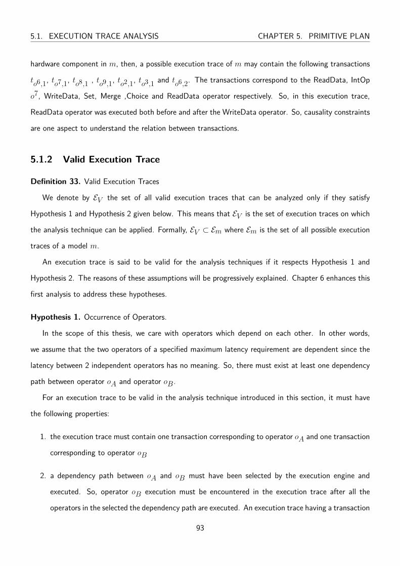
5.1. EXECUTION TRACE ANALYSIS CHAPTER 5. PRIMITIVE PLAN
hardware component in m, then, a possible execution trace of m may contain the following transactions
to6,1, to7,1, to8,1 , to9,1, to2,1, to3,1 and to6,2. The transactions correspond to the ReadData, IntOp
o7, WriteData, Set, Merge ,Choice and ReadData operator respectively. So, in this execution trace,
ReadData operator was executed both before and after the WriteData operator. So, causality constraints
are one aspect to understand the relation between transactions.
5.1.2 Valid Execution Trace
Definition 33. Valid Execution Traces
We denote by EV the set of all valid execution traces that can be analyzed only if they satisfy
Hypothesis 1 and Hypothesis 2 given below. This means that EV is the set of execution traces on which
the analysis technique can be applied. Formally, EV ⊂ Em where Em is the set of all possible execution
traces of a model m.
An execution trace is said to be valid for the analysis techniques if it respects Hypothesis 1 and
Hypothesis 2. The reasons of these assumptions will be progressively explained. Chapter 6 enhances this
first analysis to address these hypotheses.
Hypothesis 1. Occurrence of Operators.
In the scope of this thesis, we care with operators which depend on each other. In other words,
we assume that the two operators of a specified maximum latency requirement are dependent since the
latency between 2 independent operators has no meaning. So, there must exist at least one dependency
path between operator oA and operator oB .
For an execution trace to be valid in the analysis technique introduced in this section, it must have
the following properties:
1. the execution trace must contain one transaction corresponding to operator oA and one transaction
corresponding to operator oB
2. a dependency path between oA and oB must have been selected by the execution engine and
executed. So, operator oB execution must be encountered in the execution trace after all the
operators in the selected the dependency path are executed. An execution trace having a transaction
93

CHAPTER 5. PRIMITIVE PLAN 5.1. EXECUTION TRACE ANALYSIS
toB ,1 without having transactions corresponding to all operators of at least one dependency path
between operator oA and operator oB is considered invalid. The execution trace is considered
as invalid in this case since the execution of operator oB does not depend on the execution of
operator oA. Thus, the notation of latency is not relevant as the executed operators that are in
the dependency path between operator oA and operator oB are one of the main parameters to
classify transactions.
To have a clearly defined dependency path between oA and oB whose operators are executed before the
execution of oB , we add a hypothesis.
Let us consider a HW/SW Partitioning Model m whose application and allocation models are shown
in Figure 5.2 and Figure 5.3 respectively. In Figure 5.2, two functions f1 and f2 communicate through
2 data channels dc3 and dc4. Operator o13 writes data to data channel dc3 and operator o22 reads data
from data channel dc3. Operator o14 writes data to data channel dc4 and operator o23 reads data from
data channel dc4. In Figure 5.2, functions f1 and f2 are allocated to an execution hardware component
h40 and the data channels dc3 and dc4 are allocated to a communication hardware component h41 and
a storage hardware component h42.
Let a maximum latency requirement r = 〈o11, o27, 15〉 be a requirement on m. In this requirement,
we are interested in the timing delay between f1 sending data and f2 finishing to process data in operator
o27 after receiving them from f1. The dependency paths between the two operators of interest in r are:
−−−−→o11o27
1=o11o12, o12o13, o13o22, o22o24, o24o26, o26o27
−−−−→o11o27
2=o11o12, o12o14, o14o23, o23o25, o25o26, o26o27
A possible execution trace x of m is shown in Listing 5.1.
94
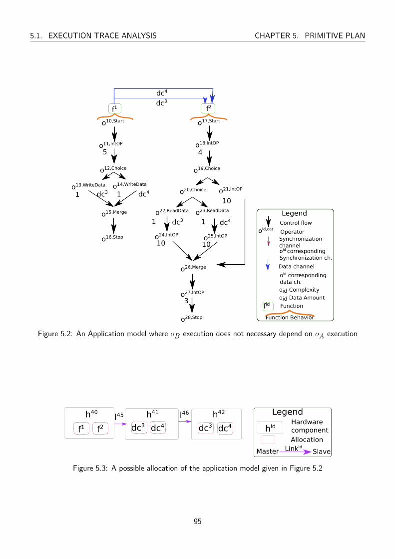
5.1. EXECUTION TRACE ANALYSIS CHAPTER 5. PRIMITIVE PLAN
f1
o10,Start
o11,IntOP
o14,WriteData
o16,Stop
o27,IntOP
o19,Choice
dc3
f2
o17,Start
o28,Stop
o22,ReadData
o21,IntOP
o24,IntOP
o12,Choice
o13,WriteData
o15,Merge
o18,IntOP
o20,Choice
o23,ReadData
o25,IntOP
o26,Merge
dc4
Legend
oid,cat
fid
Function Behavior
Control flow
Operator
Function
Synchronization channel
Data channel
oid correspondingdata ch.
oid corresponding
Synchronization ch.
oid Complexity
oid Data Amount
5
1 dc3 dc4
4
10
10 10
3
dc3 dc4
1
1 1
Figure 5.2: An Application model where oB execution does not necessary depend on oA execution
h40 h41 h42
f1 f2 dc3 dc4 dc3 dc4
Legend
hidHardware componentAllocation
l45 l46
SlaveLinkidMaster
Figure 5.3: A possible allocation of the application model given in Figure 5.2
95

CHAPTER 5. PRIMITIVE PLAN 5.1. EXECUTION TRACE ANALYSIS
Listing 5.1: A possible execution trace shown in XML format of a HW/SW partitioning model whose
allocation model is shown in Figure 5.3
<tran seq= "1" starttime="0" endtime="0" hc="40" id="10" />
<tran seq= "2" starttime="0" endtime="5" hc="40" id="11" />
<tran seq= "3" starttime="5" endtime="5" hc="40" id="12" />
<tran seq= "4" starttime="5" endtime="6" hc="40" id="13" />
<tran seq= "5" starttime="5" endtime="6" hc="41" id="13" />
<tran seq= "6" starttime="5" endtime="6" hc="42" id="13" />
<tran seq= "7" starttime="6" endtime="6" hc="40" id="17" />
<tran seq= "8" starttime="6" endtime="10" hc="40" id="18" />
<tran seq= "9" starttime="10" endtime="10" hc="40" id="19" />
<tran seq= "10" starttime="10" endtime="20" hc="40" id="21" />
<tran seq= "11" starttime="20" endtime="20" hc="40" id="26" />
<tran seq= "12" starttime="20" endtime="23" hc="40" id="27" />
<tran seq= "13" starttime="23" endtime="23" hc="40" id="28" />
In Listing 5.1, operators o11, o12 and o13 of f1 are first executed and then are followed by operators
o18, o19, o21, o26 and o27 of function f2. So, there is no dependency path for which all operators were
executed. This implies that operator o27 was executed regardless of the execution of operator o11. So,
this trace is invalid.
Another possible execution trace x of m is shown in Listing 5.2.
96

5.1. EXECUTION TRACE ANALYSIS CHAPTER 5. PRIMITIVE PLAN
Listing 5.2: Another possible execution trace shown in XML format of a HW/SW partitioning model
whose allocation model is shown in Figure 5.3
<tran seq= "1" starttime="0" endtime="0" hc="40" id="10" />
<tran seq= "2" starttime="0" endtime="5" hc="40" id="11" />
<tran seq= "3" starttime="5" endtime="5" hc="40" id="12" />
<tran seq= "4" starttime="5" endtime="6" hc="40" id="13" />
<tran seq= "5" starttime="5" endtime="6" hc="41" id="13" />
<tran seq= "6" starttime="5" endtime="6" hc="42" id="13" />
<tran seq= "7" starttime="5" endtime="6" hc="40" id="15" />
<tran seq= "8" starttime="5" endtime="6" hc="40" id="16" />
<tran seq= "9" starttime="6" endtime="6" hc="40" id="17" />
<tran seq= "10" starttime="6" endtime="10" hc="40" id="18" />
<tran seq= "11" starttime="10" endtime="10" hc="40" id="19" />
<tran seq= "12" starttime="10" endtime="10" hc="40" id="20" />
<tran seq= "13" starttime="10" endtime="11" hc="41" id="22" />
<tran seq= "14" starttime="10" endtime="11" hc="42" id="22" />
<tran seq= "15" starttime="10" endtime="11" hc="40" id="22" />
<tran seq= "16" starttime="11" endtime="21" hc="40" id="24" />
<tran seq= "17" starttime="21" endtime="21" hc="40" id="26" />
<tran seq= "18" starttime="21" endtime="24" hc="40" id="27" />
<tran seq= "19" starttime="24" endtime="24" hc="40" id="28" />
In Listing 5.2, operators o10, o11, o12, o13, o15 and o16 of f1 are first executed and then operators
o17, o18, o19, o20, o22, o24, o26 and o27 of function f2 are executed. So, the dependency path−−−−→o11o27
1
was executed. So, this trace is valid. In this case, RV (m,x, 〈o11, o27, 15〉)
= false.
Let us define a sequence of operators included in an execution trace x, where opSeq(x) denotes
operator sequences “included” in x, i.e.
{〈o1, · · · , on〉 ∈ Onm | n ∈ N ∧ ∃{t1, · · · tn} ⊆ x such that
97

CHAPTER 5. PRIMITIVE PLAN 5.1. EXECUTION TRACE ANALYSIS
(∀i ∈ [1, n], oti = oi ∧ ∀i ∈ [1, n[seqti < seqti+1)}
In our example, opSeq(x) = 〈o11, o13, o18, o21, o27〉.
Moreover, for any dependency path p = o1o2, · · · , on−1on let us define 〈p〉 that denotes the se-
quence of operators of a dependency path 〈o1, · · · , on〉
An execution trace is considered valid if there is at least one sequence of operators of a dependency
path from oA to oB that belongs to the sequence of operators included in an execution trace x.
In our example, there exists two dependency paths−−−−→o11o27
1and−−−−→o11o27
2whose sequence of operators
are:
〈−−−−→o11o27
1〉 = 〈o11, o12, o13, o22, o24, o26, o27〉
〈−−−−→o11o27
2〉 = 〈o11, o12, o14, o23, o25, o26, o27〉
In Listing 5.1, neither 〈−−−−→o11o27
1〉 /∈ opSeq(x) nor 〈
−−−−→o11o27
2〉 /∈ opSeq(x). So, the execution trace is
invalid. However in Listing 5.2,〈−−−−→o11o27
1〉 ∈ opSeq(x). So, the execution trace is valid.
Formally, Hypothesis 1 is defined as:
x ∈ EV ⇒ ∃−−−→oAoB ∈ DP−−−→oAoB
, 〈−−−→oAoB〉 ∈ opSeq(x)
Hypothesis 2. No interleaving between transactions of operators in the same dependency path.
To enforce a dependency path, two transactions corresponding to two consecutive operators in the
same dependency path must not overlap. That is the end time of the first transaction must be smaller
than the start time of the second one.
Thus, we assume that an execution trace is valid implies that transactions corresponding to operators
in the same dependency path are not interleaved.
Hypothesis 2 ensures that τtoB,1e − τ
toA,1s is not negative. Hypothesis 2 enforce the Non-Blocking
98
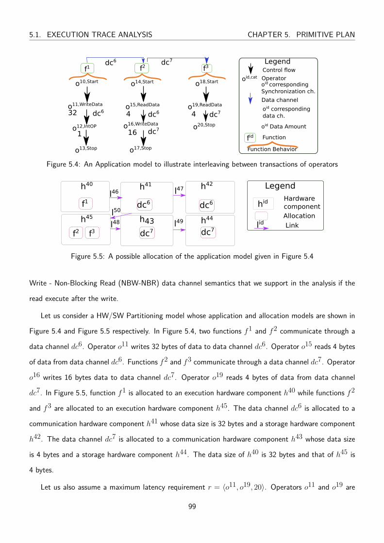
5.1. EXECUTION TRACE ANALYSIS CHAPTER 5. PRIMITIVE PLAN
f1
o10,Start
o12,IntOP
o11,WriteData
o13,Stop
o16,WriteData
f3
o19,ReadData
dc6 dc7
f2
o14,Start o18,Start
o20,Stop
o17,Stop
o15,ReadData
Legend
oid,cat
fid
Function Behavior
Control flow
Operator
Function
Data channel
oid correspondingdata ch.
oid Data Amount
32 dc6 4 dc6 4 dc7
16 dc7
oid corresponding
Synchronization ch.
1
Figure 5.4: An Application model to illustrate interleaving between transactions of operators
h40 h41 h42
f1 dc6 dc6
Legend
hid Hardware componentAllocation
Linklid
l46 l47
h43 h44
dc7 dc7l48 l49h45
f2 f3
l50
Figure 5.5: A possible allocation of the application model given in Figure 5.4
Write - Non-Blocking Read (NBW-NBR) data channel semantics that we support in the analysis if the
read execute after the write.
Let us consider a HW/SW Partitioning model whose application and allocation models are shown in
Figure 5.4 and Figure 5.5 respectively. In Figure 5.4, two functions f1 and f2 communicate through a
data channel dc6. Operator o11 writes 32 bytes of data to data channel dc6. Operator o15 reads 4 bytes
of data from data channel dc6. Functions f2 and f3 communicate through a data channel dc7. Operator
o16 writes 16 bytes data to data channel dc7. Operator o19 reads 4 bytes of data from data channel
dc7. In Figure 5.5, function f1 is allocated to an execution hardware component h40 while functions f2
and f3 are allocated to an execution hardware component h45. The data channel dc6 is allocated to a
communication hardware component h41 whose data size is 32 bytes and a storage hardware component
h42. The data channel dc7 is allocated to a communication hardware component h43 whose data size
is 4 bytes and a storage hardware component h44. The data size of h40 is 32 bytes and that of h45 is
4 bytes.
Let us also assume a maximum latency requirement r = 〈o11, o19, 20〉. Operators o11 and o19 are
99

CHAPTER 5. PRIMITIVE PLAN 5.1. EXECUTION TRACE ANALYSIS
connected by one dependency path−−−−→o11o19. A possible execution trace is shown in Listing 5.3.
Listing 5.3: A possible execution trace shown in XML format of a HW/SW partitioning model whose
allocation model is shown in Figure 5.5
<tran seq= "1" starttime="0" endtime="0" hc="40" id="10" />
<tran seq= "2" starttime="0" endtime="0" hc="45" id="14" />
<tran seq= "3" starttime="0" endtime="1" hc="40" id="11" />
<tran seq= "4" starttime="0" endtime="1" hc="41" id="11" />
<tran seq= "5" starttime="0" endtime="1" hc="42" id="11" />
<tran seq= "6" starttime="1" endtime="2" hc="42" id="15" />
<tran seq= "7" starttime="1" endtime="2" hc="41" id="15" />
<tran seq= "8" starttime="1" endtime="2" hc="45" id="15" />
<tran seq= "9" starttime="1" endtime="2" hc="40" id="11" />
<tran seq= "10" starttime="2" endtime="3" hc="41" id="11" />
<tran seq= "11" starttime="2" endtime="3" hc="42" id="11" />
<tran seq= "12" starttime="2" endtime="3" hc="45" id="16" />
<tran seq= "13" starttime="2" endtime="3" hc="43" id="16" />
<tran seq= "14" starttime="2" endtime="3" hc="44" id="16" />
<tran seq= "15" starttime="3" endtime="3" hc="43" id="18" />
<tran seq= "16" starttime="3" endtime="4" hc="41" id="12" />
<tran seq= "17" starttime="3" endtime="4" hc="44" id="19" />
<tran seq= "18" starttime="3" endtime="4" hc="43" id="19" />
<tran seq= "19" starttime="3" endtime="4" hc="45" id="19" />
<tran seq= "20" starttime="4" endtime="4" hc="41" id="13" />
<tran seq= "21" starttime="4" endtime="4" hc="45" id="20" />
<tran seq= "22" starttime="4" endtime="5" hc="45" id="16" />
<tran seq= "23" starttime="4" endtime="5" hc="43" id="16" />
<tran seq= "24" starttime="4" endtime="5" hc="44" id="16" />
<tran seq= "25" starttime="5" endtime="6" hc="45" id="16" />
100
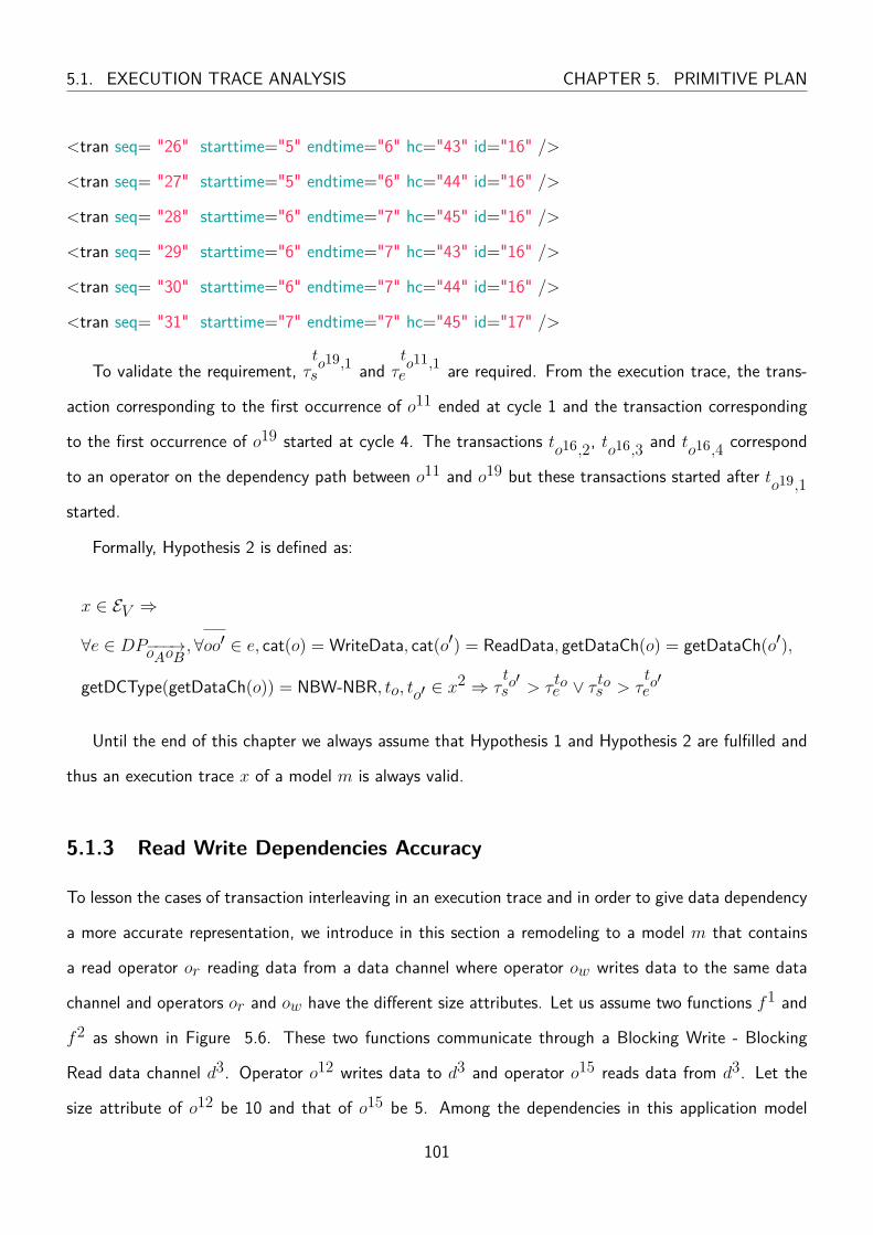
5.1. EXECUTION TRACE ANALYSIS CHAPTER 5. PRIMITIVE PLAN
<tran seq= "26" starttime="5" endtime="6" hc="43" id="16" />
<tran seq= "27" starttime="5" endtime="6" hc="44" id="16" />
<tran seq= "28" starttime="6" endtime="7" hc="45" id="16" />
<tran seq= "29" starttime="6" endtime="7" hc="43" id="16" />
<tran seq= "30" starttime="6" endtime="7" hc="44" id="16" />
<tran seq= "31" starttime="7" endtime="7" hc="45" id="17" />
To validate the requirement, τto19,1s and τ
to11,1e are required. From the execution trace, the trans-
action corresponding to the first occurrence of o11 ended at cycle 1 and the transaction corresponding
to the first occurrence of o19 started at cycle 4. The transactions to16,2, to16,3 and to16,4 correspond
to an operator on the dependency path between o11 and o19 but these transactions started after to19,1started.
Formally, Hypothesis 2 is defined as:
x ∈ EV ⇒
∀e ∈ DP−−−→oAoB,∀oo′ ∈ e, cat(o) = WriteData, cat(o′) = ReadData, getDataCh(o) = getDataCh(o′),
getDCType(getDataCh(o)) = NBW-NBR, to, to′ ∈ x2 ⇒ τ
to′s > τ toe ∨ τ tos > τ
to′e
Until the end of this chapter we always assume that Hypothesis 1 and Hypothesis 2 are fulfilled and
thus an execution trace x of a model m is always valid.
5.1.3 Read Write Dependencies Accuracy
To lesson the cases of transaction interleaving in an execution trace and in order to give data dependency
a more accurate representation, we introduce in this section a remodeling to a model m that contains
a read operator or reading data from a data channel where operator ow writes data to the same data
channel and operators or and ow have the different size attributes. Let us assume two functions f1 and
f2 as shown in Figure 5.6. These two functions communicate through a Blocking Write - Blocking
Read data channel d3. Operator o12 writes data to d3 and operator o15 reads data from d3. Let the
size attribute of o12 be 10 and that of o15 be 5. Among the dependencies in this application model
101

CHAPTER 5. PRIMITIVE PLAN 5.1. EXECUTION TRACE ANALYSIS
let us consider the dependency o12o15. So, operator o15 depends on operator o12. This dependency is
valid but not accurate when taking into account the size attribute of o12 and o15. In our example, o15
reads 5 size of data thus it only depends on o12 writing 5 size of data and not 10.
To have accurate dependencies in our model, for any read operator or reading data from a data
channel where operator ow writes data to the same data channel, operators or and ow must have the
same size. In other words, the read operator reading x data size must depend on a write operator writing
the same data size. To achieve this, we replicate in the model the operator with the greater size, assign
to its size attribute the difference between or and ow sizes and set the sizes of or and ow to the same
value (the minimum size among them). In our example, getDataSize(ow) > getDataSize(or). So, we
replicate operator ow. Let us refer to this new operator as o′w. The size of ow is updated to 5 to be
equal to or and the size of o′w is set to 5 since 10 − 5 = 5. Functions f1 and f2 in Figure 5.6 are
updated as shown in Figure 5.7.
While this replication is straight forward when there is one write operator and one read operator for
a data channel, extra computation is required when there is more than one ReadData operator and/or
more than one WriteData operator.
Let us consider the example in Figure 5.8. In this example, the data size of each read/write operator
is shown in Coral color beside it. Operators o13 and o15 write to data channel d3 and operators o19, o22
and o25 read from data channel d3. In this case, we order the operators in a list according to their data
size attribute starting with the smallest one. In our example: o25,o22,o15,o13,o19. We start by choosing
the operator with the smallest data size, o25 in this case. Since o25 is a read data operator and there
is no write data operator of the same size, we replicate all ReadData and WriteData operators of the
corresponding data channel to represent reading and writing this amount of data. Thus, the application
model in Figure 5.8 can be represented as shown in Figure 5.9. Repeating the same procedure for the
second operator in our list o22. Operator o22 had a data size equal to 4 at the start of our example and
now it has a data size of 3 followed by an operator o31 having a data size equals to 1. Operator o31 has
now the smallest data size and there is no write operator with the same data size. So, the application
model can be remodeled as in Figure 5.10. At this step, operator o15 has been remodeled with two
operators where the last perator o29 has a data size of 1 so it can not be further remodeled. Operators
102
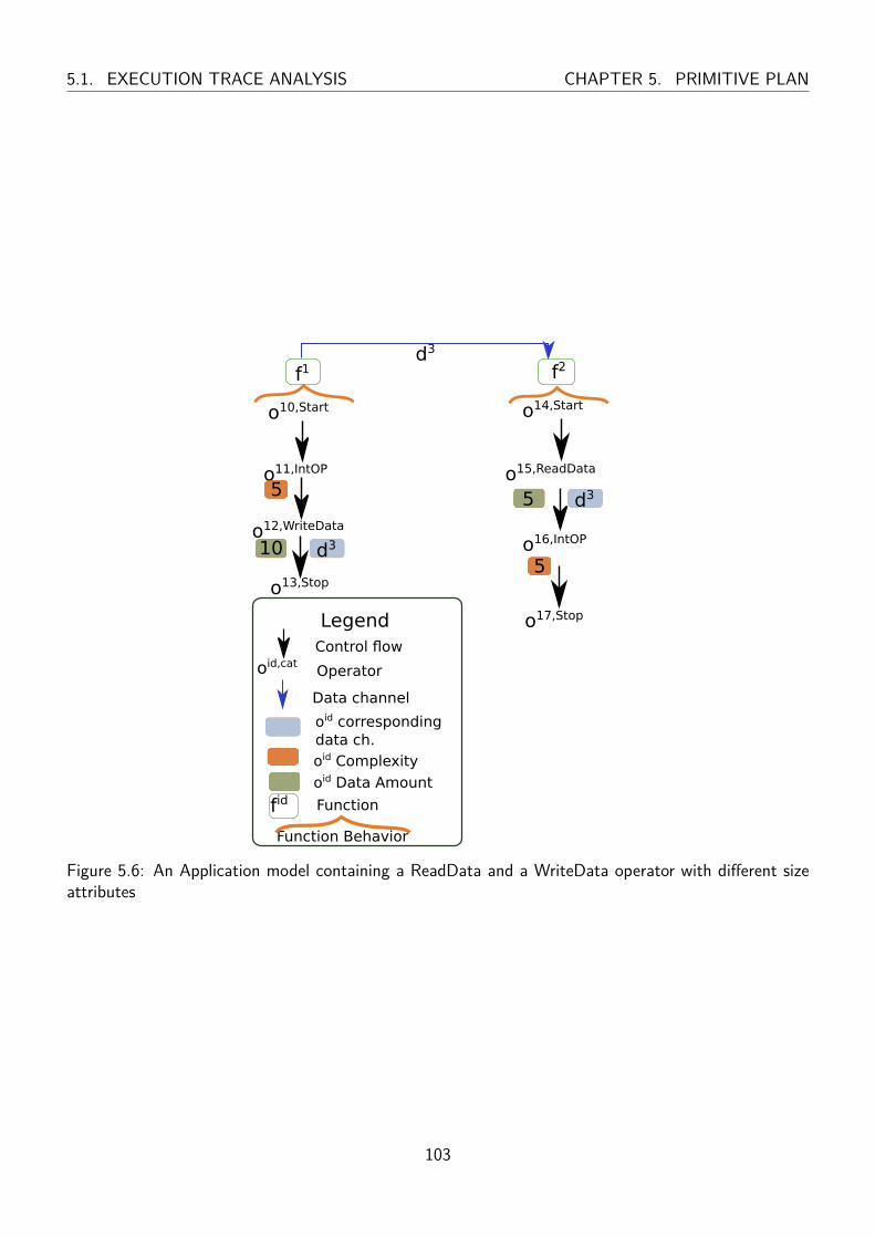
5.1. EXECUTION TRACE ANALYSIS CHAPTER 5. PRIMITIVE PLAN
f1
o10,Start
o11,IntOP
o12,WriteData
o13,Stop
d3
f2
o14,Start
o17,Stop
o15,ReadData
o16,IntOP
Legend
oid,cat
fid
Function Behavior
Control flow
Operator
Function
Data channel
oid correspondingdata ch.oid Complexity
oid Data Amount
5
10 d3
5 d3
5
Figure 5.6: An Application model containing a ReadData and a WriteData operator with different sizeattributes
103
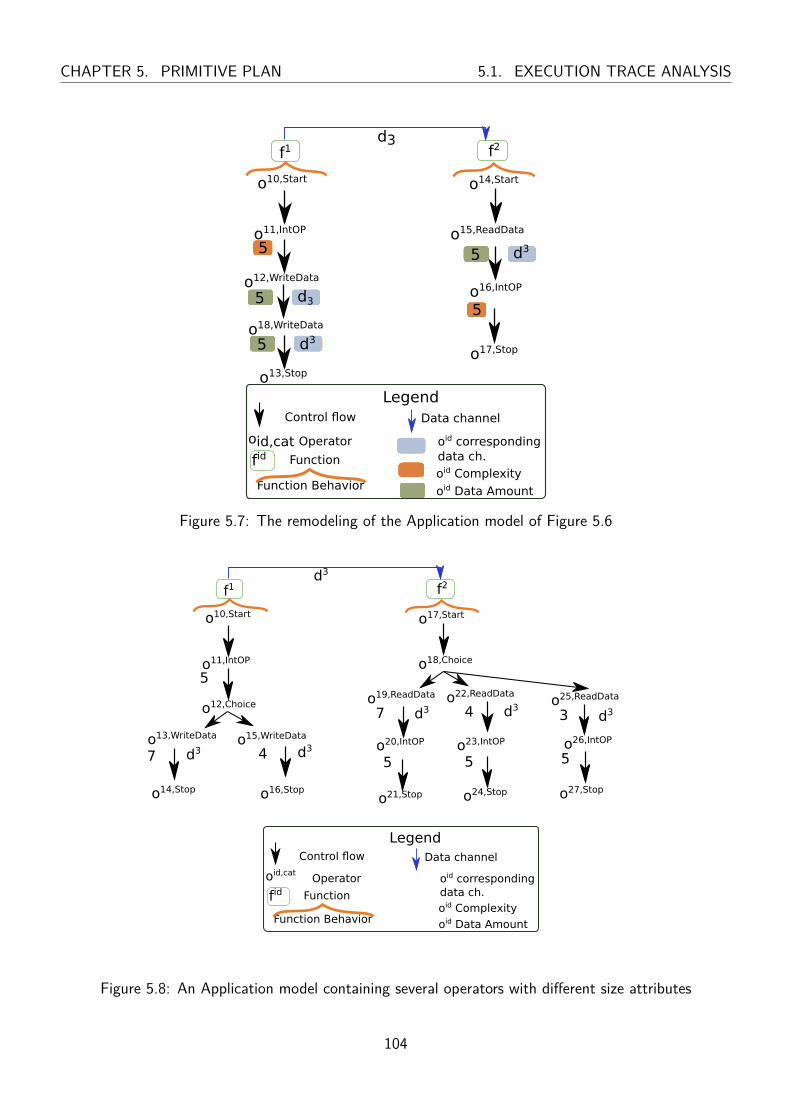
CHAPTER 5. PRIMITIVE PLAN 5.1. EXECUTION TRACE ANALYSIS
f1
o10,Start
o11,IntOP
o12,WriteData
o18,WriteData
d3f2
o14,Start
o17,Stop
o15,ReadData
o16,IntOP
o13,Stop
Legend
oid,catfid
Function Behavior
Control flow
Operator
Function
Data channel
oid correspondingdata ch.oid Complexity
oid Data Amount
5
55 d3
5 d3
5 d3
Figure 5.7: The remodeling of the Application model of Figure 5.6
f1
o10,Start
o11,IntOP
o14,Stop
o18,Choice
d3
f2
o17,Start
o21,Stop
o19,ReadData o22,ReadData
o24,Stop
o12,Choice
o13,WriteData o15,WriteData
o16,Stop
o25,ReadData
o27,Stop
o20,IntOP o23,IntOP o26,IntOP
Legend
oid,cat
fid
Function Behavior
Control flow
Operator
Function
Data channel
oid correspondingdata ch.oid Complexity
oid Data Amount
5
5 5 57 d3 4 d3
7 d3 4 d33 d3
Figure 5.8: An Application model containing several operators with different size attributes
104
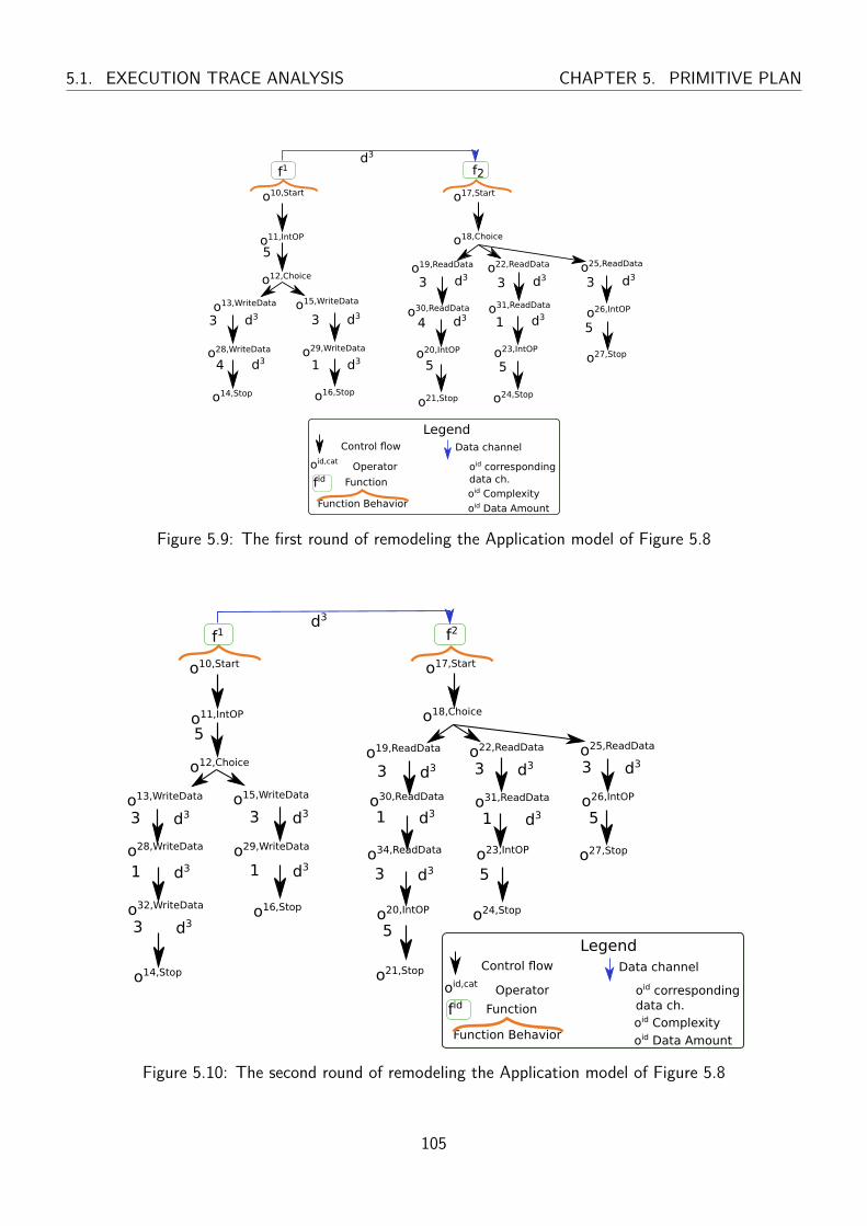
5.1. EXECUTION TRACE ANALYSIS CHAPTER 5. PRIMITIVE PLAN
f1
o10,Start
o11,IntOP
o14,Stop
o18,Choice
d3
f2
o17,Start
o21,Stop
o19,ReadData o22,ReadData
o24,Stop
o12,Choice
o13,WriteData o15,WriteData
o16,Stop
o25,ReadData
o27,Stopo20,IntOP o23,IntOPo28,WriteData o29,WriteData
o26,IntOPo30,ReadData o31,ReadData
Legend
oid,cat
fid
Function Behavior
Control flow
Operator
Function
Data channel
oid correspondingdata ch.oid Complexity
oid Data Amount
5 5
5
5
3 d3
4 d3 1 d3
3 d3
3 d3
4 d3
3 d3
1 d3
3 d3
Figure 5.9: The first round of remodeling the Application model of Figure 5.8
f1
o10,Start
o11,IntOP
o14,Stop
o18,Choice
d3
f2
o17,Start
o21,Stop
o19,ReadData o22,ReadData
o12,Choice
o13,WriteData o15,WriteData
o16,Stop
o25,ReadData
o27,Stop
o20,IntOP
o28,WriteData o29,WriteData
o26,IntOPo30,ReadData o31,ReadData
o32,WriteData
o34,ReadData
5
5
5o24,Stop
o23,IntOP
5
Legend
oid,cat
fid
Function Behavior
Control flow
Operator
Function
Data channel
oid correspondingdata ch.oid Complexity
oid Data Amount
3 d3
3 d3
1 d3
3 d3
1 d3
1 d3 1 d3
3 d3
3 d3 3 d3 3 d3
Figure 5.10: The second round of remodeling the Application model of Figure 5.8
105
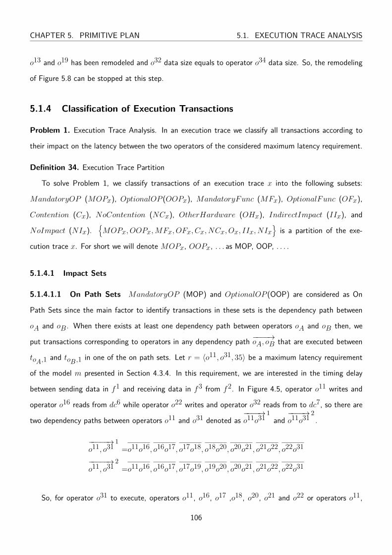
CHAPTER 5. PRIMITIVE PLAN 5.1. EXECUTION TRACE ANALYSIS
o13 and o19 has been remodeled and o32 data size equals to operator o34 data size. So, the remodeling
of Figure 5.8 can be stopped at this step.
5.1.4 Classification of Execution Transactions
Problem 1. Execution Trace Analysis. In an execution trace we classify all transactions according to
their impact on the latency between the two operators of the considered maximum latency requirement.
Definition 34. Execution Trace Partition
To solve Problem 1, we classify transactions of an execution trace x into the following subsets:
MandatoryOP (MOPx), OptionalOP (OOPx), MandatoryFunc (MFx), OptionalFunc (OFx),
Contention (Cx), NoContention (NCx), OtherHardware (OHx), IndirectImpact (IIx), and
NoImpact (NIx).{MOPx, OOPx,MFx, OFx, Cx, NCx, Ox, IIx, NIx
}is a partition of the exe-
cution trace x. For short we will denote MOPx, OOPx, . . . as MOP, OOP, . . . .
5.1.4.1 Impact Sets
5.1.4.1.1 On Path Sets MandatoryOP (MOP) and OptionalOP (OOP) are considered as On
Path Sets since the main factor to identify transactions in these sets is the dependency path between
oA and oB . When there exists at least one dependency path between operators oA and oB then, we
put transactions corresponding to operators in any dependency path −−−−→oA, oB that are executed between
toA,1 and toB ,1 in one of the on path sets. Let r = 〈o11, o31, 35〉 be a maximum latency requirement
of the model m presented in Section 4.3.4. In this requirement, we are interested in the timing delay
between sending data in f1 and receiving data in f3 from f2. In Figure 4.5, operator o11 writes and
operator o16 reads from dc6 while operator o22 writes and operator o32 reads from to dc7, so there are
two dependency paths between operators o11 and o31 denoted as−−−−→o11o31
1and−−−−→o11o31
2.
−−−−−→o11, o31
1=o11o16, o16o17, o17o18, o18o20, o20o21, o21o22, o22o31
−−−−−→o11, o31
2=o11o16, o16o17, o17o19, o19o20, o20o21, o21o22, o22o31
So, for operator o31 to execute, operators o11, o16, o17 ,o18, o20, o21 and o22 or operators o11,
106

5.1. EXECUTION TRACE ANALYSIS CHAPTER 5. PRIMITIVE PLAN
o16, o17, o19, o20, o21 and o22 need to execute.
We consider an operator that belongs to all dependency paths between oA and oB as a mandatory
operator to execute for operator oB execution and in the classifications of transactions, a transaction
corresponding to a mandatory operator between oA and oB is added to MandatoryOP set. While an
operator that belongs to at least one but not all dependency paths between oA and oB is considered as
an optional operator for operator oB execution and in the classifications of transactions, a transaction
corresponding to an optional operator between oA and oB is added to OptionalOP set.
Thus, in the example in Figure 4.5, according to−−−−→o11o31
1and −−−−→o11o31
2, operators o11, o16, o17, o20
and o21 must execute for operator o31 to execute while operators o18 and o19 may execute as they do
not belong to all dependency paths between o11 and o31. So, transactions executed between toA,1 and
toB ,1 corresponding to o11, o16, o17, o20 and o21 are added to MandatoryOP set while transactions
corresponding to o18 and o19 are added to OptionalOP set.
Definition 35. Transaction Executes Between Two Transactions
A transaction t is said to execute at least partially between two transactions t1 and t2 if t ends after
the start time of t1 and t starts before the end time of t2.
Figure 5.11 shows two transactions t1 and t2. Transactions that start in the pink range and end in
the green range are said to execute at least partially between t1 and t2.
Formally, function cross takes as argument t, t1 and t2 and returns true if and only if t ends after
the start time of t1 and t starts before the end time of t2.
cross(t, t1, t2) =
true τ te > τ
t1s ∧ τ ts < τ
t2e
false Otherwise
Definition 36. Mandatory Operator Between Two Operators
An operator o is a mandatory operator between two operators oi and oj in model m if and only if
operator o occurs in all the dependency paths between oi and oj . Function Mop takes model m and
two operators oi and oj as arguments and returns the set of mandatory operator between oi and oj in
model m.
107
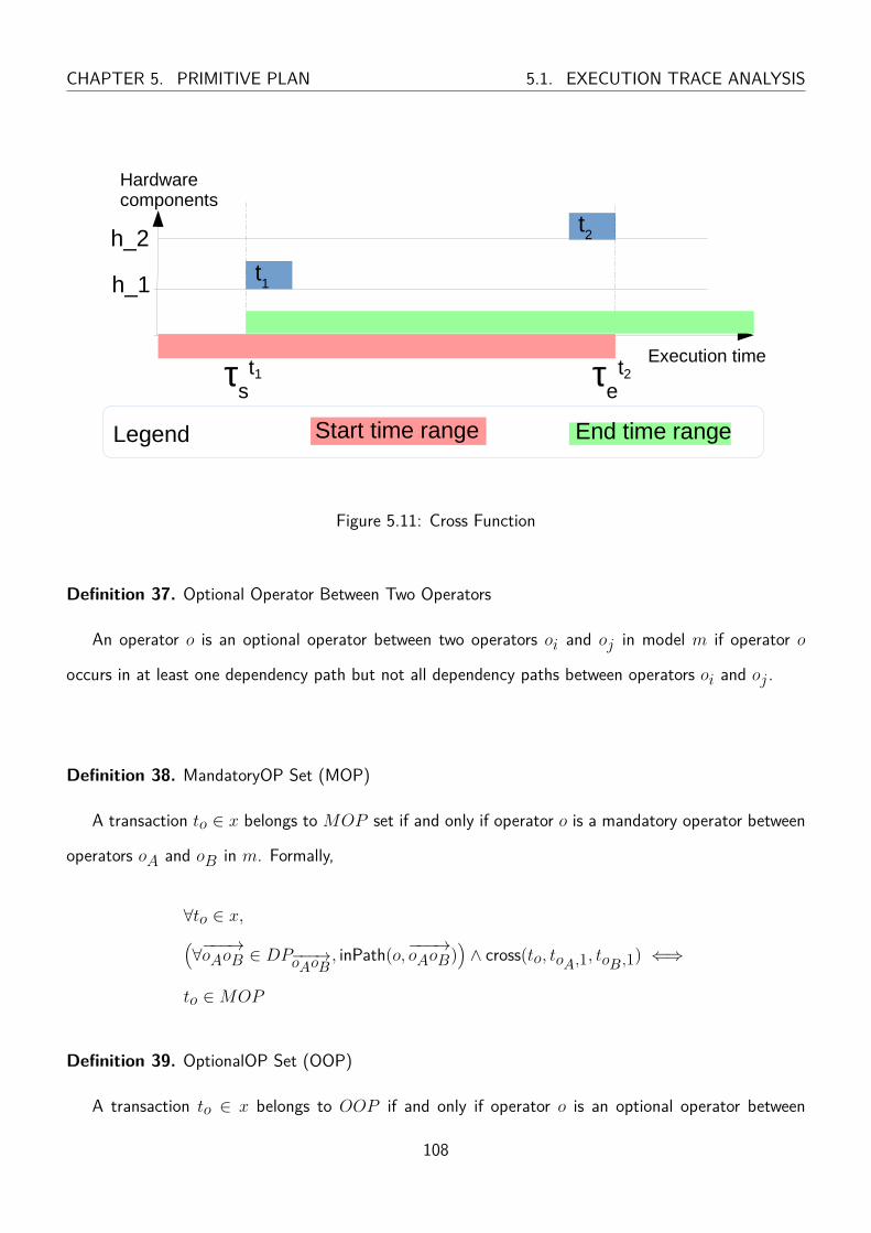
CHAPTER 5. PRIMITIVE PLAN 5.1. EXECUTION TRACE ANALYSIS
h_1
h_2
t1
t2
τst1 τ
et2
Start time range End time rangeLegend
Hardware components
Execution time
Figure 5.11: Cross Function
Definition 37. Optional Operator Between Two Operators
An operator o is an optional operator between two operators oi and oj in model m if operator o
occurs in at least one dependency path but not all dependency paths between operators oi and oj .
Definition 38. MandatoryOP Set (MOP)
A transaction to ∈ x belongs to MOP set if and only if operator o is a mandatory operator between
operators oA and oB in m. Formally,
∀to ∈ x,(∀−−−→oAoB ∈ DP−−−→oAoB
, inPath(o,−−−→oAoB))∧ cross(to, toA,1, toB ,1) ⇐⇒
to ∈MOP
Definition 39. OptionalOP Set (OOP)
A transaction to ∈ x belongs to OOP if and only if operator o is an optional operator between
108

5.1. EXECUTION TRACE ANALYSIS CHAPTER 5. PRIMITIVE PLAN
operators oA and oB in m.
∀to ∈ x, ∀−−−→oAoB ∈ DP−−−→oAoB,
inPath(o,−−−→oAoB) ∧ to /∈MOP ∧ cross(to, toA,1, toB ,1)⇔ to ∈ OOP
5.1.4.1.2 In Functions Sets The set of all operators which have corresponding transactions in
an execution trace x and are in a dependency path between oA and oB can not execute before their
previous operators in their functions are executed. Each operator in this set belongs to a function. So,
the execution trace must contain transactions corresponding to operators that are in the dependency
path between the St operator of the function to which an operator from the set belongs and the operator.
Let us assume o3 is in Of and in the dependency path between oA and oB . Moreover, o3 is executed
and have a corresponding transaction in the execution trace. Operator Stf have a dependency path to
o3. Thus, the execution trace contains transactions corresponding to operators in the dependency path
from Stf to o3.
For instance, in function f2 in Fig. 4.5, if operator o16 was to be executed between o11 and o31 which
is an operator in a dependency path between operator o11 and o31, then since operator o15 belongs to
the only dependency path betweenStf2 and o16, so in this case, operator o15 has to be executed.
Let us assume we have two functions f and f ′. Moreover, we assume operator o in function f
belongs to a dependency path −−−→oAoB . If Wait operator in function f belongs to a dependency path−−→Stfo, then the Notify operator in function f ′ that have dependency to the Wait operator in function
f must have completed its execution before operator o can start executing. Thus, there must exist in
the execution trace transactions corresponding to operators in the dependency path between Stf ′ and
the Notify operator in function f ′. Same condition applies if Notify and Wait operators are replaced
by ReadData and WriteData operators. For instance, let the requirement of interest in Fig. 5.12 be
r = 〈o7, i, o14, j, λmax〉. In function f2 , if o13 was to be executed between o7 and o14 which is an
operator in a dependency path between operator o7 and o14, then since operator o12 is on the only
dependency path between Stf2 and o13, so in this case, operator o12 has to execute. For o12 to
execute, o18 in function f3 must also execute since there is a dependency between o18 and o12. Thus,
all operators of one dependency path between Stf3 (o16) and operator o18 must execute.
109
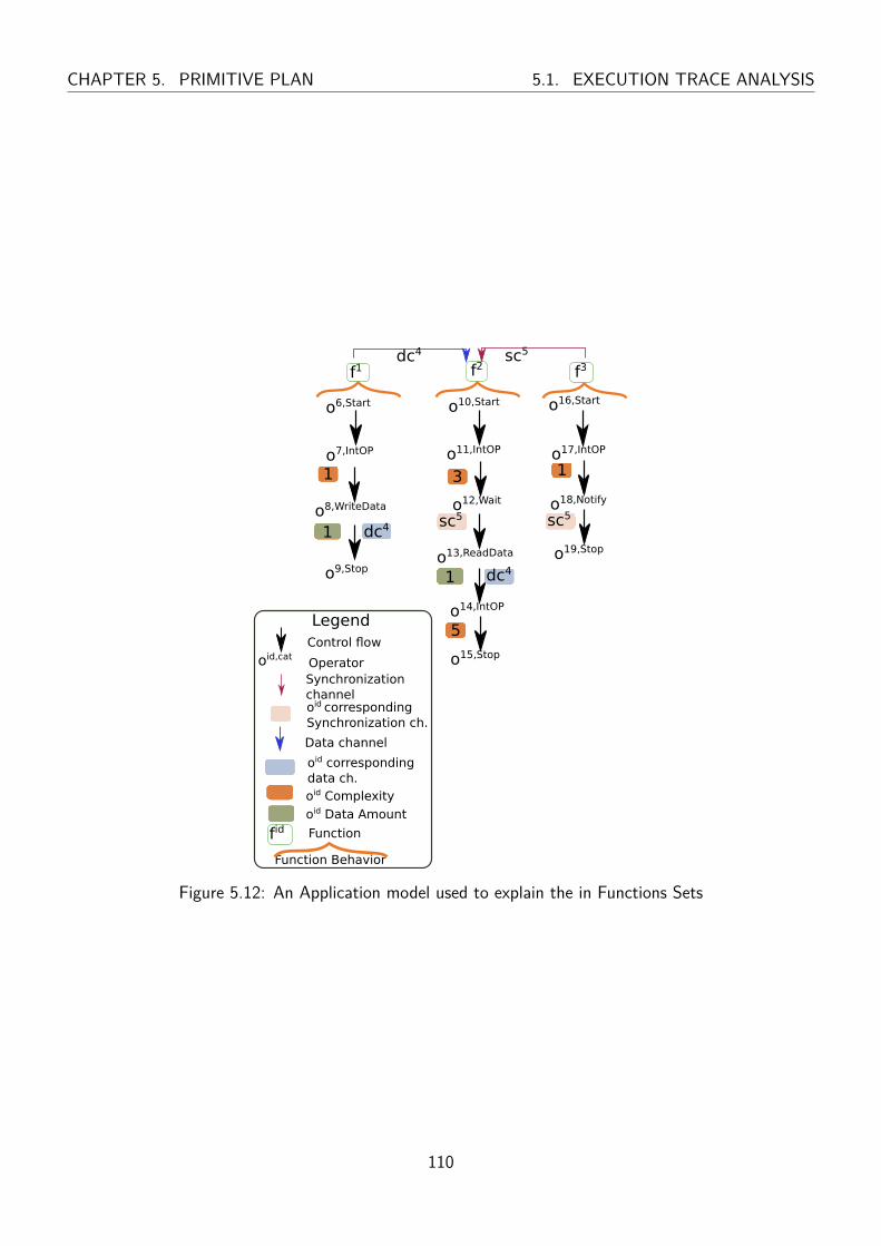
CHAPTER 5. PRIMITIVE PLAN 5.1. EXECUTION TRACE ANALYSIS
o17,IntOP
f2
o12,Wait
f1
o8,WriteData
o7,IntOP
f3
o18,Notify
o19,Stop
sc5
o6,Start o10,Start o16,Start
o13,ReadData
o9,Stop
o11,IntOP
o14,IntOP
dc4
o15,Stop
Legend
oid,cat
fid
Function Behavior
Control flow
Operator
Function
Synchronization channel
Data channel
oid correspondingdata ch.
oid correspondingSynchronization ch.
oid Complexity
oid Data Amount
1 3
5
1
dc41
dc41
sc5 sc5
Figure 5.12: An Application model used to explain the in Functions Sets
110

5.1. EXECUTION TRACE ANALYSIS CHAPTER 5. PRIMITIVE PLAN
In general, given a requirement r = 〈oA, oB , λmax〉, a function f having a start operator Stf ,
operators o and o3 in Of where there exists at least one dependency path between o and o3 and
operator o3 belongs to at least one dependency path between oA and oB .
Operator o is considered as mandatory to execute in function f before operator o3 starts executing
if operator o3 is a mandatory operator between oA and oB and operator o is a mandatory operator
between the Stf and o3.
Operator o is considered as optional to execute in function f before operator o3 starts executing if
either o3 is an optional operator between oA and oB or operator o3 is a mandatory operator between
oA and oB but operator o is an optional operator between Stf and o3.
In the classifications of transactions, a transaction executed between toA,1 and toB ,1 corresponding to
a mandatory operator o in function f is added toMandatoryFunc set while a transaction corresponding
to an optional operator in function f is added to OptionalFunc set.
For instance, in Fig. 4.5, operator o31 is an operator on all dependency paths between o11 and o31
and the dependency paths between o25 and o31 are:
−−−−→o25o31
1=o25o26, o26o27, o27o29, o29o30, o30o31
−−−−→o25o31
2=o25o26, o26o28, o28o29, o29o30, o30o31
Thus, according to−−−−→o25o31
1and−−−−→o25o31
2, operators o25, o26, o29 and o30 are mandatory in function
f3 while o27 and o28 are optional for the execution of o31. So, in Listing 4.1, to30,1 belongs to
MandatoryFunc set and to27,1 belongs to OptionalFunc set.
Definition 40. MandatoryFunc Set (MF)
For a requirement r = 〈oA, oB , λmax〉 between oA and oB , a transaction to ∈ x belongs to MF
set if and only if it does not belong to MOP or OOP sets and there exists an operator o3 that is a
mandatory operator between oA and oB and operator o a mandatory operator between StgetF (m,o) and
111

CHAPTER 5. PRIMITIVE PLAN 5.1. EXECUTION TRACE ANALYSIS
o3. Formally,
∀to ∈ x,(∃o3 ∈Mop(oA, oB)∀p ∈ DP−−−−−−−−−−→
StgetF (m,o)o3, inPath(o, p)
)∧ to /∈MOP ∪OOP ∧ cross(to, toA,1, toB ,1) ⇐⇒
to ∈MF
Definition 41. OptionalFunc Set (OF)
For a requirement r = 〈oA, oB , λmax〉 between oA and oB , a transaction to ∈ x belongs to OF set
if and only if it does not belong to MOP , OOP or MF sets and if there exists an operator o3 that is an
optional operator between oA and oB and there exists a dependency path between o and o3 or operator
o3 is a mandatory operator between oA and oB but operator o is an optional operator between Stf and
o3. Formally,
∀to ∈ x,
∀o3 ∈ Om, ∀−−−→oAoB ∈ DP−−−→oAoB, ∀−−−−−−−−−−→StgetF (m,o)o3 ∈ DP−−−−−−−−−−→StgetF (m,o)o3
,
inPath(o3,−−−→oAoB) ∧ inPath(o,−−−−−−−−−−→StgetF (m,o)o3) ∧ to /∈MOP ∪OOP ∪MF ∧ cross(to, toA,1, toB ,1)
⇔ to ∈ OF
5.1.4.1.3 Contention Set Let us now deal with the contention set. Contention occurs when two
concurrent functions using the same execution hardware want to execute a transaction at the same
time. Contentions may also occur when two functions want to use the same communication hardware
component at the same time. When a contention occurs, one of the two functions is delayed until the
resource it has requested is available. This delay is called a contention delay. A transaction belongs to
the contention set if its execution causes a contention delay in the execution for at least one transac-
tion belonging to either OptionalFunc, MandatoryFunc, OptionalOP or MandatoryOP set. To
identify transactions that belong to the contention set, we need first to identify the set of hardware com-
112
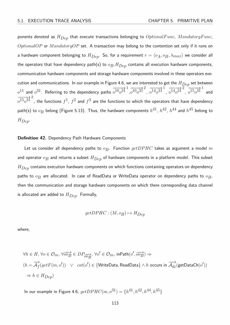
5.1. EXECUTION TRACE ANALYSIS CHAPTER 5. PRIMITIVE PLAN
ponents denoted as HDep that execute transactions belonging to OptionalFunc, MandatoryFunc,
OptionalOP or MandatoryOP set. A transaction may belong to the contention set only if it runs on
a hardware component belonging to HDep. So, for a requirement r = 〈oA, oB , λmax〉 we consider all
the operators that have dependency path(s) to oB .HDep contains all execution hardware components,
communication hardware components and storage hardware components involved in these operators exe-
cution and communications. In our example in Figure 4.6, we are interested to get the HDep set between
o11 and o31. Referring to the dependency paths−−−−→o10o31
1,−−−−→o10o31
2,−−−−→o14o31
1,−−−−→o14o31
2,−−−−→o15o31
1and
−−−−→o15o31
2, the functions f1, f2 and f3 are the functions to which the operators that have dependency
path(s) to oB belong (Figure 5.13). Thus, the hardware components h41, h42, h44 and h45 belong to
HDep.
Definition 42. Dependency Path Hardware Components
Let us consider all dependency paths to oB . Function getDPHC takes as argument a model m
and operator oB and returns a subset HDep of hardware components in a platform model. This subset
HDep contains execution hardware components on which functions containing operators on dependency
paths to oB are allocated. In case of ReadData or WriteData operator on dependency paths to oB ,
then the communication and storage hardware components on which there corresponding data channel
is allocated are added to HDep. Formally,
getDPHC : (M, oB) 7→ HDep
where,
∀h ∈ H, ∀o ∈ Om, ∀−−→ooB ∈ DP−−→ooB , ∀o′ ∈ Om, inPath(o′,−−→ooB)⇒
(h = −→Af (getF (m, o′)) ∨ cat(o′) ∈ {WriteData,ReadData} ∧ h occurs in −−→Adc(getDataCh(o′))
⇒ h ∈ HDep)
In our example in Figure 4.6, getDPHC(m, o31) = {h41, h42, h44, h45}
113
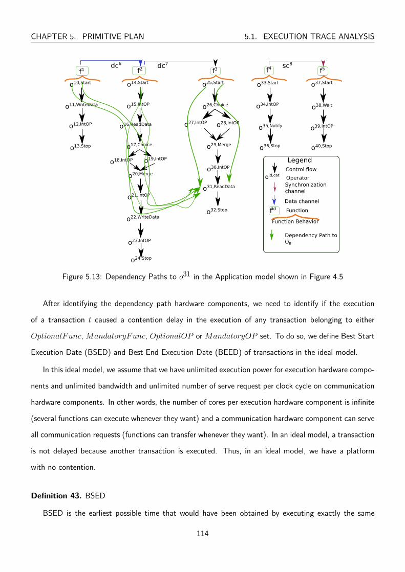
CHAPTER 5. PRIMITIVE PLAN 5.1. EXECUTION TRACE ANALYSIS
f1
o10,Start
o12,IntOP
o11,WriteData
o13,Stop
o39,IntOP
o22,WriteData
f4
o35,Notify
o17,Choice
f3
o31,ReadData
o26,Choice
o28,IntOP
o29,Merge
o30,IntOP
o27,IntOP
f5
o38,Wait
o40,Stop
dc6 dc7 sc8
f2
o14,Start o25,Start o33,Start o37,Start
o36,Stop
o32,Stop
o24,Stop
o16,ReadData
o15,IntOP
o18,IntOP o19,IntOP
o20,Merge
o21,IntOP
o23,IntOP
o34,IntOP
Legend
oid,cat
fid
Function Behavior
Control flow
Operator
Function
Synchronization channel
Data channel
Dependency Path to OB
Figure 5.13: Dependency Paths to o31 in the Application model shown in Figure 4.5
After identifying the dependency path hardware components, we need to identify if the execution
of a transaction t caused a contention delay in the execution of any transaction belonging to either
OptionalFunc, MandatoryFunc, OptionalOP orMandatoryOP set. To do so, we define Best Start
Execution Date (BSED) and Best End Execution Date (BEED) of transactions in the ideal model.
In this ideal model, we assume that we have unlimited execution power for execution hardware compo-
nents and unlimited bandwidth and unlimited number of serve request per clock cycle on communication
hardware components. In other words, the number of cores per execution hardware component is infinite
(several functions can execute whenever they want) and a communication hardware component can serve
all communication requests (functions can transfer whenever they want). In an ideal model, a transaction
is not delayed because another transaction is executed. Thus, in an ideal model, we have a platform
with no contention.
Definition 43. BSED
BSED is the earliest possible time that would have been obtained by executing exactly the same
114
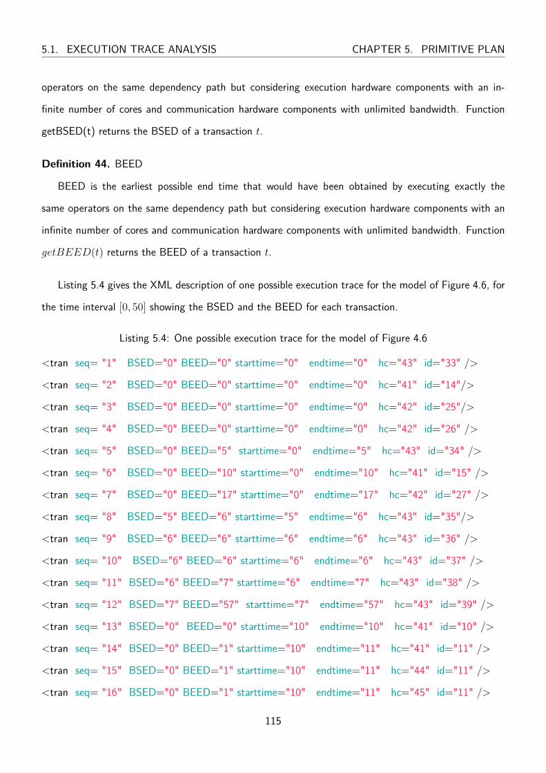
5.1. EXECUTION TRACE ANALYSIS CHAPTER 5. PRIMITIVE PLAN
operators on the same dependency path but considering execution hardware components with an in-
finite number of cores and communication hardware components with unlimited bandwidth. Function
getBSED(t) returns the BSED of a transaction t.
Definition 44. BEED
BEED is the earliest possible end time that would have been obtained by executing exactly the
same operators on the same dependency path but considering execution hardware components with an
infinite number of cores and communication hardware components with unlimited bandwidth. Function
getBEED(t) returns the BEED of a transaction t.
Listing 5.4 gives the XML description of one possible execution trace for the model of Figure 4.6, for
the time interval [0, 50] showing the BSED and the BEED for each transaction.
Listing 5.4: One possible execution trace for the model of Figure 4.6
<tran seq= "1" BSED="0" BEED="0" starttime="0" endtime="0" hc="43" id="33" />
<tran seq= "2" BSED="0" BEED="0" starttime="0" endtime="0" hc="41" id="14"/>
<tran seq= "3" BSED="0" BEED="0" starttime="0" endtime="0" hc="42" id="25"/>
<tran seq= "4" BSED="0" BEED="0" starttime="0" endtime="0" hc="42" id="26" />
<tran seq= "5" BSED="0" BEED="5" starttime="0" endtime="5" hc="43" id="34" />
<tran seq= "6" BSED="0" BEED="10" starttime="0" endtime="10" hc="41" id="15" />
<tran seq= "7" BSED="0" BEED="17" starttime="0" endtime="17" hc="42" id="27" />
<tran seq= "8" BSED="5" BEED="6" starttime="5" endtime="6" hc="43" id="35"/>
<tran seq= "9" BSED="6" BEED="6" starttime="6" endtime="6" hc="43" id="36" />
<tran seq= "10" BSED="6" BEED="6" starttime="6" endtime="6" hc="43" id="37" />
<tran seq= "11" BSED="6" BEED="7" starttime="6" endtime="7" hc="43" id="38" />
<tran seq= "12" BSED="7" BEED="57" starttime="7" endtime="57" hc="43" id="39" />
<tran seq= "13" BSED="0" BEED="0" starttime="10" endtime="10" hc="41" id="10" />
<tran seq= "14" BSED="0" BEED="1" starttime="10" endtime="11" hc="41" id="11" />
<tran seq= "15" BSED="0" BEED="1" starttime="10" endtime="11" hc="44" id="11" />
<tran seq= "16" BSED="0" BEED="1" starttime="10" endtime="11" hc="45" id="11" />
115

CHAPTER 5. PRIMITIVE PLAN 5.1. EXECUTION TRACE ANALYSIS
<tran seq= "17" BSED="1" BEED="5" starttime="11" endtime="15" hc="41" id="12" />
<tran seq= "18" BSED="5" BEED="5" starttime="15" endtime="15" hc="41" id="13" />
<tran seq= "19" BSED="10" BEED="11" starttime="15" endtime="16" hc="45" id="16" />
<tran seq= "20" BSED="10" BEED="11" starttime="15" endtime="16" hc="44" id="16" />
<tran seq= "21" BSED="10" BEED="11" starttime="15" endtime="16" hc="41" id="16" />
<tran seq= "22" BSED="11" BEED="11" starttime="16" endtime="16" hc="41" id="17" />
<tran seq= "23" BSED="11" BEED="26" starttime="16" endtime="31" hc="41" id="18" />
<tran seq= "24" BSED="17" BEED="17" starttime="17" endtime="17" hc="42" id="29" />
<tran seq= "25" BSED="17" BEED="19" starttime="17" endtime="19" hc="42" id="30" />
<tran seq= "26" BSED="26" BEED="26" starttime="31" endtime="31" hc="41" id="20" />
<tran seq= "27" BSED="26" BEED="40" starttime="31" endtime="45" hc="41" id="21" />
<tran seq= "28" BSED="40" BEED="41" starttime="45" endtime="46" hc="41" id="22" />
<tran seq= "29" BSED="40" BEED="41" starttime="45" endtime="46" hc="44" id="22" />
<tran seq= "30" BSED="40" BEED="41" starttime="45" endtime="46" hc="45" id="22" />
<tran seq= "31" BSED="41" BEED="42" starttime="46" endtime="47" hc="45" id="31" />
<tran seq= "32" BSED="41" BEED="42" starttime="46" endtime="47" hc="44" id="31" />
<tran seq= "33" BSED="41" BEED="42" starttime="46" endtime="47" hc="42" id="31" />
<tran seq= "34" BSED="41" BEED="45" starttime="46" endtime="50" hc="41" id="23" />
<tran seq= "35" BSED="42" BEED="42" starttime="47" endtime="47" hc="42" id="32" />
<tran seq= "36" BSED="45" BEED="45" starttime="50" endtime="50" hc="41" id="24" />
<tran seq= "37" BSED="57" BEED="57" starttime="57" endtime="57" hc="43" id="40" />
Let us now come back to regular execution and communication hardware components. We say that
a transaction is delayed if its start and/or end execution date with regular execution and communication
hardware components (starttime and endtime) is higher than the one with ideal model execution and
communication hardware components (BSED and BEED).
To know if a transaction t executed on hardware component h delayed any transaction on h, we
need to retrieve the lists of transactions of all delayed transactions that were executed on a hardware
component h. In the contention set we are interested in the delay of transactions that belong to
116

5.1. EXECUTION TRACE ANALYSIS CHAPTER 5. PRIMITIVE PLAN
OptionalFunc, MandatoryFunc, OptionalOP or MandatoryOP set. So, we define two functions
getStartDList and getEndDList that take as arguments a model m, an execution trace of this model
x and a hardware component h in the platform model of m and return a list of transactions that had
their start time and end time delayed respectively. Since we are interested in transactions that belong
to OptionalFunc, MandatoryFunc, OptionalOP or MandatoryOP set, the hardware component of
these two functions must be a dependency path hardware component. Formally,
getStartDList : (m,x, h) 7→ {t ∈ x |ht = h ∧BSED(t) 6= τ ts∧
t ∈MOPS ∪OOPS ∪MFS ∪OFS}
getEndDList : (m,x, h) 7→ {t ∈ x |h(t) = h ∧BEED(t) 6= τe(t)∧
t ∈MOPS ∪OOPS ∪MFS ∪OFS}
In our example in Listing 5.4:
getStartDList(m,x, h41) ={to11,1, to16,2, to18,1, to21,1, to22,1}
getStartDList(m,x, h42) ={to31,1}
getStartDList(m,x, h44) ={to11,2, to16,2, to22,2, to31,2}
getEndDList(m,x, h41) ={to11,1, to16,2, to18,1, to21,1, to22,1}
getEndDList(m,x, h42) ={to31,1}
getEndDList(m,x, h44) ={to11,2, to16,2, to22,2, to31,2}
So, for a transaction t executing on hardware component h to delay transactions that belong to
117

CHAPTER 5. PRIMITIVE PLAN 5.1. EXECUTION TRACE ANALYSIS
h_1 t’
BSED(t’) BEED(t’)
t’
τet’τ
st’
t
τet Execution time
Hardware components
Figure 5.14: First case where a transaction t′ is delayed due to contention
h_1 t’
BSED(t’)
BEED(t’)
t’
τe
t’τst’
t
τet
τst Execution time
Hardware components
Figure 5.15: Second case where a transaction t′ is delayed due to contention
OptionalFunc, MandatoryFunc, OptionalOP or MandatoryOP set, t must not correspond to an
operator whose execution may be required for the execution of oB . Thus, transaction t must not belong
to OptionalFunc, MandatoryFunc, OptionalOP or MandatoryOP set. Moreover, for a transaction
t to cause delay, either (1) for some transaction t′ returned by getStartDList(m,x, h), the end time of
t (τ te) must be greater than or equal to BSEDt′ and less than or equal to τ t′s , or (2) for a transaction
t′ returned by getEndDList(m,x, h) the end time of t is greater than or equal to BEED(t′) and less
than or equal to τ t′e .
Figure 5.14 and Figure 5.15 show two cases where a transaction t′ is delayed. In these figures, if
transaction t′ belongs to OptionalFunc, MandatoryFunc, OptionalOP or MandatoryOP set and t
does not belong to the latter sets, then, transaction t belongs to the contention set.
In Listing 5.4, to12,1 does not belong toOptionalFunc,MandatoryFunc, OptionalOP orMandatoryOP
118
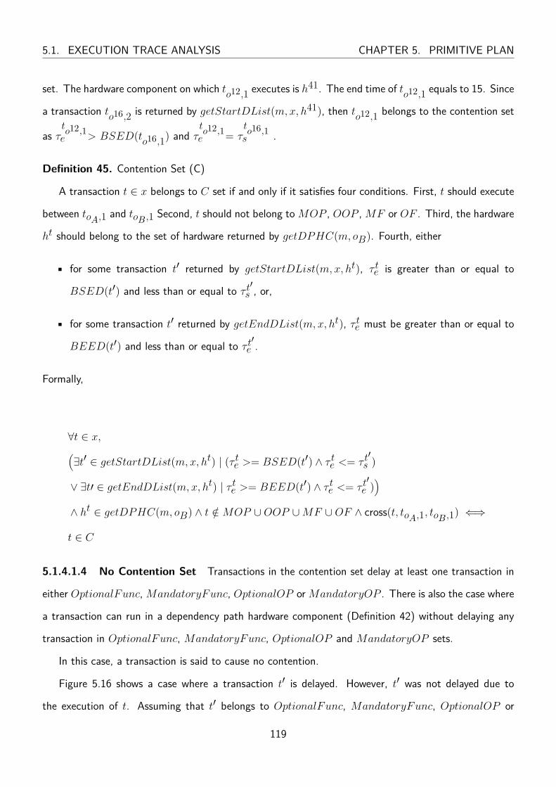
5.1. EXECUTION TRACE ANALYSIS CHAPTER 5. PRIMITIVE PLAN
set. The hardware component on which to12,1 executes is h41. The end time of to12,1 equals to 15. Since
a transaction to16,2 is returned by getStartDList(m,x, h41), then to12,1 belongs to the contention set
as τto12,1e > BSED(to16,1) and τ
to12,1e = τ
to16,1s .
Definition 45. Contention Set (C)
A transaction t ∈ x belongs to C set if and only if it satisfies four conditions. First, t should execute
between toA,1 and toB ,1 Second, t should not belong toMOP , OOP ,MF or OF . Third, the hardware
ht should belong to the set of hardware returned by getDPHC(m, oB). Fourth, either
• for some transaction t′ returned by getStartDList(m,x, ht), τ te is greater than or equal to
BSED(t′) and less than or equal to τ t′s , or,
• for some transaction t′ returned by getEndDList(m,x, ht), τ te must be greater than or equal to
BEED(t′) and less than or equal to τ t′e .
Formally,
∀t ∈ x,(∃t′ ∈ getStartDList(m,x, ht) | (τ te >= BSED(t′) ∧ τ te <= τ t
′s )
∨ ∃t′ ∈ getEndDList(m,x, ht) | τ te >= BEED(t′) ∧ τ te <= τ t′e ))
∧ ht ∈ getDPHC(m, oB) ∧ t /∈MOP ∪OOP ∪MF ∪OF ∧ cross(t, toA,1, toB ,1) ⇐⇒
t ∈ C
5.1.4.1.4 No Contention Set Transactions in the contention set delay at least one transaction in
either OptionalFunc,MandatoryFunc, OptionalOP orMandatoryOP . There is also the case where
a transaction can run in a dependency path hardware component (Definition 42) without delaying any
transaction in OptionalFunc, MandatoryFunc, OptionalOP and MandatoryOP sets.
In this case, a transaction is said to cause no contention.
Figure 5.16 shows a case where a transaction t′ is delayed. However, t′ was not delayed due to
the execution of t. Assuming that t′ belongs to OptionalFunc, MandatoryFunc, OptionalOP or
119
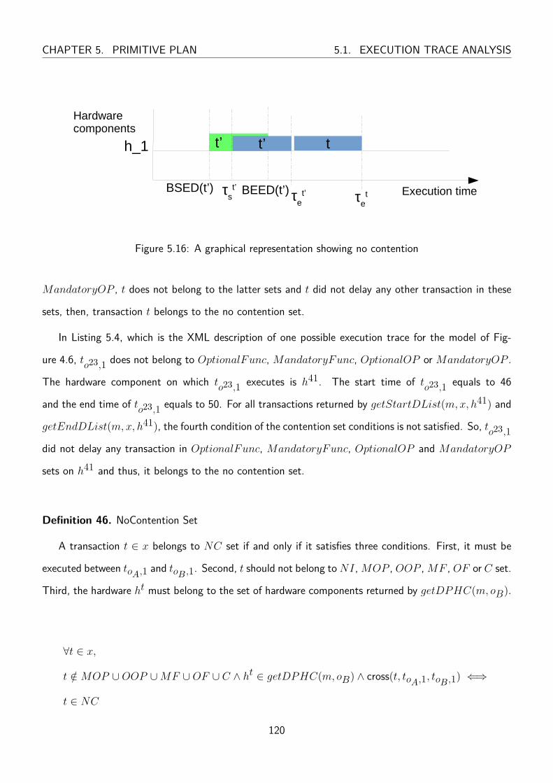
CHAPTER 5. PRIMITIVE PLAN 5.1. EXECUTION TRACE ANALYSIS
h_1 t’
BSED(t’) BEED(t’)
t’
τe
t’τst’
t
τet
Hardware components
Execution time
Figure 5.16: A graphical representation showing no contention
MandatoryOP , t does not belong to the latter sets and t did not delay any other transaction in these
sets, then, transaction t belongs to the no contention set.
In Listing 5.4, which is the XML description of one possible execution trace for the model of Fig-
ure 4.6, to23,1 does not belong to OptionalFunc, MandatoryFunc, OptionalOP or MandatoryOP .
The hardware component on which to23,1 executes is h41. The start time of to23,1 equals to 46
and the end time of to23,1 equals to 50. For all transactions returned by getStartDList(m,x, h41) and
getEndDList(m,x, h41), the fourth condition of the contention set conditions is not satisfied. So, to23,1did not delay any transaction in OptionalFunc, MandatoryFunc, OptionalOP and MandatoryOP
sets on h41 and thus, it belongs to the no contention set.
Definition 46. NoContention Set
A transaction t ∈ x belongs to NC set if and only if it satisfies three conditions. First, it must be
executed between toA,1 and toB ,1. Second, t should not belong toNI,MOP , OOP ,MF , OF or C set.
Third, the hardware ht must belong to the set of hardware components returned by getDPHC(m, oB).
∀t ∈ x,
t /∈MOP ∪OOP ∪MF ∪OF ∪ C ∧ ht ∈ getDPHC(m, oB) ∧ cross(t, toA,1, toB ,1) ⇐⇒
t ∈ NC
120

5.1. EXECUTION TRACE ANALYSIS CHAPTER 5. PRIMITIVE PLAN
5.1.4.1.5 Other Hardware Set (OH) Transactions executed between toA,1 and toB ,1 belong to
Other Hardware set if they execute between toA,1 and toB ,1 and do not belong to any set defined
previously (MOP , OOP , MF , OF , NC and C).
In the example of Section 4.3.4, to39,1 is executed between time 7 and 57 on h43 and does not
belong to MOP , OOP , MF , OF , NC or C set. Thus, to39,1 belongs to OH set.
Definition 47. OtherHardware Set
A transaction t ∈ x belongs to OH if and only if it execute between toA,1 and toB ,1 but it does not
belong to any previous classification sets. Formally,
∀t ∈ x,
t /∈MOP ∪OOP ∪MF ∪OF ∪NC ∪ C ∧ cross(t, toA,1, toB ,1) ⇐⇒
t ∈ OH
5.1.4.1.6 Indirect Impact Set When a maximum latency requirement is not satisfied, in addition
to the impact of transactions that were executed between toA,1 and toB ,1 we are interested to know if a
transaction executed before toA,1 led to a delay in transactions executed between toA,1 and toB ,1. We
define function SDL that takes a model, an execution trace and hardware component from the HDepset as input and return a set of transaction that were executed between the beginning of execution (τ0)
and τtoA,1s and have their BSED different than their start time.
SDL : (m,x, h) 7→{t ∈ x | ht = h ∧BSED(t) 6= τ ts ∧ τ ts ≤ τtoA,1s }
Similarly for end time we define function EDL that takes a model, an execution trace and hardware
component as input and return a set of transaction that were executed between the beginning of execution
(τ0) and τtoA,1e and have their BEED different than their end time. Formally,
EDL : (m,x, h) 7→{t ∈ x | ht = h ∧BEED(t) 6= τ te ∧ τ te ≤ τtoA,1e }
121
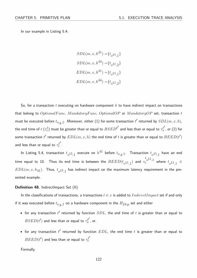
CHAPTER 5. PRIMITIVE PLAN 5.1. EXECUTION TRACE ANALYSIS
In our example in Listing 5.4:
SDL(m,x, h41) ={to11,1}
SDL(m,x, h44) ={to11,2}
EDL(m,x, h41) ={to11,1}
EDL(m,x, h44) ={to11,2}
So, for a transaction t executing on hardware component h to have indirect impact on transactions
that belong to OptionalFunc, MandatoryFunc, OptionalOP or MandatoryOP set, transaction t
must be executed before toA,1. Moreover, either (1) for some transaction t′ returned by SDL(m,x, h),
the end time of t (τ te) must be greater than or equal to BSEDt′ and less than or equal to τ t′s , or (2) for
some transaction t′ returned by EDL(m,x, h) the end time of t is greater than or equal to BEED(t′)
and less than or equal to τ t′e .
In Listing 5.4, transaction to15,1 execute on h41 before toA,1. Transaction to15,1 have an end
time equal to 10. Thus its end time is between the BEED(to11,1) and τto11,1e where to11,1 ∈
EDL(m,x, h41). Thus, to15,1 has indirect impact on the maximum latency requirement in the pre-
sented example.
Definition 48. IndirectImpact Set (II)
In the classifications of transactions, a transactions t ∈ x is added to IndirectImpact set if and only
if it was executed before toA,1 on a hardware component in the HDep set and either
• for any transaction t′ returned by function SDL, the end time of t is greater than or equal to
BSED(t′) and less than or equal to τ t′s , or.
• for any transaction t′ returned by function EDL, the end time t is greater than or equal to
BEED(t′) and less than or equal to τ t′e
Formally,
122
5.2. CONCLUSION CHAPTER 5. PRIMITIVE PLAN
∀t ∈ x,(∃t′ ∈ SDL(m,x, ht) | (τ te >= BSED(t′) ∧ τ te <= τ t
′s )
∨ ∃t′ ∈ EDL(m,x, ht) | τ te >= BEED(t′) ∧ τ te <= τ t′e
)∧ ht ∈ getDPHC(m, oB) ∧ τ ts < τ
toA,1e ⇐⇒
t ∈ II
5.1.4.1.7 No Impact Set All transactions that do not belong to any classification set defined before
are added to NoImpact set.
Definition 49. NoImpact Set (NI)
A transaction t ∈ x executed on hardware component h belongs to the no impact set if and only if
it does not belong to any classification set defined before. Formally,
∀t ∈ x,
t /∈MOP ∪OOP ∪MF ∪OF ∪NC ∪ C ∪ II ⇐⇒
to ∈ NI
5.2 Conclusion
In this chapter, the formal representation of a new latency analysis approach was introduced. However
several Hypothesis were taken to ensure that the two operators of a maximum latency requirement are
executed such that the first occurrence of the first operator corresponds to the first occurrence of the
second operator. In this chapter, the latency analysis approach assumes an 1-to-1 relation between the
two operators of the requirement. In the next chapter, we target these hypothesis. Targeting these
hypothesis enables us to specify more transaction traces as valid. To overcome this assumption, an
approach based on graph tainting is introduced in the next chapter.
123

Chapter 6
Advanced Precise Latency Analysis
Approach Using Graph Tainting (PLAN-GT)
“Without continual growth and progress, such words as improvement, achievement, and
success have no meaning.”
-Benjamin Franklin
6.1 Motivation
The primitive PLAN approach already discussed helps the designer to investigate the cause of a latency re-
quirement violation in modelm between two operators oA and oB for a requirement r = 〈oA, oB , λmax〉
when the two transactions corresponding to oA and oB appear once in the execution trace.
In Chapter 5, we proposed several hypotheses to make it easier to identify these occurrences in an
execution trace. These hypotheses led to defining a one-to-one relation between oA and oB . Execution
traces that do not satisfy these assumptions are identified as invalid in our previous analysis.
In this chapter, we would like to be able to analyze execution traces that we could not analyze before.
We would like to analyze traces that have several occurrences of oA and oB . Said differently, we would
like to analyze traces even when Hypothesis 1 does not hold.
The identification of an occurrence of operator oB that corresponds to an occurrence of operator oA
124

6.2. EXAMPLE 2 CHAPTER 6. ADVANCED PLAN
may not be trivial when removing this assumption since, in this case, operator oB can execute regardless
of operator oA execution. In other words, if there is no defined relation like the 1-to-1 relation between
the two operators, identifying the transactions to calculate the latency is not straight forward.
In this chapter, we would like to relate several occurrences of oA and oB . By relating we mean
identifying the occurrence of operator oB that corresponds to the occurrence of operator oA. For
example, if operator oA is a WriteData operator and operator oB is a ReadData operator that write and
read data respectively from a Non Blocking Write Non Blocking Read data communication channel, then
operator oA can infinitely write and operator oB never blocks when attempting to read data through
the data channel. In this case, the execution trace may have several transactions corresponding to data
writing and several transactions corresponding to data reading. Thus, it is difficult to identify which
transaction(s) having operator oB corresponds to an occurrence of operator oA.
Identifying these transactions is the topic of the chapter. Removing the 1-to-1 relation assumption
opens new avenues. So, we need to know which occurrence of oB corresponds to an occurrence of
oA. To know what is the corresponding occurrence of oB we need to trace the execution to find this
occurrence. Tainting is the way we do this tracing.
In this chapter, we introduce how PLAN is applied after finding the occurrence of oA and its corre-
sponding occurrence of oB using tainting. Tainting enables us to handle long traces and verify several
latencies between oA and oB . In particular, we use taint to characterize the correspondence between oAand oB . The taint value will indeed allow us to identify the occurrence of oA and oB that corresponds
to each other by considering occurrence of the same taint value.
6.2 Example 2
Let us consider a HW/SW Partitioning model whose application and allocation models are shown in
Figure 6.1 and Figure 6.2 respectively. In Figure 6.2, two functions f1 and f2 communicate through a
Blocking Write - Blocking Read data channel dc4. Functions f2 and f3 communicate through a Non-
Blocking Write - Non-Blocking Read data channel dc5. Operators o7 and o15 write 1 byte of data to
data channels dc4 and dc5 respectively. Operators o9 and o21 read 1 byte of data from data channels
125

CHAPTER 6. ADVANCED PLAN 6.2. EXAMPLE 2
f1
o6,Start
o7,WriteData
o8,Stop
o15,WriteData
f3dc4 dc5
v1=0f2
o9,ReadData
o17,Start
o16,Stop
o11,Choice
o10,Merge
o14,IntOP o12,IntOP
o19,Choice
o18,Merge
o23,Stop o20,IntOP
o21,ReadData
o13,Set
o22,Set
1 dc4
1 dc5
1 dc4
1 dc5
20 50
Legend
oid,cat
fid
Function Behavior
Control flow
Operator
FunctionData channel
oid correspondingdata ch.
oid Complexity
oid Data Amount
100
v2=0
v1<3
v1=v1+1
v1⩾3
v2<3v2⩾3
v2=v2+1
Variable
New Value
Function
Variable
o24,Start
o24,Choice
o25,IntOP
80
o26,Merge
Figure 6.1: Graphical representation of an Application model with loops
dc4 and dc5 respectively. Functions f2 and f3 have variables v1 and v2 respectively. These variables
are initiated to zero and used to control the loop iterations inside the functions.
In Figure 6.2, function f1 is allocated to an execution hardware component h40, function f2 is
allocated to an execution hardware component h41 and functions f3 is allocated to an execution hardware
component h42. The data channels dc4 and dc5 are allocated to a communication hardware component
h43 and a storage hardware component h44.
Let a maximum latency requirement r = 〈o7, o21, 150〉 be a requirement of this HW/SW Partitioning
model. Operators o7 and o21 are connected by one dependency path −−−→o7o21. Two possible execution
126

6.2. EXAMPLE 2 CHAPTER 6. ADVANCED PLAN
h40 h41 h42
f1 Legend
hid Hardware componentAllocation
l45l46
h43 h44
dc4
l48
f2 f3
dc5 dc4 dc5
l47
SlaveLinkidMaster
Figure 6.2: Graphical representation for the Allocation model of Figure 6.1
traces are shown in Table 6.1 and Table 6.2. The transactions executed on h44 and the transactions
of Start, Stop, Choice, Merge and Set operators are not shown in Table 6.1 and Table 6.2. The
corresponding execution trace of Table 6.2 is shown in XML format in Listing B.1.
Table 6.1: A possible execution trace shown in tabular format of a HW/SW partitioning model whoseallocation model is shown in Figure 6.2
hc 40 41 42 43id 7 9 12 14 15 25 20 21 7 9 15 21seq 4 12 15 23 27 31 32 9 22 38 6 11 33 37τ ts 0 1 2 52 102 152 172 0 80 180 0 1 172 180τ te 1 2 52 102 152 172 173 80 180 181 1 2 173 181
Table 6.2: Another possible execution trace shown in tabular format of a HW/SW partitioning modelwhose allocation model is shown in Figure 6.2
hc 40 41 42 43id 7 9 12 14 15 20 21 7 9 15 21seq 2 9 12 16 20 24 25 34 41 48 37 44 51 3 8 36 36 43 50τ ts 0 1 2 52 102 152 172 0 101 202 100 201 302 0 1 172 100 201 302τ te 1 2 52 102 152 172 173 100 201 302 101 202 303 1 2 173 101 202 303
In Table 6.1, the first occurrence of o21 corresponds to the first occurrence of o7. However, in
Table 6.2, the hypotheses of Chapter 5 do not hold. The first occurrence of o7 does not correspond to
the first occurrence of o21 because the WriteData operator o15 executes after the ReadData operator o21.
Thus, to correctly calculate the latency, we must track the execution transactions along the HW/SW
Partitioning model to determine the corresponding occurrence of o21. For the HW/SW Partitioning
model presented in this section, manually tracking transactions in the second execution trace reveals
that the second occurrence of o21 corresponds to the first occurrence of o7. Thus, the latency between
o7 and o21 for r = 〈o7, o21, 150〉 equals to 202. So, the maximum latency requirement is not valid.
127
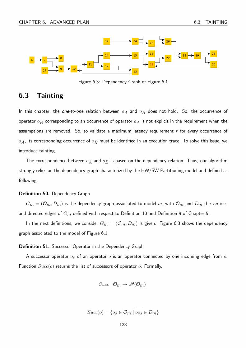
CHAPTER 6. ADVANCED PLAN 6.3. TAINTING
Figure 6.3: Dependency Graph of Figure 6.1
6.3 Tainting
In this chapter, the one-to-one relation between oA and oB does not hold. So, the occurrence of
operator oB corresponding to an occurrence of operator oA is not explicit in the requirement when the
assumptions are removed. So, to validate a maximum latency requirement r for every occurrence of
oA, its corresponding occurrence of oB must be identified in an execution trace. To solve this issue, we
introduce tainting.
The correspondence between oA and oB is based on the dependency relation. Thus, our algorithm
strongly relies on the dependency graph characterized by the HW/SW Partitioning model and defined as
following.
Definition 50. Dependency Graph
Gm = (Om, Dm) is the dependency graph associated to model m, with Om and Dm the vertices
and directed edges of Gm defined with respect to Definition 10 and Definition 9 of Chapter 5.
In the next definitions, we consider Gm = (Om, Dm) is given. Figure 6.3 shows the dependency
graph associated to the model of Figure 6.1.
Definition 51. Successor Operator in the Dependency Graph
A successor operator os of an operator o is an operator connected by one incoming edge from o.
Function Succ(o) returns the list of successors of operator o. Formally,
Succ : Om →P(Om)
Succ(o) = {os ∈ Om | oos ∈ Dm}
128
6.3. TAINTING CHAPTER 6. ADVANCED PLAN
As a reminder, transactions in the trace are ordered with respect to their sequence number. Intu-
itively, the algorithm handles these transactions sequentially with respect to this order. Each time an
oA-transaction tA is encountered in the trace, its operator is tainted with a new fresh taint value and the
transaction is added to a list. Then, while handling the following transactions, the algorithm progressively
propagates this taint value to the encountered operators respecting the dependency relation (i.e., tainted
operators have a dependency path from oA included in the trace). Finally, when an oB-transaction is
encountered and tainted, it is associated with the oA-transaction that have the same taint value. At
this moment, the algorithm calculates the latency between these two transactions to identify when the
latency is greater than λmax.
More technically, the algorithm can be seen as a main loop on transactions that updates an internal
state by handling a transaction at each iteration and outputs a result when the transaction operator is
oB . The tainting algorithm is based on the definition of two kinds of attributes. Attributes which are
static that are applied to all the trace analysis and attributes which depend upon the transaction which is
under analysis in the main loop. These attributes are called dynamic attributes and they are grouped into
a set which is called state. Thus, an execution of the algorithm for a trace t1, · · · , tn can be represented
by s0t1−→ s1
t2−→ · · · tn−−→ sn, where each si is a state in Sx, Sx being the set of all possible internal
states of an execution trace. Sx = {si} denotes the set of all possible internal states of an execution
trace. So, there is one state per transaction analyzed in our algorithm. A state is build upon tainting
attributes associated to each operator. Function TaintG takes as inputs a transaction, a state and an
execution trace and outputs a new state. Function TaintG updates the attributes of s according to the
execution of the operator corresponding to t.
TaintG(x, t, s) 7→ s′
In Figure 6.4, considering transaction tn+1 evolves state sn to sn+1.
More formally, a static attribute is a function stat_att : Om → V alues and a dynamic attribute
is a function dyn_att : S × Om → V alues. The type of value depends on attributes. Some attribute
values are complex ones, thus some attribute functions have more parameters, which allow to access
components of structured values.
129
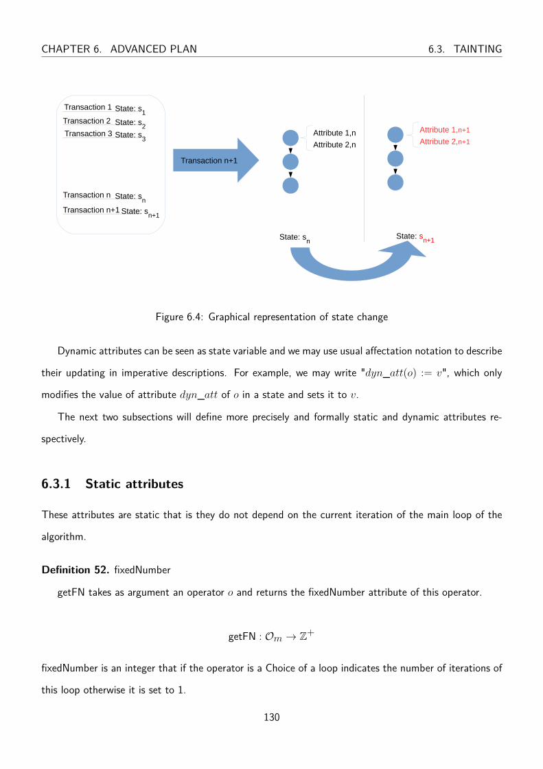
CHAPTER 6. ADVANCED PLAN 6.3. TAINTING
State: sn
State: sn+1
Transaction 1
Transaction 2
Transaction 3
Transaction n
Transaction n+1
Attribute 1,n
Attribute 2,n
Attribute 1,n+1
Attribute 2,n+1
State: s1
State: s2
State: s3
State: sn
Transaction n+1 State: sn+1
Figure 6.4: Graphical representation of state change
Dynamic attributes can be seen as state variable and we may use usual affectation notation to describe
their updating in imperative descriptions. For example, we may write "dyn_att(o) := v", which only
modifies the value of attribute dyn_att of o in a state and sets it to v.
The next two subsections will define more precisely and formally static and dynamic attributes re-
spectively.
6.3.1 Static attributes
These attributes are static that is they do not depend on the current iteration of the main loop of the
algorithm.
Definition 52. fixedNumber
getFN takes as argument an operator o and returns the fixedNumber attribute of this operator.
getFN : Om → Z+
fixedNumber is an integer that if the operator is a Choice of a loop indicates the number of iterations of
this loop otherwise it is set to 1.
130
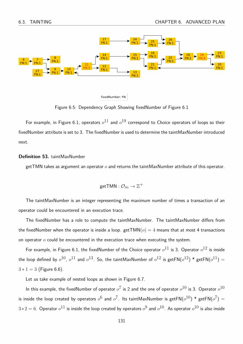
6.3. TAINTING CHAPTER 6. ADVANCED PLAN
Figure 6.5: Dependency Graph Showing fixedNumber of Figure 6.1
For example, in Figure 6.1, operators o11 and o19 correspond to Choice operators of loops so their
fixedNumber attribute is set to 3. The fixedNumber is used to determine the taintMaxNumber introduced
next.
Definition 53. taintMaxNumber
getTMN takes as argument an operator o and returns the taintMaxNumber attribute of this operator.
getTMN : Om → Z+
The taintMaxNumber is an integer representing the maximum number of times a transaction of an
operator could be encountered in an execution trace.
The fixedNumber has a role to compute the taintMaxNumber. The taintMaxNumber differs from
the fixedNumber when the operator is inside a loop. getTMN(o) = 4 means that at most 4 transactions
on operator o could be encountered in the execution trace when executing the system.
For example, in Figure 6.1, the fixedNumber of the Choice operator o11 is 3. Operator o12 is inside
the loop defined by o10, o11 and o13. So, the taintMaxNumber of o12 is getFN(o12) * getFN(o11) =
3 ∗ 1 = 3 (Figure 6.6).
Let us take example of nested loops as shown in Figure 6.7.
In this example, the fixedNumber of operator o7 is 2 and the one of operator o10 is 3. Operator o10
is inside the loop created by operators o6 and o7. Its taintMaxNumber is getFN(o10) * getFN(o7) =
3∗2 = 6. Operator o11 is inside the loop created by operators o9 and o10. As operator o10 is also inside
131
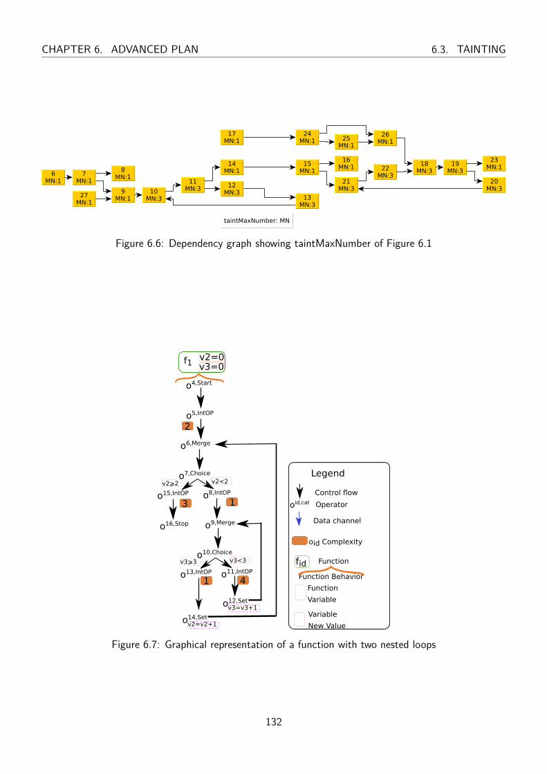
CHAPTER 6. ADVANCED PLAN 6.3. TAINTING
Figure 6.6: Dependency graph showing taintMaxNumber of Figure 6.1
v3=0f1
o5,IntOP
o16,Stop
o7,Choice
o6,Merge
o15,IntOP o8,IntOP
o12,Set
3
v2<2
v3=v3+1
v2⩾2
Legend
oid,cat
fidFunction Behavior
Control flow
Operator
Function
Data channel
oid Complexity
Variable
New Value
Function
Variable
2
1
o10,Choice
o9,Merge
o11,IntOP
4 1
v3<3
v2=0
v3⩾3
o13,IntOP
o14,Setv2=v2+1
o4,Start
Figure 6.7: Graphical representation of a function with two nested loops
132

6.3. TAINTING CHAPTER 6. ADVANCED PLAN
Figure 6.8: Dependency graph showing taintMaxNumber of Figure 6.7
the loop created by operators o6 and o7, then the taintMaxNumber of o11 equals the multiplication
of all the fixedNumber of the Choice operators of these two loops. Thus, taintMaxNumber of o11 is
getFN(o11) * getFN(o10)* getFN(o7) = 1 ∗ 3 ∗ 2 = 6 (Figure 6.8).
In general, an operator that belongs to the iterations of nested loops, its taintMaxNumber equals to
the multiplication of all the fixedNumber of the Choice operators of these loops.
This taintMaxNumber represent only the worst case scenario of how many times each operator will
be executed when executing the model. For instance, if there is a Choice operator inside a loop and
this Choice operators is not part of any loop, the number of times each branch will be executed can not
be decided statically in the general case. This taintMaxNumber might not be always reachable in some
cases. In other words, when executing a loop, taintMaxNumber represents the maximum number each
operator could be executed in this loop.
6.3.2 Dynamic attributes
The values of dynamic attributes depend on the state. For all functions to come, the state is an implicit
parameter.
Definition 54. Taint Values oATaint values correspond to the occurrences of oA in the execution trace. A fresh taint value denoted
as Γ is created each time a transaction of oA of the requirement under study is encountered when
iterating over the execution trace. AllΓ is the set of all taint values generated by all algorithm iterations
133
CHAPTER 6. ADVANCED PLAN 6.3. TAINTING
of one execution trace.
Each operator has an ordered set of taint values. These taint values correspond to the occurrences
of oA. Taint value Γ is associated to an operator each time it is executed and there is a dependency
relation between this operator execution and the execution of operator oA that is tainted with Γ. Taint
values in this set are linked to transactions of the execution trace that have already been handled by the
algorithm.
The order of the taint values in the sequence is based on when they are added. Taint_size represents
the size of the sequence of taint values. Formally,
Taint_size : Om → N
Then, for all o in Om,
• Taint takes as argument an operator o and returns the sequence of the taint values of this operator.
So, Taint(o) : [1,Taint_size(o)]→ AllΓ
As taint values are “fresh” when generated, Taint(o) is injective.
• oΓ is the ordered set of taint values of o.
oΓ = {Γ ∈ AllΓ | ∃i ∈ [1,Taint_size(o)], Taint(o)(i) = Γ}
• Taint_trans provides each taint value in oΓ with the encountered o-transaction while propagating
it during the execution of algorithm (Section 6.3.3).
Taint_trans(o) : oΓ → P(x) (where x is the execution trace)
∀Γ ∈ oΓTaint_trans(o)(Γ) ∈ P(x)
Definition 55. taintConsideredNumber
for all o in Om and all Γ in oΓ, getCN takes as an argument an operator o and a taint value Γ and
returns the taintConsideredNumber attribute of this operator for the taint value.
getCN(o,Γ) ∈ N
The taintConsideredNumber represents, at the current state of an execution trace browsing, the
134

6.3. TAINTING CHAPTER 6. ADVANCED PLAN
number of times a transaction corresponding to an operator has been encountered with a taint value.
Initially, when a taint value is assigned to an operator, its corresponding taintConsideredNumber is set
to zero.
Let us assume an operator o6 in a function f allocated to a hardware component h40. Let Γ be a
taint value for o6. Initially, getCN(o6,Γ) = 0. Table 6.3 shows 3 transactions for this operator and the
value of the taintConsideredNumber for this operator when a transaction is encountered in the trace.
Thus, getCN(o6,Γ) = 3 means that 3 transactions corresponding to o6 were encountered in an execution
trace for taint value Γ.
Table 6.3: Part of an execution trace in tabular format
hc 40id 6τ ts 0 11 21τ te 1 12 22
getCN(o6,Γ) 1 2 3
Definition 56. sampleNumber
getSN takes as argument an operator o and returns the sampleNumber attribute of this operator.
getSN : Om → Z+
A ReadData, WriteData or IntOp operator may have several transactions corresponding to one exe-
cution of this operator. The sampleNumber is an integer representing, at a specific time of the analysis,
the number of bytes that are written or read in case of a ReadData or WriteData operator or the integer
cycles in case of IntOp operator. The sampleNumber is zero when the execution of an operator begins. It
is incremented when the successive transactions that correspond to this operator are encountered during
analysis. For example, if a ReadData operator o with size 13 has two transactions corresponding to
reading 10 then reading 3 data size respectively in the execution trace, sampleNumber of o starts as
zero, then it is set to 10 when the first transaction is encountered. Then, sampleNumber is set to 13
(10+3) when the second transaction is encountered.
135
CHAPTER 6. ADVANCED PLAN 6.3. TAINTING
Thus, sampleNumber is used to detect the end of one execution of an operator while handling the
transactions corresponding to this operator execution. When the operator execution terminates, the
sampleNumber is reset.
6.3.3 Tainting Algorithm
Figure 6.9 is a flow chart presenting how latency can be computed using tainting. The flow chart in
Figure 6.9 presents an algorithm that takes as input a HW/SW Partitioning model m which defines a
dependency graph Gm, an execution trace x and a maximum latency requirement r = 〈oA, oB , λmax〉.
The algorithm iterates sequentially over the transactions in the execution trace. At each iteration, it
updates dynamic attributes of the operators of the graph. It then outputs for each occurrences of oA a
corresponding occurrence of oB if it exists. And then computes the latency between each couple (oA,
corresponding oB) in order to figure out whether the latency between these occurrences is greater than
λmax or not. Moreover, it collects transactions associated to taint values in order to classify them later
with respect to their impact on latency. The formal definition of this classification is part of our future
work but we expect it to be similar classification presented in previous chapter.
This simplified view of the algorithm considers operator transactions are atomic, which is not always
the case. However, this simplified view is relevant although it hides some details of the complete
algorithm, as explained in the next section. This atomicity is discussed in the next sub section.
6.3.4 Operator Transactions Granularity
Figure 6.9 considers that the execution of one operator produces exactly one transaction. But actually
this assumption does not hold for two reasons:
1. When an operator is executed on an execution hardware component, its executions may be pre-
empted by the scheduler and so this execution can produce more than one transaction
2. The transactions of ReadData and WriteData operators can be split with respect to the communi-
cation path on which data channels are allocated and with respect to the size of the components
of the communication path.
136
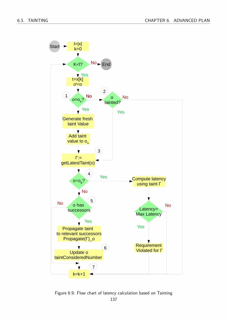
6.3. TAINTING CHAPTER 6. ADVANCED PLAN
Start
End
l=|x|k=0
K<l?
t=x[k]ot=o
o=oA?
Generate fresh taint Value
Add taint value to o
A
o has successors
Propagate taint to relevant successors
Propagate(Γ)_o
Update o taintConsideredNumber
k=k+1
o tainted?
o=oB?
Γ:=getLatestTaint(o)
Compute latencyusing taint Γ
Latency>Max Latency
Requirement Violated for Γ
Yes
No
Yes
Yes
No
No
No
No
No
No
Yes
Yes
Yes
12
3
4
5
6
7
Figure 6.9: Flow chart of latency calculation based on Tainting137
CHAPTER 6. ADVANCED PLAN 6.3. TAINTING
Transaction split by scheduling:
In case an operator o is either ReadData, WriteData or IntOp operator, the sampleNumber attribute
introduced in Definition 56 is used to identify the last transaction corresponding to one execution of an
operator o. In case where the execution of an operator is implemented by several transactions, we consider
the last one as the significant transaction. We say an operator o is executed once in the execution trace
x when a transaction corresponding to o is encountered in x and either (1) the sampleNumber equals
to the size of o in case o is a ReadData or WriteData operator or (2) the sampleNumber equals to the
complexity of o in case o is an IntOp operator.
Let us come back to our main algorithm (Figure 6.9). Let us assume that at stage two the considered
transaction corresponds to an IntOp operator o. Let us assume that the sampleNumber returned by
getSN(o) is less than the complexity of o. At the next iterations steps, when a transaction t also
corresponds to the execution of o is encountered, the sample number is incremented and compared to
the complexity of o. If the sample number is lower than complexity of o, other dynamic attributes of o
are not modified. Otherwise, once the sampleNumber returned by getSN(o) is equal to the operators
complexity, the sampleNumber is reset as explained previously and the taint value is propagated to the
successors as stated before and detailed in the next section.
WriteData or ReadData operator are handled similarly, depending on the sampleNumber and the
operator data size.
Execution split with respect to a communication path:
To keep things simple, we assume that all WriteData and ReadData operators must have a data size less
than or equal than the data size of all components of a communication path where they are allocated.
So, for WriteData or ReadData operator there is one transaction for each component in the preceptive
communication path. Communication paths consist of write and read paths. In this chapter, and for
simplicity, we will abstract transactions on hardware components of a read/write path and consider such
transactions as atomic. The transaction executed on the last hardware component of a read or write
path marks the end of a ReadData or WriteData operator execution respectively. Transactions executed
on other hardware components of a read or write path different than the last hardware component is
138

6.3. TAINTING CHAPTER 6. ADVANCED PLAN
referred to as intermediate transactions. Handling such intermediate transactions does not modify the
dynamic attributes of a state. Only the transaction associated to the last hardware component of a read
or write path does this. Thus, in this chapter, the last transaction of a read or write path is seen as
an atomic transaction associated to a ReadData or WriteData operator, handled following the process
described in the next section. According to Definition 24, the atomic transaction of WriteData is on the
storage component of the write path. According to Definition 25, the atomic transaction of ReadData
is on the execution component of the read path.
In the next sections we assume that a transaction is not preempted and the algorithm can select
the latest transaction of any operator execution. Thus, as a consequence we consider a transaction is
atomic. Similar to other operators in the model, for a maximum latency requirement r = 〈oA, oB , λmax〉,
operators oA and oB are also assumed to execute in one transaction. Thus, from now we consider that
operators execute in one transaction.
6.3.5 Calculating latency based on tainting
Figure 6.9 presents the actions performed by the algorithm each time a transaction of the execution trace
is picked up. Since we consider transactions are atomic as explained in previous section, each transaction
corresponds to an execution of an operator.
The execution of an action may lead to modify the general state for each algorithm step. Thus, the
state evolves. The state is modified by the following actions which are executed in the order they are
presented. Let transaction t correspond to the execution of operator o. So, we are here at a moment
where all transactions before transaction t have been handled and we describe the handling of t.
1. if o is oA (otherwise, goto 2):
generate a fresh taint value Γ (Γ /∈ AllΓ). Add it along with the transaction to attributes of o,
and set taintConsideredNumber to zero. More formally:
apply Update_oA = {
Γ = generate_fresh(AllΓ);
AllΓ = AllΓ ∪ {Γ};
Taint_size(o) := Taint_size(o) + 1;
139

CHAPTER 6. ADVANCED PLAN 6.3. TAINTING
Figure 6.10: A transaction corresponding to oA is encountered (o = oA)
Taint(o)(Taint_size(o)) = Γ;
Taint_trans(o,Γ) := {t};
getCN(o,Γ) := 0; }
then, goto 3.
Figure 6.10 shows the attributes when a transaction corresponding to oA is encountered. Attributes
in green correspond to step 5.
2. if o is not tainted (i.e Taint_size(o) ≤ 0. Otherwise, goto 3):
transaction is skipped as it is not dependent on any transaction representing an occurrence of oA.
More formally: goto 7.
3. At this step we know that o is tainted and we identify the latest taint value(Γ), in order to propagate
it to successors.
We consider an operator as tainted when the size of the taint values sequence is greater than zero
(Taint_size(o) > 0). getLatestTaint takes as an argument an operator o and returns a taint
value.
getLatestTaint : Om → AllΓ
140

6.3. TAINTING CHAPTER 6. ADVANCED PLAN
The value returned by getLatestTaint is important to determine which taint value is the right taint
to propagate to the successors of an operator as described next.
Beware that this function assumes that there is only one possible execution path in all loops.
More Formally: Γ := getLatestTaint(o).
getLatestTaint(o){
∀Γ ∈ oΓ do
if(getCN(o,Γ) < getTMN(o))
return Γ;
}
4. if o is not oB then goto 5. Since o is oB : compute latency. The latency is computed and verified
with respect to the requirement. The latency is computed between the current occurrence of
oB (tainted by the last taint value Γ ) and the occurrence of oA tainted by Γ and according to
Section 6.4. If the requirement is not satisfied, a violation alert is raised.
5. Propagate taint to successors. Successors are characterized by Definition 51 and the propagation
of their taint value depends on the operator category and attributes. The next paragraph explain
the propagation of specific operators.
Taint propagation for Choice operator not used for loops For a Choice operator o,
soonest(x, t, o, getNext(o)) returns an operator os that belongs to getNext(o). os is first op-
erator in the branch actually chosen to execute by the Choice if it exists. If os is empty, go to 7.
Otherwise, if os exists it means that os is among getNext(o) and there is a transaction for os in
the remaining of the execution trace such that this transaction has the smallest sequence num-
ber among all the transactions corresponding to operators in getNext(o) and a sequence number
greater than the transaction of o.
When o is a Choice operator not part of a loop, the operator returned by soonest(x, t, o, getNext(o))
is tainted after the latest taint of the Choice operator is identified. We remind that getNext(o) is
defined in Section 4.3.1. Formally,
141
CHAPTER 6. ADVANCED PLAN 6.3. TAINTING
soonest(x, t, o, getNext(o)) =
os if os ∈ getNext(o) ∧ ∃ts ∈ x,(ots = os ∧ seqts > seqt∧
@(oi, ti) ∈ getNext(o)× x, oi = o ∧ seqt < seqti < seqts)
∅ otherwise
Taint propagation for Choice operator for loops A Choice operator of a loop lf exists,
the operator corresponding to the exit loop branch (getOutsideLoop(lf )) is tainted when the
taintConsideredNumber of the Choice operator equals its taintMaxNumber as explained next.
Choice operators inside loops but not being a choice of a loop Tainting Choice operators
inside loops is discussed in Section 6.3.5.1.
taint propagation for other operator For other operators than Choice, all their next are
tainted with the current taint value. More formally:
apply Propagate(Γ)_o = {
if(cat(o) = Choice ∧ ¬isLoopChoice(o))
{
os = soonest(x, t, o, getNext(o))
addTaint(os,Γ, t)
}
elseif(cat(o) = Choice ∧ isLoopChoice(o) ∧ getCN(o,Γ) < getTMN(o)))
{
os = getInsideLoop(〈om, o, os, v, nbr〉)
addTaint(os,Γ, t)
}
elseif(cat(o) = Choice ∧ isLoopChoice(o) ∧ getCN(o,Γ) = getTMN(o)))
{
os = getOutsideLoop(〈om, o, os, v, nbr〉)
142
6.3. TAINTING CHAPTER 6. ADVANCED PLAN
addTaint(os,Γ, t)
}
else
{
For Each os ∈ Succ(o)
addTaint(os,Γ, t)
}
}
addTaint(o,Γ, t) = {
if(Γ /∈ oΓ)
{
Taint_size(o) := Taint_size(o) + 1;
Taint(o)(Taint_size(o)) = Γ;
getCN(o,Γ) := 0; }
}
Taint_trans(o,Γ) := Taint_trans(o,Γ) ∪ {t};
}
In Figure 6.10, the update of attributes in green correspond to propagating the taint value to the
successors of operator o7.
6. Update taintConsideredNumber.
When operator o is not a Choice operator, after all successor operators of operator o are tainted,
the taintConsideredNumber of operator o is incremented by one to indicate that the taint value is
already propagated once to its successors.
When operator o is a Choice operator but not used to create loops, the taintConsideredNumber of
operator o is incremented by one when the soonest operator is tainted.
143

CHAPTER 6. ADVANCED PLAN 6.3. TAINTING
Figure 6.11: Transaction corresponding to o8 is encountered
Figure 6.12: Transaction corresponding to o9 is encountered
taintConsideredNumber update for Choice when used for loops The
taintConsideredNumber for the Choice operator used in the loop is incremented once all
operators along the loop iteration are tainted and considered once for the taint value. This
is known when the operator having an outgoing edge to the Merge operator is tainted. For
example, in Figure 6.1, the operator o14 is considered 3 times when o13 inside the loop iteration
is considered 3 times.
7. pick up the next transaction if it exists, else exit: end of transaction handling
Figure 6.11, Figure 6.12, Figure 6.13, Figure 6.14 and Figure 6.15 show the state change for 8 encountered
transactions as indicated per each figure.
144
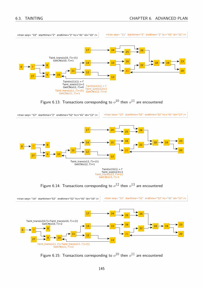
6.3. TAINTING CHAPTER 6. ADVANCED PLAN
Figure 6.13: Transactions corresponding to o10 then o11 are encountered
Figure 6.14: Transactions corresponding to o12 then o13 are encountered
Figure 6.15: Transactions corresponding to o10 then o11 are encountered
145
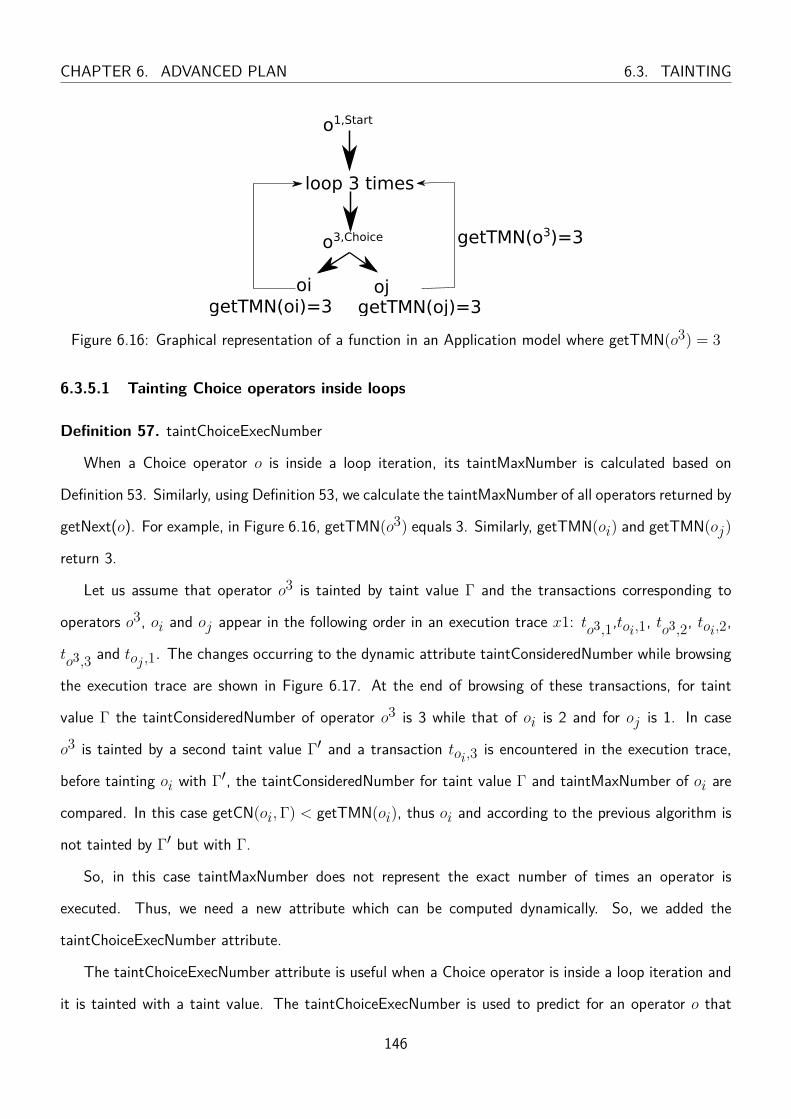
CHAPTER 6. ADVANCED PLAN 6.3. TAINTING
o3,Choice
o1,Start
loop 3 times
oi ojgetTMN(oi)=3 getTMN(oj)=3
getTMN(o3)=3
Figure 6.16: Graphical representation of a function in an Application model where getTMN(o3) = 3
6.3.5.1 Tainting Choice operators inside loops
Definition 57. taintChoiceExecNumber
When a Choice operator o is inside a loop iteration, its taintMaxNumber is calculated based on
Definition 53. Similarly, using Definition 53, we calculate the taintMaxNumber of all operators returned by
getNext(o). For example, in Figure 6.16, getTMN(o3) equals 3. Similarly, getTMN(oi) and getTMN(oj)
return 3.
Let us assume that operator o3 is tainted by taint value Γ and the transactions corresponding to
operators o3, oi and oj appear in the following order in an execution trace x1: to3,1,toi,1, to3,2, toi,2,
to3,3 and toj ,1. The changes occurring to the dynamic attribute taintConsideredNumber while browsing
the execution trace are shown in Figure 6.17. At the end of browsing of these transactions, for taint
value Γ the taintConsideredNumber of operator o3 is 3 while that of oi is 2 and for oj is 1. In case
o3 is tainted by a second taint value Γ′ and a transaction toi,3 is encountered in the execution trace,
before tainting oi with Γ′, the taintConsideredNumber for taint value Γ and taintMaxNumber of oi are
compared. In this case getCN(oi,Γ) < getTMN(oi), thus oi and according to the previous algorithm is
not tainted by Γ′ but with Γ.
So, in this case taintMaxNumber does not represent the exact number of times an operator is
executed. Thus, we need a new attribute which can be computed dynamically. So, we added the
taintChoiceExecNumber attribute.
The taintChoiceExecNumber attribute is useful when a Choice operator is inside a loop iteration and
it is tainted with a taint value. The taintChoiceExecNumber is used to predict for an operator o that
146

6.3. TAINTING CHAPTER 6. ADVANCED PLAN
o3,Choice
o1,Start
loop 3 times
oi oj
o3,Choice
o1,Start
loop 3 times
oi oj
o3,Choice
o1,Start
loop 3 times
oi oj
toi,2: toj,1: toi,1:
getCN(oi, Γ)=1 getCN(oi, Γ)=2 getCN(oi, Γ)=1
o3,Choice
o1,Start
loop 3 times
oi oj
getCN(o3, Γ)=1
o3,Choice
o1,Start
loop 3 times
oi oj
o3,Choice
o1,Start
loop 3 times
oi oj
to3,2: to3,3: to3,1:
getCN(o3, Γ)=2 getCN(o3, Γ)=3
(a)
(b)
(c)
(d)
(e)
(f)
Figure 6.17: Changes occurring to the dynamic attribute taintConsideredNumber of Figure 6.16 operatorswhile browsing the execution trace
belongs to getNext(oc) of the Choice operator oc the correct number of times a transaction corresponding
to o is encountered in an execution trace for a taint value.
For all o in Om and all Γ in oΓ, getCEN takes as an argument an operator o and a taint value value
Γ and returns the taintChoiceExecNumber attribute of this operator for the taint value.
getCEN(o,Γ) ∈ N
Initially, when a taint value is assigned to a Choice operator o that is inside a loop iteration, the
taintChoiceExecNumber of all its successors is set to zero. When a transaction corresponding to the
Choice operator o is encountered in the trace, and the taintConsideredNumber of the Choice operator
for the taint value is less than its taintMaxNumber, the soonest operator os to execute among its
successors is identified and tainted according the Section 6.3.5. Once os is identified and tainted, its
taintChoiceExecNumber attribute is incremented by os fixedNumber. All operators in the same function
as operator os and that are in the dependency path between os and the Merge operator of the loop have
147
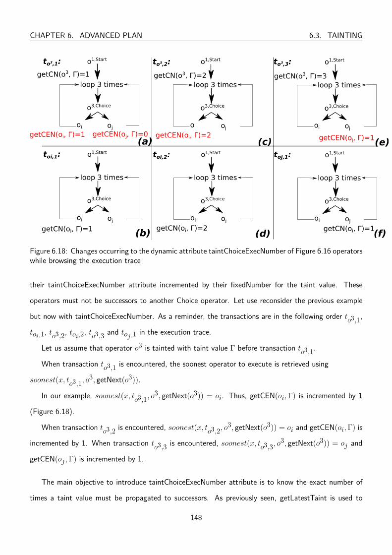
CHAPTER 6. ADVANCED PLAN 6.3. TAINTING
o3,Choice
o1,Start
loop 3 times
oi oj
o3,Choice
o1,Start
loop 3 times
oi oj
o3,Choice
o1,Start
loop 3 times
oi oj
toi,2: toj,1: toi,1:
getCN(oi, Γ)=1 getCN(oi, Γ)=2 getCN(oi, Γ)=1
o3,Choice
o1,Start
loop 3 times
oi oj
getCN(o3, Γ)=1
o3,Choice
o1,Start
loop 3 times
oi oj
o3,Choice
o1,Start
loop 3 times
oi oj
to3,2: to3,3: to3,1:
getCN(o3, Γ)=2 getCN(o3, Γ)=3
getCEN(oi, Γ)=1 getCEN(oj, Γ)=0 getCEN(oi, Γ)=2 getCEN(oj, Γ)=1(a) (c) (e)
(b) (d) (f)
Figure 6.18: Changes occurring to the dynamic attribute taintChoiceExecNumber of Figure 6.16 operatorswhile browsing the execution trace
their taintChoiceExecNumber attribute incremented by their fixedNumber for the taint value. These
operators must not be successors to another Choice operator. Let use reconsider the previous example
but now with taintChoiceExecNumber. As a reminder, the transactions are in the following order to3,1,
toi,1, to3,2, toi,2, to3,3 and toj ,1 in the execution trace.
Let us assume that operator o3 is tainted with taint value Γ before transaction to3,1.
When transaction to3,1 is encountered, the soonest operator to execute is retrieved using
soonest(x, to3,1, o3, getNext(o3)).
In our example, soonest(x, to3,1, o3, getNext(o3)) = oi. Thus, getCEN(oi,Γ) is incremented by 1
(Figure 6.18).
When transaction to3,2 is encountered, soonest(x, to3,2, o3, getNext(o3)) = oi and getCEN(oi,Γ) is
incremented by 1. When transaction to3,3 is encountered, soonest(x, to3,3, o3, getNext(o3)) = oj and
getCEN(oj ,Γ) is incremented by 1.
The main objective to introduce taintChoiceExecNumber attribute is to know the exact number of
times a taint value must be propagated to successors. As previously seen, getLatestTaint is used to
148
6.4. COLLECT TRANSACTIONS AND COMPUTE LATENCIES CHAPTER 6. ADVANCED PLAN
return the taint value that must be propagated to the successors of an operator.
After introducing taintChoiceExecNumber, getLatestTaint(o) definition is updated. getLatestTaint(o)
starts by sequentially checking the taint values of the operator o. If the taintChoiceExecNumber of o for
a taint value is greater than zero, this means that taintChoiceExecNumber value should be considered
instead of the taintMaxNumber to retrieve the latest taint value.
More Formally: Γ := getLatestTaint(o).
getLatestTaint(o){
∀Γ ∈ oΓ do
if(getCEN(o,Γ) > 0 ∧ getCN(o,Γ) < getCEN(o,Γ))
return Γ;
elseif(getCN(o,Γ) < getTMN(o))
return Γ;
}
6.4 Collect transactions and compute latencies
The actions presented in Figure 6.9 are repeated with every transaction encountered in the execution
trace. However, when the latest taint of operator o is retrieved and o is oB , then, the transaction
corresponding to operator oB is encountered,. Let the latest taint value be Γ. Then, the encountered
transaction is considered the occurrence of operator oB of a taint value Γ corresponding to the occurrence
of operator oA of the same taint value.
Lets denote by tA,Γ the transaction of Taint_trans(oA)(Γ) and by tB,Γ the transaction returned by
Taint_trans(oB)(Γ).
The latency λΓ between the occurrence of operator oA and its corresponding occurrence of operator
oB for a taint value Γ is computed as:
λΓ = τtB,Γe − τ
tA,Γs
In our example, oA is tainted once with Γ when a transaction corresponding to o7 is encountered.
149
CHAPTER 6. ADVANCED PLAN 6.5. CONCLUSION
This taint value Γ propagates according to the steps defined before and reach operator o15 at time 172
in the execution trace. Thus, with the first occurrence of oB , the operator o21 is not tainted yet. As
o21 is a successor to o15, operator o21 is tainted at 173 and the second occurrence of o21 is considered
the occurrence of operator oB of a taint value Γ. The latency λΓ is calculated as 202− 0 = 202.
6.5 Conclusion
In this chapter, we introduced an advanced version of the latency analysis approach. Advanced PLAN
overcome the assumption of 1-to-1 relation between the two operators of the maximum latency require-
ment. The advanced approach is capable to identify for each executed operator A, the corresponding
execution of operator B based on graph tainting. Thus, latency computation is possible in wider range
of execution traces than primitive PLAN.
In the next chapter, we will see how the designer can automatically retrieve the computed latency by
discussing the integration of the primitive and advance PLAN within TTool.
150
Chapter 7
Integration into Model-Driven Engineering
Framework
“To understand the best is to work on its implementation.”
-Jean-Marie Guyau
One of the objectives of this thesis is to implement PLAN and provide the results to the designer in a
user-friendly way. The analysis results should be presented in a clear and informative way so the designer
can depend on them to make decisions to enhance the system model. TTool and more precisely one of
its modeling profiles named SysML-Sec was chosen for this implementation. In TTool, the designer can
draw a system model that confirms with our formal model thanks to TTool diagramming facilities.
In this chapter, the integration of a prototype of the PLAN approach within TTool is presented.
First, we will discuss how our formal model maps to SysML diagrams. Then, in Section 7.2, we show
how a designer can instantiate PLAN in TTool. PLAN can be started from a graphical window interface
or from command line. In Section 7.3 and Section 7.4, we demonstrate respectively using two real-world
use cases from H2020 AQUAS project how primitive PLAN approach and advanced PLAN approach can
be efficiently applied to verify latency requirements by analyzing simulation traces.
151
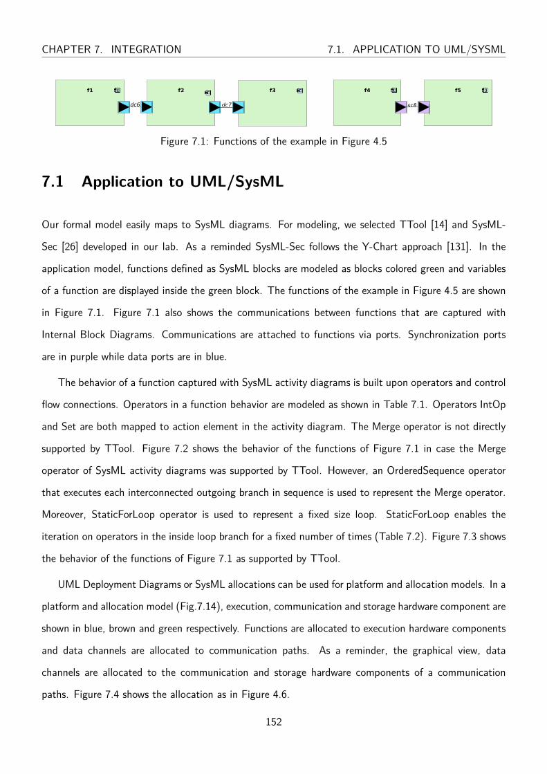
CHAPTER 7. INTEGRATION 7.1. APPLICATION TO UML/SYSML
f1 f3 f4f2 f5
dc6 dc7 sc8
Figure 7.1: Functions of the example in Figure 4.5
7.1 Application to UML/SysML
Our formal model easily maps to SysML diagrams. For modeling, we selected TTool [14] and SysML-
Sec [26] developed in our lab. As a reminded SysML-Sec follows the Y-Chart approach [131]. In the
application model, functions defined as SysML blocks are modeled as blocks colored green and variables
of a function are displayed inside the green block. The functions of the example in Figure 4.5 are shown
in Figure 7.1. Figure 7.1 also shows the communications between functions that are captured with
Internal Block Diagrams. Communications are attached to functions via ports. Synchronization ports
are in purple while data ports are in blue.
The behavior of a function captured with SysML activity diagrams is built upon operators and control
flow connections. Operators in a function behavior are modeled as shown in Table 7.1. Operators IntOp
and Set are both mapped to action element in the activity diagram. The Merge operator is not directly
supported by TTool. Figure 7.2 shows the behavior of the functions of Figure 7.1 in case the Merge
operator of SysML activity diagrams was supported by TTool. However, an OrderedSequence operator
that executes each interconnected outgoing branch in sequence is used to represent the Merge operator.
Moreover, StaticForLoop operator is used to represent a fixed size loop. StaticForLoop enables the
iteration on operators in the inside loop branch for a fixed number of times (Table 7.2). Figure 7.3 shows
the behavior of the functions of Figure 7.1 as supported by TTool.
UML Deployment Diagrams or SysML allocations can be used for platform and allocation models. In a
platform and allocation model (Fig.7.14), execution, communication and storage hardware component are
shown in blue, brown and green respectively. Functions are allocated to execution hardware components
and data channels are allocated to communication paths. As a reminder, the graphical view, data
channels are allocated to the communication and storage hardware components of a communication
paths. Figure 7.4 shows the allocation as in Figure 4.6.
152
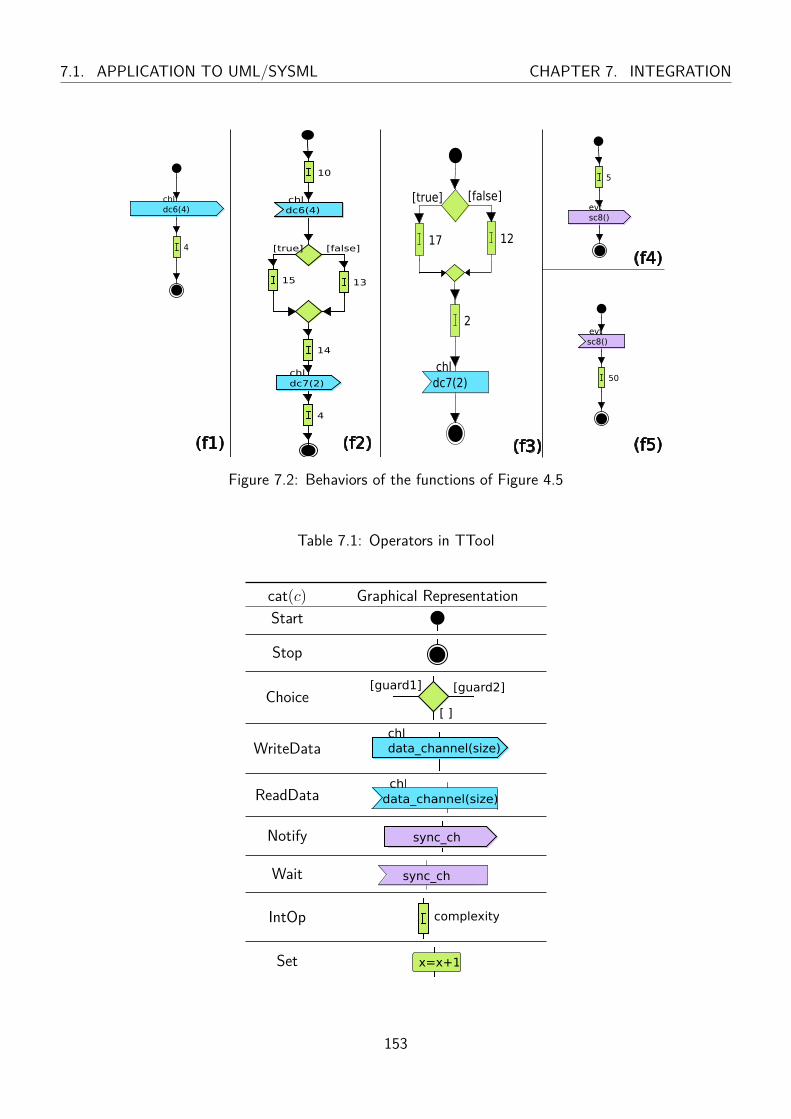
7.1. APPLICATION TO UML/SYSML CHAPTER 7. INTEGRATION
10
[true] [false]
15 13
14
chldc6(4)
chldc7(2)
4
chldc6(4)
417
[true] [false]
2
12
chldc7(2)
5
evtsc8()
evtsc8()
50
(f1) (f2) (f3)
(f4)
(f5)
Figure 7.2: Behaviors of the functions of Figure 4.5
Table 7.1: Operators in TTool
cat(c) Graphical RepresentationStart
Stop
Choice[guard1] [guard2]
[ ]
WriteDatachldata_channel(size)
ReadDatachldata_channel(size)
Notify sync_ch
Wait sync_ch
IntOp complexity
Set x=x+1
153

CHAPTER 7. INTEGRATION 7.1. APPLICATION TO UML/SYSML
10
[true] [false]
[ ]
15 13
>>
14
chldc6(4)
chldc7(2)
4
chldc6(4)
4
17
[true] [ ]
[false]
>>
2
12
chldc7(2)
5
evtsc8()
evtsc8()
50
(f1) (f2)
(f3)
(f4) (f5)
Figure 7.3: Behaviors of the functions of Figure 4.5 in TTool154

7.1. APPLICATION TO UML/SYSML CHAPTER 7. INTEGRATION
Table 7.2: OrderedSequence and StaticForLoop operators in TTool
Operator Graphical RepresentationOrderedSequence >>
branch1 branch2 branch3
StaticForLoop Loop 10 timesinside loop
exit loop
<<MEMORY>>h45
f::dc7
channel
f::dc6
channel
<<CPURRPB>>h41
f::f2f::f1
<<CPURR>>h42
f::f3
<<BUS-RR>>h44
f::dc6
channel
f::dc7
channel
<<CPU>>h43
f::f5f::f4
Figure 7.4: A possible allocation of the application model given in the example in Figure 4.6
155
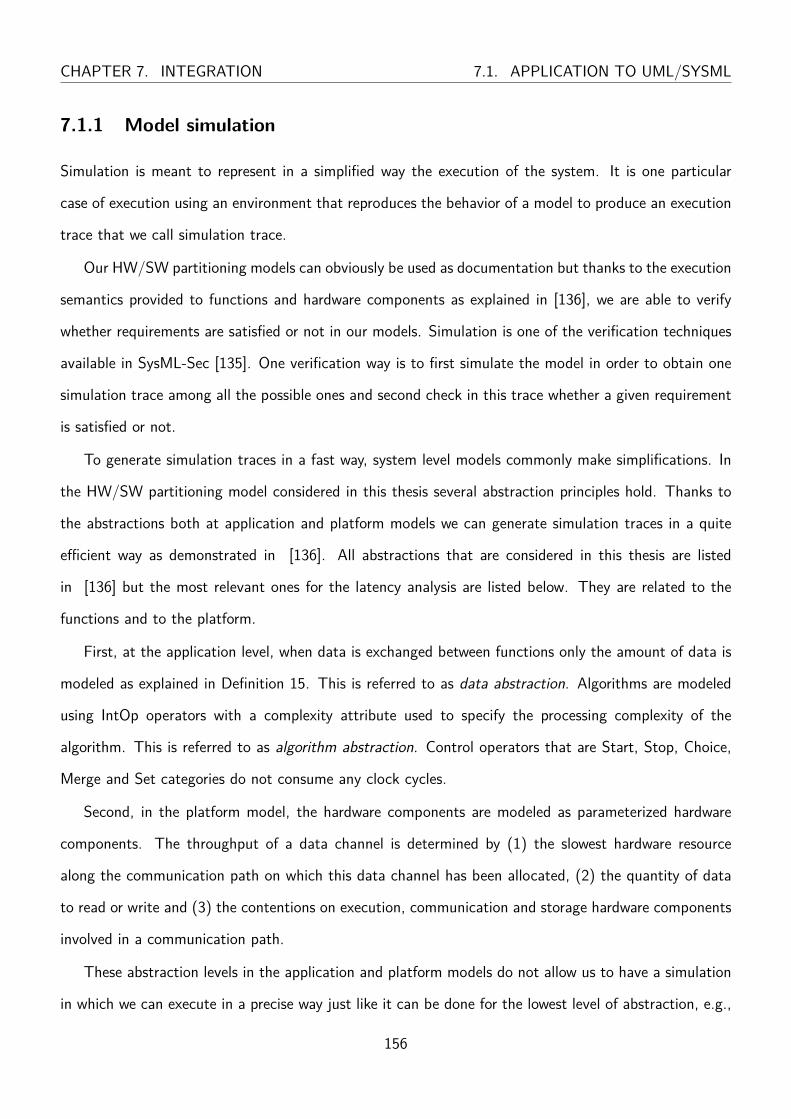
CHAPTER 7. INTEGRATION 7.1. APPLICATION TO UML/SYSML
7.1.1 Model simulation
Simulation is meant to represent in a simplified way the execution of the system. It is one particular
case of execution using an environment that reproduces the behavior of a model to produce an execution
trace that we call simulation trace.
Our HW/SW partitioning models can obviously be used as documentation but thanks to the execution
semantics provided to functions and hardware components as explained in [136], we are able to verify
whether requirements are satisfied or not in our models. Simulation is one of the verification techniques
available in SysML-Sec [135]. One verification way is to first simulate the model in order to obtain one
simulation trace among all the possible ones and second check in this trace whether a given requirement
is satisfied or not.
To generate simulation traces in a fast way, system level models commonly make simplifications. In
the HW/SW partitioning model considered in this thesis several abstraction principles hold. Thanks to
the abstractions both at application and platform models we can generate simulation traces in a quite
efficient way as demonstrated in [136]. All abstractions that are considered in this thesis are listed
in [136] but the most relevant ones for the latency analysis are listed below. They are related to the
functions and to the platform.
First, at the application level, when data is exchanged between functions only the amount of data is
modeled as explained in Definition 15. This is referred to as data abstraction. Algorithms are modeled
using IntOp operators with a complexity attribute used to specify the processing complexity of the
algorithm. This is referred to as algorithm abstraction. Control operators that are Start, Stop, Choice,
Merge and Set categories do not consume any clock cycles.
Second, in the platform model, the hardware components are modeled as parameterized hardware
components. The throughput of a data channel is determined by (1) the slowest hardware resource
along the communication path on which this data channel has been allocated, (2) the quantity of data
to read or write and (3) the contentions on execution, communication and storage hardware components
involved in a communication path.
These abstraction levels in the application and platform models do not allow us to have a simulation
in which we can execute in a precise way just like it can be done for the lowest level of abstraction, e.g.,
156

7.2. PLAN INTEGRATION INTO TTOOL CHAPTER 7. INTEGRATION
Figure 7.5: Save simulation trace in XML format
cycle-accurate, bit accurate (CABA) [52].
From the simulation interface of TTool, the simulation trace can be saved in different formats includ-
ing VCD, HTML, txt and XML format (Figure 7.5). In the scope of this thesis, we are interested in the
XML format. Having the simulation data stored in XML format facilitates its analysis and manipulation.
This XML saved simulation trace forms an input to the PLAN approach.
7.2 PLAN integration into TTool
We chose to integrate PLAN into TTool as it captures our model by SysML diagrams and simulates it.
Moreover, TTool is free and open source and it is developed in our lab. The designer can instantiate
PLAN from TTool graphical interface or from the command line.
When using the graphical interface, PLAN is instantiated on a saved XML simulation trace. Each
simulation trace contains the name of its corresponding model. Thus, the simulation trace and its
corresponding model are taken as inputs for PLAN. The PLAN user interface opens in a separate window
as the corresponding dependency graph is generated in the background (Figure 7.6). To construct the
graph, we used jGraphT [167] a Java library. A progress bar shows the progress of graph generation and
a message is displayed when the graph is successfully generated indicating the number of vertexes and
edges of the graph.
157
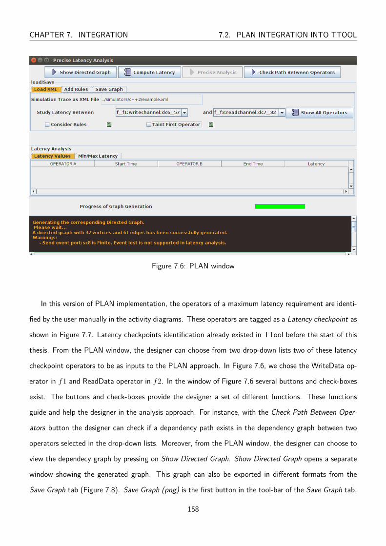
CHAPTER 7. INTEGRATION 7.2. PLAN INTEGRATION INTO TTOOL
Figure 7.6: PLAN window
In this version of PLAN implementation, the operators of a maximum latency requirement are identi-
fied by the user manually in the activity diagrams. These operators are tagged as a Latency checkpoint as
shown in Figure 7.7. Latency checkpoints identification already existed in TTool before the start of this
thesis. From the PLAN window, the designer can choose from two drop-down lists two of these latency
checkpoint operators to be as inputs to the PLAN approach. In Figure 7.6, we chose the WriteData op-
erator in f1 and ReadData operator in f2. In the window of Figure 7.6 several buttons and check-boxes
exist. The buttons and check-boxes provide the designer a set of different functions. These functions
guide and help the designer in the analysis approach. For instance, with the Check Path Between Oper-
ators button the designer can check if a dependency path exists in the dependency graph between two
operators selected in the drop-down lists. Moreover, from the PLAN window, the designer can choose to
view the dependecy graph by pressing on Show Directed Graph. Show Directed Graph opens a separate
window showing the generated graph. This graph can also be exported in different formats from the
Save Graph tab (Figure 7.8). Save Graph (png) is the first button in the tool-bar of the Save Graph tab.
158
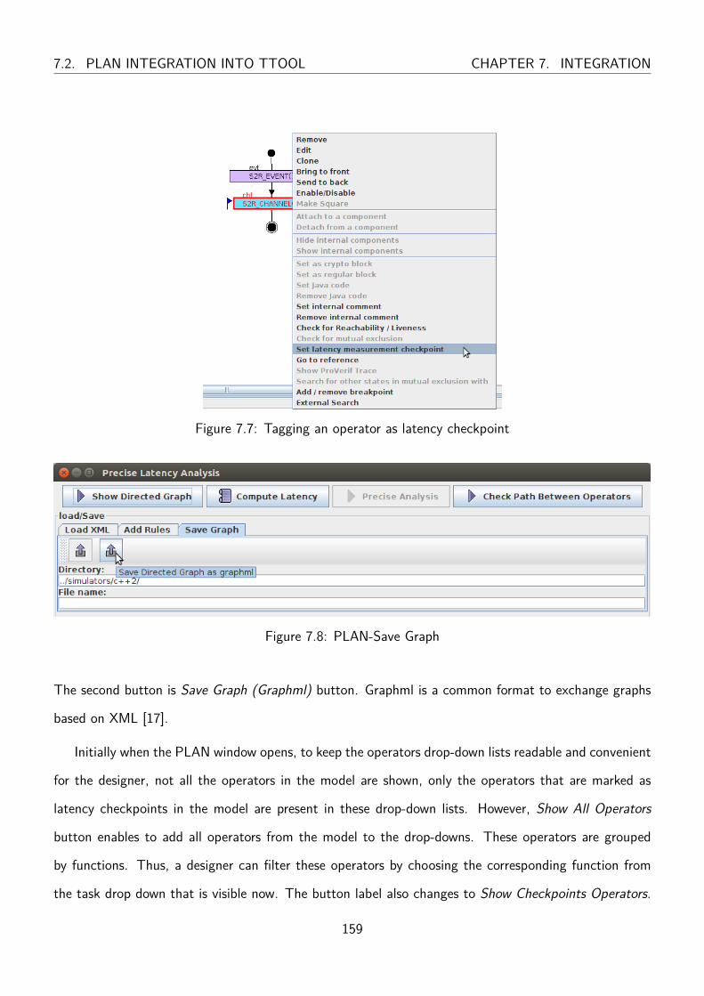
7.2. PLAN INTEGRATION INTO TTOOL CHAPTER 7. INTEGRATION
Figure 7.7: Tagging an operator as latency checkpoint
Figure 7.8: PLAN-Save Graph
The second button is Save Graph (Graphml) button. Graphml is a common format to exchange graphs
based on XML [17].
Initially when the PLAN window opens, to keep the operators drop-down lists readable and convenient
for the designer, not all the operators in the model are shown, only the operators that are marked as
latency checkpoints in the model are present in these drop-down lists. However, Show All Operators
button enables to add all operators from the model to the drop-downs. These operators are grouped
by functions. Thus, a designer can filter these operators by choosing the corresponding function from
the task drop down that is visible now. The button label also changes to Show Checkpoints Operators.
159
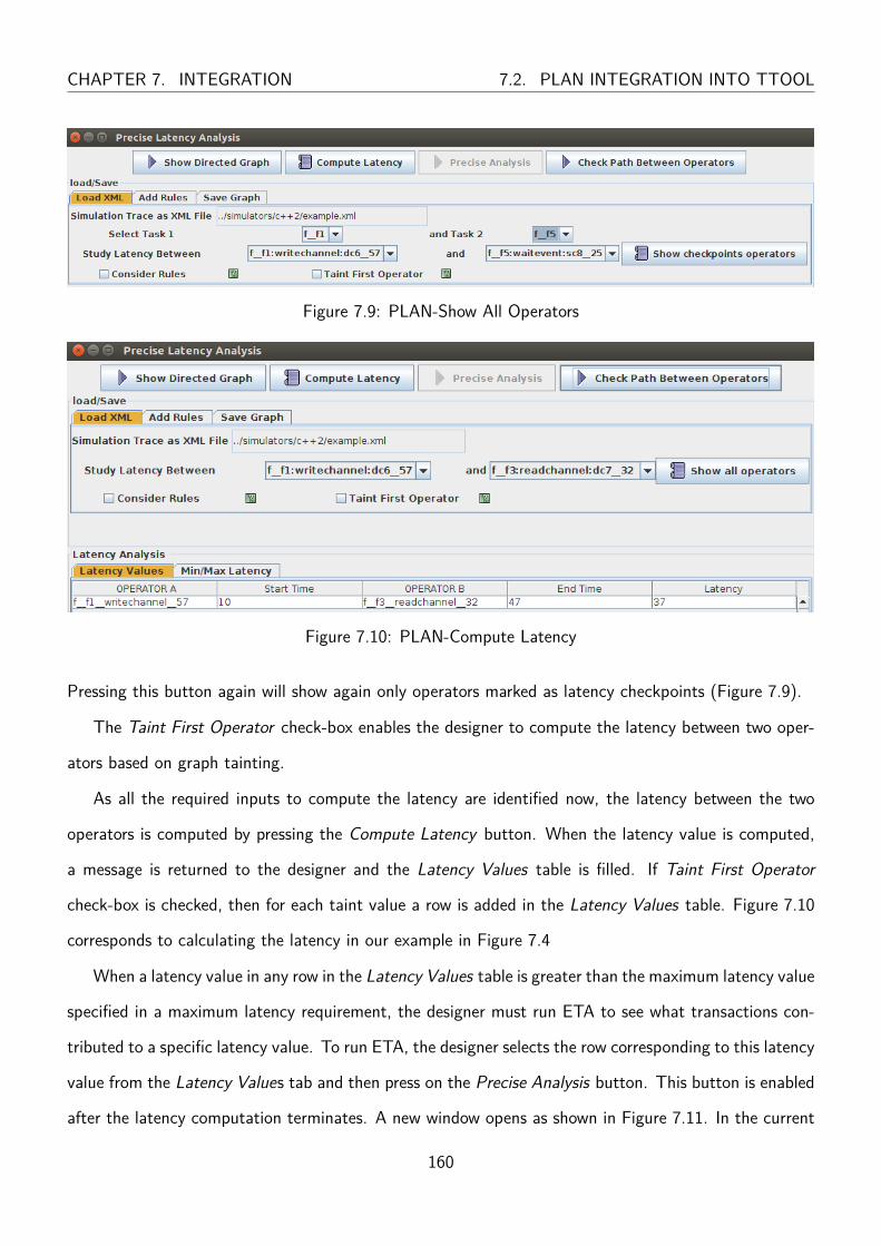
CHAPTER 7. INTEGRATION 7.2. PLAN INTEGRATION INTO TTOOL
Figure 7.9: PLAN-Show All Operators
Figure 7.10: PLAN-Compute Latency
Pressing this button again will show again only operators marked as latency checkpoints (Figure 7.9).
The Taint First Operator check-box enables the designer to compute the latency between two oper-
ators based on graph tainting.
As all the required inputs to compute the latency are identified now, the latency between the two
operators is computed by pressing the Compute Latency button. When the latency value is computed,
a message is returned to the designer and the Latency Values table is filled. If Taint First Operator
check-box is checked, then for each taint value a row is added in the Latency Values table. Figure 7.10
corresponds to calculating the latency in our example in Figure 7.4
When a latency value in any row in the Latency Values table is greater than the maximum latency value
specified in a maximum latency requirement, the designer must run ETA to see what transactions con-
tributed to a specific latency value. To run ETA, the designer selects the row corresponding to this latency
value from the Latency Values tab and then press on the Precise Analysis button. This button is enabled
after the latency computation terminates. A new window opens as shown in Figure 7.11. In the current
160

7.2. PLAN INTEGRATION INTO TTOOL CHAPTER 7. INTEGRATION
Figure 7.11: PLAN classification output for a latency value
implementation of ETA, the transactions in MandatoryOP and OptionalOP sets are referred to as
Mandatory Transactions. The other transactions are referred to as Non-Mandatory Transactions. Among
the Non-Mandatory Transactions, the transactions in MandatoryFunc, OptionalFunc, Contention
and NoContention sets are identified. The transactions in MandatoryFunc and OptionalFunc are
referred to as Functions Transactions. To identify transactions in the Contention set, we referred to an
attribute returned by the simulator named the runnableTime attribute which is the point in time when
the operator is ready to execute as the best case execution time.
In the window in Figure 7.11, the simulation transactions that are considered as mandatory are listed
in the Mandatory Transaction panel and those that are not mandatory are listed in the Non-Mandatory
Transaction panel. For each of these transactions, the hardware on which they are executed, the start
time and end time are also displayed. In the third panel of this window, a table is shown. In this table,
each row corresponds to one hardware component in the system and each column represents a one-
time slot in the simulation. Transactions are placed according to when and where they were executed.
The mandatory transactions are displayed in green, the non-mandatory transactions that contributed to
increasing the latency value due to contentions are colored red, the functions transactions are colored
gray and those that are not mandatory but did not belong to the previous sets (i.e., NoContention) are
colored orange. In our example, as shown previously in the formal definitions, the IntOp operator in f1
161
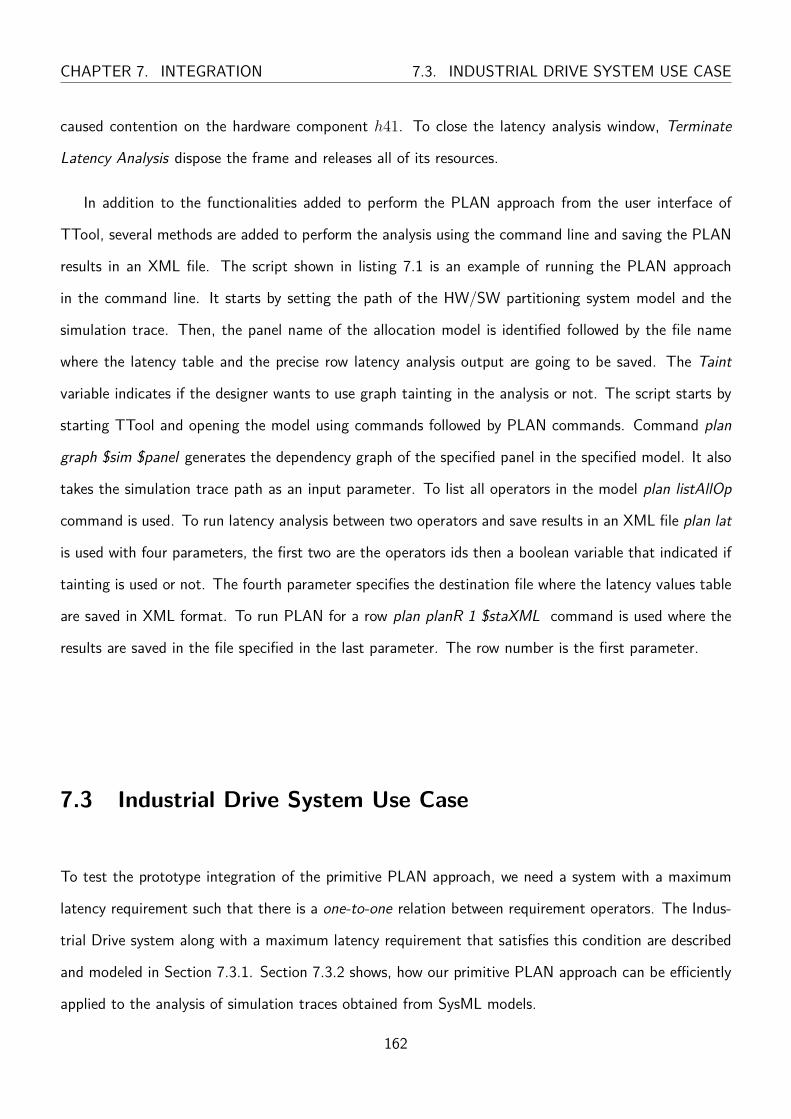
CHAPTER 7. INTEGRATION 7.3. INDUSTRIAL DRIVE SYSTEM USE CASE
caused contention on the hardware component h41. To close the latency analysis window, Terminate
Latency Analysis dispose the frame and releases all of its resources.
In addition to the functionalities added to perform the PLAN approach from the user interface of
TTool, several methods are added to perform the analysis using the command line and saving the PLAN
results in an XML file. The script shown in listing 7.1 is an example of running the PLAN approach
in the command line. It starts by setting the path of the HW/SW partitioning system model and the
simulation trace. Then, the panel name of the allocation model is identified followed by the file name
where the latency table and the precise row latency analysis output are going to be saved. The Taint
variable indicates if the designer wants to use graph tainting in the analysis or not. The script starts by
starting TTool and opening the model using commands followed by PLAN commands. Command plan
graph $sim $panel generates the dependency graph of the specified panel in the specified model. It also
takes the simulation trace path as an input parameter. To list all operators in the model plan listAllOp
command is used. To run latency analysis between two operators and save results in an XML file plan lat
is used with four parameters, the first two are the operators ids then a boolean variable that indicated if
tainting is used or not. The fourth parameter specifies the destination file where the latency values table
are saved in XML format. To run PLAN for a row plan planR 1 $staXML command is used where the
results are saved in the file specified in the last parameter. The row number is the first parameter.
7.3 Industrial Drive System Use Case
To test the prototype integration of the primitive PLAN approach, we need a system with a maximum
latency requirement such that there is a one-to-one relation between requirement operators. The Indus-
trial Drive system along with a maximum latency requirement that satisfies this condition are described
and modeled in Section 7.3.1. Section 7.3.2 shows, how our primitive PLAN approach can be efficiently
applied to the analysis of simulation traces obtained from SysML models.
162

7.3. INDUSTRIAL DRIVE SYSTEM USE CASE CHAPTER 7. INTEGRATION
Listing 7.1: PLAN Command Line Script#modelset model ./../ttool/GraphTestModel.xml#simulation traceset sim ./../ttool/graphTestSimulationTrace.xml#model panelset panel Architecture2#latency table output destinationset latXML latOutput.xml#precise row latency analysis output destinationset staXML staOutput.xml#indicated if the tainting is used or notset taint true# start ttoolaction startwait 2#open modelaction open $modelwait 4#generate graph for specific panel in the modelplan graph $sim $panel# list all operators idplan listAllOp# run latency analysis between two operators and save results in xmlplan lat 44 26 $taint $latXML# run precise analysis for one row an save the results in xmlplan planR 1 $staXML
163
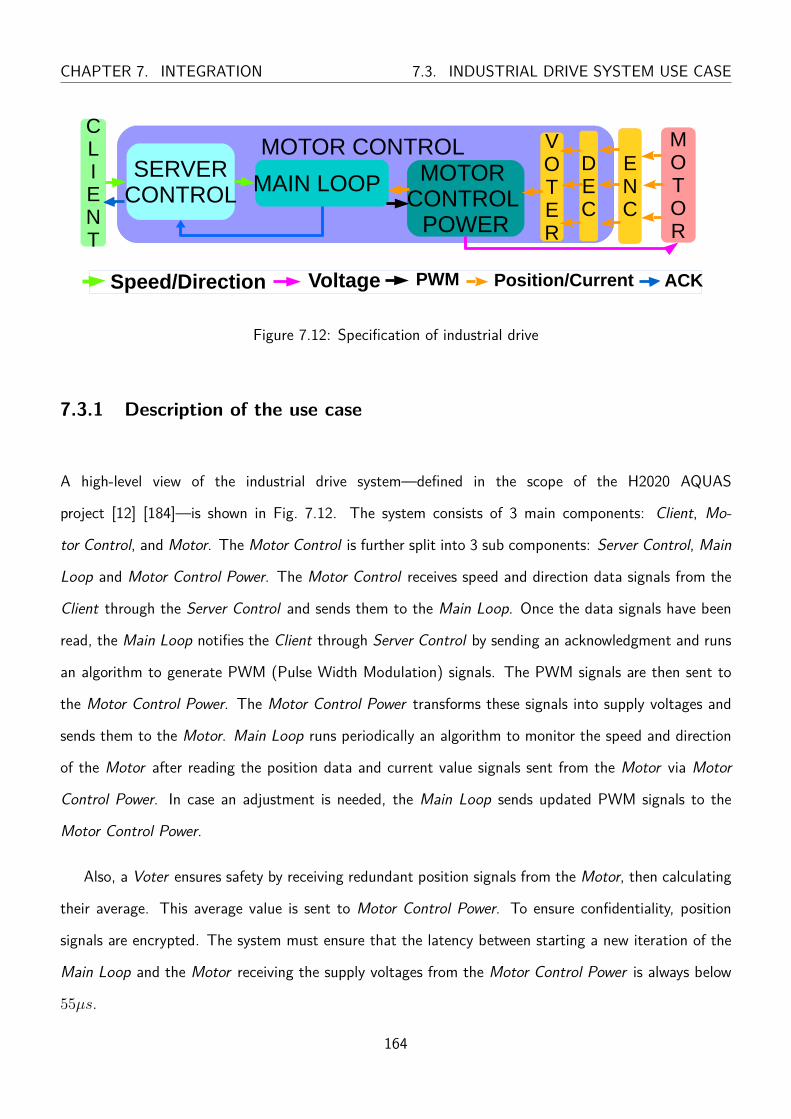
CHAPTER 7. INTEGRATION 7.3. INDUSTRIAL DRIVE SYSTEM USE CASE
MOTOR CONTROL CLIENT
MOTOR
SERVERCONTROL MAIN LOOP MOTOR
CONTROL POWER
Speed/Direction Voltage Position/CurrentPWM
ENC
ENC
DEC
VOTER
ACK
Figure 7.12: Specification of industrial drive
7.3.1 Description of the use case
A high-level view of the industrial drive system—defined in the scope of the H2020 AQUAS
project [12] [184]—is shown in Fig. 7.12. The system consists of 3 main components: Client, Mo-
tor Control, and Motor. The Motor Control is further split into 3 sub components: Server Control, Main
Loop and Motor Control Power. The Motor Control receives speed and direction data signals from the
Client through the Server Control and sends them to the Main Loop. Once the data signals have been
read, the Main Loop notifies the Client through Server Control by sending an acknowledgment and runs
an algorithm to generate PWM (Pulse Width Modulation) signals. The PWM signals are then sent to
the Motor Control Power. The Motor Control Power transforms these signals into supply voltages and
sends them to the Motor. Main Loop runs periodically an algorithm to monitor the speed and direction
of the Motor after reading the position data and current value signals sent from the Motor via Motor
Control Power. In case an adjustment is needed, the Main Loop sends updated PWM signals to the
Motor Control Power.
Also, a Voter ensures safety by receiving redundant position signals from the Motor, then calculating
their average. This average value is sent to Motor Control Power. To ensure confidentiality, position
signals are encrypted. The system must ensure that the latency between starting a new iteration of the
Main Loop and the Motor receiving the supply voltages from the Motor Control Power is always below
55µs.
164
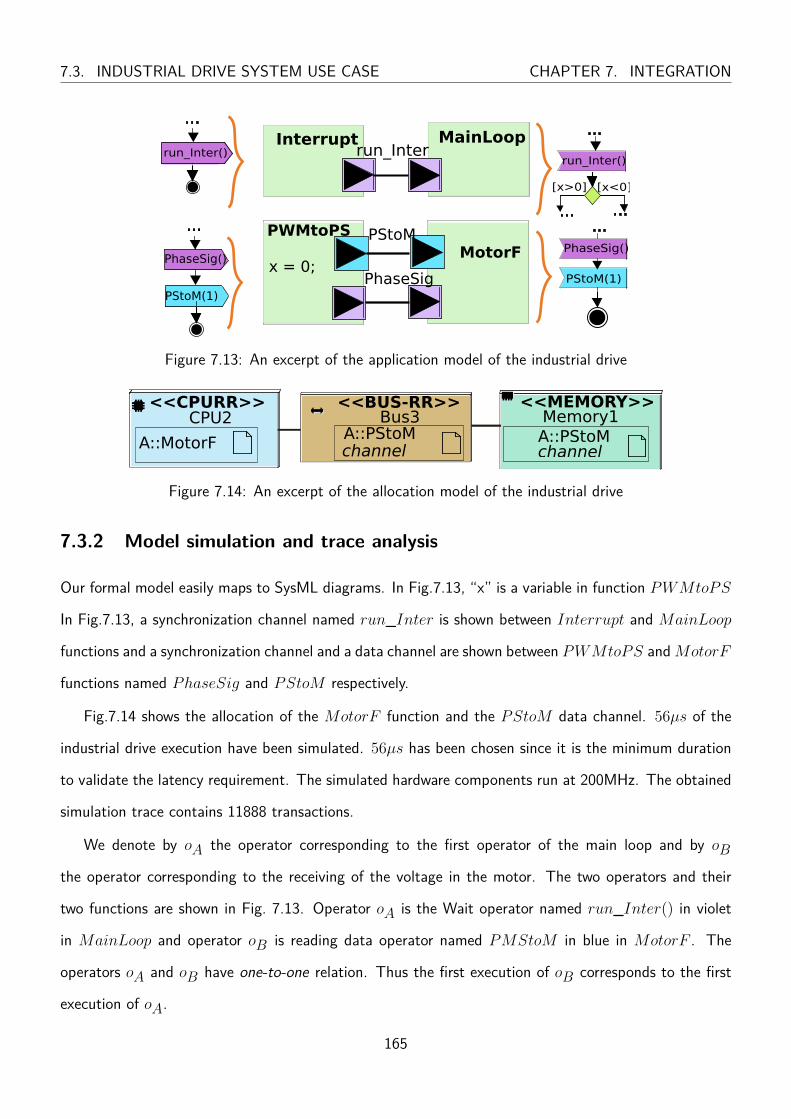
7.3. INDUSTRIAL DRIVE SYSTEM USE CASE CHAPTER 7. INTEGRATION
Interrupt MainLooprun_Inter()
...
PWMtoPSMotorF
PhaseSig
PStoMPhaseSig()
PStoM(1)x = 0;
...
...
[x>0] [x<0]
... ......
PStoM(1)
PhaseSig()
run_Interrun_Inter()
Figure 7.13: An excerpt of the application model of the industrial drive
<<BUS-RR>>Bus3
A::PStoMchannel
<<CPURR>>CPU2
A::MotorF
<<MEMORY>>Memory1A::PStoMchannel
Figure 7.14: An excerpt of the allocation model of the industrial drive
7.3.2 Model simulation and trace analysis
Our formal model easily maps to SysML diagrams. In Fig.7.13, “x” is a variable in function PWMtoPS
In Fig.7.13, a synchronization channel named run_Inter is shown between Interrupt and MainLoop
functions and a synchronization channel and a data channel are shown between PWMtoPS andMotorF
functions named PhaseSig and PStoM respectively.
Fig.7.14 shows the allocation of the MotorF function and the PStoM data channel. 56µs of the
industrial drive execution have been simulated. 56µs has been chosen since it is the minimum duration
to validate the latency requirement. The simulated hardware components run at 200MHz. The obtained
simulation trace contains 11888 transactions.
We denote by oA the operator corresponding to the first operator of the main loop and by oBthe operator corresponding to the receiving of the voltage in the motor. The two operators and their
two functions are shown in Fig. 7.13. Operator oA is the Wait operator named run_Inter() in violet
in MainLoop and operator oB is reading data operator named PMStoM in blue in MotorF . The
operators oA and oB have one-to-one relation. Thus the first execution of oB corresponds to the first
execution of oA.
165

CHAPTER 7. INTEGRATION 7.3. INDUSTRIAL DRIVE SYSTEM USE CASE
Figure 7.15: PLAN output showing contention
Figure 7.16: PLAN output showing no contention
The start time of toA,1 in the simulation trace is “2” and the end time of the toB ,1 is “11115”.
Thus, the latency in this case is 11113 cycles (i.e., 55.56µs). Thus, the requirement is not satisfied, thus
leading to use PLAN. PLAN is implemented in TTool: the transactions are classified and displayed in a
table. Transactions in the graphical table (e.g., Fig. 7.15) are displayed according to the hardware that
executed them and the time of execution. Since transactions are colored according to their category,
contention transactions are easy to identify. For example, transactions in MandatoryOp set are colored
in green, those in Contention, NoContention and MandatoryFunc sets are colored in red, orange
and gray respectively. In our use case, after generating a dependency graph of 552 vertexes and 965
edges and running the execution trace analysis, contentions were spotted on the execution hardware
component on which the Motor Control functions are allocated (Fig. 7.15). The contention is due to
the Server Control function processing data to write acknowledgment to the Client while the encryption
function was ready to execute but its the resource was busy.
To resolve this execution contention, an execution hardware component is added to the platform and
the Server Control function is now allocated to it. Running PLAN again, the latency is now equal to
10604 cycles (i.e., 53.02µs) since the start time of toA,1 is noted as 2 and the end time of the toB ,1is 10606. Thus, the latency requirement is satisfied. To see how the transaction classifications changed
between the two models, we used PLAN even though the requirement was satisfied. The output in
Fig. 7.16 reveals that no contention was detected and that the Server Control function could process
data to write acknowledgment to the Client while the decryption function was executing.
166

7.4. RAIL CARRIAGE MECHANISMS USE CASE CHAPTER 7. INTEGRATION
7.4 Rail Carriage Mechanisms Use Case
After analyzing a use case that satisfies the assumptions of primitive PLAN approach, in this section we
would like to test the prototype integration of the advanced PLAN approach. To illustrate the benefits of
graph tainting we use the Rail Carriage Mechanisms use case defined in the scope of the H2020 AQUAS
project [12], with a focus on the control of automatic platform gates. The Rail Carriage Mechanisms
system along with a maximum latency requirement are described and modeled in Section 7.4.1. Sec-
tion 7.4.2 shows how our advanced PLAN approach can be efficiently applied to the analysis of simulation
traces to assist in adjusting the model to satisfy requirements.
7.4.1 Description of the use case
The Rail Carriage Mechanisms system consists of Lidars with their processing units, a main computing
unit, a relay and a PSD (Platform Screen Doors) controller. The Lidars are divided in two categories.
Positioning Lidars scan for a train presence and door Lidars scan the train doors to determine their status.
The processing unit of the positioning Lidars calculates the position and the speed of the train once it is
present while the processing unit of the door Lidars detects the state of doors e.g. opening, open, closing
and closed. The main computing unit gathers data from the Lidars processing units and issues orders to
relays to open or close the platform screening doors. This open/close authorization is sent to the PSD
controller through the relay.
Our design captures four Lidars (2 positioning Lidars and 2 door Lidars). We also consider the four
following requirements:
1. Req_1: The delay between sending the data from the positioning Lidar and the relay receiving
the order from the main computing unit shall be less than 130ms (safety requirement)
2. Req_2: The delay between sending the data from the positioning Lidar and processing it in the
corresponding processing unit shall be less than 85ms. (safety requirement)
3. Req_3: Data sent from the Lidars processing units (speed and direction, or door status) to the
main computing unit should remain authentic (security requirement)
167

CHAPTER 7. INTEGRATION 7.4. RAIL CARRIAGE MECHANISMS USE CASE
4. Req_4: Data sent from the Lidars to their corresponding processing units should remain confi-
dential (security requirement)
7.4.1.1 HW/SW partitioning models
Figure 7.17 shows the functional view of the use case where only one Lidar is presented. The function
PL1 is used to represent sending data by the first positioning Lidar. PL1 sends 1 frame of data once
triggered by triggerPL1 every 67ms. This frame is received by another primitive component named
F1_1and2_PL1 where the frame is copied to the algorithm buffer then checked for validity by checking
its length and CRC calculation. After being checked, a detection algorithm is run that includes rotational
mapping, filters and pattern detection. The computation complexity of this algorithm is modeled in the
activity diagram using complexity operators. F1_3_PL1 reads the output of the detection algorithm,
runs CRC calculation and sends a message to the F3_1_MsgAcquisition component. F1_3_PL1 is
triggered every 50ms. F1_1and2_PL1 and F1_3_PL1 represent the functionality of the positioning
lidar processing unit. All these blocks are duplicated for the 3 remaining Lidars. The door Lidars are
triggered every 20ms.
F3_1_MsgAcquisition is a function in a composite component named SafetyComponent. In TTool,
composite components (colored in yellow) serve as containers for functions. F3_1_MsgAcquisition
reads data from F1_3_PL1. The same applies for the data received from the other 3 Lidars pro-
cessing unit functions. In the composite component SafetyComponent, another primitive component
named F3_2_MsgAcquisition_SafePart is a redundant function added to the model to ensure safety.
F3_2_MsgAcquisition_SafePart is triggered every 50ms. It runs a validity check and a sequence algo-
rithm (represented by computation complexity) to compute the adequate result to be sent to Relay. The
later is triggered every 33 ms.
The architecture of the system is as follows. Each Lidar is captured by its own set of processors, buses,
memories, while the safety platform is built upon a CPU (MainCPU) and 2 memories: MainMemory and
RelayMemory. The mapping model associates LIDAR blocks triggerPL1, PL1, F1_1and2_PL1 and
F1_3_PL1 and their communications to their corresponding hardware while safety blocks are mapped
to MainCPU. A share memory helps exchanging data between a MainCPU and Relay.
168
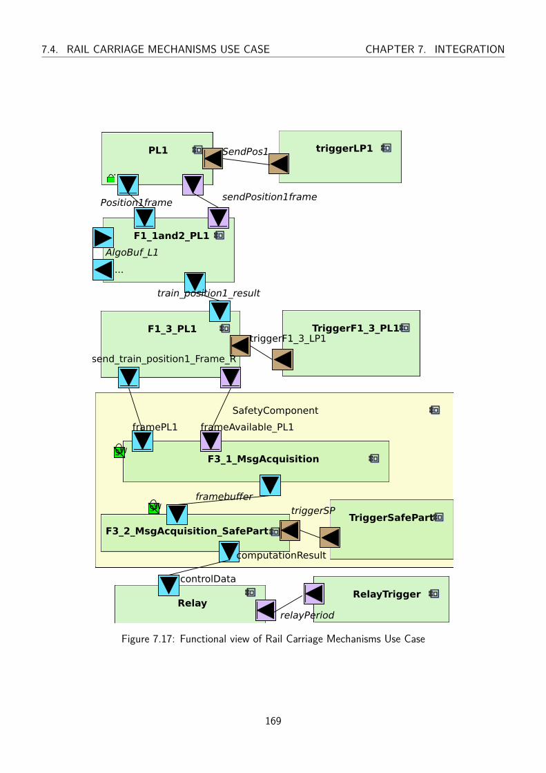
7.4. RAIL CARRIAGE MECHANISMS USE CASE CHAPTER 7. INTEGRATION
SafetyComponent
F3_1_MsgAcquisition
frameAvailable_PL1framePL1
F3_2_MsgAcquisition_SafePart
computationResult
TriggerSafePart
TriggerF1_3_PL1triggerF1_3_LP1
F1_1and2_PL1
...
PL1
...
Relay
controlData
triggerLP1
F1_3_PL1
send_train_position1_Frame_R
RelayTrigger
SendPos1
sendPosition1framePosition1frame
AlgoBuf_L1
train_position1_result
framebuffer
relayPeriod
triggerSP
SW
SW
Figure 7.17: Functional view of Rail Carriage Mechanisms Use Case
169
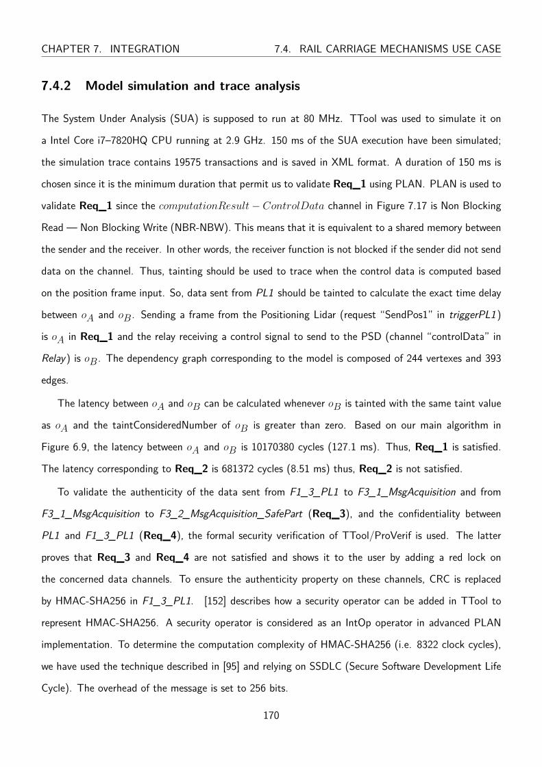
CHAPTER 7. INTEGRATION 7.4. RAIL CARRIAGE MECHANISMS USE CASE
7.4.2 Model simulation and trace analysis
The System Under Analysis (SUA) is supposed to run at 80 MHz. TTool was used to simulate it on
a Intel Core i7–7820HQ CPU running at 2.9 GHz. 150 ms of the SUA execution have been simulated;
the simulation trace contains 19575 transactions and is saved in XML format. A duration of 150 ms is
chosen since it is the minimum duration that permit us to validate Req_1 using PLAN. PLAN is used to
validate Req_1 since the computationResult− ControlData channel in Figure 7.17 is Non Blocking
Read — Non Blocking Write (NBR-NBW). This means that it is equivalent to a shared memory between
the sender and the receiver. In other words, the receiver function is not blocked if the sender did not send
data on the channel. Thus, tainting should be used to trace when the control data is computed based
on the position frame input. So, data sent from PL1 should be tainted to calculate the exact time delay
between oA and oB . Sending a frame from the Positioning Lidar (request “SendPos1” in triggerPL1)
is oA in Req_1 and the relay receiving a control signal to send to the PSD (channel “controlData” in
Relay) is oB . The dependency graph corresponding to the model is composed of 244 vertexes and 393
edges.
The latency between oA and oB can be calculated whenever oB is tainted with the same taint value
as oA and the taintConsideredNumber of oB is greater than zero. Based on our main algorithm in
Figure 6.9, the latency between oA and oB is 10170380 cycles (127.1 ms). Thus, Req_1 is satisfied.
The latency corresponding to Req_2 is 681372 cycles (8.51 ms) thus, Req_2 is not satisfied.
To validate the authenticity of the data sent from F1_3_PL1 to F3_1_MsgAcquisition and from
F3_1_MsgAcquisition to F3_2_MsgAcquisition_SafePart (Req_3), and the confidentiality between
PL1 and F1_3_PL1 (Req_4), the formal security verification of TTool/ProVerif is used. The latter
proves that Req_3 and Req_4 are not satisfied and shows it to the user by adding a red lock on
the concerned data channels. To ensure the authenticity property on these channels, CRC is replaced
by HMAC-SHA256 in F1_3_PL1. [152] describes how a security operator can be added in TTool to
represent HMAC-SHA256. A security operator is considered as an IntOp operator in advanced PLAN
implementation. To determine the computation complexity of HMAC-SHA256 (i.e. 8322 clock cycles),
we have used the technique described in [95] and relying on SSDLC (Secure Software Development Life
Cycle). The overhead of the message is set to 256 bits.
170
7.4. RAIL CARRIAGE MECHANISMS USE CASE CHAPTER 7. INTEGRATION
To ensure the confidentiality property on the channel between PL1 and F1_3_PL1 (Req_4) encryp-
tion/decryption operators are added. Also encryption/decryption operators are considered as an IntOp
operator in advanced PLAN implementation. We chose the AES algorithm in Cipher Block Chaining
(CBC) mode and set the computational complexity to 3000 as indicated in [95].
By adding authenticity and confidentiality mechanisms, we could formally prove that Req_3 and
Req_4 are now satisfied. The concerned data channels are annotated with green locks in figure 7.17. In
TTool, channels can be either private or public and only attacks on public channels are considered [155].
We run again PLAN along with its new model and new simulation trace. The time delay corresponding
to Req_1 is now 10249025 cycles (128.1 ms) while the time delay corresponding to Req_2 is 683551
cycles (8.54 ms). From the classification sets, we notice that the increase of the time delay of Req_2
is due to the added encryption/decryption operators and the increase of the time delay of Req_1 is due
to the scheduling policy of the mainCPU.
To satisfy Req_2 while keeping the confidentiality property of Req_4 valid, we replace AES CBC
with AES CTR (counter mode). The computational complexity is now set to 428 cycles. This value is
obtained by applying the same interaction as indicated in [95]. The security verification indicates that
the confidentiality property still holds. The latency was recalculated in a similar manner as mentioned
before. The maximum delay corresponding to Req_2 now is 678029 cycles (8.47 ms). The maximum
delay of Req_1 was not effected as the latency for Req_1 depend on the trigger time and scheduling
policy of mainCPU.
Table 7.3 summarizes the result of each requirement along each tested model in this use case. While
replacing AES CBC with AES CTR mode enhanced performance by decreasing the latency proportionally
to the decrease in the computational complexity cycles, several other methods can be tested in case
further performance enhancement is required, e.g. by adding hardware accelerators for cryptographic
functions, by using other security algorithms, by trying a different mapping, by adjusting the scheduling
policy of CPUs or buses, of by using more powerful processing units, . . . . After applying the required
enhancements, the designer can simulate the model and run the verification process again to test if the
requirements still hold.
171

CHAPTER 7. INTEGRATION 7.5. CONCLUSION
Table 7.3: Requirement Satisfaction Summary Table
Security Req 1 Req 2 Req 3 Req 4CRC Yes No No No
HMAC + AES CBC Yes No Yes YesHMAC + AES CTR Yes Yes Yes Yes
7.5 Conclusion
In this chapter, we presented the integration of the PLAN approach into TTool. First, we showed that the
toy example we used in the previous chapters can be modeled and simulated in TTool. Then, we analyzed
a simulation trace of this toy example model with the implemented primitive PLAN approach. This
analysis revealed the expected results for the latency computation and the classification of transactions.
Thus, the root cause of the latency violation in this example matched the expected results.
Moreover, we test the implemented primitive PLAN approach on Industrial Drive system. Using
PLAN output we were able to detect contention on a hardware component. This contention was the
main reason for latency requirement violation. Knowing the reason behind the latency value enabled us to
enhance the system model. While we chose to add a new hardware component and update the allocation
model, a designer can decide to test other alternatives to see how it affect the latency value. However,
we expect the alternative solutions a designer might choose to be guided by the PLAN approach output.
As a reminder, PLAN approach outputs classification sets that reveal the root cause of a latency value
based on dependencies between the system model elements and the causality between transactions in an
execution trace.
In the Industrial Drive system, the primitive PLAN approach could be applied as the one-to-one
relation between the requirement operators hold. However, for Rail Carriage Mechanisms use case,
the requirement operators do not respect this relation. So, we used the implemented prototype of the
advanced PLAN approach. In the latter use case, we took several requirements into account and we saw
how the PLAN approach output can assist a designer to satisfy these requirements. In these two use
cases, we showed that PLAN approach satisfied its objective by providing the root cause of a maximum
latency requirement dissatisfaction.
The complexity of PLAN approach can be directly linked to the size of a system model and the size
172
7.5. CONCLUSION CHAPTER 7. INTEGRATION
of an execution trace (the number of transactions in the trace). For instance, to check if there is a
dependency path between oA and oB , we choose to check the shortest path between these operators, if
the shortest path is non empty then these operators are dependent. The complexity of Dijkstra’s Shortest
Path algorithm is specified in [30] as: O(|E|+ |V |log|V |), where |E| is the number of edges and |V | is
the number of vertexes in a graph. Also, to check if an operator o is in the dependency path between
oA and oB , we check the shortest path between oA and o and the shortest path between o and oB .
Knowing that our algorithm iterates over all the transactions in an execution trace x, checking if the
operator of each transaction is in the dependency path between oA and oB results in a complexity of
O((| x |) ∗ (|E|+ |V |log|V |)
).
Further computations are required to estimate the complexity of the whole algorithm. While the part
of the complexity that is linked to the size of the analyzed execution trace is inevitable, the complexity
related to checking if an operator is in a dependency path directly depends on the inPath function.
While in our implementation, computing the classification of transactions runs in reasonable time,
further enhancement to avoid computing several times the same elements can be applied to the im-
plemented approach. For instance, one direction of the future work is to test whether the complexity
of searching all possible dependency paths between oA and oB at the beginning of the algorithm and
classifying the operators of these paths as mandatory and optional brings significant gain in the algorithm
performance. While this suggested implementation might decrease the complexity of theMandatoryOP
and OptionalOP sets since the operators of the dependency paths between oA and oB will be analyzed
once instead of dynamically for each transaction, further investigation is required to test the impact of
the implementation complexity on the other classification sets such as MandatoryFunc and OptionalFunc
sets. Since in the latter sets the number of the dependency paths to study at the beginning of the analysis
might be large.
173
Chapter 8
Conclusion
“The measure of greatness in a scientific idea is the extent to which it stimulates thought
and opens up new lines of research.”
-Paul Dirac
When designing an embedded system, a common way to do is to make a model of the system,
simulate or execute it to obtain traces, then check in these traces whether functional and non functional
requirements are satisfied or not. In this thesis, our idea was to provide for the designer more than the
satisfaction results of these requirements. We aimed to provide, if a requirement is unsatisfied, what
are the root causes of this dissatisfaction. This means to understand why it is unsatisfied. For instance,
when there is a latency requirement violation, we intended to help the designer know what are the root
causes of this latency violation.
An embedded system model is expected to include software and hardware components. In these
components, several factors determine when a software operation is executed. One of these factors is
the hardware component and its support software on which this operator is allocated. For instance,
the scheduling process of a bus or a processor, the bandwidth mismatch between buses, the bus band-
width,. . . have a significant contribution on the time of execution of an operation. Another factor is the
dependency between operators in the application of an embedded system. For instance, an operator
might be waiting another operator to finish execution before it executes.
174

8.1. RESUME OF CONTRIBUTIONS Conclusion
When the delay between two operators must be less than a maximum value, we refer to this con-
straint as maximum latency requirement. To understand the reasons of a maximum latency requirement
violation, in this thesis, we captured dependencies in the system model and accordingly we classified
transactions of an execution trace. The classification of transactions was based on their impact on the
latency between the two operators of the requirement. We refer to this advanced approach that analyzes
traces as PLAN.
In Chapter 1, we identified that it may be difficult to figure out which parts of the system contributed
to a delay between two operations. Thus, when a maximum latency requirement is not satisfied it might
be difficult for a designer to enhance an embedded system design to satisfy this requirement as the
factors contributing to the delay might be unknown. Thus, this thesis addressed requirement verification
of embedded systems by focusing on trace analysis using a new trace analysis technique (PLAN).
By identifying dependencies between model elements and classifying transactions in an execution
trace with respect to latency requirement, we identified and highlighted which software functions and/or
hardware components contributed to this delay. In this chapter, we summarize the contributions of this
thesis and provide a list of further research ideas to extend our work.
8.1 Resume of Contributions
Problem Formalization We have formally defined the three inputs to our approach: the system
model, the model execution trace and the maximum latency requirement. The system model follows
the Y-Chart approach to partition the system between hardware and software: application and platform
are modeled independently before the application is allocated to the platform. The execution trace built
upon a set of transactions can be obtained from a model simulation, or from a model-to-code generation
and then code execution. The requirement can be explicitly linked to execution traces of a systems. The
requirement specifies a maximum delay between the start and end times of two operators. Having these
inputs formally defined enables us to easily adapt our approach to different tools and methods concerned
with embedded system design.
175

Conclusion 8.1. RESUME OF CONTRIBUTIONS
Primitive PLAN In Chapter 5, PLAN approach was introduced. PLAN can investigate an execution
trace produced from a system-level model corresponding to an application, an architecture and the
allocation of the application on the architecture. PLAN aims to facilitate the localization of the reason
that caused an embedded system model to violate a user-provided latency requirement. To to so,
the approach takes three inputs: (1) an allocation model that describes how software functions and
communication channels (application model) are allocated to hardware units (platform model), (2) an
execution trace built on execution transactions where each transaction represents the execution of an
operator on a hardware component and (3) a latency requirement that provides an upper bound on the
time delay between the occurrences of two basic software operations. In Chapter 5, we assumed that
for each of the two operators in the latency requirement we have a unique execution transaction in the
execution trace. The classifications of transaction in Chapter 5 are formalized and presented based on
this assumption.
We classified transactions into eight different sets. Among these sets, the contention set is an
important set that the designer should take into consideration to update the model since it contains
transactions that are the root causes that contributed to increasing the delay between latency requirement
operators.
Advanced PLAN In Chapter 5, PLAN could analyze the execution traces that contained only one
transaction per each operator of a maximum latency requirement.
In order to analyze a wider range of execution traces, i.e., the execution traces that contain more
than one transaction per each operator of a maximum latency requirement, we introduced graph tainting
in Chapter 6.
The key of advanced PLAN in Chapter 6 is to “taint” a directed dependency graph derived from
SysML activity diagrams, and by analyzing execution transaction in a trace to propagate these “taint”
along the graph to determine the latency values.
The approach in Chapter 6 is based on a dependency graph that captures all relevant dependencies
between operators in an application model. The transactions in an execution trace are sequentially studied
to update the state of the operators in the dependency graph. A transaction can add a taint value for to
176
8.2. PERSPECTIVES Conclusion
an operator in a graph. The propagation of taint value along the graph helps us identify the transactions
corresponding to the occurrence of the first operator of the requirement and the corresponding occurrence
of second operator mentioned in the requirement.
For that, we store a taint value for every transaction corresponding to the first operation of the latency
requirement and propagate it till the taint value reaches the first operation of the latency requirement.
This enables us to overcome the 1:1 relation between latency requirement operators, and thus we can
handle one-to-many-relations between these operators.
PLAN Integration into TTool In Chapter 7, a prototype implementing PLAN was realized. We
started by explaining how our formal models can be easily captured by SysML diagrams. Then, Section 7.2
gives an overview of the implementation of the prototype. More specifically, it gives an overview on
how the designer can initiate PLAN using the graphical interface or the command line and how the
classification results can be obtained. Moreover, in Chapter 7, we have demonstrated PLAN approach
on two use cases defined in the scope of the H2020 AQUAS project: the industrial drive system and the
rail carriage mechanisms system.
For these two use cases, the PLAN approach identified the root cause behind having a latency value
higher than the maximum latency. Thus, we showed how the PLAN approach can be used to guide a
designer to update the system model to satisfy a maximum latency requirement.
8.2 Perspectives
The goal of this thesis was to guarantee that a timing requirement in a system model is satisfied and in
case of non satisfaction to guide the designer to the reason behind this non satisfaction. By knowing the
reason a requirement is not satisfied, the designer might find it easier to update the model. We have
chosen latency requirement at it is frequently verified to ensure designing safe and efficient embedded
systems.
While this thesis has proposed an advanced trace analysis approach, there still exists significant
future work. One important future research direction is providing designers with automated suggestions
for enhancing the model such that the timing constraints are all met especially when safety and security
177

Conclusion 8.2. PERSPECTIVES
measures are iteratively added to the model.
8.2.1 Model enhancements at current abstraction level
Support of more communication channel semantics The hypothesis taken in Chapter 5 restrict
the communication channels whose operates are along the dependency path of the requirement operator
to behave as Blocking Notify - Blocking Wait synchronization channel or Blocking Write - Blocking Read
data channel. Chapter 5 targets this assumption however it does not take into account the buffer size
of these channels. Knowing how many messages are stored in a buffer before an operator is tainted is
an important aspect to accurately taint a dependency graph and compute latency.
To target this point, we started by modeling the data channel as a vertex in the dependency graph
where its ReadData operator and WriteData operator are connected to it. We assign attributes to
this data channel vertex including the current buffer size attribute per hardware component. The later
attribute returns the amount of data already stored in the buffer on a hardware component before the
WriteData was tainted. In the future, we would like to update the tainting algorithm to check the current
buffer size attribute before propagating the taint. We would also need to test if this solution is accurate
to model the different semantics of the data channel. If it is, we would like to apply the same for the
synchronization channel.
Extend the model to support more operators The categories of operators presented in Chapter 4
enable the designer to model an algorithm having a precise complexity. To model an algorithm having a
complexity either value 1 or value 2, the designer has to use a Choice operator and for each branch of
the Choice operator an IntOp represent the complexity value (value 1 or value 2).
As part of the future work, we want to extend the model to support more operators. For instance, to
support an IntOp with two values: minimum value and maximum value. The complexity can be between
these two values. Primitive PLAN can easily be adapted to the addition of the latter operator. However,
for advanced PLAN additional work is required. To add such operator with indeterministic complexity
value, advanced PLAN requires to have additional information in the transaction corresponding to the
operator that indicates the precise complexity taken in execution. This value is required since we need
178
8.2. PERSPECTIVES Conclusion
to know when to propagate the taint value to the operators successors.
8.2.2 Model enhancement to support different abstraction levels
PLAN application to different abstraction levels As seen in the system model formal definition,
our model does not give a precise abstraction level apart from a few operators for instance the WriteData
and ReadData operators. These operators exchange an amount of data and not data values. So, in the
system model we do not have data values. Thus, our analysis analysis is adapted to data abstraction
which we can consider on high level of abstraction.
For instance, in assembly we get the operators we presented in Section 4.3.1 but we have some
abstractions that might make the latency analysis impossible. For example, we cannot trace exactly
how the data was manipulated and we cannot guarantee that the data we send is the same the one we
received. So, in the current version of PLAN we cannot exchange data or reuse data values.
It is part of the future work to extend the expression capacity of the operators we propose to cover
different levels of abstractions.
8.2.3 Verification aspects
Proof of correctness of the execution trace partitioning In this thesis, we have formally defined
for primitive PLAN the different classification sets of transactions. In future work, we should prove the
correctness of this classification and that a transaction is always correctly added to the set it should
belong to. Moreover, for advanced PLAN, we should define the different classification sets which we
expect to be similar to primitive PLAN classification sets with conditions added with respect to taint
values.
Complexity computation We have tested our approach on two realistic use cases in the scope of
AQUAS [184] project. However, in the future we should compute the complexity of our approach with
respect to the model size (or dependency graph size) and the execution trace size. Computing the
complexity will help us to better compare our approach with the existing simulation/execution trace
analysis approaches.
179
Conclusion 8.2. PERSPECTIVES
8.2.4 Tooling aspects
Enhance the implementation Currently, only a prototype of PLAN is implemented. In this prototype,
only the transactions that are executed along the latency interval of a maximum latency requirement are
shown to the designer in PLAN window in TTool. In future work, we should classify the transactions
that belong to all the formally defined sets. Moreover, for the contention set, we should provide more
accurate values for the BSED and BEED. Ideally, the values of BSED and BEED should be provided by
the executor per transaction in the execution trace.
PLAN application to Security Countermeasures in Safety Critical Systems One of the chal-
lenges when designing embedded systems is to satisfy altogether its safety, security and performance
requirements. The advantages of designing embedded systems while taking the interactions of safety,
security and performance requirements into consideration early in the design cycle is highlighted in several
approaches [105] [94] [184] [22]. Mainly, it results in a decrease in the development time and efforts and
an increase in product quality [92].
To deal with requirements of different kind (safety, security, performance), industrial and academic
partners collaborated on several projects including MERgE [6], Sesamo [7], CRYSTAL [4], etc. While
most of these projects considered the relation between safety and security, some also added performance
to the scope like, for example, SAFURE [16], AMASS [194], EVITA [5] and AQUAS [12].
A model changes by adding or removing software or hardware components, updating hardware re-
sources parameters or changing a functional behavior. These changes may occur when adding safety
or security mechanisms. For example, the addition of encryption/decryption mechanisms can support
more secure message exchanges or a new security algorithm can increase the system security level.
These changes may result in extra computations and communications. In addition, extra contentions on
resources may result from the transfer of longer messages [243].
Several contributions specifically address the impact of security on performance. In [243], a cross-
layer design framework combines control-theoretic methods and cybersecurity techniques. The result of
this framework is a Pareto front between two normalized metrics representing control performance and
security level. The provided region denotes all feasible solutions for the requirements under study, an
180
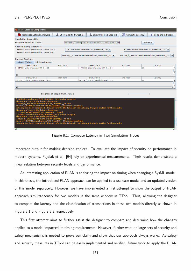
8.2. PERSPECTIVES Conclusion
Figure 8.1: Compute Latency in Two Simulation Traces
important output for making decision choices. To evaluate the impact of security on performance in
modern systems, Fujdiak et al. [94] rely on experimental measurements. Their results demonstrate a
linear relation between security levels and performance.
An interesting application of PLAN is analyzing the impact on timing when changing a SysML model.
In this thesis, the introduced PLAN approach can be applied to a use case model and an updated version
of this model separately. However, we have implemented a first attempt to show the output of PLAN
approach simultaneously for two models in the same window in TTool. Thus, allowing the designer
to compare the latency and the classification of transactions in these two models directly as shown in
Figure 8.1 and Figure 8.2 respectively.
This first attempt aims to further assist the designer to compare and determine how the changes
applied to a model impacted its timing requirements. However, further work on large sets of security and
safety mechanisms is needed to prove our claim and show that our approach always works. As safety
and security measures in TTool can be easily implemented and verified, future work to apply the PLAN
181

Conclusion 8.2. PERSPECTIVES
Figure 8.2: Compare PLAN Output Window for Two Rows
182

8.2. PERSPECTIVES Conclusion
approach on safety and security-related model changes may be easier.
183
Chapter 9
Résumé
Lors de la conception d’un système embarqué, une façon courante de procéder est de faire un modèle du
système, de le simuler ou de l’exécuter pour obtenir des traces, puis de vérifier si ces traces respectent
les exigences fonctionnelles et non fonctionnelles. Dans cette thèse, notre idée est d’aider le concepteur
au-delà de la simple satisfaction des exigences. Ainsi, notre objectif est de savoir, si une exigence n’est
pas satisfaite, quelles en sont les causes. Nous voulons de plus appliquer cela à des exigences de latence.
Un modèle de système embarqué inclut des composants logiciels et matériels. Dans ces composants,
plusieurs facteurs déterminent le moment où une opération logicielle d’une fonction applicative est exé-
cutée. L’un de ces facteurs est le composant matériel (par exemple, un processeur, un bus) et son
logiciel support (un système d’exploitation) sur lesquels la fonction est allouée. Par exemple, le proces-
sus d’ordonnancement d’un bus ou d’un processeur, l’inadéquation de la bande passante entre les bus,
la largeur de bande du bus,. . . ont une contribution significative sur le temps d’exécution des fonctions
applicatives. Un autre facteur est la dépendance entre les fonctions d’une application. Par exemple, un
opérateur d’une fonction doit attendre la fin de l’exécution d’un autre opérateur avant de s’exécuter.
Lorsque le délai entre deux opérateurs doit être inférieur à une valeur maximale, nous appelons cette
contrainte « exigence de latence maximale ». Pour comprendre les raisons d’une violation d’une telle
exigence, dans cette thèse, nous modélisons les dépendances dans le modèle du système : à partir de ces
dépendances, nous pouvons classer les transactions d’une trace d’exécution en fonction de leur impact
sur la latence. Nous désignons par le terme PLAN cette approche avancée d’analyse des traces.
184

Conclusion
Dans le chapitre 1, nous avons expliqué pourquoi il est difficile de déterminer quelles parties du système
ont contribué à un retard entre deux opérations. Ainsi, lorsqu’une exigence de latence maximale n’est
pas satisfaite, il peut être difficile pour un concepteur d’améliorer la conception d’un système embarqué
pour satisfaire cette exigence, car les facteurs contribuant au retard peuvent être inconnus et multiples.
Ainsi, cette thèse aborde la vérification des exigences des systèmes embarqués en se concentrant sur
l’analyse des traces en utilisant une nouvelle technique d’analyse des traces (PLAN). En identifiant les
dépendances entre les éléments du modèle et en classifiant les transactions dans une trace d’exécution
par rapport à une exigence de latence, nous avons identifié et mis en évidence les fonctions logicielles
et/ou les composants matériels qui ont contribué à ce retard.
Le chapitre 2 a donné un aperçu des systèmes embarqués, l’ingénierie dirigée par les modèles (MDE)
et les contraintes temporelles. De plus, dans le chapitre 2, nous avons expliqué le profil SysML-Sec dans
lequel notre contribution est intégrée. Le chapitre 3 présente les travaux connexes, où les approches de
vérification des performances et les méthodes d’analyse des traces de simulation sont étudiées.
Au chapitre 4, nous avons formellement défini les trois entrées de notre approche: la modélisation
système, la trace d’exécution du modèle et l’exigence de latence maximale. La modélisation système
suit l’approche Y-Chart pour partitionner le système entre matériel et logiciel : l’application et la plate-
forme sont modélisées indépendamment avant que l’application ne soit allouée à la plate-forme. La trace
d’exécution construite sur un ensemble de transactions peut être obtenue à partir d’une simulation de
modèle, ou à partir de la génération de code exécutable depuis le modèle, puis de l’exécution de ce code.
L’exigence peut être explicitement liée aux traces d’exécution d’un système. L’exigence spécifie un délai
maximal entre les temps de début et de fin de deux opérateurs. Le fait d’avoir ces entrées formellement
définies nous permet d’adapter facilement notre approche aux différents outils et méthodes concernés
par la conception de systèmes embarqués.
L’approche PLAN a été présentée au chapitre 5. PLAN peut investiguer une trace d’exécution
produite à partir d’un modèle de niveau système correspondant à une application, une architecture et
l’allocation de l’application sur l’architecture. PLAN a pour but de faciliter la localisation de la raison pour
laquelle un modèle de système embarqué a violé une exigence de latence fournie par l’utilisateur. Pour
ce faire, l’approche prend trois entrées : (1) un modèle d’allocation qui décrit comment les fonctions
185

Conclusion
logicielles et les canaux de communication (modèle d’application) sont alloués aux unités matérielles
(modèle de plateforme), (2) une trace d’exécution construite sur des transactions d’exécution où chaque
transaction représente l’exécution d’un opérateur sur un composant matériel et (3) une exigence de
latence qui fournit une limite supérieure sur le délai entre les occurrences de deux opérations logicielles
de base. Dans le chapitre 5, nous avons supposé que pour chacun des deux opérateurs de l’exigence de
latence, nous avons une transaction d’exécution unique dans la trace d’exécution. Les classifications des
transactions du chapitre 5 sont formalisées et présentées sur la base de cette hypothèse. Nous avons
classé les transactions en neuf ensembles différents. Parmi ces ensembles, l’ensemble « contention » est
un ensemble important que le concepteur doit prendre en compte pour mettre à jour le modèle car il
contient les transactions qui sont les causes premières ayant contribué à augmenter le délai entre les
opérateurs de l’exigence de latence.
Dans le chapitre 5, PLAN a permis d’analyser les traces d’exécution qui ne contenaient qu’une
transaction pour chaque opérateur d’une exigence de latence maximale. Afin d’analyser une gamme plus
large de traces d’exécution, c’est-à-dire les traces d’exécution qui contiennent plus d’une transaction par
opérateur d’une exigence de latence maximale, nous avons introduit une nouvelle technique d’analyse
basée sur le "tainting" de graphes au chapitre 6.
La clé de cette version plus avancée de PLAN du chapitre 6 est de marquer un graphe de dépendance
construit depuis les diagrammes d’activité SysML et en analysant la transaction d’exécution dans une
trace, de propager ce marquage le long du graphe pour déterminer les valeurs de latence. Ce graphe de
dépendance comporte toutes les dépendances pertinentes entre les opérateurs d’un modèle d’application.
Les transactions dans une trace d’exécution sont étudiées séquentiellement pour mettre à jour l’état des
opérateurs dans le graphe de dépendance. Une transaction peut ajouter une valeur pour un marquage
donné pour un opérateur dans un graphe. La propagation de cette valeur le long du graphe nous
aide à identifier les transactions correspondant à l’occurrence du premier opérateur de l’exigence et à
l’occurrence correspondante du second opérateur mentionné dans l’exigence. Pour cela, nous stockons
une valeur de "taint" pour chaque transaction correspondant à la première opération de l’exigence de
latence et la propageons jusqu’à ce que la valeur du marquage atteigne la deuxième opération de l’exigence
de latence. Cela nous permet de lever la restriction de dépendance 1 à 1 des opérateurs.
186

Conclusion
Dans le chapitre 7, un prototype mettant en œuvre PLAN a été réalisé. Nous avons commencé par
expliquer comment nos modèles formels peuvent être facilement capturés par des diagrammes SysML.
Ensuite, la section 7.2 donne un aperçu de l’implémentation du prototype. Plus précisément, elle donne
un aperçu de la façon dont le concepteur peut lancer PLAN à l’aide de l’interface graphique ou d’une
interface en ligne de commandes et de la façon dont les résultats de la classification peuvent être obtenus.
De plus, dans le chapitre 7, nous avons démontré l’approche PLAN sur deux cas d’utilisation définis dans
le cadre du projet H2020 AQUAS : le système d’entraînement industriel et le système de mécanismes de
wagons. Pour ces deux cas d’utilisation, l’approche PLAN a permis d’identifier la raison principale pour
laquelle la latence est supérieure à la latence maximale. Ainsi, nous avons montré comment l’approche
PLAN peut être utilisée pour guider un concepteur dans la mise à jour du modèle du système afin de
satisfaire une exigence de latence maximale.
Le chapitre 8 résume les contributions de cette thèse et fournit une liste de nouvelles idées de
recherche pour étendre notre travail. Notre objectif ultime est de fournir aux concepteurs des sugges-
tions automatisées pour améliorer le modèle de façon à ce que les contraintes de temps soient toutes
respectées.
187

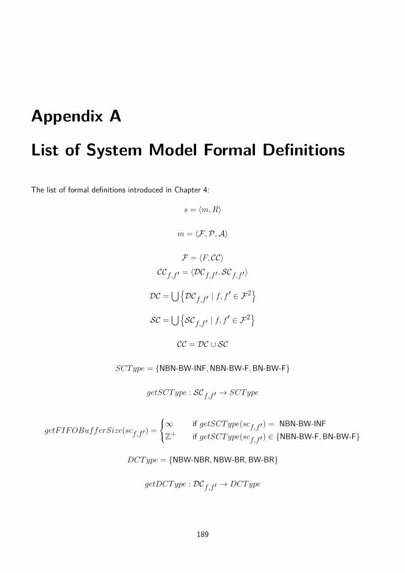
Appendix A
List of System Model Formal Definitions
The list of formal definitions introduced in Chapter 4:
s = 〈m,R〉
m = 〈F ,P ,A〉
F = 〈F, CC〉
CCf,f ′ = 〈DCf,f ′ ,SCf,f ′〉
DC =⋃{DCf,f ′ | f, f
′ ∈ F2}
SC =⋃{SCf,f ′ | f, f
′ ∈ F2}
CC = DC ∪ SC
SCType = {NBN-BW-INF,NBN-BW-F,BN-BW-F}
getSCType : SCf,f ′ → SCType
getFIFOBufferSize(scf,f ′) =
∞ if getSCType(scf,f ′) = NBN-BW-INFZ+ if getSCType(scf,f ′) ∈ {NBN-BW-F,BN-BW-F}
DCType = {NBW-NBR,NBW-BR,BW-BR}
getDCType : DCf,f ′ → DCType
189

getBufferSize(dcf,f ′) =
∞ if getDCType(dcf,f ′) ∈ { NBW-NBR,NBW-BR}Z+ if getDCType(dcf,f ′) = BW-BR
f = 〈{v1,f , v2,f , . . . , vn,f}, Bf 〉
Bf = 〈Of = {o1, o2, . . . , on}, Lf , Cf ⊂ {(oi, oj) ∈ O2f | i 6= j}〉
Om =⋃f∈F
Of
inPath(o,−−→o1o2) =
true if ∃oioj ∈−−→o1o2 | oi = o ∨ oj = o
false otherwise
getNext(o) = {oi | (o, oi) ∈ Cf}
cat(o) ∈{Start, Stop, Choice,Merge, IntOp, Set,WriteData,ReadData,Notify,Wait
}.
getF (m, o) = f | o ∈ Of
getComplexity : Of,IntOp → Z+
getDataChannel : Of,WriteData ∪Of,ReadData → DC
getDataSize : Of,WriteData ∪Of,ReadData → Z+
getSyncChannel : Of,Notify ∪Of,Wait → SC
insideLoop(o, 〈om, oc, os, v, nbr〉) =
true if inPath(o,−−−→ocom)false otherwise
getInsideLoop(〈om, oc, os, v, nbr〉) = o | o ∈ getNext(oc) ∧ insideLoop(o, 〈om, oc, os, v, nbr〉)
getOutsideLoop(〈om, oc, os, v, nbr〉) = o | o ∈ getNext(oc) ∧ ¬insideLoop(o, 〈om, oc, os, v, nbr〉)
190
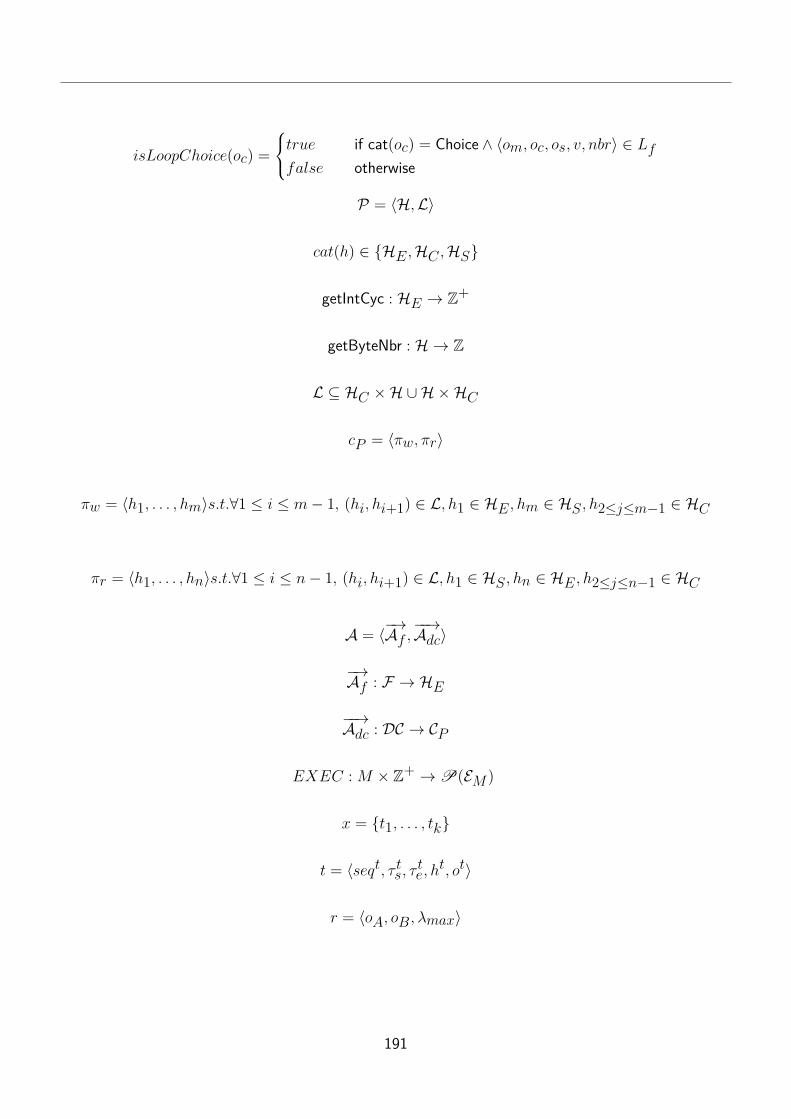
isLoopChoice(oc) =
true if cat(oc) = Choice ∧ 〈om, oc, os, v, nbr〉 ∈ Lffalse otherwise
P = 〈H,L〉
cat(h) ∈ {HE ,HC ,HS}
getIntCyc : HE → Z+
getByteNbr : H → Z
L ⊆ HC ×H ∪H×HC
cP = 〈πw, πr〉
πw = 〈h1, . . . , hm〉s.t.∀1 ≤ i ≤ m− 1, (hi, hi+1) ∈ L, h1 ∈ HE , hm ∈ HS , h2≤j≤m−1 ∈ HC
πr = 〈h1, . . . , hn〉s.t.∀1 ≤ i ≤ n− 1, (hi, hi+1) ∈ L, h1 ∈ HS , hn ∈ HE , h2≤j≤n−1 ∈ HC
A = 〈−→Af ,−−→Adc〉
−→Af : F → HE
−−→Adc : DC → CP
EXEC : M × Z+ →P(EM )
x = {t1, . . . , tk}
t = 〈seqt, τ ts, τ te, ht, ot〉
r = 〈oA, oB , λmax〉
191

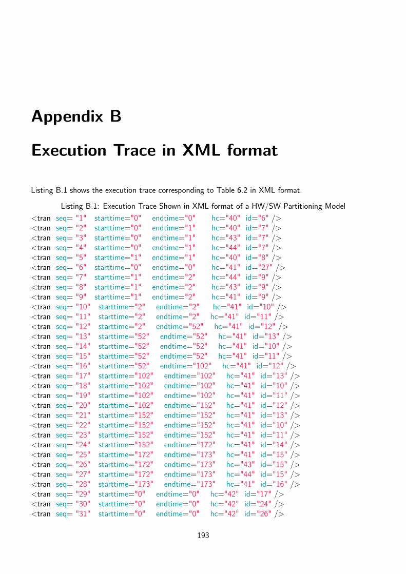
Appendix B
Execution Trace in XML format
Listing B.1 shows the execution trace corresponding to Table 6.2 in XML format.
Listing B.1: Execution Trace Shown in XML format of a HW/SW Partitioning Model<tran seq= "1" starttime="0" endtime="0" hc="40" id="6" /><tran seq= "2" starttime="0" endtime="1" hc="40" id="7" /><tran seq= "3" starttime="0" endtime="1" hc="43" id="7" /><tran seq= "4" starttime="0" endtime="1" hc="44" id="7" /><tran seq= "5" starttime="1" endtime="1" hc="40" id="8" /><tran seq= "6" starttime="0" endtime="0" hc="41" id="27" /><tran seq= "7" starttime="1" endtime="2" hc="44" id="9" /><tran seq= "8" starttime="1" endtime="2" hc="43" id="9" /><tran seq= "9" starttime="1" endtime="2" hc="41" id="9" /><tran seq= "10" starttime="2" endtime="2" hc="41" id="10" /><tran seq= "11" starttime="2" endtime="2" hc="41" id="11" /><tran seq= "12" starttime="2" endtime="52" hc="41" id="12" /><tran seq= "13" starttime="52" endtime="52" hc="41" id="13" /><tran seq= "14" starttime="52" endtime="52" hc="41" id="10" /><tran seq= "15" starttime="52" endtime="52" hc="41" id="11" /><tran seq= "16" starttime="52" endtime="102" hc="41" id="12" /><tran seq= "17" starttime="102" endtime="102" hc="41" id="13" /><tran seq= "18" starttime="102" endtime="102" hc="41" id="10" /><tran seq= "19" starttime="102" endtime="102" hc="41" id="11" /><tran seq= "20" starttime="102" endtime="152" hc="41" id="12" /><tran seq= "21" starttime="152" endtime="152" hc="41" id="13" /><tran seq= "22" starttime="152" endtime="152" hc="41" id="10" /><tran seq= "23" starttime="152" endtime="152" hc="41" id="11" /><tran seq= "24" starttime="152" endtime="172" hc="41" id="14" /><tran seq= "25" starttime="172" endtime="173" hc="41" id="15" /><tran seq= "26" starttime="172" endtime="173" hc="43" id="15" /><tran seq= "27" starttime="172" endtime="173" hc="44" id="15" /><tran seq= "28" starttime="173" endtime="173" hc="41" id="16" /><tran seq= "29" starttime="0" endtime="0" hc="42" id="17" /><tran seq= "30" starttime="0" endtime="0" hc="42" id="24" /><tran seq= "31" starttime="0" endtime="0" hc="42" id="26" />
193

<tran seq= "32" starttime="0" endtime="0" hc="42" id="18" /><tran seq= "33" starttime="0" endtime="0" hc="42" id="19" /><tran seq= "34" starttime="0" endtime="100" hc="42" id="20" /><tran seq= "35" starttime="100" endtime="101" hc="44" id="21" /><tran seq= "36" starttime="100" endtime="101" hc="43" id="21" /><tran seq= "37" starttime="100" endtime="101" hc="42" id="21" /><tran seq= "38" starttime="101" endtime="101" hc="42" id="22" /><tran seq= "39" starttime="101" endtime="101" hc="42" id="18" /><tran seq= "40" starttime="101" endtime="101" hc="42" id="19" /><tran seq= "41" starttime="101" endtime="201" hc="42" id="20" /><tran seq= "42" starttime="201" endtime="202" hc="44" id="21" /><tran seq= "43" starttime="202" endtime="202" hc="43" id="21" /><tran seq= "44" starttime="202" endtime="202" hc="42" id="21" /><tran seq= "45" starttime="202" endtime="202" hc="42" id="22" /><tran seq= "46" starttime="202" endtime="202" hc="42" id="18" /><tran seq= "47" starttime="202" endtime="202" hc="42" id="19" /><tran seq= "48" starttime="202" endtime="302" hc="42" id="20" /><tran seq= "49" starttime="302" endtime="303" hc="44" id="21" /><tran seq= "50" starttime="302" endtime="303" hc="43" id="21" /><tran seq= "51" starttime="302" endtime="303" hc="42" id="21" /><tran seq= "52" starttime="303" endtime="303" hc="42" id="22" /><tran seq= "53" starttime="302" endtime="302" hc="42" id="18" /><tran seq= "54" starttime="302" endtime="302" hc="42" id="19" /><tran seq= "55" starttime="302" endtime="302" hc="42" id="23" />
194
Bibliography
[1] ISO/IEC 27000 family - Information security management systems. URL https://www.iso.org/isoiec-27001-information-security.html.
[2] The mars 2020 rover’s brains. https://mars.nasa.gov/mars2020/spacecraft/rover/brains/. Accessed: 2021-09-24.
[3] Sample handling. https://mars.nasa.gov/mars2020/spacecraft/rover/sample-handling/. Accessed: 2021-09-24.
[4] CRYSTAL: CRitical sYSTem engineering AcceLeration. URL http://www.crystal-artemis.eu/.
[5] EVITA:E-safety vehicle intrusion protected applications. URL https://www.evita-project.org/.
[6] MERgE. URL http://www.merge-project.eu/.
[7] SESAMO:Security and Safety Modelling. URL http://www.sesamo-project.eu/.
[8] Vision zero initiative. https://trimis.ec.europa.eu/?q=project/vision-zero-initiative#tab-outline. Accessed: 2020-07-08.
[9] What are the carbon monoxide levels that will sound the alarm? https://www.kidde.com/home-safety/en/us/support/help-center/browse-articles/articles/what_are_the_carbon_monoxide_levels_that_will_sound_the_alarm_.html, 04/10/2019. Accessed:2021-09-24.
[10] Boston scientific recalls ingenio family of pacemakers and crt-ps due to risk of transi-tion to safety mode. hhttps://www.fda.gov/medical-devices/medical-device-recalls/boston-scientific-recalls-ingenio-family-pacemakers-and-crt-ps-due-risk-transition-safety-mode,08/10/2021. Accessed: 2021-09-24.
[11] UML Profile for MARTE, volume 1.1. Object Management Group, 2011. URL https://www.omg.org/spec/MARTE/1.1/.
[12] Aggregated quality assurance for systems (aquas). https://aquas-project.eu, 2013. Accessed:2019-09-24.
[13] Retro-ingénerie de traces d’analyse de simulation et d’exécution de systèmes temps-réel – rt-simex.https://anr.fr/Projet-ANR-08-SEGI-0015, 2013. Accessed: 2019-09-24.
195
BIBLIOGRAPHY
[14] Ttool, 2013. URL https://ttool.telecom-paris.fr.
[15] Automatic braking system issues. https://www.abrahamwatkins.com/blog/2015/07/automatic-braking-system-issues.shtml, 2015. Accessed: 2020-10-16.
[16] Safure - safety and security by design for interconnected mixed-critical cyber-physical systems,2015-2018. URL https://safure.eu/.
[17] What is graphml?, 2019. URL http://graphml.graphdrawing.org/.
[18] Road safety: Commission welcomes agreement on new eu rules to help save lives. https://ec.europa.eu/commission/presscorner/detail/en/IP_19_1793, 2019-04-26. Accessed: 2020-07-08.
[19] Mobility and transport road safety. https://ec.europa.eu/transport/road_safety/what-we-do_en, 2020-07-10. Accessed: 2020-07-10.
[20] Nissan’s aeb is suddenly stopping vehicles for no reason. http://www.nissanproblems.com/aeb/, 21/03/2019. Accessed: 2021-09-24.
[21] E. A. Aboussoror, I. Ober, and I. Ober. Significantly increasing the usability of model analysistools through visual feedback. In International SDL Forum, pages 107–123. Springer, 2013.
[22] N. Alhirabi, O. Rana, and C. Perera. Security and privacy requirements for the internet of things:A survey. ACM Transactions on Internet of Things, 2(1):1–37, 2021.
[23] A. Alshamrani and A. Bahattab. A comparison between three sdlc models waterfall model, spiralmodel, and incremental/iterative model. International Journal of Computer Science Issues (IJCSI),12(1):106, 2015.
[24] K. M. Alshmrany, M. Aldughaim, A. Bhayat, and L. C. Cordeiro. Fusebmc: An energy-efficienttest generator for finding security vulnerabilities in c programs. In International Conference onTests and Proofs, pages 85–105. Springer, 2021.
[25] R. Andriatsimandefitra and V. V. T. Tong. Capturing android malware behaviour using systemflow graph. In International Conference on Network and System Security, pages 534–541. Springer,2015.
[26] L. Apvrille and Y. Roudier. Sysml-sec: A sysml environment for the design and development ofsecure embedded systems. APCOSEC, Asia-Pacific Council on Systems Engineering, pages 8–11,2013.
[27] P. Axer, R. Ernst, H. Falk, A. Girault, D. Grund, N. Guan, B. Jonsson, P. Marwedel, J. Reineke,C. Rochange, et al. Building timing predictable embedded systems. ACM Transactions on Em-bedded Computing Systems (TECS), 13(4):82, 2014.
[28] P. Bagade, A. Banerjee, and S. K. Gupta. Validation, verification, and formal methods for cyber-physical systems. In Cyber-Physical Systems, pages 175–191. Elsevier, 2017.
[29] R. Baldoni, E. Coppa, D. C. D’elia, C. Demetrescu, and I. Finocchi. A survey of symbolic executiontechniques. ACM Computing Surveys (CSUR), 51(3):1–39, 2018.
196
BIBLIOGRAPHY
[30] M. Barbehenn. A note on the complexity of dijkstra’s algorithm for graphs with weighted vertices.IEEE transactions on computers, 47(2):263, 1998.
[31] C. Barrett. Sat solvers: Theory and practice. Summer School on Verification Technology, Systemsand Applications, New York, USA, pages 1–98, 2008.
[32] J. Baumeister, B. Finkbeiner, S. Schirmer, M. Schwenger, and C. Torens. Rtlola cleared for take-off: monitoring autonomous aircraft. In International Conference on Computer Aided Verification,pages 28–39. Springer, 2020.
[33] F. Bause, H. Beilner, M. Fischer, P. Kemper, and M. Völker. The proc/btoolset for the modellingand analysis of process chains. In International Conference on Modelling Techniques and Tools forComputer Performance Evaluation, pages 51–70. Springer, 2002.
[34] M. Bekooij, R. Hoes, O. Moreira, P. Poplavko, M. Pastrnak, B. Mesman, J. D. Mol, S. Stuijk,V. Gheorghita, and J. Van Meerbergen. Dataflow analysis for real-time embedded multiprocessorsystem design. In Dynamic and robust streaming in and between connected consumer-electronicdevices, pages 81–108. Springer, 2005.
[35] M. Ben Ayed, A. Massaoudi, S. A. Alshaya, and M. Abid. System-level co-simulation for embeddedsystems. AIP Advances, 10(3):035113, 2020.
[36] I. E. Bennour. Formal verification of timed synchronous dataflow graphs using lustre. Journal ofLogical and Algebraic Methods in Programming, 121:100678, 2021.
[37] S. Bernardi, U. Gentile, S. Marrone, J. Merseguer, and R. Nardone. Security modelling and formalverification of survivability properties: Application to cyber–physical systems. Journal of Systemsand Software, 171:110746, 2021.
[38] F. Berner and J. Sametinger. Dynamic taint-tracking: Directions for future research. In ICETE(2), pages 294–305, 2019.
[39] F. Berner, R. Mayrhofer, and J. Sametinger. Dynamic taint tracking simulation. In InternationalConference on E-Business and Telecommunications, pages 203–227. Springer, 2019.
[40] S. Bhalerao, D. Puntambekar, and M. Ingle. Generalizing agile software development life cycle.International journal on computer science and engineering, 1(3):222–226, 2009.
[41] A. Biere, A. Cimatti, E. Clarke, and Y. Zhu. Symbolic model checking without bdds. In Internationalconference on tools and algorithms for the construction and analysis of systems, pages 193–207.Springer, 1999.
[42] A. Biere, A. Cimatti, E. Clarke, and Y. Zhu. Symbolic model checking without bdds. In Internationalconference on tools and algorithms for the construction and analysis of systems, pages 193–207.Springer, 1999.
[43] A. Biere, A. Cimatti, E. M. Clarke, M. Fujita, and Y. Zhu. Symbolic model checking using satprocedures instead of bdds. In Proceedings of the 36th annual ACM/IEEE Design AutomationConference, pages 317–320, 1999.
[44] A. Biere, A. Cimatti, E. M. Clarke, O. Strichman, and Y. Zhu. Bounded model checking. 2003.
197
BIBLIOGRAPHY
[45] B. Blanchet, B. Smyth, V. Cheval, and M. Sylvestre. Proverif 2.00: Automatic cryptographicprotocol verifier, user manual and tutorial. Version from, pages 05–16, 2018.
[46] Y. Blein. ParTraP: A Language for the Specification and Runtime Verification of ParametricProperties. PhD thesis, Université Grenoble Alpes, 2019.
[47] D. S. Board. Who is in control? road safety and automation in road traffic, 2019.
[48] B. W. Boehm. A spiral model of software development and enhancement. Computer, 21(5):61–72,1988.
[49] G. Bolch, S. Greiner, H. de Meer, and K. Trivedi. Queueing Networks and Markov Chains:Modeling and Performance Evaluation with Computer Science Applications. Wiley, 2006. ISBN9780471791560. URL https://books.google.fr/books?id=8Mei8w6YUHYC.
[50] D. Boxler and K. R. Walcott. Static taint analysis tools to detect information flows. In Proceedingsof the International Conference on Software Engineering Research and Practice (SERP), pages 46–52. The Steering Committee of The World Congress in Computer Science, Computer . . . , 2018.
[51] J. Brandenburg and B. Stabernack. Simulation-based hw/sw co-exploration of the concurrentexecution of hevc intra encoding algorithms for heterogeneous multi-core architectures. Journal ofSystems Architecture, 77:26–42, 2017.
[52] R. Buchmann, F. Pétrot, and A. Greiner. Fast cycle accurate simulator to simulate event-drivenbehavior. In International Conference on Electrical, Electronic and Computer Engineering, 2004.ICEEC’04., pages 35–38. IEEE, 2004.
[53] J. R. Burch, E. M. Clarke, K. L. McMillan, D. L. Dill, and L.-J. Hwang. Symbolic model checking:1020 states and beyond. Information and computation, 98(2):142–170, 1992.
[54] G. C. Buttazzo. Hard real-time computing systems: predictable scheduling algorithms and appli-cations, volume 24. Springer Science & Business Media, 2011.
[55] A. Carelli, A. Vallero, and S. Di Carlo. Performance monitor counters: interplay between safety andsecurity in complex cyber-physical systems. IEEE Transactions on Device and Materials Reliability,2019.
[56] K. Carruthers. Internet of things and beyond: Cyber-physical systems. IEEE Internet of ThingsNewsletter, 10, 2014.
[57] Z. B. Celik, L. Babun, A. K. Sikder, H. Aksu, G. Tan, P. McDaniel, and A. S. Uluagac. Sensi-tive information tracking in commodity iot. In 27th {USENIX} Security Symposium ({USENIX}Security 18), pages 1687–1704, 2018.
[58] H. Chai, G. Zhang, J. Zhou, J. Sun, L. Huang, and T. Wang. A short review of security-awaretechniques in real-time embedded systems. Journal of Circuits, Systems and Computers, 28(02):1930002, 2019.
[59] D. Chatterjee and V. Bertacco. Equipe: Parallel equivalence checking with gp-gpus. In 2010 IEEEInternational Conference on Computer Design, pages 486–493. IEEE, 2010.
198
BIBLIOGRAPHY
[60] X. Chen, H. Hsieh, F. Balarin, and Y. Watanabe. Automatic trace analysis for logic of constraints.In Proceedings of the 40th annual Design Automation Conference, pages 460–465, 2003.
[61] X. Chen, H. Hsieh, F. Balarin, and Y. Watanabe. Logic of constraints: A quantitative performanceand functional constraint formalism. IEEE Transactions on Computer-Aided Design of IntegratedCircuits and Systems, 23(8):1243–1255, 2004.
[62] X. Chen, H. Hsieh, and F. Balarin. Verification approach of metropolis design framework forembedded systems. International Journal of Parallel Programming, 34(1):3–27, 2006.
[63] K. Cheng, Q. Li, L. Wang, Q. Chen, Y. Zheng, L. Sun, and Z. Liang. Dtaint: detecting the taint-style vulnerability in embedded device firmware. In 2018 48th Annual IEEE/IFIP InternationalConference on Dependable Systems and Networks (DSN), pages 430–441. IEEE, 2018.
[64] B. N. Chhaya and S. Jafer. Simulation-based and formal verification of domain-specific languagemodel. In AIAA Scitech 2020 Forum, page 0897, 2020.
[65] E. Clarke, O. Grumberg, S. Jha, Y. Lu, and H. Veith. Counterexample-guided abstraction re-finement. In International Conference on Computer Aided Verification, pages 154–169. Springer,2000.
[66] J. Clause, W. Li, and A. Orso. Dytan: A generic dynamic taint analysis framework. In Proceedingsof the 2007 International Symposium on Software Testing and Analysis, ISSTA ’07, page 196–206,New York, NY, USA, 2007. Association for Computing Machinery. ISBN 9781595937346. doi:10.1145/1273463.1273490. URL https://doi.org/10.1145/1273463.1273490.
[67] A. Coen-Porisini, G. Denaro, C. Ghezzi, and M. Pezzé. Using symbolic execution for verifyingsafety-critical systems. In Proceedings of the 8th European software engineering conference heldjointly with 9th ACM SIGSOFT international symposium on Foundations of software engineering,pages 142–151, 2001.
[68] I. R. Committee et al. The international technology roadmap for semiconductors (2005), 2010.
[69] W. A. Conklin. It vs. ot security: A time to consider a change in cia to include resilienc. In 201649th Hawaii International Conference on System Sciences (HICSS), pages 2642–2647. IEEE, 2016.
[70] L. Convent, S. Hungerecker, M. Leucker, T. Scheffel, M. Schmitz, and D. Thoma. Tessla: temporalstream-based specification language. In Brazilian Symposium on Formal Methods, pages 144–162.Springer, 2018.
[71] D. Currie, X. Feng, M. Fujita, A. J. Hu, M. Kwan, and S. Rajan. Embedded software verificationusing symbolic execution and uninterpreted functions. International Journal of Parallel Program-ming, 34(1):61–91, 2006.
[72] M. Dam, G. Le Guernic, and A. Lundblad. Treedroid: a tree automaton based approach toenforcing data processing policies. In Proceedings of the 2012 ACM conference on Computer andcommunications security, pages 894–905, 2012.
[73] B. d’Angelo, S. Sankaranarayanan, C. Sánchez, W. Robinson, B. Finkbeiner, H. B. Sipma,S. Mehrotra, and Z. Manna. Lola: runtime monitoring of synchronous systems. In 12th In-ternational Symposium on Temporal Representation and Reasoning (TIME’05), pages 166–174.IEEE, 2005.
199

BIBLIOGRAPHY
[74] B. Dasarathy. Timing constraints of real-time systems: Constructs for expressing them, methodsof validating them. IEEE transactions on Software Engineering, (1):80–86, 1985.
[75] R. I. Davis. A review of fixed priority and edf scheduling for hard real-time uniprocessor systems.ACM SIGBED Review, 11(1):8–19, 2014.
[76] J. H. Dawes. Towards Automated Performance Analysis of Programs by Runtime Verification. PhDthesis, Manchester U., 2021.
[77] J. Deantoni. Towards Formal System Modeling: Making Explicit and Formal the Concurrent andTimed Operational Semantics to Better Understand Heterogeneous Models. PhD thesis, UniversitéCôte d’Azur, CNRS, I3S, France, 2019.
[78] J. DeAntoni and F. Mallet. Timesquare: Treat your models with logical time. In InternationalConference on Modelling Techniques and Tools for Computer Performance Evaluation, pages 34–41. Springer, 2012.
[79] J. DeAntoni, F. Mallet, F. Thomas, G. Reydet, J.-P. Babau, C. Mraidha, L. Gauthier, L. Rioux,and N. Sordon. Rt-simex: retro-analysis of execution traces. In Proceedings of the eighteenthACM SIGSOFT international symposium on Foundations of software engineering, pages 377–378,2010.
[80] L. Delligatti. SysML distilled: A brief guide to the systems modeling language. Addison-Wesley,2013.
[81] K. Edelberg, P. Backes, J. Biesiadecki, S. Brooks, D. Helmick, W. Kim, T. Litwin, B. Metz, J. Reid,A. Sirota, et al. Software system for the mars 2020 mission sampling and caching testbeds. In2018 IEEE Aerospace Conference, pages 1–11. IEEE, 2018.
[82] W. Enck, P. Gilbert, S. Han, V. Tendulkar, B.-G. Chun, L. P. Cox, J. Jung, P. McDaniel, andA. N. Sheth. Taintdroid: an information-flow tracking system for realtime privacy monitoring onsmartphones. ACM Transactions on Computer Systems (TOCS), 32(2):1–29, 2014.
[83] A. ENRICI, L. APVRILLE, D. CAMARA, and R. PACALET. The ψ-chart design approach inttool/diplodocus: Co-design of data-dominated systems-on-chip. Architecture, 3:2.
[84] A. Enrici, L. Li, L. Apvrille, and D. Blouin. A tutorial on ttool. DIPLODOCUS: an Open-sourceToolkit for the Design of Data-flow Embedded Systems, 2018.
[85] Y. Falcone, K. Havelund, and G. Reger. A tutorial on runtime verification. Engineering dependablesoftware systems, pages 141–175, 2013.
[86] Y. Falcone, S. Krstić, G. Reger, and D. Traytel. A taxonomy for classifying runtime verificationtools. International Journal on Software Tools for Technology Transfer, 23(2):255–284, 2021.
[87] J. M. Fernandes and R. J. Machado. Can uml be a system-level language for embedded software?In IFIP Working Conference on Distributed and Parallel Embedded Systems, pages 1–10. Springer,2002.
[88] M. Fisher, V. Mascardi, K. Y. Rozier, B.-H. Schlingloff, M. Winikoff, and N. Yorke-Smith. Towardsa framework for certification of reliable autonomous systems. Autonomous Agents and Multi-AgentSystems, 35(1):1–65, 2021.
200
BIBLIOGRAPHY
[89] K. Forsberg and H. Mooz. The relationship of system engineering to the project cycle. In INCOSEInternational Symposium, volume 1, pages 57–65. Wiley Online Library, 1991.
[90] M. Foughali and P.-E. Hladik. Bridging the gap between formal verification and schedulabilityanalysis: The case of robotics. Journal of Systems Architecture, 111:101817, 2020.
[91] R. France and B. Rumpe. Model-driven development of complex software: A research roadmap.In Future of Software Engineering (FOSE’07), pages 37–54. IEEE, 2007.
[92] S. Friedenthal, A. Moore, and R. Steiner. A practical guide to SysML: the systems modelinglanguage. Morgan Kaufmann, 2014.
[93] L. Fuentes-Fernández and A. Vallecillo-Moreno. An introduction to uml profiles. 2004.
[94] R. Fujdiak, P. Mlynek, P. Blazek, M. Barabas, and P. Mrnustik. Seeking the relation betweenperformance and security in modern systems: Metrics and measures. In 2018 41st InternationalConference on Telecommunications and Signal Processing (TSP), pages 1–5. IEEE, 2018.
[95] R. Fujdiak, P. Blazek, L. Apvrille, Z. Martinasek, P. Mlynek, R. Pacalet, D. Smekal, P. Mrnustik,M. Barabas, and M. Zoor. Modeling the trade-off between security and performance to supportthe product life cycle. In 2019 8th Mediterranean Conference on Embedded Computing (MECO),pages 1–6. IEEE, 2019.
[96] A. Fuxman, M. Pistore, J. Mylopoulos, and P. Traverso. Model checking early requirementsspecifications in tropos. In Proceedings Fifth IEEE International Symposium on RequirementsEngineering, pages 174–181. IEEE, 2001.
[97] D. D. Gajski, S. Abdi, A. Gerstlauer, and G. Schirner. Embedded system design: modeling,synthesis and verification. Springer Science & Business Media, 2009.
[98] L. George, V. V. T. Tong, and L. Mé. Blare tools: A policy-based intrusion detection systemautomatically set by the security policy. In International Workshop on Recent Advances in IntrusionDetection, pages 355–356. Springer, 2009.
[99] A. Gerstlauer, C. Haubelt, A. D. Pimentel, T. P. Stefanov, D. D. Gajski, and J. Teich. Electronicsystem-level synthesis methodologies. IEEE Transactions on Computer-Aided Design of IntegratedCircuits and Systems, 28(10):1517–1530, 2009.
[100] M. Glinz. On non-functional requirements. In 15th IEEE International Requirements EngineeringConference (RE 2007), pages 21–26. IEEE, 2007.
[101] A. E. Goodloe and L. Pike. Monitoring distributed real-time systems: A survey and future direc-tions. National Aeronautics and Space Administration, Langley Research Center, 2010.
[102] D. M. Gordon and P. Kemper. On clustering simulation traces. In Proceedings Eighth Interna-tional Workshop on Performability Modelling of Computer and Communication Systems (PMCCS-82007). Edinburgh, Scotland, UK, 2007.
[103] M. Graa, N. Cuppens-Boulahia, F. Cuppens, and A. Cavalli. Detecting control flow in smarphones:Combining static and dynamic analyses. In Cyberspace Safety and Security, pages 33–47. Springer,2012.
201

BIBLIOGRAPHY
[104] T. Grimm, D. Lettnin, and M. Hübner. A survey on formal verification techniques for safety-criticalsystems-on-chip. Electronics, 7(6):81, 2018.
[105] T. Gruber, C. Schmittner, M. Matschnig, and B. Fischer. Co-engineering-in-the-loop. In Interna-tional Conference on Computer Safety, Reliability, and Security, pages 151–163. Springer, 2018.
[106] A. Hansson, M. Wiggers, A. Moonen, K. Goossens, and M. Bekooij. Applying dataflow analysisto dimension buffers for guaranteed performance in networks on chip. In Second ACM/IEEEInternational Symposium on Networks-on-Chip (nocs 2008), pages 211–212. IEEE, 2008.
[107] C. Hauser, F. Tronel, J. Reid, and C. Fidge. A taint marking approach to confidentiality violationdetection. In Information Security 2012-Proceedings of the Tenth Australasian Information SecurityConference (AISC 2012): Conferences in Research and Practice in Information Technology, Volume125:, pages 83–90. Australian Computer Society, 2012.
[108] S. Heath. Embedded systems design. Elsevier, 2002.
[109] D. Hedde and F. Pétrot. A non intrusive simulation-based trace system to analyse multipro-cessor systems-on-chip software. In 2011 22nd IEEE International Symposium on Rapid SystemPrototyping, pages 106–112. IEEE, 2011.
[110] H. Hermanns, U. Herzog, and J.-P. Katoen. Process algebra for performance evaluation. Theoret-ical computer science, 274(1-2):43–87, 2002.
[111] N. Hillary. Measuring performance for real-time systems. Freescale Semiconductor, November,2005.
[112] J. Hillston. Process algebras for quantitative analysis. In 20th Annual IEEE Symposium on Logicin Computer Science (LICS’05), pages 239–248. IEEE, 2005.
[113] C. A. R. Hoare. An axiomatic basis for computer programming. Communications of the ACM, 12(10):576–580, 1969.
[114] F. Hojaji, T. Mayerhofer, B. Zamani, A. Hamou-Lhadj, and E. Bousse. Model execution tracing:a systematic mapping study. Software and Systems Modeling, 18(6):3461–3485, 2019.
[115] J. Hou. Performability analysis of networks-on-chips. 2021.
[116] O. Iegorov, V. Leroy, A. Termier, J.-F. Méhaut, and M. Santana. Data mining approach to temporaldebugging of embedded streaming applications. In 2015 International Conference on EmbeddedSoftware (EMSOFT), pages 167–176. IEEE, 2015.
[117] P. Isaias and T. Issa. Information system development life cycle models. In High Level Models andMethodologies for Information Systems, pages 21–40. Springer, 2015.
[118] I. ISO. 26262: Road vehicles-functional safety. International Standard ISO/FDIS, 26262, 2011.
[119] Y. J. Jia, Q. A. Chen, S. Wang, A. Rahmati, E. Fernandes, Z. M. Mao, A. Prakash, and S. Un-viersity. Contexlot: Towards providing contextual integrity to appified iot platforms. In NDSS,2017.
[120] M. Jiménez, R. Palomera, and I. Couvertier. Introduction to embedded systems. Springer, 2013.
202

BIBLIOGRAPHY
[121] R. Kamal. Embedded systems: architecture, programming and design. Tata McGraw-Hill Educa-tion, 2011.
[122] M. G. Kang, S. McCamant, P. Poosankam, and D. Song. Dta++: dynamic taint analysis withtargeted control-flow propagation.
[123] T. Kangas, P. Kukkala, H. Orsila, E. Salminen, M. Hännikäinen, T. D. Hämäläinen, J. Riihimäki,and K. Kuusilinna. Uml-based multiprocessor soc design framework. ACM Transactions on Em-bedded Computing Systems (TECS), 5(2):281–320, 2006.
[124] C. K. Keerthi, M. Jabbar, and B. Seetharamulu. Cyber physical systems (cps): Security issues,challenges and solutions. In 2017 IEEE International Conference on Computational Intelligenceand Computing Research (ICCIC), pages 1–4. IEEE, 2017.
[125] P. Kemper. A trace-based visual inspection technique to detect errors in simulation models. In2007 Winter Simulation Conference, pages 747–755. IEEE, 2007.
[126] P. Kemper and C. Tepper. Trace based analysis of process interaction models. In Proceedings ofthe Winter Simulation Conference, 2005., pages 10–pp. IEEE, 2005.
[127] P. Kemper and C. Tepper. Automated analysis of simulation traces-separating progress fromrepetitive behavior. In Fourth International Conference on the Quantitative Evaluation of Systems(QEST 2007), pages 101–110. IEEE, 2007.
[128] P. Kemper, C. Tepper, T. Schulze, G. Horton, B. Preim, and S. Schlechtwego. Visualizing thedynamic behavior of proc/b models. In SimVis, pages 63–74, 2005.
[129] V. Kemper and C. Tepper. Trace analysis-gain insight through modelchecking and cycle reduction.Technical report, SFB 559, 2006.
[130] M. Khlif, O. Tahan, and M. Shawky. Co-simulation trace analysis (cosita) tool for vehicle electronicarchitecture diagnosability analysis. In 2010 IEEE Intelligent Vehicles Symposium, pages 572–578.IEEE, 2010.
[131] B. Kienhuis, E. F. Deprettere, P. Van der Wolf, and K. Vissers. A methodology to design pro-grammable embedded systems. In International Workshop on Embedded Computer Systems, pages18–37. Springer, 2001.
[132] B. Kienhuis, F. Deprettere, P. van der Wolf, and K. Vissers. The y-chart approach. In Embeddedprocessor design challenges, page 18. Springer, 2002.
[133] J. C. King. Symbolic execution and program testing. Communications of the ACM, 19(7):385–394,1976.
[134] J. C. Knight. Safety critical systems: challenges and directions. In Proceedings of the 24thinternational conference on software engineering, pages 547–550. ACM, 2002.
[135] D. Knorreck. UML-based design space exploration, fast simulation and static analysis. PhD thesis,Telecom ParisTech, 2011.
203
BIBLIOGRAPHY
[136] D. Knorreck, L. Apvrille, and R. Pacalet. Fast simulation techniques for design space exploration. InInternational Conference on Objects, Components, Models and Patterns, pages 308–327. Springer,2009.
[137] D. Knorreck, L. Apvrille, and P. de Saqui-Sannes. Tepe: a sysml language for time-constrainedproperty modeling and formal verification. ACM SIGSOFT Software Engineering Notes, 36(1):1–8, 2011.
[138] P. Kocher, R. Lee, G. McGraw, A. Raghunathan, S. Moderator-Ravi, and S. Moderator-Ravi.Security as a new dimension in embedded system design. In Proceedings of the 41st annual DesignAutomation Conference, pages 753–760. ACM, 2004.
[139] H. Kopetz. The time-triggered model of computation. In Proceedings 19th IEEE Real-TimeSystems Symposium (Cat. No. 98CB36279), pages 168–177. IEEE, 1998.
[140] J. Kraft. Enabling timing analysis of complex embedded software systems. PhD thesis, MälardalenUniversity, 2010.
[141] S. Kriaa, L. Pietre-Cambacedes, M. Bouissou, and Y. Halgand. A survey of approaches combiningsafety and security for industrial control systems. Reliability engineering & system safety, 139:156–178, 2015.
[142] V. Kumar, L. Singh, and A. K. Tripathi. Reliability analysis of safety-critical and control systems:a state-of-the-art review. IET Software, 12(1):1–18, 2017.
[143] T. B. La Fosse, Z. Cheng, J. Rocheteau, and J.-M. Mottu. Model-driven engineering of monitoringapplication for sensors and actuators networks. In Software Engineering and Advanced Applications,2020.
[144] S. Lagraa, A. Termier, and F. Pétrot. Data mining mpsoc simulation traces to identify concurrentmemory access patterns. In 2013 Design, Automation & Test in Europe Conference & Exhibition(DATE), pages 755–760. IEEE, 2013.
[145] Y.-C. Lai, Y.-D. Lin, F.-C. Wu, T.-Y. Huang, and F. C. Lin. Embedded tainttracker: Lightweightrun-time tracking of taint data against buffer overflow attacks. IEICE TRANSACTIONS on Infor-mation and Systems, 94(11):2129–2138, 2011.
[146] P. Lantz, A. Desnos, and K. Yang. Droidbox: Android application sandbox, 2012.
[147] J. Lapalme, B. Theelen, N. Stoimenov, J. Voeten, L. Thiele, and E. M. Aboulhamid. Y-chart basedsystem design: a discussion on approaches. In conference; PhD Thesis, pages 23–56. Universitede Montreal, 2009.
[148] K. G. Larsen, P. Pettersson, and W. Yi. Uppaal in a nutshell. International journal on softwaretools for technology transfer, 1(1):134–152, 1997.
[149] Y. B. Leau, W. K. Loo, W. Y. Tham, and S. F. Tan. Software development life cycle agilevs traditional approaches. In International Conference on Information and Network Technology,volume 37, pages 162–167, 2012.
204
BIBLIOGRAPHY
[150] E. A. Lee. Cyber physical systems: Design challenges. In 2008 11th IEEE International Symposiumon Object and Component-Oriented Real-Time Distributed Computing (ISORC), pages 363–369.IEEE, 2008.
[151] I. Lee. Invited talk: Challenges in medical cyber-physical systems. In IEEE/IFIP InternationalConference on Dependable Systems and Networks Workshops (DSN 2012), pages 1–1. IEEE,2012.
[152] L. Li. Approche orientée modèles pour la sûreté et la sécurité des systèmes embarqués. PhD thesis,Paris Saclay, 2018.
[153] L. Li, T. F. Bissyandé, M. Papadakis, S. Rasthofer, A. Bartel, D. Octeau, J. Klein, and L. Traon.Static analysis of android apps: A systematic literature review. Information and Software Technol-ogy, 88:67–95, 2017.
[154] M. Lindorfer, M. Neugschwandtner, L. Weichselbaum, Y. Fratantonio, V. Van Der Veen, andC. Platzer. Andrubis–1,000,000 apps later: A view on current android malware behaviors. In2014 third international workshop on building analysis datasets and gathering experience returnsfor security (BADGERS), pages 3–17. IEEE, 2014.
[155] F. Lugou, L. W. Li, L. Apvrille, and R. Ameur-Boulifa. Sysml models and model transformationfor security. In 2016 4th International Conference on Model-Driven Engineering and SoftwareDevelopment (MODELSWARD), pages 331–338. IEEE, 2016.
[156] D. Lyons and S. Zahra. Using taint analysis and reinforcement learning (tarl) to repair autonomousrobot software. In 2020 IEEE Security and Privacy Workshops (SPW), pages 181–184. IEEE, 2020.
[157] R. Malan and D. Bredemeyer. Defining non-functional requirements, 2001. URL https://www.bredemeyer.com/pdf_files/NonFunctReq.PDF.
[158] T. Margaria and B. Steffen. Leveraging Applications of Formal Methods, Verification, and Vali-dation: 4th International Symposium on Leveraging Applications, ISoLA 2010, Heraklion, Crete,Greece, October 18-21, 2010, Proceedings, Part I, volume 6415. Springer, 2010.
[159] T. Markmann, D. Gessner, and D. Westhoff. Quantdroid: Quantitative approach towards miti-gating privilege escalation on android. In 2013 IEEE International Conference on Communications(ICC), pages 2144–2149. IEEE, 2013.
[160] G. Martin, B. Bailey, and A. Piziali. ESL design and verification: a prescription for electronicsystem level methodology. Elsevier, 2010.
[161] P. Marwedel. Embedded system design, volume 1. Springer, 2006.
[162] P. Marwedel. Evaluation and Validation, pages 239–293. Springer International Publishing, Cham,2021. ISBN 978-3-030-60910-8. doi: 10.1007/978-3-030-60910-8_5. URL https://doi.org/10.1007/978-3-030-60910-8_5.
[163] P. Marwedel. Evaluation and validation. In Embedded System Design, pages 239–293. Springer,2021.
[164] A. Matović. Case studies on modeling security implications on safety, 2019.
205

BIBLIOGRAPHY
[165] M. McCormick. Waterfall vs. agile methodology. MPCS, N/A, 2012.
[166] K. E. Mendoza. Efficient SMT-based Verification of Software Programs. PhD thesis, King’s CollegeLondon, 2020.
[167] D. Michail, J. Kinable, B. Naveh, and J. V. Sichi. Jgrapht—a java library for graph data structuresand algorithms. ACM Transactions on Mathematical Software (TOMS), 46(2):1–29, 2020.
[168] K. Möller, M. Kumm, C.-F. Müller, and P. Zipf. Model-based hardware design for fpgas usingfolding transformations based on subcircuits. arXiv preprint arXiv:1508.06811, 2015.
[169] G. A. Moreno and P. Merson. Model-driven performance analysis. In International Conference onthe Quality of Software Architectures, pages 135–151. Springer, 2008.
[170] T. D. Morton. Embedded microcontrollers. Prentice Hall PTR, 2000.
[171] S. Mubeen, E. Lisova, and A. Vulgarakis Feljan. Timing predictability and security in safety-criticalindustrial cyber-physical systems: A position paper. Applied Sciences, 10(9):3125, 2020.
[172] M. Mulazzani. Reliability versus safety. IFAC Proceedings Volumes, 18(12):141–146, 1985.
[173] T. Murata. Petri nets: Properties, analysis and applications. Proceedings of the IEEE, 77(4):541–580, 1989.
[174] G. Mussbacher, D. Amyot, R. Breu, J.-M. Bruel, B. H. Cheng, P. Collet, B. Combemale, R. B.France, R. Heldal, J. Hill, et al. The relevance of model-driven engineering thirty years from now.In International Conference on Model Driven Engineering Languages and Systems, pages 183–200.Springer, 2014.
[175] M. Ouimet and K. Lundqvist. Formal software verification: Model checking and theorem proving.Embedded Systems Laboratory Technical Report ESL-TIK-00214, 2007.
[176] G. Pagano and V. Marangozova-Martin. SoC-trace infrastructure. PhD thesis, Inria, 2012.
[177] G. Pagano, D. Dosimont, G. Huard, V. Marangozova-Martin, and J.-M. Vincent. Trace manage-ment and analysis for embedded systems. In 2013 IEEE 7th International Symposium on EmbeddedMulticore Socs, pages 119–122. IEEE, 2013.
[178] A. Pardo. Automatic abstraction techniques for formal verification of digital systems. PhD thesis,PhD thesis, University of Colorado at Boulder, Dept. of Computer Science . . . , 1997.
[179] M. Pavlidis, S. Islam, and H. Mouratidis. A case tool to support automated modelling and anal-ysis of security requirements, based on secure tropos. In International Conference on AdvancedInformation Systems Engineering, pages 95–109. Springer, 2011.
[180] I. Perez, F. Dedden, and A. Goodloe. Copilot 3. Technical report, Technical Report NASA/TM-2020-220587, National Aeronautics and Space . . . , 2020.
[181] L. Pierre and L. Ferro. Dynamic verification of systemc transactional models, 2011.
[182] L. Pierre, L. Ferro, Z. B. H. Amor, P. Bourgon, and J. Quévremont. Integrating psl propertiesinto systemc transactional modeling—application to the verification of a modem soc. In 7th IEEEInternational Symposium on Industrial Embedded Systems (SIES’12), pages 220–228. IEEE, 2012.
206

BIBLIOGRAPHY
[183] R. Pinciroli, C. U. Smith, and C. Trubiani. Qn-based modeling and analysis of software performanceantipatterns for cyber-physical systems. In Proceedings of the ACM/SPEC International Conferenceon Performance Engineering, pages 93–104, 2021.
[184] L. Pomante, V. Muttillo, B. Křena, T. Vojnar, F. Veljković, P. Magnin, M. Matschnig, B. Fischer,J. Martinez, and T. Gruber. The aquas ecsel project aggregated quality assurance for systems:Co-engineering inside and across the product life cycle. Microprocessors and Microsystems, 69:54–67, 2019.
[185] R. Pooley and P. King. The unified modelling language and performance engineering. IEEProceedings-Software, 146(1):2–10, 1999.
[186] H. Posadas, J. Merino, and E. Villar. Data flow analysis from uml/marte models based on binarytraces. In 2020 XXXV Conference on Design of Circuits and Integrated Systems (DCIS), pages1–6. IEEE, 2020.
[187] R. S. Pressman. Software engineering: a practitioner’s approach. Palgrave macmillan, 2005.
[188] A. Qasem, P. Shirani, M. Debbabi, L. Wang, B. Lebel, and B. L. Agba. Automatic vulnerabilitydetection in embedded devices and firmware: Survey and layered taxonomies. ACM ComputingSurveys (CSUR), 54(2):1–42, 2021.
[189] C. Qian, X. Luo, Y. Shao, and A. T. Chan. On tracking information flows through jni in androidapplications. In 2014 44th Annual IEEE/IFIP International Conference on Dependable Systemsand Networks, pages 180–191. IEEE, 2014.
[190] R. Rajkumar, I. Lee, L. Sha, and J. Stankovic. Cyber-physical systems: the next computingrevolution. In Design Automation Conference, pages 731–736. IEEE, 2010.
[191] V. Rastogi, Y. Chen, and W. Enck. Appsplayground: automatic security analysis of smartphoneapplications. In Proceedings of the third ACM conference on Data and application security andprivacy, pages 209–220, 2013.
[192] W. W. Royce. Managing the development of large software systems: concepts and techniques. InProceedings of the 9th international conference on Software Engineering, pages 328–338, 1987.
[193] K. Y. Rozier. From simulation to runtime verification and back: Connecting single-run verificationtechniques. In 2019 Spring Simulation Conference (SpringSim), pages 1–10. IEEE, 2019.
[194] A. Ruiz, B. Gallina, J. L. de la Vara, S. Mazzini, and H. Espinoza. Architecture-driven, multi-concern and seamless assurance and certification of cyber-physical systems. In International Con-ference on Computer Safety, Reliability, and Security, pages 311–321. Springer, 2016.
[195] N. B. Ruparelia. Software development lifecycle models. ACM SIGSOFT Software EngineeringNotes, 35(3):8–13, 2010.
[196] G. Russello, B. Crispo, E. Fernandes, and Y. Zhauniarovich. Yaase: Yet another android securityextension. In 2011 IEEE Third International Conference on Privacy, Security, Risk and Trust and2011 IEEE Third International Conference on Social Computing, pages 1033–1040. IEEE, 2011.
207

BIBLIOGRAPHY
[197] G. Russello, M. Conti, B. Crispo, and E. Fernandes. Moses: supporting operation modes on smart-phones. In Proceedings of the 17th ACM symposium on Access Control Models and Technologies,pages 3–12, 2012.
[198] A. Saaksvuori and A. Immonen. Product lifecycle management. Springer Science & BusinessMedia, 2008.
[199] SAFURE. Architecture models and patterns for safety and security, 2017.
[200] A. Sangiovanni-Vincentelli. Quo vadis, sld? reasoning about the trends and challenges of systemlevel design. Proceedings of the IEEE, 95(3):467–506, 2007.
[201] J. Sanguinetti. Abstraction levels and hardware design. https://www.eetimes.com/abstraction-levels-and-hardware-design/#, 2007-07-17. Accessed: 2020-11-25.
[202] K. Scheibler, F. Winterer, T. Seufert, T. Teige, C. Scholl, and B. Becker. Icp and ic3. In Design,Automation & Test in Europe Conference & Exhibition, DATE, volume 2021, 2021.
[203] D. C. Schmidt. Model-driven engineering. Computer-IEEE Computer Society-, 39(2):25, 2006.
[204] R. Scottow, A. Hopkins, and K. McDonald-Maier. Instrumentation of real-time embedded systemsfor performance analysis. In 2006 IEEE Instrumentation and Measurement Technology ConferenceProceedings, pages 1307–1310. IEEE, 2006.
[205] S. Sean. Latency in embedded systems, 2019. URL https://cs.uwaterloo.ca/~mkarsten/cs856-W10/lec06.pdf.
[206] R. Sebastiani. Lazy satisfiability modulo theories. Journal on Satisfiability, Boolean Modeling andComputation, 3(3-4):141–224, 2007.
[207] S. A. Seshia, S. Hu, W. Li, and Q. Zhu. Design automation of cyber-physical systems: challenges,advances, and opportunities. IEEE Transactions on Computer-Aided Design of Integrated Circuitsand Systems, 36(9):1421–1434, 2016.
[208] P. Shankar, B. Morkos, D. Yadav, and J. D. Summers. Towards the formalization of non-functionalrequirements in conceptual design. Research in Engineering Design, 31(4):449–469, 2020.
[209] J. Shen, L. Liu, X. Hu, G. Zhang, and J. Xiao. Evaluate concurrent state machine of sysml modelwith petri net. In 2018 13th IEEE Conference on Industrial Electronics and Applications (ICIEA),pages 2106–2111. IEEE, 2018.
[210] R. Shrestha, H. Mehrpouyan, and D. Xu. Model checking of security properties in industrial controlsystems (ics). In Proceedings of the Eighth ACM Conference on Data and Application Securityand Privacy, pages 164–166, 2018.
[211] S. Sinha, N. K. Goyal, and R. Mall. Reliability and availability prediction of embedded systemsbased on environment modeling and simulation. Simulation Modelling Practice and Theory, 108:102246, 2021.
[212] C. U. Smith. Performance engineering of software systems. Addison-Wesley Longman PublishingCo., Inc., 1990.
208

BIBLIOGRAPHY
[213] D. Song, D. Brumley, H. Yin, J. Caballero, I. Jager, M. G. Kang, Z. Liang, J. Newsome,P. Poosankam, and P. Saxena. Bitblaze: A new approach to computer security via binary analysis.In International Conference on Information Systems Security, pages 1–25. Springer, 2008.
[214] M. Spreitzenbarth, T. Schreck, F. Echtler, D. Arp, and J. Hoffmann. Mobile-sandbox: combiningstatic and dynamic analysis with machine-learning techniques. International Journal of InformationSecurity, 14(2):141–153, 2015.
[215] J. A. Stankovic. Misconceptions about real-time computing: A serious problem for next-generationsystems. Computer, 21(10):10–19, 1988.
[216] J. A. Stankovic. Real-time and embedded systems. ACM Computing Surveys (CSUR), 28(1):205–208, 1996.
[217] M. Steiner. Integrating security concerns into safety analysis of embedded systems using componentfault trees. 2016.
[218] R. Stemmer, H.-D. Vu, M. Fakih, K. Grüttner, S. Le Nours, and S. Pillement. Feasibility Studyof Probabilistic Timing Analysis Methods for SDF Applications on Multi-Core Processors. PhDthesis, IETR; OFFIS, 2019.
[219] S. Stuijk, T. Basten, M. Geilen, and H. Corporaal. Multiprocessor resource allocation forthroughput-constrained synchronous dataflow graphs. In Proceedings of the 44th annual DesignAutomation Conference, pages 777–782, 2007.
[220] J. J. Tan, K. N. Otto, and K. L. Wood. Relative impact of early versus late design decisions insystems development. Design Science, 3, 2017.
[221] G. Tepper and P. Kemper. Traviando-debugging simulation traces with message sequence charts.In Third International Conference on the Quantitative Evaluation of Systems-(QEST’06), pages135–136. IEEE, 2006.
[222] L. Thiele and E. Wandeler. Performance analysis of distributed embedded systems. EmbeddedSystems Handbook, 2, 2005.
[223] L. Thiele, E. Wandeler, and W. Haid. Performance analysis of distributed embedded systems. In In-ternational Conference On Embedded Software: Proceedings of the 7 th ACM & IEEE internationalconference on Embedded software, volume 30, pages 10–10. Citeseer, 2007.
[224] M. TREzzY, I. Ober, I. Ober, and R. OliVEiRA. Applying mde to ros systems: A comparativeanalysis. In The 4th Working Formal Methods Symposium, 2021.
[225] J. J. P. Tsai, S. J. Yang, and Y.-H. Chang. Timing constraint petri nets and their application toschedulability analysis of real-time system specifications. IEEE transactions on Software Engineer-ing, 21(1):32–49, 1995.
[226] F. Vahid and T. D. Givargis. Embedded system design: a unified hardware/software introduction.John Wiley & Sons, 2001.
[227] J.-P. Vasseur and A. Dunkels. Interconnecting smart objects with ip: The next internet. MorganKaufmann, 2010.
209
BIBLIOGRAPHY
[228] G. Venkataramani, K. Kintali, S. Prakash, and S. van Beek. Model-based hardware design. In2013 IEEE/ACM International Conference on Computer-Aided Design (ICCAD), pages 69–73.IEEE, 2013.
[229] S. Verma, T. Gruber, P. Puschner, C. Schmittner, and E. Schoitsch. A quantitative approach forthe likelihood of exploits of system vulnerabilities. In International Conference on Computer Safety,Reliability, and Security, pages 177–189. Springer, 2018.
[230] A. Viehl, T. Schönwald, O. Bringmann, and W. Rosenstiel. Formal performance analysis andsimulation of uml/sysml models for esl design. In Proceedings of the conference on Design,automation and test in Europe: Proceedings, pages 242–247. European Design and AutomationAssociation, 2006.
[231] S. Vilardell, I. Serra, H. Tabani, J. Abella, J. D. Castillo, and F. J. Cazorla. Cleanet: enabling timingvalidation for complex automotive systems. In Proceedings of the 35th Annual ACM Symposiumon Applied Computing, pages 554–563, 2020.
[232] E. Villar, J. Merino, H. Posadas, R. Henia, and L. Rioux. Mega-modeling of complex, distributed,heterogeneous cps systems. Microprocessors and microsystems, 78:103244, 2020.
[233] M. A. Wahab. Hardware support for the security analysis of embedded softwares: applications oninformation flow control and malware analysis. PhD thesis, CentraleSupélec, 2018.
[234] H. Wang, D. Zhong, and T. Zhao. Avionics system failure analysis and verification based on modelchecking. Engineering failure analysis, 105:373–385, 2019.
[235] T. Wilmshurst. An introduction to the design of small-scale embedded systems. Palgrave, 2001.
[236] M. Wolf. Computers as components: principles of embedded computing system design. Elsevier,2012.
[237] M. Woodside, G. Franks, and D. C. Petriu. The future of software performance engineering. InFuture of Software Engineering (FOSE’07), pages 171–187. IEEE, 2007.
[238] J. Wu and S. Yang. Process algebra approach to verifying safety specification of hybrid embeddedsystems. In 2009 International Conference on Communication Software and Networks, pages 129–133. IEEE, 2009.
[239] M. Xia, L. Gong, Y. Lyu, Z. Qi, and X. Liu. Effective real-time android application auditing. In2015 IEEE Symposium on Security and Privacy, pages 899–914. IEEE, 2015.
[240] D. Yue, V. Joloboff, and F. Mallet. Trap: trace runtime analysis of properties. Frontiers ofComputer Science, 14(3):143201, 2020.
[241] Y. Zhang, M. Yang, B. Xu, Z. Yang, G. Gu, P. Ning, X. S. Wang, and B. Zang. Vetting undesirablebehaviors in android apps with permission use analysis. In Proceedings of the 2013 ACM SIGSACconference on Computer & communications security, pages 611–622, 2013.
[242] Y. Zhang, F. Mallet, H. Zhu, Y. Chen, B. Liu, and Z. Liu. A clock-based dynamic logic forschedulability analysis of ccsl specifications. Science of Computer Programming, 202:102546,2021.
210

BIBLIOGRAPHY
[243] B. Zheng, P. Deng, R. Anguluri, Q. Zhu, and F. Pasqualetti. Cross-layer codesign for securecyber-physical systems. IEEE Transactions on Computer-Aided Design of Integrated Circuits andSystems, 35(5):699–711, 2016.
211
Titre: Vérification de la latence dans les traces d’exécution du modèle de partitionnement HW/SWMots clés: Systèmes embarqués, Analyse de la trace d’exécution, Analyse temporelle, Simulation,Graphes de dépendance, SysMLRésumé: Alors que de nombreux travaux derecherche visent à définir de nouvelles techniquesde vérification (formelle) pour vérifier les exi-gences dans un modèle, la compréhension dela cause profonde de la violation d’une exi-gence reste un problème ouvert pour les plate-formes complexes construites autour de com-posants logiciels et matériels. Par exemple,la violation d’une exigence de latence est-elledue à un ordonnancement temps réel défavor-able, à des conflits sur les bus, aux caractéris-tiques des algorithmes fonctionnels ou des com-posants matériels ? Cette thèse introduit uneapproche d’analyse précise de la latence appeléePLAN. PLAN prend en entrée une instance d’unmodèle de partitionnement HW/SW, une traced’exécution, et une contrainte de temps ex-primée sous la forme suivante : la latence entrel’opérateur A et l’opérateur B doit être inférieureà une valeur de latence maximale. PLAN véri-fie d’abord si la condition de latence est satis-faite. Si ce n’est pas le cas, l’intérêt principal
de PLAN est de fournir la cause première dela non satisfaction en classant les transactionsd’exécution en fonction de leur impact sur la la-tence : transaction obligatoire, transaction in-duisant une contention, transaction n’ayant au-cun impact, etc. Une première version de PLANsuppose une exécution pour laquelle il existe uneexécution unique de l’opérateur A et une exécu-tion unique de l’opérateur B. Une seconde versionde PLAN peut calculer, pour chaque opérateur Aexécuté, l’opérateur B correspondant. Pour cela,notre approche s’appuie sur des techniques detainting. La thèse formalise les deux versions dePLAN et les illustre par des exemples ludiques.Ensuite, nous montrons comment PLAN a étéintégré dans un Framework Dirigé par le Mod-èle (TTool). Les deux versions de PLAN sontillustrées par deux études de cas tirées du pro-jet H2020 AQUAS. En particulier, nous mon-trons comment l’altération peut traiter efficace-ment les multiples et occurrences concurrentesdu même opérateur.
Title: Latency Verification in Execution Traces of HW/SW Partitioning ModelKeywords: Embedded systems, Execution Trace Analysis, Timing analysis, Simulation, Depen-dency Graph, SysMLAbstract: While many research works aim atdefining new (formal) verification techniques tocheck for requirements in a model, understand-ing the root cause of a requirement violation isstill an open issue for complex platforms builtaround software and hardware components. Forinstance, is the violation of a latency requirementdue to unfavorable real-time scheduling, to con-tentions on buses, to the characteristics of func-tional algorithms or hardware components? Thisthesis introduces a Precise Latency ANalysis ap-proach called PLAN. PLAN takes as input aninstance of a HW/SW partitioning model, an ex-ecution trace, and a time constraint expressed inthe following format: the latency between op-erator A and operator B should be less than amaximum latency value. First PLAN checks ifthe latency requirement is satisfied. If not, themain interest of PLAN is to provide the root
cause of the non satisfaction by classifying ex-ecution transactions according to their impacton latency: obligatory transaction, transactioninducing a contention, transaction having no im-pact, etc. A first version of PLAN assumes anexecution for which there is a unique execution ofoperator A and a unique execution of operator B.A second version of PLAN can compute, for eachexecuted operator A, the corresponding operatorB. For this, our approach relies on tainting tech-niques. The thesis formalizes the two versionsof PLAN and illustrates them with toy examples.Then, we show how PLAN was integrated into aModel-Driven Framework (TTool). The two ver-sions of PLAN are illustrated with two case stud-ies taken from the H2020 AQUAS project. Inparticular, we show how tainting can efficientlyhandle the multiple and concurrent occurrencesof the same operator.
Institut Polytechnique de Paris91120 Palaiseau, France