ALGORITHM DESIGN FOR LOW LATENCYCOMMUNICATION IN WIRELESS NETWORKS

DISSERTATION

Presented in Partial Fulfillment of the Requirements for the Degree Doctor of

Philosophy in the Graduate School of the Ohio State University

By

Sherif ElAzzouni, B.S. M.S.

Graduate Program in Electrical and Computer Engineering

The Ohio State University

2020

Dissertation Committee:

Eylem Ekici, Advisor

Ness B. Shroff, Advisor

Atilla Eryilmaz

c© Copyright by

Sherif ElAzzouni

2020

ABSTRACT

The new generation of wireless networks is expected to be a key enabler of a myr-

iad of new industries and applications. Disruptive technologies such as autonomous

driving, cloud gaming, smart healthcare, and virtual reality are expected to rely

on a robust wireless infrastructure to support those applications’ vast and diverse

communication requirements. The successful realization of a large number of those

applications hinges on timely information exchange, and thus, Latency arises as

the critical requirement essential to unlock the true potential of the new 5G wire-

less generation. In order to ensure reliable low latency communication, new network

algorithms and protocols prioritizing latency need to be developed across different

layers of the network stack. Furthermore, a theoretical framework is needed to better

demonstrate the behavior of delay at the wireless edge and the proposed solutions’

performance.

In this dissertation, we study the problem of designing algorithms for low latency

communication by addressing traditional problems such as resource allocation and

scheduling from a delay-oriented standpoint, as well as, new problems that arise from

the new 5G architecture such as caching and Heterogeneous Networks (HetNets)

access. We start by a addressing the problem of designing real-time cellular downlink

resource allocation algorithms for flows with hard deadlines. Attempting to solve

this problem brings about the following two key challenges: (i) The flow arrival

and the wireless channel state information are not known to the Base Station (BS)

ii

apriori, thus, the allocation decisions need to be made in an online manner. (ii)

Resource allocation algorithms that attempt to maximize a reward in the wireless

setting will likely be unfair, causing unacceptable service for some users. We model

the problem of allocating resources to deadline-sensitive traffic as an online convex

optimization problem. We address the question of whether we can efficiently solve

that problem with low complexity. In particular, whether we can design a constant-

competitive scheduling algorithm that is oblivious to requests’ deadlines. To this

end, we propose a primal-dual Deadline-Oblivious (DO) algorithm, and show it is

approximately 3.6-competitive. We also explore the issues of fairness and long-term

performance guarantees. We then address the potential of caching at wireless end-

users where caches are typically very small, orders of magnitude smaller than the

catalog size. We develop a predictive multicasting and caching scheme, where the

BS in a wireless cell proactively multicasts popular content for end-users to cache,

and access locally if requested. We analyze the impact of this joint multicasting and

caching on delay performance and show that predictive caching fundamentally alters

the asymptotic throughput-delay scaling. This practically translates to a several-

fold delay improvement in simulations over the baseline at high network loads. We

highlight a fundamental delay-memory trade-off in the system and identify the correct

memory scaling to fully benefit from the network multicasting gains.

We then shift our focus from centralized wireless networks to distributed wire-

less adhoc networks. We build on recent results in wireless networks that show

that CSMA can be made throughput optimal by optimizing over activation rates

at the cost of poor delay performance, especially for large networks. Motivated by

those shortcomings, we propose a Node-Based version of the throughput optimal

CSMA (NB-CSMA) as opposed to traditional link-based CSMA algorithms, where

iii

links were treated as separate entities. Our algorithm is fully distributed and corre-

sponds to Glauber dynamics with “Block updates”. We show analytically and via

simulations that NB-CSMA outperforms conventional link-based CSMA in terms of

delay, highlighting that, exploiting the natural “hotspots” in wireless networks can

greatly improve delay performance. Finally, we shift our attention to the problem

of Heterogeneous Networks (HetNets) access, where a cellular device can connect to

multiple Radio Access Technologies (RATs) simultaneously including costly ubiqui-

tous cellular technologies and other cheap intermittent technologies such as WiFi and

mmWave. A natural question arises “How should traffic be distributed over differ-

ent interfaces, taking into account different application QoS requirements and the

diverse nature of radio interfaces?”. To this end, we propose the Discounted Rate

Utility Maximization (DRUM) framework with interface costs as a means to quan-

tify application preferences in terms of throughput, delay, and cost. We propose an

online predictive algorithm that exploits the predictability of wireless connectivity

for a small look-ahead window w. We show that the proposed algorithm achieves a

constant competitive ratio independent of the time horizon. Furthermore, the com-

petitive ratio approaches 1 as the prediction window increases. We conduct experi-

ments to better demonstrate the behavior of both delay-sensitive and delay-tolerant

applications under intermittent connectivity.

Our research demonstrates how low-complexity algorithms at the wireless edge

could be designed to enable reliable low-latency communication and enables a deeper

understanding of algorithm performance analysis from a delay standpoint.

iv

To my parents, Waguih ElAzzouni and Mary Iskander.

v

ACKNOWLEDGMENTS

First, I would like to express my sincere gratitude to my advisors. It was a privilege

working under the guidance of Prof. Eylem Ekici throughout my PhD journey. As

my advisor, Prof. Ekici taught me to think analytically and critically about research

problems, and how to translate an idea into a research problem. He also offered a lot

of guidance and advice on how to find interesting research directions, how to look at

the problem from all sides, and how to present my work effectively. I am very grateful

for the effort he put into my growth as a researcher, through continuous guidance and

thought-provoking feedback, as well his genuine care for his students’ success. As a

friend, Prof. Ekici was a source of continuous support and encouragement. I was also

very lucky to work under the guidance of Prof. Ness Shroff. Prof. Shroff’s mentorship

was invaluable for me as he guided me on how to conduct good research and how

to formulate an interesting research problem. His breadth of knowledge and level of

rigor were also immensely integral to my growth and evolution as an independent

researcher and are something I will forever benefit from in my career moving forward.

I am also very appreciative of Prof. Shroff’s perspective during our meetings as he

always offered an enlightening point of view. On the personal level, Prof. Shroff was

always a wise, supportive, and caring friend.

I am also thankful for Prof. Atilla Eryilmaz for serving on my candidacy com-

mittee, providing many insightful comments and suggestions, and for all the courses

he taught and I attended at OSU. I have immensely benefited from Prof. Eryilmaz’s

vi

inspiring work in our field and teaching talent. My discussions with Prof. Eryilmaz

were very helpful and enjoyable to me. I would also like to thank Prof. Abhishek

Gupta for serving on my candidacy committee. Prof. Gupta’s useful feedback and

insightful comments have significantly helped me into improving my dissertation. I

would also like to thank Dr. Gagan Choudhury for hosting me and being my mentor

during my summer internship. His guidance during our collaboration was very useful

for me and my perspective of our field. I would also like to thank my collaborator

Fei Wu for our joint work on caching. It has been a pleasure working together and it

has definitely benefited me greatly. I am also very grateful for all the useful courses I

have attended and discussions I’ve had with Prof. Can Emre Koksal, Prof. Hesham

El Gamal, Prof. Andrea Serrani, and Prof. Tasos Sidiropoulos. I would also like to

thank all my friends and colleagues at the IPS lab, for their continued support and

for all the discussions and time we had together.

On a personal level, I am immensely grateful for my family for being my support

system, especially my parents, my brother Karim, and my cousin Omar. I would also

like to thank all my friends in Egypt and USA for all the time we shared, and for

their continued support and advice throughout my PhD duration.

vii

VITA

November 6th, 1988 . . . . . . . . . . . . . . . . . . . Born in Alexandria, Egypt

2010 . . . . . . . . . . . . . . . . . . . . . . . . . . . . . . . . . . B.S., Electrical Engineering, AlexandriaUniversity

2014 . . . . . . . . . . . . . . . . . . . . . . . . . . . . . . . . . . M.S., Wireless Technologies, Nile Univer-sity

2014-Present . . . . . . . . . . . . . . . . . . . . . . . . . . Graduate Research Associate, GraduateTeaching Associate, The Ohio State Uni-versity

PUBLICATIONS

Sherif ElAzzouni, and Eylem Ekici “A Node-Based CSMA Algorithm For ImprovedDelay Performance in Wireless Networks”, in Proceedings of ACM MobiHoc, Pader-born, Germany, July 2016.

Sherif ElAzzouni, and Eylem Ekici “Node-Based Distributed Channel Access withEnhanced Delay Characteristics”, IEEE/ACM Transactions on Networking, 2018.

Sherif ElAzzouni, Eylem Ekici, and Ness Shroff “QoS-Aware Predictive Rate Allo-cation Over Heterogeneous Wireless Interfaces”, Proceedings of WiOpt, Shanghai,China, May 2018.

Sherif ElAzzouni, Eylem Ekici, and Ness Shroff “Is Deadline Oblivious SchedulingEfficient for controlling real-time traffic in cellular downlink systems?”, To appear inInfocom, Toronto, Canada, 2020.

viii

Sherif ElAzzouni, Fei Wu, Ness Shroff, and Eylem Ekici “Predictive Caching at TheWireless Edge Using Near-Zero Caches”, To appear in ACM Mobihoc, Shanghai,China, 2020.

FIELDS OF STUDY

Major Field: Electrical and Computer Engineering

Specialization: Network Science

ix

TABLE OF CONTENTS

Abstract . . . . . . . . . . . . . . . . . . . . . . . . . . . . . . . . . . . . . . . ii

Dedication . . . . . . . . . . . . . . . . . . . . . . . . . . . . . . . . . . . . . . iv

Acknowledgments . . . . . . . . . . . . . . . . . . . . . . . . . . . . . . . . . . vi

Vita . . . . . . . . . . . . . . . . . . . . . . . . . . . . . . . . . . . . . . . . . viii

List of Figures . . . . . . . . . . . . . . . . . . . . . . . . . . . . . . . . . . . xiii

CHAPTER PAGE

1 Introduction . . . . . . . . . . . . . . . . . . . . . . . . . . . . . . . . . 1

1.1 Resource Allocation for Cellular Real-Time Traffic . . . . . . . . . 21.2 Caching at The Wireless Edge . . . . . . . . . . . . . . . . . . . . 31.3 Distributed Throughput-Optimal Low-Latency Scheduling . . . . . 51.4 Managing Cellular Access across Heterogeneous Wireless Interfaces 71.5 Contribution and Thesis Organization . . . . . . . . . . . . . . . . 9

2 Resource Allocation for Cellular Real-Time Traffic . . . . . . . . . . . . 13

2.1 Introduction . . . . . . . . . . . . . . . . . . . . . . . . . . . . . . 132.2 System Model . . . . . . . . . . . . . . . . . . . . . . . . . . . . . 152.3 Problem Formulation . . . . . . . . . . . . . . . . . . . . . . . . . 172.4 Deadline Oblivious (DO) Algorithm . . . . . . . . . . . . . . . . . 20

2.4.1 Algorithm . . . . . . . . . . . . . . . . . . . . . . . . . . . 202.4.2 Analysis . . . . . . . . . . . . . . . . . . . . . . . . . . . . 212.4.3 Lightweight Algorithm . . . . . . . . . . . . . . . . . . . . 25

2.5 Stochastic Setting with timely throughput constraints . . . . . . . 262.5.1 Virtual Queue Structure . . . . . . . . . . . . . . . . . . . 282.5.2 D Look-ahead Algorithm . . . . . . . . . . . . . . . . . . . 292.5.3 Long-term Fair Deadline Oblivious (LFDO) Algorithm . . 32

2.6 Numerical Results . . . . . . . . . . . . . . . . . . . . . . . . . . . 342.7 Conclusion and Future Work . . . . . . . . . . . . . . . . . . . . . 37

x

3 Predictive Caching at the Wireless Edge . . . . . . . . . . . . . . . . . 39

3.1 Introduction . . . . . . . . . . . . . . . . . . . . . . . . . . . . . . 393.2 System Model . . . . . . . . . . . . . . . . . . . . . . . . . . . . . 42

3.2.1 Basline On-demand Unicast System . . . . . . . . . . . . . 423.2.2 Predictive Caching . . . . . . . . . . . . . . . . . . . . . . 44

3.3 Analysis of Unicast On-Demand System . . . . . . . . . . . . . . . 473.4 Duality Framework . . . . . . . . . . . . . . . . . . . . . . . . . . 49

3.4.1 Capacity of Predictive Caching . . . . . . . . . . . . . . . 493.4.2 Duality between Scheduling and Routing . . . . . . . . . . 51

3.5 Performance of Predictive Caching . . . . . . . . . . . . . . . . . . 533.5.1 Main Result . . . . . . . . . . . . . . . . . . . . . . . . . . 533.5.2 Discussion of Main Result . . . . . . . . . . . . . . . . . . 553.5.3 Proof of Main Result . . . . . . . . . . . . . . . . . . . . . 573.5.4 Closed-Form Delay-Memory Trade-off for the approximate

model . . . . . . . . . . . . . . . . . . . . . . . . . . . . . 643.6 Simulations . . . . . . . . . . . . . . . . . . . . . . . . . . . . . . . 663.7 Conclusion and Future Work . . . . . . . . . . . . . . . . . . . . . 69

4 Distributed Node-Based Low Latency Scheduling . . . . . . . . . . . . 71

4.1 Introduction . . . . . . . . . . . . . . . . . . . . . . . . . . . . . . 714.2 Related Work . . . . . . . . . . . . . . . . . . . . . . . . . . . . . 754.3 System Model . . . . . . . . . . . . . . . . . . . . . . . . . . . . . 764.4 Node Based CSMA : Glauber Dynamics with Block updates . . . . 80

4.4.1 Step 1: Forming Blocks . . . . . . . . . . . . . . . . . . . . 814.4.2 Step 2: Updating Blocks . . . . . . . . . . . . . . . . . . . 82

4.5 Performance of the NB-CSMA Algorithm . . . . . . . . . . . . . . 834.6 Collocated Networks . . . . . . . . . . . . . . . . . . . . . . . . . . 95

4.6.1 Q-CSMA Starvation time . . . . . . . . . . . . . . . . . . . 974.6.2 NB-CSMA Starvation time . . . . . . . . . . . . . . . . . . 100

4.7 Numerical Results . . . . . . . . . . . . . . . . . . . . . . . . . . . 1044.7.1 General Networks . . . . . . . . . . . . . . . . . . . . . . . 1044.7.2 Collocated Networks . . . . . . . . . . . . . . . . . . . . . 108

4.8 Practical Implementation of NB-CSMA . . . . . . . . . . . . . . . 1104.9 Conclusion . . . . . . . . . . . . . . . . . . . . . . . . . . . . . . . 115

5 Cellular Access Over Heterogeneous Wireless Interfaces . . . . . . . . . 117

5.1 Introduction . . . . . . . . . . . . . . . . . . . . . . . . . . . . . . 1175.2 System Model . . . . . . . . . . . . . . . . . . . . . . . . . . . . . 121

5.2.1 Channel Model . . . . . . . . . . . . . . . . . . . . . . . . 1225.2.2 Flow Utility . . . . . . . . . . . . . . . . . . . . . . . . . . 123

5.3 Problem Formulation . . . . . . . . . . . . . . . . . . . . . . . . . 1245.4 Online Predictive Rate Allocation . . . . . . . . . . . . . . . . . . 125

xi

5.4.1 Receding Horizon Control . . . . . . . . . . . . . . . . . . 1255.4.2 Average Fixed Horizon control (AFHC) . . . . . . . . . . . 127

5.5 Competitive Ratio of AFHC . . . . . . . . . . . . . . . . . . . . . 1285.6 Numerical Results . . . . . . . . . . . . . . . . . . . . . . . . . . . 1325.7 Conclusion . . . . . . . . . . . . . . . . . . . . . . . . . . . . . . . 137

6 Conclusion . . . . . . . . . . . . . . . . . . . . . . . . . . . . . . . . . . 139

Appendix A: Proofs for Chapter 2 . . . . . . . . . . . . . . . . . . . . . . . . 146

A.1 Proof of Lemma 2.4.2 . . . . . . . . . . . . . . . . . . . . . . . . . 146A.2 Proof of Lemma 2.4.3 . . . . . . . . . . . . . . . . . . . . . . . . . 146A.3 Proof of Lemma 2.4.5 . . . . . . . . . . . . . . . . . . . . . . . . . 147A.4 Proof of Theorem 2.4.1 . . . . . . . . . . . . . . . . . . . . . . . . 148A.5 Proof of Theorem 2.5.2 . . . . . . . . . . . . . . . . . . . . . . . . 148

Appendix B: Proofs for Chapter 3 . . . . . . . . . . . . . . . . . . . . . . . . . 151

B.1 Proof of Lemma 3.3.1 . . . . . . . . . . . . . . . . . . . . . . . . . 151B.2 Proof of Proposition 3.5.1 . . . . . . . . . . . . . . . . . . . . . . . 152

Appendix C: Proofs for Chapter 4 . . . . . . . . . . . . . . . . . . . . . . . . . 155

C.1 Proof of Theorem 4.5.1 . . . . . . . . . . . . . . . . . . . . . . . . 155C.2 Proof of Theorem 4.5.2 . . . . . . . . . . . . . . . . . . . . . . . . 156C.3 Proof of Theorem 4.5.4 . . . . . . . . . . . . . . . . . . . . . . . . 158C.4 Proof of Theorem 4.5.6 . . . . . . . . . . . . . . . . . . . . . . . . 161

Appendix D: Proofs for Chapter 5 . . . . . . . . . . . . . . . . . . . . . . . . 163

D.1 Proof of Lemma 5.5.1 . . . . . . . . . . . . . . . . . . . . . . . . . 163D.2 Proof of Lemma 5.5.2 . . . . . . . . . . . . . . . . . . . . . . . . . 164D.3 Proof of Theorem 5.5.1 . . . . . . . . . . . . . . . . . . . . . . . . 165

Bibliography . . . . . . . . . . . . . . . . . . . . . . . . . . . . . . . . . . . . 167

xii

LIST OF FIGURES

FIGURE PAGE

2.1 Real-Time Cellular Traffic System Model . . . . . . . . . . . . . . . . 16

2.2 Comparison of performance of different algorithms . . . . . . . . . . 36

2.3 Resource allocation per user under DO and LFDO . . . . . . . . . . 37

3.1 On-Demand Unicast Baseline System Model . . . . . . . . . . . . . . 42

3.2 Predictive Caching Model . . . . . . . . . . . . . . . . . . . . . . . . 44

3.3 Predictive Caching Model . . . . . . . . . . . . . . . . . . . . . . . . 47

3.4 Capacity Region of different delivery systems . . . . . . . . . . . . . 51

3.5 Duality between routing and scheduling problems . . . . . . . . . . . 53

3.6 Scaling of (3.5.25) . . . . . . . . . . . . . . . . . . . . . . . . . . . . 66

3.7 Effect of Predictive Caching on Delay . . . . . . . . . . . . . . . . . . 67

3.8 Normalized Cache Size supporting Predictive Caching . . . . . . . . 67

3.9 Empirical Delay-Cache size Trade-off . . . . . . . . . . . . . . . . . . 69

4.1 An Example of a simple 5 node network topology and the correspond-ing conflict graph (1-Hop interference relationship) . . . . . . . . . . 77

4.2 State space of Q-CSMA in collocated network, equal throughput case 98

4.3 State space of NB-CSMA in collocated network, equal throughput case 100

4.4 600x600m Random Network Topology . . . . . . . . . . . . . . . . . 105

4.5 Average Queue Length per link vs. ρ . . . . . . . . . . . . . . . . . 106

4.6 Average Queue Length per link vs. ρ (Delayed CSMA, T = 2, T = 8.) 107

xiii

4.7 Mean Starvation time of link 1 vs. ρ . . . . . . . . . . . . . . . . . . 108

4.8 Average Queue Length per link vs. ρ (Collocated Networks) . . . . . 109

4.9 The POLLING/CTU exchange in the contention period . . . . . . . 113

5.1 System Model . . . . . . . . . . . . . . . . . . . . . . . . . . . . . . . 122

5.2 Secondary Interface capacity process . . . . . . . . . . . . . . . . . . 132

5.3 Optimal Rate Allocations of heterogeneous flows, U(r) = log(1 +r), pc = 0.75. . . . . . . . . . . . . . . . . . . . . . . . . . . . . . . . 133

5.4 Competitive Ratios of RHC and AFHC compared to the functionf(w) = 1− 1

w+1. U(r) = r(1−α)

1−α , pc = 0.55, β = 0, 0.7, 0.95, α = 0.5. 134

5.5 Competitive Ratios of RHC and AFHC as a function of βmax. U(r) =r(1−α)

1−α , pc = 0.55, β = 0, 0.3, βmax, α = 0.5, w = 3. . . . . . . . . . . 134

5.6 Reward obtained by OPT, RHC and AFHC as a function of βmax.U(r) = r(1−α)

1−α , pc = 0.55, β = 0, 0.3, βmax, α = 0.5, w = 3. . . . . . . 135

5.7 Comparison between theoretical lower bound and simulated competi-

tive ratio, β = 0.2, 0.4, 0.6, U(r) = (1+r)(1−α)

1−α − 11−α , α = 0.5. . . . . 137

B.1 Generic Resource Pooling queue . . . . . . . . . . . . . . . . . . . . . 151

xiv

CHAPTER 1

INTRODUCTION

The last few years have witnessed an explosion in the proliferation, capability, and

ubiquity of mobile devices and networks. This growth has opened the door for a

new “5G” ecosystem, where mobile networks are increasingly relied on for the tech-

nological advancements that are expected to power the economic growth, and shape

various aspects of our lives in the next decade. Applications like remote medicine,

autonomous driving, Internet-of-Things (IoT), and virtual/augmented reality are ex-

amples of new disruptive applications that are expected to heavily rely on the robust

communication infrastructure promised by the new wireless technology generation.

For many of the applications that 5G aims to facilitate, such as critical commu-

nication and interactive applications, Latency is the most important performance

consideration. The survey in [1] identifies several key 5G services that require an

end-to-end latency on the order of 1 millisecond (ms). This requirement is much

more stringent than the delays seen in current LTE 4G Networks, reported to be in

the 20-60 ms range [2] [3]. Network Latency or Network Delay (we shall use the terms

interchangeably) is the time it takes for data to travel between the transmitter and

the receiver. Thus, the total latency seen by the average packet is affected by every

layer in the stack in both radio and core networks. This means that a novel network

architecture aiming to provide reliable low-latency communication has to redesign

every layer in the network with this fundamental goal in mind.

1

From a theoretical standpoint, latency is a complicated metric to analyze and

optimize in algorithm design due to the complex interactions between different as-

pects of the system. This is exacerbated for wireless networks due to the interaction

between wireless channel conditions such as fading, scattering, shadowing, path-loss,

etc., physical layer techniques employed by the network, and the higher layer design

choices. This means that a wireless low-latency communication system design should

target different problems in the system from traditional ones such as scheduling to

new ones included in the 5G design with the goal of reducing latency such as caching.

In this dissertation, we focus on system design and evaluation across four aspects

of the low-latency communication system: 1. Resource Allocation for Cellular Real-

Time Traffic. 2. Caching at The Wireless Edge. 3. Distributed Throughput-Optimal

Low-Latency Scheduling. 4. Managing Cellular Access across Heterogeneous Wireless

Interfaces.

1.1 Resource Allocation for Cellular Real-Time Traffic

Next generation mobile networks are poised to support a set of diverse applications,

many of which are both bandwidth-intensive and latency-sensitive, having strict re-

quirements on end-to-end delay. In applications like Virtual Reality, Cloud Gaming,

and Video Streaming, it is critical that end users receive the bulk of their data within

a prespecified hard deadline. Any extra delay would usually render the transmission

useless. On the other hand, the high bandwidth requirements of those applications

would often make streaming all users’ data within the deadline impossible, thus,

a good scheduler has to balance those two goals, intelligently making decisions on

how to use the available bandwidth to maximize end users’ satisfaction. This mo-

tivates the design of resource allocation schemes that jointly account for bandwidth

2

requirements, hard deadlines and applications’ priorities in terms of what has to be

transmitted to end-users to maintain a seamless experience.

Due to the continuous arrivals of flows and change in the wireless channel state, the

resource allocation of spectrum has to be made online without knowledge of future

events. The central question becomes “Can we find a constant-competitive

solution that has low-complexity?”. Specifically, we are interested in the class

of “deadline-oblivious” algorithms, that make scheduling decisions without taking

individual flows’ deadline requirements into account. Those algorithms have low

complexity, are more amenable to implementation than deadline-aware schedulers,

and are robust against deadline information absence or inaccuracy.

We show that the answer to this question is affirmative and develop an online

primal-dual algorithm that is provably constant-competitive and has an empirical

performance that is very close to the offline optimal as illustrated by simulations. We

then address the problem of long-term fairness by reformulating the online optimiza-

tion resource allocation problem as a stochastic optimization problem and modifying

our algorithm to account for long-term throughput fairness between users. We then

combine the primal-dual analysis of online algorithms with the Lyapunov tools for

stochastic control to show that our modified algorithm tracks the offline problem

closely in terms of reward while satisfying long-term stochastic constraints. Thus,

we show that deadline-oblivious scheduling algorithms can be efficient in controlling

real-time cellular traffic.

1.2 Caching at The Wireless Edge

Caching is poised to play a key role in most proposed future network architectures.

The huge increase in mobile traffic, expected to reach 77 exabytes of data per month

by 2022 [4], and higher user expectations in terms of high throughput and low latency

3

have pushed the networking community to rely on edge caching as a central pillar

of emerging architectures due to its potential to increase network capacity, reduce

latency, and alleviate peak-hour congestion among other expected benefits. Recently,

there has been a special IEEE JSAC issue that was dedicated to answer the question of

“What role will caching play in future communication systems?” [5]. As an example,

the Information Centric Networks (ICN) [6] proposal is an ambitious project to evolve

the internet away from the host-centric paradigm to a new content-centric paradigm

that decouples senders and receivers. In ICN, the sender requests a certain object,

rather than establishing a connection with the object’s host, and the network then

leverages in-network caches to locate that item and deliver it to the user. The

reliance on caching has motivated modeling ICN as a “network of caches”. Another

domain where caching has been gaining significant traction is 5G cellular networks.

There have been many works examining the potential of caching in both the core and

the RAN edge [7] [1], and significant commercialization efforts to deploy caching in

existing networks, enabling the operation of the Radio Access Network as a Content

Delivery Network [8] [9].

Central to the recent increased interest in caching is the possibility of caching at

the wireless edge [10]. Utilizing Base Stations (BSs)/Access Points (APs) to cache

popular content has been proposed [11], which has sometimes been referred to as

femtocaching. This enables users to fetch content from the closest Base Station,

if possible. This decreases the Round-trip delay of communication. Furthermore,

femtocaching reduces network congestion by alleviating the need to continuously move

popular content between the core servers and edge devices (such as RANs). Although

femtocaching can significantly reduce access delay, femtocaching cannot reduce the

last mile wireless network delay, thus, we present the following question: “If caching

content in last mile edge devices can cause significant delay reduction, can we go

4

one step further and push popular content to end-users devices’ caches?”. Users can

access cached content locally with zero-delay. Furthermore, this helps reduce the

overall delay by avoiding having to continuously transmit redundant content over the

wireless medium, which dissipates expensive wireless resources, that may be the delay

bottleneck especially during the busy hour. We address that fundamental question

“Can small cache sizes at the end-users be exploited to significantly reduce delay?”.

To this end, we propose a predictive caching scheme whereby popular content

is multicast to all users proactively and have end users cache that content. We

formalize the notion of “small caches” by defining the concept of “vanishing caches”,

where the usable cache size goes to zero as the network approaches full-load. To

analyze the effect of our proposed scheme, we apply the heavy-traffic analysis in a

novel way, and show that predictive caching has the ability to fundamentally alter

the delay-throughput scaling, practically translating to multiple fold delay increases.

We quantify the effect of cache sizes on delay savings highlighting the fundamental

delay-memory trade-off in the system. Furthermore, we identify the correct memory

scaling to obtain multicasting gains. We expect this result to aid in future practical

cache dimensioning at the wireless edge.

1.3 Distributed Throughput-Optimal Low-Latency Schedul-

ing

Scheduling is an essential task for resource allocation in communication networks.

This task is especially challenging in wireless networks due to inherent mutual inter-

ference among wireless links, and for various networks, the absence of central control

and/or resource management decision making. Typically, a good scheduling algo-

rithm should be able to achieve three goals; i)High Throughput: Characterized by

5

the fraction of the network capacity region a scheduling algorithm achieves. Ideally

a scheduling algorithm should be able to support any set of arrival rates within the

capacity region. ii)Low Delay: A good scheduling algorithm should be able to main-

tain the throughput required by the application without incurring excessive delay at

any of the links. Furthermore, the expected delay should scale favorably with the

size of the network. iii)Low Complexity: Required to ensure easy implementation

and to minimize resources required to run the algorithm.

A recent breakthrough in wireless network scheduling happened when it was shown

that CSMA-like algorithms can be made throughput optimal if every link’s acti-

vation rate is optimized [12] or taken to be an appropriate function of the queue

length [13], [14]. This result is attractive because CSMA algorithms are fully dis-

tributed. However, despite the promise of those algorithms, they were found to suffer

from poor delay performance due to the well-known CSMA starvation problem. A

weakness of the current implementations of throughput-optimal CSMA algorithms

is that they tend to treat all wireless links as separate autonomous entities that do

not communicate. This is not true in many instances of wireless networks. In many

practical wireless network deployments (e.g. wireless mesh networks and wireless ad-

hoc networks), nodes typically control multiple outgoing links. We use this fact to

motivate our proposed Node-Based CSMA (NB-CSMA) algorithm, where scheduling

decisions are made on a node level rather than a link level. This allows us to exploit

the interdependence between links along with the presence of hotspots in wireless net-

works to guide the scheduling process. We design our NB-CSMA algorithms guided

by the Glauber dynamics with block transitions idea from statistical physics to en-

sure throughput optimality and fully exploit link interdependies to minimize delay.

We rigorously analyze the proposed NB-CSMA: First, we demonstrate that for fixed

6

networks the delay performance of NB-CSMA is no worse than the baseline by ana-

lyzing the second order properties of link starvation times. Second, we analyze the

fraction of the capacity region where the delay is guaranteed to grow as a polynomial

in the size of the network (as opposed to exponential) and show that the fraction

in NB-CSMA networks is larger than that of link-based CSMA. Third, we derive a

closed-form mean-starvation time for collocated networks for both NB-CSMA and

the baseline which further highlights the key reasons node-based scheduling improves

delay performance. Finally, to assess our proposed algorithm we build a simulator

to test different distributed scheduling algorithms for arbitrary topologies and show

that NB-CSMA consistently achieves around 50% delay reduction over the baseline

for a variety of practical scenarios.

1.4 Managing Cellular Access across Heterogeneous Wire-

less Interfaces

The demand growth is straining cellular networks, as it is becoming clear that oper-

ators cannot increase capacity to meet the demand by deploying more base stations.

Thus, alternative approaches to capacity increase must be undertaken to provide

users with the bandwidth needed to support their applications. One such approach

is exploiting alternative Radio Access Technologies (RATs) that may be available to

smart phones such as WiFi, Bluetooth, mmWave, etc., to aid the cellular network in

data transmission [15]. Furthermore, the Dynamic Spectrum Access (DSA) technol-

ogy [16] could also be used to aid the cellular network in data transfer. An interesting

question arises from this proposal: How can we best distribute mobile traffic

over heterogeneous RATs, taking into account the inherent differences between

interfaces? Cellular networks are ubiquitous but have high cost on the operator in

7

terms of congesting the cellular network, as well as having high energy consumption

that may drain the phone battery. WiFi networks, if accessible, are usually free, but

WiFi coverage is not always present. Furthermore, it is typical for public places to

throttle WiFi rates. DSA is usually free-of-charge and has high rates. However, the

connection is intermittent as the user is only allowed to access this spectrum when

the spectrum owner is absent. These heterogeneous properties necessitate a frame-

work for mobile users to take all these factors into account and make a decision on

traffic allocation that is optimal in terms of throughput, Quality of Service (QoS)

constraints satisfaction, and cost.

The “correct” solution of this problem is different for different applications. For

example, for interactive applications such as phone/video calls, it is critical that a

minimum amount of throughput be available all the time irrespective of the interface,

whereas, a delay tolerant application such as downloads would be served better by

waiting until a“cheap” connection such as WiFi is available. The challenge in manag-

ing cellular access is that all those applications are contending for available resources,

thus, a good scheduler needs to balance the available resources along with application

specific QoS requirements. We approach the problem by designing an application spe-

cific utility function that proportionally weighs the long-term throughput as well as

the short-term service regularity to capture each application QoS requirements. We

then leverage the link prediction capability of mobile users that has been well docu-

mented to design predictive QoS-aware resource allocation algorithms that provable

maximizes applications’ utility while minimizing the expensive cellular link usage. We

rigorously analyze our predictive solutions and assess the effect of prediction quality

on the competitive ratio showing that our algorithms are O( 1

w

)-competitive, where

w is the length of the prediction window. We demonstrate via simulations how our

8

predictive solutions allocate available resources across applications and adapts to the

intermittency of secondary connections such as WiFi.

1.5 Contribution and Thesis Organization

This dissertation focuses on designing efficient network control algorithms to enable

robust low-latency communication by addressing four specific networking areas: re-

source allocation for real-time traffic (Chapter 2), caching and multicasting at the

wireless edge (Chapter 3), distributed scheduling (Chapter 4), and heterogeneous

network access (Chapter 5). Specifically, in Chapter 2, we investigate the capability

of low-complexity deadline-oblivious algorithms have in controlling real-time wireless

traffic. In Chapter 3, we analyze predictive wireless caching using multicasting and

its effect on the asymptotic delay-throughput relationship. In Chapter 4, we inves-

tigate throughput optimal distributed algorithms outlining how exploiting interlink

dependencies can significantly improve delay performance. In Chapter 5, we address

the problem of heterogeneous network access for contending applications, and how

predictability of link quality can be exploited for resource allocation tailored to ap-

plications’ needs. The contributions of this dissertation are described in more detail

below.

In Chapter 2, we study the problem of resource allocation for cellular traffic with

hard-deadlines. Attempting to solve this problem brings about the following two key

challenges: (i) The flow arrival and the wireless channel state information are not

known to the Base Station (BS) apriori, thus, the allocation decisions need to be

made in an online manner. (ii) Resource allocation algorithms that attempt to maxi-

mize a reward in the wireless setting will likely be unfair, causing unacceptable service

for some users. We model the problem of allocating resources to deadline-sensitive

traffic as an online convex optimization problem, where the BS acquires a per-request

9

reward that depends on the amount of traffic transmitted within the required dead-

line. We address the question of whether we can efficiently solve that problem with

low complexity. In particular, whether we can design a constant-competitive schedul-

ing algorithm that is oblivious to requests’ deadlines. To this end, we propose a

primal-dual Deadline-Oblivious (DO) algorithm, and show it is approximately 3.6-

competitive. Furthermore, we show via simulations that our algorithm tracks the

prescient offline solution very closely, significantly outperforming several algorithms

that were previously proposed. Our results demonstrate that even though a sched-

uler may not know the deadlines of each flow, it can still achieve good theoretical and

empirical performance. In the second part, we impose a stochastic constraint on the

allocation, requiring a guarantee that each user achieves a certain timely throughput

(amount of traffic delivered within the deadline over a period of time). We propose

a modified version of our algorithm, called the Long-term Fair Deadline Oblivious

(LFDO) algorithm for that setup. We combine the Lyapunov framework for stochas-

tic optimization with the Primal-Dual analysis of online algorithms, to show that

LFDO retains the high-performance of DO, while satisfying the long-term stochastic

constraints.

In Chapter 3, we study the effect of predictive caching on the delay of wireless

networks. We explore the possibility of caching at the wireless end-users where caches

are typically very small, orders of magnitude smaller than the catalog size. We develop

a predictive multicasting and caching scheme, where the Base Station (BS) in a

wireless cell proactively multicasts popular content for end-users to cache, and access

locally if requested. We analyze the impact of this joint multicasting and caching

on the delay performance. Our analysis uses a novel application of Heavy-Traffic

theory under the assumption of vanishing caches to show that predictive caching

fundamentally alters the asymptotic throughput-delay scaling. This in turn translates

10

to a several-fold delay improvement in simulations over the baseline as the network

operates close to the full load. We highlight a fundamental delay-memory trade-off in

the system and identify the correct memory scaling to fully benefit from the network

multicasting gains.

In Chapter 4, we consider the problem of distributed scheduling in wireless ad-

hoc networks. We build on recent studies in wireless scheduling have shown that

CSMA can be made throughput optimal by optimizing over activation rates. It

has been found those throughput optimal CSMA algorithms suffer from poor delay

performance, especially at high throughputs where the delay can potentially grow

exponentially in the size of the network. We argue that exploiting interdependencis

between wireless links can greatly improve delay performance while preserving the

fully distributed scheduling functionality of CSMA. We propose a Node-Based version

of the throughput optimal CSMA (NB-CSMA) as opposed to traditional link-based

CSMA algorithms, where links were treated as separate entities. Our algorithm is

fully distributed and corresponds to Glauber dynamics with “Block updates”. We

show analytically and via simulations that NB-CSMA outperforms conventional link-

based CSMA in terms of delay for any fixed-size network. We also characterize the

fraction of the capacity region for which the average queue lengths (and the average

delay) grow polynomially in the size of the network, for networks with bounded-degree

conflict graphs. This fraction is no smaller than the fraction known for link-based

CSMA, and is significantly larger for many instances of practical wireless ad-hoc

networks. Finally, we restrict our focus to the special case of collocated networks,

analyze the mean starvation time using a Markov chain with rewards framework and

use the results to quantitatively demonstrate the improvement of NB-CSMA over the

baseline link-based algorithm.

In Chapter 5, we focus on the problem of heterogeneous network access through

11

multiple radio interfaces. A natural approach to alleviate cellular networks conges-

tion is to use, in addition to the cellular interface, secondary interfaces such as WiFi,

Dynamic spectrum and mmWave to aid cellular networks in handling mobile traf-

fic. The fundamental question now becomes: How should traffic be distributed over

different interfaces, taking into account different application QoS requirements and

the diverse nature of radio interfaces. To this end, we propose the Discounted Rate

Utility Maximization (DRUM) framework with interface costs as a means to quantify

application preferences in terms of throughput, delay, and cost. The flow rate alloca-

tion problem can be formulated as a convex optimization problem. However, solving

this problem requires non-causal knowledge of the time-varying capacities of all radio

interfaces. To this end, we propose an online predictive algorithm that exploits the

predictability of wireless connectivity for a small look-ahead window w. We show

that, under some mild conditions, the proposed algorithm achieves a constant com-

petitive ratio independent of the time horizon T . Furthermore, the competitive ratio

approaches 1 as the prediction window increases. We also propose another predictive

algorithm based on the “Receding Horizon Control” principle from control theory

that performs very well in practice. Numerical simulations serve to validate our for-

mulation, by showing that under the DRUM framework: the more delay-tolerant the

flow, the less it uses the cellular network, preferring to transmit in high rate bursts

over the secondary interfaces. Conversely, delay-sensitive flows consistently transmit

irrespective of different interfaces’ availability. Simulations also show that the pro-

posed online predictive algorithms have near-optimal performance compared to the

offline prescient solution under all considered scenarios.

Finally, concluding remarks and possible future research directions are presented

in Chapter 6.

12

CHAPTER 2

RESOURCE ALLOCATION FOR CELLULAR

REAL-TIME TRAFFIC

2.1 Introduction

In this chapter, we address the problem of resource allocation for real-time cellu-

lar traffic [17]. To model the problem of resource allocation and scheduling for

bandwidth-intensive latency-critical applications, we propose approaching the prob-

lem as an online scheduling problem, where requests arrive to the BS carrying a

payload, a hard deadline, and a concave reward function that rewards successful par-

tial transmission within the prespecified hard deadline. Our motivations is that, in

many applications, completing a request partially within a deadline is acceptable.

For example in video transmission, frame-dropping and error concealment are used

to adapt to lower bandwidths, thus, this fits our model where 1. transmitting a

frame after the deadline is useless, 2. the portion of the request completed exhibits

a diminishing return. Another example is VR applications and/or 360 videos where

tiles outside field-of-view can be adaptively streamed at a lower rate if needed [18].

A third example is mobile cloud gaming, where the cloud server adaptively trans-

mit most-likely sequences depending on the bandwidth availability [19], thus, also an

example of a high-bandwidth hard deadline application with diminishing returns.

We focus on the class of Deadline Oblivious algorithms that allocate resources

13

without taking deadline information into account. Deadline Oblivious algorithms are

preferable due to their lower complexity as the scheduler need not track individual

flows’ deadlines, and their robustness against deadline information absence or inaccu-

racy. Our solution to the problem follows the online primal-dual approach presented

in [20] for online linear programs and used in [21] [22] [23] in the context of datacenter

scheduling. The problem of online deadline-sensitive scheduling in wireless networks

presents the following unique challenges: 1. Time-varying complex non-orthogonal

capacity regions due to the nature of the wireless channel, and a set of power control,

coding and MIMO capabilities, that a Base Station (BS) can use to achieve rates

within the capacity region. Our problem formulation treats instantaneous capacity

region as a time-varying closed convex region with no assumptions on the orthogonal-

ity of user rates. 2. Susceptibility of opportunistic scheduling to unfairness, as any

utility-maximizing algorithm would prefer users with consistently good channels. We

tackle long-term unfairness through stochastic timely-throughput constraints. Our

key contributions can be summarized as follows:

1. We develop a Primal-Dual Deadline Oblivious (DO) algorithm to solve the

problem of scheduling deadline sensitive traffic, and show in Theorem 2.4.1,

that our online solution provides a 3.6 competitive ratio compared to the offline

prescient solution that has all the information apriori.

2. We show in Theorem 2.5.3 that the Primal-Dual algorithm can be modified to

satisfy long-term stochastic “Timely Throughput” constraints. Timely through-

put is the amount of traffic delivered to the end user within the allowed dead-

line over a certain time period. We show that this modification causes minimal

sacrifice to performance by utilizing a virtual queue structure and Lyapunov

arguments in a novel way.

14

3. We show via simulations that our algorithm outperforms some well-known al-

gorithms proposed in the literature for deadline-sensitive traffic scheduling. We

also show that our algorithm closely tracks the offline optimal solution. Further-

more, we verify the efficacy of the modified Long-term Fair Deadline Oblivious

(LFDO) algorithm in satisfying timely throughput constraints.

Online Scheduling of Deadline-constrained traffic is a classical problem in networking

[24]. This problem has received increased recent attention with the proliferation of

deadline-sensitive applications in datacenters. A preemptive algorithm that relies on

the slackness metric was proposed in [22]. In [23], it was shown that online primal-

dual algorithms are also energy efficient. Perhaps closest to our setup is the work

in [21], where hard-deadlines and partial utilities are considered for multi-resource

allocation. We compare our algorithm to the one in [21] in the simulation section

and show that our algorithm has better performance due to reliance on primal-dual

updates rather than only primal updates. The aforementioned works however do

not take into account the fundamental challenges of the wireless setup that we have

discussed.

In the wireless setting, there has been an increasing interest in deadline-constrained

traffic. In particular, the concept of “timely-throughput” has been proposed and

studied extensively [25] [26] [27] for packets with deadlines. However, these works

target packet transmissions and do not consider the “diminishing returns” properties

of bandwidth-intensive traffic at the flow level.

2.2 System Model

The system model is shown in Fig.1. Every time slot, we model every job/request j

arriving at the BS as the tuple (aj, dj, Yj, fj(.), Uj), representing arrival time, deadline,

job size, concave reward function that rewards the amount of the job served x with

15

!!

!"

"!

""Problem Setup

Capacity Region of two Users

Time

Jobs

Sequence of Jobs

(#!:Arrival time, %!:Deadline, '!: Job Size, (! . : Reward Function, *!:User)

+

(!(+)

'!

Figure 2.1: Real-Time Cellular Traffic System Model

fj(x), and an intended user among an available N users, that is, Uj ∈ 1, 2, . . . , N.

At each time slot, t, the BS calculates an instantaneous feasible rate region R[t],

based on the CSI feedback. The feasible rate region determines the rates that the BS

can allocate to different users at each time slot. We do not make any assumptions

on R[t], except that it is closed, bounded, and convex. We model the feasible rate

regions over time in this way to capture both the time variability characteristic of

wireless networks as well as the BS capabilities to employ power control, coding, and

MIMO to extend the rate region beyond the simple orthogonal capacity region (see

for example [28]). We remark that this assumption changes the problem significantly

from the typical datacenter job-resource pairing (e.g. [21]), where the capacity is

assumed to be orthogonal with no time-variation.

Each job j is active between its arrival time, aj, and its deadline dj, after which

the job expire and no reward would be gained from transmitting it. At each time slot

t, each active job j is allocated a rate xtj. We use the variable Atj as an indicator of

whether a job j is active at time t. We collect those indicators at time t in a diagonal

matrix that we refer to as At. We denote all the jobs that arrive over the problem

horizon by the set J , and all rates given to all jobs at time t by xt = (xt1, xt2, . . . , xtJ).

16

We assume that utility functions fj(.) are continuous, strictly concave, non-

decreasing, and differentiable with a gradient ∂fj(.) and fj(0) = 0 for all jobs

j. This captures the diminishing return properties of the job service. With some

abuse of notation we will refer to the vector of the gradients of all functions as

∇f( ) = (∂f1( ), ∂f2( ), . . . , ∂fJ( )).

2.3 Problem Formulation

We model the problem as a finite-horizon online convex optimization problem aiming

to maximize the total utility obtained from the total resources received by each job

prior to expiry. Formally:

maxx1,x2,...,xt

∑j∈J

fj(T∑t=1

Atjxtj) (2.3.1a)

subject toT∑t=1

xtj ≤ Yj, ∀j (2.3.1b)

xt ∈ R[t], ∀t = 1, 2, . . . , T. (2.3.1c)

The objective function (2.3.1a) is the utility achieved by each job, due to the sum

of resources allocated to that job over its activity window. The constraint (2.3.1b)

ensures jobs are not allocated more than their size. The constraint (2.3.1c) ensures

that the rates allocated by the BS are feasible w.r.t the rate region estimated from

the CSI feedback. Technically, this constraint should be on the users rates, not on

the jobs. However, it is easy to transform the constraints on users’ sum rates to

constraints on individual jobs, since every job has a single intended user.

Our performance metric throughout will be the Competitive Ratio (CR). The

Competitive Ratio, γ, guarantees that the online algorithm always achieves at least,

a1

γfraction of the total reward achieved by an optimal offline prescient solution

17

that knows all jobs’ details before-hand as well as all the rate regions, independent

of the problem size. Denote the total reward achieved by an online algorithm as

P =∑j∈J

fj(T∑t=1

Atjxtj). We call the offline optimal algorithm OPT, and denote the

total reward achieved by OPT as P ∗ =∑j∈J

fj(T∑t=1

Atjx∗tj)

Definition 2.3.1. Competitive Ratio: An online algorithm is γ-competitive if the

following holds:

γ ≤ supSj ,R[1],R[2],...,R[T ]

P ∗

P(2.3.2)

where Sj is the input job sequence over all slots.

Dual Problem

Since our solution is based on simultaneously updating the primal and dual solutions,

we start by deriving the dual optimization problem:

minα,β

T∑t=1

maxxt∈R[t]

< Atα− β,x > +βTY −J∑j=1

f ∗j (αj) (2.3.3a)

subject to α, β ≥ 0 (2.3.3b)

where α = [α1, . . . , αJ ] is the J × 1 Fenchel Dual vector , β = [β1, . . . , βJ ] is the J × 1

multiplier of the constraint (2.3.1b), and Y = [Y1, . . . , YJ ]. The operator < , > is the

inner product operator. The function f ∗j (αj) is the cocave conjugate of the function

fj( ) [29], which can be written as:

f ∗j (αj) = infx≥0

< αj, x > −fj(x) (2.3.4)

18

A solution (x, α, β) is a primal-dual solution if and only if:

xt = argmaxx∈R[t]

< Atα− β,x >, αj = ∂(fj(T∑t=1

Atjxtj)). (2.3.5)

To derive a Competitive Ratio bound for our algorithm, we use the following theorem

on primal and dual problems:

Theorem 2.3.1. (Weak and Strong Duality [29]) Let (x1, . . . ,xT ) and (α, β) be fea-

sible solutions for the Primal and the Dual problems respectively, then the following

holds:

D =

T∑t=1

σt(α, β) + βTY −J∑j=1

f∗j (αj) ≥∑j∈J

fj(

T∑t=1

Atjxtj) = P (2.3.6)

where σt(α, β) = maxx∈R[t]

< Atα − β,x >. For the optimal offline Primal and Dual

solutions, assuming strong duality, the following holds:

D ≥ D∗ = P ∗ ≥ P (2.3.7)

This gives us a method to bound the competitive ratio of any primal-dual online

algorithm by showing thatD ≤ γP , which implies that P ∗ ≤ D ≤ γP . This technique

is covered in depth for online linear programs in [20] (e.g. Theorem 2.3), for many

applications. We use the same idea to analyze our online algorithm presented in the

next section.

19

2.4 Deadline Oblivious (DO) Algorithm

2.4.1 Algorithm

Before presenting our algorithm, we give some intuition on how we developed it.

It is useful to think of our problem as an online fractional matching problem with

edge weights on a bipartite graph. One side of the graph are the jobs, and on the

other side are the time slots. Each time slot brings new information on the capacity,

edge weights, and utility functions. It is well known that for the simplest online

matching problem with linear rewards, there exists an e−1-competitive Primal-Dual

algorithm that outperforms the simple Greedy Algorithm that is 2-competitive [30].

Later, this framework was extended for concave reward functions for covering/packing

problems [31], and for online matching problems [32]. In fact, our algorithm builds

on the algorithm presented in [32] for online matching with capacity constraints only

and no job size constraints. We develop a complete resource allocation algorithm

for deadline sensitive traffic with job sizes constraints, as well as tackling the long-

term stochastic constraints. The algorithm continuously allocates resources to active

jobs by controlling xt, and updates the per-job dual variables αt = [αt1, . . . , αtJ ], and

βt = [βt1, . . . , βtJ ] every time slot accordingly. Line 4 of the algorithm jointly allocates

the primal and dual variables by solving a low complexity saddle point problem. We

will later show how to use approximation to further reduce the complexity of the

problem. Line 5 updates the dual variable β that ensures that no job is allocated

more resources than its size. This discounts the reward obtained from any job as it

gets closer to completion, hence, this discounting gives priority to jobs that have more

work remaining. Note that the instantaneous primal and dual allocations of all jobs

do not use the knowledge of the activity window after time t. Since the algorithm is

20

Algorithm 1: Deadline Oblivious (DO) Algorithm

1 Initialize: At t = 0, set βtj = 0, ∀j2 for t = 1 to T do3 BS receives new jobs arriving at time t, and calculates R[t]4 Calculate the pair (αt,xt) that solves the following saddle point problem:

minα≥0

maxx∈R[t]

− f ∗(α)+ < α− βt−1,

t−1∑s=1

Asxs + Atx >

Update the dual variable for every job βtj as follows:

βtj =∂f(∑t

s=1 Asjxsj)

∂f(∑t−1

s=1 Asjxsj)

(1 +

AtjxtjYj

)βt−1j

+∂f(∑t

s=1Asjxsj)Atjxtj(C − 1)Yj

deadline oblivious, decisions only depend on current activity of a job and do not take

into account the future activity until the deadline.

We define the capacity-to-file-size ratio, Fmax, as the maximum ratio between

the resources any job can receive at any one time slot and the total job size. We

assume, that Fmax > 1, i.e., no job can be fully transmitted over one time-slot. This

assumption is essential to obtain a constant competitive ratio. This is equivalent to

the “bid-to-budget” ratio assumption in online matching problems [30]. Also, let C

in line 5 of the algorithm be C = (1 +Fmax)1

Fmax . Note that as Fmax approaches zero,

C approaches e, which will be useful when we derive the competitive ratio.

2.4.2 Analysis

In the next few Lemmas, we will show that the DO algorithm has some useful prop-

erties that enable us to derive a relationship between the primal and dual objectives.

We first define a complementary pair

21

Definition 2.4.1. x and α are said to be a Complementary Pair if any one of those

properties hold (It can be shown that they are all equivalent)

f ′(x) = α, f ∗′(α) = x, f(x) + f ∗(α) = xα,

where f ∗(α) is the concave conjugate defined in (2.3.4).

Lemma 2.4.1. DO produces a primal-dual solution (x, α, β) that guarantees the fol-

lowing for all time slots:

1. (αtj,t∑

s=1

Asjxsj) are a complementary pair for all time slots t, and for all jobs

j ∈ J , i.e., αtj ∈ ∂fj(t∑

s=1

Asjxsj)

2. xt ∈ argmaxx∈R[t]

< α− β,t−1∑s=1

Asxs + Atx >

The Proof of the Lemma is immediate from the properties of the concave-conjugate

property and the inner maximization problem in line 4 of the algorithm. The next

two Lemmas ensures that DO produces a feasible primal-dual solution

Lemma 2.4.2. For any job j, the dual variable βtj grows as a geometric series that

can be bounded from below as follows

βtj ≥∂f(∑t

s=0Asjxsj)

C − 1(C

∑ts=0 Asjxsj

Yj − 1) (2.4.1)

Proof. see Appendix A.1.

Lemma 2.4.3. (Properties of DO) DO produces a primal solution [xtj],∀j ∈ J , and

a dual solution (αtj, βtj),∀j ∈ J , for all time slots t, with the following properties:

1. The dual solution is feasible for all jobs at all time-slots:

αtj ≥ 0,∀j ∈ J, ∀t = 1, 2, . . . , T (2.4.2)

22

βtj ≥ 0, ∀j ∈ J, ∀t = 1, 2, . . . , T (2.4.3)

2. The Primal solution is almost feasible for all jobs at all time slots. The following

conditions are satisfied:

xt ∈ R[t],∀t = 1, 2, . . . , T (2.4.4)T∑t=1

xtj ≤ Yj(1 + Fmax),∀j ∈ J (2.4.5)

We say that the solution is “almost feasible” since the job size constraint can

be slightly violated as seen in (2.4.5). In particular, allocations of a job can exceed

the job size by Fmax, which we assume to be small. We can easily obtain a feasible

solution by multiplying all allocations xtj by (1− Fmax).

Proof. See Appendix A.2

To prove a competitive ratio bound, we will bound the Dual cost in terms of the

Primal reward using the next key theorem, and then use the weak duality in Theorem

2.3.1 to obtain our main result.

Theorem 2.4.1. (Key Theorem) The dual cost given the Primal-Dual online solution

obtained by DO can be bounded as follows:

D =T∑t=1

σt(ATt αT − βT ) + βTT Y −

J∑j=1

f ∗j (αTj) (2.4.6)

≤ P + P + P

(1 +

1

C − 1

)= P

(3 +

1

C − 1

)(2.4.7)

To prove the Theorem, we will give three lemmas. Each of those lemmas is to

bound one term on the RHS of (2.4.6).

23

Lemma 2.4.4. For any time slot t, DO chooses an allocation that satisfies the fol-

lowing:

< αt,Atxt >≤ 4P (2.4.8)

where 4P =∑j

4Pj =∑j

fj(t∑

s=1

Atjxtj)−fj(t−1∑s=1

Atjxtj) is the instantaneous utility

obtained by DO at time t.

Proof. Let f(y) =∑j

fj(yj). By Lemma 2.4.1, we know that αt ∈ ∇f(t∑

s=1

Asxs).

Substituting in the LHS of (2.4.8), and using the concavity of utility function, we get

the following

< ∇f(t∑

s=1

Asxs),Atxt >≤ f(t∑

s=1

Asxs)− f(t−1∑s=1

Asxs) = 4P (2.4.9)

Lemma 2.4.5. The sequence of vectors [β1, β2, . . . , βt] produced by DO has the fol-

lowing property:

(βt − βt−1)TY ≤ 4P(

1 +1

C − 1

)(2.4.10)

Proof. See Appendix A.3

The next Lemma bounds the last term in (2.4.6) by bounding the concave conju-

gate in terms of the original function.

Lemma 2.4.6. The concave conjugate f ∗(α) can be bounded using the term, µf given

by

µf = supc|f ∗(α) ≥ cf(u), α ∈ ∂f(u), u ∈ K (2.4.11)

24

for a proper cone K, and −1 ≤ µf ≤ 0.

The proof is straightforward from Lemma 2.4.1. A complete proof of this property

is given in Lemma 1 in [32].

We are now ready to proof our key Theorem:

Proof. (Theorem 2.4.1): See Appendix A.4

Corollary 2.4.1.1. The online solution found by DO is (3 +1

C − 1)-competitive.

We note two things about our results

1. To guarantee primal feasibility, the BS can multiply the resource allocation

solution by (1 − Fmax) at each time slot. This adds an extra factor to the

Competitive Ratio making the algorithm (3 +1

C − 1)(1− Fmax)-competitive.

2. Practically, we expect Fmax to be small as the job service times have a slower

time scale than the scheduling job completion time scale. Thus we expect

Fmax → 0 making the algorithm approximately 3 +1

e− 1-competitive.

2.4.3 Lightweight Algorithm

The complexity of the DO Algorithm can be further reduced by splitting the saddle

point problem in line 4 into two separate steps as follows:

maxx∈R[t]

< αt−1 − βt−1, Atx >, αtj ∈ ∂(fj(t∑

s=1

Asjxsj))

This approximation was proposed in [32] in the context of online bipartite matching.

This formulation approximates the saddle point problem with a Linear Programming

problem, reducing complexity. However, the price of this reduction in complexity is an

increase in the constant-competitive ratio bound that depends on the specific utility

25

function gradients ( [32] analyzes this penalty in the bipartite matching problem).

We will show using numerical simulations that this approximation retains the good

performance of the DO algorithm.

2.5 Stochastic Setting with timely throughput constraints

Although the job/reward formulation in (2.3.3) has been used extensively in modeling

scheduling with hard deadlines, for example [21] [22] [23] , a formulation that aims to

maximize total rewards of jobs is susceptible to unfairness. For example, the BS can

maximize the sum of rewards by consistently allocating resources to a nearby user

experiencing better channels all the time. This phenomenon was reported in previous

works [33] and is further validated by simulations. Furthermore, the results in the

previous section hold for adversarial models, designed for “worst case” inputs. In

practice however, both the job arrivals processes and the rate regions are stochastic.

We propose a new model to deal with those two issues that have the following extra

assumptions:

Assumption 2.5.1. 1. We assume a frame structure: At the beginning of a frame

of size D, some jobs arrive to the BS to be transmitted to users. By the end of

the frame after D slots, all jobs expire, and the system is empty. Note that jobs

can still have different deadlines as long as they are all upper bounded by D.

The frame structure has been extensively used in modeling deadline-constrained

traffic [25] [34] [35]. This assumption has been shown to adequately approximate

practical scenarios, while enabling the design of efficient scheduling algorithms

with deterministic bounds on delay.

2. We assume that there are l-job classes with specified deadlines, reward func-

tions, and sizes. Each of these l-classes arrive at the beginning of the frame

26

according to an i.i.d arrival process Ak. We assume that the number of the new

jobs arriving at the beginning of a frame can be deterministically bounded, i.e.,

(m(t)) ≤M , where m(t) is a random variable representing the number of active

jobs at time t.

3. We assume that the instantaneous rate region R[t] is sampled every time slot

from a set of finite convex regions in an i.i.d manner unknown to the BS. The

realization of rate regions over a frame is denoted as Rk.

The new formulation is presented in (2.5.1). Our goal now is to maximize the

long-term average expected rewards over frames k = 1, . . . , K. We denote the jobs

that arrive at frame k as Jk. In (2.5.1b), we introduce a new constraint to guarantee

fairness by ensuring that every user gets an expected timely-throughput higher

than δn. Timely-throughput is the amount of traffic delivered within the deadline

over a period of time. It has been used extensively to analyze networks with real-

time traffic [25] [26]. The function U( ) simply maps the job j to its intended user n.

maxx1,...,xt

lim infK→∞

1

K

K∑k=1

E∑j∈Jk

fj(

(k+1)D−1∑t=kD

Atjxtj)

(2.5.1a)

subject to lim infK→∞

1

K

K∑k=1

E ∑j∈Jk∩U(j)=n

(k+1)D−1∑t=kD

Atjxtj

≥ δn (2.5.1b)

T∑t=1

xtj ≤ Yj, ∀j (2.5.1c)

xt ∈ R[t], ∀t = 1, 2, . . . , T. (2.5.1d)

We refer to a random realization of job arrivals and rate regions over a frame as q.

The optimization problem (2.5.1) can be solved by a stationary scheduler that maps

27

q = Ak,Rk into the set of feasible actions over the frame: χ = x|(k+1)D−1∑t=kD

xtj ≤

Yj, ∀j ∈ Jk,xt ∈ R[t],∀t = kD, . . . , (k + 1)D − 1 with probabilities pqχ. Thus, the

optimal solution can be derived by finding the probabilities pqχ that solve (2.5.2).

This is practically infeasible as the probabilities q are typically unknown to the BS.

Even if the probabilities were known, the BS needs to non-causally know the rate

regions for the entire frame. This motivates us to extend our DO algorithm for the

stochastic setting to solve (2.5.2) and derive performance guarantees.

maxpqχ

∑q

νq

∫χ∈Xq

pqχ∑j

fj(

(K+1)D−1∑t=KD

Atjxtj)dχ (2.5.2a)

subject to∑q

νq

∫χ∈Xq

pqχ∑

j|U(j)=n

(K+1)D−1∑t=KD

Atjxtjdχ ≥ δn (2.5.2b)∫χ∈Xq

pqχdχ = 1 ∀q (2.5.2c)∫χ∈Xq

pqχ ≥ 0 ∀q (2.5.2d)

2.5.1 Virtual Queue Structure

To deal with the new timely throughput constraints (2.5.1b) for each user n, we define

a virtual queue that records constraint violations. For every frame, the amount of

unserved work under the δn requirement, δn −T∑t=1

Atjxtj is added to the queue, i.e.,

the queue is updated as follows:

Qn[k + 1] = (Qn[k] + δn −∑

j∈Jk∩U(j)=n

(k+1)D−1∑t=kD

Atjxtj)+, (2.5.3)

where (x)+ = max(0, x). There are two time-scales at play here. First, the slower

frame-level time scale. At the beginning of a frame, jobs arrive and by the end of the

frame, those jobs expire. Second, the faster slot level time-scale, where the channels

28

change and the BS allocates rates x. Each frame consists of D time slots where all

jobs are guaranteed to expire by the end of the frame by Assumption 2.5.1. Virtual

queues are used to analyze the time-average constraint violation for a given scheduling

policy. It can be shown that stability of the virtual queue ensures that the constraint

is satisfied in the long term. We state that well-known result as a Lemma without

proof (The proof is simple and can be found in [36] [37])

Lemma 2.5.1. For any user n, the virtual queue length upper bounds the constraint

violation at all times as follows:

Qn[K]

K− Qn[0]

K≥ δn −

1

K

K∑k=1

∑j∈Jk∩U(j)=n

(k+1)D−1∑t=kD

Atjxtj (2.5.4)

Furthermore the mean rate stability defined as:

limK→∞

E(Qn[K])

K= 0 (2.5.5)

implies that the constraint (2.5.1b) is satisfied in the long-term.

2.5.2 D Look-ahead Algorithm

Before explaining our algorithm, we present and analyze a non-causal frame-based

algorithm that we refer to as the D look-ahead algorithm. The benefits of this hy-

pothetical algorithm are two-fold: First, it guides our design of the practical LFDO

algorithm in the next section, and second, it will be crucial in analyzing the perfor-

mance of LFDO.

The D look-ahead algorithm observes the jobs Jk at the beginning of the frame and

non-causally observes all rate regions over the frame R[k],R[k+ 1], . . . ,R[k+D−1],

29

and allocates rates x′ of jobs over the frame k by solving the following optimization

problem:

maxxkD,..,x(k+1)D−1

V∑j∈Jk

fj(

(k+1)D−1∑t=kD

Atjxtj)

+N∑n=1

Qn[k]

( ∑j|U(j)=n

(k+1)D−1∑t=kD

Atjxtj

) (2.5.6a)

subject toT∑t=1

xtj ≤ Yj, ∀j ∈ Jk (2.5.6b)

xt ∈ R[t], ∀t ∈ [kD, (k + 1)D − 1] (2.5.6c)

where V is a free parameter that will be used to manage the trade-off between the

timely-throughput short-term constraint violation and total reward achieved by the

algorithm. The D look-ahead algorithm is essentially a version of the well-known drift-

plus-penalty algorithm introduced in [36] that has been used extensively in stochastic

constrained optimization problems, where a queue structure can be used to deal with

long-term constraints.

To simplify the notation, we will refer to the frame k D look-ahead reward and

timely throughput, respectively as follows:

P ′[k] =∑j∈Jk

fj(

(k+1)D−1∑t=kD

Atjx′tj) (2.5.7)

b′n[k] =

( ∑j∈Jk|U(j)=n

(k+1)D−1∑t=kD

Atjx′tj

)(2.5.8)

30

We define the quadratic Lyapunov function L(Q[t]) =1

2

N∑n=1

Q2n[t]. We also define

the one step Lyapunov drift and bound it as follows:

4Θ(Q) = E(L(Q[k + 1])− L(Q[k])|Q[k] = Q)

≤ B +N∑n=1

Qn[k](δn − bn[k]) (2.5.9)

where B is a bound on the term E((δn− bn[k])2

), which is guaranteed to exist due to

the boundedness of the number of jobs and the job sizes. It can be seen that the D

Look-ahead algorithm in (2.5.6) attempts to maximize the reward while minimizing

the drift (and subsequently the queue lengths), using the parameter V to manage the

trade-off. We are now ready to state the theorem that bounds the performance of

the D look-ahead theorem.

Theorem 2.5.2. Suppose there exists a solution that can achieve a timely throughput

strictly greater than δn + ε, for some ε > 0, for all users. Under the D look-ahead

solution, the queues Qn,∀n are mean-rate stable, and the following holds:

lim infK→∞

1

K

K∑k=1

E(P ′[k]) ≥ P ∗ − B

V(2.5.10)

lim supK→∞

1

K

K∑k=1

N∑n=1

E(Qn[k]) ≤ B + VMfmax(Ymax)

ε(2.5.11)

Before giving the proof, we point out that Theorem 2.5.2 shows that the D look-

ahead algorithm can be made arbitrarily close to OPT by increasing V , at the cost of

increasing the queue lengths, which implies higher short term violation of the timely

throughput constraint. The main assumption of the theorem is a mild assumption

31

that a strictly feasible solution exists, i.e., timely throughput constraints cannot be

set arbitrarily and must be strictly feasible under some solution. This corresponds to

the “Slater conditions” that are essential to applying the Lyapunov arguments [36].

Proof. See Appendix A.5

2.5.3 Long-term Fair Deadline Oblivious (LFDO) Algorithm

We are now ready to present our modified deadline oblivious algorithm that can

satisfy long-term timely throughput constraints. As can be seen in Algorithm 2,

Algorithm 2: Long-term Fair Deadline Oblivious (LFDO) Algorithm

Initialize: At k = 0, set Qn[k] = 0, ∀n1 for k = 1 to K do

Initialize Frame: Receive jobs at the beginning of the frame2 for t = kD to (k + 1)D − 1 do3 Perform the DO algorithm with the modified job reward function, gj:4

gj(x) = V fj(x) +N∑n=1

1(U(j) = n)Qn[k]Atjxtj (2.5.12)

5 Update the queues according to (2.5.3)

LFDO is a modified version of the DO algorithm incorporating long term timely

throughput guarantees. This is done by building on the virtual queue idea shown in

the D look-ahead solution. There are two time scales at play here:

• Frame time scale: The slower time scale where virtual queues are updated according

to the LFDO solution over the frame duration.

32

• Slot time scale: The faster time scale where the DO algorithm operates. Every

frame length acts as the “horizon” for the DO algorithm. At the beginning of the

frame, DO re-initializes to serve the jobs that belong to that frame.

The reward function in line 3 has been modified to add the user queue length infor-

mation to the job reward function. This follows the drift-plus-reward maximization

used to obtain the D look-ahead solution in (2.5.6). The difference is, unlike the D

look-ahead solution, LFDO does not know the future rate regions. Thus, on time-

slot scale, LFDO uses the primal-dual optimization used for DO with the modified

reward. We are now ready to combine our results of the DO algorithm performance

and the D look-ahead solution performance to obtain a powerful performance result

for the LFDO algorithm in the next theorem

Theorem 2.5.3. Under the LFDO Algorithm in the stochastic setting, all queues are

mean rate-stable. Furthermore, the expected reward and the expected queue length can

be bounded as follows:

lim infK→∞

1

K

K∑k=1

E(P [k]) ≥ 1

γ(P ∗ − B

V) (2.5.13)

lim supK→∞

1

K

K∑k=1

N∑n=1

E(Qn[k]) ≤ γ(B + VMfmax(Ymax))

ε(2.5.14)

where γ is the Competitive Ratio achieved by the DO algorithm.

This result asserts that the LFDO algorithm maintains its power when moving

from the adversarial to the stochastic setting. In particular, LFDO satisfies the

timely throughput constraint by (2.5.14). This comes at the cost of a larger queue

length compared to the D Look-ahead algorithm. Similarly, the LFDO algorithm can

be made arbitrarily close to achieve a1

γ-fraction of the stationary optimal reward,

where γ is the constant competitive ratio achieved by the DO algorithm in Corollary

33

2.4.1.1. This reduction of reward compared to the D Look-ahead algorithm is due

to the non-causality advantage that the D look-ahead algorithm has over the LDFO

algorithm. However, Theorem 2.5.3 shows that LFDO guarantees each user a long-

term stochastic timely throughput while achieving a constant fraction of the long-term

optimal reward independent of the problem size. Proving 2.5.3 is straight-forward

given the machinery we have already built.

Proof. We prove the theorem by applying the key Theorem 2.4.1 with reward-plus-

drift function, over the frame length. Since LFDO maximizes the sum of gj( ) func-

tions over every frame, Theorem 2.4.1 guarantees that LFDO achieves a modified

reward that is at least a1

γ-fraction of the reward achieved by any offline solution.

Thus, we can relate the reward-plus-drift achieved by the LFDO (in the LHS) to the

one achieved by the D look-ahead (in the RHS) as follows:

γ

( N∑n=1

Qn[k](δn − bn[k])− V P [k])≤

N∑n=1

Qn[k](δn − b′n[k])− V P ′[k] (2.5.15)

The rest of the proof is straight-forward and follows exactly the steps of the proof of

Theorem 2.5.2

2.6 Numerical Results

We assess the performance of our proposed algorithms with numerical simulations.

We first show that Lightweight DO tracks the offline solution very closely, outper-

forming several existing algorithms in the literature. We compare DO to a state of

the art algorithm that was proposed in [21] in the datacenter context. We call that

algorithm “Primal” since it is also a deadline oblivious algorithm that only relies on

the primal but not the dual updates to determine the allocation. Despite being a dat-

acenter algorithm, Primal also attempts to maximize total partial job rewards, and is

34

therefore comparable to DO (although the competitive ratio results were derived for a

wired setting only). We also compare the performance against the Earliest-Due Date

(EDD) that was analyzed in [38] for packets as a benchmark, and a greedy algorithm

that was proposed for linear reward functions in [39].

Setup: We simulate a downlink cell with three users (we chose a small number

of users to enable the offline solver to run with reasonable memory requirements).

Each time slot, for each user, a new jobs arrive to the BS intended to that user with

probability p. Thus, p represents the traffic intensity of the system. The job sizes

are uniformly distributed between 5 and 25 units. Each job has a random deadline

uniformly distributed between 2 and Dmax time slots. Dmax represents the laxity

of the system. Smaller Dmax means tighter deadlines. Large Dmax implies more

variety in traffic. The instantaneous rate region is generated by sampling a uniformly

random distribution for each user, then taking the convex hull of those user samples.

The resultant rate region is non-orthogonal. Finally, each job has a random reward

function ofv(0.1 + x)(1−ψ)

1− ψ, where v and ψ are uniformly distributed between 0 and

1.

Performance of DO: In Fig. 2.2a, we plot the performance of different al-

gorithms and OPT while varying traffic intensity, p. It is clear that DO tracks the

OPT very closely, confirming our premise that Deadline Oblivious scheduling is ef-

ficient for real-time traffic. DO consistently performs 8 − 15% better than Primal

at a lower complexity, since lightweight DO has the complexity of a linear program

while primal solves a general convex program. Greedy and EDD perform significantly

worse. In Fig. 2.2b, we vary Dmax between 2 and 40 time slots to simulate different

workloads. The results are similar to the previous figure with DO closely tracking

OPT. Interestingly, there is a slight performance degradation for very small values

35

0.1 0.2 0.3 0.4 0.5 0.6 0.7 0.8 0.9

1

2

3

4

5

6

7

8

9

(a) Varying p

0 10 20 30 402

3

4

5

6

7

8

(b) Varying Dmax

Figure 2.2: Comparison of performance of different algorithms

of Dmax when deadlines are very tight. This is consistent with our findings regarding

the dependence of competitive ratio bound on Fmax, the job-size-to-capacity ratio.

Performance of LFDO: In Fig. 2.3, we simulate the system for five users. We

set up the simulation, such that User 1 consistently gets low feasible rates compared

to other users. In particular, we sample the random rates such that User 1 can get

a maximum timely throughput of 0.05, and other users can get up to 0.5 timely

throughput. The instantaneous rate region is the convex hull of random rates. We

set a minimum timely throughput constraint of 0.045, thus pushing the system to the

boundary of the “capacity region” by forcing User 1 to operate very close to its upper

limit. In Fig. 2.3a, we show the timely throughput of all users under DO. Since DO

tries to maximize reward with no regard to timely throughput constraints, we see

that User 1 converges to a timely throughput well below the requirement. In Fig.

2.3b, we run LFDO for the same system with V = 1. Despite the improvement over

DO, the convergence to the required timely-throughput level is slow since virtual

queues are allowed to backlog before being cleared. In Fig. 2.3c, we set V = 0.1

emphasizing the importance of timely throughput constraints. The result is that

36

0 100 200 3000

0.1

0.2

0.3

0.4

0.5

(a) DO

0 100 200 3000

0.1

0.2

0.3

0.4

0.5

(b) LFDO, V = 1

0 100 200 3000

0.1

0.2

0.3

0.4

0.5

(c) LFDO, V = 0.1

Figure 2.3: Resource allocation per user under DO and LFDO

User 1 can now satisfy the constraint with fairly quick convergence at the expense of

slightly decreased reward (within 95% of DO reward). This outlines the previously

stated trade-off between the reward and the timely throughput guarantees.

2.7 Conclusion and Future Work

We have studied the problem of resource-allocation of low-latency bandwidth-intensive

traffic. We have formulated the problem as an online convex optimization problem,

developed a low-complexity Primal-Dual DO algorithm and derived its competitive

ratio. We have demonstrated that our algorithm is efficient and does not rely on

deadline information. We have also proposed the LFDO algorithm, that modifies

DO to satisfy long-term stochastic timely-throughput constraints. We have shown

via simulations that our proposed algorithms tracks the offline optimal solution very

closely and performs better than existing solutions. In the future work, we aim to

understand the properties of DO algorithm better, for example, we aim to analyze

how many jobs are served to their completion. This will enable us to expand the

algorithm to serve traffic that must be served to completion as well as traffic that

has the partial utility property. We aim to develop our work to take the unreliability

37

of wireless channels and inaccurate channel estimations into account. We also plan

to test our algorithm with a real-time setup through the variety of traffic seen in 5G

networks.

38

CHAPTER 3

PREDICTIVE CACHING AT THE WIRELESS EDGE

3.1 Introduction

In this chapter, we investigate the potential of caching at mobile end-users in wire-

less networks. While Base Station (BS) caching has been extensively studied, we

present the following question: “If caching content in last mile edge devices can cause

significant delay reduction, can we go one step further and push popular content to

end-users devices’ caches?”. Users can access cached content locally with zero-delay.

Furthermore, this helps reduce the overall delay by avoiding having to continuously

transmit redundant content over the wireless medium, which dissipates expensive

wireless resources, that may be the delay bottleneck especially during the busy hour.

We address that fundamental question “Can small cache sizes at the end-users be

exploited to significantly reduce delay?”. The motivating principle behind our work

is the “commonality of information”, i.e., the same content being requested by a

large number of users over a short period of time. Indeed, most content publishers

and sharing platforms often exhibit their trending content, encouraging more users

to request that content. This phenomena has been widely studied and a significant

effort has been done to statistically model it [40]. From a networking standpoint,

serving trending content in an on-demand unicast fashion (as is prevalent in today’s

39

networks) unnecessarily strains the network, wasting radio resources on fulfilling re-

dundant requests. Intuitively, the network is better off multicasting trending content

to all users that may request it, exploiting the broadcast nature of the wireless chan-

nel. Thus, instead of using a single resource (for example the number of LTE resource

blocks needed to transmit a video) per each user request, the operator can use a single

resource to fulfill all requests.

The joint deployment of multicasting and caching has been previously proposed

in [41] for energy minimization for transmissions that can tolerate a small amount of

delay. Joint caching and multicasting was studied for minimization of delay, power,

and fetching cost in [42], and maximization of successful transmission probability

in [43]. A deep reinforcement learning approach was undertaken in [44] to determine

which content to multicast. Despite the interest in joint caching and multicasting,

a study of the effect of combining both on delay has been absent. The fundamental

idea of multicasting popular content for end users to cache faces two fundamental

challenges. The first challenge is that users are likely to request the same content

at different times. Some works [41] have circumvented that obstacle by waiting for a

constant window before multicasting content to all users with outstanding requests,

forcing users to wait until the end of the window (on the order of a few minutes)

which might be unacceptable for users less tolerant to delay. Conversely, we propose

proactively multicasting popular content upon generation then exploiting end-users

caches to hold popular content. We refer to this scheme as Predictive Caching. Pre-

dictive Caching consists of two steps:1. Popular content is proactively multicast to

all users in the cell. 2. End users cache that content upon receipt in their local caches

for a duration equal to the typical requests lifetime, before discarding that content

to empty cache space for newer content. The users can then access that content any

time from the local cache with zero-delay. The second challenge is that end-users

40

have very limited cache sizes. Much of the previous work on wireless caching [11] [45]

assumed that the local cache size is on the order of the catalog size. This assumption

is not suitable for a variety of wireless networks, where the end devices (e.g., smart

phones, tablets, etc.) have limited memory. Thus, we carry out our analysis under

the assumption that cache sizes at end users can be very small. More precisely, we

show that significant delay reductions are attained even if the end-user cache sizes

vanish as the load increases. Our contributions can be summarized as follows:

1. We propose a predictive caching system whereby a BS (or an AP) divides the

bandwidth as a load-dependent θ-fraction (constrained by the cache sizes) for

predictive caching and a (1 − θ)-fraction for traditional on-demand unicast.

The BS then uses that θ-fraction to proactively multicast popular content for

end-users to cache by exploiting the wireless broadcast channel.

2. We model the predictive caching system as a downlink scheduling problem.

We introduce the Heavy-Traffic (HT) queuing framework to analyze the delay

performance under predictive caching. We use a novel duality framework to

simplify the scheduling problem with a load-dependent capacity region into a

single dimensional routing problem that is easier to analyze using standard HT

tools.

3. We analyze the predictive caching system for vanishing cache sizes vis-a-vis the

baseline unicast on-demand system. We show that predictive caching alters

the asymptotic delay scaling in the heavy traffic limit. This means that the

average delay of the predictive caching regime grows slower than the baseline

as a function of the network load, leading to significant delay savings as the

network approaches full load. We also illustrate via simulations that this delay

41

scaling altering translates to many-fold savings in delay for reasonable cache

sizes.

4. We characterize the effect of cache sizes, popularity distribution, number of

users in the system, and network load on the delay. We identify and formalize

the inherent delay-memory trade-off in the system, which is expected to aid

in end-user cache dimensioning. We also characterize the memory scaling as a

function of throughput to attain favorable delay scaling.

3.2 System Model

3.2.1 Basline On-demand Unicast System

New

Content

generated

with rate r

Edge

Server:

Receives

and routes

requestsShared Wireless Channel

Figure 3.1: On-Demand Unicast Baseline System Model

The system model is shown in Fig. 3.1. We assume new content is continu-

ously generated by the network with rate r. Each new content/item has a popularity

p ∈ [0, 1] drawn from a prior popularity distribution f(p). Upon content generation,

each user will request this new content with probability p. For ease of presentation,

42

we assume the popularity distribution is homogeneous across different users. Never-

theless, the theoretical framework could be extended to the case with heterogeneous

popularity distributions. The Base Station (BS) keeps a queue, Qi, for each user

i, to hold their requests until they are served. Each queue has an arrival rate Ai[t]

depending on the content requests and a service rate Si[t] that depends on the BS

scheduling algorithm. We assume that the channel between the BS and the end users

is a collision channel, where each time slot, the BS can transfer one item to one user.

For simplicity, we assume that all items are equal in size, which is justified by the fact

that large items can be split up to smaller chunks of equal size. The BS can deploy

any scheduling algorithm to serve outstanding requests. However, in the on-demand

unicast system, requests have to be fulfilled individually and reactively.

Formally, the on-demand unicast queues evolve as follows:

Qi[t+ 1] = (Qi[t] + Ai[t]− Si[t])+, ∀i = 1, . . . , N,where (3.2.1)

Si[t] ∈ 0, 1, ∀i = 1, . . . , N.,N∑i=1

Si[t] ≤ 1, ∀i = 1, . . . , N. (3.2.2)

λ = E[Ai[t]] = r

∫ 1

0

pf(p)dp (3.2.3)

ε = E(SΣ[t])− E(AΣ[t]) = 1−Nλ, (3.2.4)

where (x)+ = max(0, x). AΣ[t] and SΣ[t] are the sum of arrivals and service of all

queues at time t, respectively, and ε quantifies the network load, so a network with

ε→ 0 is said to be operating at full load. Condition (3.2.2) highlights that only one

user can be served at a a time-slot We can see from Fig. 1 that popular contents that

are requested by multiple users over a short period of time cause a lot of redundancy

in the queues, which for crowded cells can cause users to experience large delays.

This phenomena was empirically verified in [46], where the traffic from big events

43

0 0.1 0.2 0.3 0.4 0.5 0.6 0.7 0.8 0.9 1

Content Popularity: p

0

0.5

1

1.5

2

2.5

3

3.5

4

4.5

PD

F: f(

p)

Popular Content

Proactively multicast

and cached by

all users

(a) Popularity Distribution highlightingγ(θ, ε)

New

Content

generated

with rate r

Edge

Server:

Receives

and routes

requestsShared Wireless Channel

Multicast

Channel

𝜽-fraction

(1-𝜽)-fraction

Popular content

sent to

predictive

multicast queue

(b) Predictive Caching System Model

Figure 3.2: Predictive Caching Model

was analyzed (in this case the superbowl), and it was reported that popular content

(in this case game related content) constituted the majority of traffic requests by

users. However, it was reported that simultaneous requests for same content were

rare, rendering direct multicast ineffective. This motivates our predictive caching

solution that we now present.

3.2.2 Predictive Caching

In order to reduce the redundancy in the network and exploit the commonality of

information and temporal locality in users’ content requests, we propose the model

in Fig. 3.2. The main idea is that content that is known to be popular is likely to be

widely requested, thus, the BS can proactively multicast those items and have end

users cache them and access them locally. In order to do that, we propose the BS

divides the bandwidth into a θ(ε)-fraction dedicated to multicasting, and a (1− θ(ε))-

fraction dedicated to on-demand unicast. The choice of θ(ε) is determined by two

things: The first is the network load ε, and the second is the amount of physical

44

memory available at the end users. Physical memory imposes a constraint on how

large θ(ε) can be independent of the load. To see this, assume that all items have a

lifetime T , for which they can be requested. This approximates the temporal locality

phenomenon of content requests reported in [40]. Assuming a physical cache size of

M (with respect to a normalized item size), θ(ε) can be bounded proportionally to

M

Tto ensure that items are available in the cache for a duration no shorter than

their lifetime. From here on, we will use the multicast bandwidth fraction, θ(ε), as

representative of the amount of end user cache used to hold content. We further

assume that the multicast channel has a rate of 1 to transmit an item to all users.

Once new content is generated in the network, the BS makes a choice on whether

to predictively multicast that content and have end-users cache it. The BS makes

that decision by simply setting a popularity threshold γ(θ, ε). Any item that has

popularity greater than γ(θ, ε) is automatically multicast, where the threshold is

chosen to ensure that the multicast queue is stable. Thus, the contents are divided

into two sets, as shown in Fig. 3.2(a), a popular set to be multicast, C(θ,ε), and a

unicast on-demand set, C(θ,ε)

.

C(θ,ε) =

c ∈ Contents |p(c) ≥ γ(ε, θ) = F−1

(1− θ(ε)

r

), (3.2.5)

where F−1 denotes the inverse CDF of the popularity distribution. This can be

equivalently written in terms of the cache arrival rate by picking the threshold to

ensure a certain arrival rate of items to the cache size that guarantees that, with

high probability, items stay in the cache for a duration no shorter than their request

lifetime:

r

∫ 1

γ(θ,ε)

f(p)dp = θ(ε) (3.2.6)

45

Predictive caching reduces both the arrival rates and service rates of unicast queues.

We denote those two quantities as A∗i [t], S∗i [t], respectively. We can now write down

the equations that make up the unicast queues of the Predictive Caching system as

follows:

Qi[t+ 1] = (Qi[t] + A∗i [t]− S∗i [t])+, ∀i = 1, . . . , N. (3.2.7)

S∗i [t] ∈ 0, 1, ∀i = 1, . . . , N,N∑i=1

S∗i [t] =

0 w.p. θ(ε),

1 w.p. 1− θ(ε).

(3.2.8)

E[A∗i [t]] = λ∗ = r

∫ γ(θ,ε)

0

pf(p)dp (3.2.9)

δ(ε, θ) = E[SΣ[t]]− E[AΣ[t]] = 1− θ(ε) −Nλ∗ (3.2.10)

Note that the now in the predictive caching regime, arrivals to the unicast queues

excludes items that belong to the set C(θ,ε), since those items are multicast, cached,

and accessed locally by end-users whenever requested. Similarly, the channel is acces-

sible by unicast queues in (3.2.8) only for a fraction of 1− θ(ε), and for a θ(ε)-fraction,

the wireless channel is dedicated to serving the multicast queue. Thus, the load

of delivering those requests is now deferred to the multicast queue at the cost of a

θ(ε)-fraction of the bandwidth.

The key question in this chapter is: Can we achieve delay gains even if the cache

available is asymptotically zero as the network approaches the full load, i.e., θ(ε) → 0

as ε→ 0? An affirmative answer to that question means that in practice, even small

caches at end users could be leveraged to reduce the overall user delay. We carry

out a detailed analysis that shows that indeed, predictive caching can improve the

asymptotic delay scaling for vanishing caches.

46

λ "

λ #

(λ #, λ ")

𝜖

ℱ(#)

𝑐 #(*)1

1

Figure 3.3: Predictive Caching Model

3.3 Analysis of Unicast On-Demand System

We start by analyzing the baseline unicast on-demand system to provide a basis

for comparison when we analyze the predictive caching scheme. We first derive a

lower bound on the sum queue lengths at the BS by utilizing the resource pooling

lower bound [47]. In the unicast problem, the BS scheduler makes a decision on

which user should be served every time slot depending possibly on the requests’

queue lengths (For example the scheduler can give the channel to the user with

the longest queue of outstanding requests). It is known that the capacity region is

R = Convex Hull(S), where S is the set of feasible schedules. Under our assumption

of a collision homogeneous channel, S could be written as S = Si, i = 1, . . . , N, |Si ∈

0, 1,∀i,N∑i=1

Si = 1

Since the number of users, N , is finite, the region S is a polyhedron that can be

fully described by as intersection of hyperplanes as follows:

R = r ≥ 0 : 〈c(k), r〉 ≤ b(k), k = 1, . . . , K (3.3.1)

where K is the number of hyperplanes describing the polyhedron. The notation

〈., .〉 indicates an inner product. The k−th hyperpane, H(k), can be described by the

47

pair (c(k), b(k)). For the special case of the collision channel, the capacity region can

be described by the single hyperplane R = r : r ≥ 0,1√N〈1, r〉 ≤ 1√

N. We plot in

Fig. 3.3 the capacity region for the two user case.

Having defined the capacity region, we can now utilize the “resource pooling”

system to derive a lower bound on the steady-state queue lengths in the heavy traffic

setting. The queue lengths process Qi[t]Ni=1 can be modelled as a Markov chain

that converges in distribution to steady-state QiNi=1 when the system is stable, i.e.,

the Markov chain is positive Harris recurrent. We are interested in characterizing the

steady-state of the sum queue lengths. Intuitively, pooling the resources of all queues

into one queue leads to a natural lower bound on the system. We parameterize the

system with the network load, ε = 1 − Nλ, and derive the steady-state sum queue

lengths at this loadN∑i=1

Q(ε)

, in particular, we are interested in the behavior of the

system in the Heavy-traffic limit, i.e., when ε → 0 pushing the operating point to

the boundary of the capacity region. This idea was introduced and applied in [47]

for both the routing and scheduling problems. The next Lemma characterizes the

resource pooling lower bound for the on-demand unicast baseline system:

Lemma 3.3.1. In the on-demand unicast system described above, let ε = 1 − Nλ,

the sum queue lengths in the network is lower-bounded as follows:

E[N∑i=1

Q(ε)

i ] ≥ ζ(ε)

2ε− 1

2(3.3.2)

where ζ(ε) =√N(σ

(ε)A )2 + ε2, and (σ

(ε)A )2 is the variance of the arrivals for each queue

at each time slot. Furthermore, using the conditional variance of the arrivals, we

can show that (σ(ε)A )2 = µ(ε)

p − (µ(ε)p )2, where µp is the mean of the prior popularity

distribution. Furthermore, taking the heavy traffic limit as ε → 0, the steady-state

48

sum queue lengths limit is asymptotically lower bounded as follows:

lim infε→0

εE[ N∑i=1

Qi

]≥ ζ

2(3.3.3)

Where Qi is the limit of Q(ε)

i as ε → 0. ζ =√Nσ2

A, where σ2A = lim

ε→0(σ

(ε)A )2. Equiva-

lently, the sum queue lengths in the steady-state asymptotically scales as Ω(1

ε).

Proof. The proof of the result can be directly obtained by applying the resource

pooling lower bound for the generic single queue in [47] to a queue with an arrival

rate of 〈1,A[t]〉, where 1 = [1, 1, . . . , 1] and a deterministic service rate equal to 1. A

complete proof is given in Appendix B.1

The important thing to note in Lemma 1 is that the expected steady state sum

queue lengths in the on-demand system scales as Ω(1

ε). We will show that the predic-

tive caching fundamentally alters this scaling to a slower scaling leading to arbitrarily

large delay saving in the HT limit. In order to do that we introduce the duality frame-

work that maps the scheduling problem into an easier routing problem.

3.4 Duality Framework

3.4.1 Capacity of Predictive Caching

In order to motivate our duality framework, it is essential to understand how pre-

dictive caching alters the capacity region. Consider a general capacity region, C, for

an on-demand system. Recall that the predictive caching reserves a fraction θ(ε) for

multicasting popular content for end users to cache. We make the key design choice

of vanishing cache size: θ(ε) → 0 as ε → 0, i.e., as the network load approaches the

full load, the multicast bandwidth decreases until this multicast bandwidth vanishes

at the full-load. The motivation for this choice is two-fold:

49

1. We aim to show that small memory sizes typical of end-user devices, such as

hand held devices, can still be used to achieve significant delay savings. Having

the vanishing cache size assumption emphasizes that even diminishing caches

can be useful at high network loads, furthermore, a smaller cache at high load

can be more useful than a larger cache at lower load. This is crucial to show that

our results hold for practical systems and do not make the common assumption

in wirless caching previous works [11] [48] [45] [49] that the cache size can hold

a significant fraction of the content catalog.

2. As the network approaches full-load, less resources could be dedicated to pre-

dictive caching, and the scheduler needs to dedicate all of the resources to fulfill

on-demand requests to guarantee stability.

Since θ(ε) of the the bandwidth is sacrificed to predictive caching, the BS unicast

scheduler sees a reduced capacity region C(ε), as shown in Fig. 4. Specifically, the

scheduler gets an aggregate 1 − θ(ε) capacity to allocate to unicast traffic. However,

the average user arrival rate is also reduced from λi to λ∗i due to predictive caching

of popular content. Thus, the network load changes from ε to a new load: δ(ε, θ) (we

write the new load δ as a function of ε and θ to emphasize the dependence). Ideally,

we design our algorithm such that δ(ε, θ) > ε. If we can show that the average delay of

the unicast queues under predictive caching scales as O(1

δ(ε, θ)), then this establishes

that predictive caching alters the asymptotic scaling of delay at the heavy-traffic

leading to arbitrarily large delay savings as ε→ 0.

We can see in Fig. 4 that the capacity region, C(ε) is dependent on the load, ε, with

the property that limε→∞C(ε) = C, due to the vanishing caches assumption. The standard

analysis for scheduling algorithms in the HT regime [47] [50] [51] [52] is carried out

under the assumption of a fixed capacity region independent of ε. It is unclear how the

analysis can be altered to fit the load-dependent regime, since now the Hyperplanes

50

!"

!#

!

! (#)

! (&)

! (")' (")' (#)' (&)

(a) On-demand Unicast CapacityRegion: C

𝜃(#) Multicast

𝜆∗

𝜆/

𝜆0 1 − 𝜃(#) Unicast

δ(𝜖, 𝜃) (8)δ(𝜖, 𝜃)

(0)

δ(𝜖, 𝜃) (/)

𝜆 ∗(0)

𝜆 ∗(8)

𝜆 ∗(/)

(b) Predictive Caching CapacityRegion: C(ε)

Figure 3.4: Capacity Region of different delivery systems

that define the capacity region are dependent on ε. To avoid a complicated analysis,

we introduce a duality framework that transforms the scheduling problem into a

simpler routing problem more amenable to standard HT tools.

3.4.2 Duality between Scheduling and Routing

We now present a method to map the scheduling problem into an equivalent routing

problem that allows us to extend the existing HT framework to directly analyze the

predictive caching problem. Intuitively, scheduling a non-empty queue (denoted as

i) over a time-slot leads to reduction of that queue by one request. This can be

equivalently viewed as all queues except queue i adding one request if all queues have

a constant independent service equal to 1 request/slot, as shown in Fig. 5. Thus,

Instead of solving the scheduling problem by determining which queue to schedule at

time t, we can equivalently solve a routing problem by determining where to route

N − 1 “artificial arrivals”. We denote those artificial arrivals as B[t]. We formalize

this intuition in the next Theorem.

Theorem 3.4.1. Duality of Routing and Scheduling Problems: Given two Systems

U1 and U2. U1 is a scheduling problem described by equations (3.2.1)-(3.2.4) and some

51

(possibly random) scheduling rule s[t] = g(Q[t]), that depends on the queue lengths at

time t. U2 is an (N − 1)-routing problem described by the following equations:

Qi[t+ 1] = (Qi[t] + Ai[t] +Bi[t]− Si[t])+, ∀i = 1, . . . , N. (3.4.1)

Si[t] = 1, E[Ai[t]] = λ, ∀i = 1, . . . , N.

Bi[t] ∈ 0, 1, BΣ[t] =N∑i=1

Bi[t] = N − 1, ∀i = 1, . . . , N.

ε = E[SΣ]− E[AΣ]− E[BΣ] = 1−Nλ (3.4.2)

Where the router makes routing decisions according to some, possibly random func-

tion, B[t] = h(Q[t]), depending on the queue lengths at time t. If the scheduling rule

in U1 and the routing rule in U2 satisfy:

Pg(Q) chooses Qifor scheduling = Ph(Q) routes requests to

all queues except Qi ∀i = 1, . . . , N (3.4.3)

Then the systems U2 and U1 are Sample-path equivalent, i.e., for the same sample

path (same realizations of requests arrivals and scheduling/routing random decisions),

Q[t] are equal in U1 and U2 with probability 1 at all times t, assuming the same initial

state Q[0].

The Proof is straightforward by induction. We give two examples to further

illustrate the duality condition (3.4.3). The first example is the Longest-Queue-First

(LQF) scheduling algorithm, breaking ties uniformly at random. Thus g(Q[t]) =

RANDargmax(Q[t]). This scheduling rule can be mapped to the Join-the-Shortest

N − 1 Queues (JS(N − 1)Q), as we can express the routing rule that routes to N − 1

shortest queues as follows g(Q[t]) = Q \ RANDargmax(Q[t]). where ‘\’ is the set

52

𝐴"[𝑡]

𝑺 𝑡 =𝑆( 𝑡 , i = 1, . . , N |𝑆 𝑡 𝜖 0,1,∑(2"3 𝑆( 𝑡 =1

𝐴4[𝑡]

𝐴5[𝑡]

𝑆"[𝑡]

𝑆4[𝑡]

𝑆5[𝑡]

Scheduler

(a) Single Resource Scheduling Problem

𝐴"[𝑡]𝑩 𝑡 =𝐵( 𝑡 , i =1, . . , n |𝐵( 𝑡 𝜖 0,1,∑(2"3 𝐵( 𝑡 =N-1 𝐴4[𝑡]

𝐴5[𝑡]

𝑆" 𝑡 = 1

Router

𝑆5 𝑡 = 1

𝑆4 𝑡 = 1

𝐵"[𝑡]

𝐵5[𝑡]

𝐵4[𝑡]𝐵7 𝑡 = 𝑁 − 1

(b) N − 1-Routing problem

Figure 3.5: Duality between routing and scheduling problems

difference notation. It is straightforward to see that LQF and JS(N − 1)Q satisfy

(3.4.3). Another example is Random Scheduling (RS) and (N−1)−Random Routing

(N − 1)-RR which respectively make the routing and scheduling decisions uniformly

at random (where each queue can get at most one request in the routing system). It

is easy to see that RS and (N − 1)RR satisfy (3.4.3).

3.5 Performance of Predictive Caching

3.5.1 Main Result

We now analyze a predictive caching algorithm that we call Predictive Caching

Longest-Queue First (PC-LQF) that follows the outline of Section II. PC-LQF mul-

ticasts items that have a popularity p higher than threshold γ(ε, θ) for end users to

cache, and unicasts all other items. PC-LQF serves the multicast queue with prob-

ability θ(ε), and the unicast queue with probability 1 − θ(ε). In the unicast mode,

the BS schedules the longest queue for unicast transmissions breaking ties randomly.

PC-LQF is summarized in Algorithm 1. Having described the PC-LQF algorithm.

We are now interested in the delay scaling in the HT limit as ε→ 0, under the vanish-

ing caches assumption. In particular, we are interested in the scaling as it compares

53

Algorithm 3: Predictive Caching-Longest Queue First (PC-LQF)

1 for time slot t do2 Receive new content items generated by the network3 if new item c has popularity pc ≥ γ(ε, θ) then4 Send item c to Multicast Queue QM to be sent to all users to cache

5 else6 Only forward c to Qi when requested by user i

7 w.p. θ(ε)

8 Serve Multicast Queue, QM

9 w.p. 1− θ(ε)

10 Choose the longest unicast queue to serve, i.e.,

s[t] = RANDargmaxi

Qi[t]

to Lemma 3.3.1. We are also interested in how different factors such as popularity

distribution, cache sizes, and number of users in the network affect the asymptotic

delay scaling. The result in Theorem 1 exactly characterizes that

Theorem 3.5.1. Main Result: Consider the Predictive Caching System shown in Fig.

3.2 with homogeneous arrivals equal to λi = r

∫ 1

0

pf(p)dp, satisfying ε = 1−Nλ > 0.

If the BS applies Algorithm 1, then, the system is stable as long as γ(θ, ε) >1

N, and

the limiting steady-state queue length vector Q(ε) satisfies the following:

E[ N∑i=1

Q(ε)

i

]≤ ζ∗(ε)

2δ(ε, θ)+B

∗(ε)(3.5.1)

where ζ∗(ε) = (N(σ(ε)A )2 + θ(1− θ) + δ(ε, θ)2), and B

∗(ε)= o(

1

δ(ε, θ)), with (σ

(ε)A )2 being

the variance of a single queue arrival at any time slot. Furthermore, the scaling factor

54

δ(ε, θ) can be bounded as follows

ε+ θ(Nγ(θ, ε)− 1) ≤ δ(ε, θ) ≤ ε+ θ(N − 1) (3.5.2)

Additionally, in the Heavy-traffic limit as ε → 0, which implies Nrλ → 1,

(σ(ε)A )2 → σ2

A, and θ(ε) → 0, by the vanishing caches assumption, the asymptotic

limit becomes:

lim supε→0

δ(ε, θ)E[ N∑i=1

Qi

]≤ ζ

2(3.5.3)

where ζ = Nσ2A.

Finally, PC-LQF is Heavy-Traffic optimal within all algorithms with predictive

caching capability.

3.5.2 Discussion of Main Result

Before proving our main result, we highlight a few key observations from the main

theorem:

1. The most important observation is that predictive caching alters the asymptotic

delay scaling, namely, it significantly “slows down” the delay build-up as ε

vanishes. To see that it is useful to contrast the scaling in Theorem 3.5.1 with

Lemma 3.3.1. We see that for the baseline unicast system, the sum queue

lengths in the steady state is lower bounded by a Ω(1

ε) scaling, whereas the

PC-LQF system is upper bounded by O(1

δ(ε, θ)) scaling. Under the assumption

that δ(ε, θ) > ε (we will show the mild conditions for this assumption to be

true), the average queue lengths under PC-LQF are arbitrarily smaller than

55

the unicast system as ε→ 0. This leads to many-fold delay savings in practical

heavily-loaded systems as seen in simulations.

2. To get a sufficient condition for delay scaling improvement, it is useful to note

that having γ(ε,θ) >1

N, guarantees δ(ε, θ) > ε. This means that the BS should

use the rule in (3.2.5) for caching as long as the item’s popularity p >1

N. This

is expected since this rule guarantees that an item that is multicast and cached

is expected to be requested more than once, giving multicasting gains over the

unicast system. Thus, this rule can lead the BS to be more conservative in

multicasting in cases where end users have no commonality of information to

be exploited.

3. The main result answers the question of “How should cache sizes scale with

respect to the network load to maintain asymptotic reduction in delay?”. This

can be seen by inspecting (3.5.2): To obtain asymptotic delay improvement, we

need the second term in the bound to be on the order of Ω(ε). The next corollary

characterizes the expected improvement in delay according to the cache size

scaling with ε.

Corollary 3.5.1.1. Under a mild condition that limε→0

γ(ε, θ) > c, for some con-

stant c, the cache-size scaling with the network load ε determines the improve-

ment in delay as follows:

(a) Case I: θ(ε) = o(ε): No improvement in delay asymptotics can be achieved

since δ(ε, θ) and ε are on the same order.

(b) Case II: θ(ε) = Θ(ε): Improves the constant in the delay asymptotics.

(c) Case III: θ(ε) = ω(ε): Improves the scaling in the delay asymptotics.

This corollary introduces the fundamental requirement for delay improvement

56

in terms of cache scaling. This requirement can translate practically by having

end-users allocate the appropriate device memory for content caching at high

network loads when instructed by the BS. Thus at congestion, the end-users

can still decrease their cache sizes to zero as long as the decrease is slower than

ε.

4. From Corollary 3.5.1.1 , we see that scaling memory as Ω(ε) alters the asymp-

totic delay scaling as O( 1

ε+NΩ(ε)

), reducing the average delay linearly in the

number of users N . This is the Multicasting Gain that the predictive caching

offers over the baseline system.

5. Finally, the theorem points to the effect of “commonality of information”. Given

any value of ε, we see from (3.2.5), that a heavier tail of the popularity distribu-

tion means a higher value for the threshold γ(ε, θ) which in turn further slows

down the delay scaling lower bound as ε grows. This is expected since a heavier

tail means the existence of more high popularity items that are useful to cache.

Equivalently, a heavier tail implies that users are more likely to request similar

contents from the distribution tail which increases the multicasting gains.

3.5.3 Proof of Main Result

The proof of the main result utilizes the main idea used in HT analysis of routing

and scheduling algorithms presented in [47]. The outline of the proof can be broken

down into four steps.

1. We find the appropriate dual system (as in Fig. 3.5) that satisfies Theorem

3.4.1. The analysis is carried out for the dual system.

2. We derive the resource pooling lower bound to be used to show Heavy-traffic

optimality of PC-LQF.

57

3. We show that under PC-LQF, the queue lengths are close to each other at high

network loads. This is formally known as the State-space collapse.

4. We use the results from state-space collapse to derive the main result in Theorem

3.5.1.

Deriving the Dual System

We follow the guidelines implied by Theorem 3.4.1 to derive an equivalent dual sys-

tem to the PC-LQF system. We refer to the dual system as Predictve Caching-Join

the Shortest (N − 1) Queues (PC-JS(N − 1)Q). The new system retains the struc-

ture of PC-LQF by forwarding the most popular content to a multicast queue, and

splitting the bandwidth between on-demand unicast and multicast. However, the key

difference is that in the new system model, the queues are not contending for the

wireless shared channel. The dual system equations can be derived from Theorem

3.4.1 as follows:

Qi[t+ 1] = Qi[t] + A∗i [t] +B∗i [t]− S∗i [t] + Ui[t], ∀i = 1, . . . , N.

BΣ[t] =

0 w.p. θ(ε),

N − 1 w.p. 1− θ(ε).

, Si[t] =

0 w.p. θ(ε),

1 w.p. 1− θ(ε).

E[A∗i [t]] = λ∗ =

∫ γ(θ,ε)

0

pf(p)dp, δ(ε, θ) = 1− θ(ε) − rNλ∗

Where BΣ[t] is the sum of “artificial” arrivals to be routed in the new equivalent dual

problem. Also Si[t] and BΣ[t] are coupled, meaning they follow the same “coin flip”

to decide the value they take at time t. Finally, Ui[t] denotes the unused service of

queue i at time t, namely, Ui[t] = max(0, Si[t]− Ai[t]−Bi[t]−Qi[t]) .

58

Resource Pooling Lower Bound

We start by providing a lower bound for the queue lengths in the next lemma

Lemma 3.5.1. For any predictive caching system, the steady-state sum queue lengths

for a load 1−Nλ = ε can be lower bounded as follows:

E[N∑i=1

Q(ε)

i ] ≥ ζ ′(ε)

2δ(ε, θ)− N

2(3.5.4)

where ζ ′(ε) = N(σ(ε)A )2 + θ(1− θ) + δ(ε, θ)2

The proof is identical to the resource pooling lower bound in Appendix B.1 applied

to the predictive caching system.

State-Space Collapse

In order to prove state-space collapse, we use the result in [53] for bounding the

moments of a Markov Chain defined on a countable state-space:

Lemma 3.5.2. [53] For an irreducible and aperiodic Markov chain Q[t]t≥0 over

a countable state space χ, suppose Z : χ → R+ is a nonnegative-valued Lyapunov

function. We define the drift of Z at Q as:

∆(Z)4= [Z(Q[t+ 1])− Z(Q[t])]I(Q[t] = Q), (3.5.5)

where I(.) is the indicator function. If the following conditions are satisfied:

1. The exists η > 0 and B <∞ such that:

E[∆Z(Q)|Q[t] = Q] ≤ −η, ∀Q ∈ χ with Z(Q) ≥ B. (3.5.6)

59

2. There exists a D <∞ such that

P(|δZ(Q)| ≤ D) = 1 for all Q ∈ χ (3.5.7)

Then, there exists θ∗ > 0 and C∗ <∞ such that

lim supt→∞

E[eθ∗Z(Q[t])] ≤ C∗ (3.5.8)

Furthermore, if Q[t]t is positive recurrent. Then Z(Q[t]) converges in distribution

to a random variable that satisfies

E[eθ∗Z ] ≤ C∗ (3.5.9)

which implies all moments of Z exist and are finite.

A key step of proving our main result is showing that as ε → 0, under PC-

JS(N − 1)Q, all user queue lengths are close to each other in size. This enables us to

show that at the steady state, the system behaves as a single resource pooling queue

that scales slower than the unicast regime. We parametrize the model by the

unicast ε = 1−Nλ(ε), where λ = r

∫ 1

0

pf(p)dp. We are interested in the queue-length

process Q(ε)[t]t and its steady state Q(ε)

under the PC-JS(N − 1)Q policy. This

is done by decomposing the queue lengths vector into two components: a parallel

component that averages all queue lengths, i.e., a projection of the Q onto the vector

c =1√N

1, and a perpendicular component that quantifies the differences in queue

lengths:

Q(ε)‖

∆=

∑Ni=1Q

(ε)i

N1 Q

(ε)⊥

∆=

[Qi −

1

N

N∑i=1

Q(ε)i

]Ni=1

60

From the continuous mapping theorem, we know that the convergence of Q(ε)[t]t

implies the convergence of Q(ε)‖ [t]t and Q(ε)

⊥ [t]t. Following the approach of [47],

we are interested in showing that Q(ε)

⊥ is uniformly bounded for all ε > 0.

Proposition 3.5.1. Under the dual system considered parametrized by ε = 1 − Nλ

, applying the JS(N − 1)Q routing to the arrivals BΣ[t]t. Then for any feasible

arrival rate, i.e., Nλ < 1, there exists a sequence of finite numbers Nrr=1,2,... such

that E[ ∥∥∥Q(ε)

⊥

∥∥∥r ] < Nr, for all ε > 0, and for all r = 1, 2, . . ..

Before proving the preposition, we state an important Lemma from [47] that

bounds the Lyapunov function of Q⊥ in terms of other functions that are easier to

manipulate.

Lemma 3.5.3. [47] For any queuing system where the arrival and service processes of

each queue are bounded every time slot by Amax and Smax, respectively. Let ∆L(X) =

(L(X[t+ 1])− L(X[t]))1(X[t] = X), denote the single-step drift for any appropriate

Lyapunov function, L, and any state, X. Then the following bounds hold for V⊥(Q):

∆V⊥(Q) ≤ 1

2 ‖Q⊥‖(∆W (Q)−∆W‖(Q)), ∀Q ∈ RN

+ (3.5.10)

|∆V⊥(Q)| ≤ 2√N max(Amax, Smax)∀Q ∈ RN

+ (3.5.11)

We are now ready to prove the main state-space collapse result:

Proof. See Appendix B.2

Deriving Upper Bounds on queues

The next step in our proof is utilizing Proposition 3.5.1 to obtain the sum-queue

lengths bound on the main Theorem. We state a Lemma from [47] applied to our

predictive caching system which enables us to bound the sum queue lengths in the

steady-state.

61

Lemma 3.5.4. [47] Given the dual predictive caching routing system where with ar-

rival A[t], artificial arrival B[t], and service S[t] vectors at time t, where the artificial

arrivals depend on the queue lengths. Suppose Q[t]t converges in distribution to a

random vector Q with all bounded moments, then for any positive vector c ∈ RN+ , the

following applies

E[〈c,Q〉〈c,S−A−B(Q)〉] =E[〈c,S−A−B(Q)〉2]

2+

E[〈c,U(Q)〉2]

2

(3.5.12)

+E[〈c,S−A−B(Q)〉〈c,U(Q)〉], (3.5.13)

where the term in (3.5.13) can be further bounded as follows

(3.5.13) ≤√

E[‖Q⊥‖2]E[U(‖Q‖2] (3.5.14)

The proof of Lemma is a straightforward application of Lemma 8 and Lemma

9 in [47] into our system. We can now bound the expression (3.5.12) (3.5.13) to

conclude the main Theorem. We start by analyzing the LHS in (3.5.12) as follows

E[〈c,Q〉〈c,S−A−B(Q)〉] =δ(ε, θ)

NE[ N∑i=1

Q(ε)

i

](3.5.15)

Denote the first term in the RHS asζ(ε)

2. This can be calculated directly as

ζ(ε) ∆= E[〈c,S−A−B(Q)〉2] =

1

N(N(σ

(ε)A )2 + θ(1− θ) + δ(ε, θ)2) (3.5.16)

The second term in the RHS of (3.5.12) can be bounded as follows:

E[〈c,U(Q)〉2] ≤ 〈c,1〉E[〈c,U(Q)〉] ≤ δ(ε, θ) (3.5.17)

62

Similarly, we can bound (3.5.13) by applying Proposition 3.5.1 into the bound (3.5.14)

as follows:

(3.5.13) ≤√

E[‖Q⊥‖2]E[‖U(Q)‖2]

≤√

E[‖Q⊥‖2]E[〈1, U(Q)〉] ≤√N2δ(ε, θ) (3.5.18)

Substituting (3.5.15), (3.5.16), (3.5.17), and (3.5.18) into Lemma 3.5.4:

δ(ε, θ)

NE[ N∑i=1

Q(ε)i

]≤ ζ(ε)

2+δ(ε, θ)

2+√N2δ(ε, θ) (3.5.19)

This proves (3.5.1). Taking the limit as ε → 0 leads to to the expression in (3.5.3).

Also taking the limit and comparing to the lower bound in Lemma 3.5.1 establishes

HT optimality since the lower and the upper bound match asymptotically.

Deriving δ(ε, θ)

To conclude the proof of Theorem 3.5.1, it remains to find the bounds characterizing

δ(ε, θ). This could be obtained by rewriting δ(ε, θ) as follows:

δ(ε, θ) = E[S∗Σ]− E[A∗Σ] = 1− θ(ε) − rN∫ γ(θ,ε)

0

pf(p)dp (3.5.20)

=1− λ+ rN

∫ 1

γ(θ,ε)

pf(p)dp− θ = ε+ rN

∫ 1

γ(θ,ε)

pf(p)dp− θ (3.5.21)

We use the fact that

∫ 1

γ(θ,ε)

pf(p)dp ≥∫ 1

γ(θ,ε)

γ(θ, ε)f(p)dp to obtain the following

lower bound:

δ(ε, θ) ≥ ε+ rNγ(θ, ε)

∫ 1

γ(θ,ε)f(p)dp

(a)= ε+ θ(Nγ(θ, ε)− 1) (3.5.22)

63

Where (a) follows the substitution in (3.2.6). Similarly, an upper bound can be

obtained for δ(ε, θ) by using the inequality

∫ 1

γ(θ,ε)

pf(p)dp ≤∫ 1

γ(θ,ε)

1f(p)dp.

δ(ε, θ) ≤ ε+ rNγ(θ, ε)

∫ 1

γ(θ,ε)

f(p)dp(a)= ε+Nθ − θ = ε+ θ(N − 1) (3.5.23)

3.5.4 Closed-Form Delay-Memory Trade-off for the approximate model

The result in Theorem 3.5.1 illustrates the fundamental delay-memory trade-off in

the predictive caching system. Intuitively, larger cache sizes at the users mean more

bandwidth can be used to multicasting, which in turn implies more items can be

served locally which leads to lower delay. We further illustrate that by proposing a

specific approximate model.

We use the Poisson Shot Noise model that was found to empirically fit content

requests well in [40] and used in the caching literature [54] to obtain an approximate

request model as follows:

1. The aggregate requests from all users for a single item follows a Poisson(Nrλ)

distribution.

2. The parameter λ is random for every item, sampled from a Pareto distribu-

tion, i.e., λ ∼ βαβ

(λ+ α)β, λ > 0, where α, β are the scale and shape parameter,

respectively.

The Pareto distribution approximates the well known Zipf distribution [55] used to

model content requests in the infinite catalog regime. We use this model for its

practical utility and analytic tractability, as the scaling term δ(ε, θ) in (3.5.1) can be

obtained exactly in closed-form in the next corollary:

64

Corollary 3.5.1.2. For the approximate Poisson-Pareto model, the PC-LQF algo-

rithm multicasts the items with a Poisson Parameter λ > γ(θ, ε), where the threshold

can be quantified as follows:

γ(θ, ε) = α

((rN

θ

) 1β

− 1

))(3.5.24)

then, PC-LQF achieves the an asymptotic (1

δ(ε, θ), θ(ε))-Queue length scaling-Memory

trade-off, where δ(ε, θ), is quantified as follows

δ(ε, θ) = ε+Nrα

[1

(β − 1)( rNθ

)1− 1β

+α(( rNθ

)1β − 1

)rNθ

]− θ (3.5.25)

The Corollary is a straightforward application of Theorem 3.5.1 applied to the

approximate model. Although the theorem was derived for a different model, an

identical proof can be carried out with the exception that now the Poisson arrivals

every slot cannot be bounded by a number Amax as required by Lemma 3.5.3, however,

it was shown in [56] that the boundedness condition could be relaxed to a bound on

the Moment Generating Function, which is satisfied for our Poisson arrivals, since the

parameter γ clips the Poisson parameter of the arrivals at any slot. We proceed to

plot the Queue length Scaling-Memory trade-off of the approximate model in Fig. 3.6,

with a Pareto(1,3.5) popularity distribution, and a cell with 100 users, for different

values of network utilization ρ =E[AΣ]

E[SΣ], to further illustrate the essential dynamic

in our system. We note two important observations: 1. Reduction in scaling is

more significant at higher network utilization confirming the utility of our proposal

in congested networks. 2. The relationship between the queue length scaling and the

cache size is concave and decreasing. The decreasing part highlights that intelligent

caching indeed causes continuous decrease in scaling as the cache sizes increases (as

long as items being cached have expected requests higher than 1, and the unicast

65

regime is stable). The concave part highlights diminishing returns of increasing cache

sizes: A relatively small cache that can hold most of the “trending content” can offer

great savings by eliminating most redundancy. Once the cache sizes increase beyond

that, the BS starts multicasting less popular items that are otherwise, not widely

requested by the networks causing the savings to slow down. This further confirms

our main message that small practical cache sizes can be very beneficial in reducing

delay.

0 0.005 0.01 0.015 0.020

20

40

60

80

100

Figure 3.6: Scaling of (3.5.25)

3.6 Simulations

We simulate a cellular downlink channel with 100 users, following our request system

model. We are interested in the effect of predictive caching at the “busy hour”, i.e.,

in a congested network. Thus we define the network utilization, ρ =E[AΣ]

E[SΣ], and

simulate cells with varying values of ρ. Note that ρ → 1 is equivalent to ε → 0. We

simulate three scenarios, the baseline unicast on-demand system, a predictive caching

66

;0.8 0.85 0.9 0.95 1

Ave

rage

del

ay (

slot

)

0

10

20

30

40

50

60Baseline: LQFPC-LQF, 3 = 0:1# 0PC-LQF, 3 = 0:0447#

p0

(a) Average Delay vs ρ, f(p) : Beta(1, 4)

;0.8 0.85 0.9 0.95 1

Ave

rage

del

ay (

slot

)

0

10

20

30

40

50Baseline: LQFPC-LQF, 3 = 0:1# 0PC-LQF, 3 = 0:0447#

p0

(b) Average Delay vs ρ, f(p) : Beta(1, 9)

Figure 3.7: Effect of Predictive Caching on Delay

;0.8 0.85 0.9 0.95 1

Nor

mal

ized

cac

he s

ize

0

0.5

1

1.5

2

2.5Baseline: LQFPC-LQF, 3 = 0:1 # 0PC-LQF, 3 = 0:0447 #

p0

(a) Normalized Cache Size vs ρ, f(p) :Beta(1, 4)

;0.8 0.85 0.9 0.95 1

Nor

mal

ized

cac

he s

ize

0

0.5

1

1.5

2

2.5Baseline: LQF

PC-LQF, 3 = 0:1 # 0

PC-LQF, 3 = 0:0447 #p0

(b) Normalized Cache Size vs ρ, f(p) :Beta(1, 9)

Figure 3.8: Normalized Cache Size supporting Predictive Caching

67

system with cache sizes that scale as c1ε, and a predictive caching system with cache

sizes that scale as c2

√ε , i.e., a scaling of ω(ε) (as ε decays to 0).

In Fig. 3.7, we plot the average delay by varying network utilization, ρ, for

two scenarios: Fig. 3.7 (a) for contents sampled from the popularity distribution

Beta(1,4). and (b) sampled from Beta(1,9). We plot the corresponding normalized

cache sizes (with respect to the user request rate, r) in Fig. 3.8. Fig 3.8 constitutes

the price we pay to get delay savings in terms of cache size. Following the vanishing

cache sizes assumption, the normalized cache sizes decay to zero for both the θ(ε)

and the θ(√ε) scaling. The first thing to note in both figures, is the vast delay

reduction for predictive caching over the baseline as ρ → 1, for example as ρ =

0.99, predictive caching offers 10 times delay reduction for θ(ε) cache sizes, and 30

times delay reduction for θ(√ε) cache sizes, which indicates the benefits of predictive

caching. This comes at the cost of a normalized cache sizes of 0.1 and 0.5, roughly

meaning a cache size equal to 10% − 50% of user request rate per content lifetime

(often on the order of a day/few days [40]) , respectively, indicating the power of a

small cache to offer great delay reduction at a congested network. The second thing

to notice is that the figures further solidify our intuition gained from Corollary 3.5.1.1,

since the θ(√ε) offers favorable scaling that empirically alters delay asymptotics as

the delay build-up is very slow compared to the other case. Finally, the discrepancy

between the average delay in Fig. 3.7 (a) and Fig. 3.7 (b) points out to the effect of

popularity distributions on the average delay. The reason case (a) has better delay

performance is because the Beta(1,4) distribution has a heavier tail than the Beta

(1,9) distribution. Heavier tails imply more items with high popularity suggesting

more homogeneity in user requests which increases the multicasting gains in delay

saving. Thus, predictive caching exploits that commonality information which might

68

offer a guiding principle in design that users with similar tastes should be grouped in

physical or virtual cells to fully realize the benefits of predictive caching.

In Fig. 3.9, we plot the empirical delay-memory tradeoff by directly plotting the

delay vs. the cache size for various values of ρ. The average delay value for the

on-demand unicast system(equivalently when the cache sizes are zero) appears on

the Y-axis. and the predictive caching average delay appear on the X-axis. The

figure further highlights that a small cache can offer very significant delay reductions

especially in congested networks.

Figure 3.9: Empirical Delay-Cache size Trade-off

3.7 Conclusion and Future Work

We have studied the potential of predictive caching to reduce delay at wireless cells

especially at high traffic. We introduced a novel duality framework between routing

and scheduling problems that we expect to be of independent interest in simplifying

analysis of scheduling algorithms. We have shown that under a vanishing cache size

assumption, predictive caching that utilizes multicasting alters the delay-throughput

69

scaling as the network approaches full-load, which translates to many-fold reduction in

average delay in simulations. We highlighted a fundamental delay memory trade-off in

the system and characterized the correct delay scaling to obtain linear multicasting

gains in the number of users. Future works include the treatment of personalized

predictions where multicasting and caching can be done taking into account some

information of user tastes. This combines the advances in recommender systems and

online learning with the delivery problem that aims to build efficient multicasting

trees. Furthermore, we aim to develop the PC-LQF scheduling algorithm to operate

under non-ideal radio conditions, such as fading, where achievable rates can vary

for various receivers. Choosing the correct multicasting rate becomes a non-trivial

problem. We also plan to test that practical algorithm with real-life data traces using

testbeds to accurately quantify the empirical effect of memory usage on delay.

70

CHAPTER 4

DISTRIBUTED NODE-BASED LOW LATENCY

SCHEDULING

4.1 Introduction

In this chapter, we study the design, analysis, and empirical performance of node-

based distributed scheduling algorithms [57] [58] . It is well known that distributed

scheduling algorithms in large wireless networks is very challenging due to inter-

ference between wireless link and lack of central coordination. This problem has

hampered the development and deployment of wireless adhoc networks and wireless

mesh networks on a large scale. Thus, developing efficient fully-distributed schedul-

ing algorithm is of utmost importance to realize large wireless decentralized networks

and fully benefit from their capabilities. A good scheduling algorithms balances three

objects: i)High Throughput: Characterized by the fraction of the network capac-

ity region a scheduling algorithm achieves. Ideally a scheduling algorithm should be

able to support any set of arrival rates within the capacity region. ii)Low Delay: A

good scheduling algorithm should be able to maintain the throughput required by the

application without incurring excessive delay at any of the links. Furthermore, the

expected delay should scale favorably with the size of the network. iii)Low Com-

plexity: Required to ensure easy implementation and to minimize resources required

to run the algorithm.

71

The seminal work of [59] is the first example of a throughput-optimal scheduling

algorithm, which can support any arrival rate vector within the network capacity

region without any of the link queues growing to infinity. It was shown that if the in-

terference relationships of the network is modeled by a conflict graph, the max-weight

algorithm, where the weight of the link is taken to be the queue size, is throughput

optimal. However, max-weight based algorithms suffer from high complexity: In

general networks, determining the maximum weight independent set is NP-hard.

It was recently shown that CSMA-like algorithms could be made throughput-

optimal, if designed intelligently, namely, if every static link’s activation rate is opti-

mized [12] according to the network topology and operating point or taken as appro-

priate function of the queue length [13], [14]. This result is attractive because CSMA

algorithms are fully distributed. The idea behind such algorithms is to run a Markov

chain of collision-free schedules that have a stationary distribution approximating the

max-weight solution. When the Markov chain converges to the max-weight solution,

throughput optimality is achieved. A major shortcoming of these algorithms is their

delay performance which has been shown to be unsatisfactory for many cases [60].

For example, in [61], it has been shown that the delay can grow exponentially with

the size of the network in general graphs. Furthermore, it was shown in [62] that there

exists worst case topologies, such that, even to attain a fraction of the capacity region,

either the delay or the complexity must increase exponentially. The canonical exam-

ple that illustrates the poor performance of CSMA is the network that has a torus

or lattice conflict graph. We can easily see the existence of two optimal schedules:

the “odd” and the “even” schedules. As the network size increases the transitions

between the “odd” and “even” schedules become less frequent, causing the average

delay to increase. This is known as the starvation problem of CSMA [63]. CSMA

gets stuck in a “good” schedule for a very long time. This means that the key to

72

decreasing the average-delay of CSMA-like algorithms, is to decrease the starvation

time of all links.

Throughput-optimal CSMA algorithms tend to treat links as separate autonomous

entities that do not communicate. We argue that this squanders the opportunity to

exploit hotspots in the networks that can control a large number of outgoing links

to obtain favorable delay performance. In many practical wireless network, such as

wireless mesh networks and wireless ad-hoc networks, many nodes typically control

multiple outgoing links, and thus those nodes can use that to make better scheduling

decisions. Furthermore, it is a desirable trait for wireless ad-hoc networks to be k -

connected [64] to ensure connectivity and fault tolerance. This means that every node

will have a minimum of k outgoing links. Thus, we use those practical properties

in networks to motivate a new Node-Based CSMA (NB-CSMA), where scheduling

decisions are made on a node level rather than a link level. The node-based CSMA

implementation was touched upon in [14], however the node based implementation

is described as a straight-forward extension to the link based Q-CSMA, that is, it

still relies on “single-site updates” in the underlying Glauber dynamics as opposed to

the proposed NB-CSMA that relies on updating a number of vertices in the conflict

graph jointly. The motivation behind the NB-CSMA algorithm is our observation

that at high throughput regimes, activation rates tend to be high and links tend to

be increasingly greedy acquiring and keeping the medium. Thus, a node’s ability to

switch between two links in one slot without having to go through an idle slot is

expected to make switching between dominant schedules more frequent. This causes

the starvation period of all links to decrease. Our contributions can be summarized

as follows:

73

1. We propose a new throughput-optimal distributed Node-Based CSMA (NB-

CSMA) algorithm, where the scheduling decisions are made on a node level

rather than a link level.

2. We compare the Node-Based CSMA (NB-CSMA) to the link based CSMA

(Q-CSMA) [14] in terms of expected delay for any fixed network. We show

analytically and via simulations that NB-CSMA performs no worse than Q-

CSMA for any network setting.

3. We use mixing time analysis to characterize the fraction of the capacity region

where under the NB-CSMA algorithm, the expected queue lengths and expected

delay can be bounded by a polynomial in the size of the network (as opposed to

exponential mixing). We show that this fraction is no smaller than the known

fraction of capacity region under Q-CSMA.

4. For a special class of networks, namely, collocated networks, we derive analyti-

cally a closed-form for the link mean starvation time using a Markov chain with

rewards framework. We then use the results in the case where all link through-

puts are equal to quantitatively demonstrate the improvement of NB-CSMA

over Q-CSMA as a function of both topology and network load.

This list shows that NB-CSMA achieves all three objectives of scheduling: Throughput-

Optimality, improved delay over Q-CSMA and distributed implementation. Throughput-

Optimality can be shown by analyzing the Markov chain generated by the scheduling

algorithm. Delay performance, however, is very hard to analyze. Therefore, to show

the delay benefits of NB-CSMA, we look at different angles of delay performance,

namely, the second order behavior of the per-link service late under NB-CSMA as

compared to Q-CSMA, the delay scaling as a function of the network size and the

per-link mean starvation time. These different angles give us a comprehensive view

74

of delay improvements of NB-CSMA. We supplement the analysis using extensive

numerical simulations that show that NB-CSMA results in around a 50% reduction

of average delay over Q-CSMA for all considered scenarios.

4.2 Related Work

Delay performance of throughput optimal CSMA algorithms have been discussed in

the literature in several works. In [65], it was shown via a mixing time analysis that

for bounded-degree graphs and for a fraction of the capacity region, the delay growth

is upper bounded by a polynomial in the size of the network. In [66], it was further

shown that for a reduced fraction of the capacity region, the delay is bounded by a

constant independent of the network size. In addition to delay analysis, much of the

existing research focused on how to alter the CSMA algorithms to improve the net-

work delay performance while maintaining throughput optimality and low complexity.

In [61], resetting the algorithm periodically is proposed to prevent starvation in the

network. This was shown to be order optimal (with respect to the size of the network)

for networks that have a torus or lattice shaped conflict graphs. In [67], the authors

propose a new update rule, where the Metropolis algorithm is used as a substitute to

the underlying Glauber dynamics-based algorithm to update the schedule. This was

shown to have better delay performance for fixed sized networks. In [68], a modified

version of the CSMA algorithm is proposed, where only links with queue lengths ex-

ceeding a certain threshold where allowed to contend for the medium. This has the

effect of reducing the number of contending links every time slot and consequently

reducing average delay. Elegant solutions to the delay problem were proposed in [69]

and [70] where multiple Markov chains of collision free schedules are run in parallel,

and the actual schedule is chosen from them probabalistically [69] or periodically [70].

Intuitively, as the number of parallel Markov Chains increases, the probability that

75

the scheduling algorithm gets “stuck” in one good schedule for a long time decreases,

decreasing the expected delay. It was also showed in [71] that the delayed-CSMA pro-

posed in [70], with a suitable number of parallel schedules, achieves order optimal per

link steady state delay. However, this vast improvement of steady state delay comes

at the cost of fast increase of convergence time as the number of parallel schedules

increases. This has a detrimental effect on the transient delay, i.e., these algorithms

have favorable steady state delay performance, however the time to get to that steady

state can still be exponential in the size of the network. Therefore, the resulting de-

lay performance can still be unsatisfactory. Complementary to delay analysis, some

works such as [63] [72] have focused their efforts on studying link starvation; another

quantity of interest that relates to delay. Link starvation can be roughly defined

as the time it takes the link to regain the transmission medium after ceasing trans-

mission. Some works such as [69] and [68] have also studied starvation performance

of their respective proposed algorithms and related it to the Head-Of-Line packet

waiting time and average delay respectively.

4.3 System Model

We model the wireless network by the connectivity graph G(K,V ) where K is the set

of nodes in the network and V is the set of the directional links. Links are assumed to

have binary interference relationships. The interference relationship between different

links in the network can be represented by a conflict graph G(V,E), where V is the

set of communication links in the network. An undirected edge (i, j) ∈ E exists if

link i and link j interfere with each other. This is called the Interference Graph

Model, and can be used to model any interference relationship such as Geometric,

M-Hop, etc., as long as interference relationships between links are binary. We define

the neighbors of a link v, Nv = w ∈ V : (v, w) ∈ E. Neighboring links in the

76

1

2

3

4

5

A

BE

C

DF

(a) G(K,V )

E

A

B

C

D

F

K1

(b) G(V,E)

Figure 4.1: An Example of a simple 5 node network topology and the correspondingconflict graph (1-Hop interference relationship)

conflict graph are not allowed to transmit simultaneously to avoid collision. We

assume that a node can only activate one outgoing link in each slot, which is the case

in most wireless networks. Note that under this assumption, outgoing links of node

k ∈ K form a clique (complete subgraph) in the conflict graph. We denote this set

of links as Kk. Fig. 1 is an example of this modeling for a simple 5-node network

with primary exclusive constraints, i.e., links can be scheduled if and only if they

constitute a matching in G. The clique K1 is also highlighted as an example.

We consider a slotted system, where each slot is divided into a contention period

and a transmission period. Our system follows the Discrete-time Synchronous-CSMA

framework. At the beginning of each time slot, there is a fixed contention period

where all links cease transmission and start contending for the medium while sensing

to determine whether they should transmit or sense for the transmission period of the

current time slot. We define a schedule s(t) = (sv)v∈V (t) ∈ 0, 1|V | which represents

a set of transmitting links in a given time slot, i.e., link v is active at time t if sv(t) = 1.

We use the bold notation s(t) to denote the schedule of all links in a certain time slot.

77

The mean service rates of all links are E(s(t)) = µ. A feasible schedule is one which

does not violate the conflict relationships of E, therefore a schedule s is feasible if

si + sj ≤ 1 ∀(i, j) ∈ E. We denote the set of all feasible schedules by Ω. Note that a

feasible schedule is mapped to an independent set of vertices in the conflict graph.

Each link v has a queue qv to store incoming packets. We assume an independent

stationary arrival process av(t) at each link with a mean equal to E(av(t)) = νv. The

queue dynamics for each link are given by

qv(t+ 1) = (qv(t)− sv(t) + av(t))+ ∀v ∈ V (4.3.1)

We assume all traffic is single hop, where a packet exits the network right after a

successful transmission. These assumptions imply that the queue state of all links

(q1(t), q2(t), . . . , q|V |(t)) evolves as a discrete-time Markov chain. We define the Ca-

pacity Region of the network, Λ ⊆ [0, 1]n to be the set of arrival rate vectors νvv∈V ,

of which there exists a scheduling algorithm that can stabilize all the queues, i.e.,

under some feasible scheduling algorithm, the expected queue length remains finite

for all links in the network. A condition for stability is that the Markov chain of the

queue evolution process is positive recurrent. It was shown in [59], that the Capacity

Region of any network is the convex hull of all feasible schedules:

Λ = ν 0 : ∃µ ∈ Co(Ω), ν ≺ µ (4.3.2)

where Co(.) is the convex hull operator, and vector inequalities are component-wise.

Definition 4.3.1. A scheduling algorithm is said to be Throughput-Optimal if it

can keep all queues stable for any arrival rate vector ν ∈ Λ.

78

CSMA: Glauber Dynamics Single Site Update

We now briefly explain the discrete time throughput optimal link-based CSMA pro-

posed in [14] (Q-CSMA) to motivate and introduce our NB-CSMA algorithm in the

next section. The throughput-optimal CSMA algorithm applies the Glauber dy-

namics from statistical physics with appropriate activation rates. Here, a feasible

schedule corresponds to an independent set in the conflict graph G. One application

of Glauber dynamics is sampling independents sets on a graph. This is known in

the statistical physics literature as the hardcore model (see [73] for details and ex-

amples). Q-CSMA is basically an application of Glauber dynamics on the conflict

graph to sample weighted independent sets. In every time slot t, a link v is randomly

chosen to update as follows:

• If∑w∈Nv

sw(t) = 0, then

sv(t+ 1) = 1 w.p.

λv1 + λv

sv(t+ 1) = 0 w.p.1

1 + λv

• Otherwise, sv(t+ 1) = 0

• and for all w 6= v, let sw(t+ 1) = sw(t)

The schedule s(t) then forms an irreducible aperiodic reversible Markov chain with

stationary distribution:

π(s) =1

Z

∏v∈V

λsvv (4.3.3)

where Z =∑sv∈Ω

∏v∈V

λsvv is a normalizing constant. The throughput optimal Q-CSMA

[14] uses a modified version of the Glauber dynamics where multiple parallel updates

at non-conflicting links are allowed using the same update rule. The activation rate

or fugacity (we use those two expressions interchangeably), λv, of any link v changes

dynamically over time depending on a local weight function wv that is taken as a

79

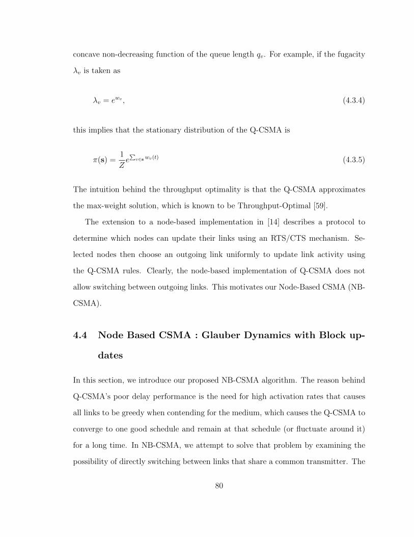
concave non-decreasing function of the queue length qv. For example, if the fugacity

λv is taken as

λv = ewv , (4.3.4)

this implies that the stationary distribution of the Q-CSMA is

π(s) =1

Ze∑v∈s wv(t) (4.3.5)

The intuition behind the throughput optimality is that the Q-CSMA approximates

the max-weight solution, which is known to be Throughput-Optimal [59].

The extension to a node-based implementation in [14] describes a protocol to

determine which nodes can update their links using an RTS/CTS mechanism. Se-

lected nodes then choose an outgoing link uniformly to update link activity using

the Q-CSMA rules. Clearly, the node-based implementation of Q-CSMA does not

allow switching between outgoing links. This motivates our Node-Based CSMA (NB-

CSMA).

4.4 Node Based CSMA : Glauber Dynamics with Block up-

dates

In this section, we introduce our proposed NB-CSMA algorithm. The reason behind

Q-CSMA’s poor delay performance is the need for high activation rates that causes

all links to be greedy when contending for the medium, which causes the Q-CSMA to

converge to one good schedule and remain at that schedule (or fluctuate around it)

for a long time. In NB-CSMA, we attempt to solve that problem by examining the

possibility of directly switching between links that share a common transmitter. The

80

intuition is that the network will then switch between dominant schedules more often,

without having to pay the price of an idle time slot every time a switch happens.

4.4.1 Step 1: Forming Blocks

We now explain how NB-CSMA works. Recall that the outgoing links of every node

k ∈ K are mapped to a clique in the conflict graph that we call Kk. At the beginning

of each slot, a subset of nodes is selected for update. Each one of those selected nodes

chooses a subset of outgoing links to update in that slot. We call this subset of links

the update clique, Ck, for a node k that is allowed to update this slot. The selection

of update cliques Ck is made such that

1. Ck ⊆ Kk

2. For any two nodes that will update at the same slot k, l ∈ K, we have (v, w) /∈

E ∀v ∈ Ck, w ∈ Cl

The first condition simply states that each update clique Ck is a subset of the outgoing

links that have a common transmitter node k ∈ K. This ensures that the algorithm

is fully distributed with respect to the nodes, i.e., the only information needed to

make a scheduling decision comes from the queue lengths at each physical node. The

second condition is more subtle: It states that the links (vertices on conflict graph)

of update cliques should not have an edge between them, i.e., they do not interfere.

This requirement is necessary to ensure that the resulting schedule is feasible since

the update clique can turn any of its links on. We denote the collection of update

cliques at each time slot as C. A simple RTS/CTS-like scheme can be used, whereby

each node polls its outgoing links and adds them to the update clique if no conflict

exists. This simple scheme can be shown to find update cliques that satisfy the two

81

conditions with no siginificant messaging overhead. We denote the probability of

choosing a particular update clique collection C at any time slot as P (C).

4.4.2 Step 2: Updating Blocks

Now that the update cliques C have been found, we proceed to explain how the

schedule shall be updated. We call x(t+1) the proposed schedule. This schedule will

be used to obtain the actual schedule s(t + 1). The NB-CSMA update procedure is

given in Algorithm 4. We can see that lines 3-8 in Algorithm 4 describe an operation

Algorithm 4: NB-CSMA Algorithm

1 for Ck in C do2 if ∃v ∈ Ck s.t. sv(t) = 1 then

3 w.p.1

|Ck|4 sv(t+ 1) = 1, sw(t+ 1) = 0, ∀w ∈ Ck \ v w.p.

λv1 + λv

5 sv(t+ 1) = 0, sw(t+ 1) = 0, ∀w ∈ Ck \ v w.p.1

1 + λv

6 w.p.|Ck| − 1

|Ck|7 xw(t+ 1) = 1, xz(t+ 1) = 0, ∀z ∈ Ck \ w w.p.

λw∑z∈Ck(1 + λz)

, ∀w ∈ Ck \ v

8 xw(t+ 1) = sw(t), ∀w ∈ Ck Otherwise

9 else10 pick link w ∈ Ck uniformly at random

11 xw(t+ 1) = 1 w.p.λw

1 + λw

12 xw(t+ 1) = 0 w.p.1

1 + λw13 if xw(t+ 1) + sz(t) ≤ 1, ∀w ∈ Ck, ∀z ∈ Nw \ Ck then14 sw(t+ 1) = xw(t+ 1), ∀w ∈ Ck15 else16 sw(t+ 1) = sw(t), ∀w ∈ Ck

82

where an already active link is chosen to be updated according to a procedure similar

to the Q-CSMA. Similarly, lines 10-12 describe how an inactive link with no active

neighbor is chosen randomly and added to the schedule with some probability. This

is again similar to the Q-CSMA procedure, i.e., lines 3-8 and 10-12 just describe the

classical Glauber dynamics to generate independent sets with some desired distribu-

tion. Lines 6-8 represent the addition provided by making the CSMA algorithm node

based. A node can switch from one active link to an inactive one according to the

probability defined in line 7. Lines 14-18 state that a link update is only accepted if

the new schedule is an independent set to ensure that no collisions happen; otherwise

the links’ state in the new time slot remains identical to the one in the previous time

slot.

Note that the NB-CSMA algorithms corresponds to performing “Block updates”

as opposed to single site updates in Q-CSMA. The block updates have been used

before for Glauber dynamics to analyze the mixing time [74], [73].

4.5 Performance of the NB-CSMA Algorithm

Since the schedule s(t+1) depends only on the schedule of the previous time slot s(t),

the evolution of schedules over time forms a Discrete Time Markov Chain (DTMC)

with state space Ω. To write the transition probability between two feasible schedules

s and s′, it is useful to look at the conditional transition probabilities given a particular

choice of update cliques C. Let sCk(t) be the schedule of clique Ck at time slot t.

We can breakdown update cliques into three types and characterize their different

transition probabilities P (sCk , s′Ck)

1. Type A: CA: sw(t) = 0, ∀w ∈ CA and s′v(t + 1) = 1, ∃v ∈ CA and

P (sCA , s′CA) =

1

|CA|λv

1 + λv

83

2. Type B: CB: sv(t) = 1, ∃v ∈ CB and s′w(t + 1) = 0, ∀w ∈ CB and

P (sCB , s′CB) =

1

|CB|1

1 + λv

3. Type C: CC: sv(t) = 1, ∃v ∈ CC and s′w(t + 1) = 1, ∃w ∈ CC \ v and

P (sCC , s′CC ) =

|CC | − 1

|CC |λw∑

z∈CC (1 + λz)

Since changes over different cliques at each time slot are independent, the conditional

transition probability given some update cliques C, P (s, s′|C), is calculated by multi-

plying the transition probabilities over every clique depending on the transition type

as described above. Let CA,CB and CC be the cliques that will have a transition of

type A, B or C respectively. The total transition probability follows.

P (s, s′) =∑C

P (C)P (s, s′|C) (4.5.1)

=∑(C)

P (C)( ∏CA∈CA

P (sCA , s′CA)

∏CB∈CB

P (sCB , s′CB)

∏CC∈CC

P (sCC , s′CC ))

(4.5.2)

The DTMC of transmission schedules is both irreducible and aperiodic. Irreducibility

can be checked by noticing that starting from the state s, sv = 0 ∀v ∈ V , any

feasible state s′ ∈ Ω can be reached in finite number of steps. Aperiodicity is easy

to check as well, by noticing that every schedule s ∈ Ω has a self transition if every

clique in the update cliques makes no transition, which always happens with a non-

zero probability.

Theorem 4.5.1. The DTMC is reversible with stationary distribution given by

π(s) =1

Z

∏v∈V

λsvv (4.5.3)

where Z =∑sv∈Ω

∏v∈V

λsvv is a normalizing constant.

Proof. See Appendix C.1

84

Throughput Optimality

It was shown in [14] that any scheduling algorithm that has the stationary distribu-

tion of the form (4.5.3) is Throughput-Optimal under the time-scale separation as-

sumption, i.e., assuming that the DTMC of schedules converges on a fast time-scale

compared to the queue evolution. This means that it is sufficient for the schedul-

ing algorithm to have the “correct” stationary distribution in (4.5.3) in order to be

Throughput-Optimal, thus, NB-CSMA is Throughput-Optimal. The time-scale

separation assumption means that the schedules can be assumed to be always at the

stationary distribution. This assumption was justified in [75]. The intuition behind

Throughput-Optimality can be shown by defining a weight function of link v as

wv = f(qv), ∀v ∈ V (4.5.4)

where f is a concave nondecreasing function of the queue length q (usually taken as

a function slower than log( ) for technical reasons). Then, if we take the link fugacity

to be:

λv = ewv , (4.5.5)

we obtain the stationary distribution of the DTMC as:

π(s) =1

Ze∑v∈s wv(t). (4.5.6)

Intuitively, (4.5.6) approximates the max-weight solution that is known to be Throughput-

Optimal every time slot [59]. We note that the stationary distribution of NB-CSMA

is equal to the one of Q-CSMA in [14], that is, in terms of the stationary distribution

85

of schedules, NB-CSMA and Q-CSMA are equivalent. It is the second-order behavior

that is different, which causes NB-CSMA to have favorable delay performance.

Delay Performance

Due to complex interactions between different links, the delay performance is gener-

ally hard to assess. However, several tools have been used to analyze the delay of

CSMA-like algorithms. We begin our delay performance assessment by comparing

the delay performance between Q-CSMA and NB-CSMA for a fixed size network,

showing that under NB-CSMA algorithm, each link sees a service process that has

less variability, implying better delay performance. We then proceed to test how NB-

CSMA scales as the network size increases. In particular, we are interested in char-

acterizing the fraction of the capacity region where the queue sizes can be bounded

polynomially in the number of links (as opposed to exponentially). A similar result

for Q-CSMA was found in [65]. We show that the fraction of the throughput region

where the NB-CSMA is fast mixing is usually larger that the one found in [65], except

for some special cases when the two regions coincide. Before we proceed, we make

three simplifying assumptions for the sake of tractability:

A1 All fugacities, λv ∀v, are fixed and possibly heterogeneous, as opposed to the

dynamic fugacities used to prove throughput optimality. Suitable fixed fugac-

ities can be found using the problem formulation/solution in [12] to stabilize

any arrival rate vector in the capacity region.

A2 We assume for our comparison purposes that both NB-CSMA and Q-CSMA

perform a single update per time slot, i.e., in Q-CSMA one link (vertex in the

conflict graph) is updated, and in NB-CSMA one node (clique in the conflict

graph) is updated. This does not change the stationary distribution in (4.5.3);

86

it just provides easier grounds for comparison at the cost of slower convergence

to the stationary distribution since only one update per slot is allowed.

A3 We assume that in Q-CSMA, each time slot, a link is chosen uniformly at

random to be updated (with probability1

n, where n is the number of links).

We assume on the other hand in NB-CSMA, each time slot a node k is updated

at random with probability proportional to the number of outgoing links (with

probability|Kk|n

). This makes the probability that a particular link is turned

ON or OFF equal in both Q-CSMA and NB-CSMA.

We note that A2-A3 suit the case of continuous-time CSMA. However, in discrete-time

NB-CSMA, the network has to perform parallel updates (dropping A2-A3) for two

reasons: 1. Performing single-site updates require network-wide coordination which

is not practical in large networks. 2. Parallel updates enables the network to track

the optimal max-weight solution faster (and speeds up mixing time by O(n) [65])

which translates to a reduction in network delay.

Comparison to Q-CSMA for fixed size networks

In a fixed size network setting, we are interested in comparing the steady-state delay

performance between Q-CSMA and NB-CSMA. The approach we use is similar to the

one used in [67] to compare fixed size networks. This approach depends on looking at

the service process of any link v in isolation. First, define the service process of link

v under NB-CSMA and Q-CSMA algorithms as σv(t) and σv(t), respectively. Also

define P, P , π, π to be the transition matrix and the stationary distribution of the

NB-CSMA and the Q-CSMA Markov chains, respectively. Throughout this analysis,

we assume that both Markov chains P and P have already converged to their steady

state distribution.

87

Let B be the subset of schedules that include link v in them: B = s ∈ Ω : sv = 1.

The service process σv(t) is a 0-1 process with

P (σv(t) = 1) =∑s∈B

π(s). (4.5.7)

We define

T1 = mint ≥ 0 : σv(t) = 1 (4.5.8)

Ti+1 = mint > Ti : σv(t) = 1. (4.5.9)

For the states s ∈ B, Let τi = Ti+1 − Ti (i ≥ 1) be the sequence of recurrence times

and πB be their steady state probability. The quantities πB, σ(t), τi are defined simi-

larly. We are interested in comparing the quantities E(τi),E(τ 2i ) with the quantities

E(τi),E(τi2).

Theorem 4.5.2. Under assumptions A1-A3, for any link v, the following inequalities

hold

E(τi) = E(τi) (4.5.10)

E(τ 2i ) ≤ E(τ 2

i ) (4.5.11)

Proof. See Appendix C.2

Fast Mixing Activation Rates

We are now interested in characterizing the asymptotic delay performance of the NB-

CSMA as the size of the network grows for networks with bounded-degree conflict

graphs. It was shown in [61], that at high throughput values, the delay of the con-

ventional CSMA algorithm grows exponentially with the number of the links in the

88

network, which makes the delay performance unacceptable in large networks. Our

goal is to characterize the throughput region where the average delay is bounded by

a polynomial, because this is the region where the network is guaranteed to operate

with acceptable delay performance. In [65], this region was shown to be contained in

the region where the schedules Markov chain is “fast mixing”. Thus, our target is to

find the fraction of the capacity region that makes the network fast mixing.

We first define the total variation distance between the Markov chain distribution

at time t starting from state x and the stationary distribution π:

dTV (P tx, π) = max

A⊂Ω|P tx(A)− π(A)| (4.5.12)

The mixing time of the Markov Chain is defined as

Tmix(ε) = mint |maxx

dTV (P tx, π) < ε. (4.5.13)

Our tool for bounding the mixing time will be coupling. The coupling of two Markov

chains is a pair process (X t, Y t) such that

1. Each of the Markov Chains (X t, Y t) when viewed in isolation remains faithful

to the original Markov Chain.

2. If X t = Y t then X t+1 = Y t+1.

The mixing time is bounded by the stopping time taken for any two coupled processes

to meet, that is

Tmix ≤ maxx,y

mint : X t = Y t|X0 = x, Y 0 = y. (4.5.14)

89

Equivalently, instead of computing the stopping time explicitly, we can define a dis-

tance metric on Ω, and compute the time taken for the distance between the two

processes to go to zero. Path coupling introduced in [76] is a powerful tool that

makes it easier to design and analyze couplings, by showing that to bound the mix-

ing time, it is enough to restrict the couplings to pairs of states that are adjacent

in the metric. This is much easier than bounding mixing time using couplings for

arbitrary pairs of states. Formally:

Theorem 4.5.3. [76] Let δ be an integer valued metric on Ω×Ω which takes values

0, ..., D . Let S be a subset of Ω×Ω such that for all (xt, yt) ∈ Ω×Ω, there exists

a path xt = e0, e1, ..., er = yt between xt and yt such that (el, el+1) ∈ S, ∀ 0 ≤ l < r

and

r−1∑l=0

δ(el, el+1) = δ(xt, yt) (4.5.15)

Define a coupling (x, y)→ (x′, y′) on the Markov Chain P on all pairs (x, y) ∈ S and

suppose there exists β ≤ 1 s.t. E(δ(x′, y′)) ≤ βδ(x, y) for all x, y ∈ S . If β < 1 the

mixing time Tmix(ε) satisfies

Tmix(ε) ≤log(Dε−1)

1− β, (4.5.16)

where D = maxx,y∈Ω

δ(x, y), i.e., the maximum distance between any two states in terms

of the metric δ(x, y).

Later, we shall apply this theorem with the Hamming distance metric, i.e., δ(x, y) =∑v∈V

1(xv 6= yv). Thus, for our results, we can substitute D with the number of links

in the network, n. Instead of analyzing the NB-CSMA Markov chain, P , we analyze

a different Markov Chain Q that is linearly related to the original Markov chain P ,

90

and rely on the relationship between P and Q to estimate the mixing time of P .

Throughout this section, we shall assume that assumptions A1, A2 and A3 hold. For

notational convenience, we refer to the set of outgoing links of node k, that contains

link v as Kv. Recall that Kv is also a clique in the conflict graph. Furthermore under

A2, since only one node gets to update its schedule every time slot, we assume this

node always chooses to update all outgoing links Kv. Let λ1 ≤ λ2... ≤ λmax be the set

of fugacities of all links v ∈ V . Define the transitions of Markov Chain Q as specified

in Algorithm 5. It is not difficult to check that the Markov Chain Q has a stationary

distribution equal to that of (4.3.3) and (4.5.3).

Theorem 4.5.4. Given the Markov Chain Q, if λmax <1

maxv

(dv − |Kv|), then the

mixing time of Q satisfies

Tmix(ε) ≤2n(1 + λmax) log(nε−1)

1−maxv

(dv − |Kv|)λmax

= O(n log n). (4.5.17)

Where dv is the interference degree of link v (number of neighbors in conflict graph

or number of interferers).

Proof. See Appendix C.3

Now that we have bounded the mixing time of Q, we need to relate it to the mixing

time of P . We make use of the following Lemma stated as Theorem 5.3 in [77].

Lemma 4.5.1. [77] Given two Markov chains P and Q, let their mixing times be

T Pmix and TQmix respectively. If

P ≥ αQ, (4.5.18)

then T Pmix ≤ 2α−1TQmix log(π∗(2ε)−1) where π∗ = maxx∈Ω

√1− π(x)

π(x).

91

Algorithm 5: Evolution of Markov Chain Q

1 Pick a Clique Kv to update randomly w.p.|Kv|n

2 w.p.1

23 s(t+ 1) = s(t)

4 w.p.1

25 if ∃v ∈ Kv s.t. sv(t) = 1 then

6 w.p.1

|Kv|7 sv(t+ 1) = 1, sw(t+ 1) = 0, ∀w ∈ Kv \ v w.p.

λv1 + λmax

8 sv(t+ 1) = 0, sw(t+ 1) = 0, ∀w ∈ Kv \ v w.p.1

1 + λmax

9 w.p.|Kv| − 1

|Kv|10 xw(t+ 1) = 1, xz(t+ 1) = 0, ∀z ∈ Kv \ w w.p.

λw2(|Kv| − 1)(1 + λmax)

, ∀w ∈ Kv \ v

11 xw(t+ 1) = sw(t), ∀w ∈ Kv otherwise

12 else13 pick link w ∈ Kv uniformly at random

14 xw(t+ 1) = 1 w.p.λw

1 + λmax

15 xw(t+ 1) = 0 w.p.1

1 + λmax

16 if xw(t+ 1) + sz(t) ≤ 1, ∀w ∈ Kv, ∀z ∈ Nw \Kv then17 sw(t+ 1) = xw(t+ 1), ∀w ∈ Kv

18 else19 sw(t+ 1) = sw(t), ∀w ∈ Kv

92

Before we apply this Lemma to bound the mixing time of P, we state another

Lemma

Lemma 4.5.2. Let P ∗ be the lazy version of the Markov Chain P (by having a self

transition with probability1

2every time slot). Then P ∗ ≥ αQ, where α =

1

2.

Proof. Denote the transition from s to s′ as P ∗(s, s′) and Q(s, s′) in the P ∗ and Q

chains respectively. We verify that α =1

2for all three types of transitions (and we

add type 4 for self-transitions

T1 P ∗(s, s′) =λv

2n(1 + λv)≥ λv

2n(1 + λmax)≥ Q(s, s′) ≥ αQ(s, s′)

T2 P ∗(s, s′) =1

2n(1 + λv)≥ 1

2n(1 + λmax)≥ Q(s, s′) ≥ αQ(s, s′)

T3 P ∗(s, s′) =|Kv| − 1

2n

λw∑z∈Kv(1 + λz)

≥ |Kv| − 1

2n

λw|Kv|(1 + λmax)

≥ αQ(s, s′)

T4 P ∗(s, s′) ≥ 1

2≥ α ≥ αQ(s, s′)

We can now directly bound the mixing time of P using the following theorem:

Theorem 4.5.5. Given the NB-CSMA Markov Chain P, if λmax <1

maxv

(dv − |Kv|),

then the mixing time of P can be bounded as

Tmix(ε) = O(n2 log n). (4.5.19)

Proof. The theorem is proved by applying Lemma 5 for P ∗ with α =1

2from Lemma

6. Also, for any graph, log(π∗) = O(n) [77]. Applying Lemma 5 with these quantities,

and noticing that P ∗ has double the mixing time of P concludes the theorem.

93

It remains to find the fraction of the capacity region that causes the Markov

chain P to be fast mixing, and consequently causes the queue lengths of links to be

polynomially bounded in the number of links. Before we state our main theorem we

state a related result from [12] as a Lemma

Lemma 4.5.3. [12] Given any ν ∈ Λ, there exists suitable activation rates λ such

that for every link v, the mean service rate E(sv) is equal to the mean arrival rate νv.

The last Lemma ensures the existence of fixed activation rates (fugacities) that

stabilize the queues whenever the arrival rate vector falls within the capacity region.

Now we are ready to present our final theorem

Theorem 4.5.6. Given an arrival rate vector ν that satisfies ν ∈ γΛ, where

γ =1

maxv

(dv − |Kv|+ 1), (4.5.20)

the Markov chain P is fast mixing, and the expected queue lengths of any link v can

be bounded by

E(qv(t)) = O(Tmix) = O(n2log(n)) (4.5.21)

Proof. See Appendix C.4

Discussion

In the last theorem, we characterized the fraction of the capacity region that makes

the Markov chain P fast-mixing. This is the fraction of the capacity region for which

the average queue lengths grow polynomially in the number of links n. The region

in Theorem 6 is no smaller than the regions found in [65] and [66]. In fact the result

in [65] showed that the network was fast-mixing for ν ∈ 1

4Λ, where 4 = max

vdv is

94

the conflict graph degree. The difference between this result and ours is the following:

In [65] we have to decrease the throughput as the number of interferers increase to

get acceptable delay performance. In Theorem 9, we have to decrease the throughput

only when the number of external interferers increase (interferers that have a different

transmitter). We expect the difference to be significant in ad-hoc networks when the

average node degree increases as the network becomes dense. Another difference is

the following: The mixing time bound obtained in [65] was O(log(n)) under parallel-

updates assumption (with assumption A2 removed). However the mixing time of Q-

CSMA for single-site updates is lower bounded by Ω(n log(n)) [78]. Furthermore, in

Theorem 9, an additional O(n) factor comes from the log(π∗) term in the comparison

theorem in Lemma 5. Thus the mixing time upper bound of P is of order O(n)

larger than that of Q. However, as asserted in [77], this additional O(n) factor is

almost certainly an artifact of the analysis. Thus, although the bound of Theorem 9

is O(n2) times that of [65], we do not expect the mixing time of Q-CSMA to be less

than that of NB-CSMA for any arrival rate vector. This will be further validated by

simulations.

4.6 Collocated Networks

In this section, we restrict our study to collocated networks where every link interferes

with all other links. It is easy to see that the resulting conflict graph is complete and

at most one link can be active each time slot, i.e., for a network with n links, we have

n+1 feasible schedules enumerating all links in the network plus the empty schedule.

We focus on collocated networks for both their relative simplicity compared to general

networks which have O(2n) feasible schedules and their practical importance as they

are often used to model wireless local area networks. Several works have analyzed

collocated networks separately: [65] analyzed the mixing time of the schedules Markov

95

chain. [79] formulated the link access probability as an optimization problem, and [80]

derived a lower bound on mean delay for dynamic activation rates. Our goals in this

section are

1. We analyze collocated networks using the Markov Chain with rewards frame-

work [81] to derive a closed-form expression for the mean starvation time for

individual links under both Q-CSMA and NB-CSMA.

2. We use mean starvation expressions to infer, in a quantifiable way, the expected

gains from using NB-CSMA over Q-CSMA as a function of activation rates and

network topology. To this end, we use simplifying assumptions for the network

for the sake of obtaining closed-form expressions.

We remark that our approach is inspired by [66] where the marginal service rate

process along with stochastic dominance were used to derive average delay bound for

any link in a general network with bounded-degree conflict graph. However, we note

that finding the mean-delay bounds obtained in [66] involves inverting the transition

matrix, which is only possible computationally and does not offer clear insights on how

the bound depends on different network parameters. We first note that for any

collocated network, feasible schedules can be enumerated as (0, e1, e2, ..., en), where

eu = s|su = 1 and sv = 0, ∀v 6= u. For the rest of our analysis, we will consider the

behavior of link 1, without loss of generality. Similar to our analysis in Section 5.2,

we define ζi as the ith starvation time. Formally, we have ζi = Ti+1 − Ti| s1(Ti) =

1, s1(Ti+1) = 1 and s1(t) = 0 ∀Ti < t < Ti+1. Note that the difference between

starvation time ζi and recurrence time τi is that starvation time counts the time

between two “ON” slots such that all the slots between them link 1 is “OFF”, whereas

recurrence time counts the time between “ON” slots even if they are consecutive. Our

96

goal is to explicitly express E(ζi) for a collocated network performing both Q-CSMA

and NB-CSMA and relating their performance ratio to the network topology

4.6.1 Q-CSMA Starvation time

General Case

To compute the mean starvation time for a collocated network executing Q-CSMA,

we assume without loss of generality that one link is chosen uniformly at random

to update each time slot w.p.1

n. We then modify the Markov chain governing the

schedules by making the state e1 absorbing (by modifying probabilities such that

P11 = 1 and P1u = 0, for u 6= 1. We can now write the modified Markov chain

transition matrix SQ (where the transitions from/to schedule e1 were moved to the

last row/column respectively) as follows:

1−∑n

i=1λi

n(1+λi)λ2

n(1+λ2)λn

n(1+λn)λ1

n(1+λ1)

. . . . . . . . . . . . . . .

1n(1+λn)

. . . 1− 1n(1+λn)

0

0 0 0 1

(4.6.1)

Let vi be the expected first-passage time from ei to e1. The vector v can be found

using a a first-step analysis by solving the following linear equations [81, Chapter 4.5]

v = 1 +Qv (4.6.2)

which can be simplified to:

v0 = 1 +n∑i=2

λin(1 + λi)

vi +

(1−

n∑i=2

λin(1 + λi)

)v0 (4.6.3)

97

1 0 B

1

n(1 + λ)

1− 1

n(1 + λ) (n− 1)λ

n(1 + λ)

1

(1 + λ)

λ

n(1 + λ)

1

n(1 + λ)

1− 1

n(1 + λ)

Figure 4.2: State space of Q-CSMA in collocated network, equal throughput case

vi = 1 +1

n(1 + λi)v0 +

(1− 1

n(1 + λi)

)vi, 1 < i ≤ n (4.6.4)

We can easily solve these linear equations to obtain vi for i = 0 and all i > 1. Note

that under Q-CSMA, the scheduling Markov chain can only depart schedule e1 to

schedule 0, i.e., we have E(ζ1) = v0, thus, solving (4.6.3) and (4.6.4) we get

E(ζ1) = v0 =(∑n

i=2 λi + 1)(n(1 + λ1))

λ1

. (4.6.5)

Equal Throughput Case

If we further simplify the network to assume all links in the network having the same

arrival rate, we can assume that all activation rates in the network are fixed and

equal, we drop the subscript and refer to this unified fugacity as λ. Under these

assumptions, we can simplify the state space of the scheduling Markov chain s(t) by

making the following observation: Link 1 only sees the medium in three states: 1.

ON: whenever s(t) = e1, i.e., link 1 currently owns the medium and freely transmits

if it has any packets in its queues, 2. IDLE: whenever s(t) = e0: No link owns

the medium, link 1 can acquire the medium with probabilityλ

n(1 + λ), and finally, 3.

98

BLOCKED: whenever s(t) ∈ e2, e3, ..., en. The state diagram of the new transition

matrix is shown in Fig. 2. The reason of this is when activation rates are equal, it

does not make a difference what other link has the medium from the point of view

of link 1. More formally, the states e2, e3, ..., en are statistically indistinguishable

when we are interested in analyzing the behavior of link 1. We consolidate these

states into a single state eB and rewrite the matrix Q in (4.6.1) as

Q =

1

1+λ(n−1)λn(1+λ)

λn(1+λ)

1n(1+λ)

1− 1n(1+λ)

0

0 0 1

(4.6.6)

Performing a first-step analysis for the new Markov Chain to obtain the mean-first

passage times (v0, vB) starting from the schedules (e0, eB), respectively, we get:

v0 = 1 +1

1 + λv0 +

(n− 1)λ

n(1 + λ)vB (4.6.7)

vB =1

n(1 + λ)v0 + (1− 1

n(1 + λ))v2 (4.6.8)

Solving the two linear equations, we get the following expression for the mean-

starvation time

E(ζQ1 ) = v0 = n2 + n(n− 1)λ+n

λ, (4.6.9)

where we have used the fact that any starvation epoch will have to start from the

state e0 since the state e1 can only transition to state e0. As a sanity check, we note

that letting all activation rates λi = λ for all links in (4.6.5) gives us the expression

in (4.6.9).

99

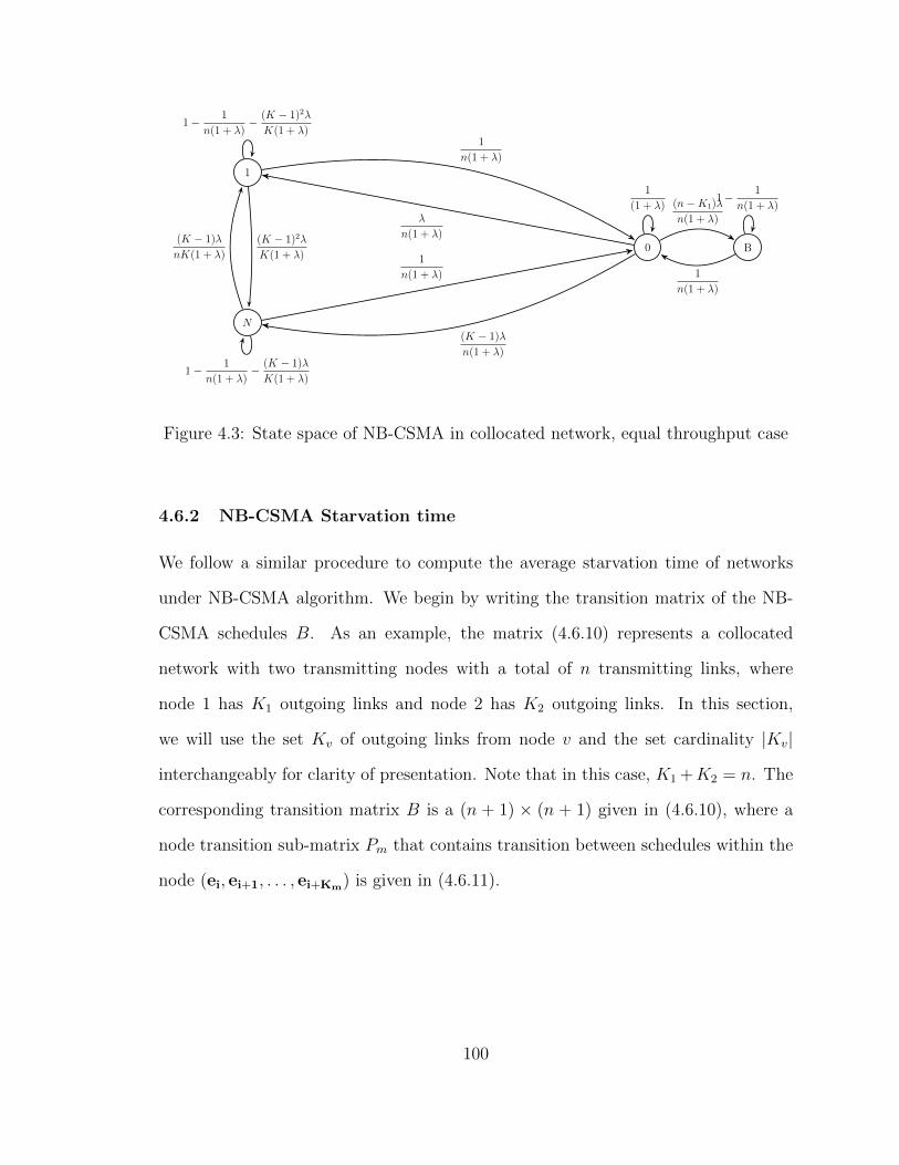
1

N

0 B

1

n(1 + λ)

1− 1

n(1 + λ)− (K − 1)2λ

K(1 + λ)

(K − 1)2λ

K(1 + λ)

(n−K1)λ

n(1 + λ)

1

(1 + λ)λ

n(1 + λ)

(K − 1)λ

n(1 + λ)

1

n(1 + λ)

1− 1

n(1 + λ)

1

n(1 + λ)

1− 1

n(1 + λ)− (K − 1)λ

K(1 + λ)

(K − 1)λ

nK(1 + λ)

Figure 4.3: State space of NB-CSMA in collocated network, equal throughput case

4.6.2 NB-CSMA Starvation time

We follow a similar procedure to compute the average starvation time of networks

under NB-CSMA algorithm. We begin by writing the transition matrix of the NB-

CSMA schedules B. As an example, the matrix (4.6.10) represents a collocated

network with two transmitting nodes with a total of n transmitting links, where

node 1 has K1 outgoing links and node 2 has K2 outgoing links. In this section,

we will use the set Kv of outgoing links from node v and the set cardinality |Kv|

interchangeably for clarity of presentation. Note that in this case, K1 +K2 = n. The

corresponding transition matrix B is a (n + 1) × (n + 1) given in (4.6.10), where a

node transition sub-matrix Pm that contains transition between schedules within the

node (ei, ei+1, . . . , ei+Km) is given in (4.6.11).

100

B =

1−∑n

i=1λi

(1+λi)λ1

n(1+λ1). . .

λK1

n(1+λK1)

λK1+1

n(1+λK1+1). . . λn

n(1+λn)

1−∑n

i=1λi

(1+λi)

λ1n(1+λ1)

...

λK1

n(1+λK1)

P1 0

1−− 1n(1+λK1+1)

...

1n(1+λn)

0 P2

(4.6.10)

We can repeat the steps in the previous section to obtain a result similar to (4.6.5).

However due to the less-sparse structure of the matrix B, we cannot get a closed-form

solution for the mean starvation time of any link in a network operating under the

NB-CSMA scheduling algorithm. Therefore, we focus on the special case of equal

throughputs.

Similar to Section 4.6.1, when studying the mean starvation time of link 1 of node

1, which has a total of K1 outgoing links under the equal throughput assumption, we

simplify the state space into four states relevant to link 1: 1. ON: whenever s(t) = e1,

i.e., link 1 currently owns the medium and freely transmits if it has any packets in its

queues, 2. IDLE: whenever s(t) = e0: No link owns the medium, link 1 can acquire

Pm =

1− 1

n(1+λi)−∑j 6=i

(Km−1)λj

n∑i+Km

l=i (1+λl)

(km−1)λi+1

n∑i+Km

l=i (1+λl)

(km−1)λi+Km

n∑i+Km

l=i (1+λl)(km−1)λi

n∑i+Km

l=i (1+λl)1− 1

n(1+λi+1)−∑j 6=i+1

(Km−1)λj

n∑i+Km

l=i (1+λl). . .

(km−1)λi+Km

n∑i+Km

l=i (1+λl)

. . . . . . . . . . . .(km−1)λi

n∑i+Km

l=i (1+λl)1− 1

n(1+λi+Km ) −∑j 6=i+Km

λj∑i+Kml=i (1+λl)

(4.6.11)

101

the medium with probabilityλ

n(1 + λ), 3. NEIGHBOR: The medium is owned by a

link that is outgoing from node 1, thus at anytime the schedule can switch to link

1 w.p.(K1 − 1)λ

nK1(1 + λ). The NEIGHBOR state is entered whenever s(t) ∈ eK1 \ e1

4. BLOCKED: whenever s(t) ∈ eS \ (eK1 ∪ e0). In the rest of this section, we will

denote K1 simply as K for clarity of presentation. The state diagram of the new

transition matrix is shown in Fig. 4.3.

To derive the mean starvation time of link 1, we modify the Markov chain in Fig.

4.3 of schedules by making the state e1 absorbing. We repeat the procedure of Section

4.6.1.A. to derive the first-passage time of all states to the target state e1. Solving

the associated linear equations, we obtain the vector of mean first passage times

[vN , v0, vB]. Under the NB-CSMA in Fig. 4.3, the schedule can transition out of state

e1 to either the IDLE state e0 or the NEIGHBOR state eN with probabilityP10

P10 + P1N

andP1N

P10 + P1N

respectively. Therefore, to compute the mean starvation time we take

the inner product between the initial distribution α = [P10

P10 + P1N

P1N

P10 + P1N

0] and

the mean first-passage time α = [v0 vN vB] to obtain:

E(ζN1 ) = αᵀv =Kn(λ+ 1)(nλ− λ+ 1)

λ(λk2 + (1− 2λ)k + λ)(4.6.12)

In this section, we compare the service processes of both Q-CSMA and NB-CSMA

in the case of collocated networks in the equal throughput case, when all nodes have K

outgoing links. We first begin by stating the following Lemma in choosing activation

rates λ in our special case of equal throughputs.

Lemma 4.6.1. Given a collocated network running Q-CSMA or NB-CSMA with

equal throughputs for all links, an activation rate of λ =ρ

n(1− ρ)+ ε for any ε > 0

stabilizes any throughput requirement ν =ρ

nfor 0 < ρ < 1.

The proof is immediate by checking that the stationary probability of the Markov

102

chain π(ei) =λ

1 + nλ>ρ

nwhich guarantees the stability of all queues. Recall that the

stability region of a collocated network is given by ν|n∑i=1

ν < 1 and for the special

case of equal throughputs the stability conditions reduces to the single condition of

ν <1

n. The ρ in Lemma 4.6.1 takes values between 0 and 1 and represents the traffic

intensity in the network.

We are now ready to compare the ratio between mean starvation times of both

Q-CSMA and NB-CSMA in the following theorem

Theorem 4.6.1. Given a collocated network with n links,K

nnodes each with K

outgoing links and equal throughputs at all links with ν =ρ

n, the ratio r between

mean starvation times of NB-CSMA and Q-CSMA is given by

r =K

K + λ(K2 − 2K + 1)(4.6.13)

where

λ =ρ

n(1− ρ)+ ε, for any ε > 0. (4.6.14)

The proof is immediate by dividing (4.6.12) by (4.6.9). The ratio gives the decrease

observed when using NB-CSMA instead of Q-CSMA in a given network. Theorem

4.6.1 leads to the following observations:

1. The ratio decreases with outgoing links K as Θ(K2), which means that for a

given network, we see greater improvement in starvation times as the number of

outgoing links per node increases. This result is expected since larger K means

that many decisions will be centralized for more links.

2. The ratio decreases as Θ(1

(1− ρ)2) as well, which means: the higher the network

103

traffic intensity, the more improvement we expect to get from NB-CSMA in

terms of starvation times.

3. Each link will see an alternating renewal service process with equal long-term

mean service times between all links under both NB-CSMA and Q-CSMA

scheduling algorithms. However, the service process under each algorithm will

be as follows

Q-CSMA: The link will be ON for a Geometrically distributed, Geo(1

n(1 + λ)),

epoch, then OFF for an epoch that has a discrete Phase-Type distribution with

mean E(ζQ1 ) given in (4.6.9).

NB-CSMA: The link will be ON for a Geometrically distributed, Geo(1

n(1 + λ)+

(K − 1)2λ

K(1 + λ)), epoch, then OFF for an epoch that has a discrete Phase-Type dis-

tribution with mean E(ζN1 ) given in (4.6.12).

4.7 Numerical Results

4.7.1 General Networks

We simulate a random topology where 20 wireless nodes are placed uniformly at

random in a 600x600m square. A wireless link is established with probability 1, if

the transmitter node is within 150m from the receiver node, and with probability

0.5 if the transmitter is within 250m from the receiver. All links in this simulation

are unidirectional. We assume a geometric interference relationship between links

whereby two links interfere with each other if a)they share a transmitter node, b)they

share a receiver node, c)the transmitter node of one link is within 250m of the receiver

node of the other one. The resulting instance of the geometric random network has

48 links. To determine the decision schedule of Q-CSMA and the update blocks of

104

0 100 200 300 400 500 600

X

0

100

200

300

400

500

600

700

Y

Nodes

Links

Figure 4.4: 600x600m Random Network Topology

the NB-CSMA, we use a contention window of size 8 and a random back-off scheme,

where every link waits a random time, then attempts to include itself in the update

blocks (decision schedule). If no conflict happens, the inclusion is successful. We also

use the dynamic fugacities λv =log(1 + qv)

log(e+ log(1 + qv))found to have the best delay

performance [75]. Thus effectively in the simulation we have dropped assumptions

(A1-A3) of Section 4.5. The arrivals at different links are independent Bernoulli

processes. We determine the arrival rates of all links using the following three steps:

a) We compute all the maximal independent sets of the conflict graphG of the network

G in Fig. 4.4, we call this set of independent sets AM . b) For each of these sets,

Am∈M , we obtain an arrival rate vector νm on the boundary of the capacity region

by setting the arrival rates of all links v included in the set to νvm = 1, ∀v ∈ m

and otherwise νvm = 0, ∀v /∈ m. c) By taking the average of νm that is, taking the

average of the binary vector [νvm]m∈M at each link v, we get an arrival rate vector

ν∗ at the boundary of the capacity region that has a strictly positive arrival rate

for every link v ∈ V . We multiply ν∗ by a factor ρ ∈ (0, 1) that we call “Traffic

105

0 0.1 0.2 0.3 0.4 0.5 0.6 0.7 0.8

Traffic Intensity (ρ)

0

50

100

150

200

250

300

350

Avera

ge Q

ueue L

ength

Per

Lin

k

NB-CSMA

Q-CSMA

Figure 4.5: Average Queue Length per link vs. ρ

Intensity” to simulate the network at different levels of throughput. In Fig. 4.5,

we plot the time-average queue lengths per link against the traffic intensity ρ. We

calculate the average queue lengths for 2 × 105 time slots. In all simulations, we

neglect the evolution of queue lengths for the first half of the simulation time when

calculating time-averages, to make sure that we have minimized the influence of the

transient behavior at the beginning of the simulation. We can see as expected that

NB-CSMA outperforms Q-CSMA for all values of ρ. In this example, the average

queue lengths of NB-CSMA is on average half of that of Q-CSMA for all values of

ρ. By Little’s la w [81], we know that the average delay is the ratio of the average

queue length of any link (and of the whole network) to the arrival rate. Thus, for

this example, NB-CSMA results in 50% decrease in average delay for any arrival rate

vector within the capacity region.

We consider a recent proposal that greatly improves the performance of Q-CSMA,

and compare the performance of the modified Q-CSMA to the performance of NB-

CSMA when they both implement the same modification. Namely, we consider the

106

0 0.1 0.2 0.3 0.4 0.5 0.6 0.7 0.8

Traffic Intensity ( )

0

50

100

150

200

250

300

350

Ave

rag

e Q

ue

ue

Le

ng

th P

er

Lin

k

Delayed CSMA, T=2 [16]

Delayed NB-CSMA, T=2

Delayed CSMA, T=8 [16]

Delayed NB-CSMA, T=8

Figure 4.6: Average Queue Length per link vs. ρ (Delayed CSMA, T = 2, T = 8.)

case of “Delayed CSMA” proposed in [70] [71] (and slightly differently in [69], [72])

whereby the links keep T parallel schedules and update each schedule independently.

For instance, if T = 2, then the network keeps two separate schedules: one for even

time slots and one for odd time slots. Intuitively, when two or more schedules evolve

independently, it becomes less likely that any link will be starved for a long time.

In Fig. 4.6, the resullts of the implementation of Delayed-CSMA for both Q-CSMA

and NB-CSMA are presented. We simulate the network in Fig. 4.4 for different

traffic intensities. We note that, both Q-CSMA and NB-CSMA see improvements

when the number of parallel schedules T , grow from 2 to 8. In fact, Q-CSMA sees a

28% reduction in average delay, whereas NB-CSMA sees a 33% reduction, i.e., NB-

CSMA sees more reduction when the schedules are parallelized. Also when T = 8

at high throughputs, the average delay under Delayed NB-CSMA is 40-50% that

of Delayed-CSMA. This suggests that the benefits of improvements to link-based

CSMA algorithms, such as parallelization, carry over to NB-CSMA whenever those

improvements are implemented on top of NB-CSMA.

107

0.6 0.65 0.7 0.75 0.8 0.85 0.9 0.95

Traffic Intensity ( )

200

300

400

500

600

700

800

900

1000

1100

1200

Me

an

Sta

rva

tion

Tim

e:

E(

)

Q-CSMA-Analytical

Q-CSMA-Simulated

NB-CSMA-Analytical

NB-CSMA-Simulated

0.4776 0.4639 0.4467 0.4248 0.3956 0.3550 0.2945 0.1949

Ratio: r

0.4776

0.4639

0.4467

0.4248

0.3956

0.3550

Figure 4.7: Mean Starvation time of link 1 vs. ρ

4.7.2 Collocated Networks

We simulate a collocated topology with the assumptions of Section 4.6 (symmetric

networks, fixed fugacities, equal throughputs), with four nodes each having six out-

going links (K = 6, n = 24) for 106 slots. In Fig. 4.7, we plot the analytical and

simulated mean starvation times against the traffic intensity ρ. We also added the

corresponding ratio r for each ρ at the top x-axis. We first note that the mean starva-

tion time increases as we increase ρ for Q-CSMA whereas it decreases for NB-CSMA.

The behavior of Q-CSMA can be explained by taking the derivative of (4.6.9) with

respect to λ. We find that the mean starvation time is decreasing for λ <

√1

n− 1

and increasing for λ >

√1

n− 1. Therefore, at high traffic intensities we observe a

sharp increase in mean starvation times. The behavior of NB-CSMA is more compli-

cated, as the expression in (4.6.12) is a fractional polynomial, thus, increasing traffic

intensity may cause mean starvation time to increase, decrease or oscillate depending

on the network topology. As traffic intensity increases, there are two forces that affect

108

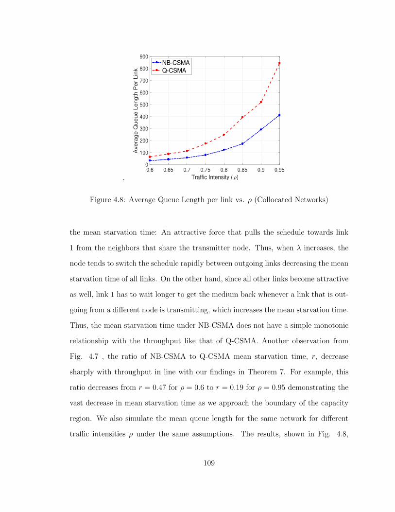
.0.6 0.65 0.7 0.75 0.8 0.85 0.9 0.95

Traffic Intensity ( )

0

100

200

300

400

500

600

700

800

900

Ave

rag

e Q

ue

ue

Le

ng

th P

er

Lin

k

NB-CSMA

Q-CSMA

Figure 4.8: Average Queue Length per link vs. ρ (Collocated Networks)

the mean starvation time: An attractive force that pulls the schedule towards link

1 from the neighbors that share the transmitter node. Thus, when λ increases, the

node tends to switch the schedule rapidly between outgoing links decreasing the mean

starvation time of all links. On the other hand, since all other links become attractive

as well, link 1 has to wait longer to get the medium back whenever a link that is out-

going from a different node is transmitting, which increases the mean starvation time.

Thus, the mean starvation time under NB-CSMA does not have a simple monotonic

relationship with the throughput like that of Q-CSMA. Another observation from

Fig. 4.7 , the ratio of NB-CSMA to Q-CSMA mean starvation time, r, decrease

sharply with throughput in line with our findings in Theorem 7. For example, this

ratio decreases from r = 0.47 for ρ = 0.6 to r = 0.19 for ρ = 0.95 demonstrating the

vast decrease in mean starvation time as we approach the boundary of the capacity

region. We also simulate the mean queue length for the same network for different

traffic intensities ρ under the same assumptions. The results, shown in Fig. 4.8,

109

show that NB-CSMA consistently achieves around 50% of the delay achieved by Q-

CSMA across all traffic intensities ρ. Interestingly, this is similar to the reduction we

obtained in the random topology with unequal throughputs and adaptive fugacities.

4.8 Practical Implementation of NB-CSMA

We now discuss the practical implementation of NB-CSMA. NB-CSMA is synchro-

nized, in the sense that all nodes perform contention simaltanuously. As we shall

show, this completely eliminates problems such as Hidden-Terminal problem and

Exposed-terminal problem. This is unlike the 802.11 protocol model which is asyn-

chronous, but follows earlier practical implementations for throughput-optimal CSMA,

such as [14], which are synchronous. A similar discussion was presented in [14] for

the link-based Q-CSMA. We give the Node-based counterpart of the implementation

that satisfies the NB-CSMA requirements and procedures.

Similar to the WiFi RTS/CTS/Data/ACK scheme, our implementation of NB-

CSMA takes four steps:

1. POLLING: Sent by a potentially transmitting node, S, each time slot to explore

outgoing link states.

2. Clear To Update (CTU): Sent by a receiving node, R, as a response to the

POLLING signal by S, to indicate that a link (S,R) is available for update this

time slot.

3. Data: Transmission of the packet by transmitter node S to receiver node R.

4. ACK: Sent by receiver R to acknowledge successfully receiving a packet.

For the purposes of Forming Blocks (Section 4.4-Step 1 ), each node keeps a num-

ber of flag bits that are updated each time slot:

110

• AVAILABLE Tx, AVAILABLE Rx : A bit that indicates whether a node is

available or blocked as a transmitter or a receiver, respectively.

• SENSE Tx, SENSE Rx : A bit that indicates that a node has sensed an active

transmitter or receiver, respectively, in its neighborhood in the previous slot.

• ACTIVE Tx, ACTIVE Rx : A bit that indicates that a node was active as a

transmitter or receiver, respectively, in the previous slot.

Recall from Section 4.4, Each node k has a set of out going links Kk. Each time slot,

node k forms an update clique Ck where schedule updates take place. Furthermore,

we define Hk as the set of nodes that can overhear a transmission from node k and

vice-versa. We assume Symmetry in hearing, i.e. if k′ ∈ Hk then k ∈ Hk′ . Finally,

each nodes keep a set of potential receivers, Rk, where a link (k, k′) exists if k′ ∈ Rk,

and a set of potential transmitters, Tk, where a link (k′, k) exists if k′ ∈ Tk.

A the beginning of each time slot, there is a contention period of length W mini-

slots, where the “Forming Blocks” step takes place. Each frame in the contention

window consists of V + 1 sub-mini-slots. Nodes use the contention window to form

the update cliques Ck that follow both conditions stated in Section 4.4, Step 1. We

will shortly give the details of how that is achieved, and later show that this takes

care of both the Hidden and the Exposed Terminal problems.

First we give the details of how each node performs the step of “Updating Blocks”

in Section 4.4, Step 2. In order perform that step, each node needs to know the state

of the neighboring links to each of its outgoing links in the previous time slot, t. This

is achieved as follows:

Updating Blocks: At time t, node k updates its flags as follows.

1. If one of the outgoing links of node k (say (k, k′)) was active as a transmitter

in the previous time slot, then node k sets ACTIVE Tx and ACTIVE Rx to

111

1 and 0 respectively. By the collision-free nature of the algorithm, No other

transmitter or receiver neighbor can be active in the previous time slot, thus,

SENSE Tx and SENSE Rx are set to 0. Using this information, node k knows

that sk,k′(t) = 1. Thus, by Algorithm 1, node k is free to activate any of it’s

outgoing links (k, j) at time t+ 1 provided that 1.(k, j) ∈ Ck(t+ 1) and 2.The

CTU message from k′ confirms that k′ sensed no other active transmitter in

the previous time slot.

2. If one of the incoming links of node k was active at time t (say (k′, k), then

node k sets ACTIVE Rx= 1, and all other flags to 0. At time slot t + 1, node

k knows that none of it’s outgoing or incoming links can be activated at time

slot t + 1, except for (k′, k). This informs node k that∑

z∈N(w)

sz = 1, ∀w ∈ Tk

and by lines 17-20 in Algorithm 1, none of the links in Tk can be active at t+ 1

to avoid collisions. Thus, node k sets all outgoing links to OFF at t+ 1.

3. If node k overhears a Data packet at time slot t, it sets SENSE Tx to 1. At

time t + 1, node k knows it cannot be active as a receiver (by lines 17-20 in

Algorithm 1). Furthermore, node k piggybacks its flags on the CTU messages

at the next time slot to inform potential transmitters they can not transmit in

the next slot to avoid Hidden-terminal collision.

4. If node k overhears an ACK packet at time slot t intended to another node,

it sets SENSE Rx to 1. At time t + 1, node k knows it can not be active as

a transmitter (by lines 17-20 in Algorithm 1). Thus, node k sets all outgoing

links to OFF at time t+ 1.

5. If node k was neither transmitting or receiving at time t, and does not sense a

Data or an ACK packet, then node k is free to be a transmitter or a receiver

112

S

R1

R2

R3

POLLING

t=1

POLLING CTU1

POLLING CTU1 CTU2

POLLING CTU1 CTU2 CTU3

t=1 t=2 t=3 t=4

t=2t=1 t=3

t=1 t=2

Figure 4.9: The POLLING/CTU exchange in the contention period

at time t if one of the outgoing/incoming links (k, k′) is included in Ck and is

updated to ON.

We note that as mentioned in [14], the state flags SENSE Tx, SENSE Rx, AC-

TIVE Tx, ACTIVE Rx can be piggybacked on the CTU message to inform the

transmitter with the state of its potential receiver. This eliminates any possibility

of collision due to hidden-terminals, since the transmitter k knows whether any of

the neighbors of its receiver k′ were active (through the SENSE Tx bit of node k′

piggybacked on the CTU packet from k′ to k) during the previous time slot. Also,

each node differentiates between being blocked as a transmitter and as a receiver,

which eliminates the exposed terminal problem, since a node blocked as a receiver

can still be a transmitter given its receiver is not blocked.

Forming Blocks: At the beginning of each contention period, Each node sets

the bits AVAILABLE Tx and AVAILABLE Rx to 1. Each node randomly chooses

an integer TBackoff between [0,W − 1]. This will be the back-off time of that node at

the current contention period. Node k then does the following:

113

1. At time TBackoff, if node k has AVAILABLE Tx= 1, it will randomly choose

min(Kk, V ) outgoing links at random (Recall that Kk is the set of outgoing

links from node k, and V + 1 is the number of contention sub-mini-slots in each

contention mini-slot). Node k then sends a POLLING message, directing those

min(Kk, V ) chosen potential receivers to send a CTU message in a designated

sub-mini-slot as shown in Fig. 4.9. Node k then listens for CTU messages from

potential receivers. If node k hears a CTU message from k′, then (k, k′) will

be included in the update block Ck. At the “Update Block” step, node k can

utilize the information piggy-packed on the CTU message to infer the state of

k′ neighbors. Node k then sets AVAILABLE Rx= 0, indicating that the no

block can contain any incoming links to k.

2. At time t < TBackoff, if node k hears a POLLING message directed to it (possibly

among other potential receivers), node k will first check the AVAILABLE Rx

bit. if the AVAILABLE Rx bit is 1, node k will set both AVAILABLE Tx

and AVAILABLE Rx to 0 and then send a CTU message in its designated

sub-mini-slot as instructed by the POLLING message.

3. At time t < TBackoff, if node k hears a CTU message not directed to it. Node

k knows it can not include any outgoing links to avoid collisions and thus, sets

AVAILABLE Tx bit to 0.

4. At time t < TBackoff, if node k hears a POLLING message not directed to it,

node k will set AVAILABLE Rx= 0, indicating that none of the incoming links

to node k can be included in the update block Ck′ of any node.

5. At time t < TBackoff, if node k hears a collision of POLLING messages from two

transmitters, node k will set AVAILABLE Rx= 0, indicating that none of the

incoming links to node k can be included in the update block Ck′ of any node.

114

Theorem 4.8.1. The Update Cliques formed using the abouve signalling protocols

satisfy the conditions:

1. Ck ⊆ Kk

2. For any two nodes that will update at the same slot k, l ∈ K, we have (v, w) /∈

E ∀v ∈ Ck, w ∈ Cl

It is straight-forward to see that the update cliques formed by the provided

POLLING/CTU scheme is non-interfering. The key is noticing that the handshake

is successful only if none of the links that interfere with Ck are included in any up-

date clique Ck′ . Steps 2-5 indicate that a CTU message is only sent as a response

to a POLLING message only if: 1. In the previous mini-slots there were no other

POLLING messages heard. 2. A successful POLLING message was received with

no collisions. This completely eliminates the hidden-terminal problem. Furthermore,

differentiating between transmitter and receiver availability of any node eliminates

the exposed-terminal problem.

To summarize, Our model assumes a discrete-time synchronized CSMA system,

where all nodes have a common contention period. Nodes keep multiple flags to indi-

cate availability as a transmitter or a receiver as well as sensing results. Following a

POLLING/CTU handshake, update cliques can be formed that satisfy the theoreti-

cal conditions needed to prove our results. Furthermore, the synchronization as well

as the signaling scheme eliminate the possibility of hidden or exposed terminals.

4.9 Conclusion

We have proposed a node-based CSMA algorithm that is throughput optimal and

outperforms link-based CSMA. The improvement margin depends on network topol-

ogy, but for practical ad-hoc networks, we expect the improvement to be significant.

115

NB-CSMA is also fully distributed, in the sense that the nodes make their decisions

based solely on local information. Our mixing time analysis gives an insight on how

topology affects the low delay fraction of the capacity region. In particular, we have

shown that interferers that originate from the same transmitter do not contribute to

the shrinkage of the fraction of the capacity region with low delays under NB-CSMA.

Furthermore, our framework of deriving mean starvation times assists us in under-

standing how making node-based decisions affects link starvation. Our simulation

results show a significant improvement in mean delay and mean starvation time over

link-based CSMA. In future work, we can investigate the delay performance of NB-

CSMA in multihop ad-hoc networks and refine our delay analysis to include dynamic

update rules and more general topologies. We will also investigate how our mean

starvation time framework could be extended to obtain bounds on the mean delay in

both special collocated and more general networks.

116

CHAPTER 5

CELLULAR ACCESS OVER HETEROGENEOUS

WIRELESS INTERFACES

5.1 Introduction

In this chapter, we tackle the problem of allocating resources to different applications

with Quality of Service (QoS) requirements across different radio interfaces [82]. Mo-

bile devices are often presented with two types of connectivity coming from their

accessible Radio Access Technologies (RATs): A ubiquitous expensive cellular RAT

coming from the cellular provider and an intermittent cheap connection coming from

different alternative RATs such as WiFi, mmWave, and Dynamic Spectrum Access

in white spaces. The interesting question is: How can we best distribute mo-

bile traffic over heterogeneous RATs, taking into account availability and cost

differences between interfaces? Furthermore, different applications have different con-

nectivity requirements in terms of long-term throughput and short-term regularity.

The heterogeneous cost and availability properties, along with different applications’

connectivity requirements introduce the need for schedulers that could balance ap-

plications’ utilities along with RATs properties.

In general, two approaches have been employed to address this question. The first

approach is Intelligent Network Selection by choosing the suitable RAT for each

application. This approach assumes that the user is allowed to use only one RAT at

117

any given time. The current default policy employed by Android phones falls into this

category: Android default policy is to choose WiFi over LTE whenever possible with

the option of setting some applications to only use WiFi. This is known as delayed

offloading, where delay tolerant applications are only allowed to use WiFi. If WiFi is

not immediately available, then these applications will delay their transmissions up

to a deadline or until a WiFi connection is established. This policy was proposed and

analyzed in [83] and [84,85], respectively. However, this solution is more suitable for

3G deployments, where WiFi consistently offers significantly higher rates than the

cellular network. More recently, however, [86] has shown that this is not the case in

LTE deployments. In particular, it was shown that LTE outperforms WiFi in terms

of rate 40% of the time. One feature that has been used in the literature is the

predictability of wireless connectivity. In particular, it was shown in [87] that short-

term future wireless connectivity can be forecast accurately. Thus, a slightly delay-

tolerant application can delay a transmission if the connectivity forecast indicates

that preferable network conditions will be available in the near future. Using this

predictive ability, [88] modeled the problem as a Finite-Horizon Markov Decision

Process where the user follows a network-selection policy that minimizes the expected

energy when uploading a single file before a deadline. In [89], a Lyapunov drift-plus-

penalty approach was taken for network selection with the aim of minimizing power

subject to queue stability. In [90], the different applications’ QoS needs in terms of

throughput, delay and cellular cost were quantified as a utility function. Then, each

user solves an open-loop planning problem to choose the best transmission time for

each application according to its QoS and the availability of WiFi at any given time.

Aside from client-controlled solutions, [91,92] proposed network-controlled centralized

solutions to the problem, where a single entity has a perfect view of all RAT states, of

all users, and can assign users to RATs accordingly. The centralized control, however,

118

is not realistic in today’s settings as different networks are often controlled by different

entities. This is somewhat similar to our approach, however, as will be seen later, the

paper did not consider the possibility of operating multiple interfaces simaltanuously.

Furthermore, the timescale assumed in this paper is in terms of hours whereas we

consider decisions that are made over a few seconds. Finally this paper considered

deferring whole files to future time-slots whereas we consider elastic traffic sources

with no pre-defined file size.

The second possible approach to solve the problem is Simultaneously utilizing

all RATs at any given time. This is sometimes referred to as multihoming. This

approach is more flexible as it gives the user the opportunity to utilize the entire

bandwidth from all available RATs at any given time. Our problem formulation

takes this approach. The current de-facto solution for utilizing different RATs is the

MPTCP protocol [93]. However, MPTCP suffers from a variety of problems such as

high energy consumption [94] and over-utilization of the cellular link [95], which might

cause an increased monetary cost to the user. Several other approaches have been

proposed to exploit different RATs: [96] models the scheduling over different RATs

as a Mixed-Linear-Integer-Program and propose a greedy heuristic to defer delay

tolerant flows to later times. In [97], the problem is considered with flow-interface

assignment constraints. A minimum deficit round-robin policy is proposed and it is

shown that this policy is max-min fair. However, the result strongly depends on the

policy being work-conserving, which might cause over-utilization of a metered cellular

link. In [95], managing several RATs is studied for the case of transmission of video

chunks. The problem is formulated as a 0-1 min-knapsack problem that takes into

account different bandwidths, usage costs, and deadlines of video chunks. A practical

online heuristic is proposed and good performance is established via simulations.

In [98], the authors proposed an integrated transport layer that modifies SCTP to

119

allow the exploitation of heterogeneous RATs in vehicular networks. The paper uses

a Network Utility Maximization formulation with link costs. However, the issues of

QoS differentiation per application, application-level fairness and temporal variation

in secondary capacity are not addressed as implementation details are emphasized.

There are many challenges in solving the problem of rate-allocation over hetero-

geneous RATS: 1) Cellular and Secondary interfaces have different costs. While the

cellular network is usually metered, secondary RATs such as public WiFi are often

free to use. This may cause the optimal policy in terms of throughput, cost, and

QoS to be non-work conserving which complicates the problem. 2) Secondary

interfaces are inherently intermittent and unreliable. WiFi have limited coverage and

DSA is only allowed to access spectrum in absence of the spectrum owner. 3) Differ-

ent applications have different requirements in terms of delay and throughput. Thus,

a good rate-allocation policy has to incorporate individual application requirements

when allocating rates. However, all these applications share the same RATs that

have limited capacity. Thus, the allocations of all applications are coupled. Our

contributions can be summarized as follows:

1. We apply the DRUM framework, proposed in [99], in the context of allocating

rates to different cellular users to exploit temporal diversity, to the problem of

application rate allocation over different RATs. We demonstrate that using the

DRUM framework with a discount tied to application delay sensitivity results

in a fair allocation with desirable characteristics in terms of balancing the per-

application trade-off between throughput, delay, and cost.

2. We propose two online low complexity algorithms that exploit limited look-head

predictions of future connectivity.

3. We analyze one of those online algorithms and show that: in the presence of a

120

prediction window of length w time slots, under some mild conditions, the on-

line algorithm achieves a reward that is no less than (1− c

w + 1)Reward(OPT),

where c is a constant and OPT is the prescient offline solution. Thus, the pro-

posed algorithm is constant-competitive independent of the time horizon T , and

approaches the optimal reward as the prediction window increases. Simulations

show that, in practice, these proposed algorithms perform much better than

the theoretical bound under all considered scenarios.

Our work relates to [89] by being predictive and QoS-aware. The difference is that [89]

does not offer differentiated service to flows. The formulation in [98] relates to our

formulation of utility with link costs. However, [98] does not differentiate between

flows, nor does it consider time variations of secondary RAT, and instead, attempts

to solve a static optimization problem every time slot. Perhaps the closest work to

our problem are [90, 96] which considered all three factors of throughput, delay and

cost. [96] considered inelastic traffic that needs to be served over T time slots, whereas

[90] considered a mixture of inelastic and fixed-time elastic traffic. However, both of

these papers assumed full knowledge (or a good estimate) on all future connectivity,

and used heuristics to find good solutions for the hard traffic assignment problem.

5.2 System Model

We consider a mobile user running N applications, where each application creates a

flow i. At each time slot, the mobile user can use the cellular network, the secondary

network or both to transmit traffic belonging to flow i. We denote the rate received

by flow i over the cellular network at time t as yi[t], and the rate received by flow i

over the secondary network as xi[t].

121

Figure 5.1: System Model

5.2.1 Channel Model

We consider a smart-phone with two interfaces as shown in Fig. 5.1 a cellular in-

terface and a secondary interface. The extension of the formulation and the online

algorithms to the case of multiple secondary interfaces is straightforward. The sec-

ondary interface has a time varying capacity c[t] every time slot to capture the effects

of intermittence, unreliability, and possible user mobility. We do not have any statis-

tical assumptions on c[t]. We assume the user can accurately predict the secondary

capacity up to a future window of w time slots. The predictability assumption has

been used extensively for similar problems [83, 89, 100], and the feasibility of WiFi

prediction was shown in [87, 101]. We assume that the cellular interface has a con-

stant normalized capacity equal to 1 every time slot, i.e., we assume that the cellular

operator offers a constant rate to the user throughout the time-horizon. This cap-

tures the effect of ubiquity of the cellular network in contrast to intermittence of the

secondary network. Although the cellular network is affected by fading, we assume

that the cellular operator can employ scheduling, resource-block allocation, MIMO,

etc., to guarantee that the client gets a constant rate every time slot over the problem

horizon. The “time-slot” in the system is in the order of a few seconds, a sufficient

122

time for the state of secondary interface connectivity to change. In our model, the

rates xi[t] and yi[t] take continuous non-negative values. Finally, we assume that all

queues carrying different flows are infinitely backlogged, i.e., we assume that the flows

are elastic.

5.2.2 Flow Utility

We use the Discounted Rate Utility framework introduced in [99] to capture the

utility of flow i

Definition 5.2.1. (β-Discounted Rate [99]): For a given β ∈ [0, 1], we define the

β-discounted rate of flow i at time t ≥ 0 as:

R(βi)i [t]

∆=

∑tτ=0 β

t−τ (xi[τ ] + yi[τ ])∑tτ=0 β

t−τ(5.2.1)

As an illustrative example, we write down the β-discounted rate for β = 0, β ∈

(0, 1) and β = 1 as follows:

R(βi)i [t] =

xi[t] + yi[t] if β = 0,∑tτ=0 β

t−τ (xi[τ ] + yi[τ ])∑tτ=0 β

t−τif β ∈ (0, 1),

1

t

t∑τ=0

(xi[τ ] + yi[τ ]) if β = 1.

(5.2.2)

The β-discounted rate ties the utility of a certain flow to both the throughput and

average delay by adding a weight β to the history of allocated rates. Closer inspection

of (5.2.2) shows when β = 0, the β-discounted rate is equal to the instantaneous rate,

representing maximum delay sensitivity as no weight is given to the rate allocation

history. When β = 1, the β-discounted rate represents the time-average of allocated

rates since time 0. This is suitable for modeling a flow with no delay sensitivity.

123

To summarize, an increase in β models less delay sensitivity, thus, an application

with a high value of β can afford to wait for “favorable” transmission opportunities,

whereas lower β represents a flow that emphasizes importance of delay over possible

cost. Finally, we model the cost of using the cellular network as a linear coefficient

pc. Thus, every flow i has to pay a cost of pcyi[t] every time slot, in order to transmit

at rate yi[t] on the cellular network. This cost corresponds to a cellular operator that

meters usage of the cellular network. Furthermore, cellular cost helps as a factor

discouraging delay tolerant applications from using the cellular interface if they can

afford to wait and transmit on the secondary interface. This encapsulates the idea

of delayed offloading. However, while most existing literature of delayed offloading

considers inelastic traffic that should be transmitted in full, our model considers

elastic traffic that balances the trade-off between throughput and delay by using β

as a control knob.

5.3 Problem Formulation

We formulate the Finite-Horizon Discounted-Rate Utility Maximization (DRUM)

problem. For a horizon of T slots and N flows, each having its own discount fac-

tor β(i) we can write the problem as:

P1 : maxx[1],y[1],...,x[T ],y[T ]

T∑t=1

N∑i=1

wiU(R(βi)i [t])− pcyi[t] (5.3.1)

subject to (5.3.2)

N∑i=1

xi[t] ≤ c[t], t = 1, . . . , T (5.3.3)

N∑i=1

yi[t] ≤ 1, t = 1, . . . , T (5.3.4)

xi[t], yi[t] ≥ 0, i = 1, . . . , N, and t = 1, . . . , T, (5.3.5)

124

where the bold notation in x[t],y[t] refers to the allocation of all flows (x1[t], x2[t], . . . , xN [t])

and (y1[t], y2[t], . . . , yN [t]) at time t, respectively. Also, wi is a positive weight and

U() is a suitable concave non-decreasing utility function that aims to achieve fairness

between different flows. Examples of utility functions that provide fairness are the α-

fairness functions of the form U(r) =r(1−α)

1− αthat were introduced in [102]. However,

the difference between that formulation and the standard Network Utility Maximiza-

tion (NUM) framework is that the utility function is taken over a β-discounted rate

that puts a weight β on the history of rate allocated. Every flow i is parameterized

with the pair (wi, β(i)) where wi indicates a higher priority in rate allocation and a

lower βi indicates higher sensitivity to delay. The constraint (5.3.3) ensures that the

sum of the rates allocated on the secondary interface does not exceed the instanta-

neous capacity c[t]. Similarly, the constraint (5.3.4) ensures that the sum of rates

allocated on the cellular interface does not exceed the constant normalized cellular

capacity. The problem P1 is a standard constrained convex optimization problem

with 2NT decision variables (rate per flow per time-slot per interface) and 2T +2NT

constraints. Solving this problem requires non-causal knowledge of secondary ca-

pacities (c[1], c[2], . . . , c[T ]). In the next section, we provide two predictive online

solutions that depend on the knowledge of capacities up to a window w and have

theoretical bounds on worst-case performance as well as good practical performance.

5.4 Online Predictive Rate Allocation

5.4.1 Receding Horizon Control

RHC, also referred to in control literature as Model Predictive Control (MPC) [103,

104], is a feedback control technique that provides an online solution to the original

125

problem by approximating the original problem as a sequence of open-loop optimiza-

tion problems over the prediction horizon [t, t+w]. After solving the open-loop prob-

lem and obtaining the solution, the algorithm implements the first step of the solution

only, i.e., (x[t],y[t]), updates the state, finds the new prediction at time t+w+1 and

repeats the procedure at time t + 1. We now give a detailed description of the algo-

rithm. System State: Since the optimization is over the β-discounted rate, which

is a function of the rates allocated in the past, the system has to keep a “memory”

of past allocations. Since the equivalent rates in (5.2.2) are updated as a discounted

sum, it is sufficient to save a vector R[t−1] = (R(β1)1 [t−1], R

(β2)2 [t−1], . . . , R

(βN )N [t−1])

of the equivalent rates at time t − 1. Define the control input θi[t] = (xi[t], yi[t])T

where ( )T is the vector transpose notation. It can be shown from (5.2.2), that the

β-discounted rate of flow i is updated over time as follows:

R(βi)i [t] = βiR

(βi)i [t− 1]

(1− βt−1

i (1− βi)1− βti

)+

1− βi1− βti

1T θi[t]

≈ βiR(βi)i [t− 1] + (1− βi)1T θi[t] (5.4.1)

To obtain the online rate allocation, we first solve the following open-loop RHC

optimization problem. Let A = [1, 0]T and B = [0, 1]T . Also define the vector

Θ(R[t− 1]) = (θ[t|R[t− 1]], θ[t+ 1|R[t− 1]], . . . , θ[t+w|R[t− 1]]) as the 2× (w+ 1)

vector that solves the following open-loop optimization problem:

P2: maxθ[t],...,θ[t+w]

t+w∑τ=t

N∑i=1

wiU(R(βi)i [τ ])− pcBT θi[τ ] (5.4.2)

subject to

R(βi)i [τ ] = βiR

(βi)i [τ − 1] + (1− βi)1T θi[τ ], (5.4.3)

τ = t, t+ 1, . . . , t+ w, and i = 1, . . . , N

126

N∑i=1

AT θi[τ ] ≤ c[τ ], τ = t, t+ 1, . . . , t+ w (5.4.4)

N∑i=1

BT θi[τ ] ≤ 1, τ = t, t+ 1, . . . , t+ w (5.4.5)

θi[τ ] ≥ 0, i = 1, . . . .N, and τ = t, t+ 1, . . . , t+ w (5.4.6)

After solving the RHC optimization problem, the scheduler implements only the first

step of the solution, i.e.,

θRHC[t] = Θ(R[t− 1])[t] (5.4.7)

The state R[t] is then updated according to (5.4.1), the new prediction c[t + w + 1]

is obtained from the predictor, and the procedure is repeated to obtain the updated

solution.

5.4.2 Average Fixed Horizon control (AFHC)

The AFHC algorithm was proposed in [105] and analyzed in [106] for online convex

optimization (where the objective function is unknown every time slot) with switching

costs. AFHC is more amenable to theoretical analysis and sometimes outperforms

RHC. Similar to RHC, AFHC approximates the offline problem with a series of open-

loop optimization problems. However unlike RHC, AFHC does not only implement

the first step of the solution and discards the rest of the solution. Instead, AFHC

saves all solutions from all open-loop approximations and averages them out. Thus,

both algorithms have the same time complexity. However, AFHC needs 2N space

whereas RHC only needs N space. We next give the algorithm formally.

First, we define the Fixed Horizon Control parametrized by k where k = 0, 1, . . . , w.

FHC(k) only solves the problem at time slots Ωk = z : z ≡ kmod(w+1), i.e., FHC(k)

127

solves the problem P2 every w+1 slots at times k, k+(w+1), k+2(w+1), . . . etc., and

implements the solutions for the entire horizon. Let θ(k)[t] be the solution obtained

by FHC(k) for time t, we have

[θ(k)[t], θ(k)[t+ 1], . . . , θ(k)[t+ w]] = Θ(R[t− 1]), ∀t ∈ Ωk (5.4.8)

For example FHC(0) will implement the solution by solving the problem at 0, w+

1, 2(w + 1), . . . etc., FHC(1) will implement the solution by solving the problem at

1, 1 + (w + 1), 1 + 2(w + 1), . . . etc., and so on up to k = w. To complete the AFHC

solution, at time slot t ∈ Ωk, the scheduler will first solve FHC(k) to obtain the

allocation [θ(k)[t], θ(k)[t+ 1], . . . , θ(k)[t+ w]] and then sets

θi,AFHC[t] =

∑wk=0 θ

(k)i [t]

w + 1, ∀i = 1, . . . , N (5.4.9)

5.5 Competitive Ratio of AFHC

A natural question to ask is how well does the proposed algorithm perform under dif-

ferent conditions: number of flows, (wi, βi) of each flow, length of prediction window,

etc. While it is known that deriving competitive ratios for general online convex op-

timization problems is hard [106], under some mild conditions, we are able to derive

a lower bound on the competitive ratio (the competitive ratio here is w.r.t to reward

rather than cost, so we are looking for lower bounds to the ratio between rewards

achieved by the online algorithm and offline algorithm, respectively).

Definition 5.5.1. (Competitive Ratio): An algorithm ALG is said to be γ-competitive

if

infc[1],c[2],...,c[T ]

Reward(ALG)

Reward(OPT)≥ γ (5.5.1)

128

where Reward( ) is the function that computes the objective function according to

(5.3.1), and OPT is the offline prescient solution of P1.

Note that the definition we use here is slightly different from the definition used in

most online algorithms’ literature. Conventionally, an algorithm is called c-competitive

if Reward(ALG) ≥ 1

cReward(OPT). We choose to use γ =

1

cin Definition 1, instead

of the conventional c-competitive notation, since it makes our results more intuitive

and understandable.

Theorem 5.5.1. Given N flows, all with weights wi = 1 and β ∈ [0, 1). Under the

following assumptions:

A1 U(0) = 0 and U(r)− pcr > 0 for all r > 0.

A2 The (sub)-gradient of U( ) is uniformly bounded by G over the feasible domain.

A3 c[t] ≤ cmax,∀t ∈ 1, 2, . . . , T , we take the cellular capacity to be y[t] = yc,∀t

(instead of the normalized value 1 in the RHS of (5.3.4) to derive a more general

result.)

then, under AFHC:

Competitive Ratio ≥ 1− 1

w + 1

Gβmax

D(1− βmax)(5.5.2)

where

D = min

(U(yc)− pcyc

yc,U(yc + cmax)− pcyc

yc + cmax

)(5.5.3)

Before proving the theorem, we discuss the implications of this result. First, it is

clear that the bound improves with increased prediction window w. This is expected

since better foresight enables the scheduler to make better instantaneous decisions.

129

Second, the factor1

1− βimplies that an increase in β worsens the bound. This is

also expected since a delay tolerant flow has more flexibility on when it should be

allocated optimally. Thus, prediction window discards important information about

future opportunities to defer delay tolerant transmissions. Since the competitive ratio

bound is valid for all sequences of secondary capacities (c[1], c[2], . . . , c[T ]), even cases

where an adversary can observe the system state and controls, then generate future

secondary capacities accordingly. The bound is expectedly loose for practical cases,

and the empirical competitive ratio does not increase sharply with β as suggested by

the bound. In order to prove Theorem 5.5.1, three Lemmas are needed. The proof

generally follows the same approach as [105] by bounding the difference between

the reward of OPT and the reward of FHC(k) over a short horizon, and then using

Jensen Inequality to bound the competitive ratio. The difference between our proof

and [105] is that: 1. The formulation in [105] minimizes a convex function of the

current control action only plus a switching cost that penalizes difference between

current and previous control actions, whereas in our formulation, the reward is a

function of a state that depends on both control action and previous state. Thus, we

need extra steps of using first-order conditions to bound difference between rewards

(Lemma 5.5.2). 2. The way we define the Competitive Ratio in (5.5.1) requires

finding a linear underestimator of the reward function (Lemma 5.5.1).

Lemma 5.5.1. Given a vector of β-discounted rate vectors (R[1],R[2], . . . ,R[T ]),

the total reward achieved by this vector according to (5.3.1) satisfies the following

linear bound

T∑t=1

N∑i=1

U(R(βi)i [t])− pcyi[t] ≥

T∑t=1

N∑i=1

DR(βi)i [t] (5.5.4)

where D is given by (5.5.3).

130

Proof. See Appendix D.1

The next Lemma provides a bound on the difference between the reward achieved

by the offline solution and the reward achieved by the approximation P2. We first

write the reward achieved in the interval [t, t + w] with a control decision vector

(θ[t], θ[t+ 1], . . . , θ[t+ w]) as a function of the initial state at time t− 1 as follows:

g(R[t− 1]; θ[t], . . . , θ[t+ w]) =t+w∑τ=t

N∑i=1

U(R(βi)i [τ ])− pcBT θi[τ ]

=N∑i=1

t+w∑τ=t

U(βτ−t+1R(βi)i [t− 1] +

τ∑η=t

βη−t(1− β)1T θ[η])

−pcN∑i=1

t+w∑τ=t

BT θn[τ ]. (5.5.5)

Lemma 5.5.2. Denote the offline solution (OPT) of problem P1 and the resulting

states as (θ∗[1], θ∗[2], . . . , θ∗[T ]) and (R∗[1],R∗[2], . . . ,R∗[T ]), respectively. Suppose

we were running the FHC(k) algorithm from time 0 up to time t ∈ Ωk. Let the

system state at time t − 1 be R(k)[t − 1] and denote the online solution at time

t of problem P2 given R(k)[t − 1] as Θ(k)(R(k)[t − 1]) = (θ(k)[t|R(k)[t − 1]], θ(k)[t +

1|R(k)[t−1]], . . . , θ(k)[t+w|R(k)[t−1]]). Under assumptions A1-A3 of Theorem 5.5.1,

the following inequality holds:

g(R(k)[t− 1]; Θ(k)(R(k)[t− 1])) ≥ g(R∗[t− 1]; θ∗[t], . . . , θ∗[t+ w])

−N∑i=1

Gβi1− βi

(R(βi)∗

i [t − 1] − R(βi)(k)

i [t − 1]) (5.5.6)

where G is the uniform bound of the (sub)-gradient of the function U( ) over the

domain as stated by A2 in Theorem 5.5.1.

131

c[t] = 0 c[t] = 2 c[t] = 4

0.15

0.85

0.25

0.6

0.15 0.25

0.75

Figure 5.2: Secondary Interface capacity process

Proof. See Appendix D.2

The next Lemma bounds the total reward achieved by the FHC(k) algorithm as a

function of the total reward achieved by OPT. With some abuse of the notation, we

denote the reward gained over the horizon of AFHC, FHC(k), and OPT as g1:T (θAFHC),

g1:T (θ(k)), and g1:T (θ∗), respectively.

Lemma 5.5.3. Given any k = 0, 1, . . . , w, the following holds

g1:T (θ(k)) ≥ g1:T (θ∗)

−∑τ∈Ωk

N∑i=1

Gβi1− βi

(R(βi)∗

i [t − 1] − R(βi)(k)

i [t − 1]) (5.5.7)

The proof of this Lemma is straight-forward by summing the expression in (5.5.6)

over the set Ωk.

Proof of Theorem 5.5.1. See Appendix D.3

5.6 Numerical Results

To validate our formulation, we first assume that the secondary capacity generation

process follows the Markov chain in Fig. 5.2. We simulate the case when two flows

132

0 50 100 150 200 250 300 350 400 450 500

0

1

2

3

4

0 50 100 150 200 250 300 350 400 450 500

0

0.2

0.4

0.6

0.8

1

Figure 5.3: Optimal Rate Allocations of heterogeneous flows, U(r) = log(1 + r), pc =0.75.

exist, a delay sensitive flow with β = 0 and a delay tolerant flow with β = 0.9. Fig.

5.3 shows the allocation of OPT when the utility function U(r) = log(1 + r) and

the cellular price, pc = 0.75. We note the following: The delay tolerant flow cellular

usage is almost non-existent (less than 1% of the total flow rate) whereas the delay

sensitive flow uses the cellular interface whenever the secondary connectivity is weak

or absent. In Fig. 5.3, the delay sensitive flow transmits 15% of its traffic over the

cellular interface. The delay tolerant flow transmits in bursts whenever a secondary

network is available. Furthermore, the delay tolerant flow tends to increase its rate

whenever it predicts a period with no secondary connectivity at the expense of the

delay sensitive flow. The burstiness effect can be captured by noticing the following:

the means of total rate allocated to the delay-tolerant and the delay sensitive flows

are 1.01 and 0.87 respectively, whereas the variance of the total rate allocated to the

delay-tolerant flow is 1.11, more than 4 times that of the delay sensitive flow 0.27.

133

0 10 20 30 40

0.5

0.6

0.7

0.8

0.9

1

Figure 5.4: Competitive Ratios of RHC and AFHC compared to the function f(w) =

1− 1

w + 1. U(r) =

r(1−α)

1− α, pc = 0.55, β = 0, 0.7, 0.95, α = 0.5.

0.4 0.5 0.6 0.7 0.8 0.9 1

0.75

0.8

0.85

0.9

0.95

1

Figure 5.5: Competitive Ratios of RHC and AFHC as a function of βmax. U(r) =r(1−α)

1− α, pc = 0.55, β = 0, 0.3, βmax, α = 0.5, w = 3.

.

134

0.4 0.5 0.6 0.7 0.8 0.9 11900

2000

2100

2200

2300

2400

2500

2600

Figure 5.6: Reward obtained by OPT, RHC and AFHC as a function of βmax. U(r) =r(1−α)

1− α, pc = 0.55, β = 0, 0.3, βmax, α = 0.5, w = 3.

.

In Fig. 5.4, we simulate three flows with β values equal to 0, 0.7, 0.95, repre-

senting different delay sensitivities for a horizon T = 500. The secondary capacity

evolves as the Markov Chain shown in Fig. 5.2. We take the utility function as the

α-fairness function with α = 0.5. We set pc to be equal to 0.55. We plot the empirical

competitive ratio as a function of w. We see that the RHC performance is slightly

superior to AFHC for all values of prediction window w. Naturally, we see that the

competitive ratio increases with the increase of w. Interestingly, the empirical rate of

increase is very similar to the growth of the function 1− 1

w + 1, which suggests that

our theoretical lower bound matches the empirical results order-wise up to a constant

factor. However our findings confirm that the CR converges to 1 as w increases. It is

worth noting that the α-fairness functions do not satisfy the assumption A2 in Theo-

rem 1, since the gradient is unbounded. However, this can be fixed by modifying the

utility functions to be U(r) =(ε+ r)(1−α)

(1− α)− ε

1− α. This will cause the gradient to be

bounded by ε. A small ε approximates α-fairness functions efficiently at the expense

135

of a loose lower bound on the competitive ratio. Thus, to get a fairly tight bound

we have to either use a larger ε or refine the bound in Lemma 2 by using special

properties of the utility function such as strong concavity.

In Fig. 5.5, we use the same setup as the previous case to simulate the empir-

ical performance of three flows with parameters 0, 0.3, βmax, where βmax is varied

between 0.4 and 0.99. We use a small prediction window with w = 3. Our lower

bound have suggested that there might be some performance degradation of online

algorithms as flows become more delay tolerant. However, while our lower bound

suggests very fast degradation in performance (as1

1− βmax

), simulations show that

degradation happens at a much slower rate, and that a small window, w = 3 achieves

over 85% of the utility of OPT, even as βmax is increased to 0.95. In Fig. 5.6, we

plot the objective function of OPT, AFHC, and RHC under the same setup. Fig. 5.6

shows that while Reward(OPT) is guaranteed to be non-decreasing with increased

βmax, since more delay tolerance enables flows to defer transmissions until favorable

conditions appear. On the other hand, Reward(AFHC) and Reward(RHC) are not

guaranteed to increase with βmax.

In Fig. 5.7, we compare the lower bound derived from Theorem 1 to the empirical

lower bound. For this figure we assume that c[t] is an i.i.d random variable that takes

a value uniformly distributed between 0 and 5. We use a modified α-fairness function

as our utility value function. In particular, we use U(r) =(1 + r)(1−α)

1− α− 1

1− α, which

is concave increasing and satisfies assumptions A1-A3. The system for this figure has

3 flows with β = 0.2, 0.4, 0.6. We can see that the lower bound is loose. This is

due to two reasons. First, the lower bound covers all possible sequences of secondary

capacities including adversarial cases, where an adversary can view the scheduler’s

decision and generate future capacities to minimize the scheduler’s reward. In Fig.

5.7, the capacities are sampled as an i.i.d sequence, which naturally performs much

136

0 5 10 15

0

0.2

0.4

0.6

0.8

1

Figure 5.7: Comparison between theoretical lower bound and simulated competitive

ratio, β = 0.2, 0.4, 0.6, U(r) =(1 + r)(1−α)

1− α− 1

1− α, α = 0.5.

better than the adversarial worst-case. Second, The approximation in Lemma 1 is

very coarse since it must apply to all possible utility functions. We can see that up to

w = 2, there is no theoretical guarantee for performance whereas practically, AFHC

achieves over 90% of the utility achieved by OPT. However, the bound gets tighter

as the prediction window increases.

5.7 Conclusion

In this chapter, we have studied the problem of application rate allocation over dif-

ferent radio interfaces. We have addressed the issue of different delay requirements

of applications using the discounted-rate framework. We have proposed two online

predictive algorithms to handle the intermittence of secondary interface(s). We have

shown that for the AFHC algorithm, the competitive ratio is 1 − Ω(1

w + 1) when

using a prediction window of length w. We have tested our algorithms for a number

137

of practical scenarios using different utility functions. The empirical performance of

the proposed online algorithms are consistently near-optimal using small prediction

windows. We intend to extend our work in two directions: 1. We plan to consider

systems with arrivals, whereby flows of different classes arrive randomly. The flows

are then served at a rate determined by the proposed algorithms and exit the system

once they receive a total rate equal to their random size. The interesting questions

include a characterization of the stable region of the proposed algorithms (in the sense

of [107]), as well as the effect of (wi, βi) on the mean flow response time. 2. We plan

on testing our algorithm in realistic scenarios using real world traces of user mobility

and mobile flows that belong to real applications, which will enable us to compare

the performance of the proposed algorithms to other solutions in the literature.

138

CHAPTER 6

CONCLUSION

In this dissertation, we have studied the design of algorithms to enable low latency

communication in wireless networks. We have identified the fundamental properties

that make low latency wireless communication a challenge, and how network algo-

rithms and protocols across the stack could be designed to enable it. Furthermore,

we have shown how a wide set of theoretical tools from optimization and queuing

theory can be applied to analyze the performance analysis from a delay standpoint.

Our research results enable a deeper understanding of how reliable high-throughput

low-latency wireless communication needed to support many 5G applications can be

realized using delay-oriented algorithm design across the network stack.

First, we looked at the fundamental problem of cellular downlink resource allo-

cation for real-time traffic. Specifically, we were interested in bandwidth-intensive

latency-critical traffic with hard deadlines such as Virtual/Augmented Reality and

Cloud Gaming. We were able to show that deadline-oblivious resource allocation

schemes can be very efficient by approaching the problem as an online convex op-

timization problem and utilizing primal-dual analysis tools from online algorithms.

139

Furthermore, we developed a modified version of our deadline-oblivious resource al-

location algorithm to account for long-term fairness and were able to show via com-

bining primal-dual analysis with Lyapunov stochastic control tools that deadline-

oblivious schedulers can be competitive while satisfying long-term performance guar-

antees. This result is important as it shows that efficient real-time schedulers need

not know the individual jobs’ deadlines which drastically reduces their complexity

compared to schedulers that track individual jobs’ deadlines. We expect this result

to guide in the MAC layer protocol design of 5G bandwidth-intensive traffic as we

have outlined the theoretical guidelines in designing low-complexity schedulers along

with methods to assess their performance.

Second, we studied the problem of predictive caching in wireless networks. As

storage and networking become increasingly intertwined in datacenters and content

delivery networks, there is a similar trend in wireless networks of relying on edge

caches for content dissemination to mobile users. We have proposed pushing the

problem of edge caching one step further by caching popular content at end users’

mobile devices, utilizing the wireless channel broadcast property. To model the small

end users’ caches, we have the developed the notion of “diminishing caches” to ana-

lyze the system in heavy traffic as cache size approaches zero in the limit. We have

studied the delay effect of this wireless “predictive caching” system and have shown

that intelligent predictive caching fundamentally alters the delay-throughput scaling

in the heavy traffic translating to several fold practical savings in delay as the wire-

less link approaches full-utilization. To this end, we applied the heavy-traffic tools

from queuing theory to characterize the fundamental delay-memory trade-off in the

system highlighting the critical memory dimensioning with throughput increase to

realize multicasting gains in delay savings. This result motivates the practical im-

plementation of predictive caching which can utilize existing LTE/5G multicasting

140

protocols to reduce delay, and further lays a theoretical foundation for analyzing the

interplay between delay and storage as caching becomes an integral part of emerging

wireless systems.

Third, we addressed the classical open problem of distributed wireless scheduling.

Building on recent developments [13] [14] that have shown that distributed CSMA

algorithms can be made throughput optimal but were shown to suffer from poor de-

lay performance due to the CSMA starvation problem. We proposed a Node-Based

CSMA (NB-CSMA) algorithm that exploits inter-dependencies between links and the

presence of hotspots in large wireless networks. The underlying algorithm design built

on ideas from statistical physics Glauber dynamics with “Block Updates”, this en-

abled us to preserve the throughput optimality of the algorithm. We have shown that

NB-CSMA has superior delay performance for fixed networks by analyzing the second

order properties of the underlying scheduling Markov chains. We have also shown

that NB-CSMA further expands the polynomial delay fraction (the capacity-region

fraction where delay scales polynomially with the size of the network) of the compa-

rable link-based CSMA algorithms in the literature. We also studied the special case

of Collocated networks and presented a new simple method to obtain the expected

per-link starvation time. We have utilized that to further highlight the benefits of

NB-CSMA and the network topology effects. To empirically assess NB-CSMA, we

built a simulator that can assess the performance of any scheduling algorithm for

any network topology. We have shown that NB-CSMA provides around 50% delay

reduction consistently over comparable link-based algorithms in the literature. This

work can guide the design of layer 2 protocols in large wireless ad-hoc networks,

and illustrates the benefits of designing node-based layer 2 scheduling protocols while

maintaining the fully distributed properties of CSMA.

141

Finally, we studied the problem of managing different cellular interfaces in a mo-

bile device. This problem is especially relevant as Heterogeneous Networks (HetNets)

are becoming an integral part of the 5G architecture. As mobile devices add more Ra-

dio Access Technology (RAT) capabilities, how to manage interfaces becomes critical

to realizing the full potential of the emerging technologies such as mmWave. In mobile

devices, there are usually two connection modes: A ubiquitous “expensive” cellular

connection (in terms of congestion to the cellular network, cost, or energy), and an

intermittent cheap connection such WiFi, Dynamic Spectrum Access, and mmWave.

A scheduler allocates those two types of resources to applications with different QoS

requirements. Finally, some works have shown that wireless link can be reliably pre-

dicted for a few minutes ahead from mobility information [87]. We modelled the

problem of allocating wireless resources over different RATs to applications as an on-

line convex optimization problem. We leveraged the prediction capability to develop

two low complexity allocation algorithms to proactively allocate wireless resources

to applications. We have shown that our allocation schemes appropriately serve ap-

plications according to their QoS preference maintaining a consistent throughput for

delay-stringent applications while taking advantage of cheap connections for delay

tolerant ones by transmitting into bursts. We also analyzed the effect of prediction

quality on allocation efficiency quantified by the competitive ratio, showing that the

competitive ratio shrinks as O( 1

w

)with the prediction window length, w. The im-

plications of this work are two-fold: first, we give a simple client-base predictive rate

allocation scheme for different applications over radio interfaces, second: we quantify

the benefit of link-prediction using online convex optimization tools. We expect this

to aid in designing and assessing the benefits of predictive resource allocation schemes

in other wireless networking domains.

The investigations in this dissertation show how Online Convex Optimization

142

could be used to assess wireless resource allocation algorithms. Traditionally, convex

optimization has been used for resource allocation in networks [108] [109] [110] to

optimize long-term averages. However, traditional convex optimization techniques

are not suited to real-time traffic with deadlines as in Chapter 2 or non-stochastic

models such as the mobility model in Chapter 5. This dissertation demonstrates how

these cases can be approached using an Online Convex Optimization framework. Fur-

thermore, it is shown how Primal-Dual and Predictive algorithms can be designed to

obtain performance that is constant-competitive compared to the offline optimal.

We also show in Chapter 2 how to combine Online Convex Optimization tools with

traditional Stochastic Control tools to obtain powerful algorithms for real-time traffic

satisfying long-term constraints.

We have also provided a novel method to analyze caching from a network delay

standpoint. Caching networks are notoriously hard to analyze due to non-linearities

in the system and the curse of dimensionality. Thus, the effect of caching on network

delay has been mostly empirically studied without proper theoretical understanding.

To this end, we have introduced a novel application of the Heavy-Traffic framework,

used to analyze delay scaling when the network approaches the full-load, that is

suited to analyze caching systems. We have introduced the “zero caches” notion to

capture the practical limitations of end-user cache sizes. We have leveraged those

two developments to present a strong delay scaling result for caching systems. Thus,

this investigation reveals the applicability of Heavy-traffic tools for analyzing delay

aspects of caching systems, which could be leveraged to understand more caching

systems from a theoretical delay standpoint.

Regarding the main focus in this dissertation, there are still many interesting

open problems to fully realize reliable low-latency wireless communication in the next

generation of networks. One line of work that could be extended in this dissertation is

143

a better understanding of the interplay of delay and caching in wireless networks. As

networking and storage become more coupled at the edge, new frameworks are needed

to approach networking and caching jointly as one problem at the wireless edge.

For instance, cache replacement policies are well understood from a miss-probability

standpoint but combining the costs of delivery of predictive or opportunistic caching

along with networking metrics such as throughput and delay, open up new spaces

to better understand cache policies from a networking standpoint. Furthermore,

building on our result that multicasting and caching can still reduce delay open the

door to designing complex multicast algorithms that target users with personalized

content, instead of broadcasting globally popular content to every user in the cell.

Thus, combining recommender systems, caching, and multicasting could aid us in

developing new network/link layers that intelligently disseminate content in novel

ways that drastically reduce delay. There is a need for such a holistic approach in

both 5G and Information Centric Networks.

Another interesting research direction is the control of real-time traffic in cellular

downlinks. We have shown that deadline-oblivious algorithms can indeed be very

efficient in the “best effort” model, where a concave reward is obtained according

to the amount of traffic served from every flow. While this model is accurate in

applications such as Virtual Reality and Cloud gaming, a 5G downlink has to allocate

resources to other applications that do not necessarily fit this model, for example,

some applications are only rewarded if they are fully served, thus their reward function

is a step function not a concave smooth function. Modifications would be needed to

accommodate that type of traffic. It is also worth investigating whether premeption

might be the right solution for this type of traffic. Other real-time cellular traffic

includes Ultra Low Latency Reliable Communication (URLLC) traffic that requires

deterministic delay along with very high reliability. In that case, the scheduler needs

144

to take into account coding and retransmissions along with very stringent reliability

constraints. This also implies that the functionality of the scheduler needs to be

significantly expanded and new algorithms need to be developed to accommodate

that large variety of low-latency communication.

Finally, low-latency communication would further require developments across

all the network layer stack, starting from physical layer new technologies such as

mmWave and massive MIMO, to radio layer developments such as HetNets addressed

in Chapter 5, to upper layers developments such as caching capabilities addressed in

Chapter 3. Novel holistic approaches are still needed to fully integrate the benefits

offered by the developments across each layer to further enhance wireless networks

capability in supporting low latency communication.

145

APPENDIX A: PROOFS FOR CHAPTER 2

A.1 Proof of Lemma 2.4.2

We prove the Lemma by induction. The base case is t = 0, where βtj ≥ 0 is trivially

satisfied. Suppose the claim is true for t−1, then substituting in the update equation

in Algorithm 1, line 5, we obtain the following:

βtj =∂f(∑t

s=1Asjxsj)

∂f(∑t−1

s=1Asjxsj)

(1 +

AtjxtjYj

)βt−1j

+∂f(∑t

s=1Asjxsj)Atjxtj(C − 1)Yj

(A.1.1)

(a)

≥ ∂f(∑t

s=1Asjxsj)

C − 1

(C

∑t−1s=0 Asjxsj

Yj(1 +

AtjxtjYj

)− 1

)(A.1.2)

(b)

≥ ∂f(∑t

s=1Asjxsj)

C − 1

(C

∑ts=0 Asjxsj

Yj − 1

), (A.1.3)

where (a) is from the induction hypothesis and (b) follows the inequalitylog(1 + y)

y≤

log(1 + x)

xwhen y ≥ x, and we have chosen Fmax ≥

AtjxtjYj

, ∀j, ∀t.

A.2 Proof of Lemma 2.4.3

eqrefdual1 is straightforward, since by line 4 in the algorithm, α ≥ 0. (2.4.3) can be

shown by noticing that for any job j, βtj is a non-decreasing geometric series that

starts from 0, thus, βtj ≥ 0, ∀j ∀t. (2.4.4) is also guaranteed by the choice of xt by line

4 in the algorithm. (2.4.5) is a consequence of Lemma 2.4.1 and Lemma 2.4.2. Given

146

that a job is completely served, i.e.,t∑

s=1

Atjxtj ≥ Yj, Lemma 2.4.2 guarantees it’s dual

variable βtj ≥ ∂(f(t∑

s=1

Atjxtj)). Lemma 2.4.1 tells us that αtj = ∂f(t∑

s=1

Atjxtj) ≤ βtj.

Since DO tries to maximize the inner product < α − β,t−1∑s=1

Asxs + Atx >, having

αtj ≤ βtj implies that xtj = 0 is optimal. It follows that when a job is completely

served, no resources are allocated to that job from thereon. There can only be one

iteration where a job can be served over its size, bounding that excess resources by

FmaxYj concludes the Lemma.

A.3 Proof of Lemma 2.4.5

For any active job j, we can bound each element in the LHS inner product as follows:

(βt − βt−1)TY(a)

≤βt−1jYj

(∂f(∑t

s=1 Asjxsj)

∂f(∑t−1

s=1Asjxs)

(1 +

AtjxtjYj

)− 1

)+∂f(∑t

s=1 Asjxsj)Atjxtj(C − 1)

(A.3.1)

(b)

≤ ∂f(t∑

s=1

Asjxsj)Atjxtj

(βt−1j

∂f(∑t−1

s=1Asjxsj)+

1

C − 1

)(A.3.2)

(c)

≤ 4Pj(1 +1

C − 1) (A.3.3)

Here (a) is due to the update equation of β. (b) is obtained by noticing that

∂f(t∑

s=1

Asxs) ≤ ∂f(t−1∑s=1

Asxs) by concavity. (c) is because βt−1j ≤ ∂f(t−1∑s=1

Asxs) if

xtj > 0 (since this implies that αt−1j > βt−1j).

147

A.4 Proof of Theorem 2.4.1

The first two terms in (2.4.6) can be bounded as follows

D′ =T∑t=1

σt(ATt αT − βT ) + βTT Y (A.4.1)

=T∑t=1

< αT − βT ,t∑

s=1

Asxs > +βTT Y (A.4.2)

(a)

≤T∑t=1

< αT ,

t∑s=1

Asxs > +βTT Y (A.4.3)

(b)

≤T∑t=1

< αt,t∑

s=1

Asxs > +βTT Y (A.4.4)

(c)=

T∑t=1

< αt,t∑

s=1

Asxs > +T∑t=1

(βt − βt−1)TY (A.4.5)

(d)

≤T∑t=1

4P (2 +1

C − 1) = P (2 +

1

C − 1) (A.4.6)

where (a) is because βT ≥ 0, so dropping the term < −βT,t∑

s=1

Asxs > can only

increase the objective. (b) is because αt ≥ αT , by Lemma 2.4.1 and the concavity of

the function, thus decreasing gradients. (c) is true due to telescoping and the fact that

β0 = 0. (d) holds by substituting the bounds from Lemmas 2.4.4 and 2.4.5. Finally

by (2.4.6), we have D = D′ −J∑j=1

f ∗j (αTj). We can bound that extra −J∑j=1

f ∗j (αTj)

term on the RHS by P utilizing Lemma 2.4.6. Adding that bound to the bound on

D′ concludes the proof.

A.5 Proof of Theorem 2.5.2

Let the reward achieved and the amount of traffic served by the D look-ahead be

denoted by P ′[k] and b′[k] as in (2.5.7) and (2.5.8), respectively. Similarly OPT

148

achieves P ∗[k] and b∗[k]. By the maximization in (2.5.6a), we have:

N∑n=1

Qn[k](δn − b′n[k])− V P ′[k] ≤N∑n=1

Qn[k](δn − b∗n[k])− V P ∗[k] (A.5.1)

for any frame instance, thus, the inequality holds for the conditional expectation

given the queue lengths equal to Q. Noting the definition of the drift in (2.5.9), we

can bound E(4Θ′(Q))− V E(P ′[k]|Q) as follows:

≤ E(4Θ∗(Q))− V E(P ∗[k]|Q) (A.5.2)

(a)

≤ B +N∑n=1

Qn[k]E(δn − b∗n[k])− V E(P ∗[k]|Q) (A.5.3)

(b)

≤ B − V E(P ∗[k]|Q) (A.5.4)

where (a) is by the bound in (2.5.9), and (b) is because the optimal stationary solution

satisfies the constraint in expectation independent of Q. Taking the expectation over

Q and taking the time average over all the frames, we can use telescoping sums to

arrive at the key equation

L(Q[k])− L(Q[0])− V

K

K∑k=1

E(P ′[k]) ≤ B − V P ∗ (A.5.5)

Noting that L(Q[k]) is non-negative, initializing L(Q[0]) to 0, and rearranging the

sum gives (2.5.10). To prove (2.5.11), we can follow the same steps by comparing

the solution produced by the D Look-ahead algorithm to another solution that can

strictly satisfy the constraint (2.5.1b), i.e., E(δn − bn[k]) < −ε,∀n, for some ε > 0.

This solution is guaranteed to exist by the assumption in the Theorem statement. We

denote the reward of that solution as P (ε). Repeating the same steps up to (A.5.3)

149

we get the following inequality:

E(4Θ′(Q[k]))− V E(P ′[k]) ≤ B − εN∑n=1

E(Qn[k])− V E(P (ε)[k]|Q) (A.5.6)

Similar to last part, we can take the time average over frames and telescope to get

1

K

K∑k=1

N∑n=1

E(Qn[k]) ≤ B + V E(P (ε))− E(P ′)) + E(L(Q[0])

ε

Bounding P (ε) by the Mfmax(Ymax), the maximum achievable reward over the frame,

and taking the limit gives (2.5.11).

150

APPENDIX B: PROOFS FOR CHAPTER 3

B.1 Proof of Lemma 3.3.1

To prove a lower bound, we follow the resource pooling approach in [47], by first

defining the generic queuing system shown in Fig. 5 that evolves as follows:

φ[t+ 1] = (φ[t] + α[t]− β[t])+ (B.1.1)

= φ[t] + α[t]− β[t] + χ[t] (B.1.2)

where χ[t] is the unused work equal to max(0, β[t] − α[t] − φ[t]). We assume that

both distribution have finite support, i.e., there exists αmax and βmax, such that,

α[t] ≤ αmax, and β[t] ≤ βmax, for all t almost surely. The means and variances of the

arrival and service rates respectively are µα, σ2α and µβ, σ2

β. It was shown in [47] that

in the steady-state, the expected queue length can be lower bounded as follows:

E[φ] ≥ ζ(ε)

2ε−B1 (B.1.3)

[#]ɸ[#]

β[#]

Figure B.1: Generic Resource Pooling queue

151

where ζ(ε) = σ2A + µ2

β + ε2, and B1 =βmax

2. A resource pooling lower bound for

the on-demand system can be obtained from the capacity region face, F , by taking

the arrival to be α[t] = 〈c, A[t]〉, where c = [1√N,

1√N, . . . ,

1√N

], and b =1√N

. We

have used the assumption that the users’ arrivals are homogeneous, as well as the

assumption of a collision channel. Applying the resource pooling lower bound on the

scheduling problem in [47], we obtain the following bound on the steady state queue

lengths:

E[〈c,Q(ε)〉] ≥(σ(ε))2 + ε2

Nε√N

− 1

2√N

(B.1.4)

Multiplying the LHS and RHS by√N gives (3.3.2). Taking ε→ 0 gives (3.3.3).

B.2 Proof of Proposition 3.5.1

We begin the proof by analyzing the Lyapunov drift of the function W (Q). For

convenience we drop the ε superscript notation and the time index t.

E[∆W [Q]] = E[‖Q[t+ 1]‖2 − ‖Q[t]‖2 |Q] (B.2.1)

=E[‖Q + A + B− S‖2 + 2〈Q + A + B− S,U〉+ ‖U‖2 − ‖Q‖2 |Q]

(a)

≤E[‖Q + A + B− S‖2 − ‖Q‖2 |Q](b)

≤ 2E[〈Q,A + B− S〉|Q] + 2N (B.2.2)

where (a) follows form (Qi +Ai +Bi− Si)Ui < 0), and (b) is since Ai, Bi, and Si are

all bounded by 1. We proceed to bound the first term in LHS in (B.2.2) by defining

a hypothetical arrival rate λB =(1− θ)(N − 1)

N1. Denote the expectation of the

service rate as E[Si[t]] = µ. The term can be then bounded as follows:

E[〈Q,A + B− S〉|Q] = E[〈Q,B− λB〉|Q] + E[〈Q, λB + A− S〉|Q]

152

= 〈Q,E[B|Q]〉 − 〈Q, λB〉+ 〈Q, λ∗A + λB − µ〉

(a)

≤ (1− θ)( N∑i=1

Qi −Qmax

)−

N∑i=1

(1− θ)(N − 1)Qi

N− δ(ε, θ)√

N

∥∥Q‖∥∥=−(1− θ)

N

N∑i=1

(Qmax1−Qi)−δ(ε, θ)√N

∥∥Q‖∥∥=−(1− θ)

N‖Qmax1−Q‖1 −

δ(ε, θ)√N

∥∥Q‖∥∥(b)

≤ −(1− θ)N

‖Qmax1−Q‖ − δ(ε, θ)√N

∥∥Q‖∥∥(c)

≤ −(1− θ)N

∥∥∥∥∥1∑N

i=1 Qi

N−Q

∥∥∥∥∥− δ(ε, θ)√N

∥∥Q‖∥∥(d)= −(1− θ)

N‖Q⊥‖ −

δ(ε, θ)√N

∥∥Q‖∥∥ (B.2.3)

where the first term in (a) follows from the fact that the JS(N − 1)Q routing policy

increases the lengths of all queues by 1 except for one queue having the maximal

length whenever N − 1 requests arrive to the router which happens with probability

(1− θ), the second term is by direct computation, and the third term is by the fact

that λ∗A + λB − µ = −[(1− θ)N

− r

∫ τ(θ,ε)

0

pf(p)dp]1 = −δ(ε, θ)N

1. (b) follows from

the fact that for any vector x ∈ RN , ‖x‖1 ≥ ‖x‖, i.e., the L1 norm of any vector is

always greater than or equal the L2 norm. (c) follows from the fact that the average

is less than or equal than the maximum. (d) is by definition of Q⊥. The next step in

the proof is finding a lower bound for E[W‖(Q)|Q]. It is straightforward to show the

following holds:

E[W‖(Q)|Q] =E[〈c,Q+ A+B − S + U〉2 − 〈c,Q〉2|Q]

≥2〈c,Q〉〈c, λ∗ + E[B|Q]− µ〉 − 2E[〈c, S〉〈c, U〉]

≥− 2δ(ε, θ)√N

∥∥Q‖∥∥− 2δ(ε, θ) (B.2.4)

153

We can plug the bounds in (B.2.2), (B.2.3), and (B.2.4) in (3.5.10) to get:

E[∆V⊥(Q)|Q] ≤ −(1− θ)N

+N + 1

‖Q⊥‖(B.2.5)

This inequality establishes the first condition (3.5.6) in Lemma 3.5.2. The second

condition is satisfied by assumption, and thus, applying the conclusion of the Lemma

3.5.2 in (3.5.9) to V⊥(Q) concludes the proof.

154

APPENDIX C: PROOFS FOR CHAPTER 4

C.1 Proof of Theorem 4.5.1

Given the update cliques C, for two feasible schedules (s, s′), define the symmetric

difference as s4s′ = (s \ s′) ∪ (s′ \ s). It is easy to see that for the transition to

happen, the update cliques should fulfill the condition that

s4s′ ⊆ C (C.1.1)

Given any such selection of update cliques, we have for any Ck ∈ C:

1. If ∃!v ∈ Ck∩ (s′ \s) s.t. s4s′∩Ck = v, then P (sCk , s′Ck) is a Type A transition,

where ∃!a means “there exists a unique a”.

2. If ∃!w ∈ Ck∩(s\s′) s.t. s4s′∩Ck = w, then P (sCk , s′Ck) is a Type B transition.

3. If ∃x, y ∈ Ck s.t. x ∈ (s \ s′) and y ∈ (s′ \ s), then P (sCk , s′Ck) is a Type C

transition.

A straight-forward substitution shows that

π(s)P (s, s′|C) = π(s′)P (s′, s|C)) (C.1.2)∑C

P (C)π(s)P (s, s′|C) =∑C

P (C)π(s′)P (s′, s|C)) (C.1.3)

π(s)P (s, s′) = π(s′)P (s′, s) (C.1.4)

155

Thus the stationary distribution satisfies the detailed balance equations.

C.2 Proof of Theorem 4.5.2

When comparing the reversible Markov Chains P, P we first notice that π(s) =

π(s), ∀s ∈ Ω by (4.3.3) and (4.5.3). It is a well-known fact of Markov Chains that

the stationary distribution of a state is the reciprocal of its expected recurrence time,

i.e., for any state (or group of states) the following holds by (4.3.3) and (4.5.3)

1

E(τi)= πB = πB =

1

E(τi)(C.2.1)

Next we define the Dirichlet form ε(f, f) for functions f : Ω→ R [73] by

ε(f, f) =1

2

∑x,y∈Ω

(f(x)− f(y))2π(x)P (x, y) (C.2.2)

The comparison method in [111] provides a method to compare the Dirichlet forms

of two reversible Markov Chains defined on the same state space Ω to obtain linear

inequalities between them when the Markov Chains do not necessarily have a linear

relationship. Define E = (x, y) : P (x, y) > 0. An E-path from x to y is a sequence

Γ = (e1, e2, ..., em) of edges in E such that e1 = (x, x1), e2 = (x1, x2), ...., em =

(xm−1, y) for some states x1, ..., xm−1 ∈ Ω. The length of E-path Γ is denoted by

|Γ|. Suppose that for each (x, y) ∈ E there is an E-path from x to y. We refer to this

path as Γxy. Now, define the congestion ratio as

A = max(z,w)∈E

1

π(z)P (z, w)

∑E(z,w)

|Γxy|π(x)P (x, y) (C.2.3)

156

The comparison theorem then states that

ε(f, f) ≤ Aε(f, f). (C.2.4)

The key to calculating the congestion ratio A is noticing that all the Q-CSMA Markov

chain’s transitions are contained within the NB-CSMA Markov chain’s transitions.

In particular, line 4, line 5, line 11 and line 12 of Algorithm 4 are exactly Q-CSMA

operations. Furthermore, the first and third assumption ensures that the probability

of “refreshing” any link v ∈ V is equal for both Q-CSMA and NB-CSMA, i.e.:

P (x, y) = P (x, y), ∀x, y ∈ Ω s.t. P (x, y) > 0. (C.2.5)

We argue that the extra “transitions” in NB-CSMA Markov chain entails better delay

performance. To apply the comparison theorem, we simply take the E-path Γxy given

any x and y to be (x, y). Furthermore, by the equation in (C.2.5), and the fact that

both chains have the same stationary distribution, the computation of the congestion

ratio in (C.2.3) gives A = 1. By the comparison theorem

ε(f, f) ≤ ε(f, f). (C.2.6)

Define the hitting time HB as (HB is defined similarly)

HB = mint ≥ 0 : σv(t) = 1. (C.2.7)

The hitting time HB is the time needed to reach the subset of states B where link v

is active. We are interested in the expected hitting time: The time needed to reach

subset B starting from a randomly chosen state. By the formula in [67] (Presented

157

originally in [112, Ch.3, Proposition 41]) we have

E(H) = supg 1

ε(g, g): −∞ < g <∞, g(.) = 1 on B and

∑s∈Ω

π(s)g(s) = 0 (C.2.8)

By the equality of stationary distributions of the two chains, and substituting with

the inequality relating their Dirichlet forms (C.2.6) in (C.2.8), we get that

E(H) ≤ E(H), (C.2.9)

Again from [112], we obtain an important relationship relating the recurrence time

and the hitting time

E(τ 2i ) =

2E(H) + 1

πB(C.2.10)

Substituting Inequality (C.2.9) in (C.2.10)

E(τ 2i ) =

2E(H) + 1

πB≤ 2E(H) + 1

πB= E(τ 2

i ) (C.2.11)

C.3 Proof of Theorem 4.5.4

We choose our distance metric function δ(x, y) to be the Hamming distance between

the two schedules x and y, δ(x, y) =∑v∈V

1(xv 6= yv). We take the subset S ⊆ Ω to

be the states that are different at only 1 link , i.e., δ(x, y) = 1. It is straightforward

to check that the subset S satisfies the condition (4.5.15). Line 2 in Algorithm 5 has

the effect of making the Markov chain lazy (probability of staying in any state is at

least1

2). Making the Markov chain lazy makes the task of relating the mixing time

of Q to the mixing time of P easier in Theorem 4.5.5. Also, making Q lazy has the

effect of doubling the mixing time. Therefore we neglect this self transition (Line 2

158

and Line 3 in Algorithm 5) in the analysis and compensate for it by a factor of 2 at

the end of the analysis. We will use the prime symbol to donate states after one slot

has elapsed, for example P (X ′, Y ′|x, y) is the distribution of the schedule at time slot

t + 1 given that the Markov chain was at state (x, y) at time t. The next step is to

calculate E(δ(x′, y′)), that is, the expected distance between the states after one time

slot has elapsed.

Let x and y be two feasible schedules on Ω that agree everywhere except at link

v. Suppose WLOG that xv = 1 and yv = 0. Note that this directly implies that

xw = yw = 0 ∀w ∈ Nv. We run the Markov chain Q for one slot and estimate the

expected distance metric after one time slot δ(x′, y′). There are 5 different cases that

result in different E(δ(x′, y′)). We define the coupling for each of these cases:

1. Kv is chosen to be updated w.p.|Kv|n

for both (X, Y ). Furthermore both

(X, Y ) choose link v to update w.p.1

|Kv|(where x is performing lines 7, 8

of algorithm 5 and y is performing lines 13, 14 of algorithm 5), and P (X ′ =

X, Y ′ = X) =λv

n(1 + λmax), P (X ′ = Y, Y ′ = Y ) =

1

n(1 + λmax). Thus, in this

case δ(x′, y′) = 0 w.p. 1.

2. Kv is chosen to be updated w.p.|Kv|n

for both (X, Y ), also both X and Y

attempt to activate a new link w ∈ Kv that has xz(t) = yz(t) = 0, ∀z ∈ Nw \v.

Define the coupling as follows

P (X ′ = Y ∪ w, Y ′ = Y ∪ w) =1

2n

λw(1 + λmax)

(C.3.1)

P (X ′ = X, Y ′ = Y ∪ w) =1

2n

λw(1 + λmax)

(C.3.2)

where x is performing lines 10, 11 and y is performing lines 14, 15 of Algorithm

5. Since Both contributions are equal we have E(δ(x′, y′)) = 1.

159

3. A link w ∈ Nv \Kv where w ∈ Cw and∑w∈Cw

xw =∑w∈Cw

yw = 0 . Now both x and

y are performing lines 13, 14 of Algorithm refnb:QMC. We have the following

coupling

P (X ′ = X, Y ′ = Y ∪ w) =λw

n(1 + λmax)(C.3.3)

P (X ′ = X, Y ′ = Y ) =1

n(1 + λmax)(C.3.4)

Thus, in the first equation δ(x′, y′) = 2, and in the second equation δ(x′, y′) = 1.

4. A link w ∈ Nv \Kv where w ∈ Cw and∑w∈Cw

xw =∑w∈Cw

yw = 1 . Now both x and

y are performing lines 10, 11 of Algorithm 5. We have the following coupling

P (X ′ = X, Y ′ = Y ∪ w) =λw

2n(1 + λmax)(C.3.5)

P (X ′ = X, Y ′ = Y ) =1

2n(1 + λmax)(C.3.6)

Thus, in the first equation δ(x′, y′) = 3 and the second equation δ(x′, y′) = 1.

5. A link w is chosen to updated where w does not fall in any of the previous four

categories. In that case, the coupling is defined to make both X and Y perform

the same update. In this case, we have δ(x′, y′) = 1.

It is straightforward to see that there are at most |Kv| − 1 links satisfying case 2,

and at most dv − |Kv| + 1 satisfying case 3 and case 4. By collecting the individual

contributions of all cases we obtain the following result

E(δ(x′, y′)− 1) ≤ 1

n

( ∑w∈Nv\Kv

λw1 + λmax

− 1)

(C.3.7)

≤ 1

n

((dv − |Kv|+ 1)

λmax

1 + λmax

− 1)

(C.3.8)

160

Now by taking λmax < minv

1

dv − |Kv|=

1

maxv

(dv − |Kv|), we get the β term in Theo-

rem 4.5.3 as

β = 1− 1

n

(1−maxv

(dv − |Kv|)λmax + 1)

1 + λmax

< 1 (C.3.9)

Directly applying Theorem 3 proves the theorem.

C.4 Proof of Theorem 4.5.6

We follow the approach of [65] to prove the theorem. The first equality states that

the expected per-link queue length is bounded order-wise by the underlying Markov

Chain mixing time. This result was proven in [65] using a Lyapunov analysis.

To prove the second equality, we need to show that the mixing time of the Markov

Chain is bounded order-wise by O(n2 log(n)). We have seen in Theorem 5 that, if the

activation rates are bounded by1

maxv

(dv − |Kv|), then the mixing time bound holds.

The critical part in the proof is showing that there exist a set of activation rates that

satisfies λv <1

dv − |Kv|, ∀v ∈ V that stabilizes the network when ν ∈ γΛ, i.e., those

activation rates cause all the queues to see a service rate no lower than the arrival

rate when the arrival rate vector is in the region γΛ.

Now Suppose that E(sv) = νv, this implies stability of any arrival rate in γΛ.

Let pv0 be the probability that the medium as seen by link v is not blocked. It is

straightforward to see (and proved in detail in [65]) that the service rate satisfies

E(sv) =λv

1 + λvpv0. By the union bound we have

1− pv0 ≤∑j∈Kv

sj +∑

k∈Nv\Kv

sk =∑j∈Kv

νj +∑

k∈Nv\Kv

νk (C.4.1)

161

Also, note that ν ′ =1

γν ∈ Λ. Hence, there exists another set of activation rates sch2

(λ′1, λ′2, . . . , λ

′|V |) which can stabilize ν ′. Under sch2, we have 1 − ν ′v as the fraction

of time where link v is idle. During these idle slots, at most 1 link from Kv and

dv − |Kv|+ 1 links from Nv \Kv are active, but the total service of link v neighbors

cannot exceed (1− ν ′v) to ensure that v is stable, thus

∑j∈Kv

ν ′j +∑

k∈Nv\Kv

ν ′k ≤ (dv − |Kv|+ 2)(1− ν ′v). (C.4.2)

Combining (C.4.1) and (C.4.2)

1− pv0 ≤∑j∈Kv

νj +∑

k∈Nv\Kv

νk ≤ γ(dv − |Kv|+ 2)(1− νvγ

) ≤ (1− νvγ

) (C.4.3)

Hence, νv ≤ γpv0 which impliesλv

1 + λv≤ γ. A direct substitution gives λv ≤

1

dv − |Kv|, and this concludes the proof.

162

APPENDIX D: PROOFS FOR CHAPTER 5

D.1 Proof of Lemma 5.5.1

Taking 1T θi[t] = xi[t] + yi[t] in (5.4.1) we get the following bound:

yi[t] ≤1

1− βi(R

(βi)i [t]− βR(βi)

i [t− 1]). (D.1.1)

The reward per-flow every time slot can be bounded as follows

U(R(βi)i [t])− pcyi[t] ≥ U(R

(βi)i [t])− pc

1− βi( Ri[t]− βRi[t− 1]). (D.1.2)

Setting R[0] = 0 and summing over all flows and over all time slots, we have the

following inequality:

T∑t=1

N∑i=1

U(R(βi)i [t])− pcyi[t] ≥

T∑t=1

N∑i=1

U(R(βi)i [t])− pcR(βi)

i [t]. (D.1.3)

By noting that the linear cost at the RHS cannot exceed pcyc (since the cellular

allocation cannot exceed the cellular capacity), we can refine the bound on the LHS

of (D.1.3)

≥

T∑t=1

N∑i=1

U(R(βi)i [t])− pcR(βi)

i [t] forN∑i=1

Ri[t] ≤ yc

T∑t=1

N∑i=1

U(R(βi)i [t])− pcyc for

N∑i=1

Ri[t] ≥ yc

163

(a)

≥

T∑t=1

N∑i=1

U(yc)− pcycyc

R(βi)i [t] for

N∑i=1

Ri[t] ≤ yc

T∑t=1

N∑i=1

U(yc + cmax)− pcycyc + cmax

R(βi)i [t] for

N∑i=1

Ri[t] ≥ yc

≥T∑t=1

N∑i=1

DR(βi)i [t]

where inequality (a) comes from the fact that the two summand functions on the

LHS are concave in Ri[t], thus, each of those two one-dimensional functions can

be lower bounded by a straight line connecting points (0, U(yc) − pcyc), (U(yc) −

pcyc, U(yc + cmax) − pcyc), respectively. Those two straight lines in turn lie between

linesU(yc)− pcyc

ycRi[t] and

U(yc + cmax)− pcycyc + cmax

Ri[t], thus taking the minimum will

give us a lower bound everywhere in the domain.

D.2 Proof of Lemma 5.5.2

By concavity of the function U( ), it is straight-forward to see that the function

g(R[t−1]; Θ(R[t−1]) is concave in the variable R[t−1]. By first order conditions of

concavity in the variable R[t−1] only (where Θ(R[t−1]) are treated as parameters):

g(R∗[t− 1]; θ∗[t], .., θ∗[t+ w]) ≤ g(R(k)[t− 1]; θ∗[t], .., θ∗[t+ w])

+∇g(R(k)[t− 1]; θ∗[t], . . . , θ∗[t+ w]))T (R∗[t− 1]−R(k)[t− 1]) (D.2.1)

Where ∇ is the gradient operator w.r.t. R[t − 1]. The first term in the RHS of

(D.2.1) can be bounded as follows:

g(R(k)[t− 1]; θ∗[t], .., θ∗[t+ w]) ≤ g(R(k)[t− 1];Θ(k)(R(k)[t− 1])) (D.2.2)

164

This is because, given the initial state R(k)[t−1], Θ(k)(R(k)[t−1]) is the maximizing

vector of g(R(k)[t− 1]; θ[t], .., θ[t+w]) according to the formulation in P2. To bound

the second term in the RHS, we can use the expression in (5.5.5) to explicitly derive

the gradient w.r.t. the vector R[t − 1]. The ith term of the gradient vector can be

bounded as follows:

∂g( )

∂Ri[t− 1]=

t+w∑τ=t

βτ−t+1i U ′

(βτ−t+1i Rn[t− 1])

+τ∑η=t

βη−ti (1− βi)1T θi[η])) (b)

≤ Gt+w∑τ=t

βτ−t+1i ≤ Gβi

(1− βi)(D.2.3)

Where (b) comes from assumption A2 in Theorem 5.5.1. Taking the inner product

of the gradient in (D.2.3) and (R∗[t − 1] − R(k)[t − 1]) and combining the bounds

gives the desired result.

D.3 Proof of Theorem 5.5.1

The reward obtained over the horizon by the AFHC control algorithm can be lower

bounded as follows

g1:T (θ(AFHC))(c)

≥ 1

w + 1

w+1∑k=1

g1:T (θ(k))

(d)

≥ g1:T (θ∗)

− 1

w + 1

w+1∑k=1

∑τ∈Ωk

N∑i=1

Gβi1− βi

(R(βi)∗

i [t− 1]−R(βi)(k)

i [t− 1])

≥ g1:T (θ∗)− 1

w + 1

T∑t=1

N∑i=1

Gβi1− βi

R(βi)∗

i [t− 1]

165

≥ g1:T (θ∗)− 1

w + 1

Gβmax

1− βmax

N∑i=1

T∑t=1

R(βi)∗

i [t− 1]

Where (c) is by Jensen Inequality (averaging property of AFHC) and (d) is a

result of Lemma 3. Dividing both sides by g1:T (θ∗) results in the Competitive Ratio

(CR) lower bound

CR ≥ 1− 1

w + 1

Gβmax

1− βmax

∑Tt=1

∑Ni=1R

(βi)∗

i [t− 1]

g1:T (θ∗)(D.3.1)

Using Lemma 1 to bound g1:T (θ∗) linearly and noticing that R[0] = 0 gives the

desired result.

166

BIBLIOGRAPHY

[1] I. Parvez, A. Rahmati, I. Guvenc, A. I. Sarwat, and H. Dai, “A survey on lowlatency towards 5g: Ran, core network and caching solutions,” IEEE Commu-nications Surveys & Tutorials, vol. 20, no. 4, pp. 3098–3130, 2018.

[2] H. Holma and A. Toskala, LTE for UMTS: Evolution to LTE-advanced. JohnWiley & Sons, 2011.

[3] M. Laner, P. Svoboda, P. Romirer-Maierhofer, N. Nikaein, F. Ricciato, andM. Rupp, “A comparison between one-way delays in operating hspa and ltenetworks,” in 2012 10th International Symposium on Modeling and Optimiza-tion in Mobile, Ad Hoc and Wireless Networks (WiOpt), pp. 286–292, IEEE,2012.

[4] C. V. Forecast, “Cisco visual networking index: Global mobile data trafficforecast update, 2017–2022 white paper,” 2019.

[5] G. S. Paschos, G. Iosifidis, M. Tao, D. Towsley, and G. Caire, “The role ofcaching in future communication systems and networks,” IEEE Journal onSelected Areas in Communications, 2018.

[6] B. Ahlgren, C. Dannewitz, C. Imbrenda, D. Kutscher, and B. Ohlman, “Asurvey of information-centric networking,” IEEE Communications Magazine,2012.

[7] X. Wang, M. Chen, T. Taleb, A. Ksentini, and V. C. Leung, “Cache in theair: Exploiting content caching and delivery techniques for 5g systems,” IEEECommunications Magazine, 2014.

[8] “Qwilt’s* open edge cloud* puts content delivery at the network edge,” WhitePaper, 2018.

[9] “Saguna* and intel – using mobile edge computing to improve mobile networkperformance and profitability,” White Paper, 2018.

[10] G. Paschos, E. Bastug, I. Land, G. Caire, and M. Debbah, “Wireless caching:Technical misconceptions and business barriers,” IEEE Communications Mag-azine, 2016.

167

[11] K. Shanmugam, N. Golrezaei, A. G. Dimakis, A. F. Molisch, and G. Caire,“Femtocaching: Wireless content delivery through distributed caching helpers,”IEEE Transactions on Information Theory, 2013.

[12] L. Jiang and J. Walrand, “A distributed csma algorithm for throughput andutility maximization in wireless networks,” IEEE/ACM Transactions on Net-working (TON), 2010.

[13] S. Rajagopalan, D. Shah, and J. Shin, “Network adiabatic theorem: an effi-cient randomized protocol for contention resolution,” in ACM SIGMETRICSPerformance Evaluation Review, 2009.

[14] J. Ni, B. Tan, and R. Srikant, “Q-csma: queue-length-based csma/ca algo-rithms for achieving maximum throughput and low delay in wireless networks,”IEEE/ACM Transactions on Networking, 2012.

[15] M. Wang, J. Chen, E. Aryafar, and M. Chiang, “A survey of client-controlledhetnets for 5g,” IEEE Access, 2017.

[16] I. F. Akyildiz, W.-Y. Lee, M. C. Vuran, and S. Mohanty, “Next generation/dynamicspectrum access/cognitive radio wireless networks: A survey,” Computer net-works, 2006.

[17] S. ElAzzouni, E. Ekici, and N. Shroff, “Is deadline oblivious scheduling efficientfor controlling real-time traffic in cellular downlink systems?,” arXiv preprintarXiv:2002.06474, 2020.

[18] M. Hosseini and V. Swaminathan, “Adaptive 360 vr video streaming: Divideand conquer,” in 2016 IEEE International Symposium on Multimedia (ISM),pp. 107–110, IEEE, 2016.

[19] K. Lee, D. Chu, E. Cuervo, J. Kopf, Y. Degtyarev, S. Grizan, A. Wolman,and J. Flinn, “Outatime: Using speculation to enable low-latency continuousinteraction for mobile cloud gaming,” in Proceedings of the 13th Annual Interna-tional Conference on Mobile Systems, Applications, and Services, pp. 151–165,ACM, 2015.

[20] N. Buchbinder, J. S. Naor, et al., “The design of competitive online algorithmsvia a primal–dual approach,” Foundations and Trends R© in Theoretical Com-puter Science, vol. 3, no. 2–3, pp. 93–263, 2009.

[21] Z. Zheng and N. B. Shroff, “Online multi-resource allocation for deadline sensi-tive jobs with partial values in the cloud,” in Computer Communications, IEEEINFOCOM 2016-The 35th Annual IEEE International Conference on, pp. 1–9,IEEE, 2016.

168

[22] B. Lucier, I. Menache, J. S. Naor, and J. Yaniv, “Efficient online scheduling fordeadline-sensitive jobs,” in Proceedings of the twenty-fifth annual ACM sympo-sium on Parallelism in algorithms and architectures, pp. 305–314, ACM, 2013.

[23] N. R. Devanur and Z. Huang, “Primal dual gives almost optimal energy-efficientonline algorithms,” ACM Transactions on Algorithms (TALG), 2018.

[24] K. Pruhs, J. Sgall, and E. Torng, “Online scheduling.,” 2004.

[25] I.-H. Hou, “Scheduling heterogeneous real-time traffic over fading wireless chan-nels,” IEEE/ACM Transactions on Networking, vol. 22, no. 5, pp. 1631–1644,2014.

[26] S. Lashgari and A. S. Avestimehr, “Timely throughput of heterogeneous wire-less networks: Fundamental limits and algorithms,” IEEE Transactions on In-formation Theory, vol. 59, no. 12, pp. 8414–8433, 2013.

[27] S. Shakkottai and R. Srikant, “Scheduling real-time traffic with deadlines overa wireless channel,” Wireless Networks, vol. 8, no. 1, pp. 13–26, 2002.

[28] L. Dai, B. Wang, Y. Yuan, S. Han, I. Chih-Lin, and Z. Wang, “Non-orthogonalmultiple access for 5g: solutions, challenges, opportunities, and future researchtrends,” IEEE Communications Magazine, 2015.

[29] S. Boyd and L. Vandenberghe, Convex optimization. Cambridge universitypress, 2004.

[30] A. Mehta et al., “Online matching and ad allocation,” Foundations and Trends R©in Theoretical Computer Science, 2013.

[31] Y. Azar, N. Buchbinder, T. H. Chan, S. Chen, I. R. Cohen, A. Gupta, Z. Huang,N. Kang, V. Nagarajan, J. Naor, et al., “Online algorithms for covering andpacking problems with convex objectives,” in IEEE 57th Annual Symposiumon Foundations of Computer Science (FOCS), 2016, pp. 148–157, IEEE, 2016.

[32] R. Eghbali and M. Fazel, “Designing smoothing functions for improved worst-case competitive ratio in online optimization,” in Advances in Neural Informa-tion Processing Systems, pp. 3287–3295, 2016.

[33] X. Liu, E. K. P. Chong, and N. B. Shroff, “Opportunistic transmission schedul-ing with resource-sharing constraints in wireless networks,” IEEE Journal onSelected Areas in Communications, vol. 19, no. 10, pp. 2053–2064, 2001.

[34] J. J. Jaramillo and R. Srikant, “Optimal scheduling for fair resource allocationin ad hoc networks with elastic and inelastic traffic,” IEEE/ACM Transactionson Networking (TON), vol. 19, no. 4, pp. 1125–1136, 2011.

169

[35] L. Deng, C.-C. Wang, M. Chen, and S. Zhao, “Timely wireless flows with gen-eral traffic patterns: Capacity region and scheduling algorithms,” IEEE/ACMTransactions on Networking, vol. 25, no. 6, pp. 3473–3486, 2017.

[36] M. J. Neely, “Stochastic network optimization with application to communica-tion and queueing systems,” Synthesis Lectures on Communication Networks,vol. 3, no. 1, pp. 1–211, 2010.

[37] B. Tan and R. Srikant, “Online advertisement, optimization and stochasticnetworks,” IEEE Transactions on Automatic Control, vol. 57, no. 11, pp. 2854–2868, 2012.

[38] A. Dua and N. Bambos, “Downlink wireless packet scheduling with deadlines,”IEEE Transactions on Mobile Computing, vol. 6, no. 12, pp. 1410–1425, 2007.

[39] M. Agarwal and A. Puri, “Base station scheduling of requests with fixed dead-lines,” in Proceedings. Twenty-First Annual Joint Conference of the IEEEComputer and Communications Societies, vol. 2, pp. 487–496, IEEE, 2002.

[40] S. Traverso, M. Ahmed, M. Garetto, P. Giaccone, E. Leonardi, and S. Niccolini,“Temporal locality in today’s content caching: why it matters and how to modelit,” ACM SIGCOMM Computer Communication Review, 2013.

[41] K. Poularakis, G. Iosifidis, V. Sourlas, and L. Tassiulas, “Exploiting cachingand multicast for 5g wireless networks,” IEEE Transactions on Wireless Com-munications, 2016.

[42] B. Zhou, Y. Cui, and M. Tao, “Optimal dynamic multicast scheduling for cache-enabled content-centric wireless networks,” IEEE Transactions on Communi-cations, 2017.

[43] Y. Cui and D. Jiang, “Analysis and optimization of caching and multicasting inlarge-scale cache-enabled heterogeneous wireless networks,” IEEE transactionson Wireless Communications, 2016.

[44] S. O. Somuyiwa, A. Gyorgy, and D. Gunduz, “Multicast-aware proactive cachingin wireless networks with deep reinforcement learning,” in IEEE SPAWC, 2019.

[45] M. Ji, G. Caire, and A. F. Molisch, “Wireless device-to-device caching networks:Basic principles and system performance,” IEEE Journal on Selected Areas inCommunications, 2015.

[46] J. Erman and K. K. Ramakrishnan, “Understanding the super-sized traffic ofthe super bowl,” in Proceedings of the 2013 conference on Internet measurementconference, ACM, 2013.

[47] A. Eryilmaz and R. Srikant, “Asymptotically tight steady-state queue lengthbounds implied by drift conditions,” Queueing Systems, 2012.

170

[48] S. Gitzenis, G. S. Paschos, and L. Tassiulas, “Asymptotic laws for joint contentreplication and delivery in wireless networks,” IEEE Transactions on Informa-tion Theory, 2012.

[49] M. A. Maddah-Ali and U. Niesen, “Fundamental limits of caching,” IEEETransactions on Information Theory, 2014.

[50] W. Wang, K. Zhu, L. Ying, J. Tan, and L. Zhang, “Maptask scheduling inmapreduce with data locality: Throughput and heavy-traffic optimality,” IEEE/ACMTransactions on Networking (TON), vol. 24, no. 1, pp. 190–203, 2016.

[51] S. T. Maguluri and R. Srikant, “Heavy traffic queue length behavior in a switchunder the maxweight algorithm,” Stochastic Systems, vol. 6, no. 1, pp. 211–250,2016.

[52] B. Li, R. Li, and A. Eryilmaz, “Wireless scheduling design for optimizing bothservice regularity and mean delay in heavy-traffic regimes,” IEEE/ACM Trans-actions on Networking, vol. 24, no. 3, pp. 1867–1880, 2015.

[53] B. Hajek, “Hitting-time and occupation-time bounds implied by drift analysiswith applications,” Advances in Applied probability, vol. 14, 1982.

[54] M. Leconte, G. Paschos, L. Gkatzikis, M. Draief, S. Vassilaras, and S. Chou-vardas, “Placing dynamic content in caches with small population,” in IEEEINFOCOM, 2016.

[55] M. E. Newman, “Power laws, pareto distributions and zipf’s law,” Contempo-rary physics, 2005.

[56] X. Zhou, F. Wu, J. Tan, K. Srinivasan, and N. Shroff, “Degree of queue im-balance: Overcoming the limitation of heavy-traffic delay optimality in loadbalancing systems,” Proceedings of the ACM on Measurement and Analysis ofComputing Systems, 2018.

[57] S. ElAzzouni and E. Ekici, “A node-based csma algorithm for improved delayperformance in wireless networks,” in Proceedings of the 17th ACM Interna-tional Symposium on Mobile Ad Hoc Networking and Computing, pp. 31–40,2016.

[58] S. ElAzzouni and E. Ekici, “Node-based distributed channel access with en-hanced delay characteristics,” IEEE/ACM Transactions on Networking, vol. 26,no. 3, pp. 1474–1487, 2018.

[59] L. Tassiulas and A. Ephremides, “Stability properties of constrained queueingsystems and scheduling policies for maximum throughput in multihop radionetworks,” IEEE Transactions on Automatic Control, 1992.

171

[60] N. Bouman, S. C. Borst, and J. S. van Leeuwaarden, “Delay performance inrandom-access networks,” Queueing Systems, 2014.

[61] M. Lotfinezhad and P. Marbach, “Throughput-optimal random access withorder-optimal delay,” in INFOCOM, IEEE, 2011.

[62] D. Shah, D. N. Tse, and J. N. Tsitsiklis, “Hardness of low delay network schedul-ing,” IEEE Transactions on Information Theory, 2011.

[63] K.-K. Lam, C.-K. Chau, M. Chen, and S.-C. Liew, “Mixing time and temporalstarvation of general csma networks with multiple frequency agility,” in ISIT,IEEE, 2012.

[64] C. Bettstetter, “On the minimum node degree and connectivity of a wirelessmultihop network,” in Proceedings of the 3rd ACM MobiHoc, 2002.

[65] L. Jiang, M. Leconte, J. Ni, R. Srikant, and J. Walrand, “Fast mixing of par-allel glauber dynamics and low-delay csma scheduling,” IEEE Transactions onInformation Theory, 2012.

[66] V. G. Subramanian and M. Alanyali, “Delay performance of csma in networkswith bounded degree conflict graphs.,” in ISIT, 2011.

[67] C.-H. Lee, D. Y. Eun, S.-Y. Yun, and Y. Yi, “From glauber dynamics tometropolis algorithm: Smaller delay in optimal csma,” in IEEE ISIT, 2012.

[68] D. Xue and E. Ekici, “On reducing delay and temporal starvation of queue-length-based csma algorithms,” in Allerton, IEEE, 2012.

[69] P.-K. Huang and X. Lin, “Improving the delay performance of csma algorithms:A virtual multi-channel approach,” in INFOCOM, IEEE, 2013.

[70] J. Kwak, C.-H. Lee, et al., “A high-order markov chain based scheduling algo-rithm for low delay in csma networks,” in INFOCOM, IEEE, 2014.

[71] D. Lee, D. Yun, J. Shin, Y. Yi, and S.-Y. Yun, “Provable per-link delay-optimalcsma for general wireless network topology,” in INFOCOM, IEEE, 2014.

[72] C. H. Kai and S. C. Liew, “Temporal starvation in csma wireless networks,” inICC, IEEE, 2011.

[73] D. A. Levin, Y. Peres, and E. L. Wilmer, Markov chains and mixing times.American Mathematical Soc., 2009.

[74] F. Martinelli, “Lectures on glauber dynamics for discrete spin models,” in Lec-tures on probability theory and statistics, pp. 93–191, Springer, 1999.

[75] J. Ghaderi and R. Srikant, “On the design of efficient csma algorithms forwireless networks,” in 49th IEEE CDC, 2010, IEEE, 2010.

172

[76] R. Bubley and M. Dyer, “Path coupling: A technique for proving rapid mixingin markov chains,” in 38th FOCS, IEEE, 1997.

[77] M. Dyer and C. Greenhill, “On markov chains for independent sets,” Journalof Algorithms, 2000.

[78] T. P. Hayes and A. Sinclair, “A general lower bound for mixing of single-sitedynamics on graphs,” in 46th FOCS, IEEE, 2005.

[79] J. Ghaderi and R. Srikant, “Effect of access probabilities on the delay perfor-mance of q-csma algorithms,” in INFOCOM, IEEE, 2012.

[80] N. Bouman, S. Borst, J. van Leeuwaarden, and A. Proutiere, “Backlog-basedrandom access in wireless networks: fluid limits and delay issues,” in Proceedingsof the 23rd International Teletraffic Congress, 2011.

[81] R. G. Gallager, “Discrete stochastic processes,” 2012.

[82] S. ElAzzouni, E. Ekici, and N. B. Shroff, “Qos-aware predictive rate alloca-tion over heterogeneous wireless interfaces,” in 2018 16th International Sympo-sium on Modeling and Optimization in Mobile, Ad Hoc, and Wireless Networks(WiOpt), pp. 1–8, IEEE, 2018.

[83] A. Balasubramanian, R. Mahajan, and A. Venkataramani, “Augmenting mobile3g using wifi,” in Proceedings of MobiSys, ACM, 2010.

[84] K. Lee, J. Lee, Y. Yi, I. Rhee, and S. Chong, “Mobile data offloading: Howmuch can wifi deliver?,” IEEE/ACM Transactions on Networking (TON), 2013.

[85] F. Mehmeti and T. Spyropoulos, “Is it worth to be patient? analysis andoptimization of delayed mobile data offloading,” in INFOCOM, IEEE, 2014.

[86] S. Deng, R. Netravali, A. Sivaraman, and H. Balakrishnan, “Wifi, lte, or both?:Measuring multi-homed wireless internet performance,” in Proceedings of the2014 Conference on Internet Measurement Conference, ACM, 2014.

[87] A. J. Nicholson and B. D. Noble, “Breadcrumbs: forecasting mobile connectiv-ity,” in MobiCom, ACM, 2008.

[88] M. H. Cheung and J. Huang, “Optimal delayed wi-fi offloading,” in WiOpt,IEEE, 2013.

[89] H. Yu, M. H. Cheung, L. Huang, and J. Huang, “Predictive delay-aware networkselection in data offloading,” in GLOBECOM, IEEE, 2014.

[90] Y. Im, C. Joe-Wong, S. Ha, S. Sen, M. Chiang, et al., “Amuse: Empoweringusers for cost-aware offloading with throughput-delay tradeoffs,” IEEE Trans-actions on Mobile Computing, 2016.

173

[91] R. Mahindra, H. Viswanathan, K. Sundaresan, M. Y. Arslan, and S. Rangara-jan, “A practical traffic management system for integrated lte-wifi networks,”in MobiCom, ACM, 2014.

[92] H. Deng and I.-H. Hou, “Online scheduling for delayed mobile offloading,” inINFOCOM, IEEE, 2015.

[93] A. Ford, C. Raiciu, M. Handley, S. Barre, and J. Iyengar, “Architectural guide-lines for multipath tcp development,” tech. rep., 2011.

[94] A. Nikravesh, Y. Guo, F. Qian, Z. M. Mao, and S. Sen, “An in-depth under-standing of multipath tcp on mobile devices: Measurement and system design,”in MobiCom, ACM, 2016.

[95] B. Han, F. Qian, L. Ji, V. Gopalakrishnan, and N. Bedminster, “Mp-dash:Adaptive video streaming over preference-aware multipath.,” in CoNEXT, 2016.

[96] O. B. Yetim and M. Martonosi, “Adaptive delay-tolerant scheduling for efficientcellular and wifi usage,” in WoWMoM, IEEE, 2014.

[97] K.-K. Yap, T.-Y. Huang, Y. Yiakoumis, S. Chinchali, N. McKeown, and S. Katti,“Scheduling packets over multiple interfaces while respecting user preferences,”in Proceedings of the ninth ACM conference on Emerging networking experi-ments and technologies, ACM, 2013.

[98] X. Hou, P. Deshpande, and S. R. Das, “Moving bits from 3g to metro-scale wififor vehicular network access: An integrated transport layer solution,” in ICNP,IEEE, 2011.

[99] A. Eryilmaz and I. Koprulu, “Discounted-rate utility maximization (drum): Aframework for delay-sensitive fair resource allocation,” in WiOpt, IEEE, 2017.

[100] S. Deng, A. Sivaraman, and H. Balakrishnan, “Delphi: A software controllerfor mobile network selection,” 2016.

[101] J. Pang, B. Greenstein, M. Kaminsky, D. McCoy, and S. Seshan, “Wifi-reports:Improving wireless network selection with collaboration,” IEEE Transactionson Mobile Computing, 2010.

[102] J. Mo and J. Walrand, “Fair end-to-end window-based congestion control,”IEEE/ACM Transactions on Networking (ToN), 2000.

[103] J. Mattingley, Y. Wang, and S. Boyd, “Receding horizon control,” IEEE ControlSystems, 2011.

[104] D. Q. Mayne, J. B. Rawlings, C. V. Rao, and P. O. Scokaert, “Constrainedmodel predictive control: Stability and optimality,” Automatica, 2000.

174

[105] M. Lin, Z. Liu, A. Wierman, and L. L. Andrew, “Online algorithms for ge-ographical load balancing,” in Green Computing Conference (IGCC), IEEE,2012.

[106] N. Chen, A. Agarwal, A. Wierman, S. Barman, and L. L. Andrew, “Online con-vex optimization using predictions,” in SIGMETRICS Performance EvaluationReview, ACM, 2015.

[107] J. Liu, A. Proutiere, Y. Yi, M. Chiang, and H. V. Poor, “Stability, fairness, andperformance: A flow-level study on nonconvex and time-varying rate regions,”IEEE Transactions on Information Theory, 2009.

[108] D. P. Palomar and M. Chiang, “A tutorial on decomposition methods for net-work utility maximization,” IEEE Journal on Selected Areas in Communica-tions, vol. 24, no. 8, pp. 1439–1451, 2006.

[109] F. P. Kelly, A. K. Maulloo, and D. K. Tan, “Rate control for communicationnetworks: shadow prices, proportional fairness and stability,” Journal of theOperational Research society, vol. 49, no. 3, pp. 237–252, 1998.

[110] X. Lin, N. B. Shroff, and R. Srikant, “A tutorial on cross-layer optimization inwireless networks,” IEEE Journal on Selected Areas in Communications, 2006.

[111] P. Diaconis and L. Saloff-Coste, “Comparison theorems for reversible markovchains,” The Annals of Applied Probability, 1993.

[112] D. Aldous and J. Fill, “Reversible markov chains and random walks on graphs.(monographin preparation.),” 2002.

175