Listener latency profiling: Measuring the perceptible performance of interactive Java applications

Science of Computer Programming 76 (2011) 1054–1072

Contents lists available at ScienceDirect

Science of Computer Programming

journal homepage: www.elsevier.com/locate/scico

Listener latency profiling: Measuring the perceptible performance ofinteractive Java applicationsMilan Jovic ∗, Matthias HauswirthFaculty of Informatics, University of Lugano, Lugano, Switzerland

a r t i c l e i n f o

Article history:Received 20 July 2009Received in revised form 19 October 2009Accepted 2 December 2009Available online 29 April 2010

Keywords:Event-based applicationsListenersLatencyProfiling

a b s t r a c t

When developers need to improve the performance of their applications, they usuallyuse one of the many existing profilers. These profilers generally capture a profile thatrepresents the execution time spent in each method. The developer can thus focus heroptimization efforts on the methods that consume the most time. In this paper we arguethat this type of profile is insufficient for tuning interactive applications. Interactiveapplications respond to user events, such as mouse clicks and key presses. The perceivedperformance of interactive applications is directly related to the response time of theprogram.

In this paper we present listener latency profiling, a profiling approach with twodistinctive characteristics. First, we call it latency profiling because it helps developers tofind long latency operations. Second, we call it listener profiling because it abstracts awayfrom method-level profiles to compute the latency of the various listeners. This allows adeveloper to reason about performance with respect to listeners, also called observers, thehigh level abstraction at the core of any interactive Java application.

We present our listener latency profiling approach, describe LiLa, our implementation,validate it on a set ofmicrobenchmarks, and evaluate it on a complex real-world interactiveapplication. We then perform case studies where we use LiLa to tune the perceptibleperformance of two interactive applications, and we show that LiLa is able to pinpointperformance problems even if their causes are embedded in the largest interactive Javaapplication we are aware of.

© 2010 Elsevier B.V. All rights reserved.

1. Introduction

In this paper we present a profiling approach for interactive applications that helps developers to quickly focus on theperformance issues that actually are perceptible by users. We present our listener latency profiling approach and a concreteimplementation called LiLa, and we evaluate LiLa on microbenchmarks and complex real-world applications.

A significant body of research in human–computer interaction has studied the connection between the humanperceptionof system performance and the response latency of interactive systems. Shneiderman [1] finds that lengthy or unexpectedresponse time can produce frustration, annoyance, and eventually anger. Moreover, he reports [2] that user productivitydecreases as response time increases. Ceaparu et al. [3] write that users reported that they lost above 38% of their timeworking on computers due to frustration, and they identify time delays as a significant reason for such frustration.

∗ Corresponding author.E-mail addresses: [email protected] (M. Jovic), [email protected] (M. Hauswirth).

0167-6423/$ – see front matter© 2010 Elsevier B.V. All rights reserved.doi:10.1016/j.scico.2010.04.009

http://dx.doi.org/10.1016/j.scico.2010.04.009

http://www.elsevier.com/locate/scico

http://www.elsevier.com/locate/scico

mailto:[email protected]

mailto:[email protected]

http://dx.doi.org/10.1016/j.scico.2010.04.009

M. Jovic, M. Hauswirth / Science of Computer Programming 76 (2011) 1054–1072 1055

MacKenzie and Ware [4] study lag as a determinant of human performance in virtual reality environments. They testedlags up to 225 ms and found that user performance significantly decreased with increasing lag. Dabrowski and Munson [5]study the threshold of detection for responses of interactive applications, showing that for keyboard input, users noticeresponse times greater than 150 ms, while for mouse input, the detection threshold is at 195 ms.

All this prior research shows that the key determinant of perceptible performance is the system’s latency in handlinguser events. The goal of this paper is to introduce an approach to profile this latency for interactive Java applications. Mostof today’s interactive Java applications are written on top of one of two GUI toolkits: AWT/Swing1 [6], which is part of theJava platform, or SWT [7], which is part of IBM’s Eclipse rich-client platform [8]. Our LiLa profiler abstracts away from theintricacies of these toolkits and can profile applications based on either of them.

The main contributions of this paper are:

• We present a measure of interactive application performance which we call ‘‘cumulative latency distribution’’.• We provide a technique for instrumenting, tracing, analyzing, and visualizing the behavior of interactive applications in

order to understand their performance.• We describe LiLa, our implementation of that technique, that can profile applications written on either of the two

dominating Java GUI toolkits.• We develop a set of GUI microbenchmarks for both the Swing and SWT GUI toolkits.• We evaluate our LiLa profiler on the microbenchmarks and on complex real-world applications (NetBeans and our LiLa

profile viewer itself).• We conduct case studies using LiLa to characterize and tune the performance of two GUI applications.

The remainder of this paper is structured as follows: Section 2 presents background on the architecture and thedifferences between the Swing and the SWT Java GUI toolkits. Section 3 presents our listener latency profiling approachand its implementation in the form of the LiLa profiler. Section 4 evaluates our approach using microbenchmarks and real-world applications. Section 5 presents two case studies using LiLa to measure and tune perceptible performance. Section 6discusses related work, and Section 7 concludes.

2. Java GUI toolkits

Developers of interactive Java applications are faced with the choice between two powerful GUI toolkits. While Swing ispart of the Java platform, and can thus be considered the default Java GUI toolkit, SWT is at the basis of the Eclipse rich-clientplatform, probably the dominant rich-client platform for Java, which forms the foundation of the well-known Eclipse IDE.In order to be useful for the majority of GUI applications, we aim at providing a latency profiling approach that works withboth of those prevalent GUI toolkits.

In this section we identify the differences between these two toolkits that affect our profiling approach. But beforehighlighting the differences, we first point out an important commonality: Both toolkits allow only a single thread, theGUI thread, to call into their code.2 Thus, all GUI activities are essentially single-threaded. The GUI thread runs in a loop (the‘‘event loop’’). In each loop iteration it dequeues an event from an event queue and dispatches that event to the toolkit or theapplication. As part of this dispatching process, listeners may be notified. These invocations of the listeners are the programpoints we instrument and track with our LiLa profiler.

Besides these commonalities, the Swing and SWT toolkits differ in important architectural aspects. They (1) use differentapproaches to event handling, they (2) use different approaches to modality,3 and they (3) delegate different kinds ofresponsibilities to native code. Because these differences affect our profiling approach, we briefly describe how Swing andSWT implement these aspects.

Swing takes on the responsibility of performing the event loop, calling back to the application to handle eachindividual event. It automatically creates a GUI thread that runs the event loop and thus executes all GUI-relatedcode, including the notifications of all listeners. Swing handles modality automatically, and does so in a ‘‘blocking’’fashion: when the GUI thread makes a modal component visible (such as a modal dialog that prevents interaction withthe underlying windows), that component’s setVisible() method does not return until the modal component is madeinvisible. Finally, Swing reimplements all Swing components on top of ‘‘empty’’ native components, and thus even ‘‘built-in’’ components, such as message boxes or file dialogs are fully implemented in Java and thus instrumentable by ourapproach.

1 Java’s built-in GUI toolkit consists of two parts, the original AWT,which is still used as the foundation, and Swing,which reimplements the AWTwidgetsin Java and adds many more powerful widgets. In the remainder of this paper we are going to use the name ‘‘Swing’’ to refer to this combination of Swingrunning on top of AWT for brevity.2 There are a few exceptions to this rule, most notably Display.asyncExec() in SWT and EventQueue.invokeLater() in Swing that allow other threads to

enqueue a Runnable object for later execution in the event thread.3 A modal dialog is a window that disables user interaction with other windows while it is showing.

1056 M. Jovic, M. Hauswirth / Science of Computer Programming 76 (2011) 1054–1072

SWT leaves the implementation of the event loop to the application. A typical SWT event loop looks as follows:

while ( ! she l l . isDisposed ( ) ) {i f ( ! display . readAndDispatch ( ) ) {

display . sleep ( ) ;}

}

It loops until the top-level component (shell) gets disposed. In each iteration it reads and dispatches one event fromthe queue, or it sleeps if the queue is empty, to be woken up when a new event gets enqueued. The application developerdecides which thread will be handling the GUI events: The first time a thread enters the GUI toolkit, it is turned into the GUIthread. SWT, like Swing, only supports a single GUI thread, no other thread is allowed to access the GUI. SWT applicationsmay, and indeed often do, contain multiple event loops. Besides the main event loop which often serves the main windowof an application, applications may mimic Swing’s behavior of ‘‘blocking’’ modal components by placing an event loop rightafter the (non-blocking) open() method call that opens the modal component. The thread can then remain in that loopuntil the component is disposed. Finally, SWT uses the built-in components provided by the native platform. This meansthat components like message boxes or file dialogs do not use Java listeners in their implementation, and, in case thesecomponents are modal, implement their own event loop in native code. Thus, on the level of Java we cannot instrumenttheir event loop or their listeners to include their behavior in the latency profile.

3. Listener latency profiling

The goal of our listener latency profiling approach is the determination of (a) the overall characterization of theresponsiveness of a given application in the form of a cumulative listener latency distribution, and (b) a listener latencyprofile that shows the long latency listeners of that application along with information about their context.

Our profiling approach consists of four steps. We (1) instrument the code, (2) run the instrumented application togenerate a trace, (3) analyze the trace and build a profile, and (4) visualize the profile to identify perceptible performancebottlenecks. In the following subsections we describe these four steps alongwith our implementation in the form of the LiLaprofiling infrastructure.

3.1. Instrumentation

Our instrumentation consists of two parts: instrumenting listener calls and instrumenting the toolkit’s event dispatchingcode. The main goal of our instrumentation is to capture all calls to and returns from listener methods. For this weautomatically instrument all corresponding call sites in the application and runtime library classes. Additionally, wemanually instrument the Swing and SWT event dispatching code in order to measure how much time was spent handlingevents outside Java listeners. This requires only minimal instrumentation in a single class of Swing and SWT respectively.

The purpose of this manual instrumentation is to verify whether measuring the time spent in listeners gives us arepresentative picture of the overall time spent handling GUI events. Not all GUI events are necessarily handled by listeners,but all GUI events that reach Java are dispatched in a central location. Note that while instrumenting this central dispatchcode gives us a more complete picture of the event handling latency, it does not provide us with much information aboutthe code that is responsible for the long latency. Thus, also instrumenting listener calls is of critical importance.

3.1.1. Responsibility of instrumentationThe instrumentations we insert into the existing classes do not have to do much: their only purpose is to call a

static method of a class that performs all the work. Fig. 1 shows the outline of that Profiler class. The dispatchStart()and dispatchEnd() methods are invoked by our manual instrumentation of the event dispatch code. The listenerCall() andlistenerReturn()methods are called by the instrumentation that surrounds each listener call. They have two arguments, thefirst receives the listener object that is the target of the call, and the second receives the name of the method invoked onthat object. For example, the two arguments would allow us to determine that PrintAction.actionPerformed() was called, orthat GraphCanvas.Highlighter.mouseMoved() returned.

SWT uses listener notifications to request components to repaint their contents. Swing, though, does not go throughlisteners, but directly calls paint methods on the components. Given that painting a component’s contents can be a time-consuming activity (e.g. when rendering a complex visualization), wewant to be able to attribute the fraction of latency thatoccurred due to painting. The profiler thus includes paintCall() and paintReturn() methods that are supposed to be invokedby instrumentation before and after each component is requested to paint itself. These methods also have two arguments,providing information aboutwhich componentwas painted andwhich of the various versions of paintmethodswas invokedon that component.

Our system only instruments Java code because our binary instrumentation approach cannot instrument native code.For this reason we also instrument all transitions from Java code to native code, to capture potentially long-running nativeoperations. The profiler thus includes nativeCall() and nativeReturn() methods to track the time spent in native code. Thesemethods have two arguments to track the object and the native method that was invoked on it.


class P ro f i l e r {s ta t i c void dispatchStart ( ) { . . . }s ta t i c void dispatchEnd ( ) { . . . }s ta t i c void l i s t ene rCa l l ( EventListener l i s tener , Str ing methodName) { . . . }s ta t i c void l i s tenerReturn ( EventListener l i s tener , Str ing methodName) { . . . }s ta t i c void paintCa l l (Component component , Str ing methodName) { . . . }s ta t i c void paintReturn (Component component , Str ing methodName) { . . . }s ta t i c void nat iveCa l l ( Object object , Str ing methodName) { . . . }s ta t i c void nativeReturn ( Object object , S tr ing methodName) { . . . }

}

Fig. 1. Interface of the LiLa Profiler class.

3.1.2. Manual instrumentation of event dispatchTo capture the start and end of event dispatching in Swing, we instrument the dispatchEvent() method of

java.awt.EventQueue, surrounding it with calls to the Profiler.

protected void dispatchEvent (AWTEvent ev ) {try {

P r o f i l e r . d ispatchStart ( ) ;. . . / / o r i g i n a l code here

} f ina l l y {P r o f i l e r . dispatchEnd ( ) ;

}}

In SWT, we capture event dispatching activity analogously by instrumenting the readAndDispatch() method oforg.eclipse.swt.widgets.Display:

public boolean readAndDispatch ( ) {try {

P r o f i l e r . d ispatchStart ( ) ;. . . / / o r i g i n a l code here

} f ina l l y {P r o f i l e r . dispatchEnd ( ) ;

}}

3.1.3. Automatic instrumentation of listener callsTo instrument all listener method invocations we perform an off-line instrumentation pass over all application and Java

library classes. We use the ASM [9] library to perform binary rewriting of the corresponding Java class files.While traversing the entire code of a method, we look for bytecode instructions that represent method invocations.

Calls to listeners usually correspond to INVOKEINTERFACE bytecode instructions.4 However, we do not instrument all suchmethod calls, as we are only interested in calls to (and returns from) listener methods. Collecting a full method call profilewould be prohibitively expensive, and might significantly perturb the resulting measurements. We thus use a simple staticanalysis to determine whether the target of a call corresponds to a listener, and we only instrument the call if this is thecase.

Our static analysis is based on the simple fact that listeners in Swing aswell as SWT implement the java.util.EventListenerinterface.We only instrument the call site if (1) the static type of the call target is a subtype of EventListener and (2) the targetmethod is declared in an interface that extends EventListener. The second clause is crucial. It prevents the instrumentationof calls to non-listener methods of classes implementing EventListener. Note that this second clause is the reason why wecannot use existing probe or instrumentation-based tools to do listener latency profiling. Many existing profiling or tracingapproaches can instrument program points based on class or method names, some even based on the supertype of a class.However, none of the existing approaches can do the type-based analysis required to check the second clause.

We instrument each listener call site by surrounding it with extra instructions. These instructions prepare thenecessary arguments (listener object and method name) and invoke (INVOKESTATIC) the Profiler class’ listenerCall() resp.listenerReturn()method. Surrounding each call site with such instrumentation allows the Profiler to determine the start andend of a listener method execution.

4 In rare situations (if the static type of the callee is not an interface, but a subclass implementing such an interface) listener calls could also beimplemented with INVOKEVIRTUAL. We also instrument such calls if they occur.


...dispatchStart 14 296380441352951dispatchEnd 14 296380443289230dispatchStart 14 296380665901043

listenerCall 14 296380666001335 java.awt.Toolkit$SelectiveAWTEventListener eventDispatchedlistenerCall 14 296380666030878 java.awt.LightweightDispatcher eventDispatchedlistenerReturn 14 296380666055671 java.awt.LightweightDispatcher eventDispatched

listenerReturn 14 296380666080605 java.awt.Toolkit$SelectiveAWTEventListener eventDispatchedlistenerCall 14 296380666120135 ch.unisi.inf.performance.test.awt.MouseButtonLatencyCanvas$1 mouseReleasedlistenerReturn 14 296381569377812 ch.unisi.inf.performance.test.awt.MouseButtonLatencyCanvas$1 mouseReleased

dispatchEnd 14 296381569494865...

Fig. 2. Segment of a LiLa trace.

3.1.4. Automatic instrumentation of paint callsTo trace paint calls we instrument all call sites that invoke java.awt.Component.paint(), java.awt.Component.update(), or

javax.swing.JComponent.paintComponent(). These are the three methods that are responsible for painting a component’scontents in AWT/Swing. Swing always calls at least one of these methods whenever a component needs to be painted,for example when it first appears on screen, when it becomes exposed again after having been hidden under a differentwindow, or when a repaint is requested programmatically with a call to Component.repaint(). We do not need to add specialinstrumentation for SWT, because SWT’s paintingmechanism follows the listener pattern (SWT notifies a PaintListener, whois responsible for painting the component).

3.1.5. Automatic instrumentation of native callsInstrumenting call sites that call native methods is trivial, because the fact that a method is a native method is directly

reflected in that method’s meta-information, which is easily available at instrumentation time.

3.2. Execution

Once we have instrumented the application and runtime library classes, we can run the application to collect a profile.In order to use the instrumented version of the Swing runtime library, we use the -Xbootclasspath/p command lineargument to java to prepend the instrumented classes to the boot classpath. Since the SWT toolkit is not part of the Javalibrary, we can just replace the normal SWT JAR file with the instrumented version (e.g. by using the -classpath argumentto java). We include our Profiler class with the instrumented toolkit classes.

Oncewe run the application, each listener call, paint call, native call, and each event dispatchwill trigger two notificationsto the Profiler, one before and one after the call. Since Java supportsmultiple threads, and since listeners and nativemethodsmay be used even outside the single GUI thread, our profiler has to be thread-safe. We thus keep track of informationbetween profile notifications in ThreadLocals.

The profiler is relatively straightforward. It basically writes a trace into a simple text file. Each listener, paint, or nativecall and return and each start and end of an event dispatch leads to one trace record that we represent as one line in the tracefile. Each such line consists of several tab-delimited fields. For each of the eight kinds of trace records, we include a fieldwith the trace record type (e.g. ‘‘ListenerCall’’), the thread that caused that record (using Thread.getId()), and a timestamp(using System.nanoTime()5). ListenerCall, ListenerReturn, PaintCall, PaintReturn, NativeCall, and NativeReturn trace recordsalso include the class and method name of their call targets.

Fig. 2 shows ten trace records from a trace of our ‘‘MouseButton’’ microbenchmark (Section 4). Each record shows therecord type, followed by the thread id and the timestamp6 in nanoseconds. The first two lines show that an event wasdispatched by thread 14, and that handling that event did not involve any listeners (dispatchStart is immediately followedby dispatchEnd). The third line starts another dispatch, which ends with the last line. During the handling of that event,three listeners are notified. First we see a nesting of two listeners: while handling the eventDispatched listener notification,the SelectiveAWTEventListener notifies the LightweightDispatcher listener. Both of these classes are part of the Swingimplementation. The third listener call, at the bottom, represents part of the application (as can easily be seen from thepackage name). It is implemented as an anonymous inner class ($1) in the MouseButtonLatencyCanvas, and the methodinvoked is mouseReleased. This listener has a particularly high latency of 903 ms, as we can see from the timestamp field.It is these kinds of calls we intend to identify with our approach.

3.3. Trace analysis

The trace analysis converts a trace into a cumulative latency distribution and a listener latency profile. The profile shows,for each listener method, the maximum, average, and minimum latency of all its invocations.

5 Java provides twoways to retrieve a timestamp, onewithmillisecond and the other with nanosecond resolution. Given thatmany episodes are shorterthan one millisecond, we use nanosecond timestamps.6 The figure represents a segment of an actual trace. Our traces include absolute timestamps. To simplify the human reasoning about timing, our

visualizations present times relative to the beginning of the program run or the dispatchStart.


Fig. 3. Trace analysis.

Fig. 4. Trace analysis and injection of modal phases.

Analyzing the trace is relatively straightforward and is very similar to computing a traditional method profile from atrace of method calls and returns. We compute the latency of each call to a listener by subtracting the timestamp of theListenerReturn record from the timestamp of the ListenerCall record, and we keep track of the number of calls and theirlatencies for each listener method.

A slight complication arises from nested listener calls: the activity happening during a listener call may itself leadto a notification of other listeners. Fig. 3 gives a visual representation of a LiLa trace. Time goes from left to right. They axis represents nesting (an abstraction of the call stack) of listener calls and/or event dispatches. The first dispatch(without annotations) includes a nested listener call, which itself includes another nested listener call. We will now focuson the listener call (bold outline) within the second dispatch. The annotations in the figure show how we compute itsinclusive duration (end minus start timestamp) and its exclusive duration (inclusive duration minus inclusive durationsof its children). The figure also shows that traces can contain dispatches that do not contain nested listener calls.

Note that both inclusive and exclusive durations represent important information. The inclusive latency shows how longthat listener (and all its nested listeners) took. It is the time noticed by the user. The exclusive time helps to find the listenerresponsible for the long latency. Usually listeners are loosely coupled (their entire purpose is to decouple observers fromobservables), that is, a listener (e.g. ActionListener.actionPerformed()) that triggers the notification of another listener (e.g.DocumentListener.documentSaved()) usually is not aware of who its nested listener is, and what it does. Depending on thesituation, blaming a listener for the latency caused by nested listeners might thus be wrong.

3.3.1. Modal phase injectionThe above analysis is a straightforward adoption of the approach taken by traditional call profilers: they provide

information about inclusive and exclusive time spent in each method. Unfortunately, in the context of listener latencyprofiling of interactive applications, the above analysis is incomplete, because it does not address the problem of modality.If a listener opens a modal dialog, the above approach may attribute the entire period where the modal dialog was open(and the user interacted with it) to the latency of that listener. This clearly is wrong.

Fig. 4 shows, on the left side, an example of such a problem trace. The annotations show when the user opened a modaldialog, when the dialog actually appeared on the screen, and for how long the dialog stayed open. The trace shows that thelistener that was responsible for opening that dialog does not return until after the dialog is closed. This is because modaldialogs contain their own event loop, and the thread opening the dialog enters that nested event loop when the dialog isshown. It only returns after the dialog disappears.


This is a problem for our accounting, as wewill charge that listener (resp. its inclusive and exclusive time) for all the timethe dialog was showing. That includes all the user’s thinking time in that interval (highlighted in Fig. 4 with surroundingovals). The listener should only be accountable for the time it took to open up (and maybe close) the dialog, but not forthe time during which the user interacted with it. We want to exclude such periods of modal activity. However, detectingmodal activity with instrumentation (e.g. to capture when a modal dialog appears and disappears) is complicated, and insome cases is impossible on the Java level.We thus use a simple heuristic to detect such nestedmodal periods. This heuristicworks with just the information available in our traces. It makes use of the fact that during modal dialogs we encounterdispatch intervals nested within the listener interval that opened the dialog.7

Fig. 4 shows howwe use our heuristic to transform the original trace into a trace including a new type of interval: amodalphase.We call this transformation ‘‘modal phase injection’’. The left side of the figure shows the trace before phase injection.The right side shows the result of phase injection, consisting of the same trace with one additional interval injected betweenthe listener call interval and its nested dispatch intervals. This modal phase interval represents the interval during whichthe modal dialog blocked our listener, starting with the start of the first nested dispatch interval and ending with the lastnested dispatch interval.

After modal phase injection we can compute the listener call duration in a new way: we compute end-to-end durationas the end minus start timestamp, inclusive duration as end-to-end duration minus the duration of children that are modalphases, and exclusive duration as end-to-end duration minus the duration of all children.

3.3.2. Cumulative latency distributionGiven the transformed trace we compute the cumulative latency distribution. This distribution represents how long the

user had to wait for a response to a user action. We compute it by measuring the latencies of all episodes. An episodecorresponds to an event dispatch interval or a listener, paint or native call interval. It either is at the very bottom of the stack(in the trace), thus representing the handling of an event in the main window, or it is a child of a modal phase, representingthe handling of an event in a modal dialog. The latency distribution (a histogram) simply consists of the episode countsbinned by inclusive latency (e.g. 30 episodes with an inclusive duration of 100 ms, 40 episodes with 110 ms, . . . ). We get thecumulative distribution from the basic distribution by adding all counts of episodes with a latency as long or longer than thegiven bin.

The cumulative latency distribution allows us to quickly see how responsive an application is: We want to have fewepisodes with a latency greater than 100 ms, and even fewer episodes longer than 1 s.

3.3.3. Listener latency profileThe listener latency profile allows a developer to find the causes of long latency episodes. It groups all listener, paint,

and native call intervals by their respective class and method names. Thus, all calls to a given listener method (e.g. toReSortAction.actionPerformed()) are grouped together. For each such group we determine the maximum, average, andminimum inclusive and exclusive latency, as well as the number of calls of that kind.

3.4. Visualization

In our implementation, LiLa, analysis and visualization happen in the same program, the LiLa Viewer. The LiLa Vieweranalyzes the trace when the user opens the trace file. It then provides a multitude of interacting visualizations of the trace,the latency distribution, and the listener latency profile, in graphical, tabular, and tree form. Fig. 5 shows the LiLa Viewervisualizing a listener latency profile of a 207-second run of a JHotDraw application. The viewer consists of four panels. Foreasier reference we have numbered these panels in the figure from top (1) to bottom (4) on their right side.

The ‘‘Latency Distribution’’ (1) panel presents the cumulative latency distribution graph. The x-axis shows the latency,from 0 to 10 s. The y-axis represents the number of episodes. A point (x, y) on the curve shows that y episodes took x secondsor longer. This graph gives an overview of the perceptible performance of the program run. It includes dark vertical lines at100ms and 1 s, indicating Shneiderman’s latency limits. This graph gives a quick overview of the interactive performance ofthe application. A responsive application would lead to an L-shaped curve, where all episodes are below 100 ms. If episodestake longer than 100ms, or even longer than 1 s, this is a reason for performance tuning. The developer can use the remainingpanels of the LiLa Viewer to identify such long latency episodes. As a first step, the developer can use the cumulative latencydistribution graph as a filter, by clicking on it to set a latency threshold. This will focus the remaining panels on the episodesthat are longer than the given threshold.

The ‘‘Trace Timeline’’ (2) panel gives an overview of the entire trace. The x-axis corresponds to time, from the start tothe end of the program run. The small strip at the top of the panel shows all episodes, and episodes longer than the chosen

7 This happens because the GUI thread, after entering the listener method (starting the listener interval), enters the modal dialog’s event dispatch loop.The thread stays in that loop until the user closes themodal dialog. In that loop, it dispatches all the events corresponding to the user’s interaction with themodal dialog. These dispatches show up in our trace as dispatchStart and dispatchEnd records, representing dispatch intervals nested inside the listenerinterval (event dispatches otherwise are top-level intervals, not nested inside any other intervals). When the user closes the dialog the thread leaves theloop and eventually returns from the listener method (ending the listener interval).


Fig. 5. LiLa viewer.

latency threshold are highlighted. This allows a developer to quickly determine when in the program execution the longlatency episodes took place. Below that strip is a collection of tabs (three tabs in our case), one tab for each Java threadthat executed any listener, paint, or native code. Usually the GUI thread is responsible for most calls to listeners, but someapplications also call listeners from within other threads. Each thread tab shows the timeline of that thread. As in the stripabove, the x-axis corresponds to the entire execution time. The y-axis corresponds to the call stack of the thread. Listenercalls can be nested, and this nesting is visually indicated by stacking these calls. The outermost call appears at the bottom,while nested calls are stacked on top. Note that listener calls are method calls, so the call stack shown is an abstraction ofthe full call stack. It is only an abstraction because LiLa does not trace all method calls, only listener, paint, and native calls.

The ‘‘Intervals’’ (3) panel provides three tabs with different tabular presentations of the individual intervals in the trace.The most important tab, ‘‘Listener Profile’’, presents the actual profile: The top table contains one row per listener method.Each row shows the name of the listener (e.g. the highlighted row shows org.jhotdraw.util.CommandMenu) and its method(e.g. actionPerformed), howmany times the method got called (32), as well as the maximum (388ms), average (29 ms), andminimum (0 ms) latency of these calls. The latency is shown as inclusive (including the latency of nested listener calls) orexclusive (excluding the time spent in nested listener calls). All tables in the LiLa Viewer are sortable by any of the columns.The table shown is sorted by the maximum exclusive latency. This leads to the most costly listeners appearing at the top,allowing the developer to quickly focus on the problem cases. The bottom table shows one row per invocation of the listenerchosen in the top table (in the example, it contains 32 rows). This allows the investigation of how the listener’s behaviorvaries across different invocations.

The bottom panel, ‘‘Selected Interval’’ (4), shows details about the interval that the user selected in the ‘‘Trace Timeline’’or ‘‘Intervals’’ panel. These details can be shown as a timeline zoomed in to just that interval (as seen in the figure), or as atree showing the nested listener calls with all their information. This detailed information is important for finding the causeof the long latency.

4. Validation

In this section we validate LiLa on a set of microbenchmarks and then evaluate LiLa for profiling real-world applications.

4.1. Microbenchmarks

To determine the generality of our profiling approach, we implemented a set of validation benchmarks on top of bothSwing and SWT. Note that it is not the goal of this evaluation to compare the performance of the Swing or SWT toolkits, nor oftheir respectivewidgets. The goal of this validation is to determine the limitations of our profiling approach inmeasuring theresponsiveness of applications in all situations on both frameworks. In particular, we are interested to determine whether


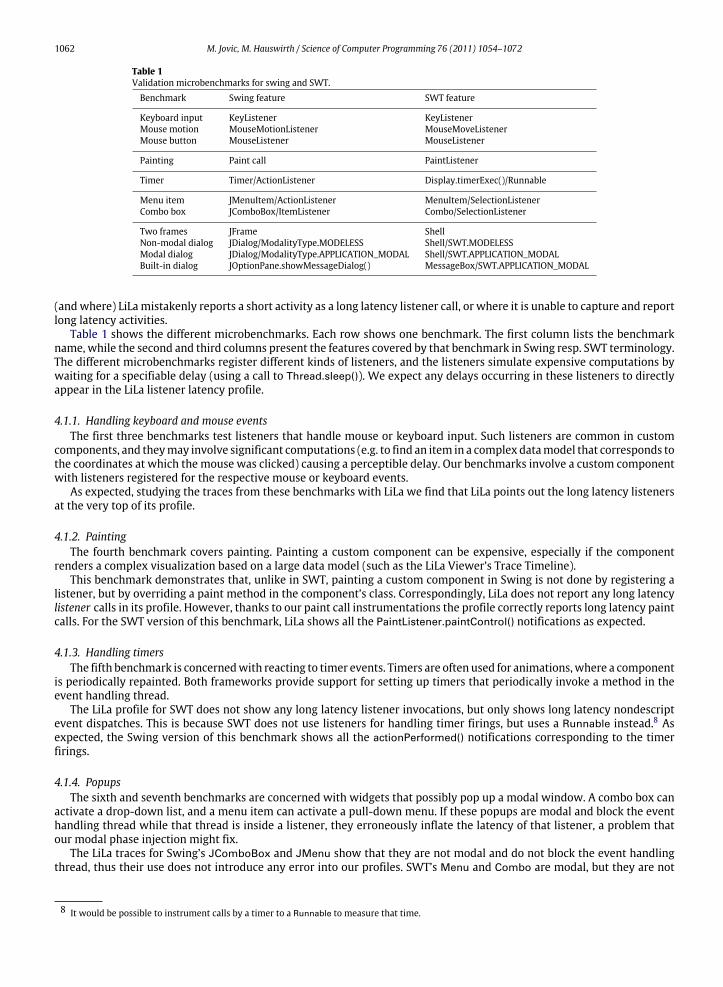
Table 1Validation microbenchmarks for swing and SWT.Benchmark Swing feature SWT feature

Keyboard input KeyListener KeyListenerMouse motion MouseMotionListener MouseMoveListenerMouse button MouseListener MouseListener

Painting Paint call PaintListener

Timer Timer/ActionListener Display.timerExec()/Runnable

Menu item JMenuItem/ActionListener MenuItem/SelectionListenerCombo box JComboBox/ItemListener Combo/SelectionListener

Two frames JFrame ShellNon-modal dialog JDialog/ModalityType.MODELESS Shell/SWT.MODELESSModal dialog JDialog/ModalityType.APPLICATION_MODAL Shell/SWT.APPLICATION_MODALBuilt-in dialog JOptionPane.showMessageDialog() MessageBox/SWT.APPLICATION_MODAL

(andwhere) LiLamistakenly reports a short activity as a long latency listener call, or where it is unable to capture and reportlong latency activities.

Table 1 shows the different microbenchmarks. Each row shows one benchmark. The first column lists the benchmarkname, while the second and third columns present the features covered by that benchmark in Swing resp. SWT terminology.The different microbenchmarks register different kinds of listeners, and the listeners simulate expensive computations bywaiting for a specifiable delay (using a call to Thread.sleep()). We expect any delays occurring in these listeners to directlyappear in the LiLa listener latency profile.

4.1.1. Handling keyboard and mouse eventsThe first three benchmarks test listeners that handle mouse or keyboard input. Such listeners are common in custom

components, and theymay involve significant computations (e.g. to find an item in a complex datamodel that corresponds tothe coordinates at which the mouse was clicked) causing a perceptible delay. Our benchmarks involve a custom componentwith listeners registered for the respective mouse or keyboard events.

As expected, studying the traces from these benchmarks with LiLa we find that LiLa points out the long latency listenersat the very top of its profile.

4.1.2. PaintingThe fourth benchmark covers painting. Painting a custom component can be expensive, especially if the component

renders a complex visualization based on a large data model (such as the LiLa Viewer’s Trace Timeline).This benchmark demonstrates that, unlike in SWT, painting a custom component in Swing is not done by registering a

listener, but by overriding a paint method in the component’s class. Correspondingly, LiLa does not report any long latencylistener calls in its profile. However, thanks to our paint call instrumentations the profile correctly reports long latency paintcalls. For the SWT version of this benchmark, LiLa shows all the PaintListener.paintControl() notifications as expected.

4.1.3. Handling timersThe fifth benchmark is concernedwith reacting to timer events. Timers are often used for animations,where a component

is periodically repainted. Both frameworks provide support for setting up timers that periodically invoke a method in theevent handling thread.

The LiLa profile for SWT does not show any long latency listener invocations, but only shows long latency nondescriptevent dispatches. This is because SWT does not use listeners for handling timer firings, but uses a Runnable instead.8 Asexpected, the Swing version of this benchmark shows all the actionPerformed() notifications corresponding to the timerfirings.

4.1.4. PopupsThe sixth and seventh benchmarks are concerned with widgets that possibly pop up a modal window. A combo box can

activate a drop-down list, and a menu item can activate a pull-down menu. If these popups are modal and block the eventhandling thread while that thread is inside a listener, they erroneously inflate the latency of that listener, a problem thatour modal phase injection might fix.

The LiLa traces for Swing’s JComboBox and JMenu show that they are not modal and do not block the event handlingthread, thus their use does not introduce any error into our profiles. SWT’s Menu and Combo are modal, but they are not

8 It would be possible to instrument calls by a timer to a Runnable to measure that time.


opened from within a Java listener, and so do not introduce an error into the listener profile either. However, the Menublocks the event handling thread, causing one single long dispatch interval (for the duration the menu is open). As we havedescribed in Section 3.3, the episode used for the latency distribution include dispatch intervals. Thus, opening Menus inSWT negatively affects the cumulative latency distribution (leading to a erroneously high count of long episodes).

4.1.5. ModalityThe last four benchmarks constitute tests for examining different modalities of top-level components (Swing’s JFrame,

JDialog, and JOptionPane vs. SWT’s Shell and MessageBox).The first two of those benchmarks use two main windows (two JFrames or two non-modal Shells) or they open a

non-modal dialog (non-modal JDialog or non-modal Shell). They do not affect the validity of our profiles because theydo not involve any modal activity. The last two benchmarks involve modal windows. The cases using a modal JDialog, aJOptionPane, and a modal Shell are correctly handled by our modal phase injection approach: the listener opening thesemodal windows is not charged for the time the windows are open and block the remaining application. However, the caseusing an SWTMessageBox cannot be detectedwith our heuristic. Because theMessageBox is entirely implemented in nativecode, when we open it fromwithin a listener (as is normal), it blocks the thread and does not cause nested event dispatchesvisible within Java. This affects the listener latency profile (the listener is charged for the entire duration the user looked atthe message box), as well as the latency distribution (adding one overly long episode).

4.1.6. AccuracyIn all of our microbenchmarks we deliberately introduced latencies between 10 ms and 1 s by calling Thread.sleep(). We

thus approximately9 know the actual latency. We have found that the latency reported by LiLa and the requested sleepingtime usually differ by less than 3 ms. This accuracy is sufficient for our purposes, as we are interested in finding episodeswith latencies significantly longer than 100 ms.

4.1.7. SummaryIn conclusion, the listener latency profile computed by LiLa provides detailed information about most of the important

interactive events. It lacks detailed information about SWT timers, but still captures the latency of such events because itreports all event dispatches, no matter whether they include listener notifications or not. Our heuristic to infer intervals ofmodal activity is successful, but it is not able to determine such periods when they happen entirely in native code (such aswhen showing an SWTMessageBox). We thus canmistakenly attribute the latency of showing amessage box to the listenerthat opened up that dialog. Since showing a message box is a relatively rare event, and since it usually takes a user severalseconds before she dismisses a message box, such long latency listener calls are easy to spot and skip by the performanceanalyst. Moreover, SWT dialogs implemented in Java are properly handled by our heuristic.

4.2. Real-world applications

In this subsection we evaluate the applicability of our profiler to real-world applications. We picked our own LiLaViewer and the NetBeans IDE, which, with its over 45000 classes is one of the most complex open source interactive Javaapplications.

4.2.1. OverheadThe slowdown due to our instrumentation is hard to quantify, becausewewould need tomeasure the performance of the

uninstrumented application. While we could measure the end-to-end execution time of the uninstrumented application,this would be meaningless (we argue in this paper that the end-to-end execution time of an interactive application is nota useful measure of its performance). What we really would want to compare is the listener latency distribution of theinstrumented and the uninstrumented application. Unfortunately, we cannot measure the listener latency distributionwithout our instrumentation, and thus we cannot precisely evaluate the impact of our instrumentation on perceptibleperformance.

However, the evaluation of the accuracywith ourmicrobenchmarks suggests that for these programs the instrumentationdoes not significantly affect performance. Moreover, we measured the rate at which the instrumented real-worldapplications produced traces to quantify one relevant aspect of the overhead. For the 18 runs we captured (9 of NetBeans, 9of the LiLa Viewer), we observed data rates from 100 kB/s to 1.4 MB/s. Note that we could reduce these rates, according toour experiments by about a factor of 15, by compressing the traces before writing them to disk. In future work we plan toevaluate the overhead of LiLawith a study of real users, and to use online analysis approaches to further reduce the overheadwhere necessary.

9 Thread.sleep() is not completely accurate, and listeners also execute a minimal amount of code, such as the call to Thread.sleep(), besides sleeping.


ms

0

0.5

1

1.5

2

2.5

3

3.5

4

4.5

Epi

sode

s pe

r se

cond

100500 150 200 250 300 350 400

NetBeans 1

NetBeans 2

NetBeans 3

LiLa Viewer 1

LiLa Viewer 2

LiLa Viewer 3

Fig. 6. Cumulative latency distribution.

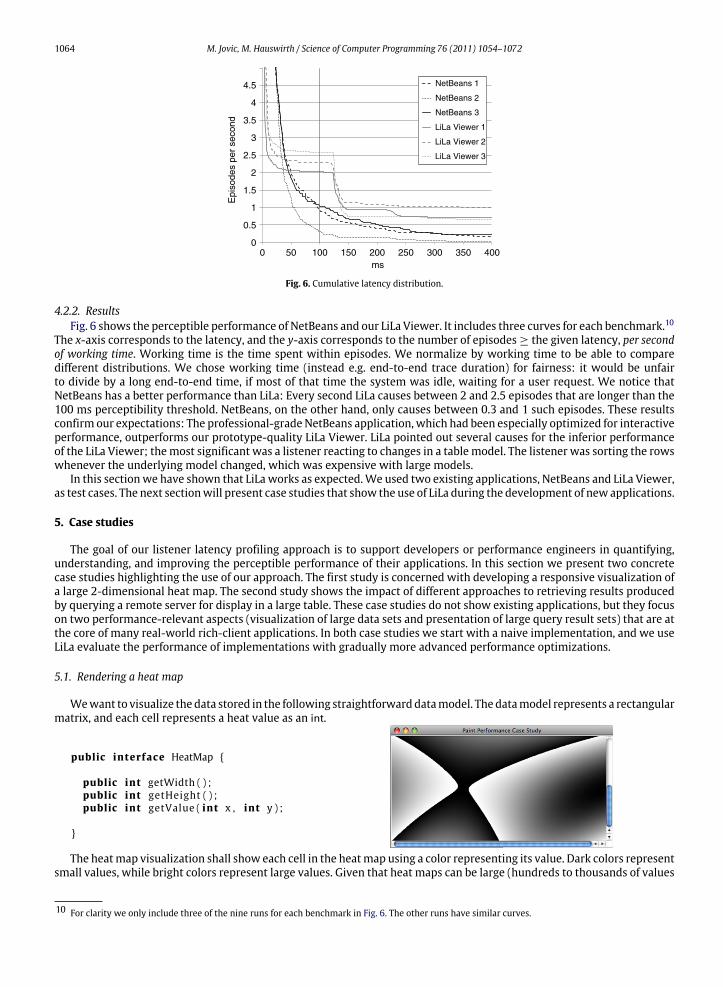
4.2.2. ResultsFig. 6 shows the perceptible performance of NetBeans and our LiLa Viewer. It includes three curves for each benchmark.10

The x-axis corresponds to the latency, and the y-axis corresponds to the number of episodes ≥ the given latency, per secondof working time. Working time is the time spent within episodes. We normalize by working time to be able to comparedifferent distributions. We chose working time (instead e.g. end-to-end trace duration) for fairness: it would be unfairto divide by a long end-to-end time, if most of that time the system was idle, waiting for a user request. We notice thatNetBeans has a better performance than LiLa: Every second LiLa causes between 2 and 2.5 episodes that are longer than the100 ms perceptibility threshold. NetBeans, on the other hand, only causes between 0.3 and 1 such episodes. These resultsconfirm our expectations: The professional-grade NetBeans application, which had been especially optimized for interactiveperformance, outperforms our prototype-quality LiLa Viewer. LiLa pointed out several causes for the inferior performanceof the LiLa Viewer; themost significant was a listener reacting to changes in a table model. The listener was sorting the rowswhenever the underlying model changed, which was expensive with large models.

In this sectionwe have shown that LiLa works as expected.We used two existing applications, NetBeans and LiLa Viewer,as test cases. The next sectionwill present case studies that show the use of LiLa during the development of new applications.

5. Case studies

The goal of our listener latency profiling approach is to support developers or performance engineers in quantifying,understanding, and improving the perceptible performance of their applications. In this section we present two concretecase studies highlighting the use of our approach. The first study is concerned with developing a responsive visualization ofa large 2-dimensional heat map. The second study shows the impact of different approaches to retrieving results producedby querying a remote server for display in a large table. These case studies do not show existing applications, but they focuson two performance-relevant aspects (visualization of large data sets and presentation of large query result sets) that are atthe core of many real-world rich-client applications. In both case studies we start with a naive implementation, and we useLiLa evaluate the performance of implementations with gradually more advanced performance optimizations.

5.1. Rendering a heat map

Wewant to visualize the data stored in the following straightforwarddatamodel. Thedatamodel represents a rectangularmatrix, and each cell represents a heat value as an int.

public interface HeatMap {

public int getWidth ( ) ;public int getHeight ( ) ;public int getValue ( int x , int y ) ;

}

The heatmap visualization shall show each cell in the heatmap using a color representing its value. Dark colors representsmall values, while bright colors represent large values. Given that heat maps can be large (hundreds to thousands of values

10 For clarity we only include three of the nine runs for each benchmark in Fig. 6. The other runs have similar curves.


Fig. 7. Naive canvas and its perceptible performance.

along both axes), wewant to place the visualization inside a scroll pane, so the user can scroll to different regions of interest.We do not want to provide support for zooming, andwemap each value of thematrix to one pixel on the screen. This simpleproblemhas a surprisingly rich set of possible solutions, and each solutionhas its specific impact onperceptible performance.

We create a GUI canvas (a subclass of Swing’s JComponent class) to visualize the heat map, and we place that canvasinside a Swing JScrollPane. The canvas does not need to know about scrolling, it just has to know the width and height (inpixels) it needs in order to draw the entire heat map, and it has to be able to paint its contents. The scroll pane handles thescrolling and clipping of the visible part of the heat map canvas.

5.1.1. Naive implementationWe start with a naive implementation of the canvas, which, whenever it is asked to paint itself, will iterate through the

entire heat map and render each value as a pixel. Fig. 7 shows an excerpt of the source code and the resulting perceptibleperformance for different map sizes. The perceptible performance, as gathered by LiLa, is visualized in the form of acumulative latency distribution on the right.

The x-axis of the cumulative latency distribution plot represents latency in milliseconds. In this figure it extends to 10 s.The y-axis shows the absolute number of episodes that took longer than x. We wrote a small program that embeds thecanvas inside a JScrollPane that has a visible area of 256 by 256 pixels, and adds that scroll pane into a JFrame. The programthen programmatically scrolls left and right by 256 pixels, thus triggering a total of 50 paint requests. Given that, a programrun will contain at least 50 episodes, and the curves in the cumulative latency distribution extend to above 50 at x = 0. Thecumulative latency distribution plot shows 6 curves representing six program runs with different heat map sizes. We fixedthe height of the heat map to 512, and we show one curve for each of the six widths we studied.

For this naive canvas, our program ran for 538.3 s for the biggest heat map. The cumulative latency distribution in Fig. 7shows that the responsiveness of the program clearly depends on the size of the heat map: The curve for the 16384 pixelwide heat map extends past 10 s, meaning that each of the 50 repaint requests took longer than 10 s. This is over 100 timesabove the 100 ms perceptibility threshold. Smaller maps lead to more responsive behavior, but even the map that is 512pixels wide takes a clearly perceptible 514 ms for each paint request.

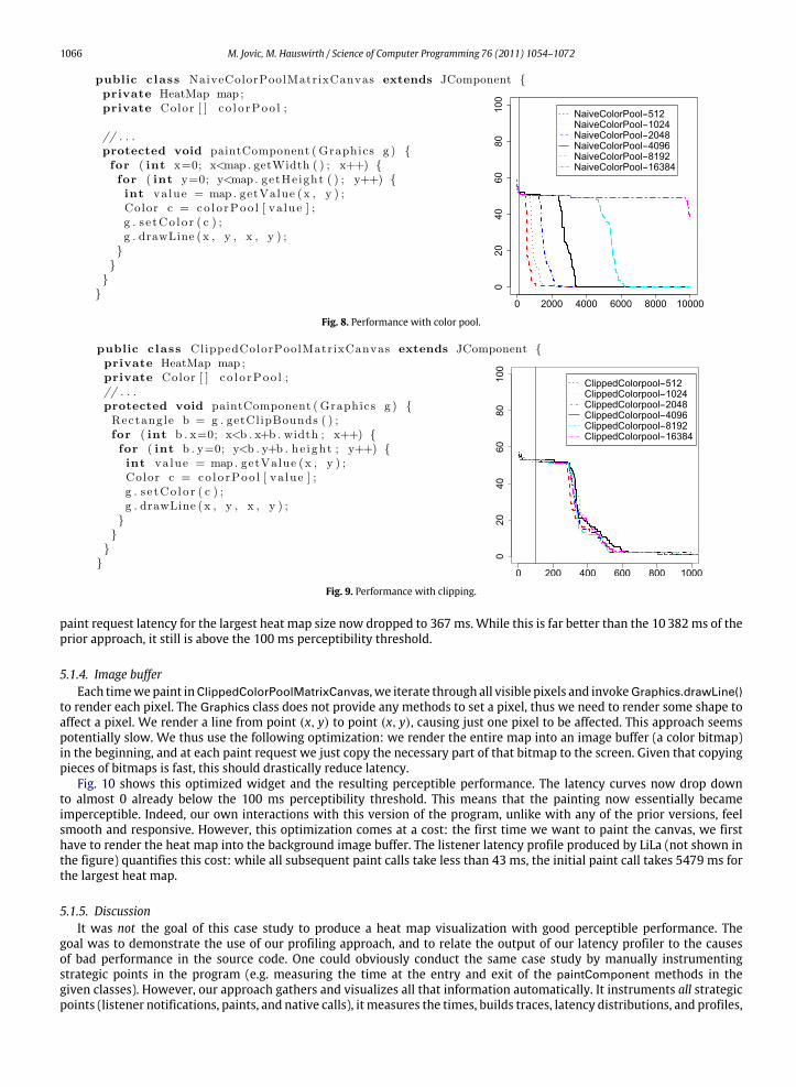
5.1.2. Using a pool of color objectsA look at the NaiveMatrixCanvas class shows that this naive widget creates a new Color object for each pixel it paints.

Given the large number of pixels (our biggest heat map has eight megapixels), these object allocations may impactperceptible performance. As a straightforward optimization, we thus introduce a pool of 256 pre-allocated colors, one ofeach possible heat value.

Fig. 8 shows this optimized variant of the canvas and the resulting perceptible performance. Unfortunately thisoptimization has little effect on the latency distribution. The six curves still extend to almost the same latency. The averagepaint latency for the largest heat map only was reduced to 10382 ms (from the 10933 ms for the naive version).

5.1.3. ClippingThe next optimization is based on the finding that we always only see a small piece (the size of the scroll pane’s viewport,

whichwe fixed to 256by256pixels in our experiments) of the largeheatmap. To render the entiremapat every paint requestthus constitutes a large waste of time. Class ClippedColorPoolMatrixCanvas in Fig. 9 thus uses the clipping informationprovided by the scroll pane to focus the painting to only the pixels that can actually be seen. Thus, in our usage scenario,instead of rendering 8 megapixels we render only 64 kilopixels per paint request.

The cumulative latency distribution in Fig. 9 shows the big gain in perceptible performance due to this simpleoptimization. It also shows, as expected, that the latency does not depend on the size of the heat map anymore. The average


Fig. 8. Performance with color pool.

Fig. 9. Performance with clipping.

paint request latency for the largest heat map size now dropped to 367ms. While this is far better than the 10382ms of theprior approach, it still is above the 100 ms perceptibility threshold.

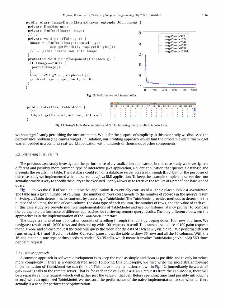
5.1.4. Image bufferEach timewepaint inClippedColorPoolMatrixCanvas, we iterate through all visible pixels and invokeGraphics.drawLine()

to render each pixel. The Graphics class does not provide any methods to set a pixel, thus we need to render some shape toaffect a pixel. We render a line from point (x, y) to point (x, y), causing just one pixel to be affected. This approach seemspotentially slow. We thus use the following optimization: we render the entire map into an image buffer (a color bitmap)in the beginning, and at each paint request we just copy the necessary part of that bitmap to the screen. Given that copyingpieces of bitmaps is fast, this should drastically reduce latency.

Fig. 10 shows this optimized widget and the resulting perceptible performance. The latency curves now drop downto almost 0 already below the 100 ms perceptibility threshold. This means that the painting now essentially becameimperceptible. Indeed, our own interactions with this version of the program, unlike with any of the prior versions, feelsmooth and responsive. However, this optimization comes at a cost: the first time we want to paint the canvas, we firsthave to render the heat map into the background image buffer. The listener latency profile produced by LiLa (not shown inthe figure) quantifies this cost: while all subsequent paint calls take less than 43 ms, the initial paint call takes 5479 ms forthe largest heat map.

5.1.5. DiscussionIt was not the goal of this case study to produce a heat map visualization with good perceptible performance. The

goal was to demonstrate the use of our profiling approach, and to relate the output of our latency profiler to the causesof bad performance in the source code. One could obviously conduct the same case study by manually instrumentingstrategic points in the program (e.g. measuring the time at the entry and exit of the paintComponent methods in thegiven classes). However, our approach gathers and visualizes all that information automatically. It instruments all strategicpoints (listener notifications, paints, and native calls), it measures the times, builds traces, latency distributions, and profiles,


Fig. 10. Performance with image buffer.

Fig. 11. Swing’s TableModel interface and GUI for browsing query results in tabular form.

without significantly perturbing the measurements. While for the purpose of simplicity in this case study we discussed theperformance problem (the canvas widget) in isolation, our profiling approach would find the problem even if this widgetwas embedded in a complex real-world application with hundreds or thousands of other components.

5.2. Retrieving query results

The previous case study investigated the performance of a visualization application. In this case study we investigate adifferent and possibly more common type of interactive Java application, a client application that queries a database andpresents the results in a table. The database could run on a database server accessed through JDBC, but for the purposes ofthis case study we implemented a simple server as a Java RMI application. To keep the example simple, the server does notactually provide away to specify the query to be executed. It only allows us to retrieve the results of a predefined hard-codedquery.

Fig. 11 shows the GUI of such an interactive application. It essentially consists of a JTable placed inside a JScrollPane.The table has a given number of columns. The number of rows corresponds to the number of records in the query’s result.In Swing, a JTable determines its contents by accessing a TableModel. The TableModel provides methods to determine thenumber of columns, the title of each column, the data type of each column, the number of rows, and the value of each cell.In this case study we provide multiple implementations of TableModel and use our listener latency profiler to comparethe perceptible performance of different approaches for retrieving remote query results. The only difference between theapproaches is in the implementation of the TableModel interface.

The usage scenario of our application consists of scrolling through the table by paging down 100 rows at a time. Wenavigate a result set of 10000 rows, and thus end upwith 100 requests to scroll. This causes a sequence of 100 paint requeststo the JTable, and on each request the tablewill query themodel for the data of each newly visible cell.We perform differentruns, using 2, 4, 8, and 16 column-tables. Our scroll pane allows the table to show 35 rows and all the 16 columns. With the16-column table, one repaint thus needs to render 16 ∗ 35 cells, which means it invokes TableModel.getValueAt() 560 timesper paint request.

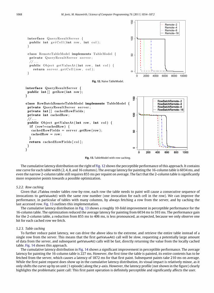
5.2.1. Naive approachA common approach in software development is to keep the code as simple and clean as possible, and to only introduce

more complexity if there is a demonstrated need. Following this philosophy, we first write the most straightforwardimplementation of TableModel we can think of. This naive implementation, shown in Fig. 12, immediately forwards allgetValueAt() calls to the remote server. That is, for each table cell value a JTable requests from the TableModel, there willbe a separate remote request, which will gather just the value of that cell. Before spending time (and possibly introducingerrors) with an optimized TableModel, we measure the performance of the naive implementation to see whether thereactually is a need for performance optimization.


Fig. 12. Naive TableModel.

Fig. 13. TableModel with row caching.

The cumulative latency distribution on the right of Fig. 12 shows the perceptible performance of this approach. It containsone curve for each tablewidth (2, 4, 8, and 16 columns). The average latency for painting the 16-column table is 6034ms, andeven the narrow 2-column table still requires 855ms per repaint on average. The fact that the 2-column table is significantlymore responsive points towards a possible optimization.

5.2.2. Row cachingGiven that JTables render tables row-by-row, each row the table needs to paint will cause a consecutive sequence of

invocations to getValueAt() with the same row number (one invocation for each cell in the row). We can improve theperformance, in particular of tables with many columns, by always fetching a row from the server, and by caching thelast accessed row. Fig. 13 outlines this implementation.

The cumulative latency distribution in Fig. 13 shows a roughly 10-fold improvement in perceptible performance for the16-column table. The optimization reduced the average latency for painting from 6034ms to 593ms. The performance gainfor the 2-column table, a reduction from 855 ms to 406 ms, is less pronounced, as expected, because we only observe onehit for each cached row we fetch.

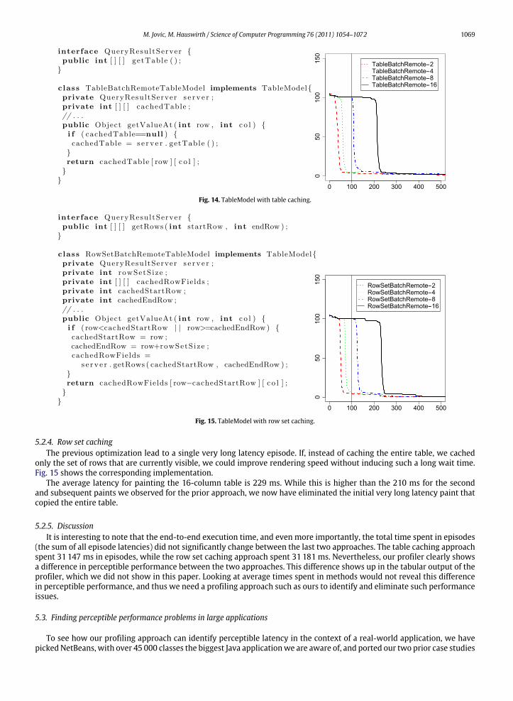
5.2.3. Table cachingTo further reduce paint latency, we can drive the above idea to the extreme, and retrieve the entire table instead of a

single row from the server. This means that the first getValueAt() call will be slow, requesting a potentially large amountof data from the server, and subsequent getValueAt() calls will be fast, directly returning the value from the locally cachedtable. Fig. 14 shows this approach.

The cumulative latency distribution in Fig. 14 shows a significant improvement in perceptible performance. The averagelatency for painting the 16-column table is 227 ms. However, the first time the table is painted, its entire contents has to befetched from the server, which causes a latency of 1872 ms for that first paint. Subsequent paints take 210 ms on average.While the first paint request does show up in the cumulative latency distribution, its visual impact is relatively minor, as itonly shifts the curve up by on unit (1 episode) along the y-axis. However, the latency profile (not shown in the figure) clearlyhighlights the problematic paint call: This first paint operation is definitely perceptible and significantly affects the user.


Fig. 14. TableModel with table caching.

Fig. 15. TableModel with row set caching.

5.2.4. Row set cachingThe previous optimization lead to a single very long latency episode. If, instead of caching the entire table, we cached

only the set of rows that are currently visible, we could improve rendering speed without inducing such a long wait time.Fig. 15 shows the corresponding implementation.

The average latency for painting the 16-column table is 229 ms. While this is higher than the 210 ms for the secondand subsequent paints we observed for the prior approach, we now have eliminated the initial very long latency paint thatcopied the entire table.

5.2.5. DiscussionIt is interesting to note that the end-to-end execution time, and even more importantly, the total time spent in episodes

(the sum of all episode latencies) did not significantly change between the last two approaches. The table caching approachspent 31147 ms in episodes, while the row set caching approach spent 31181 ms. Nevertheless, our profiler clearly showsa difference in perceptible performance between the two approaches. This difference shows up in the tabular output of theprofiler, which we did not show in this paper. Looking at average times spent in methods would not reveal this differencein perceptible performance, and thus we need a profiling approach such as ours to identify and eliminate such performanceissues.

5.3. Finding perceptible performance problems in large applications

To see how our profiling approach can identify perceptible latency in the context of a real-world application, we havepickedNetBeans, with over 45000 classes the biggest Java applicationwe are aware of, and ported our two prior case studies


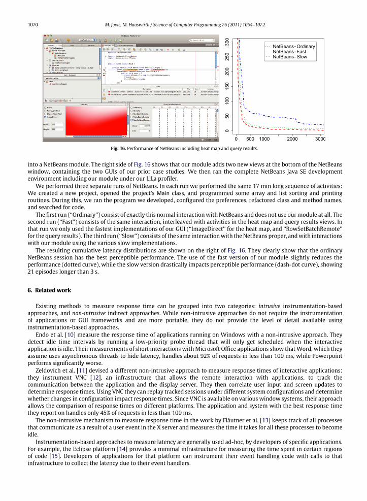
Fig. 16. Performance of NetBeans including heat map and query results.

into a NetBeans module. The right side of Fig. 16 shows that our module adds two new views at the bottom of the NetBeanswindow, containing the two GUIs of our prior case studies. We then ran the complete NetBeans Java SE developmentenvironment including our module under our LiLa profiler.

We performed three separate runs of NetBeans. In each run we performed the same 17 min long sequence of activities:We created a new project, opened the project’s Main class, and programmed some array and list sorting and printingroutines. During this, we ran the program we developed, configured the preferences, refactored class and method names,and searched for code.

The first run (‘‘Ordinary’’) consist of exactly this normal interactionwith NetBeans and does not use ourmodule at all. Thesecond run (‘‘Fast’’) consists of the same interaction, interleaved with activities in the heat map and query results views. Inthat run we only used the fastest implementations of our GUI (‘‘ImageDirect’’ for the heat map, and ‘‘RowSetBatchRemote’’for the query results). The third run (‘‘Slow’’) consists of the same interactionwith theNetBeans proper, andwith interactionswith our module using the various slow implementations.

The resulting cumulative latency distributions are shown on the right of Fig. 16. They clearly show that the ordinaryNetBeans session has the best perceptible performance. The use of the fast version of our module slightly reduces theperformance (dotted curve), while the slow version drastically impacts perceptible performance (dash-dot curve), showing21 episodes longer than 3 s.

6. Related work

Existing methods to measure response time can be grouped into two categories: intrusive instrumentation-basedapproaches, and non-intrusive indirect approaches. While non-intrusive approaches do not require the instrumentationof applications or GUI frameworks and are more portable, they do not provide the level of detail available usinginstrumentation-based approaches.

Endo et al. [10] measure the response time of applications running on Windows with a non-intrusive approach. Theydetect idle time intervals by running a low-priority probe thread that will only get scheduled when the interactiveapplication is idle. Their measurements of short interactions withMicrosoft Office applications show thatWord, which theyassume uses asynchronous threads to hide latency, handles about 92% of requests in less than 100 ms, while Powerpointperforms significantly worse.

Zeldovich et al. [11] devised a different non-intrusive approach to measure response times of interactive applications:they instrument VNC [12], an infrastructure that allows the remote interaction with applications, to track thecommunication between the application and the display server. They then correlate user input and screen updates todetermine response times. Using VNC they can replay tracked sessions under different system configurations and determinewhether changes in configuration impact response times. Since VNC is available on various window systems, their approachallows the comparison of response times on different platforms. The application and system with the best response timethey report on handles only 45% of requests in less than 100 ms.

The non-intrusive mechanism to measure response time in the work by Fláutner et al. [13] keeps track of all processesthat communicate as a result of a user event in the X server andmeasures the time it takes for all these processes to becomeidle.

Instrumentation-based approaches to measure latency are generally used ad-hoc, by developers of specific applications.For example, the Eclipse platform [14] provides a minimal infrastructure for measuring the time spent in certain regionsof code [15]. Developers of applications for that platform can instrument their event handling code with calls to thatinfrastructure to collect the latency due to their event handlers.


TIPME [16] is a system for finding the causes of long latency that lie in the operating system. TIPME runs on BSD Unixusing an X server. It traces X events and scheduling and I/O activity in the operating system. Users can press a hot key toindicate irritatingly high latency, causing TIPME to dump the trace buffers for later manual causal analysis.

Besides approaches focused on latency measurement, some general purpose tracing approaches also have a relationshipto LiLa. DTrace [17], for example, can dynamically trace a running system (kernel, native user code, and even Java code).DTrace allows the user to specify which places to instrument and what to do when these places are executed. However,DTrace would not provide themeans to trace all listener calls, because it does not provide the type information necessary todecide whether a call target indeed is a listener method (Section 3.1.3). Aspect weavers, such as AspectJ [18], also provides amechanism for specifying program points and actions to perform when these points are executed. This feature has alreadybeen used by djProf [19], a profiler for Java built on top of AspectJ. However, like DTrace, AspectJ-based approaches alsolack a means to specifically identify listener methods. One could instrument all call sites and determine dynamically (in theinstrumentation) whether a call target is a listener method call. However, the large amount of instrumentation and extradynamic checks could drastically perturb the measurements. Our colleagues at the University of Lugano are working onovercoming the limitations of current Java aspect weaving approaches, including the ability to instrument runtime libraryclasses [20]. It would be interesting to see our listener latency profiling approach ported to such a system.

7. Conclusions

In this paperwe introduced listener latency profiling, an approach for profiling the perceptible performance of interactiveJava applications. Our approach is applicable for both Swing and SWT applications. We have presented the cumulativelatency distribution as a means to characterize performance, and the listener latency profile as a means to highlight thecomponents responsible for sluggish application behavior. We have implemented our idea for Swing and SWT platformsand validated it on a new suite of microbenchmarks.We have shown that our approachworks with all of the complexities ofreal-world Java GUI applications by using it to profile our own LiLa profile viewer as well as the professional-grade NetBeansIDE. Finally, we demonstrate our new profiling approach in two performance tuning case studies, and we show that we canidentify performance problems even if they lie deep inside a complex real-world application. We intend to further improvethe usability of LiLa and to release11 it as open source, so Java developers can start to use it for understanding the perceptibleperformance of their applications.

Acknowledgements

We would like to thank the anonymous reviewers for their valuable feedback and suggestions. This work has beenconducted in the context of the Binary Translation and Virtualization cluster of the EU HiPEAC Network of Excellence. Ithas been funded by the Swiss National Science Foundation under grant number 200021-116333/1.

References

[1] B. Shneiderman, Designing the User Interface: Strategies for Effective Human-computer Interaction, Addison-Wesley, 1986.[2] B. Shneiderman, Response time and display rate in human performance with computers, ACM Computing Surveys 16 (3) (1984).

doi:http://doi.acm.org/10.1145/2514.2517.[3] I. Ceaparu, J. Lazar, K. Bessiere, J. Robinson, B. Shneiderman, Determining causes and severity of end-user frustration, International Journal of Human-

Computer Interaction 17 (3) (2004). URL: citeseer.ist.psu.edu/ceaparu02determining.html.[4] I.S. MacKenzie, C. Ware, Lag as a determinant of human performance in interactive systems, in: CHI’93: Proceedings of the INTERACT ’93 and CHI ’93

Conference on Human Factors in Computing Systems, ACM, New York, NY, USA, 1993, pp. 488–493. doi:http://doi.acm.org/10.1145/169059.169431.[5] J.R. Dabrowski, E.V. Munson, Is 100 ms too fast? in: CHI’01: CHI’01 Extended Abstracts on Human Factors in Computing Systems, ACM, New York, NY,

USA, 2001, pp. 317–318. doi:http://doi.acm.org/10.1145/634067.634255.[6] K. Walrath, M. Campione, A. Huml, S. Zakhour, The JFC Swing Tutorial: A Guide to Constructing GUIs, 2nd ed., Addison-Wesley, 2004.[7] S. Northover, M. Wilson, SWT: The Standard Widget Toolkit, Volume 1, Addison-Wesley, 2004.[8] J. McAffer, J.-M. Lemieux, Eclipse Rich Client Platform : Designing, Coding, and Packaging Java Applications, Addison-Wesley, 2005.[9] ObjectWeb, ASM, Web pages at http://asm.objectweb.org/.

[10] Y. Endo, Z. Wang, J.B. Chen, M. Seltzer, Using latency to evaluate interactive system performance, in: OSDI’96: Proceedings of the Second USENIXSymposium on Operating Systems Design and Implementation, ACM, New York, NY, USA, 1996, pp. 185–199.doi:http://doi.acm.org/10.1145/238721.238775.

[11] N. Zeldovich, R. Chandra, Interactive performance measurement with vncplay, in: ATEC’05: Proceedings of the Annual Conference on USENIX AnnualTechnical Conference, USENIX Association, Berkeley, CA, USA, 2005, pp. 189–198.

[12] T. Richardson, Q. Stafford-Fraser, K.R. Wood, A. Hopper, Virtual network computing, IEEE Internet Computing 02 (1) (1998).doi:http://doi.ieeecomputersociety.org/10.1109/4236.656066.

[13] K. Flautner, R. Uhlig, S. Reinhardt, T. Mudge, Thread-level parallelism and interactive performance of desktop applications, in: ASPLOS-IX: Proceedingsof the Ninth International Conference on Architectural Support for Programming Languages and Operating Systems, ACM, New York, NY, USA, 2000,pp. 129–138. doi:http://doi.acm.org/10.1145/378993.379233.

[14] Eclipse Foundation, Eclipse Project, 2009. URL: http://www.eclipse.org/eclipse/.[15] Eclipse Foundation, The PerformanceStats API: Gathering performance statistics in Eclipse, 2005. URL: http://www.eclipse.org/eclipse/platform-

core/documents/3.1/perf_stats.html.

11 http://www.inf.unisi.ch/phd/jovic/MilanJovic/Lila/Lila.html.

http://dx.doi.org/doi:10.1145/2514.2517

http://citeseer.ist.psu.edu/ceaparu02determining.html



http://asm.objectweb.org/




http://www.eclipse.org/eclipse/

http://www.eclipse.org/eclipse/platform-core/documents/3.1/perf_stats.html



http://www.inf.unisi.ch/phd/jovic/MilanJovic/Lila/Lila.html












[16] Y. Endo, M. Seltzer, Improving interactive performance using tipme, in: SIGMETRICS’00: Proceedings of the 2000 ACM SIGMETRICS InternationalConference on Measurement and Modeling of Computer Systems, ACM, New York, NY, USA, 2000, pp. 240–251.doi:http://doi.acm.org/10.1145/339331.339420.

[17] B.M. Cantrill, M.W. Shapiro, A.H. Leventhal, Dynamic instrumentation of production systems, in: Proceedings of the USENIX 2004 Annual TechnicalConference, USENIX, 2004, pp. 15–28. URL: http://www.sun.com/bigadmin/content/dtrace/.

[18] G. Kiczales, E. Hilsdale, J. Hugunin, M. Kersten, J. Palm, W.G. Griswold, An overview of aspectj, in: ECOOP’01: Proceedings of the 15th EuropeanConference on Object-Oriented Programming, Springer-Verlag, London, UK, 2001, pp. 327–353.

[19] D.J. Pearce, M. Webster, R. Berry, P.H.J. Kelly, Profiling with AspectJ, Software: Practice and Experience 37 (7) (2007) 747–777.doi:http://dx.doi.org/10.1002/spe.788.

[20] A. Villazón, W. Binder, P. Moret, D. Ansaloni, Comprehensive aspect weaving for Java, Science of Computer Programming, in this issue(doi:10.1016/j.scico.2010.04.007).


http://www.sun.com/bigadmin/content/dtrace/

http://dx.doi.org/doi:10.1002/spe.788

http://dx.doi.org/doi:10.1016/j.scico.2010.04.007

Listener latency profiling: Measuring the perceptible performance of interactive Java applications

Documents

Transcript of Listener latency profiling: Measuring the perceptible performance of interactive Java applications