When to Crossover from Earth to Space for Lower Latency ...

IEEE TRANSACTIONS ON AEROSPACE AND ELECTRONIC SYSTEMS, VOL. XX, NO. XX, AUGUST 202X 1

When to Crossover from Earth to Space for LowerLatency Data Communications?

Aizaz U. Chaudhry, Senior Member, IEEE, and Halim Yanikomeroglu, Fellow, IEEE

Abstract—For data communications over long distances, op-tical wireless satellite networks (OWSNs) can offer lower latencythan optical fiber terrestrial networks (OFTNs). However, whenis it beneficial to switch or crossover from an OFTN to anOWSN for lower latency data communications? In this work, weintroduce a crossover function that enables to find the crossoverdistance, i.e., a distance between two points on the surface ofthe Earth beyond which switching or crossing over from anOFTN to an OWSN for data communications between thesepoints is useful in terms of latency. Numerical results revealthat a higher refractive index of optical fiber (or 𝑖) in an OFTNand a lower altitude of satellites (or ℎ) in an OWSN result ina shorter crossover distance. To account for the variation in theend-to-end propagation distance that occurs over the OWSN,we examine the crossover function in four different scenarios.Numerical results indicate that the crossover distance varieswith the end-to-end propagation distance over an OWSN andis different for different scenarios. We calculate the averagecrossover distance over all scenarios for different ℎ and 𝑖 anduse it to evaluate the simulation results. Furthermore, for acomparative analysis of OFTNs and OWSNs in terms of latency,we study three different OFTNs having different refractiveindices and three different OWSNs having different satellitealtitudes in three different scenarios for long-distance inter-continental data communications, including connections betweenNew York and Dublin, Sao Paulo and London, and Toronto andSydney. All three OWSNs offer better latency than OFTN2 (with𝑖2 = 1.3) and OFTN3 (with 𝑖3 = 1.4675) in all scenarios. Forexample, for Toronto–Sydney connection, OWSN1 (with ℎ1 =300 km), OWSN2 (with ℎ2 = 550 km) and OWSN3 (with ℎ3= 1,100 km) perform better than OFTN2 by 18.11%, 16.08%,and 10.30%, respectively, while they provide an improvement inlatency of 27.46%, 25.67%, and 20.54%, respectively, comparedto OFTN3. The OWSN1 performs better than OFTN1 (with 𝑖1= 1.1) for Sao Paulo–London and Toronto–Sydney connectionsby 2.23% and 3.22%, respectively, while OWSN2 outperformsOFTN1 for Toronto–Sydney connection by 0.82%. For NewYork–Dublin connection, all OWSNs while for Sao Paulo–Londonconnection, OWSN2 and OWSN3 exhibit higher latency thanOFTN1 as the corresponding average crossover distances aregreater than the shortest terrestrial distances between cities inthese scenarios. Multiple satellites (or laser inter-satellite links) onits shortest paths drive up the propagation distance to the extentthat OWSN3 ends up with a higher latency than OFTN1 for theToronto–Sydney inter-continental connection scenario althoughthe related average crossover distance is less than the shortestterrestrial distance between Toronto and Sydney. The challengesrelated to OWSNs and OFTNs that may arise from this work infuture are also highlighted.

Index Terms—Crossover distance, crossover function, LEO,network latency, optical fiber terrestrial networks, optical wire-less satellite networks, satellite constellations.

A.U. Chaudhry and H. Yanikomeroglu are with the Department of Systemsand Computer Engineering, Carleton University, Ottawa, ON, Canada – K1S5B6, e-mail: {auhchaud, halim}@sce.carleton.ca.

I. INTRODUCTION

OPTICAL wireless satellite networks (OWSNs), alsoknown as free-space optical satellite networks, will

be created in space by employing laser inter-satellite links(LISLs) between satellites in upcoming low Earth orbit (LEO)or very low Earth orbit (VLEO) satellite constellations, likeSpaceX’s Starlink [1] and Telesat’s Lightspeed [2]. The LISLs[3], also known as optical inter-satellite links, will be essentialin ensuring low-latency paths (or routes) within the OWSN[4], [5]. Without LISLs, a long-distance inter-continental datacommunications connection between two cities, such as NewYork and Dublin, will have to bounce up and down betweenground stations and satellites, and this will negatively affectlatency of the satellite network.

The provision of long-distance low-latency data communi-cations could be the primary use case of an OWSN that iscreated by using LISLs in an upcoming LEO/VLEO satelliteconstellation like Phase I of Starlink [6]. An OWSN can offersuch type of communications as a premium service to thefinancial hubs around the globe, and such a use-case can bebeneficial in recovering the cost of deploying and sustainingsuch satellite networks. In high-frequency trading (HFT) ofstocks at the stock exchange, a one millisecond advantage cantranslate into $100 million a year in revenues for a majorbrokerage firm [7]. An advantage of a few milliseconds inHFT could mean billions of dollars of revenues for thesefirms. Technological solutions in the form of communicationsnetworks that can provide lower latency data communicationsare being highly coveted by such firms, and a low-latencyOWSN could be the ideal solution.

Unlike optical fiber terrestrial networks (OFTNs) wheredata is sent using a laser beam over a guided medium, i.e.,optical fiber, data communications in OWSNs takes placesover LISLs by using laser beams between satellites over anunguided medium, i.e., vacuum of space. The refractive indexof a medium indicates the speed of light through that medium,and a higher refractive index means a slower transmissionof light [8]. Optical fibers typically have a refractive indexof approximately 1.5. This means that the speed of light inan optical fiber is approximately 𝑐/1.5, where 𝑐 is the speedof light in vacuum [9]. This translates into speed of light invacuum being approximately 50% higher than the speed oflight in optical fiber. This has significant implications, and thehigher speed of light in OWSNs operating in the vacuum ofspace gives them a critical advantage over OFTNs in terms oflatency for long-distance data communications.

The delay from source to destination in the network is


composed of transmission delay, processing delay, queueingdelay, and propagation delay [10]. For optical communicationsin OFTNs or OWSNs over optical fiber or vacuum of space,propagation delay is the delay arising from the transmission ofthe optical signal along the medium. It is directly proportionalto the distance between the source and the destination andbecomes very significant in long-distance data communica-tions [11]. In this work, we study the latency of OWSNs andOFTNs, and we define latency (or end-to-end network latency)as the propagation delay from the source to the destination.

Firstly, we propose a crossover function for data communi-cations between two points on the surface of the Earth over anOFTN and an OWSN. The crossover function is then used tocalculate the crossover distance that indicates when switchingor crossing over from an OFTN to an OWSN can be beneficialfor data communications in terms of latency. The crossoverfunction and thereby the crossover distance depend upon therefractive index of the optical fiber in an OFTN and the altitudeof satellites in an OWSN. From numerical results, we observethat a higher optical fiber refractive index and a lower altitudeof satellites result in a shorter crossover distance.

We examine crossover function in four different scenariosto account for the different end-to-end propagation distancesthat occur over the OWSN due to the orbital movement ofsatellites with time. The end-to-end propagation distance overan OWSN is smallest in Scenario 3, increases in Scenario 1,increases further in Scenario 4, and is largest in Scenario 2.The numerical results show that the crossover distance varieswith the end-to-end propagation distance over an OWSN, itis minimum for Scenario 3, it is higher for Scenario 1 ascompared to that for Scenario 3, it is more for Scenario 4than that for Scenario 1, and it is maximum for Scenario 2. Wecalculate the average crossover distance over all scenarios fordifferent altitudes of satellites and different refractive indices.We later use the average crossover distance to evaluate thesimulation results.

Next, we investigate the impact on latency of differentoptical fiber refractive indices in OFTNs and different altitudesof satellites in OWSNs and conduct a comparative analysis ofthese networks. To this end, we consider three different OFTNswith different refractive indices and three different OWSNshaving different satellite altitudes, and compare them in termsof latency under three different scenarios for long-distanceinter-continental data communications, including connectionsbetween New York and Dublin, Sao Paulo and London, andToronto and Sydney. For this comparison, we use Starlink’sPhase I constellation and LISLs between satellites to simulatean OWSN. Using three different altitudes of satellites for thisconstellation including 300 km, 550 km, and 1,100 km, wesimulate the three different OWSNs. We consider 1.1, 1.3,and 1.4675 as the refractive indices for the three differentOFTNs. Note that 1.4675 [12] is assumed as the refractiveindex for one of these OFTNs since it is the refractive index ofexisting long-haul submarine optical fiber cables that provideinter-continental connectivity. Optical fiber refractive indicesmay be reduced in future due to advancements in the opticalfiber technology and thereby we consider OFTNs with lowerrefractive indices of 1.3 and 1.1 as well.

For each scenario, we find minimum-latency paths betweencities over these six different networks. From the results, weobserve that all three OWSNs outperform the OFTN witha realistic refractive index of 1.4675 as well as the OFTNwith a refractive index of 1.3 in terms of latency in allscenarios. The OWSN operating at 300 km altitude performsclosely to the OFTN with a refractive index of 1.1 for theNew York–Dublin connection and outperforms it for the SaoPaulo–London and Toronto–Sydney connections while theOWSN at 550 km altitude offers lower latency than this OFTNfor the Toronto–Sydney connection. Within all scenarios, it isobserved that the lower the refractive index of an OFTN orthe lower the altitude of satellites in an OWSN, the lower thelatency of a network. For data communications in differentscenarios over a network, it is seen that the greater the inter-continental distance between cities, the higher the latency of anetwork. Preliminary work in this regard has appeared in [13].

Unlike LISLs that are established between satellites in thevacuum of space, laser uplink (i.e., laser link between aground station and a satellite) and laser downlink (i.e., laserlink between a satellite and a ground station) communicationsuffers from atmospheric attenuation, such as Mie scatteringand geometrical scattering [14], as the laser beam propagatesthrough Earth’s atmosphere. This attenuation affects the per-formance of uplink and downlink communication and caneven disrupt this communication on days when the line-of-sight between a ground station and the overhead satelliteis blocked by cloudy weather. A possible solution to dealwith link outage caused by adverse weather conditions is sitediversity, which involves selecting the best ground station thatprovides the best channel conditions [15]. Another possiblesolution, referred to as hybrid radio frequency and free-spaceoptical communication, consists of using radio frequency linkin combination with free-space optical (or laser) link andselecting one of them for uplink and downlink communicationdepending on the weather conditions [16]. Note that the focusof the work in our paper is on latency in OFTNs and OWSNsand investigating link outage in laser uplink and laser downlinkcommunication and its possible solutions are out of the scopeof this work.

The rest of the paper is organized as follows. The relatedwork along with some use cases and the motivation of thiswork are discussed in Section II. Section III presents crossoverfunctions for the different scenarios and the related numericalresults. Our methodology for calculating latency of an inter-continental connection between cities over an OFTN and anOWSN is given in Section IV. Section V presents results forthe comparison of different OFTNs and different OWSNs interms of latency. Conclusions are summarized in Section VI.Section VII highlights future challenges.

II. MOTIVATION

In addition to providing an ideal solution for low-latencylong-distance inter-continental data communications for HFTbetween stock exchanges around the globe, OWSNs can alsobe beneficial in other scenarios. In one such use case, anOWSN can help in extending broadband Internet to rural


and remote areas when integrated as a backbone with theexisting 4G/5G networks. The OWSN can provide a backhaulnetwork to connect the 4G/5G access networks in rural andremote areas to their core network. By providing the abilityto connect any two points on Earth over the OWSN arisingfrom employing LISLs between satellites in their upcomingsatellite constellation Lightspeed, Telesat plans to enable theprovision of broadband Internet to unserved and underservedcommunities and individuals in rural and remote areas. Telesathas already successfully demonstrated this use case for Internetbackhauling with TIM Brasil – an Internet Service Provider –in their 4G network where a Lightspeed’s Phase I satellite wasused to connect remote communities in Brazil to the Internetby linking TIM Brasil’s access network to its core [17].

In another use case for OWSNs, the European SpaceAgency’s High thRoughput Optical Network (HydRON)project is targeting a “Fiber in the Sky” network in space[18]. The goal of this project is to enable an all-opticaltransport network in space. It will utilize all-optical pay-loads interconnected via Tbps optical inter-satellite links torealize a true “Fiber in the Sky” network. The HydRONsystem is expected to have the following main functionali-ties: bidirectional very high-capacity laser inter-satellite linksand reliable very high-capacity optical feeder links; interfacecompatibility with RF/optical customer payloads for trafficdistribution/collection to/from these payloads; on-board fasttransparent optical switching and on-board fast regenerativeelectrical switching; and network optimization using artificialintelligence [19].

Developing a better understanding of latency in satellitenetworks arising from upcoming LEO/VLEO satellite constel-lations has been the focus of the research community [4], [5],[13], [20]–[27]. A study has investigated the use of ground-based relays as a substitute of inter-satellite links to providelow-latency communications over satellite networks [4]. It isconcluded that lower latency is achieved when inter-satellitelinks are used between satellites in a satellite constellationat 550 km altitude than using ground stations as relays. Itis reported in a study that inter-satellite links substantiallyreduce latency variations in the satellite network [5]. A sim-ulator for studying different parameters, including latency, ofsatellite networks arising from upcoming LEO/VLEO satelliteconstellations has been developed [20]. It is stated in [21] thata satellite network using inter-satellite links within a satelliteconstellation can provide lower latency than an OFTN for datacommunications over long distances greater than 3,000 km.

It is mentioned that a dense small satellite network (i.e., asatellite network arising from a satellite constellation consist-ing of hundreds of satellites, such as Starlink and Lightspeed)has the potential to provide lower latency than any terrestrialnetwork of comparable length due to the higher speed of lightin free space than in optical fiber [22]. It is further stated thatalthough the target latency of 1 ms for 5G cellular systemscannot be directly attained with the help of a dense smallsatellite network, it may indirectly support 5G networks indecreasing latency by offering alternate backhaul. Consideringthe very narrow beam divergence of optical communicationsbetween satellites, the architecture of two different satellite

networks consisting of 120 and 1,600 satellites, respectively,is evaluated with respect to satellite antenna steering capabilityand satellite visibility [23]. Guidelines are given for designinga visibility matrix for the time-varying satellite topology. Theproposed approach shows better performance than the classicalapproach of pre-assigned links in terms of end-to-end linkdistance.

It is noted that the low altitude of LEO satellites comparedto medium Earth orbit and geostationary Earth orbit satellitesenables users to experience a round-trip delay that is similarto the one on terrestrial links [24]. It is also mentioned thatdue to the ultra-dense topology of a LEO satellite network,a terrestrial satellite terminal has multiple LEO satellites tochoose from and tends to select the shortest terrestrial satelliteterminal-to-satellite link to reduce the propagation delay forthe access part of the satellite network. The network delayhas been analyzed in a multihop satellite network, where thesatellites are modelled as a queue network connected in series[25]. The network delay is modelled as a function of thesystem utilization load, and it is observed that the networkdelay increases with the system utilization load. Insights areprovided for designing multihop satellite networks for latency-sensitive applications.

A study considers a hypothetical constellation of 1,600 LEOsatellites in 40 orbital planes with 40 satellites in each orbitalplane at 550 km altitude and 53º inclination, and shows amedian round trip time improvement of 70% with the satellitenetwork based on this constellation when comparing withInternet latency [26]. However, this cannot be considered afair comparison as it overly favors the satellite network. Delaysdue to sub-optimal routing, congestion, queueing, and forwarderror correction are not considered in the satellite networkwhile such delays are counted in measuring Internet latency.In our work, a comparison of an OWSN and an OFTN maybe favorable to the OFTN. We consider the shortest distancebetween two cities over an OFTN along the Earth’s surface,which is not the case in reality. An OFTN cannot provide theshortest distance path along surface of the Earth between citiesin different continents. Note that long-haul submarine opticalfiber cables are laid along paths that avoid earthquake proneareas and difficult seabed terrains with high slopes instead offollowing the shortest path to connect two points on Earth’ssurface [28].

In an earlier work on the use of free-space optics fornext-generation satellite networks, we investigate a use casethat checks the suitability of OWSNs for providing low-latency communications over long distances as their primaryservice [27]. It is shown that an OWSN operating at 550km altitude can outperform an OFTN in terms of latencywhen data communications takes place over distances that aregreater than 3,000 km. In preliminary work [13], we built onour work in [27] and studied the latency of OWSNs versusOFTNs in realistic scenarios. Unlike any previous work in theliterature, we introduce a novel crossover function in this workand subsequently use it to calculate the crossover distance,i.e., a parameter which indicates when to crossover from anOFTN on Earth to an OWSN in space for lower latency datacommunications. Furthermore, we study the impact on latency


of different optical fiber refractive indices in OFTNs anddifferent altitudes of satellites in OWSNs in different scenariosfor long-distance inter-continental data communications andconduct a comparative analysis of these networks in terms oflatency. To the best of our knowledge, such a study does notexist in the literature.

III. CROSSOVER FUNCTION

The crossover function can be defined as a function that canbe used towards deciding whether to send the data traffic overthe OFTN or the OWSN, i.e., when switching or crossingover from one network to the other is beneficial for datacommunications in terms of latency. In the following, wepresent this crossover function in four different scenarios.

A. Scenario 1

Let us consider the first scenario (i.e., Scenario 1) shown inFig. 1, where the Earth is shown in blue color, two points 𝐴

and 𝐵 on the surface of the Earth are shown in green color andtwo LEO satellites 𝑋 and 𝑌 at altitude ℎ are shown in yellowcolor. Let us assume that 𝐴 and 𝐵 can communicate overoptical fiber along the Earth’s surface in the OFTN and thesepoints also have the option to communicate using satellites 𝑋

and 𝑌 in the OWSN.

Fig. 1. Scenario 1 illustrating end-to-end propagation distance between 𝐴 and𝐵 over the OFTN and the OWSN. Earth is shown in blue color, points 𝐴 and𝐵 (which can be optical fiber relay stations in the OFTN or ground stations inthe OWSN) on the surface of the Earth are shown in green, and LEO satellites𝑋 and 𝑌 in space are shown in yellow. The dashed circle indicates the orbitof the satellites and the point 𝑂 represents the center of the Earth.

Let \ be the angular spacing in degrees between 𝐴 and 𝐵

and between 𝑋 and 𝑌 . The distance between 𝑂 and 𝐴 is equalto the radius of the Earth and is denoted as 𝑅. The distancebetween 𝑂 and 𝑋 is equal to 𝑅 + ℎ and is denoted as 𝑟 .

For the OFTN, the end-to-end propagation distance between𝐴 and 𝐵 on this network is equal to the length of the optical

fiber along the surface of the Earth between 𝐴 and 𝐵. This isequal to the length of the arc 𝐴𝐵 and is given by

𝑑AB_OFTN = 2𝜋𝑅(

\

360

). (1)

Note that a LISL between two satellites in the OWSN propa-gates in a straight line between these satellites and not alongan arc.

Unlike the OFTN where the propagation distance is calcu-lated along an arc, the propagation distance between 𝑋 and𝑌 on the OWSN is length of the straight line between thesesatellites. This is equal to the length of the chord 𝑋𝑌 and isgiven by

𝑑XY_OWSN = 2𝑟sin((\

2

) ( 𝜋

180

)). (2)

Substituting 𝑟 = 𝑅 + ℎ in (2), we get

𝑑XY_OWSN = 2 (𝑅 + ℎ) sin((\

2

) ( 𝜋

180

)). (3)

When the data communications between 𝐴 and 𝐵 takesplace over the OWSN, this incurs an extra propagation distanceℎ for uplink (i.e., the distance between 𝐴 and satellite 𝑋) aswell as an extra propagation distance ℎ for downlink (i.e., thedistance between satellite 𝑌 and 𝐵). Now the end-to-end prop-agation distance between 𝐴 and 𝐵 for data communicationsover the OWSN in Scenario 1 can be calculated as

𝑑AB_OWSN = 2ℎ + 2 (𝑅 + ℎ) sin((\

2

) ( 𝜋

180

)). (4)

Let 𝑖 be the refractive index of optical fiber in the OFTNand 𝑐 be the speed of light in vacuum. Then, the end-to-endlatency (or propagation delay) for the end-to-end propagationdistance 𝑑AB_OFTN over the OFTN is given by

𝑡AB_OFTN = 𝑑AB_OFTN

(𝑖

𝑐

). (5)

Substituting 𝑑AB_OFTN in (5), we get

𝑡AB_OFTN = 2𝜋𝑅(

\

360

) (𝑖

𝑐

). (6)

Similarly, the end-to-end latency for the end-to-end propa-gation distance 𝑑AB_OWSN over the OWSN is given by

𝑡AB_OWSN =𝑑AB_OWSN

𝑐. (7)

Substituting 𝑑AB_OWSN in (7), we get

𝑡AB_OWSN =2ℎ + 2 (𝑅 + ℎ) sin

( (\2) (

𝜋180

) )𝑐

. (8)

Crossover function is the ratio of the end-to-end latenciesover the two networks and is given by

𝑓𝑐𝑟𝑜𝑠𝑠𝑜𝑣𝑒𝑟 (\) =𝑡AB_OWSN

𝑡AB_OFTN. (9)

Substituting 𝑡AB_OWSN and 𝑡AB_OFTN in (9) and after cancelling𝑐 in the numerator and the denominator, we get crossoverfunction for Scenario 1 as

𝑓1_𝑐𝑟𝑜𝑠𝑠𝑜𝑣𝑒𝑟 (\) =2ℎ + 2 (𝑅 + ℎ) sin

( (\2) (

𝜋180

) )2𝜋𝑅

(\

360)(𝑖)

. (10)


Let 𝑟𝑔𝑠 denote the range of ground stations at points 𝐴 and𝐵 and Y represent the elevation angle between 𝐴 and satellite𝑋 or 𝐵 and satellite 𝑌 . For a given elevation angle Y, therange of a ground station (also known as slant range betweena ground station and a satellite) can be calculated using [29]

𝑟𝑔𝑠 = 𝑅

√︄(

𝑅 + ℎ

𝑅

)2− cos2 (Y) − sin(Y)

, (11)

where 𝑅 is the radius of the Earth and ℎ is the altitude of thesatellites in the constellation. The crossover function in (10)can then be written as

𝑓1_𝑐𝑟𝑜𝑠𝑠𝑜𝑣𝑒𝑟 (\) =2𝑟𝑔𝑠 + 2 (𝑅 + ℎ) sin

( (\2) (

𝜋180

) )2𝜋𝑅

(\

360)(𝑖)

. (12)

Substituting 𝑟𝑔𝑠 in (12), we get (13). In this scenario, thesatellites are assumed to be exactly over the ground stationsin space, which means that Y = 90º, 𝑟𝑔𝑠 = ℎ, and the crossoverfunctions in (10) and (13) yield the same result.

The crossover function decreases monotonically with in-crease in \. Using (10), we calculate the value of \ wherethe crossover function is equal to 1. We call this value of \

as crossover \ or \𝑐𝑟𝑜𝑠𝑠𝑜𝑣𝑒𝑟 . Putting the value of crossover\ in (1) gives us the value of the crossover distance or𝑑𝑐𝑟𝑜𝑠𝑠𝑜𝑣𝑒𝑟 . If the distance between 𝐴 and 𝐵 is greater than thecrossover distance, then the latency of data communicationsbetween 𝐴 and 𝐵 over the OWSN will be less than thatover the OFTN. This means that crossing over or switchingto OWSN from OFTN is beneficial in terms of latency fordata communications between two points on Earth when thedistance between them is greater than the crossover distance.

Note that the value of crossover \ from (10) and hence thecrossover distance from (1) depend upon the following twoparameters:

• the altitude of the satellites in the OWSN or ℎ, and• the refractive index of the optical fiber in the OFTN or 𝑖.

Let us consider an example where we assume ℎ = 550 kmand 𝑖 = 1.5. The radius of the Earth or 𝑅 is considered as6,378 km. Using these values in (10), we get crossover \ or\𝑐𝑟𝑜𝑠𝑠𝑜𝑣𝑒𝑟 equal to 23.4533º and a plot of crossover functionversus \ for this case is shown in Fig. 2. Substituting this valueof \𝑐𝑟𝑜𝑠𝑠𝑜𝑣𝑒𝑟 in (1), we obtain the value of crossover distanceequal to 2611 km for this scenario when ℎ = 550 km and 𝑖 =1.5. This means that the OWSN operating at 550 km altitudewith ingress and egress satellites at an elevation angle of 90ºwill have an advantage over the OFTN (consisting of opticalfiber having a refractive index of 1.5) in terms of latency(or propagation delay) when data communications takes placebetween two points on Earth that are separated by a distancethat is more than 2,611 km.

We calculate results for \𝑐𝑟𝑜𝑠𝑠𝑜𝑣𝑒𝑟 and 𝑑𝑐𝑟𝑜𝑠𝑠𝑜𝑣𝑒𝑟 for dif-ferent values of ℎ and 𝑖 and these are given in Table 1.Note that ℎ and 𝑟𝑔𝑠 are same in this scenario as shown inthis table. We can see from these results that as the valueof optical fiber refractive index 𝑖 decreases for some valueof ℎ, the values of the crossover parameters \𝑐𝑟𝑜𝑠𝑠𝑜𝑣𝑒𝑟 and

Fig. 2. Plot of crossover function for Scenario 1 vs. \ at ℎ = 550 km and 𝑖

= 1.5. The value of \ when the crossover function is equal to 1 is 23.4533,and we call it the crossover \ . Putting this value of crossover \ in (1) givesthe crossover distance of 2,611 km for Scenario 1 when ℎ = 550 km and 𝑖 =1.5.

𝑑𝑐𝑟𝑜𝑠𝑠𝑜𝑣𝑒𝑟 increase. For example, at ℎ = 550 km in Table1, 𝑑𝑐𝑟𝑜𝑠𝑠𝑜𝑣𝑒𝑟 is 2,611 km, 2,820 km, 3,371 km, 4,632 km,6,730 km, and 9,636 km at 𝑖 = 1.5, 1.4675, 1.4, 1.3, 1.2,and 1.1, respectively. The same trend is evident from Fig.3 where crossover distance is plotted against 𝑖 at differentvalues of ℎ. This means that the smaller the 𝑖, the larger thecrossover distance and the higher the distance between twopoints on Earth when data communications between them overan OWSN is more beneficial compared to an OFTN in termsof latency.

On the other hand, as the altitude of satellites or ℎ increasesfor some 𝑖, we can see from Table 1 that the crossoverparameters increase indicating that the higher the ℎ, the largerthe crossover distance. For example, at 𝑖 = 1.4675 in Table 1,𝑑𝑐𝑟𝑜𝑠𝑠𝑜𝑣𝑒𝑟 is 1,420 km, 2,525 km, 2,820 km, 3,747 km, 5,055km, and 6,402 km at ℎ = 300 km, 500 km, 550 km, 700km, 900 km, and 1,100 km, respectively. A plot of crossoverdistance against ℎ at different values of 𝑖 in Fig. 4 clearlyillustrates this trend. In summary, we can say that a highervalue of 𝑖 and a lower value of ℎ will result in a smaller valueof the crossover distance which will be favorable to an OWSNin making it more efficient than an OFTN in terms of latency.On the other hand, a lower 𝑖 and a higher ℎ will favor theOFTN.

B. Scenario 2

This scenario is illustrated in Fig. 5, where points 𝑋 ′ and 𝑌 ′

indicate the positions of the satellites in Scenario 1, and yellowcircles represent the positions of the satellites 𝑋 and 𝑌 in thisscenario. When assuming an anti-clockwise orbital movementof satellites, note that the LEO satellites 𝑋 and 𝑌 are locatedbefore 𝑋 ′ and after 𝑌 ′, respectively, in this scenario.

The end-to-end propagation distance over the OWSN in thisscenario is equal to


TABLE 1SCENARIO 1 – CROSSOVER \ AND CROSSOVER DISTANCE FOR

DIFFERENT VALUES OF ℎ AND 𝑖; Y = 90º.

h(km) i 𝒓𝒈𝒔

(km)𝜽𝒄𝒓𝒐𝒔𝒔𝒐𝒗𝒆𝒓(degrees)

𝒅𝒄𝒓𝒐𝒔𝒔𝒐𝒗𝒆𝒓(km)

300

1.5

300

11.8502 1,3191.4675 12.7523 1,420

1.4 15.1405 1,6851.3 20.8331 2,3191.2 32.3167 3,5971.1 56.6665 6,308

500

1.5

500

21.0061 2,3381.4675 22.6813 2,525

1.4 27.0892 3,0161.3 37.3393 4,1571.2 55.1800 6,1431.1 81.4951 9,072

550

1.5

550

23.4533 2,6111.4675 25.3295 2,820

1.4 30.2780 3,3711.3 41.6112 4,6321.2 60.4530 6,7301.1 86.5597 9,636

700

1.5

700

31.1414 3,4671.4675 33.6584 3,747

1.4 40.1980 4,4751.3 54.3524 6,0501.2 74.9743 8,3461.1 99.9820 11,130

900

1.5

900

42.0708 4,6831.4675 45.4115 5,055

1.4 53.8290 5,9921.3 70.4686 7,8441.2 91.5861 10,1951.1 114.9038 12,791

1,100

1.5

1,100

53.4698 5,9521.4675 57.5088 6,402

1.4 67.2808 7,4901.3 85.0740 9,4701.2 105.7243 11,7691.1 127.5217 14,195

𝑑AB_OWSN = 𝑑𝐴𝑋 + 𝑑𝑋𝑋′ + 𝑑𝑋′𝑌 ′ + 𝑑𝑌 ′𝑌 + 𝑑𝑌𝐵, (14)

where 𝑑𝐴𝑋 = 𝑑𝑌𝐵 = 𝑟𝑔𝑠 . The length of the chord 𝑋 ′𝑌 ′ in thisscenario is the same as the length of the chord 𝑋𝑌 in Scenario1, i.e.,

𝑑𝑋′𝑌 ′ = 2 (𝑅 + ℎ) sin((\

2

) ( 𝜋

180

)). (15)

Also, 𝑑𝑋𝑋′ = 𝑑𝑌 ′𝑌 and can be calculated using the Law ofCosines as

𝑑𝑋𝑋′ = 𝑑𝑌 ′𝑌 =

√︂ℎ2 + 𝑟𝑔𝑠

2 − 2ℎ𝑟𝑔𝑠cos(𝛼

( 𝜋

180

)), (16)

where 𝛼 = 90º - Y. Here, note that 𝑑𝑋𝑋′ = 𝑑𝑌 ′𝑌 << 𝑑𝑋′𝑌 ′ andwe assume the length of the chord 𝑋𝑌 in this scenario to beequal to 𝑑𝑋𝑌 = 𝑑𝑋𝑋′ + 𝑑𝑋′𝑌 ′ + 𝑑𝑌 ′𝑌 .

Substituting values of different distances in (14), we get(17). Finally, the crossover function for this scenario can becalculated as in (18). Substituting 𝑟𝑔𝑠 in (18), we get (19).

Fig. 3. Plot of crossover distance (km) for Scenario 1 vs. 𝑖 at different valuesof ℎ (km). As the value of optical fiber refractive index 𝑖 decreases for somevalue of satellite altitude ℎ, the value of the crossover distance increases. Thistrend is similar for all values of ℎ.

Fig. 4. Plot of crossover distance (km) for Scenario 1 vs. ℎ (km) at differentvalues of 𝑖. As ℎ increases for some 𝑖, the crossover distance increases. Asimilar trend is seen for all values of 𝑖.

C. Scenario 3

In this scenario, which is depicted in Fig. 6, the satellite 𝑋

lies after 𝑋 ′ and satellite 𝑌 lies before 𝑌 ′, and the end-to-endpropagation distance over the OWSN in this scenario is equalto

𝑑AB_OWSN = 𝑑𝐴𝑋 + 𝑑𝑋′𝑌 ′ − 𝑑𝑋′𝑋 − 𝑑𝑌𝑌 ′ + 𝑑𝑌𝐵, (20)

where

𝑑𝑋′𝑋 = 𝑑𝑌𝑌 ′ =

√︂ℎ2 + 𝑟𝑔𝑠


( 𝜋

180

)). (21)

Substituting values of different distances in (20), we get (22).The crossover function for this scenario is given by (23).


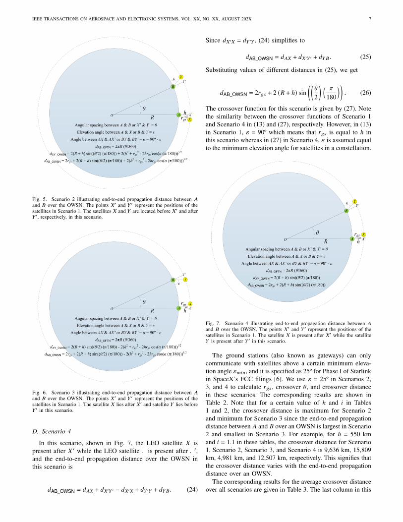
Fig. 5. Scenario 2 illustrating end-to-end propagation distance between 𝐴

and 𝐵 over the OWSN. The points 𝑋′ and 𝑌 ′ represent the positions of thesatellites in Scenario 1. The satellites 𝑋 and 𝑌 are located before 𝑋′ and after𝑌 ′, respectively, in this scenario.


and 𝐵 over the OWSN. The points 𝑋′ and 𝑌 ′ represent the positions of thesatellites in Scenario 1. The satellite 𝑋 lies after 𝑋′ and satellite 𝑌 lies before𝑌 ′ in this scenario.

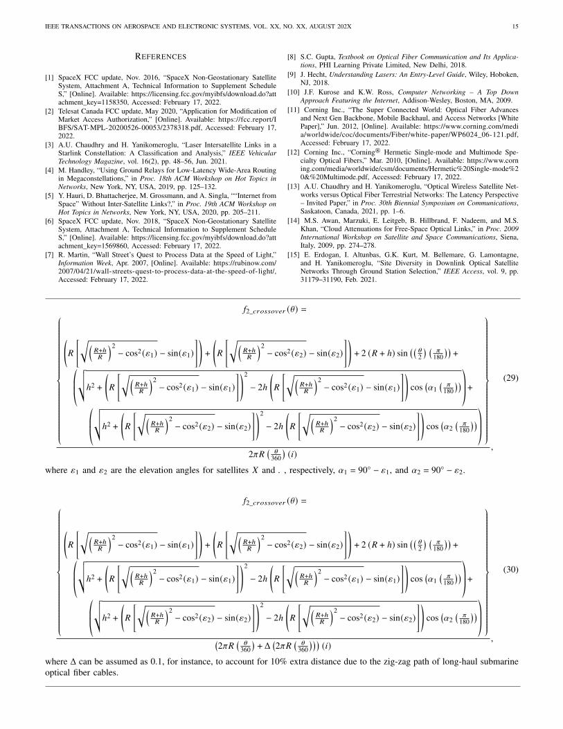
D. Scenario 4

In this scenario, shown in Fig. 7, the LEO satellite 𝑋 ispresent after 𝑋 ′ while the LEO satellite 𝑌 is present after 𝑌 ′,and the end-to-end propagation distance over the OWSN inthis scenario is

𝑑AB_OWSN = 𝑑𝐴𝑋 + 𝑑𝑋′𝑌 ′ − 𝑑𝑋′𝑋 + 𝑑𝑌 ′𝑌 + 𝑑𝑌𝐵. (24)

Since 𝑑𝑋′𝑋 = 𝑑𝑌 ′𝑌 , (24) simplifies to

𝑑AB_OWSN = 𝑑𝐴𝑋 + 𝑑𝑋′𝑌 ′ + 𝑑𝑌𝐵. (25)

Substituting values of different distances in (25), we get

𝑑AB_OWSN = 2𝑟𝑔𝑠 + 2 (𝑅 + ℎ) sin((\

2

) ( 𝜋

180

)). (26)

The crossover function for this scenario is given by (27). Notethe similarity between the crossover functions of Scenario 1and Scenario 4 in (13) and (27), respectively. However, in (13)in Scenario 1, Y = 90º which means that 𝑟𝑔𝑠 is equal to ℎ inthis scenario whereas in (27) in Scenario 4, Y is assumed equalto the minimum elevation angle for satellites in a constellation.


and 𝐵 over the OWSN. The points 𝑋′ and 𝑌 ′ represent the positions of thesatellites in Scenario 1. The satellite 𝑋 is present after 𝑋′ while the satellite𝑌 is present after 𝑌 ′ in this scenario.

The ground stations (also known as gateways) can onlycommunicate with satellites above a certain minimum eleva-tion angle Y𝑚𝑖𝑛, and it is specified as 25º for Phase I of Starlinkin SpaceX’s FCC filings [6]. We use Y = 25º in Scenarios 2,3, and 4 to calculate 𝑟𝑔𝑠, crossover \, and crossover distancein these scenarios. The corresponding results are shown inTable 2. Note that for a certain value of ℎ and 𝑖 in Tables1 and 2, the crossover distance is maximum for Scenario 2and minimum for Scenario 3 since the end-to-end propagationdistance between 𝐴 and 𝐵 over an OWSN is largest in Scenario2 and smallest in Scenario 3. For example, for ℎ = 550 kmand 𝑖 = 1.1 in these tables, the crossover distance for Scenario1, Scenario 2, Scenario 3, and Scenario 4 is 9,636 km, 15,809km, 4,981 km, and 12,507 km, respectively. This signifies thatthe crossover distance varies with the end-to-end propagationdistance over an OWSN.

The corresponding results for the average crossover distanceover all scenarios are given in Table 3. The last column in this


𝑓1_𝑐𝑟𝑜𝑠𝑠𝑜𝑣𝑒𝑟 (\) =

2 ©«𝑅√︄(

𝑅 + ℎ

𝑅

)2− cos2 (Y) − sin(Y)

ª®¬ + 2 (𝑅 + ℎ) sin((\

2

) ( 𝜋

180

))2𝜋𝑅

(\

360

)(𝑖)

(13)


2

) ( 𝜋

180

))+ 2

(√︂ℎ2 + 𝑟𝑔𝑠


( 𝜋

180

)))(17)

𝑓2_𝑐𝑟𝑜𝑠𝑠𝑜𝑣𝑒𝑟 (\) =2𝑟𝑔𝑠 + 2 (𝑅 + ℎ) sin

((\

2

) ( 𝜋

180

))+ 2

(√︂ℎ2 + 𝑟𝑔𝑠


( 𝜋

180

)))2𝜋𝑅

(\

360

)(𝑖)

(18)


2

(𝑅

[√︂(𝑅+ℎ𝑅

)2− cos2 (Y) − sin(Y)

])+ 2 (𝑅 + ℎ) sin

( (\2) (

𝜋180

) )+

2©«√√√ℎ2 +

(𝑅

[√︂(𝑅+ℎ𝑅

)2− cos2 (Y) − sin(Y)

])2

− 2ℎ

(𝑅

[√︂(𝑅+ℎ𝑅

)2− cos2 (Y) − sin(Y)

])cos

(𝛼

(𝜋

180) )ª®®¬

2𝜋𝑅

(\

360

)(𝑖)

(19)


2

) ( 𝜋

180

))− 2

(√︂ℎ2 + 𝑟𝑔𝑠


( 𝜋

180

)))(22)


2

(𝑅

[√︂(𝑅+ℎ𝑅

)2− cos2 (Y) − sin(Y)

])+ 2 (𝑅 + ℎ) sin

( (\2) (

𝜋180

) )−

2©«√√√ℎ2 +

(𝑅

[√︂(𝑅+ℎ𝑅

)2− cos2 (Y) − sin(Y)

])2

− 2ℎ

(𝑅

[√︂(𝑅+ℎ𝑅

)2− cos2 (Y) − sin(Y)

])cos

(𝛼

(𝜋

180) )ª®®¬

2𝜋𝑅

(\

360

)(𝑖)

(23)


2 ©«𝑅√︄(

𝑅 + ℎ

𝑅

)2− cos2 (Y) − sin(Y)

ª®¬ + 2 (𝑅 + ℎ) sin((\

2

) ( 𝜋

180

))2𝜋𝑅

(\

360

)(𝑖)

(27)


TABLE 2DIFFERENT SCENARIOS – CROSSOVER \ AND CROSSOVER DISTANCE FOR DIFFERENT VALUES OF ℎ AND 𝑖; Y = 25º (I.E., 𝛼 = 90º - Y).

h(km) i 𝒓𝒈𝒔

(km)Scenario 2 Scenario 3 Scenario 4

𝜽𝒄𝒓𝒐𝒔𝒔𝒐𝒗𝒆𝒓(degrees)






300

1.5

649

46.1906 5,141 2.3870 265 25.2535 2,8111.4675 49.1359 5,469 2.5716 286 27.0867 3,015

1.4 56.3166 6,269 3.0628 340 31.8062 3,5401.3 70.0930 7,802 4.2709 475 42.1522 4,6921.2 87.9298 9,788 7.0397 783 58.7719 6,5421.1 109.0009 12,134 18.7669 2,089 82.5393 9,188

500

1.5

1,032

72.0282 8,018 4.0254 402 41.6482 4,6361.4675 75.8936 8,448 4.3609 485 44.5585 4,960

1.4 84.7855 9,438 5.2735 587 51.7962 5,7651.3 100.0770 11,140 7.6348 849 66.1116 7,3591.2 117.5468 13,085 13.6754 1,522 85.0675 9,4691.1 136.5127 15,196 39.5710 4,404 107.3817 11,953

550

1.5

1,123

77.7858 8,658 4.4469 495 45.6406 5,0801.4675 81.7732 9,102 4.8250 537 48.7809 5,430

1.4 90.8551 10,114 5.8596 652 56.4986 6,2891.3 106.2106 11,823 8.5729 954 71.3952 7,9471.2 123.4653 13,744 15.7126 1,749 90.4590 10,0701.1 142.0222 15,809 44.7475 4,981 112.3582 12,507

700

1.5

1,389

93.5624 10,415 5.7532 575 57.2647 6,3741.4675 97.7698 10,883 6.2736 698 60.9731 6,787

1.4 107.1297 11,925 7.7218 859 69.7980 7,7691.3 122.3882 13,624 11.6972 1,302 85.7696 9,5471.2 138.9859 15,472 23.0123 2,561 104.7135 11,6561.1 156.5317 17,425 58.7699 6,542 125.4435 13,964

900

1.5

1,727

111.6662 12,430 7.6188 848 71.7972 7,9921.4675 115.9666 12,909 8.3708 931 75.9976 8,459

1.4 125.3375 13,952 10.5211 1,171 85.6506 9,5341.3 140.1980 15,606 16.8177 1,872 102.0762 11,3631.2 156.0126 17,367 35.5476 3,957 120.4220 13,4051.1 172.5383 19,206 74.1914 8,258 139.8560 15,568

1,100

1.5

2,049

127.1727 14,156 9.6810 1,077 85.1195 9,4751.4675 131.4531 14,633 10.7311 1,194 89.5840 9,972

1.4 140.6841 15,661 13.8224 1,538 99.5820 11,0851.3 155.0975 17,265 23.4653 2,612 115.9216 12,9041.2 170.2490 18,952 49.7480 5,537 133.5734 14,8691.1 186.0006 20,705 86.8717 9,670 151.9652 16,916

table is the average crossover distance, which is the averageof the crossover distances of all four scenarios. For example,for ℎ = 550 km and 𝑖 = 1.1 in this table, the correspondingaverage crossover distance is 10,733 km and it is the averageof 9,636 km, 15,809 km, 4,981 km, and 12,507 km, which arethe crossover distances for Scenario 1, Scenario 2, Scenario 3,and Scenario 4, respectively, at this ℎ and 𝑖 in Tables 1 and 2.While simulating an OWSN (as described later in Sections IVand V), we calculate shortest paths over the OWSN at all timeslots. We use the average crossover distance over all scenariosin Table 3 to evaluate and explain the simulation results forthe latency comparison of OFTNs and OWSNs in Section V.We consider this a reasonable approach since the end-to-endlatency of a simulated OWSN is the average of the end-to-endlatencies of the shortest paths over the OWSN at all time slots.An illustration of the crossover distance in different scenariosas well as the average crossover distance vs. 𝑖 is provided inFig. 8 when ℎ = 550 km.

IV. METHODOLOGY FOR CALCULATING LATENCY OF ANOFTN AND AN OWSN

In this section, we describe in detail the different steps ofour methodology for calculating the latency in an OFTN and

an OWSN. The values used in this study of the different pa-rameters for the three different OFTNs and the three differentOWSNs are listed in Table 4.

A. Optical Fiber Terrestrial NetworkFor the three OFTNs, we use three different refractive

indices, 𝑖1 for the first OFTN (or OFTN1), 𝑖2 for the secondOFTN (or OFTN2), and 𝑖3 for the third OFTN (or OFTN3).We consider different refractive indices for OFTN1, OFTN2,and OFTN3 to study the impact of optical fiber refractiveindex on latency in OFTNs as well as for comparative analysisof latency between OFTNs and OWSNs. For example, weuse 1.4675 as the value for 𝑖3, which is the refractive indexof a single-mode optical fiber (manufactured by Corning®)that is suitable for long-distance communications at 1,310 nmoperating wavelength [12]. Technological developments maylead to a reduction of optical fiber refractive index in future andwe assume lower values for 𝑖2 and 𝑖1 accordingly. The speed oflight in optical fiber with a refractive index 𝑖 can be calculatedusing 𝑐/𝑖, where the value of the speed of light in vacuum or 𝑐is 299,792,458 m/s [30]. For example, we consider the speedof light in OFTN3 to be 𝑐/1.4675 or 204,287,876 m/s.

We calculate the latency of an inter-continental long-distance connection between two cities over an OFTN by


TABLE 3AVERAGE CROSSOVER DISTANCE.

h(km) i Average 𝒅𝒄𝒓𝒐𝒔𝒔𝒐𝒗𝒆𝒓

(km)

300

1.5 2,3841.4675 2,548

1.4 2,9591.3 3,8221.2 5,1781.1 7,430

500

1.5 3,8491.4675 4,105

1.4 4,7021.3 5,8761.2 7,5551.1 10,156

550

1.5 4,2111.4675 4,472

1.4 5,1071.3 6,3391.2 8,0731.1 10,733

700

1.5 5,2081.4675 5,529

1.4 6,2571.3 7,6311.2 9,5091.1 12,265

900

1.5 6,4881.4675 6,839

1.4 7,6621.3 9,1711.2 11,2311.1 13,956

1,100

1.5 7,6651.4675 8,050

1.4 8,9441.3 10,5631.2 12,7821.1 15,372

TABLE 4VALUES AND DESCRIPTIONS OF PARAMETERS FOR OFTNS AND OWSNS.

Parameter Value Description𝑖1 1.1 Refractive index of optical fiber in OFTN1𝑖2 1.3 Refractive index of optical fiber in OFTN2𝑖3 1.4675 Refractive index of optical fiber in OFTN3ℎ1 300 km Altitude of satellites in OWSN1ℎ2 550 km Altitude of satellites in OWSN2ℎ3 1,100 km Altitude of satellites in OWSN3𝑟1 3,400 km LISL range of satellites in OWSN1𝑟2 5,016 km LISL range of satellites in OWSN2𝑟3 7,540 km LISL range of satellites in OWSN3

Y𝑚𝑖𝑛 25º Minimum elevation angle𝑟𝑔𝑠1 649 km Range of ground stations in OWSN1𝑟𝑔𝑠2 1,123 km Range of ground stations in OWSN2𝑟𝑔𝑠3 2,049 km Range of ground stations in OWSN3

dividing the shortest distance between two cities along thesurface of the Earth with the speed of light in optical fiberin that OFTN. To calculate the shortest distance between twocities, we use their coordinates (latitudes and longitudes) onthe surface of the Earth. To this end, we use the coordinatesfor the locations of the financial stock markets (i.e., New YorkStock Exchange, Dublin Stock Exchange, Sao Paulo StockExchange, London Stock Exchange, Toronto Stock Exchange,and Sydney Stock Exchange) within these cities, and the short-est distance for New York–Dublin, Sao Paulo–London, and

Fig. 8. Plot of crossover distance (km) for different scenarios as well asaverage crossover distance (km) vs. 𝑖 at ℎ = 550 km. For different values of 𝑖 inthis figure, the crossover distance is maximum for Scenario 2 (depicted by thesolid red line with square markers) and minimum for Scenario 3 (representedby the solid magenta line with triangle markers). The solid black line withdiamond markers shows the average crossover distance. Similar trends existat ℎ = 300 km and ℎ = 1,100 km and so the corresponding plots are omittedto avoid redundancy.

Toronto–Sydney inter-continental connections along Earth’ssurface is calculated as 5,121 km, 9,514 km, and 15,585km, respectively. For this calculation, the radius of the Earthis considered as 6,378 km. For example, the latency of theshortest distance path for the Toronto–Sydney inter-continentalconnection over OFTN3 having a refractive index of 1.4675and a speed of light in optical fiber of 204,287,876 m/s iscalculated as 76.29 ms.

B. Optical Wireless Satellite Network

To simulate an OWSN, we employ the satellite constellationfor Phase I of Starlink and assume LISLs between satellites inthis constellation. This constellation will consist of 1,584 LEOsatellites in 24 orbital planes with 66 satellites per plane. Theinclination of this constellation will be 53º and its altitude willbe 550 km. We assume this constellation to be uniform, whichmeans an equal spacing between orbital planes and an equalspacing between satellites within an orbital plane is assumed.

To study the impact of altitude of satellites on the latency ofOWSNs as well as for the comparative analysis with OFTNs,we consider three different OWSNs based on this constellationat different altitudes. For the first OWSN (or OWSN1), ℎ1 isthe altitude of its satellites and it is 300 km; for the secondOWSN (or OWSN2), ℎ2 is the altitude of its satellites and itis 550 km; and for the third OWSN (or OWSN3), ℎ3 is thealtitude of its satellites and it is 1,100 km. Note that ℎ2 is equalto the altitude of satellites in Starlink’s Phase I constellation.We also consider OWSNs at a lower and a higher altitude asnumerous upcoming satellite constellations are being plannedat various VLEO and LEO altitudes.

The LISL range of a satellite is the distance over whichit can establish LISLs with other satellites that are within its


range. We consider the maximum LISL range for all satellitesin an OWSN. The maximum LISL range of a satellite is arange that is only constrained by visibility. As described in[3], the maximum LISL range of satellites at 550 km altitudecan be calculated as 5,016 km. Similarly, we calculate themaximum LISL range for satellites at 300 km and 1,100km altitudes as 3,400 km and 7,540 km, respectively. Wedenote 𝑟1, 𝑟2, and 𝑟3 as LISL ranges for satellites in OWSN1,OWSN2, and OWSN3, and set them to 3,400 km, 5,016 km,and 7,540 km, respectively. Using Y = 25º (i.e., the minimumelevation angle specified for Phase I of Starlink in SpaceX’sFCC filings [6]), 𝑅 = 6,378 km, and ℎ = 300 km, 550 km,and 1,100 km in (11), we set the range of ground stations inOWSN1, OWSN2, and OWSN3, i.e., 𝑟𝑔𝑠1, 𝑟𝑔𝑠2, and 𝑟𝑔𝑠3 as649 km, 1,123 km, and 2,049 km, respectively.

To calculate latency in an OWSN, we consider the speedof light in vacuum for LISLs and for laser links betweenground stations and satellites. We identify all possible linksin an OWSN, find their lengths, and calculate the latency ofeach link by dividing the length of a link by the speed oflight in vacuum. Using Dijkstra’s algorithm [31], we find theshortest path between two cities over an OWSN in terms oflink latency; this is in fact the minimum-latency route betweencities over that OWSN. The latency (or end-to-end latency) ofthe shortest path over an OWSN includes the latency of thelaser link from the ground station in the source city on Earthto the ingress satellite of the OWSN in space, the latenciesof the laser inter-satellite links in this path, and the latency ofthe laser link from the egress satellite of the OWSN in spaceto the ground station in the destination city on Earth.

We divide the time into time slots of one second duration,where a time slot represents a snapshot of an OWSN at thatsecond. We find a shortest path (i.e., a route with minimum la-tency) at each time slot for an OWSN. We calculate the latency(or end-to-end latency) of an inter-continental connection overan OWSN by taking the average of the end-to-end latenciesof all shortest paths at all time slots over the entire simulationduration. We run the simulation for a duration of one hour, i.e.,3,600 seconds or time slots. For example, the latency (or end-to-end latency) of OWSN1 for the New York–Dublin inter-continental connection is calculated as 18.84 ms, which is theaverage of the end-to-end latencies of the shortest paths at all3,600 time slots.

V. LATENCY COMPARISON – OFTNS VS. OWSNS

To study the impact on latency of optical fiber refractiveindex in OFTNs and altitude of satellites in OWSNs, weconsider three different OFTNs and three different OWSNs asspecified in Table 4. To compare these OFTNs and OWSNsin terms of latency, we examine them in three different inter-continental connection scenarios, including New York–Dublin,Sao Paulo–London, and Toronto–Sydney. We simulate thethree different OWSNs using the well-known satellite constel-lation simulator STK Version 12.1 [32], the satellite constella-tion for Phase I of Starlink, and the parameters given in Table4 and described in Section IV-B. For example, to simulate theOWSN1, we generate Starlink’s Phase I constellation using ℎ1

as the altitude of satellites, 𝑟1 as the LISL range of satellites,and 𝑟𝑔𝑠1 as the range of ground stations; and we generatedistinct IDs for the 1,584 satellites within the constellation.

After generating the satellite constellation corresponding toan OWSN and ground stations at locations of stock exchangesin various cities in STK, we extract the data of the OWSN fromSTK into Python, such as positions of satellites and groundstations, links between satellites, links between satellites andground stations, and duration of the existence of these links.This data that is obtained from the STK simulator is discretizedinto time slots in Python. The discretized data includes all linksthat exist at a time slot as well as the positions of satellitesat that time slot. Using this discretized data, we calculate thelength and the latency for all links that exist at a time slot.Finally, we use the NetworkX library in Python [33] to find theshortest (or minimum-latency) path between ground stationsin different cities over the OWSN at each time slot.

The orbital velocity 𝑣𝑜 of a satellite orbiting the Earth canbe calculated using [34]

𝑣𝑜 =

√︂𝐺𝑀𝐸

𝑅 + ℎ, (28)

where 𝐺 is the gravitational constant, 𝑀𝐸 is the mass ofthe Earth, 𝑅 is Earth’s radius, and ℎ is the altitude of thesatellite. Using 𝐺 = 6.673 × 10−11 Nm2/kg2, 𝑀𝐸 = 5.98 ×1024 kg, and 𝑅 = 6.378 × 106 m in (28), one can determinethat the satellites in OWSN1 at 300 km altitude, OWSN2 at550 km altitude, and OWSN3 at 1,100 km altitude travel atspeeds of approximately 7.7 km/s, 7.6 km/s, and 7.3 km/s,respectively. Due to this high orbital speed of satellites in anOWSN, the ground station-to-ingress satellite link, satellite-to-satellite links, and egress satellite-to-ground station link or thelatencies of these links change constantly. Consequently, theshortest path of an inter-continental connection over an OWSNbetween ground stations in two cities and/or its latency changeat every time slot. As also stated earlier, we run the simulationof an OWSN for one hour or 3,600 time slots and find theshortest (or minimum-latency) path between ground stations intwo cities over the OWSN at every time slot. For example, theshortest path calculated at the first time slot over OWSN3 forthe Toronto–Sydney inter-continental connection is shown inFig. 9. The shortest path is shown in yellow color in this figurewhile the satellites on this shortest path are shown in pink.This shortest path consists of the ground station at Toronto(located at the Toronto Stock Exchange), satellites x12112(ingress), x10203 (intermediate hop), and x10161 (egress) inthe OWSN, and the ground station at Sydney (located at theSydney Stock Exchange). In addition, the shortest distancepath over an OFTN for the Toronto–Sydney inter-continentalconnection along Earth’s surface is illustrated in this figure ingreen color.

Table 5 shows the latency (i.e., the end-to-end latencybetween source and destination points in two cities) of thethree OFTNs and the three OWSNs for the three differentinter-continental connection scenarios. Note that the latency ofan inter-continental connection over an OWSN shown in thistable is the average of the end-to-end latencies of the shortestpaths that are found at all time slots. It is observed that the


Fig. 9. The shortest path at first time slot for Toronto–Sydney inter-continentalconnection over OWSN3 is shown in yellow color and the satellites on thispath are shown in pink. It consists of the ground station at Toronto StockExchange, satellites x12112 (ingress), x10203 (intermediate hop), and x10161(egress) in the OWSN, and the ground station at Sydney Stock Exchange. It’slength is 18,201 km, and it’s latency over OWSN3 having an altitude of 1,100km is 60.71 ms. Furthermore, the shortest distance path for Toronto–Sydneyinter-continental connection over an OFTN is shown in green color. This isthe shortest path between Toronto and Sydney along the surface of the Earth,it’s length is 15,585 km, and it’s latency over OFTN3 having a refractiveindex of 1.4675 is 76.29 ms.

latency of OFTNs increases with the increase in the opticalfiber refractive index in all scenarios. For example, the latencyof OFTN1, OFTN2, and OFTN3 is 18.79 ms, 22.21 ms, and25.07 ms, respectively, for the New York–Dublin connection.Recall that 𝑖1 or the optical fiber refractive index for OFTN1,𝑖2 or the optical fiber refractive index for OFTN2, and 𝑖3 orthe optical fiber refractive index for OFTN3 are 1.1, 1.3, and1.4675, respectively. The higher the optical fiber refractiveindex, the slower the speed of light through an OFTN, andthe higher the latency.

We also observe that the latency (or average latency) ofOWSNs increases with the increase in the altitude of satel-lites in all scenarios. For example, the latency for the SaoPaulo–London connection is 34.13 ms, 35.31 ms, and 37.84ms for OWSN1, OWSN2, and OWSN3, respectively. It shouldbe noted that ℎ1, i.e., the altitude of satellites in OWSN1,ℎ2, i.e., the altitude of satellites in OWSN2, and ℎ3, i.e., thealtitude of satellites in OWSN3 are 300 km, 550 km, and1,100 km respectively. A higher altitude of satellites in anOWSN translates into longer uplink (i.e., the link betweensource ground station and ingress satellite), longer satellite-to-satellite links, and longer downlink (i.e., the link betweenegress satellite and destination ground station), which in turntranslate into higher latency.

The results in Table 5 indicate that the latency of an OFTNor an OWSN is lowest for the New York–Dublin connection,increases for the Sao Paulo–London connection, and is highestfor the Toronto–Sydney connection. For example, the latency

of OFTN2 is 22.21 ms, 41.26 ms, and 67.58 ms, and thelatency of OWSN2 is 19.58 ms, 35.31 ms, and 56.71 ms for theNew York–Dublin, Sao Paulo–London, and Toronto–Sydneyconnections, respectively. One may recall that the short-est distance for New York–Dublin, Sao Paulo–London, andToronto–Sydney connections along the Earth’s surface is 5,121km, 9,514 km, and 15,585 km, respectively. The longer thedistance between two cities of an inter-continental connection,the higher the latency over an OFTN or an OWSN.

It is clearly seen from the results in Table 5 that allthree OWSNs outperform OFTN2 and OFTN3 in terms oflatency in all scenarios. For example, OWSN3 provides alatency improvement of 2.66%, 8.29%, and 10.30% for theNew York–Dublin, Sao Paulo–London, and Toronto–Sydneyconnections, respectively, compared to OFTN2. The longerthe inter-continental connection between a pair of cities, thegreater the gain due to the higher speed of light over laserlinks in vacuum of space in OWSN3 compared to the speedof light over laser links in optical fiber in OFTN2, and thebetter the latency improvement offered by OWSN3 comparedto OFTN2. The OWSN1 performs closely to OFTN1 forthe New York–Dublin connection and outperforms it forSao Paulo–London and Toronto–Sydney connections; OWSN2performs better than OFTN1 for the Toronto–Sydney connec-tion; and OWSN3 shows higher latency than OFTN1 in allscenarios.

As per Table 3, the average crossover distance is 7,430 kmat 𝑖 = 1.1 and ℎ = 300 km, it is 10,733 km at 𝑖 = 1.1 andℎ = 550 km, and it is 15,372 km at 𝑖 = 1.1 and ℎ = 1,100km. These average crossover distances correspond to OFTN1and OWSN1, OFTN1 and OWSN2, and OFTN1 and OWSN3,respectively. An OWSN can outperform an OFTN in terms oflatency if the shortest terrestrial distance between two pointson Earth is greater than the average crossover distance. Forexample, OWSN1 can outperform OFTN1 for communicationbetween two points on Earth if the shortest distance betweenthem is greater than 7,430 km. Note that the shortest distancebetween New York and Dublin along Earth’s surface is 5,121km. Since this distance is less than these three averagecrossover distances, OWSN1, OWSN2, and OWSN3 are notable to outperform OFTN1 for this connection. Similarly, theshortest terrestrial distance between Sao Paulo and London is9,514 km, which is less than the average crossover distanceof 10,733 km and 15,372 km. Hence, OWSN2 and OWSN3cannot perform better than OFTN1 for the Sao Paulo–Londonconnection.

Recall that the shortest terrestrial distance between Torontoand Sydney is 15,585 km, which is more than the averagecrossover distance of 15,372 km. However, OWSN3 exhibitsa higher latency than OFTN1 for the Toronto–Sydney con-nection. Note that the average crossover distance of 15,372km is calculated based on an OFTN having a refractiveindex of 1.1 and an OWSN at 1,100 km altitude where twosatellites communicate directly without any intermediate hopsor satellites. However, as discussed in Section IV-B, the LISLrange of satellites (i.e., the maximum distance for any twosatellites to communicate directly without any intermediatehops) is limited to 7,540 km in OWSN3. This LISL range


TABLE 5LATENCY – OFTNS VS. OWSNS.

Inter-Continental Connection Latency (ms)OFTN1 OFTN2 OFTN3 OWSN1 OWSN2 OWSN3

New York–Dublin 18.79 22.21 25.07 18.84 19.58 21.62Sao Paulo–London 34.91 41.26 46.57 34.13 35.31 37.84Toronto–Sydney 57.18 67.58 76.29 55.34 56.71 60.62

leads to three hops or satellites on the first shortest path (i.e.,the shortest path at first time slot) for the Toronto–Sydneyconnection over OWSN3 as shown in Fig. 9. Instead of a directLISL between satellites x12112 and x10161, the two satellitesare connected through an intermediate hop or satellite x10203(resulting in two LISLs) due to the limitation on their LISLrange, and this drives up the propagation distance to 18,201km over this shortest path producing a latency of 60.71 ms forthis shortest path over OWSN3 – a latency that is higher thanthat of OFTN1 for this connection. Similar to first shortestpath over OWSN3 for the Toronto–Sydney connection, 3,500shortest paths over this OWSN for this connection have threesatellites or hops (or two LISLs) while 100 have four (orthree LISLs), which translates into a higher average latencyfor OWSN3 compared to OFTN1 for this connection.

VI. CONCLUSIONS

A crossover function is proposed to enable the determinationof the crossover distance for switching from an OFTN on Earthto an OWSN in space for lower latency data communications.The crossover distance depends upon the optical fiber refrac-tive index 𝑖 in an OFTN and the altitude of satellites ℎ in anOWSN. The numerical results indicate that a higher 𝑖 and alower ℎ result in a shorter crossover distance. The crossoverfunction is examined in four different scenarios to account forthe different end-to-end propagation distances that occur overthe OWSN due to the orbital movement of satellites with time.It is observed from the numerical results that the crossoverdistance varies with the end-to-end propagation distance overan OWSN. It is minimum for Scenario 3 and maximum forScenario 2 since the end-to-end propagation distance overan OWSN is smallest in Scenario 3 and largest in Scenario2. The average crossover distance, which is the average ofthe crossover distances of all four scenarios, is calculated fordifferent ℎ and 𝑖, and is used to evaluate the simulation results.

Furthermore, three different OFTNs having different 𝑖s andthree different OWSNs with different ℎs are compared in termsof latency under three different scenarios for long-distanceinter-continental data communications. The simulation resultsindicate that OWSN1 (i.e., the first OWSN with ℎ1 = 300km), OWSN2 (i.e., the second OWSN with ℎ2 = 550 km)and OWSN3 (i.e., the third OWSN with ℎ3 = 1,100 km)outperform OFTN2 (i.e., the second OFTN with 𝑖2 = 1.3) andOFTN3 (i.e., the third OFTN with 𝑖3 = 1.4675) in all scenarios.For New York–Dublin connection, OWSN1, OWSN2, andOWSN3 perform better than OFTN2 by 15.17%, 11.84%,and 2.66%, respectively, while they provide an improvementin latency of 24.85%, 21.90%, and 13.76%, respectively,compared to OFTN3. For Sao Paulo–London connection, they

perform better than OFTN2 by 17.28%, 14.42%, and 8.29%,respectively, and better than OFTN3 by 26.71%, 24.18%,and 18.75%, respectively. For Toronto–Sydney connection,they show an improvement of 18.11%, 16.08%, and 10.30%,respectively, compared to OFTN2 and an improvement of27.46%, 25.67%, and 20.54%, respectively, compared toOFTN3.

Compared to OFTN1 (i.e., the first OFTN with 𝑖1 =1.1), OWSN1 performs better for the Sao Paulo–London andToronto–Sydney connections by 2.33% and 3.22%, respec-tively, and OWSN2 performs better for the Toronto–Sydneyconnection by 0.82%. For the New York–Dublin connection,the corresponding average crossover distances are greaterthan the shortest terrestrial distance between New York andDublin, and the three OWSNs are not able to offer lowerlatency than OFTN1 for this connection. Similarly, the cor-responding average crossover distances are greater than theshortest terrestrial distance between Sao Paulo and London,and consequently OWSN2 and OWSN3 underperform for thisconnection compared to OFTN1. The OWSN3 shows a higherlatency than OFTN1 for the Toronto–Sydney connection al-though the corresponding average crossover distance is smallerthan the shortest terrestrial distance between Toronto andSydney. The shortest or minimum-latency paths over OWSN3for this connection mostly require three satellites (i.e., twoLISLs) and sometimes four (i.e., three LISLs) resulting in ahigher latency (or average latency) than OFTN1.

Furthermore, we observe for all scenarios that the latencyof OWSNs increases as the altitude of satellites increasesfrom 300 km to 1,100 km. Similarly, the latency of OFTNsincreases with the increase in optical fiber refractive indexfrom 1.1 to 1.4675. We also notice that the latency of anOFTN or an OWSN increases with the increase in lengthof the inter-continental connection from New York–Dublinto Toronto–Sydney. Compared to current OFTN comprisinglong-distance submarine optical fiber cables having a refrac-tive index of 1.4675, OWSNs at all three altitudes show asignificant improvement in latency. They can also offer betterlatency than a future OFTN with a refractive index of 1.3 in allscenarios. An OWSN at a lower altitude can even outperforma future OFTN with a refractive index of 1.1 for longer inter-continental connections. These findings identify OWSNs asa promising solution for HFT firms seeking revenue gainsvia improvement in latency of data communications amongfinancial stock markets around the globe.

VII. FUTURE CHALLENGES

In the following, we highlight some future challenges re-lated to OWSNs and OFTNs that can arise from this work.


A. Incorporating Processing Delay in the End-to-End Latencyof OFTNs and OWSNs:

For congestion-free OFTNs and OWSNs with very highdata rate links, the queueing and transmission delays can beconsidered as negligible, and the end-to-end latency consistsof processing and propagation delays. Therefore, in additionto the propagation delay, processing delay is an importantpart of the end-to-end latency that needs to be considered inboth OWSN and OFTN. It is the delay that is incurred by ahop/node (i.e., an optical fiber relay station or a satellite) toprocess a packet, such as the time used to read the packetheader to make appropriate routing and switching decisions,before sending the packet to the appropriate next hop. Itdepends upon the number of hops between the source anddestination points (i.e., optical fiber relay stations or satelliteground stations) on the Earth’s surface and becomes significantwhen the data communications has to go through severalintermediate hops. The crossover function could be extendedto incorporate this delay. It would also be interesting to studythe effect of this delay on the end-to-end latency in OWSN andOFTN and to compare these two networks after incorporatingthis delay in the simulations.

B. Making the Crossover Decision at Each Time Slot Basedon Current Ingress and Egress Elevation Angles in the OWSN:

Instead of comparing the average crossover distance andthe shortest terrestrial distance, another approach to switchfrom the OFTN to the OWSN for long-distance lower latencydata communications can be based on checking the elevationangles of the ingress and egress satellites at every time slot,calculating the corresponding crossover distance at a time slot,and comparing it with the shortest terrestrial distance betweencities to make the crossover decision at that time slot. Forinstance, the crossover function for Scenario 2 in this casecan be written as in (29). It would be interesting to evaluatesuch an approach in future.

C. Incorporating Extra Distance to Account for the Zig-ZagPath of OFTNs:

In this work, we consider the shortest distance between twocities over the OFTN along the Earth’s surface. In reality,long-haul submarine optical fiber cables do not adhere to theshortest path to connect two points on Earth’s surface and areinstalled along paths that avoid earthquake prone areas anddifficult seabed terrains with high slopes. Another approachto model the shortest distance between cities over the OFTNcan be to add an extra distance to account for the extra lengthof the long-haul submarine optical fiber cables due to the zig-zag nature of their path. This extra distance can be added tothe shortest distance as a percentage of the shortest distance.For example, the crossover function for Scenario 2 in (29) canbe calculated in this case as in (30). Such an approach couldbe investigated in future.

D. Incorporating LISL Setup Delay in the End-to-End Latencyof OWSNs:

Due to pointing and acquisition during the formation ofa LISL between a pair of satellites equipped with lasercommunication terminals, the delay to set up a LISL (whichcan also be referred to as the LISL setup delay) can beanother significant component of the end-to-end latency inOWSNs. This delay is incurred whenever new LISLs arerequired to be established between pairs of satellites whenthere is a change in the shortest path between source anddestination ground stations and one or more new satellitesare introduced in the path requiring creation of new LISLs.Currently, this delay can vary from a few seconds to tensof seconds, e.g., Mynaric’s CONDOR laser communicationterminal needs approximately 30 seconds to establish LISLsbetween pairs of satellites in the OWSN for the first time butonce the position and altitude of the satellites are exchanged,this delay reduces to 2 seconds [35]. This delay could beincorporated in the end-to-end latency of the shortest pathsover the OWSN for a more accurate comparison of OWSN andOFTN in terms of latency. The current LISL setup times areprohibitive and in next-generation OWSNs (that may becomefully operational by mid to late 2020s), a satellite will belimited to set up only permanent LISLs [3] with neighboringsatellites that are always within its LISL range. Our workaims at next-next-generation OWSNs that may come intoexistence in early to mid-2030s where we envisage LISL setuptimes in milliseconds due to advancements in satellite lasercommunication terminal’s pointing, acquisition, and trackingtechnology, which will enable a satellite to instantaneouslyset up an LISL with any neighboring satellite that is currentlywithin its LISL range.

E. Investigating the Effect of Different LISL Ranges on theEnd-to-End Latency of OWSNs:

In this work, we consider the maximum LISL range for allsatellites in an OWSN, where the maximum LISL range ofa satellite is a range that is only constrained by visibility.Different LISL ranges are likely to impact latency of anOWSN differently. It has been concluded that the numberof neighbors of a satellite increases with the increase inLISL range of satellites [3]. The LISL range may affect theconnectivity of satellites within the OWSN. This may impactthe shortest paths over the OWSN for long-distance inter-continental data communications between ground stations indifferent cities, and this may influence the latency of theOWSN. It would be interesting to investigate the effect ofdifferent LISL ranges on the latency (or end-to-end latency)of an OWSN.

ACKNOWLEDGMENT

This work has been supported by the National ResearchCouncil Canada’s (NRC) High Throughput Secure Networksprogram (CSTIP Grant #CH-HTSN-625) within the OpticalSatellite Communications Consortium Canada (OSC) frame-work. The authors would like to thank AGI for the STKplatform.


REFERENCES

[1] SpaceX FCC update, Nov. 2016, “SpaceX Non-Geostationary SatelliteSystem, Attachment A, Technical Information to Supplement ScheduleS,” [Online]. Available: https://licensing.fcc.gov/myibfs/download.do?attachment_key=1158350, Accessed: February 17, 2022.

[2] Telesat Canada FCC update, May 2020, “Application for Modification ofMarket Access Authorization,” [Online]. Available: https://fcc.report/IBFS/SAT-MPL-20200526-00053/2378318.pdf, Accessed: February 17,2022.

[3] A.U. Chaudhry and H. Yanikomeroglu, “Laser Intersatellite Links in aStarlink Constellation: A Classification and Analysis,” IEEE VehicularTechnology Magazine, vol. 16(2), pp. 48–56, Jun. 2021.

[4] M. Handley, “Using Ground Relays for Low-Latency Wide-Area Routingin Megaconstellations,” in Proc. 18th ACM Workshop on Hot Topics inNetworks, New York, NY, USA, 2019, pp. 125–132.

[5] Y. Hauri, D. Bhattacherjee, M. Grossmann, and A. Singla, ““Internet fromSpace” Without Inter-Satellite Links?,” in Proc. 19th ACM Workshop onHot Topics in Networks, New York, NY, USA, 2020, pp. 205–211.

[6] SpaceX FCC update, Nov. 2018, “SpaceX Non-Geostationary SatelliteSystem, Attachment A, Technical Information to Supplement ScheduleS,” [Online]. Available: https://licensing.fcc.gov/myibfs/download.do?attachment_key=1569860, Accessed: February 17, 2022.

[7] R. Martin, “Wall Street’s Quest to Process Data at the Speed of Light,”Information Week, Apr. 2007, [Online]. Available: https://rubinow.com/2007/04/21/wall-streets-quest-to-process-data-at-the-speed-of-light/,Accessed: February 17, 2022.

[8] S.C. Gupta, Textbook on Optical Fiber Communication and Its Applica-tions, PHI Learning Private Limited, New Delhi, 2018.

[9] J. Hecht, Understanding Lasers: An Entry-Level Guide, Wiley, Hoboken,NJ, 2018.

[10] J.F. Kurose and K.W. Ross, Computer Networking – A Top DownApproach Featuring the Internet, Addison-Wesley, Boston, MA, 2009.

[11] Corning Inc., “The Super Connected World: Optical Fiber Advancesand Next Gen Backbone, Mobile Backhaul, and Access Networks [WhitePaper],” Jun. 2012, [Online]. Available: https://www.corning.com/media/worldwide/coc/documents/Fiber/white-paper/WP6024_06-121.pdf,Accessed: February 17, 2022.

[12] Corning Inc., “Corning® Hermetic Single-mode and Multimode Spe-cialty Optical Fibers,” Mar. 2010, [Online]. Available: https://www.corning.com/media/worldwide/csm/documents/Hermetic%20Single-mode%20&%20Multimode.pdf, Accessed: February 17, 2022.

[13] A.U. Chaudhry and H. Yanikomeroglu, “Optical Wireless Satellite Net-works versus Optical Fiber Terrestrial Networks: The Latency Perspective– Invited Paper,” in Proc. 30th Biennial Symposium on Communications,Saskatoon, Canada, 2021, pp. 1–6.

[14] M.S. Awan, Marzuki, E. Leitgeb, B. Hillbrand, F. Nadeem, and M.S.Khan, “Cloud Attenuations for Free-Space Optical Links,” in Proc. 2009International Workshop on Satellite and Space Communications, Siena,Italy, 2009, pp. 274–278.

[15] E. Erdogan, I. Altunbas, G.K. Kurt, M. Bellemare, G. Lamontagne,and H. Yanikomeroglu, “Site Diversity in Downlink Optical SatelliteNetworks Through Ground Station Selection,” IEEE Access, vol. 9, pp.31179–31190, Feb. 2021.


(𝑅

[√︂(𝑅+ℎ𝑅

)2− cos2 (Y1) − sin(Y1)

])+

(𝑅

[√︂(𝑅+ℎ𝑅

)2− cos2 (Y2) − sin(Y2)

])+ 2 (𝑅 + ℎ) sin

( (\2) (

𝜋180

) )+

©«√√√ℎ2 +

(𝑅

[√︂(𝑅+ℎ𝑅

)2− cos2 (Y1) − sin(Y1)

])2

− 2ℎ

(𝑅

[√︂(𝑅+ℎ𝑅

)2− cos2 (Y1) − sin(Y1)

])cos

(𝛼1

(𝜋

180) )ª®®¬+©«

√√√ℎ2 +

(𝑅

[√︂(𝑅+ℎ𝑅

)2− cos2 (Y2) − sin(Y2)

])2

− 2ℎ

(𝑅

[√︂(𝑅+ℎ𝑅

)2− cos2 (Y2) − sin(Y2)

])cos

(𝛼2

(𝜋

180) )ª®®¬

2𝜋𝑅

(\

360)(𝑖)

,

(29)

where Y1 and Y2 are the elevation angles for satellites 𝑋 and 𝑌 , respectively, 𝛼1 = 90◦ − Y1, and 𝛼2 = 90◦ − Y2.


(𝑅

[√︂(𝑅+ℎ𝑅

)2− cos2 (Y1) − sin(Y1)

])+

(𝑅

[√︂(𝑅+ℎ𝑅

)2− cos2 (Y2) − sin(Y2)

])+ 2 (𝑅 + ℎ) sin

( (\2) (

𝜋180

) )+

©«√√√ℎ2 +

(𝑅

[√︂(𝑅+ℎ𝑅

)2− cos2 (Y1) − sin(Y1)

])2

− 2ℎ

(𝑅

[√︂(𝑅+ℎ𝑅

)2− cos2 (Y1) − sin(Y1)

])cos

(𝛼1

(𝜋

180) )ª®®¬+©«

√√√ℎ2 +

(𝑅

[√︂(𝑅+ℎ𝑅

)2− cos2 (Y2) − sin(Y2)

])2

− 2ℎ

(𝑅

[√︂(𝑅+ℎ𝑅

)2− cos2 (Y2) − sin(Y2)

])cos

(𝛼2

(𝜋

180) )ª®®¬

(2𝜋𝑅

(\

360)+ Δ

(2𝜋𝑅

(\

360) ) )

(𝑖),

(30)

where Δ can be assumed as 0.1, for instance, to account for 10% extra distance due to the zig-zag path of long-haul submarineoptical fiber cables.


TABLE 6LIST OF ABBREVIATIONS.

Abbreviation DescriptionHFT High-frequency tradingHydRON High thRoughput Optical NetworkLEO Low Earth orbitLISL Laser inter-satellite linkOFTN Optical fiber terrestrial networkOFTN1 First optical fiber terrestrial networkOFTN2 Second optical fiber terrestrial networkOFTN3 Third optical fiber terrestrial networkOWSN Optical wireless satellite networkOWSN1 First optical wireless satellite networkOWSN2 Second optical wireless satellite networkOWSN3 Third optical wireless satellite networkVLEO Very low Earth orbit

[16] O.B. Yahia, E. Erdogan, G.K. Kurt, I. Altunbas, and H. Yanikomeroglu,“A Weather-Dependent Hybrid RF/FSO Satellite Communication forImproved Power Efficiency,” IEEE Wireless Communications Letters(Early Access), doi: 10.1109/LWC.2021.3136444.

[17] Telesat, “Telesat and TIM Brasil Partner for First-of-its-Kind LEO Testin Brazil,” May 2021, [Online]. Available: https://www.telesat.com/press/press-releases/telesat-and-tim-brasil-partner-for-first-of-its-kind-leo-test-in-brazil/, Accessed: February 17, 2022.

[18] H. Hauschildt, C. Elia, and A. Jones, “ESAs ScyLight Programme, Ac-tivities and Status of the High thRoughput Optical Network “HydRON”,”in Proc. 2018 International Conference on Space Optics, Chania, Greece,2018, pp. 1–7.

[19] H. Hauschildt et al., “HydRON: High thRoughput Optical Network,” inProc. 2019 IEEE International Conference on Space Optical Systems andApplications (ICSOS), Portland, Oregon, USA, 2019, pp. 1–11.

[20] S. Kassing, D. Bhattacherjee, A.B. Águas, J.E. Saethre, and A. Singla,“Exploring the “Internet from Space” with Hypatia,” in Proc. 2020ACM Internet Measurement Conference, New York, NY, USA, 2020, pp.214–229.

[21] M. Handley, “Delay is Not an Option: Low Latency Routing in Space,”in Proc. 17th ACM Workshop on Hot Topics in Networks, Redmond, WA,USA, 2018, pp. 85–91.

[22] N.U.L. Hassan, C. Huang, C. Yuen, A. Ahmad, and Y. Zhang, “DenseSmall Satellite Networks for Modern Terrestrial Communication Systems:Benefits, Infrastructure, and Technologies,” IEEE Wireless Communica-tions, vol. 27(5), pp. 96–103, Oct. 2020.

[23] Y. Lee and J.P. Choi, “Connectivity Analysis of Mega ConstellationSatellite Networks with Optical Inter-Satellite Links,” IEEE Trans-actions on Aerospace and Electronic Systems (Early Access), doi:10.1109/TAES.2021.3090914.

[24] B. Di, L. Song, Y. Li, and H.V. Poor, “Ultra-Dense LEO: Integrationof Satellite Access Networks into 5G and Beyond,” IEEE WirelessCommunications, vol. 26(2), pp. 62–69, Apr. 2019.

[25] B. Soret, S. Ravikanti, and P. Popovski, “Latency and Timelinessin Multi-Hop Satellite Networks,” in Proc. 2020 IEEE InternationalConference on Communications (ICC), Dublin, Ireland, 2020, pp. 1–6.

[26] D. Bhattacherjee and A. Singla, “Network Topology Design at 27,000km/hour,” in Proc. 15th International Conference on Emerging Net-working Experiments and Technologies, Orlando, FL, USA, 2019, pp.341–354.

[27] A.U. Chaudhry and H. Yanikomeroglu, “Free Space Optics for Next-Generation Satellite Networks,” IEEE Consumer Electronics Magazine,vol. 10(6), pp. 21–31, Nov. 2021.

[28] Z. Wang, Q. Wang, B. Moran, and M. Zukerman, “Terrain ConstrainedPath Planning for Long-Haul Cables,” Optic Express, vol. 27(6), pp.8221–8235, Mar. 2019.

[29] A. Guidotti, “Beam Size Design for New Radio Satellite Communica-tions Systems,” IEEE Transactions on Vehicular Technology, vol. 68(11),pp. 11379–11383, Nov. 2019.

[30] R.J. MacKay and R.W. Oldford, “Scientific Method, Statistical Methodand the Speed of Light,” Statistical Science, vol. 15(3), pp. 254–278, Aug.2000.

[31] E.W. Dijkstra, “A Note on Two Problems in Connexion with Graphs,”Numerische Mathematik, vol. 1, pp. 269–271, Dec. 1959.

[32] AGI, “Systems Tool Kit (STK),” [Online]. Available: https://www.agi.com/products/stk, Accessed: February 17, 2022.

[33] NetworkX Developers, “NetworkX – Network Analysis in Python,”[Online]. Available: https://networkx.org/, Accessed: February 17, 2022.

[34] T. Pratt and J. Allnutt, Satellite Communications, Wiley, Hoboken, NJ,2020.

[35] C. Carrizo, M. Knapek, J. Horwath, D.D. Gonzalez, and P. Cornwell,“Optical Inter-Satellite Link Terminals for Next Generation Satellite Con-stellations,” in Proc. Society of Photo-Optical Instrumentation Engineers(SPIE), vol. 11272, article id. 1127203, 2020, pp. 1–11.

Aizaz U. Chaudhry (M’10–SM’20) received theB.Sc. degree in Electrical Engineering from theUniversity of Engineering and Technology Lahore in1999. He received the M.A.Sc. and Ph.D. degrees inElectrical and Computer Engineering from CarletonUniversity in 2010 and 2015, respectively. He isa Senior Research Associate with the Departmentof Systems and Computer Engineering at CarletonUniversity. Previously, he worked as an NSERCPostdoctoral Research Fellow at CommunicationsResearch Centre Canada. His research interests in-

clude the application of machine learning and optimization in wirelessnetworks. His research work has been published in refereed venues, andhas received several citations. He has authored and co-authored more thanthirty publications. He is a licensed Professional Engineer in the Provinceof Ontario, a Senior Member of IEEE, and a Member of IEEE ComSoc’sTechnical Committee on Satellite and Space Communications.

Halim Yanikomeroglu (F’17) is a Full Professorat Carleton University. He received his Ph.D. fromUniversity of Toronto in 1998. He contributed to4G/5G technologies and non-terrestrial networks.His industrial collaborations resulted in 39 grantedpatents. He supervised or hosted in his lab a total of140 postgraduate researchers. He co-authored IEEEpapers with faculty members in 80+ universities in25 countries. He is a Fellow of IEEE, EngineeringInstitute of Canada, and Canadian Academy of En-gineering, and an IEEE Distinguished Speaker for

ComSoc and VTS. He is currently chairing the WCNC Steering Committee,and he is a Member of PIMRC Steering Committee and ComSoc EmergingTechnologies Committee. He served as the General Chair of two VTCs andTP Chair of three WCNCs. He chaired ComSoc’s Technical Committee onPersonal Communications. He received several awards including ComSocWireless Communications TC Recognition Award (2018), VTS Stuart MeyerMemorial Award (2020), and ComSoc Fred W. Ellersick Prize (2021).

When to Crossover from Earth to Space for Lower Latency ...

Documents

Transcript of When to Crossover from Earth to Space for Lower Latency ...