MOEA/D-DRA with two Crossover Operators

MOEA/D-DRA with Two Crossover Operators

Wali Khan and Qingfu Zhang

Abstract—Different genetic operators suit different problems.Using several crossover operators should be an effective ap-proach for improving the performance of an evolutionary algo-rithm. This paper studies the effect of the use of two crossoveroperators on MOEA/D-DRA for multi-objective optimization.It considers two crossover operators, namely, simplex crossoveroperator (SPX) and center of mass crossover operator (CMX).The probability of the use of each operator at each generationis updated in a adaptive way. The preliminary experimentalresults have indicated that this approach is promising.

I. INTRODUCTION

In this paper, we consider the following multiobjectiveoptimization problem (MOP) in its general form:

minimize F (x) = (f1(x), f2(x) . . . , fm(x)) (1)such that x ∈ X , X ⊆ Rn

where x = (x1, . . . , xn)T ∈ X is an n-dimensional vector

of the decision variables, X is the decision (variable) space,and F is the objective vector function that contains m realvalued functions.

Multiobjective optimization based on decomposition(MOEA/D) [1], [2], [3] is an evolutionary algorithmframework for multiobjective and MOEA/D-DRA [4], oneof its recent versions, has exhibited some good performanceon some hard multiobjective optimization problems [5].

Crossover operators are a major operator in mostevolutionary algorithms for generating new solutions.It is well-known that different crossovers suit differentproblems. Recently, using multiple crossover operatorsin one algorithm has been received some attention andproduced very good results [6], [7], [8].

In this paper, we employ two crossover operators, namely,simplex crossover (SPX) [9] and center of mass crossover(CMX) [10] in the framework of MOEA/D-DRA [4]. Theprobability of the use of each operator is adjusted in anadaptive way. We study the performance of the resultantimplementation on UF1-UF10, the test instance in CEC2009 algorithm competition [5].

The rest of this paper is organized as follows. Section IIintroduces the two crossover operators SPX, CMX and theTchebycheff aggregation function. Section III describes the

W. Khan is with the Department of Mathematical Sciences, University ofEssex, Colchester CO4 3SQ, UK. phone: +44-1206-873032; fax: +44-1206-3040; email: [email protected].

Q. Zhang is with the School of Computer Science and ElectronicEngineering, University of Essex, Colchester CO4 3SQ, U.K. (e-mail:[email protected]).

proposed probabilistic approach for the selection of SPX andCMX in the reproduction step of MOEA/D-DRA, Section IVpresents the major steps of the algorithm. Section V givesthe experimental settings and results. In Section VI, a briefconclusion and future work outline is given.

II. CROSSOVER OPERATORS AND TCHEBYCHEFFAGGREGATION FUNCTION

A. Simplex Crossover (SPX) [9], [11], [10]Given three parents, x1, x2, x3, the SPX generates three

offsprings as follows :

y(k) = (1 + ϵ)(x(k) − o), k = 1, 2, 3. (2)

where o = 13

∑3k=1 x

(k) is the center of the parents and ϵ ≥ 0is a scaling parameter. In our implementation, we generateone offspring as in [9]:

z =

3∑i=1

αiyi + o,

where αi > 0 are randomly which satisfy∑3

i=1 αi = 1.

B. Center of Mass Crossover (CMX) [10], [9], [12]:Given three parents, x1, x2, x3, the CMX operator in our

experiments works as follows• compute

o =1

3

3∑i=1

xi (3)

and

vi = 2o− xi (4)

• randomly select a vj and a parent xi and then applythe simulated binary crossover operator [13] on then togenerate one offspring.

C. Tchebycheff Aggregation FunctionMOEA/D decomposes a given MOP into N single objec-

tive subproblems by using an aggregation function. In thispaper, we use the Tchebycheff aggregation function for thispurpose, which is given as follows [14]:

minimize g(x|λ, z) = max1≤j≤mλj |fj(x)− z∗j |} (5)

where

x ∈ X

z∗ = {z1, z2, . . . , zm}zj = min{fj(x)|x ∈ X}λ = (λ1, λ2, . . . , λm)

λj ≥ 0∑mj=1 λj = 1

III. PROPOSED PROBABILISTIC APPROACH FOR THESELECTION OF SPX AND CMX

We use two crossover operators, i.e., SPX and CMX,in MOEA/D to generate offspring. Let p1t and p2t be theprobability of the use of SPX and CMX at generation t,respectively. We update p1t and p2t and select two crossoversas follows:

1) p11 and p21 is initialized to be 0.5 at generation 1.2) In Step 3 in the algorithm (the details are given in the

next section), in p1t × 100% of the subproblems, SPXwill be used for generating new solutions. The rest ofsubproblems will use CMX.

3) Compute the success rate of each crossover operatorsat the current generation: r1 and r2 1. Then set:

pit+1 = 0.5× pit + 0.5× ri

r1 + r2

for i = 1, 2.

IV. FRAMEWORK OF MOEA/D-DRA

Let λ1, . . . , λN be a set of even spread weight vectors andz∗ be the reference point. The problem of approximation ofthe PF of (1) can be decomposed into N scalar optimizationsubproblems and the objective function of the j-th subprob-lem is:

gte(x|λj , z∗) = max1≤i≤m

{λji |fi(x)− z∗i |} (6)

where λj = (λj1, . . . , λ

jm)T .

During the search, MOEA/D-DRA with the Tchebycheffapproach maintains:

• a population of N points x1, . . . , xN ∈ X , where xi isthe current solution to the i-th subproblem;

• FV 1, . . . , FV N , where FV i is the F -value of xi, i.e.FV i = F (xi) for each i = 1, . . . , N ;

• z = (z1, . . . , zm)T , where zi is the best (lowest) valuefound so far for objective fi;

• π1, . . . , πN : where πi utility of subproblem i.• gen: the current generation number.The algorithm works as follows:Input: • MOP (1);

• a stopping criterion;• N : the number of the subproblems considered

in MOEA/D;• a uniform spread of N weight vectors:

λ1, . . . , λN ;• T : the number of the weight vectors in the

neighborhood of each weight vector.Output: {x1, . . . , xN} and {F (x1), . . . , F (xN )}Step 1 Initialization

Step 1.1 Compute the Euclidean distances betweenany two weight vectors and then find the T closestweight vectors to each weight vector. For eachi = 1, . . . , N , set B(i) = {i1, . . . , iT } where

1A crossover operator is successful if its offspring can replace at leastone old solution

λi1 , . . . , λiT are the T closest weight vectors to λi.Step 1.2 Generate an initial population x1, . . . , xN

by uniformly randomly sampling from the searchspace.Step 1.3 Initialize z = (z1, . . . , zm)T by settingzi = min{fi(x1), fi(x

2), . . . , fi(xN )}.

Step 1.4 Set gen = 0 and πi = 1 for alli = 1, . . . , N .

Step 2 Selection of Subproblems for Search: theindexes of the subproblems whose objectives areMOP individual objectives fi are selected to forminitial I . By using 10-tournament selection basedon πi, select other [N5 ]−m indexes and add themto I .

Step 3 For each i ∈ I , do:Step 3.1 Selection of Mating/Update Range:Uniformly randomly generate a number rand from(0, 1). Then set

P =

{B(i) if rand < δ,{1, . . . , N} otherwise.

Step 3.2 Reproduction: Set r1 = i and randomlyselect two indexes r2 and r3 from P , and thengenerate a solution y from xr1 , xr2 and xr3 bySPX or CMX. Then apply the polynomial mutationoperator with probability pm on it.Step 3.3 Repair: If an element of y is out of theboundary of X , its value is reset to be a randomlyselected value inside the boundary.Step 3.4 Update of z: For each j = 1, . . . ,m, ifzj > fj(y), then set zj = fj(y).Step 3.5 Update of Solutions: Set c = 0 and thendo the following:

(1) If c = nr or P is empty, go to Step 4.Otherwise, randomly pick an index j fromP .(2) If g(y|λj , z) ≤ g(xj |λj , z), then setxj = y, FV j = F (y) and c = c+ 1.(3) Delete j from P and go to (1).

Step 4 Stopping Criteria If the stopping criteria issatisfied, then stop and output {x1, . . . , xN} and{F (x1), . . . , F (xN )}.

Step 5 gen = gen+ 1.If gen is a multiplication of 50, then compute∆i, the relative decrease of the objective for eachsubproblem i during the last 50 generations, update

πi =

{1 if ∆i > 0.001;(0.95 + 0.05 ∆i

0.001 )πi otherwise.

endifGo to Step 2.

In 10-tournament selection in Step 2, the index withthe highest πi value from 10 uniformly randomly selected

indexes are chosen to enter I . We should do this selection[N5 ]−m times.

In Step 5, the relative decrease is defined asold function value-new function value

old function valueIf ∆i is smaller than 0.001, the value of πi will be reduced.

In Step 3.2, Two crossover operators are employed as ex-plained in Section III and polynomial mutation as explainedbelow:

yk =

{yk + σk(uk − lk) with probability pm

yk with probability 1− pm(7)

Where lk, uk are the lower and upper bound of the the kthdecision variable respectively.

σk =

{(2× rand)

1η+1 − 1 if rand < 0.5

1− (2− 2× rand)1

η+1 otherwise

Where rand ∈ [0, 1] is a uniformly random number. Themutation rate pm and distribution index η are the two controlparameter.

V. EXPERIMENTAL SETTINGS AND RESULTS

A. Parameters settingIn this paper, we use the same parameters settings as in [4]

with the exception of DE parameters and are give as under:• N = 600 for two objective test instances.• N = 1000 for three objective test instances.• T = 0.1N , it defines the number of neighbors of one

single optimization problem (SOP);• nr = 0.01N , it restricts the maximum time of the

successful updates;• δ = 0.9, it is the probability which decide that wether

the candidate of parents are coming from the wholepopulation or from the neighbors of SOP;

• η = 20 and pm = 1/n in the polynomial mutationoperator, where n is parameter space dimension of MOPand η is the distribution index;

• The parameter for SPX is ϵ =√n+ 1 for each

problems except UF4 while for UF4, ϵ =√√

n+ 1 inboth single and double crossover operators strategies.

• The algorithm stops after 300, 000 function evaluations;

B. Weight vectors selectionA set of N weight vectors, W , is generated by using the

following criteria [4]:1) Uniformly randomly generate 5, 000 weight vectors

for forming the set W1. Set W is initialized as theset containing all the weight vectors (1, 0, . . . , 0, 0),(0, 1, . . . , 0, 0), . . . , (0, 0, . . . , 0, 1).

2) Find the weight vector in set W1 with the largestdistance to set W , add it to set W and delete it fromset W1.

3) If the size of set W is N , stop and return set W .Otherwise, go to 2).

C. Performance metric

The performance metric IGD [15] used to measure thealgorithm performance. Let P ∗ be a set of uniformly dis-tributed points along the PF. Let A be an approximate set tothe PF, the average distance from P ∗ to A is defined as [1],[5]:

D(A,P ) =

∑v∈P∗ d(v,A)

|P ∗|where d(v,A) is the minimum Euclidean distance betweenv and the points in A. If P ∗ is large enough to represent thePF very well, D(A,P ) could measure both the diversity andconvergence of A in a sense.

D. Results

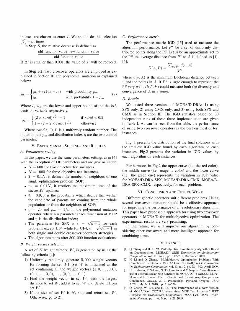
We tested three versions of MOEA/D-DRA: 1) usingSPX only, 2) using CMX only, and 3) using both SPX andCMX as in Section III. The IGD statistics based on 30independent runs of these three implementation are givenin Table I. As can be seen from the table, the performanceof using two crossover operators is the best on most of testinstances.

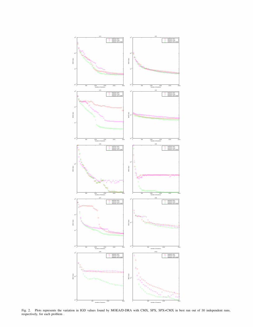
Fig. 1 presents the distribution of the final solutions withthe smallest IGD value found by each algorithm on eachinstances. Fig.2 presents the variation in IGD values byeach algorithm on each instances.

Furthermore, in Fig.2 the upper curve (i.e, the red color),the middle curve (i.e., magenta color) and the lower curve(i.e., the green one) represents the variation in IGD valuefor MOEA/D-DRA-SPX, MOEA/D-DRA-CMX, MOEA/D-DRA-SPX+CMX, respectively, for each problem.

VI. CONCLUSION AND FUTURE WORK

Different genetic operators suit different problems. Usingseveral crossover operators should be a effective approachfor improving the performance of an evolutionary algorithm.This paper have proposed a approach for using two crossoveroperators in MOEA/D for multiobjective optimization. Theexperimental results are very promising.

In the future, we will improve our algorithm by con-sidering other crossovers and more intelligent approach forcombining them.

REFERENCES

[1] Q. Zhang and H. Li, “A Multiobjective Evolutionary Algorithm Basedon Decomposition: MOEA/D,” IEEE Transaction on EvolutionaryComputation, vol. 11, no. 6, pp. 712–731, December 2007.

[2] H. Li and Q. Zhang, “Multiobjective Optimization Problems WithComplicated Pareto Sets: MOEA/D and NSGA-II,” IEEE TranssationOn Evolutionary Computation, vol. 13, no. 2, pp. 284–302, April 2009.

[3] H. Ishibuchi, Y. Sakane, N. Tsukamoto, and Y. Nojima, “Simultaneoususe of different scalarizing functions in MOEA/D,” in GECCO, M. Pe-likan and J. Branke, Eds. Genetic and Evolutionary ComputationConference, GECCO 2010, Proceedings, Portland, Oregon, USA:ACM, July 7-11 2010, pp. 519–526.

[4] Q. Zhang, W. Liu, and H. Li, “The Performance of a New Versionof MOEA/D on CEC09 Unconstrained MOP Test Instances,” IEEECongress On Evolutionary Computation (IEEE CEC 2009), Trond-heim, Norway, pp. 1–6, May, 18-21 2009.

0.0 0.2 0.4 0,6 0.8 1.0 1.20.0

0.2

0.4

0,6

0.8

1.0

1.2

f1

f2

UF1 Pareto Front

Real PFObtained PF−MOEA/D−CMXObtained PF−MOEA/D−SPXObtained PF−MOEA/D−CMX+SPX

0.0 0.2 0.4 0,6 0.8 1.0 1.20.0

0.2

0.4

0,6

0.8

1.0

1.2

f1

f2

UF2 Pareto Front


0.0 0.2 0.4 0,6 0.8 1.0 1.20.0

0.2

0.4

0,6

0.8

1.0

1.2

f1

f2

UF3 Pareto Front


0.0 0.2 0.4 0,6 0.8 1.0 1.20.0

0.2

0.4

0,6

0.8

1.0

1.2

f1

f2

UF4 Pareto Front


0.0 0.2 0.4 0,6 0.8 1.0 1.20.0

0.2

0.4

0,6

0.8

1.0

1.2

f1

f2

UF5 Pareto Front


0.0 0.2 0.4 0,6 0.8 1.0 1.20.0

0.2

0.4

0,6

0.8

1.0

1.2

f1

f2

UF6 Pareto Front


0.0 0.2 0.4 0,6 0.8 1.0 1.20.0

0.2

0.4

0,6

0.8

1.0

1.2

f1

f2

UF7 Pareto Front


0.00.2

0.40,6

0.81.0

1.2

0.00.2

0.40,6

0.81.0

1.2

0.0

0.2

0.4

0,6

0.8

1.0

1.2

f1

UF8 Pareto Front

f2

f3


0.00.2

0.40,6

0.81.0

1.2

0.00.2

0.40,6

0.81.0

1.2

0.0

0.2

0.4

0,6

0.8

1.0

1.2

f1

UF9 Pareto Front

f2

f3


0.00.2

0.40,6

0.81.0

1.2

0.00.2

0.40,6

0.81.0

1.2

0.00.20.40,60.81.01.2

f3

f1

UF10 Pareto Front

f2


Fig. 1. Plots of the final approximated solutions with the lowest IGD value in the objective space found by MOEA/D-DRA with CMX, SPX, SPX+CMXin 30 independent runs.

0 500 1000 1500 2000 250010

−3

10−2

10−1

100

UF1

Number of Iterations

BIG

D V

alue

MOEA/D−SPXMOEA/D−CMXMOEA/D−SPX+CMX

0 500 1000 1500 2000 250010

−3

10−2

10−1

100

UF2


BIG

D V

alue


0 500 1000 1500 2000 250010

−3

10−2

10−1

100

UF3


BIG

D V

alue


0 500 1000 1500 2000 250010

−2

10−1

100

UF4


BIG

D V

alue


0 500 1000 1500 2000 2500

100

UF5


BIG

D V

alue


0 500 1000 1500 2000 2500

100

UF6


BIG

D V

alue


0 500 1000 1500 2000 250010

−3

10−2

10−1

100

UF7


BIG

D V

alue


0 500 1000 150010

−2

10−1

100

UF8


BIG

D V

alue


0 500 1000 150010

−2

10−1

100

UF9


BIG

D V

alue


0 500 1000 1500

100

UF10


BIG

D V

alue


Fig. 2. Plots represents the variation in IGD values found by MOEA/D-DRA with CMX, SPX, SPX+CMX in best run out of 30 independent runs,respectively, for each problem .

TABLE ITHE IGD STATISTICS BASED ON 30 INDEPENDENT RUNS OF MOEA/D-DRA WITH CMX, SPX, SPX+CMX ON UNCONSTRAINED MULTIOBJECTIVE

TEST INSTANCES, UF1-UF10.

MOEA/D-DRA-SPX, MOEA/D-DRA-CMX, MOEA/D-DRA-SPX+CMXProb min median mean std max Crossover

UF10.004084 0.0046905 0.0051250 0.0034 0.0079980 CMX0.005077 0.008203 0.008652 0.004079 0.026533 SPX0.003985 0.004171 0.004292 0.000263 0.005129 SPX+CMX

UF20.0050340 0.0066460 0.0071868 0.00190157 0.012719 CMX0.004952 0.005596 0.005717 0.000487 0.007131 SPX0.005149 0.005472 0.005615 0.000412 0.006778 SPX+CMX

UF30.0049430 0.0432895 0.04153040 0.0239478 0.0855450 CMX0.005455 0.022374 0.030286 0.03823 0.091197 SPX0.004155 0.005313 0.011165 0.013093 0.068412 SPX+CMX

UF40.0508390 0.0632330 0.0628110 0.00476440 0.0734990 CMX

0.0502 0.0573 0.0573 0.0038 0.0657 SPX0.055457 0.063524 0.064145 0.004241 0.075361 SPX+CMX

UF50.1676280 0.3791160 0.363792 0.0813385 0.5085780 CMX

0.2186 0.3889 0.3963 0.0742 0.5704 SPX0.211058 0.379241 0.418508 0.135554 0.707093 SPX+CMX

UF60.0710280 0.44046750 0.3665337 0.12022382 0.60331490 CMX0.445548 0.507600 0.532296 0.070171 0.670946 SPX0.056972 0.248898 0.327356 0.185717 0.792910 SPX+CMX

UF70.0045910 0.006100 0.00762145 0.00526699 0.0317640 CMX0.005776 0.010898 0.062154 0.152973 0.533897 SPX0.003971 0.004745 0.006262 0.003307 0.014662 SPX+CMX

UF80.0559350 0.070072250 0.077114571 0.02153013 0.1310650 CMX0.078084 0.142313 0.136907 0.053748 0.272108 SPX0.051800 0.056872 0.057443 0.003366 0.065620 SPX+CMX

UF90.2075150 0.2875470 0.2807007 0.046701797 0.343310 CMX0.064034 0.181923 0.159370 0.053077 0.216422 SPX0.033314 0.144673 0.097693 0.054285 0.151719 SPX+CMX

UF100.4175320 0.4898737 0.4945660 0.0460605756 0.5991810 CMX0.445548 0.507600 0.532296 0.070171 0.670946 SPX0.391496 0.467715 0.462653 0.038698 0.533234 SPX+CMX

[5] Q. Zhang, A. Zhou, S. Zhaoy, P. N. Suganthany, W. Liu, and S. Ti-wariz, “Multiobjective optimization Test Instances for the CEC 2009Special Session and Competition,” Technical Report CES-487, 2009.

[6] J. A. Vrugt, B. A. Robinson, and J. M. Hyman, “Self-Adapotive Mul-timethod Search for Global Optimization in Real-Parameter Spaces,”IEEE Transsation On Evolutionary Computation, vol. 13, no. 2, pp.243–259, April 2009.

[7] J. A. Vrugt and B. A. Robinson, “Improved Evolutionary Optimizationfrom genetically adaptive mutimethod search,” Proceedings of theNational Academy of Sciences of the United States of America: PNAS(USA), vol. 104, no. 3, pp. 708–701, Jaunuary 16, 2007.

[8] D. Thierens, “An Adaptive Pursuit Strategy for Allocation OperatorProbabilities,” GECCO’05, pp. 1539–1546, June 2005.

[9] S. Tsutsui, “Multi-parent recombination in genetic algorithms withsearch space boundary extension by mirroring,” in PPSN V: Proceed-ings of the 5th International Conference on Parallel Problem Solvingfrom Nature. London, UK: Springer-Verlag, 1998, pp. 428–437.

[10] S. Tsutsui, M. Yamamura, and T. Higuchi, “Multi-parent Recombi-

nation with Simplex Crossover in Real Coded Genetic Algorithms,”Proc. of the GECCO-99, pp. 657–374, 1999.

[11] Z. Cai and Y. Wang, “A multiobjective optimization-based evolution-ary algorithm for constrained optimization,” IEEE Transactions OnEvolutionary Computation, vol. 10, no. 6, pp. 658–675, December2006.

[12] S. Tsutsui and A. Ghosh, “A Study on the Effect of Multi-parentRecombination in Realcoded Genetic Algorithms,” Proc. of the IEEEICEC, pp. 828–833, 1998.

[13] K. Deb, Multi-Objective Optimization using Evolutionary Algorithms.,First ed. John Wiley and Sons, Chichester, UK, 2001.

[14] K. M. Miettinien, Nonlinear Multiobjective Optimization, ser. Kluwer’sInternational Series. Norwell, MA: Academic Publishers Kluwer,1999.

[15] E. Zitzler, L. Thiele, M. Laumanns, C. M. Fonseca, and V. G.da Fonseca, “Performance Assessment of Multiobjective Optimizers:An Analysis and Review,” IEEE Transactions on Evolutionary Com-putation, vol. 7, pp. 117–132, 2003.

MOEA/D-DRA with two Crossover Operators

Documents

Transcript of MOEA/D-DRA with two Crossover Operators