Decision Sciences Volume 31 Number I Winter 2000 Printed in the U.S.A.

Fitting the Lognormal Distribution to Surgical Procedure Times* Jerrold H. May Joseph M. Katz Graduate School of Business, University of Pittsburgh, Pittsburgh, PA 15260, email: jerrymay @katz.pitt.edu

David P. Strum Department of Anesthesiology, Department of Anesthesiology, Queen’s Universiv, Kingston General Hospital, 76 Stuart St., Kingston, Ontario K7L 2V7, email: strumd@post.queensu.ca

Luis G. Vargas Joseph M. Katz Graduate School of Business, University of Pittsburgh, Pittsburgh, PA 15260, email: vargas@ katz.pitt.edu

ABSTRACT Minimum surgical times are positive and often large. The lognormal distribution has been proposed for modeling surgical data, and the three-parameter form of the lognor- mal, which includes a location parameter, should be appropriate for surgical data. We studied the goodness-of-fit performance, as measured by the Shapiro-Wilk p-value, of three estimators of the location parameter for the lognormal distribution, using a large data set of surgical times. Alternative models considered included the normal distribu- tion and the two-parameter lognormal model, which sets the location parameter to zero. At least for samples with n > 30, data adequately fit by the normal had significantly smaller skewness than data not well fit by the normal, and data with larger relative min- ima (smallest order statistic divided by the mean) were better fit by a lognormal model. The rule “If the skewness of the data is greater than 0.35, use the three-parameter log- normal with the location parameter estimate proposed by Muralidhar & Zanakis (1992), otherwise, use the two-parameter model” works almost as well at specifying the lognor- mal model as more complex guidelines formulated by linear discriminant analysis and by tree induction.

Subject Areas: Hospital Management, Planning and Scheduling, Probability Models, and Statistics.

*This research was supported in part by a grant from the Institute for Industrial Competitiveness. Three. anonymous referees made valuable, constructive comments on this paper. We especially thank the associate editor, whose extensive and thorough recommendations played a key role in both the conceptual develop- ment and the presentation of our work.

129

130 Modeling Surgical Time Distributions

INTRODUCTION In an era of cost-constrained health care, health care institutions must schedule elective surgeries efficiently to contain the costs of surgical services and ensure their own survival. Efficient scheduling in a hospital is complicated by the vari- ability inherent in surgical procedures, therefore, accurately modeling time distri- butions is the essential first step in constructing a planning and scheduling system. Modeling the nature of that variability has been of interest for the past 35 years. Rossiter and Reynolds (1963), for example, noted that the two-parameter lognor- mal distribution visually appears to fit a waiting time distribution. In the literature, both the normal (Barnoon & Wolfe, 1968; Dexter, 1996) and the two-parameter lognormal (Hancock, Walter, More, & Glick, 1988; Robb & Silver, 1996) distribu- tions have been proposed for describing surgical times.

As part of a larger project, we were provided with a large set of patient data. We wanted to determine the best distribution for each procedure and type of anes- thesia. Our criterion for “best distribution” is the one that gives the best overall fit, using an appropriate statistical test. The literature suggested that the normal and lognormal distributions were the only two viable candidate distributions to con- sider. Scatterplots of the data suggested that the lognormal would be the superior choice. However, minimum surgical procedure times, even for the simplest proce- dures, are strictly positive. Very common procedures, such as cardiac bypass, require at least several hours in the operating room. A lognormal distribution with a nonzero minimum (also called the origin, threshold, or location parameter) had to be considered, in addition to the usual, two-parameter lognormal. At least three methods to estimate the location parameter have been proposed in the literature. Assuming that our data set is typical of that which appears in at least other medical contexts, we recognized that a thorough analysis of the information could be used to derive rules about when to use a location parameter as part of the modeling proc- ess and, if so, which one to use.

The validity of rules extracted from an empirical study depends on the appro- priateness of the selection of the data sets used in the study. Muralidhar and Zanakis (1992) used synthetic data, varied the coefficient of variation by 0.1 from 0.1 to 2, and used sample sizes of 10, 20, 30, 50, 100, 200, and 500, holding the mean and location constant, to compare the bias in three different estimators of the location parameter, and had equal sample sizes in all cells of the design matrix. Because our research is based on actual data, the frequencies and characteristics are a function of the population of surgical procedure times. To the extent that our population (we have a census, not a sample of it) mirrors that which might be encountered in real applications, the overall patterns of behavior on which our guidelines are based should be more useful than ones based on synthetic data. If surgical times are fundamentally different from those that might arise in other sit- uations, that might not follow. Muralidhar and Zanakis based their selection pro- cedures on the coefficient of variation of the data. We found the skewness to be important and the coefficient of variation to have little impact. Determining whether the difference in guidelines is due to the difference in objective (theirs being to minimize bias, ours being to maximize goodness of fit) or because of the differences in data used for empirical analysis, requires further research.

May, Strum, and Vargas 131

In the next section, we describe the nature of the surgical data set used for our investigations. Following that, we discuss the way in which we implemented the location parameter estimators. Then, we compare the normal distribution with the best of the four lognormal alternatives (the two-parameter lognormal and the three possible three-parameter lognormals), and show that, in general, a lognormal model fits our data better than the normal model does. Having established that fact, in the following section, we analyze the behavior of the three location parameter estimators as a function of characteristics of the samples and derive decision rules for selecting which one to use, if any, in order to optimize goodness of fit.

THE DATA SET

Our data set consists of 60,643 surgical cases from a large university teaching hos- pital performed from July 1, 1989, until November 1, 1995. All data were collected using a previously described computerized system (Bashein & Barna, 1985). Vari- ables collected include the anesthetic agents used; the date and time at which anes- thesia began, the patient was ready for surgery, surgery began, surgery ended, and the patient emerged from anesthesia; and the surgical procedures performed (up to three), categorized by Current Procedural Terminology code (CPT) (Kirschner, Burkett, Marcinowslu, Kotowicz, Leoni, Malone, O’Heron, O’Hara, Scholten, & Willard, 1995). Of the 60,643 surgical records, 779 were omitted from analysis due to incomplete data. Exactly 46,322 cases were coded with only a single procedure code, 10,470 patients had exactly two different procedures, and 2,802 patients had exactly three procedures during surgery.

In this paper, we focus on two durations: the time between anesthesia start and end-the total time; and the time between surgery start and wound closure- the surgical time. Total time is important because it represents the amount of time the patient occupies an operating room, which we need to know in order to build an operating room schedule. Surgical time represents the amount of time the sur- geon is with the patient. Because surgeons may operate sequentially on a series of patients in different operating rooms, surgical time is important for scheduling and sequencing patients. We used anesthetic codes to categorize the type of anesthesia administered into six categories: general, local, monitored, pain procedure, regional, and none. Only general, local, monitored, and regional anesthesia occurred often enough to be further analyzed. We categorized the data by proce- dure and by type of anesthesia. A total of 5,125 different procedure-anesthesia combinations were represented in the 46,322 cases involving exactly one proce- dure. Although about 13,542 cases involved two or three procedures, frequencies for such cases are typically too small to do meaningful distributional fits at the procedure-anesthesia combination level, and are therefore not discussed in this paper.

The 3,160 procedure-anesthesia combinations vary widely in coefficient of variation (the ratio of the standard deviation to the mean) and skewness, the two characteristics we later use to derive guidelines for choosing a distributional alter- native. The observed values of coefficient of variation and skewness are also not equally distributed by the number of observations in each procedure-anesthesia combination, nor is skewness independent of coefficient of variation, as it might be

132 Modeling Surgical Time Distributions

in a designed experiment. Table 1 shows a cross-tabulation of the number of pro- cedures in a procedure-anesthesia combination versus coefficient of variation. The coefficient of variation appears to decrease as sample size increases; the p-value from the chi-square test for independence is .0230. Table 2 shows a cross-tabula- tion of the number of procedures in a procedure-anesthesia combination versus skewness. Skewness strongly appears to increase with larger sample sizes; the p- value from the chi-square test for independence is less than .0001. Table 3 shows that skewness tends to increase with coefficient of variation; the p-value for the chi-square test for independence is also less than .0001.

LOCATION PARAMETER ESTIMATION

For an ordered data series x1 I x, I . . .I xn known to be lognormally distributed, Muralidhar and Zanakis (1 992) proposed estimating the location parameter as:

Alternatives to their approach are an estimator due to Dannenbring (1977),

a, = 2r, -x,,

and one suggested by Dubey (1967),

a* = (xlxn - x22) / (XI + xn - b,).

To be conceptually meaningful for our purposes, the location parameter must be positive and less than xl. With data measured only to nearest minute, at best, we could have x1 = x,, presenting a difficulty for a,. It is also possible for the denom- inators of $ or a, to be zero and for the numerators or denominators to be nega- tive. Augmenting the suggestions in Muralidhar and Zanakis (1992), we used the following for the three estimators, where the data are given in seconds. Because the data are accurate, at best, to the nearest minute, subtracting one second from the smallest order statistic yields a strictly positive value.

A l = max (0,min ( a , , x , - I)),

A, = if (bl + xn - 2r, I > 0) and a, < xl), then max (a,, 01, otherwise A , .

b -

Tab

le 1

: Cro

ss-ta

bula

tion o

f the

num

ber o

f ite

ms i

n a

proc

edur

e-an

esth

esia

com

bina

tion (n

) ver

sus t

he c

oeff

icie

nt of

var

iatio

n (C

V) o

f its

2

valu

es (n

umbe

r of p

roce

dure

-ane

sthe

sia c

ombi

natio

ns, T

OW

perc

enta

ge).

j

B E

3 n

53

0

607

(22.

79)

400

(15.

02)

730

(27.

40)

427

(16.

03)

500

(1 8.

77)

2664

(84.

30)

4 3

Num

ber o

f Ite

ms@

) CV

20.

25

0.25

< C

V 2

0.3

0.3

< CV

50.

4 0.

4 <

CV 10.5

CV >

0.5

Tota

l

30

<n

I60

48

(18.

60)

40 (1

5.50

) 93

(36.

05)

38 (1

4.73

) 39

(15.

12)

258

(8.1

6)

60

<n

S 10

0 19

(18.

27)

16 (1

5.38

) 37

(35.

58)

15 (1

4.42

) 17

(16.

35)

104

(3.2

9)

100

< n I 20

0 12

(13.

95)

20 (2

3.26

) 29

(33.

72)

17 (1

9.77

) 8

(9.3

0)

86

(2.7

2)

200<

n 14

(29.

17)

10 (2

0.83

) 11

(22.

92)

4 (8

.33)

9

(18.

75)

48

(1.5

2)

Total

70

0 (2

2.15

) 48

6 (1

5.38

) 90

0 (2

8.48

) 50

1 (1

5.85

) 57

3 (1

8.13

) 31

60

(100

)

Tab

le 2

: Cro

ss-ta

bula

tion o

f the

num

ber o

f ite

ms i

n a

proc

edur

e-an

esth

esia

com

bina

tion

vers

us th

e sk

ewne

ss (s

k) of

its

val

ues (

num

ber o

f pr

oced

ure-

anes

thes

ia co

mbi

natio

ns, r

ow p

erce

ntag

e).

Num

ber o

f Ite

ms (

n)

sk I 0.

0 0.

0 < sk I 0.

4 0.

4 < sk 5

0.75

0.

75 <

sk I 1.

15

sk>

1.1

5 To

tal

n I 30

60

7 (2

2.79

) 61

7 (2

3.16

) 54

7 (2

0.53

) 44

2 (1

6.59

) 45

1 (1

6.93

) 26

64 (8

4.30

) 3

0<

nI6

0

14

(5.4

3)

50 (1

9.38

) 49

(18.

99)

57 (

22.0

9)

88 (3

4.11

) 25

8 ((

8.16

) 6

0<

nI1

00

8

(7.6

9)

4 (3

.85)

14

(13.

46)

29 (

27.8

8)

49 (4

7.12

) 10

4 (3

.29)

10

0 < n I 20

0 3

(3.4

9)

8 (9

.30)

10

(11.

63)

29 (3

3.72

) 36

(41.

86)

86

(2.7

2)

200<

n 0

(0.0

0)

3 (6

.25)

6

(12.

50)

13 (2

7.08

) 26

(54.

17)

48

(1.5

2)

Tota

l 63

2 (2

0.00

) 68

2 (2

1.58

) 62

6 (1

9.81

) 57

0 (1

8.04

) 65

0 (2

0.57

) 31

60

(100

)

1

W

W

e

W

P

Tab

le 3

: Cro

ss-ta

bula

tion

of th

e co

effic

ient

of v

aria

tion

(CV

) of t

he v

alue

s of

a pr

oced

ure-

anes

thes

ia c

ombi

natio

n ve

rsus

the

skew

ness

(sk)

of

thos

e va

lues

(num

ber o

f pro

cedu

re-a

nest

hesia

com

bina

tions

, row

per

cent

age)

.

Var

iation

(CV

) sk

I 0

.0

0.0 <

sk I 0.

4 0.

4 <

sk I 0.

75

0.75

<sk

I 1.

15

sk>

1.1

5 To

tal

CV 1

0.25

23

5 (3

3.57

) 19

3 (2

7.57

) 13

9 (1

9.86

) 71

(10.

14)

62

(8.8

6)

700

(22.

15)

0.3

< C

V 1

0.4

182

(20.

22)

196

(21.

78)

179

(19.

89)

175

(19.

44)

168

(18.

67)

900

(28.

48)

0.4

< C

V 2

0.5

69 (1

3.77

) 10

5 (2

0.96

) 10

3 (2

0.56

) 10

2 (2

0.36

) 12

2 (2

4.35

) 50

1 (1

5.85

) 0.

5 <

CV

28

(4

.89)

62

(10.

82)

100

(17.

45)

137

(23.

91)

246

(42.

93)

576

(18.

13)

3 ..I C

oeffi

cient

of

f i?

6 0.

25 <

CV I

0.3

118

(24.

28)

126

(25.

93)

105

(21.

60)

85 (

17.4

9)

52 (1

0.70

) 48

6 (1

5.38

) 3 m

9 0 - h' ..I -. -i

Tota

l 63

2 (2

0.00

) 68

2 (2

1.58

) 62

6 (1

9.81

) 57

0 (1

8.04

) 65

0 (2

0.57

) 31

60

(100

) e-

5. 3 3. 5 a 8 i? 2 2 0

F 'b 2

May, Strum, and Vargas 135

NORMAL VERSUS LOGNORMAL FITS

Because we want to derive our conclusions from actual data, as opposed to synthetic data from a Monte-Carlo procedure, we must first establish that the data are best fit by a lognormal distribution before we can draw inferences about the best way to esti- mate the location parameter. Our comparison is based on p-values from a test of goodness of fit. Bratley, Fox, and Schrage ( 1987, pp. 133- 134) strongly criticized the approach of using goodness-of-fit tests on a variety of distributions to choose a data model, so we limit our consideration to the normal and the lognormal, both of which have been previously proposed in the literature. We measure goodness of fit using the Shapiro-Wilk test, because it has been described as the best omnibus test of its type (D’ Agostino, 1986, p. 406). The IMSL routine to perform the Shapiro-Wilk test can be used with a sample size as small as 3, but we did not test anything smaller than 5 because almost any model may appear to fit a sample that small.

Our data are rounded (nominally) to the nearest minute and, in some cases, appeared to be rounded to the nearest five minutes. D’ Agostino (1986, p. 405) pointed out that the Shapiro-Wilk test can be affected by rounding. He noted that rounding has a significant effect if the ratio of the standard deviation of the distri- bution to the rounding interval is 3 or 5, but only minimal effect when the ratio is 10. Based on a one-minute rounding scheme, the average ratio of standard devia- tion to rounding interval for the 3,160 distributions we studied is 54.3. In two cases, the ratio is 5 or less, and in 45 of the 3,160 distributions the ratio is less than 10. If the data are actually rounded to the nearest five minutes, then the average ratio of standard deviation to the rounding interval is 10.9; in 621 cases the ratio is 5 or less; and in 1,853 of the distributions, the ratio is less than 10. Because many of the cases have recorded times other than at multiples of five minutes, we believe that the Shapiro-Wilk test is appropriate for our purposes.

We tested for normality using the IMSL routine SPWILK. We tested for log- normality by first determining all the candidate location parameters. If a location parameter was positive, we subtracted it from all the observed times, took the nat- ural logs of the times, and tested the resulting series for normality. Our numerical results support the contention that the lognormal model is superior to the normal model for our data, and that the difference between the models increases as the sample size becomes larger. The second conclusion is not surprising, because goodness-of-fit tests are not particularly powerful for small sample sizes.

We cross-tabulated the observed Shapiro-Wilk p-values for the best lognor- mal model against sample size in order to see how the lognormal model’s goodness of fit changes as sample size increases. We divided p-values into four categories and sample size into five categories, as shown in Table 4. The row percentages for the column p > . l , for which a good fit by the lognormal model is strongly sup- ported by the test, decrease from about 90% in the row for very small (30 or less) samples to about 52% in the row for large sized (over 200) samples. Correspond- ingly, the row percentages in the column for p < .01, for which the lognormal does not appear to adequately fit the sample, go up from about 2% for small samples to almost 30% for large ones.

Tables 5 and 6 show how the best of the lognormal fits perform in direct com- parison with the competing model, the normal. Table 5 tabulates the goodness-of-fit

Tabl

e 4:

Cro

ss-ta

bula

tion o

f the

num

ber o

f ite

ms i

n a

proc

edur

e-an

esth

esia

com

bina

tion v

ersu

s the

p-v

alue

of t

he S

hapi

ro-W

ilk go

odne

ss-o

f-

fit te

st fo

r the

bes

t of t

he lo

gnor

mal

alte

rnat

ives

(num

ber o

f pro

cedu

re-a

nest

hesi

a com

bina

tions

, row

per

cenr

age)

.

Num

ber o

f Ite

ms@

) p

< .0

1 .0

1 <

p I .05

.05

<p

5.1

p

>.l

T

otal

s

30

en

I60

24

(9

.30)

15

(5.8

1)

10

(3.8

8)

209

(81.

01)

258

(8.1

6)

60

<n

I10

0

17 (1

6.35

) 1

(0.9

6)

7 (6

.73)

79

(75.

96)

104

(3.2

9)

6 (1

2.50

) 25

(52

.08)

48

(1

.52)

n>

200

14 (2

9.17

) 3

(6.2

5)

133

(4.2

1)

114

(3.6

1)

125

(3.9

6)

2788

(88.

23)

3160

(1

00)

Tot

als

55

nI3

0

6 (2

.25)

89

(3.3

4)

99

(3.7

2)

2416

(90.

69)

2664

(84.

30)

100 <

n 5

200

18 (2

0.93

) 6

(6.9

8)

3 (3

.49)

59

(68.

60)

86

(2.7

2)

3

.T it =. 3 00

k

b'

a 00 0 -. b 9 h

Tab

le 5

: Cro

ss-ta

bula

tion o

f the

Sha

piro

-Wilk

p-va

lue

for t

he b

est l

ogno

rmal

fit(B

estL

N) v

ersu

s tha

t of t

he n

orm

al (N

or) f

or p

roce

dure

- an

esth

esia

com

bina

tions

of 3

0 or

few

er it

ems

(num

ber o

f pro

cedu

re-a

nest

hesi

a com

bina

tions

, row

per

cent

age)

.

Cat

egor

y N

or@

I .0

1)

Nor

(.Ol <

p I .0

5)

Nor

(.O5

<p

I .1

) N

or@

>. 1)

T

otal

s Be

stLN

(p I

.01)

4

(0.1

5)

14

(0.5

3)

14 (0

.53)

28

(1

.05)

Be

stLN

(.01

<p

I .0

5)

5 (0

.19)

11

(0

.41)

Be

stLN

(.05

< p I .l

) 6

(0.2

3)

2 (0

.08)

17

(0.6

4)

74

(2.7

8)

99

(3.7

2)

- g. 60

(2

.25)

-.

20 (

0.75

) 53

(1.9

9)

89

(3.3

4)

E 5. B

BestL

N (p

>. 1

) 24

6 (9

.23)

26

5 (9

.95)

16

1 (6

.04)

17

44 (6

5.47

) 24

16 (9

0.69

) %

Tot

als

261

(9.8

0)

292

(10.

96)

212

(7.%

) 18

99 (

71.2

8)

2664

(1

00)

a B a h

3 d E T

able

6: C

ross

-tabu

latio

n of t

he S

hapi

ro-W

ilk p-

valu

e fo

r the

bes

t log

norm

al fi

t (B

estL

N) v

ersu

s tha

t of t

he n

orm

al (N

or) f

or p

roce

dure

- an

esth

esia

com

bina

tions

of 3

1 or

mor

e ite

ms

(num

ber o

f pro

cedu

re-a

nest

hesi

a com

bina

tions

, row p

erce

ntag

e).

Con

tinge

ncy

Tab

le - S

ampl

e siz

e vs

. Goo

dnes

s of F

it(Fr

eque

ncy,

Tab

le)

Cat

egor

y N

or@

I .01)

Nor

(.Ol <

p I

.05)

N

or(.O

5 <

p 2.

1)

Nor

@ >

.I)

Tota

ls

Bes

tLN

(p I .0

1)

31

(6.2

5)

3 (0

.60)

4

(0.8

1)

35

(7.0

6)

73 (1

4.72

) B

estL

N (.

O 1 c

p 2

.05

) 11

(2

.22)

2

(0.4

0)

1 (0

.20)

11

(2

.22)

25

(5

.04)

B

estL

N (.

05 <

p 5

.l)

20

(4.0

3)

1 (0

.20)

0

(0.0

0)

5 (1

.01)

26

(5

.24)

B

estL

N (p

>. 1

) 24

0 (4

8.39

) 41

(8.

27)

22 (

4.44

) 69

(13.

91)

372

(75.

00)

Tota

ls

302

(60.

89)

47 (

9.48

) 27

(5.

44)

120

(24.

19)

496

(100

)

e

W

21

138 Modeling Surgical Time Distributions

p-values, categorized as before, for the best of the lognormals against the normal for the 2,664 samples with n c 30, and Table 6 is a similar cross-tabulation for the 496 samples of 3 1 or more. For small sample size problems, the normal distribution gives a good fit (p of at least . l) about 7 1 % of the time, and the best of the lognor- mals about 90% of the time. The quality of the fit of the two models is the same for about 67% of the samples. The best of the lognormals gives a better quality fit than the normal for about 26% of the samples, and the normal is better for the remaining 8%. For larger sample size problems, the normal gives a good fit to about 24% of the samples, and the best of the lognormals does so 75% of the time. The two mod- els give the same quality fit for 21 % of the samples; the best of the lognormals beats the normal 68% of the time and is inferior for 12% of the samples. Tables 5 and 6 show that the lognormal appears to be superior to the normal, overall, and its ability to fit the data drops off much more slowly for larger samples than does the normal’s.

The same pattern holds if we consider the Shapiro-Wilk p-values without categorizing them into four groups. For sample sizes of 30 and below, the best of the lognormals yields a goodness-of-fit p-value larger than that of the normal 65% of the time (1,743 out of 2,664); for sample sizes of 3 1 to 60,74% of the time (191 out of 258); for sample sizes of 61 to 100,8796 of the time (90 out of 104); for sam- ple sizes of 101 to 200,83% of the time (71 out of 86); and for sample sizes of 201 or more, 77% of the time (37 out of 48). The numerical results strongly suggest that if we could find a way to determine which lognormal distribution to fit (two- parameter or, if a three-parameter, which estimator of the location parameter to use), the resulting model would be superior to using the normal distribution.

The samples that fall into the four corners of Table 6 provide some insight as to (1) what characteristics of the data could be associated with the model that better fits the data, and (2) how well each model fits the data. The four corners include the samples of size 3 1 or larger for which neither model fits well (p-values below .O 1 for both), where one fits but the other does not (one has p > . l , the other has p c .Ol), and where both fit well (p-values above .1 for both). All four cells have frequency above 30, and they together include over 75% of the samples repre- sented. One-way ANOVA results with 95% Tukey intervals indicate that skewness of the data distinguishes those samples the normal fits from those that it doesn’t (Figure 1) and that the size of the smallest order statistic ( x , ) relative to the mean separates the four comers into four distinct groupings (Figure 2).

OVERALL PERFORMANCE OF THE LOCATION ESTIMATORS

The previous section compared the normal distribution to the best of the lognormal fits. In this section, we discuss the differences among the four different lognormal fit strategies, and the ways in which those differences are related to characteristics of the samples. In the next section, we derive a decision tree to recommend a mod- eling strategy as a function of sample characteristics.

First, do the four different lognormal alternatives have different goodness- of-fit performance? Looking only at the 3,160 Shapiro-Wilk p-values for each of the lognormal alternatives, we ran a one-way ANOVA of those values against the location parameter estimator that was used. That approach may need to be treated with caution because there is no reason to presume that the p-values are normally

May, Strum, and Vargas 139

Figure 1: Means and 95% Tukey HSD intervals for skewness for the four comer cells of Table 6.

1.8

1.4

0.2

-0.2 BestLN(p<.Ol) BestLN@>.I) BestLN@<.Ol) BestLN@>.I)

Figure 2: Means and 95% Tukey HSD intervals (for smallest order statistic/ mean) for the four corner cells of Table 6.

.6

.5 B -5 .- .4

B .3 + .-

0 ’ Nor(fi.01) Nor@<.O I ) Nor@>. 1 ) Nor@>. 1 ), BestLN@<.Ol) BestLN@>. 1) BestLN@<.Ol) BestLN@>. I )

distributed. In addition, both Cochrane’s C test and Bartlett’s test for homogeneity of variances show that the four groups’ standard deviations are not the same (p is essentially zero for both tests). Nevertheless, the means and 95% Tukey HSD interval plot shown in Figure 3, where 2LN means the two-parameter lognormal, shows that the four groups have significantly different average goodness-of-fit behavior, overall. Surprisingly, although all the samples should have minima strictly bounded away from zero, using the three-parameter lognormal with esti- mators A, or A, appears to give poorer performance than ignoring the location parameter altogether, when no other characteristics of the data are taken into

140 Modeling Surgical Time Distributions

Figure 3: Means and 95% Tukey HSD intervals for goodness-of-fit p-values for the four lognormal alternatives on all procedure-anesthesia combinations.

.6 s a .5 ?

0 2LN A1 A2 A3 Location estimation method

account. As shown in Figure 3, the three-parameter lognormal using estimator A, gives a better overall fit, followed closely by the two-parameter lognormal.

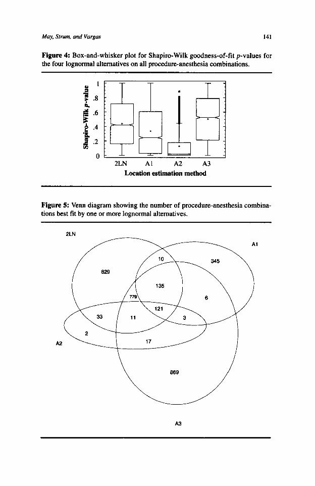
A Kruskal-Wallace test on the same data shows that there may be more to the story, though. The average ranks of the four alternatives are significantly different @- value is essentially zero), but a box-and-whisker plot, with the median notched, the mean marked with a plus sign and outliers indicated (displayed in Figure 4), appears to show that the behavior of the three-parameter lognormal using estimator A,, espe- cially, may be highly related to factors not accounted for in an overall analysis.

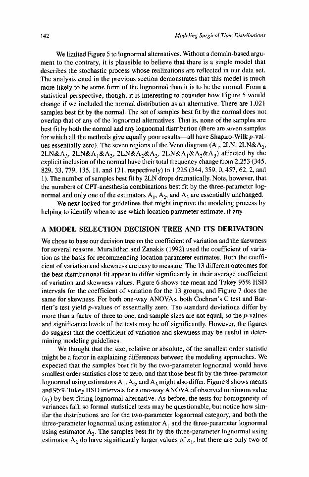
The Venn diagram in Figure 5 shows the frequency of the best fit by model- ing approach, where “modeling approach” is limited to the lognormal alternatives. The effect of including the normal distribution as an alternative is discussed in the next paragraph. Each region of Figure 5 shows the number of samples for which the alternative or group of alternatives gives the best goodness of fit. For example, 345 procedure-anesthesia combinations are best fit by the three-parameter lognor- mal using estimator A, alone; 121 are best fit by all four alternatives (the two- parameter lognormal, the three-parameter lognormal using estimator A,, the three- parameter lognormal using estimator A,, and the three-parameter lognormal using estimator A,); and 11 by the two-parameter lognormal, the three-parameter log- normal using estimator A,, and the three-parameter lognormal using estimator A,. Note that 2,045 times there is a unique best alternative, but only twice is it the three-parameter lognormal using estimator A,. Although the samples should be strictly bounded away from zero, 26% (829/3,160) of the time using the three- parameter lognormal with any of the three estimators yields a model strictly infe- rior to ignoring the location parameter entirely. The single best pure strategy is to use the three-parameter lognormal with estimator A,, but it only yields a “best” estimate 61% of the time and is almost indistinguishable from always ignoring the location parameter. Always using the three-parameter lognormal with estimator A, results in a best fit 1,941 out of 3,160 times as compared with ignoring the loca- tion parameter, which gives a best fit 1,918 out of 3,160 times.

May, Strum, and Vargas 141

Figure 4: Box-and-whisker plot for Shapiro-Wilk goodness-of-fit p-values for the four lognormal alternatives on all procedure-anesthesia combinations.

2LN A1 A2 A3 Location estimation method

Figure 5: Venn diagram showing the number of procedure-anesthesia combina- tions best fit by one or more lognormal alternatives.

A2

A3

142 Modeling Surgical Time Distributions

We limited Figure 5 to lognormal alternatives. Without a domain-based argu- ment to the contrary, it is plausible to believe that there is a single model that describes the stochastic process whose realizations are reflected in our data set. The analysis cited in the previous section demonstrates that this model is much more likely to be some form of the lognormal than it is to be the normal. From a statistical perspective, though, it is interesting to consider how Figure 5 would change if we included the normal distribution as an alternative. There are 1,021 samples best fit by the normal. The set of samples best fit by the normal does not overlap that of any of the lognormal alternatives. That is, none of the samples are best fit by both the normal and any lognormal distribution (there are seven samples for which all the methods give equally poor results-all have Shapiro-Wilk p-val- ues essentially zero). The seven regions of the Venn diagram (A,, 2LN, 2LN&A,, 2LN&A,, 2LN&A,&A,, 2LN&A,&A,, 2LN&A,&A,&A,) affected by the explicit inclusion of the normal have their total frequency change from 2,253 (345, 829,33,779, 135, 11, and 121, respectively) to 1,225 (344, 359,0,457,62,2, and 1). The number of samples best fit by 2LN drops dramatically. Note, however, that the numbers of CPT-anesthesia combinations best fit by the three-parameter log- normal and only one of the estimators A,, A,, and A, are essentially unchanged.

We next looked for guidelines that might improve the modeling process by helping to identify when to use which location parameter estimate, if any.

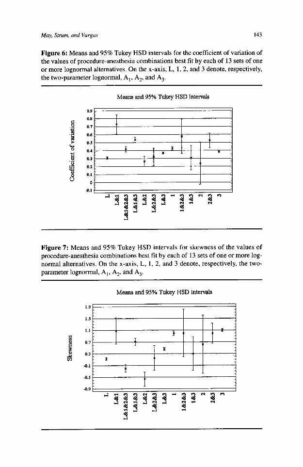
A MODEL SELECTION DECISION TREE AND ITS DERIVATION We chose to base our decision tree on the coefficient of variation and the skewness for several reasons. Muralidhar and Zanakis (1992) used the coefficient of varia- tion as the basis for recommending location parameter estimates. Both the coeffi- cient of variation and skewness are easy to measure. The 13 different outcomes for the best distributional fit appear to differ significantly in their average coefficient of variation and skewness values. Figure 6 shows the mean and Tukey 95% HSD intervals for the coefficient of variation for the 13 groups, and Figure 7 does the same for skewness. For both one-way ANOVAs, both Cochran’s C test and Bar- tlett’s test yield p-values of essentially zero. The standard deviations differ by more than a factor of three to one, and sample sizes are not equal, so the p-values and significance levels of the tests may be off significantly. However, the figures do suggest that the coefficient of variation and skewness may be useful in deter- mining modeling guidelines.

We thought that the size, relative or absolute, of the smallest order statistic might be a factor in explaining differences between the modeling approaches. We expected that the samples best fit by the two-parameter lognormal would have smallest order statistics close to zero, and that those best fit by the three-parameter lognormal using estimators A,, A,, and A, might also differ. Figure 8 shows means and 95% Tukey HSD intervals for a one-way ANOVA of observed minimum value (x,) by best fitting lognormal alternative. As before, the tests for homogeneity of variances fail, so formal statistical tests may be questionable, but notice how sim- ilar the distributions are for the two-parameter lognormal category, and both the three-parameter lognormal using estimator A, and the three-parameter lognormal using estimator A,. The samples best fit by the three-parameter lognormal using estimator A, do have significantly larger values of xl, but there are only two of

May, Strum, and Vargas 143

Figure 6: Means and 95% Tukey HSD intervals for the coefficient of variation of the values of procedure-anesthesia combinations best fit by each of 13 sets of one or more lognormal alternatives. On the x-axis, L, 1,2, and 3 denote, respectively, the two-parameter lognormal, A,, A,, and A,.

Means and 95% Tukey HSD Intervals

0.9 L

Figure 7: Means and 95% Tukey HSD intervals for skewness of the values of procedure-anesthesia combinations best fit by each of 13 sets of one or more log- normal alternatives. On the x-axis, L, 1, 2, and 3 denote, respectively, the two- parameter lognormal, A,, A,, and A,.

Means and 95% Tukey HSD Intervals

144 Modeling Surgical Time Distributions

Figure 8: Means and 95% Tukey HSD intervals for the smallest order statistic (in seconds) of the values of procedure-anesthesia combinations best fit by each of 13 sets of one or more lognormal alternatives. On the x-axis, L, 1, 2, and 3 denote, respectively, two-parameter lognormal, A,, A,, and A,.

Marma and 95% "ukey HSD Intad8

them. Redoing the analysis displayed in Figure 8, using xllmean instead of xl, did not separate further the three-parameter lognormal using estimator A, and the two- parameter lognormal, the two most significant contenders.

The Venn diagram in Figure 5 illustrates the difficulty in using a technique for extracting rules for selecting a modeling approach. If the sets of CPT-anesthe- sia combinations best fit by a particular alternative were disjoint, the task at this point would be to find functions that best separate those sets. The sets have con- siderable overlap. We applied two different methodologies, linear discriminant analysis (LDA) and a tree induction program (See5) (Rulequest Research, 1998). See5 is an improved version of C4.5 (Quinlan, 1993) and a descendant of ID3, a machine learning algorithm for discrete classification. See5 uses hyperplanes to define the boundaries between sets, but only chooses hyperplanes parallel to the coordinate axes. At each branch of the tree, it uses an entropy-based measure to identify a new dividing line for the region not yet classified.

Note that both LDA and See5 determine functions, on the basis of which dis- joint clusters may be separated. How do we deal with a situation such as ours, in which over 35% of the cases are actually best fit by at least two different alterna- tives? We considered two options. First, we used extraction techniques on the 2,045 data points for which only one alternative was best, and then evaluated the resulting rules on the entire data set. Second, we assigned each point for which multiple alternatives were optimal to all alternatives that best fit it, extracted rules, and then evaluated them on the entire data set. The second option expanded the data set to 4,666 cases.

The performance on the total data set of the four models derived from using the two classification methods and the two representations is shown in Table 7.

t? T

able

7:

Perf

orm

ance

of t

he f

ive

deci

sion

met

hods

on

the

com

plet

e da

ta se

t. C

ells

val

ues

are

num

ber

of i

nsta

nces

cor

rect

ly i

dent

ifie

d, a

nd

$ ro

w p

erce

ntag

e.

B s L

DA

on

LD

A on

Se

e5 o

n Se

e5 o

n Si

ngle

6;:

Bes

t Fitt

ing

Mod

el(s

) 2,

045

Cas

es

4,66

6 C

ases

2,

045

Cas

es

4,66

6 C

ases

Sk

ewne

ss R

ule

Tota

l E

ALA

pA3

3 (1

00)

3 (1

00)

3 (1

00)

3 (1

00)

3 (1

00)

3 (0

.09)

A

, 12

4 (3

5.94

) 99

(28.

70)

10

(2.9

0)

8 (2

.32)

0

(0)

345

(10.

92)

l(16

.67)

3

(50.

00)

3 (5

0.00

) 3

(50.

00)

3 (5

0.00

) 6

(0.1

9)

A2

0 (0

) 0

(0)

0 (0

) 0

(0)

0 (0

) 2

(0.0

6)

7 (4

1.18

) 8

(47.

06)

16 (9

4.12

) 14

(82.

35)

15 (8

8.24

) 17

(0

.54)

A3

33

2 (3

8.20

) 56

7 (6

5.25

) 8 1

5 (9

3.79

) 73

8 (8

4.93

) 80

7 (9

2.87

) 86

9 (2

7.50

) Tw

o-pa

ram

eter

logn

orm

al

540

(65.

14)

317

(38.

24)

552

(66.

59)

621

(74.

91)

556

(67.

07)

829

(26.

23)

Two-

para

met

er lo

gnor

mal

, A,

10

(100

) 10

(1

00)

0 (0

) 0

(0)

0 (0

) 10

(0

.32)

Tw

o-pa

ram

eter

logn

orm

al, A

,,A,,A

, 12

1 (1

00)

121

(100

) 12

1 (1

00)

121

(100

) 12

1 (1

00)

121

(3.8

3)

Two-

para

met

er lo

gnor

mal

, A, ,

A3

135

(100

) 99

(73.

33)

135

(100

) 13

5 (1

00)

135

(100

) 13

5 (4

.27)

Tw

o-pa

ram

eter

logn

orm

al, A

, 33

(1

00)

33

(100

) 33

(1

00)

33

(100

) 33

(1

00)

33

(100

) Tw

o-pa

ram

eter

logn

orm

al, A

,,A,

11

(100

) 10

(90.

91)

11

(100

) 11

(1

00)

11

(100

) 11

(0

.35)

Tw

o-pa

ram

eter

logn

orm

al, A

, 47

7 (6

1.23

) 53

1 (6

8.16

) 76

6 (9

8.33

) 77

9 (1

00)

779

(100

) 77

9 (2

4.65

) To

tal

1794

(56.

77)

1801

(56.

99)

2465

(78.

01)

2466

(78.

04)

2463

(77.

94)

3160

(1

00)

146 Modeling Surgical Time Distributions

The LDA classifiers correctly identify fewer of the model fits than do the corre- sponding See5 classifiers, but they are better at recognizing samples best fit by shift A,. The representation alternatives are to ignore samples for which more than one strategy is optimal, leaving 2,045 cases for a method to analyze, and to assign such samples to all optimal strategies, resulting in 4,666 cases. The performance of both LDA and See5 are almost identical using both representations. After manu- ally examining the patterns in the See5 classifiers, we found that a simple rule of using no shift if skewness 50.35 and A, if skewness > 0.35 does almost as well overall as the more complex rules constructed by See5. The performance of the single rule is given in the sixth column of Table 7.

CONCLUSIONS

Based on a census of surgical times that appear to be lognormally distributed, we found that what minimizes bias also maximizes goodness of fit 61% of the time. Although our data sets should, on conceptual grounds, be strictly bounded away from zero, a strategy of leaving the location parameter out of the model entirely does almost as well as choosing the location parameter so as to minimize bias. Decision rules based on the skewness and coefficient of variation of the data can be used to identify the correct alternative 78% of the time, but do not do any better than a single rule based on the skewness.

It is possible that the existing estimators for the location parameter are also the best when goodness of fit is the criterion of interest, if we could only find the proper way of identifying which one to use. Skewness and the coefficient of vari- ation do not appear to be adequate for that task; neither does the size of the smallest order statistic. The types of data for which the three-parameter lognormal using estimator A, is superior to the three-parameter lognormal using estimator A, are particularly elusive. As shown in Table 7, the See5 decision trees for the 2,045 and 4,666 case analyses correctly identify, respectively, 10 and 8 of the 345 procedure- anesthesia combinations best fit by the three-parameter lognormal using estimator A,. The single skewness rule, which is as accurate, overall, as the See5 decision trees, correctly identifies none of those combinations. It is also possible that an altogether different type of estimator should be used when goodness of fit is the criterion of interest. Because accurate data modeling is critical to our planning and reasoning systems, we welcome further work that would determine which, if either, of the above possibilities is correct [Received: October 24, 1996. Accepted: March 15, 19991.

REFERENCES

Barnoon, S., & Wolfe, H. (1968). Scheduling a multiple operating room system: A

Bashein, G., & Barna, C. (1985). A comprehensive computer system for anesthetic

Bratley, P., Fox, B. L., & Schrage, L. E. (1987). A guide to simulation (2nd ed.).

simulation approach. Health Services Research, 3(4), 272-285.

record retrieval. Anesthesia Analgesia, 64,425-43 1.

New York: Springer-Verlag.

May, Strum, and Vargas 147

D’Agostino, R. B. (1986). Tests for the normal distribution. In R. B. D’Agostino & M. A. Stephens (Eds.), Goodness-of@ techniques. New York: Marcel Dek- ker, Inc., 367-419.

Dannenbring, D. G. (1977). Procedures for estimating optimal solution values for large combinatorial problems. Management Science, 23, 1273-1283.

Dexter, F. (1996). Application of prediction levels to OR scheduling. AORN Jour- nal, 63(3), 1-8.

Dubey, S. D. (1967). Some percentile estimators for Weibull parameters. Techno- metrics, 9, 119-129.

Hancock, W. M., Walter, P. F., More, R. A., & Glick, N. D. (1988). Operating room scheduling data base analysis for scheduling. Journal of Medical Systems,

Kirschner, C. G., Burkett, R. C., Marcinowski, D., Kotowicz, G. M., Leoni, G., Malone, Y., O’Heron, M., O’Hara, K. E., Scholten, K. R., & Willard, D. M. (1995). Physicians ’ Current Procedural Terminology 1995, Chicago: Amer- ican Medical Association.

Muralidhar, K., & Zanakis, S. H. (1992). A simple minimum-bias percentile esti- mator of the location parameter for the gamma, Weibull, and log-normal dis- tributions. Decision Sciences, 23, 862-879.

Quinlan, J. R. (1993). C4.5: Programs for machine learning. San Mateo, CA: Morgan Kaufmann.

Robb, D. J., & Silver, E. A. (1996). Scheduling in a management context: Uncer- tain processing times and non-regular performance measures. Decision Sci- ences, 24(6), 1085-1106.

Rossiter, C. E., & Reynolds, J. A. (1963). Automatic monitoring of the time waited in out-patient departments. Medical Care, 1,218-225.

See5 (release 1.09) (1998). [Computer software]. St Ives, NSW, Australia: Rule- quest Research Pty Ltd.

12,397-409.

Jerrold H. May is a professor of decision sciences and artificial intelligence at the Katz Graduate School of Business, University of Pittsburgh, and is also the director of the Artificial Intelligence in Management Laboratory there. He has more than 60 refereed publications in a variety of outlets, ranging from management journals such as Operations Research and Information Systems Research to medical ones such as Anesthesiology and Journal of the American Medical Informatics Association. Professor May’s current work focuses on modeling, planning, and control problems, the solutions to which combine management science, statistical analysis, and artificial intelligence, particularly for operational tasks in health- related applications.

David P. Strum earned his M.D. degree from Dalhousie University, trained at the University of Toronto and the University of California, San Francisco, and is board certified in both critical care medicine and anesthesiology. Previously on the

148 Modeling Surgical Time Distributions

faculties at the University of Washington, University of Pittsburgh, and University of Arkansas. Dr. Strum is currently an associate professor of anesthesiology at Queen’s University, Ontario, Canada. Dr. Strum was also a visiting scholar at the Katz Graduate School of Business, University of Pittsburgh from 1996-97. He has published numerous papers in refereed journals such as Anesthesiology, JAMIA, Science, Anesthesia and Analgesia, and Decision Sciences. His research interests are in operations research and management for surgical services.

Luis G. Vargas is a professor of decision sciences and artificial intelligence at the Katz Graduate School of Business, University of Pittsburgh, and co-director of the AIM Laboratory. He has published over 40 publications in refereed journals such as Management Science, Operations Research, Anesthesiology, JAMIA, and EJOR, and three books on applications of the Analytic Hierarchy Process with Thomas L. Saaty. Professor Vargas’ current work focuses on the use of operations research and artificial intelligence methods in health care environments.