The genetic structure of recombinant inbred mice: High-resolution consensus maps for complex trait...

Deposited research articleThe genetic structure of recombinant inbred mice: High-resolution consensus maps for complex trait analysisRobert W Williams*†, Jing Gu*, Shuhua Qi* and Lu Lu*†

Address: *Center of Genomics and Bioinformatics, *Center for Neuroscience, †Department of Anatomy and Neurobiology, University ofTennessee Health Science Center, College of Medicine, Memphis, TN 38163, USA.

Correspondence: Robert W Williams. E-mail: [email protected]

http://genomebiology.com/2001/2/8/preprint/0007.1

com

ment

reviews

reports

deposited research

interactions

inform

ation

refereed research

.deposited research

AS A SERVICE TO THE RESEARCH COMMUNITY, GENOME BIOLOGY PROVIDES A 'PREPRINT' DEPOSITORY

TO WHICH ANY PRIMARY RESEARCH CAN BE SUBMITTED AND WHICH ALL INDIVIDUALS CAN ACCESS

FREE OF CHARGE. ANY ARTICLE CAN BE SUBMITTED BY AUTHORS, WHO HAVE SOLE RESPONSIBILITY FOR

THE ARTICLE'S CONTENT. THE ONLY SCREENING IS TO ENSURE RELEVANCE OF THE PREPRINT TO

GENOME BIOLOGY'S SCOPE AND TO AVOID ABUSIVE, LIBELLOUS OR INDECENT ARTICLES. ARTICLES IN THIS SECTION OF

THE JOURNAL HAVE NOT BEEN PEER REVIEWED. EACH PREPRINT HAS A PERMANENT URL, BY WHICH IT CAN BE CITED.

RESEARCH SUBMITTED TO THE PREPRINT DEPOSITORY MAY BE SIMULTANEOUSLY OR SUBSEQUENTLY SUBMITTED TO

GENOME BIOLOGY OR ANY OTHER PUBLICATION FOR PEER REVIEW; THE ONLY REQUIREMENT IS AN EXPLICIT CITATION

OF, AND LINK TO, THE PREPRINT IN ANY VERSION OF THE ARTICLE THAT IS EVENTUALLY PUBLISHED. IF POSSIBLE, GENOME

BIOLOGY WILL PROVIDE A RECIPROCAL LINK FROM THE PREPRINT TO THE PUBLISHED ARTICLE.

Posted: 18 July 2001

Genome Biology 2001, 2(8):preprint0007.1-0007.44

The electronic version of this article is the complete one and can befound online at http://genomebiology.com/2001/2/6/preprint/0006

© BioMed Central Ltd (Print ISSN 1465-6906; Online ISSN 1465-6914)

Received: 25 June 2001

This is the first version of this article to be made available publicly. This article has been submitted to Genome Biology for peer review.

This information has not been peer-reviewed. Responsibility for the findings rests solely with the author(s).

2 Genome Biology Deposited research (preprint)

Research

The genetic structure of recombinant inbred mice: High-resolution

consensus maps for complex trait analysis

Robert W Williams*†, Jing Gu*, Shuhua Qi* and Lu Lu*

†

Address: *Center of Genomics and Bioinformatics, *Center for Neuroscience, †Department of

Anatomy and Neurobiology, University of Tennessee Health Science Center, College of

Medicine, Memphis, TN 38163, USA

E-mail: [email protected]; [email protected]; [email protected]; [email protected]

Correspondence: Robert W Williams

All authors: TELE: (901) 448-7018, FAX (901) 448-7193

Running Title: Genetic structure of RI genomes


ABSTRACT

Background: Recombinant inbred (RI) strains of mice are an important resource used to map

and analyze complex traits. They have proved particularly effective in multidisciplinary genetic

studies. Widespread use of RI strains has been hampered by their modest numbers and by the

difficulty of combining results derived from different RI sets.

Results: We have increased the density of typed microsatellite markers 2- to 5-fold in each of

several major RI sets that share C57BL/6 as a parental strain (AXB, BXA, BXD, BXH, and

CXB). A common set of 490 markers was genotyped in just over 100 RI strains. Genotypes of

another ~1100 microsatellites were generated, collected, and error checked in one or more RI

sets. Consensus RI maps that integrate genotypes of ~1600 microsatellite loci were assembled.

The genomes of individual strains typically incorporate 45–55 recombination breakpoints. The

collected RI set—termed the BXN set—contains approximately 5000 breakpoints. The

distribution of recombinations approximates a Poisson distribution and distances between

breakpoints average about 0.5 cM. Locations of most breakpoints have been defined with a

precision of < 2cM. Genotypes deviate from Hardy-Weinberg equilibrium in only a small

number of intervals.

Conclusions: Consensus maps derived from RI strains conform almost precisely with theoretical

expectation and are close to the length predicted by the Haldane-Waddington equation (X3.6 for

a 2–3 cM interval between markers). Non-syntenic associations among different chromosomes

introduce predictable distortions in QTL data sets that can be partly corrected using two-locus

correlation matrices.

BACKGROUND

Recombinant inbred (RI) strains have been used extensively to map a wide range of Mendelian

and quantitative traits [1]. They offer compelling advantages for mapping complex genetic traits,

particularly those that have modest heritabilities. Each recombinant genome is replicated in the

form of an entire isogenic line [2-6] and variance associated with environmental factors and

technical errors can be suppressed to low levels. This elevates heritability and improves the

prospects of mapping underlying quantitative trait loci (QTLs). Recently, we have used RI

strains to map QTLs that generate variation in the architecture of the mouse CNS [7-14]. The


main advantage in this context is that the complex genetic and epigenetic correlations between

interconnected parts of the brain can be explored using complementary molecular,

developmental, structural, pharmacological, and behavioral techniques. Gene effects can also be

tested under a spectrum of environmental perturbations and experimental conditions. RI strains

can be exploited to expose gene-environment interactions and gene pleiotropy. These important

facets of genetics can only be explored with difficulty using conventional mapping populations

in which each genome is unique.

A third advantage of RI strains is that genotypes generated by different groups using a variety of

methods can be pooled to generate high-density linkage maps. As a result, loci that segregate in

RI sets can often be mapped with impressive precision without genotyping. This attribute was a

significant advantage before the advent of efficient and easy PCR genotyping methods [15].

Unfortunately, over the last decade databases of RI genotypes have accumulated many typing

errors. Each error expands distances between marker loci and degrades linkage, inevitably

blurring associations between genotypes and phenotypes and making it difficult to map traits,

whether they are Mendelian or quantitative in nature. The accumulation of false recombinations

has become extreme in common RI sets. For example, the map of Chr 1 in the complete BXD

data set (Mouse Genome Informatics Release 2.5:

www.informatics.jax.org/searches/riset_form.shtml) is based on 160 linked marker loci and is an

astonishing 1305 cM long. This map is approximately 12 times the length of an F2 map of Chr 1,

and just over 3 times the length expected of an RI map of Chr 1. The accumulation of typing

errors has led to efforts to reconstitute maps using curated subsets of markers for which

genotypes can be adequately and independently verified. Sampson and colleagues [16]

assembled maps for the AXB and BXA recombinant inbred strains that improved the utility of

this set. Similarly, Taylor and colleagues [17] assembled comparable high quality maps for the

complete set of 36 BXD strains that are based almost entirely on easily typed and verified

microsatellite markers.

Our study's aims complement this previous work. Our first aim has been to generate reliable

high-resolution genetic maps for each of five widely used sets of RI strains: AXB, BXA, BXD,

BXH, and CXB. These RI sets all share C57BL/6 alleles, and they can be assembled into a BXN

superset consisting of just over 100 lines. The introduction of the RIX cross by Threadgill and

colleagues (Threadgill DW, Manly KF, Williams, RW, personal comm) provides an impetus to

precisely define recombination breakpoints in RI strains. RIX progeny are isogenic F1 hybrids


made between pairs of RI strains and 5050 unique isogenic but non-inbred RIX genometypes can

be constructed from 101 RI strains. Selected subsets of this huge pool of recombinant F1

genomes can be made by crossing those RI strains with breakpoints in intervals thought to harbor

QTLs. These interval-specific RIX progeny are phenotyped and used to refine the genetic

analysis of complex traits. Knowing the precise location of breakpoints in RI lines also makes it

possible to map modifier loci of mutations by simply making a series of F1 crosses between

inbred carrier stock (for example a knockout carried on a C57BL/6 background) and fully typed

RI lines. These F1 crosses have a genetic structure similar to a conventional N2 backcross, but

they will not need to be genotyped and they have the major advantage that groups of isogenic

backcross progeny can be typed to obtain much more reliable scores.

Our second aim has been to describe the recombination characteristics of typical RI strains and

their chromosomes in a more theoretical context. We empirically tested the Haldane-Waddington

equation of map expansion in sib-mated RI strains. We also tested relatedness among RI lines,

and measured deviations from Hardy-Weinberg equilibrium associated with 10–30 years of

inbreeding, genetic drift, mutation, and selection.

Our third aim has been to help resolve a serious but unrecognized problem in QTL mapping that

arises from non-syntenic genetic correlations within mapping panels. Genetic correlations

between intervals on different chromosomes can be high in RI sets and this can result in spurious

results and false positive QTLs. We provide detailed correlation matrices that can be used to

detect and control for non-syntenic association.

RESULTS

The results are divided into two sections. The first summarizes the RI consensus map and

genotypes of individual strains. The second section considers the structure of the multiple

generation meiotic recombination maps of RI strains. We highlight the problem of non-syntenic

association that is a feature of these maps and we outline a solution to minimize the risk of type I

and type II error in QTL mapping studies.

RI consensus maps of mouse chromosomes

Mapping complex genetic traits involves matching strain distribution patterns (SDPs) of

genotypes with those of phenotypes. The utility of an RI set and the probability of successfully

mapping any heritable quantitative trait or novel Mendelian trait is therefore a function of the


number of well defined and correctly positioned SDPs of marker loci. We therefore concentrated

genotyping efforts on those intervals with comparatively low densities of fully typed

microsatellite markers or those intervals that harbored large numbers of recombinations between

neighboring markers. One goal in generating dense maps for each chromosome was to discover

and verify as many recombination breakpoints and SDPs as possible using available

microsatellite primer pairs. Ideally, in high density genetic maps the number of markers should

exceed the number of SDPs, and all recombination breakpoints in an set RI would be defined

with subcentimorgan precision. We have worked with more than 1600 microsatellite markers, a

number that is still insufficient to reach a subcentimorgan goal. However, the density of markers

on most chromosomes is sufficient to locate the majority of recombination breakpoints within ±2

cM.

Fewer than 25 common microsatellite markers had been typed on all major RI sets when we

began this work. This number has been increased to 490 common makers (Table 1). These

markers were used to assemble the consensus BXN maps—B for the C57BL/6 allele that all sets

have in common and N for the not-B6 parental allele that differ among the four RI sets (A/J in

AXB-BXA, DBA/2J in BXD, C3H/HeJ in BXH, and BALB/cByJ in CXB). The set of 490

shared markers are supported by an additional 1089 MIT markers that we or other groups have

typed in at least one RI set (Table 2). In the BXN database summarized in Table 1 any pair of RI

sets shares between 500 and 600 fully genotyped markers. The two largest RI sets, AXB-BXA

and BXD, have been typed at 591 common markers. The composite BXN maps are based on a

total of just under 1600 microsatellite makers and just over 100 RI strains (Tables 1 and 2).

Undiscovered recombinations and SDPs. The number of recombinations in RI sets still

significantly exceeds the number of SDPs that have been unequivocally defined. Based on

current marker density we estimate that we have defined from 37% (AXB/BXA) to 59% (CXB)

of the total set of SDPs (Table 3). The entire BXN set contains approximately 4800 known

recombination breakpoints (Tables 3 and 4). There are likely to be another 400 breakpoints that

we have not yet detected. To discover 623 (41%) of the 1492 SDPs in the BXD set required 936

selected markers. Recovering the majority of the remaining SDPs could require an additional

1000 to 1500 well placed marker loci. The density of informative microsatellite markers is not

yet dense enough to define many more SDPs in the BXN set, but once SNP and microsatellite

maps have been fully integrated into chromosome sequence databases, it will be straightforward

to generate additional markers and use these to define all 5000–6000 SDPs in the BXN set.


Error checking. To minimize genotyping errors we retyped many markers, particularly those

that were associated with unusually large numbers of recombination events. We were

particularly interested in minimizing the number of genotypes that appeared to be associated

with two closely located recombination events—what are sometime referred to as double

recombinant haplotypes. These haplotypes appear to be the result of two separate crossover

events, one of which is just proximal to a particular marker and the other of which is just distal to

the same marker. For example, the haplotype of a short chromosome interval, -B-B-B-N-B-B-B-,

is associated with two recombinations that flank the central marker with the N genotype. Because

of interference, the occurrence of two recombinations within 10 cM is highly improbable in an

F2 intercross, and consequently, double recombinants are often used as a measure of genotyping

error or incorrect marker order. However, in RI strains recombination events accumulate over

many generations, and two or more recombinations can therefore be extremely close to each

other and can produce true double recombinant haplotypes. It is therefore necessary to verify,

rather than discard, all apparent double recombinants in RI strains. We checked our own marker

genotypes and the majority of microsatellite markers typed by other investigators genotypes they

were associated with double recombination events in one of more RI strain. When two or more

strains contributed to double recombinants we usually retyped all strains. Approximately 150

double recombinant haplotypes (and 300 false recombinations) were eliminated in the process of

error checking. Our genotypes therefore differ from those of many microsatellites reported in

original publications and listed in the MGI release 2.5 (www.jax.org). In a few instances, our

revisions have generated new (but verified) double recombinant haplotypes.

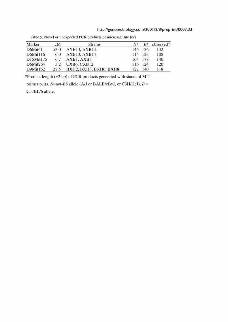
We discovered unexpected polymorphisms at several loci in a few lines and all were scored as

unknown (U) (Table 5). The clustering of aberrant products in AXB13 and AXB14 is consistent

with the common origin of these strains from a partly inbred progenitor line. However the

genotypes of the other three sets of strains (e.g., AXB1 and AXB3) are generally completely

independent.

PCR primer pairs in several intervals gave two bands consistent with a genuine heterozygous

haplotype. Heterozygous loci are rare among the fully inbred RI strains but they are fairly

common among new BXH strains that were genotyped at the tenth to 16 generation of

inbreeding. In scoring recombination frequency we treated all heterozygous loci and intervals as

if they had not been typed. Mutations in microsatellite loci may be responsible for some

heterozygosity [18].


Changed locus order. The order of loci of the BXN consensus maps generally conforms to that

of the chromosome committee reports (CCR) and the MIT-Whitehead genetic maps (Table 2). In

about 130 instances we have changed the order of loci over short intervals. For example,

D1Mit276 and D1Mit231 on proximal Chr 1 do not recombine in the MIT F2 cross, but in the

BXN set there is a single recombination between these markers in BXA11 that is most consistent

with a reversal of order relative to the CCR (compare the columns labeled CCRcM, MITcM, and

BXNcM in Table 2). The only non-trivial discrepancy was on proximal Chr 15. We reordered

approximately 32 loci on Chr 15 to improve linkage statistics. We have not attempted to

integrate the BXN data with numerous other mapping panels, and it is likely that original CCR

order will often be well supported by other large mapping panels or rapidly improving physical

maps. Full sequence data will soon resolve these minor inconsistencies.

Reassigned microsatellite loci. A number of microsatellite loci were reassigned to locations on

chromosomes other than those expected on the basis of their original assignments (Table 6).

Mapping data in one or more of the RI sets is consistent with a reassignment of 16 microsatellite

loci to different chromosomes. All of these reassignments are provisional, particularly those with

LOD scores of less than 10. In several cases, (e.g., D10Nds10) we have reassigned microsatellite

loci typed by other investigators that now are linked to new and firmly mapped markers. All

primers used to amplify these microsatellites (except D10Nds10) were resynthesizing to confirm

that they are identical to those originally specified by Dietrich and colleagues [19].

Individual maps are based on genotypes of as few as 37 markers (Chr X) to as many as 129

makers (Chr 1) per chromosome (Table 1). The mean separation between markers is

approximately 1 cM (0.95 cM using CCR maps as a reference and 0.87 cM using the RI maps

themselves). When the 577 markers that do not have unique SDPs are excluded from the

analysis, the average separation increases to 1.2 cM using CCR maps and 1.4 cM using the RI

data. Typical resolution of the BXN set for mapping a Mendelian trait is 1–2 cM. Approximately

90% the mouse genome is currently less than 2 cM from a typed microsatellite marker in the RI

set. The asymptotic resolution of the set of BXN strains given infinitely dense maps in which

every possible SDP has been characterized would average about 0.3–0.4 cM. There are currently

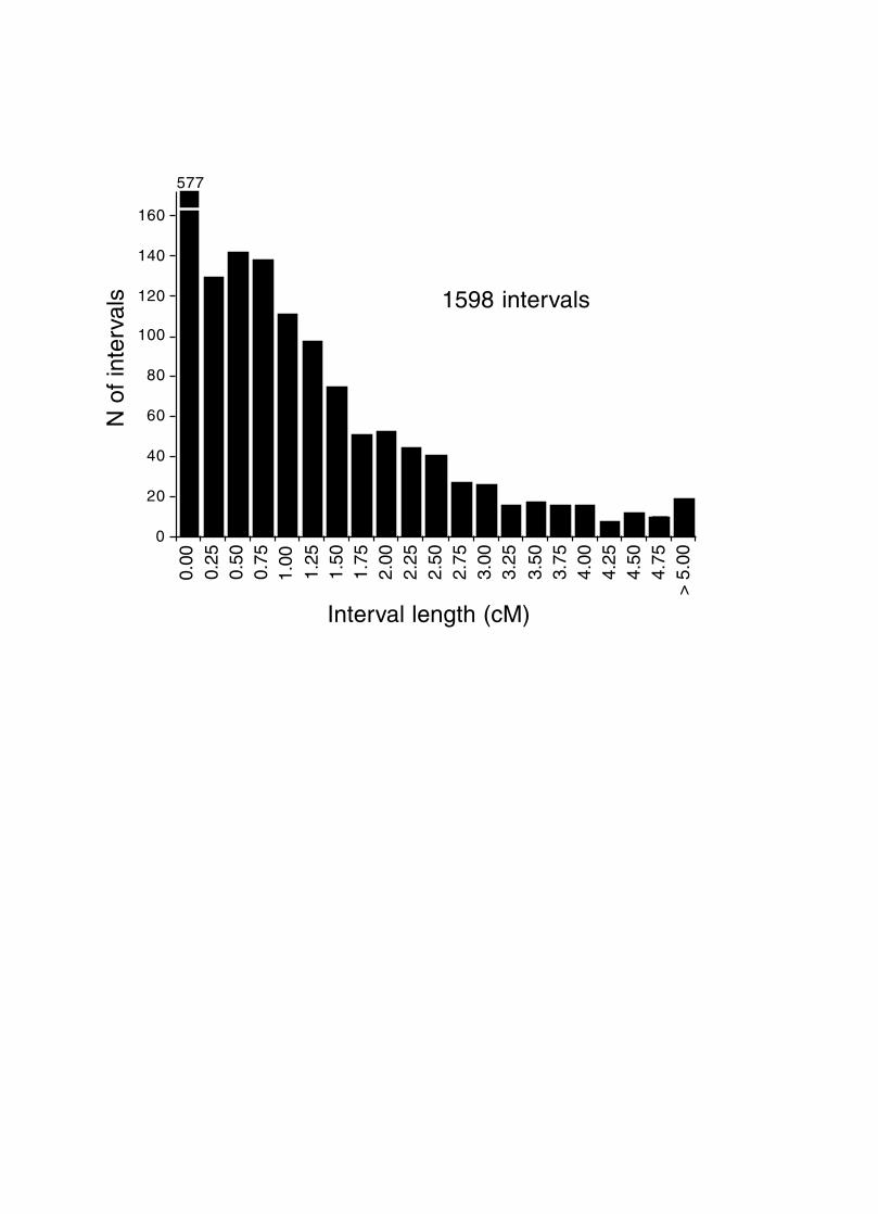
14 poorly typed regions. These regions are operationally defined as intervals of 5 to 12 cM

between adjacent markers (Fig. 1). The largest is on proximal Chr 2 between 9 and 21 cM (Table

2).


Strain independence. Several RI strains share common haplotypes and recombination

breakpoints. This non-independence of RI lines will distort genetic maps. To systematically

search for and eliminate partial duplicate RI lines we constructed a genotype similarity matrix for

all strains using the QTL analysis program Qgene [20]. An example of a small part of this matrix

is illustrated in Table 7 for the CXB set.

As already noted by Sampson et al. [16], three sets of AXB and BXA strains show high genetic

similarity, and genotypes of four strains should be excluded from most genome-wide mapping

panels. Phenotype data obtained from members of the three groups listed below should often be

collapsed and treated as a single strain.

1. BXA8 and BXA17: 99.8% genetic identity. Only two markers are known to be

polymorphic, D3Mit392 and D6Mit108. The polymorphism at D6Mit108 has been

verified using independent DNA samples from these two strains. BXA17 is actually a

direct derivative of BXA8 separated in 1996–1997 [16]. Any divergence in genotypes or

phenotypes is due to the recent generation and fixation of new mutations in these two

separately maintained lines.

2. AXB18, AXB19, and AXB20: 97% to 99% identity among any of the three pairs.

3. AXB13 and AXB14: 92% identity.

These three sets of strains were treated as three single strains when analyzing recombination

frequencies.

The mean allele similarity of the remaining strains averages almost precisely 50%. The

distribution of values is symmetrical about the mean (Fig. 2) with the great majority of strain

pairs falling in the range of 30% to 70% similarity. The highest remaining similarities within RI

sets are between BXD13 and BXD41 (74%), AXB6 and AXB17 (73%), BXHB2 and BXH9

(71%), AXB6 and AXB12 (70%), BXD28 and BXD33 (69%), BXD19 and BXD29 (68%), and

AXB11 and AXB14 (67%). These values are not significantly higher than the similarity scores

typically noted across RI sets.

Residual heterozygosity. In theory a set of 75,000 genotypes generated across the genome of

100 RI strains should detect only a single residual heterozygous loci at generation F55 of

inbreeding (Fig. 2, fine line; the inbreeding coefficient at F55 is 0.99998812). DNA from most

lines was extracted in the 1990s at F generations between F20 and F70 (see Methods and

Materials). We detected a total of 13 strains that were still heterozygous (BXA20 from D1Mit77


to D1Mit490; AXB21 from D2Mit102 to D2Mit420, AXB24 at D3Mit62, BXA23 at D5Mit95,

AXB3 and BXA16 at D12Mit167, BXA20 from D13Mit224 to D13Mit254; BXD31 at

D9Mit243, BXD34 at D7Mit281, BXD37 at D1Mit83; BXH12 at D1Mit417, BXH10 at

D12Mit167; CXB8 from D1Mit361 to D1Mit291). DNA samples were taken from single animals

of each strain and for this reason these estimates of residual heterozygosity underestimate the

total heterozygosity about twofold.

The central part of Chr 1 is interesting because it is heterozygous in three strains (BXD37,

BXH12, and BXA20). There is also an interval that is approximately 2.5-cM-long that is

apparently maintained in heterozygosity in AXB21 on Chr 2. Such maintenance should be

accompanied by reduced fecundity in this line if homozygotes are lethal or sublethal. This would

account for poor breeding performance. It is also possible the heterozygosity is the result of a

mutation, but if this were the case we would expect novel length polymorphisms, and the two

alleles were usually the expected parental lengths.

Structure of RI genomes

RI mean map lengths. The mean frequency of recombinations, CRI,between two linked markers

in an RI strain generated by breeding siblings is approximately 4c/(1+6c) where c is the

recombination fraction per meiosis [21, 22]. An infinitely dense RI map should average four

times the length of the conventional one-generation F2 map. Most expansion is achieved in the

first few generations, and by F7 the genetic map is approximately three times the length of an F2

map (Fig. 3). The expectation is that a map based on loci that are spaced at intervals of 1 cM (c =

0.01 in an intercross) will be expanded approximately 3.66-fold. Similarly, a low-density map

based on markers that are spaced at 16 cM intervals will be expanded 2-fold. F2 and N2 maps

generated using uniform typing procedures typically have a cumulative length of 1300 to 1400

cM. Five conventional crosses that we generated (four F2s and one N2, each genotyped at 91 to

148 loci) average 1320 ± 50 (SEM) cM in length. In comparison the fully error-checked native

BXN map is approximately 3.6- to 3.7-fold longer, or a total of 4786 cM. The expansion

averages approximately 3.4-fold when the comparison is made to the CCR consensus maps (Fig.

4, Table 4). The expansion between common proximal and distal markers ranges from 2.8 in Chr

5 to 3.8 in Chr 12. In general, the expansion estimate of 3.6-fold agrees well with the Haldane-

Waddington expectation given a mean spacing between neighboring markers of 2–3 cM. The X


chromosome only recombines with half the frequency of the autosomes, and for this reason its

expansion is only 1.8 fold.

Comparison to other maps. The summed length of all chromosomes is approximately 1413 cM

when values are converted from RI recombination frequencies to those expected of typical

single-generation meiotic maps. The corresponding CCR maps have a cumulative length of 1494

cM between the same markers. The MIT-Whitehead microsatellite maps have a cumulative

length of approximately 1384 cM. The agreement is excellent.

Recombination density per RI strain. Individual RI strains contain an average of 47

recombinations with a range that typically lies between 40 and 60 (Fig. 4). The 13 CXB strains

are associated with a total of 671 recombinations, an average of 52 per strain. The BXD strains

are associated with approximately 1500 recombinations, an average of about 42 per strain, and

approximately one recombination per centimorgan on a standard genetic map (Tables 3 and 4).

There is considerable variation in the total load of recombinations and map expansion per strain:

from a low expansion of 2.24 in BXD40 (the RI strain with the fewest recombinations) to a high

of about 6 in BXH6 (Fig. 4). These estimates are systematically deflated by a failure to discover

recombinations in sparsely mapped regions (regions where the recombination fraction c is as

high as 0.1) but are inflated by residual typing errors and errors of marker order.

Recombination density per chromosome. Single chromosomes in RI strains accumulate as

many as 12 recombinations, but across the whole set the recombination density averages about

2.4 recombinations per chromosome. The mean extends from 3.47 recombinations for Chr 1 to

1.88 for Chr 9. A Poisson model fits the distribution of recombination events per chromosome

reasonably well and most chromosomes have insignificant �2 values. High �2 for individual

chromosomes are generally due to a small number of apparently highly recombinant

chromosomes in particular strains. These highly recombinant chromosomes are probably

associated with residual typing errors or incorrect marker order.

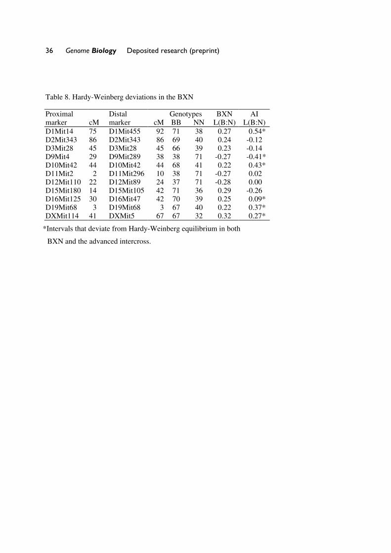
Segregation distortion and Hardy-Weinberg equilibrium expectation of allele fixation in RI

sets. In the absence of selection, approximately 50% of the strains should have inherited B alleles

at each marker. A chi-square statistic can be used to assess whether the segregation ratio of a

particular marker differs significantly from expectation. Only the 11 intervals listed in Table 8

have chi-squared values that are significant at the 0.01 level. Eight of 11 intervals are biased in

favor of B alleles. This is most extreme on chromosomes 1, 15, and X, where there are about


twice as many strains with B alleles as N alleles. The opposite pattern is seen on chromosomes 9,

11, and 12. Given the large number of comparisons, many instances of segregation distortion

may be type I statistical errors. In collaboration with the Mammalian Genotyping Service

(http://research.marshfieldclinic.org/genetics/Genotyping_Service/mgsver2.htm), we recently

genotyped a tenth-generation advanced intercross between C57BL/6J and DBA/2J (genotype

data for this cross are available at www.nervenet.org. It is therefore possible to test whether

similar segregation distortion patterns are present in this related multigeneration cross. The short

answer is that the segregation distortions noted in the BXN RI strains are replicated in 6 of 11

intervals. The correlation between ratios of alleles (logarithm of B:N) in these intervals was

positive (r = 0.41). It is therefore likely that several of the intervals marked in Table 8 with

asterisks represent regions that harbor loci that affect fitness.

Non-syntenic associations. One important issue in using RI strains for mapping complex traits

is that intervals on different chromosomes can become tightly associated in a statistical sense.

This non-syntenic association can arise either as a result of random fixation of alleles on

different chromosomes during the production of RI strains or can arise as a result of selection for

particular combinations of alleles on different chromosomes. Similar patterns of non-syntenic

disequilibrium are common in recently admixed human populations and often lead to false

positive signals when mapping complex traits. In mice even a modest selection coefficient

expressed over 10 generations of inbreeding can generate positive and negative non-syntenic

disequilibrium throughout the genome. For example, if the combination of B alleles on distal Chr

1 and B alleles on proximal Chr 19 is favorable for fitness, then these two intervals will

effectively be in linkage disequilibrium in the final RI set. Disequilibrium can also take on the

form of strong negative correlations and B alleles may be associated strongly with the group of N

alleles.

We searched for marked deviations from the expected Hardy-Weinberg two-locus equilibrium

by making a series of large correlation matrices of SDPs of marker pairs. This was done for the

entire BXN set and for the constituent RI sets. Table 9 summarizes the most extreme positive

and negative correlations among the composite set of 102 independent BXN RI strains. Whether

due to chance fixation, selection and epistasis, non-syntenic associations of the sort illustrated in

Table 9 are a major source of both false positive and negative results in using RI sets for

mapping. It is helpful to examine the correlation matrix once a set of QTLs has been


provisionally mapped to see how summed effects of single or multiple QTLs might produce

spurious QTLs in regions not actually associated with trait variance.

Controlling for non-syntenic association. Non-syntenic associations among loci and intervals

can be computed in advance of QTL mapping. It is therefore possible to statistically control for

genetic correlations. For example, in Table 9 the genotypes at marker D1Mit83 can be partly

predicted by genotypes at markers on Chr 7 and Chr 10. If the genotype at D1Mit83 is treated

statistically as a dependent variable and markers on Chr 7 and 10 are used as predictors, then one

can compute the residual genotype, or independent contribution of D1Mit83 and any other

marker or interval to the quantitative trait. Unlike composite interval mapping, the set of

controlled loci will vary for each marker and interval. This procedure will reduce Type I error,

but there will be a regional loss of power. The correction will introduce blind spots in a genome

scan. In extreme cases (usually small RI sets), intervals that can be perfectly predicted by small

numbers of other non-syntenic intervals will effectively be eliminated from a mapping study and

QTLs in those intervals will be missed. For this reason, it is essential to perform each genome-

wide scan both with and without control for non-syntenic association. Single QTLs may

occasionally be assigned to two or more physically unlinked intervals.

DISCUSSION

Synopsis

Recombinant inbred strains are currently one of the best genetic resources for exploring

phenotypic variance modulated by complex mixtures of genetic and environmental factors.

Having a renewable resource of genetically defined genomes is a tremendous advantage in

exploring gene pleiotropy, genetic correlation, epistasic interactions, and reaction norms.

However, their modest numbers have impeded the widespread adoption of RI strains by

mammalian geneticists. To improve the utility and power of complex trait analysis and to

provide a better basis for community-based QTL mapping we have increased marker density in

several of the major sets of RI lines and have merged data from over 100 mouse RI strains using

a framework based on 490 shared markers. Approximately 1000 unique strain distribution

patterns (SDPs)—an average of about one per 1.5 cM were defined and mapped in the collected

set. Three to four times as many SDPs remain to be discovered in the BXN set. At the current

marker density the cumulative RI map is about 5000 cM in length, roughly 3.6 times the length

of standard intercross or backcross maps. When corrected using the Haldane-Waddington


equation, the RI maps have a cumulative length of 1400 cM, perfectly consistent with those of

chromosome committee reports.

Making better RI resources

The usefulness of RI strains for mapping is largely a function of the number of known

recombination breakpoints that they harbor. By genotyping and selectively breeding the most

highly recombinant F2 animals it should be possible to generate RI strain sets that significantly

exceed the map expansion predicted by the Haldane-Waddington equation; an equation that

assumes random mating of sibs. A 6x to 8x map should be attainable, particularly if

recombinations are tracked during the inbreeding process (Fig 3). Recombination density could

be further increased by starting RI strains using either advanced intercross progeny or

heterogeneous stock (Fig. 3).

Use of the BXN set

Most mapping software applications used by mouse geneticists are adapted for diallele crosses

of various types. The BXN data set has therefore been formatted in a way that collapses all non-

B6 alleles into a single N class so that the collected set of just over 100 strains can be used

without complication with software such a Map Manger QTX [23]. There are obvious

limitations that follow from the collapse of all non-B alleles (A/J, DBA/2J, C3H/HeJ, and

BALB/cByJ) into a single category. Geneticists using the BXN set should begin virtually all

studies of non-Mendelian traits by mapping with the individual component RI sets (AXB-BXA,

BXD, BXH, and CXB) to maximize power and to detect possible levels of allele effects.

Because the BXN set includes 490 common marker loci and a consistent alignment and

integration of the component RI maps, it is now much easier to combine linkage likelihood

ratios from the component RI sets. A simple method based on Fisher’s method is described by

Williams and colleagues [8] in a study that pooled data from BXD and BXH sets. More

sophisticated methods to automatically extract and combine linkage statistics from the multi-

allele BXN sets will require modification of mapping application programs. Pooling data will

require judicious and well justified statistical procedures. Combining data across the BXN sets

can easily degrade a linkage analysis. The statistical exploration of different combinations of RI

sets provides new degrees of freedom that may generate false positive results, but that may also

generate interesting hypotheses regarding QTL action.

The BXN map could be refined further by interpolating genotypes of other markers and genes

that have been mapped independently by many investigators in single RI sets. For example, our


BXD database includes only microsatellite loci and excludes hundreds of potentially informative

polymorphic loci, many in interesting genes. We regret having to employ this procrustean

approach, but because of the difficulty of verifying genotypes and because numerous loci

introduce improbable double-recombinant haplotypes, we have used exclusive criteria to ensure

high quality maps. Those investigators interested in recovering some of these lost data should

certainly refer to the comprehensive lists of genotypes maintained by the Mouse Genome

Database (www.informatics.jax.org/searches/riset_form.shtml). However, genotypes of any

marker or gene that introduce new double-recombinants into the BXN map should be regarded

with a high level of suspicion.

Maximizing RI resources by the RIX method

The most common criticisms leveled at QTL mapping using RI strains is that the small number

of lines limits both precision and power and that only those QTLs with very large effects can be

detected reliably. The BXN set provides a partial solution to this problem by expanding the set

of RI strains that can be treated statistically as a complex cross. A second objection to using RI

strains to map traits is that fully inbred strains may provide unrepresentative trait values

precisely because they are inbred. The abnormal genetic architecture of inbred strains and the

fixation of multiple alleles that affect fitness will almost inevitably produce unusual pleiotropic

and epistatic effects on a range of complex traits.

There is a surprisingly simple solution to these problems; namely to map QTLs using a set of F1

intercrosses between RI strains ([24], Threadgill DW, Williams RW and Manly KF personal

comm). QTLs mapped using RI sets can be quickly verified and positionally refined by

generating sets of RI F1 intercrosses (RIX) and RI backcrosses among individual RI lines with

recombinations in critical QTL intervals. The RIX method has already proved to be a highly

effective way to extract QTLs from the tiny set of 13 CXB strains [24]. The 13 inbred lines can

be converted to as many as156 F1 lines. This greatly increases the power to detect QTLs in the

presence of strong genetic, parental, and developmental background noise and simultaneously

exposed gene dominance deviations to help refine QTL effect and position. The BXN opens up a

huge RIX domain for analysis. Approximately 88 of the BXN RI strains are now available from

the Jackson Laboratory, and these strains can be crossed to generate about 88x87/2 (3828)

genetically unique recombinant inbred intercross progeny (RIX progeny) with breakpoints in

precisely defined intervals. Each one of these F1s can be made in reciprocal pairs to assess the


role of parental effects (e.g., a BXD1 mother crossed to a AXB2 father, or vice versa). Like RI

strains many isogenic individuals can be typed to reduce the non-genetic variance.

F1 and F2 crosses among any of the RI strains can also be used to verify the original

assignment. Once QTLs have been mapped to candidate intervals, the subset of strains with

recombinations within those intervals become an important resource for confirming and refining

QTL location [25]. This is especially the case if one exploits the RIX method. For example, if a

QTL maps between 10 and 25 cM on Chr 1 in the BXD set (that is between D1Mit430 and

D1Mit375), and if B alleles in this interval are associated with high phenotypes, then the cross of

BXD15 by BXD20 may be particularly informative because the F1 hybrid is an obligatory B

homozygote on a short interval between 15 cM and 17 cM and is also an obligatory D

homozygote proximal to 13 cM and distal to 18 cM. A set of isogenic F1 RIX progeny made by

crossing several RI lines with recombinations in a critical interval can be used to refine the

probable position of a QTL. Map Manger QTX has now been updated to automatically generate

the genotypes of the RIX progeny produced by a one-generation cross of RI parents

(http://mapmgr.roswellpark.org/mmQTX.html). Given this huge sample of unique F1 genomes,

even modest quantitative differences between C57BL/6 and other strains should be readily

mapped (or confirmed) using the BXN and RIX mapping.

Information content of RI strain sets

Despite the accumulation of genotypes in RI strains, these genetic resources have often not been

typed with sufficient density to accurately define the frequency and positions of recombination

breakpoints. For example, in the venerable set of 13 CXB strains only 11 unique SDPs had been

assigned to Chr 1 prior to our work. With a more dense map of Chr 1 that is now based on

approximately 60 markers we have recovered at total of 38 recombinations on Chr 1—

approximately 3 recombinations per strain. The positions of these recombinations has been

defined with a precision that ranges from 0.5 to 6.0 cM intervals (2.3 cM average) as referenced

to standard CCR maps. Twenty-one of the 38 SDPs are represented by one or more of the marker

genotype, but at least 17 SDPs remain to be defined and these SDPs unfortunately cannot be

predicted unambiguously. For example, if two adjacent markers P and D have genotypes

BBCCC and CCCCC, then there must be at least one unrecovered SDP between P and D.

Unfortunately, until we actually type markers in the P-D interval, we do not know whether the

intercalated SDP is BCCCC or CBCCC. To discover the missing SDP may require considerable

effort especially if available polymorphic markers on the P-D interval have been exhausted. All


unrecovered SDPs lower the information content of an RI set. Their absence can significantly

reduce linkage of both Mendelian and quantitative traits that are unlucky enough to be controlled

by loci in the intervals with ambiguous SDPs.

How dense should a marker map be to define more than 90% of the total number of SDPs? With

862 markers, we were able to define approximately 60% of all likely SDPs among the 13 CXB

strains. However, in the collected set of BXN RI strains, only 23% of the estimated 5000

possible SDP have be confidently defined with MIT microsatellites. We can estimate the density

of the marker map that would be necessary to define 95% of the SDPs. For example, for the

BXD set if one assumes a random and independent distribution of breakpoints across strains and

a random distribution of markers, it would take a map with about 2,700 markers to define 95%

of the 1,536 SDPs.

Power and precision of 100 RI strains

A set of 100 conventional RI strains will have twice the genetic variance as a matched set of 100

F2 progeny and four times that of 100 backcross progeny. This increased genetic variance

comes at some cost: 100 F2 animals represent 200 meioses and contain almost 200 unique

haplotypes per chromosome (the non-recombinant chromosomes reduce this number somewhat).

RI strains are fully inbred and 100 lines represent almost 100 unique haplotypes per

chromosome. A set of 100 RI strains therefore has approximately twice the load of

recombinations as 100 F2s. For a semidominant Mendelian trait or marker, 100 RI strains

therefore provide twice the precision of 100 F2 progeny and four times the precision of 100 N2

progeny. When both genetic variance and recombination load are considered together, a set of

100 RI strains should be approximately four times as effective (precise) for mapping complex

traits as an F2, and 8 times as effective as a backcross. This estimate assumes that only a single

RI animal is sampled per line; a strategy that is appropriate for mapping marker loci and other

Mendelian loci. The gain for mapping quantitative trait will be greater and will depend strongly

on the heritability and to a lesser extent on the degree of dominance at each locus. Belknap [3]

has compared the relative power of RI strains and F2 intercrosses under several models and

assuming different levels of heritability. For morphometric traits such as brain weight, with

narrow sense heritabilities of around 0.5, 100 RI strains will provide a level of precision and

power that is conservatively equivalent to that of 600–1000 F2 intercross progeny. The

advantage shifts further in favor of RI strains for traits with lower heritability.


BXN and sequencing efforts

Five of the widely used sets of RI strains that we have typed and analyzed share C57BL/6 as a

parental strain. The genome of C57BL/6J is currently being sequenced as part of a public effort

[26] and for this reason, the utility of the BXN set for converting QTLs to strong candidate genes

will increase significantly in the next few years [27]. It will become far easier to generate

complete lists of positional candidate genes and then to obtain data on gene and protein

expression patterns. The two other major strains incorporated into the BXN set—A/J and

DBA/2J—are also being sequence by Celera Genomics, and in principle, it will be possible to

compare sequences of these three major strains to generate lists of possible allelic variants in

positional candidate genes. The recent cloning of the Sac QTL, a locus controlling sugar and

saccharin preference on distal Chr 4, provides a fine example of the increased power of QTL

analysis. This QTL was initially mapped using 20 BXD stains [28, 29]. In the absence of high-

resolution mapping, but with astute analysis of human and mouse sequence data, Sac has been

identified almost simultaneously by several groups as the T1R3 receptor gene [30-34]. In a few

years, the cloning of Sac will probably be no more of a special exception than the cloning of

huntingtin was in the early 1990s [35].

MATERIALS AND METHODS

Strains and DNA

Genomic DNA from most recombinant inbred and parental strains was purchased from the

Jackson Laboratory (www.jax.org). DNA was obtained from 40 of 41 AXB and BXA strains and

35 of 36 BXD strains, 13 CXB strains, and 12 BXH strains—100 strains total. For visual clarity

in this paper we have dropped hyphens and substrain designations from RI strain names. For

example, strain BXD-1/Ty is referred to as BXD1. Databases and web-accessible data tables at

www.nervenet.org also use this simplified nomenclature.

All DNA from the Jackson Laboratory Mouse DNA Resource was extracted from individual

male mice. The RI animals that we genotyped were, with a few exceptions, the progeny of more

than 20 serial matings between siblings. Data on the particular generation that we used for

genotyping and the current generation of RI animals are listed in one of several web accessible

tables that accompany this publication (www.nervenet.org/papers/bxn.html). DNA from seven

new BXH strains generated by Dr. Linda Siracusa (Thomas Jefferson Medical College,


Philadelphia) was extracted from the spleen using a high salt procedure [36]. The new BXH

strains were generated by crossing C57BL/6J-c2J/c2J

albino males with C3H/HeJ females and their

production and genotyping will be described in detail elsewhere (L Siracusa and RW Williams,

personal comm). Three of the new BXH albino strains are no longer available (C2, D1, and E2).

We genotyped 107 of RI strains. Several sets of strains share haplotypes (Table 10). We deleted

redundant strains (AXB18, ABX20 and BXA17).

Strains BXHD1, BXHE1, BXHE2 were backcrossed to C57BL/6J for one generation before sib

matings were begun. There is therefore a pronounced increase in the number chromosomal

segments inherited from C57BL/6J. These N2-derived RI strains were dropped from most

aspects of the analysis of RI genome structure. BXD41 has been extinct for several years and

was never complete inbred. Although we have DNA for this strain our sample is from a F12

generation male. We did not genotype BXD41 in this study.

We refer to the collected RI set as the BXN set because each of the strains includes C57BL/6 (B6

or B) as one of the parental strains—the common substrain C57BL/6J in the case of AXB, BXA,

BXD, and BXH; and the substrain C57BL/6By in the case of CXB. The other parental strain in

the BXN set is not B6-derived: A/J in both AXB and BXA sets, DBA/2J in BXD, C3H/HeJ in

BXH, and BALB/cBy in CXB.

PCR

Microsatellite loci distributed across all autosomes and the X chromosome were typed using a

modified version of the protocol of Love and colleagues [37] and Dietrich and colleagues [19]

described in detail at www.nervenet.org/papers/pcr.html. A total of 1773 primer pairs (MapPairs)

that selectively amplify polymorphic MIT microsatellite loci were purchased from Research

Genetics (www.resgen.com). Each 10 �l PCR reaction mixture contained 1X PCR buffer, 1.92

mM MgCl2, 0.25 units of Taq DNA polymerase, 0.2 mM of each deoxynucleotide, 132 nM of the

primers, and 50 ng of genomic DNA. Reactions were set up using a 96-channel pipetting station.

A loading dye (60% sucrose, 1.0 mM cresol red) was added to the reaction before the PCR [38].

PCRs were carried out in 96-well microtiter plates. We used a high-stringency touchdown

protocol in which the annealing temperature was lowered progressively from 60 °C to 50 °C in 2

°C steps over the first 6 cycles [39]. After 30 cycles, PCR products were run on cooled 2.5%

Metaphor agarose gels (FMC Inc., Rockland ME), stained with ethidium bromide, and

photographed. Gel photographs were scored and directly entered into relational database files.


Eighteen primer pairs were resynthesized at our request by Research Genetics using the original

sequence data (Whitehead/MIT SSLP Release 8) to verify that our chromosome reassignments of

microsatellite loci were not due to the use of incorrect primer sequences.

Common Markers

When we began this work fewer than 25 MIT markers had been typed on each of the four major

RI sets. We were able to increase to 489 markers. We relied on these loci to assemble consensus

RI maps. The additional 986 MIT markers were typed by us and other groups in at least one set

of RI strains. The BXN genotype database includes 1578 markers. Any pair of RI sets share

between 500 and 600 fully genotyped markers. For example, the two largest RI sets—AXB/BXA

and BXD—have been typed at 591 common microsatellite markers.

Databases

Relational database files were assembled from the 1998–2000 chromosome committee reports,

the Portable Dictionary of the Mouse Genome [40] and the MIT/Whitehead SSLP database

Release 8. These files contain a summary of information on chromosomal positions of 6332 MIT

microsatellite markers and information on an additional 15000 genes and markers. We have

included Nuffield Department of Surgery (Nds) microsatellite markers for which primer

sequences are available. Additional databases devoted to each RI set were assembled from text

files downloaded from the Mouse Genome Database (www.jax.org). New and corrected

genotypes were entered directly into these files.

Additional data

Additional data files available with the online version of this article include Excel, FileMaker

Pro, Map Manager QTX, and text files (Informatics Center fore Mouse Neurogenetics

[http://www.nervenet.org/papers/bxn.html]).

Acknowledgements

This research project was support by a Human Brain Project/Neuroinformatics program project

(Informatics Center for Mouse Neurogenetics) funded jointly by the National Institute of Mental

Health, National Institute on Drug Abuse, and the National Science Foundation (P20-MH

62009). The authors thank Dr. Xiyun Peng for her assistance in genotyping CXB and BXH mice.

The authors thank Research Genetics Inc. (Invitrogen) and Ms. Felisha Scruggs for

resynthesizing 18 MapPairs for us. We thank Susan Deveau of the Jackson Laboratory DNA


Resource for information on the generation numbers of RI DNA samples. We thank Drs. David

Threadgill, Gary Churchill, and Kenneth Manly for comments on this paper .

REFERENCES

1. Taylor BA: Recombinant inbred strains. In (Lyon ML, Searle AG, eds) Genetic variants and

strains of the laboratory mouse 2nd Ed Oxford UP, Oxford. pp 773–796, 1989.

2. Bailey DW: Strategic uses of recombinant inbred and congenic strains in behavior genetics

research. In Genetic research strategies for psychogiology and psychiatry. Gershon ES,

Matthysse S, Breakefield XO, Ciaranello ED, eds. Plenum NY pp 189–198, 1981.

3. Belknap JK: Effect of within-strain sample size on QTL detection and mapping using

recombinant inbred strains of mice. Behav Genet 1998, 28:29–38.

4. Crabbe JC, Wahlsten D, Dudek BC: Genetics of mouse behavior: interactions with laboratory

environment. Science 1999, 284:1670–1672.

5. Toth LA, Williams RW: A quantitative genetic analysis of slow-wave sleep in influenza-

infected CXB recombinant inbred mice. Behav Genet 1999, 29:339-348.

6. Hain HS, Crabbe JC, Bergeson SE, Belknap JK: Cocaine-induced seizure thresholds:

quantitative trait loci detection and mapping in two populations derived from the C57BL/6

and DBA/2 mouse strains. J Pharmacol Exp Ther 2000, 293:180–187.

7. Williams RW: Neuroscience meets quantitative genetics: Using morphometric data to map

genes that modulate CNS architecture. In: Morrison J, Hof P (eds) Short course in

quantitative neuroanatomy. Society of Neuroscience, Washington DC, pp 66–78, 1998.

<http://www.nervenet.org/papers/shortcouerse98.html>

8. Williams RW, Strom RC, Goldowitz D: Natural variation in neuron number in mice is linked

to a major quantitative trait locus on Chr 11. J Neurosci 1998a, 18:138–146.

<http://www.nervenet.org/papers/nnc1.pdf>

9. Strom RC, Williams RW Cell production and cell death in the generation of variation in

neuron number. J Neurosci 1998, 18:9948–9953.

<http://www.nervenet.org/papers/strom&wiliams98.pdf>


10. Williams RW: Mapping genes that modulate mouse brain development: a quantitative

genetic approach. In: Mouse brain development. (Goffinet A, Rakic P, eds), pp 21–49.

Berlin: Springer, 2000. <http://www.nervenet.org/papers/brainrev99.html>

11. Williams RW, Airey DC, Kulkarni A, Zhou G, Lu L: Genetic dissection of the olfactory bulb

of mice: QTLs on chromosomes 4, 6, 11, and 17 modulate bulb size. Behav Genet 2001,

31:61-77. <http://www.nervenet.org/papers/ob/ob2000.html>

12. Lu L, Airey DC, Williams RW: Complex trait analysis of the hippocampus: Mapping and

biometric analysis of two novel gene loci with specific effects on hippocampal structure in

mice. J Neurosci 2001, 21:3503–3514. <http://www.nervenet.org/papers/hipp2000.html>

13. Airey DC, Lu L, Williams RW: Genetic control of the mouse cerebellum: localization of

quantitative trait loci modulating size and architecture. J Neurosci 2001, 21 (in press).

<http://www.nervenet.org/papers/cerebellum2000.html>

14. Rosen GD, Williams RW: Complex trait analysis of the mouse striatum: independent QTLs

modulate volume and neuron number. BMC Neurosci 2001, 2:5.

<http://www.biomedcentral.com/1471-2202/2/5>

15. Weber JL, Broman KW: Genotyping for human whole-genome scans: past, present, and

future. Adv Genet 2001, 42:77–96.

16. Sampson SB, Higgins DC, Elliot RW, Taylor BA, Lueders KK, Koza RA, Paigen B: An

edited linkage map for the AXB and BXA recombinant inbred mouse strains. Mamm Gen

1998, 9:688–694.

17. Taylor BA, Wnek C, Kotlus BS, Roemer N, MacTaggart T, Phillips SJ: Genotyping new

BXD recombinant inbred mouse strains and comparison of BXD and consensus maps.

Mamm Gen 1999, 10:335–348.

18. Jeffreys AJ, Wilson V, Kelly R, Taylor BA, Bulfield G: Mouse DNA “fingerprints”:

Analysis of chromosome localization and germ-line stability of hypervariable loci in

recombinant inbred strains. Nuclei Acids Res 1987, 15:2823–2836.

19. Dietrich WF, Katz H, Lincoln SE: A genetic map of the mouse suitable for typing in

intraspecific crosses. Genetics 1992, 131:423–447.


20. Nelson JC: QGENE: software for maker-based genomics analysis and breeding. Molec

Breeding 1997, 3:239–245. <http://www.qgene.com>

21. Haldane JBS, Waddington CH: Inbreeding and linkage. Genetics 1931, 16:357–374.

22. Lynch M, Walsh B: Genetics and analysis of quantitative traits. Sinauer Associates, Inc.

Sunderland, MA. 1998.

23. Manly KF, Olson JM: Overview of QTL mapping software and introduction to map manager

QT. Mamm Gen 1999, 10:327–334. see <http://mapmgr.roswellpark.org/mmQTX.html>.

24. Williams RW, Threadgill DW, Airey DC, Gu J, Lu L: RIX Mapping: A demonstration using

CXB RIX hybrids to map QTLs modulating brain weight in mice. Soc Neurosci Abstr 2001,

27 (in press).

25. Darvasi A: Experimental strategies for the genetic dissection of complex traits in animals.

Nat Genet 1998, 18:19–24.

26. Marshall E: Celera assembles mouse genome; public labs plan new strategy. Science 2001,

292:822–823.

27. Belknap JK, Crabbe JC, Phillips TJ, Hitzemann R, Buck KJ, Williams RW: Quantitative trait

loci and genome-wide mutagenesis: two phenotype-driven approaches to the dissection of

complex murine traits. Behav Genet 2001, 31:5–15.

<http://www.nervenet.org/papers/belknap2001.html>.

28. Belknap JK, Crabbe JC, Plomin R, McClearn GE, Sampson KE, O'Toole LA, Gora-Maslak

G: Single-locus control of saccharin intake in BXD/Ty recombinant inbred (RI) mice: some

methodological implications for RI strain analysis. Behav Genet 1992, 22:81-100.

29. Phillips TJ, Crabbe JC, Metten P, Belknap JK: Localization of genes affecting alcohol

drinking in mice. Alcohol Clin Exp Res 1994. 18:931–941.

30. Li X, Inoue M, Reed DR, Huque T, Puchalski RB, Tordoff MG, Ninomiya Y, Beauchamp

GK, Bachmanov AA: High-resolution genetic mapping of the saccharin preference locus

(Sac) and the putative sweet taste receptor (T1R1) gene (Gpr70) to mouse distal

Chromosome 4. Mamm Gen 2001, 12:13-16.


31. Montmayeur JP, Liberles SD, Matsunami H, Buck LB: A candidate taste receptor gene near

a sweet taste locus. Nat Neurosci 2001, 4:492–498.

32. Max M, Shanker YG, Huang L, Rong M, Liu Z, Campagne F, Weinstein H, Damak S,

Margolskee RF: Tas1r3, encoding a new candidate taste receptor, is allelic to the sweet

responsiveness locus Sac. Nat Genet 2001, 28:58–63.

33. Sainz E, Korley JN, Battey JF, Sullivan SL: Identification of a novel member of the T1R

family of putative taste receptors. J Neurochem 2001, 77:896–903.

34. Kitagawa M, Kusakabe Y, Miura H, Ninomiya Y, Hino A: Molecular genetic identification

of a candidate receptor gene for sweet taste. Biochem Biophys Res Commun 2001, 283:236-

242.

35. Bates GP, MacDonald ME, Baxendale S, Sedlacek Z, Youngman S, Romano D, Whaley WL,

Allitto BA, Poustka A, Gusella JF, et al.: A yeast artificial chromosome telomere clone

spanning a possible location of the Huntington disease gene. Am J Hum Genet 1990, 46:762-

775.

36. Laird PW, Zijderveld A, Linders K, Rudnicki M, Jaenisch R, Berns A: Simplified

mammalian DNA isolation procedure. Nucleic Acids Res 1991, 19:4293.

37. Love JM, Knight AM, McAleer MA, Todd JA: Towards construction of a high resolution

map of the mouse genome using PCR-analyzed microsatellites. Nucleic Acids Res 1990,

18:4123–4130.

38. Routman E, Cheverud J: A rapid method of scoring simple sequence repeat polymorphisms

with agarose gel electrophoresis. Mamm Gen 1994, 5:187–188.

39. Don RH, Cox PT, Wainwright BJ, Baker K, Mattick JS: "Touchdown" PCR to circumvent

spurious priming during gene amplification. Nucleic Acids Res 1991, 19:4008.

40. Williams RW: The Portable Dictionary of the Mouse Genome: a personal database for gene

mapping and molecular biology. Mamm Gen 1994, 5:372-375.


FIGURE LEGENDS

Figure 1. Histogram of interval length in centimorgan between neighboring microsatellite

markers in the BXN set.

Figure 2. Genetic similarity of RI strains. The percentage of identical genotypes was computed

for all two-way combinations of 108 RI strains. Those pairs of strains for which the

percentage of shared genotypes was greater than 75% (see text) were flagged and one

member of the pair was eliminated from the BXN set.

Figure 3. Progressive expansion of RI genetic maps during inbreeding. The middle series of

points (red) that start at generation 2 shows the addition of map length—and the

proportional increase in the numbers of recombination breakpoints—relative to a

standard one meiotic generation F2 map. For example, at generation 7, approximately 2

map lengths have been added to the initial map. By F24 the total RI map is almost

precisely 4 times as long as a standard F2 map. This same addition characterizes other

diallele crosses that start near Hardy-Weinberg equilibrium, including advanced

intercrosses. A two-strain G8 advanced intercross with a 6000 cM map length would

ultimately produce a G8 RI set with map length of 6000 + 3x1400 cM = 10200 cM. The

upper series of points (blue) illustrate the accumulation in map length in a four-strain

intercross at Hardy-Weinberg equilibrium at generation 0. This cross will gain up to

3.75 map equivalents. The lowest set of point is the inbreeding coefficient at each

generation. For a tabulation of these data and methods for calculating two- and four-

strain expansion values see www.nervenet.org/papersBXN.html.

Figure 4. Mean expansion of the genetic map in RI strains. The average is approximately 3.7 for

100 independent RI lines. The X axis can also be considered the mean number of

recombinations per 100 cM in different RI strains. The X axis can be transformed into

the total number of recombinations per strain by multiplying by the genetic length of

the mouse genome in morgans (approximately 14 morgans; 2.25x = 31.5

recombinations/strain, 3.00x = 42 recombinations/strain, 4.0xx = 56 recombinations per

strain; and 6.00x = 84 recombinations per strain).

Figure 5. Density of recombinations for all autosomes compared to a Poisson model. We scored

the number of recombinations for each of 2072 chromosomes (all strains; Chr X

excluded). The mean number is 2.43 recombination breakpoints per chromosome. The


particular distribution assumes all 19 autosomes have a length of about 70 cM and this

simplification accounts for the high �2 (125, P <<0.001, 10 df). Two hundred and fifty

non-recombinant chromosomes were observed but only 182 were expected. There are

also significantly more chromosomes with an apparent excess of recombinations. These

deviations are of course expected because short chromosomes (<70 cM) will contribute

more non-recombinants and long chromosomes (>70 cM) will contribute more highly

recombinant chromosomes than predicted by the model.


Table 1. Number of marker per chromosome*

Chr 1 2 3 4 5 6 7 8 9 10 11 12 13 14 15 16 17 18 19 X AXB/BXA 80 68 54 53 46 56 70 43 50 46 61 44 52 36 34 35 49 26 39 24 BXD 84 68 45 58 46 58 67 44 55 32 66 39 32 39 41 34 46 32 32 20 BXH 58 49 37 44 38 38 53 41 50 28 44 33 33 31 45 30 37 28 30 21 CXB 62 50 46 49 44 49 72 49 51 30 55 42 41 38 34 32 36 32 32 22 common BXN

36 34 28 32 27 28 29 32 39 17 27 18 21 18 13 15 22 17 23 13

total BXN 129 104 80 83 76 93 107 69 75 65 115 75 71 65 90 68 70 53 53 37

*Table 1 summarizes the number of microsatellite markers for which we generated or collected genotypes for each set of RI strains on each chromosome. In the case of the AXB-BXA strains we pooled our genotypes with those generated by Sampson and colleagues (1998). Our new BXD data were pooled with genotypes of Taylor and colleagues (1999), and CXB genotypes were pooled with the genotypes of Panoutsakopoulou and colleagues (1997). All data were eventually transferred to Map Manager QT and QTX. Both individual RI databases and the composite BXN database are available as text files formatted for used with Map Manager QTX files at www.nervenet.org/papers/BXN.html. The text files are compatible with Windows and Macintosh versions of Map Manager QTX and can be imported into a text editor or spreadsheet program.


Table 2. The BXN map of the mouse genome*


��


*The full table 2 is available online at www.nervenet.org/papers/bxn.html in several formats (graphic, text, and Map Manager QTX). Column definitions from left to right: Chr: chromosome assignment based on BXN data set. Our assignments differ in a number of cases from those of the Chromosome Committees Reports. Locus: an abbreviated version of the locus symbol. To improve legibility we have truncated D1MitNN to D1M NN. CCR cM: the position of the locus given in the most recent chromosome committee reports (2000 or 2001), MIT: the position of the locus given in databases at the Whitehead Institute, BXN: The position computed from the current RI data set adjusted for map expansion, UTM: whole genome position in morgans with a 5 cM buffer (0.05 M) between chromosomes. This UTM column can be used to construct whole-genome LOD score plots. Opening the GIF version of this file in Photoshop requires approximately 100 MB of RAM.


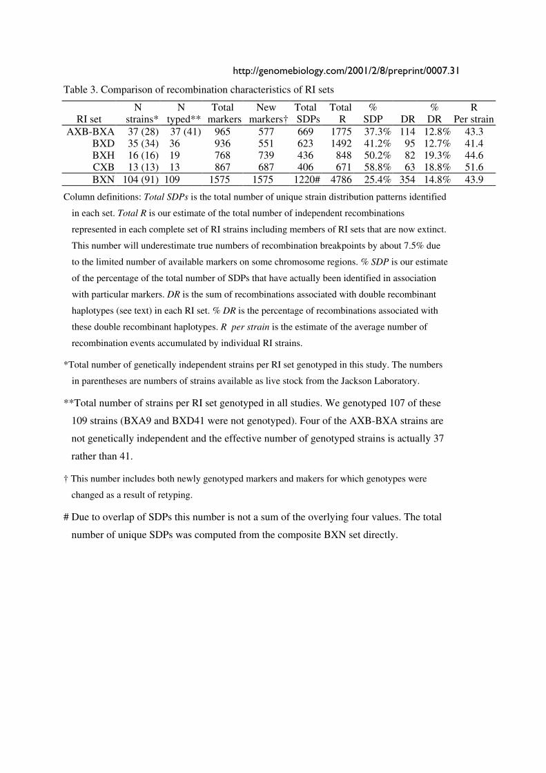
Table 3. Comparison of recombination characteristics of RI sets

N N Total New Total Total % % R RI set strains* typed** markers markers† SDPs R SDP DR DR Per strain

AXB-BXA 37 (28) 37 (41) 965 577 669 1775 37.3% 114 12.8% 43.3 BXD 35 (34) 36 936 551 623 1492 41.2% 95 12.7% 41.4 BXH 16 (16) 19 768 739 436 848 50.2% 82 19.3% 44.6 CXB 13 (13) 13 867 687 406 671 58.8% 63 18.8% 51.6 BXN 104 (91) 109 1575 1575 1220# 4786 25.4% 354 14.8% 43.9

Column definitions: Total SDPs is the total number of unique strain distribution patterns identified

in each set. Total R is our estimate of the total number of independent recombinations

represented in each complete set of RI strains including members of RI sets that are now extinct.

This number will underestimate true numbers of recombination breakpoints by about 7.5% due

to the limited number of available markers on some chromosome regions. % SDP is our estimate

of the percentage of the total number of SDPs that have actually been identified in association

with particular markers. DR is the sum of recombinations associated with double recombinant

haplotypes (see text) in each RI set. % DR is the percentage of recombinations associated with

these double recombinant haplotypes. R per strain is the estimate of the average number of

recombination events accumulated by individual RI strains.

*Total number of genetically independent strains per RI set genotyped in this study. The numbers

in parentheses are numbers of strains available as live stock from the Jackson Laboratory.

**Total number of strains per RI set genotyped in all studies. We genotyped 107 of these

109 strains (BXA9 and BXD41 were not genotyped). Four of the AXB-BXA strains are

not genetically independent and the effective number of genotyped strains is actually 37

rather than 41.

† This number includes both newly genotyped markers and makers for which genotypes were

changed as a result of retyping.

# Due to overlap of SDPs this number is not a sum of the overlying four values. The total

number of unique SDPs was computed from the composite BXN set directly.


Table 4. Recombinations per chromosome

Chr 1 2 3 4 5 6 7 8 9 10 11 12 13 14 15 16 17 18 19 X AXB/BXA 132 128 109 101 117 87 98 75 75 103 96 82 84 70 75 88 82 58 61 54 BXD 111 128 79 88 87 89 89 65 62 52 88 78 65 48 60 68 68 71 58 38 BXH 65 57 46 65 40 40 37 48 27 29 61 33 41 42 48 42 31 36 36 24 CXB 36 44 41 47 25 36 37 39 29 47 37 32 30 29 31 23 30 34 29 15 BXN 344 357 275 301 269 252 261 227 193 231 282 225 220 189 214 221 211 199 123 131 BXN cM* 344 357 275 301 269 252 261 227 193 231 282 225 220 189 214 221 211 199 123 131 CCR cM* 104 108 86 83 94 74 72 74 64 68 77 59 71 63 60 68 56 56 56 72 Expansion 3.3 3.3 3.2 3.6 2.9 3.4 3.6 3.1 3.0 3.4 3.7 3.8 3.1 3.0 3.6 3.3 3.8 3.6 2.2 1.8

*The distance in centimorgans between the most proximal and the most distal markers on each

chromosome. The mean number of strains typed at each marker is approximately 100 and thus

distances in centimorgans match the actual number of recombination events per chromosome. In

the case of the CCR maps we have truncated map lengths to match the most proximal and distal

markers genotyped in the BXN set.


Table 5. Novel or unexpected PCR products of microsatellite loci

Marker cM Strains N* B* observed* D6Mit61 53.0 AXB13, AXB14 146 136 142 D6Mit116 6.0 AXB13, AXB14 114 123 108 D15Mit175 6.7 AXB1, AXB3 164 178 140 D6Mit264 3.2 CXB6, CXB12 116 124 120 D9Mit162 28.5 BXH2, BXH3, BXH6, BXH8 122 140 118

*Product length (±2 bp) of PCR products generated with standard MIT

primer pairs. N=not-B6 allele (A/J or BALB/cByJ, or C3H/HeJ), B =

C57BL/6 allele.


Table 6. Loci mapped to unexpected chromosomes

Symbol New Chr cM LOD Linked to cM Sets D12Mit63 1 13.5 22.9 D1Mit169 14.0 BXN D15Mit139 3 84.9 32.3 D3Mit116 84.9 BXN D1Mit167 5 0.5 3.9 D5Mit346 0.5 CXB D7Mit284 6 42.0 3.9 D6Mit230 43.0 CXB D12Mit38 7 49.5 29.7 D7Mit38 49.8 BXN D10Nds10 8 44.6 7.5 D8Mit266 44.5 BXD D10Mit198 9 28.6 26.3 D9Mit4 29.0 BXN D8Mit18 11 56.0 3.9 D11Mit98 58.0 CXB D13Mit217 12 11.5 10.0 D12Mit106 12.0 AXB-BXA D1Mit464 12 13.0 32.2 D12Mit136 13.0 BXD, BXH, CXB D1Mit163 13 48.0 3.9 D13Mit107 3.0 CXB D18Mit128 14 46.9 5.8 D14Mit265 48.0 BXD D15Mit19 17 3.5 16.8 D17Mit267 3.0 BXN D14Mit207 19 21.0 7.2 D19Mit13 20.0 BXD, BXH D4Mit50 19 55.5 21.1 D19Mit6 55.7 AXB-BXA D6Mit324 x 26.5 28.3 DxMit1 27.0 BXN


Table 7. Sample of the strain similarity matrix*

strain CXB13 CXB12 CXB11 CXB10 CXB9 CXB8 CXB7 CXB6 CXB5 CXB4 CXB3 CXB2 CXB12 0.55 CXB11 0.44 0.42 CXB10 0.57 0.53 0.40 CXB9 0.35 0.47 0.53 0.50 CXB8 0.52 0.54 0.59 0.51 0.50 CXB7 0.53 0.52 0.53 0.43 0.46 0.67 CXB6 0.53 0.54 0.50 0.49 0.45 0.49 0.53 CXB5 0.51 0.37 0.53 0.47 0.43 0.47 0.46 0.50 CXB4 0.51 0.61 0.52 0.52 0.43 0.49 0.48 0.54 0.48 CXB3 0.47 0.46 0.52 0.51 0.49 0.53 0.49 0.45 0.51 0.49 CXB2 0.58 0.53 0.51 0.40 0.54 0.53 0.52 0.45 0.56 0.45 0.48 CXB1 0.48 0.44 0.51 0.48 0.51 0.42 0.53 0.39 0.43 0.50 0.47 0.43

*The fraction of identical genotypes was computed for all two-way combinations of 109 RI

strains. Those pairs of strains for which the percentage of shared genotypes was greater than

75% were flagged and one member of the pair was eliminated from the BXN set. Corresponding

matrices for AXB-BXA, BXD, BXH and the complete BXN matrix are available online at

www.nervenet.org/papers/bxn.html in text format.


Table 8. Hardy-Weinberg deviations in the BXN�

Proximal Distal Genotypes BXN AI marker cM marker cM BB NN L(B:N) L(B:N) D1Mit14 75 D1Mit455 92 71 38 0.27 0.54* D2Mit343 86 D2Mit343 86 69 40 0.24 -0.12 D3Mit28 45 D3Mit28 45 66 39 0.23 -0.14 D9Mit4 29 D9Mit289 38 38 71 -0.27 -0.41* D10Mit42 44 D10Mit42 44 68 41 0.22 0.43* D11Mit2 2 D11Mit296 10 38 71 -0.27 0.02 D12Mit110 22 D12Mit89 24 37 71 -0.28 0.00 D15Mit180 14 D15Mit105 42 71 36 0.29 -0.26 D16Mit125 30 D16Mit47 42 70 39 0.25 0.09* D19Mit68 3 D19Mit68 3 67 40 0.22 0.37* DXMit114 41 DXMit5 67 67 32 0.32 0.27*

*Intervals that deviate from Hardy-Weinberg equilibrium in both

BXN and the advanced intercross.


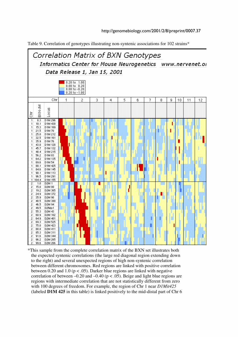
Table 9. Correlation of genotypes illustrating non-syntenic associations for 102 strains*

�

*This sample from the complete correlation matrix of the BXN set illustrates both the expected syntenic correlations (the large red diagonal region extending down to the right) and several unexpected regions of high non-syntenic correlation between different chromosomes. Red regions are linked with positive correlation between 0.20 and 1.0 (p < .05). Darker blue regions are linked with negative correlation of between –0.20 and –0.40 (p < .05). Beige and light blue regions are regions with intermediate correlation that are not statistically different from zero with 100 degrees of freedom. For example, the region of Chr 1 near D1Mit425 (labeled D1M 425 in this table) is linked positively to the mid-distal part of Chr 6


and negatively to proximal Chr 7. The full table 9 is available online in several formats at www.nervenet.org/papers/bxn.html.�


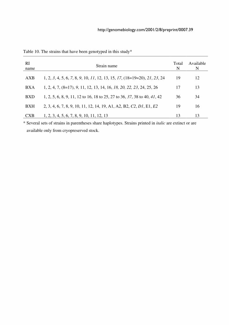
Table 10. The strains that have been genotyped in this study*

RI name

Strain name Total N

Available N

AXB 1, 2, 3, 4, 5, 6, 7, 8, 9, 10, 11, 12, 13, 15, 17, (18=19=20), 21, 23, 24 19 12

BXA 1, 2, 4, 7, (8=17), 9, 11, 12, 13, 14, 16, 18, 20, 22, 23, 24, 25, 26 17 13

BXD 1, 2, 5, 6, 8, 9, 11, 12 to 16, 18 to 25, 27 to 36, 37, 38 to 40, 41, 42 36 34

BXH 2, 3, 4, 6, 7, 8, 9, 10, 11, 12, 14, 19, A1, A2, B2, C2, D1, E1, E2 19 16

CXB 1, 2, 3, 4, 5, 6, 7, 8, 9, 10, 11, 12, 13 13 13

* Several sets of strains in parentheses share haplotypes. Strains printed in italic are extinct or are

available only from cryopreserved stock.

577

0

20

40

60

80

100

120

140

1600.

25

0.75

1.25

1.75

2.25

2.75

3.25

3.75

4.25

4.75

Interval length (cM)

1598 intervals

17

N o

f int

erva

ls

0.50

1.00

1.50

2.00

2.50

3.00

3.50

4.00

4.50

> 5

.00

0.00

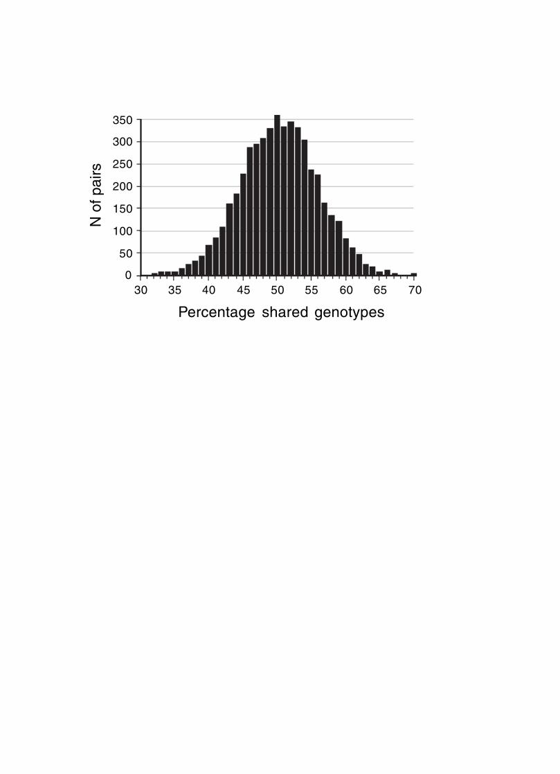
350

300

250

200

150

100

50

030 35 40 45 50 55 60 65 70

N o

f pai

rs

Percentage shared genotypes

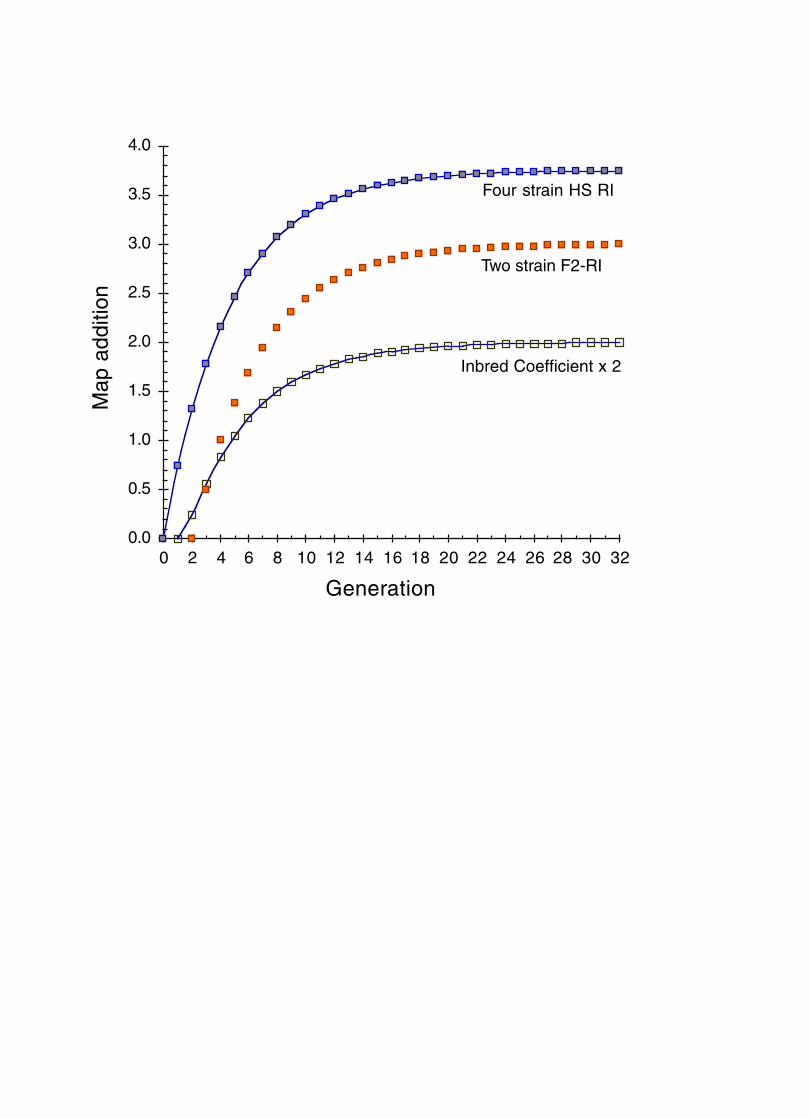
0.0

0.5

1.0

1.5

2.0

2.5

3.0

3.5

4.0

0 2 4 6 8 10 12 14 16 18 20 22 24 26 28 30 32

Generation

Two strain F2-RI

Four strain HS RI

Inbred Coefficient x 2

Map

add

ition

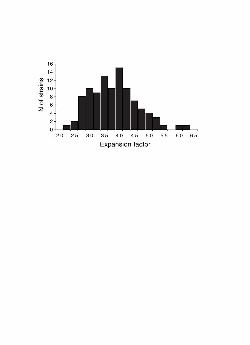
0

2

4

6

8

10

12

14

16

2.0 2.5 3.0 3.5 4.0 4.5 5.0 5.5 6.0

Expansion factor

N o

f str

ains

6.5

0

100

200

300

400

500

600

0 1 2 3 4 5 6 7 8 9 10

RealPoisson

Recombinations per Chromosome

N o

f Chr

omos

ome

The genetic structure of recombinant inbred mice: High-resolution consensus maps for complex trait...

Documents

Transcript of The genetic structure of recombinant inbred mice: High-resolution consensus maps for complex trait...