This article appeared in a journal published by Elsevier. The attachedcopy is furnished to the author for internal non-commercial researchand education use, including for instruction at the authors institution

and sharing with colleagues.

Other uses, including reproduction and distribution, or selling orlicensing copies, or posting to personal, institutional or third party

websites are prohibited.

In most cases authors are permitted to post their version of thearticle (e.g. in Word or Tex form) to their personal website orinstitutional repository. Authors requiring further information

regarding Elsevier’s archiving and manuscript policies areencouraged to visit:

http://www.elsevier.com/authorsrights

Author's personal copy

Computational Statistics and Data Analysis 69 (2014) 67–80

Contents lists available at ScienceDirect

Computational Statistics and Data Analysis

journal homepage: www.elsevier.com/locate/csda

The gamma-normal distribution: Properties and applications

Ayman Alzaatreh a, Felix Famoye b,∗, Carl Lee b

a Department of Mathematics & Statistics, Austin Peay State University, Clarksville, TN 37044, United Statesb Department of Mathematics, Central Michigan University, Mount Pleasant, MI 48859, United States

a r t i c l e i n f o

Article history:Received 7 December 2012Received in revised form 24 July 2013Accepted 24 July 2013Available online 3 August 2013

Keywords:T–X distributionsHazard functionMomentsEstimation

a b s t r a c t

In this paper, someproperties of gamma-X family are discussed and amember of the family,the gamma-normal distribution, is studied in detail. The limiting behaviors, moments,mean deviations, dispersion, and Shannon entropy for the gamma-normal distribution areprovided. Bounds for the non-central moments are obtained. The method of maximumlikelihood estimation is proposed for estimating the parameters of the gamma-normaldistribution. Two real data sets are used to illustrate the applications of the gamma-normaldistribution.

© 2013 Elsevier B.V. All rights reserved.

1. Introduction

There are several methods to generate continuous distributions. Many of these methods are discussed in the book byJohnson et al. (1994, Chapter 12). Since the publication of the book, newmethods continue to appear in the literature. Eugeneet al. (2002) introduced the beta-generated class of distributions and pointed out that the distributions of order statistics arespecial cases of beta-generated distributions. Jones (2004) studied some properties of beta-generated distributions. Manybeta-generated distributions have been studied (e.g., Famoye et al. (2004, 2005), Nadarajah and Kotz (2006), Akinsete et al.(2008), Barreto-Souza et al. (2010), and Alshawarbeh et al. (2012)). Themethod leading to beta-generated distributions wasextended by using a generalized beta distribution as the generator (Jones, 2009; Cordeiro and de Castro, 2011). Ferreira andSteel (2006) used inverse probability integral transformation method to generate skewed distributions, which include theskewed normal family introduced by Azzalini (1985, 2005) as a special class. Recently, Alzaatreh et al. (2013b) developeda new method to generate family of distributions and called it the T–X family of distributions. For a review of methods forgenerating univariate continuous distributions, onemay refer to Lee et al. (2013). This article has two purposes. First, we takeT as a gamma random variable, X as any continuous random variable and study some general properties of the gamma-Xfamily. Second, we study in detail the gamma-normal distribution, which is a member of the gamma-X family.

Let F(x) be the cumulative distribution function (CDF) of any random variable X and r(t) be the probability densityfunction (PDF) of a random variable T defined on [0,∞). The CDF of the T–X family of distributions defined by Alzaatrehet al. (2013b) is given by

G(x) =

− log(1−F(x))

0r(t)dt. (1.1)

∗ Corresponding author. Tel.: +1 989 774 5497; fax: +1 989 774 2414.E-mail address: felix.famoye@cmich.edu (F. Famoye).

0167-9473/$ – see front matter© 2013 Elsevier B.V. All rights reserved.http://dx.doi.org/10.1016/j.csda.2013.07.035

Author's personal copy

68 A. Alzaatreh et al. / Computational Statistics and Data Analysis 69 (2014) 67–80

Alzaatreh et al. (2013b) named the family of distributions defined in (1.1) the ‘Transformed-Transformer’ family (or T–Xfamily). When X is a continuous random variable, the probability density function of the T–X family is

g(x) =f (x)

1 − F(x)r (− log (1 − F(x))) = h(x) r (H(x)) . (1.2)

Thus, the family of distributions defined in (1.2) can be viewed as a family of distributions arising from hazard functions. Ifa random variable T follows the gamma distribution with parameters α and β , r(t) = (βα Γ (α))−1 tα−1e−t/β , t ≥ 0. Thedefinition in (1.2) leads to the gamma-X family with the PDF

g(x) =1

Γ (α)βαf (x) (− log (1 − F(x)))α−1 (1 − F(x))1/β−1 . (1.3)

The CDF of the gamma-X distribution in (1.3) can be written as

G(x) =γ {α,− log(1 − F(x))/β}

Γ (α), (1.4)

where γ (α, t) = t0 uα−1e−udu is the incomplete gamma function.

The Weibull-X family along with a member, Weibull–Pareto distribution, was studied by Alzaatreh et al. (2013a). Byusing geometric distribution as the distribution of the random variable X in the T–X family, Alzaatreh et al. (2012) derivedthe family of discrete analogues of continuous random variables. In Section 2, we provide some properties of the gamma-Xfamily. In the remaining sections, the gamma-normal distribution is studied in detail. In Section 3, we study some propertiesof the gamma-normal distribution including unimodality, quantile function and Shannon’s entropy. Series representationand bounds for the non-central moments of the gamma-normal distribution are studied in Section 3. Section 4 deals withthe method of maximum likelihood for estimating the parameters of the gamma-normal distribution. Applications of thedistribution to real data sets are provided in Section 5.

2. The gamma-X family

In this section, some general properties of the gamma-X in (1.3) are discussed. The following are some special cases ofthe gamma-X family:

1. When α = 1, the gamma-X family in (1.3) reduces to g(x) = β−1f (x) (1 − F(x))1/β−1, which is the distribution of thefirst order statistic from a random sample of size n (= β−1)with PDF f (x).

2. Arnold et al. (1998, Chapter 2) defined the CDF of the upper record value Un as

GU(u) = P(Un ≤ u) =

− log(1−F(u))

0[wne−w/n!]dw. (2.1)

The corresponding PDF is

gU(u) = f (u)[− log(1 − F(u))]n/n! (2.2)

If the ‘‘transformed’’ random variable T in (1.1) follows a gamma distribution with α = n+1 and β = 1, the distributionin (1.1) reduces to (2.1) and the PDF in (1.3) reduces to the PDF in (2.2). Thus, the family of upper record value distributionsis a special case of gamma-X family.

3. Gamma-X distribution in (1.3) can be written as

g(x) =f (x) (− log[1 − F(x)])α−1 λα (1 − F(x))λ−1

Γ (α)= q(x)λα (1 − F(x))λ−1

= q(x)w(x). (2.3)

The function q(x) is the gamma-generated PDF by Zografos and Balakrishnan (2009), which is given by setting β = 1 in(1.3). The function w(x) in (2.3) can be viewed as a weight function. Thus, the gamma-X PDF is the gamma-generateddistribution q(x)weighted byw(x). The weightw(x) is a function of the survival function of the random variable X withCDF F(x). When λ > 1, w(x) is a decreasing function of x and when λ < 1, w(x) is an increasing function of x.

4. Similar to the result in (1.3) for the distributions of the upper record values, one can derive a family of distributionsarising from distribution of the lower record values by using the CDF

GL(x) = 1 −

− log(F(x))

0(βα Γ (α))

−1 tα−1e−t/βdt, (2.4)

and the corresponding PDF

gL(x) = [Γ (α)βα]−1f (x) (− log (F(x)))α−1 (F(x))1/β−1 . (2.5)

When α = n + 1 and β = 1, the density in (2.5) is the density of the nth lower record value.

Author's personal copy

A. Alzaatreh et al. / Computational Statistics and Data Analysis 69 (2014) 67–80 69

Table 1Some members of gamma-X family of distributions.

X PDF of X PDF of gamma-X

Uniform 1b−a [(b − a)βαΓ (α)]−1

[− log(u)]α−1u(1/β)−1, u =b−xb−a

Weibull (c/γ )(x/γ )c−1e−(x/γ )c c[γΓ (α)βα]−1(x/γ )cα−1e−(x/γ )c /β

Logistic e(x−θ)(1 + e(x−θ))−2 (Γ (α)βα)−1ex−θlog(1 + ex−θ )

α−1(1 + ex−θ )−1/β−1

Exponentiated exponential cλe−λx(1 − e−λx)c−1 cλ(1−u)uc−1

Γ (α)βα[− log(1 − uc)]α−1

[1 − uc]1/β−1, u = 1 − eλx

Log–logistic ba

xa

b−11 +

xa

b−2b(x/a)b−1

aΓ (α)βα

log

1 +

xa

bα−1 1 +

xa

b−1/β−1

Type-2 Gumbel abx−a−1e−bx−a abαx−a−1e−bx−a

Γ (α)βα

− log(1 − e−bx−a

)α−1

1 − e−bx−a1/β−1

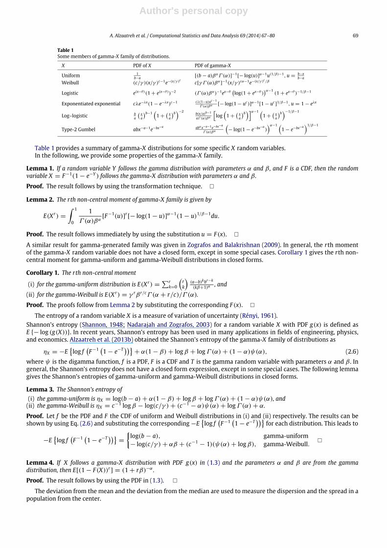
Table 1 provides a summary of gamma-X distributions for some specific X random variables.In the following, we provide some properties of the gamma-X family.

Lemma 1. If a random variable Y follows the gamma distribution with parameters α and β , and F is a CDF, then the randomvariable X = F−1(1 − e−Y ) follows the gamma-X distribution with parameters α and β .

Proof. The result follows by using the transformation technique. �

Lemma 2. The rth non-central moment of gamma-X family is given by

E(X r) =

1

0

1Γ (α)βα

[F−1(u)]r [− log(1 − u)]α−1(1 − u)1/β−1du.

Proof. The result follows immediately by using the substitution u = F(x). �

A similar result for gamma-generated family was given in Zografos and Balakrishnan (2009). In general, the rth momentof the gamma-X random variable does not have a closed form, except in some special cases. Corollary 1 gives the rth non-central moment for gamma-uniform and gamma-Weibull distributions in closed forms.

Corollary 1. The rth non-central moment

(i) for the gamma-uniform distribution is E(X r) =r

k=0

rk

(a−b)kbr−k

(kβ+1)α , and

(ii) for the gamma-Weibull is E(X r) = γ rβr/cΓ (α + r/c)/Γ (α).

Proof. The proofs follow from Lemma 2 by substituting the corresponding F(x). �

The entropy of a random variable X is a measure of variation of uncertainty (Rényi, 1961).Shannon’s entropy (Shannon, 1948; Nadarajah and Zografos, 2003) for a random variable X with PDF g(x) is defined asE {− log (g(X))}. In recent years, Shannon’s entropy has been used in many applications in fields of engineering, physics,and economics. Alzaatreh et al. (2013b) obtained the Shannon’s entropy of the gamma-X family of distributions as

ηX = −Elog f

F−1

1 − e−T + α(1 − β)+ logβ + logΓ (α)+ (1 − α)ψ(α), (2.6)

where ψ is the digamma function, f is a PDF, F is a CDF and T is the gamma random variable with parameters α and β . Ingeneral, the Shannon’s entropy does not have a closed form expression, except in some special cases. The following lemmagives the Shannon’s entropies of gamma-uniform and gamma-Weibull distributions in closed forms.

Lemma 3. The Shannon’s entropy of(i) the gamma-uniform is ηX = log(b − a)+ α(1 − β)+ logβ + logΓ (α)+ (1 − α)ψ(α), and(ii) the gamma-Weibull is ηX = c−1 logβ − log(c/γ )+ (c−1

− α)ψ(α)+ logΓ (α)+ α.

Proof. Let f be the PDF and F the CDF of uniform and Weibull distributions in (i) and (ii) respectively. The results can beshown by using Eq. (2.6) and substituting the corresponding −E

log f

F−1

1 − e−T

for each distribution. This leads to

−Elog f

F−1

1 − e−T =

log(b − a), gamma-uniform− log(c/γ )+ αβ + (c−1

− 1)(ψ(α)+ logβ), gamma-Weibull. �

Lemma 4. If X follows a gamma-X distribution with PDF g(x) in (1.3) and the parameters α and β are from the gammadistribution, then E[(1 − F(X))r ] = (1 + rβ)−α .

Proof. The result follows by using the PDF in (1.3). �

The deviation from the mean and the deviation from the median are used to measure the dispersion and the spread in apopulation from the center.

Author's personal copy

70 A. Alzaatreh et al. / Computational Statistics and Data Analysis 69 (2014) 67–80

Lemma 5. If we denote themedian byM, then themean deviation from themean, D(µ), and themean deviation from themedian,D(M), for the gamma-X distribution with PDF g(x) are given by

D(µ) = [2µ/Γ (α)]γ {α,−β−1 log(1 − F(µ))} − 2Iµ, and D(M) = µ− 2IM ,

where Ic = c−∞

xg(x)dx.

Proof. See the Appendix.

The hazard function of the gamma-X family is given by

h(x) =g(x)

1 − G(x)=

f (x)[− log(1 − F(x))]α−1[1 − F(x)](1/β)−1

βαΓ (α)− γ

α,−β−1 log (1 − F(x))

, −∞ < x < ∞. (2.7)

From (2.7), the hazard functions of gamma-uniform and gamma-Weibull distributions, respectively, are given by

(i) h(x) =(− log(u))α−1u(1/β)−1

(b−a)βα{Γ (α)−γ (α,−β−1 log(u))}, a < x < b, where u =

b−xb−a .

(ii) h(x) =c(x/γ )cα−1e−(x/γ )

c /β

γ βα{Γ (α)−γ (α,β−1(x/γ )c )}, x > 0.

3. Gamma-normal distribution and some of its properties

We now focus on the gamma-X family member with normal random variable X . If X is a normal random variable withPDF φ(x) and CDFΦ(x), then (1.3) gives the gamma-normal distribution with parameters α, β, µ and σ as

g(x) =1

Γ (α)βαφ(x)[− log(1 − Φ(x))]α−1

[1 − Φ(x)](1/β)−1, −∞ < x < ∞, (3.1)

where α > 0, β > 0, σ > 0 and −∞ < µ < ∞.

When α = β = 1, the gamma-normal distribution in (3.1) reduces to the normal distribution with parameters µ andσ . Thus, (3.1) is a generalization of the normal distribution. From (1.4), the CDF of the gamma-normal distribution can bewritten as

G(x) = γ {α,− log(1 − Φ(x))/β}/Γ (α).

Some of the general properties discussed in Section 2 for the gamma-X family are derived in detail for gamma-normaldistribution. Similar to Lemma 1, if a random variable Y follows the gamma distribution with parameters α and β , thenthe random variable X = Φ−1(1 − e−Y ) follows the gamma-normal distribution with parameters α, β, µ and σ . Randomsample data from the gamma-normal distribution in (3.1) can be simulated by first simulating random sample, Y , fromgamma distribution with parameters α and β , then computing X = Φ−1(1 − e−Y ), which follows the gamma-normaldistribution.

The hazard function associated with the gamma-normal distribution is

h(x) =g(x)

1 − G(x)=β−αφ(x)[− log(1 − Φ(x))]α−1

[1 − Φ(x)](1/β)−1

Γ (α)− γ {α,−β−1 log(1 − Φ(x))}, −∞ < x < ∞. (3.2)

The limit of the gamma-normal density function as x → ∓∞ is 0 and the limits of the gamma-normal hazard function asx → ∞ and x → −∞ are, respectively, ∞ and 0.

In Figs. 1 and 2, various graphs of g(x) and h(x) when µ = 0, σ = 1 and for various values of α and β are provided.Fig. 1 indicates that the gamma-normal PDF can be left skewed, right skewed, or symmetric. When changing the locationparameter µ, the identical graphs are shifted accordingly. When changing the scale parameter σ , the scale of the graphis changed to have flatter or higher peak accordingly, without affecting the shape. The plots in Fig. 2 indicate that thegamma-normal hazard function is monotonically increasing. The patterns of hazard functions remain the same for differentcombinations of µ and σ . The following observations are from Fig. 1 and additional graphs of the density functions that arenot included in order to save space. For fixed α, the left tail becomes more negatively skewed as β (<1) decreases. Also, forfixed α, the distribution becomes more platykurtic (the peak of the distribution becomes lower and more flat-shaped) asβ increases. For fixed β , the distribution becomes more leptokurtic (the peak of the distribution becomes higher and morecone-shaped) as α increases.

Theorem 1. The mode of the gamma-normal distribution is the solution of the equation

x = σ 2hN(x)(α − 1)/HN(x)− β−1

+ 1

+ µ, (3.3)

where hN(x) = φ(x)/[1 − Φ(x)] and HN(x) = − log[1 − Φ(x)], are respectively, the hazard and cumulative hazard functionsfor the normal distribution.

Author's personal copy

A. Alzaatreh et al. / Computational Statistics and Data Analysis 69 (2014) 67–80 71

Fig. 1. The gamma-normal PDF for various values of α and β .

Fig. 2. The gamma-normal hazard function for various values of α and β .

Proof. By using the fact that φ′(x) = −σ−2(x − µ)φ(x), the derivative with respect to x of (3.1) can be simplified to

g ′(x) =1

Γ (α)βαφ(x)[− log(1 − Φ(x))]α−2

[1 − Φ(x)](1/β)−2 k(x), (3.4)

where k(x) = σ−2(x −µ) log[1 −Φ(x)] [1 −Φ(x)] + (β−1− 1)φ(x) log[1 −Φ(x)] + (α − 1)φ(x). Setting (3.4) to 0, the

mode of g(x) is the solution of equation k(x) = 0. The result of the theorem follows by noting that k(x) = 0 is equivalent toEq. (3.3). �

When µ = 0, Eq. (3.3) shows that the mode is non-negative when α ≥ 1 and β ≥ 1; and the mode is negative whenα ≤ 1, β < 1 or α < 1, β ≤ 1. Also, the mode is an increasing function of α, β , µ and σ . The graphical displays ofmany combinations of the parameters indicate that the gamma-normal distribution appears to be unimodal. Numericalcomputation for Eq. (3.3) shows that there is only one mode for values of α and β between 0 and 20. However, no analyticalmethod has been used to show that the distribution is unimodal. Thus, gamma-normal distribution appears to be unimodalcompared to the beta-normal distribution (Eugene et al., 2002) which can be unimodal or bimodal.

The following lemma gives the quantile function for the gamma-normal distribution.

Lemma 6. If Q (λ), 0 < λ < 1 denotes the quantile function for the gamma-normal distribution, then

Q (λ) = Φ−1 1 − exp{−βγ−1(α, λΓ (α))}

. (3.5)

Proof. The result follows immediately by using G(Q (λ)) = λ and (1.4) with F(x) replaced byΦ(x). �

Lemma 7. The Shannon’s entropy for the gamma-normal distribution is given by

ηX = logσ√2π

+ 0.5 (v + m2)+ logΓ (α)+ logβ + α(1 − β)+ (1 − α)ψ(α), (3.6)

where m and v are the mean and the variance of the gamma-normal distribution with parameters α, β, 0 and 1.

Author's personal copy

72 A. Alzaatreh et al. / Computational Statistics and Data Analysis 69 (2014) 67–80

Proof. We first need to find −Elog f

F−1

1 − e−T

, where f (x) = φ(x) and F(x) = Φ(x). Since log(φ(x)) = − log(σ

√2π) − [(x − µ)/σ ]

2/2, we have −Elog f

F−1

1 − e−T

= log(σ

√2π) + [E{(Φ−1(1 − e−T ) − µ)/σ }]

2/2, where Tfollows the gamma distribution. By Lemma 1,Φ−1(1 − e−T ) follows a gamma-normal distribution with parameter α, β, µ,and σ , which implies that (Φ−1(1 − e−T ) − µ)/σ follows a gamma-normal distribution with parameters α, β, 0, and 1.Thus, −E

log f

F−1(1 − e−T )

= log(σ

√2π)+ (v + m2)/2. The result follows from Eq. (2.6). �

Note that when α = β = 1, (3.6) reduces to ηX = log(σ√2π) + 0.5 which is the Shannon’s entropy of the normal

distribution with parameters µ and σ .

3.1. Moments of gamma-normal distribution

By using Lemma 1, the non-central moments for the gamma-normal distribution in (3.1) can be written as E(X r) =

EΦ−1(1 − e−T )

r where T follows the gamma distribution with parameters α and β . It is easy to see thatΦ−1(1− e−T ) =√2 σerf−1(1 − 2e−T )+ µ. Hence,

E(X r) = E√

2 σerf−1(1 − 2e−T )+ µr

=

rj=0

rj

2j/2σ j E

(erf−1(1 − e−T ))j

µr−j. (3.7)

On using the series representation for erf−1(1 − 2e−T ) (Wolfram.com, 2012), we get

erf−1(1 − 2e−T ) =

∞k=0

ak√π/2

2k+1(1 − 2e−T )2k+1,

where ak =ck

2k+1 , ck =k−1

j=0cjck−1−j

(j+1)(2j+1) , and c0 = 1.

This implies

erf−1(1 − 2e−T )

j=

∞k1=0

∞k2=0

· · ·

∞kj=0

A(k1, k2, . . . , kj)(1 − 2e−T )2sj+j, (3.8)

where A(k1, k2, . . . , kj) = (√π/2)2sj+jak1ak2 · · · akj and sj = k1 + k2 + · · · + kj.

By using the binomial expansion on (1 − 2e−T )2sj+j, (3.8) can be written as

erf−1(1 − 2e−T )

j=

∞k1=0

∞k2=0

· · ·

∞kj=0

2sj+ji=0

A(k1, k2, . . . , kj)2sj + j

i

(−2)ie−iT . (3.9)

On using Eq. (3.9), Eq. (3.7) can be written as

E(X r) =

rj=0

∞k1=0

∞k2=0

· · ·

∞kj=0

2sj+ji=0

2j/2σ jµr−jA(k1, k2, . . . , kj)rj

2sj + j

i

(−2)iE(e−iT ). (3.10)

But E(e−iT ) = (1 + βi)−α , hence

E(X r) =

rj=0

∞k1=0

∞k2=0

· · ·

∞kj=0

2sj+ji=0

2j/2σ jµr−jA(k1, k2, . . . , kj)rj

2sj + j

i

(−2)i(1 + βi)−α. (3.11)

Table 2 provides the mode, mean, variance, skewness, and kurtosis of the gamma-normal distribution when µ = 0 andσ = 1 for various combinations of α and β . The means and variances in Table 2 agree with the corresponding values for theupper record values from standard normal distribution in Arnold et al. (1998, p. 65). For fixed α, the mode, the mean, thevariance, and the skewness, are increasing functions of β , while the kurtosis is a decreasing function of β . Also, for fixed β ,the mode and the mean are increasing functions of α whereas the variance is a decreasing function of α.

Over-dispersion in a distribution is a situation in which the variance exceeds themean, under-dispersion is the opposite,and equi-dispersion occurs when the variance is equal to the mean. From Table 2, the gamma-normal distribution satisfiesthe over-dispersion property when α ≤ 1. However, for values of α > 1, the distribution can be over-dispersed, under-dispersed or equi-dispersed. Table 2 also shows that the gamma-normal distribution can be left skewed, symmetric, or rightskewed.

Since the moments of gamma-normal distribution are not in closed form, a numerical method is used to determine thepoints where the distribution is equi-dispersed and the point where the skewness equals zero where µ = 0 and σ = 1.A function relating α to 1/β is obtained for the situation when the distribution is equi-dispersed and the points when the

Author's personal copy

A. Alzaatreh et al. / Computational Statistics and Data Analysis 69 (2014) 67–80 73

Table 2Mode, mean, variance, skewness and kurtosis when µ = 0, σ = 1 and for some values of α and β .

α β Mode Mean Variance Skewness Kurtosis

0.5 0.1 −1.8286 −2.0915 0.6412 −0.6207 3.58040.2 −1.5387 −1.7995 0.7797 −0.5058 3.39160.5 −1.1162 −1.2984 1.0691 −0.3183 3.16621 −0.7606 −0.8614 1.4323 −0.1500 3.04222 −0.3671 −0.3339 2.0276 0.0355 2.9855

1 0.1 −1.4202 −1.5388 0.3443 −0.4099 3.33150.2 −1.0615 −1.1630 0.4475 −0.3026 3.20080.5 −0.5061 −0.5642 0.6817 −0.1370 3.06171 0 0 1 0 32 0.6120 0.7043 1.5572 0.1372 2.9831

2 0.1 −0.9845 −1.0339 0.2092 −0.2203 3.12950.2 −0.5441 −0.5795 0.2909 −0.1331 3.06460.5 0.1727 0.1703 0.4905 −0.0075 3.00701 0.8638 0.9032 0.7799 0.0870 2.98902 1.7450 1.8475 1.3123 0.1728 2.9902

5 0.1 −0.3159 −0.3273 0.1271 −0.0646 3.02220.2 0.2725 0.2713 0.1930 −0.0058 3.00470.5 1.2860 1.3072 0.3670 0.0694 2.99401 2.3190 2.3667 0.6353 0.1184 2.99372 3.6949 3.7805 1.1501 0.1575 2.9964

Fig. 3. Dispersion regions for the gamma-normal distribution for µ = 0, σ = 1.

Fig. 4. Dispersion regions for the gamma-normal distribution for µ = 1, σ = 2.

distribution is symmetric. Fig. 3 shows the regions in which the gamma-normal distribution is over-dispersed and under-dispersed. The linear curve in Fig. 3 connects the points where gamma-normal distribution is equi-dispersed.

In addition to the case with µ = 0 and σ = 1, we also tried other combinations of µ and σ . As expected, the points ofequi-dispersion depend on µ and σ . However, it is interesting to point out that the relationship between α and 1/β for theequi-dispersed points remains linear for every combination of µ and σ . Fig. 4 displays the relationship between α and 1/βfor the equi-dispersed points when µ = 1 and σ = 2.

Author's personal copy

74 A. Alzaatreh et al. / Computational Statistics and Data Analysis 69 (2014) 67–80

Fig. 5. Skewness regions for the gamma-normal distribution.

Fig. 5 shows the regions in which the gamma-normal distribution is left skewed or right skewed. The cubic function inFig. 5 connects the points where gamma-normal distribution is symmetric. In addition to the case with µ = 0 and σ = 1,we also tried other combinations of µ and σ . As expected, the points of symmetry for gamma-normal distribution do notdepend on µ and σ , since µ is a location parameter and σ is a scale parameter.

3.2. Bounds for the non-central moments of gamma-normal distribution

The following two theorems give bounds for the non-central moments of gamma-normal distribution.

Theorem 2. If 1 ≤ α ≤ 1/β , then E(|X − µ|r) ≤

σ r2r/2√πβαΓ (α)

Γ r+1

2

.

Proof. We need the following inequality introduced by Abramowitz and Stegun (1964, p. 68) for the proof.

− log(1 − x) < x/(1 − x), x < 1 and x = 0. (3.12)

Using (3.12) we get − log[1 − Φ(x)] < Φ(x)/[1 − Φ(x)]. For α ≥ 1, this implies that

E(|X − µ|r) ≤

1Γ (α)βα

∞

−∞

|x − µ|rφ(x)(Φ(x))α−1

[1 − Φ(x)](1/β)−αdx. (3.13)

If α ≤ 1/β, (Φ(x))α−1[1 − Φ(x)](1/β)−α ≤ 1. Hence, E(|X − µ|

r) ≤ β−α(Γ (α))−1EN(|X − µ|r), where EN(|X − µ|

r) is theexpected value of |X−µ|

r whereX has thenormal distribution. It can be shown that EN(|X−µ|r) = σ r2r/2π−1/2Γ ((r+1)/2),

which completes the proof. �

Corollary 2. If 1 ≤ α ≤ 1/β , then |E((X − µ)r)| ≤

σ r

βαΓ (α)

2k+1/2√π

k!, r = 2k + 1

σ r

βαΓ (α)

ki=1(2i − 1), r = 2k.

Proof. The proof follows immediately fromTheorem2 and the fact thatΓ (k+1/2) = 2−k√πk

i=1(2i−1) (see Abramowitzand Stegun (1964, p. 255)). �

A shaper bound for expected value of gamma-normal distribution can be obtained when both α and 1/β > 1/2 as shownin the following Theorem 3.

Theorem 3. If α, 1β> 1

2 , then |E(X)| ≤ σ

Γ (2α−1)Γ 2(α)β(2−β)2α−1 − 1 + µ.

Proof. See the Appendix.

The inequality in Theorem 3 is sharp. To see this; if α = β = 1 then |E(X)| ≤ µ, and hence E(X) = µ, which is the meanfor the normal distribution.

Author's personal copy

A. Alzaatreh et al. / Computational Statistics and Data Analysis 69 (2014) 67–80 75

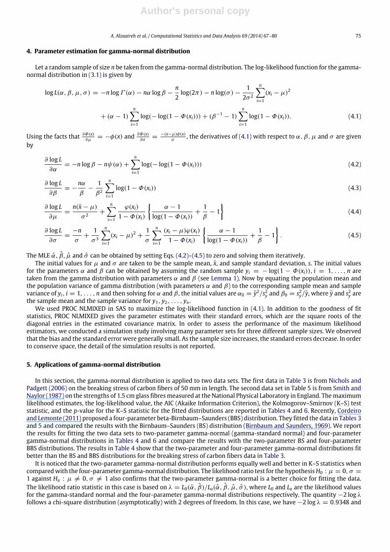
4. Parameter estimation for gamma-normal distribution

Let a random sample of size n be taken from the gamma-normal distribution. The log-likelihood function for the gamma-normal distribution in (3.1) is given by

log L(α, β, µ, σ ) = −n logΓ (α)− nα logβ −n2log(2π)− n log(σ )−

12σ 2

ni=1

(xi − µ)2

+ (α − 1)n

i=1

log(− log(1 − Φ(xi)))+ (β−1− 1)

ni=1

log(1 − Φ(xi)). (4.1)

Using the facts that ∂Φ(x)∂µ

= −φ(x) and ∂Φ(x)∂σ

=−(x−µ)φ(x)

σ, the derivatives of (4.1) with respect to α, β, µ and σ are given

by

∂ log L∂α

= −n logβ − nψ(α)+

ni=1

log(− log(1 − Φ(xi))) (4.2)

∂ log L∂β

= −nαβ

−1β2

ni=1

log(1 − Φ(xi)) (4.3)

∂ log L∂µ

=n(x − µ)

σ 2+

ni=1

ϕ(xi)1 − Φ(xi)

α − 1

log(1 − Φ(xi))+

1β

− 1

(4.4)

∂ log L∂σ

=−nσ

+1σ 3

ni=1

(xi − µ)2 +1σ

ni=1

(xi − µ)ϕ(xi)1 − Φ(xi)

α − 1

log(1 − Φ(xi))+

1β

− 1. (4.5)

The MLE α, β , µ and σ can be obtained by setting Eqs. (4.2)–(4.5) to zero and solving them iteratively.The initial values for µ and σ are taken to be the sample mean, x, and sample standard deviation, s. The initial values

for the parameters α and β can be obtained by assuming the random sample yi = − log(1 − Φ(xi)), i = 1, . . . , n aretaken from the gamma distribution with parameters α and β (see Lemma 1). Now by equating the population mean andthe population variance of gamma distribution (with parameters α and β) to the corresponding sample mean and samplevariance of yi, i = 1, . . . , n and then solving for α and β , the initial values are α0 = y2/s2y and β0 = s2y/y, where y and s2y arethe sample mean and the sample variance for y1, y2, . . . , yn.

We used PROC NLMIXED in SAS to maximize the log-likelihood function in (4.1). In addition to the goodness of fitstatistics, PROC NLMIXED gives the parameter estimates with their standard errors, which are the square roots of thediagonal entries in the estimated covariance matrix. In order to assess the performance of the maximum likelihoodestimators, we conducted a simulation study involving many parameter sets for three different sample sizes. We observedthat the bias and the standard errorwere generally small. As the sample size increases, the standard errors decrease. In orderto conserve space, the detail of the simulation results is not reported.

5. Applications of gamma-normal distribution

In this section, the gamma-normal distribution is applied to two data sets. The first data in Table 3 is from Nichols andPadgett (2006) on the breaking stress of carbon fibers of 50 mm in length. The second data set in Table 5 is from Smith andNaylor (1987) on the strengths of 1.5 cm glass fibresmeasured at the National Physical Laboratory in England. Themaximumlikelihood estimates, the log-likelihood value, the AIC (Akaike Information Criterion), the Kolmogorov–Smirnov (K–S) teststatistic, and the p-value for the K–S statistic for the fitted distributions are reported in Tables 4 and 6. Recently, Cordeiroand Lemonte (2011) proposed a four-parameter beta-Birnbaum–Saunders (BBS) distribution. They fitted the data in Tables 3and 5 and compared the results with the Birnbaum–Saunders (BS) distribution (Birnbaum and Saunders, 1969). We reportthe results for fitting the two data sets to two-parameter gamma-normal (gamma-standard normal) and four-parametergamma-normal distributions in Tables 4 and 6 and compare the results with the two-parameter BS and four-parameterBBS distributions. The results in Table 4 show that the two-parameter and four-parameter gamma-normal distributions fitbetter than the BS and BBS distributions for the breaking stress of carbon fibers data in Table 3.

It is noticed that the two-parameter gamma-normal distribution performs equally well and better in K–S statistics whencomparedwith the four-parameter gamma-normal distribution. The likelihood ratio test for the hypothesisH0 : µ = 0, σ =

1 against Ha : µ = 0, σ = 1 also confirms that the two-parameter gamma-normal is a better choice for fitting the data.The likelihood ratio statistic in this case is based on λ = L0(α, β)/La(α, β, µ, σ ), where L0 and La are the likelihood valuesfor the gamma-standard normal and the four-parameter gamma-normal distributions respectively. The quantity −2 log λfollows a chi-square distribution (asymptotically) with 2 degrees of freedom. In this case, we have −2 log λ = 0.9348 and

Author's personal copy

76 A. Alzaatreh et al. / Computational Statistics and Data Analysis 69 (2014) 67–80

Table 3Breaking stress of carbon fibers data.

3.70 2.74 2.73 2.50 3.60 3.11 3.27 2.87 1.47 3.11 3.564.42 2.41 3.19 3.22 1.69 3.28 3.09 1.87 3.15 4.90 1.572.67 2.93 3.22 3.39 2.81 4.20 3.33 2.55 3.31 3.31 2.851.25 4.38 1.84 0.39 3.68 2.48 0.85 1.61 2.79 4.70 2.031.89 2.88 2.82 2.05 3.65 3.75 2.43 2.95 2.97 3.39 2.962.35 2.55 2.59 2.03 1.61 2.12 3.15 1.08 2.56 1.80 2.53

Table 4Parameter estimates (standard errors in parentheses) for the carbon fibers data.

Distribution Birnbaum–Saunders Beta Birnbaum–Saunders Two-parameter gamma-normal Four-parameter gamma-normal

Parameter estimates a = 0.4371 (0.0381)b = 2.5154 (0.1321)

α = 0.1930 (0.0259)β = 1876.732 (605.05)a = 1.0445 (0.0036)b = 57.6001 (0.3313)

α = 4.7966 (0.8076)β = 1.2932 (0.2296)

α = 0.8263 (3.2578)β = 0.6190 (2.8315)µ = 3.3464 (1.1621)σ = 0.9614 (2.1593)

Log-likelihood −100.1900 −91.3550 −85.9070 −85.4396

AIC 204.3800 190.7100 175.8140 178.8792

K–S 0.1731 0.1271 0.0693 0.0737K–S p-value 0.0383 0.2369 0.9090 0.8662

the p-value is 0.6266. Fig. 6 displays the empirical and the fitted cumulative distribution functions for the breaking stress ofcarbon fibers data in Table 3.

The results in Table 6 show that the BBS, the two-parameter gamma-normal and the four-parameter gamma-normaldistributions provide adequate fits and the four-parameter gamma-normal distribution is the best for fitting the strengthof 1.5 cm glass fibres data in Table 5. When comparing the fits between the two-parameter and the four-parameter gammanormal distributions, the likelihood ratio test for the hypothesis H0 : µ = 0, σ = 1 against Ha : µ = 0, σ = 1 showsthat −2 log λ = 3.6806 with p-value = 0.16. This suggests that the four-parameter gamma-normal distribution does notsignificantly perform better than the two-parameter gamma normal distribution for the strength of 1.5 cm glass fibres datain Table 5. The fact that the two-parameter gamma-normal distribution has only two parameters adds an extra advantageto the distribution over both the four-parameter BBS and four-parameter gamma-normal distributions. Fig. 7 displays theempirical and the fitted cumulative distribution functions for the strength of 1.5 cm glass fibres data in Table 5.

Fig. 6. CDF for fitted distributions of the breaking stress of carbon fibres data.

One reviewer asked ‘‘What situations (data) would suggest a gamma-normal model?’’ In order to answer the question,we simulated a few data sets that are right-skewed, left-skewed and nearly symmetric from gamma-normal distributionby using sample sizes n = 100 and 200. Both gamma-normal and normal distributions were fitted to each data set and theresiduals were plotted. The simulated data are taken to be the observed values. The expected value corresponding to eachobserved value under gamma-normal or normal distribution is obtained by using the quantile function of the distributionevaluated at the empirical CDF for the observed value. The residuals are plotted against the observed values. For right-skewed (left-skewed) data, a large number of the residuals are positive (negative). For symmetric data sets, the residualstend to randomly distribute around zero. When the residual plots are not randomly distributed around zero, one should use

Author's personal copy

A. Alzaatreh et al. / Computational Statistics and Data Analysis 69 (2014) 67–80 77

Table 5Strength of 1.5 cm glass fibres data.

0.55 0.74 0.77 0.81 0.84 0.931.04 1.11 1.13 1.24 1.25 1.271.28 1.29 1.30 1.36 1.39 1.421.48 1.48 1.49 1.49 1.50 1.501.51 1.52 1.53 1.54 1.55 1.551.58 1.59 1.60 1.61 1.61 1.611.61 1.62 1.62 1.63 1.64 1.661.66 1.66 1.67 1.68 1.68 1.692.00 2.01 2.24

Table 6Parameter estimates (standard errors in parentheses) for the glass fibres data.

Distribution Birnbaum–Saunders Beta Birnbaum–Saunders Two-parameter gamma-normal Four-parameter gamma-normal

Parameter estimates a = 0.2699 (0.0267)b = 1.3909 (0.0521)

α = 0.3638 (0.0709)β = 7857.566 (3602.2)a = 1.0505 (0.0101)b = 30.4783 (0.5085)

α = 18.0840 (3.5490)β = 0.1459 (0.0290)

α = 0.5872 (0.7805)β = 0.1871 (0.5139)µ = 2.0895 (0.7495)σ = 0.3910 (0.3872)

Log-likelihood −22.1890 −14.7760 −15.0551 −13.2148

AIC 48.3780 37.5520 34.1102 34.4296

K–S 0.1988 0.1590 0.1627 0.1620K–S p-value 0.0355 0.1518 0.1343 0.1377

Fig. 7. CDF for fitted distributions of the strength of 1.5 glass fibres data.

a gamma-normal distribution instead of a normal distribution. Thus, one should obtain a graphical display (e.g. histogram)for an observed data and/or compute a numericalmeasure of skewness. If the data is skewed, one should fit a gamma-normaldistribution instead of a normal distribution.

6. Summary

In this article, some properties of the gamma-X family are provided. A special case of the gamma-X family, the gamma-normal distribution is studied. The gamma-normal distribution is a generalization of normal distribution. In general, thegamma-X distribution is a generalization of the X distribution. Various properties of the gamma-normal distribution areinvestigated, including moments, bounds for non-central moments, hazard function, and entropy. The gamma-normaldistribution can be over-, equi- or under-dispersed; as well as left skewed, right skewed or symmetric. Two real data sets arefitted to the gamma-normal distribution and compared with other known distributions. The results show that the gamma-normal distribution provides a good fit to each data set.

Author's personal copy

78 A. Alzaatreh et al. / Computational Statistics and Data Analysis 69 (2014) 67–80

Acknowledgments

The authors are grateful for the comments and suggestions by the referees and the Associate Editor. Their comments andsuggestions have greatly improved the paper.

Appendix

Proof of Lemma 5. Let g(x) and G(x) be the PDF and CDF of gamma-X distribution. By definition,

D(µ) =

µ

−∞

(µ− x)g(x)dx +

∞

µ

(x − µ)g(x)dx = 2 µ

−∞

(µ− x)g(x)dx

= 2µG(µ)− 2 µ

−∞

xg(x)dx. (A.1)

D(M) =

M

−∞

(M − x)g(x)dx +

∞

M(x − M)g(x)dx = 2

M

−∞

(M − x)g(x)dx + E(X)− M

= µ− 2 M

−∞

xg(x)dx. (A.2)

Now, consider the integral

Ic =

c

−∞

xg(x)dx =1

βαΓ (α)

c

−∞

xf (x)[− log(1 − F(x))]α−1[1 − F(x)](1/β)−1dx. (A.3)

By using the substitution u = − log(1 − F(x)), the Eq. (A.3) can be written as

Ic =1

βαΓ (α)

− log(1−F(c))

0F−1(1 − e−u)uα−1e−u/βdu. (A.4)

By using (1.4) and (A.4) in Eqs. (A.1) and (A.2), the mean deviation from the mean and the mean deviation from the medianare, respectively, given by

D(µ) = [2µ/Γ (α)]γ {α,−β−1 log(1 − F(µ))} − 2Iµ, and D(M) = µ− 2IM . �

Proof of Theorem 3. Consider

E(X) =1

Γ (α)βα

∞

−∞

xφ(x)[− log(1 − Φ(x))]α−1[1 − Φ(x)](1/β)−1dx. (A.5)

Let u = Φ(x), then (A.5) can be written as

E(X) =

1

0β−α(Γ (α))−1x(u)(− log(1 − u))α−1(1 − u)(1/β)−1du, (A.6)

where x(u) = Φ−1(u). The transformation u = Φ(x) leads to the following conditions

(i) 1

0x(u)du = µ and (ii)

1

0x2(u)du = σ 2

+ µ2. (A.7)

Following themethod of Gumbel (1954), we can use the variation techniques to obtain a bound for Eq. (A.6) with conditionsin (A.7). Consider the first variation of Eq. (A.6), 1

0

β−α(Γ (α))−1x(u)(− log(1 − u))α−1(1 − u)(1/β)−1

− λ1x2(u)− λ2x(u)du = 0, (A.8)

where 0 ≤ u ≤ 1 and the conditions (A.7) hold. The stationary solution of (A.7) satisfies the following equation 1

0

∂

∂x

β−α(Γ (α))−1x(u)(− log(1 − u))α−1(1 − u)(1/β)−1

− λ1x2(u)− λ2x(u)du = 0.

This implies that

β−α(Γ (α))−1(− log(1 − u))α−1(1 − u)(1/β)−1− 2λ1x(u)− λ2 = 0. (A.9)

Author's personal copy

A. Alzaatreh et al. / Computational Statistics and Data Analysis 69 (2014) 67–80 79

Eq. (A.9) reduces to

x(u) =1

2λ1

β−α(Γ (α))−1(− log(1 − u))α−1(1 − u)(1/β)−1

− λ2. (A.10)

On integrating both sides in (A.9) we get 1

0β−α(Γ (α))−1(− log(1 − u))α−1(1 − u)(1/β)−1du − 2λ1

1

0x(u)du − λ2 = 0. (A.11)

Using the substitution v = − log(1 − u) for the first integration and using part (i) of (A.7) for the second integration, onecan get

λ2 = 1 − 2µλ1. (A.12)

Substituting λ2 = 1 − 2µλ1 in (A.10) and then using part (ii) of (A.7), one can show that

λ1 = ±12σ

Γ (2α − 1)

Γ 2(α)β(2 − β)2α−1− 1, where α,

1β>

12. (A.13)

Using the values of λ1 and λ2 from Eqs. (A.12) and (A.13) in (A.10), (A.10) reduces to

x(u) = ±σ

Γ 2(α)β(2 − β)2α−1

Γ (2α − 1)− Γ 2(α)β(2 − β)2α−1×

(βαΓ (α))−1(− log(1 − u))α−1(1 − u)(1/β)−1

− 1

+ µ. (A.14)

Using (A.14) in (A.6) and noting that the maximum and minimum values of E(X), respectively, occurs at the positive andnegative values of λ1, we get

|E(X)| ≤ σ

Γ 2(α)β(2 − β)2α−1

Γ (2α − 1)− Γ 2(α)β(2 − β)2α−1

1

0β−2α(Γ (α))−2(− log(1 − u))2α−2(1 − u)(2/β)−2du

−

1

0β−α(Γ (α))−1(− log(1 − u))α−1(1 − u)(1/β)−1du

+µ

1

0β−α(Γ (α))−1(− log(1 − u))α−1(1 − u)(1/β)−1du. (A.15)

Using the substitution v = − log(1 − u) in (A.15), one can easily get

|E(X)| ≤ σ

Γ (2α − 1)

Γ 2(α)β(2 − β)2α−1− 1 + µ, where α,

1β>

12. �

References

Abramowitz, M., Stegun, I.A., 1964. Handbook of Mathematical Functions with Formulas, Graphs andMathematical Tables, Vol. 55. Dover Publication, Inc.,New York.

Akinsete, A., Famoye, F., Lee, C., 2008. The beta-Pareto distribution. Statistics 42, 547–563.Alshawarbeh, E., Lee, C., Famoye, F., 2012. Beta-Cauchy distribution. Journal of Probability and Statistical Science 10, 41–58.Alzaatreh, A., Famoye, F., Lee, C., 2013a. Weibull–Pareto distribution and its applications. Communications in Statistics-Theory & Methods 42, 1673–1691.Alzaatreh, A., Lee, C., Famoye, F., 2013b. A new method for generating families of continuous distributions. Metron 71 (1), 63–79.Alzaatreh, A., Lee, C., Famoye, F., 2012. On the discrete analogues of continuous distributions. Statistical Methodology 9, 589–603.Arnold, B.C., Balakrishnan, N., Nagaraja, H.N., 1998. Records. John Wiley and Sons, Inc., New York.Azzalini, A., 1985. A class of distributions which includes the normal ones. Scandinavian Journal of Statistics 12, 171–178.Azzalini, A., 2005. The skew-normal distribution and related multivariate families. Scandinavian Journal of Statistics 32 (2), 159–188.Barreto-Souza, W., Santos, A., Cordeiro, G., 2010. The beta generalized exponential distribution. Journal of Statistical Computation and Simulation 80 (2),

159–172.Birnbaum, Z.W., Saunders, S.C., 1969. A new family of life distributions. Journal of Applied Probability 6, 319–327.Cordeiro, G.M., de Castro, M., 2011. A new family of generalized distributions. Journal of Statistical Computation and Simulation 81 (7), 883–898.Cordeiro, G.M., Lemonte, A.J., 2011. The β-Birnbaum–Saunders distribution: an improved distribution for fatigue life modeling. Computational Statistics

and Data Analysis 55 (3), 1445–1461.Eugene, N., Lee, C., Famoye, F., 2002. The beta-normal distribution and its applications. Communications in Statistics-Theory andMethods 31 (4), 497–512.Famoye, F., Lee, C., Eugene, N., 2004. Beta-normal distribution: bimodality properties and applications. Journal of Modern Applied Statistical Methods 3

(1), 85–103.Famoye, F., Lee, C., Olumolade, O., 2005. The beta-Weibull distribution. Journal of Statistical Theory and Applications 4 (2), 121–136.Ferreira, J.T.A.S., Steel, M.F.J., 2006. A constructive representation of univariate skewed distributions. Journal of the American Statistical Association 101

(474), 823–829.Gumbel, E.J., 1954. The maxima of the mean largest value and of the range. Annals of Mathematical Statistics 25, 76–84.Johnson, N.L., Kotz, S., Balakrishnan, N., 1994. Continuous Univariate Distributions, Vol. 1, second ed. John Wiley and Sons, Inc., New York.

Author's personal copy

80 A. Alzaatreh et al. / Computational Statistics and Data Analysis 69 (2014) 67–80

Jones, M.C., 2004. Families of distributions arising from distributions of order statistics. Test 13 (1), 1–43.Jones, M.C., 2009. Kumaraswamy’s distribution: a beta-type distribution with tractability advantages. Statistical Methodology 6, 70–81.Lee, C., Famoye, F., Alzaatreh, A., 2013. Methods for generating families of univariate continuous distributions in the recent decades. WIREs Computational

Statistics 5, 219–238.Nadarajah, S., Kotz, S., 2006. The beta exponential distribution. Reliability Engineering & System Safety 91, 689–697.Nadarajah, S., Zografos, K., 2003. Formulas for Rényi information and related measures for univariate distributions. Information Sciences 155, 119–138.Nichols, M.D., Padgett, W.J., 2006. A bootstrap control for Weibull percentiles. Quality and Reliability Engineering International 22, 141–151.Rényi, A., 1961. On measures of entropy and information. In: Proceedings of the Fourth Berkeley Symposium on Mathematical Statistics and Probability, I.

University of California Press, Berkeley, pp. 547–561.Shannon, C.E., 1948. A mathematical theory of communication. Bell System Technical Journal 27, 379–432.Smith, R.L., Naylor, J.C., 1987. A comparison of maximum likelihood and Bayesian estimators for the three-parameterWeibull distribution. Journal of Royal

Statistical Society Series C 36, 358–369.Wolfram website: http://functions.wolfram.com/GammaBetaErf/InverseErf/06/01/02/0004/. Retrieved on December 03, 2012.Zografos, K., Balakrishnan, N., 2009. On families of beta- and generalized gamma-generated distributions and associated inference. Statistical Methodology

6, 344–362.