The Effects of Exchange Rate and Commodity Price ...

The Effects of Exchange Rate and Commodity Price Volatilities on Trade Volumes of Major Agricultural Commodities

by

A K Iftekharul Haque

A Thesis

presented to

The University of Guelph

In partial fulfillment of requirements

for the degree of

Master of Science

in

Food, Agricultural and Resource Economics

Guelph, Ontario, Canada

© A K Iftekharul Haque, September 2012

ABSTRACT

The Effects of Exchange Rate and Commodity Price Volatilities on

Trade Volumes of Major Agricultural Commodities

A K Iftekharul Haque

University of Guelph, 2012

Advisor:

Professor Getu Hailu

This thesis examines the effects of price and exchange rate volatilities on the volume of

trade corn, soybean, wheat and rice. Empirical results indicate that price volatility and

exchange rate volatilities do not have effects on Canada’s export of wheat and soybean,

and Canada’s import of corn and rice. This thesis also examined the effects of exchange

rate and commodity price volatilities on developed countries’ trade and developing

countries’ trade separately. Results show that trade between developing countries is more

sensitive to exchange rate and commodity price volatilities than trade between developed

countries.

iii

Acknowledgements

I would first like to thank my advisor, Dr. Getu Hailu, for countless reasons. His

mentorship, continuous support and extreme level of patience throughout my research

have been sources of encouragement for my professional and personal development. I

would like to thank Professor Karl Meilke for agreeing to be in my advisory committee

even after his retirement. I undoubtedly benefited from his vast knowledge of

international trade policy. I am grateful to Professor Alan Ker, another member of my

advisory committee, not only for his invaluable guidance but also taking care of all other

issues of mine during my stay at the Department of Food, Agricultural and Resource

Economies. I would also like to thank all the faculty members and staffs of the

Department of Food, Agricultural and Resource Economics, for guidance throughout the

coursework and completion of my thesis.

My sincere gratitude goes to the Canadian Agricultural Trade Policy and

Competitiveness Research Network (CATPRN) for providing me with the finances

necessary for this research.

I would also like to thank my peer group for their continuous support to my work.

Notably Xin Xie, Rebecka Elskamp, Alex Cairns, Rob Anderson, Zongyuan Shang,

Johanna Wilkes, Tor Tolhurst and Di Ai for their valuable advice, support and criticism.

I would like to thank my parents for their unconditional love; and my wife, Tasnuva, for

her extreme patience and encouragement to my work. Finally I must thank my son,

Shoummo, for being a source of joy and happiness.

iv

Table of Contents

ACKNOWLEDGEMENTS III

TABLE OF CONTENTS IV

LIST OF TABLES VI

LIST OF FIGURES VII

CHAPTER 1: INTRODUCTION 1

1.1: Background 1

1.2 Economic Problem 3

1.3 Economic Research Problem 3

1.4 Purpose and Objectives 5

CHAPTER 2: RECENT TRENDS OF EXCHANGE RATES AND COMMODITY PRICES 6

2.1 Exchange Rate Volatility 6

2.2 Agricultural Commodity Price Volatility 8

2.3 Drivers of Agricultural Commodity Price Volatilities 13

2.4. Chapter Summary 20

CHAPTER 3: LITERATURE REVIEW 21

3.1: Effects of Exchange Rate Volatilities: Theoretical Background 21

3.2 Measuring Exchange Rate and Price Volatilities 22

3.3 Empirical Literature: Exchange rate Volatility and Trade 24

3.4 Empirical Literature: Exchange Rate Volatility and Agricultural Trade 26

3.5 Chapter summary 28

CHAPTER 4: CONCEPTUAL FRAMEWORK 29

4.1 Model Description 29

v

4.2 Import Demand 29

4.3 Chapter Summary 33

CHAPTER 5: EMPIRICAL FRAMEWORK 34

5.1 Econometric specification 34

5.2 Variable Description 35

5.3 Data and sources 40

5.4 Model Selection 44

5.5 Diagnostics: Tests for Unit root, Heteroscedasticity, Serial Correlation and Multicollinearity 47


CHAPTER 6: RESULTS AND DISCUSSIONS 50

6.1 Introduction 50 6.2.1 Quarterly Imports of Wheat and Soybean from Canada 50 6.2.2. Quarterly import models of corn and rice 56

6.3 Annual Models 62 6.3.1 Top developed importers’ imports from Developed exporters 62 6.3.2 Top developing importers’ imports from developing exporters 69


CHAPTER 7: SUMMARY AND CONCLUSION 76

7.1 Summary 76

7.2 Policy implications 79

7.3 Limitations and further research 81

7.4 Research Contribution 82

REFERENCES 83

APPENDIX A 87

APPENDIX B 89

vi

List of Tables

Table 2.1: Evolution of Exchange rate Arrangements, 1996-2007 7

Table 5.1: Summary of export and import data for quarterly models 41

Table 5.2: Summary of import data for annual models 41

Table 5.3: Summery of Data Frequency and Sources for exchange rate, GDP prices 42

Table 5.4: List of Countries for Quarterly Models 42

Table 5.5: List of importing countries considered for annual models 43

Table 6.1: Fisher’s unit root test for wheat and soybean 51

Table 6.2: VIF for wheat and soybean model 53

Table 6.3: Coefficient estimates of quarterly wheat and soybean imports from

Canada from 2000 to 2009 55

Table 6.3a : Coefficient estimates of quarterly wheat and soybean imports from

Canada from 2000 to 2009 (without expected price variable) 56

Table 6.4: Fisher’s unit root test for corn and rice model 57

Table 6.5: VIF for corn and rice model 59

Table 6.6: Coefficient estimates of Canada’s corn and rice import demand from

2000-2009 60


2000-2009 (without percentage change of expected price) 61

Table 6.8: Fisher’s panel Unit Root Test 63

Table 6.9: Hausman Specification tests 64

Table 6.10: Friedman’s test for cross sectional independence 64

Table 6.11: Variance Inflation Factors 65

Table 6.12 : Wooldridge test for serial correlation 65

6.13: Coefficients estimates of developed countries’ wheat, soybean, corn and rice

imports from developed importers from 1991 to 2009 67

6.13a: Coefficients estimates of developed countries’ wheat, soybean, corn and rice

imports from developed countries from 1991 to 2009 (without percentage change of

expected price) 68

Table 6.14: Fisher’s panel Unit Root Test 69

Table 6.15: Hausman’s Specification tests 70

Table 6.16: Friedman’s test for cross-sectional independence 71

Table 6.17: Variance Inflation Factors 71

Table 6.18 : Wooldridge test for serial correlation 72

6.19: Coefficient estimates of developing importers’ imports of wheat, soybean,

corn and rice from developing exporters from 1991 to 2009 73

6.20: Coefficient estimates of developing importers’ imports of wheat, soybean,

corn and rice from developing exporters from 1991 to 2009 (without percentage

change of expected price) 74

vii

List of Figures

Figure 2.1: Exchange Rate movements of major currencies 7

Figure 2.2a: Monthly Corn price (F.O.B) in selected market from January 2000

(USD/Ton) 8

Figure 2.2b: Historical volatility of corn price 9

Figure 2.3a: Monthly wheat price (F.O.B) in selected market from January 2000

(USD/Ton) 10

Figure 2.3b: Historical volatility of wheat price 10

Figure 2.4a: US Soybean monthly F.O.B. Price from January 2000 11

Figure 2.4b: Historical volatility of soybean price 11

Figure 2.5a: Monthly rice price (F.O.B) in selected market from January 2000 to

January 2012 (USD/Ton) 12

Figure 2.5b: Historical volatility of rice price 12

Figure 2.6: Global Ethanol Production (in million Gallons) 14

Figure 2.7 : Share of US Corn used to produced ethanol, 1980-2011 14

Figure 2.8: Monthly Volume of Future Trades of Wheat, Maize and Soybeans at

Chicago Board of Trade (CBOT) 15

Figure 2.9: Per Capita Income Level by Developing Region 17

Figure 2.10: GDP Per Capita of India and China (Constant US Dollar) 17

Figure 2.11 a: Major Exporters of Maize in 2008 18

Figure 2.11 b: Major Exporters of Wheat in 2008 18

Figure 2.11 c: Major Exporters of Rice in 2008 19

Figure 2.12: Stocks to cereal use ratio 20

1

Chapter 1: Introduction

1.1: Background

Agricultural commodity price and exchange rate volatilities drew a global attention

because of their potential effects on international trade and domestic food prices.

Although the effects of exchange rate volatilities on international agricultural trade have

been examined for long time, the effects of price volatilities have not been examined at

large. Most of the recent studies (IFPRI, 2011,; Braun and Tadesse, 2012; Weersink et al

2008; OECD and FAO, 2012 ) on commodity price volatilities reviewed the reasons for

agricultural commodity price volatility. The purpose of this study is to examine the

effects of both exchange rate and commodity price volatilities on international

agricultural commodity trade and to estimate the effects of volatilities on developed and

developing countries separately.

Effects of exchange rate volatilities on trade flows became a center of interest

from early 1970 when a floating exchange rate regime began to replace the former fixed

exchange rate regime. The floating exchange rate system allows the value of a currency

to fluctuate based on the foreign exchange market fundamentals. Smith’s (1999) review

show that a number of studies were conducted to determine the impact of exchange rate

volatilities on trade flows, and find that the empirical evidence is mixed. For example,

Cushman (1983), Thursby and Thursby (1987) and Bini-Smaghi (1991) find that an

increase in exchange rate volatility leads to a reduction in the volume of international

trade. In contrast, Frankel and Wei (1995) and Sercu and Uppal (2003) claim that

exchange rate volatilities may not have any effect on the volume of international trade.

2

While the effect of exchange rate volatility is still uncertain, agricultural commodity price

volatility has recently received much attention after the unprecedented spike in crop

prices and volatilities that occurred in 2007-08. The rise in the level of commodity prices

and volatilities resulted in a number of countries adopting policies that restricted food

imports and exports (IFPRI, 2011).

Commodity price volatility may have implications for the volume of agricultural

commodity trade when individual countries adopt policies that restrict imports or exports

(e.g., export bans) as a method of coping with price variations. Although the

consequences of exchange rate volatility on trade have extensively been examined and at

the centre of debate, research on the effects of commodity price volatility on international

trade (e.g., on volume) is limited. Volatility in the world market prices can have major

effects on agricultural trade since agricultural products and agricultural industry have

many characteristics, such as perishable nature of products and less supply

responsiveness to short term price fluctuation that distinguished them from other

industries. Uncertainty in the world agricultural market has a greater impact on farm income

in both developed and developing countries (Koo and Kennedy, 2007) and food security in

developing and low income countries (IFPRI, 2011).

In this study, I examine the effects of price and exchange rate volatilities on Canada’s

trade with its major trading partners using quarterly data for wheat, soybean, corn and

rice, and examine the effects of exchange rate and price volatilities on developed and

developing countries’ trade separately with annual models.

3

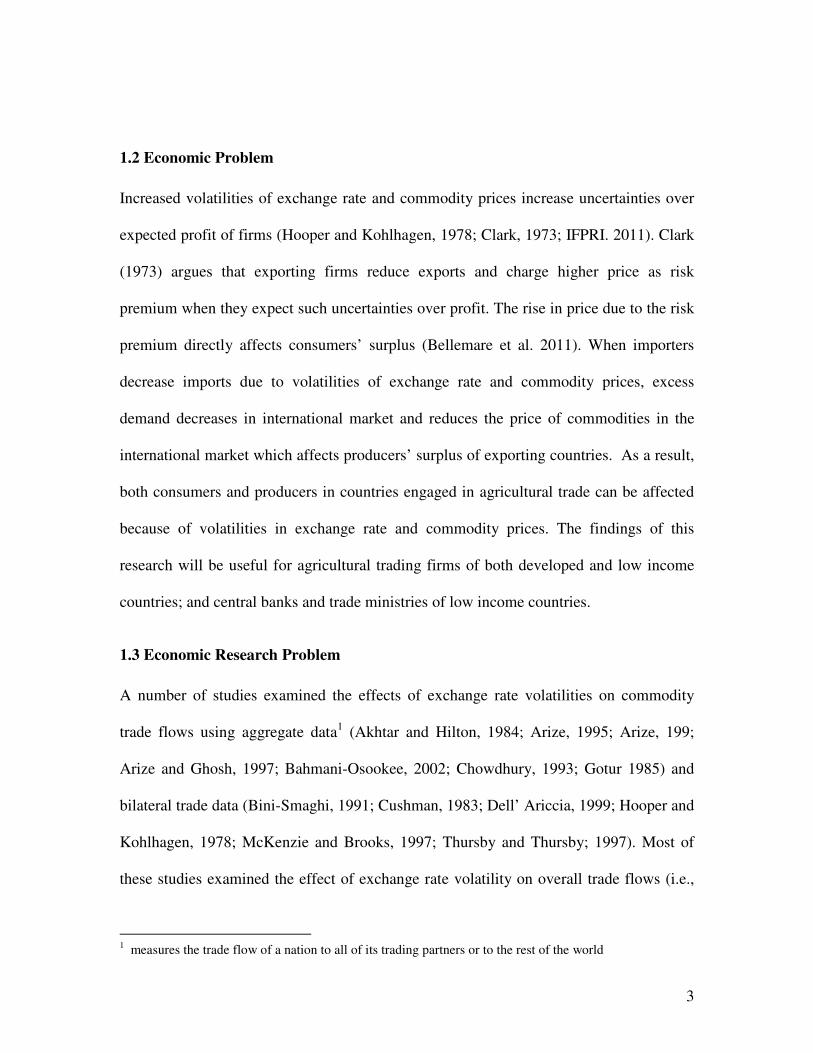
1.2 Economic Problem

Increased volatilities of exchange rate and commodity prices increase uncertainties over

expected profit of firms (Hooper and Kohlhagen, 1978; Clark, 1973; IFPRI. 2011). Clark

(1973) argues that exporting firms reduce exports and charge higher price as risk

premium when they expect such uncertainties over profit. The rise in price due to the risk

premium directly affects consumers’ surplus (Bellemare et al. 2011). When importers

decrease imports due to volatilities of exchange rate and commodity prices, excess

demand decreases in international market and reduces the price of commodities in the

international market which affects producers’ surplus of exporting countries. As a result,

both consumers and producers in countries engaged in agricultural trade can be affected

because of volatilities in exchange rate and commodity prices. The findings of this

research will be useful for agricultural trading firms of both developed and low income

countries; and central banks and trade ministries of low income countries.

1.3 Economic Research Problem

A number of studies examined the effects of exchange rate volatilities on commodity

trade flows using aggregate data1 (Akhtar and Hilton, 1984; Arize, 1995; Arize, 199;

Arize and Ghosh, 1997; Bahmani-Osookee, 2002; Chowdhury, 1993; Gotur 1985) and

bilateral trade data (Bini-Smaghi, 1991; Cushman, 1983; Dell’ Ariccia, 1999; Hooper and

Kohlhagen, 1978; McKenzie and Brooks, 1997; Thursby and Thursby; 1997). Most of

these studies examined the effect of exchange rate volatility on overall trade flows (i.e.,

1 measures the trade flow of a nation to all of its trading partners or to the rest of the world

4

total of trade in all sectors) rather than trade flows of a specific sector (e.g., agriculture)

or specific commodity (e.g., wheat, corn). Sector specific studies mostly attempted to

estimate the effects of exchange rate volatilities on trade of manufacturing goods (Di Vita

and Abott, 2004; Klein, 1990; Maskus, 1986; Belanger et al. 1992, Chou, 2000). Only a

few studies estimated the effects exchange rate volatilities on agricultural commodity

trade flows (Cho et al. 2002, Sun et al. 2002, Kandilov, 2008; Giorgioni and Thompso,

2002, Villanueva and Sarker 2009). However, most of these studies (Cho et al 2002,

Kandilov 2008; Giorgioni and Thompson, 2002) used aggregated agricultural commodity

trade data of countries. Research on the effects of exchange rate volatility on specific

agricultural commodities is limited.

Meanwhile, research on the effects of commodity price volatilities on trade flows

is also limited. Despite a few recent studies (Raddatz, 2011; FAO et al. 2011; Weersink

et al. 2008, Wright, 2011) that a reviewed the effects of food price volatilities on food

security, the effects of commodity price volatilities on trade flows remain unaddressed.

Zhang (2010) is one of the first studies to examine the effects of exchange rate, price and

freight cost volatilities on the U.S. soybean exports.

This study explores the effects of both price and exchange rate volatilities on

Canada’s wheat, corn, soybeans and rice trade using quarterly data for the period 1999:1-

2010:4. It also examines the effects of exchange rate and commodity price volatilities on

import demand of major developed and developing importers of wheat, soybean, corn

and rice.

5

1.4 Purpose and Objectives

The purpose of this research is to estimate the effect of commodity price and exchange

rate volatilities on Canada’s trade flows of wheat, corn, soybeans and rice.

The specific objectives are:

1. To estimate the effect of exchange rate and agricultural commodity price

volatilities on Canada’s exports of wheat and soybean; and Canada’s imports of

corn and rice.

2. To examine the effects of commodity price and exchange rate volatilities on the

agricultural commodity imports of developed and developing countries

separately.

After this brief introduction, chapter 2 presents recent trends of exchange rates

and commodity prices, chapter 3 reviews the key literature, chapter 4 discusses the

theoretical framework, chapter 5 presents the empirical framework of the study, chapter 6

provides the estimates of parameters of the regression models and finally chapter 7

provides summaries and conclusions.

6

Chapter 2: Recent Trends of Exchange Rates and Commodity Prices

2.1 Exchange Rate Volatility

From the early 1970s a floating exchange rate regime began to replace the former fixed

exchange rate regime which was also known as Bretton Wood System. Most of the

developing countries continued to peg their currencies either to a single important

currency, e.g., the U.S. Dollar, or to a basket of currencies. For example, in 1975, 87%

of the developing countries had some types of fixed exchange rate system. Later,

countries gradually moved from fixed to a floating exchange rate regime (see Table 2.1).

Appendix A provides a more detailed list of countries according to their exchange rate

system.

In a floating exchange rate system, exchange rates are determined by the demand

and supply of currencies in the foreign exchange market. At the beginning of the floating

exchange rate regime, exchange rates of major currencies experienced increased

fluctuations (Clark 2004). The fluctuations of major currencies under floating exchange

rate system made researchers and policy makers concerned about its potential effect on

international trade.

Figure 2.1 Shows the exchange rates of major currencies over the last four

decades. It is obvious from Figure 2.1 that key currencies of the world became unstable

after the adoption of floating exchange rate regime.

7

Table 2.1: The Evolution of Exchange rate Arrangements, 1996-2007

Year

Fixed Arrangements

(Number of Countries)

Floating Arrangements


Total Number of

Countries

1996 124 60 184

2001 93 93 186

2002 95 92 187

2003 94 93 187

2004 94 93 187

2005 98 89 187

2006 105 82 187

2007 105 83 188

Source: IMF (2007)

Note: End of period data.

Figure 2.1: Exchange Rate movements of major currencies

CAD/USD

0.5

0.7

0.9

1.1

1.3

1.5

1.7

Jan-7

1

Dec-

72

Nov-

74

Oct

-76

Sep-7

8

Aug-80

Jul-8

2

Jun-8

4

May-

86

Apr-88

Mar

-90

Feb-9

2

Jan-9

4

Dec-

95

Nov-

97

Oct

-99

Sep-0

1

Aug-03

Jul-0

5

Jun-0

7

May-

09

Apr-11

CAD/EUR

1

1.1

1.2

1.3

1.4

1.5

1.6

1.7

1.8

Jan-9

9

Sep-99

May-0

0

Jan-0

1

Sep-01

May-0

2

Jan-0

3

Sep-03

May-

04

Jan-0

5

Sep-05

May-0

6

Jan-0

7

Sep-07

May-0

8

Jan-0

9

Sep-09

May-1

0

Jan-1

1

Sep-11

May-1

2

1

1.5

2

2.5

3

Jan

-71

Jan

-73

Jan

-75

Jan

-77

Jan

-79

Jan

-81

Jan

-83

Jan

-85

Jan

-87

Jan

-89

Jan

-91

Jan

-93

Jan

-95

Jan

-97

Jan

-99

Jan

-01

Jan

-03

Jan

-05

Jan

-07

Jan

-09

Jan

-11

CAD/GBP

0.5

1

1.5

2

2.5

3

Jan

-71

Jan

-73

Jan

-75

Jan

-77

Jan

-79

Jan

-81

Jan

-83

Jan

-85

Jan

-87

Jan

-89

Jan

-91

Jan

-93

Jan

-95

Jan

-97

Jan

-99

Jan

-01

Jan

-03

Jan

-05

Jan

-07

Jan

-09

Jan

-11

USD/GBP

Source: Thompsons-Reuters Datastream

8

2.2 Agricultural Commodity Price Volatility

Agricultural commodity price volatility drew much attention of economists, policymakers

and media since the food price hike of 2007-2008(IFPRI, 2011). The food price upheaval

experienced in 2007-08 was not observed since the early 1970s (Weersink et al. 2008).

Although the food price hike of 2007-08 and the most recent in 2011 were below the

historical highest of 1970s, price volatility reached its highest level in the past 50 years

(IFPRI, 2011). This section briefly reviews the price fluctuations of major agricultural

commodities over the last decade for four major agricultural commodities- corn, wheat,

soybean and rice.

Corn

The food price crisis in 2007-08 began with a sharp rise in price of corn among the major

agricultural commodities. Figure 2.2a shows that the level of corn price of major

exporters started to rise from June 2006 and reached the peak in July 2008. It began to

decrease after July 2008 and again reached a new peak in mid-June, 2011. Figure 2.2b

suggests that corn price volatility also increased dramatically in 2007 and higher

volatilities continued.

Figure 2.2a: Monthly Corn price (F.O.B) in selected market from January 2000

(USD/Ton)

Source: FAO GIEWS Database

9

Figure 2.2b: Historical volatility of corn price

0

5

10

15

20

25

30

35

40

45

1991 1993 1995 1997 1999 2001 2003 2005 2007 2009 2011

His

tori

cal

Vo

lati

lity

(%

)

Corn price volatiltiy

Source: CME group

Wheat

Wheat Prices quoted by the major international suppliers also became volatile from mid-

2007 (Figure 2.3b). From June 2006 wheat price in all major international markets

started to increase and reached to record high level at 450 USD per ton in March 2008.

Then it started to fall until December 2008 and went through a volatile period until it

reached USD 350 per tom in March 2011 (Figure 2.3a). Figure 2.3b shows the volatility

of wheat price over last two decades. The figure reports that wheat price volatility began

to increase from 2006. From 2007 to 2008, historical volatility of wheat price increased

from 32.4% to 50.6%. Although it came down to 35% in 2010, it began to increased

again in 2011.

10

Figure 2.3a: Monthly wheat price (F.O.B) in selected market from January 2000

(USD/Ton)

0

100

200

300

400

500

600

Jun-

00

Jan-

01

Aug-

01

Mar

-02

Oct

-02

May

-03

Dec-

03

Jul-0

4

Feb-

05

Sep-

05

Apr-

06

Nov

-06

Jun-

07

Jan-

08

Aug-

08

Mar

-09

Oct

-09

May

-10

Dec-

10

Jul-1

1

Feb-

12

Argentina USA (no.2 red soft) USA (no.2 red hard


Figure 2.3b: Historical volatility of wheat price

0

10

20

30

40

50

60

1991 1993 1995 1997 1999 2001 2003 2005 2007 2009 2011

His

tori

cal

Vo

lati

lity

(%)

Wheat price volatility

Source: CME group

Soybean

Soybean price began to rise slightly from fall 2006 but did not rise to the extent of corn

price. It showed an upward trend from May 2007 and peaked at the level of 550USD/ton

in June 2008 (Figure 2.4a). Soybean price volatility reported in figure 2.4b shows that

like other major crops soybean price volatility also increased after 2006.

11

Weersink et al. (2008) report that the record high price of soybean was a spillover from

the surge in corn price. The soybean price rise can also be attributed to the surge in

demands of edible oil and reduction of soybean harvest. This decline of soybean

production was not due to bad weather condition rather largely to decline in planted area

in US as farmers shifted to corn from soybean. Volatility reached the peak in 2009 and

then it began to come down (figure 2.4b).

Figure 2.4a: US Soybean monthly F.O.B. Price from January 2000

100150200250300350400450500550600

2000M

11

2001M

04

2001M

09

2002M

02

2002M

07

2002M

12

2003M

05

2003M

10

2004M

03

2004M

08

2005M

01

2005M

06

2005M

11

2006M

04

2006M

09

2007M

02

2007M

07

2007M

12

2008M

05

2008M

10

2009M

03

2009M

08

2010M

01

2010M

06

2010M

11

2011M

04

2011M

09

US Soybean Price


Figure 2.4b: Historical volatility of soybean price

0

5

10

15

20

25

30

35

40

45

1991 1993 1995 1997 1999 2001 2003 2005 2007 2009 2011

Soybean price volatility

Source: CME group

12

Rice Price hike of rice started little later compared to other agricultural commodities. Rice

prices in major international sources were somewhat stable until the beginning of 2007.

Then it shows a slightly upward trend until the beginning g of 2008 and jumped to USD

1000 per ton in mid-2008 (Figure 2.5a). Figure 2.5b shows that rice price volatility was

low until 2007. Between 2007 and 2008 volatility increased from 16% to 34%. It came

down to 20% in 2009 but started to rise again after 2010.

Figure 2.5a: Monthly rice price (F.O.B) in selected market from January 2000 to

January 2012 (USD/Ton)

0

200

400

600

800

1000

1200

1400

Jan-

00

Sep-

00

May

-01

Jan-

02

Sep-

02

May

-03

Jan-

04

Sep-

04

May

-05

Jan-

06

Sep-

06

May

-07

Jan-

08

Sep-

08

May

-09

Jan-

10

Sep-

10

May

-11

Jan-

12

Pakistan - Rice (25% broken) - Export

Thailand: Bangkok - Rice (Thai 100% B)

USA - Rice (U.S. California Medium Grain)


Figure 2.5b: Historical volatility of rice price

0

5

10

15

20

25

30

35

40

1991

1992

1993

1994

1995

1996

1997

1998

1999

2000

2001

2002

2003

2004

2005

2006

2007

2008

2009

2010

2011

His

tori

cal

vo

lati

lity

(%

)

Rice price volatility

Source: CME group

13

2.3 Drivers of Agricultural Commodity Price Volatilities

This section briefly discusses the reasons of recent agricultural commodity price

volatilities from the recent literature.

Biofuel Policies

World ethanol production skyrocketed in the last decade from around 2000 million

gallons in 2001 to more than 13000 gallon in 2010 because of the subsidization and

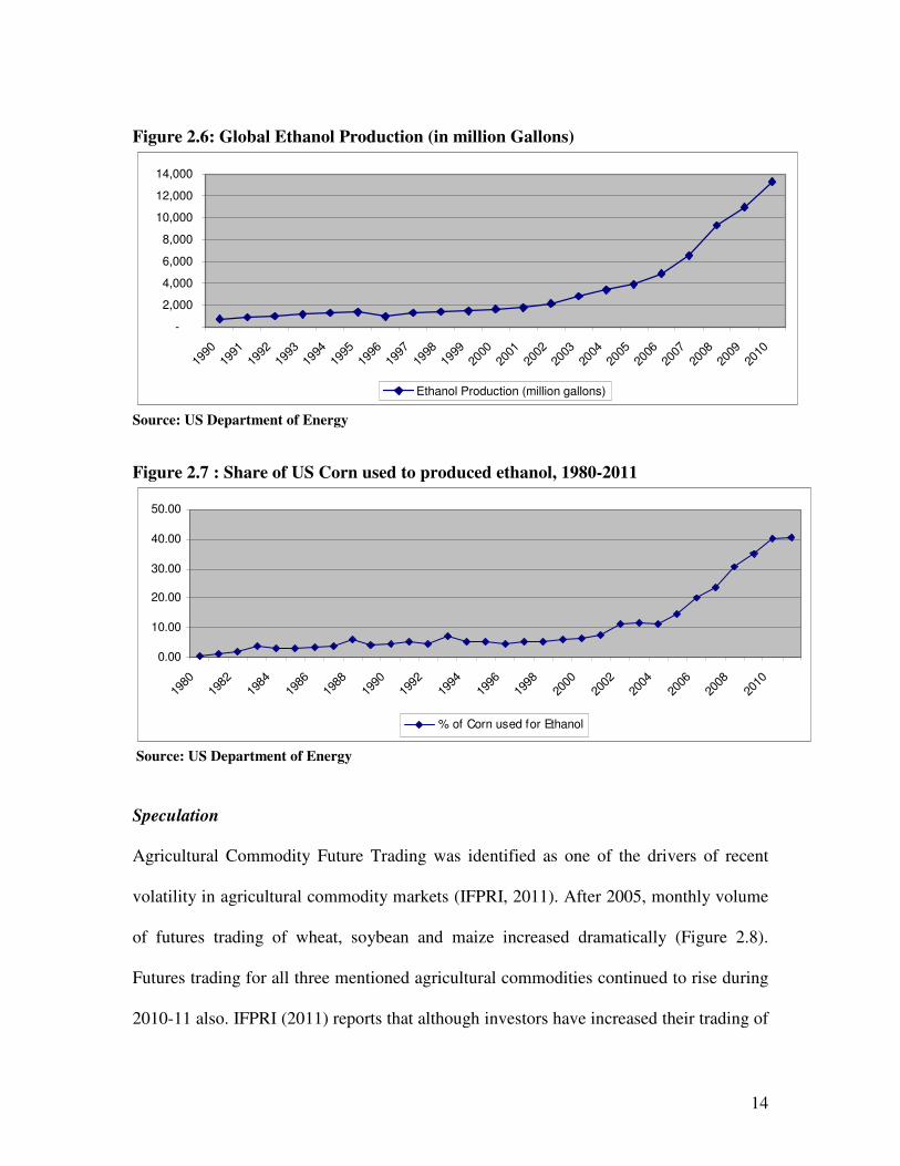
biofuel mandates set by the United States and European Union (Figure 2.6). The primary

motivation for biofuel support is that biofuels will reduce demand for imported oil. To

comply with the mandate and support, farmers switched to production of biofuel crops ,

most of which are also used as food or feed. Figure 2.7 shows that in recent years more

than 40 % of US maize is used for ethanol production. Moreover, input demand for

biofuel crops increased recent years which contributed to the overall increase of cost of

agricultural inputs (IFPRI, 2011).

Production of biofuel crops strengthens the links between two highly volatile

markets- energy market and food market (IFPRI, 2011). Since ethanol is the substitute of

fuel, when the price of one barrel of fuel increases, the demand for ethanol, a substitute

product of fuel, also increases. This eventually increases the demand and consequentially

the price for corn (Weersink et al. 2008).

14

Figure 2.6: Global Ethanol Production (in million Gallons)

-

2,000

4,000

6,000

8,000

10,000

12,000

14,000

1990

1991

1992

1993

1994

1995

1996

1997

1998

1999

2000

2001

2002

2003

2004

2005

2006

2007

2008

2009

2010

Ethanol Production (million gallons)

Source: US Department of Energy

Figure 2.7 : Share of US Corn used to produced ethanol, 1980-2011

0.00

10.00

20.00

30.00

40.00

50.00

1980

1982

1984

1986

1988

1990

1992

1994

1996

1998

2000

2002

2004

2006

2008

2010

% of Corn used for Ethanol

Source: US Department of Energy

Speculation

Agricultural Commodity Future Trading was identified as one of the drivers of recent

volatility in agricultural commodity markets (IFPRI, 2011). After 2005, monthly volume

of futures trading of wheat, soybean and maize increased dramatically (Figure 2.8).

Futures trading for all three mentioned agricultural commodities continued to rise during

2010-11 also. IFPRI (2011) reports that although investors have increased their trading of

15

food commodity futures, only two per cent of these futures contract have resulted in

delivery of real goods. For example, the volume of futures traded on exchange worldwide

for maize is more than three times greater than the global production of maize.

Commodity index fund have became attractive for the investors as investment fund

flowed from the equity market, to real estate and now to the commodity markets. This

pattern of increasing agricultural commodity futures trading and higher prices for

commodity futures can worsen the volatility of spot prices for food commodities to

excessive levels (IFPRI, 2011).

Figure 2.8: Monthly Volume of Future Trades of Wheat, Maize and Soybeans at

Chicago Board of Trade (CBOT)

Source: IFPRI (2011)

Speculative behavior by governments (i.e., export bans, large stock orders) has also

played a role in increasing the volatility in agricultural commodity market. A number of

countries adopted supply restraint policies at the beginning of the high price volatilities in

2007. For example, rice export was banned by India, Vietnam, Egypt and Cambodia; and

Argentina and Ukraine banned export of wheat. This supply cut from the major suppliers

in the global grain market fueled the price volatilities of agricultural commodities even

more.

16

Aside from supply restraint policies, foreign buyers started to stockpile food

grains in response to food crisis and riots. Countries started to order for larger orders

rather than purchase one or two month’s supply at a time regardless of price and scarcity

of food grain (Weersink et al. 2008). This kind of speculative purchasing has also

contributed to price spike and volatilities in agricultural commodity market (BIAC,

2011).

Demand from Developing Countries

In recent years, several developing countries experienced rapid economic growth . As a

result of per capita income increase (Figure 2.9), consumers of developing countries are

enjoying more purchasing power which ultimately results in increased demand of

commodities.

Figure 2.10 shows the dramatic increase of per capita GDP in China and India.

Because of Spectacular economic growth in developing countries a big portion of their

population came out of poverty and demanding more grains. On the other hand, because

of the increased income, middle and upper income population of those countries shifted

their demand from grain to other high valued commodities such as meat, dairy, fruits,

vegetables and fish. The rise in demand for meat, in turn, boosts the demand for grains to

feed animals (Weersink et al 2008). As a result, it contributes to increase of food price.

17

Figure 2.9: Per Capita Income Level by Developing Region

0

500

1000

1500

2000

2500

3000

3500

Sub-Saharan

Africa

Middle East and

North Africa

Southeast Asia South Asia East Asia

1995 2020

Source: IFPRI Impact Simulation

Figure 2.10: GDP Per Capita of India and China (Constant US Dollar)

0

500

1000

1500

2000

2500

3000

1970 1975 1980 1985 1990 1995 2000 2005 2010

China

India

Source: WDI Database

Climatic Factors

Climate factors also contributed to the price volatilities in 2007-08 and again 2010.

Export markets for major agricultural commodities are highly concentrated. For example,

in 2008, 84% of maize was exported by only 5 countries, top five exporters of wheat

18

exported 63% of total wheat exports and 85% export share of milled rice were held by

top 5 rice exporters (Figure 2.11a, 2.11b and 2.11c). Because of this high level of

concentration, the world’s capacity to cope with shocks became limited (IFPRI, 2008).

Any incidence of poor weather in the major exporting countries or other types of

production shocks immediately affect the international price and price volatilities. For

example, wheat crop failure due to drought in Australia in 2008 and Russian federation in

2010 brought strong market reaction and soaring price.

Figure 2.11 a: Major Exporters of Maize in 2008

US

53%

Argentina

15%

Brazil

6%

France

6%

India

4%

ROW

16%

US

Argentina

Brazil

France

India

Others

Source: FAOSATAT Database

Figure 2.11 b: Major Exporters of Wheat in 2008

19

US

23%

France

12%

Canada

12%

Russian

Federation

9%

Argentina

7%

ROW

37%

US

France

Canada

Russian Federation

Argentina

Others


Figure 2.11 c: Major Exporters of Rice in 2008

Thailand

37%

Vietnam

20%

Pakistan

11%

India

10%

US

7%

ROW

15%Thailand

Vietnam

Pakistan

India

US

Others


Stocks of Cereals

Global stocks of cereal, measured as stocks to cereal use, came down to historically low

level in 2007-08 and from then it always remains around 21 whereas before 2003-04 it

used to remain more than 30. IFPRI (2011) reports that stock to use ratios of wheat were

always low during the price spikes in of wheat in the 1970s, 1995-96, 2007-08 and 2010-

20

11. The current level of stocks to cereal use made the cereal market very vulnerable to

any shock. A small dip in grain stocks may lead to major volatility in world cereal

market. Wright (2012) argues that when stocks are already tight a minor shock can have

major consequences on prices of agricultural commodities.

Figure 2.12: Stocks to cereal use ratio

15.0

17.0

19.0

21.0

23.0

25.0

27.0

2002/03 2003/04 2004/05 2005/06 2006/07 2007/08 2008/09 2009/10 2010/11 2011/12 2012/13

Source: FAO Cereal Supply and Demand Brief

2.4. Chapter Summary

This chapter provides a brief overview of the recent trend of exchange rate of major

currencies, price of major agricultural commodities and their volatilities. The descriptive

statistics presented in this chapter suggests that volatilities of both exchange rate and

commodity price increased in recent years. Therefore, it is important to investigate their

effects on agricultural commodity trade. The next chapter provides a review of key

literature on effects of exchange rate volatility and commodity price volatility on

international trade.

21

Chapter 3: Literature Review

3.1: Effects of Exchange Rate Volatilities: Theoretical Background

Attention to exchange rate volatilities was first drawn after switching of the major

currencies of the world to a floating exchange rate system from the previous fixed regime

in 1973. Early theoretical contribution (Ethier, 1973) on effects of exchange rate

volatilities on trade flows asserts that exchange rate volatilities have a negative effect on

volume of trade if traders do not have idea about how exchange rate volatilities will

affect their expected profit.

Clark (1973) argued that exposure to exchange rate volatility creates risk over

firms’ profit and to insulate themselves from uncertainty over profit due to exchange rate

volatilities firms tend to reduce trade. A competitive firm (i) with no market power , (ii)

producing only one commodity which is sold entirely to one foreign market, (iii)

receiving payments in foreign currency, (iv) operating in a condition where hedging

through forward sales of the foreign currency export sales is not possible; and (v) unable

to alter its output in response to favorable or unfavorable shifts in the profitability of its

exports arising from movements in the exchange rate is adversely affected by greater

volatility in the exchange rate. This leads to a reduction in output, and hence in exports,

in order to reduce the exposure to risk (Clark, 1973).

However, in the presence of hedging possibility, the effect of exchange rate

volatility largely depends on the firm’s response to risk and uncertainty. If traders are risk

averse, an increase in exchange risk will unambiguously reduce the volume of trade

whether the risk is borne by importers or exporters. It also depends on who bears the risk.

22

If importers bear the risk, the price will fall as import demand falls, whereas if exporters

bear the risk, the price will raise as exporters charge an increasingly higher risk premium

(Hooper and Kohlhagen, 1978). With an inelastic supply (marginal cost) curve, a shift of

aggregate import demand (and thus marginal revenue) to the left caused by an increase in

exchange risk to the importer, will result in a relatively large drop in price and a

relatively small drop in quantity. If exporters bear the risk and face inelastic demand for

their output, an increase in exchange risk will shift their supply to the left and induce a

relatively large increase in price and a small decrease in quantity.

Exposure of unforeseen movements in exchange rate is low in advanced

economies where well developed forward market exists, i.e. a specific transaction can be

easily hedged (IMF, 2004). However, such markets do not exist for the currencies of

most developing and low income countries.

Opposite view of the effects of exchange rate volatilities on trade flows is also

available in literature. Increased exchange rate volatility positively affects the value of

exporting firms through the price and volume impacts of exchange rates, and also makes

an exporting strategy more attractive relative to the direct investment. As a result,

exchange rate volatility can be positively related to investment in export production

capacity (Sercu and Vanhulle, 1992).

3.2 Measuring Exchange Rate and Price Volatilities

The methods of measuring exchanged rate volatilities went through a process of

evolution in last three decades. However, still no single process dominates the

approximation of exchange rate volatilities. The most commonly use measure of

exchange rate volatilities are measure of variance. However the construction of the

23

measure of variance widely differed in from study to study (Bahmani-osokee and Hegerty

2007). Few approaches of measuring volatilities are historical volatility, implied

volatility, rolling window, within period volatility, moving standard deviation, General

Autoregressive Conditional Heteroskedasticity (GARCH) etc.

Here we will briefly discuss different measures of volatilities used in exchange

rate and trade related research in recent years.

The standard deviation of daily observations of the nominal exchange rate during

each three-month period was one of the first measures of exchange rate volatilities in

empirical literature (Akhter and Hilton, 1984). Later studies adopted the moving

standard deviation of the monthly change in the exchange rate to measure the exchange

rate volatilities (Kenen and Rodrik, 1986; Cushman, 1986; Chowdhury, 1993). This

method had some advantage over other contemporary methods for being stationary.

Autoregressive Conditional Heteroskedasticity (ARCH) became very popular in

measuring exchange rate volatilities afterwards. ARCH is a measure of volatility in time

series errors. ARCH models assume the variance of the current error term to be a function

of the actual sizes of the previous time periods' error terms. A number of studies (Arize et

al. 2005; Cho et al. 2002; McKenzie and Brooks, 1997) used ARCH process to measure

the exchange rate volatilities.

A further extension of ARCH process is Generalized Autoregressive Conditional

Heteroskedasticity (ARCH) which incorporates moving average process. GARCH

became popular in measuring exchange rate volatilities in recent years.

24

3.3 Empirical Literature: Exchange rate Volatility and Trade

The findings of empirical literature on the effect of exchange rate volatilities on trade

flows are mixed and not conclusive. This section briefly discusses the findings of some

empirical studies on this issue.

From the earlier empirical studies it was evident that exchange volatilities have a

negative impact on exports (Akhter and Hilton, 1984). The study used a polynomial

distributed lag method in their OLS estimate of the effects of exchange rate volatility on

trade flows. Their result confirms the theoretical assertion that exchange rate volatilities

reduce international trade. According to their model the export volume is a function of

foreign income, foreign capacity utilization and relative prices; and import volume is a

function of domestic income, the ratio of foreign to domestic capacity utilization, and

relative prices. They measure the using data for the USA and Germany; they estimated

their models using quarterly data over the period 1974-1981 and found that volatility had

a significantly negative effect on US imports, German exports and imports but no effect

on US exports.

However, the findings of the above study (Akhter and Hilton, 1984) were

challenged by a further study (Gotur, 1985) which used the same methodology as Akhter

and Hilton with certain modification. It included France, the UK and Japan in the model,

applied the Cochrane-Orcutt procedure to control for autocorrelation only when the

Durbin-Watson statistic calls for autocorrelation (Akhter and Hilton used it even in the

cases in which the problem was not even present ), changed the sample period under

investigation to account for lag structure and to incorporate the rate of change, rather than

the level, of the exchange rate. After these modifications she found that German exports

25

and imports have been negatively impacted, and Japanese exports are positively affected,

but the other seven trade flows were not affected.

However, both of the above mentioned studies suffer from spurious regression

problem because none of them accounted for integrating properties of variables

(Bahmani-Osokee and Hegerty, 2007).

A number of recent studies also found a negative relationship between exchange

rate volatilities and trade flows. For example, significant negative relationship between

real exchange rate volatility and export volume in short run and long run was found for

eight South American countries (Arize et al. 2008). By using Error Correction Model

Chou (2000) found significantly negative relationship between export volume and

volatility of real effective exchange rate (REER) for trade flows of industrial materials,

mineral and fuels; and manufactured good. However, the relation was not significant for

foodstuffs. Significant negative relationship was also found between exchange rate

volatilities and export supply for all the G7 countries and their partners for twenty one

industries (Peridy, 2003).

In contrast to the findings of the above mentioned studies, a positive relationship

between exchange rate volatilities and international trade flows was also found in few

empirical literature, mostly for bi-lateral trade (McKenzie and Brooks, 1997; Poon et al.

2005 ). While a number of studies found no significant effect of exchange rate volatilities

on trade flows (Kenen 1980, Thursby, 1980; IMF, 1984; Baily et al. 1986, Toneryo,

2004). As a result, the relationship between exchange rate volatilities and trade flows still

remain ambiguous.

26

The inconclusive relation between exchange rate volatilities and trade flows was

explained by the argument that exchange rate volatility is an ‘inadequate indicator’ of

price risk faced by firms since an increase in exchange rate volatilities may not

necessarily increase real domestic currency price volatilities (Smith, 1991).

Another explanation behind not getting any systematic relationship between

exchange rate volatilities and trade volume is undermining of a series of problems related

to the methods of estimation which might lead to imprecise statistical results (Bini-

Smaghi, 1997).

IMF (2004) observed that while exchange rate fluctuations have increased in

times of currency and balance of payments crises during the 1980s and 1990s, there has

not been any increase, on average, in such volatility between the 1970s and the 1990s. It

also found some empirical evidence of negative relationship between exchange rate

volatility and trade. However, such a negative relationship is not robust and It concludes

that if exchange rate volatility has a negative effect on trade, this effect would appear to

be fairly small and is not robust.

3.4 Empirical Literature: Exchange Rate Volatility and Agricultural Trade

Despite an extensive literature on effect of exchange rate volatility on overall trade, very

few studies (Cho et al. 2002; Kandilov, 2008; Zhang, 2010) explored the impact of

exchange rate and other volatilities on agricultural trade. Compared to the other sectors,

agriculture trade was found to be more sensitive to exchange rate uncertainties in

developed countries. Using a sample of bilateral trade flows across ten developed

countries (G 10 countries) Cho et al (2002) shows that the real exchange rate uncertainty

27

has had a significant negative effect on agricultural trade and the negative impact on

agricultural trade was more significant compare to the other sectors.

Agricultural exports from developing countries are much more vulnerable to

exchange rate volatilities compared to the exports from developed countries. Kandilov

(2008) found that the effect of exchange rate volatility is largest for developing country

exporters and smallest for developed exporters. Since developing countries do trade with

vehicle currency (US Dollar) only exchange rate volatility of the vehicle currency (U.S.

dollar), and not the exporter-importer currency, matters for developing country exporters

(Kandilov, 2008).

Villanueva and Sarker (2009) conducted a study to examine the effects of

exchange rate volatility on fresh tomato imports into the United States from Mexico.

They showed with the cointegration analysis that while changes in exchange rate have a

positive effect on trade flows, volatility of the exchange rate has a significant negative

effect on trade flows.

Although other volatilities (e.g. commodity price volatility and freight cost

volatility) may have much potential to affect international trade, only the effect of

exchange rate volatilities received much attention in the literature. Zhang et al (2010)

found that although commodity price and freight cost volatilities have no significant

impact on traded volume of soy bean between U.S. and Brazil, these two volatilities play

important roles in determining U.S. soy bean trade with China. The authors explained

that possibilities of hedging and market power are two important factors in determining

the effects of volatilities on trade.

28

3.5 Chapter summary

This chapter reviews the existing literature on the effects of exchange rate volatility and

commodity price volatility on international trade flows. Although a number of literature

exists on the effects of exchange rate on trade flows, literature on commodity price

volatilities on international trade is scarce. The next chapter presents the theoretical

framework used in this study.

29

Chapter 4: Conceptual Framework

4.1 Model Description

This study used Hooper and Kohlhagen’s (1978) trade model that derived the demand

and supply functions for individual firms and then aggregated to derive market demand

and supply to obtain reduced form equations for market equilibrium price and quantity.

Hooper and Kohlhagen developed the model for an individual firm importing a

commodity under exchange rate uncertainty. This study extends Hooper and kohlhagen’s

model by incorporating commodity price uncertainty into it. It is worth mentioning that

Zhang (2010) developed a model, based on Hopper and Kohlhagen’s model, which

included exchange rate, price and ocean freight cost uncertainties.

4.2 Import Demand

According to Hopper and Kohlhagen’s (1978) trade model, suppose a firm uses imported

commodity as inputs to produce final goods. The importer faces a linear demand

function for its output (Q), which is an increasing function of domestic income (Y), the

prices of substitutes (PD) and a decreasing function of its own price:

cYbPDaPQ ++= (4.1)

Following Hooper-Kohlhagen’s (1978) model, the model assumes a two period

framework where in the first period the firm receives orders for its domestic output and

places order for its imported input; and in the second period it receives the imported input

and pays for it and ships and gets paid for its own output. The firm sets the level of its

output to maximize its utility, which is an increasing function of its expected profits and a

30

decreasing function of the standard deviation of profits. The firm’s optimization problem

can be written as:

2/1))(()()(max πγππ VEUQ

−= (4.2)

where U is the total utility, π is profit, E is the expected value, V is the variance and γ is

the relative measure of risk preference where γ >0 implies risk aversion, γ =0 implies

risk neutrality and γ <0 represents risk loving.

The firm’s profit π in domestic currency can be formulated as:

π = Q * P(Q )−UC *Q − HM * iQ (4.3)

where Q is the amount of output, P is the domestic price per unit output faced by the firm,

UC is the unit cost of output, H is the weighted average cost of foreign exchange to the

importer, M is the cost of imported inputs, i is the fixed ratio of imports to total output.

If q is the quantity of imports needed to produce Q amount of output then q can be

defined as

iQq = (4.4)

In this study, I assume that the importer can hedge foreign exchange risk by purchasing

foreign exchange in advance and hedge commodity price in the future market. Suppose

the firm hedges a constant proportion (α ) in the forward market at the futures exchange

rate, ~

R ; the remain proportion (1-α ) of foreign exchange is purchased at the spot

exchange rate R. So, H can be defined as:

31

~

)1( RRH αα +−= (4.5)

~

P is the commodity future market price in foreign currency,

M=~

P (4.6)

By substituting Equations 5 and 6 into Equation 3, importer’s profit is obtained:

iQPRRQUCQPQ *])1[(*)(*~~

ααπ +−−−= (4.7)

In which Q0 denotes, ……….It is assumed that, in Equation 7, all the variable except

~

R and ~

p are known with certainty on the contract date. Thus, the variance in the

importing firm’s profit is:

2222~~~ )(].)1[()(PRp

iQiQRV σασαπ +−= (4.8)

where 2~

P

σ and 2

~`~

PR

σ are the variances of ~

P and~~

PR , respectively.

Substituting (8) into (2),

iQRiQPEHEQUCQQPUPRp

.])1[(.)()(.)( 2/122222~

~~~ γσασα +−−−−=

(4.9)

The first-order condition for equation with respect to output quantity (9) is:

0.])1[()()()()/(/ 2/122222~

~~~ =+−−−−+= iRiPEHEUCQPdQdPQdQdUPRp

γσασα

(4.10)

32

Substituting for dQdP / from Equation 1,

0.])1[()()()()/( 2/122222~

~~~ =+−−−−+ iRiPEHEUCQPaQPRp

γσασα (4.11)

Substituting iQq = from (4) into (11)

]])1[()()()[2/())(2/( 2/12222~

2

~~

~

PRP

RiPEHEaicYbPDaUCiq σασαγ +−++++=

(4.12)

Since 2

~~PR

σ = 2222~

22~

~~~~ )()(RPRP

PERE σσσσ ++ , (Bohrnstedt and Goldberger, 1969)

22~

222~~

2~~ )]([)1[()()]()1)[[(2/())(2/(PP

RERiPERERaicYbPDaUCiq σασαγαα +−++−+++=

]])]([ 22222~

2~~~

RPR

PE σσασα ++

(4.13)

If γ >0,

0}])]({[)1[()2/(/ 222~

2222~~ <++−=RP

RERaiddq σαααγσ (4.14)

and

])}([{)2/(/ 22~

222~~

pR

PEaiddq σγασ += <0

(4.15)

Therefore, from equation (14) and (15) it can be asserted that if the importers are risk

averse an increase in exchange rate or commodity price volatility will reduce the volume

of import. If the importers are risk neutral (γ =0), exchange rate or commodity price

33

volatility will not have any effect of import demand. In the case of risk-loving importers

(γ <0), an increase in exchange rate and commodity price volatility will increase the

import.

Assuming that all firms are homogenous2, firm level import demands can be summed into

the following aggregate import demand function.

(4.16)

4.3 Chapter Summary

This chapter discusses the theoretical framework used in this thesis. I used a modified

version of Hooper-Kohlhagen import demand model. Hooper and Kohlhagen (1978)

derived this model to show the effect of exchange rate volatility on imports. I

incorporated food price volatility to the original Hooper-Kohlhagen model and derived

the effects of exchange rate volatility and commodity price volatility on import demand.

2 The limitation of this assumption is that all firms may not have the same level of risk preference.

),,,)(),(,,,( ~~~~

~~

PRRP

d PEREYPDUCgQ σσσσ=

34

Chapter 5: Empirical Framework

5.1 Econometric specification

This study used panel data models to estimates the effects of exchange rate and

commodity price volatilities on trade flows using a panel data regression model.

In line with the modified Hooper-Kohlhagen model with price volatility presented in the

chapter 4, I used the following empirical model to estimate the effects of exchange rate

and commodity price volatilities on Canada’s export and import:

(5.1)

Where

itpimpln Natural logarithm of country i’s per capita import at period t

itXVln Natural logarithm of Country i’s exchange rate volatility at period t

ln itPV Natural logarithm of price volatility country i faces at period t

itPCGDPln Natural logarithm of country i’s per capita GDP at period t

itPln Natural logarithm of import price of country i at period t

)(ln 1+itt PE =lnFt,t+1 Natural logarithm of expected price of import of country i at period t,

Ln Ft,t+1 Natural logarithm of futures price

ijtERln Natural logarithm of Country i’s exchange rate with country j

D_Q2 Dummy variable3 for Quarter 2



T Time trend

3 For quarterly models



tiijtittititititit eTQDERPEPPCGDPPVXVpimp +++++++++= + 8761543210 _ln)(lnlnln.lnlnln βββββββββ

35

5.2 Variable Description

Dependent Variable: Per capita volume of import

Quarterly and annual real per capita volumes of imports of commodities measured in

metric ton are used as dependent variables respectively for quarterly and annual models.

Total import volumes are divided by the population to obtain per capita volume of

import. Since I used per capita real GDP as an independent variable, dependent variable

is also transformed to per capita. For quarterly models of wheat and soybean, per capita

import volumes of wheat and soybean from Canada by its major importers are used as

dependent variable. On the other hand, Canada’s per capita volume of import of corn and

rice from its major importing sources are used as the dependent variable. For annual

models, the per capita import volumes of top importers of each commodity are

considered as the dependent variable.

Independent Variables

Exchange Rate

Quarterly and annual nominal exchange rates (exporters’ currency per unit of importer’s

currency) of each period are used. Therefore, it is expected that if exchange rate

appreciates, cost of imports will be cheaper for importers. Exchange rate data are

obtained from Thompson-Reuters DataStream (http://online.thomsonreuters.com)

through the University of Guelph Data Resource Centre.

36

Import price

Unit price of import is considered as import price. Unit price of import is calculated by

dividing the value of import in U.S. dollar by the quantity of import measured in ton.

Since real volume of imports is used as dependent variable, nominal unit prices are

converted to real prices using U.S. Consumer Price Index (Base year 1982=100). Note

that unit price indices may create bias in estimation because of the compositional changes

in quantities and quality mix of exports and imports. Even with best practice stratification

the scope for reducing such bias is limited due to the sparse variable list available on

customs documents (Silver, 2007). Despite this issue, unit value of import and export

prices are widely used because of their relatively low cost availability compared with

price surveys.

Expected price

The modified version of Hooper-Kohlhagen’s model presented in the Chapter 4 assumes

that firms are capable of hedging the risk of price volatility by operating in the futures

market. This assumption is valid for today’s world since real time futures price data are

readily available and forms can buy and sell in the commodity exchanges. Given this

backdrop, I used the Chicago Mercantile Exchange (CME) futures price, Fit, of the next

period as expected cash price, )(ln 1+itt PE . Futures price data are obtained from

Thompson-Reuters DataStream (2012). Recently developed price forecast models, e.g.,

the World Bank’s commodity price forecast (World Bank 2012), and USDA’s season

average price forecasts (USDA 2012), are also mainly based on futures price. Therefore,

it is reasonable to use futures price as importers’ expected price.

37

Expected exchange rate

Although expected exchange rate is a variable in my theoretical framework for import

demand in the Chapter 4, this variable was dropped from the empirical model. The reason

of dropping this variable is that forward exchange rates are available for very few

countries only. In their original work Hooper and Kohlhagen (1978) used next period’s

realized exchange rate as expected exchange rate. However, by taking the realized

exchange rate of the next period, one would violate one of the main assumptions of the

model that exchange rates are uncertain and assumes that traders can forecast perfectly.

Exchange rate volatility

Exchange rate volatility is one of the main independent variables of the empirical model.

While a variety of exchange rate volatility measures have been used in the literature,

there is still no consensus on which measure is the most appropriate (Clark et al. 2004).

The disagreement is partly due to the fact that there is no generally accepted theory of the

impact of exchange rate volatility on firm behavior (Kandilv, 2008). Most often, some

variant of the standard deviation of the annual or monthly exchange rate is used to

measure volatility (Kandilov, 2008; Cho et al. 2002; Clark et al. 2004; Frankel and Wei,

1993; Rose, 2000; Tenreyro 2007 ).

Following Kandilov (2008) I measured the exchange rate volatility between

countries i and j in period t, ijtXV as the standard deviation of the first difference of

the natural logarithm of the daily exchange rate between the two countries over a period6:

6 Three months period for quarterly and one year period for annual

38

XVijt

=Std[lnXijt,d

− lnXijt,d-1

], for d = 1,2,..., end of the period. (5.2)

where

=tijXV Exchange rate volatility between country i and j over period t;

Std=Standard deviation

dijt,lnX =Natural logarithm of nominal exchange rate between country i and j on day d in

period t

1-dijt,lnX = Natural logarithm of nominal exchange rate between country i and j on day d-1

in period t

End of the period = the last day of the period; for example, for monthly data, the 30th or 31st

calendar day; for quarterly data, the 90th day of the quarter.

Both real and nominal exchange rates were widely used in the previous studies. For

example, Pick (1990), Arize, et al. (2000), and Cho et al. (2002) used real exchange rate

while Tenreyro (2007) and some other studies used nominal exchange rate. Kandilov

(2008) noted that for all industrial and developing countries there is little difference

between the real and the nominal exchange rate volatility in practice. Thursby and

Thursby (1987) also showed that real and nominal exchange rate volatilities do not have a

different effect on trade flows. As a result, it is reasonable to use nominal exchange rate

in this study.

Price volatility

We used the same method as exchange rate volatility to calculate price volatility using

monthly representative international prices for each commodity. Since daily data of

prices is not available for each commodity and country, we used monthly real price data.

39

Monthly nominal price data in U.S. dollar are obtained from FAOSTATS (FAO 2012)

and then deflated to real prices using U.S. Consumer Price Index (Base year 1982=100).

Following formula is used to compute price volatility:

PV= Std[lnPm

− lnPm-1

] (5.3)

Where

PV denotes the price volatility

Std represents standard deviation;

mlnP =Natural logarithm of price at month m;

1-mlnP =Natural logarithm of price at month m-1

It should be mentioned here that the correlation between real and nominal price volatility

is found to be very high, ranges 0.85 to 0.92.

Real Gross Domestic Product (GDP) per capita

Real GDP data for importing countries, obtained from USDA-Economic Research

Service (USDA-ERS 2012: http://www.ers.usda.gov/data-products/international-

macroeconomic-data-set.aspx), are divided by population to obtain real GDP per capita.

Since it is adjusted to the population of the importer, GDP per capita is a better measure

for country’s income and well being.

Quarterly Dummies

For our quarterly models, three quarterly dummies for second, third and fourth quarters

were used for seasonality.

40

Time trend variable

Time trend variables account for any time-variant effects that are not captured in the

regression. We used time trend variable in both quarterly and annual models.

5.3 Data and sources

The data used in this study comes from various sources such as the Canadian

International Merchandise Trade (CIMT) online database, the United States Department

of Agriculture (USDA), Thompson-Reuters DataStream, EUROSTAT and FAOSTAT

and Tri University Data Resources (TDR), University of Guelph. A detailed account of

data sources are provided in this section.

Import and Export data

Quarterly data of Imports and exports data of crops (including corn, rice, soybean and

wheat) ranging from 2000 to 2010 are obtained from the Canadian International

Merchandise Trade (CIMT: link) of Statistics Canada (CIMT, 2011). They are strongly

balanced panel data, which denotes the real volumes (in metric tons) of export and import

data for wheat, soybean, corn and rice. Table 5.1 summarizes the quarterly trade data

used in the study:

41

Table 5.1: Summary of export and import data for quarterly models

Crop Trade

Flow

Unit (‘000) Time

Period

Source

Corn Import Metric Ton 2000 Q1-

2009 Q4

Canadian International

Merchandise Trade (CIMT):

http://www.statcan.gc.ca/trade-

commerce/data-donnee-eng.htm

Rice Import Metric Ton 2000 Q1-

2009 Q4

CIMT:



Soybean Export Metric Ton 2000 Q1-

2009 Q4

CIMT:



Wheat Export Metric Ton 2000 Q1-

2009 Q4

CIMT:



For annual model, we use FAOSTATS annual detailed trade matrix to get annual imports

data of wheat, soybean, corn and rice by for individual top developing and developed

importers from 1991 to 2009. Table 5.2 summarizes the import data used for this study.

Table 5.2: Summary of import data for annual models

Crop Trade

Flow

Unit (‘000) Time Period Source

Corn Import Metric Ton 1991-2009 FAOSTAT:

http://faostat.fao.org/

Rice Import Metric Ton 1991-2009 FAOSTAT:


Soybean Import Metric Ton 1991-2009 FAOSTAT:


Wheat Import Metric Ton 1991-2009 FAOSTAT:


42

Exchange rate, price and Gross domestic product (GDP) data

Daily exchange rate data was collected from Thompson-Reuters DataStream (2012).

Monthly price and per capita real GDP of countries are obtained of commodities are

obtained from United States Department of Agriculture (hereafter ‘USDA ERS’) (2012)

and Quarterly GDP data are collected from EUROSTAT (2012). Table 5.3 summarizes

the sources and frequency of exchange rate, price, per capita GDP and GDP data uses in

this study.

Table 5.3: Summery of Data Frequency and Sources for exchange rate, GDP prices

Data Frequency Data sources

Exchange Rate Daily Thompson-Reuters DataStream7 (2012)

(http://thomsonreuters.com/)

Commodity Price Daily Tri University Data Resources(TDR), University of

Guelph (http://tdr.tug-libraries.on.ca/)

Commodity Price Monthly United States Department of Agriculture (USDA

ERS 2012); (http://www.ers.usda.gov/data-

products/international-macroeconomic-data-

set.aspx)

Per capita real

gross domestic

products

Annual USDA Economic Research Service International

macroeconomic data set (USDA ERS 2012)

Real gross

domestic products

Quarterly EUROSTAT8(2012)

(http://epp.eurostat.ec.europa.eu)and

Division of Statistics of countries in the sample.

Countries

For quarterly models, the study considered Canada’s top and regular trading partners for

wheat, soybean, rice and corn. However, few important trading partners e.g., Venezuela

for wheat, could not be incorporated in this study because of unavailability of quarterly

7 Data base of Thompson-Reuters

8 Database of European Union

43

data for few variables. Table 5.4 provides the list of Canadian trading partners included

in each crop model.

Table 5.4: List of Countries for Quarterly Models

Commodities and Trade Flows Countries

Wheat Exports from Canada U.S., Italy. Japan, Morocco

Soybean Exports from Canada U.S., Japan, Germany, France, France, Netherlands,

Belgium, Malaysia. Hong Kong, the Philippines and Italy

Canada’s Corn Imports U.S. and Rest of the World

Canada’s Rice Imports Thailand, Pakistan, Italy and U.S.

For annual models, I included top importers of each commodity. The list of top importers

is provided in the table 5.5.

Table 5.5: List of importing countries considered for annual models

Commodity Countries

Developed: Germany, Italy, Japan, The Netherlands, Republic of Korea,

Spain and USA

Wheat

Developing: Algeria, Brazil, Indonesia, Malaysia, Mexico, Pakistan, the

Philippines, Turkey

Developed: Germany, Italy, Japan, The Netherlands, Norway, Portugal,

Republic of Korea, Spain, United Kingdom

Soybean

Developing: Argentina, China, Colombia, Indonesia, Mexico, the

Philippines, Thailand, Turkey

Developed: Canada, Hong Kong, France, Singapore, United States Rice

Developing: Brazil, China, Indonesia, Malaysia, the Philippines,

Cameroon

Developed: Canada, France, Germany, Italy, Japan, the Netherlands,

Republic of Korea, Spain, United Kingdom

Corn

Developing: Algeria, China, Colombia, Indonesia, Malaysia, Mexico,

Peru, Turkey

44

5.4 Model Selection

Balance Panel data were used for both our quarterly and annual models. This section

discusses the selection process of estimation models for panel data regression from fixed

effects model, random effects model and pooled OLS.

Fixed Effects Model

The fixed effects model assumes that the intercept term captures the individual

heterogeneity which implies that every country gets it own intercept while the slope

coefficients remain the same (Baltagi, 2005).

Consider a linear unobserved effects panel data model for N observations and T periods:

NiTtuaXY itiitit ,....,1;,...,1, ==++= β (5.4)

Where itY is the dependable variable for country i at period t, itX is the KN × regressor

matrix with observable time-variant independent variables, β is a 1×K vector of

coefficients, ia is the unobserved time variant country effect and itu is the independent

and identically normal distributed error terms.

If we average the equation for each i, we get

iiii uaXY−−−

++= 1β (5.5)

Where ∑ =

−−

=T

t ityTY1

1 , ∑ =

−−

=T

t iti uTu1

1 and ∑ =

−−

=T

t iti XTX1

1

Since ia is fixed over time, it appears in both(5.4) and (5.5). If we subtract (5.4) from

(5.5) for each t we get,

itititiitiitiit uXYuuXXYY....

1 )()( +=⇒−+−=−−−−

β (5.6)

45

Random Effects Model

The random effects model assumes that the unobserved time variant individual effect, ia

in (5.2.1) is uncorrelated with each explanatory variable (Baltagi, 2005):

TtXaCov iti ,...,2,1,0),( == (5.7)

In fact, the ideal random effect assumptions include all the fixed effect assumptions plus

the additional requirement that ia is independent of all explanatory variables in all time

periods.

Hausman specification test

In order to determine whether to use fixed effects or random effects models, Hausman

specification test can be performed. Hausman specification test shows how large the

difference in estimates is in relation to the variances of estimates (Baltagi, 2005). The

computation procedure of Hausman test is as follows:

)()]()([)(^^

1^^^^ REFEREFEREFE

VarVarH ββββββ −×−×′−= − (5.8)

Where FE^

β is the coefficient estimate of fixed effects model and RE^

β is the coefficient

estimate of random effects model.

The null hypothesis of the Hausman test is that there is no systematic difference

between coefficients of fixed and random effects models models. Fixed effects models

are chosen if the null hypothesis is rejected while random effects model are chosen

otherwise (Hausman 1978).

46

Testing for random effects: Breusch-Pagan Lagrange multiplier (LM)

In order to decide between a random effects regression and a simple OLS regression,

Breusch-Pagan Lagrangian multiplier test is suggested (Breusch and Pagan, 1980). The

null hypothesis in the LM test is that variances across entities are zero. That is, no

significant difference across units (i.e., no panel effect). Rejecting the null hypothesis

indicates the presence of unobserved effects and pooled OLS would not be efficient. We

conducted Breusch-Pagan Lagrangian multiplier test to decide between random effects

and pooled OLS regression model.

Test for Cross-sectional Dependence

In panel data regression analysis, it is typically assumed that disturbances in panel data

models are cross-sectionally independent. This assumption is particularly true for panels

with large cross section dimensions. However, macro panels with smaller cross section

dimension and sufficiently large time periods may have the problem of cross section

dependence (pesaran, 2004). Cross-sectional dependence may arise due to spatial or

spillover effects, or due to unobservable common factors (Su and Zhang, 2010). Macro

panels on countries or regions with long time series that do not account for cross-country

dependence may lead to misleading inference (Baltagi, 2008). In this study, we

conducted Pesaran’s cross-sectional dependence test (CD test). But, one of the possible

drawbacks of the CD test is that adding up positive and negative correlations may result

in failing to reject the null hypothesis of cross-sectional dependence even if there is

plenty of cross-sectional dependence in the errors. Hoyos and Sarafidis (2006) suggest

conducting Fees’ and Friedman’s CD test if the average absolute correlation of the

47

residuals is high in the Pesaran’s CD test. In this study, we conduct Friedman’s and

Frees’ CD test if the average absolute correlation of the residuals was high in Pesaran’s

CD test. In case of the presence of cross-sectional dependence in the panel, we presented

regression results with Driscoll-Kraay standard errors (Hoechle 2007).

5.5 Diagnostics: Tests for Unit root, Heteroscedasticity, Serial Correlation and

Multicollinearity

This section provides an overview of the diagnostics done in this study to test for unit

root, heteroscedasticity, serial correlation and multicollinearity. Results of the test

performed are reported in the following sections for each individual crop model.

Unit root test

It is now a common practice to test for unit root in time series econometrics (Baltagi,

2008). In panel data analysis, testing for unit root is relatively recent (Levin, Lin and Chu

2002, Im et al. 2003; Harris and Tzavalis, 1999; Maddala and Wu, 1999; Choi, 2001 and

Hadri, 2000). The stationarity or non-stationarity of a time series can strongly influence

its behavior and properties. If the variables in the regression model are not stationary, the

standard assumptions of asymptotic analysis will not be valid. Because of non-

stationarity the usual ‘t-ratios’ do not follow t-distribution. Therefore, the hypothesis test

cannot be considered valid. Such estimates are termed as ‘spurious regression’ by

Gramger and Newbold (1974) since they yield results with high R-squared values and

high t-ration with no econometric meaning. The problem of non-stationarity can be

treated by applying difference operator to the series (Kennedy, 2011).

48

In this study, we conducted Levin-Lin-Chu test for panel unit root in the cases where we

find cross sectional independence. Levin, Lin and Chu (2002) argue that individual unit

root tests have limited power against alternative hypotheses with highly persistent

deviations from equilibrium. They suggested a more powerful panel unit root test than

performing a separate unit root test for each cross section (Baltagi, 2008). The null

hypothesis is that each individual time series contains a unit root against the alternative

that each time series is stationary. In presence of cross sectional dependence, Fisher panel

unit root test (Maddala and Wu, 1999) and Pesaran’s crossectionally augmented Dickey

Fuller panel unit root test was conducted to detect unit roots (Pesaran, 2007).

Test for Serial Correlation

The presence of serial correlation in panel data models potentially biases the standard

errors (Drukker, 2003). As a result, it is important to test for serial correlation in the

idiosyncratic error term. Although a number of tests have been proposed to test for

autocorrelation in a panel data model, Wooldrige test (Wooldridge 2002) is the most

attractive because it requires relatively fewer assumptions and easy to implement

(Drukke,r 2003). We performed Wooldridge test for serial correlation in our panel data

models.

Test for Heteroscedasticity

Modified Wald test was applied to test the presence of heteroscedasticty in the fixed

effect panel data models (Baum, 2001). Some of the regression models in this study are

random effects models. Since there is no specific test to detect heteroscedasticty in

49

random effects model, we reported cluster-robust covariance estimators to avoid potential

presence of heteroscedasticity in random effect model.

Test for multicollinearity

Variance Inflation Factor (VIF) was used to check the severity of multicollinearity. The

VIF shows us how much the variance of the coefficient estimate is being inflated by

multicollinearity. As a rule of thumb, VIF greater than 10 suggests to concern about

multicollinearity and VIF greater than 30 suggests severe multicollinearity (Belsley, Kuh

and Welsh, 1980).

5.6 Chapter Summary

This chapter provides the model specification used in this study. It also introduced and

described the variables to be used in the empirical model. The next chapter provides the

coefficient estimates of the regression models.

50

Chapter 6: Results and Discussions

6.1 Introduction

This chapter provides the results and discussions of both quarterly and annual models.

Results of the diagnostic tests are also provided in this chapter. We estimated the effects

of exchange rate and commodity price volatilities on Canada’s trade with its major

trading partners for wheat, soybean, corn and rice with quarterly models. In addition, the

effects of volatilities on major developed and developing importers according to their

sources of imports were estimated with the annual models.

6.2 Quarterly Models

The quarterly models are estimated for Canada’s exports of wheat and soybean and

imports of corn and rice over the period 2000:Q1 to 2010:Q4. The list of Canada’s

trading partners for each commodity is provided in table 5.4 in chapter 5.

6.2.1 Quarterly Imports of Wheat and Soybean from Canada

The parameter estimates of quarterly export models of wheat and soybean are presented

in table 6.3. Before estimation, unit root tests are conducted. Fisher’s unit root test

statistics are presented in table 6.1. For both models, the unit root test suggests that log of

price volatility and log of exchange rate volatility are level stationery. For wheat, all

other variables are difference stationery. For soybean, log of real import price is level

stationery but log of expected price and exchange rate variables are difference stationery.

Therefore, first differences of the difference stationery variables are used as independent

variables.

51

Table 6.1: Fisher’s unit root test for wheat and soybean model

Wheat Model Soybean Model

Level First Difference Level First Difference

Ln Price

volatility

105.65***

(0.000)

305.69***

(0.00)

268.93***

(0.000)

713.41***

(0.000)

Ln Exchange

rate volatility

39.63***

(0.000)

226.98***

(0.000)

85.88***

(0.000)

494.13***

(0.000)

Ln Import Price 4.67

(0.78)

42.66***

(0.00)

102.97***

(0.000)

600.59

(0.000)

Ln Expected

price

2.754

(0.9488)

77.39***

(0.000)

25.67

(0.1767)

194.45***

(0.000)

Exchange rate 4.55

(0.8037)

88.19***

(0.000)

13.67

(0.8464)

479.62***

(0.000)

Ln per capita

real GDP

6.247

(0.6195)

215.91***

(0.000)

4.19

(0.518)

587.58***

(0.000) *,** and *** denote significance level at 10%, 5% and 1% respectively. Numbers in parentheses denote P value

Based on the results of Fisher’s unit root test, my empirical framework is specified as:

(6.1)

The Hausman test is performed to test whether a fixed or random effects model is

appropriate. The Hausman's test statistic for the wheat regression is 31.68 with a p-value

of 0.000, suggesting that a fixed effects model is preferred to a random effects model. To

test for cross-sectional dependence the Friedman’s test is conducted. The test statistic for

Friedman’s test is 79.316 with a p-value of 0.000, which suggests the presence of cross-

sectional dependence for wheat quarterly model. Therefore, a fixed effects regression

with Driscoll Kraay robust standard error was chosen to estimate the wheat model.

The Hausman’s test statistic for the soybean model is 22.06 with a p-value of

0.001, suggesting that a fixed effects model is preferred to a random effects model. The

tiijtitt

ititititit

eTQDERPE

PPCGDPPVXVpimp

+++∆+∆

++∆+++=

+ 87615

43210

_ln)(ln

lnln.lnlnln

ββββ

βββββ

52

Friedman’s test statistic for the soybean regression model is 63.03 with a p-value of

0.000, which indicates the presence of cross-sectional dependence in the soybean

regression model. Therefore, soybean export model was estimated by a fixed effect

model with Driscoll-Kraay standard error.

Wooldridge test for autocorrelation in panel data is used to test if there is a serial

correlation. The statistic of this test follows F-distribution. The null hypothesis under this

test is that there is no first-order autocorrelation. For wheat model, the test statistics is

0.021 with a p-value of 0.893. Therefore, we fail to reject the null hypothesis of no serial

correlation in the wheat model at a five percent significance level. For soybean model,

Wooldridge test statistics is 3.02 with a p-value 0.11, indicating that we fail to reject the

null of no serial correlation in the soybean model at a five percent significance level.

Modified Wald test is commonly used to test if there is hetroscedasiticity in fixed

effects model. The test statistics of the Wald test follows a Chi-square distribution. The

computed statistics of Wald test statistic in the wheat model is 635 with a p-value of

0.000. Therefore, the null hypothesis of homoscedastic errors is rejected at a five percent

significance level. For the soybean model the computed statistics of Wald test is 452.23

with a p-value of 0.000, suggesting heteroscedastic errors in the soybean model.

To check for multicollinearity issues, the variance inflation factor is used. The

variance inflation factors (VIF) presented in the table 6.2 for both wheat and soybean

model shows that VIF for all variables in both models are below 2. Therefore,

multicollinearity should not be a concern for wheat and soybean model.

53

Table 6.2: VIF for wheat and soybean model

Variables VIF for wheat VIF for Soybean

Ln Price volatility 1.14 1.15

Ln Exchange rate volatility 1.41 1.21

Ln Import Price 1.44 1.81

Ln Expected price 1.06 1.03

Ln Exchange rate 1.54 1.56

Ln per capita real GDP 1.38 1.03

Time trend 1.23 1.17

Mean VIF 1.31 1.28

Table 6.3 reports the coefficients estimates of import demand of Canada’s wheat

and soybean by its major trading partners. For wheat model, results show that log of price

volatility and log of exchange rate volatility do not have significant effect on log of per

capita wheat import by canada’s major trading partners. Percentage change in real import

price has a negative and significant effect at a ten percent level of significance on log of

wheat import volume from Canada which expected because as current import price of a

commodity increases the demand for that commodity decreases. The positive and

significant (at a ten percent level significant) coefficient of percentage change in expected

price of the next period asserts that importers import more when they expect a price hike

in future. Percent change in exchange rate has a positive and significant effect on log of

per capita import of wheat at a one percent level of significance. It is expected because if

the importer’s exchange rate appreciates the cost of imports becomes cheaper for the

importer and import demand increases.

On the other hand, coefficients estimates of soybean model also yield similar results as

the wheat model. Percent change in real import price and nominal exchange rate has a

positive and significant effect on log of soybean import volume from Canada at a one

54

percent level of significance; and percentage change in expected price has a positive and

significant effect on log of per capita import volume of soybean from Canada at a one

percent level of significance. The positive and significant (at a one percent level of

significance) coefficient of time trend variable confirms that imports of soybean from

Canada by its major trading partners increased overtime.

Since expected price is usually not included in a typical import demand model

9, to

check the robustness of the results presented in table 6.3 reported, another regression

results in table 6.3a excluding the percentage change of expected price from the right

hand side. For both wheat and soybean models, log of exchange rate volatility and log

price volatility do not have significant effect on log of import volumes of wheat and

soybean from Canada. The signs of the other variables remain the same in the results

presented in the table 6.3 a.

9 Some of the literature that examine the effects of exchange rate volatility and price volatility (e.g. Zhang

2010) includes only the expected price or exchange rate. For comparison purpose results with expected

price are provided in the appendix B

55

Table 6.3: Coefficient estimates of quarterly wheat and soybean imports from

Canada from 2000 to 2009

Commodities

Dependent Variable:

Log of per capita import Wheat

Soybean

Independent variables Fixed Effect Fixed Effect

ln Price volatility

0.181

(0.122)

-0.083

(0.113)

ln Exchange rate volatility

-0.272

(0.541)

-0.1805

(0.191)

∆ ln Real Import Price 10

-1.25*

(0.722)

-0.7483***

(0.143)

∆ ln Expected Price

3.951*

(2.18)

0.6600**

(0.323)

∆ ln Exchange rate

6.241**

(4.19)

0.4716***

(0.015)

∆ ln Per Capita Real GDP

-5.639

(4.86)

-7.307

(2.56)

Dummy_Quarter 2

1.254

(0.913)

-2.0599**

(0.559_

Dummy_ Quarter3

1.0499

(1.10)

-0.7571

(0.115)

Dummy Quarter_4

0.8741

(1.07)

-0.0230

(0.134)

Timetrend

-0.011

(0.02)

0.0501***

(0.003)

Constant

-8.324*

(4.63)

-6.4412***

(1.83)

No. of Observation 171 390

R2 0.08 0.66

Prob > F 0.009 0.000 *. ** and *** denote significance level at 10%, 5% and 1% respectively. Numbers in parentheses are Driscoll-

Kraay robust standard errors

10

For soybean model, this variable was used at level since it is level stationery.

56

Table 6.3a : Coefficient estimates of quarterly wheat and soybean imports from

Canada from 2000 to 2009 (without expected price variable)

Commodities

Dependent Variable:


Soybean


ln Price volatility

0.211

(0.12)

-0.136

(0.115)


0.011

(0.74)

-0.149

(0.197)

∆ ln Real Import Price

-0.935*

(0.723)

-0.801***

(0.142)


7.404

(5.21)

0.471***

(0.015)

∆ ln Per Capita real GDP

-7.985

(5.87)

-8.207

(2.4)

Dummy_Quarter 2

1.925*

(1.05)

-2.296***

(0.52)

Dummy_ Quarter3

1.999*

(1.05)

-0.816***

(0.115)

Dummy Quarter_4

1.551

(1.13)

0.021

(0.14)

Timetrend

-0.004

(0.02)

0.051***

(0.003)

Constant

-1.902

(8.3)

-6.135***

(1.84)


R2 0.05 0.62



6.2.2. Quarterly import models of corn and rice

This section presents and discusses the coefficient estimates of corn and rice import

models. It also presents the results of regression diagnostics performed before the

estimations.

Table 6.4 reports the test statistics of Fisher’s unit root test. The null hypothesis of

the presence of unit root is rejected for log of price volatility and log of exchange rate

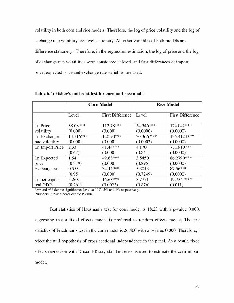
57

volatility in both corn and rice models. Therefore, the log of price volatility and the log of

exchange rate volatility are level stationery. All other variables of both models are

difference stationery. Therefore, in the regression estimation, the log of price and the log

of exchange rate volatilities were considered at level, and first differences of import

price, expected price and exchange rate variables are used.

Table 6.4: Fisher’s unit root test for corn and rice model

Corn Model Rice Model

Level First Difference Level First Difference

Ln Price

volatility

38.08***

(0.000)

112.78***

(0.000)

54.346***

(0.0000)

174.042***

(0.0000)

Ln Exchange

rate volatility

14.516***

(0.000)

120.90***

(0.000)

30.366 ***

(0.0002)

195.4121***

(0.0000)

Ln Import Price 2.33

(0.67)

41.44***

(0.000)

4.170

(0.841)

77.1910***

(0.0000)

Ln Expected

price

1.54

(0.819)

49.63***

(0.000)

3.5450

(0.895)

86.2790***

(0.0000)

Exchange rate 0.555

(0.95)

32.44***

(0.000)

5.3013

(0.7249)

87.56***

(0.0000)

Ln per capita

real GDP

5.268

(0.261)

16.68***

(0.0022)

3.7771

(0.876)

19.7347***

(0.011) *,** and *** denote significance level at 10%, 5% and 1% respectively.

Numbers in parentheses denote P value

Test statistics of Hausman’s test for corn model is 18.23 with a p-value 0.000,

suggesting that a fixed effects model is preferred to random effects model. The test

statistics of Friedman’s test in the corn model is 26.400 with a p-value 0.000. Therefore, I

reject the null hypothesis of cross-sectional independence in the panel. As a result, fixed

effects regression with Driscoll-Kraay standard error is used to estimate the corn import

model.

58

On the other hand, the Hausman’s test statistics computed for the rice model is

2490 with a p-value of 0.000. Thus, I reject the null hypothesis of that both estimates are

consistent. A fixed effect model is preferred in this case. Test statistics computed for

Friedman's test of cross sectional independence is 30.07 with a p-value of 0.00.

Therefore, I reject the null hypothesis of cross-sectional independence. A fixed effects

model with Driscoll-Kraay standard error is preferred in this case as well.

The test statistics of the Wooldridge test of serial correlation in the corn model is

16.81 with a p-value of 0.15. Therefore, I fail to reject the null hypothesis of no first

order serial correlation. For rice model, the Wooldridge test statistics is 5.807 with p-

value 0.09. Thus, I fail to reject the null hypothesis of no serial correlation at 5%

significance level for rice model also.

The test statistics of the modified Wald test for the corn model is 42.07 with a p-

value 0.000, suggesting to reject the null hypothesis of homoscedastic errors. For rice

model, the statistics of the modified Wald test is 758.03 with a p-value 0.00. This, I reject

the null hypothesis of no serial correlation.

VIFs for the explanatory variables of corn and rice model presented in the table

6.5 shows that the highest VIF for corn model is 1.97 (log of price volatility) and for rice

model is 1.5 (log of Price volatility). Since no variable of any of the two models is more

than 10, multicollinearity should not be a concern in corn and rice models.

59

Table 6.5: VIF for corn and rice model

Variables VIF for Corn VIF for Rice

Ln Price volatility 1.97 1.5

Ln Exchange rate volatility 1.42 1.47

Ln Import Price 1.37 1.1

Ln Expected price 1.35 1.09

Ln Exchange rate 1.34 1.06

Ln per capita real GDP 1.22 1.05

Time trend 1.57 1.01

Mean VIF 1.46 1.18

Table 6.6 presents the coefficient estimates of Canada’s corn and rice imports

from its major import sources. Results show that percentage change in real price and

nominal exchange rate volatilities do not have significant effects on log of per capita

import of corn and rice. Other variables also have the expected signs. Among the

significant variables, percentage change in real import price has a negative effect on the

log of per capita corn import at a ten percent level of significance and on the log of per

capita rice import at a one percent level of significance. Percentage change in per capita

real GDP has a positive and significant effect on the log of per capita corn and rice

import at a five percent and a one percent level of significance, respectively.

60


2000-2009

Dependent Variable:

Log of per capita import Corn

Rice


ln Price volatility

0.033

(0.067)

0.0307

(0.027)


-0.002

(0.167)

0.0271

(0.066)

∆ ln Real Import price

-1.022*

(0.618)

-0.460***

(0.085)


0.184

(0.404)

0.122

(0.211)


1.380

(1.18)

0.3294

(0.48)


1.381**

(0.488)

7.101***

(1.86)

Dummy_Quarter 2

-0.086

(0.127)

-1.36

(0.358)

Dummy_ Quarter3

0.029

(0.124)

-1.686***

(0.42)

Dummy Quarter_4

0.117

(0.136)

-1.211***

(0.35)

Timetrend

8.438

(0.014)

0.003***

(0.002)

Constant

2.04

(0.139)

-7.292*

(0.751)


R2 0.43 0.3257



Table 6.7 presents the coefficient estimates of corn and rice model excluding one

independent variable, i.e.; percentage change in expected price. The results show that

signs and significance of the main independent variables do not change significantly.

61


2000-2009 (without percentage change of expected price)

Commodities

Dependent Variable:


Rice


ln Price volatility

0.023

(0.06)

0.030

(0.02)


-0.014

(0.16)

0.024

(0.06)


-1.070*

(0.60)

-0.461***

(0.08)


-1.461

(1.16)

0.3292

(0.21)


1.431***

(0.46)

7.523***

(0.48)

Dummy_Quarter 2

-0.100

(0.12)

-1.43****

(0.35)

Dummy_ Quarter3

0.036

(0.121)

-1.777***

(0.42)

Dummy Quarter_4

0.135

(0.129)

-1.288***

(0.35)

Timetrend

0.13

(0.12)

0.003

(0.002)

Constant

8.750

(3.25)

-7.290***

(0.75)


R2 0.43 0.33



62

6.3 Annual Models

The previous section presented the results of quarterly regression models to examine the

effects of exchange rate and commodity price volatilities on Canada’s trade with its

major trading partners for wheat, soybean, corn and rice. This section provides the results

of the annual models which attempt to examine the effects of exchange rate commodity

price volatilities on import demand of top developed and developing importers for each

commodity. The following sections present the coefficients estimate of the following

trade flows:

1. Top developed importers’ imports from developed countries

2. Top developing importers’ import from developing countries.

6.3.1 Top developed importers’ imports from Developed exporters

This section presents and discusses the results of top developed importers’ import

demand of wheat, soybean, corn and rice from their developed trading partners.

Table 6.8 provides Fisher’s panel unit root test statistics for each variable used in

the regression models. The test statistics of the Fisher’s test reports that log of price

volatility is level stationery in all crop models except Corn. For corn, log of price

volatility is difference stationery. Log of exchange rate volatility is level stationery for all

four crops. Log of real import price, log of expected price, log of exchange rate and log

of per capita real GDP are difference stationery.

63

Table 6.8: Fisher’s panel Unit Root Test

Wheat Soybean Corn Rice

Level First

Differen

ce

Level First

Difference

Level First

Differen

ce

Level First

Difference

Ln Price

Volatility

213.30

***

(0.000)

229.51

***

(0.000)

0.2945

(1.000)

131.22

***

(0.000)

6.4049

(0.994)

286.589

***

(0.000)

40.79

***

(0.000)

99.825

***

(0.000)

Ln

Exchange

rate

Volatility

55.439

***

(0.000)

173.32

***

(0.000)

68.363

***

(0.000)

228.87

***

(0.000)

58.018

***

(0.000)

202.984

***

(0.000)

0.521

***

(0.007)

34.41

***

(0.000)

Ln Real

Import

Price

17.38

(0.17)

57.645

***

(0.000)

17.07

(0.518)

82.77

***

(0.000)

14.99

(0.662)

170.49

***

(0.000)

13.73

(0.32)

109.792

***

(0.000)

Ln

Expected

Price

21.645

(0.086)

158.96

***

(0.000)

8.29

(0.97)

71.006

***

(0.000)

11.34

(0.8791)

145.33

***

(0.000)

13.95

**

(0.31)

87.927

***

(0.000)

Ln

Exchange

rate

5.11

(0.984)

93.20

***

(0.000)

8.437

(0.971)

126.86

***

(0.000)

7.60

(0.983)

122.43

***

(0.000)

0.825

(0.991)

28.329

***

(0.001)

Ln

Percapita

real

GDP

6.725

(0.944)

17.519

***

(0.045)

10.412

(0.917)

19.435

**

(0.036)

6.92

(0.990)

18.75

**

(0.04)

3.6719

(0.072)

1.266

**

(0.009)

*,** and *** denote significance level at 10%, 5% and 1% respectively.


Table 6.9 and 6.10 presents the test statistics of Hausman model specification test

and Friedman’s test for cross-sectional independence respectively. Table reports that the

Hausman test statistics computed in the wheat model rejects the null hypothesis that both

estimates are consistent. As a result, a fixed effects model is preferred to a random effects

model for wheat regression. The test statistics for the Friedman’s test for cross sectional

independence in the wheat model rejects the null hypothesis of cross-sectional

independence. In order to address this problem, I estimate the model with Driscoll-Kraay

standard errors. Therefore, I estimate a fixed effects model with Driscoll-Kraay standard

errors to estimate the wheat model.

64

The Hausman’s statistics calculated in the soybean model fails to reject the null

hypothesis that both fixed effects and random effects estimates are consistent, suggesting

to use a fixed effects model. The Friedman test statistics in table 6.11 rejects the null

hypothesis of cross-sectional independence in the soybean model. Therefore, similar to

wheat model I estimate a pooled OLS model with Driscoll-Kraay standard error for

soybean model

The corn import model is also estimated as pooled OLS model with Driscoll-

Kraay standard errors since the Hausman’s test statistics rejects the null hypothesis that

both estimates are consistent; and Fridman’s test statistics rejects the null hypothesis of

cross-sectional independence in the panel.

The Hausman’s test statistics computed in the rice model rejects the null

hypothesis that both fixed and random effects estimates are consistent. The Friedman’s

test statistics in the table 6.11 rejects the null hypothesis of cross-sectional independence.

Thus, rice model is estimated with fixed effects model with Driscoll-Kraay standard

errors.

Table 6.9: Hausman Specification tests


Test

Statistics

P Value Test

Statistics

P Value Test

Statistics

P Value Test

Statistics

P

Value

12.59*** 0.000

0.34 0.98 28.33*** 0.001 20.97*** 0.00


Table 6.10: Friedman’s test for cross sectional independence


Test

Statistics

P Value Test

Statistics

P Value Test

Statistics

P Value Test

Statistics

P

Value

13.87** 0.03 35.956 0.000*** 24.548 0.0019** 6.181 0.04**


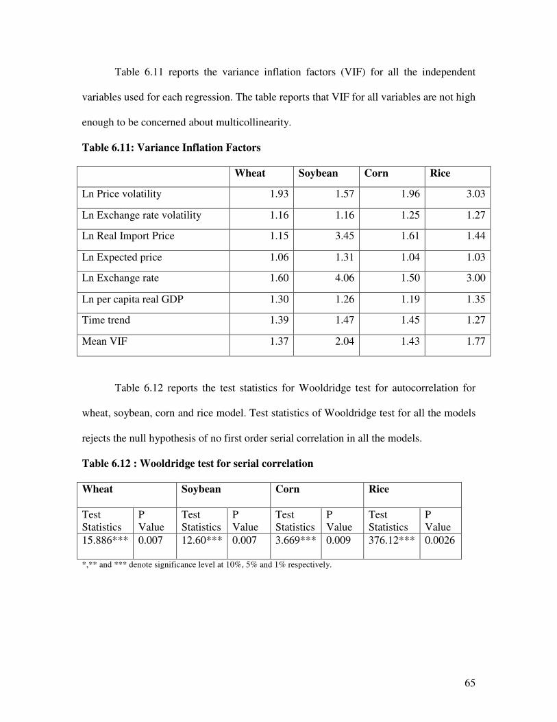
65

Table 6.11 reports the variance inflation factors (VIF) for all the independent

variables used for each regression. The table reports that VIF for all variables are not high

enough to be concerned about multicollinearity.

Table 6.11: Variance Inflation Factors


Ln Price volatility 1.93 1.57 1.96 3.03

Ln Exchange rate volatility 1.16 1.16 1.25 1.27

Ln Real Import Price 1.15 3.45 1.61 1.44

Ln Expected price 1.06 1.31 1.04 1.03

Ln Exchange rate 1.60 4.06 1.50 3.00

Ln per capita real GDP 1.30 1.26 1.19 1.35

Time trend 1.39 1.47 1.45 1.27

Mean VIF 1.37 2.04 1.43 1.77

Table 6.12 reports the test statistics for Wooldridge test for autocorrelation for

wheat, soybean, corn and rice model. Test statistics of Wooldridge test for all the models

rejects the null hypothesis of no first order serial correlation in all the models.

Table 6.12 : Wooldridge test for serial correlation


Test

Statistics

P

Value

Test

Statistics

P

Value

Test

Statistics

P

Value

Test

Statistics

P

Value

15.886*** 0.007 12.60*** 0.007 3.669*** 0.009 376.12*** 0.0026


66

Table 6.13 reports parameter estimates of the developed countries’ imports of

major agricultural commodities from their developed counterparts. Results show that log

of price volatility and log of exchange rate volatility do not have significant effect on log

of per capita import volumes of wheat, soybean and rice. Only log of per capita corn

import volume are positively affected by both log of exchange rate and log of commodity

price volatilities at a one percent level of significance. Percentage change of real import

price has a negative and significant effect on log of per capita imports of all four

commodities. On the other hand, percentage change of expected price has a positive and

significant effect on log of per capita import volumes of wheat, soybean and corn

imports. Since the traders from developed countries have access to both commodities and

financial futures, they are expected to hedge the risk of both commodity price and

exchange rate volatilities (Cho et al 2002, Kandilov 2008, Zhang 2010). Coefficients

estimates in table 6.13 also support this proposition for three out of four crops since price

and exchange rate volatilities have no significant effect on log of per capita imports of

wheat, soybean and rice. Moreover, positive and significant effect of percentage of

expected price suggest that developed countries are developed countries are responsive to

the price change in the futures market. Domestic policies of many developed countries

may also play a role in minimizing the effects of volatilities on their trade. For example,

variable import levy of the European Union (EU) insulates the EU countries from the

price and exchange rate volatilities.

Table 6.13a reports the coefficients estimates of the developed countries’ imports of

major agricultural commodities from their developed counterparts excluding the

67

percentage change in expected price variable. Results suggest no drastic change in the

signs and significances of the variables.

6.13: Coefficients estimates of developed countries’ wheat, soybean, corn and rice

imports from developed importers from 1991 to 2009

Commodities

Dependent Variable:

Log of per capita import

Wheat

Soybean Corn Rice


Fixed

Effects Pooled OLS Fixed effects Fixed effects

ln Price volatility

-0.098

(0.05)

-0.104

(0.83)

0.20**

(0.102)

-0.055

(0.191)


-0.162

(0.112)

0.316

(0.333)

0.24***

(0.08)

0.280

(0.240)


-0.039*

(0.109)

-3.571***

(0.91)

-0.19*

(0.103)

-2.398**

(0.905)


0.117*

(0.06)

3.503***

(0.909)

0.24**

(0.37)

-0.045

0.1638


0.031***

(0.006)

-0.041

(0.034)

0.06*

(0.008)

-0.046

(0.179)

∆ln Per Capita real GDP

-3.941

(2.27)

3.566

(9.96)

1.02

(1.88)

-51.728**

(21.87)

Time trend

0.003

(0.003)

-0.085**

(0.025)

-0.002**

(0.881)

0.028

(0.02)

Constant

-4.453***

(0.70)

-0.282*

(3.16)

-6.69*

(7.9)

-7.580***

(0.82)

R squared

0.07 0.128 0.97 0.61

Prob > F

0.000 0.000 0.000 0.000

Number of Observation

126 153 162 51


Numbers in parentheses are Driscoll-Kraay robust standard errors

68

6.13a: Coefficients estimates of developed countries’ wheat, soybean, corn and rice

imports from developed countries from 1991 to 2009 (without percentage change of

expected price)

Commodities

Dependent Variable:

Log of per capita

Import

Wheat

Soybean Corn Rice


Fixed

Effects Pooled OLS Fixed effects Fixed effects

ln Price volatility

-0.079

(0.05)

-0.120

(0.07)

0.797**

(0.31)

-0.328

(0.264)

ln Exchange rate

volatility

-0.158

(0.114)

0.1059

(0.35)

0.369

(0.23)

0.1531

(0.182)


-0.045*

(0.116)

-0.258*

(0.59)

-2.152***

(0.19)

-0.097

(0.196)


0.0294**

(0.006)

-0.004

(0.04)

-0.032

(0.04)

0.1196

(0.209)

∆ ln Per Capita real

GDP

-3.487

(2.27)

2.4312

(11.31)

0.757

(0.74)

-50.86

(0.016)

Time trend

0.0030

(0.003)

-0.101

(0.02)

-0.035

0.033)

-0.027

(0.041)

Constant

-4.309***

(0.807)

-2.429

(3.16)

5.884*

(3.4)

-7.501

(0.98)

R squared 0.06 0.10 0.503

0.32

Prob > F 0.000 0.000 0.000

0.000

Number of

Observation 126 153 162

51

*,** and *** denote significance level at 10%, 5% and 1% respectively. Numbers in parentheses are Driscoll-


69

6.3.2 Top developing importers’ imports from developing exporters

This section presents the coefficient estimates regression models aimed to examine the

effects of exchange rate volatility and commodity price volatility on top developing

importers’ imports of wheat, soybean, rice and corn from their developing trade partners.

Table 6.14 presents the test statistics of Fisher’s panel unit root test for wheat,

soybean, corn and rice models. Test statistics suggests that price volatility and exchange

rate volatility variables are level stationery whereas import price, expected price,

exchange rate and GDP per capita variables are difference stationery.

Table 6.14: Fisher’s panel Unit Root Test


Level First

Difference

Level First

Difference

Level First

Difference

Level First

Difference

Ln Price

Volatility

10.63

***

(0.056)

36.54

***

(0.000)

5.693

(0.991)

254.746

***

(0.000)

5.69

(0.991)

254.74

***

(0.000)

81.58

***

(0.000)

199.65

***

(0.000)

Ln

Exchange

rate

Volatility

74.92

***

(0.000)

205.05

***

(0.000)

108.57

***

(0.000)

245.61

***

(0.000)

108.57

***

(0.000)

245.61

***

(0.000)

52.640

***

(0.000)

186.187

***

(0.000)

Ln real

Import

Price

2.34

(0.12)

38.32

***

(0.000)

4.789

(0.232)

121.23

***

(0.000)

20.23

(0.205)

149.08

(0.000)

11.06

(0.19)

58.58

(0.00)

Ln

Expected

Price

18.55

(0.099)

136.25

***

(0.000)

10.084

(0.862)

129.190

***

(0.000)

10.084

(0.862)

129.19

***

(0.000)

27.91

***

(0.5)

175.85

***

(0.000)

Ln

Exchange

rate

31.40

(0.11)

48.57

***

(0.000)

13.48

***

(0.24)

169.02

***

(0.000)

14.18

***

(0.57)

166.33

***

(0.000)

14.573

(0.265)

48.729

***

(0.000)

Ln

Percapita

real

GDP

2.48

(1.00)

55.288

***

(0.000)

2.433

(1.00)

46.07

***

(0.001)

2.43

(1.000)

46.075

***

(0.000)

1.32

(0.999)

37.58

***

(0.002)



70

Table 6.15 and 6.16 present the test statistic of Hausman’s model specification

test and Friedman’ test for cross-sectional dependence respectively. The test statistics of

Hausman’s model specification test computed in the wheat model is1.16 with a p-value

0.97. Therefore I fail to reject the null hypothesis that both fixed and random effects

estimates are consistent. A random effects model is appropriate in this case. Friedman’s

test statistics of cross-sectional independence presented in table 6.18 is 12.32 with a p-

value 0.03 for wheat model. Thus, I reject the null hypothesis of cross-sectional

independence. On the basis of these two tests, the wheat import model is estimated as a

pooled OLS model with Driscoll-Kraay robust standard error.

Hausman’s test statistics presented in the Table 6.15 for soybean and corn

indicate that the null hypothesis that both fixed and random effects models are consistent

is rejected for these two models. Therefore, random effects model are preferred for

soybean, corn and rice models. Friedman’s test statistics presented in the table

6.186suggest that null hypothesis of cross-sectional independence is rejected for soybean,

corn models. Therefore, we estimated the soybean and corn model as pooled OLS model

with Driscoll-Kraay standard errors. Rice model is estimated as fixed effects model with

Driscoll-Kraay robust standard error.

Table 6.15: Hausman’s Specification tests


Test

Statistics

P

Value

Test

Statistics

P

Value

Test

Statistics

P

Value

Test

Statistics

P

Value

1.6 0.97 1.16 0.998 2.34 .8009 194*** 0.000


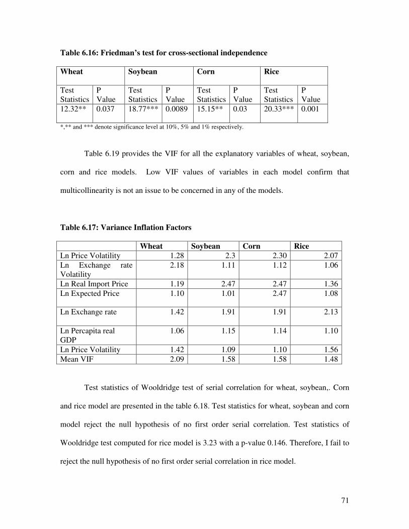
71

Table 6.16: Friedman’s test for cross-sectional independence


Test

Statistics

P

Value

Test

Statistics

P

Value

Test

Statistics

P

Value

Test

Statistics

P

Value

12.32** 0.037 18.77*** 0.0089 15.15** 0.03 20.33*** 0.001


Table 6.19 provides the VIF for all the explanatory variables of wheat, soybean,

corn and rice models. Low VIF values of variables in each model confirm that

multicollinearity is not an issue to be concerned in any of the models.

Table 6.17: Variance Inflation Factors


Ln Price Volatility 1.28 2.3 2.30 2.07

Ln Exchange rate

Volatility

2.18 1.11 1.12 1.06

Ln Real Import Price 1.19 2.47 2.47 1.36

Ln Expected Price 1.10 1.01 2.47 1.08

Ln Exchange rate 1.42 1.91 1.91 2.13

Ln Percapita real

GDP

1.06 1.15 1.14 1.10

Ln Price Volatility 1.42 1.09 1.10 1.56

Mean VIF 2.09 1.58 1.58 1.48

Test statistics of Wooldridge test of serial correlation for wheat, soybean,. Corn

and rice model are presented in the table 6.18. Test statistics for wheat, soybean and corn

model reject the null hypothesis of no first order serial correlation. Test statistics of

Wooldridge test computed for rice model is 3.23 with a p-value 0.146. Therefore, I fail to

reject the null hypothesis of no first order serial correlation in rice model.

72

Table 6.18 : Wooldridge test for serial correlation


Test

Statistics

P Value Test

Statistics

P Value Test

Statistics

P Value Test

Statistics

P Value

18.21*** 0.008 9.080** 0.01 12.20** 0.01 3.23 0.1467


Table 6.19 presents the coefficients estimates of the imports of wheat, soybean,

corn and rice by developing countries from their developing counterparts. Estimates show

that log of price volatility has a positive and significant effect on log of per capita wheat

import volume at a five percent level of significance. This result is supported by

IFPRI(2011) which reports that wheat importing developing countries have a tendency to

import more than the required amount of wheat when they face volatility so that they can

have a considerable buffer stock to avoid domestic food riots. It may be mentioned here

that wheat is the staple food in majority of the developing countries. Although log of

price volatility affects wheat import positively, it has a negative and significant effect on

log of per capita soybean import volume (at one percent level of significance) and

imports of corn and rice at five percent level of significance. Since the majority of

developing countries are unable to hedge the risk by operating in the futures market due

to financial constraints, regulation and limited storage capacity, they are more likely to be

affected negatively by price volatility. On the other hand, log of exchange rate volatility

has no effect on developing countries’ log of import volume from other developing

countries. Since a majority of developing countries follow a ‘managed floating’ exchange

rate system they are more likely to protect their traders from exchange rate volatility. As

expected, percentage change in real import price has negative and significant effects on

73

log of import volume of wheat, soybean and corn. But percentage change in expected

price has a positive and significant effect (at five percent level) on log of rice rice import

only. Log of per capita import volumes of all other crops are unaffected by expected

price. This result suggests that developing countries are less responsive to the movement

in futures market.

6.19: Coefficient estimates of developing importers’ imports of wheat, soybean, corn

and rice from developing exporters from 1991 to 2009

Commodities

Dependent Variable:

Log of per capita

Import


Independent variables

Pooled OLS Pooled OLS Pooled OLS Fixed Effects

ln Price volatility

0.687***

(0.215)

-0.2826***

(0.079)

-0.03**

(0.012)

-0.242*

(0.128)

ln Exchange rate

volatility

-0.069

(0.09)

0.334

(0.36)

0.224

(0.12)

0.026

(1.21)


-0.83**

(0.38)

-2.78***

(0.75)

-0.862***

(0.23)

-0.107

(0.07)


0.16

(0.32)

0.2159

(0.80)

-1.49

(0.685)

-0.153

(0.227)


0.344*

(0.12)

0.2051

(0.53)

0.306*

(0.84)

-1.020

(0.799)


GDP

12.25*

(0.257)

0.797

(10.22)

16.014

(11.28)

11.614

(0.61)

Time trend

0.1087***

(0.01)

0.261***

(0.03)

0.1299**

(0.02)

0.069*

(.037)

Constant

-3.13**

(1.18)

3.265*

(2.73)

-1.9*

(1.19)

-6.956***

(0.75)

R squared

0.33 0.3114 0.2762 0.1534

Prob > F

0.000 0.000 0.004 0.000


108 144 144 72



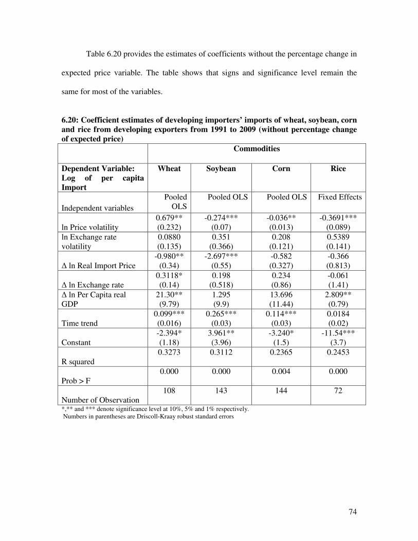
74

Table 6.20 provides the estimates of coefficients without the percentage change in

expected price variable. The table shows that signs and significance level remain the

same for most of the variables.

6.20: Coefficient estimates of developing importers’ imports of wheat, soybean, corn

and rice from developing exporters from 1991 to 2009 (without percentage change

of expected price)

Commodities

Dependent Variable:

Log of per capita

Import


Independent variables

Pooled

OLS

Pooled OLS Pooled OLS Fixed Effects

ln Price volatility

0.679**

(0.232)

-0.274***

(0.07)

-0.036**

(0.013)

-0.3691***

(0.089)

ln Exchange rate

volatility

0.0880

(0.135)

0.351

(0.366)

0.208

(0.121)

0.5389

(0.141)


-0.980**

(0.34)

-2.697***

(0.55)

-0.582

(0.327)

-0.366

(0.813)


0.3118*

(0.14)

0.198

(0.518)

0.234

(0.86)

-0.061

(1.41)


GDP

21.30**

(9.79)

1.295

(9.9)

13.696

(11.44)

2.809**

(0.79)

Time trend

0.099***

(0.016)

0.265***

(0.03)

0.114***

(0.03)

0.0184

(0.02)

Constant

-2.394*

(1.18)

3.961**

(3.96)

-3.240*

(1.5)

-11.54***

(3.7)

R squared

0.3273 0.3112 0.2365 0.2453

Prob > F

0.000 0.000 0.004 0.000


108 143 144 72



75

6.4 Chapter Summary

This chapter presented the estimates of coefficients of both quarterly and annual models

for wheat, soybean, corn and rice. The quarterly models attempted to examine the effects

of exchange rate and commodity price volatilities on Canada’s wheat and soybean export;

and corn and rice imports. The estimated coefficients suggest that price and exchange rate

volatilities do not have a significant effect on Canada’s export of wheat and soybean; and

imports of rice and corn. On the other hand, the annual models examined the effects of

exchange rate and commodity price volatilities on imports of top developed and

developing importers. Results suggest that trade between developing countries are more

affected than trade between developed countries. Next chapter provides a summary of

the study and discusses policy implications and limitations of this study

76

Chapter 7: Summary and Conclusion

This chapter provides a summary of the motivation and objectives of this study,

theoretical framework used for analysis, empirical results and discussions, limitations of

the study and future directions of research in this area.

7.1 Summary

The purpose of this thesis is to examine the effects of both exchange rate volatility and

commodity price volatility on specific agricultural commodity trade. Previous literature

on the effects of exchange rate volatility on international agricultural commodity trade

came up with mixed results (Cho et al. 2002; Kandilov, 2008; Zhang, 2010; Dell Ariccia,

1999; Villanueva and Sarker, 2009). Most of the studies on agricultural trade focused on

overall agricultural commodity trade, not specific commodity trade. At the same time,

research on the effects of commodity price volatilities on commodity trade flows is also

scarce. In recent years, agricultural commodity price volatilities also drew much attention

of the researchers. Few studies (IFPRI, 2011; World Bank, 2011, FAO, 2011) predicted

that price volatilities may have implication on agricultural commodity trade too. This

backdrop motivated a study to examine the effects of both exchange rate and commodity

price volatilities on trade of four major agricultural commodities: wheat, soybean, corn

and rice. The specific objectives of the study are (i) to estimate the effects of both

exchange rate and commodity price volatilities on agricultural trade and (ii) to examine

the effects of commodity price and exchange rate volatilities on developed and

developing countries separately.

77

This study used a modified version of Hooper and Kohlhagen’s trade model

(Hooper and Kohlhagen, 1978). The basic Hooper and Kohlhagen model theoretically

estimated the effects of exchange rate volatilities on import demand. We incorporated

price volatility into the model. The theoretical framework used in this study asserts that

the effects of exchange rate and commodity price volatilities on agricultural commodity

trade largely depends on the risk preference and ability to hedge the market risk of the

traders. Exchange rate volatility and commodity price volatility may have a negative

effect on trade if the traders are risk averse and less capable to hedge the market risk. On

the other hand, exchange rate volatility may have a positive effect on trade volume if the

traders are risk lovers and more capable to hedge the market risks.

The empirical part of this study estimates the effects of exchange rate and

commodity price volatilities in two different ways:

First, the effects of exchange rate and commodity price volatilities on Canada’s

export of wheat and soybean; and imports of corn and rice with its major trading partners

are estimated using quarterly data.

Second, the effects of exchange rate and price volatilities on wheat, soybean, corn

and rice imports of on trade between developed and developed countries; and developing

and developing countries are estimated using annual data.

The coefficient estimates of the quarterly models of Canada’s trade with its major trading

partners suggest that price volatility does not have a significant effect on Canada’s export

of wheat and soybean; whereas exchange rate volatility has a negative and significant

78

effect on Canada’s import of rice. Exchange rate volatility does not have a significant

effect on import of corn and export of wheat and soybeans.

The annual models are estimated to examine the effects of exchange rate and

commodity price volatilities on developed and developing countries’ imports separately.

Since developed countries’ traders have much wider access to commodities and financial

futures market, it is expected that trade between developed countries will remain

unaffected by volatilities. On the other hand, because of limited access to futures market

(and other derivative instruments) and the tendency towards “speculative behaviors” we

expected that trade between developing countries will be affected negatively by price and

exchange rate volatilities. Coefficients estimates of import demand of developed

countries from their developed counterparts are largely consistent with our expectations.

Price volatility and exchange rate volatility have a positive and significant effect on

developed countries’ corn imports only. But price and exchange rate volatilities do not

have a significant effect on soybean, corn and rice imports.

Developing countries’ imports from developing countries are mostly affected by

price and exchange rate volatilities. Price and exchange rate volatilities have a negative

and significant effect on soybean, corn and rice imports of developing countries’ import

from their developing trading partners. These results are expected because of developing

countries’ limited access to commodity and financial futures market; and their tendency

towards trade restrictive policies, such as export ban during the periods of volatilities

(IFPRI 2011). Previous studies, such as, Arize et al (2005), Arize et al ( 2003), Bahmani-

Oskoee(1996), and Kandilov (2008) found similar negative effects of exchange rate

volatilities on developing countries’ trade with their developing counterparts. For

79

example, Arieze et al (2003) found negative effect of exchange rate volatilities on trade

of Turkey, Korea, Malaysia, Indonesia, and Pakistan, Another study by Arize (2000)

found a negative effect of exchange rate volatility on export volume of 13 LDCs.

Kandilov (2009) showed with a gravity model that exchange rate volatility has a negative

effect on trade between developing countries.

7.2 Policy implications

The finding of this study suggests that the effects of exchange rate and commodity price

volatilities vary across the countries studied. It may largely depend on countries’

domestic policies, access to futures market and financial services and traders’ risk

preferences. In general, the finding suggests that developing countries’ trade are more

affected because of exchange rate and commodity price volatilities. Therefore, exchange

rate and commodity price volatilities may have an impact on agriculture and food

security of developing countries. Since a number of developing countries are already

food insecure because of the burden of population and low agricultural productivity,

increase in price and exchange rate and commodity price volatilities may have the

potential to further trigger food insecurity in many developing countries.

Restricting imports or reducing import tariffs in short run are very popular policy

options for many developing countries to cope with volatilities. During the periods of

volatilities in 2007-08, 43 out of 81 developing countries reduced import taxes and 25

banned exports for specific products or increased export taxes for agricultural

commodities (BIAC, 2011). Some countries, being speculative, began to import more

food than the requirement to create a buffer stock. These short term abrupt changes of

80

policies often discourages the necessary additional investment required for agricultural

production and have potential to increase volatility further. Although these policies may

help to stabilize the situation in a single country in short run, they are often counter

productive and expensive in the long run. These policies may have implications on food

securities of other countries as well. For example, ban on rice export by India during

2007-08, destabilize the world rice market and threatened food security of many

countries that are dependent on rice.

One of the findings of this study is that generally commodity price and exchange

rate volatility do not have a significant effect on developed countries’ trade. This finding

suggests that farmers and all agents in the marketing chain in developed countries may be

well protected from risk of exchange rate and price volatilities by a variety of market

based instrument. They may be able to manage the risk they face with these instruments.

Sarris (2011) says that producers and consumers of developed countries have developed

sophisticated market-based risk management system (e.g., insurance) to deal with

commodities risk. In the last three decades, they also developed a variety of innovative

financial instruments (futures, options, and other derivatives) to hedge the risk of price

and exchange rates. On the contrary, most of the developing countries do not have a well

developed futures market and their financial markets are also underdeveloped. Although

the modern markets of risk management instrument are accessible to all, traders of most

of the developing countries are unable to take this advantage because of a variety of

institutional imperfections and financial constraints. Developing countries may consider

establishing well-organized commodity exchange market. Developed countries may

81

extend their technical support in building commodity exchange markets in developing

countries.

7.3 Limitations and further research

In our quarterly models, we tried to estimate the effects of exchange rate and commodity

price volatilities with Canada’s major trading partners. Since quarterly data on GDP,

exchange rate and price were not available for many countries, specially developing

countries, we were unable to incorporate all the trading partners. If data become

available, the estimates can be done with larger sample.

The assumptions about the accessibility of importers to financial and commodity

futures could be verified with data. Although most of the developing countries do not

have access to financial and commodities futures market, some major traders of

agricultural commodities do have access to these markets. Because of the unavailability

of information about access to futures market for all countries in the panels, I was unable

consider this factor in the model.

Unit price was used as import price in this study. Unit price indices may create

bias in estimation because of the compositional changes in quantities and quality mix of

exports and imports. One can use domestic price as an independent variable since this

variable is an important component of an import demand model. As domestic prices of

all commodities for all countries in the panels are not available, we used the unit value.

Another limitation of this study is that the effects of exchange rate and

commodity piece volatilities are estimated at the country level whereas the theoretical

framework was developed for an individual firm first and then aggregated for the

82

country. Further study may also consider panel co-integration and estimating pane co-

integration regression.

7.4 Research Contribution

The purpose of this thesis was to examine the effects of both commodity price and

exchange rate volatilities on trade flows. Overwhelming percentage of previous studies

only examined the effects of exchange rate volatilities on trade flows. Inclusion of price

volatility’s effect along with exchange rate volatilities is the key contribution of this

thesis. Another important contribution of this thesis is the estimation of the effects of

exchange rate and commodity price volatilities on trade of developed and developing

countries separately.

83

References

Akhtar, M.A. and Hilton, R.S. 1984. Effects of uncertainty on German and US trade.

Federal Reserve Bank of New York. Quarterly Review 9 (1): 7-16.

Ariccia, G. D. 1998. Exchange rate fluctuations and trade flows: evidence from the

European Union. Washington, D.C.: International Monetary Fund, Research

Department.

Arize, A, T. O and D.J. Slottje. 2008. Exchange-rate volatility in Latin America and its

impact on foreign trade. International Review of Economics and Finance 17 (1):

33–44.

Arize, A. 1995. Trade flows and real exchange-rate volatility: an application of

cointegration and error-correction modeling. North American Journal of

Economics & Finance, 6(1), 37-51.

Arize, A. 1996. Reexamination of the demand for UK exports: evidence from an error

correction model. International Trade Journal, 10(4), 501-25.

Arize, A., & Ghosh, D. 1998. Exchange rate uncertainty and recent US export demand

instability. International Trade Journal, 8(3), 347.

Baltagi, B. H. 2008. Econometric analysis of panel data. Chichester: Wiley.

Be´langer, G., & Raynauld, J. 1992. Exchange rate variability and trade flows:

preliminary sectoral estimates for the US-Canada case. cole des Hautes Etudes

Commerciales: Cahiers de Recherche, 89(1), 68.

Belsley, D., E. Kuh and R. Welsch, 1980. Regression Diagnostics. New York: John

Wiley and Sons.

Bini-Smaghi, L. 1991. Exchange Rate Variability and Trade: Why Is It So Difficult to

Find any Empirical Relationship? Applied Economics 23(5): 927-35.

BIAC 2011. Price Volatility in Food and Agricultural Commodity Markets: Policy

options on how to better mitigate and manage the risks associated with the

price volatility of food and other agriculture commodities. Paris: Business

and Industry Advisory Committee to the OECD.

Bohrnstedt, G., & Goldberger, A. 1969. On the Exact Covariance of Products of

Random Variables. Journal of the American Statistical Association, 64(328),

1439-1442.

Braun, J., & Tadesse, G. 2012. Global Food Price Volatility and Spikes: An Overview

of Costs, Causes, and Solutions.. Bonn: ZEF.

Cho, G, I.M. Sheldon and S. McCorriston.2002. Exchange Uncertainty and

Agricultural Trade. American Journal of Agricultural Economics.84(4):

931-42.

84

Clark, P.B. 1973. Uncertainty, Exchange Risk, and the Level of International Trade.

Western Economic Journal 11(3): 302-13.

Clark, P., Tamirisa, N., Wei, S., Sadikov, A., & Zeng, L. (2004). A New Look at

Exchange Rate Volatility and Trade Flows Peter. Washington D.C.: The IMF.

Cho, G., Sheldon, I., & McCorriston, S. 2002. Exchange rate uncertainty and

agricultural trade. American Journal of Agricultural Economics, 84(16), 27-29.

Choi, I. 2001.Unit Root Tests for Panel Data. Journal of International Money and

Finance, 20, 249-272.

Chou, W. 2000. Exchange rate variability and China’s exports. Journal of Comparative

Economics, 28(1), 61-79.

CIMT 2011. Canadian International Merchandise Trade Databse. Retrieved September

- December, 2010, from http://www5.statcan.gc.ca/cimt-cicm/home-

accueil?lang=eng

Cushman, D. O.1983. The Effects of Real Exchange Rate Risk on International Trade.

Journal of International Economics 15(2):43-63.

Dib, A .2008. Welfare Effects of Commodity Price and Exchange Rate Volatilities in a

Multi-Sector Small Open Economy Model. Bank of Canada Working Paper No.

2008-8. Ottawa: Bank of Canada.

Drukker, D. M. 2003.Testing for serial correlation in linear panel-data models. Stata

Journal 3: 168–177.

EUROSTAT (2012). Statistical Office of the European Union. Retrieved January 2012

from http://www.eea.europa.eu/data-and-maps/data/external/national-

accounts-including-gdp-eurostat

FAOSTAT 2012. Food and Agriculture Organization of the United Nations (FAO)

Database on Agriculture. Retrieved March-April, 2012, from


Franke, G. 1991. Exchange Rate Volatility and International Trading Strategy. Journal

of International Money and Finance 10(2):292-307.

Frankel,J.A. and S.Wei. 1995. Emerging Currency Blocks. In The International

Monetary System: Its Institutions and Its Future edited by H. Genberg, pp. 11-

143.Berlin:Springer.

Giorgioni, G., & Thompson, J. 2002. Which volatility? The case of the exports of

wheat. Applied Economics Letters, 9(4), 681-4.

Gotur, P. 1985. Effects of exchange rate volatility on trade: some further evidence,

International Monetary Fund Staff Papers, 32 (3): 475-512.

85

Hadri, K. 2000. Testing for stationarity in heterogeneous panel data. Econometrics

Journal 3, 148-161.

Harris, Richard D. F. & Tzavalis, Elias, 1999. Inference for unit roots in dynamic

panels where the time dimension is fixed, Journal of Econometrics, vol. 91(2),

pages 201-226, August

Hausman, J. 1978. Specification Test in Econometrics. Econometrica, 46(6), 1251-1271.

Hoechle, D. 2007. Robust Standard Errors for Panel Regressions with Cross-Sectional

Dependence. Stata Journal 7 (3): 281–312

Hooper, P. and S.W. Kohlhagen 1978. The Effect of Exchange Rate Uncertainty on the

Prices and Volume of International Trade. Journal of International Economics 8(4):

483-511.

IFPRI. 2011. 2011 global food policy report. Washington, D.C.: International Food

Policy Research Institute.

Im, K.S., Pesaran, M.H., and Shin, Y. 2003. Testing for Unit Roots in Heterogeneous

Panels. Journal of Econometrics, 115, 1, 53-74.

Kandilov, I. 2008, The Effects of Exchange Rate Volatility on Agricultural Trade.

American Journal of Agricultural Economics 90(4): 1028-1043.

Klein, M. 1990. Sectoral effects of exchange rate volatility on United States exports.

Journal of International Money and Finance,, 9, 299-308.

Koo, W. W., & Kennedy, P. L. 2007. International Trade and Agriculture Theories and

Practices.. Chichester: John Wiley & Sons.

Levin, A., C. Lin, and C.-J. Chu .2002. Unit Root Tests in Panel Data: Asymptotic and

Finite-sample Properties. Journal of Econometrics 108, 1–24.

Maskus, K. 1986. Exchange rate risk and US trade: a sectoral analysis. Economic

Review, 71(3), 16-28. Maddala, G.S. and Wu, S. 1999. A Comparative Study of Unit Root Tests with Panel Data and

a New Simple Test. Oxford Bulletin of Economics and Statistics, special issue, 631-

652.

McKenzie, M. 1997. The impact of exchange rate volatility on German-US trade flows.

Journal of International Financial Markets, Institutions & Money, 7(1), 73-87.

Raddatz, C. 2011. Over the Hedge: Exchange rate volatiltiy, Commodity Price

Correlations, and Structure of Trade. Washington DC: The World Bank.

OECD., & FAO. 2012. OECD-FAO Agricultural Outlook 2012. Paris: OECD and FAO.

86

Schmitz, A., Moss, C., Schmitz, T., Furtan, W. H., & Schmitz, H. C. (2010). Agricultural policy, agribusiness, and rent-seeking behaviour. Toronto:

University of Toronto Press.

Sercu, P. and C. Vanhulle. 1992. Exchange Rate Volatility, International Trade, and the

Value of Exporting Firms. Journal of Banking and Finance 16(1):155-82.

Silver, Mick (2007). Do Unit Value Export, Import, and Terms of Trade Indices

Represent or Misrepresent Price Indices?, IMF Working paper: WP/07/121

Smith, C.E. 1999. Exchange Rate Variation, Commodity Price Variation and the

Implications for International Trade. Journal of International Money and Finance

18(3):471-491.

Thomson Reuters Datastream 2012. Microsoft – Exchange rate data. Retrieved

January 2012 from Datastream Advance database.

Thursby, J.G. and M. C. Thursby.1987. Bilateral Trade Flows, the Linder Hypothesis,

and Exchange Risk. The Review of Economics and Statistics 69(3): 488-95.

Villanueva, J L J and R. Sarker. 2009. Exchange Rate Sensitivity of Fresh Tomatoes

Imports from Mexico to the United States. Contributed Paper prepared for

presentation at the International Association of Agricultural Economists

Conference, Beijing, China, August 16-22, 2009

Weersink, A., Hailu, G., Fox, G., Meilke, K., & Massow, M. V. 2008. The world food

crisis: Causes and the implications for Ontario agriculture. Guelp: University of

Guelph Working Paper 08/01

Wright, B. D. 2011. The Economics of grain price volatility. Applied Economics

Perspectives and Policy, 33(1), 32-58

Zhang, Q., Reed, M., & Saghaian, S. H. 2010. The Impact of Multiple Volatilities on

Import Demand for U.S. Commodities: The Case of Soybeans.

Agribusiness, 26(2), 202–219.

87

Appendix A

Table A1: Exchange Rate Arrangements of Countries

Exchange Rate Regime


Countries

Exchange arrangements with

no separate legal tender (41)

Ecuador, El Salvador, Kiribati, Marshall Islands,

Micronesia, Fed. States of Palau, Panama, San Marino ,

Timor-Leste, Dem. Rep. of Antigua and Barbuda,

Dominica,, Grenada, St. Kitts and Nevis, St. Lucia, St.

Vincent and the Grenadines, Benin,, Burkina Faso, Côte

d'Ivoire, Guinea-Bissau, Mali,Niger, Senegal, Togo,

Cameroon, Central African Rep., Chad, Congo, Rep. of

Equatorial Guinea, Gabon

Euro Area

Currency board

arrangements (7)

Bosnia and Herzegovina, Brunei Darussalam, Bulgaria,

Hong Kong SAR, Djibouti, Estonia, Lithuania

Other conventional fixed peg

arrangements (52)

Aruba, Bahamas, Bahrain, Barbados, Belarus,, Belize,

Bhutan, Bolivia, Cape Verde, China , Comoros, Egypt,

Eritrea, Ethiopia, Guyana, Honduras, Iraq, Jordan, Kuwait,

Latvia, Lebanon, Lesotho, Macedonia, Maldives, Malta,

Mauritania, Namibia, Nepal, Netherlands Antilles, Oman,

Pakistan, Qatar , Rwanda, Saudi Arabia, Seychelles, Sierra

Leone, Solomon Islands, Suriname, Swaziland, Syrian Arab

Rep, Trinidad and Tobago, Turkmenistan, Ukraine, United

Arab Emirates, Venezuela, Rep. Bolivariana , Vietnam,

Zimbabwe

Pegged exchange rates within

horizontal

bands (6)

Cyprus, Denmark, Slovak Rep., Slovenia, Hungary

Tonga

88

Exchange Rate Regime


Countries

Crawling pegs Azerbaijan, Botswana, Costa Rica, Iran, Nicaragua

Managed floating with no pre-

determined path for the

exchange rate (51)

Argentina, Bangladesh, Cambodia, Gambia, Ghana, Haiti,

Jamaica,

Lao P.D.R., Madagascar, Malawi, Mauritius, Moldova,

Mongolia, Sri Lanka, Sudan , Tajikistan, Tunisia, Uruguay,

Yemen, Rep. of, Zambia, Colombia Czech Rep.,

Guatemala, Peru, Romania, Serbia, Rep. of,

Thailand, Afghanistan, Armenia, Georgia, Kenya,Kyrgyz

Rep, Mozambique, Algeria, Angola, Burundi, Croatia,

Dominican Rep, Guinea, India, Kazakhstan, Liberia,

Malaysia, Myanmar, Nigeria, Papua New Guinea, Paraguay,

Russian Federation , São Tomé and Príncipe, Singapore,

Uzbekistan

Independently floating (25) Albania, Congo, Dem. Rep. of, Indonesia, Uganda,

Australia, Brazil, Canada, Chile , Iceland, Israel, Korea,

Mexico, New Zealand, Norway, Philippines, Poland, South

Africa, Sweden, Turkey, United Kingdom, Tanzania, Japan,

Somalia, Switzerland

United States

Source: IMF (http://www.imf.org/external/np/mfd/er/2006/eng/0706.htm)

89

Appendix B

Table B1: Coefficient estimates of quarterly wheat and soybean imports from

Canada from 2000 to 2009 (without percentage change of real import price

variable)

Commodities

Dependent Variable:


Soybean


ln Price volatility 0.134

(0.107) -0.12

(0.10)

ln Exchange rate volatility -0.068 (0.62)

-0.43** (0.15)

∆ ln Expected Price 3.992* (3.99)

1.01 (0.38)

∆ ln Exchange rate 5.181 (4.18)

0.50*** (0.014)

∆ ln Per Capita real GDP -4.658 (4.97)

-7.58*** (2.57)

Dummy_Quarter 2 1.136 (0.90)

-2.15*** (0.56)

Dummy_ Quarter3 0.943 (1.07)

-0.75*** (0.126)

Dummy Quarter_4 0.731 (1.06)

0.05 (0.121)

Timetrend -0.012 (0.02) 0.05***

Constant -7.205 (5.05)

-12.62*** (0.003)


R2 0.07 0.000



90

Table B2: Coefficient estimates of quarterly corn and rice imports by Canada from

2000 to 2009 (without percentage change of real import price variable)

Commodities

Dependent Variable:


Rice


ln Price volatility 0.018 (0.06)

0.0398 (0.03)

ln Exchange rate volatility 0.069 (0.16)

0.0229 (0.08)

∆ ln Expected Price 0.298 (0.40)

-0.1358 (0.20)

∆ ln Exchange rate -2.074*

(1.14) 0.0695 (0.60)

∆ ln Per Capita real GDP 1.367***

(0.50) 6.0774 (1.93)

Dummy_Quarter 2 -0.060 (0.13)

-1.1617 (0.37)

Dummy_ Quarter3 0.000 (0.12)

-1.4721 (0.43)

Dummy Quarter_4 0.087 (0.13)

-0.9803 (0.36)

Timetrend 8.275 (3.46)

0.0026 (0.002)

Constant 0.018 -7.3362

(1.02)


R2 0.383 0.15



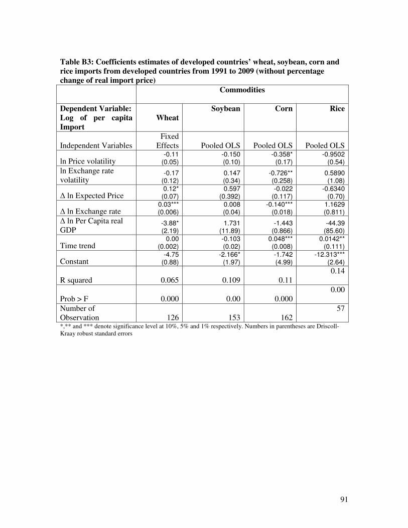
91

Table B3: Coefficients estimates of developed countries’ wheat, soybean, corn and

rice imports from developed countries from 1991 to 2009 (without percentage

change of real import price)

Commodities

Dependent Variable:

Log of per capita

Import

Wheat

Soybean Corn Rice


Fixed

Effects Pooled OLS Pooled OLS Pooled OLS

ln Price volatility -0.11

(0.05) -0.150 (0.10)

-0.358* (0.17)

-0.9502 (0.54)

ln Exchange rate

volatility -0.17

(0.12) 0.147 (0.34)

-0.726** (0.258)

0.5890 (1.08)

∆ ln Expected Price 0.12* (0.07)

0.597 (0.392)

-0.022 (0.117)

-0.6340 (0.70)

∆ ln Exchange rate 0.03*** (0.006)

0.008 (0.04)

-0.140*** (0.018)

1.1629 (0.811)


GDP -3.88* (2.19)

1.731 (11.89)

-1.443 (0.866)

-44.39 (85.60)

Time trend 0.00

(0.002) -0.103 (0.02)

0.048*** (0.008)

0.0142** (0.111)

Constant -4.75

(0.88) -2.166*

(1.97) -1.742 (4.99)

-12.313*** (2.64)

R squared 0.065 0.109 0.11

0.14

Prob > F 0.000 0.00 0.000

0.00

Number of


57



92

Table B4: Coefficients estimates of developing countries’ wheat, soybean, corn and

rice imports from developing countries from 1991 to 2009 (without percentage

change of real import price)

Commodities

Dependent Variable:

Log of per capita

Import

Wheat

Soybean Corn Rice


Fixed

Effects Pooled OLS Pooled OLS Pooled OLS

ln Price volatility 0.453 (.41)

-0.10* (0.24)

-0.037*** (0.012)

-0.370** (0.166)

ln Exchange rate

volatility 0.070 (0.14)

-0.02 (0.377)

0.175 (0.144)

0.299 (0.167)

∆ ln Expected Price -0.049 (0.25)

-1.74 (1.38)

-1.246 (0.74)

0.481** (0.182)

∆ ln Exchange rate 0.316* (0.15)

0.07 (0.69)

0.356 (0.824)

-0.702 (1.5)


GDP 16.708 (10.15)

13.23 (15.61)

13.883 (11.823)

-56.013*** (16.13)

Time trend 0.105*** (0.015)

0.23*** (5.14)

0.109 (0.026)

0.050* (0.02)

Constant -3.692 (1.97)

-10.09*** (0.75)

-6.258 (0.621)

-3.004* (1.57)

R squared 0.29 0.20 0.2556

0.2566

Prob > F 0.000 0.000 0.000

0.000

Number of


72



The Effects of Exchange Rate and Commodity Price ...

Documents

Transcript of The Effects of Exchange Rate and Commodity Price ...