Michigan Technological University Price risk management in the copper market using commodity...

Michigan Technological UniversityDigital Commons @ Michigan

TechDissertations, master's theses and master's reports -Open Dissertations, master's theses and master's reports

2005

Price risk management in the copper market usingcommodity derivatives and options strategiesBold SandagdorjMichigan Technological University

Copyright 2005 Bold Sandagdorj

Follow this and additional works at: http://digitalcommons.mtu.edu/etds

Part of the Agricultural and Resource Economics Commons

Recommended CitationSandagdorj, Bold, "Price risk management in the copper market using commodity derivatives and options strategies", Master's Thesis,Michigan Technological University, 2005.http://digitalcommons.mtu.edu/etds/448

http://www.mtu.edu/?utm_source=digitalcommons.mtu.edu%2Fetds%2F448&utm_medium=PDF&utm_campaign=PDFCoverPages

http://www.mtu.edu/?utm_source=digitalcommons.mtu.edu%2Fetds%2F448&utm_medium=PDF&utm_campaign=PDFCoverPages

http://digitalcommons.mtu.edu?utm_source=digitalcommons.mtu.edu%2Fetds%2F448&utm_medium=PDF&utm_campaign=PDFCoverPages

http://digitalcommons.mtu.edu?utm_source=digitalcommons.mtu.edu%2Fetds%2F448&utm_medium=PDF&utm_campaign=PDFCoverPages

http://digitalcommons.mtu.edu/etds?utm_source=digitalcommons.mtu.edu%2Fetds%2F448&utm_medium=PDF&utm_campaign=PDFCoverPages


http://digitalcommons.mtu.edu/etd?utm_source=digitalcommons.mtu.edu%2Fetds%2F448&utm_medium=PDF&utm_campaign=PDFCoverPages


http://network.bepress.com/hgg/discipline/317?utm_source=digitalcommons.mtu.edu%2Fetds%2F448&utm_medium=PDF&utm_campaign=PDFCoverPages

Price Risk Management in the Copper Market Using

Commodity Derivatives and Options Strategies

By

Bold Sandagdorj

A THESIS

submitted in partial fulfillment of the requirements

for the degree of

MASTER OF SCIENCE IN MINERAL ECONOMICS

MICHIGAN TECHNOLOGICAL UNIVERSITY

2005

Copyright © Bold Sandagdorj 2005

This thesis, “Price Risk Management in the Copper Market Using Commodity

Derivatives and Options Strategies”, is hereby approved in partial fulfillment of the

requirements for the Degree of MASTER OF SCIENCE IN MINERAL ECONOMICS.

School of Business and Economics

Signatures:

Thesis Advisor

Professor Mark C. Roberts, Ph. D

Department Chair

Professor Christa L. Walck, Ph. D

Date

TABLE OF CONTENTS

Page

LIST OF TABLES i - iv

LIST OF FIGURES v - vii

ACKNOWLEDGEMENTS viii - ix

ABSTRACT x – xii

CHAPTER 1: INTRODUCTION 1 – 5

CHAPTER 2: DESCRIPTION OF RISK MANAGEMENT STRATEGIES 6 - 32

2.1. Background of Metal Exchanges 6 - 7

2.2. Spot versus Futures Markets 8 - 11

2.3. Description of Basic Derivatives 11 - 21

2.4. The Costs of Hedging 21 - 24

2.5. Risks and Rewards of Derivative Market Positions 25 – 32

CHAPTER 3: VALUING COMMODITY DERIVATIVES 33 - 56

3.1. Fair Values of Futures (Forward) Contracts 33 - 36

3.2. Valuing Asian Options 37 - 42

3.3. Data Description and Collection 42 - 46

3.4. Data Analysis 46 – 56

CHAPTER 4: BACKGROUND OF ECONOMETRIC COMMODITY

MODELS AND LITERATURE REVIEW 57 – 62

CHAPTER 5: MODEL DEVELOPMENT FOR PRICE PREDICTION 63 - 104

5.1. Specification of the Model 64 - 79

5.2. Hypothesis Testing 80

5.3. Data Description and Collection 81 - 82

5.4. Two-Stage Least Squares Regression (2SLS) Analysis 83 – 104

Page

CHAPTER 6: MONTE-CARLO SIMULATION ANALYSIS

FOR THE LME COPPER PRICES 105 - 111

6.1. Short Term Forecasting of Copper Prices 105 - 107

6.2. Monte-Carlo Simulation Analysis 108 - 111

CHAPTER 7: EVALUATION OF RISK MANAGEMENT STRATEGIES 112 - 173

7.1. Options Strategies 112 - 169

7.1.1. Bull Spreads 114 - 129

7.1.2. Bear Spreads 130 - 138

7.1.3. Butterfly Spreads 139 - 169

7.2. Single Positions in Options 169 - 171

7.2.1. A Producer’s Strategies 169 – 170

7.2.2. A Consumer’s Strategies 171

7.3. Forward Contracts and Metal Swaps 172 – 173

CHAPTER 8: CONCLUSIONS AND RECOMMENDATIONS

FOR FUTURE STUDIES 174 - 176

REFERENCES 177 - 180

APPENDICES 181 - 196

i

LIST OF TABLES

# Title Page 2.1. The LME Forward Prices (Calyon) 14

2.2. The Example Data 14

2.3. The Alumbrera’s Price Fix Hedging Operation with the LME 15

2.4. Basis Risk versus Outright Risk 17

2.5. The Results of Metal Swaps Contract for 6 Months 19

2.6. A Summary Result of Price Fix Hedge on 17 March 2003 22

2.7. Producer Put Option Indications for Feb-Dec 05 23

2.8. Monthly Average Prices (LME) 23

2.9. Payoff Matrix of an Offset Hedging 25

2.10. Variations in Gains or Losses Resulting from Differences

in Cash and Future Price Movements 30

2.11. Summary of Risks and Rewards 32

3.1. Cost of Carry Formula with Convenience Yields 36

3.2. The LME Option Premiums (US$/t) for Copper 43

3.3. The LME Option Premiums (US$/t) for Copper 44

3.4. Valuations of Asian Options on 08.08.02 (Implied Vol. 01.08.02) 52





3.9. Valuations of Asian Options on 22.02.05 (Implied Vol. 21.02.05) 53-54

3.10. The Summary of Options’ Valuations 56

5.1. Correlation Coefficients between Demand

and its Exogenous Variables 71

5.2. Correlation Coefficients between Supply

and its Exogenous Variables 77

5.3. The Expected Hypothesis 80

5.4. The Units of Measurement for the Data 82

ii

5.5. Correlations between Exogenous Variables

in the Structural Equation of Demand 88

5.6. Correlations between Exogenous Variables

in the Structural Equation of Supply 88

5.7. T-tests (tr) on the Structural Equation of Demand 89

5.8. T-tests (tr) on the Structural Equation of Supply 89

5.9. VIF Tests 90

5.10. Critical d-Values 94

6.1. The Results of the Simulation 110

6.2. Probability Distributions of Copper Price Forecasts 111

7.1. The Risk Free Interest Rates and Time to Maturities

for Selected Options 113

7.2. Profit from a Bull Spread (Jan-06 Call options, X: 3100/3200) 116




7.6. The Payoffs of Bull Spreads Using Call Options

for 2006 and 2007 120-122

7.7. Profit from a Bull Spread (Jan-06 Put options, X: 2200/2300) 124

7.8. Profit from a Bull Spread (Dec-06 Put options, X: 2600/2700) 125

7.9. Profit from a Bull Spread (Jan-07 Put options, X: 2300/2400) 125

7.10. Profit from a Bull Spread (Dec-07 Put options, X: 2600/2700) 125

7.11. Bull Spreads Using Put Options for 2006 and 2007 127-129

7.12. Profit from a Bear Spread (Dec-06 Call options, X: 3400/3300) 131



7.15. Profit from a Bear Spread (Jan-06 Call options, X: 3600/3500) 133

7.16. Bear Spreads Using Call Options for 2006 and 2007 135-137

7.17. Bear Spreads Using Put Options 138

7.18. Profit from a Butterfly Spread

(Jan-06 Call options, X: 3100/3200/3300) 140

iii















7.26. Butterfly Spreads Using Call Options for 2006 and 2007 (Case A) 147-149


(Dec-06 Call options, X: 3100/3200/3300) 151















iv

7.35. Butterfly Spreads Using Call Options for 2006 and 2007 (Case B) 157-159


(Dec-06 Put options, X: 2300/2400/2500) 160


(Dec-06 Put options, X: 2400/2500/2600) 161


(Dec-06 Put options, X: 2500/2600/2700) 161


(Dec-07 Put options, X: 2300/2400/2500) 162


(Dec-07 Put options, X: 2400/2500/2600) 162


(Dec-07 Put options, X: 2500/2600/2700) 163

7.42. Butterfly Spreads Using Put Options for 2006 and 2007 165-167

7.43. Profit from a Strangle (Jan-07 Call/Put options, X: 3600/2700) 168

7.44. Probabilities for Written Call Options to be Profitable 170

7.45. Probabilities for Written Put Options to be Profitable 171

7.46. Evaluation of Risk Management Strategies in 2006-2007 173

LIST OF DIAGRAMS

# Title Page 2.1 Copper Production Processes 8

2.2. Solvent Extraction-Electrowinning (SX-EW) Process 9

2.3. The Matrix of Outcomes for an Offset Hedging 26

2.4. The Matrix of Outcomes for a Price Fix Hedging 27

v

LIST OF FIGURES

# Title Page 1.1. Monthly Trading Volumes of the

LME Futures Contracts on Copper 4

1.2. Monthly Trading Volumes of the

LME Options Contracts on Copper 4

2.1. The Relationship between Contango/Backwardation

Markets and Inventories 17

2.2. Payoff from Long Call 31

2.3. Payoff from Long Put 31

2.4. Payoff from Short Call 31

2.5. Payoff from Short Put 31

3.1. Implied Vol. (Call, 01/08/02) 47

3.2. Implied Vol. (Call, 08/08/02) 47

3.3. Implied Vol. (Call, 15/08/02) 47

3.4. Implied Vol. (Call, 22/08/02) 47

3.5. Implied Vol. (Call, 30/08/02) 47

3.6. Implied Volatilities (Call, 21/02/05) 48

3.7. Implied Volatilities (Put, 21/02/05) 48

3.8. Volatility Smile 49

5.1. The Cobweb Model 67

5.2. Supply of Funds 75

5.3. Investment Demand 75

5.4. World Cu Demand & LME Cash Prices 78

5.5. World Cu Demand & World GDP 78

5.6. World Cu Demand & Global IP Growth 78

5.7. World Cu Supply & LME Cash Prices 78

5.8. World Cu Supply & Time (Technology) 78

5.9. World Cu Supply & Price of Oil 78

5.10. World Cu Supply & USD Index 79

vi

5.11. World Cu Supply & LIBOR (1Y) Rate 79

5.12. Distribution of the Residuals (Demand) 93

5.13. Distribution of the Residuals (Supply) 93

5.14. Testing AC (Ln[QtD]) 95

5.15. Testing AC (Ln[QtS]) 95

5.16. {e(D)} vs Ln[P(t-1)] 96

5.17. {e(D)} vs Ln[GDP(t)] 96

5.18. {e(D)} vs Ln[IP%(t)] 96

5.19. {e(S)} vs Ln[P(t-1)] 96

5.20. {e(S)} vs Ln[T(t)] 97

5.21. {e(S)} vs Ln[P. Oil(t)] 97

5.22. {e(S)} vs Ln[USDI(t)] 97

5.23. {e(S)} vs Ln[LIBOR 1Y(t-6)] 97

6.1. Ex Post and Ex Ante Forecasts 106

6.2. Actual and Modeled Prices (Jan-95 to Dec-04) 107

7.1. Probabilities for Copper Prices to be

Greater than Specific Strike Prices 115

7.2. Bull Spread Using Call Options, Jan-06, X: 3100/3200 118




7.6. Bull Spread Using Put Options, Jan-06, X: 2200/2300 126

7.7. Bull Spread Using Put Options, Dec-06, X: 2600/2700 126

7.8. Bull Spread Using Put Options, Jan-07, X: 2300/2400 126

7.9. Bull Spread Using Put Options, Dec-07, X: 2600/2700 126

7.10. Bear Spread Using Call Options, Dec-06, X: 3400/3300 133



7.13. Bear Spread Using Call Options, Jan-06, X: 3600/3500 134

7.14. Butterfly Spread, Call Options, Jan-06, X: 3100/3200/3300 143


vii







7.22. Butterfly Spread, Call Options, Dec-06, X: 3100/3200/3300 153








7.30. Butterfly Spread, Put Options, Dec-06, X: 2300/2400/2500 163






7.36. Payoff Diagram of Strangle for Jan-07, X: 2700/3600 169

viii

ACKNOWLEDGEMENTS

The help and guidance of many people contributed to the preparation of this thesis.

First of all, I would like to express my deep gratitude to my thesis advisor Professor

Mark C. Roberts for his valuable advice, comments, criticisms, careful supervision,

patience, and for all his support throughout this research. I am also very grateful to my

academic advisor Professor Gary A. Campbell, who helped me to join the graduate

program at Michigan Technological University, encouraged and enhanced my efforts,

and helped me with valuable advice during the initial stages of this work.

I must also thank Professor Dean L. Johnson and Professor Brent J. Lekvin from

whom I learned derivative securities, financial engineering and financial management

through my attendance in their classes.

I am very thankful to all faculty and staff members of the School of Business and

Economics. I would also like to thank to the members of my thesis committee, Professors

Mark C. Roberts, Gary A. Campbell, Dean L. Johnson and Theodore J. Bornhorst for

their valuable time, help and recommendations.

In addition, special thanks are due to following individuals for their valuable

comments, assistance, and the provision of needed information and data:

o Mr. Maqsood Ahmed (Calyon Financial SNC of Credit Agricole Group)

o Ms. Ana Maria Rebelo (ICSG)

o Mr. Rohan Ziegelaar (Sempra Metals Group)

ix

o Mr. Robert J. Loewen

(International Metals Marketing, Commercial Advisory and Research Services)

o Mr. Peter Hollands (Bloomsbury Minerals Economics Ltd.)

o Mr. David Waite (CRM Associates)

o Mr. Batbayar Baldan

(Representative office in London, Erdenet Mining Company)

o Assistant professor Igor L. Kliakhandler

(Department of Mathematics, Michigan Technological University)

o Mr. Daniel Edelstein (The U.S. Geological Survey).

Last but not least, thank you for my father Sandagdorj Enebish and mother Nadmid

Banzar in Mongolia, for your love, enthusiasm, support and assistance.

x

ABSTRACT

Metals price risk management is a key issue related to financial risk in metal markets

because of uncertainty of commodity price fluctuation, exchange rate, interest rate

changes and huge price risk either to metals’ producers or consumers. Thus, it has been

taken into account by all participants in metal markets including metals’ producers,

consumers, merchants, banks, investment funds, speculators, traders and so on.

Managing price risk provides stable income for both metals’ producers and consumers,

so it increases the chance that a firm will invest in attractive projects.

The purpose of this research is to evaluate risk management strategies in the copper

market. The main tools and strategies of price risk management are hedging and other

derivatives such as futures contracts, swaps and options contracts. Hedging is a

transaction designed to reduce or eliminate price risk. Derivatives are financial

instruments, whose returns are derived from other financial instruments and they are

commonly used for managing financial risks. Although derivatives have been around in

some form for centuries, their growth has accelerated rapidly during the last 20 years.

Nowadays, they are widely used by financial institutions, corporations, professional

investors, and individuals. This project is focused on the over-the-counter (OTC) market

and its products such as exotic options, particularly Asian options.

The first part of the project is a description of basic derivatives and risk management

strategies. In addition, this part discusses basic concepts of spot and futures (forward)

markets, benefits and costs of risk management and risks and rewards of positions in the

derivative markets.

xi

The second part considers valuations of commodity derivatives. In this part, the

options pricing model DerivaGem is applied to Asian call and put options on London

Metal Exchange (LME) copper because it is important to understand how Asian options

are valued and to compare theoretical values of the options with their market observed

values.

Predicting future trends of copper prices is important and would be essential to

manage market price risk successfully. Therefore, the third part is a discussion about

econometric commodity models. Based on this literature review, the fourth part of the

project reports the construction and testing of an econometric model designed to forecast

the monthly average price of copper on the LME. More specifically, this part aims at

showing how LME copper prices can be explained by means of a simultaneous equation

structural model (two-stage least squares regression) connecting supply and demand

variables. A simultaneous econometric model for the copper industry is built:

��

�

��

�

�

=

⋅⋅⋅⋅⋅=

⋅⋅⋅=

−−−

−

⋅−−

−

QQ

LIBORUSDIPTPeQ

eGDPPeQ

S

t

D

t

)0561.0(6)-(t

)2432.1(t

)1559.0(OIL(t)

)1408.0(t

)5960.0(1)(t

)0785.3(S

t

)0158.0()7151.1(t

)1868.0(1)(t

)0485.5(D

tIP t

LIBORUSDIPTeGDPeP ).(6)-(t

).(t

).(OIL(t)

).(t

).().(t

).(CU1)(t

IPt 07170588111991017990020201910251652 ⋅⋅⋅⋅⋅⋅= −−⋅−−

Where, QD

tand QS

tare world demand for and supply of copper at time t respectively.

P t )1( − is the lagged price of copper, which is the focus of the analysis in this part.

xii

GDPt is world gross domestic product at time t, which represents aggregate economic

activity. In addition, industrial production should be considered here, so the global

industrial production growth that is noted as IPt is included in the model. T t is the time

variable, which is a useful proxy for technological change. A proxy variable for the cost

of energy in producing copper is the price of oil at time t, which is noted as P tOIL )( .

USDI t is the U.S. dollar index variable at time t, which is an important variable for

explaining the copper supply and copper prices. At last, LIBOR t )6( − is the 6-month

lagged 1-year London Inter bank offering rate of interest. Although, the model can be

applicable for different base metals' industries, the omitted exogenous variables such as

the price of substitute or a combined variable related to the price of substitutes have not

been considered in this study.

Based on this econometric model and using a Monte-Carlo simulation analysis, the

probabilities that the monthly average copper prices in 2006 and 2007 will be greater

than specific strike price of an option are defined. The final part evaluates risk

management strategies including options strategies, metal swaps and simple options in

relation to the simulation results. The basic options strategies such as bull spreads, bear

spreads and butterfly spreads, which are created by using both call and put options in

2006 and 2007 are evaluated. Consequently, each risk management strategy in 2006 and

2007 is analyzed based on the day of data and the price prediction model.

As a result, applications stemming from this project include valuing Asian options,

developing a copper price prediction model, forecasting and planning, and decision

making for price risk management in the copper market.

1

CHAPTER I:

INTRODUCTION

Why should we hedge?

The principles of the market economy answer what and how to produce and for whom.

How is this reflected in metal markets? Raw and semi fabricated materials, refined metals

and metal end use products such as ingots, bars, wires, foils, sheets, strips, rods and tubes

are produced using advanced technologies and traded for industrial and other needs.

Metal markets have been highly competitive since ancient history because there are many

producers and consumers. In metal markets, prices fluctuate in response to the global

economic outlook, industrial production growth, international politics, market balances,

exchange and interest rates, et cetera. Thus, no one could know exactly what will happen

to metal markets and prices in the future even though analysts make outlook and price

forecasts based on current economic, political and market conditions. If the market price

goes down, it brings unexpected loss to metals’ producers; in contrast, if the market price

rises, consumers face increased costs. Of course, this “non-resistant” or unprotected

condition against price changes will seriously impact future revenues of both metal

buyers and sellers.

Furthermore, this uncertainty has a negative impact in state budget income and the

economy of a country whose economy is strongly dependent on its metal industry. For

instance, copper concentrate is the main export product from Mongolia and one third of

the Gross Industrial Product (GIP) of Mongolia consists of copper concentrate export

income. Hence, copper price is quite influential to the Mongolian economy.

Chapter 1: Introduction

2

In 1994 and 1995, yearly average A-grade copper prices in the London Metal

Exchange (LME) were $2,307 and $2,935 per tonne respectively. The budget deficit

percentages in GDP of Mongolia were 5.4% and 0.9% in years above mentioned.

However, these indices grew sharply in connection with a dramatic decline in copper

prices in the following years and reached their highest level of 11.7% and 11.2% in 1998

and 1999 respectively when year average copper prices plunged to $1,654 and $1,573 per

tonne. Approximately 38-40% of Mongolian export income was from copper concentrate

exports, but it fell to 27% in 1998 even though the amount of exported copper had not

decreased. Generally, the reason for these bad consequences was the fall in copper prices

in the global market. Chilean, South African, and Australian metal industries have a

dominant role in their economies, so market price risk is a top concern when trading

metals for these countries too. Moreover, not only these countries, but also every

participant in the metal markets may need to carry out price risk management in order to

reduce market price risk.

How is price risk management implemented and what is the final gain from it?

Market participants buy or sell their physical metals in the physical market through

their regular channels. Alongside, they insure against their physical trading risks by using

futures or options and other derivatives in the futures or over the counter (OTC) markets.

These futures/forward and options contracts are issued by exchange brokers as Ring

Dealing Members in the LME or Floor Brokers in NYMEX and COMEX.

Futures contracts are used for managing price risk and are liquidated by buying and

selling them back before the (prompt) maturity date. Consequently, futures contract


3

results can eliminate or reduce the price risk of physical trade, which is made by the cash

settlement (spot) price.

Price risk management has the following benefits:

- It can maximize profits and minimize losses (reduce price risk) of hedgers

because of protection against strong market price volatility;

- It gives an opportunity to plan future profits by stabilizing the net price of metals;

- It can help to predict and plan taxable income from metal industry to the state

budgets.

However, risk management (hedging) is not always profitable because there can be a

possible risk and costs occur if the price of the underlying commodity changes against a

risk manager’s expectation or if a risk manager chooses an inappropriate risk

management tool (derivative). For example, a copper consumer who has a long forward

position may lose if the price of copper significantly decreases in the future. A copper

producer who has a short forward position may lose if the price of copper significantly

increases in the future. Therefore, implementing price risk management can be an

important part of the trading of metals and using a correct derivative at an appropriate

time is a very important to risk managers.

One of the most actively traded base metals either in the exchanges or on the over-

the-counter (OTC) markets is copper. Managing price risk in the copper market is very

important to producers, consumers, speculators, traders, investment funds, banks etc.


4

As seen from the figures below, trading volumes of futures and options (including

traded average price options TAPOs) contracts are pretty volatile, but have been very

high since 1997.

Figure (1.1): Monthly Trading Volumes of the LME Futures Contracts on Copper

500,000

700,000

900,000

1,100,000

1,300,000

1,500,000

1,700,000

1,900,000

2,100,000

2,300,000

Jan-97

Jun-97

Nov-97

Apr-98

Sep-98

Feb-99

Jul-99

Dec-99

May

-00

Oct-00

Mar-0

1

Aug-01

Jan-02

Jun-02

Nov-02

Apr-03

Sep-03

Feb-04

Jul-0

4

Dec-04

Vol

ume

(lots

= 2

5t)

1000

1500

2000

2500

3000

3500

Pric

e ($

/t)

Trading Volume of Futures (lots)

LME Copper Price ($/t)

Figure (1.2): Monthly Trading Volumes of the LME Options Contracts on Copper

0

50,000

100,000

150,000

200,000

250,000

300,000

350,000

Jan-97

Jun-97

Nov-97

Apr-98

Sep-98

Feb-99

Jul-9

9

Dec-99

May

-00

Oct-00

Mar-0

1

Aug-01

Jan-02

Jun-02

Nov-02

Apr-03

Sep-03

Feb-04

Jul-0

4

Dec-04

Vol

ume

(lots

= 2

5t)

0

500

1000

1500

2000

2500

3000

3500

Pric

e ($

/t)

Trading Volume of Options (lots)

LME Copper Price ($/t)


5

Everyday brokerage firms offer OTC products to their clients. The clients such as

producers and consumers need to manage market price risk using these derivative

products, but their risk management decisions will not be effective if they cannot do

reasonable research regarding evaluation of risk management strategies. Due to this lack

of experience and research, some clients have doubts about using derivative products for

managing risk. Therefore, the main purpose of this research is to evaluate risk

management strategies for copper in the OTC market including long hedge, short hedge,

metal SWAPS, options contracts, options strategies such as bull spreads, bear spreads and

butterfly spreads. The results are in 2006 and 2007 and based on the specific day of data

because market variables change everyday; thus, brokerage firms regularly offer different

indications.

In order to evaluate the OTC derivative strategies effectively, the LME copper price

prediction model is developed by a simultaneous econometric model using two-stage

least squares regression. The data observations consist of 120 months of historical data

between January 1995 and December 2004. The model is developed based on the

Cobweb model and a previously developed econometric model in the copper industry.

Using a Monte-Carlo simulation for the price prediction model, the probabilities for

monthly average copper prices to be greater or less than specific strike prices are

determined. These obtained probabilities are key factors for evaluating each risk

management strategy.

Although, the results of the evaluations are only for the specific day of the data,

copper producers, consumers, option traders and risk managers may use the model and

methodologies in this thesis for any particular events and OTC indications in the future.

6

CHAPTER II:

DESCRIPTION OF RISK

MANAGEMENT STRATEGIES

2.1. BACKGROUND OF METAL EXCHANGES

The traders of metals in the 19th and the 20th century were merchants, buying and

selling physical metals. Actually, they earned their profits by transporting the metals from

the places where metals were mined to the places where they were needed (The LME,

2001, p.2). In the 20th century, activities of major metal exchanges such as the LME, the

NYMEX and Shanghai Futures Exchange (SHFE) were developed as the world

industrialized. The early development of the LME began because of Britain’s role in

developing the global industrial revolution. The LME began in 1877 and initially became

the center of British metals trading. Today the LME is the largest derivative market for

common non-ferrous metals and the most liquid metal exchange in the world. The main

function of the LME is hedging, representing 75-85% of turnover (Martinot, Lesourd,

Morard, 2000, p.8). The LME services include reference pricing (daily official and

settlement prices, real time and indicative market prices), hedging and delivery. The

LME trades futures contracts for eight base metals: high grade primary aluminum, copper

grade A, standard lead, special high grade zinc, primary nickel, tin, aluminum alloy, and

North American Special Aluminum Alloy Contract (NASAAC). The approximate sailing

time from Chile to London for transporting copper by ships was three months. Hence,

this sailing time was the origin of the three months futures contract, which is the base of

Chapter 2: Description of Risk Management Strategies

7

futures trading (Sigmon, 1997, p.11). In 1987 the old 3-month futures contract was

extended. Contracts can now be traded up to 27 months for copper, primary aluminum,

zinc and nickel and up to 15 months for lead, tin, and aluminum alloy. This is supported

by the network of warehouses listed for the receipt of approved brands in locations in the

UK, Continental Europe, Middle East, Singapore, Japan and the United States (The LME,

2001).

Traded Average Price Options (TAPO) was introduced to copper and primary

aluminum in February of 1993, to nickel, zinc, aluminum alloy, lead and tin from

October 2000, and to NASAAC from March 2002 on the LME.

The NYMEX is the largest physical commodity futures exchange in the world. The

exchange include futures and options contracts for crude oil, gasoline, heating oil, natural

gas, gold, silver, copper, aluminum, and platinum. COMEX is one division of the

NYMEX. The COMEX division began trading gold futures in 1974 and the NYMEX

Division platinum contract was launched in 1956. Aluminum futures opened its trade in

May 1999 in the COMEX (NYMEX study material, 2003, p.1). Now, the COMEX

division lists futures and options on gold, silver, copper and aluminum.

SHFE started its formal operation in December 1999. There are five contracts on the

trading floor now and two of these contracts are metals: copper and aluminum.


8

2.2. SPOT VERSUS FUTURES MARKETS

The physical market is made up of transactions, which result in the delivery of goods.

The goods can be at any stage of production: ore concentrates or scrap metal through

semi-fabricated and fabricated materials up to the end-use products, such as cable,

electronic products, or even pots and pans.

Diagram (2.1): Copper Production Processes (Source: Claudio Agostini, 2002. p. 14)

Open Pit Mine

Underground Mine

Copper Ores

Sulfide Oxide

Leaching Flotation

Electrowinning Precipitation

Cathode Cement Copper Copper Concentrate

Smelting

Blister

Refining

Wire Bar Cathode

Foundries Brass Mills Powder Mills Wire Mills


9

The metal passes through a number of processing stages before becoming a finished

and end-use product. The processing stages of copper production are shown in the

diagram above.

The production of refined copper consists basically of four steps including mining,

concentrating, smelting and refining, according to a pyrometallurgical technology.

However, the production steps are different in the low-cost hydrometallurgical

technology (SX-EW) from traditional pyrometallurgical technology.

Diagram (2.2): Solvent Extraction-Electrowinning (SX-EW) Process

(Source: Phelps Dodge Corp., Presentation, 2002)

Mine

Dump leaching

Crusher

Conveyer

CathodeCathodeCathode

CathodeCathodeCathode

SX-EW

SX-EW

Leaching


10

As was mentioned before, many economic factors including production and

consumption, international politics, governmental export controls, global wars,

stockpiling policy, changing economic patterns, devaluations of currency, excess

speculation relative to hedging, and structural changes within the metals industry have

created considerable uncertainty to the future direction of the market and thus, to price

irregularity. On the other hand, there can be a considerable time between each processing

stage in copper production. Hence, there is a possible exposure to price risk for copper

producers and consumers. In order to protect against such price risks, market participants

can insure against their risks in physical metal exchanges through hedging. It may be

prudent to hedge each physical transaction in the futures market.

Every ring dealer or broker member of the exchanges has clients from many sectors

of the metal industry such as miners, smelters/refineries, rolling mills, extrusion plants,

merchants, fabricators, distributors, consumers, secondary merchants, secondary

smelters, banks, investment funds, speculators and so forth. These clients can hedge their

physical transactions by entering into futures (forward) contracts on each exchange.

Only a small percentage (approximately 2%) of LME contracts result in an actual

delivery because traders generally offset their futures positions before the maturity dates.

A buyer will liquidate by selling the contract and a seller will liquidate by buying back

the contract.

Copper producers and consumers consider that a stable price leads to higher returns

than a volatile price that fluctuates in response to short-term variations in demand and

supply. The price of copper substantially affects the profitability of a copper producer.

The producer will make good profits when demand for copper and prices are high.


11

Nevertheless, if copper prices fall, there is the risk that the market price for copper will be

lower than the cost of production. If the market price cannot cover the cost of production

for a long time, a bankruptcy can result for the producer. Therefore, hedging is one way

to protect against a price risk. In the case of copper producers, they hedge their position

against the risk of a fall in the price of copper.

2.3. DESCRIPTION OF BASIC DERIVATIVES

A) Futures (forward) contracts and Hedging:

The futures market is the trade of contracts for the future delivery of goods. In theory,

futures contracts are determined as an agreement to buy or sell a standard quantity of a

specified asset on a fixed date at a price agreed today. The futures contracts are

standardized and traded on exchanges. Therefore, futures contracts are guaranteed by

exchange clearinghouse. In addition, there are daily settlements; thus, futures contract

traders need to have a margin account to prevent credit risks.

By contrast, forward contracts are not standardized, so they are traded between any

two parties like financial institutions and their corporate clients. Non-standardized

derivatives such as forward contracts are traded in the over-the-counter (OTC) market,

which is an important alternative to exchanges. The OTC market operates through a

telephone and computer based network of dealers. A single payment is paid at the

maturity in forward contracts, so there is usually some credit risks.

Futures contracts have been used to manage cash market price risk for more than a

century. In a futures market, there are two parties to every contract. One party agrees to


12

buy and take delivery in the future and the other party agrees to sell and make delivery in

the future. The party agreeing to buy is said to have a long position and the party agreeing

to sell has a short position.

Hedging is a form of price insurance, which allows a market participant (producers

and consumers) to lock in prices and reduce the potential for unanticipated loss. This

means, a hedger makes his/her position certain and transfers a spot market price risk to

another party by forward dealing. Therefore, the economic purpose of the futures market

is to provide an arena for transferring risk among market participants. The hedger takes

an opposite position in the futures market from that in the spot market. The profits in one

market are offset by losses in another (Labys, Granger, 1970, p.21). A short hedge is the

case where a hedger is long in the spot market and short in the futures market in order to

protect an existing holding. In contrast, a long hedge refers to when a hedger is short in

the spot market and long in the futures market to protect an anticipated holding.

There are two types of hedges: a price fix hedge or an offset hedge. A price fix hedge

is a trade of futures contracts to fix the future purchase or sale price of a metal. An

investor; therefore, wishes to profit from a directional view in the future price movements

by fixing today the price for the future. According to the price fix hedge, there are two

cases for copper producers whether to buy forward contracts or not.

• Case 1) If metal producers feel that prices will fall between now and the time

physical contract matures, then they sell at a forward price today and buy back at

a cash settlement price at the maturity, so the selling price is fixed.

• Case 2) If metal producers feel that prices will rise between now and the time

physical contract matures, then there is no need to do a hedge.


13

For copper consumers, the cases would be:

• Case 1) If metal consumers feel that prices will rise between now and the time

physical contract matures, then they buy at a forward price today and sell back at

a cash settlement price at the maturity, so the purchasing price is fixed.

• Case 2) If metal consumers feel that prices will fall between now and the time

physical contract matures, then there is no need to do a hedge.

An offset hedge establishes an equal and opposite position in the futures market to an

existing position in the spot market. Hence, a short physical position is offset by a long

futures position, and a long physical position is offset by a short futures position. The

offset hedge positions are typically liquidated before their maturity dates.

Typically, everyday ring dealing members and floor brokers value futures prices

based on three months futures price (3-M) and carrying charges including interest rates,

insurance, and storage costs in official warehouses. Actually, the forward price should

equal the three-month price plus these carrying charges. Table (2.1) represents the

forward prices indications, which were valued on 17th of March, 2003 by Calyon

Financial SNC, one of the ring dealing members (category I) of the LME. The following

example shows a copper producer’s price fix hedging operation.

Example 1: Suppose that the Alumbrera copper mine decided to hedge 520 lots (1 lot

equals 25 tonnes) of A-grade copper in concentrate on 17th of March, 2003. Outokumpu

agreed to buy this amount of copper in concentrate for its copper wire production at a

spot price. Assume May-2003 was the delivery month, so it was also used as the


14

quotation month (in this case, the quotation period is the same as the delivery month)

which is the pricing period. Assume the Alumbrera settled in full on 2 June 2003, two

days after the quotation period ended on 31 May 2003 as shown by table (2.1).

Table 2.1: Table 2.2: The LME Forward Prices (Calyon) The Example Data

17/03/ 2003 Cash = $1655.00/t Metal type Copper Month Forward price U.S. $/t Tonnage 520 lots

Mar. 2003 1,656.00 Quotation period May-03 Apr. 2003 1,662.00 Payment made 2-Jun-03 May. 2003 1,669.00 Price available for 2-Jun-2003 $1,669.00/t Jun. 2003 1,673.75 Jul. 2003 1,676.50

Aug. 2003 1,680.25 Sep. 2003 1,684.00 Oct. 2003 1,686.00 Nov. 2003 1,688.00 Dec. 2003 1,690.00

Note: 520 lots equal to 13,000 tonnes of copper in concentrate. If Alumbrera’s copper content in concentrate was 28%, the total hedged amount of copper concentrate would be 46,429 tonnes through this contract.

On 17 March, the Alumbrera made the first LME contract with Calyon in the OTC

market. The short forward position (sell forward) with prompt date of 2 June 2003 was

opened on that day at the price of $1,669.00/t for 520 lots of copper (see table (2.1)).

Suppose the Alumbrera's production cost was $1,025.00/t in 2003. On the settlement date

of 2 June, the Alumbrera made the second LME contract with Calyon. In other words, the

mine closed out the short forward position in the OTC market by buying back 520 lots of

copper at an average cash settlement price (ACSP) of the quotation period May 2003.

The average cash settlement price (ACSP) of May-03 was $1,648.28/t on the LME. The

price difference between these two LME contracts is the nominal profit or loss.

In the physical (spot) market, the Alumbrera sold Outokumpu 520 lots of copper at

the ACSP of May 2003, which was the quotation period as mentioned in table (2.2). The

difference between the cost of production and the ACSP of the quotation period is the


15

profit or loss in the physical (spot) market. Therefore, the Alumbrera’s physical and

forward contracts would be as follows:

Table 2.3: The Alumbrera’s Price Fix Hedging Operation with the LME

The LME contract with Calyon Financial PHYSICAL contract with Outokumpu On 17 March 2003: • (The LME Contract 1) Short forward 520 lots (CU) @ $1,669.00/t Prompt 2-June-2003. On 2 June 2003: • (The LME Contract 2) Buy back 520 lots @ ACSP* of May 2003. (ACSP of May-03 = $1,648.28/t)

On 17 March 2003: • Production cost of copper in

concentrate was $1,025.00/t**. On 2 June 2003: • (Physical Contract)

Short Sell 520 lots @ ACSP of May 2003. (ACSP of May-03 = $1,648.28/t)

Nominal LME profit $20.72/t Physical profit $623.28/t

Total profit (net effects of the hedge) $644.00/t

*ACSP = Average Cash Settlement Price ** Assumed cost of production

Settlement on 2 June 2003: the difference between the LME contract [1] and the LME

contract [2].

� If the average price in the quotation period was less than $1,669.00/t (forward

price), Calyon Financial would pay Alumbrera the difference;

� If the average price in the quotation period was more than $1669.00/t (forward

price), Alumbrera would pay Calyon Financial the difference.

Net result: Irrespective of whether the copper price goes up or down in the quotation

period, Alumbrera receives $1,669.00/t (fixed price) when hedge is taken out.


16

In this example, the brokerage firm (Calyon Financial) would pay Alumbrera

$20.72/t, the difference between the forward price and the ACSP of May-03. Because of

this hedging operation, the Alumbrera mine profited by $20.72 per tonne during this

period and this totaled $269,360 excluding commission charges. The total gain would be

$8,372,000 with this hedging and $8,102,640 if hedging had not been used. In this

example, the costs of hedging including margin requirements, commission and

transaction costs are ignored.

In fact, commodity futures prices are the interplay between a number of factors

including supply and demand in the spot markets, interest rates, transportation and

storage costs etc. The principle of price risk management is based on the term “basis”,

which is the numerical difference between a futures price and a spot price (cash market

price). The basis is not constant because the relationship between supply and demand

affects the movements in the basis. If the futures prices are higher than spot prices

(positive basis), the market is said to be in contango (at a premium), otherwise (negative

basis), in backwardation (at a discount). When there is a lack of supply or very little

amount of inventory, a contango market can be altered into a backwardation. This

relationship is shown by figure (2.1).

The market moves into contango as inventories (enough material to be sold) rise. The

copper market has been in backwardation since the second half of 2003 due to its lack of

supply and low level of inventories on the exchanges.


17

Figure (2.1): The Relationship between Contango/Backwardation markets and Inventories

Example 2: To illustrate an offset hedge, consider a hedger who expects the price of

copper to decrease and protects against this risk of a price fall. In this case, the hedger

takes a short position (selling futures contract) in the futures market and a long (buying

copper) in the spot market initially (on 24 January). Before the maturity of the futures

contract, the hedger offset his/her position on 20 March by shorting back (selling copper)

in the spot and by taking a long position (buying futures contract) in the futures markets.

As can be seen from the table below, $70/t fall or loss in the price of cash copper has

been entirely offset by a $90/t gain in the futures market, so the net gain to the hedger is

$20/t resulting from the hedging operation.

Table 2.4: Basis Risk versus Outright Risk

Date Spot Market Futures Market 24 January Long @ $2,350/t Short @ $2,420/t 20 March Short @ $2,280/t Long @ $2,330/t

Loss: ($70/t) Profit: $90/t Net gain/loss $20/t

0

Basis

Inventories

Contango

Backwardation


18

B) Metal Swaps (Fixed purchase and sale):

Metal swaps are non-standardized derivatives in the OTC market. Like a price fix

hedge, they are settled against the average of the LME cash settlement prices. However,

metal swaps consist of monthly forward purchases or sales that are settled against the

average cash settlement prices each month until the final maturity of the swaps. Thus, a

producer makes fixed price sales each month, which are settled against the monthly

average of the LME cash settlement prices (floating prices). A consumer makes fixed

price purchases each month.

Hedgers can use metal swaps in order to make their future profits constantly

guaranteed for a specific time at an adequate price for them if commodity prices are very

volatile and the commodity market trend is likely to be uncertain. The following example

shows the basic procedures of metal swaps for a copper consumer.

Example 3: Suppose that copper alloy products and copper tube producer Swissmetal

needed to purchase 80 lots (2,000 tonnes) of refined copper for its tube production each

month starting from July 2004 until December 2004 for six months. The monthly average

cash price of copper on the LME was settled at $3,008.72/t in April 2004, which was the

103-month highest since September 1995 ($3,036.84/t). Because of this bullish trend in

the global copper market in the second half of 2004, Swissmetal decided to hedge against

the risk of price increases using monthly swap contracts. Assume that the fixed purchase

prices (swap) were offered in May 2004 by a LME floor broker as $2,900/t in July 2004

through December 2004 and the Swissmetal purchased monthly swaps for this time

period at this offered price $2,900/t in May 2004. Therefore, the tube producer agreed to


19

buy 80 lots of refined copper each month at $2,900/t in July-04 through December-04. In

other words, the tube producer locked its purchasing prices at $2,900 in the second half

of 2004. These swaps were settled each month against the monthly average cash

settlement prices (MACSP) of the LME. Hence, at the end of each month, Swissmetal

sold back 80 lots of refined copper at the MACSP between July and December of 2004.

The table below shows the outcomes of the metal swaps contracts for Swissmetal.

Table 2.5: The Results of Metal Swaps Contract for 6 Months

2004 Jul. Aug. Sep. Oct. Nov. Dec. Long Swap ($/t) 2,900 2,900 2,900 2,900 2,900 2,900 Short Sell @ MACSP 2,686.70 2,810.74 2,846.10 2,894.86 3,012.24 3,122.80 Swap profit/loss -213.30 -89.26 -53.90 -5.14 112.24 222.80

In the physical market, Swissmetal purchased 80 lots of copper each month at the

MACSP. As shown in the table above, the fixed purchases at $2,900/t were not profitable

for Swissmetal between July and October because the monthly average cash settlement

prices were settled below the swap prices of $2,900/t. Moreover, Swissmetal could not

eliminate price risks during the first 4 months, but it reduced price risks in the last 2

months because the tube producer profited in November and December 2004.

In this example, Swissmetal would have negative cash flows in the first 4 months, but

positive cash flows in the last 2 months. If the effective interest rate is assumed to be

1.25% per month during this period, the net present value of these cash flows would be

negative ($41.76/t) in May 2004, which is the contract date. As a result, the entire swaps

would not be profitable for Swissmetal in this example. The costs of hedging issues will

be discussed later.


20

C) Options contracts:

Options contracts are rights, but not the obligation, to buy or sell an asset at a

specified price within a certain date. Basically there are three styles of options, including

European, American and exotic options. An American option can be exercised on any

day up through the expiration date, but European style and some kinds of exotic options

are exercised only at the maturity date.

There are two types of options: a call option and a put option. An option that gives the

option holder the right to buy an asset is referred to as a call, an option that gives a holder

the right to sell an asset is called a put option. The option buyer pays the seller (writer) a

sum of money called the option price or premium. The fixed price at which the option

holder can either buy or sell the asset is called the exercise or strike price. A call option in

which the asset price at the maturity (ST) exceeds the exercise price (X) (i.e. ST > X) is

said to be in-the-money and if the asset price at the maturity is less than the exercise price

(i.e. ST < X), the call option is said to be out-of-the-money. By contrast, a put option is

said to be in-the-money, if the asset price at the option’s maturity is less than the exercise

price (i.e. ST < X). If the asset price at the option's maturity is more than the exercise

price (i.e. ST > X), the put option is said to be out-of-the-money. If the asset price at the

maturity is equal the exercise price (i.e. ST = X), the option is said to be at-the-money.

In-the-money options are exercised, but out-of-the-money options are never exercised.

Exotic options are traded in the over-the-counter (OTC) market, which is now a very

large and widely used alternative market to the exchange. These options offer different

types of payoffs. One of the widely used exotic options between financial institutions and

participants in the metals industry is an average price option known as an Asian option.


21

An Asian option is an option where the payoff is based on the average price attained

by the underlying asset during the life of the option or over a specified period of time,

which does not have to correspond to the life of the option. Asian options can take the

form of either a call or a put (Chance, 2001, p. 663).

2.4. THE COSTS OF HEDGING

Hedging is not always profitable because changes in the basis result in either a

potential profit (opportunity) or loss (threat) to investors and risk managers (hedgers). If

the prices of the underlying commodity move in the other direction from a hedger’s

expectation, there can be possible risks and costs (loss) of hedging. Of course there is not

a perfect relationship between cash and futures markets, so there is no such thing as a

perfect hedge. The possible risks and costs of hedging occur when the market prices

change against the trend expected by a hedger. The following examples illustrate this

case.

Example 4: Again using table (2.1) on page 14. The table indicates forward price

valuations on 17 March 2003. Based on this information, copper producers and

consumers could hedge in the OTC market. The first column of table (2.6) shows

different maturity dates of the forward contracts. The forward price valuations and the

monthly average cash settlement prices (MACSP) on the LME are shown in the second

and the third columns of the table respectively. The fourth column indicates all possible

profits and losses of price fix hedging operation for a copper producer on 17 March 2003.


22

A producer initially takes a short forward position in the OTC market in order to

hedge against a risk of a fall in prices. When the forward contract matures, the producer

closes his/her short forward position by buying back at the LME average cash settlement

price of the delivery month. In contrast, a copper consumer initially takes a long position

in the OTC market and closes his/her long forward position by short selling at the LME

average cash settlement price of the delivery month. The potential profits and losses of

price fix hedge for a copper consumer on the data date are shown in column six.

Table 2.6: A Summary Result of Price Fix Hedge on 17 March 2003

Month Forward price MACSP* (U.S. $/t) (U.S. $/t) Short Forward Gain/Loss Long Forward Gain/Loss

Mar. 2003 1,656.00 1,658.98 -2.98 Loss 2.98 GainApr. 2003 1,662.00 1,587.48 74.53 Gain -74.53 LossMay. 2003 1,669.00 1,648.28 20.72 Gain -20.72 LossJun. 2003 1,673.75 1,686.50 -12.75 Loss 12.75 GainJul. 2003 1,676.50 1,710.00 -33.50 Loss 33.50 Gain

Aug. 2003 1,680.25 1,760.28 -80.03 Loss 80.03 GainSep. 2003 1,684.00 1,789.52 -105.52 Loss 105.52 GainOct. 2003 1,686.00 1,920.54 -234.54 Loss 234.54 GainNov. 2003 1,688.00 2,055.43 -367.43 Loss 367.43 GainDec. 2003 1,690.00 2,201.29 -511.29 Loss 511.29 Gain

* MACSP = Monthly Average Cash Settlement Price on the LME

Valuations: 17 March 2003Hedge Profit/Loss

Cash = $1,655.00/t

As can be seen from table (2.6), a producer’s price fix hedge would only be profitable

for April-03 and May-03 contracts. Except for these two contracts, all possible hedges

would not be profitable because the producer would pay the difference between the

forward prices and the MACSP (negative values in column 4) to the counterparty

(brokerage firm) if the producer hedged on 17 March 2003. However, the situation would

be in reverse for a copper consumer. If a copper buyer used price fix hedge on 17 March

2003, he/she would gain from all possible forward contracts through 2003, except April-

03 and May-03 contracts.


23

Therefore, example 4 shows that hedging (in this example, a price fix hedge) can

result in either profit or loss. Example 3 showed the costs of hedging in case of metal

swaps contracts.

Options can also result some loss. For example, if an option is out-of-the-money, the

option will not be exercised and the option holder’s loss will be the option price

(premium) because the holder pays the premium to the option writer.

Example 5: Suppose that the Los Pelambres copper mine decided to buy an Asian

put option in the OTC market on 06 January 2005. The purpose of buying a put option

was to avoid exposure to a price fall. The LME floor broker Sempra Metals Group valued

the put options for February through December 2005 as shown by table (2.7). Table (2.8)

shows the monthly average cash settlement prices of the LME between February and

August of 2005.

Table 2.7: Table 2.8: Producer Put Option Indications for Feb-Dec 05 Monthly Average Prices (LME) Valued on 06 January 2005 Cash = $3,095.00/t Month MACSP

Strike U.S. $/t (X) Premium U.S. $/t* U.S $/t (SAVG) 2,350.00 42.00 Feb-05 3,253.70 2,450.00 61.00 Mar-05 3,379.60 2,550.00 86.00 Apr-05 3,394.48 2,650.00 117.00 May-05 3,249.10 2,750.00 156.00 Jun-05 3,524.07

Jul-05 3,614.21 Source: Rohan Ziegelaar, “Copper producer OTC indications”, Sempra Metals Group, January 6, 2005 Aug-05 3,797.75 *The premium increases with volatility, time to expiry and proximity of strike to market price.

The indications above are monthly settled Asian options. In other words, the options

are settled against the monthly average cash settlement prices. The Los Pelambres needs

to pay the premium to the Sempra Metals for insuring against a fall in prices.


24

Therefore, the option holder’s (Los Pelambres) net cash flow at time zero (on 06 January

2005) is always negative. Assume that the mine (Los Pelambres) bought put option at a

strike $2,550 with April-05 maturity. In this case, the mine would immediately pay $86

as the premium to the brokerage firm (Sempra Metals) at time zero (on 06 January 2005).

The expected payoff from this Asian put option is maximum of {0, X – SAVG}, where X

is the exercise price and SAVG is the average value of the underlying asset calculated over

a predetermined averaging period. This predetermined averaging period is April 2005 in

this example (i.e. SAVG = MACSP of April-05). The mine’s expected payoff at the

option’s maturity; therefore, is:

1) If SAVG < X, then the payoff = { X – SAVG } > 0 (the option is in-the-money)

2) If SAVG > X, then the payoff = 0 (the option is out-of-the-money)

The average cash settlement price of April-05 was $3,394.48, which greater than the

strike price ($2,550); hence, the option was not exercised and the expected payoff would

be zero. Therefore, the Los Pelambres mine would lose because it had negative cash flow

at time zero and zero cash flow in the future. As can be seen from table (2.8), the

MACSP of the LME in the predetermined averaging months were all settled at values

that are greater than the available strike prices on the valuation date of 06 January 2005,

so it indicates that all of these Asian put options were not exercised. Hence, producer put

option holders at these strike prices in this example would lose the premium.

In conclusion, there can be potential costs (loss) if the prices of the underlying

commodity move and are settled against our risk management strategy and expectations

of price fluctuations. Therefore, choosing and using a correct derivative at an appropriate

time is very important.


25

2.5. RISKS AND REWARDS OF DERIVATIVE MARKET POSITIONS

In this part, risks and rewards of different positions in the derivative market will be

summarized. Let us start with futures (forward) contracts.

Notations: S0 = the spot price at time zero St = the spot price at time t

F0 = the futures price at time zero Ft = the futures price at time t

Table 2.9: Payoff Matrix of an Offset Hedging

A Long Hedge A Short Hedge Spot

market Futures market

Spot market

Futures market

Time 0 Short (+ S0) Long (– F0) Long (– S0) Short (+ F0) Time t Long (– St) Short (+ Ft) Short (+ St) Long (– Ft)

Net Effect of Hedge

S0 – St – F0 + Ft = = (S0 – F0) – (St – Ft) = (Ft – St) – (F0 – S0) > 0

St – S0 + F0 – Ft = = (St – Ft) – (S0 – F0) = (F0 – S0) – (Ft – St) > 0

A long hedger makes a profit if backwardation (St > Ft) decreases or if contango

(Ft > St) increases because the net effect of the hedge (gain/loss) is equal to {(Ft – St) –

– (F0 – S0)}, which should be greater than zero. By contrast, a short hedger makes a profit

if backwardation (St > Ft) increases, or contango (Ft > St) declines. In this case, the net

effect of the hedge will be {(F0 – S0) – (Ft – St)}. The outcomes of different futures

positions for offset hedging with different market situations are shown in the diagram

below. The long and short positions are the positions in the futures market.

As can be seen from the diagram below, a long hedger will gain as (Ft – St)

approaches +� in a contango market, but (St – Ft) approaches zero in a backwardation

market. In contrast, a short hedger gains as (Ft – St) approaches zero if the market is

contango, but (St – Ft) approaches +� if the market is in backwardation.


26

Diagram (2.3): The Matrix of Outcomes for an Offset Hedging

In a contango market, a long hedger will be hurt as (Ft – St) approaches zero, and a

short hedger will lose as (Ft – St) approaches +�. If the market is in backwardation, a

long hedger’s loss increases as (St – Ft) approaches +�, and a short hedger’s loss

increases as (St – Ft) approaches zero.

In a price fix hedge, a long hedger will gain if ST > F0 and a short hedger will make a

profit if ST < F0, where F0 is a forward price at time zero that used to create an initial

forward position and ST is the average cash settlement price of the delivery month. The

long hedger (consumer) takes a long forward position at time zero at the forward price F0.

When the contract matures at time T, the long hedger closes his/her long forward position

by selling back at the average cash settlement price ST of the delivery month. Therefore, a

long hedger’s expected payoff from a price fix hedge is (ST – F0). In contrast, a short

hedger’s expected payoff from a price fix hedge is (F0 – ST).

Contango (Ft > St)

Backwardation (St > Ft)

If: (Ft – St) � +�

Ft >>> St

If: (St – Ft) � 0

St � Ft

If: (Ft – St) � 0

Ft � St

If: (St – Ft) � +�

St >>> Ft

LONG

SHORT

GAIN

SHORT

GAIN

LOSS

LONG

LOSS


27

Diagram (2.4): The Matrix of Outcomes for a Price Fix Hedging

A short hedger’s and a long hedger’s actual and futures transactions are opposite

because a short hedger’s gain is said to be the long hedger’s loss, and vise versa.

The cash and futures price movements have significant effects on variations in profits

or losses of different positions in the spot and the futures market, so eight different cases

of the spot and futures price movement and their outcomes are discussed here.

Notation: S0 = spot price at time 0 F0 = futures (forward) price at time 0

St = spot price at time t Ft = futures (forward) price at time t

As we saw from table (2.9), the net effect of hedge is:

o {(St – S0) + (F0 – Ft)} for a short hedge

o {(S0 – St) + (Ft – F0)} for a long hedge

� Case 1: {St} falls and {Ft} falls by same amount as {St}

a) A short hedge: If a trader is not hedged, the trader’s long position in the spot

market will result in loss of (St – S0) because (St – S0) < 0. If the trader is hedged,

the net effect of the hedge will be zero because the trader’s loss in the spot market

equals the trader’s gain in the futures market: 000 >−=− FFSS tt

LONG HEDGE

LOSS If: ST < F0

SHORT HEDGE

GAIN If: ST > F0

GAIN If: F0 > ST

LOSS If: F0 < ST


28

b) A long hedge: If a trader is not hedged, the trader will profit by (S0 – St) from

his/her short spot position because S0 > St. If the trader is hedged, the net effect of

the hedge will be zero because the trader’s profit in the spot market will be

entirely used to cover the losses in the futures market: 000 >−=− SSFF tt

� Case 2: {St} falls and {Ft} falls by greater amount than {St}

a) A short hedge: If not hedged, the trader will lose in the spot market. If hedged, the

futures market gain will be greater than the spot market loss, so the trader’s net

effect of the hedge will be profitable: FFSS tt −<− 00

b) A long hedge: If not hedged, the trader will gain in the spot market. However, the

gain in the spot market will be less than the futures market loss, if hedged.

Therefore, the net effect of the hedge will not be profitable: SSFF tt −>− 00

� Case 3: {St} falls and {Ft} falls by smaller amount than {St}

a) A short hedge: A long spot position will result in loss, if not hedged. If hedged,

the net effect of the hedge will result in loss, but the loss will be smaller than the

unhedged loss: FFSS tt −>− 00

b) A long hedge: A short spot position will result in profit, if not hedged. If hedged,

the net effect of the hedge will be profitable, but the profit will be smaller than the

unhedged profit: SSFF tt −<− 00

� Case 4: {St} falls and {Ft} rises

a) A short hedge: Without hedging, a long spot position will result in loss. If a trader

is hedged, the net effect of the hedge will also not be profitable. Moreover, the

loss will be greater than unhedged loss: (St – S0) < 0, (F0 – Ft) < 0


29

b) A long hedge: Without hedging, a short spot position will result in profit. If

hedged, the net effect of the hedge will also be profitable. Furthermore, the profit

will be greater than unhedged profit: (S0 – St) > 0, (Ft – F0) > 0

� Case 5: {St} rises and {Ft} rises by same amount as {St}

a) A short hedge: Without hedging, a long spot position will be profitable because

S0 < St. If hedged, the net effect of the hedge will result in neither profit nor loss

because the futures market loss equals the spot market gain: SSFF tt 00 −=−

b) A long hedge: If not hedged, a short spot position will result in loss. If hedged, the

net effect of the hedge will be zero because the loss in the spot market equals the

gain in the futures market: FFSS tt 00 −=−

� Case 6: {St} rises and {Ft} rises by greater amount than {St}

a) A short hedge: An unhedged long spot position will be profitable. If hedged

though, the net effect of the hedge will result in loss because the gain in the spot

market is less than the loss in the futures market: SSFF tt 00 −>−

b) A long hedge: An unhedged short position in the spot market will result in loss. If

hedged, the net effect of the hedge will be profitable because the futures market

gain is greater than the spot market loss: FFSS tt 00 −<−

� Case 7: {St} rises and {Ft} rises by smaller amount than {St}

a) A short hedge: The outcome of an unhedged long spot position is profitable. If

hedged, the net effect of the hedge will also be profitable, but the profit will be

smaller than unhedged profit: SSFF tt 00 −<−


30

b) A long hedge: The outcome of an unhedged short spot position will result in loss.

If hedged, the net effect of the hedge will not be profitable, but the loss will be

smaller than an unhedged loss: FFSS tt 00 −>−

� Case 8: {St} rises and {Ft} falls

a) A short hedge: An unhedged long spot position will result in gain. If hedged, the

net effect of the hedge will be profitable. The profit will be greater than the

unhedged profit because (St – S0) > 0, (F0 – Ft) > 0.

b) A long hedge: An unhedged short spot position will result in loss. If hedged, the

net effect of the hedge will result in loss also. The loss will be greater than the

unhedged loss because (S0 – St) < 0, (Ft – F0) < 0.

Table 2.10: Variations in Gains or Losses Resulting from Differences in Cash and Future Price Movements

Price Movements Results Long in the spot market

(i.e. Short hedge) Short in the spot market

(i.e. Long Hedge) Spot Price

Future Price Unhedged Hedged Unhedged Hedged

Falls Falls by same

amount as spot Loss Neither profit

nor loss Profit Neither profit

nor loss

Falls Falls by greater

amount than spot Loss Profit Profit Loss

Falls Falls by smaller

amount than spot Loss Loss, but smaller

than unhedged loss Profit Profit, but smaller

than unhedged profit

Falls Rises Loss Loss, and greater

than unhedged loss Profit Profit, and greater

than unhedged profit

Rises Rises by same amount as spot Profit

Neither profit nor loss Loss

Neither profit nor loss

Rises Rises by greater amount than spot Profit Loss Loss Profit

Rises Rises by smaller

amount than spot

Profit

Profit, but smaller than unhedged

profit

Loss Loss, but smaller

than unhedged loss

Rises

Falls

Profit

Profit, and greater than unhedged

profit

Loss Loss, and greater

than unhedged loss

Source: B. S. Yamey, “An Investigation of Hedging on an Organized Produce Exchange” Manchester School 19 (1951): 308 (Labys and Granger, 1970, p.24)


31

The table above shows the variations of the gains or losses due to cash and futures

price movements.

There are four types of option positions including long call, long put, short call and

short put. The party agreeing to buy an option is said to have a long option position and

the party agreeing to sell an option has a short option position. The following figures

illustrate the payoffs of these positions graphically.

Notations: C = the value of a call option ST = the spot price at the maturity T

P = the value of a put option X = the exercise price

r = the risk free interest rate T = the time to maturity

e = exponential constant PVPayoff = the present value of payoffs

Figure (2.2): Payoff from Long Call Figure (2.3): Payoff from Long Put

0>⋅−+−= −eSPV rT

T )X(CPayoff 0>⋅−+−= −eSXPV rTT )(PPayoff

Figure (2.4): Payoff from Short Call Figure (2.5): Payoff from Short Put

0>⋅−−= −eSPV rT

T )X(CPayoff 0>⋅−−= −eSXPV rTT )(PPayoff

Payoff Payoff

X X

+ C + P

ST

Payoff Payoff

X X

– C – P

ST ST

ST


32

A long position in a call option has limited risk and unlimited reward because its

payoffs at time zero and at the option’s maturity are {– C} and the maximum of {ST – X,

0} respectively. The risk of a long put option is also limited by the premium, but unlike a

long call, its reward is limited by the exercise price because the option holder will receive

the maximum of {0, X – ST} as payoff if the option is exercised. If a long call and a long

put option are not exercised, the option holders will lose their premiums, but the writers

of the options will be gained by those premiums. A call option writer (short position in a

call option) receives the premium from an option holder at time zero, so the option

writer’s reward is limited by the premium. However, the option writer’s risk is unlimited

because the writer has to pay the option holder the maximum of {0, ST – X} as payoff if

the option is exercised. Like a call option writer, a put option writer receives the premium

from an option holder at time zero. Unlike a call writer, a put option writer’s reward is

limited by the exercise price because the writer has to pay the payoff of the maximum of

{0, X – ST} if the option is exercised. Finally, the table below summarizes the risks and

rewards from the basic futures and options positions.

Table 2.11: Summary of Risks and Rewards

Position Risk Reward Payoff at t=0 Payoff at t=T • Long Call {–C} Limited to prem. Max{0, ST – X} Unlimited • Long Put {–P} Limited to prem. Max{0, X – ST} Limited by X • Short Call {+C} Unlimited -Max{0, ST – X} Limited to prem. • Short Put {+P} Unlimited -Max{0, X – ST} Limited by {-X} • Long Future IF: (Ft – St) – (F0 – S0) < 0

Almost unlimited IF: (Ft – St) – (F0 – S0) > 0

Unlimited • Short Future IF: (F0 – S0) – (Ft – St) < 0

Unlimited IF: (F0 – S0) – (Ft – St) > 0

Almost Unlimited Abbreviations: Max = Maximum, Prem. = Premium (an option’s price)

33

CHAPTER III:

VALUING COMMODITY DERIVATIVES

In this chapter, theoretical valuation issues of futures and options will be discussed

because it is important to OTC derivatives' traders to understand how theoretical (fair)

prices of the options and forward contracts are valued. The focuses of the analysis in this

chapter are: first, to calculate implied volatilities of the underlying commodity prices;

second, to value Asian options on different dates and third, to compare theoretically

determined Asian option values to their observed market values.

3.1. FAIR VALUES OF FUTURES (FORWARD) CONTRACTS

Assume that the metal is only to be used in the future.

Any consumer has two options about purchasing a metal. First, purchasing the

physical metal immediately, and alternatively, purchasing the metal in the future. In the

first case, the consumer will finance his/her purchase by borrowing or withdrawing the

money from a bank account because it is an immediate purchase. If the consumer

borrows the money, there will be an interest rate penalty, which means the loan must be

paid with its interest. If the consumer withdraws the money, there will be a loss of

interest on his/her credit balances. Additionally, the consumer must pay for insurance and

storage costs. In the second case, the consumer will only pay for the metal in the future;

hence, he/she is able to save on insurance and storage costs.

Chapter 3: Valuing Commodity Derivatives

34

Therefore, the futures price incorporates the costs of finance, insurance and storage,

which is known as the carrying charges. The minimum acceptable price (fair value) of a

forward contract today is, therefore, the cash price plus the carrying charges.

The cost of carry model is used for pricing futures/forward contracts.

Fair value

of = Cash Price + Carrying Charges (3.1) Futures contract

If storage charges are given in percentage terms, a fair value of commodity futures

will be defined as follows:

��

��

⋅++⋅=360

)(100T

CCSF SI (3.2)

Where, F0 = Futures price S0 = Spot price T = maturity (by days)

CI = Interest (% per year) CS = Storage charges (% per year)

The equation above can be written differently, depending on how interest rates and

storage costs are expressed. For instance, in the situation of a continuously compounded

interest rate, the equation below is useful.

eSF rTU )( 00 += (3.3)

r = the risk free interest rate (% per year) T = time to maturity (by years)

e = exponential constant U = the present value of all the storage costs


35

If the storage costs incurred at any time are proportional to the price of the underlying

commodity, they can be regarded as providing a negative yield (Hull, 2002, p.60). In this

case, the equation (3.3) will be converted to the equation below.

eSF Tur )(00

+= (3.4)

Where, u = the storage costs per annum as a proportion of the spot price

A consumption commodity holder gets a benefit, which is called convenience yield

(the market’s expectations concerning the future availability of the commodity) if the

holder actually owns a physical commodity. The purposes of holding an inventory of a

consumption commodity include consumption, production input, transaction and

precautionary motives, and taking advantage of temporary shortages of the material

(Johnson, 2004, p.9). Copper is a consumption commodity, so the convenience yield

should be considered for pricing forward contracts on copper. If the convenience yield

that is provided by the commodity is noted y as a per annum continuous yield, then

equations (3.3) and (3.4) become:

eSeF rTyT U )( 00 += (3.5)

eSeF TuryT )(00

+= or eSF Tyur )(00

−+= (3.6)

Replication and arbitrage table (3.1) shows derivation of equation (3.6).

In the spot market, a commodity holder gets a convenience benefit as a positive yield

because the holder has a long spot position. However, the storage costs can be regarded

as providing a negative yield. Therefore, the commodity holder’s payoff at time zero will

be { Se Tyu0

)( ⋅− − }. The payoff at time T will be ST in the spot market.


36

Table 3.1: Cost of Carry Formula with Convenience Yields

Spot Time 0 Time T - Buy the asset Se Tyu

0)( ⋅− − ST

Forward Time 0 Time T - Long forward FST 0−

- Lend eF rT−⋅0 eF rT−⋅− 0 F 0

Total eF rT−⋅− 0 ST (Source: Johnson, 2004, p. 9)

In the futures market, the payoff from a long forward position at time T is ST – F0.

The payoff at time T from the invested money eF rT−⋅− 0 will be F0. Hence, the payoff at

time T in the futures market will be: (ST – F0) + F0 = ST, which equals the payoff at time

T in the spot market. Therefore, the payoffs at time zero in the futures and spot markets

should be the same, so the following equation is true:

SeeF TyurT0

)(0 ⋅−=⋅ −−− (3.7)

eSF Tyur )(00

−+=

Where: the storage costs (u) and convenience yield (y) per annum are as proportions of

the spot price.

If the convenience yield is known, then equation (3.6) is useful, otherwise equation

(3.3) is useful. The convenience benefit is known when the commodity is bought.


37

3.2. VALUING ASIAN OPTIONS

As we mentioned before, the Over-the-Counter (OTC) market is an informal market

without a centralized exchange or trading floor. On the OTC market, derivative products

such as forwards, swaps and exotic options are traded between financial institutions and

their corporate clients. These derivatives are not standardized, so trading the OTC

derivatives give more flexibility to corporate clients, rather than the standard contracts

such as futures contracts, European options and American options.

American option is an option that can be exercised at any time up to and including the

expiration date of the option; whereas, European option is an option that can be exercised

only when it expires. American and European options are commonly traded on various

types of financial instruments such as stocks, bonds, currencies, interest rates, stock

indices, commodities on the exchanges because they are standardized.

Both European and Asian style options and futures contracts on copper are available

on the LME, but American style options are not traded on the LME. Hence, only Asian

and European options can be traded on base metals of the LME. For the LME options, the

maturity of European style options is the morning of the first Wednesday of the month. If

exercised, they result in a third Wednesday of the month position. European options on

the LME are manually exercised.

An Asian style option is one of the exotic options that is commonly traded in the OTC

market. These types of options are less expensive than regular (standard) options, so

Asian options are more appropriate than standard options for corporate customers.

The main focus of this research is in the OTC market; therefore, only Asian options are

valued in this chapter.


38

Asian options, which are traded on the LME are also known as TAPO. The acronym

TAPO stands for Traded Average Price Option. These options are available for the base

metals. The payoffs of an Asian option depend on the history of the random walk of the

asset price via some sort of average. Hence, the final payoff of an Asian option is

determined by the average price of the asset during the option’s life.

The expected payoffs from an average price call and an average price put option are

the maximum of {0, SAVG(t) – X} and the maximum of {0, X – SAVG(t)} respectively,

where SAVG(t) is the average value of the underlying asset calculated over a predetermined

averaging period (usually a month) and X is the exercise price (Hull, 2000, p.467).

As we discussed in the previous chapter, there are four different positions in options.

The payoffs of Asian call and put options positions are:

� Long Position in an Asian Call: � Long Position in an Asian Put:

0>⋅−+−= −eSPV rT)t(AVG )X(CPayoff 0>⋅−+−= −eSXPV rT

)t(AVG )(PPayoff

� Short Position in an Asian Call: � Short Position in an Asian Put:

0>⋅−−= −eSPV rT)t(AVG )X(CPayoff 0>⋅−−= −eSXPV rT

)t(AVG )(PPayoff

Where, C = the value of an Asian call option P = the value of an Asian put option

SAVG(t) = the average cash settlement price in the calculation period t

X = the exercise price r = the risk free interest rate

T = the time to maturity e = exponential constant

t = the predetermined averaging period PVPayoff = the present value of payoffs


39

Moreover, Asian style options on the LME are automatically exercised and settled

against the average of the reference price over the calculation period, which is most

commonly the calendar month on the LME. Therefore, the option expires over the course

of the month, ending on the last trading day with financial settlement typically on the

second business day of the following month. On the LME, the reference price is almost

always the month average of the LME cash settlement price.

The value of an option consists of its intrinsic (terminal) value and the time value of

the option. Options, which have intrinsic value, are described as being in-the-money, but

options which have only time value are described as being out-of-the-money. Options are

more expensive the longer the remaining life until the expiration date because writers of

the options want larger rewards for taking larger risks until the maturity. The time value

of an option will be low when the option is deep in-the-money because it is inevitable

that the option will be exercised and deep out-of-the-money because it is inevitable that

the option will not be exercised. By contrast, the time value will be greatest for options,

which are at-the-money because there is a 0.5 and 0.5 chances of the option being

exercised, so all risks and uncertainties are concentrated in the at-the-money option.

Therefore, time value helps options’ writers, but hurts options’ holders.

There are two basic models used for pricing options: Binomial and Black-Scholes

models. The best known of options pricing models is the Nobel Prize winner (‘97) Black-

Scholes model. The formulas that define the Black-Scholes options’ pricing model are:

��

��

⋅−−⋅=

⋅−⋅=

−−

−

)(NS)(NXP

)(NX)(NSC

ddeded

rT

rT

12

21 (3.8)


40

T

TrXS

Ln

dσ

��

��

�++�

�

��

�

=

σ2

2

1 and TT

TrXS

Ln

dd σ−=σ

��

��

�−+�

�

��

�

=

σ

1

2

2

2 (3.9)

where,

C = the value of a call option P = the value of a put option

S = the current asset price X = the exercise price

r = the risk-free interest rate T = the time to expiration (in years)

e = exponential constant N(d1) and N(d2) = the normal probability distributions

� = the volatility of the asset (% per year)

The determinants of an option value include the underlying asset price, the strike

price, the time to maturity, the asset’s price volatility, and the interest rate. The most

influential factor on an option’s value is the volatility, which is a measure of how much

an underlying price varies. There is a positive relationship between the volatility and the

value of an option for both calls and puts because the risk for the options’ writer becomes

large if an underlying asset varies a great deal. Accordingly, the options’ writers demand

larger premiums, so the value of the option rises.

Based upon the Black-Scholes model, Asian options can be valued using the

Derivative Gem (DerivaGem) software package. The software was developed by A-J,

Financial Systems Inc. In order to calculate theoretical option prices using DerivaGem,

the input variables of the options prices must be calculated. These are discussed next.


41

A) The Risk-Free Interest Rate:

The appropriate risk free interest rate in the options’ valuation is determined based on

the U.S. T-bill discount rates with constant maturities. The T-bill rate is less risky than

the LIBOR rate, so it is a useful and appropriate rate for defining the risk-free rate in the

options pricing model. The formula below defines the appropriate risk free interest rate,

which is one of the input variables of the pricing model.

365T

]360T

d01.01[Ln

t

]360T

d01.01[Lnr

⋅⋅−−=

⋅⋅−−= (3.10)

where, r = the risk-free interest rate d = discount yield (T-Bill rate)

T = maturity of the bill (in days) Source: (Johnson, 2004, p. 65)

B) Historical Volatility:

What traders, hedgers and risk managers want to know is how volatile an asset will be

in the future. Historical volatility is determined based upon the historical price series, so

it can be useful for pricing options. There is a rule of thumb: to set n equal to the number

of days (months) to which the volatility is to be applied. If the volatility is used to value

36-month options, 36 months of historical data are used.

U = Monthly return: ��

��

�=

−SSU

i

ii ln

1

(3.11)

SD = the standard deviation of the Ui’s: ��

��

��=−

−−

==

n

iiUU

)n(nnSD

n

ii

1

2

1

2

11

11

(3.12)


42

τ=σ

SDHistorical (3.13)

Where, Si = the asset price at the end of ith interval; � = length of time interval in years;

SE = the standard error of historical volatility estimate; i = months

�Historical = historical volatility

C) Implied Volatility:

Implied volatilities of the underlying asset price are calculated by using a pricing

model. The inputs are the spot price of an underlying asset (S), the exercise price (X), the

time to maturity (T), the interest rates (r), the averaging period (t) and the actual market

value of the option (C or P). Using the implied volatility may be better than relying on

historical volatilities, which may not fully incorporate the impact of information recently

released to the market. Therefore, instead of using historical volatilities, calculating

implied volatilities and using them for pricing options are essential. The implied volatility

estimates are calculated in data analysis section (3.4).

3.3. DATA DESCRIPTION AND COLLECTION

The data used for valuing options were collected from OTC option’s quotes on

different dates, in which some options had already expired and the others are expected to

mature. The expired options were collected from the OTC weekly quotes starting from 01

August 2002 to 05 September 2002. The options, which are expected to mature, were

collected from the 21st and 22nd of February 2005.


43

Table 3.2: The LME Option Premiums (US$/t) for Copper

Value ExpiryDate date Strike Premiums Strike Premiums

1525 67 1525 434q-02 1475 42 1575 26

01-Aug-02 1450 32 1600 201525 86 1525 94

2q-03 1475 63 1575 721450 53 1600 631525 73 1525 36

4q-02 1475 45 1575 2108-Aug-02 1450 34 1600 16

1525 91 1525 862q-03 1475 66 1575 65

1450 56 1600 561525 66 1525 36

4q-02 1475 39 1575 2015-Aug-02 1450 29 1600 15

1525 85 1525 872q-03 1475 62 1575 66

1450 51 1600 571525 59 1525 37

4q-02 1475 34 1575 2122-Aug-02 1450 24 1600 15

1525 80 1525 902q-03 1475 58 1575 68

1450 48 1600 591525 50 1525 40

4q-02 1475 27 1575 2230-Aug-02 1450 19 1600 16

1525 75 1525 972q-03 1475 53 1575 74

1450 44 1600 641525 71 1525 22

4q-02 1475 41 1575 1105-Sep-02 1450 29 1600 7

1525 92 1525 752q-03 1475 67 1575 55

1450 56 1600 471550 54 1550 32

4q-02 1500 29 1575 2312-Sep-02 1450 14 1625 12

1550 80 1550 892q-03 1500 57 1575 77

1450 39 1625 58

Put option Call option

(Source: Ahmed [2002], Credit Lyonnais Rouse Limited)


44

Category-1 members (ring dealing members) of the LME including Sempra Metals

Group and Credit Lyonnais Rouse Limited (Calyon Financial) provided average price

options’ (Asian) quotes on the LME. Both call and put options with different maturities

and different exercise prices are available for these options’ quotes. The OTC weekly

option quotes with different types, exercises prices and maturities are shown in tables

(3.2) and (3.3). These indications are monthly settled Asian options that exercised against

the average cash settlement price of the maturity month. In other words, July 2005

through December 2005 is for six monthly settled options, not one option over 6 months.

Table 3.3: The LME Option Premiums (US$/t) for Copper

21-Feb-05

Period (Maturity) SWAP 2200 2300 2400 2500 2600 2700July 2005 - Dec 2005 3027 12.46 20.52 30.19 45.75 63.55 89.82Jan 2006 - Dec 2006 2790 58.87 81.54 104.74 137.61 170.62 214.64Jan 2007 - Dec 2007 2609 105.27 137.48 168.40 210.81 258.49 311.20

22-Feb-05


21-Feb-05


22-Feb-05


STRIKE

STRIKE

STRIKE

STRIKE

PUT OPTION PREMIUMS

PUT OPTION PREMIUMS

CALL OPTION PREMIUMS

CALL OPTION PREMIUMS

(Source: Ziegelaar [2005], Sempra Metals Group)


45

Similarly, January 2006 through December 2006 is for twelve monthly settled

options, not one option over 12 months. For example, a copper producer could buy an

Asian put option with the exercise price of $2,700/t and the maturity date of January

through December 2006 at the price of $214.64/t on 21 February 2005. If the maturity

date was December-06, then the averaging period (t) would be the month of December-

06. In other words, the option would be exercised against the average cash settlement

price of December-06.

Put options are more expensive at higher strikes, but call options are more expensive

at lower strikes. In addition, these quotes contain SWAP values over a specific year. The

procedure of metal swaps contracts are basically similar to the procedure of price fix

hedges. The metal swaps consist of monthly settled forward contracts. On 21 February

2005, a copper producer could sell copper at the swap price $3,027/t in July through

December 2005, at $2,790/t in January through December 2006, and at $2,609/t in

January through December 2007.

In table (3.2), the option prices of the first week will be used for calculating implied

volatilities. For instance, the data from the previous date (01-August-02) were used to

determine implied volatilities for several different options with different exercise prices,

expiration dates and types (calls and puts) in order to value the options on the next date,

one week after, for 08 August 02. This procedure continues through all the quotes.

In table (3.3), the previous day’s quotes (21st of February) of these two consecutive

days’ data were used for calculating implied volatilities in order to value the options on

the next day of 22nd of February. All implied volatility calculations are in the data

analysis section.


46

The official web page of the Federal Reserves reports Treasury bill discount rates

with constant maturities on its statistical release. The official web page of the LME

reports daily cash settlement prices of A-grade copper.

The predetermined averaging period (t) is expressed as a time since inception in

DerivaGem software and it always equals 30 days (0.0822 years) because the Asian

options on the LME base metals are settled against the average cash settlement prices of

the maturity month.

The maturity date is the second business day of the following month of an option’s

expiration month. For instance, July-05 option matures on 2 August-05, which is the

second business day of August-05. The analysis and options valuations are in the

following section.

3.4. DATA ANALYSIS

The following figures show the implied volatility (I.V.) estimations on different dates

as that specified. The details of implied volatility estimation are illustrated in appendix 1.

Notations: I.V. = the implied volatility (% per year)

T = the maturity date X = the exercise price OTM = out-of-the-money ITM = in-the-money ATM = at-the-money


47

Figure (3.1): Implied Vol. (Call, 01/08/02)

152515751600

Oct-02Nov-02

Dec-02Apr-03

May-03

Jun-03

40

50

60

70

80

90

100

110

120

I.V.

X

T


15251575

1600

O ct-02Nov-02

Dec-02Apr-03

May-03

Jun-03

40

50

60

70

80

90

100

110

120

130

I.V.

X

T


15251575

1600

O ct-02Nov-02

Dec-02

Apr-03

May-03

Jun-03

40

50

60

70

80

90

100

110

120

130

I.V.

X

T


15251575

1600

Oct-02Nov-02

Dec-02Apr-03

May-03

Jun-03

40

50

60

70

80

90

100

110

120

130

140

I.V.

X

T


15251575

1600

Oct-02Nov-02

Dec-02

Apr-03

May-03

Jun-03

40

60

80

100

120

140

160

I.V.

X

T

OTM

OTM

OTM

OTM

OTM


48

Figure (3.6): Implied Volatilities (Call, 21/02/05)

Jul-0

5

Sep-

05

Nov

-05

Jan-

06

Mar

-06

May

-06

Jul-0

6

Sep-

06 31003200

33003400

35003600

0

10

20

30

40

50

60

70

Implied Volatility

%

T

X

OTM

ITM

Figure (3.7): Implied Volatilities (Put, 21/02/05)

Jul-0

5

Sep-

05

Nov

-05

Jan-

06

Mar

-06

May

-06

Jul-0

6

Sep-

06

Nov

-06

Jan-

07

Mar

-07

May

-07

Jul-0

7Se

p-07

Nov

-07

22002300

24002500

26002700

0

10

20

30

40

50

60

Implied Volatility

%

TX

Deep OTM


49

The volatilities could not be implied for put options based on the weekly data of

following dates from 1-Aug-02 to 30-Aug-02 using the valuation technique of Asian

options of the DerivaGem software package because all of the options’ values were less

than their intrinsic values. Therefore, the volatilities of all possible call options were

implied, and only those of call options were valued on the above dates. On 21st of

February, the volatilities of all available call and put options were implied. Figures (3.6)

and (3.7) show the implied volatility (I.V.) estimations for both call and put options on 21

February 2005.

In theory, there is a U-shape general form in the implied volatility curve which is

shown in figure (3.8). The volatility becomes progressively high as an option position

moves in either in-the-money (ITM) or out-of-the-money (OTM). However, the volatility

is relatively low for at-the-money (ATM) options (Hull, 2002, p. 286).

Figure (3.8): Volatility Smile

As can be seen from figures (3.1) through (3.5), implied volatility decreases as a call

option approaches the deep out-of-the-money (OTM) position and increases as it

becomes deep in-the-money (ITM). However, as the time to maturity increases, the

Implied Volatility

Out-of-the At-the In-the money money money

Strike price


50

implied volatility for a call option decreases as the option position becomes deep-in-the-

money (ITM) and increases as the option approaches an out-of-the-money (OTM)

position. This can be shown in figure (3.6).

For a put option, implied volatility increases as the option approaches the deep out-of-

the-money (OTM) position. However, volatility can also be high in the case where the

option is deep in-the-money (ITM) because implied volatility can be high when an option

is either deep in-the-money (ITM) or out-of-the-money (OTM), but low when the option

is at-the-money (ATM).

As can be concluded from figures (3.6), (3.7) and table A1-6 in the appendix, for

monthly settled call options July-05 through October-05, implied volatility is the highest

when these options are deep in-the-money (ITM). However, for call options November-

05 through December-07, implied volatility is also the highest when these options

approach a deep out-of-the-money (OTM) position. Implied volatility is lowest when the

call options for February-07 until December-07 are at-the-money (ATM). In case of put

options, implied volatility is the highest when all put options for July-05 through

December-05 are deep out-of-the-money (OTM). For put options from January-06 to

December-07, implied volatility is the highest when these options are deep in-the-money

(ITM).

In addition, at the specific strike price, implied volatility decreases for either call or

put options as the time to maturity increases. This is because an option will be more

expensive if the remaining life of the option is longer. Finally, the general theory about

implied volatility smile is proved by these implied volatility calculations.


51

The appropriate implied volatility, which was used for valuing an option with a

specific maturity date, was defined by the average of all implied volatilities with that

specific maturity date. For instance, let us look at table A1-1 in appendix 1. As can be

seen from this table, the calculation date was on 1 August 2002. There are three different

implied volatilities obtained for each maturity date (month) because there are three

different strike prices available, including $1,525, $1,575 and $1,600. The appropriate

implied volatility is the average of these calculated implied volatilities. As was

mentioned before, the implied volatilities in a specific day (week) were used for valuing

the options on the following day (week) of that specific day (week).

The historical volatility is calculated to be 21.51% and 14.94% per annum based on

the monthly time series data on the LME copper prices since January 1973 until January

2005, and January 2003 until January 2005 respectively. The estimated historical

volatility seems to be very low compared to the calculated implied volatilities.

Additionally, the historical volatility may not fully incorporate the impact of information

released to the market; therefore, using implied volatilities for options pricing is more

appropriate than using historical volatilities in this analysis.

The following tables represent calculated theoretical option values using the Asian

option valuation model of the Derivagem software on different dates with different

strikes and maturities.


52

Table 3.4: Valuations of Asian Options on 8-Aug-02 (Implied Vol. 01-Aug-02)

Date of Data 08-Aug-02CU Price ($/t) 1467.00

3-month 1.62 0.0164919 1.65%6-month 1.59 0.0162504 1.63%1-year 1.68 0.0173261 1.73%

T-Bill Discount Rates (%) Risk-Free Interest Rate

4Q-2002 CALL Options 2Q-2003 CALL Options Strike Market Theoretical Values Market Theoretical Values Price Values Oct-02 Nov-02 Dec-02 Values Apr-03 May-03 Jun-03 1525 36 24.91 27.35 29.04 86 79.64 80.28 80.77 1575 21 20.27 21.75 22.63 65 67.52 67.73 67.90 1600 16 18.27 19.37 19.93 56 62.10 62.14 62.16



3-month 1.62 0.0164919 1.65%6-month 1.63 0.0166626 1.67%1-year 1.78 0.0183763 1.84%


4Q-2002 CALL Options 2Q-2003 CALL Options Strike Market Theoretical Values Market Theoretical Values Price Values Oct-02 Nov-02 Dec-02 Values Apr-03 May-03 Jun-03 1525 36 21.37 24.20 26.21 87 77.74 78.72 79.40 1575 20 17.26 19.07 20.20 66 65.64 66.15 66.47 1600 15 15.50 16.90 17.69 57 60.24 60.56 60.72



3-month 1.65 0.0167986 1.68%6-month 1.68 0.017178 1.72%1-year 1.85 0.0191128 1.91%


4Q-2002 CALL Options 2Q-2003 CALL Options Strike Market Theoretical Values Market Theoretical Values Price Values Oct Nov Dec Values Apr May June 1525 37 20.35 23.64 25.96 90 80.52 81.58 82.33 1575 21 16.48 18.64 19.99 68 68.10 68.65 69.00 1600 15 14.82 16.53 17.50 59 62.55 62.88 63.08


53



3-month 1.69 0.0172075 1.72%6-month 1.67 0.0170749 1.71%1-year 1.74 0.0179559 1.80%



Table 3.8: Valuations of Asian Options on 05-Sept-02 (Implied Vol. 30-Aug-02)

Date of Data 05-Sep-02CU Price ($/t) 1463.00

3-month 1.61 0.0163897 1.64%6-month 1.58 0.0161473 1.61%1-year 1.66 0.0171163 1.71%



Table 3.9: Valuations of Asian Options on 22-Feb-05 (Implied Vol. 21-Feb-05)

Date of Data 22-Feb-05CU Price ($/t) 3367.00

6-month 2.94 0.0300296 3.00%1-year 3.12 0.0321373 3.21%2-year 3.46 0.0363534 3.64%3-year 3.62 0.0388529 3.89%



54

Strike MarketPrice Values Jul. Aug. Sep. Oct. Nov. Dec.3100 208.17 188.06 195.54 202.35 207.88 213.26 218.553200 168.40 158.12 162.48 166.41 169.56 172.57 175.533300 134.84 132.35 134.19 135.81 137.06 138.18 139.263400 106.92 110.30 110.20 110.04 109.84 109.52 109.203500 83.99 91.56 90.01 88.55 87.31 85.97 84.663600 65.42 75.72 73.15 70.80 68.86 66.86 64.93

2005 CALL OptionsTheoretical Values

Strike MarketPrice Values Jul. Aug. Sep. Oct. Nov. Dec.2200 11.29 6.07 7.33 8.21 8.81 9.33 9.762300 18.70 12.48 13.96 14.93 15.56 16.11 16.562400 27.61 23.36 24.57 25.32 25.80 26.21 26.542500 42.07 40.28 40.42 40.44 40.46 40.48 40.492600 58.63 64.70 62.64 61.26 60.41 59.70 59.132700 83.31 97.75 92.18 88.60 86.39 84.55 83.11

2005 PUT OptionsTheoretical Values

Strike MarketPrice Values Jan. Feb. Mar. Apr. May Jun. Jul. Aug. Sep. Oct. Nov. Dec.3100 159.99 203.42 207.57 212.26 216.16 219.20 223.94 227.35 233.06 235.76 252.13 256.64 260.683200 133.05 158.20 160.38 162.86 164.87 166.80 168.75 170.36 172.76 173.33 190.00 192.75 195.123300 110.09 120.88 121.53 122.25 122.77 123.20 123.55 123.73 123.43 122.31 138.37 139.56 140.443400 90.67 90.79 90.34 89.82 89.28 88.64 87.88 87.06 84.93 82.72 97.29 97.30 97.043500 74.35 67.07 65.92 64.61 63.43 62.15 60.74 59.35 56.26 53.59 66.03 65.28 64.333600 60.72 48.75 47.24 45.54 44.05 42.49 40.82 39.23 35.89 33.27 43.27 42.16 40.90









55

A call option is more expensive when the option is likely to be in-the-money. In other

words, a call option will be more expensive at a lower strike price, but less expensive at a

higher strike price. In contrast, a put option is more expensive at a higher strike price, but

less expensive at a lower strike price.

Before evaluating options’ valuations, let us consider following definitions:

a) “Overpriced by theory” is the case that if an option’s theoretically determined

value is greater than its market observed value.

b) “Underestimated by theory” is the case that if an option’s theoretical value is less

than its market value.

Determined theoretical values do not exactly match the observed market prices of the

options because there are some implied volatility biases. All these call options, which

have been valued and illustrated by tables (3.4) through (3.8) are out-of-the-money.

As can be seen from these tables, theoretical call options values are overpriced when

the call options are deep out-of-the-money (OTM). Table (3.9) represents theoretical

valuations of monthly settled call and put options for 2005, 2006 and 2007. According to

the results of this analysis, call options in 2005 are underestimated when they are in-the-

money (ITM), but all out-of-the-money (OTM) call options for 2005 are overstated.

However, all in-the-money (ITM) call options for 2006 and 2007 are overpriced and deep

out-of-the-money (OTM) call options are undervalued. The put options for 2005, 2006

and 2007 are all out-of-the-money (OTM). The put options are overpriced as the option

approaches a deep out-of-the-money (OTM) position. The table below summarizes the

valuations of monthly settled Asian options since July-05 until December-07.


56

Table 3.10: The Summary of Options’ Valuations

Year Option Type

Deep out-of-the-money (OTM)

Deep in-the-money (ITM)

2005 Call Put

Overpriced Undervalued

Undervalued -

2006 Call Put

Undervalued Overpriced

Overpriced -

2007 Call Put

Undervalued Overpriced

Overpriced -

In summary, put options are valued more accurately than call options because call

options are more sensitive than puts. As more time remains until the expiration,

theoretical call values are severely biased.

57

CHAPTER IV:

BACKGROUND OF ECONOMETRIC COMMODITY

MODELS AND LITERATURE REVIEW

Chapter V builds copper price prediction model, which is important to risk

management strategies and their decisions. Before building any econometric model, it is

important to review earlier developed and currently used models, if they are available.

Therefore, six econometric models in non-ferrous metals’ market will be briefly reviewed

in this chapter.

1. Desai’s (1966) model: The basic variables, which are used in econometric models of

commodity markets are usually supply (or production), demand (or consumption) and

price (Slade, 1984, p. 14). Desai’s model was built for the world tin industry and a main

focus of this model was on the demand side of the tin market. A simplified version of this

model is as follows:

��

�

��

�

�

−+=

=

==

−

−

−

DSIID

IP

SSVEAD

tttt

t

tt

tt

tt

f

f

f

)1(

)1(

)1(

}{

}{

}{

(4.1)

Dt, St, Pt = the demand, supply and price at time t, respectively

It = the inventory level at time t

VEAt = the value of some aggregate economic activity variable at time t

Chapter 4: Background of Econometric Commodity Models and Literature Review

58

As stated, this model assumes that neither demand nor supply is sensitive to price,

according to Desai’s analysis. The main importance of this model was the assumption

that the value of some aggregate economic activity significantly affects the demand for a

metal and this assumption is followed by latter models of the metals markets.

2. Fisher-Cootner-Baily (FCB) (1972) Model: This model was built for the world

copper industry. Unlike Desai’s model, the FCB model found both supply and demand to

be sensitive to the price of copper. In addition, FCB have argued that demand is also

related to the price of a substitute. Aluminum is a substitute base metal for copper.

Following is a simplified version of the FCB model.

��

�

��

�

�

−=

−=

=

=

∆∆∆

−−−−

−

−

−−−

DSI

PPPDI

P

SPS

DPPVEAD

ttt

ttWt

t

tt

ttt

tStttt

f

f

f

},,{

},{

},,,{

)1()1()1()1(

)1(

)1(

)1()1()1(

(4.2)

Pt = the U.S. price of copper at time t

PWt = the world price of copper at time t

PSt = the price of a substitute (aluminum) at time t

There are several main differences between the Desai’s model and the FCB model.

First, distributed lag variables have been added to all equations in the FCB model.

Second, two different copper prices including the U.S. price and the world price are used

in the FCB model. Third, the price of a substitute is included.


59

3. Charles River Associates (CRA) Model: CRA have estimated econometric models for

many important mineral industries and one of its models was built for the primary

aluminum industry in 1971. The value of aggregate economic activity, the price of an

underlying metal, and the price of a substitute are used as exogenous variables for

explaining demand for the underlying metal, primary aluminum. The unique aspect of the

CRA model is that it used the long-run average cost (LRAC) as an explanatory variable

in the price equation. Demand is a downward sloping function of price and price is a

function of LRAC and is independent of the quantity produced; therefore, supply is

obtained as the intersection of the price and demand (Slade, 1984, p.19). The system

equations below demonstrate a simplified version of the CRA model.

��

��

=

==

−

−−

},{

3,...,0},,,{

)1(

)()(

PLRACP

PPVEAD

ttt

Sitittt

f

if (4.3)

LRACt = the long run average cost at time t

In these models, copper and aluminum markets have been connected only by the price of

the exogenous substitute.

4. Copper-Aluminum Substitution (CAS) (1979) Model:

This model was built by Margaret E. Slade in 1979 in line with her Doctor of Philosophy

dissertation.

A simplified version of the model is as follows:


60

��

�

��

�

�

==

==

==

==

−

−

−−

−��

A,CJ};,,,,{f

A,CJ};,,,{f

,...,i};,{f

A,CJ};,,{f

PDITRPP

SDIVEAPS

PPDD

DPVEAD

J)t(J

t

JtJ

tJt

Jt,i

Jt

J)t(J

t

Jt

tJt

Jt

C)it(

A)it(A

t

Ct

J

J)t(

A,Ctt

J

Jt

1

1

1

30

(4.4)

DJ

t = demand for metal J at time t

VEAt = the value of some aggregate economic activity variable at time t

PtC,A = weighted average of copper and aluminum prices at time t

PJt = the price of metal J at time t

SJt = primary supply of metal J at time t

IJt = the level of inventories of metal J at time t

PJi,t = the price of the ith input to primary production of metal J at time t

RJt = a measure of the quality of resource J at time t

TJt = a measure of the state of technology in the primary production of metal J at time t

In this model, the average yield of ores mined was used as the best measure of ore

quality (RJt). In addition, technological improvement (TJ

t) was measured by higher labor

productivity.

The level of inventories is a determinant of production as well as of price. In addition,

a producer can anticipate the demand for a product and accordingly produce the product,

so the aggregate economic activity variable is also used a determinant of production in

the CAS model. The uniqueness of the CAS model is that a measure of the state of


61

technology in the primary production of a metal is used as an independent variable of a

metal price equation (Sources of these models’ reviews: Slade, 1984, p.14-23).

5. Istvan Dobozi (ID) Model: This model is a single-equation model that tries to explain

world metal consumption. Total metal consumption is a function of the level of overall

economic activity, the lagged price of the underlying metal and the lagged price of oil

(Tilton, 1990, p. 117).

ePPQY uDtOIL

Ct

Btt A ⋅⋅⋅⋅= −− )1()1( (4.5)

Yt = total metal consumption in year t

Qt = total GDP in year t

P(t-1) = metal’s world market price, lagged one year

POIL(t-1) = price of oil, lagged one year

A = intercept B = income elasticity

C = price elasticity of metal demand

D = elasticity of metal demand with respect to world price of oil

U = error term in year t

The price of oil is being used in this model because energy costs are a major part of

the costs of copper production. The price of oil is a useful proxy variable for the cost of

energy in producing copper. This model tried to explain total metal consumption in year

t, not total metal supply in year t, so the price of oil is lagged by one year. The price of oil

in the previous period affects the metal supply in that previous period (t-1), but affects the


62

metal consumption in the next period (t) because of the consumers’ reaction against the

producers’ behavior. Thus, the price of oil is lagged by one period in the ID model.

6. Bloomsbury Mineral Economics (BME) Model: Financial institutions, consulting

groups and research service organizations provide various metal price models. For

instance, Bloomsbury Minerals Economics (BME) Limited, which researches metals

markets, has an interactive LME metal price model for six base metals including

aluminum, copper, nickel, zinc, lead, tin, and precious metals including gold and silver.

According to the BME model, the LME copper price is a function of LME stock level

(ST), global industrial production (IP) growth (year-on-year IP growth), and an index of

the strength of the U.S. dollar against other major currencies (USDI).

},,{ USDIIPSTP tttt f= (4.6)

Single equation methods can devote greater attention to econometric problems of

autocorrelation. On the other hand, it is necessary to use a simultaneous system instead of

a single econometric model when demand, supply or prices of a commodity are explained

because a single econometric model lacks the theoretical basis of a simultaneous system.

Consequently, simultaneous econometric models should be specified and built when

copper supply, demand and market prices are determined.

63

CHAPTER V:

MODEL DEVELOPMENT FOR

PRICE PREDICTION

Price risk management and hedging programs for commodities are closely linked to

cycles in and trends of commodity prices. Someone who hedges throughout the copper

price cycle will come out overall the same as someone who does not hedge at all over the

whole cycle in copper prices and price fluctuations, assuming no broker’s fees. In other

words, a producer hedging when prices are increasing does less well, but has a smoother

return. In contrast, a producer who does not hedge does less well when prices are falling,

and has a more volatile return. In the long run, the overall returns may be similar between

hedgers and non-hedgers. Therefore, the only way to profit from hedging is to use price

prediction tools to estimate in advance which periods will be the increasing phase of the

price cycle and not hedge in them. For this reason, accurate price prediction is important

and would be essential to manage market price risk successfully.

Although perfect forecasting is impossible, accurate forecasting is possible and

useful. Thus, the purpose of this chapter is to model copper prices using a simultaneous

equation system (two-stage least squares regression) and important key variables for

explaining prices.

Chapter 5: Model Development for Price Prediction

64

5.1. SPECIFICATION OF THE MODEL

The most important theories and models in economics and business usually suggest

that the important endogenous variables are determined simultaneously. The price of a

commodity is simultaneously determined by the interaction of producers and consumers

in a market; thus, demand, supply and prices are obviously simultaneous (Pindyck,

Rubinfeld, 1981, p. 180). All of the endogenous variables must necessarily be correlated

with the error terms in all of the equations; hence, an important assumption, which states

that in order for Ordinary Least Squares (OLS) estimators to be the best possible, all

explanatory variables should be uncorrelated with the error term, is violated in a

simultaneous model (Studenmund, 2001, p. 462). A supply and demand simultaneous

model with three-equation has the following general form.

��

�

��

�

�

=

+⋅++⋅+⋅+=

+⋅++⋅+⋅+=

−

−

QQ

uPQ

uPQ

S

t

D

t

St

Sk

tk

S

ttS

t

Dt

Dn

tnD

ttD

t

χβχβββχαχααα

...

...1

2110

12110

(5.1)

where, �0 and �0 are the intercept terms, XDi

t and XSit are row vectors of observations on

exogenous or predetermined variables that appear respectively in the demand and supply

functions, �1 to �n and �1 to �n are corresponding parameters, and uDt and uS

t are the error

terms in the demand and supply functions. Economic theory predicts �1 < 0 and �1 > 0.

Lagged price of the underlying commodity is an essential variable for explaining demand

and supply of the underlying commodity. In a specific year t, producers and consumers

do not know the prevailing price of the underlying commodity. Their decisions in year t


65

regarding production and consumption will be based on last year’s (t-1) price because

they only know that price. Therefore, this variable is included both structural equations of

demand and supply in the simultaneous system (5.1). The Cobweb model explains more

detail about choosing the lagged price as an important exogenous variable.

The model (5.1) is explaining how the market variables including supply, demand and

price interact and how they are affected by the exogenous variables. The supply equation,

demand equation and equilibrium condition determine the market price and the quantity

supplied (and demanded) when the competitive market is in equilibrium. Therefore, the

simultaneously (jointly) determined variables QDt, QS

t and Pt-1 are called endogenous

variables and their behaviors are explained by the model. On the other hand, the system

equation contains (n + k) variables, whose values are not determined directly within the

system. These variables are called exogenous variables and their behaviors are

completely explained outside the model system. The predetermined variables include all

exogenous and lagged endogenous variables. Viewed as a system of equations, the model

(5.1) has three endogenous variables and (n + k + 1) predetermined variables. These so-

called predetermined variables help to cause the movement of the endogenous variables

within the system (Pindyck, Rubinfeld, 1981, p. 181).

A) Specification of the Variables:

As mentioned before, an important concern of a model of a commodity market is the

simultaneous estimation demand, supply and prices. The Cobweb model is useful for

explaining the volatility in commodity prices because it was originally developed for

agricultural commodities.


66

The Cobweb model is given by the system equation (5.2) for the copper market:

��

��

�

=

+⋅+=

⋅−=

εββαα −

SDPSPD

tt

t*tt

tt

10

110

�1 > 0 and �1 > 0 (5.2)

Dt = demand for copper in period t (t- refers to time)

St = supply of copper in period t

Pt-1 = market price of copper in period (t-1)

Pt* = price that producers expect to prevail at period t

�t = a zero mean stochastic supply shock and parameters �0, �0, �1 and �1 are all

positive such that �0 > �0.

There are no exogenous explanatory variables in the Cobweb model (5.2).

At the market-clearing price of {Pt}, consumers buy as much copper as they desire.

At the time of production, producers do not know the prevailing price; therefore, their

supply decision will be based on the expected price of copper {Pt*}. Assuming that last

year’s price is the expected price at time t, then {Pt*} = P(t-1). A competitive market

requires that the quantity supplied equals the quantity demanded, once the copper is

produced. The actual quantity produced is then St = { ε+⋅β+β t*t10 P }.

Hence, }{} PP{ tt

*t 11010 −⋅−=+⋅+ ααεββ (5.3)

If the stochastic error term is zero (�t = 0) and {Pt

*} = P(t-1), then following equations are

developed from equations (5.2) and (5.3).


67

αββα

+−

=−11

001Pt (5.4)

αβαββα

αββαββ

11

1010

11

0010)( +

⋅+⋅=

+−

⋅+==S SD (5.5)

These are all constant because there are no exogenous explanatory variables in the model

(5.2). However, if exogenous explanatory variables are included in the model,

simultaneous endogenous variables will not be constant.

Figure (5.1): The Cobweb Model

Assume there are no inventories. Suppose that the equilibrium quantity S* is planned

to be produced in time t. Nevertheless, let there be a negative supply shock, so the actual

quantity produced turns out to be St, where St < S*. For the quantity St, consumers are

willing to pay Pt; thus, market clearing in time t occurs at point A. Assume all subsequent

values of the supply shock are zero. This means �(t+1) = �(t+2) = … = 0. Producers expect

that the price at producing time (t+1) to be the price of the previous period t; therefore,

P

Pt

P(t+1)

A B

C D

E*

Supply

Demand

St S(t+1) Q


68

P*(t+1) = Pt. In this case, producers produce the market quantity S(t+1) at point B; however,

consumers are willing to pay only P(t+1) for the quantity S(t+1). Consumers will buy

quantity S(t+1) only if the copper price falls to P(t+1) at point C. Then market equilibrium

shifts to point D due to the producers’ reaction against the consumers’ behavior. The

process continually repeats until the market equilibrium is obtained at point E* (Enders,

2004, p. 17-19). Therefore, supply, demand and market prices are obviously determined

simultaneous, so they should be determined jointly.

Without speculation, commodity prices would be determined by ordinary supply and

demand theory. Nevertheless, there is always speculation in a commodity market; thus,

other explanatory variables should be specified and included in the simultaneous model.

Let us start with the structural equation of demand.

Stock adjustments should be considered when reporting copper demand because

inventory changes cause a divergence between reported consumption and actual demand

trends. In other words, a metal balance requires that the difference between domestic

consumption and production of the metal be equal to net imports minus changes in

inventories (Tilton, 1990. p.23; Slade, 1984, p. 252). Thus, the change in total inventories

of refined copper should be included in the estimation of refined copper demand.

��

��

�

++=+=

−−=−

∆

∆

ExInvCDImPS

InvExImPC

tttt

ttt

ttttt

(5.6)

Ct = consumption Pt = production Imt = imports

Ext = exports St = supply Dt = demand

�Invt = changes in total inventories =Additions - Withdrawals


69

Both imports and exports are omitted from the system because the world copper

market is being examined. The demand for copper is defined as total consumption plus

changes in total inventories.

According to the Cobweb model, the demand is related to the lagged value of price of

the underlying commodity-copper because the demand for copper responds with delay

when copper prices move. In the beginning of year t, consumers and producers do not

know at what point copper price will be settled; thus, their purchasing and producing

decisions will be based on a price of the previous year (t-1), so prices are lagged by one

year in both demand and supply equations. The expected sign of the coefficient estimate

of the lagged price variable is negative in the demand equation, according to the law of

demand. In addition, metal demand (consumption) depends on external influences such

as the level and trend of overall economic development and activity. The world GDP is a

useful variable to measure aggregate economic activity and the overall level of income in

the world. Additionally, business cycles are the periodic fluctuations in GDP around its

long-term growth trend, so GDP includes some aspects of the business cycles. The

demand for copper increases as global economic activity intensifies, business cycle

expanses and income increases. Hence, the expected sign of the coefficient estimate of

the GDP variable is positive. The price of close substitutes also determines the demand

for a particular commodity. Therefore, the world demand for copper is typically assumed

to be a function of the price of copper, the price of close substitute materials and the

aggregate economic activity variable (Tilton, 1990. p. 30). Although the price of a

substitute (aluminum in this case) is a useful variable for explaining the demand for

copper, it is excluded from the demand function because the primary focus of building a


70

simultaneous system in this chapter is forecasting the price of copper. Forecasting

aluminum price is another big research topic; therefore, if aluminum price is included in

the system, this would significantly reduce the accuracy of copper price forecasts because

copper and aluminum are close substitutes. In addition, if the lagged price of aluminum is

included as an exogenous explanatory variable in the demand equation, it causes

problems for the results of the two-stage least squares regression of the supply equation

as shown in table A6-2 of appendix 6 (see appendix 6). In fact, t-statistics reduced for the

lagged price of copper, the price of oil and the 6-month lagged LIBOR (1Y) variables in

the supply equation if the lagged price of aluminum is included in the demand equation.

As can be seen from table A6-2 in appendix 6, two essential variables including the

lagged price of copper and the price of oil in the supply equation had insignificant t-

scores. In addition, the price of oil variable had incorrect sign. All these outcomes were

caused by if the lagged price of aluminum is included in the system; therefore, empirical

analysis result concludes that the variable should be excluded from the demand equation.

A variable which is a proxy for the industrial cycle can be useful in the structural

equation of demand. Copper is an industrial base metal; so it is essential to consider a

variable of the global industrial production (IP) cycle or year-over-year IP growth.

According to the LME (the official web page: www.lme.co.uk), 48% of world copper is

used for building construction, 17% in electrical applications, 16% in general

engineering, 8% in light engineering, 7% in transportation, and 4% in other industries.

The general and light engineering markets include military and aerospace, power

generation, vehicle applications, marine applications, appliances, factory automation,

pumps and compressors and consumer electronics.


71

The use of IP as an explanatory variable to explain copper price in a demand equation

became popular in the 1990s and emphasized the importance of the IP cycle in explaining

metal prices. Therefore, many research organizations, including BME, used both IP and

traditional variables in their price models. Briefly, the IP growth variable is routinely

used in price models and is measured in percentage terms, not by dollar values like total

industrial production in the U.S. dollars. Therefore, this variable does not have the same

meaning as the GDP variable. The demand for copper rises as global IP growth increases;

therefore, the expected sign of the coefficient estimate of IP cycle is positive.

Consequently, the demand function must be declining with respect to the price of copper

and ascending with respect to the GDP and IP.

Table 5.1: Correlation Coefficients between Demand and its Exogenous Variables

P(t-1) GDPt IP%t

Dt -0.1312 0.7749 0.2516

The table above represents simple correlation coefficients between the endogenous

demand variable and its exogenous variables. Consequently, the structural equation of

demand is specified with expected signs as follows:

��

��

�

+=

=

∆

++−

−

InvCD

IPGDPPD

ttt

tttt f },,{ (%))()()(

)1( (5.7)

According to the Cobweb model, the supply is also related to the lagged value of

price of the underlying commodity-copper. The quantity supplied increases as price

increases, so the expected sign of the coefficient estimate is positive for the lagged price


72

variable in the structural equation of supply. The second exogenous variable that explains

copper supply is the variable measuring technological change. Technological change

reduces the quantity of inputs required to produce a unit of output. Because time-series

data on the input-output ratios are not available, it is appropriate to use time (T) as a

proxy for changes in this ratio. Technological advance is a main factor for increasing the

supply of a commodity and it leads to reductions in the cost of supply. In the copper

industry, for instance, low cost solvent extraction-electro winning (SX-EW) technology

has substantially increased refined copper production during 1990s. Technology

improvements push supply up, so copper price falls with improvements in technology (as

measured by time). Therefore, expected sign of the coefficient estimate of the time

variable is positive in the structural equation of supply.

It is essential to consider the cost of production when explaining the supply of a

certain commodity. Energy is a major element in the cost of copper production.

Approximately 34% of total production cost is for energy in world copper refineries.

The processes of copper smelters and refineries are very energy-intensive. Major energy-

consuming equipment in copper smelters and refineries include process-heating

equipments such as dryers, matte grinding and drying mills, smelting and refining

furnaces, steam generators (boilers), pumps, air compressors and electric motors, the

sulfuric acid plant, and extensive emission control facilities (DOE, 2004).

As a result, the price of oil is a useful proxy variable for the cost of energy in

producing copper. High energy prices increase the cost of copper production, so it has a

negative effect on copper production. Therefore, the expected sign of the oil price

coefficient estimate is negative in the structural equation of supply.


73

The next exogenous variable that explains copper supply is the U.S. dollar index.

According to the ICSG statistics, the U.S. produces approximately 8.3% of total refined

copper production of the world. Approximately 14.67% of total refined copper usage of

the world is from U.S. consumption. Copper prices are quoted in U.S. dollars, so the

strength and weakness of the dollar index has less effect on the U.S. copper producers (or

exporters) and consumers (or importers). However, changes in the value of the U.S.

dollar significantly influence foreign producers and consumers because domestic

currency devaluation has a positive influence on the gross revenue of the domestic

exporters, but negative effects to the domestic buyers or importers. Let us consider a brief

example:

Chile produced 37.26% of total world copper mine production in 2004. This copper is

exported to the global copper market. The currency exchange rate of the Chilean peso

(CLP) was 586.79 against one U.S. dollar (i.e. 1 USD = 586.79 CLP) as of 16:00 EST

Friday, June 3, 2005. Assume, a Chilean producer intends to export 1000 tonnes of

copper at current market price of P($/t). According to the current exchange rate, the

producer’s sales revenue is [1000t * P($/t) * 586.79 CLP/$] in pesos. If the exchange rate

of CLP weakens against the USD, for instance, to 590.80 (i.e. 1 USD = 590.80 CLP), a

Chilean producer (exporter) would make an additional profit of [1000t * P($/t) * 4.01

CLP/$] in pesos (where: 4.01 = 590.80 – 586.79) due to the devaluation of the domestic

currency (CLP) against the U.S. dollar.

Consequently, increases in the U.S. dollars value stimulates foreign producers and

exporters, but may not influence the U.S. producers. There is another reason to include

the value of the U.S. dollar in the simultaneous system. The value of the currency has a


74

strong relationship to metal price. The goal of building the simultaneous model is to get

the price equation from the system, so the relative strength and weakness of the U.S.

dollar is important. The U.S. dollar index is used as a measure of the relative value of the

dollar; hence, it is selected as an input variable for the supply equation of the

simultaneous model. A high dollar index means that the dollar is strong and less dollars

are required to purchase a unit of metal. By contrast, a weak dollar index means more

dollars required to purchase the same unit of metal. Therefore, there is a negative

correlation between the U.S. dollar index and metal prices, but positive relationship

between the U.S. dollar index and the overall level of foreign supply, so the expected sign

of the coefficient estimate of this variable is positive in the supply side equation. The

dollar index is calculated by a geometric weighted average of the change in the major

seven foreign currency (Canadian dollar-CAD, Euro-EUR, Japanese yen-JPY, British

pound-GBP, Swiss franc-CHF, Australian dollar-AUD, & Swedish kronor-SEK)

exchange rates against the U.S. dollar relative to the base date of March 1973 = 100 when

the Smithsonian agreement was made. This agreement allowed the world’s major trading

nations’ currencies to float freely against each other and it replaced the fixed rate Bretton

Woods agreement of New Hampshire (Sotowicz, June 2004, p. 28). The dollar index has

traded as high as 144 in March 1985 and as low as 80 in April 1995, and is very volatile

over time. A value of 144 means the dollar’s value has risen 44% against the basket of

major currencies since March 1973.

The last exogenous variable that is used to explain copper supply is the one-year (1Y)

LIBOR (London inter-bank offering rate) interest rate. According to the Classical Long-

Run Economic Model, the interest rate is the reward for saving and supplying funds to


75

the loanable funds market and the financial markets. The loanable fund market is where

households make their saving available to those who need additional funds (Hall,

Lieberman, 2001, p. 590). Hence, rise in the interest rate decreases household

consumption, encourages consumers to save more money and increases household

savings. Indeed, consumers spending and business spending are very sensitive to changes

in the interest rate. On the other hand, investment depends on the interest rate because

copper producers (generally businesses) need plant and equipment to carry out their

operation to produce copper. They obtain the funds for their investment from the loanable

funds market, so a key cost of any investment project is the interest rate that must be paid

for on borrowed funds.

Figure (5.2): Supply of Funds Figure (5.3): Investment Demand

As the interest rate rises, the costs of investment increase, net investment decreases,

fewer projects will be implemented, investment spending will decline, therefore, less

copper will be produced eventually. By contrast, a lower interest rate stimulates

consumers spending on durables and business spending on plant and equipment.

Moreover, at low interest rates, more funds are demanded for investment projects. This is

a long term effect on copper supply; hence, a long term lagged interest rate is a necessary

variable in the supply equation.

Interest rate

Interest rate

Supply of Funds = Savings Investment


76

Most researchers and analysts recommend using the LIBOR interest rate as the

appropriate rate of interest for econometric research because this is the key interest rate in

the Eurocurrency market, which is the international deposit and loan market: LIBOR.

Some large London banks act as brokers in the Eurocurrency market, where banks from

around the world trade overnight funds. This market is extremely competitive because

many banks participate. The LIBOR and the Fed funds are close substitutes.

The longest term LIBOR is the one-year rate. In addition, interest rate in a specific

time period does not immediately affect the decisions of copper producers (i.e. copper

supply) in that specific period of time. Therefore, the interest rate variable should be

lagged. As mentioned before, the interest rate variable has a long term effect on copper

supply, so the variable should be lagged by at least from 6 months to 12 months if there

are monthly data used. In this analysis, lagging the interest rate variable by 6 months was

statistically more significant than lagging the variable by 12 months. The outcomes of the

two-stage least squares regressions are shown in tables A7-1 and A7-2 of appendix 7. If

the interest rate variable is lagged by 12 months, then the essential exogenous

explanatory variables in the supply equation including the lagged price of copper, time as

a proxy for technology, the price of oil and the U.S. dollar index had statistically

insignificant t-scores. Hence, the variable is lagged by 6 months (please compare table

A2-3 with A7-2). The expected sign of the coefficient estimate of this interest rate

variable in the structural equation of supply is negative.

The structural function of supply is specified with expected signs as follows:

��

��

�

=

= −−

−+−++

PRODUCTION

f

tt

tttOILttt

S

YLIBORUSDIPTPS },,{ )1(,, )6()()1(

)()()()()(

(5.8)


77

According to the Cobweb model, the expected price of copper Pt* is an essential

variable for explaining copper supply as well as the price of the previous period P(t-1) is a

good proxy for the expected price of copper Pt*. Therefore, P(t-1) = Pt

* in the structural

function of supply.

Table 5.2: Correlation Coefficients between Supply and its Exogenous Variables

P(t-1) Tt POILt USDIt LIBOR(1Y)(t-6)

St -0.4798 0.9301 0.6198 0.4949 -0.6243

The correlation coefficients above are calculated on the original data which have not

been converted by any functional form such as log. As can be seen the table, the time

variable has a strong relationship with the dependent variable of copper supply. In

addition, other exogenous explanatory variables including the 6-month lagged

LIBOR(1Y), the price of oil, the U.S. dollar index and the lagged price of copper have

reasonable relationships with the dependent variable of copper supply.

B) Choosing an Appropriate Functional Form:

Figures (5.4) through (5.6) indicate the relationship between demand and its

exogenous variables and (5.7) through (5.11) between supply and its exogenous

variables. As shown in the figures, each exogenous variable is not linearly related to the

endogenous variable. In addition, most econometric models use a double logarithmic

functional form due to this non-linearity of variables. In a double log form, elasticity is

constant but the slopes are not. Therefore, I used double log form in both structural

equations of demand and supply.


78

Figure (5.4): World Cu Demand & LME Cash Prices

600

800

1,000

1,200

1,400

1,600

1,800

Jan-

95A

ug-9

5M

ar-9

6O

ct-9

6M

ay-9

7D

ec-9

7Ju

l-98

Feb-

99Se

p-99

Apr

-00

Nov

-00

Jun-

01Ja

n-02

Aug

-02

Mar

-03

Oct

-03

May

-04

Dec

-04

('000

t)

1,000

1,500

2,000

2,500

3,000

3,500

($/t)

World Cu Demand

LME Cash Prices (t-1)

Figure (5.5): World Cu Demand & World GDP

600

800

1,000

1,200

1,400

1,600

1,800

Jan-

95A

ug-9

5M

ar-9

6O

ct-9

6M

ay-9

7D

ec-9

7Ju

l-98

Feb-

99Se

p-99

Apr

-00

Nov

-00

Jun-

01Ja

n-02

Aug

-02

Mar

-03

Oct

-03

May

-04

Dec

-04

('000

t)

0

500

1,000

1,500

2,000

2,500

3,000

3,500

(Bln

. US$

)

World Cu DemandWorld GDP

Figure (5.6): World Cu Demand & Global IP Growth

600

800

1,000

1,200

1,400

1,600

1,800

Jan-

95A

ug-9

5M

ar-9

6O

ct-9

6M

ay-9

7D

ec-9

7Ju

l-98

Feb-

99Se

p-99

Apr

-00

Nov

-00

Jun-

01Ja

n-02

Aug

-02

Mar

-03

Oct

-03

May

-04

Dec

-04

('000

t)

-4

-2

0

2

4

6

8

10

(%)

World Cu Demand

Global IP growth

Figure (5.7): World Cu Supply & LME Cash Prices

800

900

1,000

1,100

1,200

1,300

1,400

1,500

Jan-

95A

ug-9

5M

ar-9

6O

ct-9

6M

ay-9

7D

ec-9

7Ju

l-98

Feb-

99Se

p-99

Apr

-00

Nov

-00

Jun-

01Ja

n-02

Aug

-02

Mar

-03

Oct

-03

May

-04

Dec

-04

('000

t)

1,000

1,500

2,000

2,500

3,000

3,500

($/t)

World Cu Production

LME Cash Prices (t-1)

Figure (5.8): World Cu Supply & Time (Technology)

800

900

1,000

1,100

1,200

1,300

1,400

1,500

Jan-

95A

ug-9

5M

ar-9

6O

ct-9

6M

ay-9

7D

ec-9

7Ju

l-98

Feb-

99Se

p-99

Apr

-00

Nov

-00

Jun-

01Ja

n-02

Aug

-02

Mar

-03

Oct

-03

May

-04

Dec

-04

('000

t)

0

20

40

60

80

100

120

140

(Mon

ths)

World Cu Production

Time

Figure (5.9): World Cu Supply & Price of Oil

800

900

1,000

1,100

1,200

1,300

1,400

1,500

Jan-

95A

ug-9

5M

ar-9

6O

ct-9

6M

ay-9

7D

ec-9

7Ju

l-98

Feb-

99Se

p-99

Apr

-00

Nov

-00

Jun-

01Ja

n-02

Aug

-02

Mar

-03

Oct

-03

May

-04

Dec

-04

('000

t)

0

10

20

30

40

50

60

($/t)

World Cu ProductionPrice of Oil


79

Figure (5.10): World Cu Supply & USD Index

800

900

1,000

1,100

1,200

1,300

1,400

1,500

Jan-

95A

ug-9

5M

ar-9

6O

ct-9

6M

ay-9

7D

ec-9

7Ju

l-98

Feb-

99Se

p-99

Apr

-00

Nov

-00

Jun-

01Ja

n-02

Aug

-02

Mar

-03

Oct

-03

May

-04

Dec

-04

('000

t)

40

50

60

70

80

90

100

110

120World Cu Production

USD Index

Figure (5.11): World Cu Supply & LIBOR (1Y) Rate

800

900

1,000

1,100

1,200

1,300

1,400

1,500

Jan-

95A

ug-9

5M

ar-9

6O

ct-9

6M

ay-9

7D

ec-9

7Ju

l-98

Feb-

99Se

p-99

Apr

-00

Nov

-00

Jun-

01Ja

n-02

Aug

-02

Mar

-03

Oct

-03

May

-04

Dec

-04

('000

t)

0

1

2

3

4

5

6

7

8

9

(%)

World Cu Production

LIBOR (1Y) Rate (t-6)

The linear function is only used for the Global IP growth variable because this

variable can both be positive and negative and the log function can not be used with

negative numbers. The mathematical model used is as follows:

Mathematical Model:

��

�

��

�

�

=

+⋅+⋅+

+⋅+⋅+⋅+=

+⋅+⋅+⋅+=

−

−

−

QQ

uLIBORUSDIPTPQLN

IPGDPPQLN

S

t

D

t

ttt

OILtttS

t

ttttD

t

LNLN

LNLNLN

LNLN

)()(

)()()()

)()()

)6(54

32)1(10

32)1(10

(

(

ββββββ

εαααα

(5.9)

��

�

��

�

�

=

⋅⋅⋅⋅⋅⋅=

⋅⋅⋅⋅=

−−

⋅−

QQ

eLIBORUSDIPTPeQ

eeGDPPeQ

S

t

D

t

ttOILttD

t

ttD

t

ut

IP

t

tt

ββββββ

εαααα

543210

3210

)6()1(

)1(%

(5.9’)


80

5.2. HYPOTHESIS TESTING

The null hypothesis is the result that we are trying to reject, so this is the opposite of

our theory, which is the alternative hypothesis. The alternative hypothesis is the range of

values of the coefficient estimates that are expected if our theory is correct.

Based upon the relevant theories, which were discussed in the previous section (5.1),

the signs of the coefficients of all exogenous variables can be hypothesized. The table

below summarizes hypothesis setting for each coefficient of the exogenous variables for

both structural equations of demand and supply.

Table 5.3: The Expected Hypothesis

Exogenous Variables

Null Hypothesis: H0 (what we hope to reject)

Our Theory: HA (what we hope to find)

Reject H0 if:

• P(t-1) �LN[P(t-1)] � 0 �LN[P(t-1)] < 0 |tLN[P(t-1)]| > tc & tLN[P(t-1)] (-) • GDP(t) �LN[GDP(t)] 0 �LN[GDP(t)] > 0 |tLN[GDP(t)]| > tc & tLN[GDP(t)] (+) • IP%(t) �IP%(t) 0 �IP%(t) > 0 |tIP%(t)| > tc & tIP%(t) (+)

Exogenous Variables

Null Hypothesis: H0 (what we hope

to reject)

Our Theory: HA (what we hope

to find)

Reject H0 if:

• P(t-1) �LN[P(t-1)] 0 �LN[P(t-1)] > 0 |tLN[P(t-1)]| > tc & tLN[P(t-1)] (+) • T(t) �LN[T(t)] 0 �LN[T(t)] > 0 |tLN[T(t)]| > tc & tLN[T(t)] (+) • POIL(t) �LN[P-OIL(t)] � 0 �LN[P-OIL(t)] < 0 |tLN[P-OIL(t)]| > tc & tLN[P-OIL(t)] (-) • USDI(t) �LN[USDI(t)] 0 �LN[USDI(t)] > 0 |tLN[USDI(t)]| > tc & tLN[USDI(t)] (+) • LIBOR(t-6) �LN[LIBOR(t-6)] � 0 �LN[LIBOR(t-6)] < 0 |tLN[LIBOR(t-6)]| > tc & tLN[LIBOR(t-6)] (-)


81

5.3. DATA DESCRIPTION AND COLLECTION

In the simultaneous equation model, all data consist of monthly time series between

January 1995 and December 2004. The data was limited by January 1995 because prior

to this date, monthly time series data of world copper production did not include net

receipts, but that is included since January 1995 (Receipts = Shipments – Production).

For this reason, there was a huge jump in the data of world production before and after

1995. Therefore, the data for production of refined copper from 1995 are not comparable

to the previous years. There are 120 months between January 1995 and December 2004,

so 120 observations are used in the two-stage least square regression analysis.

The data for the demand for refined copper were obtained by summing copper usage

and changes in total stocks of the world, as reported by ICSG. The data used for cash

copper price is monthly time series data from the LME since January 1995. Copper is

traded on three major exchanges in the world, including the LME, COMEX (branch of

the NYMEX) and Shanghai Futures Exchange (SHFE). The biggest non-ferrous metal

exchange is the LME, so the LME copper prices can represent the appropriate price for

copper that is used in the analysis. The International Monetary Fund (IMF) reports annual

world GDP data in its World Economic Outlook, and the data sums the GDP’s of 176

countries. Monthly data on world GDP were not available because there was no

organization that reports this data. Therefore, the annual data is divided by 12 in order to

obtain monthly time series. CHR Metals Ltd. publishes monthly reports that contain year-

over-year global industrial production (IP) growth. The data on the world refined copper

production were obtained from the ICSG statistics as well as the annual bulletins “Metal

Statistics”, which are published by the American Metal Market Company.


82

The price of West Texas intermediate crude oil is used as a representative price of oil

in the analysis. These data were reported by the web page Economagic.com. The U.S.

Federal Reserve reports the nominal major currencies dollar index in its statistical release

on its official web page.

The historical data on 1-year LIBOR were obtained from the web site of the HSH

Associates, Financial Publishers, which is the U.S. largest publisher of consumer loan

information. Finally, the table below represents the units of measurement for each data

series.

Table 5.4: The Units of Measurement for the Data

('000) tonnes

$U.S. per tonne

$U.S. per barrel

Billion $U.S.

Percent %

Months Index

- Cu Demand � - LME Cu Price � - World GDP � - Global IP growth � - Cu Supply � - Time � - Price of Oil � - U.S. Dollar Index � - LIBOR (1Y) �

Copper and oil prices and world GDP are in nominal (current) values because

forward prices and strike prices of options contracts are in terms of nominal values.

Therefore, forecast prices should be in current dollars in order to compare them to the

prices on the forward and options quotes.

The equations were estimated by two-stage least squares (2SLS) in order to prevent

biased and inconsistent parameter estimates due to the presence of endogenous

explanatory variables. The analysis and estimated equations are in the following section.


83

5.4. TWO-STAGE LEAST SQUARES REGRESSION (2SLS) ANALYSIS

This section presents the results of the simultaneous model estimation. As mentioned

before, simultaneous equations violate Classical Assumption III, so the solution to the

problem is to find a variable that is a good proxy for the endogenous variable and is

uncorrelated with the error term. This proxy variable is called an instrumental variable,

which replaces an endogenous variable that appears as explanatory variable on the right

side of the equation. 2SLS analysis is a method of systematically creating this

instrumental variable. The procedure for this analysis consists of two stages:

Stage 1: Run ordinary least squares (OLS) on the reduced-form equation for each of

the endogenous variables that appears as explanatory variables in the structural equations

of the model. From the system (5.9), the endogenous variable that appears as an

explanatory variable is the lagged price of copper. Therefore, the dependent variable is

the lagged price of copper P(t-1) and all predetermined variables are GDP(t), IP(t), T(t),

POIL(t), USDI(t) and LIBOR(t-6) in the reduced form equation. The results of the reduced-

form equation are as follows:

+⋅−⋅−⋅+=− ][1291.00009.0][0521.11455.6][ )1( TIPGDPP tttt LnLnLn

Standard error: (0.7693) (0.0062) (0.0286)

T-statistics: 1.3676 -0.1387 -4.5076 (5.10)

][0950.0][6069.1][2681.0 )6(LIBORUSDIP ttOILt LnLnLn −⋅+⋅−⋅+

Standard error: (0.0720) (0.2278) (0.0455)

T-statistics: 3.7248 -7.0546 2.0883

R2 = 0.78, R__ 2 = 0.77, F = 66.27, n = 120


84

There is no need to test any hypothesis on the reduced form equations.

Stage 2: Stage 2 is to substitute the reduced form dependent variables for the

endogenous variables that appear only on the right side of the structural equations, then

estimate these revised structural equations with OLS. In the revised structural equations,

the dependent variables are still the original endogenous variables (demand and supply in

our analysis) and that the substitutions are only for the endogenous variables where they

appear on the right side of the structural equations (lagged price of copper in our

analysis). Therefore, ][ )1(P tLn − from equation (5.10) is substituted into equation (5.9), so

that the following results are obtained:

IPGDPPQ tttD

tLnLnLn ⋅+⋅+⋅−−= − 0158.0][7151.1][1868.00485.5][ )1(

Standard error: (0.0436) (0.1377) (0.0040)

T-statistics: -4.2809 12.4513 3.9897 (5.11)

R2 = 0.65, R__ 2 = 0.64, F = 70.56, n = 120

+⋅−⋅+⋅+−= − ][1559.0][1408.0][5960.00785.3][ )1( PTPQ OILttt

S

tLnLnLnLn

Standard error: (0.1952) (0.0214) (0.0655)

T-statistics: 3.0537 6.5702 -2.3808 (5.12)

][0561.0][2432.1 )6(LIBORUSDI tt LnLn −⋅−⋅+

Standard error: (0.3358) (0.0129)

T-statistics: 3.7022 -4.3583

R2 = 0.91, R__ 2 = 0.91, F = 235.24, n = 120


85

As can be seen from the results of the revised structural equations (5.11) and (5.12),

the signs of the coefficient estimates correctly match their expectations in both structural

equations. The adjusted degree of fit R__ 2 is reasonable 0.64 in the structural equation of

demand and is high 0.91 in the supply-side structural equation.

The t-distribution tests whether an estimated slope coefficient is significantly different

from a hypothesized value. The t-statistic is computed as:

��

��

�

��

��

� −=

β

ββ

k

Hk

SEtk ^

^

0 (5.13)

Where: β k

^

= estimated slope coefficient SE( β k

^

) = estimated standard error

and βH 0 is the value expected in the null hypothesis.

The computed t-statistic tk is compared with the critical t-value tc with the desired level of

significance (5% in this analysis) for a one-sided test, and (n-k-1) degrees of freedom.

If |tk| > tc and tk has the sign implied by the alternative hypothesis, then the null

hypothesis will be rejected.

H0: ββ Hk 0≤

HA: ββ Hk 0>

The degrees of freedom (D.F.) equal 116 and 114 in the structural equations of demand

and supply respectively.

D.F. (demand) = n – k – 1 = 120 – 3 – 1 = 116

D.F. (supply) = n – k – 1 = 120 – 5 – 1 = 114

where, n = the number of observations and k = the number of explanatory variables


86

The t-scores of the coefficient estimates are all significant because the critical value

of the t-distribution is 1.658 for one-sided test with 5% level of significance and all |tk|

are greater than tc, as well as the sign of tks are the same as the sign of the coefficient

implied by alternative hypothesis HA. Therefore, t-statistics are significant in both

structural equations. The F-test is a method of testing the overall significance of a

regression equation and it is computed as:

)1/(

/

)1/(/

2

2

)(^

−−=

−−=

�

� −kn

k

knRSSkESS

Fe

YYi

(5.14)

Where: ESS = explained sum of squares RSS = residual sum of squares

^

Y = the estimated value of the dependent variable

Y = the mean value of the dependent variable

ei = the residuals n = the number of observations

k = the number of explanatory variables

The computed F-statistic (F) is compared with the critical F-value (Fc) with the

desired level of significance (5%) for a two-sided test, and (n-k-1) degrees of freedom for

denominator and k degrees of freedom for numerator. If calculated F is greater than Fc

(F > Fc), then the null hypothesis will be rejected. The hypotheses in the demand and

supply equations are as follows:

H0 (Demand): 0)()]([)]1([===− βββ tIPtGDPLNtPLN

HA (Demand): H0 is not true

H0 (Supply): 0)]6([)]([)])(([)]([)]1([

===== −− βββββ tLIBORLNtUSDILNtOilPLNtTLNtPLN

HA (Supply): H0 is not true


87

F-statistics for the demand and the supply equations are calculated 70.56 and 235.24

respectively. The critical F values for the demand and supply equations are 2.68 and 2.29

respectively. Hence, we reject the null hypothesis and conclude that the overall fits of the

supply and the demand equations are both significant.

Common and classical econometric problems with OLS, including multicollinearity,

autocorrelation and heteroskedasticity are tested in the following sections for both

structural equations.

A) Multicollinearity (MC):

Multicollinearity is a strong linear relationship between the exogenous variables in

the model and it can significantly affect the coefficient estimates. Perfect

multicollinearity is the violation of the classical assumption VI, which states that no

independent variable is a perfect linear function of one or more other explanatory

variables. Imperfect multicollinearity is a strong linear relationship between two or more

explanatory variables. The consequence of multicollinearity is that it is difficult to

accurately estimate the coefficients, but they will remain unbiased. Therefore, it is

essential to test whether there is a multicollinearity or not. If there is imperfect

multicollinearity, the following regression results will have these consequences:

• The coefficient estimates will not be estimated accurately;

• The standard errors of the coefficient estimates will increase for the collinear

variables;

• The t-scores will be overstated on the collinear variables;


88

• The degree of fit (R2) will mostly be unaffected and the adjusted degree of fit

( R__ 2) may decrease slightly;

• The F- statistics will be unaffected.

As can bee seen from equations (5.11) and (5.12), the low standard errors and the

significant t-statistics suggest that multicollinearity is not a problem in these structural

equations. However, the correlation matrix between the explanatory variables and

Variance Inflation Factor (VIF) are the important methods to test multicollinearity.

Table 5.5: Correlations between exogenous variables in the structural equation of demand

LN[P(t-1)] LN[GDP(t)] IP %(t)

LN[P(t-1)] 1LN[GDP(t)] 0.0002 1IP %(t) 0.6022 0.1901 1

Table 5.6: Correlations between exogenous variables in the structural equation of supply

LN[P(t-1)] LN[T(t)] LN[P Oil(t)] LN[USDI(t)] LN[LIBOR(t-6)]LN[P(t-1)] 1LN[T(t)] -0.6135 1LN[P Oil (t)] 0.1892 0.5426 1LN[USDI(t)] -0.9179 0.5046 -0.0534 1LN[LIBOR(t-6)] -0.0074 -0.5784 -0.6187 0.1522 1

The t-test is used to test if a simple correlation coefficient (r) between two explanatory

variables is statistically significant.

Hypothesis: H0: r = 0 (there is no collinearity)

HA: r 0 (there is collinearity)

The null hypothesis of no correlation between two variables can be tested with:


89

)r1(

)2n(rt

22,1

2,1r

−−⋅

= (5.15)

where: n = the number of observations, r1,2 = correlation coefficient

The calculated tr is compared against the appropriate critical t-statistics (tc) with (n-2)

degrees of freedom. The tables below show the calculated t-statistics of the correlation

coefficients.

Table 5.7: T-tests (tr) on the Structural Equation of Demand

LN[P(t-1)] LN[GDP(t)] IP %(t)LN[P(t-1)] 1LN[GDP(t)] 0.0017 1IP %(t) 8.1931 2.1034 1 Table 5.8: T-tests (tr) on the Structural Equation of Supply

LN[P(t-1)] LN[T(t)] LN[P Oil(t)] LN[USDI(t)] LN[LIBOR(t-6)]LN[P(t-1)] 1LN[T(t)] -8.4384 1LN[P Oil(t)] 2.0929 7.0172 1LN[USDI(t)] -25.1312 6.3488 -0.5805 1LN[LIBOR(t-6)] -0.0799 -7.7019 -8.5550 1.6729 1

The critical value of t-statistics (tc) is 1.98 for two-tailed test with 5% level of

significance and 118 degrees of freedom. Therefore, the t-test of the correlation

coefficients concludes that correlations exist (i.e. 98.1tt cr => ) between following

explanatory variables:

Ln[P(t-1)] and IP%(t) Ln[P(t-1)] and Ln[P. Oil(t)] Ln[P(t-1)] and Ln[USDI(t)]

Ln[P(t-1)] and Ln[T(t)] Ln[T(t)] and Ln[P. Oil(t)] Ln[T(t)] and Ln[USDI(t)]

Ln[GDP(t)] and IP%(t) Ln[T(t)] and Ln[LIBOR(t-6)] Ln[P. Oil(t)] and Ln[LIBOR(t-6)]


90

However, this test works only for a pair of variables, so it does not look at more than pair

wise multicollinearity.

Variance Inflation Factor (VIF) test:

VIF is computed by the 1/(1-R2) ratio, in which R2 is the R squared of each subsidiary

regression. According to the rule of thumb, if VIF is greater than five, severe

multicollinearity may exist. Nevertheless, multicollinearity cannot be proved or

disproved by VIF test because the test is based upon the rule of thumb, so theory is the

most important guide.

Table 5.9: VIF Tests

Structural equation of demand Dependent Variable R2 VIF = [1/(1-R2)] Severe Multicollinearity Ln[P(t-1)] 0.3762 1.60 Does not Exist IP%(t) 0.3987 1.66 Does not Exist Ln[GDP(t)] 0.0566 1.06 Does not Exist

Structural equation of supply Ln[P(t-1)] 0.9953 211.04 May Exist Ln[T(t)] 0.9787 46.89 May Exist Ln[P. Oil(t)] 0.9802 50.44 May Exist Ln[USDI(t)] 0.9901 101.22 May Exist Ln[LIBOR(t-6)] 0.8419 6.33 May Exist

As a result, the VIF tests indicate that multicollinearity does not exist in the structural

equation of demand, but exists in the structural equation of supply.

However, the VIF test has no perfect decision rule because it is a rule of thumb. In

addition, it is possible to have multicollinear effects in an equation, which has no large

VIFs. As a consequence, the VIF test is a sufficient but not necessary test for

multicollinearity (Studenmund, 2001, p. 258).


91

Theoretically, the lagged price of copper, time, price of oil and the U.S. dollar index

variables are essential and should be in the equation for explaining copper supply. On the

other hand, the multicollinearity in these variables may cause a specification bias. There

is a high correlation between the lagged price of oil and the U.S. dollar index. If the U.S.

dollar index variable is assumed to be an irrelevant variable and thus excluded from the

system, the following results are obtained:

IPGDPPQ tt)t(Dt .][Ln.][Ln..][Ln ⋅+⋅+⋅−−= − 01400730211541040795 1

Standard error: (0.0505) (0.1430) (0.0043)

T-statistics: -3.0497 12.0990 3.2592 (5.16)

R2 = 0.62, R__ 2 = 0.61, F = 63.22, n = 120

+⋅+⋅−= − ][Ln.][Ln..][Ln TPQ t)t(St 093100212077136 1

Standard error: (0.0539) (0.0146)

T-statistics: -0.3930 6.3945

][Ln.][Ln. LIBORP )t(OILt 60082003560 −⋅−⋅+ (5.17)

Standard error: (0.0270) (0.0094)

T-statistics: 1.3172 -0.8662

R2 = 0.89, R__ 2 = 0.89, F = 230.38, n = 120

If a multicollinearity is detected by removing the U.S. dollar index variable from the

supply equation, standard errors of the estimated coefficients have to be reduced, t-scores

have to be increased and R__ 2 has to be increased slightly.


92

As can be compared above results with the equations (5.11) and (5.12) though,

standard errors are increased slightly, t-scores are decreased and R__ 2 is decreased in the

demand equation. In the structural equation of supply, R__ 2 is decreased, standard errors

are decreased slightly and t-scores are also decreased due to the significant changes on

the coefficient estimates. The lagged price of copper, the price of oil, the 6-month lagged

interest rate variables have insignificant t-scores. In addition, the lagged price of copper

and the price of oil variables had unexpected (wrong) signs. All these results were caused

by omitting a relevant variable (U.S. dollar index) and the results were not met the

requirements of detecting the multicollinearity. Although there is some evidence of

multicollinearity, but it does not seem to be cause a problem in the equation. Therefore,

not trying to correct the multicollinearity is best in the structural equation of supply.

B) Autocorrelation (AC):

Serial correlation or autocorrelation is a violation of Classical Assumption IV of

OLS, which states that the observations of the error term are not correlated with each

other. If there is any sort of pattern to the residuals, autocorrelation may exist.

According to following figures, there are no visible patterns to the distribution of the

residuals. Therefore, autocorrelation is not likely a problem for both the structural

equations of demand and supply, according to this initial test.


93

Figure (5.12): Distribution of the Residuals (Demand)

-0.30

-0.25

-0.20

-0.15

-0.10

-0.05

0.00

0.05

0.10

0.15

0.20

0.25

Jun-

94

Oct

-95

Mar

-97

Jul-9

8

Dec

-99

Apr

-01

Sep-

02

Jan-

04

May

-05

Oct

-06

Res

idua

ls (e

)

Figure (5.13): Distribution of the Residuals (Supply)

-0.10

-0.08

-0.06

-0.04

-0.02

0.00

0.02

0.04

0.06

0.08

0.10

Jun-

94

Oct

-95

Mar

-97

Jul-9

8

Dec

-99

Apr

-01

Sep-

02

Jan-

04

May

-05

Oct

-06

Res

idua

ls (e

)

The Durbin-Watson (DW) d-statistic is used to test first-order autocorrelation in the

error terms of an equation. The DW test works under the following assumptions:

a) The regression model includes an intercept term;

b) The serial correlation is first order;

c) There are no lagged dependent variables used as explanatory variables.

P(t-1) is a lagged dependent variable in the system model (5.9), but is an explanatory

variable in each structural equation. Since d-statistic is testes in each structural equation,

P(t-1) is not a lagged dependent variable in the structural equations of the supply and the

demand. Therefore, all these assumptions are met in either supply or demand structural

equations, so the DW statistic should be determined to test whether there is a first order

autocorrelation or not.

The equation for the DW d-statistic for (t) observations is:


94

�

� −=

=

=−

t

1t

2t

t

2t

2

DW

e

)ee(d

1tt (5.18)

where the et are the OLS residuals.

The serial correlation is assumed to be first order in nature:

u t1tt +ε⋅ρ=ε − (5.19)

where � is the coefficient of serial correlation and u is a classical error term.

The hypothesis and appropriate decision rule are as follows:

H0: � = 0 (no serial correlation)

HA: � 0 (serial correlation)

If: d < dL Reject H0 (positive autocorrelation)

If: d > 4 – dL Reject H0 (negative autocorrelation)

If: 4 – dU > d > dU Do not reject H0 (no autocorrelation)

Otherwise Inconclusive

Durbin-Watson statistic (dDW) is estimated as 1.5640 and 1.4615 for the structural

equation of demand and supply respectively.

Table 5.10: Critical d-Values

Structural equation

Level of significance (two-sided)

Number of explanatory

variables

Number of data

observations

dL

dU

4 – dU

4 – dL

Demand 2% 3 120 1.48 1.60 2.40 2.52 Supply 2% 5 120 1.44 1.65 2.35 2.56


95

Figure (5.14): Testing AC (Ln[QtD]) Figure (5.15): Testing AC (Ln[Qt

S])

The results are inconclusive, so it is impossible to tell whether autocorrelation exists

or not in these structural equations. Rho (�) is the parameter depicting the functional

relationship between observations of the error term. The following equations are

regression results which estimate the coefficients of serial correlation �’s .

Structural equation of demand (D): Structural equation of supply (S):

ee )t(

^..)D(t 12157000010 −⋅+−= ee )t(

^..)S(t 12253000050 −⋅+−=

SE: (0.0906) SE: (0.0900)

T-stats: 2.3802 (5.20) T-stats: 2.5035 (5.21)

Rho(D) 0.2157 Rho(S) 0.2253

The coefficients of serial correlations �’s are estimated as 0.2157 and 0.2253 in the

structural equations of demand and supply respectively, which close to zero, but they are

significantly different from zero; hence, there is some sign of autocorrelation. However,

autocorrelation is not indicated by the DW d-statistics and there are no visible patterns to

the distribution of the residuals, so autocorrelation is not likely a problem in this model.

0 1.48 1.60 2.40 2.52

dL dU (4 – dU) (4 – dL)

(+) AC No AC (-) AC

1.5647, so Inconclusive

dL dU (4 – dU) (4 – dL)

0 1.44 1.65 2.35 2.56

(+) AC No AC (-) AC

1.4734, so Inconclusive


96

C) Heteroskedasticity (HS):

Heteroskedasticity is a violation of Classical Assumption VI, which says that the

error term has a constant variance for all observations and it occurs very commonly in

cross sectional data, but it may also occur in time series data.

In order to test for heteroskedasticity, plotting the residuals (e) against the various

explanatory variables and looking for possible patterns is an initial test.

Figure (5.16): {e(D)} vs Ln[P(t-1)]

-0.30

-0.25

-0.20

-0.15

-0.10

-0.05

0.00

0.05

0.10

0.15

0.20

0.25

7 7.2 7.4 7.6 7.8 8 8.2

LN[P(t-1)]

Res

idua

ls (e

)

Figure (5.17): {e(D)} vs Ln[GDP(t)]

-0.30

-0.25

-0.20

-0.15

-0.10

-0.05

0.00

0.05

0.10

0.15

0.20

0.25

7.75 7.8 7.85 7.9 7.95 8

LN[GDP]

Res

idua

ls (e

)

Figure (5.18): {e(D)} vs Ln[IP%(t)]

-0.30

-0.25

-0.20

-0.15

-0.10

-0.05

0.00

0.05

0.10

0.15

0.20

0.25

-4 -2 0 2 4 6 8 10

Global IP growth %

Res

idua

ls (e

)

Figure (5.19): {e(S)} vs Ln[P(t-1)]

-0.10

-0.08

-0.06

-0.04

-0.02

0.00

0.02

0.04

0.06

0.08

0.10

7 7.2 7.4 7.6 7.8 8 8.2

LN[P(t-1)]

Res

idua

ls (e

)


97

Figure (5.20): {e(S)} vs Ln[T(t)]

-0.10

-0.08

-0.06

-0.04

-0.02

0.00

0.02

0.04

0.06

0.08

0.10

0 1 2 3 4 5 6

LN[T]

Res

idua

ls (e

)

Figure (5.21): {e(S)} vs Ln[P. Oil(t)]

-0.10

-0.08

-0.06

-0.04

-0.02

0.00

0.02

0.04

0.06

0.08

0.10

2.00 2.50 3.00 3.50 4.00 4.50

LN[Oil P]

Res

idua

ls (e

)

Figure (5.22): {e(S)} vs Ln[USDI(t)]

-0.10

-0.08

-0.06

-0.04

-0.02

0.00

0.02

0.04

0.06

0.08

0.10

4.3 4.4 4.5 4.6 4.7 4.8

LN[USDI]

Res

idua

ls (e

)

Figure (5.23): {e(S)} vs Ln[LIBOR 1Y(t-6)]

-0.10

-0.08

-0.06

-0.04

-0.02

0.00

0.02

0.04

0.06

0.08

0.10

0 0.5 1 1.5 2 2.5

LN[LIBOR-1Y(t-6)]

Res

idua

ls (e

)

Figures (5.16) through (5.18) plot residual distributions of the structural equation of

demand against its explanatory variables. The residuals are plotted against the

explanatory variables of the supply-side equation in figures (5.19) through (5.23).

There are some sort of patterns on the figures (5.17), (5.20) and (5.23), so

heteroskedasticity should be tested for by the Park and the White tests.


98

1. The Park Test

This test is a procedure that attempts to test the residuals for heteroskedasticity and it

has three steps. First, the residuals are obtained from the original regression. There are

two structural equations including demand and supply, so two different residual

distributions are obtained. The residuals are the difference between the actual and the

predicted values.

YYe i

^

ii −= (5.22)

Second, the logarithmic function of squared errors is used as the dependent variable in a

new regression where the explanatory variable is the log function of the proportionality

factor Z. The Z variable is called a proportionate variable.

u]Z[Ln][Ln 10

2e +⋅+= αα (5.23)

where: e = the residual, Z = the possible proportionality factor,

u = a classical (homoskedastic) error term.

Finally, the results of the regression (5.23) are tested to see if there is any evidence of

heteroskedasticity (Studenmund, 2001, p. 357). The hypothesis and appropriate decision

rule are as follows:

H0: �1 = 0 (homoskedasticity)

HA: �1 0 (heteroskedasticity)

If tt cZ

1>α , then reject H0


99

In the structural equation of demand, both the log function of lagged price of copper

and GDP can be tested as proportionate variables in the structural equation of demand

because the variance of the demand for copper will be high as the price of copper and

GDP increase. The following equations report the regression results.

Ln[P(t-1)] as Z variable: Ln[GDP(t)] as Z variable:

]}[Ln{Ln..][Ln Pe t 12 457318 −⋅−= ]}[Ln{Ln..][Ln GDPe t⋅−= 9644332

SE: (8.60) (34.59)

t-stats: -0.87 (5.24) -0.14 (5.25)

The minimum critical t-value at 116 (n – k – 1 = 120 – 3 – 1) degrees of freedom and

5% level of significance with two-tailed test is 1.98, which is not less than the calculated

t-statistics in both cases (i.e. tt cZ

1<α ). Hence, we cannot reject H0, which implies that

homoskedasticity exists, so theoretically, heteroskedasticity is not likely a problem in the

structural equation of demand.

In the structural equation of supply, choosing the log function of oil price or

LIBOR(t-6) as a proportionality factor Z, is more appropriate than selecting the other

variables such as the price of copper, the U.S. dollar index, or the time (as a proxy for

technological advance) because the key factor of any commodity production is the cost.

Either price of oil or the interest rate is a cost side variable, so both can be useful as the Z

variable. The critical t-value at 114 degrees of freedom (n – k – 1 = 120 – 5 – 1) and 5%

level of significance with two-tailed test is greater than 1.98.


100

Ln[P. Oil(t)] as Z variable: Ln[LIBOR-1Y(t-6)] as Z variable:

]}[Ln{Ln..][Ln Pe OILt⋅+−= 10282102 ]}[Ln{Ln..][Ln Libore )t( 6

2 460328 −⋅−−=

SE: (2.20) (0.35)

t-stats: 0.95 (5.26) -1.31 (5.27)

In both cases, tt cZ 98.1

1<<α , so we cannot reject H0. Therefore, heteroskedasticity

may not exist in the structural equation of supply. In conclusion, heteroskedasticity is not

likely to be a problem in the simultaneous system, according to the Park test.

2. The White test

In the White test, the squared residuals are used as the dependent variable. Unlike the

Park test, the right-hand side of the secondary equation includes all the original

explanatory variables, the squares of all the original explanatory variables, and the cross

products of all the original explanatory variables with each other (Studenmund, 2001,

p.361). The White test equation with three independent variables is as follows:

uXXXXXXXXXXXX)e(

ii3i29i3i18i2i17

2i36

2i25

2i14i33i22i110

2i

+⋅⋅+⋅⋅+⋅⋅++⋅+⋅+⋅+⋅+⋅+⋅+=

αααααααααα (5.28)

The appropriate decision rule is:

If SquaredChi}n{ R2 −>⋅ statistics, then Reject H0 (homoskedasticity), and we conclude

heteroskedasticity may exist.

Where: n = sample size, R2 = unadjusted degree of fit


101

The structural equation of demand contains three explanatory variables including the

lagged price of copper, GDP and IP growth. The results of the White test regression are:

+⋅−⋅+⋅−⋅−= −− ]}P[{IPGDPPe )t(tt)t(i Ln..][Ln.][Ln.. 12

12 0100106282801535

−⋅⋅+⋅+⋅+ − ][Ln][Ln... GDPP}IP{]}GDP[Ln{ t)t(tt 122 05000030520 (5.29)

IPGDPIPP ttt)t( ][Ln.][Ln. ⋅⋅+⋅⋅− − 00100030 1

R2 = 0.0504, n = 120, }n{ R2⋅ = 6.0508

The degrees of freedom equal the number of slope coefficients in equation (5.29),

which equals 9. The critical Chi-square value with 9 degrees of freedom and 5% level of

significance is 16.92, which larger than }n{ R2⋅ = 6.05. So, we cannot reject the null

hypothesis of homoskedasticity, and conclude it is likely that we do not have a

heteroskedasticity problem in the structural equation of demand.

There are five explanatory variables in the structural equation of supply, so the White

test regression, in this case, contains 19 variables; however, the maximum number of

independent variables is 16 in MS Excel, in order to run a regression (i.e. input X cannot

contain more than 16 variables). Thus, heteroskedasticity cannot be tested in the

structural equation of supply, using the White test.

In conclusion, heteroskedasticity is not a problem in both structural equations

according to the Park and the White test results above. The evaluation of econometric

problems including multicollinearity, autocorrelation, and heteroskedasticity indicates

that the model should not be revised because these common econometric problems are


102

not likely to be causing a severe problem in the simultaneous system. The result of the

two-stage regression is:

��

��

�

⋅⋅⋅⋅⋅=

⋅⋅⋅=

−−−

−

⋅−−

−

LIBORUSDIPTPeQ

eGDPPeQ

).(6)-(t

).(t

).(OIL(t)

).(t

).(1)(t

).(St

).().(t

).(1)(t

).(Dt

IPt

056102432115590140805960007853

01580715111868004855

(5.30)

In a double-log equation, an individual regression coefficient (slopes �ks) can be

interpreted as an elasticity because:

ElasticityX/X

Y/Y)X(ln)Y(ln

Xk,Ykkk

k =∆∆=

∆∆=β (5.31)

The demand for copper is inelastic with respect to the lagged price and GDP (the

indicator of the overall economic activity and income level), as shown by the average

price-elasticity and income-elasticity of (0.1868) and 1.7151, respectively.

From the system equation (5.30), copper price can be estimated assuming quantity

supplied QSt equals quantity demanded QD

t.

+⋅−⋅+⋅+−=− ][Ln..][Ln..][Ln TIPGDPP ttt1)(t 17990020201910251652

][Ln.][Ln.][Ln. LIBORUSDIP -6)(ttOILt ⋅+⋅−⋅+ 071705881119910 (5.32)

The equations (5.30) and (5.32) match the underlying economic theories.

The equation above can be written differently as follows:


103

Equation (5.33): The Model of the LME Copper Price:

LIBORUSDIPTeGDPeP ).(

6)-(t).(

t).(

OIL(t)).(

t).().(

t).(CU

1)(tIPt 07170588111991017990020201910251652 ⋅⋅⋅⋅⋅⋅= −−⋅−

−

Where,

PCU(t-1) = Price of copper in (t-1)th month e = exponential constant

GDPt = Gross domestic product in tth month IPt = Global IP growth in tth month

T = Time variable that implies technology POIL(t) = Price of oil in tth month

USDIt = U.S. dollar index in tth month LIBOR(t-6) = LIBOR-1Y in (t-6)th month

The meaning of the resulting coefficient estimates are (holding all else is being constant):

• If GDP in year (t) increases by 1% while the other Xs are held constant, then the price

of copper in year (t-1) will increase by 2.19%.

• If T in year (t) increases by 1% while the other Xs are held constant, then the price of

copper in year (t-1) will decrease by 0.18%.

• If POIL in year (t) increases by 1% while the other Xs are held constant, then the price

of copper in year (t-1) will increase by 0.20%.

• If USDI in year (t) increases by 1% while the other Xs are held constant, then the

price of copper in year (t-1) will decrease by 1.59%.

• If 1-year LIBOR in year (t-6) increases by 1% while the other Xs are held constant,

then the price of copper in year (t-1) will increase by 0.07%.

• If Global IP growth in year (t) increases by 1 percentage point while the other Xs are

held constant, then the price of copper in year (t-1) will increase by 2.02% (0.0202

multiplied by 100).


104

The GDP, IP and currency versus copper price links are much stronger than the other

explanatory variables to price relationships, according to these results. In addition, the

model results conclude that copper prices have a strong inverse relationship with the

foreign exchange value of the dollar.

105

CHAPTER VI:

MONTE-CARLO SIMULATION ANALYSIS

FOR THE LME COPPER PRICES

6.1. SHORT TERM FORECASTING OF COPPER PRICES

A forecast is a quantitative estimate about the likelihood of future values based on

previous information. Forecasting methods can be classified as either time series model

or causal models. Both models use time series data to predict future values. A causal

model starts with a theory that identifies the explanatory variables that affect the

dependent variable. After establishing a statistical relationship between the dependent

and independent variables, a forecast is generated by substituting future values of the

independent (causal) variables into the equation of the statistical relationship. A single

equation model is a simple version of a causal model, but simultaneous models often are

theoretically stronger. Causal models are econometric models and should be based on an

econometric theory; therefore, the models can make “what if” predictions. Consequently,

one of the principle purposes for constructing these econometric models is forecasting.

In contrast, a time series forecast is a different approach from a causal model because

it is generated by using time as the underlying determinant. There are two reasons that

causal models may not be accurate. At first, establishing a close statistical relationship

between the dependent variable and explanatory variables is hard. Secondly, forecasts of

future values of the explanatory variables are inaccurate even though a close relationship

exists (Oyen, 1991, p. 392-393). Therefore, causal model application to commodity price

Chapter 6: Monte-Carlo Simulation Analysis for the LME Copper Prices

106

forecasting has been limited. Selecting a forecasting technique depends on a tradeoff

between accuracy and cost of forecasting. Finally, the outcome of forecasting is to help

decision makers and improve today’s decisions.

Forecasting can be divided into ex post and ex ante forecasts. The difference is that

for ex post forecasting, the observations on both endogenous and exogenous variables are

known with certainty because the forecast period is certain from the past until the present.

In addition, an ex post forecast is checked against the existing or actual data and can be

used to evaluate a forecasting model. By contrast, an ex ante forecast predicts values of

the dependent variable using explanatory variables, which may or may not be known with

certainty (Pindyck, Rubinfeld, 1981, p.204). The distinction between ex post and ex ante

forecasting is shown in figure (6.1).

Figure (6.1): Ex Post and Ex Ante Forecasts

Actual and modeled prices of the LME copper are plotted in figure (6.2) using the

price model (5.33), which was developed in the previous chapter. The observation period

was between January 1995 and December 2004, so it is an ex-post forecast.

T1 T2 T3 present

Estimation period Ex post forecast period Ex ante forecast period

Time t


107

Figure (6.2): Actual and Modeled Prices (Jan-95 to Dec-04)

-1,200.00

-600.00

0.00

600.00

1,200.00

1,800.00

2,400.00

3,000.00

3,600.00

4,200.00

Jan-95

Aug-95

Mar

-96

Oct-96

May

-97

Dec-97

Jul-9

8

Feb-99

Sep-99

Apr-00

Nov-00

Jun-01

Jan-02

Aug-02

Mar

-03

Oct-03

May

-04

Dec-04

($/t)

Difference (Actual - Modeled)Actual Prices ($/t)Modeled Prices ($/t)

The outcome of the results of the model (5.33) is a forecast of monthly copper prices

on the LME between January 2005 and December 2007. Forecasts for the copper price

variable are obtained through solving the equation (5.30) of the supply and demand

system. The projections of the exogenous variables including GDPt, IPt, Tt, POIL(t), USDIt

and LIBOR(1Y)(t-6) are necessary to be known in order to carry out copper price

forecasts. These values are obtained from simulation results. By substituting these

exogenous values into equation (5.33), monthly copper price forecasts for January 2005 –

December 2007 were obtained. However, not all forecasts of the exogenous variables

were available and known. Therefore, a Monte-Carlo simulation is necessary to simulate

these unknown exogenous variables and to obtain the forecasts of the endogenous

variable of lagged copper price.


108

6.2. MONTE-CARLO SIMULATION ANALYSIS

There are six exogenous variables including world GDP, global IP growth, time as a

proxy for technological change, the price of oil, the U.S. dollar index, and the 6-month

lagged LIBOR(1Y) in the copper price model, which is represented in equation (5.33).

LIBORUSDIPTeGDPeP ).(6)-(t

).(t

).(OIL(t)

).(t

).().(t

).(CU1)(t

IPt 07170588111991017990020201910251652 ⋅⋅⋅⋅⋅⋅= −−⋅−−

� The time variable increases by one, starting from 120 in December 2004.

� The following random elements were built in the copper price model:

� World GDP is expected to grow by 4.371%, 4.267%, 4.233% in 2005, 2006 and

2007 respectively, according to the World Economic Outlook of the International

Monetary Fund (The IMF, WEO March 2005, Figures: Global Indicator Growth

Rates). Therefore, the yearly GDP is forecasted to be $36,567.099, $38,127.417,

and $39,741.350 billion in 2005, 2006, and 2007 respectively, using the following

formula.

])g(E1[GDPGDP t)1t(t +⋅= − (6.1)

where, GDPt = world GDP in year t; E(g)t = expected growth of GDP in year t

Monthly GDP forecasts were calculated by dividing the annual GDP estimates

into the number of months per year and these values were calculated as

$3,047.258, $3,177.285, and $3,311.779 billion in 2005, 2006 and 2007

respectively. The GDP variable is a normal distribution with a mean value of

$3,047.258 in each month of 2005, $3,177.285 in 2006 and $3,311.779 in 2007,


109

and a standard deviation of 121.21 in every month through 2005-2007, which is

defined on monthly data between 2002 and 2004.

� IP growth: A normal distribution with a mean value of 6.22 and a standard

deviation of 0.81;

� Price of oil: A normal distribution with a mean value of $41.44 and a standard

deviation of 5.85;

� U.S. dollar index: A normal distribution with a mean value of 85.41 and a

standard deviation of 2.61;

� LIBOR (1Y): A normal distribution with a mean value of 1.5795 and a standard

deviation of 0.36.

The random numbers vary uniformly between 0 and 1. Since GDP, IP growth, the

price of oil, the U.S. dollar index and the 6-month lagged LIBOR(1Y) are normally

distributed, MS Excel has a built in function that can be used (NORMINV). The standard

deviations and the mean values in 2005-2007 were calculated based on the most recent

year data, 2004 (i.e. between January 2004 and December 2004) for IP growth, the price

of oil, the U.S. dollar index and the 6-month lagged LIBOR(1Y) variables.

At least 500 to 1000 simulation runs are required to estimate a single variable forecast

in an econometric analysis; thus, there are 1000 simulations run (number of observations)

in each monthly forecast of copper prices. For instance, a specific month forecast is

calculated by averaging 1000 observation runs for this specific month.

The average of the forecasts, standard deviations and the coefficient of variations are

shown in table below.


110

Table 6.1: The Results of the Simulation

Year Month Cu Price Forecasts ($/t)

Standard Deviation

Coefficient of Variation

2005

Jan. Feb. Mar. Apr. May Jun. Jul.

Aug. Sep. Oct. Nov. Dec.

3,065.71 3,072.51 3,081.73 3,064.20 3,048.64 3,039.66 3,066.99 3,042.47 3,046.96 3,037.93 3,026.96 3,310.11

320.91 325.38 327.06 323.81 325.04 332.93 340.11 322.75 333.12 322.68 315.45 341.18

0.11 0.11 0.11 0.11 0.11 0.11 0.11 0.11 0.11 0.11 0.10 0.10

2006



3,337.28 3,351.26 3,292.40 3,305.33 3,298.22 3,292.92 3,293.49 3,288.46 3,290.09 3,281.60 3,265.96 3,567.67

352.40 343.64 346.09 345.51 337.88 343.84 338.33 337.06 336.61 325.38 329.58 355.93

0.10 0.10 0.10 0.10 0.10 0.10 0.10 0.10 0.10 0.10 0.10 0.10

2007



3,576.32 3,577.94 3,569.52 3,570.14 3,556.49 3,569.26 3,532.42 3,532.79 3,540.91 3,541.22 3,521.37 3,528.84

360.45 365.49 365.09 358.49 362.98 368.17 364.92 365.72 369.43 361.29 343.75 369.38

0.10 0.10 0.10 0.10 0.10 0.10 0.10 0.10 0.10 0.10 0.10 0.10

Considering the probability of the copper price distribution range is better than using

these average forecasts for a risk management decision.


111

Table 6.2: Probability Distributions of Copper Price Forecasts

Months> 2500 > 2600 > 2700 > 2800 > 2900 > 3000 > 3100 > 3200 > 3300 > 3400 > 3500 > 3600

Jan-05 0.97 0.94 0.88 0.80 0.69 0.57 0.44 0.32 0.22 0.15 0.09 0.05Feb-05 0.97 0.93 0.88 0.80 0.69 0.57 0.43 0.33 0.23 0.13 0.09 0.05Mar-05 0.97 0.93 0.86 0.77 0.65 0.52 0.40 0.30 0.20 0.13 0.08 0.04Apr-05 0.96 0.92 0.85 0.76 0.67 0.55 0.43 0.29 0.21 0.15 0.08 0.05May-05 0.96 0.92 0.85 0.76 0.67 0.53 0.42 0.31 0.21 0.13 0.07 0.04Jun-05 0.98 0.94 0.86 0.77 0.67 0.55 0.41 0.29 0.20 0.13 0.07 0.04Jul-05 0.96 0.91 0.86 0.77 0.66 0.54 0.42 0.29 0.21 0.14 0.09 0.04Aug-05 0.95 0.91 0.84 0.75 0.64 0.52 0.41 0.29 0.18 0.10 0.06 0.03Sep-05 0.95 0.91 0.85 0.75 0.64 0.52 0.38 0.28 0.19 0.12 0.06 0.04Oct-05 0.96 0.93 0.87 0.77 0.65 0.53 0.39 0.27 0.18 0.11 0.07 0.03Nov-05 0.96 0.92 0.86 0.77 0.64 0.50 0.38 0.26 0.18 0.10 0.06 0.04Dec-05 1.00 0.99 0.96 0.91 0.87 0.79 0.70 0.58 0.47 0.33 0.24 0.17Jan-06 1.00 0.99 0.98 0.95 0.90 0.81 0.72 0.60 0.46 0.34 0.25 0.18Feb-06 1.00 0.99 0.97 0.93 0.87 0.79 0.68 0.56 0.44 0.33 0.23 0.14Mar-06 0.99 0.98 0.96 0.93 0.86 0.79 0.69 0.55 0.42 0.30 0.21 0.14Apr-06 0.99 0.98 0.96 0.92 0.86 0.79 0.68 0.56 0.43 0.34 0.25 0.16May-06 0.99 0.98 0.97 0.92 0.87 0.81 0.70 0.57 0.44 0.32 0.23 0.15Jun-06 0.99 0.99 0.97 0.92 0.85 0.77 0.66 0.54 0.41 0.29 0.21 0.16Jul-06 1.00 0.99 0.96 0.93 0.86 0.79 0.68 0.54 0.42 0.31 0.22 0.15Aug-06 0.99 0.98 0.95 0.92 0.87 0.79 0.68 0.55 0.44 0.31 0.20 0.14Sep-06 0.99 0.98 0.96 0.93 0.85 0.75 0.65 0.54 0.44 0.32 0.21 0.13Oct-06 0.99 0.98 0.96 0.93 0.87 0.78 0.68 0.57 0.41 0.31 0.21 0.13Nov-06 1.00 0.98 0.95 0.92 0.86 0.77 0.67 0.52 0.40 0.30 0.20 0.13Dec-06 1.00 1.00 0.99 0.99 0.98 0.95 0.90 0.85 0.76 0.64 0.52 0.42Jan-07 1.00 1.00 1.00 0.98 0.97 0.94 0.90 0.83 0.74 0.65 0.54 0.40Feb-07 1.00 1.00 1.00 0.99 0.97 0.94 0.88 0.81 0.73 0.63 0.51 0.39Mar-07 1.00 1.00 1.00 0.99 0.97 0.94 0.90 0.82 0.73 0.62 0.51 0.38Apr-07 1.00 1.00 0.99 0.99 0.97 0.95 0.90 0.83 0.73 0.63 0.51 0.40May-07 1.00 1.00 0.99 0.99 0.97 0.93 0.88 0.81 0.72 0.60 0.48 0.37Jun-07 1.00 1.00 0.99 0.99 0.97 0.94 0.88 0.81 0.70 0.60 0.48 0.35Jul-07 1.00 1.00 0.99 0.98 0.96 0.93 0.87 0.81 0.72 0.62 0.49 0.37Aug-07 1.00 1.00 0.99 0.98 0.97 0.93 0.87 0.80 0.71 0.59 0.48 0.37Sep-07 1.00 1.00 0.99 0.99 0.97 0.94 0.88 0.80 0.71 0.60 0.47 0.37Oct-07 1.00 1.00 0.99 0.98 0.97 0.93 0.88 0.81 0.73 0.61 0.49 0.38Nov-07 1.00 1.00 1.00 0.98 0.96 0.93 0.88 0.81 0.71 0.59 0.48 0.35Dec-07 1.00 1.00 1.00 0.99 0.97 0.94 0.88 0.81 0.70 0.58 0.47 0.34

Probabilities for monthly average copper prices to be greater than specific strike prices

As can be seen from these results, the monthly average price of copper on the LME

will likely be greater than $3,000 per tonne until 2007. In 2006, monthly average prices

may be greater than $3,200, but it is unlikely to be greater than $3,300 because the

probability distributions of being greater than $3,300 were centered around 0.5.

In 2007, monthly average prices could be around $3,300-$3,400 per tonne.

112

CHAPTER VII:

EVALUATION OF RISK

MANAGEMENT STRATEGIES

7.1. OPTIONS STRATEGIES

In this part, options strategies and spreads will be considered for copper as the

underlying asset. Options can be used to create a wide range of different payoff functions

depending on the situations of upturns or downturns in the price of the underlying asset

(Hull, 2002, p. 202).

As we know from the data analysis in chapter 3, options quotes were chosen in two

consecutive days on 21 February and 22 February 2005. The second day's data were used

to define and suggest a strategy, which combines positions in the underlying asset and

options. In other words, evaluations of risk management strategies in this chapter are

based on the information and indications from 22 February 2005 because both call and

put options’ quotes with different maturities and strike prices were obtained on this date.

The pricing indications are only good at the moment when they are priced. This is

referred as a disclaimer and all metal dealers use similar disclaimers on indications. Each

time period market price, variables and indications change and this means that a dealer

cannot guarantee the same level of indications, so customers must call dealers on the

telephone for a "live price". Therefore, the date of data obtained for 22 February 2005

was chosen as the value date in this chapter.

Chapter 7: Evaluation of Risk Management Strategies

113

The time value of money has not been ignored when calculating the payoff from a

trading and risk management strategy; thus, the profit is calculated as a final payoff, plus

the future value of initial payoff of a strategy. Equation (7.1) demonstrates the calculation

of total payoff of a trading and risk management strategy.

PayoffePayoffPayoff T

TrTOTAL

+⋅= ⋅ )365/(0

(7.1)

where, PayoffTOTAL = the total payoff of a strategy at time T e = exponential constant

Payoff(0) = the payoff at time zero T = the time to maturity (days)

Payoff(T) = the payoff at time T r = the risk free interest rate (%)

The following table gives the numerical values of essential variables including the

risk free interest rate (percent per year) and time to maturity (by days) in order to

determine the future value of initial payoffs of trading and risk management strategies.

The risk free interest rate is defined by formula (3.10) in chapter 3 based on T-bill

discount rate at constant maturities that is closest to an option’s expiration date.

Table 7.1: The Risk Free Interest Rates and Time to Maturities for Selected Options

The Date of Data Released22-Feb-05 Jul-05 Aug-05 Sep-05 Oct-05 Nov-05 Dec-05The Risk FreeInterest Rate (%) {r} 3.00 3.00 3.00 3.00 3.21 3.21The Time to Maturity (days) {T} 161 192 224 253 283 316

The Date of Data Released22-Feb-05 Jan-06 Feb-06 Mar-06 Apr-06 May-06 Jun-06 Jul-06 Aug-06 Sep-06 Oct-06 Nov-06 Dec-06The Risk FreeInterest Rate (%) {r} 3.21 3.21 3.21 3.21 3.21 3.21 3.21 3.64 3.64 3.64 3.64 3.64The Time to Maturity (days) {T} 345 373 406 435 465 497 526 559 588 618 650 680

The Date of Data Released22-Feb-05 Jan-07 Feb-07 Mar-07 Apr-07 May-07 Jun-07 Jul-07 Aug-07 Sep-07 Oct-07 Nov-07 Dec-07The Risk FreeInterest Rate (%) {r} 3.21 3.21 3.21 3.21 3.21 3.21 3.21 3.89 3.89 3.89 3.89 3.89The Time to Maturity (days) {T} 710 738 770 799 832 861 891 924 952 983 1015 1045

Options

Options

Options


114

A spread trading strategy involves trading a position in two or more options of the

same type: either calls or puts. Based upon the analysis in the previous chapter and the

data obtained for 22 February 2005, the opportunities made available by options

strategies will be researched here. First, let us start with spreads.

7.1.1. BULL SPREADS:

A bull spread is used by investors, option traders and commodity consumers when the

underlying asset price is expected to increase. Bull spreads can be created by taking a

long position on a call option with a specific strike price and a short position on a call

option with a higher strike price. Both options have the same maturity date.

� Bull Spreads Using Call Options:

Table (7.6) demonstrates all possible bull spread strategies using call options for 2006

and 2007 based on the indications of 22 February 2005. There are 5 different spreads

each month, so there are a total of 120 bull spread strategies developed using call options

for 24 months between Jan-06 and Dec-07.

Figure (7.1) shows the probabilities for copper prices to be greater than specific strike

prices resulting from the analysis in chapter 6. The best opportunity for using a bull

spread with call options in our example case starts from January 2006 until December

2007 using options with strike prices $3,100 and $3,200 if the probability of 60% or

greater is accepted. From table (6.2) in chapter 6, monthly copper prices will likely be

around $3,300-$3,400 starting from December 2006 because the probabilities of copper

price being more than 3300-3400 are greater than 60-70% after that date for strike prices

of 3300 and 3400 only.


115

Figure (7.1): Probabilities for Copper Prices to be Greater than Specific Strike Prices

0.20

0.30

0.40

0.50

0.60

0.70

0.80

0.90

1.00

Jan-06Feb

-06

Mar-0

6

Apr-06

May-0

6

Jun-06Jul-0

6

Aug-06

Sep-06

Oct-06

Nov-06

Dec-06

Jan-07Feb

-07

Mar-0

7

Apr-07

May-0

7

Jun-07Jul-0

7

Aug-07

Sep-07

Oct-07

Nov-07

Dec-07

Prob

abili

ty

{> 3100}{> 3200}{> 3300}{> 3400}{> 3500}

Therefore, based on the analysis in chapter 6, the best bull spread strategies involving

call options would be in the months between Jan-06 and Dec-07:

a) In 2006:

• Long position in a call option at $3,100/t and short position in a call option at

$3,200/t for January 2006 through December 2007.

12 bull spread strategies using call options would be potentially profitable.

b) In 2007:


$3,200/t for January 2007 through December 2007;


$3,300/t for January 2007 through December 2007;



36 bull spread strategies using call options would be potentially profitable.


116

As a result, there are in total 48 bull spread strategies using call options that would be

potentially profitable and useful in 2006 and 2007. From these 48 strategies, let us

construct the best four bull spreads, which have highest positive total payoffs (gain) and

lowest negative total payoffs (loss).

Bull Spread for January 2006 - Spot Price (22 Feb-05): $3,367 - Asian Call Options: January-2006 - Positions: Long Call @ 3100: premium $159.99

Short Call @ 3200: premium $133.05

Table 7.2: Profit from a Bull Spread (Jan-06 Call options, X: 3100/3200)

Copper price range

Profit from long call @ 3100

Profit from short call @ 3200

Total profit

SAVG > 3200 SAVG – 3264.92 3337.15 – SAVG 72.23 3200 � SAVG > 3100 SAVG – 3264.92 137.15 SAVG – 3127.77

SAVG 3100 – 164.92 137.15 – 27.77

If the average price of copper in January 2006 is greater than $3,200/t, the call option

that was bought at $3,100 would be exercised, so the payoff at the maturity of this long

option position would equal the future value of initial payoff (premium) -$164.92 plus

{SAVG – $3,100}. Thus, the profit from long position in a call option at $3,100 would be

{SAVG – $3,264.92}. The call option that was written at $3,200 would also be exercised if

the average price of copper is greater than $3,200. In this case, the payoff at the option's

maturity of this short option position would be the future value of initial payoff

(premium) $137.15 minus {SAVG – $3,200}, so the profit from short position in a call

option at $3200 would be {$3,337.15 – SAVG}. Hence, the total payoff of the strategy

would be $72.23 if the average price of copper in January 2006 is greater than $3,200.

If the average price of copper is between $3,200/t and $3,100/t, the payoff from the

option that was bought at $3,100 would be {SAVG – $3,264.92} at the option's maturity.


117

However, the call option that was written at $3,200 would not be exercised, so the payoff

at the option's maturity from this short option position would equal the future value of

initial payoff $137.15. The total payoff of the strategy would be {SAVG – $3,127.77}.

If the average price of copper is less than $3,100, both options that were bought and

written would not be exercised; therefore, the total payoff of the strategy would equal the

sum of the future values of options' initial payoffs. In this case, a long call position at

$3,100 would result loss of $164.92, and a short call position at $3,200 would result

profit of 137.15, so the total payoff would result loss of $27.77. Profit is made when

[SAVG(Jan-2006) > $3,127.77] and is maximum of $72.23 when [SAVG(Jan-2006) > $3,200].




Copper price range



Total profit


SAVG 3100 – 131.87 110.70 – 21.17

Profit is made when [SAVG(Jan-2007) > $3,121.17] and is maximum of $78.83 when

[SAVG(Jan-2007) > $3,200].




118


Copper price range



Total profit


SAVG 3200 – 110.70 92.63 – 18.07


[SAVG(Jan-2007) > $3,300].




Copper price range



Total profit


SAVG 3300 – 92.63 77.28 – 15.35


SAVG(Jan-2007) > $3,400.

Figure (7.2): Bull Spread Using Call Options Jan-06, X: 3100/3200

-200

-150

-100

-50

0

50

100

150

0 3100 3200

Copper Price ($/t)

Payo

ffs

($)

Long Call @ 3100Short Call @ 3200Total Payoff


-150

-100

-50

0

50

100

150

0 3100 3200

Copper Price ($/t)

Payo

ffs

($)



119


-150

-100

-50

0

50

100

150

0 3200 3300

Copper Price ($/t)

Payo

ffs

($)



-150

-100

-50

0

50

100

150

0 3300 3400

Copper Price ($/t)

Payo

ffs

($)


From these four best bull spread strategies, the spread for Jan-07 using call options at

the strike prices $3,300/$3,400 is better than for Jan-06 call options at the strike prices

$3,100/$3,200, for Jan-07 call options at the strike prices $3,100/$3,200, and

$3,200/$3,300 because its restricted loss is lower and the gain is higher. If the monthly

average copper price in January-07 is greater than $3,400, an investor will gain $84.65/t.

If the price is between $3,300 and $3,400, the written call option will not be exercised, so

the total payoff will be {SAVG – $3,315.35}. If the price falls below $3,300, the investor’s

loss is restricted by the future value of initial investment of $15.35/t (the difference

between the call options' prices). A call option’s price always declines as the strike price

increases, so the value of the option bought is always greater than the value of the option

sold (Note: $86.30 > $72.00). In conclusion, bull spread strategies using call options limit

the investor’s upside as well as the downside price risk.


120

Table 7.6: The Payoffs of Bull Spreads Using Call Options for 2006 and 2007

Call: Jan-06 Call: Jan-06 Call: Jan-06 Call: Jan-06 Call: Jan-06

S Long Short Total S Long Short Total S Long Short Total S Long Short Total S Long Short Total3100 3200 3200 3300 3300 3400 3400 3500 3500 3600

0 -164.92 137.15 -27.77 0 -137.15 113.48 -23.67 0 -113.48 93.46 -20.02 0 -93.46 76.64 -16.82 0 -76.64 62.59 -14.053100 -164.92 137.15 -27.77 3200 -137.15 113.48 -23.67 3300 -113.48 93.46 -20.02 3400 -93.46 76.64 -16.82 3500 -76.64 62.59 -14.053200 -64.92 137.15 72.23 3300 -37.15 113.48 76.33 3400 -13.48 93.46 79.98 3500 6.54 76.64 83.18 3600 23.36 62.59 85.953300 35.08 37.15 72.23 3400 62.85 13.48 76.33 3500 86.52 -6.54 79.98 3600 106.54 -23.36 83.18 3700 123.36 -37.41 85.95

Call: Feb-06 Call: Feb-06 Call: Feb-06 Call: Feb-06 Call: Feb-06S S S S S

Long Short Total Long Short Total Long Short Total Long Short Total Long Short Total3100 3200 3200 3300 3300 3400 3400 3500 3500 3600

0 -165.33 137.49 -27.84 0 -137.49 113.76 -23.73 0 -113.76 93.69 -20.07 0 -93.69 76.83 -16.86 0 -76.83 62.74 -14.083100 -165.33 137.49 -27.84 3200 -137.49 113.76 -23.73 3300 -113.76 93.69 -20.07 3400 -93.69 76.83 -16.86 3500 -76.83 62.74 -14.083200 -65.33 137.49 72.16 3300 -37.49 113.76 76.27 3400 -13.76 93.69 79.93 3500 6.31 76.83 83.14 3600 23.17 62.74 85.923300 34.67 37.49 72.16 3400 62.51 13.76 76.27 3500 86.24 -6.31 79.93 3600 106.31 -23.17 83.14 3700 123.17 -37.26 85.92

Call: Mar-06 Call: Mar-06 Call: Mar-06 Call: Mar-06 Call: Mar-06S S S S S


0 -165.81 137.89 -27.92 0 -137.89 114.09 -23.79 0 -114.09 93.97 -20.13 0 -93.97 77.05 -16.91 0 -77.05 62.93 -14.133100 -165.81 137.89 -27.92 3200 -137.89 114.09 -23.79 3300 -114.09 93.97 -20.13 3400 -93.97 77.05 -16.91 3500 -77.05 62.93 -14.133200 -65.81 137.89 72.08 3300 -37.89 114.09 76.21 3400 -14.09 93.97 79.87 3500 6.03 77.05 83.09 3600 22.95 62.93 85.873300 34.19 37.89 72.08 3400 62.11 14.09 76.21 3500 85.91 -6.03 79.87 3600 106.03 -22.95 83.09 3700 122.95 -37.07 85.87

Call: Apr-06 Call: Apr-06 Call: Apr-06 Call: Apr-06 Call: Apr-06S S S S S


0 -166.23 138.24 -27.99 0 -138.24 114.38 -23.86 0 -114.38 94.21 -20.18 0 -94.21 77.25 -16.96 0 -77.25 63.09 -14.163100 -166.23 138.24 -27.99 3200 -138.24 114.38 -23.86 3300 -114.38 94.21 -20.18 3400 -94.21 77.25 -16.96 3500 -77.25 63.09 -14.163200 -66.23 138.24 72.01 3300 -38.24 114.38 76.14 3400 -14.38 94.21 79.82 3500 5.79 77.25 83.04 3600 22.75 63.09 85.843300 33.77 38.24 72.01 3400 61.76 14.38 76.14 3500 85.62 -5.79 79.82 3600 105.79 -22.75 83.04 3700 122.75 -36.91 85.84

Call: May-06 Call: May-06 Call: May-06 Call: May-06 Call: May-06S S S S S


0 -166.67 138.60 -28.06 0 -138.60 114.69 -23.92 0 -114.69 94.45 -20.23 0 -94.45 77.45 -17.00 0 -77.45 63.25 -14.203100 -166.67 138.60 -28.06 3200 -138.60 114.69 -23.92 3300 -114.69 94.45 -20.23 3400 -94.45 77.45 -17.00 3500 -77.45 63.25 -14.203200 -66.67 138.60 71.94 3300 -38.60 114.69 76.08 3400 -14.69 94.45 79.77 3500 5.55 77.45 83.00 3600 22.55 63.25 85.803300 33.33 38.60 71.94 3400 61.40 14.69 76.08 3500 85.31 -5.55 79.77 3600 105.55 -22.55 83.00 3700 122.55 -36.75 85.80

Call: Jun-06 Call: Jun-06 Call: Jun-06 Call: Jun-06 Call: Jun-06S S S S S


0 -167.14 138.99 -28.14 0 -138.99 115.01 -23.99 0 -115.01 94.72 -20.29 0 -94.72 77.67 -17.05 0 -77.67 63.43 -14.243100 -167.14 138.99 -28.14 3200 -138.99 115.01 -23.99 3300 -115.01 94.72 -20.29 3400 -94.72 77.67 -17.05 3500 -77.67 63.43 -14.243200 -67.14 138.99 71.86 3300 -38.99 115.01 76.01 3400 -15.01 94.72 79.71 3500 5.28 77.67 82.95 3600 22.33 63.43 85.763300 32.86 38.99 71.86 3400 61.01 15.01 76.01 3500 84.99 -5.28 79.71 3600 105.28 -22.33 82.95 3700 122.33 -36.57 85.76

Call: Jul-06 Call: Jul-06 Call: Jul-06 Call: Jul-06 Call: Jul-06S S S S S


0 -167.56 139.35 -28.22 0 -139.35 115.30 -24.05 0 -115.30 94.96 -20.34 0 -94.96 77.87 -17.09 0 -77.87 63.59 -14.283100 -167.56 139.35 -28.22 3200 -139.35 115.30 -24.05 3300 -115.30 94.96 -20.34 3400 -94.96 77.87 -17.09 3500 -77.87 63.59 -14.283200 -67.56 139.35 71.78 3300 -39.35 115.30 75.95 3400 -15.30 94.96 79.66 3500 5.04 77.87 82.91 3600 22.13 63.59 85.723300 32.44 39.35 71.78 3400 60.65 15.30 75.95 3500 84.70 -5.04 79.66 3600 105.04 -22.13 82.91 3700 122.13 -36.41 85.72

Call: Aug-06 Call: Aug-06 Call: Aug-06 Call: Aug-06 Call: Aug-06S S S S S


0 -169.16 140.68 -28.48 0 -140.68 116.40 -24.28 0 -116.40 95.87 -20.53 0 -95.87 78.61 -17.26 0 -78.61 64.20 -14.413100 -169.16 140.68 -28.48 3200 -140.68 116.40 -24.28 3300 -116.40 95.87 -20.53 3400 -95.87 78.61 -17.26 3500 -78.61 64.20 -14.413200 -69.16 140.68 71.52 3300 -40.68 116.40 75.72 3400 -16.40 95.87 79.47 3500 4.13 78.61 82.74 3600 21.39 64.20 85.593300 30.84 40.68 71.52 3400 59.32 16.40 75.72 3500 83.60 -4.13 79.47 3600 104.13 -21.39 82.74 3700 121.39 -35.80 85.59

Payoff

Payoff Payoff Payoff Payoff Payoff

Payoff Payoff Payoff Payoff

Payoff



Payoff



Payoff




121

Table 7.6 continued

Call: Sep-06 Call: Sep-06 Call: Sep-06 Call: Sep-06 Call: Sep-06

S S S S SLong Short Total Long Short Total Long Short Total Long Short Total Long Short Total3100 3200 3200 3300 3300 3400 3400 3500 3500 3600

0 -169.65 141.09 -28.57 0 -141.09 116.74 -24.35 0 -116.74 96.15 -20.59 0 -96.15 78.84 -17.31 0 -78.84 64.39 -14.453100 -169.65 141.09 -28.57 3200 -141.09 116.74 -24.35 3300 -116.74 96.15 -20.59 3400 -96.15 78.84 -17.31 3500 -78.84 64.39 -14.453200 -69.65 141.09 71.43 3300 -41.09 116.74 75.65 3400 -16.74 96.15 79.41 3500 3.85 78.84 82.69 3600 21.16 64.39 85.553300 30.35 41.09 71.43 3400 58.91 16.74 75.65 3500 83.26 -3.85 79.41 3600 103.85 -21.16 82.69 3700 121.16 -35.61 85.55

Call: Oct-06 Call: Oct-06 Call: Oct-06 Call: Oct-06 Call: Oct-06S S S S S


0 -170.16 141.51 -28.65 0 -141.51 117.09 -24.42 0 -117.09 96.43 -20.65 0 -96.43 79.08 -17.36 0 -79.08 64.58 -14.503100 -170.16 141.51 -28.65 3200 -141.51 117.09 -24.42 3300 -117.09 96.43 -20.65 3400 -96.43 79.08 -17.36 3500 -79.08 64.58 -14.503200 -70.16 141.51 71.35 3300 -41.51 117.09 75.58 3400 -17.09 96.43 79.35 3500 3.57 79.08 82.64 3600 20.92 64.58 85.503300 29.84 41.51 71.35 3400 58.49 17.09 75.58 3500 82.91 -3.57 79.35 3600 103.57 -20.92 82.64 3700 120.92 -35.42 85.50

Call: Nov-06 Call: Nov-06 Call: Nov-06 Call: Nov-06 Call: Nov-06S S S S S


0 -170.70 141.96 -28.74 0 -141.96 117.46 -24.50 0 -117.46 96.74 -20.72 0 -96.74 79.33 -17.41 0 -79.33 64.79 -14.543100 -170.70 141.96 -28.74 3200 -141.96 117.46 -24.50 3300 -117.46 96.74 -20.72 3400 -96.74 79.33 -17.41 3500 -79.33 64.79 -14.543200 -70.70 141.96 71.26 3300 -41.96 117.46 75.50 3400 -17.46 96.74 79.28 3500 3.26 79.33 82.59 3600 20.67 64.79 85.463300 29.30 41.96 71.26 3400 58.04 17.46 75.50 3500 82.54 -3.26 79.28 3600 103.26 -20.67 82.59 3700 120.67 -35.21 85.46

Call: Dec-06 Call: Dec-06 Call: Dec-06 Call: Dec-06 Call: Dec-06S S S S S


0 -171.22 142.39 -28.83 0 -142.39 117.81 -24.57 0 -117.81 97.03 -20.78 0 -97.03 79.57 -17.47 0 -79.57 64.98 -14.593100 -171.22 142.39 -28.83 3200 -142.39 117.81 -24.57 3300 -117.81 97.03 -20.78 3400 -97.03 79.57 -17.47 3500 -79.57 64.98 -14.593200 -71.22 142.39 71.17 3300 -42.39 117.81 75.43 3400 -17.81 97.03 79.22 3500 2.97 79.57 82.53 3600 20.43 64.98 85.413300 28.78 42.39 71.17 3400 57.61 17.81 75.43 3500 82.19 -2.97 79.22 3600 102.97 -20.43 82.53 3700 120.43 -35.02 85.41

Call: Jan-07 Call: Jan-07 Call: Jan-07 Call: Jan-07 Call: Jan-07S S S S S


0 -131.87 110.70 -21.18 0 -110.70 92.63 -18.06 0 -92.63 77.28 -15.35 0 -77.28 64.32 -12.97 0 -64.32 53.39 -10.933100 -131.87 110.70 -21.18 3200 -110.70 92.63 -18.06 3300 -92.63 77.28 -15.35 3400 -77.28 64.32 -12.97 3500 -64.32 53.39 -10.933200 -31.87 110.70 78.82 3300 -10.70 92.63 81.94 3400 7.37 77.28 84.65 3500 22.72 64.32 87.03 3600 35.68 53.39 89.073300 68.13 10.70 78.82 3400 89.30 -7.37 81.94 3500 107.37 -22.72 84.65 3600 122.72 -35.68 87.03 3700 135.68 -46.61 89.07



0 -132.24 111.01 -21.24 0 -111.01 92.89 -18.12 0 -92.89 77.50 -15.39 0 -77.50 64.50 -13.00 0 -64.50 53.54 -10.963100 -132.24 111.01 -21.24 3200 -111.01 92.89 -18.12 3300 -92.89 77.50 -15.39 3400 -77.50 64.50 -13.00 3500 -64.50 53.54 -10.963200 -32.24 111.01 78.76 3300 -11.01 92.89 81.88 3400 7.11 77.50 84.61 3500 22.50 64.50 87.00 3600 35.50 53.54 89.043300 67.76 11.01 78.76 3400 88.99 -7.11 81.88 3500 107.11 -22.50 84.61 3600 122.50 -35.50 87.00 3700 135.50 -46.46 89.04



0 -132.67 111.36 -21.30 0 -111.36 93.19 -18.17 0 -93.19 77.75 -15.44 0 -77.75 64.70 -13.04 0 -64.70 53.71 -10.993100 -132.67 111.36 -21.30 3200 -111.36 93.19 -18.17 3300 -93.19 77.75 -15.44 3400 -77.75 64.70 -13.04 3500 -64.70 53.71 -10.993200 -32.67 111.36 78.70 3300 -11.36 93.19 81.83 3400 6.81 77.75 84.56 3500 22.25 64.70 86.96 3600 35.30 53.71 89.013300 67.33 11.36 78.70 3400 88.64 -6.81 81.83 3500 106.81 -22.25 84.56 3600 122.25 -35.30 86.96 3700 135.30 -46.29 89.01



0 -133.05 111.68 -21.37 0 -111.68 93.46 -18.23 0 -93.46 77.97 -15.49 0 -77.97 64.89 -13.08 0 -64.89 53.87 -11.023100 -133.05 111.68 -21.37 3200 -111.68 93.46 -18.23 3300 -93.46 77.97 -15.49 3400 -77.97 64.89 -13.08 3500 -64.89 53.87 -11.023200 -33.05 111.68 78.63 3300 -11.68 93.46 81.77 3400 6.54 77.97 84.51 3500 22.03 64.89 86.92 3600 35.11 53.87 88.983300 66.95 11.68 78.63 3400 88.32 -6.54 81.77 3500 106.54 -22.03 84.51 3600 122.03 -35.11 86.92 3700 135.11 -46.13 88.98

Payoff



Payoff



Payoff



Payoff




122

Table 7.6 continued

Call: May-07 Call: May-07 Call: May-07 Call: May-07 Call: May-07


0 -133.49 112.05 -21.44 0 -112.05 93.77 -18.29 0 -93.77 78.23 -15.54 0 -78.23 65.10 -13.13 0 -65.10 54.04 -11.063100 -133.49 112.05 -21.44 3200 -112.05 93.77 -18.29 3300 -93.77 78.23 -15.54 3400 -78.23 65.10 -13.13 3500 -65.10 54.04 -11.063200 -33.49 112.05 78.56 3300 -12.05 93.77 81.71 3400 6.23 78.23 84.46 3500 21.77 65.10 86.87 3600 34.90 54.04 88.943300 66.51 12.05 78.56 3400 87.95 -6.23 81.71 3500 106.23 -21.77 84.46 3600 121.77 -34.90 86.87 3700 134.90 -45.96 88.94



0 -133.88 112.38 -21.50 0 -112.38 94.04 -18.34 0 -94.04 78.46 -15.58 0 -78.46 65.29 -13.16 0 -65.29 54.20 -11.093100 -133.88 112.38 -21.50 3200 -112.38 94.04 -18.34 3300 -94.04 78.46 -15.58 3400 -78.46 65.29 -13.16 3500 -65.29 54.20 -11.093200 -33.88 112.38 78.50 3300 -12.38 94.04 81.66 3400 5.96 78.46 84.42 3500 21.54 65.29 86.84 3600 34.71 54.20 88.913300 66.12 12.38 78.50 3400 87.62 -5.96 81.66 3500 105.96 -21.54 84.42 3600 121.54 -34.71 86.84 3700 134.71 -45.80 88.91



0 -134.28 112.71 -21.56 0 -112.71 94.32 -18.39 0 -94.32 78.69 -15.63 0 -78.69 65.49 -13.20 0 -65.49 54.36 -11.133100 -134.28 112.71 -21.56 3200 -112.71 94.32 -18.39 3300 -94.32 78.69 -15.63 3400 -78.69 65.49 -13.20 3500 -65.49 54.36 -11.133200 -34.28 112.71 78.44 3300 -12.71 94.32 81.61 3400 5.68 78.69 84.37 3500 21.31 65.49 86.80 3600 34.51 54.36 88.873300 65.72 12.71 78.44 3400 87.29 -5.68 81.61 3500 105.68 -21.31 84.37 3600 121.31 -34.51 86.80 3700 134.51 -45.64 88.87



0 -135.57 113.80 -21.77 0 -113.80 95.23 -18.57 0 -95.23 79.45 -15.78 0 -79.45 66.12 -13.33 0 -66.12 54.89 -11.233100 -135.57 113.80 -21.77 3200 -113.80 95.23 -18.57 3300 -95.23 79.45 -15.78 3400 -79.45 66.12 -13.33 3500 -66.12 54.89 -11.233200 -35.57 113.80 78.23 3300 -13.80 95.23 81.43 3400 4.77 79.45 84.22 3500 20.55 66.12 86.67 3600 33.88 54.89 88.773300 64.43 13.80 78.23 3400 86.20 -4.77 81.43 3500 104.77 -20.55 84.22 3600 120.55 -33.88 86.67 3700 133.88 -45.11 88.77

Call: Sep-07 Call: Sep-07 Call: Sep-07 Call: Sep-07 Call: Sep-07S S S S S


0 -135.98 114.14 -21.84 0 -114.14 95.52 -18.63 0 -95.52 79.69 -15.83 0 -79.69 66.32 -13.37 0 -66.32 55.05 -11.273100 -135.98 114.14 -21.84 3200 -114.14 95.52 -18.63 3300 -95.52 79.69 -15.83 3400 -79.69 66.32 -13.37 3500 -66.32 55.05 -11.273200 -35.98 114.14 78.16 3300 -14.14 95.52 81.37 3400 4.48 79.69 84.17 3500 20.31 66.32 86.63 3600 33.68 55.05 88.733300 64.02 14.14 78.16 3400 85.86 -4.48 81.37 3500 104.48 -20.31 84.17 3600 120.31 -33.68 86.63 3700 133.68 -44.95 88.73



0 -136.43 114.52 -21.91 0 -114.52 95.83 -18.69 0 -95.83 79.95 -15.88 0 -79.95 66.54 -13.41 0 -66.54 55.23 -11.303100 -136.43 114.52 -21.91 3200 -114.52 95.83 -18.69 3300 -95.83 79.95 -15.88 3400 -79.95 66.54 -13.41 3500 -66.54 55.23 -11.303200 -36.43 114.52 78.09 3300 -14.52 95.83 81.31 3400 4.17 79.95 84.12 3500 20.05 66.54 86.59 3600 33.46 55.23 88.703300 63.57 14.52 78.09 3400 85.48 -4.17 81.31 3500 104.17 -20.05 84.12 3600 120.05 -33.46 86.59 3700 133.46 -44.77 88.70



0 -136.90 114.91 -21.98 0 -114.91 96.16 -18.75 0 -96.16 80.23 -15.93 0 -80.23 66.77 -13.46 0 -66.77 55.42 -11.343100 -136.90 114.91 -21.98 3200 -114.91 96.16 -18.75 3300 -96.16 80.23 -15.93 3400 -80.23 66.77 -13.46 3500 -66.77 55.42 -11.343200 -36.90 114.91 78.02 3300 -14.91 96.16 81.25 3400 3.84 80.23 84.07 3500 19.77 66.77 86.54 3600 33.23 55.42 88.663300 63.10 14.91 78.02 3400 85.09 -3.84 81.25 3500 103.84 -19.77 84.07 3600 119.77 -33.23 86.54 3700 133.23 -44.58 88.66



0 -137.33 115.28 -22.05 0 -115.28 96.47 -18.81 0 -96.47 80.48 -15.98 0 -80.48 66.98 -13.50 0 -66.98 55.60 -11.383100 -137.33 115.28 -22.05 3200 -115.28 96.47 -18.81 3300 -96.47 80.48 -15.98 3400 -80.48 66.98 -13.50 3500 -66.98 55.60 -11.383200 -37.33 115.28 77.95 3300 -15.28 96.47 81.19 3400 3.53 80.48 84.02 3500 19.52 66.98 86.50 3600 33.02 55.60 88.623300 62.67 15.28 77.95 3400 84.72 -3.53 81.19 3500 103.53 -19.52 84.02 3600 119.52 -33.02 86.50 3700 133.02 -44.40 88.62

Payoff



Payoff



Payoff



Payoff




123

� Bull Spreads Using Put Options:

Bull spreads can also be created by taking a long position on a put option with a

specific strike price and a short position on a put option with a higher strike price. Both

options have the same maturity date.

Table (7.11) demonstrates all possible bull spread strategies using put options for

2006 and 2007 based on the indications of 22 February 2005. There are 5 different

spreads each month, so there are 120 bull spread strategies possible using put options for

the 24 months between Jan-06 and Dec-07.

As seen from table (6.2) in chapter 6, the minimum probability for monthly average

copper prices in 2006 and 2007 to be greater than $2,700 is between 0.95 and 1.00, which

is close to 1. The maximum value of put options’ strike prices on the indications of 22

February 2005 is $2,700. Therefore, all 120 bull spread strategies that are shown in table

(7.11) would be profitable and useful on the valuation date of 22 February 2005. The

most profitable strategy in 2006 is created by buying a put option at $2,600/t and selling a

put option at $2,700/t for December 2006. The least profitable spread in 2006 is created

by taking a long position in a put option at $2,200/t and a short position in a put option at

$2,300/t. In 2007, the best strategy is created by taking a long position at $2,600/t and a

short position at $2,700/t. The least profitable strategy in 2007 is created by buying a put

option at $2,300/t and writing a put option at $2,400/t.

The following tables and figures construct these four bull spread strategies involving put

options.


124

Bull Spread for January 2006 (minimum profit) - Spot Price (22 Feb-05): $3,367 - Asian Put Options: January-2006 - Positions: Long Put @ 2200: premium $55.50

Short Put @ 2300: premium $77.17

Table 7.7: Profit from a Bull Spread (Jan-06 Put options, X: 2200/2300)

Copper price range

Profit from long put @ 2200

Profit from short put @ 2300

Total profit

SAVG > 2300 – 57.21 79.55 22.34 2300 � SAVG > 2200 – 57.21 SAVG – 2220.45 SAVG – 2277.66

SAVG 2200 2142.79 – SAVG SAVG – 2220.45 – 77.66

If the average price of copper in January 2006 is greater than $2,300/t, both bought

and written put options would not be exercised, so the total payoff at the maturity would

be the sum of the future values of initial payoffs (premium) -$57.21 and $79.55, which

equals $22.34. If the average price of copper is between $2,300/t and $2,200/t, the put

option that was bought at $2,200 would not be exercised, but the written put option at

$2,300 would be exercised. In this case, the payoff from long position in a put option at

$2,200 would be negative $57.21, and the payoff from short position in a put option at

$2,300 would be $79.55 plus {$2,300 – SAVG}, which equals {SAVG – $2,220.45}. At the

maturity of the options, the total payoff would be {SAVG – $2,277.66}. If the average

price of copper is less than $2,200, both put options would be exercised, and the total

payoff would result loss of -$77.66. Profit is made when [SAVG(Jan-2006) > $2,277.66] and

is maximum of $22.34 when [SAVG(Jan-2006) > $2,300].

Bull Spread for December 2006 (maximum profit) - Spot Price (22 Feb-05): $3,367 - Asian Put Options: December-2006 - Positions: Long Put @ 2600: premium $162.76



125

Table 7.8: Profit from a Bull Spread (Dec-06 Put options, X: 2600/2700)

Copper price range



Total profit


SAVG 2600 2425.82 – SAVG SAVG – 2480.17 – 54.35

Profit is made when [SAVG(Dec-2006) > $2,654.35] and is maximum of $45.65 when

[SAVG(Dec-2006) > $2,700].

Bull Spread for January 2007 (minimum profit) - Spot Price (22 Feb-05): $3,367 - Asian Put Options: January-2007 - Positions: Long Put @ 2300: premium $132.34


Table 7.9: Profit from a Bull Spread (Jan-07 Put options, X: 2300/2400)

Copper price range



Total profit


SAVG 2300 2157.95 – SAVG SAVG – 2225.75 – 67.80


[SAVG(Jan-2007) > $2,400].

Bull Spread for December 2007 (maximum profit) - Spot Price (22 Feb-05): $3,367 - Asian Put Options: December-2007 - Positions: Long Put @ 2600: premium $250.43


Table 7.10: Profit from a Bull Spread (Dec-07 Put options, X: 2600/2700)

Copper price range



Total profit


SAVG 2600 2320.07 – SAVG SAVG – 2362.25 – 42.18


126

Profit is made when [SAVG(Dec-2007) > $2,642.18] and is maximum of $57.82 when

[SAVG(Dec-2007) > $2,700].

Figures (7.6) though (7.9) illustrate profits from bull spread strategies involving put

options.

Figure (7.6): Bull Spread Using Put Options Jan-06, X: 2200/2300

-150

-100

-50

0

50

100

2100 2200 2300

Copper Price ($/t)

Payo

ffs

($)

Long Put @ 2200Short Put @ 2300Total Payoff

Figure (7.7): Bull Spread Using Put Options Dec-06, X: 2600/2700

-200

-150

-100

-50

0

50

100

150

200

250

2500 2600 2700

Copper Price ($/t)

Payo

ffs

($)


Figure (7.8): Bull Spread Using Put Options Jan-07, X: 2300/2400

-200

-150

-100

-50

0

50

100

150

200

2200 2300 2400

Copper Price ($/t)

Payo

ffs

($)


Figure (7.9): Bull Spread Using Put Options Dec-07, X: 2600/2700

-400

-300

-200

-100

0

100

200

300

400

2500 2600 2700

Copper Price ($/t)

Payo

ffs

($)



127

Table 7.11: Bull Spreads Using Put Options for 2006 and 2007



0 2142.79 -2220.45 -77.66 0 2220.45 -2297.59 -77.14 0 2297.59 -2364.97 -67.39 0 2364.97 -2432.23 -67.25 0 2432.23 -2488.25 -56.032200 -57.21 -20.45 -77.66 2300 -79.55 2.41 -77.14 2400 -102.41 35.03 -67.39 2500 -135.03 67.77 -67.25 2600 -167.77 111.75 -56.032300 -57.21 79.55 22.34 2400 -79.55 102.41 22.86 2500 -102.41 135.03 32.61 2600 -135.03 167.77 32.75 2700 -167.77 211.75 43.972400 -57.21 79.55 22.34 2500 -79.55 102.41 22.86 2600 -102.41 135.03 32.61 2700 -135.03 167.77 32.75 2800 -167.77 211.75 43.97



0 2142.65 -2220.26 -77.61 0 2220.26 -2297.34 -77.08 0 2297.34 -2364.64 -67.30 0 2364.64 -2431.81 -67.17 0 2431.81 -2487.73 -55.922200 -57.35 -20.26 -77.61 2300 -79.74 2.66 -77.08 2400 -102.66 35.36 -67.30 2500 -135.36 68.19 -67.17 2600 -168.19 112.27 -55.922300 -57.35 79.74 22.39 2400 -79.74 102.66 22.92 2500 -102.66 135.36 32.70 2600 -135.36 168.19 32.83 2700 -168.19 212.27 44.082400 -57.35 79.74 22.39 2500 -79.74 102.66 22.92 2600 -102.66 135.36 32.70 2700 -135.36 168.19 32.83 2800 -168.19 212.27 44.08



0 2142.48 -2220.02 -77.54 0 2220.02 -2297.04 -77.01 0 2297.04 -2364.25 -67.21 0 2364.25 -2431.32 -67.08 0 2431.32 -2487.11 -55.792200 -57.52 -20.02 -77.54 2300 -79.98 2.96 -77.01 2400 -102.96 35.75 -67.21 2500 -135.75 68.68 -67.08 2600 -168.68 112.89 -55.792300 -57.52 79.98 22.46 2400 -79.98 102.96 22.99 2500 -102.96 135.75 32.79 2600 -135.75 168.68 32.92 2700 -168.68 212.89 44.212400 -57.52 79.98 22.46 2500 -79.98 102.96 22.99 2600 -102.96 135.75 32.79 2700 -135.75 168.68 32.92 2800 -168.68 212.89 44.21



0 2142.34 -2219.82 -77.48 0 2219.82 -2296.78 -76.96 0 2296.78 -2363.90 -67.13 0 2363.90 -2430.89 -66.99 0 2430.89 -2486.57 -55.682200 -57.66 -19.82 -77.48 2300 -80.18 3.22 -76.96 2400 -103.22 36.10 -67.13 2500 -136.10 69.11 -66.99 2600 -169.11 113.43 -55.682300 -57.66 80.18 22.52 2400 -80.18 103.22 23.04 2500 -103.22 136.10 32.87 2600 -136.10 169.11 33.01 2700 -169.11 213.43 44.322400 -57.66 80.18 22.52 2500 -80.18 103.22 23.04 2600 -103.22 136.10 32.87 2700 -136.10 169.11 33.01 2800 -169.11 213.43 44.32



0 2142.18 -2219.61 -77.43 0 2219.61 -2296.50 -76.89 0 2296.50 -2363.54 -67.04 0 2363.54 -2430.45 -66.90 0 2430.45 -2486.01 -55.562200 -57.82 -19.61 -77.43 2300 -80.39 3.50 -76.89 2400 -103.50 36.46 -67.04 2500 -136.46 69.55 -66.90 2600 -169.55 113.99 -55.562300 -57.82 80.39 22.57 2400 -80.39 103.50 23.11 2500 -103.50 136.46 32.96 2600 -136.46 169.55 33.10 2700 -169.55 213.99 44.442400 -57.82 80.39 22.57 2500 -80.39 103.50 23.11 2600 -103.50 136.46 32.96 2700 -136.46 169.55 33.10 2800 -169.55 213.99 44.44



0 2142.02 -2219.38 -77.36 0 2219.38 -2296.21 -76.83 0 2296.21 -2363.16 -66.95 0 2363.16 -2429.97 -66.81 0 2429.97 -2485.40 -55.432200 -57.98 -19.38 -77.36 2300 -80.62 3.79 -76.83 2400 -103.79 36.84 -66.95 2500 -136.84 70.03 -66.81 2600 -170.03 114.60 -55.432300 -57.98 80.62 22.64 2400 -80.62 103.79 23.17 2500 -103.79 136.84 33.05 2600 -136.84 170.03 33.19 2700 -170.03 214.60 44.572400 -57.98 80.62 22.64 2500 -80.62 103.79 23.17 2600 -103.79 136.84 33.05 2700 -136.84 170.03 33.19 2800 -170.03 214.60 44.57



0 2141.87 -2219.18 -77.30 0 2219.18 -2295.95 -76.77 0 2295.95 -2362.81 -66.86 0 2362.81 -2429.53 -66.73 0 2429.53 -2484.85 -55.322200 -58.13 -19.18 -77.30 2300 -80.82 4.05 -76.77 2400 -104.05 37.19 -66.86 2500 -137.19 70.47 -66.73 2600 -170.47 115.15 -55.322300 -58.13 80.82 22.70 2400 -80.82 104.05 23.23 2500 -104.05 137.19 33.14 2600 -137.19 170.47 33.27 2700 -170.47 215.15 44.682400 -58.13 80.82 22.70 2500 -80.82 104.05 23.23 2600 -104.05 137.19 33.14 2700 -137.19 170.47 33.27 2800 -170.47 215.15 44.68



0 2141.32 -2218.41 -77.09 0 2218.41 -2294.95 -76.55 0 2294.95 -2361.50 -66.55 0 2361.50 -2427.91 -66.41 0 2427.91 -2482.80 -54.892200 -58.68 -18.41 -77.09 2300 -81.59 5.05 -76.55 2400 -105.05 38.50 -66.55 2500 -138.50 72.09 -66.41 2600 -172.09 117.20 -54.892300 -58.68 81.59 22.91 2400 -81.59 105.05 23.45 2500 -105.05 138.50 33.45 2600 -138.50 172.09 33.59 2700 -172.09 217.20 45.112400 -58.68 81.59 22.91 2500 -81.59 105.05 23.45 2600 -105.05 138.50 33.45 2700 -138.50 172.09 33.59 2800 -172.09 217.20 45.11

Payoff



Payoff



Payoff



Payoff




128

Table 7.11 continued



0 2141.15 -2218.17 -77.02 0 2218.17 -2294.65 -76.48 0 2294.65 -2361.10 -66.45 0 2361.10 -2427.41 -66.31 0 2427.41 -2482.17 -54.762200 -58.85 -18.17 -77.02 2300 -81.83 5.35 -76.48 2400 -105.35 38.90 -66.45 2500 -138.90 72.59 -66.31 2600 -172.59 117.83 -54.762300 -58.85 81.83 22.98 2400 -81.83 105.35 23.52 2500 -105.35 138.90 33.55 2600 -138.90 172.59 33.69 2700 -172.59 217.83 45.242400 -58.85 81.83 22.98 2500 -81.83 105.35 23.52 2600 -105.35 138.90 33.55 2700 -138.90 172.59 33.69 2800 -172.59 217.83 45.24



0 2140.97 -2217.92 -76.95 0 2217.92 -2294.33 -76.41 0 2294.33 -2360.68 -66.35 0 2360.68 -2426.89 -66.21 0 2426.89 -2481.52 -54.632200 -59.03 -17.92 -76.95 2300 -82.08 5.67 -76.41 2400 -105.67 39.32 -66.35 2500 -139.32 73.11 -66.21 2600 -173.11 118.48 -54.632300 -59.03 82.08 23.05 2400 -82.08 105.67 23.59 2500 -105.67 139.32 33.65 2600 -139.32 173.11 33.79 2700 -173.11 218.48 45.372400 -59.03 82.08 23.05 2500 -82.08 105.67 23.59 2600 -105.67 139.32 33.65 2700 -139.32 173.11 33.79 2800 -173.11 218.48 45.37



0 2140.78 -2217.66 -76.88 0 2217.66 -2294.00 -76.33 0 2294.00 -2360.24 -66.24 0 2360.24 -2426.34 -66.10 0 2426.34 -2480.82 -54.482200 -59.22 -17.66 -76.88 2300 -82.34 6.00 -76.33 2400 -106.00 39.76 -66.24 2500 -139.76 73.66 -66.10 2600 -173.66 119.18 -54.482300 -59.22 82.34 23.12 2400 -82.34 106.00 23.67 2500 -106.00 139.76 33.76 2600 -139.76 173.66 33.90 2700 -173.66 219.18 45.522400 -59.22 82.34 23.12 2500 -82.34 106.00 23.67 2600 -106.00 139.76 33.76 2700 -139.76 173.66 33.90 2800 -173.66 219.18 45.52



0 2140.61 -2217.42 -76.81 0 2217.42 -2293.68 -76.26 0 2293.68 -2359.82 -66.14 0 2359.82 -2425.82 -66.00 0 2425.82 -2480.17 -54.352200 -59.39 -17.42 -76.81 2300 -82.58 6.32 -76.26 2400 -106.32 40.18 -66.14 2500 -140.18 74.18 -66.00 2600 -174.18 119.83 -54.352300 -59.39 82.58 23.19 2400 -82.58 106.32 23.74 2500 -106.32 140.18 33.86 2600 -140.18 174.18 34.00 2700 -174.18 219.83 45.652400 -59.39 82.58 23.19 2500 -82.58 106.32 23.74 2600 -106.32 140.18 33.86 2700 -140.18 174.18 34.00 2800 -174.18 219.83 45.65



0 2091.54 -2157.95 -66.41 0 2157.95 -2225.75 -67.80 0 2225.75 -2281.30 -55.55 0 2281.30 -2331.20 -49.89 0 2331.20 -2375.68 -44.492200 -108.46 42.05 -66.41 2300 -142.05 74.25 -67.80 2400 -174.25 118.70 -55.55 2500 -218.70 168.80 -49.89 2600 -268.80 224.32 -44.492300 -108.46 142.05 33.59 2400 -142.05 174.25 32.20 2500 -174.25 218.70 44.45 2600 -218.70 268.80 50.11 2700 -268.80 324.32 55.512400 -108.46 142.05 33.59 2500 -142.05 174.25 32.20 2600 -174.25 218.70 44.45 2700 -218.70 268.80 50.11 2800 -268.80 324.32 55.51



0 2091.23 -2157.55 -66.32 0 2157.55 -2225.26 -67.71 0 2225.26 -2280.69 -55.43 0 2280.69 -2330.44 -49.75 0 2330.44 -2374.77 -44.332200 -108.77 42.45 -66.32 2300 -142.45 74.74 -67.71 2400 -174.74 119.31 -55.43 2500 -219.31 169.56 -49.75 2600 -269.56 225.23 -44.332300 -108.77 142.45 33.68 2400 -142.45 174.74 32.29 2500 -174.74 219.31 44.57 2600 -219.31 269.56 50.25 2700 -269.56 325.23 55.672400 -108.77 142.45 33.68 2500 -142.45 174.74 32.29 2600 -174.74 219.31 44.57 2700 -219.31 269.56 50.25 2800 -269.56 325.23 55.67



0 2090.88 -2157.10 -66.21 0 2157.10 -2224.70 -67.61 0 2224.70 -2279.99 -55.28 0 2279.99 -2329.58 -49.59 0 2329.58 -2373.73 -44.152200 -109.12 42.90 -66.21 2300 -142.90 75.30 -67.61 2400 -175.30 120.01 -55.28 2500 -220.01 170.42 -49.59 2600 -270.42 226.27 -44.152300 -109.12 142.90 33.79 2400 -142.90 175.30 32.39 2500 -175.30 220.01 44.72 2600 -220.01 270.42 50.41 2700 -270.42 326.27 55.852400 -109.12 142.90 33.79 2500 -142.90 175.30 32.39 2600 -175.30 220.01 44.72 2700 -220.01 270.42 50.41 2800 -270.42 326.27 55.85



0 2090.57 -2156.68 -66.11 0 2156.68 -2224.20 -67.51 0 2224.20 -2279.35 -55.16 0 2279.35 -2328.80 -49.45 0 2328.80 -2372.79 -43.992200 -109.43 43.32 -66.11 2300 -143.32 75.80 -67.51 2400 -175.80 120.65 -55.16 2500 -220.65 171.20 -49.45 2600 -271.20 227.21 -43.992300 -109.43 143.32 33.89 2400 -143.32 175.80 32.49 2500 -175.80 220.65 44.84 2600 -220.65 271.20 50.55 2700 -271.20 327.21 56.012400 -109.43 143.32 33.89 2500 -143.32 175.80 32.49 2600 -175.80 220.65 44.84 2700 -220.65 271.20 50.55 2800 -271.20 327.21 56.01

Payoff



Payoff



Payoff



Payoff




129




0 2090.21 -2156.21 -66.00 0 2156.21 -2223.62 -67.40 0 2223.62 -2278.62 -55.01 0 2278.62 -2327.90 -49.28 0 2327.90 -2371.71 -43.812200 -109.79 43.79 -66.00 2300 -143.79 76.38 -67.40 2400 -176.38 121.38 -55.01 2500 -221.38 172.10 -49.28 2600 -272.10 228.29 -43.812300 -109.79 143.79 34.00 2400 -143.79 176.38 32.60 2500 -176.38 221.38 44.99 2600 -221.38 272.10 50.72 2700 -272.10 328.29 56.192400 -109.79 143.79 34.00 2500 -143.79 176.38 32.60 2600 -176.38 221.38 44.99 2700 -221.38 272.10 50.72 2800 -272.10 328.29 56.19



0 2089.89 -2155.79 -65.90 0 2155.79 -2223.10 -67.31 0 2223.10 -2277.98 -54.88 0 2277.98 -2327.12 -49.13 0 2327.12 -2370.76 -43.642200 -110.11 44.21 -65.90 2300 -144.21 76.90 -67.31 2400 -176.90 122.02 -54.88 2500 -222.02 172.88 -49.13 2600 -272.88 229.24 -43.642300 -110.11 144.21 34.10 2400 -144.21 176.90 32.69 2500 -176.90 222.02 45.12 2600 -222.02 272.88 50.87 2700 -272.88 329.24 56.362400 -110.11 144.21 34.10 2500 -144.21 176.90 32.69 2600 -176.90 222.02 45.12 2700 -222.02 272.88 50.87 2800 -272.88 329.24 56.36



0 2089.56 -2155.36 -65.80 0 2155.36 -2222.57 -67.21 0 2222.57 -2277.32 -54.74 0 2277.32 -2326.30 -48.98 0 2326.30 -2369.77 -43.472200 -110.44 44.64 -65.80 2300 -144.64 77.43 -67.21 2400 -177.43 122.68 -54.74 2500 -222.68 173.70 -48.98 2600 -273.70 230.23 -43.472300 -110.44 144.64 34.20 2400 -144.64 177.43 32.79 2500 -177.43 222.68 45.26 2600 -222.68 273.70 51.02 2700 -273.70 330.23 56.532400 -110.44 144.64 34.20 2500 -144.64 177.43 32.79 2600 -177.43 222.68 45.26 2700 -222.68 273.70 51.02 2800 -273.70 330.23 56.53



0 2088.49 -2153.96 -65.47 0 2153.96 -2220.86 -66.90 0 2220.86 -2275.16 -54.30 0 2275.16 -2323.65 -48.49 0 2323.65 -2366.58 -42.932200 -111.51 46.04 -65.47 2300 -146.04 79.14 -66.90 2400 -179.14 124.84 -54.30 2500 -224.84 176.35 -48.49 2600 -276.35 233.42 -42.932300 -111.51 146.04 34.53 2400 -146.04 179.14 33.10 2500 -179.14 224.84 45.70 2600 -224.84 276.35 51.51 2700 -276.35 333.42 57.072400 -111.51 146.04 34.53 2500 -146.04 179.14 33.10 2600 -179.14 224.84 45.70 2700 -224.84 276.35 51.51 2800 -276.35 333.42 57.07



0 2088.16 -2153.53 -65.37 0 2153.53 -2220.32 -66.80 0 2220.32 -2274.49 -54.17 0 2274.49 -2322.83 -48.34 0 2322.83 -2365.58 -42.762200 -111.84 46.47 -65.37 2300 -146.47 79.68 -66.80 2400 -179.68 125.51 -54.17 2500 -225.51 177.17 -48.34 2600 -277.17 234.42 -42.762300 -111.84 146.47 34.63 2400 -146.47 179.68 33.20 2500 -179.68 225.51 45.83 2600 -225.51 277.17 51.66 2700 -277.17 334.42 57.242400 -111.84 146.47 34.63 2500 -146.47 179.68 33.20 2600 -179.68 225.51 45.83 2700 -225.51 277.17 51.66 2800 -277.17 334.42 57.24



0 2087.79 -2153.04 -65.25 0 2153.04 -2219.73 -66.69 0 2219.73 -2273.75 -54.02 0 2273.75 -2321.91 -48.16 0 2321.91 -2364.48 -42.572200 -112.21 46.96 -65.25 2300 -146.96 80.27 -66.69 2400 -180.27 126.25 -54.02 2500 -226.25 178.09 -48.16 2600 -278.09 235.52 -42.572300 -112.21 146.96 34.75 2400 -146.96 180.27 33.31 2500 -180.27 226.25 45.98 2600 -226.25 278.09 51.84 2700 -278.09 335.52 57.432400 -112.21 146.96 34.75 2500 -146.96 180.27 33.31 2600 -180.27 226.25 45.98 2700 -226.25 278.09 51.84 2800 -278.09 335.52 57.43



0 2087.41 -2152.54 -65.14 0 2152.54 -2219.11 -66.57 0 2219.11 -2272.97 -53.86 0 2272.97 -2320.96 -47.99 0 2320.96 -2363.33 -42.372200 -112.59 47.46 -65.14 2300 -147.46 80.89 -66.57 2400 -180.89 127.03 -53.86 2500 -227.03 179.04 -47.99 2600 -279.04 236.67 -42.372300 -112.59 147.46 34.86 2400 -147.46 180.89 33.43 2500 -180.89 227.03 46.14 2600 -227.03 279.04 52.01 2700 -279.04 336.67 57.632400 -112.59 147.46 34.86 2500 -147.46 180.89 33.43 2600 -180.89 227.03 46.14 2700 -227.03 279.04 52.01 2800 -279.04 336.67 57.63



0 2087.05 -2152.07 -65.02 0 2152.07 -2218.53 -66.47 0 2218.53 -2272.25 -53.71 0 2272.25 -2320.07 -47.82 0 2320.07 -2362.25 -42.192200 -112.95 47.93 -65.02 2300 -147.93 81.47 -66.47 2400 -181.47 127.75 -53.71 2500 -227.75 179.93 -47.82 2600 -279.93 237.75 -42.192300 -112.95 147.93 34.98 2400 -147.93 181.47 33.53 2500 -181.47 227.75 46.29 2600 -227.75 279.93 52.18 2700 -279.93 337.75 57.812400 -112.95 147.93 34.98 2500 -147.93 181.47 33.53 2600 -181.47 227.75 46.29 2700 -227.75 279.93 52.18 2800 -279.93 337.75 57.81

Payoff



Payoff



Payoff



Payoff



In conclusion, bull spread strategies using both call and put options limit the

investor’s upside as well as the downside price risk.


130

7.1.2. BEAR SPREADS:

If the underlying price is expected to decrease, a bear spread is a useful strategy.

Therefore, bear spreads are the reverse strategies of bull spreads and they are used by

option traders and commodity producers. Bear spread can be created by buying a call

option with a specific strike price, and writing a call option with a lower strike price or

buying a put option with a specific strike price, and writing a put option with a lower

strike price. Both options have the same maturity date.

� Bear Spreads Using Call Options:

Table (7.16) demonstrates all possible bear spread strategies using call options for


spreads each month, so in total there are 120 bear spread strategies developed using call

options for 24 months between Jan-06 and Dec-07. As can be seen from table (6.2),

monthly copper prices in 2006 are likely to be around $3,300/t or less. In this case, bear

spread can be created using call option with strike prices ($3,300, $3,400); ($3,400,

$3,500) or ($3,500, $3,600). Therefore, based on the analysis in chapter 6, the best bear

spread strategies involving call options might be in the months between Jan-06 and Dec-

07 as follows:

a) In 2006:






131



Totally 36 bear spread strategies using call options might be potentially profitable.

b) In 2007:

The probabilities for monthly copper prices to be less than $3,500 in 2007 are not

greater than 0.50, according to the analysis in chapter 6. Thus, all bear spreads using call

options in 2007 may not be optimal to be used because bear spreads are profitable when

monthly average copper price is equal or less than $3,500/t. The following tables

construct four different bear spreads which have maximum and minimum profits.

Bear Spread for December 2006 (maximum profit) - Spot Price (22 Feb-05): $3,367 - Asian Call Options: December-2006 - Positions: Long Call @ 3400: premium $90.67


Table 7.12: Profit from a Bear Spread (Dec-06 Call options, X: 3400/3300)

Copper price range



Total profit

SAVG > 3400 SAVG – 3497.03 3417.81 – SAVG – 79.22 3400 � SAVG > 3300 – 97.03 3417.81 – SAVG 3320.78 – SAVG

SAVG 3300 – 97.03 117.81 20.78

If monthly average copper price is greater than higher strike price of $3,400, both

bought and written call options would be exercised and this finally results $79.22 of loss.

If the average price is between $3,400/t and $3,300/t, a long call position would result

loss, which equals the future value of the call premium. The total profit would be

{3320.78 – SAVG} in this case. If the average price is less than lower strike of $3,300,

both options would not be exercised, and this finally results $20.78 of profit.


132

Profit is made when [SAVG(Dec-2006) < $3,320.78] and is maximum of $20.78 when

[SAVG(Dec-2006) $3,300].




Copper price range



Total profit


SAVG 3400 – 79.57 97.03 17.46 Profit is made when [SAVG(Dec-2006) < $3,417.46] and is maximum of $17.46 when

[SAVG(Dec-2006) $3,400].




Copper price range



Total profit


SAVG 3500 – 64.98 79.57 14.59

Profit is made when [SAVG(Dec-2006) < $3,514.59] and is maximum of $14.59 when

[SAVG(Dec-2006) $3,500].


133

Bear Spread for January 2006 (minimum profit) - Spot Price (22 Feb-05): $3,367 - Asian Call Options: January-2006 - Positions: Long Call @ 3600: premium $60.72


Table 7.15: Profit from a Bear Spread (Jan-06 Call options, X: 3600/3500)

Copper price range



Total profit


SAVG 3500 – 62.59 76.64 14.05

Profit is made when [SAVG(Jan-2006) < $3,514.05] and is maximum of $14.05 when

[SAVG(Jan-2006) $3,500].

Bear spreads, created from call options will have an initial cash inflow because a call

that is sold always has a greater value than a call which is bought.

Figure (7.10): Bear Spread Using Call Options Dec-06, X: 3400/3300

-150

-100

-50

0

50

100

150

0 3300 3400

Copper Price ($/t)

Payo

ffs

($)

Short Call @ 3300Long Call @ 3400Total Payoff


-150

-100

-50

0

50

100

150

0 3400 3500

Copper Price ($/t)

Payo

ffs

($)



134


-150

-100

-50

0

50

100

0 3500 3600

Copper Price ($/t)

Payo

ffs

($)


Figure (7.13): Bear Spread Using Call Options Jan-06, X: 3600/3500

-150

-100

-50

0

50

100

0 3500 3600

Copper Price ($/t)

Payo

ffs

($)



135

Table 7.16: Bear Spreads Using Call Options for 2006 and 2007


S S S S SShort Long Total Short Long Total Short Long Total Short Long Total Short Long Total3100 3200 3200 3300 3300 3400 3400 3500 3500 3600

0 164.92 -137.15 27.77 0 137.15 -113.48 23.67 0 113.48 -93.46 20.02 0 93.46 -76.64 16.82 0 76.64 -62.59 14.053100 164.92 -137.15 27.77 3200 137.15 -113.48 23.67 3300 113.48 -93.46 20.02 3400 93.46 -76.64 16.82 3500 76.64 -62.59 14.053200 64.92 -137.15 -72.23 3300 37.15 -113.48 -76.33 3400 13.48 -93.46 -79.98 3500 -6.54 -76.64 -83.18 3600 -23.36 -62.59 -85.953300 -35.08 -37.15 -72.23 3400 -62.85 -13.48 -76.33 3500 -86.52 6.54 -79.98 3600 -106.54 23.36 -83.18 3700 -123.36 37.41 -85.95


Short Long Total Short Long Total Short Long Total Short Long Total Short Long Total3100 3200 3200 3300 3300 3400 3400 3500 3500 3600

0 165.33 -137.49 27.84 0 137.49 -113.76 23.73 0 113.76 -93.69 20.07 0 93.69 -76.83 16.86 0 76.83 -62.74 14.083100 165.33 -137.49 27.84 3200 137.49 -113.76 23.73 3300 113.76 -93.69 20.07 3400 93.69 -76.83 16.86 3500 76.83 -62.74 14.083200 65.33 -137.49 -72.16 3300 37.49 -113.76 -76.27 3400 13.76 -93.69 -79.93 3500 -6.31 -76.83 -83.14 3600 -23.17 -62.74 -85.923300 -34.67 -37.49 -72.16 3400 -62.51 -13.76 -76.27 3500 -86.24 6.31 -79.93 3600 -106.31 23.17 -83.14 3700 -123.17 37.26 -85.92



0 165.81 -137.89 27.92 0 137.89 -114.09 23.79 0 114.09 -93.97 20.13 0 93.97 -77.05 16.91 0 77.05 -62.93 14.133100 165.81 -137.89 27.92 3200 137.89 -114.09 23.79 3300 114.09 -93.97 20.13 3400 93.97 -77.05 16.91 3500 77.05 -62.93 14.133200 65.81 -137.89 -72.08 3300 37.89 -114.09 -76.21 3400 14.09 -93.97 -79.87 3500 -6.03 -77.05 -83.09 3600 -22.95 -62.93 -85.873300 -34.19 -37.89 -72.08 3400 -62.11 -14.09 -76.21 3500 -85.91 6.03 -79.87 3600 -106.03 22.95 -83.09 3700 -122.95 37.07 -85.87



0 166.23 -138.24 27.99 0 138.24 -114.38 23.86 0 114.38 -94.21 20.18 0 94.21 -77.25 16.96 0 77.25 -63.09 14.163100 166.23 -138.24 27.99 3200 138.24 -114.38 23.86 3300 114.38 -94.21 20.18 3400 94.21 -77.25 16.96 3500 77.25 -63.09 14.163200 66.23 -138.24 -72.01 3300 38.24 -114.38 -76.14 3400 14.38 -94.21 -79.82 3500 -5.79 -77.25 -83.04 3600 -22.75 -63.09 -85.843300 -33.77 -38.24 -72.01 3400 -61.76 -14.38 -76.14 3500 -85.62 5.79 -79.82 3600 -105.79 22.75 -83.04 3700 -122.75 36.91 -85.84



0 166.67 -138.60 28.06 0 138.60 -114.69 23.92 0 114.69 -94.45 20.23 0 94.45 -77.45 17.00 0 77.45 -63.25 14.203100 166.67 -138.60 28.06 3200 138.60 -114.69 23.92 3300 114.69 -94.45 20.23 3400 94.45 -77.45 17.00 3500 77.45 -63.25 14.203200 66.67 -138.60 -71.94 3300 38.60 -114.69 -76.08 3400 14.69 -94.45 -79.77 3500 -5.55 -77.45 -83.00 3600 -22.55 -63.25 -85.803300 -33.33 -38.60 -71.94 3400 -61.40 -14.69 -76.08 3500 -85.31 5.55 -79.77 3600 -105.55 22.55 -83.00 3700 -122.55 36.75 -85.80



0 167.14 -138.99 28.14 0 138.99 -115.01 23.99 0 115.01 -94.72 20.29 0 94.72 -77.67 17.05 0 77.67 -63.43 14.243100 167.14 -138.99 28.14 3200 138.99 -115.01 23.99 3300 115.01 -94.72 20.29 3400 94.72 -77.67 17.05 3500 77.67 -63.43 14.243200 67.14 -138.99 -71.86 3300 38.99 -115.01 -76.01 3400 15.01 -94.72 -79.71 3500 -5.28 -77.67 -82.95 3600 -22.33 -63.43 -85.763300 -32.86 -38.99 -71.86 3400 -61.01 -15.01 -76.01 3500 -84.99 5.28 -79.71 3600 -105.28 22.33 -82.95 3700 -122.33 36.57 -85.76



0 167.56 -139.35 28.22 0 139.35 -115.30 24.05 0 115.30 -94.96 20.34 0 94.96 -77.87 17.09 0 77.87 -63.59 14.283100 167.56 -139.35 28.22 3200 139.35 -115.30 24.05 3300 115.30 -94.96 20.34 3400 94.96 -77.87 17.09 3500 77.87 -63.59 14.283200 67.56 -139.35 -71.78 3300 39.35 -115.30 -75.95 3400 15.30 -94.96 -79.66 3500 -5.04 -77.87 -82.91 3600 -22.13 -63.59 -85.723300 -32.44 -39.35 -71.78 3400 -60.65 -15.30 -75.95 3500 -84.70 5.04 -79.66 3600 -105.04 22.13 -82.91 3700 -122.13 36.41 -85.72



0 169.16 -140.68 28.48 0 140.68 -116.40 24.28 0 116.40 -95.87 20.53 0 95.87 -78.61 17.26 0 78.61 -64.20 14.413100 169.16 -140.68 28.48 3200 140.68 -116.40 24.28 3300 116.40 -95.87 20.53 3400 95.87 -78.61 17.26 3500 78.61 -64.20 14.413200 69.16 -140.68 -71.52 3300 40.68 -116.40 -75.72 3400 16.40 -95.87 -79.47 3500 -4.13 -78.61 -82.74 3600 -21.39 -64.20 -85.593300 -30.84 -40.68 -71.52 3400 -59.32 -16.40 -75.72 3500 -83.60 4.13 -79.47 3600 -104.13 21.39 -82.74 3700 -121.39 35.80 -85.59

Payoff



Payoff



Payoff



Payoff




136




0 169.65 -141.09 28.57 0 141.09 -116.74 24.35 0 116.74 -96.15 20.59 0 96.15 -78.84 17.31 0 78.84 -64.39 14.453100 169.65 -141.09 28.57 3200 141.09 -116.74 24.35 3300 116.74 -96.15 20.59 3400 96.15 -78.84 17.31 3500 78.84 -64.39 14.453200 69.65 -141.09 -71.43 3300 41.09 -116.74 -75.65 3400 16.74 -96.15 -79.41 3500 -3.85 -78.84 -82.69 3600 -21.16 -64.39 -85.553300 -30.35 -41.09 -71.43 3400 -58.91 -16.74 -75.65 3500 -83.26 3.85 -79.41 3600 -103.85 21.16 -82.69 3700 -121.16 35.61 -85.55



0 170.16 -141.51 28.65 0 141.51 -117.09 24.42 0 117.09 -96.43 20.65 0 96.43 -79.08 17.36 0 79.08 -64.58 14.503100 170.16 -141.51 28.65 3200 141.51 -117.09 24.42 3300 117.09 -96.43 20.65 3400 96.43 -79.08 17.36 3500 79.08 -64.58 14.503200 70.16 -141.51 -71.35 3300 41.51 -117.09 -75.58 3400 17.09 -96.43 -79.35 3500 -3.57 -79.08 -82.64 3600 -20.92 -64.58 -85.503300 -29.84 -41.51 -71.35 3400 -58.49 -17.09 -75.58 3500 -82.91 3.57 -79.35 3600 -103.57 20.92 -82.64 3700 -120.92 35.42 -85.50



0 170.70 -141.96 28.74 0 141.96 -117.46 24.50 0 117.46 -96.74 20.72 0 96.74 -79.33 17.41 0 79.33 -64.79 14.543100 170.70 -141.96 28.74 3200 141.96 -117.46 24.50 3300 117.46 -96.74 20.72 3400 96.74 -79.33 17.41 3500 79.33 -64.79 14.543200 70.70 -141.96 -71.26 3300 41.96 -117.46 -75.50 3400 17.46 -96.74 -79.28 3500 -3.26 -79.33 -82.59 3600 -20.67 -64.79 -85.463300 -29.30 -41.96 -71.26 3400 -58.04 -17.46 -75.50 3500 -82.54 3.26 -79.28 3600 -103.26 20.67 -82.59 3700 -120.67 35.21 -85.46



0 171.22 -142.39 28.83 0 142.39 -117.81 24.57 0 117.81 -97.03 20.78 0 97.03 -79.57 17.47 0 79.57 -64.98 14.593100 171.22 -142.39 28.83 3200 142.39 -117.81 24.57 3300 117.81 -97.03 20.78 3400 97.03 -79.57 17.47 3500 79.57 -64.98 14.593200 71.22 -142.39 -71.17 3300 42.39 -117.81 -75.43 3400 17.81 -97.03 -79.22 3500 -2.97 -79.57 -82.53 3600 -20.43 -64.98 -85.413300 -28.78 -42.39 -71.17 3400 -57.61 -17.81 -75.43 3500 -82.19 2.97 -79.22 3600 -102.97 20.43 -82.53 3700 -120.43 35.02 -85.41



0 131.87 -110.70 21.18 0 110.70 -92.63 18.06 0 92.63 -77.28 15.35 0 77.28 -64.32 12.97 0 64.32 -53.39 10.933100 131.87 -110.70 21.18 3200 110.70 -92.63 18.06 3300 92.63 -77.28 15.35 3400 77.28 -64.32 12.97 3500 64.32 -53.39 10.933200 31.87 -110.70 -78.82 3300 10.70 -92.63 -81.94 3400 -7.37 -77.28 -84.65 3500 -22.72 -64.32 -87.03 3600 -35.68 -53.39 -89.073300 -68.13 -10.70 -78.82 3400 -89.30 7.37 -81.94 3500 -107.37 22.72 -84.65 3600 -122.72 35.68 -87.03 3700 -135.68 46.61 -89.07



0 132.24 -111.01 21.24 0 111.01 -92.89 18.12 0 92.89 -77.50 15.39 0 77.50 -64.50 13.00 0 64.50 -53.54 10.963100 132.24 -111.01 21.24 3200 111.01 -92.89 18.12 3300 92.89 -77.50 15.39 3400 77.50 -64.50 13.00 3500 64.50 -53.54 10.963200 32.24 -111.01 -78.76 3300 11.01 -92.89 -81.88 3400 -7.11 -77.50 -84.61 3500 -22.50 -64.50 -87.00 3600 -35.50 -53.54 -89.043300 -67.76 -11.01 -78.76 3400 -88.99 7.11 -81.88 3500 -107.11 22.50 -84.61 3600 -122.50 35.50 -87.00 3700 -135.50 46.46 -89.04



0 132.67 -111.36 21.30 0 111.36 -93.19 18.17 0 93.19 -77.75 15.44 0 77.75 -64.70 13.04 0 64.70 -53.71 10.993100 132.67 -111.36 21.30 3200 111.36 -93.19 18.17 3300 93.19 -77.75 15.44 3400 77.75 -64.70 13.04 3500 64.70 -53.71 10.993200 32.67 -111.36 -78.70 3300 11.36 -93.19 -81.83 3400 -6.81 -77.75 -84.56 3500 -22.25 -64.70 -86.96 3600 -35.30 -53.71 -89.013300 -67.33 -11.36 -78.70 3400 -88.64 6.81 -81.83 3500 -106.81 22.25 -84.56 3600 -122.25 35.30 -86.96 3700 -135.30 46.29 -89.01



0 133.05 -111.68 21.37 0 111.68 -93.46 18.23 0 93.46 -77.97 15.49 0 77.97 -64.89 13.08 0 64.89 -53.87 11.023100 133.05 -111.68 21.37 3200 111.68 -93.46 18.23 3300 93.46 -77.97 15.49 3400 77.97 -64.89 13.08 3500 64.89 -53.87 11.023200 33.05 -111.68 -78.63 3300 11.68 -93.46 -81.77 3400 -6.54 -77.97 -84.51 3500 -22.03 -64.89 -86.92 3600 -35.11 -53.87 -88.983300 -66.95 -11.68 -78.63 3400 -88.32 6.54 -81.77 3500 -106.54 22.03 -84.51 3600 -122.03 35.11 -86.92 3700 -135.11 46.13 -88.98

Payoff



Payoff



Payoff



Payoff




137




0 133.49 -112.05 21.44 0 112.05 -93.77 18.29 0 93.77 -78.23 15.54 0 78.23 -65.10 13.13 0 65.10 -54.04 11.063100 133.49 -112.05 21.44 3200 112.05 -93.77 18.29 3300 93.77 -78.23 15.54 3400 78.23 -65.10 13.13 3500 65.10 -54.04 11.063200 33.49 -112.05 -78.56 3300 12.05 -93.77 -81.71 3400 -6.23 -78.23 -84.46 3500 -21.77 -65.10 -86.87 3600 -34.90 -54.04 -88.943300 -66.51 -12.05 -78.56 3400 -87.95 6.23 -81.71 3500 -106.23 21.77 -84.46 3600 -121.77 34.90 -86.87 3700 -134.90 45.96 -88.94



0 133.88 -112.38 21.50 0 112.38 -94.04 18.34 0 94.04 -78.46 15.58 0 78.46 -65.29 13.16 0 65.29 -54.20 11.093100 133.88 -112.38 21.50 3200 112.38 -94.04 18.34 3300 94.04 -78.46 15.58 3400 78.46 -65.29 13.16 3500 65.29 -54.20 11.093200 33.88 -112.38 -78.50 3300 12.38 -94.04 -81.66 3400 -5.96 -78.46 -84.42 3500 -21.54 -65.29 -86.84 3600 -34.71 -54.20 -88.913300 -66.12 -12.38 -78.50 3400 -87.62 5.96 -81.66 3500 -105.96 21.54 -84.42 3600 -121.54 34.71 -86.84 3700 -134.71 45.80 -88.91



0 134.28 -112.71 21.56 0 112.71 -94.32 18.39 0 94.32 -78.69 15.63 0 78.69 -65.49 13.20 0 65.49 -54.36 11.133100 134.28 -112.71 21.56 3200 112.71 -94.32 18.39 3300 94.32 -78.69 15.63 3400 78.69 -65.49 13.20 3500 65.49 -54.36 11.133200 34.28 -112.71 -78.44 3300 12.71 -94.32 -81.61 3400 -5.68 -78.69 -84.37 3500 -21.31 -65.49 -86.80 3600 -34.51 -54.36 -88.873300 -65.72 -12.71 -78.44 3400 -87.29 5.68 -81.61 3500 -105.68 21.31 -84.37 3600 -121.31 34.51 -86.80 3700 -134.51 45.64 -88.87



0 135.57 -113.80 21.77 0 113.80 -95.23 18.57 0 95.23 -79.45 15.78 0 79.45 -66.12 13.33 0 66.12 -54.89 11.233100 135.57 -113.80 21.77 3200 113.80 -95.23 18.57 3300 95.23 -79.45 15.78 3400 79.45 -66.12 13.33 3500 66.12 -54.89 11.233200 35.57 -113.80 -78.23 3300 13.80 -95.23 -81.43 3400 -4.77 -79.45 -84.22 3500 -20.55 -66.12 -86.67 3600 -33.88 -54.89 -88.773300 -64.43 -13.80 -78.23 3400 -86.20 4.77 -81.43 3500 -104.77 20.55 -84.22 3600 -120.55 33.88 -86.67 3700 -133.88 45.11 -88.77



0 135.98 -114.14 21.84 0 114.14 -95.52 18.63 0 95.52 -79.69 15.83 0 79.69 -66.32 13.37 0 66.32 -55.05 11.273100 135.98 -114.14 21.84 3200 114.14 -95.52 18.63 3300 95.52 -79.69 15.83 3400 79.69 -66.32 13.37 3500 66.32 -55.05 11.273200 35.98 -114.14 -78.16 3300 14.14 -95.52 -81.37 3400 -4.48 -79.69 -84.17 3500 -20.31 -66.32 -86.63 3600 -33.68 -55.05 -88.733300 -64.02 -14.14 -78.16 3400 -85.86 4.48 -81.37 3500 -104.48 20.31 -84.17 3600 -120.31 33.68 -86.63 3700 -133.68 44.95 -88.73



0 136.43 -114.52 21.91 0 114.52 -95.83 18.69 0 95.83 -79.95 15.88 0 79.95 -66.54 13.41 0 66.54 -55.23 11.303100 136.43 -114.52 21.91 3200 114.52 -95.83 18.69 3300 95.83 -79.95 15.88 3400 79.95 -66.54 13.41 3500 66.54 -55.23 11.303200 36.43 -114.52 -78.09 3300 14.52 -95.83 -81.31 3400 -4.17 -79.95 -84.12 3500 -20.05 -66.54 -86.59 3600 -33.46 -55.23 -88.703300 -63.57 -14.52 -78.09 3400 -85.48 4.17 -81.31 3500 -104.17 20.05 -84.12 3600 -120.05 33.46 -86.59 3700 -133.46 44.77 -88.70



0 136.90 -114.91 21.98 0 114.91 -96.16 18.75 0 96.16 -80.23 15.93 0 80.23 -66.77 13.46 0 66.77 -55.42 11.343100 136.90 -114.91 21.98 3200 114.91 -96.16 18.75 3300 96.16 -80.23 15.93 3400 80.23 -66.77 13.46 3500 66.77 -55.42 11.343200 36.90 -114.91 -78.02 3300 14.91 -96.16 -81.25 3400 -3.84 -80.23 -84.07 3500 -19.77 -66.77 -86.54 3600 -33.23 -55.42 -88.663300 -63.10 -14.91 -78.02 3400 -85.09 3.84 -81.25 3500 -103.84 19.77 -84.07 3600 -119.77 33.23 -86.54 3700 -133.23 44.58 -88.66



0 137.33 -115.28 22.05 0 115.28 -96.47 18.81 0 96.47 -80.48 15.98 0 80.48 -66.98 13.50 0 66.98 -55.60 11.383100 137.33 -115.28 22.05 3200 115.28 -96.47 18.81 3300 96.47 -80.48 15.98 3400 80.48 -66.98 13.50 3500 66.98 -55.60 11.383200 37.33 -115.28 -77.95 3300 15.28 -96.47 -81.19 3400 -3.53 -80.48 -84.02 3500 -19.52 -66.98 -86.50 3600 -33.02 -55.60 -88.623300 -62.67 -15.28 -77.95 3400 -84.72 3.53 -81.19 3500 -103.53 19.52 -84.02 3600 -119.52 33.02 -86.50 3700 -133.02 44.40 -88.62

Payoff



Payoff



Payoff



Payoff




138

� Bear Spreads Using Put Options:

Bear spreads can also be created by put options. Nevertheless, monthly average

copper prices will likely be more than the maximum strike price ($2,700) of all put

options, quoted on 22 February 2005 date used here, so creating a bear spread using put

options is not optimal than using a call options. This is demonstrated by the table below.

Table 7.17: Bear Spreads Using Put Options

S Short Long Total S Short Long Total2600 2700 2600 2700

0 -2425.82 2480.17 54.35 0 -2320.07 2362.25 42.192600 174.18 -119.83 54.35 2600 279.93 -237.75 42.192700 174.18 -219.83 -45.65 2700 279.93 -337.75 -57.812800 174.18 -219.83 -45.65 2800 279.93 -337.75 -57.81

Payoff PayoffPut: Dec-06 Put: Dec-07

In table (7.17), there are two bear spreads, created using put options for Dec-06 and

Dec-07. The total payoff for these spreads will be negative if monthly average copper

prices for Dec-06 and Dec-07 are $2,700 or more. The probability for monthly average

copper prices to be less than $2,700 in 2006 and 2007 is zero, according to the simulation

results in chapter 6; therefore, bear spreads using put options would not be profitable.

If estimated forecasts using simulation analysis in chapter 6 prove to be wrong, the

opposite spread types can be used. For instance, instead of using a bear spread strategy

that was created by taking a long call option position at $3,500 and a short call option

position at $3,400, a bull spread that was created by taking a long call option position at

$3,400 and a short call option position at $3,500 would be useful if the average price was

more likely to settle around $3,500 or over. Therefore, if a bull spread for a specific

position is profitable, a bear spread for that position is not profitable and vice versa.


139

7.1.3. BUTTERFLY SPREADS:

A butterfly spread is a common and useful strategy involving options. It can be used

in the situation where the underlying price is unlikely to fluctuate significantly or where it

is expected to move significantly from the middle strike price in either direction.

Generally, the middle strike price is close to the current asset price. A butterfly spread is

profitable if the asset price is settled close to the middle strike price. Otherwise, there will

be a small loss. This strategy involves option positions with three different exercise

prices. Both call and put options can be used for creating a butterfly spread. If options

with the lowest and highest strike prices expected are bought, then two options with

strike prices, halfway between the highest and lowest strikes are sold. For example, on 22

February 2005, an option trader could buy call options at $3,400 and $3,600 and write

two call options at $3,500 if the option trader anticipated that monthly average copper

price was likely around $3,500/t for the expiration month. In this case, the option trader

could make a profit if the average copper price was settled around $3,500/t, but the

option trader could lose if the average copper price moved significantly away from

$3,500/t.

If two options with the middle strike are bought instead of sold and options with the

lowest and highest strike prices are sold, the strategy will reversed. This means that the

strategy will result in a gain if there is a significant movement in the underlying price.

For instance, on 22 February 2005, an option trader could sell call options at $3,400 and

$3,600 and buy two call options at $3,500 if the option trader anticipated that monthly

average copper price was likely to move significantly from the middle strike price of

$3,500.


140

Case A: If an investor feels it is unlikely that monthly average cash settlement

prices of copper on the LME will move significantly in the future.

� Butterfly Spreads Using Call Options:

Table (7.26) constructs all possible butterfly spreads using call options for 2006 and

2007. Each spread, two call options were written (sold) at the middle strike price and call

options with the lowest and highest strike prices were bought. There were four different

butterfly spreads built using call options, so 96 butterfly spreads were available to be

used on the date of data. The tables below construct the most profitable four butterfly

spread strategies each year in four different cases including monthly average copper price

would likely to settle at each possible middle strike prices of $3,200, $3,300, $3,400 and

$3,500.

Butterfly Spread for January 2006 (maximum profit) - Spot Price (22 Feb-05): $3,367 - Asian Call Options: January-2006 - Positions: Long Call @ 3100: premium $159.99 Long Call @ 3300: premium $110.09

Short 2 Calls @ 3200: premium $133.05

Table 7.18: Profit from a Butterfly Spread (Jan-06 Call options, X: 3100/3200/3300)

Copper price Range

Profit from 1st long call @ 3100

Profit from 2nd long call @ 3300

Profit from 2 short calls @ 3200

Total profit

3100 > SAVG – 164.92 – 113.48 274.30 – 4.10 3200 > SAVG > 3100 SAVG – 3264.92 – 113.48 274.30 SAVG – 3104.10 3300 > SAVG > 3200 SAVG – 3264.92 – 113.48 6674.30 – 2SAVG 3295.90 – SAVG

SAVG > 3300 SAVG – 3264.92 SAVG – 3413.48 6674.30 – 2SAVG -4.10

If monthly average price of copper is less than the lowest strike price ($3,100), both

bought and written call options would not be exercised and this would result a loss. The

total profit would equal the sum of future values of call options' premiums.


141

If the average price is between the lowest strike price ($3,100) and the middle strike

price ($3,200), the call option that was bought at $3,100 would only be exercised and

other options would not be exercised. In this case, the payoff from the first long call

position at $3,100 would be {– 164.92 + SAVG – 3100} and equals {SAVG – 3264.92}, in

which 164.92 is the future value of the call option premium. Both payoffs from the

second long call option position and two short call option positions would equal the

future values of call options' premiums respectively. Finally, the total payoff would be

{SAVG – 3104.10}.

If the average price is between the middle strike price ($3,200) and the highest strike

price ($3,300), the first long call option would be exercised and its payoff would be the

same as the previous. The second long call option would not be exercised, so the payoff

from this position would be negative 113.48, which is the future value of the call option

premium. Two call options that were written would be exercised and the payoff from

these positions would be {274.30 – 2SAVG + 6400} and equals {6674.30 – 2SAVG}.

Finally, the total profit would be {3295.90 – SAVG} in this case. If the average price is

greater than the highest strike price ($3,300), all call options would be exercised and

finally this would result in a loss of $4.10.

Profit is made when SAVG(Jan-2006) is in the range $3,295.90 – $3,104.10 and is

maximum of $95.90 when SAVG(Jan-2006) is $3,200.




142


Copper price Range




Total profit


SAVG > 3400 SAVG – 3337.15 SAVG – 3493.46 6826.96 – 2SAVG – 3.65






Copper price Range




Total profit








143


Copper price Range




Total profit





Figure (7.14): Butterfly Spread, Call Options Jan-06, X: 3100/3200/3300

-200

-150

-100

-50

0

50

100

150

200

250

300

0 3100 3200 3300

Copper Price ($/t)

Payo

ffs

($)

1st Long Call @ 31002nd Long Call @ 33002 Short Calls @ 3200Total Payoff


-200

-150

-100

-50

0

50

100

150

200

250

0 3200 3300 3400

Copper Price ($/t)

Payo

ffs ($

)



-250

-200

-150

-100

-50

0

50

100

150

200

250

0 3300 3400 3500

Copper Price ($/t)

Payo

ffs

($)



-300

-250

-200

-150

-100

-50

0

50

100

150

200

250

0 3400 3500 3600

Copper Price ($/t)

Payo

ffs

($)



144




Copper price Range




Total profit








Copper price Range




Total profit






145




Copper price Range




Total profit








Copper price Range




Total profit






146


-200

-150

-100

-50

0

50

100

150

200

250

0 3100 3200 3300

Copper Price ($/t)

Payo

ffs

($)



-250

-200

-150

-100

-50

0

50

100

150

200

250

0 3200 3300 3400

Copper Price ($/t)

Payo

ffs

($)



-300

-250

-200

-150

-100

-50

0

50

100

150

200

250

0 3300 3400 3500

Copper Price ($/t)

Payo

ffs

($)



-300

-200

-100

0

100

200

300

0 3400 3500 3600

Copper Price ($/t)

Payo

ffs

($)


Comparing these 96 butterfly spreads, which were created using call options in 2006

and 2007, the spreads on Jan-06 and Jan-07 calls were more effective because if the price

fluctuates in either direction from the middle strike prices ($3200, $3300, $3400, $3500)

the loss would be no more than $4.10, $3.65, $3.19, $2.77 for January 2006 spreads and

$3.11, $2.72, $2.38, $2.04 for January 2007 spreads respectively. Furthermore, the gains

would be greatest if the price settles around the middle strike prices.


147

Table 7.26: Butterfly Spreads Using Call Options for 2006 and 2007 (Case A)

Call: Jan-06 Call: Jan-06 Call: Jan-06 Call: Jan-06

S S S S1st Long 2nd Long 2 Short Total 1st Long 2nd Long 2 Short Total 1st Long 2nd Long 2 Short Total 1st Long 2nd Long 2 Short Total

3100 3300 3200 3200 3400 3300 3300 3500 3400 3400 3600 35000 -164.92 -113.48 274.30 -4.10 0 -137.15 -93.46 226.96 -3.65 0 -113.48 -76.64 186.93 -3.20 0 -93.46 -62.59 153.28 -2.77

3100 -164.92 -113.48 274.30 -4.10 3200 -137.15 -93.46 226.96 -3.65 3300 -113.48 -76.64 186.93 -3.20 3400 -93.46 -62.59 153.28 -2.773200 -64.92 -113.48 274.30 95.90 3300 -37.15 -93.46 226.96 96.35 3400 -13.48 -76.64 186.93 96.80 3500 6.54 -62.59 153.28 97.233300 35.08 -113.48 74.30 -4.10 3400 62.85 -93.46 26.96 -3.65 3500 86.52 -76.64 -13.07 -3.20 3600 106.54 -62.59 -46.72 -2.773400 135.08 -13.48 -125.70 -4.10 3500 162.85 6.54 -173.04 -3.65 3600 186.52 23.36 -213.07 -3.20 3700 206.54 37.41 -246.72 -2.77

Call: Feb-06 Call: Feb-06 Call: Feb-06 Call: Feb-06S S S S

1st Long 2nd Long 2 Short Total 1st Long 2nd Long 2 Short Total 1st Long 2nd Long 2 Short Total 1st Long 2nd Long 2 Short Total3100 3300 3200 3200 3400 3300 3300 3500 3400 3400 3600 3500

0 -165.33 -113.76 274.97 -4.11 0 -137.49 -93.69 227.52 -3.66 0 -113.76 -76.83 187.39 -3.20 0 -93.69 -62.74 153.66 -2.783100 -165.33 -113.76 274.97 -4.11 3200 -137.49 -93.69 227.52 -3.66 3300 -113.76 -76.83 187.39 -3.20 3400 -93.69 -62.74 153.66 -2.783200 -65.33 -113.76 274.97 95.89 3300 -37.49 -93.69 227.52 96.34 3400 -13.76 -76.83 187.39 96.80 3500 6.31 -62.74 153.66 97.223300 34.67 -113.76 74.97 -4.11 3400 62.51 -93.69 27.52 -3.66 3500 86.24 -76.83 -12.61 -3.20 3600 106.31 -62.74 -46.34 -2.783400 134.67 -13.76 -125.03 -4.11 3500 162.51 6.31 -172.48 -3.66 3600 186.24 23.17 -212.61 -3.20 3700 206.31 37.26 -246.34 -2.78

Call: Mar-06 Call: Mar-06 Call: Mar-06 Call: Mar-06S S S S


0 -165.81 -114.09 275.77 -4.12 0 -137.89 -93.97 228.18 -3.67 0 -114.09 -77.05 187.93 -3.21 0 -93.97 -62.93 154.11 -2.793100 -165.81 -114.09 275.77 -4.12 3200 -137.89 -93.97 228.18 -3.67 3300 -114.09 -77.05 187.93 -3.21 3400 -93.97 -62.93 154.11 -2.793200 -65.81 -114.09 275.77 95.88 3300 -37.89 -93.97 228.18 96.33 3400 -14.09 -77.05 187.93 96.79 3500 6.03 -62.93 154.11 97.213300 34.19 -114.09 75.77 -4.12 3400 62.11 -93.97 28.18 -3.67 3500 85.91 -77.05 -12.07 -3.21 3600 106.03 -62.93 -45.89 -2.793400 134.19 -14.09 -124.23 -4.12 3500 162.11 6.03 -171.82 -3.67 3600 185.91 22.95 -212.07 -3.21 3700 206.03 37.07 -245.89 -2.79

Call: Apr-06 Call: Apr-06 Call: Apr-06 Call: Apr-06S S S S


0 -166.23 -114.38 276.48 -4.14 0 -138.24 -94.21 228.77 -3.68 0 -114.38 -77.25 188.41 -3.22 0 -94.21 -63.09 154.50 -2.793100 -166.23 -114.38 276.48 -4.14 3200 -138.24 -94.21 228.77 -3.68 3300 -114.38 -77.25 188.41 -3.22 3400 -94.21 -63.09 154.50 -2.793200 -66.23 -114.38 276.48 95.86 3300 -38.24 -94.21 228.77 96.32 3400 -14.38 -77.25 188.41 96.78 3500 5.79 -63.09 154.50 97.213300 33.77 -114.38 76.48 -4.14 3400 61.76 -94.21 28.77 -3.68 3500 85.62 -77.25 -11.59 -3.22 3600 105.79 -63.09 -45.50 -2.793400 133.77 -14.38 -123.52 -4.14 3500 161.76 5.79 -171.23 -3.68 3600 185.62 22.75 -211.59 -3.22 3700 205.79 36.91 -245.50 -2.79

Call: May-06 Call: May-06 Call: May-06 Call: May-06S S S S


0 -166.67 -114.69 277.21 -4.15 0 -138.60 -94.45 229.37 -3.69 0 -114.69 -77.45 188.91 -3.23 0 -94.45 -63.25 154.91 -2.803100 -166.67 -114.69 277.21 -4.15 3200 -138.60 -94.45 229.37 -3.69 3300 -114.69 -77.45 188.91 -3.23 3400 -94.45 -63.25 154.91 -2.803200 -66.67 -114.69 277.21 95.85 3300 -38.60 -94.45 229.37 96.31 3400 -14.69 -77.45 188.91 96.77 3500 5.55 -63.25 154.91 97.203300 33.33 -114.69 77.21 -4.15 3400 61.40 -94.45 29.37 -3.69 3500 85.31 -77.45 -11.09 -3.23 3600 105.55 -63.25 -45.09 -2.803400 133.33 -14.69 -122.79 -4.15 3500 161.40 5.55 -170.63 -3.69 3600 185.31 22.55 -211.09 -3.23 3700 205.55 36.75 -245.09 -2.80

Call: Jun-06 Call: Jun-06 Call: Jun-06 Call: Jun-06S S S S


0 -167.14 -115.01 277.99 -4.16 0 -138.99 -94.72 230.02 -3.70 0 -115.01 -77.67 189.44 -3.24 0 -94.72 -63.43 155.34 -2.813100 -167.14 -115.01 277.99 -4.16 3200 -138.99 -94.72 230.02 -3.70 3300 -115.01 -77.67 189.44 -3.24 3400 -94.72 -63.43 155.34 -2.813200 -67.14 -115.01 277.99 95.84 3300 -38.99 -94.72 230.02 96.30 3400 -15.01 -77.67 189.44 96.76 3500 5.28 -63.43 155.34 97.193300 32.86 -115.01 77.99 -4.16 3400 61.01 -94.72 30.02 -3.70 3500 84.99 -77.67 -10.56 -3.24 3600 105.28 -63.43 -44.66 -2.813400 132.86 -15.01 -122.01 -4.16 3500 161.01 5.28 -169.98 -3.70 3600 184.99 22.33 -210.56 -3.24 3700 205.28 36.57 -244.66 -2.81

Call: Jul-06 Call: Jul-06 Call: Jul-06 Call: Jul-06S S S S


0 -167.56 -115.30 278.70 -4.17 0 -139.35 -94.96 230.60 -3.71 0 -115.30 -77.87 189.93 -3.25 0 -94.96 -63.59 155.74 -2.823100 -167.56 -115.30 278.70 -4.17 3200 -139.35 -94.96 230.60 -3.71 3300 -115.30 -77.87 189.93 -3.25 3400 -94.96 -63.59 155.74 -2.823200 -67.56 -115.30 278.70 95.83 3300 -39.35 -94.96 230.60 96.29 3400 -15.30 -77.87 189.93 96.75 3500 5.04 -63.59 155.74 97.183300 32.44 -115.30 78.70 -4.17 3400 60.65 -94.96 30.60 -3.71 3500 84.70 -77.87 -10.07 -3.25 3600 105.04 -63.59 -44.26 -2.823400 132.44 -15.30 -121.30 -4.17 3500 160.65 5.04 -169.40 -3.71 3600 184.70 22.13 -210.07 -3.25 3700 205.04 36.41 -244.26 -2.82

Call: Aug-06 Call: Aug-06 Call: Aug-06 Call: Aug-06S S S S


0 -169.16 -116.40 281.36 -4.21 0 -140.68 -95.87 232.80 -3.74 0 -116.40 -78.61 191.74 -3.28 0 -95.87 -64.20 157.22 -2.843100 -169.16 -116.40 281.36 -4.21 3200 -140.68 -95.87 232.80 -3.74 3300 -116.40 -78.61 191.74 -3.28 3400 -95.87 -64.20 157.22 -2.843200 -69.16 -116.40 281.36 95.79 3300 -40.68 -95.87 232.80 96.26 3400 -16.40 -78.61 191.74 96.72 3500 4.13 -64.20 157.22 97.163300 30.84 -116.40 81.36 -4.21 3400 59.32 -95.87 32.80 -3.74 3500 83.60 -78.61 -8.26 -3.28 3600 104.13 -64.20 -42.78 -2.843400 130.84 -16.40 -118.64 -4.21 3500 159.32 4.13 -167.20 -3.74 3600 183.60 21.39 -208.26 -3.28 3700 204.13 35.80 -242.78 -2.84










148


Call: Sep-06 Call: Sep-06 Call: Sep-06 Call: Sep-06


3100 3300 3200 3200 3400 3300 3300 3500 3400 3400 3600 35000 -169.65 -116.74 282.17 -4.22 0 -141.09 -96.15 233.48 -3.75 0 -116.74 -78.84 192.29 -3.29 0 -96.15 -64.39 157.68 -2.85

3100 -169.65 -116.74 282.17 -4.22 3200 -141.09 -96.15 233.48 -3.75 3300 -116.74 -78.84 192.29 -3.29 3400 -96.15 -64.39 157.68 -2.853200 -69.65 -116.74 282.17 95.78 3300 -41.09 -96.15 233.48 96.25 3400 -16.74 -78.84 192.29 96.71 3500 3.85 -64.39 157.68 97.153300 30.35 -116.74 82.17 -4.22 3400 58.91 -96.15 33.48 -3.75 3500 83.26 -78.84 -7.71 -3.29 3600 103.85 -64.39 -42.32 -2.853400 130.35 -16.74 -117.83 -4.22 3500 158.91 3.85 -166.52 -3.75 3600 183.26 21.16 -207.71 -3.29 3700 203.85 35.61 -242.32 -2.85

Call: Oct-06 Call: Oct-06 Call: Oct-06 Call: Oct-06S S S S


0 -170.16 -117.09 283.02 -4.23 0 -141.51 -96.43 234.18 -3.77 0 -117.09 -79.08 192.87 -3.30 0 -96.43 -64.58 158.15 -2.863100 -170.16 -117.09 283.02 -4.23 3200 -141.51 -96.43 234.18 -3.77 3300 -117.09 -79.08 192.87 -3.30 3400 -96.43 -64.58 158.15 -2.863200 -70.16 -117.09 283.02 95.77 3300 -41.51 -96.43 234.18 96.23 3400 -17.09 -79.08 192.87 96.70 3500 3.57 -64.58 158.15 97.143300 29.84 -117.09 83.02 -4.23 3400 58.49 -96.43 34.18 -3.77 3500 82.91 -79.08 -7.13 -3.30 3600 103.57 -64.58 -41.85 -2.863400 129.84 -17.09 -116.98 -4.23 3500 158.49 3.57 -165.82 -3.77 3600 182.91 20.92 -207.13 -3.30 3700 203.57 35.42 -241.85 -2.86

Call: Nov-06 Call: Nov-06 Call: Nov-06 Call: Nov-06S S S S


0 -170.70 -117.46 283.92 -4.25 0 -141.96 -96.74 234.93 -3.78 0 -117.46 -79.33 193.48 -3.31 0 -96.74 -64.79 158.66 -2.873100 -170.70 -117.46 283.92 -4.25 3200 -141.96 -96.74 234.93 -3.78 3300 -117.46 -79.33 193.48 -3.31 3400 -96.74 -64.79 158.66 -2.873200 -70.70 -117.46 283.92 95.75 3300 -41.96 -96.74 234.93 96.22 3400 -17.46 -79.33 193.48 96.69 3500 3.26 -64.79 158.66 97.133300 29.30 -117.46 83.92 -4.25 3400 58.04 -96.74 34.93 -3.78 3500 82.54 -79.33 -6.52 -3.31 3600 103.26 -64.79 -41.34 -2.873400 129.30 -17.46 -116.08 -4.25 3500 158.04 3.26 -165.07 -3.78 3600 182.54 20.67 -206.52 -3.31 3700 203.26 35.21 -241.34 -2.87

Call: Dec-06 Call: Dec-06 Call: Dec-06 Call: Dec-06S S S S


0 -171.22 -117.81 284.77 -4.26 0 -142.39 -97.03 235.63 -3.79 0 -117.81 -79.57 194.06 -3.32 0 -97.03 -64.98 159.13 -2.883100 -171.22 -117.81 284.77 -4.26 3200 -142.39 -97.03 235.63 -3.79 3300 -117.81 -79.57 194.06 -3.32 3400 -97.03 -64.98 159.13 -2.883200 -71.22 -117.81 284.77 95.74 3300 -42.39 -97.03 235.63 96.21 3400 -17.81 -79.57 194.06 96.68 3500 2.97 -64.98 159.13 97.123300 28.78 -117.81 84.77 -4.26 3400 57.61 -97.03 35.63 -3.79 3500 82.19 -79.57 -5.94 -3.32 3600 102.97 -64.98 -40.87 -2.883400 128.78 -17.81 -115.23 -4.26 3500 157.61 2.97 -164.37 -3.79 3600 182.19 20.43 -205.94 -3.32 3700 202.97 35.02 -240.87 -2.88

Call: Jan-07 Call: Jan-07 Call: Jan-07 Call: Jan-07S S S S


0 -131.87 -92.63 221.39 -3.11 0 -110.70 -77.28 185.26 -2.72 0 -92.63 -64.32 154.57 -2.38 0 -77.28 -53.39 128.63 -2.043100 -131.87 -92.63 221.39 -3.11 3200 -110.70 -77.28 185.26 -2.72 3300 -92.63 -64.32 154.57 -2.38 3400 -77.28 -53.39 128.63 -2.043200 -31.87 -92.63 221.39 96.89 3300 -10.70 -77.28 185.26 97.28 3400 7.37 -64.32 154.57 97.62 3500 22.72 -53.39 128.63 97.963300 68.13 -92.63 21.39 -3.11 3400 89.30 -77.28 -14.74 -2.72 3500 107.37 -64.32 -45.43 -2.38 3600 122.72 -53.39 -71.37 -2.043400 168.13 7.37 -178.61 -3.11 3500 189.30 22.72 -214.74 -2.72 3600 207.37 35.68 -245.43 -2.38 3700 222.72 46.61 -271.37 -2.04



0 -132.24 -92.89 222.01 -3.12 0 -111.01 -77.50 185.78 -2.72 0 -92.89 -64.50 155.00 -2.39 0 -77.50 -53.54 128.99 -2.053100 -132.24 -92.89 222.01 -3.12 3200 -111.01 -77.50 185.78 -2.72 3300 -92.89 -64.50 155.00 -2.39 3400 -77.50 -53.54 128.99 -2.053200 -32.24 -92.89 222.01 96.88 3300 -11.01 -77.50 185.78 97.28 3400 7.11 -64.50 155.00 97.61 3500 22.50 -53.54 128.99 97.953300 67.76 -92.89 22.01 -3.12 3400 88.99 -77.50 -14.22 -2.72 3500 107.11 -64.50 -45.00 -2.39 3600 122.50 -53.54 -71.01 -2.053400 167.76 7.11 -177.99 -3.12 3500 188.99 22.50 -214.22 -2.72 3600 207.11 35.50 -245.00 -2.39 3700 222.50 46.46 -271.01 -2.05



0 -132.67 -93.19 222.72 -3.13 0 -111.36 -77.75 186.38 -2.73 0 -93.19 -64.70 155.49 -2.40 0 -77.75 -53.71 129.40 -2.053100 -132.67 -93.19 222.72 -3.13 3200 -111.36 -77.75 186.38 -2.73 3300 -93.19 -64.70 155.49 -2.40 3400 -77.75 -53.71 129.40 -2.053200 -32.67 -93.19 222.72 96.87 3300 -11.36 -77.75 186.38 97.27 3400 6.81 -64.70 155.49 97.60 3500 22.25 -53.71 129.40 97.953300 67.33 -93.19 22.72 -3.13 3400 88.64 -77.75 -13.62 -2.73 3500 106.81 -64.70 -44.51 -2.40 3600 122.25 -53.71 -70.60 -2.053400 167.33 6.81 -177.28 -3.13 3500 188.64 22.25 -213.62 -2.73 3600 206.81 35.30 -244.51 -2.40 3700 222.25 46.29 -270.60 -2.05



0 -133.05 -93.46 223.37 -3.14 0 -111.68 -77.97 186.92 -2.74 0 -93.46 -64.89 155.94 -2.40 0 -77.97 -53.87 129.78 -2.063100 -133.05 -93.46 223.37 -3.14 3200 -111.68 -77.97 186.92 -2.74 3300 -93.46 -64.89 155.94 -2.40 3400 -77.97 -53.87 129.78 -2.063200 -33.05 -93.46 223.37 96.86 3300 -11.68 -77.97 186.92 97.26 3400 6.54 -64.89 155.94 97.60 3500 22.03 -53.87 129.78 97.943300 66.95 -93.46 23.37 -3.14 3400 88.32 -77.97 -13.08 -2.74 3500 106.54 -64.89 -44.06 -2.40 3600 122.03 -53.87 -70.22 -2.063400 166.95 6.54 -176.63 -3.14 3500 188.32 22.03 -213.08 -2.74 3600 206.54 35.11 -244.06 -2.40 3700 222.03 46.13 -270.22 -2.06










149


Call: May-07 Call: May-07 Call: May-07 Call: May-07


3100 3300 3200 3200 3400 3300 3300 3500 3400 3400 3600 35000 -133.49 -93.77 224.10 -3.15 0 -112.05 -78.23 187.53 -2.75 0 -93.77 -65.10 156.46 -2.41 0 -78.23 -54.04 130.21 -2.06

3100 -133.49 -93.77 224.10 -3.15 3200 -112.05 -78.23 187.53 -2.75 3300 -93.77 -65.10 156.46 -2.41 3400 -78.23 -54.04 130.21 -2.063200 -33.49 -93.77 224.10 96.85 3300 -12.05 -78.23 187.53 97.25 3400 6.23 -65.10 156.46 97.59 3500 21.77 -54.04 130.21 97.943300 66.51 -93.77 24.10 -3.15 3400 87.95 -78.23 -12.47 -2.75 3500 106.23 -65.10 -43.54 -2.41 3600 121.77 -54.04 -69.79 -2.063400 166.51 6.23 -175.90 -3.15 3500 187.95 21.77 -212.47 -2.75 3600 206.23 34.90 -243.54 -2.41 3700 221.77 45.96 -269.79 -2.06



0 -133.88 -94.04 224.75 -3.16 0 -112.38 -78.46 188.08 -2.76 0 -94.04 -65.29 156.91 -2.42 0 -78.46 -54.20 130.58 -2.073100 -133.88 -94.04 224.75 -3.16 3200 -112.38 -78.46 188.08 -2.76 3300 -94.04 -65.29 156.91 -2.42 3400 -78.46 -54.20 130.58 -2.073200 -33.88 -94.04 224.75 96.84 3300 -12.38 -78.46 188.08 97.24 3400 5.96 -65.29 156.91 97.58 3500 21.54 -54.20 130.58 97.933300 66.12 -94.04 24.75 -3.16 3400 87.62 -78.46 -11.92 -2.76 3500 105.96 -65.29 -43.09 -2.42 3600 121.54 -54.20 -69.42 -2.073400 166.12 5.96 -175.25 -3.16 3500 187.62 21.54 -211.92 -2.76 3600 205.96 34.71 -243.09 -2.42 3700 221.54 45.80 -269.42 -2.07



0 -134.28 -94.32 225.43 -3.17 0 -112.71 -78.69 188.64 -2.77 0 -94.32 -65.49 157.38 -2.43 0 -78.69 -54.36 130.98 -2.083100 -134.28 -94.32 225.43 -3.17 3200 -112.71 -78.69 188.64 -2.77 3300 -94.32 -65.49 157.38 -2.43 3400 -78.69 -54.36 130.98 -2.083200 -34.28 -94.32 225.43 96.83 3300 -12.71 -78.69 188.64 97.23 3400 5.68 -65.49 157.38 97.57 3500 21.31 -54.36 130.98 97.923300 65.72 -94.32 25.43 -3.17 3400 87.29 -78.69 -11.36 -2.77 3500 105.68 -65.49 -42.62 -2.43 3600 121.31 -54.36 -69.02 -2.083400 165.72 5.68 -174.57 -3.17 3500 187.29 21.31 -211.36 -2.77 3600 205.68 34.51 -242.62 -2.43 3700 221.31 45.64 -269.02 -2.08



0 -135.57 -95.23 227.61 -3.20 0 -113.80 -79.45 190.46 -2.79 0 -95.23 -66.12 158.90 -2.45 0 -79.45 -54.89 132.24 -2.103100 -135.57 -95.23 227.61 -3.20 3200 -113.80 -79.45 190.46 -2.79 3300 -95.23 -66.12 158.90 -2.45 3400 -79.45 -54.89 132.24 -2.103200 -35.57 -95.23 227.61 96.80 3300 -13.80 -79.45 190.46 97.21 3400 4.77 -66.12 158.90 97.55 3500 20.55 -54.89 132.24 97.903300 64.43 -95.23 27.61 -3.20 3400 86.20 -79.45 -9.54 -2.79 3500 104.77 -66.12 -41.10 -2.45 3600 120.55 -54.89 -67.76 -2.103400 164.43 4.77 -172.39 -3.20 3500 186.20 20.55 -209.54 -2.79 3600 204.77 33.88 -241.10 -2.45 3700 220.55 45.11 -267.76 -2.10

Call: Sep-07 Call: Sep-07 Call: Sep-07 Call: Sep-07S S S S


0 -135.98 -95.52 228.29 -3.21 0 -114.14 -79.69 191.03 -2.80 0 -95.52 -66.32 159.38 -2.46 0 -79.69 -55.05 132.64 -2.103100 -135.98 -95.52 228.29 -3.21 3200 -114.14 -79.69 191.03 -2.80 3300 -95.52 -66.32 159.38 -2.46 3400 -79.69 -55.05 132.64 -2.103200 -35.98 -95.52 228.29 96.79 3300 -14.14 -79.69 191.03 97.20 3400 4.48 -66.32 159.38 97.54 3500 20.31 -55.05 132.64 97.903300 64.02 -95.52 28.29 -3.21 3400 85.86 -79.69 -8.97 -2.80 3500 104.48 -66.32 -40.62 -2.46 3600 120.31 -55.05 -67.36 -2.103400 164.02 4.48 -171.71 -3.21 3500 185.86 20.31 -208.97 -2.80 3600 204.48 33.68 -240.62 -2.46 3700 220.31 44.95 -267.36 -2.10



0 -136.43 -95.83 229.04 -3.22 0 -114.52 -79.95 191.66 -2.81 0 -95.83 -66.54 159.90 -2.47 0 -79.95 -55.23 133.08 -2.113100 -136.43 -95.83 229.04 -3.22 3200 -114.52 -79.95 191.66 -2.81 3300 -95.83 -66.54 159.90 -2.47 3400 -79.95 -55.23 133.08 -2.113200 -36.43 -95.83 229.04 96.78 3300 -14.52 -79.95 191.66 97.19 3400 4.17 -66.54 159.90 97.53 3500 20.05 -55.23 133.08 97.893300 63.57 -95.83 29.04 -3.22 3400 85.48 -79.95 -8.34 -2.81 3500 104.17 -66.54 -40.10 -2.47 3600 120.05 -55.23 -66.92 -2.113400 163.57 4.17 -170.96 -3.22 3500 185.48 20.05 -208.34 -2.81 3600 204.17 33.46 -240.10 -2.47 3700 220.05 44.77 -266.92 -2.11



0 -136.90 -96.16 229.82 -3.23 0 -114.91 -80.23 192.32 -2.82 0 -96.16 -66.77 160.45 -2.47 0 -80.23 -55.42 133.53 -2.123100 -136.90 -96.16 229.82 -3.23 3200 -114.91 -80.23 192.32 -2.82 3300 -96.16 -66.77 160.45 -2.47 3400 -80.23 -55.42 133.53 -2.123200 -36.90 -96.16 229.82 96.77 3300 -14.91 -80.23 192.32 97.18 3400 3.84 -66.77 160.45 97.53 3500 19.77 -55.42 133.53 97.883300 63.10 -96.16 29.82 -3.23 3400 85.09 -80.23 -7.68 -2.82 3500 103.84 -66.77 -39.55 -2.47 3600 119.77 -55.42 -66.47 -2.123400 163.10 3.84 -170.18 -3.23 3500 185.09 19.77 -207.68 -2.82 3600 203.84 33.23 -239.55 -2.47 3700 219.77 44.58 -266.47 -2.12



0 -137.33 -96.47 230.56 -3.24 0 -115.28 -80.48 192.93 -2.83 0 -96.47 -66.98 160.96 -2.48 0 -80.48 -55.60 133.96 -2.123100 -137.33 -96.47 230.56 -3.24 3200 -115.28 -80.48 192.93 -2.83 3300 -96.47 -66.98 160.96 -2.48 3400 -80.48 -55.60 133.96 -2.123200 -37.33 -96.47 230.56 96.76 3300 -15.28 -80.48 192.93 97.17 3400 3.53 -66.98 160.96 97.52 3500 19.52 -55.60 133.96 97.883300 62.67 -96.47 30.56 -3.24 3400 84.72 -80.48 -7.07 -2.83 3500 103.53 -66.98 -39.04 -2.48 3600 119.52 -55.60 -66.04 -2.123400 162.67 3.53 -169.44 -3.24 3500 184.72 19.52 -207.07 -2.83 3600 203.53 33.02 -239.04 -2.48 3700 219.52 44.40 -266.04 -2.12










150

� Butterfly Spreads Using Put Options:

If an investor feels it is unlikely that monthly average prices of copper on the LME

will move significantly in the future (case A), creating a butterfly spread using put

options on the date of data (22-Feb-05) was not optimal because the highest strike price

for put options was $2,700/t and chapter 6 results show that monthly average copper

prices in 2006 and 2007 will evidently be over $3,200/t and will not be around $2,700/t.

Case B: If a significant movement in the copper price is expected.

� Butterfly Spreads Using Call Options:

Table (7.35) constructs all possible butterfly spreads using call options for 2006 and

2007 if a significant movement in the copper price is expected. For each spread, two call

options were bought at the middle strike price and call options with the lowest and

highest strike prices were written (sold). There were four different butterfly spreads built

using call options, so 96 butterfly spreads were available to be used on the date of data.

Indeed, the butterfly spreads on table (7.35) are opposite strategies of the spreads on table

(7.26).

The tables below construct the most profitable and effective four butterfly spread

strategies each year in four different cases including monthly average copper price would

expected to significantly move from each possible middle strike prices of $3,200, $3,300,

$3,400 and $3,500. There are 8 most effective butterfly spreads using call options in 2006

and 2007 constructed.


151

Butterfly Spread for December 2006 (maximum profit) - Spot Price (22 Feb-05): $3,367 - Asian Call Options: December-2006 - Positions: Short Call @ 3100: premium $159.99 Short Call @ 3300: premium $110.09

Long 2 Calls @ 3200: premium $133.05

Table 7.27: Profit from a Butterfly Spread (Dec-06 Call options, X: 3100/3200/3300)

Copper price Range

Profit from 1st short call @ 3100

Profit from 2nd short call @ 3300

Profit from 2 long calls @ 3200

Total profit

3100 > SAVG 171.22 117.81 – 284.77 4.26 3200 > SAVG > 3100 3271.22 – SAVG 117.81 – 284.77 3104.26 – SAVG 3300 > SAVG > 3200 3271.22 – SAVG 117.81 2SAVG – 6684.77 SAVG – 3295.74

SAVG > 3300 3271.22 – SAVG 3417.81 – SAVG 2SAVG – 6684.77 4.26

Profit is made when SAVG(Dec-2006) is less than $3,104.26 or more than $3,295.74 and is

maximum of $4.26 when SAVG(Dec-2006) is $3,100 and less or $3,300 and more.




Copper price Range




Total profit




maximum of 3.79 when SAVG(Dec-2006) is $3,200 and less or $3,400 and more.


152




Copper price Range




Total profit








Copper price Range




Total profit






153

Figure (7.22): Butterfly Spread, Call Options Dec-06, X: 3100/3200/3300

-400

-300

-200

-100

0

100

200

0 3100 3200 3300

Copper Price ($/t)

Payo

ffs

($)

1st Short Call @ 31002nd Short Call @ 33002 Long Calls @ 3200Total Payoff


-300

-250

-200

-150

-100

-50

0

50

100

150

200

0 3200 3300 3400

Copper Price ($/t)

Payo

ffs ($

)



-250

-200

-150

-100

-50

0

50

100

150

200

250

0 3300 3400 3500

Copper Price ($/t)

Payo

ffs

($)



-250

-200

-150

-100

-50

0

50

100

150

200

250

300

0 3400 3500 3600

Copper Price ($/t)

Payo

ffs

($)


Comparing the 48 butterfly spreads, which were created using call options in 2006,

the spreads on Dec-06 calls would be more effective because if the price fluctuates in

either direction from the middle strike prices ($3200, $3300, $3400 and $3500) the profit

would be greatest for December 2006 spreads. Moreover, the loss would be no more than

$95.74, $96.21, $96.68 and $97.12 for December 2006 spreads if the price settles around

the middle strike prices.


154




Copper price Range




Total profit




maximum of $3.24 when SAVG(Dec-2007) is $3,100 and less or $3,300 and more.




Copper price Range




Total profit






155




Copper price Range




Total profit








Copper price Range




Total profit






156


-300

-250

-200

-150

-100

-50

0

50

100

150

200

0 3100 3200 3300

Copper Price ($/t)

Payo

ffs

($)



-250

-200

-150

-100

-50

0

50

100

150

200

250

0 3200 3300 3400

Copper Price ($/t)

Payo

ffs

($)



-250

-200

-150

-100

-50

0

50

100

150

200

250

300

0 3300 3400 3500

Copper Price ($/t)

Payo

ffs ($

)



-300

-200

-100

0

100

200

300

0 3400 3500 3600

Copper Price ($/t)

Payo

ffs


Comparing these 48 butterfly spreads, which were created using call options in 2007,

the spreads on Dec-07 calls would be more effective because if the price fluctuates in

either direction from the middle strike prices the profit would be greatest for December

2007 spreads. Moreover, the loss would be no more than $96.76, $97.17, $97.52 and

$97.88 for December 2007 spreads if the price settles around the middle strike prices.


157

Table 7.35: Butterfly Spreads Using Call Options for 2006 and 2007 (Case B)


S S S S1st Short 2nd Short 2 Long Total 1st Short 2nd Short 2 Long Total 1st Short 2nd Short 2 Long Total 1st Short 2nd Short 2 Long Total

3100 3300 3200 3200 3400 3300 3300 3500 3400 3400 3600 35000 164.92 113.48 -274.30 4.10 0 137.15 93.46 -226.96 3.65 0 113.48 76.64 -186.93 3.20 0 93.46 62.59 -153.28 2.77

3100 164.92 113.48 -274.30 4.10 3200 137.15 93.46 -226.96 3.65 3300 113.48 76.64 -186.93 3.20 3400 93.46 62.59 -153.28 2.773200 64.92 113.48 -274.30 -95.90 3300 37.15 93.46 -226.96 -96.35 3400 13.48 76.64 -186.93 -96.80 3500 -6.54 62.59 -153.28 -97.233300 -35.08 113.48 -74.30 4.10 3400 -62.85 93.46 -26.96 3.65 3500 -86.52 76.64 13.07 3.20 3600 -106.54 62.59 46.72 2.773400 -135.08 13.48 125.70 4.10 3500 -162.85 -6.54 173.04 3.65 3600 -186.52 -23.36 213.07 3.20 3700 -206.54 -37.41 246.72 2.77


1st Short 2nd Short 2 Long Total 1st Short 2nd Short 2 Long Total 1st Short 2nd Short 2 Long Total 1st Short 2nd Short 2 Long Total3100 3300 3200 3200 3400 3300 3300 3500 3400 3400 3600 3500

0 165.33 113.76 -274.97 4.11 0 137.49 93.69 -227.52 3.66 0 113.76 76.83 -187.39 3.20 0 93.69 62.74 -153.66 2.783100 165.33 113.76 -274.97 4.11 3200 137.49 93.69 -227.52 3.66 3300 113.76 76.83 -187.39 3.20 3400 93.69 62.74 -153.66 2.783200 65.33 113.76 -274.97 -95.89 3300 37.49 93.69 -227.52 -96.34 3400 13.76 76.83 -187.39 -96.80 3500 -6.31 62.74 -153.66 -97.223300 -34.67 113.76 -74.97 4.11 3400 -62.51 93.69 -27.52 3.66 3500 -86.24 76.83 12.61 3.20 3600 -106.31 62.74 46.34 2.783400 -134.67 13.76 125.03 4.11 3500 -162.51 -6.31 172.48 3.66 3600 -186.24 -23.17 212.61 3.20 3700 -206.31 -37.26 246.34 2.78



0 165.81 114.09 -275.77 4.12 0 137.89 93.97 -228.18 3.67 0 114.09 77.05 -187.93 3.21 0 93.97 62.93 -154.11 2.793100 165.81 114.09 -275.77 4.12 3200 137.89 93.97 -228.18 3.67 3300 114.09 77.05 -187.93 3.21 3400 93.97 62.93 -154.11 2.793200 65.81 114.09 -275.77 -95.88 3300 37.89 93.97 -228.18 -96.33 3400 14.09 77.05 -187.93 -96.79 3500 -6.03 62.93 -154.11 -97.213300 -34.19 114.09 -75.77 4.12 3400 -62.11 93.97 -28.18 3.67 3500 -85.91 77.05 12.07 3.21 3600 -106.03 62.93 45.89 2.793400 -134.19 14.09 124.23 4.12 3500 -162.11 -6.03 171.82 3.67 3600 -185.91 -22.95 212.07 3.21 3700 -206.03 -37.07 245.89 2.79



0 166.23 114.38 -276.48 4.14 0 138.24 94.21 -228.77 3.68 0 114.38 77.25 -188.41 3.22 0 94.21 63.09 -154.50 2.793100 166.23 114.38 -276.48 4.14 3200 138.24 94.21 -228.77 3.68 3300 114.38 77.25 -188.41 3.22 3400 94.21 63.09 -154.50 2.793200 66.23 114.38 -276.48 -95.86 3300 38.24 94.21 -228.77 -96.32 3400 14.38 77.25 -188.41 -96.78 3500 -5.79 63.09 -154.50 -97.213300 -33.77 114.38 -76.48 4.14 3400 -61.76 94.21 -28.77 3.68 3500 -85.62 77.25 11.59 3.22 3600 -105.79 63.09 45.50 2.793400 -133.77 14.38 123.52 4.14 3500 -161.76 -5.79 171.23 3.68 3600 -185.62 -22.75 211.59 3.22 3700 -205.79 -36.91 245.50 2.79



0 166.67 114.69 -277.21 4.15 0 138.60 94.45 -229.37 3.69 0 114.69 77.45 -188.91 3.23 0 94.45 63.25 -154.91 2.803100 166.67 114.69 -277.21 4.15 3200 138.60 94.45 -229.37 3.69 3300 114.69 77.45 -188.91 3.23 3400 94.45 63.25 -154.91 2.803200 66.67 114.69 -277.21 -95.85 3300 38.60 94.45 -229.37 -96.31 3400 14.69 77.45 -188.91 -96.77 3500 -5.55 63.25 -154.91 -97.203300 -33.33 114.69 -77.21 4.15 3400 -61.40 94.45 -29.37 3.69 3500 -85.31 77.45 11.09 3.23 3600 -105.55 63.25 45.09 2.803400 -133.33 14.69 122.79 4.15 3500 -161.40 -5.55 170.63 3.69 3600 -185.31 -22.55 211.09 3.23 3700 -205.55 -36.75 245.09 2.80



0 167.14 115.01 -277.99 4.16 0 138.99 94.72 -230.02 3.70 0 115.01 77.67 -189.44 3.24 0 94.72 63.43 -155.34 2.813100 167.14 115.01 -277.99 4.16 3200 138.99 94.72 -230.02 3.70 3300 115.01 77.67 -189.44 3.24 3400 94.72 63.43 -155.34 2.813200 67.14 115.01 -277.99 -95.84 3300 38.99 94.72 -230.02 -96.30 3400 15.01 77.67 -189.44 -96.76 3500 -5.28 63.43 -155.34 -97.193300 -32.86 115.01 -77.99 4.16 3400 -61.01 94.72 -30.02 3.70 3500 -84.99 77.67 10.56 3.24 3600 -105.28 63.43 44.66 2.813400 -132.86 15.01 122.01 4.16 3500 -161.01 -5.28 169.98 3.70 3600 -184.99 -22.33 210.56 3.24 3700 -205.28 -36.57 244.66 2.81



0 167.56 115.30 -278.70 4.17 0 139.35 94.96 -230.60 3.71 0 115.30 77.87 -189.93 3.25 0 94.96 63.59 -155.74 2.823100 167.56 115.30 -278.70 4.17 3200 139.35 94.96 -230.60 3.71 3300 115.30 77.87 -189.93 3.25 3400 94.96 63.59 -155.74 2.823200 67.56 115.30 -278.70 -95.83 3300 39.35 94.96 -230.60 -96.29 3400 15.30 77.87 -189.93 -96.75 3500 -5.04 63.59 -155.74 -97.183300 -32.44 115.30 -78.70 4.17 3400 -60.65 94.96 -30.60 3.71 3500 -84.70 77.87 10.07 3.25 3600 -105.04 63.59 44.26 2.823400 -132.44 15.30 121.30 4.17 3500 -160.65 -5.04 169.40 3.71 3600 -184.70 -22.13 210.07 3.25 3700 -205.04 -36.41 244.26 2.82



0 169.16 116.40 -281.36 4.21 0 140.68 95.87 -232.80 3.74 0 116.40 78.61 -191.74 3.28 0 95.87 64.20 -157.22 2.843100 169.16 116.40 -281.36 4.21 3200 140.68 95.87 -232.80 3.74 3300 116.40 78.61 -191.74 3.28 3400 95.87 64.20 -157.22 2.843200 69.16 116.40 -281.36 -95.79 3300 40.68 95.87 -232.80 -96.26 3400 16.40 78.61 -191.74 -96.72 3500 -4.13 64.20 -157.22 -97.163300 -30.84 116.40 -81.36 4.21 3400 -59.32 95.87 -32.80 3.74 3500 -83.60 78.61 8.26 3.28 3600 -104.13 64.20 42.78 2.843400 -130.84 16.40 118.64 4.21 3500 -159.32 -4.13 167.20 3.74 3600 -183.60 -21.39 208.26 3.28 3700 -204.13 -35.80 242.78 2.84










158




3100 3300 3200 3200 3400 3300 3300 3500 3400 3400 3600 35000 169.65 116.74 -282.17 4.22 0 141.09 96.15 -233.48 3.75 0 116.74 78.84 -192.29 3.29 0 96.15 64.39 -157.68 2.85

3100 169.65 116.74 -282.17 4.22 3200 141.09 96.15 -233.48 3.75 3300 116.74 78.84 -192.29 3.29 3400 96.15 64.39 -157.68 2.853200 69.65 116.74 -282.17 -95.78 3300 41.09 96.15 -233.48 -96.25 3400 16.74 78.84 -192.29 -96.71 3500 -3.85 64.39 -157.68 -97.153300 -30.35 116.74 -82.17 4.22 3400 -58.91 96.15 -33.48 3.75 3500 -83.26 78.84 7.71 3.29 3600 -103.85 64.39 42.32 2.853400 -130.35 16.74 117.83 4.22 3500 -158.91 -3.85 166.52 3.75 3600 -183.26 -21.16 207.71 3.29 3700 -203.85 -35.61 242.32 2.85



0 170.16 117.09 -283.02 4.23 0 141.51 96.43 -234.18 3.77 0 117.09 79.08 -192.87 3.30 0 96.43 64.58 -158.15 2.863100 170.16 117.09 -283.02 4.23 3200 141.51 96.43 -234.18 3.77 3300 117.09 79.08 -192.87 3.30 3400 96.43 64.58 -158.15 2.863200 70.16 117.09 -283.02 -95.77 3300 41.51 96.43 -234.18 -96.23 3400 17.09 79.08 -192.87 -96.70 3500 -3.57 64.58 -158.15 -97.143300 -29.84 117.09 -83.02 4.23 3400 -58.49 96.43 -34.18 3.77 3500 -82.91 79.08 7.13 3.30 3600 -103.57 64.58 41.85 2.863400 -129.84 17.09 116.98 4.23 3500 -158.49 -3.57 165.82 3.77 3600 -182.91 -20.92 207.13 3.30 3700 -203.57 -35.42 241.85 2.86



0 170.70 117.46 -283.92 4.25 0 141.96 96.74 -234.93 3.78 0 117.46 79.33 -193.48 3.31 0 96.74 64.79 -158.66 2.873100 170.70 117.46 -283.92 4.25 3200 141.96 96.74 -234.93 3.78 3300 117.46 79.33 -193.48 3.31 3400 96.74 64.79 -158.66 2.873200 70.70 117.46 -283.92 -95.75 3300 41.96 96.74 -234.93 -96.22 3400 17.46 79.33 -193.48 -96.69 3500 -3.26 64.79 -158.66 -97.133300 -29.30 117.46 -83.92 4.25 3400 -58.04 96.74 -34.93 3.78 3500 -82.54 79.33 6.52 3.31 3600 -103.26 64.79 41.34 2.873400 -129.30 17.46 116.08 4.25 3500 -158.04 -3.26 165.07 3.78 3600 -182.54 -20.67 206.52 3.31 3700 -203.26 -35.21 241.34 2.87



0 171.22 117.81 -284.77 4.26 0 142.39 97.03 -235.63 3.79 0 117.81 79.57 -194.06 3.32 0 97.03 64.98 -159.13 2.883100 171.22 117.81 -284.77 4.26 3200 142.39 97.03 -235.63 3.79 3300 117.81 79.57 -194.06 3.32 3400 97.03 64.98 -159.13 2.883200 71.22 117.81 -284.77 -95.74 3300 42.39 97.03 -235.63 -96.21 3400 17.81 79.57 -194.06 -96.68 3500 -2.97 64.98 -159.13 -97.123300 -28.78 117.81 -84.77 4.26 3400 -57.61 97.03 -35.63 3.79 3500 -82.19 79.57 5.94 3.32 3600 -102.97 64.98 40.87 2.883400 -128.78 17.81 115.23 4.26 3500 -157.61 -2.97 164.37 3.79 3600 -182.19 -20.43 205.94 3.32 3700 -202.97 -35.02 240.87 2.88



0 131.87 92.63 -221.39 3.11 0 110.70 77.28 -185.26 2.72 0 92.63 64.32 -154.57 2.38 0 77.28 53.39 -128.63 2.043100 131.87 92.63 -221.39 3.11 3200 110.70 77.28 -185.26 2.72 3300 92.63 64.32 -154.57 2.38 3400 77.28 53.39 -128.63 2.043200 31.87 92.63 -221.39 -96.89 3300 10.70 77.28 -185.26 -97.28 3400 -7.37 64.32 -154.57 -97.62 3500 -22.72 53.39 -128.63 -97.963300 -68.13 92.63 -21.39 3.11 3400 -89.30 77.28 14.74 2.72 3500 -107.37 64.32 45.43 2.38 3600 -122.72 53.39 71.37 2.043400 -168.13 -7.37 178.61 3.11 3500 -189.30 -22.72 214.74 2.72 3600 -207.37 -35.68 245.43 2.38 3700 -222.72 -46.61 271.37 2.04



0 132.24 92.89 -222.01 3.12 0 111.01 77.50 -185.78 2.72 0 92.89 64.50 -155.00 2.39 0 77.50 53.54 -128.99 2.053100 132.24 92.89 -222.01 3.12 3200 111.01 77.50 -185.78 2.72 3300 92.89 64.50 -155.00 2.39 3400 77.50 53.54 -128.99 2.053200 32.24 92.89 -222.01 -96.88 3300 11.01 77.50 -185.78 -97.28 3400 -7.11 64.50 -155.00 -97.61 3500 -22.50 53.54 -128.99 -97.953300 -67.76 92.89 -22.01 3.12 3400 -88.99 77.50 14.22 2.72 3500 -107.11 64.50 45.00 2.39 3600 -122.50 53.54 71.01 2.053400 -167.76 -7.11 177.99 3.12 3500 -188.99 -22.50 214.22 2.72 3600 -207.11 -35.50 245.00 2.39 3700 -222.50 -46.46 271.01 2.05



0 132.67 93.19 -222.72 3.13 0 111.36 77.75 -186.38 2.73 0 93.19 64.70 -155.49 2.40 0 77.75 53.71 -129.40 2.053100 132.67 93.19 -222.72 3.13 3200 111.36 77.75 -186.38 2.73 3300 93.19 64.70 -155.49 2.40 3400 77.75 53.71 -129.40 2.053200 32.67 93.19 -222.72 -96.87 3300 11.36 77.75 -186.38 -97.27 3400 -6.81 64.70 -155.49 -97.60 3500 -22.25 53.71 -129.40 -97.953300 -67.33 93.19 -22.72 3.13 3400 -88.64 77.75 13.62 2.73 3500 -106.81 64.70 44.51 2.40 3600 -122.25 53.71 70.60 2.053400 -167.33 -6.81 177.28 3.13 3500 -188.64 -22.25 213.62 2.73 3600 -206.81 -35.30 244.51 2.40 3700 -222.25 -46.29 270.60 2.05



0 133.05 93.46 -223.37 3.14 0 111.68 77.97 -186.92 2.74 0 93.46 64.89 -155.94 2.40 0 77.97 53.87 -129.78 2.063100 133.05 93.46 -223.37 3.14 3200 111.68 77.97 -186.92 2.74 3300 93.46 64.89 -155.94 2.40 3400 77.97 53.87 -129.78 2.063200 33.05 93.46 -223.37 -96.86 3300 11.68 77.97 -186.92 -97.26 3400 -6.54 64.89 -155.94 -97.60 3500 -22.03 53.87 -129.78 -97.943300 -66.95 93.46 -23.37 3.14 3400 -88.32 77.97 13.08 2.74 3500 -106.54 64.89 44.06 2.40 3600 -122.03 53.87 70.22 2.063400 -166.95 -6.54 176.63 3.14 3500 -188.32 -22.03 213.08 2.74 3600 -206.54 -35.11 244.06 2.40 3700 -222.03 -46.13 270.22 2.06










159




3100 3300 3200 3200 3400 3300 3300 3500 3400 3400 3600 35000 133.49 93.77 -224.10 3.15 0 112.05 78.23 -187.53 2.75 0 93.77 65.10 -156.46 2.41 0 78.23 54.04 -130.21 2.06

3100 133.49 93.77 -224.10 3.15 3200 112.05 78.23 -187.53 2.75 3300 93.77 65.10 -156.46 2.41 3400 78.23 54.04 -130.21 2.063200 33.49 93.77 -224.10 -96.85 3300 12.05 78.23 -187.53 -97.25 3400 -6.23 65.10 -156.46 -97.59 3500 -21.77 54.04 -130.21 -97.943300 -66.51 93.77 -24.10 3.15 3400 -87.95 78.23 12.47 2.75 3500 -106.23 65.10 43.54 2.41 3600 -121.77 54.04 69.79 2.063400 -166.51 -6.23 175.90 3.15 3500 -187.95 -21.77 212.47 2.75 3600 -206.23 -34.90 243.54 2.41 3700 -221.77 -45.96 269.79 2.06



0 133.88 94.04 -224.75 3.16 0 112.38 78.46 -188.08 2.76 0 94.04 65.29 -156.91 2.42 0 78.46 54.20 -130.58 2.073100 133.88 94.04 -224.75 3.16 3200 112.38 78.46 -188.08 2.76 3300 94.04 65.29 -156.91 2.42 3400 78.46 54.20 -130.58 2.073200 33.88 94.04 -224.75 -96.84 3300 12.38 78.46 -188.08 -97.24 3400 -5.96 65.29 -156.91 -97.58 3500 -21.54 54.20 -130.58 -97.933300 -66.12 94.04 -24.75 3.16 3400 -87.62 78.46 11.92 2.76 3500 -105.96 65.29 43.09 2.42 3600 -121.54 54.20 69.42 2.073400 -166.12 -5.96 175.25 3.16 3500 -187.62 -21.54 211.92 2.76 3600 -205.96 -34.71 243.09 2.42 3700 -221.54 -45.80 269.42 2.07



0 134.28 94.32 -225.43 3.17 0 112.71 78.69 -188.64 2.77 0 94.32 65.49 -157.38 2.43 0 78.69 54.36 -130.98 2.083100 134.28 94.32 -225.43 3.17 3200 112.71 78.69 -188.64 2.77 3300 94.32 65.49 -157.38 2.43 3400 78.69 54.36 -130.98 2.083200 34.28 94.32 -225.43 -96.83 3300 12.71 78.69 -188.64 -97.23 3400 -5.68 65.49 -157.38 -97.57 3500 -21.31 54.36 -130.98 -97.923300 -65.72 94.32 -25.43 3.17 3400 -87.29 78.69 11.36 2.77 3500 -105.68 65.49 42.62 2.43 3600 -121.31 54.36 69.02 2.083400 -165.72 -5.68 174.57 3.17 3500 -187.29 -21.31 211.36 2.77 3600 -205.68 -34.51 242.62 2.43 3700 -221.31 -45.64 269.02 2.08



0 135.57 95.23 -227.61 3.20 0 113.80 79.45 -190.46 2.79 0 95.23 66.12 -158.90 2.45 0 79.45 54.89 -132.24 2.103100 135.57 95.23 -227.61 3.20 3200 113.80 79.45 -190.46 2.79 3300 95.23 66.12 -158.90 2.45 3400 79.45 54.89 -132.24 2.103200 35.57 95.23 -227.61 -96.80 3300 13.80 79.45 -190.46 -97.21 3400 -4.77 66.12 -158.90 -97.55 3500 -20.55 54.89 -132.24 -97.903300 -64.43 95.23 -27.61 3.20 3400 -86.20 79.45 9.54 2.79 3500 -104.77 66.12 41.10 2.45 3600 -120.55 54.89 67.76 2.103400 -164.43 -4.77 172.39 3.20 3500 -186.20 -20.55 209.54 2.79 3600 -204.77 -33.88 241.10 2.45 3700 -220.55 -45.11 267.76 2.10



0 135.98 95.52 -228.29 3.21 0 114.14 79.69 -191.03 2.80 0 95.52 66.32 -159.38 2.46 0 79.69 55.05 -132.64 2.103100 135.98 95.52 -228.29 3.21 3200 114.14 79.69 -191.03 2.80 3300 95.52 66.32 -159.38 2.46 3400 79.69 55.05 -132.64 2.103200 35.98 95.52 -228.29 -96.79 3300 14.14 79.69 -191.03 -97.20 3400 -4.48 66.32 -159.38 -97.54 3500 -20.31 55.05 -132.64 -97.903300 -64.02 95.52 -28.29 3.21 3400 -85.86 79.69 8.97 2.80 3500 -104.48 66.32 40.62 2.46 3600 -120.31 55.05 67.36 2.103400 -164.02 -4.48 171.71 3.21 3500 -185.86 -20.31 208.97 2.80 3600 -204.48 -33.68 240.62 2.46 3700 -220.31 -44.95 267.36 2.10



0 136.43 95.83 -229.04 3.22 0 114.52 79.95 -191.66 2.81 0 95.83 66.54 -159.90 2.47 0 79.95 55.23 -133.08 2.113100 136.43 95.83 -229.04 3.22 3200 114.52 79.95 -191.66 2.81 3300 95.83 66.54 -159.90 2.47 3400 79.95 55.23 -133.08 2.113200 36.43 95.83 -229.04 -96.78 3300 14.52 79.95 -191.66 -97.19 3400 -4.17 66.54 -159.90 -97.53 3500 -20.05 55.23 -133.08 -97.893300 -63.57 95.83 -29.04 3.22 3400 -85.48 79.95 8.34 2.81 3500 -104.17 66.54 40.10 2.47 3600 -120.05 55.23 66.92 2.113400 -163.57 -4.17 170.96 3.22 3500 -185.48 -20.05 208.34 2.81 3600 -204.17 -33.46 240.10 2.47 3700 -220.05 -44.77 266.92 2.11



0 136.90 96.16 -229.82 3.23 0 114.91 80.23 -192.32 2.82 0 96.16 66.77 -160.45 2.47 0 80.23 55.42 -133.53 2.123100 136.90 96.16 -229.82 3.23 3200 114.91 80.23 -192.32 2.82 3300 96.16 66.77 -160.45 2.47 3400 80.23 55.42 -133.53 2.123200 36.90 96.16 -229.82 -96.77 3300 14.91 80.23 -192.32 -97.18 3400 -3.84 66.77 -160.45 -97.53 3500 -19.77 55.42 -133.53 -97.883300 -63.10 96.16 -29.82 3.23 3400 -85.09 80.23 7.68 2.82 3500 -103.84 66.77 39.55 2.47 3600 -119.77 55.42 66.47 2.123400 -163.10 -3.84 170.18 3.23 3500 -185.09 -19.77 207.68 2.82 3600 -203.84 -33.23 239.55 2.47 3700 -219.77 -44.58 266.47 2.12



0 137.33 96.47 -230.56 3.24 0 115.28 80.48 -192.93 2.83 0 96.47 66.98 -160.96 2.48 0 80.48 55.60 -133.96 2.123100 137.33 96.47 -230.56 3.24 3200 115.28 80.48 -192.93 2.83 3300 96.47 66.98 -160.96 2.48 3400 80.48 55.60 -133.96 2.123200 37.33 96.47 -230.56 -96.76 3300 15.28 80.48 -192.93 -97.17 3400 -3.53 66.98 -160.96 -97.52 3500 -19.52 55.60 -133.96 -97.883300 -62.67 96.47 -30.56 3.24 3400 -84.72 80.48 7.07 2.83 3500 -103.53 66.98 39.04 2.48 3600 -119.52 55.60 66.04 2.123400 -162.67 -3.53 169.44 3.24 3500 -184.72 -19.52 207.07 2.83 3600 -203.53 -33.02 239.04 2.48 3700 -219.52 -44.40 266.04 2.12










160

� Butterfly Spreads Using Put Options:

If a significant movement in the copper price is expected, butterfly spreads can also

be created by taking short positions on put options with the lowest and highest strike

prices and taking two long positions on a put option with the middle strike price. All

options have the same maturity date.

Table (7.42) demonstrates all possible butterfly spread strategies using put options for


spreads each month, so there are 96 butterfly spread strategies developed using put

options for 24 months between Jan-06 and Dec-07.

As seen from table (7.42), all 48 spreads in 2006 would be profitable, but the most

efficient spreads are created if the middle strike prices equal $2,600/t and $2,400. In

2007, creating butterfly spreads using January put options would not be efficient if the

middle strike price is $2,300. Hence, 84 butterfly spreads out of 96 could be useful in

2006 and 2007. The following tables construct the most efficient 3 spreads each year in

three different cases including the middle strike prices are $2,400, $2,500, and $2,600.

. Butterfly Spread for December 2006 (maximum profit) - Spot Price (22 Feb-05): $3,367 - Asian Put Options: December-2006 - Positions: Short Put @ 2300: premium $77.17 Short Put @ 2500: premium $130.99

Long 2 Puts @ 2400: premium $99.35

Table 7.36: Profit from a Butterfly Spread (Dec-06 Put options, X: 2300/2400/2500)

Copper price Range

Profit from 1st short put @ 2300

Profit from 2nd short put @ 2500

Profit from 2 long puts @ 2400

Total profit

2300 > SAVG SAVG – 2217.42 SAVG – 2359.82 4587.36 – 2SAVG 10.12 2400 > SAVG > 2300 82.58 SAVG – 2359.82 4587.36 – 2SAVG 2310.12 – SAVG 2500 > SAVG > 2400 82.58 SAVG – 2359.82 – 212.64 SAVG – 2489.88

SAVG > 2500 82.58 140.18 – 212.64 10.12


161



Butterfly Spread for December 2006 (maximum profit) - Spot Price (22 Feb-05): $3,367 - Asian Put Options: December-2006 - Positions: Short Put @ 2400: premium $99.35 Short Put @ 2600: premium $162.76



Copper price Range




Total profit


SAVG > 2600 106.32 174.18 – 280.36 0.14






Copper price Range




Total profit


SAVG > 2700 140.18 219.83 – 348.36 11.65




162




Copper price Range




Total profit


SAVG > 2500 147.93 227.75 – 362.93 12.75






Copper price Range




Total profit


SAVG > 2600 181.47 279.93 – 455.51 5.89




163




Copper price Range




Total profit


SAVG > 2700 227.75 337.75 – 559.87 5.63



Figure (7.30): Butterfly Spread, Put Options Dec-06, X: 2300/2400/2500

-250

-200

-150

-100

-50

0

50

100

150

200

250

2200 2300 2400 2500

Copper Price ($/t)

Payo

ffs (

$)

1st Short Put @ 23002nd Short Put @ 25002 Long Puts @ 2400Total Payoff


-350

-300

-250

-200

-150

-100

-50

0

50

100

150

200

2300 2400 2500 2600

Copper Price ($/t)

Payo

ffs

($)



164


-400

-300

-200

-100

0

100

200

300

2400 2500 2600 2700

Copper Price ($/t)

Payo

ffs

($)

1st Short Put @ 25002nd Short Put @ 27002 Long Puts @ 2600Total Payoffs


-400

-300

-200

-100

0

100

200

300

2200 2300 2400 2500

Copper Price ($/t)

Payo

ffs

($)



-500

-400

-300

-200

-100

0

100

200

300

400

2300 2400 2500 2600

Copper Price ($/t)

Payo

ffs ($

)



-700

-600

-500

-400

-300

-200

-100

0

100

200

300

400

2400 2500 2600 2700

Copper Price ($/t)

Payo

ffs

($)


Comparing the 84 butterfly spreads, which were created using put options in 2006

and 2007, the spreads on Dec-06 and Dec-07 puts were more effective because if the

price fluctuates in either direction from the middle strike prices, the profit would be

greatest for Dec-06 and Dec-07 spreads. Moreover, the loss would be no more than

$89.88, $99.86, and $88.35 for Dec-2006 spreads and $87.25, $94.11, and $94.37 for

Dec-2007 spreads if the price settles around the middle strike prices.


165

Table 7.42: Butterfly Spreads Using Put Options for 2006 and 2007



2200 2400 2300 2300 2500 2400 2400 2600 2500 2500 2700 26000 -2142.79 -2297.59 4440.91 0.53 0 -2220.45 -2364.97 4595.18 9.75 0 -2297.59 -2432.23 4729.95 0.13 0 -2364.97 -2488.25 4864.45 11.23

2200 57.21 -97.59 40.91 0.53 2300 79.55 -64.97 -4.82 9.75 2400 102.41 -32.23 -70.05 0.13 2500 135.03 11.75 -135.55 11.232300 57.21 2.41 -159.09 -99.47 2400 79.55 35.03 -204.82 -90.25 2500 102.41 67.77 -270.05 -99.87 2600 135.03 111.75 -335.55 -88.772400 57.21 102.41 -159.09 0.53 2500 79.55 135.03 -204.82 9.75 2600 102.41 167.77 -270.05 0.13 2700 135.03 211.75 -335.55 11.232500 57.21 102.41 -159.09 0.53 2600 79.55 135.03 -204.82 9.75 2700 102.41 167.77 -270.05 0.13 2800 135.03 211.75 -335.55 11.23



0 -2142.65 -2297.34 4440.51 0.53 0 -2220.26 -2364.64 4594.67 9.78 0 -2297.34 -2431.81 4729.28 0.13 0 -2364.64 -2487.73 4863.62 11.252200 57.35 -97.34 40.51 0.53 2300 79.74 -64.64 -5.33 9.78 2400 102.66 -31.81 -70.72 0.13 2500 135.36 12.27 -136.38 11.252300 57.35 2.66 -159.49 -99.47 2400 79.74 35.36 -205.33 -90.22 2500 102.66 68.19 -270.72 -99.87 2600 135.36 112.27 -336.38 -88.752400 57.35 102.66 -159.49 0.53 2500 79.74 135.36 -205.33 9.78 2600 102.66 168.19 -270.72 0.13 2700 135.36 212.27 -336.38 11.252500 57.35 102.66 -159.49 0.53 2600 79.74 135.36 -205.33 9.78 2700 102.66 168.19 -270.72 0.13 2800 135.36 212.27 -336.38 11.25



0 -2142.48 -2297.04 4440.05 0.53 0 -2220.02 -2364.25 4594.08 9.80 0 -2297.04 -2431.32 4728.50 0.13 0 -2364.25 -2487.11 4862.65 11.292200 57.52 -97.04 40.05 0.53 2300 79.98 -64.25 -5.92 9.80 2400 102.96 -31.32 -71.50 0.13 2500 135.75 12.89 -137.35 11.292300 57.52 2.96 -159.95 -99.47 2400 79.98 35.75 -205.92 -90.20 2500 102.96 68.68 -271.50 -99.87 2600 135.75 112.89 -337.35 -88.712400 57.52 102.96 -159.95 0.53 2500 79.98 135.75 -205.92 9.80 2600 102.96 168.68 -271.50 0.13 2700 135.75 212.89 -337.35 11.292500 57.52 102.96 -159.95 0.53 2600 79.98 135.75 -205.92 9.80 2700 102.96 168.68 -271.50 0.13 2800 135.75 212.89 -337.35 11.29



0 -2142.34 -2296.78 4439.64 0.53 0 -2219.82 -2363.90 4593.55 9.83 0 -2296.78 -2430.89 4727.80 0.14 0 -2363.90 -2486.57 4861.79 11.312200 57.66 -96.78 39.64 0.53 2300 80.18 -63.90 -6.45 9.83 2400 103.22 -30.89 -72.20 0.14 2500 136.10 13.43 -138.21 11.312300 57.66 3.22 -160.36 -99.47 2400 80.18 36.10 -206.45 -90.17 2500 103.22 69.11 -272.20 -99.86 2600 136.10 113.43 -338.21 -88.692400 57.66 103.22 -160.36 0.53 2500 80.18 136.10 -206.45 9.83 2600 103.22 169.11 -272.20 0.14 2700 136.10 213.43 -338.21 11.312500 57.66 103.22 -160.36 0.53 2600 80.18 136.10 -206.45 9.83 2700 103.22 169.11 -272.20 0.14 2800 136.10 213.43 -338.21 11.31



0 -2142.18 -2296.50 4439.22 0.53 0 -2219.61 -2363.54 4593.01 9.85 0 -2296.50 -2430.45 4727.08 0.14 0 -2363.54 -2486.01 4860.89 11.342200 57.82 -96.50 39.22 0.53 2300 80.39 -63.54 -6.99 9.85 2400 103.50 -30.45 -72.92 0.14 2500 136.46 13.99 -139.11 11.342300 57.82 3.50 -160.78 -99.47 2400 80.39 36.46 -206.99 -90.15 2500 103.50 69.55 -272.92 -99.86 2600 136.46 113.99 -339.11 -88.662400 57.82 103.50 -160.78 0.53 2500 80.39 136.46 -206.99 9.85 2600 103.50 169.55 -272.92 0.14 2700 136.46 213.99 -339.11 11.342500 57.82 103.50 -160.78 0.53 2600 80.39 136.46 -206.99 9.85 2700 103.50 169.55 -272.92 0.14 2800 136.46 213.99 -339.11 11.34



0 -2142.02 -2296.21 4438.76 0.53 0 -2219.38 -2363.16 4592.42 9.88 0 -2296.21 -2429.97 4726.32 0.14 0 -2363.16 -2485.40 4859.94 11.382200 57.98 -96.21 38.76 0.53 2300 80.62 -63.16 -7.58 9.88 2400 103.79 -29.97 -73.68 0.14 2500 136.84 14.60 -140.06 11.382300 57.98 3.79 -161.24 -99.47 2400 80.62 36.84 -207.58 -90.12 2500 103.79 70.03 -273.68 -99.86 2600 136.84 114.60 -340.06 -88.622400 57.98 103.79 -161.24 0.53 2500 80.62 136.84 -207.58 9.88 2600 103.79 170.03 -273.68 0.14 2700 136.84 214.60 -340.06 11.382500 57.98 103.79 -161.24 0.53 2600 80.62 136.84 -207.58 9.88 2700 103.79 170.03 -273.68 0.14 2800 136.84 214.60 -340.06 11.38



0 -2141.87 -2295.95 4438.35 0.53 0 -2219.18 -2362.81 4591.89 9.91 0 -2295.95 -2429.53 4725.62 0.14 0 -2362.81 -2484.85 4859.07 11.412200 58.13 -95.95 38.35 0.53 2300 80.82 -62.81 -8.11 9.91 2400 104.05 -29.53 -74.38 0.14 2500 137.19 15.15 -140.93 11.412300 58.13 4.05 -161.65 -99.47 2400 80.82 37.19 -208.11 -90.09 2500 104.05 70.47 -274.38 -99.86 2600 137.19 115.15 -340.93 -88.592400 58.13 104.05 -161.65 0.53 2500 80.82 137.19 -208.11 9.91 2600 104.05 170.47 -274.38 0.14 2700 137.19 215.15 -340.93 11.412500 58.13 104.05 -161.65 0.53 2600 80.82 137.19 -208.11 9.91 2700 104.05 170.47 -274.38 0.14 2800 137.19 215.15 -340.93 11.41



0 -2141.32 -2294.95 4436.81 0.54 0 -2218.41 -2361.50 4589.91 10.00 0 -2294.95 -2427.91 4723.00 0.14 0 -2361.50 -2482.80 4855.82 11.512200 58.68 -94.95 36.81 0.54 2300 81.59 -61.50 -10.09 10.00 2400 105.05 -27.91 -77.00 0.14 2500 138.50 17.20 -144.18 11.512300 58.68 5.05 -163.19 -99.46 2400 81.59 38.50 -210.09 -90.00 2500 105.05 72.09 -277.00 -99.86 2600 138.50 117.20 -344.18 -88.492400 58.68 105.05 -163.19 0.54 2500 81.59 138.50 -210.09 10.00 2600 105.05 172.09 -277.00 0.14 2700 138.50 217.20 -344.18 11.512500 58.68 105.05 -163.19 0.54 2600 81.59 138.50 -210.09 10.00 2700 105.05 172.09 -277.00 0.14 2800 138.50 217.20 -344.18 11.51










166




2200 2400 2300 2300 2500 2400 2400 2600 2500 2500 2700 26000 -2141.15 -2294.65 4436.34 0.54 0 -2218.17 -2361.10 4589.30 10.03 0 -2294.65 -2427.41 4722.20 0.14 0 -2361.10 -2482.17 4854.82 11.55

2200 58.85 -94.65 36.34 0.54 2300 81.83 -61.10 -10.70 10.03 2400 105.35 -27.41 -77.80 0.14 2500 138.90 17.83 -145.18 11.552300 58.85 5.35 -163.66 -99.46 2400 81.83 38.90 -210.70 -89.97 2500 105.35 72.59 -277.80 -99.86 2600 138.90 117.83 -345.18 -88.452400 58.85 105.35 -163.66 0.54 2500 81.83 138.90 -210.70 10.03 2600 105.35 172.59 -277.80 0.14 2700 138.90 217.83 -345.18 11.552500 58.85 105.35 -163.66 0.54 2600 81.83 138.90 -210.70 10.03 2700 105.35 172.59 -277.80 0.14 2800 138.90 217.83 -345.18 11.55



0 -2140.97 -2294.33 4435.85 0.54 0 -2217.92 -2360.68 4588.67 10.06 0 -2294.33 -2426.89 4721.37 0.14 0 -2360.68 -2481.52 4853.79 11.582200 59.03 -94.33 35.85 0.54 2300 82.08 -60.68 -11.33 10.06 2400 105.67 -26.89 -78.63 0.14 2500 139.32 18.48 -146.21 11.582300 59.03 5.67 -164.15 -99.46 2400 82.08 39.32 -211.33 -89.94 2500 105.67 73.11 -278.63 -99.86 2600 139.32 118.48 -346.21 -88.422400 59.03 105.67 -164.15 0.54 2500 82.08 139.32 -211.33 10.06 2600 105.67 173.11 -278.63 0.14 2700 139.32 218.48 -346.21 11.582500 59.03 105.67 -164.15 0.54 2600 82.08 139.32 -211.33 10.06 2700 105.67 173.11 -278.63 0.14 2800 139.32 218.48 -346.21 11.58



0 -2140.78 -2294.00 4435.32 0.54 0 -2217.66 -2360.24 4587.99 10.09 0 -2294.00 -2426.34 4720.48 0.14 0 -2360.24 -2480.82 4852.68 11.622200 59.22 -94.00 35.32 0.54 2300 82.34 -60.24 -12.01 10.09 2400 106.00 -26.34 -79.52 0.14 2500 139.76 19.18 -147.32 11.622300 59.22 6.00 -164.68 -99.46 2400 82.34 39.76 -212.01 -89.91 2500 106.00 73.66 -279.52 -99.86 2600 139.76 119.18 -347.32 -88.382400 59.22 106.00 -164.68 0.54 2500 82.34 139.76 -212.01 10.09 2600 106.00 173.66 -279.52 0.14 2700 139.76 219.18 -347.32 11.622500 59.22 106.00 -164.68 0.54 2600 82.34 139.76 -212.01 10.09 2700 106.00 173.66 -279.52 0.14 2800 139.76 219.18 -347.32 11.62



0 -2140.61 -2293.68 4434.83 0.55 0 -2217.42 -2359.82 4587.36 10.12 0 -2293.68 -2425.82 4719.64 0.14 0 -2359.82 -2480.17 4851.64 11.652200 59.39 -93.68 34.83 0.55 2300 82.58 -59.82 -12.64 10.12 2400 106.32 -25.82 -80.36 0.14 2500 140.18 19.83 -148.36 11.652300 59.39 6.32 -165.17 -99.45 2400 82.58 40.18 -212.64 -89.88 2500 106.32 74.18 -280.36 -99.86 2600 140.18 119.83 -348.36 -88.352400 59.39 106.32 -165.17 0.55 2500 82.58 140.18 -212.64 10.12 2600 106.32 174.18 -280.36 0.14 2700 140.18 219.83 -348.36 11.652500 59.39 106.32 -165.17 0.55 2600 82.58 140.18 -212.64 10.12 2700 106.32 174.18 -280.36 0.14 2800 140.18 219.83 -348.36 11.65



0 -2091.54 -2225.75 4315.90 -1.38 0 -2157.95 -2281.30 4451.50 12.25 0 -2225.75 -2331.20 4562.60 5.66 0 -2281.30 -2375.68 4662.39 5.412200 108.46 -25.75 -84.10 -1.38 2300 142.05 18.70 -148.50 12.25 2400 174.25 68.80 -237.40 5.66 2500 218.70 124.32 -337.61 5.412300 108.46 74.25 -284.10 -101.38 2400 142.05 118.70 -348.50 -87.75 2500 174.25 168.80 -437.40 -94.34 2600 218.70 224.32 -537.61 -94.592400 108.46 174.25 -284.10 -1.38 2500 142.05 218.70 -348.50 12.25 2600 174.25 268.80 -437.40 5.66 2700 218.70 324.32 -537.61 5.412500 108.46 174.25 -284.10 -1.38 2600 142.05 218.70 -348.50 12.25 2700 174.25 268.80 -437.40 5.66 2800 218.70 324.32 -537.61 5.41



0 -2091.23 -2225.26 4315.11 -1.39 0 -2157.55 -2280.69 4450.52 12.28 0 -2225.26 -2330.44 4561.38 5.67 0 -2280.69 -2374.77 4660.89 5.422200 108.77 -25.26 -84.89 -1.39 2300 142.45 19.31 -149.48 12.28 2400 174.74 69.56 -238.62 5.67 2500 219.31 125.23 -339.11 5.422300 108.77 74.74 -284.89 -101.39 2400 142.45 119.31 -349.48 -87.72 2500 174.74 169.56 -438.62 -94.33 2600 219.31 225.23 -539.11 -94.582400 108.77 174.74 -284.89 -1.39 2500 142.45 219.31 -349.48 12.28 2600 174.74 269.56 -438.62 5.67 2700 219.31 325.23 -539.11 5.422500 108.77 174.74 -284.89 -1.39 2600 142.45 219.31 -349.48 12.28 2700 174.74 269.56 -438.62 5.67 2800 219.31 325.23 -539.11 5.42



0 -2090.88 -2224.70 4314.19 -1.39 0 -2157.10 -2279.99 4449.41 12.32 0 -2224.70 -2329.58 4559.98 5.69 0 -2279.99 -2373.73 4659.16 5.442200 109.12 -24.70 -85.81 -1.39 2300 142.90 20.01 -150.59 12.32 2400 175.30 70.42 -240.02 5.69 2500 220.01 126.27 -340.84 5.442300 109.12 75.30 -285.81 -101.39 2400 142.90 120.01 -350.59 -87.68 2500 175.30 170.42 -440.02 -94.31 2600 220.01 226.27 -540.84 -94.562400 109.12 175.30 -285.81 -1.39 2500 142.90 220.01 -350.59 12.32 2600 175.30 270.42 -440.02 5.69 2700 220.01 326.27 -540.84 5.442500 109.12 175.30 -285.81 -1.39 2600 142.90 220.01 -350.59 12.32 2700 175.30 270.42 -440.02 5.69 2800 220.01 326.27 -540.84 5.44



0 -2090.57 -2224.20 4313.37 -1.40 0 -2156.68 -2279.35 4448.39 12.36 0 -2224.20 -2328.80 4558.70 5.71 0 -2279.35 -2372.79 4657.60 5.462200 109.43 -24.20 -86.63 -1.40 2300 143.32 20.65 -151.61 12.36 2400 175.80 71.20 -241.30 5.71 2500 220.65 127.21 -342.40 5.462300 109.43 75.80 -286.63 -101.40 2400 143.32 120.65 -351.61 -87.64 2500 175.80 171.20 -441.30 -94.29 2600 220.65 227.21 -542.40 -94.542400 109.43 175.80 -286.63 -1.40 2500 143.32 220.65 -351.61 12.36 2600 175.80 271.20 -441.30 5.71 2700 220.65 327.21 -542.40 5.462500 109.43 175.80 -286.63 -1.40 2600 143.32 220.65 -351.61 12.36 2700 175.80 271.20 -441.30 5.71 2800 220.65 327.21 -542.40 5.46










167




2200 2400 2300 2300 2500 2400 2400 2600 2500 2500 2700 26000 -2090.21 -2223.62 4312.42 -1.40 0 -2156.21 -2278.62 4447.23 12.40 0 -2223.62 -2327.90 4557.25 5.73 0 -2278.62 -2371.71 4655.81 5.48

2200 109.79 -23.62 -87.58 -1.40 2300 143.79 21.38 -152.77 12.40 2400 176.38 72.10 -242.75 5.73 2500 221.38 128.29 -344.19 5.482300 109.79 76.38 -287.58 -101.40 2400 143.79 121.38 -352.77 -87.60 2500 176.38 172.10 -442.75 -94.27 2600 221.38 228.29 -544.19 -94.522400 109.79 176.38 -287.58 -1.40 2500 143.79 221.38 -352.77 12.40 2600 176.38 272.10 -442.75 5.73 2700 221.38 328.29 -544.19 5.482500 109.79 176.38 -287.58 -1.40 2600 143.79 221.38 -352.77 12.40 2700 176.38 272.10 -442.75 5.73 2800 221.38 328.29 -544.19 5.48



0 -2089.89 -2223.10 4311.59 -1.41 0 -2155.79 -2277.98 4446.21 12.43 0 -2223.10 -2327.12 4555.96 5.74 0 -2277.98 -2370.76 4654.23 5.492200 110.11 -23.10 -88.41 -1.41 2300 144.21 22.02 -153.79 12.43 2400 176.90 72.88 -244.04 5.74 2500 222.02 129.24 -345.77 5.492300 110.11 76.90 -288.41 -101.41 2400 144.21 122.02 -353.79 -87.57 2500 176.90 172.88 -444.04 -94.26 2600 222.02 229.24 -545.77 -94.512400 110.11 176.90 -288.41 -1.41 2500 144.21 222.02 -353.79 12.43 2600 176.90 272.88 -444.04 5.74 2700 222.02 329.24 -545.77 5.492500 110.11 176.90 -288.41 -1.41 2600 144.21 222.02 -353.79 12.43 2700 176.90 272.88 -444.04 5.74 2800 222.02 329.24 -545.77 5.49



0 -2089.56 -2222.57 4310.73 -1.41 0 -2155.36 -2277.32 4445.15 12.47 0 -2222.57 -2326.30 4554.63 5.76 0 -2277.32 -2369.77 4652.60 5.512200 110.44 -22.57 -89.27 -1.41 2300 144.64 22.68 -154.85 12.47 2400 177.43 73.70 -245.37 5.76 2500 222.68 130.23 -347.40 5.512300 110.44 77.43 -289.27 -101.41 2400 144.64 122.68 -354.85 -87.53 2500 177.43 173.70 -445.37 -94.24 2600 222.68 230.23 -547.40 -94.492400 110.44 177.43 -289.27 -1.41 2500 144.64 222.68 -354.85 12.47 2600 177.43 273.70 -445.37 5.76 2700 222.68 330.23 -547.40 5.512500 110.44 177.43 -289.27 -1.41 2600 144.64 222.68 -354.85 12.47 2700 177.43 273.70 -445.37 5.76 2800 222.68 330.23 -547.40 5.51



0 -2088.49 -2220.86 4307.93 -1.42 0 -2153.96 -2275.16 4441.72 12.59 0 -2220.86 -2323.65 4550.33 5.82 0 -2275.16 -2366.58 4647.31 5.562200 111.51 -20.86 -92.07 -1.42 2300 146.04 24.84 -158.28 12.59 2400 179.14 76.35 -249.67 5.82 2500 224.84 133.42 -352.69 5.562300 111.51 79.14 -292.07 -101.42 2400 146.04 124.84 -358.28 -87.41 2500 179.14 176.35 -449.67 -94.18 2600 224.84 233.42 -552.69 -94.442400 111.51 179.14 -292.07 -1.42 2500 146.04 224.84 -358.28 12.59 2600 179.14 276.35 -449.67 5.82 2700 224.84 333.42 -552.69 5.562500 111.51 179.14 -292.07 -1.42 2600 146.04 224.84 -358.28 12.59 2700 179.14 276.35 -449.67 5.82 2800 224.84 333.42 -552.69 5.56



0 -2088.16 -2220.32 4307.06 -1.43 0 -2153.53 -2274.49 4440.65 12.63 0 -2220.32 -2322.83 4548.98 5.83 0 -2274.49 -2365.58 4645.66 5.582200 111.84 -20.32 -92.94 -1.43 2300 146.47 25.51 -159.35 12.63 2400 179.68 77.17 -251.02 5.83 2500 225.51 134.42 -354.34 5.582300 111.84 79.68 -292.94 -101.43 2400 146.47 125.51 -359.35 -87.37 2500 179.68 177.17 -451.02 -94.17 2600 225.51 234.42 -554.34 -94.422400 111.84 179.68 -292.94 -1.43 2500 146.47 225.51 -359.35 12.63 2600 179.68 277.17 -451.02 5.83 2700 225.51 334.42 -554.34 5.582500 111.84 179.68 -292.94 -1.43 2600 146.47 225.51 -359.35 12.63 2700 179.68 277.17 -451.02 5.83 2800 225.51 334.42 -554.34 5.58



0 -2087.79 -2219.73 4306.09 -1.43 0 -2153.04 -2273.75 4439.46 12.67 0 -2219.73 -2321.91 4547.49 5.85 0 -2273.75 -2364.48 4643.82 5.602200 112.21 -19.73 -93.91 -1.43 2300 146.96 26.25 -160.54 12.67 2400 180.27 78.09 -252.51 5.85 2500 226.25 135.52 -356.18 5.602300 112.21 80.27 -293.91 -101.43 2400 146.96 126.25 -360.54 -87.33 2500 180.27 178.09 -452.51 -94.15 2600 226.25 235.52 -556.18 -94.402400 112.21 180.27 -293.91 -1.43 2500 146.96 226.25 -360.54 12.67 2600 180.27 278.09 -452.51 5.85 2700 226.25 335.52 -556.18 5.602500 112.21 180.27 -293.91 -1.43 2600 146.96 226.25 -360.54 12.67 2700 180.27 278.09 -452.51 5.85 2800 226.25 335.52 -556.18 5.60



0 -2087.41 -2219.11 4305.08 -1.44 0 -2152.54 -2272.97 4438.23 12.71 0 -2219.11 -2320.96 4545.95 5.87 0 -2272.97 -2363.33 4641.92 5.622200 112.59 -19.11 -94.92 -1.44 2300 147.46 27.03 -161.77 12.71 2400 180.89 79.04 -254.05 5.87 2500 227.03 136.67 -358.08 5.622300 112.59 80.89 -294.92 -101.44 2400 147.46 127.03 -361.77 -87.29 2500 180.89 179.04 -454.05 -94.13 2600 227.03 236.67 -558.08 -94.382400 112.59 180.89 -294.92 -1.44 2500 147.46 227.03 -361.77 12.71 2600 180.89 279.04 -454.05 5.87 2700 227.03 336.67 -558.08 5.622500 112.59 180.89 -294.92 -1.44 2600 147.46 227.03 -361.77 12.71 2700 180.89 279.04 -454.05 5.87 2800 227.03 336.67 -558.08 5.62



0 -2087.05 -2218.53 4304.14 -1.44 0 -2152.07 -2272.25 4437.07 12.75 0 -2218.53 -2320.07 4544.49 5.89 0 -2272.25 -2362.25 4640.13 5.632200 112.95 -18.53 -95.86 -1.44 2300 147.93 27.75 -162.93 12.75 2400 181.47 79.93 -255.51 5.89 2500 227.75 137.75 -359.87 5.632300 112.95 81.47 -295.86 -101.44 2400 147.93 127.75 -362.93 -87.25 2500 181.47 179.93 -455.51 -94.11 2600 227.75 237.75 -559.87 -94.372400 112.95 181.47 -295.86 -1.44 2500 147.93 227.75 -362.93 12.75 2600 181.47 279.93 -455.51 5.89 2700 227.75 337.75 -559.87 5.632500 112.95 181.47 -295.86 -1.44 2600 147.93 227.75 -362.93 12.75 2700 181.47 279.93 -455.51 5.89 2800 227.75 337.75 -559.87 5.63










168

Three basic spreads involving option strategies have been analyzed using the monthly

settled average price of call and put options until 2007. Combinations such as straddles,

strips, straps and strangles are also useful option trading strategies. They involve taking a

position in both call and put options on the underlying asset (Hull, 2002, p.211-214).

Except for strangles, other combinations (straddles, strips and straps) are created by

taking positions on a call and a put option with the same exercise price. The data quotes,

which contain call and put options with the same strike price, were not available on 22

Feb-05, the day used in this analysis. Therefore, only strangles can be constructed using a

call and a put option because an investor takes a long position on a call and a put with

different strike prices and the same expiration date. However, it is appropriate to use

strangles only if there is expected to be a large movement in prices. Hence, avoiding this

risky strategy is better than expecting to bet that there will be a large price move that is

uncertain whether it will increase or decrease. For example, let us consider a strangle

strategy that is created by buying a put option at $2,700/t and buying a call option at

$3,600/t for January 2007 options.

Strangle for January 2007 (minimum profit) - Spot Price (22 Feb-05): $3,367 - Asian Call/Put Options: January-2007 - Positions: Long Call @ 3600: premium $49.74

Long Put @ 2700: premium $302.15

Table 7.43: Profit from a Strangle (Jan-07 Call/Put options, X: 3600/2700)

Copper price range



Total profit

SAVG > 3600 SAVG – 3653.39 – 324.32 SAVG – 3977.71 3600 � SAVG � 2700 – 53.39 – 324.32 – 327.71

SAVG < 2700 – 53.39 2375.68 – SAVG 2322.29 – SAVG


169

In this example, profit is maid when SAVG(Jan-2007) is less than $2,322.29 or more than

$3,977.71. If the monthly average price of Jan-07 is between $3,600 and $2,700, the loss

would be $327.71. The figure below shows this payoff pattern.

Figure (7.36): Payoff Diagram of Strangle for Jan-07, X: 2700/3600

-600

-300

0

300

600

900

1200

1800 2700 3600

Copper Price ($/t)

Payo

ffs (

$)

Long Put @ 2700Long Call @ 3600Total Payoff

7.2. SINGLE POSITIONS IN OPTIONS

In this part, single positions in call and put options will be evaluated based on 22

February 2005, the day of data.

7.2.1. A PRODUCER'S STRATEGIES:

A producer can buy a put option or sell a call option in order to insure against a fall in

copper prices. If the producer takes a long position in a put option, he/she will pay the

premium of the put option at time zero and receives the maximum of (0, X – SAVG) at the

option's maturity. If the producer takes a short position in a call option, he/she will


170

receive the premium of the call option at time zero, but pays the maximum of (X – SAVG,

0) at the option's maturity. Buying put options for 2006 and 2007 maturities was not

optimal because the highest strike price was $2,700/t on the day of data. Thus, taking a

long position in put options would not be the useful strategy.

The following table demonstrates probabilities for short call option positions to be

profitable based on the results in table (6.2).

Table 7.44: Probabilities for Written Call Options to be Profitable

Year Payoff ($) Strategy Write a Call @ Time 0 Time T

Probability of being profitable

2006

3100 3200 3300 3400 3500 3600

159.99 133.05 110.09 90.67 74.35 60.72

3100 – SAVG 3200 – SAVG 3300 – SAVG 3400 – SAVG 3500 – SAVG 3600 – SAVG

0.30 0.42 0.55 0.66 0.76 0.83

2007

3100 3200 3300 3400 3500 3600

122.86 103.13 86.30 72.00 59.92 49.74

3100 – SAVG 3200 – SAVG 3300 – SAVG 3400 – SAVG 3500 – SAVG 3600 – SAVG

0.12 0.19 0.28 0.39 0.51 0.63

As can be seen from this table, selling a call option at $3,500 or $3,600 is likely to be

profitable and the rest of strategies may not be profitable. However, it may be optimal to

producers not to implement risk management under the circumstance of a bullish trend in

the copper market. The copper market seems to be bullish in 2006 and 2007; thus, copper

producers may not suffer from a severe price risk during this period.


171

7.2.2. A CONSUMER'S STRATEGIES:

Copper consumers can take a short position in a put option or a long position in a call

option in order to protect against a rise in copper prices. Buying a call option would not

be optimal because a copper consumer would pay a call premium initially and a payoff at

the option's maturity may not fully cover this negative payout. Instead of buying a call

option, selling a put option would be optimal to copper consumers.

Table 7.45: Probabilities for Written Put Options to be Profitable

Year Payoffs ($) Strategy Write a Put @ Time 0 Time T

Probability of being profitable

2006

2200 2300 2400 2500 2600 2700

55.50 77.17 99.35

130.99 162.76 205.42

SAVG – 2200 SAVG – 2300 SAVG – 2400 SAVG – 2500 SAVG – 2600 SAVG – 2700

1.00 1.00 1.00 1.00 0.98 0.97

2007

2200 2300 2400 2500 2600 2700

101.05 132.34 162.34 203.75 250.43 302.15

SAVG – 2200 SAVG – 2300 SAVG – 2400 SAVG – 2500 SAVG – 2600 SAVG – 2700

1.00 1.00 1.00 1.00 1.00 0.99

In conclusion, taking a short position in a put option for 2006 and 2007 would be the

best strategy for copper consumers.


172

7.3. FORWARD CONTRACTS AND METAL SWAPS

The monthly average prices of copper on the LME will likely be greater than $3,000

per tonne in 2006 and 2007, according to the simulation analysis in chapter 6. Therefore,

it is not necessary to hedge and to implement a risk management strategy for copper

producers during this period. By contrast, it is useful to implement a risk management

strategy for a copper purchase for copper consumers because of the bullish trend in the

copper market. Hence, it would be a profitable hedge for a copper consumer if he/she

locked the purchasing price at $3,200 or less in 2006, and $3,400 or less in 2007.

The monthly SWAP prices that were offered to a copper producer on the day of data

were $2,815 in 2006 and $2,630 in 2007. According to the simulation result in chapter 6,

monthly average prices may be greater than $3,200 in 2006 and $3,400 in 2007;

therefore, selling copper at the SWAP prices would not be an optimal risk management

strategy to a copper producer on the day of data.

Finally, table (7.46) concludes evaluations of risk management strategies in 2006 and

2007 based on the day of data 22-February-2005. Columns 2-3 and 6-7 give the positions

that could be profitable. The probabilities for risk management strategies to be profitable

are given by table 4 and 8 and columns 5 and 9 show the total number of spreads for a

specific position.


173

Table 7.46: Evaluation of Risk Management Strategies in 2006-2007

2006 2007 Positions Positions

Risk Management

Strategy Long Short Prob. #

Long Short Prob. #

Remarks/ Users

1. Bull Spread Using Calls

3100

3200

58%

12

3100 3200 3300

3200 3300 3400

81% 72% 61%

12 12 12

48 spreads could be profitable for Investors & Consumers

2. Bull Spread Using Puts

2200 2300 2400 2500 2600

2300 2400 2500 2600 2700

100% 100% 99% 98% 97%

12 12 12 12 12

2200 2300 2400 2500 2600

2300 2400 2500 2600 2700

100% 100% 100% 100% 99%

12 12 12 12 12

120 spreads could be potentially profitable for Investors & Consumers

3. Bear Spread Using Calls

3400 3500 3600

3300 3400 3500

55% 66% 76%

12 12 12

None of the strategies would be profitable

36 spreads might be profitable for Investors & Producers

4. Bear Spread Using Puts


Case A: If it is unlikely that prices will move significantly 5. Butterfly Spread Using Calls

3100 3300

3200 3400

3300 3500

3400 3600

3200 3200

3300 3300

3400 3400

3500 3500

Indefinite

Indefinite

Indefinite Indefinite

12

12

12

12

3100 3300

3200 3400

3300 3500

3400 3600

3200 3200

3300 3300

3400 3400

3500 3500

Indefinite

Indefinite

Indefinite

Indefinite

12

12

12

12

96 spreads were available to be used by Investors & Options Traders

6. Butterfly Spread Using Puts


Case B: If a significant move in the prices is expected 7. Butterfly Spread Using Calls

3200 3200

3300 3300

3400 3400

3500 3500

3100 3300

3200 3400

3300 3500

3400 3600

58%

55%

66%

76%

12

12

12

12

3200 3200

3300 3300

3400 3400

3500 3500

3100 3300

3200 3400

3300 3500

3400 3600

81%

72%

61%

51%

12

12

12

12

96 spreads could be profitable by Investors & Options Traders

8. Butterfly Spread Using Puts

2300 2300

2400 2400

2500 2500

2600 2600

2200 2400

2300 2500

2400 2600

2500 2700

100%

100%

99%

98%

12

12

12

12

2300 2300

2400 2400

2500 2500

2600 2600

2200 2400

2300 2500

2400 2600

2500 2700

100%

100%

100%

100%

12

12

12

12

96 spreads could be potentially profitable by Investors & Options Traders

9. Short Hedge & SWAP Sells

None of the strategies would be profitable, so Not needed

Producer's

10.Long Hedge @ $3,200 or less would be profitable @ $3,400 or less would be profitable Consumer's

11. Long Call Most of the strategies would not be profitable Consumer's

12. Short Call Most of the strategies would not be profitable Producer's

13. Long Put None of the strategies would be profitable Producer's

14. Short Put All of the strategies would be profitable Consumer's

174

CHAPTER VIII:

CONCLUSIONS AND RECOMMENDATIONS

FOR FUTURE STUDIES

The main purpose of this research is the evaluation of risk management strategies for

LME copper in the OTC market. The strategies include bull spreads, bear spreads,

butterfly spreads involving both call and put options, average price call and put options

(Asian), long and short hedges and metal SWAPS.

One of the sub-studies of this research is the valuation of Asian call and put options.

This is because option traders, copper producers and consumers need to understand how

theoretical options are valued and how much market observed option values are biased

from their theoretically determined values. Asian options can be valued using the new

MS Excel based software DerivaGem. This option pricing model is applied to 180 call

and 180 put options for year of 2005, 2006 and 2007.

In order to evaluate risk management strategies, future price expectations are needed.

Therefore, the following price prediction model for the LME copper is developed by a

simultaneous econometric model using two-stage least squares (2SLS) regression.

��

��

�

⋅⋅⋅⋅⋅=

⋅⋅⋅=

−−−

−

⋅−−

−

LIBORUSDIPTPeQ

eGDPPeQ

).(6)-(t

).(t

).(OIL(t)

).(t

).(1)(t

).(St

).().(t

).(1)(t

).(Dt

IPt

056102432115590140805960007853

01580715111868004855

PCU(t-1) = Price of copper in (t-1)th month e = exponential constant

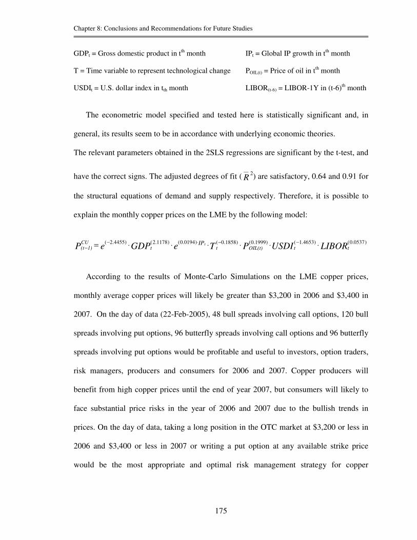
Chapter 8: Conclusions and Recommendations for Future Studies

175

GDPt = Gross domestic product in tth month IPt = Global IP growth in tth month

T = Time variable to represent technological change POIL(t) = Price of oil in tth month

USDIt = U.S. dollar index in tth month LIBOR(t-6) = LIBOR-1Y in (t-6)th month

The econometric model specified and tested here is statistically significant and, in

general, its results seem to be in accordance with underlying economic theories.

The relevant parameters obtained in the 2SLS regressions are significant by the t-test, and

have the correct signs. The adjusted degrees of fit ( R__ 2) are satisfactory, 0.64 and 0.91 for

the structural equations of demand and supply respectively. Therefore, it is possible to

explain the monthly copper prices on the LME by the following model:

LIBORUSDIPTeGDPeP ttOIL(t)ttCU

1)(tIPt )0537.0()4653.1()1999.0()1858.0()0194.0()1178.2()4455.2( ⋅⋅⋅⋅⋅⋅= −−⋅−

−

According to the results of Monte-Carlo Simulations on the LME copper prices,

monthly average copper prices will likely be greater than $3,200 in 2006 and $3,400 in

2007. On the day of data (22-Feb-2005), 48 bull spreads involving call options, 120 bull

spreads involving put options, 96 butterfly spreads involving call options and 96 butterfly

spreads involving put options would be profitable and useful to investors, option traders,

risk managers, producers and consumers for 2006 and 2007. Copper producers will

benefit from high copper prices until the end of year 2007, but consumers will likely to

face substantial price risks in the year of 2006 and 2007 due to the bullish trends in

prices. On the day of data, taking a long position in the OTC market at $3,200 or less in

2006 and $3,400 or less in 2007 or writing a put option at any available strike price

would be the most appropriate and optimal risk management strategy for copper

Chapter 8: Conclusions and Recommendations for Future Studies

176

consumers, according to the analysis result. Producers may not need to be hedged in these

years because the expected prices have a bullish trend until the end of 2007.

In a bull market, consumers should implement risk management to insure against a

rise in prices. In contrast, producers should implement risk management in a bear market

to insure against a fall in prices. A bullish trend in the copper market is likely to continue

until late 2007. Hence, copper consumers need to pay more attention for hedging and risk

management until the market shifts to a bearish trend. However, at least 1.3 million

tonnes of refined copper may be accumulated as stockpiled metal in China and this

copper could be used to make good delivery against short positions, according to the

Calyon's commodity research on 16 November 2005. In addition, analysts say that this

can be a sign of bearish trend in the copper market and fall in copper prices. In this case,

risk management will be very important to copper producers. As a result, when the

company implements risk management, it is less risky than not being hedged and hedging

may be better than no hedge in a potentially volatile copper market.

The following issues can be considered for future studies:

• In order for the model to be more accurate, the demand-side structural equation of

the price prediction model may need to be improved, since omitted variables are

likely.

• Risk management strategies can be extended by other OTC strategies such as

producer MIN-MAX collars, structured put options, extra forward contracts and

so forth.

• It will be an interesting and valuable research if the model and methodologies in

this study are applied to other base metals market such as the aluminum market.

177

REFERENCES

[1] AGOSTINI, Claudio [2002], “Estimating Market Power in the U.S. Copper Industry”, University of Michigan, Ann Arbor, Working Paper, August 2002

[2] AHMED, Maqsood [2002], “LME Metals Weekly Update: 1, 8, 15, 22, 30 August & 5,

12 September”, Credit Lyonnais Rouse Limited, London, United Kingdom; [2005], “LME Metals Weekly Update: 11 February and 01 March”, Calyon Financial Metals Group, London, United Kingdom

[3] BLAKE, David [2000], “Financial Market Analysis”, 2nd edition, John Wiley & Sons

Inc. [4] BLOOMSBURY MINERALS ECONOMICS LIMITED [2003, 2004, 2005], “Copper

Briefing Service”, Monthly Bulletins [5] CHANCE M. Don [2001], “An Introduction to Derivatives and Risk Management”, 5th

edition, Harcourt College Publishers [6] CHR METALS LIMITED [Jan-2005], “CHR Economics: Global IP Watch” [7] DAVIDSON, Russell and MACKINNON G. James [2004], “Econometric Theory and

Methods”, Oxford University Press Inc. [8] ENDERS, Walter [2004], “Applied Econometric Time Series”, Wiley series in

probability and statistics, John Wiley & Sons Inc. [9] ERRERA, Steven and BROWN L. Stewart [2002], “Fundamentals of Trading Energy

Futures and Options”, 2nd edition, PennWell Corporation [10] GOSS B. A. [1972], “The Theory of Futures Trading”, Routledge and Kegan Paul [11] GRANGER C. W. J. [1989], “Forecasting in Business and Economics”, 2nd edition,

Academic Press Inc. [12] GREENE H. William [1990], “Econometric Analysis”, Macmillan Publishing Company,

New York, Collier Macmillan Publishers, London [13] HALL E. Robert and LIEBERMAN, Marc [2001], “Economics Principles and

Applications”, 2nd edition, South-Western College Publishing [14] HULL C. John [2002], “Fundamentals of Futures and Options Markets”, 4th edition,

Pearson Education Inc. [15] HULL C. John [2000], “Options, Futures, and Other Derivatives”, 4th edition, Published

by Prentice-Hall Inc.

178

[16] HUSTED, Steven and MELVIN, Michael [2000], “International Economics”, 5th edition, The Addison Wesley Series in Economics

[17] ICSG [2004], “Copper Bulletin”, Monthly Publication, Vol. 12, No. 4, April 2004 [18] JOHNSON, Dean [2004], “BA 4460: Derivatives Securities and Financial Engineering”,

Class handout materials, School of Business and Economics, Michigan Technological University

[19] KOLB W. Robert [1993], “Financial Derivatives”, New York Institute of Finance [20] LABYS C. Walter and GRANGER C. W. J. [1970], “Speculation, Hedging and

Commodity Price Forecasts”, Heath Lexington Books, D. C. Heath and Company, Lexington, Massachusetts

[21] LABYS C. Walter and POLLAK K. Peter [1984], “Commodity Models for Forecasting

and Policy Analysis”, Nichols Publishing Company, New York [22] MARTINOT, Natacha, LESOURD , Baptiste Jean and MORARD, Bernard [2000], “On

the Information Content of Futures Prices: Application to LME non ferrous metal futures”, Working Paper, June 2000

[23] MISHKIN S. Frederic and EAKINS G. Stanley [2000], “Financial Markets and

Institutions”, 3rd edition, The Addison-Wesley Series in Finance [24] OYEN B. Duane [1991], “Business Fluctuations & Forecasting”, Dearborn Financial

Publishing Inc. [25] PHELPS DODGE CORP. [2002], “Technological issues in Morenci mine”, Presentation [26] PINDYCK S. Robert and RUBINFELD L. Daniel [1981], “Econometric Models &

Economic Forecasts”, McGraw-Hill Book Company [27] RITCHKEN, Peter [1996], “Derivative Markets: Theory, Strategy, and Applications”,

Harper Collins College Publishers [28] ROBERTS C. Mark [1989], “Forecasting Mineral Consumption for Mine Project

Evaluation”, Working paper, Multinational Conference On Mine Planning and Design, University of Kentucky, Lexington, Kentucky, May 23-26

[29] SANDAGDORJ, Bold [2004], “Application of Options Pricing in a Real World

Situation”, Project, Advisor: Professor Dean L. Johnson, School of Business and Economics, Michigan Technological University, Houghton, Michigan, United States.

[30] SEIDEL D. Andrew and GINSBERG M. Philip [1983], “Commodities Trading:

Foundations, Analysis, and Operations”, Published by Prentice-Hall Inc.

179

[31] SIGMON, Hugh [1997], “Guide to Metal Trading”, Published by American Metal Market

[32] SLADE E. Margaret [1984], “ An Econometric Model of the U.S. Copper and Aluminum

Industries: How Cost Changes Affect Substitution and Recycling”, Garland Publishing Inc., New York and London

[33] SOTOWICZ, Adam [2004], “LME Metal Price Model Tutorial”, Presentation,

Bloomsbury Minerals Economics Ltd. [34] STUDENMUND A. H. [2001], “Using Econometrics: A Practical Guide”, 4th edition,

Addison Wesley Longman Inc. [35] TALEB, Nassim [1997], “Dynamic Hedging: Managing Vanilla and Exotic Options”,

John Wiley & Sons Inc. [36] THE AMERICAN METAL MARKET CO., NEW YORK [1994, 1997, 2000, 2002],

“Metal Statistics”, The purchasing guide of the metal industries [37] THE COMMODITY RESEARCH BUREAU [2004], “The CRB Commodity Yearbook”,

John Wiley & Sons Inc. [38] THE LME [2001], “Introduction to Hedging with the LME and Introduction to LME

Traded Options”, Educational seminar, London, U.K. [39] THE NYMEX [2003], “A Guide to Metals Hedging”, Study Material [40] THE U.S. DEPARTMENT OF ENERGY [2004], “Kennecott Utah Copper Corporation:

Facility Utilizes Energy Assessments to Identify $930,000 in Potential Annual Savings”, Best Practices Plant-Wide Assessment Case Study, July 2004

[41] VERBEEK, Marno [2004], “A Guide to Modern Econometrics”, 2nd edition, Erasmus

University Rotterdam, John Wiley & Sons Ltd. [42] WILMOTT, Paul, DEWYNNE, Jeff and HOWISON, Sam [1993], “Option Pricing:

Mathematical Models and Computation”, Published by Oxford Financial Press [43] WILMOTT, Paul, HOWISON, Sam and DEWYNNE, Jeff [1995], “The Mathematics of

Financial Derivatives: A Student Introduction”, Published by the Press Syndicate of the University of Cambridge

180

Web Pages:

[1] Board of Governors of the Federal Reserve System

http://federalreserve.gov/releases/H10/Summary/indexn_m.txt [2] Economagic.com: Economic Time Series Page

http://www.economagician.com/em-cgi/data.exe/libor/day-us3m [3] HSH Associates, Financial Publishers

http://www.hsh.com/indices/libor00s.html

[4] Rates FX: Daily FOREX rates, Information about Currency Markets http://www.ratesfx.com/rates/rate-converter.html

[5] The International Monetary Fund:

http://www.imf.org/external/pubs/ft/weo/2002/02/data/index.htm#changes [6] The London Metal Exchange

http://www.lme.co.uk/ [7] The Metrod Corporation:

http://www.metrod.com/LMEAVG2004.htm [8] The New York Mercantile Exchange

http://www.nymex.com/

181

APPENDICES

Appendix 1: Implied Volatility (I.V.) Estimations

Table A1-1: I.V. Estimation on 01.08.02


3-month 1.68 0.017105 1.71%6-month 1.66 0.016972 1.70%1-year 1.75 0.018061 1.81%


Strike Market MarketPrice Value Oct-02 Nov-02 Dec-02 Value Apr-03 May-03 Jun-031525 43 112.10 85.32 68.16 94 59.66 54.34 50.431575 26 100.60 76.73 61.46 72 56.10 51.16 47.541600 20 96.01 73.37 58.87 63 54.72 49.95 46.44

Average 102.90 78.47 62.83 56.83 51.82 48.14

Implied Volatilities4Q-2002 CALL Options

Implied Volatilities2Q-2003 CALL Options



3-month 1.62 0.016492 1.65%6-month 1.59 0.016250 1.63%1-year 1.68 0.017326 1.73%



Average 106.39 79.48 62.79 56.43 51.34 47.61

4Q-2002 CALL Options 2Q-2003 CALL OptionsImplied Volatilities Implied Volatilities

182



3-month 1.62 0.0164919 1.65%6-month 1.63 0.0166626 1.67%1-year 1.78 0.0183763 1.84%



Average 113.76 82.83 64.34 57.24 51.87 47.97




3-month 1.65 0.016799 1.68%6-month 1.68 0.017178 1.72%1-year 1.85 0.019113 1.91%



Average 123.98 87.58 66.71 57.98 52.31 48.23




3-month 1.69 0.0172075 1.72%6-month 1.67 0.0170749 1.71%1-year 1.74 0.0179559 1.80%



Average 140.23 95.22 70.79 60.40 54.38 49.95


183


Date of Data 21-Feb-05CU Price ($/t) 3321.00

6-month 2.90 0.029618 2.96%1-year 3.09 0.031823 3.18%2-year 3.45 0.036245 3.62%3-year 3.62 0.038853 3.89%


Strike MarketPrice Value July August September October November December3100 192.56 68.95 56.55 47.43 41.20 35.95 31.453200 154.87 66.82 55.21 46.69 40.88 35.99 31.813300 123.27 65.04 54.11 46.09 40.62 36.02 32.093400 97.17 63.54 53.20 45.60 40.41 36.05 32.333500 75.89 62.28 52.43 45.19 40.24 36.08 32.523600 58.77 61.21 51.80 44.86 40.11 36.12 32.69

Average 64.64 53.88 45.98 40.58 36.04 32.15

Implied Volatilities2005 CALL Options


Average 38.90 39.86 39.81 39.37 38.84 38.05

2005 PUT OptionsImplied Volatilities

Strike MarketPrice Value January February March April May June3100 151.14 22.10 19.64 17.14 15.20 13.39 11.623200 125.34 24.43 22.16 19.87 18.13 16.54 15.033300 103.42 26.21 24.04 21.86 20.21 18.71 17.303400 84.95 27.63 25.53 23.42 21.82 20.37 19.013500 69.47 28.79 26.74 24.68 23.12 21.70 20.373600 56.59 29.77 27.76 25.73 24.19 22.80 21.48

Average 26.49 24.31 22.12 20.45 18.92 17.47

2006 CALL OptionsImplied Volatilities

184

Strike MarketPrice Value July August September October November December3100 151.14 10.11 7.31 5.21 - - -3200 125.34 13.81 11.95 10.88 9.84 8.79 7.843300 103.42 16.16 14.53 13.58 12.68 11.79 11.013400 84.95 17.91 16.39 15.48 14.63 13.79 13.063500 69.47 19.29 17.84 16.95 16.11 15.30 14.593600 56.59 20.42 19.01 18.14 17.31 16.51 15.81

Average 16.28 14.51 13.37 14.11 13.24 12.46

2006 CALL Options (continues)Implied Volatilities


Average 57.58 56.26 54.80 53.60 52.43 51.28



Average 50.30 49.66 48.81 47.98 47.15 46.42

2006 PUT Options (Continues)Implied Volatilities

Strike MarketPrice Value January February March April May June3100 117.13 - - - - - -3200 98.12 2.99 - - - - -3300 81.95 8.14 7.53 6.88 6.30 5.66 5.103400 68.24 10.65 10.11 9.52 9.02 8.49 8.043500 56.68 12.50 11.94 11.40 10.91 10.40 9.973600 46.96 13.96 13.44 12.87 12.39 11.88 11.46

Average 9.65 10.76 10.17 9.66 9.11 8.64

2007 CALL OptionsImplied Volatilities

185

Strike MarketPrice Value July August September October November December3100 117.13 - - - - - -3200 98.12 - - - - - -3300 81.95 4.52 2.99 1.91 - - -3400 68.24 7.59 6.73 6.33 5.90 5.47 5.083500 56.68 9.55 8.79 8.43 8.04 7.66 7.323600 46.96 11.04 10.33 9.98 9.60 9.23 8.90

Average 8.18 7.21 6.66 7.85 7.45 7.10

2007 CALL Options (continues)Implied Volatilities


Average 55.89 55.10 54.26 53.53 52.74 52.09



Average 51.45 51.13 50.59 50.02 49.46 48.95

2007 PUT Options (Continues)Implied Volatilities

186

Appendix 2: The Results of Two-Stage Least Square Regression

Table A2-1: Summary Output of the Reduced Form Equation Regression Statistics

Multiple R 0.882432794R Square 0.778687637Adjusted R Square 0.766936538Standard Error 0.119314775Observations 120

ANOVAdf SS MS F Significance F

Regression 6 5.66010515 0.943350858 66.26509066 1.01306E-34Residual 113 1.608669752 0.014236016Total 119 7.268774902

Coefficients Standard Error t Stat P-value Lower 95% Upper 95% Lower 95.0% Upper 95.0%Intercept 6.145483052 6.289703456 0.977070397 0.330621428 -6.315553503 18.60651961 -6.315553503 18.60651961LN[GDP] 1.052093337 0.769288297 1.36761906 0.174145251 -0.472005478 2.576192152 -0.472005478 2.576192152IP % -0.00085807 0.006184824 -0.13873839 0.889903832 -0.013111323 0.011395178 -0.013111323 0.011395178LN[T] -0.12909579 0.028639815 -4.50756368 1.60946E-05 -0.18583643 -0.07235515 -0.18583643 -0.072355154LN[P Oil] 0.268063148 0.071967227 3.72479475 0.000306701 0.125483097 0.410643199 0.125483097 0.410643199LN[USDI] -1.60691204 0.227782929 -7.05457622 1.47565E-10 -2.058191089 -1.15563299 -2.058191089 -1.155632986LN[Libor 1Y (t-6)] 0.094978381 0.045481106 2.088304098 0.039016835 0.004872109 0.185084653 0.004872109 0.185084653

Table A2-2: Summary Output of the Demand Equation Regression Statistics

Multiple R 0.803728263R Square 0.645979121Adjusted R Square 0.636823409Standard Error 0.081998582Observations 120



Coefficients Standard Error t Stat P-value Lower 95% Upper 95% Lower 95.0% Upper 95.0%Intercept -5.04850731 1.171494136 -4.30946016 3.44789E-05 -7.368798978 -2.72821564 -7.368798978 -2.728215637LN[P(t-1)] -0.18680493 0.043637288 -4.28085569 3.85333E-05 -0.273234078 -0.10037579 -0.273234078 -0.100375789LN[GDP] 1.71513405 0.137747297 12.4513082 4.07798E-23 1.442308181 1.987959919 1.442308181 1.987959919IP growth 0.015779157 0.003954994 3.989678576 0.000116247 0.007945792 0.023612521 0.007945792 0.023612521 Table A2-3: Summary Output of the Supply Equation

Regression StatisticsMultiple R 0.954798344R Square 0.911639878Adjusted R Square 0.907764434Standard Error 0.031964198Observations 120



Coefficients Standard Error t Stat P-value Lower 95% Upper 95% Lower 95.0% Upper 95.0%Intercept -3.07851671 2.861267559 -1.07592759 0.284231403 -8.746665524 2.589632103 -8.746665524 2.589632103LN[P(t-1)] 0.596017446 0.195177883 3.053714069 0.002813852 0.209371576 0.982663316 0.209371576 0.982663316LN[T] 0.140832545 0.021434993 6.570216654 1.56535E-09 0.098369992 0.183295099 0.098369992 0.183295099LN[P Oil] -0.15584734 0.065460607 -2.38078057 0.018934024 -0.285524297 -0.02617039 -0.285524297 -0.026170387LN[USDI] 1.243162349 0.335793409 3.702164231 0.000330944 0.577958213 1.908366485 0.577958213 1.908366485LN[Libor 1Y (t-6)] -0.05612547 0.012877799 -4.35831206 2.88383E-05 -0.081636289 -0.03061465 -0.081636289 -0.030614648

187

Appendix 3: The Results of Subsidiary Regressions

Table A3-1: Demand Equation: LN[P(t-1)] as dependent variable




Coefficients Standard Error t Stat P-value Lower 95% Upper 95% Lower 95.0% Upper 95.0%Intercept 10.993767 2.264278588 4.855306698 3.75434E-06 6.509482054 15.4780519 6.509482054 15.47805194LN[GDP] -0.46039752 0.288711001 -1.59466565 0.113484855 -1.032174506 0.11137947 -1.032174506 0.111379474IP growth % 0.055587209 0.006618073 8.399304593 1.21654E-13 0.042480463 0.06869396 0.042480463 0.068693955

Table A3-2: Demand Equation: IP growth % as dependent variable




Coefficients Standard Error t Stat P-value Lower 95% Upper 95% Lower 95.0% Upper 95.0%Intercept -112.700449 25.32468811 -4.45022059 1.96873E-05 -162.8546646 -62.5462325 -162.8546646 -62.54623249LN[P(t-1)] 6.767038031 0.805666464 8.399304593 1.21654E-13 5.171457871 8.36261819 5.171457871 8.362618191LN[GDP] 8.289155811 3.127391953 2.6505011 0.009149675 2.095520136 14.4827915 2.095520136 14.48279149

Table A3-3: Demand Equation: LN[GDP] as dependent variable



Regression 2 0.021277314 0.010638657 3.512579516 0.033002744Residual 117 0.354361485 0.003028731Total 119 0.375638799

Coefficients Standard Error t Stat P-value Lower 95% Upper 95% Lower 95.0% Upper 95.0%Intercept 8.18320557 0.214125414 38.21688155 6.17365E-68 7.759141423 8.60726972 7.759141423 8.607269717IP growth % 0.006833385 0.002578148 2.6505011 0.009149675 0.001727497 0.01193927 0.001727497 0.011939273LN[P(t-1)] -0.04620429 0.028974281 -1.59466565 0.113484855 -0.103586334 0.01117775 -0.103586334 0.011177753

188

Table A3-4: Supply Equation: LN[P(t-1)] as dependent variable




Coefficients Standard Error t Stat P-value Lower 95% Upper 95% Lower 95.0% Upper 95.0%Intercept 14.61466841 0.107178381 136.3583619 5.2446E-129 14.40236867 14.82696815 14.40236867 14.82696815LN[T] -0.10529938 0.002908908 -36.1989403 1.06658E-64 -0.111061365 -0.09953739 -0.111061365 -0.099537393LN[P Oil] 0.329079078 0.006038326 54.4983917 5.4463E-84 0.317118316 0.34103984 0.317118316 0.34103984LN[USDI] -1.70019016 0.024547192 -69.2621053 1.30995E-95 -1.748813425 -1.6515669 -1.748813425 -1.651566904LN[LIBOR 1Y(t-6)] 0.050391111 0.003971716 12.6874897 1.33488E-23 0.042523905 0.058258317 0.042523905 0.058258317

Table A3-5: Supply Equation: LN[T] as dependent variable




Coefficients Standard Error t Stat P-value Lower 95% Upper 95% Lower 95.0% Upper 95.0%Intercept 125.4678539 4.24907326 29.52828681 1.6443E-55 117.0512578 133.88445 117.0512578 133.88445LN[P Oil] 2.934786674 0.078762887 37.26103464 4.96837E-66 2.778772558 3.09080079 2.778772558 3.09080079LN[USDI] -14.3309833 0.590032947 -24.2884459 4.26953E-47 -15.49972499 -13.1622416 -15.49972499 -13.16224165LN[LIBOR 1Y(t-6)] 0.37286533 0.043928083 8.488085703 8.41303E-14 0.285852256 0.459878405 0.285852256 0.459878405LN[P(t-1)] -8.73052455 0.241181772 -36.1989403 1.06658E-64 -9.208259211 -8.2527899 -9.208259211 -8.252789898

Table A3-6: Supply Equation: LN[POIL] as dependent variable




Coefficients Standard Error t Stat P-value Lower 95% Upper 95% Lower 95.0% Upper 95.0%Intercept -42.4850181 0.958107401 -44.3426468 3.7069E-74 -44.38284439 -40.5871918 -44.38284439 -40.58719178LN[USDI] 4.936728188 0.129968478 37.9840424 6.42552E-67 4.679285655 5.194170722 4.679285655 5.194170722LN[LIBOR 1Y(t-6)] -0.15309974 0.011519951 -13.2899649 5.49552E-25 -0.175918542 -0.13028093 -0.175918542 -0.130280934LN[P(t-1)] 2.925508851 0.053680646 54.4983917 5.4463E-84 2.819177826 3.031839875 2.819177826 3.031839875LN[T] 0.314675662 0.008445167 37.26103464 4.96837E-66 0.297947412 0.331403912 0.297947412 0.331403912

189

Table A3-7: Supply Equation: LN[USDI] as dependent variable



Regression 4 0.90808728 0.22702182 2881.258046 2.8885E-114Residual 115 0.009061149 7.87926E-05Total 119 0.917148429

Coefficients Standard Error t Stat P-value Lower 95% Upper 95% Lower 95.0% Upper 95.0%Intercept 8.494864182 0.062086779 136.822433 3.5568E-129 8.371882226 8.617846139 8.371882226 8.617846139LN[LIBOR 1Y(t-6)] 0.030981514 0.002107742 14.69891315 3.60576E-28 0.026806483 0.035156545 0.026806483 0.035156545LN[P(t-1)] -0.57439992 0.008293134 -69.2621053 1.30995E-95 -0.590827018 -0.55797281 -0.590827018 -0.557972814LN[T] -0.05839536 0.002404244 -24.2884459 4.26953E-47 -0.063157704 -0.05363301 -0.063157704 -0.053633014LN[P Oil] 0.187609549 0.004939168 37.9840424 6.42552E-67 0.177826009 0.197393089 0.177826009 0.197393089

Table A3-8: Supply Equation: LN[LIBOR(t-6)] as dependent variable




Coefficients Standard Error t Stat P-value Lower 95% Upper 95% Lower 95.0% Upper 95.0%Intercept -173.704895 12.91889641 -13.4457998 2.42012E-25 -199.2947414 -148.115048 -199.2947414 -148.1150482LN[P(t-1)] 11.57528863 0.912338761 12.6874897 1.33488E-23 9.768121191 13.38245607 9.768121191 13.38245607LN[T] 1.033035796 0.121704214 8.488085703 8.41303E-14 0.791963179 1.274108412 0.791963179 1.274108412LN[P Oil] -3.95595368 0.29766472 -13.2899649 5.49552E-25 -4.545570184 -3.36633718 -4.545570184 -3.366337177LN[USDI] 21.06510665 1.43310641 14.69891315 3.60576E-28 18.22639876 23.90381454 18.22639876 23.90381454

190

Appendix 4: The Result Details of the Park Test

Table A4-1: Demand Equation: P(t-1) as Z variable

Regression StatisticsMultiple R 0.079559404R Square 0.006329699Adjusted R Square -0.00209124Standard Error 2.680448308Observations 120



Coefficients Standard Error t Stat P-value Lower 95% Upper 95% Lower 95.0% Upper 95.0%Intercept 8.3139705 17.41796095 0.477321687 0.63401597 -26.1783338 42.8062748 -26.1783338 42.8062748LN{LN[P(t-1)]} -7.45364104 8.597201418 -0.86698458 0.38771004 -24.47844023 9.57115815 -24.47844023 9.571158145

Table A4-2: Demand Equation: GDP as Z variable




Coefficients Standard Error t Stat P-value Lower 95% Upper 95% Lower 95.0% Upper 95.0%Intercept 3.429263628 71.30505812 0.048092852 0.96172355 -137.7741625 144.63269 -137.7741625 144.6326898LN{LN[GDP]} -4.95491707 34.58754691 -0.14325726 0.88633136 -73.44767558 63.5378414 -73.44767558 63.53784143

Table A4-3: Supply Equation: P(t-1) as Z variable




Coefficients Standard Error t Stat P-value Lower 95% Upper 95% Lower 95.0% Upper 95.0%Intercept -48.965805 15.43007832 -3.17339964 0.0019214 -79.52156052 -18.4100494 -79.52156052 -18.41004945LN{LN[P(t-1)]} 20.01710895 7.616017257 2.62829091 0.00972263 4.935321504 35.0988964 4.935321504 35.0988964

191

Table A4-4: Supply Equation: POIL as Z variable




Coefficients Standard Error t Stat P-value Lower 95% Upper 95% Lower 95.0% Upper 95.0%Intercept -10.823743 2.535302418 -4.2692118 3.9866E-05 -15.84433196 -5.80315403 -15.84433196 -5.803154033LN{LN[P Oil]} 2.098214192 2.200028541 0.95372135 0.34217434 -2.258441225 6.454869608 -2.258441225 6.454869608

Table A4-5: Supply Equation: USDI as Z variable




Coefficients Standard Error t Stat P-value Lower 95% Upper 95% Lower 95.0% Upper 95.0%Intercept 38.73296868 17.05148914 2.27152997 0.02492712 4.966378324 72.49955904 4.966378324 72.49955904LN{LN[USDI]} -31.105033 11.24849548 -2.76526163 0.00660282 -53.38011616 -8.82994979 -53.38011616 -8.829949785

Table A4-6: Supply Equation: LIBOR 1Y(t-6) as Z variable




Coefficients Standard Error t Stat P-value Lower 95% Upper 95% Lower 95.0% Upper 95.0%Intercept -8.31640089 0.233932946 -35.5503618 6.8924E-65 -8.779651806 -7.85314997 -8.779651806 -7.853149973LN{LN[Libor 1Y(t-6)]} -0.45940631 0.351429094 -1.30725178 0.19366878 -1.155331582 0.236518966 -1.155331582 0.236518966

192

Appendix 5: The Result Details of the White Test



Regression 9 0.000666459 7.4051E-05 0.64901157 0.752841279Residual 110 0.01255079 0.000114098Total 119 0.013217249

Coefficients Standard Error t Stat P-value Lower 95% Upper 95% Lower 95.0% Upper 95.0%Intercept 35.14957703 40.80201687 0.861466656 0.39085508 -45.71044097 116.009595 -45.71044097 116.009595LN[P(t-1)] -0.27937567 1.374582703 -0.20324399 0.83931983 -3.003475864 2.44472453 -3.003475864 2.444724527LN[GDP] -8.61534881 10.51945307 -0.81899209 0.41456176 -29.46243505 12.2317374 -29.46243505 12.23173743IP % 0.009115653 0.140925821 0.06468405 0.94854297 -0.270166239 0.28839754 -0.270166239 0.288397545

LN[P(t-1)]2 -0.00907891 0.043896933 -0.20682329 0.83653023 -0.096072323 0.07791451 -0.096072323 0.077914507

LN[GDP]2 0.518167671 0.689969051 0.751001324 0.45425547 -0.849188998 1.88552434 -0.849188998 1.885524341

(IP %)2 0.000253163 0.000278148 0.91017365 0.36472103 -0.000298061 0.00080439 -0.000298061 0.000804388LN[P(t-1)]*LN[GDP] 0.053739956 0.138693189 0.387473651 0.6991543 -0.221117382 0.32859729 -0.221117382 0.328597294LN[P(t-1)]*IP % -0.00274255 0.006093909 -0.4500471 0.65356215 -0.014819242 0.00933415 -0.014819242 0.00933415LN[GDP]*IP % 0.001262394 0.015237565 0.082847519 0.93412336 -0.028934882 0.03145967 -0.028934882 0.031459671

193


(Including PAL(t-1) as an exogenous variable in demand equation)

Table A6-1: Summary Output of the Demand Equation




Coefficients Standard Error t Stat P-value Lower 95% Upper 95% Lower 95.0% Upper 95.0%Intercept -7.13123812 1.383192377 -5.15563723 1.06284E-06 -9.871075924 -4.39140032 -9.871075924 -4.39140032LN[P(t-1)] -0.34611209 0.085954327 -4.02669773 0.000101781 -0.516371065 -0.17585312 -0.516371065 -0.175853119LN[GDP] 1.743776284 0.135261572 12.89188241 4.50812E-24 1.47584915 2.011703417 1.47584915 2.011703417IP growth 0.013645737 0.003762323 3.626944687 0.00042895 0.0061933 0.021098174 0.0061933 0.021098174LN[P(Al)(t-1)] 0.420229223 0.179859863 2.336425792 0.021200505 0.063961462 0.776496984 0.063961462 0.776496984

][4202.00137.0][7438.1][3461.01312.7][ )1()1( PIPGDPPQ ALtttt

D

tLnLnLnLn −− ⋅+⋅+⋅+⋅−−=

Standard error: (0.0860) (0.1353) (0.0038) (0.1799)

T-statistics: -4.0267 12.8919 3.6269 2.3364

R2 = 0.66, R__

2 = 0.65, F = 56.16, n = 120

Table A6-2: Summary Output of the Supply Equation




Coefficients Standard Error t Stat P-value Lower 95% Upper 95% Lower 95.0% Upper 95.0%Intercept 5.023697921 0.561051783 8.954071754 7.5153E-15 3.912258696 6.135137146 3.912258696 6.135137146LN[P(t-1)] 0.041628225 0.034957285 1.190831171 0.236193512 -0.027621886 0.110878336 -0.027621886 0.110878336LN[T] 0.082455705 0.007291014 11.30922308 2.42173E-20 0.068012262 0.096899147 0.068012262 0.096899147LN[P Oil] 0.026590552 0.017407195 1.527560952 0.129391458 -0.007892967 0.06107407 -0.007892967 0.06107407LN[USDI] 0.300595248 0.079705697 3.77131449 0.00025911 0.142698882 0.458491614 0.142698882 0.458491614LN[LIBOR 1Y(t-6)] -0.02818918 0.008771733 -3.21363858 0.001704615 -0.045565914 -0.01081244 -0.045565914 -0.010812445

194

+⋅+⋅+⋅+= − ][0266.0][0825.0][0416.00237.5][ )1( PTPQ OILttt

S

tLnLnLnLn

Standard error: (0.0350) (0.0073) (0.0174)

T-statistics: 1.1908 11.3092 1.5276

][0282.0][3006.0 )1( )6(YLIBORUSDI tt LnLn −⋅−⋅+

Standard error: (0.0797) (0.0088)

T-statistics: 3.7713 -3.2136

R2 = 0.91, R__

2 = 0.90, F = 218.69, n = 120

195


(Interest rate variable is lagged by 12 months)

Table A7-1: Summary Output of the Demand Equation




Coefficients Standard Error t Stat P-value Lower 95% Upper 95% Lower 95.0% Upper 95.0%Intercept -5.02804808 1.172487445 -4.28835984 3.74274E-05 -7.350307122 -2.70578903 -7.350307122 -2.705789032LN[P(t-1)] -0.18866592 0.043943445 -4.29338021 3.67046E-05 -0.275701445 -0.10163039 -0.275701445 -0.101630391LN[GDP] 1.714277257 0.137714076 12.44809033 4.14896E-23 1.441517186 1.987037328 1.441517186 1.987037328IP growth 0.015882604 0.003964472 4.006234287 0.000109323 0.008030468 0.02373474 0.008030468 0.02373474 Table A7-2: Summary Output of the Supply Equation




Coefficients Standard Error t Stat P-value Lower 95% Upper 95% Lower 95.0% Upper 95.0%Intercept 4.11618332 5.608534466 0.733914242 0.46450775 -6.994279901 15.22664654 -6.994279901 15.22664654LN[P(t-1)] 0.081144383 0.389228383 0.208474989 0.83523013 -0.689914021 0.852202787 -0.689914021 0.852202787LN[T] 0.082627036 0.046717605 1.768648824 0.07962711 -0.009920175 0.175174248 -0.009920175 0.175174248LN[P Oil] -0.00115352 0.126813878 -0.00909613 0.99275834 -0.252370823 0.250063792 -0.252370823 0.250063792LN[USDI] 0.46050006 0.63686041 0.723078484 0.47111261 -0.801115466 1.722115585 -0.801115466 1.722115585LN[Libor 1Y (t-12)] -0.04954203 0.014028317 -3.53157302 0.00059728 -0.077332015 -0.02175204 -0.077332015 -0.021752039

196

Appendix 8: Fluctuations of the LME CU Prices and Major Influential Economic and Market Events (Source: AIG)

1300

1500

1700

1900

2100

2300

2500

2700

2900

3100

3300

3500Ja

n-88

Jun-

88

Nov

-88

May

-89

Oct

-89

Apr

-90

Sep-

90

Mar

-91

Aug

-91

Feb-

92

Jul-9

2

Jan-

93

Jun-

93

Dec

-93

May

-94

Nov

-94

Apr

-95

Oct

-95

Mar

-96

Sep-

96

Feb-

97

Aug

-97

Jan-

98

Jul-9

8

Dec

-98

Jun-

99

Nov

-99

May

-00

Oct

-00

Apr

-01

Sep-

01

Mar

-02

Aug

-02

Feb-

03

Jul-0

3

Jan-

04

Jun-

04

Dec

-04

($/t)

June 1988: - Worldwide economic boom - Cu demand exceeds supply - JPN’s asset bubble � quickly - Conflict shuts major Cu mine Panguna

1989-1990: Japanese asset bubble bursts

June 1991: - Global economy slows, interest rates high - USSR disbands, Russian demand crashes & Me exports swamp western markets

1991-June 1992: Producers buy OTC put options

1992-June 1993: - First OTC but option price collapse - US rates cut to 3% low, economy recovers. LME stocks flow to the US on strong demand. Start of 8-year US economic boom. - Japanese economic prospects remain weak

1993-1994: Producers buy OTC put option. LME stocks fall. New mine production planned, including low cost SX-EW

1994: - US economy strong, helping Europe. In Asia, China & “Tigers” booming, Japan remains weak. - US economy bounces. Fed suggest as inflation investors & funds rush into metals

1995: LME opens first copper warehouses in the USA.

1995-1996: - Funds begin short selling. Cash -3M tightens. LME stocks rise. - LME begins investigation into copper market.

1996-1997: - May of 96 price collapse, heavy delta selling vs OTC puts - LME stocks fall. Concentrate stocks build on smelter bottleneck. Nearby backwardation grows as short cover. LME wide fund rally starts Jan. 97 - Very rapid copper extension.

1998: - Cu tightness ends & LME sells off. H2’97 Asian crisis hits. - Smelter bottleneck eases & LME stocks rise on new mine supply. SX-EW lowers global cash costs

1999: Fund rally, helped by Y2K fears in North America

1999-2000: Y2K profit taking. Producer hedging. Funds short sell LME

2000-2001: LME metals go online

2001: - Equity boom ends, & Fed cuts rates from 6.5%. US slows. Funds short Cu chart. - Producers cut. Short cover. Online offline. World economy slows. US Fed rates @ 1.75%

Michigan Technological University Price risk management in the copper market using commodity...

Documents

Transcript of Michigan Technological University Price risk management in the copper market using commodity...