University of Nebraska - LincolnDigitalCommons@University of Nebraska - Lincoln

UNL Faculty Course Portfolios Peer Review of Teaching Project

2017

AECN 436: Commodity Price Forecasting—APeer Review of Teaching Project Inquiry PortfolioFabio MattosUniversity of Nebraska-Lincoln, fmattos@unl.edu

Follow this and additional works at: http://digitalcommons.unl.edu/prtunl

Part of the Higher Education Commons, and the Higher Education and Teaching Commons

This Portfolio is brought to you for free and open access by the Peer Review of Teaching Project at DigitalCommons@University of Nebraska - Lincoln.It has been accepted for inclusion in UNL Faculty Course Portfolios by an authorized administrator of DigitalCommons@University of Nebraska -Lincoln.

Mattos, Fabio, "AECN 436: Commodity Price Forecasting—A Peer Review of Teaching Project Inquiry Portfolio" (2017). UNLFaculty Course Portfolios. 101.http://digitalcommons.unl.edu/prtunl/101

AECN 436 – Commodity Price Forecasting

Fabio Mattos

Spring 2017

University of Nebraska-Lincoln

Peer Review of Teaching Portfolio

Is there a “better” way to learn?

An investigation into AECN 436 – Commodity Price Forecasting

TABLE OF CONTENTS

Table of Contents .......................................................................................................................... 2

Introduction ................................................................................................................................... 3

Objectives of peer review course portfolio ................................................................................. 4

Description of the course .............................................................................................................. 5

Main topics: fundamental analysis and technical analysis .................................................... 6

Classroom setting .................................................................................................................... 12

Teaching methods ....................................................................................................................... 14

Analysis of student learning ....................................................................................................... 17

Evaluation procedure .............................................................................................................. 17

Students .................................................................................................................................... 17

Performance analysis .............................................................................................................. 18

Conclusions .................................................................................................................................. 27

INTRODUCTION

Instructor: Fabio L. Mattos

Department: Agricultural Economics

Course: AECN 436 – Commodity Price Forecasting

University: University of Nebrasla-Lincoln

Contact information: 303A Filley Hall

Lincoln, NE, 68583-0922

phone 402-472-1796

fmattos@unl.edu

agecon.unl.edu/faculty/fabio-mattos

OBJECTIVES OF PEER REVIEW COURSE PORTFOLIO

I have been teaching for approximately 10 years in different universities (and countries) and

different courses. I have taught from large classes (around 200 students) to small classes (about

10 students), introductory courses and advanced courses, in 4-year programs as well as 2-year

programs, at the graduate and undergraduate levels, face-to-face and online, and regular

semester-long courses as well as short courses (2-3 weeks).

Despite the diverse set of characteristics across all courses that I have taught, there is one

component that has been common to all of them: I have relied mostly on traditional lectures to

deliver the course material. In my early years as a professor, my courses would consist entirely

on traditional lectures, in which I would stand in front of the students and talk for the whole class

period. Over the years, I had the impression that some students would not always pay attention to

my lectures and, occasionally, I would find comments in the course evaluation that my class was

“boring”. Eventually, I started wondering whether the traditional lecture with recitation was still

an effective way to teach.

In recent years, I decided to try different ways to deliver the course material. The general

purpose of my new approach to teaching is to make students more attentive in class and help

them learn the material better. Overall, I tried implementing activities that can be broadly defined

as “active learning”. As a general definition, I think of active learning as teaching methods that

actively engage students in the classroom, making them participate in learning activities and

think about what they are doing.

Therefore, my objective with this portfolio is to assess whether students learn better and

become more engaged in lectures with traditional recitation or in lectures with active learning

activities.

DESCRIPTION OF THE COURSE

The motivation for the course comes from the importance of price analysis and forecasting in

various levels of commodity markets. Participants in commodity markets are constantly trying to

forecast prices. A sound analysis of expected prices in the future is important in many

dimensions. For example, it is useful for producers and merchandisers as they develop their

marketing and risk management strategies during the crop year. It is also relevant to financial

institutions providing loans to the agricultural industry as they assess financial performance and

credit risk of their clients. Another aspect of market analysis is the short-run trajectory that prices

follow until they reach their long run forecast. This information is also important as it relates to

the timing of decision-making in commodity markets. For example, it is relevant for producers

and merchandisers not only to define a marketing or risk management strategy, but also to

determine the best time to implement it.

Two methods have been widely used to forecast prices and their trajectories: fundamental

analysis and technical analysis. Fundamental analysis focuses on economic data (such as

production and consumption) to forecast prices, while technical analysis studies patterns in price

data. Market participants have long debated which method is better, but it is as easy to find

successful practitioners who rely on fundamental analysis as it is to find successful practitioners

who use technical analysis. The purpose of this course is to discuss how fundamental and

technical analysis have developed and are used in commodity price analysis and forecasting,

their strengths and weaknesses, and whether these methods can complement or substitute each

other.

The overall objective of this course is to teach students how to analyze and forecast

commodity prices using fundamental and technical approaches. The most common techniques

from each approach are discussed, focusing on how they can be implemented, their advantages

and disadvantages, how they differ and how they can complement each other. At the completion

of this course, students should be able to:

(a) have a thorough and workable knowledge of the forces that affect commodity markets;

(b) apply different techniques in fundamental and technical analysis, along with critical

thinking, to evaluate and solve real-world problems in commodity markets;

(c) discuss and support their opinions using fundamental and technical tools;

(d) appreciate the importance and complexity of fundamental and technical analysis in

commodity markets and understand that nobody can consistently make accurate

predictions about market movements;

(e) realize that no technique is complete and unfailing;

(f) understand that commodity markets are dynamic and different scenarios and

circumstances require different approaches to analyze commodity prices;

(g) realize that fundamental and technical tools are useful to organize their thoughts when

analyzing commodity markets, and not a set of facts to memorize;

(h) understand the consequences of decisions based on market forecasts and be mindful of

those consequences in their professional activities; and

(i) recognize that market analysis is a combination of science and art; i.e. effective market

analysis requires knowledge of scientific techniques as much as human judgment based

on institutional understanding about markets.

Main topics: fundamental analysis and technical analysis

Fundamental analysis is based on data related to supply and demand for a certain commodity,

and the analysis of how the data is correlated to the price of the commodity. For example, an

initial step is to gather data on supply and demand. Figure 1 presents an example of this kind of

data, which is a balance sheet collected from the United States Department of Agriculture

(USDA) showing many variables related to supply and demand for soybeans. Once the data is

collected, it is necessary to study the data to learn what each variable represents, then examine

the data set and make sure all numbers are clean (i.e. no issues such as missing values or typos).

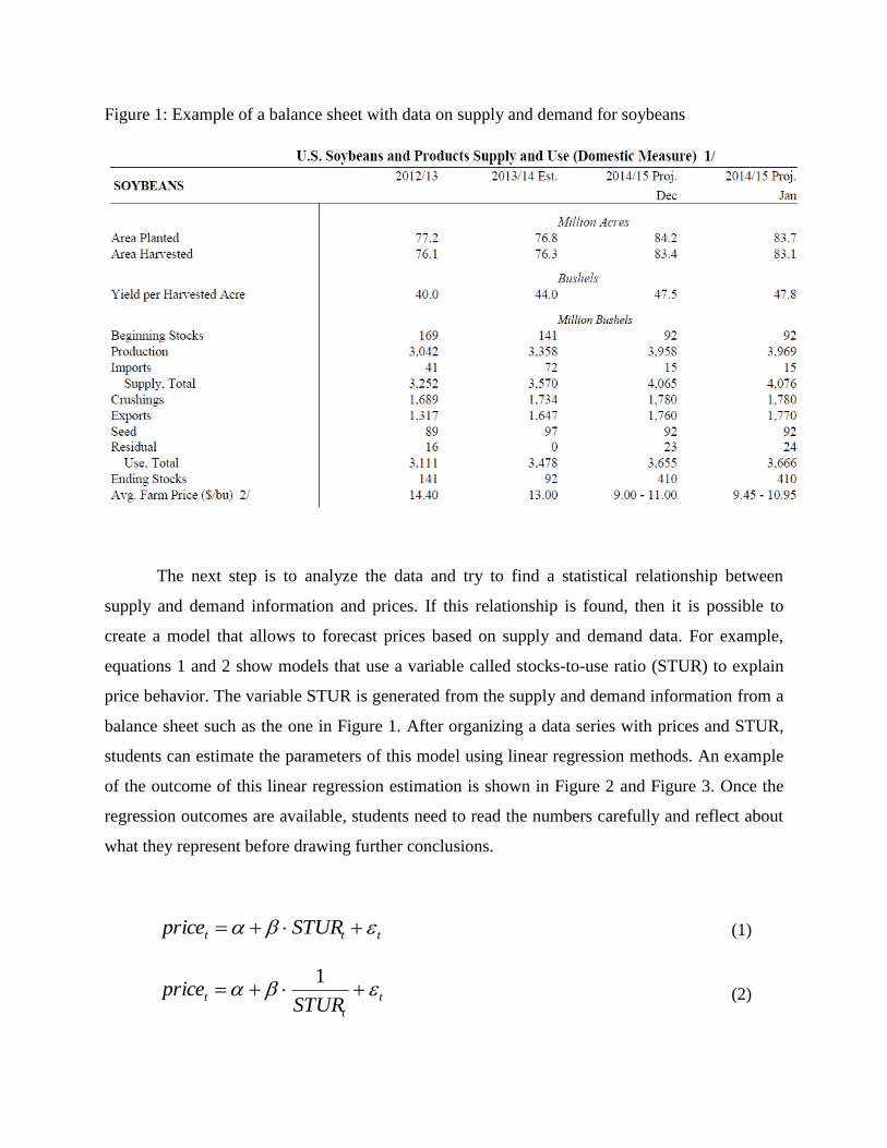
Figure 1: Example of a balance sheet with data on supply and demand for soybeans

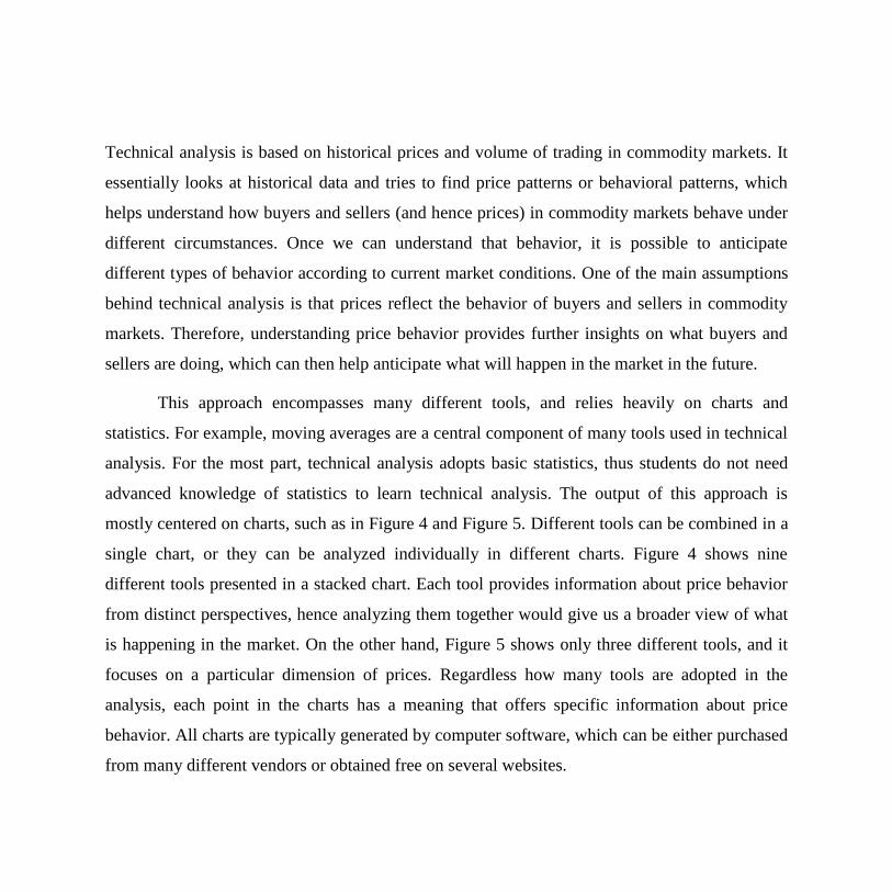
The next step is to analyze the data and try to find a statistical relationship between

supply and demand information and prices. If this relationship is found, then it is possible to

create a model that allows to forecast prices based on supply and demand data. For example,

equations 1 and 2 show models that use a variable called stocks-to-use ratio (STUR) to explain

price behavior. The variable STUR is generated from the supply and demand information from a

balance sheet such as the one in Figure 1. After organizing a data series with prices and STUR,

students can estimate the parameters of this model using linear regression methods. An example

of the outcome of this linear regression estimation is shown in Figure 2 and Figure 3. Once the

regression outcomes are available, students need to read the numbers carefully and reflect about

what they represent before drawing further conclusions.

ttt STURprice (1)

t

t

tSTUR

price 1

(2)

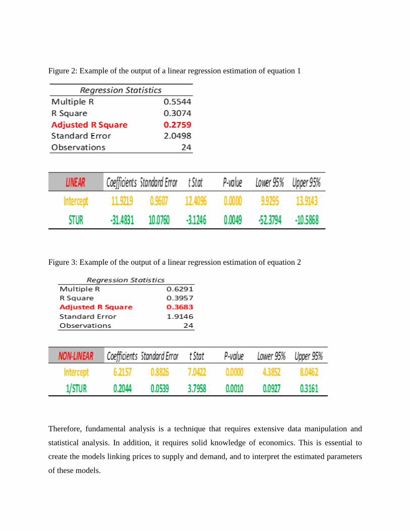
Figure 2: Example of the output of a linear regression estimation of equation 1

Figure 3: Example of the output of a linear regression estimation of equation 2

Therefore, fundamental analysis is a technique that requires extensive data manipulation and

statistical analysis. In addition, it requires solid knowledge of economics. This is essential to

create the models linking prices to supply and demand, and to interpret the estimated parameters

of these models.

Technical analysis is based on historical prices and volume of trading in commodity markets. It

essentially looks at historical data and tries to find price patterns or behavioral patterns, which

helps understand how buyers and sellers (and hence prices) in commodity markets behave under

different circumstances. Once we can understand that behavior, it is possible to anticipate

different types of behavior according to current market conditions. One of the main assumptions

behind technical analysis is that prices reflect the behavior of buyers and sellers in commodity

markets. Therefore, understanding price behavior provides further insights on what buyers and

sellers are doing, which can then help anticipate what will happen in the market in the future.

This approach encompasses many different tools, and relies heavily on charts and

statistics. For example, moving averages are a central component of many tools used in technical

analysis. For the most part, technical analysis adopts basic statistics, thus students do not need

advanced knowledge of statistics to learn technical analysis. The output of this approach is

mostly centered on charts, such as in Figure 4 and Figure 5. Different tools can be combined in a

single chart, or they can be analyzed individually in different charts. Figure 4 shows nine

different tools presented in a stacked chart. Each tool provides information about price behavior

from distinct perspectives, hence analyzing them together would give us a broader view of what

is happening in the market. On the other hand, Figure 5 shows only three different tools, and it

focuses on a particular dimension of prices. Regardless how many tools are adopted in the

analysis, each point in the charts has a meaning that offers specific information about price

behavior. All charts are typically generated by computer software, which can be either purchased

from many different vendors or obtained free on several websites.

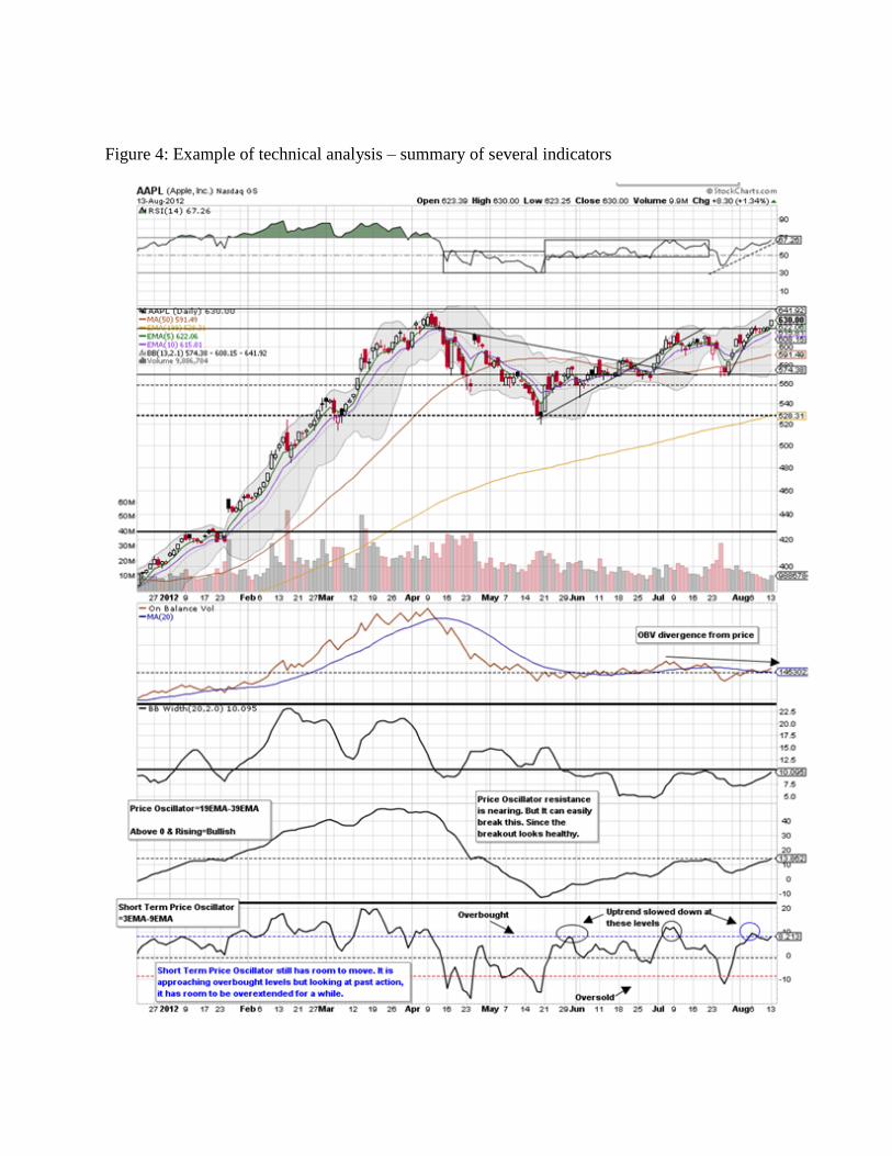
Figure 4: Example of technical analysis – summary of several indicators

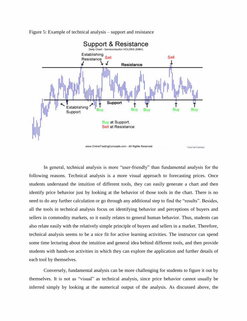
Figure 5: Example of technical analysis – support and resistance

In general, technical analysis is more “user-friendly” than fundamental analysis for the

following reasons. Technical analysis is a more visual approach to forecasting prices. Once

students understand the intuition of different tools, they can easily generate a chart and then

identify price behavior just by looking at the behavior of those tools in the chart. There is no

need to do any further calculation or go through any additional step to find the “results”. Besides,

all the tools in technical analysis focus on identifying behavior and perceptions of buyers and

sellers in commodity markets, so it easily relates to general human behavior. Thus, students can

also relate easily with the relatively simple principle of buyers and sellers in a market. Therefore,

technical analysis seems to be a nice fit for active learning activities. The instructor can spend

some time lecturing about the intuition and general idea behind different tools, and then provide

students with hands-on activities in which they can explore the application and further details of

each tool by themselves.

Conversely, fundamental analysis can be more challenging for students to figure it out by

themselves. It is not as “visual” as technical analysis, since price behavior cannot usually be

inferred simply by looking at the numerical output of the analysis. As discussed above, the

output of fundamental analysis is often a table with several numbers that need to be further

interpreted. These numbers are related to economic variables, and their relationship can be

complex. Further, the interpretation of those results is not always straightforward, and requires

solid knowledge of statistics and economics. Finally, additional calculations are usually needed

in order to identify price behavior in the market. Therefore, fundamental analysis can be puzzling

for students to explore by themselves

Classroom setting

Lectures take place in the Commodity Trading Room, located in Filley Hall. This is not a

traditional classroom and it was not designed for recitation. Students sit at computer stations

equipped with two monitors and specific software used in the course. These stations face the

south and north walls of the room, where there are big screens on which the instructor can

project course material (there are two screens on each wall). Figure 6 and Figure 7 show partial

views of the room, where we can see computer stations used by the students and the screens on

the north wall (Figure 6) and south wall (Figure 7). The instructor’s station is located by the east

wall. Since students’ seats face either the north wall or the south wall, and the instructor’s station

is by the east wall, students do not naturally face the instructor as it typically happens in a

traditional classroom.

Figure 6: Partial view of the classroom – Commodity Trading Room

Figure 7: Partial view of the classroom – Commodity Trading Room

TEACHING METHODS

The course has two main topics, technical analysis and fundamental analysis, and I chose to use

two different methods to teach each topic. For technical analysis, I developed active learning

activities in which students were more “in charge” of their learning. I would spend some time

lecturing, when I would introduce different tools in technical analysis and explain their intuition

and how they worked. Then I would turn it over to the students and give them exercises and in-

class assignments in which they had to explore charts and interpret what they were seeing. These

activities were done in pairs, such that students had the opportunity to discuss with and learn

from each other. In this process, I would use specific questions in the exercises and assignments

to direct students’ attention to particular points and guide them through certain dimensions that I

wanted them to focus on. As they worked on these exercises and assignments, I was always

available in the classroom to answer questions and discuss with them any points with which they

could be having trouble.

In addition, I also introduced a Trading Project in this part of the course. We used the

software Barchart Trader to create trading accounts for each student, such that they had access to

real-time commodity futures markets and were able to trade in those markets in the same way

that professional traders do. The only exception was that students were given fake money to

trade, so gains and losses from their trading activity did not translate into real-life changes in

their financials. Even tough real money was not involved, students quickly became very excited

with the opportunity to trade in commodity futures markets as if they were professional traders,

and they were clearly very involved in trying to make as much profit as they could.

The purpose of this activity was to give students a real-world, engaging activity that

allowed them to put in practice what they were learning in the course. I told students that they

should use the tools from technical analysis that we were discussing in class to understand what

was happening in the markets and anticipate price changes. Then they could trade accordingly

and, if they were correct, they would make profits. For example, if they used technical analysis

and concluded that prices were going to increase, they should buy in the market. If their

prediction was correct and the price indeed increased, they could later sell at a price higher than

they initially bought and make a profit. I also told them that actual trading involves more than

just anticipating price changes, i.e. successful trading requires other skills that are not part of this

course. Therefore, even if they were able to anticipate price changes, it was possible that their

trading was not profitable. Still, I would evaluate and grade their trading based only on their use

of technical analysis and interpretation of the market (and not based on their trading gains and

losses).

During this part of the course, students had to submit written reports every two weeks. In

those reports, they had to explain how they used technical analysis and discuss why they

expected prices to go up or down. They could choose to analyze and trade any commodity that

they liked, so they could focus on commodities that they were really interested in. I decided to do

that as a way to make their learning more tailored to their own interests and off-campus activities

(such as jobs and internships), making them more invested in the trading activity. After the

submission of each trading report, I would read and return them to the students with detailed

comments on what else they could have done or what parts of their analysis was incorrect.

For the other part of the course, fundamental analysis, I used very little active learning

activities and focused almost completely on traditional lectures. I would use PowerPoint

presentations to explain the course content to the students and they would be sitting in front of

their computers following the slides on their screens. I would lecture about the ideas involved in

fundamental analysis, the intuition behind the tools that we discussed, and show examples of

regression analysis and how to interpret the results. In addition, before getting into the details of

fundamental analysis, I also spent a few lectures explaining the theory behind regression analysis

and how to do it using Excel spreadsheets.

In some class periods, I would do regression analysis using Excel and ask them to follow

me on their computers. On those days, although they had a chance to do something other than

just listening to me, they were still just following what I was doing. They were not required to

engage in any activity by themselves, or discuss how to do it and how to interpret the results with

their classmates.

In this part of the course, only in one class period I asked students to work in pairs and do

fundamental analysis using regression models by themselves. This happened at the end of the

semester, after I had covered all the material related to fundamental analysis. I gave students a

data set with prices and supply and demand variables, and told them to use regression analysis to

generate a model that would allow them to forecast prices based on supply and demand

(essentially the models previously presented in equations 1 and 2). This was the only chance they

had to reflect and discuss fundamental analysis by themselves in the classroom. Except for that

day, students learned fundamental analysis just by listening to my explanations and following

what I was doing in the computer.

ANALYSIS OF STUDENT LEARNING

Evaluation procedure

I evaluated students’ learning through two exams. The first exam was on technical analysis,

while the second exam was on fundamental analysis. I compared their grades in the two exams to

assess whether they learned one type of analysis better than the other. For example, if students

earned higher grades in the first exam, it would suggest that they learned technical analysis better

than they did fundamental analysis.

Since different teaching methods were adopted in the two parts of the course, those

grades would also indicate that one method might be more effective than the other. Going back

to the previous example, if students earned higher grades in the first exam, this would suggest

that active learning activities adopted to teach technical analysis might be more effective than the

traditional lecture-style method adopted to teach fundamental analysis.

The grade comparison across the two exams will be done through analysis of the

distribution of grades and statistical tests comparing the mean grades of the exams.

Students

There were 41 students in the class, and 30 of them signed the informed consent for this project.

However, the actual sample used in this study was turned out to be smaller due to technical

issues with the learning management system (Canvas) adopted in the course. Students took the

two exams in the classroom computers. I prepared the exams on Canvas and students would type

their answers in the computer and then submit them electronically. For some reason, I could not

see the answers submitted by some students for the first exam. It is still not clear whether

students failed to submit their answers properly or if there were technical problems with Canvas

that affected the submission process. Out of the 30 students willing to participate in this project,

7 had this problem in the first exam. Therefore, I have only 23 students who signed the informed

consent and have grades for both exams.

In the sample of 23 students used in this study, 9 were seniors, 7 were juniors, 2 were

sophomores and 5 did not provide this information. All of these students were majoring in fields

related to economics and business, except for one whose major was mechanized systems

management.

Performance analysis

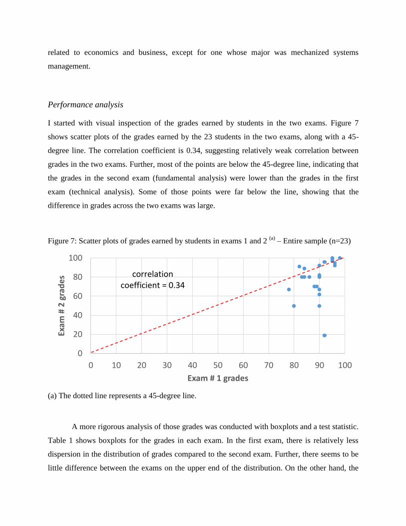
I started with visual inspection of the grades earned by students in the two exams. Figure 7

shows scatter plots of the grades earned by the 23 students in the two exams, along with a 45-

degree line. The correlation coefficient is 0.34, suggesting relatively weak correlation between

grades in the two exams. Further, most of the points are below the 45-degree line, indicating that

the grades in the second exam (fundamental analysis) were lower than the grades in the first

exam (technical analysis). Some of those points were far below the line, showing that the

difference in grades across the two exams was large.

Figure 7: Scatter plots of grades earned by students in exams 1 and 2 (a)

– Entire sample (n=23)

(a) The dotted line represents a 45-degree line.

A more rigorous analysis of those grades was conducted with boxplots and a test statistic.

Table 1 shows boxplots for the grades in each exam. In the first exam, there is relatively less

dispersion in the distribution of grades compared to the second exam. Further, there seems to be

little difference between the exams on the upper end of the distribution. On the other hand, the

0

20

40

60

80

100

0 10 20 30 40 50 60 70 80 90 100

Exam

# 2

gra

de

s

Exam # 1 grades

correlation coefficient = 0.34

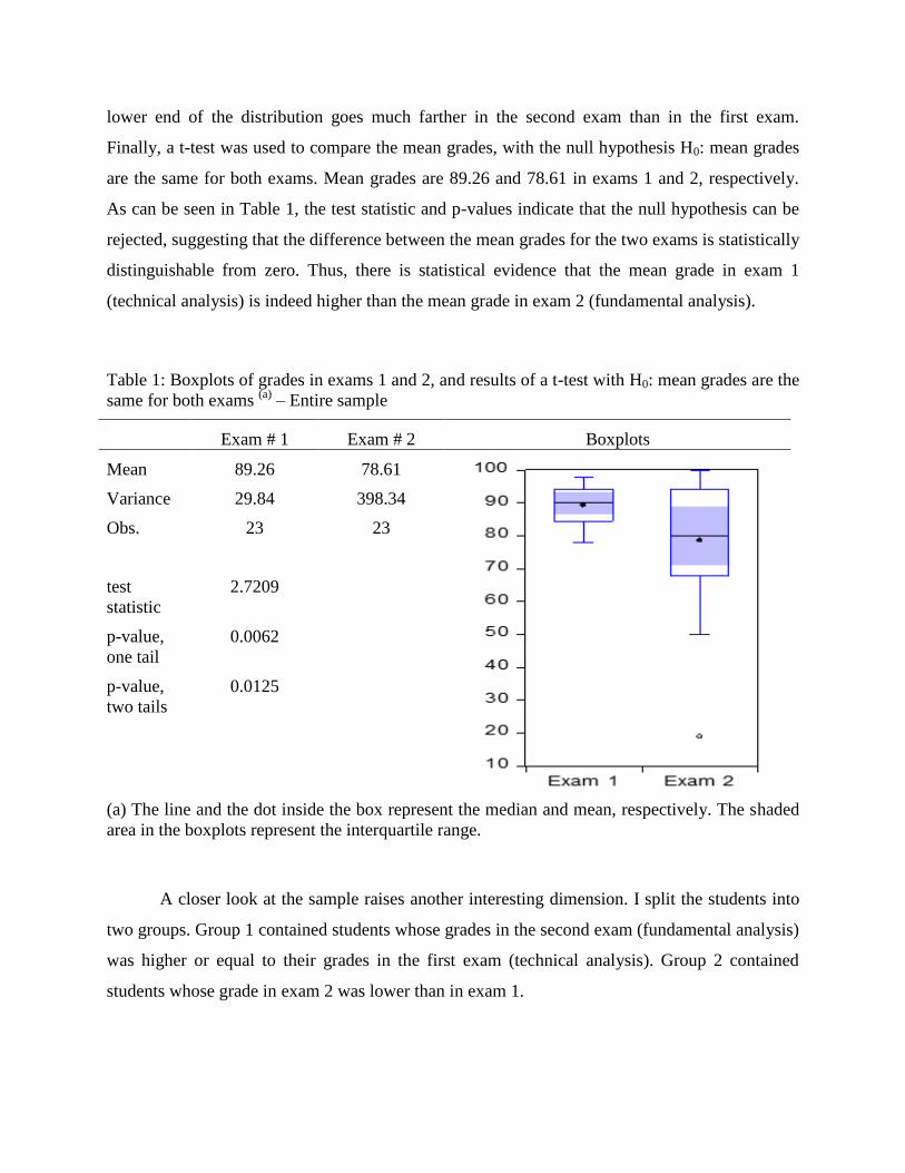
lower end of the distribution goes much farther in the second exam than in the first exam.

Finally, a t-test was used to compare the mean grades, with the null hypothesis H0: mean grades

are the same for both exams. Mean grades are 89.26 and 78.61 in exams 1 and 2, respectively.

As can be seen in Table 1, the test statistic and p-values indicate that the null hypothesis can be

rejected, suggesting that the difference between the mean grades for the two exams is statistically

distinguishable from zero. Thus, there is statistical evidence that the mean grade in exam 1

(technical analysis) is indeed higher than the mean grade in exam 2 (fundamental analysis).

Table 1: Boxplots of grades in exams 1 and 2, and results of a t-test with H0: mean grades are the

same for both exams (a)

– Entire sample

Exam # 1 Exam # 2 Boxplots

Mean 89.26 78.61

Variance 29.84 398.34

Obs. 23 23

test

statistic

2.7209

p-value,

one tail

0.0062

p-value,

two tails

0.0125

(a) The line and the dot inside the box represent the median and mean, respectively. The shaded

area in the boxplots represent the interquartile range.

A closer look at the sample raises another interesting dimension. I split the students into

two groups. Group 1 contained students whose grades in the second exam (fundamental analysis)

was higher or equal to their grades in the first exam (technical analysis). Group 2 contained

students whose grade in exam 2 was lower than in exam 1.

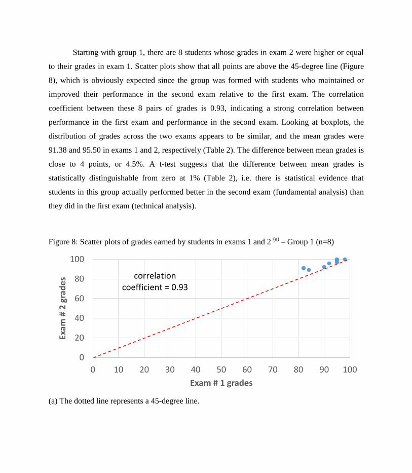
Starting with group 1, there are 8 students whose grades in exam 2 were higher or equal

to their grades in exam 1. Scatter plots show that all points are above the 45-degree line (Figure

8), which is obviously expected since the group was formed with students who maintained or

improved their performance in the second exam relative to the first exam. The correlation

coefficient between these 8 pairs of grades is 0.93, indicating a strong correlation between

performance in the first exam and performance in the second exam. Looking at boxplots, the

distribution of grades across the two exams appears to be similar, and the mean grades were

91.38 and 95.50 in exams 1 and 2, respectively (Table 2). The difference between mean grades is

close to 4 points, or 4.5%. A t-test suggests that the difference between mean grades is

statistically distinguishable from zero at 1% (Table 2), i.e. there is statistical evidence that

students in this group actually performed better in the second exam (fundamental analysis) than

they did in the first exam (technical analysis).

Figure 8: Scatter plots of grades earned by students in exams 1 and 2 (a)

– Group 1 (n=8)

(a) The dotted line represents a 45-degree line.

0

20

40

60

80

100

0 10 20 30 40 50 60 70 80 90 100

Exam

# 2

gra

de

s

Exam # 1 grades

correlation coefficient = 0.93

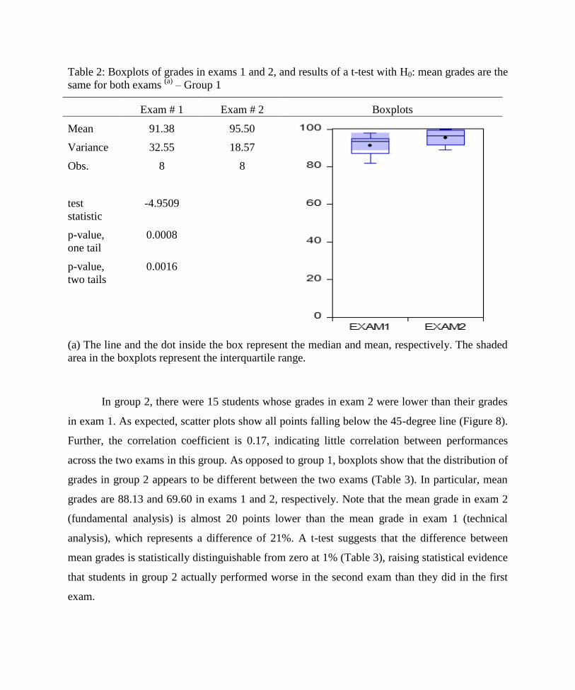
Table 2: Boxplots of grades in exams 1 and 2, and results of a t-test with H0: mean grades are the

same for both exams (a)

– Group 1

Exam # 1 Exam # 2 Boxplots

Mean 91.38 95.50

Variance 32.55 18.57

Obs. 8 8

test

statistic

-4.9509

p-value,

one tail

0.0008

p-value,

two tails

0.0016

(a) The line and the dot inside the box represent the median and mean, respectively. The shaded

area in the boxplots represent the interquartile range.

In group 2, there were 15 students whose grades in exam 2 were lower than their grades

in exam 1. As expected, scatter plots show all points falling below the 45-degree line (Figure 8).

Further, the correlation coefficient is 0.17, indicating little correlation between performances

across the two exams in this group. As opposed to group 1, boxplots show that the distribution of

grades in group 2 appears to be different between the two exams (Table 3). In particular, mean

grades are 88.13 and 69.60 in exams 1 and 2, respectively. Note that the mean grade in exam 2

(fundamental analysis) is almost 20 points lower than the mean grade in exam 1 (technical

analysis), which represents a difference of 21%. A t-test suggests that the difference between

mean grades is statistically distinguishable from zero at 1% (Table 3), raising statistical evidence

that students in group 2 actually performed worse in the second exam than they did in the first

exam.

Figure 8: Scatter plots of grades earned by students in exams 1 and 2 (a)

– Group 2 (n=15)

(a) The dotted line represents a 45-degree line.

Table 3: Boxplots of grades in exams 1 and 2, and results of a t-test with H0: mean grades are the

same for both exams (a)

– Group 2

Exam # 1 Exam # 2 Boxplots

Mean 88.13 69.60

Variance 26.69 366.69

Obs. 15 15

test

statistic

3.7839

p-value,

one tail

0.0010

p-value,

two tails

0.0020

(a) The line and the dot inside the box represent the median and mean, respectively. The shaded

area in the boxplots represent the interquartile range.

0

20

40

60

80

100

0 10 20 30 40 50 60 70 80 90 100

Exam

# 2

gra

de

s

Exam # 1 grades

correlation coefficient = 0.17

0

20

40

60

80

100

EXAM1 EXAM2

Overall, there is evidence that students generally performed better in exam 1 (technical

analysis) than they did in exam 2 (fundamental analysis). However, this does not apply to all

students in the sample. Out of 23 students, 8 performed better in the second exam (35% of the

sample) and 15 performed better in the first exam (65% of the sample). In the group of 8 students

who performed better in the second exam, the difference in mean grades was relatively small

(although statistically significant), i.e. their average performance was not much higher in the

second exam relative to the first exam. On the other hand, in the group of 15 students who

performed better in the first exam, the difference in mean grades was relatively large (and also

statistically significant), indicating that their performance in the second exam was much worse

than in the first exam.

Finally, I considered one more dimension that could potentially explain the results (at

least partially). Technical analysis requires some knowledge of statistics, and all students had

taken at least one course in statistics that allowed them to have the necessary background to

follow the initial discussion. Some students probably know or remember more statistics than

others, but they all knew enough statistics to get started in technical analysis. On the other hand,

fundamental analysis, in the form that it is taught in this course, requires some knowledge of

Excel spreadsheets and regression analysis. Knowing that the majority of students have little

knowledge about these two topics, I spent time in class discussing how to use Excel spreadsheets

and explaining what regression analysis is and how it is done. Even though I do not expect

students to have any prior knowledge of Excel and regression analysis, I realize that some of

them do. Thus, I wondered if this prior knowledge could give them an advantage in learning

fundamental analysis. The reasoning is that those students could spend more time studying

fundamental analysis itself, instead of splitting their studying time between Excel/regression

analysis and fundamental analysis. Even though students with prior knowledge of Excel and

regression analysis also have to be in class and listen to our discussion about these topics, they

can quickly go through them and focus only on fundamental analysis.

I asked students to complete a brief survey inquiring about their prior knowledge of Excel

spreadsheets and regression analysis. Out of the 23 students in the sample, 17 of them completed

the survey, being 8 students from group 1 and 9 students from group 2 (all students who did not

complete the survey were from group 2). Regarding prior knowledge of Excel spreadsheets,

students were asked the question “How familiar are you with Excel spreadsheets?”. Results are

presented in Table 4. Seven students indicated little or no knowledge of Excel (“Not familiar at

all” and “I only know the very basics”), with 1 students from group 1 and 6 students from group

2. Then, 8 students indicated intermediate knowledge of Excel (“I can do some simple data

manipulation and charts” and “I can use some formulas and do more complex charts”), with 5

students from group 1 and 3 students from group 2. Finally, 2 students indicated advanced

knowledge of Excel (“I use Excel a lot and am very comfortable with most of its tools” and “I

am an Excel master”), and both of them were from group 1. Therefore, almost all students in

group 1 (87.5%) had an intermediate or advanced knowledge of Excel. In group 2, on the other

hand, 40% of the students had little or no knowledge of Excel, and 20% had an intermediate

knowledge (the rest of the students in this group did not complete the survey).

Table 4: Answers to the question “How familiar are you with Excel spreadsheets?” (a)

Answers All students

(n=23)

Group 1

(n=8)

Group 2

(n=15)

Not familiar at all 1

(4.35%)

0

(0.00%)

1

(6.67%)

I only know the very basics 6

(26.09%)

1

(12.50%)

5

(33.33%)

I can do some simple data manipulation and charts 5

(21.74%)

3

(37.50%)

2

(13.33%)

I can use some formulas and do more complex

charts

3

(13.04%)

2

(25.00%)

1

(6.67%)

I use Excel a lot and am very comfortable with

most of its tools

2

(8.69%)

2

(25.00%)

0

(0.00%)

I am an Excel master 0

(0.00%)

0

(0.00%)

0

(0.00%)

No answer provided 6

(26.09%)

0

(0.00%)

6

(40.00%)

(a) Numbers in parentheses show proportion of each answer relative to the total of the group.

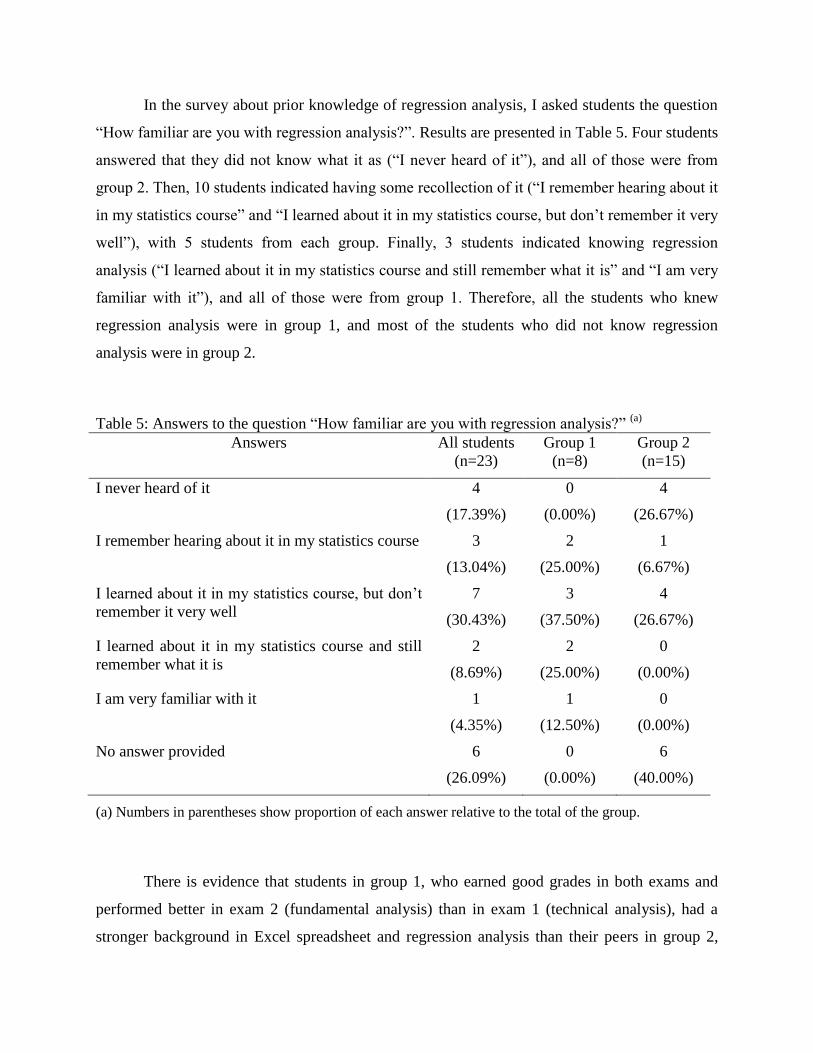
In the survey about prior knowledge of regression analysis, I asked students the question

“How familiar are you with regression analysis?”. Results are presented in Table 5. Four students

answered that they did not know what it as (“I never heard of it”), and all of those were from

group 2. Then, 10 students indicated having some recollection of it (“I remember hearing about it

in my statistics course” and “I learned about it in my statistics course, but don’t remember it very

well”), with 5 students from each group. Finally, 3 students indicated knowing regression

analysis (“I learned about it in my statistics course and still remember what it is” and “I am very

familiar with it”), and all of those were from group 1. Therefore, all the students who knew

regression analysis were in group 1, and most of the students who did not know regression

analysis were in group 2.

Table 5: Answers to the question “How familiar are you with regression analysis?” (a)

Answers All students

(n=23)

Group 1

(n=8)

Group 2

(n=15)

I never heard of it 4

(17.39%)

0

(0.00%)

4

(26.67%)

I remember hearing about it in my statistics course 3

(13.04%)

2

(25.00%)

1

(6.67%)

I learned about it in my statistics course, but don’t

remember it very well

7

(30.43%)

3

(37.50%)

4

(26.67%)

I learned about it in my statistics course and still

remember what it is

2

(8.69%)

2

(25.00%)

0

(0.00%)

I am very familiar with it 1

(4.35%)

1

(12.50%)

0

(0.00%)

No answer provided 6

(26.09%)

0

(0.00%)

6

(40.00%)

(a) Numbers in parentheses show proportion of each answer relative to the total of the group.

There is evidence that students in group 1, who earned good grades in both exams and

performed better in exam 2 (fundamental analysis) than in exam 1 (technical analysis), had a

stronger background in Excel spreadsheet and regression analysis than their peers in group 2,

who performed worse in exam 2 than in exam 1. Although there is not enough information to

make a stronger statement about this point, it is possible that part of the reason why I identified

such differences in performance between groups 1 and 2 might have been because of this prior

knowledge of Excel spreadsheets and regression analysis.

CONCLUSIONS

This study aimed to explore the impact of distinct teaching approaches on students’ learning. In

my course, we cover two main topics: technical analysis and fundamental analysis. In the spring

of 2017, I decided to teach these two topics in different ways. I used activities associated with

active learning to teach technical analysis, and traditional lectures (recitation) to teach

fundamental analysis. Then I compared students’ performance in the two exams to assess how

much they learned about each topic. Exam 1 was based only on technical analysis, while exam 2

was based only on fundamental analysis.

Results indicate that students generally performed better in exam 1 than they did in exam

2, suggesting that they learned technical analysis better than they learned fundamental analysis.

Out of the 23 students in the sample, 15 earned higher grades in exam 1 (technical analysis) and

their grades in exam 1 were much better than their grades in exam 2 (fundamental analysis),

indicating that there is a large learning gap between the two topics. Then, 8 students earned

better grades in exam 2 (fundamental analysis), but their grades in exam 2 were not much higher

than in exam 1. Actually, their improvement from exam 1 to exam 2 was relatively small,

suggesting that they might have learned both topics equally well.

It was also explored the idea that students in group 1 might have generally had an

“advantage” compared to students in group 2. Most students in group 1 came to the course with

prior knowledge of Excel spreadsheets and regression analysis, while most students in group 2

had no prior knowledge of these topics. Since Excel spreadsheets and regression analysis are

main components in the discussion of fundamental analysis, previous experience with these tools

might have assisted group 1 students learn fundamental analysis faster. While group 2 students

were trying to learn about Excel spreadsheets and regression analysis along with fundamental

analysis, group 1 students could focus mostly (or exclusively) on fundamental analysis. This

might have made helped them earn in the second exam (fundamental) a higher grade than they

did in the first exam (technical analysis). In other words, if group 1 students had the same prior

knowledge about Excel spreadsheets and regression analysis than group 2 students did, it is

possible that group 1 students would also have performed worse in the second exam.

In summary, these findings could imply that the adoption of active learning activities to

teach technical analysis might have helped students learn it more effectively, whereas the use of

traditional lectures to teach fundamental analysis might not have been as effective to help they

learn the material. Anecdotally, students’ comments during the semester were clearly in favor of

the teaching method (active learning) used for technical analysis, and their excitement and

engagement in the activities were visible during our class periods. On the other hand, I never

heard any comments about the teaching method (traditional lecture) used for fundamental

analysis, and I would often notice very little enthusiasm during our class periods in that part of

the course.

Moving forward, it would be insightful to investigate different types of active learning

activities. Active learning can come in different forms and shapes, and it is possible that certain

forms and shapes work better for some students and some disciplines. After finding evidence that

active learning is more effective than traditional lectures, a natural question is what types of

active learning are the best fit for my students and my course. Finding the answer to this question

can help me further develop my course and improve my students’ learning. Well, perhaps this is

the first step towards another peer review of teaching portfolio……