Price, exchange rate volatility and Nigeria's agricultural trade ...

Price, exchange rate volatilityand Nigeria’s agricultural trade

flows: A dynamic analysis

BYAdubi, A. A.

National Centre for Economic Managementand Administration (NCEMA)

lbadan, Nigeria

and

Okunmadewa, F.Department of Agricultural Economics

University of lbadanIbadan, Nigeria

AERC Research Paper 87African Economic Research Consortium, Nairobi

March 1999

Contents

List of tablesList of figures

I - Introduction 1

II. Objectives of the study 6

III. Trade policy regimes and the agricultural sector 7

Iv. Literature review 1 6

V . Research methodology 1 8

VI. Estimation results: Price and exchange rate volatility and trade flows 2 5

VII. Major findings and policy implications 3 1

References 3 2Appendix A 3 5

List of tables- - -

1. Output of major agricultural crops 22. Output of major agricultural product groups (‘000 tons) 33. Producer incomes from agricultural crops 44. Producer Prices and Exchange Rate 1970-95 Wtonne 95. Composition and growth of total exports 116. Estimated results for export earnings 277. Estimated results for export prices 288. Matrix of price and exchange rate volatility 30

List of figures- - - - -

1. The agricultural cash crop marketing channel in the pre-SAP period 142. The agricultural cash crop marketing channel during SAP period 15

One of the most dramatic events in Nigeria over the past decade was the devaluation ofthe Nigerian naira with the adoption of a structural adjustment programme (SAP) in1986. A cardinal objective of the SAP was the restructuring of the production base ofthe economy with a positive bias for the production of agricultural exports. The foreignexchange reforms that facilitated a cumulative depreciation of the effective exchangerate were expected to increase the domestic prices of agricultural exports and thereforeboost domestic production.

Significantly, this depreciation resulted in changes in the structure and volume ofNigeria’s agricultural exports as empirically determined by many researchers (Oyejide,1986; Ihimodu, 1993; Osuntogun et al., 1993; World Bank, 1994. The depreciation alsoincreased the prices of agricultural exports and studies have shown a marked increase involume of agricultural exports over the years. However, the volatility, frequency andinstability of the exchange rate movements since the beginning of the floating exchangerate raise a concern about the impact of such movements on agricultural trade flows.

Structural adjustment and agricultural performance

Among other measures, the structural adjustment programme (SAP), which started in1986, abolished the Commodity Board, the body that since 1960 had been responsiblefor organization and purchase of agricultural exports. As a result, farmers could selltheir products directly to foreign buyers and local processors without any intermediary,thus obtaining higher prices for their products. This was expected to remove the excessivetaxation on farmers’ products by the erstwhile marketing boards and leave producerprices to be determined by market forces. Given that agricultural output is influencedby prices among other factors, the depreciation of the naira and abolition of the commodityboards were expected to result in an overall increase in production of exports. Table 1confirms this expected trend in agricultural output. There was a major increase in fivemajor agricultural export crops that had been on the decline since the 1970s. By 1985,only 37% of the 1970 output was achieved, but by 1988 and 1989, respectively, outputreached 79% and 86% of the 1970 level.

Table 2 presents the output performance of the major product groups during the SAPperiod as compared with the pre-SAP period of 1983-1985. The crops included in eachproduct group accounted for at least 60% of all the crops in the group. A comparison of

2 RESEARCH PAPER 87

Table 1: Output of major agricultural crops

-____-

Year Output* (‘OOOtons) lndex1970=100

1970 3.047 1001971 2.871 941972 2.426 801973 1.839 601974 3.436 1131975 1.773 581976 1.754 581977 1.841 601978 1.980 651979 1.713 561980 1.833 601981 1.576 521982 1.432 47 .1983 1.435 471984 1.739 571985 1.137 371986 1.770 581987 1.364 451988 2.415 791989 2.616 861990 3.602 1181991 3.901 1281992 4.048 1331993 4.189 1371994 4.435 146

Source: CBN: 1 .Nigeria’s Principal Economic and Financial Indicators, 1970-l 994.2.Annual Reports and Statements of Accounts (several years).

*Comprises cocoa, cotton, groundnuts, palm oil and palm kernel.

the two periods shows that export crops performed best, with the average output of thegroup increasing by about 42% over the pre-SAP period. The staple crops group recordedabout 38% increase, while forestry and livestock groups were hardly influenced and theoutput of fishery fell by about 15%.As a result of very high increases in the nominal producer prices during the SAP era,coupled with the moderate output increase of most crops during the 1986-1994 period,the nominal incomes of producers rose substantially, as shown in Table 3.

The table also indicates the pattern of the increase in income over the years. Whilethere was a consistent increase in income for cocoa producers, the same cannot be saidfor producers of cottonseed and palm oil. Generally the rate of change in prices andoutput is also not predictable. According to Kwanashie et al., (1994), the degree offluctuation in prices is a major determinant of the changes in earnings given the trend inoutput over the years.

PRICE, EXCHANGE R ATE VOLATILITY AND N IGERIA’S A GRICULTURAL TRADE FLOWS 3

Table 2: Output of major agricultural product groups (‘000 tons)

Year

- __-ll_~_ .-_.-. __~

Export crops Staples Forestry Livestock Fisheries

1983 1,435 22,404 89,424 753 1321984 1,739 26,316 90,843 818 1001985 1,137 29,064 93,451 852 61Average (A) 1,437 25,928 91,239 808 98

1986 1,770 32,432 93,606 881 1071987 1,364 34,572 95,946 826 1031988 2,415 35,934 96,965 783 511989 2,616 39,888 101,168 750 70Average (B) 2,084 35,707 96,921 810 83

1990 3,602 52,154 105,187 659 2831991 3,901 52,853 107,318 689 2911992 4,048 60,976 109,787 702 2841993 4,189 64,916 112,058 724 2011994 4,435 67,702 114,944 760 199Average (C) 4,035 59,720.2 109,858.8 706.8 251.6

C/B 1.94 1.67 1.13 0.87 3.03-_--_- -~- -~

Sources: Computed from Central Bank of Nigeria, Annual Reports and statements of accounts(various issues).Notes: Export crops - Cocoa, groundnuts, cotton, palm oil and palm kernel.

Staples - Maize, millet, sorghum, rice, wheat, cassava, yam and beansForestry - Roundwood, sawnwood, wood based panelLivestock - Poultry, goat meat, beef and eggsFisheries - Artisan, coastal and brackish water, catches and land, lakes and rivers.

4

Table 3: Producer incomes from agricultural crops

Year Cocoa Groundnuts Cottonseed(f#OOO) (NWO) (WOOO)

Nominal Nominal Nominal

1983 196,000 178,2001984 180,000 384,1501985 174,000 465,7501986 602,000 640,0001987 1,162,500 1,494,2001988 2,200,oOO 1,543,5001989 3,210,OOO 5,233,1151990 2,074,OOO 5,037,1201 9 9 1 2,722,344 8,547,0801992 3,721,540 8,875,3711993 7,735,068 13,452,OOO1994 19,577,600 18,763,184

-

67,20075,60039,10030,00032,000

873,0001,036,OOO

486,2001,148,9881,167,4021,307,188

RESEARCH PAPER 87

Palm kernel Palm oilWQW (WOOO)

Nominal Nominal

64,170136,000144,000140,000300,050545,000

1,500,0002,380,OOO3,037,5757,519,132

15,322,15017,139,674

247,500330,000

650,000816,000

1,050,000910,000846,800881,600

9,877,82417,189,70017,276,280

Sources:Computed From CBN Annual Reports and Statements of Account, and Economic andFinancial Review.

Problem statement

Changes in income earnings of export crop producers come as a result of either increase/decrease in international world price of exports or devaluation of the currency and thesubsequent increase in producer prices. Such price/exchange rate changes, however, maylead to a major decline in future output if they are unpredictable and erratic. Fluctuation- whether positive or negative - is not desirable as it increases risk and uncertainty ininternational transactions and thus discourages trade. In a sense, trade will be reducedsimilarly to a reduction following an increase in transportation costs. An IMF (1984)study cites arguments that exchange rate variability would also tend to inducemacroeconomic phenomena that are undesirable, for example inflation and protectionism.Despite this assertion and that of other studies, more recent research explains why apositive effect could also be possible (de Grauwe, 1988; Caballero and Corbo, 1989).

If firms hedge against exchange rate risk, one could not expect to find a strong negativeeffect on trade. Hedging against risk can be done via future or forward markets. Whereforward markets exist, the nature of the uncertainty faced by traders is transformed. Aforward market represents, in effect, a guaranteed forecast of the exchange rate that willprevail at the end of the contract period, which a trader can take advantage of by paymentof a small margin around the forward rates. Since currency uncertainty can be removedfrom the short-term trading transaction by payment of this margin, the cost of suchuncertainty cannot be higher than the cost of purchasing insurance against it.

PRICE, EXCHANGE RATE VOLATILITY AND NIGERIA’S AGRICULTURAL TRADE FLOWS 5

Unfortunately, the future market is absent in Nigeria and the possibility of hedging viathis route is remote. In fact, most studies have not taken hedging possibilities into account.It has been argued that hedging foreign exchange via future/forward markets is animperfect and costly method of avoiding exchange rate risk. This is because, hedgingtransactions have a cost. Secondly several studies (Cumby and Obstfeld, 198 1; Frenkel,198 1; Hakkio and Rush, 1989) have indicated that the forward rate is a poor predictor ofthe future spot rate. Thus, even in the presence of forward markets for exchange ratesand hedging, trade is likely to be hurt. The IMF (1984) argues that forward/future marketscan be used to hedge against nominal exchange rate risk in the short run at small cost.However, long-term export oriented activities would be exposed to higher and possiblyunhedgeable risks.

It therefore follows that hedging notwithstanding, exchange rate volatility-which tendsto increase the risk and uncertainty in international transactions-may adversely affecttrade and investment flows. This will further increase risk on supply of exports. Exchangerate risk measures the volatility and erratic pattem of exchange rate movements: themore volatile the movements, the higher the risk. Producers exports are not only concernedwith the magnitude of the price they receive, they also bother about the stability of suchprices as it relates to earning a consistent income. In a developing country, where exportprice increases, as a result of currency devaluation are expected to be an incentive forexport growth, a primary concern is the nature and magnitude of risk introduced by theprice/exchange rate movements. This concern has strengthened in recent years in responseto increasing protectionist trends and slowing growth in world trade.

Many related empirical studies have been conducted on the effect of price or exchangerate on trade (Schuh, 1974; Ihimodu, 1993; Ogiogio, 1993; Osuntogun et al., 1993;Obadan, 1994). However, most of these efforts have concentrated on the price and exporteffects in a static setting. These studies, either econometric or judgemental, are thusincapable of portraying the dynamic adjustment to a devaluation. Also, the likelyrelationships between price and exchange rate volatility were ignored in their estimationsand a possible impact of price and exchange rate risk on trade flows was neglected.

The major goal of this study is to address these neglected issues. The research intendsto provide an empirical basis for the analysis of the effect of price and exchange ratevolatility on the volume of agricultural exports. If devaluation is expected to stronglyaffect the agricultural sector, then a major effect must come through an adjustment in theagricultural trade balance rather than through a portfolio adjustment alone. This studyintends to capture this through a dynamic multiplier analysis that appropriately considersthe major characteristics and the dynamics of the associated adjustment process.

II. Objectives of the study

The overall objective of the study is to determine empirically the dynamic effects ofexchange rate fluctuations on Nigerian agricultural export markets and to examine therelevance of exchange rate risk in agricultural trade flows.

Specifically the study intends to:

l Evaluate the nature and extent of the impact of price and exchange rate volatility onagricultural trade flows.

l Estimate the relationships between price and exchange rate volatility and analysetheir effects on exports and imports prices.

l Investigate the dynamic characteristics of the adjustments of agricultural exportsand imports to price and foreign exchange fluctuations.

III. Trade policy regimes and the agriculturalsector

The balance of payment problems of the country in the late 1960s largely dictated thetrade policies in the 1970s. The policies in the 1970s also sought to promote domesticproduction and generate revenue for government expenditure. There was considerablerestriction and regulation of the trade sector before liberalization (i.e., between 1970 and1985). Import duties and tariffs were quite high (as much as 70% in 1975) to discourageimports. There were also quantitative restrictions on some food imports through importlicensing. On the other hand, the focus of export policy was on cash crops (export crops),with the primary purpose being to raise revenue and to moderate farmers’ returns anddomestic food prices. Main export policy instruments were export duties, sales taxesand centralized marketing. Exchange rate was also administratively determined to ensurecheap imports of raw materials for import-substituting local. manufacturing industries.

The oil boom of the mid 1970s and the resulting favourable balance of paymentsposition led to an era of liberal food import policy. Import restrictions were lifted insome cases and import duties were either abolished or reduced in others. The short spellof depression in the oil market in the late 1970s gave rise to tightening of food importtariffs and import prohibition, which was again relaxed as the oil market situationimproved.

The period 1981-1986 was one of economic depression and balance of paymentcrisis. Trade controls were reintroduced to correct the severe distortion. Huge tariffs oroutright bans were imposed on most food imports. Export bans and duties were alsoreviewed to address principally the domestic inflation problem. Centralized marketingwas reinforced to increase government revenue.

The 1986 budget introduced the trade liberalization regime as a component of thestructural adjustment programme (SAP). The regime included abolition of the importlicensing system, reduction of import restrictions, modification of advance payment ofimport duties, overhauling of custom and excise duty schedules, establishment of tariffreview board, allowance of domicilliary accounts operation, abolition of exportprohibition, dissolution of commodity boards, and establishment of an export developmentfund, guarantee scheme, insurance scheme and export promotion zone.

Since 1995, there have been modifications to the liberalization era. Some importrestrictions are again in place. A new tarrif structure has been set up, with a range ofcustom duties, and some restrictions and exemptions. A dual exchange rate is now beingused, and the export market is fairly liberalized.

8 RESEARCH PAPER 87

Price and exchange rate changes and agriculturalexports in Nigeria

In the early 1960s in Nigeria, there was little concern for exchange rate policy, as it hadalmost no significance in economic management. Between 1960 and 1967, the Nigeriancurrency was adjusted in relation to the British pound with a one-to-one relationshipbetween them. Between 1967 and 1974, another fixed parity was maintained with theAmerican dollar. This system was abandoned between 1974 and late 1976, when anindependent exchange rate management policy was ushered in that pegged the naira toeither the U.S. dollar or the British pound sterling, whichever currency was stronger inthe foreign exchange market. The main objective of exchange rate policy in this phasewas to operate an independently managed exchange rate system that would influencereal economic variables in the economy and bring down the rate of inflation.Consequently, a policy of progressive appreciation of the naira was pursued over theperiod and was aided by the oil boom that occurred at the same time. Because of thehuge earnings from crude petroleum exports over the period, Nigeria persistently ranappreciable external surpluses in the balance of payments, which supported theappreciation of the naira. This practice led to considerable stability in the naira exchangerah 2.

Throughout this period the pricing of agricultural exports was done by the establishedgo\ rernment marketing boards. Specifically, these marketing boards were responsiblefor fixing prices and ensuring quality of crop exports. Though low, agricultural exportl->ric es were stable during this period and not subject to changes in the exchange rate(\vhich was more or less fixed) apart from fluctuations in the international prices ofpr,inlary products.

Late in 1976, as a result of the changing fortunes of Nigeria’s economic circumstances,a pollicy reversal was effected in the management of the naira exchange rate. There wasa deliberate policy to depreciate the naira, though this was not systematic. In the effortto realign the naira exchange rate, the monetarists were convinced that a more appropriateway to ensure stability and viability of the naira was to peg it to a basket of currencies.Hence a basket of seven currencies of Nigeria’s major trading partner countries wasadopted. Towards the end of 1985, as the economic crisis deepened, the governmentallowed the exchange rate to be determined by market forces. This led to many rates thatdiverged widely from one another. The evidence between 1985 and 1993 showed elementsof distortions in the exchange rate that made it difficult to predict the path towards stabilityof the rate (Ogiogio, 1993). In the quest for stability of the exchange rate, the Nigerianmonetary authorities tried several bidding systems, including the Dutch auction system(DAS) and the marginal rate system. An attempt to ensure viability in the market led tomany amendments of the rules, interventions by Central Bank of Nigeria, and openingof different foreign exchange windows for operations during this period. Despite this,the fluctuating rates of the exchange rate continued to be an issue of concern to theauthorities. For example, the naira exchange rate, which stood at N6.7178 = $1 duringthe month of January 1989 depreciated to N7.5871 by March 1989. The rate strengthened

PRICE, EXCHANGE RATE VOLATILITY AND N IGERIA’S A GRICULTURAL TRADE FLOWS 9

progressively from W7.5808 = $1 in April to W7.1388 = $1 in July 1989 after a series oftight monetary policy actions had been taken. The rate averaged W7.2593 = $1 in August,compared with N7.0389 = $1 in January 1989. As at December 199 1, the naira wasexchanging for the dollar at the rate of l49.9331:$1.00. By June 1993, the naira haddepreciated to N17.3760:$1.00.

Prior to the policy reforms in 1986, and especially during the 196Os, Nigeria wasknown mainly as an exporter of primary agricultural commodities and, to a relativelysmall extent, as an exporter of one or two solid minerals. From 1960, when Nigeriabecame an independent sovereign state, until 1970, its economy was largely sustained,at least from the point of view of off-shore commitments, by the export earnings fromthese basic agricultural and mineral commodities. The export list of the country withinthis period comprised groundnut, cocoa, beans, palm oil and palm kernel, cotton, rubber,ginger, hides and skins, timber, copra, zinc, columbite, tin, and lead.

The commencement of large-scale exploitation and exportation of crude petroleumbegan in the early 1970s. The huge inflow of foreign exchange revenues that accompaniedthe oil boom diverted the attention of the government and a considerable number of theproducers of the traditional commodities into activities aimed at exploiting the economicoportunities created by the huge oil revenues. This development heralded the decline ofagricultural production and the resultant drop in both volume and value of traditionalexport commodities.

Table 4 indicates the changes in producer prices of major agricultural tradedcommodities between 1970 and 1995. It also depicts the changes in relation to movementof the exchange rate. The change between 1988 and 1990 is quite significant in all cases,and more profound from 1990 to 1995 in line with the changing policy regime. Thesharp changes in the 1990s are particularly attributable to the large fluctuations in theexchange rate.

Table 4: Producer prices and exchange rates, 1970-l 995 (N/tonne)

Year C o c o a(Wtonne)

Coffee G/Nut Cotton Rubber Exchange(N/tonne) (Wtonne) (Monne) (Monne) rate

1970-75 419 na 123.4 164.2 0.64331976-80 1044 1118.3 317 339.6 6:;.3 0.60701981-85 1420 1264 550 617 850 0.77271986-90 7375 5741 2937 3775 1425 5.90231991-95 38407 67362 11929 23478.3 26003.6 19.1597

Source: CBN Annual Reports and Statements of Account (various issues) and Economic and FinancialReviews (various issues).

10 RESEARCH PAPER 87

Table 5 shows the growth of total merchandise exports, oil exports and non-oil exportsover 1960-1994. Total merchandise exports increased phenomenally, from W330.4 millionin 1960 to M4,077.00 million in 1980. In the subperiod 1960-1970, exports grew at anaverage rate of 11.3% while the rate of increase in the 1971-1981 period was muchhigher, at 32.9%.

Between 1981 and 1990, the average growth rate was negative, at -2.86%; the period1981-1985 recorded -4.54% and 1985-1990 had a growth rate of 27.06%. During 1960-1981, the average rate of growth was an impressive 22.1%, while the period 1981-1994recorded 11.6%. The impressive performance of merchandise exports before 1981 waslargely due to the advent of petroleum in the export list. In 1960, non-oil exports,comprising mainly agricultural commodities, accounted for 97.3% of total exports. Thispercentage, however, declined continuously (except for three years) to 1.8% in 1981.The percentage then fluctuated until 199 1, when it started a consistent decline to 2.6% in1994. In 1992, non-oil exports, which stood at 144227.8 million, were at their lowestlevel since 1960. At the same time, crude petroleum exports, which were valued at W8.8million or 2.7% of total exports in 1960, increased to a record level of p6201,383.9 millionor 97.9% of total exports that same year. Indeed, a closer look at Table 5 reveals thatfrom 1970 onwards, oil exports exceeded 50% of the value of total exports. The averagegrowth rate of crude oil exports has also been significant though declining, being 7 1.1%in 1960-1970,44.2% in 1971-1980 and 15.3%, in 1981-1990.

Since the introduction of SAP in 1986 and a policy shift towards support for growthof traditional non-oil exports, there has been an appreciable increase in exports. Thusgrowth of non-oil exports has been positive except in 1992. The devaluation of thecurrency, with the attendant increase in domestic prices of exports, was one of the majorfactors responsible for the increase. In the 199Os, however, the share of non-oil exportshas been consistently less than 5% of total merchandise exports. With regard to imports,exchange rate over-valuation in the 1960s and 1970s helped to cheapen imports ofcompeting food items as well as agro-based and industrial raw materials. For example,it was cheaper to import maize for domestic use than to grow it locally, while importedtalcum was found to be relatively cheaper than the palm kernel oil used by domesticsoap manufacturers. The situation was exacerbated by the liberal food imports policy,especially during 1970-1977 when there was little or no trade tariff on imported fooditems. This fostered rapid expansion in the importation of these goods to the detrimentof local production of similar goods.

When it became obvious that aggregate import demand had outstripped total foreignexchange available for imports, trade restriction through import licensing schemes wasintroduced. Unfortunately, the implementation of the schemes was grossly abused; itfavoured mainly urban political patrons and multinational corporations. With the adoptionof SAP, foreign exchange allocation and import licensing procedures were abolishedand transactions in foreign exchange were subjected to market forces under an auctionsystem. The new foreign exchange policy has helped to remove the over-valuationproblem to the extent that it is now generally felt that the naira is under-valued.

In principle, the sharp depreciation in the naira exchange rate should be expected toboost export earnings and producer prices of export crops. Available data (CBN 1994)

Table 5: Composltlon and growth of total exports

Year Total exports Change in total Crude petroleum Changeincrude Non-oil Changeinnon- Share of oil Shareofnon-exports (%) exports (Nmill) petroleum exports (%) exports (Nrnill) oil exports (%) expcrtsintotal oil export in

exports(%) total exports (%)

1960196119621963196419651966196719661969197019711972197319741975197619771976197919601961'1962196319641965196619671966196919901991199219931994

iii::if.25429:2536.6566.2463.6422.2

2 . 9 6.623.133.540.464.1

136.2165.9144.674.0

261.9510.0953.0

1176.2

162.563.0

45.0Go6

-7:11 0 . 110.39.7

2.76.7

10.010.914.925.432.429.917.541.257.673.762.063.192.692.693.693.469.193.696.196.297.596.097.395.693.692.991.294.997.096.297.997.797.4

9 7 . 39 3 . 3323.6

321.2

300.7331.1365.1400.6364.3336.6

-;*:11:2

9 0 . 069.165.174.6

26.656.715.5

25.05.6

-14.6

112.535.0 -4.1

-11.667.670.1-21.3

-46.9-12.7 346.2 2.6 62.556.650.7

39.12 5 3 . 9

-24.0

9 4 . 7

-26.5

66.923.461.0

163.4-15.036.517.9

-27.566.233.0

374.4

3 6 3 . 9

375.4340.3

429.1

256.0

Go3-9:s

42.426.31293.3

1434.22277.45794.64925.56751.17976.66064.4

10636.614077.010470.16,206.47502.59,066.O

11,720.66,920.5

30,360.l31,191.6

46.110.9

46.611.6

-24.2 16.016.956.6 1693.5

154.4 5365.7 7.47.4-15.0 4563.1

37.1 6321.6362.4 -15.5429.5 16.5 :*5

10:9

is1:6

16.2 7453.6-16.6 5401.6

523.0

670.0554.6

662.61.1

-17.0

21.6

-65.7

26.7

3E-21:650.29.9

74.330

1Z.i30:3-10.615.66 . 1

63.429.9

10166.613523.010260.36,003.27,201.26640.6

-25.6-27.6

301.3247.4

169.6

4 9 7 . 2

203.2

552.1

2.54.0- 9 . 4

17.4-11.116.521.2

- 3 4 . 170.30.6

::122.5 11,223.6-31.4 6.366.4 6.2

7.170.6 28I206.62.7 26,435.4

2,152.02,757.42,954.43,259.64.677.24;227.65,002.25,349.g

6.65.157,971.2 46.2 55,016.6 46.3

109.666.1 47.2 106.626.5 46.4 3.03.62 . 12.32.6

121I533.7205,611.7216601.1206,265.l

4i.i6:0

-6.1

116656.5 6.6201363.9 42213,776.6 5.6200,936.l - 6 . 4

Source:Central Bank of Nigeria, Annual Reports, Economic and Financial Review (various issues).FCS. Annual Abstract of Statistics (various issues).


showed that despite the declining trends in the U.S. dollar prices of Nigeria’s agriculturalexport commodities in the world market, the exchange rate depreciation has resulted insubstantial increases in the naira equivalent of the world prices and consequently in localproducer prices. Indeed, since the introduction of SAP, producer prices of all exportcommodities have risen far above what the commodity boards used to pay farmers. Thishas gone a long way to boost domestic production through improved husbandry of existingfarms and the cultivation of increased hectares.

On the imports side, exchange rate devaluation has resulted in dramatic increase inthe naira price of imports and this is expected to discourage importation of foreign fooditems, by raising the level of effective protection for domestic production. On the otherhand, the naira costs of imported items have also risen astronomically, taking most ofthese goods almost out of the reach of many consumers. The sharp rise in the costs ofimported inputs could discourage new investments in commercial ventures while themaintenance and rehabilitation of existing equipment would also pose a serious financialstrain on modern entrepreneurship.

Marketing channels for agricultural cash crops

Pre-SA P period

Before the deregulation of the Nigerian economy in 1986, the federal government’sNigerian Marketing Boards had the monopoly on export trading in the major cash crops,cocoa, palm produce, groundnut, rubber and cotton. Other agents in the channel werethe licenced buying agents, the unlicensed buying agents, and the farmers or producers.

The major functions of the marketing boards were:-

* Arrangement for purchase and onward export of produce.l Development and rehabilitation of producing areas.l Maintenance of grade standards in exported produce.l Allocation of funds, loans, grants and investments.l Supply of produce to local processors.l Stabilization of producer prices through minimum pricing.

The purchase department of the boards acquired produce through the licensed buyingagents (LBAs), who bought directly from the farmers at fixed prices. The LBAs deliveredthe quantity they bought to a specific depot nearest to the buying station and madearrangement for the grading with produce inspection staff at a gazetted produce inspectionstation. As soon as the graded produce was delivered to the depot, weighed and certifiedcorrect, the LBAs would be issued a board stored receipt (BSR). The receipt would betaken to their (LBA) bank where they would be paid 100% of the produce value by thearrangement with the board.


The licensed buying agents had the major duties of:

l Purchasing produce at uniform prices at all approved buying stations.l Arranging produce inspection services in compliance with produce inspection rules

and packaging at standard weights.l Financing purchases and providing suitable storage facilities at buying stations.l Making returns on graded stocks and purchases as the board required.l Arranging transportation of produce to final destination such as ports and local

processors through approved evacuation routes.l Complying with regulations and inspection rules for check testing and inspection at

ports.l Insuring produce.

The LBAs received an allowance for the performance of these functions and theircapital investment in the trade. They supplied chemicals to farmers to help boost theirproduction capacity, in order to improve the quality of produce and hence the demand.LBAs also acted as intermediaries between the farmers and the government and henceserved as a major channel of information flow.

Unlicensed local buying agents comprised another fact of the channel at retail level.Selling mostly to the LBAs, the unlicensed agents:

l Were located mostly in villages or rural areas close to the farmers.l Had most of their activities financed by the LBAs.l Extended credit and supply of inputs to the farmers.

This regulated marketing system was bedeviled by series of problems, such as:l Fixing of prices that were significantly lower than world prices, thus leading to reduced

production and increased smuggling activities.l Delayed payments by marketing boards to LBAs’ banks.l Delayed evacuation and marketing of products.l Increased unavailability of production inputs.

The problems and shortcomings of the regulated marketing system, and mainly theneed to conform to the principles of SAP led to the abolition of marketing boards in 1986with the consequence that cash crop marketing is now in an open market system.

The SAP period

Under the deregulation system, the marketing of cash crops is undertaken in the openmarket. All the commodity boards have been abolished and the market is characterizedby operations of private individual exporters. Most of the agents who operated in thegovernment controlled market are still operating, however, but with different linkagesand modified functions.


Figure 1: The agricultural cash crop marketing channel in the pre-SAP period

.~~~- ____~-- -

r-

- -

Farmers/producers

I I - - -l

r-

.~ Y&p-m ~_ ~~ .~

Unlicensed buying agents

Licensed buying agents

~~ \1/. ~~__~-~Government owned produce

marketing boards(

I International market

At the apex of the channel are the indigenous and non-indigenous exporters who areregistered as licensed agents in the Ministry of Trade and Commerce of the states inwhich they buy the produce. The exporters buy mostly from licensed buying agentswhose functions still remain same as in the pre-deregulation era.

One major difference in the chain compared with pre-deregulation era is that theexporter can now buy from the unlicensed buying agents and even directly from farmers.Where the exporters do buy directly from the unlicensed buying agents or farmers, theyhave to carry out the duties of the licensed buying agents (standardization, grading,packaging) before such produce becomes exportable.

Another difference is that unlike the pre-SAP period when local processors boughtonly from marketing boards, the local processors now buy from exporters and licensedbuying agents. They cannot buy from farmers and unlicensed buying agents because ofthe need to grade and standardize the produce and also the need to pay tax to the producingstate; the tax is paid at the point of grading, i.e., at LBA stage.

It must be recognized, however, that although there is now no legal restrictionpreventing the exporters from buying directly from the farmers, the bulk of exportpurchases is still through the LBAs. There are essentially three reasons for this:

l The LBAs have an association that will not allow exporters to buy directly fromfarmers because they may underprice the LBAs.


l The economy of transaction costs demands that the exporters, who need a largequantity within a very short time, prefer to deal with a few LBAs who can supplylarge quantities rather than numerous small-scale producers.

l The LBAs still perform some functions that may be very difficult for high volumeexporters to perform; for example, they extend credit and supply of inputs to thefarmers during the off-season that are paid back in kind during the produce season.This credit is given on familiarity basis without any form of security, so that if anexporter, particularly a foreign exporter, attempted it the rate of default would bevery high.

Figure 2: The agricultural cash crops marketing channel during the SAP period

Farmers/producers---I-- Farmers/producers

---------I--=~-- __- -~_____I---

c

-_ -L- -_---

Unlicensed buying agents-.-.---.~ - 1-__--_

i-I ---


Unlicensed buying agents- -.-.---.~


------__ -.---_._~- --I -

- - -

.---~------,-- =-~ .-.-. ~__-~-1 Local processors

_- - __--. _~-L

YIL--. ----___-.~International market

I__--.-

IV. Literature review

Since the adoption of floating exchange rates in the developing countries in 1973, thequestion of whether exchange rate changes/uncertainty have independent adverse effectson exports and trade has attracted a lot of attention in the literature. The introduction ofstructural adjustment programmes by many of these countries and the attendantliberalization of exchange rates have brought the discussion of this issue further intoglobal focus. A review of the literature shows that the issue is far from settled though notall studies are fully comparable. For example, Lastrapes and Koray (1990), Cushman(1988), and Caballaro and Corbo (1989) indicated a significant depressive effect ofexchange risk. IMF (1984), Gotur (1985), and Chambers and Just (1991), however,supported a contrary view. Abel (1983) showed that if one assumes perfect competition,convex and symmetric costs of adjusting capital, and risk neutrality, investment is adirect function of price (exchange rate) uncertainty.

There is also a vast body of empirical literature on exchange rate effects on externaltrade and it is reasonable to focus on the most relevant ones. Much of this researchconcentrated on the manufactured goods trade and also produced inconclusive results(Hooper and Kohlhagen, 1978; Gotur, 1985; Lastrapes and Koray, 1990).

Maskus (1986), however, provided a link between his study and previous work bycomparing the effects of exchange rate risk across major sectors of an economy, e.g.,manufactured goods, agriculture, chemicals and others. He found that aggregate bilateralagricultural trade (the United States and its major western trading partners) is particularlysensitive to exchange rate uncertainty. Maskus argued that agriculture, compared withmanufactured goods trade, is more responsive to exchange rate changes because (a)agricultural trade is relatively open to international trade (where openness is measuredby the ratio of exports and imports to domestic agricultural output), and (b) agricultureexhibits a low level of industry concentration.

In Nigeria, Ajayi (1988) and Osagie (1985), while taking the structuralist approach intheir study of external trade flow, opposed the adoption of a more flexible exchange ratepolicy in Nigeria. Their arguments were based on the structuralist thesis that exchangerate devaluation would be stagflationary and have no significant effects on the externaltrade balance in the less developed countries. This is because of low price elasticitygenerally associated with the excess import and export demand functions (Taylor andKrugman, 1977). The findings of Ajayi (1988) and Osagie (1985) support an earlierstudy by Ojo (1978), who suggested that exchange rate changes need not play anysignificant role in the explanation of Nigerian import-export balance.

PRICE, EXCHANGE R ATE VOLATILITY AND N IGERIA’S A GRICULTURAL TRADE FLOWS 17

Two other studies that are relevant to our work are Egwaikhide (1993) and Osuntogunet al. (1993). Egwaikhide worked on determinants of imports in Nigeria using a dynamicspecification. The study concentrated on imports alone, however, and left out the effectson exports. The effects on domestic disappearance were also not examined. Osuntogunet al. (1993), in their analysis of strategic issues in promoting Nigeria’s non-oil exports,determined the effects of exchange rate uncertainty on Nigeria’s non-oil exportperformance as a side analysis. Theirs is the pioneering effort in Nigeria to determine theeffects of exchange rate risk on exports. However, their model did not take intoconsideration the cross-price effects. Furthermore, estimates of the exchange rate riskobtained are not standard and are sensitive to the measure of exchange rate risk proxythat is used. As pointed out by Pick (1990), the measure of risk as postulated by Caballeroand Corbo (1989) is faulty as it over-exaggerates the risk measure. Nevertheless, thiswas the risk measure used in Osuntogun et al. The present work, apart from introducingdynamism into the study, uses a standard measure of exchange rate risk that has beenrefined in the literature.

V. Research methodology

Conceptual and methodological issues in exchange ratevolatility

Volatility or risk in international commodity trade usually emanates from two mainsources: changes in world prices or fluctuations in exchange rates. These may affecttrade by increasing the uncertainties of trade or effecting a change in the cost of transaction,processing, etc. The state of the two major sources detemtines the eventual domestictrade price of a commodity over a period of time. Thus, a decision to produce for exportinvolves uncertainties about the prices in foreign exchange that such sales will realize, aswell as the exchange rate at which foreign exchange receipts can be converted intodomestic currency. In a period of fixed exchange rates, the major source of concern ininternational trade for a developing country is the fluctuation that may arise from theworld price of primary commodities, which constitute the bulk of exports of thesecountries. With the increasing embrace of the structural adjustment programmes thathave devaluation of currency or market determination of exchange rate and all prices asthe fulcrum, the attention has shifted to the fortunes of the currencies at the foreignexchange market. Given the erratic pattern of the exchange rate in most developingcountries as a result of devaluation, there has been increasing concern about the possibleeffects of exchange rate volatility on trade. In other words, for international traders witha given price, the major source of uncertainty is the exchange rate at which they cantranslate their sales revenue in foreign currency into local currency.

There has been substantial literature on the effects of exchange rate volatility on thevolume of trade. Most of these studies focus on the argument that exchange rate volatilityincreases the risk and uncertainty in international transactions and thus discourages trade.If traders are risk averse, they will be willing to incur an added cost to avoid the riskassociated with the exchange rate volatility. Thus, a firm’s export supply (import demand)curve will shift to the left (right) in the presence of exchange rate volatility; for anyquantity of exports or imports, the corresponding price will be higher under exchangerate volatility (risk) than without it (Qian and Varangis, 1992). Some studies (e.g., deGrauwe, 1988; Caballero and Corbo, 1989; Kumar and Dhawan, 1991) have in factconcluded that due to the political economy effects of exchange rate volatility, its increasewas responsible for the slowdown in trade in the 1970s. In essence, the flexible exchangerates led to misalignments of major currencies, which led, in turn, to adjustment problemsin the tradeable goods sectors and political pressures toward protectionism.


However, it has been shown that a positive impact by exchange rate volatility ontrade is also possible. Bailey and Tavlas (1988) argue that if exporters are sufficientlyrisk averse, an increase in the exchange rate volatility raises the expected marginal utilityof export revenue and therefore induces them to increase exports. Kroner and Lastrapes(1991) also indicated that under perfect competition, convexity in profit functions,symmetric costs of capital adjustments and risk neutrality, increases in exchange ratevolatility will increase exports. According to their arguments, unfavourable exchangerate movements lead to a reduction in production by firms, a situation that will ensurethat they have more capital than is optimal. But with favourable exchange rates, firms’production increases and they will have less capital. Assuming a convex profit function,the potential profits forgone due to insufficient capital are higher than the losses due tounderutilized capital. So profit maximizing firms will tend to overinvest and thus exportmore in the face of uncertainty. If these assumptions are relaxed, however, exports willdecline with increasing exchange rate uncertainty.

Despite these arguments for positive effects, most studies have concluded that increasedexchange rate volatility reduces trade. However, the empirical evidence on this point isinconclusive. The studies by Abrams (1980), Cushman (1983,1988), Coes (1981),Akhtarand Hilton (1984), Thursby and Thursby (1987), Kenen and Rodrik (1986), Kumar andDhawan (1991), de Grauwe (1988), and Caballero and Corbo (1989) found statisticallysignificant evidence that exchange rate volatility does impede trade. Contrarily, theresults from studies by Bailey, Tavlas and Ulan (1986, 1987), Bailey and Tavlas (1988),Gotur (1985), Koray and Lastrapes (1989), Medhora (1990), IMF (1984), and Hooperand Kohlhagen (1978) could not find conclusive evidence that exchange rate volatilityhas had statistically significant deterrent effects on trade. Even in this latter group ofstudies, the results are inconsistent across countries; results from Kroner and Lastrapes(1991) also indicate that for some countries, exchange rate volatility has a negative effecton trade but for others it does not.

It has been shown that the analytical framework and testing procedure used to measurethe effects of exchange rate volatility on trade usually determine the conclusions thereof.

The model used in the majority of studies is based on a linear regression form:

Qt = a, + aI Y,+ a,RP,+ a3 y + gt (1)

where Q, is the quantity of exports or imports, Yt is a measure of real economic activity(GNP, or index of industrial production), RP, is a measure of relative prices relevant tothe analysis, V, is a measure of volatility, and Ed is a random error. In this model, astatistically significant and negative coefficient for a3 indicates the existence of a negativerelationship between volatility and trade. The most notable variations of this methodologyare by Koray and Lastrapes (1989), who use the vector autoregressive (VAR) model, andKroner and Lastrapes (1991), who use the generalized autoregressive conditionalheteroskedasticity (GARCH) in mean model.

There are three issues regarding the model. The first is how to measure exchange ratevolatility; the second is which measure of volatility, nominal or real exchange rates, isproffered in modeling. The third issue is the effects of aggregate or bilateral trade data on


the study. Qian and Varangis (1992) dealt with the issues in their work and after carefulexamination of the previous analytical frameworks on exchange rate volatility and thefactors discussed above, they concluded that there should be no imposed beliefs as towhether exchange rate volatility affects trade volumes positively or negatively; thus themodel to be used has to be general and flexible in its specification to take into account allthe dynamics in the data generation process of the exchange rate and international tradevolume variables. The data on exchange rate should be in nominal terms and eithermultilateral or bilateral trade data could be used in order to investigate differences in themagnitude of the exchange rate volatility effects on trade.

In this study, data on trade refer to the indicators of agricultural trade. The agriculturaltrade data include both import and export trade data with some exogenous variables.The data are annual but converted to quarterly using a transformation discussed byGoldstein and Khan (1976).

Analytical framework

AR/MA model

An extended vector autoregressive (EVAR) model in first differences was the statisticalframework chosen for our research work, given the concern for the model’s generality.Trade volume, relative price and other exogenous variables in levels were tested forstationarity and if found non-stationary, were differenced to ensure stationarity and toavoid the spurious regression problem. Such a model in its simplest reduced formencompasses many different types of structural models. The model allows joint estimationof relationships between volatility and agricultural trade, as well as how past informationrelated to perceived volatility, thus avoiding the problem other studies have faced in thetwo-step approach.

It has been observed that price and exchange rate movements follow a martingaleprocess. Such an assumption implies that changes in the price or exchange rate in thenext period are random and uncertain, given observations on the current and past exchangerates. See, for example Messe and Rogoff (1983), Dixit (1989), Diebold and Nasan( 1990), and Messe and Rose (1990), to mention a few.

Moreover, large changes of prices and exchange rates tend to be followed by largechanges and small changes, tend to be followed by small changes of either sign. Ageneral ARIMA model is considered very suitable to model exchange rate movementsand provides a rich class of possible parameterizations of heteroskedasticity. It has beenof interest to economists to estimate the ARIMA model explicitly in their various models,most noticeably in models estimating the time-varying risk premiums in financial markets.A multivariate ARIMA model extends to the multivariate environment to allow theconditional variance to affect the mean. Empirically, this implies that changes in exchangerate volatility (measured as conditional variance) directly affect the agricultural tradevolume.

PRICE, EXCHANGE RATE VOMTILITV AND NIGERIA’S AGRICULTURAL TRADE FLOWS 21

According to Qian and Varangis (1992), the advantages of this approach over theother approaches described above are, first, that the risk resulting from price and exchangerate volatility is explicitly modeled and included as a regressor in the trade volumeequation, thus avoiding arbitrariness in defining the measure of volatility risk. Second,possible heteroskedasticity has been taken into full account in the estimation process,thus avoiding the possibility of biased estimates of the test statistics.

The multivariate ARIMA model used by Kroner and Lastrapes (1991) andmodified by Qian and Varangis (1992) is of the form:

(2)

Ast=cso+ E, (4)

where L is the back shift operator, and ax(L), bx(L) Cx(L), up(L), b,(L) and C,(L) arepolynomials in lag operators thus denoting the coefficient structure of the system ofequations. In general, they have the form

la(L) = 1 -a,L-a$+=- -a,L” (5)

b(L) = bIL+&2 + . . . . . . . . . . . . . . . b&L6

c(L)=lc,L+c2L=+ . . . . . . . . . . . . . . . . . . . c,L”

(6)

(7)

The same structure goes for b(L) and c(L); A is the first difference operator. Xt is theexports from the home country to the rest of the world during time r, Pt is the correspondingprice of exports denominated in foreign currency; St is the exchange rate in terms of theforeign currency per unit of home currency; and C,, is a constant. Yt is the vector ofexogenous variables and (E’s are white noise processes. _fht+J is the function of theexpected time-varying conditional variance term of the exchange rate for t+ 1.

These notations are adapted in this study for Nigerian data. By following the modelby Qian and Varangis (1992), our approach does not intend to make any implicit orexplicit discrimination against any structural model; rather it quantifies the dynamics ofthe underlying true structural model of exchange rate level and exchange rate volatility.It also clarifies and simplifies their relationship in the presence of heteroskedasticitywith agricultural trade exports and other economic variable indicators. Qur approachcorrects for heteroskedasticity in exchange rate level and removes the effects of cross-covariance functions in the estimates of the dynamic structure involving the value oftrade and its prices with exchange rate level.


/den tifica tion for general A R/MA model

Suppose we have a stochastic sequence flJNtzl that is stationary and invertible. To identifywhich process to fit on {X,} we consider its autocorelation function (AU) 1, and partialautocorrelation function (PAW), aM. If the PACF cuts off after a lag P and its ACFdecays exponentially, we identify an autoregressive (AR) model of order P, but if theACT cuts off after lag 4 and its PACF decays exponentially, we identify a moving averageof order 4. But if neither the ACF nor the PAW cuts off, we identify an autoregressivemoving average ARIMA of order (p,d,q); the term d stands for the order of differencingused to attain stationarity. (See Chatfield, 1985.)

Estimation

The following equations were considered in the estimation procedure of the model:

@ (B) S,* = 0 VU ~~~ (9)

where @ (B) is constrained to be unity.

HJm) = E tr, OWN, h)l,,,=, (10)

ap)P, = e& + Jp(B) dp, + 6!.,(B) AYt + $,, H T+l + cpt (12)

where:

=zt =

the estimate of E, , in Equation 10.fast difference operator.

xt = real value of agricultural exports from Nigeria to rest of the world at time tin Nmillion. This is the nominal value of agricultural exports deflated byGDP deflator.

Pt = price of exports denominated in foreign currency. Export prices areequivalent to producer prices paid to producers and quoted by Central Bankof Nigeria annual reports.

St = Exchange rate in terms of foreign currency per unit of home currency.Yt = vector of the following exogenous variables: GDP, weather variable and a

constant level.E = white noise process.

PRICE, EXCHANGE RATE VOIATILITY AND N IGERIA’S A GRICULTURAL TRADE FLOWS 23

We estimated the autoregressive parameters using the Levinson-Durbin algorithm(Durbin, 1960) given as follows:

Start with &? = 6,, the variance of 1p and for K = 0, 1,2, . . . compute

4) k+l = ak+l,K+2 = -h$+, - i a,,i6k+l-i]cF2k r=l

(13)

and ak+l,i = - @k+l a,k+l-i (14)

with

&k+l = 8k c1 - @k+,) (15)

The errors in the moving average process are a non-linear function of the parameters,hence the iterative methods are required to minimize the residual sum of squares. Wetherefore use a non-linear least squares technique with some convenient initial values toestimate the parameters of the MA model until convergence is achieved. In particular anadvanced statistical package, SYSTAT, is used for modeling Equation 9. The exchangerate volatility is measured in Equation 10 by the conditional mean square predictor model:

H#) = E [Slt+,,,/Slt: - <T t] (16)

This estimator is chosen because it gives the minimum mean square error as follows:

Let H&m) denote the mean square error for the M-step ahead predictor. Then J”Am),that is H(m) = E[(S,+, S,*(m)Y]

where tt(rn) is any predictor. Suppose we take g,(m) as another predictor, then

f&N = E {tts,,,l;~On) + (&j - &pJ121= WSl+,,, -S &@I2 +,E (sit -S ,(m)P+ 215 NS,+m - S,(m) Pfm) -S ,(m)l

Let KS = E Ns,,, -fl(m) ($@J -~~~~I ,, ,,= EST-<T t [E CS,,, -S ,(m) (St(m) -S ,Cd& : - < T tl

q[rn) and $frn) are based on ST : - < T t , hence given S; - < T t , we haveijnr)and St(m) as mixed estimators, therefore

K, = Es&&) -i ,(m)l En < T , [ (St+, & -~,(@I = 0

Hence for HAm) =E[ St+m zlrn)/2 + E[(q(m) -il(rn)F to be minimum i,(m) = him);


that is, S,(ns) = E[S*+, Isl; - < T t ] has the smallest mean square error. In this studym is taken to be one.

The residuals of Equation 9 are not heteroskedastic, and the volatility of the exchangerate as well as the price indexes obtained in Equation 10 are used in equations 3 and 4.Equations 3 and 4 are then estimated by applying OLS. These applications will produceunbiased and consistent estimates of the model parameters.

Data sources

Quarterly data from 1986 to 1993 were used for this study. Data on price indexes, exports,imports and exchange rates were obtained from the Central Bank of Nigeria’s (CBN)Statistical Bulletin, Economic and Financial Review, and annual reports and statementsof accounts, as well as Trade Summary of the Federal Office of Statistics and Abstractsof Statistics of FOS. Foreign reserves and GDP figures were obtained from theInternational Financial Statistics of the IMF.

Exchange rates were obtained from CBN reports in quarterly series. Transformationof the other data to quarterly series was performed using the modulus of the Goldsteinand Khan (1976) approach. The series generated through this method were comparedwith the exchange rate and oil export figures and it was discovered that they follow thesame quadratic distribution, which made the generated series suitable for analysis.Agricultural imports were taken to cover all components of food imports: animal andvegetable imports, food and live animals, sugar, beverages and tobacco, stockfish, rice,wheat, flour, etc., and intermediate capital goods. Agricultural imports were assumed tobe influenced by foreign reserves, exchange rate and price of imports. Prices, exchangerate and GDP were conventionally treated as determinants of export supply. In bothexport and import equations, price and exchange rate volatilities were estimated andincorporated as independent variables.

VI. Estimation results-...---------- - ~________-- -- e---=-2 __---- ,-.- -The systems of equations 11 and 12 were estimated after correcting for heteroskedasticityin the manner described by Equation 9. The volatility was obtained from Equation 10for both the exchange rate and the trade prices. The volatility of price indexes is moresignificant in all the equations than the exchange rate volatility. The price and exchangerate volatility were used individually and jointly in equations 11 and 12 to measure theirseparate and joint effects on the endogenous variable.

First stage identification and modeling

The first difference of the price indexes and exchange rates for export and import tradewas used. The autocorrelation functions (ACF) cut off after lag 1 and the partialautocorrelation functions (PACF) decayed exponentially to zero for all the series,signifying that the series are best described by a moving average process (MA) of orderone. For a moving average process the disturbances are not autocorrelated, which removesthe problem of heteroskedasticity. The series are invertible and stationary due todifferencing conducted. Because the series met these conditions we have these MA modelswith their standard errors in brackets:

mp,, = E, - 0.873 etml, for export price indexes(0.089)

(2) pIm@ = Et - 0.925 E,, for import price(0.050)

(3) P&& = Et - 0.824 et-+ for exchange rate(0.102)

In all these models, the estimates are unbiased and efficient, as indicated by theirstandard errors. Equation 10 was then applied to obtain their respective volatilities,which were subsequently used in the second stage of estimation.


Second stage model estimation

This involves the estimation of independent equations for real export earnings, importearnings, export price, and import price and export price local. Explanatory variables inthe model are exchange rate, weather, export prices (in foreign currency), import prices,exchange rate, and price and exchange rate volatility. Both individual and joint effectsof the volatility in price and the exchange rate are observed in the models. The resultsare presented in the Appedix. Three equations each were estimated for real export earnings(Appendix tables Al-A3), real import earnings (Appendix A4-A6), export prices(Appendix A7-A9), import prices (AlO-A12) and export price local (Table A13), inorder to determine the relationship between local export price and the world price).

For all the equations, the explanatory variables determined the trade earnings andprices in all cases by well over 75% as indicated by the adjusted R*, although some of thecoefficients are not statistically significant. All the volatility coefficients are in all casesstatistically significant (except for Table A6) and the regression models used areappropriate and adequate as depicted by the probability of their F-statistics. Generally,our model specification is adequate for modeling the trade and price indexes in thepresence of heteroskedasticity. This is justified by the power of the models fitted.

In the real export earnings equation, only the exchange rate is not significant in themodel and the values of coefficients are high. For models fitted on real import earnings,the import price and foreign exchange reserves as well as the volatility of import priceare not consistently significant, but the volatility of import price and the volatility ofexchange rate are consistently significant. For the models fitted on export price, only theexchange rate is not significant, while all other variables are statistically significant. Thevolatility of the exchange rate is the only non-significant variable in the models fitted onimport price. Also, the world price and exchange rate are significant contributors onexport price.

Impact of price and exchange rate volatility on exporttrade

Appendix tables Al-A3 show the results of the three export trade models estimated.The first model examined the effect of export price and volatility on export trade, whilethe second focused on the effect of exchange rate volatility. The third model examinedthe combined effect of both variables on major agricultural exports from Nigeria to hermajor trading partners. For ease of reference, these models are presented in Table 6 asequations l-3.

PRICE, EXCHANGE R ATE VOLATILITY AND N IGERIA’S A GRICULTURAL TRADE FLOWS

Table 6: Estimated results for export earnings

27

Export Exchangeprice rate

Weatherindex

Price Exchange ratevolatility volatility

Equation 1 0.098 -1 AI65 0.001 0.012(3.94) (-2.18) (0.48) (3.18)

Equation 2 0.170 -0.777 -36.08(7.95) (-1.48) (-3.22)

Equation 3 0.117 0.133 0.007 0.14 -45.142(6.78) (0-W (5-W (5.74) (-5.77)

t-ratios are in parentheses.

The three equations were unanimous in showing that export price (in foreign currency),price volatility, and exchange rate and its volatility are major determinants of the exporttrade. The four variables exert significant direct influence on the export trade fromNigeria.

However, exchange rate volatility showed better estimates of model coefficients whencompared with export price volatility. Thus, changes in exchange rate volatility have ahigh level of impact on exports. Exchange rate volatility influences exports negatively,while export price volatility affects exports earnings positively. This is an indicationthat erratic changes in agricultural prices have been favourable to agricultural exportstrade while the volatility of the exchange rate affects production and earnings negativelyto a high magnitude. The results support the idea that exchange rate volatility showshigh significant influence on exports when aggregate data or multilateral trade data asused in this study are adopted.

In the case of Nigeria, the result can be further justified in the sense that the exchangerate has been moving downwards; that is the exchange rate has been depreciating. But itappears that the volatility of the exchange rate has masked the influence of exchange ratedepreciation (see tables Al-A3). So the cost to the exporter in terms of risk introducedby exchange rate fluctuations is more than the gains in income to exporters throughdepreciation. This is also vividly shown in Appendix Table A3, which combines theeffect of exchange rate and price and their volatilities. An interesting result here is thatthe overwhelming influence of export price caused the exchange rate variable to have apositive effect on export trade, but the volatility of the exchange rate still has a strongernegative effect on exports.

It is worthy of note that export price and its volatility influence exports positively andthis is statistically significant. The combined effects of these two variables can increaseexport earnings if the volatility of the exchange rate is not too high. However, the strongerand more statistically significant effect of exchange rate volatility is a serious indication

28 R ESEARCH P A P E R 87

of the overriding effects on exports when the exchange rate changes erratically. Thus a1% increase in exchange rate volatility can reduce export earnings by as much as W45million. The magnitude of the coefficient in the equations is high. Appendix tables A7-A9 also show the effect of the variables on export price. The results are presented asequations l-3 in Table 7.

Table 7: Estimated results for export prices

Real export Exchangeearnings rate

Int. worldprice

Price Exchange ratevolatility volatility

Equation 1 1.82(1.71)

-9.99(-2.0)

9.88(5-4)

-0.07(-2.92)

Equation 2 2.01 -2.53 0.33 122.99(2.31) (0.68) (2.39) (5.18)

Equation 3 2.05 -6.77 0.50 -0.05 107.88(2.55) (-1.78) (3.44) (-2.45) (4.75)

t-ratios are in parentheses.

Table 7 shows the results of three export price models estimated and gives an interestingpicture when complemented by the data in Table 6. The result shows that price volatilityexerts a significant negative effect on export prices. If this result is related to that presentedin Table 6, which indicates a significant positive effect on export earnings, we can concludethat price volatility exerts a positive effect on export trade in Nigeria through its positiveeffect on volume of production. Second, the results show that exchange rate volatilityexerts a positive and significant effect on export prices. In tables Al-A3, it has a negativeeffect on export earnings. This implies that an increase in exchange rate volatility willcause an increase in export prices, but a decrease in export earnings through a decline inproduction of exports.

Finally, the export price models show that the exchange rate exerts a negative influenceon the export prices of agricultural products. That is, a decline in the value of the nairawill result in an increase in export price and this will translate to increased export earnings(in local currency).

The following are the major conclusions from the discussions under this section:

l Exchange rate volatility has a direct negative effect on the level of agricultural exporttrade in Nigeria by causing a decline in export production.

l An increase in exchange rate (appreciation of the local currency) decreases exportearnings (in local currency), while an increase in export price increases exportearnings.

l Price volatility exerts a positive effect on the level of agricultural exports from Nigeria.l The more erratically the export price changes, the greater the export earnings -but a

volatile exchange rate reduces the export trade.

PRICE, EXCHANGE RATE VOLATILITY AND N IGERIA’S A GRICULTURAL TRADE FLOWS 29

Impact of price and exchange rate volatility on importtrade

Appendix tables A4 to A6 show the results of the three import trade models estimated.The first model examined the effect of import price and volatility on import trade whilethe second examined the effect of exchange rate volatility on imports. The third modelexamined the joint effect of exchange rate and price volatility on import.

Estimates of price and exchange rate volatility coefficients were not significant.Structural parameters like foreign exchange reserves played a more prominent role inthe determination of the level of imports of agricultural produce. A priori, one expectsthe foreign exchange reserves to influence import trade positively. This exactly was thecase as the sign of its coefficient was positive. However, the negative influence ofexchange rate volatility as indicated in the results in Table A5 made this impact lessprominent. This implies that although the foreign reserve is expected and does have apositive effect, its influence can be seriously affected when the volatility of the exchangerate is more prominent.

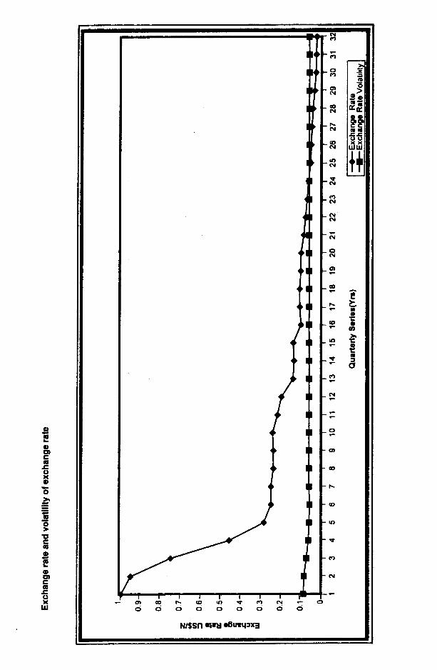
The estimated relationship among import prices and exchange rate, exchange ratevolatility, and price volatility is shown in Appendix 3 Graph and also reported in appendixtables A10 to Al 2. The estimation revealed that changes in the exchange rate and itsvolatility significantly affect import earnings, the same way they affect import prices.The exchange rate significantly affects import price in the negative direction; that is, anappreciation of the exchange rate will result in decreased import prices. However, bothexchange rate volatility and import price volatility have a positive effect on import trade,which implies that the more erratic the exchange rate and the import price, the greaterthe import trade.

The discussions under this section can support the following inferences:

l Exchange rate exerts a significant negative influence on agricultural import levels inNigeria.

l Exchange rate volatility positively and significantly affects the level of agriculturalimports into Nigeria, either directly or indirectly through import prices.

l Import price volatility affects import levels positively but has a negative effect onimport price.

A matrix (Table 8) was constructed to indicate the effects of volatility in exchangerate and prices on export and import trade. The matrix indicates only the sign of theeffect.

If earnings is taken as a function of price and quantity, then the negative effect ofexchange rate volatility on export earnings must have been to reduce the volume ofproduction since it has a positive effect on price. An increase in exchange rate (i.e., anappreciation of the local currency) also has a negative effect on both export and import

30 RESEARCH PA P E R 87

quantity and prices. Furthermore, when price is volatile, it will have a positive effect onproduction but tend to have negative effect on prices. Thus it reduces the rate of increasein prices.

Table 8: Matrix of price and exchange rate volatility

Export earnings Import value Export price Import price

--

Exchange ratevolatility

-ve +ve +ve +ve

Exchange rate -ve -ve -ve -ve

Price changes +ve -ve None None

Price Volatility +ve +ve -ve -ve

-ve+ve

= negative effect.= positive effect.

VII. Major findings and policy implications-The study was able to establish that exchange rate volatility has a negative effect onagricultural exports, while price volatility has a positive effect. Thus, the more volatilethe exchange rate changes, the lower the income earnings of farmers, which subsequentlyalso leads to a decline in output production and a reduction in export trade. However,price volatility exerts a positive effect on the level of exports. Also an appreciation ofthe local currency decreases export earnings, while an increase in export price influencesthe level of exports positively. The implication is that if the exchange rate change ismore volatile, it tends to increase the prices of export crops, but the general effect leadsto a decline in export production. Furthermore, the study also established the efficacy ofprice increase as a tool for increasing output of export crops. For import trade, theappreciation of the exchange rate reduces imports, while its volatility has a positiveeffect. If the exchange rate and import prices are volatile, they tend to increase the levelof imports. The study has also shown that the SAP era, though beneficial in terms ofprice increases of agricultural exports, has also resulted in a high level of price andexchange rate fluctuations.

Two policy implications arise from this study:

The monetary authorities should adopt a mechanism that will lead to the stability ofthe exchange rate. Erratic changes in the exchange rate have a long-term negativeeffect on production of agricultural exports.The government should monitor the marketing system of agricultural exports to ensurethat farmers are paid fully by the buying agents so that the full benefit of productionincreases resulting from liberalization can be reaped. Community exchangeprogrammes should be explored as a plausible mechanism for assisting farmers andexporters to hedge against a rash of changes in the marketing system in both pricesand exchange rates.

References

Abel, A.B. 1983. “Optimal investment under uncertainty”. American Economic Review,73( 1): 234-48.

Abrams, R.K. 1980. “International trade flows under flexible exchange rates”. EconomicReview. Federal Reserve of Kansas City, 65: 3-10.

Aktar, M.A. and R.S. Hilton. 1984. “Exchange rate uncertainty and international trade:Some conceptual issues and new estimate for Germany and the United States”.Research Paper 8403, Federal Reserve Bank of New York.

Ajayi, S. I. 1988. “Issues of overvaluation and exchange rate adjustment in Nigeria”.Prepared for Economic Development Institute (EDI), the World Bank, Washington,D.C.

Bailey, M.J. and G.S. Taulas. 1988. “Trade and investment under floating exchange rates:The U.S. experience”. The Cato Journal, ~01.8: 2.

Bailey, M.J., G.S. Taulas and M. Ulan. 1986. “Exchange rate variability and tradeperformance: Evidence for the big seven industrial countries”. WeZtwirtschajtZichesArchio 122m: 466-77.

.1987. ‘The impact of exchange rate volatility on export growth: Sometheoretical consideration and empirical results”. Journul of Policy ModelZing,vol. 9: 20543.

Bartlett, MS. 1935. “Some aspects of the time-correlation problems in regard to tests ofsignificance journal royal statistical society”. vol. 98: 536-43.

Box, G.E.P. and D.R. Cox. 1964. “An analysis of transformation (with discussion)“. J.Royal Stat. Sot. vol. B26: 211-252.

Caballero, R.J. and V. Corbo. 1989. ‘The effects of real exchange rate uncertainty onexports: Empirical evidence”. The World Bank Economic Review, ~013 (2).

Central Bank of Nigeria. Annual Reports and Statements of Accounts, various years.Central Bank of Nigeria. Nigeria’s Principal Economic and Financial Indicators. 1970-

1994.Chambers, R. G. and R. E. Just. 1991. “Effects of exchange rate changes on U.S.

agriculture.” Amex J. of Agric Econs, 73: 33-43.Chatfield C. 1984. The Analysis of Xme Series (An Introduction). Chapman and Hall.Coes, D.V. 198 1. ‘The crawling peg and exchange rate uncertainty”. In John Williamson,

ed., Exchange Rate Rules. London: Macmillan & Co., and New York: St. Martin’sPress.

PRICE, EXCHANGE RATE VOUTILITY AND NIGERIA’S AGRICULTURAL TRADE FLOWS 33

Cumby, R.E. and M. Obstfeld. 198 1. “Exchange rate expectations and nominal interestrate differentials: A test of the Fisher hypothesis”. Journal of Finance, vol.36(June): 697-703.

Cushman, D.O. 1983. “The effects of real exchange rate risk on international trade”.Journal of International Economics vol 15: 45-63.

Cushman, D.O. 1988. ‘The effects of real exchange rate risk on international trade”.Journal of International Economics, ~0124: 24-42.

de Grauwe, P. 1988. “Exchange rate variability and the slowdown in growth ofinternational trade”. ZMF StafPapers, 35: 63-84.

Diebold, F.X. and J.A. Nason. 1990. “Non-parametric exchange rate prediction”. Journalof International Economics, 28: 3 15-3 12.

Dixit, A. 1989. “Hysteresis, import penetration and exchange rate pass-Through”.Quarterly Journal of Economics, 104: 205-27.

Durbin J. 1960. ‘The fitting of time series models.” Review of International Institute ofStatisticians, vol. 28: 223-239.

Egwaikhide, F.O. 1993. “Determinants of imports in Nigeria: A dynamic specification.”Final Report. African Economic Research Consortium (AERC). Nairobi.

Frenkel, J. 198 1. “Flexible exchange rates, prices and the role of the news. “Journal ofPolitical Economy, vol. 89: 665-705.

Goldstein M. and M. Khan. 1976. “Large versus small price changes and the demand forirqorts”. IMF staff papers, 20&223.

Gotur, P. 1985. “Effects of exchange rate volatility on trade: Some further evidence”.IMF StagPaper 32: 475-5 12.

Hakkio, G.S. and M. Rush. 1989. “Market efficiency and cointegration: An applicationin the sterling and deutschemark exchange markets”. Journal of InternationalMoney and Finance, ~01.8: 75-88.

Haugh L.D. and G.E.P. Box. 1977. Identification of Dynamic Regression (DistributedLag) Models connecting IILvo Time Series. J.A.S.A., ~01.72, no.357: 121-130.

Hooper, P and S.W. Kohlhagen. 1978. ‘The effects of exchange rate risk and uncertaintyon the prices and volume of international trade”. J. of Int. Econs, 8: 483-5 11.

IMF. 1984. “Exchange rate volatility and the world trade”. Occasional Paper no. 28,IMF Research Department, Washington, D.C.

Ihimodu, 1.1. 1993. The Structural Adjustment Programme and Nigeria’s AgriculturalDevelopment. Monograph Series No. 2, National Centre for EconomicManagement and Administration, Ibadan, Nigeria.

Kenen, PT. and D.R. Rodrick. 1986. “Measuring and anal.ysing the effects of short-tern1volatility in real exchange rates”. The Review of Economics and Statistics, 68:311-15.

Koray, F. and W.D. Lastrapes. 1989. “Real exchange rate volatility and U.S. bilateraltrade: A VAR approach”. The Review of Economics and Statistics, vol. 7 1: 708-1 2 .

Kroner, K.F. and W.D. Lastrapes. 1991. ‘The impact of exchange rate volatility oninternational trade: Reduced from estimates using the GARCH-in-mean model”.Manuscript. University of Arizona.


Kumar R. and R. Dhawan. 1991. “Exchange rate volatility and Pakistan’s exports to thedeveloped world 1974-85”. World Development, ~01.19, no. 9: 1225-1240.

Kwanashie M., I. Ajilima and A. Garba. 1994. ‘The Nigerian economy response ofagriculture to adjustment policies”. AERC Research Paper 19.

Lastrapes, W. and F. Koray. 1990. “Exchange rate volatility and U.S. multilateral tradeflows”. Journal of Macroeconomics, 12(3): 134-48.

’ Maskus, K.E. 1986. “Exchange rate risks and U.S. trade: A sectoral analysis”. FederalReserve Bank of Kansas City Econ. Rev.

Medhora, R. 1990. ‘The effects of exchange rate volatility on trade: The case of WestAfrican monetary union’s imports” World Development, vol. 18, no. 2:313-324.

Messe, R.A. and K.S. Rogoff. 1983. “Empirical exchange rate models of the seventies:Are any fit to survive ?’ Journal of International Economics, vol. 14: 3-24.

Messe, R.A. and A.K. Rose. 1990. “Non linear, non-parametric, non-essential exchangerate estimation”. American Economic Review, 80: 60-72.

Obadan, M. I. 1994. Real Exchange Rates in Nigeria: A Preliminary Study. MonographSeries No. 6. National Centre for Economic Management and Administration,Ibadan, Nigeria.

Ogiogio, G.O. 1993. “The behaviour of foreign exchange rates in Nigeria: Determinantsand market efficiency”. Final Report, African Economic Research Consortium,Nairobi, Kenya.

Ojameruaye, E.O. 1991. “An application of the purchasing power parity theory to thedetermination of the realistic exchange rate of the Nigerian currency”. NigerianFinancial Review ~01.3, no.4, 1991.

Ojo, 0. et al. 1978. “A quarterly econometric model of the Nigerian economy: Somepreliminary estimates”. Ife Social Science Review l(2): 149-65.

Osagie, E. 1985. “An operational econometric model of the Nigerian economy: Somepreliminary estimates”. Ife Social Science Review, l(2): 149-165.

Osuntogun, A., C.C. Edordu and B.O. Oramah. 1993. “Promoting Nigeria’s non-oil export:An analysis of some strategic issues”. Final report. African Economic ResearchConsortium, Nairobi, Kenya.

Oyejide, T.A. 1986. The efects of trade and exchange rate policies on agriculture inNigeria. Research Report 55, International Food Policy Research Institute,Washington, D.C.

Pick, D.H. 1990. “Exchange rate risk and U.S. trade”. American Journal of Agric Econs,72(3): 694-700.

Qian, Y. and P. Varangis. 1992. “Does exchange rate volatility hinder export growth?‘.International Economics department, The World Bank Working Papers onInternational Trade. WPS 9 11, May.

Schuh, G.E. 1974. “The exchange rate and U.S. agriculture”. Amer: J. of Agric Econs,56: 1-13.

Taylor L. and P. Krugman. 1977. “Contractionary effects of devaluation”. Quarterly J.of Int. Econs, g(3): 445-456.

Thursby, J.G. and M.C. Thursby. 1987. “Bilateral trade flows, the Linder hypothesis andexchange rate risk”. The Review of Economics and Statistics. 69: 488-95.

World Bank. 1994. Nigeria StructuralAdjustment Programme: Policies Implementation,and Impact. World Bank Report No. 130534JNI.

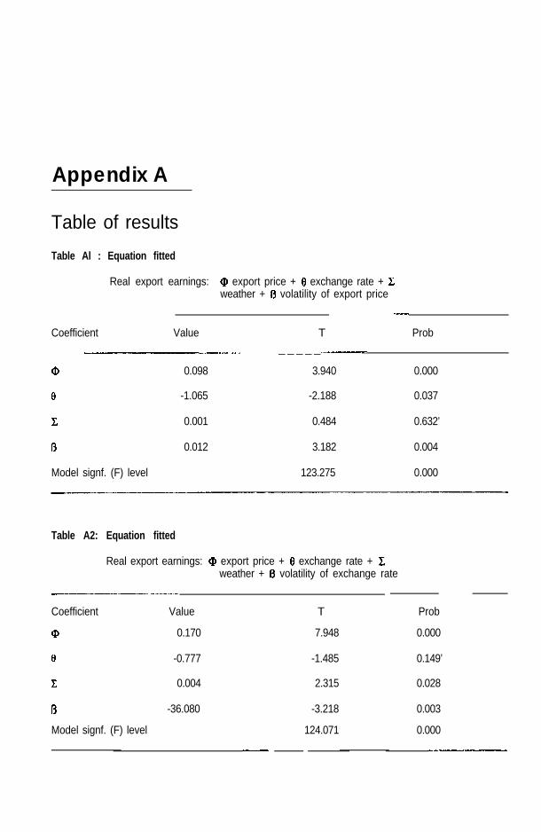
Appendix A

Table of results

Table Al : Equation fitted

Real export earnings: Q, export price + 6 exchange rate + ISweather + 0 volatility of export price

Coefficient Value T Prob_.-_.- .- - ~- ..- _ _ _ _ __I___~

cg 0.098 3.940 0.000

8 -1.065 -2.188 0.037

1 0.001 0.484 0.632’

I3 0.012 3.182 0.004

Model signf. (F) level 123.275 0.000

Table A2: Equation fitted

Real export earnings: @ export price + 6 exchange rate + Cweather + f3 volatility of exchange rate

~-

Coefficient Value T Prob

Q, 0.170 7.948 0.000

8 -0.777 -1.485 0.149’

c 0.004 2.315 0.028

I3 -36.080 -3.218 0.003

Model signf. (F) level 124.071 0.000--= ------_



Real export earnings: Q, export price + 6 exchange rate + Xweather + 0, volatility of export price + 0,volatility of exchange rate

Coefficient Value T

-~

cg 0.117 6.779

8 0.133 0.340

Iz 0.007 5.057

0, 0.014 5.738

% -45.142 -5.770

Model signf. (F) level 219.001--~ -..--

Prob

0.00

0.737’

0.000

0.000

0.000

0.000.~~ -.


Real import earnings: Cp import price + 8 exchange rate + Cforeign exchange reserves + 3volatility of import price

- ~___~.~~ ~. _ _~~--. ~~~___, _

Coefficient Value T- -

cg 0.042 0.209

8 -7.672 -0.611

z 0.031 5.439

I3 0.195 2.578

Model signf. level (F) 39.526

Prob- -

0.836’

0.546’

0.000

0.015

0.000

PRICE, EXCHANGE R ATE VOLATILITV AND N IGERIA’S A GRICULTURAL TRADE FLOWS 37

Table AS: Equation fitted

Real import earnings: cf, import price + 8 exchange rate + Zforeign exchange reserves + I3volatility of exchange rate

Coefficient

--

Value

-I__-. ._

T Prob

@ -0.150 -1.411 0.169

8 -46.040 -6.127 0.000

c 0.004 0.814 0.422’

I3 679.945 7.864 0.000



Real import earnings: Cp import price + 6 exchange rate + Zforeign exchange reserves + 0,volatility of import price + O2volatility of exchange rate

Coefficient

Q,

Value

-0.303

-__-____-

T

-2.376

Prob-_-

0.025

8 -37.149 -4.392 0.000

c 0.003 0.680 0.502’

0, 0.092 1.971 0.059’

4 628.821 7.277 0.000




Export price: @ Real export earnings + 9 exchange rate + Zint. world price + 0 volatility of export price


Q,

0

E

I3

Model signf. level (F)

1.821 1.707

-9.990 -2.000

9.883 5.444

-0.071 -2.921

247.528--___--


Export price: @ Real export earnings + 9 exchange rate + Zint. world price + f3 volatility of exchange rate

- -

Coefficient Value T

Q, 2.013 2.306

8 -2.528 -0.884

z 0.335 2.390

I3 122.992 5.178

Model signf. (F) level 389.860

0.088’

0.055’

0.000

0.007

0.000

Prob__--.--

0.029

0.499’

0.024

0.000

0.000



Export price: Q, real export earnings + 9 exchange rate + Cint. world price + 0, volatility of export price + 6,volatility of exchange rate

Value T Prob

Q, 2.049 2.549 0.017

8 -6.771 -1.775 0.087

I2 0.502 3.438 0.002

4 -0.047 -2.453 0.021

4 107.880 4.747 0.000

Model signf. (F) level 368.989

Table Al 0: Equation fitted

Import price: Cp real import value + 9 exchange rate + Zint. world price + l3 volatility of import price


Q, -0.362 -6.038 0.000

8 -32.475 -4.167 0.000

x 2.516 11.091 0.000

I3 -0.052 -2.343 0.026

Model signf. level (F) 281,527 0.000


Table All : Equation fitted

import price: Q, real import value + 8 exchange rate + Zint. world price + f3 volatiiity of exchange rate


Q, -0.505 -4.079 0.000

8 -27.230 -3.346 0.002

2 1.965 12.890 0.000

8 131.884 1.318 0.198’



Import price: Cp real import value + 6 exchange rate + Cint. world price + 0, volatility of import price + 0,volatility of exchange rate

V a l u e T Prob

cp -0.456 -3.816 0.001

8 -36.129 -4.104 0.000

I2 2.408 9.366 0.000

4 -0.094 -2.080 0.047

% 87.629 0.904 0.374

Model signf. (F) level 223.909 0.000_ _ _ ---,___I_ ._-I~ ---__

PRICE, EXCHANGE RATE VOLATILITV AND NIGERIA’S AGRICULTURAL TRADE FLOWS 41


Export price local: Q, world price + 0 exchange rate

Coefficient Value~~ -~-~~ ~~ - -

Q, 0.927

Prob

0.000

8 -9.346 -2.859 0.008

Model signf. (F) level 390.886 0.000_~ .-~ ~- ~___~~

Note: Not significant at 5% level.

Expot? price and volatility of export price

6 0

4 0

2 0

0

12 3 4 5 6 7 6 9 10 11 12 13 14 15 16 17 16 19 20 21 22 23 24 25 26 27 26 29 30 31 32

Quarterly Series(Yrs)

Price, exchange rate volatility and Nigeria's agricultural trade ...

Documents

Transcript of Price, exchange rate volatility and Nigeria's agricultural trade ...