1. IntroductionOver the past decade in

the Netherlands, volatileoutput prices have led tofluctuating profitability ofagricultural land and maytherefore have affectedland-use decisions. For aproducer, the shadow priceof land represents the land’smarginal contribution toprofit. If a producer has noconstraints on land use,profit maximization occursat the point where shadowprices are equal among allalternative land uses. How-ever, the equality of shadowprices among land uses on-ly accounts for expectedoutput prices because pro-ducers do not know outputprices at the time theychoose their production ac-tivities, and must base theirexpectation on past experience. This causes uncertainty forthe producer about the difference between the actual and ex-pected output price, which may differ per activity and throughtime. For a risk-neutral producer uncertainty will not influ-ence his production decisions. For a risk-averse producer, pro-duction activities with a high expected output price and a lowprofit variability are preferred. A risk-averse producer, facedwith increased volatility in output prices, is therefore morelikely to switch to less volatile production activities.

The European Union’s Common Agricultural Policy(CAP) is shifting away from market and price support toliberalized markets and decoupled payments from produc-tion. This is likely to result in an increased volatility of out-

put prices and hence, farmprofits, which affects thecompetitive positions ofagricultural and non-agri-cultural land uses (Ridierand Jacquet, 2002; Scko -kai and Moro, 2006;Brady et al., 2009). How-ever, because the degreeof volatility is crop-spe-cific, the effect on farmplans has so far remainedunclear.

Competing agriculturaland non-agricultural claimsarise, especially in areassuch as the Netherlandswhere land is scarce. Inthis paper our focus issolely on agricultural landuse, ignoring competitionwith other sectors andtaking the total (decreas-ing) amount of agricultur-al land as given.

There is an extensiveliterature on the estimation of models that analyze multiple-output supply decisions and agricultural land allocation de-cisions. Broadly, two lines of thinking can be distinguished:estimating a system of output supply, input demand, andland-use equations (Coyle, 1992; Oude Lansink, 1999;Sckokai and Moro, 2006), and estimating land-use responseequations (Moore and Negri, 1992; Wu and Segerson,1995; Fezzi and Bateman, 2011).

Estimating a system of output supply, input demand, andland-use equations has been applied by Coyle (1990,;1992,; 1999), who combined the effects of risk aversion,price uncertainty, and yield uncertainty on crop productiondecisions in mean-variance duality models of production.Oude Lansink (1999) elaborated on Coyle’s work by usinga linear mean-variance utility function that incorporatedrisk to determine the input demand, output supply, and areaallocation simultaneously among various crops. More re-cently, Sckokai and Moro (2006) adapted Coyle’s frame-

Effect of output price volatility on agricultural land use

Esther BOERE1,2

, Jack PEERLINGS1, Stijn REINHARD

1,2,

Tom KUHLMAN2, Win HEIJMAN

1

AbstractThe EU’s CAP reform to liberalize markets and decouple payments from produc-tion has led to increasingly volatile output prices, and therefore, more price and in-come risk. In this study, eight land use share equations are specified and estimat-ed using regional data from 2000 through 2013. A multiple-equation panel datamodel is used to determine the contribution of increased price volatility and risk toland-use change. More specifically, it is investigated how relative perceived risk af-fects land use change. We found opposite effects between complementing and sub-stituting land uses, leading to competition within the dairy sector and within cropproduction.

Keywords: CAP, land-use change, panel data, price volatility, risk perception.

RésuméLa réforme de la PAC de l’UE, visant à libéraliser les marchés et à découpler lespaiements directs de la production, a entraîné une plus forte volatilité des prix deproduction et a provoqué, par conséquent, une augmentation du risque de prix etde revenu. Le but de ce travail est de présenter et évaluer huit équations concernantles modes d’utilisation des terres, en considérant les données régionales de 2000 à2013. Un modèle à équations simultanées sur données de panel a été retenu pourmesurer l’impact de l’accroissement de la volatilité des prix et du risque de prix surle changement d’affectation des sols. En particulier, nous avons focalisé l’attentionsur le changement d’affectation des sols lié à la perception du risque relatif. Nousavons observé des effets opposés entre utilisations des terres complémentaires etde substitution, qui génèrent une concurrence au niveau du secteur laitier et de laproduction agricole.

Mots-clés: PAC, changement d’affectation des terres, données de panel, volatilitédes prix, perception du risque.

10

1 Wageningen University, Agricultural and Rural Policy Group,WUR, Wageningen, thThae Netherlands. Corresponding author: Es-ther.Boere@wur.nl2 Agricultural Economics Research Institute, LEI, tThae Hague, theNetherlands.

Jel codes: Q15, C61, Q11

NEW MEDIT N. 3/2015

work to account for the increased output price volatilitycaused by CAP reforms in a study of crop production.

Estimating land-response equations has been applied byMoore and Negri (1992) to develop land and water alloca-tion equations based on a flexible functional form of a mul-ti-crop production function. Wu and Segerson (1995) elab-orated on this model by adjusting it to account for land het-erogeneity.

The two approaches were integrated by Chambers andJust (1989), who used a two-step modeling framework: thisapproach allocates land among different production activi-ties after the optimal levels of outputs and inputs have beendetermined. Arnade and Kelch (2007) extended this frame-work by deriving shadow price equations for crop areas.Fezzi and Bateman (2011) used the Chambers and Justframework to establish a joint profit function to derive e-quations for “land-use share” (the proportion of the landarea allocated to each use) that can be estimated as a sys-tem. There also exists a great body of literature on yield risk(Just and Pope, 1979; Chavas and Holt, 1990). However, inorder to focus on price risk, we choose to ignore yield risk.Estimating land-use response equations that not only ac-count for the effect of price uncertainty on its own land use(e.g. price uncertainty of wheat on the land use of wheat),but also on alternative land uses (e.g. sugar beets) has notyet been undertaken.

The purpose of this paper is to assess the effect of volatileagricultural output prices on changes in agricultural landuse since 2000 in the Netherlands by estimating a system ofland-response equations. The land-response equations arebased on a restricted profit function, taking both risk andfarm technology into account. We used data on 66 Dutch a-gricultural regions from 2000 through 2013 to analyze theland-use decisions of producers.

In the next section we establish land use share functionsthat account for the risks that result from increased pricevolatility. Moreover, we hypothesize that the effect of agri-cultural outputs being complements and substitutes affectsland use decisions. Next, we describe the study area and da-ta sources. We then develop an empirical model in whichthe producer optimizes his profit by allocating land amongdifferent uses while accounting for risk. In the final sec-tions, we econometrically estimate the land-use share equa-tions, discuss the results, provide a general discussion, andpresent the main conclusions drawn from our study.

2. Theoretical FrameworkBuilding upon the work of, amongst others, Chavas and

Pope (1982), Coyle (1990, 1992) and Wu and Segerson(1995), we derive a system of land use share equationsbased on a utility maximizing producer. We assume a prof-it function with multiple outputs (land uses or crops), wherethe producer must decide how to allocate his/her hectares a-mong different land uses in order to maximize total profits(Wu and Segerson, 1995). The profit function is elaboratedby accounting for risk in production decisions; the produc-

er therefore becomes a utility maximizer (Oude Lansink,1999). Expected utility is determined by the expected prof-it, the variance of profit, and the coefficients of absoluterisk aversion per crop (see e.g. Coyle, 1990, 1992). Basedon utility maximization we derive land-use share functionsthat represent the proportion of the land that producer h al-locates to land use i in year t:

The land-use share of producer h for crop i in year t (sUhit)

depends on all expected output prices (p̂t) and known vari-able input prices (wt) in year t, yields (qht) of producer h inyear t, fixed input quantities (zht) of producer h in year t, thevariance of prices (Vp), and the degree of risk-aversion.The land use shares equal the number of hectares nU

hit ofproducer h allocated to crop i in year t divided by the totalnumber of hectares Nht of producer h in year t. When Vp=0,the land-use share equation for the utility-maximizing pro-ducer equals the land-use share equation for the profit-max-imizing producer. For the mathematical derivation from theprofit function to the land use shares, we refer the reader tothe Appendix.

Ratio of coefficient of variationsFigure 1 shows that for all output prices there is some de-

gree of volatility. We assume that, when determining opti-mal land use, the producer looks at the relative price volatil-ity between crops; hence the variation of a crop comparedwith the variation of the alternative crops. To take this intoaccount, we take the ratios of the coefficients of variation aselements of Vp:

where Cvr

is the 3-year moving average of the coefficientof variation, the standard deviation divided by the average,of the output price of the alternative (substitute or comple-ment) crop and Cv

iis the 3-year moving average of the co-

efficient of variation of the output price of the crop of in-terest. Hence, in ‘the ratio of the coefficients of variation’the CV of the alternative crop is in the numerator and thatof the crop of interest in the denominator.

We used coefficients of variation instead of variances be-cause, in comparison to variance, the coefficient of varia-tion is a unitized measure of risk. So, dividing the ratio oftwo coefficientcoefficients of variations (see equation 2)does not lead to a violation of the homogeneity assumption.

Substitutes and complementsIn the model presented, land use change depends on the

factors determining the land shares, i.e. expected outputprices, variable input prices, yields, quantities of fixed fac-tors and the variance of output prices. Implicit is also farmtechnology relevantce, showing to what extent the produc-

shitU = shitU p̂t,wt,qht,zht,Vp( ) = nhitU

Nht h=1,…,H; i=1,…,I; t=1,…,T . (1)

i

r

ii

rrir Cv

Cvv ==μ�μ�// i,r=1,…,I; i�r , (2)

11

NEW MEDIT N. 3/2015

er is able to adjust activities within his enterprise. One as-pect of farm technology is whether production activities arecomplements or substitutes. Complements are defined asthose activities that are in joint supply, either because ofcrop rotation requirements or because one output is neededas an input in producing another output. Substitutes are de-fined as (sets of) activities that are rival to each other.

For arable production in the Netherlands, the common ro-tation system is the joint production of cereals, potatoes andsugar beets. For dairy production, fodder maize and grass-land can be viewed as complementary to milk production.When facing a larger expected utility, it is likely to be eas-ier for a producer to switch activities within these two setsof production rather than between them.

Based on the ratios of coefficients of variation we can ex-amine whether two land uses are substitutes or comple-ments. For substitutes and in case of risk-aversion a pro-ducer will increase the share of a crop when the ratio of co-efficients of variation increases (the coefficient of variationof the crop being in the denominator). For complements theopposite is true.

3. Data We divided the Netherlands into 66 agricultural regions

using an existing classification based on homogeneity ofsoil types (Helming, 2005; Helming and Reinhard, 2009).One of the advantages of using this classification for thetypes of agricultural regions is the relative homogeneity ofthe soil within these regions. All regions can be classifiedbased on the soil type (clay, sand, or mixed soil that in-cludes peats and loams). Different soil types generate dif-ferent crop yields and therefore attract different productionactivities.

We aggregated farm structure survey (FSS) data for allfarm households in the Netherlands from 2000 through2013 into the 66 agricultural regions (Statistics Nether-

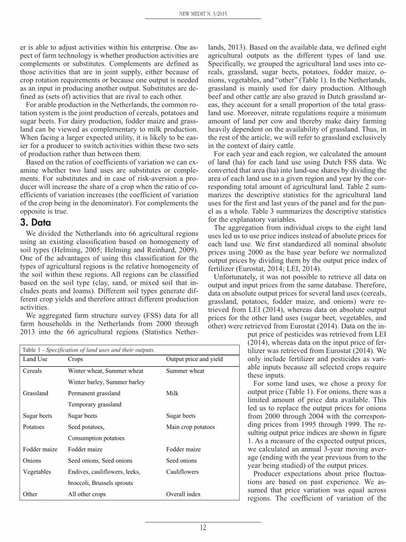
lands, 2013). Based on the available data, we defined eightagricultural outputs as the different types of land use.Specifically, we grouped the agricultural land uses into ce-reals, grassland, sugar beets, potatoes, fodder maize, o-nions, vegetables, and “other” (Table 1). In the Netherlands,grassland is mainly used for dairy production. Althoughbeef and other cattle are also grazed in Dutch grassland ar-eas, they account for a small proportion of the total grass-land use. Moreover, nitrate regulations require a minimumamount of land per cow and thereby make dairy farmingheavily dependent on the availability of grassland. Thus, inthe rest of the article, we will refer to grassland exclusivelyin the context of dairy cattle.

For each year and each region, we calculated the amountof land (ha) for each land use using Dutch FSS data. Weconverted that area (ha) into land-use shares by dividing thearea of each land use in a given region and year by the cor-responding total amount of agricultural land. Table 2 sum-marizes the descriptive statistics for the agricultural landuses for the first and last years of the panel and for the pan-el as a whole. Table 3 summarizes the descriptive statisticsfor the explanatory variables.

The aggregation from individual crops to the eight landuses led us to use price indices instead of absolute prices foreach land use. We first standardized all nominal absoluteprices using 2000 as the base year before we normalizedoutput prices by dividing them by the output price index offertilizer (Eurostat, 2014; LEI, 2014).

Unfortunately, it was not possible to retrieve all data onoutput and input prices from the same database. Therefore,data on absolute output prices for several land uses (cereals,grassland, potatoes, fodder maize, and onions) were re-trieved from LEI (2014), whereas data on absolute outputprices for the other land uses (sugar beet, vegetables, andother) were retrieved from Eurostat (2014). Data on the in-

put price of pesticides was retrieved from LEI(2014), whereas data on the input price of fer-tilizer was retrieved from Eurostat (2014). Weonly include fertilizer and pesticides as vari-able inputs because all selected crops requirethese inputs.

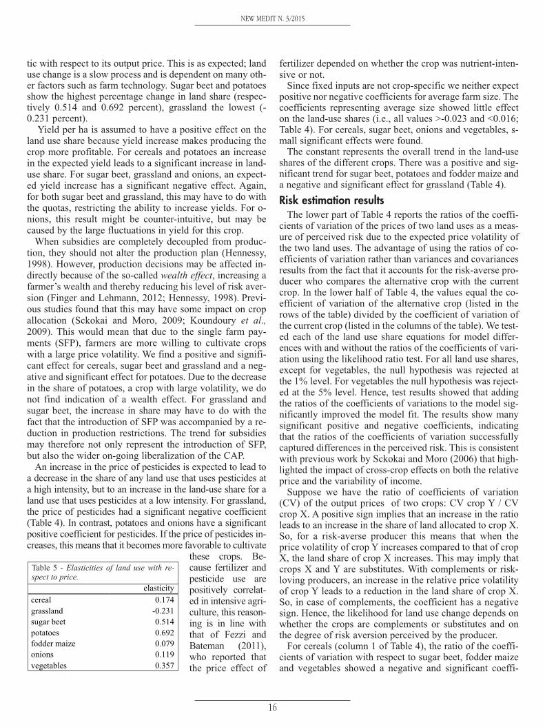
For some land uses, we chose a proxy foroutput price (Table 1). For onions, there was alimited amount of price data available. Thisled us to replace the output prices for onionsfrom 2000 through 2004 with the correspon-ding prices from 1995 through 1999. The re-sulting output price indices are shown in figure1. As a measure of the expected output prices,we calculated an annual 3-year moving aver-age (ending with the year previous from to theyear being studied) of the output prices.

Producer expectations about price fluctua-tions are based on past experience. We as-sumed that price variation was equal acrossregions. The coefficient of variation of the

Land Use Crops Output price and yield

Cereals Winter wheat, Summer wheat Summer wheat

Winter barley, Summer barley

Grassland Permanent grassland Milk

Temporary grassland

Sugar beets Sugar beets Sugar beets

Potatoes Seed potatoes, Main crop potatoes

Consumption potatoes

Fodder maize Fodder maize Fodder maize

Onions Seed onions, Seed onions Seed onions

Vegetables Endives, cauliflowers, leeks,

broccoli, Brussels sprouts

Cauliflowers

Other All other crops Overall index

Table 1 - Specification of land uses and their outputs.

NEW MEDIT N. 3/2015

12

normalized output price indices over the 3 years previous tothe year being studied was used as a proxy for the expectedvariation in output prices. In addition to the output and in-put prices, we included the quantity of fixed inputs, yieldsand the presence of direct payments as explanatory vari-ables. As a proxy for fixed inputs, we used the average sizeof a farm in a region, which was obtained from the FSS da-ta. Size is measured by the standardized annual revenue ofa specific production type per hectare of land or per animal.The average size was calculated as the sum of all farm sizesin a region, divided by the number of farms in the regionand subsequently converted into an index. For each landuse, the production (yield in kg/ha; Table 3) was convertedinto an index value similar to the way we did for outputprices (with the value in 2000 = 100). The presence of di-rect payments is referenced to as a dummy trend, starting in2006 when direct payments were introduced, and taking thevalue zero prior to 2006.

The descriptive statistics in Table 2 show that averageland use shares of the different agricultural land uses over

all regions have changed only slightlyover time. However, some land uses havechanged considerably more than others.In particular, the area of sugar beets, po-tatoes and other decreased, whereas thearea of grassland and fodder maize. Thisindicates a tendency towards dairy pro-duction. Grassland remained the mainland use throughout the study period,with a share of more than 50% of the to-tal agricultural land. The columns repre-senting standard deviations, minimumand maximum shares of land use in Table2 indicate large regional differences inland uses. This may be because of the di-vision of regions based on homogeneityof soil. In varying degrees, almost all

land uses are prevalent in each region during the whole pe-riod (see last column Table 2).

Compared to the relatively small changes in the land-useshares, figure 1 shows relatively large changes in outputprices. The output prices seemed to follow some commontrends in their fluctuations, such as decreases between 2003and 2005 and between 2007 and 2008 and an increase overthe last two years. However, large differences in the volatil-

Table 2 - Summary statistics for agricultural land uses at the start and end for the Nether-lands by year and whole panel by region and year (2000-2013).

a) (absolute = the actual area; share = absolute area divided by the total area)

2000 2013 Whole panel

Sharea) Absolute

(1000 ha)

Share Absolute (1000 ha) Share Mean S.D. Min. Max.

share non-zero obs

Cereals 183.64 0.10 182.37 0.10 0.10 0.11 0.00 0.41 0.99 Grassland 1010.02 0.52 982.95 0.54 0.53 0.27 0.09 0.99 1.00 Sugar beets 110.95 0.06 73.19 0.04 0.05 0.05 0.00 0.21 0.97 Potatoes 180.16 0.09 155.82 0.08 0.08 0.09 0.00 0.40 0.99 Fodder maize 205.30 0.09 229.74 0.11 0.10 0.08 0.00 0.40 1.00 Onions 19.27 0.01 28.17 0.01 0.01 0.02 0.00 0.12 0.84 Vegetables 6.44 0.00 6.70 0.00 0.00 0.01 0.00 0.06 0.93 Other 235.68 0.14 188.67 0.12 0.13 0.11 0.00 0.62 1.00 Total 1951.45 1.00 1847.61 1.00 1.00

NEW MEDIT N. 3/2015

13

��

���

����

����

����

����

����

����

����

��������������������������������������������������������������������

�����

�����

����

���

�������

����������

������������

���������

�������

�����������

�� ���

!������"��#��

����

���

�

�

�

� �

�

�

�

� �

�

�

�

� �

�

�

�

� �

�

�

�

� �

�

�

�

� �

�

�

�

� �

�

�

�

� �

����

���

����

���

��

����

��������

��

�

�

�

� �

�

�

�

� �

�

�

�

� �

�

�

�

� �

�

�

�

�

�

�

�

�

�

� �

�

�

�

� �

������

���������

���������

�������

������

����������

��� �

�

�

�

� �

�

�

�

� �

��

���

���

������

�

�

�

� �

�

�

�

� �

����������������������������

�

�

�

� �

�

�

�

� �

�� ��������������������

!

�

�

�

� �

�

�

�

� �#���"�����

�

�

�

� �

�

�

�

� �

�

�

�

� �

�

�

�

� �

�

�

�

� �

�

�

�

� �

�

�

�

� �

�

�

�

� �

Figure 1 - Changes in nominal output prices from 2000 to 2013. Val-ues are normalized by setting the price in the base year (2000) to 100.

a) For scaling purposes and clarity of estimation results, the ratio of co-efficients of variation areis divided by 10.

Land-use Mean Std. Dev. Min. Max.

Expected output price indices (normalized by the price of fertilizer) Cereals 0.838 0.134 0.624 1.126 Grassland 0.770 0.182 0.493 1.159 Sugar beets 0.770 0.208 0.451 1.189 Potatoes 2.500 0.633 1.511 4.023 Fodder maize 0.930 0.231 0.600 1.472 Onions 2.015 0.413 1.445 3.128 Vegetables 0.818 0.156 0.530 1.115 Other 0.876 0.113 0.653 1.069 Expected yield indices (/100 in estimation for scaling purposes) Cereals 100.910 3.382 92.647 104.902 Grassland 103.237 4.099 94.691 109.078 Sugar beets 106.949 8.335 91.952 127.030 Potatoes 94.576 1.904 90.386 97.193 Fodder maize 106.612 3.987 100.480 115.588 Onions 92.550 3.282 85.323 101.882 Vegetables 108.451 7.744 83.548 218.187 Input price indices (normalized by the price of fertilizer) Pesticides 0.724 0.147 0.450 1.000 subsidies 0.571 0.495 0.000 1.000 Fixed cost indices (/100 in estimation for scaling purposes) Farm size 118.000 18.000 48.000 198.000 Coefficient of variation of the normalized expected output price indices a) Cereals 0.182 0.121 0.058 0.469 Grassland 0.124 0.074 0.044 0.309 Sugar beets 0.129 0.077 0.021 0.329 Potatoes 0.397 0.200 0.063 0.816 Fodder maize 0.116 0.060 0.037 0.200 Onions 0.542 0.155 0.242 0.840 Vegetables 0.121 0.067 0.030 0.340 Other 0.121 0.093 0.047 0.314

Table 3 - Summary statistics of explanatory variables over the wholetime period (2000-2013).

ity of the output prices can be observed. Output pricevolatility was especially high for onions and potatoes, bothin terms of the largest increase between two years (respec-tively 237.5 and 172.7 percent) and the largest decrease be-tween two years (respectively -56.7 and -79 percent), com-pared to an average increase of 31.8 and an average de-crease of 15.7 percent over all land uses between two years.

The large differences in output price volatility are reflectedin the coefficients of variation of output prices (Table 3). Po-tatoes and onions experienced much larger price variationsthan other land uses.

4. Empirical ModelAs indicated in equation 1 the allocation of land among d-

ifferent production activities for a utility-maximizing pro-ducer does not depend only upon output and input prices,and fixed input quantities, but also depends upon the varia-tion in output prices in relation to farm technology and theproducer’s degree of risk-aversion. Given the land-useshare equations for a utility-maximizing producer devel-oped in the theoretical model, we have specified the fol-lowing reduced-form land-use share equations:

Where S*hit represents the Nht land-use shares of crop i in

region h in year t; φhi represents the region-specific inter-cept for region h and land use i; βij represents the coeffi-cients for normalized input and output prices j for crop i; Xjtrepresents the normalized input and output prices j in yeart; ρim represents the coefficients of yields m for crop i; qmtrepresents the yields m in year t; γhk represents the coeffi-cients of fixed factors k for region h; zkht represents thefixed input factors k for region h in year t; ω

irepresents the

coefficient for crop i for the presence of direct income pay-ments, gt represents the direct income payments dummytrend, δir represents the coefficients for the ratios of the co-efficients of variation of the expected prices r for crop i; νirtrepresents the ratios of the coefficients of variation of theexpected alternative prices r with respect to expected pricesi in year t; λ

irepresents the coefficient of crop i for the

trends; Tt represents the time trend; and uit represents theunobservable effects that affect land-use change for crop iin year t.

Equation 3 specifies the share of land use for each crop iin region h in year t. Because only relative prices matter, themodel has been made homogeneous of degree zero by nor-malizing the standardized output prices and the standard-ized price of pesticides using the price of fertilizer. Each

land use share equation only includes expected output priceof its own land use and not expected output prices of alter-native land uses in order to avoid multicolllinearity. Due todata limitations, the fixed input quantities (zhkt) are onlyrepresented by the average farm size per region per yearand not allocated to individual land uses. A time trend hasbeen included to account for crop-specific trends in land-use shares.

We assume the covariances of output prices to be zero. Inreality, the covariances are not zero, but the large amount ofcovariance values caused multi-collinearity problems. For aproducer, the covariance of alternative products may be ofimportance in deciding upon land allocation. However, byestimating the effect of the ratios of the coefficients of vari-ation all alternative land uses are taken into account.

We tested for censoring from below, meaning that there isa lower bound of zero for all land use shares. In case manyland use shares actually take the value zero this could leadto inconsistent estimates of the parameters (Fezzi and Bate-man, 2011). The results, provided in Table 2, show that cen-sored observations are only present for vegetables, but notenough that inconsistent estimates of the parameters maybe expected. This, together with the few non-zero observa-tions for crop shares (see Table 2), means that we do nothave to take sample selection problems into account. Wetherefore estimated the land-use share equations as a sys-tem using the seemingly unrelated regression (SUR) tech-nique taking into account that the disturbances from differ-ent share equations are likely to be correlated because ofcommon unobservable factors (Fiebig, 2001). This correla-tion could have several causes, such as weather, policychanges affecting the agricultural sector as whole, or econ-omy-wide shocks. The yearly observations over the same s-tudy areas lead to a panel that required a fixed-effects trans-formation of the SUR regression. Because we deal with na-tional values for both price and yield indices, a fixed effectstransformation using deviations from the mean was notpossible. We therefore chose a first-difference transforma-tion on the model of the eight land-use shares:

Equation 4 implies that the intercept (fhi), which repre-sents the region-specific effect, cancels out. The new inter-cept λi represents the coefficient of the crop-specific trendin equation 3. The transformed explanatory variables arecomposed of the first-differenced expected output prices(p 'it), first-differenced input prices, first-differenced yieldsper hectare (qmt), first-differenced average farm size (zhkt),first-differenced dummy trend representing the presence ofdirect income payments (gt), and the first-differenced ratiosof the coefficients of variation (νirt – νirt–1

)1. Note that thedummy time trend for government subsidies transforms in-

( ) ( ) ( ) ( )

( ) ( ) ( )11

11

1

11

11

1*

1*

�=

�=

�

�=

�=

��

�++�+�+

�+�+�=�

��

��

ititi

R

rirtirtir

K

khkthkthk

tt

M

mmtmtim

J

jjtjtijhithit

uuvvzz

ggqqxxSS

���

��

h=1,…,H; i=1,…,I; t=1,…,T (4)

1 Note that with first-differencing the panel is reduced by one year;i.e. observations start as of the second year of observations in theoriginal panel. Moreover, first-differencing only occurs betweentime periods and not between regions or land uses.

NEW MEDIT N. 3/2015

14

itti

R

rirtirti

K

kkhthk

M

mmtim

J

jjtijhihit

uTg

zqxS

++++

+++=

�

���

=

===

����

��

1

111

*

h=1,…,H; i=1,…,I; t=1,…,T (3) (3)

to a dummy representing the presence of direct payments.Tables 2 and 3 list the dependent and explanatory variablesand their descriptive statistics.

Because all land-use shares together must sum to 0 in thefirst-differenced model, estimating all the land-use equationstogether results in a singular covariance matrix of errorterms. While there are various ways to handle this singulari-ty problem (Takada et al., 1995), we decided to drop theresidual equation ‘other’ from the system (Fezzi and Bate-man, 2011). The residual equation can then be recalculatedbecause, by definition, the land-use shares must sum to 1.

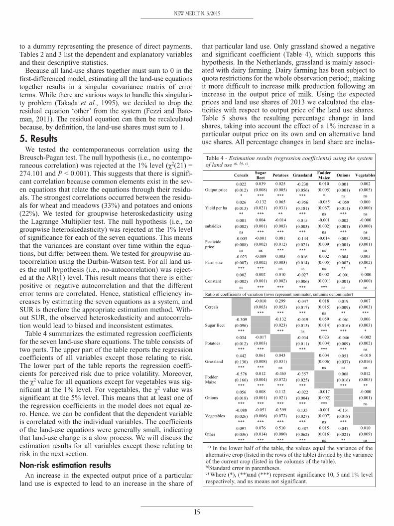
5. ResultsWe tested the contemporaneous correlation using the

Breusch-Pagan test. The null hypothesis (i.e., no contempo-raneous correlation) was rejected at the 1% level (χ2(21) =274.101 and P < 0.001). This suggests that there is signifi-cant correlation because common elements exist in the sev-en equations that relate the equations through their residu-als. The strongest correlations occurred between the residu-als for wheat and meadows (33%) and potatoes and onions(22%). We tested for groupwise heteroskedasticity usingthe Lagrange Multiplier test. The null hypothesis (i.e., nogroupwise heteroskedasticity) was rejected at the 1% levelof significance for each of the seven equations. This meansthat the variances are constant over time within the equa-tions, but differ between them. We tested for groupwise au-tocorrelation using the Durbin-Watson test. For all land us-es the null hypothesis (i.e., no-autocorrelation) was reject-ed at the AR(1) level. This result means that there is eitherpositive or negative autocorrelation and that the differenterror terms are correlated. Hence, statistical efficiency in-creases by estimating the seven equations as a system, andSUR is therefore the appropriate estimation method. With-out SUR, the observed heteroskedasticity and autocorrela-tion would lead to biased and inconsistent estimates.

Table 4 summarizes the estimated regression coefficientsfor the seven land-use share equations. The table consists oftwo parts. The upper part of the table reports the regressioncoefficients of all variables except those relating to risk.The lower part of the table reports the regression coeffi-cients for perceived risk due to price volatility. Moreover,the χ2 value for all equations except for vegetables was sig-nificant at the 1% level. For vegetables, the χ2 value wassignificant at the 5% level. This means that at least one ofthe regression coefficients in the model does not equal ze-ro. Hence, we can be confident that the dependent variableis correlated with the individual variables. The coefficientsof the land-use equations were generally small, indicatingthat land-use change is a slow process. We will discuss theestimation results for all variables except those relating torisk in the next section.

Non-risk estimation resultsAn increase in the expected output price of a particular

land use is expected to lead to an increase in the share of

that particular land use. Only grassland showed a negativeand significant coefficient (Table 4), which supports thishypothesis. In the Netherlands, grassland is mainly associ-ated with dairy farming. Dairy farming has been subject toquota restrictions for the whole observation period;, makingit more difficult to increase milk production following anincrease in the output price of milk. Using the expectedprices and land use shares of 2013 we calculated the elas-ticities with respect to output price of the land use shares.Table 5 shows the resulting percentage change in landshares, taking into account the effect of a 1% increase in aparticular output price on its own and on alternative landuse shares. All percentage changes in land share are inelas-

Cereals Sugar Beet Potatoes Grassland Fodder

Maize Onions Vegetables

Output price 0.022 0.039 0.025 -0.230 0.010 0.001 0.002

(0.012) (0.008) (0.005) (0.056) (0.005) (0.001) (0.005) * *** *** *** * ns ns

Yield per ha 0.026 -0.132 0.065 -0.956 -0.085 -0.059 0.000

(0.013) (0.021) (0.031) (0.181) (0.067) (0.011) (0.000) ** *** ** *** ns *** ns

subsidies 0.001 0.004 -0.014 0.015 -0.001 0.002 -0.000

(0.002) (0.001) (0.003) (0.003) (0.002) (0.001) (0.000) ns *** *** *** ns *** ns

Pesticide price

-0.003 -0.001 0.081 -0.144 -0.014 0.005 0.002 (0.008) (0.002) (0.012) (0.021) (0.009) (0.001) (0.001)

ns ns *** *** ns *** ns

Farm size -0.023 -0.009 0.003 0.016 0.002 0.004 0.003 (0.007) (0.002) (0.003) (0.014) (0.005) (0.002) (0.002)

*** *** ns ns ns ** *

Constant 0.002 0.002 0.010 -0.027 0.002 -0.001 -0.000

(0.002) (0.001) (0.002) (0.006) (0.001) (0.001) (0.000) ns *** *** *** *** ns ns

Ratio of coefficients of variation (rows represent nominator, columns denominator)

Cereals

-0.010 0.299 -0.047 0.018 0.019 0.007 (0.003) (0.053) (0.017) (0.015) (0.009) (0.003)

*** *** *** ns ** ***

Sugar Beet -0.309 -0.132 -0.019 0.059 -0.061 0.006 (0.096) (0.023) (0.015) (0.014) (0.016) (0.003)

*** *** ns *** *** *

Potatoes 0.034 -0.017 -0.034 0.023 -0.046 -0.002

(0.012) (0.003) (0.011) (0.004) (0.009) (0.002) *** *** *** *** *** ns

Grassland 0.442 0.061 0.043 0.004 0.051 -0.018

(0.130) (0.008) (0.031) (0.006) (0.037) (0.016) *** *** ns ns ns ns

Fodder Maize

-0.576 0.012 -0.465 -0.357 0.068 0.012 (0.166) (0.004) (0.072) (0.025) (0.016) (0.005)

*** *** *** *** *** **

Onions 0.056 0.008 0.112 -0.022 -0.017 -0.000

(0.018) (0.001) (0.021) (0.004) (0.002) (0.001) *** *** *** *** *** ns

Vegetables -0.088 -0.051 -0.399 0.135 -0.001 -0.131 (0.026) (0.006) (0.073) (0.027) (0.007) (0.018)

*** *** *** *** ns ***

Other 0.097 0.076 0.510 -0.387 0.015 0.047 0.010

(0.036) (0.014) (0.080) (0.062) (0.016) (0.021) (0.009) *** *** *** *** ns ** ns

Table 4 - Estimation results (regression coefficients) using the systemof land use a), b), c).

a) In the lower half of the table, the values equal the variance of thealternative crop (listed in the rows of the table) divided by the varianceof the current crop (listed in the columns of the table).b)Standard error in parentheses.c) Where (*), (**)and (***) represent significance 10, 5 and 1% levelrespectively, and ns means not significant.

NEW MEDIT N. 3/2015

15

tic with respect to its output price. This is as expected; landuse change is a slow process and is dependent on many oth-er factors such as farm technology. Sugar beet and potatoesshow the highest percentage change in land share (respec-tively 0.514 and 0.692 percent), grassland the lowest (-0.231 percent).

Yield per ha is assumed to have a positive effect on theland use share because yield increase makes producing thecrop more profitable. For cereals and potatoes an increasein the expected yield leads to a significant increase in land-use share. For sugar beet, grassland and onions, an expect-ed yield increase has a significant negative effect. Again,for both sugar beet and grassland, this may have to do withthe quotas, restricting the ability to increase yields. For o-nions, this result might be counter-intuitive, but may becaused by the large fluctuations in yield for this crop.

When subsidies are completely decoupled from produc-tion, they should not alter the production plan (Hennessy,1998). However, production decisions may be affected in-directly because of the so-called wealth effect, increasing afarmer’s wealth and thereby reducing his level of risk aver-sion (Finger and Lehmann, 2012; Hennessy, 1998). Previ-ous studies found that this may have some impact on cropallocation (Sckokai and Moro, 2009; Koundoury et al.,2009). This would mean that due to the single farm pay-ments (SFP), farmers are more willing to cultivate cropswith a large price volatility. We find a positive and signifi-cant effect for cereals, sugar beet and grassland and a neg-ative and significant effect for potatoes. Due to the decreasein the share of potatoes, a crop with large volatility, we donot find indication of a wealth effect. For grassland andsugar beet, the increase in share may have to do with thefact that the introduction of SFP was accompanied by a re-duction in production restrictions. The trend for subsidiesmay therefore not only represent the introduction of SFP,but also the wider on-going liberalization of the CAP.

An increase in the price of pesticides is expected to lead toa decrease in the share of any land use that uses pesticides ata high intensity, but to an increase in the land-use share for aland use that uses pesticides at a low intensity. For grassland,the price of pesticides had a significant negative coefficient(Table 4). In contrast, potatoes and onions have a significantpositive coefficient for pesticides. If the price of pesticides in-creases, this means that it becomes more favorable to cultivate

these crops. Be-cause fertilizer andpesticide use arepositively correlat-ed in intensive agri-culture, this reason-ing is in line withthat of Fezzi andBateman (2011),who reported thatthe price effect of

fertilizer depended on whether the crop was nutrient-inten-sive or not.

Since fixed inputs are not crop-specific we neither expectpositive nor negative coefficients for average farm size. Thecoefficients representing average size showed little effecton the land-use shares (i.e., all values >-0.023 and <0.016;Table 4). For cereals, sugar beet, onions and vegetables, s-mall significant effects were found.

The constant represents the overall trend in the land-useshares of the different crops. There was a positive and sig-nificant trend for sugar beet, potatoes and fodder maize anda negative and significant effect for grassland (Table 4).

Risk estimation resultsThe lower part of Table 4 reports the ratios of the coeffi-

cients of variation of the prices of two land uses as a meas-ure of perceived risk due to the expected price volatility ofthe two land uses. The advantage of using the ratios of co-efficients of variation rather than variances and covariancesresults from the fact that it accounts for the risk-averse pro-ducer who compares the alternative crop with the currentcrop. In the lower half of Table 4, the values equal the co-efficient of variation of the alternative crop (listed in therows of the table) divided by the coefficient of variation ofthe current crop (listed in the columns of the table). We test-ed each of the land use share equations for model differ-ences with and without the ratios of the coefficients of vari-ation using the likelihood ratio test. For all land use shares,except for vegetables, the null hypothesis was rejected atthe 1% level. For vegetables the null hypothesis was reject-ed at the 5% level. Hence, test results showed that addingthe ratios of the coefficients of variations to the model sig-nificantly improved the model fit. The results show manysignificant positive and negative coefficients, indicatingthat the ratios of the coefficients of variation successfullycaptured differences in the perceived risk. This is consistentwith previous work by Sckokai and Moro (2006) that high-lighted the impact of cross-crop effects on both the relativeprice and the variability of income.

Suppose we have the ratio of coefficients of variation(CV) of the output prices of two crops: CV crop Y / CVcrop X. A positive sign implies that an increase in the ratioleads to an increase in the share of land allocated to crop X.So, for a risk-averse producer this means that when theprice volatility of crop Y increases compared to that of cropX, the land share of crop X increases. This may imply thatcrops X and Y are substitutes. With complements or risk-loving producers, an increase in the relative price volatilityof crop Y leads to a reduction in the land share of crop X.So, in case of complements, the coefficient has a negativesign. Hence, the likelihood for land use change depends onwhether the crops are complements or substitutes and onthe degree of risk aversion perceived by the producer.

For cereals (column 1 of Table 4), the ratio of the coeffi-cients of variation with respect to sugar beet, fodder maizeand vegetables showed a negative and significant coeffi-

elasticity cereal 0.174 grassland -0.231 sugar beet 0.514 potatoes 0.692 fodder maize 0.079 onions 0.119 vegetables 0.357

Table 5 - Elasticities of land use with re-spect to price.

NEW MEDIT N. 3/2015

16

cient. With respect to sugar beet, the negative sign impliesthat cereals and sugar beets are considered complements.This means that a smaller area of cereals would be grown ifthe price variation of beets increases compared to the pricevariation of cereals. This result is as expected because themost common crop rotation scheme in the Netherlands in-volves cereals, sugar beet and potatoes. The ratios of the co-efficients of variation with respect to potatoes, grassland, o-nions and other show positive effects at the 1% significancelevel. This means these crops are substitutes for cereals.More relative price variation for these crops leads to an in-crease in the land share of cereals. For potatoes this resultis unexpected. A possible reason may be that especiallyseed potatoes are also grown outside the common crop ro-tation of cereals, sugar beets and potatoes.

For sugar beets (column 2 of Table 4), the ratios of the co-efficients of variation with respect to cereals, potatoes andvegetables were significant and negative, indicating thatthese are complementary products because of crop rotationrequirements. Grassland, fodder maize, onions and otherhad a significant and positive effect, indicating that they aresubstitute products.

For potatoes (column 3 of Table 4), sugar beets, foddermaize and vegetables were complements. Sugar beet is acomplement because of crop rotation requirements, where-as onions were substitutes. Cereals does not show the ex-pected negative sign, whereas fodder maize does not showthe expected positive sign. A possible explanation may bethat rotation schemes only allow limited cultivation of po-tatoes, which leads farmers to rent land from dairy produc-ers to cultivate potatoes.

Grassland and fodder maize are production activities thatare related to dairy production. For grassland (column 4 ofTable 4), the ratios of the coefficients of variation for fod-der maize had a large negative and significant effect. Thisis expected, because both are grown for dairy productionand can therefore be seen as complements. Also, potatoescan be seen as a complement as discussed previously. Theratio of coefficients of variation of vegetables showed apositive and significant effect, meaning that they can beseen as substitutes. For the other crops, onions and cereals,the estimated coefficients were negative and significant.

For fodder maize (column 5 of Table 4) the estimated co-efficients were low and often not significant. A possible ex-planation for this could be milk quotas, which have beenenforced throughout Europe as part of the CAP and are stillbinding in the Netherlands. If producers produce at the quo-ta level, a change in profit will not directly lead to a changein land use. Previous studies showed that quota hamperchanges in land use (Huettel and Jongeneel, 2011; Piet etal., 2012). Another explanation may be that land used fordairy production is more difficult to change compared withland used for crop production. This is due to the relativelylarge amount of fixed capital required for dairy productionand the fact that a large part of the soils in the Netherlandsare not suitable for crop production. Significant coefficients

are however observed for sugar beets and potatoes, actingas a substitute, and for onions, acting as a complement.

For onions (column 6 of Table 4), the volatility in pricesis so high (figure 1) that we argue that the degree of risk thecrop carries is more important than being part of a crop ro-tation system. Onions are the smallest land use; thereforeproducers may not be fully specialized in producing onions.This may lead producers to set aside some of their land forrisk-loving behavior. The ratios of the coefficients of varia-tion of onions with sugar beets, potatoes, and vegetableshad significant negative effects, indicating risk-loving be-havior.

For vegetables (column 7 of table 3), almost none of theratios of the coefficients of variation were significant. Thisis consistent with our idea that vegetables do not functionin a common rotation scheme with the other crops consid-ered and that changes in vegetable production largely takeplace within its own category. Nonetheless, we found low,but significant and positive values for cereals, sugar beetand fodder maize.

Discussion and ConclusionsThe European Union’s CAP is shifting away from market

and price support towards market liberalization and decou-pled payments. The resulting increasingly volatile outputprices and farm incomes pose challenges to agriculturalproducers that affect the competitive positions of various a-gricultural land uses. The objective of the present study wasto assess the effect of volatile agricultural output prices onchanges in agricultural land use since 2000 in the Nether-lands.

Our analysis used data on 66 Dutch agricultural regionsfrom 2000 through 2013 to analyze land-use decisions. Wedefined eight land use activities: production of cereals,grassland, sugar beets, potatoes, fodder maize, onions, veg-etables, and other crops. For each land use, we establishedrestricted profit functions that depended on expected outputprices, variable input prices, the presence of direct pay-ments, crop yields, the quantity of fixed inputs, and the ra-tios of coefficient of variation of expected output priceswith those of alternative crops. Coefficients of variationwere used in order to obtain a unitized measure of risk. Us-ing ratios enabled us to distinguish between complementsand substitutes in farmer’s activities. Land-share equationswere estimated using a multiple-equation panel-data modelto determine the contribution of increased price volatility toland-use change.

Our estimation of the non-risk variables showed that forall land-use shares except for grassland, an increase in theexpected output price of a particular land use led to an in-crease in the share of that particular land use. This is con-sistent with previous research, which showed significantpositive effects of output price on land-use responses andsuggests that price expectations are important in land-usedecision-making (Sckokai and Moro, 2006; Fezzi and Bate-man, 2011). Regression coefficients for expected yield

NEW MEDIT N. 3/2015

17

showed negative results for land uses where the level is de-pendent on quota restrictions, namely sugar beet and grass-land. For these two land uses, the introduction of singlefarm payments leads to an increase in their share of land.However, this result may be related to easing the productionrestrictions for these products that accompanied the intro-duction of the single farm payments. Therefore, the variablemay be more likely to represent the on-going liberalizationof the CAP. An increase in the price of pesticides showedvariations in their effects, suggesting that an increase in theprice of pesticides favors land uses that use these chemicalsless intensively. The average farm size in a region had littleto no effect on the land-use shares.

The ratios of the coefficients of variation of the prices oftwo alternative land uses can be used as a measure of ex-pected relative price volatility. Two main conclusions canbe drawn based on the present results. First, the resultsshow many significant positive and negative coefficients,indicating that relative price variation matters and serves asa proxy for the degree of perceived risk. Risk-loving be-havior was observed for onions and potatoes. Producers on-ly devoted a small proportion of their land to these activi-ties. These results differ from those of Sckokai and Moro(2006), who confirmed their hypothesis of risk-averse be-havior for all types of farms. A possible explanation may bethe unit of analysis; producers may be risk-averse overall,but may not show risk-averse behavior for all activities.

Second, changes between land uses depend on whetherproduction activities are complements or substitutes. Fordairy farming, fodder maize and grassland appear to becomplements. For arable farming, cereals, sugar beets, andpotatoes appear to be complements, whereas onions andgrassland appears to be a substitute. This is consistent withPhilippidis and Hubbard (2003) who find a change fromoilseeds to cereals and a change from cattle to milk underthe Agenda 2000 reform. Vegetables isare not cultivated inrotation systems with other crops, which is reflected by thelow response in relation to other land uses.

The complements within dairy farming and the comple-ments and substitutes within arable farming may indicatecompetition within both categories of land use, and separa-tion between them. A producer may view alternative pro-duction decisions only within the context of either arablefarming or dairy farming depending on their current pro-duction activities. Switches between arable and dairy farm-ing would involve higher transaction costs. This differencemay also result from the perceived difficulty of convertinggrassland into other land uses due to soil conditions. Fur-ther research, splitting the land between arable and dairysectors is necessary to test to what extent this hypothesisholds.

There are several caveats related to our approach. Datalimitations did not allow us to disaggregate yields to the re-gional level. Because the regions had largely homogeneoussoil types within a region but heterogeneous soil types be-tween regions, disaggregating yields to the regional level

could lead to more accurate estimates. Moreover, althoughwe divided the Netherlands into regions based on homo-geneity of soil type, we did not account for the effect of soiltype on cultivation decisions. Since some soils may be un-suitable for some crops, a more precise version of our mod-el would account for this. The increase in risk due to outputprice volatility may be partly offset by risk-reducing directpayments from the government (Ridier and Jacquet, 2002;Sckokai and Moro, 2006) and insurance measures such asforward contracts (Santos, 2002), which we did not accountfor in our analysis. By including a dummy trend for the in-troduction of single farm payments, we tried to account forchanges in CAP policies. However, other policies, such asproduction restrictions (quotas) or environmental regula-tions, may lead to distortions in analyzing the effects ofrisk.

ReferencesArnade C. and Kelch D., 2007. Estimation of area elas-

ticities from a standard profit function. American Journal ofAgricultural Economics, 89: 727-737.

Brady M., Kellermann K., Sahrbacher C. and Jelinek L.,2009 Impacts of decoupled agricultural support on farmstructure, biodiversity and landscape mosaic; Some EU re-sults. Journal of Agricultural Economics, 60,: 563-585.

Chambers R.G. and Just R.E., 1989. Estimating multiout-put technologies. American Journal of Agricultural Eco-nomics, 71: 980-995.

Chavas J. and Holt M., 1990. Acreage decisions underrisk: The case of corn and soybeans. American Journal ofAgricultural Economics, 72: 529-538.

Chavas J. and Pope R., 1982. Hedging and production de-cisions under a linear mean-variance preference function.Western Journal of Agricultural Economics, 7: 99-110.

Coyle B., 1990. A simple duality model of production in-corporating risk aversion and price uncertainty. CanadianJournal of Agricultural Economics, 38: 1015-1019.

Coyle B., 1992. Risk aversion and price risk in dualitymodels of production: A linear mean-variance approach.American Journal of Agricultural Economics, 74: 849-859.

Coyle B., 1999. Risk aversion and yield uncertainty in d-uality models of production: A mean-variance approach.American Journal of Agricultural Economics, 81: 553-567.

Eurostat, 2014. Agricultural prices and price indices.Available at: http://epp.eurostat.ec.europa.eu/portal/page/portal/agriculture/data/database (last accessed 4 December2014).

Fezzi C. and Bateman I.J., 2011. Structural agriculturalland use modeling for spatial agro-environmental policyanalysis, American Journal of Agricultural Economics, 93:1168-1188.

Fiebig D.G., 2001. Seemingly unrelated regression. In:B.H. Baltagi (eds), A companion to theoretical economet-rics. Massachusetts: Blackwell publishers, Massachusetts,101-121.

Finger, R., and Lehmann, N., 2012. The influence of di-

18

NEW MEDIT N. 3/2015

rect payments on farmers’ hail insurance decisions. Agri-cultural Economics 43: 343-354. Helming J., 2005. A mod-el of Dutch agriculture based on positive mathematicalprogramming with regional and environmental applica-tions, PhD dissertation, Wageningen University.

Helming J. and Reinhard. S., 2009. Modelling the eco-nomic consequences of the EU water framework directivefor Dutch agriculture. Journal of Environmental Manage-ment, 91: 114-123.

Hennessy, D.A., 1998. The Production Effects of Agri-cultural Income Support Policies under Uncertainty. Amer-ican Journal of Agricultural Economics 80: 46-57.

Huettel S. and Jongeneel R., 2001. How has the EU milkquota affected patterns of

Herd size change? European Review of Agricultural Eco-nomics, 38: 497-527.

Just R. and Pope R., 1979. Production function estimationand related risk considerations. American Journal of Agri-cultural Economics, 61: 276-284.

Koundouri, P., Laukkanen, M., Myyrä, S. and Nauges, C.,2009. The effects of EU agricultural policy changes onfarmers’ risk attitudes. European Review of Agricultural E-conomics 36(1): 53-7.

LEI, 2014. Agricultural and horticultural figures. Avail-able at: http://www.lei.wur.nl/NL/statistieken/Land-+en+tuinbouwcijfers/ (last accessed 5 December 2014).

Moore, M. and Negri, D. ., 1992. A multicrop productionmodel of irrigated agriculture, Applied to water allocationpolicy of the bureau of reclamation. Journal of Agricultur-al Economics, 17: 29-43.

Oude Lansink A., 1999. Area allocation under price un-certainty on Dutch arable farms. Journal of Agricultural E-conomics, 50: 93-105.

Philippidis G. and Hubbard L.J., 2003. Agenda 2000 re-

form on the CAP and its impacts on member states: A note.Journal of Agricultural Economics, 54: 479-486.

Piet L., Latruffe L., Le Mouël C. and Desjeux Y., 2012.How do agricultural policies

influence farm size inequality? The example of France.European Review of Agricultural Economics, 39: 5-28.

Ridier A. and Jacquet F., 2002. Decoupling direct pay-ments and the dynamics of decisions

under price risk in cattle farms. Journal of Agricultural E-conomics. 53: 549-565.

Santos J., 2002. Did futures markets stabilise US grainprices? Journal of Agricultural

Economics, . Vol. 53: (2002) pp. 25-36.Sckokai, P. and Moro. D., 2006. Modeling the reforms of the

Common Agricultural Policy for arable crops under uncertainty.American Journal of Agricultural Economics, 88: 43-56.

Sckokai, P. and Moro, D., 2009. Modelling the impact ofthe CAP Single Farm payment

on farm investment and output. European Review of A-gricultural Economics 36: 395-423.

Statistics Netherlands,. 2014. Farm structure survey.Available at: http://www.cbs.nl/nl/

NL/menu/themas/landbouw/methoden/dataverzam-eling/korteonderzoeksbeschrijvin-gen/landbouwtelling–ob.htm (last accessed 9 December2014).

Takada H., Ullah A. and Chen Y.-M., 1995. Estimation ofthe seemingly unrelated regression model when the errorcovariance matrix is singular. Journal of Applied Statistics,22: 517-530.

Wu, J. and Segerson K., 1995. The impact of policies andland characteristics on potential groundwater pollution inWisconsin. American Journal of Agricultural Economics,77: 1033-1047.

19

NEW MEDIT N. 3/2015

Profit-maximizing producerAssume a producer who takes the prices of inputs and

outputs as exogenous. We define a profit function with mul-tiple outputs (land uses or crops) that treats the total landarea as a fixed allocable input:

Subject to:

where πht(pt, wt, vht, Nht) represents the total profit for pro-ducer h in year t; pt represents the vector of exogenous out-put prices in year t; wt represents the vector of exogenousvariable input prices in year t; zht represents the vector ofquantities of fixed inputs for producer h in year t; Nht rep-resents the total number of hectares to be allocated to dif-ferent land uses by producer h in year t; πhit(pit, zht, nhit)represents the profit for a producer of land use i in year t; pitrepresents the output price of land use i in year t; nhit repre-sents the number of hectares for producer h allocated toland use i in year t.

Exogenous output prices (pit) differ among land uses andyears, whereas exogenous input prices (wt) are the same forall land uses. The use of variable inputs differs among landuses. However, although the amount of fixed inputs differsamong producers and years we make the restrictive as-sumption that land use depends on the total amount of fixedinputs on a farm. So, fixed inputs are not allocated to indi-vidual land uses. In this article, we will assume that there isno variation in soil type within regions. However, there isvariation between regions as regions are divided on the ba-sis of soil type. The total land area available to all produc-ers is , which equals the total amount of agricul-

tural land available in a specific year.

Assuming that output in terms of quantity of a crop (landuse) is the product of a fixed exogenous yield per hectare ()and the number of hectares, equation 1 can be written as:

Where qht is the vector of different crop yields for produc-er h in year t.

Because producers do not know the price for a givenproduct at the time they make their production decisions,we must deal with expected output prices instead of ob-

served output prices. Input prices are typically known at thetime of purchase, and therefore producers do not let theirland-use decisions be determined by their expectations onthe variability of input prices (Chavas and Holt, 1990).Thus, equation 3 can be rewritten as:

where Eπht(p̂t, wt, qht, zht, Nht) represents the expected prof-it for producer h in year t, and represents the vector for theexpected output prices.

Utility-maximizing producersExpected utility is determined by the expected profit de-

fined in equation 5, the variance of profit, and the coeffi-cients of absolute risk aversion per crop. The utility func-tion (Uht) can be denoted by the following equation (see e.g.Coyle, 1992):

Where Uht(p̂t, wt, qht, zht, Nht, Vπht

) represents the indirectutility for producer h in year t; Vπ

htrepresents the vector of

variance of profit for producer h and year t; and αh repre-sents a vector of coefficients of absolute risk aversion forthe different outputs for producer h.

Following the method of Coyle (1992), we assumed thatthe variance of profit is given by:

where Vp represents the symmetric, positive, definite co-variance matrix of output prices. n

htrepresents the vector of

the number of hectares allocated to the different land usesfor producer h in year t, nT

ht represents the transpose of nht.If we substitute the expected value of the profits (Eq. 5)

and the expected variance of the profits (Eq. 7) into the ex-pected utility function (Eq. 6), we obtain the following in-direct utility function:

The indirect utility function represents the relationshipbetween the maximum attainable utility (max U) and theexogenous variables p̂t, wt, qht, zht, Vp, and Nht (OudeLansink, 1999). This utility function has the followingproperties: increasing in expected output prices and yields,decreasing in variable input prices, decreasing in the vari-ance of output prices, linear homogenous and convex inoutput prices, input prices and the variance of output prices(Coyle, 1990).

The variable of absolute risk aversion αhi is measured perproducer and per crop. For any value of αhi > 0, the pro-ducer is risk-averse (Chavas and Pope, 1982). In the case of

��=h i

hitt nN

Appendix: Derivation from profit function to land use shares

( ) ��i

hithttithitnhthtttht npNhit

),,,(�max,,,� zwzwp h=1,…,H; i=1,…,I; t=1,…,T2

� =i

hthit Nn

(1)

(2)

( ) ( ){ }� ���i

hthithitthithititnhththtttht qnnqpNhit

zwzqwp ,,,C.max,,,,�

� =i

hthit Nn

(3)

(4)

2 For reasons of simplicity we discard the specification for h, i, andt from further equations.

( ) ( ){ }� ���i

hthithitthithititnhththtttht qnnqpNhit

zwzqwp ,,,C.ˆmax,,,,ˆE� (5)

( ) htht V�5.0),,,,ˆ(E�V�,,,,,ˆU hhththttththththtttht NN �zqwpzqwp �= (6)

���= htht nVpnhtV� (7)

( ) ( )(

) 5.0

,,,C.ˆUmax,,,,,ˆU

�hthth

hththtththtthtnhththttththit

N

nVpn�

znqwnqpVpzqwp

���

��= T�in (8)

20

NEW MEDIT N. 3/2015

a risk-neutral producer (αhi=0), the term that captures therisky environment, which equals the risk coefficient multi-plied by the variance of profit (0.5αhi) disappears from theequation.

The Lagrangian for the indirect utility function (Eq. 8),denoted LU

ht, equals:

where λht represents the shadow price of the land constraint.The necessary first-order conditions for an interior solutionare:

Equation 10 allocates the available land among land us-

es based on the marginal utility from each land use. The in-put constraint in Eq. 11 is binding if we require an interiorsolution. Solving equations 10 and 11 gives the optimal al-location of land use i for producer h in year t3:

Land-use Share EquationsNow, let us assume that the optimal allocation of land

(nUht) is homogeneous of degree 1 in Nht

4. For the utility-maximizing producer, we then get:

This means that if the total amount of land decreases withthe factor b, the amount of land allocated to land use i alsodecreases with the factor b. Equation 13 can be rewritten to-wards a land-use share function (see equation 1 in the maintext).

( ) ( )( )hthththththhththtththtt Nht nnVpn�znqwnqp �+�����= ��U 5.0,,,C.ˆL (9)

( ) hththhththtthttht

ht ����=�=�

�nVp�znqwqp

n,,,C'.ˆLU

0=� hthtN n

(10)

(11)

( )hththtttUht N,,,,,ˆ Vpzqwpn = (12)

( ) ( ) hththtttUhthththttt

Uht NN, 1,,,,,ˆ,,,,ˆ VpzqwpnVpzqwpn = (13)

21

NEW MEDIT N. 3/2015

3 Note that upon solving equation 12 the variable of absolute riskaversion αhi drops from the equation.4 Homogeneity of degree 1 in land is a necessary assumption tospecify the model in land use shares because this implies that anyadded land will be split up exactly among crops.