Discussion Papers

Berlin, July 2004

Declining Output Volatility in Germany: Impulses, Propagation, and the Role of Monetary Policy

Ulrich Fritsche Vladimir Kuzin

Opinions expressed in this paper are those of the author and do not necessarily reflect views of the Institute.

DIW Berlin German Institute for Economic Research Königin-Luise-Str. 5 14195 Berlin, Germany Phone +49-30-897 89-0 Fax +49-30-897 89-200 www.diw.de ISSN 1619-4535

Declining Output Volatility in Germany: Impulses, Propagation,

and the Role of Monetary Policy∗

Ulrich Fritsche†, Vladimir Kuzin‡

July 6, 2004

Abstract

We analyse the decline in output volatility in Germany. A lower level of variance in an

autoregressive model of output growth can be either due to a change in the structure of

the economy (a change in the propagation mechanism) or a reduced error term variance

(reduced impulses). In Germany the decline output volatility is due to a decline in the

persistence of the growth process. This is in contrast to the U.S. results. The structural

change is more of a gradual nature than a sudden break. The evolution of Germany’s

short-term real interest rate volatility coincides with the change of the autoregressive

parameter. A change in the conduct of monetary policy (the establishment of another

monetary policy regime) could be part of an explanation for the change in propagation.

Stochastic simulations with a New Keynesian DSGE model support our hypothesis.

JEL Classification: E32, C22, C51

Keywords: Output, Volatility, Monetary Policy, Markov Switching Model, State Space

Model, Spectral Analysis, DSGE model.

∗We would like to thank Dick van Dijk, Jorg Dopke, Jan Gottschalk, Gustav A. Horn, Oliver Holtemoller,

Robert Rasche, Boriss Siliverstovs, James Stock, Daniel Thornton, Jurgen Wolters, participants of the Tin-

bergenweek 2003 conference, participants of workshops and conferences of the German Statistical Association,

participants of the 4th Macroeconometric Workshop in Halle, and participants of the 4th Missouri Economics

Conference for helpful comments.†Corresponding author: German Institute of Economic Research (DIW Berlin), Konigin-Luise-Str. 5, D-

14195 Berlin, phone: +49 30 897 89 315, e-mail: ufritsche@diw.de.‡Statistics and Econometric Methods, Goethe-University Frankfurt, Grafstr. 78, D-60054 Frankfurt, Ger-

many, Tel: +49 69 798 25 332, Fax: +49 69 798 23 662, e-mail: kuzin@wiwi.uni-frankfurt.de.

1

1 Outline

Output volatility declined in most industrialized countries over the last decades. This was

not unexpected. Arthur Burns (1960) in his Presidential Address to the American Economic

Association already noticed and predicted a further decline in U.S. output volatility which he

labeled as being of a secular nature. He argued that a trend decline in output volatility is indeed

under way due to composition effects, the steady shift to a service economy, improvements in

capital markets and a higher ability to ’smooth’ consumption during periods of uncertain and

variable income.

Recently, several authors investigated the decline in output volatility in the U.S. economy

and in other industrialized countries (Blanchard and Simon, 2001, Simon, 2001, Stock and

Watson, 2002, 2003a,b, McConnell and Perez-Quiros, 2000, Faust and Doyle, 2003, Barrell and

Gottschalk, 2004). Most authors offer explanations for the decline in U.S. output volatility.

These explanations include changes in the conduct of monetary policy (Taylor, 1999, Stock

and Watson, 2002), a reduction in inflation volatility (Blanchard and Simon, 2001, Barrell and

Gottschalk, 2004), an improved inventory management (McConnell and Perez-Quiros, 2000)

and several other factors - including ’good luck’ or a lower intensity of shocks hitting the

economy.

With the notable exception of Buch, Dopke, and Pierdzioch (2002) there is - to our knowl-

edge - little work about this phenomenon in Germany. Our paper differs from the mentioned

paper as follows: Buch, Dopke, and Pierdzioch (2002) use SNA 95 data, recalculated tor West

Germany by the German Statistical Office. These data were seasonally adjusted using Census

X11 under standard settings by the authors and an Hodrick-Prescott-Filter was applied to

analyse the change in business cycle volatility. We use long time series of seasonally adjusted

GDP for West Germany (1970 to 1991) which were made officially available in August 2003 by

the German Statistical Office. In contrast to the data set used in Buch, Dopke, and Pierdzioch

(2002), our time series were corrected for outliers and calendar effects by the Bundesbank and

the German Statistical Office. We did not apply a Hodrick-Prescott-Filter because such a

strategy seemed to be too restrictive for us. Furthermore, we used other structural break tests

than Buch, Dopke, and Pierdzioch (2002) and a completely different modeling strategy.

In our paper we focus first and foremost on changes in the conduct of monetary policy

as the driving force of decreasing output volatility. Our main findings can be summarized as

follows: There is a decline in output volatility which is mainly due to a less persistent data

generating process. This change is more of a gradual nature than a sudden shift. The boom

period associated with the re-unification process disturbs the shift toward a less persistent

output growth regime. A decrease of the short-term real interest rate volatility goes hand in

hand with the decrease the in persistence of output growth. This, and the results of frequency

domain analysis, support the hypothesis, that a change in the conduct of monetary policy

2

is responsible for the reduced volatility. A deeper investigation of this hypothesis calls for a

structural model, however.

Our paper is organised as follows: First, we discuss some data properties (Section 2).

In Section 3 an autoregressive framework as in Blanchard and Simon (2001) will be used to

investigate the sources of Germany’s volatility decrease. We use recursive estimates to detect

possible changes in the process of output growth. Furthermore, the results of stability and

structural break tests are reported and the dates of the breaks are investigated in section

4. In Section 5 and 6 we present the estimation results for a Markov-switching model as

well as a state space model. The results support our hypothesis of a gradual shift toward

less persistent growth. Section 7 uses spectral analysis to investigate at which frequency the

variance diminished mostly. Section 8 establishes a state space model, where the change in

the autoregressive parameter is explained by a decrease of the short-term real interest rate

volatility.

Since our investigation was done in a reduced form we are interested in changes of the

structural equations as well. To that end, in Section 9 we present stochastic simulation results

stemming from a model proposed by McCallum (2001) to analyze the changes which might

stand behind the volatility change.

A final Section 10 discusses the results and gives some theoretical considerations about the

possible sources of the structural change in the output-generating process. Further research

should concentrate on the changes in the structure of the propagation mechanism to clarify, if

the supply side, the demand side or the change in the conduct of policy is responsible for the

changed patterns. This, however, calls for the empirical investigation of structural changes in

a fully specified structural model and is beyond the scope of this paper.

2 The Data

The data are quarterly real GDP values, adjusted for outliers and calendar effects and sea-

sonally adjusted using X12-ARIMA. The whole time series is calculated according to the new

SNA 95 standard for GDP calculation. From 1970 to 1990 the data are West German data,

from 1991 onwards we use the data for Germany until the second quarter 2003. All data are

in logs. The time series were chained using the relationship of the 1991 values of German real

GDP to West German real GDP as a conversion factor. For a preliminary analysis, we applied

a Baxter-King (1995) band pass filter to extract a business cycle component out of the data.

First differences and the business cycle component according to the band pass filter are plotted

in figure 1.

The visual inspection shows that output volatility seems to be a bit lower in the second

half of the sample when measured at the business cycle frequency - especially if we take into

3

account that the reunification boom was an extraordinary event in German history. To get

an impression about the decline in volatility, we divided the sample into two sub-samples

of identical length and calculated standard deviations for the first differences as well as the

Baxter-King filtered data. The results are shown in table 1 below.

In contrast to the above-cited studies about U.S. growth volatility we found no change in

the volatility between the two sub-samples when measured in first differences. However there

is a decrease in volatility measured at business cycle frequency.

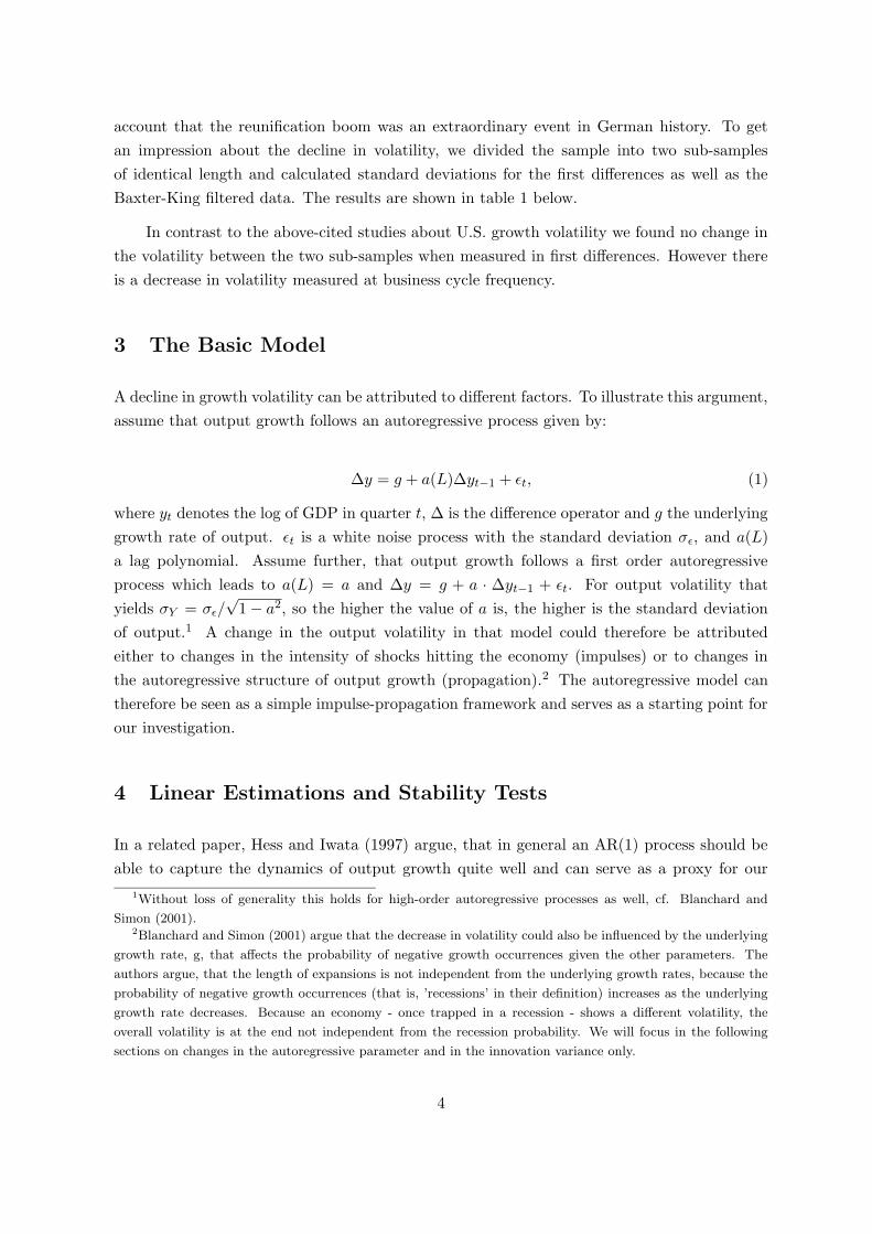
3 The Basic Model

A decline in growth volatility can be attributed to different factors. To illustrate this argument,

assume that output growth follows an autoregressive process given by:

∆y = g + a(L)∆yt−1 + εt, (1)

where yt denotes the log of GDP in quarter t, ∆ is the difference operator and g the underlying

growth rate of output. εt is a white noise process with the standard deviation σε, and a(L)

a lag polynomial. Assume further, that output growth follows a first order autoregressive

process which leads to a(L) = a and ∆y = g + a · ∆yt−1 + εt. For output volatility that

yields σY = σε/√1− a2, so the higher the value of a is, the higher is the standard deviation

of output.1 A change in the output volatility in that model could therefore be attributed

either to changes in the intensity of shocks hitting the economy (impulses) or to changes in

the autoregressive structure of output growth (propagation).2 The autoregressive model can

therefore be seen as a simple impulse-propagation framework and serves as a starting point for

our investigation.

4 Linear Estimations and Stability Tests

In a related paper, Hess and Iwata (1997) argue, that in general an AR(1) process should be

able to capture the dynamics of output growth quite well and can serve as a proxy for our

1Without loss of generality this holds for high-order autoregressive processes as well, cf. Blanchard and

Simon (2001).2Blanchard and Simon (2001) argue that the decrease in volatility could also be influenced by the underlying

growth rate, g, that affects the probability of negative growth occurrences given the other parameters. The

authors argue, that the length of expansions is not independent from the underlying growth rates, because the

probability of negative growth occurrences (that is, ’recessions’ in their definition) increases as the underlying

growth rate decreases. Because an economy - once trapped in a recession - shows a different volatility, the

overall volatility is at the end not independent from the recession probability. We will focus in the following

sections on changes in the autoregressive parameter and in the innovation variance only.

4

impulse-propagation-framework. At least in history, this process performed not worse than

much more complicated non-linear formulations of the output growth process. The appropriate

lag length for the German output growth process was investigated using lag selection tests.

Specifically, the minima of the Akaike and Schwarz criteria up to a lag order of 24, an Ljung-

Box for residual serial correlation, a Langrange multiplier test for residual serial correlation

and a general-to-simple reduction test were estimated. The results - shown in table 2 - indicate

that an AR(4) seems to be appropriate.

∆yt = 0.004(0.001)

− 0.14(0.08)

∆yt−1 + 0.04(0.08)

∆yt−2 + 0.14(0.08)

∆yt−3 + 0.26(0.08)

∆yt−4 + εt, εt ∼ N(0, σ2)

R2 = 0.10, AR(1− 5) = 0.46[0.80], ARCH(1− 4) = 0.78[0.53],

Normality = 5.76[0.05], Hetero = 0.81[0.59],

Hetero−X = 0.69[0.78], RESET = 0.55[0.45]

(2)

According to the reported criteria the equation is well specified with some signs of non-

normality.3 In spite of the fact that some lags are not significant, we decided to use the

AR(4) specification in the next sections. The specification should be flexible enough to al-

low for changes in the dynamics over time which we would like not to restrict prior to the

investigation.

In the next stage of our investigation, we tested for structural stability in the impulse-

propagation-model. We applied CUSUM and CUSUM square tests. That gave no indication

of any instability. More interesting are the results of recursive estimations which are shown

in figure 3. The recursive coefficients suggest that there might a ’change’ in the propagation

structure - the coefficient of the first lag is relatively high in the early seventies but declines

steadily over time.

We tested the hypothesis of a change in the propagation structure also within a trans-

formed version of the AR(4) model where the overall persistence is measured in one single

parameter. The AR(4) model is given by:

∆y = g + ρ1∆yt−1 + ρ2∆yt−2 + ρ3∆yt−3 + ρ4∆yt−4 + εt (3)

The transformed representation is given by:

∆y = g + (ρ1 + ρ2 + ρ3 + ρ4)∆yt−1 − (ρ2 + ρ3 + ρ4)∆2yt−1

− (ρ3 + ρ4)∆2yt−2 − ρ4∆

2yt−3 + εt(4)

3We performed the following tests: serial correlation LM test, ARCH LM test, Jarque-Bera normality test,

White heteroscedasticity tests with and without cross terms, RESET test.

5

∆y = g + ρ∆yt−1 + φ1∆2yt−1 + φ2∆

2yt−2 + φ3∆2yt−3 + εt (5)

In this specification ∆2 stands for for the second differences, i.e. ∆∆ and ρ for the sum

of the AR coefficients. The parameter ρ measures the overall persistence since it covers all

AR-parameters.

This equation is of course identical to the AR(4) model. However, the recursively estimated

ρ - as can be seen in figure 3 - makes clear that the overall persistence declined over time.

There is a growing literature about the detection and dating of structural breaks - espe-

cially if the exact break point is unknown; see Hansen (2001) for an excellent survey. The well-

known Chow test is not helpful under such circumstances because the test is appropriate only

under the assumption of a known break point. Therefore we applied the Andrews-Quandt- and

Andrews-Ploberger-Tests as described in Andrews (1993) and Andrews and Ploberger (1994)

to the AR(4) model and the error correction representation of the AR(4) model.

In short, these tests trim the range of the sample by 15 per cent (suggested value in

Andrews and Ploberger, 1994) from each side and perform Lagrange multiplier tests for each of

the possible break points for the remaining middle range of the sample. The Andrews-Quandt

test uses as the test statistic the maximum of the LM statistics, while the Andrew-Ploberger

test uses an exponentially weighted average. These both have non-standard distributions.

Asymptotic p-values are taken from Hansen (1997).

The results - see tables 3 and 4 - indicate that a structural break can be identified in the

autoregressive structure (more precisely: it is found for the AR(1) coefficient) but not in the

residuals variance. This is in contrast to the results for the U.S. economy, where a break in the

variance of the residuals is found by most methods (McConnell and Perez-Quiros, 2000). The

breakpoint for the AR(1) coefficient is dated around 1976. For the period from 1976 onwards

no further break was detected. The estimation results of the error correction representation

confirm that a break occurred in the AR(1) parameter. However, the recursive coefficients also

suggest that there might be a gradual change in persistence over time.

In a further exercise we used the procedure proposed by Bai and Perron (2003) - to check

if there are more structural breaks.4 The procedure investigates all possible models under the

assumption of a given number of breakpoints and a given minimum distance between the break

points. Then, the ’optimal’ model is chosen according to the (minimum of the) sum of squared

residuals and according to information criteria. Therefore, we had to assume the number of

breakpoints we would allow to occur in the model at maximum and calculated the optimal

break points for each model. We opted for a maximum of four breakpoints with a data range of

about thirty years. The minimum distance between two breakpoints was set equal to 6 years

- as we assume stability over the cycle. For each model, the Bayesian Information Criteria

4We thank Tom Doan of Estima for making the RATS code available to perform the Bai-Perron-Tests.

6

(BIC) was calculated to check, which of the estimated breakpoint models could be seen as the

best one.

The results are presented in table 5. According to the BIC criteria the model with 2

breaks shows the best fit. The breaks occurred in 1977Q2 and 1997Q1. We estimated equation

(5) for the sub-samples 1970Q1 to 1977Q2, 1977Q3 to 1997Q1 and 1997Q2 to 2003Q2. The

point estimates of the coefficient ρ are .48, .27, and .06 respectively. This supports both of our

hypotheses: the hypothesis of a structural break in the mid-seventies as well as the hypothesis

of a gradual shift in persistence. To explore this issue further we used a Markov switching and

state space (time-varying coefficient) models.

5 A Markov-Switching Model

The results up to here point to the possibility, that there might have been a regime shift

in volatility over time. Markov-switching models are appropriate for this kind of problems

(McConnell and Perez-Quiros, 2000).5 In line with the results of the stability tests mentioned

above, the Markov-switching version of equation (5) with a regime-dependent ρ-coefficient was

estimated.6

∆y = g + ρ(st)∆yt−1 + φ1∆2yt−1 + φ2∆

2yt−2 + φ3∆2yt−3 + ut,

ut ∼ N(0, eγ), st ∈ {1, 2}(6)

where St denotes the realizations of the underlying unobservable discrete Markov chain. Two

regimes are allowed. The transition probabilities were estimated using a logit transformation:

pjj =eϕj

1+eϕj . The estimation results and a graph of the corresponding smoothed probabilities

can be found in table 6 and figure 4.

The results indicate, that there were two major periods, where the persistence of the data

generating process was high: the early 70s and the reunification boom in the early 90s. Also

the recession period of the early 80s as well after the millennium sees an increase in persistence

which is however much less pronounced than the other two episodes. Output volatility is high

either in very pronounced booms or recessions and low in other periods. Since we had only

one of this ’extraordinary’ episodes in the second half of the sample it is not astonishing that

the volatility at the typical business cycle frequency is lower.

5A very detailed discussion of Markov-switching models and the corresponding estimation and state extrac-

tion procedures is available in Krolzig (1997).6This is an MSA-model. We implicitly assume that only ρ1 from the specification in equation (4) is changing

in dependence from the regime.

7

6 A State Space Model

Furthermore a state space model (Hamilton ,1994) with a time-varying coefficient was esti-

mated. The system consists of two equations: the space equation, which is the observable part

of the model and the state equation, which gives some structure to the unobservable part of

the model. The space equation is given by the transformed autoregressive growth model. The

coefficient ρ is modeled as a random walk and defined by the state equation. The state space

model (state space model I thereafter) is given by the following system:

∆y = g + ρt∆yt−1 + φ1∆2yt−1 + φ2∆

2yt−2 + φ3∆2yt−3 + ut

ut ∼ N(0, eλ)(7)

ρt = ρt−1 + vt, vt ∼ N(0, eψ) (8)

where the disturbance vectors ut, vt are assumed to be serially independent. The variance of

the space and the state equation are estimated as exponential functions to restrict the variance

to non-negative numbers.

The evolution of the estimated coefficient (Kalman filter result) in model I is plotted in

figure 5. The estimation results of state space model I are summarized in Table 8.

As can be seen from the figure there is a decline in persistence over time until the mid-80s.

The value of the respective coefficient is about .7 in the early 1970s, it declines in the course

of the 80s and is about .25 at the beginning of the 90s. There is an temporary increase of the

coefficient during the reunification boom. This is all in line with the results from the recursive

estimates and the Markov-switching model.

7 Spectral Analysis

A helpful tool to detect the sources of the change in persistence is furthermore given by

spectral analysis (Wolters and Konig ,1972). Analytically, the correllogram of a stationary

time series can be transformed into the frequency domain using Fourier transformation. The

spectra functions indicate the contribution of every frequency component to overall variance.

By decomposing the overall variance into frequency portions it can be informally checked if

long-run movement, business cycle fluctuations or seasonal dynamics are the driving forces of

a time series’ dynamics. Analysing the spectra functions is therefore a suitable instrument to

find out, at which frequency the changes took place. This informal test refers to an idea of

Ahmed, Levin and Wilson (2002) who used the spectra functions to investigate if the change

8

in U.S. growth volatility is due to ’good policy’, ’good practices’ or ’good luck’. They have the

following hypotheses:

Characterizing the post-1984 shift in the spectrum of GDP growth is useful

because each explanation can be associated with a specific pattern for the shift:

(1) improved monetary policy would be expected to shift the spectrum primarily at

business-cycle frequencies; (2) improved inventory management and other relevant

changes in business practices would tend to be manifested at relatively high frequen-

cies; and (3) reduced innovation variance would generate a proportional decline in

the spectrum at all frequencies. (Ahmed, Levin and Wilson ,2002, p. 1f.)

In figure 6 we plot empirical spectra functions for different periods including some grid lines

which define a business cycle frequency from 1 12 to 8 years. According to our test results we

splitted the sample in 1976. The empirical spectra functions are given in the first row of the

graph. Critics might argue that a sample of 6 years is too short for any reasonable statement

about the spectra function. Therefore we splitted the sample in the middle the overall sample

and repeated the exercise -see the figures in the second row. The results are fairly robust in

that sense that the spectra functions indicate that there must have been a distinctive decline

of variance at the business cycle frequency.7

8 A State Space Model with Real Interest Rate Volatility

The results from the spectral analysis indicate that there was a decline in the low-frequency

contribution to volatility. According to Ahmed, Levin and Wilson (2002) this could be due to a

better managed monetary policy. For a deeper investigation of this hypothesis that the ’change

in monetary policy’ could be responsible for the change in volatility again a state space model

was used (state space model II thereafter. In contrast to state space model I here an exogenous

variable is allowed to influence the time-varying coefficient ρt. Specifically as a proxy of the

monetary policy stance we estimated a GARCH(1,1) model for the real short-term interest rate

and used the result as a measure for the volatility of monetary policy (Xt for the exogenous

variable).8 From a preliminary visual inspection it is obvious that the decline in monetary

volatility seems to coincide with the decreasing persistence of output growth, measured by the

recursively estimated ρ. In figure 7 we jointly present the recursively estimated ρ from the

transformed autoregressive growth model (see figure 3) and the GARCH(1,1) results for the

short-term real interest rate.

7To estimate the spectra functions we used the source SPECTRUM.SRC in RATS 5.04 with standard settings.

The window size as well as the smoothing parameters were set automatically according to the number of

observations.8The estimation results for the GARCH(1,1) model are available from the authors on request.

9

We now used these GARCH(1,1) results as an exogenous explanatory variable for the

evolution of the persistence parameter ρt within a state space model.

The model is therefore specified as follows:

∆y = g + ρt∆yt−1 + φ1∆2yt−1 + φ2∆

2yt−2 + φ3∆2yt−3 + ut

ut ∼ N(0, eλ)(9)

ρt = δXt + vt, vt ∼ N(0, eψ) (10)

We present the results in figure 8 (Kalman filter results) and table 8. All coefficients are

significant and the short-term real interest rate’s volatility can explain the evolution of the

persistence coefficient quite well. The result points into the direction of the hypothesis of

Ahmed, Levin and Wilson (2002), namely that the decline in persistence might be due to a

change in the conduct (or the reaction to) monetary policy. This topic will be discussed in the

next sections.

9 A Theoretical Model

Up to here the result points to a steady decline of the persistence parameter ρ - which has

a strong correlation with measures of monetary policy. The estimations were performed in a

reduced form - so nothing can be said about the underlying structural changes. There are two

results - the spectral analysis as well as the second state space model including the short-term

real interest volatility - which indicate that a change in monetary policy might play a role.

There are two ways to investigate that issue further: either to estimate a structural model

and test within the structural equations for changes or to calibrate a theoretical model and

simulate the consequences of changes in the structural parameters. We opted for the second

way. Because of the difficulties involved in that the first option goes beyond the scope of this

paper and will be investigated in a separate paper.

There is surely nothing new about the fact that there was a break in the conduct of

monetary policy at the beginning of the 1980s. This is at least true for the United States,

where Fed chairman Paul Volcker started a radical disinflation in 1979. The fact that there is

a break in the conduct of monetary policy in other industrialised countries is, however, also

confirmed by studies that estimated Taylor rules for other G7 countries (Clarida, Gali and

Gertler, 1998). These studies point out that the monetary policy became more hawkish in

that sense that central banks show more aggressive reaction toward fighting against inflation

than during the heyday of Keynesian demand policy in the 1960s and the stagflationary 1970s.

But how can the reduced volatility and the detected change in propagation be explained by

10

a change in the conduct of monetary policy? To analyse these aspects, the ’New Keynesian’

(NK) model became the new workhorse in the last decade.9 The NK model starts from a

general equilibrium model with Walrasian equilibrium. The business cycle movement of such

a model could be expressed in percentage deviations from the long-run equilibrium values.

The business cycle component of output, yt, is determined by:

yt = b0 + b1 (rt) + yt+1 + vt (11)

where the parameter b1 < 0. Actual output is a (negative) function of the real interest rate

rt. This equation is called the inter-temporal IS equation and can be seen as being at the core

of most ’modern’ macroeconomic models. Output is furthermore affected by the (expected)

future income as consumers intend to ’smooth’ consumption over time. The term vt stands for

unforeseeable demand shocks such as unexpected changes in government consumption. In a lot

of models the parameter b1 stands for the elasticity of inter-temporal consumption (Boivin and

Giannoni, 2002). As it is usually done in NK models we can assume that the central bank is

able to set the real short-term interest rate. Iterating equation the inter-temporal IS equation

forward, we obtain:

yt = vt + b1rLt (12)

where

rLt = Et

∞∑

j=0

rt+j

(13)

stands for the long-run real interest rate.10 The last equation states that it is the long-run

interest rate which matters for the IS curve but the short-term real interest rate matters to

that extent as it influences the long-run interest rate. For the monetary policy rule let’s assume

for a moment a simplified version of the Taylor rule which is given by:

rt = φyt + et (14)

where φ > 0 .

Since yt stands for the ’output gap’ this equation simply states that the monetary authority

sets the interest rate according to the deviation of the actual output from its long-run path.

This does not mean, that inflation does not matter. The gap could be seen as an indicator of

the (future) inflationary pressure.11 Combining this yields:

9The section draws heavily on Boivin and Giannoni (2002). For this moment we neglect the supply side of

the NK model, the ’new’ Phillips curve, and focus on the IS curve and the monetary policy rule.10Since all values are deviations from long-run equilibrium, the sum should converge.11This does also not mean that supply shocks do not matter. They are reflected in the potential output

because they matter for the long-run (equilibrium) solution in these models.

11

yt =vt + b1et1− b1φ

(15)

Since yt is the ’gap’ (or the business cycle component of output), a reduction in σ , reflecting

a change in the elasticity of inter-temporal consumption or an increase in φ, reflecting a more

aggressive monetary policy, could change the volatility of output around the long-run path.

Our analysis so far could be interpreted in the NK framework as probably being associated

with a higher φ, stemming from a change in the importance of the reaction from potential

output of the Bundesbank since the middle/end of the 70s. For the investigation of that topic

a fully specified structural model has to be estimated to detect, where the changes in the

propagation stem from.

In the following we used a model proposed by McCallum (2001) to analyze the effects of

monetary policy on output. Here, we want to explore the effects of changes in ’deep’ structural

parameters on output volatility. We tried to keep the model as simple as possible. The model

is given by the following equations:12

yt = b0 + b1 (Rt − Et∆Pt+1) + Etyt+1 + vt (16)

∆pt = βEt∆pt+1 + αyt + ut (17)

Rt = µ0 + (1− µ3) (µ1∆pt + µ2Et−1yt) + µ3Rt−1 + et (18)

Equation (16) states the intertemporal IS curve. Actual output yt depends positively on future

expected income Etyt+1 and negatively on the (short-term) real interest rate Rt −Et∆Pt+1.13

Equation (17) defines a forward-looking Phillips curve with Calvo price setting. Actual inflation

depends on expected inflation Et∆pt+1 and the output gap yt. Equation (18) gives a standard

Taylor rule where the monetary authorities react on inflation and the output gap. Furthermore

we assume interest rate smoothing, controlled by µ3.

These equations are accompanied by the definition equation of the output gap and some

laws of motion for the stochastic terms.

12We used the MATLAB files available from Bennett McCallums homepage and some modified versions of

these files written by Jan Gottschalk. We are greatful to Jan Gottschalk who kindly offered help to implement

the files and handle the output.13It is assumed that the long-term real interest rate depends on the short-term real interest rate.

12

yt = yt − ytvt = 0 · vt−1 + νt

et = 0 · et−1 + εt

ut = 0 · ut−1 + ψt

yt = .95 · yt−1 + ηt

(19)

The model was solved using the procedure proposed by McCallum (1998) and Klein (2000).

First we solved the model under the following standard parameter settings as proposed by

McCallum (2001): b0 = µ0 = 0, b1 = −.4, β = .99, α = .03, µ1 = .54 , µ2 = .5, µ3 = .8. The

impulse response functions to an IS shock (νt), an cost-push shock (ψt) as well as a policy

rule shock (εt) are plotted in figures 9 and 10. As can be seen from the IRFs, the model

captures a lot of features relevant for macro dynamics. Note that the reaction functions of

this model do not create very much persistence. McCallum (2001) used habit formation and

a partly backward-looking Phillips curve (so-called Fuhrer-Moore specification), to get more

persistence into the model. To keep the factors of influence as limited as we can, we opted for

the simplest model we could find.

In the next step, we assumed values for the variances of the different types of shocks. We

again opted for the settings as proposed by McCallum (2001). The variances were set as follows:

the variance of νt was set equal to .03, the variance of εt was set equal to .002, the variance of

ψt was set equal to .0017, the variance of η was set equal to .007. We did stochastic simulations

with the model (10000 repetitions) and saved the autocorrelation functions. Specifically, we

were interested in the change of the autocorrelation function of the variable y - the output gap.

We focus on the output gap because empirically we found that changes at the business cycle

frequency seem to be the driving force behind the change in persistence.

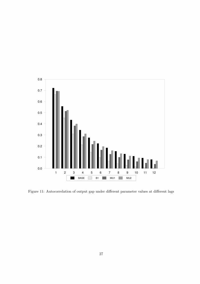
In the next step, we slightly changed some parameters of the model to see if and how the

persistence changes. Specifically, we doubled the value of b1 to -.8. In two other simulations,

we doubled the values of µ1 and µ2 to 1. We always changed only one parameter and report the

autocorrelation functions together with those from the baseline at different lags. The results

are shown in figure 11. As can be seen from that figure, changes in the structural parameters

change the implied persistence of the economy. A change in the elasticity of inter-temporal

consumption as well as policy reaction parameters can influence the volatility of output growth.

13

10 Discussion

In our paper we investigated the decline in output volatility in Germany. The results from the

structural break tests, the Markov-switching model as well as the state space models show that

the decline is more of a gradual nature than a sudden break. Results from spectral analysis

estimations as well as a state space model including short-term real interest rate volatility

indicate, that monetary policy might have played a role.

However, in contrast to the US results, it is the transmission mechanism of shocks, not

the variance of shocks itself which changed. The state space model II indicates that variance

of shocks might interplay with the changes in the structure of the economy.

To investigate the possible sources of structural changes which might be responsible for

the observed pattern, we used a calibrated DSGE model. We would interpret the results of our

stochastic simulations in the following way: changes in policy reaction parameters - as reported

for most industrialised countries around the late 70s - should have had an influence on output

volatility. Probably these changes also influenced the interest rate sensitivity of the IS curve.

This could be a typical case for a Lucas critique phenomenon because it is very plausible

that a change toward another policy regime would influence the behavior of households. These

changes, however, must be quite pronounced, to generate a significant fall in volatility - at least

in our simple model. More complicated models with habit formation and/or more persistence

in the Phillips curve could generate different result.

In a further investigation we will focus on the estimation of a fully-fledged structural model

based on empirical data and investigate the changes in the propagation within this framework.

This research is however beyond the scope of this paper.

14

References

Ahmed, S., Levin, A., Wilson, B. A. (2002): Recent U.S. Macroeconomic Stability: Good

Policies, Good Practices, or Good Luck? July 2002. (= Federal Reserve Board IFD Paper No.

730).

Andrews, D. W. K. (1993), Tests for Parameter Instability and Structural Change with Un-

known Change Point. In: Econometrica, Vol. 61, pp. 821-856.

Andrews, D. W. K. , Ploberger, Werner (1994), Optimal Tests When a Nuisance Parameter is

Present Only Under the Alternative. In: Econometrica, Vol. 62, pp 1383-1414.

Bai J., Perron, P. (2003), Computation and Analysis of Multiple Structural Change Models,

In: Journal of Applied Econometrics, pp 1-22.

Barrell, R.; Gottschalk, S. (2004): The volatility of the output gap in the G7. National

Institute Economic Review, No. 188, April 2004, pp. 100-107.

Blanchard, O.; Simon, J. (2001): The Long and Large Decline in U.S. Output Volatility, In:

Brookings Papers on Economic Activity, 2001:1, pp. 135-173.

Boivon, J.; Giannoni, M. (2002): Assessing changes in the monetary transmission mechanism:

A VAR approach. In: FRBNY Economic Review, May 2002, pp. 97-111.

Buch, C.; Dopke, J.; Pierdzioch, C. (2002): Business Cycle Volatility in Germany. Kiel (=

Kiel Working Paper. 1129).

Burns, A. (1960): Progress towards economic stability. In: American Economic Review, Vol.

50, No. 1, pp. 2-19.

Clarida, R.; Gali, J.; Gertler, M. (1998): Monetary policy rules in practice: Some international

evidence. In: European Economic Review, Vol 42, pp. 1033-1067.

Hamilton, J. (1994): Time Series Analysis. Princeton: Princeton University Press.

Hansen, B. (1991), Parameter Instability in Linear Models, In: Journal of Policy Modeling, 14

(4), pp. 517-533.

Hansen, B. (2001), The New Econometrics of Structural Change: Dating Changes in U.S.

Labor Productivity. In: Journal of Economic Perspectives, Vol. 15, pp. 117-128.

Hansen, B. (1997), Approximate Asymptotic P-Values for Structural Change Tests. In: Jour-

nal of Business and Economic Statistics, pp 60-67.

Klein, P. (2000), Using the generalized Schur form to solve a multivariate linear rational

expectations model, In: Journal of Economic Dynamics and Control, Vol. 24, No. 10, pp.

1405-1423.

Konig, H.; Wolters, J. (1972), Einfuhrung in die Spektralanalyse okonomischer Zeitreihen.

Meisenheim am Glan.

15

Krolzig, H.-M. (1997): Markov-Switching Vector Autoregressions: Modelling, Statistical In-

ference and Application to Business Cycle Analysis. Lecture Notes in Economics and Mathe-

matical Systems No. 454. Berlin.

McCallum, B. (1998): Solutions to linear rational expectations models: a compact exposition,

In: Economics Letters Vol. 61, No. 2, pp. 143-147.

McCallum, B. (2001), Should Monetary Policy Respond Strongly to Output Gaps. In: The

American Economic Review, Vol. 91, No. 2, pp. 258-262

McConnell, M.; Perez-Quiros, G. (2000): Output Fluctuations in the United States: What

Has Changed Since the Early 1980s? Paper presented at the Conference ’Structural

Change and Monetary Policy’, Federal Reserve Bank of San Francisco, March 2000, URL:

http://www.frbsf.org/economics/conferences/000303/papers/output.pdf

Nyblom, J. (1989), Testing for the Constancy of Parameters Over Time. In: Journal of the

American Statistical Association, Vol. 84, pp. 223-230.

Stock, J.; Watson, M.(2002): Has the Business Cycle Changed and Why?, Paper pre-

sented at the NBER 17th Annual Conference on Macroeconomics, April 2002, URL:

http://www.nber.org/ confer/2002/macros02/stock.pdf

Stock, J.; Watson, M. (2003a): Has the Business Cycle Changed? Evidence and Explanations,

forthcoming in Monetary Policy and Uncertainty, Federal Reserve Bank of Kansas City, 2003.

Stock, J.; Watson, M. (2003b): Understanding Changes in International Business Cycle Dy-

namics. Cambridge, Mass. July 2003 (NBER Working Paper. 9859).

Terasvirta, T. (1998): Chapter 15, Modeling Economic Relationships with STR, In: Aman

Ullah, David E. A. Giles (eds.): Handbook of Applied Economic Statistics, 1998 (Marcel

Dekker, Inc).

Zarnowitz, V. (1998): Has the business cycle been abolished?, Cambridge, Mass. (= NBER

Working Paper. 6367).

16

Appendix

Differences of logs of German GDPchained data

1970 1972 1974 1976 1978 1980 1982 1984 1986 1988 1990 1992 1994 1996 1998 2000 2002-3

-2

-1

0

1

2

3

4

Business cycle component of German GDPBaxter-King filter (6 to 32 quarters)

1970 1972 1974 1976 1978 1980 1982 1984 1986 1988 1990 1992 1994 1996 1998 2000 2002-3

-2

-1

0

1

2

3

Figure 1: Data graphs

Transformation/sample S.D.

First differences/ 1970 - 1986 4.29

First differences/ 1987 - 2003 4.38

Baxter-King filtered/ 1970 - 1986 1.32

Baxter-King filtered/ 1987 - 2003 1.13

Table 1: Standard deviations

17

Criterion Suggested Lag Length

AIC 4

BIC 0

Ljung-Box-Test 4

LM Test 0

General to Simple 4

Table 2: Results of lag length tests

Variable Break Date Andrews-Quandt p-value Andrews-Ploberger p-value

Constant 1991:02 3.26 0.50 0.37 0.55

∆yt−1 1976:02 7.61 0.08 1.29 0.13

∆yt−2 1991:02 3.90 0.39 0.41 0.51

∆yt−3 1991:02 1.40 0.93 0.11 1.00

∆yt−4 1985:02 2.60 0.64 0.41 0.58

All Coeff. 1991:02 10.85 0.44 2.58 0.61

Variance 1993:01 2.01 0.78 0.23 0.73

Table 3: Results of Andrews-Quandt-Ploberger-Test: AR(4) model [equation (3)]

Variable Break Date Andrews-Quandt p-value Andrews-Ploberger p-value

Constant 1991:02 3.26 0.50 0.37 0.55

∆yt−1 1976:02 7.61 0.08 1.29 0.13

∆2yt−1 1976:01 3.13 0.52 0.35 0.58

∆2yt−2 1976:04 1.04 0.99 0.16 0.87

∆2yt−3 1985:02 3.98 0.37 0.44 0.49

All Coeff. 1991:02 10.85 0.44 2.58 0.61

Variance 1993:01 2.01 0.78 0.23 0.73

Table 4: Results of Andrews-Quandt-Ploberger-Test: AR(4) model, transformed representa-

tion [equation (5)]

Model (breaks) Model (1) Model (2) Model (3) Model (4)

Sum of Squared Residuals 129.7 100.4 92.1 85.6

BIC 5.04 4.97 5.07 5.18

Breakpoint(s) 1977Q2 1977Q2 1977Q2 1977Q2

1997Q1 1993Q1 1987Q1

1999Q1 1993Q1

1999Q1

Table 5: Results of Bai-Perron-Test: AR(4) model [equation (3)]

18

Constant

1974 1976 1978 1980 1982 1984 1986 1988 1990 1992 1994 1996 1998 2000 2002-1.0

-0.5

0.0

0.5

1.0

1.5

2.0

Coefficient d(log(y(-1))

1974 1976 1978 1980 1982 1984 1986 1988 1990 1992 1994 1996 1998 2000 2002-0.32

-0.16

0.00

0.16

0.32

0.48

0.64

0.80

Coefficient d(log(y(-2))

1974 1976 1978 1980 1982 1984 1986 1988 1990 1992 1994 1996 1998 2000 2002-0.4

-0.3

-0.2

-0.1

-0.0

0.1

0.2

0.3

0.4

0.5

Coefficient d(log(y(-3))

1974 1976 1978 1980 1982 1984 1986 1988 1990 1992 1994 1996 1998 2000 2002-0.3

-0.2

-0.1

-0.0

0.1

0.2

0.3

0.4

0.5

0.6

Coefficient d(log(y(-4))

1974 1976 1978 1980 1982 1984 1986 1988 1990 1992 1994 1996 1998 2000 2002-0.1

0.0

0.1

0.2

0.3

0.4

0.5

0.6

0.7

Sequentially estimated S.D.

1974 1976 1978 1980 1982 1984 1986 1988 1990 1992 1994 1996 1998 2000 20020.75

0.80

0.85

0.90

0.95

1.00

1.05

1.10

Figure 2: Recursive estimation results: AR(4) model [equation (3)]

Coefficient Value Std. Error

g 0.004 0.001

ρ(st = 1) 0.61 0.21

ρ(st = 2) -0.005 0.21

φ1 -0.36 0.16

φ2 -0.39 0.12

φ3 -0.28 0.08

γ -9.42 0.14

p11 0.89 –

p22 0.94 –

logL(Θ) 417.16 –

AIC -6.33 –

Table 6: Estimation results of the Markov switching model [equation (6)]

19

Constant

1974 1976 1978 1980 1982 1984 1986 1988 1990 1992 1994 1996 1998 2000 2002-1.0

-0.5

0.0

0.5

1.0

1.5

2.0

Rho

1974 1976 1978 1980 1982 1984 1986 1988 1990 1992 1994 1996 1998 2000 2002-1.0

-0.5

0.0

0.5

1.0

1.5

2.0

Sequentially estimated S.D.

1974 1976 1978 1980 1982 1984 1986 1988 1990 1992 1994 1996 1998 2000 20020.75

0.80

0.85

0.90

0.95

1.00

1.05

1.10

Figure 3: Recursive estimation results: AR(4) model, transformed representation [equation

(5)]

20

DLGDP_NEW MS_SMOOTH

1972 1975 1978 1981 1984 1987 1990 1993 1996 1999 2002-3.2

-2.4

-1.6

-0.8

-0.0

0.8

1.6

2.4

3.2

0.00

0.25

0.50

0.75

1.00

Figure 4: Markov-Switching Results: GDP Growth and High Persistence Regime Probability

[equation (6)]

1973 1976 1979 1982 1985 1988 1991 1994 1997 2000 20030.00

0.25

0.50

0.75

1.00

Figure 5: State space model I: filtered estimate [equation (7)]

21

Coefficient Std. Error z-Statistic Prob.

g 1.47 0.58 2.52 0.012

φ1 -0.43 0.15 -2.81 0.005

φ2 -0.40 0.13 -3.05 0.002

φ3 -0.27 0.08 -3.22 0.001

λ 2.68 0.11 23.42 0.000

ψ -7.47 1.99 -3.76 0.000

Final State Root MSE z-Statistic Prob.

ρt 0.25 0.16 1.59 0.112

Log likelihood -367.60 Akaike info criterion 5.79

Parameters 6 Schwarz criterion 5.93

Diffuse priors 1 Hannan-Quinn criter. 5.85

Table 7: Estimation results: state space model I [equation (7)]

Coefficient Std. Error z-Statistic Prob.

g 1.55 0.43 3.59 0.000

φ1 -0.37 0.10 -3.58 0.000

φ2 -0.36 0.11 -3.27 0.001

φ3 -0.25 0.08 -3.21 0.001

λ 2.57 0.16 16.29 0.000

δ 0.30 0.12 2.62 0.009

ψ -2.84 1.28 -2.22 0.026

Final State Root MSE z-Statistic Prob.

ρt 0.10 0.24 0.42 0.67

Log likelihood -357.84 Akaike info criterion 5.75

Parameters 7 Schwarz criterion 5.90

Diffuse priors 1 Hannan-Quinn criter. 5.81

Table 8: Estimation results: state space model II [equation (9)]

22

Fractions of pi0.00 0.25 0.50 0.75 1.00

0.01

0.10

1.00

(a) Spectrum: sample 1970 to 1976

Fractions of pi0.00 0.25 0.50 0.75 1.00

0.01

0.10

1.00

(b) Spectrum: sample 1976 to 2003

Fractions of pi0.00 0.25 0.50 0.75 1.00

0.01

0.10

1.00

(c) Spectrum: sample 1970 to 1985

Fractions of pi0.00 0.25 0.50 0.75 1.00

0.01

0.10

1.00

(d) Spectrum: sample 1986 to 2003

Figure 6: Spectral density estimates: different sub-samples

23

RHO GARCH

1974 1977 1980 1983 1986 1989 1992 1995 1998 20010.2

0.4

0.6

0.8

1.0

1.2

1.4

0.0

0.5

1.0

1.5

2.0

2.5

3.0

3.5

Figure 7: Recursively estimated ρ coefficient [equation (3)] and GARCH(1,1) results

1973 1976 1979 1982 1985 1988 1991 1994 1997 2000 2003-0.5

0.0

0.5

1.0

1.5

2.0

Figure 8: State space model II: filtered estimates [equation (9)]

24

0 5 10 15 20−0.5

0

0.5

1

1.5y response

0 5 10 15 20−0.05

0

0.05

0.1dp response

0 5 10 15 20−0.5

0

0.5

1

1.5ygap response

0 5 10 15 20−0.02

−0.01

0

0.01

0.02R response

RESPONSES TO IS SHOCK

0 5 10 15 20−2

−1.5

−1

−0.5

0

0.5

1

1.5y response

0 5 10 15 20

0

0.5

1

1.5

2dp response

0 5 10 15 20−2

−1.5

−1

−0.5

0

0.5

1

1.5ygap response

0 5 10 15 20−0.2

0

0.2

0.4

0.6

0.8

1R response

RESPONSES TO COST−PUSH SHOCK

Figure 9: Impulse responses: theoretical model

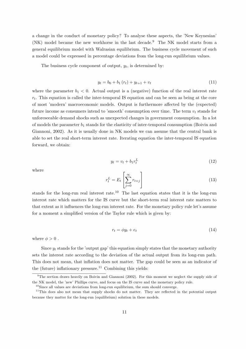
25

0 5 10 15 20−2.5

−2

−1.5

−1

−0.5

0

0.5y response

0 5 10 15 20

−0.5

−0.4

−0.3

−0.2

−0.1

0

0.1

dp response

0 5 10 15 20−2.5

−2

−1.5

−1

−0.5

0

0.5ygap response

0 5 10 15 20−0.2

0

0.2

0.4

0.6

0.8

1

1.2R response

RESPONSES TO MONETARY POLICY SHOCK

Figure 10: Impulse responses: theoretical model contd.

26

BASE B1 MU1 MU2

1 2 3 4 5 6 7 8 9 10 11 120.0

0.1

0.2

0.3

0.4

0.5

0.6

0.7

0.8

Figure 11: Autocorrelation of output gap under different parameter values at different lags

27