The Differential System Method for the Identification of Transmissivity and Storativity

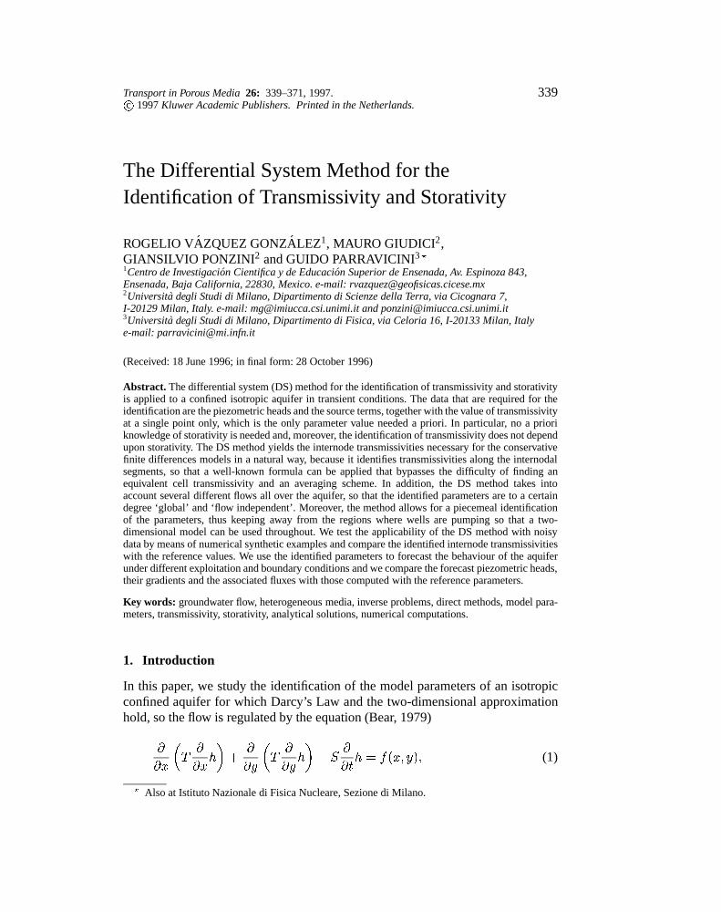
Transport in Porous Media 26: 339–371, 1997. 339c 1997 Kluwer Academic Publishers. Printed in the Netherlands.

The Differential System Method for theIdentification of Transmissivity and Storativity

ROGELIO VAZQUEZ GONZALEZ1, MAURO GIUDICI2,GIANSILVIO PONZINI2 and GUIDO PARRAVICINI3 ?1Centro de Investigacion Cientifica y de Educacion Superior de Ensenada, Av. Espinoza 843,Ensenada, Baja California, 22830, Mexico. e-mail: [email protected] degli Studi di Milano, Dipartimento di Scienze della Terra, via Cicognara 7,I-20129 Milan, Italy. e-mail: [email protected] and [email protected] degli Studi di Milano, Dipartimento di Fisica, via Celoria 16, I-20133 Milan, Italye-mail: [email protected]

(Received: 18 June 1996; in final form: 28 October 1996)

Abstract. The differential system (DS) method for the identification of transmissivity and storativityis applied to a confined isotropic aquifer in transient conditions. The data that are required for theidentification are the piezometric heads and the source terms, together with the value of transmissivityat a single point only, which is the only parameter value needed a priori. In particular, no a prioriknowledge of storativity is needed and, moreover, the identification of transmissivity does not dependupon storativity. The DS method yields the internode transmissivities necessary for the conservativefinite differences models in a natural way, because it identifies transmissivities along the internodalsegments, so that a well-known formula can be applied that bypasses the difficulty of finding anequivalent cell transmissivity and an averaging scheme. In addition, the DS method takes intoaccount several different flows all over the aquifer, so that the identified parameters are to a certaindegree ‘global’ and ‘flow independent’. Moreover, the method allows for a piecemeal identificationof the parameters, thus keeping away from the regions where wells are pumping so that a two-dimensional model can be used throughout. We test the applicability of the DS method with noisydata by means of numerical synthetic examples and compare the identified internode transmissivitieswith the reference values. We use the identified parameters to forecast the behaviour of the aquiferunder different exploitation and boundary conditions and we compare the forecast piezometric heads,their gradients and the associated fluxes with those computed with the reference parameters.

Key words: groundwater flow, heterogeneous media, inverse problems, direct methods, model para-meters, transmissivity, storativity, analytical solutions, numerical computations.

1. Introduction

In this paper, we study the identification of the model parameters of an isotropicconfined aquifer for which Darcy’s Law and the two-dimensional approximationhold, so the flow is regulated by the equation (Bear, 1979)

@

@x

�T@

@xh

�+

@

@y

�T@

@yh

�� S

@

@th = f(x; y); (1)

? Also at Istituto Nazionale di Fisica Nucleare, Sezione di Milano.

PREPROOF *INTERPRINT* J.V.: PIPS Nr.: 125614 MATHKAPtipm1237.tex; 14/05/1997; 7:29; v.6; p.1

340 ROGELIO VAZQUEZ GONZALEZ ET AL.

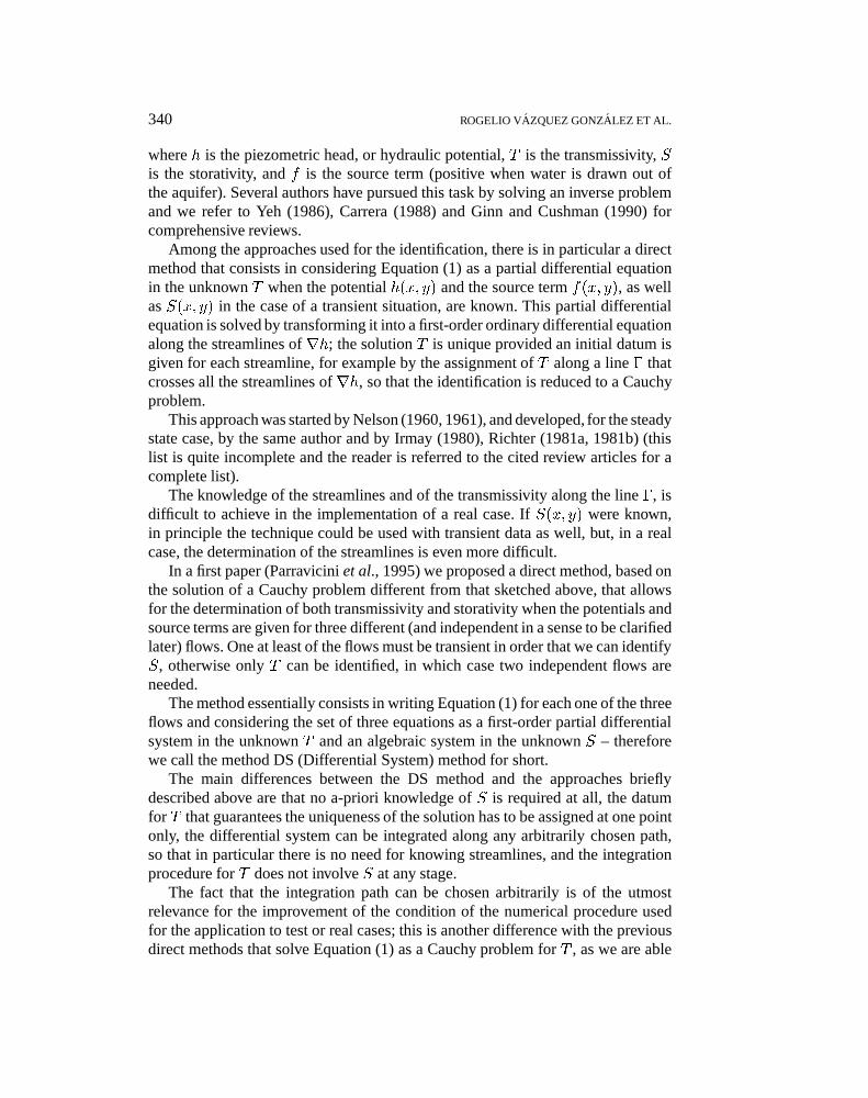
where h is the piezometric head, or hydraulic potential, T is the transmissivity, Sis the storativity, and f is the source term (positive when water is drawn out ofthe aquifer). Several authors have pursued this task by solving an inverse problemand we refer to Yeh (1986), Carrera (1988) and Ginn and Cushman (1990) forcomprehensive reviews.

Among the approaches used for the identification, there is in particular a directmethod that consists in considering Equation (1) as a partial differential equationin the unknown T when the potential h(x; y) and the source term f(x; y), as wellas S(x; y) in the case of a transient situation, are known. This partial differentialequation is solved by transforming it into a first-order ordinary differential equationalong the streamlines of rh; the solution T is unique provided an initial datum isgiven for each streamline, for example by the assignment of T along a line � thatcrosses all the streamlines of rh, so that the identification is reduced to a Cauchyproblem.

This approach was started by Nelson (1960, 1961), and developed, for the steadystate case, by the same author and by Irmay (1980), Richter (1981a, 1981b) (thislist is quite incomplete and the reader is referred to the cited review articles for acomplete list).

The knowledge of the streamlines and of the transmissivity along the line �, isdifficult to achieve in the implementation of a real case. If S(x; y) were known,in principle the technique could be used with transient data as well, but, in a realcase, the determination of the streamlines is even more difficult.

In a first paper (Parravicini et al., 1995) we proposed a direct method, based onthe solution of a Cauchy problem different from that sketched above, that allowsfor the determination of both transmissivity and storativity when the potentials andsource terms are given for three different (and independent in a sense to be clarifiedlater) flows. One at least of the flows must be transient in order that we can identifyS, otherwise only T can be identified, in which case two independent flows areneeded.

The method essentially consists in writing Equation (1) for each one of the threeflows and considering the set of three equations as a first-order partial differentialsystem in the unknown T and an algebraic system in the unknown S – thereforewe call the method DS (Differential System) method for short.

The main differences between the DS method and the approaches brieflydescribed above are that no a-priori knowledge of S is required at all, the datumfor T that guarantees the uniqueness of the solution has to be assigned at one pointonly, the differential system can be integrated along any arbitrarily chosen path,so that in particular there is no need for knowing streamlines, and the integrationprocedure for T does not involve S at any stage.

The fact that the integration path can be chosen arbitrarily is of the utmostrelevance for the improvement of the condition of the numerical procedure usedfor the application to test or real cases; this is another difference with the previousdirect methods that solve Equation (1) as a Cauchy problem for T , as we are able

tipm1237.tex; 14/05/1997; 7:29; v.6; p.2

IDENTIFICATION OF TRANSMISSIVITY AND STORATIVITY 341

to choose the integration path that minimizes the error, and we can determine thepoints where the solution might not be reliable.

Another important feature apparent in the numerical implementation of the DSmethod is that it gives the approximate value of transmissivity T (s) along thesegments that join neighbouring nodes. We profit from this fact in order to use awell known formula for the computation of internode transmissivities.

The cited article was concerned with the solution of the inverse problem by theDS method in the continuous case, and included an example of computation of thenodal values of T with steady-state data. In a second paper (Giudici et al., 1995)we discussed the theory for the numerical evaluation of the internode transmissiv-ities from steady-state data, together with considerations on the stability and thecondition of the problem, and applied it to some test cases for which exactly twosets of steady-state data are given.

In this paper we discuss the theory for the numerical evaluation of the internodetransmissivities and the node storativities, given any number p of sets of data,p > 3, of which one at least is transient, and apply it to test cases with noisydata. A feature of the method that is apparent in this paper, is that the evaluation oftransmissivity is performed in the same way whether or not the data are steady-statedata, a condition which is not always easy to assess.

Also, we exhibit an example in which we generate the independent data nec-essary for the method by switching on arrays of wells, and then apply the methodin a region away from the pumping wells. The fact that, if we wish so, we maygenerate independent data and identify the parameters in a region where no wellsare working is helpful whenever the two-dimensional model (1) close to pumpingwells is not adequate (Bear, 1979, p. 28), so that the identification based upon itwould be unreliable in that neighborhood.

2. The Mathematical Setting of the Problem

We give a short account of the method with some changes made in order toaccomodate for the use of more than three sets of data, as were used in Parraviciniet al. (1995). The formalism used here shows explicitly that the identification of Tis independent from S; the identification of S in turn depends upon T but does notdepend upon its derivatives.

Consider Equation (1) and suppose that we know the source term f(x; tr), thepotential h(x; tr) and its time derivative @h(x; tr)=@t as functions of space, withposition denoted with the vector x, at p different times tr; r = 1; 2; : : : ; p. A setof data is given by these functions, that is to say the potential, its time derivativeand the source term, considered at some assigned time, so that we have assumedto know p sets of data. Equation (1), considered at each time tr, yields the set ofequations

tipm1237.tex; 14/05/1997; 7:29; v.6; p.3


rT (x) � rh(x; tr) + T (x)r2h(x; tr)

= S(x)@

@th(x; tr) + f(x; tr); r = 1; 2; : : : ; p:

(2)

We consider this set of equations as a differential system for the unknown T (x)and as an algebraic system for the unknown S(x), and we solve it as follows. Letus define the p-component vector functions z(x) and f(x) whose rth componentsare respectively the Laplacian of the potential and the source terms evaluated attime tr

z(x) � t�r2h(x; t1);r2h(x; t2); : : : ;r2h(x; tp)

�;

f(x) � t�f(x; t1); f(x; t2); : : : ; f(x; tp)

�:

(3)

The superscript t denotes the transpose of a matrix.Given p sets of data, the p� 3 matrix A of the coefficients is defined as

A �

��

@

@xh(x; t1)

@

@yh(x; t1) �

@

@th(x; t1)

@

@xh(x; t2)

@

@yh(x; t2) �

@

@th(x; t2)

......

...

@

@xh(x; tp)

@

@yh(x; tp) �

@

@th(x; tp)

��

: (4)

We refer to Parravicini et al. (1995) for the general definition of n independent setsof data. Throughout this paper, unless explicitly stated otherwise, we refer insteadto a particular case of the general definition which is the following: n sets of dataare independent if the n associated vectors with components

@h(x; tr)@x

;@h(x; tr)

@y;

�@h(x; tr)@t

; r = 1; : : : n

are linearly independent, so that in particular the matrix of the coefficients (4) hasrank n. The maximum number of sets of data that are independent according to thisrestricted definition is n = 3 if one set at least is relative to a transient situation,and n = 2 if all the data are relative to stationary situations. Two steady-state setsof data are independent if and only if their equipotential lines do not overlap; thiscondition can be easily checked by inspection of the potential maps. Moreover, iftwo steady-state sets of data are independent and there is a third transient set ofdata, the three sets are independent (Parravicini et al., 1995, pp. 615, 620, 621).

tipm1237.tex; 14/05/1997; 7:29; v.6; p.4


At each point x of the domain, consider system (2) as a linear algebraic systemfor the unknown terms S(x); @T (x)=@x and @T (x)=@y, as though T (x) wereknown. Introduce the 3-component vector function u(x)

u(x) � t

�@

@xT (x);

@

@yT (x); S(x)

�; (5)

so that we can rewrite system (2) in the more concise form

Au = �T z + f; (6)

where we dropped the explicit dependence upon x of the involved quantities. Ifthree sets of data, among those that make up A, are independent, the equalityrank(A) = 3 holds and system (6) has a unique solution for u in the sense of the(linear) least squares (l.s. solution), given by

u = �Ta + b; (7)

where the 3-component vector functions a and b are the l. s. solutions of the linearsystems

Aa = z; (8)

Ab = f: (9)

When the data and their derivatives are exact, the vectors a;b and u are alsoalgebraic solutions of systems (8), (9) and (6) respectively, even though thesesystems are overdetermined. The l.s. solutions of these systems approximate thealgebraic solutions of the exact systems as A; f and z approximate the correspondingquantities built with the exact data and derivatives (Stoer and Bulirsch, 1992,inequality (4.8.3.3)).

Now, let us rewrite Equation (7) recalling definition (5) and writing down thedependence upon x explicitly. We have the following system for the first twocomponents of u

u1 =@

@xT (x) = �T (x)a1(x) + b1(x);

u2 =@

@yT (x) = �T (x)a2(x) + b2(x);

(10)

and the following equation for the third component of u

u3 = S(x) = �T (x)a3(x) + b3(x): (11)

System (10) is actually a first-order differential system for the unknown T (x),which was treated as a known term provisionally only, and does not involve S(x).

tipm1237.tex; 14/05/1997; 7:29; v.6; p.5


When system (10) has been solved for T (x), Equation (11) yields S(x). Therefore,the identification is complete when we solve system (10) uniquely; in order to doso, we need an initial datum, i.e. the assignment of T at one point x0 of the domain,so that we have to solve the following Cauchy problem

@

@xT (x) = �T (x)a1(x) + b1(x);

@

@yT (x) = �T (x)a2(x) + b2(x); (12)

T (x0) = T0:

In the first place, the solution of this Cauchy problem is unique if it exists. In thesecond place, if the data and the derivatives together with T0 are exact, a solutionexists, namely the ‘true’ transmissivity, which is therefore the unique solution ofproblem (12).

The solution is found at a point x by choosing an arbitrary polygonal path joiningx0 and by integrating system (12) along it. A segment [xA; xB ] is parameterized asfollows: x(s) 2 [xA; xB ] is defined as x(s) = xA + s(xB � xA), with 0 6 s 6 1.Next, define the functions a(s) and b(s) on the segment [xA; xB ] as

a(s) � a1(x(s))(xB � xA) + a2(x(s))(yB � yA);

b(s) � b1(x(s))(xB � xA) + b2(x(s))(yB � yA):(13)

Note that a(s) and b(s) are different for each segment, but we do not show thisdependence explicitly, because it is clear from the formulae which particular seg-ment is considered.

Once the value of T at the point xA is known, the solution T (s) � T (x(s))to system (12) at the point x = x(s) of the segment [xA; xB ] is obtained by theformula

T (s) = exp��

Z s

0a(r) dr

��

�

�T (xA) +

Z s

0b(r) exp

�Z r

0a(p) dp

�dr�: (14)

The solution at the point x is then found by applying formula (14) in turn alongeach segment of the path joining the initial point x0 to the point x.

The Cauchy problem (12) with approximate data, so that a;b and u are solutionsof systems (8), (9) and (6) in the l. s. sense only, or with an approximate initialvalue T0, does not have a solution, in general. However, formula (14) computedwith approximate data and initial value, approximates the solution of (12) builtwith the exact data, derivatives and initial value, as the initial value approximates

tipm1237.tex; 14/05/1997; 7:29; v.6; p.6


the true value and the vectors a and b approximate those computed with the exactdata. Indeed, it is easy to show (Giudici et al., 1995) by Gronwall’s construction(see, e.g., Stoer and Bulirsch, 1992, Theorem 7.1.4), that the following inequalityholds, where quantities without subscript are exact quantities and quantities withsubscript A are approximate quantities

jT (s)� TA(s)j

6 exp��

Z s

0aA(r) dr

��

�

�jT (0)� TA(0)j+

Z s

0exp

�Z r

0aA(p) dp

��

��jT (r)j ja(r)� aA(r)j+ jb(r)� bA(r)j

�dr�: (15)

As a consequence, formula (11), computed with the approximate functions a3

and b3 and the approximate transmissivity, yields an approximation of the truestorativity.

2.1. COMMENTS

In order to identify transmissivity and storativity, three independent sets of data aresufficient, while for the identification of transmissivity alone, two independent setsof steady-state data are sufficient; these are the situations considered in Parraviciniet al. (1995) and in Giudici et al. (1995). Since field data are affected by noise, itis reasonable to guess that the use of many sets of data might filter out the randomnoise.

When considering steady-state data only, one needs that two sets of data are inde-pendent; this can be easily checked by drawing the contour maps of the piezometricheads of two prospective independent sets of data and by determining whether theequipotential lines of the two contour maps are not parallel (independent sets) orparallel (not independent sets). In the case when transmissivity and storativity areboth to be identified, it is not as easy to check whether three sets of data are inde-pendent; we remind that a sufficient condition for this to hold is that two sets ofdata are steady-state and independent and that the third set is transient (Parraviciniet al., 1995).

The structure of system (12) and of Equation (11) shows that the identificationof transmissivity does not involve storativity, and, moreover, formula (14) andinequality (15), together with the procedure for computing the vectors a;b andu, are the same when some data are relative to a transient situation as when allthe sets of data are relative to steady situations. In this last case, though, the thirdcomponent of the relevant vectors vanishes identically, so that, of course, storativitycannot be computed.

tipm1237.tex; 14/05/1997; 7:29; v.6; p.7


The identification of storativity with Equation (11) requires that transmissivitybe previously identified, but does not depend on the derivatives of the identifiedtransmissivity, as would happen if one used Equation (1) directly, a relevant pointthat we discuss later in Subsection 3.3.

3. The Numerical Evaluation of the Model Parameters

3.1. NOTATION AND THE MODEL PARAMETERS

Here we present the numerical scheme of the forward problem in order to makeclear which are the model parameters that we choose to identify. In the first place,we fix some notations.

For the sake of simplicity, we consider a regularly spaced lattice of nodes, eachlocated at the center of a square cell, with sides parallel to the orthogonal Cartesiancoordinate axes, and with spacing �x along the x and y directions.

Nodes are labeled with the ordered pair of integer numbers (m;n), m =1; 2; : : : ;M; n = 1; 2; : : : ; N , so that the pair (m;n) represents the node x(m;n) =m�xi+n�xj, where the vectors i and j are the unit vectors of the Cartesian axes.Two nodes (m;n) and (m0; n0) are adjacent if either m0 = m � 1 and n0 = n

or else m0 = m and n0 = n � 1 hold; an internode segment is the straight linesegment [x(m;n); x(m0; n0)], joining two adjacent nodes (m;n) and (m0; n0); thecell centered at (m;n) is denoted with B(m;n).

Furthermore, we consider a set of discrete time values, ti, i a nonnegativeinteger, with t0 = 0 and ti = ti�1 + �ti, where the time-spacings �ti can beunequal.

If G is a time invariant quantity, G(m;n) is its evaluation at the node (m;n),whereas if it is a time dependent quantity, G(m;n; i) is its evaluation at the node(m;n) at time ti.

In the second place, we recall the discrete conservative scheme with finite dif-ferences (Bear, 1979, Sect. 10-5) and choose the model parameters to be identified.

Consider an interior cellB(m;n) of the domain, i.e. a cell withm= 2; 3; : : : ;M�

1 and n = 2; 3; : : : ; N � 1, and define the discrete source term F (m;n; i) �RB(m;n) f(x; y; ti) dx dy. The integral balance equation for B(m;n) to which we

refer is the following

S(m;n)[h(m;n; i) � h(m;n; i � 1)](�x)2

�ti

= �F (m;n; i) + T ((m;n); (m + 1; n))�

� [h((m+ 1; n; i)� h(m;n; i)]+

+ T ((m;n); (m� 1; n))[h((m � 1; n; i)� h(m;n; i)]+

+ T ((m;n); (m;n+ 1))[h((m;n + 1; i)� h(m;n; i)]+

tipm1237.tex; 14/05/1997; 7:29; v.6; p.8


+ T ((m;n); (m;n� 1))[h((m;n � 1; i)� h(m;n; i)]; (16)

which is a formulation of the multiple cells models (Bear, 1979, Sect. 10-5). We usethis model rather than a discrete version of Equation (1) for the following reason.The choice of space and time intervals, �x and �ti, is based on the geometry anddimension of the aquifer, on the location and areal density of the piezometers, and onthe frequency of measurements, which depend upon the feasibilty of measurementsand upon the goals of the forecasting model. It is also to be stressed that thelimitations on the spatial resolution of the hydraulic head measurements, on theother hand, determine the resolution of the forecasting model, as the two scalesare one and the same (Bear, 1979, p. 451). Therefore the space scale is fixed andwhile Equation (16) yields solutions that do satisfy conservation of mass at thegiven space scale, the discrete versions of Equation (1) yield solutions that satisfythe conservation of mass only in the limit for vanishing space and time spacing.

The discrete parameters that appear in Equation (16) are the internode transmis-sivity T ((m;n); (m0; n0)) and the cell storativity S(m;n); these are the discretemodel parameters relevant for the description of groundwater flow at the given,fixed, space and time scales (Ginn and Cushman, 1992; Giudici et al., 1995). There-fore, the goal of the discrete inverse problem is the determination of the internodetransmissivities and of the cell storativities (Ponzini and Lozej, 1982; Ponzini andCrosta, 1988; Ponzini et al., 1989; Gomez Hernandez, 1991; Giudici, 1994; GomezHernandez and Journel, 1994).

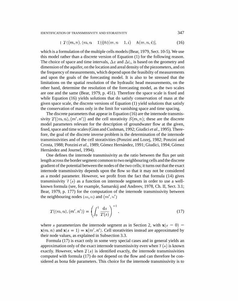
One defines the internode transmissivity as the ratio between the flux per unitlength across the border segment common to two neighbouring cells and the discretegradient of the potential between the nodes of the two cells; it turns out that the exactinternode transmissivity depends upon the flow so that it may not be consideredas a model parameter. However, we profit from the fact that formula (14) givestransmissivity T (s) as a function on internode segments in order to use a well-known formula (see, for example, Samarskij and Andreev, 1978, Ch. II, Sect. 3.1;Bear, 1979, p. 177) for the computation of the internode transmissivity betweenthe neighbouring nodes (m;n) and (m0; n0)

T ((m;n); (m0

; n0)) =

Z 1

0

dsT (s)

!�1

; (17)

where s parameterizes the internode segment as in Section 2, with x(s = 0) =x(m;n) and x(s = 1) = x(m0; n0). Cell storativities instead are approximated bytheir node values, as explained in Subsection 3.3.

Formula (17) is exact only in some very special cases and in general yields anapproximation only of the exact internode transmissivity even when T (s) is knownexactly. However, when T (s) is identified exactly, the internode transmissivitiescomputed with formula (17) do not depend on the flow and can therefore be con-sidered as bona fide parameters. This choice for the internode transmissivity is to

tipm1237.tex; 14/05/1997; 7:29; v.6; p.9


some extent arbitrary, but it relies on a function that the DS method calculatesdirectly, namely T (s), and comprises some well known cases. If, say, transmis-sivity is constant on each cell, formula (17) yields the internode transmissivity asthe harmonic mean of the node values, if, instead, transmissivity varies linearlyalong the internode segment, formula (17) yields the internode transmissivity asthe logarithmic mean of the node transmissivities, and so on. In order to applyformula (17), we do not need prior assumptions for the behaviour of T (s), whichis calculated instead.

3.2. NUMERICAL APPROXIMATION OF THE VECTORS a AND b

In order to apply the technique described in Section 2, we suppose to have measuredthe piezometric head at every node of the lattice and at every time ti.

The vector functions a and b are approximated at each node by the followingsteps. The gradient and the Laplacians of the piezometric heads at a given time ti arecomputed with the standard central differences approximations. Time derivativesare approximated with the backwards differences. These discrete space and timederivatives are the matrix elements of the matrix AA and the components of thevector zA, that are the approximations of A and z respectively. The vector f is ap-proximated by fA � t(F (m;n; t1)=(�x)

2; F (m;n; t2)=(�x)2; : : : ; F (m;n; tp)=

(�x)2). The values of a(m;n) and b(m;n) are determined as the least squaressolutions of the systems

AAa = zA; (18)

AAb = fA: (19)

The solutions to both systems are obtained by QR decomposition with House-holder reduction (Stoer and Bulirsch, 1992); our computer codes are based on thealgorithms described by Forsythe et al. (1977).

When we have evaluated a(m;n) and b(m;n), we approximate the functionsa(s) and b(s) along internode segments with the constant values aA and bA givenin formulae (22) in Appendix (Giudici et al., 1995). We use this very rough approx-imation just because it renders formulae (14) and (17) immediately computable.

3.3. NUMERICAL EVALUATION OF INTERNODE TRANSMISSIVITIES AND CELLSTORATIVITIES

As remarked above, once we have computed the functions a(s) and b(s), thecomputation of transmissivity along internode segments according to formula (14)is the same as for the steady-state case, so that we may evaluate the internodetransmissivities with formulae (24) and (25) in Appendix (Giudici et al., 1995).Also, as inequality (15) holds for the case considered here as for the steady-state case, we choose the initial point x0 and the integration path in the same

tipm1237.tex; 14/05/1997; 7:29; v.6; p.10


way as in the cited paper, namely we choose the initial node (m0; n0) where(a1(m;n))2 + (a2(m;n))2 is the smallest. Also, among the possible integrationpaths that join the node (m;n), where we want to evaluate transmissivity, to

the initial node (m0; n0) we choose that one for which the sumP(m;n)

(m0;n0)jaAj,

performed over all the internode segments connecting the vertices of the path, isthe smallest. In this way, inequality (15) guarantees that the effects of the errorson the data are minimized. The initial value T0 has to be assigned at (m0; n0); ina real case, it could be obtained by pumping tests or by using four sets of datathat are independent according to the general definition (Parravicini et al., 1995,Theorem 1, case (i)).

Next, Equation (11) yields the node storativity

u3(m;n) � S(m;n) = �T (m;n)a3(m;n) + b3(m;n): (20)

We consider this approximate value of the node storativity as an approximationof the cell storativity as well; we do not have a simple analog of formula (17)for the cell storativity. This choice is justified by the fact that the evaluation ofT (m;n); a3(m;n) and b3(m;n) takes into account several different flows over aregion that encloses some cells.

4. Numerical Examples

The DS method, as described in Section 3, is applied to a synthetic but realisticexample. In particular we consider the synthetic isotropic confined aquifer intro-duced by Giudici et al. (1995). In the next subsection we recall the basic featuresof this example and the procedure to obtain the data necessary for the DS method.We stress that in real cases these data are interpolated from measured quantities.In the second subsection we apply the DS method to noise-free data, and in thefollowing subsections we apply the method to erroneous data.

4.1. GENERATION OF THE SYNTHETIC DATA

The synthetic isotropic aquifer that we consider is divided into a square regularlattice of cells, with M = N = 9, �x = 1 000 m. Transmissivity is constant oneach cell and is given by T (m;n) = (18 � 3m + 10n) � 0:0005 m2 s�1 (with amaximum variation of about two orders of magnitude); because of this constancyand of the regular spacing of the cells, the internode transmissivities, denoted with�((m;n); (m0; n0)), are the harmonic mean of the node values. Storativity is con-stant on each cell as well and is given by �(m;n) = (18�3m+10n) �0:00002. Weconsider the internode transmissivities �((m;n); (m0; n0)) and the node storativi-ties�(m;n) as the reference parameters; the values of the internode transmissivitiesvary between 0:003 and 0:048 m2 s�1 and those of the node storativities between0:0003 and 0:0018.

tipm1237.tex; 14/05/1997; 7:29; v.6; p.11


Figure 1. Prescribed Dirichlet boundary conditions for the piezometric heads (in meters) andlocation (black squares) of the arrays of wells for the transient flow conditions.

The fact that the domain is divided into zones of constant transmissivity andstorativity and the correlation between these two parameters is just a choice, arbi-trary, for the synthetic reference aquifer and we stress that it does not play any rolein the identification process.

Dirichlet boundary conditions for the piezometric head have been assigned atthe border of the domain. The assigned values can be read from Figure 1; they donot vary with time. The initial conditions for the piezometric head are given by thesolution of a steady-state forward problem corresponding to the source term

F (m;n) = [(4:5 �m)2 + 2(n� 5:5)2] � 0:0005 m3 s�1; (21)

which represents leakage and is present in all the situations devised. The contourplot of the piezometric head corresponding to the initial situation is shown inFigure 2 (a). This will be called the flow situation 0. It corresponds to the flowsituation 1 of Giudici et al. (1995).

The transient regime is set up by the sudden start of some arrays of wells att = 0. The arrays of wells are placed in the cells corresponding to the nodes markedwith black squares in Figure 1. At these nodes the source term during the transientregime is equal to 0:1 m3s�1. This value is not too high, if we take into accountthe values of transmissivity and the width of the cells, whose area is 1 km2. Noticethat it takes about two months for the aquifer to reach the new steady state.

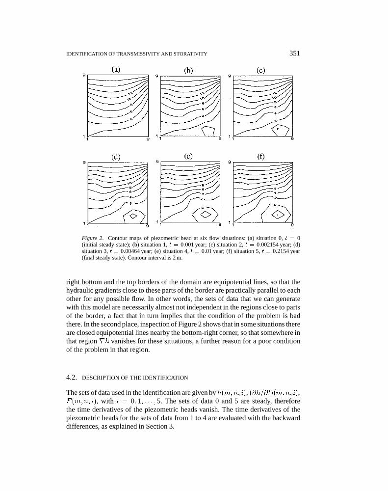
Piezometric heads at different times are obtained by solving the forward problemwith the reference parameters, the boundary and initial conditions, and the sourceterms described above. In particular flow situations 1, 2, 3, 4 and 5 are consideredat t = t1 = 0:001 year, t = t2 = 0:002154 year, t = t3 = 0:00464 year, t =t4 = 0:01 year and t = t5 = 0:2154 year respectively. The total time intervalcorresponds to about two months and a half; the aquifer is already in a steady stateat t = t5. Flow situation 5 corresponds to the flow situation 3 of Giudici et al.(1995). The contour maps of the piezometric heads for the six flow situations arerepresented in Figure 2.

The model has not been chosen in order that it be amenable but rather in orderto check how the method works with the worst conditions, so that we set twodifficulties in it. In the first place, inspection of Figures 1 and 2, shows that the

tipm1237.tex; 14/05/1997; 7:29; v.6; p.12


Figure 2. Contour maps of piezometric head at six flow situations: (a) situation 0, t = 0(initial steady state); (b) situation 1, t = 0:001 year; (c) situation 2, t = 0:002154 year; (d)situation 3, t = 0:00464 year; (e) situation 4, t = 0:01 year; (f) situation 5, t = 0:2154 year(final steady state). Contour interval is 2 m.

right bottom and the top borders of the domain are equipotential lines, so that thehydraulic gradients close to these parts of the border are practically parallel to eachother for any possible flow. In other words, the sets of data that we can generatewith this model are necessarily almost not independent in the regions close to partsof the border, a fact that in turn implies that the condition of the problem is badthere. In the second place, inspection of Figure 2 shows that in some situations thereare closed equipotential lines nearby the bottom-right corner, so that somewhere inthat region rh vanishes for these situations, a further reason for a poor conditionof the problem in that region.

4.2. DESCRIPTION OF THE IDENTIFICATION

The sets of data used in the identification are given by h(m;n; i), (@h=@t)(m;n; i),F (m;n; i), with i = 0; 1; : : : ; 5. The sets of data 0 and 5 are steady, thereforethe time derivatives of the piezometric heads vanish. The time derivatives of thepiezometric heads for the sets of data from 1 to 4 are evaluated with the backwarddifferences, as explained in Section 3.

tipm1237.tex; 14/05/1997; 7:29; v.6; p.13


In addition to the sets of data, the DS method requires the value of transmissivityT0 at a point x0, the starting point of the integration. As said before, we choose thisstarting point at the node (m0; n0)where (a1(m;n))2+(a2(m;n))2 is the smallest.As a consequence, the starting point might be different for each numerical example.The initial value of transmissivity is the value of the reference nodal transmissivityT (m0; n0) for Cases A, B, B1 and B2 below.

By applying Equation (16) to the synthetic aquifer described above, it is easyto check that we have to identify 112 values of internode transmissivities and 49values of cell storativities.

In the present paper we evaluate the performance of the DS method with differentkinds of data, taking into account the following cases.

Case A. We use the sets of data of situations from 2 to 4. Notice that, in this case,all and only the transient data are involved; if we had used the data of situation 1 aswell, the evaluation of the discrete time derivatives with the backward differenceswould have involved the steady situation 0 as well.

Case B. We use all the sets of data, situations from 0 to 5.

Identification for case A with exact data. The initial node is (m0; n0) = (2; 3).In Figure 3 (a) we represent the relative errors, "T on the identified internodetransmissivities, T ((m;n); (m0; n0))

"T =[T ((m;n); (m0; n0))� �((m;n); (m0; n0))]

�((m;n); (m0; n0)):

Only seven out of the 112 internode transmissivities are identified with an absolutevalue of the relative error greater than 0:1.

In Figure 3 (b) we represent the relative errors, "S , on the identified cell stora-tivities, S(m;n)

"S =[S(m;n)� �(m;n)]

�(m;n):

The cell storativities are identified with an absolute value of the relative errorgreater than 0.1 at four nodes out of 49.

Identification for case B with exact data. The initial node is (m0; n0) = (2; 3).In Figure 4 we show the integration path together with the order of integration ofthe nodes. Internode transmissivities between nodes connected by an arrow (e.g.between nodes (3; 6) and (3; 7) that have integration order 15 and 18) are computedwith formula (24) in Appendix; internode transmissivities between adjacent nodesthat are not connected by an arrow (e.g. between nodes (3; 6) and (2; 6) that haveorder 15 and 43) are computed with formula (25) in Appendix. We list in Figure 5the relative errors on the identified internode transmissivities and cell storativitieswhen both steady and transient error-free data are used. We remark that the relativeerrors on the identified internode transmissivities are lower than for the case of

tipm1237.tex; 14/05/1997; 7:29; v.6; p.14


Figure 3. Relative errors for identified (a) internode transmissivities and (b) cell storativities,case A with exact data. Bullets denote internode transmissivities or cell storativities that couldnot be identified or that have negative value. The shaded area singles out the region where theabsolute value of the relative error is greater than 0.4.

steady data only considered by Giudici et al. (1995); however, the results areslightly worse than for case A (transient data only). The absolute values of therelative error on cell storativity are greater than 0:1 at 10 nodes.

The fact that the parameters identified with exact data are approximate never-theless is not surprising because of the approximations that have to be made forthe numerical implementation of the technique, such as the discretization of thedifferential operators and the approximation for a(s) and b(s).

4.3. DATA WITH ERRORS

In order to show the applicability of the DS method to real cases we introduced (a)correlated and uncorrelated errors on the piezometric heads, (b) errors on the sourceterms representing leakage and (c) errors on the initial value of transmissivity.

(a) Errors on the piezometric heads. We obtain erroneous sets of data by addingtwo functions that represent a correlated and an uncorrelated noise to the piezo-metric heads represented in Figure 2. The function "c(m;n) that simulates a

tipm1237.tex; 14/05/1997; 7:29; v.6; p.15


Figure 4. Integration path and order of integration for Case B with exact data.

Figure 5. Relative errors for identified (a) internode transmissivities and (b) cell storativities,case B with exact data. Bullets and shaded area as in Figure 3.

correlated noise is chosen arbitrarily and is given by a product of sinusoidalfunctions

tipm1237.tex; 14/05/1997; 7:29; v.6; p.16


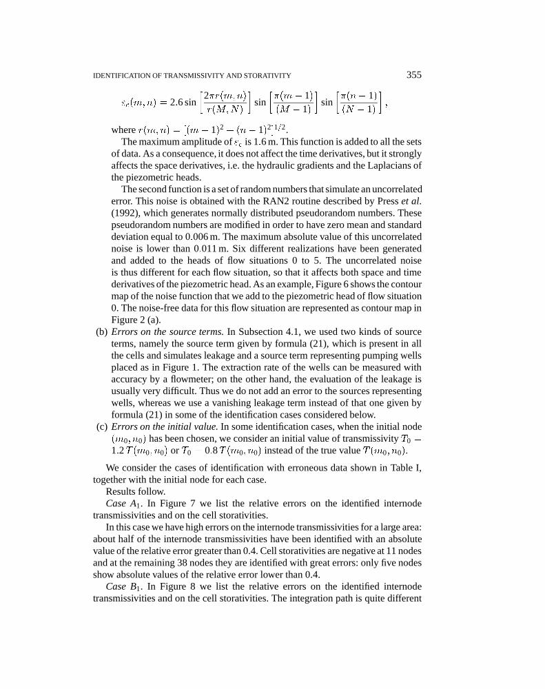
"c(m;n) = 2:6 sin�

2�r(m;n)

r(M;N)

�sin��(m� 1)(M � 1)

�sin��(n� 1)(N � 1)

�;

where r(m;n) = [(m� 1)2 + (n� 1)2]1=2.The maximum amplitude of "c is 1:6 m. This function is added to all the sets

of data. As a consequence, it does not affect the time derivatives, but it stronglyaffects the space derivatives, i.e. the hydraulic gradients and the Laplacians ofthe piezometric heads.

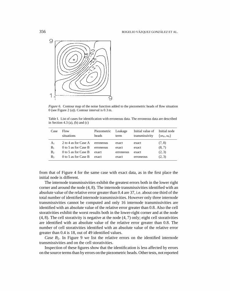
The second function is a set of random numbers that simulate an uncorrelatederror. This noise is obtained with the RAN2 routine described by Press et al.(1992), which generates normally distributed pseudorandom numbers. Thesepseudorandom numbers are modified in order to have zero mean and standarddeviation equal to 0:006 m. The maximum absolute value of this uncorrelatednoise is lower than 0:011 m. Six different realizations have been generatedand added to the heads of flow situations 0 to 5. The uncorrelated noiseis thus different for each flow situation, so that it affects both space and timederivatives of the piezometric head. As an example, Figure 6 shows the contourmap of the noise function that we add to the piezometric head of flow situation0. The noise-free data for this flow situation are represented as contour map inFigure 2 (a).

(b) Errors on the source terms. In Subsection 4.1, we used two kinds of sourceterms, namely the source term given by formula (21), which is present in allthe cells and simulates leakage and a source term representing pumping wellsplaced as in Figure 1. The extraction rate of the wells can be measured withaccuracy by a flowmeter; on the other hand, the evaluation of the leakage isusually very difficult. Thus we do not add an error to the sources representingwells, whereas we use a vanishing leakage term instead of that one given byformula (21) in some of the identification cases considered below.

(c) Errors on the initial value. In some identification cases, when the initial node(m0; n0) has been chosen, we consider an initial value of transmissivity T0 =1:2T (m0; n0) or T0 = 0:8T (m0; n0) instead of the true value T (m0; n0).

We consider the cases of identification with erroneous data shown in Table I,together with the initial node for each case.

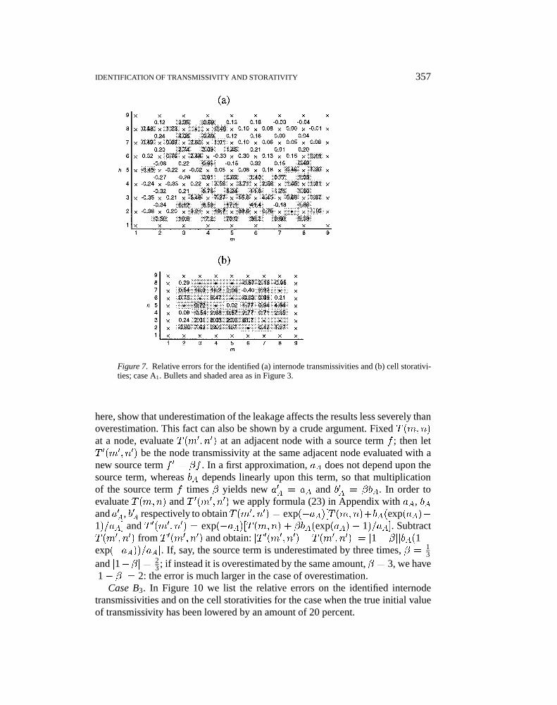
Results follow.Case A1. In Figure 7 we list the relative errors on the identified internode

transmissivities and on the cell storativities.In this case we have high errors on the internode transmissivities for a large area:

about half of the internode transmissivities have been identified with an absolutevalue of the relative error greater than 0.4. Cell storativities are negative at 11 nodesand at the remaining 38 nodes they are identified with great errors: only five nodesshow absolute values of the relative error lower than 0.4.

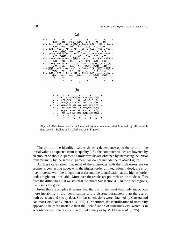
Case B1. In Figure 8 we list the relative errors on the identified internodetransmissivities and on the cell storativities. The integration path is quite different

tipm1237.tex; 14/05/1997; 7:29; v.6; p.17


Figure 6. Contour map of the noise function added to the piezometric heads of flow situation0 (see Figure 2 (a)). Contour interval is 0:3 m.

Table I. List of cases for identification with erroneous data. The erroneous data are describedin Section 4.3 (a), (b) and (c)

Case Flow Piezometric Leakage Initial value of Initial nodesituations heads term transmissivity (m0; n0)

A1 2 to 4 as for Case A erroneous exact exact (7, 8)B1 0 to 5 as for Case B erroneous exact exact (8, 7)B2 0 to 5 as for Case B exact erroneous exact (2, 3)B3 0 to 5 as for Case B exact exact erroneous (2, 3)

from that of Figure 4 for the same case with exact data, as in the first place theinitial node is different.

The internode transmissivities exhibit the greatest errors both in the lower rightcorner and around the node (4, 8). The internode transmissivities identified with anabsolute value of the relative error greater than 0.4 are 37, i.e. about one third of thetotal number of identified internode transmissivities. However only three internodetransmissivities cannot be computed and only 16 internode transmissivities areidentified with an absolute value of the relative error greater than 0.8. Also the cellstorativities exhibit the worst results both in the lower-right corner and at the node(4, 8). The cell storativity is negative at the node (4, 7) only; eight cell storativitiesare identified with an absolute value of the relative error greater than 0.8. Thenumber of cell storativities identified with an absolute value of the relative errorgreater than 0.4 is 18, out of 49 identified values.

Case B2. In Figure 9 we list the relative errors on the identified internodetransmissivities and on the cell storativities.

Inspection of these figures show that the identification is less affected by errorson the source terms than by errors on the piezometric heads. Other tests, not reported

tipm1237.tex; 14/05/1997; 7:29; v.6; p.18


Figure 7. Relative errors for the identified (a) internode transmissivities and (b) cell storativi-ties; case A1. Bullets and shaded area as in Figure 3.

here, show that underestimation of the leakage affects the results less severely thanoverestimation. This fact can also be shown by a crude argument. Fixed T (m;n)at a node, evaluate T (m0; n0) at an adjacent node with a source term f ; then letT 0(m0; n0) be the node transmissivity at the same adjacent node evaluated with anew source term f 0 = �f . In a first approximation, aA does not depend upon thesource term, whereas bA depends linearly upon this term, so that multiplicationof the source term f times � yields new a0A = aA and b0A = �bA. In order toevaluate T (m;n) and T 0(m0; n0) we apply formula (23) in Appendix with aA, bAand a0A, b0A respectively to obtain T (m0; n0) = exp(�aA)[T (m;n)+bA(exp(aA)�1)=aA] and T 0(m0; n0) = exp(�aA)[T (m;n) + �bA(exp(aA) � 1)=aA]. SubtractT (m0; n0) from T 0(m0; n0) and obtain: jT 0(m0; n0)� T (m0; n0)j = j1 � �jjbA(1 �exp(�aA))=aAj. If, say, the source term is underestimated by three times, � = 1

3and j1��j = 2

3 ; if instead it is overestimated by the same amount, � = 3, we havej1 � �j = 2: the error is much larger in the case of overestimation.

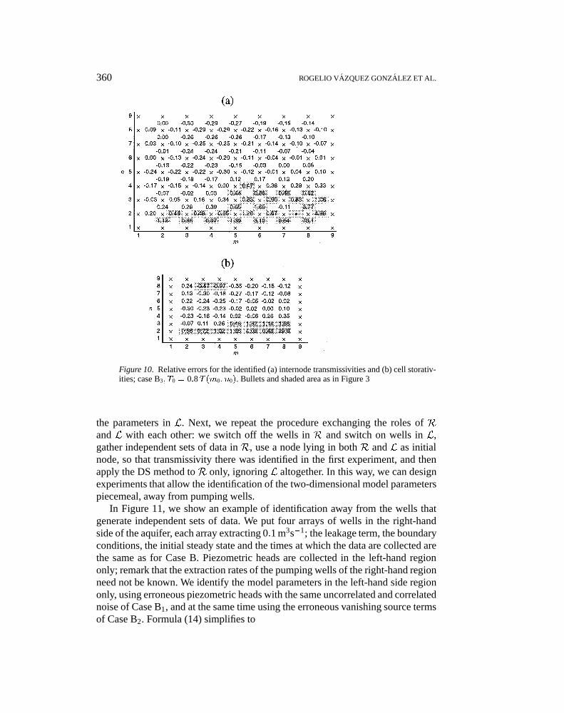
Case B3. In Figure 10 we list the relative errors on the identified internodetransmissivities and on the cell storativities for the case when the true initial valueof transmissivity has been lowered by an amount of 20 percent.

tipm1237.tex; 14/05/1997; 7:29; v.6; p.19


Figure 8. Relative errors for the identified (a) internode transmissivities and (b) cell storativi-ties; case B1. Bullets and shaded area as in Figure 3.

The error on the identified values shows a dependence upon the error on theinitial value as expected from inequality (15): the computed values are lowered byan amount of about 20 percent. Similar results are obtained by increasing the initialtransmissivity by the same 20 percent; we do not include the relative Figure.

All these cases show that most of the internodes with the high errors are onsegments connecting nodes with the highest order of integration; indeed, the errormay increase with the integration order and the identification at the highest ordernodes might not be reliable. Moreover, the results are poor where the model suffersfrom the difficulties that we stated at the end of Subsection 4.1; in the other regions,the results are good.

From these examples it seems that the use of transient data only introducesmore instability in the identification of the discrete parameters than the use ofboth transient and steady data. Similar conclusions were obtained by Carrera andNeuman (1986) and Ginn et al. (1990). Furthermore, the identification of storativityappears to be more unstable than the identification of transmissivity, which is inaccordance with the results of sensitivity analysis by McElwee et al. (1995).

tipm1237.tex; 14/05/1997; 7:29; v.6; p.20


Figure 9. Relative errors for the identified (a) internode transmissivities and (b) cell storativi-ties; case B2. Bullets and shaded area as in Figure 3.

4.4. IDENTIFICATION AWAY FROM PUMPING WELLS

It is well known (Bear, 1979, p. 28) that the two-dimensional flow approximationfails around pumping wells, up to a distance of about twice the thickness of theaquifer; in such regions, the flow is three-dimensional. This fact makes ineffectivethe techniques of identification based on two-dimensional models around pumpingwells. In principle, the DS method can identify parameters for three-dimensionalflows as well, but it is difficult to check the independence of the data for three-dimensional models (Parravicini et al., 1995); we use the method, instead, for apiecemeal identification away from pumping wells, within the framework of two-dimensional models. This is also important because around pumping wells, closedequipotential lines are possible, in which case, as we saw, the condition can bepoor.

Envision an experiment as follows. We switch on wells in a regionR and obtaina transient regime inside a nearby regionL, where no wells are working. We collectsets of data at different times in L and suppose that three of them are independentso that we can apply the DS method to the region L only, where the flow can beconsidered two-dimensional, ignoring the region R altogether, and can identify

tipm1237.tex; 14/05/1997; 7:29; v.6; p.21


Figure 10. Relative errors for the identified (a) internode transmissivities and (b) cell storativ-ities; case B3; T0 = 0:8T (m0; n0). Bullets and shaded area as in Figure 3

the parameters in L. Next, we repeat the procedure exchanging the roles of Rand L with each other: we switch off the wells in R and switch on wells in L,gather independent sets of data in R, use a node lying in both R and L as initialnode, so that transmissivity there was identified in the first experiment, and thenapply the DS method to R only, ignoring L altogether. In this way, we can designexperiments that allow the identification of the two-dimensional model parameterspiecemeal, away from pumping wells.

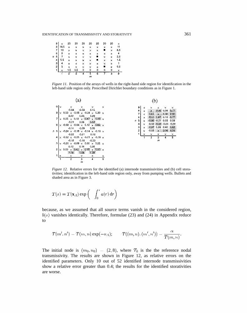
In Figure 11, we show an example of identification away from the wells thatgenerate independent sets of data. We put four arrays of wells in the right-handside of the aquifer, each array extracting 0:1 m3s�1; the leakage term, the boundaryconditions, the initial steady state and the times at which the data are collected arethe same as for Case B. Piezometric heads are collected in the left-hand regiononly; remark that the extraction rates of the pumping wells of the right-hand regionneed not be known. We identify the model parameters in the left-hand side regiononly, using erroneous piezometric heads with the same uncorrelated and correlatednoise of Case B1, and at the same time using the erroneous vanishing source termsof Case B2. Formula (14) simplifies to

tipm1237.tex; 14/05/1997; 7:29; v.6; p.22


Figure 11. Position of the arrays of wells in the right-hand side region for identification in theleft-hand side region only. Prescribed Dirichlet boundary conditions as in Figure 1.

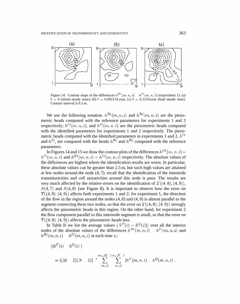
Figure 12. Relative errors for the identified (a) internode transmissivities and (b) cell stora-tivities; identification in the left-hand side region only, away from pumping wells. Bullets andshaded area as in Figure 3.

T (s) = T (xA) exp��

Z s

0a(r) dr

�

because, as we assumed that all source terms vanish in the considered region,b(s) vanishes identically. Therefore, formulae (23) and (24) in Appendix reduceto

T (m0

; n0) = T (m;n) exp(�aA); T ((m;n); (m0

; n0)) =

�

T (m;n):

The initial node is (m0; n0) = (2; 8), where T0 is the the reference nodaltransmissivity. The results are shown in Figure 12, as relative errors on theidentified parameters. Only 10 out of 52 identified internode transmissivitiesshow a relative error greater than 0.4; the results for the identified storativitiesare worse.

tipm1237.tex; 14/05/1997; 7:29; v.6; p.23


Figure 13. Prescribed Dirichlet boundary conditions for the piezometric heads (in meters) andlocations (black squares) of the arrays of wells for the transient flows of (a) experiment 1 and(b) experiment 2.

4.5. VALIDATION OF THE IDENTIFIED PARAMETERS

We validate the identification by using the parameters computed in CaseB1 in a forecasting model and comparing the results with those obtainedby solving the same forward problem with the reference parameters. We com-pare

(i) the piezometric heads,

(ii) the discrete hydraulic gradients and

(iii) the fluxes across the cell sides, to be called internode fluxes for short.

The first two comparisons could in principle be performed in a real case, whereasthe last one can only be done in a synthetic case such as here.

We consider two numerical experiments, solving the forward problem with thesame leakage term (21) for both. The boundary conditions for experiment 1 are thesame of Case B while those for experiment 2 are those of Case B rotated by 90�

counterclockwise (compare Figures 1 and 13), so that the flow for experiment 2 hasa mainly eastward direction instead of southward as for experiment 1. The sourceterms representing wells for both experiments 1 and 2 are modified and the newlocations of the arrays of wells are shown in Figure 13 (a) and (b); the discretesource terms corresponding to these nodes are equal to 0:1 m3s�1.

tipm1237.tex; 14/05/1997; 7:29; v.6; p.24


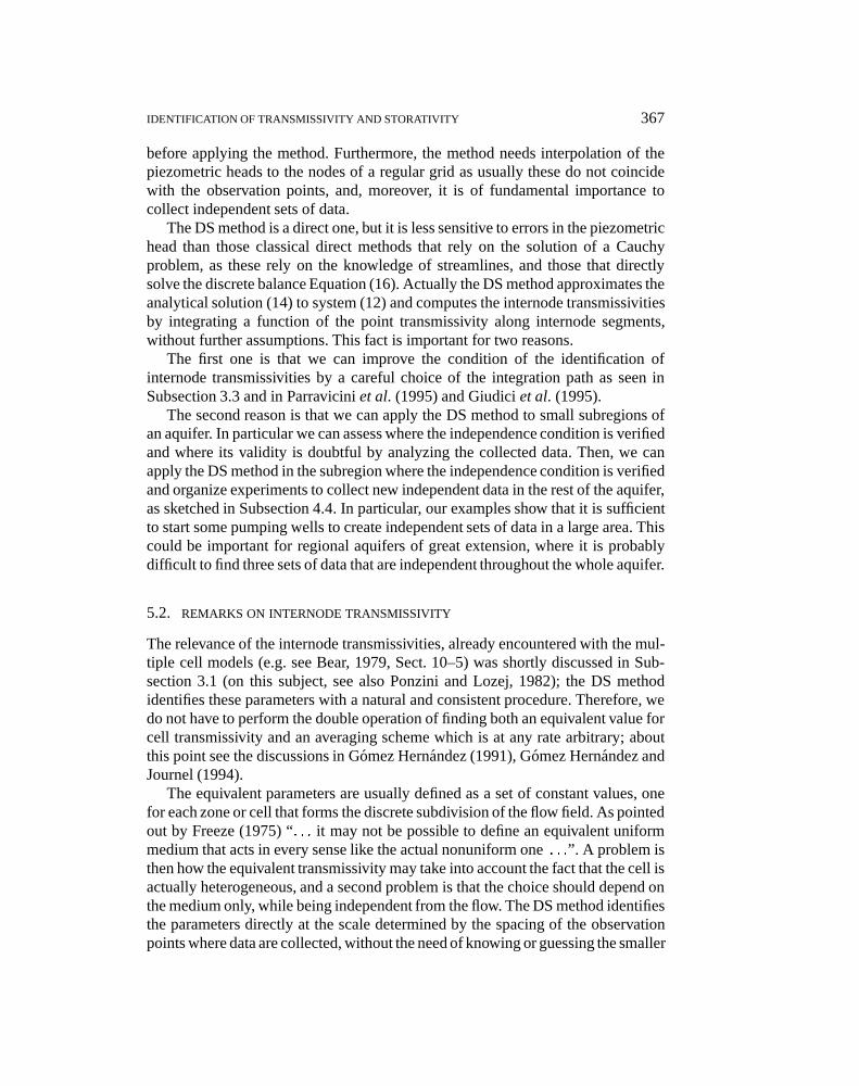
Figure 14. Contour maps of the differences hR1(m;n; i)� hI1

(m;n; i) (experiment 1): (a)t = 0 (initial steady state); (b) t = 0:002154 year; (c) t = 0:2154 year (final steady state).Contour interval is 0:5 m.

We use the following notation. hR1(m;n; i) and hR2(m;n; i) are the piezo-metric heads computed with the reference parameters for experiments 1 and 2respectively; hI1(m;n; i), and hI2(m;n; i) are the piezometric heads computedwith the identified parameters for experiments 1 and 2 respectively. The piezo-metric heads computed with the identified parameters in experiments 1 and 2, hI1

and hI2, are compared with the heads hR1 and hR2 computed with the referenceparameters.

In Figures 14 and 15 we draw the contour plots of the differences hR1(m;n; i)�hI1(m;n; i) and hR2(m;n; i) � hI2(m;n; i) respectively. The absolute values ofthe differences are highest where the identification results are worst. In particular,these absolute values can be greater than 2.5 m, but such high values are attainedat few nodes around the node (4, 7); recall that the identification of the internodetransmissivities and cell storativities around this node is poor. The results arevery much affected by the relative errors on the identification of T ((4; 8); (4; 9)),S(4; 7) and S(4; 8) (see Figure 8). It is important to observe how the error onT ((4; 8); (4; 9)) affects both experiments 1 and 2: for experiment 1, the directionof the flow in the region around the nodes (4, 8) and (4, 9) is almost parallel to thesegment connecting these two nodes, so that the error on T ((4; 8); (4; 9)) stronglyaffects the piezometric heads in this region. On the other hand, for experiment 2the flow component parallel to this internode segment is small, so that the error onT ((4; 8); (4; 9)) affects the piezometric heads less.

In Table II we list the average values hjhP (i) � hQ(i)ji over all the interiornodes of the absolute values of the differences hR1(m;n; i) � hI1(m;n; i) andhR2(m;n; i)� hI2(m;n; i) at each time ti:

hjhP (i)� hQ(i)ji

= [(M � 2)(N � 2)]�1m=M�1Xm=2

n=N�1Xn=2

jhP (m;n; i)� hQ(m;n; i)j:

tipm1237.tex; 14/05/1997; 7:29; v.6; p.25


Figure 15. Contour maps of the differences hR2(m;n; i)� hI2

(m;n; i) (experiment 2): (a)t = 0 (initial steady state); (b) t = 0:002154 year; (c) t = 0:2154 year (final steady state).Contour interval is 0:5 m.

Table II. Average values hjhP (i)� hQ(i)ji (in meters) overthe interior nodes for experiments 1 and 2

Time (year) Experiment 1 Experiment 2

hjhR1(i)� hI1

(i)ji hjhR2(i)� hI2

(i)ji

0 0.660 1.1000.001 0.663 1.1200.002154 0.649 1.0960.00464 0.682 1.0050.01 0.782 0.8710.2154 0.954 0.741

The results are excellent, taking into account that the average of the absolute valueof the noise on the data used for the inversion is 0:793 m.

In Figure 16, we compare the flow directions of the discrete gradients �rhI1

with those of �rhR1 for situation 5 (i.e. at time t5), evaluated with the centraldifferences. We chose situation 5 because it gives the worst comparison. Thecomparison of Figure 16 shows the good agreement between the flow directionscomputed with the identified parameters and those computed with the reference‘true’ parameters.

Next, we computed the internode fluxes �I1 at time t5 for experiment 1, usingthe identified internode transmissivities and the piezometric heads computed withthese, and the internode fluxes �R1 at time t5 for experiment 1, using the referenceinternode transmissivities and the piezometric heads computed with these

�I1((m;n); (m0; n0); 5)

= T ((m;n); (m0; n0))(hI1(m;n; 5)� hI1(m0; n0; 5));

tipm1237.tex; 14/05/1997; 7:29; v.6; p.26


Figure 16. Maps of the flow directions evaluated in experiment 1, situation 5 for �rhI1 and�rhR1. The length of the arrows is proportional to the magnitude of the respective discretegradients.

�R1((m;n); (m0; n0); 5)

= �((m;n); (m0; n0))(hR1(m;n; 5)� hR1(m0; n0; 5)):

We compared the results and represent the absolute errors and the relative errorsof the internode fluxes

�I1((m;n); (m0; n0); 5)� �R1((m;n); (m0; n0); 5);

[�I1((m;n); (m0; n0); 5)� �R1((m;n); (m0; n0); 5)]�

�[�R1((m;n); (m0; n0); 5)]�1;

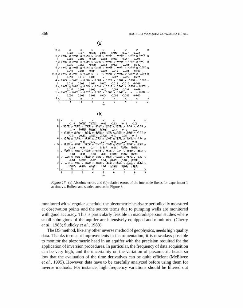
in Figure 17 (a) and (b). The errors with absolute value greater than 0:05 m3s�1 arefound only in the area surrounding node (4, 8). This is justified by the same remarksdone for Figures 14 and 15 about the effect that errors on T ((4; 8)(4; 9)), S(4; 8)and S(4; 7) have on the predicted piezometric heads. Almost all the relative errorson the internode fluxes across the internodes (m;n); (m0; n) have an absolute valuegreater than 0.4, whereas they are small for the internodes (m;n); (m;n0). Thisis consistent with two facts: first, the x-components of the flow are smaller thanthe y-components, as can be deduced from Figures 2 and 16; second, the order ofmagnitude of the absolute error is about the same for the internodes oriented alongthe x direction as for those oriented along the y direction.

5. Final Comments

5.1. APPLICABILITY OF THE DS METHOD

The data necessary to apply the DS method are those usually collected for aquifersunder control or under an investigation program. In fact, when a real aquifer is

tipm1237.tex; 14/05/1997; 7:29; v.6; p.27


Figure 17. (a) Absolute errors and (b) relative errors of the internode fluxes for experiment 1at time t5. Bullets and shaded area as in Figure 3.

monitored with a regular schedule, the piezometric heads are periodically measuredat observation points and the source terms due to pumping wells are monitoredwith good accuracy. This is particularly feasible in macrodispersion studies wheresmall subregions of the aquifer are intensively equipped and monitored (Cherryet al., 1983; Sudicky et al., 1983).

The DS method, like any other inverse method of geophysics, needs high qualitydata. Thanks to recent improvements in instrumentation, it is nowadays possibleto monitor the piezometric head in an aquifer with the precision required for theapplication of inversion procedures. In particular, the frequency of data acquisitioncan be very high, and the uncertainty on the variation of piezometric heads solow that the evaluation of the time derivatives can be quite efficient (McElweeet al., 1995). However, data have to be carefully analyzed before using them forinverse methods. For instance, high frequency variations should be filtered out

tipm1237.tex; 14/05/1997; 7:29; v.6; p.28


before applying the method. Furthermore, the method needs interpolation of thepiezometric heads to the nodes of a regular grid as usually these do not coincidewith the observation points, and, moreover, it is of fundamental importance tocollect independent sets of data.

The DS method is a direct one, but it is less sensitive to errors in the piezometrichead than those classical direct methods that rely on the solution of a Cauchyproblem, as these rely on the knowledge of streamlines, and those that directlysolve the discrete balance Equation (16). Actually the DS method approximates theanalytical solution (14) to system (12) and computes the internode transmissivitiesby integrating a function of the point transmissivity along internode segments,without further assumptions. This fact is important for two reasons.

The first one is that we can improve the condition of the identification ofinternode transmissivities by a careful choice of the integration path as seen inSubsection 3.3 and in Parravicini et al. (1995) and Giudici et al. (1995).

The second reason is that we can apply the DS method to small subregions ofan aquifer. In particular we can assess where the independence condition is verifiedand where its validity is doubtful by analyzing the collected data. Then, we canapply the DS method in the subregion where the independence condition is verifiedand organize experiments to collect new independent data in the rest of the aquifer,as sketched in Subsection 4.4. In particular, our examples show that it is sufficientto start some pumping wells to create independent sets of data in a large area. Thiscould be important for regional aquifers of great extension, where it is probablydifficult to find three sets of data that are independent throughout the whole aquifer.

5.2. REMARKS ON INTERNODE TRANSMISSIVITY

The relevance of the internode transmissivities, already encountered with the mul-tiple cell models (e.g. see Bear, 1979, Sect. 10–5) was shortly discussed in Sub-section 3.1 (on this subject, see also Ponzini and Lozej, 1982); the DS methodidentifies these parameters with a natural and consistent procedure. Therefore, wedo not have to perform the double operation of finding both an equivalent value forcell transmissivity and an averaging scheme which is at any rate arbitrary; aboutthis point see the discussions in Gomez Hernandez (1991), Gomez Hernandez andJournel (1994).

The equivalent parameters are usually defined as a set of constant values, onefor each zone or cell that forms the discrete subdivision of the flow field. As pointedout by Freeze (1975) “: : : it may not be possible to define an equivalent uniformmedium that acts in every sense like the actual nonuniform one : : :”. A problem isthen how the equivalent transmissivity may take into account the fact that the cell isactually heterogeneous, and a second problem is that the choice should depend onthe medium only, while being independent from the flow. The DS method identifiesthe parameters directly at the scale determined by the spacing of the observationpoints where data are collected, without the need of knowing or guessing the smaller

tipm1237.tex; 14/05/1997; 7:29; v.6; p.29


scale heterogeneity of cells, thus bypassing the first problem. Regarding the secondproblem, the dependence of the identified parameters upon the flow is weakenedbecause the method takes into account many flows with different directions.

The equivalent transmissivity for Equation (16) is represented by four parame-ters for each cell, that is to say the internode transmissivities: the fact that, evenif the aquifer is isotropic as in our synthetic example, its large-scale propertiesare anisotropic was pointed out already by Nelson (1960), pp. 1755–1756, and isclearly shown in the balance Equation (16), which is intrinsically anisotropic, tothe extent that it is also valid for anisotropic aquifers if the principal directionsof the transmissivity tensor are constant and the Cartesian axes are oriented alongthem.

6. Conclusions

We close with the following summary of the features of the method.

(1) The DS method uses those measurable quantities that are usually collected inaquifers under control or that can be directly interpolated from these.

(2) No prior information on storativity is required. The value of transmissivity atone point only is needed, which is the only prior information on the unknownparameters necessary to solve the inverse problem with the DS method.

(3) No initial guess of the unknown parameters is required.

(4) The DS method does not require the solution of forward problems. Hence, itallows for a piecemeal identification, if the available data are not independenteverywhere, or if one knows the value of transmissivity at more than one point,so that one may integrate starting from different points, or if one wishes toidentify the parameters away from pumping wells, and so on.

(5) The identification of transmissivity does not depend upon storativity, evenwhen only transient data are used.

(6) The DS method yields transmissivity along internodes, thus allowing for asimple calculation of internode transmissivities.

(7) The internode transmissivities and cell storativities are ready-to-use parametersfor the numerical implementation of the forward problem with conservativeschemes.

(8) As the DS method takes into account several flows with different directions,all over the aquifer, the dependence of the solution upon the flow is weakened.

(9) Furthermore, the DS method uses data on the whole flow field, so that thecomputed internode transmissivities and cell storativities take into account theflow over the whole region considered, they are not obtained by averaging justover volume supports of limited extension, as it is done in some upscalingtechniques.

tipm1237.tex; 14/05/1997; 7:29; v.6; p.30


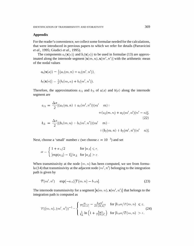
Appendix

For the reader’s convenience, we collect some formulae needed for the calculations,that were introduced in previous papers to which we refer for details (Parraviciniet al., 1995; Giudici et al., 1995).

The components ai(x(s)) and bi(x(s)) to be used in formulae (13) are approx-imated along the internode segment [x(m;n); x(m0; n0)] with the arithmetic meanof the nodal values

ai(x(s)) = 12(ai(m;n) + ai(m

0

; n0));

bi(x(s)) = 12(bi(m;n) + bi(m

0

; n0)):

Therefore, the approximations aA and bA of a(s) and b(s) along the internodesegment are

aA =�x

2[(a1(m;n) + a1(m

0

; n0))(m0 �m)+

+(a2(m;n) + a2(m0; n0)(n0 � n)];

(22)

bA =�x

2[(b1(m;n) + b1(m

0

; n0))(m0 �m)+

+(b2(m;n) + b2(m0; n0)(n0 � n)]:

Next, choose a ‘small’ number " (we choose " = 10�3) and set

� =

(1 + aA=2 for jaAj 6 ";

[exp(aA)� 1]=aA for jaAj > ":

When transmissivity at the node (m;n) has been computed, we see from formu-la (14) that transmissivity at the adjacent node (m0; n0) belonging to the integrationpath is given by

T (m0

; n0) = exp(�aA)[T (m;n) + bA�]: (23)

The internode transmissivity for a segment [x(m;n); x(m0; n0)] that belongs to theintegration path is computed as

T ((m;n); (m0

; n0))�1=

8><>:

�T (m;n) �

bA�2

2T (m;n)2 for jbA�=T (m;n)j 6 ";

1bA

ln�

1 + bA�T (m;n)

�for jbA�=T (m;n)j > ":

(24)

tipm1237.tex; 14/05/1997; 7:29; v.6; p.31


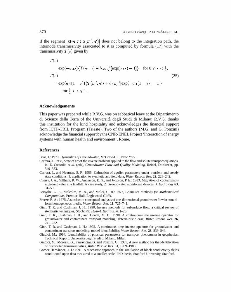
If the segment [x(m;n); x(m0; n0)] does not belong to the integration path, theinternode transmissivity associated to it is computed by formula (17) with thetransmissivity T (s) given by

T (s)

= exp(�aAs)fT (m;n) + bAa�1A [exp(aAs)� 1]g for 0 6 s < 1

2 ;

T (s)

= exp(aA(1 � s))fT (m0; n0) + bAa�1A [exp(�aA(1 � s))� 1]g

for 12 < s 6 1:

(25)

Acknowledgements

This paper was prepared while R.V.G. was on sabbatical leave at the Dipartimentodi Scienze della Terra of the Universita degli Studi di Milano: R.V.G. thanksthis institution for the kind hospitality and acknowledges the financial supportfrom ICTP-TRIL Program (Trieste). Two of the authors (M.G. and G. Ponzini)acknowledge the financial support by the CNR-ENEL Project ‘Interaction of energysystems with human health and environment’, Rome.

References

Bear, J.: 1979, Hydraulics of Groundwater, McGraw-Hill, New York.Carrera, J.: 1988, State of art of the inverse problem applied to the flow and solute transport equations,

in: E. Custodio et al. (eds), Groundwater Flow and Quality Modeling, Reidel, Dordrecht, pp.549–583.

Carrera, J., and Neuman, S. P.: 1986, Estimation of aquifer parameters under transient and steadystate conditions: 3. application to synthetic and field data, Water Resour. Res. 22, 228–242.

Cherry, J. A., Gillham, R. W., Anderson, E. G., and Johnson, P. E.: 1983, Migration of contaminantsin groundwater at a landfill: A case study, 2. Groundwater monitoring devices, J. Hydrology 63,31–50.

Forsythe, G. E., Malcolm, M. A., and Moler, C. B.: 1977, Computer Methods for MathematicalComputations, Prentice-Hall, Englewood Cliffs.

Freeze, R. A.: 1975, A stochastic-conceptual analysis of one-dimensional groundwater flow in nonuni-form homogeneous media, Water Resour. Res. 11, 725–741.

Ginn, T. R. and Cushman, J. H.: 1990, Inverse methods for subsurface flow: a critical review ofstochastic techniques, Stochastic Hydrol. Hydraul. 4, 1–26.

Ginn, T. R., Cushman, J. H., and Houch, M. H.: 1990, A continuous-time inverse operator forgroundwater and contaminant transport modeling: deterministic case, Water Resour. Res. 26,241–252.

Ginn, T. R. and Cushman, J. H.: 1992, A continuous-time inverse operator for groundwater andcontaminant transport modeling: model identifiability, Water Resour. Res. 28, 539–549.

Giudici, M.: 1994, Identifiability of physical parameters for transport phenomena in geophysics,Technical Report, Universita degli Studi di Milano, Milan.

Giudici, M., Morossi, G., Parravicini, G. and Ponzini, G.: 1995, A new method for the identificationof distributed transmissivities, Water Resour. Res. 31, 1969–1988.

Gomez Hernandez, J. J.: 1991, A stochastic approach to the simulation of block conductivity fieldsconditioned upon data measured at a smaller scale, PhD thesis, Stanford University, Stanford.

tipm1237.tex; 14/05/1997; 7:29; v.6; p.32


Gomez Hernandez, J. J. and Journel, A. G.: 1994, Stochastic characterization of grid-block perme-abilities, SPE Form. Eval. 9, 93–100.

Irmay, S.: 1980, Piezometric determination of inhomogeneous hydraulic conductivity, Water Resour.Res. 16, 691–694.

McElwee, C. D., Bohling, G. C., and Butler, J. J. Jr.: 1995, Sensitivity analysis of slug tests. Part 1.The slugged well, J. Hydrology 164, 53–67.

Nelson, R. W.: 1960, In-place measurement of permeability in heterogeneous media: 1. Theory of aproposed method, J. Geophys. Res. 65, 1753–1758.

Nelson, R. W.: 1961, In-place measurement of permeability in heterogeneous media: 2. Experimentaland computational considerations, J. Geophys. Res. 66, 2469–2478.

Parravicini, G., Giudici, M., Morossi, G. and Ponzini, G.: 1995, Minimal a priori assignment in a directmethod for determining phenomenological coefficients uniquely, Inverse Probl. 11, 611–629.

Ponzini, G. and Crosta, G.: 1988, The comparison model method: a new arithmetic approach to thediscrete inverse problem of groundwater hydrology. 1. One dimensional flow, Transport in PorousMedia 3, 415–436.

Ponzini, G., Crosta, G. and Giudici, M.: 1989, Identification of thermal conductivities by temperaturegradient profiles: one dimensional steady flow, Geophysics 54, 643–653.

Ponzini, G. and Lozej, A.: 1982, Identification of aquifer transmissivities: the comparison modelmethod, Water Resour. Res. 18, 597–622.

Press, W. H., Flannery, B. P., Teukolsky, S. A., and Vetterling, W. T.: 1992, Numerical Recipes inFORTRAN: The Art of Scientific Computing, 2nd edn, Cambridge University Press, Cambridge.

Richter, G. R.: 1981a, An inverse problem for the steady state diffusion equation, SIAM J. Math.Anal. 41, 210–221.

Richter, G. R.: 1981b, Numerical identification of a spatially varying diffusion coefficient, Math.Comput. 36, 375–386.

Samarskij A. and Andreev, V.: 1978, Methodes aux differences pour equations elliptiques, Mir,Moscow.

Stoer, J., and Bulirsch, R.: 1992, Introduction to Numerical Analysis, Springer-Verlag, New York,Berlin.

Sudicky, E. A., Cherry, J. A., and Frind, E. O.: 1983, Migration of contaminants in groundwater at alandfill: A case study, 4. A natural gradient dispersion test, J. Hydrology 63, 81–108.

Yeh, W. W-G.: 1986, Review of parameter identification procedures in groundwater hydrology: theinverse problem, Water Resour. Res. 22, 95–108.

tipm1237.tex; 14/05/1997; 7:29; v.6; p.33

The Differential System Method for the Identification of Transmissivity and Storativity

Documents

Transcript of The Differential System Method for the Identification of Transmissivity and Storativity