The Composition of Exports and Gravity

Scott French∗

December, 2012Version 3.0

Abstract

Gravity estimations using aggregate bilateral trade data implicitlyassume that the effect of trade barriers on trade flows is independentof the composition of those flows. However, I show that, in a simpleframework which is consistent with generalizations of the wide class oftrade models that imply an aggregate gravity equation, aggregate tradeflows, in general, depend on the composition of countries’ output andexpenditure across products, which varies across countries in meaning-ful ways in the data. This implies that trade cost estimates based onaggregate data are biased and that the predictions of models based onsuch estimates may be misleading.

I develop a procedure to estimate a bilateral trade cost functionusing product-level data, which accounts for the lack of comparablydisaggregated data on domestic output. This technique leads to tradecost estimates that are smaller and much more robust to distributionalassumptions than estimates obtained from aggregate data, implyingthat failure to account for the composition of output and expenditureis a more important cause of bias than failure to properly account forheteroskedasticity. Compared to a more traditional model based onaggregate data, the model based on product-level data predicts domestictrade shares that are more consistent with the data, a smaller effect ofreducing trade cost asymmetry on income differences, and very differenteffects of the growth of Chinese manufacturing on many countries.

∗School of Economics, University of New South Wales. scott.french@unsw.edu.au. I amthankful to Dean Corbae for his guidance and support. I am also thankful for advice andcomments from Kim Ruhl, Jason Abrevaya, Alan Woodland, Russell Hillberry as well asseminar participants at the University of New South Wales, University of Sydney, Universityof Melbourne, Monash University, and Australian National University. All errors are myown.

1

1 Introduction

The gravity model – which relates to bilateral trade flows to the sizes of a

pair of countries and the barriers to trade that exist between them – has long

been celebrated as a parsimonious yet empirically successful way to describe

bilateral trade flows. It is extremely useful as a framework within which to

estimate the effect of factors that determine barriers to trade on trade flows

and to predict the effects of altering these factors. Since Anderson (1979),

who showed that the empirical relationship is theoretically founded, it has also

been useful as method to quantify trade models, allowing for serious, general

equilibrium analysis of the effects of such factors on economic outcomes and

welfare. Quite often, the variables of interest are aggregate country-level or

bilateral quantities, and the data that is most readily available are also quite

aggregated, leading researchers to estimate the parameters of gravity models

using aggregate data. This practice implicitly assumes that the effect of trade

barriers on trade flows is independent of the composition of those trade flows.

In this paper, I show that this assumption is not borne out in the data,

which has important implications for the estimation of trade barriers and the

predictions of models based on such estimates. I first develop a simple frame-

work – which is consistent with generalizations of the wide class of trade models

that imply an aggregate gravity equation – in which countries choose how to

allocate their expenditure across product categories as well as across source

countries for each type of product. I show that, in general, aggregate bilateral

trade flows depend on the composition of countries’ output and expenditure

across products in addition to their overall levels of output and expenditure

and bilateral trade costs, meaning that aggregate trade flows are not consis-

tent with an aggregate gravity model. Intuitively, if a country’s exports are

concentrated in a set of goods for which a given importer buys a large fraction

from other sources, a trade barrier between the two countries only affects the

distribution of the importer’s expenditure across countries within those prod-

uct categories, so the effect depends on the elasticity of substitution across

varieties within product categories. However, if a country is the sole provider

2

of a large fraction of the products that it exports to a given importer, then the

effect of a trade barrier between the two countries is governed by the elasticity

of substitution across product categories. If varieties within product categories

are more substitutable than those across product categories, then the former

exporter is more effected by a given trade barrier than the latter.

I develop an index based on product-level trade flow data that indicates

the degree to which a trade flow between a given pair of countries is similar to

either the former or the latter of the scenarios discussed above and show that

there is a great deal of heterogeneity in this index, indicating that the effect

of trade barriers on aggregate trade flows varies greatly across the set of bilat-

eral country pairs. This implies that bilateral trade barriers cannot be inferred

from aggregate trade data because their effects on trade flows depend on inter-

actions among countries’ distributions of output and expenditure. As a result,

trade barriers must be estimated using product-level trade data, but because

output data is rarely available at such a level of disaggregation, traditional

estimation methods, which rely on such data to identify the costs associated

with national borders, cannot be used. Instead, I develop an estimation pro-

cedure based on a reformulation of the model that allows the estimation of

trade barriers using only product-level data on international trade flows and

aggregate data on domestic trade flows. Estimating trade costs in a way that

is consistent with the model implies estimates of trade costs that are lower

than those based on aggregate trade data and much more consistent across

distributional assumptions for the error term, indicating that the bias in trade

cost estimates due to ignoring the composition of trade flows is much more

severe than that due to using techniques that are not robust to varying forms

of heteroskedasticity.

Given the estimates of trade costs based on product-level data, I show that

the composition of trade flows is quite important in explaining their magni-

tude. The effect of the interaction of countries’ distributions of output and

expenditure can more than double or halve the effect of trade barriers on trade

flows between a pair of countries. And, overall, 37% of the variation in trade

flows predicted by the model is due to the effect of composition.

3

With confidence in the trade cost estimates and the predictive power of

the model, I go on to explore the implications of the composition of countries’

output and expenditure on trade flows by performing several counterfactual

experiments. To do so, I use the results of the estimation to parameterize

a version of the model of Eaton and Kortum (2002), which is generalized to

allow for differences in average productivity across product categories. I show

that while a small, uniform reduction in trade barriers has a similar effect in

a model based on product-level data and one based on aggregate data, the

removal of the asymmetric component of trade costs leads to very different

predictions in the two models. While the aggregate model predicts major

gains for small, developing countries and a 17% reduction in the 90/10 ratio

of real output per worker across countries, the product-level model predicts

much more equal gains and just over a 1% fall in the ratio.

I also examine differences in the effects of changes in technology – which

influence countries’ distributions of output and expenditure across products

– examining the effect of the growth of China as a major exporter of manu-

factured goods and finding that the product-level model makes very different

prediction for many countries. Not surprisingly, the aggregate model predicts

that effects of the growth of China are almost universally positive and heavily

dependant on geography; the countries closest to China gain the most because

they have a larger country to trade with and can do so without facing large

trade barriers. The predictions of the product-level model, on the other hand,

make clear the importance of accounting for the composition of output and

expenditure in such an exercise. It predicts that many of the nearby countries

– as well others, including many Central American countries – do not benefit

nearly as much, as they produce a similar mix of products as China, for which

they lose market share, making their exports more responsive to trade barri-

ers. In fact, real output in Cambodia and Honduras is predicted to decrease.

In addition, the developed countries of Europe and North America experience

larger gains, as the prices of the products they tend to import fall, and many

South American and Sub-Saharan African countries benefit more as demand

for the basic materials they tend to export rises.

4

In addition to a shift in productivity for one country, I consider the effects of

the removal of differences in relative productivity across countries. The model

predicts large losses in real output for most countries, an average fall of 15%

in the case of imposing the US pattern of productivity on the world. However,

these magnitudes depend heavily on the correlation between the distribution

of productivity across products in each country and exogenous determinants

of demand, indicating that one may be influential in the determination of the

other. Finally, I compare the predictions of the two models of the effect of

removing trade imbalances, showing the product-level model predicts much

larger changes in incomes as a result of the change.

This paper is related to several strands of the international trade literature.

First, it is related to a large literature using theoretically founded gravity mod-

els to study the effects of trade barriers, including Anderson and van Wincoop

(2003); Eaton and Kortum (2002); and Helpman et al. (2008). Recent papers

have offered extensions to these models which resolve discrepancies between

more traditional gravity models and the data, including Waugh (2010) and

Fieler (2010).1 This paper contributes to this literature by showing that that

the effect of trade barriers on aggregate trade flows and other macroeconomic

variables depends heavily on the composition of output and expenditure and

by providing a tractable framework that is consistent with these models in

which to study this effect.

This paper is also related to a number of other papers that address issues

related to aggregation bias in the estimation of trade costs. Anderson and van

Wincoop (2004) point out that estimates based on aggregate data can be bi-

ased if both the elasticity of substitution and bilateral trade costs vary across

products and if the two are correlated. Hillberry (2002) shows that a similar

form of aggregation bias can exist due to the specialization of countries ac-

cording to comparative advantage driven by relative trade costs. This paper is

largely complimentary to these studies. I show that even if trade costs and the

elasticity of substitution within product categories do not differ across prod-

1Anderson and van Wincoop (2004) provide a survey of older papers that have extendedthe basic gravity framework in a number of dimensions.

5

ucts – so that these forms of aggregation bias do not exist – aggregate trade

flows still depend on the composition of countries’ output and expenditure,

biasing estimates of trade costs using aggregate data. More related to this pa-

per is Hillberry and Hummels (2002), who show that, even without variation

in trade costs across industries, aggregate estimates of trade costs are biased

due to the endogenous co-location of producers and suppliers of intermediate

goods to minimize trade costs. In this paper, I take as given the patterns of

product-level output and expenditure in the data, estimate trade costs in a

model that is consistent with these patterns, and show how taking them into

account has implications for the effects of trade costs and other variables on

macroeconomic outcomes.

This is not the first paper to estimate trade barriers and parameterize a

general equilibrium trade model using disaggregated data. Papers such as

Costinot et al. (2012); Anderson and Yotov (2011); and Levchenko and Zhang

(2011) perform estimations based on industry-level data for many countries.

Das et al. (2007); Eaton et al. (2011); Hillberry and Hummels (2002); and

many others have performed estimations using firm-level data for a single

country. And, Hanson and Robertson (2010) use data from a small subset of

countries and product categories. However, most stop short of disaggregating

past the industry level or using data for a large number of countries and prod-

ucts. Presumably this is due to data limitations and computational burden.

However, in this paper, I show that trade costs can be consistently estimated

using the full set of available product-level data – for thousands of products

and well over 100 countries – accounting for the lack of correspondingly dis-

aggregated production data, and requiring no more computing power than is

available on a modern laptop computer.

The next section develops the theoretical framework and shows that aggre-

gate trade flows, in general, depend on the composition of countries’ output

and expenditure. Section 3 takes a brief look at the data, developing and

computing the Elasticity Index that measures the degree to which trade be-

tween country pairs depends on the elasticity of substitution within or across

product categories. Section 4 develops the estimation procedure and presents

6

the results. Section 5 presents the results of the counterfactual experiments,

and the final section concludes.

2 Model

The theoretical framework is closely related to the sector-level gravity model

detailed in Anderson and van Wincoop (2004), which outlines the class of

models which yield a gravity structure. As in that framework, the structure

developed here is implied by a large class of underlying international trade

models, which encompasses generalizations of several models that have become

the workhorses of the literature.2 The model implies bilateral trade flows that

follow a gravity equation at the product level – which is meant to be analo-

gous to a product category as defined by the agencies that collect international

trade statistics. It departs from Anderson and van Wincoop (2004) by explic-

itly modeling the allocation of countries’ total expenditure across products,

which I then show implies that, in general, aggregate bilateral trade flows de-

pend on the composition, and not simply the level, of countries’ output and

expenditure.

2.1 Environment

The world is made up of N countries that each produce and consume varieties

of a finite number, J , of product categories. Each country, i, produces (or

is endowed with) a nominal value of varieties of product j given by Y ji ≥ 0,

which is taken as exogenous. Each country, n, also distributes its aggregate

nominal expenditure, Xn – also taken as exogenous – across product categories

and source countries according to a nested-CES demand structure.3 Specifi-

2It is trivially generated by an Armington model, as in Anderson and van Wincoop(2003), in which countries are each endowed with a unique variety of each product. It isalso straightforward to show that it is generated by models of monopolistic competitionwith homogeneous firms, such as Helpman and Krugman (1987). The appendix shows thatgeneralizations of the Ricardian model of Eaton and Kortum (2002) and the heterogeneous-firm monopolistic competition model of Chaney (2008) also imply the same structure.

3Xi and Yi are allowed to differ from one another, meaning that trade may not bebalanced.

7

cally, the nominal value of expenditure by country n on product j from source

country i is

Xjni =

(pjidni

P jn

)−θXjn, (1)

where Xjn is the nominal value of expenditure by country n on all varieties of

product j, given by

Xjn = βjn

(P jn

Pn

)−σXn. (2)

Here pji is the appropriate source country (or factory gate) price index for

varieties of product j originating in country i. Barriers to trade, represented

by dni > 1 take the standard “iceberg” form, meaning that for one unit of a

variety to arrive in n, dni units must be shipped from i. The reduced-form

elasticities of substitution across and within product categories are 1 + σ and

1 + θ, respectively, where the assumption θ ≥ σ > 0 is maintained, which

implies that varieties within product categories are more substitutable than

those across product categories.4,5

The product-level and aggregate destination-specific CES price indexes are,

respectively,

P jn =

(∑i

(pjidni)−θ

)−1θ

(3)

and

Pn =

(∑j

βjn(P jn)−σ

)− 1σ

. (4)

The parameter βjn ≥ 0,∑

j βjn = 1, allows expenditure on a particular product

category to differ across countries due to factors not explicitly modeled.

4I refer to the elasticities of substitution as “reduced form” because, depending on theunderlying framework that implies this framework, the deep parameters that underlie theseparameters may have other interpretations.

5As there are a finite number of varieties and product categories, this assumption isnot strictly necessary for the analysis of this paper. However, I maintain it because thisspecification is a reduced form of a wide class of underlying models, and it helps to fix theintuition for the results that follow.

8

2.2 Product-Level Gravity

The market clearing condition, Y ji =

∑nX

jni, (1), and (3) imply that the set

of source country prices can be expressed as

(pji )−θ =

Y ji

Y j

(1

Πji

)−θ, (5)

where Y j =∑

i Yji and (Πj

i )−θ =

∑n

(dniP jn

)−θXjn

Y j. Substituting this expression

into (1), it can be seen that bilateral, product-level trade flows are given by

the following system:

Xjni =

XjnY

ji

Y j

(dni

P jnΠj

i

)−θ(6)

(P jn)−θ =

∑i

(dni

Πji

)−θY ji

Y j(7)

(Πji )−θ =

∑n

(dni

P jn

)−θXjn

Y j. (8)

Anderson and van Wincoop (2004) refer to the indexes P jn and Πj

i as inward

and outward multilateral resistance, which are functions of the set of bilateral

trade barriers, dni, and levels of output and expenditure, Xjn, Y

ji . These

terms summarize all the general equilibrium forces which affect the volume

of trade between a pair of countries. Intuitively, a high value of P jn – the

domestic price index for product j – implies that it is relatively difficult for

consumers in country n to obtain varieties of good j, implying that n will

import a relatively large volume of j from a given source country, i, all else

equal. Likewise, a high value of Πji implies that it is relatively difficult for

producers in i to sell their varieties of j – either because they face high trade

barriers or stiff competition – low values of Pn in potential destinations –

implying that exports to a particular destination, n, will be relatively high, all

else equal.

9

2.3 Aggregate Trade Flows

Equation (6) is a standard theoretical gravity equation. So, given data on

product-level output, expenditure, and bilateral trade flows, any further anal-

ysis could proceed using standard techniques. However, the typical strategy

in the literature is to consider the world to be a one-sector economy so that

aggregate data can be brought to bear on (6).6 The remainder of this section

considers the implications of such a practice when non-trivial differences in

output and expenditure exist across products.

2.3.1 An Aggregate Gravity Equation

Summing Xjni over all j leads to the following expression for total spending by

country n on all products from country i:

Xni =XnYiY

(dni

PnΠni

)−θ, (9)

where

(Πni)θ =

∑j

(Πji )θY

ji /YiY j/Y

βjn

(P jn

Pn

)θ−σ, (10)

and where Yi =∑

j Yji , Y =

∑i Yi, and Pn, defined in (4), can also be given

by

(Pn)−θ =∑i

(dni

Πni

)−θYiY.

Equation (9) has a gravity-like structure similar to (6), relating aggregate

bilateral trade flows to aggregate output and expenditure and bilateral trade

costs. Unlike the product-level gravity equation, though, the aggregate equa-

tion features an outward multilateral resistance term, Πni, which varies by

destination as well as source country. From (10), it is clear that the value of

6While most studies use aggregate trade data, there are many that use disaggregateddata, for example Hummels (1999), Anderson and Yotov (2011), and Hanson and Robertson(2010). However, these papers typically select a few countries and products or use datadisaggregated to at most a couple dozen sectors, which still masks great deal of heterogeneityacross thousands of product categories.

10

Πni depends product-level output and multilateral resistance variables, mean-

ing that aggregate trade flows cannot be expressed as a function of aggregate

data alone.

This new term is an index of product-level outward resistance terms, which

depends not only by the relative concentration of a source country’s output in

each product but also by a function of the variables determining expenditure on

the product by the destination country. So, Πni is not a simple summary index

of the set of Πji terms, as Pn is of the set of P j

ns. Rather, it also summarizes

the interaction between the distribution of output across products in i with

the distribution of prices and demand conditions in n. This implies exports

from i to n will be greater if country i’s output is relatively concentrated

in the products for which either βjn is higher or prices are relatively high.

The intuition behind the first effect is straightforward; a source country whose

output is relatively concentrated in the products that given destination country

prefers to consume will export relatively more to that destination.

The intuition behind the second is a bit more nuanced. First, note that

Xjni can be broken into two components: the fraction of total expenditure that

is spent on product j, βjn

(P jnPn

)−σ, and the fraction of expenditure on product

j that is is spent on varieties originating in country i,(pjidniPn

)−θ. The first is

decreasing in P jn with elasticity σ, while the second is increasing in P j

n with

elasticity θ. In other words, all else equal, a higher price of product j implies

that consumers in n spend relatively less on that product, but, holding pjidni

constant, consumers in n spend relatively more of that amount on country

i’s varieties. Since θ is greater than σ – meaning varieties within product

categories are more substitutable than varieties across categories – the latter

effect dominates, and sales of product j from country i are increasing in P jn.

2.3.2 The Trade Cost Elasticity

The fact that Πni is a function of the distribution of output and expenditure

across products implies that, in general, the effect of trade barriers on ag-

gregate trade flows will also depend on these values. To see how, note that

11

the partial elasticity of Xni with respect to dni – holding constant the source

country prices and aggregate expenditure – is equal to

εni =d ln(Xni)

d ln(dni)= −θ

(1−

∑j

Xjni

Xjn

Xjni

Xni

)− σ

(∑j

Xjni

Xjn

Xjni

Xni− Xni

Xn

). (11)

This elasticity is decreasing in absolute value as the term∑

jXjni

Xjn

Xjni

Xniin-

creases. This term is a weighted average across all products of the contribution

of country i’s varieties of product j to country n’s expenditure on j, weighted

by the fraction of total bilateral trade between i and n accounted for by prod-

uct j. Thus, it is increasing in the degree to which exports from i to n are

concentrated in product categories for which country i has a relatively large

market share for product j in n.

The summation term lies in the range[XniXn, 1], which implies that εni lies

in[−θ(1− Xni

Xn),−σ(1− Xni

Xn)]. Thus, given Xni

Xn, εni depends, at one extreme,

only on θ, and at the other, only on σ. The first case occurs when Xjni is a

constant fraction of Xjn for all products. This implies that that a change in dni

does not affect relative prices of different products in n, so there is no realloca-

tion in expenditure across products, only across sources within products. As

a result, the change in trade flows is governed by the elasticity of substitution

across varieties within product categories, θ. The second case occurs when

Xjni = Xj

n for every product for which Xjni is positive. This implies that coun-

try i supplies a unique set of products to country n. In that case, a change in

dni cannot affect the allocation of expenditure within products across sources

because no other source is producing those products, so the change in bilateral

trade flows depends only on the elasticity of substitution across products, σ.

In every other case, the trade cost elasticity is a convex combination of

these two extremes, where the weight on each extreme depends non-trivially

on the distribution of output and expenditure across products. One might

surmise that in the two extreme cases, where the responsiveness of aggregate

bilateral trade depends only on a single parameter and the exporter’s aggregate

market share in the importing country, that it would be possible to express

aggregate trade flows as a function of aggregate data and trade barriers. That

12

turns out to be correct, as the following proposition illustrates.

2.3.3 Some Special Cases

Proposition 1 lists four cases in which aggregate trade flows depends only on

aggregate variables.

Proposition 1. Suppose that βjn = βj, for all j, and any of the following hold:

1.Y jiYi

= αj,∀i, j,

2.Y jiY j∈ 0, 1,∀i, j,

3. θ = σ,

4. dni = 1, ∀n, i.

The value of aggregate trade flows from a given source, i, to a given destination,

n, is given by the following system of equations:

Xni =XnYiY

(dniPnΠi

)−η(12)

(Pn)−η =∑i

(dniΠi

)−ηYiY

(13)

(Πi)−η =

∑n

(dniPn

)−ηXn

Y, (14)

where the value of η in each case is

1. η = θ,

2. η = σ,

3. η = θ = σ,

4. η = 0.

13

The proof of Proposition 1 is in the appendix, but I will discuss the intuition

for each in turn. The first two cases correspond directly to the extreme cases

discussed above in which εni depends only on aggregate variables. In the first

case, each country’s output and expenditure are distributed identically across

all product categories, meaning that countries differ only in their overall level of

aggregate output and expenditure as well as the bilateral trade costs that they

face. As a result, relative source country prices are identical across products

for each source country (pji

pj′i

=pji′

pj′i′

), which implies that relative values of P jn are

also the same in each country, and each country spends the same fraction of

its total expenditure on each product. Thus, trade costs affect the allocation

of expenditure in each destination over each of a source country’s products in

the same way – governed by θ – so bilateral trade flows can be expressed as a

function of aggregate output, expenditure, and multilateral resistance terms.

Further, this implies that the each source country has the same market share

for every product in a particular destination, so the summation term in (11)

reduces to XniXn

, meaning that the trade cost elasticity reduces to −θ(1− XniXn

).

In the second case, each country produces a unique set of products. In

this case, since each product is provided by only one source country, P jn in

each country is equal to dnipji . As a result, as in the first case, trade costs

have the same proportional effect on the level of expenditure on each of a

country’s products, in this case governed by σ. The summation term in (11)

then reduces to 1, and the trade cost elasticity reduces to −σ(1− XniXn

).

In the third case, the elasticities of substitution within and between product

categories are equal, so varieties in a particular product category are indistin-

guishable from those in another. This is essentially a special case of case 2 in

which there is a single product of which each country produces a unique set

of varieties.

The final case, frictionless trade, implies that a product’s point of origin

is irrelevant to its price because it can reach any destination costlessly. As

a result, product-level price indexes and relative expenditure on each source

country’s varieties of each product are identical in every country, and the

revenue an exporter receives from each country for a particular product is pro-

14

portional to that country’s total expenditures. So, only the overall economic

size of each country matters in determining aggregate bilateral trade flows.

3 Comparative Advantage in the Data

In general, if product-level trade flows are characterized by a product-level

gravity relationship, it is not possible to express aggregate trade flows as a

function of only aggregate variables. However, Proposition 1 shows that there

are cases in which trade flows are consistent with an aggregate gravity equa-

tion, which leads to the question of whether any of the cases of Proposition

1 is a reasonable approximation to the data and, if not, then how trade cost

estimates and the implications of models based on aggregate trade data are

affected. This section will take a brief look at the features of the product-level

trade data to gauge the reasonableness of aggregate gravity estimations and

to gain some intuition into how the implications aggregate and product-level

gravity models might differ.

That trade is not frictionless is taken as evident given the existence of tariffs

and non-tariff barriers, an international shipping industry that makes up a

significant fraction of world GDP, and the success of gravity models featuring

trade barriers in rationalizing observed trade flows. Likewise, that the reduced-

form elasticity of substitution within product categories is greater than that

across product categories is also taken to be true in the data. This is both

intuitively appealing, given the aim of product classifications to group similar

products together, and consistent with the available evidence.7 Whether either

case 1 or case 2 provides a generally valid description of the data, however, is

less clear. To evaluate whether that is the case, I turn to an insight from the

model.

3.1 A Trade Cost Elasticity Index

The formula for εni provides a useful way to summarize the degree to which

the patterns of product-level output and consumption differ from the extreme

7See, for example, Broda and Weinstein (2006) and Eaton et al. (2011).

15

cases of Proposition 1. Toward this end, I define the following Elasticity Index:

EIni =χni

XnfXn− Xni

Xn

1− XniXn

where

χni =∑j

Xjni

Xjnf

Xjni

Xni

.

This index corresponds to the term multiplying σ in (11), which has been

scaled by 1 − XniXn

so that it is independent of an exporter’s size and lies in

the interval [0, 1]. EIni = 0 corresponds to case 1, where trade barriers affect

only the allocation of expenditure within product categories, and substitution

across sources is governed only by θ. Conversely, EIni = 1 corresponds to

case 2, where trade barriers affect only the allocation of expenditure across

product categories, and σ governs substitution across sources. Since product-

level data on domestic consumption are not available, I substitute Xjnf – the

value of total imports of j by n – for Xn in the computation of the χni term.

To ensure that EIni remains within [0, 1], the correction termXnfXn

is added.

However, omitting it does not significantly effect the results that follow.

3.2 Data

To construct the index, I use data from the United Nations Comtrade database.

I focus on a cross section of product-level bilateral trade data flows from the

year 2000, classified according to the 1996 revision of the Harmonize System.8

The analysis is restricted to manufactured goods and countries for which data

on manufacturing output is available, resulting in a sample of 148 countries

and 4,612 products. Details are in the appendix.

Figure 1 is a histogram of the values of EI for each country pair for which

aggregate trade flows are positive. Its most striking feature is that the many of

values are very close to zero, meaning that for many country pairs, the world

8The year and classification system are chosen to maximize the number and countriesand products for which data were reported in a common classification system. The resultsthat follow are not qualitatively affected by the choice of year or HS revision.

16

Figure 1: Histogram of Elasticity Index Values

0 0.1 0.2 0.3 0.4 0.5 0.6 0.7 0.8 0.9 10

500

1000

1500

2000

2500

3000

3500

4000

4500

5000All Countries

Figure 2: Histograms of Elasticity Index Value by Group

0 0.2 0.4 0.6 0.8 10

500

1000

1500

2000

2500

3000

3500Within non−OECD

0 0.2 0.4 0.6 0.8 10

50

100

150

200

250

300

350From OECD to non−OECD

0 0.2 0.4 0.6 0.8 10

200

400

600

800

1000

1200From non−OECD to OECD

0 0.2 0.4 0.6 0.8 10

10

20

30

40

50

60

70

80Within OECD

17

looks very similar to case 1. However, there is some heterogeneity, with EI

being small but significantly positive for many countries and EI being very

close to 1 for a non-negligible number of country pairs.

Figure 2 explores this heterogeneity further, sorting values of EI by whether

they correspond to trade flows originating or arriving in OECD or non-OECD

countries. It is evident that OECD exports tend to have a higher EI, while

OECD imports tend to have a lower EI, which implies that there are system-

atic differences in the set of products produced by developed and developing

countries which affects the degree to which their imports and exports respond

to trade barriers. Notably, this implies that trade barriers can have an asym-

metric effect on trade flows between a given pair countries depending on the

direction of trade, with exports from OECD to non-OECD countries facing a

lower trade cost elasticity on average than exports from non-OECD to OECD

countries.

It is clear that the elasticity index varies substantially across country pairs

and even by direction of trade. Figure 3 takes the analysis a step further in

evaluating whether the composition of countries’ output and expenditure has

a substantial effect on the relationship between trade barriers and aggregate

bilateral trade flows. The figure plots bilateral trade flows, normalized by

importer and exporter size – XniXn/YiY

– against the associated value of EI. In an

aggregate gravity model consistent with (12), these values would be unrelated.

However, there is a clear positive relationship between the size of a flow and

the corresponding value of EI, indicating that trade flows for which the model

predict trade barriers to have a smaller effect, trade flows are larger.

4 Estimation

The evidence indicates that trade barriers affect trade flows between countries

to different degrees depending on the composition, and not simply the level,

of countries’ output and expenditure. However, to effectively quantify the

importance of accounting for the composition of trade flows, it is necessary

to formally estimate a trade cost function in a way that is consistent with a

18

Figure 3: Elasticity Index and Trade Flows

0.0001 0.001 0.01 0.1 1

0.0001

.01

1

100

10000

Elasticity Index

Nor

mal

ized

Tra

de F

low

s: (

X ni/X

n)/(Y

i/Y)

generic set of product-level output and expenditure values and to parameterize

a gravity model that is consistent such patterns. This section develops and

implements such an estimation strategy.

4.1 Empirical Framework

I assume that trade costs, dni, are a semi-parametric function of a set of

bilateral relationship variables commonly used in the gravity literature, taking

the following functional form:

log (d(Ini;α)) =

αi +

∑k(α

kIkni) + αbIbni + αlI lni + αcIcni if n 6= i

0 otherwise(15)

where Ikni is an indicator that the distance between n and i lies in the interval

k, Ibni that n and i share a border, I lni that they share a common language,

and Icni that they share a colonial relationship.9 The parameter αi the cost

9The six distance intervals are (in kilometers) [0, 625); [625, 1,250); [1,250, 2500); [2,500,5,000); [5,000, 10,000); and [10,000, max]. In the estimations that follow, the dummyvariable associated with the interval [0, 625) is the one omitted to avoid multicollinearitywith the exporter-specific effect, meaning the total cost associated with shipping a good

within distance category k is e(αi+αkd).

19

associated with crossing a national border. That it varies by country implies

that trade costs can be asymmetric. The effect of this component of the trade

cost function on trade flows is identical regardless of whether it is varies by

importer (specified as αn) or by exporter, as it is here. I follow Waugh (2010),

which finds that relationship between income per worker and relative prices

or tradable goods in the data is more consistent with trade costs that vary by

exporter, in choosing the latter specification. Data on bilateral relationships

are from CEPII. Details are in the appendix.

With this specification of trade costs, the stochastic form of (6) is

Xjni =

XjnY

ji

Y j

(d(Ini;α)

P jnΠj

i

)−θ+ εjni, (16)

where

E(εjni|Xj ,Y j , I) = 0,

and P jn and Πj

i are given by (7) and (8), respectively. The error term, which

can be thought of as measurement error, is simply appended to the product-

level gravity equation in keeping with the typical practice of aggregate gravity

specifications. Of course, there are likely many other sources of variation

in trade flows, such as unobservable components of the trade cost function.

Treatment of such sources of variation – which would imply that P jn and Πj

i

are functions of the errors – is beyond the scope of this paper. Eaton et al.

(2012) is a recent attempt to deal with such issues, and Anderson and van

Wincoop (2003) discuss why biases from some such variation are likely to be

small.

Equation (16) expresses the expected value of product-level bilateral trade

flows as a function of data on product-level output and expenditure and the

set of trade cost parameters, α. Given such data, it is straightforward to

estimate the value of the trade cost parameters from product-level trade data

using standard techniques. However, data on output or expenditure are not

available at a level of disaggregation comparable to the product-level trade

data, making estimation in such a way impossible. As a result, another method

of estimating α must be employed.

20

4.2 Aggregate Estimation

The strategy typically employed in the literature is to estimate the trade costs

parameters using data on aggregate output and expenditure (or GDP) along

with aggregate bilateral trade flows. As has been discussed above, this makes

the implicit assumption that the volume of trade flows is independent of the

distribution of output and expenditure across products. For the sake of com-

pleteness, suppose that one of cases 1 - 3 of Proposition 1 describes the world

economy. Equation (16) then reduces to

Xni =XnYiY

(d(Ini;α)

PnΠi

)−η+ εni, (17)

where

E(εni|X,Y , I) =∑j

E(εjni|Xj ,Y j , I) = 0

and Pn and Πi are given by (13) and (14), respectively.

Equation (17) is typically estimated in one of two ways: 1) by using (13)

and (14) to solve for the multilateral resistance terms, making (16) a nonlinear

function of data and parameters and estimating via nonlinear least squares, as

in Anderson and van Wincoop (2003); and 2) by using importer and exporter

fixed effects to control for the multilateral resistance terms, making a (17) a log-

linear function of data and parameters, which can be estimated via OLS. The

second technique has the advantage of simplicity and robustness to country-

specific unobserved heterogeneity, while the first is more efficient, as it imposes

more of the model’s structure. The first technique also has the advantage that

the multilateral resistance terms estimated are consistent with the underlying

trade model of interest, and the predicted trade flows are consistent with

observed output and expenditure.

Both methods, when estimated in logs, present two major drawbacks,

which are discussed by Santos Silva and Tenreyro (2006): 1) all observations

for which bilateral trade is equal to zero are dropped from the estimation, and

2) the estimates are potentially biased in the presence of heteroskedasticity.

Santos Silva and Tenreyro (2006) propose using pseudo-maximum-likelihood

21

(PML) estimation – especially Poisson PML – to estimate (17) in its multi-

plicative form using the fixed effects approach. However, the first technique

can also be employed in a PML framework using the multiplicative form of

(17) and is only marginally more difficult to implement, so I employ both

techniques with variety of PML estimators below.

4.3 Product-Level Estimation

However, estimation based on aggregate data is not valid if the composition of

output and expenditure does not satisfy the cases of Proposition 1, so the lack

of product-level output data must be overcome in another way. One solution is

to reformulate the model so that the expected value of product-level bilateral

trade flows are expressed as a function total product-level exports and imports

– that is, output and expenditure net of the value of domestic trade – rather

than total output and expenditure. It turns out that the model readily admits

such a formulation, which is given by Proposition 2.

Proposition 2. Given a set of bilateral trade flows that satisfy (6), (7), and

(8), the same set also satisfy the following

Xjni =

XjnfY

jif

Y jf

(dni

P jnfΠ

jif

)−θ+ εjni (18)

(P jnf )−θ =

∑i 6=n

(d(Ini;α)

Πjif

)−θY jif

Y jf

(19)

(Πjif )−θ =

∑n6=i

(d(Ini;α)

P jnf

)−θXjnf

Y jf

, (20)

where Xjnf =

∑i 6=nX

jni, Y

jif

∑n6=iX

jni, and Y j

f =∑

i Yjif .

The stochastic form of (18) is

Xjni =

XjnfY

jif

Y jf

(d(Ini;α)

P jnfΠ

jif

)−θ+ εjni, (21)

22

where

E(εjni|Xjf ,Y

jf , I) = 0,

and the value of the error term differs from that in (16) because in this spec-

ification, total product-level imports and exports rather than output and ex-

penditure are taken as given.

Equation (18) can be estimated in its nonlinear form in exactly the same

way as discussed above except that no data on product-level domestic trade

is necessary.10 I refer to this as the “conditional” estimation strategy, as the

procedure computes expected bilateral trade flows conditional on total imports

and exports.

Employing this strategy is not entirely costless, however. Since it does not

make use of data on the value of domestic trade, it is not possible to identify the

exporter-specific border costs. This is due to the property of gravity models

made clear by Anderson and van Wincoop (2003) that bilateral trade flows

depend only on relative trade costs. Since border costs only vary between

domestic and foreign sales and not across foreign destinations, they have no

effect on the bilateral trade flows, given total imports and exports. More

formally, in (18) - (20) it is straightforward to show that a change in αi simply

causes a change in Πjif for all j which is proportional to the change in dni for

all n, such that there no change in Xjni.

It is still possible, though, to obtain a value for αi that is consistent with

data on the value of aggregate domestic trade, which is available. Given a set

of parameter estimates for bilateral component of the trade cost function, the

model’s predicted value of aggregate domestic trade for a given country is

Xnn =∑j

Xjnn =

∑j

XjnfY

jif

Y jf

(1

P jnf Π

jnf

)−θ, (22)

where P jnf and Πj

nf are the respective values of P jnf and Πj

nf as functions of

the estimated trade cost parameters as well as the exporter-specific trade cost

10Estimation of (18) using fixed effects is also theoretically possible. However, as it wouldinvolve the estimation of 2*(N-1)*(J-1) = 1,355,634 coefficients on the set of country-productdummy variables, it is practically infeasible given current computational power.

23

parameter. Since domestic trade is assumed to be costless, and the value of αi

affects only the value of Πji , the value of αi can be chosen to equate the value

of Xii with its counterpart in the data for each source country.

4.4 Results

The coefficient estimates from the four sets of estimation strategies discussed

above are presented in Table 1. These include the reduced form estimation

with fixed effects and the nonlinear estimation using aggregate data as well as

the estimation conditional on total imports and exports using both aggregate

and product-level data. The first column reports the estimates from the logged

gravity equation obtained via least squares.11 Columns 2 - 4 present the results

of PML estimations based on three different probability distributions: gamma,

Poisson, and Gaussian (which implies non-linear least squares in levels). As

is shown in Gourieroux et al. (1984), all three produce coefficient estimates

which are asymptotically consistent but make different assumptions about the

form of heteroskedasticity, meaning observations are weighted differently by

each objective function.

While the Poisson specification has become the most widely used in recent

years, it is informative to include the estimates from the gamma specification,

as it assumes the same form of heteroskedasticity as log least squares but does

not omit the zero-valued observation or suffer from bias under other forms of

heteroskedasticity. Least squares in levels is included for completeness despite

criticism by Santos Silva and Tenreyro (2006) and others that it is generally

unreliable due to its placing excessive weight on large, noisy observations. In

fact, the nonlinear least squares estimation in levels was numerically unstable,

so the parameter estimates are omitted.

The results from the aggregate estimations are roughly in line with the

literature. Bilateral trade is generally decreasing in distance and higher if

countries share a border, language, or colonial ties. The average ad valorem

tariff equivalent of the trade costs implied by these estimates is higher than

11OLS in reduced form estimation with fixed effects and nonlinear least squares otherwise.

24

Table 1: Trade Cost Estimates

Variable Log LS Gamma PML Poisson PML Least Squares

Aggregate Log-Linear Estimation

<625 km −5.31 (0.24) −3.39 (0.37) −5.92 (0.19) −6.89 (0.36)625 – 1,250 km −6.42 (0.12) −4.93 (0.22) −6.29 (0.16) −7.31 (0.32)1,250 – 2,500 km −7.55 (0.09) −6.44 (0.17) −6.61 (0.12) −7.57 (0.21)2,500 – 5,000 km −8.86 (0.06) −7.75 (0.10) −7.21 (0.11) −8.08 (0.22)5,000 – 10,000 km −9.94 (0.04) −8.88 (0.06) −8.10 (0.12) −9.04 (0.28)>10,000 km −10.60 (0.07) −9.68 (0.08) −8.13 (0.09) −8.74 (0.20)Shared Border 0.94 (0.15) 0.99 (0.26) 0.55 (0.10) 0.37 (0.15)Common Language 1.00 (0.10) 1.02 (0.12) 0.18 (0.09) 0.18 (0.17)Colonial Ties 0.88 (0.14) 1.33 (0.24) 0.01 (0.12) −0.16 (0.11)

Aggregate Non-Linear Estimation

<625 km −6.40 (0.33) −5.02 (0.21) −5.92 (0.19) – –625 – 1,250 km −6.69 (0.13) −5.34 (0.12) −6.29 (0.16) – –1,250 – 2,500 km −7.64 (0.10) −6.31 (0.11) −6.61 (0.12) – –2,500 – 5,000 km −8.94 (0.09) −7.53 (0.09) −7.21 (0.11) – –5,000 – 10,000 km −9.96 (0.05) −8.31 (0.07) −8.10 (0.12) – –>10,000 km −10.59 (0.09) −9.11 (0.08) −8.13 (0.09) – –Shared Border 0.32 (0.15) 0.48 (0.18) 0.55 (0.09) – –Common Language 1.05 (0.12) 0.86 (0.09) 0.18 (0.09) – –Colonial Ties 0.98 (0.20) 0.53 (0.14) 0.01 (0.12) – –

Aggregate Conditional Estimation

<625 km −5.08 – −4.84 – −5.92 – −6.30 –625 – 1,250 km −6.05 (0.59) −5.39 (0.30) −6.29 (0.18) −6.60 (1.28)1,250 – 2,500 km −6.25 (0.45) −6.21 (0.35) −6.61 (0.24) −6.68 (1.56)2,500 – 5,000 km −8.21 (0.48) −7.55 (0.40) −7.21 (0.27) −7.15 (1.23)5,000 – 10,000 km −9.62 (0.50) −8.23 (0.43) −8.10 (0.28) −8.28 (2.43)>10,000 km −10.10 (0.59) −8.87 (0.46) −8.13 (0.36) −7.93 (2.22)Shared Border −0.44 (0.43) 0.48 (0.22) 0.55 (0.14) 0.55 (0.67)Common Language 1.83 (0.26) 0.60 (0.14) 0.18 (0.08) −0.01 (0.34)Colonial Ties 1.64 (0.33) 0.39 (0.18) 0.01 (0.13) −0.08 (0.38)

Product-Level Conditional Estimation

<625 km −4.91 – −4.97 – −5.55 – −5.91 –625 – 1,250 km −5.79 (0.11) −5.92 (0.40) −5.95 (0.24) −6.21 (2.78)1,250 – 2,500 km −6.34 (0.13) −6.47 (0.40) −6.32 (0.33) −6.34 (2.81)2,500 – 5,000 km −7.36 (0.13) −7.46 (0.38) −6.97 (0.38) −6.83 (3.34)5,000 – 10,000 km −8.18 (0.13) −8.26 (0.43) −8.07 (0.38) −8.17 (5.22)>10,000 km −8.80 (0.13) −8.81 (0.48) −8.29 (0.46) −7.83 (5.01)Shared Border 0.57 (0.08) 0.37 (0.24) 0.58 (0.17) 0.55 (1.71)Common Language 0.54 (0.05) 0.96 (0.17) 0.17 (0.08) −0.11 (0.28)Colonial Ties 0.77 (0.07) 0.42 (0.34) 0.07 (0.11) −0.36 (0.99)

Notes: Parameters reported, β, represent −θα. The implied percentage effect of each coefficient on

ad valorem tariff equivalent trade cost is 100× (eβ/θ − 1). Distance coefficients are normalized so that∑i θαi = 0.

25

that from many previous estimations.12,13 However, this is largely due to the

use of a large sample of countries, including many small and less developed

countries, which are estimated to have higher border costs, whereas most pre-

vious studies have focused on trade among smaller sets of mostly developed

countries.

There are two features of the estimates based on product-level data that

stand out when compared with those based on aggregate data. The first is

their robustness to distributional assumptions. The second is that the implied

trade costs are generally lower than those based on estimates from aggregate

data. These features can more easily be seen in Figure 4, which plots the

estimated percentage effect on trade costs of being in each distance category

for each of the estimation strategies. While both the overall slopes and the

intercepts of the functions vary significantly in the three panes plotting the

estimates based on aggregate data, the functions based on estimates from

product-level data are nearly indistinguishable. Particularly interesting is that

the estimated effects of distance on trade flows from the log least squares

and gamma PML estimations are nearly identical, implying that biases of log

least squares resulting from heteroskedasticity and the omission of zero-valued

observations are negligible once the composition of output and expenditure

has been accounted for.

Further, it is apparent that overall trade costs are estimated to be higher

on average in estimations based on aggregate data, as the functions in the

lower-right pane of Figure 4 generally lie below those in the other panes. For

example, in the aggregate reduced form estimation, which is the standard

practice in the literature, the trade costs associated with a pair of countries

between 1,250 and 2,500 km apart ranges from a tariff equivalent of 195%

to 278%, depending on the specification, while in the estimation based on

12The ad valorem tariff equivalent trade costs is given by 100×(dni−1) = 100×(eαIni−1).Since the estimated coefficients in Table 1 represent θα, and the value of θ is not separatelyidentifiable using trade data from the trade cost parameters, I use the value of θ estimatedfrom price data by Waugh (2010) of 5.5 calculate trade costs.

13See Anderson and van Wincoop (2004) for a list of tariff equivalent trade costs estimatedin a gravity framework in other studies.

26

Figure 4: Estimated Increase in Cost Due to Distance

625 1250 2500 5000 10000 200000

100

200

300

400

500

600

700

Per

cent

(a) Aggregate Reduced Form

Log LSGamma PMLPoisson PMLNLLS

625 1250 2500 5000 10000 200000

100

200

300

400

500

600

700(b) Aggregate Asymmetric

625 1250 2500 5000 10000 200000

100

200

300

400

500

600

700(c) Aggregate Conditional

Kilometers

Per

cent

625 1250 2500 5000 10000 200000

100

200

300

400

500

600

700(d) Product−Level Conditional

Kilometers

27

Figure 5: Fixed Effect Coefficients

−12 −10 −8 −6 −4 −2 0 2

−12

−10

−8

−6

−4

−2

0

2Aggregate Estimations

Poisson PML

Log

LS

−12 −10 −8 −6 −4 −2 0 2

−12

−10

−8

−6

−4

−2

0

2Product−Level Estimations

Poisson PML

Log

LS

product-level data, it ranges from 178% to 206%, with a difference between

the two of between 11 and 76 percentage points.

Figure 5 demonstrates that the same pattern is also present in the esti-

mates of the exporter-specific border costs. The left pane of the figure plots

the estimates −θαi from the log least squares specification of the conditional

estimation using aggregate data against those from Poisson PML, while the

right set of axes plots the corresponding coefficients from the estimations using

product-level data. It is clear the coefficients of the product-level estimations

fall much closer to the 45 degree line, indicating that the differences in coef-

ficient estimates across specifications are much smaller when estimated from

product-level data. The pattern is similar for all other pairs of specifications

and for the other estimation techniques using aggregate data.

Looking deeper at the differences in coefficient estimates obtained under

different distributional assumptions reveals a clear pattern. As we move from

gamma PML to Poisson PML to least squares, the estimated average border

effect (the coefficient on the first distance category) gets larger, while the ad-

ditional effect of distance shrinks. Santos Silva and Tenreyro (2006) attribute

such differences to low levels of efficiency in finite samples of PML estimators

28

that give excessive weight to particularly noisy observations. However, it is

still useful to consider why such a patter might emerge. To this end, note that

gamma PML (as well as log least squares) assumes that the variance of the

error term is proportional to the expected value of the trade flow, meaning

that the weights implied by the likelihood function are inversely proportional

to the volume of trade. Poisson PML, assumes that the variance of the error is

independent of the volume of trade and weights all observations equally, while

least squares in levels assumes that variance of the error is inversely propor-

tional to the volume of trade and weights observation proportionally to their

size.

In a world in which trade flows follow a product-level gravity equation, the

effect of trade costs on trade flows depends on the composition of output and

expenditure across products, and as Figure 3 indicates, trade flows between

pairs of countries for which the model would predict a smaller effect of trade

costs on trade flows are larger. Therefore, in an estimation which imposes

a constant elasticity of trade flows with respect to trade costs, an estimator

that places more weight on larger observations will estimate a smaller effect of

distance on trade. This is exactly what we find in all the estimations based on

aggregate data. Why then do we see the opposite pattern in the estimates of

the effect of borders? This is because αi is identified by domestic trade flows.

So, when the estimator estimates a large trade cost due to distance, it must

also estimate a low border cost in order to keep domestic trade from being too

large, and vice versa for small distance related trade costs.

In contrast to the estimates based on aggregate data, the effects of borders

and distance are estimated to be much more similar based on product-level

data. In fact, returning to Figure 4, it is evident that the trade costs implied

by borders and distance for the four mid-range distance categories – in which

95% of country pair lie – are virtually identical.

Taken together, the evidence is strongly suggestive that the bias intro-

duced by ignoring the effect of the composition of output and expenditure on

aggregate bilateral trade flows is significant and that it is likely more severe

than the bias due to omitting zero-valued observations and using estimation

29

techniques that are not robust to different forms of heteroskedasticity. In fact,

much of differences in estimates of the distance elasticity base on different dis-

tributional assumptions appears to be the result of the inability of estimations

based on aggregate data to simultaneously fit the trade flows of a large set of

countries with differing patterns of output and expenditure.

4.5 Implications

In addition to examining the parameter estimates based on aggregate and

product-level data, there are several other implications of the estimations that

shed light on the effect of the composition of output and expenditure on trade

flows. I focus on two: the estimated values of the outward multilateral re-

sistance terms and the ability of the aggregate and product-level models to

predict domestic trade shares when export costs are not chosen specifically to

match them.

4.5.1 Outward Multilateral Resistance

The key difference between the aggregate and product-level gravity models

is that the latter allows the outward multilateral resistance term to vary by

importer. To evaluate the degree to which this variance is important in ac-

counting for aggregate bilateral trade flows, I first define a measure of average

multilateral resistance for each exporter in order to separate variance across

exporters from variance within each exporter across importers. Let

Πi =∑n

(dniPn

)−θXn

Y,

which corresponds to the definition of Πi in the aggregate model. Figure

6 shows that the values of Πi estimated using product-level data are quite

similar to the value of Πi estimated using aggregate data, indicating that it is

a sensible measure of the average value of Πni across all destinations.

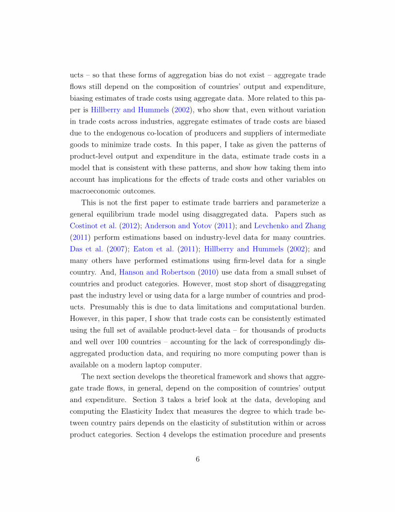
To explore the degree to which Πni typically differs from Πi for a given

pair of countries, Figure 7 plots the histogram of percent deviations of Πni

from Πi for all country pairs. Note that, all else equal, a value of Πni that

30

Figure 6: Outward Multilateral Resistance Terms

0.1 0.2 0.3 0.4 0.5 0.6 0.7 0.8 0.9 1 1.10.1

0.2

0.3

0.4

0.5

0.6

0.7

0.8

0.9

1

1.1

Aggregate Model: Πi (US = 1)

Product-Level

Model:Π

i(U

S=

1)

is 25% below Πi has the same effect on bilateral trade as a 25% increase

in dni. This indicates that the variation in Πni across country pairs has a

significant effect on bilateral trade flows. To further quantify the degree to

which differences in Πni across destinations matter for aggregate trade flows,

consider the following identity relating predicted trade flows to trade costs and

the multilateral resistance terms.

log

(Xni

Xn

/YiY

)= log(d−θni ) + log(P θ

n) + log(Πθi ) + log

((Πni

Πi

)θ)(23)

A regression the left-hand side of (23) on all the right-hand side variables ex-

cept the last has an R2 of .63, indicating that 37% of the variation in predicted

aggregate bilateral trade flows is due to the variation in Πni relative to Πni,

which is to say that it is due to the interaction between countries’ distributions

of output and expenditure across products.

The degree to which Πni differs from Πi also varies across source countries.

For instance, Figure 8 plots separately the histograms for the percentage de-

31

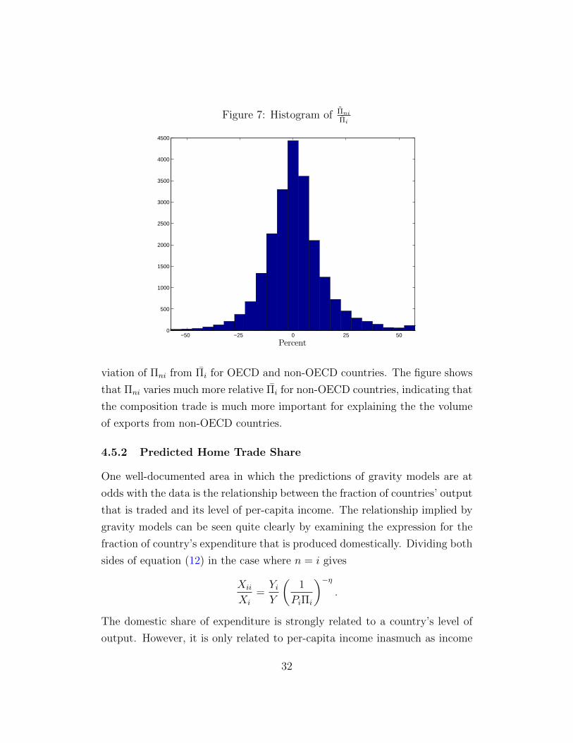
Figure 7: Histogram of ΠniΠi

−50 −25 0 25 500

500

1000

1500

2000

2500

3000

3500

4000

4500

Percent

viation of Πni from Πi for OECD and non-OECD countries. The figure shows

that Πni varies much more relative Πi for non-OECD countries, indicating that

the composition trade is much more important for explaining the the volume

of exports from non-OECD countries.

4.5.2 Predicted Home Trade Share

One well-documented area in which the predictions of gravity models are at

odds with the data is the relationship between the fraction of countries’ output

that is traded and its level of per-capita income. The relationship implied by

gravity models can be seen quite clearly by examining the expression for the

fraction of country’s expenditure that is produced domestically. Dividing both

sides of equation (12) in the case where n = i gives

Xii

Xi

=YiY

(1

PiΠi

)−η.

The domestic share of expenditure is strongly related to a country’s level of

output. However, it is only related to per-capita income inasmuch as income

32

Figure 8: Histogram of ΠniΠi

by Group

−50 −25 0 25 500

200

400

600

800

1000

Percent

OECD Exports

−50 −25 0 25 500

500

1000

1500

2000

2500

3000

3500

Percent

Non-OECD Exports

is correlated with total output or trade costs. However, in the data, the home

share of expenditure is essentially unrelated to per-capita income and has a

weaker relationship with total output than the model predicts.14

Of course, if trade costs are specified as having a country-specific compo-

nent, as in many theoretically-founded gravity estimations, the trade costs that

are systematically higher for low-income countries would reconcile the model

with the data, which Waugh (2010) documents is precisely the case for trade

costs estimated from trade data in such a framework. However, since such a

specification can mechanically replicate such a feature of the data, examining

its ability to reproduce it is not a particularly useful exercise. So, instead, I

evaluate the predictions of the model under the restriction that αi is constant

across exporters.

I use the following procedure to obtain the predicted value of expenditure

on domestic output given a common border cost. First, I set αi = α, for all

i, where α = 1N

∑i αi. In the aggregate case, it is straightforward to solve

for domestic trade using (17), (13), and (14) along with the remaining trade

cost parameters and data on Xn and Yi. In the product-level case, however, in

order to perform the same exercise using equation (16), information on Xjn and

14Fieler (2010) is a recent example which documents the relationship in the data andattempts to reconcile it with a gravity-type model.

33

Figure 9: Predicted versus Actual Home Trade Share

0 0.1 0.2 0.3 0.4 0.5 0.6 0.7 0.8 0.9 10

0.1

0.2

0.3

0.4

0.5

0.6

0.7

0.8

0.9

1

Home Trade Share (Data)

Pre

dict

ed H

ome

Tra

de S

hare

AggregateProduct Level

Y jn is required. For this, I employ the values, Xj

ii from equation (22) evaluated

at αi = αi along with the values of Xjnf and Y j

if from the data. Then, given

Xji = Xj

ii + Xjif and Y j

i = Xjii + Y j

if , it is straightforward to predict domestic

trade, given αi = α, using (16), (7), and (8).

Figure (9) illustrates the predictions of the aggregate and product-level

models, based on the conditional Poisson PML specification.15 Both are plot-

ted against the actual home shares from the data. It is clear that the pre-

dictions from the product-level model lie much closer to the 45 degree line

than those of the aggregate model, indicating that taking into account the

composition of output and expenditure goes quite far in explaining how much

of a country’s output is exported or consumed domestically even without the

inclusion of country-specific trade costs.

Table (2) shows that the product-level model also is much better at predict-

ing the relationship between the domestic expenditure share and the country

characteristics discussed above. The first column presents the coefficients from

15The predictions based on the other aggregate estimation techniques and specificationsare qualitatively similar.

34

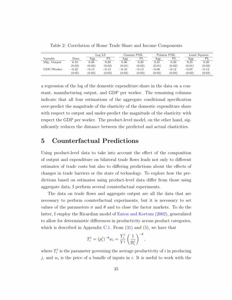
Table 2: Correlation of Home Trade Share and Income Components

Log LS Gamma PML Poisson PML Least SquaresVariable Data Agg PL Agg PL Agg PL Agg PLMfg. Output 0.18 0.26 0.20 0.26 0.20 0.25 0.20 0.25 0.20

(0.03) (0.02) (0.02) (0.01) (0.02) (0.01) (0.02) (0.01) (0.02)GDP/Worker. −0.22 −0.13 −0.13 −0.10 −0.13 −0.08 −0.12 −0.07 −0.12

(0.05) (0.03) (0.03) (0.02) (0.03) (0.02) (0.03) (0.02) (0.03)

a regression of the log of the domestic expenditure share in the data on a con-

stant, manufacturing output, and GDP per worker. The remaining columns

indicate that all four estimations of the aggregate conditional specification

over-predict the magnitude of the elasticity of the domestic expenditure share

with respect to output and under-predict the magnitude of the elasticity with

respect the GDP per worker. The product-level model, on the other hand, sig-

nificantly reduces the distance between the predicted and actual elasticities.

5 Counterfactual Predictions

Using product-level data to take into account the effect of the composition

of output and expenditure on bilateral trade flows leads not only to different

estimates of trade costs but also to differing predictions about the effects of

changes in trade barriers or the state of technology. To explore how the pre-

dictions based on estimates using product-level data differ from those using

aggregate data, I perform several counterfactual experiments.

The data on trade flows and aggregate output are all the data that are

necessary to perform counterfactual experiments, but it is necessary to set

values of the parameters σ and θ and to close the factor markets. To do the

latter, I employ the Ricardian model of Eaton and Kortum (2002), generalized

to allow for deterministic differences in productivity across product categories,

which is described in Appendix C.1. From (31) and (5), we have that

T ji = (pji )−θwi =

Y ji

Y j

(1

Πji

)−θ,

where T ji is the parameter governing the average productivity of i in producing

j, and wi is the price of a bundle of inputs in i. It is useful to work with the

35

following transformed value of T ji ,

T ji = T ji Lθi =

(Y ji )1+θ

Y j

(1

Πji

)−θ,

where Li is the effective supply of inputs devoted to the manufacturing sector

of i, and the last equality follows from the identity Yi = wiLi. To close the fac-

tor markets, I assume that labor is the only factor of production and that it is

perfectly mobile within countries across product categories but perfectly immo-

bile across countries and between the manufacturing and non-manufacturing

sectors.16 Finally, as in Dekle et al. (2008), I take each country’s nominal

trade deficit, Dn as given, which implies that Xn = Yn + Dn. Given a set of

values, T ji , βjn, σ, and θ, the equilibrium of this model is the set of values

of nominal output, Yi, which solves the following system of equations:

Yi =∑n

πni (Yn +Dn) , ∀i,

where

πni =∑j

T ji (Yidni)−θ

(P jn)−θ

βjn

(P jn

Pn

)−σ,

and P jn and Pn are as given by (31). For counterfactual predictions based on

aggregate data, I impose that T ji = Ti and βjn = 1, for all j, so that the model

is consistent with an aggregate gravity equation.

For the following counterfactual experiments, I use a value of θ of 5.5, which

is value estimated by Waugh (2010) based on price data and lies in the range

of estimates from Eaton and Kortum (2002) and other papers, and a value

of σ of 2.25, which is taken from the value θσ

= 2.46, estimated by Eaton et

16That labor is the only factor of production is maintained for convenience of interpre-tation. Li can be also be interpreted as a composite of multiple inputs without changingany of the results that follow. That labor is immobile between manufacturing and non-manufacturing sectors is very useful in that it makes it possible to explore the effect ofchanges in trade barriers and technology on the manufacturing sector – which makes up themajority of international trade – without requiring data on other sectors, which is less read-ily available. However, it is straightforward to extend the analysis to multi-sector economiesby following the methodology of Dekle et al. (2008) and Waugh (2010).

36

al. (2011) based on the exporting behavior of French firms.17 In what follows

I present the predictions of the models based on estimates from the Poisson

PML specification, as this is the specification that has been employed most

often in recent years.18

5.1 Changes in Trade Costs

The first set of counterfactual experiments involve changes in trade barriers.

The first addresses perhaps the most common question asked in the interna-

tional trade literature: what would be the effect of a decrease in barriers to

trade? To address this question, I consider a uniform reduction in all trade

barriers. However, many argue that this is not a realistic experiment, as a

large component of trade barriers is made up of natural impediments, such as

physical distance, so I also perform a second experiment, the elimination of the

asymmetric component of trade barriers. As was recently argued by Waugh

(2010), most natural barriers to trade, like distance, are inherently symmetric,

so to the degree that the barriers are estimated to be asymmetric, they may

also be policy related.

5.1.1 Uniform Fall in Trade Barriers

I first consider a uniform 10% reduction in all trade barriers. The first two

columns of Table 4 present the predicted changes in real output for each coun-

try by the aggregate and product-levels models, respectively. The results are

also summarized in Figure 10.

As can be seen from the figure, the gains from the fall in trade barriers are

quite similar in both models, with growth in real output ranging from slightly

less than 1% in both to about 15% in the product-level model and about 16%

17 These parameters are important for the magnitude of changes in the variables of interestdiscussed below, but choosing different values within a reasonable range does not have asignificant effect on the differences in the predictions of the aggregate and product-levelmodels, which are the focus of this paper.

18The results are not qualitatively different when based on other specifications, partic-ularly for the product-level model, for which the estimates of trade costs are very similaracross specifications.

37

Figure 10: Percent Change in Welfare From a 10% Fall in Trade Barriers

0 2 4 6 8 10 12 14 16 180

2

4

6

8

10

12

14

16

Percent Change in Real Output: Aggregate Model

Per

cent

Cha

nge

in R

eal O

utpu

t: P

rodu

ct−

Leve

l Mod

el

in the aggregate model, with a median of about 6% for both. This indicates

that the effects of small, uniform changes in trade barriers, do not depend

heavily on the composition of countries’ output and expenditure.

5.1.2 Elimination of Asymmetric Trade Barriers

Next, I the remove the asymmetric component of trade barriers, setting all

trade costs to be equal to the smaller value of the two directions of trade

between a given pair of countries, i.e. d′ni = mindni, din. Table 4 presents the

predicted changes in real manufacturing output for each country based on the

aggregate and product-level models. Figure 11 summarizes these predictions,

plotting the percentage change in real manufacturing output predicted by the

product-level model against that of the aggregate model.

The figure shows that, unlike in previous experiment, there are substan-

tial differences between the two models, particularly that the countries that

benefited the most in the aggregate model are predicted to benefit much less

by the product-level model. Further, it appears that the countries for which

the difference is greatest tend to be developing countries, suggesting that ac-

38

Figure 11: Percent Change in Welfare From Elimination of Asymmetric TradeBarriers

0 30 65 110 1700

30

65

110

170

Armenia

Bhutan

Solomon Is.

Burundi

Cape Verde

C.A.R.

Chad

Comoros

Cook Isl.

Benin

Ethiopia

EritreaDjibouti

Gabon

Gambia

Grenada

Guinea

Haiti

Kyrgyzstan

LaosLesotho

Malawi

MaliNicaragua

Guinea−Bissau

Timor−Leste

RwandaSt. Kitts

Saint Lucia

Seychelles

Singapore

Tajikistan

Togo

Tonga

Burkina Faso

Samoa

Aggregate Model

Pro

duct

−Le

vel M

odel

counting for the composition of trade is important for predicting the effect of

asymmetric trade barriers on income inequality.

To explore this phenomenon in more depth, I incorporate data on the size

of the manufacturing workforce, obtained from UNIDO’s INDSTAT database

for 80 of the 148 countries in the sample. Figure 12 plots the changes in

real manufacturing output per worker predicted by each model against its

initial value. While both models predict larger increases in output per worker

for those countries with low initial levels, this pattern is much weaker in the

product-level model’s predictions.

In addition, Table 3 shows that the difference is quantitatively important.

While the aggregate model predicts a 12.3% fall in the variance of log output

per worker, the product-level model predicts only a 9.7% fall. When inequality

is measured by the 90/10 ratio in output per worker, the difference is even more

striking. Compared to the 16.8% fall in the ratio predicted by the aggregate

model, the product-level model predicts only a 1.2% fall.

For comparison, the table also includes the predicted measures of inequality

in autarky and in a world of frictionless trade. With frictionless trade, the

39

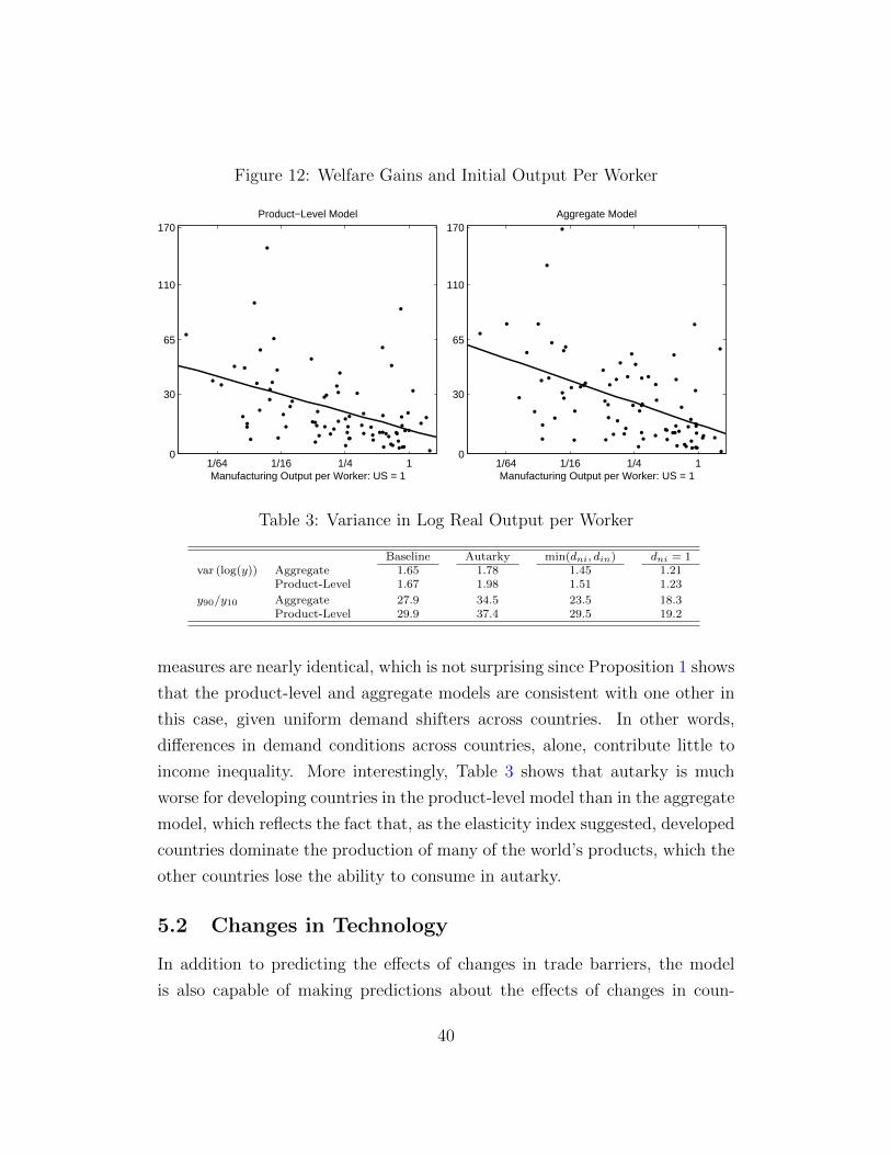
Figure 12: Welfare Gains and Initial Output Per Worker

1/64 1/16 1/4 10

30

65

110

170Aggregate Model

Manufacturing Output per Worker: US = 1

Per

cent

1/64 1/16 1/4 10

30

65

110

170Product−Level Model

Manufacturing Output per Worker: US = 1

Table 3: Variance in Log Real Output per Worker

Baseline Autarky min(dni, din) dni = 1var (log(y)) Aggregate 1.65 1.78 1.45 1.21

Product-Level 1.67 1.98 1.51 1.23

y90/y10 Aggregate 27.9 34.5 23.5 18.3Product-Level 29.9 37.4 29.5 19.2

measures are nearly identical, which is not surprising since Proposition 1 shows

that the product-level and aggregate models are consistent with one other in

this case, given uniform demand shifters across countries. In other words,

differences in demand conditions across countries, alone, contribute little to

income inequality. More interestingly, Table 3 shows that autarky is much

worse for developing countries in the product-level model than in the aggregate

model, which reflects the fact that, as the elasticity index suggested, developed

countries dominate the production of many of the world’s products, which the

other countries lose the ability to consume in autarky.

5.2 Changes in Technology

In addition to predicting the effects of changes in trade barriers, the model

is also capable of making predictions about the effects of changes in coun-

40

tries’ levels productivity. Further, while the aggregate model is only able to

make predictions about changes in countries’ overall levels of productivity, the

product-level model is also able to make predictions about changes in coun-

tries’ relative productivity across products. In this section, I discuss two such

experiments: one involving a change in a country’s overall level of productiv-

ity – which allows for a comparison between the predictions of the aggregate

and product-level models – and one involving a change in countries’ relative

productivity – highlighting the contribution of differences in product-level pro-

ductivity differences to world trade flows and welfare.

5.2.1 Rise of China

First, I consider a positive shock to the overall productivity level of China

which increases China’s nominal manufacturing output as a fraction of total

world manufacturing output by 300%, roughly the magnitude that was ob-

served between 2000 and 2007. Table 4 presents the results for both models.

While both models predict a modest median gain in real output of about

one-half of one percent, there are substantial differences in the gains for many

countries across the models. The gains predicted by the aggregate model are

heavily influenced by geography, with the greatest beneficiaries being nearby

Asian countries such as Mongolia, Sri Lanka, Singapore, Nepal, Laos, and

Vietnam. Other than Lesotho – the only country to have a loss in real output

– the countries that benefit the least are mostly large European countries,

including Germany, Italy, and France.

The picture that emerges from the product-level model is much different,

demonstrating the importance of taking into account the composition of output

and expenditure across countries. The product-level model predicts that the

list of countries whose real output falls also includes Honduras and Cambodia,

which is not surprising, given that, like China, a large fraction of the exports

of these countries are simple manufactures, such as textiles, that are bound for

developed countries. The set of countries that are predicted to benefit the most

by the product-level model, in addition to some of the same Asian countries as

with the aggregate model, includes several countries from sub-Saharan Africa,

41

such as Angola, Guinea-Bissau, and Gambia, reflecting the increased demand

by China for basic materials.

Looking at countries that made large moves through the distribution of

the gains from the growth of China reveals a similar story. The set of coun-

tries with the largest fall in gains relative to the other countries is mostly

made up of Asian and Central American countries known for exporting simple

manufactures to developed countries. The set that experienced the largest

upward move are a mixture of developed countries, such as the Netherlands,

Belgium, and the United States, which benefit largely from a fall in prices, and

countries that export a large amount of basic materials, such as Peru, Chile,

Kuwait, Saudi Arabia, and Algeria, which benefit from increased demand for

their products.

5.2.2 Removal of Comparative Advantage Across Products

To assess the degree to which trade driven by comparative advantage across

products contributes to world welfare, I perform the counterfactual experi-

ment of removing countries’ deterministic differences in productivity across

products. In other words, I impose that T ji = TiTj for all i and j. I determine

the values of Ti and T j by first selecting a reference country, i0, setting Ti0 = 1,

and then setting T j = T ji0 for all j. I choose Ti for all i 6= i0 in order keep the

level of output of each country equal to its value in the data (and the baseline

case).19

I choose the United States as the initial reference country due to the fact

that it exports varieties of every product in the data and its position as the

largest producer and exporter in the world. Table 5 presents the effect of this

change on the real output of each country. Imposing that all countries have

the same pattern of productivity across products as the US results in a 15%

decrease in real output, on average. Table 5 also presents the effects of the

same experiment with Germany and China as the reference countries, showing

19This is essentially the experiment conducted by Costinot et al. (2012), with the ma-jor difference being that this experiment is harmonizing productivity across 4,612 productcategories instead of 13 much more aggregated industries.

42

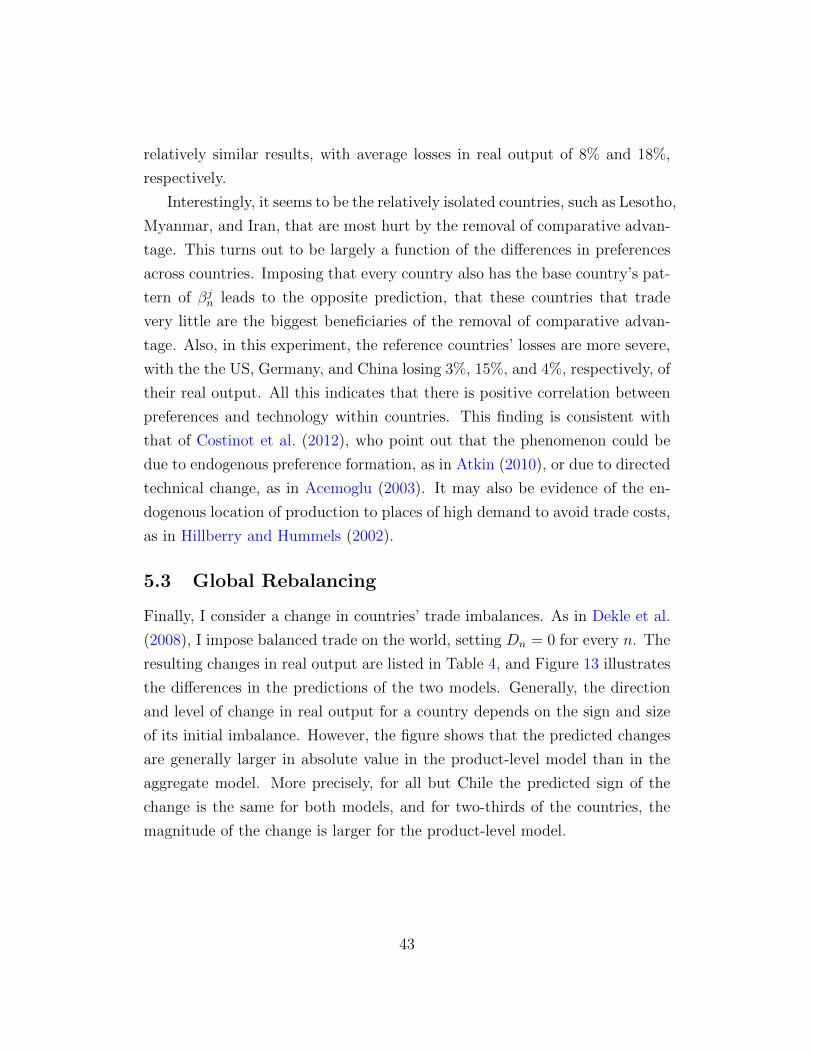
relatively similar results, with average losses in real output of 8% and 18%,

respectively.

Interestingly, it seems to be the relatively isolated countries, such as Lesotho,

Myanmar, and Iran, that are most hurt by the removal of comparative advan-

tage. This turns out to be largely a function of the differences in preferences

across countries. Imposing that every country also has the base country’s pat-

tern of βjn leads to the opposite prediction, that these countries that trade

very little are the biggest beneficiaries of the removal of comparative advan-

tage. Also, in this experiment, the reference countries’ losses are more severe,

with the the US, Germany, and China losing 3%, 15%, and 4%, respectively, of

their real output. All this indicates that there is positive correlation between

preferences and technology within countries. This finding is consistent with

that of Costinot et al. (2012), who point out that the phenomenon could be

due to endogenous preference formation, as in Atkin (2010), or due to directed

technical change, as in Acemoglu (2003). It may also be evidence of the en-

dogenous location of production to places of high demand to avoid trade costs,

as in Hillberry and Hummels (2002).

5.3 Global Rebalancing

Finally, I consider a change in countries’ trade imbalances. As in Dekle et al.

(2008), I impose balanced trade on the world, setting Dn = 0 for every n. The

resulting changes in real output are listed in Table 4, and Figure 13 illustrates

the differences in the predictions of the two models. Generally, the direction

and level of change in real output for a country depends on the sign and size

of its initial imbalance. However, the figure shows that the predicted changes

are generally larger in absolute value in the product-level model than in the

aggregate model. More precisely, for all but Chile the predicted sign of the

change is the same for both models, and for two-thirds of the countries, the

magnitude of the change is larger for the product-level model.

43

Figure 13: Percent Change in Welfare From Global Rebalancing

−25 −20 −15 −10 −5 0−25

−20

−15

−10

−5

0

Aggregate Model

Pro

duct

−Le

vel M

odel

6 Conclusion

This paper demonstrates that accounting for composition of countries output

and expenditure is important for understanding the magnitudes of their aggre-

gate bilateral trade flows. If trade flows can be characterized by a product-level

gravity equation, only under extreme circumstances can aggregate trade flows

be characterized by a gravity equation that depends only on aggregate output

and expenditure and bilateral trade costs. As a result, even if trade costs do

not vary across products, they cannot be inferred from aggregate trade data

and must be estimated using product-level data.

I have shown that trade costs can be consistently estimated using product-

level trade data even when no comparably disaggregated output data is avail-

able. Estimation based on this procedure produces estimates of trade costs

that are generally lower than those from estimations based on aggregate data,

and they are more robust to assumptions on the form of heteroskedasticity

present in the data, which indicates that it is the failure to account for the

composition of trade flows – and not incorrect assumptions about the form

44

of heteroskedasticity – that is the major cause of bias in aggregate gravity

estimations.

Counterfactual experiments conducted using a gravity model fitted to the

estimates using product-level data, in many case, predict very different out-

comes as a result of changes in trade costs and technology. The removal of

asymmetric trade barriers has a much smaller effect on income inequality than

is predicted by an aggregate model, and the effect of the rise of China as a

major manufacturer and exporter has very different on a number of countries

under the two models. Countries in Asia and Central America that export a

similar set of products to a similar set of countries as China benefit much less

– and in some cases lose – once the composition of output and expenditure

is taken into account, and countries in the global north that intensively im-

port the set of goods China produces and countries in the South America and

Sub-Saharan Africa that intensively export the set of goods China that China

demands benefit much more.

45

References

Acemoglu, Daron, “Patterns of Skill Premia,” Review of Economic Studies,

04 2003, 70 (2), 199–230.

Anderson, James E., “A Theoretical Foundation for the Gravity Equation,”

The American Economic Review, 1979, 69 (1), 106–116.

and Eric van Wincoop, “Gravity with Gravitas: A Solution to the

Border Puzzle,” The American Economic Review, 2003, 93 (1), 170–192.

and , “Trade Costs,” Journal of Economic Literature, 2004, 42 (3),

691–751.

and Yoto V. Yotov, “Specialisation: Pro and Anti-Globalizing 1990-

2002,” Working Paper, 2011.

Atkin, David, “Trade, tastes and Nutrition in India,” April 2010, (986).

Broda, Christian and David E. Weinstein, “Globalization and the Gains

from Variety*,” Quarterly Journal of Economics, 2006, 121 (2), 541–585.

Chaney, Thomas, “Distorted Gravity: the Intensive and Extensive Margins

of International Trade,” American Economic Review, 2008, 98 (4), 1707–

1721.

Costinot, Arnaud, Dave Donaldson, and Ivana Komunjer, “What

Goods Do Countries Trade? A Quantitative Exploration of Ricardo’s Ideas,”

Review of Economic Studies, 2012, 79 (2), 581–608.

Das, Sanghamitra, Mark J. Roberts, and James R. Tybout, “Market

Entry Costs, Producer Heterogeneity, and Export Dynamics,” Economet-

rica, 05 2007, 75 (3), 837–873.

Dekle, Robert, Jonathan Eaton, and Samuel Kortum, “Global Re-

balancing with Gravity: Measuring the Burden of Adjustment,” IMF Staff

Papers, July 2008, 55 (3), 511–540.

46

Eaton, Jonathan and Samuel Kortum, “Technology, Geography, and

Trade,” Econometrica, 2002, 70 (5), 1741–1779.

, , and Francis Kramarz, “An Anatomy of International Trade: Evi-

dence From French Firms,” Econometrica, 2011, 79 (5), 1453–1498.

, , and Sebastian Sotelo, “International Trade: Linking Micro and

Macro,” 2012, NBER Working Paper 17864.

Fieler, Anna C., “Nonhomotheticity and Bilateral Trade: Evidence and a

Quantitative Explanation,” 2010, Working Paper.

French, Scott, “Innovation and Product Level Trade,” 2009, Working Paper.

Gourieroux, C., A. Monfort, and A. Trognon, “Pseudo Maximum Like-

lihood Methods: Theory,” Econometrica, 1984, 52 (3), pp. 681–700.

Hanson, Gordon H. and Raymond Robertson, “China and the Manufac-

turing Exports of Other Developing Countries,” in “China’s Growing Role

in World Trade” NBER Chapters, National Bureau of Economic Research,

Inc, 2010, pp. 137–159.

Helpman, Elhanan and Paul Krugman, Market Structure and Foreign

Trade: Increasing Returns, Imperfect Competition, and the International

Economy, Vol. 1 of MIT Press Books, The MIT Press, December 1987.

, Marc Melitz, and Yona Rubinstein, “Estimating Trade Flows: Trad-

ing Partners and Trading Volumes*,” Quarterly Journal of Economics, 2008,

123 (2), 441–487.

Hillberry, Russell and David Hummels, “Explaining Home Bias in Con-

sumption: The Role of Intermediate Input Trade,” June 2002, (9020).

Hillberry, Russell H., “Aggregation Bias, Compositional Change, and the

Border Effect,” The Canadian Journal of Economics / Revue canadienne

d’Economique, 2002, 35 (3), pp. 517–530.

47

Hummels, David, “Toward a Geography of Trade Costs,” GTAP Working

Paper, 1999.

Levchenko, Andrei A. and Jing Zhang, “The Evolution of Compara-

tive Advantage: Measurement and Welfare Implications,” NBER Working

Papers 16806, National Bureau of Economic Research, Inc February 2011.

Mayer, Thierry and Soledad Zignago, “Notes on CEPIIs distances mea-

sures (GeoDist),” CEPII Working Paper, 2011.

Silva, J. M. C. Santos and Silvana Tenreyro, “The Log of Gravity,” The

Review of Economics and Statistics, 2006, 88 (4), pp. 641–658.

Waugh, Michael E., “International Trade and Income Differences,” Ameri-

can Economic Review, December 2010, 100 (5), 2093–2124.

48

Table 4: Counterfactual Percent Changes in Real Income

Country 10% Reduction Symmetric Rise of China RebalancingAgg. P.L. Agg. P.L. Agg. P.L. Agg. P.L.

Albania 15.17 14.64 38.04 14.19 0.74 0.35 -1.52 -0.87Algeria 11.16 10.64 18.92 26.24 0.38 0.74 -0.11 -0.21Angola 7.24 7.92 43.12 29.65 1.43 2.17 -7.69 -8.53Argentina 2.65 2.59 6.55 6.35 0.23 0.32 -0.55 -0.65Armenia 10.47 11.03 69.53 68.72 0.88 0.81 -3.08 -2.86Australia 3.77 3.70 4.26 3.81 0.46 0.71 -1.44 -1.48Austria 7.81 7.72 10.47 9.33 0.25 0.34 -0.70 -0.74Azerbaijan 4.06 4.38 57.29 36.92 0.49 0.70 -2.14 -2.50Bangladesh 3.76 3.61 20.60 30.14 0.41 0.01 0.25 0.11Belarus 3.87 4.13 33.79 25.14 0.45 0.60 -2.17 -2.53Belgium 11.80 11.52 7.33 19.77 0.25 0.40 -0.36 -0.46Benin 2.61 3.35 79.14 40.10 0.99 1.42 -6.49 -7.85Bhutan 2.66 2.83 151.09 114.48 0.63 0.39 -0.57 -0.56Bolivia 4.09 4.47 40.33 34.68 0.63 0.84 -2.79 -3.49Bosnia 9.96 9.83 56.88 56.64 0.80 1.06 -3.84 -3.43Brazil 1.78 1.72 3.27 3.75 0.13 0.10 -0.10 -0.06Brunei 2.73 3.08 56.79 34.05 0.65 0.70 -2.36 -3.34Bulgaria 8.54 8.18 30.79 26.95 0.36 0.33 -0.67 -0.74Burkina Faso 1.00 1.34 70.10 45.62 0.43 0.63 -2.51 -3.53Burundi 0.98 1.56 110.50 80.75 0.76 1.36 -5.25 -8.10C.A.R. 2.13 2.47 112.66 70.33 0.39 0.52 -1.78 -2.24Cambodia 5.31 4.98 55.97 46.79 0.38 -0.25 0.89 0.71Canada 8.49 8.09 13.00 13.25 0.13 0.23 -0.07 -0.04Cape Verde 3.62 4.49 110.49 113.06 1.26 1.73 -8.92 -10.86Chad 0.87 1.39 101.89 16.30 0.50 0.87 -3.18 -5.01Chile 4.67 4.50 9.17 11.70 0.30 0.71 -0.14 0.19China 2.66 2.43 1.96 2.87 277.57 284.01 0.86 0.89Colombia 3.13 3.27 23.73 17.91 0.30 0.30 -1.18 -1.37Comoros 4.04 5.43 149.60 161.53 1.43 2.13 -9.89 -12.66Cook Isl. 11.01 11.37 168.44 100.64 1.51 1.91 -6.58 -6.55Croatia 6.04 6.24 35.43 20.44 0.45 0.55 -1.96 -2.27Cyprus 6.34 6.52 39.46 12.74 0.93 1.19 -4.96 -5.95Czech Rep. 7.87 7.75 15.68 12.70 0.19 0.17 -0.15 -0.17Cte d’Ivoire 3.09 3.26 30.10 20.31 0.27 0.35 -0.63 -0.80Denmark 7.33 7.17 13.12 9.95 0.21 0.30 -0.33 -0.34Djibouti 3.98 4.97 98.86 89.94 1.98 2.93 -21.02 -23.15Dom. Rep. 8.11 7.92 31.30 11.96 0.53 0.31 -1.36 -1.69Ecuador 3.11 3.19 40.30 30.49 0.27 0.28 -0.96 -1.10Egypt 1.40 1.61 13.58 14.88 0.37 0.45 -2.01 -2.52El Salvador 4.04 3.99 42.56 28.97 0.17 0.02 -0.08 -0.15Eritrea 2.04 2.89 128.53 93.88 0.97 1.56 -6.69 -9.11Ethiopia 2.51 3.38 62.87 57.79 0.87 1.39 -5.39 -7.30Finland 4.72 4.58 9.61 10.76 0.00 0.09 0.96 1.06France 3.87 3.77 2.77 3.18 0.11 0.16 -0.13 -0.16Gabon 5.92 6.86 60.09 82.66 1.24 1.64 -6.96 -7.92Gambia 8.15 8.27 125.42 67.68 1.28 1.75 -7.45 -8.11Germany 4.32 4.20 4.26 4.39 0.04 0.11 0.44 0.44Ghana 9.54 9.40 42.23 42.40 1.03 1.27 -3.87 -3.42Greece 4.05 4.23 15.65 11.74 0.62 0.76 -3.39 -3.98Grenada 8.98 9.61 147.40 139.31 1.28 1.84 -7.87 -8.58

49

Table 4 – Counterfactual Percent Changes in Real Income (cont.)

Country 10% Reduction Symmetric Rise of China RebalancingAgg. P.L. Agg. P.L. Agg. P.L. Agg. P.L.

Guatemala 6.15 6.03 42.36 30.99 0.39 0.15 -1.00 -1.13Guinea 9.94 9.60 68.72 128.22 1.13 1.64 -4.55 -3.62Guinea-Bissau 2.93 4.34 143.01 95.17 1.25 2.15 -9.16 -11.83Haiti 6.55 6.66 83.10 19.47 0.75 0.60 -3.40 -4.14Honduras 12.58 11.57 37.39 35.89 0.47 -0.38 0.48 0.75Hungary 10.92 10.54 9.20 9.17 0.36 0.23 -0.32 -0.30Iceland 10.16 9.95 38.62 18.39 0.51 0.84 -0.74 -0.56India 1.66 1.62 6.43 5.35 0.32 0.14 0.51 0.60Indonesia 7.25 6.92 6.31 7.30 0.83 0.52 1.28 1.59Iran 0.73 0.80 9.81 7.97 0.15 0.19 -0.74 -0.91Iraq 6.16 6.61 52.44 24.05 1.47 1.62 -10.74 -12.02Ireland 12.01 11.87 7.41 14.39 0.19 0.24 0.69 0.75Israel 7.26 7.50 9.75 9.94 0.31 0.33 -0.16 -0.21Italy 3.16 3.07 2.68 2.72 0.09 0.09 -0.01 -0.03Jamaica 8.41 8.16 58.49 17.35 0.56 0.82 -1.68 -1.69Japan 1.34 1.31 1.12 1.49 0.32 0.35 0.40 0.47Jordan 4.18 4.59 38.64 28.28 0.71 1.12 -3.84 -4.32Kazakhstan 8.49 8.29 27.72 32.72 1.92 2.44 -1.00 -0.06Kenya 2.94 3.05 35.13 23.13 0.53 0.61 -2.35 -2.86Korea 3.45 3.37 2.94 3.09 0.79 0.80 0.52 0.72Kuwait 5.81 5.77 22.75 47.37 0.25 0.65 0.04 0.09Kyrgyzstan 6.40 6.61 76.79 45.86 1.72 1.47 -2.29 -2.14Laos 4.91 5.18 85.42 29.74 1.99 1.63 -2.57 -3.53Latvia 16.14 14.97 33.77 44.49 0.59 0.63 -0.30 -0.35Lebanon 2.64 3.19 33.88 26.20 0.96 1.27 -6.50 -8.11Lesotho 2.93 2.41 94.88 32.11 -0.05 -0.14 1.76 1.83Lithuania 8.98 8.65 36.42 26.03 0.39 0.39 -0.79 -0.82Luxembourg 14.99 14.42 16.38 9.36 0.33 0.36 -0.44 -0.35Macedonia 7.68 7.50 59.94 65.82 0.32 0.12 -0.50 -0.45Madagascar 7.12 6.85 49.72 39.47 0.55 0.34 -0.41 -0.50Malawi 4.69 5.15 76.84 37.87 1.14 1.36 -6.71 -8.49Malaysia 11.84 11.46 20.77 16.63 1.44 0.89 -0.34 -0.50Mali 6.35 6.92 77.13 61.46 1.44 1.62 -9.93 -10.21Malta 12.01 11.80 35.60 13.40 0.55 0.43 -1.08 -0.93Mauritius 9.37 8.69 34.24 12.69 0.68 0.61 -0.49 -0.80Mexico 13.72 13.05 11.30 12.50 0.37 0.18 -0.81 -0.83Mongolia 16.55 14.55 27.96 35.39 6.69 3.78 -0.68 -0.87Morocco 5.68 5.91 24.15 13.23 0.29 0.19 -0.72 -0.70Mozambique 3.70 3.98 49.07 29.41 0.94 1.17 -5.09 -5.82Myanmar 1.36 1.52 32.05 31.91 0.35 0.30 -0.63 -0.88Namibia 9.40 9.51 45.69 20.15 1.05 1.23 -3.60 -3.90Nepal 7.93 7.94 53.54 48.08 2.01 1.03 -1.21 -1.67Netherlands 11.85 11.28 14.06 17.65 0.25 0.43 0.07 0.03New Zealand 5.58 5.34 11.04 8.66 0.40 0.59 -0.40 -0.37Nicaragua 6.83 6.83 70.00 65.42 0.52 0.44 -1.68 -2.06Norway 5.84 5.88 12.68 9.83 0.31 0.47 -1.01 -1.06Oman 9.23 8.90 24.45 9.88 1.04 0.92 -4.09 -4.94Pakistan 2.61 2.56 18.70 19.99 0.52 0.31 0.33 0.39Panama 11.09 10.41 48.12 42.62 0.61 0.26 -0.96 -0.95Papua N.G. 12.38 11.81 50.69 55.29 0.82 0.68 -1.70 -1.29

50

Table 4 – Counterfactual Percent Changes in Real Income (cont.)

Country 10% Reduction Symmetric Rise of China RebalancingAgg. P.L. Agg. P.L. Agg. P.L. Agg. P.L.

Paraguay 3.06 3.42 37.69 45.46 0.76 1.22 -4.19 -5.14Peru 2.86 2.95 15.69 19.81 0.24 0.62 -0.47 -0.35Philippines 12.83 12.78 16.02 13.60 1.55 0.75 0.04 0.41Poland 3.85 3.88 11.92 11.55 0.23 0.22 -0.93 -1.02Portugal 5.41 5.45 9.83 7.04 0.37 0.29 -1.31 -1.46Qatar 12.81 12.06 23.76 15.40 0.92 1.53 -2.13 -2.02Romania 5.21 5.22 20.71 18.91 0.20 0.11 -0.29 -0.28Russia 6.84 6.54 6.81 6.62 0.33 0.53 1.57 2.19Rwanda 0.75 1.23 95.03 66.29 0.60 1.04 -4.06 -6.37Saint Lucia 7.46 8.47 140.44 122.52 1.45 1.80 -10.59 -11.86Samoa 8.82 9.84 103.00 28.14 1.20 0.92 -4.77 -4.82Saudi Arabia 4.26 4.45 9.17 17.37 0.47 0.86 -1.92 -2.04Senegal 5.00 5.17 55.07 30.95 0.71 0.82 -3.30 -3.85Seychelles 8.53 8.04 80.05 8.05 0.72 0.74 -1.40 -1.66Singapore 14.80 14.42 76.48 88.81 2.21 1.88 0.42 0.85Slovakia 11.20 10.77 17.28 14.83 0.31 0.30 -0.04 -0.06Slovenia 10.15 9.86 23.62 17.79 0.31 0.21 -0.43 -0.46Solomon Is. 12.53 12.04 113.50 161.72 1.21 1.16 -2.77 -2.19South Africa 2.90 2.82 6.83 7.09 0.13 0.14 0.32 0.45Spain 3.80 3.73 3.66 3.10 0.23 0.26 -0.75 -0.83Sri Lanka 14.17 13.14 13.55 12.55 2.41 0.83 -0.57 -1.39St. Kitts 15.83 14.86 97.18 61.11 0.87 0.81 -1.60 -1.28Sudan 1.80 2.27 45.35 25.16 0.69 1.09 -4.24 -5.76Swaziland 4.81 5.06 54.93 17.57 0.63 0.90 -2.50 -3.12Sweden 6.25 6.03 5.80 5.79 0.09 0.15 0.63 0.66Syria 4.96 5.45 39.51 36.32 0.71 0.88 -3.62 -4.45Tajikistan 4.71 4.65 78.46 77.95 0.98 1.71 0.61 1.73Tanzania 3.21 3.58 49.35 36.28 0.81 1.09 -4.34 -5.44Thailand 9.08 8.72 9.00 8.38 0.99 0.55 0.52 0.55Timor-Leste 1.61 2.90 160.99 157.98 1.61 3.02 -15.95 -22.42Togo 5.78 5.54 89.37 31.85 0.81 0.82 -3.66 -4.49Tonga 2.94 4.65 167.96 146.71 1.77 3.05 -16.75 -21.58Trin. and Tob. 6.44 6.21 54.35 59.49 0.23 0.29 0.03 0.14Tunisia 7.33 7.45 26.12 15.14 0.41 0.19 -1.15 -1.20Turkey 3.57 3.57 8.40 9.43 0.33 0.27 -1.39 -1.68Turkmenistan 8.39 9.01 52.50 58.22 1.13 1.44 -5.81 -6.60U.A.E. 7.39 7.04 9.31 7.51 0.82 1.19 -3.21 -3.67U.K. 4.28 4.18 3.38 3.86 0.21 0.28 -0.55 -0.61U.S.A 1.93 1.93 8.32 10.92 0.24 0.36 -0.62 -0.71Uganda 1.85 2.26 57.25 42.45 0.92 1.25 -6.05 -7.62Ukraine 6.24 5.95 20.41 17.84 0.10 0.14 0.67 0.96Uruguay 5.31 5.29 26.59 19.38 0.37 0.53 -0.60 -0.53Uzbekistan 3.95 4.18 43.58 47.55 0.73 0.78 -1.44 -1.56Venezuela 2.43 2.48 17.39 20.33 0.15 0.22 -0.35 -0.39Viet Nam 7.55 7.10 17.08 21.13 1.71 0.40 -1.12 -1.40Yemen 2.16 2.96 44.36 51.69 0.98 1.61 -6.59 -8.95Zambia 8.23 8.16 54.07 56.13 0.82 1.40 -2.25 -1.52Zimbabwe 4.74 4.60 42.44 36.11 0.37 0.25 -0.66 -0.51

51

Tab

le5:

Cou

nte

rfac

tual

Per

cent

Chan

ges

inR

eal

Inco

me

Cou

ntr

yU

.S.

Ger

.C

hin

aC

ou

ntr

yU

.S.

Ger

.C

hin

aC

ou

ntr

yU

.S.

Ger

.C

hin

aA

lban

ia-1

8.0

4-7

.26

-8.8

1G

uate

mala

-15.8

6-5

.24

-19.0

6P

ara

gu

ay

-16.9

2-8

.04

-12.1

0A

lger

ia-1

2.8

0-2

.82

-22.0

9G

uin

ea-1

3.0

9-2

.82

-15.4

0P

eru

-15.0

9-5

.17

-15.0

4A

ngola

-10.8

8-5

.23

-17.0

8G

uin

ea-B

issa

u-2

6.8

2-1

3.7

5-1

4.3

8P

hilip

pin

es4.5

1-2

.20

-19.8

8A

rgen

tin

a-1

2.1

0-0

.91

-20.5

2H

ait

i-2

2.6

8-2

0.5

7-8

.54

Pola

nd

-16.4

9-5

.22

-15.4

9A

rmen

ia-1

2.0

3-8

.00

-21.3

5H

on

du

ras

-15.4

8-6

.76

-17.3

7P

ort

ugal

-21.5

7-9

.74

-18.0

7A

ust

ralia

-11.1

6-4

.83

-19.5

2H

un

gary

-8.2

1-2

.20

-6.5

4Q

ata

r-8

.35

-2.2

3-1

1.7

3A

ust

ria

-12.8

9-4

.68

-11.6

3Ic

elan

d-1

7.9

7-1

2.1

4-1

6.1

8R

om

an

ia-1

9.4

0-9

.62

-10.4

3A

zerb

aij

an

-13.7

7-1

2.7

3-2

4.5

1In

dia

-17.9

5-1

4.3

2-2

7.3

4R

uss

ia-1

7.2

7-1

0.2

1-2

8.5

3B

an

gla

des

h-1

8.2

1-7

.93

-6.6

9In

don

esia

-8.7

5-0

.03

-20.9

7R

wan

da

-24.8

4-1

8.2

5-3

1.5

7B

elaru

s-2

1.5

1-9

.88

-26.3

6Ir

an

-29.3

5-1

7.7

7-3

6.4

3S

ain

tL

uci

a-1

1.6

3-2

.44

-6.3

8B

elgiu

m-1

1.4

1-8

.67

-15.4

6Ir

aq

-10.9

4-4

.00

-14.3

9S

am

oa

-7.9

1-1

1.3

5-2

4.6

4B

enin

-22.1

9-1

4.7

2-1

5.4

3Ir

elan

d-6

.09

-10.2

8-9

.52

Sau

di

Ara

bia

-9.4

5-2

.45

-15.9

7B

hu

tan

-19.9

7-5

.58

-29.4

8Is

rael

-12.8

0-1

8.1

4-2

4.7

4S

eneg

al

-18.7

4-1

2.9

9-1

8.9

9B

olivia

-15.8

8-1

1.3

8-2

3.3

2It

aly

-17.5

3-7

.73

-15.8

7S

eych

elle

s-2

8.5

1-2

2.7

8-2

6.0

2B

osn

ia-1

6.7

9-3

.92

-12.9

9Jam

aic

a-1

8.8

7-1

2.6

1-1

9.0

6S

ingap

ore

-2.9

8-6

.17

-13.9

5B

razi

l-1

1.4

4-2

.58

-24.4

4Jap

an

-7.0

1-5

.70

-20.4

4S

lovakia

-12.3

1-0

.83

-15.3

5B

run

ei-1

7.8

7-1

3.5

7-1

6.4

1Jord

an

-17.6

5-8

.10

-23.3

6S

loven

ia-1

6.1

7-4

.30

-17.0

4B

ulg

ari

a-1

7.9

3-8

.14

-16.1

1K

aza

kh

stan

-9.2

72.0

1-1

9.5

8S

olo

mon

Is.

-8.3

4-0

.24

-10.8

3B

urk

ina

Faso

-24.5

4-1

8.8

0-2

5.9

2K

enya

-18.0

1-8

.11

-24.4

5S

ou

thA

fric

a-9

.05

-1.0

2-1

6.5

7B

uru

nd

i-1

9.4

6-1

0.3

0-2

9.9

7K

ore

a-2

.44

-9.4

2-2

4.1

4S

pain

-17.3

0-3

.35

-20.2

7C

.A.R

.-1

5.6

1-1

2.5

1-3

6.3

2K

uw

ait

-1.9

47.0

2-4

.63

Sri

Lan

ka

-9.3

7-0

.89

-11.0

0C

am

bod

ia-2

0.3

9-9

.01

-7.1

3K

yrg

yzs

tan

-15.8

4-5

.60

-24.9

8S

t.K

itts

-9.3

1-0

.27

-5.6

0C

an

ad

a-9

.16

1.7

2-1

7.0

0L

aos

-30.8

6-2

3.1

9-1

9.7

0S

ud

an

-22.0

6-1

5.0

4-2

5.0

6C

ap

eV

erd

e-1

7.8

0-8

.25

-15.8

0L

atv

ia-1

3.0

2-2

.20

-12.6

3S

wazi

lan

d-2

4.5

6-1

6.6

8-2

6.1

0C

had

-32.3

1-3

5.6

6-4

8.8

9L

eban

on

-19.1

8-1

0.5

3-1

7.1

3S

wed

en-1

0.7

0-4

.38

-16.6

7C

hile

-11.7

6-2

.65

-13.7

0L

esoth

o-4

4.4

5-4

5.1

7-2

7.1

4S

yri

a-1

7.4

0-6

.51

-21.8

7C

hin

a-6

.94

-2.9

8-1

.94

Lit

hu

an

ia-1

7.6

9-5

.51

-16.9

9T

aji

kis

tan

-7.4

0-1

2.6

9-1

2.5

9C

olo

mb

ia-1

8.0

8-9

.06

-22.9

4L

uxem

bou

rg-1

1.3

7-5

.26

-15.9

1T

an

zan

ia-1

7.0

7-7

.48

-16.7

0C

om

oro

s-1

8.8

9-1

1.2

8-1

4.0

3M

ace

don

ia-1

7.4

9-5

.42

-19.4

0T

hailan

d-1

.65

0.0

0-1

2.6

0C

ook

Isl.

-12.4

8-6

.89

-10.4

1M

ad

agasc

ar

-21.7

3-1

1.4

0-6

.12

Tim

or-

Les

te-1

4.7

8-3

.03

-21.3

5C

roati

a-2

0.7

7-1

3.0

2-1

8.0

8M

ala

wi

-19.4

2-8

.90

-20.4

1T

ogo

-26.5

2-1

5.9

9-2

4.5

2C

yp

rus

-13.9

0-9

.56

-20.5

5M

ala

ysi

a3.1

9-1

.88

-18.5

5T

on

ga

-16.0

4-8

.29

-20.5

9C

zech

Rep

.-1

3.4

6-3

.95

-13.6

7M

ali

-16.9

7-6

.76

-21.3

3T

rin

.an

dT

ob

.-1

0.1

5-1

.07

-17.8

7C

ted

’Ivoir

e-2

3.3

5-1

8.4

5-2

4.5

4M

alt

a-0

.21

-8.6

5-1

8.8

1T

un

isia

-18.5

2-1

2.9

3-1

2.4

0D

enm

ark

-14.6

8-8

.93

-9.6

2M

au

riti

us

-23.6

4-1

2.5

2-1

0.9

5T

urk

ey-1

6.6

7-5

.33

-19.4

6D

jib

ou

ti-1

2.2

1-2

.56

-12.4

0M

exic

o-5

.24

3.4

2-6

.38

Tu

rkm

enis

tan

-12.9

60.5

0-1

6.4

3D

om

.R

ep.

-19.3

9-1

4.2

2-5

.66

Mon

golia

-8.2

25.4

3-1

4.4

5U

.A.E

.-1

1.4

5-7

.60

-9.0

6E

cuad

or

-20.0

7-1

0.3

4-2

3.4

2M

oro

cco

-19.1

8-1

4.4

3-1

4.2

6U

.K.

-7.6

6-4

.85

-10.1

4E

gyp

t-1

5.7

4-1

2.8

9-2

1.6

1M

oza

mb

iqu

e-2

0.0

8-1

0.1

3-2

1.2

6U

.S.A

0.0

0-9

.74

-17.8

2E

lS

alv

ad

or

-22.0

8-1

2.3

4-2

2.6

6M

yanm

ar

-28.6

7-2

0.3

9-1

9.8

7U

gan

da

-19.0

7-9

.03

-21.4

3E

ritr

ea-1

6.6

3-6

.09

-25.0

1N

am

ibia

-16.1

8-6

.41

-15.2

8U

kra

ine

-18.8

8-7

.76

-18.7

1E

thio

pia

-11.0

0-8

.24

-27.9

5N

epal

-18.2

9-7

.42

-21.1

8U

rugu

ay

-19.1

0-7

.93

-19.6

7F

inla

nd

-11.4

8-6

.40

-15.9

9N

eth

erla

nd

s-7

.61

-7.3

3-5

.61

Uzb

ekis

tan

-10.9

00.8

4-2

0.0

7F

ran

ce-1

0.5

3-6

.61

-15.3

6N

ewZ

eala

nd

-13.1

1-5

.52

-17.2

7V

enez

uel

a-1

5.8

6-5

.38

-20.4

4G

ab

on

-8.1

1-1

.75

-16.3

2N

icara

gu

a-1

6.7

8-4

.48

-13.5

5V

iet

Nam

-12.3

1-0

.46

-12.3

2G

am

bia

-19.0

7-6

.93

-11.8

2N

orw

ay

-15.8

6-1

2.4

4-1

5.7

9Y

emen

-20.1

8-1

1.3

1-2

2.0

0G

erm

any

-8.6

4-0

.08

-12.7

6O

man

-12.0

2-2

.54

-25.7

0Z

am

bia

-12.6

5-1

.02

-17.6

9G

han

a-6

.44

-4.6

4-1

8.1

8P

akis

tan

-19.6

1-1

2.3

0-2

8.7

0Z

imb

abw

e-1

1.7

4-2

.32

-18.4

6G

reec

e-2

0.8

1-1

1.2

1-1

4.8

1P

an

am

a-1

1.1

92.0

6-1

0.6

3G

ren

ad

a-9

.91

-0.6

5-5

.79

Pap

ua

N.G

.-9

.47

-2.5

9-1

5.9

0

52

A Data

A.1 Bilateral Trade Data

The product-level bilateral trade data are taken from the Comtrade database

provided by the United Nations Statistical Division. The data used are those

reported by national statistical agencies using the 1996 revision of the Har-

monized Commodity Description and Coding System (HS) for the year 2000.

The choice of year was made to maximize the number of countries reporting

in a common product classification. The data report trade flows valued in US

dollars reported by both importers and exporters. I use trade flows reported

by importers as these are generally considered to be of higher quality. The

data cover 247 countries and 5,132 product categories.

A.2 Gravity Variables

The bilateral relationship variables – distance, shared border, common lan-

guage, and colonial relationship – are from CEPII’s dist cepii database de-

scribed in Mayer and Zignago (2011). I use their measures of population-

weighted distances, whether countries share a common official language, and

wether countries ever had a colonial link.

A.3 Manufacturing Output

Output data for the manufacturing sector is taken primarily from the United

Nations Industrial Development Organization’s (UNIDO) Industrial Statistics

(INDSTAT) database. Data are available for manufacturing industries clas-

sified according to the International Standard Industrial Classification (ISIC)

Revision 3, for 151 3- and 4-digit industries. Since data is only available for

manufactured goods, I dropped all trade flows that did not respond to ISIC

categories beginning with 15 through 37. Product-level trade flows were al-

located to an ISIC industry using the concordance available from Comtrade.

Where manufacturing output data from INDSTAT was unavailable, I imputed

manufacturing output from data on manufacturing value added available from

53

the World Bank’s World Development Indicators (WDI). Manufacturing out-

put data were available from INDSTAT for 77 countries, while output data

could be imputed from WDI for an additional 71 countries. As a result, the

final dataset is made up up 148 countries and 4,618 manufacturing product

categories.20

B Proofs

B.1 Proposition 1

Proof of Proposition 1, Case 1. BecauseY jiY j

= αj, it follows immediately that∑j α

j = 1 andY jiYj

= YiY

. Conjecture that Πji = λjΠi, ∀i, j. Combined with (7)

we have that

(P jn)−θ = (λj)θ

∑i

(dniΠi

)−θYiY

≡ (λj)θP−θn .

Substituting into 4 (and using βjn = βj) gives

(Pn)−σ =∑j

βj

(Pnλj

)−σ= (Pn)−σ

∑j

βj(λj)σ.

Substituting into 2 yields

Xjn =

βj(λj)σ∑j β

j(λj)σXn.

Summing over n and using the market clearing condition that Y ji =

∑nX

jni

gives

Y j =βj(λj)σ∑j β

j(λj)σY,

20Due to lack of industry-level data from WDI and complications associated with theindustry-level INDSTAT data – i.e. a large number of categories are censored, and forthe remaining categories, a large fraction are reported to have output that is less thanexports indicating serious problems associated with misclassification or mis-concordance –only aggregate manufacturing output data is used in the paper.

54

which, given Y j = αjY , implies that λj =(αj

βj

) 1σ

and Pn = Pn. Substituting

the expressions for P jn and Xj

n into equation 8, we have that

(Πji )−θ =

(αj

βj

)−θσ ∑

n

(dniPn

)−θYnY

=

(αjβj

) 1σ

Πi

−θ

which verifies the conjecture. Substituting the expressions for P jn and Πj

i into

10 and combining with 9 gives the result of Proposition 1, Case 1.

Proof of Proposition 1, Case 2. Given thatY jiY j∈ 0, 1,∀i, j, 7 reduces to

P jn =

dni

Πji∗(j)

,

where i∗(j) denotes the exporter for whichY jiY j

= 1. Substituting into 4 (and

using βjn = βj gives that

(Pn)−σ =∑j

βj(dni

Πji∗

)−σ.

Substituting into 10 gives that

(Πni)θ =

(dniPn

)θ−σY

Yi

∑j∈Ωji

βj(Πji )−σ,

where Ωji = j : i = i∗(j). Define

Πi ≡

Y

Yi

∑j∈Ωji

βj(Πji )−σ

−1σ

.

Then, it is clear from 9 that

Xni =XnYiY

(dni

PnΠi

)−σ, (24)

55

and, using 4, it is straightforward to show that

P−σn =∑i

(dni

Πi

)−σYiY.

Then, summing 24 over n, using the market clearing condition Yi =∑

nXni,

and simplifying gives that

Π−σi =∑n

(dniPn

)−σXn

Y.

Proof of Proposition 1, Case 3. Given that σ = θ and that βjn = βj, 10 sim-

plifies to

Πni =

(Y

Yi

∑j

βj(Πji )−σ

)− 1σ

≡ Πi.

The rest of the proof follows exactly as for Case 2.

Proof of Proposition 1, Case 4. Given that dni = 1,∀n, i, it follow immedi-

ately that

(P jn)−θ =

∑i

(1

Πji

)−θY ji

Y j= (P j)−θ,

and that

(Πji )−θ =

∑n

(1

P jn

)−θXjn

Y j= (Πj)−θ,

which implies a system of two equations that is satisfied at P j = (Πj)−1.

Combined with 4 and given that βjn = βj, this implies that

P−σn =∑j

βj(Πj)σ = P.

Substituting for P jn and Pn in 2 and imposing the marking clearing condition,∑

nXjn = Y j, gives that

βj

(Πj)σP−σn =

Y j

Y.

56

Substituting this into 10 and simplifying gives that

Πni = P θ,

which implies that 9 reduces to

Xni =XnYiY

B.2 Reformulation of Product-Level Trade Flows

Proof of Proposition 2. Summing 6 over all i 6= n and rearranging gives that

Xjn

(P jn)−θ

=Xjnf

(P jnf )−θ,

where

(P jnf )−θ =

∑i 6=n

(dni

Πji

)−θY ji

Y j, (25)

and Xjnf =

∑i 6=nX

jni. Substituting this expression back into 6 gives that

Xjni =

XjnfY

ji

Y j

(dni

P jnfΠ

ji

)−θ. (26)

Summing 26 over all n 6= i and rearranging gives that

Y ji

Y j(Πj

i )θ =

Y jif

Y jf

(Πjif )

θ (27)

where

(Πjif )−θ =

∑n6=i

(dni

P jnf

)−θXjnf

Y jf

Y jif =

∑n6=iX

jni and Y j

f =∑

j Yjif . Substituting this express back into 26 yields

Xjni =

XjnfY

jif

Y jf

(dni

P jnfΠ

jif

)−θ.

Substituting 27 into 25 completes the specification given in Proposition 2.

57

C Models Generating Product-Level Gravity

In this appendix, I show that generalizations of two well-known trade models

– the Ricardian model of Eaton and Kortum (2002) and the monopolistic

model of Chaney (2008) – generate the product-level gravity framework laid

out in section 2. This amounts to showing that both are consistent with the

reduced-form demand system given by (1) - (4).

In both models, there are a continuum of varieties, indexed by k, in each

product category. A representative consumer in each country, n, maximizes

the following nested-CES utility function:

Un =

∑j

(βjn)1

1+γ

(∫Ωjn

qjn(k)γ

1+γ dk

)1+γγ

δ1+δ

1+δδ

subject to ∑j

∫Ωjn

xjn(k)dk ≤ Xn,

where Ωjn is the set of varieties of product j available in country n, xjn(k) =

pjn(k)qjn(k), and pjn(k) is the price of variety k of product j in country n, and

γ > δ > 0. Expenditure by country n on variety k of good j is given by

xjn(k) =

(pjn(k)

P jn

)−γβjn

(P jn

Pn

)−δXn,

where

P jn =

(∫Ωjn

(pjn(k)

)−γdk

)− 1γ

,

and

Pn =

(∑j

βjn(P jn)−δ

)−1δ

.

Each source country has a set of potential producers, each of which has a

level of productivity, zji (k), drawn from the productivity distribution, Gji (z).

58

The marginal cost of delivering variety k of product j to destination n from

source i is

cjni(k) =witni

zji (k),

where wi is the cost of a bundle of inputs in i, tni ≥ 1 is the “iceberg” trade

cost of delivering goods from i to n. I normalize tii = 1 for all i. The fixed

cost associated with delivering a positive amount of a product from i to n is

fni ≥ 0.

C.1 Ricardian Model

The Ricardian version of this framework requires the following additional

restrictions: (1) there is a fixed unit measure of varieties of each product,

k ∈ [0, 1], and each country can produce every variety; (2) fni = 0; (3) there

is perfect competition among producers of each variety; (4) the productivity

distribution is type II extreme value (Frechet) over [0,∞),

Gji (z) = e−T

ji z−θ,

where T ji > 0 governs expected productivity for a given country and product

category – i.e. comparative advantage across product categories – and θ ∈(γ,∞) governs the shape of the distribution – i.e. comparative advantage

within product categories – with a smaller value of θ implying greater variance.

This framework nests that of Eaton and Kortum (2002), differing only in that

the shift parameter of the productivity distribution varies across products, as

in Costinot et al. (2012) and French (2009).

Condition (2) implies that all varieties are available to all destination coun-

tries, and condition (3) implies that the price of each variety is equal to the

cost of delivering it there, i.e. pjni(k) = cjni(k). Each country will purchase only

the variety of each product with the lowest price, so pjn(k) = minpjni(k)Ni=1.

Following Eaton and Kortum (2002), it is straightforward to show that pjn is

distributed according to

F jn(p) = Pr(pjn(k) < p) = 1− e−Φjnp

θ

(28)

59

and the the probability that country i is the low-cost provider of a variety to

n is

πjni =T ji (witni)

−θ

Φjn

, (29)

where Φjn =

∑i T

ji (witni)

−θ.

To show that this framework is consistent with (1) - (4), I define

pjni =

(∫Ωjni

(pjni(k)

)−γdk

)− 1γ

, (30)

where Ωjni ⊂ Ωj

n denotes the set of varieties of j that n purchases from i. First,

note that ∑i

(pjni)−γ

=(P jn

)−γ.

Next, combining (30) with (28) and (29),

(pjni)−γ

=

∫ ∞0

p−γπjnidFjn(p)

= T ji (witni)−θ∫ ∞

0

pθ−γ−1θ1− e−Φjnpθ

dp

= γT ji (witni)−θ (Φj

n

)γ−θθ ,

where γ is a function of parameters.21 This implies that(P jn

)−γ= γ (Φj

n)γθ

and, therefore, that

Xjni

Xjn

=

(pjni

P jn

)−γ=T ji (witni)

−θ

Φjn

.

Similarly, summing (P jn)−δ) over j, we have that P−δn = γ

δθΦ

δθn and, thus, that

Xjn

Xn

= βjn

(P jn

Pn

)−δ= βjn

(Φjn

Φn

) δθ

.

21γ = Γ(θ−γγ

), where Γ(x) =

∫∞0tx−1e−tdt is the gamma function. The result is obtained

by substituting Φjnpθ for t.

60

where Φδθn =

∑j β

jn(Φj

n)δθ .

Now, I define the following:

pji ≡ (T ji )−1θwi

P jn ≡

(Φjn

)−1θ =

(∑i

(pji tni)−θ

)−1θ

Pn ≡ Φ−1θ

n =

(∑i

βjn(P jn

)−δ)−1δ

.

(31)

It is, then, straightforward to show that expenditure by n on varieties of j

from i is

Xjni =

(pji tni

P jn

)−θβjn

(P jn

Pn

)−δXn.

Thus, letting σ = δ, dni = tni, and βjn = βjn, it is clear that the model is

consistent with (1) - (4).

C.2 Monopolistic Competition

The monopolistic competition version of this framework requires the follow-

ing additional restrictions: (1) each producer produces a unique variety of a

product; (2) there is a measure, T ji , of producers in source country i that can

produce a variety of product j; and (3) the productivity distribution is Pareto

over [1,∞),

Gji (z) = 1− z−θ,

where θ ∈ (γ,∞). If we set γ = δ, this framework reduces to a one-sector

monopolistic competition model, similar to that studied in Helpman et al.

(2008). If we let δ → 0, then it becomes a multi-sector model in which

expenditure shares across sectors are exogenously fixed (as in Chaney (2008)).

Condition 1 implies that each producer is a monopolist in the market for its

unique variety. The CES demand structure, then, implies that each producer

will charge a constant markup, m = 1+γγ

, over the marginal cost of delivering

61

its variety to country n, so

pjni(k) = mwitni

zji (k).

A producer of a variety of product j from i with a productivity of z selling in

n will earn a profit, net of the fixed cost, of

πjni(z) =1

1 + γ

(witniz

m

P jn

)−γXjn − fni,

which is positive if z is greater than

zjni = m

(1

1 + γ

)− 1γ witni

P jn

(Xjn

fni

)− 1γ

.

Defining pjni as in (30), and using conditions 2 and 3,

(pjni)−γ

= T ji

∫ ∞zjni

(mwitniz

)−γθz−θ−1dz

= ηT ji (witni)−θf

− θ−γγ

ni (Xjn)

θ−γγ (P j

n)θ−γ,

where η is a function of parameters.22 Summing over i and rearranging gives

that (P jn

)−γ= η(Xj

n)θ−γγ (P j

n)θ−γΦjn, (32)

which implies that

Xjni

Xjn

=

(pjni

P jn

)−γ=T ji (witni)

−θf− θ−γ

γni

Φjn

.

where Φjn =

∑i T

ji (witni)

−θf− θ−γ

γni . Recalling that Xj

n = βjn

(P jnPn

)−δXn, rear-

ranging (32) yields (P jn

)−δ= (βjn)

δ−αδ (Φj

n)αθX

δ−αδ

n (Pn)δ−α

22η = m−θ θθ−γ

(1

1+γ

) θ−γγ

62

where 1α

= 1δ+1θ− 1γ

and α ∈ (0, δ). It then follows that P−δn = Xα−δδ

n (Pn)α−δΦαθn ,

and

Xjni

Xjn

= βjn

(P jn

Pn

)−δ= (βjn)2−α

δ

(Φjn

Φn

)αθ

,

where Φαθn =

∑j(β

jn)2−α

δ (Φjn)

αθ .

Now, I define the following:

βjn ≡ (βjn)2−αδ

pji ≡ (T ji )−1θwi

P jn ≡

(Φjn

)−1θ =

(∑i

(pji tnif1θ− 1γ

ni )−θ

)−1θ

Pn ≡ Φ−1θ

n =

(∑i

βjn(P jn

)−α)− 1α

.

It is, then, straightforward to show that expenditure by n on varieties of j

from i is

Xjni =

pji tnif1θ− 1γ

ni

P jn

−θ

βjn

(P jn

Pn

)−αXn.

Thus, letting σ = α and dni = tnif1θ− 1γ

ni , it is clear that the model is consistent

with the system (1) - (4).

63